Preprint of the paper published in: Expert Systems with Applications, volume 39, issue 3, pages 2759-2770, February 2012. doi:10.1016/j.eswa.2011.08.135 © 2012 Elsevier Ltd.

Generating Multimedia Presentations that Summarize the Behavior of Dynamic Systems

Using a Model-based Approach

Martin Molina, Victor Flores

Department of Artificial Intelligence, Technical University of Madrid, Campus de Montegancedo S/N, 28660 Boadilla del Monte, Madrid, Spain,

Abstract. This article describes a knowledge-based method for generating multimedia

descriptions that summarize the behavior of dynamic systems. We designed this method for

users who monitor the behavior of a dynamic system with the help of sensor networks and make

decisions according to prefixed management goals. Our method generates presentations using

different modes such as text in natural language, 2D graphics and 3D animations. The method

uses a qualitative representation of the dynamic system based on hierarchies of components and

causal influences. The method includes an abstraction generator that uses the system

representation to find and aggregate relevant data at an appropriate level of abstraction. In

addition, the method includes a hierarchical planner to generate a presentation using a model

with discourse patterns. Our method provides an efficient and flexible solution to generate

concise and adapted multimedia presentations that summarize thousands of time series. It is

general to be adapted to different dynamic systems with acceptable knowledge acquisition effort

by reusing and adapting intuitive representations. We validated our method and evaluated its

practical utility by developing several models for an application that worked in continuous real

time operation for more than one year, summarizing sensor data of a national hydrologic

information system in Spain.

Keywords: Behavior summarization, presentation model, intelligent user interface, data

abstraction, multimedia presentation, text-graphic coordination, data-to-text system

1. Introduction

The management of dynamic systems by means of sensor networks is a type of task that usually

involves teams of operators and decision makers. In general, the human teams are interested not

only in the interpretations of the values recorded by sensors, but also in the description of

possible phenomena and the evolution of these in the time. An example of a dynamic system in

the domain of hydrology is a set of geographically distributed river basins with river channels

and reservoirs. Here, human operators monitor the state of the rivers and make decisions in the

presence of problems such as floods, water contamination, or unexpected water needs (for

agriculture, hydro-electrical energy or water consumption by end-users). Other examples of this

type of dynamic system are: road traffic networks, public transport systems (by bus, railway,

subway, etc.), electrical energy distribution systems, physical phenomena related to natural

disasters (for example, seismic or volcano activity), historical records of vehicle behavior (e.g.,

a military aircraft) for maintenance purposes, etc.

Tools that automatically generate descriptions and explanations about the system’s behavior in a

can help end-users understand and analyze the meaning of data. This is especially important

when the dimension and complexity of the system is high with large amounts of quantitative

data from sensors that record different types of magnitudes periodically. To generate such type

of descriptions, it is necessary to select and abstract automatically relevant sensor data and

generate adequate interpretations. In addition, it is necessary to dynamically construct

discourses at an adequate level of abstraction that is useful for end-users according to their

information needs. The effective simulation of these reasoning processes requires representing

specialized domain knowledge about the dynamic system in a practical way, i.e., able to be

interpreted efficiently by inference methods and able to be acquired with acceptable effort.

A number of research projects have paid attention (directly or indirectly) to this type of

problem. For example, SumTime generates text descriptions that summarize temporal series

about weather forecasts [Reiter, et al., 2005], SumGen generates text summaries of a set of

events from a battle simulator [Maybury, 1995] and the method of Gautier and Gruber generates

text explanations about the behavior of a space shuttle’s reaction control system [Gautier,

Gruber, 93]. However, a limitation of these solutions is that they generate only text descriptions.

In complex dynamic systems, it is important to use also coordinated illustrations that

complement text for a better understanding of behavior data (e.g., map locations, graphics for

temporal series, etc.). Another problem of existing proposals (as it happens, for example, in

SumGen and SumTime) is that they use specific domain knowledge bases for data abstraction

and text generation that are difficult to be reused for other dynamic systems.

In this article, we describe an innovative knowledge-based method to generate descriptions that

summarize datasets corresponding to the observed behavior of dynamic systems1

. Our method

is able to generate multimedia presentations about behavior (with graphics, images, animations)

and, also, it is flexible to be adapted to different dynamic systems. Our method uses a general

and reusable representation for the dynamic system especially designed to support strategies for

summarizing data from thousands of sensors. This representation is based on approximate

knowledge that can be obtained with acceptable knowledge acquisition effort. We validated our

method and showed its practical utility by developing several models in the domain of

hydrology that work in continuous operation using real-time sensor data from a national

hydrologic information system in Spain.

In the following, we describe the method for generating descriptions that summarize behavior

datasets. First, we present the summarization goals describing the general characteristics of the

dynamic system. Next, we present the knowledge-based architecture and, then, we describe in

detail the representation for dynamic systems and other representations and inferences for

abstraction and presentation planning. We also describe how we validated our method and

evaluated its practical utility. At the end of the article, we make a comparative discussion with

similar approaches.

2. Summar ization goals

Our method generates descriptions that summarize the behavior of a certain type of dynamic

system. The general characteristics of such dynamic system are the following:

• Observable. The behavior of the system is observed with the help of sensors that

periodically measure the value of a number of quantitative properties. There are different

types of sensors that observe different types of quantities. There may be a large number of

quantities whose value change in time.

1 Some partial preliminary results related to the research work presented in this article were previously reported in [Molina & Flores, 2006a, 2006b, 2008].

• Complex. The dynamic system has different types of components and relations among

components. The system can be described at different levels of aggregation with parts that,

in turn, can be decomposed in smaller parts.

• Supervised. There are human teams that supervise the system’s behavior and make

decisions accordingly. For example, there are human operators in charge of control that

watch the system and, if necessary, change its state with the help of actuators. In addition,

there are other types of users that can be affected by the state of the system. They are

interested in the system’s behavior to make decisions about themselves and other related

systems.

• Prefixed goals. The system is controlled according to prefixed management goals that try to

keep certain indicators about the state of the system close to acceptable values.

• Abstract view for decision. There is an important distance between (1) the language (and

level of detail) in which sensors measure the quantities of the system and (2) the language

(and level of abstraction) in which users make decisions.

The input to our method is a set of measures recorded by sensors. Each measure corresponds to

an observed quantity of the dynamic system (for example the temperature of a particular

component). For each quantity there is a time series with the last t values (for example, t = 24).

We assume that each measure is recorded periodically, every ∆t (for example, ∆t = 15 minutes).

We also assume that for a particular dynamic system there is a large number N of sensors (for

example, N > 1,000).

The output of the method is a description that summarizes and explains the behavior of the

dynamic system. The description includes text summaries together with other visualization

modes (2D graphics, maps, animations, 3D images, etc.) that could be presented using different

devices (a computer desktop, a mobile phone, a fax, etc.). The method must include a solution

to coordinate adequately the text and the appropriate illustrations that help understand quickly

the information. This is especially important for dynamic systems with many components that

need to be identified not only by their name but also by spatial location (for example, using a

descriptive sketch of an installation, or using a geographic map). It is also useful to show the

temporal change of different components with comparative graphics for temporal series, or

using animations (2D or 3D animations) that help to understand the evolution of certain

phenomena. To generate such type of descriptions, we identified the following challenges:

• Relevant information. The generated description must include the relevant information.

Filtering thousands of quantitative measures to select the relevant information usually

requires specific knowledge about both the historical behavior of the dynamic system and

what is potentially useful for the end-user.

• Meaningful descriptions. The summary must explain the meaning of the measures in a

qualitative language close to the end-user. This requires knowledge to interpret the

quantitative data using appropriate meaningful qualitative linguistic labels.

• Variable level of abstraction. The summary must present condensed information as concise

as possible. The level of abstraction to describe the behavior is not prefixed but it is

dynamically chosen according to the input data and length restrictions on the output

description. Condensing information requires knowledge such as how to generalize similar

facts, how to aggregate facts corresponding to components that are part of more complex

components and how to condense different facts corresponding to the same phenomenon.

• Variable discourse. The discourse structure of the descriptions is not rigid, but is

dynamically constructed according to characteristics of the input data and the desired length

of the presentations. The specific natural language sentences and their order in paragraphs is

dynamically chosen together with the adequate illustrations that complement the

descriptions.

• Convincing descriptions. The presentation needs to include evidence that helps users to trust

the generated descriptions. This is important for users who have to assume the responsibility

for decision-making based on these descriptions. The method needs to know strategies to

select and present appropriate evidences to construct convincing descriptions.

3. The knowledge-based architecture

Our method follows a knowledge-based approach with a set of general inference steps that use

domain specific knowledge. The method performs two main tasks: (1) abstraction, to abstract

the relevant information (i.e., what to inform) and (2) planning, to generate a presentation plan

according to the type of end-user and the communication media (how to present the

information). Figure 1 shows the components of our method with the two main tasks,

abstraction and planning, together with inputs/outputs and the domain knowledge. As the figure

shows, the declarative knowledge representation is organized in meta-levels with three related

layers:

1. System model. The system model (layer 1) represents knowledge about the structure and

behavior of the dynamic system.

2. Abstraction model. The abstraction model (layer 2) represents knowledge about how to

generate abstractions. It uses knowledge representations from layer 1.

3. Presentation model. The presentation model (layer 3) represents knowledge about

presentation strategies. It uses knowledge representations from layers 1 and 2.

Briefly, the method works as follows. We generate the presentation plan in a loop involving the

two main tasks (planning and abstraction). The planning task performs a hierarchical search

over candidate partial presentations using the presentation model. At each iteration, the planning

task generates abstraction goals and the abstraction task uses the abstraction model to return the

abstractions corresponding to these goals. With this information, the planning task progressively

refines the partial presentations until the final presentation plan is constructed. In the following,

we describe the three domain models and inference processes in more detail.

Figure 1. Main components of our method. In the figure ellipses represent tasks,

rectangles represent input/output data and cylinders represent knowledge bases.

Sensor data

Abstractionmodel

Presentationmodel

Presentationplan

Systemmodel

Planning

Abstractiongoals

Abstraction

Abstractions

DeclarativeKnowledge

model

Layer 1

Layer 2

Layer 3

• Interpretation model• Aggregation model• Validation model

4. The system model

The system model is a representation of the behavior and the structure of the dynamic system.

Our method is designed to simulate summarization tasks performed by professional human

operators with partial and approximated knowledge about the dynamic system. Thus, the system

model is formulated with a qualitative approach instead of precise mathematical representations

with quantitative parameters. Our representation for the system model shares certain elements of

existing common representations and ontologies used in qualitative physics [Bobrow et al., 96;

Borst et al., 95; Gruber, Olsen, 94; Iwasaki, Low, 93].

Compared to existing qualitative approaches for system modeling, our representation is not for

simulation but, instead, for summarization, a task that in general requires less details and,

therefore, it uses knowledge that can be obtained with lower knowledge acquisition effort. Our

representation follows an intuitive component-based approach to perform abstraction processes

such as aggregation, generalization and qualitative interpretation. This is done by using

hierarchies of components (both part-of and is-a hierarchies), qualitative states and causal

influences.

We formalize the system model in many-sorted first-order logic [Meinke, Tucker, 93], an

extension of first-order logic where sorts are specified for each constant, variable, function

symbol and each argument position of each predicate and function symbol. Our representation

for the system model uses the following basic sorts: component represents a physical object of

the system (for example, a reservoir or a river), quantity is a quantitative property of a

component (e.g., the temperature or the pressure), and sensor is a device used to measure

observable quantities of components. More specific components are related to more general

components (with the is-a relation) by defining subsorts with the notation sort s: t (where s is

subsort of t). For example, sort reservoir: component defines the subsort reservoir of the sort

component.

To represent qualitative properties we use the following sorts: state represents the qualitative

state of a component at the present moment (for example, the current state of a reservoir is

empty), recent_state represents the state of a component in a recent time interval (e.g., the last

24 hours), trend represents the trend of a state (for example, with the set of values {increasing,

steady, decreasing}), and quantification is a sort that quantifies a state in a population of

components (for example, with the set of values {all, many, few, one, zero}). The recent state is

a practical solution to summarize a recent behavior in a qualitative value and it is usually

described in a more abstract level than the current state.

Sort Value Description

t_scope

series(n) A temporal series with the last n values current The value at present moment maximum(n) The maximum of the last n values minimum(n) The minimum of the last n values average(n) The average of the last n values sum(n) The sum of the last n values maximum The historical maximum value minimum The historical minimum value average The historical average value forecast(n) A temporal series with a prediction of the future n values

c_scope

maximum The maximum value in the set of the components minimum The minimum value in the set of the components average The average value in the set of the components sum The sum of values in the set of the components

Table 1. Examples of possible values for the sorts t_scope y c_scope.

In order to characterize adequately generalization levels, our representation also includes the

scope of affirmations. For example, we want to represent that the affirmation the temperature in

Spain is 32 degrees corresponds to a certain spatio-temporal scope such as the following:

maximum value of the last 24 hours and maximum value of the temperature in the main cities of

Spain. For this purpose, we use the concept of relative scope to a specific domain. We use two

sorts: t_scope, which defines a temporal scope, and c_scope, which defines the scope in a set of

subcomponents that are part of a given component. Table 1 shows possible values for these two

sorts.

<Table 2>

Table 2 shows a list of predicates to represent knowledge about the dynamic system. To

represent structural relations, we use the predicate part_of(x: component, y: component) for the

part-of relation and the predicate observe(x: sensor, y: quantity, z: component) to represent that a

quantity of a component is observed (measured) by a sensor. According to the part-of relation,

component c1 is complex when there exists another component c2 and it is defined the relation

part_of(c2, c1). In contrast, a component is single when this property is no satisfied. The

predicate state_category(x: component, y: state, z: state) defines general states that correspond

to categories of more specific states.

The model includes also an approximate view of the system behavior represented with causal

relations between quantitative properties. This intuitive relation is useful to summarizing data

corresponding to the same phenomenon and generating explanations that help to understand

data. The predicate cause(x1: quantity, y1: component, x2: quantity, y2: component, t: number)

represents a direct causal influence between two quantities. The relation includes a temporal

delay between the cause and effect.

To represent the value of a particular quantity we use the predicate value(x: quantity, y:

component, t: t_scope, v: value) for the case of a single component. This predicate defines the

value for the quantity of a component with a particular temporal scope. For example,

value(temperature, tank-T3, current, 120) represents that the temperature of tank-T3 is 120 at

the present moment and value(volume, reservoir-R8, minimum(24), 18) represents that the

minimum volume of reservoir-R8 in the last 24 hours is 18. The predicate for the case of

complex components is value(x: quantity, y: component, t: t_scope, z: c_scope, v: value). It

includes an additional argument for c_scope. For example, value(rain, Spain, current,

maximum, 27) represents that, at the present moment, the maximum rain in the set of points

where rain is measured that are part of Spain is 27.

To interpret the current state of a component we use the predicates state(x: component, y: state),

trend(x: component, y: state) and quantification(x: component, y: quantification). For example

the tuple <state(Spain, heavy-rain), trend(Spain, decreasing), quantification(Spain, few)>

represents that there is a decreasing heavy rain in a few points of Spain. The predicate

recent_state(x: component, y: recent_state) represents the qualitative recent state of a

component corresponding to a recent prefixed time interval.

5. The abstraction model

The abstraction model includes three submodels: the interpretation model, the relevance model

and the validation model. In the following, we describe these models in detail. Then, we

describe how we generate abstractions by using such models.

5.1. The interpretation model

The interpretation model represents knowledge that helps to determine the qualitative state of

components. For the case of single components, their state is determined by conditions about

quantities. The state of single components is similar to the qualitative values used in qualitative

reasoning. For instance, the state of a reservoir may have the set of values {empty, medium,

full}. We assume a total order in qualitative values. We obtain the state value of a single

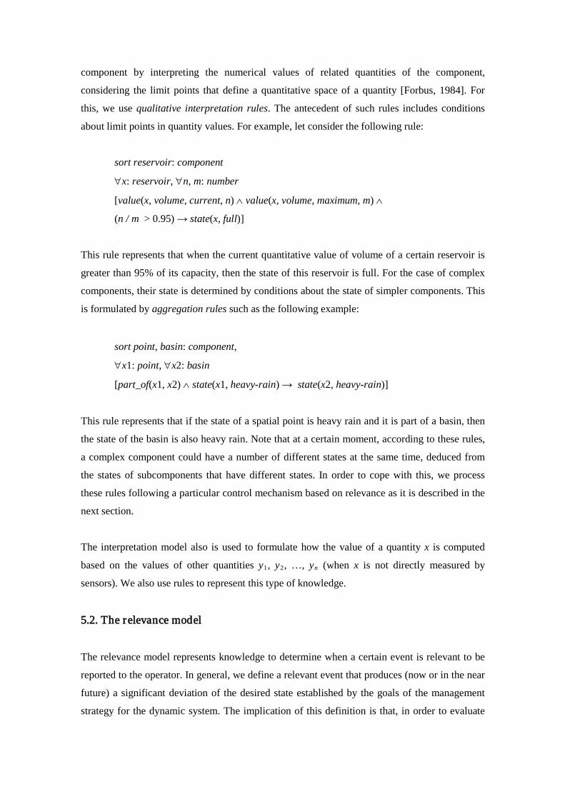
component by interpreting the numerical values of related quantities of the component,

considering the limit points that define a quantitative space of a quantity [Forbus, 1984]. For

this, we use qualitative interpretation rules. The antecedent of such rules includes conditions

about limit points in quantity values. For example, let consider the following rule:

sort reservoir: component

∀x: reservoir, ∀n, m: number

[value(x, volume, current, n) ∧ value(x, volume, maximum, m) ∧

(n / m > 0.95) → state(x, full)]

This rule represents that when the current quantitative value of volume of a certain reservoir is

greater than 95% of its capacity, then the state of this reservoir is full. For the case of complex

components, their state is determined by conditions about the state of simpler components. This

is formulated by aggregation rules such as the following example:

sort point, basin: component,

∀x1: point, ∀x2: basin

[part_of(x1, x2) ∧ state(x1, heavy-rain) → state(x2, heavy-rain)]

This rule represents that if the state of a spatial point is heavy rain and it is part of a basin, then

the state of the basin is also heavy rain. Note that at a certain moment, according to these rules,

a complex component could have a number of different states at the same time, deduced from

the states of subcomponents that have different states. In order to cope with this, we process

these rules following a particular control mechanism based on relevance as it is described in the

next section.

The interpretation model also is used to formulate how the value of a quantity x is computed

based on the values of other quantities y1, y2, …, yn

(when x is not directly measured by

sensors). We also use rules to represent this type of knowledge.

5.2. The relevance model

The relevance model represents knowledge to determine when a certain event is relevant to be

reported to the operator. In general, we define a relevant event that produces (now or in the near

future) a significant deviation of the desired state established by the goals of the management

strategy for the dynamic system. The implication of this definition is that, in order to evaluate

the relevance of facts, it would be necessary to predict the behavior of the dynamic system by

simulation. However, based on our assumption for system modeling, we follow here a

simplified and more efficient approach with approximated heuristic knowledge.

We use the predicate normal_state(x: component, y: state) to establish that the qualitative state

of a type of component does not produce significant deviations of the desired states established

by the management goals. For example, in hydrology, one of the management goals is that the

water flow in river channels should not exceed the maximum capacity of channels in order to

avoid floods. Thus, light rain is not relevant because, normally, it does not produce this

problem. This can be represented as normal_state(point, light-rain). However, if we want to

establish exceptions for this situation, we can write rules such as the following:

sort point: component, ∀x: point, ∀y: weather-forecast-region

[part_of(x, y) ∧ ¬ state(y, heavy-storm) → normal_state(x, light-rain)]

This rule represents that the state light rain is not relevant at a certain point, except when the

weather forecast predicts heavy storm in the region of such point (because it may be the

beginning of the storm).

Our notion of relevance gives also criteria to establish relevance order among events. To

represent relevance order, we use the predicate more_relevant(x, y) where x and y are states2

.

For example more_relevant(state(a, heavy-rain), state(b, light-rain)) represents that the state

heavy rain is more relevant that the state light rain. We use rules with this predicate in the

consequent to consider particular situations. For example, the state heavy-rain at certain location

x can be more relevant than the same state at location y because, for example, the capacity of the

river channels nearby x is smaller or because there are populated areas nearby x.

The relevance model plays the role of control knowledge in the complete model. The

aggregation rules of the interpretation model are used to determine the state of complex

components based on the state of single components. However, these rules need to be applied

according to a certain control mechanism because the same component can have different states.

The relevance priority is used here for this purpose taking into account that rules that interpret

qualitative states with higher priority are applied first.

2 In order to use a formula of first-order logic using the predicate more_relevant(x, y), then state(x, y) must be a term and not a predicate. We use here the technique of reification [McCarthy, 1979], which in general consists of making a formula of first-order language L1 into a term of another first-order language L2. We make atoms of L1 into terms of L2. We treat the predicate symbol of state(x, y) in L1 as a function symbol in L2 (whose sort is, for example, state_predicate). Then in L2, state(x, y) is a term.

5.3. The validation model

In real life, the measures recorded by sensors that monitor the behavior of dynamic systems

present sometimes errors due to occasional malfunctions of devices or communications. For this

purpose, it is important to have a model that represents knowledge able to detect typical

situations that correspond to these faults. We use the predicate error(x: sensor, y: malfunction)

to represent that a particular sensor is out of order (here, the sort malfunction represents a

prefixed malfunction). The validation model contains validation rules with this predicate in the

consequent. The antecedent of such rules includes conditions that analyze the values of the

quantity recorded by the sensor.

This process can detect errors corresponding to certain properties of the quantity (maximum

value, minimum values, maximum change in a time interval, etc.). A typical fault in the field of

hydrology is a pluviometer that records a constant value for a long period. According to the

behavior of the rain, it is expected a certain random behavior of the values. We can easily detect

this error with a rule with this condition in the antecedent. In addition, validation rules can

include conditions that analyze the coherence of sets of nearby sensors based on redundancy of

measures and/or causal influences.

5.4 Abstraction inferences

The abstraction model also includes a prefixed set of goals that correspond to specific

abstraction inferences. Each inference goal is identified by a predicate. For example, the

predicate abstract(x) represents an inference goal that generates x (an ordered list of qualitative

states) by abstracting the quantitative sensor measurements. Other examples of predicates are

the following: details(x, y) represents an inference goal that generates a list of states y that are

the details of the state x, causes(x, y) generates the list of states y that are cause of the state x,

and effects(x, y) generates the list of states y that are effects of the state x.

We describe below the algorithms for the abstraction goals corresponding to the predicates

abstract(x) and details(x, y). These predicates are representative examples of abstraction goals

(the other abstraction goals are implemented with small variations of these main algorithms or

they correspond to simple inferences). The algorithm for the predicate abstract(x) performs a

linear sequence of the following steps:

1. Interpret measurements. Each sensor measurement is interpreted to generate quantity

values of single components. This process filters measurements that correspond to

sensors that present malfunctions. Here, we use the predicates observe(x, y, z) from the

system model and the rules with the predicate error(x, y) in the consequent from the

validation model.

2. Interpret quantities. For every single component its qualitative state and its trend is

computed. We use the qualitative interpretation rules with the predicate state(x, y) in the

consequent from the interpretation model. Let R1 = {S1, S2, …, Sn} be the result of this

interpretation where each element Si is a pair <state(ci, ai), trend(ci, ti)> where ci is a

component, ai is a state and ti

is a trend.

3. Select relevant states. Relevant states from R1 are selected. For this purpose, we use

rules with the predicate normal_state(x, y) in the consequent from the relevance model.

Let R2 ⊆ R1 be the set of relevant states.

4. Sort states. The states of R2 are sorted according to the priority for relevance. For this

purpose, we use rules with the predicate more_relevant(x, y) in the consequent from the

relevance model. Let R3 be the resulting ordered set. More relevant states are located

first in R3.

5. Filter states. States corresponding to the same phenomenon are removed. We assume

that this happens when a state is cause of another state. For each state Si in R3

(following the priority order in R3) a second state Sk (less relevant than Si because Sk is

located after Si in R3) is removed if Sk is cause or effect of Si

(through the causal

relation established the predicate cause(x, y, z, u, v) from the system model). Let R4 be

the resulting filtered set.

6. Condense states. We condense states from R4 to generate a new set with a small

number of more abstract states. As control criteria, we condense first the states

according to the order in R4 with guarantee that the most relevant states are condensed

first. In this process, each time a condensed state is generated, we also generate a link

that relates the condensed state and the states of single components that it abstracts.

Two strategies are used for condensation:

a. State generalization. We generate a new state of a component that generalizes a

set of states of the same component. For example, the states heavy_rain and

moderate_rain are generalized by the state rain. For this purpose, we use the

predicate state_category(x, y) from the system model. We look for the most

specific category that generalizes all the states of components of the same class.

b. Component aggregation. The goal is to condense states of single components

c1, c2, …, cn of the same class to generate the state of a complex component c.

The complex component c is the smallest component that includes all the single

components c1, c2, …, cn

through the relation established by the part_of(x, y)

predicate from the system model. We determine the state of the component c

with the rules from the interpretation model that include the predicate state(x, y)

in the consequent. In addition, the trend and the quantification are evaluated.

The quantification is calculated by comparing the size of the set of states to

condense and the size of the set that includes all single components that are part

of the component c. As a result, this condensation produces a tuple with the

following format <state(c, s), trend(c, t), quantification(c, q)>.

The output of this abstraction process is an ordered set with the following format R =

{<state(c1, s1), trend(c1, t1), quantification(c1, q1)>, <state(c2, s2), trend(c2, t2),

quantification(c2, q2)>,…, <state(cn, sn), trend(cn, tn), quantification(cn, qn

)>}. The elements of

the set R are ordered by relevance. In addition, as mentioned, each state of a complex

component is linked with the set of single components that it abstracts. These links make

possible to perform an inverse inference, represented by the predicate details(x, y). Thus, when

this predicate is invoked with a value for x (the state of a component), it looks for the

corresponding link and returns the value y with the states of single components.

6. The presentation model

The presentation model is used to automatically construct presentation plans, i.e. the final

output description to be presented to the end-user. The presentation model represents knowledge

about strategies that express how to present abstracted information. We use a knowledge-based

hierarchical planner that constructs the presentation plan through a search directed by

hypotheses of partial strategies that are progressively refined until the final presentation is

generated. The knowledge base of the planner contains a set of operators that represent atomic

presentation operations.

Figure 2 shows a set of operators. In this example, operators generate text using templates (it is

also possible to have graphic operators, as it is explained below). Each operator includes a set of

conditions. In this example, the conditions establish that the operators are applicable for a

particular type of component (a river section) besides other conditions about the values of

quantities. In addition, the operator defines its effect with one or several presentation actions

that generate part of the presentation. We consider actions to generate text and actions to

generate illustrations (images, animations, graphics, etc.). In this example, the actions generate

text using the action add-text(x) that incrementally constructs the text summary.

OPERATOR: text_template_current_flow GOAL: elaborate_with_quantity(x, q)

CONDITIONS: (x: river-section) ∧ (q = flow) ∧ value(q, x, current, v) EFFECT: add-text ({“there is a flow of ”, v, “ m3/s at ”, x})

OPERATOR: text_template_flow_variation GOAL: contrast_to_previous(x, q)

CONDITIONS: (x: river-section) ∧ (q = flow) ∧ value(q, x, current, v1) ∧ value(q, x, previous , v2) ∧ (d = v1 – v2) ∧ (d > 0)

EFFECT: add-text({“which is an increase of ”, d, “ m3/s”})

OPERATOR: text_template_average_flow GOAL: contrast_to_average(x, q)

CONDITIONS: (x: river-section) ∧ (q = flow) ∧ value(q, x, average, v) EFFECT: add-text({“the average value at this point is ”, v, “ m3/s”})

…

Figure 2. Examples of planning-operators in the presentation model.

Each specific operator is associated to a general communicative goal. For example, the goal of

the last operator is contrast_to_average(x, q), i.e., to show an average value that contrast to a

previous reported value. In general, there are several candidate operators for a given

communicative goal. Each communicative goal is defined according to certain rhetorical

relations that establish the structure of discourse [Mann, Thompson, 1988]. We have identified a

set of rhetorical relations applicable in our context of dynamic system surveillance that include

relations such as: elaboration, contrast, exemplify, list, cause, preparation, etc. Table 3 shows a

list of communicative goals that implement such relations. The table includes examples of text

sentences for these communicative goals.

Communicative goal Example of generated sentence (translated into English)

summarize_ state(x) High flow in some parts of the river Ebro elaborate_with_quantity(x, q) The flow of river Ebro at Tortosa is 1285 m3/s elaborate_with_count(x) High flow in 3 rivers of the Ebro Basin elaborate_with_enumerate(x) High flow in the river Ebro, the river Jucar and the river Segura list_maximum (x, q) The river Ebro has the maximum flow list_next_maximum (x, q) The river Arga is the next river with maximum flow contrast_ to_average(x, q) The average flow at this point of the river is 309 m3/s contrast_to_previous(x, q) Compared to the previous value, this means an increase of 130 m3/s contrast_to_maximum(x, q) This value corresponds to the 78% of its capacity exemplify_with_quantity(x) For example, the flow of river Ebro at Tortosa is 1285 m3/s exemplify_with_next_quantity(x) Also, the flow of river Ebro at Asco is 973 m3/s prepare_causes The following behavior upstream can be highlighted prepare_effects The following behavior downstream can be highlighted summarize_behavior(x) Light rain in the Ebro basin in the last 24 hours elaborate_with_quantity_behavior(x, q) In the last 24 hours, the accumulated rain at Algemesí is 27 mm list_maximum_behavior(x, q) In the last 24 hours, the place with maximum accumulated rain is Algemesí list_next_maximum_behavior(x, q) The place with next maximum accumulated rain is Albalat

Table 3. Examples of communicative goals associated to text templates.

To generate a presentation, the planner searches for applicable operators. We use a hierarchy of

discourse patterns to direct this search. The hierarchy makes more efficient the search process

and helps to generate coherent presentations. Our presentation planner uses a simplified version

of Hierarchical Task Network (HTN) planning [Ghallab et al., 2004]. Besides operators, an

HTN planner includes planning-tasks and planning-methods. In our approach, each planning-

task corresponds to a communicative goal (what to present) and each planning-method

corresponds to a discourse pattern (how to present it). In our model, a discourse pattern is a

presentation template that helps to keep the coherence of the presentation. Each pattern defines

a partial presentation strategy at certain level of abstraction.

PATTERN: describe_with_causes_and_effects GOAL: inform(x)

CONDITIONS: causes(x, c) ∧ effects(y, e) DISCOURSE: {summarize_state(x), elaborate_state(x),

elaborate_causes(c), elaborate_effects(e)}

PATTERN: describe_state_of_single_component GOAL: elaborate_state(x)

CONDITIONS: (state(y, s) ∈ x) ∧ single_component(y) ∧ quantity(y, q) DISCOURSE: {elaborate_with_quantity(y, q),

contrast_to_previous (y, q), contrast_to_average(y, q)}

PATTERN: describe_state_of_complex_component GOAL: elaborate_state(x)

CONDITIONS: (state(y, s) ∈ x) ∧ ¬ single_component(y) DISCOURSE: {elaborate_with_count(x), exemplify_with_quantity(x)}

…

Figure 3: Examples of discourse patterns in the presentation model.

Figure 3 shows examples of discourse patterns. The first extract illustrates a discourse pattern

for the communicative goal inform(x). In general, several different patterns can be associated to

the same goal. The pattern defines four sub-goals: summarize_state(x), elaborate_state(x),

elaborate_causes(c) and elaborate_effects(e). The pattern includes also conditions similar to the

conditions for operators whose purpose is to establish when the pattern is applicable. Conditions

can include logical expressions with predicates related to the structure and behavior of the

dynamic system (for example, value(x, y, z, t), part_of(x, y), etc.). In the examples, value(q, x,

current, v) is used to identify the current value of a quantity, single_component(y) indicates that

y must be a single component and quantity(y, q) represents that q is a quantity of the component

y. In addition, conditions also could include predicates related to previous decisions about

presentation elements (such as the decision about the layout). Conditions can also include

predicates that invoke abstraction goals. These predicates gather additional information about

the dynamic system (for example, the predicates causes(x, c) and effects(y, e)). Abstraction

goals are invoked backwards when the presentation planner checks the conditions of a candidate

pattern.

Figure 4. Example of partial search tree developed during the presentation planning process. The

tree includes several nodes whose content is shown in Table 3. This example uses the operators

and patterns shown in Figure 2 and Figure 3 respectively. Some of the variable substitutions are

shown in the figure (e.g., <d/18> means that variable d is substituted by the value 18, as it is done,

for example, by unification in automated theorem proving).

g5

g5

pattern-1

goal-2

pattern-2

goal-4 goal-5

…

operator-1 operator-2 oerator-3

“there is a flow of 256 m3/s at Canal” “which is an increase of 18 m3/s” “the average value at this point is 45 m3/s”

goal-1

…

goal-3

goal-6 goal-7 goal-8

… … …

…<y / Canal>

<q / flow>

<v /256> <d /18> <v /45>

Using a presentation model as a knowledge base with operators and patterns is fairly flexible. It

permits the discourse planner to consider different types of presentation strategy, and it can be

easily extended to include new strategies. As the examples illustrate, the discourse patterns are

domain independent so that they can be reused (wholly or partially) for different dynamic

systems. In contrast, operators are domain dependent. For example, they define specific text

templates using specific words and sentences that are domain specific and need to be defined

with the help of domain experts. In order to have more general operators, natural language

generation (NLG) techniques could be used instead of templates (as it is done for example in

[Molina, Stent, 10]) and further research could help to identify common presentation strategies

at operator level that could be generalized for different dynamic systems.

To construct a presentation plan our planner searches the space of possible plans using the

discourse patterns (Figure 4 and Table 4). During the search, the presentation planner repeatedly

(a) selects a candidate discourse pattern for the current goal, (b) checks if the conditions of the

candidate discourse pattern are satisfied and sometimes, as a consequence of this, gathers

additional abstracted information, and (c) refines the communicative goal with sub-goals. This

process continues for each communicative goal until it can be carried out by an operator that

satisfies its conditions. Each operator produces a certain part of the presentation. The whole

presentation is formed as the sequence of all design decisions done by the operators.

Node Content goal-1 inform(<state(Canal,high-flow),trend(Canal,increase)>) goal-2 summarize_state(<state(Canal,high-flow),trend(Canal,increase)>) goal-3 elaborate_state(<state(Canal,high-flow),trend(Canal,increase)>) goal-4 elaborate_causes (<state(Canal,high-flow),trend(Canal,increase)>, …) goal-5 elaborate_effects (<state(Canal,high-flow),trend(Canal,increase)>, …) goal-6 elaborate_with_quantity (Canal, flow) goal-7 contrast_to_previous(Canal, flow) goal-8 contrast_to_average (Canal, flow) pattern-1 describe_with_causes_and_effects pattern-2 describe_state_of_single_component operator-1 text_current_flow operator-2 text_flow_variation operator-3 text_average_flow

Table 4. Content of nodes corresponding to the tree shown in Figure 4.

As mentioned, operators can include other type of actions to generate multimedia presentations.

For example, it is possible to generate 3D animations in a virtual terrain by using specific

presentation primitives that a viewer for virtual terrains can interpret. Primitives locate certain

elements in a 3D map (points, areas, point sets) and, also, text can be presented in information

globes associated to certain locations. Examples of these primitives include locate_point(x),

locate_area(x), locate_point_set(x), show_distance(x, y), show_section(x, y), show_text_globe

(x, y), show_orography(x), etc. The viewer uses a cartographic database with raster and vector

data corresponding to digital elevation models about terrains, orto-photographies, etc. An

example of planning operator with this type of presentation primitives is the following:

OPERATOR: current_flow_on_virtual_terrain

GOAL: elaborate_with_quantity (x, q)

CONDITIONS: (x: river-section) ∧ (q = flow) ∧ value(q, x, current, v)

EFFECT: {locate_point(x),

show_text_globe(x, {“there is a flow of ”, v, “ m3

/s at ”, x})}

7. Evaluation

In order to evaluate our method, we used a real world domain with enough complexity and

available data to experiment with different models. We used the domain of hydrology to

evaluate the validity of our method and its practical utility. This domain is especially

appropriate because (1) there are available large sets of measures (historical databases and in

real time) about the rivers’ behavior in Spain thanks to a national information system called

SAIH (SAIH: Spanish acronym for Automatic Information System in Hydrology), and (2) this

information is used to make decisions according to different goals such as flood alerts, water

management, hydroelectric energy, sensor validation, etc.

The SAIH system includes a sensor network to record hydrologic measures such as rainfall at

certain geographical points, flows and/or water level of river channels, water levels of

reservoirs, etc. The SAIH system consists of nine control centers in Spain, one for each main

river basin (Ebro, Tajo, Júcar, Segura, etc.). Control centers receive in real time hydrologic data

recorded by sensors. Control centers process and store this information in databases. The

Ministry of Environment of Spain coordinates and integrates part of the recorded data in a

global database. Besides other information, the database includes time series with values of the

last T hours (T = 24 hours and ∆T = 1 hour or 30 minutes).

We developed three different models for this domain according to three different management

goals: flood risk, water management, and sensor validation. For example, the flood risk

management goal is to avoid river floods. In this case, control actions are oriented to operate

reservoirs to avoid problems produced by floods and, when problems cannot be avoided, to send

information to public institutions in order to plan defensive actions. For this management goal,

the behavior summaries report relevant information of the river basin from the point of view of

potential or existing floods such as the presence of significant rain or high flow at certain

locations. We constructed two versions for the flood risk model. The first version includes a

presentation model combining text (in the form of headlines and text globes) and 3D animations

on a virtual terrain. The second version includes a presentation model combining text with

interactive maps and graphics with time series.

We formulated a common model for the dynamic system shared by the rest of the models. This

includes different types of sensors (e.g., pluviometers, flow-sensors, level-sensors) and

components (e.g., river section, reservoir, rain point, river, basin, region and nation). These

components are related with structural relations (e.g., part-of). In addition, causal relations

describe the water behavior from rain components to downstream components. The resulting

model includes 14,337 elements distributed in the following way: 1,864 values of sort sensor,

2,230 values of sort component, 2,229 instances of predicate part_of(x, y), 1,864 instances of

predicate measure(x, y, z), 2,068 instances of value(x, y, t, v) (e.g., maximum value and average

value), 2,295 instances of cause(x, y, z, u, t) for pluviometers, 687 instances of cause(x, y, z, u,

t) for river channels.

To develop such a model, we applied a semi-automatic knowledge acquisition process

supported by software tools (developed in our own research group) using different information

sources. Examples of these information sources include (1) geographic information such as

raster files with digital elevation models and vector data files with rivers, reservoirs, basins,

dams, administrative limits (provinces, regions, etc.), and (2) web applications with publicly

available information, such as web pages with hydrologic information provided by local SAIH

control centers, and the web site www.geonames.org that provides names for geographical

locations. In this process, we performed certain operations (spatial analysis, statistical analysis

and text processing) to capture and represent knowledge from the different information sources.

We developed three abstraction models and three presentation models corresponding to the

three management goals (flood risk, water management and sensor validation). The domain

abstraction models include in total 206 logic clauses. The domain presentation models include

294 logic clauses. The most complex presentation model is the model for the case of flood risk.

The first version of the presentation model includes 38 operators and 42 patterns, which

generates 3D animations on a virtual terrain (fig. 5). The second version of the presentation

model for text and, 2D maps and graphics includes 103 operators and 142 patterns.

Figure 5. Example of image corresponding to a 3D animation on a virtual terrain. The

animation shows a sequence of relevant places related to flood risks together with

explanatory text globes with details.

We evaluated the models with data corresponding to measures of SAIH sensors. This evaluation

was done in two phases. In the first phase, we prepared a set of representative cases with a

simulator that covered different hydrologic episodes of 24 hours. The method was applied every

hour to generate the corresponding summaries. For example, one of these episodes included

data for 57 pluviometers, 117 flow sensors and 71 volume sensors (since we have 24 measures

for each sensor, this includes a total number of 5,880 measures). A representative sample of the

generated summaries was evaluated with the help of a human expert in hydrology. For this

evaluation, we used a method post-edition method (as it is done for example in [Turner et al.,

09]). For each generated summary, we asked the expert to write a new text summary describing

the hydrologic situation by reusing our generated summary. Then, we compared the generated

summary and the summary written by the expert. We computed the percentage of generated text

for each generated summary that was present in the summary written by the expert. The result

of this evaluation generated an average value of 83% which was considered satisfactory. Some

of the differences between summaries were related to verb tenses and syntax rules about specific

names of locations.

Figure 6. Screen presented by the web application VSAIH. This application combines a text

summary (on the left) and interactive maps and graphics to show details about geographical

location and temporal evolution. The text is related to the map in such a way that the map

shows the corresponding locations when the user clicks relevant words in the text.

For the second phase, we validated the models by developing a web application, called VSAIH

(Figure 6), that operated on line with sensor data provided by the SAIH system. The application

includes the three models (flood risks, water management and sensor validation) and generates

summaries by processing every hour 44,736 numerical measures. This corresponds to 1,864

sensors and, for each sensor, a time series for the last 24 hours (one value per hour). The method

generates summaries for each hour in less than 30 seconds. The method was implemented in

Prolog language, both inference procedures and knowledge bases. We validated the correctness

of the models by continuous operation of this application for more than one year with the help

of three experts in hydrology who refined details of the summaries.

We estimated the practical utility of this application by comparing the VSAIH application with

existing web applications about hydrologic information. For this purpose, we selected 10

representative summaries provided by VSAIH and measured the effort (in time) to get the

reported information by other web sources. We mainly used three different types of web

sources: (1) the web site of the Ministry of Environment of Spain with information about the

measures recorded by sensors, (2) the web site of the National Agency of Meteorology of Spain,

and (3) the web site of SAIH control centers about river basins, which includes additional and

more detailed information about sensors (historical values, detailed maps, etc.). The result of

this evaluation produced a maximum value for the estimated effort of about 5 hours (exactly, 4

hours and 46 minutes). This represents the time that operators could save by using the VSAIH

application, which is a significant value, especially in the presence of hydrologic emergencies.

8. Related work

Our method integrates various types of artificial intelligence techniques related to different

fields: system modeling, explanation systems, summarization, and generation of multimedia

presentations. In the following, we compare our method with related work in each one of these

fields. We designed our representation for the system model to capture qualitative descriptions

as it is done in physical reasoning. In general, physical reasoning uses qualitative descriptions

that contrast to scientific computing that usually aims at achieving a high degree of numerical

accuracy [Davis, 08]. The qualitative approach is used in qualitative simulation [Forbus, 1984;

de Kleer, Brown, 1984; Kuipers, 2001], representation languages such as CML [Bobrow, et al.,

1996] and DME [Iwasaki, Low, 1993] and ontologies for physical systems (e.g., [Borst et al.,

95; Gruber, Olsen, 94]). As a main difference with these approaches, we designed our

representation to simulate abstraction reasoning (by qualitative interpretation, aggregation and

generalization) instead of other tasks that usually require more precision (e.g., diagnosis or

prediction). Thus, compared to other representation for physical reasoning our representation is

simpler and, therefore, more efficient for both inference and knowledge acquisition.

Our method is also related to automatic tools that generate explanations about the behavior of

dynamic systems. As mentioned, the method of Gautier and Gruber is a representative example

of this type of tool [Gautier, Gruber, 93]. This tool uses a system model represented in DME

language [Iwasaki, Low, 1993] to generate text explanations in a dialog with the user that help

to understand the behavior a space shuttle’s reaction control system. The main difference with

our method is that this tool generates explanations of single events, with limited capabilities for

abstraction. Instead, our method includes a model-based abstraction component, which is useful

to generate descriptions that abstract large amounts of related events. The method of Gautier

and Gruber defines relevance based on qualitative state transitions. Our method also uses

qualitative states to distinguish relevant situations. However, our method includes an additional

definition for relevance. Our method uses a notion of relevance based on the distance between

the system state and the management goals. This provides a clear criterion to establish degrees

of relevance. Also, it is used as control criteria to use abstraction knowledge for summarization.

Our method is also related to data-to-text systems that use techniques for summarizing time

series data. For example, our work presents commonalities with the SumTime project in the

domain of weather forecast [Reiter, et al., 2005]. The SumTime approach has been applied to

the domain of medicine [Hunter, et al., 2008] and gas turbines [Yu, et al., 2007]. The FOG

system [Goldberg, et al., 94] is a previous data-to-text system that converts weather data into

forecast text.

Our method and SumTime generate descriptions that summarize time series. The main

difference is that SumTime is restricted to text generation, while our system can generate also

descriptions with 3D animations and other multimedia presentations. SumTime includes a

natural language generation module for text generation. Instead, our method uses a hierarchical

planner with operators that follow a template-based approach for text generation [Reiter, 95].

Our planner can combine efficiently text with other media which is important for complex and

large systems with thousands of time series.

In the field of summarization, abstraction techniques go from domain dependent approaches to

domain independent solutions based on more general approaches (e.g., clustering or statistic

analysis) [Maybury, 1993]. For example, SumTime follows a domain dependent approach that

abstracts time series based on a general pattern matching method (Knowledge-based Temporal

Abstraction) [Shahar, 97]. SumGen is another case of data-to-text system [Maybury, 1995].

This approach receives as input data a set of events (e.g., events produced by a battle simulator)

and produces text descriptions that summarize the events. SumGen uses a general representation

of events and a domain model to abstract events. As SumTime and SumGen, our approach for

abstraction is also domain dependent but it uses a more specific representation for dynamic

systems (e.g., components, states, quantities, etc.). Therefore, it can be easier reused for

different dynamic systems, and it can be more efficient than general approaches. In contrast, the

applicability of our method is limited to a certain type of dynamic systems that can be described

with a component approach.

Our method is also related to multimedia presentation systems. For example, our method shares

some general ideas about presentation planning and rhetorical relations as it is done by WIP

[Wahlster et al., 93; André, Rist, 1993] and COMET [McKeown, Feiner, 1990]. The system of

Kerpedjiev in the field of meteorology [Kerpedjiev, 92] follows a similar planning approach.

The goal of COMET and WIP is to generate text explanations accompanied with static

illustrations that help users to manipulate a device (e.g., a radio receiver-transmitter or a coffee

machine). We designed our method for a different task: generating text explanations and

interactive illustrations that help users to understand the behavior of a complex dynamic system

(e.g., a network of river basins). Compared to the planners used by these systems, our

presentation planner follows a different approach. WIP constructs a presentation based on an

explicit representation of the presenter’s intentions and the effects on the receiver. In contrast,

our approach is closer to design planners used for configuration tasks [Brown, Chandrasekaran,

89; Agosta, 95]. Our planner constructs a presentation based on partial design decisions in a

search directed by partial discourse strategies. Our experience in the domain of hydrology

shows that our solution is efficient to construct automatically presentations for dynamic

systems. In addition, it is flexible enough to easily change parts of the strategies for presentation

according to new requirements.

A different approach for presentation generation is followed by ILEX [O'Donnell, 2000]. ILEX

generates presentations about pieces of a museum with text summaries and images. ILEX uses a

semantic network to represent knowledge about pieces of art and constructs a presentation using

a particular notion of relevance. ILEX uses degrees of relevance based on the distance between

facts through relations (such as generalization, contrast, etc.). Our method and ILEX generate

presentations that combine text and illustrations. However, they are designed for different tasks

with different knowledge representation and summarization procedures (for example, ILEX

does not summarize behavior).

9. Conclusions

In this article, we have described a method for generating descriptions that summarize the

behavior of a dynamic system. We have designed this method for a type of dynamic system that

is monitored with the help of sensors to help human operators to make decisions according to

certain management goals. The generated descriptions include both text and graphics such as

maps, 3D animations on virtual terrains and 2D graphics for temporal series. Our method

integrates various types of artificial intelligence techniques related to different fields: system

modeling, explanation systems, summarization, and generation of multimedia presentations.

The main original contributions of the method are the following:

• To our knowledge, our method is the first method for the task of generating descriptions

with coordinated text and graphics that summarize thousands of quantitative measures of

the behavior of a dynamic system. Our method has been validated in a real world domain.

Other related methods correspond to different tasks or partial solutions (e.g., they generate

only text, they abstract data from few sensors or they are experimental prototypes).

• We designed a general representation for dynamic systems (e.g., sensors, components,

quantities, states, etc.) to support abstraction and presentation planning. This provides

generality of the method (it is applicable to different dynamic systems) and it also provide

reusable declarative expressions that make it easier for a developer to build the domain

models for a new application. For example, the representation provides reusable predicates

and axioms to describe the dynamic system and general rules and planning operators for

abstraction and presentation. In contrast, the applicability of our method is limited to a kind

of dynamic system that can be modeled with our representation.

• We also designed specific algorithms for inference. For example, we designed original

procedures to generate efficiently abstractions by using the representation of the dynamic

system. Here, we defined a particular notion of relevance (based on the distance between

the system state and the management goals) that plays a role of control knowledge in the

global abstraction inference. In addition, we used and adapted existing planning algorithms

(e.g., planning algorithms for design tasks and HTN planning) to define an efficient solution

for the generation of multimedia presentations.

• The application that we developed in the hydrologic domain showed that our method was

able to generate efficiently useful summaries by using approximate knowledge that was

possible to acquire with acceptable effort. We especially confirmed this by building several

real-world models using available information sources and semi-automatic procedures. Our

representation was also flexible enough to easily change parts of the strategies for

presentation according to changes in the requirements.

One of the practical results of this work is the web application VSAIH that we developed for the

Ministry of Environment in Spain (Dirección General del Agua, Ministerio de Medio Ambiente,

Medio Rural y Marino). This application uses the method described in this article to generate in

real time summaries of data from thousands of hydrologic sensors. Part of our future work

includes to extend our method (for example, by including flexible dialog mechanisms that

improve the user-system interaction) and to apply our representation for other types of dynamic

systems. For example, we plan to use this solution to summarize data related to aircrafts and

radars in the context of battle scenarios (simulated or real) during military missions.

Acknowledgments

This work was possible thanks to the support of the Ministry of Environment of Spain

(Dirección General del Agua, Ministerio de Medio Ambiente, Medio Rural y Marino). The work

was also partially supported by the Ministry of Science and Innovation of Spain within the

VIOMATICA project (TIN2008-05837/TIN) and the E-VIRTUAL project (REN2003-09021-

C03-02). The authors thank the member of our research group Luis Garrote who helped with

valuable comments the design of the method. The authors also thank the members of our

research group: Javier Sánchez-Soriano for the implementation of the web application that

helped to evaluate the final version of the method, and Enrique Parodi for the implementation of

the 3D graphical viewer. The implementations of earlier versions of the method were made

possible with the help of the members of our research group Sandra Lima, Alfonso Sánchez,

Javier Bracicorto, María del Carmen Martín, Nuria Andrés and Sergio Gayoso. The authors

thank Amanda Stent for her useful comments on earlier versions of this article.

References

Agosta, J.M. (1995). Formulation and implementation of an equipment configuration problem with the

SIPE-2 generative planner. In Proceedings AAAI-95 Spring Symposium on Integrated Planning

Applications.

André, E., & Rist, T. (1993). The Design of Illustrated Documents as a Planning Task. In Maybury, M.

(Ed.), Intelligent Multimedia Interfaces (pp. 94–116). AAAI Press.

Bobrow, D., Falkenhainer, B., Farquhar, A., Fikes, R., Forbus, K.D., Gruber, T.R., Iwasaki ,Y. , &

Kuipers, B.J. (1996). A compositional modeling language. In Proceedings 10th International

Workshop on Qualitative Reasoning about Physical Systems

(pp. 12-21).

Borst, P., Akkermans, J. M., Pos, A., & Top, J. L. (1995). The PhysSys ontology for physical systems. In

Bredeweg, R. (Ed.), Working Papers Ninth International Workshop on Qualitative Reasoning

QR'95, Amsterdam, the Netherlands (pp.11-21).

Brown, D., & Chandrasekaran, B. (1989). Design Problem-solving: Knowledge Structures and Control

Strategies. Morgan Kaufman.

Davis, E. (2008). Physical Reasoning. In van Harmelen, F., Lifschitz, V., Porter B. (Eds.), Handbook of

Knowledge Representation. Elsevier, Oxford (pp. 597-620).

Forbus, K. D. (1984). Qualitative Process Theory. Artificial Intelligence, 24, 85-168.

Ghallab,

M., Nau, D., & Traverso, P. (2004). Automated Planning: Theory and Practice. Morgan

Kaufmann.

Goldberg, E., Driedger, N., & Kittredge, R.I. (1994). Using natural language processing to produce

weather forecast.

IEEE Intelligent Systems and Their Applications, 9 (2).

Gruber, T. R., & Gautier, P.O. (1993). Machine-generated explanations of engineering models: A

compositional modelling approach. In Proceedings of the 13th International Joint Conference on

Artificial Intelligence, Chambery, France (pp. 1502-1508).

Gruber, T. R., & Olsen, G. R. (1994). An Ontology for Engineering Mathematics. In Doyle, J., Torasso,

P., Sandewall, E. (Eds.), Fourth International Conference on Principles of Knowledge

Representation and Reasoning, Bonn, Germany.

Hunter, J., Gatt, A., Portet, F., Reiter, E., & Sripada, S. (2008). Using natural language generation

technology to improve information flows in intensive care units. In Proceedings 5th Conference

on Prestigious Applications of Intelligent Systems.

Iwasaki, Y., & Low, C. (1993). Model Generation and Simulation of Device Behavior with Continuous

and Discrete Changes. Intelligent Systems Engineering, 1 (2).

Kerpedjiev, S. M. (1992). Automatic generation of multimodal weather reports from datasets. In

Proceedings Third Conference on Applied Natural Language Processing, Trento, Italy (pp. 48 –

55).

de Kleer, J., & Brown, J. (1984). A Qualitative Physics Based on Confluences. Artificial Intelligence, 24,

7-83.

Kuipers, B. (2001). Qualitative simulation. In Meyers, R.A. (Ed.), Encyclopedia of Physical Science and

Technology

(3rd ed.). NY, Academic Press (pp. 287-300).

Mann, W.C., & Thompson, S.A. (1988). Rhetorical Structure Theory: Toward a Functional Theory of

Text Organization. Text journal, 8 (3), 243-281.

Maybury, M. T. (1993). Automated Event Summarization Techniques. In Endres-Niggemeyer, B.,

Hobbs, J., Sparck Jones K., (Eds.), Workshop on Summarising Text for Intelligent Communication,

Dagstuhl Seminar Report (9350). Dagstuhl, Germany.

Maybury, M. T. (1995). Generating Summaries from Event Data. Information Processing and

Management: an International Journal, 31 (5) 735 – 751.

McCarthy, J. (1979). First order theories of individual concepts and propositions. In Hayes, J. E. , Michie,

D., Mikulich L.I. (Eds.), Machine intelligence, 9 (pp. 129-148).

McKeown, K.R., & Feiner, S.K. (1990). Interactive multimedia explanation for equipment maintenance

and repair. In Proceedings DARPA Speech and Language Workshop (pp. 42-47).

Meinke, K., & Tucker J. V. (1993). Many-sorted Logic and Its Applications. John Wiley & Sons, Inc.,

Chichester, England.

Molina, M., & Flores, V. (2006a). A knowledge-based approach for automatic generation of summaries

of behavior. In J. Euzenat & J. Domingue (Eds.), Artificial intelligence: Methodology, systems,

and applications. Proceedings 12th international conference AIMSA 2006, Lecture notes in

artificial intelligence, Springer Verlag, LNAI 4183 (pp. 265–274). Varna, Bulgaria.

Molina, M., & Flores, V. (2006b). Generating adaptive presentations of hydrologic behavior. In E.

Corchado, H. Yin, V. Botti, & C. Fyfe (Eds.), Intelligent data engineering and automated learning

IDEAL 2006. Proceedings 7th international conference IDEAL 2006, Lecture notes in computer

science, Springer Verlag, LNCS 4224 (pp. 896–903). Burgos, Spain.

Molina, M., & Flores, V. (2008). A presentation model for multimedia summaries of behavior. In

Proceedings of the 2008 international conference on intelligent user interfaces (IUI). Canary

Islands, Spain.

Molina, M., & Stent, A. (2010). A Knowledge-based method for generating summaries of spatial

movement in geographic areas. International Journal on Artificial Intelligence Tools, 19 (4) 393–

415.

O'Donnell, M. (2000). Intermixing Multiple Discourse Strategies for Automatic Text Composition.

Revista Canaria de Estudios Ingleses, 40 (April). Special Issue on Intercultural and Textual

Approaches to Systemic-Functional Linguistics.

Reiter, E. (1995). NLG vs. Templates. In Proceedings Fifth European Workshop on Natural Language

Generation.

Reiter, E., Sripada, S., Hunter, J., Yu, J., & Davy, I. (2005). Choosing Words in Computer-Generated

Weather Forecasts. Artificial Intelligence, 167, 137-169.

Shahar, Y. (1997). A framework for knowledge-based temporal abstraction. Artificial Intelligence, 90 (1-

2) 79-133.

Turner, R., Sripada, S., & Reiter, E. (2009). Generating Approximate Geographic Descriptions. In

Proceedings 12th European Workshop on Natural Language Generation, Athens, Greece.

Wahlster, W., André, E., Finkler, W., Profitlich, H.-J., & Rist, T. (1993). Plan-based integration of natural

language and graphics generation. Artificial Intelligence, 63, 387-427.

Yu, J., Reiter, E., Hunter, J., & Mellish, C. (2007). Choosing the content of textual summaries of large

time-series data sets. Natural Language Engineering, 13 (1), 25-49.