Hydrologic Modelling of Maitland River Watershed and Assessing Impacts of Climate Change using SWAT

Term Project “Hydrologic Modelling of Maitland River

Watershed and Assessing Impacts of Climate Change”

Water Resource Management (06-87-590-32)

M.Eng (Civil Engineering) Winter Term

By-

Aakash Bagchi

Submitted to- Dr. Tirupati Bolisetti

Aakash Bagchi Water Resource Management

1

Executive Summary Hydrologic modelling of Maitland river watershed is conducted using Soil and Water Assessment Tool. The stages of data collection from various sources for Land-use, Soil, Topographical datasets and climate data is mentioned. Calibration of the model is done by comparing the measured and simulated streamflow values. The water budget analysis is done by simulating conditions from the years 1970 to 1980. Climate change impact assessment is done by using data from the CCCMA-CGCM version 3. Two scenarios are chosen for analysis, scenario B1 and A2. Two sets of data are collected, both historical and future. The data collected for these scenarios is checked and corrected for biases using simple statistical methods. The change in temperature over time is compared between historical and future scenarios. Change in quantity and pattern of precipitation is compared between historical and future scenarios. The SWAT model is used to simulate the streamflows for both historical and future scenarios. Analysis is done of the streamflows and evapotranspiration values and their change over time. The impacts of these changes and strategies to adapt to them are discussed in brief.


2

Table of Content 1 Introduction ........................................................................................................................ 3

1.1 A1 storyline and scenario family: ............................................................................... 4 1.2 A2 storyline and scenario family: ............................................................................... 5 1.3 B1 storyline and scenario family:................................................................................ 5 1.4 B2 storyline and scenario family:................................................................................ 5

2 Study Area and Data Collection ......................................................................................... 6 3 SWAT Model Development ............................................................................................... 8

3.1 Watershed Delineation ................................................................................................ 8 3.2 HRU Analysis ............................................................................................................. 9 3.3 Weather Data ............................................................................................................... 9

4 Results and Discussions.................................................................................................... 10 4.1 Calibration-Validation ............................................................................................... 10 4.2 Water Budget Analysis.............................................................................................. 11

4.2.1 Water Yield ........................................................................................................ 11 5 Climate Change Impact Analysis..................................................................................... 13

5.1 Bias Correction .......................................................................................................... 13 5.2 Results and Discussions ............................................................................................ 14

5.2.1 Change in Temperature over time ...................................................................... 14 5.3 Results of SWAT simulation .................................................................................... 16

5.3.1 Streamflow ......................................................................................................... 16 5.3.2 Evapotranspiration ............................................................................................. 17

6 Conclusions and Adaptation Strategies ........................................................................... 19


3

List of Tables Table 2.1: Weather Stations in the Watershed ........................................................................... 6 Table 2.2: Gaging Stations in the watershed ............................................................................. 6 Table 4.1: Water Budget for Maitland watershed .................................................................... 11 Table 5.1: Change in temperature over time ............................................................................ 14

List of Figures Figure 1.1: SRES Scenario Families .......................................................................................... 5 Figure 2.1: Maitland river watershed location ........................................................................... 6 Figure 4.1: Post-Calibration Streamflow comparison ............................................................. 10 Figure 4.2: Pre-calibration stream flow comparison ................................................................ 10 Figure 4.3: Validation of model using streamflow values ....................................................... 11 Figure 4.4: Average monthly Evapotranspiration for 1970-1980 ............................................ 12 Figure 4.5: Average monthly run-off for 1970-1980 ............................................................... 12 Figure 5.1: Bias correction of precipitation data ..................................................................... 13 Figure 5.3: Bias correction of minimum temperature data ...................................................... 14 Figure 5.2: Bias correction of maximum temperature data ..................................................... 14 Figure 5.4: Trend for Winter minimum temperatures ............................................................. 15 Figure 5.5: Trend for Summer maximum temperatures .......................................................... 15 Figure 5.6: Trend for precipitation........................................................................................... 15 Figure 5.7: Trend for number of days receiving more than 30mm of precipitation ................ 16 Figure 5.8: Monthly averages of water yield for historical simulation .................................... 16 Figure 5.9: Monthly averages of water yield for future scenario A2 ....................................... 17 Figure 5.10: Monthly averages of water yield for future scenario B1 ..................................... 17 Figure 5.11: Monthly averages of ET for future scenario A2 .................................................. 18 Figure 5.12: Monthly averages for ET for future scenarion B1 .............................................. 18 Figure 5.13: Monthly averages of ET for historical simulation ............................................... 18


4

1 Introduction Hydrological Modelling is the process of simulating the hydrological cycle in nature using some defined parameters. Data like the precipitation and temperatures are considered as input and the model then estimates the Surface run-off, Evapotranspiration etc. The accuracy of the model depends on the extent and accuracy of the data. There are various softwares available for hydrological modelling. The Soil and Water Assessment Tool (SWAT) developed by Dr.Jeff Arnold is a physically-based model. It requires extensive input data like Land-use, Soil properties, topography along with the weather data to model the movement of water through the system. It is to be used for studying the long-term impacts on the water quantity and quality and not for evaluating effects of single-rainfall events. SWAT divides the watershed into Sub-basins and finally into HRUs. Hydrological Response Units (HRUs) are the basic spatial component that the model uses. “HRUs are lumped land areas which comprise of unique combination of land-use, soil and slope within the sub-basin.”1 The model has two methods for estimating run-off- the SCS curve method and the Green and Ampt method. While there are three methods for estimating the Potential Evapo-Transpiration(PET), Penman Monteith method, Priestly Taylor method and the Hargreaves method. While the Penman Monteith method requires more input data like climate data for solar radiation, wind speeds etc, the advantage of using SWAT model is that it has a built-in weather generator which can simulate the data, if missing. The flow is computed using the Manning’s equation in the model. Climate change is one of the biggest challenges staring at humanity now. The effects of a rapidly changing climate will be catastrophic. There is increase in temperature in the atmosphere and the oceans, the ice caps at the poles are reducing causing the sea levels to rise. The Inter-governmental Panel on Climate Change(IPCC) was formed by the WMO(World Meteorological Organisation) and UNEP(United Nations Environment Programme) to study the impacts of climate change so that adaptation strategies could be evolved and measures could be taken so that factors which contribute to this phenomenon could be identified. Change in the precipitation patterns causes further changes in the hydrological cycle of the region. There are changes observed and further expected in the quality and quantity of water in the system. The IPCC developed emission scenarios to estimate how the future may unfold. These scenarios are dependent on a variety of factors which are called storylines. Each scenario family has a different storyline. There are 4 scenario families: A1, A2, B1 and B2. The difference between these are explained below. 1.1 A1 storyline and scenario family: This scenario describes a future world of very rapid economic growth. The global population is expected to peak in mid-century and decline thereafter. There is a rapid introduction of new and more efficient technologies. The A1 scenario family develops into three groups that 1 SWAT Theoretical documentation, Version 2009;Neitsch et al.


5

describe alternative directions of technological change in the energy system. The three A1 groups are distinguished by their technological emphasis:

Fossil intensive (A1FI) Non-fossil energy sources (A1T) Balance across all sources (A1B)

1.2 A2 storyline and scenario family: This scenario goes for a continuously increasing global population. The development is more fragmented and some regions progress faster than others. 1.3 B1 storyline and scenario family: Similar to A1 scenario, here the global population peaks in mid-century and declines thereafter. There is a strong emphasis on introduction of clean and resource-efficient technologies. There is an emphasis is on global solutions to economic, social, and environmental sustainability, including improved equity, but without additional climate initiatives. 1.4 B2 storyline and scenario family: This scenario focusses on an approach where the mitigation strategies are more local. Its emphasis is on local solutions to economic, social, and environmental sustainability. Like scenario A2, there is continuously increasing global population but at a rate lower than A2. The levels of economic development are intermediate. The technological changes are thus less rapid and diverse then in A1 and B1 scenarios. The figure 1.1 shows the scenario families according to their levels of global integration and emphasis on developing environmentally friendly technologies.

A1 A2

B1 B2

Global Integration

Regional Emphasis

Environ

menta

l Empha

sis Economic Emphasis Figure 1.1: SRES Scenario Families


6

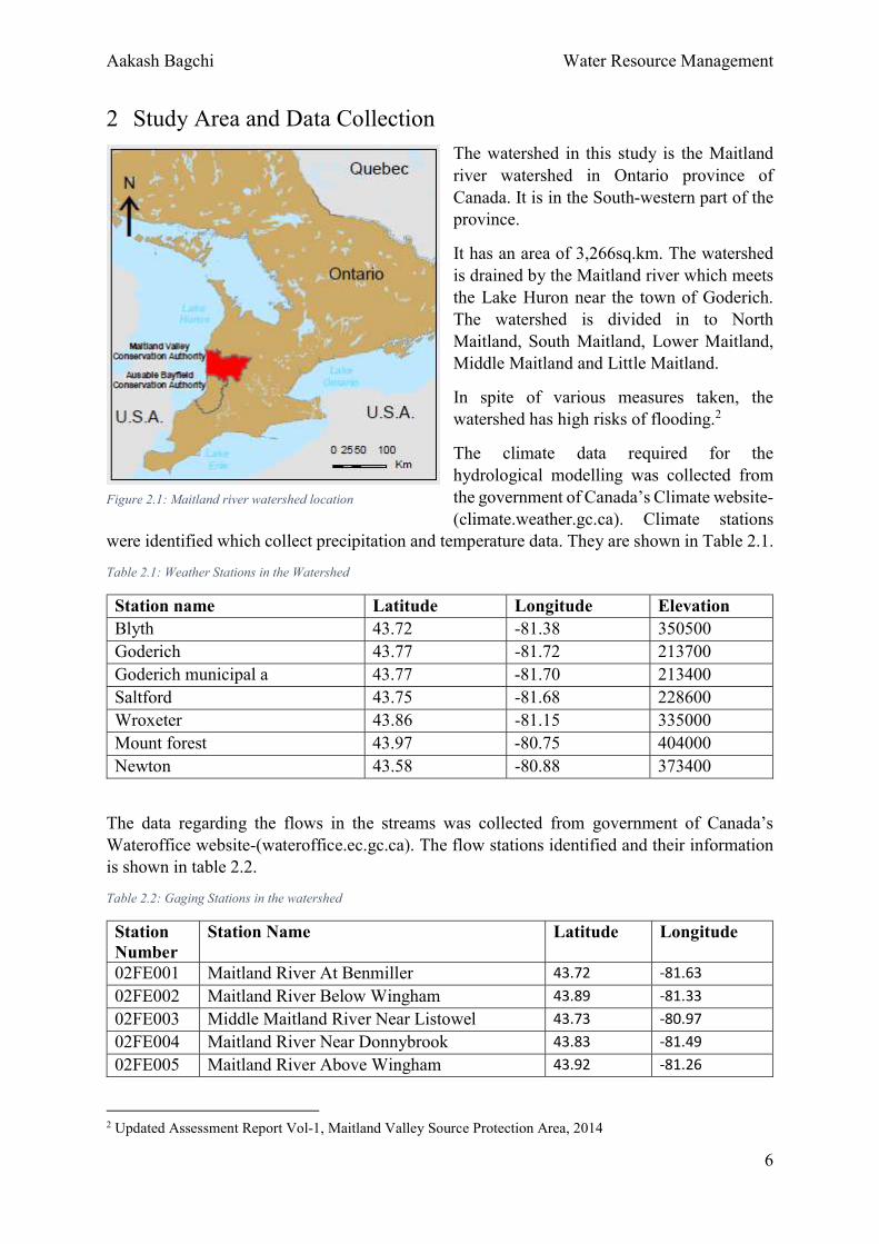
2 Study Area and Data Collection The watershed in this study is the Maitland river watershed in Ontario province of Canada. It is in the South-western part of the province. It has an area of 3,266sq.km. The watershed is drained by the Maitland river which meets the Lake Huron near the town of Goderich. The watershed is divided in to North Maitland, South Maitland, Lower Maitland, Middle Maitland and Little Maitland. In spite of various measures taken, the watershed has high risks of flooding.2 The climate data required for the hydrological modelling was collected from the government of Canada’s Climate website-(climate.weather.gc.ca). Climate stations

were identified which collect precipitation and temperature data. They are shown in Table 2.1. Table 2.1: Weather Stations in the Watershed Station name Latitude Longitude Elevation Blyth 43.72 -81.38 350500 Goderich 43.77 -81.72 213700 Goderich municipal a 43.77 -81.70 213400 Saltford 43.75 -81.68 228600 Wroxeter 43.86 -81.15 335000 Mount forest 43.97 -80.75 404000 Newton 43.58 -80.88 373400

The data regarding the flows in the streams was collected from government of Canada’s Wateroffice website-(wateroffice.ec.gc.ca). The flow stations identified and their information is shown in table 2.2. Table 2.2: Gaging Stations in the watershed Station Number

Station Name Latitude Longitude 02FE001 Maitland River At Benmiller 43.72 -81.63 02FE002 Maitland River Below Wingham 43.89 -81.33 02FE003 Middle Maitland River Near Listowel 43.73 -80.97 02FE004 Maitland River Near Donnybrook 43.83 -81.49 02FE005 Maitland River Above Wingham 43.92 -81.26

2 Updated Assessment Report Vol-1, Maitland Valley Source Protection Area, 2014

Figure 2.1: Maitland river watershed location


7

02FE007 Little Maitland River At Bluevale 43.85 -81.25 02FE008 Middle Maitland River Near Belgrave 43.81 -81.31 02FE009 South Maitland River At Summerhill 43.68 -81.54 02FE010 Boyle Drain Near Atwood 43.68 -81.07 02FE011 Maitland River Near Harriston 43.90 -80.89 02FE012 Lake Huron At Goderich 43.75 -81.73 02FE013 Middle Maitland River Above Ethel 43.72 -81.12 02FE014 Blyth Brook Below Blyth 43.76 -81.46 02FE015 Maitland River At Benmiller 43.72 -81.63 02FE016 South Maitland River At Roxboro 43.58 -81.40 02FE017 Lakelet Creek Near Gorrie 43.89 -81.06 02FF011 Silver Creek At Seaforth 43.55 -81.40 02FF015 Tricks Creek Near Clinton 43.59 -81.58 02GA042 Moorefield Creek Near Rothsay 43.82 -80.72

The topographical data required for Hydrological modelling was already available in the form of mosaic datasets (DEM-Digital Elevation Models). These were selected according to the location and converted to raster datasets for modelling purpose. The Land-use dataset was downloaded through the Scholars GeoPortal. A table was prepared to link the land-use and crop names to the default names used by SWAT. The soil database was downloaded from Ontario Soil database. An attempt was made to create a database of soils for the watershed but due to a lack of time, it could not be completed. Efforts were made to link the default soil database to soils of similar properties found in the watershed under study. But there might be variations/errors in the outputs due to the soil database not being proper.


8

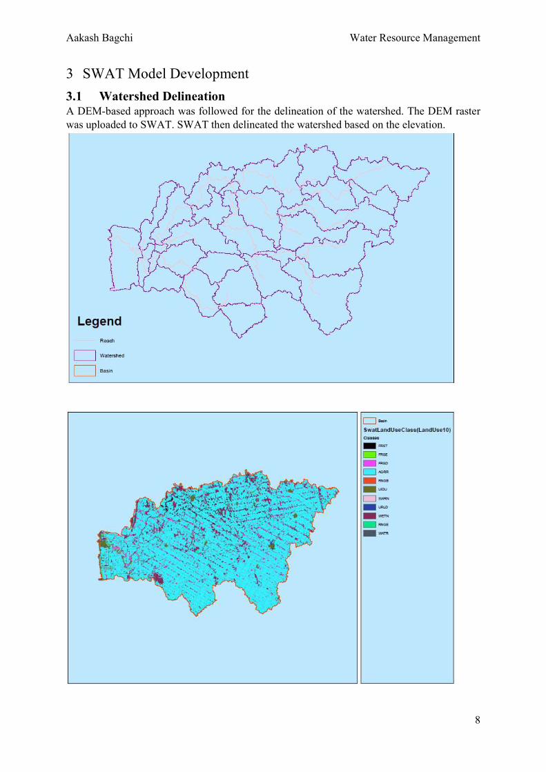
3 SWAT Model Development 3.1 Watershed Delineation A DEM-based approach was followed for the delineation of the watershed. The DEM raster was uploaded to SWAT. SWAT then delineated the watershed based on the elevation.


9

3.2 HRU Analysis The Land-use dataset was uploaded into SWAT and a look-up table was prepared to link the SWAT default crop names with those in the dataset. The soil dataset was uploaded into SWAT. The slope was classified as multiple slopes with maximum gradient of 10% in the first class. Most of the watershed is in this category.

3.3 Weather Data The period of simulation for calibration, validation of the model chosen was 1970-1980. Climate data for 3 weather stations in the watershed was available for this simulation. While Flow data was available for 8 gaging stations for this period of simulation. This was used during the calibration-validation stage.


10

4 Results and Discussions 4.1 Calibration-Validation Calibration of the model was done by changing the CN2 parameter in SWAT. Figure 4.2 shows the comparison between SWAT streamflow values and corresponding actual data acquired from the gaging station for the year 1977.

The figure 4.1 shows the comparison between simulated flow and actual after tweaking the CN2 parameter in the model. For validation puposes, the data for the year 1973 was chosen. The figure 4.3 shows the comparison between modelled and actual data for the year 1973.

050

100150200250300

1 2 3 4 5 6 7 8 9 10 11 12

1977

SWAT_1 Data

020406080

100120140160180200

1 2 3 4 5 6 7 8 9 10 11 12

1977

SWAT_2 Data

Figure 4.2: Pre-calibration stream flow comparison

Figure 4.1: Post-Calibration Streamflow comparison


11

4.2 Water Budget Analysis 4.2.1 Water Yield The analysis of the outputs from the model shows that about 80% of the total run-off in the watershed occurs during the months of December to May. (Figure 4.5) The water budget for the watershed showing average values for a 10-year period from 1970-1979 is shown in table 4.1. Table 4.1: Water Budget for Maitland watershed MON SNOW WATER

RAIN FALL IN SURF Q LAT Q YIELD ET OUT (MM) (MM) (MM) (MM) (MM) (MM)

1 99.89 56.65 156.54 8.43 6.22 83.62 15.41 113.68 2 60.83 31.94 92.77 4.57 4.2 84.27 22.5 115.54 3 71.14 31.3 102.44 8.64 3.41 87.07 40.03 139.15 4 71.5 33.52 105.02 1.81 1.37 58.35 38.55 100.08 5 93.58 45.5 139.08 5.84 0.97 41.71 50.61 99.13 6 76.88 31 107.88 7.17 0.92 29.86 70.9 108.85 7 82.3 34.66 116.96 3.32 0.66 16.51 57.4 77.89 8 93.6 36.57 130.17 1.25 0.85 10.52 36.28 48.9 9 91.57 39.47 131.04 0.93 0.91 11.08 32.87 45.79 10 85.04 39.06 124.1 0.68 0.84 12.74 29.18 43.44 11 90.04 40.21 130.25 4.94 3.69 22.49 21.6 52.72 12 100.61 51.24 151.85 26.37 8.29 79.71 16.34 130.71

0.0020.0040.0060.0080.00

100.00120.00

1 2 3 4 5 6 7 8 9 10 11 12

1973

Data SWATFigure 4.3: Validation of model using streamflow values


12

01020304050607080

1 2 3 4 5 6 7 8 9 10 11 12

ET

0102030405060708090

100

1 2 3 4 5 6 7 8 9 10 11 12

Run-off

Figure 4.5: Average monthly run-off for 1970-1980

Figure 4.4: Average monthly Evapotranspiration for 1970-1980


13

5 Climate Change Impact Analysis The climate data for climate change analysis was collected from the SWAT website (swat.tamu.edu). The scenarios chosen for analysis were A2 and B1. The IPCC recommends using as many scenarios as possible for analysis of impacts due to climate change as the probability of occurrence of each scenario is equally plausible. The data downloaded was downscaled from the CCCMA-CGCM3.1 GCM. This is the third generation of the coupled GCM developed by Canadian Centre for Climate Modelling and Analysis. The resolution of this GCM is approximately 3.75degrees lat/long over land with 31 vertical layers while over the oceans it is 1.85degress lat/long with 29 vertical layers. Historical data was for a 40-year period from 1961-2000, while the simulated climate data for both the scenarios was for a period from 2046-2064. The data was used to run the SWAT model keeping all other parameters like Land-use and Soil same as used for calibration. The data was corrected for any biases. Then the corrected data was used to run the model finally to analyse the results. 5.1 Bias Correction The model was run using historical data from the period 1970-1980 and compared with results obtained from observed data during the same period. There was a bias found in the data which was corrected. The figure 5.1 shows the difference between downloaded and bias corrected data for the precipitation during the above-mentioned period in terms of average monthly precipitation for the 10-year period. The figure 5.2 and 5.3 shows the difference between the downloaded and bias corrected data for minimum and maximum temperatures respectively, in terms of average monthly temperatures for the 10-year period.

00.5

11.5

22.5

33.5

4

1 2 3 4 5 6 7 8 9 10 11 12Downloaded Bias removed

Figure 5.1: Bias correction of precipitation data


14

A simple statistical method was used for the bias correction process. The average variation over all the data values was calculated and then the values were corrected for the same average variation. This process was followed for both the temperature and precipitation data. 5.2 Results and Discussions 5.2.1 Change in Temperature over time The analysis of the average maximum temperatures and minimum temperatures in the historical data considering 4 numbers of 10-year periods is shown in table 5.1. Table 5.1: Change in temperature over time 61-70 71-80 81-90 91-00 B1 A2 Maximum Temeratures -0.79 3.15 2.79 3.87 2.79 3.86 Winter

23.80 24.25 24.70 25.81 27.17 27.43 Summer Minimum Temperatures -6.99 -4.10 -4.06 -2.96 -3.49 -2.47 Winter

13.50 14.26 14.44 15.69 17.16 17.56 Summer

-505

1015202530

1 2 3 4 5 6 7 8 9 10 11 12

Downloaded Bias Corrected

-15-10

-505

101520

1 2 3 4 5 6 7 8 9 10 11 12

Downloaded Bias Corrected

Figure 5.3: Bias correction of maximum temperature data

Figure 5.2: Bias correction of minimum temperature data


15

The general trend as shown in figures 5.5 and 5.6 is that for every consecutive 10-year period the average temperatures tend to rise. This trend continues in both the future scenarios. The rise is steeper in the A2 scenario. The minimum winter temperatures show a decrease in the B1 scenario. Over the study period, an increase in the maximum temperature recorded in the year increases while minimum temperature recorded in the year also increases.

Similar analysis for the precipitation was done, as shown in figure 5.6.

Similar trend is shown by the precipitation chart. Precipitation tends to increase over each successive 10-year period in the historical data. Also, both scenarios show an increase in precipitation. A2 showing the highest amount. Only one decade 2046-2055 was considered in the case of future scenarios. Another analysis was done to calculate the number of days where intense rainfall was observed. For this the average number of days each month over a period of 10 years was calculated where the rainfall was more than 30mm. Interestingly, the average number of days tends to increase for each successive decade as shown in figure 5.7.

970.821 992.413 1014.855 1027.297 1056.338

1150.412

850900950

10001050110011501200

61-70 71-80 81-90 91-00 B1 A2

Precipitation

2022242628

61-70 71-80 81-90 91-00 B1 A2

Summer

-8-6-4-20

61-70 71-80 81-90 91-00 B1 A2

Winter

Figure 5.5: Trend for Summer maximum temperatures Figure 5.4: Trend for Winter minimum temperatures

Figure 5.6: Trend for precipitation


16

While there were only an average of around 2 days every month in the decade starting from 1961, the number increases to more than 3 in the decade starting 1991. In case of future scenarios, the number remains same for the B1 scenario while it increases further for the A2 scenario.

This is an important point to note. Since as the intensity of rainfall increases, the quantity of surface run-off also increases as soils become saturated. This can lead to problems like erosion, poor quality of water etc. 5.3 Results of SWAT simulation 5.3.1 Streamflow The average monthly stream flow for all three cases, historical data, scenarios B1 and A2 are compared in figures 5.8 to 5.10.

1.92.5 2.8

3.4 3.44

00.5

11.5

22.5

33.5

44.5

61-70 71-80 81-90 91-00 B1 A2

>30mm

69.5680.71

63.51

45.2 42.3532.09 27.96 23.77 24.87

31.22

50.4557.69

0102030405060708090

1 2 3 4 5 6 7 8 9 10 11 12

WATER YIELD (MM)-Historical

Figure 5.7: Trend for number of days receiving more than 30mm of precipitation

Figure 5.8: Monthly averages of water yield for historical simulation


17

There is an increase in the maximum stream flow while a decrease in the minimum flow comparing the historical and future cases. Thus, the variation in flow increases in the future scenarios. The pattern of flow has also changed. Whereas, in the historical analysis, the peak flows occurred in the month of February, in the future scenarios, the peak flows occur earlier, in the month of January. Similarly, low streamflows which generally occurred in the month of August, will occur earlier, in the month of July. 5.3.2 Evapotranspiration Increased evaporation is noticed in the future scenarios. While the amount of losses due to evaporation show a general trend of increasing, the peak values also occur earlier than before. While in the historical simulation, the peak value occurs during the month of July, the peak occurs in the month of June itself in the future scenarios. Increased evaporation is a direct result of warmer temperatures. As seen earlier in the report, the temperatures show a general increasing trend over time.

93.83

69.48 62.4652.51

32.3917.77 17.22 23.43 29.37

54.13

78.8188.05

0102030405060708090

100

1 2 3 4 5 6 7 8 9 10 11 12

WATER YIELD (MM)-B1

92.25 90.0174.44

55.76

37.78

19.07 15.24 20.53

41.02

64.15 69.98

92.12

0102030405060708090

100

1 2 3 4 5 6 7 8 9 10 11 12

WATER YIELD (MM)-A2Figure 5.10: Monthly averages of water yield for future scenario B1

Figure 5.9: Monthly averages of water yield for future scenario A2


18

5.5613.39

33.8744.41

53.7367.02

89.5975.41

48.231.15

14.17 8.150

102030405060708090

100

1 2 3 4 5 6 7 8 9 10 11 12

ET (MM)-Historical

9.5721.75

43.0350.11

66.17

92.5885.1

59.4542.04

20.689.76 7.71

0102030405060708090

100

1 2 3 4 5 6 7 8 9 10 11 12

ET(MM)-B1

10.8622.54

46.08 54.4773.91

96.3485.49

58.4435.36

19.6110 7.17

020406080

100120

1 2 3 4 5 6 7 8 9 10 11 12

ET (MM)-A2

Figure 5.13: Monthly averages of ET for historical simulation

Figure 5.12: Monthly averages for ET for future scenarion B1

Figure 5.11: Monthly averages of ET for future scenario A2


19

6 Conclusions and Adaptation Strategies The first step in this process is to understand the extent of change expected due warmer climates and erratic precipitation. In this process, the climate models developed by various organisations based on IPCC’s scenarios help. They quantify the extent of climate change expected in the near or middle future. Once the extent of change in a certain time period is found, then measures have to be taken to adapt to this change in climate. It is observed that the variability in streamflows increases in the future scenarios. Coupled with increased evaporative losses due to warmer temperatures, this will mean erratic water supply. The ground water supply will also decrease with change in pattern of precipitation. High intensity rainfall will reduce the percolation capacity of the soil, thereby reducing the groundwater content. Higher surface runoff due to reduced percolation will impact the quality of water entering the stream. This would require higher investment in water treatment infrastructure. In terms of use of water, the maximum use is in agriculture and livestock. Irrigation water is the difference of the requirement of water for a crop and the precipitation. If the water holding capacity of the soil is reduced due to change in precipitation patterns, more irrigation water will be required. Irrigation infrastructure needs to built to meet the higher requriements of the future. For industrial uses, the costs of treatment of water will increase as streamflow reduces. The change in pattern of precipitation and thus streamflows will require change in the existing water management infrastructure. As the water demand increases with increase in population and the pattern of the natural water storage in streams and reservoirs changes, it becomes important to look at efficient measn of using the available water. For domestic uses, this requires use of low-flow fixtures, harnessing the rain water through storage or recharge, putting emphasis on re-use of water etc. For Industrial uses, this requires more use of treated wastewater. In terms of process changes, this would imply using more closed loop systems where water is treated and re-used in the same system. For agricultural uses, this requires various methods like irrigation during the night so that evaporative losses are reduced, using treated effluent for irrigation, using efficient irrigation methods like drip irrigation, development of crop varieties which require less water etc.

References J.W.H. (Jan Hendrik) van Petegem, Fred Wegman, “Analyzing road design risk factors for run-off-road crashes in the Netherlands with crash prediction models”, Journal of Safety Research, Vol 49, Pg 121-127, 2014 Jan F. Feenstra, Ian Burton, Joel B. Smith, Richard S.J. Tol, “Handbook on Methods for Climate Change Impact Assessment and Adaptation Strategies”, United Nations Environment Programme, 1998 Kangsheng Wu, Carol A. Johnston, “Hydrologic response to climatic variability in a Great Lakes Watershed: A case study with the SWAT model”, Volume 337, Issues 1–2, Pg 187–199, 2007 Maitland Valley Source Protection Area, “Updated Assessment Report”, Volume-1, 2014 H. Ahmad, R. Jamieson, P. Havard, A. Madani, Q. Zaman, “Evaluation of SWAT for a small watershed in Eastern Canada”, EFITA Conference, Pg 337-343, 2009 K. Y. Raneesh, G. Thampi Santosh, “A study on the impact of climate change on streamflow at the watershed scale in the humid tropics”, Hydrological Sciences Journal, 56:6, Pg 946-965, 2011 EBNFLO Environmental AquaResource Inc., “Guide for Assessment of Hydrologic Effects of Climate Change in Ontario”, 2010 Christopher B. Field, Vicente R. Barros, “Climate Change 2014: Impacts, Adaptation, and Vulnerability”, 2014

Hydrologic Modelling of Maitland River Watershed and Assessing Impacts of Climate Change using SWAT

Documents

Transcript of Hydrologic Modelling of Maitland River Watershed and Assessing Impacts of Climate Change using SWAT