Hydraulic Design of Geosynthetic and Granular Liquid Collection Layers Comprising Two Different...
96
285 GEOSYNTHETICS INTERNATIONAL S 2000, VOL. 7, NOS. 4-6 Technical Paper by J.P. Giroud, J.G. Zornberg, and A. Zhao HYDRAULIC DESIGN OF GEOSYNTHETIC AND GRANULAR LIQUID COLLECTION LAYERS ABSTRACT: The present paper provides equations for the hydraulic design of liquid collection layers. A first series of equations gives the maximum thickness of the liquid col- lected in a liquid collection layer. These equations are used in design to check that the maxi- mum liquid thickness is less than an allowable thickness. Some of the equations make it possible to rigorously calculate the liquid thickness, whereas other equations, which are sim- pler, give an approximate value of the liquid thickness. A second series of equations makes it possible to calculate the required hydraulic conductivity of the liquid collection layer mate- rial and the required hydraulic transmissivity of the liquid collection layer. These equations are useful for selecting the material used to construct the liquid collection layer. The equa- tions provided in the present paper include reduction factors to quantify the decrease in flow capacity of liquid collection layers due to thickness reduction (caused by the applied stresses) and hydraulic conductivity reduction (caused by clogging). Practical recommendations and design examples are presented for both geosynthetic and granular liquid collection layers. KEYWORDS: Liquid collection layer, Leachate collection layer, Leakage detection and collection layer, Drainage layer, Thickness, Granular, Geosynthetic. AUTHORS: J.P. Giroud, Chairman Emeritus, GeoSyntec Consultants, 621 N.W. 53rd Street, Suite 650, Boca Raton, Florida 33487, USA, Telephone: 1/561-995-0900, Telefax: 1/561-995-0925, E-mail: [email protected]; J.G. Zornberg, Assistant Professor, Department of Civil, Environmental and Architectural Engineering, University of Colorado at Boulder, Campus Box 428, Boulder, Colorado 80309-0428, USA, Telephone: 1/303-492-4699, Telefax:1/303-492-7317, E-mail: [email protected]; and A. Zhao, Vice President of Engineering, Tenax Corp., 4800 E. Monument Street, Baltimore, Maryland 21205, USA, Telephone: 1/410-522-7000, Telefax: 1/410-522-7015, E-mail: [email protected]. PUBLICATION: Geosynthetics International is published by the Industrial Fabrics Association International, 1801 County Road B West, Roseville, Minnesota 55113-4061, USA, Telephone: 1/651-222-2508,Telefax: 1/651-631-9334. Geosynthetics International is registered under ISSN 1072-6349. DATES: Original manuscript submitted 12 July 2000, revised version received 4 October 2000, and accepted 7 October 2000. Discussion open until 1 June 2001. REFERENCE: Giroud, J.P., Zornberg, J.G., and Zhao, A., 2000, “Hydraulic Design of Geosynthetic and Granular Liquid Collection Layers”, Geosynthetics International, Special Issue on Liquid Collection Systems, Vol. 7, Nos. 4-6, pp. 285-380.
Transcript of Hydraulic Design of Geosynthetic and Granular Liquid Collection Layers Comprising Two Different...
285GEOSYNTHETICS INTERNATIONAL S 2000, VOL. 7, NOS. 4-6
Technical Paper by J.P. Giroud, J.G. Zornberg, and A. Zhao
HYDRAULIC DESIGN OF GEOSYNTHETIC ANDGRANULAR LIQUID COLLECTION LAYERS
ABSTRACT: The present paper provides equations for the hydraulic design of liquidcollection layers. A first series of equations gives the maximum thickness of the liquid col-lected in a liquid collection layer. These equations are used in design to check that the maxi-mum liquid thickness is less than an allowable thickness. Some of the equations make itpossible to rigorously calculate the liquid thickness, whereas other equations, which are sim-pler, give an approximate value of the liquid thickness. A second series of equations makesit possible to calculate the required hydraulic conductivity of the liquid collection layermate-rial and the required hydraulic transmissivity of the liquid collection layer. These equationsare useful for selecting the material used to construct the liquid collection layer. The equa-tions provided in the present paper include reduction factors to quantify the decrease in flowcapacity of liquid collection layersdue to thickness reduction (caused by the applied stresses)and hydraulic conductivity reduction (caused by clogging). Practical recommendations anddesign examples are presented for both geosynthetic and granular liquid collection layers.
KEYWORDS: Liquid collection layer, Leachate collection layer, Leakage detection andcollection layer, Drainage layer, Thickness, Granular, Geosynthetic.
AUTHORS: J.P. Giroud, Chairman Emeritus, GeoSyntec Consultants, 621 N.W. 53rdStreet, Suite 650, Boca Raton, Florida 33487, USA, Telephone: 1/561-995-0900, Telefax:1/561-995-0925, E-mail: [email protected]; J.G. Zornberg, Assistant Professor,Department of Civil, Environmental and Architectural Engineering, University of Coloradoat Boulder, Campus Box 428, Boulder, Colorado 80309-0428, USA, Telephone:1/303-492-4699, Telefax:1/303-492-7317, E-mail: [email protected]; and A. Zhao,Vice President of Engineering, Tenax Corp., 4800 E.Monument Street, Baltimore,Maryland21205, USA, Telephone: 1/410-522-7000, Telefax: 1/410-522-7015, E-mail:[email protected].
PUBLICATION: Geosynthetics International is published by the Industrial FabricsAssociation International, 1801 County Road B West, Roseville, Minnesota 55113-4061,USA, Telephone: 1/651-222-2508, Telefax: 1/651-631-9334.Geosynthetics International isregistered under ISSN 1072-6349.
DATES: Original manuscript submitted 12 July 2000, revised version received 4 October2000, and accepted 7 October 2000. Discussion open until 1 June 2001.
REFERENCE: Giroud, J.P., Zornberg, J.G., and Zhao, A., 2000, “Hydraulic Design ofGeosynthetic and Granular Liquid Collection Layers”,Geosynthetics International, SpecialIssue on Liquid Collection Systems, Vol. 7, Nos. 4-6, pp. 285-380.

GIROUD, ZORNBERG, AND ZHAO D Hydraulic Design of Liquid Collection Layers
286 GEOSYNTHETICS INTERNATIONAL S 2000, VOL. 7, NOS 4-6
1 INTRODUCTION
1.1 Liquid Collection Layers
Liquid collection layers are used to collect liquid and to convey the collected liquidby gravity to a low point such as a sump. Liquid collection layers are used in a varietyof geotechnical and geoenvironmental structures: (i) they are used as drainage blanketsin dams, embankments, roads, landslide repair, etc.; (ii) they are used as leachate collec-tion layers in landfills (where they are also called “primary leachate collection layers”);and (iii) they are used, underneath a liner, as leakage detection and collection layers inlandfills (where they are also called “secondary leachate collection layers”) and in liq-uid containment structures such as ponds, canals, reservoirs, dams, etc. Based on theseexamples, it appears that there are two categories of liquid collection layers: (i) thedrainage layers (or “primary liquid collection layers”) that collect liquid that percolatethrough a mass of soil or waste; and (ii) the leakage collection layers (or “secondaryliquid collection layers”) that collect liquid that leaks through a liner.
1.2 Liquid Collection Layer Materials
Liquid collection layers are constructed with materials that can convey liquids, i.e.materials that can perform the liquid transmission function (referred to, hereafter, as thetransmission function). Materials that can perform the transmission function includegranular materials and thick geosynthetics.
Granular materials include gravel, sand, andmixtures of these two materials. Liquidcollection layers constructed with gravel are generally protected from clogging by mi-grating particles using a filter. The filter may be a layer of sand or a geotextile.
Geosynthetics that can perform the transmission function are thick geosyntheticshaving a high hydraulic conductivity in the direction of their plane. These geosyntheticsare characterized by a high hydraulic transmissivity, which is the product of the hydrau-lic conductivity by the thickness. Geosynthetics having a high hydraulic transmissivityinclude thick needle-punched nonwoven geotextiles and a variety of geosyntheticssometimes generically called “geospacers”, such as geonets, geomats, cuspated poly-meric plates, embossed polymeric plates, formed plastic products, etc. Geospacers havea much greater hydraulic transmissivity than thick needle-punched nonwoven geotex-tiles; therefore, geospacers, in particular geonets and geomats, are usedmore often thanneedle-punched nonwoven geotextiles as liquid collection layers. However, there arenumerous examples of geotechnical structures, including dams, where thick needle-punched nonwoven geotextiles have been successfully used for drainage. Geonets, geo-mats, and other geospacers are generally in contact with a geotextile on one side or onboth sides; this geotextile serves asa filter between the geospacer and soil, or as a frictionlayer (bonded to the geospacer) to increase interface shear strength between the geo-spacer and a geomembrane. When a geospacer is bonded to one or two geotextiles ina factory, the product thus obtained is referred to as a geocomposite. The layer that per-forms the transmission function in a geocomposite is referred to as the transmissivecomponent of the geocomposite, or transmissive core. In the context of the present pa-per, the term “geocomposite” is used in all cases where a polymeric transmissivemateri-

GIROUD, ZORNBERG, AND ZHAO D Hydraulic Design of Liquid Collection Layers
287GEOSYNTHETICS INTERNATIONAL S 2000, VOL. 7, NOS. 4-6
al is associated with a geotextile, whether the transmissive material and the geotextilewere bonded together in a factory or sequentially installed against each other in the field.
1.3 Purpose and Organization of the Present Paper
The purpose of the present paper is to provide a complete methodology for the hy-draulic design of liquid collection layers. In the context of the present paper, the ter-minology “hydraulic design” refers to the design steps required to check that the liquidcollection layer being designed has sufficient flow capacity to ensure that the thicknessof liquid in the liquid collection layer is less than an allowable thickness (Section 1.6).Therefore, the hydraulic design of liquid collection layers requires the calculation ofthe maximum liquid thickness. To that end, the present paper provides in Section 2 avariety of relationships between the maximum liquid thickness, the liquid supply, thecharacteristics of the liquid collection layer, and the geometry of the slope on which theliquid collection layer is located. Some of the relationships are relatively complex andgive accurate solutions; others are relatively simple and give approximate solutions.The validity of all approximations is assessed, and practical guidance is given for theuse of the equations.
The hydraulic design of a liquid collection layer can be done by following one oftwo approaches: the “thickness approach” and the “hydraulic characteristic approach”.With the thickness approach, a given liquid collection material is considered and thedesign engineer checks that the maximum liquid thickness is less than the allowablethickness. The thickness approach is described in Section 3.With the hydraulic charac-teristic approach, the design engineer determines the hydraulic characteristics of theliquid collection material needed to ensure that the liquid thickness is less than the al-lowable thickness. The hydraulic characteristic approach is described in Section 4.De-sign examples are used to illustrate both approaches.
The equations presented in Section 2 (and the application of these equations present-ed in Sections 3 and 4) are not valid for vertical liquid collection layers. The case ofvertical (and quasi-vertical) liquid collection layers will be addressed in a future paper.
1.4 Definitions and Assumptions
1.4.1 Description and Geometry of Liquid Collection Layers
The liquid collection layer is assumed to be underlain by an impermeable liner.Therefore, no liquid is lost by infiltration into or through the material underlying theliquid collection layer.
The liquid collection layer is located on a slope with an angle β (Figure 1). The slopeangle is assumed to be less than 90_ (β< 90_). The case of vertical liquid collectionlayers is not addressed in the present paper.
There is an effective drain at the toe of the slope and the liquid level in the drain isalways significantly lower than the elevation of the liner at the toe of the slope. There-fore, the flowof liquid in the liquid collection layer is not impeded at the toe of the slope.
For the development of the equations presented in the present paper, the liquidcollection layer is assumed to be rectangular with a length, L, measured in the directionof the flow (i.e. the direction of the slope), and a width, B, perpendicular to the direction
GIROUD, ZORNBERG, AND ZHAO D Hydraulic Design of Liquid Collection Layers
288 GEOSYNTHETICS INTERNATIONAL S 2000, VOL. 7, NOS 4-6
L
Liner Drain
tLCL
Figure 1. Liquid collection layer.
β
L / cosβ
H = L tan β
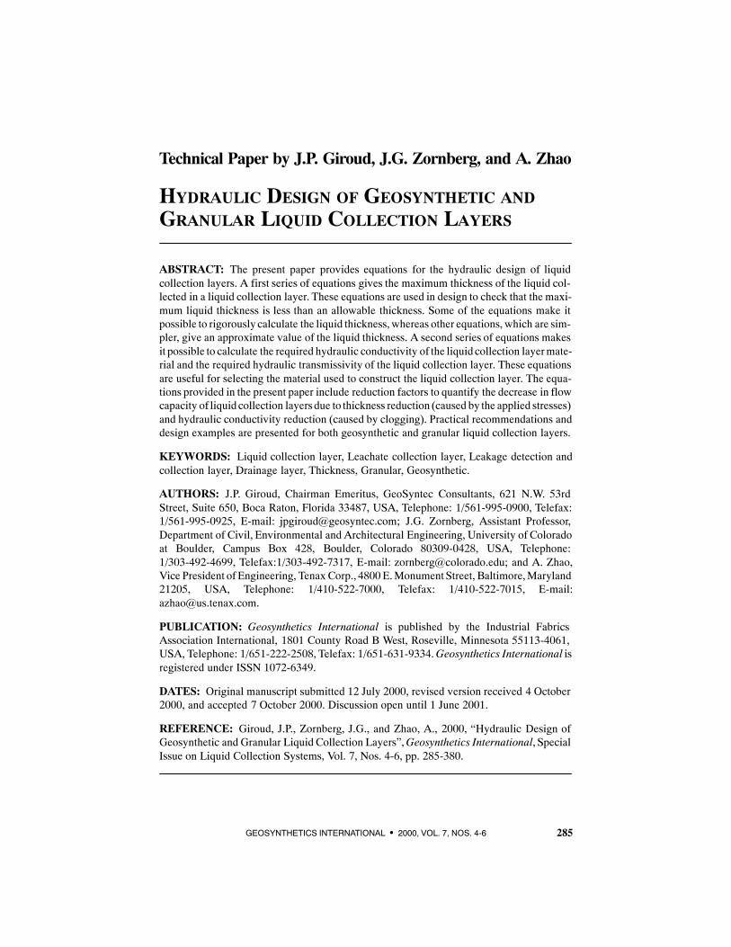
of the flow. The length, L, is measured horizontally (i.e. L is the length of the horizontalprojection of the slope), whereas the width, B, is horizontal.
The thickness of the liquid collection layer is tLCL measured perpendicular to theslope (Figure 1). It is important to note that, when a geocomposite is used as a liquidcollection layer, tLCL is the thickness of the transmissive component of the geocompo-site (i.e. the core of the geocomposite), not the total thickness of the geocomposite in-cluding the geotextile (Section 1.2).
1.4.2 Hydraulic Characteristics of Liquid Collection Layers
The liquid collection layer material is characterized by its hydraulic conductivity,k. The liquid collection layer is characterized by its hydraulic transmissivity, θ, whichis defined by the following equation:
(1)LCLk tθ =
where tLCL is the thickness of the transmissive component of the geocomposite. Whenthe liquid collection layer is a geosynthetic, the hydraulic transmissivity of the geosyn-thetic is measured using a hydraulic transmissivity test. The hydraulic conductivity ofthe geosynthetic is then derived from the hydraulic transmissivity using the followingequation derived from Equation 1:
(2)ktLCL
= θ
Equation 2 is very useful because in a number of the equations provided in the pres-ent paper, the relevant property of the liquid collection layer material is the hydraulicconductivity,whereas the given properties in the case of a geosynthetic liquid collectionlayer are generally the hydraulic transmissivity and the thickness.
It should be noted that hydraulic transmissivity and hydraulic conductivity of geo-synthetics are not constant material properties, as they are functions of the hydraulicgradient (and, consequently, of the slope of the liquid collection layer). Hydraulic trans-missivity and hydraulic conductivity values should, therefore, be obtained from testsperformed under a range of hydraulic gradients representative of field conditions.
GIROUD, ZORNBERG, AND ZHAO D Hydraulic Design of Liquid Collection Layers
289GEOSYNTHETICS INTERNATIONAL S 2000, VOL. 7, NOS. 4-6
1.4.3 Liquid Thickness, Depth, and Head
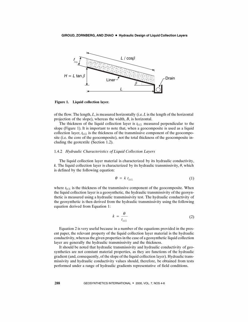
The flow is characterized by the liquid thickness, t, which is measured in the direc-tion perpendicular to the slope (Figure 2). The liquid thickness is different from the liq-uid depth, which is measured vertically. When liquid flows parallel to the slope, whichis approximately the case in all liquid collection layers (and which is exactly the caseat the location where liquid thickness is maximum), the following classical relation-ships exist:
(3)t D= cosβ
(4)t h= / cosβ
(5)2cosh D β=
where: D = liquid depth; β = slope angle; and h = hydraulic head. The hydraulic head(or, more accurately, the hydraulic head above the liner located at the base of the liquidcollection layer) is the difference in elevation between two points located on the sameequipotential surface, one being on the liquid surface, the other being on the liner (seethe note below the Figure 2 caption).
1.4.4 Liquid Supply and Flow
The amount of liquid supplied to the liquid collection layer is defined by the rate ofliquid supply, which is the volume of liquid per unit area and unit time supplied to the
Figure 2. Thickness, depth, and head of liquid on top of the liner in the case ofunconfined flow parallel to a slope.Notes: AB is an equipotential line because it is perpendicular to the flow lines. The head above the liner,h, is the difference in elevation between Points B and A.
= Liquid head= Liquid depth= Liquid thickness
hDt
h
Unconfinedflow
B
A
tD
b
b
GIROUD, ZORNBERG, AND ZHAO D Hydraulic Design of Liquid Collection Layers
290 GEOSYNTHETICS INTERNATIONAL S 2000, VOL. 7, NOS 4-6
liquid collection layer. Theoretically, any orientation may be selected for the unit areaused in the definition of the rate of liquid supply, provided that this orientation is proper-ly taken into account in the calculations. For the sake of simplicity, a horizontal unitarea is used in the definition of the rate of liquid supply for the case of liquid collectionlayers that are not vertical (i.e. the cases addressed in the present paper). The rate ofliquid supply is then noted qh and is defined by the following equation:
(6)hh
h
QqA
=
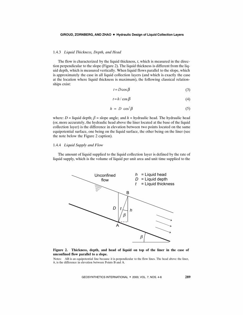
where Qh is the rate of liquid flow through a horizontal area Ah .The rate of liquid flow through a horizontal area, Ah , can be measured using a hori-
zontal pan with a surface area Ah (Figure 3):
(7)/h h LQ A D t∗= ∆
where DL is the depth of liquid collected in the pan during the time Δt* .Combining Equations 6 and 7 gives:
(8)Lh
Dqt∗
=∆
Equations 6, 7, and 8 can be used with any set of coherent units. The basic SI unitsare: Qh (m3/s), Ah (m2), DL (m), Δt* (s), and qh (m/s). For example, if the liquid supplyis rainwater, and 100 mm of rain is collected in one day, DL = 0.1 m and Δt* = 1 day= 86,400 s. Equation 8 then gives qh = 0.1/86,400 = 1.157 × 10⁻⁶ m/s.
Figure 3. Measurement of the rate of liquid flow through a horizontal area.
DL
Horizontal pan
Precipitation
GIROUD, ZORNBERG, AND ZHAO D Hydraulic Design of Liquid Collection Layers
291GEOSYNTHETICS INTERNATIONAL S 2000, VOL. 7, NOS. 4-6
It should be noted that no assumption is required regarding the orientation of therainfall; i.e., whether the rain falls vertically or at an angle, the definition of qh remainsthe same. In the present paper, it is assumed that the rate of liquid supply is uniformoverthe entire area of the liquid collection layer and is constant over time (i.e. steady-stateflow conditions are assumed).
Water and aqueous liquids are incompressible; therefore, mass conservation resultsin volume conservation. Since steady-state flow conditions are assumed, the principleof mass conservation results not only in volume conservation, but also in flow rate con-servation. Also, the flow is assumed to be unconfined (Section 1.3), i.e. the consideredequations are valid only if the maximum liquid thickness, tmax , is less than the thicknessof the liquid collection layer, tLCL .
Capillarity affects essentially unsaturated flow (i.e. flow in zones where the liquidcollection layer material is not saturated) and flow under transient conditions that pre-cede the establishment of steady-state flow conditions. In the present paper, the liquidcollection layer material is assumed to be saturated in the entire zone comprised belowthe liquid surface, and steady-state flow conditions are assumed, as mentioned above.Therefore, capillarity has no effect, or a negligible effect, on the type of flow discussedin the present paper. Consequently, capillarity is not considered in the present paper.
1.5 Description of Flow in Liquid Collection Layers
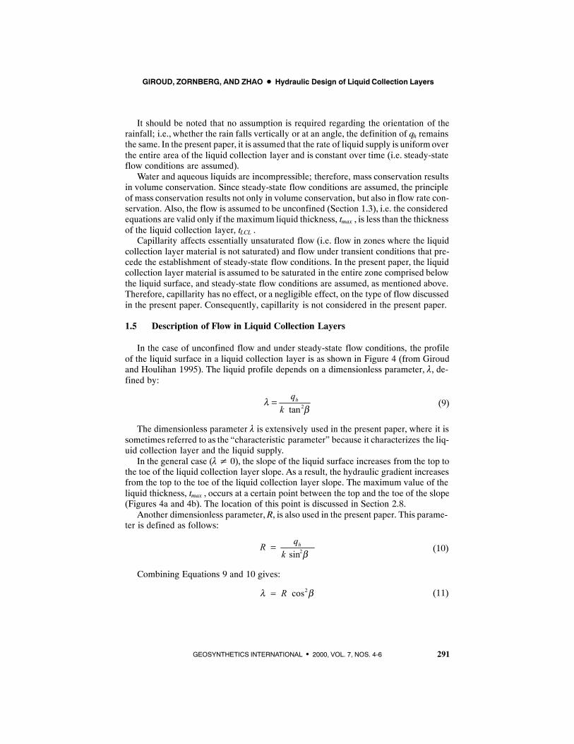
In the case of unconfined flow and under steady-state flow conditions, the profileof the liquid surface in a liquid collection layer is as shown in Figure 4 (from Giroudand Houlihan 1995). The liquid profile depends on a dimensionless parameter, λ, de-fined by:
(9)2tanhq
kλ
β=
The dimensionless parameter λ is extensively used in the present paper, where it issometimes referred to as the “characteristic parameter” because it characterizes the liq-uid collection layer and the liquid supply.
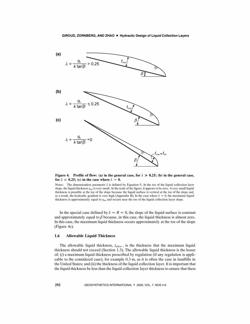
In the general case (λ≠ 0), the slope of the liquid surface increases from the top tothe toe of the liquid collection layer slope. As a result, the hydraulic gradient increasesfrom the top to the toe of the liquid collection layer slope. The maximum value of theliquid thickness, tmax , occurs at a certain point between the top and the toe of the slope(Figures 4a and 4b). The location of this point is discussed in Section 2.8.
Another dimensionless parameter,R, is also used in the present paper. This parame-ter is defined as follows:
(10)2sinhqR
k β=
Combining Equations 9 and 10 gives:
(11)2cosRλ β=
GIROUD, ZORNBERG, AND ZHAO D Hydraulic Design of Liquid Collection Layers
292 GEOSYNTHETICS INTERNATIONAL S 2000, VOL. 7, NOS 4-6
≈
≈
tmax
tmax
b
b
b
bqh
k tan2l = > 0.25
bqh
k tan2l = < 0.25
bqh
k tan2l = 0
tmax tlim
Notes: The dimensionless parameter λ is defined by Equation 9. At the toe of the liquid collection layerslope, the liquid thickness ttoe is very small. At the scale of the figure, it appears to be zero. A very small liquidthickness is possible at the toe of the slope because the liquid surface is vertical at the toe of the slope and,as a result, the hydraulic gradient is very high (Appendix B). In the case where λ≈ 0, the maximum liquidthickness is approximately equal to tlim and occurs near the toe of the liquid collection layer slope.
Figure 4. Profile of flow: (a) in the general case, for λ>>>> 0.25; (b) in the general case,for λ≤ 0.25; (c) in the case where λ≈ 0.
(a)
(b)
(c)
In the special case defined by λ≈ R≈ 0, the slope of the liquid surface is constantand approximately equal to β because, in this case, the liquid thickness is almost zero.In this case, the maximum liquid thickness occurs approximately at the toe of the slope(Figure 4c).
1.6 Allowable Liquid Thickness
The allowable liquid thickness, tallow , is the thickness that the maximum liquidthickness should not exceed (Section 1.3). The allowable liquid thickness is the lesserof: (i) a maximum liquid thickness prescribed by regulation (if any regulation is appli-cable to the considered case), for example 0.3 m, as it is often the case in landfills inthe United States; and (ii) the thickness of the liquid collection layer. It is important thatthe liquid thickness be less than the liquid collection layer thickness to ensure that there
GIROUD, ZORNBERG, AND ZHAO D Hydraulic Design of Liquid Collection Layers
293GEOSYNTHETICS INTERNATIONAL S 2000, VOL. 7, NOS. 4-6
is no pressure buildup in the liquid collection layer. In other words, the flow must be“unconfined”. A detailed discussion of the rationale for the unconfined flow require-ment is provided by Giroud et al. (2000a).
In the case of a geocomposite, the thickness of the liquid collection layer is the thick-ness of the transmissive component of the geocomposite (i.e. the core of the geocompo-site). The thickness of geosynthetics currently used as liquid collection layers isvirtually always less than the maximum liquid thickness prescribed by regulations.Therefore, in the case of a geosynthetic liquid collection layer, the allowable liquidthickness is virtually always the thickness of the liquid collection layer. A regulatoryrequirement such as a maximum liquid thickness of 0.3 m is essentially intended forgranular liquid collection layers, since these layers may be thicker than 0.3 m.
Regulatory requirements regarding maximum liquid thickness exist essentially inthe case of geoenvironmental structures that contain liquids likely to contaminate theground or the groundwater if they leak through the liner underlying the liquid collectionlayer. In contrast with the case of geoenvironmental structures, there are generally noliquid thickness requirements in the case of liquid collection layers typically used ingeotechnical structures where the liquid is water. In this case, the allowable liquid thick-ness is the thickness of the liquid collection layer.
1.7 Long-Term-In-Soil Performance
1.7.1 Decrease in Flow Capacity
As indicated Section 1.3, a liquid collection layer must have sufficient flow capacityto ensure that there is no pressure buildup in the liquid collection layer. Therefore, toensure long-term performance, the hydraulic design of a liquid collection layer mustensure that the liquid collection layer has sufficient flow capacity under the conditionsthat exist in the field during the entire design life of the liquid collection layer. The flowcapacity under those conditions is referred to as “long-term-in-soil flow capacity”. Inother words, the design engineer must check that the long-term-in-soil flow capacityis adequate.
The long-term-in-soil flow capacity is likely to be less than the “virgin” flow capac-ity, i.e. the flow capacity of the liquid collection layer under ideal conditions, beforeit has been subjected to any stress or mechanism that could decrease its hydraulic char-acteristics. The decrease from the virgin flow capacity to the long-term-in-soil flow ca-pacity results from instantaneous and time-dependent mechanisms that take place in adrainage medium located in the soil. These mechanisms are discussed in Section 1.7.2for geosynthetic liquid collection layers and in Section 1.7.3 for granular liquid collec-tion layers.
1.7.2 Flow Capacity Reduction in the Case of Geosynthetic Liquid Collection Layers
On a given slope (characterized by the slope angle and the slope length), the flowcapacity of a liquid collection layer depends on the thickness of the liquid collectionlayer and the hydraulic conductivity of the liquid collection layer material. Geosynthet-ic liquid collection layers are typically constructed using geocomposites (Section 1.2).Therefore, the discussion presented below is essentially related to geocomposites. It
GIROUD, ZORNBERG, AND ZHAO D Hydraulic Design of Liquid Collection Layers
294 GEOSYNTHETICS INTERNATIONAL S 2000, VOL. 7, NOS 4-6
should be remembered that, as indicated in Section 1.4.1, when a geocomposite is usedto construct a liquid collection layer, the thickness of the liquid collection layer is thethickness of the transmissive component of the geocomposite (i.e. the core of the geo-composite), not the total thickness of the geocomposite including the geotextile.
The flow capacity of a geocomposite in the field can be reduced by a variety ofmechanisms that depend on the following parameters: applied load, time, contact withadjacent materials, and environmental conditions (e.g. presence of chemicals, biologi-cal activity, and temperature). More specifically, the thickness and/or the hydraulicconductivity of the transmissive core of a geocomposite may be reduced by instanta-neous compression of the transmissive core, intrusion of the geotextile filter into thetransmissive core, time-dependent compression (i.e. creep) of the transmissive core,and additional intrusion of the geotextile due to time-dependent deformation of the geo-synthetic; these four mechanisms are caused by the applied stresses. In addition, chemi-cal degradation of the polymeric compound(s) used to make the geocomposite mayreduce its effective thickness and/or its hydraulic conductivity. Finally, clogging of thetransmissive core may reduce its effective thickness and/or its hydraulic conductivity.Clogging results from physical, chemical, and biological mechanisms; biological clog-ging is typically caused by the growth of micoorganisms (Giroud 1996), but an extremecase is that of clogging due to root penetration in the drainage medium.A given mecha-nism (e.g. compression or clogging) may result in (or may be interpreted as) a reductionin effective thickness and/or a reduction in hydraulic conductivity. Therefore, to evalu-ate the decrease in flow capacity of a geocomposite, it is simpler to use the hydraulictransmissivity, which is the product of thickness and hydraulic conductivity (Equation1). Accordingly, from a practical standpoint, the decrease in flow capacity due to themechanisms described above is expressed by using reduction factors on the hydraulictransmissivity as follows:
(12)( )measured measured
LTISIMCO IMIN CR IN CD PC CC BCRF RF RF RF RF RF RF RF RF
θ θθ = =× × × × × × ×∏
where: θLTIS = long-term-in-soil hydraulic transmissivity of the considered geosynthet-ic, i.e. the minimum hydraulic transmissivity calculated for the geosynthetic subjectedto the maximum stress anticipated in the soil during the design life of the liquid collec-tion layer and subjected to all mechanisms likely to reduce its hydraulic transmissivity;θmeasured =value of hydraulic transmissivity measured in a laboratory test;Π(RF) = prod-uct of all reduction factors; RFIMCO = reduction factor for immediate compression, i.e.decrease of hydraulic transmissivity due to compression of the transmissive core imme-diately following the application of stress; RFIMIN = reduction factor for immediate in-trusion, i.e. decrease of hydraulic transmissivity due to geotextile intrusion into thetransmissive core immediately following the application of stress;RFCR = reduction fac-tor for creep, i.e. time-dependent hydraulic transmissivity reduction due to creep of thetransmissive core under the applied stress; RFIN = reduction factor for delayed intrusion,i.e. decrease of hydraulic transmissivity over time due to geotextile intrusion into thetransmissive core resulting from time-dependent deformation of the geotextile; RFCD= reduction factor for chemical degradation, i.e. decrease of hydraulic transmissivitydue to chemical degradation of the polymeric compound(s) used to make the geocompo-site; RFPC = reduction factor for particulate clogging, i.e. decrease of hydraulic trans-
GIROUD, ZORNBERG, AND ZHAO D Hydraulic Design of Liquid Collection Layers
295GEOSYNTHETICS INTERNATIONAL S 2000, VOL. 7, NOS. 4-6
missivity due to clogging by particles migrating into the transmissive core; RFCC =reduction factor for chemical clogging, i.e. decrease of hydraulic transmissivity due tochemical clogging of the transmissive core; and RFBC = reduction factor for biologicalclogging, i.e. decrease of hydraulic transmissivity due to biological clogging of thetransmissive core.
The following comments can be made:
S θLTIS is sometimes called θallow , i.e. allowable hydraulic transmissivity. The ter-minology “long-term-in-soil hydraulic transmissivity” is preferred in the present pa-per because it lends more clarity to discussions, in particular discussions on thefactor of safety.
S Each reduction factor corresponds to a mechanism that reduces the hydraulic trans-missivity of the considered material in the field. If one of these mechanisms occursduring hydraulic transmissivity testing in the laboratory, to the same extent as in thefield, then the corresponding reduction factor is equal to 1.0. (It is important to un-derstand that a reduction factor equal to one does not necessarily mean that the re-lated mechanism affecting the hydraulic transmissivity of a virgin material does notexist; it simply means that the effect of this mechanism is already incorporated inthe value of θmeasured .) An ideal hydraulic transmissivity test would perfectly simu-late in the laboratory all the mechanisms that reduce the hydraulic transmissivity inthe field. In this ideal case, all reduction factors would be equal to 1.0. However,such a test is not achievable from a practical standpoint because it would be extreme-ly complex and would require a very long time.
S RFIMCO and RFIMIN correspond to instantaneous mechanisms (i.e. mechanisms thattake place as soon as the stress is applied), whereas the other reduction factors corre-spond to time-dependent mechanisms.
S RFIMCO , RFIMIN , RFCR , and RFIN result from mechanical mechanisms, i.e. they aredirectly related to the applied stress. In contrast, RFCD ,RFPC ,RFCC , and RFBC resultfrom physico-chemical mechanisms and, as such, they are not directly related to theapplied stress.
S The physico-chemical mechanisms do not occur during typical hydraulic transmis-sivity tests that are performed with pure water. In contrast, the mechanical mecha-nisms may occur during the hydraulic transmissivity test, which affects themagnitude of RFIMCO , RFIMIN , RFCR , and RFIN , as discussed below.
It is important to note that the four reduction factors that result from mechanicalmechanisms depend on the conditions under which the hydraulic transmissivity is mea-sured. These conditions include: the stress applied to the specimen of transmissivemate-rial (e.g. the transmissive core or the geocomposite) during the hydraulic transmissivitytest, the time during which the stress is applied before the flow rate (fromwhich the hy-draulic transmissivity is derived) is measured (the “seating time”), and the nature andbehavior of the materials in contact with the transmissive material during the hydraulictransmissivity test. From this viewpoint, the following comments can be made:
S RFIMCO can be eliminated (i.e. RFIMCO = 1.0) if the hydraulic transmissivity is mea-sured after a stress equal to, or greater than, the stress in the soil is applied to thespecimen of transmissive material subjected to the hydraulic transmissivity test.
GIROUD, ZORNBERG, AND ZHAO D Hydraulic Design of Liquid Collection Layers
296 GEOSYNTHETICS INTERNATIONAL S 2000, VOL. 7, NOS 4-6
S RFIMIN can be eliminated (i.e. RFIMIN = 1.0) if the hydraulic transmissivity test simu-lates the boundary conditions created by the presence of materials adjacent to thetransmissive material.
S RFCR and RFIN can be decreased if the hydraulic transmissivity is measured after thestress has been applied for a certain period of time (seating time), because part ofthe creep of the transmissive core and part of the delayed intrusion would have oc-curred before the hydraulic transmissivity is measured.
The extreme theoretical case would be the case where the hydraulic transmissivityis measured on the transmissive core placed between two smooth plates, under no load,with pure water (so none of the physico-bio-chemical mechanisms can take place), andduring a period of time that is so short that none of the time-dependent mechanisms candevelop. In this extreme theoretical case, all of the eight reduction factors defined abovewould have their maximumvalue. This extreme theoretical casemay not exist in reality.A typical hydraulic transmissivity test is between: (i) the ideal case where all mecha-nisms are perfectly simulated and, consequently, all reduction factors would be equalto 1.0; and (ii) the extreme theoretical case where all of the eight reduction factorswould have their maximum value. Two typical cases of laboratory test conditions canbe considered and are described below.
In the first typical case of test conditions, the transmissive core is placed betweentwo rigid plates and a load equal to or greater than the design load is sustained for a cer-tain period of time (the seating time). In this case, the instantaneous compression takesplace before the hydraulic transmissivity is measured. Therefore, RFIMCO = 1.0. Also,some creep occurs during the seating time. As a result, the value of RFCR is less thanin the theoretical case where the hydraulic transmissivity would be measured at timezero. Equation 12 then becomes:
(13)( )measured measured
allowIMIN CR IN CD PC CC BCRF RF RF RF RF RF RF RF
θ θθ = =× × × × × ×∏
Seating times of 100 or 300 hours are often recommended in theUnited States (Holtzet al. 1997). During such seating times, a significant amount of creep takes place. Asa result, RFCR is significantly less than it would be if the seating time were short.
If a geocomposite (i.e. transmissive core plus one or two geotextiles) is placed be-tween the two rigid plates (instead of only the transmissive core), then, in addition tocreep, some time-dependent intrusion of geotextile into the transmissive core channelsoccurs during the seating time. As a result, the longer the seating time, the smaller thevalue of RFIN .
In the second typical case of test conditions, the boundary conditions created by thepresence of adjacent materials are simulated. To that end, the geocomposite is placedbetween two materials (soil or geosynthetic) that are identical to, or that simulate, thematerials that are adjacent to the considered geocomposite in the field, and the sustainedload is equal to or greater than the design load. Therefore, RFIMCO = 1.0 and RFIMIN =1.0. Also, some creep and some time-dependent intrusion of geotextile into the trans-missive core channels occur during the seating time. As a result, the values of RFCR andRFIN are less than in the theoretical case where the hydraulic transmissivity would bemeasured at time zero. Equation 12 then becomes:
GIROUD, ZORNBERG, AND ZHAO D Hydraulic Design of Liquid Collection Layers
297GEOSYNTHETICS INTERNATIONAL S 2000, VOL. 7, NOS. 4-6
(14)( )measured measured
LTISCR IN CD PC CC BCRF RF RF RF RF RF RF
θ θθ = =× × × × ×∏
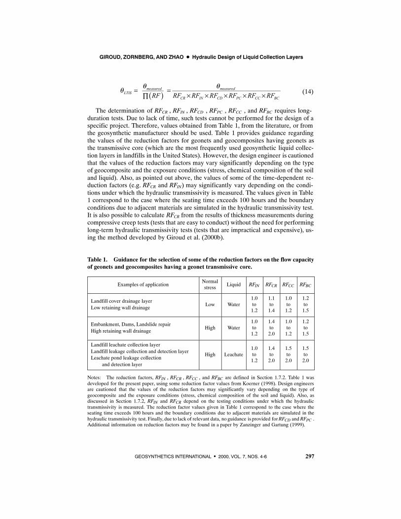
The determination of RFCR , RFIN , RFCD , RFPC , RFCC , and RFBC requires long-duration tests. Due to lack of time, such tests cannot be performed for the design of aspecific project. Therefore, values obtained from Table 1, from the literature, or fromthe geosynthetic manufacturer should be used. Table 1 provides guidance regardingthe values of the reduction factors for geonets and geocomposites having geonets asthe transmissive core (which are the most frequently used geosynthetic liquid collec-tion layers in landfills in the United States). However, the design engineer is cautionedthat the values of the reduction factors may vary significantly depending on the typeof geocomposite and the exposure conditions (stress, chemical composition of the soiland liquid). Also, as pointed out above, the values of some of the time-dependent re-duction factors (e.g. RFCR and RFIN) may significantly vary depending on the condi-tions under which the hydraulic transmissivity is measured. The values given in Table1 correspond to the case where the seating time exceeds 100 hours and the boundaryconditions due to adjacent materials are simulated in the hydraulic transmissivity test.It is also possible to calculate RFCR from the results of thickness measurements duringcompressive creep tests (tests that are easy to conduct) without the need for performinglong-term hydraulic transmissivity tests (tests that are impractical and expensive), us-ing the method developed by Giroud et al. (2000b).
Table 1. Guidance for the selection of some of the reduction factors on the flow capacityof geonets and geocomposites having a geonet transmissive core.
Examples of applicationNormalstress Liquid RFIN RFCR RFCC RFBC
Landfill cover drainage layerLow retaining wall drainage
Low Water1.0to1.2
1.1to1.4
1.0to1.2
1.2to1.5
Embankment, Dams, Landslide repairHigh retaining wall drainage
High Water1.0to1.2
1.4to2.0
1.0to1.2
1.2to1.5
Landfill leachate collection layerLandfill leakage collection and detection layerLeachate pond leakage collection
and detection layer
High Leachate1.0to1.2
1.4to2.0
1.5to2.0
1.5to2.0
Notes: The reduction factors, RFIN , RFCR , RFCC , and RFBC are defined in Section 1.7.2. Table 1 wasdeveloped for the present paper, using some reduction factor values from Koerner (1998). Design engineersare cautioned that the values of the reduction factors may significantly vary depending on the type ofgeocomposite and the exposure conditions (stress, chemical composition of the soil and liquid). Also, asdiscussed in Section 1.7.2, RFIN and RFCR depend on the testing conditions under which the hydraulictransmissivity is measured. The reduction factor values given in Table 1 correspond to the case where theseating time exceeds 100 hours and the boundary conditions due to adjacent materials are simulated in thehydraulic transmissivity test. Finally, due to lack of relevant data, no guidance is provided forRFCD and RFPC .Additional information on reduction factors may be found in a paper by Zanzinger and Gartung (1999).
GIROUD, ZORNBERG, AND ZHAO D Hydraulic Design of Liquid Collection Layers
298 GEOSYNTHETICS INTERNATIONAL S 2000, VOL. 7, NOS 4-6
Also, it should be noted that RFCR , RFCD , RFCC , and RFBC (and, to a lesser degree,RFIN and RFPC) correspond to time-dependent mechanisms. Therefore, the values ofRFCR , RFCD , RFCC , and RFBC (and, to a lesser degree, RFIN and RFPC) selected by thedesign engineer depend on the design life of the liquid collection layer. In cases wherethe liquid supply rate varies with time, the design engineer may consider several timeperiods. For example, in the case of landfills with no leachate recirculation, three phasesmay be considered: (i) construction and pre-operational phase; (ii) operational phase;and (iii) post-closure phase.As time elapses, the leachate collection systemwill typical-ly experience a reduction in the rate of leachate that needs to be collected, but may con-currently experience a reduction of its flow capacity due to time-dependentmechanisms such as creep and clogging.
The above discussion is for geocomposites, in particular, for geocomposites whosetransmissive core is a geonet (which are the most frequently used geosynthetic liquidcollection layers in landfills in the United States). In the case where the geosyntheticliquid collection layer is a thick needle-punched nonwoven geotextile, the mechanismsdescribed above exist with the exception of geotextile intrusion into the transmissivecore since, in this case, the geotextile itself is the transmissive medium. In this case, thereduction factors presented above exist, but no guidance is proposed herein regardingtheir values.
It should be noted that the various reduction factors may not be completely indepen-dent. For example, chemical degradation may affect creep resistance (i.e. may increaseRFCR), and, as shown by Palmeira and Gardoni (2000), the presence of soil particles ina needle-punched nonwoven geotextile (i.e. particulate clogging) may reduce the geo-textile’s compressibility (i.e. it may reduce RFIMCO and RFCR while increasing RFPC).
Finally, it should be noted that, contrary to the case of geosynthetics used for soilreinforcement, no reduction factor for installation damage is included in Equations 12to 14. Indeed, it is generally considered that damage caused by installation is not likelyto affect the hydraulic transmissivity of the geosynthetics typically used in liquidcollection layers. However, design engineers may use a reduction factor for installationdamage in all cases where this may appear appropriate. Also, it is possible to find inthe technical literature “survivability criteria” that evaluate the ability of geotextiles,used alone or as part of geocomposites, to resist damage during installation.
1.7.3 Flow Capacity Reduction in the Case of Granular Liquid Collection Layers
When a granular liquid collection layer is used, the mechanisms of thickness reduc-tion are negligible because granular materials do not exhibit any significant instanta-neous thickness reduction (compression) nor time-dependent thickness reduction(creep), and the reduction in flow capacity due to geotextile intrusion is negligible be-cause the geotextile thickness is negligible with respect to the thickness of the granularlayers. Furthermore, chemical degradation that could affect the thickness and the hy-draulic conductivity of a granular liquid collection layer can be avoided by properselection of the granular material. Therefore, in the case of a granular liquid collectionlayer, the only relevant reduction affecting the flow capacity is the reduction of hydrau-lic conductivity due to clogging. As a result, the reduction in flow capacity results froma reduction in hydraulic conductivity, which can be expressed as follows:

GIROUD, ZORNBERG, AND ZHAO D Hydraulic Design of Liquid Collection Layers
299GEOSYNTHETICS INTERNATIONAL S 2000, VOL. 7, NOS. 4-6
(15)( )measured measured
LTISPC CC BC
k kkRF RF RF RF
= =× ×∏
where: kLTIS = long-term-in-soil hydraulic conductivity of the granular material, i.e. hy-draulic conductivity of the granular material located in the soil and subjected to condi-tions that can cause the development of clogging during the design life of the liquidcollection layer; and kmeasured = hydraulic conductivity of a specimen of granular mate-rial representative of the granular material as installed, measured in a hydraulic con-ductivity test performed with water during a short period of time so that clogging doesnot develop.
1.7.4 Factor of Safety
In addition to the reduction factors described in Sections 1.7.2 and 1.7.3, a factor ofsafety, FS, is used in all calculations to take into account possible uncertainties, suchas the fact that themeasurement of hydraulic characteristics (i.e. hydraulic conductivityand hydraulic transmissivity) is generally delicate and prone to errors. Values such as2 or 3, or sometimes greater values, are typically recommended for the factor of safety.
In the equations provided in the present paper, there are two ways of using a factorof safety. The factor of safety can be applied to the maximum liquid thickness, FST ,or to the relevant hydraulic characteristic, FSH , i.e. the hydraulic transmissivity in thecase of a geosynthetic liquid collection layer or the hydraulic conductivity in the caseof a granular liquid collection layer. The two ways (factor of safety on the maximumliquid thickness and factor of safety on the hydraulic characteristic) will be compared.
It is important to note that FST and FSH are not partial factors of safety to be usedsimultaneously. They are two ways of expressing the factor of safety of the liquidcollection layer.
1.7.5 Use of Reduction Factors and Factor of Safety
As indicated in Section 1.3, there are two design approaches: the thickness approach(described in Section 3) that consists of calculating the maximum liquid thickness, andthe hydraulic characteristic approach (described in Section 4) that consists of calculat-ing the required hydraulic conductivity of the liquid collection layer material or the hy-draulic transmissivity of the liquid collection layer. Use of the reduction factors in thesetwo approaches is described in Section 3 for the thickness approach and in Section 4for the hydraulic characteristic approach.
1.8 Design Options
The flow capacity of a liquid collection layer depends on two sets of characteristics:the intrinsic characteristics of the liquid collection layer and the characteristics of theslope on which the liquid collection layer is installed. The intrinsic characteristics arethe thickness of the liquid collection layer and the hydraulic conductivity of the liquidcollection layer material (or the hydraulic transmissivity of the liquid collection layer,which is the product of the thickness and hydraulic conductivity). The characteristics
GIROUD, ZORNBERG, AND ZHAO D Hydraulic Design of Liquid Collection Layers
300 GEOSYNTHETICS INTERNATIONAL S 2000, VOL. 7, NOS 4-6
of the slope on which the liquid collection layer is installed are the slope angle and theslope length.
If design calculations show that the considered liquid collection layer material doesnot provide adequate flow capacity, the design engineer has the following options: (i)a liquid collection layer with a greater thickness (but this option is inappropriate if, inthe original design, the liquid thickness was equal to a regulatory maximum liquidthickness); (ii) a different drainage material with a greater hydraulic conductivity (orgreater hydraulic transmissivity); and (iii) a liquid collection layer with a shorter lengthand/or a steeper slope. The last option is the only one available if the liquid collectionlayer and its material may not be changed. However, slope steepness may be limitedby stability and/or by waste storage capacity considerations.
2 AVAILABLE EQUATIONS AND DISCUSSIONS
2.1 Overview
As indicated in Section 1.5, the liquid flowing in a liquid collection layer has amaxi-mum thickness at a certain location along the slope on which the liquid collection layeris constructed. Equations given in Section 2 provide the maximum liquid thickness asa function of the following parameters: the hydraulic conductivity of the liquid collec-tion layer material; the length and slope of the liquid collection layer; and the rate ofliquid supply. Some solutions provide an accurate value of the maximum liquid thick-ness, some provide an approximate value. The validity of the equations that provideapproximate values is assessed. Section 2 only presents the equations and discussestheir accuracy. The use of the equations will be presented in Sections 3 and 4.
2.2 Solution Based on Simplified Assumptions
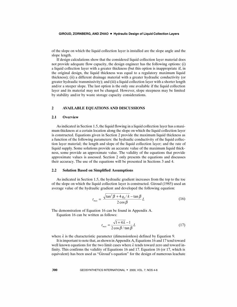
As indicated in Section 1.5, the hydraulic gradient increases from the top to the toeof the slope on which the liquid collection layer is constructed. Giroud (1985) used anaverage value of the hydraulic gradient and developed the following equation:
(16)tq k
Lhmax =
+ −tan / tancos
2 42
β ββ
The demonstration of Equation 16 can be found in Appendix A.Equation 16 can be written as follows:
(17)t Lmax =+ −1 4 1
2λ
β βcos / tan
where λ is the characteristic parameter (dimensionless) defined by Equation 9.It is important to note that, as shown in Appendix A, Equations 16 and 17 tend toward
well known equations for the two limit cases where λ tends toward zero and toward in-finity. This confirms the validity of Equations 16 and 17. Equation 16 (or 17, which isequivalent) has been used as “Giroud’s equation” for the design of numerous leachate
GIROUD, ZORNBERG, AND ZHAO D Hydraulic Design of Liquid Collection Layers
301GEOSYNTHETICS INTERNATIONAL S 2000, VOL. 7, NOS. 4-6
collection layers and leakage collection layers in many landfills in the United States.Giroud’s equation has progressively replaced the use, in the United States, of “Moore’sequations”, which had been presented in documents published by the US Environmen-tal Protection Agency (Moore 1980, 1983; USEPA 1989), but for which no derivationwas ever published or otherwise made available, to the best of the authors’ knowledge.In the early 1980s, the senior author suspected the validity of Moore’s equations be-cause they did not tend toward the well-known limits when λ tends toward zero or to-ward infinity. This prompted the development of equations by the senior author. In theremainder of the present paper, Equation 16 (or 17) will be referred to as the “originalGiroud’s equation”.
2.3 Governing Differential Equation
2.3.1 Establishment of the Governing Differential Equation
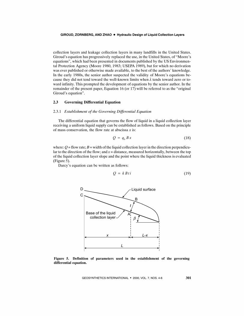
The differential equation that governs the flow of liquid in a liquid collection layerreceiving a uniform liquid supply can be established as follows. Based on the principleof mass conservation, the flow rate at abscissa x is:
(18)hQ q B x=
where:Q= flow rate; B=width of the liquid collection layer in the direction perpendicu-lar to the direction of the flow; and x = distance, measured horizontally, between the topof the liquid collection layer slope and the point where the liquid thickness is evaluated(Figure 5).
Darcy’s equation can be written as follows:
(19)Q k Bt i=
Figure 5. Definition of parameters used in the establishment of the governingdifferential equation.
t
L
x L-x
Liquid surface
Base of the liquidcollection layer
B
D
A
C
b
GIROUD, ZORNBERG, AND ZHAO D Hydraulic Design of Liquid Collection Layers
302 GEOSYNTHETICS INTERNATIONAL S 2000, VOL. 7, NOS 4-6
where i is the hydraulic gradient.Combining Equations 18 and 19 gives:
(20)hq x k t i=
The hydraulic gradient, i, is derived as follows from the hydraulic head:
(21)d
d / coshi
x β= −
where h is the hydraulic head, which is given by the following equation:
(22)( ) tan ABh L x hβ= − +
where hAB is the hydraulic head that corresponds to the liquid thickness AB (Figure 5).In Equation 22, the term (L--x) tanβ represents the elevation of Point A.
Combining Equation 4 with h = hAB and Equations 21 and 22 gives:
(23)2 dsin cosd
tix
β β= −
It should be noted that Equation 4 is valid when the liquid surface is parallel to theslope. As shown in Figure 4, this is true only at the location of the maximum liquidthickness. Since the ultimate goal is to calculate the maximum liquid thickness, theapproximation made when Equation 4 is used should be acceptable. Further discussionon approximations associated with the evaluation of the hydraulic head may be foundin Section 2.6.
Combining Equations 20 and 23 gives:
(24)2 dsin cosdh
tq x k tx
β β = − Equation 24 is the differential equation governing the flow of liquid in a liquid
collection layer exposed to a uniform liquid supply. In the present paper, this equationis referred to as the “governing equation”. Equation 24 can also be written as follows:
(25)2 dsin cosd
hq x tt tk x
β β= −
Combining Equations 9 and 25 gives the following expression for the governing dif-ferential equation:
(26)2 4
2
cos cos dsin sin d
t tx tx
β βλβ β
= −
2.3.2 Limit Cases
The governing differential equation, Equation 24 (or Equations 25 and 26, which areequivalent), becomes simpler in two extreme cases. In each of these two cases, the gov-erning differential equation can easily be solved, as shown below.

GIROUD, ZORNBERG, AND ZHAO D Hydraulic Design of Liquid Collection Layers
303GEOSYNTHETICS INTERNATIONAL S 2000, VOL. 7, NOS. 4-6
tmax
L
qh
Figure 6. Profile of the liquid surface in the limit case where β = 0.
Case Where β = 0. In this case (Figure 6), Equation 25 becomes:
(27)d dhq x x t tk
= −
Integration of this differential equation gives:
(28)2 2hqt x Ck
= − +
where C is a constant with respect to the variable x. The value of the constant, C, canbe determined by considering that t = 0 for x = L, hence:
(29)2hqC Lk
=
Combining Equations 28 and 29 gives:
(30)( )2 2hqt L xk
= −
The maximum liquid thickness occurs for x = 0, hence:
(31)hmax
qt Lk
=
Equation 31 is well known. It is used to design horizontal liquid collection layers,such as drainage layers under road pavements. It should be noted that, based on Equa-tion 9, λ tends toward infinity when β tends toward zero.
Case Where λ is Very Small. The characteristic parameter λ is very small if qh is verysmall and/or k and β are very large. If λ is very small, Equation 26 shows that t mustbe small. Consequently, tdt is negligible compared to t, and Equation 26 becomes:
GIROUD, ZORNBERG, AND ZHAO D Hydraulic Design of Liquid Collection Layers
304 GEOSYNTHETICS INTERNATIONAL S 2000, VOL. 7, NOS 4-6
(32)2cos
sintx βλ
β≈
hence:
(33)2
sin tancos cos
x xt λ β λ ββ β
≈ =
Combining Equations 9 and 33 gives:
(34)sinhq xt
k β=
Equation 34 shows that, when λ is very small, the liquid thickness, t, varies linearlywith the abscissa, x. Therefore, the maximum value of t occurs for x = L, hence:
(35)2
sin tancos cos sin
hmax
q LL Ltk
λ β λ ββ β β
≈ = =
Equation 35 is well known because it can easily be obtained using Darcy’s equation,as shown in Section 2.8. Further discussion of Equation 35 can be found in Sections 2.8and 2.11.
2.3.3 Numerical Solution
In 1992, the governing differential equation was solved numerically (Giroud et al.1992). To solve the differential equation, the boundary condition used to represent freedrainage at the toe of the liquid collection layer (in accordance with an assumption pre-sented in Section 1.4.1) was zero liquid thickness and infinite hydraulic gradient. Thevalidity of this boundary condition is discussed in Appendix B. The numerical solutionwas deemed accurate because it was consistent with values obtained analytically forthe two limit cases, i.e. when λ tends toward infinity (Equation 31) and toward zero(Equation 35).
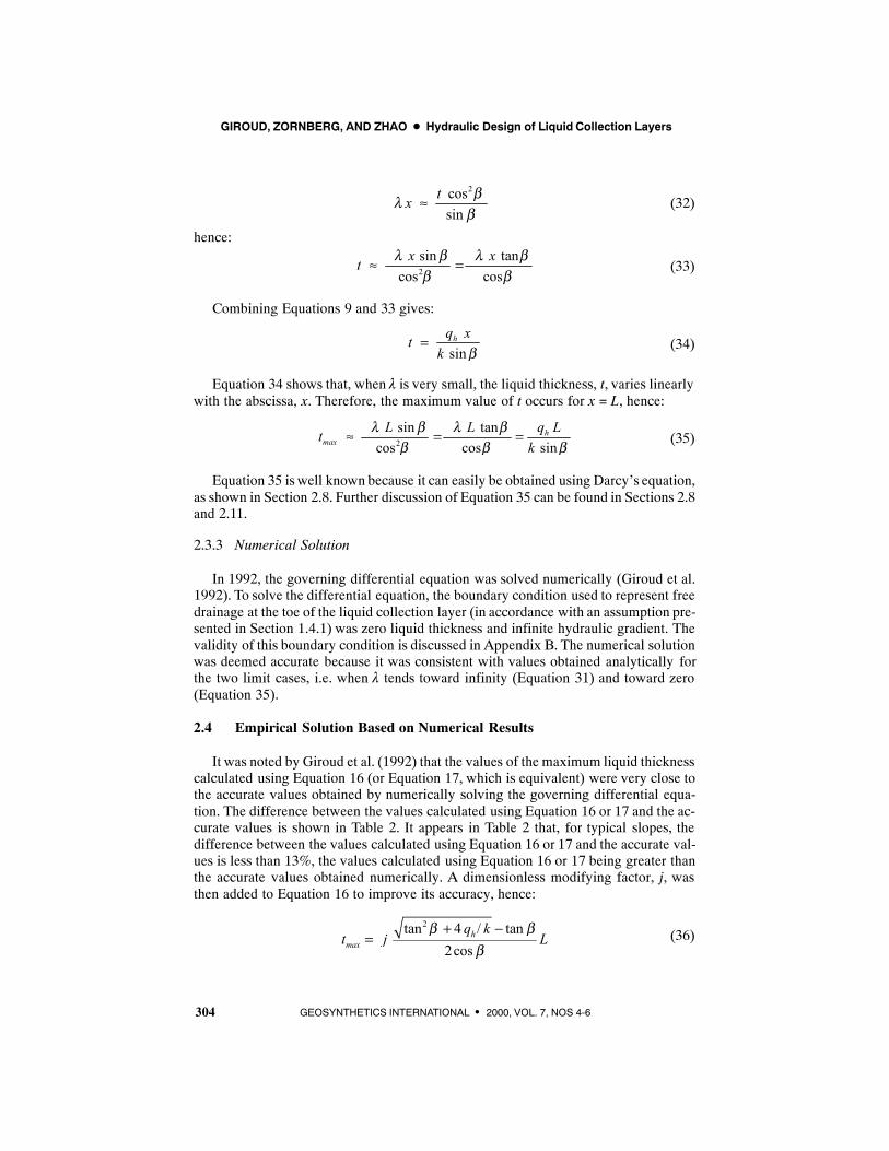
2.4 Empirical Solution Based on Numerical Results
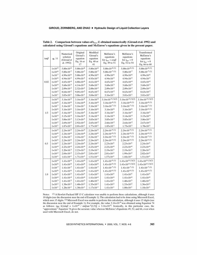
It was noted by Giroud et al. (1992) that the values of the maximum liquid thicknesscalculated using Equation 16 (or Equation 17, which is equivalent) were very close tothe accurate values obtained by numerically solving the governing differential equa-tion. The difference between the values calculated using Equation 16 or 17 and the ac-curate values is shown in Table 2. It appears in Table 2 that, for typical slopes, thedifference between the values calculated using Equation 16 or 17 and the accurate val-ues is less than 13%, the values calculated using Equation 16 or 17 being greater thanthe accurate values obtained numerically. A dimensionless modifying factor, j, wasthen added to Equation 16 to improve its accuracy, hence:
(36)2tan 4 / tan
2cosh
maxq k
t j Lβ β
β+ −
=
GIROUD, ZORNBERG, AND ZHAO D Hydraulic Design of Liquid Collection Layers
305GEOSYNTHETICS INTERNATIONAL S 2000, VOL. 7, NOS. 4-6
Table 2. Comparison between values of tmax /L obtained numerically (Giroud et al. 1992) andcalculated using Giroud’s equations and McEnroe’s equations given in the present paper.
tanβ qh / k
Numericalsolution(Giroud etal. 1992)
OriginalGiroud’sequationEq. 16 or
17
ModifiedGiroud’sequationEq. 40 or
41
McEnroe’sequations
for itoe = cosβEq. 49 to 51
McEnroe’sequationsfor ttoe = 0Eq. 52 to 54
TransformedMcEnroe’sequationsfor ttoe = 0Eq. 66 to 68
0.02
1×10⁻⁹
1×10⁻⁸
1×10⁻⁷
1×10⁻⁶
1×10⁻⁵
1×10⁻⁴
1×10⁻³
1×10⁻²
1×10⁻¹
5.00×10⁻⁸
5.00×10⁻⁷
4.99×10⁻⁶
4.94×10⁻⁵
4.65×10⁻⁴
3.68×10⁻³
2.09×10⁻²
8.64×10⁻²
3.03×10⁻¹
5.00×10⁻⁸
5.00×10⁻⁷
5.00×10⁻⁶
4.99×10⁻⁵
4.88×10⁻⁴
4.14×10⁻³
2.32×10⁻²
9.05×10⁻²
3.06×10⁻¹
5.00×10⁻⁸
5.00×10⁻⁷
4.99×10⁻⁶
4.93×10⁻⁵
4.61×10⁻⁴
3.68×10⁻³
2.08×10⁻²
8.65×10⁻²
3.04×10⁻¹
5.00×10⁻⁸ (1)
5.00×10⁻⁷ (1)
4.99×10⁻⁶
4.94×10⁻⁵
4.65×10⁻⁴
3.68×10⁻³
2.09×10⁻²
8.67×10⁻²
3.16×10⁻¹
5.00×10⁻⁸ (1)
5.00×10⁻⁷
4.99×10⁻⁶
4.94×10⁻⁵
4.65×10⁻⁴
3.68×10⁻³
2.09×10⁻²
8.63×10⁻²
3.01×10⁻¹
5.00×10⁻⁸ (1)
5.00×10⁻⁷ (1)
4.99×10⁻⁶
4.94×10⁻⁵
4.65×10⁻⁴
3.68×10⁻³
2.09×10⁻²
8.63×10⁻²
3.01×10⁻¹
1/3
1×10⁻⁹
1×10⁻⁸
1×10⁻⁷
1×10⁻⁶
1×10⁻⁵
1×10⁻⁴
1×10⁻³
1×10⁻²
1×10⁻¹
3.16×10⁻⁹
3.16×10⁻⁸
3.16×10⁻⁷
3.16×10⁻⁶
3.16×10⁻⁵
3.15×10⁻⁴
3.06×10⁻³
2.69×10⁻²
1.87×10⁻¹
3.16×10⁻⁹
3.16×10⁻⁸
3.16×10⁻⁷
3.16×10⁻⁶
3.16×10⁻⁵
3.16×10⁻⁴
3.13×10⁻³
2.92×10⁻²
2.01×10⁻¹
3.16×10⁻⁹
3.16×10⁻⁸
3.16×10⁻⁷
3.16×10⁻⁶
3.16×10⁻⁵
3.14×10⁻⁴
3.03×10⁻³
2.65×10⁻²
1.77×10⁻¹
3.16×10⁻⁹ (1)(2)
3.16×10⁻⁸ (1)
3.16×10⁻⁷ (1)
3.16×10⁻⁶
3.16×10⁻⁵
3.14×10⁻⁴
3.05×10⁻³
2.66×10⁻²
1.85×10⁻¹
3.16×10⁻⁹ (1)(2)
3.16×10⁻⁸ (1)
3.16×10⁻⁷ (1)
3.16×10⁻⁶
3.16×10⁻⁵
3.14×10⁻⁴
3.05×10⁻³
2.64×10⁻²
1.73×10⁻¹
3.16×10⁻⁹ (1)(2)
3.16×10⁻⁸ (1)
3.16×10⁻⁷ (1)
3.16×10⁻⁶ (1)
3.16×10⁻⁵
3.15×10⁻⁴
3.06×10⁻³
2.67×10⁻²
1.78×10⁻¹
0.5
1×10⁻⁹
1×10⁻⁸
1×10⁻⁷
1×10⁻⁶
1×10⁻⁵
1×10⁻⁴
1×10⁻³
1×10⁻²
1×10⁻¹
2.24×10⁻⁹
2.24×10⁻⁸
2.24×10⁻⁷
2.24×10⁻⁶
2.24×10⁻⁵
2.23×10⁻⁴
2.20×10⁻³
2.04×10⁻²
1.61×10⁻¹
2.24×10⁻⁹
2.24×10⁻⁸
2.24×10⁻⁷
2.24×10⁻⁶
2.24×10⁻⁵
2.24×10⁻⁴
2.23×10⁻³
2.15×10⁻²
1.71×10⁻¹
2.24×10⁻⁹
2.24×10⁻⁸
2.24×10⁻⁷
2.24×10⁻⁶
2.24×10⁻⁵
2.23×10⁻⁴
2.19×10⁻³
2.01×10⁻²
1.51×10⁻¹
2.24×10⁻⁹ (1)
2.24×10⁻⁸ (1)
2.24×10⁻⁷ (1)
2.24×10⁻⁶ (1)
2.23×10⁻⁵
2.23×10⁻⁴
2.19×10⁻³
2.01×10⁻²
1.57×10⁻¹
2.24×10⁻⁹ (1)
2.24×10⁻⁸ (1)
2.24×10⁻⁷ (1)
2.24×10⁻⁶ (1)
2.23×10⁻⁵
2.23×10⁻⁴
2.19×10⁻³
1.99×10⁻²
1.44×10⁻¹
2.24×10⁻⁹ (1)
2.24×10⁻⁸ (1)
2.24×10⁻⁷ (1)
2.24×10⁻⁶ (1)
2.24×10⁻⁵
2.23×10⁻⁴
2.20×10⁻³
2.02×10⁻²
1.51×10⁻¹
1.0
1×10⁻⁹
1×10⁻⁸
1×10⁻⁷
1×10⁻⁶
1×10⁻⁵
1×10⁻⁴
1×10⁻³
1×10⁻²
1×10⁻¹
1.41×10⁻⁹
1.41×10⁻⁸
1.41×10⁻⁷
1.41×10⁻⁶
1.41×10⁻⁵
1.41×10⁻⁴
1.41×10⁻³
1.38×10⁻²
1.28×10⁻¹
1.41×10⁻⁹
1.41×10⁻⁸
1.41×10⁻⁷
1.41×10⁻⁶
1.41×10⁻⁵
1.41×10⁻⁴
1.41×10⁻³
1.40×10⁻²
1.30×10⁻¹
1.41×10⁻⁹
1.41×10⁻⁸
1.41×10⁻⁷
1.41×10⁻⁶
1.41×10⁻⁵
1.41×10⁻⁴
1.40×10⁻³
1.35×10⁻²
1.17×10⁻¹
1.41×10⁻⁹ (1)
1.41×10⁻⁸ (1)
1.41×10⁻⁷ (1)
1.41×10⁻⁶ (1)
1.41×10⁻⁵
1.41×10⁻⁴
1.41×10⁻³
1.41×10⁻²
1.41×10⁻¹
1.41×10⁻⁹ (1)(2)
1.41×10⁻⁸ (1)(2)
1.41×10⁻⁷ (1)
1.41×10⁻⁶ (1)
1.41×10⁻⁵
1.41×10⁻⁴
1.40×10⁻³
1.33×10⁻²
1.08×10⁻¹
1.41×10⁻⁹ (1)(2)
1.41×10⁻⁸ (1)(2)
1.41×10⁻⁷ (1)
1.41×10⁻⁶ (1)
1.41×10⁻⁵
1.41×10⁻⁴
1.40×10⁻³
1.36×10⁻²
1.18×10⁻¹
Notes: (1) A Hewlett Packard HP 15 C calculator was unable to perform these calculations, although it uses10 digits (see the discussion near the end of Example 1). The calculation had to be done using Microsoft Excel,which uses 15 digits. (2) Microsoft Excel was unable to perform this calculation, although it uses 15 digits (seethe discussion near the end of Example 1). For example, the value 3.16×10⁻⁹ was obtained using Equation 74as follows: (qh / k)/sinβ = 1×10⁻⁹ / sin[tan-1(1/3)] = 3.16×10⁻⁹. Ironically, in this particular case, the“approximate” Equation 74 gives the accurate value whereas McEnroe’s Equations 49, 52, and 66, even whenused with Microsoft Excel, do not.
GIROUD, ZORNBERG, AND ZHAO D Hydraulic Design of Liquid Collection Layers
306 GEOSYNTHETICS INTERNATIONAL S 2000, VOL. 7, NOS 4-6
Similarly, Equation 17 becomes:
(37)1 4 12cos / tanmaxt j Lλ
β β+ −=
The derivation of the modifying factor, j, is provided in Appendix C. The expressionof the modifying factor, j, is:
(38)jq kh= − −FHG
IKJ
LNMM
OQPP
L
NMM
O
QPP1 0 12
85 2
5 8 2
. exp log/
tan
/b gβ
Combining Equations 9 and 38 gives:
(39)j = − − FHGIKJ
LNM
OQP
LNMM
OQPP1 0 12 8
5
5 8 2
. exp log/λ
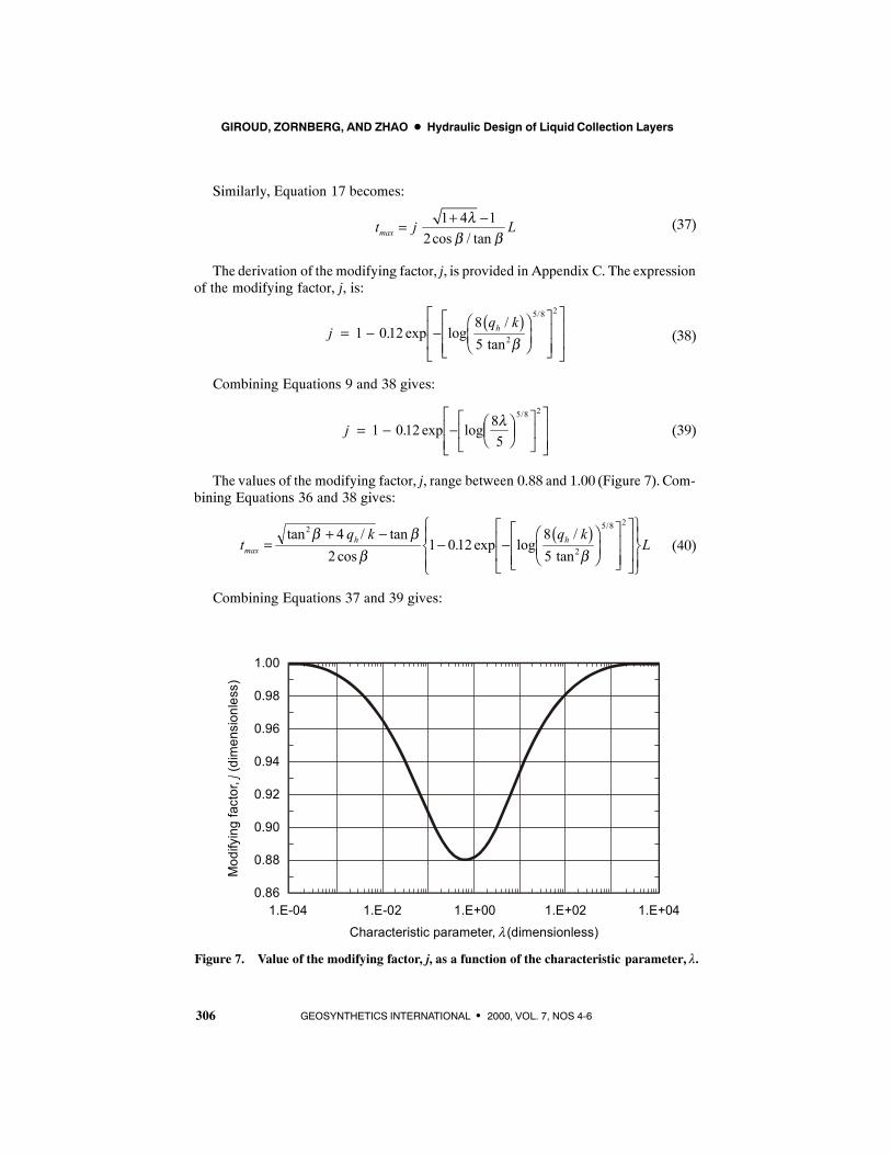
The values of the modifying factor, j, range between 0.88 and 1.00 (Figure 7). Com-bining Equations 36 and 38 gives:
(40)tq k q k
Lh hmax =
+ −− −
FHG
IKJ
LNMM
OQPP
L
NMM
O
QPP
RS|T|
UV|W|
tan / tancos
. exp log/
tan
/2
2
5 8 24
21 0 12
85
β ββ β
b g
Combining Equations 37 and 39 gives:
Mod
ifyin
g fa
ctor
, (d
imen
sion
less
)j
1.E-04 1.E-02 1.E+00 1.E+02 1.E+040.86
0.88
0.90
0.92
0.94
0.96
0.98
1.00
Characteristic parameter, (dimensionless)l
Figure 7. Value of the modifying factor, j, as a function of the characteristic parameter, λ.
GIROUD, ZORNBERG, AND ZHAO D Hydraulic Design of Liquid Collection Layers
307GEOSYNTHETICS INTERNATIONAL S 2000, VOL. 7, NOS. 4-6
(41)t Lmax =+ − − − F
HGIKJ
LNM
OQP
LNMM
OQPP
RS|T|
UV|W|
1 4 12
1 0 12 85
5 8 2λ
β βλ
cos / tan. exp log
/
Table 2 shows that values of the maximum liquid thickness calculated using Equa-tions 40 (or 41, which is equivalent) are within 1% of the accurate results obtained bynumerically solving the governing differential equation forqh/k less than 1×10⁻¹,whichis the case in virtually all practical applications. Equation 40 (or Equation 41) has beenused as the “modified Giroud’s equation” in a number of applications. Since the modi-fied Giroud’s equation was developed based on the results of the numerical solution ofthe governing differential equation, it is legitimate to consider that the modified Gi-roud’s equation corresponds to boundary conditions identical to those used to numeri-cally solve the governing differential equation, i.e. zero liquid thickness at the toe of theliquid collection layer (ttoe = 0), which implies an infinite hydraulic gradient at the toeof the liquid collection layer (itoe = ∞).
Equations 36 to 41 can be used with any set of coherent units. The relevant basic SIunits are: tmax (m), qh (m/s), k (m/s), L (m), and β (_); λ and j are dimensionless.
2.5 Analytical Solution
McEnroe (1993) used the following differential equation for the flow in a liquidcollection layer:
(42)2 dcos tandhDq x k Dx
β β = −
Equation 42 is different from Equation 25. In Equation 42, the liquid depth, D, isused, whereas, in Equation 25, the liquid thickness, t, is used. A detailed comparisonbetween Equations 25 and 42 is presented in Section 2.6.
McEnroe (1993) analytically solved Equation 42, which was a major step forwardin the design of liquid collection layers. The analytical solution consists of a set of threeequations giving the maximumdepth of liquid. Each of the three equations correspondsto a value or a range of values of the dimensionless parameter R defined by Equation10. The equations presented below were obtained bymultiplying by cosβ the equationsoriginally presented by McEnroe in order to obtain the liquid thickness from the liquiddepth, in accordance with Equation 3, hence:
(43)( )
( )
( )1/ 2
1/ 2221 2 1sin
sinsin sin 21 2 1
sin
A
toe
toe toemax
toe
tA R ALt tt L R
L L tA R AL
ββ
β ββ
∗
∗ ∗
∗ ∗
− − + − = − + + − − −
S for R< 0.25
GIROUD, ZORNBERG, AND ZHAO D Hydraulic Design of Liquid Collection Layers
308 GEOSYNTHETICS INTERNATIONAL S 2000, VOL. 7, NOS 4-6
( )
21 2sin sin 4 sinsinsin exp exp
1 2 2 sin 221 1 2sin
toe toe
toemax toe
toetoe
t tR RL L t LLt L t
R L tt RL
β β ββββ
β
− − − = = − − − − − (44)
S for R = 0.25
(45)
S for R> 0.251/ 22
1 1
2 11 1 2 1sinsin exp tan tan
sin sin
toe
toe toemax
tt t RLt L R
L L B B B Bββ
β β− −
∗ ∗ ∗ ∗
− − = − + −
where ttoe is the liquid thickness at the toe of the liquid collection layer slope, R is de-fined by Equation 10, and A* and B* are dimensionless parameters defined by:
(46)1 4 4 1A R B R∗ ∗= − = −
Two expressions of tmax are given for R = 0.25 (Equation 44): the first expression isthat given byMcEnroe (1993) and the second expression was simplified by the authorsof the present paper usingR= 0.25. Equations 43 to 45 depend on the value of the liquidthickness at the toe of the liquid collection layer slope, ttoe . To select the value of ttoethat represents free drainage at the toe, McEnroe (1993) made an assumption on the hy-draulic head at the toe of the liquid collection layer slope. This assumption is discussedin Appendix B where it is shown that the liquid thickness at the toe that results fromthis assumption is:
(47)cosh
toeq Lt
k β=
and the hydraulic gradient at the toe that results from this assumption is:
(48)costoei β=
Combining Equations 43 to 45 with Equation 47 gives the following equations,which were proposed by McEnroe for the case where there is free drainage at the toe:
(49)
S for R< 0.25
( ) ( )( )( )( )
( )1/ 21/ 22 1 2 1 2 tan
sin tan tan1 2 1 2 tan
A
max
A R A Rt L R R R
A R A R
ββ β β
β
∗∗ ∗
∗ ∗
− − + − = − + + − − −
GIROUD, ZORNBERG, AND ZHAO D Hydraulic Design of Liquid Collection Layers
309GEOSYNTHETICS INTERNATIONAL S 2000, VOL. 7, NOS. 4-6
(50)
S for R = 0.25
( ) ( )( )( )
1 2 tan 2 tan 1 sin tan tan 1sin exp 1 exp tan1 2 1 2 tan 1 2 2 2 12
max
R R R Lt LR R R
β β β β ββ ββ
− − − = = − − − − −
(51)
S for R> 0.25
( )1/ 22 1 11 2 tan 1 1 2 1sin tan tan exp tan tanmax
R Rt L R R RB B B B
ββ β β − −∗ ∗ ∗ ∗
− − = − + −
Equations 49 to 51 are known as McEnroe’s equations. Herein, Equations 49 to 51will be referred to as “McEnroe’s equations for itoe = cosβ ”, when necessary for clarity.Two expressions of tmax are given for R = 0.25 (Equation 50): the first expression is thatgiven by McEnroe (1993) and the second expression was simplified by the authors ofthe present paper using R = 0.25.
It is interesting to derive, from Equations 43 to 45, equations for the case where thecondition for free drainage at the toe of the liquid collection layer slope is expressed byttoe =0, the boundary condition used byGiroud et al. (1992). The resulting equations are:
(52)
S for R< 0.25
( )( )( )( )
( )1/ 21 2 1
sin1 2 1
A
max
A R At L R
A R Aβ
∗∗ ∗
∗ ∗
− − + =
+ − −
(53)S for R = 0.25
( )sin exp 1 0.18394 sin2max
Lt Lβ β= − =
(54)1 11 1 1 2 1sin exp tan tanmaxRt L R
B B B Bβ − −
∗ ∗ ∗ ∗
− − = −
S for R> 0.25
Equations 52 to 54 will be referred to as “McEnroe’s equations for ttoe = 0”. Theseequations are simpler than Equations 49 to 51.
It will be shown in Section 2.7 that McEnroe’s equations are not easy to use for thenumerical calculations typically involved in the design of practical applications. How-ever, being an analytical solution, McEnroe’s equations should be regarded as the refer-ence against which other solutions are to be evaluated.
2.6 Transformed Analytical Solution
To compare the two differential equations mentioned in preceding sections, Equa-tions 25 and 42, the authors of the present paper combined Equations 3 and 42 to obtainthe following differential equation where the variable is t instead of D:
GIROUD, ZORNBERG, AND ZHAO D Hydraulic Design of Liquid Collection Layers
310 GEOSYNTHETICS INTERNATIONAL S 2000, VOL. 7, NOS 4-6
(55)dsind
hq x tt tk x
β= −
Inspection of Equation 25, the governing differential equation provided in the pres-ent paper, and Equation 55, which is equivalent to the differential equation used byMcEnroe (1993), reveals a difference between these two equations. The difference iscos2β in the last term of the equation (which indicates that the two differential equationsare very close if β is small). The difference between the two equations results from dif-ferent approximations made in the evaluation of the hydraulic head in the developmentof Equations 25 and 42. Approximations are needed because the hydraulic head variesalong the liquid collection layer slope. The approximation made in the present paperconsists of using the hydraulic head for the case of flow parallel to the slope, whereasthe flow is parallel to the slope only at the location of the maximum thickness. Theapproximation made by McEnroe (1993) consists of assuming that the hydraulic headis equal to the liquid depth, which is only correct when β is small. The authors of thepresent paper believe that it is preferable to use the hydraulic head for flow parallel tothe slope because the liquid surface, as an average, is parallel to the slope. Furthermore,the discussion presented in Section 2.9 tends to show that Equation 25 is a better govern-ing differential equation than Equation 42 because it leads to normalized solutions thatdo not directly depend on β.
Combining Equations 10 and 55 gives:
(56)2
dsin sin d
t t tR xxβ β
= −
Equation 26 can be written as follows:
(57)( )22 2
2
d coscos cossin sin d
tt txx
ββ βλβ β
= −
Comparing Equations 56 and 57 shows that Equation 56 (equivalent to Equation 42,the differential equation used by McEnroe) becomes identical to Equation 57 (equiva-lent to Equation 25, the differential equation used in the present paper) if R is replacedby λ and t is replaced by t cos2β, which can be summarized as follows:
(58)2cosRt t
λβ
→→
This simple transformation makes is possible to convert the analytical solutions ob-tained by McEnroe for Equation 42 into analytical solutions for Equation 25, the gov-erning equation provided in the present paper. Thus, the following equations werederived from Equations 43 to 45:
GIROUD, ZORNBERG, AND ZHAO D Hydraulic Design of Liquid Collection Layers
311GEOSYNTHETICS INTERNATIONAL S 2000, VOL. 7, NOS. 4-6
( )
( )
( )1/ 2
1/ 222 cos1 2 1
tancos costancos tan tan 2 cos1 2 1
tan
A
toe
toe toemax
toe
tA ALt tt L
L L tA AL
βλββ ββ λ
β β β βλβ
′ ′ ′− − + − = − + ′ ′+ − − −
(59)
S for λ< 0.25
(60)
S for λ = 0.25
4 tan / costan exp2cos tan / cos 2
toemax toe
toe
t LLt tL t
β βββ β β
−= − −
(61)
S for λ> 0.25
1/ 221 1
2 cos 1cos costan 1 1 2 1tanexp tan tan
cos tan tan
toe
toe toemax
tt t Lt LL L B B B B
ββ ββ λβλ
β β β− −
− − = − + − ′ ′ ′ ′
where A′ and B′ are dimensionless parameters defined by:
(62)1 4 4 1A Bλ λ′ ′= − = −
Using the transformation defined by Equation 58 on Equations 49 to 51 gives thefollowing equations for the case where free drainage at the toe is represented by Equa-tions 47 and 48:
(63)
S for λ< 0.25
( ) ( )( )( )( )
( )1/ 21/ 22 1 2 1 2 tantan tan tan
cos 1 2 1 2 tan
A
max
A At L
A Aλ λ ββ λ λ β λ β
β λ λ β
′ ′ ′− − + − = − + ′ ′+ − − −
(64)
S for λ = 0.25
tan tan tan 11 exp tan2 cos 2 12
maxLt β β β
ββ
− = − −
( )1/ 22 1 1tan 1 2 tan 1 1 2 1tan tan exp tan tan
cosmaxt LB B B B
β λ β λλ λ β λ ββ
− − − − = − + − ′ ′ ′ ′ (65)
S for λ> 0.25

GIROUD, ZORNBERG, AND ZHAO D Hydraulic Design of Liquid Collection Layers
312 GEOSYNTHETICS INTERNATIONAL S 2000, VOL. 7, NOS 4-6
Equations 63 to 65 will be referred to as the “transformed McEnroe’s equations foritoe = cosβ ”, or simply as “transformed McEnroe’s equations”.
Finally, the transformed McEnroe’s equations for the case where the condition forfree drainage at the toe of the liquid collection layer slope is expressed by ttoe = 0, theboundary condition used by Giroud et al. (1992), can be derived from Equations 52 to54 using the transformation defined by Equation 58. The transformed equations are:
1 1tan 1 1 1 2 1exp tan tancosmaxt L
B B B Bβ λλβ
− − − − = − ′ ′ ′ ′
(66)
S for λ< 0.25
(67)( )tan tanexp 1 0.183942cos cosmaxL Lt β β
β β= − =
S for λ = 0.25
(68)S for λ> 0.25
( )( )( )( )
( )1/ 21 2 1tan
cos 1 2 1
A
max
A At L
A Aλβ λ
β λ
′ ′ ′− − +
= ′ ′+ − −
Equations 66 to 68 will be referred to as the “transformed McEnroe’s equations forttoe = 0”. These equations are simpler than Equations 63 to 65.
As an ultimate example of the transformation defined by Equation 58, the modifiedGiroud’s equation (Equation 37) can be transformed backward, which gives:
(69)2sin 4 / sin 1 4 1sin
2 2h
max
q k Rt j L j Lβ β
β+ − + −= =
where the dimensionless factor j is defined by Equation 39 with R instead of λ.Equation 69 is not used in the present paper. However, it would be an appropriate
equation for calculating the maximum liquid thickness if it were shown that Equation42 is a better governing differential equation than Equation 25. This discussion ismost-ly of academic interest because, as will be shown in Section 2.7, the two differentialequations lead to numerical results that are extremely close. Furthermore, the discus-sion presented in Section 2.9 tends to show that Equation 25 is a better governing differ-ential equation than Equation 42 because it leads to normalized solutions that do notdirectly depend on β.
2.7 Comparison of the Available Equations
Table 2 compares, for four liquid collection layer slopes (tanβ = 0.02, 1/3, 0.5, and1.0), values of the maximum liquid thickness obtained as follows: (i) by numerical solu-tion of the governing differential equation for the case where ttoe = 0 (Giroud et al.1992); (ii) calculated using the original Giroud’s equation (Equation 16 or 17); (iii) cal-culated using the modified Giroud’s equation (Equation 40 or 41); (iv) calculated usingMcEnroe’s equations for itoe = cosβ (Equations 49 to 51), i.e. the equations proposedby McEnroe for free drainage at the toe; (v) calculated using McEnroe’s equations forttoe = 0 (Equations 52 to 54), i.e. the equations derived by the authors of the present pa-
GIROUD, ZORNBERG, AND ZHAO D Hydraulic Design of Liquid Collection Layers
313GEOSYNTHETICS INTERNATIONAL S 2000, VOL. 7, NOS. 4-6
per, from the general equations developed by McEnroe, to represent free drainage atthe toe of the liquid collection layer slope better than by the McEnroe’s equations foritoe = cosβ ; and (vi) calculated using the transformed McEnroe’s equations for ttoe = 0(Equations 66 to 68). The following comments can be made based on inspection ofTable 2:
S The difference between the results obtained using the McEnroe’s equations with thetwo considered boundary conditions is generally very small. For qh/k ≤ 1 × 10⁻², thedifference is less than 1% except for tanβ = 1.0 where the difference is 9%. For qh/k= 1 × 10⁻¹, the difference is less than 7% for tanβ≤ 0.5 and is 23% for tanβ = 1.0.
S For qh/k ≤ 1 × 10⁻², there is an excellent agreement between the numerical solution(Giroud et al. 1992) and the values calculated using McEnroe’s equations, for bothboundary conditions. There are some discrepancies for qh/k = 1 × 10⁻¹. The discrep-ancies become very small when the transformed McEnroe’s equations are used.
S There is very little difference between the values calculated using McEnroe’s equa-tions for itoe = cosβ and the modified Giroud’s equation: the difference is less than1%, except for qh/k = 1 × 10⁻¹ where the difference is 5% for tanβ = 1/3 and 17%for tanβ =1.0. There is virtually no difference between the values calculated usingMcEnroe’s equations for ttoe = 0 and the modified Giroud’s equation (which also cor-responds to ttoe = 0, as pointed out in Section 2.3) for qh/k ≤ 1 × 10⁻². The differencedisappears almost completely, even for qh/k = 1 × 10⁻¹, when the transformedMcEn-roe’s equations are used. Considering that this boundary condition is the most rele-vant of the two considered types of boundary conditions (as discussed in AppendixB), it may be concluded that the modified Giroud’s equation is equivalent to McEn-roe’s equations for the usual range of parameter values.
S The difference between the values calculated using the original Giroud’s equationand accurate solutions (i.e. McEnroe’s equations and the modified Giroud’s equa-tion) is always small and is, at most, 13% for the usual range of parameter values.
In conclusion, from the viewpoint of the calculated numerical values: (i) there isvirtually no difference between the two considered differential equations; (ii) there isvirtually no difference between the two considered types of boundary conditions at thetoe of the liquid collection layer slope; (iii) the modified Giroud’s equation is as accu-rate as McEnroe’s equations; and (iv) the original Giroud’s equation provides anapproximation that is sufficient in most applications.
From a practical standpoint, Giroud’s equations have the following advantages,compared to McEnroe’s equations:
S When the original Giroud’s equation or the modified Giroud’s equation are used,only one equation is needed to cover the entire range of parameters, whereas threeMcEnroe’s equations are necessary.
S Giroud’sequations are simpler thanMcEnroe’sequations,whilebeingalmostasaccu-rate. ThemodifiedGiroud’s equation is virtually as accurate asMcEnroe’sequations.
S Numerical calculations with theMcEnroe’s equation forR< 0.25 require extremelyhigh precision (15 digits or more in some cases), which is very impractical for engi-neering calculations. This problem does not exist with Giroud’s equations. This im-portant point is illustrated by Example 1, below. See also the notes below Table 2.
GIROUD, ZORNBERG, AND ZHAO D Hydraulic Design of Liquid Collection Layers
314 GEOSYNTHETICS INTERNATIONAL S 2000, VOL. 7, NOS 4-6
S The original Giroud’s equation (i.e. Equation 16 or 17) can be solved for all parame-ters: k, qh , or even β.
Because it is simple and accurate, the modified Giroud’s equation (i.e. Equation 40or 41) will be used extensively in the remainder of the present paper. Also, because itis accurate and easily programmable, the modified Giroud’s equation is the recom-mended equation for parametric studies where precision is required. Finally, the origi-nal Giroud’s equation is recommended for usual design calculations because it is verysimple, while being sufficiently accurate for all values of the parameters.
The purpose of Example 1, which follows, is to illustrate the comparison betweenvarious equations. For the sake of simplicity, and to focus the attention on the compari-sons between equations, the reduction factors presented in Section 1.7 are not used inExample 1. Therefore, Example 1 should not be considered as a “design example”. De-sign examples illustrating the use of reduction factors and factor of safety are presentedin Sections 3 and 4.
Example 1. A liquid collection layer used in a landfill cover has a length (measuredhorizontally) of 30 m and a 2% slope. The rate of liquid supply is 100 mm per day. Adrainage geocomposite having a core thickness of 9 mm is used. Its hydraulic transmis-sivity, measured under hydraulic gradients consistent with a slope of 2%, is 3.6 × 10⁻³m2/s. Calculate the maximum liquid thickness.
The liquid supply rate is calculated using Equation 8 as follows:
qh = = × −0 186 400
1157 10 6.,
. m/s
The hydraulic conductivity of the geosynthetic is derived from its hydraulic trans-missivity and its thickness using Equation 2 as follows:
k = ××
=−
−
3 6 109 10
03
3
. .4 m/s
An approximate value of the maximum liquid thickness can be obtained by usingthe original Giroud’s equation (i.e. Equation 16) as follows:
tmax =+ × −L
NMM
O
QPP = × =
−
−−
0 02 4 1157 10 0 0 02
2 0 0230 4 31 10 4 31
2 6
13
. . / .4 .
cos tan .. .
a f a fc hc h a f m mm
An accurate value of the maximum liquid thickness can be obtained by using themodified Giroud’s equation (i.e. Equation 36), which is equivalent to multiplying thevalue calculated above using Equation 16 by the dimensionless modifying factor, j, cal-culated using Equation 38 as follows:
j = − −×L
NMM
OQPP
LNMM
OQPP
RS|T|
UV|W|
=−
1 0 128 1157 10 0
5 0 020 972
6
2
5 8 2
. exp log. / .4
..
/a fc h a fa fa f
GIROUD, ZORNBERG, AND ZHAO D Hydraulic Design of Liquid Collection Layers
315GEOSYNTHETICS INTERNATIONAL S 2000, VOL. 7, NOS. 4-6
hence:
tmax = × =4 31 0 972 4 19. . . mm
Alternatively, the dimensionless characteristic parameter, λ, can be calculated usingEquation 9 as follows:
( )( )6
32
1.157 10 7.231 100.4 0.02
λ−
−×= = ×
Then, the maximum liquid thickness can be calculated using Equation 17 as follows:
( )( )( ) ( )( )
33
1
1 4 7.231 10 10.02 30 4.31 10 m 4.31mm
2cos tan 0.02maxt−
−−
+ × − = = × =
Then, the dimensionless modifying factor, j, can be calculated using Equation 39 asfollows:
( )( )25/838 7.231 10
1 0.12exp log 0.9725
j− × = − − =
Another way to calculate an accurate value of the maximum liquid thickness con-sists of usingMcEnroe’s equations. First,McEnroe’s equations will be used as proposedby McEnroe, i.e. as expressed by Equations 49 to 51, that is for the case where theboundary condition at the toe of the liquid collection layer slope is defined by itoe = cosβ.The use of McEnroe’s equations requires two steps. First, the dimensionless parameterRmust be calculated to determine which one of the three McEnroe’s equations shouldbe used.
The dimensionless parameter R is calculated using Equation 10 as follows:
R = × = ×−
−−1157 10
0 0 027 234143 10
6
2 13.
.4 sin tan ..a f c h
Since R is less than¼, Equation 49 is to be used. To use this equation, it is necessaryto first calculate the dimensionless parameter A* using Equation 46 as follows:
( )( )31 4 7.234143 10 0.9854255A∗ −= − × =
It should be noted that R and A* are calculated with great precision. The reason forthat will be discussed later. Then, Equation 49 can be used as follows:
GIROUD, ZORNBERG, AND ZHAO D Hydraulic Design of Liquid Collection Layers
316 GEOSYNTHETICS INTERNATIONAL S 2000, VOL. 7, NOS 4-6
( ) ( ) ( )( ) ( )( ){ }( )( ) ( )( )( )( )( ) ( )( )( )
1/ 221 3 3 3
3 3
3 3
30 sin tan 0.02 7.234143 10 7.234143 10 0.02 7.234143 10 0.02
1 0.9854255 2 7.234143 10 1 0.9854255 2 7.234143 10 0.02
1 0.9854255 2 7.234143 10 1 0.9854255 2 7.234143 10 0.02
maxt − − − −
− −
− −
= × − × + ×
− − × + − × + − × − − ×
12 0.9854255×
hence:tmax = =0 00422 4 22. .m mm
It should be noted that the two equations that are supposed to give an accurate valueof the maximum liquid thickness indeed give virtually the same result (4.19 and 4.22mm). However, as seen above, the modified Giroud’s equation (i.e. Equation 36) ismuch simpler and easier to use for numerical calculations than McEnroe’s equation. Itis important to note that the value of tmax calculated using McEnroe’s equation for R<0.25 (Equation 49)may vary significantly according to the precision of the calculationsbecause one of its terms is extremely sensitive to the number of decimal places in theinput parameters. For example, using seven digits for the dimensionless parameters Rand A*, leads to the correct value of 4.22mm,whereas using four digits leads to a calcu-lated value of 4.70 mm, i.e. an inaccuracy of 11%. This is due to the following termwhose value calculated with four-digit input parameters is:
1 0 9854 2 7 234 10 1 320 103 4− − × = ×− −. . .a fc hwhereas the value of the same term calculated with seven-digit input parameters is:
1 0 9854255 2 7 234143 10 1 062140 103 4− − × = ×− −. . .a fc hThis difference results in the 11% inaccuracy on the final result when only four digits
are used. Clearly, it is impractical to have to use seven digits for ordinary engineeringcalculations and it is potentially unsafe to use an equation that is so sensitive to the pre-cision of the input parameters. There are even cases where the use of McEnroe’s equa-tion for R< 0.25 (Equation 49) requires a number of digits that exceeds the capacityof electronic calculators (e.g. Hewlett Packard 15 C) or software (e.g. Microsoft Excel)routinely used for engineering calculations, as illustrated by the difficulty encounteredin the preparation ofTable 2where, for some entries, the 10 digits used byHewlett Pack-ard 15 C or the 15 digits used byMicrosoft Excel were not sufficient. This problem doesnot exist with Giroud’s equations. In fact, Giroud’s equations can be used with roundedvalues of the input parameters for quick calculations, as illustrated by the following ex-ample using the original Giroud’s equation (i.e. Equation 16):
tmax =+ × −L
NMM
O
QPP = × =
−−
0 02 4 1 2 10 0 0 02
2 130 4 5 10 4 5
2 63
. . / .4 .. .
a f a fc ha fa f a f m mm
which is a good approximation considering that the more accurate calculation using thesame equation with non-rounded values of the parameters gave 4.31 mm.
GIROUD, ZORNBERG, AND ZHAO D Hydraulic Design of Liquid Collection Layers
317GEOSYNTHETICS INTERNATIONAL S 2000, VOL. 7, NOS. 4-6
Finally,McEnroe’s equations for the case where the boundary conditions are definedby ttoe = 0, i.e. Equations 52 to 54, are used. Since R is less than 0.25, Equation 52 mustbe used, hence:
( ) ( )
( )( ) [ ]( )( ) [ ]
1 3
12 0.98542553
3
30 sin tan 0.02 7.234143 10
1 0.9854255 2 7.234143 10 1 0.9854255
1 0.9854255 2 7.234143 10 1 0.9854255
maxt − −
×−
−
= ×
− − × + + − × −
hence:tmax = =0 00422 4 22. .m mm
It is interesting to note that the same result as with Equation 49 is obtained, whichconfirms the comments made in Section 2.5 regarding the fact that there is virtually nodifference between the two considered types of boundary conditions at the toe of theliquid collection layer slope.
In conclusion, Example 1 shows that using Giroud’s equations is as accurate andmuch simpler than using McEnroe’s equations.
ENDOFEXAMPLE1
2.8 Limit Case
The limit case where qh is small and β and k are large is considered. If qh is small(i.e. if there is little liquid to convey) and β and k are large (i.e. if the liquid collectionlayer has a high flow capacity), the thickness of liquid in the liquid collection layer isvery small (Figure 4c). As a result, the slope of the liquid surface in the liquid collectionlayer is virtually identical to the slope of the liner underlying the liquid collection layer.The hydraulic gradient is then approximately constant along the slope and equal to theratio between the height and the length of the slope, which can be expressed as follows(Figure 1):
i LL
= =tan/ cos
sinββ
β (70)
In this case, the maximum liquid thickness occurs approximately at the toe of theslope (Figure 4c). To calculate the maximum liquid thickness, Darcy’s equation can beused at the toe of the slope. Darcy’s equation is:
Q k i A= (71)
where A is the cross-sectional area of the flow. The cross-sectional area of the flow atthe toe of the slope is:
limA B t= (72)
GIROUD, ZORNBERG, AND ZHAO D Hydraulic Design of Liquid Collection Layers
318 GEOSYNTHETICS INTERNATIONAL S 2000, VOL. 7, NOS 4-6
where tlim is the maximum thickness of the liquid in the limit case defined at the begin-ning of this Section. Based on the principle of mass conservation, and consideringsteady-state flow conditions, the flow rate in the liquid collection layer at the toe of theslope (where tlim occurs) is equal to the rate of liquid supplied to the entire liquid collec-tion layer, hence:
(73)Q q L Bh=
Combining Equations 9 and 70 to 73 gives the following equation:
(74)tansin cos
hlim
q L Ltk
λ ββ β
= =
Equation 74 is identical to Equation 35 obtained from the differential equation.Equation 74 could have been derived from Equation 41 as follows. If qh is small andβ and k are large, λ is small. In this case, a limited series calculation gives the followinglimit for tmax when λ tends toward zero:
(75)( ) { } { }1 2 1 tan tan1 0.12 e 12cos / tan cos cosmax limt t L L L
λ λ β λ ββ β β β
−∞+ −→ = − = =
which is identical to Equation 74.The case where tmax is exactly equal to tlim cannot be represented in Figure 4 because,
in this case, λ = 0 and Equation 74 shows that tlim = 0. Therefore, only the case wheretmax≈ tlim can be represented (Figure 4c). In this case, the maximum thickness occursnear the toe, but not exactly at the toe.
2.9 Normalized Solutions
Themaximum liquid thickness expressed by the equations presented in Sections 2.2,2.3, and 2.4 can be normalized using, as a reference value, the limit liquid thicknessdefined by Equation 74.
The maximum liquid thickness expressed by the original Giroud’s equation can benormalized as follows by combining Equations 17 and 74:
(76)1 4 12
max
lim
tt
λλ
+ −=
Similarly, the maximum liquid thickness expressed by the modified Giroud’s equa-tion can be normalized as follows by combining Equations 36 and 74:
(77)1 4 12
max
lim
t jt
λλ
+ −=
Replacing j by its value as a function of λ given by Equation 38 gives:
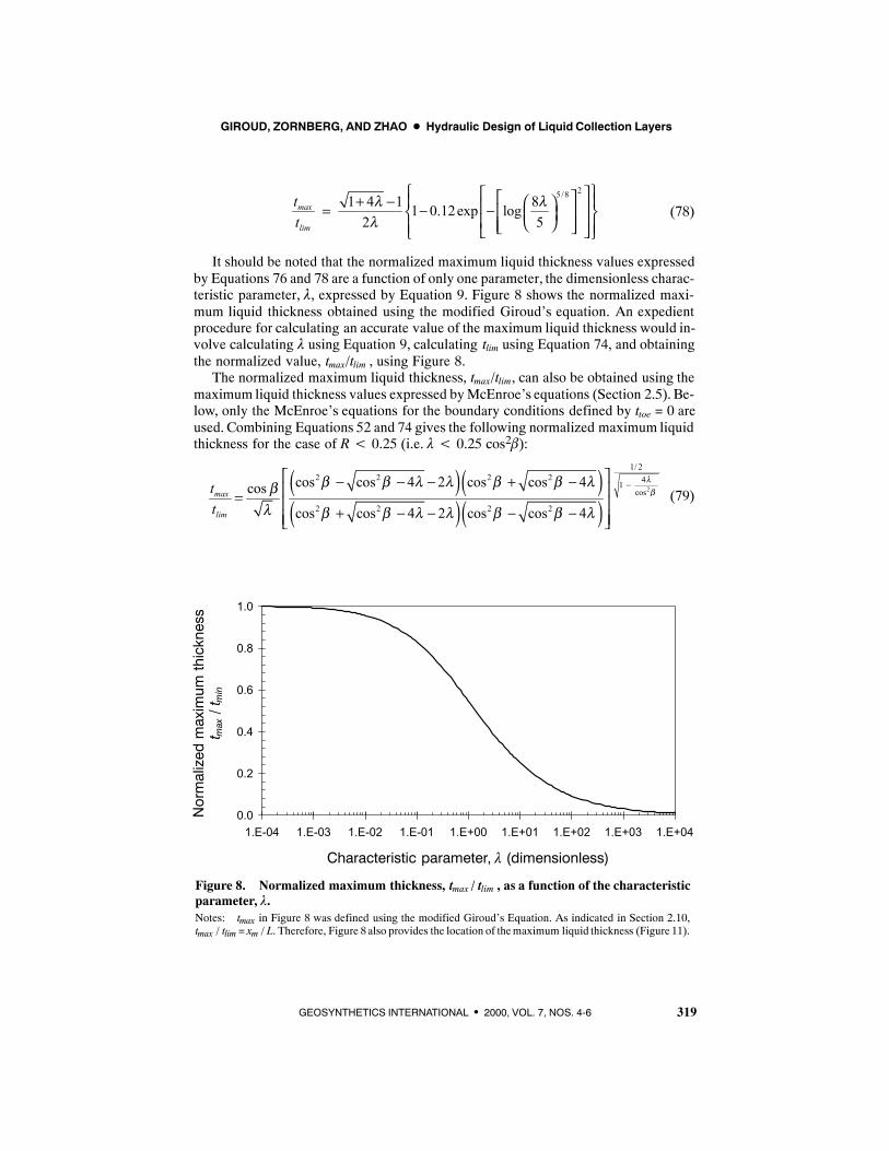
GIROUD, ZORNBERG, AND ZHAO D Hydraulic Design of Liquid Collection Layers
319GEOSYNTHETICS INTERNATIONAL S 2000, VOL. 7, NOS. 4-6
(78)
25/81 4 1 81 0.12exp log2 5
max
lim
tt
λ λλ
+ − = − −
It should be noted that the normalized maximum liquid thickness values expressedby Equations 76 and 78 are a function of only one parameter, the dimensionless charac-teristic parameter, λ, expressed by Equation 9. Figure 8 shows the normalized maxi-mum liquid thickness obtained using the modified Giroud’s equation. An expedientprocedure for calculating an accurate value of the maximum liquid thickness would in-volve calculating λ using Equation 9, calculating tlim using Equation 74, and obtainingthe normalized value, tmax/tlim , using Figure 8.
The normalized maximum liquid thickness, tmax/tlim, can also be obtained using themaximum liquid thickness values expressed byMcEnroe’s equations (Section 2.5). Be-low, only the McEnroe’s equations for the boundary conditions defined by ttoe = 0 areused. Combining Equations 52 and 74 gives the following normalized maximum liquidthickness for the case of R< 0.25 (i.e. λ< 0.25 cos2β):
(79)( )( )( )( )
2
1/ 22 2 2 2 41
cos
2 2 2 2
cos cos 4 2 cos cos 4cos
cos cos 4 2 cos cos 4max
lim
tt
λβ
β β λ λ β β λβλ β β λ λ β β λ
− − − − + − = + − − − −
0.0
0.2
0.4
0.6
0.8
1.0
1.E-04 1.E-03 1.E-02 1.E-01 1.E+00 1.E+01 1.E+02 1.E+03 1.E+04
Figure 8. Normalized maximum thickness, tmax / tlim , as a function of the characteristicparameter, λ.Notes: tmax in Figure 8 was defined using the modified Giroud’s Equation. As indicated in Section 2.10,tmax / tlim = xm / L.Therefore, Figure 8 also provides the location of themaximum liquid thickness (Figure 11).
Characteristic parameter, λ (dimensionless)
Normalizedmaximumthickness
t max/tmin

GIROUD, ZORNBERG, AND ZHAO D Hydraulic Design of Liquid Collection Layers
320 GEOSYNTHETICS INTERNATIONAL S 2000, VOL. 7, NOS 4-6
Combining Equations 53 and 74 gives the following normalized maximum liquidthickness for the case of R = 0.25 (i.e. λ = 0.25 cos2β ):
(80)2 exp( 1) 0.73576max
lim
tt
= − =
Combining Equations 54 and 74 gives the following normalized maximum liquidthickness for the case of R> 0.25 (i.e. λ> 0.25 cos2β ):
21 1
2 2 2
cos cos cos 2 cosexp tan tan4 cos 4 cos cos 4 cos
max
lim
tt
β β β λ βλ λ β λ β β λ β
− − − − = − − − −
(81)
As already mentioned in Section 2.7, threeMcEnroe’s equations are necessary whileonly one Giroud’s equation is valid for the entire range of values of λ. Also, a compari-son ofEquations 79 to 81, on one hand, and Equations 76 or 78, on the other hand, showsthat the normalized McEnroe’s equations are more complex than Giroud’s equationsand depend on two parameters, λ and β, whereas the normalized Giroud’s equations de-pend on only λ.
Figures 9 and 10 show comparisons between the normalized maximum liquid thick-ness obtained using the original Giroud’s equation (Equation 17), the modified Giroud’sequation (Equation 41), and McEnroe’s equations for ttoe = 0 (Equations 52 to 54). Thecurves for the normalized Giroud’s equations depend only on λ, whereas the curves forthe normalized McEnroe’s equations depend on both λ and β.
Figure 9 shows the normalized maximum liquid thickness obtained using McEn-roe’s equations for tanβ = 0.05, the original Giroud’s equation, and the modified Gi-roud’s equation. Figure 9 illustrates the fact that three McEnroe’s equations are neededto generate the entire curve, whereas one Giroud’s equation suffices. For the slope usedin Figure 9 (tanβ = 0.05), there is an excellent agreement between McEnroe’s equationsand the modified Giroud’s equation for the entire range of λ values. Figure 9 also showsthat the original Giroud’s equation gives a good approximation (sufficient in most prac-tical cases) for the entire range of λ values.
Figure 10 illustrates the influence of β on results obtained withMcEnroe’s equations(Equations 52 to 54). Inspection of Figure 10 reveals an excellent agreement betweenMcEnroe’s equations and themodified Giroud’s equation for the entire range of λvalueswhen tanβ = 1/3. It may, therefore, be concluded from Figures 9 and 10 that there is anexcellent agreement between McEnroe’s equations and the modified Giroud’s equationfor the entire range of λ values when 0≤ tanβ≤ 1/3. Figure 10 shows some discrepan-cy between McEnroe’s equations and the modified Giroud’s equation for large valuesof λwhen tanβ> 1/3. However, it should be noted that, when tanβ> 1/3, the character-istic parameter, λ, is usually small (Equation 9) because qh/k is generally less than 1 ×10⁻¹ (and is often much less than 1 × 10⁻¹); for example, when tanβ = 1.0, λ is generallyless than 1 × 10⁻¹ (and is often much less than 1 × 10⁻¹). For such small values of λ, Fig-ure 10 shows a very good agreement between McEnroe’s equations and both the origi-nal Giroud’s equation and the modified Giroud’s equation for all values of the slopeangle, β. In conclusion, there is a very good agreement between McEnroe’s equations
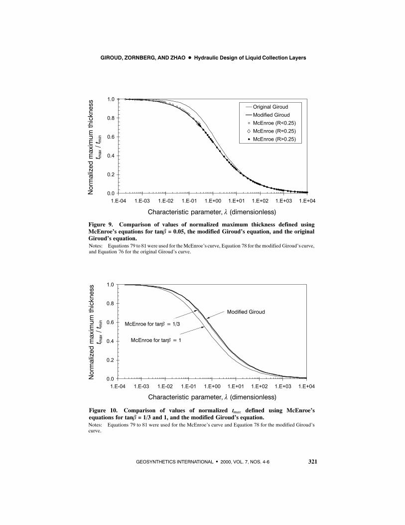
GIROUD, ZORNBERG, AND ZHAO D Hydraulic Design of Liquid Collection Layers
321GEOSYNTHETICS INTERNATIONAL S 2000, VOL. 7, NOS. 4-6
0.0
0.2
0.4
0.6
0.8
1.0
1.E-04 1.E-03 1.E-02 1.E-01 1.E+00 1.E+01 1.E+02 1.E+03 1.E+04
Original GiroudModified GiroudMcEnroe (R<0.25)McEnroe (R=0.25)McEnroe (R>0.25)
0.0
0.2
0.4
0.6
0.8
1.0
1.E-04 1.E-03 1.E-02 1.E-01 1.E+00 1.E+01 1.E+02 1.E+03 1.E+04
Characteristic parameter, λ (dimensionless)
Normalizedmaximumthickness
t max/tmin
Characteristic parameter, λ (dimensionless)
Normalizedmaximumthickness
t max/tmin McEnroe for tanβ = 1/3
McEnroe for tanβ = 1
Modified Giroud
Notes: Equations 79 to 81 were used for theMcEnroe’s curve, Equation 78 for themodified Giroud’s curve,and Equation 76 for the original Giroud’s curve.
Figure 9. Comparison of values of normalized maximum thickness defined usingMcEnroe’s equations for tanβ = 0.05, the modified Giroud’s equation, and the originalGiroud’s equation.
Notes: Equations 79 to 81 were used for the McEnroe’s curve and Equation 78 for the modified Giroud’scurve.
Figure 10. Comparison of values of normalized tmax defined using McEnroe’sequations for tanβ = 1/3 and 1, and the modified Giroud’s equation.
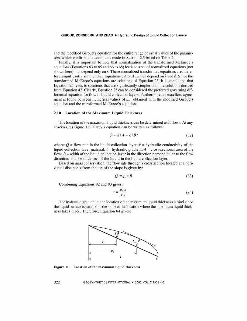
GIROUD, ZORNBERG, AND ZHAO D Hydraulic Design of Liquid Collection Layers
322 GEOSYNTHETICS INTERNATIONAL S 2000, VOL. 7, NOS 4-6
and the modified Giroud’s equation for the entire range of usual values of the parame-ters, which confirms the comments made in Section 2.5 based on Table 2.
Finally, it is important to note that normalization of the transformed McEnroe’sequations (Equations 63 to 65 and 66 to 68) leads to a set of normalized equations (notshown here) that depend only on λ. These normalized transformed equations are, there-fore, significantly simpler than Equations 79 to 81, which depend on λ and β. Since thetransformed McEnroe’s equations are solutions of Equation 25, it is concluded thatEquation 25 leads to solutions that are significantly simpler than the solutions derivedfrom Equation 42. Clearly, Equation 25 can be considered the preferred governing dif-ferential equation for flow in liquid collection layers. Furthermore, an excellent agree-ment is found between numerical values of tmax obtained with the modified Giroud’sequation and the transformed McEnroe’s equations.
2.10 Location of the Maximum Liquid Thickness
The location of the maximum liquid thickness can be determined as follows. At anyabscissa, x (Figure 11), Darcy’s equation can be written as follows:
(82)Q k i A k i Bt= =
where: Q = flow rate in the liquid collection layer; k = hydraulic conductivity of theliquid collection layer material; i = hydraulic gradient; A = cross-sectional area of theflow; B = width of the liquid collection layer in the direction perpendicular to the flowdirection; and t = thickness of the liquid in the liquid collection layer.
Based on mass conservation, the flow rate through a cross section located at a hori-zontal distance x from the top of the slope is given by:
(83)Q q x Bt h=
Combining Equations 82 and 83 gives:
(84)t q xk ih=
The hydraulic gradient at the location of the maximum liquid thickness is sinβ sincethe liquid surface is parallel to the slope at the location where themaximum liquid thick-ness takes place. Therefore, Equation 84 gives:
Figure 11. Location of the maximum liquid thickness.
tmax
t
Lxm
x
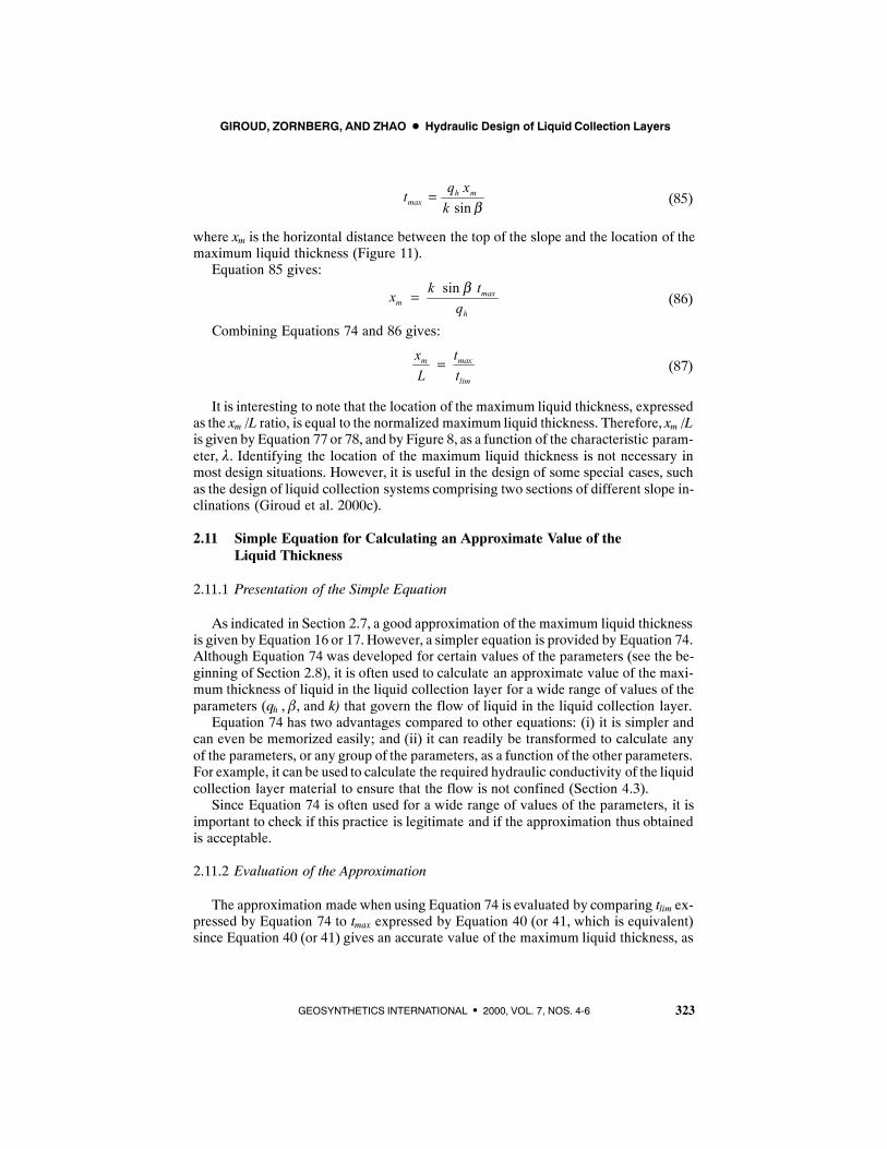
GIROUD, ZORNBERG, AND ZHAO D Hydraulic Design of Liquid Collection Layers
323GEOSYNTHETICS INTERNATIONAL S 2000, VOL. 7, NOS. 4-6
(85)t q xk
h mmax =
sin β
where xm is the horizontal distance between the top of the slope and the location of themaximum liquid thickness (Figure 11).
Equation 85 gives:
(86)sin max
mh
k txqβ=
Combining Equations 74 and 86 gives:
(87)m max
lim
x tL t
=
It is interesting to note that the location of the maximum liquid thickness, expressedas the xm /L ratio, is equal to the normalized maximum liquid thickness. Therefore, xm /Lis given by Equation 77 or 78, and by Figure 8, as a function of the characteristic param-eter, λ. Identifying the location of the maximum liquid thickness is not necessary inmost design situations. However, it is useful in the design of some special cases, suchas the design of liquid collection systems comprising two sections of different slope in-clinations (Giroud et al. 2000c).
2.11 Simple Equation for Calculating an Approximate Value of theLiquid Thickness
2.11.1 Presentation of the Simple Equation
As indicated in Section 2.7, a good approximation of the maximum liquid thicknessis given by Equation 16 or 17. However, a simpler equation is provided by Equation 74.Although Equation 74 was developed for certain values of the parameters (see the be-ginning of Section 2.8), it is often used to calculate an approximate value of the maxi-mum thickness of liquid in the liquid collection layer for a wide range of values of theparameters (qh , β, and k) that govern the flow of liquid in the liquid collection layer.
Equation 74 has two advantages compared to other equations: (i) it is simpler andcan even be memorized easily; and (ii) it can readily be transformed to calculate anyof the parameters, or any group of the parameters, as a function of the other parameters.For example, it can be used to calculate the required hydraulic conductivity of the liquidcollection layer material to ensure that the flow is not confined (Section 4.3).
Since Equation 74 is often used for a wide range of values of the parameters, it isimportant to check if this practice is legitimate and if the approximation thus obtainedis acceptable.
2.11.2 Evaluation of the Approximation
The approximation made when using Equation 74 is evaluated by comparing tlim ex-pressed by Equation 74 to tmax expressed by Equation 40 (or 41, which is equivalent)since Equation 40 (or 41) gives an accurate value of the maximum liquid thickness, as
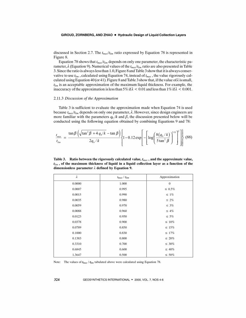
GIROUD, ZORNBERG, AND ZHAO D Hydraulic Design of Liquid Collection Layers
324 GEOSYNTHETICS INTERNATIONAL S 2000, VOL. 7, NOS 4-6
discussed in Section 2.7. The tmax/tlim ratio expressed by Equation 78 is represented inFigure 8.
Equation 78 shows that tmax/tlim depends on only one parameter, the characteristic pa-rameter, λ (Equation 9). Numerical values of the tmax/tlim ratio are also presented in Table3.Since the ratio is always less than 1.0,Figure 8andTable3showthat it is alwaysconser-vative to use tlim , calculated using Equation 74, instead of tmax , the value rigorously cal-culated usingEquation 40 (or41).Figure 8andTable 3showthat, if thevalue ofλ issmall,tlim is an acceptable approximation of the maximum liquid thickness. For example, theinaccuracy of the approximation is less than 5%ifλ<0.01and less than 1%ifλ<0.001.
2.11.3 Discussion of the Approximation
Table 3 is sufficient to evaluate the approximation made when Equation 74 is usedbecause tmax/tlim depends on only one parameter, λ. However, since design engineers aremore familiar with the parameters qh /k and β, the discussion presented below will beconducted using the following equation obtained by combining Equations 9 and 78:
(88)( ) ( )
22 5/8
2
tan tan 4 / tan 8 /1 0.12exp log
2 / 5 tanh hmax
lim h
q k q ktt q k
β β β
β
+ − = − −
Table 3. Ratio between the rigorously calculated value, tmax , and the approximate value,tlim , of the maximum thickness of liquid in a liquid collection layer as a function of thedimensionless parameter λ defined by Equation 9.
λ tmax / tlim Approximation
0.0000
0.0007
0.0015
0.0035
0.0059
0.0088
0.0123
0.0378
0.0789
0.1000
0.1383
0.3310
0.6845
1.3647
1.000
0.995
0.990
0.980
0.970
0.960
0.950
0.900
0.850
0.830
0.800
0.700
0.600
0.500
0
≤ 0.5%
≤ 1%
≤ 2%
≤ 3%
≤ 4%
≤ 5%
≤ 10%
≤ 15%
≤ 17%
≤ 20%
≤ 30%
≤ 40%
≤ 50%
Note: The values of tmax / tlim tabulated above were calculated using Equation 78.
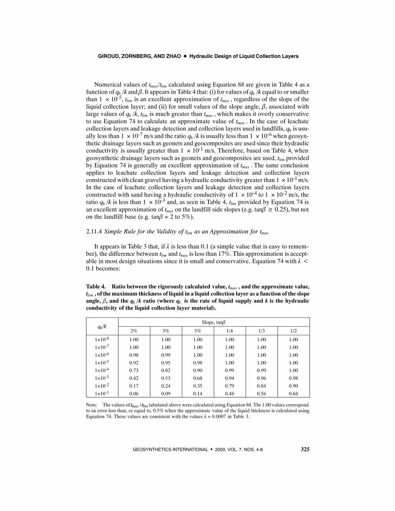
GIROUD, ZORNBERG, AND ZHAO D Hydraulic Design of Liquid Collection Layers
325GEOSYNTHETICS INTERNATIONAL S 2000, VOL. 7, NOS. 4-6
Numerical values of tmax/tlim calculated using Equation 88 are given in Table 4 as afunction of qh /k and β. It appears in Table 4 that: (i) for values ofqh /k equal to or smallerthan 1 × 10⁻⁵, tlim is an excellent approximation of tmax , regardless of the slope of theliquid collection layer; and (ii) for small values of the slope angle, β, associated withlarge values of qh /k, tlim is much greater than tmax , which makes it overly conservativeto use Equation 74 to calculate an approximate value of tmax . In the case of leachatecollection layers and leakage detection and collection layers used in landfills, qh is usu-ally less than 1 × 10⁻⁷ m/s and the ratio qh /k is usually less than 1 × 10⁻⁶ when geosyn-thetic drainage layers such as geonets and geocomposites are used since their hydraulicconductivity is usually greater than 1 × 10⁻¹ m/s. Therefore, based on Table 4, whengeosynthetic drainage layers such as geonets and geocomposites are used, tlim providedby Equation 74 is generally an excellent approximation of tmax . The same conclusionapplies to leachate collection layers and leakage detection and collection layersconstructed with clean gravel having a hydraulic conductivity greater than 1 × 10⁻¹m/s.In the case of leachate collection layers and leakage detection and collection layersconstructed with sand having a hydraulic conductivity of 1 × 10⁻⁴ to 1 × 10⁻² m/s, theratio qh /k is less than 1 × 10⁻³ and, as seen in Table 4, tlim provided by Equation 74 isan excellent approximation of tmax on the landfill side slopes (e.g. tanβ≥ 0.25), but noton the landfill base (e.g. tanβ = 2 to 5%).
2.11.4 Simple Rule for the Validity of tlim as an Approximation for tmax
It appears in Table 3 that, if λ is less than 0.1 (a simple value that is easy to remem-ber), the difference between tlim and tmax is less than 17%. This approximation is accept-able in most design situations since it is small and conservative. Equation 74 with λ<0.1 becomes:
Table 4. Ratio between the rigorously calculated value, tmax , and the approximate value,tlim , of themaximum thickness of liquid in a liquid collection layer as a function of the slopeangle, β, and the qh /k ratio (where qh is the rate of liquid supply and k is the hydraulicconductivity of the liquid collection layer material).
q /kSlope, tanβ
qh/k2% 3% 5% 1/4 1/3 1/2
1×10⁻⁸
1×10⁻⁷
1×10⁻⁶
1×10⁻⁵
1×10⁻⁴
1×10⁻³
1×10⁻²
1×10⁻¹
1.00
1.00
0.98
0.920.73
0.42
0.17
0.06
1.00
1.00
0.99
0.950.82
0.53
0.24
0.09
1.00
1.00
1.00
0.980.90
0.68
0.35
0.14
1.00
1.00
1.00
1.000.99
0.94
0.79
0.48
1.00
1.00
1.00
1.000.99
0.96
0.84
0.56
1.00
1.00
1.00
1.001.00
0.98
0.90
0.68
Note: The values of tmax / tlim tabulated above were calculated using Equation 88. The 1.00 values correspondto an error less than, or equal to, 0.5% when the approximate value of the liquid thickness is calculated usingEquation 74. These values are consistent with the values λ = 0.0007 in Table 3.
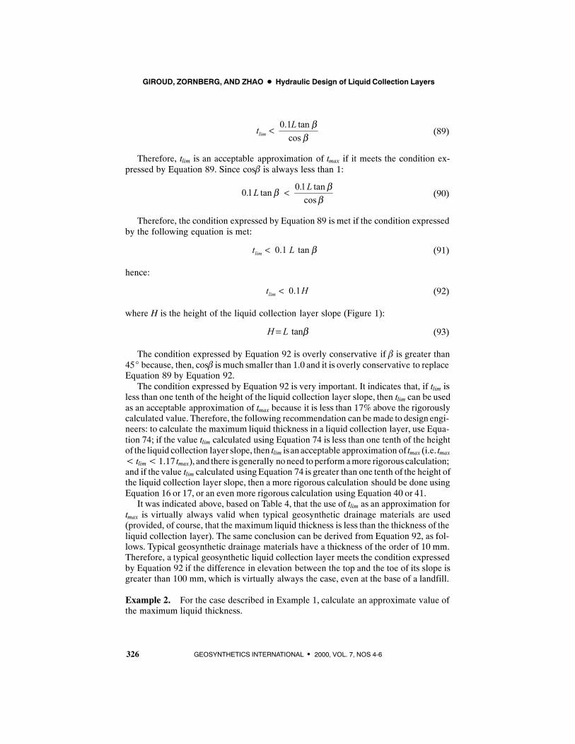
GIROUD, ZORNBERG, AND ZHAO D Hydraulic Design of Liquid Collection Layers
326 GEOSYNTHETICS INTERNATIONAL S 2000, VOL. 7, NOS 4-6
(89)0.1 tan
coslimLt β
β<
Therefore, tlim is an acceptable approximation of tmax if it meets the condition ex-pressed by Equation 89. Since cosβ is always less than 1:
(90)0 1 0 1. tan . tancos
L Lβ ββ
<
Therefore, the condition expressed by Equation 89 is met if the condition expressedby the following equation is met:
(91)0.1 tanlimt L β<
hence:
(92)0.1limt H<
where H is the height of the liquid collection layer slope (Figure 1):
(93)H L= tanβ
The condition expressed by Equation 92 is overly conservative if β is greater than45_ because, then, cosβ is much smaller than 1.0 and it is overly conservative to replaceEquation 89 by Equation 92.
The condition expressed by Equation 92 is very important. It indicates that, if tlim isless than one tenth of the height of the liquid collection layer slope, then tlim can be usedas an acceptable approximation of tmax because it is less than 17% above the rigorouslycalculated value. Therefore, the following recommendation can bemade to design engi-neers: to calculate the maximum liquid thickness in a liquid collection layer, use Equa-tion 74; if the value tlim calculated using Equation 74 is less than one tenth of the heightof the liquid collection layer slope, then tlim isan acceptable approximation of tmax (i.e. tmax< tlim<1.17 tmax), and there isgenerally noneed toperform amore rigorous calculation;and if the value tlim calculated usingEquation 74 is greater than one tenth of the height ofthe liquid collection layer slope, then a more rigorous calculation should be done usingEquation 16 or 17, or an even more rigorous calculation using Equation 40 or 41.
It was indicated above, based on Table 4, that the use of tlim as an approximation fortmax is virtually always valid when typical geosynthetic drainage materials are used(provided, of course, that the maximum liquid thickness is less than the thickness of theliquid collection layer). The same conclusion can be derived from Equation 92, as fol-lows. Typical geosynthetic drainage materials have a thickness of the order of 10 mm.Therefore, a typical geosynthetic liquid collection layer meets the condition expressedby Equation 92 if the difference in elevation between the top and the toe of its slope isgreater than 100 mm, which is virtually always the case, even at the base of a landfill.
Example 2. For the case described in Example 1, calculate an approximate value ofthe maximum liquid thickness.
GIROUD, ZORNBERG, AND ZHAO D Hydraulic Design of Liquid Collection Layers
327GEOSYNTHETICS INTERNATIONAL S 2000, VOL. 7, NOS. 4-6
As indicated in Example 1, the liquid supply rate is 1.157 × 10⁻⁶ m/s and the hydrau-lic conductivity of the geosynthetic, measured under hydraulic gradients consistentwith a slope of 2%, is 0.4 m/s.
An approximate value of the maximum liquid thickness, tmax , is provided by tlim ,calculated using Equation 74 as follows:
( )( )( ) ( )
63
1
1.157 10 304.34 10 m 4.34mm
0.4 sin tan 0.02limt−
−−
×= = × =
The accurately calculated value is 4.22 mm, as indicated in Example 1. Therefore,the value of 4.34 mm calculated using Equation 74 is a good approximation. Anothergood approximation (4.31 mm) was obtained in Example 1 by using the original Gi-roud’s equation (Equation 16). However, there is a major difference between these twoequations: (i) the original Giroud’s equation always (i.e. for any value of λ) gives a goodapproximation since the difference between the values given by this equation and theaccurate values is always less than 13%, as pointed out in Section 2.3; and (ii) Equation74 gives a good approximation only if the condition expressed by Equation 92 is satis-fied, which is the case in Example 2. Indeed, 4.2mmismuch smaller than 60mm,whichis one tenth of the height of the liquid collection layer given by Equation 93 as follows:
H = =30 0 02 0 60a fa f. . m = 600 mm
The approximation made by using Equation 74 would not be good if the conditionexpressed by Equation 92 were not met.
ENDOFEXAMPLE2
2.12 Other Solutions for the Hydraulic Design of Liquid Collection Layers
The focus of Section 2 was on the presentation and evaluation of a set of equations,both simple and accurate, for the design of liquid collection layers, as will be describedin Sections 3 and 4. However, in addition to the “simple” equation (Equation 74), theoriginal Giroud equation (Equation 16), the modified Giroud equation (Equation 40),and McEnroe’s equations (Equations 49 to 51), other solutions have been proposed tothis problem.Theseother solutions include the original Moore’sequation (Moore 1980),the revised Moore’s equation (1983), the equation developed by Lesaffre (1987), theequations proposed byMcEnroe (1989b), and the equations proposed byMasada (1998).Appendix D presents a brief overview and discussion of some of these other solutions.
3 HYDRAULIC DESIGN BY DETERMINATION OF LIQUID THICKNESS
3.1 Scope of Section 3
In a number of design situations, a given liquid collection layer is considered. In suchcases, the thickness of the liquid collection layer is known. For example: (i) if a granular
GIROUD, ZORNBERG, AND ZHAO D Hydraulic Design of Liquid Collection Layers
328 GEOSYNTHETICS INTERNATIONAL S 2000, VOL. 7, NOS 4-6
material (sand, gravel) is used, the thickness is typically of the order of 0.2 to 0.6 m;and (ii) if a geosynthetic drainage material is used, the thickness to consider is the thick-ness of the geotextile (if the geosynthetic drainage material is a transmissive geotextile,such as a needle-punched nonwoven geotextile) or the thickness of the transmissivecore (if the geosynthetic drainage material is a geocomposite, which is the typical casewhen a geosynthetic is used). It is important to note that, in the case where a geosynthet-ic liquid collection layer is used, the thickness of the liquid collection layer depends onthe applied load.
In those cases where the liquid collection layer is given, the hydraulic design of theliquid collection layer consists of checking that the maximum liquid thickness is lessthan an allowable liquid thickness, tallow ,which is the lesser of the thickness of the liquidcollection layer and a maximum thickness prescribed by regulation, if any (Section1.6). This is the approach referred to as the “thickness approach” in Section 1.3. Thethickness approach is summarized by the following equation:
(94)max allow LTISt t t< ≤
where tLTIS is the long-term-in-soil thickness of the transmissive core of the geosynthet-ic. Section 3 is devoted to the thickness approach. The general methodology for thethickness approach is presented in Section 3.2, and the implementation of the method-ology is presented in Section 3.3 for geosynthetic liquid collection layers and in Section3.4 for granular liquid collection layers. Design examples are provided in Section 3.5,and conclusions of Section 3 are presented in Section 3.6.
3.2 General Methodology for the Thickness Approach
Themaximum liquid thickness during the design life of the considered liquid collec-tion layer is calculated using one of the equations presented in Section 2. These equa-tions give the maximum liquid thickness as a function of the hydraulic conductivity ofthe liquid collection layer material. There are two different ways of using these equa-tions, depending on the type of factor of safety that is used, i.e. factor of safety on themaximum liquid thickness or factor of safety on the relevant hydraulic characteristicof the liquid collection layer (Section 1.7.4).
If the factor of safety is applied to the maximum liquid thickness, the long-term-in-soil hydraulic conductivity of the liquid collection layer material, kLTIS , must be usedin the equations to obtain the maximum liquid thickness during the design life of theconsidered liquid collection layer, hence the symbol tmax(kLTIS), i.e. tmax as a function ofkLTIS . Then the factor of safety of the liquid collection layer is calculated as the ratiobetween the allowable liquid thickness and the maximum liquid thickness thus calcu-lated, hence:
(95)( )allow
Tmax LTIS
tFSt k
=
If the factor of safety is applied to the relevant hydraulic characteristic (hydraulicconductivity or hydraulic transmissivity) of the liquid collection layer, the factoredlong-term-in-soil hydraulic conductivity of the liquid collection layer material, kLTISFS ,must be used in the equations to obtain the maximum liquid thickness during the design
GIROUD, ZORNBERG, AND ZHAO D Hydraulic Design of Liquid Collection Layers
329GEOSYNTHETICS INTERNATIONAL S 2000, VOL. 7, NOS. 4-6
life of the considered liquid collection layer, hence the symbol tmax(kLTISFS). The factoredlong-term-in-soil hydraulic conductivity is:
(96)LTISLTISFS
H
kkFS
=
Then, the ratio between the allowable liquid thickness and the maximum liquidthickness thus calculated is equal to 1.0 since the factor of safety, FSH , is included inthe term kLTISFS , hence:
(97)( ) 1.0allow
max LTISFS
tt k
=
Values ofFSH and FST are compared in Appendix E. It appears that, in most practicalcases, FSH is slightly greater than FST . However, FST can be larger than FSH for largevalues of λ and β.
The implementation of the general methodology presented in Section 3.2 is dis-cussed in Section 3.3 for the case of geosynthetic liquid collection layers and in Section3.4 for the case of granular liquid collection layers.
3.3 The Thickness Approach for Geosynthetic Liquid Collection Layers
3.3.1 The Problem With Geosynthetic Liquid Collection Layers
As indicated in Section 1.6, the allowable liquid thickness in the case of geosyntheticliquid collection layers is virtually always the thickness of the liquid collection layer,i.e. the thickness of the transmissive core if the geosynthetic is a geocomposite. Thisthickness decreases under load andwith time from the virgin thickness to the long-term-in-soil thickness. Therefore, in the case of geosynthetic liquid collection layers, the al-lowable liquid thickness is the long-term-in-soil thickness of the transmissive core ofthe geosynthetic, tLTIS . As a result, in the case of a geosynthetic liquid collection layer,Equation 95 becomes:
(98)( )LTIS
Tmax LTIS
tFSt k
=
and Equation 97 becomes:
(99)( )max LTISFS LTISt k t=
The problem that results from the fact that the thickness of the geosynthetic varieswith time is compounded by the fact that tLTIS , kLTIS , and kLTISFS are generally unknownbecause only the hydraulic transmissivity is typically reported for the geosyntheticsused in liquid collection layers. This problem is solved as shown in Sections 3.3.2 and3.3.3. In Section 3.3.2, a simple solution using an approximate value of tmaxwill be used.In Section 3.3.3, a more complex solution using an accurate value of tmax will be used.The two solutions will be compared in Section 3.3.4.
GIROUD, ZORNBERG, AND ZHAO D Hydraulic Design of Liquid Collection Layers
330 GEOSYNTHETICS INTERNATIONAL S 2000, VOL. 7, NOS 4-6
3.3.2 Solution Using an Approximate Value of the Maximum Liquid Thickness
A first solution to the problemmentioned in Section 3.3.1 consists of using Equation74 to calculate an approximate value, tlim , of the maximum liquid thickness, tmax . Asindicated in Section 2.11, in most cases with geosynthetic liquid collection layers,Equation 74 provides a good approximation of the maximum liquid thickness (i.e. tlimis a good approximation of tmax).
In accordance with Section 1.3, twoways of applying the factor of safety are consid-ered: factor of safety applied to the maximum liquid thickness, FST , and factor of safetyapplied to the relevant hydraulic characteristic of the liquid collection layer, FSH .These two ways are addressed below.
Factor of Safety onMaximum Liquid Thickness. To determine FST using Equation 98,it is necessary to calculate tmax(kLTIS). Using Equation 74 to calculate tmax(kLTIS) gives:
(100)( )sin
hmax LTIS
LTIS
q Lt kk β
=
Combining Equations 98 and 100 gives:
(101)sin
T LTIS LTISh
FS k tq L
β=
From Equation 1:
(102)LTIS LTIS LTISk tθ =
Combining Equations 101 and 102 gives:
(103)sin
T LTISh
FSq L
βθ=
Combining Equations 12 and 103 gives:
(104)( )sinmeasured
Th
FSRF q L
θ β=∏
hence, from Equation 12:
(105)sinmeasured
TIMCO IMIN CR IN CD PC CC BC h
FSRF RF RF RF RF RF RF RF q L
θ β=× × × × × × ×
Clearly, it appears that, when tmax(kLTIS) is calculated using Equation 74 (i.e. whentlim is used as an approximation for tmax), the problem mentioned in Section 3.3.1 issolved easily. The use of Equations 104 and 105 is illustrated by Example 3.
Factor of Safety on Hydraulic Characteristic. To determine FSH using Equations 96and 99, it is necessary to calculate tmax(kLTISFS). Using Equation 74 to calculatetmax(kLTISFS) gives:
GIROUD, ZORNBERG, AND ZHAO D Hydraulic Design of Liquid Collection Layers
331GEOSYNTHETICS INTERNATIONAL S 2000, VOL. 7, NOS. 4-6
(106)( )sin
hmax LTISFS
LTISFS
q Lt kk β
=
Combining Equations 99 and 106 gives:
(107)sin
hLTIS LTISFS
q Lt kβ
=
Combining Equations 96 and 107 gives:
(108)sin
LTIS LTIS h
H
t k q LFS β
=
Combining Equations 102 and 108 gives:
(109)sin
H LTISh
FSq L
βθ=
Combining Equations 12 and 109 gives:
(110)( )sinmeasured
Hh
FSRF q L
θ β=∏
hence, from Equation 12:
(111)sinmeasured
HIMCO IMIN CR IN CD PC CC BC h
FSRF RF RF RF RF RF RF RF q L
θ β=× × × × × × ×
The expression obtained for FSH (Equation 110 or 111) is the same as the expressionobtained for FST (Equation 104 or 105). This is due to the fact that, when Equation 74is used to calculate tmax (i.e. when tlim is used as an approximate value for tmax), tmax isproportional to k. Therefore, the factor of safety is the same whether it is applied to tor to k. It will be shown in Section 3.3.3 that this is not the case when Equation 40 (or41) is used.
3.3.3 Solution Using an Accurate Value of the Maximum Liquid Thickness
Instead of using the approximate Equation 74, the maximum liquid thickness canbe calculated with more precision using the original Giroud’s equation (Equation 16 or17) or, with even more precision, using the modified Giroud’s equation (Equation 36,37, 40, or 41). The use of Giroud’s equations is described below.
In accordance with Section 1.3, twoways of applying the factor of safety are address-ed: factor of safety applied to the maximum liquid thickness, FST , and factor of safetyapplied to the relevant hydraulic characteristic of the liquid collection layer, FSH .
Factor of Safety onMaximum Liquid Thickness. To determine FST using Equation 98,it is necessary to calculate tmax(kLTIS). To use Equations 16, 17, 40, or 41 to calculatetmax(kLTIS) it is necessary to have the value of the long-term-in-soil hydraulic conductiv-
GIROUD, ZORNBERG, AND ZHAO D Hydraulic Design of Liquid Collection Layers
332 GEOSYNTHETICS INTERNATIONAL S 2000, VOL. 7, NOS 4-6
ity of the geosynthetic, kLTIS . Since the long-term-in-soil hydraulic conductivity is usu-ally unknown, as indicated in Section 3.3.1, the following method is proposed.
As indicated in Section 1.7.2, the decrease of hydraulic transmissivity from θvirgin(hydraulic transmissivity of the virgin geosynthetic) to θLTIS is due in part to a decreaseof thickness and in part to a decrease of hydraulic conductivity. It is assumed here thatthe decrease of hydraulic transmissivity is entirely due to a decrease of hydraulic con-ductivity. Therefore, Equation 98 becomes:
(112)( )virgin
Tmax LTIS
tFS
t k=
where tvirgin is the thickness of the liquid collection layer under no compressive stress.Combining Equations 1 and 12 gives:
(113)( )/measured virgin
LTIS
tk
RFθ
=∏
hence, from Equation 12:
(114)/measured virgin
LTISIMCO IMIN CR IN CD PC CC BC
tk
RF RF RF RF RF RF RF RFθ
=× × × × × × ×
The methodology for obtaining FST for a geosynthetic liquid collection layer usingan accurate calculation of tmax the factor of safety with equation 16 or 19 can be summa-rized as follows: (i) calculate kLTIS using Equation 113 or 114; (ii) calculate tmax usingEquation 16 (or 17, which is equivalent) or 36 (or 37, 40, or 41, which are equivalent)with kLTIS; and (iii) calculate the factor of safety,FST , using Equation 112. Themethod-ology is illustrated by Example 3.
Factor of Safety on Hydraulic Characteristic. To determine FSH using Equation 96,it is necessary to calculate tmax(kLTISFS). To use Equations 16, 17, 36, 37, 40, and 41 tocalculate tmax(kLTISFS) it is necessary to have the value of the factored long-term-in-soilhydraulic conductivity of the geosynthetic, kLTISFS . Since the factored long-term-in-soilhydraulic conductivity is usually unknown, as indicated in Section 3.3.1, the followingmethod is proposed.
As indicated in Section 1.7.2, the decrease of hydraulic transmissivity from θvirginto θLTIS is due in part to a decrease of thickness and in part to a decrease of hydraulicconductivity. It assumed here that the decrease of hydraulic transmissivity is entirelydue to a decrease of hydraulic conductivity. Therefore, Equation 99 becomes:
(115)( )max LTISFS virgint k t=
Combining Equations 1 and 12 gives:
(116)( )/measured virgin
LTISFSH
tk
FS RFθ
=×∏
hence, from Equation 12:
GIROUD, ZORNBERG, AND ZHAO D Hydraulic Design of Liquid Collection Layers
333GEOSYNTHETICS INTERNATIONAL S 2000, VOL. 7, NOS. 4-6
(117)/measured virgin
LTISFSH IMCO IMIN CR IN CD PC CC BC
tk
FS RF RF RF RF RF RF RF RFθ
=× × × × × × × ×
The methodology for obtaining FSH for a geosynthetic liquid collection layer usingan accurate calculation of tmax can be summarized as follows: (i) select a tentative valuefor FSH ; (ii) calculate kLTISFS using Equation 116 or 117; (iii) calculate tmax using Equa-tion 16 (or 17, which is equivalent) or 36 (or 37, 40, or 41, which are equivalent) withkLTISFS; and (iv) try several values ofFSH until Equation 115 is satisfied. Themethodolo-gy is illustrated by Example 3.
3.3.4 Comparison of the Two Solutions
The solution which consists of calculating the factor of safety based on an accuratecalculation of the maximum liquid thickness (Section 3.3.3) has two drawbacks: (i) thecalculation ofFSH is complex; and (ii) the values obtained forFST andFSH are different.Furthermore, the factor of safety estimated using an accurate calculation of the maxi-mum liquid thickness (Section 3.3.3) is not significantly more accurate than the factorof safety estimated using an approximate calculation of the maximum liquid thickness(Section 3.3.2). Indeed, it has been shown in Section 2.11 that Equation 74 (which isused for the approximate calculation of tmax in Section 3.3.2) provides a good approxi-mation of the maximum liquid thickness in the case of geosynthetic liquid collectionlayers. Also, as shown in Section 2.9, the approximation that results from the use ofEquation 74 is conservative, which adds to the merit of the approximate method pre-sented in Section 3.3.2. Therefore, the use of the method described in Section 3.3.2 isrecommended for the case of geosynthetic liquid collection layers. This method givesthe same value for FST and FSH (Equations 104 or 105 for FST , and 110 or 111 forFSH).As indicated in Section 1.7.4, it is important to note that FST and FSH are not partialfactors of safety to be used simultaneously. They are two ways of expressing the factorof safety of the liquid collection layer.
3.4 The Thickness Approach for Granular Liquid Collection Layers
3.4.1 General Methodology for Granular Liquid Collection Layers
When a granular liquid collection layer is used, the mechanisms of thickness reduc-tion are negligible as indicated in Section 1.7.3. Therefore, the thickness of the liquidcollection layer is constant. As a result, the allowable liquid thickness is constant since,as indicated in Section 1.6, the allowable liquid thickness is the lesser of the thicknessof the liquid collection layer and amaximum thickness prescribed by regulation, if any.Equation 95 can then be used to calculate FST and Equation 97 to calculate FSH . Twocases can be considered for the calculation of tmax to be used in Equations 95 and 97:a simple solution using an approximate value of tmax (Section 3.4.2) and amore complexsolution using an accurate value of tmax (Section 3.4.3). The two solutions will becompared in Section 3.4.4.
GIROUD, ZORNBERG, AND ZHAO D Hydraulic Design of Liquid Collection Layers
334 GEOSYNTHETICS INTERNATIONAL S 2000, VOL. 7, NOS 4-6
3.4.2 Solution Using an Approximate Value of the Maximum Liquid Thickness
As indicated in Section 2.9, under certain conditions, Equation 74 provides a goodapproximation of the maximum liquid thickness. A method to determine the factor ofsafety of the liquid collection layer based on maximum liquid thickness calculated us-ing Equation 74 is presented below.
In accordance with Section 1.3, two ways of applying the factor of safety are ad-dressed: factor of safety applied to the maximum liquid thickness, FST , and factor ofsafety applied to the relevant hydraulic characteristic of the liquid collection layer,FSH .
Factor of Safety onMaximum Liquid Thickness. To determine FST using Equation 95,it is necessary to calculate tmax(kLTIS). Using Equation 74 to calculate tmax(kLTIS) givesEquation 100. Combining Equations 95 and 100 gives:
(118)sin
T LTIS allowh
FS k tq L
β=
Combining Equations 15 and 118 gives:
(119)( )sinmeasured allow
Th
k tFSRF q L
β=∏
hence, from Equation 15:
(120)sinmeasured allow
TPC CC BC h
k tFSRF RF RF q L
β=× ×
It should be noted that Equations 119 and 120 are valid only if the conditions for thevalidity of Equation 74 are met (Section 2.9).
Factor of Safety on Hydraulic Characteristic. To determine FSH using Equation 96,it is necessary to calculate tmax(kLTISFS). Using Equation 74 to calculate tmax(kLTISFS) givesEquation 106. Combining Equations 97 and 106 gives:
(121)sin
hallow LTISFS
q Lt kβ
=
Combining Equations 96 and 121 gives:
(122)sin
H LTIS allowh
FS k tq L
β=
Combining Equations 15 and 122 gives:
(123)( )sinmeasured allow
Hh
k tFSRF q L
β=∏
hence, from Equation 15:
GIROUD, ZORNBERG, AND ZHAO D Hydraulic Design of Liquid Collection Layers
335GEOSYNTHETICS INTERNATIONAL S 2000, VOL. 7, NOS. 4-6
(124)sinmeasured allow
HPC CC BC h
k tFSRF RF RF q L
β=× ×
The expression obtained forFSH (Equation 123 or 124) is the same as the expressionobtained for FST (Equation 119 or 120). This is due to the fact that, when Equation 74is used to calculate tmax (i.e. when tlim is used as an approximate value for tmax), tmax isproportional to k. Therefore, the factor of safety is the same whether it is applied to tor to k. This is very convenient. However, Equation 74 is often not valid for the caseof granular liquid collection layers, as shown in Section 2.11. Therefore, it is generallynecessary, in the case of granular liquid collection layers, to use an equation more accu-rate than Equation 74 to calculate tmax . This is shown in Section 3.4.3, where it appearsthat different values are obtained for FST and FSH .
3.4.3 Solution Using an Accurate Value of the Maximum Liquid Thickness
As indicated in Section 3.4.2, in the case of a granular liquid collection layer, it isoften necessary to calculate the maximum liquid thickness more accurately than by us-ing Equation 74. As indicated in Section 2.5, an accurate calculation of the maximumliquid thickness can be done using the original Giroud’s equation (Equation 16 or 17)or the modified Giroud’s equation (Equation 40 or 41).
In accordance with Section 1.3, twoways of applying the factor of safety are consid-ered: factor of safety applied to the maximum liquid thickness, FST , and factor of safetyapplied to the relevant hydraulic characteristic of the liquid collection layer, FSH .These two ways are addressed below.
Factor of Safety onMaximum Liquid Thickness. To determine FST using Equation 95,it is necessary to calculate tmax(kLTIS). To use Equations 16, 17, 40, or 41 to calculatetmax(kLTIS) it is necessary to have the value of the long-term-in-soil hydraulic conductiv-ity of the granular liquid collection layer material, kLTIS . This is given by Equation 15.
The methodology for obtaining FST for a granular liquid collection layer using anaccurate calculation of the maximum liquid thickness is the following: (i) select the al-lowable liquid thickness in accordance with Section 1.6; (ii) calculate kLTIS using Equa-tion 15; (iii) calculate tmax using Equation 16 (or 17, which is equivalent) or 40 (or 41,which is equivalent) with kLTIS; and (iv) calculate FST using Equation 95. Themethodol-ogy is illustrated by Example 4.
Factor of Safety on Hydraulic Characteristic. To determine FSH using Equations 96and 97, it is necessary to calculate tmax(kLTISFS). To use Equations 16, 17, 40, or 41 tocalculate tmax(kLTISFS) it is necessary to first calculate the value of the factored long-term-in-soil hydraulic conductivity of the granular material, kLTISFS , using the followingequation derived from Equation 15:
(125)( )measured measured
LTISFSH H PC CC BC
k kkFS RF FS RF RF RF
= =× × × ×∏
Themethodology for obtaining FSH for a granular liquid collection layer using an ac-curate calculation of themaximum liquid thickness is the following: (i) select the allow-
GIROUD, ZORNBERG, AND ZHAO D Hydraulic Design of Liquid Collection Layers
336 GEOSYNTHETICS INTERNATIONAL S 2000, VOL. 7, NOS 4-6
able liquid thickness in accordance with Section 1.6; (ii) select a tentative value forFSH ;(iii) calculate kLTISFS using Equation 125; (iv) calculate tmax using Equation 16 (or 17,which is equivalent) or40 (or41,which is equivalent) with kLTISFS ; and (v) try several val-ues of FSH until Equation 97 is satisfied. The methodology is illustrated by Example 4.
3.4.4 Comparison of the Two Solutions
The solution which consists of calculating the factor of safety of a granular liquidcollection layer based on an accurate value of the maximum liquid thickness (Section3.4.3) has two drawbacks: (i) the calculation of FSH is complex; and (ii) the values ob-tained for FST and FSH are different. However, it is generally necessary to use this solu-tion in the case of granular liquid collection layers. This is because the approximatemethod presented in Section 3.4.2 is often not applicable since Equation 74 on whichit is based is often not valid in the case of granular liquid collection layers (Section 2.9).This is a major difference between the approaches used for geosynthetic and granularliquid collection layers.
As indicated in Section 1.7.4, it is important to note that FST and FSH are not partialfactors of safety to be used simultaneously. They are two ways of expressing the factorof safety of the liquid collection layer.
3.5 Design Examples
Example 3. Aliquid collection layer is designed for a landfill cover. The rate of liquidsupply is 100 mm per day. A drainage geocomposite having a core thickness of 9 mmunder no load has been selected. A hydraulic transmissivity test was performed on thisgeocomposite (including the geotextile filters) under stresses and hydraulic gradientsconsistent with those expected in the field. The stresses were applied for 100 hours be-fore the hydraulic transmissivity was measured. The transmissivity value thus mea-sured was 3.6 × 10⁻³ m2/s The following geometric characteristics of the liquidcollection layer are tentatively considered: a length (measured horizontally) of 30 mand a 2% slope. Check that the factor of safety is greater than 2.5, or redesign.
The liquid supply rate is calculated using Equation 8 as follows:
qh = = × −0 186 400
1157 10 6.,
. m/s
The following values are selected for the reduction factors:
S RFIMCO = 1.0 and RFIMIN = 1.0 because the hydraulic transmissivity is measured afterthe load application (Section 1.7.2).
S RFCR = 1.1, RFIN = 1.2, RFCC = 1.2, RFBC = 1.5, based on Table 1.S RFPC = 1.0, assuming that the geotextile filter has been properly selected, and RFCD
= 1.0, assuming that the geocomposite will not degrade during the design life of thelandfill cover, considering that the landfill cover will not be exposed to chemicals.
GIROUD, ZORNBERG, AND ZHAO D Hydraulic Design of Liquid Collection Layers
337GEOSYNTHETICS INTERNATIONAL S 2000, VOL. 7, NOS. 4-6
Alternative 1. A first alternative consists of using the approximate method describedin Section 3.3.2. Equations 105 and 111 are used as follows:
( )( )( )
13
6
sin tan 0.023.6 10 0.871.0 1.0 1.1 1.2 1.0 1.0 1.2 1.5 1.157 10 30T HFS FS
−−
−
×= = = × × × × × × × ×
Since the factor of safety is less than the target value of 2.5, the liquid collection layermust be redesigned. Based on the discussion in Section 1.8, the only solution is tochange the geometry of the liquid collection layer. The following new values are con-sidered for the geometry of the liquid collection layer: a slope of 3% and a length (mea-sured horizontally) of 15 m. Equations 105 an 111 can then be written as follows:
( )( )( )
13
6
sin tan 0.033.6 10 2.621.0 1.0 1.1 1.2 1.0 1.0 1.2 1.5 1.157 10 15T HFS FS
−−
−
×= = = × × × × × × × ×
This factor of safety is greater than 2.5 and, therefore, the new geometry (slope 3%and length 15 m) is acceptable.
Alternative 2. A second alternative consists of using the solution described in Section3.3.3. In this case, different values are obtained for FST and FSH .
First, FST is calculated. The three steps described in Section 3.3.3, after Equation114, are followed.
The first step consists of calculating kLTIS using Equation 114 as follows:
( ) ( )3 33.6 10 / 9 100.1684 m/s
1.0 1.0 1.1 1.2 1.0 1.0 1.2 1.5LTISk− −× ×
= =× × × × × × ×
The second step consists of calculating tmax using Equation 17 with the value of kLTIScalculated above. To that end, λ is calculated using Equation 9 as follows:
( )( )6
21.157 10 0.0172
0.1684 0.02λ
−×= =
At this point, after having calculated the value of λ, the engineer may quickly assessthe accuracy of the method used for Alternative 1, which consists of using tlim as anapproximate value for tmax . This can be done by using Figure 8, which shows that, forλ = 0.0172, tmax / tlim = 0.94. This indicates that tlim is a close approximation of tmax . Con-sequently, it is anticipated that a more rigorous estimate of tmax will not yield a factorof safety significantly different from the one calculated using the Alternative 1 method(FST = FSH = 0.87 for the case of the 2% slope). Indeed, the values calculated beloware 0.89 and 0.93.
Then, tmax(kLTIS) is calculated using Equation 17 as follows:
( ) ( )( )( ) ( ) ( ) 2
1
1 4 0.0172 130 1.015 10 m 10.15 mm
2 cos tan 0.02 / 0.02max LTISt k −−
+ −= = × =
GIROUD, ZORNBERG, AND ZHAO D Hydraulic Design of Liquid Collection Layers
338 GEOSYNTHETICS INTERNATIONAL S 2000, VOL. 7, NOS 4-6
The third step consists of calculating FST using Equation 112 as follows:
9 0.8910.15TFS = =
Instead of Equation 17, Equation 37 can be used for more precision. Equation 37 isequal to Equation 17 multiplied by the dimensionless factor j. The value of j is calcu-lated using Equation 39 as follows:
( )( )25/8
8 0.01721 0.12exp log 0.954
5j
= − − =
Then, tmax is calculated using Equation 37 as follows:
( ) ( )( )0.954 10.15 9.68 mmmax LTISt k = =
Finally, FST is calculated using Equation 112 as follows:
9 0.939.68TFS = =
Since the factor of safety (0.89 or 0.93) is less than the target value of 2.5, the liquidcollection layer must be redesigned. Based on the discussion in Section 1.8, the onlysolution is to change the geometry of the liquid collection layer. The following new val-ues are considered for the geometry of the liquid collection layer: a slope of 3% and alength (measured horizontally) of 15m.The newvalue of λ is calculated usingEquation9 as follows:
( )( )6
32
1.157 10 7.634 100.1684 0.03
λ−
−×= = ×
At this point, after having calculated the value of λ, the engineer may quickly assessthe accuracy of the method used for Alternative 1, which consists of using tlim as anapproximate value for tmax . This can be done by using Figure 8, which shows that, forλ = 0.0076, tmax / tlim = 0.99. This indicates that tlim is a very close approximation of tmax .Consequently, it is anticipated that a more rigorous estimate of tmaxwill not yield a factorof safety significantly different from the one calculated using the Alternative 1 method(FST = FSH = 2.62 for the case of the 3% slope). Indeed, the values calculated belowusing Alternative 2 are 2.64 and 2.72 for FST , and 2.67 and 2.82 for FSH .
Then, tmax(kLTIS) is calculated using Equation 17 as follows:
( )( )( )
( ) ( ) ( )3
31
1 4 7.634 10 115 3.41 10 m 3.41 mm
2 cos tan 0.03 / 0.03max LTISt k−
−−
+ × −= = × =
The third step consists of calculating FST using Equation 112 as follows:
GIROUD, ZORNBERG, AND ZHAO D Hydraulic Design of Liquid Collection Layers
339GEOSYNTHETICS INTERNATIONAL S 2000, VOL. 7, NOS. 4-6
9 2.643.41TFS = =
Instead of Equation 17, Equation 37 can be used for more precision. Equation 37 isequal to Equation 17 multiplied by the dimensionless factor j. The value of j is calcu-lated using Equation 39 as follows:
( )( )25/838 7.634 10
1 0.12exp log 0.9715
j− × = − − =
Then, tmax is calculated using Equation 37 as follows:
( ) ( )( )0.971 3.41 3.31 mmmax LTISt k = =
Finally, FST is calculated using Equation 112 as follows:
9 2.723.31TFS = =
Then, the method described in Section 3.3.3 is used for calculating FSH . The foursteps described at the end of Section 3.3.3 are followed. At this point, one could skip thecalculation of FSH for tanβ = 0.02 and L = 30 and immediately calculate FSH for tanβ =0.03 and L= 15, knowing that the liquid collection layer has to be redesigned. However,FSH is calculated herein for both set of values of tanβ and L to give a complete example.
The first step consists of selecting a tentative value for FSH . The value of 2.5is selected.
The second step consists of calculating kLTISFS using Equation 117 as follows:
( ) ( )3 32
3.6 10 / 9 106.734 10 m/s
2.5 1.0 1.0 1.1 1.2 1.0 1.0 1.2 1.5LTISFSk− −
−× ×
= = ×× × × × × × × ×
The third step consists of calculating tmax using Equation 17 with the value of kLTISFScalculated above. To that end, λ is calculated using Equation 9 as follows:
( )( )6
22
1.157 10 0.04306.734 10 0.02
λ−
−
×= =×
Then, tmax(kLTISFS) is calculated using Equation 17 as follows:
( ) ( )( )( ) ( ) ( ) 2
1
1 4 0.0430 130 2.478 10 m 24.78 mm
2 cos tan 0.02 / 0.02max LTISFSt k −−
+ −= = × =
The fourth step consists of comparing tmax(kLTISFS) with tvirgin in accordance withEquation 115. It appears that tmax(kLTISFS) is much greater than tvirgin (which is 9 mm).Clearly, the factor of safety is much less than the target value of 2.5. The liquid collec-

GIROUD, ZORNBERG, AND ZHAO D Hydraulic Design of Liquid Collection Layers
340 GEOSYNTHETICS INTERNATIONAL S 2000, VOL. 7, NOS 4-6
tion layer must be redesigned. The following new values are considered for the geome-try of the liquid collection layer: a slope of 3% and a length (measured horizontally)of 15 m. A new value of λ is calculated using Equation 9 as follows:
( )( )6
22
1.157 10 0.01916.734 10 0.03
λ−
−
×= =×
Then, tmax(kLTISFS) is calculated using Equation 17 as follows:
( ) ( )( )( ) ( ) ( ) 3
1
1 4 0.0191 115 8.44 10 m 8.44 mm
2 cos tan 0.03 / 0.03max LTISFSt k −−
+ −= = × =
Finally, tmax(kLTISFS) is compared with tvirgin in accordance with Equation 115. It ap-pears that tmax(kLTISFS), i.e. 8.4 mm, is close to and slightly less than tvirgin (which is 9mm). Therefore, the target factor of safety of 2.5 is slightly exceeded. Then several it-erations (not shown herein) were performed to determine that the value of FSH for thisexample, which is 2.67.
The above calculations could be redone using Equation 36 (or Equations 37, 40, or41, which are equivalent) for more precision. The lengthy calculations, including itera-tions, are not shown herein. A value of 2.82 is obtained for FSH .
Comparison of the Two Alternatives. The calculations presented in Example 3 can besummarized as follows:
S The method based on an approximate calculation of the maximum liquid thickness(Section 3.3.2) gives FST = FSH = 2.62 and the calculations involved are simple andshort.
S Themethod based on an accurate calculation of the maximum liquid thickness (Sec-tion 3.3.3) using the original Giroud’s equation gives FST = 2.64 and FSH = 2.67.Thecalculations involved are simple andmoderately long for FST , but are very long (in-cluding iterations) forFSH . (Iterations can, however, be done rapidly using availablecomputer programs.)
S Themethod based on an accurate calculation of the maximum liquid thickness (Sec-tion 3.3.3) using the modified Giroud’s equation (which is more precise than theoriginal Giroud’s equation) gives FST = 2.72 and FSH = 2.82. The calculations in-volved are simple and rather long for FST and are extremely long (including itera-tions) for FSH . (Iterations can, however, be done rapidly using available computerprograms.)
S The factors of safety obtained using the approximate Equation 74 are more conser-vative (i.e. lower) than those obtained using more accurate approaches.
Example 3 confirms that the approximate method based on Equation 74 (i.e. themethod that consists of using tlim as an approximate value of tmax) and described in Sec-tion 3.3.2 gives an excellent approximation of the factor of safety in the case of geosyn-thetic liquid collection layers. Example 3 confirms that the extra precision obtainedwith the method based on an accurate calculation of the maximum liquid thickness anddescribed in Section 3.3.3 is not worth the effort required to use this method. Therefore,
GIROUD, ZORNBERG, AND ZHAO D Hydraulic Design of Liquid Collection Layers
341GEOSYNTHETICS INTERNATIONAL S 2000, VOL. 7, NOS. 4-6
confirming the recommendation made in Section 3.3.4, the method described in Sec-tion 3.3.2 is recommended for the case of geosynthetic liquid collection layers.
ENDOFEXAMPLE3
Example 4. Agranular liquid collection layer is designed for a landfill cover. The rateof liquid supply is 100 mm per day. The thickness of the liquid collection layer is 0.45mand the hydraulic conductivity of the granular material is 1.6× 10⁻² m/s, as measuredin a laboratory test. The following geometric characteristics of the liquid collection lay-er are tentatively considered: a length (measured horizontally) of 30 m and a 2% slope.Themaximum liquid thickness prescribed by the applicable regulation is 0.30m.Checkthat the factor of safety is greater than 2.0, or redesign.
The liquid supply rate is calculated using Equation 8 as follows:
qh = = × −0 186 400
1157 10 6.,
. m/s
The following values are selected for the reduction factors:
S RFCC = 1.2 and RFBC = 1.5, using Table 1 for guidance, even though Table 1 wasdeveloped for geonets.
S RFPC = 1.0, assuming that an adequate filter has been selected.
The allowable liquid thickness is tallow = 0.3 m, which is the lesser of the prescribedmaximum liquid thickness and the thickness of the liquid collection layer.
A first alternative consists of using the approximate method described in Section3.4.2, even though it is realized that this approximate method is often inaccurate forgranular liquid collection layers. Equations 120 and 124 are used as follows:
( ) ( )( )( )
12
6
0.3 sin tan 0.021.6 10 1.541.0 1.2 1.5 1.157 10 30T HFS FS
−−
−
×= = = × × ×
If the calculated factor of safety of 1.54 is correct, the liquid collection layer shouldbe redesigned since 1.54 is less than the target value of 2.0. Knowing that the value of1.54 was obtained using the approximate method, its validity must be checked beforemaking the decision of redesigning the liquid collection layer. A factor of safety of 1.54means that the calculated liquid thickness is 0.3/1.54 = 0.195 m. This is greater thanone tenth of the height of the liquid collection layer, which is 0.06m, based on the heightof the liquid collection layer, which is calculated using Equation 93 as follows:
H = =30 0 02 0 60a fa f. . m
Therefore, the condition of validity of Equation 74 expressed by Equation 92 is notmet. Consequently, to determine whether or not the liquid collection layer must be rede-signed, the factor of safety must be calculated using the more accurate method de-scribed in Section 3.4.3. In this case, different values are obtained for FST and FSH .
GIROUD, ZORNBERG, AND ZHAO D Hydraulic Design of Liquid Collection Layers
342 GEOSYNTHETICS INTERNATIONAL S 2000, VOL. 7, NOS 4-6
First,FST is calculated. The three steps described in Section 3.4.3 for the calculationof FST are followed.
The first step consists of selecting the allowable liquid thickness. A value of 0.3 mwas selected at the beginning of Example 4.
The second step consists of calculating kLTIS using Equation 15 as follows:2
31.6 10 8.889 10 m/s1.0 1.2 1.5LTISk
−−×= = ×
× ×
The third step consists of calculating tmax using Equation 17 with the value of kLTIScalculated above. To that end, λ is calculated using Equation 9 as follows:
( )( )6
23
1.157 10 0.32548.889 10 0.02
λ−
−
×= =×
For this value of λ, Figure 8 shows that tmax / tlim = 0.70, which indicates that tlim isnot a close approximation of tmax . This confirms the need of using amore rigorousmeth-od to estimate the maximum liquid thickness and the factor of safety.
Then, tmax(kLTIS) is calculated using the original Giroud’s equation (Equation 17) asfollows:
( ) ( )( )( ) ( ) ( )1
1 4 0.3254 130 0.155 m
2 cos tan 0.02 / 0.02max LTISt k−
+ −= =
The fourth step consists of calculating FST using Equation 95 as follows:
0.3 1.940.155TFS = =
If the calculated factor of safety of 1.94 is correct, the liquid collection layer shouldbe redesigned since 1.94 is less than the target value of 2.0. However, before makingthe decision of redesigning the liquid collection layer, another calculation can be madeusing the modified Giroud’s equation, which is more precise than the original Giroud’sequation that was used above.
The modified Giroud’s equation (Equation 37) is equal to Equation 17 multipliedby the dimensionless factor j. The value of j is calculated using Equation 39 as follows:
( )( )25/8
8 0.32541 0.12exp log 0.884
5j
= − − =
Then, tmax is calculated using Equation 37 as follows:
( ) ( )( )0.884 0.155 0.137 mmax LTISt k = =
GIROUD, ZORNBERG, AND ZHAO D Hydraulic Design of Liquid Collection Layers
343GEOSYNTHETICS INTERNATIONAL S 2000, VOL. 7, NOS. 4-6
It should be noted that the accurately calculated maximum liquid thickness (0.137m) is 70% of the previously calculated value (0.195 m), which confirms a commentmade above.
Then FST is calculated using Equation 95 as follows:
0.3 2.190.137TFS = =
This is the correct value of FST because the modified Giroud’s equation gives anaccurate value of the maximum liquid thickness. Since FST is greater than the targetvalue of 2.0, the considered granular liquid collection layer is satisfactory from theviewpoint of FST . Then, FSH is calculated using the methodology presented at the endof Section 3.4.3.
The first step consists of selecting the allowable thickness. The value selected is 0.3m, as indicated above.
The second step consists of selecting a tentative value for FSH . For the consideredvalue of λ (0.3254), no guidance is provided in Appendix E regarding the FSH /FSTratio. The value of 2.5 is tentatively selected.
The third step consists of calculating kLTISFS using Equation 125 as follows:2
31.6 10 3.556 10 m/s2.5 1.0 1.2 1.5LTISFSk
−−×= = ×
× × ×
The fourth step consists of calculating tmax using Equation 41with the value of kLTISFScalculated above. To that end, λ is calculated using Equation 9 as follows:
( )( )6
23
1.157 10 0.81353.556 10 0.02
λ−
−
×= =×
Then, tmax(kLTISFS) is calculated using Equation 41 as follows:
( ) ( )( )( ) ( ) ( )
25/8
1
1 4 0.8135 18 0.81351 0.12exp log 305 2 cos tan 0.02 / 0.02max LTISFSt k
−
+ −× = − −
hence:
( ) 0.281mmax LTISFSt k =
The fourth step consists of comparing tmax(kLTISFS) with tallow in accordance withEquation 97. It appears that tmax(kLTISFS) is less than tallow (which is 0.3 m). This meansthat FSH is greater than 2.5. Iterations show that FSH = 2.73.
Example 4 shows that:
S Based on the calculated value for themaximum liquid thickness (0.137m), the targetfactor of safety of 2.0 is met.
S The value of the maximum liquid thickness calculated using the original Giroud’sequation (0.155 m) is a good approximation, but it leads to believe that the targetfactor of safety of 2.0 is not met.
GIROUD, ZORNBERG, AND ZHAO D Hydraulic Design of Liquid Collection Layers
344 GEOSYNTHETICS INTERNATIONAL S 2000, VOL. 7, NOS 4-6
S The value of the maximum liquid thickness calculated using tlim (0.195 m) is incor-rect because Equation 74 was used outside the range of values of the parameters forwhich it is valid.
Clearly, Example 4 shows that it was worth using Giroud’s equations, in particularthe modified Giroud’s equation, in the case of granular liquid collection layers.
ENDOFEXAMPLE4
3.6 Conclusions of Section 3
The discussions presented in Section 3 and Example 3 show that, in the case of geo-synthetic liquid collection layers, the use of tlim as an approximate value for tmax (i.e. theuse of Equation 74) is sufficiently accurate, and the use of Giroud’s equations (Equa-tions 16, 17, 40, and 41) provides an additional precision that is insignificant, while re-quiring significantly more effort from the design engineer. In contrast, the discussionspresented in Section 3 and Example 4 show that, in the case of granular liquid collectionlayers, Equation 74 is often overconservative and the use of Giroud’s equations (Equa-tions 16 or 17, and 40 or 41) is recommended.
When tlim is used as an approximation of tmax , the numerical value of the factor ofsafety is the same whether the factor of safety is applied to the maximum liquid thick-ness, FST , or to the hydraulic characteristics of the liquid collection layer,FSH . In con-trast, when Giroud’s equations are used, different values are obtained for FST and FSH .
4 HYDRAULIC DESIGN BY DETERMINATION OF REQUIREDCHARACTERISTICS OF THE LIQUID COLLECTION LAYER
4.1 Scope of Section 4
In Section 3, it was assumed that the liquid collection layer material had been pre-viously selected and the task of the design engineer was to check that the maximum liq-uid thickness is less than an allowable value. In Section 4, the situation that exists ata preliminary design stage is considered. The liquid collection layer material has notbeen selected yet, and the task of the design engineer is to specify the material to be usedto construct the liquid collection layer. To that end, the design engineer must determinethe hydraulic characteristics that the liquid collection layer should have to provide therequired flow capacity. This is the approach referred to as the “hydraulic characteristicapproach” in Section 1.3.
Section 4 is devoted to the hydraulic characteristic approach. The general methodol-ogy for implementing this approach is presented in Section 4.2. Essentially, Section 4.2shows how to derive equations for the required hydraulic transmissivity of the liquidcollection layer from the equations presented in Section 2. Then, Sections 4.3 and 4.4present equations developed using the methodology presented in Section 4.2, Section4.3 presents equations that provide the required hydraulic transmissivity of geosynthet-ic liquid collection layers, and Section 4.4 presents equations that provide the required
GIROUD, ZORNBERG, AND ZHAO D Hydraulic Design of Liquid Collection Layers
345GEOSYNTHETICS INTERNATIONAL S 2000, VOL. 7, NOS. 4-6
hydraulic conductivity of granular liquid collection layers. Design examples are pro-vided in Section 4.5, and conclusions of Section 4 are presented in Section 4.6.
4.2 General Methodology
4.2.1 Principle
A liquid collection layer has the required flow capacity if the maximum liquid thick-ness calculated using the long-term-in-soil hydraulic conductivity, kLTIS , is less than theallowable thickness, tallow (which is the lesser of the thickness of the liquid collectionlayer and the maximum liquid thickness prescribed by the applicable regulations), af-fected by a factor of safety (typically equal to 2.0 or more). Two ways of applying thefactor of safety are described in Section 3.2: a factor of safety applied to the maximumliquid thickness, FST , and a factor of safety applied to the relevant hydraulic character-istic of the liquid collection layer, FSH . The equations (Equations 95 to 97), presentedin Section 3.2, that define these two factors of safety will be used in Section 4.
4.2.2 Development of Equations
To express the required value of the hydraulic conductivity based on Equations 95to 97, it is necessary to use an equation that gives the hydraulic conductivity, k, of theliquid collection layer material as a function of themaximum liquid thickness, tmax . Theequations presented in Section 2 give the opposite: they give tmax as a function of k.Therefore, to be used in Section 4, the equations presented in Section 2 must first besolved for k. Some of the equations presented in Section 2 (i.e. Equations 16 (or 17,which is equivalent) and 74) can be solved in a way that gives an explicit value of k asa function of tmax . In contrast, Equation 40 (or 41, which is equivalent) cannot be solvedin away that gives an explicit value of k as a function of tmax .When this equation is used,iterations are needed to obtain the required hydraulic conductivity. Finally,McEnroe’sequations (Equations 49 to 54) appear to be unsuitable to analytically solve for k.
Solving Equation 74 for the hydraulic conductivity is straightforward. It gives:
(126)k q Lt
h=max sinβ
The solutions presented in Section 4 based on Equation 126 will only be valid if theuse of Equation 74 for calculating tmax is legitimate. Equation 74 gives tlim , which is anapproximate value of tmax only when the dimensionless parameter λ is small (Section2.9.2 and Figure 6). The condition of validity of Equation 74 is also expressed by Equa-tion 92 (Section 2.9.4). Therefore, solutions presented in Section 4 based on Equation126 will only be valid for certain values of the parameters. In contrast, Equation 17 (the“original Giroud’ equation”) always provides a good approximation of tmax and can beconsidered as an accurate equation for the purpose of Section 4.
Equation 17 can be written as follows:
(127)2 1 4 1t
Lmax cos
tanβ
βλ= + −
GIROUD, ZORNBERG, AND ZHAO D Hydraulic Design of Liquid Collection Layers
346 GEOSYNTHETICS INTERNATIONAL S 2000, VOL. 7, NOS 4-6
hence:
(128)1 4 1 4 2 12
2
+ = + = +FHG
IKJλ λ β
βd i tL
max costan
hence:
(129)λ ββ
ββ
= +FHG
IKJ
tL
tL
max maxcostan
costan
2
Combining Equations 9 and 129 gives:
(130)qk
tL
tL
h = + FHGIKJmax maxsin cosβ β 2
hence, the hydraulic conductivity as a function of tmax :
(131)k q
tL
tL
h=+ FH
IKmax maxsin cosβ β 2
Equation 131 was derived from Equation 17. The same derivation from Equation36 gives:
(132)2
sin cosh
max max
qkt t
j L j Lβ β
=
+
Equation 132 does not give an explicit value of k because j depends on k (Equation38). Therefore, iterations are required when Equation 132 and equations derived fromEquation 132 are used. Equations 126, 131, and 132 are the three equations that serveas a basis for developing the equations that will give the required hydraulic characteris-tics of the liquid collection layer.
As indicated in Section 4.3.1, there are two ways of applying the factor of safety.These two ways are discussed below.
If the factor of safety is applied to the maximum liquid thickness, the governingequation is Equation 95 and, to use Equation 95, one need to express kLTIS as a functionof tmax . Equation 131 gives:
(133)( ) ( ) 2sin cos
hLTIS
max LTIS max LTIS
qkt k t k
L Lβ β
=
+
If the factor of safety is applied to hydraulic characteristics, the governing equationsare Equations 96 and 97. To use Equation 97, one must express kLTISFS as a function oftmax . Equation 131 gives:
GIROUD, ZORNBERG, AND ZHAO D Hydraulic Design of Liquid Collection Layers
347GEOSYNTHETICS INTERNATIONAL S 2000, VOL. 7, NOS. 4-6
(134)( ) ( ) 2sin cos
hLTISFS
max LTISFS max LTISFS
qkt k t k
L Lβ β
=
+
Similarly, Equation 132 gives:
(135)
(136)
( ) ( ) 2sin cos
hLTIS
max LTIS max LTIS
qkt k t k
j L j Lβ β
=
+
( ) ( ) 2sin cos
hLTISFS
max LTISFS max LTISFS
qkt k t k
j L j Lβ β
=
+
Equations 133 to 136 will be used for both the geosynthetic and the granular liquidcollection layers, in Sections 4.3 and 4.4, respectively.
4.2.3 Validity of the Equations
Equations 132, 135, and 136 are accurate, but iterations are required to use them.Equations 131, 133, and 134 are always valid for design purposes. As pointed out inSection 2.3, the maximum error that can bemade when Equation 17 (fromwhich Equa-tions 131, 133, and 134 are derived) is used is 13%.
In contrast, Equation 126 is valid for a certain range of the values of the parameters,as indicated in Section 4.2.2. Comparison of Equations 126 and 131 shows that Equa-tion 126 is a good approximation of Equation 131 if the second term of the denominatorof Equation 131 is small compared to the first term, e.g. if the ratio between the twoterms is 10 or more:
(137)2cos sin0.1max maxt t
L Lβ β ≤
hence:(138)0.1 tan / cosmaxt L β β≤
This is consistent with the discussion of the validity of Equation 74 presented in Sec-tion 2.9.4, which confirms that the validity of Equation 126 is linked to the validity ofEquation 74.
4.3 Required Hydraulic Characteristics of a Geosynthetic Liquid CollectionLayer
4.3.1 General Methodology For Geosynthetic Liquid Collection Layers
As indicated in Sections 1.6 and 3.3.1, the allowable liquid thickness in the case ofgeosynthetic liquid collection layers is virtually always the thickness of the liquid
GIROUD, ZORNBERG, AND ZHAO D Hydraulic Design of Liquid Collection Layers
348 GEOSYNTHETICS INTERNATIONAL S 2000, VOL. 7, NOS 4-6
collection layer, i.e. the thickness of the transmissive core when the liquid collectionlayer is a geocomposite. This thickness decreases with time due to creep. Therefore,in the case of geosynthetic liquid collection layers, the allowable thickness is the mini-mum thickness that the liquid collection layer will have during its design life, i.e. it isthe long-term-in-soil thickness of the transmissive core of the geosynthetic, tLTIS . Asa result, in the case of a geosynthetic liquid collection layer, the basic equations thatdefine the factors of safety, Equations 95 and 97, become Equations 98 and 99, respec-tively. Two types of solutions are presented below: solution based on an approximatevalue of the maximum liquid thickness (i.e. solutions based on Equation 126) and solu-tion based on an accurate value of the maximum liquid thickness (i.e. solutions basedon Equations 131 and 132).
4.3.2 Solution Using an Approximate Value of the Maximum Liquid Thickness
The use of Equation 126 leads to the same considerations as in Section 3.3.2. There-fore, the equations presented in Section 3.3.2 can be solved for θ to express the requiredhydraulic transmissivity. Thus, Equations 104 and 110 give:
(139)( )sin
hmeasured req
q LFS RFθβ− = ∏
where θmeasured-req indicates that the required hydraulic transmissivity of the geosynthet-ic must be evaluated in a hydraulic transmissivity test performed under the conditionsthat correspond to the values of the reduction factors used in Equation 139, andΠ(RF)is, according to Equations 105 and 111:
(140)( ) IMCO IMIN CR IN CD PC CC BCRF RF RF RF RF RF RF RF RF= × × × × × × ×∏
It is important to note that, based on the equations presented in Section 3.3.2, thefactor of safety, FS, is the same whether it is applied to the maximum liquid thickness(FST) or the hydraulic characteristics of the liquid collection layer (FSH).
The use of Equations 139 and 140 is illustrated by Example 5.
4.3.3 Solution Using an Accurate Value of the Maximum Liquid Thickness
Instead of using the approximate solution presented in Section 4.3.2, one may wantto use the more precise solution based on Equation 131 or Equation 132. This is de-scribed below.
In accordance with Section 1.3, twoways of applying the factor of safety are consid-ered: factor of safety applied to the maximum liquid thickness, FST , and factor of safetyapplied to the relevant hydraulic characteristic of the liquid collection layer, FSH .These two ways are addressed below.
Factor of Safety Applied to Maximum Liquid Thickness. For the long-term-in-soil sit-uation, Equation 131 gives Equation 133.
As indicated in Section 4.3.1, in the case of a geosynthetic liquid collection layer,the allowable liquid thickness, tallow , is virtually always the thickness of the liquid
GIROUD, ZORNBERG, AND ZHAO D Hydraulic Design of Liquid Collection Layers
349GEOSYNTHETICS INTERNATIONAL S 2000, VOL. 7, NOS. 4-6
collection layer, and the governing equation, Equation 95, becomes Equation 98. Com-bining Equations 98 and 133 gives:
(141)2
sin cosh
LTIS
LTIS LTIS
T T
qkt t
L FS L FSβ β
=
+
Combining Equations 102 and 141 gives:
(142)2sin cos
T hLTIS LTIS LTIS
LTIS
T
FS q Lk ttL FS
θβ β
= =
+
Combining Equations 12 and 142, and using the notation θmeasured-req for the requiredhydraulic transmissivity, gives:
(143)( )
2sin cos
T hmeasured req
LTIS
T
FS RF q LtL FS
θβ β
−∏
=
+
where Π(RF) is given by Equation 140.In Equation 143, tLITS is unknown. To be conservative, it can be replaced by a known
value that is smaller. Since the mechanisms that are quantified by the reduction factorsaffect partly the thickness and partly the hydraulic conductivity:
(144)( )virgin
LTIS
tt
RF>
∏
Therefore, it is conservative to combine Equations 143 and 144, which gives:
(145)
( )
( )2/
sin cos
T hmeasured req
virgin
T
FS RF q Lt L
FS RF
θβ β
−∏=
+ ∏
Since tvirgin is small compared to L, the second term in the denominator is smallcompared to the first term. Therefore, the values of θmeasured-req calculated using Equa-tion 145 are close to the values calculated using Equation 139. It is concluded that theextra effort associated with the use of Equation 145, compared with Equation 139, isnot justified in the case of geosynthetic liquid collection layers. This will be illustratedby Example 5. It would be even less justified to derive an equation from Equation 135.The use of this equation would be time-consuming due to the iterations and it wouldnot result in more precision.
Factor of Safety Applied to Hydraulic Characteristic. For the long-term-in soil situa-tion,with the factor of safety,FSH , included in the hydraulic conductivity, Equation 131gives Equation 134. Combining Equations 96, 99, and 134 gives:
GIROUD, ZORNBERG, AND ZHAO D Hydraulic Design of Liquid Collection Layers
350 GEOSYNTHETICS INTERNATIONAL S 2000, VOL. 7, NOS 4-6
(146)2sin cosLTIS h
H LTIS LTIS
k qFS t t
L Lβ β
= +
Combining Equations 102 and 146 gives:
(147)2sin cosH h
LTIS LTIS LTISLTIS
FS q Lk t tL
θβ β
= =+
Combining Equations 12 and 147 gives:
(148)( )
2sin cos
H hmeasured req
LTIS
FS RF q Lt
L
θβ β
−∏=+
Combining Equations 144 and 148 gives:
(149)( )
( )2/
sin cos
H hmeasured req
virgin
FS RF q Lt L
RF
θβ β
−∏
=+
∏
Equation 149 is similar to Equation 145. The only difference is the presence of thefactor of safety in the denominator of Equation 145. As a result, for similar values ofFST and FSH , a slightly greater value of θmeasured-req is obtained with Equation 145 ratherthan with Equation 149.
Since tvirgin is small compared to L, the second term in the denominator is smallcompared to the first term. Therefore, the values of θmeasured-req calculated using Equa-tion 149 are close to the values calculated using Equation 139. It is concluded that theextra effort associated with the use of Equation 149, compared with Equation 139, isnot justified in the case of geosynthetic liquid collection layers. It would be even lessjustified to derive an equation from Equation 136. The use of this equation would betime-consuming due to the iterations and it would not result in more precision.
4.3.4 Discussion
The analysis presented in Section 4.3 shows, and Example 5 will confirm, that, inthe case of geosynthetic liquid collection layers, the required hydraulic transmissivityshould be calculated using Equation 139, which was derived from Equation 74. Usingthemore precise Equations 145 and 149 adds insignificant precision and requires signif-icantly more effort. It should also be noted that the approximation provided byEquation139 is not only excellent, but it is also conservative.
GIROUD, ZORNBERG, AND ZHAO D Hydraulic Design of Liquid Collection Layers
351GEOSYNTHETICS INTERNATIONAL S 2000, VOL. 7, NOS. 4-6
4.4 Required Hydraulic Characteristics of a Granular Liquid Collection Layer
4.4.1 General Methodology for Granular Liquid Collection Layers
When a granular liquid collection layer is used, the mechanisms of thickness reduc-tion are negligible as indicated in Section 1.7.3. Therefore, the thickness of the liquidcollection layer is constant. As a result, the allowable liquid thickness is constant since,as indicated in Section 1.6, the allowable liquid thickness is the lesser of the thicknessof the liquid collection layer and a maximum liquid thickness prescribed by regulation,if any. Therefore, the case of a granular liquid collection layer is simpler than the caseof a geosynthetic liquid collection layer.
The governing equations are Equation 95, for the case where the factor of safety isapplied to the maximum liquid thickness, and Equations 96 and 97, for the case wherethe factor of safety is applied to the hydraulic characteristics of the liquid collection lay-er. Two types of solutions are presented below: solution based on an approximate valueof the maximum liquid thickness (i.e. solution based on Equation 126) and solutionsusing an accurate value of the maximum liquid thickness (i.e. solutions based on Equa-tion 131 or 132). These two cases are discussed in Sections 4.4.2 and 4.4.3, respectively.
4.4.2 Solution Using an Approximate Value of the Maximum Liquid Thickness
The use of Equation 126 for a granular liquid collection layer leads to the same con-siderations as in Section 3.4.2. The equations presented in Section 3.4.2 can be solvedfor θ to express the required hydraulic conductivity. Thus, Equations 119 and 123 give:
(150)( )sin
hmeasured req
allow
q Lk FS RFt β− = ∏
where kmeasured-req indicates that the required hydraulic conductivity of the geosyntheticmust be evaluated in a hydraulic conductivity test performed under the conditions thatcorrespond to the values of the reduction factors used in Equation 150, and Π(RF) is,according to Equation 120 or 124:
(151)( ) PC CC BCRF RF RF RF= × ×∏
The use of Equation 150 is illustrated by Example 6. It should be noted that Equation150 is valid only when tlim is a good approximation of tmax (i.e. when the use of Equation74 for calculating tmax is legitimate). The conditions for the validity ofEquation 74 (and,therefore, Equation 150) are discussed in Section 2.11, where it is shown that Equation74 is often not valid for the case of granular liquid collection layers. Therefore, it is gen-erally necessary, in the case of granular liquid collection layers, to use an equation moreaccurate than Equation 74 to calculate tmax . This is addressed in Section 4.4.3.
4.4.3 Solution Using an Accurate Value of the Maximum Liquid Thickness
As indicated in Section 4.4.2, it is often necessary in the case of granular liquidcollection layers to use solutions derived from Equations 131 and 132, because equa-
GIROUD, ZORNBERG, AND ZHAO D Hydraulic Design of Liquid Collection Layers
352 GEOSYNTHETICS INTERNATIONAL S 2000, VOL. 7, NOS 4-6
tions derived from Equation 126 (such as Equation 150) are often not valid in the caseof granular liquid collection layers. Accordingly, Section 4.4.3 presents solutions de-rived from Equations 131 and 132.
In accordance with Section 1.3, twoways of applying the factor of safety are consid-ered: factor of safety applied to the maximum liquid thickness, FST , and factor of safetyapplied to the relevant hydraulic characteristic of the liquid collection layer, FSH .These two ways are addressed below.
Factor of Safety Applied to Maximum Liquid Thickness. For the long-term-in-soilconditions, Equation 131 gives Equation 133. Combining Equations 95 and 133 gives:
(152)2
sin cosh
LTIS
allow allow
T T
qkt t
FS L FS Lβ β
=
+
Combining Equations 12 and 152, and using the notation kmeasured-req for the requiredhydraulic conductivity, gives:
(153)
( )2
sin cosh
measured req
allow allow
T T
RF qk
t tFS L FS L
β β−
∏=
+
Similarly, combining Equations 12, 95, and 135 gives:
(154)
( )2
sin cosh
measured req
allow allow
T T
RF qk
t tj FS L j FS L
β β−
∏=
+
Equation 153 is explicit, whereas Equation 154 requires iterations. The use of Equa-tions 153 and 154 will be illustrated by Example 6.
Factor of Safety Applied to Hydraulic Characteristic. For the long-term-in-soilconditions, and considering a factor of safety,FSH , applied to the hydraulic conductiv-ity, Equation 131 becomes Equation 134. Combining Equations 96, 97, and 134 gives:
(155)2sin cosLTIS h
H allow allow
k qFS t t
L Lβ β
= +
Combining Equations 12 and 155 gives:
(156)( )
2sin cosH h
measured reqallow allow
FS RF qk
t tL L
β β−
∏=
+
Similarly, combining Equations 12, 96, and 136 gives:
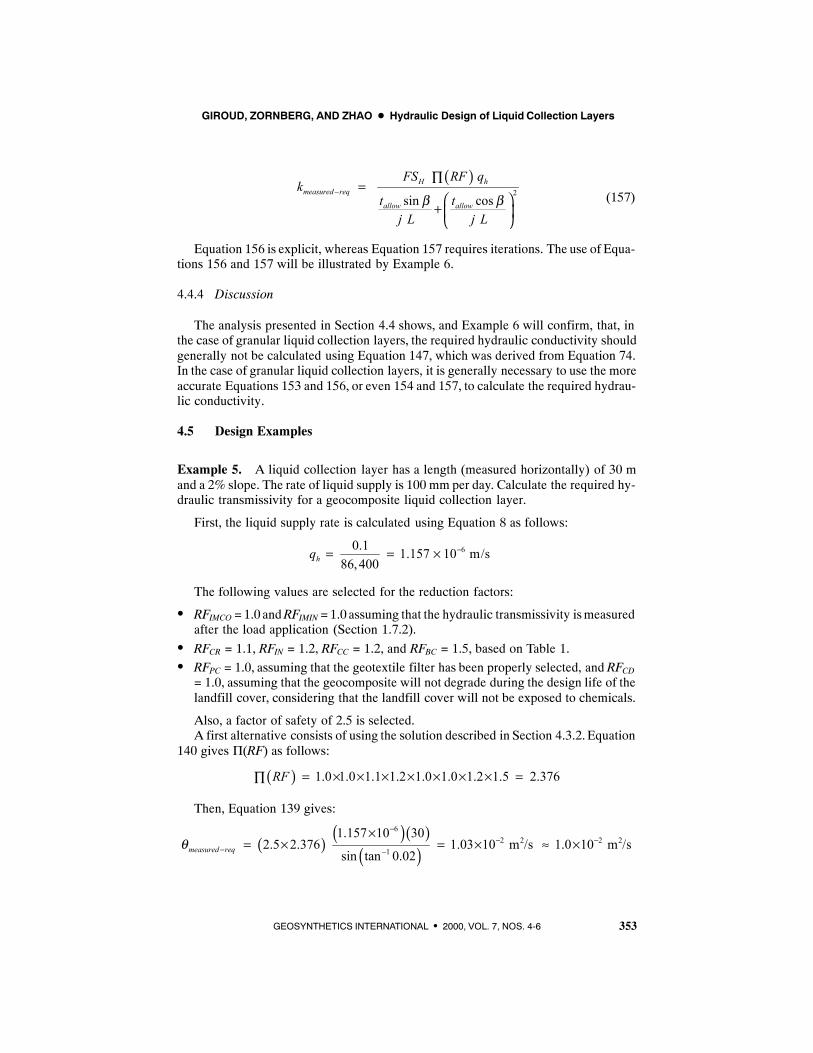
GIROUD, ZORNBERG, AND ZHAO D Hydraulic Design of Liquid Collection Layers
353GEOSYNTHETICS INTERNATIONAL S 2000, VOL. 7, NOS. 4-6
(157)
( )2
sin cosH h
measured req
allow allow
FS RF qk
t tj L j L
β β−
∏=
+
Equation 156 is explicit, whereas Equation 157 requires iterations. The use of Equa-tions 156 and 157 will be illustrated by Example 6.
4.4.4 Discussion
The analysis presented in Section 4.4 shows, and Example 6 will confirm, that, inthe case of granular liquid collection layers, the required hydraulic conductivity shouldgenerally not be calculated using Equation 147, which was derived from Equation 74.In the case of granular liquid collection layers, it is generally necessary to use the moreaccurate Equations 153 and 156, or even 154 and 157, to calculate the required hydrau-lic conductivity.
4.5 Design Examples
Example 5. A liquid collection layer has a length (measured horizontally) of 30 mand a 2% slope. The rate of liquid supply is 100 mm per day. Calculate the required hy-draulic transmissivity for a geocomposite liquid collection layer.
First, the liquid supply rate is calculated using Equation 8 as follows:
60.1 1.157 10 m/s86, 400hq −= = ×
The following values are selected for the reduction factors:
S RFIMCO =1.0 andRFIMIN =1.0 assuming that the hydraulic transmissivity ismeasuredafter the load application (Section 1.7.2).
S RFCR = 1.1, RFIN = 1.2, RFCC = 1.2, and RFBC = 1.5, based on Table 1.S RFPC = 1.0, assuming that the geotextile filter has been properly selected, and RFCD
= 1.0, assuming that the geocomposite will not degrade during the design life of thelandfill cover, considering that the landfill cover will not be exposed to chemicals.
Also, a factor of safety of 2.5 is selected.A first alternative consists of using the solution described in Section 4.3.2. Equation
140 gives Π(RF) as follows:
( ) 1.0 1.0 1.1 1.2 1.0 1.0 1.2 1.5 2.376RF = × × × × × × × =∏
Then, Equation 139 gives:
( ) ( )( )( )
62 2 2 2
1
1.157 10 302.5 2.376 1.03 10 m /s 1.0 10 m /s
sin tan 0.02measured reqθ−
− −− −
×= × = × ≈ ×

GIROUD, ZORNBERG, AND ZHAO D Hydraulic Design of Liquid Collection Layers
354 GEOSYNTHETICS INTERNATIONAL S 2000, VOL. 7, NOS 4-6
Based on this result, the selected geocomposite should have a hydraulic transmissiv-ity of at least 1.0 × 10⁻² m2/s. This hydraulic transmissivity should be measured in ahydraulic transmissivity test performed under a stress equal to the maximum stress ex-pected in the actual liquid collection layer and with a seating time of at least 100 hours,since these are the testing conditions assumed to develop Table 1 that was used to selectthe values of the reduction factors. Furthermore, the hydraulic transmissivity testshould be performed with a hydraulic gradient of 0.02 or more, since the hydraulictransmissivity tends to decrease with increasing hydraulic gradient.
A second alternative consists of using the solution described in Section 4.3.3. Thesolution described in Section 4.3.3 depends on the thickness of the liquid collection lay-er. Since no thickness is given in Example 5, a thickness of 9mm is assumed. In the caseof the solution described in Section 4.3.3, two different values are obtained for the re-quired hydraulic transmissivity depending on how the factor of safety is applied.
If the factor of safety is applied to the maximum liquid thickness, Equation 145gives:
( )( )( )( )
( ) ( )( )( ) ( )
62 2
31 2 1
2.5 2.376 1.157 10 301.03 10 m /s
9 10 / 30sin tan 0.02 cos tan 0.02
2.5 2.376
measured reqθ−
−− −
− −
×= = ×
×+
If the factor of safety is applied to the hydraulic transmissivity, Equation 149 gives:
( )( )( )( )
( ) ( )( ) ( )
62 2
31 2 1
2.5 2.376 1.157 10 301.02 10 m /s
9 10 / 30sin tan 0.02 cos tan 0.02
2.376
measured reqθ−
−− −
− −
×= = ×
×+
The very small difference between 1.02 and 1.03 confirms that Equation 139 givesa good approximation of the required hydraulic transmissivity in the case of geosynthet-ic liquid collection layers. This is consistent with the comment made at the end of Sec-tion 4.4.2.
ENDOFEXAMPLE5
Example 6. A liquid collection layer has a length (measured horizontally) of 30 mand a 2% slope. A granular liquid collection layer with a thickness of 0.45 m is consid-ered at the design stage. The rate of liquid supply is 100 mm per day. The maximumliquid thickness value prescribed by the applicable regulation is 0.3 m. Calculate therequired hydraulic conductivity of the granular liquid collection layer.
First, the liquid supply rate is calculated using Equation 8 as follows:
qh = = × −0 186 400
1157 10 6.,
. m/s
The following values are selected for the reduction factors:

GIROUD, ZORNBERG, AND ZHAO D Hydraulic Design of Liquid Collection Layers
355GEOSYNTHETICS INTERNATIONAL S 2000, VOL. 7, NOS. 4-6
S RFCC = 1.2 and RFBC = 1.5, using Table 1 for guidance, even though Table 1 wasdeveloped for geonets.
S RFPC = 1.0, assuming that an adequate filter has been selected.
Also, a factor of safety of 2.5 is selected.Then, it is necessary to know the allowable thickness. As indicated in Section 3.2.3,
it is the lesser of: (i) a maximum liquid thickness prescribed by regulations; and (ii) thethickness of the liquid collection layer. Therefore, the allowable thickness is 0.3 m.
A first approximation of the required hydraulic conductivity can be calculated usingEquation 150. This equation is valid only if the condition expressed by Equation 92 ismet. The height of the liquid collection layer is given by Equation 93 as follows:
H = =30 0 02 0 60a fa f. . m
The allowable liquid thickness is greater than one tenth of the height of the liquidcollection layer. As a result, Equation 150 is not valid in the considered case. Therefore,the more accurate Equations 153, 154, 156, and 157 must be used.
Equation 153, which corresponds to the case where the factor of safety is appliedto the maximum liquid thickness gives:
( )( )( ) ( )
( )( )( ) ( )
( )( )
62
21 1
1.0 1.2 1.5 1.157 102.16988 10 m/s
0.3 sin tan 0.02 0.3 cos tan 0.022.5 30 2.5 30
measured reqk−
−−
− −
× × ×= = ×
+
hence:
22.17 10 m/smeasured reqk −− = ×
Equation 156, which corresponds to the case where the factor of safety is appliedto the hydraulic conductivity of the liquid collection layer gives:
( )( )( )( ) ( ) ( ) ( )
62
21 1
2.5 1.0 1.2 1.5 1.157 101.73596 10 m/s
0.3 sin tan 0.02 0.3 cos tan 0.0230 30
measured reqk−
−−
− −
× × ×= = ×
+
hence:
21.74 10 m/smeasured reqk −− = ×
Equations 153 and 156 are explicit. More precision can be obtained from Equations154 and 157 that require iterations. The values obtained using Equations 153 and 156are used to start the iteration process.
To use Equation 154, it is necessary to first calculate λ to calculate j. Equation 9gives:
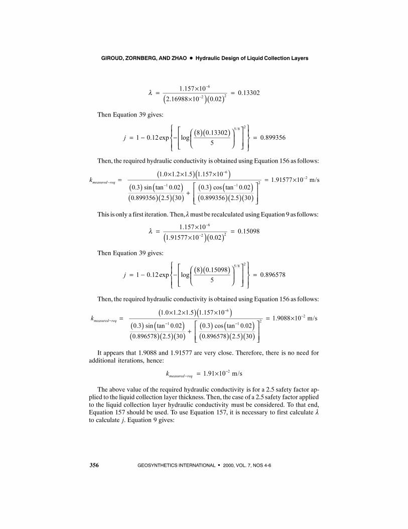
GIROUD, ZORNBERG, AND ZHAO D Hydraulic Design of Liquid Collection Layers
356 GEOSYNTHETICS INTERNATIONAL S 2000, VOL. 7, NOS 4-6
( )( )6
22
1.157 10 0.133022.16988 10 0.02
λ−
−
×= =×
Then Equation 39 gives:
( )( )25/8
8 0.133021 0.12exp log 0.899356
5j
= − − =
Then, the required hydraulic conductivity is obtained using Equation 156 as follows:
( )( )( ) ( )( )( )( )
( ) ( )( )( )( )
62
21 1
1.0 1.2 1.5 1.157 101.91577 10 m/s
0.3 sin tan 0.02 0.3 cos tan 0.020.899356 2.5 30 0.899356 2.5 30
measured reqk−
−−
− −
× × ×= = ×
+
This is only a first iteration. Then, λmust be recalculated usingEquation 9 as follows:
( )( )6
22
1.157 10 0.150981.91577 10 0.02
λ−
−
×= =×
Then Equation 39 gives:
( )( )25/8
8 0.150981 0.12exp log 0.896578
5j
= − − =
Then, the required hydraulic conductivity is obtained using Equation 156 as follows:
( )( )( ) ( )( )( )( )
( ) ( )( )( )( )
62
21 1
1.0 1.2 1.5 1.157 101.9088 10 m/s
0.3 sin tan 0.02 0.3 cos tan 0.020.896578 2.5 30 0.896578 2.5 30
measured reqk−
−−
− −
× × ×= = ×
+
It appears that 1.9088 and 1.91577 are very close. Therefore, there is no need foradditional iterations, hence:
21.91 10 m/smeasured reqk −− = ×
The above value of the required hydraulic conductivity is for a 2.5 safety factor ap-plied to the liquid collection layer thickness. Then, the case of a 2.5 safety factor appliedto the liquid collection layer hydraulic conductivity must be considered. To that end,Equation 157 should be used. To use Equation 157, it is necessary to first calculate λto calculate j. Equation 9 gives:
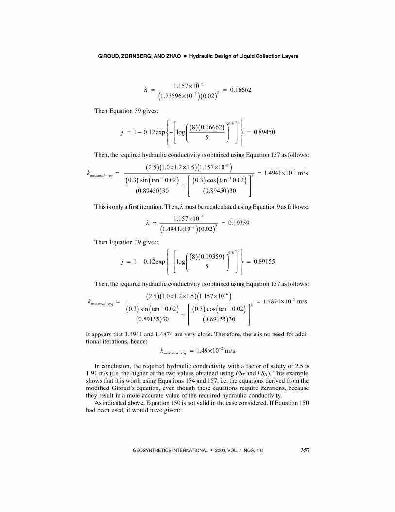
GIROUD, ZORNBERG, AND ZHAO D Hydraulic Design of Liquid Collection Layers
357GEOSYNTHETICS INTERNATIONAL S 2000, VOL. 7, NOS. 4-6
( )( )6
22
1.157 10 0.166621.73596 10 0.02
λ−
−
×= =×
Then Equation 39 gives:
( )( )25/8
8 0.166621 0.12exp log 0.89450
5j
= − − =
Then, the required hydraulic conductivity is obtained using Equation 157 as follows:
( )( )( )( ) ( )
( )( ) ( )
( )
62
21 1
2.5 1.0 1.2 1.5 1.157 101.4941 10 m/s
0.3 sin tan 0.02 0.3 cos tan 0.020.89450 30 0.89450 30
measured reqk−
−−
− −
× × ×= = ×
+
This is only a first iteration. Then, λmust be recalculated usingEquation 9 as follows:
( )( )6
22
1.157 10 0.193591.4941 10 0.02
λ−
−
×= =×
Then Equation 39 gives:
( )( )25/8
8 0.193591 0.12exp log 0.89155
5j
= − − =
Then, the required hydraulic conductivity is obtained using Equation 157 as follows:
( )( )( )( ) ( )
( )( ) ( )
( )
62
21 1
2.5 1.0 1.2 1.5 1.157 101.4874 10 m/s
0.3 sin tan 0.02 0.3 cos tan 0.020.89155 30 0.89155 30
measured reqk−
−−
− −
× × ×= = ×
+
It appears that 1.4941 and 1.4874 are very close. Therefore, there is no need for addi-tional iterations, hence:
21.49 10 m/smeasured reqk −− = ×
In conclusion, the required hydraulic conductivity with a factor of safety of 2.5 is1.91 m/s (i.e. the higher of the two values obtained using FST and FSH). This exampleshows that it is worth using Equations 154 and 157, i.e. the equations derived from themodified Giroud’s equation, even though these equations require iterations, becausethey result in a more accurate value of the required hydraulic conductivity.
As indicated above, Equation 150 is not valid in the case considered. If Equation 150had been used, it would have given:
GIROUD, ZORNBERG, AND ZHAO D Hydraulic Design of Liquid Collection Layers
358 GEOSYNTHETICS INTERNATIONAL S 2000, VOL. 7, NOS 4-6
( )( )( ) ( )
62
1
1.157 10 302.5 1.0 1.2 1.5 2.60 10 m/s
0.3 sin tan 0.02measured reqk−
−− −
×= × × × = ×
It appears that Equation 150 overestimates the required hydraulic conductivity.
ENDOFEXAMPLE6
4.6 Conclusion of Section 4
Based on the discussions presented in Section 4 and Example 5, it appears that theapproximate solution (Equation 139) derived from Equation 74 (i.e. tlim used as anapproximate value for tmax) provides a good approximation of the required hydraulictransmissivity of the liquid collection layer in all cases where a geosynthetic liquidcollection layer is used. Use of the more accurate equations (i.e. equations derived fromGiroud’s equations) requires significantly more effort, but does not provide significantimprovement in accuracy.
In contrast, based on the discussions presented in Section 4 and Example 6, it appearsthat, in the case of granular liquid collection layers, the use of equations derived fromEquation 74 is not accurate and leads to an overestimate of the required hydraulic con-ductivity. Therefore, in the case of granular liquid collection layers it is recommendedto useEquations 153, 154, 156, and 157 (i.e. equations derived fromGiroud’sequations)to calculate the required hydraulic conductivity of the liquid collection layer material.When Equation 74 is used, the numerical value of the factor of safety is the samewheth-er the factor of safety is applied to the maximum liquid thickness, FST , or to the hydrau-lic characteristics of the liquid collection layer, FSH . In contrast, when Giroud’sequations are used, different values are obtained for FST and FSH .
5 CONCLUSIONS
The basic requirement for the hydraulic design of liquid collection layers is that themaximum thickness of liquid in the liquid collection layer be less than an allowablethickness. Accordingly, equations are presented for calculating the maximum liquidthickness in liquid collection layers. Also, equations are presented for determining therequired hydraulic conductivity of the liquid collection layer material and the requiredhydraulic transmissivity of the liquid collection layer to ensure that the maximum liquidthickness is less than the allowable thickness.
The following conclusions can be drawn from the present paper:
S The differential equation governing the thickness of liquid in a liquid collection lay-er has been solved numerically by Giroud et al. (1992) and analytically byMcEnroe(1993) for the maximum liquid thickness. The development of the analytical solu-tion byMcEnroe is a major step forward in the design of liquid collection layers. Thenumerical values of the maximum liquid thickness provided by both the numericaland analytical solutions are very close. It may, therefore, be concluded that bothsolutions are correct.

GIROUD, ZORNBERG, AND ZHAO D Hydraulic Design of Liquid Collection Layers
359GEOSYNTHETICS INTERNATIONAL S 2000, VOL. 7, NOS. 4-6
S The analytical solution by McEnroe consists of a set of three equations (known as“McEnroe’s equations”, Equations 49 to 51). The use of McEnroe’s equations re-quires lengthy calculations. Furthermore, one ofMcEnroe’s equations (i.e. the equa-tion for R< 0.25) is extremely sensitive to the precision of the input parameters.For some values of the parameters, calculations must be performed with more than10 digits (and even, in some cases, more than 15) to avoid significant inaccuracies.Thismakes it potentially unsafe to useMcEnroe’s equations with pocket calculatorsroutinely used for engineering calculations. However, being the correct analyticalsolution to the governing differential equation, McEnroe’s equations should be re-garded as the reference against which other solutions are to be evaluated.
S For practical applications, an accurate value of the maximum thickness of liquid ina liquid collection layer can be calculated using a semi-empirical equation knownas the “modified Giroud’s equation” (Equation 40). This equation is simple to useand is not overly sensitive to the precision of the input parameters. The differencebetween values of the maximum liquid thickness calculated using the modified Gi-roud’s equation and the reference values calculated using McEnroe’s equations isvery small; it is less than 1% for most usual values of the parameters. Therefore, useof the modified Giroud’s equation is the recommended approach for the design ofliquid collection layers when accurate determination of the maximum liquid thick-ness is needed. Differently than in McEnroe’s solution, which requires a set of threeequations to cover the entire range of parameter values, the modified Giroud’s equa-tion is a single equation that covers the entire range of parameter values.
S Agood approximation of the maximum thickness of liquid in a liquid collection lay-er is provided by a simple equation known as the “original Giroud’s equation”(Equation 16). The difference between values of the maximum liquid thickness cal-culated using the original Giroud’s equation and the reference values calculated us-ing McEnroe’s equations is less than 13% for the entire range of usual values of theparameters. This degree of precision is sufficient in most applications. Furthermore,the use of the original Giroud’s equation is conservative (i.e. the values of the maxi-mumliquid thickness calculated using the original Giroud’s equation are higher thanthe reference values calculated using McEnroe’s equations).
S An advantage of both the original and the modified Giroud’s equations is that theyare particularly suitable to perform parametric studies.
S A very simple equation (Equation 74) provides an approximate value of the liquidthickness in a liquid collection layer that is valid only within a certain range of pa-rameter values. A discussion of the influence of the parameters (Section 2.11) showsthat, if the approximate value of the maximum liquid thickness calculated usingEquation 74 is less than one tenth of the height of the liquid collection layer slope,this approximate value is an acceptable approximation because it is less than 17%above the rigorously calculated value. As a result, Equation 74 is valid in virtuallyall cases where a typical geosynthetic drainage layer is used, provided that the maxi-mum liquid thickness is less than the thickness of the geosynthetic drainage layer.
S The various equations proposed for calculating the maximum liquid thickness canbe normalized in relation to the liquid thickness that corresponds to the limit caseinwhich the dimensionless parameter λ tends toward zero, tlim . The normalized solu-
GIROUD, ZORNBERG, AND ZHAO D Hydraulic Design of Liquid Collection Layers
360 GEOSYNTHETICS INTERNATIONAL S 2000, VOL. 7, NOS 4-6
tions are helpful for comparing of the accuracy of different solutions and for definingthe location of the maximum liquid thickness along the liquid collection layer.
S The governing differential equation used by McEnroe (Equation 42) is slightly dif-ferent from the governing differential equation used in the present paper (Equation25). The difference is due to different approximations regarding the hydraulic head.These approximations are needed because the hydraulic head varies along the liquidcollection layer slope. A discussion presented in Section 2.9 shows that Equation25 is preferable because it leads to normalized solutions that do not directly dependon β.
S Giroud’s equations (Equation 16 and 40) and the simple equation (Equation 74) canbe solved for the hydraulic conductivity and can, therefore, be used to obtain equa-tions that give the required value of the hydraulic conductivity of the liquid collec-tion layer material and the hydraulic transmissivity of the liquid collection layer.
S The use of the McEnroe’s equations appears to be unsuitable for the determinationof the characteristics of the liquid collection material needed to ensure that the liquidthickness is less than the allowable thickness.
S From a practical standpoint, the equations provided in the present paper are usedwith reduction factors and a factor of safety. The reduction factors account for thedecrease in hydraulic properties (characteristics) of the liquid collection layer insoil, under stress, and with time. The factor of safety can be applied in two ways:it can be applied to the maximum liquid thickness, FST , or to the hydraulic charac-teristics of the liquid collection layer,FSH. Detailed guidance on the use of reductionfactors and factor of safety is provided in Sections 3 and 4.
S Equations other than McEnroe’s and Giroud’s have been published and are dis-cussed in Appendix D.Most of these equations lead to incorrect values of the liquidthickness. This is, in particular, the case of Moore’s equations, which are still widelyused in the United States, even though they may lead to unconservative designs.
In conclusion, it appears that all the equations required for the hydraulic design ofliquid collection layers are available. The present paper provides an overview of theavailable equations (Section 2) and provides guidance for the use of these equations(Sections 3 or 4). In particular, the present paper provides detailed guidance for the useof reduction factors to quantify the decrease in flow capacity of liquid collection layersdue to a variety of mechanisms, such as thickness reduction caused by the appliedstresses and hydraulic conductivity reduction caused by clogging. Also, the present pa-per provides guidance for the use of safety factors. Two design approaches are present-ed: the “thickness approach” (Section 3) and the “hydraulic characteristic approach”(Section 4). With the thickness approach, a given liquid collection material is consid-ered and the design engineer checks that the maximum liquid thickness is less than theallowable thickness; with the hydraulic characteristic approach, the design engineerdetermines the required hydraulic characteristics of the liquid collection layer. The twoapproaches are equivalent, and a careful design engineer will use both.
GIROUD, ZORNBERG, AND ZHAO D Hydraulic Design of Liquid Collection Layers
361GEOSYNTHETICS INTERNATIONAL S 2000, VOL. 7, NOS. 4-6
ACKNOWLEDGMENTS
The support of GeoSyntec Consultants is acknowledged. Also, the authors are grate-ful to J.D. Frost for his valuable comments and to R. Ortiz and H.A. King for the prepa-ration of the figures.
REFERENCES
Demetracopoulos, A.C., Korfiatis, G.P., and Nawy, E.G., 1984, “Modeling for Designof Landfill Bottom Liners”, Journal of Environmental Engineering, ASCE, Vol. 110,No. 6, pp. 1084-1098.
Giroud, J.P., 1985, “Height of Leachate in a Drainage Layer”, Unpublished ProjectNotes, GeoSyntec Consultants, August 1985.
Giroud, J.P., 1996, “Granular Filters and Geotextile Filters”, Proceedings of GeoFilters’96, Lafleur, J. and Rollin, A.L., Editors, Montréal, Québec, Canada, May 1996, pp.565 - 680.
Giroud, J.P., Gross, B.A., and Darasse, J., 1992, “Flow in Leachate Collection Layers,Steady-State Condition”, GeoSyntec Consultants Report, 62 p.
Giroud, J.P. and Houlihan, M.F., 1995, “Design of Leachate Collection Layers”, Pro-ceedings of the Fifth International Landfill Symposium, Vol. 2, Sardinia, Italy, Octo-ber 1995, pp. 613-640.
Giroud, J.P., Zhao, A., and Bonaparte, R., 2000a, “TheMyth of Hydraulic Transmissiv-ity Equivalency Between Geosynthetic and Granular Liquid Collection Layers”,Geosynthetics International, Special Issue on Liquid Collection Systems, Vol. 7,Nos. 4-6, pp. 381-401.
Giroud, J.P., Zhao, A., and Richardson, G.N., 2000b, “Effect of Thickness ReductiononGeosynthetic Hydraulic Transmissivity”, Geosynthetics International, Special Is-sue on Liquid Collection Systems, Vol. 7, Nos. 4-6, pp. 433-452.
Giroud, J.P., Zornberg, J.G., andBeech, J.F., 2000c, “Hydraulic Design ofGeosyntheticand Granular Liquid Collection Layers Comprising Two Different Slopes”, Geosyn-thetics International, Special Issue on Liquid Collection Systems, Vol. 7, Nos. 4-6,pp. 453-489.
Holtz, R.D., Christopher, B.R., and Berg, R.R., 1997, “Geosynthetic Engineering”, Bi-tech Publishers, British Columbia, Canada, 452 p.
Koerner, R.M., 1999, “Designing With Geosynthetics”, Fourth Edition, Prentice Hall,Englewood Cliffs, New Jersey, USA, 761 p.
Lentz, J.J., 1981, “Apportionment of Net Discharge in Landfill Covering Layer intoSeparate Components of Vertical Leakage and Horizontal Seepage”, Water Re-sources Research, Vol. 17, No. 4, pp. 1231-1234.
Lesaffre, B., 1987, “Analytical Formulae for Traverse Drainage of Sloping Lands withConstant Rainfall”, Irrigation and Drainage Systems, Vol. 1, pp. 105-121.
GIROUD, ZORNBERG, AND ZHAO D Hydraulic Design of Liquid Collection Layers
362 GEOSYNTHETICS INTERNATIONAL S 2000, VOL. 7, NOS 4-6
Masada, T., 1998, “Leachate Flow Mound Equations for Steady-State Flow Over aLandfill Geosynthetic Bottom Liner”,Geosynthetics International, Vol. 5, No. 4, pp.383-397.
McEnroe, B.M., 1989a, “Drainage of Landfill Covers and Bottom Liners: UnsteadyCase”, Journal of Environmental Engineering, ASCE, Vol. 115, No. 6, pp.1103-1113.
McEnroe, B.M., 1989b, “Steady Drainage of Landfill Covers and Bottom Liners”,Journal of Environmental Engineering, ASCE, Vol. 115, No. 6, pp. 1114-1122.
McEnroe, B.M., 1993, “Maximum Saturated Depth Over Landfill Liner”, Journal ofEnvironmental Engineering, ASCE, Vol. 119, No. 2, pp. 262-270.
Moore, C.A., 1980, “Landfill and Surface Impoundment Performance Evaluation”,U.S. Environmental Protection Agency, Washington, DC, USA, SW-869, 63 p.
Moore, C.A., 1983, “Landfill and Surface Impoundment Performance Evaluation”,U.S. Environmental Protection Agency, Washington, DC, USA, SW-869, 69 p.
Palmeira, E.M. and Gardoni, M.G., 2000, “The Influence of Partial Clogging and Pres-sure on the Behaviour of Geotextiles in Drainage Systems”, Special Issue on LiquidCollection Systems, Geosynthetics International, Vol. 7, Nos. 4-6, pp. 403-431.
USEPA, 1989, “Requirements for Hazardous Waste Landfill Design, Construction, andClosure”, August 1989, Seminar Publication, EPA/625/4-89/022, USEnvironmentalProtection Agency, Cincinnati, Ohio, USA, 128 p.
Wong, J., 1977, “The Design of a System for Collecting Leachate from a Lined LandfillSite”, Water Resources Research, Vol. 13, No. 2, pp. 404-410.
Zanzinger, H. and Gartung, E., 1999, “Hydraulic Design of Drainage Geocompositesfor Landfill Covers—Use ofReduction Factors”,Proceedings of Rencontres 99,Vol.1, French Committee on Geosynthetics, Bordeaux, France, October 1999, pp. 89-96.
NOTATIONS
Basic SI units are given in parentheses.
A = cross-sectional area of flow (m2)A′ = parameter defined by Equation 62 (dimensionless)A* = parameter defined by Equation 46 (dimensionless)Ah = horizontal area through which flow rate Qh is measured (m2)B = width of liquid collection layer in direction perpendicular to direction of
flow (m)B′ = parameter defined by Equation 62 (dimensionless)B* = parameter defined by Equation 46 (dimensionless)C = constant used in integration (m2)D = depth (measured vertically) of liquid in liquid collection layer (m)DL = depth of liquid collected in horizontal pan during time Δt* (m)
GIROUD, ZORNBERG, AND ZHAO D Hydraulic Design of Liquid Collection Layers
363GEOSYNTHETICS INTERNATIONAL S 2000, VOL. 7, NOS. 4-6
FS = factor of safety (dimensionless)FSH = factor of safety applied to hydraulic characteristics of liquid collection
layer (dimensionless)FST = factor of safety applied to maximum liquid thickness (dimensionless)g = acceleration due to gravity (m/s2)H = height (measured vertically) of liquid collection layer (m)h = hydraulic head (m)hA = hydraulic head at Point A (m)hAB = hydraulic head corresponding to liquid thickness AB (m)hB = hydraulic head at Point B (m)hmax = hydraulic head related to the maximum liquid thickness (m)i = hydraulic gradient (dimensionless)iequiv = equivalent hydraulic gradient (dimensionless)itoe = hydraulic gradient at toe of liquid collection layer slope
(dimensionless)j = modifying factor applied to original Giroud’s equation to obtain
modified Giroud’s equation (dimensionless)k = hydraulic conductivity of liquid collection layer material (m/s)kLTIS = long-term-in-soil hydraulic conductivity, i.e. hydraulic conductivity of
liquid collection layer material subjected to conditions that can causedevelopment of chemical and/or biological clogging during design lifeof liquid collection layer (m/s)
kLTISFS = factored long-term-in-soil hydraulic conductivity, i.e. in-soil-long-termhydraulic conductivity divided by overall factor of safety (m/s)
kmeasured = hydraulic conductivity of specimen of granular material, representativeof granular material as installed, measured in hydraulic conductivity testperformed with water during short periods of time so that cloggingdoes not develop (m/s)
kmeasured-req = required value of hydraulic conductivity of liquid collection layermaterial (m/s)
L = length (measured horizontally) of rectangular liquid collection layer indirection of flow (m)
p = liquid pressure (Pa)pB = liquid pressure at Point B (Pa)Q = rate of flow in liquid collection layer (m3/s)Qh = rate of liquid flow through horizontal area Ah (m3/s)Qt = rate of flow through cross section located at horizontal distance x from
top of slope (m3/s)qh = rate of liquid supply expressed per unit surface area measured
horizontally (m/s)
GIROUD, ZORNBERG, AND ZHAO D Hydraulic Design of Liquid Collection Layers
364 GEOSYNTHETICS INTERNATIONAL S 2000, VOL. 7, NOS 4-6
R = parameter defined by Equation 9 (dimensionless)RF = reduction factor (dimensionless)RFBC = reduction factor for flow capacity decrease due to biological clogging of
liquid collection layer material (dimensionless)RFCC = reduction factor for flow capacity decrease due to chemical clogging of
liquid collection layer material (dimensionless)RFCD = reduction factor for chemical degradation, i.e. decrease of hydraulic
transmissivity due to chemical degradation of polymeric compound(s)used to make geocomposite (dimensionless)
RFCR = reduction factor for flow capacity decrease due to creep of transmissivecore of geocomposite or other geosynthetic liquid collection layer(dimensionless)
RFIMCO = reduction factor for immediate compression, i.e. decrease of hydraulictransmissivity due to compression of transmissive core followingimmediate application of stress (dimensionless)
RFIMIN = reduction factor for immediate intrusion, i.e. decrease of hydraulictransmissivity due to geotextile intrusion into transmissive corefollowing immediate application of stress (dimensionless)
RFIN = reduction factor for delayed intrusion, i.e. decrease of hydraulictransmissivity over time due to geotextile intrusion into transmissivecore resulting from time-dependent deformation of geotextile(dimensionless)
RFPC = reduction factor for particulate clogging, i.e. decrease of hydraulictransmissivity due to clogging by particles migrating into transmissivecore (dimensionless)
r = parameter defined by Equation D-5 (dimensionless)t = thickness (measured perpendicular to slope) of liquid in liquid collection
layer (m)tLCL = thickness of liquid collection layer (m)tLTIS = long-term-in-soil thickness of transmissive core of geosynthetic (m)tallow = allowable thickness of liquid in liquid collection layer, i.e. lesser of:
(i) maximum liquid thickness prescribed by regulations; and(ii) thickness of liquid collection layer (m)
tlim = maximum thickness of liquid in liquid collection layer in special casewhere qh is small and k and β are large (m)
tmax = maximum thickness of liquid in liquid collection layer (m)tmax(kLTIS) = maximum thickness of liquid in liquid collection layer as a function of
kLTIS (m)tmax(kLTISFS)
= maximum thickness of liquid in liquid collection layer as a function ofkLTISFS (m)
ttoe = liquid thickness at toe of liquid collection layer slope (m)
GIROUD, ZORNBERG, AND ZHAO D Hydraulic Design of Liquid Collection Layers
365GEOSYNTHETICS INTERNATIONAL S 2000, VOL. 7, NOS. 4-6
tvirgin = thickness of liquid collection layer under no compressive stress (m)v = liquid velocity (m/s)X = distance measured along slope between top of slope and considered cross
section of liquid collection layer (m)x = horizontal distance between top of slope and considered cross section of
liquid collection layer (m)xm = horizontal distance between top of slope and location of maximum liquid
thickness (m)z = elevation (m)zA = elevation of Point A (m)zB = elevation of Point B (m)β = slope angle (_)Δt* = period of time (s)λ = parameter (sometimes called characteristic parameter) defined by
Equation 10 (dimensionless)Ã = liquid density (kg/m3)θ = hydraulic transmissivity of liquid collection layer (m2/s)θLTIS = long-term-in-soil hydraulic transmissivity, i.e. hydraulic transmissivity
of geosynthetic in soil under maximum stress anticipated during designlife of liquid collection layer and subjected to time-dependentmechanisms (such as creep, chemical clogging, and biological clogging)during design life of liquid collection layer (m2/s)
θmeasured = value of hydraulic transmissivity of liquid collection layer measured inlaboratory test (m2/s)
θmeasured-req= required value of hydraulic transmissivity of liquid collection layer(m2/s)
θvirgin = hydraulic transmissivity of virgin geosynthetic, i.e. geosyntheticsubjected to hydraulic transmissivity test under no stress (or, at amaximum, small stress needed to keep geosynthetic flat during hydraulictransmissivity test) and performed with water during short period of timeso that clogging does not develop (m2/s)
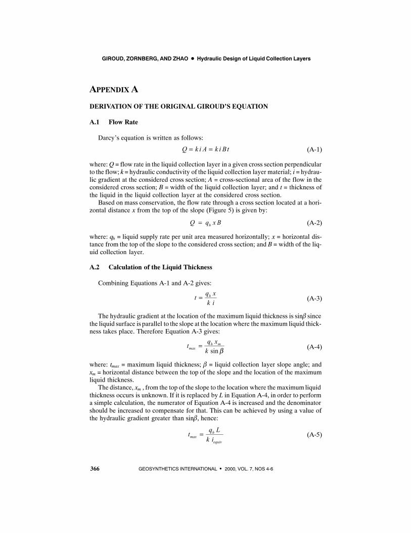
GIROUD, ZORNBERG, AND ZHAO D Hydraulic Design of Liquid Collection Layers
366 GEOSYNTHETICS INTERNATIONAL S 2000, VOL. 7, NOS 4-6
APPENDIX A
DERIVATION OF THE ORIGINAL GIROUD’S EQUATION
A.1 Flow Rate
Darcy’s equation is written as follows:
Q k i A k i Bt= = (A-1)
where:Q= flow rate in the liquid collection layer in a given cross section perpendicularto the flow; k=hydraulic conductivity of the liquid collection layer material; i =hydrau-lic gradient at the considered cross section; A = cross-sectional area of the flow in theconsidered cross section; B = width of the liquid collection layer; and t = thickness ofthe liquid in the liquid collection layer at the considered cross section.
Based on mass conservation, the flow rate through a cross section located at a hori-zontal distance x from the top of the slope (Figure 5) is given by:
hQ q x B= (A-2)
where: qh = liquid supply rate per unit area measured horizontally; x = horizontal dis-tance from the top of the slope to the considered cross section; and B = width of the liq-uid collection layer.
A.2 Calculation of the Liquid Thickness
Combining Equations A-1 and A-2 gives:
t q xk ih= (A-3)
The hydraulic gradient at the location of the maximum liquid thickness is sinβ sincethe liquid surface is parallel to the slope at the location where themaximum liquid thick-ness takes place. Therefore Equation A-3 gives:
t q xk
h mmax =
sin β (A-4)
where: tmax = maximum liquid thickness; β = liquid collection layer slope angle; andxm = horizontal distance between the top of the slope and the location of the maximumliquid thickness.
The distance, xm , from the top of the slope to the location where the maximum liquidthickness occurs is unknown. If it is replaced by L in Equation A-4, in order to performa simple calculation, the numerator of Equation A-4 is increased and the denominatorshould be increased to compensate for that. This can be achieved by using a value ofthe hydraulic gradient greater than sinβ, hence:
(A-5)t q Lk i
h
equivmax =
GIROUD, ZORNBERG, AND ZHAO D Hydraulic Design of Liquid Collection Layers
367GEOSYNTHETICS INTERNATIONAL S 2000, VOL. 7, NOS. 4-6
where iequiv is the equivalent hydraulic gradient used for the calculation of themaximumliquid thickness, tmax , using Equation A-5. As indicated above, this equivalent hydrau-lic gradient must be greater than sinβ.
A.3 Selection of an Equivalent Hydraulic Gradient
As a guidance for the selection of the equivalent hydraulic gradient, the well-knowncase where β = 0 was considered. In this case (Figure 6 in the main text of the presentpaper), the maximum liquid thickness occurs for xm = 0 and is given by the followingclassical equation (Giroud and Houlihan 1995):
(A-6)tL
qk
hmax =
The derivation of Equation A-6 may be found in Section 2.3.2. Equation A-6 canbe written:
(A-7)2
h max max maxq t t tk L L L
= =
hence:
(A-8)( )/h
maxmax
q Ltk t L
=
Comparing Equations A-5 and A-8 shows that Equation A-6 could have been de-rived from Equation A-5 using the following value for the equivalent hydraulic gradi-ent, iequiv :
(A-9)maxequiv
tiL
=
The hydraulic gradient must be defined based on the hydraulic head, not the liquidthickness. In the case shown in Figure 6, β = 0; therefore, Equation 4 (in the main textof the present paper) gives:
(A-10)h tmax max=
where hmax is the hydraulic head related to the maximum liquid thickness.Combining Equations A-9 and A-10 shows that, in reality, in Equation A-6, the hy-
draulic gradient is:
(A-11)maxequiv
hiL
=
The foregoing analysis shows that it was possible to establish Equation A-6 by usingan equivalent hydraulic gradient equal to the hydraulic head associated with the maxi-mum thickness divided by the horizontal projection of the length of the liquid collectionlayer. This approach, which gave Equation A-11 for the special case where β = 0, givesthe following equation for the general case where β≠ 0:
GIROUD, ZORNBERG, AND ZHAO D Hydraulic Design of Liquid Collection Layers
368 GEOSYNTHETICS INTERNATIONAL S 2000, VOL. 7, NOS 4-6
(A-12)i hLequiv = +sin
/ cosβ
βmax
Equation 4 (in the main text of the present paper) gives:
(A-13)h tmax max= cosβ
Combining Equations A-12 and A-13 gives:
(A-14)2sin cosmaxequiv
tiL
β β= +
Combining Equations A-5 and A-14 gives:
(A-15)qk
tL
tL
h = +FH
IKmax maxsin cosβ β2
hence:
(A-16)tL
tL
qk
hmax maxFHIK + − =
22 0cos sinβ β
Solving this quadratic equation gives:
(A-17)tL
qk
qk
h h
max =+ −
=+ −sin cos sin
cos
tan tan
cos
2 2
2
24
2
4
2
β β β
β
β β
β
Equation A-17 is identical to Equation 16 in the main text of the present paper.
A.4 Limit Cases
To confirm the validity of Equation A-17, it is important to check that it tends towardthewell known equations for the two limit cases: whenβ=0, andwhen qh/k is very small.
When β = 0, Equation A-17 gives:
(A-18)tL
qk q
k
h
hmax = =
4
2
Equation A-18 is the well-known equation for the case where β = 0 (see Equation31 in the main text of the present paper, and Equation A-6). Therefore, Equation A-17tends toward the appropriate limit for β = 0.
Equation A-17 can be written as follows:
(A-19)tL
qk
h
max =+ −1 1
2
2tancos / tan
ββ β
When qh/k is very small, the following classical relationship can be used:
GIROUD, ZORNBERG, AND ZHAO D Hydraulic Design of Liquid Collection Layers
369GEOSYNTHETICS INTERNATIONAL S 2000, VOL. 7, NOS. 4-6
(A-20)2 21 1tan 2 tan
h hq qk kβ β
+ ≈ +
Combining Equations A-19 and A-20 gives:
(A-21)tL
qk q
k
h
hmax ≈ ≈22
2tancos
tansin
βββ
β
Equation A-21 is the well-known equation for the case where qh/k is very small(Section 2.8). Therefore, Equation A-17 tends toward the appropriate limit when qh/kis very small.
The fact that Equation A-17 tends toward the well-known equations for the two limitcases confirms the validity of Equation A-17.
GIROUD, ZORNBERG, AND ZHAO D Hydraulic Design of Liquid Collection Layers
370 GEOSYNTHETICS INTERNATIONAL S 2000, VOL. 7, NOS 4-6
APPENDIX B
BOUNDARY CONDITIONS AT THE TOE OF THE LIQUID COLLECTIONLAYER SLOPE
B.1 Hydraulic Gradient
The hydraulic gradient is defined by:
dd / cos
hix β
= − (B--1)
where: x = horizontal distance from the top of the slope to the considered cross section;β = liquid collection layer slope angle; and h = hydraulic head defined by:
(B--2)2
2p vh zg gρ
= + +
where: z = elevation; p = pressure; Ã = liquid density; g = acceleration due to gravity;and v = liquid velocity. The term v2 is negligible in the case of laminar flow, hence:
(B--3)ph zgρ
= +
In Figure 2 (in the main text of the present paper), the hydraulic head is the samein A and B since AB is an equipotential line. Therefore:
(B--4)BA B B
ph h h zgρ
= = = +
where: hA = hydraulic head at Point A; hB = hydraulic head at Point B; zB = elevationat Point B; and hB = pressure at Point B.
If A is at the horizontal distance x from the top of the liquid collection layer slope,the elevation of B can be calculated as follows based on Figures 2 and 5:
(B--5)( ) tan cosBz L x tβ β= − +
where t is the liquid thickness.Combining Equations B-4 and B-5 gives:
(B--6)( ) tan cos Bph L x tg
β βρ
= − + +
The pressure in B, pB , is the atmospheric pressure, which does not vary as a functionof x. Therefore, combining Equations B-1 and B-6 gives:
(B--7)2 dsin cosd
tix
β β= −
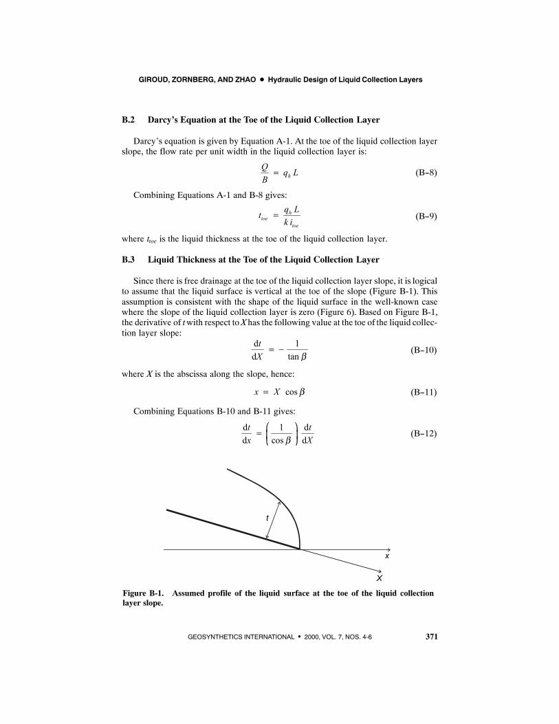
GIROUD, ZORNBERG, AND ZHAO D Hydraulic Design of Liquid Collection Layers
371GEOSYNTHETICS INTERNATIONAL S 2000, VOL. 7, NOS. 4-6
B.2 Darcy’s Equation at the Toe of the Liquid Collection Layer
Darcy’s equation is given by Equation A-1. At the toe of the liquid collection layerslope, the flow rate per unit width in the liquid collection layer is:
(B--8)hQ q LB
=
Combining Equations A-1 and B-8 gives:
(B--9)htoe
toe
q Ltk i
=
where ttoe is the liquid thickness at the toe of the liquid collection layer.
B.3 Liquid Thickness at the Toe of the Liquid Collection Layer
Since there is free drainage at the toe of the liquid collection layer slope, it is logicalto assume that the liquid surface is vertical at the toe of the slope (Figure B-1). Thisassumption is consistent with the shape of the liquid surface in the well-known casewhere the slope of the liquid collection layer is zero (Figure 6). Based on Figure B-1,the derivative of twith respect toXhas the following value at the toe of the liquid collec-tion layer slope:
(B--10)d 1d tan
tX β
= −
where X is the abscissa along the slope, hence:
(B--11)cosx X β=
Combining Equations B-10 and B-11 gives:
(B--12)d 1 dd cos d
t tx Xβ
=
t
x
X
Figure B-1. Assumed profile of the liquid surface at the toe of the liquid collectionlayer slope.
GIROUD, ZORNBERG, AND ZHAO D Hydraulic Design of Liquid Collection Layers
372 GEOSYNTHETICS INTERNATIONAL S 2000, VOL. 7, NOS 4-6
Combining Equations B-10 and B-12 gives:
(B--13)d 1 1 1d cos tan sin
tx β β β
= − = −
Combining Equations B-7 and B-13 gives the hydraulic gradient at the toe of the liq-uid collection layer slope as follows:
(B--14)2 2 2cos sin cos 1sin
sin sin sintoei β β βββ β β
+= − = = −
Combining B-9 and B-14 gives the thickness of liquid at the toe of the liquid collec-tion layer slope as follows:
(B--15)sinhtoe
q Ltk
β=
In the special case where β = 0, itoe = ∞ according to Equation B-14 and ttoe = 0 ac-cording to Equation B-15. This is consistent with Figure 6. It is important to note thatvertical flow corresponds to a hydraulic gradient of one only if the liquid collection lay-er is vertical. If the liquid collection layer is horizontal, vertical flow corresponds to aninfinite gradient. If the liquid collection layer slope is β, vertical flow corresponds toa hydraulic gradient of 1/sinβ, as shown above.
B.4 Boundary Conditions at Toe Used for the Development of Equations
To solve the governing differential equation numerically, Giroud et al. (1992) as-sumed ttoe = 0 for all values of β, which implies itoe = ∞ for all values of β. Since themodified Giroud’s equation was developed based on the results of the numerical solu-tion of the governing differential equation (Section 2.3), it is legitimate to consider thatthe modified Giroud’s equation corresponds to the same boundary conditions, i.e. ttoe= 0 and itoe = ∞. The same boundary conditions were used by the authors of the presentpaper to derive Equations 52 to 54, i.e. the McEnroe’s equations for ttoe = 0.
To develop his equations for free drainage at the toe of the liquid collection layerslope, McEnroe (1993) used the boundary conditions defined by:
(B--16)d 1dhx
= −
The rationale presented byMcEnroe (1993) for this assumption shows that it is plau-sible, but does not demonstrate that it is the best possible assumption to represent freedrainage conditions at the toe. Combining Equations B-1 and B-16 gives:
(B--17)costoei β=
It should be noted that the assumption made by McEnroe does not correspond to ahydraulic gradient of one at the toe of the slope (contrary to what is sometimes statedby users of McEnroe’s equations).
Combining Equations B-9 and B-17 gives:

GIROUD, ZORNBERG, AND ZHAO D Hydraulic Design of Liquid Collection Layers
373GEOSYNTHETICS INTERNATIONAL S 2000, VOL. 7, NOS. 4-6
(B--18)cos
htoe
q Ltβ
=
A summary of the boundary conditions used by different authors is presented inTable B-1. The values of ttoe resulting from the analysis presented in Section B.3 (basedon vertical liquid surface assumption at the toe) and from the assumptions made by Gi-roud et al. (1992) and McEnroe (1993) are compared in Table B-2. Inspection of TableB-2 shows that the value of ttoe used by Giroud et al. (1992) is closer than the value usedby McEnroe (1993) to the value of ttoe obtained for vertical flow at the toe, which maybe considered as the most logical assumption.
B.5 Conclusions
The purpose of Appendix B was to clarify the question of the boundary conditionsat the toe of a liquid collection layer slope. It appears that different boundary conditionswere used byGiroud et al. (1992) and McEnroe (1993), and it appears that these bound-ary conditions may not be as logical as the boundary conditions that consist of assumingthat the liquid flow is vertical at the toe of the liquid collection layer slope. Fortunately,the comparisons presented in Section 2.5 show that the boundary conditions used byGiroud et al. (1992) and McEnroe (1993) have a negligible influence on the calculatedvalue of the maximum liquid thickness.
Table B-1. Summary of boundary conditions at the toe of a liquid collection layer.
Reference Assumption itoe ttoe
The present paper Vertical liquid surface at toe 1sin β
qh L sinβk
Giroud et al. (1992) Zero liquid thickness at toe ∞ 0
McEnroe (1993) dhdx=− 1 at toe cosβ qh L
k cosβ
Table B-2. Values of ttoe for different boundary conditions at the toe of a liquid collectionlayer.
β tanβ
The present paper
ttoeqh L∕k
= sin βGiroud et al. (1992)
ttoe= 0Giroud et al. (1992)ttoeqh L∕k
= 1cos β
0_
1.1_
5.7_
18.4_
26.6_
45.0_
0
0.02
0.10
0.33
0.50
1.00
0
0.02
0.10
0.32
0.45
0.71
0
0
0
0
0
0
1.00
1.00
1.00
1.05
1.12
1.41
GIROUD, ZORNBERG, AND ZHAO D Hydraulic Design of Liquid Collection Layers
374 GEOSYNTHETICS INTERNATIONAL S 2000, VOL. 7, NOS 4-6
APPENDIX C
DERIVATION OF THE MODIFYING FACTOR
As indicated in Section 2.3.3 in the main text of the present paper, the governing dif-ferential equation for the liquid thickness was solved numerically (Giroud et al. 1992).The senior author then compared values calculated using the original Giroud’s equation(i.e. Equation 16 in the main text of the present paper) with the accurate values of themaximum liquid thickness obtained numerically. It appeared that the difference be-tween the values calculated using the original Giroud’s equation and the values ob-tained numerically depended only on the dimensionless parameter λ defined byEquation 9. The senior author noted that, when the difference was plotted as a functionof logλ, it was represented by an inverted bell-shaped curve (Figure 7) with values be-tween 1.00 and 0.88. Therefore, the senior author proposed the following equation forthe dimensionless factor j:
(C-1)j y= − −1 0 12 2. e
where y is a function of logλ.After trial and errors, the senior author found that the following equation ensures that,
when Equation A-17 is multiplied by the dimensionless factor j, one obtains values ofthe maximum liquid thickness very close to the accurate values obtained numerically:
(C-2)jq kh= − −FHG
IKJ
LNMM
OQPP
L
NMM
O
QPP1 0 12
85 2
5 8 2
. exp log/
tan
/b gβ
GIROUD, ZORNBERG, AND ZHAO D Hydraulic Design of Liquid Collection Layers
375GEOSYNTHETICS INTERNATIONAL S 2000, VOL. 7, NOS. 4-6
APPENDIX D
REVIEW OF OTHER REPORTED SOLUTIONS FOR THE MAXIMUMLIQUID THICKNESS IN LIQUID COLLECTION LAYERS
D.1 Presentation of the Equations
As indicated in Section 2.12, solutions other than those discussed in the present pa-per have been proposed in the technical literature for the maximum liquid thickness inliquid collection layers. A brief review is presented below. Different authors have re-ported their solutions as the maximum head, maximum depth, or maximum thicknessof the liquid. For consistency, all equations below are reported as maximum liquidthickness, tmax.
Moore (1980) proposed an equation (“the first Moore’s equation”) for which, to thebest of the authors’ knowledge, no derivation was published. The equation is:
(D-1)2
2tan tancos 1 tanh hmax
h h
q qk kt Lk q q k
β ββ β
= + − +
Giroud and Houlihan (1995) compared the first Moore’s equation (Equation D-1)to the accurate numerical solution (Giroud et al. 1992) and showed that the firstMoore’sequation significantly overestimates the leachate thickness in most practical cases (e.g.overestimation by a ratio of 1.0 to 1500, i.e. by 0 to 150,000%).
Moore (1983) proposed another equation (“the secondMoore’sequation”) forwhich,to the best of the authors’ knowledge, no derivation was published. The equation is:
(D-2)2cos tan tanhmax
qt Lk
β β β
= + −
Giroud and Houlihan (1995) compared the secondMoore’s equation (Equation D-2)to the accurate numerical solution (Giroud et al. 1992) and showed that the secondMoore’s equation significantly underestimates the leachate thickness in most practicalcases, which leads to unconservative designs (e.g. underestimation by 55%).
Lesaffre (1987) proposed the following equation:
(D-3)1/ 22
24cos 1 tan
max
h h
Ltk k
q qβ β
= + −
Lesaffre equation (Equation D-3) was developed only for the case illustrated by Fig-ure 4b, and gives accurate numerical values for that case. This equation should not beused for the case illustrated by Figure 4a.
Masada (1998) developed a solution by making a number of simplifying assump-tions. The solution proposed by Masada (1998) for the conditions illustrated by Figure4a is:
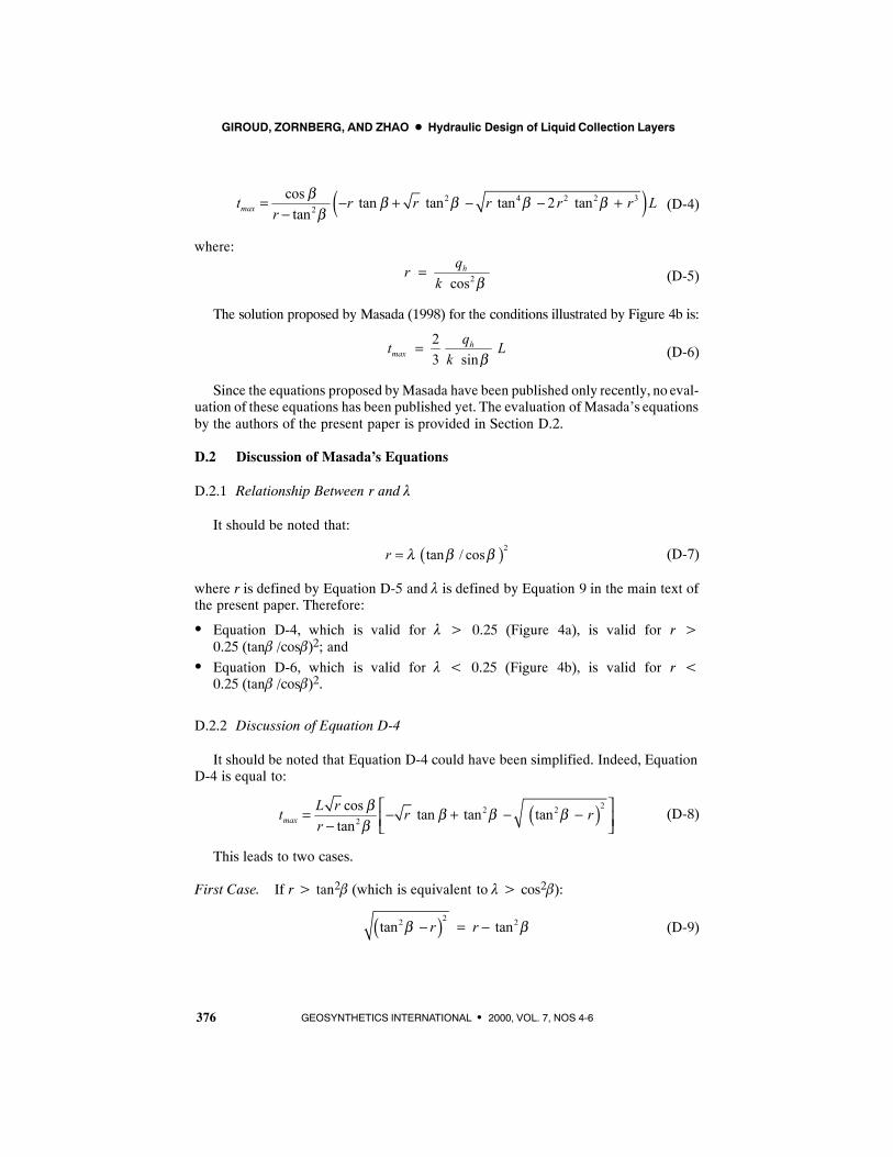
GIROUD, ZORNBERG, AND ZHAO D Hydraulic Design of Liquid Collection Layers
376 GEOSYNTHETICS INTERNATIONAL S 2000, VOL. 7, NOS 4-6
(D-4)( )2 4 2 2 32
cos tan tan tan 2 tantanmaxt r r r r r L
rβ β β β ββ
= − + − − +−
where:
(D-5)2coshqr
k β=
The solution proposed by Masada (1998) for the conditions illustrated by Figure 4b is:
(D-6)23 sin
hmax
qt Lk β
=
Since the equations proposed byMasada have been published only recently, no eval-uation of these equations has been published yet. The evaluation of Masada’s equationsby the authors of the present paper is provided in Section D.2.
D.2 Discussion of Masada’s Equations
D.2.1 Relationship Between r and λ
It should be noted that:
(D-7)( )2tan / cosr λ β β=
where r is defined by Equation D-5 and λ is defined by Equation 9 in the main text ofthe present paper. Therefore:
S Equation D-4, which is valid for λ > 0.25 (Figure 4a), is valid for r >0.25 (tanβ /cosβ)2; and
S Equation D-6, which is valid for λ < 0.25 (Figure 4b), is valid for r <0.25 (tanβ /cosβ)2.
D.2.2 Discussion of Equation D-4
It should be noted that Equation D-4 could have been simplified. Indeed, EquationD-4 is equal to:
(D-8)( )22 22
cos tan tan tantanmax
L rt r rr
β β β ββ
= − + − − −
This leads to two cases.
First Case. If r> tan2β (which is equivalent to λ> cos2β):
(D-9)( )22 2tan tanr rβ β− = −
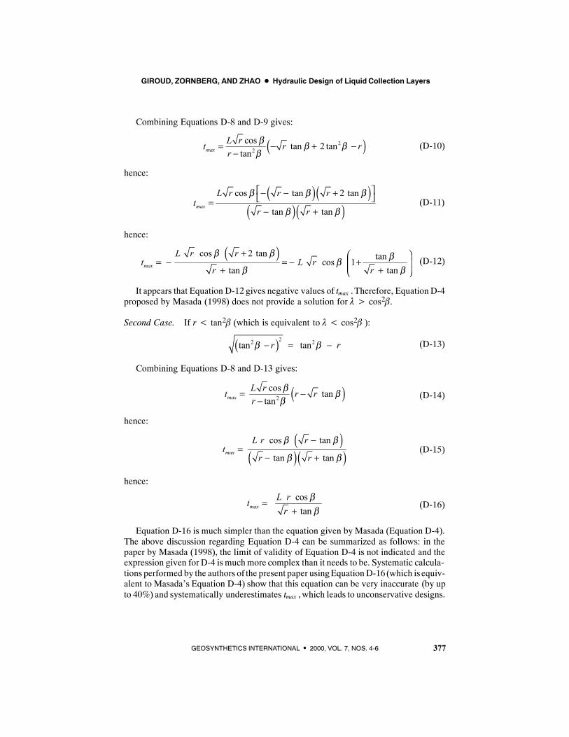
GIROUD, ZORNBERG, AND ZHAO D Hydraulic Design of Liquid Collection Layers
377GEOSYNTHETICS INTERNATIONAL S 2000, VOL. 7, NOS. 4-6
Combining Equations D-8 and D-9 gives:
(D-10)( )22
cos tan 2 tantanmax
L rt r rr
β β ββ
= − + −−
hence:
(D-11)( )( )
( )( )cos tan 2 tan
tan tanmax
L r r rt
r r
β β β
β β
− − + =− +
hence:
(D-12)( )cos 2 tan tancos 1tan tanmax
L r rt L r
r r
β β βββ β
+ = − = − +
+ +
It appears that Equation D-12 gives negative values of tmax . Therefore, Equation D-4proposed by Masada (1998) does not provide a solution for λ> cos2β.
Second Case. If r< tan2β (which is equivalent to λ< cos2β ):
(D-13)( )22 2tan tanr rβ β− = −
Combining Equations D-8 and D-13 gives:
(D-14)( )2
cos tantanmax
L rt r rr
β ββ
= −−
hence:
(D-15)( )
( )( )cos tan
tan tanmax
L r rt
r r
β β
β β
−=
− +
hence:
(D-16)cos
tanmaxL rt
rββ
=+
Equation D-16 is much simpler than the equation given byMasada (Equation D-4).The above discussion regarding Equation D-4 can be summarized as follows: in thepaper by Masada (1998), the limit of validity of Equation D-4 is not indicated and theexpression given for D-4 ismuchmore complex than it needs to be. Systematic calcula-tions performed by the authors of the present paper usingEquation D-16 (which is equiv-alent to Masada’s Equation D-4) show that this equation can be very inaccurate (by upto 40%) and systematically underestimates tmax ,which leads to unconservative designs.
GIROUD, ZORNBERG, AND ZHAO D Hydraulic Design of Liquid Collection Layers
378 GEOSYNTHETICS INTERNATIONAL S 2000, VOL. 7, NOS 4-6
D.2.3 Discussion of Equation D-6
The equation proposed by Masada (1998) for the case where λ< 0.25, EquationD-6, appears to be incorrect, because it is Equation 74 of the present paper multipliedby an arbitrary factor 2/3. In particular, Equation D-6 does not provide the accuratesolution for the well-known limit case where qh/k is very small.
D.2.4 Conclusion on Masada’s Equations
In conclusion, the equations provided by Masada do not appear to provide an accu-rate solution for the maximum liquid thickness in a liquid collection layer.
D.3 Conclusion of Appendix D
The equations discussed in Appendix D do not provide a valid solution for the maxi-mum liquid thickness in a liquid collection layer. One equation (Lesaffre’s equation)is correct, but was developed for another field of application, the drainage of slopes,and cannot be used for the liquid collection layers discussed in the present paper. Com-parisons of the other equations with accurate solutions show significant inaccuracies,which often lead to major unconservatism.
It should be emphasized that the solutions discussed in Appendix D were obtained forsteady-state conditions. Insight into the evaluation of the liquid thickness in liquid collec-tion layers under unsteady-state conditions is provided by Wong (1977), Lentz (1981),Demetracopoulos et al. (1984), McEnroe (1989a), and Giroud and Houlihan (1995).
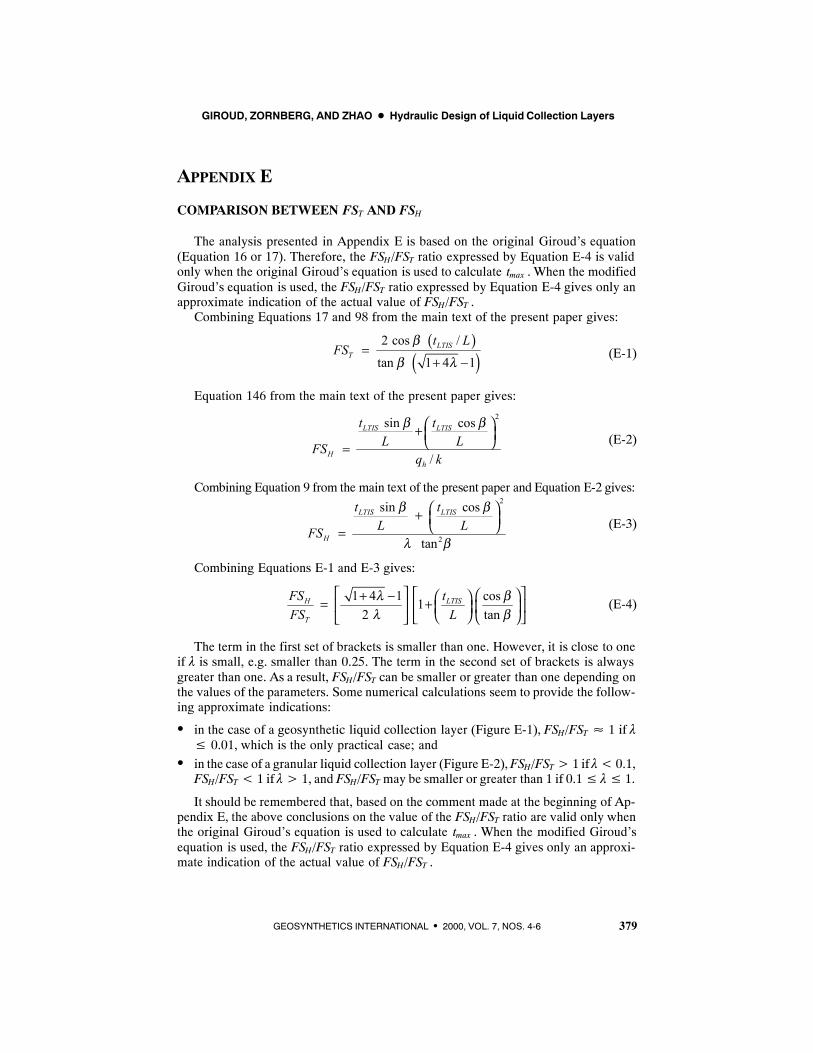
GIROUD, ZORNBERG, AND ZHAO D Hydraulic Design of Liquid Collection Layers
379GEOSYNTHETICS INTERNATIONAL S 2000, VOL. 7, NOS. 4-6
APPENDIX E
COMPARISON BETWEEN FST AND FSH
The analysis presented in Appendix E is based on the original Giroud’s equation(Equation 16 or 17). Therefore, the FSH/FST ratio expressed by Equation E-4 is validonly when the original Giroud’s equation is used to calculate tmax . When the modifiedGiroud’s equation is used, the FSH/FST ratio expressed by Equation E-4 gives only anapproximate indication of the actual value of FSH/FST .
Combining Equations 17 and 98 from the main text of the present paper gives:
(E-1)( )
( )2 cos /
tan 1 4 1LTIS
T
t LFS
β
β λ=
+ −
Equation 146 from the main text of the present paper gives:
(E-2)
2sin cos
/
LTIS LTIS
Hh
t tL LFS
q k
β β + =
Combining Equation 9 from the main text of the present paper and Equation E-2 gives:
(E-3)
2
2
sin cos
tan
LTIS LTIS
H
t tL LFS
β β
λ β
+ =
Combining Equations E-1 and E-3 gives:
(E-4)1 4 1 cos1
2 tanLTISH
T
tFSFS L
λ βλ β
+ − = +
The term in the first set of brackets is smaller than one. However, it is close to oneif λ is small, e.g. smaller than 0.25. The term in the second set of brackets is alwaysgreater than one. As a result, FSH/FST can be smaller or greater than one depending onthe values of the parameters. Some numerical calculations seem to provide the follow-ing approximate indications:
S in the case of a geosynthetic liquid collection layer (Figure E-1), FSH/FST ≈ 1 if λ≤ 0.01, which is the only practical case; and
S in the case of a granular liquid collection layer (Figure E-2),FSH/FST> 1 if λ< 0.1,FSH/FST< 1 if λ> 1, and FSH/FST may be smaller or greater than 1 if 0.1≤ λ≤ 1.
It should be remembered that, based on the comment made at the beginning of Ap-pendix E, the above conclusions on the value of the FSH/FST ratio are valid only whenthe original Giroud’s equation is used to calculate tmax . When the modified Giroud’sequation is used, the FSH/FST ratio expressed by Equation E-4 gives only an approxi-mate indication of the actual value of FSH/FST .
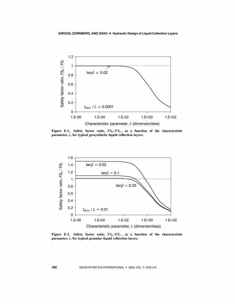
GIROUD, ZORNBERG, AND ZHAO D Hydraulic Design of Liquid Collection Layers
380 GEOSYNTHETICS INTERNATIONAL S 2000, VOL. 7, NOS 4-6
0
0.2
0.4
0.6
0.8
1
1.2
1.E-06 1.E-04 1.E-02 1.E+00 1.E+02
Safetyfactorratio,FS H/FS T
Characteristic parameter, λ (dimensionless)
tanβ ≤ 0.02
tallow / L = 0.0001
0
0.2
0.4
0.6
0.8
1
1.2
1.4
1.6
1.E-06 1.E-04 1.E-02 1.E+00 1.E+02
Figure E-1. Safety factor ratio, FSH /FST , as a function of the characteristicparameter, λ, for typical geosynthetic liquid collection layers.
Safetyfactorratio,FS H/FS T
Characteristic parameter, λ (dimensionless)
tanβ = 0.02
tanβ = 0.1
tanβ = 0.33
tallow / L = 0.01
Figure E-2. Safety factor ratio, FSH /FST , as a function of the characteristicparameter, λ, for typical granular liquid collection layers.


![Smith's Canadian gazetteer [microform] : comprising statistical and ...](https://static.fdokumen.com/doc/165x107/631d3ef36c6907d36801aca9/smiths-canadian-gazetteer-microform-comprising-statistical-and-.jpg)