Hybridization methods for the analysis of nonlinear systems

Acta Informatica manuscript No.(will be inserted by the editor)

Eugene Asarin · Thao Dang · AntoineGirard

Hybridization Methods for theAnalysis of Nonlinear Systems

Received: date / Revised: date

Abstract In this article, we describe some recent results on the hybridiza-tion methods for the analysis of nonlinear systems. The main idea of ourhybridization approach is to apply the hybrid systems methodology as a sys-tematic approximation method. More concretely, we partition the state spaceof a complex system into regions that only intersect on their boundaries, andthen approximate its dynamics in each region by a simpler one. Then, theresulting hybrid system, which we call a hybridization, is used to yield ap-proximate analysis results for the original system. We also prove importantproperties of the hybridization, and propose two effective hybridization con-struction methods, which allow approximating the original nonlinear systemwith a good convergence rate.

Keywords: Nonlinear hybrid systems, hybridization, formal analysis.

E. AsarinUniversite Paris 7, LIAFA2 pl. Jussieu75251 Paris, Cedex 5, FRANCEE-mail: [email protected]

T. DangVERIMAG2 ave. de Vignate38610 Gieres, FRANCEE-mail: [email protected]

A. GirardUniversite Joseph Fourier, LMCB.P. 53,38041 Grenoble Cedex 9, FRANCEE-mail: [email protected]

2 Eugene Asarin et al.

1 Introduction

Hybrid systems, that is, systems exhibiting both continuous and discretedynamics, have proven to be a useful mathematical model for various physicalphenomena and engineering systems. One typical example is a chemical batchplant where a computer is used to supervise complex sequences of chemicalreactions, each of which is modeled as a continuous process. In addition todiscontinuities introduced by the computer, most physical processes admitcomponents (e.g. switches, valves) and phenomena (e.g. collision, emptyingof tanks) whose most useful models are discrete. Hybrid system models arisein many applications, such as chemical process control, avionics, robotics,automobiles, and most recently in molecular biology.

Due to the safety critical features of many such applications, formal analy-sis is a topic of particular interest. The goal of formal verification is to provethat the (designed) system satisfies a property, and the goal of controllersynthesis is to control the system (in other words to design a controller) sothat the system satisfies a desired specification. Due to the complexity andscale of real-life applications, automatic analysis is very desirable. This isa motivation to adopt the algorithmic approach which consists in buildingsoftware tools that can analyze automatically all the behaviors of a givensystem. Although the research on the algorithmic analysis of hybrid systemshas achieved considerable results in the development of theoretical founda-tions and tools, their applications to real-life problems are still limited. Amajor component in any algorithm for analyzing hybrid systems is an effi-cient method to handle their continuous dynamics described by differentialequations (since their discrete dynamics can be handled using well-developedverification methods in computer science). While many well-known proper-ties of affine or piecewise affine systems and other simpler systems (suchas systems with piecewise constant derivatives) can be exploited to designrelatively efficient methods, nonlinear systems are much more difficult toanalyze.

In this paper, our object of study is a complex system (that could be hy-brid or not), and we apply the hybrid systems methodology as a systematicapproximation method. More concretely, we propose an approach to study acomplex system (with nonlinear dynamics for example) by approximating itwith a simpler system, for which well-developed analysis tools exist. To thisend, we partition the state space of the system into regions that only intersecton their boundaries and then approximate locally its dynamics in each regionby a simpler dynamics. Globally, the dynamics of the approximate systemchanges when moving from one region to another. Due to these switchings,the approximate system behaves like a hybrid system and we thus call thisapproximation process hybridization. Then, the resulting system is used toyield approximate analysis results for the original system. The usefulness ofthis approach (in terms of accuracy and computational tractability) dependson the choice of the approximate system. We consider two classes of approx-imate systems: piecewise affine and piecewise multi-affine. We show that theuse of these classes allows approximating the original nonlinear system witha good convergence rate.

Hybridization Methods for the Analysis of Nonlinear Systems 3

The essence behind the hybridization approach is not new. However, thenovelty in our work is that our approximation method is “systematic” in thesense that given a complex system, the method can automatically computea system which approximates the original system with a guaranteed errorbound and thus preserves the properties of interest. In addition, the approx-imate system can be studied using available tools for the formal analysis ofhybrid systems.

The paper is organized as follows. In Section 2, we discuss the model weuse for describing hybrid systems. We then discuss some common propertiesof hybrid systems and briefly review the existing results on their algorithmicanalysis. This section includes the basic definitions and notations neccessaryfor subsequent discussions. In Section 3, we describe the main principles ofour hybridization approach. In Section 4, we prove important properties ofthe method and present a comparison of our method with previous results. InSection 5, we show two effective methods for constructing hybridizations: oneproduces affine hybridizations and the other produces multi-affine hybridiza-tions. The last section contains some examples illustrating our approach.

2 Hybrid Systems Framework

2.1 Hybrid Model

A hybrid system is a system whose evolution consists of successions of con-tinuous phases and discrete events. Various hybrid systems models have beenproposed and this remains an active research area [2,15,39]. In this paper, weuse the following model, which is a variant of the hybrid automaton proposedin [1]. The reason we choose this model is that it can capture naturally a widerange of hybrid behaviors and, moreover, provides a framework suitable forthe problems we tackle in this work.

Definition 1 A hybrid system H = (L, n, p, E, F, Inv, G,R) consists of:

– A set of discrete locations L.– An integer n, the dimension of the continous state space.– An integer p, the dimension of the continuous input.– A set of discrete transitions E ⊆ L× L.– A collection of continuous vector fields F = Fl| l ∈ L. For each location

l ∈ L, Fl = (Ul, fl) where Ul ⊂ Rp is a set of inputs and fl : Rn × Ul →Rn. We assume that the vector fields fl are Lipschitz continuous1. Theadmissible input functions are piecewise continuous.

– A collection of invariants Inv = Invl| l ∈ L. For each location l ∈ L,Invl ⊆ Rn.

– A collection of guards G = Ge| e ∈ E. For each discrete transitione = (l, l′) ∈ E, Ge ⊆ Invl.

– A collection of reset relations R = Re| e ∈ E. For each discrete tran-sition e = (l, l′) ∈ E, Re ⊆ Ge × Invl′ .

1 This requirement is needed for existence of continuous trajectories as well asfor error estimation.


The hybrid state space of H is S =⋃

l∈Ll × Invl. Then, the state of thehybrid system is a pair (l, x) where the discrete state is l ∈ L and the con-tinuous state is x ∈ Invl. A hybrid system can be thought as the interactionbetween a discrete and a continuous process. The discrete part of the systemis described by an automaton (L, E) whose transitions are triggered whenthe continuous variable reaches the associated guard. Between two transi-tions, the continuous process evolves according to the continuous vector fieldassociated with the active discrete state. In the following, we define formallythe notion of traces of a hybrid system.

Definition 2 Let L be a set of discrete locations and n ∈ N, a hybrid tra-jectory on L× Rn is a triple (I,Q,X ) where

– I = Ik| 0 ≤ k ≤ N is a sequence of intervals (we can have N = +∞)such that• If N = +∞, then for all k ∈ N, Ik = [tk, t′k] with t′k = tk+1.• If N < +∞, then IN = [tN , t′N ] or IN = [tN ,+∞) and for all 0 ≤ k ≤

N − 1, Ik = [tk, t′k] with t′k = tk+1.• In both cases, the initial time is t0 = 0.

– Q = qk| 0 ≤ k ≤ N is a sequence of locations.– X = xk| 0 ≤ k ≤ N is a sequence of continuous, piecewise differentiable

functions. For all 0 ≤ k ≤ N , xk : Ik → Rn. The dotted function xk

denotes the derivative of xk.

If N < +∞ and IN = [tN , t′N ] then the hybrid trajectory is said to be finite.If N = +∞ and limk→+∞ tk < +∞ then the hybrid trajectory is said to beZeno. Otherwise, it is said to be infinite.

It should be noted that for simplicity, the functions xk are assumed to be con-tinuous and piecewise differentiable. However, it is possible to consider largerand thus more expressive classes of functions, such as absolutely continuousfunctions (see for instance [12]).

Intuitively, the intervals Ik represent the time intervals where the hybridsystem evolves continuously according to a differential equation satisfied bythe function xk. The time point t′k is the instant where a discrete transitionoccurs to switch from the location qk to the location qk+1. More formally,the evolution of a hybrid system is described by the notion of hybrid traces.

Definition 3 Let H = (L, n, p, E, F, Inv, G, R), a hybrid trajectory τh =(I,Q,X ) on L×Rn is a hybrid trace of the hybrid system H if the followingconditions hold:

– continuous evolution: For all 0 ≤ k ≤ N , there exists a piecewisecontinuous input uk such that for all t ∈ Ik, xk(t) ∈ Invqk

, uk(t) ∈ Uqk

and at each time t where uk is continuous:

xk(t) = fqk(xk(t), uk(t)).

– discrete evolution: For all 0 ≤ k ≤ N − 1, ek = (qk, qk+1) ∈ E,xk(t′k) ∈ Gek

and (xk(t′k), xk+1(tk+1)) ∈ Rek.


The set of hybrid traces of H is denoted by Th(H). The subset of Th(H)consisting of the infinite hybrid trajectories is denoted by T ∞h (H).

We remark that the continuous dynamics of a hybrid system are describedby differential equations with inputs which might not be control inputs, andin this case they must be thought as disturbances or uncertainties. Hence,a hybrid system is in general non-deterministic (though non-stochastic) inthe sense of admitting more than one trajectory (in fact, uncountably manytrajectories) from a given initial state. In this paper, we are mainly inter-ested in the evolution of the continuous state of the hybrid system. We thusintroduce the following notion of continuous traces.

Definition 4 A continuous trace of the hybrid system H is a pair τc = (I, x)consisting of an interval I and a piecewise C1 function2 x : I → Rn such thatthere exists at hybrid trace (I,Q,X ) of H satisfying:

– I =⋃k=N

k=0 Ik.– For all 0 ≤ k ≤ N , for all t ∈ (tk, t′k), x(t) = xk(t).– For all 0 ≤ k ≤ N − 1, x(t′k) = (xk(t′k) + xk+1(tk+1))/2.

The set of continuous traces of H is denoted Tc(H). If I = [0,+∞), τc is saidto be infinite. The set of infinite continuous traces of H is denoted T ∞c (H).

Let us remark that at the continuous time point τ = t′k = tk+1, which isthe (k + 1)th switching time, a hybrid trajectory takes on two (possibly dis-tinct) continuous values: the value xk(t′k) before the switch, and the valuexk+1(tk+1) after the switch. In the definition of a continuous trace, we arbi-trarily choose to take the average of these two values. As we will see later,in the systems generated by the hybridization process, all the reset relationsare given by the identity map restricted to the guard sets, and hence theabove definition of x(t′k) implies the continuity of the function x becausex(t′k) = xk(t′k) = xk+1(tk+1).

We can now introduce the notion of continuous reachable set. Let X0 ⊆ Rn

be a set of continuous initial states. The continuous reachable set of H fromX0 within the time interval J is denoted by Reachc(H,X0, J) and defined asfollows. An element y ∈ Rn is in Reachc(H,X0, J) if and only if there is acontinuous trace τc = (I, x) ∈ Tc(H) with x(0) ∈ X0 such that there existst ∈ I∩J : x(t) = y. The reachable set for the time interval [0,+∞) is denotedby Reachc(H,X0) for short.

2.2 Properties of Hybrid Systems

Hybrid systems have been mainly studied by researchers from computer sci-ence and control theory, who focus on different properties and approachesreflecting their background and view of hybrid systems. Control engineers areoften interested in properties which are important in the design of a control

2 A function with k continuous derivatives is called a Ck function. Thus, a con-tinuously differentiable function is a C1 function.


system, such as stability, attraction, controllability, optimality... Computerscientists are interested in “sequential” properties expressed in some tempo-ral logics, such as Linear Temporal Logic (LTL) and Computation Tree Logic(CTL) (see for example [25,45]). We will mention here some of the propertiesof hybrid systems that have been subject to investigation recently.

Stability and Attraction. Roughly speaking, stability means that applyingsmall perturbations on the system only results in small deviations in itsresponses. Depending on what is defined as perturbations and responses, thisgives rise to a number of notions of stability. Stability of points is a widelyused notion. Essentially, it requires that the state of the system remains inthe neighborhood of some point under some small perturbations in the initialstate. Given a hybrid system as in Definition 1, the (general) stability of apoint x∗ ∈ Rn can be defined as follows (see e.g. [53]):

∀ε > 0, ∃δ > 0, ∀τc = (I, x) ∈ Tc(H) :||x∗ − x(0)|| < δ ⇒ ∀t ∈ I : ||x∗ − x(t)|| < ε.

where || · || denotes a norm on Rn. Asymptotic stability of x∗ additionallyrequires that

∃δ > 0, ∀τc = (I, x) ∈ T ∞c (H) : ||x∗ − x(0)|| < δ ⇒ limt→+∞

x(t) = x∗.

The geometric meaning of the stability of x∗ is that for any neighborhood Nr

of the point x∗, there exists a neighborhood Np of the initial state such thatno pertubation of the initial state in Np makes the system’s response leave Nr.In control theory, this stability of points for deterministic systems is oftencalled Lyapunov stability. Stability is naturally one of the most importantproperties of control systems, since it guarantees that the system’s evolutionalways stays close to some points representing the desired behaviors or thereference operation modes.

Besides stability, attraction is also of interest. For example, one can expectthat the system not only stays close but also returns to the desired points (ortrajectories), and this involves attraction properties. Intuitively, attraction ofa point means that every neighborhood of the point must be reached after afinite amount of time. A set of such points is called attractor and is formallydefined as follows. An attractor A is a subset of the continuous state spaceRn that satisfies the following two conditions [54]:

1. The set A is invariant:

∀τc = (I, x) ∈ T ∞c (H) : x(0) ∈ A ⇒ ∀t ≥ 0 : x(t) ∈ A.

2. The set A attracts a neighborhood B of itself (i.e. A ⊂ B ⊆ Rn):

∀τc = (I, x) ∈ T ∞c (H) : x(0) ∈ B ⇒ limt→+∞

d(x(t), A) = 0.


The first condition means that if the continuous state is in A, then it staysin A forever. In the second condition, the distance d(y, A) from the point yto the set A is defined as d(y, A) = infx∈A ||y − x||, and the set B is saidto be in the basin of attraction of the attractor A. Two simple examples ofattractors are the asymptotically stable fixed point and the asymptoticallystable limit cycle. Note that stability and attraction are two closely relatednotions. Indeed, we can see that a point x∗ is asymptotically stable if andonly if it is stable and it is an attractor.

On the other hand, computer scientists approach the study of hybridsystems by applying the methodology of formal description and verification.They consider properties that can be formally described in some mathemat-ical logics. As mentioned earlier, temporal logic is a popular formalism todescribe properties involving the behavior of a system over time. In the fol-lowing we briefly describe safety and eventuality properties, which are themost elementary classes of such properties.

Safety and Eventuality. Safety properties, and in particular invariance prop-erties, have gained most of the attention in hybrid systems research. Intu-itively, a safety property expresses that nothing “bad” will happen. Invarianceproperties are the simplest form of such properties, and an invariance prop-erty of the hybrid system H is of the form:Starting from some set X0 of initial states, all the continuous traces of H

remain in a subset XI of the continuous state space Rn.This is equivalent to a reachability property: The reachable set Reachc(H,X0)is included in XI . Therefore, invariance properties can be checked usingreachable set computations. In temporal logic, the above invariance prop-erty is often expressed by the formula 2P where 2 is the temporal quantifieralways, and P is a predicate (formula) describing the set XI . General safetyproperties are expressed by more complicated temporal logic formulae, butit is possible to express most interesting safety properties as invariance prop-erties.

Eventuality properties assert that something “good” must happen. Anexample of such properties is:Starting from some set X0 of initial states, all the continuous traces of H

eventually reaches a subset XF of the continuous state space Rn.Note that a safety property is violated in finite time (since any infinite traceviolating the property has a finite prefix that is “bad”). Hence, consideringfinite traces allow disproving safety properties. However, finite traces do notallow to disprove an eventuality property since there might be a finite tracethat can be extended so that the resulting infinite trace satisfies this property.

2.3 Hybrid Systems Analysis: a Brief Review

Stability and attraction properties are mainly analyzed using various hybridextensions of tools for continuous systems in control theory, such as Lya-punov functions [53], Poincare maps [36]. It is well-known that the stability


of a hybrid system is not guaranteed by the stability of all its continuouscomponents, and one possible solution is to search for a global Lyapunovfunction in some fixed form, such as piecewise quadratic [37,22] or more gen-eral piecewise polynomial functions [49]. Stability of switched systems (whichare systems consisting of a family of continuous dynamics and a rule to switchbetween them) has also been thoroughly studied in a number of publications(see [44] and references therein). The application of Poincare maps to hybridsystems has also been explored, for example, in [61].

Formal analysis of hybrid systems is known to be a very difficult taskdue to the complexity and scale of the systems. Concerning specification,some temporal logics for hybrid systems have been developed (see for exam-ple [5,21]). Concerning verification, one is interested in designing an algo-rithm which, for a given hybrid system and a desired property, can answerafter a finite number of steps whether the system satisfies the property. Thedecidability question is important in the algorithmic verification of hybridsystems, due to their infinite state space. A lot of research effort has beenbeen devoted to the question of identifying the classes of hybrid systems andproperties for which the verification problem is decidable. Temporal logicmodel-checking problems are not decidable for most general hybrid systems.However, decidability results have been proven for some particular classes ofhybrid systems (see [5] for a survey). These classes must be restricted eitherin continuous dynamics (e.g. systems with piecewise constant derivatives [11,4,1,35]), or in discrete dynamics (e.g. [42,6]). Based on these results, variousverification tools have been implemented, such as Kronos [62] and Uppaal [43]for timed automata, HyTech [33] for linear hybrid automata3 and Requiem[42] for hybrid systems where linear differential equations have special eigen-structure and discrete dynamics can only have memoryless resets. The basisof these tools is a procedure for exactly characterizing and manipulating theset of all possible trajectories (using computer algebra tools for example).

However, this is no longer possible for more general hybrid systems. In-deed, even to prove simple safety properties, there exists no general exactreachable set computation method. For this reason, there has been growinginterest in developing methods for the approximate representation and com-putation of sets of states and system traces, in particular with a focus onreachable set computation. These methods can be roughly classified into twocategories. The methods of the first category try to approximate reachablesets as accurately as possible by tracking their evolution under the continuousflows using some set represention (such as polyhedra, ellipsoids, level sets).This results in a variety of approximation schemes (such as [29,20,16,41,14,7,59,46,28,38,18]), and implemented by a number of tools such as Coho[29],CheckMate [16], d/dt [8], VeriShift [14], HYSDEL [60], MPT [47], HJB tool-box [46]. Since accurate reachable set approximations are computationallyexpensive, the methods of the second category seek approximations that aresufficiently good to prove the property of interest (such as barrier certificates[48], polynomial invariants [58]). Abstraction methods for hybrid systems are

3 In linear hybrid automata, continuous dynamics are described by linear con-straints on the derivatives, such as Ax ≤ b. They should not be confused with hybridsystems where continuous dynamics are described by linear differential questions.


also close in spirit to these methods. Indeed, their main idea is to start witha rough (and conservative) discrete approximation of a hybrid system andthen iteratively refine it4. This refinement is often local in the sense thatit uses the previous analysis results to determine where the approximationerror is too large to prove the property (see for example [57,3,17]).

The literature on hybrid systems analysis is vast; for more details thereader is referred to recent proceedings of the conference HSCC (Hybrid Sys-tems: Computation and Control). We finish this brief review by remarkingthat while many well-known properties of affine differential equations canbe exploited to design relatively efficient algorithms, systems with nonlineardifferential equations are much more difficult to analyze. For these systems,the existing tools can only handle a small number of continuous variables.This motivated us to search for a method to deal with nonlinear systemsusing tools available for simpler systems.

3 Principles of Hybridization

Intuitively, the main idea of hybridization is to approximate the complex con-tinuous dynamics of a system by a collection of simpler continuous dynam-ics. Here, by “simpler” we mean the types of dynamics that can be analyzedmore easily and efficiently. For example, we can approximate a nonlinear con-tinuous dynamics by a piecewise affine dynamics. The collection of simplercontinuous dynamics indeed defines a hybrid system. Then, the analysis ofthe resulting hybrid system can provide knowledge about the behavior of theoriginal system. Hence, one can see another utility of hybrid systems: theycan be used not only as a mathematical model but also as an approximationmethod.

For simplicity of presentation, we explain the principle of the hybridiza-tion approach for continuous, autonomous (i.e. without inputs) dynamicalsystems. However, the approach can be extended to handle continuous dy-namical systems with inputs as well as hybrid systems, which will be dis-cussed later in this section. We consider a nonlinear continuous dynamicalsystem D that is defined on a domain Ω ⊆ Rn by a differential equation ofthe form:

x(t) = f(x(t)), x(t) ∈ Ω, t ≥ 0.

This continuous dynamical system can be seen as a hybrid system with aunique location (denoted by ω) and no discrete transition:

D = (ω, n, 0, ∅, (∅, f), Ω, ∅, ∅).

As mentioned earlier, the idea of hybridization consists in approximating thenonlinear vector field f by a hybrid system with a collection of simpler (e.g.constant or affine) vector fields. To do so, the domain Ω of the dynamicalsystem D is split into several regions that form a mesh of Ω. Then, witheach element of this mesh, we associate a simple approximate vector field.

4 Most proofs of decidability result for certain classes of hybrid systems are oftenbased on the existence of a finite discrete abstraction (see [5])


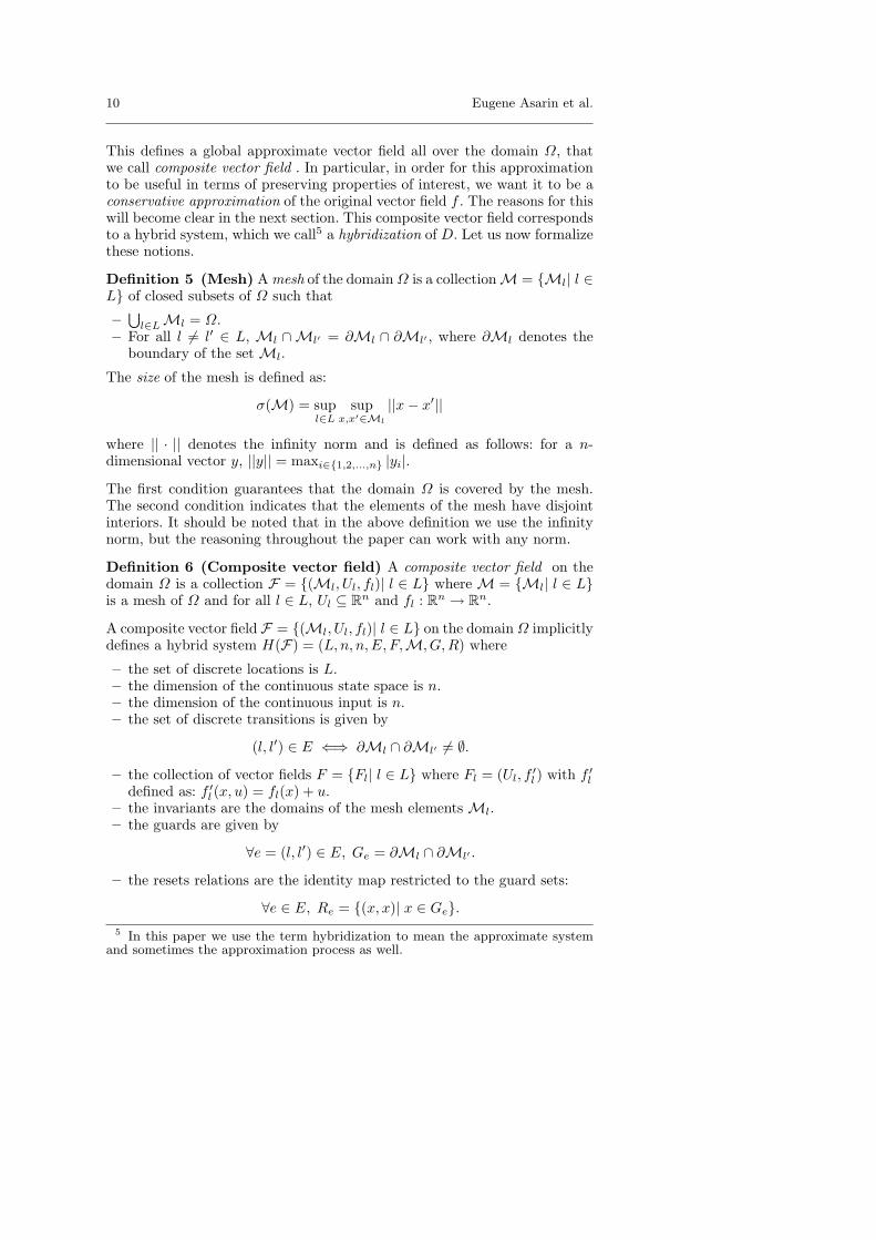
This defines a global approximate vector field all over the domain Ω, thatwe call composite vector field . In particular, in order for this approximationto be useful in terms of preserving properties of interest, we want it to be aconservative approximation of the original vector field f . The reasons for thiswill become clear in the next section. This composite vector field correspondsto a hybrid system, which we call5 a hybridization of D. Let us now formalizethese notions.

Definition 5 (Mesh) A mesh of the domain Ω is a collectionM = Ml| l ∈L of closed subsets of Ω such that

–⋃

l∈LMl = Ω.– For all l 6= l′ ∈ L, Ml ∩Ml′ = ∂Ml ∩ ∂Ml′ , where ∂Ml denotes the

boundary of the set Ml.

The size of the mesh is defined as:

σ(M) = supl∈L

supx,x′∈Ml

||x− x′||

where || · || denotes the infinity norm and is defined as follows: for a n-dimensional vector y, ||y|| = maxi∈1,2,...,n |yi|.

The first condition guarantees that the domain Ω is covered by the mesh.The second condition indicates that the elements of the mesh have disjointinteriors. It should be noted that in the above definition we use the infinitynorm, but the reasoning throughout the paper can work with any norm.

Definition 6 (Composite vector field) A composite vector field on thedomain Ω is a collection F = (Ml, Ul, fl)| l ∈ L where M = Ml| l ∈ Lis a mesh of Ω and for all l ∈ L, Ul ⊆ Rn and fl : Rn → Rn.

A composite vector field F = (Ml, Ul, fl)| l ∈ L on the domain Ω implicitlydefines a hybrid system H(F) = (L, n, n,E, F,M, G,R) where

– the set of discrete locations is L.– the dimension of the continuous state space is n.– the dimension of the continuous input is n.– the set of discrete transitions is given by

(l, l′) ∈ E ⇐⇒ ∂Ml ∩ ∂Ml′ 6= ∅.

– the collection of vector fields F = Fl| l ∈ L where Fl = (Ul, f′l ) with f ′l

defined as: f ′l (x, u) = fl(x) + u.– the invariants are the domains of the mesh elements Ml.– the guards are given by

∀e = (l, l′) ∈ E, Ge = ∂Ml ∩ ∂Ml′ .

– the resets relations are the identity map restricted to the guard sets:

∀e ∈ E, Re = (x, x)| x ∈ Ge.5 In this paper we use the term hybridization to mean the approximate system

and sometimes the approximation process as well.


Such a composite vector field is used to approximate the vector field f of anautonomous system, and the role of the input is to model the error betweenvalues of f in each mesh cell Ml and its approximation fl in that cell.

Definition 7 A composite vector field F = (Ml, Ul, fl)| l ∈ L on thedomain Ω is a conservative approximation of the vector field f if

∀l ∈ L, x ∈Ml, ∃u ∈ Ul, f(x) = fl(x) + u.

If F is a conservative approximation of the vector field f then the hybridsystem H(F) is said to be a hybridization of the system D. The precision ofthe hybridization is given by:

π(F , f) = supl∈L

(sup

x∈Ml, u∈Ul

‖fl(x) + u− f(x)‖)

.

Extension to continuous systems with input and to hybrid systems. It isstraightforward to extend the above definitions to continuous systems withinput by choosing appropriately the sets Ul of the hybridization, which allowstaking into account the effect of the input of the system. As an example, weconsider a continuous system with input of the form x(t) = f(x(t)) + v(t)where v(t) ∈ V . Let F = (Ml, Ul, fl)| l ∈ L be a hybridization of thecorresponding autonomous system x(t) = f(x(t)). Then, the hybridizationof the system with input can be defined as F = (Ml, U l, fl)| l ∈ L wherethe input set U l = Ul ⊕ V , and ⊕ denotes the Minkowski sum.

Regarding hybrid systems, the global approximate system can be obtainedby a composition of the hybridizations of the continuous dynamics in eachlocation. The hybridization process can also be partial in the sense that it isused only in some locations.

4 Approximation Properties of Hybridizations

In order for a hybridization to be a useful approximation, a question thatarises is whether the hybridization preserves the properties of interest. Inthe following we show several important approximation properties of the hy-bridization defined in the previous section. We also discuss how these resultscan be used in the analysis of complex continuous and hybrid systems. Letus make the following assumption:

Assumption 1 (Finite Variability [13]) For all continuous trace (I, x) ∈Tc(D), for all interval of finite length J ⊆ I, the function x can move fromone cell of the mesh M to another only a finite number of times during timeinterval J .

As we will see, this assumption is necessary so that the corresponding con-tinuous traces of the hybridization do not exhibit a Zeno behaviors. Thisassumption is necessary for our approach but also for all discrete abstractionprocesses based on a partition of the state space [5,57,3,17]. Let us remarkthat in practice, the finite variability assumption generally holds. An interest-ing investigation is to determine the conditions that the vector field f must


satisfy so that the finite variability assumption holds. This is not done hereas it would require complex mathematical considerations and it is preferableto focus our attention on the main scope of the paper.

4.1 Trace Inclusion and Approximation

The first approximation property involves the conservativeness of the hy-bridization in terms of sets of traces.

Theorem 1 Let H(F) be a hybridization of the dynamical system D. Then,the set of continuous traces of D is included in the set of continuous tracesof H(F), that is

Tc(D) ⊆ Tc(H(F)).

Proof Let (I, x) ∈ Tc(D). We assume that I is of the form [0, T ], andthe situation where I = [0,+∞) can be handled in a similar way. Since⋃

l∈LMl = Ω, there exists a piecewise constant function q : I → L such that

∀t ∈ I, x(t) ∈Mq(t).

Let t0 = 0 and let tk| 1 ≤ k ≤ N be the sequence of instants at whichthe value of the function q changes. From the finite variability assumption,we have that necessarily N is finite. For 0 ≤ k ≤ N , qk denotes the constantvalue of q(t) on the open interval (tk, tk+1). Given an interval Ik = [tk, tk+1],the function xk : Ik → Rn is such that for all t ∈ Ik, xk(t) = x(t). We nowshow that (Ik| 0 ≤ k ≤ N, qk| 0 ≤ k ≤ N, xk| 0 ≤ k ≤ N) is a hybridtrace of H(F).

For 0 ≤ k ≤ N and for all t ∈ (tk, tk+1), x(t) ∈ Mqk. By continuity

of x and closedness of Mqk, it then follows that: for all t ∈ Ik = [tk, tk+1],

x(t) ∈Mqk. We define an input function uk : Ik → Rn as:

∀t ∈ Ik, uk(t) = f(xk(t))− fqk(xk(t)).

Note that since the composite vector field F is a conservative approximationof f , uk(t) ∈ Uqk

for all t ∈ Ik. Moreover,

∀t ∈ Ik, xk(t) = f(xk(t)) = fqk(xk(t)) + uk(t).

Furthermore, xk(tk+1) ∈ Mqk∩ Mqk+1 , thus ek = (qk, qk+1) ∈ E and

xk(tk+1) ∈ Gek. In addition, since xk(tk+1) = x(tk+1) = xk+1(tk+1), we

have that (xk(tk+1), xk+1(tk+1)) ∈ Rek. Hence, (Ik| 0 ≤ k ≤ N, qk| 0 ≤

k ≤ N, xk| 0 ≤ k ≤ N) is in the set Th(H(F)) of hybrid traces of H(F).We end the proof by remarking that (I, x) is the continuous trace of H(F)associated with the hybrid trace (Ik| 0 ≤ k ≤ N, qk| 0 ≤ k ≤ N, xk| 0 ≤k ≤ N). ut

Let us remark that the hybridization H(F) is indeed a simulation of theoriginal system D. An important consequence of this theorem is that thehybridization H(F) can be used to check safety and eventuality propertiesof the continuous dynamical system D [10,26,35]. Indeed, if these properties


hold for the set of all continuous traces of the hybridization H(F), then itfollows from the inclusion relation that they hold for the set of all continuoustraces of the dynamical system D. In terms of temporal logics, this meansthat the universal fragment ∀CTL∗ [25] is preserved by the hybridization.Since LTL properties are part of ∀CTL∗ [25], they are also preserved by thehybridization.

We have seen that the hybridization method allows over-approximatingthe set of continuous traces of D. Now to measure the quality of over-approximation, we use the distance between the set of continuous tracesof H(F) and that of D.

Theorem 2 We assume that f is λ-Lipschitz on Ω, that is

∀x, z ∈ Ω, ‖f(x)− f(z)‖ ≤ λ‖x− z‖.

Then, for all (I, x) ∈ Tc(D), (J, z) ∈ Tc(H(F)), such that x(0) = z(0), thefollowing inequality holds:

∀t ∈ I ∩ J, ‖x(t)− z(t)‖ ≤ π(F , f)λ

(eλt − 1). (1)

Proof The proof relies heavily on the fundamental inequality, and for claritywe first recall this theorem.

Theorem 3 Let Ω be a subset of Rn, let f : Ω → Rn be a λ-Lipschitz vectorfield. Let x : I → Rn and z : J → Rn be piecewise differentiable functionssuch that I ∩ J is not empty and contains 0 and for all t ∈ I ∩ J , x(t) ∈ Ωand z(t) ∈ Ω. If in addition, for all t ∈ I ∩ J , where x is differentiable‖x(t)− f(x(t))‖ ≤ α, and for all t ∈ I ∩ J , where z is differentiable ‖z(t)−f(z(t))‖ ≤ β, then the following inequality holds:

∀t ∈ I ∩ J, ‖x(t)− z(t)‖ ≤ ‖x(0)− z(0)‖eλ|t| +α + β

λ(eλ|t| − 1). (2)

The fundamental inequality is a central theorem of the theory of differentialequations. A detailed proof can be found in [24]. We now proceed with theproof of Theorem 2. Let (I, x) ∈ Tc(D), then x is differentiable on I andfor all t ∈ I ‖x(t) − f(x(t))‖ = 0. Let (J, z) ∈ Tc(H(F)). Let (Jk| 0 ≤k ≤ N, qk| 0 ≤ k ≤ N, zk| 0 ≤ k ≤ N) be the hybrid trace of H(F)associated with (J, z). For all 0 ≤ k ≤ N , for all piecewise continuous inputuk : Jk → Uqk

such that for all t ∈ Jk where uk is continuous,

‖z(t)− f(z(t))‖ = ‖fqk(z(t)) + uk(t)− f(z(t))‖ ≤ π(F , f).

Then, the inequality (1) follows from the application of the fundamentalinequality. ut

The above theorem states that the distance between the set of continuoustraces of H(F) and that of D depends linearly on the precision π(F , f). Thetheorem thus shows that one can approximate the set of traces of the systemD with an arbitrarily small error by using an appropriate hybridization (i.e.


with a sufficiently good precision). This result was also used in the previ-ous works [23,27] to justify the application of the hybridization method toapproximate solutions of differential equations. Indeed, assuming that eachinput sets Ul contains the origin, that is 0 ∈ Ul, one can effectively computean approximate solution of the equation x = f(x) by computing the contin-uous traces of H(F) corresponding to the input functions uk| 0 ≤ k ≤ Nsatisfying uk(t) = 0 for all t ∈ Jk.

4.2 Preservation of Attractors

Theorems 1 and 2 can also be used to prove another important property ofhybridizations involving the preservation of attractors. Let us assume thatthe dynamical system D has an attractor A, attracting a compact set B. Inaddition, let us assume that the following conditions hold:

1. ∀x0 ∈ B, ∃(I, x) ∈ T ∞c (D) : x(0) = x0.2. ∃δ > 0 : N (A, δ) = x ∈ Rn| ∃xa ∈ A, ‖x− xa‖ ≤ δ ⊆ B.

The set N (A, δ) is called δ-neighborhood of A.

Theorem 4 For all ε ∈ (0, δ], there exists ν > 0, such that if π(F , f) ≤ ν,then there exists a set A(F), which is an attractor for the hybrid systemH(F) and such that

A ⊆ A(F) ⊆ N (A, ε).

Moreover, B is in the basin of attraction of A(F).

The theorem states that attractors are preserved by hybridization, and onecan thus use the hybridization method to check attraction properties of con-tinuous and hybrid systems.

Proof Since A attracts the compact set B, there exists a time T > 0 suchthat

∀(I, x) ∈ T ∞c (D), x(0) ∈ B =⇒ ∀t ≥ T, x(t) ∈ N (A, ε/2). (3)

We defineν =

ελ

2(eλ2T − 1).

Let us assume that π(F , f) ≤ ν. Let (J, z) ∈ T ∞c (H(F)) such that z(0) ∈ B.Then, there exists (I, x) ∈ T ∞c (D) such that x(0) = z(0). From Theorem 2,we have that

∀t ∈ [0, 2T ], ‖x(t)− z(t)‖ ≤ π(F , f)λ

(eλ2T − 1) ≤ ε/2. (4)

Then, from the equation (3), it follows that

∀(J, z) ∈ T ∞c (H(F)), z(0) ∈ B =⇒ ∀t ∈ [T, 2T ], z(t) ∈ N (A, ε). (5)

Let us now show by induction that this actually holds for all t ≥ T . We firstassume that the previous equation holds for all t ∈ [T, kT ] for some k ≥ 2.


Let (J, z) ∈ T ∞c (H(F)) such that z(0) ∈ B, let t ∈ [kT, (k + 1)T ], let (I , z)be defined by

I = [0,+∞), z(t) = z(t− T + t).

Intuitively, z is the suffix of z obtained by truncating off the initial lengtht − T , and starting with z(0) = z(t − T ). It is easy to show that (I , z) ∈T ∞c (H(F)). Moreover, z(0) = z(t − T ). Since t − T ∈ [T, kT ], we obtain:z(0) ∈ N (A, ε) ⊆ B. From the equation (5), it follows that z(T ) ∈ N (A, ε).Since z(T ) = z(t), we proved by induction that

∀(J, z) ∈ T ∞c (H(F)), z(0) ∈ B =⇒ ∀t ∈ [T,+∞), z(t) ∈ N (A, ε). (6)

Now let us define the set A(F) by

A(F) = z(t)| (J, z) ∈ T ∞c (H(F)), z(0) ∈ B, t ≥ T ∪ (7)z(t)| (J, z) ∈ T ∞c (H(F)), z(0) ∈ A, t ≥ 0

= z(t)| (J, z) ∈ T ∞c (H(F)), z(0) ∈ B, t ≥ T ∪z(t)| (J, z) ∈ T ∞c (H(F)), z(0) ∈ A, t ∈ [0, T ]

Clearly A ⊆ A(F). Moreover, from the equation (6)

z(t)| (J, z) ∈ T ∞c (H(F)), z(0) ∈ B, t ≥ T ⊆ N (A, ε). (8)

Let (J, z) ∈ T ∞c (H(F)), such that z(0) ∈ A, there exists (I, x) ∈ T ∞c (D)such that x(0) = z(0). Let t ∈ [0, T ]; since A is an attractor for D, x(t) ∈ A.Then, it follows from equation (4) that z(t) ∈ N(A, ε/2). Hence,

z(t)| (J, z) ∈ T ∞c (H(F)), z(0) ∈ A, t ∈ [0, T ] ⊆ N (A, ε/2). (9)

Thus, we have proved that A(F) ⊆ N(A, ε). Next, we prove that A(F) isan attractor for H(F) and that B is in its basin of attraction. Let (J, z) ∈T ∞c (H(F)), such that z(0) ∈ A(F). There are two possible situations. Eitherthere exists (J , z) ∈ T ∞c (H(F)) and t ≥ T such that z(0) ∈ B and z(t) =z(0), or there exists (J , z) ∈ T ∞c (H(F)) and t ≥ 0 such that z(0) ∈ A andz(t) = z(0). We consider only the first situation, and the second one can behandled in a similar way. We define (J , z) as

J = [0,+∞), z(t) =

z(t), if t ∈ [0, t]z(t− t), if t ∈ [t,+∞) (10)

We can show that (J , z) ∈ T ∞c (H(F)), thus from the definition of A(F),for all t ≥ T , z(t) ∈ A(F). Therefore, since t ≥ T , for all t ≥ 0, z(t) =z(t+ t) ∈ A(F). This implies that A(F) is invariant for H(F). It now remainsto show that it attracts B. Let (J, z) ∈ T ∞c (H(F)), such that z(0) ∈ B.From the definition of A(F), for all t ≥ T , z(t) ∈ A(F). It then follows thatlimt→+∞ d(z(t), A(F)) = 0. ut


Relation to previous work. Before continuing to explain how to actually con-struct a hybridization, let us discuss the relation of the method to someprevious work. Regarding the approximation and abstraction categories dis-cussed in Section 2.3, our hybridization method has elements of both. Onone hand, it provides approximations with error bounds. It should be notedthat for safety verification it is sufficient to prove the property on an over-approximation of the original system; however for other problems, such ascontroller synthesis where under-approximations are used, the accuracy cri-terion is important since we do not want to disregard too much control-lable behavior. On the other hand, our method has some similarity with theabstraction methods mentioned in Section 2.3, since the approximate sys-tems we construct are indeed abstractions of the original system, which aremore precise at the price of being more complex. Therefore, the refinementideas [57,3,17] can be straightforwardly applied in our approach.

Our hybridization method also has some common elements with the via-bility algorithms [52] for approximating viability kernels of differential inclu-sions. The approximation in the viability algorithms involves not only a spacediscretization but also a time discretization, which results in a hybrid sys-tem in discrete time. In our hybridization, the resulting approximate systemis in continuous time. Similar hybridization ideas were previously exploredin [50,35,55,26] where the approximate systems are systems with piecewiseconstant slopes or rectangular inclusions. As mentioned earlier, similar ideashave been used for numerical integration of nonlinear differential equations[23,27]. On the other hand, the reachability method proposed in [29] uses lin-ear approximation in each integration step to obtain better approximationsof the reachable sets in 2 dimensions. In [30], a control problem for a classof piecewise linear systems, similar to our affine hybridizations, is solved interms of reachability conditions. In [51], a hybridization approach is used tosolve optimal control problems.

5 Effective Construction of Hybridizations

In the previous section, we have shown that hybridizations can be used toanalyze a fairly large class of properties. In this section, we deal with thequestion of constructing hybridizations for systems with possibly complexnonlinear continuous dynamics. We propose two methods to do so, and abound on the precision of the hybridization is also provided. Let us recall thecontinuous system under study:

x(t) = f(x(t)), x(t) ∈ Ω, t ≥ 0.

5.1 Affine Hybridization

The first hybridization construction method, called affine hybridization, com-putes a piecewise affine vector field by partitioning the state space into sim-plices. The use of such approximate vector fields is motivated by a largechoice of available methods for reachability computation of piecewise affine


systems (see for instance [7,16,28]). It is worth emphasizing that, besidesreachability properties, the hybridization can be used to verify other classesof properties of the original system, provided that we are equipped with atool to verify these properties on the hybridization.

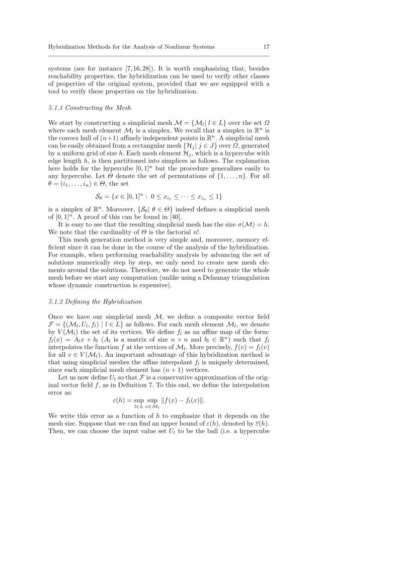
5.1.1 Constructing the Mesh

We start by constructing a simplicial mesh M = Ml| l ∈ L over the set Ωwhere each mesh element Ml is a simplex. We recall that a simplex in Rn isthe convex hull of (n+1) affinely independent points in Rn. A simplicial meshcan be easily obtained from a rectangular mesh Hj | j ∈ J over Ω, generatedby a uniform grid of size h. Each mesh element Hj , which is a hypercube withedge length h, is then partitioned into simplices as follows. The explanationhere holds for the hypercube [0, 1]n but the procedure generalizes easily toany hypercube. Let Θ denote the set of permutations of 1, . . . , n. For allθ = (i1, . . . , in) ∈ Θ, the set

Sθ = x ∈ [0, 1]n : 0 ≤ xi1 ≤ · · · ≤ xin ≤ 1

is a simplex of Rn. Moreover, Sθ| θ ∈ Θ indeed defines a simplicial meshof [0, 1]n. A proof of this can be found in [40].

It is easy to see that the resulting simplicial mesh has the size σ(M) = h.We note that the cardinality of Θ is the factorial n!.

This mesh generation method is very simple and, moreover, memory ef-ficient since it can be done in the course of the analysis of the hybridization.For example, when performing reachability analysis by advancing the set ofsolutions numerically step by step, we only need to create new mesh ele-ments around the solutions. Therefore, we do not need to generate the wholemesh before we start any computation (unlike using a Delaunay triangulationwhose dynamic construction is expensive).

5.1.2 Defining the Hybridization

Once we have our simplicial mesh M, we define a composite vector fieldF = (Ml, Ul, fl) | l ∈ L as follows. For each mesh element Ml, we denoteby V (Ml) the set of its vertices. We define fl as an affine map of the form:fl(x) = Alx + bl (Al is a matrix of size n × n and bl ∈ Rn) such that fl

interpolates the function f at the vertices ofMl. More precisely, f(v) = fl(v)for all v ∈ V (Ml). An important advantage of this hybridization method isthat using simplicial meshes the affine interpolant fl is uniquely determined,since each simplicial mesh element has (n + 1) vertices.

Let us now define Ul so that F is a conservative approximation of the orig-inal vector field f , as in Definition 7. To this end, we define the interpolationerror as:

ε(h) = supl∈L

supx∈Ml

‖f(x)− fl(x)‖.

We write this error as a function of h to emphasize that it depends on themesh size. Suppose that we can find an upper bound of ε(h), denoted by ε(h).Then, we can choose the input value set Ul to be the ball (i.e. a hypercube


for the infinity norm) that is centered at the origin and has radius ε(h). Weestimate this bound for two cases: the vector field f is Lipschitz and f is aC2 function. The proofs can be found in Appendix.

Proposition 1 If f is λ-Lipschitz, then

ε(h) ≤ h2n λ

n + 1= ε(h).

An important remark is that the second partial derivatives of the affine ap-proximation fl vanish; therefore, if f is a C2 function, we can obtain a bettererror bound. Exceptionally, to write the second partial derivatives of f , weuse superscripts to indicate the components of f , that is f = (f1, f2, . . . , fn).

Proposition 2 If f is C2 on Ω with bounded second order derivatives then

ε(h) ≤ Kn2

2(n + 1)2h2 = ε(h)

where

K = maxi∈1,...,n

supx∈Ω

p1=n∑p1=1

p2=n∑p2=1

∣∣∣∣ ∂2f i(x)∂xp1∂xp2

∣∣∣∣ .

The main drawback of affine hybridization is the cardinality of the simplicialpartition of Ω. We have seen that n! simplices are needed to partition ahypercube in Rn. In the next section, we propose a similar method but basedon a rectangular mesh. As a consequence, the complexity of the resultinghybridization is lower and therefore systems in higher dimensions can beconsidered.

5.2 Multi-affine Hybridization

Rectangular meshes and multi-affine interpolation can be thought of as asimple generalization of affine interpolation. The technique is most easilyexplained in two dimensions, but the case of higher dimensions is analogousin every way.

5.2.1 Constructing the Mesh

We assume that the state space is a rectangle Ω = [x1, x1] × [x2, x2] ⊂ R2,let

x1 = x11 < x2

1 < . . . < xm1 = x1, x2 = x1

2 < x22 < . . . < xp

2 = x2

such that for all 1 ≤ i ≤ m, xi+11 −xi

1 = h and for all 1 ≤ j ≤ m, xj+12 −xj

2 =h. This defines a uniform mesh with (m − 1)(p − 1) elementary rectanglesand mp interpolating points (xi

1, xj2). Hence, the index set L of the mesh M

is L = 1, 2, . . . , (m− 1)(p− 1).


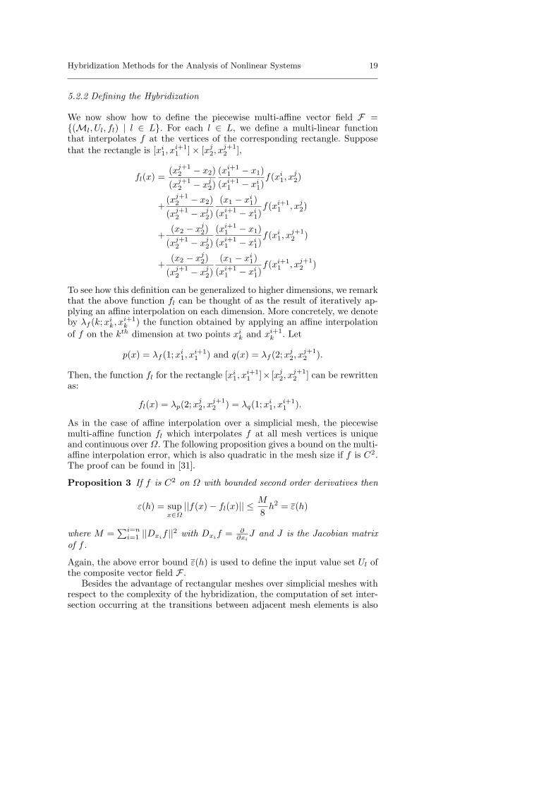
5.2.2 Defining the Hybridization

We now show how to define the piecewise multi-affine vector field F =(Ml, Ul, fl) | l ∈ L. For each l ∈ L, we define a multi-linear functionthat interpolates f at the vertices of the corresponding rectangle. Supposethat the rectangle is [xi

1, xi+11 ]× [xj

2, xj+12 ],

fl(x) =(xj+1

2 − x2)(xj+1

2 − xj2)

(xi+11 − x1)

(xi+11 − xi

1)f(xi

1, xj2)

+(xj+1

2 − x2)(xj+1

2 − xj2)

(x1 − xi1)

(xi+11 − xi

1)f(xi+1

1 , xj2)

+(x2 − xj

2)(xj+1

2 − xj2)

(xi+11 − x1)

(xi+11 − xi

1)f(xi

1, xj+12 )

+(x2 − xj

2)(xj+1

2 − xj2)

(x1 − xi1)

(xi+11 − xi

1)f(xi+1

1 , xj+12 )

To see how this definition can be generalized to higher dimensions, we remarkthat the above function fl can be thought of as the result of iteratively ap-plying an affine interpolation on each dimension. More concretely, we denoteby λf (k;xi

k, xi+1k ) the function obtained by applying an affine interpolation

of f on the kth dimension at two points xik and xi+1

k . Let

p(x) = λf (1;xi1, x

i+11 ) and q(x) = λf (2;xj

2, xj+12 ).

Then, the function fl for the rectangle [xi1, x

i+11 ]× [xj

2, xj+12 ] can be rewritten

as:

fl(x) = λp(2;xj2, x

j+12 ) = λq(1;xi

1, xi+11 ).

As in the case of affine interpolation over a simplicial mesh, the piecewisemulti-affine function fl which interpolates f at all mesh vertices is uniqueand continuous over Ω. The following proposition gives a bound on the multi-affine interpolation error, which is also quadratic in the mesh size if f is C2.The proof can be found in [31].


ε(h) = supx∈Ω

||f(x)− fl(x)|| ≤ M

8h2 = ε(h)

where M =∑i=n

i=1 ||Dxif ||2 with Dxif = ∂∂xi

J and J is the Jacobian matrixof f .

Again, the above error bound ε(h) is used to define the input value set Ul ofthe composite vector field F .

Besides the advantage of rectangular meshes over simplicial meshes withrespect to the complexity of the hybridization, the computation of set inter-section occurring at the transitions between adjacent mesh elements is also


simpler (due to the axis-aligned boundary between the mesh elements). Then,reachability computation for the approximate piecewise multi-affine systemcan be done using the method proposed in [9]. The main idea of this methodis to project away some continuous variables and consider them as inputstaking values in the corresponding mesh element ranges. This results in apiecewise bilinear system with uncertain inputs, which is then handled bya reachability analysis method using the Maximum principle. Alternatively,one can apply our recent method for polynomial systems [18] which exploitsthe geometric properties of polynomial maps without resorting to variableprojection.

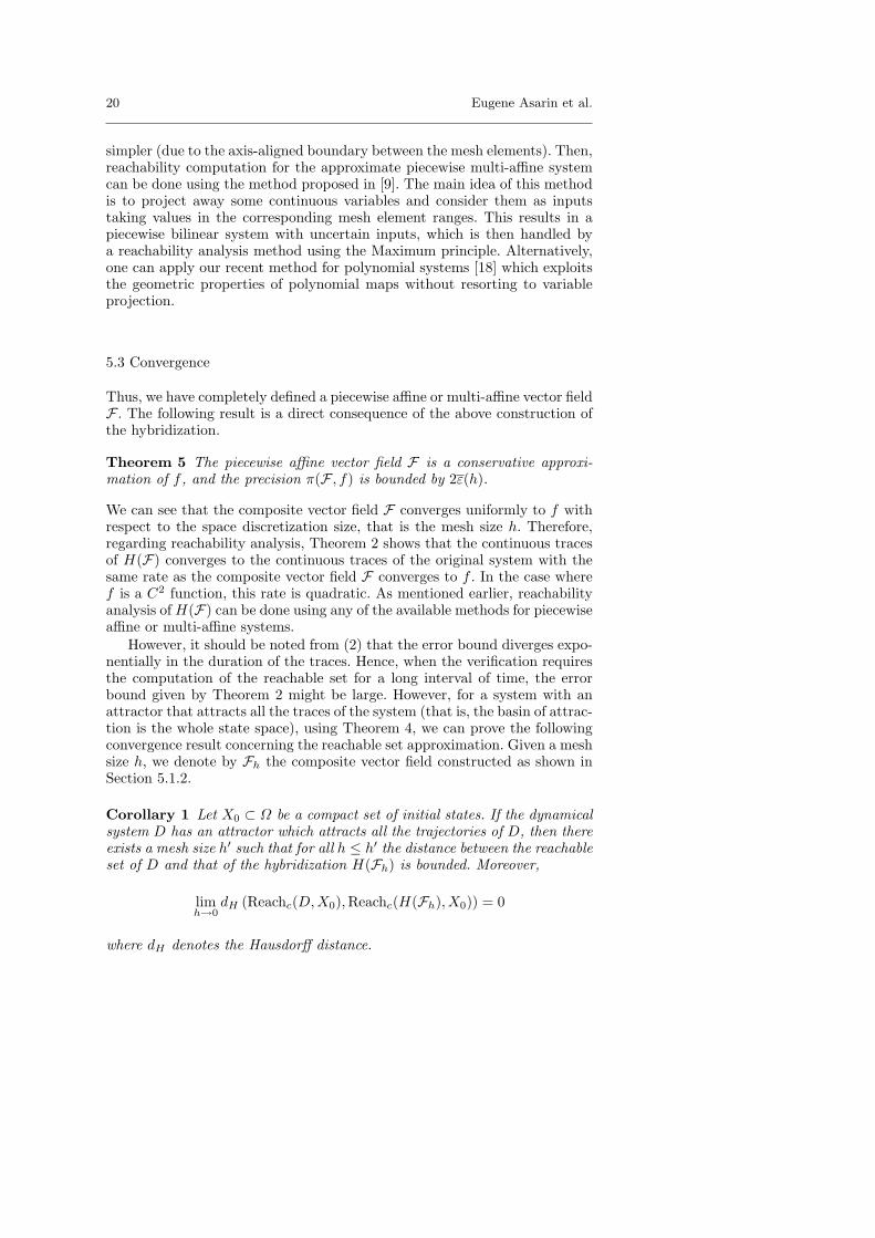
5.3 Convergence

Thus, we have completely defined a piecewise affine or multi-affine vector fieldF . The following result is a direct consequence of the above construction ofthe hybridization.

Theorem 5 The piecewise affine vector field F is a conservative approxi-mation of f , and the precision π(F , f) is bounded by 2ε(h).

We can see that the composite vector field F converges uniformly to f withrespect to the space discretization size, that is the mesh size h. Therefore,regarding reachability analysis, Theorem 2 shows that the continuous tracesof H(F) converges to the continuous traces of the original system with thesame rate as the composite vector field F converges to f . In the case wheref is a C2 function, this rate is quadratic. As mentioned earlier, reachabilityanalysis of H(F) can be done using any of the available methods for piecewiseaffine or multi-affine systems.

However, it should be noted from (2) that the error bound diverges expo-nentially in the duration of the traces. Hence, when the verification requiresthe computation of the reachable set for a long interval of time, the errorbound given by Theorem 2 might be large. However, for a system with anattractor that attracts all the traces of the system (that is, the basin of attrac-tion is the whole state space), using Theorem 4, we can prove the followingconvergence result concerning the reachable set approximation. Given a meshsize h, we denote by Fh the composite vector field constructed as shown inSection 5.1.2.

Corollary 1 Let X0 ⊂ Ω be a compact set of initial states. If the dynamicalsystem D has an attractor which attracts all the trajectories of D, then thereexists a mesh size h′ such that for all h ≤ h′ the distance between the reachableset of D and that of the hybridization H(Fh) is bounded. Moreover,

limh→0

dH (Reachc(D,X0),Reachc(H(Fh), X0)) = 0

where dH denotes the Hausdorff distance.


6 Applications

We have implemented the hybridization method and integrated it in the ver-ification tool d/dt [7,8]. The tool d/dt was initially designed to handle thefollowing class of hybrid systems: the continuous dynamics are linear andpossibly with bounded uncertain inputs, and the guard and staying con-ditions associated with discrete transitions and locations are described bylinear contraints (or convex polytopes). The main functionality of the tool isthe verification of safety and reachability properties, based on reachable setcomputations. The integration of the hybridization method in the tool ex-tended its scope to hybrid systems with nonlinear continuous dynamics. Wehave experimented this new functionality of the tool on various applications[10,19,9]. In this section, we illustrate the method with some examples.

Before continuing, we remark that in the implementation of the hybridiza-tion method, we use a dynamical construction of the mesh, that is, only thecells around the trajectories under exploration are created. This is an impor-tant advantage of the hybridization approach, compared to the grid-basedapproaches that requires the whole mesh to be constructed before startingthe computation (such as [52,46]). However, in our approach, treating thetransitions between the cells requires computing the intersection with thecell boundaries, which is expensive especially in high dimensions. We arecurrently working on a method that reduces this intersection computationby defining a transient dynamics in a neighborhood of the cell boundaries.

The Van der Pol System

The first example is the two dimensional Van der Pol oscillator:x(t) = y(t)y(t) = y(t)(1− x2(t))− x(t)

It is well-known that the Van der Pol oscillator has a limit cycle which at-tracts all the trajectories of the system. Thus, it satisfies the condition ofCorollary 1. We used a triangular mesh of size h = 0.05 to construct thehybridization. In this example, we use the bound in Proposition 2. An inputwas added to account for the approximation error. The reachable set com-puted by the hybridization method is shown in Figure 1, where the dottedset represents the set of initial values. The figure shows that the reachableset indeed contains the limit cycle.

Biquad Lowpass Filter

The second application is a second order biquad lowpass filter circuit, shownin Figure 2. This example is taken from [32]. Recently, analog and mixedsignal circuit design has attracted a lot of attention of researchers in mi-croelectronic systems design. With this example, we attemped to show theapplicability of hybrid systems techniques to formal verification of such cir-cuits.


Fig. 1 Reachable set of the Van der Pol oscillator.

The behavior of the circuit can be described by the following differential-algebraic equations:

uC1 =uC2 + uo − uC1

C1R2, (11)

uC2 =Ui − uC2 − uo

C2R1− uC2 + uo − uC1

C2R2, (12)

uo − Vmax tanh(

(uC2 − uo)Ve

Vmax

)+ Uom = 0, (13)

io = −C2 uC2, (14)Uom = V(i0), (15)

V(io) = Kio + 0.5√

K1i2o − 2K1ioIs + K1I2s + K2

− 0.5√

K1i2o + 2K1ioIs + K1I2s + K2. (16)

The state variables are (uC1, uC2), the voltages across the capacitors C1 andC2. The algebraic constraints (13-16) come from the characteristics of theoperational amplifier (OPAM) where uo is the output voltage and Uom is tothe output voltage decrease caused by the output current io. The other vari-ables are circuit parameters. By differentiating (13) the circuit equations canbe transformed into a nonlinear ODE on a manifold as with state variablesx = (uC1, uC2, uo). Then, the resulting system is treated using the methodfor ODEs on manifolds [19]. This method indeed combines the hybridizationmethod to deal with the differential part of the dynamics and the projectionintegration approach to deal with the algebraic part.

A property of interest to verify is the absence of overshoots. The param-eters of the circuit equations are: K = 0.1e11, K1 = 0.1e21, K2 = 2e4,Ve = 1e4, Vmax = 1.5, Is = 0.5e − 2. For the highly damped case (whereC1 = 0.5e− 8, C2 = 2e− 8, and R1 = R2 = 1e6), Figure 3 shows the projec-tion of the reachable set on uC1 and uC2. The reachable set here is representedas a set of convex polyhedra. The hybridization was done using a mesh ofsize h = 0.1. The initial set is a box: uC1 ∈ [−0.3, 0.3], uC2 ∈ [−0.3, 0.3] anduo ∈ [−0.2, 0.2]. From the figure, one can see that uC1 indeed remains in the


range [−2, 2], as desired. Details on the computation results can be found in[19].

Fig. 2 Lowpass filter

Fig. 3 Reachable set projected on variables uC1 and uC2

7 Concluding remarks

In this paper, we proposed a framework for approximate analysis of complexnonlinear systems by means of approximate systems that we call hybridiza-tions. We also developed two methods for constructing hybridizations, whichallows analyzing the original system with an arbitrary precision and a goodconvergence rate. These results can be readily applied to the verification ofinteresting properties of hybrid systems.

The results presented in the paper open various interesting directions forfuture research. One direction concerns the problem of hierarchical mesh re-finement that is guided by the information obtained in the process of provingthe property, as in the abstraction approaches. Another promising direction isto use mixed rectangular-simplicial meshes in order to achieve a good trade-off between accuracy and computational cost. In addition, the convergence


can be improved by using higher degree approximants, such as piecewisequadratic, and the reachability method for polynomial systems [18] can thenbe used. Finally, an important theoretical question to address is whetherother new properties can be verified using the hybridization approach.

Appendix

Proof of Proposition 1

Proposition 4 If f is λ-Lipschitz, then

ε(h) ≤ h2n λ

n + 1= ε(h).

Proof We first estimate an upper bound of ||f(x) − fl(x)|| for all points xinside a mesh elementMl. Let v be a vertex ofMl. By the triangle inequality,we have ||f(x)− fl(x)|| ≤ ||f(x)− f(v)||+ ||f(v)− fl(x)||. The function f isλ-Lipschitz, then

||f(x)− fl(x)|| ≤ λ||x− v||+ ||f(v)− fl(x)||. (17)

Let V (Ml) = v0, v1, . . . , vn. A point x ∈ V (Ml) can be written as:

x =n∑

i=0

αi vi, withn∑

i=0

αi = 1 and ∀i ∈ 1, . . . , n, αi ≥ 0. (18)

Since fl is affine, we have

fl(x) =n∑

i=0

αi fl(vi) =n∑

i=0

αi f(vi).

Thus,

||f(v)− fl(x)|| ≤ ||f(v)−n∑

i=0

αi f(vi)|| ≤n∑

i=0

αi||f(v)− f(vi)||

≤ λn∑

i=0

αi||v − vi||.

Equation (17) becomes

||f(x)− fl(x)|| ≤ 2λn∑

i=0

αi||v − vi||.

Note that the above inequality holds for any vertex v ∈ V (Ml). We observe,from the conditions (18), that there exists j ∈ 0, . . . , n such that αj ≥ 1

n+1 .Since for all i 6= j, ||vi − vj || ≤ h then

||f(x)− fl(x)|| ≤ 2λn∑

i=0

αi||vj − vi|| ≤ 2λ(1− αj)h ≤ h2n λ

n + 1.

This completes the proof of the proposition. ut


An important remark is that the second partial derivatives of the linear ap-proximation fl vanish; therefore, if f is a C2 function, we can obtain a bettererror bound. Exceptionally, to write the second partial derivatives of f , weuse superscripts to indicate the components of f , that is f = (f1, f2, . . . , fn).

Proof of Proposition 2


ε(h) ≤ Kn2

2(n + 1)2h2 = ε(h)

where

K = maxi∈1,...,n

supx∈Ω

p1=n∑p1=1

p2=n∑p2=1

∣∣∣∣ ∂2f i(x)∂xp1∂xp2

∣∣∣∣ .

Proof For a given mesh element Ml, we define the function e(x) = f i(x) −f i

l (x) where f i and f il denotes the i-th components of the vector fields f and

fl. Let x∗ = arg maxx∈Ml|e(x)| (note that the simplex Ml is compact). Let

v be a vertex of Ml, and all points in the line segment connecting x∗ and vcan be written as: x(γ) = x∗ + γ (v − x∗), γ ∈ [0, 1]. To determine a boundon e(x∗), we define a function z(γ) = e(x(γ)) for γ ∈ [0, 1]. Expanding z withrespect to γ gives

z(1) = z(0) +dz

dγ(0) +

∫ 1

0

d2z

dγ2(s) (1− s)ds. (19)

We can see that dx(γ)/dγ = (v − x∗). Thus,

dz

dγ(γ) =

p1=n∑p1=1

∂e

∂xp1

(x(γ)) (vp1 − x∗p1),

d2z

dγ2(γ) =

p1=n∑p1=1

p2=n∑p2=1

∂2e

∂xp1∂xp2

(x(γ)) (vp1 − x∗p1) (vp2 − x∗p2

).

Since the second order derivatives of fl vanish, then

∀p1, p2 ∈ 1, . . . , n, ∂2e

∂xp1∂xp2

=∂2f i

∂xp1∂xp2

.

Similar to the proof of Lemma 1, we can show that there exists v ∈ V (Ml)such that ||v − x∗|| ≤ hn/(n + 1). Then, using the bound K on the secondorder derivatives of the function f , we obtain∣∣∣∣d2z

dγ2(γ)

∣∣∣∣ ≤ h2 n2 K

(n + 1)2.


In addition, |e(x)| attains a maximum at x∗, which implies that dz(0)/dγ = 0.By definition of the interpolating function, f i(v) = f i

l (v), then z(1) = 0.Therefore, (19) becomes:

f i(x∗)− f il (x

∗) +∫ 1

0

d2z

dγ2(s) (1− s)ds = 0.

Using the above bound on the second order derivative of z(γ), we get

|f i(x∗)− f il (x

∗)| ≤ h2 n2 K

(n + 1)2

∫ 1

0

(1− s)ds = h2 n2 K

2 (n + 1)2.

We complete the proof by remarking that such an equality holds for allcomponents of the vector fields f and fl. ut

Acknowledgements We would like to thank our colleagues at the laboratoriesVerimag and LMC in Grenoble for their collaboration and encouragement. Wewould also like to thank the anonymous reviewers for their useful comments andsuggestions.

References

1. Alur, R., Courcoubetis, C., Halbwachs, N., Henzinger, T.A., Ho, P.-H, Nicollin,X., Olivero, A., Sifakis, J., Yovine, S.: The algorithmic analysis of hybrid sys-tems. Theoretical Computer Science, 138(1), 3-34, (1995).

2. Alur, R., Dang, T., Esposito, J., Hur, Y., Ivancic, F., Kumar, V., Lee, I., Mishra,P., Pappas, G.J., Sokolsky, O.: Hierarchical modeling and analysis of embeddedsystems. Proceedings of the IEEE, 91(1), 11-28, (2003).

3. Alur, R., Dang, T., Ivancic, F.: Counter-example guided predicate abstractionof hybrid systems. Theoretical Computer Science, 354(2), 250-271, (2006).

4. Alur, R., Dill, D.L.: A theory of timed automata. Theoretical Computer Science,126(2), 183-235, (1994).

5. Alur, R., Henzinger, T.A., Lafferriere, G., Pappas, G.: Discrete abstractions ofhybrid systems. Proceedings of the IEEE, 88(2), 971-984, (2000).

6. Anai, H., Weispfenning, V.: Reach set computations using real quantifier elimi-nation. In: Di Benedetto, M.D., Sangiovanni-Vincentelli, A. (eds.) Hybrid Sys-tems: Computation and Control, vol 2034 in LNCS, 63-75. Springer, (2001).

7. Asarin, E., Bournez, O., Dang, T., Maler, O.: Approximate reachability analysisof piecewise-linear dynamical systems. In: Krogh, B.H., Lynch, N. (eds.) HybridSystems: Computation and Control, vol 1790 in LNCS, 20-31. Springer, (2000).

8. Asarin, E., Dang, T., Maler, O.: d/dt: A tool for verification of hybrid systems.In: Ed Brinksma, Kim Guldstrand Larsen (eds.) Computer Aided Verification,vol 2404 in LNCS, 365-370. Springer, (2002).

9. Asarin, E., Dang, T.: Abstraction by projection and application to multi-affinesystems. In: Alur, R., Pappas, G.J. (eds) Hybrid Systems: Control and Compu-tation, vol 2993 LNCS, 32-47. Springer, (2004).

10. Asarin, E., Dang, T., Girard, A.: Reachability analysis of nonlinear systemsusing conservative approximations. In: Maler, O., Pnueli, A. (eds.) Hybrid Sys-tems: Computation and Control, vol 2623 in LNCS, 20-35. Springer, (2003).

11. Asarin, E., Maler, O., Pnueli, A.: Reachability analysis of dynamical systemshaving piecewise-constant derivatives. Theoretical Computer Science, 138(1),35-66, (1995).

12. Aubin, J.-P., Lygeros, J., Quincampoix, M., Sastry, S., Seube, N.: Impulsedifferential inclusions: a viability approach to hybrid systems. IEEE Trans. Au-tomatic Control, 47(1), 2-20, 2002.


13. Barringer, H., Kuiper, R., Pnueli, A.: A really abstract concurrent model andits temporal logic. In: POPL’86: Principles of Programming Languages, pp 173-183, 1986.

14. Botchkarev, O., Tripakis, S.: Verification of hybrid systems with linear differ-ential inclusions using ellipsoidal approximations. In: Krogh B., Lynch N. (eds.),Hybrid Systems: Computation and Control, vol 1790 in LNCS, 73-88. Springer,(2000).

15. Branicky, M.S., Borkar, V.S., Mitter, S.K.: A unified framework for hybridcontrol: model and optimal control theory. IEEE Trans. on Automatic Control,43(1), 31-45, (1998).

16. Chutinan, A., Krogh, B.H.: Verification of polyhedral-invariant hybrid au-tomata using polygonal flow pipe approximations. In: Vaandrager, F.W., vanSchuppen, J.H. (eds.) Hybrid systems: Computation and Control, vol 1569 inLNCS, 76-90. Springer, (1999).

17. Clarke, E., Fehnker, A., Han, Z., Krogh, B., Ouaknine, J., Stursberg, O.,Theobald, M.: Abstraction and counterexample-guided refinement in modelchecking of hybrid systems. Int. Journal of Foundations of Computer Science,14(4), 583-604, (2003).

18. Dang, T.: Approximate reachability computation for polynomial systems. In:Hespanha, J., Tiwari, A. (eds.) Hybrid Systems: Control and Computation, vol3927 in LNCS, 138-152. Springer, (2006).

19. Dang, T., Donze, A., Maler, O.: Verification of analog and mixed-signal circuitsusing hybrid systems techniques. In: Hu, A., Martin, A. (eds.) Formal Methodsfor Computer Aided Design, vol 3312 in LNCS, 21-36. Springer, (2004).

20. Dang, T., Maler, O.: Reachability Analysis via Face Lifting. In: Henzinger,T.A., Sastry, S. (eds.), Hybrid Systems: Computation and Control, vol 1386 inLNCS, 96-109. Springer, (1998).

21. Davoren, J.M., Coulthard, V., Markey, N., Moor, T.: Non-deterministic tem-poral logics for general flow systems. In: Alur, R., G.J. Pappas, G.J. (eds.) Hy-brid Systems: Computation and Control HSCC04, vol 2993 in LNCS, 280-295.Springer, (2004).

22. Decarlo, R.A., Branicky, M.S., Pettersson, S., Lennartson, B.: Perspectives andresults on the stability and stabilizability of hybrid systems. Proceedings of theIEEE, 88(7), 1069-1082, (2000).

23. Della Dora, J., Maignan, A., Mirica-Ruse, M., Yovine, S.: Hybrid computation.In: Proceedings International Symposium on Symbolic and Algebraic Compu-tation ISSAC’01, (2001).

24. Dieudonne, J.: Calcul Infinitesimal. Collection Methodes, Hermann, Paris(1968).

25. Emerson, E.A.: Temporal and modal logic. In: van Leeuwen, J. (ed.), Handbookof Theoretical Computer Science, vol B, 995-1072. Elsevier Science Publishers,(1990).

26. Frehse, G.: PHAVer: Algorithmic verification of hybrid systems past HyTech.In: Morari, M., Thiele, L. (eds.) Hybrid Systems: Computation and Control, vol3414 in LNCS, 258-273. Springer, (2005).

27. Girard, A.: Approximate solutions of ODEs using piecewise linear vector fields.In: Proceedings of the Int. Workshop on Computer Algebra in Scientific Com-puting CASC’02, (2002).

28. Girard, A.: Reachability of uncertain linear systems using zonotopes. In:Morari, M., Thiele, L. (eds.) Hybrid Systems: Computation and Control, vol3414 in LNCS, 291-305. Springer, (2005).

29. Greenstreet, M.R., Mitchell, I.: Reachability analysis using polygonal projec-tions. In: Vaandrager, F., van Schuppen, J.H. (eds.) Hybrid Systems: Compu-tation and Control, vol 1569 in LNCS, 76-90. Springer, (1999).

30. Habets, L.C.G.J.M., van Schuppen, J.H.: Control of piecewise-linear hybridsystems on simplices and rectangles. In: Di Benedetto, M.D., Sangiovanni-Vincentelli, A. (eds.) Hybrid systems: Computation and Control, vol. 2034LNCS, 261-273. Springer, (2001).

31. Hammerlin G., Karl-Heinz Hoffmann K.-H.: Numerical Mathematics. Springer,(1991).


32. Hartong, W., Hedrich, L., Barke, E.: On discrete modelling and model checkingfor nonlinear analog systems. In: Ed Brinksma, Kim Guldstrand Larsen (eds.)Computer Aided Verification, vol 2404 in LNCS, 401-413. Springer, (2002).

33. Henzinger, T.A., Ho, P.-H., Wong-Toi, H.: HyTech: A model checker for hybridsystems. Software Tools for Technology Transfer, 1(1-2), 110-122, (1997).

34. Henzinger, T.A., Ho, P.-H., Wong-Toi, H., Algorithmic analysis of nonlinearhybrid systems. IEEE Trans. on Automatic Control, 43(4), 540-554, (1998).

35. Henzinger, T.A., Kopke, P.W., Puri, A., Varaiya, P.: What’s decidable abouthybrid automata? Journal of Computer and System Sciences, 57(1), 94-124,(1998).

36. Hubbard, J., West, B.: Differential equations: a dynamical system approach,part 2: higher dimensional systems. Texts in Applied Mathematics, 18, Springer,(1995).

37. Johansson, M., Rantzer, A.: Computation of piecewise quadratic Lyapunovfunctions for hybrid systems. IEEE Transactions on Automatic Control, 43(4),555-559, (1998).

38. Kloetzer, M., Belta, C.: Reachability analysis of multi-affine systems. In: Hes-panha, J., Tiwari, A. (eds.) Hybrid Systems: Computation and Control, vol 3927in LNCS, 348-362. Springer, (2006).

39. Kratz, F., Sokolsky, O., Pappas, G.J., Lee, I.: R-Charon : a modeling languagefor reconfigurable hybrid systems. In: Hespanha, J., Tiwari, A. (eds.) Hybrid Sys-tems: Computation and Control, vol 3927 in LNCS, 392-406. Springer, (2006).

40. Kuhn, H.W.: Some combinatorial lemmas in topology. IBM Journal of Researchand Development, 4(5), 518-524, (1960).

41. Kurzhanski, A., Varaiya, P.: Ellipsoidal techniques for reachability analysis.In: Krogh, B., Lynch, N. (eds.) Hybrid Systems: Computation and Control, vol1790 in LNCS, 202-214. Springer, (2000).

42. Lafferriere. G., Pappas. G., Yovine. S.: Symbolic reachability computation offamilies of linear vector fields. Journal of Symbolic Computation, 32(3), 231-253, Academic Press, (2001).

43. Larsen. K., Pettersson. P., Yi. W.: Uppaal in a nutshell. Software Tools forTechnology Transfert, 1(1-2), 134-152, (1997).

44. Liberzon. D.: Switching in systems and control. Volume in series Systems andControl: Foundations and Applications. Birkhauser, Boston, MA, (2003).

45. Manna. Z., Pnueli. A.: The temporal logic of reactive and concurrent systems:specification. Springer-Verlag, New York (1991).

46. Mitchell. I., Templeton. J.A.: A toolbox of Hamilton-Jacobi solvers for analysisof nondeterministic continuous and hybrid Systems. In: Morari, M., Thiele, L.(eds.) Hybrid Systems: Computation and Control, vol 3414 in LNCS, 480-494.Springer, (2005).

47. Kvasnica, M., Grieder, P., Baoti, M., Morari, M.: Multi-Parametric Toolbox(MPT). In: Alur, R., Pappas, G.J. (eds.) Hybrid Systems: Computation andControl, vol. 2993 in LNCS, 448-462. Springer, (2004).

48. Prajna S., Jadbabaie A.: Safety verification of hybrid systems using barriercertificates. In: Alur, A., Pappas, G. (eds.) Hybrid Systems: Computation andControl, vol. 2993 LNCS, 477-492. Springer, (2004).

49. Prajna S., Papachristodoulou A.: Analysis of switched and hybrid systems -beyond piecewise quadratic methods. In: Proceedings of the American ControlConference ACC, (2003).

50. Puri, A., Varaiya, P.: Verification of sybrid systems using abstraction. In:Antsaklis, P., Kohn, W., Nerode, A., Sastry, S. (eds.) Hybrid Systems II, vol999 in LNCS, 359-369, Springer, (1995).

51. Rondepierre, A., Dumas, J.G.: Algorithms for hybrid optimal control. Technicalreport IMAG-ccsd-00004191, arXiv math.OC/0502172, (2005).

52. Saint-Pierre, P.: Approximation of Viability Kernels and Capture Basin forHybrid Systems. In: Proc. of European Control Conference ECC’01, 2776-2783,(2001).

53. Sastry, S.: Nonlinear systems: analysis, stability and control. Springer, (1999).54. Stuart, A.M., Humphries, A.R.: Dynamical systems and numerical analysis.

Cambridge Monographs on Applied and Computational Mathematics, Cam-bridge University Press, (1996).


55. Stursberg, O., Kowalewski, S.: Approximating switched continuous systemsby rectangular automata. In: Proceedings European Control Conference ECC,(1999).

56. Tabuada, P., Pappas, G.: Model-checking LTL over controllable linear systemsis decidable, In: Maler, O., Pnueli, A. (eds.) Hybrid Systems: Computation andControl, vol 2623 LNCS, 498-513, Springer, (2003).

57. Tiwari, A., Khanna, G.: Series of abstractions for hybrid automata. In: Tomlin,C., Greenstreet, M.R. (eds.) Hybrid Systems: Computation and Control, vol2289 LNCS, 465-478, (2002).

58. Tiwari, A., Khanna, A.: Nonlinear systems: approximating reach sets. In: Alur,R., Pappas, G.J. (eds.) Hybrid Systems: Computation and Control, vol 2993LNCS, 600-614. Springer, (2004).

59. Tomlin, C., Mitchell, I., Bayen, A., Oishi, M.: Computational techniques forthe verification of hybrid systems. Proceedings of the IEEE, 91(7), 986-1001,(2003).

60. Torrisi, F.D., Bemporad, A.: HYSDEL - A tool for generating computationalhybrid models. IEEE Transactions on Control Systems Technology, 12(2), 235-249, (2004).

61. Van der Schaft, A.J., Schumacher, J.M.: An introduction to hybrid dynamicalsystems. Lect. Notes in Control and Information Sciences, Vol. 251, Springer,London, (2000).

62. Yovine, S.: Kronos: A verification tool for real-time systems. Software Tools forTechnology Transfer, 1(1-2), 123-133, (1997).

Hybridization methods for the analysis of nonlinear systems

Documents

Transcript of Hybridization methods for the analysis of nonlinear systems