
HVAC Pump Handbook - we are refrigeration
645
-
Upload
khangminh22 -
Category
Documents
-
view
1 -
download
0
Transcript of HVAC Pump Handbook - we are refrigeration


Table of Contents Part I: The Basic Tools Part II: HVAC Pumps and Their Performance Part III: The HVAC World Part IV: Pumps for Open HVAC Cooling Systems Part V: Pumps for Closed HVAC Cooling Systems Part VI: Pumps for HVAC Hot Water Systems Part VII: Installing and Operating HVAC Pumps SUMMARY OF HVAC ENERGY EVALUATIONS Chapters 1 DIGITAL ELECTRONICS AND HVAC PUMPS 2 PHYSICAL DATA FOR HVAC SYSTEM DESIGN 3 PIPING SYSTEM FRICTION 4 BASICS OF PUMP DESIGN 5 PHYSICAL DESCRIPTION OF HVAC PUMPS 6 HVAC PUMP PERFORMANCE 7 PUMP DRIVERS AND VARIABLE-SPEED DRIVES 8 THE USE OF WATER IN HVAC SYSTEMS 9 CONFIGURING AN HVAC WATER SYSTEM 10 BASICS OF PUMP APPLICATION FOR HVAC SYSTEMS 11 OPEN COOLING TOWER PUMPS 12 PUMPS FOR PROCESS COOLING 13 PUMPING OPEN THERMAL STORAGE TANKS 14 CHILLERS AND THEIR PUMPS 15 CHILLED WATER DISTRIBUTION SYSTEMS 16 CLOSED CONDENSER WATER SYSTEMS 17 PUMPS FOR CLOSED ENERGY STORAGE SYSTEMS
18 PUMPS FOR DISTRICT COOLING AND HEATING 19 STEAM AND HOT WATER BOILERS 20 LOW-TEMPERATURE HOT WATER HEATING SYSTEMS 21 PUMPS FOR MEDIUM- AND HIGH-TEMPERATURE WATER SYSTEMS 22 CONDENSATE, BOILER FEED, AND DEAERATOR SYSTEMS 23 INSTRUMENTATION AND CONTROL FOR HVAC PUMPING SYSTEMS 24 TESTING HVAC CENTRIFUGAL PUMPS 25 INSTALLING HVAC PUMPS AND PUMPING SYSTEMS 26 FACTORY-ASSEMBLED PUMPING SYSTEMS 27 OPERATING HVAC PUMPS 28 MAINTAINING HVAC PUMPS 29 RETROFITTING EXISTING HVAC WATER SYSTEMS 30 SUMMARY OF HVAC ENERGY EVALUATIONS 31 THE MODERN TWO-PIPE HEATING AND COOLING SYSTEM 31 ADVANCED HEAT RECOVERY

The Basic Tools
Part
1
Rishel_CH01.qxd 20/4/06 5:11 PM Page 1
Downloaded from Digital Engineering Library @ McGraw-Hill (www.digitalengineeringlibrary.com)Copyright © 2006 The McGraw-Hill Companies. All rights reserved.
Any use is subject to the Terms of Use as given at the website.
Source: HVAC Pump Handbook

Rishel_CH01.qxd 20/4/06 5:11 PM Page 2
Downloaded from Digital Engineering Library @ McGraw-Hill (www.digitalengineeringlibrary.com)Copyright © 2006 The McGraw-Hill Companies. All rights reserved.
Any use is subject to the Terms of Use as given at the website.
The Basic Tools

Chapter
3
1Digital Electronicsand HVAC Pumps
1.1 Introduction
The emergence of digital electronics has had a tremendous impact on in-dustrial societies throughout the world. In the heating, ventilating, andair-conditioning (HVAC) industry, the development of digital electronicshas brought an end to the use of many mechanical devices; typical ofthis is the diminished use of mechanical controls for HVAC air andwater systems. Today’s digital control systems, with built-in intelligence,more accurately evaluate water and system conditions and adjust pumpoperation to meet the desired water flow and pressure conditions.
Drafting boards and drafting machines have all but disappeared fromthe design rooms of heating, ventilating, and air-conditioning engineersand have been replaced by computer-aided drafting (CAD) systems.Tedious manual calculations are being done more quickly and accuratelyby computer programs developed for specific design applications. Allthis has left more time for creative engineering on the part of designersto the benefit of the client.
1.2 Computer-Aided Calculation of HVACLoads and Pipe Friction
The entire design process for today’s water systems, from initial designto final commissioning, has been simplified and improved as a result ofthe new, sophisticated computer programs. One of the most capableprograms for sizing and analyzing flow in fluid systems is the pipingsystems analysis program developed by APEC, Inc. (AutomatedProcedures for Engineering Consultants), headquartered in Dayton,
Rishel_CH01.qxd 20/4/06 5:11 PM Page 3
Downloaded from Digital Engineering Library @ McGraw-Hill (www.digitalengineeringlibrary.com)Copyright © 2006 The McGraw-Hill Companies. All rights reserved.
Any use is subject to the Terms of Use as given at the website.
Source: HVAC Pump Handbook

4 The Basic Tools
Ohio. APEC, a nonprofit, worldwide association of consulting engineersand in-house design group, is dedicated to improving quality and pro-ductivity in the design of HVAC air and water systems through the de-velopment and application of advanced computer software.
The APEC PSA-1 program accurately calculates the friction lossesand sizes of pipes as well as simulating flow under different operatingconditions in either new or existing piping systems. Analyzing thefluid flow in systems with diversified loads, multiple pumps, andchillers or boilers is essential if engineers are to truly understand thereal operating conditions of large HVAC water systems. This under-standing can only be achieved through the use of a computer programcapable of such thorough analysis.
1.2.1 Typical input for APEC piping systemanalysis program
The following is representative system data into an APEC’s computerprogram for calculating pipe sizing, friction, and flow analysis, andtypical output.
Master Data files
Pipe, fitting, and valve files
Material friction loss
Actual ID for nominal copper type (M,L)
Steel schedule other
Standard pipe pre-entered or custom. Cost estimation optional.
Insulation file
Type
K valueThickness
Cost estimation optional
Fluids. Provisions for all fluid types with:
Density Temperature
Viscosity Specific heat
System data
Pipe environment Required for heat/loss gain
Space temperature Outside air temperature
Soil conductivity Burial depth
Rishel_CH01.qxd 20/4/06 5:11 PM Page 4
Downloaded from Digital Engineering Library @ McGraw-Hill (www.digitalengineeringlibrary.com)Copyright © 2006 The McGraw-Hill Companies. All rights reserved.
Any use is subject to the Terms of Use as given at the website.
Digital Electronics and HVAC Pumps

Digital Electronics and HVAC Pumps 5
Program options
System sizing
Flow simulation
Cost estimate
Flow simulation options-typical entries
Maximum iterations 30
Intermediate results Every 3 iterations
Temperature tolerance for convergence 0.50
Relaxation parameters 0.50°F
Fill pressure 46 ft of head (or H2O)
Pump data
Variable or constant speed
Points for pump curves
Terminal data (coils, etc.)
Fluid flow
Pressure drop
Coil cfm (ft3/min)
Inlet air temperature
Leaving air set point
Valve data
Valve coefficient
Trial setting
Valve control
1.2.2 Typical output for APEC pipingsystem analysis program
Table 1.1 includes samples of output headings, with one line of outputfor only three output forms available. The output also has forms thatmirror the input, so the designer has a complete record of the entireanalysis.
This program is now being expanded to include many additionalpiping features and to accommodate contemporary computer prac-tices such as Windows, to speed the development and manipulation ofproject data.
Rishel_CH01.qxd 20/4/06 5:11 PM Page 5
Downloaded from Digital Engineering Library @ McGraw-Hill (www.digitalengineeringlibrary.com)Copyright © 2006 The McGraw-Hill Companies. All rights reserved.
Any use is subject to the Terms of Use as given at the website.
Digital Electronics and HVAC Pumps

TABLE 1.1 Sample Output Headings
Pressure-drop analysis*
Node PipePipe
TerminalCV Fitting Special Total
From To Diameter Length, ft PD Flow PD PD PD PD PD
5 6 2.50 22.5 0.75 70 22 31.0 0.21 53.96
System estimate†
Material LaborTotal
Item Size Description Quantity Unit Unit Cost Unit Cost Cost
1 2.00 Schedule 40 115.0 LF 2.42 278 42 4830 5108
Final simulation results
LinkPipe
Flow (gpm) Pressure head (ft)
Start End diameter Input Actual At start Node Temperature, °F
4 5 2.5 70 75.3 34.4 (79.37) 160
*Chiller or boiler pressure drop not included.†Labor and cost units are entered by user as master data for given localities. Cost estimates are not in-
tended to give accurate costs for bidding purposes.
6 The Basic Tools
1.3 Hydraulic-Gradient Diagrams
The hydraulic-gradient diagram provides a visual description of thechanges in total pressure in a water system. To date, these diagramshave been drawn manually; the actual drawing of the hydraulic-gradient diagram is now being evaluated for conversion to software;when this is completed, the diagram will appear automatically on thecomputer screen after the piping friction calculations are completed.
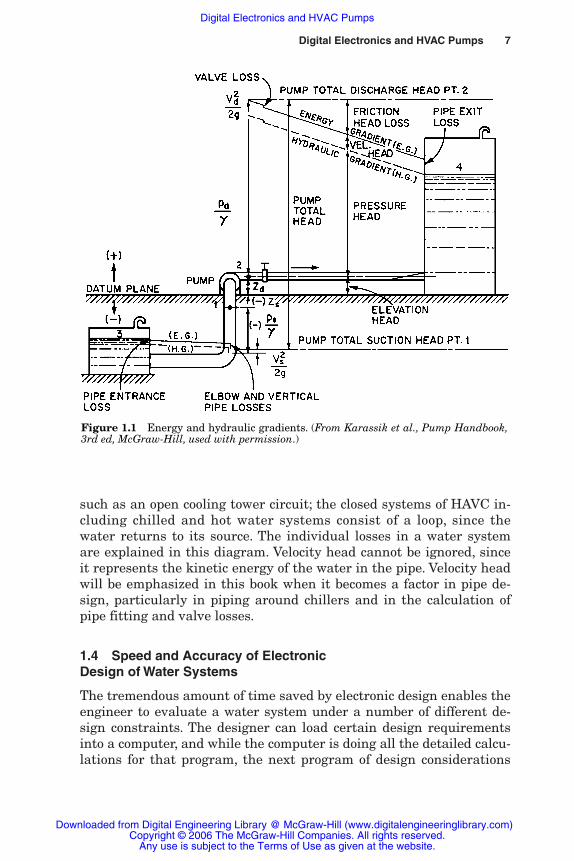
The hydraulic-gradient diagram has proved to be an invaluable toolin the development of a water system. It will appear throughout thisbook for various types of water systems. Its generation will be ex-plained in Chap. 3. Clarification should be made between an energygradient and the hydraulic gradient of a water system. The energy gra-dient includes the velocity head V 2/2 g, of the water system, while thehydraulic gradient includes only the static and pressure heads. Velocityhead is usually a number less than 5 ft and is not used to move waterthrough pipe, as are static and pressure heads. Using the energy gradi-ent with the velocity head increases the calculations for developingthese diagrams; therefore, the hydraulic gradient is used instead.
1.3.1 Energy and hydraulic gradients
Figure 1.1 describes the difference between the energy gradient andthe hydraulic gradient. This diagram is typical for an open system
Rishel_CH01.qxd 20/4/06 5:11 PM Page 6
Downloaded from Digital Engineering Library @ McGraw-Hill (www.digitalengineeringlibrary.com)Copyright © 2006 The McGraw-Hill Companies. All rights reserved.
Any use is subject to the Terms of Use as given at the website.
Digital Electronics and HVAC Pumps
Digital Electronics and HVAC Pumps 7
such as an open cooling tower circuit; the closed systems of HAVC in-cluding chilled and hot water systems consist of a loop, since thewater returns to its source. The individual losses in a water systemare explained in this diagram. Velocity head cannot be ignored, sinceit represents the kinetic energy of the water in the pipe. Velocity headwill be emphasized in this book when it becomes a factor in pipe de-sign, particularly in piping around chillers and in the calculation ofpipe fitting and valve losses.
1.4 Speed and Accuracy of ElectronicDesign of Water Systems
The tremendous amount of time saved by electronic design enables theengineer to evaluate a water system under a number of different de-sign constraints. The designer can load certain design requirementsinto a computer, and while the computer is doing all the detailed calcu-lations for that program, the next program of design considerations
Figure 1.1 Energy and hydraulic gradients. (From Karassik et al., Pump Handbook,3rd ed, McGraw-Hill, used with permission.)
Rishel_CH01.qxd 20/4/06 5:11 PM Page 7
Downloaded from Digital Engineering Library @ McGraw-Hill (www.digitalengineeringlibrary.com)Copyright © 2006 The McGraw-Hill Companies. All rights reserved.
Any use is subject to the Terms of Use as given at the website.
Digital Electronics and HVAC Pumps
8 The Basic Tools
can be set up for calculations by the computer. After all the programshave been run, the designer can select the one that provides the op-timal system conditions that meet the specifications of the client.The designer now has time to play “what if ” to achieve the best pos-sible design for a water system. In the past, the engineer was oftentime driven and forced to utilize much of a past design to reach adeadline for a current project. Now the engineer can model pumpingsystem performance under a number of different load conditions andsecure a much more complete document on the energy consumptionof proposed pumping systems.
The designer can compute the diversity of an HVAC system withmuch greater accuracy. Diversity is merely the actual maximal heat-ing or cooling load on an HVAC system divided by the capacity of theinstalled equipment. For example, assume that the total cooling loadon a chilled water system is 800 tons, but there are 1000 tons of cool-ing equipment installed on the system to provide cooling to all parts ofthat system. This disparity is caused by changing some loads or differ-ences in occupancy. The diversity in this case would be 800/1000, or0.80 (80 percent).
This is a simpler and easier definition of diversity than a moretechnical definition that states that diversity is the maximal heatingor cooling load divided by the sum of all the individual peak loads. Forexample, a 10-ton air handler might have a peak load of only 9.2 ton.The true diversity might be slightly less than that acquired by usingthe installed load.
1.4.1 Equation solution by computer
A number of equations are provided herein for the accurate solutionof pressures, flows, and energy consumptions of HVAC water systems.These equations have been kept to the algebraic level of mathematicsto aid the HVAC water system designer in the application of them tocomputer programs. Computer software is now available commerciallyto assist in the manipulation of these equations. Typical of them isthe EES—Engineering Equation Solver program, available from F-Chart Software, Middleton, Wis.
1.5 Databasing
After the designer has completed the overall evaluation of a watersystem, databasing can be used to search elements of past designs foruse on a current project. Databasing is a compilation of informationon completed designs in computer memory that can be recalled for
Rishel_CH01.qxd 20/4/06 5:11 PM Page 8
Downloaded from Digital Engineering Library @ McGraw-Hill (www.digitalengineeringlibrary.com)Copyright © 2006 The McGraw-Hill Companies. All rights reserved.
Any use is subject to the Terms of Use as given at the website.
Digital Electronics and HVAC Pumps

Digital Electronics and HVAC Pumps 9
use on future projects. To use it, the designer can enter key factorsthat would describe a current project and then allow the computer tosearch a database for similar completed designs that would have thesame defining elements. For example, a project designed withoutdatabasing may have a total of 5000 design hours. After searching thedatabase, a design might be found that could provide 3000 designhours from a previous project, leaving a requirement for 2000 new de-sign hours. When this current project is completed, it would be en-tered into the database for similar future reference.
1.6 Electronic Communication
With the technical advances that are occurring in communications,rapid communication is available between various architectural andengineering offices. Databasing can be linked between main andbranch offices of a multioffice firm so that job and data sharing can beestablished between the various offices as desired by the engineeringmanagement.
Interoffice communication also has been accelerated with the use ofelectronic mail such as e-mail. Such mail can reduce the time for ask-ing crucial questions and receiving responses. It reduces error withregard to documentation and maintains a file on the correspondence.
1.7 Electronic Design of the Piping and Accessories
Similar to load calculations and general system layout, digital elec-tronics has invaded the actual configuration of the water system it-self. This includes the methods of generating hot or cold water, stor-age of the same, and distribution of the water in the system. Thedistribution of water in an HVAC system is no longer dependent onmechanical devices such as pressure-regulating valves, balancingvalves, crossover bridges, reverse-return piping, and other energy-con-suming mechanical devices that force the water through certain partsof the system. Almost all mechanical devices are disappearing, otherthan temperature-control valves for heating and cooling coils. Howthis is done will be described in detail in Chaps. 10 and 15 during ac-tual designing of HVAC systems.
HVAC water systems are being reduced to major equipment such asboilers or chillers, heating and cooling coils, pumping systems, con-necting piping, and electronic control. Simplicity of system design isruling the day with very few flow- or pressure-regulating devices; thisresults in much higher overall system operating efficiencies.
Rishel_CH01.qxd 20/4/06 5:11 PM Page 9
Downloaded from Digital Engineering Library @ McGraw-Hill (www.digitalengineeringlibrary.com)Copyright © 2006 The McGraw-Hill Companies. All rights reserved.
Any use is subject to the Terms of Use as given at the website.
Digital Electronics and HVAC Pumps
10 The Basic Tools
1.8 Electronic Selection of HVAC Equipment
A major part of the designer’s work is the selection of equipment for awater system. This includes, for example, chillers, cooling towers, boil-ers, pumping systems, heating and cooling coils, and control systems.In the past, designers depended on manufacturers’ catalogs to furnishthe technical information that provided the selection of the correctequipment for a water system. This had to do with the hope that thecatalogs were current. Now comes the CD-ROM disc and on-line dataservices that provide current information and rapid selection ofequipment that meets the designer’s specifications. Many manufac-turers are converting their technical catalogs to software such as CD-ROM discs, providing both performance and dimensional data. Theday of the technical catalog is almost gone.
1.9 Electronic Control of HVAC Water Systems
Along with these changes in mechanical design, electronic control ofHVAC water systems, in the form of direct digital control or program-mable-logic controllers, has all but eliminated older mechanical controlsystems such as pneumatic control. The advent of universal protocolssuch as BACnet® has enabled most control and equipment manufactur-ers to interface together on a single installation. BACnet description isavailable from ASHRAE headquarters in Atlanta, Georgia.
1.10 Electronics and HVAC Pumps
How do all these electronic procedures relate to HVAC pumps?Efficient pump selection and operation depend on the accurate calcu-lation of a water system’s flow and pump head requirements. Digitalelectronics has created greater design accuracy, which guarantees bet-ter pump selection. Incorrect system design will result in (1) pumpsthat are too small and incapable of operating the water system or (2)pumps that are too large with excess flow and head resulting in ineffi-cient operation. The use of electronic design aids has improved thechances of selecting an efficient pumping system for each application.Accurate calculation of flow and head requirements of constant-vol-ume HVAC systems has reduced the energy destroyed in balancevalves that are used to eliminate excessive pressure.
1.11 Electronics and Variable-Speed Pumps
One of the greatest effects on HVAC water systems of electronics isthe development of variable-frequency drives for fans and pumps. Theday of the constant-speed pump with its fixed head-capacity curve is
Rishel_CH01.qxd 20/4/06 5:11 PM Page 10
Downloaded from Digital Engineering Library @ McGraw-Hill (www.digitalengineeringlibrary.com)Copyright © 2006 The McGraw-Hill Companies. All rights reserved.
Any use is subject to the Terms of Use as given at the website.
Digital Electronics and HVAC Pumps
Digital Electronics and HVAC Pumps 11
coming to an end, giving way to the variable-speed pump, which canadjust more easily to system conditions with much less energy andsmaller forces on the pump itself. Along with the constant-speedpump go the mechanical devices described earlier that overcame theexcess pressures and flows of that constant-speed pump. The vari-able-frequency drive with electronic speed control and pump pro-gramming matches the flow and head developed by pumps to the flowand head required by the water system without mechanical devicessuch as balance valves.
1.12 Electronic Commissioning
Another great asset of electronics applied to water systems is its useduring the commissioning process. There are always changes in draw-ings and equipment during the final stage of starting and operating awater system for the first time. Many of these changes in equipmentand software can be recorded easily through the use of portable com-puters or other handheld electronics. The agony of ensuring that “as-built” drawings are correct has been reduced greatly.
Electronic instrumentation and recording devices have acceleratedthe commissioning of water systems. Verification of compliance of theequipment of a water system is enhanced by these instruments.
1.13 Purpose of This Book
It is one of the basic purposes of this book to describe in detail all thepreceding uses of electronics in the design and application of pumpsto HVAC water systems. This must be done with recognition that therapid development of new software and equipment is liable to rele-gate any description of digital electronics to obsolescence at the timeof writing. The development of online data services is going to changeeven further the way we design these water systems.
The HVAC design engineers must understand where their officesare in the use of available electronic equipment and services; this en-sures that they are providing current system design at a minimumcost to their company. The engineers who do not use electronic equip-ment, network the office, or subscribe to online data services as theycome available will not be able to keep up with his or her contempo-raries in design accuracy and speed.
One of the reasons for the writing of this book was to produce ahandbook for HVAC pumps that would provide basic design and ap-plication data and embrace the many and rapid changes that have oc-curred in water system design and operation. This Handbook hasbeen written to guide the student and inexperienced designer and, at
Rishel_CH01.qxd 20/4/06 5:11 PM Page 11
Downloaded from Digital Engineering Library @ McGraw-Hill (www.digitalengineeringlibrary.com)Copyright © 2006 The McGraw-Hill Companies. All rights reserved.
Any use is subject to the Terms of Use as given at the website.
Digital Electronics and HVAC Pumps

the same time, provide the knowledgeable designer with some of thelatest procedures for improving water system design and operation.
The advent of electronic control and the variable-speed pump hasobsoleted many of the older designs of these water systems. We havethe opportunity now to produce highly efficient systems and to tracktheir performance electronically, ensuring that the projected design isachieved in actual operation.
1.14 Bibliography
Piping Systems Analysis–1, APEC, Inc., Dayton, Ohio, 1988.
12 The Basic Tools
Rishel_CH01.qxd 20/4/06 5:11 PM Page 12
Downloaded from Digital Engineering Library @ McGraw-Hill (www.digitalengineeringlibrary.com)Copyright © 2006 The McGraw-Hill Companies. All rights reserved.
Any use is subject to the Terms of Use as given at the website.
Digital Electronics and HVAC Pumps
Chapter
13
2Physical Data for
HVAC System Design
2.1 Introduction
There can be confusion about the standards that exist for the designand operation of HVAC systems and equipment such as pumps. It isimportant for the designer to understand what these standards are,both for the HVAC equipment and for the water systems themselves.These standards can be established by technical societies, governmen-tal agencies, trade associations, and as codes for various governingbodies. The designer must be aware of the standards and codes thatgovern each application.
Included in this chapter are standard operating conditions forHVAC equipment; also, this chapter has brought together much of thetechnical data on air, water, and electricity necessary for designingand operating these water systems. The only information on water notincluded in this chapter is pipe friction, as described in Chap. 3, andthe specific heat of water at higher temperatures, as described inChap. 21 for medium- and high-temperature water systems. Also in-cluded in this chapter are standard operating conditions for HVACequipment.
It is hoped that most of the technical information needed by theHVAC system designer for pump application is included in this book.The cross-sectional area, in square feet, and the volume, in gallons, ofcommercial steel pipe and circular tanks have been included on a linear-foot basis. This is valuable information for the designer in calculatingthe liquid volume of HVAC water systems and energy storage tanks.
Rishel_CH02.qxd 20/4/06 5:13 PM Page 13
Downloaded from Digital Engineering Library @ McGraw-Hill (www.digitalengineeringlibrary.com)Copyright © 2006 The McGraw-Hill Companies. All rights reserved.
Any use is subject to the Terms of Use as given at the website.
Source: HVAC Pump Handbook
14 The Basic Tools
2.2 Standard Operating Conditions
Every piece of HVAC equipment available is based on some particularoperating conditions such as maximum temperature or pressure; usu-ally, these conditions are spelled out by the manufacturer. It is the re-sponsibility of the design engineer to check these conditions and toensure that they are compatible with the system conditions. It is veryimportant that variations in electrical service as well as maximumambient air temperature be verified for all operating equipment.
2.2.1 Standard air conditions
Standard air conditions must be defined for ambient and ventilationair. Ambient air is the surrounding air in which all HVAC equipmentmust operate. Standard ambient air is usually listed as 70°F, whilemaximum ambient air temperature is normally listed at 104°F. Thistemperature is the industry standard for electrical and electronicequipment. For some boiler room work, the ambient air may be listedas high as 140°F. It is incumbent on the designer to ensure that his orher equipment is compatible with such ambient air conditions.
Along with ambient air temperature, the designer must be con-cerned with the quality of ventilation air. This is the air that is usedto cool the operating equipment as well as provide ventilation for thebuilding. The designer must ensure that the equipment rooms are notaffected by surrounding processes that contain harmful substances.This includes chemicals in the form of gases or particulate matter.Hydrogen sulfide is particularly dangerous to copper-bearing equip-ment such as electronics. Many sewage treatment operations gener-ate this gas, so it is very important that any HVAC equipment in-stalled in sewage treatment facilities be protected from ambient airthat can include this chemical. Dusty industrial processes must beseparate from equipment rooms to keep equipment clean. Dust thatcoats heating or cooling coil surfaces or electronics will have a sub-stantial effect on the performance and useful life of that equipment.The designer must be aware of the presence of any such substancesthat will harm the HVAC equipment.
Ventilation air does not bother the operation of the pump itself, but itdoes affect the pump motor or variable-speed drive. This is the air thatis used to cool this electrical equipment. Evaluating ventilation air ispart of the design process for the selection of such equipment and istherefore very important in equipment selection. Outdoor air data in-cluding maximum wet bulb and dry bulb temperatures is listed in theAmerican Society of Heating, Refrigerating, and Air-ConditioningEngineers’ (ASHRAE’s) Systems and Equipment Handbook for most of
Rishel_CH02.qxd 20/4/06 5:13 PM Page 14
Downloaded from Digital Engineering Library @ McGraw-Hill (www.digitalengineeringlibrary.com)Copyright © 2006 The McGraw-Hill Companies. All rights reserved.
Any use is subject to the Terms of Use as given at the website.
Physical Data for HVAC System Design
Physical Data for HVAC System Design 15
the principal cities. Indoor air quality must be verified as well, bothfrom a chemical content basis as well as from a temperature basis.Heat generation in the equipment rooms must be removed by ventila-tion or mechanical cooling to ensure that the design standards of theequipment are not exceeded.
2.2.2 Operating pressures
Gauge pressure is the water or steam pressure that is measured by agauge on a piece of HVAC equipment. Following is the basic equationfor gauge, absolute, and atmospheric pressures.
psia � psig � Pe (2.1)
where psia � absolute pressure, lb/in2 (psi)psig � gauge pressure, lb/in2 (psi)
Pe � atmospheric pressure, lb/in2 (psi)
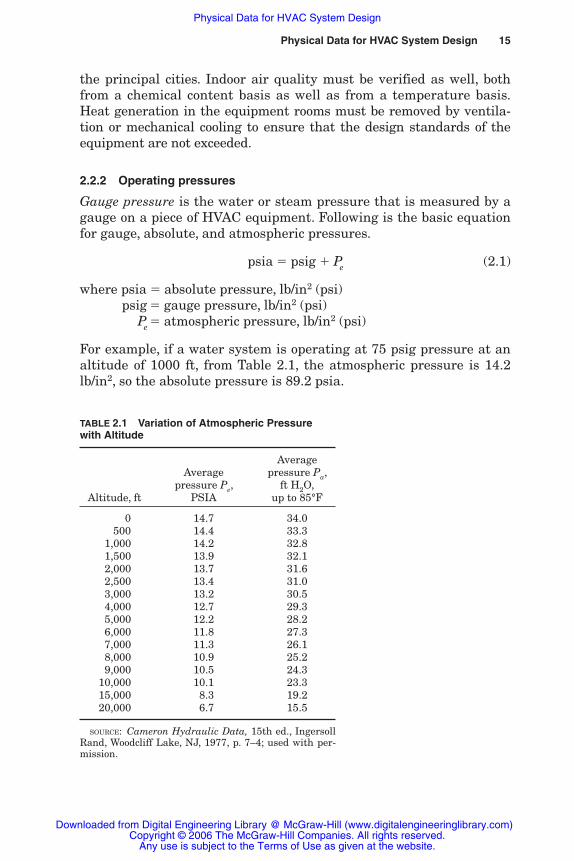
For example, if a water system is operating at 75 psig pressure at analtitude of 1000 ft, from Table 2.1, the atmospheric pressure is 14.2lb/in2, so the absolute pressure is 89.2 psia.
TABLE 2.1 Variation of Atmospheric Pressurewith Altitude
Average Average pressure Pa,
pressure Pe, ft H2O,Altitude, ft PSIA up to 85°F
0 14.7 34.0500 14.4 33.3
1,000 14.2 32.81,500 13.9 32.12,000 13.7 31.62,500 13.4 31.03,000 13.2 30.54,000 12.7 29.35,000 12.2 28.26,000 11.8 27.37,000 11.3 26.18,000 10.9 25.29,000 10.5 24.3
10,000 10.1 23.315,000 8.3 19.220,000 6.7 15.5
SOURCE: Cameron Hydraulic Data, 15th ed., IngersollRand, Woodcliff Lake, NJ, 1977, p. 7–4; used with per-mission.
Rishel_CH02.qxd 20/4/06 5:13 PM Page 15
Downloaded from Digital Engineering Library @ McGraw-Hill (www.digitalengineeringlibrary.com)Copyright © 2006 The McGraw-Hill Companies. All rights reserved.
Any use is subject to the Terms of Use as given at the website.
Physical Data for HVAC System Design
16 The Basic Tools
The atmospheric pressure of outdoor air varies with the altitude ofthe installation of HVAC equipment and must be recognized in therating of most HVAC equipment. Table 2.1 describes the variation ofatmospheric pressure with altitude. This table lists atmospheric pres-sure in feet of water as well as pounds per square inch. For water tem-perature in the range of 32 to 85°F, the feet of head can be used directlyin the net positive suction head (NPSH) and cavitation equationsfound in Chap. 6 on pump performance. For precise calculations andhigher-temperature waters, the atmospheric pressure in lb/in2 ab-solute must be corrected for the specific volume of water at the operat-ing temperature. See Eq. 6.10, which corrects the atmospheric pres-sure in feet of water to the actual operating temperature of the water.
2.3 Thermal Equivalents
There are some basic thermal and power equivalents that should besummarized for HVAC water system design. This book is based on1 Btu (British thermal unit) being equal to 778.0 ft � lb (foot pounds).Other sources list 1 Btu as equal to 778.0 to 778.26 ft � lb, which re-sults in different thermal equivalents. For example, the ASHRAESystems and Equipment Handbook lists 1 Btu as equal to 778.17 ft � lb,while Keenan and Keyes’s Thermodynamic Properties of Steam de-fines 1 Btu as 778.26 ft � lb. The following thermal and power equiva-lents will be found in this book:
1 Btu (British thermal unit) � 778.0 ft � lb
1 brake horsepower, bhp � 33,000 ft � lb/min
1 brake horsepower hour, bhph � 2545 Btu/h
� 0.746 kWh (kilowatthour)
1 kWh � 1.341 bhp
� 3412.0 Btu/h
2.4 Water Data
Water is not as susceptible to varying atmospheric conditions as is air,but its temperature and quality must be measured. Standard watertemperature can be stated as 32, 39.2 (point of maximum density), or60°F. It is not very important which of these temperatures is used forHVAC pump calculations, since water has a density near 1.0 and aviscosity around 1.5 cSt (centistokes) at all these temperatures.
Rishel_CH02.qxd 20/4/06 5:13 PM Page 16
Downloaded from Digital Engineering Library @ McGraw-Hill (www.digitalengineeringlibrary.com)Copyright © 2006 The McGraw-Hill Companies. All rights reserved.
Any use is subject to the Terms of Use as given at the website.
Physical Data for HVAC System Design

Physical Data for HVAC System Design 17
Operations with water at temperatures above 85°F must take intoconsideration both the specific gravity and viscosity. Tables 2.2, 2.3,and 2.4 provide these data for water from 32 to 450°F.
2.4.1 Viscosity of water
There are two basic types of viscosity: dynamic or absolute, and kine-matic. Dynamic viscosity is expressed in force-time per square lengthterms and in the metric system usually as centipoise (cP). In mostcases, the viscosity of water will be stated as kinematic viscosity incentistokes (cSt) in the metric system and in square feet per second inthe English system. If the viscosity of a liquid is expressed as an ab-solute viscosity in centipoise, the conversion formula to kinematic vis-cosity in square feet per second is
� ��6.7197 �
�
10�4 � � (2.2)
where � � kinematic viscosity, ft2/s � absolute viscosity, cP� � specific weight, lb/ft3
TABLE 2.2 Viscosity of Water
Temperature Absolute Kinematic of water, °F viscosity, cP viscosity, ft2/s
32 1.79 1.9310�5
40 1.55 1.6710�5
50 1.31 1.4110�5
60 1.12 1.2110�5
70 0.98 1.0610�5
80 0.86 0.9310�5
90 0.77 0.8310�5
100 0.68 0.7410�5
120 0.56 0.6110�5
140 0.47 0.5110�5
160 0.40 0.4410�5
180 0.35 0.3910�5
200 0.30 0.3410�5
212 0.28 0.3210�5
250 0.23 0.2710�5
300 0.19 0.2210�5
350 0.15 0.1810�5
400 0.13 0.1610�5
450 0.12 0.1610�5
SOURCE: Engineering Data Book, Hydraulic Institute,Parsippany, NJ, 1990, p. 19; and Systems and EquipmentHandbook, ASHRAE, Atlanta, Ga., p. 14.3; used with per-mission.
Rishel_CH02.qxd 20/4/06 5:13 PM Page 17
Downloaded from Digital Engineering Library @ McGraw-Hill (www.digitalengineeringlibrary.com)Copyright © 2006 The McGraw-Hill Companies. All rights reserved.
Any use is subject to the Terms of Use as given at the website.
Physical Data for HVAC System Design
18 The Basic Tools
If the viscosity is expressed as the kinematic viscosity in the metricsystem in centistokes, the conversion formula for kinematic viscosityin the English system is
�, ft2/s � 1.0764 � 10�5 � �, cSt (2.3)
Kinematic viscosity in English units of square feet per second is theeasiest expression of viscosity to use where other English units oflength, flow, and head are used in HVAC pumping. This is the termrequired for computing the Reynolds number with English units.Contemporary computer programs for pipe friction automatically
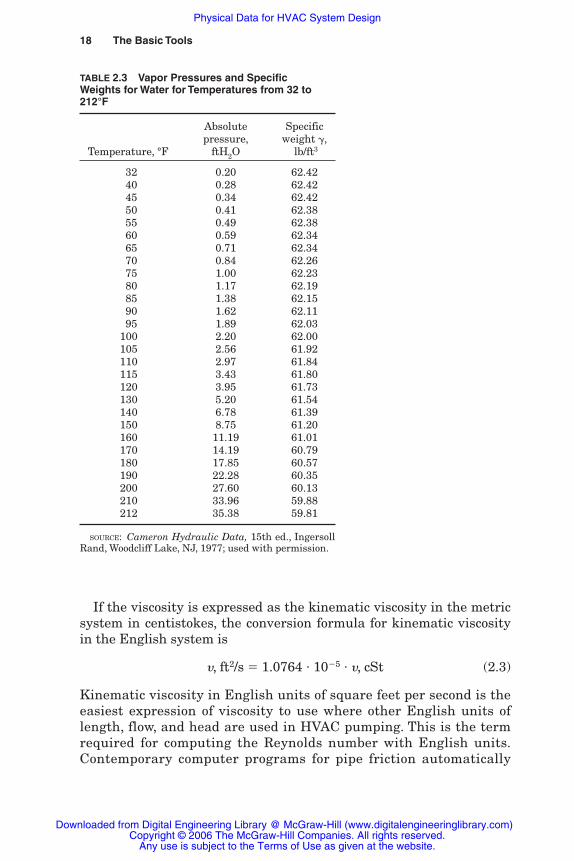
TABLE 2.3 Vapor Pressures and SpecificWeights for Water for Temperatures from 32 to212°F
Absolute Specific pressure, weight �,
Temperature, °F ftH2O lb/ft3
32 0.20 62.4240 0.28 62.4245 0.34 62.4250 0.41 62.3855 0.49 62.3860 0.59 62.3465 0.71 62.3470 0.84 62.2675 1.00 62.2380 1.17 62.1985 1.38 62.1590 1.62 62.1195 1.89 62.03
100 2.20 62.00105 2.56 61.92110 2.97 61.84115 3.43 61.80120 3.95 61.73130 5.20 61.54140 6.78 61.39150 8.75 61.20160 11.19 61.01170 14.19 60.79180 17.85 60.57190 22.28 60.35200 27.60 60.13210 33.96 59.88212 35.38 59.81
SOURCE: Cameron Hydraulic Data, 15th ed., IngersollRand, Woodcliff Lake, NJ, 1977; used with permission.
Rishel_CH02.qxd 20/4/06 5:13 PM Page 18
Downloaded from Digital Engineering Library @ McGraw-Hill (www.digitalengineeringlibrary.com)Copyright © 2006 The McGraw-Hill Companies. All rights reserved.
Any use is subject to the Terms of Use as given at the website.
Physical Data for HVAC System Design
Physical Data for HVAC System Design 19
include these data for the water under consideration. Table 2.2 pro-vides the absolute viscosity in centipoise and the kinematic viscosityin square feet per second.
2.4.2 Vapor pressure and specific weightfor water, 32 to 212°F
The vapor pressure of water for temperatures up to 450°F must be in-cluded, since this information is necessary in evaluating the possibili-ties of cavitation and in the calculation of net positive suction headavailable for pumps, which is included in Chap. 6 on pump perfor-mance. Vapor pressure is the absolute pressure, psia, at which waterwill change from liquid to steam at a specific temperature. For eachtemperature of water, there is an absolute pressure at which waterwill change from a liquid to a gas. Table 2.3 provides these vapor pres-sures up to 210°F, as well as the specific weight of water at these tem-peratures. The vapor pressures are shown in feet of water and notpounds per square inch at these temperatures for NPSH calculations.Specific weight � is the density in pounds per cubic feet of water at aparticular temperature.
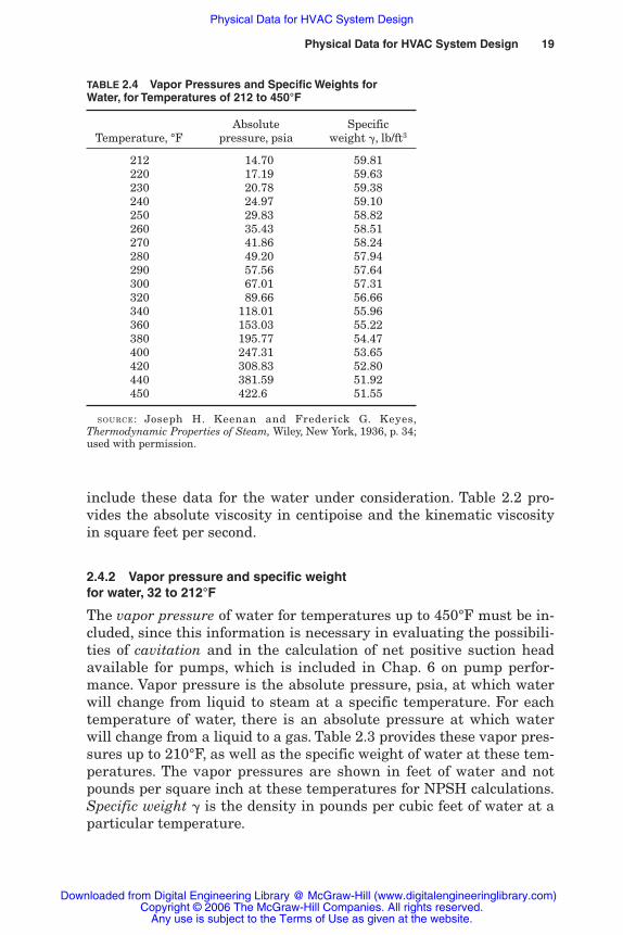
TABLE 2.4 Vapor Pressures and Specific Weights forWater, for Temperatures of 212 to 450°F
Absolute Specific Temperature, °F pressure, psia weight �, lb/ft3
212 14.70 59.81220 17.19 59.63230 20.78 59.38240 24.97 59.10250 29.83 58.82260 35.43 58.51270 41.86 58.24280 49.20 57.94290 57.56 57.64300 67.01 57.31320 89.66 56.66340 118.01 55.96360 153.03 55.22380 195.77 54.47400 247.31 53.65420 308.83 52.80440 381.59 51.92450 422.6 51.55
SOURCE: Joseph H. Keenan and Frederick G. Keyes,Thermodynamic Properties of Steam, Wiley, New York, 1936, p. 34;used with permission.
Rishel_CH02.qxd 20/4/06 5:13 PM Page 19
Downloaded from Digital Engineering Library @ McGraw-Hill (www.digitalengineeringlibrary.com)Copyright © 2006 The McGraw-Hill Companies. All rights reserved.
Any use is subject to the Terms of Use as given at the website.
Physical Data for HVAC System Design
20 The Basic Tools
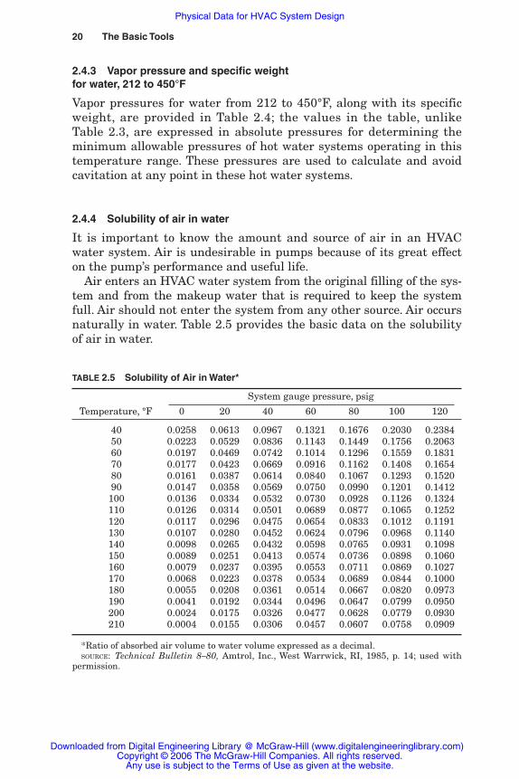
TABLE 2.5 Solubility of Air in Water*
System gauge pressure, psig
Temperature, °F 0 20 40 60 80 100 120
40 0.0258 0.0613 0.0967 0.1321 0.1676 0.2030 0.238450 0.0223 0.0529 0.0836 0.1143 0.1449 0.1756 0.206360 0.0197 0.0469 0.0742 0.1014 0.1296 0.1559 0.183170 0.0177 0.0423 0.0669 0.0916 0.1162 0.1408 0.165480 0.0161 0.0387 0.0614 0.0840 0.1067 0.1293 0.152090 0.0147 0.0358 0.0569 0.0750 0.0990 0.1201 0.1412100 0.0136 0.0334 0.0532 0.0730 0.0928 0.1126 0.1324110 0.0126 0.0314 0.0501 0.0689 0.0877 0.1065 0.1252120 0.0117 0.0296 0.0475 0.0654 0.0833 0.1012 0.1191130 0.0107 0.0280 0.0452 0.0624 0.0796 0.0968 0.1140140 0.0098 0.0265 0.0432 0.0598 0.0765 0.0931 0.1098150 0.0089 0.0251 0.0413 0.0574 0.0736 0.0898 0.1060160 0.0079 0.0237 0.0395 0.0553 0.0711 0.0869 0.1027170 0.0068 0.0223 0.0378 0.0534 0.0689 0.0844 0.1000180 0.0055 0.0208 0.0361 0.0514 0.0667 0.0820 0.0973190 0.0041 0.0192 0.0344 0.0496 0.0647 0.0799 0.0950200 0.0024 0.0175 0.0326 0.0477 0.0628 0.0779 0.0930210 0.0004 0.0155 0.0306 0.0457 0.0607 0.0758 0.0909
*Ratio of absorbed air volume to water volume expressed as a decimal.SOURCE: Technical Bulletin 8–80, Amtrol, Inc., West Warrwick, RI, 1985, p. 14; used with
permission.
2.4.3 Vapor pressure and specific weightfor water, 212 to 450°F
Vapor pressures for water from 212 to 450°F, along with its specificweight, are provided in Table 2.4; the values in the table, unlikeTable 2.3, are expressed in absolute pressures for determining theminimum allowable pressures of hot water systems operating in thistemperature range. These pressures are used to calculate and avoidcavitation at any point in these hot water systems.
2.4.4 Solubility of air in water
It is important to know the amount and source of air in an HVACwater system. Air is undesirable in pumps because of its great effecton the pump’s performance and useful life.
Air enters an HVAC water system from the original filling of the sys-tem and from the makeup water that is required to keep the systemfull. Air should not enter the system from any other source. Air occursnaturally in water. Table 2.5 provides the basic data on the solubilityof air in water.
Rishel_CH02.qxd 20/4/06 5:13 PM Page 20
Downloaded from Digital Engineering Library @ McGraw-Hill (www.digitalengineeringlibrary.com)Copyright © 2006 The McGraw-Hill Companies. All rights reserved.
Any use is subject to the Terms of Use as given at the website.
Physical Data for HVAC System Design

Physical Data for HVAC System Design 21
As indicated in the table, the amount of air that can be dissolved inwater decreases with temperature and increases with system pres-sure. This table demonstrates Henry’s law, which states that theamount of air dissolved in water is proportional to the pressure of thewater system. This table should be used in place of similar charts foropen tanks and deaerators where the only pressure is atmosphericpressure at 0 psig, and the amount of air dissolved in water approacheszero at 212°F. It is evident from this table that makeup water that issupplied by the domestic water system can contain a great amount ofair.
To demonstrate the release of air from water, assume that the re-turn water has a temperature of 180°F and the system pressure is 40psig. Makeup water entering the system at 50°F will have at least a0.0836 ratio of air to water. It could have much more air than this,since it may have been reduced from a higher city water pressure.When the makeup water is heated to 180°F at 40 psig, the air contentwill drop to a ratio of 0.0361, which is less than half that of the coldmakeup water.
An interesting and easy experiment to observe the release of airwhen water is heated is as follows:
1. Take a frying pan and fill it with potable water from the kitchencold water faucet.
2. Place it on the stove, and heat the water to boiling.
3. Note that bubbles form as soon as the temperature begins to rise.This is air coming out of solution with the water, since the watercannot hold as much air with the higher temperature.
4. As the water approaches 212°F, the water begins to boil.
5. Allow the water to cool, and then reheat the water to boiling.
6. Note that this time bubbles do not appear until steam begins toform. This demonstrates that the water has been deaerated duringthe first boiling. It also provides a visual example of what happensto cold water when it is heated in an HVAC water system.
As shown in Table 2.5, when water passes through pumps and thepressure is increased, the water will increase its affinity for air. It istherefore imperative that the air in the makeup water be removedfrom the water as soon as it reaches system temperature by locatingthe water makeup near the air-elimination equipment such as anair separator. The optimal location for the air-elimination equipmentdepends on the configuration of the water system. Generally, it may
Rishel_CH02.qxd 20/4/06 5:13 PM Page 21
Downloaded from Digital Engineering Library @ McGraw-Hill (www.digitalengineeringlibrary.com)Copyright © 2006 The McGraw-Hill Companies. All rights reserved.
Any use is subject to the Terms of Use as given at the website.
Physical Data for HVAC System Design
22 The Basic Tools
be best to locate an air separator near the suctions of the distribu-tion pumps with air vents at the high points where the system pres-sure is the lowest. For heating systems with high supply water tem-peratures, it may be advisable to add a dip tube and an air vent atthe water discharge from the heater or boiler. These tables alsodemonstrate that it is wise to have manual or automatic air vents atthe top of a building where the system pressure is the lowest. A de-tailed discussion of air removal from HVAC water systems is includedin Chap. 9.
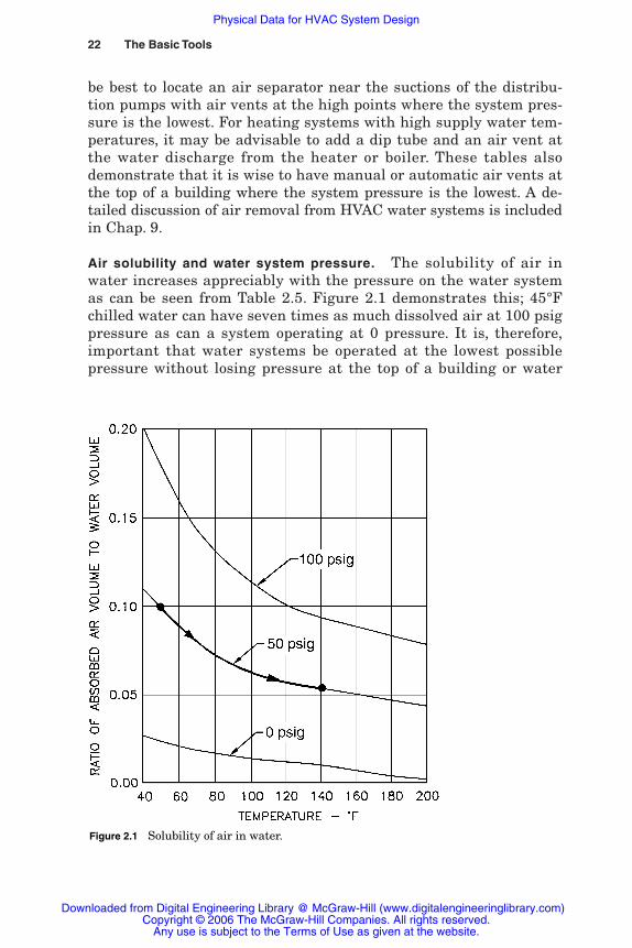
Air solubility and water system pressure. The solubility of air inwater increases appreciably with the pressure on the water systemas can be seen from Table 2.5. Figure 2.1 demonstrates this; 45°Fchilled water can have seven times as much dissolved air at 100 psigpressure as can a system operating at 0 pressure. It is, therefore,important that water systems be operated at the lowest possiblepressure without losing pressure at the top of a building or water
Figure 2.1 Solubility of air in water.
Rishel_CH02.qxd 20/4/06 5:13 PM Page 22
Downloaded from Digital Engineering Library @ McGraw-Hill (www.digitalengineeringlibrary.com)Copyright © 2006 The McGraw-Hill Companies. All rights reserved.
Any use is subject to the Terms of Use as given at the website.
Physical Data for HVAC System Design
Physical Data for HVAC System Design 23
system. Ten psig is adequate pressure at the top of most buildingsor water systems.
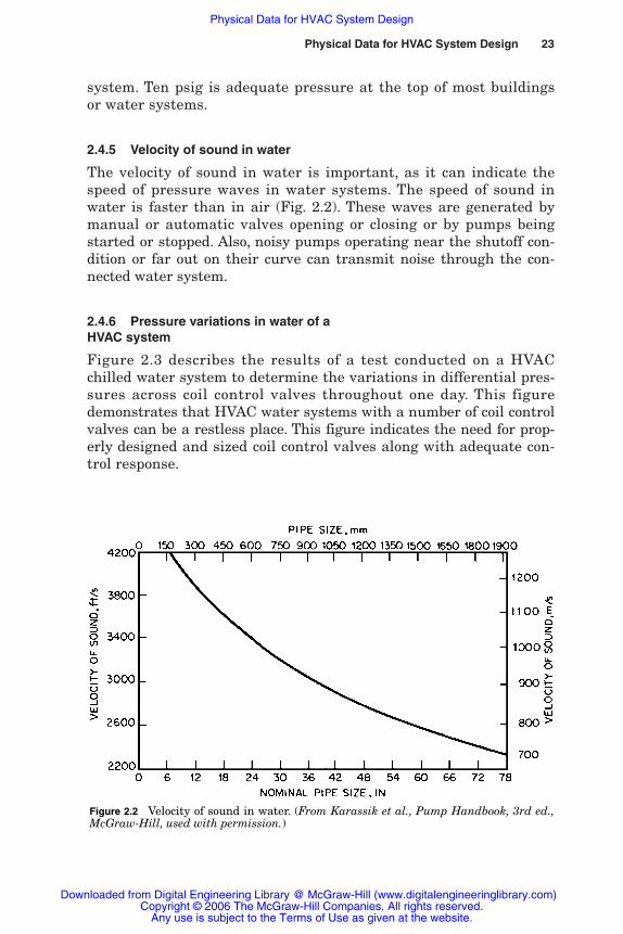
2.4.5 Velocity of sound in water
The velocity of sound in water is important, as it can indicate thespeed of pressure waves in water systems. The speed of sound inwater is faster than in air (Fig. 2.2). These waves are generated bymanual or automatic valves opening or closing or by pumps beingstarted or stopped. Also, noisy pumps operating near the shutoff con-dition or far out on their curve can transmit noise through the con-nected water system.
2.4.6 Pressure variations in water of aHVAC system
Figure 2.3 describes the results of a test conducted on a HVACchilled water system to determine the variations in differential pres-sures across coil control valves throughout one day. This figuredemonstrates that HVAC water systems with a number of coil controlvalves can be a restless place. This figure indicates the need for prop-erly designed and sized coil control valves along with adequate con-trol response.
Figure 2.2 Velocity of sound in water. (From Karassik et al., Pump Handbook, 3rd ed.,McGraw-Hill, used with permission.)
Rishel_CH02.qxd 20/4/06 5:13 PM Page 23
Downloaded from Digital Engineering Library @ McGraw-Hill (www.digitalengineeringlibrary.com)Copyright © 2006 The McGraw-Hill Companies. All rights reserved.
Any use is subject to the Terms of Use as given at the website.
Physical Data for HVAC System Design

24 The Basic Tools
2.5 Glycol-Based Heat-Transfer Fluid (HTF) Solutions
Glycol-based heat-transfer solutions are prevalent in the HVAC in-dustry. Glycol is used to (1) avoid freezing in equipment of anHVAC water system such as heating and cooling coils and (2) totransfer heat to and from energy storage tanks that use ice. Thereis a substantial variation in both viscosity and density of the solu-tion as the percentage of glycol is varied with temperature.Information is provided on ethylene glycol–based heat-transfer flu-ids, since they have been the most used in the HVAC industry.Special applications of glycol-based heat-transfer fluids, such ascontact with potable water or food, may require the use of propy-lene glycol–based solutions.
Figure 2.4 provides information on the viscosity and Fig. 2.5 on thespecific gravity of ethylene glycol–based heat-transfer solutions. Careshould be taken to avoid using glycol solutions near their freezingcurves because slush occurs there that will change radically thepump’s performance. Figure 2.6 provides the freezing curve for an eth-ylene glycol–based heat-transfer fluid. Verification of the minimum
As loads and flows vary, differential pressure variation across controlvalves is even more pronounced than the differential pressure acrossthe whole building.
40
35
30
25
20
15
Bui
ldin
g di
ffere
ntia
l pre
ssur
e (p
si)
Time over one day (Summer 2003)
Figure 2.3 Typical building differential pressure profile. (Courtesy of FlowControl Industries. Woodinville, WA.)
Rishel_CH02.qxd 20/4/06 5:13 PM Page 24
Downloaded from Digital Engineering Library @ McGraw-Hill (www.digitalengineeringlibrary.com)Copyright © 2006 The McGraw-Hill Companies. All rights reserved.
Any use is subject to the Terms of Use as given at the website.
Physical Data for HVAC System Design

Physical Data for HVAC System Design 25
percentage of glycol to prevent slush formation at the minimum oper-ating temperature should be sought from the supplier of the heat-transfer fluid.
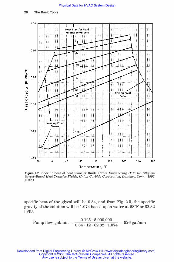
There is an appreciable variation in the specific heat of glycol-basedheat-transfer solutions. It is less than that of water for most percent-ages of glycol. Figure 2.7 provides the specific heat for ethyleneglycol–based heat-transfer solutions. The pump flow, in gallons per
Figure 2.4 Viscosity of heat transfer fluids. (From Engineering Data for EthyleneGlycol–Based Heat Transfer Fluids, Union Carbide Corporation, Danbury, Conn., 1993,p. 20.)
Rishel_CH02.qxd 20/4/06 5:13 PM Page 25
Downloaded from Digital Engineering Library @ McGraw-Hill (www.digitalengineeringlibrary.com)Copyright © 2006 The McGraw-Hill Companies. All rights reserved.
Any use is subject to the Terms of Use as given at the website.
Physical Data for HVAC System Design

26 The Basic Tools
minute, is calculated from Eq. 2.4:
Pump flow, gal/min �
� (2.4)0.125 � Btu/h��
cp � �T�°F � �
Btu/h � 7.48 gal/ft3����
cp � �T�°F � � � 60 min/h
Figure 2.5 Specific gravity of heat transfer fluids. (From Engineering Data for EthyleneGlycol–Based Heat Transfer Fluids, Union Carbide Corporation, Danbury, Conn., 1993,p. 18.)
Rishel_CH02.qxd 20/4/06 5:13 PM Page 26
Downloaded from Digital Engineering Library @ McGraw-Hill (www.digitalengineeringlibrary.com)Copyright © 2006 The McGraw-Hill Companies. All rights reserved.
Any use is subject to the Terms of Use as given at the website.
Physical Data for HVAC System Design

Physical Data for HVAC System Design 27
where cp � specific heat of ethylene glycol heat-transfer solution atconstant pressure
�T � differential temperature� � specific weight of water
Note. All these values must be at the operating temperature of thesolution. For many glycol installations, this calculation should be runat several different operating temperatures. For example, assumethat an ethylene glycol based heat-transfer fluid has a heating load of5 million Btu/h at 30°F with a differential temperature of 12°F. Thepumps will be operating with a 40% glycol solution. From Fig. 2.7, the
Figure 2.6 Freezing points of heat transfer fluids. (From Engineering Data for EthyleneGlycol–Based Heat Transfer Fluids, Union Carbide Corporation, Danbury, Conn., 1993,p. 10.)
Rishel_CH02.qxd 20/4/06 5:13 PM Page 27
Downloaded from Digital Engineering Library @ McGraw-Hill (www.digitalengineeringlibrary.com)Copyright © 2006 The McGraw-Hill Companies. All rights reserved.
Any use is subject to the Terms of Use as given at the website.
Physical Data for HVAC System Design
28 The Basic Tools
specific heat of the glycol will be 0.84, and from Fig. 2.5, the specificgravity of the solution will be 1.074 based upon water at 68°F or 62.32lb/ft3.
Pump flow, gal/min � � 926 gal/min0.125 � 5,000,000
���0.84 � 12 � 62.32 � 1.074
Figure 2.7 Specific heat of heat transfer fluids. (From Engineering Data for EthyleneGlycol–Based Heat Transfer Fluids, Union Carbide Corporation, Danbury, Conn., 1993,p. 24.)
Rishel_CH02.qxd 20/4/06 5:13 PM Page 28
Downloaded from Digital Engineering Library @ McGraw-Hill (www.digitalengineeringlibrary.com)Copyright © 2006 The McGraw-Hill Companies. All rights reserved.
Any use is subject to the Terms of Use as given at the website.
Physical Data for HVAC System Design

Physical Data for HVAC System Design 29
2.6 Steam Data
Steam is used for many heating processes in HVAC. Most of the steamdata come from one source, namely, Keenan and Keyes’Thermodynamic Properties of Steam. This is a fundamental referencefor any engineer working with steam. Table 2.6 provides the basicsteam data, while vapor pressures are included in Tables 2.3 and 2.4for the computation of net positive suction head available and the de-termination of cavitation pressures at various operating temperatures.
In HVAC, there are two basic steam pressure ranges: (1) up to 15psig (250°F) and (2) above 15 psig steam pressure. This is derivedfrom the American Society of Mechanical Engineers’ (ASME) boilercodes, (1) the Heating Boiler Code for steam pressures up to 15 psigand (2) the Power Boiler Code for steam pressures above 15 psig. SeeChap. 19 for additional information on boilers.
TABLE 2.6 Basic Steam Data
Enthalpy, Btu/lb
Absolute Steam Saturated Saturated pressure, lb/in2 temperature, °F liquid Evaporation vapor
14.7 212.00 180.07 970.3 1150.416 216.32 184.42 967.6 1152.018 222.41 190.56 963.6 1154.220 227.96 196.16 960.1 1156.322 233.07 201.33 956.8 1158.124 237.82 206.14 953.7 1159.826 242.25 210.62 950.7 1161.328 246.41 214.83 947.9 1162.730 250.33 218.82 945.3 1164.135 259.28 227.91 939.2 1167.140 267.25 236.03 933.7 1169.745 274.44 243.36 928.6 1172.050 281.01 250.09 924.0 1174.160 292.71 262.09 915.5 1177.670 202.92 272.61 907.9 1180.680 312.03 282.02 901.1 1183.190 320.27 290.56 894.7 1185.3
100 327.81 298.40 888.8 1187.2125 344.33 315.68 875.4 1191.1150 358.42 330.51 863.6 1194.1174 370.29 343.10 853.3 1196.4200 381.79 355.36 843.0 1198.4
NOTE: Absolute pressure � gauge � atmospheric pressures.SOURCE: Joseph H. Keenan and Frederick G. Keyes, Thermodynamic Properties of Steam,
Wiley, New York, 1936.
Rishel_CH02.qxd 20/4/06 5:13 PM Page 29
Downloaded from Digital Engineering Library @ McGraw-Hill (www.digitalengineeringlibrary.com)Copyright © 2006 The McGraw-Hill Companies. All rights reserved.
Any use is subject to the Terms of Use as given at the website.
Physical Data for HVAC System Design
30 The Basic Tools
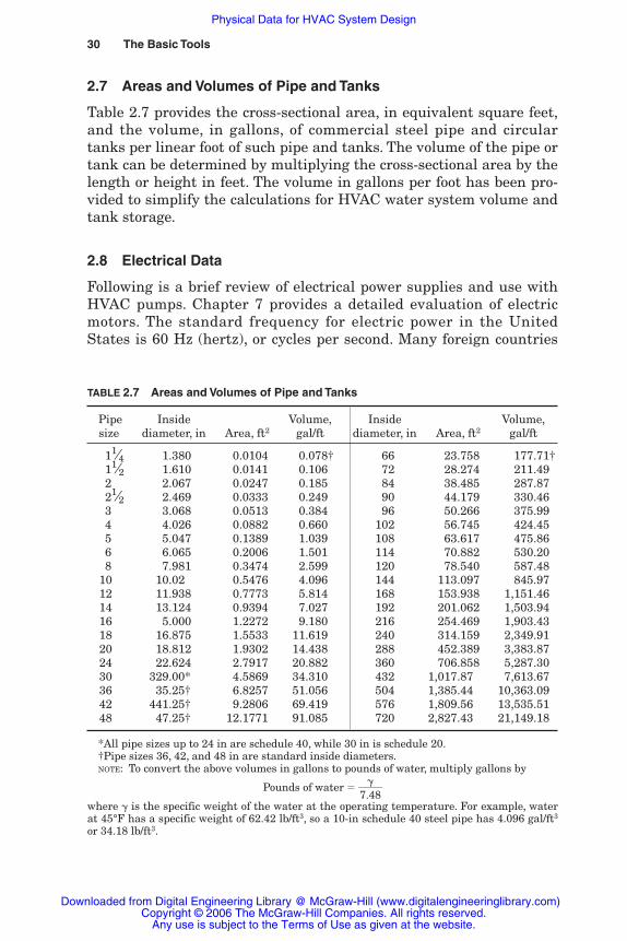
2.7 Areas and Volumes of Pipe and Tanks
Table 2.7 provides the cross-sectional area, in equivalent square feet,and the volume, in gallons, of commercial steel pipe and circulartanks per linear foot of such pipe and tanks. The volume of the pipe ortank can be determined by multiplying the cross-sectional area by thelength or height in feet. The volume in gallons per foot has been pro-vided to simplify the calculations for HVAC water system volume andtank storage.
2.8 Electrical Data
Following is a brief review of electrical power supplies and use withHVAC pumps. Chapter 7 provides a detailed evaluation of electricmotors. The standard frequency for electric power in the UnitedStates is 60 Hz (hertz), or cycles per second. Many foreign countries
TABLE 2.7 Areas and Volumes of Pipe and Tanks
Pipe Inside Volume, Inside Volume,size diameter, in Area, ft2 gal/ft diameter, in Area, ft2 gal/ft
11⁄4 1.380 0.0104 0.078† 66 23.758 177.71†11⁄2 1.610 0.0141 0.106 72 28.274 211.492 2.067 0.0247 0.185 84 38.485 287.8721⁄2 2.469 0.0333 0.249 90 44.179 330.463 3.068 0.0513 0.384 96 50.266 375.994 4.026 0.0882 0.660 102 56.745 424.455 5.047 0.1389 1.039 108 63.617 475.866 6.065 0.2006 1.501 114 70.882 530.208 7.981 0.3474 2.599 120 78.540 587.48
10 10.02 0.5476 4.096 144 113.097 845.9712 11.938 0.7773 5.814 168 153.938 1,151.4614 13.124 0.9394 7.027 192 201.062 1,503.9416 5.000 1.2272 9.180 216 254.469 1,903.4318 16.875 1.5533 11.619 240 314.159 2,349.9120 18.812 1.9302 14.438 288 452.389 3,383.8724 22.624 2.7917 20.882 360 706.858 5,287.3030 329.00* 4.5869 34.310 432 1,017.87 7,613.6736 35.25† 6.8257 51.056 504 1,385.44 10,363.0942 441.25† 9.2806 69.419 576 1,809.56 13,535.5148 47.25† 12.1771 91.085 720 2,827.43 21,149.18
*All pipe sizes up to 24 in are schedule 40, while 30 in is schedule 20.†Pipe sizes 36, 42, and 48 in are standard inside diameters.NOTE: To convert the above volumes in gallons to pounds of water, multiply gallons by
Pounds of water � �7.
�
48�
where � is the specific weight of the water at the operating temperature. For example, waterat 45°F has a specific weight of 62.42 lb/ft3, so a 10-in schedule 40 steel pipe has 4.096 gal/ft3
or 34.18 lb/ft3.
Rishel_CH02.qxd 20/4/06 5:13 PM Page 30
Downloaded from Digital Engineering Library @ McGraw-Hill (www.digitalengineeringlibrary.com)Copyright © 2006 The McGraw-Hill Companies. All rights reserved.
Any use is subject to the Terms of Use as given at the website.
Physical Data for HVAC System Design

Physical Data for HVAC System Design 31
have standardized on 50 Hz; there also may be rural areas of theUnited States still operating on 50-Hz power. Tables 2.8 and 2.9 pro-vide nominal power distribution voltages and standard nameplatevoltages for motors operating at both 60 and 50 Hz. Electric powerutilities are allowed a variation of �5 percent from the distributionsystem voltages listed in these tables.
TABLE 2.8 Standard 60-Hz Voltages
Nominal distribution Motor nameplate voltage
system voltage Below 125 hp 125 hp and up
Polyphase208 200 —240 230 —480 460 460600 575 575
2400 2300 23004160 4000 4000
Single-phase120 115 —208 200 —240 230 —
SOURCE: AC Motor Selection and Application Guide, Bulletin GET �6812B, General Electric Company, Fort Wayne, Ind., 1993, p. 2; usedwith permission.
TABLE 2.9 Standard 50-Hz Voltages
Nominal distribution Motor nameplate voltage
system voltage Below 125 hp 125 hp and up
Polyphase (see note) 200 200220 —380 380415 415440 440550 550
3000 3000Single-phase (see note) 110 —
200 —220 —
NOTE: Distribution system voltages vary from country to country;therefore, motor nameplate voltage should be selected for the countryin which the motor will be operated.
SOURCE: AC Motor Selection and Application Guide, Bulletin GET �6812B, General Electric Company, Fort Wayne, Ind., 1999, p. 2; usedwith permission.
Rishel_CH02.qxd 20/4/06 5:13 PM Page 31
Downloaded from Digital Engineering Library @ McGraw-Hill (www.digitalengineeringlibrary.com)Copyright © 2006 The McGraw-Hill Companies. All rights reserved.
Any use is subject to the Terms of Use as given at the website.
Physical Data for HVAC System Design
The most popular power for HVAC applications is 480 V, three-phase. Single-phase power is seldom used above 71⁄2 hp. The 208 Vservice is derived from a Y-connected transformer in the buildingbeing served; three-phase motors as high as 60 hp are available forthis voltage. The higher voltages of 2400 and 4160 V are used generallyon motors of 750 hp and larger.
Electrical machinery such as motors and variable-speed drives havespecified voltage tolerances that exceed those of the electrical utility.The electrical design engineer must develop the building power distri-bution to ensure that its voltage drop does not exceed the voltage tol-erances of the electrical equipment. Typically, the voltage tolerance ofmost electric motors is �10%, and those for most variable-speed dri-ves appear to be �10 percent and �5 percent. The actual tolerancesfor this equipment should be verified by the HVAC water system de-signer. For example, the utility voltage at a building transformer maybe 480 V �5 percent, or 456 to 504 V. A 460-V variable-speed drivehas an allowable voltage variation of 437 to 506 V. Therefore, thebuilding power distribution system must be designed so that thepower supply to the variable-speed drive does not drop below 437 Vunder any load condition.
Power factor correction equipment can be required by public utilitiesor state law above a certain size of motor. This should be checked by thedesigner at the beginning of the development of a specific project.Generally, public utilities do not require power factor correction at mostplaces in their electrical distribution until the load approaches 500 kVA.
The popularity of the variable-frequency drive has created a prob-lem for public utilities. This is the harmonic distortion caused by thealteration of the sine wave by the variable-frequency drive. The publicutility furnishing power on a project may have a specification on themaximum allowable harmonic distortion. Also, the owner of the facilitymay have tolerances on harmonic distortion.
More information on power factor correction and harmonic distor-tion is included in Chap. 7.
2.9 Efficiency Evaluations of HVAC Water Systems
Several expressions of efficiency will be provided in the followingchapters that relate to the effectiveness of pump selection and appli-cation. These will include:
1. System efficiency, which determines the quality of use of pumphead in a water system. This will be expressed as a percentage,coefficient of performance, kW/ton, or kW/1000 mbh.
32 The Basic Tools
Rishel_CH02.qxd 20/4/06 5:13 PM Page 32
Downloaded from Digital Engineering Library @ McGraw-Hill (www.digitalengineeringlibrary.com)Copyright © 2006 The McGraw-Hill Companies. All rights reserved.
Any use is subject to the Terms of Use as given at the website.
Physical Data for HVAC System Design
2. Kilowatt input and wire-to-water efficiency of a pumping system,which demonstrate the use of energy in a pumping system.
3. Kilowatts per ton efficiency for an entire chilled-water plant,which includes the energy consumption of the pumps and coolingtowers, not just the efficiency of the chillers themselves.
4. Boiler efficiency as a percentage as related to entering water tem-perature.
These efficiencies are possible now that digital computers are avail-able to make the calculations rapidly and accurately. The equationsfor HVAC systems and equipment included herein enable the HVACoperator to observe these water systems and ensure that they arefunctioning at optimal efficiency.
2.10 Additional Reading
It is important that the HVAC designer be well versed in the basic flu-ids and services available at the point of installation of each project.Local codes and services must be checked for compatibility with thefinal design. The manuals of the technical societies are excellent sourcesfor additional reading, particularly those of the American Society ofHeating, Refrigerating, and Air-Conditioning Engineers (ASHRAE) andthe Institute of Electrical and Electronics Engineers (IEEE).
2.11 Bibliography
Cameron Hydraulic Data, 15th ed., Ingersoll Rand, Woodcliff, NJ, 1966.Engineering Data Book, 2d. ed., Hydraulic Institute, Parsippany, NJ, 1990.Eshbach, Ovid W., Eshbach’s Handbook of Engineering Fundamentals, John Wiley &
Sons, New York, 1990.Grimm, Nils R., and Robert C. Rosaler, Handbook of HVAC Design, McGraw-Hill, New
York, 1990.Handbook of Essential Engineering Information and Data, McGraw-Hill, New York,
1991.Handbook of Fundamentals, American Society of Heating, Refrigerating, and Air-
Conditioning Engineers, Atlanta, Ga, 1993.Keenan, Joseph H., and Frederick G. Keyes, Thermodynamic Properties of Steam, John
Wiley & Sons, New York, 1936.Mark’s Standard Handbook for Mechanical Engineers, 9th ed., McGraw-Hill, New York,
1978.
Physical Data for HVAC System Design 33
Rishel_CH02.qxd 20/4/06 5:13 PM Page 33
Downloaded from Digital Engineering Library @ McGraw-Hill (www.digitalengineeringlibrary.com)Copyright © 2006 The McGraw-Hill Companies. All rights reserved.
Any use is subject to the Terms of Use as given at the website.
Physical Data for HVAC System Design

Rishel_CH02.qxd 20/4/06 5:13 PM Page 34
Downloaded from Digital Engineering Library @ McGraw-Hill (www.digitalengineeringlibrary.com)Copyright © 2006 The McGraw-Hill Companies. All rights reserved.
Any use is subject to the Terms of Use as given at the website.
Physical Data for HVAC System Design

Chapter
35
3Piping System Friction
A comprehensive chapter on pipe friction has been included in thisHandbook for HVAC pumps because the sizing of pumps is deter-mined principally on pump capacity and head. A poor computation ofsystem friction will have a disastrous effect on pump selection andoperation. There is not a more critical subject facing HVAC watersystem designers than the development of better procedures for cal-culating pump head for these systems.
As pointed out in the introduction to this book, pipe friction analysisis, at best, an inexact science. Much needs to be done to achieve betterinformation on pipe and fitting friction. Research work on reducingpipe friction through the use of additives to water is being carried out;surfactants are one class of chemicals that are being studied to reducepiping friction. The increase in cost of energy will provide the drivingforce to achieve better piping friction data and better piping design.
Good piping design always balances first cost against operatingcost, taking into consideration all factors that exist on each installa-tion. These are the two basic parameters that influence pipe sizing inthe HVAC industry, since excessive corrosion or fouling should notexist in these water systems.
Obviously, piping costs increase and power costs decrease withincreases in pipe diameter. The American Society of Heating,Refrigerating, and Air-Conditioning Engineers (ASHRAE) has infor-mation that indicates velocities in the range of 10 to 17 ft/s in HVACsystems do not create erosion or noise in the larger sizes of pipe. Theoverall controlling factor is friction, which increases exponentiallywith velocity. Friction in piping is the principal source of increasedoperating costs for these water systems.
Rishel_CH03.qxd 20/4/06 5:35 PM Page 35
Source: HVAC Pump Handbook
Downloaded from Digital Engineering Library @ McGraw-Hill (www.digitalengineeringlibrary.com)Copyright © 2006 The McGraw-Hill Companies. All rights reserved.
Any use is subject to the Terms of Use as given at the website.

36 The Basic Tools
3.1 Maximum Velocity in Pipe
There are a number of conflicting tables on the maximum allowablewater velocity in HVAC piping. The failure of many of these tables ofmaximum velocity is their lack of consideration of the hydraulic radiusof commercial pipe. The hydraulic radius of a pipe is the cross-sectionalarea of a pipe divided by the circumference of its inner surface. It iscalculated as follows:
Area � ��
4d2�
Circumference � �d
Hydraulic radius ��circu
amrfeearence�� �
d4
� (3.1)
where d � inside diameter, inObviously, the hydraulic radius increases with pipe diameter, and
therefore, the allowable velocity should increase with the pipe diame-ter. Hydraulic radii for commercial pipe are shown in Table 3.1. It isquite clear that 36-in inside diameter (ID) pipe with a hydraulic radiusof 9.0 in must be rated velocity-wise differently than 3-in schedule40 pipe with a hydraulic radius of 0.8 in.
Hydraulic radius may introduce a new guideline for the reevalua-tion of friction for flow of water in piping and pipe fittings. The cur-rent information on pipe friction and recommended velocities in pipeare too dependent on testing done on small pipe; often the data arethen extrapolated for larger pipe. It is very difficult to test large pipefittings such as those with diameters greater than 20 in.
There are several recommendations for allowable velocity in HVACpipe; some are based on a maximum friction loss per 100 ft. Actually,as indicated previously, final pipe velocity is within the province ofthe designer who is responsible for first cost as well as operatingcosts. Here is an excellent point at which the designer can use com-puter capability in sizing piping. Several computer runs at differentpipe sizes can be done to achieve the economically desirable pipesize. This should be done for the major piping such as loops andheaders. The size of smaller branches and coil connections will fallmore into the realm of the designer’s experience. Table 3.2 providesan elementary example of this program comparing 12-, 14-, and 16-indiameter commercial pipe.
The operating cost decreases while maintenance and amortizationof the first cost increase with the pipe size. The economic pipe size isat the minimum point of the sum of the two values or curves.
Rishel_CH03.qxd 20/4/06 5:35 PM Page 36
Piping System Friction
Downloaded from Digital Engineering Library @ McGraw-Hill (www.digitalengineeringlibrary.com)Copyright © 2006 The McGraw-Hill Companies. All rights reserved.
Any use is subject to the Terms of Use as given at the website.
Piping System Friction 37
TABLE 3.2 Total Owning Cost of Piping
Amortized first Annual Total annual Pipe size, in cost per year operating cost owning cost
12 $12,000 $16,000 $28,00014 14,000 12,000 26,00016 17,000 10,000 27,000
TABLE 3.1 Maximum Water Capacities of Steel Pipe (in gal/min)
Maximum Hydraulic Size, in Schedule flow, gal/min Velocity, ft/s Loss, ft/100 ft radius, in
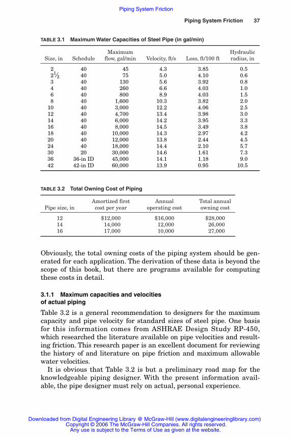
02 40 00,045 4.3 3.85 0.5021⁄2 40 00,075 5.0 4.10 0.603 40 00,130 5.6 3.92 0.804 40 00,260 6.6 4.03 1.006 40 00,800 8.9 4.03 1.508 40 01,600 10.3 3.82 2.010 40 03,000 12.2 4.06 2.512 40 04,700 13.4 3.98 3.014 40 06,000 14.2 3.95 3.316 40 08,000 14.5 3.49 3.818 40 10,000 14.3 2.97 4.220 40 12,000 13.8 2.44 4.524 40 18,000 14.4 2.10 5.730 20 30,000 14.6 1.61 7.336 36-in ID 45,000 14.1 1.18 9.042 42-in ID 60,000 13.9 0.95 10.5
Obviously, the total owning costs of the piping system should be gen-erated for each application. The derivation of these data is beyond thescope of this book, but there are programs available for computingthese costs in detail.
3.1.1 Maximum capacities and velocities of actual piping
Table 3.2 is a general recommendation to designers for the maximumcapacity and pipe velocity for standard sizes of steel pipe. One basisfor this information comes from ASHRAE Design Study RP-450,which researched the literature available on pipe velocities and result-ing friction. This research paper is an excellent document for reviewingthe history of and literature on pipe friction and maximum allowablewater velocities.
It is obvious that Table 3.2 is but a preliminary road map for theknowledgeable piping designer. With the present information avail-able, the pipe designer must rely on actual, personal experience.
Rishel_CH03.qxd 20/4/06 5:35 PM Page 37
Piping System Friction
Downloaded from Digital Engineering Library @ McGraw-Hill (www.digitalengineeringlibrary.com)Copyright © 2006 The McGraw-Hill Companies. All rights reserved.
Any use is subject to the Terms of Use as given at the website.

38 The Basic Tools
3.1.2 Pipe velocity is the designer’sresponsibility
It is also very clear from Table 3.2 that sizing all pipe, particularlylarge pipe in the range from 20 to 42 in in diameter, requires a detailedanalysis of the entire piping system to achieve the economical size fora particular installation. It cannot be based on a rule that limits pipevelocity. Reiterating, it is the designer’s responsibility to determinepipe size and maximum velocity. There are so many judgment calls inthe final selection of pipe diameter that it is not a simple process. Fora hypothetical example, if you have 12,000 gal/min flowing in a chillerheader in a central energy plant, you could use 20-in-diameter steelpipe if the header is only 100 ft long. This would reduce the cost of thepiping and tees where the chillers are connected. On the other hand,if a chilled water supply main runs for 1000 ft to a group of buildings,you might use 24-in-diameter pipe to reduce the overall friction loss.The cost of piping accessories and the length of pipe involved affect thedecision on the final pipe size. These are the evaluations that a goodpipe designer must make.
The physical pressure that the pipe must operate under and thepossibilities of corrosion as well as availability determine the scheduleor wall thickness of steel pipe. The designer should make the velocitycalculation and, therefore, the friction calculations based on the actualinside diameter of the pipe to be used in the water system. The designershould check the actual project conditions to ensure that the pipeinside diameter to be used for each pipe size is available at the job siteat the time of construction.
3.2 Pipe and Fitting Specifications
Elements of an HVAC water system are connected together by meansof piping. In most cases, this piping is steel, although various types ofplastic piping are now appearing in this industry.
Most steel piping used in the HVAC industry for low-temperatureapplications conforms to American Society for Testing and Materials(ASTM) Specifications A53 or A120. Higher-temperature applicationssuch as high-pressure steam and high-temperature water may requireseamless piping per ASTM A106; local and ASME codes should bechecked for detailed pipe, flange, bolting, and fitting specifications forparticular applications such as high-temperature water and high-pressure steam. Steel fittings follow American National StandardsInstitute (ANSI) Specification B16.5, whereas threaded cast iron fittingscomply with ANSI Specification B16.4 and flanged cast iron fittingswith ANSI B16.1.
Rishel_CH03.qxd 20/4/06 5:35 PM Page 38
Piping System Friction
Downloaded from Digital Engineering Library @ McGraw-Hill (www.digitalengineeringlibrary.com)Copyright © 2006 The McGraw-Hill Companies. All rights reserved.
Any use is subject to the Terms of Use as given at the website.

TABLE 3.4 Rating of Cast Iron Pipe Fittings (Flanged Fittings, ANSI B16.1)
Working pressures, nonshock, psig
Class 125 Class 250
Temperature, °F 1–12 in 14–24 in 30–48 in 1–12 in 14–24 in*
�20 to 150 200 150 150 500 300200 190 135 115 460 280225 180 130 100 440 270250 175 125 85 415 260275 170 120 65 395 250300 165 110 50 375 240325 155 105 NA 355 230350† 150 100 NA 335 220375 145 NA NA 315 210400‡ 140 NA NA 290 200425 130 NA NA 270 NA450 125 NA NA 250 NA
NOTE: NA � not acceptable.*For liquid service, these ratings are for class 250 flanges only, not for class 250 fittings.†353°F to reflect 125-psig steam pressure.‡406°F to reflect 250-psig steam pressure.
Piping System Friction 39
TABLE 3.3 Rating of Cast Iron Pipe Fittings(Threaded Fittings, ANSI B16.4)
Working pressures,nonshock, psig
Temperature, °F Class 125 Class 250
�20 to 150 175 400200 165 370250 150 340300 140 310350 125 280400 NA 250
NOTE: NA � not acceptable.
The pressure and temperature ratings of steel pipe, fittings, andflanges are beyond the scope of this book, since there are a number ofcodes for specific applications. Tables 3.3 and 3.4 list the temperatureand pressure ratings for cast iron fittings that are in common use inHVAC water systems. The cast iron data are included in this bookbecause of cast iron’s greater reduction in allowable pressure withhigher temperatures.
Rishel_CH03.qxd 20/4/06 5:35 PM Page 39
Piping System Friction
Downloaded from Digital Engineering Library @ McGraw-Hill (www.digitalengineeringlibrary.com)Copyright © 2006 The McGraw-Hill Companies. All rights reserved.
Any use is subject to the Terms of Use as given at the website.
40 The Basic Tools
3.3 Steel Pipe Friction Analysis
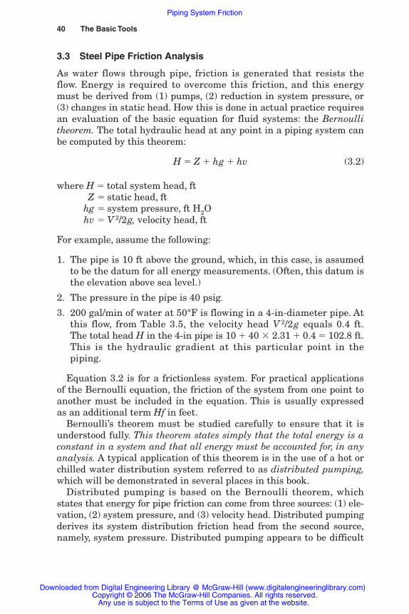
As water flows through pipe, friction is generated that resists theflow. Energy is required to overcome this friction, and this energymust be derived from (1) pumps, (2) reduction in system pressure, or(3) changes in static head. How this is done in actual practice requiresan evaluation of the basic equation for fluid systems: the Bernoullitheorem. The total hydraulic head at any point in a piping system canbe computed by this theorem:
H � Z � hg � hv (3.2)
where H � total system head, ftZ � static head, ft
hg � system pressure, ft H2Ohv � V 2/2g, velocity head, ft
For example, assume the following:
1. The pipe is 10 ft above the ground, which, in this case, is assumedto be the datum for all energy measurements. (Often, this datum isthe elevation above sea level.)
2. The pressure in the pipe is 40 psig.
3. 200 gal/min of water at 50°F is flowing in a 4-in-diameter pipe. Atthis flow, from Table 3.5, the velocity head V 2/2g equals 0.4 ft.The total head H in the 4-in pipe is 10 � 40 � 2.31 � 0.4 � 102.8 ft.This is the hydraulic gradient at this particular point in thepiping.
Equation 3.2 is for a frictionless system. For practical applicationsof the Bernoulli equation, the friction of the system from one point toanother must be included in the equation. This is usually expressedas an additional term Hf in feet.
Bernoulli’s theorem must be studied carefully to ensure that it isunderstood fully. This theorem states simply that the total energy is aconstant in a system and that all energy must be accounted for, in anyanalysis. A typical application of this theorem is in the use of a hot orchilled water distribution system referred to as distributed pumping,which will be demonstrated in several places in this book.
Distributed pumping is based on the Bernoulli theorem, whichstates that energy for pipe friction can come from three sources: (1) ele-vation, (2) system pressure, and (3) velocity head. Distributed pumpingderives its system distribution friction head from the second source,namely, system pressure. Distributed pumping appears to be difficult
Rishel_CH03.qxd 20/4/06 5:35 PM Page 40
Piping System Friction
Downloaded from Digital Engineering Library @ McGraw-Hill (www.digitalengineeringlibrary.com)Copyright © 2006 The McGraw-Hill Companies. All rights reserved.
Any use is subject to the Terms of Use as given at the website.
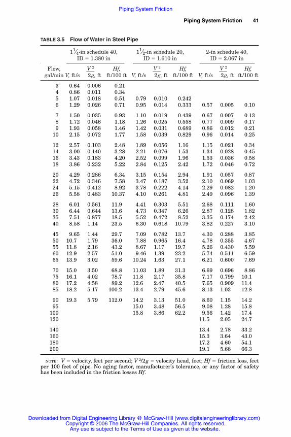
TABLE 3.5 Flow of Water in Steel Pipe
11⁄4-in schedule 40, 11⁄2-in schedule 20, 2-in schedule 40,ID � 1.380 in ID � 1.610 in ID � 2.067 in
Flow, Hf, Hf, Hf,gal/min V, ft /s
�V2g
2�
, ft ft /100 ft V, ft /s�V2g
2�
, ft ft /100 ft V, ft /s�V2g
2�
, ft ft /100 ft
003 00.64 0.006 000.21004 00.86 0.011 000.34005 01.07 0.018 000.51 00.79 0.010 00.242006 01.29 0.026 000.71 00.95 0.014 00.333 00.57 0.005 00.10
007 01.50 0.035 000.93 01.10 0.019 00.439 00.67 0.007 00.13008 01.72 0.046 001.18 01.26 0.025 00.558 00.77 0.009 00.17009 01.93 0.058 001.46 01.42 0.031 00.689 00.86 0.012 00.21010 02.15 0.072 001.77 01.58 0.039 00.829 00.96 0.014 00.25
012 02.57 0.103 002.48 01.89 0.056 01.16 01.15 0.021 00.34014 03.00 0.140 003.28 02.21 0.076 01.53 01.34 0.028 00.45016 03.43 0.183 004.20 02.52 0.099 01.96 01.53 0.036 00.58018 03.86 0.232 005.22 02.84 0.125 02.42 01.72 0.046 00.72
020 04.29 0.286 006.34 03.15 0.154 02.94 01.91 0.057 00.87022 04.72 0.346 007.58 03.47 0.187 03.52 02.10 0.069 01.03024 05.15 0.412 008.92 03.78 0.222 04.14 02.29 0.082 01.20026 05.58 0.483 010.37 04.10 0.261 04.81 02.49 0.096 01.39
028 06.01 0.561 011.9 04.41 0.303 05.51 02.68 0.111 01.60030 06.44 0.644 013.6 04.73 0.347 06.26 02.87 0.128 01.82035 07.51 0.877 018.5 05.52 0.472 08.52 03.35 0.174 02.42040 08.58 1.14 023.5 06.30 0.618 10.79 03.82 0.227 03.10
045 09.65 1.44 029.7 07.09 0.782 13.7 04.30 0.288 03.85050 10.7 1.79 036.0 07.88 0.965 16.4 04.78 0.355 04.67055 11.8 2.16 043.2 08.67 1.17 19.7 05.26 0.430 05.59060 12.9 2.57 051.0 09.46 1.39 23.2 05.74 0.511 06.59065 13.9 3.02 059.6 10.24 1.63 27.1 06.21 0.600 07.69
070 15.0 3.50 068.8 11.03 1.89 31.3 06.69 0.696 08.86075 16.1 4.02 078.7 11.8 2.17 35.8 07.17 0.799 10.1080 17.2 4.58 089.2 12.6 2.47 40.5 07.65 0.909 11.4085 18.2 5.17 100.2 13.4 2.79 45.6 08.13 1.03 12.8
090 19.3 5.79 112.0 14.2 3.13 51.0 08.60 1.15 14.2095 15.0 3.48 56.5 09.08 1.28 15.8100 15.8 3.86 62.2 09.56 1.42 17.4120 11.5 2.05 24.7
140 13.4 2.78 33.2160 15.3 3.64 43.0180 17.2 4.60 54.1200 19.1 5.68 66.3
NOTE: V � velocity, feet per second; V 2/2g � velocity head, feet; Hf � friction loss, feetper 100 feet of pipe. No aging factor, manufacturer’s tolerance, or any factor of safetyhas been included in the friction losses Hf.
Piping System Friction 41
Rishel_CH03.qxd 20/4/06 5:35 PM Page 41
Piping System Friction
Downloaded from Digital Engineering Library @ McGraw-Hill (www.digitalengineeringlibrary.com)Copyright © 2006 The McGraw-Hill Companies. All rights reserved.
Any use is subject to the Terms of Use as given at the website.

42
TABLE 3.5 Flow of Water in Steel Pipe (Continued )
21⁄2-in schedule 40, 3-in schedule 40, 4-in schedule 40,ID � 2.469 in ID � 3.068 in ID � 4.026 in
Flow, Hf, Hf, Hf,gal/min V, ft /s
�V2g
2�
, ft ft /100 ft V, ft /s�V2g
2�
, ft ft /100 ft V, ft /s�V2g
2�
, ft ft /100 ft
014 00.94 0.014 00.09016 01.07 0.018 00.24018 01.21 0.023 00.30020 01.34 0.028 00.36 00.87 0.012 00.13 00.50 0.004 00.03
022 01.47 0.034 00.43 00.95 0.026 00.15 00.55 0.005 00.04024 01.61 0.040 00.50 01.04 0.036 00.18 00.60 0.006 00.05026 01.74 0.047 00.58 01.13 0.047 00.21 00.66 0.007 00.06028 01.88 0.055 00.66 01.22 0.059 00.25 00.71 0.008 00.07
030 02.01 0.063 00.75 01.30 0.073 00.26 00.76 0.009 00.07035 02.35 0.086 01.00 01.52 0.089 00.35 00.88 0.012 00.10040 02.68 0.112 01.28 01.74 0.105 00.44 01.01 0.016 00.12045 03.02 0.141 01.60 01.95 0.124 00.55 01.14 0.020 00.15
050 03.35 0.174 01.94 02.17 0.143 00.66 01.26 0.025 00.18055 03.69 0.211 02.32 02.39 0.165 00.79 01.39 0.030 00.21060 04.02 0.251 02.72 02.60 0.187 00.92 01.51 0.036 00.25065 04.36 0.295 03.16 02.82 0.211 01.07 01.64 0.042 00.29
070 04.69 0.342 03.63 03.04 0.237 01.22 01.76 0.048 00.33075 05.03 0.393 04.13 03.25 0.264 01.39 01.89 0.056 00.37080 05.36 0.447 04.66 03.47 0.293 01.57 02.02 0.063 00.42085 05.70 0.504 05.22 03.69 0.354 01.76 02.15 0.071 00.47
090 06.03 0.565 05.82 03.91 0.421 01.96 02.27 0.080 00.52095 06.37 0.630 06.45 04.12 0.495 02.17 02.40 0.089 00.57100 06.70 0.698 07.11 04.34 0.574 02.39 02.52 0.099 00.62110 07.37 0.844 08.51 04.77 0.659 02.86 02.77 0.119 00.74
120 08.04 1.00 10.0 05.21 0.749 03.37 03.02 0.142 00.88130 08.71 1.18 11.7 05.64 0.846 03.92 03.28 0.167 01.02140 09.38 1.37 13.5 06.08 0.948 04.51 03.53 0.193 01.17150 10.05 1.57 15.4 06.51 1.06 05.14 03.78 0.222 01.32
160 10.7 1.79 17.4 06.94 1.17 05.81 04.03 0.253 01.49170 11.4 2.02 19.6 07.38 1.42 06.53 04.28 0.285 01.67180 12.1 2.26 21.9 07.81 1.69 07.28 04.54 0.320 01.86190 12.7 2.52 24.2 08.25 1.98 08.07 04.79 0.356 02.06
200 13.4 2.79 26.7 08.68 2.29 08.90 05.04 0.395 02.27220 14.7 3.38 32.2 09.55 2.63 10.7 05.54 0.478 02.72240 16.1 4.02 38.1 10.4 3.00 12.6 06.05 0.569 03.21260 17.4 4.72 44.5 11.3 3.38 14.7 06.55 0.667 03.74
280 18.8 5.47 51.3 12.2 3.79 16.9 07.06 0.774 04.30300 20.1 6.28 58.5 13.0 4.23 19.2 07.56 0.888 04.89320 13.9 4.68 22.0 08.06 1.01 05.51340 14.8 24.8 08.57 1.14 06.19
360 15.6 27.7 09.07 1.28 06.92380 16.5 30.7 09.58 1.43 07.68400 17.4 33.9 10.1 1.58 08.47420 10.6 1.74 09.30
440 11.1 1.91 10.2460 11.6 2.09 11.1480 12.1 2.27 12.0500 12.6 2.47 13.0
550 13.9 2.99 15.7600 15.1 3.55 18.6650 16.4 4.17 21.7700 17.6 4.84 25.0
NOTE: V � velocity, feet per second; V 2/2g � velocity head, feet; Hf � friction loss, feetper 100 feet of pipe. No aging factor, manufacturer’s tolerance, or any factor of safetyhas been included in the friction losses Hf.
Rishel_CH03.qxd 20/4/06 5:35 PM Page 42
Piping System Friction
Downloaded from Digital Engineering Library @ McGraw-Hill (www.digitalengineeringlibrary.com)Copyright © 2006 The McGraw-Hill Companies. All rights reserved.
Any use is subject to the Terms of Use as given at the website.
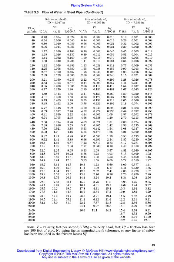
43
TABLE 3.5 Flow of Water in Steel Pipe (Continued )
5-in schedule 40, 6-in schedule 40, 8-in schedule 40,ID � 5.047 in ID � 6.065 in ID � 7.981 in
Flow, Hf, Hf, Hf,gal/min V, ft /s
�2V
g
2�
, ft ft /100 ft V, ft /s�2V
g
2�
, ft ft /100 ft V, ft /s�2V
g
2�
, ft ft /100 ft
0030 00.48 00.004 00.024 00.33 00.002 00.010 00.19 0.001 00.0030040 00.64 00.006 00.040 00.44 00.003 00.016 00.26 0.001 00.0040050 00.80 00.010 00.059 00.56 00.005 00.024 00.32 0.002 00.0070060 00.96 00.014 00.081 00.67 00.007 00.034 00.39 0.002 00.009
0070 01.12 00.020 00.108 00.78 00.009 00.045 00.45 0.003 00.0120080 01.28 00.026 00.137 00.89 00.012 00.056 00.51 0.004 00.0150090 01.44 00.032 00.169 01.00 00.016 00.070 00.58 0.005 00.0190100 01.60 00.040 00.204 01.11 00.019 00.084 00.64 0.006 00.022
0120 01.92 00.058 00.286 01.33 00.028 00.118 00.77 0.009 00.0310140 02.25 00.078 00.380 01.55 00.038 00.155 00.90 0.013 00.0410160 02.57 00.102 00.487 01.78 00.049 00.198 01.03 0.016 00.0520180 02.89 00.129 00.606 02.00 00.062 00.246 01.15 0.021 00.064
0200 03.21 00.160 00.736 02.22 00.077 00.299 01.28 0.026 00.0780220 03.53 00.193 00.879 02.44 00.093 00.357 01.41 0.031 00.0930240 03.85 00.230 01.035 02.66 00.110 00.419 01.54 0.037 00.1090260 04.17 00.270 01.20 02.89 00.130 00.487 01.67 0.043 00.126
0280 04.49 00.313 01.38 03.11 00.150 00.560 01.80 0.050 00.1440300 04.81 00.360 01.58 03.33 00.172 00.637 01.92 0.058 00.1630320 05.13 00.409 01.78 03.55 00.196 00.719 02.05 0.066 00.1840340 05.45 00.462 02.00 03.78 00.222 00.806 02.18 0.074 00.206
0360 05.77 00.518 02.22 04.00 00.240 00.898 02.31 0.083 00.2290380 06.09 00.577 02.46 04.22 00.277 00.993 02.44 0.092 00.2530400 06.41 00.639 02.72 04.44 00.307 01.09 02.57 0.102 00.2790420 06.74 00.705 02.98 04.66 00.338 01.20 02.70 0.113 00.308
0440 07.06 00.774 03.26 04.89 00.371 01.31 02.83 0.124 00.3380460 07.38 00.846 03.55 05.11 00.405 01.42 02.96 0.135 00.3690480 07.70 00.921 03.85 05.33 00.442 01.54 03.08 0.147 00.4020500 08.02 01.0 04.16 05.55 00.479 01.66 03.21 0.160 00.424
0550 08.82 01.21 04.98 06.11 00.580 01.99 03.53 0.193 00.5070600 09.62 01.44 05.88 06.66 00.690 02.34 03.85 0.230 00.5970650 10.4 01.69 06.87 07.22 00.810 02.73 04.17 0.271 00.6940700 11.2 01.96 07.93 07.77 00.939 03.13 04.49 0.313 00.797
0750 12.0 02.25 09.05 08.33 01.08 03.57 04.81 0.360 00.9070800 12.8 02.56 10.22 08.88 01.23 04.03 05.13 0.409 01.020850 13.6 02.89 11.5 09.44 01.38 04.53 05.45 0.462 01.150900 14.4 03.24 12.9 09.99 01.55 05.05 05.77 0.518 01.27
0950 15.2 03.61 14.3 10.5 01.73 05.60 06.09 0.577 01.411000 16.0 04.00 15.8 11.1 01.92 06.17 06.41 0.639 01.561100 17.6 04.84 19.0 12.2 02.32 07.41 07.05 0.773 01.871200 19.2 05.76 22.5 13.3 02.76 08.76 07.70 0.920 02.201300 20.8 06.75 26.3 14.4 03.24 10.2 08.34 1.08 02.56
1400 22.5 07.83 30.4 15.5 03.76 11.8 08.98 1.25 02.951500 24.1 08.99 34.8 16.7 04.31 13.5 09.62 1.44 03.371600 25.7 10.2 39.5 17.8 04.91 15.4 10.3 1.64 03.821700 27.3 11.6 44.5 18.9 05.54 17.3 10.9 1.85 04.29
1800 28.8 12.9 49.7 20.0 06.21 19.4 11.5 2.07 04.791900 30.5 14.4 55.2 21.1 06.92 21.6 12.2 2.31 05.312000 32.1 16.0 61.0 22.2 07.67 23.8 12.8 2.56 05.862200 24.4 09.27 28.8 14.1 3.09 07.02
2400 26.6 11.1 34.2 15.4 3.68 08.312600 16.7 4.32 09.702800 18.0 5.01 11.203000 19.2 5.75 12.8
NOTE: V � velocity, feet per second; V 2/2g � velocity head, feet; Hf � friction loss, feetper 100 feet of pipe. No aging factor, manufacturer’s tolerance, or any factor of safetyhas been included in the friction losses Hf.
Rishel_CH03.qxd 20/4/06 5:35 PM Page 43
Piping System Friction
Downloaded from Digital Engineering Library @ McGraw-Hill (www.digitalengineeringlibrary.com)Copyright © 2006 The McGraw-Hill Companies. All rights reserved.
Any use is subject to the Terms of Use as given at the website.
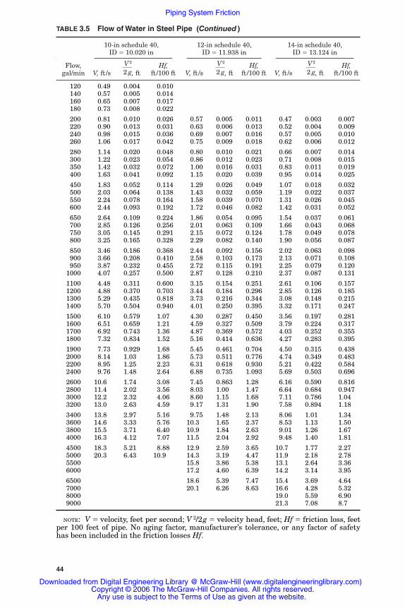
44
TABLE 3.5 Flow of Water in Steel Pipe (Continued )
10-in schedule 40, 12-in schedule 40, 14-in schedule 40,ID � 10.020 in ID � 11.938 in ID � 13.124 in
Flow, Hf, Hf, Hf,gal/min V, ft /s
�2V
g
2�
, ft ft /100 ft V, ft /s�2V
g
2�
, ft ft /100 ft V, ft /s�2V
g
2�
, ft ft /100 ft
0120 00.49 0.004 00.0100140 00.57 0.005 00.0140160 00.65 0.007 00.0170180 00.73 0.008 00.022
0200 00.81 0.010 00.026 00.57 0.005 0.011 00.47 0.003 0.0070220 00.90 0.013 00.031 00.63 0.006 0.013 00.52 0.004 0.0090240 00.98 0.015 00.036 00.69 0.007 0.016 00.57 0.005 0.0100260 01.06 0.017 00.042 00.75 0.009 0.018 00.62 0.006 0.012
0280 01.14 0.020 00.048 00.80 0.010 0.021 00.66 0.007 0.0140300 01.22 0.023 00.054 00.86 0.012 0.023 00.71 0.008 0.0150350 01.42 0.032 00.072 01.00 0.016 0.031 00.83 0.011 0.0190400 01.63 0.041 00.092 01.15 0.020 0.039 00.95 0.014 0.025
0450 01.83 0.052 00.114 01.29 0.026 0.049 01.07 0.018 0.0320500 02.03 0.064 00.138 01.43 0.032 0.059 01.19 0.022 0.0370550 02.24 0.078 00.164 01.58 0.039 0.070 01.31 0.026 0.0450600 02.44 0.093 00.192 01.72 0.046 0.082 01.42 0.031 0.052
0650 02.64 0.109 00.224 01.86 0.054 0.095 01.54 0.037 0.0610700 02.85 0.126 00.256 02.01 0.063 0.109 01.66 0.043 0.0680750 03.05 0.145 00.291 02.15 0.072 0.124 01.78 0.049 0.0780800 03.25 0.165 00.328 02.29 0.082 0.140 01.90 0.056 0.087
0850 03.46 0.186 00.368 02.44 0.092 0.156 02.02 0.063 0.0980900 03.66 0.208 00.410 02.58 0.103 0.173 02.13 0.071 0.1080950 03.87 0.232 00.455 02.72 0.115 0.191 02.25 0.079 0.1201000 04.07 0.257 00.500 02.87 0.128 0.210 02.37 0.087 0.131
1100 04.48 0.311 00.600 03.15 0.154 0.251 02.61 0.106 0.1571200 04.88 0.370 00.703 03.44 0.184 0.296 02.85 0.126 0.1851300 05.29 0.435 00.818 03.73 0.216 0.344 03.08 0.148 0.2151400 05.70 0.504 00.940 04.01 0.250 0.395 03.32 0.171 0.247
1500 06.10 0.579 01.07 04.30 0.287 0.450 03.56 0.197 0.2811600 06.51 0.659 01.21 04.59 0.327 0.509 03.79 0.224 0.3171700 06.92 0.743 01.36 04.87 0.369 0.572 04.03 0.252 0.3551800 07.32 0.834 01.52 05.16 0.414 0.636 04.27 0.283 0.395
1900 07.73 0.929 01.68 05.45 0.461 0.704 04.50 0.315 0.4382000 08.14 1.03 01.86 05.73 0.511 0.776 04.74 0.349 0.4832200 08.95 1.25 02.23 06.31 0.618 0.930 05.21 0.422 0.5842400 09.76 1.48 02.64 06.88 0.735 1.093 05.69 0.503 0.696
2600 10.6 1.74 03.08 07.45 0.863 1.28 06.16 0.590 0.8162800 11.4 2.02 03.56 08.03 1.00 1.47 06.64 0.684 0.9473000 12.2 2.32 04.06 08.60 1.15 1.68 07.11 0.786 1.043200 13.0 2.63 04.59 09.17 1.31 1.90 07.58 0.894 1.18
3400 13.8 2.97 05.16 09.75 1.48 2.13 08.06 1.01 1.343600 14.6 3.33 05.76 10.3 1.65 2.37 08.53 1.13 1.503800 15.5 3.71 06.40 10.9 1.84 2.63 09.01 1.26 1.674000 16.3 4.12 07.07 11.5 2.04 2.92 09.48 1.40 1.81
4500 18.3 5.21 08.88 12.9 2.59 3.65 10.7 1.77 2.275000 20.3 6.43 10.9 14.3 3.19 4.47 11.9 2.18 2.785500 15.8 3.86 5.38 13.1 2.64 3.366000 17.2 4.60 6.39 14.2 3.14 3.95
6500 18.6 5.39 7.47 15.4 3.69 4.647000 20.1 6.26 8.63 16.6 4.28 5.328000 19.0 5.59 6.909000 21.3 7.08 8.7
NOTE: V � velocity, feet per second; V 2/2g � velocity head, feet; Hf � friction loss, feetper 100 feet of pipe. No aging factor, manufacturer’s tolerance, or any factor of safetyhas been included in the friction losses Hf.
Rishel_CH03.qxd 20/4/06 5:35 PM Page 44
Piping System Friction
Downloaded from Digital Engineering Library @ McGraw-Hill (www.digitalengineeringlibrary.com)Copyright © 2006 The McGraw-Hill Companies. All rights reserved.
Any use is subject to the Terms of Use as given at the website.

Piping System Friction 45
TABLE 3.5 Flow of Water in Steel Pipe (Continued )
16-in schedule 40, 18-in schedule 40, 20-in schedule 40,ID � 15.000 in ID � 16.876 in ID � 18.812 in
Flow, Hf, Hf, Hf,gal/min V, ft /s
�2V
g
2�
, ft ft /100 ft V, ft /s�2V
g
2�
, ft ft /100 ft V, ft /s�2V
g
2�
, ft ft /100 ft
00300 00.55 0.005 0.008 00.43 0.003 0.004 00.35 0.002 0.00300400 00.73 0.008 0.013 00.57 0.005 0.007 00.46 0.003 0.00400500 00.91 0.013 0.019 00.72 0.008 0.011 00.58 0.005 0.00600600 01.09 0.018 0.027 00.86 0.012 0.015 00.69 0.007 0.009
00700 01.27 0.025 0.036 01.00 0.016 0.020 00.81 0.010 0.01200800 01.45 0.033 0.045 01.15 0.021 0.026 00.92 0.013 0.01500900 01.63 0.042 0.056 01.29 0.026 0.032 01.04 0.017 0.01901000 01.82 0.051 0.068 01.43 0.032 0.039 01.15 0.021 0.023
01200 02.18 0.074 0.095 01.72 0.046 0.054 01.38 0.030 0.03201400 02.54 0.100 0.127 02.01 0.063 0.072 01.62 0.041 0.04201600 02.90 0.131 0.163 02.30 0.082 0.092 01.85 0.053 0.05401800 03.27 0.166 0.203 02.58 0.104 0.114 02.08 0.067 0.067
02000 03.63 0.205 0.248 02.87 0.128 0.139 02.31 0.083 0.08102500 04.54 0.320 0.377 03.59 0.200 0.211 02.89 0.129 0.12303000 05.45 0.461 0.535 04.30 0.288 0.297 03.46 0.186 0.17403500 06.35 0.627 0.718 05.02 0.392 0.397 04.04 0.254 0.232
04000 07.26 0.820 0.921 05.74 0.512 0.511 04.62 0.331 0.29804500 08.17 1.04 1.15 06.45 0.647 0.639 05.19 0.419 0.37205000 09.08 1.28 1.41 07.17 0.799 0.781 05.77 0.517 0.45506000 10.9 1.84 2.01 08.61 1.15 1.11 06.92 0.745 0.645
07000 12.7 2.51 2.69 10.0 1.57 1.49 08.08 1.014 0.86208000 14.5 3.28 3.49 11.5 2.05 1.93 09.23 1.32 1.1109000 16.3 4.15 4.38 12.9 2.59 2.42 10.39 1.68 1.3910000 18.2 5.12 5.38 14.3 3.20 2.97 11.5 2.07 1.70
12000 21.8 7.38 7.69 17.2 4.60 4.21 13.8 2.98 2.4414000 20.1 6.27 5.69 16.2 4.06 3.2916000 22.9 8.19 7.41 18.5 5.30 4.2618000 20.8 6.71 5.3520000 23.1 8.28 6.56
NOTE: V � velocity, feet per second; V 2/2g � velocity head, feet; Hf � friction loss, feetper 100 feet of pipe. No aging factor, manufacturer’s tolerance, or any factor of safetyhas been included in the friction losses Hf.
to understand until this simple fact is realized. Figure 3.1 has beengenerated to demonstrate the use of this theorem.
It should be noted in the preceding example that velocity headV 2/2g is so small that it is seldom used in water distribution calcula-tions. Therefore, it is not included in the pressure gradients describedin this Handbook. The total hydraulic gradient for a water systemdoes include the velocity head. Velocity head should not be ignoredtotally, since it does come into importance when determining the flowin pipe around chillers and boilers. Also, it is the correct basis for com-puting friction loss in pipe fittings.
Rishel_CH03.qxd 21/4/06 6:07 PM Page 45
Piping System Friction
Downloaded from Digital Engineering Library @ McGraw-Hill (www.digitalengineeringlibrary.com)Copyright © 2006 The McGraw-Hill Companies. All rights reserved.
Any use is subject to the Terms of Use as given at the website.
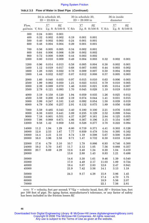
46
TABLE 3.5 Flow of Water in Steel Pipe (Continued )
24-in schedule 40, 30-in schedule 20, 36-in inside ID � 22.624 in ID � 29.000 in diameter
Flow, Hf, Hf, Hf,gal/min V, ft /s
�2V
g
2�
, ft ft /100 ft V, ft/s�2V
g
2�
, ft ft /100 ft V, ft /s�2V
g
2�
, ft ft /100 ft
00300 00.24 0.001 0.00100400 00.32 0.002 0.002 00.19 0.001 0.00100500 00.40 0.002 0.003 00.24 0.001 0.00100600 00.48 0.004 0.004 00.29 0.001 0.001
00700 00.56 0.005 0.005 00.34 0.002 0.00100800 00.64 0.006 0.006 00.39 0.002 0.00200900 00.72 0.008 0.008 00.44 0.003 0.00201000 00.80 0.010 0.009 00.49 0.004 0.003 00.32 0.002 0.001
01200 00.96 0.014 0.013 00.58 0.005 0.004 00.38 0.002 0.00101400 01.12 0.019 0.017 00.68 0.007 0.005 00.44 0.003 0.00201600 01.28 0.025 0.022 00.78 0.009 0.007 00.50 0.004 0.00201800 01.44 0.032 0.027 00.87 0.012 0.008 00.57 0.005 0.003
02000 01.60 0.040 0.033 00.97 0.015 0.010 00.63 0.006 0.00302500 01.99 0.062 0.050 01.21 0.023 0.015 00.79 0.010 0.00503000 02.39 0.089 0.070 01.46 0.033 0.021 00.95 0.014 0.00703500 02.79 0.121 0.093 01.70 0.045 0.028 01.10 0.019 0.010
04000 03.19 0.158 0.120 01.94 0.059 0.035 01.26 0.025 0.01204500 03.59 0.200 0.149 02.19 0.074 0.044 01.41 0.031 0.01505000 03.99 0.247 0.181 02.43 0.092 0.054 01.58 0.039 0.01906000 04.79 0.356 0.257 02.91 0.132 0.075 01.89 0.056 0.026
07000 05.59 0.485 0.343 03.40 0.180 0.100 02.21 0.076 0.03508000 06.38 0.633 0.441 03.89 0.235 0.129 02.52 0.099 0.04409000 07.18 0.801 0.551 04.37 0.297 0.161 02.84 0.125 0.05510000 07.98 0.989 0.671 04.86 0.367 0.196 03.15 0.154 0.06712000 09.58 1.42 0.959 05.83 0.528 0.277 03.78 0.222 0.094
14000 11.2 1.94 1.29 06.80 0.719 0.371 04.41 0.303 0.12616000 12.8 2.53 1.67 07.77 0.939 0.478 05.04 0.395 0.16218000 14.4 3.21 2.10 08.74 1.19 0.598 05.67 0.500 0.20320000 16.0 3.96 2.58 09.71 1.47 0.732 06.30 0.618 0.248
22000 17.6 4.79 3.10 10.7 1.78 0.886 06.93 0.746 0.30024000 19.2 5.70 3.67 11.7 2.12 1.05 07.56 0.888 0.35726000 20.7 6.69 4.29 12.6 2.48 1.24 08.20 1.04 0.41928000 13.6 2.88 1.43 08.83 1.21 0.486
30000 14.6 3.30 1.61 09.46 1.39 0.54035000 17.0 4.49 2.17 11.03 1.89 0.72440000 19.4 5.87 2.83 12.6 2.47 0.94145000 21.9 7.42 3.56 14.1 3.13 1.18
50000 24.3 9.17 4.38 15.8 3.86 1.4555000 17.4 4.70 1.7560000 18.9 5.56 2.0770000 22.1 7.56 2.81
NOTE: V � velocity, feet per second; V 2/2g � velocity head, feet; Hf � friction loss, feetper 100 feet of pipe. No aging factor, manufacturer’s tolerance, or any factor of safetyhas been included in the friction losses Hf.
Rishel_CH03.qxd 20/4/06 5:35 PM Page 46
Piping System Friction
Downloaded from Digital Engineering Library @ McGraw-Hill (www.digitalengineeringlibrary.com)Copyright © 2006 The McGraw-Hill Companies. All rights reserved.
Any use is subject to the Terms of Use as given at the website.
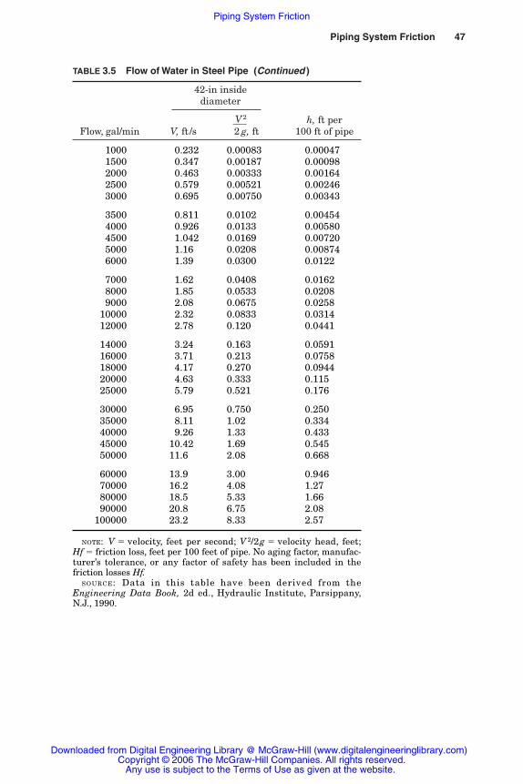
Piping System Friction 47
TABLE 3.5 Flow of Water in Steel Pipe (Continued )
42-in inside diameter
h, ft per Flow, gal/min V, ft /s
�2V
g
2�
, ft 100 ft of pipe
001000 0.232 0.00083 0.00047001500 0.347 0.00187 0.00098002000 0.463 0.00333 0.00164002500 0.579 0.00521 0.00246003000 0.695 0.00750 0.00343
003500 0.811 0.0102 0.00454004000 0.926 0.0133 0.00580004500 1.042 0.0169 0.00720005000 1.16 0.0208 0.00874006000 1.39 0.0300 0.0122
007000 1.62 0.0408 0.0162008000 1.85 0.0533 0.0208009000 2.08 0.0675 0.0258010000 2.32 0.0833 0.0314012000 2.78 0.120 0.0441
014000 3.24 0.163 0.0591016000 3.71 0.213 0.0758018000 4.17 0.270 0.0944020000 4.63 0.333 0.115025000 5.79 0.521 0.176
030000 6.95 0.750 0.250035000 8.11 1.02 0.334040000 9.26 1.33 0.433045000 10.420 1.69 0.545050000 11.6 2.08 0.668
060000 13.9 3.00 0.946070000 16.2 4.08 1.27080000 18.5 5.33 1.66090000 20.8 6.75 2.08100000 23.2 8.33 2.57
NOTE: V � velocity, feet per second; V 2/2g � velocity head, feet;Hf � friction loss, feet per 100 feet of pipe. No aging factor, manufac-turer’s tolerance, or any factor of safety has been included in thefriction losses Hf.
SOURCE: Data in this table have been derived from theEngineering Data Book, 2d ed., Hydraulic Institute, Parsippany,N.J., 1990.
Rishel_CH03.qxd 20/4/06 5:35 PM Page 47
Piping System Friction
Downloaded from Digital Engineering Library @ McGraw-Hill (www.digitalengineeringlibrary.com)Copyright © 2006 The McGraw-Hill Companies. All rights reserved.
Any use is subject to the Terms of Use as given at the website.

48 The Basic Tools
Figure 3.1 Bernoulli diagram.
3.3.1 Pipe friction formulas
The amount of friction that is created by flow of water in piping hasbeen determined by a number of sources. Today, there are two princi-pal formulas for determining pipe friction. These are the DarcyWeisbach (Fanning) and the Williams and Hazen formulas:
Darcy Weisbach formula (Basis for Table 3.5)
Hf � f � �DL
� � �2V
g
2� (3.3)
where Hf � friction loss, ft of liquidL � pipe length, in ftD � average inside diameter, ftf � friction factor
Rishel_CH03.qxd 20/4/06 5:35 PM Page 48
Piping System Friction
Downloaded from Digital Engineering Library @ McGraw-Hill (www.digitalengineeringlibrary.com)Copyright © 2006 The McGraw-Hill Companies. All rights reserved.
Any use is subject to the Terms of Use as given at the website.
Piping System Friction 49
The friction factor f is usually derived from the Colebrook equation:
��1
f�� � �2 log10��
3.7
D� � �
R
2.
�51
f��� (3.4)
where R � Reynolds number � absolute roughness parameter (typically 0.00015 for steel
pipe)
For practical purposes, the friction factor f is calculated from theMoody diagram described later.
Williams and Hazen formula
Hf � 0.002083 � L � ��1C00��
1.85
� �ga
dl/m
4.8
i6
n55
1.85
� (3.5)
where C � a design factor determined for various types of piped � inside diameter of pipe, in
There are a number of sources for securing the data for the afore-mentioned equations in either tabular or software form. Before anydata on pipe friction are used, either in tabular or computer softwareform, be sure that the pipe under consideration has the same insidediameter as that in the tables or computer software! The followingpages demonstrate some of the sources for pipe friction data in tabu-lar form. A principal source is the Hydraulic Institute’s EngineeringData Book. This book is based on the Darcy Weisbach formula, andTable 3.5 has been developed from Hydraulic Institute data for steelpipe. It is strongly recommended that this data book be acquired byanyone who is involved in piping design.
3.3.2 Reynolds number and the Moody diagram
The Hydraulic Institute’s Engineering Data Book contains somevery practical information on the generation and use of Reynoldsnumber. Reynolds number is a dimensionless number that simpli-fies the calculation of pipe friction under varying velocities andviscosities.
Reynolds number R � �V
� D� (3.6)
where V � velocity, ft /sD � pipe diameter, ft � kinematic viscosity, ft2/s
Rishel_CH03.qxd 20/4/06 5:35 PM Page 49
Piping System Friction
Downloaded from Digital Engineering Library @ McGraw-Hill (www.digitalengineeringlibrary.com)Copyright © 2006 The McGraw-Hill Companies. All rights reserved.
Any use is subject to the Terms of Use as given at the website.
50 The Basic Tools
For example, assume that 50°F water is flowing through 4-inschedule 40 steel pipe at 200 gal/min. From Table 3.5, the velocity is5.04 ft/s, and the diameter of the pipe is 4.026 in, or 0.336 ft. FromTable 2.2, the kinematic viscosity for 50°F water is 1.41�10�5 ft2/s.The Reynolds number is
�51.0.441�
�
01.03
�
356
�� 1.20�105
From the Moody diagram shown in Fig. 3.2, the friction factor f is0.0198.
The Moody diagram, named after its originator, is described inFig. 3.2. This diagram generates the friction factor f of the Colebrookequation (Eq. 3.4) for a broad variety of Reynolds numbers and, there-fore, velocities and viscosities. This particular diagram accepts a con-stant relative roughness factor of 0.00015 and provides curves forall popular sizes of steel pipe. This is adequate for most HVAC appli-cations of steel pipe.
Another diagram that is useful for work with a number of liquidswhere the kinematic viscosity is known is shown in Fig. 3.3. TheReynolds number can be selected from this diagram once the pipediameter, water velocity, and viscosity of the liquid are developed.Also, if the temperature of the liquid is determined, the kinematic vis-cosity of that liquid can be determined from this figure.
The practical use of Reynolds number and the Moody diagram canbe demonstrated by the following example. Assume that
1. A condenser water system is used for cooling computer air-conditioners employing a propylene glycol solution of 50% wherethe liquid temperature can vary from 30 to 130°F.
2. The flow rate is 750 gal/min at 30°F in a 6-in-diameter steel pipe.
Question. What is the variation in friction loss in feet per 100 feet oflength as the liquid varies from 30 to 130°F?
Factual data
1. From Fig. 2.4, the viscosity of the glycol solution is 8.5 cP at 30°Fand 1.4 cP at 130°F.
2. From Fig. 2.5, the specific gravity of the glycol solution at 30 °F is1.09 � water at 60°F, or 67.95 lb/ft3. Likewise, the specific gravityat 130°F is 1.06 � water at 60°F, or 66.08 lb/ft3.
3. From Table 3.5, the inside diameter of 6-in steel schedule 40 pipeis 6.065 in, or 0.505 ft. Also from this table, with 750 gal /min
Rishel_CH03.qxd 20/4/06 5:35 PM Page 50
Piping System Friction
Downloaded from Digital Engineering Library @ McGraw-Hill (www.digitalengineeringlibrary.com)Copyright © 2006 The McGraw-Hill Companies. All rights reserved.
Any use is subject to the Terms of Use as given at the website.
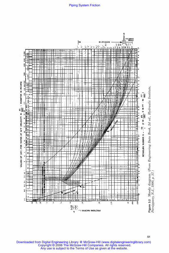
51
Fig
ure
3.2
Moo
dy d
iagr
am.
(Fro
m E
ngi
nee
rin
g D
ata
Boo
k,2d
ed
.,H
ydra
uli
c In
stit
ute
,P
arsi
ppan
y,N
.J.,
1990
,p.3
7.)
Rishel_CH03.qxd 20/4/06 5:35 PM Page 51
Piping System Friction
Downloaded from Digital Engineering Library @ McGraw-Hill (www.digitalengineeringlibrary.com)Copyright © 2006 The McGraw-Hill Companies. All rights reserved.
Any use is subject to the Terms of Use as given at the website.
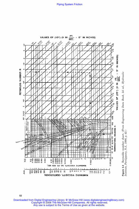
52
Fig
ure
3.3
Rey
nol
ds n
um
ber
char
t.(F
rom
En
gin
eeri
ng
Dat
a B
ook,
2d e
d.,
Hyd
rau
lic
Inst
itu
te,P
arsi
ppan
y,N
.J.,
1990
,p.4
2.)
Rishel_CH03.qxd 20/4/06 5:35 PM Page 52
Piping System Friction
Downloaded from Digital Engineering Library @ McGraw-Hill (www.digitalengineeringlibrary.com)Copyright © 2006 The McGraw-Hill Companies. All rights reserved.
Any use is subject to the Terms of Use as given at the website.

Piping System Friction 53
flowing through this pipe, the velocity is 8.33 ft /s, and the velocityhead is 1.08 ft.
Computing the kinematic viscosity first in square feet per second from Eq. 2.2.
At 30°F,
� � 0.841�10�4
At 130°F,
� � 0.142�10�4
The data have now been collected to compute the Reynolds numberat the two temperatures. At 30°F,
R � �V �
D� � � 5.00�104
At 130°F,
R � � 2.96� 105
The friction factors can now be selected from the Moody diagram(Fig. 3.2). At 30°F and a Reynolds number of 5.00�104, the frictionfactor f is 0.022. At 130°F and a Reynolds number of 2.96�105, thefriction factor f is 0.017.
The friction in feet per 100 ft can now be calculated from the DarcyWeisbach equation (Eq. 3.3). At 30°F,
Hf � � 4.71 ft /100 ft
At 130°F,
Hf � � 3.64 ft /100 ft
This example demonstrates the use of Reynolds number and theMoody diagram. It also emphasizes the variation in pipe friction withviscosity. In this case, the friction at 130°F was 77 percent of that at30°F. Also, this demonstrates that the friction for water at 60°F fromTable 3.5 of 3.57 ft /100 ft should not be used in calculating frictionlosses for this glycol solution.
0.017 ⋅ 100 ⋅ 1.08���
0.505
0.022 ⋅ 100 ⋅ 1.08���
0.505
8.33 ⋅ 0.505��0.142 ⋅ 10�5
8.33 ⋅ 0.505��0.841 ⋅ 10�4
6.7197 ⋅ 1.4 ⋅ 10�4���
66.08
6.7197 ⋅ 8.5 ⋅ 10�4���
67.95
Rishel_CH03.qxd 20/4/06 5:35 PM Page 53
Piping System Friction
Downloaded from Digital Engineering Library @ McGraw-Hill (www.digitalengineeringlibrary.com)Copyright © 2006 The McGraw-Hill Companies. All rights reserved.
Any use is subject to the Terms of Use as given at the website.

54 The Basic Tools
3.3.3 Use of the Darcy Weisbach equation
For those who wish to study pipe friction further or use the DarcyWeisbach equation for generating their own computer program forpipe friction, the preceding example provides a guide for doing so.Also, the two figures from the Hydraulic Institute’s Engineering DataBook (Figs. 3.2 and 3.3) should clarify the use of Reynolds number forthe calculation of pipe friction.
Another source for Darcy Weisbach data is Cameron HydraulicData, published by the Ingersoll Rand Company. Like the data bookof the Hydraulic Institute, it is an excellent source for pipe and waterdata and is a necessary reference manual for any serious designer ofpiping.
Both these sources do not include any allowance in their tables forpipe aging, variation in pipe manufacture, or field assembly. TheHydraulic Institute recommends that 15 percent allowance be madefor these factors; I consider this factor adequate for loop-type systemssuch as hot or chilled water systems. It is not adequate for coolingtower water, which is exposed to air in the water; it is recommendedthat a factor of 20 percent be added for this service if steel pipe isused. This possible increase in friction for steel pipe may demonstratethe application for plastic pipe on cooling tower water; its use is limitedby size and structural capability.
3.3.4 Use of the Williams-Hazen formula
The Williams-Hazen formula is very popular in the civil engineeringfield and can be used for HVAC piping design if it is understoodproperly. This formula gives accurate values for liquids that have aviscosity of around 1.1 cSt, such as water at 60°F. It is thereforeacceptable for chilled water and even condenser water. It will show anerror as much as 20 percent high if used for hot water over 200°F.
This formula is based on design factors that relate to the roughnessof the pipe involved. These design factors are called C factors thatappear in the preceding equation and range from 80 to 160, 80 beingfor the roughest pipe and 160 for the smoothest pipe.
Table 3.6 is taken from an older edition of Cameron Hydraulic Dataand includes the C factors for various types of pipe. If a C factor of140 is used with the Williams-Hazen formula, it will yield frictiondata for steel pipe that is somewhat comparable with the DarcyWeisbach formula with the 15 percent aging factor as recommendedpreviously. This is adequate for closed piping such as chilled waterbut should not be used with cooling tower piping. Cooling tower pip-ing should be calculated with a C factor of 130 for steel pipe whenusing the Williams-Hazen formula.
Rishel_CH03.qxd 20/4/06 5:35 PM Page 54
Piping System Friction
Downloaded from Digital Engineering Library @ McGraw-Hill (www.digitalengineeringlibrary.com)Copyright © 2006 The McGraw-Hill Companies. All rights reserved.
Any use is subject to the Terms of Use as given at the website.
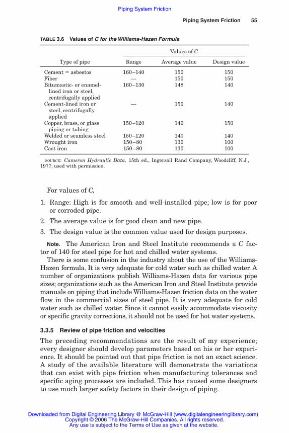
Piping System Friction 55
TABLE 3.6 Values of C for the Williams-Hazen Formula
Values of C
Type of pipe Range Average value Design value
Cement � asbestos 160–140 150 150Fiber — 150 150Bitumastic- or enamel- 160–130 148 140
lined iron or steel,centrifugally applied
Cement-lined iron or — 150 140steel, centrifugally applied
Copper, brass, or glass 150–120 140 150piping or tubing
Welded or seamless steel 150–120 140 140Wrought iron 150–80 130 100Cast iron 150–80 130 100
SOURCE: Cameron Hydraulic Data, 15th ed., Ingersoll Rand Company, Woodcliff, N.J.,1977; used with permission.
For values of C,
1. Range: High is for smooth and well-installed pipe; low is for pooror corroded pipe.
2. The average value is for good clean and new pipe.
3. The design value is the common value used for design purposes.
Note. The American Iron and Steel Institute recommends a C fac-tor of 140 for steel pipe for hot and chilled water systems.
There is some confusion in the industry about the use of the Williams-Hazen formula. It is very adequate for cold water such as chilled water. Anumber of organizations publish Williams-Hazen data for various pipesizes; organizations such as the American Iron and Steel Institute providemanuals on piping that include Williams-Hazen friction data on the waterflow in the commercial sizes of steel pipe. It is very adequate for coldwater such as chilled water. Since it cannot easily accommodate viscosityor specific gravity corrections, it should not be used for hot water systems.
3.3.5 Review of pipe friction and velocities
The preceding recommendations are the result of my experience;every designer should develop parameters based on his or her experi-ence. It should be pointed out that pipe friction is not an exact science.A study of the available literature will demonstrate the variationsthat can exist with pipe friction when manufacturing tolerances andspecific aging processes are included. This has caused some designersto use much larger safety factors in their design of piping.
Rishel_CH03.qxd 20/4/06 5:35 PM Page 55
Piping System Friction
Downloaded from Digital Engineering Library @ McGraw-Hill (www.digitalengineeringlibrary.com)Copyright © 2006 The McGraw-Hill Companies. All rights reserved.
Any use is subject to the Terms of Use as given at the website.

56 The Basic Tools
The figures and tables of this chapter provide data that can bereferred to during a piping design procedure. Software is also avail-able that implements the formulas and eliminates much of thedrudgery in calculating pipe friction. Software packages are availablefrom various sources at reasonable costs. It is urged that the designbasis for such software be fully understood before it is used on a pro-ject. Designers with knowledge of software and computers can devel-op some of their own computer programs for pipe friction by using theaforementioned equations.
3.4 Steel and Cast Iron Pipe Fittings
A significant part of the friction loss for HVAC piping is caused by thevarious fittings that are used to connect the piping. There have beensome very unacceptable practices used for the calculation of fittinglosses. For example, some people recommend that the pipe friction becalculated and a percentage of that loss be added for the pipe fittingand valve losses. This is a very poor and inexact method of computingfriction losses for valves and fittings. The proper method of computingfitting loss is to determine that loss for each and every fitting andvalve. Again, the Hydraulic Institute’s Engineering Data Book andIngersol Rand’s Cameron Hydraulic Data are excellent sources for fit-ting and valve losses. Interesting data on the possible variations inthe friction losses for fittings and valves are included in Table 32(c) ofthe Hydraulic Institute’s Engineering Data Book; variations from �10percent to as high as �50 percent are described.
Most fitting losses are referenced to the velocity head V 2/2g of thewater flowing in the pipe. Table 3.5 for steel pipe friction lists the veloc-ity head at various flows in the pipe. A K factor has been developed formany of the popular pipe fittings so that the loss through fittings Hf is
Hf � K � �2V
g
2� (3.7)
The Hydraulic Institute provides various K factors for valves andfittings in their Engineering Data Book; these are listed in Tables 3.7through 3.12 as approximate values. Unfortunately, at this writing,many popular fittings such as reducing elbows or tees have no data.Also, welded steel pipe reducers have significant losses, and there areno reliable data on them.
Miscellaneous K factors
Couplings and unions. Couplings and unions depend on the quality ofmanufacture. Assume an average K factor of 0.05 for them.
Rishel_CH03.qxd 20/4/06 5:35 PM Page 56
Piping System Friction
Downloaded from Digital Engineering Library @ McGraw-Hill (www.digitalengineeringlibrary.com)Copyright © 2006 The McGraw-Hill Companies. All rights reserved.
Any use is subject to the Terms of Use as given at the website.
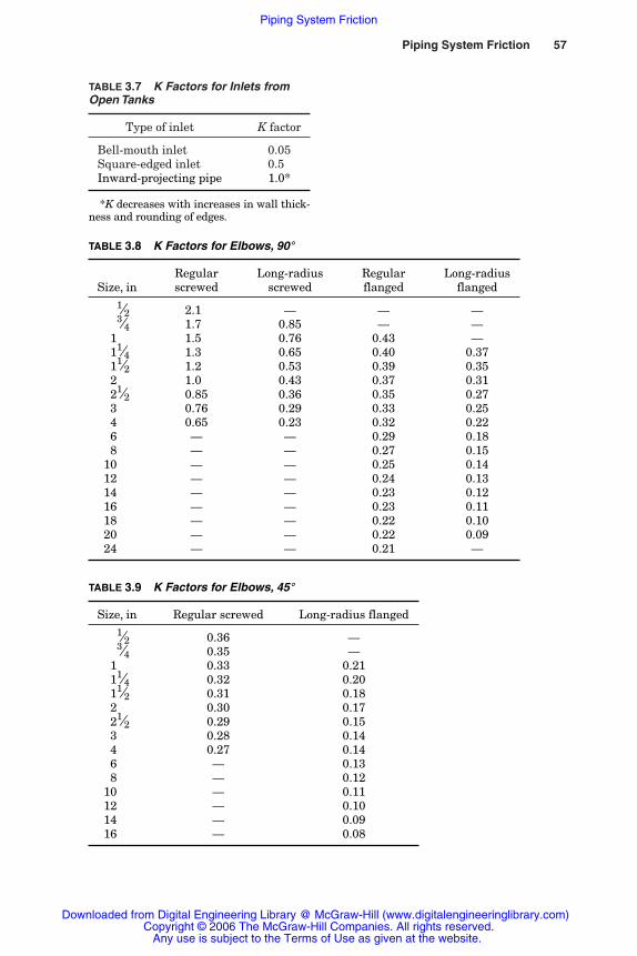
Piping System Friction 57
TABLE 3.7 K Factors for Inlets fromOpen Tanks
Type of inlet K factor
Bell-mouth inlet 0.05Square-edged inlet 0.50Inward-projecting pipe 1.0*
*K decreases with increases in wall thick-ness and rounding of edges.
TABLE 3.8 K Factors for Elbows, 90°
Regular Long-radius Regular Long-radius Size, in screwed screwed flanged flanged
001⁄2 2.10 — — —003⁄4 1.70 0.85 — —01 1.50 0.76 0.43 —011⁄4 1.30 0.65 0.40 0.37011⁄2 1.20 0.53 0.39 0.3502 1.00 0.43 0.37 0.31021⁄2 0.85 0.36 0.35 0.2703 0.76 0.29 0.33 0.2504 0.65 0.23 0.32 0.2206 — — 0.29 0.1808 — — 0.27 0.1510 — — 0.25 0.1412 — — 0.24 0.1314 — — 0.23 0.1216 — — 0.23 0.1118 — — 0.22 0.1020 — — 0.22 0.0924 — — 0.21 —
TABLE 3.9 K Factors for Elbows, 45°
Size, in Regular screwed Long-radius flanged
001⁄2 0.36 —003⁄4 0.35 —01 0.33 0.21011⁄4 0.32 0.20011⁄2 0.31 0.1802 0.30 0.17021⁄2 0.29 0.1503 0.28 0.1404 0.27 0.1406 — 0.1308 — 0.1210 — 0.1112 — 0.1014 — 0.0916 — 0.08
Rishel_CH03.qxd 20/4/06 5:35 PM Page 57
Piping System Friction
Downloaded from Digital Engineering Library @ McGraw-Hill (www.digitalengineeringlibrary.com)Copyright © 2006 The McGraw-Hill Companies. All rights reserved.
Any use is subject to the Terms of Use as given at the website.

58 The Basic Tools
TABLE 3.10 K Factors for Tees
Screwed-type, Flanged, Flanged,Size, in branch flow line flow branch flow
001⁄2 2.40 — —003⁄4 2.10 — —01 1.90 0.27 1.00011⁄4 1.70 0.25 0.94011⁄2 1.60 0.23 0.9002 1.40 0.20 0.83021⁄2 1.30 0.18 0.8003 1.20 0.17 0.7504 1.10 0.15 0.7006 — 0.12 0.6108 — 0.10 0.5810 — 0.09 0.5412 — 0.09 0.5214 — 0.08 0.5116 — 0.08 0.4718 0.07 0.4420 — 0.07 0.42
NOTE: For screwed-type, line flow tees, a K factor of 0.90 is used forall sizes.
TABLE 3.11 K Factors for Globe and Gate Valves (100 percentopen)
Globe valves Gate valves
Size, in Screwed Flanged Screwed Flanged
001⁄2 14.0 — 0.32 —003⁄4 10.0 — 0.28 —01 08.7 14.0 0.24 —011⁄4 08.0 12.0 0.22 —011⁄2 07.5 10.0 0.20 —02 06.9 08.5 0.17 —021⁄2 06.5 07.9 0.15 —03 06.0 07.0 0.14 0.2204 05.8 06.4 0.12 0.1606 — 05.9 — 0.1108 — 05.7 — 0.0810 — 05.7 — 0.0612 — 05.6 — 0.0514 — 05.6 — 0.0516 — 05.6 — 0.0518 — 05.6 — 0.0420 — 05.6 — 0.03
Rishel_CH03.qxd 20/4/06 5:35 PM Page 58
Piping System Friction
Downloaded from Digital Engineering Library @ McGraw-Hill (www.digitalengineeringlibrary.com)Copyright © 2006 The McGraw-Hill Companies. All rights reserved.
Any use is subject to the Terms of Use as given at the website.

Piping System Friction 59
TABLE 3.12 K Factors for Miscellaneous Valves (100 percent open)
Screwed Angle valve Ball Butterfly Size, in check Screwed Flanged valve* valve
1⁄2 5.6 — — — —3⁄4 3.7 5.5 — 0.11 —
1 3.0 4.7 5.0 0.10 —11⁄4 2.7 3.8 3.7 0.09 —11⁄2 2.5 3.0 3.0 0.09 —2 2.3 2.2 2.5 0.08 —21⁄2 2.2 1.7 2.3 0.07 3.53 2.2 1.4 2.2 0.07 3.04 2.2 1.0 2.2 0.06 1.56 — — 2.1 0.05 1.08 — — 2.1 0.05 0.8
10 — — 2.1 0.05 0.712 — — 2.1 0.04 0.714 — — 2.1 0.04 0.616 — — 2.1 0.04 0.618 — — 2.1 — —20 — — 2.1 — —
NOTE: Flanged check valves are assumed to have a K factor of 2.0 for all sizes.
Reducing bushings and couplings. The K factor for reducing bushingscan vary from 0.05 to 2.0. Replace them wherever possible withthreaded tapered fittings.
Sudden enlargements. Sudden enlargements such as reducing flangescan have a K factor as high as 1.0. Replace them with tapered fittingswherever possible.
3.4.1 Tapered fittings
There are a number of tests and equations for computing the K fac-tors for tapered fittings. Like other fitting calculations, they are, atbest, approximate. Two of the most accurate calculations seem to bethose included in Cameron Hydraulic Data.
Tapered reducing fittings
K � 0.8 sin �2�
� �1 � �dd
1
2
2
2�� (3.8)
where � � total angle of reductiond1 � smaller, leaving pipe diameterd2 � larger, entering pipe diameter
Rishel_CH03.qxd 20/4/06 5:35 PM Page 59
Piping System Friction
Downloaded from Digital Engineering Library @ McGraw-Hill (www.digitalengineeringlibrary.com)Copyright © 2006 The McGraw-Hill Companies. All rights reserved.
Any use is subject to the Terms of Use as given at the website.
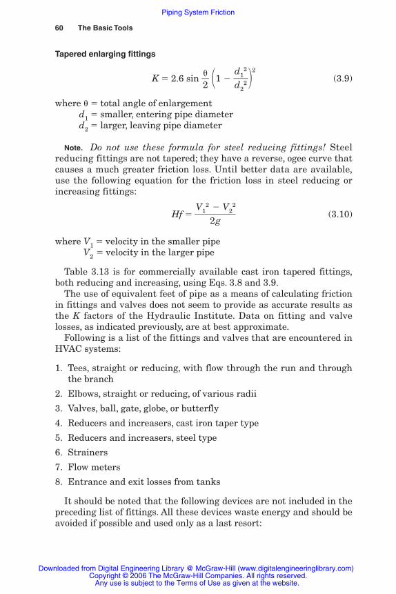
60 The Basic Tools
Tapered enlarging fittings
K � 2.6 sin �2�
� �1 � �dd
1
2
2
2��2
(3.9)
where � � total angle of enlargementd1 � smaller, entering pipe diameterd2 � larger, leaving pipe diameter
Note. Do not use these formula for steel reducing fittings! Steelreducing fittings are not tapered; they have a reverse, ogee curve thatcauses a much greater friction loss. Until better data are available,use the following equation for the friction loss in steel reducing orincreasing fittings:
Hf � �V1
2
2�
gV2
2
� (3.10)
where V1 � velocity in the smaller pipeV2 � velocity in the larger pipe
Table 3.13 is for commercially available cast iron tapered fittings,both reducing and increasing, using Eqs. 3.8 and 3.9.
The use of equivalent feet of pipe as a means of calculating frictionin fittings and valves does not seem to provide as accurate results asthe K factors of the Hydraulic Institute. Data on fitting and valvelosses, as indicated previously, are at best approximate.
Following is a list of the fittings and valves that are encountered inHVAC systems:
1. Tees, straight or reducing, with flow through the run and throughthe branch
2. Elbows, straight or reducing, of various radii
3. Valves, ball, gate, globe, or butterfly
4. Reducers and increasers, cast iron taper type
5. Reducers and increasers, steel type
6. Strainers
7. Flow meters
8. Entrance and exit losses from tanks
It should be noted that the following devices are not included in thepreceding list of fittings. All these devices waste energy and should beavoided if possible and used only as a last resort:
Rishel_CH03.qxd 20/4/06 5:35 PM Page 60
Piping System Friction
Downloaded from Digital Engineering Library @ McGraw-Hill (www.digitalengineeringlibrary.com)Copyright © 2006 The McGraw-Hill Companies. All rights reserved.
Any use is subject to the Terms of Use as given at the website.
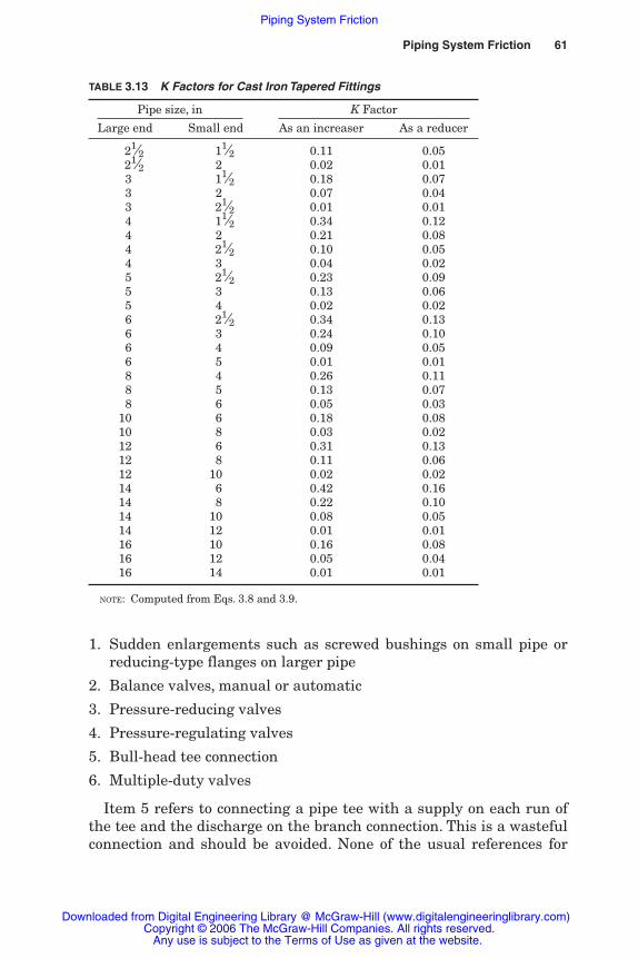
Piping System Friction 61
TABLE 3.13 K Factors for Cast Iron Tapered Fittings
Pipe size, in K Factor
Large end Small end As an increaser As a reducer
21⁄2 11⁄2 0.11 0.0521⁄2 2 0.02 0.013 11⁄2 0.18 0.073 2 0.07 0.043 21⁄2 0.01 0.014 11⁄2 0.34 0.124 2 0.21 0.084 21⁄2 0.10 0.054 3 0.04 0.025 21⁄2 0.23 0.095 3 0.13 0.065 4 0.02 0.026 21⁄2 0.34 0.136 3 0.24 0.106 4 0.09 0.056 5 0.01 0.018 4 0.26 0.118 5 0.13 0.078 6 0.05 0.03
10 6 0.18 0.0810 8 0.03 0.0212 6 0.31 0.1312 8 0.11 0.0612 10 0.02 0.0214 6 0.42 0.1614 8 0.22 0.1014 10 0.08 0.0514 12 0.01 0.0116 10 0.16 0.0816 12 0.05 0.0416 14 0.01 0.01
NOTE: Computed from Eqs. 3.8 and 3.9.
1. Sudden enlargements such as screwed bushings on small pipe orreducing-type flanges on larger pipe
2. Balance valves, manual or automatic
3. Pressure-reducing valves
4. Pressure-regulating valves
5. Bull-head tee connection
6. Multiple-duty valves
Item 5 refers to connecting a pipe tee with a supply on each run ofthe tee and the discharge on the branch connection. This is a wastefulconnection and should be avoided. None of the usual references for
Rishel_CH03.qxd 20/4/06 5:35 PM Page 61
Piping System Friction
Downloaded from Digital Engineering Library @ McGraw-Hill (www.digitalengineeringlibrary.com)Copyright © 2006 The McGraw-Hill Companies. All rights reserved.
Any use is subject to the Terms of Use as given at the website.

62 The Basic Tools
friction losses through tees includes any data for this type of connec-tion, which is known to have a sizable friction loss.
Item 6, multiple-duty valves, refers to a combination check, balancing,and shutoff valve. These valves can be wasteful of energy, since they canbe set at an intermediate position and left there at a high friction loss.These valves should not be used without downstream shutoff valves,since the check-valve portion cannot be repaired without draining thesystem. In most cases, the cost of this multiple-duty valve is so muchmore than that for an ordinary check valve and shutoff valve that theyare not economical. Also, their friction loss is usually greater than thatfor an individual check valve and butterfly valve (see Fig. 5.8).
Certain crossover bridges can be piping practices that waste energyby using return pressure-reducing valves. The additional piping lossesalso can increase the energy consumption of the total piping system.
3.4.1 Effect of fabrication on steel fitting loss
The great variation in steel pipe fitting friction loss is due to someextent to the method of fabricating steel pipe assemblies. The fittinglosses listed previously are for factory-formed fittings such as teesand elbows. Figure 3.4a describes the three ways that a steel tee canbe fabricated: (1) a factory-fabricated tee with dimensions conformingto ANSI Specification B16.5, (2) a “fishmouth” fabrication in whichthe end of the branch pipe is cut to a curve equal to the outside diam-eter of the main pipe, and (3) an unacceptable fabrication that shouldnever be used. Unfortunately, if the inspection is of questionable qual-ity, this type of fabrication may result. A fourth method that is avail-able is an acceptable practice and is called a saddle tee.
It is obvious that the friction loss for the factory-fabricated tee willbe less than that for the field-fabricated tees, particularly for the type3 tee, where the branch pipe projects into the main pipe. The loss forthe latter may be two to three times that for the factory-fabricatedtee. The smooth radii of the factory-fabricated tee reduce appreciablythe friction of the sharp corners of the type 2 tee and the reentrantloss of the type 3 tee.
Another case of fabricated fittings is the 45- and 90-degree elbows.Figure 3.4b describes (1) a standard production elbow and (2) a typicalfield-fabricated mitered elbow. If a sizable radius is maintained on themitered elbow, its friction loss will be similar to that of the factory-fabricated elbow. Often designers reduce their fitting losses throughelbows by specifying long-sweep elbows with a greater radius.
Field fabrication and selection of fittings have a great impact on theoverall friction loss in the piping of an HVAC water system. Continued
Rishel_CH03.qxd 20/4/06 5:35 PM Page 62
Piping System Friction
Downloaded from Digital Engineering Library @ McGraw-Hill (www.digitalengineeringlibrary.com)Copyright © 2006 The McGraw-Hill Companies. All rights reserved.
Any use is subject to the Terms of Use as given at the website.
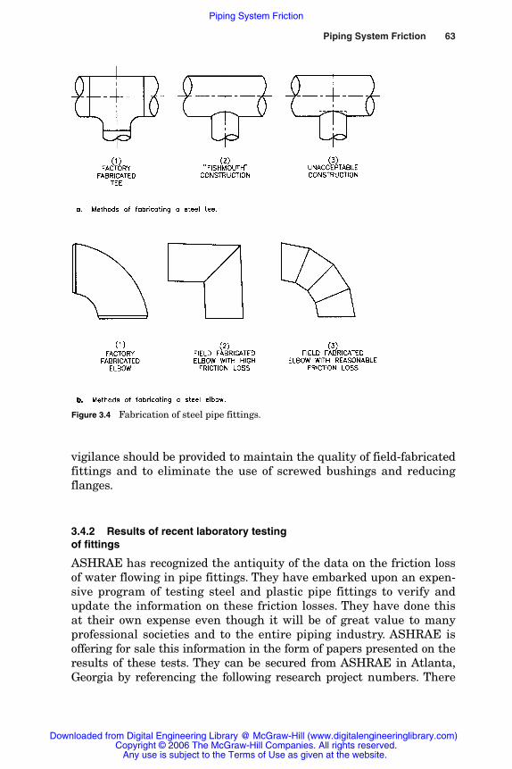
Piping System Friction 63
Figure 3.4 Fabrication of steel pipe fittings.
vigilance should be provided to maintain the quality of field-fabricatedfittings and to eliminate the use of screwed bushings and reducingflanges.
3.4.2 Results of recent laboratory testingof fittings
ASHRAE has recognized the antiquity of the data on the friction lossof water flowing in pipe fittings. They have embarked upon an expen-sive program of testing steel and plastic pipe fittings to verify andupdate the information on these friction losses. They have done thisat their own expense even though it will be of great value to manyprofessional societies and to the entire piping industry. ASHRAE isoffering for sale this information in the form of papers presented on theresults of these tests. They can be secured from ASHRAE in Atlanta,Georgia by referencing the following research project numbers. There
Rishel_CH03.qxd 20/4/06 5:35 PM Page 63
Piping System Friction
Downloaded from Digital Engineering Library @ McGraw-Hill (www.digitalengineeringlibrary.com)Copyright © 2006 The McGraw-Hill Companies. All rights reserved.
Any use is subject to the Terms of Use as given at the website.
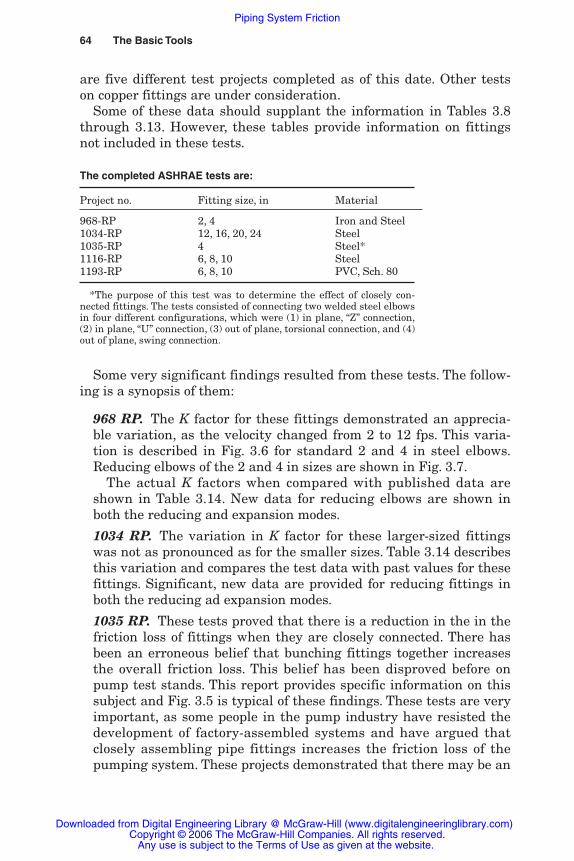
64 The Basic Tools
are five different test projects completed as of this date. Other testson copper fittings are under consideration.
Some of these data should supplant the information in Tables 3.8through 3.13. However, these tables provide information on fittingsnot included in these tests.
The completed ASHRAE tests are:
Project no. Fitting size, in Material
968-RP 2, 4 Iron and Steel1034-RP 12, 16, 20, 24 Steel1035-RP 4 Steel*1116-RP 6, 8, 10 Steel1193-RP 6, 8, 10 PVC, Sch. 80
*The purpose of this test was to determine the effect of closely con-nected fittings. The tests consisted of connecting two welded steel elbowsin four different configurations, which were (1) in plane, “Z” connection,(2) in plane, “U” connection, (3) out of plane, torsional connection, and (4)out of plane, swing connection.
Some very significant findings resulted from these tests. The follow-ing is a synopsis of them:
968 RP. The K factor for these fittings demonstrated an apprecia-ble variation, as the velocity changed from 2 to 12 fps. This varia-tion is described in Fig. 3.6 for standard 2 and 4 in steel elbows.Reducing elbows of the 2 and 4 in sizes are shown in Fig. 3.7.
The actual K factors when compared with published data areshown in Table 3.14. New data for reducing elbows are shown inboth the reducing and expansion modes.
1034 RP. The variation in K factor for these larger-sized fittingswas not as pronounced as for the smaller sizes. Table 3.14 describesthis variation and compares the test data with past values for thesefittings. Significant, new data are provided for reducing fittings inboth the reducing ad expansion modes.
1035 RP. These tests proved that there is a reduction in the in thefriction loss of fittings when they are closely connected. There hasbeen an erroneous belief that bunching fittings together increasesthe overall friction loss. This belief has been disproved before onpump test stands. This report provides specific information on thissubject and Fig. 3.5 is typical of these findings. These tests are veryimportant, as some people in the pump industry have resisted thedevelopment of factory-assembled systems and have argued thatclosely assembling pipe fittings increases the friction loss of thepumping system. These projects demonstrated that there may be an
Rishel_CH03.qxd 20/4/06 5:35 PM Page 64
Piping System Friction
Downloaded from Digital Engineering Library @ McGraw-Hill (www.digitalengineeringlibrary.com)Copyright © 2006 The McGraw-Hill Companies. All rights reserved.
Any use is subject to the Terms of Use as given at the website.

Piping System Friction 65
energy savings for factory assembled pumping systems by havingclosely connected pipe fittings.
1116 RP. These tests on 6, 8, and 10 in steel pipe fittings indicatethe same findings as those for 968 RP and 1034 RP, namely, thatthe K factors for them vary with the velocity of the water.
All of the above projects were for steel fittings. This significantnew fact that the K factor varies with the velocity of the water inthe fittings is shown in Fig. 3.6 and 3.7. Publication of tables simi-lar to 3.12 is needed for all pipe fittings to insure that the K factorsare accurate.
1193 RP. This project for plastic pipe fittings was quite significant,as this may be the first precise laboratory tests for such fittings.
Table 3.14 Data Summary of Test Data for Ells, Reducers, and Expansions
USU USU USU Past 4 fps 8 fps 12 fps
2′′ S.R. Ell (R/D = 1). Thread 0.60 to 1.0 (1.0)* 0.60 0.68 0.7364′′ S.R. Ell (R/D = 1) Weld 0.30 to 0.34 0.37 0.34 0.33
1′′ L.R. Ell (R/D = 1.5) Weld 0.39 to 1.0 ------ ------ ------2′′ L.R. Ell (R/D = 1.5) Weld 0.50 to 0.7 ------ ------ ------4′′ L.R. Ell (R/D = 1.5) Weld 0.22 to 0.33 (.22)* 0.26 0.24 0.236′′ L.R. Ell (R/D = 1.5) Weld 0.25 0.26 0.24 0.24†
8′′ L.R. Ell (R/D = 1.5) Weld 0.20 to 0.26 0.23 0.20 0.19†
10′′ L.R. Ell (R/D = 1.5) Weld 0.17 0.21 0.17 0.16†
12′′ L.R. Ell (R/D = 1.5) Weld 0.16 0.17 0.17 0.1716′′ L.R. Ell (R/D = 1.5) Weld 0.12 0.12 0.2 0.1120′′ L.R. Ell (R/D = 1.5) Weld 0.09 0.12 0.10 0.1024′′ L.R. Ell (R/D = 1.5) Weld 0.07 0.098 0.089 0.089
Reducer (2′′ × 1.5′′) Thread ------ 0.53 0.28 0.20Reducer (4′′ × 3′′) Weld 0.22 0.23 0.14 0.10Reducer (12′′ × 10′′) Weld ------ 0.14 0.14 0.14Reducer (16′′ × 12′′) Weld ------ 0.17 0.16 0.17Reducer (20′′ × 16′′) Weld ------ 0.16 0.13 0.13Reducer (24′′ × 20′′) Weld ------ 0.053 0.053 0.055
Expansion (1.5′′ × 2′′) Thread ------ 0.16 0.13 0.02Expansion (3′′ × 4′′) Weld ------ 0.11 0.11 0.11Expansion (10′′ × 12′′) Weld ------ 0.11 0.11 0.11Expansion (12′′ × 16′′) Weld ------ 0.073 0.076 0.073Expansion (16′′ × 20′′) Weld ------ 0.024 0.021 0.022Expansion (20′′ × 24′′) Weld ------ 0.020 0.023 0.020
NOTE: Past (published data by Freeman, Crane, Hydraulics Institute)USU (Utah Sate University Data)S.R. short radius or regular Ell; L.R. = long radius Ell( )* Data published in ASHRAE Fundamentals.†Data received from ASHRAE Research Project No. 1116 RP by University of Minnesota.SOURCE: Copyright 1999. American Society of Heating, Refrigerating and Air-Conditioning
Engineers, Inc. www.ashrae.org. Reprinted by permission from ASHRAE Transactions,Vol. 105, Part 1.
Rishel_CH03.qxd 20/4/06 5:35 PM Page 65
Piping System Friction
Downloaded from Digital Engineering Library @ McGraw-Hill (www.digitalengineeringlibrary.com)Copyright © 2006 The McGraw-Hill Companies. All rights reserved.
Any use is subject to the Terms of Use as given at the website.
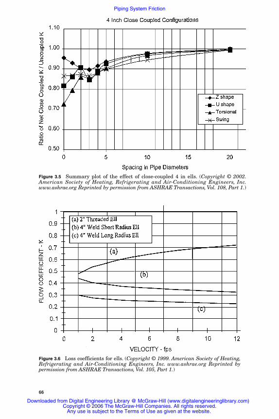
66
Figure 3.5 Summary plot of the effect of close-coupled 4 in ells. (Copyright © 2002.American Society of Heating, Refrigerating and Air-Conditioning Engineers, Inc.www.ashrae.org Reprinted by permission from ASHRAE Transactions, Vol. 108, Part 1.)
Figure 3.6 Loss coefficients for ells. (Copyright © 1999. American Society of Heating,Refrigerating and Air-Conditioning Engineers, Inc. www.ashrae.org Reprinted bypermission from ASHRAE Transactions, Vol. 105, Part 1.)
Rishel_CH03.qxd 20/4/06 5:35 PM Page 66
Piping System Friction
Downloaded from Digital Engineering Library @ McGraw-Hill (www.digitalengineeringlibrary.com)Copyright © 2006 The McGraw-Hill Companies. All rights reserved.
Any use is subject to the Terms of Use as given at the website.
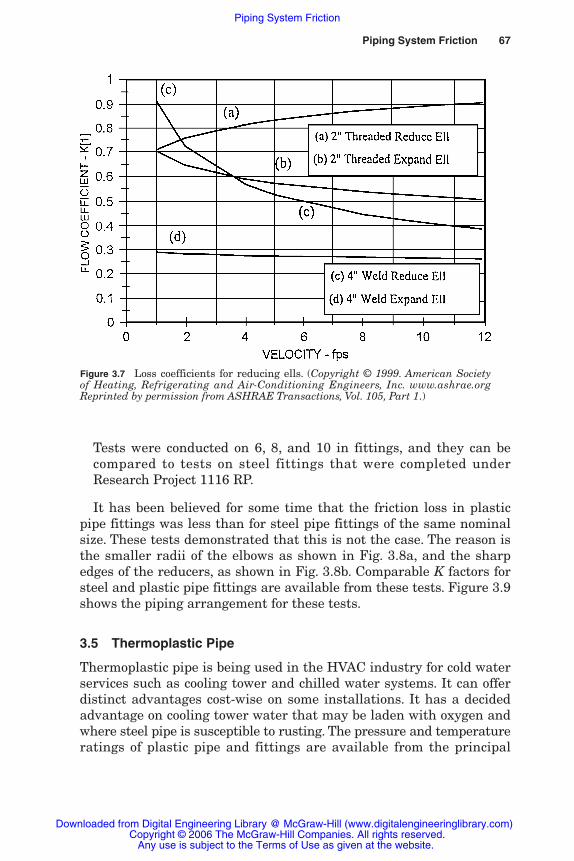
Piping System Friction 67
Tests were conducted on 6, 8, and 10 in fittings, and they can becompared to tests on steel fittings that were completed underResearch Project 1116 RP.
It has been believed for some time that the friction loss in plasticpipe fittings was less than for steel pipe fittings of the same nominalsize. These tests demonstrated that this is not the case. The reason isthe smaller radii of the elbows as shown in Fig. 3.8a, and the sharpedges of the reducers, as shown in Fig. 3.8b. Comparable K factors forsteel and plastic pipe fittings are available from these tests. Figure 3.9shows the piping arrangement for these tests.
3.5 Thermoplastic Pipe
Thermoplastic pipe is being used in the HVAC industry for cold waterservices such as cooling tower and chilled water systems. It can offerdistinct advantages cost-wise on some installations. It has a decidedadvantage on cooling tower water that may be laden with oxygen andwhere steel pipe is susceptible to rusting. The pressure and temperatureratings of plastic pipe and fittings are available from the principal
Figure 3.7 Loss coefficients for reducing ells. (Copyright © 1999. American Societyof Heating, Refrigerating and Air-Conditioning Engineers, Inc. www.ashrae.orgReprinted by permission from ASHRAE Transactions, Vol. 105, Part 1.)
Rishel_CH03.qxd 20/4/06 5:35 PM Page 67
Piping System Friction
Downloaded from Digital Engineering Library @ McGraw-Hill (www.digitalengineeringlibrary.com)Copyright © 2006 The McGraw-Hill Companies. All rights reserved.
Any use is subject to the Terms of Use as given at the website.
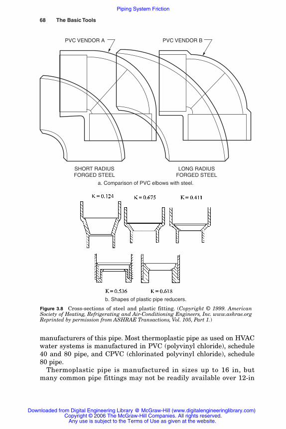
68 The Basic Tools
SHORT RADIUSFORGED STEEL
LONG RADIUSFORGED STEEL
PVC VENDOR A PVC VENDOR B
a. Comparison of PVC elbows with steel.
b. Shapes of plastic pipe reducers.
Figure 3.8 Cross-sections of steel and plastic fitting. (Copyright © 1999. AmericanSociety of Heating, Refrigerating and Air-Conditioning Engineers, Inc. www.ashrae.orgReprinted by permission from ASHRAE Transactions, Vol. 105, Part 1.)
manufacturers of this pipe. Most thermoplastic pipe as used on HVACwater systems is manufactured in PVC (polyvinyl chloride), schedule40 and 80 pipe, and CPVC (chlorinated polyvinyl chloride), schedule80 pipe.
Thermoplastic pipe is manufactured in sizes up to 16 in, butmany common pipe fittings may not be readily available over 12-in
Rishel_CH03.qxd 20/4/06 5:35 PM Page 68
Piping System Friction
Downloaded from Digital Engineering Library @ McGraw-Hill (www.digitalengineeringlibrary.com)Copyright © 2006 The McGraw-Hill Companies. All rights reserved.
Any use is subject to the Terms of Use as given at the website.
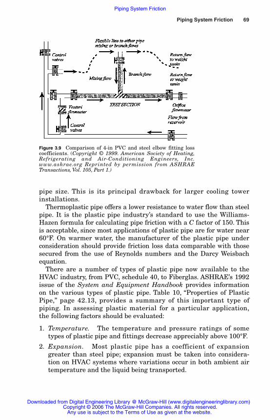
Piping System Friction 69
Figure 3.9 Comparison of 4-in PVC and steel elbow fitting losscoefficients. (Copyright © 1999. American Society of Heating,Refrigerating and Air-Conditioning Engineers, Inc.www.ashrae.org Reprinted by permission from ASHRAETransactions, Vol. 105, Part 1.)
pipe size. This is its principal drawback for larger cooling towerinstallations.
Thermoplastic pipe offers a lower resistance to water flow than steelpipe. It is the plastic pipe industry’s standard to use the Williams-Hazen formula for calculating pipe friction with a C factor of 150. Thisis acceptable, since most applications of plastic pipe are for water near60°F. On warmer water, the manufacturer of the plastic pipe underconsideration should provide friction loss data comparable with thosesecured from the use of Reynolds numbers and the Darcy Weisbachequation.
There are a number of types of plastic pipe now available to theHVAC industry, from PVC, schedule 40, to Fiberglas. ASHRAE’s 1992issue of the System and Equipment Handbook provides informationon the various types of plastic pipe. Table 10, “Properties of PlasticPipe,” page 42.13, provides a summary of this important type ofpiping. In assessing plastic material for a particular application,the following factors should be evaluated:
1. Temperature. The temperature and pressure ratings of sometypes of plastic pipe and fittings decrease appreciably above 100°F.
2. Expansion. Most plastic pipe has a coefficient of expansiongreater than steel pipe; expansion must be taken into considera-tion on HVAC systems where variations occur in both ambient airtemperature and the liquid being transported.
Rishel_CH03.qxd 20/4/06 5:35 PM Page 69
Piping System Friction
Downloaded from Digital Engineering Library @ McGraw-Hill (www.digitalengineeringlibrary.com)Copyright © 2006 The McGraw-Hill Companies. All rights reserved.
Any use is subject to the Terms of Use as given at the website.

3. Hydraulic shock. Plastic pipe does not have the withstandabilityof steel pipe. The actual configuration of the plastic pipe installa-tion, including methods of support, should be approved by themanufacturer of the plastic pipe.
4. Maximum allowable velocity. Table 3.2 outlines maximum veloci-ties for steel pipe. These velocities are excessive for most types ofplastic pipe. Actual maximum velocities under consideration for aspecific installation of plastic pipe should be approved by the man-ufacturer of the plastic pipe.
Most manufacturers of plastic pipe have very good application man-uals that provide most of the answers to the preceding installationvariables.
3.5.1 Types of plastic pipe used in HVAC
Following is information on the some of the more common plastic pipeused in HVAC water systems:
PVC. Polyvinyl chloride pipe: ASTM D-1784 Class 12454-B
CPVC. Chlorinated polyvinyl chloride pipe: ASTM D-1784 Class23447-B
PVC pipe has been the preferred plastic pipe for HVAC water sys-tems for many years. For installations operating at higher tempera-tures, CPVC has provided an excellent material for piping. Thepressure-temperature relationships for these types of plastic pipe areprovided in Table 3.15.
70 The Basic Tools
TABLE 3.15 Maximum OperatingPressure (psig) versus Temperature (°F)
Operating temperature PVC CPVC
Up to 100 150 150110 135 140120 110 130130 75 120140 50 110150 N.R. 100160 N.R. 90170 N.R. 80180 N.R. 70190 N.R. 60200 N.R. 50
Rishel_CH03.qxd 20/4/06 5:35 PM Page 70
Piping System Friction
Downloaded from Digital Engineering Library @ McGraw-Hill (www.digitalengineeringlibrary.com)Copyright © 2006 The McGraw-Hill Companies. All rights reserved.
Any use is subject to the Terms of Use as given at the website.

Hydraulic shock and ambient temperature are factors that must beconsidered with plastic pipe; greater care must be exerted with plasticpipe than while designing with steel pipe of equivalent sizes.
Like other types of piping, the inside diameter of the pipe underconsideration must be checked before consulting a pipe friction table.Table 3.16 provides the inside pipe diameters for the Schedules 40and 80 PVC and CPVC pipe. Friction losses for Schedule 40 PVC andCPVC pipe can be determined from Fig. 3.10 and Schedule 80 PVCand CPVC pipe from Fig. 3.11.
3.6 Copper Pipe and Tubing
Copper pipe is not used extensively in HVAC systems like steel pipe.It is of value on HVAC equipment assemblies, and tables for frictionof water in it up to 2 in size are included in Table 3.17. The frictionlosses in copper fittings should be evaluated as has been done forplastic pipe; ASHRAE has under consideration the testing of theflow of water in the smaller copper fittings. Questions about frictionof refrigerant flow in copper pipe should be referred to the refriger-ant manufacturers.
3.7 Glycol Solutions
Few special liquids are used in the HVAC industry, but both ethyleneglycol and propylene glycol are found in these water systems. Thefriction for ethylene glycol–based, heat transfer solutions can be com-puted using Fig. 2.4, which shows the variation in viscosity for vari-ous temperatures and percent of solution. Once the viscosity isknown, the Reynolds number can be determined, and then the f fac-tor can be computed for the Darcy Weisbach equation. The pump
Piping System Friction 71
TABLE 3.16 PVC and CPVC Plastic Pipe: Inside Diameters (in)
Schedule 40 Schedule 801⁄2 − 0.622 3 − 3.068 1⁄2 − 0.546 3 − 2.9003⁄4 − 0.824 4 − 4.026 3⁄4 − 0.742 4 − 3.8261 − 1.049 6 − 6.065 1 − 0.957 6 − 5.761
11⁄4 − 1.380 8 − 7.981 11⁄4 − 1.278 8 − 7.62511⁄2 − 1.610 10 − 10.020 11⁄2 − 1.500 10 − 9.564
2 − 2.067 12 − 11.938 2 − 1.939 12 − 11.37621⁄2 − 2.469 14 − 13.124 21⁄2 − 2.323 14 − 12.500
16 − 15.000 16 − 14.314
Rishel_CH03.qxd 20/4/06 5:35 PM Page 71
Piping System Friction
Downloaded from Digital Engineering Library @ McGraw-Hill (www.digitalengineeringlibrary.com)Copyright © 2006 The McGraw-Hill Companies. All rights reserved.
Any use is subject to the Terms of Use as given at the website.
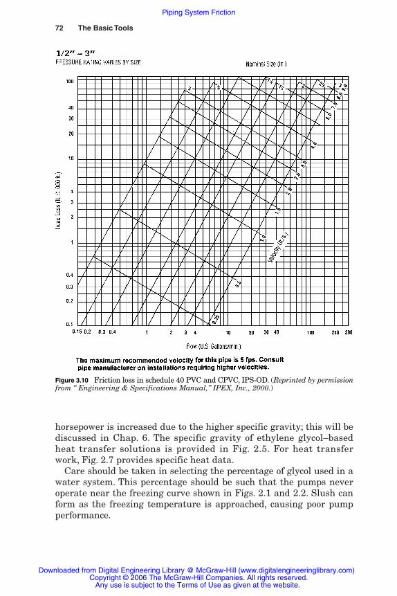
horsepower is increased due to the higher specific gravity; this will bediscussed in Chap. 6. The specific gravity of ethylene glycol–basedheat transfer solutions is provided in Fig. 2.5. For heat transferwork, Fig. 2.7 provides specific heat data.
Care should be taken in selecting the percentage of glycol used in awater system. This percentage should be such that the pumps neveroperate near the freezing curve shown in Figs. 2.1 and 2.2. Slush canform as the freezing temperature is approached, causing poor pumpperformance.
72 The Basic Tools
Figure 3.10 Friction loss in schedule 40 PVC and CPVC, IPS-OD. (Reprinted by permissionfrom “ Engineering & Specifications Manual,” IPEX, Inc., 2000.)
Rishel_CH03.qxd 20/4/06 5:35 PM Page 72
Piping System Friction
Downloaded from Digital Engineering Library @ McGraw-Hill (www.digitalengineeringlibrary.com)Copyright © 2006 The McGraw-Hill Companies. All rights reserved.
Any use is subject to the Terms of Use as given at the website.
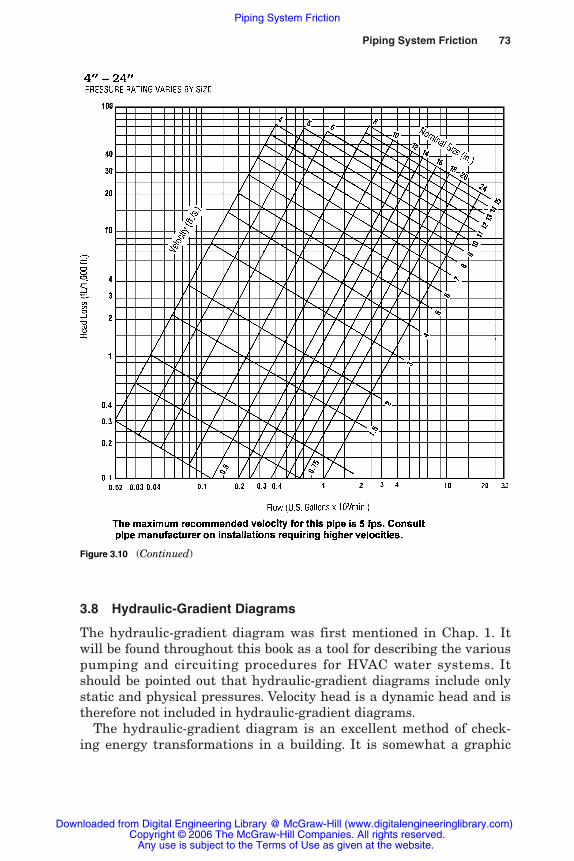
3.8 Hydraulic-Gradient Diagrams
The hydraulic-gradient diagram was first mentioned in Chap. 1. Itwill be found throughout this book as a tool for describing the variouspumping and circuiting procedures for HVAC water systems. Itshould be pointed out that hydraulic-gradient diagrams include onlystatic and physical pressures. Velocity head is a dynamic head and istherefore not included in hydraulic-gradient diagrams.
The hydraulic-gradient diagram is an excellent method of check-ing energy transformations in a building. It is somewhat a graphic
Piping System Friction 73
Figure 3.10 (Continued)
Rishel_CH03.qxd 20/4/06 5:35 PM Page 73
Piping System Friction
Downloaded from Digital Engineering Library @ McGraw-Hill (www.digitalengineeringlibrary.com)Copyright © 2006 The McGraw-Hill Companies. All rights reserved.
Any use is subject to the Terms of Use as given at the website.

representation of Bernoulli’s theorem. The vertical dimension of thesediagrams is to scale and is shown normally in feet of head (see Eq. 4.1for computing feet of head from known pressures and temperatures).The horizontal dimension is not to scale and is used to separate thespecific changes in static and friction losses in various parts of thesystem.
Pump head is usually shown vertically upward, while friction lossescan be shown vertically downward or diagonally. Computer programsare now being evaluated to facilitate the development of diagramssimilar to those shown here.
74 The Basic Tools
Figure 3.11 Friction loss in schedule 80 PVC and CPVC, IPS-OD. (Reprinted by permis-sion from “Engineering & Specifications Manual,” IPEX, Inc., 2000.)
Rishel_CH03.qxd 20/4/06 5:35 PM Page 74
Piping System Friction
Downloaded from Digital Engineering Library @ McGraw-Hill (www.digitalengineeringlibrary.com)Copyright © 2006 The McGraw-Hill Companies. All rights reserved.
Any use is subject to the Terms of Use as given at the website.
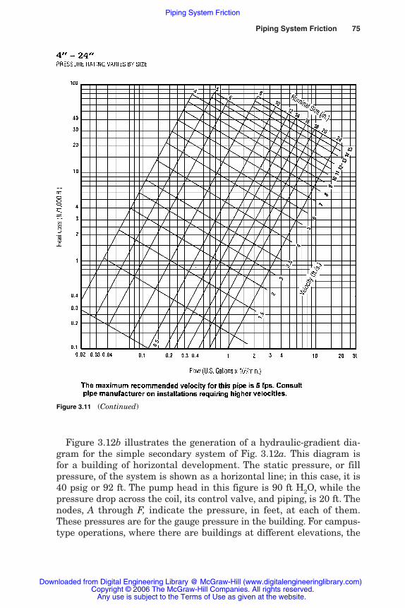
Figure 3.12b illustrates the generation of a hydraulic-gradient dia-gram for the simple secondary system of Fig. 3.12a. This diagram isfor a building of horizontal development. The static pressure, or fillpressure, of the system is shown as a horizontal line; in this case, it is40 psig or 92 ft. The pump head in this figure is 90 ft H2O, while thepressure drop across the coil, its control valve, and piping, is 20 ft. Thenodes, A through F, indicate the pressure, in feet, at each of them.These pressures are for the gauge pressure in the building. For campus-type operations, where there are buildings at different elevations, the
Piping System Friction 75
Figure 3.11 (Continued)
Rishel_CH03.qxd 20/4/06 5:35 PM Page 75
Piping System Friction
Downloaded from Digital Engineering Library @ McGraw-Hill (www.digitalengineeringlibrary.com)Copyright © 2006 The McGraw-Hill Companies. All rights reserved.
Any use is subject to the Terms of Use as given at the website.
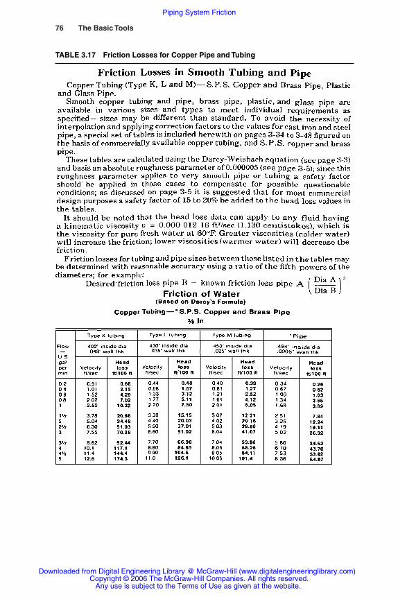
76 The Basic Tools
TABLE 3.17 Friction Losses for Copper Pipe and Tubing
Rishel_CH03.qxd 20/4/06 5:35 PM Page 76
Piping System Friction
Downloaded from Digital Engineering Library @ McGraw-Hill (www.digitalengineeringlibrary.com)Copyright © 2006 The McGraw-Hill Companies. All rights reserved.
Any use is subject to the Terms of Use as given at the website.

Piping System Friction 77
TABLE 3.17 Friction Losses for Copper Pipe and Tubing
Rishel_CH03.qxd 20/4/06 5:35 PM Page 77
Piping System Friction
Downloaded from Digital Engineering Library @ McGraw-Hill (www.digitalengineeringlibrary.com)Copyright © 2006 The McGraw-Hill Companies. All rights reserved.
Any use is subject to the Terms of Use as given at the website.
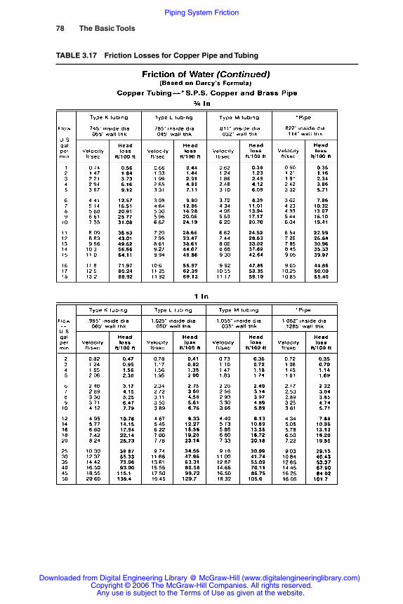
78 The Basic Tools
TABLE 3.17 Friction Losses for Copper Pipe and Tubing
Rishel_CH03.qxd 20/4/06 5:35 PM Page 78
Piping System Friction
Downloaded from Digital Engineering Library @ McGraw-Hill (www.digitalengineeringlibrary.com)Copyright © 2006 The McGraw-Hill Companies. All rights reserved.
Any use is subject to the Terms of Use as given at the website.
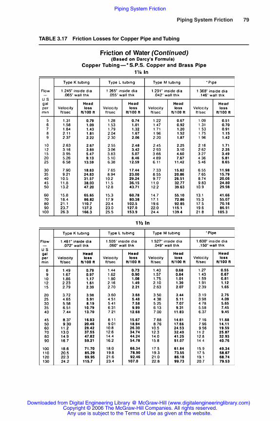
Piping System Friction 79
TABLE 3.17 Friction Losses for Copper Pipe and Tubing
Rishel_CH03.qxd 20/4/06 5:35 PM Page 79
Piping System Friction
Downloaded from Digital Engineering Library @ McGraw-Hill (www.digitalengineeringlibrary.com)Copyright © 2006 The McGraw-Hill Companies. All rights reserved.
Any use is subject to the Terms of Use as given at the website.

80 The Basic Tools
TABLE 3.17 Friction Losses for Copper Pipe and Tubing
Rishel_CH03.qxd 20/4/06 5:35 PM Page 80
Piping System Friction
Downloaded from Digital Engineering Library @ McGraw-Hill (www.digitalengineeringlibrary.com)Copyright © 2006 The McGraw-Hill Companies. All rights reserved.
Any use is subject to the Terms of Use as given at the website.
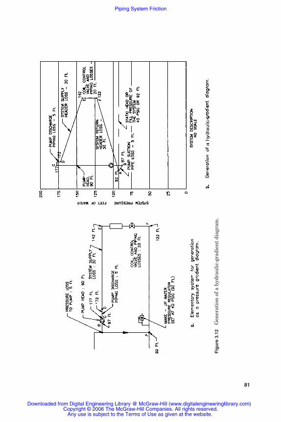
81
Fig
ure
3.1
2G
ener
atio
n o
f a
hyd
rau
lic-
grad
ien
t di
agra
m.
Rishel_CH03.qxd 20/4/06 5:35 PM Page 81
Piping System Friction
Downloaded from Digital Engineering Library @ McGraw-Hill (www.digitalengineeringlibrary.com)Copyright © 2006 The McGraw-Hill Companies. All rights reserved.
Any use is subject to the Terms of Use as given at the website.
82 The Basic Tools
nodes must indicate elevations above sea level to demonstrate changesin static pressure.
Typical buildings with their hydraulic-gradient diagrams areshown in Figs. 3.13 and 3.14 for both horizontal and verticaldevelopments. A very important use of the hydraulic gradient isdemonstrated in Fig. 3.14. Note that the circulating pump is locatedon the discharge of the generator; this reduces the pressure on thegenerator. If the pump were located on the inlet to the generator, itwould have to withstand 160 psig of pressure. If the generator were achiller, it might require high-pressure water boxes.
The hydraulic-gradient diagram should be developed with no flowon the building with the pumps running at shutoff head or no-flowcondition. This condition provides the maximum possible head on thesystem. The second condition for the pressure-gradient diagramshould be at the full flow or design situation for the system. The max-imum pressure for the system can be computed easily by addingthe pump shutoff head to the operating pressure of the building. InFig. 3.14b, if the water system is 231 ft high from the highest point tothe lowest point and the desired minimum pressure is 10 lb/in2 at thehighest point, the operating pressure is 231 divided by 2.31 � 10, or110 psig. If the pump shutoff head (no-flow condition) is 115 ft or 50psig, the maximum pressure that can be exerted on any part of thebuilding is 110 � 50, or 160 psig. It is important that this zero-flowcondition be computed to secure the maximum possible pressure thatcan be exerted on a water system. Just because a pump is variable-speed does not mean that this calculation should not be made. If thevariable-speed pump controls fail, the pump could be operated atmaximum speed.
Examples of the hydraulic-gradient diagram will be includedthroughout this book. It is a very useful tool for calculating operatingpressures, as well as in determining system overpressure that mayoccur due to incorrect piping or pumping design. The overpressureindicated by the hydraulic-gradient diagram demonstrates energy-saving possibilities that can be achieved by revision of the pumps orpiping.
3.9 Piping Network Analyses
Multibuilding or multizone installations create friction analysis prob-lems due to the various flow rates that can occur in parallel and seriespiping loops. Special software has been developed to compute the fric-tion for such complex chilled or hot water systems. This software isnow available for use on personal computers. Calculation of friction
Rishel_CH03.qxd 20/4/06 5:35 PM Page 82
Piping System Friction
Downloaded from Digital Engineering Library @ McGraw-Hill (www.digitalengineeringlibrary.com)Copyright © 2006 The McGraw-Hill Companies. All rights reserved.
Any use is subject to the Terms of Use as given at the website.

Piping System Friction 83
Figure 3.13 Hydraulic-gradient diagram for a horizontal building.
Rishel_CH03.qxd 21/4/06 6:08 PM Page 83
Piping System Friction
Downloaded from Digital Engineering Library @ McGraw-Hill (www.digitalengineeringlibrary.com)Copyright © 2006 The McGraw-Hill Companies. All rights reserved.
Any use is subject to the Terms of Use as given at the website.

84
Fig
ure
3.1
4H
VA
C s
yste
m f
or a
ver
tica
l bu
ildi
ng.
(Fro
m:P
atte
rson
Pu
mp
Com
pan
y H
VA
C P
um
ps a
nd
Sys
tem
s M
anu
al,2
004.
)
Chi
ller
CED
C
Chi
ller
FGA
B
OP
23'
43'C
oil n
o.1
Exp
ansi
on ta
nk,
10 p
sig
Coi
ls
Chi
ller
bypa
ssw
ith a
utom
atic
cont
rol v
alve
.
Two-
way
con
trol
valv
es
Var
iabl
e sp
eed
prim
ary
pum
ps o
nch
iller
dis
char
ge
a. V
ertic
al b
uild
ing
deve
lopm
ent
Pum
p di
scha
rge
fittin
gs
Pum
p he
ad
Chi
ller
loss
D 258
338'
342
262
C
Pum
p su
ctio
nfit
tings
Oth
er c
oils
E F G 43
23
Coi
l #1 E
xpan
sion
tank
pre
ssur
e23
ft. (
10 p
sig)
0A50B
100
150
200
250
278
300
350
400
Pum
p sh
ut-o
ff he
ad36
5 F
7. (
158
psig
)
System head - ft.
b. H
ydra
ulic
gra
dien
t ver
tical
dev
elop
men
t
Rishel_CH03.qxd 20/4/06 5:35 PM Page 84
Piping System Friction
Downloaded from Digital Engineering Library @ McGraw-Hill (www.digitalengineeringlibrary.com)Copyright © 2006 The McGraw-Hill Companies. All rights reserved.
Any use is subject to the Terms of Use as given at the website.

85
P-4
P-5
P-6
P-1
7
P-1
6
P-2
0
P-1
9P
-11
P-1
0
P-1
8
P-1
3P
-12
P-1
5
P-1
4
J-3
Cle
ar W
ell R
-1
R-1
P-9
P-8
P-1
P-3
: 193
' LO
NG
P-2
1: 2
91' L
ON
G
PU
MP
Fig
ure
3.1
5S
yste
m a
rran
gem
ent
for
net
wor
kin
g.(C
ourt
esy
of U
niv
ersi
ty o
f K
entu
cky,
Dep
artm
ent
of E
ngi
nee
rin
g.)
Rishel_CH03.qxd 20/4/06 5:35 PM Page 85
Piping System Friction
Downloaded from Digital Engineering Library @ McGraw-Hill (www.digitalengineeringlibrary.com)Copyright © 2006 The McGraw-Hill Companies. All rights reserved.
Any use is subject to the Terms of Use as given at the website.

for piping networks was originated in the municipal water field; typi-cal of this was the Hardy Cross method developed by Hardy Cross atthe University of Illinois in 1936. Development of such software forcontemporary computers has been completed by several universitiesand software companies. An example of this software is that producedby Donald Wood and James Funk at the University of Kentucky. Thissoftware is known as KYPIPE Hydraulic Modeling Software.
Figure 3.15 provides a typical application of this procedure.Although this figure is for municipal water distribution, a chilledwater distribution for a campus type installation is similar. The sys-tem is divided into nodes, and the friction loss is computed for eachsegment of pipe between nodes. A number of simulations are madefor various loads on the system so that the maximum possible fric-tion loss can be ascertained for design of the chilled water pumps.Table 3.18 provides the data for one of a number of simulations. Thisprocedure can be helpful in determining the type of chilled waterpumping system that should be used to achieve minimum energyconsumption.
86 The Basic Tools
TABLE 3.18 Tabulated Computer Results for Simulation No. 2
External Hydraulic Note Pressure Node Node Node demand grade elevation head pressurename title (gpm) (ft) (ft) (ft) (psi)
J-1 9.00 748.10 607.00 141.10 61.14J-10 15.00 745.98 611.00 134.98 58.49J-11 45.00 745.31 610.00 135.31 58.64J-12 0.00 748.22 610.00 138.22 59.90J-13 60.00 745.58 630.00 115.58 50.08J-14 0.00 746.37 610.00 136.37 59.09J-15 0.00 748.16 605.00 143.16 62.03J-16 0.00 748.19 605.00 143.19 62.05J-2 75.00 744.24 617.00 127.24 55.14J-3 0.00 748.18 605.00 143.18 62.04J-4 0.00 746.37 602.00 144.37 62.56J-5 45.00 746.01 613.00 133.01 57.64J-6 21.00 746.48 611.00 135.48 58.71J-7 0.00 746.07 613.00 133.07 57.66J-8 18.00 746.88 611.00 135.88 58.88J-9 30.00 746.53 615.00 131.53 56.99Pump-1 0.00 610.00 610.00 0.00 0.00R-1 –– 610.00 605.00 5.00 2.17T-1 –– 750.00 630.00 120.00 52.00T-2 –– 749.00 625.00 124.00 53.73Pump-1 0.00 748.18 610.00 138.18 59.88
Rishel_CH03.qxd 20/4/06 5:35 PM Page 86
Piping System Friction
Downloaded from Digital Engineering Library @ McGraw-Hill (www.digitalengineeringlibrary.com)Copyright © 2006 The McGraw-Hill Companies. All rights reserved.
Any use is subject to the Terms of Use as given at the website.

3.10 Summary
Care in determining pipe friction for a prospective HVAC water sys-tem cannot be overemphasized! There are so many systems in opera-tion where too much pump head has been applied, and this excesshead is destroyed by balance valves and pressure-reducing valves.System efficiency is described in Chap. 8; it emphasizes the need forcare in computing pipe friction and in the avoidance of piping acces-sories that waste pumping energy.
3.11 Bibliography
Cameron Hydraulic Data, 15th ed., Ingersoll Rand, Woodcliff, N.J., 1977.Engineering Data Book, 2d ed., Hydraulic Institute, Parsippany, N.J., 1990.Mohinder, L. Nayyar, Piping Handbook, 6th ed., McGraw-Hill, New York, 1992.The Handbook of Steel Pipe, Bulletin AISI SP 229-884-15M-SP, American Iron and
Steel Institute, Washington, D.C., 1984.
Piping System Friction 87
Rishel_CH03.qxd 20/4/06 5:35 PM Page 87
Piping System Friction
Downloaded from Digital Engineering Library @ McGraw-Hill (www.digitalengineeringlibrary.com)Copyright © 2006 The McGraw-Hill Companies. All rights reserved.
Any use is subject to the Terms of Use as given at the website.

Rishel_CH03.qxd 20/4/06 5:35 PM Page 88
Piping System Friction
Downloaded from Digital Engineering Library @ McGraw-Hill (www.digitalengineeringlibrary.com)Copyright © 2006 The McGraw-Hill Companies. All rights reserved.
Any use is subject to the Terms of Use as given at the website.

HVAC Pumps and Their Performance
Part
2
Rishel_CH04.qxd 20/4/06 6:01 PM Page 89
Downloaded from Digital Engineering Library @ McGraw-Hill (www.digitalengineeringlibrary.com)Copyright © 2006 The McGraw-Hill Companies. All rights reserved.
Any use is subject to the Terms of Use as given at the website.
Source: HVAC Pump Handbook

Rishel_CH04.qxd 20/4/06 6:01 PM Page 90
Downloaded from Digital Engineering Library @ McGraw-Hill (www.digitalengineeringlibrary.com)Copyright © 2006 The McGraw-Hill Companies. All rights reserved.
Any use is subject to the Terms of Use as given at the website.
HVAC Pumps and Their Performance

Chapter
91
4Basics of Pump Design
4.1 Introduction
A pump is a wheel rotating on stick. Some wheel; some stick! So muchhas been written on pumps, but often this material had to be in tech-nical terms that made it difficult for the HVAC designer to under-stand how a pump functions. It is the intent of this Handbook to pre-sent pumps so that it is easy for the HVAC water system designer oroperator to understand their operation. This can be done becausemost HVAC systems use water, not hydrocarbons or other liquidswith broad ranges of viscosity and specific gravity. Several chaptersare devoted to pumps to clarify (1) the basics of pump design, (2) thepump’s physical arrangement, (3) pump performance, (4) motors anddrives for pumps, and finally, (5) applying pumps to HVAC systems.
The centrifugal pump creates pressure on a water stream that can beused to move that water through a system of piping and equipment. Theamount of pressure that the pump can create depends on the flowthrough it. Its fundamental performance curve is called a head-capacitycurve and is described in Fig. 4.1a. The flow measured in gallons perminute, is plotted horizontally, while the head measured in feet, isplotted vertically. Pump head is always shown in feet of liquid ratherthan pounds of pressure. With head measured in feet, the pump curveis applicable to any liquid of any specific gravity. Only when calculatingthe brake horsepower of the pump does specific gravity become involved.
The feet of head per pound of pressure for any liquid is
� (4.1)144�
�
Feet of head H���Pounds of pressure
Rishel_CH04.qxd 20/4/06 6:01 PM Page 91
Downloaded from Digital Engineering Library @ McGraw-Hill (www.digitalengineeringlibrary.com)Copyright © 2006 The McGraw-Hill Companies. All rights reserved.
Any use is subject to the Terms of Use as given at the website.
Source: HVAC Pump Handbook

92 HVAC Pumps and Their Performance
Figure 4.1 Typical pump head-flow curves.
80
77
200
0
200150
10080
60
40
20
10
6
4
20
40
60
80
100
120
140
160
180
Pum
p he
ad—
FT
Pum
p he
ad—
FT
0 200 1600140012001000800600400
20%
30 40
50 60
70 74
80 82
84 85
86
85 84
82
77
69
59%
Not here
Pump efficiencies – % Pumps must operate here
Not here
10 20 40 60 80 100
200
400
800
1000
2000
3000
4000
5000
Pump flow—GPM
Pump flow—GPM
a. Typical pump head—flow curve for one pump size.
b. Family of pump head—flow curves.
Rishel_CH04.qxd 20/4/06 6:01 PM Page 92
Downloaded from Digital Engineering Library @ McGraw-Hill (www.digitalengineeringlibrary.com)Copyright © 2006 The McGraw-Hill Companies. All rights reserved.
Any use is subject to the Terms of Use as given at the website.
Basics of Pump DesignBasics of Pump Design
Basics of Pump Design 93
where � is the specific weight of the liquid in pounds per cubic foot. Forexample, from Table 2.3, water at 180°F has a specific weight of 60.57lb/ft3. Thus H, for 180°F water, is 144/60.57, or 2.38 ft/ lb of pressure.
The words pump duty are often used when describing a pump’s per-formance. Pump duty is usually defined as a certain flow in gallonsper minute at a specific head in feet. This is the point at which thepump has been selected for a particular application. Usually, thispoint is selected as closely as possible to the best efficiency of a pumpimpeller, which, for Fig. 4.1a, is 86 percent.
Other common terms that are encountered in the pump industry are:
1. Carry out or run-out. This means that the pump is operating at thefar right of its curve, where the efficiency is poor.
2. Shutoff head. This is the head produced by a pump when it is run-ning at the “no flow,” or zero capacity, point.
3. Churn. A pump is said to be in churn when it is operating at shut-off head or no flow.
4.2 Centrifugal Pump Impeller Design
Centrifugal pumps, as their name implies, depend on centrifugal forceto produce flow through the pumps. When an impeller rotates, thewater in the impeller rotates as well, so there are two forces acting onthat water, namely centrifugal and rotational. The impeller of thepump rotates in a body to utilize these forces which are imposed onthe water in the impeller. These forces are aided by the shaping of theimpeller to produce the correct passages in the impeller that will usethis centrifugal force as well as the rotating velocity of the water inthe impeller. Internal vanes are designed into the impeller that directthe flow through and out of the impeller. The relatively high efficien-cy of HVAC pumps, up to 90 percent, is due to the fact that the pumpdesigner can design these vanes for maximum efficiency without con-cern for dirty or stringy material and without consideration forcorrosive or erosive liquids. Figure 4.2a illustrates a cross section of acentrifugal pump impeller with vanes that direct the water throughthe impeller.
This figure provides the basic vector diagram for a centrifugalpump. It describes the forces imparted on a molecule of water leavingthe impeller. W2 is the centrifugal force and V2 is the rotational forcedeveloped by the rotating energy of the impeller. These two forces pro-duce the pump head and flow. The net force acting on the water is thevector diagram for these two forces. The vector diagram that the pump
Rishel_CH04.qxd 20/4/06 6:01 PM Page 93
Downloaded from Digital Engineering Library @ McGraw-Hill (www.digitalengineeringlibrary.com)Copyright © 2006 The McGraw-Hill Companies. All rights reserved.
Any use is subject to the Terms of Use as given at the website.
Basics of Pump Design

94 HVAC Pumps and Their Performance
Figure 4.2 Basic centrifugal pump configurations.
designer works with during the actual design of an efficient impeller ismuch more complicated, since it must take into consideration entrancelosses and other factors such as friction losses inside the impeller. Thenet angle of this vector diagram is the angle at which the water leavesthe impeller and is particularly important to the pump designer becauseit plays a great part in determining the efficiency of a pump. Figure 4.3describes all of the vector diagrams that must be evaluated by the pumpdesigner.
Rishel_CH04.qxd 20/4/06 6:01 PM Page 94
Downloaded from Digital Engineering Library @ McGraw-Hill (www.digitalengineeringlibrary.com)Copyright © 2006 The McGraw-Hill Companies. All rights reserved.
Any use is subject to the Terms of Use as given at the website.
Basics of Pump Design

Basics of Pump Design 95
Inspection of an HVAC centrifugal pump impeller will reveal slots onthe periphery of the impeller. These slots are narrow for low-capacitypumps and wide for higher-capacity pumps. The angle of the vane asit reaches the periphery of the impeller reveals the angle that thepump designer has selected for the vector W2 (Fig. 4.2a).
Pumps are highly specialized devices designed for very particularapplications in order to achieve maximum efficiency and ease of use.HVAC pumps come under the broadest classification of centrifugalpumps—those for clear water service. Since corrosion and erosion arenot factors in this pump service, the designer can concentrate on firstcost, efficiency, and ease of operation and maintenance, the three dri-ving forces in any product design. Much work is done by the pumpdesigner in developing the internal passages of the impeller toachieve maximum, economical smoothness that will provide a mini-mum of friction to the water passing through the pump. Here lies asimple evaluation that can be made by any buyer of pumps. Howsmooth and how well are the internal passages of a pump impellerdeveloped? How uniform are the internal vanes and leaving ports ofthe impeller? How uniform and smooth are the vanes at the suction
Figure 4.3 Inlet and discharge vector diagrams. (From Karassik et al., PumpHandbook, 3d ed., McGraw-Hill, used with permission.)
Rishel_CH04.qxd 20/4/06 6:01 PM Page 95
Downloaded from Digital Engineering Library @ McGraw-Hill (www.digitalengineeringlibrary.com)Copyright © 2006 The McGraw-Hill Companies. All rights reserved.
Any use is subject to the Terms of Use as given at the website.
Basics of Pump Design

96 HVAC Pumps and Their Performance
port of the impeller? How smooth are the internal surfaces of thepump body, namely, the volute, or the bowl.
Figure 4.4 illustrates these points and describes the differencebetween a pump impeller with quality finish and one with poor finish.It is obvious which impeller will develop the highest pump efficiency.
Likewise, the quality of the volute or bowl will determine the pump’sefficiency. A critical point in a volute pump’s construction is at thetongue or cut water where water continues to the discharge connectionor is recirculated inside the pump; Figure 4.5 describes this. A poorlydefined or cast tongue will increase turbulence and loss of energy. Awell defined and cast tongue will improve pump performance. Oneongoing effort that must be made in pump manufacturing is mainte-nance of the patterns for the pump castings.
4.3 General Performance of a Centrifugal Pump
Figure 4.1a provides general performance of a centrifugal pump, aswell as typical hydraulic efficiencies for that pump. It should be notedthat this efficiency drops to zero at zero flow and then increases to apoint called the best efficiency point for the pump. As flow increases
Outside of impellerpolished
Vanes sharplydefined
Smooth interiorof impeller
a. Quality finish.
Outside of impellernot polished
Only hubsmachined
Vanes poorlydefined
Rough interiorof impeller
b. Poor finish.
Figure 4.4 Comparison of pump impellers.
Rishel_CH04.qxd 20/4/06 6:01 PM Page 96
Downloaded from Digital Engineering Library @ McGraw-Hill (www.digitalengineeringlibrary.com)Copyright © 2006 The McGraw-Hill Companies. All rights reserved.
Any use is subject to the Terms of Use as given at the website.
Basics of Pump Design

Basics of Pump Design 97
through the pump beyond this point, friction increases internally, andthe efficiency starts to fall again. The best efficiency point of a pumpwill be emphasized in many parts of this book. Every water systemdesigner should know where the best efficiency point occurs for eachof the pumps involved in an HVAC water system.
The pump designer develops a basic configuration of a pump impellerand then selects various pump impeller diameters and speeds to cre-ate the vector diagrams that will produce the flow-head relationshipsneeded for the broad application of that pump to HVAC water services.The capacity or flow range for a volute-type pump is determined bythe size of its discharge connection. Therefore, the pump designerworks with the vector diagrams and discharge connection areas to pro-duce a number of pumps that will cover this broad range of flows andheads. The result is a number of head-capacity curves, as shown inFig. 4.1b. This is often called a family of pump curves and provides aquick guide to the water system designer as to which size of pumpmay fit the needed flow and head for a particular application.
4.4 Sizing Centrifugal Pumps
As will be shown later, two types of centrifugal pumps are used inHVAC service, namely, volute and axial-flow pumps. Volute pump sizeis designated by the sizes of the suction and discharge connections, aswell as by the pump diameter. A typical sizing for such a pump would
Poorly definedor cast tongue
Turbulence withenergy loss
Smooth flow withlittle turbulence
Accurately definedand cast tongue
a. Poor construction. b. Quality construction.
Figure 4.5 Comparison of pump constructions.
Rishel_CH04.qxd 20/4/06 6:01 PM Page 97
Downloaded from Digital Engineering Library @ McGraw-Hill (www.digitalengineeringlibrary.com)Copyright © 2006 The McGraw-Hill Companies. All rights reserved.
Any use is subject to the Terms of Use as given at the website.
Basics of Pump Design

98 HVAC Pumps and Their Performance98 HVAC Pumps and Their Performance
be 6 in � 4 in � 8 in. This indicates that the pump has a 6-in diame-ter suction, a 4-in discharge, and an 8-in nominal size impeller. Theimpeller may have been trimmed to a specific diameter such as 73⁄4 into achieve the best efficiency at the specified flow and head. Manypump companies would call this a 4-in pump, since they use the dis-charge connection size to classify their pumps.
Axial-flow pump sizing is determined by the suction and dischargeconnections of the body or bowl. The suction and discharge connec-tions are almost always the same size. A 6-in suction and dischargewould indicate a 6-in pump or bowl.
4.5 Specific Speed of a Pump
The experienced pump designer uses a formula called specific speed Nsto develop a pump impeller for a specific range of flows and heads,knowing that a certain specific speed will produce the desirable ratiobetween pump head and pump capacity. This formula (Eq. 4.2) is of greatimportance to the designer but of little interest to the user of pumps.
Ns � �S
h
�
3
�/4
Q�� (4.2)
where S � pump speed, in rev/minQ � pump flow, in gal/minh � pump head, in ft
For example, assume that a pump has a capacity of 1500 gal/min at100 ft of head and is rotating at 1760 rev/min. Then,
Specific speed ��1750
10
�
0
�3/
1�4
5�0�0��� 2143
With the aid of this formula and a great amount of experience andtesting, the designer can develop the above-mentioned family of pumpcurves.
Most HVAC pumps are of moderate specific speed in the range of1000 to 5000; some large cooling tower pumps may have specific speedsas high as 8000. High-specific-speed pumps, as the preceding formulawould indicate, are high capacity with low head, while low-specific-speed pumps are high head with low capacity. Figure 4.6 describes thevariation of impeller types with specific speed. The high-head pumpswith low specific speed have narrow vanes indicating high head andlow flow. The high-specific-speed pumps have the shorter and widevanes for high delivery at low-pump heads.
Rishel_CH04.qxd 20/4/06 6:01 PM Page 98
Downloaded from Digital Engineering Library @ McGraw-Hill (www.digitalengineeringlibrary.com)Copyright © 2006 The McGraw-Hill Companies. All rights reserved.
Any use is subject to the Terms of Use as given at the website.
Basics of Pump Design

99
Fig
ure
4.6
Rel
atio
n o
f im
pell
er t
ypes
wit
h s
peci
fic
spee
d.(F
rom
Kar
assi
k et
al.
,P
um
p H
and
book
,3d
ed
.,M
cGra
w-H
ill,
use
d w
ith
pe
rmis
sion
.)
Rishel_CH04.qxd 20/4/06 6:01 PM Page 99
Downloaded from Digital Engineering Library @ McGraw-Hill (www.digitalengineeringlibrary.com)Copyright © 2006 The McGraw-Hill Companies. All rights reserved.
Any use is subject to the Terms of Use as given at the website.
Basics of Pump Design
4.6 Critical Speed of a Pump
Every rotating device has a natural frequency at which vibrationsbecome pronounced; the vibrations can increase until noise becomesobjectionable, and there is danger in a pump that the rotating equip-ment will become damaged. The speed at which this occurs is calledthe critical speed of that rotating element. Some pumps will actuallyhave more than one critical speed. Fortunately, for HVAC pumps, theimpeller diameters are relatively small and the rotational energy low.All pump designers must take critical speed into consideration in thestructural design of their pumps, but it is of little concern to theHVAC system designer in the selection of pumps.
The diameter or stiffness of the impeller shaft determines the criti-cal speed of a pump. Therefore, the pump designer ensures that thecritical speed of the pump is out of the normal range of pump opera-tion. If a pump has a normal operating range of up to 1800 rev/min,the pump designer will ensure that the critical speed of that pump isat some speed such as 2500 rev/min. Therefore, in most cases, criticalspeed of HVAC pumps is not part of the HVAC pump selection process.
4.7 Minimum Speed for a Variable-Speed Pump
Minimum speed for a variable-speed HVAC pump will be discussedhere, where information is also included on specific and criticalspeeds. There is no minimum speed for these HVAC pumps. Misinfor-mation about specific, critical, and minimum speeds for HVAC pumpshas caused misapplication of them along with the installation ofunnecessary speed controls. As will be reviewed in Chap. 6, variable-speed centrifugal pumps can be operated down to any speed requiredby the water system. Since they are variable-torque machines, verylittle energy is required to turn them at low speeds. Information onthis subject is included in Chap. 7 on pump drivers and drives as tothe minimum speed required by motors for their cooling.
The HVAC water system designer really has no need to be con-cerned with the specific, critical, or minimum speeds of these pumps.Only on extremely low speed operations where variable-speed pumpsare connected in series does the designer need to verify pump motorperformance with respect to heating.
4.8 Minimum Flow for HVAC Pumps
The question often arises as to the minimum flow that is requiredthrough a pump to prevent it from overheating. The following equa-tion provides this flow:
100 HVAC Pumps and Their Performance
Rishel_CH04.qxd 20/4/06 6:01 PM Page 100
Downloaded from Digital Engineering Library @ McGraw-Hill (www.digitalengineeringlibrary.com)Copyright © 2006 The McGraw-Hill Companies. All rights reserved.
Any use is subject to the Terms of Use as given at the website.
Basics of Pump Design

Minimum flow Qm �
� (4.3)
where pump bhp � brake horsepower of the pump near the shutoff orno-flow condition
�T � allowable rise in temperature in °F of the water� � specific weight of the water at the inlet water
temperature
The difficulty with this equation is getting the actual brake horse-power consumed by the pump at very low flows. Some pump compa-nies do publish pump brake horsepower curves down to zero flow.Other equations that use pump efficiency have the same problem,since the efficiency of a centrifugal pump approaches zero at very lowflows. If this information is not available, the pump company shouldprovide the minimum flow that will hold the temperature rise to thedesired maximum. The obvious advantage of the variable-speed pumpover the constant-speed pump appears here because there is muchless energy imparted to the water at minimum flows and speeds.
For most HVAC applications, there should not be temperature risesin a pump higher than 10°F. Do not bypass water to a pump suction!This continues to elevate the suction temperature. Bypass watershould be returned to a boiler feed system or deaerator on boiler feedsystems or to the cooling tower, boiler, or chiller on condenser, hot, orchilled water systems. Since it is desired to maintain supply tempera-ture in hot and chilled water mains, flow-control valves should belocated at the far ends of these mains to maintain their water tem-perature. Usually, the heat loss or heat gain for these mains requiresa flow that is greater than that required to maintain temperature inthe pump itself.
4.9 Two Types of Centrifugal Pumps forHVAC Service
As indicated earlier, there are two basic types of centrifugal pumps forHVAC water systems. These are volute and axial-flow pumps. Volutepumps are found in most of the low-flow applications, while axial-flowpumps are used in the very high volume or low-flow, high-head appli-cations. Chapter 5 will describe the various applications in detail.
317.2 � pump bhp���
�T � �
pump bhp � 2544��
�T � 60(�/7.48)
Basics of Pump Design 101
Rishel_CH04.qxd 20/4/06 6:01 PM Page 101
Downloaded from Digital Engineering Library @ McGraw-Hill (www.digitalengineeringlibrary.com)Copyright © 2006 The McGraw-Hill Companies. All rights reserved.
Any use is subject to the Terms of Use as given at the website.
Basics of Pump Design

4.9.1 Volute-type centrifugal pumps
The pump impeller produces the pump head, but it must be housed ina body that collects the water and delivers it to the system piping. Involute-type pumps, the body collects the water from the impeller andmoves it around to the pump discharge connection (Fig. 4.2b, c). Thisbody is called the volute. Unlike the axial-flow pump, normally, thereare no collecting vanes in the body or volute to aid the flow. The costof adding these volute vanes or diffusers would be prohibitive in volute-type pumps.
Most small HVAC centrifugal pumps are volute pumps, since thistype of pump lends itself to many different configurations that will bedescribed in Chap. 5. Larger volute pumps may be equipped withwhat is called a double volute (Fig. 4.2c). This pump has a second volutecast into its casing. Radial thrust on a pump shaft can be reduced bymeans of the double-volute construction. The second passage in thevolute should not be confused with the diffusers of axial-flow pumps.There is very little need for double-volute pumps in HVAC work, par-ticularly with variable-speed pumps, in which the radial thrust is verylow under most operating conditions. Radial thrust will be describedin detail in Chap. 6.
4.9.2 Axial-flow centrifugal pumps
Axial flow pumps are arranged to pass water through a body that iscalled a bowl. This bowl has suction and discharge ports and containsdiffuser vanes that aid the flow of water through the bowl. Because ofthe vanes, these pumps are often called diffuser pumps. Water flowsout uniformly 360 degrees around the impeller; Fig. 4.7 illustratesthis flow. The pump body or bowl vanes are similar to the impellervanes and they aid the diffusion of water out of the impeller into thebowl and then into the discharge pipe or another bowl.
4.10 Open or Closed Impellers
There are several types of impellers available for clear service (cleanwater): closed, semiopen, and open. Most of the impellers of pumps inthe HVAC industry are of the closed type. Closed-type impellers have ashroud and utilize case wear rings to impede bypassing. Other impellersare open type without shrouds or case wear rings. Usually, they arefound in larger axial-flow pumps. For most HVAC applications, theclosed impeller with case wear rings provides the highest efficiency;this efficiency is sustained longer due to the ability of the pump designerto develop the smallest possible clearance between the impeller and the
102 HVAC Pumps and Their Performance
Rishel_CH04.qxd 20/4/06 6:01 PM Page 102
Downloaded from Digital Engineering Library @ McGraw-Hill (www.digitalengineeringlibrary.com)Copyright © 2006 The McGraw-Hill Companies. All rights reserved.
Any use is subject to the Terms of Use as given at the website.
Basics of Pump Design

Basics of Pump Design 103
Figure 4.7 Cross-section of an axial flow bowl. (CourtesyPeerless Pumps.)
Rishel_CH04.qxd 20/4/06 6:01 PM Page 103
Downloaded from Digital Engineering Library @ McGraw-Hill (www.digitalengineeringlibrary.com)Copyright © 2006 The McGraw-Hill Companies. All rights reserved.
Any use is subject to the Terms of Use as given at the website.
Basics of Pump Design
case wear ring. This reduces the flow of water from the discharge areawith its higher pressure back to the suction connection with its lowerpressure. This unwanted water flow is called bypassing or suction recir-culation in the pump industry. Certified testing, which is discussedlater, proves the quality of the pump designer’s work and the pumpmanufacturing to produce the lowest amount of water bypassing at thecase rings and therefore the highest pump efficiency.
4.11 General Pump Design Information
This chapter offers some very preliminary information on pump design.The pump types used in the HVAC industry are very standard designsthat have been available for many years. Much has been done to securemaximum efficiency from these pumps. Like any other industry, thereare practices that reduce the quality of pump design and manufactur-ing. Poor casting and finishing of impellers and volutes as well aseliminating casing wear rings on some designs reduces the possibili-ties of sustained, high pump efficiencies.
There is considerable additional information available in the pumpindustry for the HVAC design engineer who desires to study pumpdesign further. Most of the pump manufacturers provide extensiveinformation on their pump designs. Hydraulic Institute maintainspump design and testing standards that are available to water sys-tem designers.
4.12 The Quality of HVAC Pumps
Over the years, the industrial and municipal pump industries havebeen derisive of HVAC pumps, calling them “throw-away” pumps.Such may have been the case in the past, but most of the pumps soldfor HVAC installations now are of a quality equal to those of otherindustries. Energy is of concern in this industry causing developmentof pumps equal in efficiency to other pumps. As in any pump applica-tion, concern should be made to ensure the quality of the pumps.
Figures 4.4 and 4.5 should be reviewed to discern the differencebetween quality and inferior pumps. A simple inspection of the pumpsuction can reveal the difference. Figure 4.8a provides how the qualityof an end-suction pump can be determined by inspecting its suction.The throat of the suction should transform smoothly to the internaldiameter of the impeller as shown in Fig. 4.8a. There should be noabrupt change from the throat to the internal diameter of the impelleras described in Fig. 4.8b. On large installations involving a number of
104 HVAC Pumps and Their Performance
Rishel_CH04.qxd 20/4/06 6:01 PM Page 104
Downloaded from Digital Engineering Library @ McGraw-Hill (www.digitalengineeringlibrary.com)Copyright © 2006 The McGraw-Hill Companies. All rights reserved.
Any use is subject to the Terms of Use as given at the website.
Basics of Pump Design
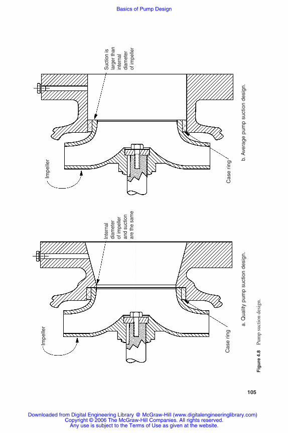
105
Fig
ure
4.8
Pum
p su
ctio
n de
sign
.
Cas
e rin
g
Impe
ller
Inte
rnal
diam
eter
of im
pelle
ran
d su
ctio
nar
e th
e sa
me
Impe
ller
Cas
e rin
g
Suc
tion
isla
rger
than
inte
rnal
diam
eter
of im
pelle
r
a. Q
ualit
y pu
mp
suct
ion
desi
gn.
b. A
vera
ge p
ump
suct
ion
desi
gn.
Rishel_CH04.qxd 21/4/06 6:25 PM Page 105
Downloaded from Digital Engineering Library @ McGraw-Hill (www.digitalengineeringlibrary.com)Copyright © 2006 The McGraw-Hill Companies. All rights reserved.
Any use is subject to the Terms of Use as given at the website.
Basics of Pump Design

pumps, a random selection of a pump should be made, and it should bedissembled for full inspection of the impeller and interior finish of thevolute.
4.13 Bibliography
Pump Handbook, McGraw-Hill, New York, 1996.Centrifugal Pump Standards, Hydraulics Institute, Parsippany, N.J., 1996.
106 HVAC Pumps and Their Performance
Rishel_CH04.qxd 20/4/06 6:01 PM Page 106
Downloaded from Digital Engineering Library @ McGraw-Hill (www.digitalengineeringlibrary.com)Copyright © 2006 The McGraw-Hill Companies. All rights reserved.
Any use is subject to the Terms of Use as given at the website.
Basics of Pump DesignBasics of Pump Design
Chapter
107
5Physical Description of
HVAC Pumps
5.1 Introduction
A number of different types of centrifugal pumps are used to handleall the various pump applications in the HVAC industry. HVACpumps can vary from small in-line circulators with a capacity of 20gal/min at 10 ft of head and fractional horsepower motors to largecooling tower pumps with capacities of 50,000 gal/min at 100 ft ofhead and equipped with 1500-hp motors. These pumps can be con-stant speed or variable speed. This chapter provides a physicaldescription of the various pumps that are popular with HVAC design-ers for chilled, hot, and condenser water service.
5.2 Physical Description of HVAC Pumps
Centrifugal pumps account for most of the pump applications in theHVAC industry. Some positive-displacement pumps are found onHVAC systems, but they are used for specific applications with smallcapacities, not for distributing water in hot, chilled, and condenserwater or cooling tower applications. A specific duty for positive-displacement pumps in the HVAC field is the metering of chemicalsinto water systems.
Table 5.1 provides a chart that describes the various types of cen-trifugal pumps found on HVAC systems. There is not universal agree-ment on some of the generic names applied to these pumps. For exam-ple, the double-suction pumps listed are often called horizontal splitcase pumps. The words diffuser, axial flow, and turbine are used inter-changeably for one class of centrifugal pumps; axial flow appears to
Rishel_CH05.qxd 21/4/06 6:12 PM Page 107
Downloaded from Digital Engineering Library @ McGraw-Hill (www.digitalengineeringlibrary.com)Copyright © 2006 The McGraw-Hill Companies. All rights reserved.
Any use is subject to the Terms of Use as given at the website.
Source: HVAC Pump Handbook

108 HVAC Pumps and Their Performance
be the least confusing and will be the name used herein. Hopefully,this chart will prove to be a guide for the designer to the most populartypes of pumps used on these water systems.
5.3 Two Basic Types of Centrifugal Pumps
As demonstrated in Chap. 4, there are two principal types of centrifu-gal pumps for HVAC water systems; these are volute and axial-flowpumps. The volute pump is offered in many configurations and han-dles much of the pump duty on HVAC systems.
Although not as popular as the volute pump, the axial-flow pumphandles some very important services. The words axial flow best
TABLE 5.1 Classification of HVAC Pumps
Rishel_CH05.qxd 21/4/06 6:12 PM Page 108
Downloaded from Digital Engineering Library @ McGraw-Hill (www.digitalengineeringlibrary.com)Copyright © 2006 The McGraw-Hill Companies. All rights reserved.
Any use is subject to the Terms of Use as given at the website.
Physical Description of HVAC Pumps

Physical Description of HVAC Pumps 109
describe these pumps, because water is diffused around the entireperiphery of the impeller and flows axially through the pump. Thereis no volute to collect the water from the impeller. Instead, theimpeller is housed in a bowl assembly that has a suction connectionand a discharge section. Water enters the pump bowl and passesthrough the impeller and the bowl vanes to the discharge connection.With this arrangement, it is very easy to make up these pumps inwhat is called stages. A two-stage pump merely indicates that twobowls and impellers are installed in series together, as shown inFig. 4.2d. How pumps operate in series or parallel is described indetail in Chap. 6.
5.3.1 Volute-type pumps
Volute-type pumps are provided in many different configurations andsizes to accommodate all the HVAC applications. They can be brokendown into two fundamental types, single suction and double suction.These pumps are shown in Fig. 5.1a and b. There are no clearly definedconditions where each of these pump types are applied. Generally, theuse of double-suction pumps begins with capacities around 500 gal/minand up to many thousands of gallons per minute. Single-suction pumpsare applied in the smaller capacities, although there are excellent single-suction pumps that function with capacities as high as 4000 gal/min.
Figure 5.1 Basic configurations of volute impellers.
Rishel_CH05.qxd 21/4/06 6:12 PM Page 109
Downloaded from Digital Engineering Library @ McGraw-Hill (www.digitalengineeringlibrary.com)Copyright © 2006 The McGraw-Hill Companies. All rights reserved.
Any use is subject to the Terms of Use as given at the website.
Physical Description of HVAC Pumps
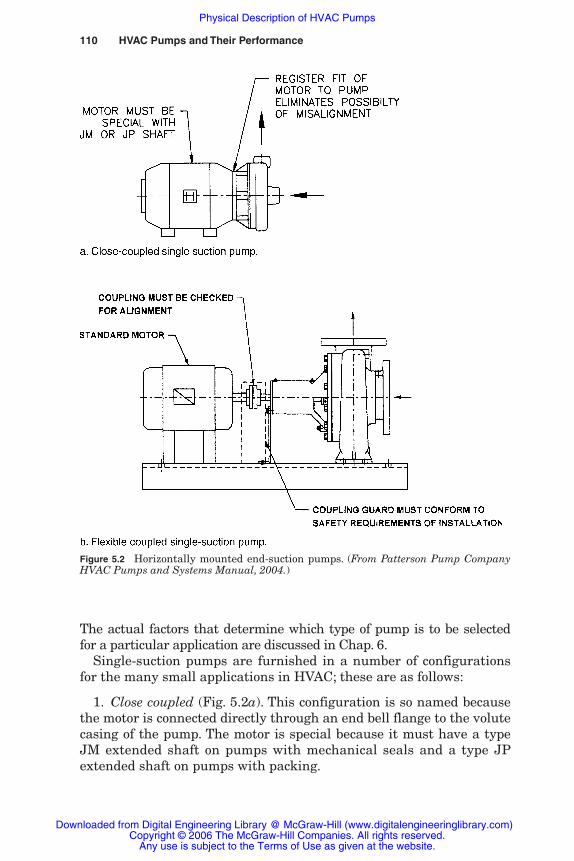
110 HVAC Pumps and Their Performance
Figure 5.2 Horizontally mounted end-suction pumps. (From Patterson Pump CompanyHVAC Pumps and Systems Manual, 2004.)
The actual factors that determine which type of pump is to be selectedfor a particular application are discussed in Chap. 6.
Single-suction pumps are furnished in a number of configurationsfor the many small applications in HVAC; these are as follows:
1. Close coupled (Fig. 5.2a). This configuration is so named becausethe motor is connected directly through an end bell flange to the volutecasing of the pump. The motor is special because it must have a typeJM extended shaft on pumps with mechanical seals and a type JPextended shaft on pumps with packing.
Rishel_CH05.qxd 21/4/06 6:12 PM Page 110
Downloaded from Digital Engineering Library @ McGraw-Hill (www.digitalengineeringlibrary.com)Copyright © 2006 The McGraw-Hill Companies. All rights reserved.
Any use is subject to the Terms of Use as given at the website.
Physical Description of HVAC Pumps

Physical Description of HVAC Pumps 111
The advantage of this configuration is the fact that the motor andpump cannot be misaligned with each other. Many designers preferthis pump over the flexibly coupled single-suction pump because ofthis. Another advantage of this pump is its physical space require-ments, which are less than those required by the flexibly coupledsingle-suction pump. As indicated previously, the motor is specialbecause of the end bell mounting and the shaft extension and is notstocked as readily as the standard motor.
2. Flexibly coupled (Fig. 5.2b). This pump is mounted on a base andconnected through a coupling to a standard motor. It can be equippedwith a spacer-type coupling that allows removal of the pump bracketand impeller without moving the motor or its electrical connections.
This arrangement requires more equipment room space and mustbe aligned carefully after the pump base is set in place. The flexiblecoupling always must have a coupling guard in place before the pumpis operated. The principal advantage of this pump is the fact that ituses a standard motor. In large motor sizes, it is less expensive thanthe close-coupled pump. The pump base must be grouted to maintainalignment of pump and motor.
3. Vertical mount (Fig. 5.3). The vertically mounted single-suctionpump is a close-coupled pump mounted on a pedestal-type long-sweepelbow that provides the suction connection as well as the support forthe pump and motor. This pump, like the in-line pump, can saveequipment room floor space. A unique advantage of this pump is itsability to rotate the discharge to accommodate the discharge piping.
4. In-line (Fig. 5.4). This configuration is so named because thepump can be inserted directly in a pipeline. The suction and dischargeconnections are in the same line, so there is no need for offsets orelbows in the connecting piping.
Figure 5.3 Vertically mounted,end-suction pump.
Rishel_CH05.qxd 21/4/06 6:12 PM Page 111
Downloaded from Digital Engineering Library @ McGraw-Hill (www.digitalengineeringlibrary.com)Copyright © 2006 The McGraw-Hill Companies. All rights reserved.
Any use is subject to the Terms of Use as given at the website.
Physical Description of HVAC Pumps
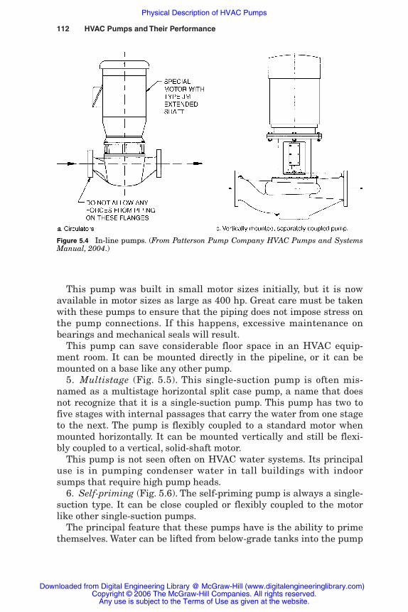
112 HVAC Pumps and Their Performance
This pump was built in small motor sizes initially, but it is nowavailable in motor sizes as large as 400 hp. Great care must be takenwith these pumps to ensure that the piping does not impose stress onthe pump connections. If this happens, excessive maintenance onbearings and mechanical seals will result.
This pump can save considerable floor space in an HVAC equip-ment room. It can be mounted directly in the pipeline, or it can bemounted on a base like any other pump.
5. Multistage (Fig. 5.5). This single-suction pump is often mis-named as a multistage horizontal split case pump, a name that doesnot recognize that it is a single-suction pump. This pump has two tofive stages with internal passages that carry the water from one stageto the next. The pump is flexibly coupled to a standard motor whenmounted horizontally. It can be mounted vertically and still be flexi-bly coupled to a vertical, solid-shaft motor.
This pump is not seen often on HVAC water systems. Its principaluse is in pumping condenser water in tall buildings with indoorsumps that require high pump heads.
6. Self-priming (Fig. 5.6). The self-priming pump is always a single-suction type. It can be close coupled or flexibly coupled to the motorlike other single-suction pumps.
The principal feature that these pumps have is the ability to primethemselves. Water can be lifted from below-grade tanks into the pump
Figure 5.4 In-line pumps. (From Patterson Pump Company HVAC Pumps and SystemsManual, 2004.)
Rishel_CH05.qxd 21/4/06 6:12 PM Page 112
Downloaded from Digital Engineering Library @ McGraw-Hill (www.digitalengineeringlibrary.com)Copyright © 2006 The McGraw-Hill Companies. All rights reserved.
Any use is subject to the Terms of Use as given at the website.
Physical Description of HVAC Pumps

Physical Description of HVAC Pumps 113
without special priming equipment. Typical applications are chillersumps and open energy storage tanks such as are used in cold wateror ice storage systems.
Because of their self-priming requirements, the efficiency of thesepumps is lower than the efficiency for other single-suction pumps of
Figure 5.5 Horizontal, multistage, volute pump, flexible coupled for clear service. (FromPatterson Pump Company HVAC Pumps and Systems Manual, 2004.)
Rishel_CH05.qxd 21/4/06 6:12 PM Page 113
Downloaded from Digital Engineering Library @ McGraw-Hill (www.digitalengineeringlibrary.com)Copyright © 2006 The McGraw-Hill Companies. All rights reserved.
Any use is subject to the Terms of Use as given at the website.
Physical Description of HVAC Pumps

114 HVAC Pumps and Their Performance
equal size. The impellers are usually of the open type without casingrings, which reduces the overall, lasting efficiency of this type ofpump.
This pump is designed to operate on reasonable NPSH availableconditions and can handle gases; therefore, it can be self-priming. Themaximum dry-priming lift conditions for these pumps are usuallyshown on the head-capacity curves for them. The maximum allowablesuction lift is the allowable lift or height of the pump above the mini-mum tank water surface. Under this condition, the pump is assumedto be dry. This means that within these lift conditions, the pump willprime itself as long as the NPSHR conditions are not exceeded.Manufacturers of self-priming pumps should provide information onthe priming, repriming, and suction lift capabilities of their pumpsbefore they are applied to an actual installation.
The suction pipe for most self-priming pumps should be the samesize as the pump suction. This adds friction loss to the pumpinginstallation and must be charged to the friction loss of the pumpfittings. Due to this and the overall efficiency of self-priming pumps,the wire-to-water efficiency for such pumping systems is much lowerthan that for other centrifugal pumping systems of equal capacityand pump head.
Figure 5.6 Horizontal, self-priming, volute pump, flexible coupled for clear service.(Courtesy Gorman Rupp Co.)
Rishel_CH05.qxd 21/4/06 6:12 PM Page 114
Downloaded from Digital Engineering Library @ McGraw-Hill (www.digitalengineeringlibrary.com)Copyright © 2006 The McGraw-Hill Companies. All rights reserved.
Any use is subject to the Terms of Use as given at the website.
Physical Description of HVAC Pumps

Physical Description of HVAC Pumps 115
5.3.2 Double-suction pumps
The workhorse of the HVAC field is the double-suction pump. It is byfar the preference of most designers when the flow in a water systemexceeds 1000 gal/min. The principal reasons for this popularity are itsrelatively high efficiency and its ability to be opened, inspected, andserviced without disturbing either the pump rotor, motor, or the con-necting piping.
The latter feature is available if the pump casing is split parallel tothe pump rotor or shaft. With this construction, called axially split,the top half of the casing can be removed, affording internal inspectionof the impeller, case rings, and internal surfaces of the casing.Usually, there is no need for realignment of the pump and motor after ithas been inspected, since the rotating element has not been disturbed.
The double-suction pump can be furnished in a casing that is splitvertically or perpendicularly to the pump shaft. This constructionrequires pulling the rotating element out of the pump end to inspectthe impeller interior; the pump should be realigned with its motorafter being inspected and reassembled. This pump is almost alwaysmounted horizontally. Contrary to claims, this pump does not saveequipment room space in most cases because of the distance requiredat the pump end for removal of the rotating element.
The double-suction pump (Fig. 5.7) that has a casing split parallelto the pump shaft can be furnished mounted horizontally or vertically.This is why the popular name horizontal split case should not beused. The double-suction pump is always flexibly coupled to the elec-tric motor, never close coupled. The vertically mounted double-suctionpump uses a vertical, solid-shaft motor.
5.3.3 Axial-flow pumps
Axial-flow pumps are furnished in a number of different configura-tions. They are classified by impeller design and by their general con-struction and arrangement. An axial-flow pump consists of four basicsubassemblies: (1) the bowl assembly that houses the impellers, (2)the column assembly that consists of pump shafting and piping totransfer the water from the bowl assembly to the discharge head, (3)the discharge head that receives water from the column assembly anddelivers it to the system piping, and (4) the motor or other type of dri-ver that powers the pump.
The three principal impeller classifications are turbine, mixed flow,and propeller.
1. Turbine. Turbine pumps are designed with lower specific speeds andare the type usually found in HVAC applications. Most of these pumpsare equipped with enclosed impellers, although some manufacturers
Rishel_CH05.qxd 21/4/06 6:12 PM Page 115
Downloaded from Digital Engineering Library @ McGraw-Hill (www.digitalengineeringlibrary.com)Copyright © 2006 The McGraw-Hill Companies. All rights reserved.
Any use is subject to the Terms of Use as given at the website.
Physical Description of HVAC Pumps
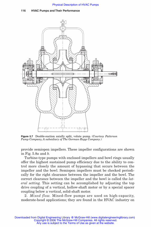
116 HVAC Pumps and Their Performance
provide semiopen impellers. These impeller configurations are shownin Fig. 5.8a and b.
Turbine-type pumps with enclosed impellers and bowl rings usuallyoffer the highest sustained pump efficiency due to the ability to con-trol more closely the amount of bypassing that occurs between theimpeller and the bowl. Semiopen impellers must be checked periodi-cally for the right clearance between the impeller and the bowl. Thecorrect clearance between the impeller and the bowl is called the lat-eral setting. This setting can be accomplished by adjusting the topdrive coupling of a vertical, hollow-shaft motor or by a special spacercoupling below a vertical, solid-shaft motor.
2. Mixed flow. Mixed-flow pumps are used on high-capacity,moderate-head applications; they are found in the HVAC industry on
Figure 5.7 Double-suction axially split, volute pump. (Courtesy PattersonPump Company, A subsidiary of The Gorman-Rupp Company.)
Rishel_CH05.qxd 21/4/06 6:12 PM Page 116
Downloaded from Digital Engineering Library @ McGraw-Hill (www.digitalengineeringlibrary.com)Copyright © 2006 The McGraw-Hill Companies. All rights reserved.
Any use is subject to the Terms of Use as given at the website.
Physical Description of HVAC Pumps
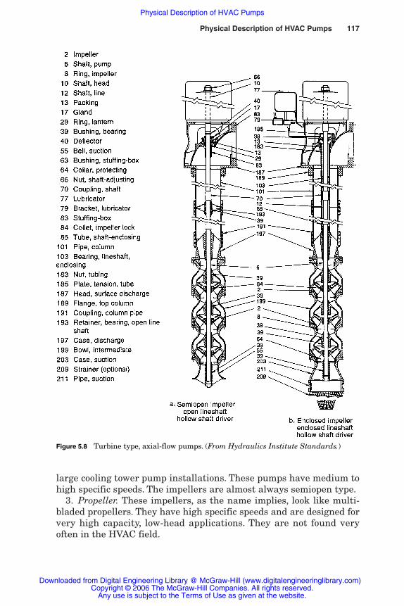
Physical Description of HVAC Pumps 117
large cooling tower pump installations. These pumps have medium tohigh specific speeds. The impellers are almost always semiopen type.
3. Propeller. These impellers, as the name implies, look like multi-bladed propellers. They have high specific speeds and are designed forvery high capacity, low-head applications. They are not found veryoften in the HVAC field.
Figure 5.8 Turbine type, axial-flow pumps. (From Hydraulics Institute Standards.)
Rishel_CH05.qxd 21/4/06 6:12 PM Page 117
Downloaded from Digital Engineering Library @ McGraw-Hill (www.digitalengineeringlibrary.com)Copyright © 2006 The McGraw-Hill Companies. All rights reserved.
Any use is subject to the Terms of Use as given at the website.
Physical Description of HVAC Pumps
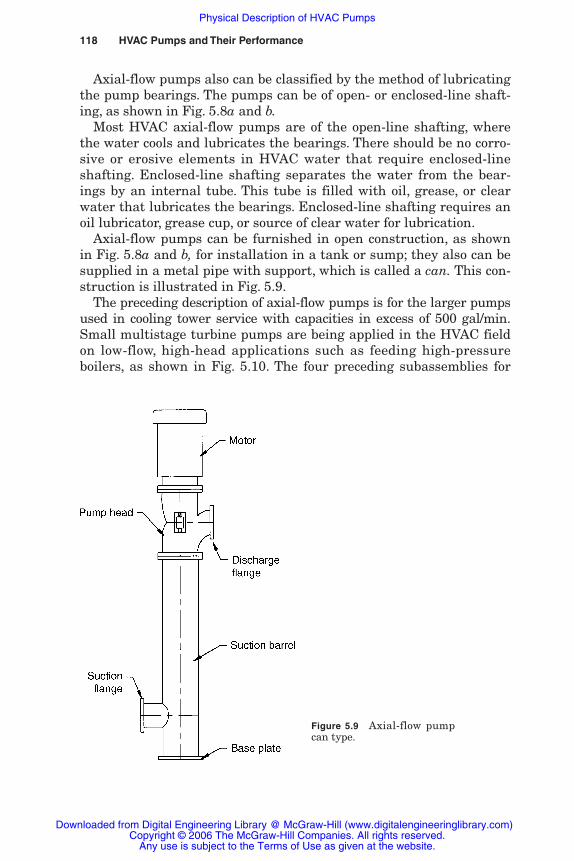
118 HVAC Pumps and Their Performance
Axial-flow pumps also can be classified by the method of lubricatingthe pump bearings. The pumps can be of open- or enclosed-line shaft-ing, as shown in Fig. 5.8a and b.
Most HVAC axial-flow pumps are of the open-line shafting, wherethe water cools and lubricates the bearings. There should be no corro-sive or erosive elements in HVAC water that require enclosed-lineshafting. Enclosed-line shafting separates the water from the bear-ings by an internal tube. This tube is filled with oil, grease, or clearwater that lubricates the bearings. Enclosed-line shafting requires anoil lubricator, grease cup, or source of clear water for lubrication.
Axial-flow pumps can be furnished in open construction, as shownin Fig. 5.8a and b, for installation in a tank or sump; they also can besupplied in a metal pipe with support, which is called a can. This con-struction is illustrated in Fig. 5.9.
The preceding description of axial-flow pumps is for the larger pumpsused in cooling tower service with capacities in excess of 500 gal/min.Small multistage turbine pumps are being applied in the HVAC fieldon low-flow, high-head applications such as feeding high-pressureboilers, as shown in Fig. 5.10. The four preceding subassemblies for
Figure 5.9 Axial-flow pumpcan type.
Rishel_CH05.qxd 21/4/06 6:12 PM Page 118
Downloaded from Digital Engineering Library @ McGraw-Hill (www.digitalengineeringlibrary.com)Copyright © 2006 The McGraw-Hill Companies. All rights reserved.
Any use is subject to the Terms of Use as given at the website.
Physical Description of HVAC Pumps

Physical Description of HVAC Pumps 119
Figure 5.10 Vertical, multistage pump, flexibly coupled. (CourtesyGrundfos Pumps Corporation, Clovis, CA.)
Rishel_CH05.qxd 21/4/06 6:12 PM Page 119
Downloaded from Digital Engineering Library @ McGraw-Hill (www.digitalengineeringlibrary.com)Copyright © 2006 The McGraw-Hill Companies. All rights reserved.
Any use is subject to the Terms of Use as given at the website.
Physical Description of HVAC Pumps

120 HVAC Pumps and Their Performance
this type of pump are furnished in a compact assembly and verticallymounted, which saves equipment room space. The smaller pumps areflexibly coupled through an integral bracket to a vertical, solid-shaftelectric motor. A slightly larger pump of this configuration can be fur-nished mounted vertically with the same motor, or it can be suppliedmounted horizontally and connected through a flexible coupling to astandard, horizontally mounted motor. The motor and pump aremounted on a structural base, as is the case with many volute-typepumps. These small turbine pumps are equipped with high-temperaturemechanical seals for 250°F water.
5.4 Positive-Displacement Pumps
Positive-displacement pumps as used in HVAC applications are smallin size because, typically, they are used only for chemical feed service inother applications where a positive amount of material is required.Most of these pumps are of the rotary or reciprocating type. Since thesepumps seldom enter into the overall performance of HVAC water sys-tems, no further discussion of them will be included. HydraulicInstitute’s Centrifugal Pump Standards is an excellent reference man-ual for these pumps.
5.5 Regenerative Turbine Pumps
A specialty pump that cannot be classified as a centrifugal pump or apositive-displacement pump is the regenerative turbine pump, asshown in Fig. 5.11. This pump is used in the HVAC field primarily forlow-flow, high-head applications such as boiler feed service. It has verytight clearances and, therefore, must be equipped with a very goodsuction strainer. Its efficiency is lower than other centrifugal pumps ofsimilar size. It has been replaced on many applications by the small,multistage, turbine-type centrifugal pump, as shown in Fig. 5.10.
5.6 Pump Construction
Most centrifugal pumps for the HVAC industry do not require therugged construction found in industrial and power plant installa-tions. Compared with other pump applications, HVAC pumping iseasy pump duty. All the major liquids used in this field should benoncorrosive and nonabrasive. Therefore, these pumps must offerlong life with very little in the way of repairs. Chapter 25 on mainte-nance of pumps will review, in detail, the causes for abnormal wearin pumps.
Rishel_CH05.qxd 21/4/06 6:12 PM Page 120
Downloaded from Digital Engineering Library @ McGraw-Hill (www.digitalengineeringlibrary.com)Copyright © 2006 The McGraw-Hill Companies. All rights reserved.
Any use is subject to the Terms of Use as given at the website.
Physical Description of HVAC Pumps

Physical Description of HVAC Pumps 121
The description that follows pertains to most of the HVAC pumps.Understanding the basic parts of a pump, regardless of the type, willbe helpful in selecting and observing the operation of a pump.
5.6.1 Typical parts of a centrifugal pump
Figure 5.12 describes a typical cross section of a single-suction, flexi-bly connected pump. The purpose of this drawing is to familiarizedesigners with the generic parts of a pump. This pump drawing illus-trates the case rings mentioned below, and it also points out most ofthe parts found in HVAC pumps; some of the more important partsare as follows:
Part name Part number
Casing, body, or volute 01Impeller 02Shaft 06Inboard bearing 16Outboard Bearing 18Case rings 7
Figure 5.11 Horizontal, regenerative turbine, flexible coupled. (Courtesy AuroraPumps.)
Rishel_CH05.qxd 21/4/06 6:12 PM Page 121
Downloaded from Digital Engineering Library @ McGraw-Hill (www.digitalengineeringlibrary.com)Copyright © 2006 The McGraw-Hill Companies. All rights reserved.
Any use is subject to the Terms of Use as given at the website.
Physical Description of HVAC Pumps

122 HVAC Pumps and Their Performance
Other pump parts relating to axial-flow pumps can be found in Fig. 5.8,the drawings for the turbine pump.
5.6.2 Materials of construction
Since most HVAC pumps do not operate under corrosive or erosiveoperating conditions and are not of extremely high pressure, they arenormally cast iron, bronze fitted. This means that the pump body iscast iron and the internal trim is bronze. The impeller and case rings
Figure 5.12 Cross-section of an end-suction, volute type pump.
Rishel_CH05.qxd 21/4/06 6:12 PM Page 122
Downloaded from Digital Engineering Library @ McGraw-Hill (www.digitalengineeringlibrary.com)Copyright © 2006 The McGraw-Hill Companies. All rights reserved.
Any use is subject to the Terms of Use as given at the website.
Physical Description of HVAC Pumps
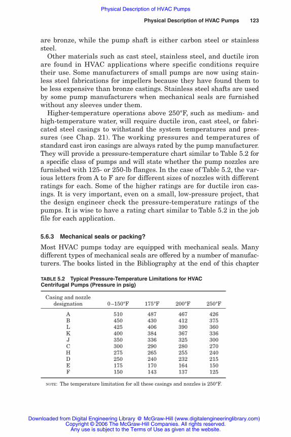
Physical Description of HVAC Pumps 123
are bronze, while the pump shaft is either carbon steel or stainlesssteel.
Other materials such as cast steel, stainless steel, and ductile ironare found in HVAC applications where specific conditions requiretheir use. Some manufacturers of small pumps are now using stain-less steel fabrications for impellers because they have found them tobe less expensive than bronze castings. Stainless steel shafts are usedby some pump manufacturers when mechanical seals are furnishedwithout any sleeves under them.
Higher-temperature operations above 250°F, such as medium- andhigh-temperature water, will require ductile iron, cast steel, or fabri-cated steel casings to withstand the system temperatures and pres-sures (see Chap. 21). The working pressures and temperatures ofstandard cast iron casings are always rated by the pump manufacturer.They will provide a pressure-temperature chart similar to Table 5.2 fora specific class of pumps and will state whether the pump nozzles arefurnished with 125- or 250-lb flanges. In the case of Table 5.2, the var-ious letters from A to F are for different sizes of nozzles with differentratings for each. Some of the higher ratings are for ductile iron cas-ings. It is very important, even on a small, low-pressure project, thatthe design engineer check the pressure-temperature ratings of thepumps. It is wise to have a rating chart similar to Table 5.2 in the jobfile for each application.
5.6.3 Mechanical seals or packing?
Most HVAC pumps today are equipped with mechanical seals. Manydifferent types of mechanical seals are offered by a number of manufac-turers. The books listed in the Bibliography at the end of this chapter
TABLE 5.2 Typical Pressure-Temperature Limitations for HVACCentrifugal Pumps (Pressure in psig)
Casing and nozzle designation 0 –150°F 175°F 200°F 250°F
A 510 487 467 426B 450 430 412 375L 425 406 390 360K 400 384 367 336J 350 336 325 300C 300 290 280 270H 275 265 255 240D 250 240 232 215E 175 170 164 150F 150 143 137 125
NOTE: The temperature limitation for all these casings and nozzles is 250°F.
Rishel_CH05.qxd 21/4/06 6:12 PM Page 123
Downloaded from Digital Engineering Library @ McGraw-Hill (www.digitalengineeringlibrary.com)Copyright © 2006 The McGraw-Hill Companies. All rights reserved.
Any use is subject to the Terms of Use as given at the website.
Physical Description of HVAC Pumps
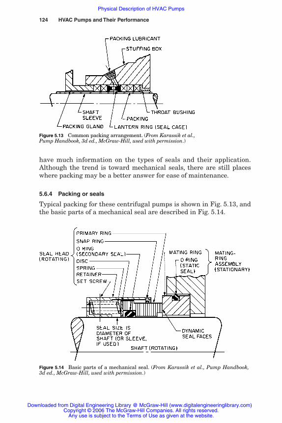
have much information on the types of seals and their application.Although the trend is toward mechanical seals, there are still placeswhere packing may be a better answer for ease of maintenance.
5.6.4 Packing or seals
Typical packing for these centrifugal pumps is shown in Fig. 5.13, andthe basic parts of a mechanical seal are described in Fig. 5.14.
124 HVAC Pumps and Their Performance
Figure 5.13 Common packing arrangement. (From Karassik et al.,Pump Handbook, 3d ed., McGraw-Hill, used with permission.)
Figure 5.14 Basic parts of a mechanical seal. (From Karassik et al., Pump Handbook,3d ed., McGraw-Hill, used with permission.)
Rishel_CH05.qxd 21/4/06 6:12 PM Page 124
Downloaded from Digital Engineering Library @ McGraw-Hill (www.digitalengineeringlibrary.com)Copyright © 2006 The McGraw-Hill Companies. All rights reserved.
Any use is subject to the Terms of Use as given at the website.
Physical Description of HVAC Pumps

Any application that has a possibility of dirt or other foreign mattermay be an application for packing. Typical of these are condenserpumps taking water from cooling tower sumps. Also, large facilitieswith full-time maintenance personnel who are experienced in thetechnique of installing packing in all types of rotating elements maybe candidates for packed pumps. Properly installed packing can elimi-nate waste water caused by continuous dripping.
Why use packing? A mechanical seal, when it fails, may throw wateraround the equipment room, while packing, as it starts to fail, justleaks water from the gland. Its failure is much more gradual than thatof mechanical seals. The other reason may be because the client’s per-sonnel prefer packing; therefore, this is one question that the designershould ask when considering the pumps on a particular installation.
5.7 Internal Forces and Leakages inCentrifugal Pumps
The centrifugal pump, regardless of type, is subjected to dynamic forcesand leakages, which must be controlled to ensure that a successfuldesign is achieved for each particular application. It is important thatthe water system designer understand these basic conditions of cen-trifugal pump operation. Figure 5.15 describes these forces and leakagesfor a volute-type pump, while Fig. 5.16 provides the same for an axial-flow-type pump, which has a common name of “vertical turbine.”
Physical Description of HVAC Pumps 125
Figure 5.15 Forces and leakages in a volute-type pupm.
Rishel_CH05.qxd 21/4/06 6:12 PM Page 125
Downloaded from Digital Engineering Library @ McGraw-Hill (www.digitalengineeringlibrary.com)Copyright © 2006 The McGraw-Hill Companies. All rights reserved.
Any use is subject to the Terms of Use as given at the website.
Physical Description of HVAC Pumps
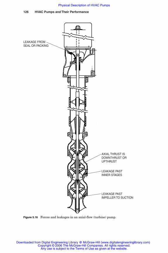
126 HVAC Pumps and Their Performance
LEAKAGE FROMSEAL OR PACKING
AXIAL THRUST ISDOWNTHRUST ORUPTHRUST
LEAKAGE PAST INNER STAGES
LEAKAGE PASTIMPELLER TO SUCTION
Figure 5.16 Forces and leakages in an axial-flow (turbine) pump.
Rishel_CH05.qxd 21/4/06 6:12 PM Page 126
Downloaded from Digital Engineering Library @ McGraw-Hill (www.digitalengineeringlibrary.com)Copyright © 2006 The McGraw-Hill Companies. All rights reserved.
Any use is subject to the Terms of Use as given at the website.
Physical Description of HVAC Pumps

5.7.1 Forces on centrifugal pumps
The forces exerted on a volute-type pump are: (1) axial and (2) radial,as shown in Fig. 5.15 for a volute-type pump. The axial thrust is com-puted by the pump designer who provides the correct type of thrustbearing to withstand the imbalance of radial thrusts that exist insuch a pump. Figure 5.17 illustrates these forces for both a single anda double-suction pump.
The axial forces for a double-suction pump appear to be balanced,and such is the case for a perfect design and installation of this typeof pump. This assumes that the flows into each of the suctions areequal. In actual practice, this may not be true due to uneven machin-ing of the suction passages of the impeller or by not having theimpeller centered in the casing. Also, improper configuration of thesuction piping may cause the flow into the two suctions to be unequal.The pump designer realizes this can happen and provides a thrustbearing that will withstand the thrust of some unequal flow. Since thedirection of thrust can be either way, the bearings must be designedfor the force in both directions. This is unlike the single-suction pumpwhere the axial thrust is almost always toward the pump suction.
The single-suction impeller for the volute pump does have unequalaxial thrusts since the suction pressure exerts less force on theimpeller than that generated by the higher discharge pressure. Thethrust bearing for this pump must be designed to accommodate thisdifference. It is obvious that single-suction, volute pumps designed forhigh heads must have thrust bearings capable of handling suchhigher differences in radial thrusts.
When axial-flow pumps are installed vertically, the axial thrusts arenamed “downthrust” or “upthrust.” Due to the weight of the rotating
Physical Description of HVAC Pumps 127
Figure 5.17 Axial thrust in volute-type pumps. (From Karassik et al., Pump Handbook,3d ed., McGraw-Hill, used with permission.)
Rishel_CH05.qxd 21/4/06 6:12 PM Page 127
Downloaded from Digital Engineering Library @ McGraw-Hill (www.digitalengineeringlibrary.com)Copyright © 2006 The McGraw-Hill Companies. All rights reserved.
Any use is subject to the Terms of Use as given at the website.
Physical Description of HVAC Pumps

assembly and the water pressure developed by the pump, most axial-flow impellers exert a downthrust on the rotating assembly at thedesign condition. Upthrust, if great enough, can create problems inmotor bearings. Figure 5.18 describes typical upthrust and down-thrust curves for various axial-flow pumps with different types ofimpellers and, therefore, different specific speeds. Generally, openimpellers are free of upthrust while enclosed impellers have pronouncedupthrust when they run out to capacities in excess of 120 percent offlow at the best efficiency point (BEP). It is obvious from the curves ofFig. 5.18 that great care should be exerted to avoid operation of pumpswith enclosed impellers at flows greater than 110 percent of that at theBEP. The actual thrust curve should be provided with the purchase ofan axial-flow pump.
Radial thrust is not a problem in most axial-flow pumps, since theflow of water from the impeller into the bowl exit should be uniformly
128 HVAC Pumps and Their Performance
Figure 5.18 Axial thrust vs. rate of flow curves for axial-flow pumps.
Rishel_CH05.qxd 21/4/06 6:12 PM Page 128
Downloaded from Digital Engineering Library @ McGraw-Hill (www.digitalengineeringlibrary.com)Copyright © 2006 The McGraw-Hill Companies. All rights reserved.
Any use is subject to the Terms of Use as given at the website.
Physical Description of HVAC Pumps
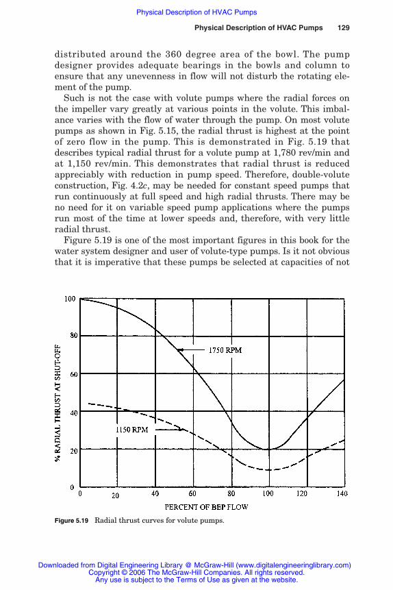
distributed around the 360 degree area of the bowl. The pumpdesigner provides adequate bearings in the bowls and column toensure that any unevenness in flow will not disturb the rotating ele-ment of the pump.
Such is not the case with volute pumps where the radial forces onthe impeller vary greatly at various points in the volute. This imbal-ance varies with the flow of water through the pump. On most volutepumps as shown in Fig. 5.15, the radial thrust is highest at the pointof zero flow in the pump. This is demonstrated in Fig. 5.19 thatdescribes typical radial thrust for a volute pump at 1,780 rev/min andat 1,150 rev/min. This demonstrates that radial thrust is reducedappreciably with reduction in pump speed. Therefore, double-voluteconstruction, Fig. 4.2c, may be needed for constant speed pumps thatrun continuously at full speed and high radial thrusts. There may beno need for it on variable speed pump applications where the pumpsrun most of the time at lower speeds and, therefore, with very littleradial thrust.
Figure 5.19 is one of the most important figures in this book for thewater system designer and user of volute-type pumps. Is it not obviousthat it is imperative that these pumps be selected at capacities of not
Physical Description of HVAC Pumps 129
Figure 5.19 Radial thrust curves for volute pumps.
Rishel_CH05.qxd 21/4/06 6:12 PM Page 129
Downloaded from Digital Engineering Library @ McGraw-Hill (www.digitalengineeringlibrary.com)Copyright © 2006 The McGraw-Hill Companies. All rights reserved.
Any use is subject to the Terms of Use as given at the website.
Physical Description of HVAC Pumps
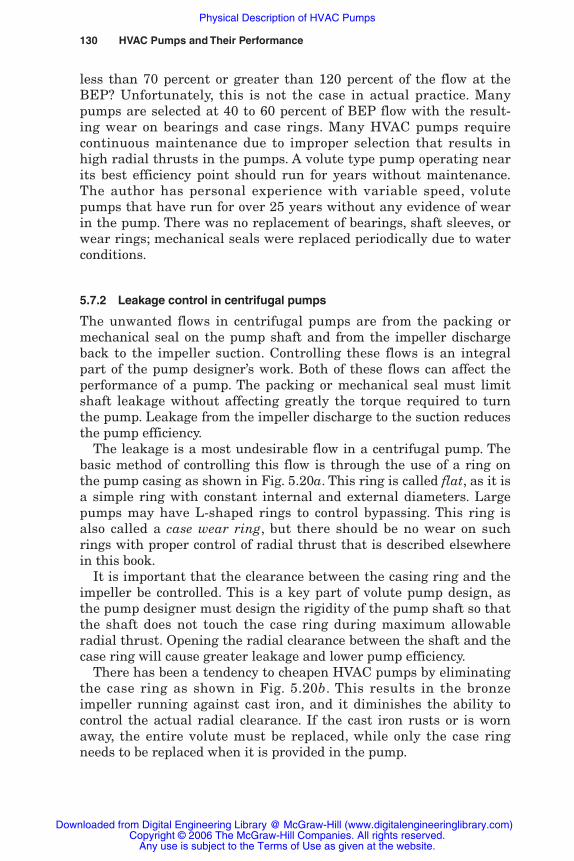
less than 70 percent or greater than 120 percent of the flow at theBEP? Unfortunately, this is not the case in actual practice. Manypumps are selected at 40 to 60 percent of BEP flow with the result-ing wear on bearings and case rings. Many HVAC pumps requirecontinuous maintenance due to improper selection that results inhigh radial thrusts in the pumps. A volute type pump operating nearits best efficiency point should run for years without maintenance.The author has personal experience with variable speed, volutepumps that have run for over 25 years without any evidence of wearin the pump. There was no replacement of bearings, shaft sleeves, orwear rings; mechanical seals were replaced periodically due to waterconditions.
5.7.2 Leakage control in centrifugal pumps
The unwanted flows in centrifugal pumps are from the packing ormechanical seal on the pump shaft and from the impeller dischargeback to the impeller suction. Controlling these flows is an integralpart of the pump designer’s work. Both of these flows can affect theperformance of a pump. The packing or mechanical seal must limitshaft leakage without affecting greatly the torque required to turnthe pump. Leakage from the impeller discharge to the suction reducesthe pump efficiency.
The leakage is a most undesirable flow in a centrifugal pump. Thebasic method of controlling this flow is through the use of a ring onthe pump casing as shown in Fig. 5.20a. This ring is called flat, as it isa simple ring with constant internal and external diameters. Largepumps may have L-shaped rings to control bypassing. This ring isalso called a case wear ring, but there should be no wear on suchrings with proper control of radial thrust that is described elsewherein this book.
It is important that the clearance between the casing ring and theimpeller be controlled. This is a key part of volute pump design, asthe pump designer must design the rigidity of the pump shaft so thatthe shaft does not touch the case ring during maximum allowableradial thrust. Opening the radial clearance between the shaft and thecase ring will cause greater leakage and lower pump efficiency.
There has been a tendency to cheapen HVAC pumps by eliminatingthe case ring as shown in Fig. 5.20b. This results in the bronzeimpeller running against cast iron, and it diminishes the ability tocontrol the actual radial clearance. If the cast iron rusts or is wornaway, the entire volute must be replaced, while only the case ringneeds to be replaced when it is provided in the pump.
130 HVAC Pumps and Their Performance
Rishel_CH05.qxd 21/4/06 6:12 PM Page 130
Downloaded from Digital Engineering Library @ McGraw-Hill (www.digitalengineeringlibrary.com)Copyright © 2006 The McGraw-Hill Companies. All rights reserved.
Any use is subject to the Terms of Use as given at the website.
Physical Description of HVAC Pumps
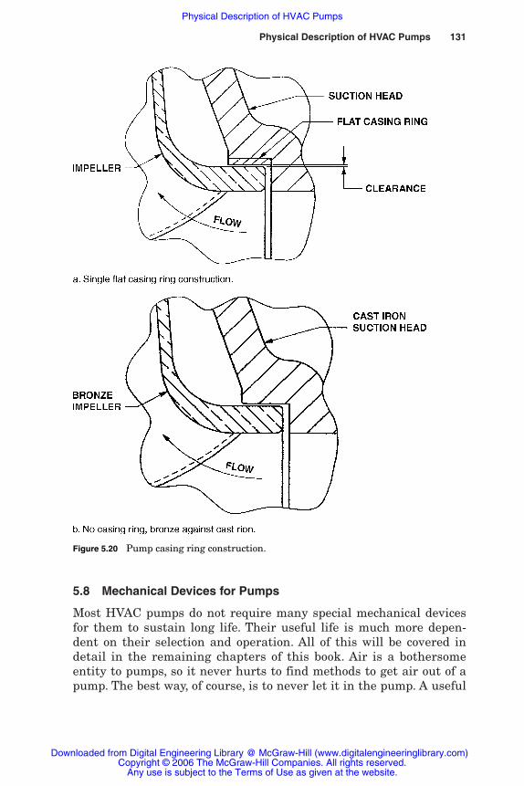
5.8 Mechanical Devices for Pumps
Most HVAC pumps do not require many special mechanical devicesfor them to sustain long life. Their useful life is much more depen-dent on their selection and operation. All of this will be covered indetail in the remaining chapters of this book. Air is a bothersomeentity to pumps, so it never hurts to find methods to get air out of apump. The best way, of course, is to never let it in the pump. A useful
Physical Description of HVAC Pumps 131
Figure 5.20 Pump casing ring construction.
Rishel_CH05.qxd 21/4/06 6:12 PM Page 131
Downloaded from Digital Engineering Library @ McGraw-Hill (www.digitalengineeringlibrary.com)Copyright © 2006 The McGraw-Hill Companies. All rights reserved.
Any use is subject to the Terms of Use as given at the website.
Physical Description of HVAC Pumps

and inexpensive device is a manual petcock installed on top of thepump volute that will allow manual removal of air that collectsthere. If air continually enters the pump and cannot be stopped, thispet cock can be replaced with an automatic air vent. The automaticair vent should have a discharge line near to a floor drain, since theyare notorious for leaking water. If the water carries grit or othersmall particulate matter, a cyclone separator can be installed on eachflushing line to the seals or packing. Methods of venting air fromwater systems are included in Chap. 9.
There is much argument over the value of strainers on HVAC sys-tems other than condenser water flowing to chillers. Many similarindustrial applications are not equipped with strainers. The normallocation of the strainer is on the suction of the pump. In the case ofcooling tower water feeding a chiller, the strainer should be installedon the discharge of the pump, as shown in Chap. 11. The strainer isthere to protect the tubes of the condenser, not the pump. The coolingtower sump strainer is adequate to keep rocks and other debris out ofthe pump. Installing the strainer on the pump discharge prevents thestrainer from being obliterated with algae and ruining the pump. Ifthe strainer becomes clogged when located on the pump suction, avacuum will be generated on the pump suction, and it will bedestroyed by steam and heat. For other HVAC applications, someengineers prefer to use strainers for start-up service only. After thesystem has been flushed and operated for a while, the strainerscreens or baskets are removed.
Coupling guards conforming to Occupational Safety and HealthAdministration (OSHA) or particular state codes should be locatedover the rotating coupling and pump shaft where it is exposed.OSHA’s requirements should be checked from time to time to ensurethat their requirements are met.
Balance valves should never be installed on the discharge of anypump, let alone variable-speed pumps. Some designers feel that theyare a safeguard to prevent overpressuring a system; this is a terriblewaste of energy. On constant-speed pumps, the amount of overpres-sure should be determined and the impeller trimmed to eliminate asmuch of the overpressure as possible. See Chap. 29 on the procedurefor trimming an impeller. On variable-speed pumps, the pump con-trols should be designed to prevent this overpressuring by limitingthe maximum speed of the pump.
Multiple-duty valves that include the features of a check valve, abalance valve, and a shutoff valve should never be used on the dis-charge of any pump and particularly on the discharge of a variable-speed pump (Fig. 5.21). Some multiple-duty valves can be closed
132 HVAC Pumps and Their Performance
Rishel_CH05.qxd 21/4/06 6:12 PM Page 132
Downloaded from Digital Engineering Library @ McGraw-Hill (www.digitalengineeringlibrary.com)Copyright © 2006 The McGraw-Hill Companies. All rights reserved.
Any use is subject to the Terms of Use as given at the website.
Physical Description of HVAC Pumps

partially without any indication of this condition. This creates a terri-ble waste of pumping energy. Also, some multipurpose valves musthave another valve downstream of them to repair the check-valve fea-ture of the multipurpose valve. A separate check valve and shutoffvalve should be provided instead. They are lower in cost and usuallyhave a lower friction loss than comparable multiple-duty valves.
On continuously running pumps taking suction from a tank belowthe pumps, the greater efficiency of the standard centrifugal pumpshould give it priority over a self-priming pump. It will be necessaryto provide a priming means to get the pump started. This can be apriming tank or a separate source of water. This tank holds enoughwater to keep the pump flooded until it has primed the suction line.With a properly sized priming system, the standard centrifugal pumpevacuates the air in the suction line and continues to pump waterfrom the lower tank. There are manufacturers of priming systems forcentrifugal pumps, and there is considerable information in the pumpreferences on the actual design of a priming system. The NPSHRcharacteristics of the pump must be checked carefully when takingsuction from lower tanks.
5.9 Bibliography
Additional centrifugal pump descriptions and performance can be foundin the catalogs of (1) the AC Pump Division of the ITT Fluid Technology;
Physical Description of HVAC Pumps 133
Figure 5.21 Discharge valvesfor variable-speed pumps.
Rishel_CH05.qxd 21/4/06 6:12 PM Page 133
Downloaded from Digital Engineering Library @ McGraw-Hill (www.digitalengineeringlibrary.com)Copyright © 2006 The McGraw-Hill Companies. All rights reserved.
Any use is subject to the Terms of Use as given at the website.
Physical Description of HVAC Pumps

(2) Aurora Pump, a Unit of General Signal, Aurora, IL; (3) GouldsPumps, Seneca Falls, NY; (4) Ingersoll Rand, Woodcliff Lakes, NJ; (5)Paco Pumps, a Flow Technologies Company, Houston, TX; and (6)Peerless Pumps, Indianapolis, IN.ANSI/HI 1.1-1.5-1994, Centrifugal Pumps, Hydraulic Institute, Parsippany, N.J., 1994.ANSI/HI 2.1-2.5-1994, Vertical Pumps, Hydraulic Institute, Parsippany, N.J., 1994.Pump Handbook, McGraw-Hill, New York, 1996.
134 HVAC Pumps and Their Performance
Rishel_CH05.qxd 21/4/06 6:12 PM Page 134
Downloaded from Digital Engineering Library @ McGraw-Hill (www.digitalengineeringlibrary.com)Copyright © 2006 The McGraw-Hill Companies. All rights reserved.
Any use is subject to the Terms of Use as given at the website.
Physical Description of HVAC Pumps

Chapter
135
6HVAC Pump Performance
6.1 Introduction
This evaluation of HVAC pump performance is limited to centrifugalpumps. The use of positive-displacement and regenerated turbinepumps in HVAC systems is for highly specialized low-volume, high-head applications. They are not used on the water services that con-sume most of the pumping energy in HVAC systems. Their applica-tion is so specialized that the performance required of these pumps,when encountered, should be sought from the manufacturer of thepump under consideration.
This review of HVAC pump performance will attempt to provide ageneral approach that is applicable to all pumps from small circulatorsto very large condenser pumps. It is imperative that we understandhow to select HVAC pumps and then how to operate them so that theenergy consumed is as low as economically possible. Efforts will bemade to describe pump performance so that the pumps are selectedproperly and operated closely to the pumps’ best efficiency curves.
6.2 Pump Head-Flow Curves
A study of centrifugal pump operations must begin with an evalua-tion of the basic performance of such a pump. The pressure or headthat is developed by any pump depends on the flow through thatpump. This basic head-flow relationship is called the pump’s head-flow curve. This was shown in elementary form in Chap. 4 and is nowdemonstrated with other accompanying curves in Fig. 6.1. Figure 6.1a
Rishel_CH06.qxd 20/4/06 6:06 PM Page 135
Downloaded from Digital Engineering Library @ McGraw-Hill (www.digitalengineeringlibrary.com)Copyright © 2006 The McGraw-Hill Companies. All rights reserved.
Any use is subject to the Terms of Use as given at the website.
Source: HVAC Pump Handbook

136 HVAC Pumps and Their Performance
is the head-flow curve for a medium-sized constant-speed pump, andit is in the form normally found in pump manufacturers’ catalogs.Included in this figure are the efficiency curves, the brake horsepowercurves, and a net positive suction head (NPSH) curve. The NPSHrequired curve will be discussed later in this chapter.
Figure 6.1 Typical head-flow curves for most HVAC pumps.
Rishel_CH06.qxd 20/4/06 6:06 PM Page 136
Downloaded from Digital Engineering Library @ McGraw-Hill (www.digitalengineeringlibrary.com)Copyright © 2006 The McGraw-Hill Companies. All rights reserved.
Any use is subject to the Terms of Use as given at the website.
HVAC Pump Performance
HVAC Pump Performance 137
6.2.1 Constant-speed head-flow curves
Most HVAC pump head-flow curves provided by the pump manufactur-ers are constant-speed curves for a particular speed such as 875, 1150,or 1750 rev/min. These curves are derived from dynamometer tests inthe pump manufacturer’s plant. The newer, high efficiency motors havehigher, full speeds such as 885, 1180, and 1775 rev/min. Pump manu-facturers are now furnishing flow-head curves at such speeds.
Head-flow curves for pumps can have several shapes depending onthe specific speed of the pump. Figure 6.1a is for a pump of moderatespecific speed, 1560, and is called a continuously rising characteristiccurve because the head increases continuously to the shutoff, or no-flow,condition. High-specific-speed pumps such as mixed-flow or propellerpumps can have a looped head-flow curve, as shown in Fig. 6.2a.Normally, manufacturers of such pumps do not provide a completehead-flow curve in their catalogs. Only the right-hand portion of thecurve where the pump is to be operated is provided, as shown in Fig. 6.2b.These pumps require some care in their application due to the factthat they can operate at several flows at the same head; this isshown in Fig. 6.2a, where the pump at 34 ft of head can operate at800, 1700, and 2700 gal/min. The pump can shift from one flow to anoth-er, causing shock and vibration in the pump itself and in the water sys-tem. Only experienced pump application engineers should handle theselection, installation, and operation of these large pumps.
The head-flow curve describes the net head available for usefulpumping after all internal losses of the pump are deducted from thetheoretical head that could be produced by an impeller of a particu-lar diameter and operating at a certain speed. The efficiency curvessuperimposed on the head-flow curve demonstrate how efficient thepump is when operated at a specific point on its head-flow curve.Some pump manufacturers provide efficiency curves similar to thosein Fig. 6.1. Others provide a separate efficiency curve from zero effi-ciency at zero flow to maximum flow, as shown in Fig. 6.3. This is arising curve to the point of maximum efficiency at the optimal flow.This maximum efficiency point on such a curve is called the best effi-ciency point. Great emphasis will be placed on the importance of thisbest efficiency point in Chap. 10. Some pump manufacturers, partic-ularly of small pumps, do not provide efficiency curves; instead, theyprovide a performance curve for a certain impeller diameter andwith a specific size of electric motor. Such pump curves should not beused for selection of HVAC pumps. If the manufacturer cannot pro-vide an efficiency curve for a pump, another manufacturer should beconsulted.
Rishel_CH06.qxd 20/4/06 6:06 PM Page 137
Downloaded from Digital Engineering Library @ McGraw-Hill (www.digitalengineeringlibrary.com)Copyright © 2006 The McGraw-Hill Companies. All rights reserved.
Any use is subject to the Terms of Use as given at the website.
HVAC Pump Performance

138 HVAC Pumps and Their Performance
6.2.2 Power balance curves
The best efficiency point of a pump will be emphasized in many partsof this book. Every water system designer should know where the best
Figure 6.2 Head-flow curves for a high specific speed, axial-flowpump.
Rishel_CH06.qxd 20/4/06 6:06 PM Page 138
Downloaded from Digital Engineering Library @ McGraw-Hill (www.digitalengineeringlibrary.com)Copyright © 2006 The McGraw-Hill Companies. All rights reserved.
Any use is subject to the Terms of Use as given at the website.
HVAC Pump Performance

HVAC Pump Performance 139
efficiency point occurs for each of the pumps involved on the water sys-tem under consideration. It should be of interest to the HVAC systemdesigner as to how the efficiency curve of Fig. 6.3 is developed.
The efficiency of a pump at any flow is dependent upon a number ofconditions within the pump. The losses that exist in a centrifugalpump and reduce the efficiency are: (1) mechanical, (2) leakage, (3) recir-culation, and (4) hydraulic. Figure 6.4 describes these losses for a 12 indouble suction, volute-type pump with a specific speed of 1900 andoperating at a constant speed of 1750 rev/min. This diagram is calleda “power balance diagram” in the pump industry. The mechanicallosses are incurred primarily in the bearings and mechanical seals orpacking. The leakage loss, which is discussed in Chap. 5, is caused bywater flowing past the case rings from the impeller discharge backthe impeller suction.
GUARANTEEDEFFICIENCY POINT.
Figure 6.3 Total efficiency curve.
Rishel_CH06.qxd 20/4/06 6:06 PM Page 139
Downloaded from Digital Engineering Library @ McGraw-Hill (www.digitalengineeringlibrary.com)Copyright © 2006 The McGraw-Hill Companies. All rights reserved.
Any use is subject to the Terms of Use as given at the website.
HVAC Pump Performance

140 HVAC Pumps and Their Performance
Recirculation losses are caused by circulation of the water withinthe volute or bowl. The water does not flow smoothly in and out of theimpeller. At flows through the pump that are less than that at thebest efficiency point, the water recirculates and causes substantiallosses.
Hydraulic losses are the losses that are caused by the friction devel-oped by the water flowing through the impeller and volute or bowl.Again, this demonstrates that the losses in small pumps with low spe-cific speeds are going to be greater than those for large, low-specific-speed pumps.
Figure 6.4 Power balance at constant speed. (From Centrifugal andAxial Flow Pumps, A.J. Stepanoff, Ph.D, John Wiley and sons, NewYork, NY 1957.)
Rishel_CH06.qxd 20/4/06 6:06 PM Page 140
Downloaded from Digital Engineering Library @ McGraw-Hill (www.digitalengineeringlibrary.com)Copyright © 2006 The McGraw-Hill Companies. All rights reserved.
Any use is subject to the Terms of Use as given at the website.
HVAC Pump Performance
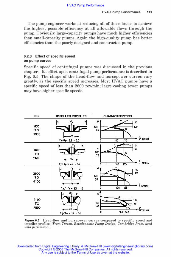
HVAC Pump Performance 141
The pump engineer works at reducing all of these losses to achievethe highest possible efficiency at all allowable flows through thepump. Obviously, large-capacity pumps have much higher efficienciesthan small-capacity pumps. Again the high-quality pump has betterefficiencies than the poorly designed and constructed pump.
6.2.3 Effect of specific speed on pump curves
Specific speed of centrifugal pumps was discussed in the previouschapters. Its effect upon centrifugal pump performance is described inFig. 6.5. The shape of the head-flow and horsepower curves varygreatly, as the specific speed increases. Most HVAC pumps have aspecific speed of less than 2600 rev/min; large cooling tower pumpsmay have higher specific speeds.
Figure 6.5 Head-flow and horsepower curves compared to specific speed and impeller profiles. (From Turton, Rotodynamic Pump Design, Cambridge Press, usedwith permission.)
Rishel_CH06.qxd 20/4/06 6:06 PM Page 141
Downloaded from Digital Engineering Library @ McGraw-Hill (www.digitalengineeringlibrary.com)Copyright © 2006 The McGraw-Hill Companies. All rights reserved.
Any use is subject to the Terms of Use as given at the website.
HVAC Pump Performance

142 HVAC Pumps and Their Performance
6.2.4 Typical constant-speed pump head-flow curves
Figure 6.6 through d describes typical pump head-flow curves for abroad range of HVAC applications. No particular type of centrifugalpump is represented. These curves are for pumps with good formationand have best efficiencies that are at the level desired for these watersystems. Almost all HVAC applications should have pumps with thebest efficiency above 80 percent, excepting small pumps or pumps inlow-flow, high-head applications.
Velocity head, V2/2g of the pump connections, must be consideredwhen the head-flow curve is developed. On pumps with suction pipes,the difference between the velocity head for the water flowing out ofthe discharge connection and for the water flowing into the pump suc-tion is included in these head-flow curves. On axial-flow pumps tak-ing water directly from a sump, there is no inlet velocity head deductedfrom the discharge velocity head. There may be an efficiency reduc-tion for single-impeller performance that does account for some entrancelosses.
Normal pump head-flow curves are provided by manufacturers atparticular induction motor speeds such as 875, 1150, and 1750 min.The newer, high efficiency, induction motors have higher, full loadspeeds such as 885, 1180, and 1775 rev/min. Pump manufacturers arenow providing pump curves at such full speeds. A range of impellerdiameters will be shown on each curve. A pump is considered to betrimmed to a specific diameter for each particular application. Therange of impeller trimming is shown on a typical head-flow curve,from minimum to maximum diameter. For example, the pump curvedescribed in Fig. 6.6d has an unusual impeller diameter range, from8.2 to 13.0 in diameter. Although this much trimming is allowed, cut-ting the impeller to such an extent has a great effect on pump efficiency. This particular pump has a peak efficiency of 87 percent;cutting the impeller to its minimum diameter would reduce the effi-ciency to 75 percent. Great care must be taken in trimming pumpimpellers; an alternative is to install a variable-speed drive and operate the pump at a lesser speed. Pumps must never be trimmedbelow the minimum diameter shown by the pump manufacturer onthe published head-flow curves.
Note. All manufacturers’ pump head-flow curves are dynamometercurves at a fixed speed such as 1750 rev/min. Actual field performancewill be different from these curves when the pumps are operated by induction motors whose speed varies from 1750 rev/min fully loaded to1800 rev/min unloaded. Manufacturers’ pump curves should not be
Rishel_CH06.qxd 20/4/06 6:06 PM Page 142
Downloaded from Digital Engineering Library @ McGraw-Hill (www.digitalengineeringlibrary.com)Copyright © 2006 The McGraw-Hill Companies. All rights reserved.
Any use is subject to the Terms of Use as given at the website.
HVAC Pump Performance
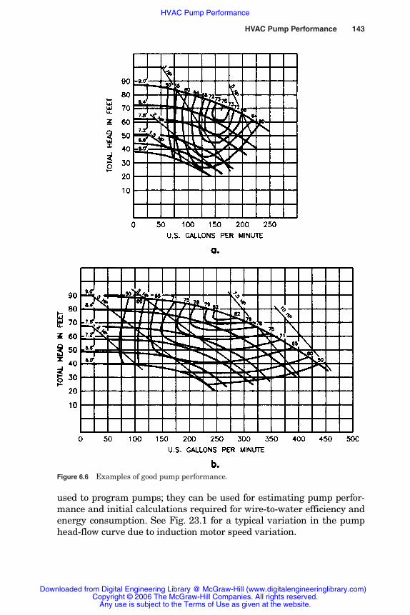
HVAC Pump Performance 143
Figure 6.6 Examples of good pump performance.
used to program pumps; they can be used for estimating pump perfor-mance and initial calculations required for wire-to-water efficiency andenergy consumption. See Fig. 23.1 for a typical variation in the pumphead-flow curve due to induction motor speed variation.
Rishel_CH06.qxd 20/4/06 6:06 PM Page 143
Downloaded from Digital Engineering Library @ McGraw-Hill (www.digitalengineeringlibrary.com)Copyright © 2006 The McGraw-Hill Companies. All rights reserved.
Any use is subject to the Terms of Use as given at the website.
HVAC Pump Performance
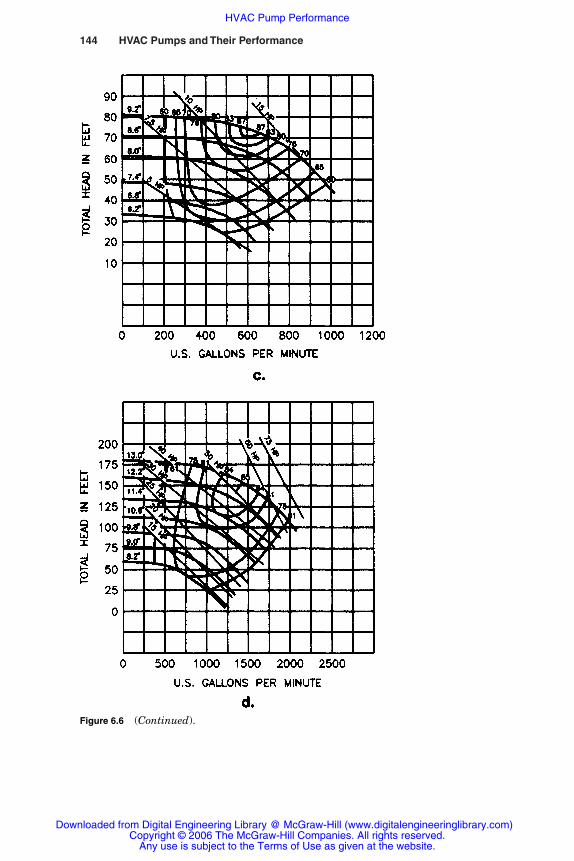
144 HVAC Pumps and Their Performance
Figure 6.6 (Continued).
Rishel_CH06.qxd 20/4/06 6:06 PM Page 144
Downloaded from Digital Engineering Library @ McGraw-Hill (www.digitalengineeringlibrary.com)Copyright © 2006 The McGraw-Hill Companies. All rights reserved.
Any use is subject to the Terms of Use as given at the website.
HVAC Pump Performance

HVAC Pump Performance 145
6.2.5 Variable-speed pump head-flow curves
Since speed variation is an added factor, the variable-speed pump’shead-flow curves must be provided for at least one diameter of im-peller. If another impeller diameter is desired, a second set of curvesshould be provided for that diameter. The speed variation is usuallyshown from around 45 to 100 percent speed, or typically from 800 to1750 rev/min. Below 45 percent speed, pump performance becomes avariable, and the pump manufacturers do not like to certify pumpperformance at such low speeds for most HVAC pumps. Figure 6.1bdescribes a typical set of pump curves for a large centrifugal pumpoperating at a maximum speed of 1750 rev/min. This pump has a spe-cific speed of 1860. It must be remembered that this group of curves isfor one impeller diameter, while Fig. 6.1a is for another pump at con-stant speed and various impeller diameters.
Due to the many variable-speed pumps that are now used in theHVAC field, it is important that the HVAC water system designer become familiar with what happens when the speed of a pump is var-ied from minimum to maximum speed. Figure 6.1b is one of the mostimportant figures in this book. Of particular importance in this figureis the curve describing the parabolic path of the best efficiency pointas the pump changes speed. This curve will help the water system designer understand how the efficiency of a pump varies as the speedchanges. The variations in efficiency at different points on the pumphead-flow curves are also provided in this figure as lines of constantefficiency. Lastly, this figure is a graphic representation of the pumpaffinity laws that are so important.
6.2.6 Best efficiency curves
In variable-speed pumping, the most important pump curve is thebest efficiency curve; it was first seen in Fig. 6.1b. This is the parabol-ic curve that the best efficiency point follows, as the speed of thepump is reduced. As will be seen later, it is the basic rule of variablespeed pump control that the pump operate as closely to this curve asis possible. Programming of multiple pumps operating in parallel isbased upon keeping the pumps in operation close to this curve.Other best efficiency curves are seen in Fig. 6.7 and 6.13. Figure 6.7describes the best efficiency curves for four small but popular end-suction pumps.
There will be a number of pump operations in this book that placegreat emphasis on the best efficiency curve. Radial thrust discussionswill emphasize that this thrust is the lowest at the best efficiency
Rishel_CH06.qxd 20/4/06 6:06 PM Page 145
Downloaded from Digital Engineering Library @ McGraw-Hill (www.digitalengineeringlibrary.com)Copyright © 2006 The McGraw-Hill Companies. All rights reserved.
Any use is subject to the Terms of Use as given at the website.
HVAC Pump Performance
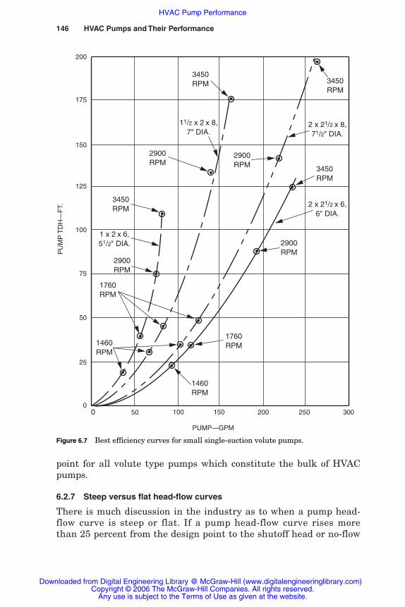
146 HVAC Pumps and Their Performance
point for all volute type pumps which constitute the bulk of HVACpumps.
6.2.7 Steep versus flat head-flow curves
There is much discussion in the industry as to when a pump head-flow curve is steep or flat. If a pump head-flow curve rises morethan 25 percent from the design point to the shutoff head or no-flow
500 100 150 200 250
PUMP—GPM
0
25
50
75
100
125
150
175
200P
UM
P T
DH
—F
T.
300
3450RPM 3450
RPM
2 x 21/2 x 8,71/2" DIA.
2 x 21/2 x 6,6" DIA.
1 x 2 x 6,51/2" DIA.
3450RPM
2900RPM
1760RPM
1460RPM
1460RPM
1760RPM
3450RPM
11/2 x 2 x 8,7" DIA.
2900RPM
2900RPM
2900RPM
Figure 6.7 Best efficiency curves for small single-suction volute pumps.
Rishel_CH06.qxd 20/4/06 6:06 PM Page 146
Downloaded from Digital Engineering Library @ McGraw-Hill (www.digitalengineeringlibrary.com)Copyright © 2006 The McGraw-Hill Companies. All rights reserved.
Any use is subject to the Terms of Use as given at the website.
HVAC Pump Performance
point, it is considered to be steep; it is considered flat if this rise is lessthan 25 percent. For example, if the design condition of a pump is 500 gal/min at 100 ft of head and the shutoff (no-flow) condition is 120 ft, it would be considered a flat-curved pump. If the shutoff condi-tion were 135 ft, the pump would be considered steep-curved. Thepump curves in Fig. 6.8 are considered to be flat. The shape of thepump curve was of great concern when constant volume-water sys-tems were popular. It was desired to have relatively steep pump curvesfor these operations so that a minor change in system head would notmake a great change in system flow. Steep curves were preferred, andflat-curved pumps were avoided. Small, constant-speed pumping sys-tems with three-way control valves on the heating or cooling coilsmust be concerned with the shape of the pump curve. A flat-curvedpump may create instability in the operation of the three-way valves.
With the advent of variable-volume water systems utilizing variable-speed pumps and system differential pressure controls, there is very lit-tle need to be concerned about the shape of the pump curve. Peak effi-ciency is what is sought, not the shape of the curve. In fact, flat-curvedpumps are desired. Pumps with flat-curved head-flow characteristicsshould be sought for variable-speed pumping applications, providedthere is no loss in pump efficiency. There is less speed reduction with aflat-curved pump than with a steep-curved pump. With less speedreduction, the wire-to-shaft efficiency of the variable-speed drive andmotor is greater because the speed reduction is less.
6.3 Series/Parallel Operation of Centrifugal Pumps
The broad variation in water requirements in HVAC systems usuallyrequires more than one pump to handle all the system flows from mini-mum to maximum capacities. Likewise, condenser water service in sometall buildings requires pump heads that cannot be handled economicallyby a single-stage pump. The first condition requires parallel operation ofmore than one pump, and the second condition requires more than oneimpeller operating in series. By far most HVAC applications consist ofmultiple pumps in parallel with few of them in series operation. Figure6.8 describes the various resulting head-flow curves when operatingpumps in parallel and in series.
Parallel operation enables the water system designer to select a num-ber of pumps that will produce efficient operation from minimum tomaximum system flow. Operating pumps of equal size and head in par-allel results in the capacities of the pumps being multiplied together, asshown in Fig. 6.8a. This figure describes two pumps with such equal
HVAC Pump Performance 147
Rishel_CH06.qxd 20/4/06 6:06 PM Page 147
Downloaded from Digital Engineering Library @ McGraw-Hill (www.digitalengineeringlibrary.com)Copyright © 2006 The McGraw-Hill Companies. All rights reserved.
Any use is subject to the Terms of Use as given at the website.
HVAC Pump Performance

148
Fig
ure
6.8
Ser
ies/
para
llel
per
form
ance
of
HV
AC
pu
mps
.(F
rom
th
e W
ater
Man
agem
ent
Man
ual
,S
yste
con
,In
c.,W
est
Ch
este
r,O
hio
,199
2,F
ig.3
–18.
)
Rishel_CH06.qxd 20/4/06 6:06 PM Page 148
Downloaded from Digital Engineering Library @ McGraw-Hill (www.digitalengineeringlibrary.com)Copyright © 2006 The McGraw-Hill Companies. All rights reserved.
Any use is subject to the Terms of Use as given at the website.
HVAC Pump Performance
HVAC Pump Performance 149
head-flow curves operating in parallel; the head is the same for one ortwo pumps operating, but the capacity is doubled for two-pump opera-tion. Parallel operation of pumps requires great care to ensure that thenumber of pumps running is the most efficient for a particular flow andhead condition. When operating pumps in parallel, the total capacityand head of the pumps must be that required by the uniform systemhead curve or any point within the system head area. (See Chap. 9 for adescription of uniform system head curves and system head areas.)
The great mistake that is often made with operating pumps in par-allel is to measure the capacity of one existing pump at a certainhead, install another equal pump, and find out that the two pumps donot produce twice the capacity. Pump operation cannot be predictedwithout computing the system head curve or system head area of thewater system. This is pointed out here because of the danger of tryingto run pumps in parallel without evaluating the head of the watersystem. This will be covered, in detail, in Chap. 10.
Considerable care should be exercised in trying to operate pumpsin parallel that have different head-flow curves; this is described inFig. 6.8b. There is great danger that the pump with the lower head-flow curve, pump A in this figure, can be operated at the shutoffhead condition and cause heating in the pump. This will happenif these pumps are operated together at any less than 62 percentcapacity of one pump. Also, it may be very difficult to program andoperate the pumps together at an adequate wire-to-water efficiency.
Pumps are operated in series when the flow can be handled by onepump throughout the operating range but the head is so high that anumber of pumps in series is needed. Figure 6.8c describes the factthat with pumps in series, the head developed by all the pumps isadded together at the same system flow. Turbine-type pumps are ex-cellent for such high-head, low-flow service. Two or more bowls orstages are connected in series to provide the required head.
Some large HVAC systems exist in which multistage pumps mustoperate in parallel; in this case, the resulting pump curves for twopumps are a combination of Fig. 6.8a and c with 200 percent capacityand 200 percent head of one pump impeller.
6.3.1 Pumps operating in parallel
The broad variation of water requirements in HVAC water systemsusually requires more than one pump in parallel to handle all of thesystem flow-head requirements. Also, standby capacity may necessitatethe installation of an extra pump. By far, most of these pump applica-tions consist of multiple pumps operating in parallel with few of themin series operation.
Rishel_CH06.qxd 20/4/06 6:06 PM Page 149
Downloaded from Digital Engineering Library @ McGraw-Hill (www.digitalengineeringlibrary.com)Copyright © 2006 The McGraw-Hill Companies. All rights reserved.
Any use is subject to the Terms of Use as given at the website.
HVAC Pump Performance

150 HVAC Pumps and Their Performance
Parallel operation enables the water system designer to select anumber of pumps that will produce efficient operation from minimumto maximum system flow. Parallel operation of pumps requires greatcare to ensure that the number of pumps running is the most efficientfor a particular flow and head condition. When operating pumps inparallel, the total capacity and head of the pumps must be that re-quired by the uniform system head curve or any point within the sys-tem head area. (See Chap. 9 on “Configuration of a Water System” fora description of uniform system head curves and system head areas.)
The great mistake that is often made when operating pumps in par-allel is to measure the capacity of one existing pump at a certain head,install another equal pump, and find out that the two pumps do notproduce twice the capacity. Pump operation cannot be predicted with-out computing the system head curve or system head area of the watersystem. This is pointed out here because of the danger of trying to runpumps in parallel without evaluating the head of the water system.This will be covered, in detail, in Chap. 10 on pump application.
Figure 6.9 is a composite of head-flow curves for three pumps eachwith a capacity of 1700 gal/min at 60 ft head operating at a speed of
90
80
70
60
50
40
30
20
10
0
Sys
tem
and
pum
p he
ad—
FT.
0 1000 2000 3000 4000 5000
System flow—GPM
1780 RPM
Twopumps
Onepump
Threepumps
5,100 GPMat 60 FT.
System head curve
Figure 6.9 Head-flow curves for three equal pumps operating in parallel.
Rishel_CH06.qxd 20/4/06 6:06 PM Page 150
Downloaded from Digital Engineering Library @ McGraw-Hill (www.digitalengineeringlibrary.com)Copyright © 2006 The McGraw-Hill Companies. All rights reserved.
Any use is subject to the Terms of Use as given at the website.
HVAC Pump Performance
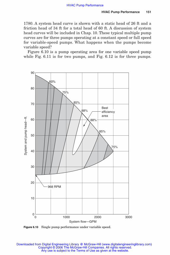
HVAC Pump Performance 151
1780. A system head curve is shown with a static head of 26 ft and afriction head of 34 ft for a total head of 60 ft. A discussion of systemhead curves will be included in Chap. 10. These typical multiple pumpcurves are for three pumps operating at a constant speed or full speedfor variable-speed pumps. What happens when the pumps becomevariable speed?
Figure 6.10 is a pump operating area for one variable speed pumpwhile Fig. 6.11 is for two pumps, and Fig. 6.12 is for three pumps.
90
80
70
60
50
40
30
20
10
00 1000 2000 3000
System flow—GPM
Sys
tem
and
pum
p he
ad—
ft.
60%
75%
88%
85%
85%
88%
75%
Bestefficiencyarea
968 RPM
Figure 6.10 Single pump performance under variable speed.
Rishel_CH06.qxd 20/4/06 6:06 PM Page 151
Downloaded from Digital Engineering Library @ McGraw-Hill (www.digitalengineeringlibrary.com)Copyright © 2006 The McGraw-Hill Companies. All rights reserved.
Any use is subject to the Terms of Use as given at the website.
HVAC Pump Performance

152 HVAC Pumps and Their Performance
The minimum speed for these pumps with the 26 ft of constant headon the system is 935. These figures of operating areas are shaded toshow the best efficiency are a in white and the worst operating areasin dark cross-hatching. This is a pictorial representation of the con-trol algorithm for the operation of this pumping system. Pump addi-tion and subtraction points will be superimposed upon these figuresin Chap. 11 to demonstrate the control protocol necessary for effi-cient control of these pumps in the application chapters of this book.
Pump selection with variable-speed pumping allows great latitudein the selection of the actual pump diameter. Chapter 11 will provideinformation on the over speeding and under speeding of these pumpsto achieve maximum wire-to-water efficiency.
It should be noted that the system head curve in Fig. 6.9 is not asmooth curve as is often shown. This is due to the variation in the
60%50%
75%
85%
88%
88%
Bestefficiencyarea
Sys
tem
and
pum
p he
ad—
ft90
80
70
60
50
40
30
20
10
00 1000 2000 3000
System flow—GPM4000
Figure 6.11 Two-pump performance under variable speed.
Rishel_CH06.qxd 20/4/06 6:06 PM Page 152
Downloaded from Digital Engineering Library @ McGraw-Hill (www.digitalengineeringlibrary.com)Copyright © 2006 The McGraw-Hill Companies. All rights reserved.
Any use is subject to the Terms of Use as given at the website.
HVAC Pump Performance
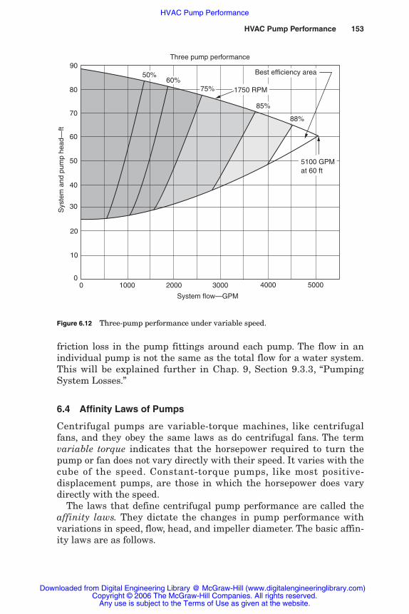
HVAC Pump Performance 153
friction loss in the pump fittings around each pump. The flow in anindividual pump is not the same as the total flow for a water system.This will be explained further in Chap. 9, Section 9.3.3, “PumpingSystem Losses.”
6.4 Affinity Laws of Pumps
Centrifugal pumps are variable-torque machines, like centrifugalfans, and they obey the same laws as do centrifugal fans. The termvariable torque indicates that the horsepower required to turn thepump or fan does not vary directly with their speed. It varies with thecube of the speed. Constant-torque pumps, like most positive-displacement pumps, are those in which the horsepower does vary directly with the speed.
The laws that define centrifugal pump performance are called theaffinity laws. They dictate the changes in pump performance withvariations in speed, flow, head, and impeller diameter. The basic affin-ity laws are as follows.
00 1000 2000 3000
System flow—GPM
4000 5000
Sys
tem
and
pum
p he
ad—
ft90
80
70
60
50
40
30
20
10
5100 GPMat 60 ft
Best efficiency area
88%
85%
75%60%
50%
1750 RPM
Three pump performance
Figure 6.12 Three-pump performance under variable speed.
Rishel_CH06.qxd 20/4/06 6:06 PM Page 153
Downloaded from Digital Engineering Library @ McGraw-Hill (www.digitalengineeringlibrary.com)Copyright © 2006 The McGraw-Hill Companies. All rights reserved.
Any use is subject to the Terms of Use as given at the website.
HVAC Pump Performance

154 HVAC Pumps and Their Performance
For a fixed-diameter impeller:
1. The pump capacity varies directly with the speed.
1
2
� � �SS
1
2
� (6.1)
2. The pump head varies as the square of the speed.
�hh
1
2
� � �SS
1
2
2
2� (6.2)
3. The pump brake horsepower required varies as the cube of thespeed:
�bbhh
pp
1
2
� � �SS
1
2
3
3� (6.3)
Figure 6.13a describes these three laws graphically. These are thebasic laws that must be understood in any attempt to comprehendcentrifugal pump performance. It must be remembered that theselaws pertain to the pump itself. They do not describe pump perfor-mance when the pump is connected to a system of piping containingboth constant and variable head.
Figure 6.13b describes the variation in flow, head, and power for avariable-speed pump operating with a constant head of 20 ft; data forthese curves are provided in Table 6.2 later in this chapter. This con-stant head can be static head on a cooling tower or constant differen-tial pressure on a secondary chilled or hot water system. It is obviousthat there is no comparison between the curves in Fig. 6.13a and b. At50 percent speed and 885 rev/min, the flow is 36 percent, not 50 per-cent, the head is 30 percent, and the brake horsepower is 10 percent,not 12.5 percent. This demonstrates the need to evaluate pump per-formance with the actual system conditions and not depend on theclassic affinity laws of Fig. 6.13a.
This is emphasized at this point because it may appear from Fig. 6.1athat pump impellers can be changed just through observation of thebasic affinity laws of Fig. 6.13a. Pump impeller diameter should not bechanged without a thorough evaluation of the system head curve orarea.
Changing the pump impeller diameter changes pump performance,as does pump speed.
Rishel_CH06.qxd 20/4/06 6:06 PM Page 154
Downloaded from Digital Engineering Library @ McGraw-Hill (www.digitalengineeringlibrary.com)Copyright © 2006 The McGraw-Hill Companies. All rights reserved.
Any use is subject to the Terms of Use as given at the website.
HVAC Pump Performance
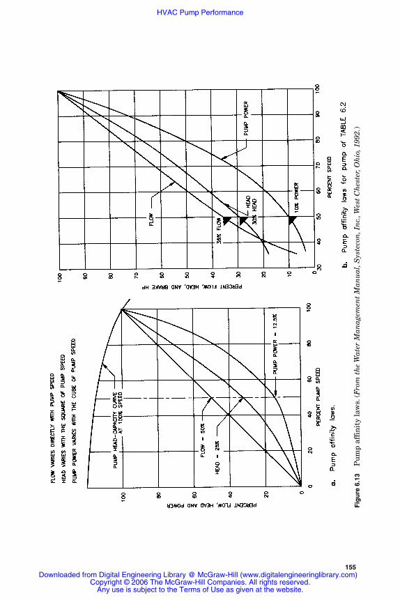
Fig
ure
6.1
3P
um
p af
fin
ity
law
s.(F
rom
th
e W
ater
Man
agem
ent
Man
ual
,Sys
teco
n,I
nc.
,Wes
t C
hes
ter,
Oh
io,1
992.
)
155
Rishel_CH06.qxd 20/4/06 6:06 PM Page 155
Downloaded from Digital Engineering Library @ McGraw-Hill (www.digitalengineeringlibrary.com)Copyright © 2006 The McGraw-Hill Companies. All rights reserved.
Any use is subject to the Terms of Use as given at the website.
HVAC Pump Performance

156 HVAC Pumps and Their Performance
For a fixed pump speed:
1. The pump capacity varies directly with the impeller diameter:
1
2
� � �dd
1
2
� (6.4)
2. The pump head varies as the square of the impeller diameter:
�hh
1
2
� � �dd
1
2
2
2� (6.5)
3. The pump brake horsepower required varies as the cube of the impeller diameter:
�bbhh
pp
1
2
� � �dd
1
2
3
3� (6.6)
It should be reemphasized that pump impellers should not bechanged without a thorough review of the water system characteristics.
6.4.1 Affinity laws
Unfortunately, the specific speed of the pump may change from mini-mum allowable impeller diameter to maximum diameter. Therefore,the affinity laws for impeller change may not be accurate. Figure 6.14describes an actual set of pump curves for a particular pump withdifferent impeller diameters and a constant dynamometer speed of1750 rev/min. The parabolic path of the best efficiency point is drawnon this curve. The best efficiency point with a full diameter is shownas point A at 1335 gal/min and 72 ft of head with 88 percent efficiency.If the affinity laws were to prevail, the equivalent point for a 7 in diam-eter impeller should be at point B or 960 gal/min at 38 ft. Instead theactual point for this impeller diameter is at Point C or 900 gal/min at33 ft. This is about a 6 percent loss in pump duty. One might arguethat this isn’t much considering that the maximum and minimumallowable impeller diameters were used. However, any anomaly inthese calculations creates a feeling of distrust of the whole program.
As demonstrated in the previous section, as the pump impellerdiameter changes, the specific speed of the pump may change alsoso that the pump performance does not follow these affinity laws forimpeller diameter change. (Specific speed has been defined in Chap.4.) Not all pumps evince this variation in specific speed with impellerdiameter, but there is appreciable evidence of changes in specific
Rishel_CH06.qxd 20/4/06 6:06 PM Page 156
Downloaded from Digital Engineering Library @ McGraw-Hill (www.digitalengineeringlibrary.com)Copyright © 2006 The McGraw-Hill Companies. All rights reserved.
Any use is subject to the Terms of Use as given at the website.
HVAC Pump Performance
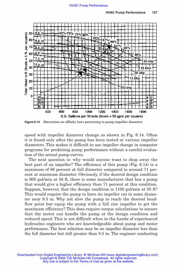
HVAC Pump Performance 157
speed with impeller diameter change as shown in Fig. 6.14. Oftenit is found only after the pump has been tested at various impellerdiameters. This makes it difficult to use impeller change in computerprograms for predicting pump performance without a careful evalua-tion of the actual pump curves.
The next question is: why would anyone want to chop away thebest part of an impeller? The efficiency of this pump (Fig. 6.14) is amaximum of 88 percent at full diameter compared to around 71 per-cent at minimum diameter. Obviously, if the desired design conditionis 900 gal/min at 38 ft, there is some manufacturer that has a pumpthat would give a higher efficiency than 71 percent at this condition.Suppose, however, that the design condition is 1100 gal/min at 55 ft?This would require the pump to have its impeller cut to some diame-ter near 8.5 in. Why not slow the pump to reach the desired head-flow point but equip the pump with a full size impeller to get themaximum efficiency? This does require torque calculations to ensurethat the motor can handle the pump at the design condition andreduced speed. This is not difficult when in the hands of experiencedhydraulics engineers who are knowledgeable about pump and motorperformance. The best selection may be an impeller diameter less thanthe full diameter but still greater than 8.5 in. The engineer conducting
Figure 6.14 Aberration on affinity laws pertaining to pump impeller diameter.
Rishel_CH06.qxd 20/4/06 6:06 PM Page 157
Downloaded from Digital Engineering Library @ McGraw-Hill (www.digitalengineeringlibrary.com)Copyright © 2006 The McGraw-Hill Companies. All rights reserved.
Any use is subject to the Terms of Use as given at the website.
HVAC Pump Performance
158 HVAC Pumps and Their Performance
the computer calculations will determine the impeller diameter thatprovides the maximum wire-to-water efficiency throughout the loadrange for the pump. These computer calculations include taking intoconsideration the flow and head ranges of the water system as wellas the number of pumps provided in parallel for that system.Further, the pump efficiency and the wire-to-shaft efficiency of themotor/variable speed drive combination must be computed as thewater system conditions vary from minimum to maximum waterflow. All of these factors will be discussed in the chapters on pumpapplication.
6.5 Pump Suction Limitations
Centrifugal pumps operate on water, a liquid stream that can changeits state under certain pressure-temperature relationships. Some par-ticular characteristics of water were included in Chap. 1 to help under-stand these conditions. One of the first rules of thermodynamics isthat there is a temperature for every absolute pressure at whichwater will change its state from a liquid to a gas. A little understoodword is cavitation. Cavitation is the result of the changing of part of awater stream from a liquid to a gas. It occurs when the temperatureof the water reaches the evaporation temperature for the absolutepressure of that stream. The specific gravity of the gas (steam) ismuch less than that of the liquid water, so the result is “hammering”as dense water and then “light” steam hit the internal parts of awater system. Such hammering can erode the internal parts of theimpeller or casing of a pump. Cavitation can damage many parts of awater system; the damage usually occurs first in a pump due to thefact that the suction of a pump may be the point of lowest pressure inthe water system.
For example, assume that a hot water system requires 240°F water.From Table 2.4, the vapor pressure for 240°F water is 24.97 psia or10.27 psig with an atmospheric pressure of 14.7 psi. At least a 10-psiacushion, or 21 psig, should be maintained on this hot water system sothat no part of the system approaches the vapor pressure of the 240°Fwater. If the pressure does drop, cavitation will occur whenever thishot water pressure falls below 24.97 psia.
How can cavitation be avoided in a water system? Simply by ensur-ing that the water pressure in every part of the water system isgreater than the evaporation pressure for any potential temperatureof water in that system. Tables 2.3 and 2.4 provide vapor pressuresfor water at different temperatures. There is so much informationavailable and tools such as the pressure-gradient diagram that there
Rishel_CH06.qxd 20/4/06 6:06 PM Page 158
Downloaded from Digital Engineering Library @ McGraw-Hill (www.digitalengineeringlibrary.com)Copyright © 2006 The McGraw-Hill Companies. All rights reserved.
Any use is subject to the Terms of Use as given at the website.
HVAC Pump Performance

HVAC Pump Performance 159
is no excuse for cavitation to occur in a normally operating HVACwater system. Since the pump appears to be the HVAC equipmentmost vulnerable to cavitation, it is a good place for the designer tostart the evaluation process needed to avoid cavitation.
6.5.1 Net positive suction head
Centrifugal pumps are tested very carefully to determine the net pos-itive suction pressure that must be placed on the pump suction atvarious flows through that pump to eliminate cavitation. This is calledthe net positive suction head required (NPSHR) curve and appears inFigs. 6.1a and 6.1b as the net positive suction head required by thepump. Most of the centrifugal pumps used in the HVAC field cannotpull water into the pump casing; it must be pushed. The NPSHRcurve merely defines the amount of push. If this amount of pressureis maintained on the pump suction, cavitation will not occur in thepump. Figure 6.1a provides the type of NPSHR curve found on mostpump curves; more precise NPSHR curves are shown in Fig. 6.1b.Figure 6.15a describes the pressure gradient along the liquid path intoa pump.
How do we calculate the net positive suction head needed to avoidcavitation? The actual NPSH on the pump suction must always beequal to or greater than the NPSH required by the pump. The actualsuction pressure is called the net positive suction head available(NPSHA), so
NPSHA ≥ NPSHR (6.7)
The problem for the uninitiated designer when calculating NPSHAis the attempt to do so in absolute pressures (psia). If the calculationsare made in feet of head, they become much easier. This is reasonable,because the NPSHR curve of the pump is always in feet of head.Equation 6.8 is acceptable for HVAC operations at temperatures up to85°F. The amount of “push” available, or net positive suction pressureavailable, is simply the atmospheric pressure plus the system pres-sure minus the vapor pressure of the water minus the friction of thesuction pipe. Figure 6.15b demonstrates this using the most commonpoint in HVAC systems for calculating NPSHA, namely, a coolingtower. As shown,
NPSHA � Pa � Ps � Pvp � Pf , in ft of head (6.8)
where Pa � atmospheric pressure in feet at the installation altitude(This can be done by reading the value directly from Table2.1 for water from 32 to 85°F.)
Rishel_CH06.qxd 20/4/06 6:06 PM Page 159
Downloaded from Digital Engineering Library @ McGraw-Hill (www.digitalengineeringlibrary.com)Copyright © 2006 The McGraw-Hill Companies. All rights reserved.
Any use is subject to the Terms of Use as given at the website.
HVAC Pump Performance

Fig
ure
6.1
5N
PS
H c
ondi
tion
s fo
r H
VA
C p
um
ps.
(Fro
m R
ober
t K
ern
,H
ow t
o d
esig
n p
ipin
g fo
r pu
mp-
suct
ion
con
dit
ion
s,C
hem
ical
En
gin
eeri
ng,
Apr
il 2
8,19
75,p
.119
.)
160
Rishel_CH06.qxd 20/4/06 6:06 PM Page 160
Downloaded from Digital Engineering Library @ McGraw-Hill (www.digitalengineeringlibrary.com)Copyright © 2006 The McGraw-Hill Companies. All rights reserved.
Any use is subject to the Terms of Use as given at the website.
HVAC Pump Performance
HVAC Pump Performance 161
Ps � static head of water level above the pump impeller (Thisis negative if water level is below the impeller.)
Pvp � vapor pressure of water, in feet, at operating temperature(see Tables 2.3 and 2.4)
Pf � friction of suction pipe, fittings, and valves, in feet of head
Equation 6.8 can be used for higher temperatures and elevations.Assume the following:
1. The maximum cooling tower water temperature is 95°F, so Pvp �1.9 ft of vapor pressure. From Table 2.3.
2. The cooling tower sump is above the pump impeller, and Ps � 5 ft.
3. The installation altitude is 1000 ft; From Table 2.1, the atmosphericpressure, Pa = 32.8 ft.
4. The friction loss of the suction pipe, fittings, and valves Pf is 6 ft.Thus
NPSHA � 32.8 � 5 � 1.9 � 6 � 29.9 ft
Any pump handling this water must have an NPSHR of less than29.9 ft at any possible flow through the pump.
Warning. Calculation of NPSHA for a cooling tower should be madeat the maximum possible operating water temperature in the tower, notthe design water temperature.
6.5.2 Air entrainment and vortexing
A companion to cavitation is air entrainment in the suction of cen-trifugal pumps. Air can enter the water system at several points, asshown in Fig. 6.16a. The effect of air entrainment on pump perfor-mance is described in Fig. 6.16b; it indicates the drastic reduction inboth head and capacity when air is present. Every effort must bemade to ensure that the water in a pump is free of air.
Air entrainment is often confused with cavitation when drawingwater from a tank. It is thought that air entrainment cannot happenwhen a tank of water is 10 to 15 ft deep. Air entrainment can occur eas-ily when water is taken from a free surface of water regardless of thedepth of the water. Figure 6.17 describes the air entrainment that canoccur if water is not removed properly from an open tank. As shownin Fig. 6.17a, a small whirlpool occurs on the surface, and this deep-ens into a vortex that will extend down to the water outlet from thetank, and finally, air will pass into the impeller of the pump, causing
Rishel_CH06.qxd 20/4/06 6:06 PM Page 161
Downloaded from Digital Engineering Library @ McGraw-Hill (www.digitalengineeringlibrary.com)Copyright © 2006 The McGraw-Hill Companies. All rights reserved.
Any use is subject to the Terms of Use as given at the website.
HVAC Pump Performance
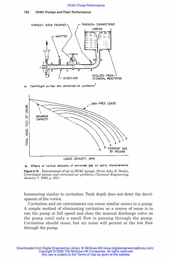
162 HVAC Pumps and Their Performance
hammering similar to cavitation. Tank depth does not deter the devel-opment of the vortex.
Cavitation and air entrainment can cause similar noises in a pump.A simple method of eliminating cavitation as a source of noise is torun the pump at full speed and close the manual discharge valve onthe pump until only a small flow is passing through the pump.Cavitation should cease, but air noise will persist at the low flowthrough the pump.
Figure 6.16 Entrainment of air in HVAC pumps. (From John H. Doolin,Centrifugal pumps and entrained-air problems, Chemical Engineering,January 7, 1963, p. 103.)
Rishel_CH06.qxd 20/4/06 6:06 PM Page 162
Downloaded from Digital Engineering Library @ McGraw-Hill (www.digitalengineeringlibrary.com)Copyright © 2006 The McGraw-Hill Companies. All rights reserved.
Any use is subject to the Terms of Use as given at the website.
HVAC Pump Performance

HVAC Pump Performance 163
Vortexing can occur easily when water is taken from a tank, partic-ularly if the water outlet is on the side or bottom of the tank, asshown in Fig. 6.17a; a fully developed vortex is shown in this figure.Vortexing can be eliminated by placing an antivortexing plate above a
Figure 6.17 Vortexing in HVAC pumps. (From James H. Ingram, Suction side problems:Gas entrainment, Pump and System Magazine, September 1994, p. 34.)
Rishel_CH06.qxd 20/4/06 6:06 PM Page 163
Downloaded from Digital Engineering Library @ McGraw-Hill (www.digitalengineeringlibrary.com)Copyright © 2006 The McGraw-Hill Companies. All rights reserved.
Any use is subject to the Terms of Use as given at the website.
HVAC Pump Performance

164 HVAC Pumps and Their Performance
bottom inlet, as shown in Fig. 6.17b; a side inlet can be corrected byplacing an antivortexing plate above the inlet (Fig. 6.17c). On shallowcooling tower sumps, if vortexing persists, it may be necessary to in-stall a slotted vortex breaking tube, as shown in Fig. 6.18d. As an al-ternative, an elbow can be installed on the suction connection of aside inlet and pointed downward, as shown in Fig. 6.17e. If vortexingstill occurs, a square plate can be installed on the suction of the elbow.Vortex-breaking devices must be designed to avoid substantial addi-tional friction losses. Normally, the friction loss of an entrance from atank is equal to about 0.5 � V 2/2g, where V is the velocity of thewater in the entering pipe. The vortex-breaking device should notincrease this entrance loss if possible.
A simple method to determine if vortexing is occurring is to placemats or rafts on the water surface above the inlet from the tank. Thisprevents the vortex from forming and can be done without drainingthe tank.
Vortexing should not occur in HVAC tanks and sumps. The precau-tions are so simple that the design of these tanks and sumps shouldalways accommodate them.
6.5.3 Submergence of pumps in wet pits oropen tanks
Pumps installed in a tank, such as vertical turbine pumps, have aspecific submergence requirement. The submergence, or distanceabove the inlet bell of such a pump, must be great enough to ensurethat the friction loss of the water passing through the bell and enter-ing the pump is made up by the static height of the water over thesuction bell. This height is determined by whether the suction of thepump is or is not equipped with a suction strainer. Most manufactur-ers of axial-flow pumps have adequate data on submergence andclearance from the bottom of the tank for the water system designer;their recommendations should always be followed. Table 6.1 describes
TABLE 6.1 Typical Submergences for Vertical Turbine Pumps (for Operation at1750 rev/min)
Bowl size, in Submergence, in Bowl size, in Submergence, in
04 07 13 2306 11 14 3008 12 15 3210 16 16 3611 20 18 3612 24 20 42
Rishel_CH06.qxd 20/4/06 6:06 PM Page 164
Downloaded from Digital Engineering Library @ McGraw-Hill (www.digitalengineeringlibrary.com)Copyright © 2006 The McGraw-Hill Companies. All rights reserved.
Any use is subject to the Terms of Use as given at the website.
HVAC Pump Performance

HVAC Pump Performance 165
typical submergences for vertical turbine pumps operating at 1750rev/min; these submergences should not be applied to any specificmanufacturer’s pumps.
6.6 Pumping Energy
Following is a review of the various energy equations that must beused in determining the energy requirements of a water system andthe energy consumed by pumps and their drivers in satisfying thoserequirements. It is important that the HVAC system designer under-stand the difference between the energy absorbed by the water andthat consumed by the pump or its motor.
6.6.1 Water horsepower
The energy required by a pump, as indicated by the affinity laws,depends on its speed and the diameter of its impeller. The energyimparted to the water by a pump is called the water horsepower(whp). Its equation is
whp � �Q
3�
9h60
� s� (6.11)
where Q � flow, in gal/minh � head, in fts � specific gravity
Most HVAC water systems operate from 32 to 240°F water, wherethe specific gravity can vary from 1.001 at 32°F to 0.948 at 240°F. Forthese applications, the specific gravity is generally assumed to be1.00; systems designed to operate at 240°F must be able to function atstartup with water temperatures near 50°F or at specific gravities ofaround 1.00. Water horsepower for these systems usually ignores thespecific gravity and assumes it to be 1.00. This should not be the casewith medium- and high-temperature water systems, where the oper-ating temperatures can vary from 250 to 450°F. The specific gravity of450°F water is 0.825 and should not be ignored in calculating pumpoperating energy for these systems. Again, pump motor or driverbrake horsepower should recognize that the pump may be required tooperate with colder water and specific gravities near 1.0.
Following is an example of water horsepower: If a pump is deliver-ing 1000 gal/min at a total head of 100 ft, the water horsepower is
whp � �100
309�
60100
� � 25.25 whp
Rishel_CH06.qxd 20/4/06 6:06 PM Page 165
Downloaded from Digital Engineering Library @ McGraw-Hill (www.digitalengineeringlibrary.com)Copyright © 2006 The McGraw-Hill Companies. All rights reserved.
Any use is subject to the Terms of Use as given at the website.
HVAC Pump Performance
166 HVAC Pumps and Their Performance
6.6.2 Pump brake horsepower
The energy required to operate a pump is determined in brake horse-power (bhp); the difference between water horsepower and pumpbrake horsepower is the energy lost in the pump. The pump brakehorsepower equation is therefore
bhp � �wPh
�
p� (6.12)
where P�
is the pump efficiency as a decimal.For example, if the pump in the preceding example is operating at
an efficiency of 85 percent,
bhp � �205.8.255
� � 29.7 hp
6.6.3 Pump motor power in kilowatts
The electrical energy, pump kilowatts, for a motor-driven pump musttake in consideration the efficiency of the motor on constant-speedpumps and the wire-to-shaft efficiency of the motor and variable-speed drive on variable-speed pumps. Again, the difference betweenthe pump brake horsepower and electric power input to the motor orvariable-speed drive and motor is the efficiency of these devices. Thepower must be converted from brake horsepower to kilowatts, so thepump brake horsepower must be multiplied by 0.746. The equation is
Pump kW � �bhp
E� 0
�
.746� (6.13)
where E�
is the efficiency of the electric motor or the motor and vari-able-speed drive as a decimal.
For example, if the preceding pump is variable speed with a wire-to-shaft efficiency of 89 percent for the variable-speed drive and high-efficiency motor, then
Pump kW � �29.7
0�
.809.746
� � 24.9 kW
Summarizing Eqs. 6.11 through 6.13,
Pump kW ��530
Q8 �
�
Ph
�
� s� E�
� (6.14)
As will be explained in Chap. 7, the combined efficiency of an elec-tric motor and a variable-speed drive cannot be just the multiplication
Rishel_CH06.qxd 20/4/06 6:06 PM Page 166
Downloaded from Digital Engineering Library @ McGraw-Hill (www.digitalengineeringlibrary.com)Copyright © 2006 The McGraw-Hill Companies. All rights reserved.
Any use is subject to the Terms of Use as given at the website.
HVAC Pump Performance

HVAC Pump Performance 167
of the efficiencies of the motor and the variable-speed drive. It must bedetermined by the variable-speed drive manufacturer with recognitionof the manufacturer and the quality of the electric motor.
Steam turbine–driven pumps also will be reviewed in Chap. 7; theenergy required by them is usually based on a water rate in poundsper pump brake horsepower. Equation 6.12 is used to compute themaximum water rate at maximum flow and head.
6.6.4 Actual energy consumedby variable-speed pumps
The energy consumed by variable-speed pumps requires knowledge ofthe water system head curve or area on which they are operating.These curves and areas will be described in Chap. 9. Table 6.2 describesthe variation in pump efficiency, pump brake horsepower, speed,motor kilowatts, and overall wire-to-water efficiency of the pump,motor, and variable-speed drive with a system head curve that con-tains a constant head of 20 ft. The pump fitting losses are accounted forin these calculations. The pump head-capacity curve in Fig. 6.1a is usedin these calculations.
The computer program for calculating the wire-to-water efficiencyfor this pump is available from manufacturers of variable-speedpumping systems. The data for the wire-to-shaft efficiency included inthis table are secured from the variable-speed drive manufacturer.The overall wire-to-water efficiency of variable-speed pumping sys-tems that have two or more pumps operating in parallel is discussedin detail in Chap. 10.
TABLE 6.2 System and Pump Variables
Pump Pump Wire-to-shaft Wire-to-water System Pump speed, efficiency, Pump efficiency, Total efficiency,gal/min head, ft rev/min % bhp % kW %
0100 020.9 0626 41.1 01.3 58.1 01.7 23.80200 023.4 0674 63.2 01.9 61.4 02.3 38.40300 027.2 0742 74.3 02.8 65.8 03.1 47.90400 032.2 0826 79.7 04.1 70.7 04.3 54.70500 038.6 0918 82.6 05.9 75.4 05.8 59.90600 046.1 1013 84.1 08.3 79.5 07.8 63.80700 054.7 1113 85.0 11.4 83.0 10.2 66.80800 064.5 1217 85.4 15.3 85.9 13.3 69.10900 075.4 1324 85.6 20.0 88.1 17.0 70.61000 087.5 1433 85.7 25.8 89.7 21.4 71.71100 100.6 1544 85.8 32.6 90.7 26.8 72.21200 114.8 1656 85.8 40.5 91.3 33.1 72.51300 120.0 1770 85.7 49.8 91.7 40.5 72.6
Rishel_CH06.qxd 20/4/06 6:06 PM Page 167
Downloaded from Digital Engineering Library @ McGraw-Hill (www.digitalengineeringlibrary.com)Copyright © 2006 The McGraw-Hill Companies. All rights reserved.
Any use is subject to the Terms of Use as given at the website.
HVAC Pump Performance
168 HVAC Pumps and Their Performance
6.7 Pump Noise
Pump noise in HVAC water systems is objectionable since it cantravel through the piping to other areas of the building outside theequipment rooms. Also, the noise may indicate trouble in the pumpor its motor with the possibility of expensive maintenance. Further, anoisy pump often indicates inefficient pump operation. An interest-ing article appeared in the September 2004 issue of HPACEngineering Magazine on how low-frequency noise impairs learning.There is absolutely no reason to allow noisy pump operation; noise inpumps comes from improper installation, selection, or faulty opera-tion. Pump noise is much more prevalent in constant-speed pumpsthan in variable-speed pumps. Pump noise originates from outside ofor inside the pump.
6.7.1 Noise outside the pump
The outside noises stem from the motor or misalignment of the pumpand motor. Motor noise comes basically from speed. Most HVAC pumpmotors operate quietly at either 1200 or 1800 rev/min synchronousspeeds. At these speeds there should not be any objectionable noise.Often, there are opportunities to achieve higher pump efficiencies byoperating the pumps at 3600 rev/min synchronous on high-head, vari-able-speed applications. Care should be taken, in this case, to ensurethat objectionable noise will not travel outside the equipment roomwhen the pump must operate near its design condition.
The other major outside sources of noise are caused by misalign-ment of the pump and motor or distortion of the pump by the con-nected piping. These are easily corrected by realignment of thepump and its motor and checking the piping to ensure that it issupported properly. Standard procedures for pump alignment areavailable from pump manufacturers and the Hydraulic Institute.Misalignment may also be caused by a poor pump foundation or thepump base itself. See Chap. 25 for the proper installation of HVACpumps.
Most of the pump companies and the Hydraulic Institute have verygood instructions and diagrams for proper design of pump founda-tions. Pump bases vary; some have more than adequate strength tomaintain pump and motor alignment while others may be question-able. The design of pump bases should be scrutinized carefully to ensureadequate construction. Dowling of pump bases is not required in mostHVAC installations other than large cooling tower pumps and somelarge chilled water pumps. Likewise, vibration and temperature detec-tors are seldom required on HVAC pumps and motors.
Rishel_CH06.qxd 20/4/06 6:06 PM Page 168
Downloaded from Digital Engineering Library @ McGraw-Hill (www.digitalengineeringlibrary.com)Copyright © 2006 The McGraw-Hill Companies. All rights reserved.
Any use is subject to the Terms of Use as given at the website.
HVAC Pump Performance
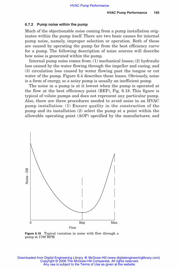
HVAC Pump Performance 169
6.7.2 Pump noise within the pump
Much of the objectionable noise coming from a pump installation orig-inates within the pump itself. There are two basic causes for internalpump noise, namely, improper selection or operation. Both of theseare caused by operating the pump far from the best efficiency curvefor a pump. The following description of noise sources will describehow noise is generated within the pump.
Internal pump noise comes from: (1) mechanical losses; (2) hydraulicloss caused by the water flowing through the impeller and casing, and(3) circulation loss caused by water flowing past the tongue or cutwater of the pump. Figure 6.4 describes these losses. Obviously, noiseis a form of energy, so a noisy pump is usually an inefficient pump.
The noise in a pump is at it lowest when the pump is operated atthe flow at the best efficiency point (BEP), Fig. 6.18. This figure istypical of volute pumps and does not represent any particular pump.Also, there are three procedures needed to avoid noise in an HVACpump installation: (1) Ensure quality in the construction of thepump and its installation (2) select the pump at a point within theallowable operating point (AOP) specified by the manufacturer, and
Bep Max.0
Noi
se -
DB
Flow
Figure 6.18 Typical variation in noise with flow through apump at 1780 RPM
Rishel_CH06.qxd 20/4/06 6:06 PM Page 169
Downloaded from Digital Engineering Library @ McGraw-Hill (www.digitalengineeringlibrary.com)Copyright © 2006 The McGraw-Hill Companies. All rights reserved.
Any use is subject to the Terms of Use as given at the website.
HVAC Pump Performance
170 HVAC Pumps and Their Performance
(3) ensure that the pump always operates within this flow range, par-ticularly with constant-speed pumps. It is obvious that one of the greatadvantages of a variable-speed pump, properly controlled, is the abilityto operate it near its BEP curve at all loads on the water system.
6.8 Sources of Pump Information
It is obvious that the information included in this chapter on pumpperformance requires substantial data from the pump manufacturerson the selection and operation of pumps on HVAC water systems.Most of the pump manufacturers active in this market have gone togreat lengths to provide technical information on their pumps.
Traditionally, pump catalogs contain detailed information on pumpphysical dimensions and general arrangement as well as pump head-capacity curves at 1150, 1750, and 3500 rev/min. Data on slower speedssuch as 850 and 720 rev/min are provided for larger-capacity pumps.The development of computers has enabled pump manufacturers toprovide these data in software form such as diskettes or CD ROM.Some pump manufacturers are furnishing computer selection programswhere the required pump head and capacity are inserted and the pumpselection is made for the designer. This selection can be on the basis of(1) the most efficient, or (2) the most economical in first cost.
6.9 Summary
The increase in cost of energy has thrust efficiency of operation to theforefront. Highly efficient centrifugal pumps are now available at lit-tle added cost over less efficient pumps. The first and foremost evalu-ation of HVAC pumps should therefore be efficiency. Since so many ofthese pumps are now variable speed, efficiency throughout the oper-ating range must be considered.
Ease of pump maintenance was of major concern in the past. Thereduction of pump maintenance due to variable speed has lessenedthe concern for maintenance capability. Traditionally, pumps havebeen given much more space for operation than centrifugal fans.Many fans are tucked up in air handling units where repair is quitedifficult. With the application of variable speed and greater care inpump operation, the large spaces around HVAC pumps are no longerneeded. Most HVAC pumps should operate for years without any seri-ous maintenance.
Along with efficiency and first cost, these pumps should be evaluat-ed for the space they require. As can be seen in Chap. 5, there aremany different pump configurations for all the applications in the
Rishel_CH06.qxd 20/4/06 6:06 PM Page 170
Downloaded from Digital Engineering Library @ McGraw-Hill (www.digitalengineeringlibrary.com)Copyright © 2006 The McGraw-Hill Companies. All rights reserved.
Any use is subject to the Terms of Use as given at the website.
HVAC Pump Performance
HVAC industry. The development of vertical pump assemblies hasreduced the space needed without sacrificing ease of maintenance.Typical of this is the large in-line double-suction pump, which offersspace saving as well as ease of maintenance.
The HVAC industry has many capable manufacturers of pumps andpumping systems that can provide efficient pumping for any applica-tion encountered in heating ventilating and air conditioning.
6.10 Bibliography
John H. Doolin, Centrifugal pumps and entrained-air problems, Chemical Engineering,January 7, 1963.
James H. Ingram, Suction side problems: Gas entrainment, Pumps and SystemsMagazine, September 1994.
Robert Kern, How to design piping for pump-suction conditions, Chemical Engineering,April 28, 1975.
The Water Management Manual, Systecon, Inc., West Chester, Ohio, 1992.
HVAC Pump Performance 171
Rishel_CH06.qxd 20/4/06 6:06 PM Page 171
Downloaded from Digital Engineering Library @ McGraw-Hill (www.digitalengineeringlibrary.com)Copyright © 2006 The McGraw-Hill Companies. All rights reserved.
Any use is subject to the Terms of Use as given at the website.
HVAC Pump Performance

Rishel_CH06.qxd 20/4/06 6:06 PM Page 172
Downloaded from Digital Engineering Library @ McGraw-Hill (www.digitalengineeringlibrary.com)Copyright © 2006 The McGraw-Hill Companies. All rights reserved.
Any use is subject to the Terms of Use as given at the website.
HVAC Pump Performance
Chapter
173
7Pump Drivers and
Variable-Speed Drives
7.1 Introduction
HVAC pumps are driven by electric motors, steam turbines, and gas-or oil-fueled engines. By far most of the pumps are operated by electricmotors. Steam turbine–driven pumps are found on large centralchilled water or cogeneration plants where steam is available fromboilers or exhaust steam from turbine-driven chillers or electric gener-ators. Engine-driven pumps are found on large pumping installationswhere a source other than electricity is needed; this can be in areas ofpower curtailment or where emergency pump operation is required.
7.2 Electric Motors
The following discussion makes reference to two principal organizationsin the electrical industry. These are (1) the Institute of Electrical andElectronic Engineers (IEEE) and (2) the National ElectricalManufacturers Association (NEMA).
Most electric motor–driven pumps in the U.S. HVAC market are single-or three-phase, 60 Hz. Table 2.8 provides the motor nameplate voltagesand the accompanying distribution system voltages. This table providesthe best match of motor voltages to distribution voltages and meetscurrent motor design practice.
Although 50-Hz power is generally not used in the United States,HVAC designers will encounter it occasionally in the United States andwhen working in foreign countries. Table 2.9 also includes informationon 50-Hz power and motors. Standard pump curves are available from
Rishel_07.qxd 20/4/06 6:29 PM Page 173
Downloaded from Digital Engineering Library @ McGraw-Hill (www.digitalengineeringlibrary.com)Copyright © 2006 The McGraw-Hill Companies. All rights reserved.
Any use is subject to the Terms of Use as given at the website.
Source: HVAC Pump Handbook

174 HVAC Pumps and Their Performance
the pump manufacturers for operation with 50-Hz motors at inductionmotor speeds of around 960 and 1450 rev/min, compared with 1150 and1750 rev/min for such motors operating on 60-Hz power.
Almost all electric motors in the HVAC field are induction-type. Largecooling tower or condenser motors over 1000 hp may be synchronous-type, running at 1200 and 1800 rev/min. Wound rotor and direct-currentmotors offer few advantages for most of these pump applications.
7.2.1 Electric motor power characteristics
All electric motors are designed to operate with some variation in theelectric power supplied to them. Following are some general rules forthe variation in power characteristics:
1. Voltage variation must be limited to �10 percent at rated frequency.
2. Frequency variation must be limited to �5 percent at rated voltage.
3. Combined variation of voltage and frequency must be limited tothe arithmetic sum of 10 percent.
4. On polyphase motors, the voltage imbalance should be kept within1 percent between phases. Table 7.1 describes the great decrease inmotor rating caused by greater imbalances. Balancing of loadsbetween phases in a building becomes a necessity to ensure maxi-mum output from the polyphase electric motors.
TABLE 7.1 Derating Factors Due to VoltageImbalance for Polyphase Motors
Percent voltage imbalance Derating factor
0.0 1.000.5 1.001.0 1.001.5 0.972.0 0.952.5 0.933.0 0.893.5 0.854.0 0.824.5 0.785.0 0.76
SOURCE: AC Motor Selection and ApplicationGuide, Bulletin GET-6812B, General ElectricCompany, Fort Wayne, Ind., 1993, p. 3; used withpermission.
Rishel_07.qxd 20/4/06 6:29 PM Page 174
Downloaded from Digital Engineering Library @ McGraw-Hill (www.digitalengineeringlibrary.com)Copyright © 2006 The McGraw-Hill Companies. All rights reserved.
Any use is subject to the Terms of Use as given at the website.
Pump Drivers and Variable-Speed Drives

Pump Drivers and Variable-Speed Drives 175
7.2.2 Motor output ratings
The following discussion pertains to induction-type electric motors,since most of the pump motors in the HVAC industry are of this design.These ratings are for 104°F ambient air and for motors installedbetween sea level and 3300 ft of elevation. For motors installed athigher elevations:
1. A motor with a service factor of 1.15 can be operated at higher ele-vations with a service factor of 1.0.
2. A motor can be operated at its normal service factor at higher ele-vations at lower ambient temperatures. Refer to the manufacturer’snameplate information.
3. Medium- and high-voltage motors should be operated at higherelevations with caution due to a corona effect.
All high-altitude motor operations should be referred to the motormanufacturer for approval.
7.2.3 Motor speed
The speed at which an induction motor will operate depends on theinput power frequency and the number of electrical magnetic poles forwhich the motor is wound. The speed of a pump varies linearly withthe frequency; the higher the frequency, the faster the motor runs.This is how the present electronic-type variable-speed drives aredesigned and why they are therefore called variable-frequency drives.Conversely, the more magnetic poles in a motor, the slower it runs.For an induction-type motor, the speed of the rotating magnetic fieldin the stator is called the synchronous speed, and it is determined bythe following equation:
Synchronous speed, rev/min � (7.1)
For example, a motor operating at 60 Hz with four poles would havea synchronous speed of
�60 � 2
4� 60� � 1800 rev/min
In the pump industry, a 1200 rev/min motor is called a six-pole machine,an 1800 rev/min motor, a four-pole machine; and a 3600 rev/minmotor, a two-pole machine.
60 � 2 � frequency���number of poles
Rishel_07.qxd 20/4/06 6:29 PM Page 175
Downloaded from Digital Engineering Library @ McGraw-Hill (www.digitalengineeringlibrary.com)Copyright © 2006 The McGraw-Hill Companies. All rights reserved.
Any use is subject to the Terms of Use as given at the website.
Pump Drivers and Variable-Speed Drives

176 HVAC Pumps and Their Performance
7.2.4 Types of polyphase motors and code letters
NEMA has established four different motor designs and has giventhem a letter for each design, namely, A, B, C, and D. Each of thesefour designs has unique speed-torque-slip relationships. The typeused on HVAC pump motors is usually design B.
Polyphase motors from 1 to 200 hp have been designated by NEMAwith reference to their speed-torque relationships; NEMA has developedthese code letters that include percentage of slip. Full-load speed for aninduction motor differs from synchronous speed by the percentage ofslip. All induction motors are designed to various amounts of slip andare included in the design letters from A to D as described in Table 7.2.
Most HVAC pump motors are NEMA design B with a maximumslip of 5 percent. There is little need for high-slip motors since theyare used on pump applications with high starting torques. There maybe some very large cooling tower pumps that are high specific speed,mixed flow pumps that do require high-slip motors.
In the past, 1200 rev/min, six pole, induction motors had full-loadspeeds of around 1150-rev/min speeds while 1800-rev/min, four-pole,induction motors had full-load speeds around 1750 rev/min. Today,most HVAC pump installations utilize high-efficiency motors wherethe full-load speeds are nearer to 1180 and 1770 rev/min.
TABLE 7.2 Comparison of NEMA Designs for Induction Motors
NEMA Locked-design Percentage Starting rotor Breakdown letter of slip current torque torque Applications
A Max. 5% High to Normal Normal Broad application medium including fans
and pumpsB Max. 5% Low High Normal Normal starting
torque for fans,blowers, and pumps
C Max. 5% Low High Normal For equipment with high inertia start such as positive displace-ment pumps
D — Low Very high — Very high inertia starts, choice of slip to match the load
5 to 8% — — — Punch presses, etc.8 to 13% — — — Cranes, hoists, etc.
SOURCE: AC Motor Selection and Application Guide, Bulletin GET-6812B, GeneralElectric Company, Fort Wayne, Ind., 1993, p. 7; used with permission.
Rishel_07.qxd 20/4/06 6:29 PM Page 176
Downloaded from Digital Engineering Library @ McGraw-Hill (www.digitalengineeringlibrary.com)Copyright © 2006 The McGraw-Hill Companies. All rights reserved.
Any use is subject to the Terms of Use as given at the website.
Pump Drivers and Variable-Speed Drives

Pump Drivers and Variable-Speed Drives 177
Figure 7.1 Electric motor performance curves. (From AC MotorSelection and Application Guide, Bulletin GET-6812B, GeneralElectric Company, Fort Wayne, Ind., 1993, p. 5.)
7.2.5 Torque and horsepower
Torque is the turning force acting through a radius and is rated inpound feet. Horsepower is the rate of doing work and is rated in footpounds per minute. Thus
1 hp � 33,000 (ft � lb)/min (7.2)
There are several torques for an induction motor, and they aredescribed in Fig. 7.1 for torque, speed, and motor current curves.Locked-rotor torque is also called starting torque. This is the torquethat the motor can develop when at rest or zero speed. Pull-up torqueis the minimum torque developed by the motor as it runs from zero tofull-load speed.
Since most centrifugal pumps in the HVAC field are variable-torque machines, where the torque varies as the cube of the speed, thelocked-rotor or pull-up torque developed by NEMA design B motors isadequate for most of these pumps. The only torque required of the
Rishel_07.qxd 20/4/06 6:29 PM Page 177
Downloaded from Digital Engineering Library @ McGraw-Hill (www.digitalengineeringlibrary.com)Copyright © 2006 The McGraw-Hill Companies. All rights reserved.
Any use is subject to the Terms of Use as given at the website.
Pump Drivers and Variable-Speed Drives
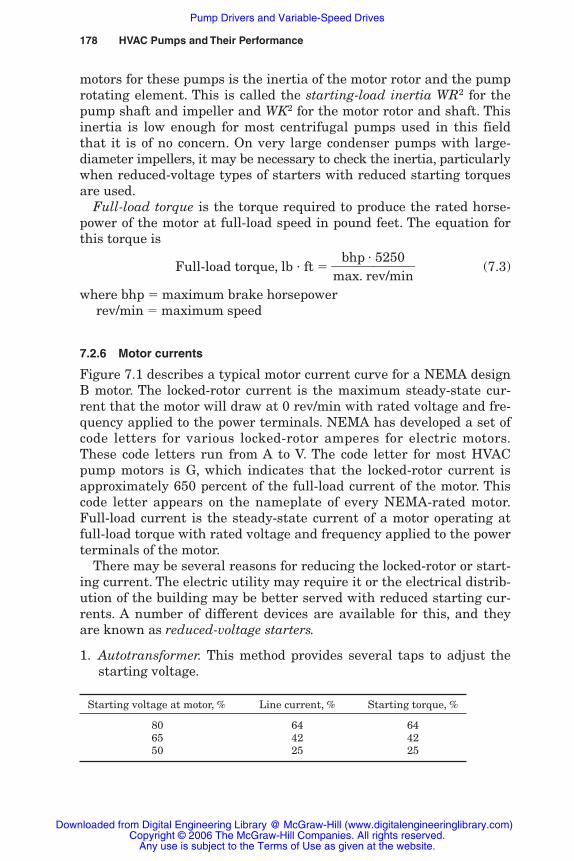
178 HVAC Pumps and Their Performance
motors for these pumps is the inertia of the motor rotor and the pumprotating element. This is called the starting-load inertia WR2 for thepump shaft and impeller and WK2 for the motor rotor and shaft. Thisinertia is low enough for most centrifugal pumps used in this fieldthat it is of no concern. On very large condenser pumps with large-diameter impellers, it may be necessary to check the inertia, particularlywhen reduced-voltage types of starters with reduced starting torquesare used.
Full-load torque is the torque required to produce the rated horse-power of the motor at full-load speed in pound feet. The equation forthis torque is
Full-load torque, lb � ft ��m
bahxp. r
�
e5v2/m50
in� (7.3)
where bhp � maximum brake horsepowerrev/min � maximum speed
7.2.6 Motor currents
Figure 7.1 describes a typical motor current curve for a NEMA designB motor. The locked-rotor current is the maximum steady-state cur-rent that the motor will draw at 0 rev/min with rated voltage and fre-quency applied to the power terminals. NEMA has developed a set ofcode letters for various locked-rotor amperes for electric motors.These code letters run from A to V. The code letter for most HVACpump motors is G, which indicates that the locked-rotor current isapproximately 650 percent of the full-load current of the motor. Thiscode letter appears on the nameplate of every NEMA-rated motor.Full-load current is the steady-state current of a motor operating atfull-load torque with rated voltage and frequency applied to the powerterminals of the motor.
There may be several reasons for reducing the locked-rotor or start-ing current. The electric utility may require it or the electrical distrib-ution of the building may be better served with reduced starting cur-rents. A number of different devices are available for this, and theyare known as reduced-voltage starters.
1. Autotransformer. This method provides several taps to adjust thestarting voltage.
Starting voltage at motor, % Line current, % Starting torque, %
80 64 6465 42 4250 25 25
Rishel_07.qxd 20/4/06 6:29 PM Page 178
Downloaded from Digital Engineering Library @ McGraw-Hill (www.digitalengineeringlibrary.com)Copyright © 2006 The McGraw-Hill Companies. All rights reserved.
Any use is subject to the Terms of Use as given at the website.
Pump Drivers and Variable-Speed Drives
Pump Drivers and Variable-Speed Drives 179
With the preceding three taps of 80, 65, or 50 percent, the start-ing current is limited to approximately 125 to 390 percent of full-load current. This starter is large and expensive.
2. Primary resistor. Starting characteristics are fixed; starting cur-rent is 390 percent of full-load current. This starter has an addedpower loss in the resistors.
3. Part winding. Starting characteristics are fixed; starting current is390 percent of full-load current. It requires special motor connec-tions for 460-V service. It is the smallest and least expensive reduced-voltage starter.
4. Wye delta. Starting current is approximately 200 percent of full-load current; starting torque is low, only 33 percent of full-loadtorque. This starter requires special motor design and more com-plex control than the other reduced-voltage starters.
5. Solid state. Solid-state starters are being used on both constant-speed and variable-speed pumps due to their adjustability andsize. A typical range of adjustable starting currents is from 100 to400 percent of full-load current. They may or may not be less expen-sive than other types of reduced-voltage starters.
6. Variable-frequency drive. The variable-frequency drive has provedto be an excellent method for reducing the current inrush. Sincethe starting torque on most HVAC pumps is limited to inertiatorque WR2, the variable-frequency drive can be used on almost allHVAC pump motors. It is usually more expensive at this date thanother reduced-voltage starters; its ability to be programmed intothe overall duty cycle of HVAC pumps often results in its selectiondue to the energy savings achieved through variable speed.
Due to special motor windings, the part winding and wye deltatypes of reduced-voltage starters cannot be used as standby startersfor variable-speed drives at 460-V power supply.
7.2.7 Output horsepower
A motor is designed to produce its rated horsepower with nameplatevoltages and frequency applied to its power terminals. Most HVACpump motors have a service factor that has been developed by NEMAfor standard polyphase motors. These service factors are defined asthe permissible overload beyond nameplate rating with standardvoltage and frequency. Most NEMA design B, open-frame, drip-proofmotors have a service factor of 1.15 up to 200 hp and 1.0 for over 200hp. Totally enclosed, fan-cooled (TEFC) and explosion-proof (class 1,
Rishel_07.qxd 20/4/06 6:29 PM Page 179
Downloaded from Digital Engineering Library @ McGraw-Hill (www.digitalengineeringlibrary.com)Copyright © 2006 The McGraw-Hill Companies. All rights reserved.
Any use is subject to the Terms of Use as given at the website.
Pump Drivers and Variable-Speed Drives
180 HVAC Pumps and Their Performance
group D) motors may have a service factor of 1.0 and no overload or1.15. The manufacturer or supplier of a motor should verify the actualservice factor for a motor. Also, the nameplate for existing motorsshould be inspected to confirm the allowable service factor.
7.2.8 Power factor
The power factor for a three-phase motor recognizes the magnetizingcurrent of the motor. Its equation is
Power factor � (7.4)
Power factor is a characteristic of a polyphase electric motor’s opera-tion. Electric utilities may charge penalties for low power factor. Like-wise, some governing bodies may establish a minimum power factor.
Power factor can be improved by purchasing motors with highpower factor ratings, providing no loss in efficiency results. A moresatisfactory method may be the installation of power factor correctioncapacitors. Total power factor correction programs are within theprovince of the consulting electrical engineer, but the HVAC designershould have a working knowledge of power factor and its correction.
One advantage for some variable-speed drives, particularly pulsewidth modulation type, is that the input power factor of the variable-speed drive and the motor as a combination is equal to the power fac-tor of the drive itself. Most of these drives have a power factor close to95 percent. More on power factor will be discussed later in Sec. 7.3 ofthis chapter.
7.2.9 Motor efficiency
Motor efficiency is an important design consideration and has beenthe object of much redesign and rating in the motor industry. Theequation is
Motor efficiency ��hp
woautttspu
intp�
u7t46
� (7.5)
IEEE has established and NEMA has adopted Standard 112, MethodB for the Testing of Electrical Motors. This test establishes uniformmethods of testing and rating electric motors and is the basis for ratingmotors for compliance with the latest government requirements.
The Energy Policy Act of 1992 establishes nominal full-load effi-ciencies for both open and closed motors. Table 7.3 lists these efficien-cies for up to 200-hp motor sizes. These efficiencies apply to all motorsmanufactured after October 1997.
watts applied����3� � volts � amps
Rishel_07.qxd 20/4/06 6:29 PM Page 180
Downloaded from Digital Engineering Library @ McGraw-Hill (www.digitalengineeringlibrary.com)Copyright © 2006 The McGraw-Hill Companies. All rights reserved.
Any use is subject to the Terms of Use as given at the website.
Pump Drivers and Variable-Speed Drives
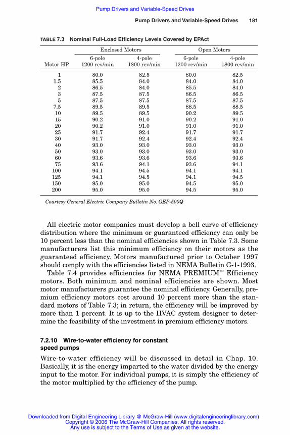
Pump Drivers and Variable-Speed Drives 181
TABLE 7.3 Nominal Full-Load Efficiency Levels Covered by EPAct
Enclosed Motors Open Motors
6-pole 4-pole 6-pole 4-poleMotor HP 1200 rev/min 1800 rev/min 1200 rev/min 1800 rev/min
0 01 80.0 82.5 80.0 82.5001.5 85.5 84.0 84.0 84.0
002 86.5 84.0 85.5 84.0003 87.5 87.5 86.5 86.5005 87.5 87.5 87.5 87.5
007.5 89.5 89.5 88.5 88.5010 89.5 89.5 90.2 89.5015 90.2 91.0 90.2 91.0020 90.2 91.0 91.0 91.0025 91.7 92.4 91.7 91.7030 91.7 92.4 92.4 92.4040 93.0 93.0 93.0 93.0050 93.0 93.0 93.0 93.0060 93.6 93.6 93.6 93.6075 93.6 94.1 93.6 94.1100 94.1 94.5 94.1 94.1125 94.1 94.5 94.1 94.5150 95.0 95.0 94.5 95.0200 95.0 95.0 94.5 95.0
Courtesy General Electric Company Bulletin No. GEP-500Q
All electric motor companies must develop a bell curve of efficiencydistribution where the minimum or guaranteed efficiency can only be10 percent less than the nominal efficiencies shown in Table 7.3. Somemanufacturers list this minimum efficiency on their motors as theguaranteed efficiency. Motors manufactured prior to October 1997should comply with the efficiencies listed in NEMA Bulletin G-1-1993.
Table 7.4 provides efficiencies for NEMA PREMIUM™ Efficiencymotors. Both minimum and nominal efficiencies are shown. Mostmotor manufacturers guarantee the nominal efficiency. Generally, pre-mium efficiency motors cost around 10 percent more than the stan-dard motors of Table 7.3; in return, the efficiency will be improved bymore than 1 percent. It is up to the HVAC system designer to deter-mine the feasibility of the investment in premium efficiency motors.
7.2.10 Wire-to-water efficiency for constantspeed pumps
Wire-to-water efficiency will be discussed in detail in Chap. 10.Basically, it is the energy imparted to the water divided by the energyinput to the motor. For individual pumps, it is simply the efficiency ofthe motor multiplied by the efficiency of the pump.
Rishel_07.qxd 20/4/06 6:29 PM Page 181
Downloaded from Digital Engineering Library @ McGraw-Hill (www.digitalengineeringlibrary.com)Copyright © 2006 The McGraw-Hill Companies. All rights reserved.
Any use is subject to the Terms of Use as given at the website.
Pump Drivers and Variable-Speed Drives
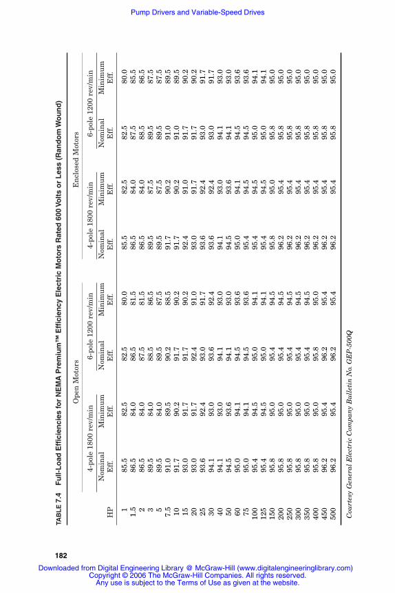
TAB
LE
7.4
Fu
ll-L
oad
Eff
icie
nci
es fo
r N
EM
A P
rem
ium
™E
ffic
ien
cy E
lect
ric
Mo
tors
Rat
ed 6
00 V
olt
s o
r L
ess
(Ran
do
m W
ou
nd
)
Ope
n M
otor
sE
ncl
osed
Mot
ors
4-po
le 1
800
rev/
min
6-po
le 1
200
rev/
min
4-
pole
180
0 re
v/m
in6-
pole
120
0 re
v/m
in
Nom
inal
Min
imu
mN
omin
alM
inim
um
Nom
inal
Min
imu
mN
omin
alM
inim
um
HP
Eff
.E
ff.
Eff
.E
ff.
Eff
.E
ff.
Eff
.E
ff.
001
85.5
82.5
82.5
80.0
85.5
82.5
82.5
80.0
001.
586
.584
.086
.581
.586
.584
.087
.585
.500
286
.584
.087
.581
.586
.584
.088
.586
.500
389
.584
.088
.586
.589
.587
.589
.587
.500
589
.584
.089
.587
.589
.587
.589
.587
.500
7.5
91.0
89.5
90.2
88.5
91.7
90.2
91.0
89.5
010
91.7
90.2
91.7
90.2
91.7
90.2
91.0
89.5
015
93.0
91.7
91.7
90.2
92.4
91.0
91.7
90.2
020
93.0
91.7
92.4
91.0
93.0
91.7
91.7
90.2
025
93.6
92.4
93.0
91.7
93.6
92.4
93.0
91.7
030
94.1
93.0
93.6
92.4
93.6
92.4
93.0
91.7
040
94.1
93.0
94.1
93.0
94.1
93.0
94.1
93.0
050
94.5
93.6
94.1
93.0
94.5
93.6
94.1
93.0
060
95.0
94.1
94.5
93.6
95.0
94.1
94.5
93.6
075
95.0
94.1
94.5
93.6
95.4
94.5
94.5
93.6
100
95.4
94.5
95.0
94.1
95.4
94.5
95.0
94.1
125
95.4
94.5
95.0
94.1
95.4
94.5
95.0
94.1
150
95.8
95.0
95.4
94.5
95.8
95.0
95.8
95.0
200
95.8
95.0
95.4
94.5
96.2
95.4
95.8
95.0
250
95.8
95.0
95.4
94.5
96.2
95.4
95.8
95.0
300
95.8
95.0
95.4
94.5
96.2
95.4
95.8
95.0
350
95.8
95.0
95.4
94.5
96.2
95.4
95.8
95.0
400
95.8
95.0
95.8
95.0
96.2
95.4
95.8
95.0
450
96.2
95.4
96.2
95.4
96.2
95.4
95.8
95.0
500
96.2
95.4
96.2
95.4
96.2
95.4
95.8
95.0
Cou
rtes
y G
ener
al E
lect
ric
Com
pan
y B
ull
etin
No.
GE
P-5
00Q
182
Rishel_07.qxd 20/4/06 6:29 PM Page 182
Downloaded from Digital Engineering Library @ McGraw-Hill (www.digitalengineeringlibrary.com)Copyright © 2006 The McGraw-Hill Companies. All rights reserved.
Any use is subject to the Terms of Use as given at the website.
Pump Drivers and Variable-Speed Drives
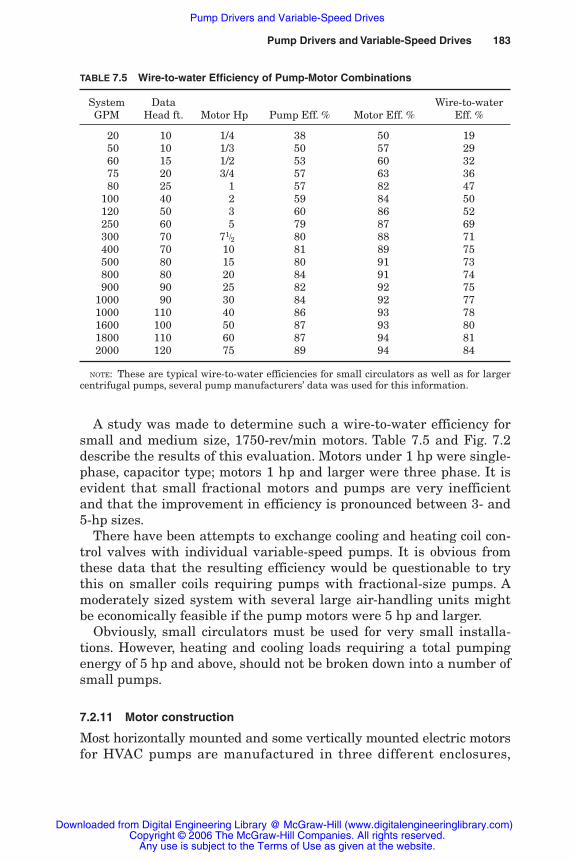
Pump Drivers and Variable-Speed Drives 183
A study was made to determine such a wire-to-water efficiency forsmall and medium size, 1750-rev/min motors. Table 7.5 and Fig. 7.2describe the results of this evaluation. Motors under 1 hp were single-phase, capacitor type; motors 1 hp and larger were three phase. It isevident that small fractional motors and pumps are very inefficientand that the improvement in efficiency is pronounced between 3- and5-hp sizes.
There have been attempts to exchange cooling and heating coil con-trol valves with individual variable-speed pumps. It is obvious fromthese data that the resulting efficiency would be questionable to trythis on smaller coils requiring pumps with fractional-size pumps. Amoderately sized system with several large air-handling units mightbe economically feasible if the pump motors were 5 hp and larger.
Obviously, small circulators must be used for very small installa-tions. However, heating and cooling loads requiring a total pumpingenergy of 5 hp and above, should not be broken down into a number ofsmall pumps.
7.2.11 Motor construction
Most horizontally mounted and some vertically mounted electric motorsfor HVAC pumps are manufactured in three different enclosures,
TABLE 7.5 Wire-to-water Efficiency of Pump-Motor Combinations
System Data Wire-to-waterGPM Head ft. Motor Hp Pump Eff. % Motor Eff. % Eff. %
20 10 1/4 38 50 1950 10 1/3 50 57 2960 15 1/2 53 60 3275 20 3/4 57 63 3680 25 1 57 82 47
100 40 2 59 84 50120 50 3 60 86 52250 60 5 79 87 69300 70 71/2 80 88 71400 70 10 81 89 75500 80 15 80 91 73800 80 20 84 91 74900 90 25 82 92 75
1000 90 30 84 92 771000 110 40 86 93 781600 100 50 87 93 801800 110 60 87 94 812000 120 75 89 94 84
NOTE: These are typical wire-to-water efficiencies for small circulators as well as for largercentrifugal pumps, several pump manufacturers’ data was used for this information.
Rishel_07.qxd 20/4/06 6:29 PM Page 183
Downloaded from Digital Engineering Library @ McGraw-Hill (www.digitalengineeringlibrary.com)Copyright © 2006 The McGraw-Hill Companies. All rights reserved.
Any use is subject to the Terms of Use as given at the website.
Pump Drivers and Variable-Speed Drives

184 HVAC Pumps and Their Performance
namely, drip-proof; totally enclosed, fan cooled; and explosion-proof.Particular atmospheres that are dusty or contain specific chemicals mayrequire special motor enclosures.
Drip-proof motors are designed for cooling by ambient air and arecalled open-frame on horizontal motors and weather-protected (WP1)on vertical motors. Open-frame drip-proof motors are designed for
Figure 7.2 WWE of pump-motor combinations.
Rishel_07.qxd 20/4/06 6:29 PM Page 184
Downloaded from Digital Engineering Library @ McGraw-Hill (www.digitalengineeringlibrary.com)Copyright © 2006 The McGraw-Hill Companies. All rights reserved.
Any use is subject to the Terms of Use as given at the website.
Pump Drivers and Variable-Speed Drives
Pump Drivers and Variable-Speed Drives 185
relatively clean indoor applications, whereas weather-protectedmotors can be used outdoors and are so constructed to minimize theentrance of rain, snow, and airborne particles. Drip-proof motors areadequate for most HVAC equipment room installations.
Totally enclosed, fan-cooled motors are cooled by an external fanmounted on the motor shaft. This enclosure is available for applica-tions where the motor is wetted periodically. It should not be used forroutine motor applications in this industry. Usually, it does not haveany higher efficiency than an open-frame drip-proof motor.
Explosion-proof class 1, group D construction is for applicationswhere the ambient air may contain combustibles such as gasoline,petroleum, naphtha, or natural gas. There are other types of explosion-proof constructions for other hazardous atmospheres. Most HVACatmospheres do not contain any combustibles. If a specific hazardousmaterial is encountered, the insuring agency should verify the correctmotor enclosure. These motors should not be used with variable-frequency drives without approval of the motor manufacturer. Theymay not be certified for this use.
Vertical motors are available in two physical constructions, verticalhollow shaft (VHS) and vertical solid shaft (VSS). The hollow-shaftconstruction is usually applied to vertical turbine pumps due to theability to adjust the lateral setting on these pumps without disassem-bling the motor. This motor has a top drive coupling with an adjust-ment nut that provides this adjustment.
Most motors for HVAC pumps are single speed. Although two-speedmotors are available for these applications, the variable-speed drivehas all but eliminated the use of multispeed motors for these pumps.The added cost of the special two-speed motor and two-speed starteris usually less than the cost of a variable-speed drive. However, thecomplex control and the energy loss due to only two speeds, i.e., twopump head-flow curves, usually result in the selection of a variable-speed drive instead of a two-speed motor. Another disadvantage fortwo-speed motors on large HVAC water systems is the hydraulicshock that is produced when the motor changes from one speed to theother.
7.2.12 Motor sizing for constant andvariable speed HVAC pumps
The important factors on most HVAC installations in the proper sizingof an electric motor are long life and efficient operation. These factorsdictate that the motor should not operate beyond its nameplate rating.For example, assume that a pump is selected for 2000 gal/min at 125 ft
Rishel_07.qxd 20/4/06 6:29 PM Page 185
Downloaded from Digital Engineering Library @ McGraw-Hill (www.digitalengineeringlibrary.com)Copyright © 2006 The McGraw-Hill Companies. All rights reserved.
Any use is subject to the Terms of Use as given at the website.
Pump Drivers and Variable-Speed Drives

186 HVAC Pumps and Their Performance
Figure 7.3 Running limit for variable frequency drives.
of head and a 75-hp motor is fully loaded at the pump’s selection point.If the pump can carry out to (operate at) capacities greater than 2000gal /min, the brake horsepower required will exceed 75 hp, and themotor will be overloaded. For long life and efficient operation, a 100-hpmotor should be selected for this pump. It is recommended that thespecification for electric motors for pumps include the statement thatthe motor will not be overloaded beyond its nameplate rating when thepump operates at any point on its head-flow curve.
The above recommended procedure is necessary for all constant-speed pumps. Fortunately, motors equipped with variable-frequencydrives can be sized to the brake horsepower required at the pumpdesign condition. The drive can be sized by the maximum motor horse-power at this design condition.
A simple control technology is now available that eliminates thenormal oversizing of pump motors and drives. This is the developmentof the “running limit” that prevents the motor from overloading thedrive. For example, in Fig. 7.3 if we must comply with the requirement
0 200 400 600 800 1000 1200 1400
528
627
1023
2013
8.8"
9.6"
10.4"
11.2"
12.0"
12.8"
GALLONS PER MINUTE
0
25
50
75
100
125
150
175
200
TOTA
L H
EA
D IN
FE
ET
10 HP
15 HP
20 HP
25 HP30 HP
40 HP50 HP
60 65 70
70
75
75
80
8084
84
RUNNING LIMIT OF VARIABLESPEED/DRIVE FORCES PUMPTO FOLLOW THE HORSEPOWERCURVE, NOT THE PUMP CURVE.
Rishel_07.qxd 20/4/06 6:29 PM Page 186
Downloaded from Digital Engineering Library @ McGraw-Hill (www.digitalengineeringlibrary.com)Copyright © 2006 The McGraw-Hill Companies. All rights reserved.
Any use is subject to the Terms of Use as given at the website.
Pump Drivers and Variable-Speed Drives
Pump Drivers and Variable-Speed Drives 187
that the pump should not overload the motor beyond its nameplaterating, a 40-hp motor would be required with a drive equaling thenameplate rating of the motor in amperage.
With the running limit of the drive, it is possible to furnish a 25-hpmotor and drive since that is the motor horsepower required at thedesign condition of 700 gal/min at 116 ft. The drive prevents the pumpfrom overloading the motor beyond 25 hp. The pump follows the motorhorsepower curve, not the pump curve. This does not guarantee higherpump performance, i.e., efficiency, since that is determined by thespeed control and sequencing described in Chap. 10, “Basics of PumpApplication.”
7.3 Variable-Speed Drives for Electric Motors
7.3.1 History
Up to about 1970, variable-speed drives in the HVAC industry usuallymeant eddy-current or fluid couplings between a fixed-speed induc-tion motor and a variable-speed pump. The coupling was controlledelectrically or hydraulically to allow a variable slip between the motorspeed and that of the coupled load. These drives established a highorder of reliability and were quite satisfactory for pump loads inwhich the torque requirements dropped off rapidly as the speed wasreduced. In such applications, the losses inherent in the couplingbetween the motor and the pump were offset by the reduction inlosses due to overpressuring caused by a constant-speed pump. Fornew installations, however, this arrangement has largely been super-seded by variable-frequency drives. On applications that have environ-ments hostile to variable-frequency drives, mechanical variable-speeddrives should still be used. This includes dusty or corrosive atmos-pheres and high ambient temperatures where it is impossible to pro-vide adequate cooling for the variable-frequency drive.
The advantages of variable-frequency drives (VFDs) for fans,pumps, and chillers have been known for many years. They permitthe use of simple, reliable, and inexpensive induction motors yet pro-vide the operating economies of variable speed. Unfortunately, motorgenerator sets, thyratrons, and ignitrons, the only methods of obtain-ing a variable-frequency source, were too expensive for all but themost critical applications.
The invention of the thyristor (SCR) in the mid-1960s changed thepicture dramatically. Here was a device that could control power atthe megawatt level yet was both economical and reliable.
Variable-speed drives soon appeared for direct-current (dc) motorsand shortly thereafter for alternating-current (ac) induction motors.
Rishel_07.qxd 20/4/06 6:29 PM Page 187
Downloaded from Digital Engineering Library @ McGraw-Hill (www.digitalengineeringlibrary.com)Copyright © 2006 The McGraw-Hill Companies. All rights reserved.
Any use is subject to the Terms of Use as given at the website.
Pump Drivers and Variable-Speed Drives

188 HVAC Pumps and Their Performance
The early variable-frequency thyristor drives, which were mostly volt-age source inverters, were sometimes less than ideal in their charac-teristics; they opened up a huge new field of application in the HVACindustry. Now, drive designs have matured, but there are still impor-tant new developments that solve some of the major application prob-lems on the electrical side.
7.3.2 Types of variable-frequency drives
For many years the variable-frequency drive field has been dominatedby six-pulse voltage-source and current-source thyristor inverters(Fig. 7.4). Block diagrams of these drives are shown in Fig. 7.4a. Bothgenerate the output ac voltage by alternately switching between threepairs of thyristors. Capacitor banks are used to force the load currentto switch from one set to the other. In the voltage-source inverter, aset of six diodes in a rectifier is used to charge a filter capacitor bankto a dc voltage equal to the peak output voltage of the load. The filtercapacitor bank serves to isolate the inverter from the ac line. This fil-ter capacitor bank is, in addition to the capacitors, used for switching.
The current-source inverter replaces the filter capacitor bank with alarge inductor that serves the same purpose of isolation and filteringbut makes the drive more tolerant of line and load disturbances. It alsopermits regenerating energy from the load to the line, an importantadvantage when high-inertia loads must be brought to rest quickly.
Both these drives, in their basic form, generate a six-step outputwaveform, voltage for the voltage source, and current for the currentsource. Typical waveforms are shown in Fig. 7.4b. The magnitude ofthe voltage is directly proportional to the load frequency so that thevolts-per-hertz ratio remains constant. The motor operates at a con-stant flux level and, except for ventilation considerations, is able tooperate at constant torque. Harmonics in the output current causeadditional heating, however, and this generally results in a deratingof 10 to 15 percent in horsepower for standard motors.
PWM Drives. The development of large power transistors in the 1980sspawned a new type of variable-frequency drive (Fig. 7.5). Theacronym PWM stands for pulse-width modulation, a totally differenttechnique from the six-step unit for obtaining voltage control and avariable output frequency. Whereas the six-step voltage and currentsource drives vary the amplitude of the switched voltage, PWM drivesvary the output voltage by repetitively connecting and disconnectinga fixed voltage at rapid intervals. The ratio of “on” to “off” periods deter-mines the voltage magnitude. Figure 7.5a illustrates this process ingenerating a 320-V rms, 40-Hz sine-wave approximation from a
Rishel_07.qxd 20/4/06 6:29 PM Page 188
Downloaded from Digital Engineering Library @ McGraw-Hill (www.digitalengineeringlibrary.com)Copyright © 2006 The McGraw-Hill Companies. All rights reserved.
Any use is subject to the Terms of Use as given at the website.
Pump Drivers and Variable-Speed Drives

Pump Drivers and Variable-Speed Drives 189
Figure 7.4 Current-source and voltage source drives. (From Keith H.Sneker, private communication, Halmar Robicon Group, Pittsburgh,Pa., 1994.)
675-V constant-potential bus. This is an actual requirement for aPWM drive on a 480-V, 60-Hz motor. The switching frequency is about1 kHz in this example.
At the beginning and end of the 40-Hz sine wave, the switching ismostly “off,” but the duty cycle rises to two-thirds at the peak to generate
Rishel_07.qxd 20/4/06 6:29 PM Page 189
Downloaded from Digital Engineering Library @ McGraw-Hill (www.digitalengineeringlibrary.com)Copyright © 2006 The McGraw-Hill Companies. All rights reserved.
Any use is subject to the Terms of Use as given at the website.
Pump Drivers and Variable-Speed Drives
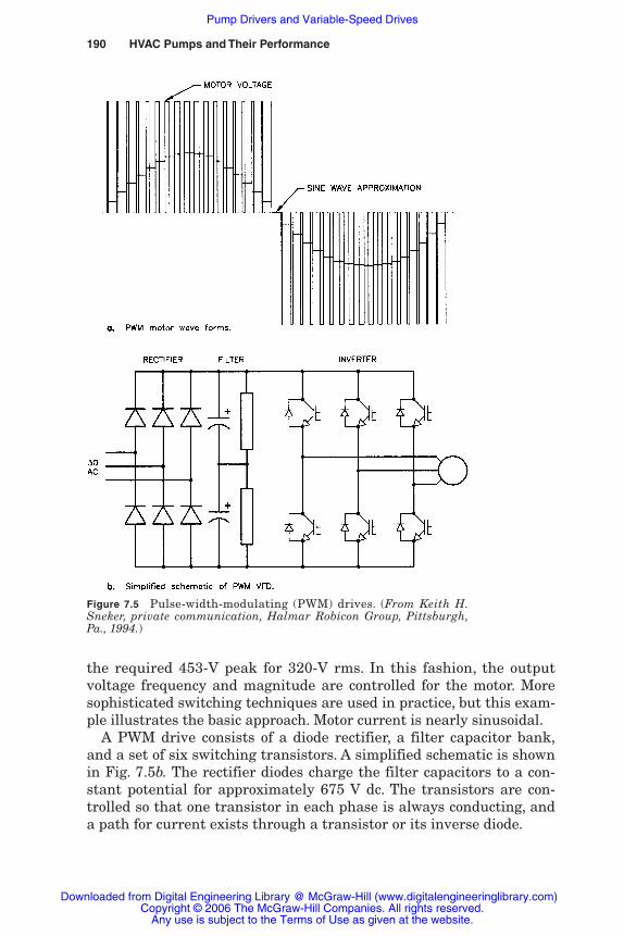
190 HVAC Pumps and Their Performance
the required 453-V peak for 320-V rms. In this fashion, the outputvoltage frequency and magnitude are controlled for the motor. Moresophisticated switching techniques are used in practice, but this exam-ple illustrates the basic approach. Motor current is nearly sinusoidal.
A PWM drive consists of a diode rectifier, a filter capacitor bank,and a set of six switching transistors. A simplified schematic is shownin Fig. 7.5b. The rectifier diodes charge the filter capacitors to a con-stant potential for approximately 675 V dc. The transistors are con-trolled so that one transistor in each phase is always conducting, anda path for current exists through a transistor or its inverse diode.
Figure 7.5 Pulse-width-modulating (PWM) drives. (From Keith H.Sneker, private communication, Halmar Robicon Group, Pittsburgh,Pa., 1994.)
Rishel_07.qxd 20/4/06 6:29 PM Page 190
Downloaded from Digital Engineering Library @ McGraw-Hill (www.digitalengineeringlibrary.com)Copyright © 2006 The McGraw-Hill Companies. All rights reserved.
Any use is subject to the Terms of Use as given at the website.
Pump Drivers and Variable-Speed Drives

Pump Drivers and Variable-Speed Drives 191
The diode rectifier and filter capacitor act to greatly reduce theharmonic effects on the power system. Although the low-frequencyharmonic currents remain, line notching is virtually eliminated.The interference potential is much less, but elimination of the low-frequency current harmonics still requires corrective measures atincreased cost. Power factor is also much better for the PWM drivethan for the six-step units. It is always 90 percent or better and isnearly independent of motor speed.
Multipulse input circuits. An input transformer or autotransformer canbe used to power two or three input rectifiers to a drive. Phase-shiftedvoltages cancel the low-frequency current harmonics and greatly reducethe line-current distortion. Block diagrams of 12- and 18-pulse sys-tems are shown in Fig. 7.6. The disadvantage of multipulse systems isan increase in cost over the simpler systems. In drives over 500 hp,however, multipulse operation is usually the arrangement of choice. Ingeneral, a 12-pulse drive is sufficient, and the added cost and complex-ity of an 18-pulse drive are seldom warranted.
Clean power variable-speed drives. A dramatic series of technical devel-opments has recently yielded variable-frequency drives that will meetthe requirements of IEEE Standard 519-1992 with no filters or multi-pulse circuitry. All these new PWM drives are based on fast-switchingpower transistors. Most use an active filter that detects the currentdistortion and injects corrective currents to cancel the harmonics.Some manufacturers, however, employ an ingenious switching algo-rithm that eliminates the harmonic currents in the first place. Thisarrangement requires transistors in place of the rectifier diodes, but itneeds no active filter. It also permits regeneration for rapid decelera-tion of an overhauling load. These clean power drives are currentlyavailable through 1000 hp.
Figure 7.6 Twelve- and eighteen-pulse drives. (From Keith H. Sneker, private communi-cation, Halmar Robicon Group,Pittsburgh, Pa., 1994.)
Rishel_07.qxd 20/4/06 6:29 PM Page 191
Downloaded from Digital Engineering Library @ McGraw-Hill (www.digitalengineeringlibrary.com)Copyright © 2006 The McGraw-Hill Companies. All rights reserved.
Any use is subject to the Terms of Use as given at the website.
Pump Drivers and Variable-Speed Drives

192 HVAC Pumps and Their Performance
Medium-voltage drives. Medium-voltage drives (2300 and 4000 V)have become available for large chilled water pumps with horse-power ratings of 750 hp and larger. These motors can be synchro-nous or induction types. Smaller motors may be economically feasiblefor medium voltages if the chillers are equipped with medium-voltagemotors.
It is obvious that motors of this size and type need quality drives toachieve the efficiency and reliability required for such large installa-tions. The complexity of these drives necessitates that they be evalu-ated and selected by an electrical engineer experienced in variablespeed drive technology.
A detailed paper evaluating most of the current types of medium-volt-age drives has been provided by Mr. Richard H. Osman, Vice Presidentof Technology for Robicon titled “Medium–Voltage VariableFrequency Drives for Induction and Synchronous Motors.” This is animportant document that should be studied by electrical engineersinvolved in large chiller plant design.
The following is a condensation of this material that describes thefour types of medium-voltage drives that may be encountered in theHVAC industry.
Filter commutated current-fed inverter. The electrical circuit forthis drive is shown in Fig. 7.7 and the wave forms for output torque,voltage, and current are described in Fig. 7.8.
Current-fed VFD using GTO/IGCT inverter stage. The electricalcircuit for this drive is shown in Fig. 7.9, and the wave forms forvoltage and current are shown in Fig. 7.10.
Output filter
Inductionmotor
Series thyristors
3-Phase MV input
Input filter forpower factor andharmonic correction
12 Pulse thyrister converter Filter commutated MV inverter
Typical snubberand sharing
Figure 7.7 MV filter-commutated thyrister drive.
Rishel_07.qxd 20/4/06 6:29 PM Page 192
Downloaded from Digital Engineering Library @ McGraw-Hill (www.digitalengineeringlibrary.com)Copyright © 2006 The McGraw-Hill Companies. All rights reserved.
Any use is subject to the Terms of Use as given at the website.
Pump Drivers and Variable-Speed Drives
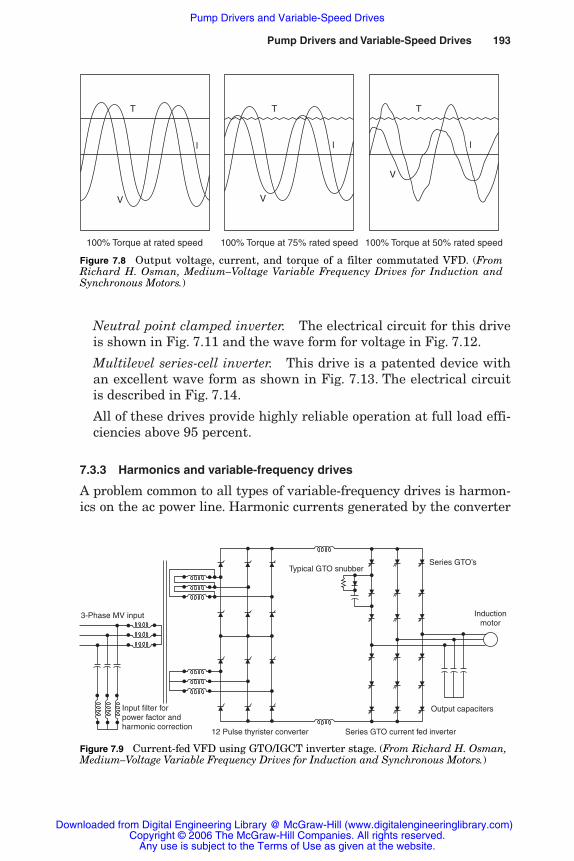
Pump Drivers and Variable-Speed Drives 193
Neutral point clamped inverter. The electrical circuit for this driveis shown in Fig. 7.11 and the wave form for voltage in Fig. 7.12.
Multilevel series-cell inverter. This drive is a patented device withan excellent wave form as shown in Fig. 7.13. The electrical circuitis described in Fig. 7.14.
All of these drives provide highly reliable operation at full load effi-ciencies above 95 percent.
7.3.3 Harmonics and variable-frequency drives
A problem common to all types of variable-frequency drives is harmon-ics on the ac power line. Harmonic currents generated by the converter
100% Torque at rated speed 100% Torque at 75% rated speed 100% Torque at 50% rated speed
T T T
V
l
V
l
V
l
Figure 7.8 Output voltage, current, and torque of a filter commutated VFD. (FromRichard H. Osman, Medium–Voltage Variable Frequency Drives for Induction andSynchronous Motors.)
Input filter forpower factor andharmonic correction
3-Phase MV input
12 Pulse thyrister converter Series GTO current fed inverter
Output capaciters
Series GTO’sTypical GTO snubber
Inductionmotor
Figure 7.9 Current-fed VFD using GTO/IGCT inverter stage. (From Richard H. Osman,Medium–Voltage Variable Frequency Drives for Induction and Synchronous Motors.)
Rishel_07.qxd 20/4/06 6:29 PM Page 193
Downloaded from Digital Engineering Library @ McGraw-Hill (www.digitalengineeringlibrary.com)Copyright © 2006 The McGraw-Hill Companies. All rights reserved.
Any use is subject to the Terms of Use as given at the website.
Pump Drivers and Variable-Speed Drives
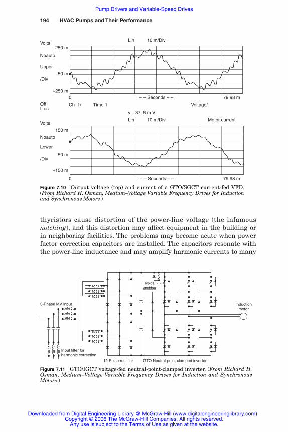
194 HVAC Pumps and Their Performance
thyristors cause distortion of the power-line voltage (the infamousnotching), and this distortion may affect equipment in the building orin neighboring facilities. The problems may become acute when powerfactor correction capacitors are installed. The capacitors resonate withthe power-line inductance and may amplify harmonic currents to many
Lin 10 m/Div
Lin 10 m/Div Motor current
Volts250 m
−250 m
−150 m
50 m
50 m
Noauto
Noauto
Upper
Lower
/Div
/Div
Offt: os
Volts
150 m
0
Ch–1/ Voltage/
0
79.98 m– – Seconds – –
79.98 m– – Seconds – –
Time 1
y: –37. 6 m V
Figure 7.10 Output voltage (top) and current of a GTO/SGCT current-fed VFD.(From Richard H. Osman, Medium–Voltage Variable Frequency Drives for Inductionand Synchronous Motors.)
12 Pulse rectifier
Input filter forharmonic correction
3-Phase MV input
GTO Neutral-point-clamped inverter
Typicalsnubber
Inductionmotor
Figure 7.11 GTO/IGCT voltage-fed neutral-point-clamped inverter. (From Richard H.Osman, Medium–Voltage Variable Frequency Drives for Induction and SynchronousMotors.)
Rishel_07.qxd 20/4/06 6:29 PM Page 194
Downloaded from Digital Engineering Library @ McGraw-Hill (www.digitalengineeringlibrary.com)Copyright © 2006 The McGraw-Hill Companies. All rights reserved.
Any use is subject to the Terms of Use as given at the website.
Pump Drivers and Variable-Speed Drives
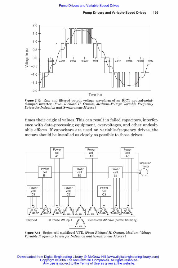
Pump Drivers and Variable-Speed Drives 195
times their original values. This can result in failed capacitors, interfer-ence with data-processing equipment, overvoltages, and other undesir-able effects. If capacitors are used on variable-frequency drives, themotors should be installed as closely as possible to those drives.
2.0
1.5
1.0
0.5
0.0
−0.5
−1.0
−1.5
−2.0
Vol
tage
in p
u
Time in s
0.020.0180.0160.0140.0120.010.0080.0060.0040.0020
Figure 7.12 Raw and filtered output voltage waveform of an IGCT neutral-point-clamped inverter. (From Richard H. Osman, Medium–Voltage Variable FrequencyDrives for Induction and Synchronous Motors.)
PowercellC1
PowercellB1
PowercellA1
PowercellA2
PowercellA3
PowercellB2
PowercellB3
PowercellC3
PowercellC2
Phrmckt Series cell MV drive (perfect harmony)3 Phase MV input
Inductionmotor
Figure 7.13 Series-cell multilevel VFD. (From Richard H. Osman, Medium–VoltageVariable Frequency Drives for Induction and Synchronous Motors.)
Rishel_07.qxd 20/4/06 6:29 PM Page 195
Downloaded from Digital Engineering Library @ McGraw-Hill (www.digitalengineeringlibrary.com)Copyright © 2006 The McGraw-Hill Companies. All rights reserved.
Any use is subject to the Terms of Use as given at the website.
Pump Drivers and Variable-Speed Drives

196 HVAC Pumps and Their Performance
Harmonics were addressed by the IEEE, which, in 1981, issuedStandard 519-1981 establishing limits on the allowable voltage dis-tortion on a feeder common to several facilities. In most cases, thetotal harmonic voltage distortion was limited to 5 percent. The use ofa current-source or voltage-source thyristor inverter often requiredthe installation of a high-pass filter to control the distortion. In addi-tion to increasing the cost of the installation, the filter introducedlosses that reduced operating efficiency. Nonetheless, these filters didthe required job, and thousands are presently in service.
In 1992, an IEEE committee revised the standard and issuedStandard 519-1992, IEEE Recommended Practices and Requirementsfor Harmonic Control in Electrical Power System. This documentspelled out, for the first time, the allowable levels of harmonic cur-rents injected into the utility system. The limit values depend on how“stiff” the supply system is and on the particular harmonic involved.In general, the limits are much more severe and difficult to meet thanwere the previous limits on voltage distortion only.
Harmonic distortion is of great concern to electric utilities andbuilding or plant operators. The projected harmonic distortion can becomputed for a new or existing installation of variable-frequency drives.Figure 7.15 is a form that can be used by the variable-frequency drivemanufacturer to estimate the harmonic distortion for most installa-tions. The following information is required:
Figure 7.14 Output voltage and current of a series-cell multilevel VFD. (FromRichard H. Osman, Medium–Voltage Variable Frequency Drives for Induction andSynchronous Motors.)
Current
Voltage
0
2047
2040
Rishel_07.qxd 20/4/06 6:29 PM Page 196
Downloaded from Digital Engineering Library @ McGraw-Hill (www.digitalengineeringlibrary.com)Copyright © 2006 The McGraw-Hill Companies. All rights reserved.
Any use is subject to the Terms of Use as given at the website.
Pump Drivers and Variable-Speed Drives
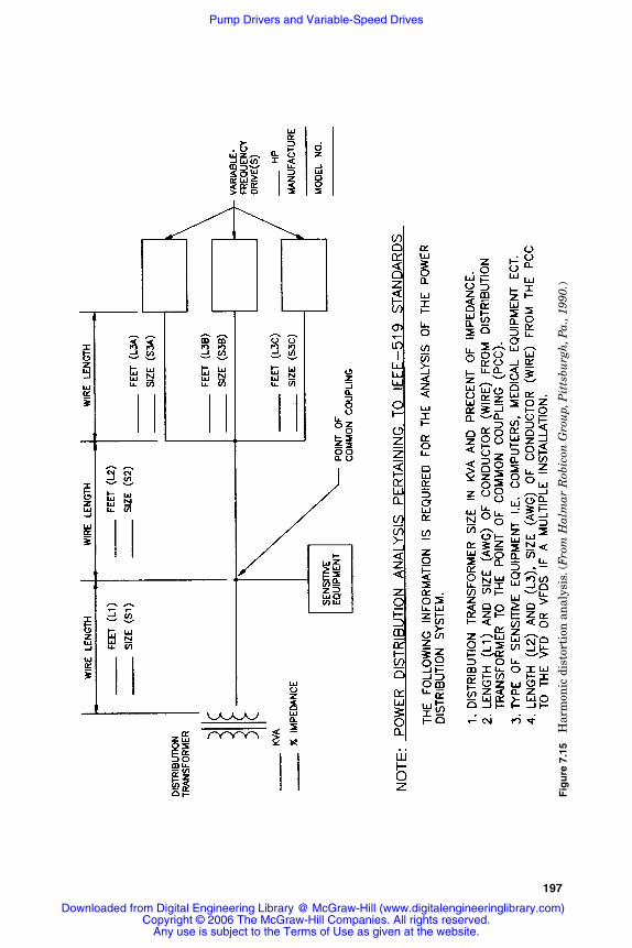
Fig
ure
7.1
5H
arm
onic
dis
tort
ion
an
alys
is.(
Fro
m H
alm
ar R
obic
on G
rou
p,P
itts
burg
h,P
a.,1
990.
)
197
Rishel_07.qxd 20/4/06 6:29 PM Page 197
Downloaded from Digital Engineering Library @ McGraw-Hill (www.digitalengineeringlibrary.com)Copyright © 2006 The McGraw-Hill Companies. All rights reserved.
Any use is subject to the Terms of Use as given at the website.
Pump Drivers and Variable-Speed Drives
198 HVAC Pumps and Their Performance
1. Size in kilovoltamperes and percentage impedance of the distribu-tion transformer
2. For current source and voltage source drives, the wire sizes andlengths between any sensitive equipment and the distributiontransformer as well as wire sizes and lengths between any sensi-tive equipment and the variable-speed drive installation (Wiresizes and distances between variable-speed drives should besecured where more than one is installed.)
Most public utilities or electrical designers will specify a maximumallowable harmonic voltage distortion in percent for a specific instal-lation. Typically, this can be 3 or 5 percent.
7.3.4 Advantages of variable-frequency drives
Variable-frequency drives are available for nearly any HVAC applica-tion and have been the preferred means of varying the speed of apump. They have become the drive of choice for new applications formany reasons, such as
1. First cost is lower in most sizes.
2. All are air-cooled. Larger slip-type drives require water cooling.
3. Wire-to-shaft efficiency is much higher than any slip-type drive.For typical wire-to-shaft efficiencies for variable-frequency drives,see Table 10.2.
4. It is very easy to integrate drive-control software into the softwareof pumping systems or building management systems.
7.3.5 Application of variable-speed drives
The application of variable-frequency drives requires some care toensure proper operation and reasonably useful life. The manufac-turer’s installation instructions should be reviewed carefully.Following are some of the more pertinent concerns for installation.Contemporary variable-speed drives are very reliable and will provideyears of uninterrupted service if installed and operated properly.
1. Ventilation. On variable-torque applications such as centrifugalpumps, the heat expended by the variable-speed drive can be computedeasily.
Btu/h � max. kW of drive � 3412 � (1�E�) (7.6)
Rishel_07.qxd 20/4/06 6:29 PM Page 198
Downloaded from Digital Engineering Library @ McGraw-Hill (www.digitalengineeringlibrary.com)Copyright © 2006 The McGraw-Hill Companies. All rights reserved.
Any use is subject to the Terms of Use as given at the website.
Pump Drivers and Variable-Speed Drives

where 3412 � thermal equivalent of a kW in btu/hE
�� efficiency of the drive as a fraction at maximum speed
If the energy consumption of the drive is 100 kW and the efficiencyis 95 percent, the heat expended would be 100 � 3412 � (1 � 0.95), or17,060 Btu/h.
2. Cleanliness. Most commercial variable-frequency drives operatevery well in normal HVAC equipment rooms. Industrial applicationsthat are dusty may require special enclosures to keep the dust awayfrom the internals of the variable-speed drive. NEMA 12 enclosureswith internal air-conditioners may be required. The air-conditionersare usually air-cooled, so provisions must be made to keep clean thecondenser coil on any air-conditioner.
Some terribly dusty or dirty applications should be equipped with awater-cooled drive instead of a variable-frequency drive. The water-cooled drive could be a slip-type drive using an eddy-current or fluidcoupling.
Sometimes a variable-frequency drive can be cooled with clean out-side air through ducts that eliminate the dirt or dust problem.Adequate duct size or auxiliary fans must be furnished so that thereis no external static on the ventilating fans inside the drive.
3. Chemical attack. Variable-frequency drives contain many copperor copper-alloy parts that are susceptible to attack by acids or othersulfur-bearing compounds. Again, most HVAC installations do nothave such atmospheres, but some industrial cooling and heating sys-tems do. For example, very small quantities of hydrogen sulfide inthe air can have a deleterious effect on variable-speed drives. Whenthese conditions exist, special construction must be used such asNEMA 12 enclosures with internal air-conditioners or ducted fresh airas described above for dusty atmospheres (see Fig. 7.16a). The con-denser coils for these air-conditioners must be coated with a compound,such as heresite, that resists attack from the hydrogen sulfide.
4. Maximum temperature. The maximum ambient temperature formost variable-speed drives is 104°F (40°C); for higher ambient tem-peratures, internal air-conditioners or ducted cool air should be con-sidered for these applications.
5. Location. Variable-speed drives should be located in dry areaswhere they cannot be wetted by either surface water or water fromoverhead pipes. When there is no other location than under water orsteam pipes, the cabinets should be equipped with drip shields. Neverlocate variable-speed drives outdoors in the open where they are exposedto sunlight! If it is necessary to install them outdoors, locate themunder a sun shield that will protect them from direct sunlight.
Pump Drivers and Variable-Speed Drives 199
Rishel_07.qxd 20/4/06 6:29 PM Page 199
Downloaded from Digital Engineering Library @ McGraw-Hill (www.digitalengineeringlibrary.com)Copyright © 2006 The McGraw-Hill Companies. All rights reserved.
Any use is subject to the Terms of Use as given at the website.
Pump Drivers and Variable-Speed Drives

200 HVAC Pumps and Their Performance
Figure 7.16 Enclosures for variable-frequency drives.
Rishel_07.qxd 20/4/06 6:29 PM Page 200
Downloaded from Digital Engineering Library @ McGraw-Hill (www.digitalengineeringlibrary.com)Copyright © 2006 The McGraw-Hill Companies. All rights reserved.
Any use is subject to the Terms of Use as given at the website.
Pump Drivers and Variable-Speed Drives
6. Power supply. Variable-frequency drives are like any other com-mercial power equipment in that they are capable of withstanding theacceptable variations of commercial power that were defined earlierin this chapter. Likewise, they may not be able to operate properlywith harmonic distortions in the power supply that exceed the accept-able percentages established by the IEEE.
7. Number of drives. The simplest arrangement for HVAC pumps isone drive for each pump that is to be variable speed. More than onepump can be operated on a single drive. Usually, the cost of transitionequipment to add motors to an operating drive is so expensive that itis cheaper to purchase multiple drives instead. Also, a multiplicity ofdrives provides better standby capability. Almost without exception inthe HVAC industry, a variable-speed drive is furnished for everypump that is to be variable speed.
7.3.6 Variable-speed drive accessories and requirements
Following are popular accessories and requirements for variable-frequency drives:
1. Certification. Variable-frequency drives are often part of pumpingsystems that bear the label of various approving agencies such asUnderwriters Laboratories (UL), Electric Testing Laboratories(ETL), or in Canada, the Canadian Standards Association (CSA).Care must be taken in evaluating these drives and their accessorieswhen compliance is required with such standards.
For example, some drive manufacturers have a certain approvalon their basic drives, but they do not have such approval on thedrive’s accessories or enclosures. It is imperative that such approvalbe ascertained to avoid expensive field approvals or changes.
2. Bypass starters. Bypass starters were required for variable-frequencydrives when they were new and untried. These drives havebecome so reliable and low in cost that standby starters are notneeded on most HVAC installations. Their cost has remained highso that there are other economical means to achieve standby capa-bility. Often, adding a standby drive or even an additional pump,motor, and drive offer a better solution. It is the decision of thesystem designer to determine the best solution for a particularinstallation. If a standby starter is determined to be the optimumsolution for standby power, it should be designed around the fol-lowing recommendations.a. Configuration. Bypass starters are often used to keep a pump in
operation during failure of the variable-speed drive. The designer
Pump Drivers and Variable-Speed Drives 201
Rishel_07.qxd 20/4/06 6:29 PM Page 201
Downloaded from Digital Engineering Library @ McGraw-Hill (www.digitalengineeringlibrary.com)Copyright © 2006 The McGraw-Hill Companies. All rights reserved.
Any use is subject to the Terms of Use as given at the website.
Pump Drivers and Variable-Speed Drives

must determine how critical the standby operation of a pump isduring drive failure. The designer should not just indiscriminatelyput a bypass starter on every drive.
The designer also must realize that the use of bypass startersforces the pump to full speed when operating with the bypassstarter. On high-pump-head applications, it may be necessaryfor the operator to adjust the pump discharge manual valve toalleviate some of the pressure on the water system.
Facilities with critical operations such as hospitals, computercenters, and research facilities should have consideration forthese starters. It is doubtful that commercial buildings or edu-cational facilities require them. It is the responsibility of thedesigner to make this decision.
Bypass starters must be designed properly. First, the decisionmust be made as to whether across-the-line starting is accept-able or whether some form of reduced-voltage starting is required.When this decision is under consideration, if reduced-voltagestarting is required, the type used must have the same motorwiring as that required by the variable-speed drive. Usually,this eliminates part-winding or wye delta types of starters on460-V power service. The solid-state starter is proving to be avery acceptable means of accomplishing reduced-voltagestarting.
The arrangement of the bypass starter is critical to ensurethat adequate safety is provided to the operator or service per-sonnel. Figure 7.16b describes a bypass starter arrangementthat provides some safety for operators. Although it is recom-mended that the variable-speed drive be serviced with both thedrive and bypass starter depowered, it is recognized that this isimpossible on some facilities. Only qualified electricians shouldservice this equipment. As indicated in the previous section, itis imperative that the bypass starter, its enclosure, and thearrangement be approved by the same standard as the basicdrive.
b. Starting. Transferring pump operation from a variable-speeddrive to a bypass starter can be accomplished two ways, manu-ally and automatically by transferring the pump motor fromthe drive to the bypass starter and returning the pump to fullspeed.(1) Manual transition. Under this procedure, the operator rec-
ognizes a failure because the pump is usually stopped ondrive failure. The power is transferred manually from thedrive to the bypass starter, and the pump is returned to
202 HVAC Pumps and Their Performance
Rishel_07.qxd 20/4/06 6:29 PM Page 202
Downloaded from Digital Engineering Library @ McGraw-Hill (www.digitalengineeringlibrary.com)Copyright © 2006 The McGraw-Hill Companies. All rights reserved.
Any use is subject to the Terms of Use as given at the website.
Pump Drivers and Variable-Speed Drives

full speed. This procedure has several advantages: (a) theoperator can inspect the equipment and ensure that it isacceptable to return the pump to duty, and (b) the operatorcan adjust the discharge valve on the pump to avoid theimposition of excessive water pressures on the system.This is the recommended procedure for utilizing standbystarters with variable-speed drives. The use of multiplepumps in parallel provides the best method of handlingvariable-speed drive failure.
(2) Automatic transition with stopped pump. If the water sys-tem cannot accept a stopped pump until an operator cantransfer the pump to a bypass starter, the pump motor canbe transferred automatically. The pump-control system,upon sensing a drive failure, transfers the pump motor to itsstandby starter and starts the pump. This has disadvan-tages, since there is no visual inspection during the transi-tion, and there may be a possibility that the pump operat-ing at full speed may overpressure the water system.
3. Drive enclosures. Standard NEMA 1 enclosures are adequate for mostindoor HVAC installations of variable-speed drives (see Fig. 7.16b).Figure 7.16b describes a typical variable-speed drive assemblywith control center and bypass starters. There is seldom any needfor closed, nonventilated enclosures such as NEMA 3, 3R, or 4.Special ambient conditions such as the presence of water mayrequire these enclosures. For hazardous locations, NEMA 7 or 9enclosures may be required. Local and insurance codes will dictatethe use of these special types of enclosures.
If there is a need for a nonventilated enclosure for use with internalair-conditioners or ducted cooling air, the Nema 12 type is usually thebest enclosure (see Fig. 7.16a).
4. Instrumentation. All drives should have at least the followinginstrumentation.a. Ammeter for supply powerb. Percent speed meterc. Hand-off-automatic switchd. Manual speed potentiometere. Common fault alarm
Some drives have a number of diagnostic indications and proce-dures that replace the common fault alarm. Others provide addi-tional information digitally.
5. Control. Variable-speed drives can be furnished with internalmicroprocessors for controlling the speed of pumps. However,pump speed control is only part of the pump-control algorithm.
Pump Drivers and Variable-Speed Drives 203
Rishel_07.qxd 20/4/06 6:29 PM Page 203
Downloaded from Digital Engineering Library @ McGraw-Hill (www.digitalengineeringlibrary.com)Copyright © 2006 The McGraw-Hill Companies. All rights reserved.
Any use is subject to the Terms of Use as given at the website.
Pump Drivers and Variable-Speed Drives
Total pump control is so dependent on the water system character-istics that it is often included with its software in a pumping sys-tem control center (see Fig. 7.16b).
Contemporary software is so flexible that the pump-control cen-ter can be interfaced with the rest of the building managementsystem through data-gathering panels or protocols such asBACnet that is being developed by ASHRAE. Practically, there isseldom any need for any special software or interfacing at thepoint of installation.
Variable-frequency drives have become so standard for the HVACpumping industry that there is no reason why there should not be areliable variable-frequency drive with a minimum of service for anyHVAC variable-speed pumping system.
7.4 Steam Turbine Drives for HVAC Pumps
On a central energy plant with high-pressure boilers, there may behigh-pressure steam available for operating HVAC pumps. Theseturbine-operated pumps could be for boiler feed service as well aschilled and hot water system pumps. Steam turbine drives on pumpsmay be economical where large chillers are driven by steam turbines.The overall heat cycle for the boiler plant may indicate economies ifthe pumps are turbine-driven as well, taking exhaust steam from thechiller turbines. This is a detailed economic evaluation that must bemade by the boiler room designer.
On installations where high-pressure steam is available but thechillers or other major boiler house equipment are not turbine-driven,it may be economical to equip certain pumps with turbines for useduring periods that have high electrical demand charges. Typical ofthis are systems using storage chilled water to reduce the peak powerduring these periods of high demand charges.
Steam turbines usually operate with horizontal double-suctionpumps. Steam turbine selection is based on the maximum brakehorsepower required by the pump. Other parameters that must bedetermined are minimum supply steam pressure and maximumexhaust pressure.
Turbines are rated in brake horsepower capability at a certainwater rate. Water rate is the pounds of steam per hour consumedwhen the turbine is operating at a particular speed and brake horse-power.
Turbine speed control consists of a supply steam pressure regulatorthat receives an analog signal from the pumping system controller.Turbine speed control is much like that for variable-frequency drives.
204 HVAC Pumps and Their Performance
Rishel_07.qxd 20/4/06 6:29 PM Page 204
Downloaded from Digital Engineering Library @ McGraw-Hill (www.digitalengineeringlibrary.com)Copyright © 2006 The McGraw-Hill Companies. All rights reserved.
Any use is subject to the Terms of Use as given at the website.
Pump Drivers and Variable-Speed Drives
7.5 Engine-Driven Pumps
Engine-driven pumps are not common today in the HVAC field. Theyare used for emergency backup in event of power failure on criticalinstallations or for peak shaving where high demand charges occurduring a specific period of the day. Their value is contingent on the rela-tive costs of electric power, fuel oil, and natural gas. Natural gas–drivenengines may become more common as the peak cooling loads increaseon electric power distribution systems. They can be an economic alter-native to ice or chilled water storage on some installations.
Engines for this purpose normally operate on natural gas, whilesome may operate on no. 2 fuel oil. All parts of the fuel storage or deliv-ery installation must meet the requirements of an approving agencysuch as Underwriters Laboratories or the attending insuring agency.
Noise abatement may be a problem with the use of these engines.Also, the exhaust effluent of these engines must meet local environ-mental codes, particularly oil-fired engines with the higher carbonpercentage in the fuel.
7.6 Summary
The selection of motors and drives for HVAC pumps is critical for therealization of a cost-effective and efficient installation. It is obviousthat there are a number of calculations and decisions that must bemade by the designer to actualize such a pumping installation. Careshould be taken in the selection of electric motors, ensuring that thebest type, rating, and enclosure have been selected for each application.Too often the motor is just specified as a three-phase induction motor.
7.7 Bibliography
AC Motor Selection and Application Guide, Bulletin GET-6812B, General ElectricCompany, Fort Wayne Ind., 1993.
Energy Policy Act of 1993 as It Relates to Motors, Bulletin GEK-100919, GeneralElectric Company, Fort Wayne, Ind., 1993.
Keith H. Sucker, PE, Private Communication, Halmar Robicon Group, Pittsburgh, Pa.,1994.
Richard H. Osman, Medium Voltage Drives for Induction and Synchronous Motors,2001.
Private Communication, Halmar Robicon Group, Pittsburgh, Pa., 1990.
Pump Drivers and Variable-Speed Drives 205
Rishel_07.qxd 20/4/06 6:29 PM Page 205
Downloaded from Digital Engineering Library @ McGraw-Hill (www.digitalengineeringlibrary.com)Copyright © 2006 The McGraw-Hill Companies. All rights reserved.
Any use is subject to the Terms of Use as given at the website.
Pump Drivers and Variable-Speed Drives

Rishel_07.qxd 20/4/06 6:29 PM Page 206
Downloaded from Digital Engineering Library @ McGraw-Hill (www.digitalengineeringlibrary.com)Copyright © 2006 The McGraw-Hill Companies. All rights reserved.
Any use is subject to the Terms of Use as given at the website.
Pump Drivers and Variable-Speed Drives

The HVAC World
Part
3
Rishel_CH08.qxd 21/4/06 6:16 PM Page 207
Downloaded from Digital Engineering Library @ McGraw-Hill (www.digitalengineeringlibrary.com)Copyright © 2006 The McGraw-Hill Companies. All rights reserved.
Any use is subject to the Terms of Use as given at the website.
Source: HVAC Pump Handbook

Rishel_CH08.qxd 21/4/06 6:16 PM Page 208
Downloaded from Digital Engineering Library @ McGraw-Hill (www.digitalengineeringlibrary.com)Copyright © 2006 The McGraw-Hill Companies. All rights reserved.
Any use is subject to the Terms of Use as given at the website.
The HVAC World

Chapter
209
8The Use of Waterin HVAC Systems
8.1 Efficiency of Operation
The use of water in HVAC systems has been much like the ordinaryuse of water in our civilization. Water has been plentiful and cheap, sowhy not use it? Such has been the situation in HVAC water systems.Now the cost of energy to move water through these systems is nolonger less than a penny per kilowatthour, and water itself should beconserved. Conservation must be practiced, and we have the tools toachieve the efficient use of pumping energy in HVAC water systems.The development of digital electronics has opened the door to theachievement of higher efficiency in the movement of water throughthese systems. This added efficiency is most pronounced in hot water,chilled water, and condenser water systems in the HVAC field. Theelimination of energy-consuming mechanical devices, the use of variable-speed pumps, and the wiser control of water temperatures to increasethe efficiency of boilers and chillers have all brought conservation ofenergy in the HVAC field.
The major users of water and pumping energy in the HVAC fieldare chilled, condenser, hot, and boiler feed water. This chapter reviewsthe design considerations that are common to all these systems. Laterchapters will be devoted to the specific design requirements for eachof the water systems. Energy consumption is a major concern for allthese systems.
For hot water systems, the development of the condensing-typeboiler has brought a much higher level of boiler efficiency, over 90 per-cent compared with the traditional 80 percent for noncondensing boil-ers. This means also that hot water systems need not be designed with
Rishel_CH08.qxd 21/4/06 6:16 PM Page 209
Downloaded from Digital Engineering Library @ McGraw-Hill (www.digitalengineeringlibrary.com)Copyright © 2006 The McGraw-Hill Companies. All rights reserved.
Any use is subject to the Terms of Use as given at the website.
Source: HVAC Pump Handbook

210 The HVAC World
higher water temperatures to avoid condensing. Noncondensing boil-ers cannot operate with water at temperatures below 140°F. Thedevelopment of the condensing boiler has enabled the designer toselect great differential temperatures between the supply and returntemperatures. This has reduced appreciably the water flow and,therefore, the pump flow and horsepower.
Likewise, on chilled water systems, it is recognized that chillersoperate at lower kilowatt per ton rates with higher chilled water tem-peratures. In recognition of these facts, HVAC water systems shouldbe designed for lower hot water temperatures and higher chilledwater temperatures. Reset of system water temperature at boilers orchillers should be used rather than zone reset in most cases. Zonereset should use efficient pumping such as distributed pumping,which will be described in Chaps. 15 and 20 on chilled and hot waterdistribution systems.
Condenser water systems are realizing greater efficiencies throughthe use of variable-speed pumps. The types of controls that are avail-able today for removing heat from the chillers have allowed the use ofthese variable-speed condenser pumps. The consumption of energy forboiler feedwater is relatively less than that for the other major HVACwater systems.
8.1.1 Determination of useful energy
The advent of digital electronics, as discussed in Chap. 1, provides themeans to determine rapidly the efficient use of pumping energy for allHVAC water systems. It remains for us to develop what is efficientuse and what is not. Following are some guidelines that will help usin this determination of the value of various practices that consumepumping energy.
Useful consumption of pumping energy
1. Pipe friction required to transport water
2. Friction in fittings to connect the pipe
3. Friction in heating and cooling coils
4. Properly sized pumps and motors
5. Properly selected variable-speed drives
6. Friction in properly evaluated chillers and boilers
Inefficient use of energy
1. Temperature-control valves
2. Balance valves, manual or automatic
Rishel_CH08.qxd 21/4/06 6:16 PM Page 210
Downloaded from Digital Engineering Library @ McGraw-Hill (www.digitalengineeringlibrary.com)Copyright © 2006 The McGraw-Hill Companies. All rights reserved.
Any use is subject to the Terms of Use as given at the website.
The Use of Water in HVAC Systems

The Use of Water in HVAC Systems 211
3. Pressure-reducing or pressure-regulating valves
4. Most crossover bridges
5. Any other mechanical device that regulates water flow
6. Constant-speed pump overpressure
There may be some question about the preceding categories of effi-cient and inefficient uses of pump energy, particularly temperature-control valves on heating and cooling coils. Any device that forceswater into a certain path or circuit must be considered inefficienteven if it is useful, as are these temperature-control valves for heat-ing and cooling coils. A perfect system would be one that did not needa control valve to regulate the water flow through a coil. Unfortunately,the inefficiency of small pumps (see Table 7.5) makes the controlvalve a more efficient answer than the individual pump on mostinstallations. Typical of this would be a water system with a variable-speed pump for each coil and no control valve. The objective here is toestablish a means of determining the overall efficiency of a water sys-tem. Likewise, it should be our objective to reduce pumping energy byeliminating, wherever possible, the devices listed above as inefficientusers of energy.
8.1.2 Calculation of system efficiency
There has been little effort to determine how efficient are HVACwater distribution systems. It is quite simple to develop a coefficientof performance (COP) for these systems. This, of course, would beaccomplished by determining how much heating or cooling would betransferred per hour divided by the energy required for this distribu-tion. Therefore, the following equation would define the system COP.
System COP �
(8.1)
Equation 8.1 is applicable to three basic types of HVAC water sys-tems. These are: (1) hot water systems consisting of direct radiationonly, (2) hot or chilled water systems utilizing direct radiation andfan-driven radiation such as fan-coil and air-handling units, and (3)condenser water systems. This comprises most of the HVAC waterdistribution systems.
In all of these systems, if energy is applied in any other form thanelectric motors, it must be included in the calculations. In most ofthem, the energy is applied only through pump and fan motors. The
useful energy transferred to the system per hour������
energy applied to the system per hour
Rishel_CH08.qxd 21/4/06 6:16 PM Page 211
Downloaded from Digital Engineering Library @ McGraw-Hill (www.digitalengineeringlibrary.com)Copyright © 2006 The McGraw-Hill Companies. All rights reserved.
Any use is subject to the Terms of Use as given at the website.
The Use of Water in HVAC Systems
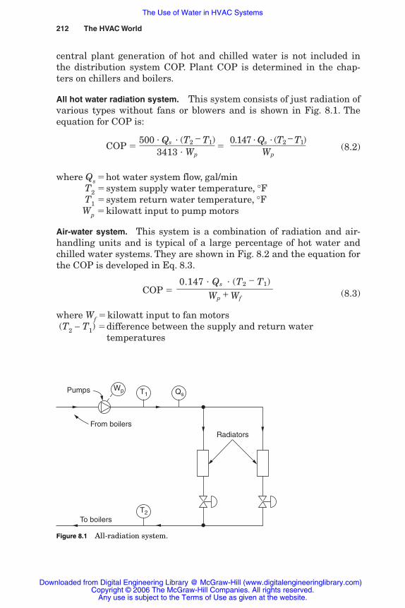
212 The HVAC World
central plant generation of hot and chilled water is not included inthe distribution system COP. Plant COP is determined in the chap-ters on chillers and boilers.
All hot water radiation system. This system consists of just radiation ofvarious types without fans or blowers and is shown in Fig. 8.1. Theequation for COP is:
COP � � (8.2)
where Qs �hot water system flow, gal/minT2 �system supply water temperature, °FT1 �system return water temperature, °FWp �kilowatt input to pump motors
Air-water system. This system is a combination of radiation and air-handling units and is typical of a large percentage of hot water andchilled water systems. They are shown in Fig. 8.2 and the equation forthe COP is developed in Eq. 8.3.
COP � (8.3)
where Wf �kilowatt input to fan motors(T2 − T1) �difference between the supply and return water
temperatures
0.147 � Qs � (T2 − T1)���
Wp + Wf
0.147 � Qs � (T2 − T1)���Wp
500 � Qs � (T2 − T1)���3413 � Wp
Wp T1
T2
Qs
Radiators
To boilers
Pumps
From boilers
Figure 8.1 All-radiation system.
Rishel_CH08.qxd 21/4/06 6:16 PM Page 212
Downloaded from Digital Engineering Library @ McGraw-Hill (www.digitalengineeringlibrary.com)Copyright © 2006 The McGraw-Hill Companies. All rights reserved.
Any use is subject to the Terms of Use as given at the website.
The Use of Water in HVAC Systems
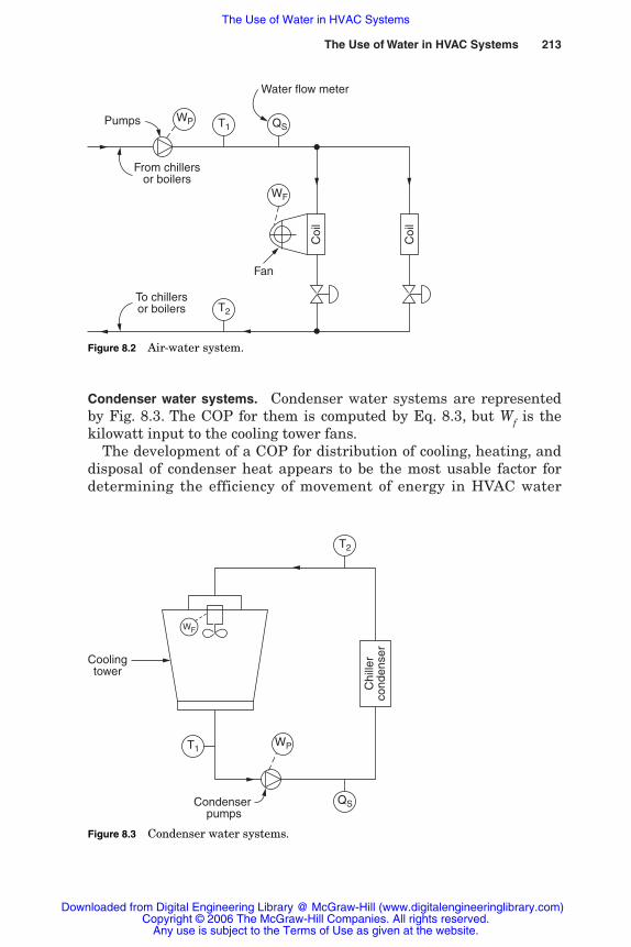
The Use of Water in HVAC Systems 213
Condenser water systems. Condenser water systems are representedby Fig. 8.3. The COP for them is computed by Eq. 8.3, but Wf is thekilowatt input to the cooling tower fans.
The development of a COP for distribution of cooling, heating, anddisposal of condenser heat appears to be the most usable factor fordetermining the efficiency of movement of energy in HVAC water
WP
WF
T1
T2
QSPumps
Coi
l
Coi
l
Fan
From chillersor boilers
To chillersor boilers
Water flow meter
Figure 8.2 Air-water system.
WP
Condenser pumps
QS
T1
T2
Chi
ller
cond
ense
r
WF
Coolingtower
Figure 8.3 Condenser water systems.
Rishel_CH08.qxd 21/4/06 6:16 PM Page 213
Downloaded from Digital Engineering Library @ McGraw-Hill (www.digitalengineeringlibrary.com)Copyright © 2006 The McGraw-Hill Companies. All rights reserved.
Any use is subject to the Terms of Use as given at the website.
The Use of Water in HVAC Systems

214 The HVAC World
systems. For example, an analysis can be made of a chilled watersystem utilizing fan-coil and small air handlers versus all large airhandlers with extensive duct systems. A first cost evaluation againstenergy consumption can be conducted to determinate the optimumselection for a particular application.
The overall efficiency of a water system is like any other equationfor efficiency—the useful energy divided by the energy input. The use-ful energy is the friction of the piping, fittings, and heating and cool-ing coils; their sizing obviously affects the amount of useful energy.The engineer must, as indicated in Chap. 3, balance friction againstfirst cost of the pipe to achieve an economical answer for the watersystem under design.
The efficient energy for an HVAC water system Ke can be calculatedin kilowatts as follows:
Ke �
Ke � (8.4)
The energy consumed by such a system Ki can be the energy inputto the system if it is known, or it can be calculated (in kilowatts) asfollows:
Ki � (8.5)
The efficiency of a water system WS�
utilizing electric motor–drivenpumps can be computed by dividing the useful kilowatts by the kilo-watt input to the pump variable-speed drives or motors Ki:
WS�
� �KK
e
i
� � 100% (8.6)
Using as an example a chilled water system with variable-speedpumping, if the friction of the piping, fittings, and cooling coils on thissystem with a capacity of 1000 gal/min amounted to 75 ft of head, theuseful energy would be
Ke � �10
50300�
875
� � 14.1 kW
To calculate Ki, assume that the friction loss through control valvesand other appurtenances amounts to 20 ft; the total pump head would
total system head (ft) � system flow (gal/min)������
5308 � P�
� E�
useful frictions (ft) � system flow (gal/min)�����
5308
useful frictions (ft) � system flow (gal/min) � 0.746������
3960
Rishel_CH08.qxd 21/4/06 6:16 PM Page 214
Downloaded from Digital Engineering Library @ McGraw-Hill (www.digitalengineeringlibrary.com)Copyright © 2006 The McGraw-Hill Companies. All rights reserved.
Any use is subject to the Terms of Use as given at the website.
The Use of Water in HVAC Systems
The Use of Water in HVAC Systems 215
then be 75 � 20 for a total of 95 ft. If the equipment efficiencies were83 percent for the pumps and 90 percent for the wire-to-shaft efficiencyof the motor and variable-speed drive, the input energy Ki would be
Ki � � 24.0 kW
The efficiency of the system WS�
would be
WS�
� �1244..10
� � 100 � 58.8 percent
The preceding calculations are for the system at full flow and withno overpressure generated by the pumps. It is apparent that for thisequation to be meaningful, similar calculations must be made underpart-load conditions.
For example, assume that the system is operating at 50 percentload, where the system flow is 500 gal/min and the useful systemhead has dropped to 40 ft. The useful kilowatts, therefore, are
Ke � �50
5030
�
840
� � 3.8 kW
Also assume that a constant-speed pump is used on the precedingapplication at 50 percent load. At this point, the pump has moved upits curve and is operating at 500 gal/min, 105 ft of head, and an effi-ciency of 78 percent. Since no variable-speed drive is involved, E
�is
the efficiency of the electric motor, which would be near 91 percent.Ki, therefore, becomes
Ki � � 13.9 kW
The overall efficiency of the water system becomes
WS�
� �3.8
13�
.1900
� � 27.3 percent
This demonstrates that only slightly more than one-fourth of theenergy applied to the pump motors is being used for efficient trans-portation of the water through the system. As dramatic as this mayseem, there are water systems utilizing constant-speed pumps andmechanical devices to overcome the pump overpressure where lessthan 10 percent of the energy applied is used to move the neededwater through the system at moderate and low loads on the system.
500 � 105���5308 � 0.78 � 0.91
1000 � 95���5308 � 0.83 � 0.90
Rishel_CH08.qxd 21/4/06 6:16 PM Page 215
Downloaded from Digital Engineering Library @ McGraw-Hill (www.digitalengineeringlibrary.com)Copyright © 2006 The McGraw-Hill Companies. All rights reserved.
Any use is subject to the Terms of Use as given at the website.
The Use of Water in HVAC Systems
216 The HVAC World
These equations for energy consumed, energy applied, and systemefficiency are for the water system in total. Similar evaluations forenergy consumption must be made for all parts of a water system toensure that maximum system efficiency is achieved. In Chap. 6, wire-to-water efficiency for pumping systems was addressed. Examples ofthis efficiency will be found throughout this book.
The use of Eq. 8.3 to evaluate the efficiency of pumping for anHVAC system may be cumbersome and the answer difficult to deter-mine. Also, the use of small pipe and high friction losses may providea relatively high efficiency for a poorly designed system. The use ofEq. 8.3 is more relative than absolute in comparing different pipingsystem designs with the same level of pipe friction.
Energy consumption of water distribution. There are other equationsfor chilled water and hot water systems that are useful to determinethe effectiveness of pumping. They are easier to compute than Eq. 8.3and provide absolute values. For example, for chilled water,
kW/100 tons � (8.7)
where H � system headP
�� pump efficiency
E�
� motor efficiency or wire-to-shaft efficiency of a variable-speed drive and motor for variable-speed pumps
�T � system temperature difference
For example, if the system head H is 100 ft, the pump efficiency 82percent, the wire-to-shaft efficiency 89 percent, and the temperaturedifferential 12°F, then
kW/100 tons � � 5.16 kW/100 tons
If flow and watt transmitters are measuring system flow and kilo-watts of the pumps for the chilled water, an alternate equation (Eq. 8.5)utilizes values measured from the actual system. This equationenables the operators of the water system to measure continuouslythe energy consumed in distributing the chilled water.
kW/100 tons � (8.8)
For example, if secondary pumps are pumping 1000 gal/min at a sys-tem temperature difference of 12°F and are consuming 25.8 kW, then
2400 � �pump kW���
gal/min � �T�°F
0.452 � 100��0.82 � 0.89 � 12
0.452 � H��P
�� E
�� �T�°F
Rishel_CH08.qxd 21/4/06 6:16 PM Page 216
Downloaded from Digital Engineering Library @ McGraw-Hill (www.digitalengineeringlibrary.com)Copyright © 2006 The McGraw-Hill Companies. All rights reserved.
Any use is subject to the Terms of Use as given at the website.
The Use of Water in HVAC Systems

The Use of Water in HVAC Systems 217
kW/100 tons � �21400000�
�
2152.8
� � 5.16 kW/100 tons
for hot water,
kW/1000 mbh � (8.9)
where is the specific weight of the hot water at operating tempera-ture. See Tables 2.3 and 2.4.
Like chilled water, if watt transmitters are available to measure theenergy input to the hot water pumps, the following equation can beused:
kW/1000 mbh � (8.10)
For example, if the secondary hot water pumps are pumping 500gal/min of 180°F water at a system temperature difference of 40°Fand are consuming 10.2 kW, then
kW/1000 mbh ��510204
�
,74000
�
�
6100.5.27
�� 1.05 kW/1000 mbh
where 60.57 is the specific weight of water at 180°F.Examples of these energy rates in kilowatts per 100 tons or kilo-
watts per 1000 mbh will be included in various chapters of this book.
8.1.3 Energy lost to mechanical flow-control devices
In this day of concern over energy conservation, as we begin thedesign of an HVAC water system, it is imperative that we reevaluateour standard practices to see where we are wasting energy. Withcomputer-aided design, it is much easier to develop part-load informa-tion and a closer evaluation of diversity on hot and chilled water sys-tems. This provides the basis for more efficient piping designs that donot need mechanical devices to circulate the water throughout thesystem. For example, on a recent evaluation of a Midwestern univer-sity, a chilled water pumping system was in operation with balancevalves on the pump discharges. There was a 58-lb/in2 pressure dropacross these balance valves, and each year around 900,000 kWh waswasted by them.
As discussed in Chap. 2, the thermal equivalent of a brake horse-power is 2545 Btu/h, and that for a kilowatthour is 3412 Btu/h. Thisenergy must be accounted for in the calculation of heating and cooling
124,700 � �pump kW���
gal/min � �T�°F �
23.48 � H���P
�� E
�� �T�°F �
Rishel_CH08.qxd 21/4/06 6:16 PM Page 217
Downloaded from Digital Engineering Library @ McGraw-Hill (www.digitalengineeringlibrary.com)Copyright © 2006 The McGraw-Hill Companies. All rights reserved.
Any use is subject to the Terms of Use as given at the website.
The Use of Water in HVAC Systems

218 The HVAC World
loads. Motor horsepower is, therefore, a plus for heating loads and is adeduction when computing the total heating load for a building. It isan added load on chilled water systems and must be included in thetotal cooling load of a building. It is important that we watch forenergy wasters, particularly on chilled water systems. Following is anevaluation of such mechanical devices that are used on hot andchilled water systems. Appreciable energy is used to circulate water toall the terminal units that are on such a system. The HVAC industryis full of various devices that regulate the flow of water to achieve adesired flow distribution of hot or chilled water in a building.
Typical energy consumers
1. Balance valves, manual and automatic
2. Pressure-regulating valves
3. Pressure-reducing valves
4. Three-way temperature-control valves
5. Most crossover bridges
The most popular of the preceding are balance valves; many ofthem may be installed in a single building. Usually, a manual-typebalance valve has two ports that are used to measure the pressureloss across the valve. Each manufacturer publishes a table for thevalve that will provide the flow in gallons per minute at the measuredpressure loss.
8.1.4 Energy losses for an element of awater system
All the calculations and formulas in this chapter are based on electricmotor–driven pumps. Following are calculations that can be used todetermine how much energy is being consumed by any element in orpart of a water system such as a single balance valve on a hot orchilled water system. This procedure also can be used for pressure-reducing and pressure-regulating valves, but it may be difficult toaccurately determine the flow through these valves.
The basic formula for computing pump horsepower also computesthe energy loss hPv for part of a system such as a balance valve. Thisformula is as follows, where Qv is the flow in gallons per minutethrough the part of a system being evaluated or for a balance valve;likewise, Hv is the loss in feet of head for that part of a system or for abalance valve.
Rishel_CH08.qxd 21/4/06 6:16 PM Page 218
Downloaded from Digital Engineering Library @ McGraw-Hill (www.digitalengineeringlibrary.com)Copyright © 2006 The McGraw-Hill Companies. All rights reserved.
Any use is subject to the Terms of Use as given at the website.
The Use of Water in HVAC Systems
The Use of Water in HVAC Systems 219
hpv � �3Q96
v
0� H
� Pv
�
� (8.11)
To convert to kilowatts,
kWv � �hpv �
E0
�
.746� (8.12)
or
kWv ��530
Q8
v
�
�
PH
�
v
� E�
� (8.13)
where P�
� pump efficiencyE
�� motor efficiency for constant-speed pumps and wire-to-
shaft efficiency for variable-speed pumps
This formula (8.11) computes the energy lost through part of a systemsuch as a balance valve by inserting the flow and head differencerecorded for each balance valve. The following discussion will bebased on balance valves.
A quick formula for estimating this energy loss without knowingthe pump and motor efficiencies is as follows: Assuming that the aver-age pump efficiency is 75 percent and the average motor efficiency is90 percent, Eq. 8.5 can be reduced to the following:
Lost kWv � �Q3v
6�
0H0
v� (8.14)
If the pressure drop Hv is indicated in psig, multiply it by 2.31.The annual lost energy is
Annual kWh � kWv � annual hours (8.15)
Although Eq. 8.11 is an approximation, it is accurate enough to deter-mine generally how much energy is being lost in a building due tobalance valves. If the loss is appreciable, a further study should bemade using Eqs. 8.8 and 8.9 with actual pump and motor efficiencies.
Serious studies of the energy consumption of condenser, chilled, andhot water systems are now under way. Out of this work has come evi-dence of the great loss that can be incurred by balance valves on cool-ing coils in particular. A specific study was conducted by a balancingcontractor and supervised by a consulting engineer that showed apronounced reduction in energy consumption by opening wide exist-ing balance valves on a variable-volume, variable-speed chilled watersystem in a high school. Table 8.1 is a summary of these data.
Rishel_CH08.qxd 21/4/06 6:16 PM Page 219
Downloaded from Digital Engineering Library @ McGraw-Hill (www.digitalengineeringlibrary.com)Copyright © 2006 The McGraw-Hill Companies. All rights reserved.
Any use is subject to the Terms of Use as given at the website.
The Use of Water in HVAC Systems
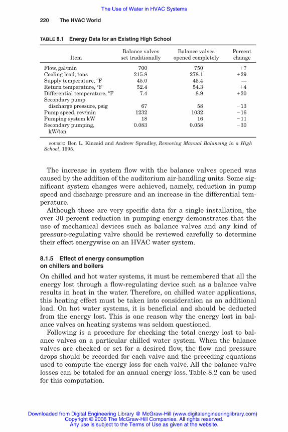
220 The HVAC World
The increase in system flow with the balance valves opened wascaused by the addition of the auditorium air-handling units. Some sig-nificant system changes were achieved, namely, reduction in pumpspeed and discharge pressure and an increase in the differential tem-perature.
Although these are very specific data for a single installation, theover 30 percent reduction in pumping energy demonstrates that theuse of mechanical devices such as balance valves and any kind ofpressure-regulating valve should be reviewed carefully to determinetheir effect energywise on an HVAC water system.
8.1.5 Effect of energy consumption on chillers and boilers
On chilled and hot water systems, it must be remembered that all theenergy lost through a flow-regulating device such as a balance valveresults in heat in the water. Therefore, on chilled water applications,this heating effect must be taken into consideration as an additionalload. On hot water systems, it is beneficial and should be deductedfrom the energy lost. This is one reason why the energy lost in bal-ance valves on heating systems was seldom questioned.
Following is a procedure for checking the total energy lost to bal-ance valves on a particular chilled water system. When the balancevalves are checked or set for a desired flow, the flow and pressuredrops should be recorded for each valve and the preceding equationsused to compute the energy loss for each valve. All the balance-valvelosses can be totaled for an annual energy loss. Table 8.2 can be usedfor this computation.
TABLE 8.1 Energy Data for an Existing High School
Balance valves Balance valves Percent Item set traditionally opened completely change
Flow, gal/min 700 750 �7Cooling load, tons 215.8 278.1 �29Supply temperature, °F 45.0 45.4 —Return temperature, °F 52.4 54.3 �4Differential temperature, °F 7.4 8.9 �20Secondary pump
discharge pressure, psig 67 58 �13Pump speed, rev/min 1232 1032 �16Pumping system kW 18 16 �11Secondary pumping, 0.083 0.058 �30
kW/ton
SOURCE: Ben L. Kincaid and Andrew Spradley, Removing Manual Balancing in a HighSchool, 1995.
Rishel_CH08.qxd 21/4/06 6:16 PM Page 220
Downloaded from Digital Engineering Library @ McGraw-Hill (www.digitalengineeringlibrary.com)Copyright © 2006 The McGraw-Hill Companies. All rights reserved.
Any use is subject to the Terms of Use as given at the website.
The Use of Water in HVAC Systems

The Use of Water in HVAC Systems 221
TABLE 8.2 Energy Calculations for Balance Valves on Constant-Volume Systems
Building:_____________________________________ Date: ___________________
Valve number Head loss Energy loss,or location Flow, gal/min in ft kW
Total kW for building:________________
Annual hours: _____________________
Annual energy loss � _________________ Total kW __________________ hours
� ________________ kWh
NOTE: See text for calculation of added chiller energy consumption due to balance valves.
Rishel_CH08.qxd 21/4/06 6:16 PM Page 221
Downloaded from Digital Engineering Library @ McGraw-Hill (www.digitalengineeringlibrary.com)Copyright © 2006 The McGraw-Hill Companies. All rights reserved.
Any use is subject to the Terms of Use as given at the website.
The Use of Water in HVAC Systems

222 The HVAC World
This annual energy loss in kilowatthours can be used to determinethe additional annual energy consumption of the chillers due to thebalance valves:
Added chiller kWh �
� (8.16)
where total annual kWhv is for the balance valves, and average kilo-watts per ton is the annual kilowatthour consumption of the chillersdivided by the annual ton-hours of cooling produced by the chillers.
For example, if the annual loss due to balance valves is 100,000kWh and the average kilowatthours per ton-hour is 0.80, then
Added chiller kWh ��100,0
30.502� 0.80
�
� 22,727 kWh
The total annual loss for the balance valves is therefore 100,000 �22,727 kWh, or 122,727 kWh.
The energy loss for the balance valves on hot water systems mustrecognize the heating effect of the energy consumed in these valves.This is done as follows for gas fired boilers. The equivalent fuel perkilowatt EF/kW in cubic feet is calculated first, and then the netdeduction in percent is developed:
�kEWF� � � ft3 gas/kW (8.17)
where B�
is boiler efficiency as a decimal. The heating value of nat-ural gas is assumed to be 1000 Btu/ft3. Thus, heating effect Hef inpercent is
Hef � � % reduction (8.18)
Using these equations, with a natural gas cost of $4 per 1000 ft3, or0.4 cents/ft3, overall power cost of 6 cents/kW, and a boiler efficiency of80 percent,
EF/kW � �0.8
3�
4110200
� � 4.265 ft3/kW
Hef ��4.265 � 0
6.4 � 100�� 28.4 percent reduction
EF/kW � fuel cost (cents/ft3) � 100����
overall power cost (cents/kW)
3412 Btu/kW��B
�� 1000 Btu/ft3
annual kWhv � average kW/ton����
3.52
annual kWhv � 3412 � average kW/ton�����
12,000
Rishel_CH08.qxd 21/4/06 6:16 PM Page 222
Downloaded from Digital Engineering Library @ McGraw-Hill (www.digitalengineeringlibrary.com)Copyright © 2006 The McGraw-Hill Companies. All rights reserved.
Any use is subject to the Terms of Use as given at the website.
The Use of Water in HVAC Systems

The Use of Water in HVAC Systems 223
If the annual loss to balance valves is 100,000 kW, recognizingthe heating value of this energy is achieved by multiplying100,000 (1�0.284), which gives a net energy loss of 71,600 kW/year.
On hot and chilled water systems, the advent of variable-speedpumping and digital control has made possible the conversion ofconstant-volume systems to variable-volume systems. This isaccomplished through the replacement of three-way control valvesby two-way valves and adjusting of the balance valves to the full-open position. The procedure included herein for computing energylosses of balance valves can be used to help determine the energysavings that could be achieved by installing variable-speed pumpswith proper control, replacing the three-way valves with two-wayvalves, and opening the balance valves.
8.2 Efficient Use of Water in HVAC Systems
The preceding discussion points the way to efficient use of water andpumping energy in HVAC systems. The remainder of this chapter willbe used to develop the load range for a water system and to describethe various uses of water in these systems.
8.2.1 Load range for a water system
All of this chapter has been devoted to an analysis of energy atdesign load or maximum water flow. Unfortunately, in manyinstances on actual water systems this is the last part of the analy-sis. It is of utmost importance that the minimum load as well as themaximum load be determined for a water system to achieve an accu-rate consumption of energy. Part-load calculation is a subject of con-siderable study by the American Society of Heating, Refrigerating,and Air Conditioning Engineers (ASHRAE). Its Handbook onFundamentals describes the “bin” method for computing part-loadsystem flows. Using the formula for pipe friction, the system headscan be calculated for these part-load conditions. Likewise, withproper use of the affinity laws, the energy consumption of the pumpscan be computed from minimum to maximum load. In all the systemevaluations that will be discussed in this book, minimum load willalways be included when computing pumping system performanceand energy consumption.
8.2.2 Energy consumption and water uses in HVAC
The use of the energy consumers, as described in the previous section,develops a possibility that the water system could have been designeddifferently; this would have eliminated the need for their use and
Rishel_CH08.qxd 21/4/06 6:16 PM Page 223
Downloaded from Digital Engineering Library @ McGraw-Hill (www.digitalengineeringlibrary.com)Copyright © 2006 The McGraw-Hill Companies. All rights reserved.
Any use is subject to the Terms of Use as given at the website.
The Use of Water in HVAC Systems

224 The HVAC World
reduced the energy consumption in the system. It must be remem-bered that many existing systems were designed at a time whenenergy was lower in cost and the use of these mechanical devices wasthe most economical procedure at that time. The following discussionwill review the use of water in hot and chilled water systems. A simi-lar evaluation will be made for condenser water in Chap. 11.
8.3 Hot and Chilled Water Systems
There are three zones of different activity in a hot or chilled water sys-tem. The first zone is energy generation, the second zone is transporta-tion of that energy, and the third zone is use of the energy (Fig. 8.4).
Zone 1: Energy generation. Energy for hot and chilled water systems isgenerated in boilers and chillers. The efficiency of the boilers andchillers may be affected appreciably by how the water is circulatedthrough them. The development of bypasses and special pipingarrangements has been achieved to enhance their efficiency.
Figure 8.4 Three zones of a chilled or hot water system.
Rishel_CH08.qxd 21/4/06 6:16 PM Page 224
Downloaded from Digital Engineering Library @ McGraw-Hill (www.digitalengineeringlibrary.com)Copyright © 2006 The McGraw-Hill Companies. All rights reserved.
Any use is subject to the Terms of Use as given at the website.
The Use of Water in HVAC Systems

The Use of Water in HVAC Systems 225
The efficiency of boilers and chillers should not be compromised inan effort to save pumping energy. Here lies one of the major responsi-bilities of the water system designer, who must evaluate various con-nections and pumping arrangements to acquire the optimal configu-ration for a particular system.
Zone 2: Transportation of energy. Once the hot or chilled water has beengenerated, it must be moved out to the heating or cooling coils. Com-bining the pumps for this transportation with the pumps for the boil-ers or chillers may or may not improve the efficiency of the entirewater system.
Often, the most efficient system of delivering the water to the enduses is to develop the transportation pumps strictly for the purpose ofdistributing the water and not to generate the energy. A number ofdifferent pumping and piping arrangements are provided herein toassist the designer in selecting the most efficient system for a particu-lar water system.
Zone 3: Use of the energy. Water in hot and chilled water systems isused by hot and chilled water coils, heat exchangers, and processequipment. Most of these energy users are equipped with a controlvalve to regulate the flow of water through them.
Some coils are operated without control valves and are called “wild”coils. They are often equipped with face and bypass dampers that con-trol the use of energy by them. The water flows continuously throughthe coil, and the air flows around the coil on low heating or coolingloads. Wild coils should not be used on systems with high pumpingheads and broad load ranges due to the pumping energy wasted bythem. Some designers use these coils on outside makeup air to pre-vent freezing in the coil. There are other methods to prevent freezingbesides wild coils that control the flow and therefore conserve pumpingenergy. The other problem with these uncontrolled coils is the return ofthe water unused to the boilers and chillers. This raises the returnwater temperature on hot water systems and lowers the return watertemperature on chilled water systems.
Much will be made of different coil connections to develop the effi-ciencies or inefficiencies of the various systems that are used inHVAC systems today. It is obvious that the three-way valve on a heat-ing or cooling coil is a wasteful device like the wild coil with a faceand bypass damper. Water is bypassed around the coil and returnedto the boiler or chiller unused.
Sizing of coils from a standpoint of water friction loss is becoming avery detailed task. From a standpoint of pumping energy, if the coil issized with too great a friction drop, energy is wasted. If the coil is
Rishel_CH08.qxd 21/4/06 6:16 PM Page 225
Downloaded from Digital Engineering Library @ McGraw-Hill (www.digitalengineeringlibrary.com)Copyright © 2006 The McGraw-Hill Companies. All rights reserved.
Any use is subject to the Terms of Use as given at the website.
The Use of Water in HVAC Systems

226 The HVAC World
sized with a low velocity in the tubes and low friction loss, laminarflow develops and excessive water flow results. The designer mustbalance the selection of coils between high water pressure loss andlaminar flow. The flow of water in the coil should not pass into thelaminar range at any known load on the coil.
How well we use hot or chilled water will determine the efficiencyof operation of the entire water system. Hot and chilled water systemsare described together here, because there is so much similaritybetween hot water and chilled water coils in their use and in theirconnections.
Hot and chilled water coil connections must be studied in detail toensure that the supply water is being used efficiently. There are anumber of ways to connect these coils, and many are being advocatedin the HVAC industry. Some of them are being sold to solve a particu-lar system problem.
The system problems that are being addressed with these connec-tions are:
1. Laminar flow in coils
2. Dirty coils—water side, air side, or both
3. Improperly sized coil control valves or valve actuators
4. Poorly constructed control valves
8.3.1 Three-way valves for hot and chilled water coils
When three-way valves were used predominantly on these coils, thesystems were constant flow, and there was little concern for energysavings. The three-way control valve wastes energy by bypassing thesupply water around the coil, as shown in Fig. 8.5a. On variable-volume chilled water systems, this has a negative effect on thechillers, since the return temperature to the chillers is reduced. Thechillers reach rated water flow long before they achieve design load intons. This forces more than one chiller to operate when the coolingload is less than the capacity of one chiller.
8.3.2 Two-way valve with circulator
Recognizing the deficiency of the three-way valve, efforts have beenmade to control the return water temperature by replacing the three-way valve with a two-way valve using a circulator on the coil (seeFig. 8.5b). Laminar flow was eliminated with this arrangement, butdirty coils could still pass water through the control valve belowdesign temperature on chilled water systems. The significant defect ofthis arrangement is the continuous operation of the coil pump whenever
Rishel_CH08.qxd 21/4/06 6:16 PM Page 226
Downloaded from Digital Engineering Library @ McGraw-Hill (www.digitalengineeringlibrary.com)Copyright © 2006 The McGraw-Hill Companies. All rights reserved.
Any use is subject to the Terms of Use as given at the website.
The Use of Water in HVAC Systems
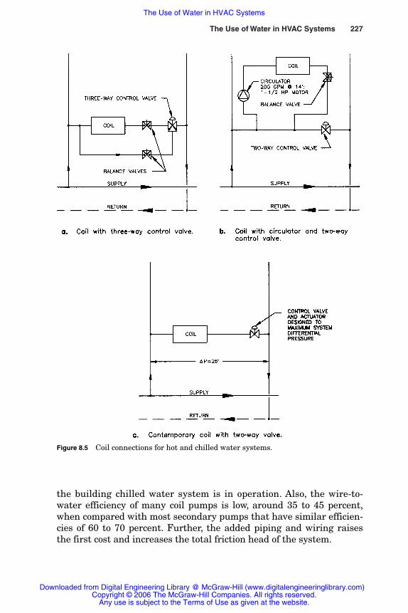
The Use of Water in HVAC Systems 227
Figure 8.5 Coil connections for hot and chilled water systems.
the building chilled water system is in operation. Also, the wire-to-water efficiency of many coil pumps is low, around 35 to 45 percent,when compared with most secondary pumps that have similar efficien-cies of 60 to 70 percent. Further, the added piping and wiring raisesthe first cost and increases the total friction head of the system.
Rishel_CH08.qxd 21/4/06 6:16 PM Page 227
Downloaded from Digital Engineering Library @ McGraw-Hill (www.digitalengineeringlibrary.com)Copyright © 2006 The McGraw-Hill Companies. All rights reserved.
Any use is subject to the Terms of Use as given at the website.
The Use of Water in HVAC Systems

228 The HVAC World
8.3.3 Contemporary two-way valve connection
The ability to evaluate more accurately the pressure drops that couldoccur across control valves has resulted in the selection of valves bet-ter fitted to a specific application. This has culminated in use of thetwo-way valve directly connected to its coil and the supply and returnheaders (see Fig. 8.5c). With proper calculation of maximum possiblepressure drop across the valve, the valve and its actuator can be sizedto operate under these pressures without damage or lifting of thevalve head off the valve seat.
8.3.4 Energy evaluations for three differentcoil connections
Following are energy analyses using these three coil and control-valveconnections. This energy audit should demonstrate the need to elimi-nate three-way valves and coil circulators on most variable-volumesystems. Circulators in coil bypasses do have specific uses on existingsystems, and these will be demonstrated in this chapter.
It is difficult to locate the right place in this book for the followingenergy discussion. This is so important that it must be addressedbefore specific installations are reviewed. Chapter 9 will develop theprimary/secondary pumping systems that were used with the oldercoil circulator and three-way valve installations shown in Fig. 8.6aand 8.6b. Variable primary pump will also be described there; it is
Figure 8.6 Water systems with the three coil connections.
Coi
l
Supply header loss = 25 ft.
3–constant speed pumps1000 GPM EA. @ 84 ft.
8 ft. lossacross pumpfittings
Fromchillers
Chillerloop bypass
To chillersReturn header loss = 25 ft.
Tencoils
26 Ft. lossacross coil,valve, and
piping
a. Secondary chilled water system with three-way control valves.
Rishel_CH08.qxd 21/4/06 6:16 PM Page 228
Downloaded from Digital Engineering Library @ McGraw-Hill (www.digitalengineeringlibrary.com)Copyright © 2006 The McGraw-Hill Companies. All rights reserved.
Any use is subject to the Terms of Use as given at the website.
The Use of Water in HVAC Systems
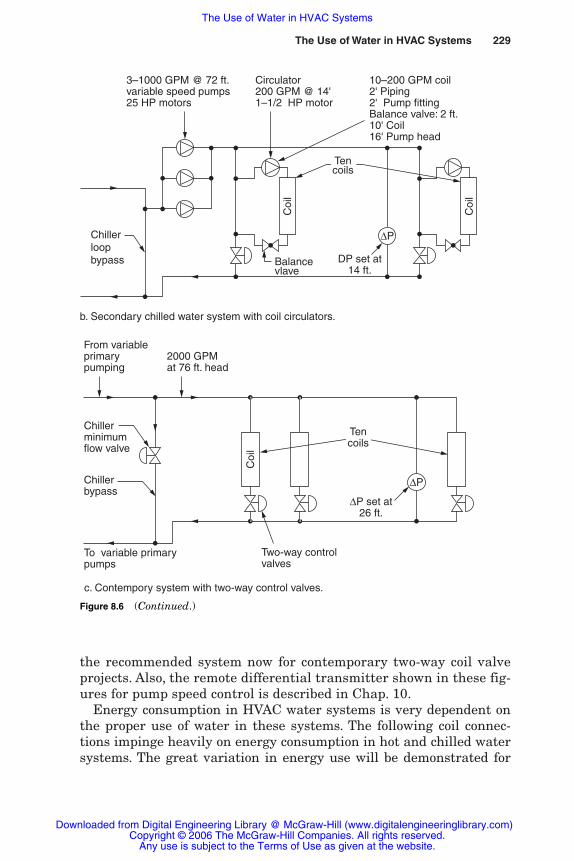
The Use of Water in HVAC Systems 229
the recommended system now for contemporary two-way coil valveprojects. Also, the remote differential transmitter shown in these fig-ures for pump speed control is described in Chap. 10.
Energy consumption in HVAC water systems is very dependent onthe proper use of water in these systems. The following coil connec-tions impinge heavily on energy consumption in hot and chilled watersystems. The great variation in energy use will be demonstrated for
Coi
l
Coi
l
Chillerloopbypass
∆P
Balancevlave
Tencoils
DP set at14 ft.
10–200 GPM coil2' Piping2' Pump fittingBalance valve: 2 ft.10' Coil16' Pump head
Circulator200 GPM @ 14'1–1/2 HP motor
3–1000 GPM @ 72 ft.variable speed pumps25 HP motors
b. Secondary chilled water system with coil circulators.
∆P
Tencoils
∆P set at26 ft.
Two-way controlvalves
To variable primarypumps
Chillerbypass
Chillerminimumflow valve
2000 GPMat 76 ft. head
From variableprimarypumping
Coi
l
c. Contempory system with two-way control valves.
Figure 8.6 (Continued.)
Rishel_CH08.qxd 21/4/06 6:16 PM Page 229
Downloaded from Digital Engineering Library @ McGraw-Hill (www.digitalengineeringlibrary.com)Copyright © 2006 The McGraw-Hill Companies. All rights reserved.
Any use is subject to the Terms of Use as given at the website.
The Use of Water in HVAC Systems
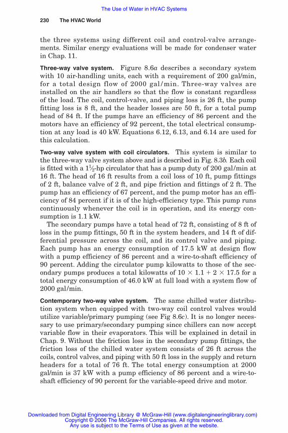
230 The HVAC World
the three systems using different coil and control-valve arrange-ments. Similar energy evaluations will be made for condenser waterin Chap. 11.
Three-way valve system. Figure 8.6a describes a secondary systemwith 10 air-handling units, each with a requirement of 200 gal/min,for a total design flow of 2000 gal / min. Three-way valves areinstalled on the air handlers so that the flow is constant regardlessof the load. The coil, control-valve, and piping loss is 26 ft, the pumpfitting loss is 8 ft, and the header losses are 50 ft, for a total pumphead of 84 ft. If the pumps have an efficiency of 86 percent and themotors have an efficiency of 92 percent, the total electrical consump-tion at any load is 40 kW. Equations 6.12, 6.13, and 6.14 are used forthis calculation.
Two-way valve system with coil circulators. This system is similar tothe three-way valve system above and is described in Fig. 8.3b. Each coilis fitted with a 11⁄2-hp circulator that has a pump duty of 200 gal/min at16 ft. The head of 16 ft results from a coil loss of 10 ft, pump fittingsof 2 ft, balance valve of 2 ft, and pipe friction and fittings of 2 ft. Thepump has an efficiency of 67 percent, and the pump motor has an effi-ciency of 84 percent if it is of the high-efficiency type. This pump runscontinuously whenever the coil is in operation, and its energy con-sumption is 1.1 kW.
The secondary pumps have a total head of 72 ft, consisting of 8 ft ofloss in the pump fittings, 50 ft in the system headers, and 14 ft of dif-ferential pressure across the coil, and its control valve and piping.Each pump has an energy consumption of 17.5 kW at design flowwith a pump efficiency of 86 percent and a wire-to-shaft efficiency of90 percent. Adding the circulator pump kilowatts to those of the sec-ondary pumps produces a total kilowatts of 10 1.1 � 2 17.5 for atotal energy consumption of 46.0 kW at full load with a system flow of2000 gal/min.
Contemporary two-way valve system. The same chilled water distribu-tion system when equipped with two-way coil control valves wouldutilize variable/primary pumping (see Fig 8.6c). It is no longer neces-sary to use primary/secondary pumping since chillers can now acceptvariable flow in their evaporators. This will be explained in detail inChap. 9. Without the friction loss in the secondary pump fittings, thefriction loss of the chilled water system consists of 26 ft across thecoils, control valves, and piping with 50 ft loss in the supply and returnheaders for a total of 76 ft. The total energy consumption at 2000gal/min is 37 kW with a pump efficiency of 86 percent and a wire-to-shaft efficiency of 90 percent for the variable-speed drive and motor.
Rishel_CH08.qxd 21/4/06 6:16 PM Page 230
Downloaded from Digital Engineering Library @ McGraw-Hill (www.digitalengineeringlibrary.com)Copyright © 2006 The McGraw-Hill Companies. All rights reserved.
Any use is subject to the Terms of Use as given at the website.
The Use of Water in HVAC Systems
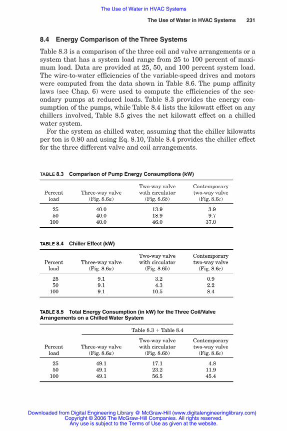
The Use of Water in HVAC Systems 231
8.4 Energy Comparison of the Three Systems
Table 8.3 is a comparison of the three coil and valve arrangements or asystem that has a system load range from 25 to 100 percent of maxi-mum load. Data are provided at 25, 50, and 100 percent system load.The wire-to-water efficiencies of the variable-speed drives and motorswere computed from the data shown in Table 8.6. The pump affinitylaws (see Chap. 6) were used to compute the efficiencies of the sec-ondary pumps at reduced loads. Table 8.3 provides the energy con-sumption of the pumps, while Table 8.4 lists the kilowatt effect on anychillers involved, Table 8.5 gives the net kilowatt effect on a chilledwater system.
For the system as chilled water, assuming that the chiller kilowattsper ton is 0.80 and using Eq. 8.10, Table 8.4 provides the chiller effectfor the three different valve and coil arrangements.
TABLE 8.3 Comparison of Pump Energy Consumptions (kW)
Two-way valve Contemporary Percent Three-way valve with circulator two-way valve
load (Fig. 8.6a) (Fig. 8.6b) (Fig. 8.6c)
025 40.0 13.9 3.9050 40.0 18.9 9.7100 40.0 46.0 37.0
TABLE 8.5 Total Energy Consumption (in kW) for the Three Coil/ValveArrangements on a Chilled Water System
Table 8.3 � Table 8.4
Two-way valve Contemporary Percent Three-way valve with circulator two-way valve
load (Fig. 8.6a) (Fig. 8.6b) (Fig. 8.6c)
025 49.1 17.1 04.8050 49.1 23.2 11.9100 49.1 56.5 45.4
TABLE 8.4 Chiller Effect (kW)
Two-way valve Contemporary Percent Three-way valve with circulator two-way valve
load (Fig. 8.6a) (Fig. 8.6b) (Fig. 8.6c)
025 9.1 03.2 0.9050 9.1 04.3 2.2100 9.1 10.5 8.4
Rishel_CH08.qxd 21/4/06 6:16 PM Page 231
Downloaded from Digital Engineering Library @ McGraw-Hill (www.digitalengineeringlibrary.com)Copyright © 2006 The McGraw-Hill Companies. All rights reserved.
Any use is subject to the Terms of Use as given at the website.
The Use of Water in HVAC Systems
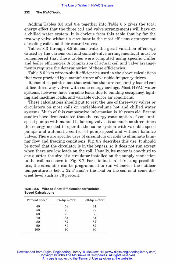
232 The HVAC World
Adding Tables 8.3 and 8.4 together into Table 8.5 gives the totalenergy effect that the three coil and valve arrangements will have ona chilled water system. It is obvious from this table that by far thetwo-way valve without a circulator is the most efficient arrangementof cooling coils and their control valves.
Tables 8.3 through 8.5 demonstrate the great variation of energycaused by the various coil and control-valve arrangements. It must beremembered that these tables were computed using specific chillerand boiler efficiencies. A comparison of actual coil and valve arrange-ments requires the determination of these efficiencies.
Table 8.6 lists wire-to-shaft efficiencies used in the above calculationsthat were provided by a manufacturer of variable-frequency drives.
It should be pointed out that systems that are constantly loaded canutilize three-way valves with some energy savings. Most HVAC watersystems, however, have variable loads due to building occupancy, light-ing and machine loads, and variable outdoor air conditions.
These calculations should put to rest the use of three-way valves orcirculators on most coils on variable-volume hot and chilled watersystems. Much of this comparative information is 10 years old. Recentstudies have demonstrated that the energy consumption of constant-speed pumps with manual balancing valves is as much as three timesthe energy needed to operate the same system with variable-speedpumps and automatic control of pump speed and without balancevalves. There are specific uses of circulators on coils to eliminate lami-nar flow and freezing conditions; Fig. 8.7 describes this use. It shouldbe noted that the circulator is in the bypass, so it does not run exceptwhen there are low loads on the coil. Usually, its motor is one-third toone-quarter the size of a circulator installed on the supply connectionto the coil, as shown in Fig. 8.7. For elimination of freezing possibili-ties, the circulator can be programmed to run whenever the outdoortemperature is below 32°F and/or the load on the coil is at some dis-creet level such as 70 percent.
TABLE 8.6 Wire-to-Shaft Efficiencies for Variable-Speed Calculations
Percent speed 25-hp motor 30-hp motor
40 58 6150 70 7260 79 8070 84 8480 87 8790 89 89
100 90 90
Rishel_CH08.qxd 21/4/06 6:16 PM Page 232
Downloaded from Digital Engineering Library @ McGraw-Hill (www.digitalengineeringlibrary.com)Copyright © 2006 The McGraw-Hill Companies. All rights reserved.
Any use is subject to the Terms of Use as given at the website.
The Use of Water in HVAC Systems

The Use of Water in HVAC Systems 233
8.5 The Use of Balance Valves on Variable-Volume Systems
Most HVAC chilled and hot water systems are variable volume, notconstant volume. Figure 8.8 describes why balance valves cannot beused on these systems.
Figure 8.8 describes the problem with trying to balance a variable-volume system with manual-balance valves. Two cooling coils demon-strate the problem with mechanically balancing direct return systemsthrough the use of balance valves. Coil No. 1 has no load on and yethas 96 ft of head on its control valve while Coil No. 2 is fully loadedwith 88.9 ft of head on its coil and control valve. This demonstratesthe great amount of head that can be imposed upon the coil valveswhere the coils are located near the central plant. If the coil, its pip-ing, and control valve have a total loss of 20 ft, the balance valvewould be set to eliminate around 76 ft of head. If you try to manuallybalance out this high head at full flow in the system, you will starvethe coils when they operate at full flow but with reduced total load onthe system. Therefore, a variable-volume system cannot be balancedwith manual or automatic balance valves. This demonstrates that the
Figure 8.7 Heating or cooling coil pump for freezeprotection or laminar flow. (From The WaterManagement Manual, Systecon, Inc., West Chester,Ohio, 1992, Fig. 4.3.)
Rishel_CH08.qxd 21/4/06 6:16 PM Page 233
Downloaded from Digital Engineering Library @ McGraw-Hill (www.digitalengineeringlibrary.com)Copyright © 2006 The McGraw-Hill Companies. All rights reserved.
Any use is subject to the Terms of Use as given at the website.
The Use of Water in HVAC Systems

234 The HVAC World
coil control valve must be selected correctly to maintain the desiredflow in the coils, whether there is near full load or little load on thechilled water system.
8.6 Elimination of Pump Head-Wasting Devices
Whenever we add a mechanical device to a water system, we shouldask why do we need it and what energy does it cost in the form of lostpump head? Here are four mechanical devices that must be removedwherever possible.
Balance valves, manual and automatic. As we saw in the previoussection, variable-volume water systems cannot be balanced withany kind of a balance valve. Since most, sizable HVAC water sys-tems are variable volume with variable speed pumps, there is no
190
170
150
130
110
90
70
50
Sys
tem
hea
d (f
t.)Pump discharge loss
Chiller loss
Pump head
Pump suction loss
Coil 1 Coil 2 96.0'41.6 psi
88.9'38.5 psi
Coil furthest fromthe plant
Coil 1 is at no loadCoil 2 is at 100% load
Chilled water distribution system (no scale)
Figure 8.8 Hydraulic gradient full load. (From Patterson Pump Company, HVACPumps and Systems Manual, 2004.)
Rishel_CH08.qxd 21/4/06 6:16 PM Page 234
Downloaded from Digital Engineering Library @ McGraw-Hill (www.digitalengineeringlibrary.com)Copyright © 2006 The McGraw-Hill Companies. All rights reserved.
Any use is subject to the Terms of Use as given at the website.
The Use of Water in HVAC Systems
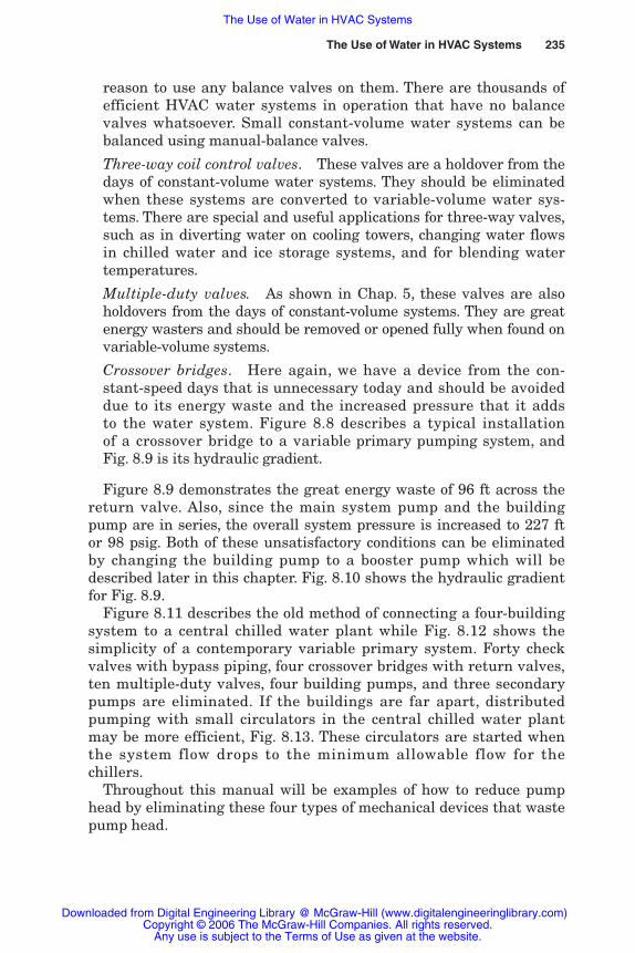
reason to use any balance valves on them. There are thousands ofefficient HVAC water systems in operation that have no balancevalves whatsoever. Small constant-volume water systems can bebalanced using manual-balance valves.
Three-way coil control valves. These valves are a holdover from thedays of constant-volume water systems. They should be eliminatedwhen these systems are converted to variable-volume water sys-tems. There are special and useful applications for three-way valves,such as in diverting water on cooling towers, changing water flowsin chilled water and ice storage systems, and for blending watertemperatures.
Multiple-duty valves. As shown in Chap. 5, these valves are alsoholdovers from the days of constant-volume systems. They are greatenergy wasters and should be removed or opened fully when found onvariable-volume systems.
Crossover bridges. Here again, we have a device from the con-stant-speed days that is unnecessary today and should be avoideddue to its energy waste and the increased pressure that it addsto the water system. Figure 8.8 describes a typical installationof a crossover bridge to a variable primary pumping system, andFig. 8.9 is its hydraulic gradient.
Figure 8.9 demonstrates the great energy waste of 96 ft across thereturn valve. Also, since the main system pump and the buildingpump are in series, the overall system pressure is increased to 227 ftor 98 psig. Both of these unsatisfactory conditions can be eliminatedby changing the building pump to a booster pump which will bedescribed later in this chapter. Fig. 8.10 shows the hydraulic gradientfor Fig. 8.9.
Figure 8.11 describes the old method of connecting a four-buildingsystem to a central chilled water plant while Fig. 8.12 shows thesimplicity of a contemporary variable primary system. Forty checkvalves with bypass piping, four crossover bridges with return valves,ten multiple-duty valves, four building pumps, and three secondarypumps are eliminated. If the buildings are far apart, distributedpumping with small circulators in the central chilled water plantmay be more efficient, Fig. 8.13. These circulators are started whenthe system flow drops to the minimum allowable flow for thechillers.
Throughout this manual will be examples of how to reduce pumphead by eliminating these four types of mechanical devices that wastepump head.
The Use of Water in HVAC Systems 235
Rishel_CH08.qxd 21/4/06 6:16 PM Page 235
Downloaded from Digital Engineering Library @ McGraw-Hill (www.digitalengineeringlibrary.com)Copyright © 2006 The McGraw-Hill Companies. All rights reserved.
Any use is subject to the Terms of Use as given at the website.
The Use of Water in HVAC Systems

8.7 Categorization of HVAC Water Systems
HVAC water systems can be categorized by whether they are open orclosed. Any classification will create some confusion, but these cate-gories should be adequate for evaluating pumps on all HVAC watersystems.
Open systems have no external pressures placed on them, and usu-ally, they include an open tank holding a reservoir of water. Watermakeup is made to these systems at the reservoir or tank. Followingis a listing of open-type systems and chapter of this book thatdescribes them.
Cooling tower pumps Chap. 11
Pumps for process cooling Chap. 12
Open thermal storage systems Chap. 13
236 The HVAC World
96'
Chi
ller
Variableprimarypump
DP
C
C
Crossover bridge
Return valve lossis equal to hydraulicgradient of system
Building coils withcontrol valves
Building pump
Figure 8.9 Energy waste of crossover bridges on variable speed systems.(From Patterson Pump Company, HVAC Pumps and Systems Manual, 2004.)
Rishel_CH08.qxd 21/4/06 6:16 PM Page 236
Downloaded from Digital Engineering Library @ McGraw-Hill (www.digitalengineeringlibrary.com)Copyright © 2006 The McGraw-Hill Companies. All rights reserved.
Any use is subject to the Terms of Use as given at the website.
The Use of Water in HVAC Systems

Closed systems utilize external pressure to maintain the desiredoperating pressure. This is accomplished through the use of makeupwater that is fed through a pressure regulator. Since they are closedsystems, they have an expansion tank to accommodate thermal expan-sion and contraction caused by changes in system water temperature.Following is a similar listing for closed systems described in this book.
Chillers and their pumps Chap. 14
Chilled water systems Chap. 15
Closed condenser water systems Chap. 16
Closed thermal storage systems Chap. 17
District heating and cooling Chap. 18
Hot water boilers Chap. 19
The Use of Water in HVAC Systems 237
Loss acrossreturn valve
96.0'41.6 psi
Coil furthestfrom the plant
Building pump - 60 ft. head
Building hydraulic gradient
Building pump shut-off head 227 ft.building pressure or 98 psig
Return valve
230
210
190
170
150
130
110
90
70
50
Sys
tem
hea
d (f
t.)
Chilled water distribution system (no scale)
Figure 8.10 Hydraulic gradient for figure 8.9. (From Patterson PumpCompany, HVAC Pumps and Systems Manual, 2004.)
Rishel_CH08.qxd 21/4/06 6:16 PM Page 237
Downloaded from Digital Engineering Library @ McGraw-Hill (www.digitalengineeringlibrary.com)Copyright © 2006 The McGraw-Hill Companies. All rights reserved.
Any use is subject to the Terms of Use as given at the website.
The Use of Water in HVAC Systems

Fig
ure
8.1
1C
onst
ant
flow
fou
r-zo
ne
syst
em.
Chiller
Chiller
Chiller
Sec
onda
ry p
umps
,co
nsta
nt s
peed
Prim
ary
pum
ps, c
onst
ant s
peed
Mul
tiple
-dut
y va
lves
Ret
urn
valv
esM
ultip
le-d
uty
valv
es
Cro
ssov
erbr
idge
sC
onst
ant s
peed
Mul
tiple
-du
ty v
alve
s
Coi
lsB
alan
ce v
alve
Thr
ee-w
ay v
alve
s
238
Rishel_CH08.qxd 21/4/06 6:16 PM Page 238
Downloaded from Digital Engineering Library @ McGraw-Hill (www.digitalengineeringlibrary.com)Copyright © 2006 The McGraw-Hill Companies. All rights reserved.
Any use is subject to the Terms of Use as given at the website.
The Use of Water in HVAC Systems

Fig
ure
8.1
2V
aria
ble
prim
ary
syst
em (
fou
r zo
nes
in o
ne
buil
din
g.)
DP
DP
DP
DP
Diff
eren
tial
pres
sure
tran
smitt
ers
Two-
way
valv
esC
oils
Chiller
Chiller
No
cros
sove
r br
idge
s or
retu
rn w
ater
val
ves
Ord
inar
ych
eck
valv
es
Aut
omat
ic s
hut-
off
valv
es
Var
iabl
e sp
eed
prim
ary
pum
ps
C
Chiller
239
Rishel_CH08.qxd 21/4/06 6:16 PM Page 239
Downloaded from Digital Engineering Library @ McGraw-Hill (www.digitalengineeringlibrary.com)Copyright © 2006 The McGraw-Hill Companies. All rights reserved.
Any use is subject to the Terms of Use as given at the website.
The Use of Water in HVAC Systems

DP
DP
DP
DP
Coi
lsTw
o-w
ayva
lves
Diff
eren
tial
pres
sure
tran
smitt
ers
Var
iabl
e sp
eed,
build
ing
pum
ps
C C
CC
C
Chiller
Chiller
Chiller
Con
stan
t spe
edci
rcul
ator
s
FT
Circ
ulat
or c
ontr
ol
Con
trol
Aut
omat
ic v
alve
s
Fig
ure
8.1
3D
istr
ibu
ted
pum
pin
g w
ith
sm
all c
ircu
lato
rs in
ch
ille
r pl
ant.
240
Rishel_CH08.qxd 21/4/06 6:16 PM Page 240
Downloaded from Digital Engineering Library @ McGraw-Hill (www.digitalengineeringlibrary.com)Copyright © 2006 The McGraw-Hill Companies. All rights reserved.
Any use is subject to the Terms of Use as given at the website.
The Use of Water in HVAC Systems
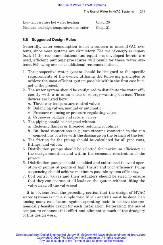
Low-temperature hot water heating Chap. 20
Medium- and high-temperature hot water Chap. 21
8.8 Suggested Design Rules
Generally, water consumption is not a concern in most HVAC sys-tems, since most systems are circulatory. The use of energy is impor-tant! If the recommendations and equations developed herein areused, efficient pumping procedures will result for these water sys-tems. Following are some additional recommendations.
1. The prospective water system should be designed to the specificrequirements of the owner, utilizing the following principles toachieve the most efficient system possible within the first cost bud-get of the project.
2. The water system should be configured to distribute the water effi-ciently with a minimum use of energy-wasting devices. Thesedevices are listed here:a. Three-way temperature-control valvesb. Balancing valves, manual or automaticc. Pressure-reducing or pressure-regulating valvesd. Crossover bridges and return valves
3. The piping should be designed withouta. Reducing flanges or threaded reducing couplingsb. Bullhead connections (e.g., two streams connected to the run
connections of a tee with the discharge on the branch of the tee)4. The friction for the piping should be calculated for all pipe runs,
fittings, and valves.5. Distribution pumps should be selected for maximum efficiency at
the design condition and within the economic constraints of theproject.
6. Distribution pumps should be added and subtracted to avoid oper-ation of pumps at points of high thrust and poor efficiency. Pumpsequencing should achieve maximum possible system efficiency.
7. Coil control valves and their actuators should be sized to ensurethat they can operate at all loads on the system without lifting thevalve head off the valve seat.
It is obvious from the preceding section that the design of HVACwater systems is not a simple task. Much analysis must be done, bal-ancing many cost factors against operating costs to achieve the eco-nomically feasible design for each installation. Reiterating, the use ofcomputers enhances this effort and eliminates much of the drudgeryof this design work.
The Use of Water in HVAC Systems 241
Rishel_CH08.qxd 21/4/06 6:16 PM Page 241
Downloaded from Digital Engineering Library @ McGraw-Hill (www.digitalengineeringlibrary.com)Copyright © 2006 The McGraw-Hill Companies. All rights reserved.
Any use is subject to the Terms of Use as given at the website.
The Use of Water in HVAC Systems

8.9 Eliminating Energy Waste During Commissioning
Every effort should be made in the design, testing, and initial opera-tion of HVAC water systems to eliminate the waste of energy in suchsystems. Typical of this is the testing and balancing procedures thatare used to commission a new chilled or hot water system. In the past,a calibrated balance valve was used to check the flow through an indi-vidual coil. This balance valve was adjusted until the design flow wasachieved through that coil. This is shown in Fig. 8.14a; Fig. 8.14b
242 The HVAC World
a. Calibrated balance valve to determine flow.
b. Permanent loss of balance valve is eliminatedby measuring friction loss of coil or control valveand determining flow from this data.
∆P
Control valve
Figure 8.14 Testing for coil flow.
Rishel_CH08.qxd 21/4/06 6:16 PM Page 242
Downloaded from Digital Engineering Library @ McGraw-Hill (www.digitalengineeringlibrary.com)Copyright © 2006 The McGraw-Hill Companies. All rights reserved.
Any use is subject to the Terms of Use as given at the website.
The Use of Water in HVAC Systems
describes the correct method for checking the flow through such coils.The differential pressure across the coil or control valve in Fig. 8.14bis checked, and the flow is verified from technical data on that coil.This is just as accurate as the balance-valve method; it may providegreater accuracy because a much larger differential signal is achievedby measuring the pressure drop across the coil. The permanent lossacross the calibrated balance valve is eliminated. The flow throughthe coil during commissioning should be controlled by its controlvalve, not any other device. This should check the coil flow and thecontrol-valve operation at the same time.
Every traditional practice during initial operation of a water sys-tem such as this coil testing must be evaluated to determine if anyenergy waste is occurring.
8.10 Bibliography
Ben L. Kincaid and Andrew Spradley, Removing Manual Balancing in a High School,1995.
The Water Management Manual, SYSTECON, Inc., West Chester, Ohio, 1992.
The Use of Water in HVAC Systems 243
Rishel_CH08.qxd 21/4/06 6:16 PM Page 243
Downloaded from Digital Engineering Library @ McGraw-Hill (www.digitalengineeringlibrary.com)Copyright © 2006 The McGraw-Hill Companies. All rights reserved.
Any use is subject to the Terms of Use as given at the website.
The Use of Water in HVAC Systems

Rishel_CH08.qxd 21/4/06 6:16 PM Page 244
Downloaded from Digital Engineering Library @ McGraw-Hill (www.digitalengineeringlibrary.com)Copyright © 2006 The McGraw-Hill Companies. All rights reserved.
Any use is subject to the Terms of Use as given at the website.
The Use of Water in HVAC Systems
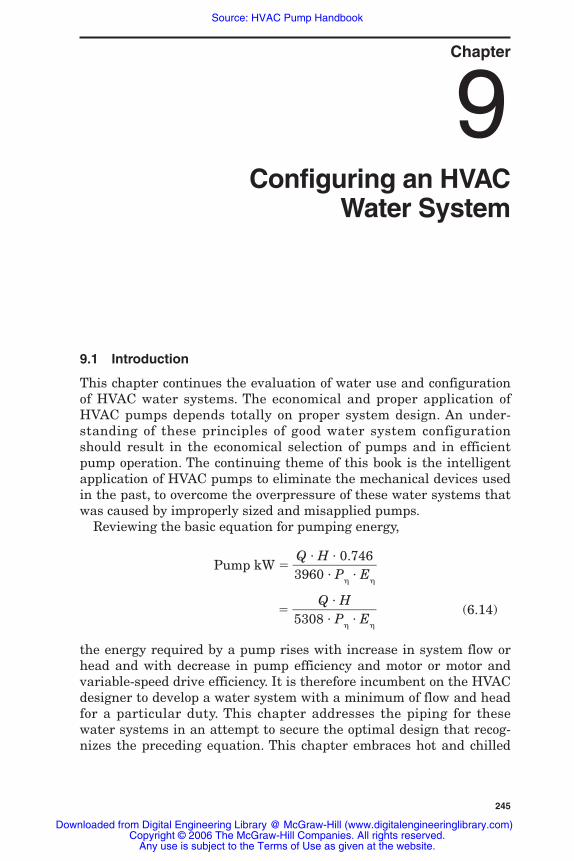
Chapter
245
9Configuring an HVAC
Water System
9.1 Introduction
This chapter continues the evaluation of water use and configurationof HVAC water systems. The economical and proper application ofHVAC pumps depends totally on proper system design. An under-standing of these principles of good water system configurationshould result in the economical selection of pumps and in efficientpump operation. The continuing theme of this book is the intelligentapplication of HVAC pumps to eliminate the mechanical devices usedin the past, to overcome the overpressure of these water systems thatwas caused by improperly sized and misapplied pumps.
Reviewing the basic equation for pumping energy,
Pump kW ��3Q96
�
0H
�
�
P0
�
.7�
4E6
�
�
��5308
Q�
�
PH
�� E
�
� (6.14)
the energy required by a pump rises with increase in system flow orhead and with decrease in pump efficiency and motor or motor andvariable-speed drive efficiency. It is therefore incumbent on the HVACdesigner to develop a water system with a minimum of flow and headfor a particular duty. This chapter addresses the piping for thesewater systems in an attempt to secure the optimal design that recog-nizes the preceding equation. This chapter embraces hot and chilled
Rishel_09.qxd 20/4/06 6:34 PM Page 245
Downloaded from Digital Engineering Library @ McGraw-Hill (www.digitalengineeringlibrary.com)Copyright © 2006 The McGraw-Hill Companies. All rights reserved.
Any use is subject to the Terms of Use as given at the website.
Source: HVAC Pump Handbook
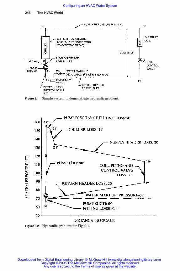
246 The HVAC World
Figure 9.1 Simple system to demonstrate hydraulic gradient.
Figure 9.2 Hydraulic gradient for Fig. 9.1.
Rishel_09.qxd 20/4/06 6:34 PM Page 246
Downloaded from Digital Engineering Library @ McGraw-Hill (www.digitalengineeringlibrary.com)Copyright © 2006 The McGraw-Hill Companies. All rights reserved.
Any use is subject to the Terms of Use as given at the website.
Configuring an HVAC Water System
Configuring an HVAC Water System 247
water systems, whereas the energy economies of condenser water sys-tems are included in Chaps. 11 and 16.
Figure 9.1 describes the basic pump head losses in a chilled waterdistribution system. A condenser water or cooling tower circuit wouldbe similar by changing the chiller evaporator to the chiller condenserand replacing the cooling coil with the cooling tower. Likewise, hotwater systems would be similar by exchanging the chiller evaporatorwith the loss through the boiler. The losses through both of these sys-tems are usually much less than those for the chilled water system.Figure 9.2 describes the hydraulic gradient and the losses for Fig. 9.1.Note that unnecessary losses such as balance valves or multiple-dutyvalves are not shown.
9.2 Selection of Temperature Differential
The first decision a designer of a chilled or hot water system mustmake is the selection of the temperature differential. Temperature dif-ferential is the difference between the supply water and the returnwater temperatures. A number of conditions must be recognized beforemaking the final selection of temperature differential:
1. An increase in temperature differential decreases water flow andtherefore saves pumping energy.
2. An increase in temperature differential may increase the cost ofcoils that must operate with a higher mean temperature difference.
3. Higher temperature differentials increase the possibilities of lossof temperature difference in coils due to dirt on the air side andchemical deposits on the water side of them.
4. Laminar flow on the water side due to lower velocities at low loadson a coil is always a concern of the water system designer. The possi-bility of laminar flow is greater with higher temperature differences.
The quick promise of energy savings with higher temperature dif-ferences can be offset later by problems in system operation due tofailure to have enough pumping capacity after the system has aged.Only experienced designers should entertain water temperature dif-ferences in excess of 12°F on chilled water and 40°F on hot water sys-tems. A careful balance between energy savings and first cost shouldbe made by the designer. There is no one temperature difference for thechilled or hot water systems.
Following are two formulas for calculating the water flow, in gallonsper minute, for hot and chilled water systems:
Rishel_09.qxd 20/4/06 6:34 PM Page 247
Downloaded from Digital Engineering Library @ McGraw-Hill (www.digitalengineeringlibrary.com)Copyright © 2006 The McGraw-Hill Companies. All rights reserved.
Any use is subject to the Terms of Use as given at the website.
Configuring an HVAC Water System
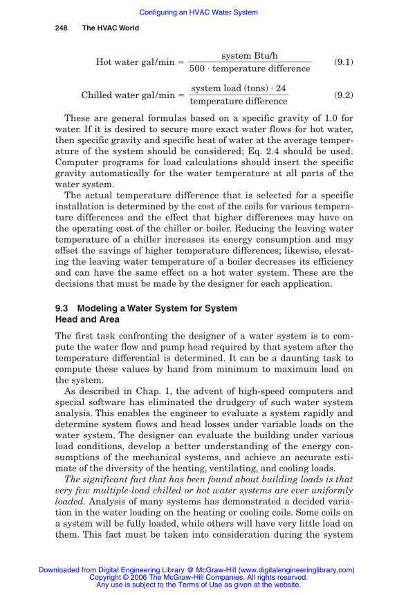
248 The HVAC World
Hot water gal/min � (9.1)
Chilled water gal/min � (9.2)
These are general formulas based on a specific gravity of 1.0 forwater. If it is desired to secure more exact water flows for hot water,then specific gravity and specific heat of water at the average temper-ature of the system should be considered; Eq. 2.4 should be used.Computer programs for load calculations should insert the specificgravity automatically for the water temperature at all parts of thewater system.
The actual temperature difference that is selected for a specificinstallation is determined by the cost of the coils for various tempera-ture differences and the effect that higher differences may have onthe operating cost of the chiller or boiler. Reducing the leaving watertemperature of a chiller increases its energy consumption and mayoffset the savings of higher temperature differences; likewise, elevat-ing the leaving water temperature of a boiler decreases its efficiencyand can have the same effect on a hot water system. These are thedecisions that must be made by the designer for each application.
9.3 Modeling a Water System for SystemHead and Area
The first task confronting the designer of a water system is to com-pute the water flow and pump head required by that system after thetemperature differential is determined. It can be a daunting task tocompute these values by hand from minimum to maximum load onthe system.
As described in Chap. 1, the advent of high-speed computers andspecial software has eliminated the drudgery of such water systemanalysis. This enables the engineer to evaluate a system rapidly anddetermine system flows and head losses under variable loads on thewater system. The designer can evaluate the building under variousload conditions, develop a better understanding of the energy con-sumptions of the mechanical systems, and achieve an accurate esti-mate of the diversity of the heating, ventilating, and cooling loads.
The significant fact that has been found about building loads is thatvery few multiple-load chilled or hot water systems are ever uniformlyloaded. Analysis of many systems has demonstrated a decided varia-tion in the water loading on the heating or cooling coils. Some coils ona system will be fully loaded, while others will have very little load onthem. This fact must be taken into consideration during the system
system load (tons) � 24���temperature difference
system Btu/h����500 � temperature difference
Rishel_09.qxd 20/4/06 6:34 PM Page 248
Downloaded from Digital Engineering Library @ McGraw-Hill (www.digitalengineeringlibrary.com)Copyright © 2006 The McGraw-Hill Companies. All rights reserved.
Any use is subject to the Terms of Use as given at the website.
Configuring an HVAC Water System

Configuring an HVAC Water System 249
analysis, as well as during the piping and control design. Computer-assisted evaluation allows the designer to study the many load varia-tions that can occur on the prospective water system.
Chapter 3 provided the means to calculate pipe friction in HVAC pip-ing systems. This chapter will use those data to demonstrate how thehead changes in a water system as the flow varies in that system. Itshould be remembered that most hot and chilled water systems areactually a number of small systems using common supply pipes. Eachheating or cooling coil is a water system in itself, since each coil has adifferent total friction head. These friction loads for a specific coil consistof the supply main loss, branch main loss, and loss through the coil itselfwith its piping and control-valve losses. If the designer recognizes thisindividuality of every coil and seeks to design the water system withrecognition of this fact, a simpler and more efficient system will result.
Traditionally, the pump head required for a water system has beenshown as a curve that results when the system head in feet is plottedagainst the system flow in gallons per minute. Therefore, this curvehas been named the system head curve. Through many years of workwith HVAC water systems, it has been demonstrated that the headrequirements for many water systems cannot be represented by thissimple parabolic curve. Instead, the head varies through a broad areathat may be difficult to calculate. Before tackling this knotty problem,the elements of a system head curve or area should be reviewed.
9.3.1 System head curve components
A system head curve consists of plotting the flow in the system, in gal-lons per minute, horizontally and the system head vertically, in feet ofhead. The system head must be broken down into variable head andconstant head. Variable head is the friction head of the water distribu-tion system. Constant head can be divided into either static head orconstant friction head. Static head is simply raising water from onelevel to another. Typical of this is the height of a cooling tower.Constant friction head can be the loss across a heating or cooling coil,its control valve, and connecting piping, as shown in Fig. 9.3a. Thisconstant head is typified by the differential pressure maintainedacross a heating or cooling coil and its appurtenances at a constantvalue by a differential pressure transmitter. This is the signal used tocontrol the system to which the coil is connected. Constant frictionhead occurs in many systems with two-way temperature-controlvalves on the coils; it is not found in old systems that used three-waytemperature-control valves. Constant friction head is plotted verticallysimilar to static head of a cooling tower. A typical system head curve isthat for a variable-volume system with two-way temperature controlvalves or a system head curve for a cooling tower installation.
Rishel_09.qxd 20/4/06 6:34 PM Page 249
Downloaded from Digital Engineering Library @ McGraw-Hill (www.digitalengineeringlibrary.com)Copyright © 2006 The McGraw-Hill Companies. All rights reserved.
Any use is subject to the Terms of Use as given at the website.
Configuring an HVAC Water System

250
Fig
ure
9.3
Mod
el b
uil
din
g fo
r sy
stem
hea
d ev
alu
atio
n.
Rishel_09.qxd 20/4/06 6:34 PM Page 250
Downloaded from Digital Engineering Library @ McGraw-Hill (www.digitalengineeringlibrary.com)Copyright © 2006 The McGraw-Hill Companies. All rights reserved.
Any use is subject to the Terms of Use as given at the website.
Configuring an HVAC Water System
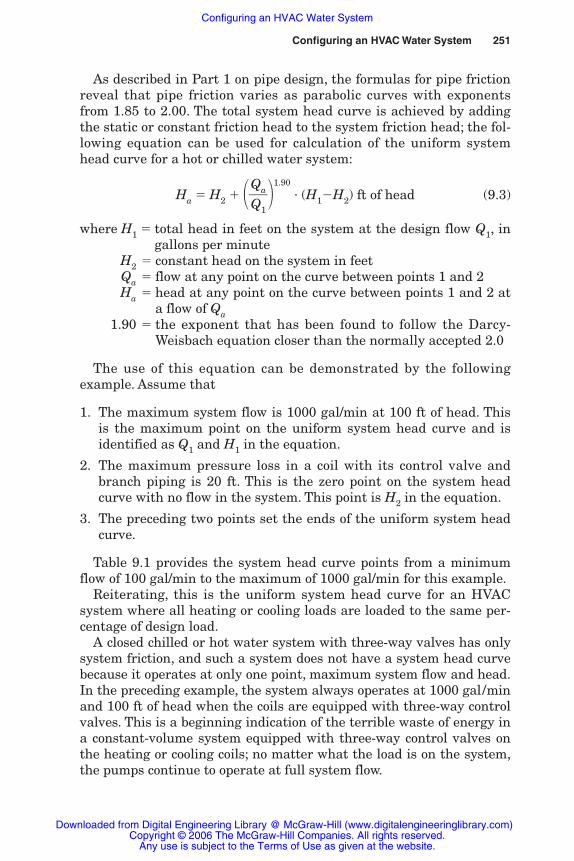
As described in Part 1 on pipe design, the formulas for pipe frictionreveal that pipe friction varies as parabolic curves with exponentsfrom 1.85 to 2.00. The total system head curve is achieved by addingthe static or constant friction head to the system friction head; the fol-lowing equation can be used for calculation of the uniform systemhead curve for a hot or chilled water system:
Ha � H2 � ��QQ
a
1
��1.90
� (H1�H2) ft of head (9.3)
where H1 � total head in feet on the system at the design flow Q1, ingallons per minute
H2 � constant head on the system in feetQa � flow at any point on the curve between points 1 and 2Ha � head at any point on the curve between points 1 and 2 at
a flow of Qa1.90 � the exponent that has been found to follow the Darcy-
Weisbach equation closer than the normally accepted 2.0
The use of this equation can be demonstrated by the followingexample. Assume that
1. The maximum system flow is 1000 gal/min at 100 ft of head. Thisis the maximum point on the uniform system head curve and isidentified as Q1 and H1 in the equation.
2. The maximum pressure loss in a coil with its control valve andbranch piping is 20 ft. This is the zero point on the system headcurve with no flow in the system. This point is H2 in the equation.
3. The preceding two points set the ends of the uniform system headcurve.
Table 9.1 provides the system head curve points from a minimumflow of 100 gal/min to the maximum of 1000 gal/min for this example.
Reiterating, this is the uniform system head curve for an HVACsystem where all heating or cooling loads are loaded to the same per-centage of design load.
A closed chilled or hot water system with three-way valves has onlysystem friction, and such a system does not have a system head curvebecause it operates at only one point, maximum system flow and head.In the preceding example, the system always operates at 1000 gal/minand 100 ft of head when the coils are equipped with three-way controlvalves. This is a beginning indication of the terrible waste of energy ina constant-volume system equipped with three-way control valves onthe heating or cooling coils; no matter what the load is on the system,the pumps continue to operate at full system flow.
Configuring an HVAC Water System 251
Rishel_09.qxd 20/4/06 6:34 PM Page 251
Downloaded from Digital Engineering Library @ McGraw-Hill (www.digitalengineeringlibrary.com)Copyright © 2006 The McGraw-Hill Companies. All rights reserved.
Any use is subject to the Terms of Use as given at the website.
Configuring an HVAC Water System

252 The HVAC World
TABLE 9.1 System Head CurveCoordinates
System flow, gal/min System head, ft
0100 021.00200 023.80300 028.10400 034.00500 041.40600 050.30700 060.60800 072.40900 085.51000 100.0
9.3.2 System head areas
The preceding example and data describe systems with uniform flow inall heating or cooling coils. Obviously, this does not exist in most actualbuildings, since some coils will be loaded while others will not have anyload on them. If the building has windows, as the sun moves aroundthe building during the day, the loads on the various coils will changeeven with constant outdoor temperature and internal load. This is alsodemonstrated by the term diversity, which was defined in Chap. 1.
Recognizing that systems are not loaded uniformly and that diver-sity does exist, we must evaluate chilled and hot water systems todetermine how to compute and display graphically the actual head onthem. Figure 9.3a describes a typical building with 10 air-handlingunits on different floors; this will be our model building to illustrate atypical system head area. The uniform system head curve for thisbuilding is shown in Fig. 9.3b. Assume that a 40 percent uniform loadoccurs on each of the 10 air-handling units; this is detailed graphi-cally in Fig. 9.4a. Now, let the 40 percent load shift so that only thefour bottom coils are fully loaded and the top six coils have no load onthem (see Fig. 9.4b). Since these four coils are nearer to the pumpsthan all 10 coils, the system friction will be less than that for all 10coils uniformly loaded at 40 percent each, namely 2 ft of friction, next,transfer all the 40 percent load to the upper four coils (see Fig. 9.4c).Now the load is farther than all the 10 coils uniformly loaded, and thesystem friction head will be greater than that for the uniformly loadedcondition, in this case, the system friction will be 72 ft. This procedurecan be done for various loads on the building, from 10 to 90 percentload. The result of these moves of the load on the building is shown inFig. 9.5a; this is a system head area, and it exists for almost any build-ing with more than one heating or cooling coil. This is one of the mostimportant figures in this entire book, since it makes the designer
Rishel_09.qxd 20/4/06 6:34 PM Page 252
Downloaded from Digital Engineering Library @ McGraw-Hill (www.digitalengineeringlibrary.com)Copyright © 2006 The McGraw-Hill Companies. All rights reserved.
Any use is subject to the Terms of Use as given at the website.
Configuring an HVAC Water System

Configuring an HVAC Water System 253
aware of how complex true system evaluation can be and that a HVACwater system cannot be represented by a simple system head curve.
Figure 9.5b describes an analysis made of actual data from achilled water system. This demonstrates that the load never reacheddesign flow or head and did not have the broad head range calculatedfor Fig. 9.5a.
Figure 9.4 Model building loading.
Rishel_09.qxd 20/4/06 6:34 PM Page 253
Downloaded from Digital Engineering Library @ McGraw-Hill (www.digitalengineeringlibrary.com)Copyright © 2006 The McGraw-Hill Companies. All rights reserved.
Any use is subject to the Terms of Use as given at the website.
Configuring an HVAC Water System

254 The HVAC World
One of the great opportunities available to us now with contempo-rary computers is the ability to actually track and develop a systemhead area for an existing system. Figure 9.6 describes the instrumenta-tion needed, namely, a flow meter and a differential pressure transmit-ter located across the headers of the pumping system. The computersimultaneously reads these two signals and plots a point within theactual system head area. This can be done once a minute, an hour, orwhatever is needed for a particular installation. After a period of time,the actual system head area will evolve with all of the flow-head pointsplotted on a head-flow diagram. The result may be something like thatshown in Fig. 9.5b where the actual system head area is plotted over aperiod of time.
Of what value is this? This diagram provides the true head-flowrelationship for a variable-speed pumping system. From this, ananalysis can be made of the actual compatibility of the pumping sys-tem with the water system.
Loads active far fromwater source
Uniform systemhead curve
Loads active nearwater source
60(18.3)
50(15.3)
40(12.2)
30(9.2)
20(6.1)
10(3.1)
0(0) 0
(0)100
(22.7)200
(45.4)300
(68.1)400
(90.9)500
(113.6)600
(136.3)
Building flow—GPM (CU. meters/HR.)
Bui
ldin
g he
ad—
ft. o
f wat
er (
Met
ers)
Figure 9.5a System head area.
Rishel_09.qxd 20/4/06 6:34 PM Page 254
Downloaded from Digital Engineering Library @ McGraw-Hill (www.digitalengineeringlibrary.com)Copyright © 2006 The McGraw-Hill Companies. All rights reserved.
Any use is subject to the Terms of Use as given at the website.
Configuring an HVAC Water System

Configuring an HVAC Water System 255
This is elementary manual modeling of a water system. With com-puters, such system head areas can be developed easily. Without a com-puter, a simple procedure that works practically is to adjust the distrib-ution friction at 50 percent water flow, i.e., 11 ft in our model buildingat 50 percent load. This variable or distribution friction can be multi-plied by 20 percent for the lower curve and then by 150 percent for theupper curve. Drawing curves similar to Fig. 9.5a through these pointswill generate an approximate system head area. This system head areawill give designers a rough idea of what the system head area will be,and it will enable them to predict pump performance within this sys-tem head area. A further discussion of the operation of pumps with thesystem head area will be presented in Chap. 15.
Campus-type installations with a number of buildings, as shown inFig. 9.7a, create another dimension in system head areas and systemmodeling. As demonstrated in this figure, there are buildings near thecentral energy plant and buildings far from it. This figure has two ofour model buildings, building A near the central plant and building Bfar from the central plant. It is obvious that the campus loop loss will
Static head
0 500 1000 1500 2000 2500
System flow—GPM
Sys
tem
hea
d—ft.
0
20
40
60
80
Design flow2160 GPM
Design point
Figure 9.5b Actual system head area.
Rishel_09.qxd 20/4/06 6:34 PM Page 255
Downloaded from Digital Engineering Library @ McGraw-Hill (www.digitalengineeringlibrary.com)Copyright © 2006 The McGraw-Hill Companies. All rights reserved.
Any use is subject to the Terms of Use as given at the website.
Configuring an HVAC Water System

256 The HVAC World
be greater for building B than for building A. If the loop loss is 30 ft inthe distribution mains out and back for building B with all the build-ings fully loaded, this loss will be determined by how active are all theintermediate buildings. There are two ultimate conditions that mustbe checked: first, with all the intermediate buildings fully loaded, andsecond, with all these buildings having no load. Using the precedingprocedure for determining system head produces the system head areaof Fig. 9.7b. The upper curve is for the first condition, where all theintermediate buildings are fully loaded, and the bottom curve is forthe second condition, where these buildings have no load. This figuredemonstrates the great variation that can occur in the head requiredfor a campus building located far from the central energy plant. Hereagain, computer modeling can produce system head areas for everybuilding on a campus under a number of different load conditions.
DPT
FT
Flow meter
Differentialpressure
transmitter
VFD
VFD
VFD
Controlcenter
Figure 9.6 Instrumentation for generating an actual system head area.
Rishel_09.qxd 20/4/06 6:34 PM Page 256
Downloaded from Digital Engineering Library @ McGraw-Hill (www.digitalengineeringlibrary.com)Copyright © 2006 The McGraw-Hill Companies. All rights reserved.
Any use is subject to the Terms of Use as given at the website.
Configuring an HVAC Water System

257
Fig
ure
9.7
Cam
pus-
type
ch
ille
d or
hot
wat
er s
yste
m.
Rishel_09.qxd 20/4/06 6:34 PM Page 257
Downloaded from Digital Engineering Library @ McGraw-Hill (www.digitalengineeringlibrary.com)Copyright © 2006 The McGraw-Hill Companies. All rights reserved.
Any use is subject to the Terms of Use as given at the website.
Configuring an HVAC Water System

258 The HVAC World
Figure 9.7b is a typical head variation for many campus buildings.Most college and university campuses now utilize many energy-wastingdevices such as balance valves, pressure-reducing valves, andcrossover bridges to overcome this friction variation. This system headarea demonstrates how broad are the actual head requirements of acampus-type system. For example, at 50 percent load on the building,the pump head can vary from 27 to 74 ft. With constant-speed pumps,all this head difference must be destroyed by mechanical devices tomaintain adequate flow to all parts of the building. With the correctpumping arrangement and variable-speed pumps, all this wasted headcan be eliminated. With proper control, the variable-speed pump willalways operate at the needed system flow and head without any over-pressure or wasted energy. A careful review of this figure will be madein Chap. 15, as well as how pump performance is affected by suchbroad variations in system head.
9.3.3 Pumping system losses
All the foregoing discussion has been for water system flow and headevaluation. Losses through pumping systems themselves are oftenignored or included with the system head losses. It has been learnedthat pumping system losses can be significant and should be analyzedseparately from the water system losses. Figure 9.8a describes an endview of an actual pumping system consisting of five pumps, each witha capacity of 700 gal/min, for a total system capacity of 3500 gal/min.The individual loss for each fitting is shown along with its K factor.The total loss for the pump fittings is 6.9 ft. Recognizing HydraulicInstitute’s estimate that the losses in pipe fittings can vary by asmuch as 10 to 35 percent, these losses have been multiplied by plus20 percent to achieve a reasonable loss for the fittings. The losses forthis system would therefore be 8 ft with 700 gal/min flowing throughan individual pump. Figure 9.8b is the pump curve for this system;each pump could operate at a maximum flow of 1100 gal/min ifimproperly controlled. At 1100 gal/min, the pump fitting loss becomes(1100/700)1.90 � 8, or 18.9 ft. A loss of only 8 ft may not raise muchconcern, but a loss of close to 19 ft should be of concern to anyonemaking a serious energy evaluation of this water system.
This system had a differential pressure of 30 ft across the largestcoil and its control valve and a system loss of 78 ft. With the esti-mated 8 ft of loss throughout the pump fittings, the total system lossbecomes 116 ft. Figure 9.8c describes the uniform system head curvefor this system, which has been adjusted to recognize the variableloss through the pump fittings. Again, no longer is the uniform sys-tem curve a smooth curve, but rather it is one of scalloped shape. It is
Rishel_09.qxd 20/4/06 6:34 PM Page 258
Downloaded from Digital Engineering Library @ McGraw-Hill (www.digitalengineeringlibrary.com)Copyright © 2006 The McGraw-Hill Companies. All rights reserved.
Any use is subject to the Terms of Use as given at the website.
Configuring an HVAC Water System

difficult to select the most efficient pump add points without a com-puter program similar to the energy programs that will be describedin Chap. 10. In this example, the pump add/subtract points in Fig.9.8c were set arbitrarily at 800 gal /min for each pump. This is not
Configuring an HVAC Water System 259
Figure 9.8 Friction losses for a pumping system.
Rishel_09.qxd 20/4/06 6:34 PM Page 259
Downloaded from Digital Engineering Library @ McGraw-Hill (www.digitalengineeringlibrary.com)Copyright © 2006 The McGraw-Hill Companies. All rights reserved.
Any use is subject to the Terms of Use as given at the website.
Configuring an HVAC Water System

260 The HVAC World
necessarily the most efficient point to change the number of operat-ing pumps. This curve demonstrates conclusively that the old tradi-tion of just running one pump until it cannot pump any more is awasteful practice.
It is obvious that the system head curves and areas described ear-lier in this chapter are affected by this variation in pump fittinglosses. How do designers incorporate pump fitting losses into theircalculations for a proposed system? It is difficult unless a computerprogram is available for system friction loss calculation that includessuch fitting loss calculations. The energy evaluations that will bereviewed in various chapters account for pump fitting losses. Theseevaluations separates the pump fitting losses from system losses toachieve a reasonable procedure for estimating system performanceand sequencing of pumps on multiple-pump systems.
System flow and head evaluation are very important matters, sinceefficient pump selection depends on them. The preceding discussiondemonstrates that it can be a complicated subject. Any time devotedto such an evaluation is well worth its cost.
One important factor that emerges from true system evaluation isthe indication of losses that are caused by energy wasters such as bal-ance valves, pressure-reducing valves, and the like. Their lossesbecome pronounced under this type of careful scrutiny. It should benoted that most of the HVAC water systems that are reviewed in thisbook seldom use these devices.
The advent of computer software has enabled the designer toachieve better part-load evaluation as well as a closer estimate of thetrue diversity of the system under examination. Many different hypo-thetical loads can be inserted as data in the computer by the designer,who can then select the design that most closely fits the economicparameters of the proposed system.
9.4 Static Pressure
The static pressure of an HVAC system is the system pressure thatavoids (1) drying out the tops of the water system or (2) imposing toohigh a system pressure on the water system. Basically, the static pres-sure for most systems consists of the height of the building plus acushion at the top of the building. Usually this cushion is around 5 to10 lb/in2 or 10 to 20 ft. With a 200-ft-tall building and a cushion of 20ft on top of the building, the static pressure would be 200 � 20, or 220ft minimum (95.2 psig at 60°F). When the water system is totallywithin a building, the actual elevation above sea level of the buildingcan be ignored.
Rishel_09.qxd 20/4/06 6:34 PM Page 260
Downloaded from Digital Engineering Library @ McGraw-Hill (www.digitalengineeringlibrary.com)Copyright © 2006 The McGraw-Hill Companies. All rights reserved.
Any use is subject to the Terms of Use as given at the website.
Configuring an HVAC Water System

Such is not the case with a campus-type installation consisting of sev-eral buildings. With this application, actual elevations of the buildingsmust be included. The elevations of the tops of all the buildings mustbe recorded as well as the elevation of the expansion tank at the oper-ating level in the central plant. Static pressure is the elevation at thetop of the highest building minus the elevation at the operating levelof the central energy plant plus the required cushion at the top of thetallest building. That is,
Static pressure � �Zb
(
�
14
Z
4c
/
�
)
Zp� psig (9.4)
where Zb � elevation of the top of the tallest buildingZp � elevation of the operating floor of the central energy plantZc � cushion required on top of that building in ft of head � specific weight of the water at the operating temperature
For example, assume that the top of the tallest building is 650 ft,the desired cushion on that building is 10 ft, the operating level of thecentral energy plant is 420 ft, and the system is a hot water systemoperating at 180°F (60.57 lb/ft3). Thus,
Static pressure � � 101 psig
Distributed pumping, which relies on static pressure for movementof the water in the system, requires special calculation of the staticpressure. The remote building whose height, cushion, and distribu-tion loss are the greatest determines the static pressure. Equation 9.4becomes
Static pressure � (9.5)
where Hd � distribution loss in feet H2O from central plant to thebuilding that determines the static pressure
If the building in the preceding example were the building thatdetermines the static pressure for the system and the friction lossbetween it and the central energy plant was 50 ft at design flow, thenthe static pressure would be
� 122 psig650 � 10 � 420 � 50���
(144/60.57)
Zb � Zc � Zp � Hd���
(144/)
650 � 10�420��
(144/60.57)
Configuring an HVAC Water System 261
Rishel_09.qxd 20/4/06 6:34 PM Page 261
Downloaded from Digital Engineering Library @ McGraw-Hill (www.digitalengineeringlibrary.com)Copyright © 2006 The McGraw-Hill Companies. All rights reserved.
Any use is subject to the Terms of Use as given at the website.
Configuring an HVAC Water System

262 The HVAC World
This will be explained further in this book with other design criteriafor this important method of water distribution.
9.5 Three Zones of HVAC Water Systems
Almost all HVAC water systems are of the loop type; this means thatthe water is returned to its source such as a chiller, cooling tower, orboiler. In rare cases, groundwater is used for cooling and is dumpedinto a sewer or stream after use.
Most of these water systems consist of three zones, namely, (1) anenergy source, (2) energy transportation, and (3) energy use asdescribed in Fig. 8.4 for chilled or hot water. Cooling towers are simi-lar in arrangement. Chapter 8 discussed the use of water, or the thirdzone. It is important to understand that each of these three zonesmust be designed individually for optimal use of energy. Therefore,these zones often are combined together with resulting poor energygeneration, transportation, or use. Each zone must be evaluated sepa-rately; the first and second zones will be reviewed in the chapters onchillers and boilers. True energy conservation in HVAC systemsbegins with careful analysis of energy consumption in boilers, chillers,or cooling towers. Chapters 11, 14, and 19 of this book will study thisanalysis of energy consumption.
Many times the second zone, energy transportation, is mixed withenergy generation; this can result in poor energy generation andtransportation if care is not used in evaluating the total energy con-sumption of the system. Efficient energy transportation will be dis-cussed in Chaps. 15, 16, 18, and 20 on cooling and heating systems.
Finally, the use of water in cooling and heating coils or heatexchangers must be efficient or pumping costs will be excessive. Asindicated in Chap. 8, the indiscriminate use of balance valves, three-way control valves, and improper heating and cooling coil connectionsresults in poor system efficiency. If these three zones are rememberedduring design and each treated as efficiently as possible, this effortshould result in a good pumping and piping system.
9.6 Piping Configurations
A number of different piping configurations are used in HVAC watersystems; only the more popular types will be discussed here. These are:
1. Open or closed systems and how water is returned to the source,namely, direct or reverse return
2. Number of pipes to transport the water through the system
Rishel_09.qxd 20/4/06 6:34 PM Page 262
Downloaded from Digital Engineering Library @ McGraw-Hill (www.digitalengineeringlibrary.com)Copyright © 2006 The McGraw-Hill Companies. All rights reserved.
Any use is subject to the Terms of Use as given at the website.
Configuring an HVAC Water System
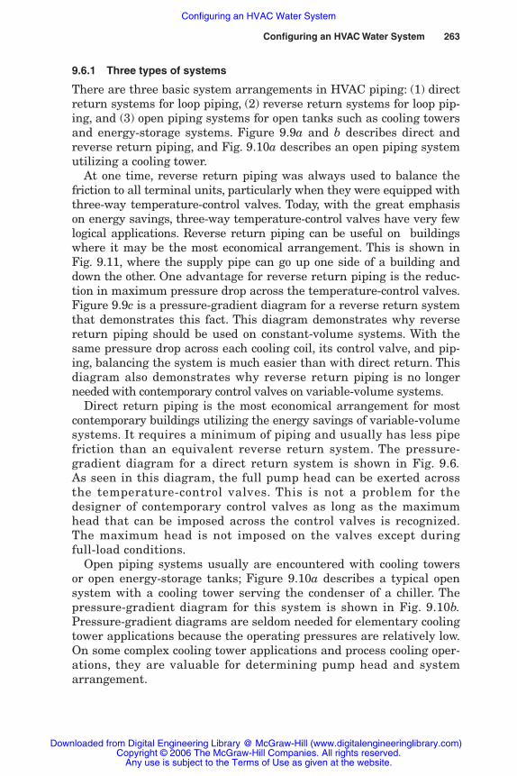
Configuring an HVAC Water System 263
9.6.1 Three types of systems
There are three basic system arrangements in HVAC piping: (1) directreturn systems for loop piping, (2) reverse return systems for loop pip-ing, and (3) open piping systems for open tanks such as cooling towersand energy-storage systems. Figure 9.9a and b describes direct andreverse return piping, and Fig. 9.10a describes an open piping systemutilizing a cooling tower.
At one time, reverse return piping was always used to balance thefriction to all terminal units, particularly when they were equipped withthree-way temperature-control valves. Today, with the great emphasison energy savings, three-way temperature-control valves have very fewlogical applications. Reverse return piping can be useful on buildingswhere it may be the most economical arrangement. This is shown inFig. 9.11, where the supply pipe can go up one side of a building anddown the other. One advantage for reverse return piping is the reduc-tion in maximum pressure drop across the temperature-control valves.Figure 9.9c is a pressure-gradient diagram for a reverse return systemthat demonstrates this fact. This diagram demonstrates why reversereturn piping should be used on constant-volume systems. With thesame pressure drop across each cooling coil, its control valve, and pip-ing, balancing the system is much easier than with direct return. Thisdiagram also demonstrates why reverse return piping is no longerneeded with contemporary control valves on variable-volume systems.
Direct return piping is the most economical arrangement for mostcontemporary buildings utilizing the energy savings of variable-volumesystems. It requires a minimum of piping and usually has less pipefriction than an equivalent reverse return system. The pressure-gradient diagram for a direct return system is shown in Fig. 9.6.As seen in this diagram, the full pump head can be exerted acrossthe temperature-control valves. This is not a problem for thedesigner of contemporary control valves as long as the maximumhead that can be imposed across the control valves is recognized.The maximum head is not imposed on the valves except duringfull-load conditions.
Open piping systems usually are encountered with cooling towersor open energy-storage tanks; Figure 9.10a describes a typical opensystem with a cooling tower serving the condenser of a chiller. Thepressure-gradient diagram for this system is shown in Fig. 9.10b.Pressure-gradient diagrams are seldom needed for elementary coolingtower applications because the operating pressures are relatively low.On some complex cooling tower applications and process cooling oper-ations, they are valuable for determining pump head and systemarrangement.
Rishel_09.qxd 20/4/06 6:34 PM Page 263
Downloaded from Digital Engineering Library @ McGraw-Hill (www.digitalengineeringlibrary.com)Copyright © 2006 The McGraw-Hill Companies. All rights reserved.
Any use is subject to the Terms of Use as given at the website.
Configuring an HVAC Water System

264
Fig
ure
9.9
Dir
ect
and
reve
rse
retu
rn s
yste
ms.
Rishel_09.qxd 20/4/06 6:34 PM Page 264
Downloaded from Digital Engineering Library @ McGraw-Hill (www.digitalengineeringlibrary.com)Copyright © 2006 The McGraw-Hill Companies. All rights reserved.
Any use is subject to the Terms of Use as given at the website.
Configuring an HVAC Water System

Configuring an HVAC Water System 265
H
Return pipefriction, 5 ft.
Supply pipefriction, 5 ft.
E G
FDCB
Chillercondenser
Friction, 25 ft.
A
(a) Open piping system.
Figure 9.10 Open water systems.
50
40
30
20
10
0
10
Sys
tem
hea
d —
ft.
Pump head,56 ft.
Chiller condenserloss
Free fall through towerwater level
Supply pipe
Pump discharge fittings
E
F
D
G
H
A
Suction pipe
Pump suction fittings
(b) Pressure gradient for open system.
Cooling tower
No scale
PC
B
Return pipe
Rishel_09.qxd 20/4/06 6:34 PM Page 265
Downloaded from Digital Engineering Library @ McGraw-Hill (www.digitalengineeringlibrary.com)Copyright © 2006 The McGraw-Hill Companies. All rights reserved.
Any use is subject to the Terms of Use as given at the website.
Configuring an HVAC Water System

9.6.2 Number of pipes in a loop system
There are three different numbers of pipes found in HVAC systems.These are:
Two-pipe. Two-pipe systems have been used where there is onlyheating or cooling; digital control has brought back the use of thetwo-pipe system. Chapter 30 describes this in detail.
Three-pipe. This is an old configuration that is seldom usedtoday. There are two supply pipes and one return pipe; one supplypipe is for heating, and the other is for cooling. There is a commonreturn pipe for both the heating and cooling systems. The possibili-ties of energy waste are obvious with improper control.
Four-pipe: This has been the preferred piping arrangement forbuildings that have simultaneous heating and cooling loads. Mostbuildings in the temperate zones are of this configuration and havesimultaneous heating and cooling loads, particularly in the spring
266 The HVAC World
DP1 DP2
Cooling coilssuch as fan-coilor water sourceheat pumps
Chiller
ChillerC
Figure 9.11 Reverse return for low control valve differentialpressures.
Rishel_09.qxd 20/4/06 6:34 PM Page 266
Downloaded from Digital Engineering Library @ McGraw-Hill (www.digitalengineeringlibrary.com)Copyright © 2006 The McGraw-Hill Companies. All rights reserved.
Any use is subject to the Terms of Use as given at the website.
Configuring an HVAC Water System
and fall. All the systems discussed in this book will be of the four-pipe variety, two pipes for cooling and two pipes for heating.
9.7 Location of Expansion Tanks
Expansion tanks should be located at the point where the system is tobe stabilized, not necessarily at the suction of the pumping system.With the advent of variable-speed pumps and their digital control, theoperation of a pump is not dependent on its suction pressure beingconstant. In the past, the expansion tank was always located at thepump suction and took its air from the air separator. This expansiontank was of the plain type without an internal bladder that separatesthe air from the water. The result was absorption of air by the waterand waterlogging of the tank.
This nuisance was eliminated by the bladder-type expansion tank.This expansion tank is located away from the air separator, and thisenables the designer to locate the expansion tank at the desired pointof pressure regulation in the water system, not just at the point ofinstallation of the air removal equipment.
On low-rise buildings, the expansion tank for both hot and chilledwater systems can be located at the suction of the pumps. On high-rise buildings, the expansion tank and water makeup equipmentshould be located at the top of the building to ensure continuous pres-sure at that point in the system.
9.8 Elimination of Air in HVAC Systems
In the past, air elimination from HVAC water systems depended onmechanical devices such as air vents and mechanical separators. Thedevelopment of better chemical treatment for these systems hasresulted in the use of chemicals for complete removal of air. Themechanical separator did not remove any of the dissolved air from awater system. The so-called pot feeder is an economical chemicalfeeder that can accept a passivating chemical such as sodium sulfitefor removing all the oxygen from an HVAC water system. It is muchless costly than a mechanical separator for many sizes of pipe.
On chilled water systems, mechanical separators do very little airseparation except at the initial fill of the water into the system. Thereason for this is the fact that the temperature of the makeup wateris equal to or greater than the chilled water operating temperature.For example, the makeup water may be at 60°F and then reduced to40 to 50°F. The solubility of air in the water is actually increased.Table 2.5 demonstrates this.
Configuring an HVAC Water System 267
Rishel_09.qxd 20/4/06 6:34 PM Page 267
Downloaded from Digital Engineering Library @ McGraw-Hill (www.digitalengineeringlibrary.com)Copyright © 2006 The McGraw-Hill Companies. All rights reserved.
Any use is subject to the Terms of Use as given at the website.
Configuring an HVAC Water System
268 The HVAC World
Chilled water systems should be equipped with manual air vents atthe high points of the system. These air vents should be equippedwith air-collection chambers below them. The chemical feeder shouldbe installed at the central energy plant for complete treatment of theentire water system. Larger systems might be equipped with auto-matic chemical feeders. Chemical feeders offer a better and in manycases less expensive method of removing air from these systems thandepending on a mechanical separator, which cannot eliminate all theoxygen from a water system. Reiterating, mechanical separators can-not remove dissolved air!
Hot water systems can use mechanical separators to remove someof the air, as is shown in Figs. 3.6a and 3.7a. Seldom should they belocated on the discharge from boilers. Little additional air removal isachieved on most installations, and the location on the discharge pipefrom boilers may be cumbersome. The use of dip tubes on boilers,manual air vents, and a chemical feeder may produce a more econom-ical and better method of removing air from hot water systems thanlarge mechanical separators.
9.9 Control of Return Water Temperature
As we began this chapter with system temperature difference, so wewill leave it. Return water temperature is one of the most importantoperating values for a chilled or hot water system. It tells the operatorjust how good a job the control system and coils are doing in convert-ing energy from the chillers or boilers to the air or water systemsthat are cooling or heating the building. This is such a basic criterionthat it should be addressed early in the design of a chilled or hotwater system. Individual coils should be equipped with thermometersor insertion plugs on their return connections, as described in Fig. 9.12a;zone or building returns should be equipped with temperature transmit-ters, as also shown in this figure. This information should be displayedand recorded at the central data-acquisition point for the entire system.
There is a great argument ongoing in the HVAC industry abouthow to control return water temperature in loop-type systems suchas chilled and hot water systems. The proper method of controllingreturn temperature is through the correct selection of controlvalves and heating and cooling coils. The use of return temperature-control valves, as shown in Fig. 9.12b, is a quick way to solve manysystem operating problems, but it is fraught with its own problems.For example,
1. The return temperature-control valve adds head loss to the entiresystem and is therefore an energy waster.
Rishel_09.qxd 20/4/06 6:34 PM Page 268
Downloaded from Digital Engineering Library @ McGraw-Hill (www.digitalengineeringlibrary.com)Copyright © 2006 The McGraw-Hill Companies. All rights reserved.
Any use is subject to the Terms of Use as given at the website.
Configuring an HVAC Water System

269
Fig
ure
9.1
2R
etu
rn w
ater
tem
pera
ture
indi
cati
on a
nd
con
trol
.
Rishel_09.qxd 20/4/06 6:34 PM Page 269
Downloaded from Digital Engineering Library @ McGraw-Hill (www.digitalengineeringlibrary.com)Copyright © 2006 The McGraw-Hill Companies. All rights reserved.
Any use is subject to the Terms of Use as given at the website.
Configuring an HVAC Water System

270 The HVAC World
2. There is a danger that warm return water will be bypassed throughthe crossover bridge back to the supply side of a coil that is fullyloaded and needs design supply temperature at that moment. Theresult is that the coil will not supply the load required of it. Forexample, in Fig. 9.12b, the fully loaded coil no. 5 needs 44°F waterto produce 10 tons of cooling; since it is receiving 50°F water, it canproduce only around 5 tons of cooling.
3. If certain coils are exhibiting laminar flow, circulating pumps can beinstalled on the coils to avert this problem, as described in Fig. 8.4.This is an excellent method for controlling laminar flow in a heatingcoil. It was stated in Chap. 8 that, in most cases, pumps or circula-tors should not be piped in series with the coil but in the bypass, asshown in Fig. 8.7.
4. Return temperature-control valves obliterate the true return watertemperature from the system and prevent the operating and main-tenance people from understanding which coils or control valvesare creating problems. Return temperature is the operator’s guide toefficient use of water in HVAC systems.
5. Return water temperature control lulls maintenance people intobelieving that there is no problem with any of their coils whensome of those coils may be very dirty on the air or water side.
In conclusion, one of the designer’s most important tasks is theselection of a sound temperature differential that will providemaximum possible system efficiency. The second step in thisprocess is to ensure that differential is maintained after the systemis commissioned.
9.10 Heat Exchangers for Hot and Chilled Water
High-rise buildings, as shown in Fig. 9.12b, can create static pressureproblems on water systems where the remainder of the system is lowrise. The answer to this problem, often, is the use of a heat exchanger,as shown in Fig. 9.13. The heat exchanger eliminates the static pres-sure of the tall building from the water system pressure. The supplytemperature to the building is controlled by the supply control valve. Ifthis is a critical load or at the highest pressure loss of the system, a dif-ferential pressure transmitter should be connected across the supplyside of the heat exchanger to ensure that adequate water is available tothe building at all loads on it.
Rishel_09.qxd 20/4/06 6:34 PM Page 270
Downloaded from Digital Engineering Library @ McGraw-Hill (www.digitalengineeringlibrary.com)Copyright © 2006 The McGraw-Hill Companies. All rights reserved.
Any use is subject to the Terms of Use as given at the website.
Configuring an HVAC Water System
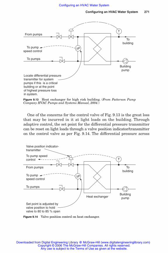
One of the concerns for the control valve of Fig. 9.13 is the great lossthat may be incurred in it at light loads on the building. Throughadaptive control, the set point for the differential pressure transmittercan be reset on light loads through a valve position indicator/transmitteron the control valve as per Fig. 9.14. The differential pressure across
Configuring an HVAC Water System 271
T
∆P
From pumps
To pumps
To pumpspeed control
Tobuilding
Buildingpump
Locate differential pressuretransmitter for systempumps if this is a criticalbuilding or at the pointof highest pressure lossin system.
Figure 9.13 Heat exchanger for high risk building. (From Patterson PumpCompany HVAC Pumps and Systems Manual, 2004.)
T
∆P
From pumps
To pumps
To pumpspeed control
Tobuilding
Buildingpump
Set point is adjusted byvalve position to holdvalve to 80 to 85 % open
Valve position indicator-transmitter
To pump speedcontrol
Heat exchanger
Figure 9.14 Valve position control on heat exchanger.
Rishel_09.qxd 20/4/06 6:34 PM Page 271
Downloaded from Digital Engineering Library @ McGraw-Hill (www.digitalengineeringlibrary.com)Copyright © 2006 The McGraw-Hill Companies. All rights reserved.
Any use is subject to the Terms of Use as given at the website.
Configuring an HVAC Water System
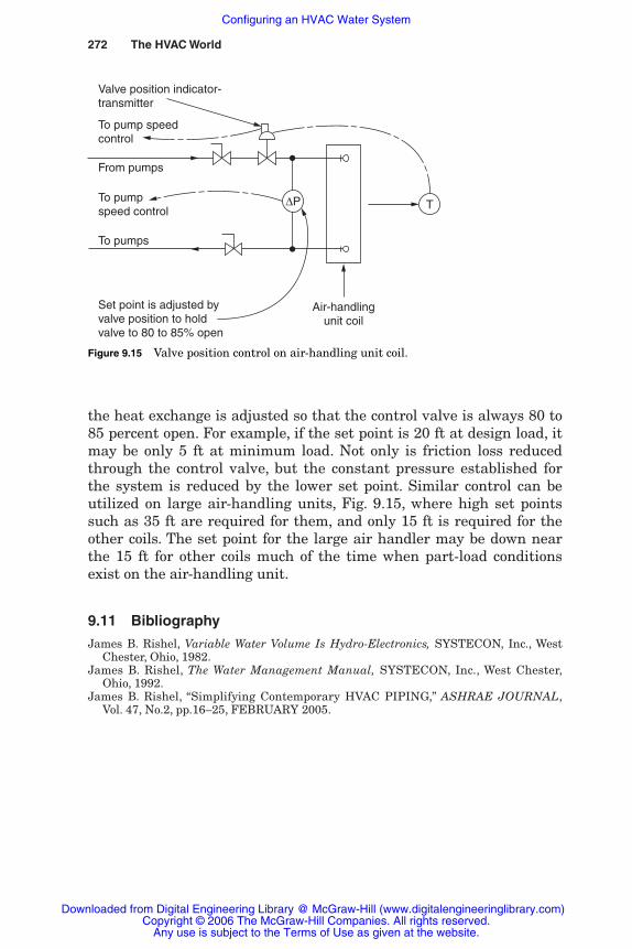
the heat exchange is adjusted so that the control valve is always 80 to85 percent open. For example, if the set point is 20 ft at design load, itmay be only 5 ft at minimum load. Not only is friction loss reducedthrough the control valve, but the constant pressure established forthe system is reduced by the lower set point. Similar control can beutilized on large air-handling units, Fig. 9.15, where high set pointssuch as 35 ft are required for them, and only 15 ft is required for theother coils. The set point for the large air handler may be down nearthe 15 ft for other coils much of the time when part-load conditionsexist on the air-handling unit.
9.11 Bibliography
James B. Rishel, Variable Water Volume Is Hydro-Electronics, SYSTECON, Inc., WestChester, Ohio, 1982.
James B. Rishel, The Water Management Manual, SYSTECON, Inc., West Chester,Ohio, 1992.
James B. Rishel, “Simplifying Contemporary HVAC PIPING,” ASHRAE JOURNAL,Vol. 47, No.2, pp.16–25, FEBRUARY 2005.
272 The HVAC World
∆P
From pumps
To pumps
To pumpspeed control
Set point is adjusted byvalve position to holdvalve to 80 to 85% open
Valve position indicator-transmitter
To pump speedcontrol
T
Air-handlingunit coil
Figure 9.15 Valve position control on air-handling unit coil.
Rishel_09.qxd 20/4/06 6:34 PM Page 272
Downloaded from Digital Engineering Library @ McGraw-Hill (www.digitalengineeringlibrary.com)Copyright © 2006 The McGraw-Hill Companies. All rights reserved.
Any use is subject to the Terms of Use as given at the website.
Configuring an HVAC Water System

Chapter
273
10Basics of Pump
Application for HVAC Systems
10.1 Introduction
The configuration of a hot or chilled water system was emphasized inChap. 9 to achieve the desired heating or cooling with a minimum offlow and head. This chapter undertakes evaluation of the pumpsthemselves to achieve optimal energy consumption for the pumps. Itwas necessary for the readers to have a basic understanding of HVACwater systems before initiating this application of pumps.
Before embarking on the actual application of pumps to HVACwater systems, there should be a discussion of when to use constant-speed pumps and when to use variable-speed pumps. With the rapidreduction in the cost of variable-speed drives, there is almost no limit,in terms of motor size, for the use of variable-speed pumps. Very lowhead pumps, i.e., less than 50 ft, can still be constant-speed pumpswhen applied to small systems. Otherwise, the rule should be constant-speed pumps for constant-volume systems and variable-speed pumpsfor variable-volume systems.
If a water system has a large variation in its flow, from less than 50to 100 percent of design, it is probably a candidate for variable speed.Likewise, if the flow rarely changes and there is little variation intemperature or viscosity, this is a constant-speed pump application.
As was pointed out elsewhere, variable-speed pumping offers greatsavings in maintenance as well as in energy. Further, variable-speedpumps, if controlled properly, operate at the system’s flow and headrequirements, not necessarily at the design conditions. They eliminateoverpressuring, which causes operational problems as well as loss ofpumping energy.
Rishel_CH10.qxd 21/4/06 6:20 PM Page 273
Downloaded from Digital Engineering Library @ McGraw-Hill (www.digitalengineeringlibrary.com)Copyright © 2006 The McGraw-Hill Companies. All rights reserved.
Any use is subject to the Terms of Use as given at the website.
Source: HVAC Pump Handbook
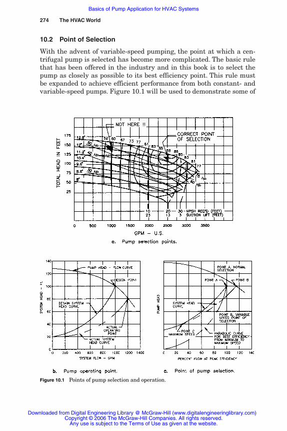
274 The HVAC World
10.2 Point of Selection
With the advent of variable-speed pumping, the point at which a cen-trifugal pump is selected has become more complicated. The basic rulethat has been offered in the industry and in this book is to select thepump as closely as possible to its best efficiency point. This rule mustbe expanded to achieve efficient performance from both constant- andvariable-speed pumps. Figure 10.1 will be used to demonstrate some of
Figure 10.1 Points of pump selection and operation.
Rishel_CH10.qxd 21/4/06 6:20 PM Page 274
Downloaded from Digital Engineering Library @ McGraw-Hill (www.digitalengineeringlibrary.com)Copyright © 2006 The McGraw-Hill Companies. All rights reserved.
Any use is subject to the Terms of Use as given at the website.
Basics of Pump Application for HVAC Systems
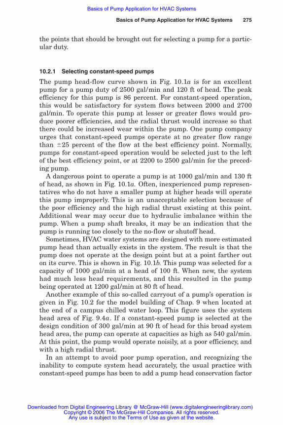
Basics of Pump Application for HVAC Systems 275
the points that should be brought out for selecting a pump for a partic-ular duty.
10.2.1 Selecting constant-speed pumps
The pump head-flow curve shown in Fig. 10.1a is for an excellentpump for a pump duty of 2500 gal/min and 120 ft of head. The peakefficiency for this pump is 86 percent. For constant-speed operation,this would be satisfactory for system flows between 2000 and 2700gal/min. To operate this pump at lesser or greater flows would pro-duce poorer efficiencies, and the radial thrust would increase so thatthere could be increased wear within the pump. One pump companyurges that constant-speed pumps operate at no greater flow rangethan �25 percent of the flow at the best efficiency point. Normally,pumps for constant-speed operation would be selected just to the leftof the best efficiency point, or at 2200 to 2500 gal/min for the preced-ing pump.
A dangerous point to operate a pump is at 1000 gal/min and 130 ftof head, as shown in Fig. 10.1a. Often, inexperienced pump represen-tatives who do not have a smaller pump at higher heads will operatethis pump improperly. This is an unacceptable selection because ofthe poor efficiency and the high radial thrust existing at this point.Additional wear may occur due to hydraulic imbalance within thepump. When a pump shaft breaks, it may be an indication that thepump is running too closely to the no-flow or shutoff head.
Sometimes, HVAC water systems are designed with more estimatedpump head than actually exists in the system. The result is that thepump does not operate at the design point but at a point farther outon its curve. This is shown in Fig. 10.1b. This pump was selected for acapacity of 1000 gal/min at a head of 100 ft. When new, the systemhad much less head requirements, and this resulted in the pumpbeing operated at 1200 gal/min at 80 ft of head.
Another example of this so-called carryout of a pump’s operation isgiven in Fig. 10.2 for the model building of Chap. 9 when located atthe end of a campus chilled water loop. This figure uses the systemhead area of Fig. 9.4a. If a constant-speed pump is selected at thedesign condition of 300 gal/min at 90 ft of head for this broad systemhead area, the pump can operate at capacities as high as 540 gal/min.At this point, the pump would operate noisily, at a poor efficiency, andwith a high radial thrust.
In an attempt to avoid poor pump operation, and recognizing theinability to compute system head accurately, the usual practice withconstant-speed pumps has been to add a pump head conservation factor
Rishel_CH10.qxd 21/4/06 6:20 PM Page 275
Downloaded from Digital Engineering Library @ McGraw-Hill (www.digitalengineeringlibrary.com)Copyright © 2006 The McGraw-Hill Companies. All rights reserved.
Any use is subject to the Terms of Use as given at the website.
Basics of Pump Application for HVAC Systems

276 The HVAC World
and then pick the pump to the left of the best efficiency point to ensurethat the pump will operate without damage at the higher flows andlower heads. The other practice has been to install a balancing valveon the pump discharge, either manual or automatic, and add enoughfriction to prevent some of the operation at higher flows. One of theadvantages of variable-speed pumps is that this “carryout” condition iseliminated by their controls without all the inefficiencies of pumphead conservation factors and balancing valves.
Figure 10.2 Pump operation with system head area.
Rishel_CH10.qxd 21/4/06 6:20 PM Page 276
Downloaded from Digital Engineering Library @ McGraw-Hill (www.digitalengineeringlibrary.com)Copyright © 2006 The McGraw-Hill Companies. All rights reserved.
Any use is subject to the Terms of Use as given at the website.
Basics of Pump Application for HVAC Systems
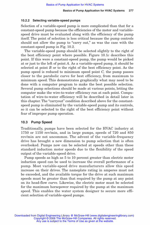
Basics of Pump Application for HVAC Systems 277
10.2.2 Selecting variable-speed pumps
Selection of a variable-speed pump is more complicated than that for aconstant-speed pump because the efficiencies of the motor and variable-speed drive must be evaluated along with the efficiency of the pumpitself. The point of selection is less critical because the pump controlsshould not allow the pump to “carry out,” as was the case with theconstant-speed pump in Fig. 10.2.
The variable-speed pump should be selected slightly to the right ofthe best efficiency point where possible. Figure 10.1c describes thispoint. If this were a constant-speed pump, the pump would be pickedat or just to the left of point A. As a variable-speed pump, it should beselected at point B or to the right of the best efficiency point. As thepump speed is reduced to minimum speed point C, the pump passescloser to the parabolic curve for best efficiency, from maximum tominimum speed. This demonstrates graphically what may need to bedone with a computer program to make the best possible selection.Several pump selections should be made at various points, letting thecomputer make the wire-to-water efficiency run at each point. Compu-tation of wire-to-water efficiency will be described in detail later inthis chapter. The “carryout” condition described above for the constant-speed pump is eliminated by the variable-speed pump and its controls,so it can be selected to the right of the best efficiency point withoutfear of improper pump operation.
10.3 Pump Speed
Traditionally, pumps have been selected for the HVAC industry at1750 or 1150 rev/min, and in large pumps, speeds of 720 and 850rev/min are not uncommon. The advent of the variable-frequencydrive has brought a new dimension to pump selection that is oftenoverlooked. Pumps now can be selected at speeds other than thesestandard induction motor speeds due to the flexibility of the speedoutput of the variable-speed drive.
Pump speeds as high as 5 to 10 percent greater than electric motorinduction speed can be used to increase the overall performance of apump. Most variable-speed drive manufacturers allow this speedincrease on their drives. The nameplate rating in amperes must notbe exceeded, and the available torque for the drive at such maximumspeeds must be greater than that required by the pump at any pointon its head-flow curve. Likewise, the electric motor must be selectedfor the maximum horsepower required by the pump at the maximumspeed. This enables the water system designer to secure more effi-cient selection of variable-speed pumps.
Rishel_CH10.qxd 21/4/06 6:20 PM Page 277
Downloaded from Digital Engineering Library @ McGraw-Hill (www.digitalengineeringlibrary.com)Copyright © 2006 The McGraw-Hill Companies. All rights reserved.
Any use is subject to the Terms of Use as given at the website.
Basics of Pump Application for HVAC Systems

Following is an example of this pump selection procedure. Assumepump duty at 700 gal/min at 70 ft of head. There is one selection at1750 rev/min: a 6 � 6 � 9 pump with a 25-hp motor and efficiency of72 percent at the design point (Fig. 10.3a). A desirable pump would bethe 6 � 4 � 9 pump, but it does not quite achieve the head capacityrequired at 1750 rev/min (Fig. 10.3b). An alternate selection would bethe same 6 � 4 � 9 pump with a 20-hp motor operating at 1789rev/min and at 87 percent efficiency at the design point (Fig. 10.3c).
The alternate selection was determined by computing the capacityof the smaller pump at a higher speed using the pump affinity laws.The pump speed was calculated at a point where the required condi-tion of 700 gal/min at 70 ft was achieved by the smaller pump.Following is the method of computing the desired speed. From theaffinity laws:
�Qh
1
1
2
� � �Qh
2
2
2
�
where Q1 and h1 are the desired conditions of 700 gal/min and 70 ft.Q2 and h2 are the equivalent points on the known pump curve.
By trial and error, the equivalent flow Q2 can be computed and is 685gal/min (see Eq. 10.1 developed in Sec. 10.4 on the use of the affinitylaws for pumps). The required speed S1 of the pump, therefore, is
S1 � �760805
� � 1750 � 1789 rev/min
Figure 10.3c describes the actual operating curve for the 6 � 4 � 9pump operating at 1789 rev/min. It is obvious that a 20-hp motor andvariable-speed drive will be adequate because the maximum brakehorsepower at any point on this curve is 16.8 bhp. The motor anddrive manufacturers can certify that their equipment is acceptable foroperation at this speed and brake horsepower.
An examination of Figs. 10.3b and c reveals that the use of this tech-nique has increased the pump efficiency from 72.5 to 87 percent andhas reduced the nonoverloading motor horsepower from 25 to 20 hp.This demonstrates the added dimension that variable-speed drives canprovide in the selection of pumps. Engineers should not be concernedabout the operation of a pump near its maximum impeller diameter;pump manufacturers will certify their pumps within the impellerdiameters listed in their catalogs. Other engineers are reluctant toselect pumps at maximum impeller diameter in anticipation of futureincreases in pumping requirements. This procedure of using speeds as
278 The HVAC World
Rishel_CH10.qxd 21/4/06 6:20 PM Page 278
Downloaded from Digital Engineering Library @ McGraw-Hill (www.digitalengineeringlibrary.com)Copyright © 2006 The McGraw-Hill Companies. All rights reserved.
Any use is subject to the Terms of Use as given at the website.
Basics of Pump Application for HVAC Systems

279
Fig
ure
10.
3S
peci
al p
um
p sp
eeds
.
Rishel_CH10.qxd 21/4/06 6:20 PM Page 279
Downloaded from Digital Engineering Library @ McGraw-Hill (www.digitalengineeringlibrary.com)Copyright © 2006 The McGraw-Hill Companies. All rights reserved.
Any use is subject to the Terms of Use as given at the website.
Basics of Pump Application for HVAC Systems

280 The HVAC World
high as 1210 or 1840 rev/min provides an additional load factor.Reiterating, in all this work, the maximum pump horsepower must becalculated to ensure that the motor and the variable-speed drive arenot overloaded. Likewise, it is wise to verify that the pump manufac-turer approves the operation of the pump at the proposed speed.
10.3.1 Variable-speed pump operation
Most variable-speed pump operations in HVAC water systems track asystem head curve as was defined by Eq. 9.3 in the previous chapter.Both the flow and head vary with this curve. As will be seen in thechapters on chilled and hot water distribution, a remote differentialpressure transmitter is utilized to cause the pump head and flow tofollow the system head curve or the desirable point in the systemhead area.
There are other useful variable-speed operations in the HVAC field,such as constant flow, variable head. In this case, the pump flowremains constant while the pump head and speed change with systemconditions. Typical of this is constant flow through a chiller condenser.The head increases as more chillers are placed in operation as shownin Fig. 10.4. The flow is a constant 2000 gal/min as the system headincreases and decreases. Such an operation can result in relativelyhigh pump efficiency, as shown in Fig. 10.5.
This figure describes the pump efficiency, as it cuts across thecurves of constant efficiency. In all variable-speed operations, thisshould be observed to ensure that the pumps are operating at the best
1000 RPM
1175 RPM
800 RPM
80
60
40
20
00 320028002400200016001200800400
U.S. Gallons per minute
Pum
p he
ad—
ft.
70%
75%
80%
83%
86%
86%
83%
87%
Individuallines ofefficiency
Bep curve
Figure 10.4 Constant flow, variable head process.
Rishel_CH10.qxd 21/4/06 6:20 PM Page 280
Downloaded from Digital Engineering Library @ McGraw-Hill (www.digitalengineeringlibrary.com)Copyright © 2006 The McGraw-Hill Companies. All rights reserved.
Any use is subject to the Terms of Use as given at the website.
Basics of Pump Application for HVAC Systems
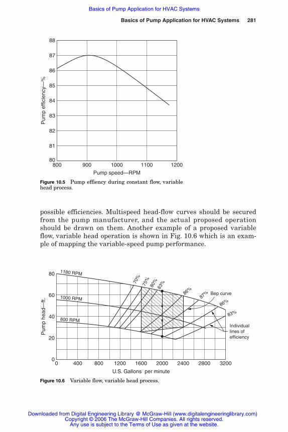
possible efficiencies. Multispeed head-flow curves should be securedfrom the pump manufacturer, and the actual proposed operationshould be drawn on them. Another example of a proposed variableflow, variable head operation is shown in Fig. 10.6 which is an exam-ple of mapping the variable-speed pump performance.
Basics of Pump Application for HVAC Systems 281
88
80
81
82
83
84
85
86
87
Pum
p ef
ficie
ncy—
%
800 900 1000 1100 1200
Pump speed—RPM
Figure 10.5 Pump effiency during constant flow, variablehead process.
Figure 10.6 Variable flow, variable head process.
1000 RPM
1180 RPM
800 RPM
80
60
40
20
00 320028002400200016001200800400
U.S. Gallons per minute
Pum
p he
ad—
ft.
70%
75%
80%
83%
86%
86%
83%
87%
Individuallines ofefficiency
Bep curve
Rishel_CH10.qxd 21/4/06 6:20 PM Page 281
Downloaded from Digital Engineering Library @ McGraw-Hill (www.digitalengineeringlibrary.com)Copyright © 2006 The McGraw-Hill Companies. All rights reserved.
Any use is subject to the Terms of Use as given at the website.
Basics of Pump Application for HVAC Systems
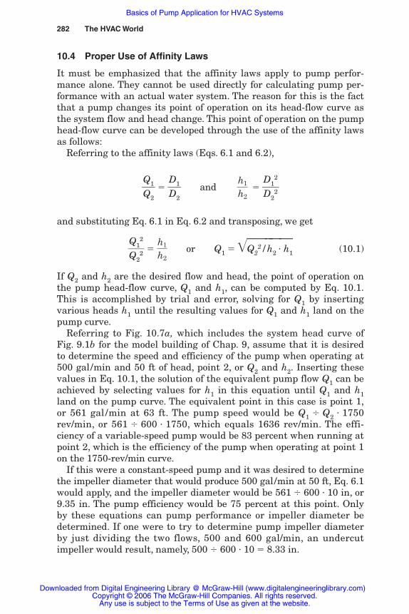
282 The HVAC World
10.4 Proper Use of Affinity Laws
It must be emphasized that the affinity laws apply to pump perfor-mance alone. They cannot be used directly for calculating pump per-formance with an actual water system. The reason for this is the factthat a pump changes its point of operation on its head-flow curve asthe system flow and head change. This point of operation on the pumphead-flow curve can be developed through the use of the affinity lawsas follows:
Referring to the affinity laws (Eqs. 6.1 and 6.2),
1
2
� � �DD
1
2
� and � �DD
1
2
2
2�
and substituting Eq. 6.1 in Eq. 6.2 and transposing, we get
1
2
2
2� � or Q1 � �Q�22�/�h�2� �� h�1� (10.1)
If Q2 and h2 are the desired flow and head, the point of operation onthe pump head-flow curve, Q1 and h1, can be computed by Eq. 10.1.This is accomplished by trial and error, solving for Q1 by insertingvarious heads h1 until the resulting values for Q1 and h1 land on thepump curve.
Referring to Fig. 10.7a, which includes the system head curve ofFig. 9.1b for the model building of Chap. 9, assume that it is desiredto determine the speed and efficiency of the pump when operating at500 gal/min and 50 ft of head, point 2, or Q2 and h2. Inserting thesevalues in Eq. 10.1, the solution of the equivalent pump flow Q1 can beachieved by selecting values for h1 in this equation until Q1 and h1land on the pump curve. The equivalent point in this case is point 1,or 561 gal /min at 63 ft. The pump speed would be Q1 � Q2 � 1750rev/min, or 561 � 600 � 1750, which equals 1636 rev/min. The effi-ciency of a variable-speed pump would be 83 percent when running atpoint 2, which is the efficiency of the pump when operating at point 1on the 1750-rev/min curve.
If this were a constant-speed pump and it was desired to determinethe impeller diameter that would produce 500 gal/min at 50 ft, Eq. 6.1would apply, and the impeller diameter would be 561 � 600 � 10 in, or9.35 in. The pump efficiency would be 75 percent at this point. Onlyby these equations can pump performance or impeller diameter bedetermined. If one were to try to determine pump impeller diameterby just dividing the two flows, 500 and 600 gal/min, an undercutimpeller would result, namely, 500 � 600 � 10 � 8.33 in.
h1
h2
h1
h2
Rishel_CH10.qxd 21/4/06 6:20 PM Page 282
Downloaded from Digital Engineering Library @ McGraw-Hill (www.digitalengineeringlibrary.com)Copyright © 2006 The McGraw-Hill Companies. All rights reserved.
Any use is subject to the Terms of Use as given at the website.
Basics of Pump Application for HVAC Systems
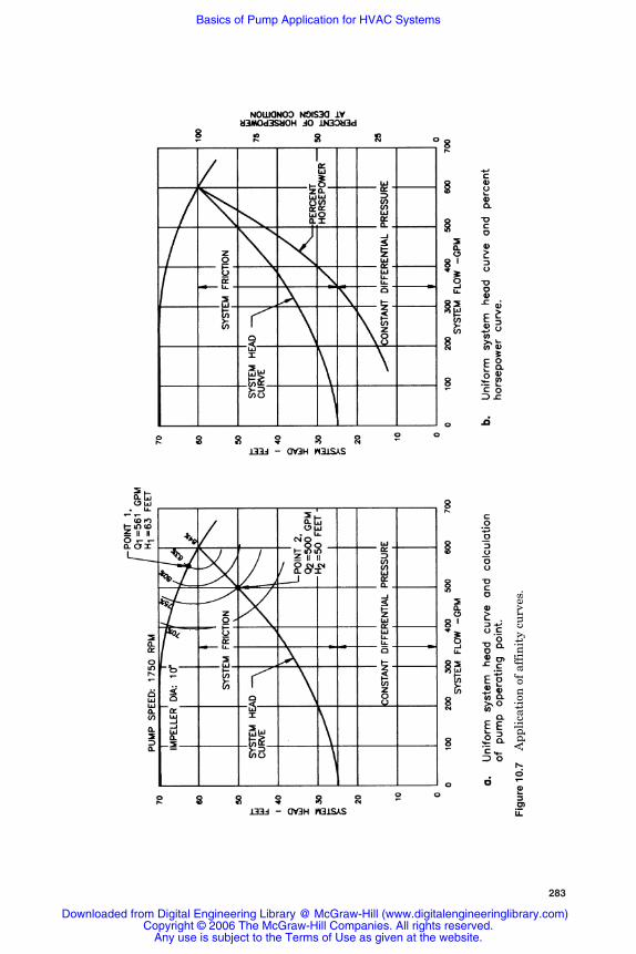
283
Fig
ure
10.
7A
ppli
cati
on o
f af
fin
ity
curv
es.
Rishel_CH10.qxd 21/4/06 6:20 PM Page 283
Downloaded from Digital Engineering Library @ McGraw-Hill (www.digitalengineeringlibrary.com)Copyright © 2006 The McGraw-Hill Companies. All rights reserved.
Any use is subject to the Terms of Use as given at the website.
Basics of Pump Application for HVAC Systems
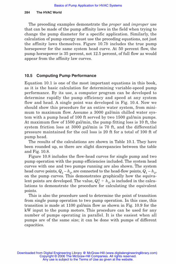
The preceding examples demonstrate the proper and improper usethat can be made of the pump affinity laws in the field when trying tochange the pump diameter for a specific application. Similarly, thecalculation of pump energy must use the preceding equations, not justthe affinity laws themselves. Figure 10.7b includes the true pumphorsepower for the same system head curve. At 50 percent flow, thepump horsepower is 35 percent, not 12.5 percent, of full flow as wouldappear from the affinity law curves.
10.5 Computing Pump Performance
Equation 10.1 is one of the most important equations in this book,as it is the basic calculation for determining variable-speed pumpperformance. By its use, a computer program can be developed todetermine rapidly the pump efficiency and speed at any systemflow and head. A single point was developed in Fig. 10.4. Now weshould show this procedure for an entire water system, from mini-mum to maximum flow. Assume a 3000 gal/min chilled water sys-tem with a pump head of 100 ft served by two 1500 gal/min pumps.At maximum flow of 1500 gal/min, the pump fitting loss is 10 ft, thesystem friction loss at 3000 gal/min is 70 ft, and the differentialpressure maintained for the coil loss is 20 ft for a total of 100 ft ofpump head.
The results of the calculations are shown in Table 10.1. They havebeen rounded up, so there are slight discrepancies between the tableand Fig. 10.8.
Figure 10.8 includes the flow-head curves for single pump and twopump operation with the pump efficiencies included. The system headcurves with one and two pumps running are also shown. The systemhead curve points, Q2 – h2, are connected to the head-flow points, Q1 – h2,on the pump curves. This demonstrates graphically how the equiva-lent points are developed. The value, Q2
2 � h2, is included in the calcu-lations to demonstrate the procedure for calculating the equivalentpoints.
This is also the procedure used to determine the point of transitionfrom single pump operation to two pump operation. In this case, thistransition is made at 1100 gal/min flow as shown in Fig. 10.9 for thekW input to the pump motors. This procedure can be used for anynumber of pumps operating in parallel. It is the easiest when allpumps are of the same size; it can be done with pumps of differentcapacities.
284 The HVAC World
Rishel_CH10.qxd 21/4/06 6:20 PM Page 284
Downloaded from Digital Engineering Library @ McGraw-Hill (www.digitalengineeringlibrary.com)Copyright © 2006 The McGraw-Hill Companies. All rights reserved.
Any use is subject to the Terms of Use as given at the website.
Basics of Pump Application for HVAC Systems

285
TAB
LE
10.1
Pu
mp
Per
form
ance
Cal
cula
tio
ns
No
Sys
tem
Sys
tem
Fit
tin
gT
otal
Equ
iv.
Equ
iv.
Pu
mp
Pu
mp
Pu
mp
Pu
mp
Wir
epu
mp
flow
h
ead,
loss
hea
d,ft
hea
dfl
owef
fy,
spee
dsp
eed
BH
Psh
aft
kwru
nG
PM
Qe
ftft
h2
Q2 2�
h2
h1
Q1
%%
RP
MH
Pef
fy,%
inpu
t
130
00.
90.
421
.342
2512
472
470
41.4
729
2.3
56.4
3.0
160
03.
31.
624
.914
,458
112
1273
8447
.182
94.
570
.54.
81
900
7.1
3.6
30.7
26,3
8495
1583
85.5
56.9
1001
8.2
75.4
8.1
112
0012
.36.
438
.737
,209
8517
7880
67.5
1188
14.7
82.4
13.3
115
0018
.810
.048
.846
,107
4418
8474
79.6
1401
25.0
87.5
21.3
290
07.
10.
928
.028
,128
122
1852
77.5
48.6
855
8.2
66.3
9.2
212
0012
.31.
633
.942
,477
117
2229
82.5
53.8
947
12.5
73.4
12.7
215
0018
.92.
541
.454
,348
113
2478
85.5
60.5
1065
18.3
78.0
17.5
218
0026
.53.
650
.164
,670
109
2655
86.3
67.8
1193
26.4
82.9
23.7
221
0035
.54.
960
.473
,013
107
2795
87.1
75.1
1322
36.8
86.5
31.7
224
0045
.86.
472
.279
,778
104
2880
87.2
83.3
1466
50.2
88.4
42.3
227
0057
.38.
185
.485
,362
102
2950
87.1
91.5
1610
66.9
90.6
55.0
230
0070
10.0
100
—10
0—
8710
017
6087
.191
.870
.8
Rishel_CH10.qxd 21/4/06 6:20 PM Page 285
Downloaded from Digital Engineering Library @ McGraw-Hill (www.digitalengineeringlibrary.com)Copyright © 2006 The McGraw-Hill Companies. All rights reserved.
Any use is subject to the Terms of Use as given at the website.
Basics of Pump Application for HVAC Systems
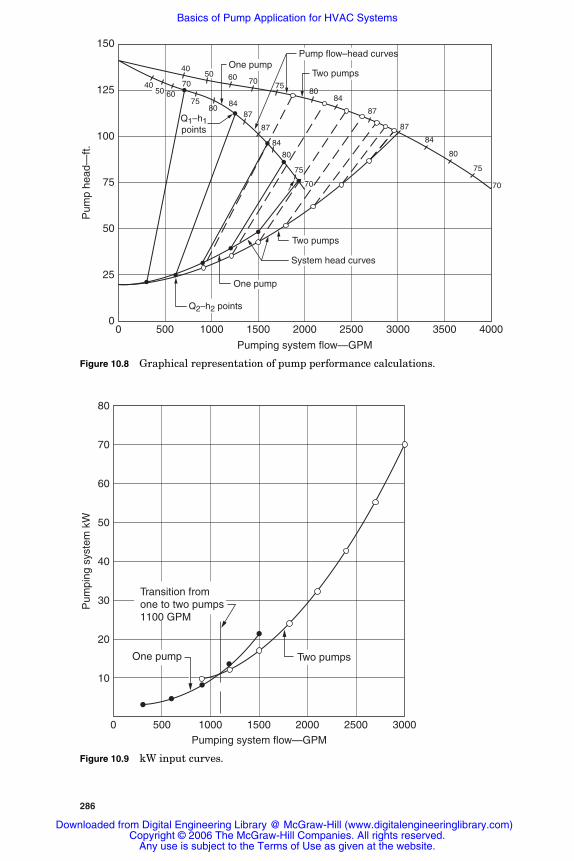
286
70
75
80
84
87
8480
7570605040
87
4050 60
7580
87
84
75
70
80
87
84
70
One pumpPump flow–head curves
Two pumps
Q1–h1points
System head curves
Two pumps
One pump
Q2–h2 points
0 500 1000 1500 2000 2500 3000 3500 4000
Pumping system flow—GPM
150
125
100
75
50
25
0
Pum
p he
ad—
ft.
Figure 10.8 Graphical representation of pump performance calculations.
80
70
60
50
40
30
20
10
Pum
ping
sys
tem
kW
0 500 1000 1500 2000 2500 3000Pumping system flow—GPM
One pump Two pumps
Transition fromone to two pumps1100 GPM
Figure 10.9 kW input curves.
Rishel_CH10.qxd 21/4/06 6:20 PM Page 286
Downloaded from Digital Engineering Library @ McGraw-Hill (www.digitalengineeringlibrary.com)Copyright © 2006 The McGraw-Hill Companies. All rights reserved.
Any use is subject to the Terms of Use as given at the website.
Basics of Pump Application for HVAC Systems

Basics of Pump Application for HVAC Systems 287
10.6 Number of Pumps
Most HVAC water systems have a broad range of operation due to thevariation in heating, cooling, and ventilating loads. As was discussedin Chap. 8, it is imperative that the minimum load as well as themaximum load on a HVAC water system be computed before anyadditional evaluation be made of that system.
Most HVAC systems also have more than one pump per water sys-tem due to (1) the broad range of loads and (2) to provide some redun-dancy in case of pump failure. Thus, HVAC systems can range fromone pump on small systems with a specific flow range and little needfor standby pump capability up to a number of pumps operating inparallel to accommodate load range and reliability.
It is obvious that the water system designer must make decisionsearly in the system design to ensure that the desired levels of effi-ciency and reliability are achieved for a water system. Let us reviewthe two factors that affect the number of pumps operating in parallel.
“Fear of pump failure” has affected the determination of the number ofpumps when it should not be considered. Pumps have a reliability com-parable with that of other HVAC equipment. Seldom are two fansinstalled in parallel because of fear of failure. The consequences of sys-tem failure should be determined to develop the redundancy needed onevery water system. Hospitals and institutions and critical facilities suchas research laboratories and computer centers obviously should havestandby pump capability to ensure that there is continuous service.
The question on critical installations is how much standby capacityshould be provided? The two most frequent selections are two 100percent capacity or three 50 percent capacity pumps. The three 50percent capacity pumps are usually the best selection because theyoffer three chances to total failure and the pumps and motors aresmaller. For example, assume a chilled water system for a hospitalhas a maximum requirement of 2500 gal/min at 100 ft of head and asystem head curve as shown in Fig. 10.10a. This curve shows a con-stant friction head of 20 ft that is maintained across all the coolingcoils and control valves. Two pumps at 100 percent capacity wouldrequire two 75-hp motors, while three pumps at 50 percent capacityeach would require three 40-hp motors. Figure 10.10b provides thepump head-flow curve for the pumps of the two-pump system, whileFig. 10.10c does so for the three-pump system. The total horsepowerfor the two pumps would be 150 hp compared with 120 hp for thethree pumps. If space is available for the three pumps, it would appearthat the three pumps would be more acceptable for this application; afinal decision should be made after a wire-to-water evaluation ismade. This will be discussed later in this chapter.
Rishel_CH10.qxd 21/4/06 6:20 PM Page 287
Downloaded from Digital Engineering Library @ McGraw-Hill (www.digitalengineeringlibrary.com)Copyright © 2006 The McGraw-Hill Companies. All rights reserved.
Any use is subject to the Terms of Use as given at the website.
Basics of Pump Application for HVAC Systems
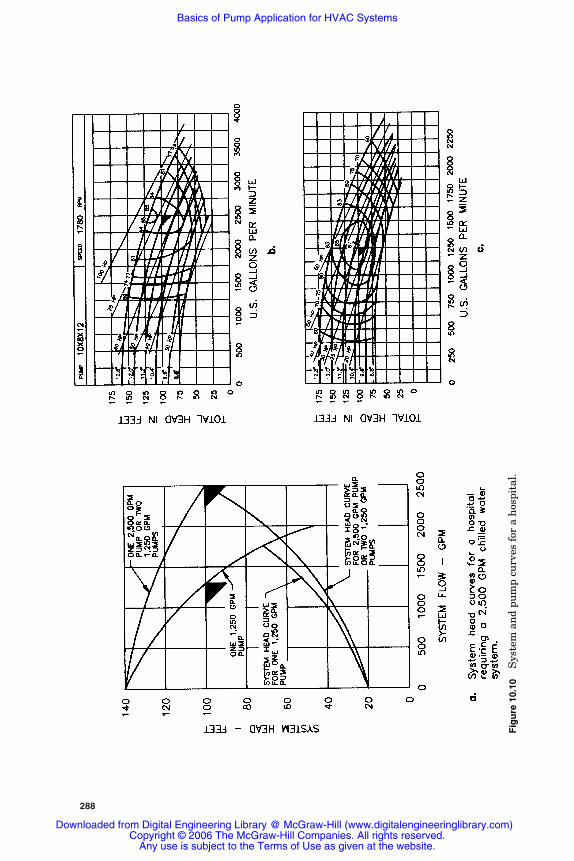
288
Fig
ure
10.
10S
yste
m a
nd
pum
p cu
rves
for
a h
ospi
tal.
Rishel_CH10.qxd 21/4/06 6:20 PM Page 288
Downloaded from Digital Engineering Library @ McGraw-Hill (www.digitalengineeringlibrary.com)Copyright © 2006 The McGraw-Hill Companies. All rights reserved.
Any use is subject to the Terms of Use as given at the website.
Basics of Pump Application for HVAC Systems

Basics of Pump Application for HVAC Systems 289
Noncritical installations such as some office and commercial build-ings do not require as much redundancy or standby as the buildingsmentioned in the previous paragraph. For example, if a commercialbuilding had a system head curve as shown previously for a hospital(Fig. 10.10a), only two 50 percent pumps could be installed, since onepump would have a maximum capacity of 1750 gal/min, or 70 percentof the total system capacity. It would be a decision for the water systemdesigner or the owner of the building as to whether two or three pumpswould be installed. With the reliability and reduced wear of variable-speed pumps, the two-pump installation would offer a desirablearrangement for this office building.
10.7 Mixing Constant- and Variable-Speed Pumps
It should be understood that pumps in parallel must always operateat the same speed! There may be some unusual, sophisticated caseswhere parallel pumps are operated at different speeds, but only expe-rienced pump designers should make evaluations for such a proposedoperation. Also, it is better on most HVAC operations to use pumps ofthe same size when operating them in parallel. This ensures that theoperating pumps are producing the same flow, and this simplifiesevaluation of the efficiency of operation of the pumps. Small jockeypumps that operate the system on low loads are not justified on mostsystems. Variable-speed pumps should be controlled so that pumpsoperating in parallel never have over a 1 percent difference in actualoperating speeds.
Mixing of constant- and variable-speed pumps is encountered in theHVAC field, often with disastrous results. Following is a discussion ofthe problems that can occur when a constant-speed pump is operatedin parallel with a variable-speed pump (use Fig. 10.11a to follow thisdiscussion):
1. Assume that one variable-speed pump is operating at point A.
2. Next, assume that the flow in the system increases until thevariable-speed pump operates at full speed at point B.
3. Let the system load now increase to point C, where one pump can-not handle the load.
4. The system controls will turn on the next pump in an attempt tomaintain the system flow.
5. Let the next pump be a constant-speed pump of the same size asthe operating variable-speed pump. It will operate at point D2because it cannot vary its speed.
Rishel_CH10.qxd 21/4/06 6:20 PM Page 289
Downloaded from Digital Engineering Library @ McGraw-Hill (www.digitalengineeringlibrary.com)Copyright © 2006 The McGraw-Hill Companies. All rights reserved.
Any use is subject to the Terms of Use as given at the website.
Basics of Pump Application for HVAC Systems
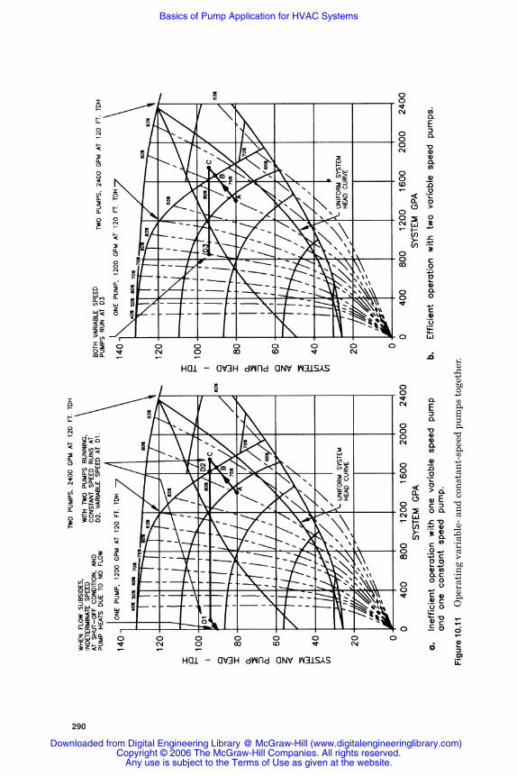
290
Fig
ure
10.
11O
pera
tin
g va
riab
le-
and
con
stan
t-sp
eed
pum
ps t
oget
her
.
Rishel_CH10.qxd 21/4/06 6:20 PM Page 290
Downloaded from Digital Engineering Library @ McGraw-Hill (www.digitalengineeringlibrary.com)Copyright © 2006 The McGraw-Hill Companies. All rights reserved.
Any use is subject to the Terms of Use as given at the website.
Basics of Pump Application for HVAC Systems
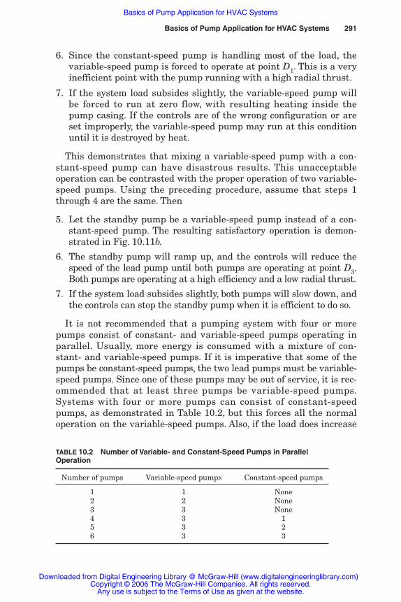
Basics of Pump Application for HVAC Systems 291
6. Since the constant-speed pump is handling most of the load, thevariable-speed pump is forced to operate at point D1. This is a veryinefficient point with the pump running with a high radial thrust.
7. If the system load subsides slightly, the variable-speed pump willbe forced to run at zero flow, with resulting heating inside thepump casing. If the controls are of the wrong configuration or areset improperly, the variable-speed pump may run at this conditionuntil it is destroyed by heat.
This demonstrates that mixing a variable-speed pump with a con-stant-speed pump can have disastrous results. This unacceptableoperation can be contrasted with the proper operation of two variable-speed pumps. Using the preceding procedure, assume that steps 1through 4 are the same. Then
5. Let the standby pump be a variable-speed pump instead of a con-stant-speed pump. The resulting satisfactory operation is demon-strated in Fig. 10.11b.
6. The standby pump will ramp up, and the controls will reduce thespeed of the lead pump until both pumps are operating at point D3.Both pumps are operating at a high efficiency and a low radial thrust.
7. If the system load subsides slightly, both pumps will slow down, andthe controls can stop the standby pump when it is efficient to do so.
It is not recommended that a pumping system with four or morepumps consist of constant- and variable-speed pumps operating inparallel. Usually, more energy is consumed with a mixture of con-stant- and variable-speed pumps. If it is imperative that some of thepumps be constant-speed pumps, the two lead pumps must be variable-speed pumps. Since one of these pumps may be out of service, it is rec-ommended that at least three pumps be variable-speed pumps.Systems with four or more pumps can consist of constant-speedpumps, as demonstrated in Table 10.2, but this forces all the normaloperation on the variable-speed pumps. Also, if the load does increase
TABLE 10.2 Number of Variable- and Constant-Speed Pumps in ParallelOperation
Number of pumps Variable-speed pumps Constant-speed pumps
1 1 None2 2 None3 3 None4 3 15 3 26 3 3
Rishel_CH10.qxd 21/4/06 6:20 PM Page 291
Downloaded from Digital Engineering Library @ McGraw-Hill (www.digitalengineeringlibrary.com)Copyright © 2006 The McGraw-Hill Companies. All rights reserved.
Any use is subject to the Terms of Use as given at the website.
Basics of Pump Application for HVAC Systems

292 The HVAC World
often to where the fourth pump is required, higher operating effi-ciency is achieved by making it a variable-speed pump.
A careful evaluation of the constant-speed pumps must be madewhen they are used, including calculating where they will operate ontheir head-flow curves, to ensure that they do not operate at an ineffi-cient or high radial thrust point.
10.8 Efficiency of a Pumping System
The efficiency of a pumping system is more than just the efficiency ofthe individual pumps. There are three different energy losses in aconstant-speed electric motor–driven pumping system:
1. Loss in the motor
2. Loss in the pump
3. Friction loss in the pump and header fittings
The variable-speed pumping system has a fourth loss, that of thevariable-speed drive.
There may be some concern as to why the pump fitting and headerlosses are included in the efficiency evaluation for a pumping system.These losses must be computed separately because they are part ofthe pumping system, not part of the water distribution system. Also,on multiple-pump systems, they must be separated from the watersystem loss because they do not vary with the total flow on the sys-tem. Rather, they vary with the flow through the pump to which theyare connected. The flow rate through these fittings affects appreciablythe overall efficiency of such a pumping system. The friction loss forthese fittings varies closely with the square of the flow through them.The points at which pumps are programmed on and off on a multiple-pump system have a definite impact on the efficiency of the overallpumping system; these points are affected by the variation in frictionin the pump fittings and valves.
There can be six to ten specific losses in the fittings and valves on apumping system:
1. Entrance loss from suction header
2. Suction shutoff valve
3. Suction strainer
4. Suction piping
5. Pump suction reducer
6. Pump discharge increaser
7. Check valve
Rishel_CH10.qxd 21/4/06 6:20 PM Page 292
Downloaded from Digital Engineering Library @ McGraw-Hill (www.digitalengineeringlibrary.com)Copyright © 2006 The McGraw-Hill Companies. All rights reserved.
Any use is subject to the Terms of Use as given at the website.
Basics of Pump Application for HVAC Systems
Basics of Pump Application for HVAC Systems 293
8. Discharge shutoff valve
9. Discharge piping
10. Exit loss into discharge header
Wire-to-water efficiency is an old term that has been used for manyyears in the pumping industry to determine the overall efficiency of apump and motor combination. This efficiency was used first for constant-speed pumps of considerable size, where large motors were involved.When these pumps were equipped with variable-speed drives, thewire-to-water efficiency represented the overall efficiency of drives,motors, and pumps. Wire-to-water efficiency has now been applied tosmaller pumping systems because the computer capability is nowavailable to accomplish the tedious calculations.
The wire-to-water efficiency of a proposed pumping system can beestimated using the following procedure:
1. A computer program can be developed to calculate the overallwire-to-water efficiency of a pumping system from minimum tomaximum system flow. This program utilizes a standard curve-tracing technique through the calculation of binomial equations forthe following curves:a. Pump head-flow curveb. Pump efficiency curvec. Motor efficiency or wire-to-shaft efficiency curve for the variable-
speed drive and motord. System head curvee. Pump fitting loss curve
2. These equations are then used to compute system performanceusing the pump energy equations of Chap. 6; values computed are:a. System flow and headb. Water horsepowerc. Pump gallons per minuted. Pump fitting losse. Pump brake horsepowerf. Pump revolutions per minuteg. Pump efficiencyh. System brake horsepoweri. Wire-to-shaft efficiency (variable-speed drive and motor effi-
ciencies combined)j. Input kilowattsk. Wire-to-water efficiency
For variable-speed pumping systems using variable-frequency drives,the wire-to-shaft efficiency for the motor and variable-speed drivelisted in the previous paragraph, is a single efficiency developed by
Rishel_CH10.qxd 21/4/06 6:20 PM Page 293
Downloaded from Digital Engineering Library @ McGraw-Hill (www.digitalengineeringlibrary.com)Copyright © 2006 The McGraw-Hill Companies. All rights reserved.
Any use is subject to the Terms of Use as given at the website.
Basics of Pump Application for HVAC Systems
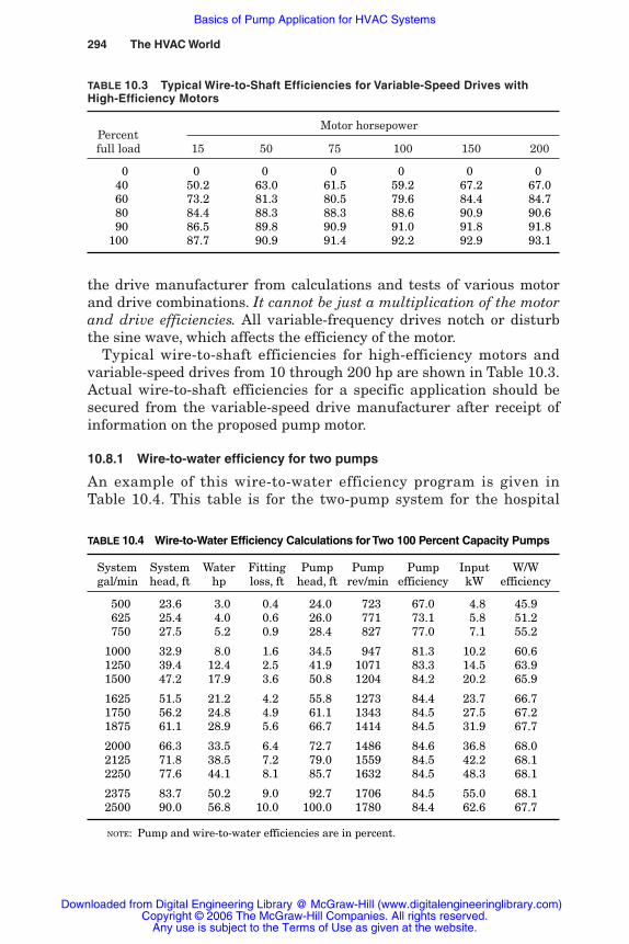
294 The HVAC World
the drive manufacturer from calculations and tests of various motorand drive combinations. It cannot be just a multiplication of the motorand drive efficiencies. All variable-frequency drives notch or disturbthe sine wave, which affects the efficiency of the motor.
Typical wire-to-shaft efficiencies for high-efficiency motors andvariable-speed drives from 10 through 200 hp are shown in Table 10.3.Actual wire-to-shaft efficiencies for a specific application should besecured from the variable-speed drive manufacturer after receipt ofinformation on the proposed pump motor.
10.8.1 Wire-to-water efficiency for two pumps
An example of this wire-to-water efficiency program is given inTable 10.4. This table is for the two-pump system for the hospital
TABLE 10.3 Typical Wire-to-Shaft Efficiencies for Variable-Speed Drives withHigh-Efficiency Motors
Motor horsepowerPercent full load 15 50 75 100 150 200
000 0 0 0 0 0 0040 50.2 63.0 61.5 59.2 67.2 67.0060 73.2 81.3 80.5 79.6 84.4 84.7080 84.4 88.3 88.3 88.6 90.9 90.6090 86.5 89.8 90.9 91.0 91.8 91.8100 87.7 90.9 91.4 92.2 92.9 93.1
TABLE 10.4 Wire-to-Water Efficiency Calculations for Two 100 Percent Capacity Pumps
System System Water Fitting Pump Pump Pump Input W/W gal/min head, ft hp loss, ft head, ft rev/min efficiency kW efficiency
0500 23.6 3.0 0.4 24.0 723 67.0 4.8 45.90625 25.4 4.0 0.6 26.0 771 73.1 5.8 51.20750 27.5 5.2 0.9 28.4 827 77.0 7.1 55.2
1000 32.9 8.0 1.6 34.5 947 81.3 10.2 60.61250 39.4 12.4 2.5 41.9 1071 83.3 14.5 63.91500 47.2 17.9 3.6 50.8 1204 84.2 20.2 65.9
1625 51.5 21.2 4.2 55.8 1273 84.4 23.7 66.71750 56.2 24.8 4.9 61.1 1343 84.5 27.5 67.21875 61.1 28.9 5.6 66.7 1414 84.5 31.9 67.7
2000 66.3 33.5 6.4 72.7 1486 84.6 36.8 68.02125 71.8 38.5 7.2 79.0 1559 84.5 42.2 68.12250 77.6 44.1 8.1 85.7 1632 84.5 48.3 68.1
2375 83.7 50.2 9.0 92.7 1706 84.5 55.0 68.12500 90.0 56.8 10.0 100.0 1780 84.4 62.6 67.7
NOTE: Pump and wire-to-water efficiencies are in percent.
Rishel_CH10.qxd 21/4/06 6:20 PM Page 294
Downloaded from Digital Engineering Library @ McGraw-Hill (www.digitalengineeringlibrary.com)Copyright © 2006 The McGraw-Hill Companies. All rights reserved.
Any use is subject to the Terms of Use as given at the website.
Basics of Pump Application for HVAC Systems
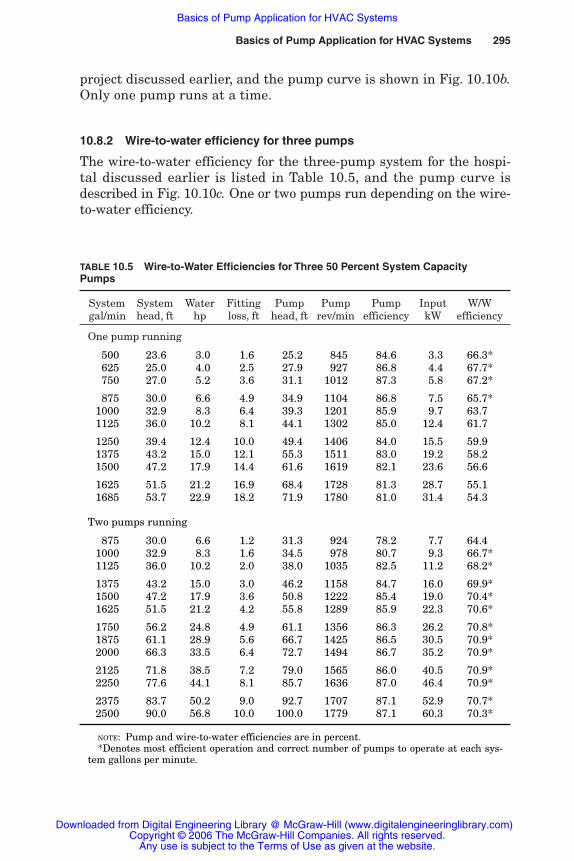
Basics of Pump Application for HVAC Systems 295
project discussed earlier, and the pump curve is shown in Fig. 10.10b.Only one pump runs at a time.
10.8.2 Wire-to-water efficiency for three pumps
The wire-to-water efficiency for the three-pump system for the hospi-tal discussed earlier is listed in Table 10.5, and the pump curve isdescribed in Fig. 10.10c. One or two pumps run depending on the wire-to-water efficiency.
TABLE 10.5 Wire-to-Water Efficiencies for Three 50 Percent System CapacityPumps
System System Water Fitting Pump Pump Pump Input W/W gal/min head, ft hp loss, ft head, ft rev/min efficiency kW efficiency
One pump running
0500 23.6 3.0 1.6 25.2 845 84.6 3.3 66.3*0625 25.0 4.0 2.5 27.9 927 86.8 4.4 67.7*0750 27.0 5.2 3.6 31.1 1012 87.3 5.8 67.2*
0875 30.0 6.6 4.9 34.9 1104 86.8 7.5 65.7*1000 32.9 8.3 6.4 39.3 1201 85.9 9.7 63.71125 36.0 10.2 8.1 44.1 1302 85.0 12.4 61.7
1250 39.4 12.4 10.0 49.4 1406 84.0 15.5 59.91375 43.2 15.0 12.1 55.3 1511 83.0 19.2 58.21500 47.2 17.9 14.4 61.6 1619 82.1 23.6 56.6
1625 51.5 21.2 16.9 68.4 1728 81.3 28.7 55.11685 53.7 22.9 18.2 71.9 1780 81.0 31.4 54.3
Two pumps running
0875 30.0 6.6 1.2 31.3 924 78.2 7.7 64.41000 32.9 8.3 1.6 34.5 978 80.7 9.3 66.7*1125 36.0 10.2 2.0 38.0 1035 82.5 11.2 68.2*
1375 43.2 15.0 3.0 46.2 1158 84.7 16.0 69.9*1500 47.2 17.9 3.6 50.8 1222 85.4 19.0 70.4*1625 51.5 21.2 4.2 55.8 1289 85.9 22.3 70.6*
1750 56.2 24.8 4.9 61.1 1356 86.3 26.2 70.8*1875 61.1 28.9 5.6 66.7 1425 86.5 30.5 70.9*2000 66.3 33.5 6.4 72.7 1494 86.7 35.2 70.9*
2125 71.8 38.5 7.2 79.0 1565 86.0 40.5 70.9*2250 77.6 44.1 8.1 85.7 1636 87.0 46.4 70.9*
2375 83.7 50.2 9.0 92.7 1707 87.1 52.9 70.7*2500 90.0 56.8 10.0 100.0 1779 87.1 60.3 70.3*
NOTE: Pump and wire-to-water efficiencies are in percent.*Denotes most efficient operation and correct number of pumps to operate at each sys-
tem gallons per minute.
Rishel_CH10.qxd 21/4/06 6:20 PM Page 295
Downloaded from Digital Engineering Library @ McGraw-Hill (www.digitalengineeringlibrary.com)Copyright © 2006 The McGraw-Hill Companies. All rights reserved.
Any use is subject to the Terms of Use as given at the website.
Basics of Pump Application for HVAC Systems
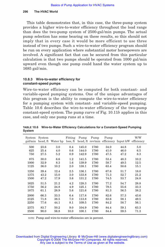
296 The HVAC World
This table demonstrates that, in this case, the three-pump systemprovides a higher wire-to-water efficiency throughout the load rangethan does the two-pump system of 2500-gal/min pumps. The actualpump selection has some bearing on these results, so this should notimply that in every case it would be more efficient to use threeinstead of two pumps. Such a wire-to-water efficiency program shouldbe run on every application where substantial motor horsepowers areinvolved. A significant fact that can be secured from this particularcalculation is that two pumps should be operated from 1000 gal/minupward even though one pump could hand the water system up to1685 gal/min.
10.8.3 Wire-to-water efficiency forconstant-speed pumps
Wire-to-water efficiency can be computed for both constant- andvariable-speed pumping systems. One of the unique advantages ofthis program is the ability to compute the wire-to-water efficiencyfor a pumping system with constant- and variable-speed pumping.Table 10.6 describes the wire-to-water efficiency of the two-pumpconstant-speed system. The pump curve of Fig. 10.11b applies in thiscase, and only one pump runs at a time.
TABLE 10.6 Wire-to-Water Efficiency Calculations for a Constant-Speed PumpingSystem
System System Fitting Pump Pump Pump W/W gal/min head, ft Water hp loss, ft head, ft rev/min efficiency Input kW efficiency
0500 23.6 3.0 0.4 145.0 1780 34.0 44.8 5.00625 25.4 4.0 0.6 144.0 1780 41.0 46.0 6.50750 27.5 5.2 0.9 142.9 1780 47.5 47.2 8.3
0875 30.0 6.6 1.2 141.5 1780 53.4 48.3 10.21000 32.9 8.3 1.6 139.9 1780 58.7 49.5 12.51125 36.0 10.2 2.0 138.1 1780 63.4 50.6 15.1
1250 39.4 12.4 2.5 136.1 1780 67.6 51.7 18.01375 43.2 15.0 3.0 133.8 1780 71.3 52.7 21.21500 47.2 17.9 3.6 131.2 1780 74.5 53.7 24.8
1625 51.5 21.2 4.2 128.3 1780 77.2 54.7 28.81750 56.2 24.8 4.9 125.1 1780 79.5 55.6 33.31875 61.1 28.9 5.6 121.6 1780 81.3 56.5 38.2
2000 66.3 33.5 6.4 117.8 1780 82.6 57.3 43.62125 71.8 38.5 7.0 113.8 1780 83.6 58.1 49.52250 77.6 44.1 8.1 109.5 1780 84.2 58.7 56.1
2375 83.7 50.2 9.0 104.9 1780 84.4 59.1 63.32500 90.0 56.8 10.0 100.1 1780 84.4 59.5 71.3
NOTE: Pump and wire-to-water efficiencies are in percent.
Rishel_CH10.qxd 21/4/06 6:20 PM Page 296
Downloaded from Digital Engineering Library @ McGraw-Hill (www.digitalengineeringlibrary.com)Copyright © 2006 The McGraw-Hill Companies. All rights reserved.
Any use is subject to the Terms of Use as given at the website.
Basics of Pump Application for HVAC Systems

Basics of Pump Application for HVAC Systems 297
Figure 10.12 provides the data of Tables 10.4, 10.5, and 10.6 ascurves plotted with system gallons per minute. This figure demon-strates the advantage of the three-pump variable-speed systemenergy-wise over the two-pump variable-speed system. It also showsthe dramatic energy savings of either variable-speed system over theconstant-speed system. Not only do the variable-speed systems saveenergy, but they also reduce appreciably the overpressure on thewater system and the radial thrust on the pumps themselves.
It should be noted that these tables are based on standard water at50°F. If wire-to-water efficiencies are computed for liquids of otherdensities or viscosities, the head inserted in the tables should be cor-rected for the actual density and viscosity.
10.9 Wire-to-Water Efficiency Indication
Wire-to-water efficiency indication for an actual pumping system canbe developed easily through the recording of the system flow, netpump head, and pumping system kilowatts. This instrumentation for
Figure 10.12 Wire-to-water efficiency curves for Tables10.4, 10.5, and 10.6.
Rishel_CH10.qxd 21/4/06 6:20 PM Page 297
Downloaded from Digital Engineering Library @ McGraw-Hill (www.digitalengineeringlibrary.com)Copyright © 2006 The McGraw-Hill Companies. All rights reserved.
Any use is subject to the Terms of Use as given at the website.
Basics of Pump Application for HVAC Systems
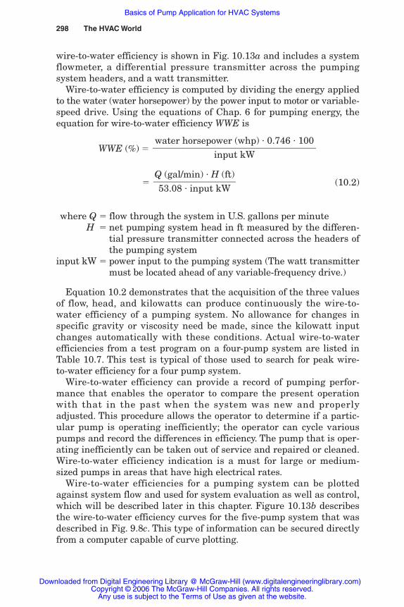
298 The HVAC World
wire-to-water efficiency is shown in Fig. 10.13a and includes a systemflowmeter, a differential pressure transmitter across the pumpingsystem headers, and a watt transmitter.
Wire-to-water efficiency is computed by dividing the energy appliedto the water (water horsepower) by the power input to motor or variable-speed drive. Using the equations of Chap. 6 for pumping energy, theequation for wire-to-water efficiency WWE is
WWE (%) �
� (10.2)
where Q � flow through the system in U.S. gallons per minuteH � net pumping system head in ft measured by the differen-
tial pressure transmitter connected across the headers ofthe pumping system
input kW � power input to the pumping system (The watt transmittermust be located ahead of any variable-frequency drive.)
Equation 10.2 demonstrates that the acquisition of the three valuesof flow, head, and kilowatts can produce continuously the wire-to-water efficiency of a pumping system. No allowance for changes inspecific gravity or viscosity need be made, since the kilowatt inputchanges automatically with these conditions. Actual wire-to-waterefficiencies from a test program on a four-pump system are listed inTable 10.7. This test is typical of those used to search for peak wire-to-water efficiency for a four pump system.
Wire-to-water efficiency can provide a record of pumping perfor-mance that enables the operator to compare the present operationwith that in the past when the system was new and properlyadjusted. This procedure allows the operator to determine if a partic-ular pump is operating inefficiently; the operator can cycle variouspumps and record the differences in efficiency. The pump that is oper-ating inefficiently can be taken out of service and repaired or cleaned.Wire-to-water efficiency indication is a must for large or medium-sized pumps in areas that have high electrical rates.
Wire-to-water efficiencies for a pumping system can be plottedagainst system flow and used for system evaluation as well as control,which will be described later in this chapter. Figure 10.13b describesthe wire-to-water efficiency curves for the five-pump system that wasdescribed in Fig. 9.8c. This type of information can be secured directlyfrom a computer capable of curve plotting.
Q (gal/min) � H (ft)���
53.08 � input kW
water horsepower (whp) � 0.746 � 100�����
input kW
Rishel_CH10.qxd 21/4/06 6:20 PM Page 298
Downloaded from Digital Engineering Library @ McGraw-Hill (www.digitalengineeringlibrary.com)Copyright © 2006 The McGraw-Hill Companies. All rights reserved.
Any use is subject to the Terms of Use as given at the website.
Basics of Pump Application for HVAC Systems

Basics of Pump Application for HVAC Systems 299
Figure 10.13 Wire-to-water efficiency instrumentation and typical wire-to-water effi-ciency curves for a five-pump system.
Rishel_CH10.qxd 21/4/06 6:20 PM Page 299
Downloaded from Digital Engineering Library @ McGraw-Hill (www.digitalengineeringlibrary.com)Copyright © 2006 The McGraw-Hill Companies. All rights reserved.
Any use is subject to the Terms of Use as given at the website.
Basics of Pump Application for HVAC Systems
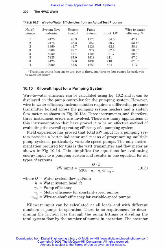
300 The HVAC World
10.10 Kilowatt Input for a Pumping System
Wire-to-water efficiency can be calculated using Eq. 10.2 and it can bedisplayed on the pump controller for the pumping system. However,wire-to-water efficiency instrumentation requires a differential pressuretransmitter located across the pumping system headers and a systemflow meter, as shown in Fig. 10.13a. Three instruments, and therefore,three instrument errors are involved. There are many applications ofthis instrumentation that have proved it to be an effective method ofevaluating the overall operating efficiency of a pumping system.
Field experience has proved that total kW input for a pumping sys-tem provides a better indicator and means of programming multiplepump systems, particularly variable-speed pumps. The only instru-mentation required for this is the watt transmitter and flow meter asshown in Fig 10.14. This simplifies the equations for evaluatingenergy input to a pumping system and results in one equation for alltypes of systems.
kW input � (10.3)
where Q � Water system flow, gal/minh � Water system head, ft�P � Pump efficiency�E � Motor efficiency for constant-speed pumps
�WW � Wire-to-shaft efficiency for variable-speed pumps
Kilowatt input can be calculated at all loads and with differentnumbers of pumps in operation. There is no requirement for deter-mining the friction loss through the pump fittings or dividing thetotal system flow by the number of pumps in operation. The operator
Q � h���5308 � �P � �E or �WW
TABLE 10.7 Wire-to-Water Efficiencies from an Actual Test Program
No. of System flow, System Pump Wire-to-water pumps gal/min head, ft rev/min Input, kW efficiency, %
1 2475 28.3 1170 34.6 47.42 2475 28.3 852 30.7 53.4*2 3960 42.7 1123 62.6 58.43 3960 42.7 977 62.4 58.6*3 4950 55.4 1124 91.7 62.53 7425 97.0 1518 211 67.03 7425 97.0 1394 210 67.3*4 9900 153.6 1759 404 71.7
*Transition points from one to two, two to three, and three to four pumps for peak wire-to-water efficiency.
Rishel_CH10.qxd 21/4/06 6:20 PM Page 300
Downloaded from Digital Engineering Library @ McGraw-Hill (www.digitalengineeringlibrary.com)Copyright © 2006 The McGraw-Hill Companies. All rights reserved.
Any use is subject to the Terms of Use as given at the website.
Basics of Pump Application for HVAC Systems
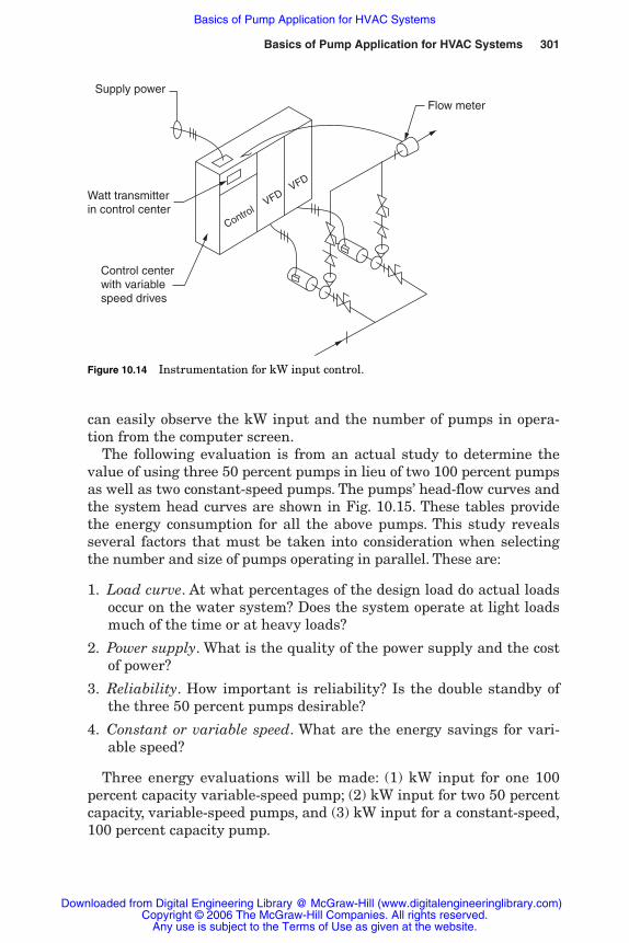
Basics of Pump Application for HVAC Systems 301
can easily observe the kW input and the number of pumps in opera-tion from the computer screen.
The following evaluation is from an actual study to determine thevalue of using three 50 percent pumps in lieu of two 100 percent pumpsas well as two constant-speed pumps. The pumps’ head-flow curves andthe system head curves are shown in Fig. 10.15. These tables providethe energy consumption for all the above pumps. This study revealsseveral factors that must be taken into consideration when selectingthe number and size of pumps operating in parallel. These are:
1. Load curve. At what percentages of the design load do actual loadsoccur on the water system? Does the system operate at light loadsmuch of the time or at heavy loads?
2. Power supply. What is the quality of the power supply and the costof power?
3. Reliability. How important is reliability? Is the double standby ofthe three 50 percent pumps desirable?
4. Constant or variable speed. What are the energy savings for vari-able speed?
Three energy evaluations will be made: (1) kW input for one 100percent capacity variable-speed pump; (2) kW input for two 50 percentcapacity, variable-speed pumps, and (3) kW input for a constant-speed,100 percent capacity pump.
Control
VFDVFD
Supply power
Watt transmitterin control center
Control centerwith variablespeed drives
Flow meter
Figure 10.14 Instrumentation for kW input control.
Rishel_CH10.qxd 21/4/06 6:20 PM Page 301
Downloaded from Digital Engineering Library @ McGraw-Hill (www.digitalengineeringlibrary.com)Copyright © 2006 The McGraw-Hill Companies. All rights reserved.
Any use is subject to the Terms of Use as given at the website.
Basics of Pump Application for HVAC Systems
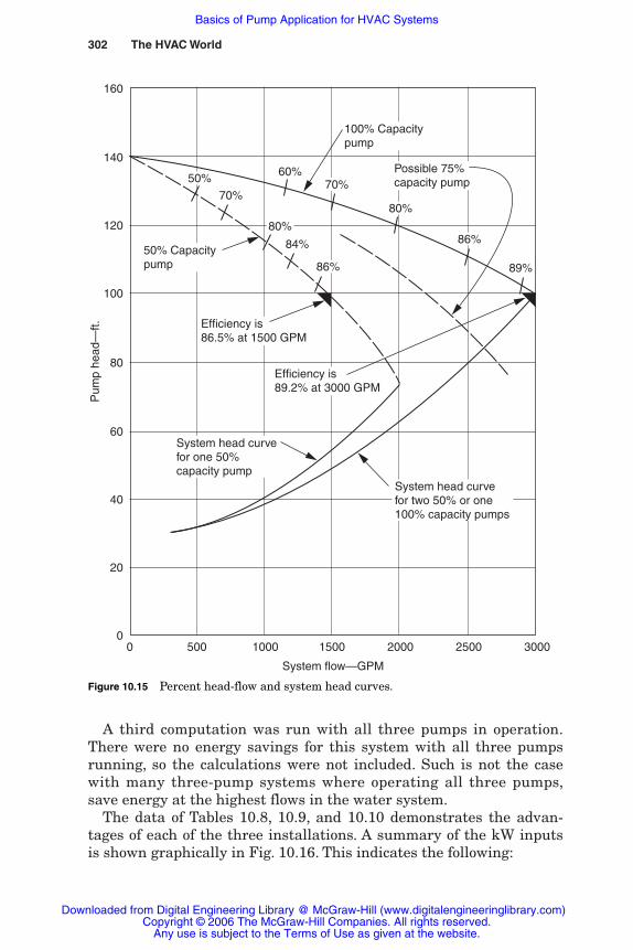
302 The HVAC World
A third computation was run with all three pumps in operation.There were no energy savings for this system with all three pumpsrunning, so the calculations were not included. Such is not the casewith many three-pump systems where operating all three pumps,save energy at the highest flows in the water system.
The data of Tables 10.8, 10.9, and 10.10 demonstrates the advan-tages of each of the three installations. A summary of the kW inputsis shown graphically in Fig. 10.16. This indicates the following:
0 500 1000 1500 2000 2500 3000
System flow—GPM
Pum
p he
ad—
ft.
0
20
40
60
80
100
120
140
160
System head curvefor one 50%capacity pump
System head curvefor two 50% or one100% capacity pumps
Efficiency is86.5% at 1500 GPM
Efficiency is89.2% at 3000 GPM
Possible 75%capacity pump
50% Capacitypump
100% Capacitypump
50%
70%
60%70%
80%
86%
89%
80%
84%
86%
Figure 10.15 Percent head-flow and system head curves.
Rishel_CH10.qxd 21/4/06 6:20 PM Page 302
Downloaded from Digital Engineering Library @ McGraw-Hill (www.digitalengineeringlibrary.com)Copyright © 2006 The McGraw-Hill Companies. All rights reserved.
Any use is subject to the Terms of Use as given at the website.
Basics of Pump Application for HVAC Systems
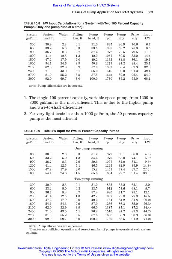
Basics of Pump Application for HVAC Systems 303
1. The single 100 percent capacity, variable-speed pump, from 1200 to3000 gal/min is the most efficient. This is due to the higher pumpand wire-to-shaft efficiencies.
2. For very light loads less than 1000 gal/min, the 50 percent capacitypump is the most efficient.
TABLE 10.8 kW Input Calculations for a System with Two 100 Percent CapacityPumps (Only one pump runs at a time)
System System Water Fitting Pump Pump Pump Drive Inputgal/min head, ft hp loss, ft head, ft rpm effy effy kW
300 30.9 2.3 0.1 31.0 845 36.9 70.6 6.7600 33.2 5.0 0.3 33.5 898 59.2 75.3 8.5900 36.7 8.3 0.7 37.4 972 72.5 79.5 11.0
1200 41.4 12.5 1.3 42.0 1057 80.5 83.2 14.41500 47.2 17.9 2.0 49.2 1162 84.8 86.1 19.11800 54.1 24.6 2.9 50.8 1273 87.2 88.4 25.12100 62.0 32.9 3.9 57.0 1393 88.4 89.9 32.82400 71.0 43.0 5.1 66.0 1516 89.0 91.3 42.42700 81.0 55.2 6.5 87.5 1645 89.2 92.4 54.03000 92.0 69.7 8.0 100.0 1780 89.2 93.0 68.1
NOTE: Pump efficiencies are in percent.
TABLE 10.9 Total kW Input for Two 50 Percent Capacity Pumps
System System Water Fitting Pump Pump Pump Drive Inputgal/min head, ft hp loss, ft head, ft rpm effy effy kW
One pump running
300 30.9 2.3 0.3 31.2 879 59.1 66.0 4.5∗600 33.2 5.0 1.3 34.4 970 83.0 74.1 6.3∗900 36.7 8.3 2.9 39.6 1097 87.0 81.1 9.5∗
1200 41.4 12.5 5.1 46.5 1265 82.9 85.9 14.8∗1500 47.2 17.9 8.0 55.2 1451 77.4 89.2 22.61800 54.1 24.6 11.5 65.6 1654 72.7 91.4 33.5
Two pump running
300 30.9 2.3 0.1 31.0 853 35.2 62.1 8.0600 33.2 5.0 0.3 33.5 912 57.6 68.1 9.7900 36.7 8.3 0.7 37.4 980 71.7 73.1 12.1
1200 41.4 12.5 1.3 42.7 1067 79.8 77.8 15.51500 47.2 17.9 2.0 49.2 1164 84.2 81.8 20.2∗1800 54.1 24.6 2.9 57.0 1266 86.3 85.0 26.3∗2100 62.0 32.9 3.9 66.0 1387 87.1 87.2 34.4∗2400 71.0 43.0 5.1 76.2 1510 87.2 89.3 44.2∗2700 81.0 55.2 6.5 87.5 1638 86.9 90.9 56.3∗3000 92.0 69.7 8.0 100.0 1760 86.5 91.9 71.2∗
NOTE: Pump efficiencies are in percent.∗Denotes most efficient operation and correct number of pumps to operate at each system
gal/min.
Rishel_CH10.qxd 21/4/06 6:20 PM Page 303
Downloaded from Digital Engineering Library @ McGraw-Hill (www.digitalengineeringlibrary.com)Copyright © 2006 The McGraw-Hill Companies. All rights reserved.
Any use is subject to the Terms of Use as given at the website.
Basics of Pump Application for HVAC Systems
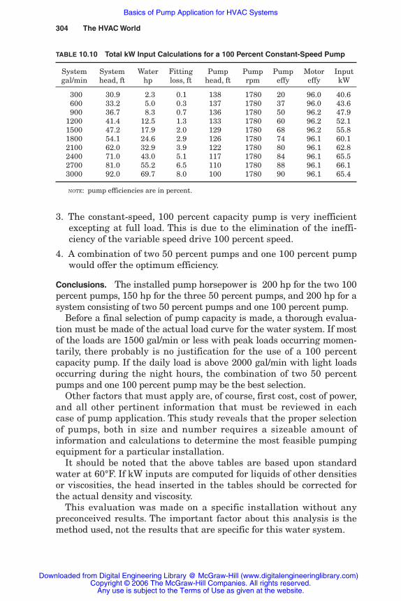
304 The HVAC World
3. The constant-speed, 100 percent capacity pump is very inefficientexcepting at full load. This is due to the elimination of the ineffi-ciency of the variable speed drive 100 percent speed.
4. A combination of two 50 percent pumps and one 100 percent pumpwould offer the optimum efficiency.
Conclusions. The installed pump horsepower is 200 hp for the two 100percent pumps, 150 hp for the three 50 percent pumps, and 200 hp for asystem consisting of two 50 percent pumps and one 100 percent pump.
Before a final selection of pump capacity is made, a thorough evalua-tion must be made of the actual load curve for the water system. If mostof the loads are 1500 gal/min or less with peak loads occurring momen-tarily, there probably is no justification for the use of a 100 percentcapacity pump. If the daily load is above 2000 gal/min with light loadsoccurring during the night hours, the combination of two 50 percentpumps and one 100 percent pump may be the best selection.
Other factors that must apply are, of course, first cost, cost of power,and all other pertinent information that must be reviewed in eachcase of pump application. This study reveals that the proper selectionof pumps, both in size and number requires a sizeable amount ofinformation and calculations to determine the most feasible pumpingequipment for a particular installation.
It should be noted that the above tables are based upon standardwater at 60°F. If kW inputs are computed for liquids of other densitiesor viscosities, the head inserted in the tables should be corrected forthe actual density and viscosity.
This evaluation was made on a specific installation without anypreconceived results. The important factor about this analysis is themethod used, not the results that are specific for this water system.
TABLE 10.10 Total kW Input Calculations for a 100 Percent Constant-Speed Pump
System System Water Fitting Pump Pump Pump Motor Inputgal/min head, ft hp loss, ft head, ft rpm effy effy kW
300 30.9 2.3 0.1 138 1780 20 96.0 40.6600 33.2 5.0 0.3 137 1780 37 96.0 43.6900 36.7 8.3 0.7 136 1780 50 96.2 47.9
1200 41.4 12.5 1.3 133 1780 60 96.2 52.11500 47.2 17.9 2.0 129 1780 68 96.2 55.81800 54.1 24.6 2.9 126 1780 74 96.1 60.12100 62.0 32.9 3.9 122 1780 80 96.1 62.82400 71.0 43.0 5.1 117 1780 84 96.1 65.52700 81.0 55.2 6.5 110 1780 88 96.1 66.13000 92.0 69.7 8.0 100 1780 90 96.1 65.4
NOTE: pump efficiencies are in percent.
Rishel_CH10.qxd 21/4/06 6:20 PM Page 304
Downloaded from Digital Engineering Library @ McGraw-Hill (www.digitalengineeringlibrary.com)Copyright © 2006 The McGraw-Hill Companies. All rights reserved.
Any use is subject to the Terms of Use as given at the website.
Basics of Pump Application for HVAC Systems

Basics of Pump Application for HVAC Systems 305
10.10.1 Total kW input indication and pump programming
Total kW input indication for an actual pumping system can be dis-played easily on the pumping system controller. The operator canobserve the kW input before a pump is added or subtracted.
kW input is an excellent procedure for programming variable-speedpumps in a multiple-pump installation. Rather than waiting for a system
0 500 1000 1500 2000 2500 3000
System flow—GPM
kW In
put
0
10
20
30
40
50
60
70
80
One pump,100% capacity,constant speed
Two pumps,50% capacity,variable speed
One pump50% capacity,variable speed One pump
100% capacity,variable speed
Figure 10.16 kW input for Tables 10.8, 10.9, and 10.10.
Rishel_CH10.qxd 21/4/06 6:20 PM Page 305
Downloaded from Digital Engineering Library @ McGraw-Hill (www.digitalengineeringlibrary.com)Copyright © 2006 The McGraw-Hill Companies. All rights reserved.
Any use is subject to the Terms of Use as given at the website.
Basics of Pump Application for HVAC Systems
306 The HVAC World
condition to start or stop pumps, the kW input control starts or stopsa pump when these actions indicate a possibility of saving energy. Forexample, in Table 10.9 and Fig. 10.16, the data indicates that the sec-ond pump should be started when the system flow reaches 1300gal/min and not wait until 1800 gal/min flow where one pump can nolonger sustain the desired water system conditions. At 1800 gal/min,the kW input with one pump running is 33.5 kW and is 26.3 kW withtwo pumps running. This is a 21 percent savings in energy.
The software of the pump controller can include this control proce-dure to ensure that the most efficient number of pumps is running in amultiple-pump installation. The points of addition and subtraction forpumps are easily adjustable in contemporary pump controllers. One ofthe advantages of this control is the ability of the operators to check thecontrol procedure to ensure that the pump addition and subtractionpoints are correct. This is as follows and assumes that the desired oper-ating pressure is maintained as pumps are added and subtracted.
1. The total kW input should drop when a pump is added. If it increasesinstead, the pump should not have been added, and the set point forpump addition should be increased until the kW input drops or doesnot change when a pump is added.
2. The total kW input should drop when a pump is subtracted. Likethe pump addition, if the kW input increases when a pump is sub-tracted, the point of subtraction should be lowered until the kWinput drops or does not change when subtracting a pump.
This is a very simple procedure even for installations with a multi-ple of large pumps. The operators become familiar with what the kWinput should be at particular flows in the water system and can tellwhen adverse conditions appear.
10.11 Pump Control
Since variable-speed pumps have entered the HVAC market, thereare two aspects to pump control: (1) pump start-stop procedures and(2) pump speed control. These procedures must be developed for bothconstant- and variable-speed pumping systems.
Pump start-stop procedures consist of a number of control techniques:
1. With system activation or shutdown
2. By system demands such as flow or pressure
3. By system energy evaluation such as wire-to-water efficiency orkW input
Rishel_CH10.qxd 21/4/06 6:20 PM Page 306
Downloaded from Digital Engineering Library @ McGraw-Hill (www.digitalengineeringlibrary.com)Copyright © 2006 The McGraw-Hill Companies. All rights reserved.
Any use is subject to the Terms of Use as given at the website.
Basics of Pump Application for HVAC Systems
Basics of Pump Application for HVAC Systems 307
4. By emergencies caused by pump failure
5. Duty sharing such as alternation
Pumping systems can be interfaced easily so that they can bestarted or stopped by the building management system. When achilled or hot water system is actuated, any pumping system involvedcan be started automatically at that time.
10.11.1 Sequencing of pumps on systemdemands of flow or pressure
Multiple-pump systems require care in the addition and subtractionof pumps in order to achieve maximum pumping efficiency from mini-mum to maximum system flow. Items 2 and 3 mentioned previouslylist the procedures used for accomplishing this.
Which procedure is used to sequence multiple pumps can have agreat bearing on the efficiency of the pumping system. There are sev-eral methods of sequencing pumps, and these are:
1. Maximum flow sequencing. This old method let one pump rununtil it could no longer handle the system requirements; the controlsthen started the next pump in the pumping sequence. This has provedto be wasteful in energy because the pump operates far to the right ofthe design point at a poor efficiency. Also, the pump then operates at apoint of high radial or axial thrust with greater wear on bearings,sleeves, and mechanical seals. Maximum flow should be used as abackup control system to maintain system flow on failure of more effi-cient control systems, such as best efficiency or wire-to-water efficiencycontrol. Arbitrarily selecting a percentage of speed of the operatingpumps such as 80 percent to add and subtract pumps does not achievepeak efficiency; this is an attempt to control pumps without evaluatingall the system characteristics that determine operating efficiency.
2. Best efficiency control. Recognizing the problems with maxi-mum flow sequencing, this procedure was developed to eliminate thepreceding inefficient and high-thrust operation with maximum flowsequencing. It has been called best efficiency control because thepumps are sequenced so that they operate as closely as possible totheir best efficiency point. This is achieved by evaluating the systemhead for the proposed system and selecting pump sequencing so thatthe pumps do not “carry out” but operate near their best efficiencypoint. This is demonstrated in Fig. 10.17, a system with two pumpsoperating at design load. With maximum flow sequencing, one pumpcould operate until 167 percent capacity of one pump was reached; atthis point, the pump efficiency would be very low compared with that
Rishel_CH10.qxd 21/4/06 6:20 PM Page 307
Downloaded from Digital Engineering Library @ McGraw-Hill (www.digitalengineeringlibrary.com)Copyright © 2006 The McGraw-Hill Companies. All rights reserved.
Any use is subject to the Terms of Use as given at the website.
Basics of Pump Application for HVAC Systems
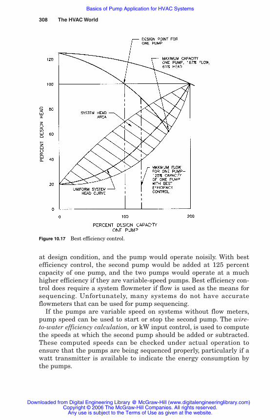
308 The HVAC World
at design condition, and the pump would operate noisily. With bestefficiency control, the second pump would be added at 125 percentcapacity of one pump, and the two pumps would operate at a muchhigher efficiency if they are variable-speed pumps. Best efficiency con-trol does require a system flowmeter if flow is used as the means forsequencing. Unfortunately, many systems do not have accurateflowmeters that can be used for pump sequencing.
If the pumps are variable speed on systems without flow meters,pump speed can be used to start or stop the second pump. The wire-to-water efficiency calculation, or kW input control, is used to computethe speeds at which the second pump should be added or subtracted.These computed speeds can be checked under actual operation toensure that the pumps are being sequenced properly, particularly if awatt transmitter is available to indicate the energy consumption bythe pumps.
Figure 10.17 Best efficiency control.
Rishel_CH10.qxd 21/4/06 6:20 PM Page 308
Downloaded from Digital Engineering Library @ McGraw-Hill (www.digitalengineeringlibrary.com)Copyright © 2006 The McGraw-Hill Companies. All rights reserved.
Any use is subject to the Terms of Use as given at the website.
Basics of Pump Application for HVAC Systems
Basics of Pump Application for HVAC Systems 309
3. Wire-to-water efficiency control. Field experience with best effi-ciency control has proved that pumps still were not being sequencedefficiently under all system conditions. This led to further evaluationof pumping system operation and its refinement by wire-to-water effi-ciency control, which utilizes the procedures listed in the previoussection for wire-to-water indication.
The wire-to-water efficiency determination can be used to selectapproximately the points at which the pumps should be added or sub-tracted. The transition points can be selected from the wire-to-waterefficiency tables and inserted into the pump-control program. Theactual pump operation can be checked by wire-to-water efficiencyindication, and the set points can be changed in the field until thepumps are operating on the most efficient program. How the transi-tion points are secured is shown in Table 10.7, data from an actualtest for wire-to-water efficiency.
The value of wire-to-water efficiency control is shown dramaticallyin Table 10.5. If one pump were allowed to operate as high as 1625gal/min, the input kilowatts would be 28.7 and the wire-to-water effi-ciency 55.1 percent compared with two pumps operating at 1625gal/min with an input kilowatts of 22.3 and a wire-to-water efficiencyof 70.6 percent.
4. kW input control. This control is described previously. Adaptivecontrol accomplishes the same adjustment in the set point, establishedto stop one of the running pumps. Typical use of adaptive control occursin chilled water systems with a sizeable system head area, Fig. 10.18;this is for the model building of Chap. 9 and Fig. 9.3. It is impossible toestablish a simple set point based upon one rate of system flow on asystem with such an appreciable system head area.
Adaptive control will be used in other control procedures herein,such as variable condenser water temperature and add-subtractpoints for boilers and chillers.
5. Adaptive control. The perfection of digital control has resultedin the use of adaptive control to adjust set points to variable condi-tions. As has been demonstrated in a number of figures in this book,transition from one to two pumps, two to three pumps, and so forthcan be accomplished by wire-to-water efficiency or kW input control.With adaptive control, the actual point of transition, such as 1100gal/min in Fig. 10.19, can be continuously adjusted to secure the opti-mum point of transition. This is accomplished by sensing the changein kW input as transition is made, say from one to two pumps. If thekW increases, the second pump should not be added. The next time therequirement for a pump addition occurs, the adaptive control proce-dure adjusts the set point up to 1300 gal/min as shown in Fig. 10.19.
Rishel_CH10.qxd 21/4/06 6:20 PM Page 309
Downloaded from Digital Engineering Library @ McGraw-Hill (www.digitalengineeringlibrary.com)Copyright © 2006 The McGraw-Hill Companies. All rights reserved.
Any use is subject to the Terms of Use as given at the website.
Basics of Pump Application for HVAC Systems

310 The HVAC World
Figure 10.18 Adaptive control with system head areas. (Courtesy, tekWorxLLC, Cincinnati, Ohio.)
Two pumps
Calculated kW curves
Calculated pointof addition
One pump
One pump
Actual kW curves
Actual pointof addition
Two pumps
30
20
10
00 200015001000500
System flow—GPM
kW in
put
Figure 10.19 Use of adaptive control for pump sequencing. (Courtesy, tekWorxLLC, Cincinnati, Ohio.)
Rishel_CH10.qxd 21/4/06 6:20 PM Page 310
Downloaded from Digital Engineering Library @ McGraw-Hill (www.digitalengineeringlibrary.com)Copyright © 2006 The McGraw-Hill Companies. All rights reserved.
Any use is subject to the Terms of Use as given at the website.
Basics of Pump Application for HVAC Systems
All this discussion on the efficient control of pumps demonstratesthe great capability now available to HVAC water system designersthrough the use of digital electronics in the evaluation of a water sys-tem and the application of pumps.
10.11.2 Emergency backup on pump failure
Equipment failure is always troublesome, and it should be met in away that will cause the least amount of trouble for the water system.Pump failure must be handled so that the system is not momentarilyout of water. The control system must interrogate operating pumps sothat a standby pump is started when pump failure is sensed, notwhen the water system reacts to the failure of a pump. This may seemto be a minor detail to be included in a pump handbook, but it can bea terrible operating problem if the standby pump control procedure isnot executed properly. Reiterating, pump failure should be sensedimmediately, and the standby pump started then, not waiting for sys-tem pressures to indicate the failure.
10.11.3 Alternation of operating pumps
Over the years of automatic control, almost every conceivable methodof alternating the lead or operating pumps has been used in the pumpindustry. There are systems called “first on, first off” or “last on, firstoff.” There are duty cycle or run time cycles. All these alternationmethods were designed to provide equal wear on all the pumps.
Two facts have resulted from these procedures. First, equal wear isnot necessarily the best procedure. As in several cases with largepumps, all the pumps wore out during the same month and year,causing an emergency repair program because all the pumps failedtogether. Second, automatic alternation in itself allows the operator toneglect the pumps.
A third factor has arisen, and that is the reduction in wear of HVACpumps. The use of variable-speed pumps and factory-assembledpumping systems where pumps are programmed correctly hasreduced the incidence of pump failure. This has resulted in the elimi-nation of most of the preceding alternation cycles. The simplest andcheapest procedure is manual operation by the operator. Equippingthe pump control center with an elapsed time meter for each pumpmotor enables the operator to maintain around 2000 to 4000 operat-ing hours between pumps so that they do not all fail at the same time.More on this subject is included in Chap. 26.
Basics of Pump Application for HVAC Systems 311
Rishel_CH10.qxd 21/4/06 6:20 PM Page 311
Downloaded from Digital Engineering Library @ McGraw-Hill (www.digitalengineeringlibrary.com)Copyright © 2006 The McGraw-Hill Companies. All rights reserved.
Any use is subject to the Terms of Use as given at the website.
Basics of Pump Application for HVAC Systems
10.11.4 Pump speed control
All the preceding discussion has been on programming the pumpsefficiently. The second part of operating variable-speed pumps is con-trol of the pump speed itself. Development of the variable-frequencydrive has greatly changed the design, selection, and operation ofpumps. The resulting variable-speed pump offers many benefits suchas reduced power consumption and lower radial thrusts on the pumpshafts. The variable-speed drives themselves have been reviewed inChap. 7. Contemporary speed control of a pumping system hasevolved over the past 25 years.
The basic control arrangement for these variable-speed pumps con-sists of a water system sensor, a pump controller, and a variable-speeddrive (Fig. 10.20a). In most cases, the water system sensor can be for(1) temperature, (2) differential temperature, (3) pressure, (4) differen-tial pressure, (5) water level, (6) flow, and (7) kilowatts. Special sys-tems may use other physical or calculated values for varying the speedof the pumps.
The pump controller can be of many different configurationsdepending on the response time required to adequately control thepump speed without continual speed changes or hunting. With initialuse of variable-speed drives on HVAC systems, it was assumed thatsince the loads did not change rapidly on these water systems, therewas no need for rapid speed regulation of the pumps. It was learnedduring actual operation of these pumps on HVAC systems that rapidspeed regulation was required, particularly on systems where pres-sure or differential pressure sensors were used to regulate the speedof the pumps. Although the load on these systems was not changingrapidly, pressure waves within the water systems created changes atthe sensors that caused speed changes. Also, with digital control,after computation of the Propotional-Integral-Derivative error, anoutput signal is given the variable-speed drive to increase ordecrease the speed of the pump. PID error for proportional-integral-derivative control is the difference between the setpoint and theprocess value. This increase or decrease continues until the next sig-nal change. Attempts to reduce the sensitivity of the pump controlonly caused increased variation in the actual pressure or differentialpressure at the point where the sensor was installed. Currently, 500 mshas proved to be an adequate response time for most HVAC variable-speed pumping systems. If HVAC variable-speed pumps continuouslychange their speed, the response time is inadequate, or another controlproblem exists! Properly controlled variable-speed pumps in thisindustry should not change their speed so that the changes areeither visible or audible.
312 The HVAC World
Rishel_CH10.qxd 21/4/06 6:20 PM Page 312
Downloaded from Digital Engineering Library @ McGraw-Hill (www.digitalengineeringlibrary.com)Copyright © 2006 The McGraw-Hill Companies. All rights reserved.
Any use is subject to the Terms of Use as given at the website.
Basics of Pump Application for HVAC Systems
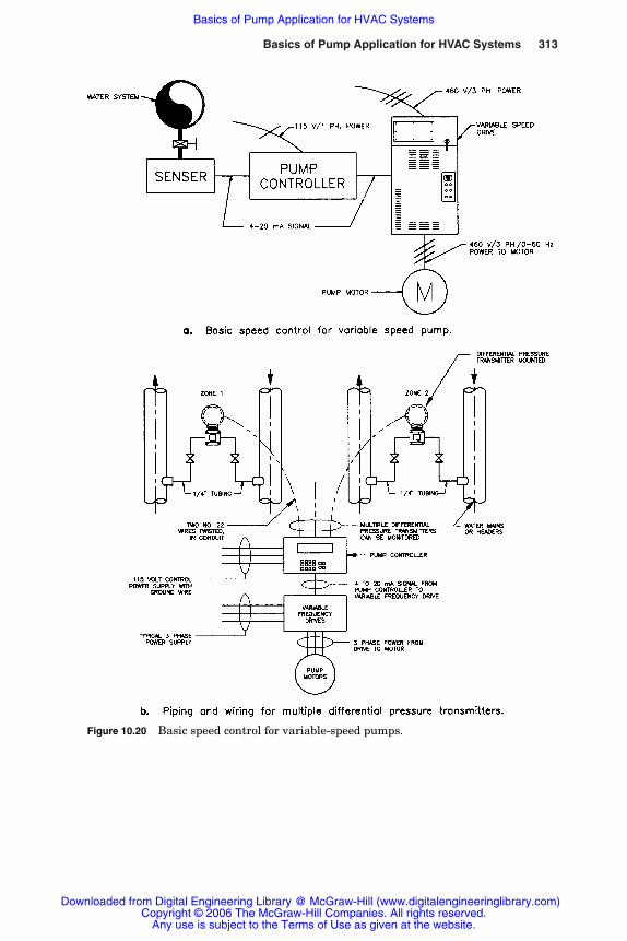
Basics of Pump Application for HVAC Systems 313
Figure 10.20 Basic speed control for variable-speed pumps.
Rishel_CH10.qxd 21/4/06 6:20 PM Page 313
Downloaded from Digital Engineering Library @ McGraw-Hill (www.digitalengineeringlibrary.com)Copyright © 2006 The McGraw-Hill Companies. All rights reserved.
Any use is subject to the Terms of Use as given at the website.
Basics of Pump Application for HVAC Systems
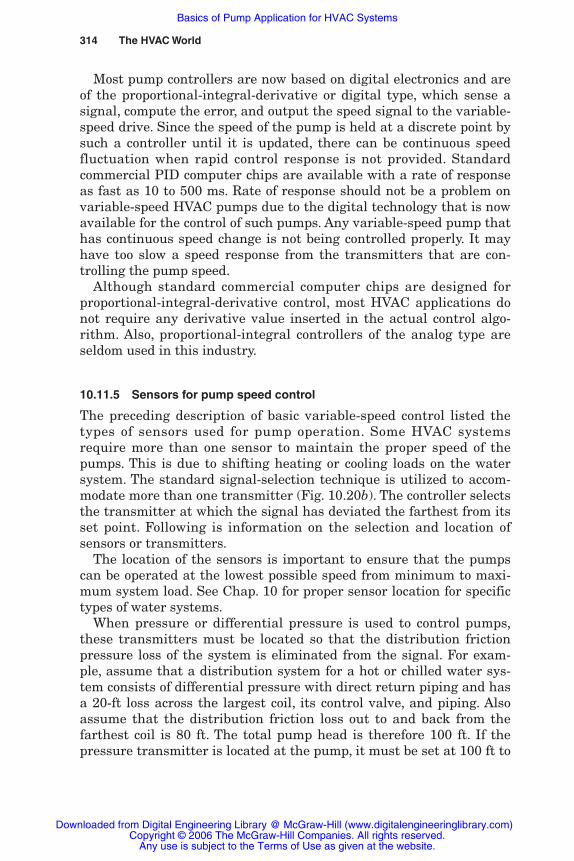
Most pump controllers are now based on digital electronics and areof the proportional-integral-derivative or digital type, which sense asignal, compute the error, and output the speed signal to the variable-speed drive. Since the speed of the pump is held at a discrete point bysuch a controller until it is updated, there can be continuous speedfluctuation when rapid control response is not provided. Standardcommercial PID computer chips are available with a rate of responseas fast as 10 to 500 ms. Rate of response should not be a problem onvariable-speed HVAC pumps due to the digital technology that is nowavailable for the control of such pumps. Any variable-speed pump thathas continuous speed change is not being controlled properly. It mayhave too slow a speed response from the transmitters that are con-trolling the pump speed.
Although standard commercial computer chips are designed forproportional-integral-derivative control, most HVAC applications donot require any derivative value inserted in the actual control algo-rithm. Also, proportional-integral controllers of the analog type areseldom used in this industry.
10.11.5 Sensors for pump speed control
The preceding description of basic variable-speed control listed thetypes of sensors used for pump operation. Some HVAC systemsrequire more than one sensor to maintain the proper speed of thepumps. This is due to shifting heating or cooling loads on the watersystem. The standard signal-selection technique is utilized to accom-modate more than one transmitter (Fig. 10.20b). The controller selectsthe transmitter at which the signal has deviated the farthest from itsset point. Following is information on the selection and location ofsensors or transmitters.
The location of the sensors is important to ensure that the pumpscan be operated at the lowest possible speed from minimum to maxi-mum system load. See Chap. 10 for proper sensor location for specifictypes of water systems.
When pressure or differential pressure is used to control pumps,these transmitters must be located so that the distribution frictionpressure loss of the system is eliminated from the signal. For exam-ple, assume that a distribution system for a hot or chilled water sys-tem consists of differential pressure with direct return piping and hasa 20-ft loss across the largest coil, its control valve, and piping. Alsoassume that the distribution friction loss out to and back from thefarthest coil is 80 ft. The total pump head is therefore 100 ft. If thepressure transmitter is located at the pump, it must be set at 100 ft to
314 The HVAC World
Rishel_CH10.qxd 21/4/06 6:20 PM Page 314
Downloaded from Digital Engineering Library @ McGraw-Hill (www.digitalengineeringlibrary.com)Copyright © 2006 The McGraw-Hill Companies. All rights reserved.
Any use is subject to the Terms of Use as given at the website.
Basics of Pump Application for HVAC Systems
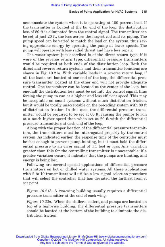
accommodate the system when it is operating at 100 percent load. Ifthe transmitter is located at the far end of the loop, the distributionloss of 80 ft is eliminated from the control signal. The transmitter canbe set at just 20 ft, the loss across the largest coil and its piping. Thepump speed can be varied to match the load on the system, thus sav-ing appreciable energy by operating the pump at lower speeds. Thepump will operate with less radial thrust and have less repair.
The water system just described is of the direct return type; if itwere of the reverse return type, differential pressure transmitterswould be required at both ends of the distribution loop. Both thedirect and reverse return systems and their transmitter locations areshown in Fig. 10.21a. With variable loads in a reverse return loop, ifall the loads are located at one end of the loop, the differential pres-sure transmitter located at the other end will not provide adequatecontrol. One transmitter can be located at the center of the loop, butone-half the distribution loss must be set into the control signal, thusforcing the pump to run at a higher and less efficient speed. This maybe acceptable on small systems without much distribution friction,but it would be totally unacceptable on the preceding system with 80 ftof distribution friction. In this case, the differential pressure trans-mitter would be required to be set at 60 ft, causing the pumps to runat a much higher speed than when set at 20 ft with the differentialpressure transmitters at each end of the loop.
Along with the proper location of the differential pressure transmit-ters, the transmitters must be interrogated properly by the controlsystem. As indicated earlier, the response time of the controller mustbe fast enough to prevent pump hunting, but it must hold the differ-ential pressure to an error signal of �1 foot or less. Any variationgreater than this for the controlling transmitter is unacceptable; if agreater variation occurs, it indicates that the pumps are hunting, andenergy is being lost.
Following are several special applications of differential pressuretransmitters on hot or chilled water systems. All these applicationswith 2 to 10 transmitters will utilize a low signal selection procedurethat will select the controller that has deviated the farthest from itset point.
Figure 10.21b. A two-wing building usually requires a differentialpressure transmitter at the end of each wing.
Figure 10.22a. When the chillers, boilers, and pumps are located ontop of a high-rise building, the differential pressure transmittersshould be located at the bottom of the building to eliminate the dis-tribution friction.
Basics of Pump Application for HVAC Systems 315
Rishel_CH10.qxd 21/4/06 6:20 PM Page 315
Downloaded from Digital Engineering Library @ McGraw-Hill (www.digitalengineeringlibrary.com)Copyright © 2006 The McGraw-Hill Companies. All rights reserved.
Any use is subject to the Terms of Use as given at the website.
Basics of Pump Application for HVAC Systems
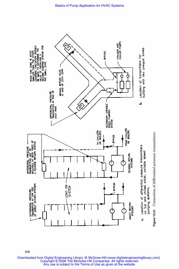
316
Fig
ure
10.
21C
onn
ecti
on o
f di
ffer
enti
al p
ress
ure
tra
nsm
itte
rs.
Rishel_CH10.qxd 21/4/06 6:20 PM Page 316
Downloaded from Digital Engineering Library @ McGraw-Hill (www.digitalengineeringlibrary.com)Copyright © 2006 The McGraw-Hill Companies. All rights reserved.
Any use is subject to the Terms of Use as given at the website.
Basics of Pump Application for HVAC Systems
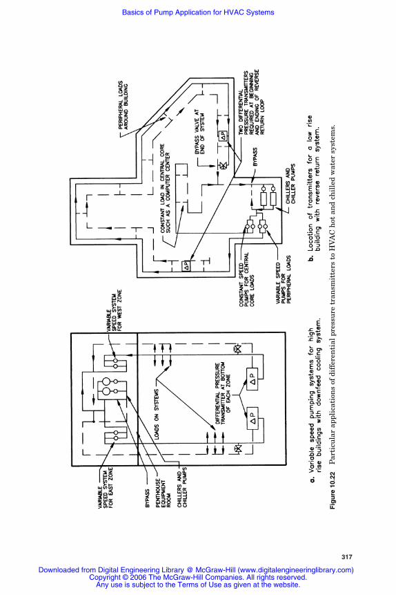
317
Fig
ure
10.
22P
arti
cula
r ap
plic
atio
ns
of d
iffe
ren
tial
pre
ssu
re t
ran
smit
ters
to
HV
AC
hot
an
d ch
ille
d w
ater
sys
tem
s.
Rishel_CH10.qxd 21/4/06 6:20 PM Page 317
Downloaded from Digital Engineering Library @ McGraw-Hill (www.digitalengineeringlibrary.com)Copyright © 2006 The McGraw-Hill Companies. All rights reserved.
Any use is subject to the Terms of Use as given at the website.
Basics of Pump Application for HVAC Systems
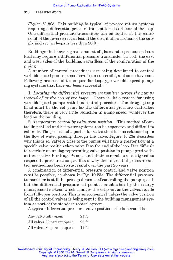
Figure 10.22b. This building is typical of reverse return systemsrequiring a differential pressure transmitter at each end of the loop.One differential pressure transmitter can be located at the centerpoint of the reverse return loop if the distribution friction of the sup-ply and return loops is less than 20 ft.
Buildings that have a great amount of glass and a pronounced sunload may require a differential pressure transmitter on both the eastand west sides of the building, regardless of the configuration of thepiping.
A number of control procedures are being developed to controlvariable-speed pumps; some have been successful, and some have not.Following are control techniques for loop-type variable-speed pump-ing systems that have not been successful:
1. Locating the differential pressure transmitter across the pumpsinstead of at the end of the loops. There is little reason for usingvariable-speed pumps with this control procedure. The design pumphead must be the set point for the differential pressure controller;therefore, there is very little reduction in pump speed, whatever theload on the building.
2. Temperature control by valve stem position. This method of con-trolling chilled and hot water systems can be expensive and difficult tocalibrate. The position of a particular valve stem has no relationship tothe flow of water passing through the valve. Figure 10.23a describeswhy this is so. Valve A close to the pumps will have a greater flow at aspecific valve position than valve B at the end of the loop. It is difficultto correlate an analog representing valve position to pump speed with-out excessive hunting. Pumps and their controls are designed torespond to pressure changes; this is why the differential pressure con-trol method has been so successful over the past 25 years.
A combination of differential pressure control and valve positionreset is possible, as shown in Fig. 10.23b. The differential pressuretransmitter is still the principal means of controlling the pump speed,but the differential pressure set point is established by the energymanagement system, which changes the set point as the valves recedefrom full-open position. This is uneconomical unless the valve positionof all the control valves is being sent to the building management sys-tem as part of the standard control system.
A typical differential pressure–valve position schedule would be
Any valve fully open: 25 ft
All valves 90 percent open: 22 ft
All valves 80 percent open: 19 ft
318 The HVAC World
Rishel_CH10.qxd 21/4/06 6:20 PM Page 318
Downloaded from Digital Engineering Library @ McGraw-Hill (www.digitalengineeringlibrary.com)Copyright © 2006 The McGraw-Hill Companies. All rights reserved.
Any use is subject to the Terms of Use as given at the website.
Basics of Pump Application for HVAC Systems
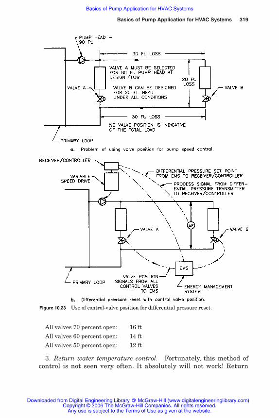
All valves 70 percent open: 16 ft
All valves 60 percent open: 14 ft
All valves 50 percent open: 12 ft
3. Return water temperature control. Fortunately, this method ofcontrol is not seen very often. It absolutely will not work! Return
Basics of Pump Application for HVAC Systems 319
Figure 10.23 Use of control-valve position for differential pressure reset.
Rishel_CH10.qxd 21/4/06 6:20 PM Page 319
Downloaded from Digital Engineering Library @ McGraw-Hill (www.digitalengineeringlibrary.com)Copyright © 2006 The McGraw-Hill Companies. All rights reserved.
Any use is subject to the Terms of Use as given at the website.
Basics of Pump Application for HVAC Systems

water temperature has no relationship to system load on variable-volume systems; it should be maintained as closely as possible to aconstant value. For example, a chilled water system operating with44°F supply temperature and 56°F return temperature should holdthese temperatures whether the load is heavy or light on the system. There-fore, return temperature cannot possibly be used as a control parameter forvariable-speed pumping. Often there has been confusion of variablereturn water temperature that results from the use of three-wayvalves; these systems were, of course, constant-volume systems andnot used with variable-speed pumps for most applications.
10.11.6 Communication from remote transmitters
The method of communication with remote transmitters is particu-larly important to ensure that a noninterrupted signal is received atthe pump controller at the rate of response specified by the pump con-trol manufacturer. The route that the signal takes is of importance tothe water system designer.
Most signals from remote transmitters are direct current and 4 to20 mA in strength. These signals must be protected from electromag-netic and radiofrequency interference. Therefore, the interconnectingcabling must be shielded and grounded at the pump controller end.Table 10.11 provides typical distances between the transmitter andthe pump controller that can be used with various sizes of wire.
These cables can be installed in conduit or cable trays that carryother instrument, data, or telephone signals. They must be shieldedfor electromagnetic and radio frequency interference, and the shieldmust be grounded at the end of the cable near the pumping systemcontroller.
On some large installations, the cable installation for pump controlcan become expensive; an alternate procedure is to install modems
320 The HVAC World
TABLE 10.11 Maximum LinearDistances for Transmitters from PumpControllers
Wire size, AWG Linear distance, ft
16 20,00018 11,00020 800022 500024 350026 2000
Rishel_CH10.qxd 21/4/06 6:20 PM Page 320
Downloaded from Digital Engineering Library @ McGraw-Hill (www.digitalengineeringlibrary.com)Copyright © 2006 The McGraw-Hill Companies. All rights reserved.
Any use is subject to the Terms of Use as given at the website.
Basics of Pump Application for HVAC Systems

at the remote differential pressure transmitter and at the pumpingsystem. This procedure allows the use of ordinary telephone cables fortransmission of the control signals.
Care should be taken to avoid routing the control signals throughbuilding management systems that reduce the rate of response fromthe transmitter; the signal and data load on these central manage-ment systems may be such that the transmitter signal for pumpspeed control cannot be processed faster than 2 to 4 seconds. This istoo slow for accurate pump speed control. This must not occur rou-tinely or when the central management system is responding to emer-gency conditions such as fire or building power failure.
10.12 Effects of Water Systems on Pump Performance
The pump is the heart of every water system; when it fails, the sys-tem fails. Unfortunately, many times pump failure is due to the watersystem’s effects on the pump’s performance and physical condition.The problems with cavitation and entrained air on pump performanceand damage have already been discussed in Chap. 6.
Other deleterious effects on pumps are control systems that forcepumps to run in the high-thrust areas, namely, at very low or highflow rates. The pump wears rapidly, and it is not the pump’s fault.
One of the most disastrous practices in pump application is theinstallation of a relief valve on a pump discharge that returns thewater to the pump suction, as shown in Fig. 10.24a. It should beremembered that the thermal equivalent of a brake horsepower is2544 Btu/h. All the energy destroyed by the relief valve is returned tothe pump suction. If the system is operating at low loads, where theflow through the pump is low, it is very apparent that heat will builduntil the pump can become very hot. Also, hot water will surgethrough the system when the flow does increase.
Relief valves should be avoided wherever possible on chilled watersystems because every brake horsepower destroyed by the relief valveadds one-fifth of a ton load on the chillers. If there is no other way tocontrol the water through the system than by a relief valve, it shouldbe connected as shown in Fig. 10.24b. The heat is returned to thechiller, and the pump continues to receive and deliver chilled water.
Heating and cooling coils that are dirty on the air or water side orare operating with laminar flow increase the system flow beyond thedesign flow rates. Often pumps are blamed for their inability to providethese greater flows; good system control is the answer for many systemproblems that cause unnecessary pump wear and maintenance.
Basics of Pump Application for HVAC Systems 321
Rishel_CH10.qxd 21/4/06 6:20 PM Page 321
Downloaded from Digital Engineering Library @ McGraw-Hill (www.digitalengineeringlibrary.com)Copyright © 2006 The McGraw-Hill Companies. All rights reserved.
Any use is subject to the Terms of Use as given at the website.
Basics of Pump Application for HVAC Systems
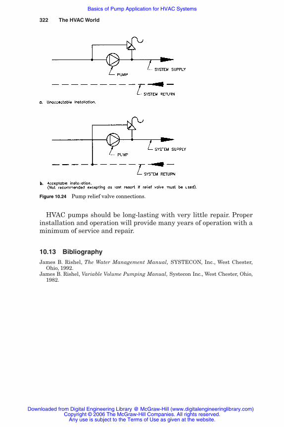
HVAC pumps should be long-lasting with very little repair. Properinstallation and operation will provide many years of operation with aminimum of service and repair.
10.13 Bibliography
James B. Rishel, The Water Management Manual, SYSTECON, Inc., West Chester,Ohio, 1992.
James B. Rishel, Variable Volume Pumping Manual, Systecon Inc., West Chester, Ohio,1982.
322 The HVAC World
Figure 10.24 Pump relief valve connections.
Rishel_CH10.qxd 21/4/06 6:20 PM Page 322
Downloaded from Digital Engineering Library @ McGraw-Hill (www.digitalengineeringlibrary.com)Copyright © 2006 The McGraw-Hill Companies. All rights reserved.
Any use is subject to the Terms of Use as given at the website.
Basics of Pump Application for HVAC Systems

Pumps for Open HVACCooling Systems
Part
4
Rishel_CH11.qxd 20/4/06 6:37 PM Page 323
Downloaded from Digital Engineering Library @ McGraw-Hill (www.digitalengineeringlibrary.com)Copyright © 2006 The McGraw-Hill Companies. All rights reserved.
Any use is subject to the Terms of Use as given at the website.
Source: HVAC Pump Handbook

Rishel_CH11.qxd 20/4/06 6:37 PM Page 324
Downloaded from Digital Engineering Library @ McGraw-Hill (www.digitalengineeringlibrary.com)Copyright © 2006 The McGraw-Hill Companies. All rights reserved.
Any use is subject to the Terms of Use as given at the website.
Pumps for Open HVAC Cooling Systems

Chapter
325
11Open Cooling Tower Pumps
11.1 Introduction
Most of the air-conditioning systems in the HVAC industry or processcooling systems having a net cooling capacity in excess of approxi-mately 4,000,000 Btu /h (333 tons) transmit the heat load to theatmosphere evaporatively through an open cooling tower. Evaporatinga pound of water removes around 1000 Btu from the remaining water.This equates to about 1 percent of the water flow being evaporated tocool the balance of the water over a temperature difference of 10°F atdesign conditions. This is in contrast to the “once-through” water cool-ing systems (100 percent makeup), in which only 10 Btu are removedwhen 1 lb of water is cooled 10°F.
Cooling towers were developed to take the place of lakes and sprayponds, which required considerable space to accomplish the sameamount of evaporative heat transfer. The cooling tower industry pros-pered as system owners and operators were told that water was avaluable commodity that should not be wasted. Once-through watercooling systems have been outlawed in many parts of the world.
Since the evaporative process depends on wet-bulb temperature, awater-cooled refrigerant condenser is significantly more efficient thanan air-cooled condenser. The air-cooled condenser must be designedfor the highest dry-bulb temperature that will be encountered on eachspecific application.
Cooling towers have been the subject of much research to achievethe most efficient operation and the maximum amount of capacityper cubic foot of tower volume. Cooling towers are normally rated intons of cooling, 12,000 Btu/ton. Alternate ratings are in gallons per
Rishel_CH11.qxd 20/4/06 6:37 PM Page 325
Downloaded from Digital Engineering Library @ McGraw-Hill (www.digitalengineeringlibrary.com)Copyright © 2006 The McGraw-Hill Companies. All rights reserved.
Any use is subject to the Terms of Use as given at the website.
Source: HVAC Pump Handbook
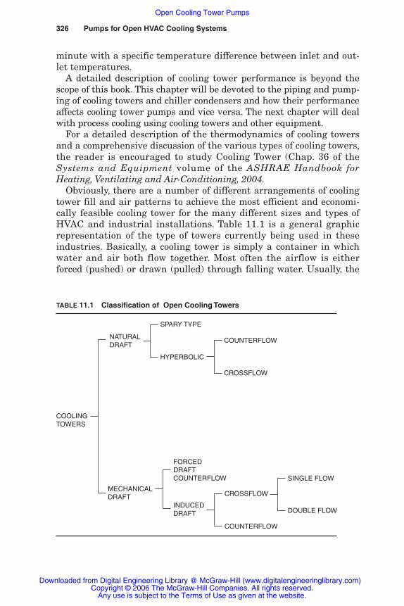
326 Pumps for Open HVAC Cooling Systems
minute with a specific temperature difference between inlet and out-let temperatures.
A detailed description of cooling tower performance is beyond thescope of this book. This chapter will be devoted to the piping and pump-ing of cooling towers and chiller condensers and how their performanceaffects cooling tower pumps and vice versa. The next chapter will dealwith process cooling using cooling towers and other equipment.
For a detailed description of the thermodynamics of cooling towersand a comprehensive discussion of the various types of cooling towers,the reader is encouraged to study Cooling Tower (Chap. 36 of theSystems and Equipment volume of the ASHRAE Handbook forHeating, Ventilating and Air-Conditioning, 2004.
Obviously, there are a number of different arrangements of coolingtower fill and air patterns to achieve the most efficient and economi-cally feasible cooling tower for the many different sizes and types ofHVAC and industrial installations. Table 11.1 is a general graphicrepresentation of the type of towers currently being used in theseindustries. Basically, a cooling tower is simply a container in whichwater and air both flow together. Most often the airflow is eitherforced (pushed) or drawn (pulled) through falling water. Usually, the
TABLE 11.1 Classification of Open Cooling Towers
COOLINGTOWERS
NATURALDRAFT
SPARY TYPE
HYPERBOLIC
COUNTERFLOW
CROSSFLOW
MECHANICALDRAFT
FORCEDDRAFTCOUNTERFLOW
INDUCEDDRAFT
CROSSFLOW
COUNTERFLOW
SINGLE FLOW
DOUBLE FLOW
Rishel_CH11.qxd 20/4/06 6:37 PM Page 326
Downloaded from Digital Engineering Library @ McGraw-Hill (www.digitalengineeringlibrary.com)Copyright © 2006 The McGraw-Hill Companies. All rights reserved.
Any use is subject to the Terms of Use as given at the website.
Open Cooling Tower Pumps

Open Cooling Tower Pumps 327
falling water cascades over various types of fill or media that arespecifically designed to slow the water fall rate and thus increase thetime that the water is in contact with the air; this increases the evap-orative process. There are special types of cooling towers that use nei-ther media (fill) or air-moving systems (fans). The largest cooling tow-ers without fans are the hyperbolic towers most often associated withelectrical generating plants. The most basic categorization of towers isby the method used for air movement through the tower, whether nat-ural or mechanical draft.
Cooling towers also can be characterized as to whether they arefactory assembled or field erected and can be divided into variousshapes such as rectilinear, round, or octagonal. Some cooling towersare described by their basic material of construction, such as ceramictowers.
11.1.1 Cooling tower fans
Cooling tower fans, until recently, were always constant speed or two-speed. The availability and cost of variable-speed drives has made themeconomical on many cooling tower installations. Some of the operatingproblems with cooling towers have disappeared with the ability toadjust the fan speed to the actual operating condition. This hasresulted in more precise control of the leaving water temperature.
11.2 Water Flow Conditions for Cooling Towers
A cooling tower has a very specific range of flow that provides accept-able performance. This flow range can be only 80 to 100 percent ofdesign flow on most cooling towers. Some towers can have their flowranges extended by the manufacturer making modifications in thecooling tower’s water distribution system. If the actual flow rate is lessor greater than the specified range, operating problems will develop;the water flow through the tower can become nonuniform with unevenairflow. It is the responsibility of the designer to ensure that the flowrate of the water system meets the needs of the cooling tower.
Matching the pump to the cooling tower may compromise otherdesign requirements such as the flow rates required by chiller con-densers. It must be recognized that this dichotomy exists, and thewater system design must satisfy both the flow rate of the using equip-ment and that of the cooling towers. Revelation of this fact has led tothe development of a number of different chiller sumps and pumpingarrangements that satisfy both the tower and the equipment using thetower water. Some of these solutions are provided later in this chapter.
Rishel_CH11.qxd 20/4/06 6:37 PM Page 327
Downloaded from Digital Engineering Library @ McGraw-Hill (www.digitalengineeringlibrary.com)Copyright © 2006 The McGraw-Hill Companies. All rights reserved.
Any use is subject to the Terms of Use as given at the website.
Open Cooling Tower Pumps
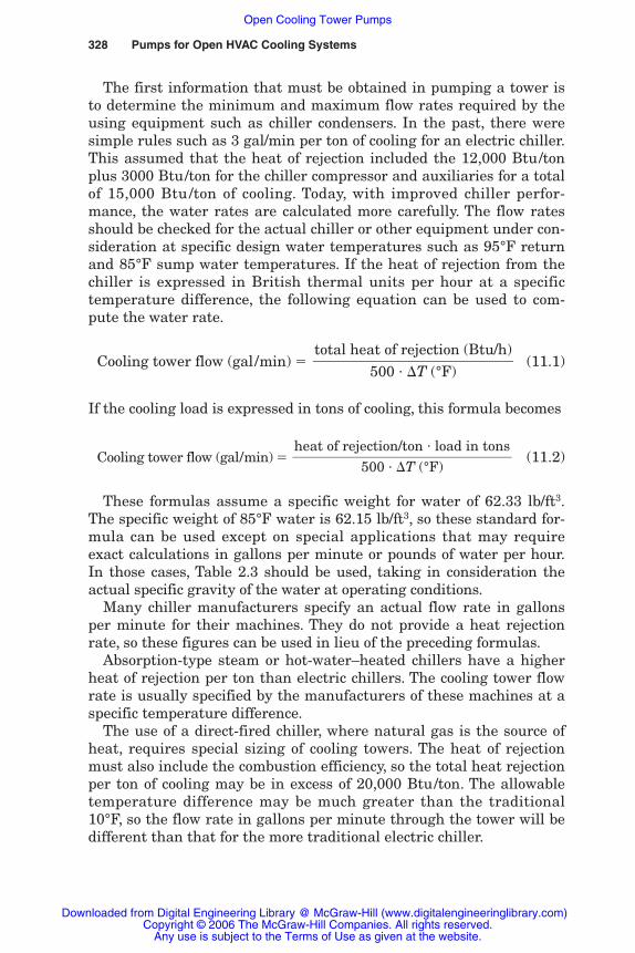
328 Pumps for Open HVAC Cooling Systems
The first information that must be obtained in pumping a tower isto determine the minimum and maximum flow rates required by theusing equipment such as chiller condensers. In the past, there weresimple rules such as 3 gal/min per ton of cooling for an electric chiller.This assumed that the heat of rejection included the 12,000 Btu/tonplus 3000 Btu/ton for the chiller compressor and auxiliaries for a totalof 15,000 Btu /ton of cooling. Today, with improved chiller perfor-mance, the water rates are calculated more carefully. The flow ratesshould be checked for the actual chiller or other equipment under con-sideration at specific design water temperatures such as 95°F returnand 85°F sump water temperatures. If the heat of rejection from thechiller is expressed in British thermal units per hour at a specifictemperature difference, the following equation can be used to com-pute the water rate.
Cooling tower flow (gal/min) � (11.1)
If the cooling load is expressed in tons of cooling, this formula becomes
Cooling tower flow (gal/min) � (11.2)
These formulas assume a specific weight for water of 62.33 lb/ft3.The specific weight of 85°F water is 62.15 lb/ft3, so these standard for-mula can be used except on special applications that may requireexact calculations in gallons per minute or pounds of water per hour.In those cases, Table 2.3 should be used, taking in consideration theactual specific gravity of the water at operating conditions.
Many chiller manufacturers specify an actual flow rate in gallonsper minute for their machines. They do not provide a heat rejectionrate, so these figures can be used in lieu of the preceding formulas.
Absorption-type steam or hot-water–heated chillers have a higherheat of rejection per ton than electric chillers. The cooling tower flowrate is usually specified by the manufacturers of these machines at aspecific temperature difference.
The use of a direct-fired chiller, where natural gas is the source ofheat, requires special sizing of cooling towers. The heat of rejectionmust also include the combustion efficiency, so the total heat rejectionper ton of cooling may be in excess of 20,000 Btu/ton. The allowabletemperature difference may be much greater than the traditional10°F, so the flow rate in gallons per minute through the tower will bedifferent than that for the more traditional electric chiller.
heat of rejection/ton � load in tons����
500 � �T (°F)
total heat of rejection (Btu/h)����
500 � �T (°F)
Rishel_CH11.qxd 20/4/06 6:37 PM Page 328
Downloaded from Digital Engineering Library @ McGraw-Hill (www.digitalengineeringlibrary.com)Copyright © 2006 The McGraw-Hill Companies. All rights reserved.
Any use is subject to the Terms of Use as given at the website.
Open Cooling Tower Pumps

11.3 Cooling Tower Piping
The most basic and conventional cooling tower pumping system isshown in Fig. 11.1a for one tower cell and one chiller condenser. Thisconfiguration is for a constant-speed pump providing constant flowthrough the chiller condenser. A three-way valve is included in thereturn piping to the tower for cold weather operation; this is a two-position nonthrottling valve. In very cold weather, the pipe to the cool-ing tower may freeze when the water flow is in the bypass position fora long period of time. An alternate way to pipe cooling tower bypassesis shown in Figure 11.1b. The piping is arranged so that the velocityhead of the water is directed toward the bypass valve. Also, this valveshould be sized so that the pressure loss across the bypass valve andthe piping to the chiller sump is relatively low. This results in very lit-tle water being backed up in the tower pipe. For example, if thereturn pipe is 8-in steel carrying 1200 gal/min, the velocity head ofthe water is 0.920 ft of head. If a 10-in bypass valve is installed, thevalve and exit loss to the tower sump should not exceed the velocityhead of the 8-in pipe. An advantage of this two-way valve is the factthat the cooling tower piping drains when the condenser pump isstopped.
Figure 11.1 describes relatively simple pumping installations, sincethe flow through the tower is constant and equal to the needs of thecondenser on the chiller. The tower can be picked directly from a cool-ing tower catalog or through computer software. The tower is sized tothe approach temperature and actual outdoor wet bulb temperatureat design conditions.
The cooling tower should be piped in such a way as to enable it toachieve optimal performance. The piping also must aid the flow oftower water to the using equipment. The water should leave a coolingtower basin so that air entrainment or water vortexing is avoided.Vortexing is discussed in Chap. 6.
Piping for cooling towers has been mostly steel. Recognizing thegreat amount of oxygen carried by this pipe, many designers are nowusing thermoplastic piping. This material is available in sizes up to12 in in diameter. If steel pipe is selected for a cooling tower installa-tion, the pipe should either be coated internally or the friction shouldbe calculated using a 1.2 multiplier on the Darcy-Weisbach dataincluded in Table 3.5.
It has been a tradition to install strainers on the suction side ofcooling tower pumps. As shown in Fig. 11.1, the strainer should beinstalled on the discharge of the pump. The strainer is installed toprotect the tubes in a chiller condenser or process equipment such asa heat exchanger; it is not there to protect the pump. The strainer in
Open Cooling Tower Pumps 329
Rishel_CH11.qxd 20/4/06 6:37 PM Page 329
Downloaded from Digital Engineering Library @ McGraw-Hill (www.digitalengineeringlibrary.com)Copyright © 2006 The McGraw-Hill Companies. All rights reserved.
Any use is subject to the Terms of Use as given at the website.
Open Cooling Tower Pumps

330
Fig
ure
11.
1C
ooli
ng
tow
er p
ipin
g.
Rishel_CH11.qxd 20/4/06 6:37 PM Page 330
Downloaded from Digital Engineering Library @ McGraw-Hill (www.digitalengineeringlibrary.com)Copyright © 2006 The McGraw-Hill Companies. All rights reserved.
Any use is subject to the Terms of Use as given at the website.
Open Cooling Tower Pumps
the cooling tower sump is normally adequate to keep rocks and otherlarge debris out of the pump. A suction strainer on a cooling towerpump hazards a chance that the strainer could be obliterated withalgae; the pump could then overheat and be destroyed before it couldbe stopped. Installing the strainer on the pump discharge protects thepump. If the strainer becomes clogged, the pump will be protectedwith only a small flow through the strainer. The equipment being sup-plied by the cooling tower pump will indicate flow problems longbefore the strainer is totally clogged.
11.4 Location of Cooling Tower Pumps
Cooling tower pumping is not severe duty for centrifugal pumps, butapplying pumps to cooling towers is much more detailed than mostHVAC pump installations. This is caused by the cooling tower loopsbeing open-type water systems with the possibility of oxygen, air-borne dirt, and chemicals existing in the water.
Every cooling tower installation should be checked to ensure thatadequate net positive suction head (NPSH) available exists for thepumps selected for that cooling tower. Chapter 6 provides informationon NPSH and how to calculate the available NPSH. Pumps shouldnot be selected for cooling tower duty without knowing the NPSHrequired by them.
As the NPSH available equation (Eq. 6.8) indicates, the friction inthe suction pipe to end-suction and double-suction pumps should bekept low. The pumps should be located as near as possible to the cool-ing towers; the suction pipe should contain a minimum of pipe fit-tings such as elbows (Fig. 11.2a). If there are doorways between thecooling tower and a chiller, the pump should be located near the cool-ing tower to avoid a loop in the suction piping (Fig. 11.2b). If the cool-ing tower location is such that it is difficult to provide adequate suc-tion conditions for end-suction or double-suction pumps, an alternateis the use of turbine-type pumps located in the cooling tower sump.The cooling tower should not be planned for installation at a specificpoint with the hope that there is a way to pump the water from it.Pumping the cooling tower should be settled before final location ismade for the tower.
Cooling tower pumps should not necessarily be located on the sup-ply side of chiller condensers. On high-rise buildings where there isadequate NPSH available under all load conditions, the condenserpumps can be located on the discharge of the condenser, as shown inFig. 11.3a. This reduces the pressure on the condenser water boxes andmay eliminate the cost of higher-pressure construction. The maximum
Open Cooling Tower Pumps 331
Rishel_CH11.qxd 20/4/06 6:37 PM Page 331
Downloaded from Digital Engineering Library @ McGraw-Hill (www.digitalengineeringlibrary.com)Copyright © 2006 The McGraw-Hill Companies. All rights reserved.
Any use is subject to the Terms of Use as given at the website.
Open Cooling Tower Pumps

332
Fig
ure
11.
2C
ooli
ng
tow
er s
upp
ly p
ipin
g ar
ran
gem
ent.
Rishel_CH11.qxd 20/4/06 6:37 PM Page 332
Downloaded from Digital Engineering Library @ McGraw-Hill (www.digitalengineeringlibrary.com)Copyright © 2006 The McGraw-Hill Companies. All rights reserved.
Any use is subject to the Terms of Use as given at the website.
Open Cooling Tower Pumps
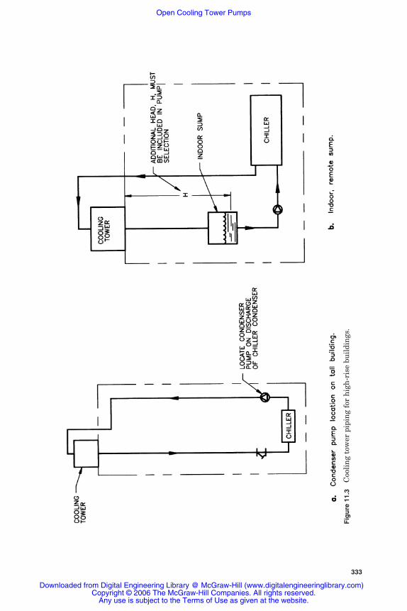
333
Fig
ure
11.
3C
ooli
ng
tow
er p
ipin
g fo
r h
igh
-ris
e bu
ildi
ngs
.
Rishel_CH11.qxd 20/4/06 6:37 PM Page 333
Downloaded from Digital Engineering Library @ McGraw-Hill (www.digitalengineeringlibrary.com)Copyright © 2006 The McGraw-Hill Companies. All rights reserved.
Any use is subject to the Terms of Use as given at the website.
Open Cooling Tower Pumps

334 Pumps for Open HVAC Cooling Systems
static pressure must be calculated to determine the working pressurefor these water boxes.
11.4.1 Remote cooling tower sumps
Many of the problems involved in operating cooling towers in coldweather and with chiller condensers are solved through the use ofspecial cooling tower sumps. These sumps can be located indoors toprevent freezing, as shown in Fig. 11.3b. When the sump is locatedremotely from the tower, as in this figure, the added height Z must beincluded in the pump total dynamic head. This indoor sump musthave a drain-down capacity to handle the water of the system whenthe pump is stopped. Most tower manufacturers provide the drain-down volume in gallons for their towers; to this must be added anypipe capacity that is drained at the same time.
A sump that solves many application problems is the hot-well, cold-well type of Fig. 11.4a. This sump offers freezing protection and alsoseparates the cooling tower loop from the process or chiller loop. Thisprovides maximum flexibility for modulating the heat load that is sentto the cooling tower. The cooling tower receives the correct water flowregardless of the load on the equipment being cooled. A hot-well pumpcirculates the cooling tower, while the process or condenser pump cir-culates the process equipment or the condenser on the chiller. In warmclimates where there is no concern about freezing, the primary-secondary circuiting that is described later in this chapter eliminatesthe need for this sump.
The concrete sump and turbine pump of Fig. 11.4b is the typicalinstallation for large cooling towers. A battery of turbine pumps oper-ating in parallel can develop an efficient flow program with a sub-stantial load range.
Large cooling towers require careful evaluation of the cooling towersump. The intake of water from the sump to the pumps requires cor-rect design to avoid suction problems for the pumps.
The Hydraulic Institute has summarized the entire subject ofintake design in their ANSI/HI 9.8-1998 American National Standardon Pump Intake Design. This document should be considered beforeany serious design is initiated for pump intakes. They have intro-duced a new structure known as a trench-type intake that may sim-plify sump design for large cooling towers, Fig. 11.5. It is urged that adesigner of large cooling tower installations should have a copy of theabove standard to assist in the design of any type sump, whether rec-tangular, circular, or trench configuration.
The exit of water from cooling tower sumps should be designedcarefully to avoid vortexing. Figure 6.16 should be reviewed to ensure
Rishel_CH11.qxd 20/4/06 6:37 PM Page 334
Downloaded from Digital Engineering Library @ McGraw-Hill (www.digitalengineeringlibrary.com)Copyright © 2006 The McGraw-Hill Companies. All rights reserved.
Any use is subject to the Terms of Use as given at the website.
Open Cooling Tower Pumps
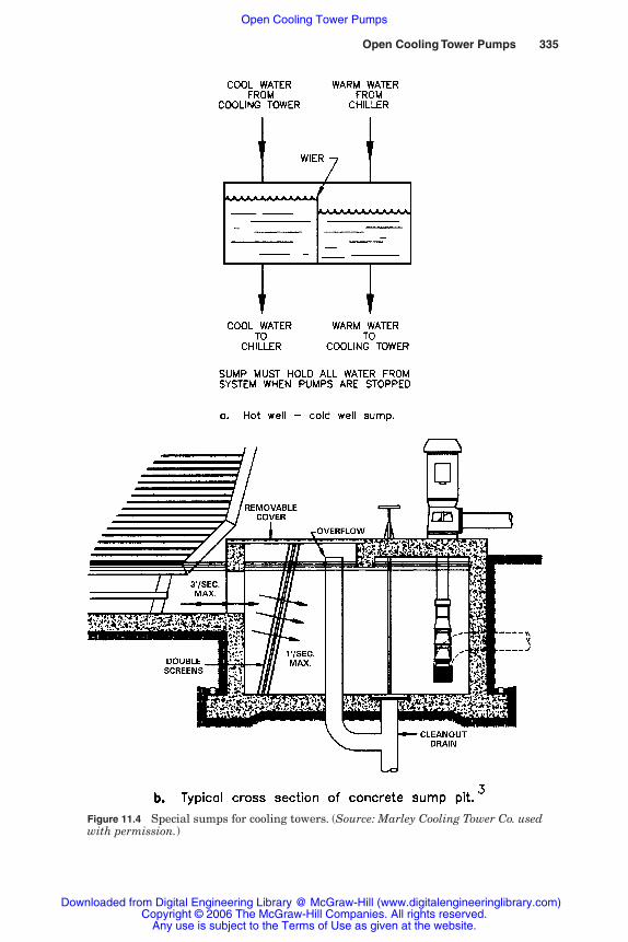
Open Cooling Tower Pumps 335
Figure 11.4 Special sumps for cooling towers. (Source: Marley Cooling Tower Co. usedwith permission.)
Rishel_CH11.qxd 20/4/06 6:37 PM Page 335
Downloaded from Digital Engineering Library @ McGraw-Hill (www.digitalengineeringlibrary.com)Copyright © 2006 The McGraw-Hill Companies. All rights reserved.
Any use is subject to the Terms of Use as given at the website.
Open Cooling Tower Pumps

that the possibility of vortexing is eliminated from the cooling towerwater system.
11.5 Selection and Operation of Condenser Pumps
The selection and operation of condenser pumps for water-cooledchillers embraces a broad range of pump sizes and arrangements. Thesmaller chillers need only constant-speed end-suction pumps with apump for each chiller (Fig. 11.6a). If a standby pump is needed, it canbe added as shown in this figure. Normally, with this installation, acooling tower cell is furnished for each chiller. The programming forthe condenser pumps may consist of just starting and stopping eachpump with its chiller. Headering the condenser pumps as shown inFig. 11.6b is more expensive than the standby pump of Fig. 11.6a. Itrequires another pipe header, and each chiller must be equipped witha two-way automatic shutoff valve. On both these multiple-towerinstallations in cold weather areas, the piping must be arranged toprevent freezing when a tower or tower cell is taken out of service. Abypass valve may be needed for each of the towers or tower cells toprevent freezing in the tower piping.
As chiller installations become larger and consist of different typesof chillers, the pumping procedures become complex and require care-ful and detailed analyses to achieve the most efficient and cost-effective installation. The decision to use base-mounted double-suctionpumps or vertical turbine pumps in the cooling tower sump is a major
336 Pumps for Open HVAC Cooling Systems
Figure 11.5 Trench-type sump as per ANSI/HI 9.8–1998 standard for pump intakedesign.
Maximum Velocity4 ft./sec.
Rishel_CH11.qxd 20/4/06 6:37 PM Page 336
Downloaded from Digital Engineering Library @ McGraw-Hill (www.digitalengineeringlibrary.com)Copyright © 2006 The McGraw-Hill Companies. All rights reserved.
Any use is subject to the Terms of Use as given at the website.
Open Cooling Tower Pumps

337
Fig
ure
11.
6C
onst
ant-
spee
d co
nde
nse
r pu
mps
.
Rishel_CH11.qxd 20/4/06 6:37 PM Page 337
Downloaded from Digital Engineering Library @ McGraw-Hill (www.digitalengineeringlibrary.com)Copyright © 2006 The McGraw-Hill Companies. All rights reserved.
Any use is subject to the Terms of Use as given at the website.
Open Cooling Tower Pumps
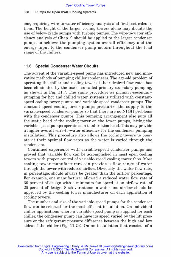
one, requiring wire-to-water efficiency analysis and first-cost calcula-tions. The height of the larger cooling towers alone may dictate theuse of below-grade sumps with turbine pumps. The wire-to-water effi-ciency analysis of Chap. 9 should be applied to the larger condenserpumps to achieve the pumping system overall efficiency and theenergy input to the condenser pump motors throughout the loadrange of the chillers.
11.6 Special Condenser Water Circuits
The advent of the variable-speed pump has introduced new and inno-vative methods of pumping chiller condensers. The age-old problem ofoperating the chiller and cooling tower at their desired flow rates hasbeen eliminated by the use of so-called primary-secondary pumping,as shown in Fig. 11.7. The same procedure as primary-secondarypumping for hot and chilled water systems is utilized with constant-speed cooling tower pumps and variable-speed condenser pumps. Theconstant-speed cooling tower pumps pressurize the supply to thevariable-speed condenser pumps so that there are no NPSH problemswith the condenser pumps. This pumping arrangement also puts allthe static head of the cooling tower on the tower pumps, letting thevariable-speed pumps operate on a total friction head. This may providea higher overall wire-to-water efficiency for the condenser pumpinginstallation. This procedure also allows the cooling towers to oper-ate at their optimal flow rates as the water is varied through thecondensers.
Continued experience with variable-speed condenser pumps hasproved that variable flow can be accomplished in most open coolingtowers with proper control of variable-speed cooling tower fans. Mostcooling tower manufacturers can provide a flow range of waterthrough the tower with reduced airflow. Obviously, the water flow rate,in percentage, should always be greater than the airflow percentage.For example, one manufacturer allowed a reduced water flow rate of30 percent of design with a minimum fan speed at an airflow rate of25 percent of design. Such variations in water and airflow should beapproved by the cooling tower manufacturer on each application ofcooling towers.
The number and size of the variable-speed pumps for the condenserflow can be selected for the most efficient installation. On individualchiller applications where a variable-speed pump is supplied for eachchiller, the condenser pump can have its speed varied by the lift pres-sure or the refrigerant pressure difference between the high and lowsides of the chiller (Fig. 11.7a). On an installation that consists of a
338 Pumps for Open HVAC Cooling Systems
Rishel_CH11.qxd 20/4/06 6:37 PM Page 338
Downloaded from Digital Engineering Library @ McGraw-Hill (www.digitalengineeringlibrary.com)Copyright © 2006 The McGraw-Hill Companies. All rights reserved.
Any use is subject to the Terms of Use as given at the website.
Open Cooling Tower Pumps
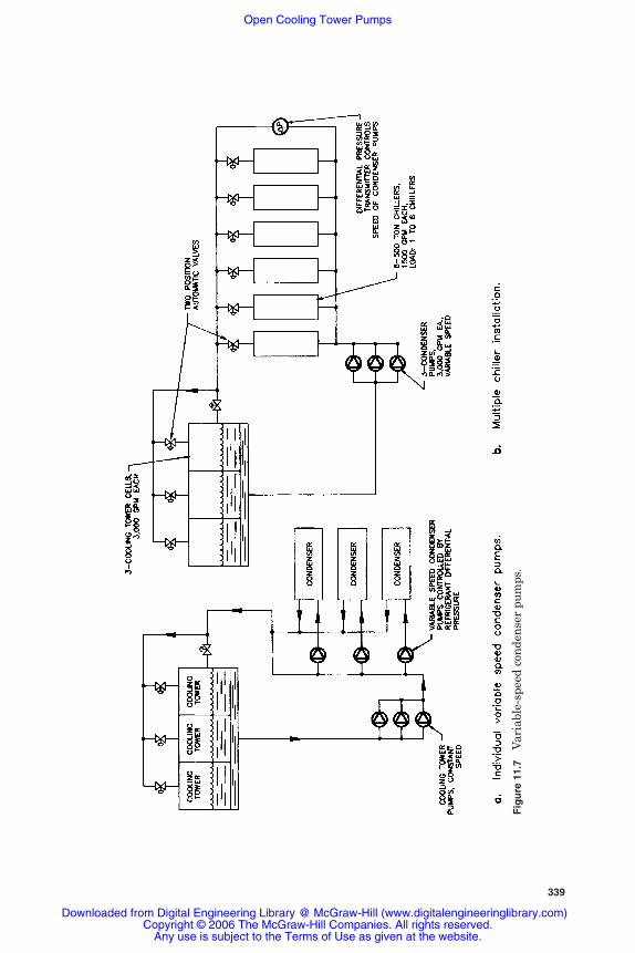
339
Fig
ure
11.
7V
aria
ble-
spee
d co
nde
nse
r pu
mps
.
Rishel_CH11.qxd 20/4/06 6:37 PM Page 339
Downloaded from Digital Engineering Library @ McGraw-Hill (www.digitalengineeringlibrary.com)Copyright © 2006 The McGraw-Hill Companies. All rights reserved.
Any use is subject to the Terms of Use as given at the website.
Open Cooling Tower Pumps

340 Pumps for Open HVAC Cooling Systems
number of chillers (Fig. 11.7b), the variable-speed pumps also can becontrolled by the pressure drop across the condensers. As a chiller isstarted or stopped, the control valve on the chiller condenser watercircuit opens and closes. The optimal number and size of pumpsappear to be three 50 percent system capacity pumps on most of themultiple-chiller applications. Table 11.2 is a tabulated analysis of thepumps for the chillers in Fig. 11.7b.
This wire-to-water efficiency analysis indicates the number ofpumps that should be run with various chillers in operation. Eventhough two pumps are required to handle the maximum load of 9000gal/min, this evaluation indicates that it is more efficient to operateall three pumps at full load.
11.6.1 Operating absorption andcentrifugal chillers together
A problem that the variable-speed pump is solving is the operation ofan absorption and an electric chiller from the same cooling towerinstallation. In the past, this was unacceptable because of the differ-ence in condenser supply water temperatures. The absorptionmachine required fairly constant supply water temperature, while theelectric chiller preferred colder condenser water that improved itsperformance. With variable-speed condenser pumps, the inlet watertemperature to the condenser no longer need be a constant. With vari-able flow through the condenser, the control procedure now is tomaintain the heat balance in the condenser like any other heatexchanger. The variable-speed pump for the electric machine is con-trolled by the lift pressure of the chiller, while the absorption machineis controlled by leaving water temperature and minimum flow. If thecooling tower water drops as low as 60°F, it may be necessary to reset
TABLE 11.2 Pumping System Analysis for Chillers in Fig. 11.6b
Condenser water No. of pumps Wire-to-wireflow, gal/min running System bhp Input kW efficiency, %
1500 1 20.0 17.8 56.6*3000 1 36.6 31.0 68.6*4500 1 66.1 54.1 63.54500 2 60.8 52.1 66.0*6000 2 86.3 72.0 69.8*7500 2 121.3 99.4 70.0*9000 2 167.8 135.7 68.77500 3 122.9 102.5 67.99000 3 161.3 132.7 70.3*
*Optimal number of pumps.
Rishel_CH11.qxd 20/4/06 6:37 PM Page 340
Downloaded from Digital Engineering Library @ McGraw-Hill (www.digitalengineeringlibrary.com)Copyright © 2006 The McGraw-Hill Companies. All rights reserved.
Any use is subject to the Terms of Use as given at the website.
Open Cooling Tower Pumps
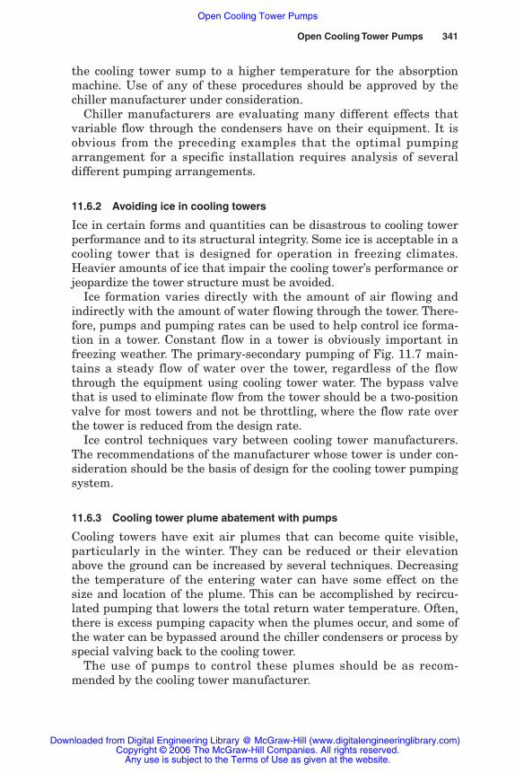
Open Cooling Tower Pumps 341
the cooling tower sump to a higher temperature for the absorptionmachine. Use of any of these procedures should be approved by thechiller manufacturer under consideration.
Chiller manufacturers are evaluating many different effects thatvariable flow through the condensers have on their equipment. It isobvious from the preceding examples that the optimal pumpingarrangement for a specific installation requires analysis of severaldifferent pumping arrangements.
11.6.2 Avoiding ice in cooling towers
Ice in certain forms and quantities can be disastrous to cooling towerperformance and to its structural integrity. Some ice is acceptable in acooling tower that is designed for operation in freezing climates.Heavier amounts of ice that impair the cooling tower’s performance orjeopardize the tower structure must be avoided.
Ice formation varies directly with the amount of air flowing andindirectly with the amount of water flowing through the tower. There-fore, pumps and pumping rates can be used to help control ice forma-tion in a tower. Constant flow in a tower is obviously important infreezing weather. The primary-secondary pumping of Fig. 11.7 main-tains a steady flow of water over the tower, regardless of the flowthrough the equipment using cooling tower water. The bypass valvethat is used to eliminate flow from the tower should be a two-positionvalve for most towers and not be throttling, where the flow rate overthe tower is reduced from the design rate.
Ice control techniques vary between cooling tower manufacturers.The recommendations of the manufacturer whose tower is under con-sideration should be the basis of design for the cooling tower pumpingsystem.
11.6.3 Cooling tower plume abatement with pumps
Cooling towers have exit air plumes that can become quite visible,particularly in the winter. They can be reduced or their elevationabove the ground can be increased by several techniques. Decreasingthe temperature of the entering water can have some effect on thesize and location of the plume. This can be accomplished by recircu-lated pumping that lowers the total return water temperature. Often,there is excess pumping capacity when the plumes occur, and some ofthe water can be bypassed around the chiller condensers or process byspecial valving back to the cooling tower.
The use of pumps to control these plumes should be as recom-mended by the cooling tower manufacturer.
Rishel_CH11.qxd 20/4/06 6:37 PM Page 341
Downloaded from Digital Engineering Library @ McGraw-Hill (www.digitalengineeringlibrary.com)Copyright © 2006 The McGraw-Hill Companies. All rights reserved.
Any use is subject to the Terms of Use as given at the website.
Open Cooling Tower Pumps

342 Pumps for Open HVAC Cooling Systems
11.6.4 Free cooling with cooling tower water
Free cooling is the name applied to processes that use the tower water forcooling chilled water systems instead of the chiller. Free cooling can bedeveloped through a number of piping and equipment arrangements.Basically, these systems break down into two classes, direct and indirect.
Direct free cooling. Direct free cooling defines the fact that the coolingtower water circulates directly in the chilled water system instead ofthrough the chiller condenser. Two-way valves are provided for thischange. The water passes into the chilled water system at the bypass,as shown in Fig. 11.8a. It circulates water through the chiller bypassand acts like the primary chiller pump. The secondary or distributionpumps pick up the cooling tower water and move it through the chilledwater system as with the chillers in operation. The condenser pumphead may be less in the free cooling mode than during normal opera-tion with the chiller condenser. Both modes of operation must be eval-uated to ensure that the condenser pump performance is adequate.
The principal drawback of direct free cooling is mixing of the coolingtower water and its chemistry with the relatively clean chilled water.Cooling tower water has to have a number of airborne contaminants,since cooling towers are efficient air washers. Cleaning cooling towerwater can be accomplished with either full filtration such as sand fil-ters or sidestream filters mounted at the cooling tower. Neither ofthese systems can guarantee complete removal of all the objectionablematerial that may be in the cooling tower water. The sidestream filtershould not affect the condenser pump performance; the full sand filtermay have a pressure drop greater than that for the chiller condenser.This must be included in the condenser pump evaluation.
One of the advantages of direct free cooling is the lower water tem-peratures that are available from the cooling tower compared withthe higher temperature emanating from the heat exchanger on indi-rect free cooling systems.
Indirect free cooling. Indirect free cooling can be supplied in severalforms. The simplest and most common is through the use of a heatexchanger that separates the cooling tower water from the chilledwater (Fig. 11.8b). As indicated earlier, some temperature difference islost across the heat exchanger. The designer must determine the dif-ference in head between the friction loss through the chiller con-denser and the loss through the heat exchange and size the condenserpump to accommodate both the friction losses.
An alternative method of indirect free cooling is described in Fig. 11.9where the heat exchanger is located in tandem with the chiller evapo-rator. This installation is used where chilled water is required with
Rishel_CH11.qxd 20/4/06 6:37 PM Page 342
Downloaded from Digital Engineering Library @ McGraw-Hill (www.digitalengineeringlibrary.com)Copyright © 2006 The McGraw-Hill Companies. All rights reserved.
Any use is subject to the Terms of Use as given at the website.
Open Cooling Tower Pumps
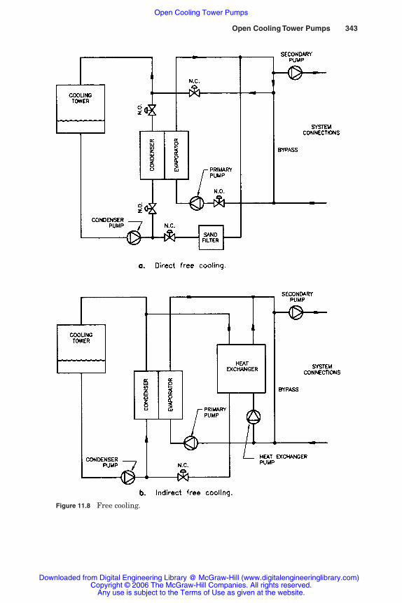
Open Cooling Tower Pumps 343
Figure 11.8 Free cooling.
Rishel_CH11.qxd 20/4/06 6:37 PM Page 343
Downloaded from Digital Engineering Library @ McGraw-Hill (www.digitalengineeringlibrary.com)Copyright © 2006 The McGraw-Hill Companies. All rights reserved.
Any use is subject to the Terms of Use as given at the website.
Open Cooling Tower Pumps
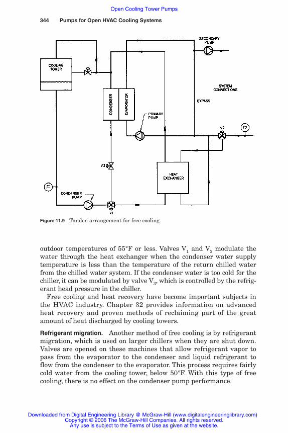
344 Pumps for Open HVAC Cooling Systems
outdoor temperatures of 55°F or less. Valves V1 and V2 modulate thewater through the heat exchanger when the condenser water supplytemperature is less than the temperature of the return chilled waterfrom the chilled water system. If the condenser water is too cold for thechiller, it can be modulated by valve V3, which is controlled by the refrig-erant head pressure in the chiller.
Free cooling and heat recovery have become important subjects inthe HVAC industry. Chapter 32 provides information on advancedheat recovery and proven methods of reclaiming part of the greatamount of heat discharged by cooling towers.
Refrigerant migration. Another method of free cooling is by refrigerantmigration, which is used on larger chillers when they are shut down.Valves are opened on these machines that allow refrigerant vapor topass from the evaporator to the condenser and liquid refrigerant toflow from the condenser to the evaporator. This process requires fairlycold water from the cooling tower, below 50°F. With this type of freecooling, there is no effect on the condenser pump performance.
Figure 11.9 Tanden arrangement for free cooling.
Rishel_CH11.qxd 20/4/06 6:37 PM Page 344
Downloaded from Digital Engineering Library @ McGraw-Hill (www.digitalengineeringlibrary.com)Copyright © 2006 The McGraw-Hill Companies. All rights reserved.
Any use is subject to the Terms of Use as given at the website.
Open Cooling Tower Pumps
Open Cooling Tower Pumps 345
Partial indirect cooling can be accomplished by placing the freecooling heat exchanger in series with a chiller. This reduces thereturn water temperature to the chiller and enables it to operate at alower load. Like the heat exchanger above, the friction loss in bothloops must be evaluated.
All these free cooling methods require careful energy and cost eval-uations by the system designer to determine the optimal procedurefor a particular system.
11.7 Understanding Legionnaires’ Disease
Although cooling tower water pumping in itself has little effect on theprevention of Legionnaires’ disease, it does not hurt to have some spe-cific information included in this book on this disease. Legionnella,the bacteria that causes it, thrives in water of temperatures from 70 to140°F. This temperature range is the same as that for operation ofmost HVAC cooling towers. Therefore, it is urgent that all cooling tow-ers be equipped with a comprehensive water treatment system thatnot only controls corrosion and scale but also limits biologic con-tamination. The system operator should become familiar with the rec-ommendations of various authorities as contained in publicationssuch as those of the Occupational Safety and Health Administration.Another source for this information is the 1995 ASHRAE Handbook,Heating, Ventilating, and Air-Conditioning Applications, Chap. 44,Corrosion Control and Water Treatment. Spills of water around cool-ing tower pumps and leaks from cooling tower pumps should be elimi-nated to aid in the control of this disease.
11.8 Summary
Cooling towers remain the best method of rejecting heat in HVAC andindustrial process water systems. It should be emphasized how muchheat is passed out through a cooling tower. Equation 11.3 developsthis as total heat per year:
Btu/year � heat/ton � tons � annual hours (11.3)
For example, if a 1000-ton chiller has an average heat rejection of15,000 Btu/ton and operates an equivalent of 2000 hours per year atfull load, the annual heat rejection is
Btu/year � 15,000 � 1000 � 2000 � 30,000,000,000
This is 30 billion British thermal units per year! With an overallboiler efficiency of 80 percent and a cost of $3 per 1000 ft3 of natural
Rishel_CH11.qxd 20/4/06 6:37 PM Page 345
Downloaded from Digital Engineering Library @ McGraw-Hill (www.digitalengineeringlibrary.com)Copyright © 2006 The McGraw-Hill Companies. All rights reserved.
Any use is subject to the Terms of Use as given at the website.
Open Cooling Tower Pumps
346 Pumps for Open HVAC Cooling Systems
gas at 1000 Btu/ft3, this is equivalent to 37,500 mcf of natural gas, or$112,500 per year.
Unfortunately, the average return water temperature to cooling tow-ers is only 95°F. As HVAC water processes reduce their temperature,more of this heat will become economically retrievable. Programs arenow being evaluated for raising the condenser leaving water tempera-ture and balancing the cost of eliminating boiler operation against thehigher kilowatt per ton cost incurred by running the chillers at higherleaving condenser temperatures.
This is an excellent place to again evaluate kilowatt per ton instru-mentations and calculations for heat recovery systems. By measuringthe kilowatt consumption of the chillers, pumps, and cooling towers,as well as the tonnage on the chilled water system, the data areachieved for measuring kilowatts per ton for the heat recovery sys-tem. Also, by determining the heat recovered from closed condenserheat recovery circuits, a total energy statement can be derived thatwill provide a guide for the central plant operator to program theequipment at the maximum possible efficiency. There is no way anoperator can read all these system values simultaneously and developa manual algorithm that will give the continuous and accurate datathat are achievable with these computer programs.
The great amount of heat rejected by cooling towers should beremembered as we go about the business of making chilled and hotwater systems more efficient. Some of the current efforts will be foundin Chap. 16 on closed condenser systems. Also, systems are prime can-didates for evaluation for heat recovery from cooling towers if theyhave chillers and boilers that operate at the same time. Chiller opera-tion in the winter and boiler operation in the summer may be signalsto evaluate the economics of heat recovery.
11.9 Bibliography
James B. Rishel, The Water Management Manual, SYSTECON, Inc., West Chester,Ohio, 1992.
Cooling Tower Fundamentals, The Marley Cooling Tower Company, Mission, Kan.,1985.
Rishel_CH11.qxd 20/4/06 6:37 PM Page 346
Downloaded from Digital Engineering Library @ McGraw-Hill (www.digitalengineeringlibrary.com)Copyright © 2006 The McGraw-Hill Companies. All rights reserved.
Any use is subject to the Terms of Use as given at the website.
Open Cooling Tower Pumps
Chapter
347
12Pumps for
Process Cooling
12.1 Introduction
Although, in a strict sense, process cooling is not part of the HVACindustry, many designers of HVAC systems are also involved with thiscooling due to their experience with cooling towers and chillers. Thischapter reviews some of the basic cooling systems that are used inindustry.
Process cooling systems, like HVAC systems, can receive their coolingfrom cooling towers or chillers. The actual temperature of the indus-trial process determines whether cooling towers or chillers are used forthe cooling. A great many industrial processes require water no colderthan 85°F, so cooling towers can be used for these applications.
Process cooling can consist of cooling liquid or gas streams. Manyliquid cooling processes include heat exchangers with the process liq-uid on one side and cooling water on the other side. Such heatexchangers are used when the process liquid is dirty, toxic, difficult tohandle, or too valuable to pass directly through a cooling tower. Gasstreams include many special chemical processes that will not bereviewed here. Some gas streams will be discussed that are nontoxicand can be cooled by water injection or water-cooled heat exchangers.
12.2 Liquid Cooling
Liquid cooling in industrial processes can utilize cooling towersdirectly, but owing to the conditions mentioned earlier, many of these
Rishel_CH12.qxd 20/4/06 6:39 PM Page 347
Downloaded from Digital Engineering Library @ McGraw-Hill (www.digitalengineeringlibrary.com)Copyright © 2006 The McGraw-Hill Companies. All rights reserved.
Any use is subject to the Terms of Use as given at the website.
Source: HVAC Pump Handbook

348 Pumps for Open HVAC Cooling Systems
processes use heat exchangers of the shell and tube or plate andframe types that are cooled by cooling tower water. The piping of suchheat exchangers is similar to that for heat exchangers in the HVACfield; however, there are some conditions that may be found in theseindustrial processes that require special circuiting of the heatexchangers. There are some industrial processes that use heating orcooling coils for gas streams. The pumping and piping connections ofthese coils are much like those for HVAC heating and cooling coils.
The pressure drops across industrial heat exchangers may begreater than those of HVAC applications because of the cost of theheat exchangers. It is imperative that the designer determine exactlythe true pressure drop across the heat exchanger and its controlvalve. The manufacturer of such process equipment may provide ahigher overall pressure to ensure that adequate water is available tothe equipment.
Some industrial processes may contaminate the cooling towerwater, and it may be necessary to provide cleaning of the water beforeit is returned to the cooling tower. Figure 12.1a describes a coolingsystem where the return water is collected in a trough and returnedto a hot well where it is cleaned before being pumped through thecooling tower. The primary-secondary pumping described in this figureallows for constant flow through the cooling tower and variable flowto the process loop. This provides excellent cooling tower operationthroughout the year. A bypass valve is shown for bypassing the wateraround the tower under very low process loads in freezing weather.One method of regulating this valve is through the installation of atemperature transmitter on the return water line to the tower. A pres-sure transmitter at the end of the loop controls the system pumpspeed and maintains the needed pressure in the supply header. Theset point can be varied with the load or type of cooling being carriedon in the loop.
Other industrial processes may be such that a typical closed loopcan be used on the cooling tower water (Fig. 12.1b). If there is stillsome contamination of the cooling tower water, cleaning equipmentcan be provided at the cooling tower pumps. With the closed loop, adifferential pressure transmitter should be used instead of a pressuretransmitter for controlling pump speed to maintain the desired differ-ential pressure for the heat exchangers. This is due to the variablepressure drop in the return header. On some applications, the pressure-gradient diagram (Fig. 12.2) may be helpful in evaluating the totalinstallation.
The hot-well, cold-well sump of Fig. 12.1a may be required in coldareas where the heat from the process load is a variable. The bypassvalve of Fig. 12.1b may be acceptable as long as there is no possibility
Rishel_CH12.qxd 20/4/06 6:39 PM Page 348
Downloaded from Digital Engineering Library @ McGraw-Hill (www.digitalengineeringlibrary.com)Copyright © 2006 The McGraw-Hill Companies. All rights reserved.
Any use is subject to the Terms of Use as given at the website.
Pumps for Process Cooling
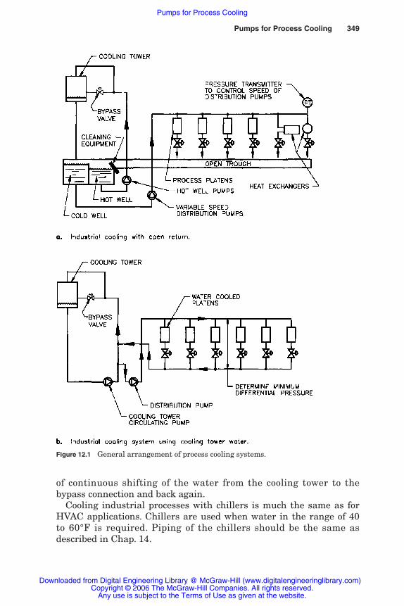
Pumps for Process Cooling 349
Figure 12.1 General arrangement of process cooling systems.
of continuous shifting of the water from the cooling tower to thebypass connection and back again.
Cooling industrial processes with chillers is much the same as forHVAC applications. Chillers are used when water in the range of 40to 60°F is required. Piping of the chillers should be the same asdescribed in Chap. 14.
Rishel_CH12.qxd 20/4/06 6:39 PM Page 349
Downloaded from Digital Engineering Library @ McGraw-Hill (www.digitalengineeringlibrary.com)Copyright © 2006 The McGraw-Hill Companies. All rights reserved.
Any use is subject to the Terms of Use as given at the website.
Pumps for Process Cooling
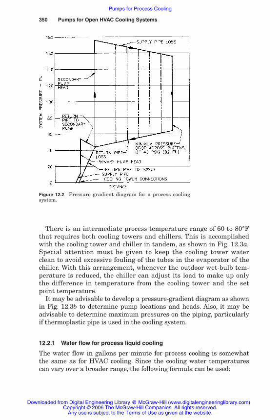
350 Pumps for Open HVAC Cooling Systems
Figure 12.2 Pressure gradient diagram for a process coolingsystem.
There is an intermediate process temperature range of 60 to 80°Fthat requires both cooling towers and chillers. This is accomplishedwith the cooling tower and chiller in tandem, as shown in Fig. 12.3a.Special attention must be given to keep the cooling tower waterclean to avoid excessive fouling of the tubes in the evaporator of thechiller. With this arrangement, whenever the outdoor wet-bulb tem-perature is reduced, the chiller can adjust its load to make up onlythe difference in temperature from the cooling tower and the setpoint temperature.
It may be advisable to develop a pressure-gradient diagram as shownin Fig. 12.3b to determine pump locations and heads. Also, it may beadvisable to determine maximum pressures on the piping, particularlyif thermoplastic pipe is used in the cooling system.
12.2.1 Water flow for process liquid cooling
The water flow in gallons per minute for process cooling is somewhatthe same as for HVAC cooling. Since the cooling water temperaturescan vary over a broader range, the following formula can be used:
Rishel_CH12.qxd 20/4/06 6:39 PM Page 350
Downloaded from Digital Engineering Library @ McGraw-Hill (www.digitalengineeringlibrary.com)Copyright © 2006 The McGraw-Hill Companies. All rights reserved.
Any use is subject to the Terms of Use as given at the website.
Pumps for Process Cooling
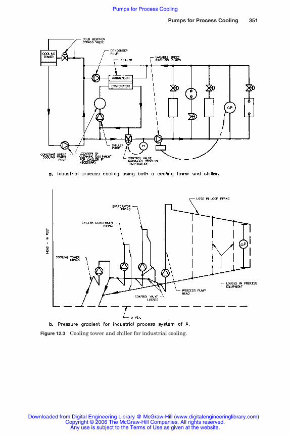
Pumps for Process Cooling 351
Figure 12.3 Cooling tower and chiller for industrial cooling.
Rishel_CH12.qxd 20/4/06 6:39 PM Page 351
Downloaded from Digital Engineering Library @ McGraw-Hill (www.digitalengineeringlibrary.com)Copyright © 2006 The McGraw-Hill Companies. All rights reserved.
Any use is subject to the Terms of Use as given at the website.
Pumps for Process Cooling

352 Pumps for Open HVAC Cooling Systems
Flow (gal/min) �
� (12.1)
where � is the specific weight of water at cooling tower return watertemperature
12.3 Energy Recovery
Some industrial processes operate with higher return water tempera-tures to the cooling towers. This increases the possibilities of energyrecovery, as discussed in Chap. 11 on cooling towers and as will bereviewed in Chap. 16 on closed condenser water systems.
12.4 Gas Stream Cooling
Gas stream cooling with cooling towers or special spray towers is lim-ited mostly to those gases which are exhausted to the atmosphere.Typical of these are gas turbine, boiler, and incinerator exhausts.Many of these processes also scrub the gases, so the water from themwill contain chemicals that may be abrasive or corrosive to pumps.This is particularly so if scrubbers are used to clean the gases and toabsorb specific chemicals that are known to exist in the gases.
Specific attention should be paid to the metallurgy of the pumps forscrubbers. Erosion also may be a problem, necessitating the use ofrubber-lined pumps to provide a useful life of the volute. Most pumpsfor such services are end-suction pumps to simplify the constructionand repair capabilities. Special mechanical seals with flushing equip-ment may be required to keep the pumpage out of the seal cavities.Ease of maintenance, not efficiency, is often the prerequisite for thesepumps, which is the opposite of that for most HVAC pumps.
The water flow rates should be determined by the user or manufac-turer of the cooling equipment. The actual water flow is determinednot only by cooling rates but also by flushing or filtering requirements.
12.5 Bibliography
James B. Rishel, The Water Management Manual, SYSTECON, Inc., West Chester,Ohio, 1992.
heat transferred � (Btu/h)����
8.02 � � � �T (°F)
heat transferred � (Btu/h)����
(� /7.48) � 60 � �T (°F)
Rishel_CH12.qxd 20/4/06 6:39 PM Page 352
Downloaded from Digital Engineering Library @ McGraw-Hill (www.digitalengineeringlibrary.com)Copyright © 2006 The McGraw-Hill Companies. All rights reserved.
Any use is subject to the Terms of Use as given at the website.
Pumps for Process Cooling

Chapter
353
13Pumping Open Thermal
Storage Tanks
13.1 Introduction
Thermal storage in the HVAC industry consists of both hot and chilledwater storage. Hot water storage has not been prevalent, since it is notnecessary for most hot water systems. As energy conservation growswith large chilled water plants, there may be some economic reasons tostore hot water that is generated by the heat rejection from chillers.
13.2 Cool Thermal Storage
Cool thermal storage in HVAC systems has become popular inattempts to reduce overall energy costs. The driving force has beenthe demand charges put in place by the electric utilities as theyattempted to reduce their electrical demand due to cooling load dur-ing the afternoon hours of the summer days. This demand chargenecessitated the shifting of this load from the daytime to nighttimehours. Thermal storage provided this shift, using either ice, chillerwater, or eutectic salt to provide cooling during the peak hoursinstead of electric motor–driven chillers.
The disappointing fact of this effort has been that the peak loadwas reduced in most cases, but the overall energy consumption wasincreased due to the higher kilowatts per ton of cooling required forchillers making ice or chilled water at night. The mission of many ofthese efforts was only peak shaving by the electric utility and demandcharge reduction for the customer, not overall energy conservation.
Rishel_CH13.qxd 20/4/06 6:40 PM Page 353
Downloaded from Digital Engineering Library @ McGraw-Hill (www.digitalengineeringlibrary.com)Copyright © 2006 The McGraw-Hill Companies. All rights reserved.
Any use is subject to the Terms of Use as given at the website.
Source: HVAC Pump Handbook

354 Pumps for Open HVAC Cooling Systems
TABLE 13.1 Chiller Performance(Mean kw/ton per 5% Increment of Chiller Load)
Percent Number of Kilowatts chiller load seasonal hours per ton
10–15 108 1.5315–20 542 1.3220–25 389 1.1525–30 303 1.0330–35 311 0.9435–40 209 0.8740–45 225 0.8345–50 262 0.7950–55 230 0.7655–60 137 0.7460–65 211 0.7265–70 128 0.7070–75 120 0.7075–80 122 0.7080–85 104 0.7085–90 32 0.6790–95 11 0.6195–100 4 0.59
NOTE: The values for chillers shown in this tableare for chillers manufactured around 1994. Recentvalues (circa 2005) have indicated improved chillerperformance; actual data should be secured for anychiller under consideration.
A number of studies of the energy consumed by chillers have beenconducted by various companies to determine the value of energystorage in reducing on-peak demand charges and overall efficientoperation of chillers. The data shown in Table 13.1 are typical of thefindings of some of these studies. This information is for chillers pro-viding cooling of the chilled water without energy storage.
The data in Table 13.1 demonstrate that the programming ofchillers needs to eliminate the operation of chillers at light loads. Oneof the most important advantages of these cool storage systems is the“flywheel effect” they can have on chiller operation. The proper designof energy storage systems therefore should provide for chiller opera-tion at optimal efficiency as well as to ensure adequate cooling duringthe peak demand charge period. The actual programming of thecharging of the tanks should not be just to recharge the tanks as fastas possible but to use the storage and the chillers during light systemloads to achieve optimal overall energy consumption.
For example, in Table 13.1, most of the hours of operation werefrom 15 to 50 percent design load on the chiller, where the kilowattsper ton varied from 1.32 to 0.79. With chilled water storage, the
Rishel_CH13.qxd 20/4/06 6:40 PM Page 354
Downloaded from Digital Engineering Library @ McGraw-Hill (www.digitalengineeringlibrary.com)Copyright © 2006 The McGraw-Hill Companies. All rights reserved.
Any use is subject to the Terms of Use as given at the website.
Pumping Open Thermal Storage Tanks

Pumping Open Thermal Storage Tanks 355
chiller could operate at a higher loading with the combined systemand storage load. Obviously, the total economics of the installationmust be evaluated before committing to chilled water storage, but thepossibility of reduced chiller energy is another factor in the evalua-tion of chilled water storage.
Most studies concentrated on the energy consumption of the chillersalone and did not include evaluations of pumping energy. Also, manyof the pumping and piping installations for these systems have notbeen conducive to energy-efficient pumping.
A number of pumping and piping arrangements for energy storagehave resulted in too many control valves and piping circuits and inef-ficient pumping systems. One of the first objectives for the designer ofthese systems should be to evaluate the physical configuration of theinstallation and find ways to eliminate control valves and branch cir-cuits. There are some very efficient and simple pumping and pipingsystems for energy storage. The pressure-gradient diagram providesthe designer with a working tool to achieve maximum possible effi-ciency in design and operation.
13.3 Types of Cool Water Storage Systems
There are five basic open-type cool storage systems. They are chilledwater, ice harvester, external ice melt, encapsulated ice, and eutecticsalt. Each has specific advantages and disadvantages; no attempt willbe made here to recommend a particular type of energy storage.Emphasis will be placed on the pumping requirements for each sys-tem. Following is a description of these systems that use an open stor-age tank; particular attention will be paid to the optimal methods ofpumping cold water to and from these tanks.
No matter which cool storage system is selected, the pumping costscan be appreciable, particularly since the pumps must operate at peri-ods of high electrical demand charges. Great care must be taken inthe evaluation of variable-speed versus constant-speed pumps to ver-ify if the power savings of variable-speed pumps are worthwhile.
13.4 Chilled Water Storage
Chilled water storage has the following advantages and disadvan-tages when compared with other types of cool storage:
1. Standard chillers can be used because the storage temperature isnear that of most HVAC chilled water systems. On existing instal-lations, the chillers can be reused in many cases.
Rishel_CH13.qxd 20/4/06 6:40 PM Page 355
Downloaded from Digital Engineering Library @ McGraw-Hill (www.digitalengineeringlibrary.com)Copyright © 2006 The McGraw-Hill Companies. All rights reserved.
Any use is subject to the Terms of Use as given at the website.
Pumping Open Thermal Storage Tanks
356 Pumps for Open HVAC Cooling Systems
2. The electrical power cost is lower than for all other types of coolstorage except eutectic salt. This is due particularly to the higherleaving water temperature for the chillers, around 40°F instead of26°F for the ice systems.
3. Special liquids such as the glycols are not needed.
4. The storage cost is much higher than for the smaller ice systemsbecause of the greater volume. On large systems, the storage costmay be equal to or less than that for ice systems. The storage costis almost always less than for eutectic salt installations.
13.4.1 Chilled water storage system configuration
There are many different chilled water storage systems; the actualdesign for a specific application is often contingent on installation fac-tors such as size and location of the chilled water storage. One ofthe most important design factors in any storage system is to providethe “flywheel effect” mentioned earlier that can be used to operate thechillers at the optimal kilowatts per ton. Figure 13.1a provides apiping circuit for a typical water storage system that uses the storedwater as a chiller bypass and enables the chillers to operate at theoptimal kilowatts per ton.
Table 13.2 provides typical chiller kilowatts per ton data for contem-porary chillers that include the energy consumption of the condenserand primary chilled water pumps with the chiller that is deliveringwater at 40°F. Also, these data are for 85°F condenser water suppliedto the chiller. Chillers running at lower condenser temperatures willdemonstrate much lower kilowatt per ton figures.
It is obvious from the data in Table 13.2 that the chilled water stor-age system must be designed so that this chiller never runs below 50percent of full load. The backpressure valves shown in Fig. 13.1a areunnecessary if the storage tank is higher than the rest of the chilledwater system, as could be the case for low-rise or single-floor buildings.
In most chilled water systems, it is undesirable to reverse the flowin the chiller bypass. With the chilled water storage tank serving asthe chiller bypass, the flow reverses automatically through the tankto provide the flow needed for the chilled water system when thechillers are stopped, as would be the case during high-demand chargeperiods. With the kilowatt per ton data of Table 13.2, the chillersshould run at around 70 percent loading to achieve minimum energyconsumption. In actual operation, it has been found most economicalto operate most chillers as closely to full load as possible. This can beverified during actual operation if total kilowatts per ton are recorded
Rishel_CH13.qxd 20/4/06 6:40 PM Page 356
Downloaded from Digital Engineering Library @ McGraw-Hill (www.digitalengineeringlibrary.com)Copyright © 2006 The McGraw-Hill Companies. All rights reserved.
Any use is subject to the Terms of Use as given at the website.
Pumping Open Thermal Storage Tanks
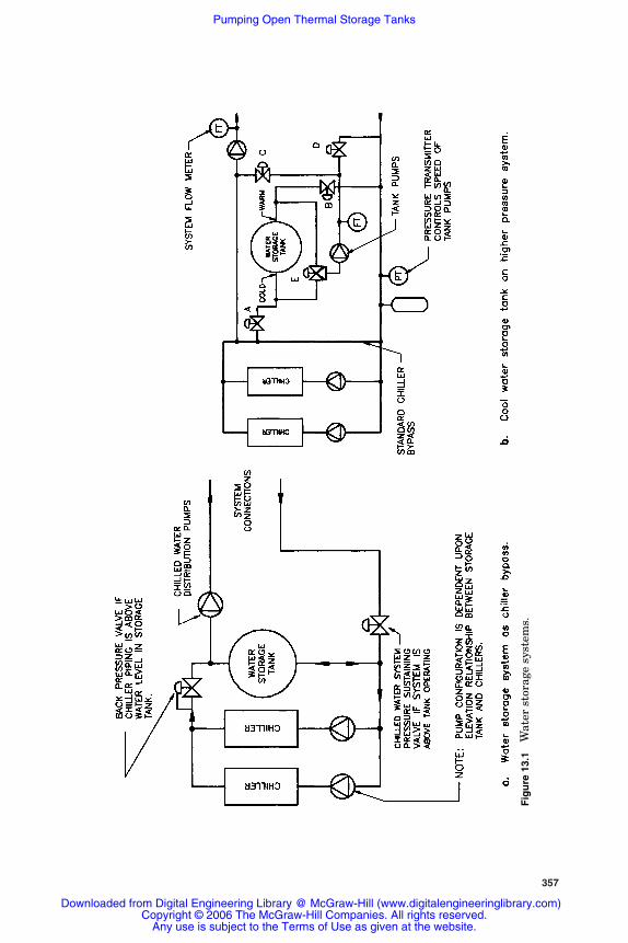
357
Fig
ure
13.
1W
ater
sto
rage
sys
tem
s.
Rishel_CH13.qxd 20/4/06 6:40 PM Page 357
Downloaded from Digital Engineering Library @ McGraw-Hill (www.digitalengineeringlibrary.com)Copyright © 2006 The McGraw-Hill Companies. All rights reserved.
Any use is subject to the Terms of Use as given at the website.
Pumping Open Thermal Storage Tanks

358 Pumps for Open HVAC Cooling Systems
TABLE 13.2 Chiller Kilowatt per Ton Data with Condenser andPrimary Pump Kilowatts Included
Percent load Total kW/ton Percent load Total kW/ton
10 1.69 60 0.6920 1.05 70 0.6830 0.84 80 0.6940 0.74 90 0.7050 0.71 100 0.72
for all percentages of system load. Operating chillers in off-peak sea-sons with lower condenser water temperatures also dictates the needto observe actual kilowatt per ton readings to secure optimal chilleroperation. Obviously, poor operation of chillers at very low loads andhigh kilowatts per ton should be avoided.
For existing systems where chilled water storage is to be added tobuildings with high static pressures, Fig. 13.1b describes another sys-tem in which the water storage system is separated from the princi-pal chilled water system. The actual system design conditions willdetermine the need for this separation of the storage from the watersystem and the extra valving and tank pumps.
To aid in understanding the operation of the chilled water storagesystem in Fig. 13.1b, the five different phases of its operation are asfollows:
1. Standard chilled water system operation without the chilledwater storage system. The storage tank valves A through D are closed,and the system functions as any other chilled water system withoutstorage; the tank pumps are stopped.
2. Serve the chilled water system and store chilled water. Valve A ismodulating and valve D is open; valves B and C are closed. Valve E onthe tank is open to the tank discharge position. Valve A is modulatedto provide the flow rate desired into the storage tank. The tank pumpvaries its speed to maintain return water pressure in the chilledwater system. This prevents the development of low pressure in thesystem caused by water flowing into the tank.
This control procedure allows the operator to adjust the rate of stor-age, and it enables operation of the chillers at optimal kilowatts perton for the entire chilled water plant.
This operation can occur at any off-peak loading on the chilledwater system.
3. Serve the chilled water system with chillers and stored chilledwater. This operation provides peak shaving by allowing the operator
Rishel_CH13.qxd 20/4/06 6:40 PM Page 358
Downloaded from Digital Engineering Library @ McGraw-Hill (www.digitalengineeringlibrary.com)Copyright © 2006 The McGraw-Hill Companies. All rights reserved.
Any use is subject to the Terms of Use as given at the website.
Pumping Open Thermal Storage Tanks
Pumping Open Thermal Storage Tanks 359
to select the amount of water needed from the storage tank to achievethe desired chiller operation and reduction in power consumption.
Valve C is open while valves A and D are closed. Valve B is modu-lating to provide the desired flow from the storage tank. The tankvalve E is open to the cold water connection of the tank.
4. Store chilled water only. This procedure is very similar to phase 2except that there is no system cooling load. Again, the operator shouldprogram the chillers and operate them at a rate of cooling that willensure minimum energy consumption in the overall kilowatts per ton inthe central energy plant. Recognition should be given to the lower kilo-watts per ton that can be achieved with reduced condenser water tem-peratures from the cooling tower during lower outdoor temperatures.
5. Serve the chilled water system only from the storage tank. Thisphase is similar to 3. excepting that the chillers are stopped, and allcooling is derived from the storage tank. Valve B is modulating, valveC is open, and valves A and D are closed. The tank valve E is in thecold water discharge connection on the tank. Valve B is modulated bythe flowmeter to achieve the desired flow through the storage tank,and the tank pump’s speed is controlled to maintain the desired pres-sure on the chilled water system.
The supply temperature to the system can be varied by blendingreturn water with the tank water. Also, the storage tank flow rate canbe paced by the system flowmeter. The type of control desired for aspecific application will depend on the overall parameters that affectsystem operation.
Most chilled water systems do not incorporate the glycols to preventfreezing, since the water is seldom stored below 40°F. The advantageof chilled water over the other systems is the lower overall energyconsumption in kilowatts per ton of cooling; the disadvantage is thelower British thermal units stored per cubic foot of tank volume. Ifthere is space for a chilled water tank, it should be used in lieu of theice-formation types of energy storage.
13.4.2 Temperature control of open thermalstorage tanks
Temperature control of thermal storage tanks is important to ensurethat the thermal cline is maintained, Fig. 13.2, and a maximum per-centage of the tank volume is used before the leaving water tempera-ture begins to rise. The temperature must be sensed at several levelsto ensure that the tank is under proper control. ASHRAE’s manual oncool storage provides the designer with excellent data on the designand operation of thermal storage tanks.
Rishel_CH13.qxd 20/4/06 6:40 PM Page 359
Downloaded from Digital Engineering Library @ McGraw-Hill (www.digitalengineeringlibrary.com)Copyright © 2006 The McGraw-Hill Companies. All rights reserved.
Any use is subject to the Terms of Use as given at the website.
Pumping Open Thermal Storage Tanks

360 Pumps for Open HVAC Cooling Systems
13.5 Open Ice Storage Systems
For systems that do not have space for chilled water storage, open icestorage systems can be used with smaller tanks. When ice storage isunder consideration, the designer must evaluate both open- and closed-type ice systems. This chapter reviews open-type ice systems, whileclosed-type ice systems are part of Chap. 17. Open ice systems consistof the ice harvester, external melt ice, and encapsulated ice types.
13.5.1 Ice harvester
This system offers compact installations including prepackaged ice-making machines Fig. 13.3. Its storage cost is lower than that of any
Figure 13.3 Ice harvester system. (From Patterson Pump Company HVACPumps and Systems Manual, 2004.)
Figure 13.2 Typical general arrangement of open chilled water tanks.
Cold water header
Warm water header
Warm water
Cold water
Thermal cline
T
Temperature transmitter
Undergroundstorage
Self-priming pumpor standard pumpwith priming system
Variable speedsystem pump
Chilled water system
Actual piping as perice maker’s recommendations.
Ice maker
Rishel_CH13.qxd 20/4/06 6:40 PM Page 360
Downloaded from Digital Engineering Library @ McGraw-Hill (www.digitalengineeringlibrary.com)Copyright © 2006 The McGraw-Hill Companies. All rights reserved.
Any use is subject to the Terms of Use as given at the website.
Pumping Open Thermal Storage Tanks

Pumping Open Thermal Storage Tanks 361
other cool storage systems, but it has the most expensive chiller costs.Its power costs of generating ice are as high as for any of the coolenergy storage systems. Another disadvantage pump-wise is the com-mon use of underground tanks for storage, since the ice-makingequipment must be located above the tanks. This enables the ice tofall by gravity away from the ice machine into the tank. Harvester-type ice storage systems can be provided with above-ground storagetanks and are the preferable arrangement if vertical clearance isavailable.
With the underground tank, self-priming pumps may be requiredfor ease of operation. If the system is seldom shut down, standardcentrifugal pumps with priming systems can be used. The disadvan-tage of self-priming pumps is their efficiency, which can be as much as20 percent lower than that for standard centrifugal pumps. As men-tioned earlier, this is not advantageous, since these pumps must runduring periods of high electrical demand charges. Several very impor-tant points must be made in the use of self-priming pumps:
1. The pump suction piping must be designed with low friction losses.
2. Care must be taken that the NPSH available, is adequate evenwhen the tank water is at ambient conditions. The system muststart with no ice in the tank, so the water temperature must beassumed to be equal to the surrounding air temperature.
3. If more than one self-priming pump is installed, each should haveits own suction line sized to the recommendations of the pumpmanufacturer. Headered suction lines to pumps offer possibilitiesof air leaks and loss of priming water.
4. All pumps taking a suction lift, particularly self-priming pumps,always should be installed strictly in accordance with the pumpmanufacturer’s recommendations.
There are a number of different pumping arrangements for iceharvesters. Some may have one pump for circulating the chillerand delivering water to a heat exchanger for the chilled water sys-tem. Others may have dual pumps with a constant-speed pump forthe chiller and a separate variable-speed pump for the chilledwater system heat exchanger. The actual pumping arrangement iscontingent on the size of the cool storage system and on the loadconfiguration.
Ice harvesters can be used in conjunction with standard chillers aspeak shaving systems to reduce the overall cost of the installation. Itis obvious that the economics of these systems play a great part in thefinal selection of equipment.
Rishel_CH13.qxd 20/4/06 6:40 PM Page 361
Downloaded from Digital Engineering Library @ McGraw-Hill (www.digitalengineeringlibrary.com)Copyright © 2006 The McGraw-Hill Companies. All rights reserved.
Any use is subject to the Terms of Use as given at the website.
Pumping Open Thermal Storage Tanks

362 Pumps for Open HVAC Cooling Systems
13.5.2 Encapsulated ice systems
Encapsulated ice systems of cool storage use various types and shapesof bottles or containers filled with water. A low-temperature liquidsuch as one of the glycols flows through the tank to either freeze thewater in the containers during the charging cycle or to melt the ice dur-ing the energy-using cycle. The advantages of these systems are verylow storage volumes with relatively low chiller costs. The storage costwith respect to the other cool energy systems varies with the size of theinstallation.
There are no specific pumping problems with these systemsbecause they are usually installed above grade with the pumpingequipment beside the tanks. The circuiting of the piping depends onthe manufacturer of the encapsulation containers. Otherwise, thepumping arrangement can be like many other open tank chilledwater systems.
13.5.3 External ice melt systems
Generally, these systems use an open tank that has refrigerant coilsimmersed in it. Some systems are provided in closed pressure tanks.Cold refrigerant passes through the coils to develop ice around thecoils. When the ice has built up to a specified thickness, the refriger-ant flow is stopped, and the tank is ready for use as an energy source.Water flows through the tank much like the encapsulated ice systemsdelivering cool water to the chilled water system heat exchanger. Also,like the encapsulated ice systems, there are no particular problems inpumping these systems. The pumping equipment is again locatedbeside the tanks, so there usually are no NPSH problems.
13.6 Eutectic Salt Systems
Eutectic salt systems are much like encapsulated water systemsexcept that the liquid in the containers is not water but a materialthat has a higher melting temperature than the 32°F of water. Someof these salts freeze at 47°F; current developments indicate that othersalts with freezing temperatures of around 40°F may be available forthe cool storage industry.
Eutectic salts have the advantage of using standard chillers, sotheir power costs are similar to those of chilled water and much lessthan those of ice storage systems. They have a high storage cost dueto the special materials that are involved with the salts and theircontainers. Their tank volume is around one-half that for chilledwater.
Rishel_CH13.qxd 20/4/06 6:40 PM Page 362
Downloaded from Digital Engineering Library @ McGraw-Hill (www.digitalengineeringlibrary.com)Copyright © 2006 The McGraw-Hill Companies. All rights reserved.
Any use is subject to the Terms of Use as given at the website.
Pumping Open Thermal Storage Tanks

Pumping Open Thermal Storage Tanks 363
These systems again are much like encapsulated ice and externalice melt systems as far as pumping equipment is concerned. Thepumping systems are located beside the tanks, so there are no prob-lems with NPSH or priming.
13.7 Decision as to the Type of EnergyStorage System
The decision whether to use chilled water, ice storage, or eutectic saltsis beyond the scope of this book. The designer for energy storage mustmake this decision based on the parameters of each installation, suchas first cost, space for energy storage, electrical charges, and efficien-cies of various types of chilled water and ice-generation equipment.This decision requires a number of evaluations and calculations. Thedevelopment of the gas-fired engine–driven chiller and absorptionchillers for electric power reduction during high-demand periods hasadded to all the evaluations that must be made for a particular instal-lation.
Most of these cool storage systems require some form of pumping ofthe water from open tanks; the location and type of pumping vary witheach system, as described previously. However, with proper applicationof the pumps, their required power should not have a great bearing onthe type of energy storage system selected for a specific application.
13.8 Basics of Pump Application to OpenEnergy Storage Tanks
Regardless of the type of open energy storage system, there are somefundamentals on pumping that must be recognized. The followingprinciples should be adhered to on these applications:
1. The viscosity and specific gravity of the liquids involved should bechecked and used in calculations for pipe and fitting friction andpumping horsepower. Water at 32°F has a higher viscosity thanwater at 50°F, namely, 1.93 � 10�5 ft2/s at 32°F compared with1.41 � 10�5 ft2/s at 50°F.
2. When using glycol systems, ensure that the pumps will never oper-ate near the freeze curve or slush line of the glycol (see Figs. 2.1,2.2, and 2.3).
3. On chilled water and all other installations except ice harvestersystems, always locate the working level of the energy storagetank higher than the chillers if at all possible. This eliminates theneed for backpressure valves on the chiller circuit. It is wise to run
Rishel_CH13.qxd 20/4/06 6:40 PM Page 363
Downloaded from Digital Engineering Library @ McGraw-Hill (www.digitalengineeringlibrary.com)Copyright © 2006 The McGraw-Hill Companies. All rights reserved.
Any use is subject to the Terms of Use as given at the website.
Pumping Open Thermal Storage Tanks

364 Pumps for Open HVAC Cooling Systems
a pressure-gradient diagram on energy storage systems, since thisdiagram will reveal problems with water circuiting and will exposeneedless energy waste in control valves.
4. Check the NPSH available for pumps taking water from the openstorage tank. NPSH is not a problem on most of these systemsunless there is a great amount of pipe or valve friction between theopen tank and the tank pumps.
5. Do not locate any control valves between the tank and the tankpumps (Fig. 13.4a). Control valves reduce the NPSH available forthe pumps, and they can cause cavitation in the pumps. Three-waytwo-position valves can be located on the suction of the pumps,since one of the valves is always open (see Fig. 13.5a). This doesnot apply to self-priming pumps or other pumps taking a suctionlift from the tanks, since no valves of any configuration should beinstalled in these lines.
Figure 13.4 Location of valveson open storage systems.
Rishel_CH13.qxd 20/4/06 6:40 PM Page 364
Downloaded from Digital Engineering Library @ McGraw-Hill (www.digitalengineeringlibrary.com)Copyright © 2006 The McGraw-Hill Companies. All rights reserved.
Any use is subject to the Terms of Use as given at the website.
Pumping Open Thermal Storage Tanks
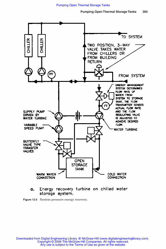
Pumping Open Thermal Storage Tanks 365
Figure 13.5 System pressure energy recovery.
Rishel_CH13.qxd 20/4/06 6:40 PM Page 365
Downloaded from Digital Engineering Library @ McGraw-Hill (www.digitalengineeringlibrary.com)Copyright © 2006 The McGraw-Hill Companies. All rights reserved.
Any use is subject to the Terms of Use as given at the website.
Pumping Open Thermal Storage Tanks
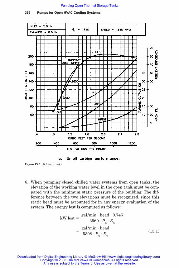
366 Pumps for Open HVAC Cooling Systems
6. When pumping closed chilled water systems from open tanks, theelevation of the working water level in the open tank must be com-pared with the minimum static pressure of the building. The dif-ference between the two elevations must be recognized, since thisstatic head must be accounted for in any energy evaluation of thesystem. The energy lost is computed as follows:
kW lost �
� (13.1)gal/min � head��5308 � P
�� E
�
gal/min � head � 0.746���
3960 � P�
� E�
Figure 13.5 (Continued )
Rishel_CH13.qxd 20/4/06 6:40 PM Page 366
Downloaded from Digital Engineering Library @ McGraw-Hill (www.digitalengineeringlibrary.com)Copyright © 2006 The McGraw-Hill Companies. All rights reserved.
Any use is subject to the Terms of Use as given at the website.
Pumping Open Thermal Storage Tanks

Pumping Open Thermal Storage Tanks 367
where gal/min � flow of water from pressurized systemhead � pump head required to return the water to the
systemP
�� efficiency of pump
E�
� efficiency of pump motor for constant-speed pumpsor the wire-to-shaft efficiency of the motor andvariable-speed drive for variable-speed pumps
The energy calculation for a system is as follows: Assume thatthe top of the building is at elevation 730 ft, and the working levelin the energy storage tank is 520 ft. These elevations are in actuallevels above sea level. Also, assume that there is an expansiontank located at the top of the building and that 10 psig is main-tained in this tank by the makeup water system.
The pressure gradient required to maintain the 10 psig at the topof the building is 730 � (10 � 2.31), or 763 ft. The pressure gradientfor the working water level of the storage tank is 520 ft. The pres-sure difference between the pressure at the top of the building, 763 ft,and the open tank, 520 ft, is 243 ft. With 15 ft of pipe friction in thepiping between the storage tank and the water system, the totalhead required for the pump is 258 ft. If the system flow is 1000gal/min, the pump efficiency 83 percent and the wire-to-shaft effi-ciency of a motor and variable-speed drive is 89 percent,
kW lost �
� 65.8 kW
7. If the static pressure of a closed system is greater than the eleva-tion of the open tank, some means must be used to maintain theminimum pressure at the top of the building. There are severalmethods of achieving this:a. Backpressure valves (Fig. 13.4b) can be used, but they should
maintain the pressure on top of the building, not the inlet pres-sure to these valves. Self-operating valves should not be used inmany cases because the friction of the return water main betweenthe valves and the top of the building is a variable. The valvesshould be equipped with a control system that measures the pres-sure at the top of the building and adjusts the valve position tomaintain that pressure. Normally, a pressure transmitter locatedat the top of the building along with a proportional-integral con-troller can adjust the valve position to maintain the desired
1000 � 258���5308 � 0.83 � 0.89
Rishel_CH13.qxd 20/4/06 6:40 PM Page 367
Downloaded from Digital Engineering Library @ McGraw-Hill (www.digitalengineeringlibrary.com)Copyright © 2006 The McGraw-Hill Companies. All rights reserved.
Any use is subject to the Terms of Use as given at the website.
Pumping Open Thermal Storage Tanks

368 Pumps for Open HVAC Cooling Systems
pressure on top of the building. Usually, this control procedure isadequate for small buildings where the energy loss from the pres-surized system to the open tank is minimal.
b. On larger buildings with high pressures, it may be desirable tosave this energy lost from the depressurization of the water.Figure 13.5a describes a procedure that can be used, that of apressure recovery pump. This pump is driven by a similar pumpequipped with a turbine wheel. A typical performance curve forsuch a turbine is shown in Fig. 13.5b. The energy recovered bysuch a pumping system can vary from 10 to around 67 percentof the pressure difference between the chilled water system andthe open tank. A variable-speed pump responding to the chilledwater system return pressure is installed in series with therecovery pump.
The variable-speed pump in series with the energy-recoverypump provides a more efficient arrangement for most applicationsthan combining the variable-speed motor with the turbine andenergy-recovery pump on one base. The difficulty of this one-basearrangement is the fact that the turbine must run at the samespeed as the variable-speed pump. The turbine should operate atthe speed caused by the flow of water from the system and theforce on the turbine shaft created by the driven pump. The variable-speed pump runs at a speed necessary to maintain the systempressure. They are seldom the same speed.
An excellent article on the savings of the turbine-driven pump inlieu of a heat exchanger and where to use it is available inASHRAE Transactions DA-88-27-2 by R. M. Tackett. The evaluationsincluded in this article will assist the designer in the evaluation ofthe cost of these pumps versus heat exchangers to determine theamortization periods.c. The use of a heat exchanger to overcome the pressure difference
between the open tank and the pressurized chilled water sys-tem (Fig. 13.6) may not be an efficient procedure for chilledwater storage systems because of the temperature drop acrossthe heat exchanger. If it is desired to store chilled water at 40°Fwith a temperature approach of 3°F for the heat exchanger,chilled water must be generated at 37°F, thus increasing thekilowatts per ton of the chiller. Also, in like manner, only 43°Fwater is available for use by the chilled water system. The heatexchanger therefore causes a total temperature swing of 6°F.The savings in static pressure for high-rise buildings throughthe use of a heat exchanger must be offset with the friction lossof the heat exchanger as well as this temperature loss across it.
Rishel_CH13.qxd 20/4/06 6:40 PM Page 368
Downloaded from Digital Engineering Library @ McGraw-Hill (www.digitalengineeringlibrary.com)Copyright © 2006 The McGraw-Hill Companies. All rights reserved.
Any use is subject to the Terms of Use as given at the website.
Pumping Open Thermal Storage Tanks

Pumping Open Thermal Storage Tanks 369
The decision to use the heat exchanger does require a carefulfirst cost and energy evaluation of its installation. On open-typeice systems, the heat exchanger is the normal procedurebecause of the great difference between the water temperaturein the tank and that in the chilled water system. The higherkilowatt per ton energy requirement for the chiller has alreadybeen expended to generate the ice.
13.9 Types of Pumps for Thermal Storage
When the thermal storage tanks are installed above grade or when theworking water level of the tank is above the pump suction, the besttype of pumps are volute, single or double suction, as would be thecase for cooling towers. These pumping systems should be selected andprogrammed to achieve the maximum possible pumping efficiency.
Figure 13.6 Chilled water storage with building heat exchanger. (FromPatterson Pump Company HVAC Pumps and Systems Manual, 2004.)
DP
C
T
T
Building heat exchangerand control valve. See
section 9.10 andfigures 9.13 and 9.14
Tank pumps
Tank temperaturecontrol valve
Variable speedbuilding pumps
Chiller
Expansion tank
Coils
Open waterstorage tank
Rishel_CH13.qxd 20/4/06 6:40 PM Page 369
Downloaded from Digital Engineering Library @ McGraw-Hill (www.digitalengineeringlibrary.com)Copyright © 2006 The McGraw-Hill Companies. All rights reserved.
Any use is subject to the Terms of Use as given at the website.
Pumping Open Thermal Storage Tanks

When the open tank is below grade, the pumps can be vertical tur-bine installed in the tank with the motors above grade, or they can beself-priming pumps. Installation of the vertical turbine pumps would bemuch like that for large cooling towers. Usually, the self-priming pumpshave a lower efficiency than the turbine pumps, so they should be usedonly on smaller installations. As indicated earlier, self-priming pumpsshould be installed with individual suction pipes, not with a suctionheader. The size of these suction pipes must be the same as that of thesuction connection on the pumps themselves. This can add to the pumphead and reduce further the efficiency of the self-priming pumping sys-tem. The NPSH required and dry priming capabilities of these pumpsshould be checked carefully with the pump manufacturer.
13.10 Operating Pumps on Thermal Storage Systems
The pumps for thermal storage systems deserve the same evaluationfor efficient operation as other HVAC systems. It is wise on larger sys-tems to run a pressure-gradient diagram at minimum and maximumloading to determine the value of variable-speed pumping.
Where there is a significant friction loss in the thermal storage anddistribution system, the use of variable-speed pumps may be justified.On ice systems using glycol solutions, a careful evaluation of the vis-cosity range of the glycol should be made to determine the variationin friction head due to changes in viscosity of the glycol solution.
It is not within the scope of this book to evaluate the overall use ofenergy in the various types of open energy storage systems. Any auditof energy consumption for a particular system should include thepumping energy; the procedures outlined in this book for evaluatingthe efficiency of pump operation should be included in such a study.The overall kilowatts per ton or coefficient of performance should berun for the cool energy storage system under all phases of operationand at various loads on the chilled water system.
13.11 Hot Water Storage
With the development of the condensing boiler, greater opportunitiesare appearing for the use of rejected heat from chillers and industrialprocesses. Some installations may merit the storage of hot water.Whether this storage would be in open or pressurized tanks willdepend on the physical characteristics of the actual installation. Thiswill be discussed in Chap. 16 on heat recovery from chiller condensersystems.
370 Pumps for Open HVAC Cooling Systems
Rishel_CH13.qxd 20/4/06 6:40 PM Page 370
Downloaded from Digital Engineering Library @ McGraw-Hill (www.digitalengineeringlibrary.com)Copyright © 2006 The McGraw-Hill Companies. All rights reserved.
Any use is subject to the Terms of Use as given at the website.
Pumping Open Thermal Storage Tanks

13.12 Summary
The use of energy storage and the rejected heat of chillers offers newopportunities for achieving higher coefficients of performance for bothchilled and hot water generating plants. Again, the variable-speedpump and digital control are the tools that can be applied to thesemore efficient systems.
Comparisons between the various types of energy storage are at bestgeneralizations; each application must be evaluated for first cost andenergy consumption and not depend on the estimates provided herein.
13.13 Bibliography
Hydro Turbines, The Cornell Pump Company, Portland, Oreg., 1986.Design Guide for Cool Thermal Storage, American Society of Heating, Refrigerating,
and Air-Conditioning Engineers, Atlanta, Ga., 1993.
Pumping Open Thermal Storage Tanks 371
Rishel_CH13.qxd 20/4/06 6:40 PM Page 371
Downloaded from Digital Engineering Library @ McGraw-Hill (www.digitalengineeringlibrary.com)Copyright © 2006 The McGraw-Hill Companies. All rights reserved.
Any use is subject to the Terms of Use as given at the website.
Pumping Open Thermal Storage Tanks

Rishel_CH13.qxd 20/4/06 6:40 PM Page 372
Downloaded from Digital Engineering Library @ McGraw-Hill (www.digitalengineeringlibrary.com)Copyright © 2006 The McGraw-Hill Companies. All rights reserved.
Any use is subject to the Terms of Use as given at the website.
Pumping Open Thermal Storage Tanks

Pumps for ClosedHVAC Cooling Systems
Part
5
Rishel_CH14.qxd 20/4/06 6:41 PM Page 373
Downloaded from Digital Engineering Library @ McGraw-Hill (www.digitalengineeringlibrary.com)Copyright © 2006 The McGraw-Hill Companies. All rights reserved.
Any use is subject to the Terms of Use as given at the website.
Source: HVAC Pump Handbook

Rishel_CH14.qxd 20/4/06 6:41 PM Page 374
Downloaded from Digital Engineering Library @ McGraw-Hill (www.digitalengineeringlibrary.com)Copyright © 2006 The McGraw-Hill Companies. All rights reserved.
Any use is subject to the Terms of Use as given at the website.
Pumps for Closed HVAC Cooling Systems
Chapter
375
14Chillers and
Their Pumps
14.1 Introduction
In 1994, when the first edition of this book was being written, thedigitally-controlled chiller was making its entrance into the HVACindustry. This type of chiller allows variable flow in its evaporatorand frees the chilled water piping designer to seek the most efficientand cost-effective pumping system. Much of the original version ofthis chapter was based upon primary-secondary pumping whichallowed constant flow in the evaporator regardless of the water flowrate in the chilled water system. Now, variable primary pumpingand distributed pumping have become the most popular and effi-cient pumping configurations. Chapter 15 describes all of thesewater distribution systems.
Most of the information on primary-secondary pumping has beenretained for use in understanding the correct design for them and toassist in converting them to the more efficient variable primary pump-ing as explained in Chap. 15. Is it not obvious that variable primarypumping has simplified greatly the design of the chiller bypass? Thiswill be demonstrated in the following sections that describe the designof the bypass with variable primary pumping.
The proper installation and operation of chillers on HVAC chilledwater systems are among the most important factors in the develop-ment of efficient and cost-effective chilled water generating plants.This is obvious given the great amount of energy consumed by chillers.
Much work has been done to improve the efficiency of chillers usingthe latest state-of-the art-technology. For example, chiller efficiency
Rishel_CH14.qxd 20/4/06 6:41 PM Page 375
Downloaded from Digital Engineering Library @ McGraw-Hill (www.digitalengineeringlibrary.com)Copyright © 2006 The McGraw-Hill Companies. All rights reserved.
Any use is subject to the Terms of Use as given at the website.
Source: HVAC Pump Handbook
376 Pumps for Closed HVAC Cooling Systems
has improved and energy consumption has dropped from around 0.86kW/ton in 1970 to the current level of approximately 0.52 kW/ton foran efficient machine operating at its point of design peak perfor-mance. It is imperative that the chillers be installed to permit them totake advantage of this level of efficiency.
The pumps for both the chillers and the chilled water system mustbe installed and operated so that they aid the chillers’ performance.Pumping equipment should never be installed in a manner that willadversely affect the chiller energy consumption and efficiency. Thedesigner must understand how pumps or pumping can positively ornegatively affect chiller performance; this is the reason for this exten-sive chapter on chillers and their pumps.
This review of water chillers will be limited to the installation ofconnecting piping, the pumping to and from them, and operation andcontrol of the pumps and chillers as a system. If there are specificpumping requirements for one type of chiller, that chiller will be dis-cussed with respect to its particular operation.
Briefly, an HVAC chiller has an evaporator that cools the systemwater and a condenser or other means that rejects the heat from thesystem to the cooling tower or closed-circuit cooler. All chillers needan energy source for their operation.
Chillers secure their energy for operation from electricity, naturalgas, or steam. By far the most popular driver for chillers is the electricmotor. Other methods of chilled water generation are becoming popu-lar in areas where there are high electrical demand charges or short-ages during the periods of maximum chilled water use.
Electric motor–driven chillers are available in four principal types:(1) reciprocating, (2) scroll, (3) helirotor (screw), and (4) centrifugal.Following are approximate ranges in tons for the various types ofchillers. Reciprocating units are for smaller tonnages in the rangefrom 10 to 200 tons, scroll units from 10 to 60 tons, screw types from25 to 1200 tons, and centrifugal machines from 100 to 10,000 tons.
Absorption water-chilling machines are available in both steam- orhot water–heated (indirect-fired) units or fuel-fired (direct-fired)units. Fuel-fired chillers are currently available in the range of 100 to1100 tons, while steam- and hot water–heated units are generallyavailable in the range of 100 to 1600 ton.
Centrifugal machines are also available with engine or turbine dri-ves in the medium to large models; they may offer energy cost savingson some installations. Although uncommon today, gas-fired engine–driven chillers or total energy plants may increase in use as coolingloads increase on electric power distribution systems. Chilled watersystems under consideration for energy storage such as cold water or
Rishel_CH14.qxd 20/4/06 6:41 PM Page 376
Downloaded from Digital Engineering Library @ McGraw-Hill (www.digitalengineeringlibrary.com)Copyright © 2006 The McGraw-Hill Companies. All rights reserved.
Any use is subject to the Terms of Use as given at the website.
Chillers and Their Pumps
Chillers and Their Pumps 377
ice should evaluate gas engine–driven chillers as a possible life-cyclecost alternative. Currently, the consumer cost of natural gas on anequivalent basis can be one-fourth to one-fifth of that for electric power.
The condenser water operation of water chillers is described inChap. 11 on cooling tower pumps and in Chap. 16 on closed condenserwater systems.
14.2 Rating of Chillers
Water chillers for HVAC systems are rated in tons of cooling; 1 ton ofcooling is equal to 12,000 Btu/h. For pumping and control procedures, itis convenient sometimes to rate chillers by the amount of chilled waterthat is produced by them. As described in Chap. 9, the chilled watercapacity, in gallons per minute, is determined by the following formula
Chiller capacity, gal/min � (9.2)
where temperature difference is the water temperature drop acrossthe chiller evaporator. For example, a 1000-ton chiller operating at achilled water temperature difference of 12°F will have a chilled watercapacity of 2000 gal/min.
14.3 Chiller Energy Consumption
The efficiency of chillers is a function of their energy consumption; forexample, electric motor–driven chillers are rated in kilowatts per ton.The efficiency of absorption chillers is stated in either fuel per ton,pounds of steam per ton, or a coefficient of performance. Coefficient ofperformance COP for any type of equipment is
COP � (14.1)
Coefficient of performance for chillers can be based on eitherBritish thermal units or kilowatts. Another ratio that may be of valueis the energy efficiency ratio EER, which is defined by the AmericanSociety of Heating, Refrigerating and Air-Conditioning Engineers(ASHRAE) as the net cooling capacity in British thermal units perhour divided by the watt-hours applied, or
EER � (14.2)Btu/h net cooling effect���
Wh applied
useful energy acquired���
energy applied
rated tons � 24����temperature difference, °F
Rishel_CH14.qxd 20/4/06 6:41 PM Page 377
Downloaded from Digital Engineering Library @ McGraw-Hill (www.digitalengineeringlibrary.com)Copyright © 2006 The McGraw-Hill Companies. All rights reserved.
Any use is subject to the Terms of Use as given at the website.
Chillers and Their Pumps
378 Pumps for Closed HVAC Cooling Systems
The relationship between the coefficient of performance and theenergy efficiency ratio is
EER � 3.412 � COP (14.3)
To demonstrate the calculations between kilowatts per ton, COP,and EER, assume that a chiller has an energy consumption rate of0.52 kW/ton. This energy is equal to 0.52 � 3412, or 1774 Btu/h input.Therefore, from Eq. 14.1,
COP � �1127,07040
� � 6.76
From Eq. 14.2,
EER � �12
5,20000
� � 23.1
From Eq. 14.3,
EER � 3.412 � 6.76 � 23.1
The energy rate for electric motor–driven chillers varies from 0.50 to1.00 kW/ton at full load, while the steam rate for steam-heatedabsorption machines varies from 12 to 20 lb/ton.
14.3.1 Electric motor–driven chiller consumption
The cooling load on an electric motor–driven chiller determines to alarge extent the energy consumption, although the temperatures ofboth the chiller water leaving the evaporator and the condenser watercoming from the cooling tower or closed-circuit cooler also will affectenergy usage. Following are some simple rules:
1. The kilowatts per ton for an electric motor–driven chiller are usu-ally lowest in load ranges from 50 to 100 percent of full load andhighest in load ranges below 40 percent of full load.
2. The kilowatts per ton are lowest at high leaving chilled water tem-peratures and highest for low leaving chilled water temperatures.
3. The kilowatts per ton are lowest for low condenser water tempera-tures and highest for high condenser water temperatures.
These rules offer some simple guidelines for the application ofchillers to standard installations as well as energy storage systems.
Rishel_CH14.qxd 20/4/06 6:41 PM Page 378
Downloaded from Digital Engineering Library @ McGraw-Hill (www.digitalengineeringlibrary.com)Copyright © 2006 The McGraw-Hill Companies. All rights reserved.
Any use is subject to the Terms of Use as given at the website.
Chillers and Their Pumps
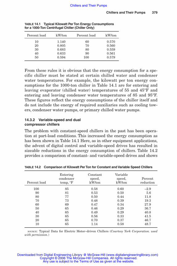
Chillers and Their Pumps 379
TABLE 14.1 Typical Kilowatt Per Ton Energy Consumptionsfor a 1000-Ton Centrifugal Chiller (Chiller Only)
Percent load kW/ton Percent load kW/ton
10 1.140 60 0.57020 0.805 70 0.56030 0.683 80 0.55940 0.633 90 0.56150 0.594 100 0.579
From these rules it is obvious that the energy consumption for a spe-cific chiller must be stated at certain chilled water and condenserwater temperatures. For example, the kilowatt per ton energy con-sumptions for the 1000-ton chiller in Table 14.1 are for entering andleaving evaporator (chilled water) temperatures of 55 and 45°F andentering and leaving condenser water temperatures of 85 and 95°F.These figures reflect the energy consumptions of the chiller itself anddo not include the energy of required auxiliaries such as cooling tow-ers, condenser water pumps, or primary chilled water pumps.
14.3.2 Variable-speed and dual compressor chillers
The problem with constant-speed chillers in the past has been opera-tion at part-load conditions. This increased the energy consumption ashas been shown in Table 14.1 Here, as in other equipment applications,the advent of digital control and variable-speed drives has resulted insizeable reductions in the energy consumption of chillers. Table 14.2provides a comparison of constant- and variable-speed drives and shows
TABLE 14.2 Comparison of Kilowatt Per Ton for Constant and Variable Speed Chillers
Entering Constant Variablecondenser speed, speed, Percent
Percent load temp, °F kW/ton kW/ton reduction
100 85 0.58 0.60 –2.990 81 0.53 0.50 5.680 77 0.50 0.44 11.870 73 0.48 0.39 19.360 69 0.47 0.34 27.950 65 0.46 0.29 36.740 65 0.49 0.29 40.830 65 0.56 0.33 41.520 65 0.70 0.37 46.710 65 1.14 0.58 48.7
SOURCE: Typical Data for Electric Motor–driven Chillers (Courtesy York Corporation. usedwith permission.)
Rishel_CH14.qxd 20/4/06 6:41 PM Page 379
Downloaded from Digital Engineering Library @ McGraw-Hill (www.digitalengineeringlibrary.com)Copyright © 2006 The McGraw-Hill Companies. All rights reserved.
Any use is subject to the Terms of Use as given at the website.
Chillers and Their Pumps
380 Pumps for Closed HVAC Cooling Systems
average energy savings as high as 30 percent. This table is based uponARI conditions which allow for reduced condenser water temperaturesat part-loadings on the chiller. The kilowatt data for Table 14.1 is basedupon a constant condenser water temperature of 85°F. Table 14.2demonstrates that a great advantage of the variable-speed chiller isoperation at light loads of less than 50 percent of design tonnage.
On installations requiring chillers up to around 1200 tons capacity,another alternative to constant- or variable-speed chillers is thosewith dual compressors. Since each compressor can be sized for 50percent capacity, the part-load performance is greatly improved overthat for the constant-speed chiller. Typical data for a dual compressorchiller with a design capacity of 1000 tons had the following kilowattsper ton energy consumption under ARI conditions.
The decision on what type of chiller is optimum for a particularinstallation is dependent upon the cost of the installation and energy.Detailed evaluations are available from chiller manufacturers toassist this work. Energy consumptions in kilowatts per ton should bebased upon specific condenser water temperatures and supply andreturn chilled water temperatures.
14.3.3 Total energy consumption for achilled water plant
The great emphasis has been on the efficiency of the chillers them-selves; the chiller manufacturers have worked diligently to improvethe efficiency of their machines. As this work was being carried out,very little was done to evaluate the energy consumption of the chiller’sauxiliaries, namely, the primary chilled water pumps, the condenserwater pumps, and the cooling tower fans. Often, at low-load conditionson the water chiller, the total energy consumption of these auxiliariesexceeded that of the chillers themselves. Recognizing this situation,work has been initiated in the HVAC industry to develop a total kilo-watt per ton or coefficient of performance for the total chiller plant.The equation for this calculation is
kW/ton � (14.4)
where plant consumptions in kilowatts equals the energy consump-tion in kilowatts of (1) the water chillers themselves, (2) the con-denser water pump motors, (3) the primary water pump motors, and
� plant consumptions (kW)����
tons of cooling on system
100% Load 0.58 kW/ton 50% Load 0.37 kW/ton75% Load 0.48 kW/ton 25% Load 0.49 kW/ton
Rishel_CH14.qxd 20/4/06 6:41 PM Page 380
Downloaded from Digital Engineering Library @ McGraw-Hill (www.digitalengineeringlibrary.com)Copyright © 2006 The McGraw-Hill Companies. All rights reserved.
Any use is subject to the Terms of Use as given at the website.
Chillers and Their Pumps

Chillers and Their Pumps 381
(4) the cooling tower fan motors or the air-cooled condenser motors.The secondary or distribution pumps are not included because theyare considered to be part of the chilled water system and figure in theoverall chilled water system efficiency.
The increase in energy cost has fueled interest in actual total energyconsumptions of central chilled water plants. The ASHRAE is cur-rently developing a guideline for determining the actual kilowatts perton for electric motor–driven chiller plants. The committee preparingthis guideline is identified as GPC22. Figure 14.1 describes the instru-mentation required for developing kilowatts per ton. It should benoted that the chilled water pumps are not included in this calcula-tion. The chilled water pumps on most systems are part of the energyrequired to distribute the water, not part of the generation process. Inmany cases, the economics of chiller plant operation require that theenergy for the chilled water pumps be part of the overall kilowatts perton. There is no difficulty with this as long as it is noted that this isthe procedure used; the kilowatts per ton for such a plant will, obvi-ously, be higher than a plant where the chilled water pump energy isnot included. The most important use of kilowatts per ton should be bythe plant operators who can track the actual kilowatts per ton and beable to find the source for unplanned increases in the kilowatts per tonfor their plant.
It is hoped that several years of generating actual kilowatts perton data will result in benchmark information that can be used forcomparing one chiller plant’s kilowatts per ton with a comparableplant of similar equipment and size. Ultimately, we should be able topredict an overall plant kilowatts per ton once the parameters ofthat plant have been developed. Eventually, design criteria may
Figure 14.1 Kilowatts per ton instrumentation.
kW
kW
kW
Chillercondnsr
Chillercondnsr
Chi
ller
evap
rtr
Chi
ller
evap
rtr
T2
F T1
To chilledwater system
From chilledwater system
Rishel_CH14.qxd 20/4/06 6:41 PM Page 381
Downloaded from Digital Engineering Library @ McGraw-Hill (www.digitalengineeringlibrary.com)Copyright © 2006 The McGraw-Hill Companies. All rights reserved.
Any use is subject to the Terms of Use as given at the website.
Chillers and Their Pumps

382 Pumps for Closed HVAC Cooling Systems
specify a maximum allowable kilowatts per ton at design load and atcertain part-load conditions.
The load in tons of cooling on the system is computed by the formula
Tons of cooling �
� �Q � (T
242�T1)� (14.5)
where T2 � system return water temperature, °FT1 � system supply water temperature, °FQ � system flow, gal/min
All the data required to compute the kilowatts per ton for a centralchilled water plant are easily available in analog signals for digitalcomputers to do the calculations shown in the previous paragraph.
The significant fact about central plant kilowatts per ton figures istheir cost-effectiveness for the medium- to large-sized chiller plants.The instrumentation cost is usually less than $10,000 at current pric-ing unless the flowmeter or a Btu meter is a required addition. Anaccurate flowmeter is recommended, with an accuracy of �1 percentof flow rate through a range of 1 to 15 ft /s water velocity.
Kilowatts per ton should be displayed prominently in the equip-ment room to permit operators to observe the effect on the overallenergy consumption when another chiller, pump, or cooling tower isput into service. Reiterating, with overall kilowatts per ton, the effectof pumps and cooling towers on central plant efficiency should beincluded in the plant operating displays.
14.4 Circuiting Chilled Water to Chillers
There are fundamentals for the circuiting of chillers that should notbe violated in order to achieve maximum efficiency. Some of these are
1. Design the piping so that energy consumption of chillers is notincreased.
2. Arrange the piping so that all chillers receive the same returnwater temperature.
3. Ensure that the required minimum water flow through the evapo-rators is maintained.
4. Always install the chillers in accordance with the recommendationof their manufacturers.
500 � Q � (T2�T1)��12,000
Rishel_CH14.qxd 20/4/06 6:41 PM Page 382
Downloaded from Digital Engineering Library @ McGraw-Hill (www.digitalengineeringlibrary.com)Copyright © 2006 The McGraw-Hill Companies. All rights reserved.
Any use is subject to the Terms of Use as given at the website.
Chillers and Their Pumps

Chillers and Their Pumps 383
Much energy is wasted because of improper circuiting of chillers.Chillers seem to be more vulnerable to incorrect installation thanother equipment owing to the fact that their energy consumption isgreatly affected by the actual piping arrangement. When chillers arebeing considered for installation, the designer must ensure that thepiping arrangement does not adversely affect the energy consumptionof this equipment.
Even when the first edition this book was being written, new elec-tronic controls for chillers were being introduced into the industrythat permitted variation of flow in the chiller evaporator down to aspecific velocity in the evaporator tubes. Variable flow in the evapora-tor is a subject that must be approved by each chiller manufacturerand depends on the chiller controls and refrigerant involved. More onthis subject will be presented in Chap. 15.
Variable primary pumping has simplified chiller piping. The chillerbypass is much simpler as shown in Fig. 14.2. There no longer is anyconcern for reverse flow in the bypass which required longer bypassesand careful circuiting Fig. 14.4 and 14.5. Figure 14.2a shows the pip-ing with tandem connection of the pumps and Fig. 14.2b for headered,primary pumps. Tandem connection is often the preferred arrange-ment when chillers are of different sizes. If all of the chillers are ofthe same size, headering the pumps offers flexibility in pump opera-tion. Also, if there is a possibility of low return water temperature, itseffect can be eliminated by running two pumps with one chiller andoverflow the chiller up to its maximum allowable velocity such as10 ft/sec in the evaporator tubes.
Figure 14.3 compares the chiller bypass variable primary pumpingwith that for a sizeable primary-secondary arrangement. This 12,000gal/min system requires 24 in pipe for the supply and returns in thechiller plant. It was good practice to have the bypass the same sizeand 10 diameters (24 ft) long. If the minimum flow through anychiller is 1500 gal/min, the bypass can be 10 in pipe and long enoughonly to accommodate the bypass valve and its isolation valves.
The following discussion will be based on primary-secondary pump-ing with constant flow through the chiller evaporator, since that hasbeen the preference for existing chillers and some variable-speedchillers, whether driven by engines or turbines.
Equal return water temperature is probably the most important ofpiping fundamentals for chillers, regardless of the type of chiller orflow through their evaporators. This critical fact can be demonstratedby the information in Table 14.1. It is obvious that the chiller cannotbe operated below 30 percent load without a sizable increase inenergy consumption for every ton of cooling produced. If one chiller on
Rishel_CH14.qxd 20/4/06 6:41 PM Page 383
Downloaded from Digital Engineering Library @ McGraw-Hill (www.digitalengineeringlibrary.com)Copyright © 2006 The McGraw-Hill Companies. All rights reserved.
Any use is subject to the Terms of Use as given at the website.
Chillers and Their Pumps

384 Pumps for Closed HVAC Cooling Systems
an installation of several chillers is forced to operate at 5 to 20 percentof design capacity, the kilowatts per ton for that chiller will be exces-sive. There is considerable argument in the industry about preferentialloading of chillers by water flow. Preferential loading will be discussedlater, and it will be demonstrated how optimal loading of efficientchillers can be achieved without using special water circuits.
How can we be sure that the return water is the same for all chillers?By connecting the piping so that all return water and any water from abypass are thoroughly mixed before any of the water enters a chiller.Figure 14.4a demonstrates the proper method of connecting chillers forprimary-secondary systems that include a bypass around them. This
Short distance
Bypass with valve
a. Tandem pumps
b. Headered pumps
Figure 14.2 Piping arrangements for variable primarypumps.
Rishel_CH14.qxd 20/4/06 6:41 PM Page 384
Downloaded from Digital Engineering Library @ McGraw-Hill (www.digitalengineeringlibrary.com)Copyright © 2006 The McGraw-Hill Companies. All rights reserved.
Any use is subject to the Terms of Use as given at the website.
Chillers and Their Pumps
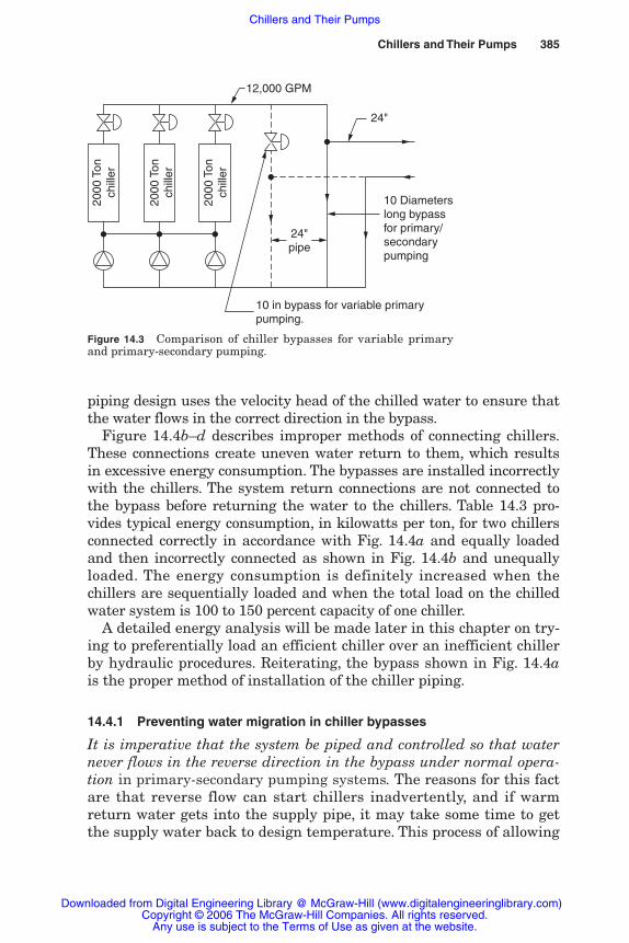
Chillers and Their Pumps 385
piping design uses the velocity head of the chilled water to ensure thatthe water flows in the correct direction in the bypass.
Figure 14.4b–d describes improper methods of connecting chillers.These connections create uneven water return to them, which resultsin excessive energy consumption. The bypasses are installed incorrectlywith the chillers. The system return connections are not connected tothe bypass before returning the water to the chillers. Table 14.3 pro-vides typical energy consumption, in kilowatts per ton, for two chillersconnected correctly in accordance with Fig. 14.4a and equally loadedand then incorrectly connected as shown in Fig. 14.4b and unequallyloaded. The energy consumption is definitely increased when thechillers are sequentially loaded and when the total load on the chilledwater system is 100 to 150 percent capacity of one chiller.
A detailed energy analysis will be made later in this chapter on try-ing to preferentially load an efficient chiller over an inefficient chillerby hydraulic procedures. Reiterating, the bypass shown in Fig. 14.4ais the proper method of installation of the chiller piping.
14.4.1 Preventing water migration in chiller bypasses
It is imperative that the system be piped and controlled so that waternever flows in the reverse direction in the bypass under normal opera-tion in primary-secondary pumping systems. The reasons for this factare that reverse flow can start chillers inadvertently, and if warmreturn water gets into the supply pipe, it may take some time to getthe supply water back to design temperature. This process of allowing
Figure 14.3 Comparison of chiller bypasses for variable primaryand primary-secondary pumping.
24"
10 Diameterslong bypassfor primary/secondarypumping
24"pipe
12,000 GPM20
00 T
onch
iller
2000
Ton
chill
er
2000
Ton
chill
er
10 in bypass for variable primarypumping.
Rishel_CH14.qxd 20/4/06 6:41 PM Page 385
Downloaded from Digital Engineering Library @ McGraw-Hill (www.digitalengineeringlibrary.com)Copyright © 2006 The McGraw-Hill Companies. All rights reserved.
Any use is subject to the Terms of Use as given at the website.
Chillers and Their Pumps

386 Pumps for Closed HVAC Cooling Systems
Figure 14.4 Correct and incorrect chiller piping. (From TheWater Management Manual, SYSTECON, Inc., West Chester,Ohio, 1992, Fig. 6.2.)
Rishel_CH14.qxd 20/4/06 6:41 PM Page 386
Downloaded from Digital Engineering Library @ McGraw-Hill (www.digitalengineeringlibrary.com)Copyright © 2006 The McGraw-Hill Companies. All rights reserved.
Any use is subject to the Terms of Use as given at the website.
Chillers and Their Pumps
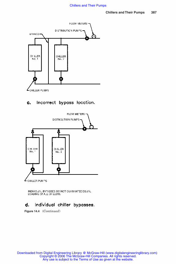
Chillers and Their Pumps 387
Figure 14.4 (Continued)
Rishel_CH14.qxd 20/4/06 6:41 PM Page 387
Downloaded from Digital Engineering Library @ McGraw-Hill (www.digitalengineeringlibrary.com)Copyright © 2006 The McGraw-Hill Companies. All rights reserved.
Any use is subject to the Terms of Use as given at the website.
Chillers and Their Pumps
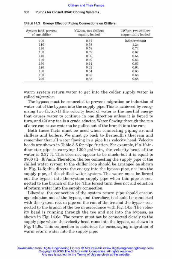
warm system return water to get into the colder supply water iscalled migration.
The bypass must be connected to prevent migration or induction ofwater out of the bypass into the supply pipe. This is achieved by recog-nizing two facts: (1) the velocity head of water is the inertial energythat causes water to continue in one direction unless it is forced toturn, and (2) any tee is a crude eductor. Water flowing through the runof a tee can cause water to be pulled out of the branch into the run.
Both these facts must be used when connecting piping aroundchillers and boilers. We must go back to Bernoulli’s theorem andremember that all water flowing in a pipe has velocity head. Velocityheads are shown in Table 3.5 for pipe friction. For example, if a 10-in-diameter pipe is carrying 1200 gal /min, the velocity head of thewater is 0.37 ft. This does not appear to be much, but it is equal to3700 (ft � lb)/min. Therefore, the tee connecting the supply pipe of thechilled water system to the chiller loop should be arranged as shownin Fig. 14.5; this directs the energy into the bypass pipe, not into thesupply pipe, of the chilled water system. The water must be forcedout the bypass into the system supply pipe when this pipe is con-nected to the branch of the tee. This forced turn does not aid eductionof return water into the supply connection.
Likewise, the connection of the system return pipe should encour-age eduction out of the bypass, and therefore, it should be connectedwith the system return pipe on the run of the tee and the bypass con-nected to the branch of the tee in accordance with Fig. 14.5. The veloc-ity head is running through the tee and not into the bypass, asshown in Fig. 14.6a. The return must not be connected closely to thesupply pipe where the velocity head rams into the bypass, as shown inFig. 14.6b. This connection is notorious for encouraging migration ofwarm return water into the supply pipe.
388 Pumps for Closed HVAC Cooling Systems
TABLE 14.3 Energy Effect of Piping Connections on Chillers
System load, percent kW/ton, two chillers kW/ton, two chillers of one chiller equally loaded sequentially loaded
100 0.57 Indeterminant110 0.58 1.24120 0.58 0.74130 0.59 0.67140 0.60 0.64150 0.60 0.63160 0.61 0.63170 0.62 0.64180 0.64 0.65190 0.66 0.66200 0.68 0.68
Rishel_CH14.qxd 20/4/06 6:41 PM Page 388
Downloaded from Digital Engineering Library @ McGraw-Hill (www.digitalengineeringlibrary.com)Copyright © 2006 The McGraw-Hill Companies. All rights reserved.
Any use is subject to the Terms of Use as given at the website.
Chillers and Their Pumps
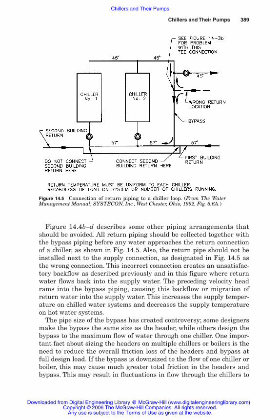
Chillers and Their Pumps 389
Figure 14.4b–d describes some other piping arrangements thatshould be avoided. All return piping should be collected together withthe bypass piping before any water approaches the return connectionof a chiller, as shown in Fig. 14.5. Also, the return pipe should not beinstalled next to the supply connection, as designated in Fig. 14.5 asthe wrong connection. This incorrect connection creates an unsatisfac-tory backflow as described previously and in this figure where returnwater flows back into the supply water. The preceding velocity headrams into the bypass piping, causing this backflow or migration ofreturn water into the supply water. This increases the supply temper-ature on chilled water systems and decreases the supply temperatureon hot water systems.
The pipe size of the bypass has created controversy; some designersmake the bypass the same size as the header, while others design thebypass to the maximum flow of water through one chiller. One impor-tant fact about sizing the headers on multiple chillers or boilers is theneed to reduce the overall friction loss of the headers and bypass atfull design load. If the bypass is downsized to the flow of one chiller orboiler, this may cause much greater total friction in the headers andbypass. This may result in fluctuations in flow through the chillers to
Figure 14.5 Connection of return piping to a chiller loop. (From The WaterManagement Manual, SYSTECON, Inc., West Chester, Ohio, 1992, Fig. 6.6A.)
Rishel_CH14.qxd 20/4/06 6:41 PM Page 389
Downloaded from Digital Engineering Library @ McGraw-Hill (www.digitalengineeringlibrary.com)Copyright © 2006 The McGraw-Hill Companies. All rights reserved.
Any use is subject to the Terms of Use as given at the website.
Chillers and Their Pumps

390
Fig
ure
14.
6V
eloc
ity
hea
d in
pip
e te
es.
Rishel_CH14.qxd 20/4/06 6:41 PM Page 390
Downloaded from Digital Engineering Library @ McGraw-Hill (www.digitalengineeringlibrary.com)Copyright © 2006 The McGraw-Hill Companies. All rights reserved.
Any use is subject to the Terms of Use as given at the website.
Chillers and Their Pumps
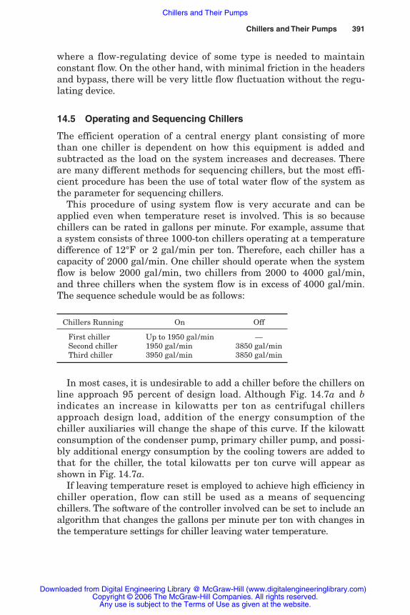
Chillers and Their Pumps 391
where a flow-regulating device of some type is needed to maintainconstant flow. On the other hand, with minimal friction in the headersand bypass, there will be very little flow fluctuation without the regu-lating device.
14.5 Operating and Sequencing Chillers
The efficient operation of a central energy plant consisting of morethan one chiller is dependent on how this equipment is added andsubtracted as the load on the system increases and decreases. Thereare many different methods for sequencing chillers, but the most effi-cient procedure has been the use of total water flow of the system asthe parameter for sequencing chillers.
This procedure of using system flow is very accurate and can beapplied even when temperature reset is involved. This is so becausechillers can be rated in gallons per minute. For example, assume thata system consists of three 1000-ton chillers operating at a temperaturedifference of 12°F or 2 gal/min per ton. Therefore, each chiller has acapacity of 2000 gal/min. One chiller should operate when the systemflow is below 2000 gal/min, two chillers from 2000 to 4000 gal/min,and three chillers when the system flow is in excess of 4000 gal/min.The sequence schedule would be as follows:
Chillers Running On Off
First chiller Up to 1950 gal/min —Second chiller 1950 gal/min 3850 gal/minThird chiller 3950 gal/min 3850 gal/min
In most cases, it is undesirable to add a chiller before the chillers online approach 95 percent of design load. Although Fig. 14.7a and bindicates an increase in kilowatts per ton as centrifugal chillersapproach design load, addition of the energy consumption of thechiller auxiliaries will change the shape of this curve. If the kilowattconsumption of the condenser pump, primary chiller pump, and possi-bly additional energy consumption by the cooling towers are added tothat for the chiller, the total kilowatts per ton curve will appear asshown in Fig. 14.7a.
If leaving temperature reset is employed to achieve high efficiency inchiller operation, flow can still be used as a means of sequencingchillers. The software of the controller involved can be set to include analgorithm that changes the gallons per minute per ton with changes inthe temperature settings for chiller leaving water temperature.
Rishel_CH14.qxd 20/4/06 6:41 PM Page 391
Downloaded from Digital Engineering Library @ McGraw-Hill (www.digitalengineeringlibrary.com)Copyright © 2006 The McGraw-Hill Companies. All rights reserved.
Any use is subject to the Terms of Use as given at the website.
Chillers and Their Pumps

392
Fig
ure
14.
7T
ypic
al k
W/t
on c
urv
es f
or a
cen
trif
uga
l ch
ille
r.(F
rom
Th
e W
ater
Man
agem
ent
Man
ual
,S
YS
TE
CO
N,
Inc.
,W
est
Ch
este
r,O
hio
,199
2,F
igs.
6.6B
an
d 6
.8)
Not
e:T
his
dat
a is
for
ch
ille
rs m
anu
fact
ure
d ar
oun
d 19
90.
Rishel_CH14.qxd 20/4/06 6:41 PM Page 392
Downloaded from Digital Engineering Library @ McGraw-Hill (www.digitalengineeringlibrary.com)Copyright © 2006 The McGraw-Hill Companies. All rights reserved.
Any use is subject to the Terms of Use as given at the website.
Chillers and Their Pumps

Chillers and Their Pumps 393Chillers and Their Pumps 393
14.5.1 Unsatisfactory methods of sequencing chillers
There are a number of unsatisfactory methods of sequencing chillers:
1. By means of chiller power input in amperes. Amperes cannot beused owing to the variation in power input with leaving condenserwater temperature or leaving chilled water temperature. Figure 14.7bdescribes the variation in energy consumption due to changes in leav-ing condenser water temperature. Also, electric utilities are allowed avariation of �5 percent in voltage, which will, of course, change theamperes consumed by the machine.
2. By chiller leaving water temperature. Leaving water temperaturecan be used to add chillers, but it cannot be used to stop a machinebecause the running chillers will adjust the leaving temperature tothe load on the system. Stopping the chillers by return temperaturecan be approximate due to the fluctuation in return temperature fromthe chilled water system. Chillers can be added by leaving tempera-ture and subtracted by system flow.
3. By reverse flow in the bypass. When reverse flow occurs in thebypass, a sizable amount of warm return water will have flowed intothe supply piping before the next chiller can be started and begin toproduce cool water.
Sequencing chillers by system flow has proved to be the most pre-cise method of sequencing chillers. Also, many of the problems justdescribed with bypasses and hydraulically loading of chillers can beeliminated by chilled water storage if there is space for its inclu-sion. Chapter 13 has described in detail the advantages of chilledwater storage in evening out the production of chilled water by thechillers.
14.6 Preferentially Loading Chillers
This subject was deferred until the discussion on sequencing chillerswas completed. Preferential loading of chillers is desirable to ensurethat the most efficient chillers handle most of the cooling load. Trying todo this through water circuiting has proven to be futile because of thepoor efficiency of most chillers at very low percentages of design load.The connecting of an efficient chiller with an older, less efficient chillerrequires special operating procedures to ensure that the most effi-cient chiller is first loaded as high as possible before starting the lessefficient chiller. The following example will describe this problem.
Assume that two 800-ton chillers, one old and one new, are to beoperated together, and their kilowatt per ton consumptions are as
Rishel_CH14.qxd 20/4/06 6:41 PM Page 393
Downloaded from Digital Engineering Library @ McGraw-Hill (www.digitalengineeringlibrary.com)Copyright © 2006 The McGraw-Hill Companies. All rights reserved.
Any use is subject to the Terms of Use as given at the website.
Chillers and Their Pumps

394 Pumps for Closed HVAC Cooling Systems394 Pumps for Closed HVAC Cooling Systems
shown in Table 14.4. In each case, these data include the energyrequirements of both their condenser and primary pumps, which will beassumed as constant speed. The pump motors consume 52 kW for boththe efficient and inefficient chillers. It will be assumed also that thecooling tower cells will be sequenced in such a manner that they are notrelated to one particular chiller but to the total load on the system.
Table 14.5 describes the energy consumption with preferential pip-ing, as shown in Fig. 14.4b. The standby chiller must be started at 100percent load on the high-efficiency machine. This may cause thestandby, low-efficiency chiller to start and stop frequently because ofthe very low load on that chiller.
The total energy expended by preferential piping should be com-pared with the energy expended by equalized piping (Table 14.6).
TABLE 14.4 Chiller Kilowatts Per Ton with Two UnequalChillers
Chiller load, % Efficient chiller Less efficient chiller
010 1.88 2.20020 1.13 1.30030 0.87 1.03040 0.75 0.89050 0.70 0.84060 0.68 0.82070 0.67 0.81080 0.69 0.81090 0.71 0.82100 0.75 0.83
NOTE: Pump kW/ton is included in the chiller kW/ton.
TABLE 14.5 Chiller Energy Consumption with Preferential Piping
% Load of % Load and kW % Load and kW on Total kW of one chiller on efficient chiller inefficient chiller two chillers
080 80–442 — 442090 90–513 — 513100 100–596 — 596110 100–596 10–175 771120 100–596 20–209 805130 100–596 30–246 842140 100–596 40–286 882150 100–596 50–332 928160 100–596 60–393 989170 100–596 70–455 1051180 100–596 80–519 1115190 100–596 90–592 1188200 100–596 100–660 1256
Rishel_CH14.qxd 20/4/06 6:41 PM Page 394
Downloaded from Digital Engineering Library @ McGraw-Hill (www.digitalengineeringlibrary.com)Copyright © 2006 The McGraw-Hill Companies. All rights reserved.
Any use is subject to the Terms of Use as given at the website.
Chillers and Their Pumps
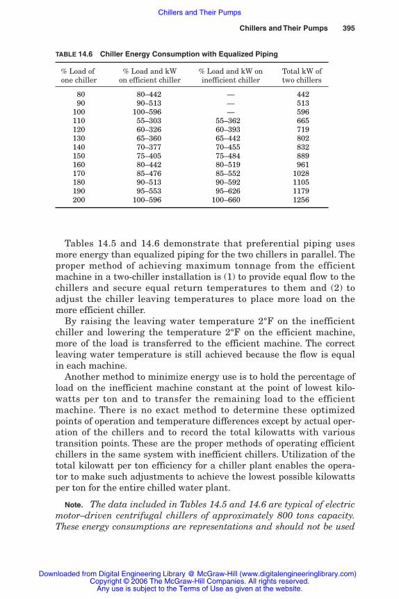
Chillers and Their Pumps 395
Tables 14.5 and 14.6 demonstrate that preferential piping usesmore energy than equalized piping for the two chillers in parallel. Theproper method of achieving maximum tonnage from the efficientmachine in a two-chiller installation is (1) to provide equal flow to thechillers and secure equal return temperatures to them and (2) toadjust the chiller leaving temperatures to place more load on themore efficient chiller.
By raising the leaving water temperature 2°F on the inefficientchiller and lowering the temperature 2°F on the efficient machine,more of the load is transferred to the efficient machine. The correctleaving water temperature is still achieved because the flow is equalin each machine.
Another method to minimize energy use is to hold the percentage ofload on the inefficient machine constant at the point of lowest kilo-watts per ton and to transfer the remaining load to the efficientmachine. There is no exact method to determine these optimizedpoints of operation and temperature differences except by actual oper-ation of the chillers and to record the total kilowatts with varioustransition points. These are the proper methods of operating efficientchillers in the same system with inefficient chillers. Utilization of thetotal kilowatt per ton efficiency for a chiller plant enables the opera-tor to make such adjustments to achieve the lowest possible kilowattsper ton for the entire chilled water plant.
Note. The data included in Tables 14.5 and 14.6 are typical of electricmotor–driven centrifugal chillers of approximately 800 tons capacity.These energy consumptions are representations and should not be used
TABLE 14.6 Chiller Energy Consumption with Equalized Piping
% Load of % Load and kW % Load and kW on Total kW of one chiller on efficient chiller inefficient chiller two chillers
080 80–442 — 442090 90–513 — 513100 100–596 — 596110 55–303 55–362 665120 60–326 60–393 719130 65–360 65–442 802140 70–377 70–455 832150 75–405 75–484 889160 80–442 80–519 961170 85–476 85–552 1028180 90–513 90–592 1105190 95–553 95–626 1179200 100–596 100–660 1256
Rishel_CH14.qxd 20/4/06 6:41 PM Page 395
Downloaded from Digital Engineering Library @ McGraw-Hill (www.digitalengineeringlibrary.com)Copyright © 2006 The McGraw-Hill Companies. All rights reserved.
Any use is subject to the Terms of Use as given at the website.
Chillers and Their Pumps
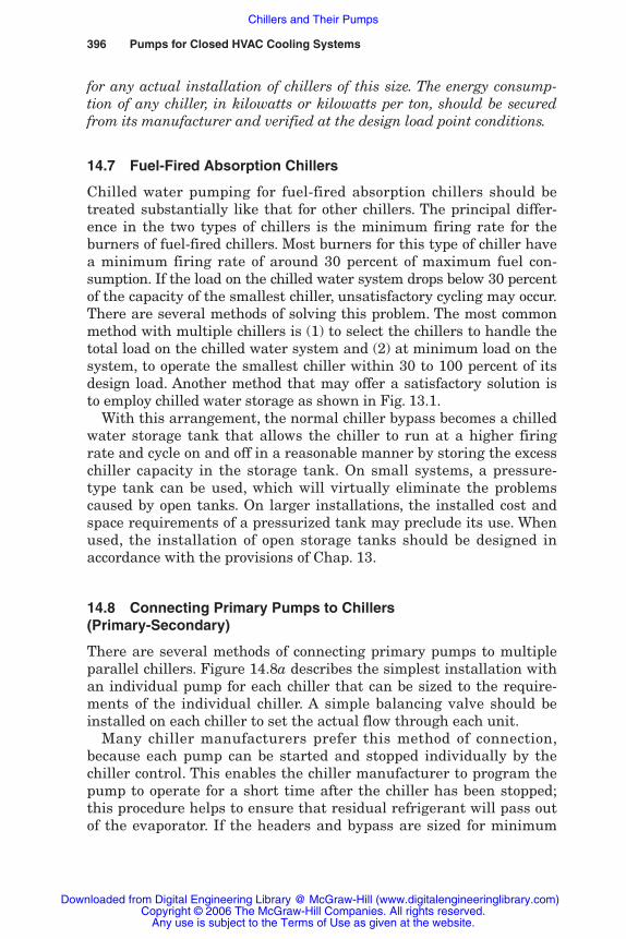
for any actual installation of chillers of this size. The energy consump-tion of any chiller, in kilowatts or kilowatts per ton, should be securedfrom its manufacturer and verified at the design load point conditions.
14.7 Fuel-Fired Absorption Chillers
Chilled water pumping for fuel-fired absorption chillers should betreated substantially like that for other chillers. The principal differ-ence in the two types of chillers is the minimum firing rate for theburners of fuel-fired chillers. Most burners for this type of chiller havea minimum firing rate of around 30 percent of maximum fuel con-sumption. If the load on the chilled water system drops below 30 percentof the capacity of the smallest chiller, unsatisfactory cycling may occur.There are several methods of solving this problem. The most commonmethod with multiple chillers is (1) to select the chillers to handle thetotal load on the chilled water system and (2) at minimum load on thesystem, to operate the smallest chiller within 30 to 100 percent of itsdesign load. Another method that may offer a satisfactory solution isto employ chilled water storage as shown in Fig. 13.1.
With this arrangement, the normal chiller bypass becomes a chilledwater storage tank that allows the chiller to run at a higher firingrate and cycle on and off in a reasonable manner by storing the excesschiller capacity in the storage tank. On small systems, a pressure-type tank can be used, which will virtually eliminate the problemscaused by open tanks. On larger installations, the installed cost andspace requirements of a pressurized tank may preclude its use. Whenused, the installation of open storage tanks should be designed inaccordance with the provisions of Chap. 13.
14.8 Connecting Primary Pumps to Chillers(Primary-Secondary)
There are several methods of connecting primary pumps to multipleparallel chillers. Figure 14.8a describes the simplest installation withan individual pump for each chiller that can be sized to the require-ments of the individual chiller. A simple balancing valve should beinstalled on each chiller to set the actual flow through each unit.
Many chiller manufacturers prefer this method of connection,because each pump can be started and stopped individually by thechiller control. This enables the chiller manufacturer to program thepump to operate for a short time after the chiller has been stopped;this procedure helps to ensure that residual refrigerant will pass outof the evaporator. If the headers and bypass are sized for minimum
396 Pumps for Closed HVAC Cooling Systems
Rishel_CH14.qxd 20/4/06 6:41 PM Page 396
Downloaded from Digital Engineering Library @ McGraw-Hill (www.digitalengineeringlibrary.com)Copyright © 2006 The McGraw-Hill Companies. All rights reserved.
Any use is subject to the Terms of Use as given at the website.
Chillers and Their Pumps
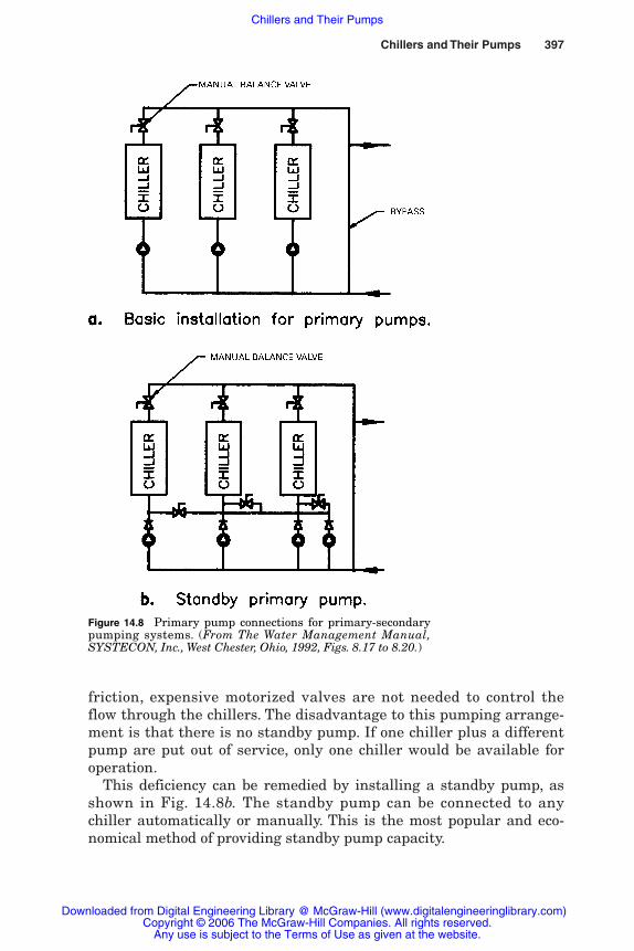
Chillers and Their Pumps 397
friction, expensive motorized valves are not needed to control theflow through the chillers. The disadvantage to this pumping arrange-ment is that there is no standby pump. If one chiller plus a differentpump are put out of service, only one chiller would be available foroperation.
This deficiency can be remedied by installing a standby pump, asshown in Fig. 14.8b. The standby pump can be connected to anychiller automatically or manually. This is the most popular and eco-nomical method of providing standby pump capacity.
Figure 14.8 Primary pump connections for primary-secondarypumping systems. (From The Water Management Manual,SYSTECON, Inc., West Chester, Ohio, 1992, Figs. 8.17 to 8.20.)
Rishel_CH14.qxd 20/4/06 6:41 PM Page 397
Downloaded from Digital Engineering Library @ McGraw-Hill (www.digitalengineeringlibrary.com)Copyright © 2006 The McGraw-Hill Companies. All rights reserved.
Any use is subject to the Terms of Use as given at the website.
Chillers and Their Pumps
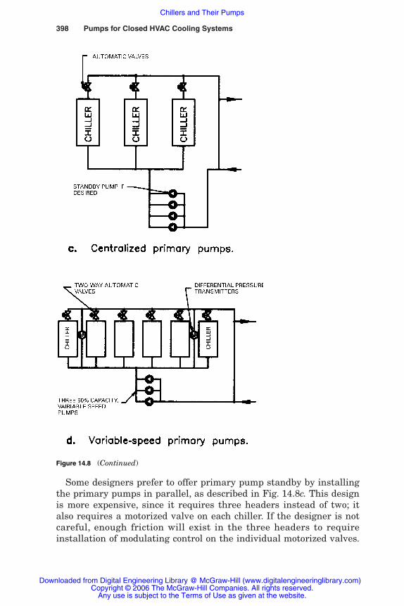
Some designers prefer to offer primary pump standby by installingthe primary pumps in parallel, as described in Fig. 14.8c. This designis more expensive, since it requires three headers instead of two; italso requires a motorized valve on each chiller. If the designer is notcareful, enough friction will exist in the three headers to requireinstallation of modulating control on the individual motorized valves.
398 Pumps for Closed HVAC Cooling Systems
Figure 14.8 (Continued)
Rishel_CH14.qxd 20/4/06 6:41 PM Page 398
Downloaded from Digital Engineering Library @ McGraw-Hill (www.digitalengineeringlibrary.com)Copyright © 2006 The McGraw-Hill Companies. All rights reserved.
Any use is subject to the Terms of Use as given at the website.
Chillers and Their Pumps
Chillers and Their Pumps 399
There are few installations that justify this method of connecting pri-mary pumps to chillers.
Another method of handling the primary pumping where there is anumber of parallel chillers is to install variable-speed primary pumps,as shown in Fig. 14.8d. This installation with six chillers will be bet-ter served by installing three variable-speed primary pumps, eachwith 50 percent of the total capacity of all six chillers. With this proce-dure, the primary pump’s speed is controlled by differential pressuretransmitters that maintain the desired constant differential pressureacross the chiller evaporators. The standby pumps are added and sub-tracted by the best efficiency or wire-to-water efficiency methodsdescribed in Chap. 10 of this book. The actual control selected willdepend on the size of the primary pumps. The flow through eachevaporator is constant because the differential pressure transmittersmaintain a constant pressure drop across them.
There are several significant advantages to variable-speed pumpingin large, multiple-chiller installations. First, the flow through eachchiller evaporator is relatively constant, whether one or all of thechillers are in operation. This is due to the precise control by the dif-ferential pressure transmitter and the digital pump speed control.Second, since the pressure drop through the chiller loop piping is notincluded in the differential pressure set point, this loop can bereduced to a more economical size without affecting the flow throughany of the chillers.
All the preceding diagrams show the primary pumps on the inletside of the chiller. On high-rise buildings where the static pressure isgreat, it may be advisable to install the primary pumps on the dis-charge of the chiller evaporator to help reduce the total pressure onthe evaporators (see Fig. 14.9a). High-rise buildings can create somespecial problems owing to the great amount of static head possible onequipment installed in these buildings. This static head has beendescribed in a pressure-gradient diagram (Fig. 14.6b) for the buildingin Fig. 14.9a. For purposes of this example, this building has an overallheight of 462 ft and a minimum of 10 psig (23 ft) at the top of the build-ing for a total static head of 485 ft. The diagram shown in Fig. 14.9bprovides the pressure gradients for both the maximum-flow and thezero-flow conditions. The zero-flow diagram demonstrates that the cas-ing pressure for the pumps and the design pressure of piping andvalves at the bottom of the building must be based on the shutoffhead of the secondary pump. In this case, the shutoff head is 264 psig.
Locating chillers and pumps on top of a high-rise building will cer-tainly reduce the pressure on the equipment, but the piping and coilsat the bottom of the building will still be subjected to the high pres-sure shown in the pressure gradients of Fig. 14.9b.
Rishel_CH14.qxd 20/4/06 6:41 PM Page 399
Downloaded from Digital Engineering Library @ McGraw-Hill (www.digitalengineeringlibrary.com)Copyright © 2006 The McGraw-Hill Companies. All rights reserved.
Any use is subject to the Terms of Use as given at the website.
Chillers and Their Pumps

400
Fig
ure
14.
9P
rim
ary
pum
p lo
cati
on f
or h
igh
-ris
e bu
ildi
ngs
.(F
rom
Th
e W
ater
Man
agem
ent
Man
ual
,S
YS
TE
CO
N,
Inc.
,W
est
Ch
este
r,O
hio
,199
2,F
ig.8
.21C
,D.)
Rishel_CH14.qxd 20/4/06 6:41 PM Page 400
Downloaded from Digital Engineering Library @ McGraw-Hill (www.digitalengineeringlibrary.com)Copyright © 2006 The McGraw-Hill Companies. All rights reserved.
Any use is subject to the Terms of Use as given at the website.
Chillers and Their Pumps

14.9 Connecting Multiple Chiller Plants
A common and desirable situation encountered on campus-typeinstallations and very large building complexes is to connect severalchiller plants together to serve the chilled water requirements of allthe buildings or zones. This provides significant advantages over thearrangement of individual chillers for each building; these are (1)standby capacity is provided to all buildings, (2) operating chillers onvery low loads is avoided because one chiller can handle the minimumloads for a number of buildings, and (3) by connecting the chillerstogether, the ability to reduce the chiller plant size is often realizeddue to the combined large load diversity of all the buildings. Thisincreases greatly the efficiency of chiller operation.
Figure 14.10 describes such an arrangement. This installation hasfour buildings with chillers and two without. The buildings withoutchillers are new; there is no desire or need to install chillers in thesebuildings because there is more than enough excess chiller capacity inthe other buildings to serve these two new buildings.
To utilize this excess capacity, it is necessary to install a campussupply and return loop. The following are other design parametersthat should be followed for such a facility:
1. No new central pump stations are to be used.
2. A minimum of energy-wasting devices is to be used.
3. Any building must be capable of being served by any of the chillerplants.
4. The central control center operator must have the ability to selectthe most efficient chillers without changing any valving in thebuildings.
5. The flow in any chiller evaporator must not be restricted.
6. If a chiller fails, any building load must be picked up automaticallywithout any changes in coil valve position.
7. Flowmeters must be installed in the loop bypass and in each build-ing to determine individual building loads and to indicate theamount of excess capacity occurring in the bypass. A temperaturetransmitter also must be located in the bypass to indicate reverseflow that should not occur under normal operation.
The building connections are described in Fig. 14.10a for buildingsboth with and without chillers. The chiller pumps are constant-speedpumps, and the building pumps are variable-speed pumps. The build-ing pumps are controlled by differential pressure transmitters located
Chillers and Their Pumps 401
Rishel_CH14.qxd 20/4/06 6:41 PM Page 401
Downloaded from Digital Engineering Library @ McGraw-Hill (www.digitalengineeringlibrary.com)Copyright © 2006 The McGraw-Hill Companies. All rights reserved.
Any use is subject to the Terms of Use as given at the website.
Chillers and Their Pumps

402
Fig
ure
14.
10M
ult
iple
ch
ille
r pl
ant
con
nec
tion
s.(F
rom
Th
e W
ater
Man
agem
ent
Man
ual
,S
YS
TE
CO
N,
Inc.
,W
est
Ch
este
r,O
hio
,19
92,F
ig.6
.9.)
Rishel_CH14.qxd 20/4/06 6:41 PM Page 402
Downloaded from Digital Engineering Library @ McGraw-Hill (www.digitalengineeringlibrary.com)Copyright © 2006 The McGraw-Hill Companies. All rights reserved.
Any use is subject to the Terms of Use as given at the website.
Chillers and Their Pumps
properly in each building. The flow transmitters also provide the cen-tral control operator with data on each building’s load and the flowfrom the supply loop that is occurring in each building.
The central bypass, as described in Fig. 14.10b, is necessary toensure that the flow in any chiller evaporator is not reduced. Suddenchanges in campus load could drastically reduce the flow in a chillerevaporator and cause possible freezing in the tubes without thisbypass.
Questions often arise on how to calculate the head for the chillerpumps and the building pumps as well as sizing the supply andreturn loops. Both the chiller and building pumps must have thecapacity to pump to and from the loop bypass under the most diverseload conditions that can occur on the entire installation. Likewise, thedesign engineer must evaluate all the possible load conditions andselect the one that requires the largest flows in the loops.
This will enable the system designer not only to select the head forboth the chiller and building pumps but also to size the loop piping. Inactual operation, the normal load on the loops is much less than themaximum possible load. This explains the need for the variable-speedbuilding pumps.
If there is a great head variation on the chiller pumps, they alsoshould be variable-speed pumps with differential pressure transmit-ters across the evaporators to maintain constant flow through eachevaporator. If the variation of this flow is expected to be moderate, thechiller pumps may be constant-speed pumps with an automatic flowcontrol valve on each chiller.
The maximum head for the chiller pumps and that for the buildingpumps must be checked to ensure that the chiller or loop head neverapproaches that of the buildings. Otherwise, the chiller pumps havethe possibility of overpressuring the building pumps. If there is a pos-sibility of this, a pressure gradient should be developed for the condi-tion to verify the pressure relationship.
If designer determines that significant energy can be saved bypumping a building with its chiller pumps, the building pumps shouldbe equipped with a bypass. This enables the building pumps to beshut down when adequate pressure is developed by the chiller pumps.
There are several advantages to this method of connecting multiplechiller plants over those systems which depend on computerization offlow and temperature transmitters to interconnect the chiller plants:(1) the central bypass ensures that adequate flow will be provided forall the chiller evaporators that have been placed in operation, (2) thesystem can operate with the central computer totally shut down, and(3) the central bypass method is much simpler, less expensive, andmore reliable than the computerized control system.
Chillers and Their Pumps 403
Rishel_CH14.qxd 20/4/06 6:41 PM Page 403
Downloaded from Digital Engineering Library @ McGraw-Hill (www.digitalengineeringlibrary.com)Copyright © 2006 The McGraw-Hill Companies. All rights reserved.
Any use is subject to the Terms of Use as given at the website.
Chillers and Their Pumps

404 Pumps for Closed HVAC Cooling Systems
There are other procedures for interconnecting multiple chillerplants. Their use depends on the actual physical arrangement of theentire facility. Some multiple-chiller systems have been designed touse energy wasters such as three-way temperature-control valves orreturn temperature-control valves; as a general rule, where possible,these systems should be avoided.
14.9.1 Connecting large chiller plants
Large campus operations are often served by two chiller plants witheach plant serving part of the overall facility. This necessitated therunning of two plants at part-load conditions where it would be moreeconomical to run just one plant. Current control procedures nowallow connection of the two plants together so that only one plant isneeded at the reduced load conditions. Figure 14.11 illustrates thisprocedure.
In Figure 14.11, this campus is divided into two parts with chillerplant A serving one and chiller plant B, the other. The work that mustbe done to allow either plant to serve the entire facility requires first,the connection of the two parts into one hydraulic system. A networkanalysis as described in Chap. 3 and Fig. 3.14 should be completed todetermine the size and number of connections that should be madebetween the two systems. In the following control discussion, it isassumed that all of the distribution pumps are variable speed.Figure 3.14 shows plant A as an older plant with primary-secondarypumping while plant B is a newer plant with variable primary pump-ing. There are four system differential pressure transmitters (DP1 toDP4) that control the distribution of water in the entire campus. Thereare two additional differential pressure transmitters (DPA and DPB)that determine the actual pump head being developed by each plant.
Through the use of these transmitters, control procedures are usedto achieve optimum distribution of chilled water in the campus. Sincethe distribution pumps of one chiller plant are almost always of dif-ferent head than the other, the two pumping systems cannot be run inparallel. This is averted by making one of the two plants as the leadand the other as the lag plant. Usually, either plant can be put on thelead or lag positions. The four system differential pressure transmit-ter signals are sent to the lead plant, and the campus water distribu-tion is maintained by that plant. When the lead plant can no longer sup-ply the required amount of water to all of the system, a chiller is startedin the lag plant and delivers a discrete amount of water to the system.
After continued operation, it may prove to be more efficient to runmore than one chiller in the lag plant. Of course, as the load increaseson the campus, more than one chiller may be needed in the lag plant.
Rishel_CH14.qxd 20/4/06 6:41 PM Page 404
Downloaded from Digital Engineering Library @ McGraw-Hill (www.digitalengineeringlibrary.com)Copyright © 2006 The McGraw-Hill Companies. All rights reserved.
Any use is subject to the Terms of Use as given at the website.
Chillers and Their Pumps

The differential pressure transmitters across the supply and returnmains of the chiller plants provide additional information on the pro-gramming of the chillers in the two plants. A combination of thechiller plant flows and differential pressures enable the operators todetermine the energy to pump the combined system and select theoptimum number and location of the chillers to achieve the minimumenergy required for chilled water distribution under all cooling loads.
Chillers and Their Pumps 405
DPADP1
DP2
DP3
DP4
DPB
F
F
Possible secondconnection
New connection
Chiller plant B(variable primary)
Chiller plant A(primary-secondary)
Figure 14.11 Connecting two chilled water systems.
Rishel_CH14.qxd 20/4/06 6:41 PM Page 405
Downloaded from Digital Engineering Library @ McGraw-Hill (www.digitalengineeringlibrary.com)Copyright © 2006 The McGraw-Hill Companies. All rights reserved.
Any use is subject to the Terms of Use as given at the website.
Chillers and Their Pumps
This procedure seems quite complicated, but it is not difficult. It iscalled “profile pumping,” as the actual size and location of variouscooling loads can be determined by it.
14.10 Effect of Water Temperatures on Chiller Performance
The actual performance of a chiller can be far from its rating in kilo-watts per ton. This is due to variations in condenser water tempera-ture and return chilled water temperature. It is important to end thischapter with this review of condenser water temperature and returnchilled water temperature.
14.10.1 Condenser water temperature
The actual energy consumption of a chiller is reduced with colder con-denser water. Chillers are rated in accordance with the specificationsestablished by the American Refrigeration Institute. Centrifugalchillers at part-load are rated at specific entering condenser watertemperatures such as 85°F at 100 percent load and down to 65°F atpart–loads of 50 percent or less. This reduces the energy input to thechiller appreciably at lower loadings on the chiller.
Unfortunately, in real life, chillers often operate at reduced loadingwith constant condenser water temperatures such as 85°F. The effectof condenser temperature upon a chiller’s kilowatts per ton is pro-nounced as is seen in Fig. 14.12 where the kilowatts per ton for ARIcondenser water temperatures is compared to that for a constant con-denser temperature of 85°F. This demonstrates the need to operatechillers at the optimum condenser water temperature. Also, this high-lights the need to maintain higher loads on operating chillers byensuring the highest possible return chilled water temperature. Aswill be seen in Sec. 14.10.2, poor chilled water differential tempera-ture lowers the percent load on a chiller, which increases the kilo-watts per ton for the chiller.
14.10.2 The effect of low return watertemperature on chiller capacity
Emphasis will be made throughout this book on the need for main-taining design return water temperature on chilled water systems.Here, we want to demonstrate the great effect that return water tem-perature has on available chiller capacity.
If you are a chiller plant manager, did you ever wonder whetheryour chillers are really producing their design tonnage? One quick andeasy way to find out is to just check the chilled water temperatures to
406 Pumps for Closed HVAC Cooling Systems
Rishel_CH14.qxd 20/4/06 6:41 PM Page 406
Downloaded from Digital Engineering Library @ McGraw-Hill (www.digitalengineeringlibrary.com)Copyright © 2006 The McGraw-Hill Companies. All rights reserved.
Any use is subject to the Terms of Use as given at the website.
Chillers and Their Pumps
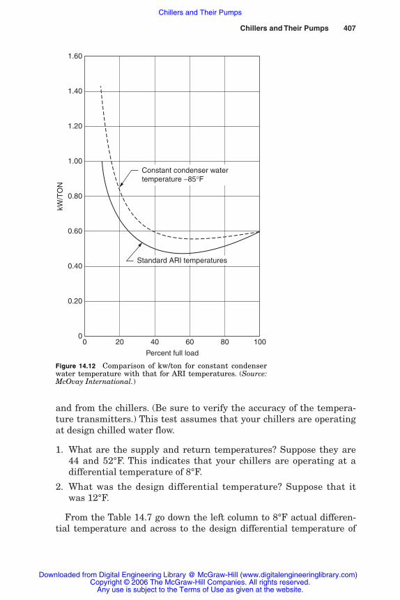
and from the chillers. (Be sure to verify the accuracy of the tempera-ture transmitters.) This test assumes that your chillers are operatingat design chilled water flow.
1. What are the supply and return temperatures? Suppose they are44 and 52°F. This indicates that your chillers are operating at adifferential temperature of 8°F.
2. What was the design differential temperature? Suppose that itwas 12°F.
From the Table 14.7 go down the left column to 8°F actual differen-tial temperature and across to the design differential temperature of
Chillers and Their Pumps 407
1.60
1.40
1.20
1.00
0.80
0.60
0.40
0.20
00
kW/T
ON
20 40 60 80 100
Percent full load
Standard ARI temperatures
Constant condenser watertemperature −85°F
Figure 14.12 Comparison of kw/ton for constant condenserwater temperature with that for ARI temperatures. (Source:McOvay International.)
Rishel_CH14.qxd 20/4/06 6:41 PM Page 407
Downloaded from Digital Engineering Library @ McGraw-Hill (www.digitalengineeringlibrary.com)Copyright © 2006 The McGraw-Hill Companies. All rights reserved.
Any use is subject to the Terms of Use as given at the website.
Chillers and Their Pumps
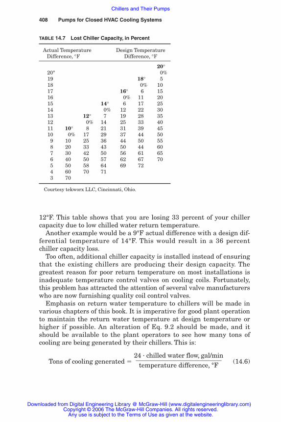
12°F. This table shows that you are losing 33 percent of your chillercapacity due to low chilled water return temperature.
Another example would be a 9°F actual difference with a design dif-ferential temperature of 14°F. This would result in a 36 percentchiller capacity loss.
Too often, additional chiller capacity is installed instead of ensuringthat the existing chillers are producing their design capacity. Thegreatest reason for poor return temperature on most installations isinadequate temperature control valves on cooling coils. Fortunately,this problem has attracted the attention of several valve manufacturerswho are now furnishing quality coil control valves.
Emphasis on return water temperature to chillers will be made invarious chapters of this book. It is imperative for good plant operationto maintain the return water temperature at design temperature orhigher if possible. An alteration of Eq. 9.2 should be made, and itshould be available to the plant operators to see how many tons ofcooling are being generated by their chillers. This is:
Tons of cooling generated � (14.6)24 · chilled water flow, gal/min����temperature difference, °F
408 Pumps for Closed HVAC Cooling Systems
TABLE 14.7 Lost Chiller Capacity, in Percent
Actual Temperature Design TemperatureDifference, °F Difference, °F
20°20° 0%19 18° 518 0% 1017 16° 6 1516 0% 11 2015 14° 6 17 2514 0% 12 22 3013 12° 7 19 28 3512 0% 14 25 33 4011 10° 8 21 31 39 4510 0% 17 29 37 44 509 10 25 36 44 50 558 20 33 43 50 44 607 30 42 50 56 61 656 40 50 57 62 67 705 50 58 64 69 724 60 70 713 70
Courtesy tekworx LLC, Cincinnati, Ohio.
Rishel_CH14.qxd 20/4/06 6:41 PM Page 408
Downloaded from Digital Engineering Library @ McGraw-Hill (www.digitalengineeringlibrary.com)Copyright © 2006 The McGraw-Hill Companies. All rights reserved.
Any use is subject to the Terms of Use as given at the website.
Chillers and Their Pumps

where the temperature difference is the return water temperatureto the chiller minus the water temperature leaving the chiller.
This should be compared to the rating of the chiller; as mentionedearlier, this may prove that more chiller capacity is not needed.Rather, better use of the chilled water is the objective of improvedchiller plant operation.
14.11 Bibliography
ASHRAE Terminology of Heating, Ventilation, Air Conditioning and Refrigeration, 2ded., ASHRAE, Atlanta, Ga., 1991.
Engineers Newsletter, 23(1), 1994, The Trane Company, La Crosse, Wis.The Water Management Manual, SYSTECON, Inc., West Chester, Ohio, 1992.
Chillers and Their Pumps 409
Rishel_CH14.qxd 20/4/06 6:41 PM Page 409
Downloaded from Digital Engineering Library @ McGraw-Hill (www.digitalengineeringlibrary.com)Copyright © 2006 The McGraw-Hill Companies. All rights reserved.
Any use is subject to the Terms of Use as given at the website.
Chillers and Their Pumps

Rishel_CH14.qxd 20/4/06 6:41 PM Page 410
Downloaded from Digital Engineering Library @ McGraw-Hill (www.digitalengineeringlibrary.com)Copyright © 2006 The McGraw-Hill Companies. All rights reserved.
Any use is subject to the Terms of Use as given at the website.
Chillers and Their Pumps

Chapter
411
15Chilled Water
Distribution Systems
15.1 Introduction
The advent of digital control in refrigerants in chillers has provided new,cost effective methods of distributing chilled water. No longer is it neces-sary to design these systems to accommodate constant flow in chillerevaporators. With digital control, contemporary chillers can now allowbroad flow variations in the evaporators without fear of freezing them.Chiller manufacturers are now stating minimum flow rates in the evapo-rators to be from 1.5 to 3.0 ft/s velocities. The actual minimum flow rateshould be verified by the chiller manufacturer on a job to job basis.
Variable flow in the evaporators allows the use of variable-speedprimary pumps, and such systems have become known as “variableprimary” or just “VP”. Already, there have been some descriptions ofVP systems in Chap. 8. The various types of these systems will bedescribed here as well as their use with distributed pumping.
Much of this chapter will still retain information on primary-secondary systems, since many engineers and owners of chilled watersystems have not accepted the use of VP systems totally. There arethousands of VP systems now in operation, and there really is no rea-son to design new primary-secondary chilled water systems.
Experience implies that the required minimum flow should, tosome degree, be related to the distribution system temperature differ-ential. However, chiller manufacturers recommend minimum flowbased on calculated or “rule of thumb” minimum velocities.
Chapter 8 described basic uses of water in HVAC systems, whileChap. 14 reviewed the proper application of chillers and primary or
Rishel_CH15.qxd 20/4/06 6:43 PM Page 411
Downloaded from Digital Engineering Library @ McGraw-Hill (www.digitalengineeringlibrary.com)Copyright © 2006 The McGraw-Hill Companies. All rights reserved.
Any use is subject to the Terms of Use as given at the website.
Source: HVAC Pump Handbook
412 Pumps for Closed HVAC Cooling Systems
chiller pumps. This chapter describes the various methods of distrib-uting chilled water in a building or group of buildings. It pertainsprincipally to the second zone of a chilled water system, that of trans-porting the chilled water from the chiller plant to the terminal unitsor coils.
The principal emphasis of contemporary design of chilled water sys-tems is to move the water with the highest efficiency and lowestenergy consumption possible within the economic constraints of theinstallation. This is of greater importance for chilled water than forhot water because of the larger volumes of water required with chilledwater systems. Because of their extensive piping, chilled water sys-tems usually have higher pump heads and larger pump motors.
Chilled water distribution systems should be configured to avoidinterfering with the efficient operation of the chillers. This was dis-cussed in Chap. 14 and must be emphasized again here. There havebeen efforts to produce complicated pumping systems to save pumpingenergy at the expense of chiller energy consumption. Resetting chillerleaving water temperature upward almost always affords greater energysavings than resetting zone water temperatures to save pumping energy.The added friction of zone control valves and extra piping often nulli-fies much of the savings in pumping energy achieved by zone tempera-ture reset. It is the responsibility of the system designer to ascertainthis on each prospective installation. It should be emphasized that thedesigner must always ensure that the system chilled water tempera-ture is low enough to satisfy the latent load on the cooling coils.
Chapter 8 provides some specific information on the energy wastedin extra piping, fittings, and valves when three-way valves or zonereset with circulators is used on chilled water. Table 8.3 providesinformation for a specific application. Almost every detailed analysisof zone reset proves that energy is lost as a result of extra frictionlosses and loss of energy savings in the chillers themselves.
There are a number of different chilled water distribution systems;all the major types will be reviewed in this chapter. The principaltypes are (1) primary, (2) primary-secondary, (3) primary-secondary-tertiary, and (4) distributed. The discussion will review pumpingenergy, first cost, ease of control, and general operating considerations.
15.2 Primary Systems
The original primary chilled water system was a constant-volume sys-tem utilizing three-way valves on the cooling coils. (Fig. 15.1a). Whenenergy was relatively cheap, this system was used. It had severalenergy-wasting conditions that are no longer acceptable. For example,
Rishel_CH15.qxd 20/4/06 6:43 PM Page 412
Downloaded from Digital Engineering Library @ McGraw-Hill (www.digitalengineeringlibrary.com)Copyright © 2006 The McGraw-Hill Companies. All rights reserved.
Any use is subject to the Terms of Use as given at the website.
Chilled Water Distribution Systems

Chilled Water Distribution Systems 413
1. Constant-speed pumps were used; any overpressure caused byselecting too high a design head for the pumps was eliminated inthe balance valves.
2. The balance valves consumed energy even though the pump headwas selected correctly; this is due to the differences in distributionfriction between the cooling coils.
a. Constant volume, primary system.
b. Small constant-volume system.
Figure 15.1 Constant volume system.
Rishel_CH15.qxd 20/4/06 6:43 PM Page 413
Downloaded from Digital Engineering Library @ McGraw-Hill (www.digitalengineeringlibrary.com)Copyright © 2006 The McGraw-Hill Companies. All rights reserved.
Any use is subject to the Terms of Use as given at the website.
Chilled Water Distribution Systems
414 Pumps for Closed HVAC Cooling Systems
3. As the cooling loads subsided on this system, the return tempera-ture dropped as a result of bypassing of cold water around the cool-ing coils. This caused the chiller or chillers to operate at very lowloads and very high energy rates in kilowatts per ton.
Because of these energy problems, this system should not be usedon any chilled water systems. On top of the energy losses, this is anexpensive system in terms of cost because of the three-way valves andtheir piping. In some cases, actual bids for this system have proved itto be higher in first cost than a variable-speed, variable primary sys-tem of the same size.
Another problem with this system involves rebalancing the flowthrough it whenever a major load is removed from operation. As thesystem aged or changes in the piping occurred, rebalancing also wasrequired. This rebalancing was eliminated by automatic balancingvalves that contained springs and orifices which limited the loadthrough a particular coil or terminal unit to its design flow. Thissolved the rebalancing problem but added appreciable friction to thewater system. Further, full design flow required by the chiller was notachieved under all load conditions. The basic primary system hasbeen modified to eliminate some of its problems.
15.2.1 Small primary pumping system
An exception to the preceding statements about primary three-wayvalve systems is a relatively small system consisting of a chiller andair-handling units located near the chiller, Fig. 15.1b. In such aninstallation, the distribution friction is very low, so there is no greatenergy loss resulting from the use of three-way valves. Concernshould still be given to the chiller operation, since a single chillercould cause very poor chiller efficiencies under low loads on the airhandlers. The use of a multiple-compressor reciprocating chiller maysolve this problem.
15.2.2 Variable-volume primary systemwith bypass valve
Some designers used a pressure-relief valve in the bypass on a pri-mary system with two-way control valves, as shown in Fig. 15.2. Thisis not recommended because it merely eliminates the rise to shutoff ofthe pump head and does not guarantee proper flow through thechillers. Also, this relief valve maintains high differential pressures inthe control valves on the cooling coils when the system friction sub-sides at low loads. This may cause lifting of the valve stems or wire
Rishel_CH15.qxd 20/4/06 6:43 PM Page 414
Downloaded from Digital Engineering Library @ McGraw-Hill (www.digitalengineeringlibrary.com)Copyright © 2006 The McGraw-Hill Companies. All rights reserved.
Any use is subject to the Terms of Use as given at the website.
Chilled Water Distribution Systems
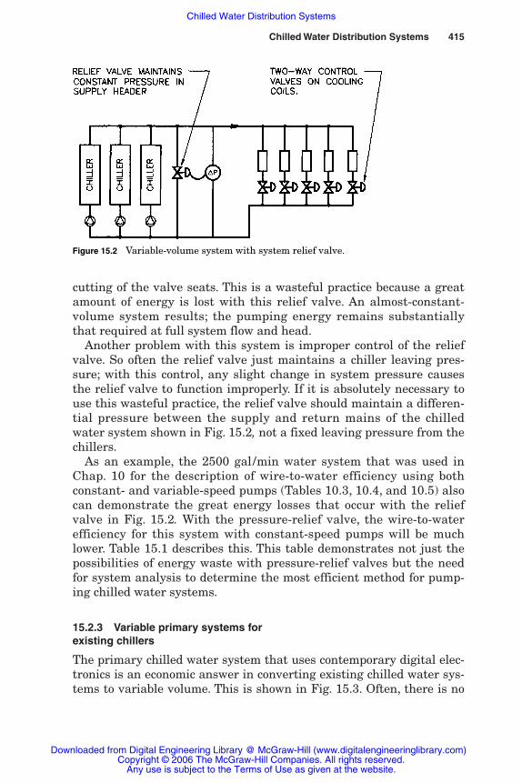
Chilled Water Distribution Systems 415
cutting of the valve seats. This is a wasteful practice because a greatamount of energy is lost with this relief valve. An almost-constant-volume system results; the pumping energy remains substantiallythat required at full system flow and head.
Another problem with this system is improper control of the reliefvalve. So often the relief valve just maintains a chiller leaving pres-sure; with this control, any slight change in system pressure causesthe relief valve to function improperly. If it is absolutely necessary touse this wasteful practice, the relief valve should maintain a differen-tial pressure between the supply and return mains of the chilledwater system shown in Fig. 15.2, not a fixed leaving pressure from thechillers.
As an example, the 2500 gal /min water system that was used inChap. 10 for the description of wire-to-water efficiency using bothconstant- and variable-speed pumps (Tables 10.3, 10.4, and 10.5) alsocan demonstrate the great energy losses that occur with the reliefvalve in Fig. 15.2. With the pressure-relief valve, the wire-to-waterefficiency for this system with constant-speed pumps will be muchlower. Table 15.1 describes this. This table demonstrates not just thepossibilities of energy waste with pressure-relief valves but the needfor system analysis to determine the most efficient method for pump-ing chilled water systems.
15.2.3 Variable primary systems forexisting chillers
The primary chilled water system that uses contemporary digital elec-tronics is an economic answer in converting existing chilled water sys-tems to variable volume. This is shown in Fig. 15.3. Often, there is no
Figure 15.2 Variable-volume system with system relief valve.
Rishel_CH15.qxd 20/4/06 6:43 PM Page 415
Downloaded from Digital Engineering Library @ McGraw-Hill (www.digitalengineeringlibrary.com)Copyright © 2006 The McGraw-Hill Companies. All rights reserved.
Any use is subject to the Terms of Use as given at the website.
Chilled Water Distribution Systems
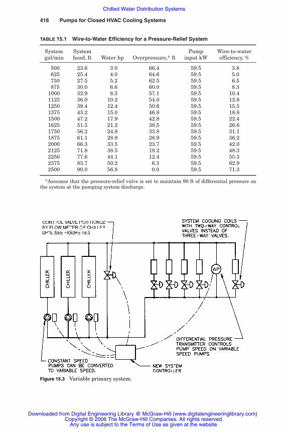
416 Pumps for Closed HVAC Cooling Systems
TABLE 15.1 Wire-to-Water Efficiency for a Pressure-Relief System
System System Pump Wire-to-water gal/min head, ft Water hp Overpressure,* ft input kW efficiency, %
500 23.6 3.0 66.4 59.5 3.8625 25.4 4.0 64.6 59.5 5.0750 27.5 5.2 62.5 59.5 6.5875 30.0 6.6 60.0 59.5 8.3
1000 32.9 8.3 57.1 59.5 10.41125 36.0 10.2 54.0 59.5 12.81250 39.4 12.4 50.6 59.5 15.51375 43.2 15.0 46.8 59.5 18.81500 47.2 17.9 42.8 59.5 22.41625 51.5 21.2 38.5 59.5 26.61750 56.2 24.8 33.8 59.5 31.11875 61.1 28.9 28.9 59.5 36.22000 66.3 33.5 23.7 59.5 42.02125 71.8 38.5 18.2 59.5 48.32250 77.6 44.1 12.4 59.5 55.32375 83.7 50.2 6.3 59.5 62.92500 90.0 56.8 0.0 59.5 71.3
*Assumes that the pressure-relief valve is set to maintain 90 ft of differential pressure onthe system at the pumping system discharge.
Figure 15.3 Variable primary system.
Rishel_CH15.qxd 20/4/06 6:43 PM Page 416
Downloaded from Digital Engineering Library @ McGraw-Hill (www.digitalengineeringlibrary.com)Copyright © 2006 The McGraw-Hill Companies. All rights reserved.
Any use is subject to the Terms of Use as given at the website.
Chilled Water Distribution Systems

Chilled Water Distribution Systems 417
physical room to change to other systems such as primary-secondarypumping, which requires the addition of secondary pumps. Thechanges required in the system in Fig. 15.1a include (1) replacing thethree-way control valves on the coils with two-way valves and (2)installing a chiller bypass with a control valve and its control.
With these changes, the system becomes a variable-volume systemwith the opportunity to achieve the design return water tempera-ture. The bypass with its control valve provides the minimum flowrequired by the chiller manufacturer through the chiller evaporator.If the chiller manufacturer approves a minimum evaporator flow,such as 2.0 ft/s velocity, this can be set easily into the control algo-rithm. This system functions on single-chiller, multiple-chiller instal-lations.
The pumps on variable primary systems are variable speed. Thespeed of these variable-speed pumps is controlled by remote differen-tial pressure transmitters that hold the desired pressure differentialacross the cooling coils, their control valves, and the branch piping.
15.2.4 Variable-volume primary systemwith contemporary chillers
New computer systems for controlling chillers are being offered to theindustry. These control systems utilize digital control that providesclose operation of the chillers so that the flow can be varied throughthe chiller evaporators. The chiller manufacturer specifies a minimumflow or velocity through the evaporator tubes in feet per second thatmust be maintained by the variable-speed pumps; the bypass valvearrangement, as shown in Fig. 15.3, varies its position to maintain thedesired flow in the evaporator. Minimum flow control in the evapora-tor can be accomplished by a system flowmeter or differential pressuretransmitters across the chiller evaporators as shown in Fig. 15.4. Bothprocedures are being used with success in the control of VP systems.The differential pressure transmitters are more precise than flowme-ters in their control of the minimum flow; also, they can be used toprevent excessive flow in the evaporators. If the flow exceeds the max-imum allowable velocity, usually 10 to 11 ft/s, the differential pressurecan sense this and add a chiller or sound an alarm. The flowmeter hasthe advantage of sensing minimum flow when two or more chillersare in operation. If the minimum flow in one chiller is 500 gal/min,with two chillers in operation the minimum flow becomes 1000gal/min. Also, if different-sized chillers with different minimum flowsare in operation, the flowmeter can provide the minimum flow for allchillers in operation. These systems will replace many of the primary-secondary pumping arrangements offered below when chillers are
Rishel_CH15.qxd 20/4/06 6:43 PM Page 417
Downloaded from Digital Engineering Library @ McGraw-Hill (www.digitalengineeringlibrary.com)Copyright © 2006 The McGraw-Hill Companies. All rights reserved.
Any use is subject to the Terms of Use as given at the website.
Chilled Water Distribution Systems

418 Pumps for Closed HVAC Cooling Systems
Figure 15.4 Minimum chiller flow control. (From Patterson PumpCompany HVAC Pumps and Systems Manual, 2004.)
available with precise control of their refrigeration and leaving watertemperature. Chapter 29 describes the conversion of primary-sec-ondary systems to variable primary.
15.3 Primary-Secondary Systems
The primary-secondary system was developed to separate the genera-tion zone of a chilled water system from the transportation or distrib-ution zone. This system really should be called a chiller/distributionsystem, but the industry has settled on the words primary-secondary.This system does separate the chillers from the distribution system,as shown in Fig. 15.5a, and to reduce the differential pressure dropsacross the coil control valves. With this system, the chiller piping canbe designed to provided optimal performance. The flow through thechiller can be constant or whatever flow the chiller manufacturerdesires in the evaporator.
The drawbacks of this system are that (1) two sets of pumps arerequired, and (2) the chiller bypass water is sent back to the chillersunused. With proper chiller sequencing, the energy lost to the bypass
Rishel_CH15.qxd 20/4/06 6:43 PM Page 418
Downloaded from Digital Engineering Library @ McGraw-Hill (www.digitalengineeringlibrary.com)Copyright © 2006 The McGraw-Hill Companies. All rights reserved.
Any use is subject to the Terms of Use as given at the website.
Chilled Water Distribution Systems
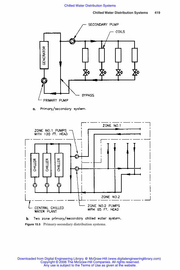
Chilled Water Distribution Systems 419
Figure 15.5 Primary-secondary distribution systems.
Rishel_CH15.qxd 20/4/06 6:43 PM Page 419
Downloaded from Digital Engineering Library @ McGraw-Hill (www.digitalengineeringlibrary.com)Copyright © 2006 The McGraw-Hill Companies. All rights reserved.
Any use is subject to the Terms of Use as given at the website.
Chilled Water Distribution Systems
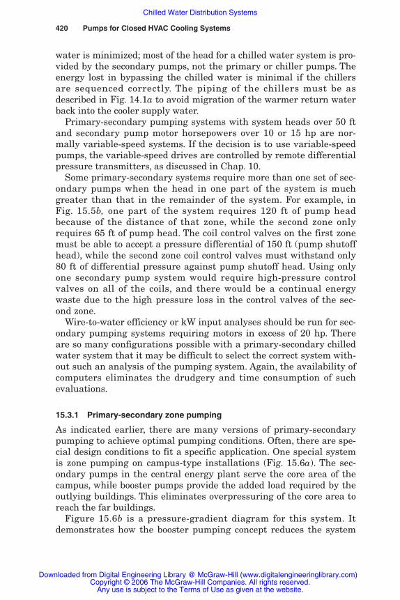
420 Pumps for Closed HVAC Cooling Systems
water is minimized; most of the head for a chilled water system is pro-vided by the secondary pumps, not the primary or chiller pumps. Theenergy lost in bypassing the chilled water is minimal if the chillersare sequenced correctly. The piping of the chillers must be asdescribed in Fig. 14.1a to avoid migration of the warmer return waterback into the cooler supply water.
Primary-secondary pumping systems with system heads over 50 ftand secondary pump motor horsepowers over 10 or 15 hp are nor-mally variable-speed systems. If the decision is to use variable-speedpumps, the variable-speed drives are controlled by remote differentialpressure transmitters, as discussed in Chap. 10.
Some primary-secondary systems require more than one set of sec-ondary pumps when the head in one part of the system is muchgreater than that in the remainder of the system. For example, inFig. 15.5b, one part of the system requires 120 ft of pump headbecause of the distance of that zone, while the second zone onlyrequires 65 ft of pump head. The coil control valves on the first zonemust be able to accept a pressure differential of 150 ft (pump shutoffhead), while the second zone coil control valves must withstand only80 ft of differential pressure against pump shutoff head. Using onlyone secondary pump system would require high-pressure controlvalves on all of the coils, and there would be a continual energywaste due to the high pressure loss in the control valves of the sec-ond zone.
Wire-to-water efficiency or kW input analyses should be run for sec-ondary pumping systems requiring motors in excess of 20 hp. Thereare so many configurations possible with a primary-secondary chilledwater system that it may be difficult to select the correct system with-out such an analysis of the pumping system. Again, the availability ofcomputers eliminates the drudgery and time consumption of suchevaluations.
15.3.1 Primary-secondary zone pumping
As indicated earlier, there are many versions of primary-secondarypumping to achieve optimal pumping conditions. Often, there are spe-cial design conditions to fit a specific application. One special systemis zone pumping on campus-type installations (Fig. 15.6a). The sec-ondary pumps in the central energy plant serve the core area of thecampus, while booster pumps provide the added load required by theoutlying buildings. This eliminates overpressuring of the core area toreach the far buildings.
Figure 15.6b is a pressure-gradient diagram for this system. Itdemonstrates how the booster pumping concept reduces the system
Rishel_CH15.qxd 20/4/06 6:43 PM Page 420
Downloaded from Digital Engineering Library @ McGraw-Hill (www.digitalengineeringlibrary.com)Copyright © 2006 The McGraw-Hill Companies. All rights reserved.
Any use is subject to the Terms of Use as given at the website.
Chilled Water Distribution Systems

Chilled Water Distribution Systems 421
pressure in the core area. Only the far building is shown for the corearea for clarity. As shown, the booster pumping procedure reduces themaximum discharge pressure from 277 to 212 ft. This also reducesthe total energy consumption of the system and cuts the first costrequired for high-pressure control valves and accessories.
The booster pumping systems must be designed to operate in con-junction with the secondary pumps in the central plant. If the sec-ondary pumps are constant-speed pumps, it may be necessary toequip the booster systems with bypasses and building control valves(Fig. 15.6c). The bypass around the booster pumps enables the build-ing to be served by the central plant secondary pumps under lightloads when the secondary pumps may produce adequate head to servethe building. This results in added pumping efficiency, since thebooster pumps can be shut down during this period. The building con-trol valve is necessary if the central plant secondary pumps can over-pressure the building. This valve is controlled by the same remote dif-ferential pressure transmitter that controls the speed of the boosterpumps when they are in operation.
If the secondary pumps are variable-speed pumps, they are con-trolled by differential pressure transmitters located remotely at key
Figure 15.6 Secondary pumping systems with boostersystems.
Rishel_CH15.qxd 20/4/06 6:43 PM Page 421
Downloaded from Digital Engineering Library @ McGraw-Hill (www.digitalengineeringlibrary.com)Copyright © 2006 The McGraw-Hill Companies. All rights reserved.
Any use is subject to the Terms of Use as given at the website.
Chilled Water Distribution Systems
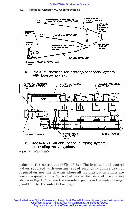
422 Pumps for Closed HVAC Cooling Systems
points in the central zone (Fig. 15.6a). The bypasses and controlvalves required with constant-speed secondary pumps are notrequired on most installations where all the distribution pumps arevariable-speed pumps. Typical of this is the hospital installationshown in Fig. 15.7, where the secondary pumps in the central energyplant transfer the water to the hospital.
Figure 15.6 (Continued)
Rishel_CH15.qxd 20/4/06 6:43 PM Page 422
Downloaded from Digital Engineering Library @ McGraw-Hill (www.digitalengineeringlibrary.com)Copyright © 2006 The McGraw-Hill Companies. All rights reserved.
Any use is subject to the Terms of Use as given at the website.
Chilled Water Distribution Systems

Chilled Water Distribution Systems 423
Figure 15.7 Distributed pumping in a large hospital.
Rishel_CH15.qxd 20/4/06 6:43 PM Page 423
Downloaded from Digital Engineering Library @ McGraw-Hill (www.digitalengineeringlibrary.com)Copyright © 2006 The McGraw-Hill Companies. All rights reserved.
Any use is subject to the Terms of Use as given at the website.
Chilled Water Distribution Systems
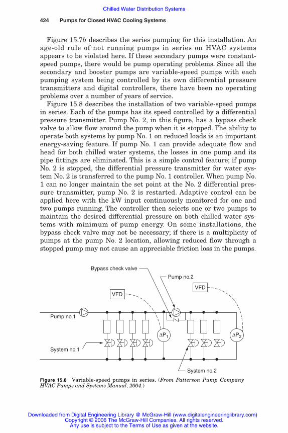
Figure 15.7b describes the series pumping for this installation. Anage-old rule of not running pumps in series on HVAC systemsappears to be violated here. If these secondary pumps were constant-speed pumps, there would be pump operating problems. Since all thesecondary and booster pumps are variable-speed pumps with eachpumping system being controlled by its own differential pressuretransmitters and digital controllers, there have been no operatingproblems over a number of years of service.
Figure 15.8 describes the installation of two variable-speed pumpsin series. Each of the pumps has its speed controlled by a differentialpressure transmitter. Pump No. 2, in this figure, has a bypass checkvalve to allow flow around the pump when it is stopped. The ability tooperate both systems by pump No. 1 on reduced loads is an importantenergy-saving feature. If pump No. 1 can provide adequate flow andhead for both chilled water systems, the losses in one pump and itspipe fittings are eliminated. This is a simple control feature; if pumpNo. 2 is stopped, the differential pressure transmitter for water sys-tem No. 2 is transferred to the pump No. 1 controller. When pump No.1 can no longer maintain the set point at the No. 2 differential pres-sure transmitter, pump No. 2 is restarted. Adaptive control can beapplied here with the kW input continuously monitored for one andtwo pumps running. The controller then selects one or two pumps tomaintain the desired differential pressure on both chilled water sys-tems with minimum of pump energy. On some installations, thebypass check valve may not be necessary; if there is a multiplicity ofpumps at the pump No. 2 location, allowing reduced flow through astopped pump may not cause an appreciable friction loss in the pumps.
424 Pumps for Closed HVAC Cooling Systems
∆P1 ∆P2
Pump no.2
Bypass check valve
System no.1
System no.2
Pump no.1
VFDVFD
Figure 15.8 Variable-speed pumps in series. (From Patterson Pump CompanyHVAC Pumps and Systems Manual, 2004.)
Rishel_CH15.qxd 20/4/06 6:43 PM Page 424
Downloaded from Digital Engineering Library @ McGraw-Hill (www.digitalengineeringlibrary.com)Copyright © 2006 The McGraw-Hill Companies. All rights reserved.
Any use is subject to the Terms of Use as given at the website.
Chilled Water Distribution Systems
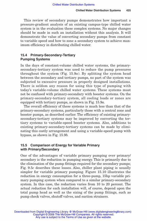
Chilled Water Distribution Systems 425
This review of secondary pumps demonstrates how important apressure-gradient analysis of an existing campus-type chilled watersystem is in the evaluation these complex systems. No major changesshould be made in such an installation without this analysis. It willdemonstrate the value of converting secondary pumps from constantto variable speed and how to zone a secondary system to achieve max-imum efficiency in distributing chilled water.
15.4 Primary-Secondary-Tertiary Pumping Systems
In the days of constant-volume chilled water systems, the primary-secondary-tertiary system was used to reduce the pump pressuresthroughout the system (Fig. 15.9a). By splitting the system headbetween the secondary and tertiary pumps, no part of the system wassubjected to excessive pressure in properly designed installations.There is seldom any reason for using this type of pumping withtoday’s variable-volume chilled water systems. These systems mustnot be confused with primary-secondary with booster systems. On theprimary-secondary-tertiary system, all cooling loads or zones areequipped with tertiary pumps, as shown in Fig. 15.9a.
The overall efficiency of these systems is much less than that of theprimary-secondary systems, particularly those with a central zone andbooster pumps, as described earlier. The efficiency of existing primary-secondary-tertiary systems may be improved by converting the ter-tiary systems to variable-speed booster systems. Also, additions toexisting primary-secondary-tertiary systems can be made by elimi-nating this costly arrangement and using a variable-speed pump withbypass, as shown in Fig. 15.9b.
15.5 Comparison of Energy for Variable Primary with Primary/Secondary
One of the advantages of variable primary pumping over primary/secondary is the reduction in pumping energy. This is primarily due tothe elimination of the pump fittings required for the secondary pumps;Fig. 9.5c describes these losses. Also, chiller plant piping is usuallysimpler for variable primary pumping. Figure 15.10 illustrates thereduction in energy consumption for a three-pump, 15hp variable pri-mary pumping system when compared to a similar primary-secondarysystem. In this case, the reduction varies from 10 to 20 percent. Theactual reduction for each installation will, of course, depend upon thetotal pump head as well as the sizing of the pump fittings, such aspump check valves, shutoff valves, and suction strainers.
Rishel_CH15.qxd 20/4/06 6:43 PM Page 425
Downloaded from Digital Engineering Library @ McGraw-Hill (www.digitalengineeringlibrary.com)Copyright © 2006 The McGraw-Hill Companies. All rights reserved.
Any use is subject to the Terms of Use as given at the website.
Chilled Water Distribution Systems
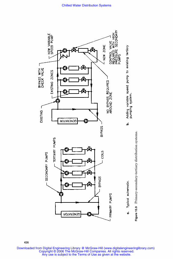
426
Fig
ure
15.
9P
rim
ary-
seco
nda
ry-t
erti
ary
dist
ribu
tion
sys
tem
s.
Rishel_CH15.qxd 20/4/06 6:43 PM Page 426
Downloaded from Digital Engineering Library @ McGraw-Hill (www.digitalengineeringlibrary.com)Copyright © 2006 The McGraw-Hill Companies. All rights reserved.
Any use is subject to the Terms of Use as given at the website.
Chilled Water Distribution Systems

Chilled Water Distribution Systems 427
15.6 Distributed Pumping
Distributed pumping was developed around 1967 to secure a simplerpumping system for campus-type installations where some buildingswere near the central energy plant and others were far from thatplant. Distributed pumping also was developed to eliminate many ofthe energy consumers such as crossover bridges, three-way controlvalves, and return temperature-control valves. It is obvious from thepreceding descriptions of other types of systems that much energy iswasted in pumping circuits. Sizable reductions in pump horsepower,pumping energy, and initial cost have been achieved with this type ofpumping. In most cases, the system friction and pump motors havebeen large enough to always justify variable-speed pumps in the build-ings. There is no reason why this principle cannot be used in smallsystems with relatively low pump head and constant-speed pumps.
Distributed pumping is a very simple pumping arrangement aswell as the most efficient pumping system for (1) large, multiple-zone
40.00
35.00
30.00
25.00
20.00
15.00
10.00
5.00
0.00
Pum
p kW
10% 20% 30% 40% 50% 60% 70% 80% 90% 100%
% GPM
Primary-secondary
Primary-only
Figure 15.10 Comparison of energy for variable primary pumping withprimary/secondary. (From Primary Only vs. Primary SecondaryVariable Flow Systems, Steven T. Taylor, PE, ASHRAE Journal,February 2002. Used with permission.)
Rishel_CH15.qxd 20/4/06 6:43 PM Page 427
Downloaded from Digital Engineering Library @ McGraw-Hill (www.digitalengineeringlibrary.com)Copyright © 2006 The McGraw-Hill Companies. All rights reserved.
Any use is subject to the Terms of Use as given at the website.
Chilled Water Distribution Systems
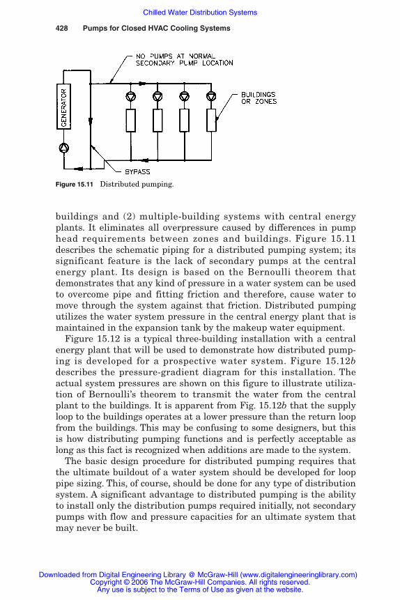
428 Pumps for Closed HVAC Cooling Systems
buildings and (2) multiple-building systems with central energyplants. It eliminates all overpressure caused by differences in pumphead requirements between zones and buildings. Figure 15.11describes the schematic piping for a distributed pumping system; itssignificant feature is the lack of secondary pumps at the centralenergy plant. Its design is based on the Bernoulli theorem thatdemonstrates that any kind of pressure in a water system can be usedto overcome pipe and fitting friction and therefore, cause water tomove through the system against that friction. Distributed pumpingutilizes the water system pressure in the central energy plant that ismaintained in the expansion tank by the makeup water equipment.
Figure 15.12 is a typical three-building installation with a centralenergy plant that will be used to demonstrate how distributed pump-ing is developed for a prospective water system. Figure 15.12bdescribes the pressure-gradient diagram for this installation. Theactual system pressures are shown on this figure to illustrate utiliza-tion of Bernoulli’s theorem to transmit the water from the centralplant to the buildings. It is apparent from Fig. 15.12b that the supplyloop to the buildings operates at a lower pressure than the return loopfrom the buildings. This may be confusing to some designers, but thisis how distributing pumping functions and is perfectly acceptable aslong as this fact is recognized when additions are made to the system.
The basic design procedure for distributed pumping requires thatthe ultimate buildout of a water system should be developed for looppipe sizing. This, of course, should be done for any type of distributionsystem. A significant advantage to distributed pumping is the abilityto install only the distribution pumps required initially, not secondarypumps with flow and pressure capacities for an ultimate system thatmay never be built.
Figure 15.11 Distributed pumping.
Rishel_CH15.qxd 20/4/06 6:43 PM Page 428
Downloaded from Digital Engineering Library @ McGraw-Hill (www.digitalengineeringlibrary.com)Copyright © 2006 The McGraw-Hill Companies. All rights reserved.
Any use is subject to the Terms of Use as given at the website.
Chilled Water Distribution Systems

429
Fig
ure
15.
12T
ypic
al t
hre
e-bu
ildi
ng
dist
ribu
ted
pum
pin
g sy
stem
.
Rishel_CH15.qxd 20/4/06 6:43 PM Page 429
Downloaded from Digital Engineering Library @ McGraw-Hill (www.digitalengineeringlibrary.com)Copyright © 2006 The McGraw-Hill Companies. All rights reserved.
Any use is subject to the Terms of Use as given at the website.
Chilled Water Distribution Systems

430 Pumps for Closed HVAC Cooling Systems
One of the most important advantages of distributed pumping is theelimination of overpressuring of the zones or buildings near the centralplant. This will be described by the use of the two building installationsof Fig. 15.13a. Figure 15.13b is a hydraulic gradient diagram for thissystem as a primary-secondary system at full design load. It is obviousthat building 1 is being overpressured by the secondary pumps in theireffort to provide adequate flow and head to building 2. Figure 15.14
Figure 15.13 Two-building distributed pumping system.
Rishel_CH15.qxd 20/4/06 6:43 PM Page 430
Downloaded from Digital Engineering Library @ McGraw-Hill (www.digitalengineeringlibrary.com)Copyright © 2006 The McGraw-Hill Companies. All rights reserved.
Any use is subject to the Terms of Use as given at the website.
Chilled Water Distribution Systems

431
Fig
ure
15.
14H
ydra
uli
c gr
adie
nts
for
th
e tw
o-bu
ildi
ng
dist
ribu
ted
pum
pin
g sy
stem
.
Rishel_CH15.qxd 20/4/06 6:43 PM Page 431
Downloaded from Digital Engineering Library @ McGraw-Hill (www.digitalengineeringlibrary.com)Copyright © 2006 The McGraw-Hill Companies. All rights reserved.
Any use is subject to the Terms of Use as given at the website.
Chilled Water Distribution Systems
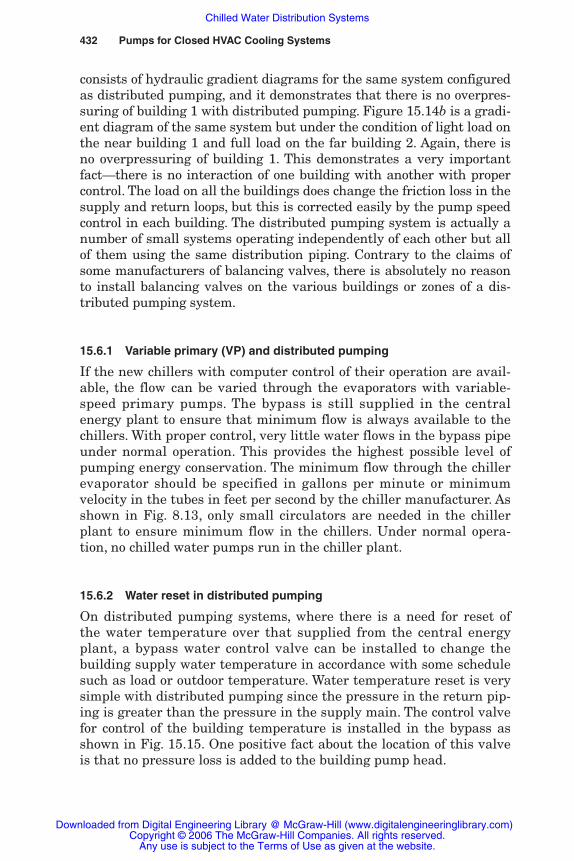
432 Pumps for Closed HVAC Cooling Systems
consists of hydraulic gradient diagrams for the same system configuredas distributed pumping, and it demonstrates that there is no overpres-suring of building 1 with distributed pumping. Figure 15.14b is a gradi-ent diagram of the same system but under the condition of light load onthe near building 1 and full load on the far building 2. Again, there isno overpressuring of building 1. This demonstrates a very importantfact—there is no interaction of one building with another with propercontrol. The load on all the buildings does change the friction loss in thesupply and return loops, but this is corrected easily by the pump speedcontrol in each building. The distributed pumping system is actually anumber of small systems operating independently of each other but allof them using the same distribution piping. Contrary to the claims ofsome manufacturers of balancing valves, there is absolutely no reasonto install balancing valves on the various buildings or zones of a dis-tributed pumping system.
15.6.1 Variable primary (VP) and distributed pumping
If the new chillers with computer control of their operation are avail-able, the flow can be varied through the evaporators with variable-speed primary pumps. The bypass is still supplied in the centralenergy plant to ensure that minimum flow is always available to thechillers. With proper control, very little water flows in the bypass pipeunder normal operation. This provides the highest possible level ofpumping energy conservation. The minimum flow through the chillerevaporator should be specified in gallons per minute or minimumvelocity in the tubes in feet per second by the chiller manufacturer. Asshown in Fig. 8.13, only small circulators are needed in the chillerplant to ensure minimum flow in the chillers. Under normal opera-tion, no chilled water pumps run in the chiller plant.
15.6.2 Water reset in distributed pumping
On distributed pumping systems, where there is a need for reset ofthe water temperature over that supplied from the central energyplant, a bypass water control valve can be installed to change thebuilding supply water temperature in accordance with some schedulesuch as load or outdoor temperature. Water temperature reset is verysimple with distributed pumping since the pressure in the return pip-ing is greater than the pressure in the supply main. The control valvefor control of the building temperature is installed in the bypass asshown in Fig. 15.15. One positive fact about the location of this valveis that no pressure loss is added to the building pump head.
Rishel_CH15.qxd 20/4/06 6:43 PM Page 432
Downloaded from Digital Engineering Library @ McGraw-Hill (www.digitalengineeringlibrary.com)Copyright © 2006 The McGraw-Hill Companies. All rights reserved.
Any use is subject to the Terms of Use as given at the website.
Chilled Water Distribution Systems
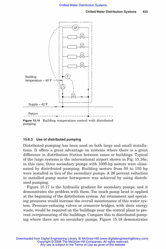
15.6.3 Use of distributed pumping
Distributed pumping has been used on both large and small installa-tions. It offers a great advantage on systems where there is a greatdifference in distribution friction between zones or buildings. Typicalof the large systems is the international airport shown in Fig. 15.16a;in this case, three secondary pumps with 1000-hp motors were elimi-nated by distributed pumping. Building motors from 50 to 150 hpwere installed in lieu of the secondary pumps. A 26 percent reductionin installed pump motor horsepower was achieved by using distrib-uted pumping.
Figure 15.17 is the hydraulic gradient for secondary pumps, and itdemonstrates the problem with them. Too much pump head is appliedat the beginning of the distribution system. Air retainment and operat-ing pressures would increase the overall maintenance of this water sys-tem. Pressure-reducing valves or crossover bridges, with their energywaste, would be required on the buildings near the central plant to pre-vent overpressuring of the buildings. Compare this to distributed pump-ing where there are no secondary pumps. Figure 15.18 demonstrates
Chilled Water Distribution Systems 433
∆P
Supply – 42°F
Return
Buildingtemperature – 45°F
T
Figure 15.15 Building temperature control with distributedpumping.
Rishel_CH15.qxd 20/4/06 6:43 PM Page 433
Downloaded from Digital Engineering Library @ McGraw-Hill (www.digitalengineeringlibrary.com)Copyright © 2006 The McGraw-Hill Companies. All rights reserved.
Any use is subject to the Terms of Use as given at the website.
Chilled Water Distribution Systems
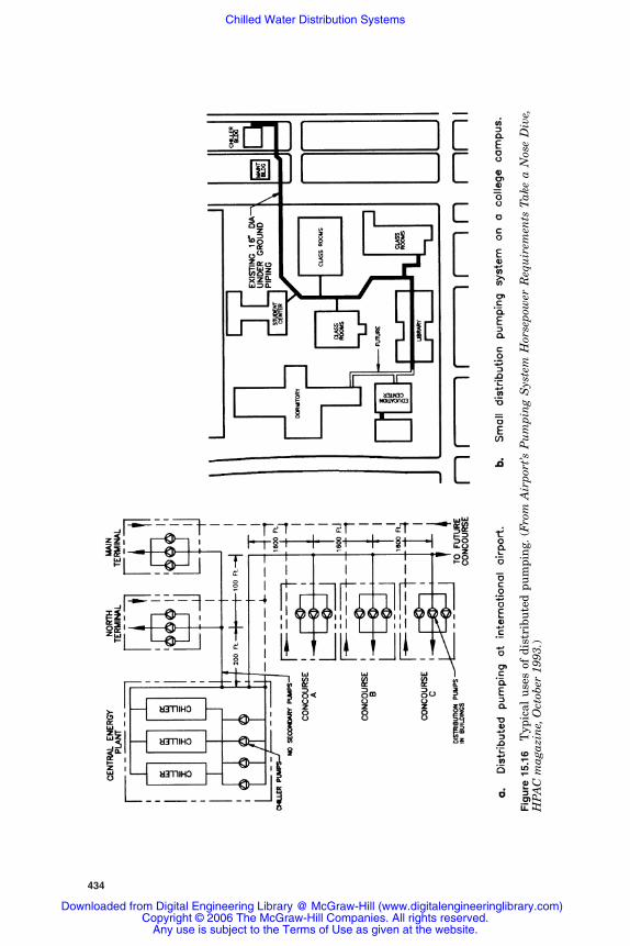
434
Fig
ure
15.
16T
ypic
al u
ses
of d
istr
ibu
ted
pum
pin
g.(F
rom
Air
port
’s P
um
pin
g S
yste
m H
orse
pow
er R
equ
irem
ents
Tak
e a
Nos
e D
ive,
HP
AC
mag
azin
e,O
ctob
er 1
993.
)
Rishel_CH15.qxd 20/4/06 6:43 PM Page 434
Downloaded from Digital Engineering Library @ McGraw-Hill (www.digitalengineeringlibrary.com)Copyright © 2006 The McGraw-Hill Companies. All rights reserved.
Any use is subject to the Terms of Use as given at the website.
Chilled Water Distribution Systems

Chilled Water Distribution Systems 435
Sys
tem
pre
ssur
e, ft
of w
ater
Secondary pumps Central plant pressure
Building loss
Over pressure
Mai
n te
rmin
al
Con
cour
se A
Con
cour
se B
Con
cour
se C
Fut
ure
conc
ours
e D
Fed
eral
insp
ectio
n se
rvic
e ar
eaan
d of
fice
build
ing
Figure 15.17 Typical hydraulic gradient diagram for a conventional secondary pumploop. (From Airport’s Pumping System Horsepower Requirements Take a Nose Dive,HPAC magazine, October 1993.)
Fut
ure
conc
ours
e D
Con
cour
se C
Con
cour
se B
Con
cour
se A
Fed
eral
insp
ectio
n se
rvic
ear
ea a
nd o
ffice
bui
ldin
g
Mai
n te
rmin
al
Sys
tem
pre
ssur
e, ft
of w
ater
Central plantpressure
Distribution pumps
Figure 15.18 Typical hydraulic gradient diagram for distributed pumping at fullload dotted lines represent pressure gradient after future concourse expansion.
Rishel_CH15.qxd 20/4/06 6:43 PM Page 435
Downloaded from Digital Engineering Library @ McGraw-Hill (www.digitalengineeringlibrary.com)Copyright © 2006 The McGraw-Hill Companies. All rights reserved.
Any use is subject to the Terms of Use as given at the website.
Chilled Water Distribution Systems
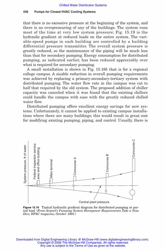
that there is no excessive pressure at the beginning of the system, andthere is no overpressuring of any of the buildings. The system runsmost of the time at very low system pressure; Fig. 15.19 is thehydraulic gradient at reduced loads on the entire system. The vari-able-speed pumps in each building are controlled by a buildingdifferential pressure transmitter. The overall system pressure isgreatly reduced, so the maintenance of the piping will be much lessthan that for secondary pumping. Energy consumption for distributedpumping, as indicated earlier, has been reduced appreciably overwhat is required for secondary pumping.
A small installation is shown in Fig. 15.16b that is for a regionalcollege campus. A sizable reduction in overall pumping requirementswas achieved by replacing a primary-secondary-tertiary system withdistributed pumping. The water flow rate in the campus was cut tohalf that required by the old system. The proposed addition of chillercapacity was canceled when it was found that the existing chillerscould handle the campus with ease with the greatly reduced chilledwater flow.
Distributed pumping offers excellent energy savings for new sys-tems. Unfortunately, it cannot be applied to existing campus installa-tions where there are many buildings; this would result in great costfor modifying existing pumping, piping, and control. Usually, there is
436 Pumps for Closed HVAC Cooling Systems
Central plant pressure
Con
cour
se C
Con
cour
se B
Con
cour
se A
Mai
n te
rmin
al
Fed
eral
insp
ectio
n se
rvic
ear
ea a
nd o
ffice
bui
ldin
g
Sys
tem
pre
ssur
e, ft
of w
ater
Figure 15.19 Typical hydraulic gradient diagram for distributed pumping at par-tial load. (From Airport’s Pumping System Horsepower Requirements Take a NoseDive, HPAC magazine, October 1993.)
Rishel_CH15.qxd 20/4/06 6:43 PM Page 436
Downloaded from Digital Engineering Library @ McGraw-Hill (www.digitalengineeringlibrary.com)Copyright © 2006 The McGraw-Hill Companies. All rights reserved.
Any use is subject to the Terms of Use as given at the website.
Chilled Water Distribution Systems
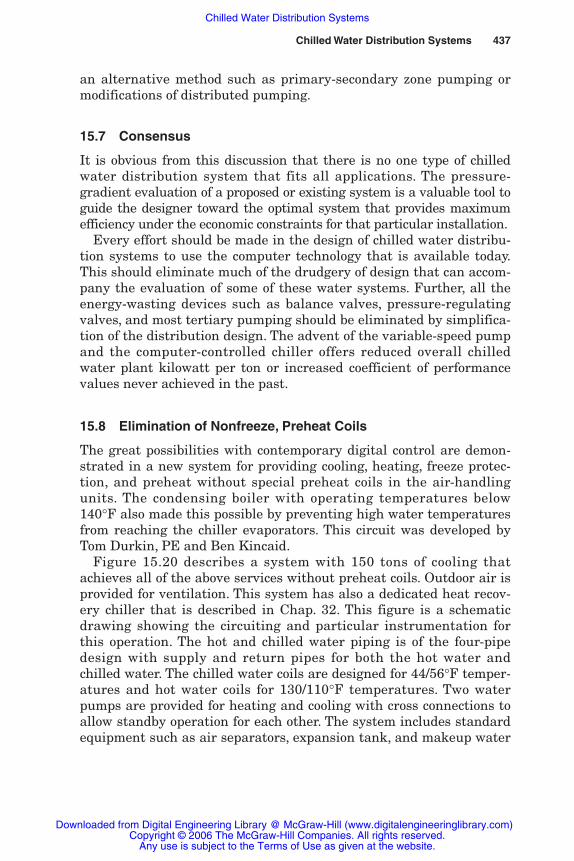
an alternative method such as primary-secondary zone pumping ormodifications of distributed pumping.
15.7 Consensus
It is obvious from this discussion that there is no one type of chilledwater distribution system that fits all applications. The pressure-gradient evaluation of a proposed or existing system is a valuable tool toguide the designer toward the optimal system that provides maximumefficiency under the economic constraints for that particular installation.
Every effort should be made in the design of chilled water distribu-tion systems to use the computer technology that is available today.This should eliminate much of the drudgery of design that can accom-pany the evaluation of some of these water systems. Further, all theenergy-wasting devices such as balance valves, pressure-regulatingvalves, and most tertiary pumping should be eliminated by simplifica-tion of the distribution design. The advent of the variable-speed pumpand the computer-controlled chiller offers reduced overall chilledwater plant kilowatt per ton or increased coefficient of performancevalues never achieved in the past.
15.8 Elimination of Nonfreeze, Preheat Coils
The great possibilities with contemporary digital control are demon-strated in a new system for providing cooling, heating, freeze protec-tion, and preheat without special preheat coils in the air-handlingunits. The condensing boiler with operating temperatures below140°F also made this possible by preventing high water temperaturesfrom reaching the chiller evaporators. This circuit was developed byTom Durkin, PE and Ben Kincaid.
Figure 15.20 describes a system with 150 tons of cooling thatachieves all of the above services without preheat coils. Outdoor air isprovided for ventilation. This system has also a dedicated heat recov-ery chiller that is described in Chap. 32. This figure is a schematicdrawing showing the circuiting and particular instrumentation forthis operation. The hot and chilled water piping is of the four-pipedesign with supply and return pipes for both the hot water andchilled water. The chilled water coils are designed for 44/56°F temper-atures and hot water coils for 130/110°F temperatures. Two waterpumps are provided for heating and cooling with cross connections toallow standby operation for each other. The system includes standardequipment such as air separators, expansion tank, and makeup water
Chilled Water Distribution Systems 437
Rishel_CH15.qxd 20/4/06 6:43 PM Page 437
Downloaded from Digital Engineering Library @ McGraw-Hill (www.digitalengineeringlibrary.com)Copyright © 2006 The McGraw-Hill Companies. All rights reserved.
Any use is subject to the Terms of Use as given at the website.
Chilled Water Distribution Systems

438
Mai
n ch
iller
on
Clo
sed
A/S
On
On
COND
EVAP
CH
R =
54.
5°F
T1
V1
V2
TT
To
sing
leE
xp. t
ank
and
mak
e-up
Chi
ller
min
. flo
wva
lve
(mod
ulat
ing)
Hea
tre
cove
rych
iller
on
CHS
CHR
DH
RC
EV
AP
out
= 5
0°F
Coi
l
O/A
55°F
LA
T
CH
S =
44°
FC
HR
= 5
6°F
Mod
ulat
ingR/A
Mix
ed a
ir
Typ
ical
VA
V A
HU
DH
RC
con
d. o
ut =
130
°F
130°
F
A/S
HWS
HWR
T2
TT
O/A
Des
ign
tem
pera
ture
s
HW
R =
110
°FH
WS
= 1
30°F
Boi
ler
Boi
ler
To
othe
rco
olin
g co
ilsT
o he
atin
g an
dre
heat
coi
ls
Fig
ure
15.
202x
4 P
ipe
(ch
ille
d w
ater
ch
ange
over
)—m
ode
#1 (
spri
ng,
sum
mer
an
d fa
ll)
oper
atio
n.
Rishel_CH15.qxd 20/4/06 6:43 PM Page 438
Downloaded from Digital Engineering Library @ McGraw-Hill (www.digitalengineeringlibrary.com)Copyright © 2006 The McGraw-Hill Companies. All rights reserved.
Any use is subject to the Terms of Use as given at the website.
Chilled Water Distribution Systems
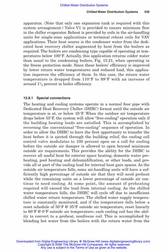
apparatus. (Note that only one expansion tank is required with thissystem arrangement.) Valve V1 is provided to ensure minimum flowin the chiller evaporator. Reheat is provided by coils in the air-handlingunits for single-zone applications or terminal reheat coils for VAVapplications. Their heat source is the condenser water from the dedi-cated heat recovery chiller augmented by heat from the boilers asrequired. The boilers are condensing type capable of operating at tem-peratures below 100°F. Actually, this application returns colder waterthan usual to the condensing boilers, Fig. 15.21, when operating inthe freeze protection mode. Since these boilers’ efficiency is improvedby lower return water temperatures and reduced load, this applica-tion improves the efficiency of them. In this case, the return watertemperature is dropped from 110°F to 99°F with an increase ofaround 11/2 percent in boiler efficiency.
15.8.1 Special connections
The heating and cooling systems operate in a normal four pipe withDedicated Heat Recovery Chiller (DHRC) format until the outside airtemperature is at, or below 35°F. When the outdoor air temperaturedrops below 55°F, the system will allow “free-cooling” operation only ifthe building heating loads are satisfied. This is accomplished byreversing the conventional “free-cooling” sequence of operation. Inorder to allow the DHRC to have the first opportunity to transfer theheat before it is ejected through the building relief, the cooling coilcontrol valve modulates to 100 percent open on a call for coolingbefore the outside air damper is allowed to open beyond minimumoutside air requirements. This provides the ability for the DHRC torecover all useful heat for exterior space heating, domestic water pre-heating, pool heating and dehumidification, or other loads, and pro-vide all or part of the cooling load for internal heat gain spaces. As theoutside air temperature falls, some air-handling units will have a suf-ficiently high percentage of outside air that they will need preheatwhile the remaining units on a lower percentage of outside air con-tinue to need cooling. At some point, the amount of preheatingrequired will exceed the load from internal cooling. As the chilledwater temperature falls, the DHRC will cycle off due to insufficientchilled water return temperature. The chilled water supply tempera-ture is constantly monitored, and if the temperature falls below areset schedule of 50°F @ 35°F outside air temperature, reset linearlyto 60°F @ 0°F outside air temperature; each cooling coil has the abil-ity to convert to a preheat, nonfreeze coil. This is accomplished byblending hot water from the boilers with the return water from the
Chilled Water Distribution Systems 439
Rishel_CH15.qxd 20/4/06 6:43 PM Page 439
Downloaded from Digital Engineering Library @ McGraw-Hill (www.digitalengineeringlibrary.com)Copyright © 2006 The McGraw-Hill Companies. All rights reserved.
Any use is subject to the Terms of Use as given at the website.
Chilled Water Distribution Systems

440
Mai
n ch
iller
off
C/H
Wpu
mp
HW
pum
p
COND
EVAP
T1
V2
21
4
TT
To
sing
leE
xp. t
ank
and
mak
e-up
Chi
ller
min
. flo
wva
lve
clos
ed
Hea
tre
cove
rych
iller
off
CHS
CHR
Coi
l
O/A
55°F
LA
T
C/H
S =
60°
FC
/HR
= 5
4°F
Mod
ulat
ing
R/A
Mix
ed a
ir
Typ
ical
VA
V A
HU
on
99°F
130°
F
HWS
HWR
T2
TT
Des
ign
tem
pera
ture
s
HW
S =
130
°FH
WR
= 1
10°F
at 0
°F O
AT
To
othe
rco
olin
g co
ilsT
o he
atin
g an
dre
heat
coi
ls
Mod
ulat
ing
3B
oile
r
Boi
ler
Boi
ler
= o
ff
67 G
PM
@ 5
6°F
O/A
At m
ixed
air
belo
w 5
5°F
,co
il co
ntro
l val
ves
reve
rses
ope
ratio
n, fr
omco
olin
g to
hea
ting.
1
At o
utsi
de a
ir te
mpe
ratu
rebe
low
35°
F, v
alve
is o
pen
whe
n A
HU
is o
ff.
2
Will
54°
F w
ater
pro
tect
chill
er?
Che
ck w
ithch
iller
man
ufac
ture
r.
3
Res
et s
ched
ule:
50°
F a
t35
°F, o
utsi
de a
irte
mpe
ratu
re u
p to
60°
Fat
0°F
out
side
air
tem
pera
ture
.
4 Fig
ure
15.
212x
4 P
ipe
(ch
ille
d w
ater
ch
ange
over
)—m
ode
#2 b
elow
35°
F o
uts
ide
air
tem
pera
ture
.
Rishel_CH15.qxd 20/4/06 6:43 PM Page 440
Downloaded from Digital Engineering Library @ McGraw-Hill (www.digitalengineeringlibrary.com)Copyright © 2006 The McGraw-Hill Companies. All rights reserved.
Any use is subject to the Terms of Use as given at the website.
Chilled Water Distribution Systems
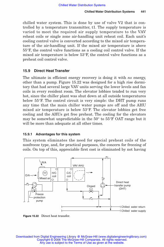
chilled water system. This is done by use of valve V2 that is con-trolled by a temperature transmitter, t1. The supply temperature isvaried to meet the required air supply temperature to the VAVreheat coils or single zone air-handling unit reheat coil. Each unit’scooling control valve is converted according to the mixed air tempera-ture of the air-handling unit. If the mixed air temperature is above55°F, the control valve functions as a cooling coil control valve. If themixed air temperature is below 53°F, the control valve functions as apreheat coil control valve.
15.9 Direct Heat Transfer
The ultimate in efficient energy recovery is doing it with no energy,other than a pump. Figure 15.22 was designed for a high rise dormi-tory that had several large VAV units serving the lower levels and fancoils in every resident room. The elevator lobbies tended to run veryhot, since the chiller plant was shut down at all outside temperaturesbelow 55°F. The control circuit is very simple: the DHT pump runsany time that the main chiller water pumps are off and the AHUmixed air temperature is below 53°F. The elevator lobbies get freecooling and the AHUs get free preheat. The cooling for the elevatorsmay be somewhat unpredictable in the 50° to 55°F OAT range but itwill be more than adequate at all other times.
15.9.1 Advantages for this system
This system eliminates the need for special preheat coils of thenonfreeze type, and, for practical purposes, the concern for freezing ofcoils. On top of this, appreciable first cost is eliminated by not having
Chilled Water Distribution Systems 441
TT
Mixed air
H/Ccoil
C/Ccoil
Direct heattransfer pump
(DHT)
Chilled water return
Chilled water supply
Closed
VAV AHUR/A
O/A
Freezeprotection
pump
Figure 15.22 Direct heat transfer.
Rishel_CH15.qxd 20/4/06 6:43 PM Page 441
Downloaded from Digital Engineering Library @ McGraw-Hill (www.digitalengineeringlibrary.com)Copyright © 2006 The McGraw-Hill Companies. All rights reserved.
Any use is subject to the Terms of Use as given at the website.
Chilled Water Distribution Systems
preheat coils in the air-handling units, including the piping, controlvalves, controls, and associated fittings. This system reduces hotwater, the pump capacity and piping distribution system sizes. It alsoeliminates the need for two expansion tanks and makeup connec-tions. It allows the most efficient transfer of internal heat to exteriorspaces without the operation of the DHRC. This function couldalmost be called, “free-airside preheating” and “free watersidecooling.” This has to be better than just “free airside cooling.” Thisalso eliminates the glycol system.
If the chiller serving the facility is an air-cooled, packaged chillerwith the evaporator packaged outside, this system can provide winterfreeze protection as insurance against a failure of normal heat tracingsystems for both the evaporator and the chilled water piping outside.
15.10 Bibliography
James B. Rishel, Twenty Years Experience with Variable Speed Pumps, transaction no.OT-88-09-2, vol. 94 (2), American Society of Heating, Refrigerating and Air-Conditioning Engineers, Atlanta, Ga., 1988.
James B. Rishel, The Water Management Manual, SYSTECON, Inc., West Chester,Ohio, 1992.
James B. Rishel, Distributed Pumping for Chilled and Hot Water Systems, TransactionNo. 94-24-3, vol. 100(1), American Society of Heating, Refrigerating and Air-Conditioning Engineers, Atlanta, Ga., 1994.
442 Pumps for Closed HVAC Cooling Systems
Rishel_CH15.qxd 20/4/06 6:43 PM Page 442
Downloaded from Digital Engineering Library @ McGraw-Hill (www.digitalengineeringlibrary.com)Copyright © 2006 The McGraw-Hill Companies. All rights reserved.
Any use is subject to the Terms of Use as given at the website.
Chilled Water Distribution Systems
Chapter
443
16Closed Condenser
Water Systems
16.1 Introduction
Although this chapter was written in 1994, it is still current in mostcases of closed condenser water design. Recent developments in geo-thermal cooling and heating are now included along with improve-ments in heat recovery. Proper control of condenser water tempera-ture can result in appreciable energy savings.
Closed condenser water systems are those which reject thermalenergy to heat exchanger surfaces, not cooling towers, which are opensystems. Open-type condenser systems are included in Chap. 11 oncooling towers. The heat exchanger can be a plate and frame or shelland tube type. The heat exchanger can be operated with a coolingtower (Fig. 16.1a,) or be part of a closed-circuit cooler (Fig. 16.1b).The basic circuitry of a closed-circuit cooler consists of a cooling coil(the heat exchanger), fans to move air over the coil, and a circulat-ing pump to wet the coil surfaces. These coolers can be operated wetwith the circulating pump running or dry with the pump stopped.The closed-circuit cooler is also known as an evaporative coolerbecause most of the heat transfer is by evaporation. It can be aninduced-draft unit, where the fan is located on top of the unit andpulls the cooling air across the coils containing the warm water, orit can be a forced-draft unit, which pushes the cooling air throughthe unit. This type uses blower fans that usually require more fanhorsepower. Forced-draft units are used mainly for ducted systems,where it is necessary to transport the moist leaving air to a specificlocation.
Rishel_CH16.qxd 20/4/06 6:45 PM Page 443
Downloaded from Digital Engineering Library @ McGraw-Hill (www.digitalengineeringlibrary.com)Copyright © 2006 The McGraw-Hill Companies. All rights reserved.
Any use is subject to the Terms of Use as given at the website.
Source: HVAC Pump Handbook
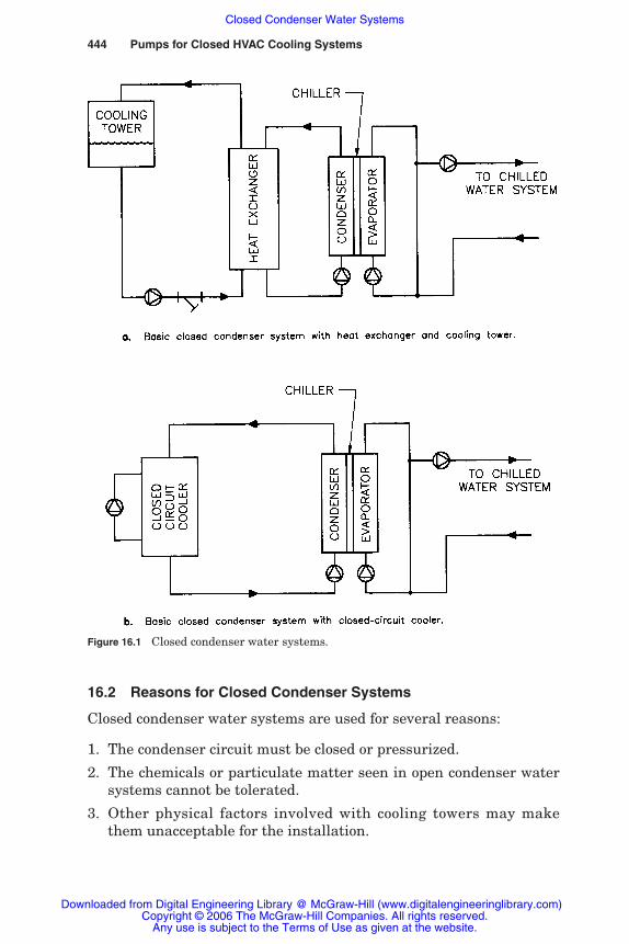
444 Pumps for Closed HVAC Cooling Systems
Figure 16.1 Closed condenser water systems.
16.2 Reasons for Closed Condenser Systems
Closed condenser water systems are used for several reasons:
1. The condenser circuit must be closed or pressurized.
2. The chemicals or particulate matter seen in open condenser watersystems cannot be tolerated.
3. Other physical factors involved with cooling towers may makethem unacceptable for the installation.
Rishel_CH16.qxd 20/4/06 6:45 PM Page 444
Downloaded from Digital Engineering Library @ McGraw-Hill (www.digitalengineeringlibrary.com)Copyright © 2006 The McGraw-Hill Companies. All rights reserved.
Any use is subject to the Terms of Use as given at the website.
Closed Condenser Water Systems
Closed Condenser Water Systems 445
4. There is a desire to capture and use the heat of rejection from thechiller or process.
5. Chemicals such as glycol are used that cannot be passed through acooling tower.
16.3 Types of Closed Condenser Systems
There are standard closed-circuit condenser systems, special-use sys-tems, and heat-recovery condenser systems. The most elementalpumping arrangement for a closed condenser circuit is shown inFig. 16.1b for a chiller rejecting its heat to a closed-circuit cooler. Noattempt is being made in this case to use the heat of rejection. A smallcirculator is supplied with the closed-circuit cooler for the spraywater. Figure 16.1a describes another simple closed system using aheat exchanger and a cooling tower. This system, of course, requiresboth condenser and cooling tower pumps. In both these cases, thepumping systems are very straightforward and have been describedin other chapters of this book. The decision as to whether cooling tow-ers with heat exchangers or closed-circuit coolers are used depends onthe costs and installation factors of each application. The size of thisequipment may be reduced through the use of heat-recovery equip-ment described later.
The heat exchanger and closed-circuit cooler are water-to-air heat-rejection systems. A third system using underground coils has beendeveloped for closed condenser systems; this is a water-to-groundheat-rejection system. Such an installation is particularly suitable forvariable-speed pumps owing to the greater friction of the under-ground coils.
16.3.1 Special closed condenser systems
There are special-use closed condenser systems that are designed toaccommodate specific types of equipment that must be cooled. A specialuse of closed condenser circuits is the pumping of condenser water forcomputer air-conditioners. A typical installation is shown in Fig. 16.2a.Normally, this water system would be filled with a glycol solution if itmust sustain a broad range of temperatures from summer to winteroperation. Such a temperature variation with glycol may produce a siz-able change in viscosity and therefore in pumping head and energy. Asimple method of solving this problem is through the use of variable-speed pumps that maintain the required differential pressure at thecondenser coils of the computer air-conditioners regardless of the tem-perature and viscosity of the glycol solution. An energy evaluation must
Rishel_CH16.qxd 20/4/06 6:45 PM Page 445
Downloaded from Digital Engineering Library @ McGraw-Hill (www.digitalengineeringlibrary.com)Copyright © 2006 The McGraw-Hill Companies. All rights reserved.
Any use is subject to the Terms of Use as given at the website.
Closed Condenser Water Systems

446 Pumps for Closed HVAC Cooling Systems
Figure 16.2 Special closed condenser water systems. (From Variable Water Volume IsHydro-Electronics, SYSTECON, Inc., West Chester, Ohio, 1986, p. 30.)
be run at minimum and maximum temperatures to determine the vari-ation in pump head due to the changes in viscosity and specific gravityof the glycol solution. Although this is substantially a constant-volume,variable-head system, the variable-speed pump allows the system torun at the true diversity of the system under all load conditions. Also,individual air-conditioners or groups of them can be shut down, and noreadjustment of the cooling system is required.
Changes 3-wayvalves to two-way
-
Rishel_CH16.qxd 20/4/06 6:45 PM Page 446
Downloaded from Digital Engineering Library @ McGraw-Hill (www.digitalengineeringlibrary.com)Copyright © 2006 The McGraw-Hill Companies. All rights reserved.
Any use is subject to the Terms of Use as given at the website.
Closed Condenser Water Systems

Closed Condenser Water Systems 447
16.4 Heat-Recovery Condenser Systems
There has been a desire to capture the heat of rejection from water-cooling equipment such as chillers. This has resulted in heat-recoveryequipment such as water source heat pumps and heat-reclaimchillers. Water source heat pumps can be terminal-type located nearthe heating and cooling loads or they can be central-type located inmajor equipment rooms.
The amount of heat recoverable is appreciable; for example, a1000-ton chiller operating over a cooling season of 2000 hours withan average heat rejection of 15,000 Btu/ton has a total heat rejec-tion of 30 billion Btu! If only 50 percent of this energy is reclaimed,this amounts to 15 billion Btu, which, at an overall boiler efficiencyof 80 percent, is equivalent 18,750,000 ft3 of natural gas with aheating value of 1000 Btu/ft3. At a cost of $500 per thousand cubicfeet, the annual savings would be over $93,000. An audit should bemade on cooling tower installations to determine the economic fea-sibility of energy recovery. The development of plate and frame heatexchangers and condensing boilers has resulted in low-temperaturethermal operations that can enhance the recovery of heat fromchiller condensers. See Chap. 32.
16.4.1 Terminal-type water source heat pumps
Another special use of closed condenser systems for specific equip-ment and the simplest heat-reclaiming system in terms of pumps isthe terminal-type water source heat pump, where the heat of rejectionfrom a unit under cooling load is transferred to a unit with a heatingload. Figure 16.2b describes a typical installation of a number ofsmall water source heat pumps utilizing a central boiler and closed-circuit cooler for any needed heat addition or rejection. Figure 16.3provides another circuiting that employs reverse return piping toeliminate the loop friction loss from the differential pressure acrossthe coil control valves. Often, these valves cannot operate with over10 psig differential pressure across the valve seat. With reversereturn, only the loss in the coil and its piping results in differentialpressure across the coil control valve. The boiler should be designedfor this low-temperature duty or be circuited in accordance with theboiler manufacturer’s instructions. The new condensing boilers areideal for this service.
The circulating pumps can be constant- or variable-speed pumps;variable-speed pumping is shown in this figure with control by meansof differential pressure transmitters located at the top of each building.With high diversities, which can be common for installations of water
Rishel_CH16.qxd 20/4/06 6:45 PM Page 447
Downloaded from Digital Engineering Library @ McGraw-Hill (www.digitalengineeringlibrary.com)Copyright © 2006 The McGraw-Hill Companies. All rights reserved.
Any use is subject to the Terms of Use as given at the website.
Closed Condenser Water Systems

448 Pumps for Closed HVAC Cooling Systems
source heat pumps, there can be substantial savings through the use ofvariable-speed pumping. Such systems that contain a number of watersource heat pumps must have a water-regulating valve on each watersource heat pump. If constant-speed water pumps are used, an auto-matic balance valve must be used on each water source heat pump.With variable-speed pumping, the water-regulating valve can be self-operating, responding to head pressure in the heat pump, as shown inFig. 16.4a, or it can be electric of the on-off type, as in Fig. 16.4b.Usually an automatic balancing valve is furnished with the electricvalve to provide the amount of water required by the heat pump. Theactual coil connections should be made in accordance with the require-ments of the manufacturer of the heat pump. Some manufacturersrequire close control of the flow rate through the condenser coil.
16.4.2 Central plant heat-reclaiming equipment
The water source heat pumps shown in Fig. 16.2b consist of units locatedout near the actual heating and cooling loads. Other heat-recovery
Figure 16.3 Water source heat pumps with closed circuit cooler.
DP1
Water sourceheat pumps
C
Cooler
Boiler
DP2
Rishel_CH16.qxd 20/4/06 6:45 PM Page 448
Downloaded from Digital Engineering Library @ McGraw-Hill (www.digitalengineeringlibrary.com)Copyright © 2006 The McGraw-Hill Companies. All rights reserved.
Any use is subject to the Terms of Use as given at the website.
Closed Condenser Water Systems
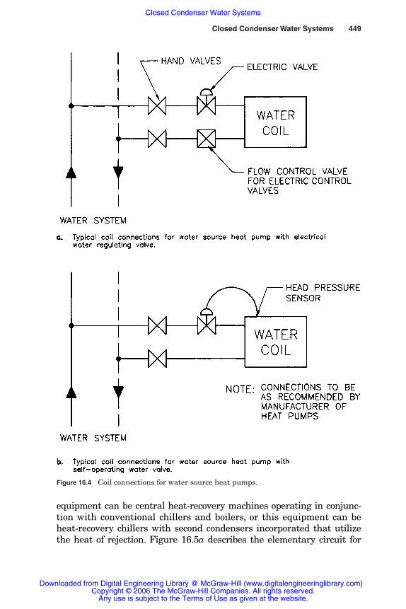
Closed Condenser Water Systems 449
Figure 16.4 Coil connections for water source heat pumps.
equipment can be central heat-recovery machines operating in conjunc-tion with conventional chillers and boilers, or this equipment can beheat-recovery chillers with second condensers incorporated that utilizethe heat of rejection. Figure 16.5a describes the elementary circuit for
Rishel_CH16.qxd 20/4/06 6:45 PM Page 449
Downloaded from Digital Engineering Library @ McGraw-Hill (www.digitalengineeringlibrary.com)Copyright © 2006 The McGraw-Hill Companies. All rights reserved.
Any use is subject to the Terms of Use as given at the website.
Closed Condenser Water Systems

450 Pumps for Closed HVAC Cooling Systems
Figure 16.5 Central heat reclaim systems.
Rishel_CH16.qxd 20/4/06 6:45 PM Page 450
Downloaded from Digital Engineering Library @ McGraw-Hill (www.digitalengineeringlibrary.com)Copyright © 2006 The McGraw-Hill Companies. All rights reserved.
Any use is subject to the Terms of Use as given at the website.
Closed Condenser Water Systems

the central heat-recovery water source heat pump, while Fig. 16.5b pro-vides the circuit for a heat-recovery chiller. The decision as to which typeof equipment to use for heat recovery on a specific installation dependson the economics of each application and is not within the scope of thisbook.
16.5 Uses of Heat Reclaimed from Chillers
Some of the uses for the recovered heat are
1. Space heating
2. Reheat coils
3. Outdoor air-heating coils for air-conditioning or industrial process
4. Radiant surface heating
5. Domestic water heating
6. Snow melting
7. Process heating
8. Natatoriums
9. Dehumidification
The piping and pumping, as well as control of the various circuitsfor use of the heat, must be arranged so that the most efficient useof this heat is achieved. Also, the circuiting must be such that theoperation required by the chiller is achieved. There must be positivecontrol of (1) the performance of the chiller from a cooling stand-point and (2) achievement of the optimal heat balance for the entireinstallation. For example, under some load conditions it may bemost economical to use the heat for reheat, whereas in other situa-tions it may be better to use the heat for snow melting. Also, theheat rejection from the chiller may be such that an increased leav-ing water temperature from the chiller condenser is achieved at theexpense of the chiller efficiency, but a separate boiler operation iseliminated.
Following are some basic methods for saving the 30 billion Btu peryear that was discussed in this chapter and in Chap. 11 on coolingtowers.
16.6 Condensing-Type Boiler Improves Heat Recovery
Another development that is increasing the use of heat-recoveryequipment is the emergence of the condensing boiler, which operates
Closed Condenser Water Systems 451
Rishel_CH16.qxd 20/4/06 6:45 PM Page 451
Downloaded from Digital Engineering Library @ McGraw-Hill (www.digitalengineeringlibrary.com)Copyright © 2006 The McGraw-Hill Companies. All rights reserved.
Any use is subject to the Terms of Use as given at the website.
Closed Condenser Water Systems
452 Pumps for Closed HVAC Cooling Systems
most efficiently at water temperatures around 100°F or less. Conven-tional gas-fired boilers that are noncondensing cannot be operatedbelow 140°F without corrosion in their flue collectors. This lower-temperature boiler operation with the condensing-type boiler offersgreater savings with the heat-recovery equipment described earlier.The efficiency of the condensing boiler with different leaving watertemperatures is described in Chap. 19.
The reduced temperature at which condensing boilers operateenables them to be installed without heat exchangers or pumpedsubloops on these heat-recovery systems. The entire heating efficiencyof the hot water system is greatly improved with operation from 80 to140°F. This is particularly true with radiant surface systems in floorsand ceilings for heating.
16.7 Pumping Aspects of Heat Recovery
What is important from a pumping standpoint is the location of thepumps and their operation in these heat-recovery circuits, which canbecome complex. Pumps should be located to eliminate as much pres-sure as possible on the operating equipment. Since these are closedsystems, adequate pressure can be provided on pump suctions thatwill eliminate possibilities of cavitation. Variable-speed pumping withproper control can result in efficient and often simplified circuits forthese heat-recovery systems. Constant or variable flow through thechiller evaporators for heat recovery is determined by the chillermanufacturer.
The evaluation of (1) when to use heat-recovery systems and (2)what type of heat-recovery equipment is most economical is a complexsubject. Proper pumping systems and their location can have a sub-stantial effect on the success of such heat-recovery applications.Following is a list of some of the factors that must be considered whenevaluating the pumping for these systems:
1. Consider both constant- and variable-speed pumps. Variable-speedpumps offer so much more flexibility on these systems, which mayhave complex piping arrangements.
2. Avoid, wherever possible, energy-consuming devices such as balancevalves, pressure regulators, and bypasses.
3. Locate pumps to keep pump pressure off the central equipment wher-ever possible (see Chap. 19 on the location of pumps with boilers).
4. Consider distributed pumping on multiple-building systems forboth the hot and chilled water systems.
Rishel_CH16.qxd 20/4/06 6:45 PM Page 452
Downloaded from Digital Engineering Library @ McGraw-Hill (www.digitalengineeringlibrary.com)Copyright © 2006 The McGraw-Hill Companies. All rights reserved.
Any use is subject to the Terms of Use as given at the website.
Closed Condenser Water Systems
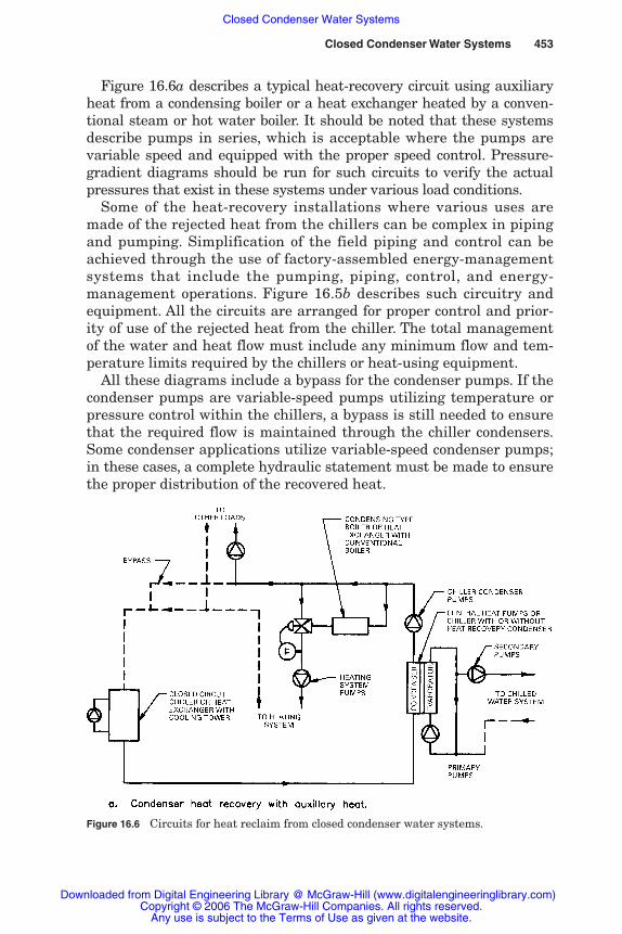
Figure 16.6a describes a typical heat-recovery circuit using auxiliaryheat from a condensing boiler or a heat exchanger heated by a conven-tional steam or hot water boiler. It should be noted that these systemsdescribe pumps in series, which is acceptable where the pumps arevariable speed and equipped with the proper speed control. Pressure-gradient diagrams should be run for such circuits to verify the actualpressures that exist in these systems under various load conditions.
Some of the heat-recovery installations where various uses aremade of the rejected heat from the chillers can be complex in pipingand pumping. Simplification of the field piping and control can beachieved through the use of factory-assembled energy-managementsystems that include the pumping, piping, control, and energy-management operations. Figure 16.5b describes such circuitry andequipment. All the circuits are arranged for proper control and prior-ity of use of the rejected heat from the chiller. The total managementof the water and heat flow must include any minimum flow and tem-perature limits required by the chillers or heat-using equipment.
All these diagrams include a bypass for the condenser pumps. If thecondenser pumps are variable-speed pumps utilizing temperature orpressure control within the chillers, a bypass is still needed to ensurethat the required flow is maintained through the chiller condensers.Some condenser applications utilize variable-speed condenser pumps;in these cases, a complete hydraulic statement must be made to ensurethe proper distribution of the recovered heat.
Closed Condenser Water Systems 453
Figure 16.6 Circuits for heat reclaim from closed condenser water systems.
Rishel_CH16.qxd 20/4/06 6:45 PM Page 453
Downloaded from Digital Engineering Library @ McGraw-Hill (www.digitalengineeringlibrary.com)Copyright © 2006 The McGraw-Hill Companies. All rights reserved.
Any use is subject to the Terms of Use as given at the website.
Closed Condenser Water Systems
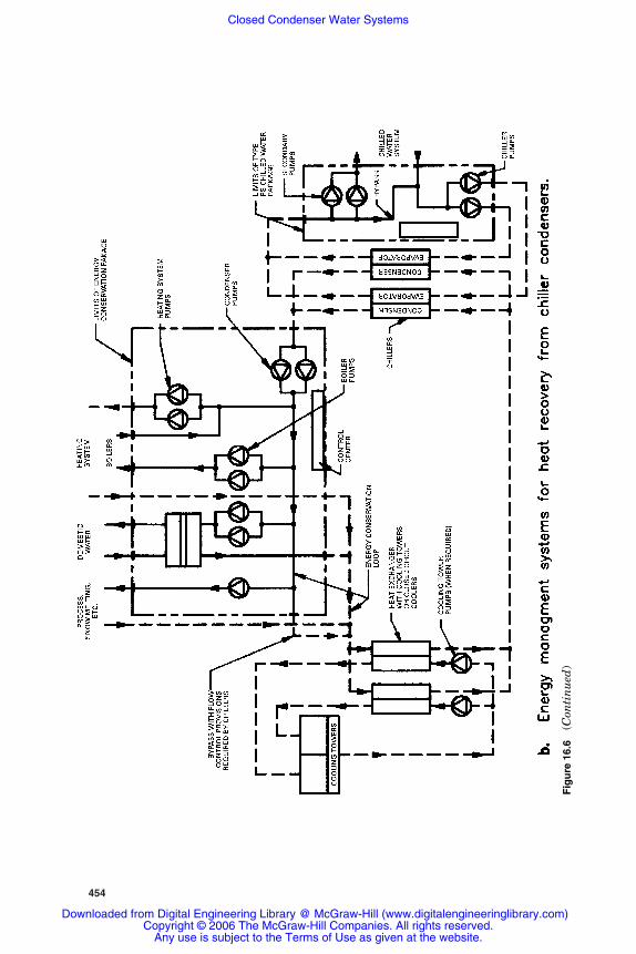
454
Fig
ure
16.
6(C
onti
nu
ed)
Rishel_CH16.qxd 20/4/06 6:45 PM Page 454
Downloaded from Digital Engineering Library @ McGraw-Hill (www.digitalengineeringlibrary.com)Copyright © 2006 The McGraw-Hill Companies. All rights reserved.
Any use is subject to the Terms of Use as given at the website.
Closed Condenser Water Systems
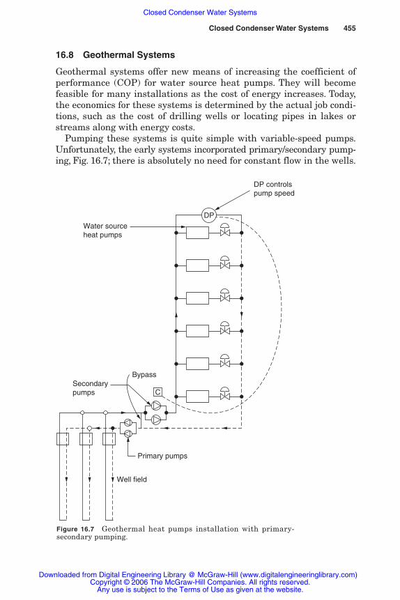
Closed Condenser Water Systems 455
16.8 Geothermal Systems
Geothermal systems offer new means of increasing the coefficient ofperformance (COP) for water source heat pumps. They will becomefeasible for many installations as the cost of energy increases. Today,the economics for these systems is determined by the actual job condi-tions, such as the cost of drilling wells or locating pipes in lakes orstreams along with energy costs.
Pumping these systems is quite simple with variable-speed pumps.Unfortunately, the early systems incorporated primary/secondary pump-ing, Fig. 16.7; there is absolutely no need for constant flow in the wells.
Figure 16.7 Geothermal heat pumps installation with primary-secondary pumping.
DP
C
Primary pumps
BypassSecondarypumps
Well field
Water sourceheat pumps
DP controlspump speed
Rishel_CH16.qxd 20/4/06 6:45 PM Page 455
Downloaded from Digital Engineering Library @ McGraw-Hill (www.digitalengineeringlibrary.com)Copyright © 2006 The McGraw-Hill Companies. All rights reserved.
Any use is subject to the Terms of Use as given at the website.
Closed Condenser Water Systems

456 Pumps for Closed HVAC Cooling Systems
Figure 16.8 describes the correct pump and piping arrangement for alow-rise building while Fig. 16.9 does so for a high-rise building. Thepumps should be installed on the discharge of the wells on the high-rise installation to keep the pump head off the wells. For example, ifyou have a high-rise building with a height of 300 ft, the static pres-sure on the wells would be 130 psig. If the pumps have a shutoff headof 120 ft (52 psig), the maximum pressure on the wells would be 182
DP
Well field
Water sourceheat pumps
DP controlspump speed
C Expansion tankand water makeup
Figure 16.8 Geothermal heat pump installation for low-rise bldg.
Rishel_CH16.qxd 20/4/06 6:45 PM Page 456
Downloaded from Digital Engineering Library @ McGraw-Hill (www.digitalengineeringlibrary.com)Copyright © 2006 The McGraw-Hill Companies. All rights reserved.
Any use is subject to the Terms of Use as given at the website.
Closed Condenser Water Systems
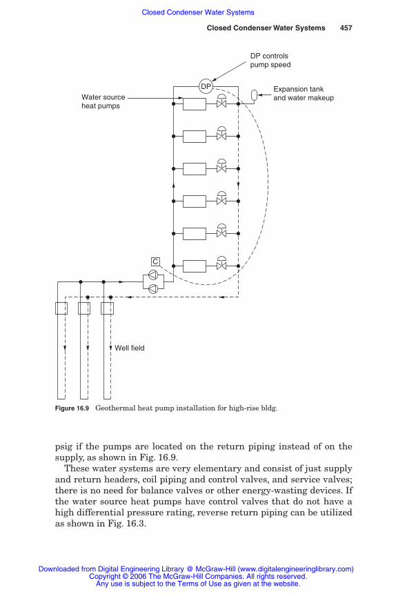
psig if the pumps are located on the return piping instead of on thesupply, as shown in Fig. 16.9.
These water systems are very elementary and consist of just supplyand return headers, coil piping and control valves, and service valves;there is no need for balance valves or other energy-wasting devices. Ifthe water source heat pumps have control valves that do not have ahigh differential pressure rating, reverse return piping can be utilizedas shown in Fig. 16.3.
Closed Condenser Water Systems 457
Figure 16.9 Geothermal heat pump installation for high-rise bldg.
DP
C
Well field
Water sourceheat pumps
DP controlspump speed
Expansion tankand water makeup
Rishel_CH16.qxd 20/4/06 6:45 PM Page 457
Downloaded from Digital Engineering Library @ McGraw-Hill (www.digitalengineeringlibrary.com)Copyright © 2006 The McGraw-Hill Companies. All rights reserved.
Any use is subject to the Terms of Use as given at the website.
Closed Condenser Water Systems

Most geothermal systems to date have utilized water source heatpumps as the terminal units. The development of the modern two-pipe system has resulted in a more efficient geothermal heating andcooling system that is applicable to typical facilities such as elemen-tary and secondary schools. These systems use VAV boxes and unitventilators; this is described in Chap. 31 and Fig. 31.6.
16.9 Storage of Hot Water
The reclamation of heat from chillers has so many interesting possibil-ities that there may be cases that justify the storage of excess heatrather than waste of the heat through a closed-circuit cooler or a cool-ing tower. Open storage of hot water would, as far as pumping is con-cerned, be very similar to cold water storage, as described in Chap. 13.
16.10 Summation
Closed-circuit condenser systems offer many different possibilitiesfor energy-efficient systems. The energy audits require substantialcalculations and the consideration of a number of different circuits.Energy storage in the form of chilled or hot water also can play a partin these systems. From a pumping standpoint, the variable-speedpump offers so much flexibility without balance valves or pressure-regulating valves and without any excessive pumping pressure.
The closed condenser system will become much more popular thanit is today because of the heat-recovery possibilities. What bettermethod of plume abatement of cooling towers is there than to preventthe heat from getting to the closed-circuit cooler or cooling tower.
16.11 Bibliography
James B. Rishel, Variable Water Volume Is Hydro-Electronics, SYSTECON, Inc., WestChester, Ohio, 1986.
Cooling Tower Fundamentals, 2/e, The Marloy Cooling Tower Company, Mission, Kan.,1985.
458 Pumps for Closed HVAC Cooling Systems
Rishel_CH16.qxd 20/4/06 6:45 PM Page 458
Downloaded from Digital Engineering Library @ McGraw-Hill (www.digitalengineeringlibrary.com)Copyright © 2006 The McGraw-Hill Companies. All rights reserved.
Any use is subject to the Terms of Use as given at the website.
Closed Condenser Water Systems
Chapter
459
17Pumps for Closed
Energy Storage Systems
17.1 Introduction
Closed energy storage systems consist of pressure tanks for both hotand chilled water as well as ice systems with open tanks that aredescribed as ice-on-tube systems. The growth of energy-conservationefforts has resulted in the use of a number of different procedures forstoring energy. Closed energy storage systems differ from the openstorage systems of Chap. 13 in the storage of the energy at systemoperating pressures; this results in the ability to maintain systempressure throughout the energy storage system.
17.2 Pressure Tanks for Energy Storage
Pressure tanks have not been popular because of the cost of the tanksthemselves. Of course, it is the responsibility of the water systemdesigner to determine the most economical means of storage of energyon a specific installation.
Closed tanks offer the specific advantage of operating at systempressure. All the pressure-control devices needed in open storagetanks are not required for these systems. The tank can be located inthe system at the point most advantageous for the operation of theequipment and the storage of energy.
For example, on chilled water systems, the pressure tank can beinstalled in the chiller bypass, as shown in Fig. 17.1. With thisarrangement, the chillers can be operated at peak efficiency and,therefore, at the lowest kilowatts per ton. On very light loads, the
Rishel_CH17.qxd 20/4/06 6:46 PM Page 459
Downloaded from Digital Engineering Library @ McGraw-Hill (www.digitalengineeringlibrary.com)Copyright © 2006 The McGraw-Hill Companies. All rights reserved.
Any use is subject to the Terms of Use as given at the website.
Source: HVAC Pump Handbook
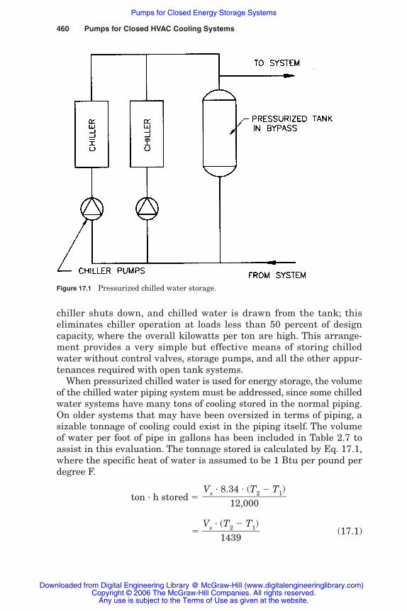
460 Pumps for Closed HVAC Cooling Systems
Figure 17.1 Pressurized chilled water storage.
chiller shuts down, and chilled water is drawn from the tank; thiseliminates chiller operation at loads less than 50 percent of designcapacity, where the overall kilowatts per ton are high. This arrange-ment provides a very simple but effective means of storing chilledwater without control valves, storage pumps, and all the other appur-tenances required with open tank systems.
When pressurized chilled water is used for energy storage, the volumeof the chilled water piping system must be addressed, since some chilledwater systems have many tons of cooling stored in the normal piping.On older systems that may have been oversized in terms of piping, asizable tonnage of cooling could exist in the piping itself. The volumeof water per foot of pipe in gallons has been included in Table 2.7 toassist in this evaluation. The tonnage stored is calculated by Eq. 17.1,where the specific heat of water is assumed to be 1 Btu per pound perdegree F.
ton � h stored �
��Vs � (
1T4
2
3�
9T1)� (17.1)
Vs � 8.34 � (T2 � T1)���12,000
Rishel_CH17.qxd 20/4/06 6:46 PM Page 460
Downloaded from Digital Engineering Library @ McGraw-Hill (www.digitalengineeringlibrary.com)Copyright © 2006 The McGraw-Hill Companies. All rights reserved.
Any use is subject to the Terms of Use as given at the website.
Pumps for Closed Energy Storage Systems

Pumps for Closed Energy Storage Systems 461
where Vs � volume of the system, galT2 � system return water temperature, °FT1 � system supply water temperature, °F
There have been some unusual installations such as airports wherethe total gallons of water in the distribution system provided enoughstorage that there was no need for additional chilled water storage forenergy curtailment.
Eutectic salts can be used to reduce the volume of the pressurizedstorage tanks. The eutectic salt tanks can be as much as one-third toone-half the size of those for straight water storage.
17.3 Closed Energy Storage Systems with Open Tanks
On chilled water systems that cannot justify pressure tanks forenergy storage, the closed water circuit that uses open ice tanks pro-vides an economical option for many systems. This type of systempasses glycol through tubes in an open tank and either creates ormelts ice on the external surfaces of the tubes as required by the sys-tem demands. A storage tank for this system is shown in Fig. 17.2.The storage tanks can be single, large tanks or modular systems com-prised of a number of small tanks. Larger systems use rectangulartanks, as shown in Fig. 17.3.
Figure 17.2 Modular internal melt icestorage tank.
Rishel_CH17.qxd 20/4/06 6:46 PM Page 461
Downloaded from Digital Engineering Library @ McGraw-Hill (www.digitalengineeringlibrary.com)Copyright © 2006 The McGraw-Hill Companies. All rights reserved.
Any use is subject to the Terms of Use as given at the website.
Pumps for Closed Energy Storage Systems

462 Pumps for Closed HVAC Cooling Systems
Such a system is called an internal melt ice-on-coil system becausethe glycol passes through the pressurized coils in the tank and iceforms on the outside of these coils. The design of this system offerssome general advantages over the other types of ice storage systemsthat were described in Chap. 13. For example,
1. Chiller cost is much the same as for chilled water and the otherforms of ice storage other than the ice harvester system, which hasa much higher chiller cost.
2. Tank volume is equivalent to that of most of the other forms ofice storage except the ice harvester system, which requires 10 to20 percent more storage volume.
3. Storage cost is similar to that for external ice melt and encapsulat-ed ice; it is greater than for the ice harvester system and much lessthan for the eutectic salt system.
4. Power costs per ton-hour are comparable with those for all theother ice storage systems; they are much higher than for chilledwater storage or for the eutectic salt system.
5. A great advantage of this system is the ability to run the chillersat normal chilled water system temperatures such as 44°F leavingwater and 56°F return water when ice is not being used or gener-ated. This brings the power costs down to close to that of ordinarychilled water operation.
Figure 17.3 Closed glycolsystem for large ice storage facilities.
Glycolchiller
T
Heat exchanger
Cooling systemtemperaturecontrol valve
Tank valve
Open tankwith glycol coils
Glycol pumps
Chilled water system
Variable-speedchilled water pumps
Rishel_CH17.qxd 20/4/06 6:46 PM Page 462
Downloaded from Digital Engineering Library @ McGraw-Hill (www.digitalengineeringlibrary.com)Copyright © 2006 The McGraw-Hill Companies. All rights reserved.
Any use is subject to the Terms of Use as given at the website.
Pumps for Closed Energy Storage Systems

Pumps for Closed Energy Storage Systems 463
The arrangement of the piping and pumping in this method of energystorage is very important in order to achieve efficient and trouble-freeoperation. All the different phases of operation for the chilled waterand storage systems must be recognized and evaluated to achieve thedesired results from this energy system. These phases are:
1. Operate the chilled water system without the ice storage system.
2. Serve the chilled water system and generate ice.
3. Serve the chilled water system with the chillers and from the icestorage.
4. Serve the chilled water system from only the ice storage.
5. Generate ice only.
Not all systems will require all five of these phases. It is up to thedesigner to develop the phases or cycles required for a particularapplication.
17.4 Circuiting Internal Ice Melt Systems
There are a number of different methods of circuiting these energystorage systems; one of these is shown in Fig. 17.4. Figure 17.4adescribes a system with the chiller upstream from the ice storagetanks, while Fig. 17.4b provides the arrangement with the chillersdownstream from the ice storage tanks. A variation of this latterhookup is shown in Fig. 17.4c with two chillers in parallel operation. Inthe first two designs, a three-way valve is shown for varying the supplytemperature to the chilled water system. The system of Fig. 17.4c isdesigned to receive either a constant low-temperature glycol under allloads or a higher temperature when the stored ice is not being used.
Installing the chiller upstream from the storage reduces the powerconsumption in kilowatts per ton because the water in the evaporatoris higher in temperature; the total storage may be reduced because ofthe temperatures of the system. Installing the chiller downstreamfrom the storage may increase the overall kilowatts per ton as aresult of the lower temperatures in the evaporator. The total systemstorage may be improved because of the colder temperatures leavingthe ice storage tanks. In any of these variations, the total kilowattsper ton of the chilled water plant must be run under all loads to verifythe total cost of energy for each system.
Figure 17.4c is a variation of the downstream chiller arrangementthat provides flexibility in system operation. Either chiller can makeice simultaneously with the other chiller providing the system watertemperature as required. The chiller making ice could be operating at
Rishel_CH17.qxd 20/4/06 6:46 PM Page 463
Downloaded from Digital Engineering Library @ McGraw-Hill (www.digitalengineeringlibrary.com)Copyright © 2006 The McGraw-Hill Companies. All rights reserved.
Any use is subject to the Terms of Use as given at the website.
Pumps for Closed Energy Storage Systems
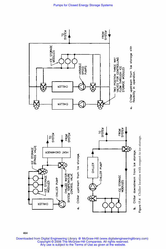
464
Fig
ure
17.
4C
hil
ler
loca
tion
wit
h r
espe
ct t
o ic
e st
orag
e.
Rishel_CH17.qxd 20/4/06 6:46 PM Page 464
Downloaded from Digital Engineering Library @ McGraw-Hill (www.digitalengineeringlibrary.com)Copyright © 2006 The McGraw-Hill Companies. All rights reserved.
Any use is subject to the Terms of Use as given at the website.
Pumps for Closed Energy Storage Systems

Pumps for Closed Energy Storage Systems 465
leaving water temperatures of 26°F and at around 0.90 kW/ton, whilethe other chiller could be making chilled water for the system at 44°Fand at 0.60 kW/ton. Another advantage of this arrangement is theability of the chillers to operate at any desired load and maintain aconstant leaving temperature as the ice is depleted.
Like other water systems containing glycol, these internal ice meltsystems must be equipped with heat exchangers if it is desired tokeep the glycol out of the chilled water system. Figure 17.4a includessuch a heat exchanger, while Figs. 17.4b and c do not. This is a deci-sion for the designer and the client. Generally, chilled water systemsutilizing large air-handling systems do not require the heatexchanger, while systems with a number of small terminal units suchas fan coil do require them.
17.5 Pumping Internal Ice Melt Systems
The variable-speed pump offers some appreciable advantages inpumping internal ice melt systems because of the sizable changes inviscosity of the glycol solution as it varies from 26 to 55°F. Thevariable-speed pump can be controlled by any desirable parametersuch as flow through the chiller evaporator. The flowmeter for thiscircuit provides a 4- to 20-mA signal to the pump controller thatvaries the pump speed and maintains the desired flow as the glycoltemperature changes.
The friction loss in the various loops for this ice system varies as towhether ice is being used or bypassed. The variable-speed pump auto-matically adjusts its speed to accommodate these variations causedby the control valves that determine the phase of operation for theenergy storage system.
Further, as indicated in Fig. 17.4b, the use of variable-speed pumpson the chiller circuit eliminates other pumps that might be requiredwith heat exchangers or the ice storage itself.
17.5.1 Pumps for internal ice melt systems
This type of ice storage system requires a minimum of special provi-sions and controls for the pumping system, since it is a closed systemwhere system pressures are easily controlled. There should be no con-cern for cavitation in the pumps other than the usual precautionsthat should be taken for any system.
Most of the pumps for these systems are either single- or double-suction volute-type pumps. Standard bronze-fitted construction isvery adequate for these applications.
Rishel_CH17.qxd 20/4/06 6:46 PM Page 465
Downloaded from Digital Engineering Library @ McGraw-Hill (www.digitalengineeringlibrary.com)Copyright © 2006 The McGraw-Hill Companies. All rights reserved.
Any use is subject to the Terms of Use as given at the website.
Pumps for Closed Energy Storage Systems

466 Pumps for Closed HVAC Cooling Systems
Many of the standard pumping and distribution systems for ordi-nary chilled water systems are usable with internal melt ice storagesystems.
17.6 Bibliography
ASHRAE Handbook Fundamentals, American Society of Heating, Refrigerating, andAir-Conditioning Engineers, Atlanta, Ga., 1993.
Design Guide for Cool Thermal Storage, ASHRAE, Atlanta, Ga., 1993.
Rishel_CH17.qxd 20/4/06 6:46 PM Page 466
Downloaded from Digital Engineering Library @ McGraw-Hill (www.digitalengineeringlibrary.com)Copyright © 2006 The McGraw-Hill Companies. All rights reserved.
Any use is subject to the Terms of Use as given at the website.
Pumps for Closed Energy Storage Systems

Chapter
467
18Pumps for District
Cooling and Heating
18.1 Introduction
Although this chapter has been included in this part on pumps forclosed cooling systems, district heating is included here because it isso similar to district cooling in layout and pumping. Much of the fol-lowing discussion on pumping district cooling can be applied to dis-trict heating systems. Usually, district hot water capacities are muchsmaller than those for district cooling.
District cooling and heating is the name for the centralization ofchilled and hot water plants that will supply water to a number ofindependent buildings. District cooling and heating is increasing inpopularity because of the cost advantages and efficiencies that can beachieved in the generation of the chilled water.
One of the important parts of these installations is the cost of mov-ing the chilled water from the central energy plant to the buildings.Pumping energy must be evaluated using computer programs tosecure the optimal method of pumping. Most of these systems haveutilized primary-secondary pumping to distribute water to the build-ings. Primary-secondary pumping was explained in Chap. 15, as wasdistributed pumping. Distributed pumping is an alternative proce-dure for district hot and chilled water systems. It uses the centralenergy plant water system pressure to distribute the water to thebuildings. As mentioned before, it is based on the Bernoulli theorem,which demonstrates that there are three different pressures in awater system, namely, static head, velocity head, and pressure head.Any of these three can be used to move water through a system of
Rishel_CH18.qxd 20/4/06 6:47 PM Page 467
Downloaded from Digital Engineering Library @ McGraw-Hill (www.digitalengineeringlibrary.com)Copyright © 2006 The McGraw-Hill Companies. All rights reserved.
Any use is subject to the Terms of Use as given at the website.
Source: HVAC Pump Handbook
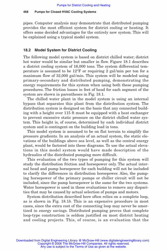
468 Pumps for Closed HVAC Cooling Systems
pipes. Computer analysis may demonstrate that distributed pumpingprovides the most efficient system for district cooling or heating. Itoffers some decided advantages for the entirely new system. This willbe explained using a typical model system.
18.2 Model System for District Cooling
The following model system is based on district chilled water; districthot water would be similar but smaller in flow. Figure 18.1 describesa district cooling system of 16,000 tons. The system differential tem-perature is assumed to be 12°F or requiring 2 gal/min per ton for amaximum flow of 32,000 gal/min. This system will be modeled usingprimary-secondary and distributed pumping, demonstrating theenergy requirements for this system when using both these pumpingprocedures. The friction losses in feet of head for each segment of thesystem are shown in parentheses in Fig. 18.1.
The chilled water plant in the model system is using an internalbypass that separates this plant from the distribution system. Thedistribution system is designed on the basis that any connected build-ing with a height over 115 ft must be equipped with a heat exchangerto prevent excessive static pressure on the district chilled water sys-tem. This height is, of course, determined by each individual districtsystem and is contingent on the building load in tons.
This model system is assumed to be on flat terrain to simplify thepressure gradients. In an analysis of an actual system, the static ele-vations of the buildings above sea level, as well as the central energyplant, would be factored into these diagrams. To use the actual eleva-tions in this model system would have made description of thehydraulics of the distributed pumping more difficult.
This evaluation of the two types of pumping for this system willstudy the distribution friction and horsepower only. The actual inter-nal head and pump horsepower for each building will not be includedto clarify the differences in distribution horsepower. Also, the pump-ing horsepower of the primary pumps or chiller circuit will not beincluded, since the pump horsepower is the same for the two systems.Water horsepower is used in these evaluations to remove any dispari-ties that may be caused by actual selection of pumps and motors.
System distribution described here often relies on a complete loop,as is shown in Fig. 18.1b. This is an expensive procedure in mostcases, since the extra cost of the connecting loop may never be amor-tized in energy savings. Distributed pumping proves that completeloop-type construction is seldom justified on most district heatingand cooling projects. This, of course, is an evaluation that the
Rishel_CH18.qxd 20/4/06 6:47 PM Page 468
Downloaded from Digital Engineering Library @ McGraw-Hill (www.digitalengineeringlibrary.com)Copyright © 2006 The McGraw-Hill Companies. All rights reserved.
Any use is subject to the Terms of Use as given at the website.
Pumps for District Cooling and Heating
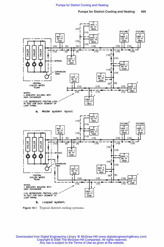
Pumps for District Cooling and Heating 469
Figure 18.1 Typical district cooling systems.
Rishel_CH18.qxd 20/4/06 6:47 PM Page 469
Downloaded from Digital Engineering Library @ McGraw-Hill (www.digitalengineeringlibrary.com)Copyright © 2006 The McGraw-Hill Companies. All rights reserved.
Any use is subject to the Terms of Use as given at the website.
Pumps for District Cooling and Heating
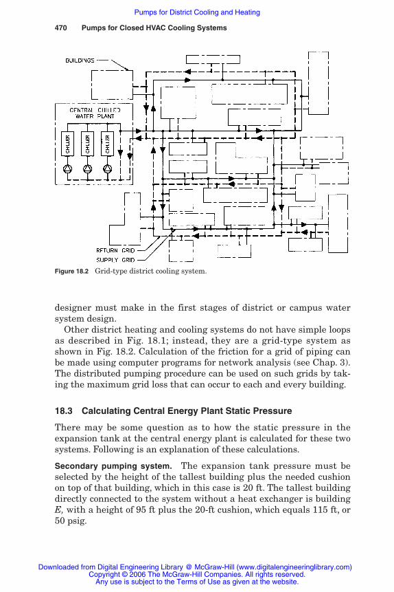
470 Pumps for Closed HVAC Cooling Systems
Figure 18.2 Grid-type district cooling system.
designer must make in the first stages of district or campus watersystem design.
Other district heating and cooling systems do not have simple loopsas described in Fig. 18.1; instead, they are a grid-type system asshown in Fig. 18.2. Calculation of the friction for a grid of piping canbe made using computer programs for network analysis (see Chap. 3).The distributed pumping procedure can be used on such grids by tak-ing the maximum grid loss that can occur to each and every building.
18.3 Calculating Central Energy Plant Static Pressure
There may be some question as to how the static pressure in theexpansion tank at the central energy plant is calculated for these twosystems. Following is an explanation of these calculations.
Secondary pumping system. The expansion tank pressure must beselected by the height of the tallest building plus the needed cushionon top of that building, which in this case is 20 ft. The tallest buildingdirectly connected to the system without a heat exchanger is buildingE, with a height of 95 ft plus the 20-ft cushion, which equals 115 ft, or50 psig.
Rishel_CH18.qxd 20/4/06 6:47 PM Page 470
Downloaded from Digital Engineering Library @ McGraw-Hill (www.digitalengineeringlibrary.com)Copyright © 2006 The McGraw-Hill Companies. All rights reserved.
Any use is subject to the Terms of Use as given at the website.
Pumps for District Cooling and Heating
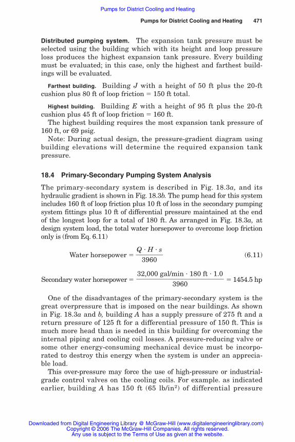
Pumps for District Cooling and Heating 471
Distributed pumping system. The expansion tank pressure must beselected using the building which with its height and loop pressureloss produces the highest expansion tank pressure. Every buildingmust be evaluated; in this case, only the highest and farthest build-ings will be evaluated.
Farthest building. Building J with a height of 50 ft plus the 20-ftcushion plus 80 ft of loop friction � 150 ft total.
Highest building. Building E with a height of 95 ft plus the 20-ftcushion plus 45 ft of loop friction � 160 ft.
The highest building requires the most expansion tank pressure of160 ft, or 69 psig.
Note: During actual design, the pressure-gradient diagram usingbuilding elevations will determine the required expansion tankpressure.
18.4 Primary-Secondary Pumping System Analysis
The primary-secondary system is described in Fig. 18.3a, and itshydraulic gradient is shown in Fig. 18.3b. The pump head for this systemincludes 160 ft of loop friction plus 10 ft of loss in the secondary pumpingsystem fittings plus 10 ft of differential pressure maintained at the endof the longest loop for a total of 180 ft. As arranged in Fig. 18.3a, atdesign system load, the total water horsepower to overcome loop frictiononly is (from Eq. 6.11)
Water horsepower � �Q
3�
9H60
� s� (6.11)
Secondary water horsepower � � 1454.5 hp
One of the disadvantages of the primary-secondary system is thegreat overpressure that is imposed on the near buildings. As shownin Fig. 18.3a and b, building A has a supply pressure of 275 ft and areturn pressure of 125 ft for a differential pressure of 150 ft. This ismuch more head than is needed in this building for overcoming theinternal piping and cooling coil losses. A pressure-reducing valve orsome other energy-consuming mechanical device must be incorpo-rated to destroy this energy when the system is under an apprecia-ble load.
This over-pressure may force the use of high-pressure or industrial-grade control valves on the cooling coils. For example. as indicatedearlier, building A has 150 ft (65 lb/in2) of differential pressure
32,000 gal/min � 180 ft � 1.0����
3960
Rishel_CH18.qxd 20/4/06 6:47 PM Page 471
Downloaded from Digital Engineering Library @ McGraw-Hill (www.digitalengineeringlibrary.com)Copyright © 2006 The McGraw-Hill Companies. All rights reserved.
Any use is subject to the Terms of Use as given at the website.
Pumps for District Cooling and Heating
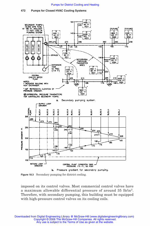
472 Pumps for Closed HVAC Cooling Systems
imposed on its control valves. Most commercial control valves havea maximum allowable differential pressure of around 35 lb/in2.Therefore, with secondary pumping, this building must be equippedwith high-pressure control valves on its cooling coils.
Figure 18.3 Secondary pumping for district cooling.
Rishel_CH18.qxd 20/4/06 6:47 PM Page 472
Downloaded from Digital Engineering Library @ McGraw-Hill (www.digitalengineeringlibrary.com)Copyright © 2006 The McGraw-Hill Companies. All rights reserved.
Any use is subject to the Terms of Use as given at the website.
Pumps for District Cooling and Heating
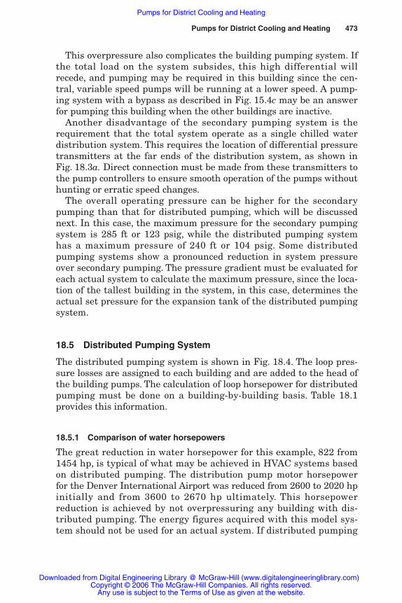
Pumps for District Cooling and Heating 473
This overpressure also complicates the building pumping system. Ifthe total load on the system subsides, this high differential willrecede, and pumping may be required in this building since the cen-tral, variable speed pumps will be running at a lower speed. A pump-ing system with a bypass as described in Fig. 15.4c may be an answerfor pumping this building when the other buildings are inactive.
Another disadvantage of the secondary pumping system is therequirement that the total system operate as a single chilled waterdistribution system. This requires the location of differential pressuretransmitters at the far ends of the distribution system, as shown inFig. 18.3a. Direct connection must be made from these transmitters tothe pump controllers to ensure smooth operation of the pumps withouthunting or erratic speed changes.
The overall operating pressure can be higher for the secondarypumping than that for distributed pumping, which will be discussednext. In this case, the maximum pressure for the secondary pumpingsystem is 285 ft or 123 psig, while the distributed pumping systemhas a maximum pressure of 240 ft or 104 psig. Some distributedpumping systems show a pronounced reduction in system pressureover secondary pumping. The pressure gradient must be evaluated foreach actual system to calculate the maximum pressure, since the loca-tion of the tallest building in the system, in this case, determines theactual set pressure for the expansion tank of the distributed pumpingsystem.
18.5 Distributed Pumping System
The distributed pumping system is shown in Fig. 18.4. The loop pres-sure losses are assigned to each building and are added to the head ofthe building pumps. The calculation of loop horsepower for distributedpumping must be done on a building-by-building basis. Table 18.1provides this information.
18.5.1 Comparison of water horsepowers
The great reduction in water horsepower for this example, 822 from1454 hp, is typical of what may be achieved in HVAC systems basedon distributed pumping. The distribution pump motor horsepowerfor the Denver International Airport was reduced from 2600 to 2020 hpinitially and from 3600 to 2670 hp ultimately. This horsepowerreduction is achieved by not overpressuring any building with dis-tributed pumping. The energy figures acquired with this model sys-tem should not be used for an actual system. If distributed pumping
Rishel_CH18.qxd 20/4/06 6:47 PM Page 473
Downloaded from Digital Engineering Library @ McGraw-Hill (www.digitalengineeringlibrary.com)Copyright © 2006 The McGraw-Hill Companies. All rights reserved.
Any use is subject to the Terms of Use as given at the website.
Pumps for District Cooling and Heating

474 Pumps for Closed HVAC Cooling Systems
Figure 18.4 Distributed pumping for district cooling.
Rishel_CH18.qxd 20/4/06 6:47 PM Page 474
Downloaded from Digital Engineering Library @ McGraw-Hill (www.digitalengineeringlibrary.com)Copyright © 2006 The McGraw-Hill Companies. All rights reserved.
Any use is subject to the Terms of Use as given at the website.
Pumps for District Cooling and Heating

Pumps for District Cooling and Heating 475
TABLE 18.1 Distribution Horsepower for Distributed Pumping
Building Tons Gal/min Loop head, ft Water hp
A 600 1,200 20 6.1B 1,200 2,400 30 18.2C 1,400 2,800 80 56.6D 2,400 4,800 70* 84.8E 2,000 4,000 90 90.9F 800 1,600 110 44.4G 2,000 4,000 150* 151.5H 1,800 3,600 150* 136.4J 1,200 2,400 160 97.0K 1,600 3,200 100* 80.8L 1,000 2,000 110 55.6TOTALS 16,000 32,000 822.3
*Ten feet of pump head has been added to these buildings for the friction loss for a pump-ing system that may be needed for the heat exchangers.
is considered for an actual system, the computer calculations andpressure gradient should be run for that system as it was done herewith this model system.
18.5.2 Features of distributed pumping
One of the most significant features of distributed pumping is its sim-plicity. There are no crossover bridges, balancing valves, or pressureregulators that consume energy. Another feature is total independentcontrol for each building. The building pumps are usually variable-speed pumps because of the tremendous variation in total head fromminimum to maximum flow. Speed control is maintained for the pumpsin each building. The only effect that one building has on another is thechange in the loop pressure that is caused by a load change in a build-ing. This is picked up quickly by the pump controllers in each buildingwithout hunting or rapid changes in pressure. There is absolutely noreason to install balance valves on each building; these systems arecompletely self-balancing.
The principal disadvantage of a pure distributed pumping system isits inability to be applied to an existing installation, particularly if thereare many buildings on the system. In some cases, the installed cost ofthe existing pumping and piping makes it prohibitive to try to utilizethe principles of distributive pumping. Because of this, there are manyversions of existing primary-secondary pumping for district cooling andheating systems operating with distributed pumping in newer build-ings. For example, distributed pumping as booster systems simulatesdistributed pumping in new sections of a system. This can be called zone
Rishel_CH18.qxd 20/4/06 6:47 PM Page 475
Downloaded from Digital Engineering Library @ McGraw-Hill (www.digitalengineeringlibrary.com)Copyright © 2006 The McGraw-Hill Companies. All rights reserved.
Any use is subject to the Terms of Use as given at the website.
Pumps for District Cooling and Heating

476 Pumps for Closed HVAC Cooling Systems
pumping where the existing central energy plant has distributionpumps with enough head to pump the central zone of a campus. Thiswas demonstrated in Figs. 15.4, 15.5, and 15.6. Instead of boosting cen-tral plant pressures to accommodate new buildings or extensions,booster pumping systems each with a bypass can be installed. Thebooster pumping systems usually employ variable-speed pumps, andthey provide the additional head required under peak load conditionswhen the central pumps cannot meet the head requirement of theperipheral buildings. Typical of these is the system shown in Fig. 15.4.
As mentioned elsewhere in this book, there is great fear aboutrunning variable-speed pumps in series. This has been done suc-cessfully on many installations. The important factor is proper con-trol of both pumps; with this control, there should not be any con-cern over the first pump forcing the second pump to runinefficiently, and vice versa.
18.5.3 Distributed pumping withoutprimary pumps
One additional advantage for distributed pumping in district heat-ing and cooling is the opportunity to eliminate any possibility ofreverse flow of chilled water through the chiller bypass. This is doneby the elimination of the primary pumps as shown in Fig. 18.5.Under normal operation, no chilled water pumps are running in thechilled water plant. Circulators are there to maintain minimumflow in the chiller evaporators under very low cooling loads on thesystem. It is the author’s opinion that at some time in the future, acirculator will be furnished, mounted on the chiller that will elimi-nate all field piping; also, the circulator will be selected for the min-imum flow requirements of each size and type of chiller.
18.6 Differential Temperature
The question always arises as to what differential temperatureshould be used in the transportation of water from the central plantto the buildings on the system. This is a function of piping costs andchilled water generation costs. As described elsewhere in this book,reducing the chilled water temperature leaving a chiller increases thekilowatts per ton for that chiller. This is an overall economic evalua-tion that must be made by the designers and operators of a districtcooling system. If it is in the best interests to market low-temperaturecooling water such as 40°F, the distributed pumping system offers asimple procedure for blending the water at the building to a highertemperature such as 45°F. Figure 18.6 describes the blending-valveinstallation on a distributed pumping system.
Rishel_CH18.qxd 20/4/06 6:47 PM Page 476
Downloaded from Digital Engineering Library @ McGraw-Hill (www.digitalengineeringlibrary.com)Copyright © 2006 The McGraw-Hill Companies. All rights reserved.
Any use is subject to the Terms of Use as given at the website.
Pumps for District Cooling and Heating

Pumps for District Cooling and Heating 477
Figure 18.5 Distributed pumping without primary pumps.
Figure 18.6 Blending or chilled water reset with distributed pumping.
L1000 T.
75 fthigh
G2000 T.230 fthigh
F800 T.60 fthigh
(Future)
R1600 T.125 fthigh
(Future)
A600 T.40 fthigh
B1200 T.
60 fthigh
J1200 T.
50 fthigh
H1800 T.120 fthigh
E2000 T.
95 fthigh
D2400 T.300 fthigh
C1400 T.
90 fthigh120
130
140145
190
200
150 125 115 105
215205195175175170
240 230 220 230
No primarypumps
Chi
ller
Chi
ller
Chi
ller
∗
∗
∗
80 90 100
215
205
105
115
90
Circulator forminimum flow
Bypass
No secondarypumps
Central chilledwater plant
Notes: ∗Indicates building with heat exchanger.
Notes: 1. Each building has variable-speed pumps. 2. Expansion tank not shown. Location dependent upon the configuration of the water system.
“240” represents elevationof pressure gradient.
Check valve
Rishel_CH18.qxd 20/4/06 6:47 PM Page 477
Downloaded from Digital Engineering Library @ McGraw-Hill (www.digitalengineeringlibrary.com)Copyright © 2006 The McGraw-Hill Companies. All rights reserved.
Any use is subject to the Terms of Use as given at the website.
Pumps for District Cooling and Heating

478 Pumps for Closed HVAC Cooling Systems
The distributed pumping system has a particular advantage overother systems when blending water because the return pressure isalways higher than the supply pressure. This reduces the energylost in the blending procedure because the supply valve is normallyopen.
18.7 Building Connections
Building connections are very important in district cooling. Figure 18.7adescribes suggested connections for a building without a heatexchanger, while Fig. 18.7b provides the connections with a heatexchanger. It should be noted that there is no return temperature-control valve included in Fig. 18.7, as is often suggested. Use of thisvalve can cause some very complex problems.
There should be no attempt to artificially control the return watertemperature in a particular building. This has been tried with disas-trous results by installing a return temperature-control valve thatlimits the return temperature to a value such as 57°F or higher. Totalloss of building humidity control can result due to the high supplywater temperature that is caused by this valve that bypasses returnwater back to the supply.
The return temperature from each building is the result of thequality of design and maintenance in that building. Low return tem-perature is caused principally by operating cooling coils in the lami-nar flow range or allowing them to become dirty on the water or airside. It should be the responsibility of the building management toensure a minimum return water temperature. If they are lax in theirdesign or maintenance, they should pay for it.
18.8 District Heating
Much of the information on district cooling also applies to districtheating. Similar evaluations for primary-secondary and distributedpumping can be made for hot water systems. One advantage of heat-ing over cooling is the ability to transmit hot water at much higherdifferential temperatures such as 40 to 150°F. This reduces the pump-ing costs and may require more heat exchangers in the buildingsserved. For example, high-temperature water at 300°F may be deliv-ered to a building requiring only 160°F for its heating system. Theadded thermal cost of generating higher-temperature water must beconsidered in the economic evaluation of the system.
The building connections for hot water are, again, the same asthose for chilled water, as described in Fig. 18.7. Obviously, piping
Rishel_CH18.qxd 20/4/06 6:47 PM Page 478
Downloaded from Digital Engineering Library @ McGraw-Hill (www.digitalengineeringlibrary.com)Copyright © 2006 The McGraw-Hill Companies. All rights reserved.
Any use is subject to the Terms of Use as given at the website.
Pumps for District Cooling and Heating
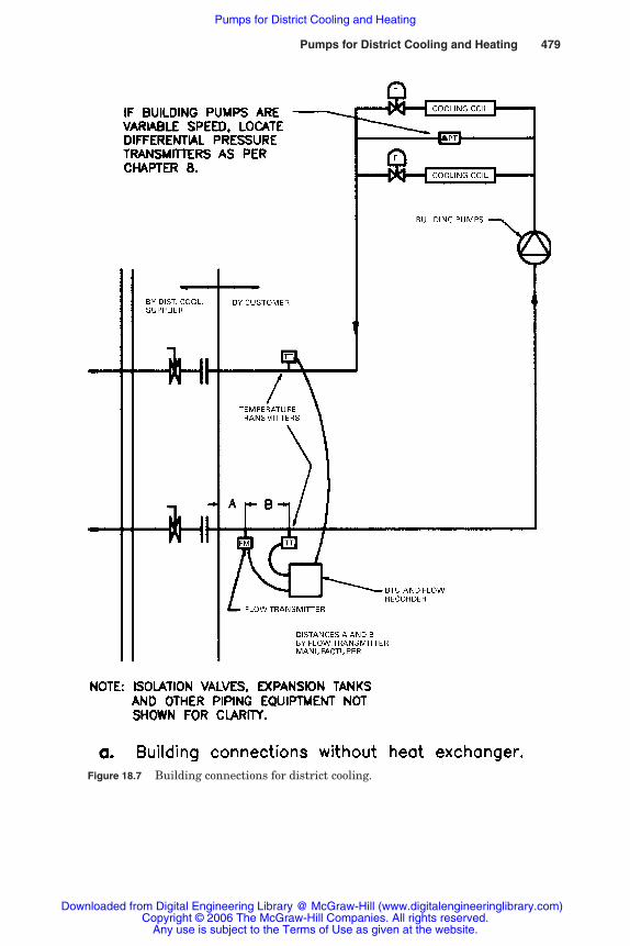
Pumps for District Cooling and Heating 479
Figure 18.7 Building connections for district cooling.
Rishel_CH18.qxd 20/4/06 6:47 PM Page 479
Downloaded from Digital Engineering Library @ McGraw-Hill (www.digitalengineeringlibrary.com)Copyright © 2006 The McGraw-Hill Companies. All rights reserved.
Any use is subject to the Terms of Use as given at the website.
Pumps for District Cooling and Heating

480 Pumps for Closed HVAC Cooling Systems
Figure 18.7 (Continued)
for high-temperature water is different from that for chilled water,but the general configuration is much the same. Thermal expansionprovisions obviously are greater for medium- or high-temperaturewater than for chilled water.
Rishel_CH18.qxd 20/4/06 6:47 PM Page 480
Downloaded from Digital Engineering Library @ McGraw-Hill (www.digitalengineeringlibrary.com)Copyright © 2006 The McGraw-Hill Companies. All rights reserved.
Any use is subject to the Terms of Use as given at the website.
Pumps for District Cooling and Heating
18.9 Conclusions
Recognizing that return water temperature from a building is a vari-able should prompt the operators of district chilled water systems tomarket their energy as is done in the electric power distribution indus-try. Both flow and differential temperature at each building should bemeasured with a calculation of total British thermal units. Each build-ing management should pay a commodity charge for their Britishthermal unit consumption plus a demand charge based on their maxi-mum flow in gallons per minute. This places the responsibility onthem for maintaining the highest possible return water temperature.
The development of digital electronics and the variable-speed drivehas offered the district cooling industry new tools in the design andoperation of their distribution systems. The most important part ofthis review of district pumping is the use of pressure-gradient dia-grams to evaluate and achieve the most efficient method of water dis-tribution in a particular district cooling system. The pressure-gradientdiagram provides the designer with a graphic representation of thesystem’s pressures, pressure losses, and overpressure. The equationsfor system energy consumption (Eqs. 8.4 through 8.7) should be usedto determine the most efficient method of distributing water in dis-trict cooling and heating systems.
18.10 Bibliography
James H. Ottmer and James B. Rishel, Airport’s pumping system horsepower take nosedive, Heating, Piping and Air-Conditioning Magazine, vol. 65, no. 10, pp. 51–55,October 1993.
James B. Rishel, Pumping district chilled water systems, Ninth Annual CoolingConference, International District Energy Association, October 1994.
Pumps for District Cooling and Heating 481
Rishel_CH18.qxd 20/4/06 6:47 PM Page 481
Downloaded from Digital Engineering Library @ McGraw-Hill (www.digitalengineeringlibrary.com)Copyright © 2006 The McGraw-Hill Companies. All rights reserved.
Any use is subject to the Terms of Use as given at the website.
Pumps for District Cooling and Heating

Rishel_CH18.qxd 20/4/06 6:47 PM Page 482
Downloaded from Digital Engineering Library @ McGraw-Hill (www.digitalengineeringlibrary.com)Copyright © 2006 The McGraw-Hill Companies. All rights reserved.
Any use is subject to the Terms of Use as given at the website.
Pumps for District Cooling and Heating

Pumps for HVACHot Water Systems
Part
6
Rishel_CH19.qxd 20/4/06 6:48 PM Page 483
Downloaded from Digital Engineering Library @ McGraw-Hill (www.digitalengineeringlibrary.com)Copyright © 2006 The McGraw-Hill Companies. All rights reserved.
Any use is subject to the Terms of Use as given at the website.
Source: HVAC Pump Handbook

Rishel_CH19.qxd 20/4/06 6:48 PM Page 484
Downloaded from Digital Engineering Library @ McGraw-Hill (www.digitalengineeringlibrary.com)Copyright © 2006 The McGraw-Hill Companies. All rights reserved.
Any use is subject to the Terms of Use as given at the website.
Pumps for HVAC Hot Water Systems

Chapter
485
19Steam and Hot Water
Boilers
19.1 Introduction
This chapter reviews all HVAC boilers as well as the circuiting andpumping of hot water boilers. Condensate pumping and steam boilerfeed will be discussed in Chap. 22. A brief synopsis will be given of thetypes of boilers that are used in the HVAC industry today.
19.2 Classification of Boilers
Boilers are governed by the American Society of MechanicalEngineers’ (ASME) Boiler and Pressure Vessel Code, of which thereare two sections, Sec. 4, “Rules for Construction of Heating Boilers”(low pressure), and Sec. 1, “Rules for Construction of Power Boilers”(high pressure). The limits between these two codes are by tempera-ture as well as pressure. Heating boilers cannot exceed 15 psig steam,160 psig water, or 250°F temperature. This temperature is the evapo-ration or saturation temperature for water at 29.83 psia or approxi-mately 15 psig pressure. All boilers, water or steam, operating above250°F must be designed to the ASME power boiler code.
Clarification should be made of the term hot water boilers.Normally the word boiler indicates a piece of equipment that boils aliquid to the gaseous or vapor state. Originally, these boilers werecalled hot water generators. This created confusion in the HVACindustry because heaters of domestic water also were called hot watergenerators. It is now the American Society of Heating, Refrigerating
Rishel_CH19.qxd 20/4/06 6:48 PM Page 485
Downloaded from Digital Engineering Library @ McGraw-Hill (www.digitalengineeringlibrary.com)Copyright © 2006 The McGraw-Hill Companies. All rights reserved.
Any use is subject to the Terms of Use as given at the website.
Source: HVAC Pump Handbook

486 Pumps for HVAC Hot Water Systems
and Air-Conditioning Engineers’ (ASHRAE) definition that a boiler isa vessel in which a liquid is heated with or without vaporization. Forthe HVAC industry, the liquid is water; if it is a fluid such as air, thevessel is called a furnace.
19.3 Types of Boilers by Materials of Construction
Boilers, both steam and hot water, are manufactured of cast iron,steel, copper, and other materials that may be used in condensing-type boilers. For many years, low-pressure heating boilers were man-ufactured from cast iron, while high-pressure boilers were of rivetedsteel design. As welding technology progressed, all steel boilers werewelded and became available for low-pressure heating applications.Copper-tube boilers were developed for both low and high pressuresbecause of their flexibility.
Today, most HVAC boilers are of steel, copper, or cast iron construc-tion. Steel and copper boilers can be made for both low- and high-pressure service, while cast iron boilers are designed for 15-psigsteam or 30-psig water working pressures. Both steel and cast ironboilers are made in a number of configurations for the firing of spe-cific fuels or to fit the thermodynamic design of the manufacturer.Electrically, heated boilers are usually of steel or alloy construction.
Steel boilers can be of fire-tube, with the products of combustion inthe tubes, or of water-tube construction, where the water or steam isin the tubes and the products of combustion surround the tubes. Bothtypes of boilers are made in small and large sizes; the largest steamboilers are of water-tube design.
Some boilers are made of a rigid construction that makes themsusceptible to thermal shock. Thermal shock is an expression in theboiler industry that denotes uneven expansion in a boiler thatcauses leakage around the tubes. This can cause severe damage tothe boiler in some cases. The boiler manufacturer will stipulate thedifferences between supply and return water temperatures and mayspecify a maximum rate of temperature change in the supply water.The boiler manufacturer may provide a circulating pump that willsolve this problem or will specify the flow requirements of a primaryor boiler pump furnished by others. This will determine whetherprimary or primary-secondary pumping systems are required withcertain boilers.
Medium- and high-temperature water boilers must be designed tothe ASME power boiler code because they operate above 250°F. Theycan be steam boilers, where the steam is used principally as an
Rishel_CH19.qxd 20/4/06 6:48 PM Page 486
Downloaded from Digital Engineering Library @ McGraw-Hill (www.digitalengineeringlibrary.com)Copyright © 2006 The McGraw-Hill Companies. All rights reserved.
Any use is subject to the Terms of Use as given at the website.
Steam and Hot Water Boilers

Steam and Hot Water Boilers 487
expansion cushion, or they can be water-tube boilers with specialcircuits for high-temperature water. Further description of these boil-ers will be made in Chap. 21 on medium- and high-temperaturewater.
19.4 Types of Boilers: Condensing,or Noncondensing
Hot water boilers also can be classified as to their operation, whethercondensing or noncondensing. For many years, hot water boilers wereoperated noncondensing. This means that the water vapor in theproducts of combustion does not condense within any part of theboiler. To avoid condensing the water vapor, the boilers were designedso that any of the water next to the heating surfaces of the boilernever dropped below 140°F. For most natural gases, the dew point ofwater vapor at 20 percent excess air is around 130°F. Therefore, a10°F temperature difference between the water and the flue gaseswas maintained at 140°F to avoid condensation.
Why is condensation undesirable in these boilers? Many of themare made of ferrous products (steel or cast iron). A mixture of carbondioxide and water vapor produces carbonic acid, which attacks steelor cast iron and causes severe rusting. For many years, control of com-bustion and boiler design prevented the use of condensing boilers.
Why is condensing of water vapor desirable in boilers manufac-tured of materials that withstand attack by carbonic acid? An investi-gation of the steam tables will reveal that the heat of evaporation forwater vapor at the partial pressures at which it exists in flue gasproducts is over 1025 Btu/lb. Most of this heat is transferred to thewater being heated if condensation occurs. Figure 19.1 describes theefficiency of a boiler that can be operated condensing. This figure isapproximate and is considered to be for a boiler operating at full fir-ing rate. Boilers with modulating burners may provide even higherefficiencies.
The maximum possible efficiency of a gas-fired boiler without con-densing is around 87 percent; this efficiency may be difficult toachieve without condensing in the boiler itself or in the flue system.Condensing boilers operating with low return water temperaturesfrom the heating system can produce combustion and thermal effi-ciencies in excess of 95 percent. It is obvious from these efficiency dif-ferences that it is imperative that every effort be made to reduceoperating water temperatures where possible to take advantage ofthese improved boiler efficiencies.
Rishel_CH19.qxd 20/4/06 6:48 PM Page 487
Downloaded from Digital Engineering Library @ McGraw-Hill (www.digitalengineeringlibrary.com)Copyright © 2006 The McGraw-Hill Companies. All rights reserved.
Any use is subject to the Terms of Use as given at the website.
Steam and Hot Water Boilers
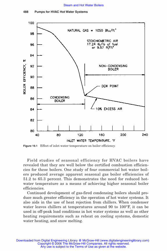
488 Pumps for HVAC Hot Water Systems
Figure 19.1 Effect of inlet water temperature on boiler efficiency.
Field studies of seasonal efficiency for HVAC boilers haverevealed that they are well below the certified combustion efficien-cies for these boilers. One study of four commercial hot water boil-ers produced average apparent seasonal gas boiler efficiencies of51.2 to 65.3 percent. This demonstrates the need for reduced hot-water temperature as a means of achieving higher seasonal boilerefficiencies.
Continued development of gas-fired condensing boilers should pro-duce much greater efficiency in the operation of hot water systems. Italso aids in the use of heat rejection from chillers. When condenserwater leaves chillers at temperatures around 90 to 100°F, it can beused in off-peak load conditions in hot water systems as well as otherheating requirements such as reheat on cooling systems, domesticwater heating, and snow melting.
Rishel_CH19.qxd 20/4/06 6:48 PM Page 488
Downloaded from Digital Engineering Library @ McGraw-Hill (www.digitalengineeringlibrary.com)Copyright © 2006 The McGraw-Hill Companies. All rights reserved.
Any use is subject to the Terms of Use as given at the website.
Steam and Hot Water Boilers

Steam and Hot Water Boilers 489
19.5 Rating of Boilers
Low-pressure steam boilers are rated in pounds of steam per hour fromand at 212°F, British thermal units per hour, or boiler horsepower. Boilerhorsepower is not used as often as in the past; it is equivalent to 34.5 lbof steam per hour from and at 212°F or 33,475 Btu/h. The expressionfrom and at means from feedwater at 212°F to steam at 212°F.
Hot water boilers are rated in thousands of British thermal unitstransferred per hour, which is abbreviated as MBH. This rating maybe specified by the manufacturer at some specific temperature suchas 180°F. Boiler ratings are established by boiler manufacturers’ asso-ciations and government agencies. They can be so-called gross or netratings. For the designer of a water system, from a pumping stand-point, the only rating of concern is the maximum boiler output or heatflow to the water system in MBH.
19.6 Computing Boiler Water Flow
The standard formula for calculating water flow in gallons per minuteis as defined in Chap. 9:
Hot water system gal/min � (9.1)
This formula assumes that the specific weight of water is always 62.3lb/ft3, which is not true. If precise flow is desired, the true specificweight � at the operating temperature must be used in the followingformula:
Hot water system gal/min �
� (19.1)
where 7.48 � U.S. gallons per cubic foot� � specific weight of water from Table 2.3
For example, assume that system load is 5000 MBH with a 200°Fsupply water temperature and a differential temperature of 40°F. FromTable 2.3, the specific weight of water at 200°F is 60.13 lb/ft3. Thus
Gal/min � �16205.1
�
35�
04000
�
� 259.9 gal/min
125 � system MBH���
� � �T (°F)
system MBH � 1000���(��7.48) � 60 � �T °F
system MBH � 1000���
500 � �T (°F)
Rishel_CH19.qxd 20/4/06 6:48 PM Page 489
Downloaded from Digital Engineering Library @ McGraw-Hill (www.digitalengineeringlibrary.com)Copyright © 2006 The McGraw-Hill Companies. All rights reserved.
Any use is subject to the Terms of Use as given at the website.
Steam and Hot Water Boilers

490 Pumps for HVAC Hot Water Systems
This formula assumes an average specific heat of water to be 1 Btuper pound per degree F. For most hot water operations below 250°F,this is acceptable; it cannot be used for medium- and high-temperaturewater systems, where the actual specific heat must be factored into theequations for water flow.
19.7 Connecting Pumps to Boilers
Condensate return and connecting pumps to steam boilers will bereviewed in Chap. 22. Of great concern to the hot water systemdesigner is the location of the pumps with respect to the boiler andwhether a circulating pump is required to maintain a minimum flowrate through the boiler regardless of the flow to the hot water system.Both these factors must be settled before the design of the boiler roomis completed. The cost of the installation and its successful operationare very dependent on these two decisions.
19.7.1 Minimum flow through the hot water boiler
As indicated earlier, the boiler manufacturer whose boiler is underconsideration must provide information as to minimum flow rate and,in some cases, the maximum change in flow rate. These two factorsmay or may not be important. The boiler manufacturer should guar-antee the boiler against thermal shock under specific flow conditions.
Thermal shock is avoided by providing a minimum flow rate in theboiler. Minimum flow rate is maintained by providing a circulatingpump on the boiler or by primary-secondary pumping. Other manu-facturers depend on bypass valves rather than the boiler or primarypump. It is the boiler manufacturer’s responsibility to providedetailed pumping and piping instructions for the boiler installation toensure that thermal shock does not occur in the boiler.
19.7.2 Classifying boilers by flow requirements
Boilers are classified by their flow requirements to ensure that ade-quate flow is maintained in them. The boiler manufacturer shouldalways be consulted for minimum flow and temperature requirements.
Partial or full flow. Most fire tube and cast iron boilers require sub-stantial flow under most load conditions on the water system. It ispartiularly important to have the actual boiler manufacturer of thesetypes to state the minimum allowable flow at various loads andwater temperatures.
Rishel_CH19.qxd 20/4/06 6:48 PM Page 490
Downloaded from Digital Engineering Library @ McGraw-Hill (www.digitalengineeringlibrary.com)Copyright © 2006 The McGraw-Hill Companies. All rights reserved.
Any use is subject to the Terms of Use as given at the website.
Steam and Hot Water Boilers
Steam and Hot Water Boilers 491
Minimum flow. Water tube boilers, manufactured of steel or coppertubes, often require a minimum flow that is specified by their man-ufacturer.
No flow requirement. Many new condensing boilers do not require anyminimum flow. This, of course should be certified by the manufac-turer, whether at full or minimum load on the system.
19.7.3 Locating pumps at boilers
The question always arises as to the location of the pump with respectto the boiler. There are some accepted rules in the HVAC industrythat have no foundation. The selection of the pump location withrespect to the boiler must be determined by the physical conditions ofthe actual application. For example,
1. The pumps should be located, if possible, on the cooler returnwater to the boiler. This enables the pump internals such as themechanical seal to have a longer useful life.
2. Locating the pumps on the cooler return water also does notexpose the pumps to the air released from the water in the boiler(see Table 2.5).
3. The static pressure of the building determines the required operat-ing pressure of the boiler. If putting the pump on the inlet to theboiler increases the design pressure of the boiler, either the boilerconstruction should be changed or the pump should be located onthe discharge of the boiler.
Often, boilers constructed of steel can be equipped with pressure-relief valves set at pressures required by the installation with thepump installed on the return water connection to the boiler. Locationof the pump with respect to the boiler is a decision that must be madeby the designer, taking in consideration all the conditions that existon a particular installation.
19.8 Reset of Boiler Temperature versusZone Reset
A controversy exists in the HVAC industry over the relative merits ofboiler temperature reset and the reset of zone temperatures. It isimportant that this be addressed in this chapter, since many designersare losing sight of what achieves lowest possible energy consumption ina hot water system. Operation of the boilers at the lowest acceptable
Rishel_CH19.qxd 20/4/06 6:48 PM Page 491
Downloaded from Digital Engineering Library @ McGraw-Hill (www.digitalengineeringlibrary.com)Copyright © 2006 The McGraw-Hill Companies. All rights reserved.
Any use is subject to the Terms of Use as given at the website.
Steam and Hot Water Boilers

492 Pumps for HVAC Hot Water Systems
leaving water temperature provides the lowest energy consumption ina hot water system. Figure 19.1 demonstrates the great increase in effi-ciency secured by operating a boiler at low entering water tempera-tures. The condensing-type boiler increases these opportunities.
Zone reset of water temperature may appear to have some advan-tages, but on most installations, the economies of boiler reset andeliminating zone reset valving more than offset the energy saved byzone temperature reset. Specific installations where some zones havemuch more glass load than others might justify reset of the zone tem-perature on a particular zone. Chapter 8 on the use of water in HVACsystems has specific information on the pumping costs of zone reset.
19.9 Boiler Controls
A brief review of boiler control should be included, since boilersequencing and interfacing with pump controls are often encoun-tered on HVAC heating systems. There are three basic types of boilercontrol:
1. On-off control. The operating controller, such as a thermostat orpressure control, starts and stops the boiler firing equipment. Theboiler operates at design firing rate. This is the least efficient controlsystem, since there is a standby loss whenever the boiler is not oper-ating. Also, the flue gas loss is highest at design firing rate.
2. High-low-off control. This control procedure is more efficientthan the on-off control, but it does not eliminate all inefficient opera-tion. Instead of turning on and off, the burner returns to a low firingrate before stopping. With proper adjustment, the boiler can operatebetween low and high firing continuously on much of the load range.
3. Modulated firing. This control varies the firing rate and combus-tion airflow with the load and eliminates much of the starting andstopping of the boiler. The load range for most noncondensing boilersis around 30 through 100 percent of full-load firing. Some condensingboiler manufacturers quote operating ranges as broad as 8 to 100 per-cent. This great range reduces the time the boiler is shut down, andtherefore, the standby loss is reduced appreciably.
Modulating firing is the most efficient boiler control because it elim-inates much of the standby loss and accomplishes most of the opera-tion at an off-peak firing rate. This type of control is easy to interfacewith boiler reset and other control algorithms, since the firing con-trols can accept a standard 4- to 20-mA signal from the other systemcontrols.
Rishel_CH19.qxd 20/4/06 6:48 PM Page 492
Downloaded from Digital Engineering Library @ McGraw-Hill (www.digitalengineeringlibrary.com)Copyright © 2006 The McGraw-Hill Companies. All rights reserved.
Any use is subject to the Terms of Use as given at the website.
Steam and Hot Water Boilers

Interfacing boilers efficiently with hot water systems has becomemuch easier with digital electronics; piping has become simpler too.Studies have shown that existing, older boilers have seasonal efficien-cies as low as 50 percent. With the newer digital controls and the con-temporary boilers, particularly condensing boilers, the seasonal boilerefficiencies should rise dramatically.
19.10 Bibliography
Systems and Equipment Handbook, ASHRAE, Atlanta, Ga., 1992.
Steam and Hot Water Boilers 493
Rishel_CH19.qxd 20/4/06 6:48 PM Page 493
Downloaded from Digital Engineering Library @ McGraw-Hill (www.digitalengineeringlibrary.com)Copyright © 2006 The McGraw-Hill Companies. All rights reserved.
Any use is subject to the Terms of Use as given at the website.
Steam and Hot Water Boilers

Rishel_CH19.qxd 20/4/06 6:48 PM Page 494
Downloaded from Digital Engineering Library @ McGraw-Hill (www.digitalengineeringlibrary.com)Copyright © 2006 The McGraw-Hill Companies. All rights reserved.
Any use is subject to the Terms of Use as given at the website.
Steam and Hot Water Boilers

Chapter
495
20Low-Temperature Hot
Water Heating Systems
20.1 Introduction
Low-temperature hot water heating systems comprise the majority ofHVAC hot water heating systems. The obvious reason for this is thelack of a need for water temperatures in excess of 250°F on most ofthese systems. Also, the advent of the condensing boiler has drivendown the design water temperature of many systems. As was dis-cussed in Chap. 19, lower operating water temperatures increaseappreciably the boiler efficiency. This fact and the development of thevariable-speed pump constitute two of the greatest improvements inthe efficiency of space heating in commercial, governmental, educa-tional, institutional, and industrial buildings. Residential heating by hotwater will not be included herein, since this is a specific field by itself.Also, the pumps for residential heating consist of small circulatorswhose horsepower is not of major consideration in terms of energy use.
20.2 Classification of Hot Water Systems
Hot water systems in HVAC can be classified as to the source of theirheat as well as by use of the hot water. These systems receive their heatfrom (1) electric or fuel-fired boilers, (2) low- and high-pressure steam,(3) medium- and high-temperature water, (4) district heating, and (5)heat recovery. Hot water is used for (1) space heating, (2) heating of out-side air, (3) reheat in cooling systems, and (4) process heating in indus-try. Heating of domestic water is not considered to be an HVAC hotwater system.
Rishel_CH20.qxd 20/4/06 6:49 PM Page 495
Downloaded from Digital Engineering Library @ McGraw-Hill (www.digitalengineeringlibrary.com)Copyright © 2006 The McGraw-Hill Companies. All rights reserved.
Any use is subject to the Terms of Use as given at the website.
Source: HVAC Pump Handbook

496 Pumps for HVAC Hot Water Systems
20.3 Sources of Heat for Hot Water Systems
20.3.1 Hot water boilers
Most of the discussion of hot water boilers was included in Chap. 19.From a hot water heating system standpoint, the boiler type shouldbe selected that offers optimal efficiency, simplicity in the design ofthe hot water system, and ease of installation. First cost is, of course,a consideration on many installations.
The static pressure imposed on the hot water system will havesome effect on the type of boiler selected. For example, high-rise build-ings have high static pressures, and steel boilers designed to 100- or160-psig working pressure are suitable for these applications. If theboilers are installed in equipment rooms on top of these buildings,low-pressure boilers can be used.
20.3.2 Low- and high-pressure steam
Steam systems provide an important source of heat for hot water heat-ing systems. Both low- and high-pressure steam are used for heatinghot water. There is very little difference in the configuration of heatexchangers for generating this hot water. The traditional method forconnecting these heat exchangers is shown in Fig. 20.1. The principaldifference between the use of low- and high-pressure steam is in the
Figure 20.1 Traditional method for connecting a steam-heated heat exchanger.
Rishel_CH20.qxd 20/4/06 6:49 PM Page 496
Downloaded from Digital Engineering Library @ McGraw-Hill (www.digitalengineeringlibrary.com)Copyright © 2006 The McGraw-Hill Companies. All rights reserved.
Any use is subject to the Terms of Use as given at the website.
Low-Temperature Hot Water Heating Systems
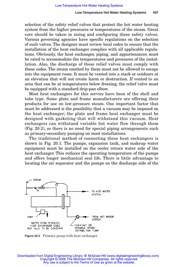
Low-Temperature Hot Water Heating Systems 497
Figure 20.2 Primary pump with heat exchanger.
selection of the safety relief valves that protect the hot water heatingsystem from the higher pressures or temperatures of the steam. Greatcare should be taken in sizing and configuring these safety valves.Various governing agencies have specific regulations on the selectionof such valves. The designer must review local codes to ensure that theinstallation of the heat exchanger complies with all applicable regula-tions. Obviously, the heat exchanger, piping, and appurtenances mustbe rated to accommodate the temperatures and pressures of the instal-lation. Also, the discharge of these relief valves must comply withthese codes. The steam emitted by them must not be allowed to escapeinto the equipment room. It must be vented into a stack or outdoors atan elevation that will not create harm or destruction. If vented to anarea that can be at temperatures below freezing, the relief valve mustbe equipped with a standard drip-pan elbow.
Most heat exchangers for this service have been of the shell andtube type. Some plate and frame manufacturers are offering theirproducts for use on low-pressure steam. One important factor thatmust be addressed is the possibility that a vacuum may be imposed onthe heat exchanger; the plate and frame heat exchanger must bedesigned with gasketing that will withstand this vacuum. Heatexchangers can withstand variable hot water flow through them(Fig. 20.2), so there is no need for special piping arrangements suchas primary-secondary pumping on most installations.
The traditional method of connecting these heat exchangers isshown in Fig. 20.1. The pumps, expansion tank, and makeup waterequipment must be installed on the cooler return water side of theheat exchanger. This reduces the operating temperature of the pumpsand offers longer mechanical seal life. There is little advantage tolocating the air separator and the pumps on the discharge side of the
Rishel_CH20.qxd 20/4/06 6:49 PM Page 497
Downloaded from Digital Engineering Library @ McGraw-Hill (www.digitalengineeringlibrary.com)Copyright © 2006 The McGraw-Hill Companies. All rights reserved.
Any use is subject to the Terms of Use as given at the website.
Low-Temperature Hot Water Heating Systems

498 Pumps for HVAC Hot Water Systems
heat exchanger; a review of Table 2.5 will reveal that only a smallamount of air is removed with additional heating of the water. Most ofthe air coming into the system is from the makeup water. The useof chemical treatment, as discussed in Chap. 9, is the proper method ofeliminating air and therefore oxygen from these systems.
The traditional arrangement of the heat exchanger and its piping asshown in Fig. 20.1 has had some operational difficulties on variable-volume hot water systems. The use of variable-speed hot water pumpsand the resulting low flow through the heat exchanger have createdoperational problems. These problems are as follows:
1. At very low heating loads, the steam temperature regulatorreduces the steam flow until a vacuum occurs in the heat exchang-er. This causes the heat exchanger to fill with air or condensatethrough the vacuum breaker. If air is injected into the heat exchanger, this increases the possibility of corrosion in the internalparts of the heat exchanger. Control of the temperature of waterrequired by the system is lost.
2. If the heat exchanger is filled with condensate, any increase inload in the water system will cause the steam valve to open widein an attempt to recover the water temperature. Full steam pres-sure may be exerted on the condensate in the heat exchanger todrive the condensate out of the heat exchanger. This can causehammering and pounding in the heat exchanger.
3. The steam trap on the heat exchanger is overloaded and may limitthe flow of condensate out of the heat exchanger.
An attempt has been made to solve these problems by using twosteam temperature regulators, one for one-third of the design loadand the other for two-thirds of the design load. This has solved theseproblems in some installations, but a hunting problem may existwhen the steam control transfers from the one-third control valve tothe two-thirds control valve.
An alternative to the standard method of piping and pumping theseheat exchangers is described in Fig. 20.3. A three-way mixing valve isused to control system temperature, and on most systems, a constantsteam pressure is maintained on the heat exchanger. Following aresolutions to the problems of the standard hookup:
1. Since a constant steam temperature is maintained on the heat exchanger, there is no vacuum produced in it, and it is not filledwith air or condensate. This provides a constant-temperaturesource for the hot water system.
Rishel_CH20.qxd 20/4/06 6:49 PM Page 498
Downloaded from Digital Engineering Library @ McGraw-Hill (www.digitalengineeringlibrary.com)Copyright © 2006 The McGraw-Hill Companies. All rights reserved.
Any use is subject to the Terms of Use as given at the website.
Low-Temperature Hot Water Heating Systems

Low-Temperature Hot Water Heating Systems 499
Figure 20.3 Heat exchanger installation with three-way valve control.
2. The steam valve can consist of one valve in most cases, not themore complex one-third, two-thirds valve arrangement.
3. The steam trap receives a steady flow of condensate that is basedon the load on the hot water system; its overloading is eliminated.
The steam pressure required in the heat exchanger is determinedby the condensate system that exists at the heat exchanger. If thecondensate drops to a condensate pump, a minimum steam pressureof 1 or 2 psig gauge pressure may be adequate. If the condensate issent to a condensate return pipe, the elevation of that pipe withrespect to the elevation of the heat exchanger will determine thesteam pressure. A rule of thumb that is used in the industry is toallow 1 lb of steam pressure per foot of elevation difference. Thisaccounts for the elevation plus pipe friction. A more precise method isto calculate the pipe friction and the elevation change to arrive at theexact steam pressure in the heat exchanger.
There is a requirement for the sizing of the three-way control valveon these systems, and that is minimum flow. Manual control valvesshould be located out in the system at its far ends to (1) maintainwater temperature in the supply mains, (2) provide minimum flowthrough the pumps, and (3) ensure some flow through the three-wayvalve to aid in the control of water temperature. Usually, this flow can
Rishel_CH20.qxd 20/4/06 6:49 PM Page 499
Downloaded from Digital Engineering Library @ McGraw-Hill (www.digitalengineeringlibrary.com)Copyright © 2006 The McGraw-Hill Companies. All rights reserved.
Any use is subject to the Terms of Use as given at the website.
Low-Temperature Hot Water Heating Systems
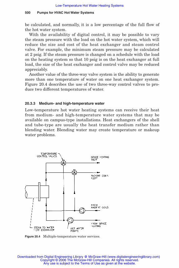
500 Pumps for HVAC Hot Water Systems
be calculated, and normally, it is a low percentage of the full flow ofthe hot water system.
With the availability of digital control, it may be possible to varythe steam pressure with the load on the hot water system, which willreduce the size and cost of the heat exchanger and steam controlvalve. For example, the minimum steam pressure may be calculatedat 2 psig. If the steam pressure is changed on a schedule with the loadon the heating system so that 10 psig is on the heat exchanger at fullload, the size of the heat exchanger and control valve may be reducedappreciably.
Another value of the three-way valve system is the ability to generatemore than one temperature of water on one heat exchanger system.Figure 20.4 describes the use of two three-way control valves to pro-duce two different temperatures of water.
20.3.3 Medium- and high-temperature water
Low-temperature hot water heating systems can receive their heatfrom medium- and high-temperature water systems that may beavailable on campus-type installations. Heat exchangers of the shelland tube-type are usually the heat transfer medium rather thanblending water. Blending water may create temperature or makeupwater problems.
Figure 20.4 Multiple-temperature water services.
Rishel_CH20.qxd 20/4/06 6:49 PM Page 500
Downloaded from Digital Engineering Library @ McGraw-Hill (www.digitalengineeringlibrary.com)Copyright © 2006 The McGraw-Hill Companies. All rights reserved.
Any use is subject to the Terms of Use as given at the website.
Low-Temperature Hot Water Heating Systems
Low-Temperature Hot Water Heating Systems 501
The heat exchangers for this service are much like those discussedearlier for low- and high-pressure steam. The problems with conden-sate and vacuums that were reviewed do not exist on medium- andhigh-temperature water sources. The heat exchangers must complywith any applicable codes for pressure vessels of the size and temper-atures involved.
20.3.4 District heating systems
District heating systems can be a heat source for low-temperaturehot water systems. Chapter 18 provides information on such low-temperature hot water systems.
20.3.5 Heat-recovery processes
Heat recovery from various sources can be applied to low-temperaturehot water systems. Utilization of the heat of rejection from chillers isreviewed in detail in Chap. 16. Heat recovery from exhaust air orother gas streams can be a source of heat for these water systems.Special hot water heating coils are provided for these applications;usually, they are installed upstream from the main hot water heatingcoil. The metallurgy of the heating coil must be designed for the con-ditions of the gas stream. Dirty process gases may require cleaningequipment ahead of the heating coil.
20.4 Uses of Hot Water in HVAC Systems
Low-temperature hot water is used for (1) space heating, (2) heatingof outside air, (3) reheat in cooling systems, and (4) process heating inindustry. All these uses of hot water employ a heating coil when thereceiving fluid is air. Some industrial heating processes may use aheat exchanger to heat other liquids.
The same problems with laminar flow and freezing that occur incooling coils also exist in heating coils. The discussion in Chap. 9 thatcovers most of these problems also should be applied to hot water coils.
The distribution of hot water to all the preceding uses is much thesame. Some industrial processes might require special cleaning orsensors to detect unacceptable material in the return water.
20.5 Distribution of Low-Temperature Hot Water
The distribution of low-temperature hot water is substantially thesame as that for chilled water, as developed in Chap. 15. Greater con-cern must be given to air elimination, thermal expansion, and corrosioncontrol.
Rishel_CH20.qxd 20/4/06 6:49 PM Page 501
Downloaded from Digital Engineering Library @ McGraw-Hill (www.digitalengineeringlibrary.com)Copyright © 2006 The McGraw-Hill Companies. All rights reserved.
Any use is subject to the Terms of Use as given at the website.
Low-Temperature Hot Water Heating Systems
502 Pumps for HVAC Hot Water Systems
20.5.1 Primary systems
There are more primary systems in hot water than in chilled waterowing to the ability of some boilers to accept variable flow throughthem. Most fire-tube boilers are subject to thermal shock without pri-mary pumps of some type.
Some boiler manufacturers provide a circulating pump with theboiler. This gives such boilers the ability to control minimum flow.Other boiler manufacturers require standard primary pumps withconstant flow through the boilers similar to that of chillers. Also, con-trol for limiting return water temperature may be recommended andfurnished by some boiler manufacturers. As discussed in Chap. 19, itis imperative that the boiler manufacturer’s recommendations oninstallation and operation be adhered to without exception.
20.5.2 Primary-secondary systems
As indicated earlier, primary-secondary pumping should be used forboilers that require constant flow. This includes some cast iron andsteel fire-tube boilers. There is very little difference to this methodfor piping low-temperature hot water boilers from that described inChap. 15 on chilled water distribution systems. The principal differencefor hot water is the ability to use much higher differential tempera-tures than is possible for chilled water. Differential temperatures ashigh as 100°F are designed into some hot water installations.
20.5.3 Primary-secondary-tertiary systems
There is even less reason to use primary-secondary-tertiary pumpingon hot water than on chilled water owing to the lower water flowsand pump horsepowers. There are very few hot water systems thatshould utilize this complicated pumping system. Some retrofit pro-jects may justify it, but even in these instances, variable-speed zonepumping or a modification of distributed pumping may offer moreenergy savings.
20.5.4 Distributed pumping
The advantages of distributed pumping as fully developed in Chap. 15on chilled water systems also apply to campus-type hot water sys-tems. The energy savings may not be as dramatic as those for chilledwater because the pumps are usually smaller. There are no specialdesign conditions for hot water over those already described forchilled water.
Rishel_CH20.qxd 20/4/06 6:49 PM Page 502
Downloaded from Digital Engineering Library @ McGraw-Hill (www.digitalengineeringlibrary.com)Copyright © 2006 The McGraw-Hill Companies. All rights reserved.
Any use is subject to the Terms of Use as given at the website.
Low-Temperature Hot Water Heating Systems

Low-Temperature Hot Water Heating Systems 503
20.5.5 Special distribution systems
There are some special hot water systems that utilize manometerfittings that divert water into coils from a single pipe loop; with thedevelopment of digital electronics and other contemporary controls,the use of these systems seldom can be justified except, possibly, onsmall residential heating systems.
20.6 Hot Water Design and DifferentialTemperatures
With the development of the condensing boiler, the classic water tem-perature difference of 20°F for low-temperature hot water systemscan be expanded to as much as 100°F. In the past, in an attempt tosecure higher differential temperatures, operating temperatures var-ied from 240°F at design load down to 140°F at minimum load. Thistemperature range reduced greatly the pumping energy, but it ele-vated the boiler’s stack temperature and resulted in a maximum com-bustion efficiency of around 80 percent. It should be pointed out thatthe reset of water temperature with percentage of load is usuallyaccomplished through the use of outdoor temperature as the parame-ter for changing water temperature. With digital electronics, anyrange that is desired can be inserted into the control algorithm. Indays of mechanical control, only two or three ranges were available.
It is now recognized that for most installations it is better to designwith lower water temperatures to secure higher combustion efficien-cies. If noncondensing boilers are utilized, a typical temperature rangewould be 200°F at design and 140°F at minimum load. At a 60°F dif-ferential temperature, efficiency in pumping has been achieved with abetter combustion efficiency for the boiler, smaller pipe, and lower heatlosses from the pipe surface.
With the advent of the condensing boiler, it is more important toevaluate carefully the design temperature difference selected for hotwater heating systems. Figure 20.5 describes the pronounced reductionin hot water flow when higher temperature differences are utilized.This figure also illustrates the reduction in pipe size with comparablefriction losses per 100 ft of piping. The actual pipe selection along withthe temperature difference is determined by the energy and installa-tion costs that apply to each installation.
The condensing boiler goes beyond this overall efficiency and offersa new level of efficiency of operation that was never attained withnoncondensing boilers. For example, low-temperature hot water sys-tems can be operated with a 60°F differential temperature with a maxi-mum temperature of 150°F at full load and 90°F at minimum load on
Rishel_CH20.qxd 20/4/06 6:49 PM Page 503
Downloaded from Digital Engineering Library @ McGraw-Hill (www.digitalengineeringlibrary.com)Copyright © 2006 The McGraw-Hill Companies. All rights reserved.
Any use is subject to the Terms of Use as given at the website.
Low-Temperature Hot Water Heating Systems
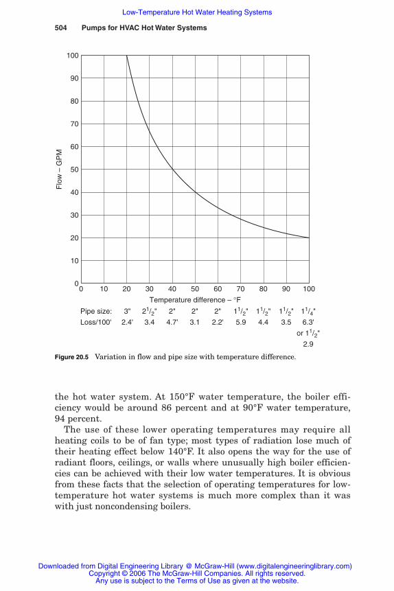
504 Pumps for HVAC Hot Water Systems
the hot water system. At 150°F water temperature, the boiler effi-ciency would be around 86 percent and at 90°F water temperature,94 percent.
The use of these lower operating temperatures may require allheating coils to be of fan type; most types of radiation lose much oftheir heating effect below 140°F. It also opens the way for the use ofradiant floors, ceilings, or walls where unusually high boiler efficien-cies can be achieved with their low water temperatures. It is obviousfrom these facts that the selection of operating temperatures for low-temperature hot water systems is much more complex than it waswith just noncondensing boilers.
100
90
80
70
60
50
40
30
20
10
00
Flo
w –
GP
M
10 20 30 40 50 60 70 80 90 100
Temperature difference – °FPipe size: 3" 21/2" 2" 2" 2" 11/2" 11/2" 11/2" 11/4"
Loss/100' 2.4' 3.4 4.7' 3.1 2.2' 5.9 4.4 3.5 6.3'
or 11/2"
2.9
Figure 20.5 Variation in flow and pipe size with temperature difference.
Rishel_CH20.qxd 20/4/06 6:49 PM Page 504
Downloaded from Digital Engineering Library @ McGraw-Hill (www.digitalengineeringlibrary.com)Copyright © 2006 The McGraw-Hill Companies. All rights reserved.
Any use is subject to the Terms of Use as given at the website.
Low-Temperature Hot Water Heating Systems
20.6.1 Reset of boiler water temperatureversus zone reset
As demonstrated in Chap. 8 on the use of water in HVAC systems, inmost cases the reset of water temperature at the boiler offers greaterenergy savings than does resetting water temperature in variouszones of a hot water system. The preceding dramatic increases inboiler efficiency with condensing boilers illustrate what can be donewith resetting the boiler temperature. Also, the coil circulating pumpsfor hot water systems are small with low pump efficiency.
On heating coils, a substantial savings in pumping energy can beachieved by using central pumps with their higher pump efficiencies;small circulators for individual coils have much lower efficiencies. Ifthere is a pronounced difference in zones for heating in a hot watersystem, such as a north zone and a south zone on a building, an alter-native could be the use of two sets of central pumps, as described inFig. 15.5 for chilled water.
20.7 Bibliography
James B. Rishel, The Water Management Manual, SYSTECON, Inc., West Chester,Ohio, 1992.
Low-Temperature Hot Water Heating Systems 505
Rishel_CH20.qxd 20/4/06 6:49 PM Page 505
Downloaded from Digital Engineering Library @ McGraw-Hill (www.digitalengineeringlibrary.com)Copyright © 2006 The McGraw-Hill Companies. All rights reserved.
Any use is subject to the Terms of Use as given at the website.
Low-Temperature Hot Water Heating Systems

Rishel_CH20.qxd 20/4/06 6:49 PM Page 506
Downloaded from Digital Engineering Library @ McGraw-Hill (www.digitalengineeringlibrary.com)Copyright © 2006 The McGraw-Hill Companies. All rights reserved.
Any use is subject to the Terms of Use as given at the website.
Low-Temperature Hot Water Heating Systems
Chapter
507
21Pumps for Medium- and
High-TemperatureWater Systems
21.1 Introduction
This chapter has been retained even though the cost of energy iseliminating many of the previous applications for medium- and high-temperature water systems. Section 21.2 does provide the procedurefor calculating the exact water flow for large water systems usingwater at temperatures below 250°F. Large hot water, campus-type sys-tems can utilize 240°F water with a 100°F differential temperature toachieve the reduced flow that was available with high-temperaturewater.
Medium- and high-temperature water systems are economicalwhere large quantities of hot water must be transported over anappreciable distance. The ability to operate at differential tempera-tures in excess of 100°F has reduced greatly the volume of water thatmust be pumped in these systems.
The efficiency of boilers for these systems cannot be as great as thatof some of the contemporary low-temperature hot water boilers; this isdue to the higher stack temperatures of the boilers for these higher-temperature waters. Most high-temperature water boilers operate withstack temperatures 100 to 150°F higher than the leaving steam orwater temperatures. The actual stack temperature for a specific appli-cation should be certified by the boiler manufacturer at the design loadand temperature. Boilers for these systems must be designed to theAmerican Society of Mechanical Engineers’ (ASME) power boiler code.
Rishel_CH21.qxd 21/4/06 6:36 PM Page 507
Downloaded from Digital Engineering Library @ McGraw-Hill (www.digitalengineeringlibrary.com)Copyright © 2006 The McGraw-Hill Companies. All rights reserved.
Any use is subject to the Terms of Use as given at the website.
Source: HVAC Pump Handbook

508 Pumps for HVAC Hot Water Systems
The decision to use these systems must weigh the pumping energysaved against the energy lost due to the lower efficiency of the boilers.Likewise, the savings in the cost of reduced pipe sizes achieved withthe high differential temperatures must be balanced against the highercost of the high-pressure boilers, valves, and other appurtenances.
Medium-temperature water systems are those which have watertemperatures in excess of 250°F, the maximum for low-temperaturewater systems. Many of the medium-temperature water systems havea maximum operating pressure of 125 psig. This enables the use ofvalves, piping accessories, and pump casings designed for 125 psigand the actual operating temperature. This includes some of the class125 cast iron fittings and the class 150 steel fittings. Depending onthe cushion pressure required at high points in these water systems,the maximum temperature for them is around 320 to 340°F. Thetables in Chap. 2 for temperatures and allowable pressures for castiron fittings should be consulted as well as valve manufacturers’ cata-logs for temperature-pressure ratings for valves. Copper and brassmaterials generally are not considered suitable above 300°F, so thismay be a point of differentiation between medium- and high-temperature water for some designers.
High-temperature water systems are all of those hot water systemsthat exceed the limits defined earlier for medium-temperature watersystems. The practical upper limit for high-temperature water sys-tems appears to be in the range of 430 to 450°F. The vapor pressurefor 450°F water is 422.6 psia, so 500-psig pump casings may provide apractical limit for high-temperature water systems. For heatingprocesses requiring higher temperatures, there are a number of spe-cial liquids manufactured by chemical companies for heat-transferservice with special heat exchangers. Seldom are they used in HVACheating systems.
21.2 Calculation of Water Flow
The water flow for medium- and high-temperature water is calculatedwith recognition of the variation in specific heat and specific gravityof water at these higher temperatures. The water flow is oftenexpressed in pounds per hour:
lb/h ��sy
�
sTte
(m°F
B)t�
uc/
p
h� (21.1)
where cp � specific heat of water at maximum operating watertemperature
�T � design differential temperature, °F
Rishel_CH21.qxd 21/4/06 6:36 PM Page 508
Downloaded from Digital Engineering Library @ McGraw-Hill (www.digitalengineeringlibrary.com)Copyright © 2006 The McGraw-Hill Companies. All rights reserved.
Any use is subject to the Terms of Use as given at the website.
Pumps for Medium-and High-Temperature Water Systems

Pumps for Medium- and High-Temperature Water Systems 509
TABLE 21.1 Specific Heat of Pure Water at Higher Temperatures
Temper- Specific Temper- Specific Temper- Specific ature, °F heat, Btu/°F ature, °F heat, Btu/°F ature, °F heat, Btu/°F
200 1.005 280 1.022 370 1.062210 1.007 290 1.025 380 1.070212 1.008 300 1.032 390 1.077220 1.010 310 1.035 400 1.085230 1.012 320 1.040 410 1.090240 1.013 330 1.042 420 1.096250 1.015 340 1.047 430 1.107260 1.018 350 1.052 440 1.115270 1.020 360 1.057 450 1.121
SOURCE: Keenan and Keyes, Thermodynamic Properties of Steam, John Wiley & Sons, NewYork, 1936, pp. 30–32. Used by permission.
The basic formula for calculating required pump flow in gallons perminute is
Pump gal/min �
� (21.2)
where � � specific weight of water at maximum operating tempera-ture, lb/ft3 (see Tables 2.3 and 2.4)
Equation 21.2 can be used for any water system of any water tem-perature where very precise water flows in gallons per minute arerequired, but on most low-temperature water applications, the specificheat of water is assumed to be 1.00. Table 21.1 provides the specificheat for pure water at temperatures from 200 to 450°F.
A sample calculation would be as follows: Assume:
System Btu/h � 50,000,000 Btu/h
Operating temperature � 400°F
Differential temperature � 150°F
From Tables:
� � 53.65 lb/ft3 at 400°F
cp � 1.085
Pump gal/min � � 716 gal/min0.125 � 50,000 000���53.65 � 150 � 1.085
0.125 � system Btu/h���
� � �T (°F) � cp
system Btu/h���(�/7.48) � 60 � �T (°F) � cp
Rishel_CH21.qxd 21/4/06 6:36 PM Page 509
Downloaded from Digital Engineering Library @ McGraw-Hill (www.digitalengineeringlibrary.com)Copyright © 2006 The McGraw-Hill Companies. All rights reserved.
Any use is subject to the Terms of Use as given at the website.
Pumps for Medium-and High-Temperature Water Systems

510 Pumps for HVAC Hot Water Systems
21.3 Calculation of Pump Head
Rather than using pipe friction tables that are acceptable for low-temperature water, the calculation of pump head for these higher-temperature water systems requires actual calculations using theDarcy-Weisbach formula, Reynolds number, and a Moody’s diagramfor developing the Colebrook friction factor f. Thus, the reduction inthe viscosity of water at these higher temperatures can be accountedfor in the piping design.
For example, assume that the preceding flow is to commence in a 6-in steel pipe with an internal diameter of 6.065 in (0.505 ft) and avelocity of 7.95 ft/s. The kinematic viscosity of water at 400°F is 0.16 ×10�5 ft2/s. Thus
Reynolds number � �V
�
� D� � �
70..9156
�
�
01.05
�
055
� (3.6)
� 2.51 � 106
From the Moody chart (Fig. 3.2), with a Reynolds number of2.51106 and 6-in pipe, the friction factor f is 0.015.
Using the Darcy-Weisbach equation (Eq. 3.3),
Hf � f � �DL
� � �2Vg
2� � 0.015 � �
01.50005
� � �76.49.54
2�
� 2.92 ft/100 ft
Adding 15 percent for variation in pipe diameter, construction, etc.,
Hf � 3.36 ft/100 ft
Although these calculations may be laborious when done by hand,the computer programs now available simplify the use of Reynoldsnumbers to determine friction losses in pipe and fittings more accu-rately. The entire medium- or high-temperature water system can becomputed, thus, to determine the required pump head.
21.4 Medium- and High-TemperatureWater Generators
The generation of heat for these water systems can be by steam boilerswith an internal steam cushion for expansion or hot water boilers withexternal expansion tanks. The technology is such that it is beyond thescope of this book to review all the methods of hot water generation.
Rishel_CH21.qxd 21/4/06 6:36 PM Page 510
Downloaded from Digital Engineering Library @ McGraw-Hill (www.digitalengineeringlibrary.com)Copyright © 2006 The McGraw-Hill Companies. All rights reserved.
Any use is subject to the Terms of Use as given at the website.
Pumps for Medium-and High-Temperature Water Systems

Pumps for Medium- and High-Temperature Water Systems 511
Excellent texts are available to the designer on the construction andoperation of these boilers and generators. Some medium-temperaturewater systems receive their heat from high-temperature water sys-tems through water-to-water heat exchangers and others from ordi-nary high-pressure steam boilers and steam-to-water heat exchangers.
21.5 Distribution of Medium- and High-Temperature Water
Most of the principles of low-temperature water distribution apply tothese systems (see Chap. 20). Added caution must be maintained toensure that cavitation does not occur in any part of these water sys-tems. The operating temperatures are so much higher that adequatepressure must be maintained in all parts of a system. For example, forthe preceding system with 400°F water, from Table 2.4, the evapora-tion pressure is 247.31 psia. At this temperature, the system pressureshould not drop below 250 to 275 psig wherever the water is at 400°F.
The pressure-gradient diagram is an excellent tool for the design ofthese water systems. It enables the designer to verify that cavitationwill not appear in any part of the water system. The pressure headsused in these diagrams must account for the lower specific gravity ofthe high-temperature water. This can be done by using Eq. 4.1, wherethe pressure is determined by 144 �, the specific weight of water inpounds per cubic feet.
Distributed pumping should be considered for these systemsbecause of the distances normally encountered between buildings orindividual loads.
21.6 Pumps for Medium- and High-Temperature Water Systems
Pump selection for high-temperature water systems is much like that forother HVAC water systems, namely, to achieve maximum efficiency withrespect for the economic factors of the installation. There is one addi-tional factor that is not encountered in the other water systems thatmust be recognized on these higher-temperature water systems. This iscooling of the mechanical seals that are normally used on these pumps.
Mechanical seal cooling must be designed to eliminate as muchwaste of cooling water as possible. Many pump manufacturers supply-ing high-temperature water pumps are experienced in providing thecorrect type of mechanical seal and cooling medium. The use of a heatexchanger mounted on the pump base and furnished by the pumpmanufacturer with interconnecting piping and control provides theoptimal seal cooling system for most applications. If domestic water is
Rishel_CH21.qxd 21/4/06 6:36 PM Page 511
Downloaded from Digital Engineering Library @ McGraw-Hill (www.digitalengineeringlibrary.com)Copyright © 2006 The McGraw-Hill Companies. All rights reserved.
Any use is subject to the Terms of Use as given at the website.
Pumps for Medium-and High-Temperature Water Systems

512 Pumps for HVAC Hot Water Systems
used for this cooling, the heat exchanger must be on the load side ofan approved backflow preventer.
Because of the need for mechanical seal cooling and the relative lowpump capacities, single-suction pumps with one mechanical seal arenormally selected for these services. The metallurgy of the pumpsmust meet the higher pressures and temperature of these water sys-tems. Cast iron volutes are seldom used, whereas ductile iron may beacceptable for medium-temperature systems. Most high-temperaturewater systems require cast or welded steel volutes with steel or duc-tile iron brackets. Although bronze impellers may be acceptable below300°F temperature, the pump manufacturer should specify animpeller material such as iron or stainless steel no. 316. The mini-mum clearances between the impeller and the case wear rings mayneed to be increased for stainless steel because of possible galling.This increases bypassing and may decrease pump efficiency.
Most of the pumps for these higher water temperatures should beequipped with expansion joints or means on the pump connectionflanges to ensure that piping stress is not imposed on the flanges.These expansion means must have the correct pressure and tempera-ture ratings and must be installed in a position that will ensure thatno pipe stress is imposed on the pump flanges.
Variable-speed pumping offers energy savings for these systemsthat have a sizable variation in the heating loads in them. Again, thepressure-gradient diagram may be a valuable tool for evaluating sys-tem pressures with variable-speed pumps.
Some manufacturers of hot water generators for these systemshave very specific requirements for circulating the water throughtheir equipment. These circulating pumps may be mounted on thegenerator itself, or they can be field mounted. Any field-mountedboiler circulating pump must comply strictly with the boiler or gener-ator manufacturer’s requirements.
21.7 Bibliography
Following are some sources for additional information on high tempera-ture hot water design and types of generators for these systems. Thesetexts were written before the current technology was available on vari-able frequency drives and their application to HVAC water systems.Nils R. Grimm and Robert C. Rosaler, Handbook of HVAC Design, McGraw-Hill, Inc.,
New York, N.Y., 1990.Erwin G. Hansen, Hydronic System Design and Operation, McGraw-Hill, Inc., New
York, N.Y., 1985.Joseph H. Keenan and Frederick G. Keyes, Thermodynamic Properties of Steam, John
Wiley & Sons, Inc., New York, N.Y., 1936.
Rishel_CH21.qxd 21/4/06 6:36 PM Page 512
Downloaded from Digital Engineering Library @ McGraw-Hill (www.digitalengineeringlibrary.com)Copyright © 2006 The McGraw-Hill Companies. All rights reserved.
Any use is subject to the Terms of Use as given at the website.
Pumps for Medium-and High-Temperature Water Systems

Chapter
513
22Condensate, Boiler Feed,
and Deaerator Systems
22.1 Introduction
Steam is the name given to the vapor phase of water and is producedby boiling water in steam boilers. It was the principal method oftransmitting heat in HVAC systems before the development of hotwater systems and hot water pumps. Although steam and processheating systems are not as prevalent as in the past, they are stillused extensively in HVAC operations.
Heat is given up to steam-heated systems by the condensing of thesteam back to the liquid state of water. The condensate from thesesystems should be returned to the boilers. Some low-pressure steamsystems return the condensate directly to the boilers withoutpumps. Other low-pressure systems and all high-pressure steamsystems utilize condensate, vacuum, or boiler feed pumps for returnof the condensate.
22.2 Review of Steam Systems
Steam systems are either low- or high-pressure systems in accor-dance with the American Society of Mechanical Engineers’ (ASME)boiler codes. Low-pressure steam systems are 15 psig or less; all sys-tems higher than 15 psig are high-pressure steam systems. MostHVAC steam heating systems are low-pressure systems; high-pressuresteam is used in hospitals and buildings where other high-pressuresteam heating services are required. High-pressure steam is used indistrict heating systems or other campus-type installations where
Rishel_CH22.qxd 20/4/06 6:50 PM Page 513
Downloaded from Digital Engineering Library @ McGraw-Hill (www.digitalengineeringlibrary.com)Copyright © 2006 The McGraw-Hill Companies. All rights reserved.
Any use is subject to the Terms of Use as given at the website.
Source: HVAC Pump Handbook

514 Pumps for HVAC Hot Water Systems
long distances are required for the transmission of steam. Today,medium- and high-temperature hot water systems have replacedhigh-pressure steam on many large systems with long piping runs toremote buildings.
22.2.1 Rating of heating systems
Steam heating systems are rated in (1) MBH (thousands of BTU perhour) like hot water systems, (2) in pounds of steam per hour fromfeedwater at 212°F to steam at 212°F, or (3) in square feet of radia-tion. A square foot of steam radiation is equal to 240 Btu/h. Since apound of steam at 212°F has a heat of evaporation of 970.3 Btu, it hasan approximate equivalent of 4 ft2 of steam radiation. When steamwas the principal heating medium, cast iron and other radiators wererated in square feet of radiation; today, most steam heating coils arerated in MBH like other heating coils.
22.3 Low-Pressure Steam Systems
Low-pressure steam systems can range in pressure from vacuum sys-tems up to 15 psig. Before the advent of hot water heating systems,many buildings were heated with vacuum-type steam systems. Oldertall buildings still are heated successfully and very efficiently by vac-uum steam systems. These vacuum systems allow a broad range ofoperation, and some of them vary the steam temperature with theload on the system.
A review of the steam tables will reveal lower steam temperaturesfor pressures less than atmospheric or under vacuum conditions.Vacuum systems were developed to reduce the operating temperatureof the steam. For example, steam at a vacuum of 15 inHg has a tem-perature of near 178°F. This enabled the radiators and heating coilsto operate at temperatures lower than 212°F and provided better con-trol of the heating system.
With the development of heating coils other than direct radiation,low-pressure steam systems were used in place of the vacuum sys-tems. The pressure on these systems is normally in the range of 5 to12 psig. These systems can provide low-pressure steam to other ser-vices such as domestic water heaters and converters. Converter is thename given to heat exchangers for converting steam to hot water forspace heating systems that use coils, radiation, and convectors.
Steam traps are used to trap the steam in a heating coil but let thecondensate through to return to the boilers or condensate pumps.Most steam traps used on low-pressure steam systems are thermo-static on small steam-heated equipment or float and thermostatic on
Rishel_CH22.qxd 20/4/06 6:50 PM Page 514
Downloaded from Digital Engineering Library @ McGraw-Hill (www.digitalengineeringlibrary.com)Copyright © 2006 The McGraw-Hill Companies. All rights reserved.
Any use is subject to the Terms of Use as given at the website.
Condensate, Boiler Feed, and Deaerator Systems
Condensate, Boiler Feeds, and Deaerator Systems 515
larger equipment. These traps pass air as well as condensate throughthe use of thermostatic elements that expand and close when higher-temperature steam reaches the elements.
22.3.1 Configuration of low-pressure steam systems
The shape of the building in which the steam system is installeddetermines the equipment used in that system. The rate of return ofthe condensate determines the type of steam system that should beused. If the condensate can be returned rapidly to the boilers, low-pressure steam can be used without condensate or boiler feed pumps.One disadvantage of such direct return is the feeding of makeupwater directly into the boiler. This may result in the injection of air,and therefore, oxygen directly into the boiler.
Tall buildings with boilers installed in the basement are candidates forsuch a system. The condensate passes through the steam traps anddrops back into the boilers. As the steam system becomes broader inshape, the ability of the condensate to return rapidly to the boilers isreduced. This necessitates the use of condensate pumps to receive thecondensate from the steam traps and return it to the boilers. If the steamsystem is extensive and the delay of the condensate return to the boilersis appreciable, a boiler feed system may be needed to provide storagespace for the condensate as it is returned by the condensate systems.This prevents the undesirable condition of freshwater makeup enteringthe boiler because of the delay in the condensate returning to the boiler.
22.4 High-Pressure Steam Systems
High-pressure steam systems are used for (1) transporting steam overdistances, (2) providing higher temperatures for heating equipment,and (3) high-pressure steam turbines. High-pressure steam is used inbuildings such as hospitals that can be extensive in layout andrequire high temperatures for such services as sterilization.
Most high-pressure steam systems in the HVAC field operate withsteam pressures from 40 to 110 psig. Many cast iron pipe fittings andvalves are rated for 125- or 250-psig steam, so the steam operatingpressure is kept below 125 psig. Steam at 110 psig or near 125 psiapressure has an evaporation temperature of 344°F, which providesadequate thermal difference for many heating services.
If steam is required for turbines that are driving chillers or othermechanical equipment, the steam may be generated at higher pres-sures or temperatures. In rare cases in HVAC systems, the steam maybe superheated, which means that the steam is heated to a higher
Rishel_CH22.qxd 20/4/06 6:50 PM Page 515
Downloaded from Digital Engineering Library @ McGraw-Hill (www.digitalengineeringlibrary.com)Copyright © 2006 The McGraw-Hill Companies. All rights reserved.
Any use is subject to the Terms of Use as given at the website.
Condensate, Boiler Feed, and Deaerator Systems

516 Pumps for HVAC Hot Water Systems
temperature than saturation temperature. If the steam is generatedat 186 psig or 200 psia and passed through a superheater in theboiler so that the leaving steam temperature is 432°F instead of382°F saturation temperature, it has 50°F of superheat. Instead ofrating the steam in pounds of steam per hour from and at 212°F, itmay be necessary to rate the capacity of the boiler in pounds of steamat a feedwater temperature to a steam pressure with so many degreesof superheat. It is important when specifying the capacity of a high-pressure boiler that the pounds of steam per hour be defined by feed-water temperature and operating steam pressure and temperature.
22.5 Steam Boilers
Steam heating boilers are rated in boiler horsepower or pounds of steamper hour. A boiler horsepower is equivalent to 33,475 Btu/h or 34.5 lb/hfrom feedwater at 212°F to steam at 212°F and 0 psig steam pressure.
Small high-pressure boilers are rated in boiler horsepower or poundsof steam per hour from and at 212°F. Most large high-pressure steamboilers are rated in just pounds of steam per hour at 212°F. High-pressure boilers that provide steam to steam turbines are rated inpounds of steam from a certain feedwater temperature to the actualoperating pressure and temperature. As mentioned earlier, the boilertemperature may include superheat if large steam turbines areinvolved.
22.6 Condensate Systems for Steam Boilers
There are four distinct types of condensate systems for steam sys-tems: (1) vacuum pumps, (2) condensate return systems, (3) boilerfeed systems, and (4) deaerators. Each has its place in returning con-densate to boilers.
22.6.1 Vacuum pumps
Vacuum pumps are used on vacuum steam systems to perform twoservices: (1) return the condensate to the boilers, a boiler feed system,or a deaerator, and (2) maintain the desired vacuum on the steam sys-tem. Vacuum systems have been rated in thousands of square feet ofradiation at a specified vacuum. Two different pumps were used onmany vacuum systems: (1) to return the condensate and (2) to main-tain the vacuum on the steam system. Few new vacuum systems arebeing used today as a result of the development of alternative meth-ods of heating buildings. Vacuum pumps are still manufactured forexisting and new systems.
Rishel_CH22.qxd 20/4/06 6:50 PM Page 516
Downloaded from Digital Engineering Library @ McGraw-Hill (www.digitalengineeringlibrary.com)Copyright © 2006 The McGraw-Hill Companies. All rights reserved.
Any use is subject to the Terms of Use as given at the website.
Condensate, Boiler Feed, and Deaerator Systems

Condensate, Boiler Feeds, and Deaerator Systems 517
22.6.2 Condensate return systems
Condensate return systems are designed to return condensate from thesteam traps back to the boilers, a deaerator, or a boiler feed system.Condensate return systems (Fig. 22.1a), consist of a receiver, a floatswitch, and the condensate pump. The condensate fills the receiver, andat a preset level, the float switch starts the condensate pump. Thepump removes the condensate from the receiver, and at a second, lowerpreset level, the float switch stops the pump. There is no other controlprocedure for these pumps to return the condensate to boilers. They arecalled condensate return systems because this is their principal duty.They do not include any storage volume for the condensate.
The condensate return system can be rated in square feet of radia-tion, pounds of condensate per hour, or MBH. Usually, this rating isspecified at a discharge pressure such as 10 psig.
The pressure rating of the condensate system is determined by thetype of condensate piping that is installed in the building. There aregravity returns where the condensate piping is pitched toward theboiler room and pressure returns where the condensate is pumpedback to the boiler room by the condensate pumps.
If the condensate piping is of the gravity type, the condensatereturn system is only required to lift the condensate to the nearestreturn. Under this condition, the discharge pressure need only thefriction loss of the discharge piping and the static lift of the conden-sate to the gravity return pipe. The lift is the difference between theelevation of the condensate return system and the condensate pipe.The equation for the pressure is
Discharge pressure � (22.1)
where hf � pressure loss in feet for the discharge piping and valves�� specific weight of water at the condensate pump discharge
temperature
If the condensate piping is of the pressure type, the discharge pres-sure must include the pressure loss of the piping between the conden-sate system and the point of delivery in the boiler room, the differencein elevation between the condensate return system and the point ofdelivery, and the pressure in either the boilers or the deaerator.
Equation 22.1 becomes
Discharge pressure � � Ip psig (22.2)hf � static lift��
144/�
hf � static lift��
144/� psig
Rishel_CH22.qxd 20/4/06 6:50 PM Page 517
Downloaded from Digital Engineering Library @ McGraw-Hill (www.digitalengineeringlibrary.com)Copyright © 2006 The McGraw-Hill Companies. All rights reserved.
Any use is subject to the Terms of Use as given at the website.
Condensate, Boiler Feed, and Deaerator Systems
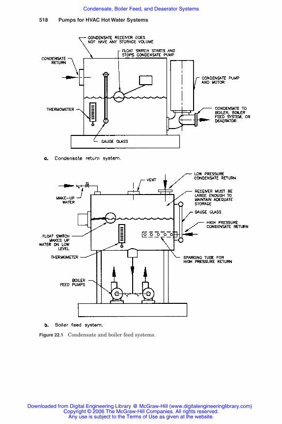
518 Pumps for HVAC Hot Water Systems
Figure 22.1 Condensate and boiler feed systems.
Rishel_CH22.qxd 20/4/06 6:50 PM Page 518
Downloaded from Digital Engineering Library @ McGraw-Hill (www.digitalengineeringlibrary.com)Copyright © 2006 The McGraw-Hill Companies. All rights reserved.
Any use is subject to the Terms of Use as given at the website.
Condensate, Boiler Feed, and Deaerator Systems
Condensate, Boiler Feeds, and Deaerator Systems 519
where hf � pressure loss in feet for the piping and valves between thecondensate return system and the point of delivery in theboiler room
Ip� pressure in the boilers or the deaerator
If the condensate is delivered to a boiler feed system, the dischargepressure for the condensate return system is similar to Eq. 22.1, wherehf is the friction loss of the piping between the condensate systemand the boiler feed system; likewise, the static lift is the differencebetween the elevation of the condensate system and the level of thecondensate return connection on the boiler feed system.
22.6.3 Boiler feed systems
A boiler feed system (Fig. 22.1b) receives low- and/or high-pressurecondensate from steam traps and holds that condensate until it iscalled for by the boilers. It has a much larger receiver or tank thana condensate return system, since it must provide storage of thecondensate between periods of high and low steam production. The con-temporary steam boilers with small water volumes are in greater needfor condensate storage outside the boiler and therefore in the boiler feedsystem or deaerator.
The boiler feed system also maintains a minimum level in itsreceiver by means of a float valve or any other water level controlsystem that adds makeup water to the receiver. This has a decidedadvantage over injection of makeup water directly into the boilers.Most of the air and oxygen is released in the boiler feed systemreceiver, not in the boilers. Boiler feed systems can be equipped withsparging tubes for injection of steam into the receiver water so that itcan be maintained at 210°F. As demonstrated in Table 2.5, almost all theair is released from water at 0 psig pressure and 210°F temperature.
Unlike condensate return and vacuum pumping systems, thepumps on the boiler feed system are started and stopped or otherwisecontrolled by the boiler water level controller. These pumps are there-fore called boiler feed pumps. When the water in the boiler drops to apreset level, a switch is closed in that controller, and the boiler feedpump is started; when the desired level in the boiler is reached, thisswitch opens, and the boiler feed pump stops. Few boilers that are fedby boiler feed systems are equipped with feedwater regulators; thepumps normally start and stop. Variable-speed pumps are seldomused on boiler feed systems because the system head curve for suchpumps is so shallow or flat that very little energy is saved by varying
Rishel_CH22.qxd 20/4/06 6:50 PM Page 519
Downloaded from Digital Engineering Library @ McGraw-Hill (www.digitalengineeringlibrary.com)Copyright © 2006 The McGraw-Hill Companies. All rights reserved.
Any use is subject to the Terms of Use as given at the website.
Condensate, Boiler Feed, and Deaerator Systems

520 Pumps for HVAC Hot Water Systems
Figure 22.2 Typical deaerator.
the speed of the pump. On larger boilers, the boiler feed pump runscontinuously with a feedwater regulator controlling the rate of flow offeedwater into the boiler.
Boiler feed systems are superior to condensate return systems inoperation because the amount of air and oxygen fed into the boiler isgreatly reduced. Boiler feed systems are used on low- and high-pressuresteam systems that are relatively small and do not have strictrequirements for oxygen content in the boiler feedwater. Large high-pressure boilers are almost always equipped with deaerators.
22.6.4 Deaerators
Deaerators (Fig. 22.2) are boiler feed systems with guaranteed airand oxygen content in the feedwater. This is accomplished by a num-ber of different mechanical devices and arrangements. Deaeratorsaccomplish the following duties:
1. Receive both low- and high-pressure condensate from the steamsystems.
2. Maintain a minimum water level in the deaerator by adding make-up water.
3. Deaerate both condensate and makeup water to some guaranteedlevel of oxygen content such as 0.005 cc/liter.
4. Provide adequate boiler feedwater storage to pump the boilers
Rishel_CH22.qxd 20/4/06 6:50 PM Page 520
Downloaded from Digital Engineering Library @ McGraw-Hill (www.digitalengineeringlibrary.com)Copyright © 2006 The McGraw-Hill Companies. All rights reserved.
Any use is subject to the Terms of Use as given at the website.
Condensate, Boiler Feed, and Deaerator Systems

Condensate, Boiler Feeds, and Deaerator Systems 521
under all steaming rates without excessive makeup water. Theamount of makeup water should be limited to evaporation or leak-age losses, and it should not include water needed to maintainlevel in the deaerator under heavy load swings on the steam sys-tem. Figure 22.2 describes a typical deaerator without a separatestorage section. Some deaerators have a second storage section forlarger volumes of low-pressure condensate; they are used on largelow-pressure steam heating systems.
5. Maintain all the preceding duties without excessive steam loss upthe vent pipe or pipes of the deaerator. Deaerators are usually soldunder a guarantee of so much steam lost up the vent pipe perthousand pounds of water processed.
Deaerators are manufactured in a number of configurations, of trayor spray type and with or without the separate condensate sections.Manufacturers of deaerators with both a condensate section and adeaerated water section claim better performance for their units.Low-pressure condensate and makeup water are fed into the conden-sate section, while high-pressure condensate is returned to the deaer-ated water section. Other manufacturers claim better performancewithout the storage section.
The deaerator section can use a number of different mechanicaldevices for deaeration of the water; most deaerators are either sprayor tray type. In spray-type deaerators, the condensate and makeupwater from the condensate section are heated and sprayed over thewater in the deaerator section, thus releasing any gases in the water.The gases, such as oxygen, pass up the vent pipe. In tray-type deaera-tors (Fig. 22.2), low-pressure condensate drops down over trays andsteam passes through the trays, scrubbing the gases from the conden-sate. This configuration appears to be the preference where very lowlevels of oxygen are required.
Deaerators also can be classified as atmospheric or pressure type.Atmospheric deaerators operate with no steam pressure in the deaer-ation section, while pressure deaerators maintain a minimum steampressure such as 5 psig in this section. Usually, the pressure typeoffers a higher level of deaeration than the atmospheric type. Thequestion often raised is what is the necessary level of deaeration onmany HVAC steam systems? Also, on many HVAC boilers the finalremoval of oxygen can be accomplished chemically with the feeding ofsodium sulfite or similar chemicals into the feedwater. This increasesthe amount of surface blowdown required at the boiler. It is the deci-sion of the steam system designer as to which is the best method forcontrolling corrosion in boilers and steam systems.
Rishel_CH22.qxd 20/4/06 6:50 PM Page 521
Downloaded from Digital Engineering Library @ McGraw-Hill (www.digitalengineeringlibrary.com)Copyright © 2006 The McGraw-Hill Companies. All rights reserved.
Any use is subject to the Terms of Use as given at the website.
Condensate, Boiler Feed, and Deaerator Systems
522 Pumps for HVAC Hot Water Systems
22.7 Design and Selection of Boiler Feed Pumps
Boiler feed pumping can be troublesome if some application problemsare not addressed. Relatively high temperatures (200 to 230°F) at lowNPSH available conditions and high discharge pressures requirecareful selection of boiler feed pumps.
22.7.1 Design of boiler feed pumps
Boiler feed pumps for HVAC boilers are almost always centrifugal ofsingle-stage construction for low-pressure boilers and multistage forhigh-pressure boilers. Some small high-pressure process boilers useperipheral turbine-type pumps that have a relatively low efficiency.
Feed pumps for HVAC boilers usually are equipped with mechani-cal seals, not packing. The mechanical seal eliminates most of theleakage and evaporation at the stuffing boxes. The mechanical sealsmust be designed for the maximum temperature encountered withthe hot condensate.
The boiler feed pump must have a low NPSH, since the condensatewill be at or near evaporation temperature. Most boiler feed pumpshave a required NPSH of less than 10 ft. The required NPSH must beevaluated at the maximum pumping rate that can be encountered inthe boiler feeding cycle. The boiler feed pump may require a dischargepressure regulator that maintains a continuous discharge pressure onthe boiler feed pump regardless of the boiler pressure. This reduces theability of the pump to run at high capacities and high required NPSH.
Small low-pressure boiler feed pumps are normally single-suction,single-stage pumps flexibly coupled to standard electric motors. Smallhigh-pressure boiler feed pumps can be peripheral turbine pumps, butfor pump efficiency and continuous service, the multistage turbinepump is the preferred type. This pump should be designed for 250°Fservice and provided with flexibly coupled electric motors.
Large high-pressure boiler feed pumps can be multistage turbine orsingle-suction pumps. The multistage single-suction pump, oftencalled a multistage horizontal split case pump, has been the standardpump of the medium-sized boiler. The multistage turbine pump hasbeen developed to the point that it is often the most efficient, econom-ical pump for this service.
22.7.2 Selection of boiler feed pumps
Boiler feed pumps must be selected for capacity, head, and NPSHavailable for each application. Each of these factors is critical in theselection of boiler feed pumps.
Rishel_CH22.qxd 20/4/06 6:50 PM Page 522
Downloaded from Digital Engineering Library @ McGraw-Hill (www.digitalengineeringlibrary.com)Copyright © 2006 The McGraw-Hill Companies. All rights reserved.
Any use is subject to the Terms of Use as given at the website.
Condensate, Boiler Feed, and Deaerator Systems

Condensate, Boiler Feeds, and Deaerator Systems 523
Boiler feed pump capacity. The capacity of boiler feed pumps mustaccommodate not only the feedwater requirements of the boilers butalso the quality of the steam produced by the boilers as well as theblowdown requirements of the boiler treatment. Quality is the namegiven to wetness of the steam produced by the boiler. Pure steam is allgas and has no liquid content. Large boilers have water separatorsand scrubbers that enable the steam leaving the boiler to have verylittle water and are said to produce steam with close to 100 percentquality. Most of the steam boilers on HVAC steam systems have nosteam separators and smaller steam releasing areas, so they do notproduce high-quality steam. Because of this, a factor of 5 to 10 percentmust be added to the boiler feedwater requirements to secure ade-quate pumping capacity. The following equation provides the methodof calculating boiler feed pump capacity:
Boiler feed pump gal/min �
� (22.3)
where � � specific weight of water at the feedwater temperature0.90 � contingency for steam quality, leakage, and the like
For example, if a 10,000 lb/h boiler is being fed with 230°F feedwater, from Table 2.4, � � 59.38 lb/ft3, and
Pump gal/min � �7.2
120
�
,05090.38
� � 23.3 gal/min
Some designers will add a greater contingency than the 90 percentincluded in the preceding formula, particularly if peripheral turbine-type pumps are used as boiler feed pumps. The close tolerances in theseboiler feed pumps can subject them to wear. Often, the boiler feed pumpcapacity is selected at double the boiler capacity for these pumps.
If the boiler capacity is provided in boiler horsepower, Eq. 22.3becomes
Boiler feed pump gal/min �
� (22.4)
If the boiler feed pump operates continuously with the boiler feedrate controlled by a feedwater regulator, a circulating flow in the
4.78 � boiler capacity (hp)���
�
boiler capacity (hp) � 34.5���
60 � (�/7.48) � 0.90
boiler lb steam/h���
7.22 � �
boiler lb steam/h���60 � (�/7.48) � 0.90
Rishel_CH22.qxd 20/4/06 6:50 PM Page 523
Downloaded from Digital Engineering Library @ McGraw-Hill (www.digitalengineeringlibrary.com)Copyright © 2006 The McGraw-Hill Companies. All rights reserved.
Any use is subject to the Terms of Use as given at the website.
Condensate, Boiler Feed, and Deaerator Systems
524 Pumps for HVAC Hot Water Systems
amount to keep the boiler feed pump from overheating must be addedto the pump capacity. This can be computed by the boiler feed pumpmanufacturer and is often in the range of 5 to 20 gal/min.
Calculation of boiler feed pump head. Boiler feed pump head requiresmore care than other HVAC pumps due to the boiler pressure thatmust be included in the equation for the boiler feed head hb:
hb � Pf � Pd � boiler pressure (psig) � �14
�
4� (22.5)
where Pf � suction piping friction loss, ftPd � discharge piping friction loss, ft
The suction piping friction loss Pf must include (1) the exit loss fromthe deaerator or boiler feed system tank, (2) pipe and fitting losses,and, (3) strainer losses if they exist. Suction piping friction must becalculated carefully, since it is also part of the NPSH calculation.
The discharge piping friction loss Pd must include (1) piping and fit-ting losses and (2) losses through feedwater regulators, if they exist.
The difference in elevation between the water in the boiler feed sys-tem or deaerator tank and the boiler is not figured in the equation forboiler feed pump head for most HVAC boilers. If for some reason theboilers are installed at a level different from that for the boiler feedsystem or deaerator, the elevation difference should be included in theboiler feed pump head equation.
NPSHA calculations for boiler feed pumps. NPSHA calculation is veryimportant for boiler feed pumps because the feedwater temperature isclose to the evaporation temperature. This means that the atmosphericpressure Pa and the vapor pressure Pvp in Eq. 6.8 cancel out; thisequation reduces to the following:
NPSHA � Pz � Pf (22.6)
where Pz � static height of the water level in the boiler feed system ordeaerator above the suction level of the boiler feed pump
Pf � friction loss in the suction piping
For example, if the maximum NPSHR for the pump at the peakflow rate is 8 ft and the friction loss in the suction piping is 2 ft, theworking level of the deaerator must be 10 ft above the suction connec-tion of the boiler feed pump. NPSHA ≥ NPSHR, so NPSHA must begreater than 8 ft.
NPSHA � 10 � 2 � 8 ft
Rishel_CH22.qxd 20/4/06 6:50 PM Page 524
Downloaded from Digital Engineering Library @ McGraw-Hill (www.digitalengineeringlibrary.com)Copyright © 2006 The McGraw-Hill Companies. All rights reserved.
Any use is subject to the Terms of Use as given at the website.
Condensate, Boiler Feed, and Deaerator Systems

Condensate, Boiler Feeds, and Deaerator Systems 525
Some designers will prefer to have a safety factor in the NPSH avail-able and will add several feet to Eq. 22.6.
22.8 Number of Boiler Feed Pumps
Boiler feed pumps are much like pumps for chillers or hot water boil-ers. If the boilers are utilizing on-off control of the boiler feed pumps,individual boiler feed pumps should be used with a standby pump, asdescribed in Fig. 14.5b for chiller pumps.
If the boilers are equipped with feedwater regulators, centralpumps can be used with one pump providing water to several boilers.The number of pumps installed depends on the characteristics of theactual installation, such as total number of boilers, size of the boilers,amount of standby capacity required, and the like.
The selection of the number of boiler feed pumps is a process thatrequires careful consideration. Since most pumps on HVAC boilersare constant-speed pumps, it must be ensured that no pump operatesat a minimum flow at low efficiency and high radial thrust when aboiler is operating at minimum load. The pumps should go from con-tinuous operation into an on-off method of control when this mini-mum flow occurs.
22.9 Condensate Transfer Pumps for Deaerators
A special application of pumps exists on deaerators, which have a con-densate section and a deaeration section. The condensate must betransferred from the condensate section to the deaerator section.These pumps comply with the equations illustrated earlier for boilerfeed pumps except that the pressure in the deaerator section must besubstituted for the boiler pressure.
22.10 Summary
Although condensate and boiler feed applications are small in capacityand motor horsepower on most installations, they are critical servicesfor most buildings, and care should be given to their design and appli-cation. Calculation of NPSH available is a simple yet very necessaryprocedure for these pump installations.
Rishel_CH22.qxd 20/4/06 6:50 PM Page 525
Downloaded from Digital Engineering Library @ McGraw-Hill (www.digitalengineeringlibrary.com)Copyright © 2006 The McGraw-Hill Companies. All rights reserved.
Any use is subject to the Terms of Use as given at the website.
Condensate, Boiler Feed, and Deaerator Systems

Rishel_CH22.qxd 20/4/06 6:50 PM Page 526
Downloaded from Digital Engineering Library @ McGraw-Hill (www.digitalengineeringlibrary.com)Copyright © 2006 The McGraw-Hill Companies. All rights reserved.
Any use is subject to the Terms of Use as given at the website.
Condensate, Boiler Feed, and Deaerator Systems

Installing andOperating HVAC Pumps
Part
7
Rishel_CH23.qxd 20/4/06 6:51 PM Page 527
Downloaded from Digital Engineering Library @ McGraw-Hill (www.digitalengineeringlibrary.com)Copyright © 2006 The McGraw-Hill Companies. All rights reserved.
Any use is subject to the Terms of Use as given at the website.
Source: HVAC Pump Handbook

Rishel_CH23.qxd 20/4/06 6:51 PM Page 528
Downloaded from Digital Engineering Library @ McGraw-Hill (www.digitalengineeringlibrary.com)Copyright © 2006 The McGraw-Hill Companies. All rights reserved.
Any use is subject to the Terms of Use as given at the website.
Installing and Operating HVAC Pumps

Chapter
529
23Instrumentation and Control for HVAC Pumping Systems
23.1 Introduction
The ability to operate HVAC pumping systems efficiently depends onthe quality of the instrumentation used to operate the pumps andtheir water systems. Digital electronics gives us tools by which we cansecure efficient operation, but without accurate instrumentation, wehave no idea what we are achieving in actual operation.
Instrumentation includes transmitters, indicators, and controllers.Transmitters measure values such as pump speed, temperature, differ-ential temperature, pressure, differential pressure, level, and electricalcharacteristics such as voltage, amperage, kilowatts, and power factor.Indicators display similar operating values such as temperature, pres-sure, level, and electrical values. Controllers compute pumping systemvalues such as wire-to-water efficiency, start and stop pumps, andcontrol their speed if they are equipped with variable-speed drives. Allinstrumentation on HVAC installations where appreciable amounts ofenergy are consumed should be traced to the standards of the NationalInstitute of Standards and Technology (NIST).
Following are some definitions and terms that may be helpful in theevaluation of instrumentation:
Accuracy. Degree of conformity of an indicated value to a recog-nized acceptable standard value.
Accuracy is usually expressed in percentage of span or of the mea-sured rate. The preferable method is the latter, the measured rate.Accuracy usually will be a combined accuracy including linearity,hysteresis, and repeatability.
Rishel_CH23.qxd 20/4/06 6:51 PM Page 529
Downloaded from Digital Engineering Library @ McGraw-Hill (www.digitalengineeringlibrary.com)Copyright © 2006 The McGraw-Hill Companies. All rights reserved.
Any use is subject to the Terms of Use as given at the website.
Source: HVAC Pump Handbook
530 Installing and Operating HVAC Pumps
There is no universally accepted procedure for calculating theoverall accuracy of a system with a number of instruments, eachwith its individual accuracy. Only actual system calibration canreliably establish the accuracy of that system of instruments.Adding all the individual inaccuracies together will provide a veryconservative and probably an excessive system inaccuracy. Anotherprocedure is to use the instrument with the greatest inaccuracy asthe system accuracy. This may be closer, but it is still poorer thanactual evaluation of the system.
Analog signal. A signal representing a variable such as pressure,temperature level, and so forth. Usually, they are direct current ofmagnitude 4 to 20 mA where 4 mA is the minimum point of thespan and 20 mA is the maximum point of the span. If a control loopfor pressure reads from 10 to 150 psig, the analog signal would read4 mA at 10 psig and 20 mA at 150 psig.
Digital signal. A discrete value at which an action is performed. Adigital signal is a binary signal with two distinct states, on and off.The on or off state is usually determined by a condition such as onfor failure and off for operational, this being typical for an alarmsignal. An operational digital signal would be a pressure switchthat opens above 75 psig and closes below 73 psig. The state of adigital signal is usually determined by an instrument signal, suchas a voltage level, where 0 V is “off” and 5 V is “on.”
Dead band. The range through which an input can be varied with-out initiating an observable response.
Deviation. Any departure from a desired value or expected valueor pattern. For example, if the actual pressure is 101 psig and theset point is 100 psig, the deviation is 1 psig.
Overshoot. A control term indicating the amount that the processexceeds the set point during a changing load on a system.
Process. The actual value in a control loop. For example, if theactual pressure being measured is 101 psig, the process is 101 psig.
Response time. The rate of interrogating a transmitter. This isvery critical in the control of variable-speed pumps. If the pumpsvary their speed continuously, there probably is a problem withthe response time. On continuous service, changes in HVAC pumpspeed should never be audible or visual.
Set point. An input variable that sets the desired value of the con-trolled variable. For example, in the preceding control loop, if apressure of 100 psig is desired, the set point is 100 psig.
Rishel_CH23.qxd 20/4/06 6:51 PM Page 530
Downloaded from Digital Engineering Library @ McGraw-Hill (www.digitalengineeringlibrary.com)Copyright © 2006 The McGraw-Hill Companies. All rights reserved.
Any use is subject to the Terms of Use as given at the website.
Instrumentation and Control for HVAC Pumping Systems
Instrumentation and Control for HVAC Pumping Systems 531
P-I control (ANSI/IEEE Standard 100-1977). Proportional plusintegral control systems. Control action in which the output is pro-portional to a linear combination of the input and the time integralof the input.
P-I-D control (ANSI/IEEE Standard 100-1977). Proportionalplus integral plus derivative control systems. Control action inwhich the output is proportional to a linear combination of theinput, the time integral of the input, and the time rate of change ofthe input.
Repeatability. The variation in outputs for an instrument or proce-dure for the same input.
Span. The range of an instrument; for example, if a pressuregauge reads from 10 to 150 psig, its span is 140 psig.
These are a few instrument terms that may be encountered in thisbook. Many excellent books exist on instrumentation and control.
This chapter reviews instrumentation for the operation of pumpingsystems; instrumentation for the testing of pumps and pumping sys-tems requires a greater accuracy and is discussed in Chap. 24 on thetesting of pumping systems.
23.2 Transmitters
Transmitters sense the actual values of an operating pumping system.Therefore, the accuracy of transmitters is of great importance in theoperation of such pumping systems. Skimping on quality in theseinstruments is shortsighted economically. The recommended quality forHVAC water systems results from the tolerances and features listedhereafter for each type of transmitter.
23.2.1 Flowmeters
Flowmeters are some of the most misunderstood and misappliedinstruments in this field. The result is questionable accuracy and reli-ability. Flowmeters can be classed into (1) head-loss instruments, (2)propeller instruments, and (3) electronic measurement instruments.
Head-loss meters. Head-loss flowmeters measure head loss to deter-mine the flow. This class includes venturi, pitot tube, insertion tube,special valves, and any impact-measuring type of meter that uses fric-tion or velocity head loss as a measurement of flow. This class offlowmeters is acceptable for measuring water systems that have asteady flow with very little variation. The reason for this is the fact
Rishel_CH23.qxd 20/4/06 6:51 PM Page 531
Downloaded from Digital Engineering Library @ McGraw-Hill (www.digitalengineeringlibrary.com)Copyright © 2006 The McGraw-Hill Companies. All rights reserved.
Any use is subject to the Terms of Use as given at the website.
Instrumentation and Control for HVAC Pumping Systems
532 Installing and Operating HVAC Pumps
that the velocity head of a water stream varies with the square of theflow (see Chap. 6). They are not acceptable for the measurement offlow in variable-volume water systems that have a flow range equiva-lent to a velocity of 1 to 10 ft/s. Such systems are said to have a turn-down ratio of 10 to 1.
For example, an 8-in pipe carrying 1200 gal/min has a velocity headof 0.920 ft. At 400 gal /min, this velocity head has been reduced to0.102 ft. This demonstrates that the accuracy of these meters dropsoff rapidly with broad changes in flow rate. Most head-loss meters arenot used with turndown ratios much greater than 3 to 1. The develop-ment of electronic transmitters for these meters may extend theirrange somewhat.
Propeller meters. Propeller meters use an insertion device that con-tains some type of rotating element that measures the flow. The speedof rotation of the propeller varies with the flow rate. These instru-ments have served the water industries well for years with greaterflow ranges than the head-loss instruments. The actual flow range andaccuracy for a specific meter should be certified by the manufacturer.These meters must not be of the magnetic type, since the use of mag-nets will cause welding spatter and other bits of metal in the water tocling to them, thus causing cleaning problems. Propeller meters can befull throated (across the entire pipe area) or insertion type.
Because of the moving parts of propeller meters, they should be cal-ibrated often to ensure their accuracy. Impact of water-borne particlesmay damage them; also, the axles that the propellers turn on canwear due to loss of lubrication or dirt.
Insertion-type propeller meters are quite popular now, due to theirease of installation. Their configuration is similar to that shown inFig. 23.3 for insertion magnetic meters but they have small propellersthat rotate with flow. Cost-wise, they are substantially less that theinsertion magnetic meter. The manufacturer should state the usefullife of the propellers due to the need for accurate flow in most of theuseful energy measurements that are needed today.
Electronic meters. Great strides have been made in flow measure-ment through the development of electronic instruments. Thesemeters emit an electronic signal across the water stream and usesome method of evaluating the quality or quantity of that signal whenit is received. These meters can be full throated, insertion type, orstrap-on, where they are attached to the exterior surface of the pipe.
Full-throated magnetic meters provide the greatest flow range, 1to 30 ft/s, at probably the highest accuracies. Some manufacturersquote accuracies as high as �0.5 percent from 1 to 30 ft/s velocity.
Rishel_CH23.qxd 20/4/06 6:51 PM Page 532
Downloaded from Digital Engineering Library @ McGraw-Hill (www.digitalengineeringlibrary.com)Copyright © 2006 The McGraw-Hill Companies. All rights reserved.
Any use is subject to the Terms of Use as given at the website.
Instrumentation and Control for HVAC Pumping Systems
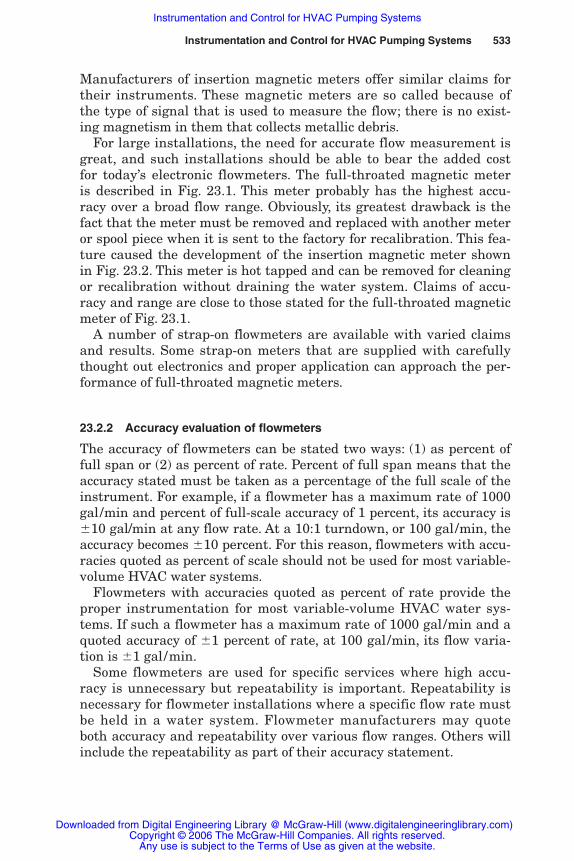
Instrumentation and Control for HVAC Pumping Systems 533
Manufacturers of insertion magnetic meters offer similar claims fortheir instruments. These magnetic meters are so called because ofthe type of signal that is used to measure the flow; there is no exist-ing magnetism in them that collects metallic debris.
For large installations, the need for accurate flow measurement isgreat, and such installations should be able to bear the added costfor today’s electronic flowmeters. The full-throated magnetic meteris described in Fig. 23.1. This meter probably has the highest accu-racy over a broad flow range. Obviously, its greatest drawback is thefact that the meter must be removed and replaced with another meteror spool piece when it is sent to the factory for recalibration. This fea-ture caused the development of the insertion magnetic meter shownin Fig. 23.2. This meter is hot tapped and can be removed for cleaningor recalibration without draining the water system. Claims of accu-racy and range are close to those stated for the full-throated magneticmeter of Fig. 23.1.
A number of strap-on flowmeters are available with varied claimsand results. Some strap-on meters that are supplied with carefullythought out electronics and proper application can approach the per-formance of full-throated magnetic meters.
23.2.2 Accuracy evaluation of flowmeters
The accuracy of flowmeters can be stated two ways: (1) as percent offull span or (2) as percent of rate. Percent of full span means that theaccuracy stated must be taken as a percentage of the full scale of theinstrument. For example, if a flowmeter has a maximum rate of 1000gal/min and percent of full-scale accuracy of 1 percent, its accuracy is�10 gal/min at any flow rate. At a 10:1 turndown, or 100 gal/min, theaccuracy becomes �10 percent. For this reason, flowmeters with accu-racies quoted as percent of scale should not be used for most variable-volume HVAC water systems.
Flowmeters with accuracies quoted as percent of rate provide theproper instrumentation for most variable-volume HVAC water sys-tems. If such a flowmeter has a maximum rate of 1000 gal/min and aquoted accuracy of �1 percent of rate, at 100 gal/min, its flow varia-tion is �1 gal/min.
Some flowmeters are used for specific services where high accu-racy is unnecessary but repeatability is important. Repeatability isnecessary for flowmeter installations where a specific flow rate mustbe held in a water system. Flowmeter manufacturers may quoteboth accuracy and repeatability over various flow ranges. Others willinclude the repeatability as part of their accuracy statement.
Rishel_CH23.qxd 20/4/06 6:51 PM Page 533
Downloaded from Digital Engineering Library @ McGraw-Hill (www.digitalengineeringlibrary.com)Copyright © 2006 The McGraw-Hill Companies. All rights reserved.
Any use is subject to the Terms of Use as given at the website.
Instrumentation and Control for HVAC Pumping Systems
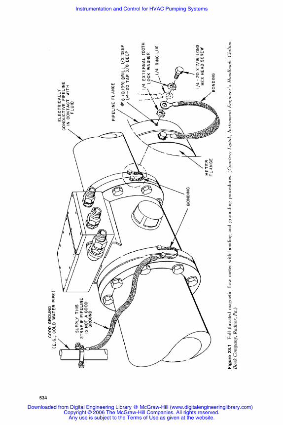
534
Fig
ure
23.
1F
ull-
thro
ated
mag
neti
c fl
ow m
eter
wit
h bo
ndin
g an
d gr
ound
ing
proc
edur
es.
(Cou
rtes
y L
ipta
k, I
nstr
umen
t E
ngin
eer’
s H
andb
ook,
Chi
lton
Boo
k C
ompa
ny, R
adno
r, P
a.)
Rishel_CH23.qxd 20/4/06 6:51 PM Page 534
Downloaded from Digital Engineering Library @ McGraw-Hill (www.digitalengineeringlibrary.com)Copyright © 2006 The McGraw-Hill Companies. All rights reserved.
Any use is subject to the Terms of Use as given at the website.
Instrumentation and Control for HVAC Pumping Systems
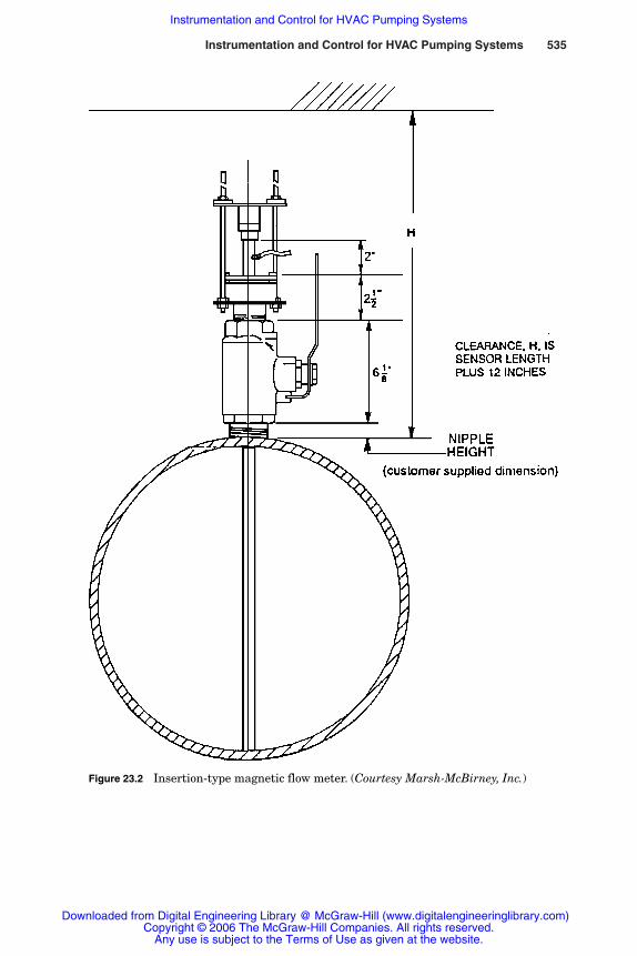
Instrumentation and Control for HVAC Pumping Systems 535
Figure 23.2 Insertion-type magnetic flow meter. (Courtesy Marsh-McBirney, Inc.)
Rishel_CH23.qxd 20/4/06 6:51 PM Page 535
Downloaded from Digital Engineering Library @ McGraw-Hill (www.digitalengineeringlibrary.com)Copyright © 2006 The McGraw-Hill Companies. All rights reserved.
Any use is subject to the Terms of Use as given at the website.
Instrumentation and Control for HVAC Pumping Systems
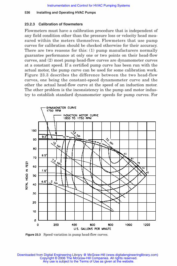
536 Installing and Operating HVAC Pumps
23.2.3 Calibration of flowmeters
Flowmeters must have a calibration procedure that is independent ofany field condition other than the pressure loss or velocity head mea-sured within the meters themselves. Flowmeters that use pumpcurves for calibration should be checked otherwise for their accuracy.There are two reasons for this: (1) pump manufacturers normallyguarantee performance at only one or two points on their head-flowcurves, and (2) most pump head-flow curves are dynamometer curvesat a constant speed. If a certified pump curve has been run with theactual motor, the pump curve can be used for some calibration work.Figure 23.3 describes the difference between the two head-flowcurves, one being the constant-speed dynamometer curve and theother the actual head-flow curve at the speed of an induction motor.The other problem is the inconsistency in the pump and motor indus-try to establish standard dynamometer speeds for pump curves. For
Figure 23.3 Speed variation in pump head-flow curves.
Rishel_CH23.qxd 20/4/06 6:51 PM Page 536
Downloaded from Digital Engineering Library @ McGraw-Hill (www.digitalengineeringlibrary.com)Copyright © 2006 The McGraw-Hill Companies. All rights reserved.
Any use is subject to the Terms of Use as given at the website.
Instrumentation and Control for HVAC Pumping Systems
Instrumentation and Control for HVAC Pumping Systems 537
example, dynamometer speeds for pump catalog curves for four-polemotors vary from 1750 to 1790 rev/min. A catalog curve for a partic-ular pump may be 1750 rev/min, and it may be equipped with amotor that has a rated speed of 1770 rev/min at full load. The actualperformance of a pump will vary greatly from its published cataloghead-flow curve. It is obvious that pump curves should not be usedto calibrate flowmeters.
23.2.4 Installation of flowmeters
Flowmeters always should be installed in strict compliance with theinstructions of the manufacturer. Most such companies require 10pipe diameters in length of clear pipe ahead of the flow measure-ment point and five pipe diameters downstream. Often, it is difficultto get 15 diameters of length of straight pipe without valves, elbows,or other pipe accessories. If shorter lengths must be considered,some flowmeter manufacturers will advise the effect on the accuracyof the meter that is caused by the shorter distances. Compromisingon the length of straight pipe around a flow sensor can have disas-trous effects on transmitter accuracy and should not be done withoutthe flow transmitter manufacturer’s knowledge.
If there are two elbows upstream of the flowmeter that change thedirection of flow twice in a short span of pipe, a torsional effect will beimparted to the water stream that may require straightening vanesor other devices to prevent a deterioration of flowmeter accuracy. Theflowmeter manufacturer must be made aware of such specific instal-lation details.
Magnetic-type flowmeters are not affected by dirt in the water, sincethey are used on sewage. Propeller-type flowmeters may be damagedby water-borne dirt, so care should be taken to ensure that suchmeters are protected from physical damage. Insertion-type flowmeters,which can be of several different types, should be equipped with hottap assemblies that enable the flowmeter to be removed for inspection,cleaning, or repair without draining the pipe. Most manufacturers ofinsertion-type flowmeters have hot tap assemblies that include a gatevalve and other piping accessories that enable removal of the trans-mitter from a pipe under water pressure.
23.2.5 Selection of type of flowmeter
It is obvious from the preceding discussion that there is a great differ-ence in the cost of flowmeters. Before a flowmeter is selected, the deci-sion must be made as to its primary use. Following are several usesfor flowmeters:
Rishel_CH23.qxd 20/4/06 6:51 PM Page 537
Downloaded from Digital Engineering Library @ McGraw-Hill (www.digitalengineeringlibrary.com)Copyright © 2006 The McGraw-Hill Companies. All rights reserved.
Any use is subject to the Terms of Use as given at the website.
Instrumentation and Control for HVAC Pumping Systems
538 Installing and Operating HVAC Pumps
1. Proof of flow in a pipe.
2. Approximate flow rate for rough calculations.
3. Precise flow rate for accurate calculations.
Some flowmeters are used strictly as flow switches to verify flows ina pipe. They may be selected instead of a flow switch due to theirruggedness and lack of any moving parts. Also, the flow may be variedas to where the switching function is to take place.
Other flowmeters are used for approximate calculations; high accu-racy is not needed. Contrary to these applications, the development ofonline calculations of energy consumptions requires high accuracy andbroad flow ranges. Typical values now being computed using preciseflow rates are (1) pump performance, (2) pump wire-to-water efficiency,(3) system flow rates, (4) system British thermal units and tonnages,(5) kilowatt per ton calculations, and (6) coefficient of performance orenergy efficiency ratio.
Flowmeters for precise calculations must have their control proce-dures checked to ensure that they can provide the desired results.This can become critical when pump speed or valve position is pacedto the output of a flowmeter. Such use of flowmeter output should beavoided wherever possible.
Along with the preceding uses, the size of the pipe comes into thedecision as to the type of flowmeter. For example, a small pipe such as 2-in diameter with a requirement that a flow of 50 gal/min be maintainedin the pipe would be best suited for a head-loss or propeller-typeflowmeter. A flowmeter for a 10-in pipe could be served by an insertionimpeller meter if a flow range of 300 to 2000 gal/min is required withreasonable accuracy. If precise flow is required in this pipe for energyevaluations such as kilowatts per ton or wire-to-water efficiency, afull-throated magnetic meter may be the best selection. If a 36-in pipewith great variations in flow exists, an insertion-type magnetic metermay be cost-effective. The exact duties of a flowmeter should be estab-lished to ensure proper selection of the type of meter.
Flowmeters should be selected also with consideration for rugged-ness, ease of service, frequency of cleaning, location of the installation,and general reputation of the manufacturer in providing an instru-ment that will function properly under the intended use.
23.2.6 Pressure and differential pressure transmitters
Pressure and differential pressure transmitters measure and transmitsignals that provide the information on these values at specific points
Rishel_CH23.qxd 20/4/06 6:51 PM Page 538
Downloaded from Digital Engineering Library @ McGraw-Hill (www.digitalengineeringlibrary.com)Copyright © 2006 The McGraw-Hill Companies. All rights reserved.
Any use is subject to the Terms of Use as given at the website.
Instrumentation and Control for HVAC Pumping Systems

Instrumentation and Control for HVAC Pumping Systems 539
in an HVAC water system. In many cases, they are the most vitalinstrument in the operation of a pumping system or in reporting thequality of an entire water system’s operation. They provide the infor-mation needed to calculate an individual pump’s performance or thatfor a complete pumping system.
Pressure and differential pressure transmitters must be rugged forinstallation on most HVAC systems. This is due to the possibility ofwater hammer when systems are filled initially or when air collects ina system and is suddenly removed. Most manufacturers are providingcasing design pressures as high as 1000 psig. Differential pressuretransmitters should not require equalizing valves between the twopressure taps on the instrument. The diaphragm in the instrumentmust be rugged enough to withstand any differential pressure towhich the instrument is subjected. The equalizing valve can be forgot-ten by the service personnel and the diaphragm destroyed when oneof the two taps is closed inadvertently.
Accuracies in the range of �0.25 percent of calibrated span arequoted by manufacturers of this instrumentation. This accuracyincludes the combined effects of linearity, hysteresis, and repeatability.
These transmitters should be located where they can be removedeasily; a manual shutoff valve should be installed on all pressure-sensing lines for removal without draining the water system.
23.2.7 Temperature transmitters
Temperature transmitters are rated by accuracy, as are flow and pres-sure transmitters; usually, this accuracy is in the range �0.25 percentof span. Temperature transmitters have an additional requirement,which is stability with respect to changes in ambient temperature andvoltage changes in the power supply for the transmitter. Stability for atemperature transmitter should be around �0.01 percent of span perdegree Celsius change in ambient temperature and �0.001 percent ofspan per volt change in line voltage.
Temperature transmitters should be installed where accessible andprovided with stainless steel thermowells for ease of removal.
23.2.8 Level transmitters
Level transmitters are not used as often in HVAC water systems asother types of transmitters. Their installation is so specific that theaccuracy, repeatability, and ruggedness cannot be defined but mustmeet the requirements of the installation. The supplier shoulddemonstrate that the accuracy and structural capability of the instru-ment do meet that required for the actual application.
Rishel_CH23.qxd 20/4/06 6:51 PM Page 539
Downloaded from Digital Engineering Library @ McGraw-Hill (www.digitalengineeringlibrary.com)Copyright © 2006 The McGraw-Hill Companies. All rights reserved.
Any use is subject to the Terms of Use as given at the website.
Instrumentation and Control for HVAC Pumping Systems

540 Installing and Operating HVAC Pumps
23.2.9 Watt transmitters
Watt transmitters are becoming more popular in the HVAC waterindustries due to the need to monitor power consumption of HVACequipment including pumps. Watt transmitters consist of the trans-mitter itself and current transformers mounted on at least two ofthe three wires of a three-phase power supply.
Extreme care is required with the connections between the trans-formers and the transmitter. High voltage can exist between thesewires if they are disconnected from the transmitter. The manufacturer’sinstructions should be followed carefully in installing and servicingthese units. Only qualified electricians or instrument techniciansshould handle these transmitters.
A new type of watt transmitter is available with the currenttransformers as part of the instrument itself. This model reducesthe danger of high voltage from the current transformer wires.These transmitters are available in sizes from 4 to 1000 A.
The accuracy of watt transmitters should be in the range of �0.25percent of span. This should be the total accuracy for the currenttransformers and the instrument.
Watt transmitters should be installed in power cubicles that areserviceable only by trained electricians. Extreme danger can resultfrom touching the unconnected wires of the current transformersbecause of the very high voltages that are generated by these trans-formers.
23.3 Indicators
Indicators at one time were quite simple, most of them being of theanalog type found on pressure gauges. Today indicators can rangefrom such simple analog types to colored flat screens that includeswitching and control functions.
Analog indicators include all types of gauges that use the dial faceof a gauge or a vertical bar that is calibrated to the span of thetransmitter analog or process. Digital indicators are the alphanu-meric type that display the process in numbers and letters. Thereare a number of different types of such indicators, such as (1) theseven-segment neon number, (2) liquid crystal, (3) plasma, and (4)vacuum fluorescent. These indicators must be selected for the appli-cation conditions. Some of them must be read directly in front; thislimits their use where the display must be read at angles fromdirectly in front of the instrument. Sunlight and interior lighting canadversely affect the readability of some of these digital indicators.
Rishel_CH23.qxd 20/4/06 6:51 PM Page 540
Downloaded from Digital Engineering Library @ McGraw-Hill (www.digitalengineeringlibrary.com)Copyright © 2006 The McGraw-Hill Companies. All rights reserved.
Any use is subject to the Terms of Use as given at the website.
Instrumentation and Control for HVAC Pumping Systems
23.4 Controllers
Controllers can range from simple switches to complex programmablelogic controllers with and without indication or operator interfaces.This subject is so broad that only a synopsis of the controllers includedin the HVAC water industries can be included in this chapter.
23.4.1 Simple controllers
Simple electric controllers include manual switches that can start orstop HVAC pumps, or they can be switches that are set to open orclose an electric circuit at a discrete process value. Such switches areoperated by pressure, differential pressure, temperature, differentialtemperature, level, flow, speed, volts, and amperes. Most of themhave an internal adjustment to control the set point at which theswitch either opens or closes an electric circuit.
Elementary mechanical controllers consist of pressure regulators,pressure-relief valves, balance valves, and self-operated temperaturecontrollers. Pressure-relief valves protect water systems from exces-sive pressures. Care should be taken in the use of pressure regulatorsand balance valves because of the possibilities of energy waste.
Other basic controllers are of the analog type such as pneumatically-operated controllers where the output is directly proportional to controlpressure or follows a known curve with respect to control pressure.
23.4.2 Digital controllers
Most HVAC systems are operated by some form of digital controller.There are a number of different digital controllers ranging from simplesingle-function controllers to complete universal controllers handlingall functions of the interrogation and control of a HVAC water system.
Digital controllers can use either PI or PID control for the operationof HVAC water systems. The development of the control loop mustrecognize the rate of reaction of the water system and the needed rateof response. Too often, HVAC control systems for pumps do not pro-vide the necessary rate of response, and the result is hunting of thepump speed and unnecessary starting and stopping of pumps.
The evolving influence of software-based HVAC control systems hashad a pronounced impact on improving total plant energy performance(that is, the energy to heat/cool the water and distribute it around thefacility as measured in kilowatts per ton for a chiller plant or Britishthermal units per thousands of BTU per hour for a boiler plant.)Techniques such as adaptive control provide a means to continuouslyand automatically make incremental changes in equipment sequences
Instrumentation and Control for HVAC Pumping Systems 541
Rishel_CH23.qxd 20/4/06 6:51 PM Page 541
Downloaded from Digital Engineering Library @ McGraw-Hill (www.digitalengineeringlibrary.com)Copyright © 2006 The McGraw-Hill Companies. All rights reserved.
Any use is subject to the Terms of Use as given at the website.
Instrumentation and Control for HVAC Pumping Systems

and operating levels that substantially reduce operator involvement.Such techniques actually adjust set points and control sequences inreal time to adjust for changes in load and system conditions such asdifferential temperature.
In addition, the use of standard communication protocols and webtechnology have greatly aided equipment and control manufacturersin producing well-integrated systems with improved energy perfor-mance. Care should be taken though; some protocols still do nothave well-defined interoperability standards as of this writing. Thelack of this aspect of a standard may not affect installations whereall components are provided by the same supplier. However, systemswhich employ unlike components from different suppliers, still pre-sent a significant degree of risk and potential expense for achievingfull and seamless integration. This must be clarified before usingsuch protocols.
23.4.3 Quality of controllers
The quality and reliability of a controller for HVAC pump operationsshould be established by testing facilities such as UnderwritersLaboratories or Electrical Testing Laboratories. The manufacturer ofsuch controllers should be able to specify the levels of quality used inthe development of a particular instrument. For example, the UnitedStates military standards MIL-STD-810D provides an excellent pro-cedure for testing instrumentation and controllers for environmentalstability, including temperature, humidity, and vibration.
23.5 Control Wiring
Control wiring should be designed and installed as recommended bythe Instrument Society of America. Control wiring should be of thesizes recommended by this society; wire sizes between transmittersand pump controller are included in Table 10.7.
Of particular importance is keeping instrument and control wiringaway from power wiring. Electromagnetic interference (EMI) andradio frequency interference (RFI) should be kept within the levelsrecommended by the instrument and controller manufacturers thatare involved on a specific project.
23.6 Control Valves
Great emphasis has been placed in this book on avoiding three-waycontrol valves wherever possible because of the possibility of energy
542 Installing and Operating HVAC Pumps
Rishel_CH23.qxd 20/4/06 6:51 PM Page 542
Downloaded from Digital Engineering Library @ McGraw-Hill (www.digitalengineeringlibrary.com)Copyright © 2006 The McGraw-Hill Companies. All rights reserved.
Any use is subject to the Terms of Use as given at the website.
Instrumentation and Control for HVAC Pumping Systems
waste. There are applications of such control valves that are neces-sary and do not waste energy, such as changing the routing of waterstreams from chillers to boilers. Another application is the blending oftwo different water temperatures to produce a third temperature.
The quality of control valves and their actuators for these operationsis very important. The valve itself should be of a metallurgy necessaryfor the application and should be the product of a manufacturer whocan verify the quality of design and manufacture. The characteristic ofa control valve, namely, flow versus valve position, should be knownbefore that valve is applied to a specific application. For example, abutterfly valve is acceptable on some applications but not on others.
Valve actuators are available for HVAC water applications that canbe either pneumatic or electronic. Pneumatic actuators with electronicpilots have proved to be very reliable for HVAC water systems.Electronic actuators are now available that have a quality that willprovide years of continuous operation without continual service andrepair.
23.6.1 Heating and cooling coil control valves
One of the greatest advances in energy conservation for HVAC watersystems has been the development of quality control valves to preventleakage of hot or cold water through the coil control valves at part-load operation and at high differential pressures across the controlvalve. Often, poor control valves will allow leakage so that the tem-perature difference is only 5°F instead of 12 to 16°F design on chilledwater systems. This results in terrible performance of the chillerswith the inability to get more than 50 percent of their rated tonnage.
There have been two types of valves made available recently. Bothof them are designed with rotary instead of linear actuators. Onegroup of valves uses a constant differential pressure to control theflow through the valves. This type is shown in Fig. 23.4 and is calledan independent pressure valve since all of the differential pressureacross the valve excepting 2 psi is absorbed in a pressure relief por-tion downstream from the control surfaces. The 2 psi across thecontrol surfaces provides precise control regardless of the total differ-ential pressure differential across the entire valve; this is illustratedin Fig. 23.5. The minimum pressure drop across the valve is 5 psi.
The other valve is a positive shutoff valve at very low flows withthree hundred-to-one turndown ratio, Fig. 23.6. The maximumallowable differential pressure is 200 psi in temperatures up to400°F. This allowable differential pressure is very important since
Instrumentation and Control for HVAC Pumping Systems 543
Rishel_CH23.qxd 20/4/06 6:51 PM Page 543
Downloaded from Digital Engineering Library @ McGraw-Hill (www.digitalengineeringlibrary.com)Copyright © 2006 The McGraw-Hill Companies. All rights reserved.
Any use is subject to the Terms of Use as given at the website.
Instrumentation and Control for HVAC Pumping Systems

544 Installing and Operating HVAC Pumps
Diaphragm seal
Adjustable Cv shaft
Static referencepressure port (P1)
Inlet (P1) Outlet (P3)
Intermediate pressure (P2)
Piston spring
Piston
Valve body
Figure 23.4 Independent pressure valve. (Courtesy, Flow Control Industries, Inc.,Woodinville Washington.)
80
70
60
50
40
30
20
10
0
Power at 9° delta T
Power at 15° delta T
VSD pump curves
18° 15° 12° 9° 6°
0% 20% 40% 60% 80% 100%
Flow rate—%
Sys
tem
pre
ssur
e—ft
Control curve
System curve
5 psidacrossremotecontrolvalve
Delta Tat 50%load for
12 deg Fsystem
Figure 23.5 Constant 5 PSI differential pressure curve with system load.(Courtesy, Flow Control Industries, Inc., Woodinville Washington.)
Rishel_CH23.qxd 21/4/06 7:42 PM Page 544
Downloaded from Digital Engineering Library @ McGraw-Hill (www.digitalengineeringlibrary.com)Copyright © 2006 The McGraw-Hill Companies. All rights reserved.
Any use is subject to the Terms of Use as given at the website.
Instrumentation and Control for HVAC Pumping Systems
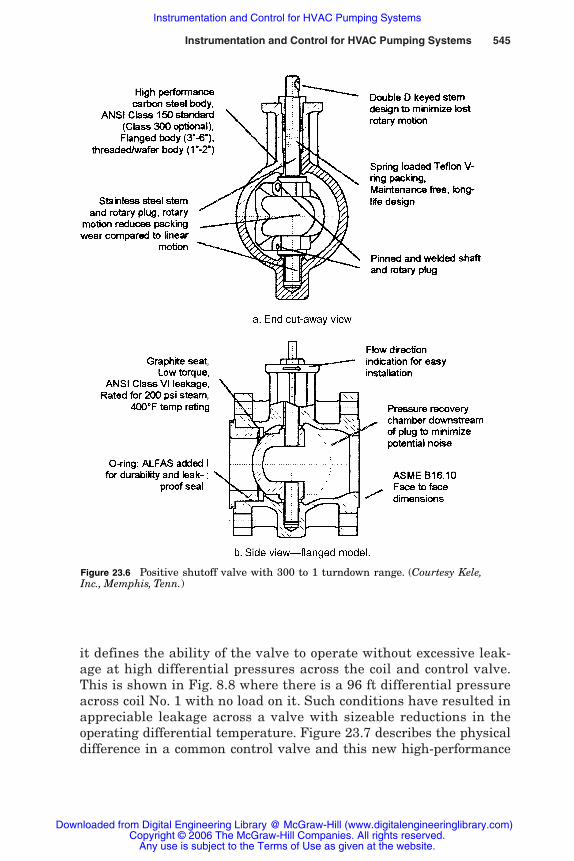
it defines the ability of the valve to operate without excessive leak-age at high differential pressures across the coil and control valve.This is shown in Fig. 8.8 where there is a 96 ft differential pressureacross coil No. 1 with no load on it. Such conditions have resulted inappreciable leakage across a valve with sizeable reductions in theoperating differential temperature. Figure 23.7 describes the physicaldifference in a common control valve and this new high-performance
Instrumentation and Control for HVAC Pumping Systems 545
Figure 23.6 Positive shutoff valve with 300 to 1 turndown range. (Courtesy Kele,Inc., Memphis, Tenn.)
Rishel_CH23.qxd 20/4/06 6:51 PM Page 545
Downloaded from Digital Engineering Library @ McGraw-Hill (www.digitalengineeringlibrary.com)Copyright © 2006 The McGraw-Hill Companies. All rights reserved.
Any use is subject to the Terms of Use as given at the website.
Instrumentation and Control for HVAC Pumping Systems

546 Installing and Operating HVAC Pumps
Figure 23.7 Physical comparison of ordinary and new coil control valves. (Courtesy KeleInc., Memphis, Tenn.)
Rishel_CH23.qxd 20/4/06 6:51 PM Page 546
Downloaded from Digital Engineering Library @ McGraw-Hill (www.digitalengineeringlibrary.com)Copyright © 2006 The McGraw-Hill Companies. All rights reserved.
Any use is subject to the Terms of Use as given at the website.
Instrumentation and Control for HVAC Pumping Systems

valve. One additional characteristic of this new valve is the increasedflow capacity. For example, the CV of a 2-in valve is 96 compared to49 for a common control valve. The added cost of the newer, heavyduty valve is offset to a great extent by this size reduction.
This improvement in coil control valve performance cannot beunderestimated. It will result in huge savings in HVAC water sys-tem operation with increased capacity for chillers and boilers. Thiswill enable hot and chilled water pumps to run closer to theirdesign point, not at a runout condition. The problem of low returnwater temperature in chilled water systems will be eliminated for themost part; continued problems with low return water temperaturewill indicate water leakage from open bypasses or dirty cooling coils.
23.7 Summation
Quality instrumentation becomes more of a necessity as attemptsare made to improve the overall efficiency of HVAC water systems.Every designer of these systems should establish specifications andother requirements that ensure that the desired instrumentation isinstalled.
23.8 Bibliography
Bela G. Liptak, Instrument Engineers Handbook, Chilton Book Company, Radnor, Pa.,1982.
Charles L. Phillips and Royce D. Harbor, Feedback Control Systems, Prentice Hall,Englewood Cliffs, N.J., 1988.
Flaherty M., Application of Adaptive Control to Central Chilled Water Plant Operation,tekworx LLC, Cincinnati, Ohio.
Instrumentation and Control for HVAC Pumping Systems 547
Rishel_CH23.qxd 20/4/06 6:51 PM Page 547
Downloaded from Digital Engineering Library @ McGraw-Hill (www.digitalengineeringlibrary.com)Copyright © 2006 The McGraw-Hill Companies. All rights reserved.
Any use is subject to the Terms of Use as given at the website.
Instrumentation and Control for HVAC Pumping Systems

Rishel_CH23.qxd 20/4/06 6:51 PM Page 548
Downloaded from Digital Engineering Library @ McGraw-Hill (www.digitalengineeringlibrary.com)Copyright © 2006 The McGraw-Hill Companies. All rights reserved.
Any use is subject to the Terms of Use as given at the website.
Instrumentation and Control for HVAC Pumping Systems

Chapter
549
24Testing HVAC
Centrifugal Pumps
24.1 Introduction
The continued need for a higher efficiency of operation of HVAC watersystems necessitates the testing of HVAC centrifugal pumps or pump-ing systems for their actual performance. They must be tested forflow, head, and efficiency.
The Hydraulic Institute (HI) has produced a test standard for cen-trifugal pumps that has been approved by the National StandardsInstitute (ANSI). This standard is entitled ANSI/HI 1.6-2000,Centrifugal Pump Tests. This standard should be in the possession ofdesigners of HVAC water systems and buyers of HVAC pumps orpumping systems. A general review of the scope of this standard isincluded herein. Table 24.1 provides a list of current HydraulicInstitute Standards for centrifugal pumps. These standards should bein the library of any designer of HVAC water systems.
24.2 Objective
The objective of this test standard is to provide uniform standards forthe hydrostatic, hydraulic, and mechanical testing of pumps and for therecording of test results. In the HVAC industry, this standard allowsdesigners to establish levels of quality and performance and enablespump and pumping system manufacturers to demonstrate that theyhave met those levels.
Vibration and acoustic standards may be required on some installa-tions. Hydraulic Institute’s Standard ANSI/HI 1.1-1.2-2000,
Rishel-Ch24.qxd 20/4/06 6:52 PM Page 549
Downloaded from Digital Engineering Library @ McGraw-Hill (www.digitalengineeringlibrary.com)Copyright © 2006 The McGraw-Hill Companies. All rights reserved.
Any use is subject to the Terms of Use as given at the website.
Source: HVAC Pump Handbook

550 Installing and Operating HVAC Pumps
Centrifugal Pumps, includes acceptable vibration levels for centrifu-gal pumps. Standard ANSI/HI 9.1-9.5-2000, Pumps—GeneralGuidelines, includes procedures for the measurement of airbornesound.
24.3 Types of Tests
The ANSI/HI test standard provides for the following tests:
1. Hydrostatic test of the pressure for the liquid container of thepump, namely, the volute or bowl
2. Performance test to demonstrate the hydraulic and mechanicalacceptability (capacity, total head, power, and speed are measured.)
3. Net positive suction head required test
4. Priming time test of self-priming pumps
24.3.1 Hydrostatic test
The hydrostatic test demonstrates that the pump, when subjected tohydrostatic pressure, will not leak or fail structurally. Each part of apump that contains liquid under pressure must be subjected to thefollowing tests:
One hundred and fifty percent of the pressure that would occur inthat part when the pump is operating at rated condition for thegiven application of the pump
TABLE 24.1 Current HI Standards for Centrifugal Pumps
Standard number Subject
ANSI/HI 1.1-1.2-2000 Centrifugal NomenclatureANSI/HI 1.3-2000 Centrifugal Application & DesignANSI/HI 1.4-2000 Centrifugal I, O, & MANSI/HI 1.6-2000 Centrifugal TestANSI/HI 2.1-2.2-2000 Vertical NomenclatureANSI/HI 2.3-2000 Vertical Application & DesignANSI/HI 2.4-2000 Vertical I, O, & MANSI/HI 2.6-2000 Vertical TestANSI/HI 9.1-9.5-2000 General GuidelinesANSI/HI 9.6.3-1997 Allowable Operating RegionANSI/HI 9.6.4-2000 Cent/Vert VibrationANSI/HI 9.6.5-2000 Condition MonitoringANSI/HI 9.8-1998 Intake Design
Rishel-Ch24.qxd 20/4/06 6:52 PM Page 550
Downloaded from Digital Engineering Library @ McGraw-Hill (www.digitalengineeringlibrary.com)Copyright © 2006 The McGraw-Hill Companies. All rights reserved.
Any use is subject to the Terms of Use as given at the website.
Testing HVAC Centrifugal Pumps
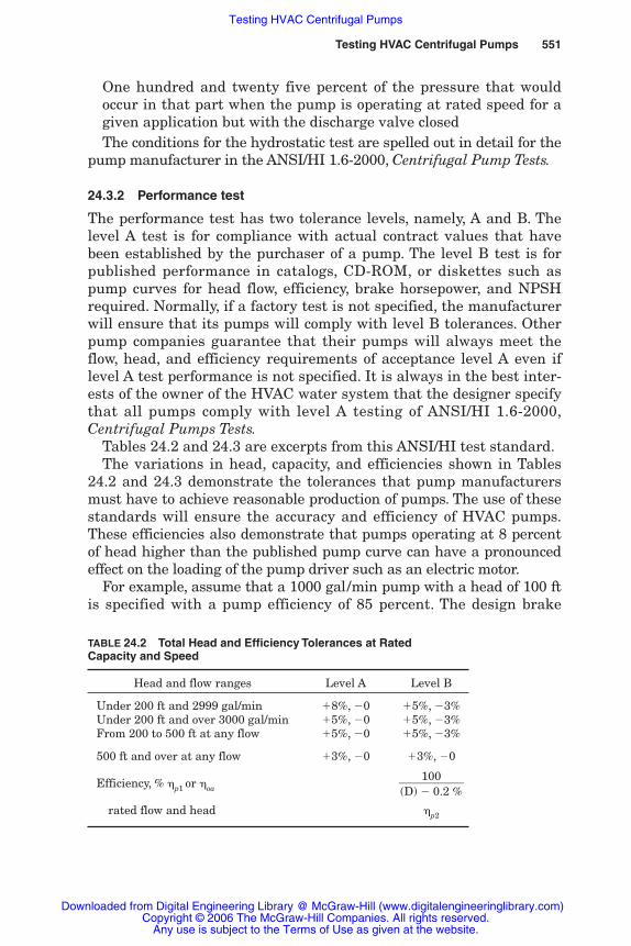
Testing HVAC Centrifugal Pumps 551
One hundred and twenty five percent of the pressure that wouldoccur in that part when the pump is operating at rated speed for agiven application but with the discharge valve closedThe conditions for the hydrostatic test are spelled out in detail for the
pump manufacturer in the ANSI/HI 1.6-2000, Centrifugal Pump Tests.
24.3.2 Performance test
The performance test has two tolerance levels, namely, A and B. Thelevel A test is for compliance with actual contract values that havebeen established by the purchaser of a pump. The level B test is forpublished performance in catalogs, CD-ROM, or diskettes such aspump curves for head flow, efficiency, brake horsepower, and NPSHrequired. Normally, if a factory test is not specified, the manufacturerwill ensure that its pumps will comply with level B tolerances. Otherpump companies guarantee that their pumps will always meet theflow, head, and efficiency requirements of acceptance level A even iflevel A test performance is not specified. It is always in the best inter-ests of the owner of the HVAC water system that the designer specifythat all pumps comply with level A testing of ANSI/HI 1.6-2000,Centrifugal Pumps Tests.
Tables 24.2 and 24.3 are excerpts from this ANSI/HI test standard.The variations in head, capacity, and efficiencies shown in Tables
24.2 and 24.3 demonstrate the tolerances that pump manufacturersmust have to achieve reasonable production of pumps. The use of thesestandards will ensure the accuracy and efficiency of HVAC pumps.These efficiencies also demonstrate that pumps operating at 8 percentof head higher than the published pump curve can have a pronouncedeffect on the loading of the pump driver such as an electric motor.
For example, assume that a 1000 gal/min pump with a head of 100 ftis specified with a pump efficiency of 85 percent. The design brake
TABLE 24.2 Total Head and Efficiency Tolerances at RatedCapacity and Speed
Head and flow ranges Level A Level B
Under 200 ft and 2999 gal/min �8%, �0 �5%, �3%Under 200 ft and over 3000 gal/min �5%, �0 �5%, �3%From 200 to 500 ft at any flow �5%, �0 �5%, �3%
500 ft and over at any flow �3%, �0 �3%, �0
Efficiency, % �p1 or �oa �(D) �
1000.2 %
�
rated flow and head �p2
Rishel-Ch24.qxd 20/4/06 6:52 PM Page 551
Downloaded from Digital Engineering Library @ McGraw-Hill (www.digitalengineeringlibrary.com)Copyright © 2006 The McGraw-Hill Companies. All rights reserved.
Any use is subject to the Terms of Use as given at the website.
Testing HVAC Centrifugal Pumps
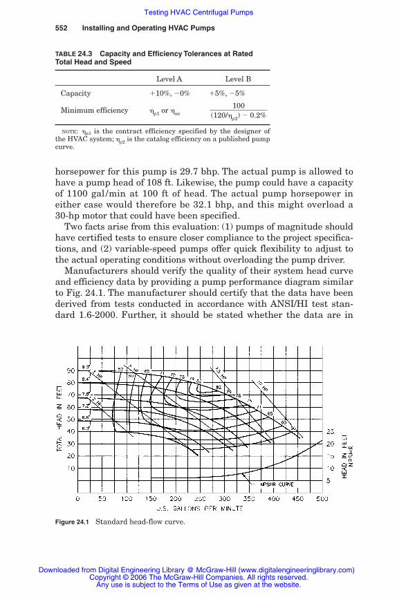
552 Installing and Operating HVAC Pumps
Figure 24.1 Standard head-flow curve.
horsepower for this pump is 29.7 bhp. The actual pump is allowed tohave a pump head of 108 ft. Likewise, the pump could have a capacityof 1100 gal /min at 100 ft of head. The actual pump horsepower ineither case would therefore be 32.1 bhp, and this might overload a30-hp motor that could have been specified.
Two facts arise from this evaluation: (1) pumps of magnitude shouldhave certified tests to ensure closer compliance to the project specifica-tions, and (2) variable-speed pumps offer quick flexibility to adjust tothe actual operating conditions without overloading the pump driver.
Manufacturers should verify the quality of their system head curveand efficiency data by providing a pump performance diagram similarto Fig. 24.1. The manufacturer should certify that the data have beenderived from tests conducted in accordance with ANSI/HI test stan-dard 1.6-2000. Further, it should be stated whether the data are in
TABLE 24.3 Capacity and Efficiency Tolerances at RatedTotal Head and Speed
Level A Level B
Capacity �10%, �0% �5%, �5%
Minimum efficiency �p1 or �oa
NOTE: �p1 is the contract efficiency specified by the designer ofthe HVAC system; �p2 is the catalog efficiency on a published pumpcurve.
100��(120/�p2) � 0.2%
Rishel-Ch24.qxd 20/4/06 6:52 PM Page 552
Downloaded from Digital Engineering Library @ McGraw-Hill (www.digitalengineeringlibrary.com)Copyright © 2006 The McGraw-Hill Companies. All rights reserved.
Any use is subject to the Terms of Use as given at the website.
Testing HVAC Centrifugal Pumps

Testing HVAC Centrifugal Pumps 553
compliance with acceptance level A or B as stated in paragraph1.6.5.3 of this standard.
24.3.3 Net positive suction head (NPSH)required test
This test enables the pump manufacturer to develop the NPSHrequired curves that are included with the head-flow curves for thepumps. Very detailed procedures are provided for the pump manufac-turer to determine the NPSH required for each pump size at variousflow rates. None of this information is of importance to the HVAC sys-tem designer; what is important to the designer is that the NPSHrequired curves provided for these pumps have been derived fromNPSH required tests that have been carried out in accordance withthe ANSI/HI test standard.
24.3.4 Priming time test for self-priming pumps
Although self-priming pumps are not used extensively in the HVACfield, when they are used, the priming time test enables the pumpmanufacturer to demonstrate to the HVAC system designer that thepump is truly self-priming.
Like the NPSH required test, detailed testing procedures are providedto the pump manufacturer to verify the time required to prime each sizepump at various capacities. The HVAC designer should specify that thepriming time for self-priming pumps has been determined in accordancewith the requirements of the ANSI/HI test standard.
24.4 Testing Procedures
The ANSI/HI test standard establishes the requirements for thepretest data requirements, test stand configuration, instrumentation,records, calculations, and reports. All these subjects are of importanceto the manufacturer of pumps to ensure that its pumps comply withthe levels of performance provided previously. These matters are notof importance to the designer or purchaser of the pumps as long asthe pump performance is ensured by certification that the pumpswere tested in accordance with the standard as described previously.
24.5 Field Testing of Pumps
Testing arrangements and instrumentation for testing are of impor-tance to HVAC designers and pump buyers, as it is often recommendedthat pumps be tested in the field under questionable conditions. A
Rishel-Ch24.qxd 20/4/06 6:52 PM Page 553
Downloaded from Digital Engineering Library @ McGraw-Hill (www.digitalengineeringlibrary.com)Copyright © 2006 The McGraw-Hill Companies. All rights reserved.
Any use is subject to the Terms of Use as given at the website.
Testing HVAC Centrifugal Pumps
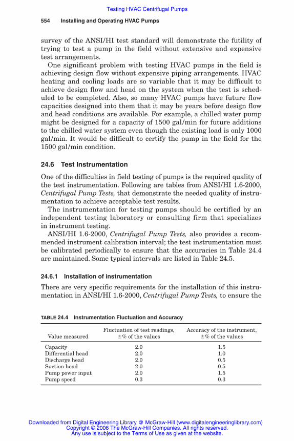
554 Installing and Operating HVAC Pumps
survey of the ANSI/HI test standard will demonstrate the futility oftrying to test a pump in the field without extensive and expensivetest arrangements.
One significant problem with testing HVAC pumps in the field isachieving design flow without expensive piping arrangements. HVACheating and cooling loads are so variable that it may be difficult toachieve design flow and head on the system when the test is sched-uled to be completed. Also, so many HVAC pumps have future flowcapacities designed into them that it may be years before design flowand head conditions are available. For example, a chilled water pumpmight be designed for a capacity of 1500 gal/min for future additionsto the chilled water system even though the existing load is only 1000gal/min. It would be difficult to certify the pump in the field for the1500 gal/min condition.
24.6 Test Instrumentation
One of the difficulties in field testing of pumps is the required quality ofthe test instrumentation. Following are tables from ANSI/HI 1.6-2000,Centrifugal Pump Tests, that demonstrate the needed quality of instru-mentation to achieve acceptable test results.
The instrumentation for testing pumps should be certified by anindependent testing laboratory or consulting firm that specializesin instrument testing.
ANSI/HI 1.6-2000, Centrifugal Pump Tests, also provides a recom-mended instrument calibration interval; the test instrumentation mustbe calibrated periodically to ensure that the accuracies in Table 24.4are maintained. Some typical intervals are listed in Table 24.5.
24.6.1 Installation of instrumentation
There are very specific requirements for the installation of this instru-mentation in ANSI/HI 1.6-2000, Centrifugal Pump Tests, to ensure the
TABLE 24.4 Instrumentation Fluctuation and Accuracy
Fluctuation of test readings, Accuracy of the instrument,Value measured �% of the values �% of the values
Capacity 2.0 1.5Differential head 2.0 1.0Discharge head 2.0 0.5Suction head 2.0 0.5Pump power input 2.0 1.5Pump speed 0.3 0.3
Rishel-Ch24.qxd 20/4/06 6:52 PM Page 554
Downloaded from Digital Engineering Library @ McGraw-Hill (www.digitalengineeringlibrary.com)Copyright © 2006 The McGraw-Hill Companies. All rights reserved.
Any use is subject to the Terms of Use as given at the website.
Testing HVAC Centrifugal Pumps
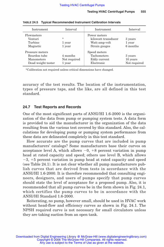
Testing HVAC Centrifugal Pumps 555
accuracy of the test results. The location of the instrumentation,types of pressure taps, and the like, are all defined in this teststandard.
24.7 Test Reports and Records
One of the most significant parts of ANSI/HI 1.6-2000 is the organi-zation of the data from pump or pumping system tests. A data formis provided to aid the manufacturer in the organization of the dataresulting from the various test covered by this standard. Also, the cal-culations for developing pump or pumping system performance fromthese data are delineated completely in this test standard.
How accurate are the pump curves that are included in pumpmanufacturers’ catalogs? Some manufacturers base their curves onacceptance level A, which allows �0, �8 percent variation in pumphead at rated capacity and speed; others use level B, which allows�3, �5 percent variation in pump head at rated capacity and speed(see Table 24.1). It is not clear whether all pump manufacturers pub-lish curves that are derived from tests in accordance with theANSI/HI 1.6-2000. It is therefore recommended that consulting engi-neers, designers, and users of pumps specify that pump curvesshould state the level of acceptance for a proposed pump. Also, it isrecommended that all pump curves be in the form shown in Fig. 24.1,which certifies the pump curves to be in accordance with theANSI/HI Standard 1.6-2000.
Reiterating, no pump, however small, should be used in HVAC workwithout head-flow and efficiency curves as shown in Fig. 24.1. TheNPSH required curve is not necessary for small circulators unlessthey are taking suction from an open tank.
TABLE 24.5 Typical Recommended Instrument Calibration Intervals
Instrument Interval Instrument Interval
Flowmeters Power metersVenturi * kilowatt transducer 3 yearsTurbine 1 year Watt-amp-volt 1 yearMagnetic 1 year Strain gauges 6 months
Pressure meters Speed metersBourdon tube 4 months Tachometers 3 yearsManometers Not required Eddy current 10 yearsDead weight tester 1 year Electronic Not required
*Calibration not required unless critical dimensions have changed.
Rishel-Ch24.qxd 20/4/06 6:52 PM Page 555
Downloaded from Digital Engineering Library @ McGraw-Hill (www.digitalengineeringlibrary.com)Copyright © 2006 The McGraw-Hill Companies. All rights reserved.
Any use is subject to the Terms of Use as given at the website.
Testing HVAC Centrifugal Pumps
24.8 Summation
To ensure the quality of HVAC pumps, the designer of HVAC watersystems should specify that all pumps be tested in accordance withthe standards of the Hydraulic Institute. Small pumps should meet atleast level B performance, while large pumps should be factory testedand certified to level A performance.
Pumps can be certified by the manufacturer of pumping systems,where the entire pumping system is tested for flow, head, power andefficiency. A wire-to-water efficiency test should be conducted on theentire pumping system. This is described in Chap. 26.
The ANSI/HI test standard is so complete for this testing and theinterpretation of the results that there truly is a criterion now forcomplete evaluation of pumps or pumping systems for the HVACindustry.
24.9 Bibliography
ANSI/HI 1.1-1.5-2000, Centrifugal Pumps, Hydraulic Institute, Parsippany, N.J., 2000.ANSI/HI 9.1-9.5-2000, Pumps—General Guidelines, Hydraulic Institute, Parsippany,
N.J., 2000.ANSI/HI 1.6-2000, American National Standard for Centrifugal Pump Tests, Hydraulic
Institute, Parsippany, N.J., 2000.
556 Installing and Operating HVAC Pumps
Rishel-Ch24.qxd 20/4/06 6:52 PM Page 556
Downloaded from Digital Engineering Library @ McGraw-Hill (www.digitalengineeringlibrary.com)Copyright © 2006 The McGraw-Hill Companies. All rights reserved.
Any use is subject to the Terms of Use as given at the website.
Testing HVAC Centrifugal Pumps
Chapter
557
25Installing HVAC Pumpsand Pumping Systems
25.1 Introduction
A pump’s useful life is determined more by its installation than by itsquality of manufacture. More pumps wear out because of improperinstallation and operation than from any other factors. As has beenmentioned often in this book, HVAC pump duty is easy pump dutycompared with other industries or applications of pumps.
HVAC pumps should not have unusual maintenance. The way toavoid maintenance is to install the pumps or pumping systems prop-erly. Almost all pump and pumping system manufacturers havedetailed installation instructions that should be followed carefully.
The basic effort in installing this equipment is to conclude with aninstallation that imposes no external forces on the pumps or pumpingsystems. This is achieved by setting the pump base properly and con-necting the piping and electrical connections so that no forces areimposed on the finished assembly.
25.2 Preinstallation Procedures
Much agony and frustration would be eliminated if all pumps werechecked carefully prior to installation. On many HVAC installations,there can be dozens of pumps of different sizes. Great care should betaken before setting any pumps on their foundations. Following arespecific details that should be checked:
1. Each pump should be tagged with its project number and particu-lar service, such as pump no. 1A, primary chilled water pump no. 1.
Rishel_CH25.qxd 20/4/06 6:53 PM Page 557
Downloaded from Digital Engineering Library @ McGraw-Hill (www.digitalengineeringlibrary.com)Copyright © 2006 The McGraw-Hill Companies. All rights reserved.
Any use is subject to the Terms of Use as given at the website.
Source: HVAC Pump Handbook
558 Installing and Operating HVAC Pumps
2. Each pump should be checked for model number, impeller diameter,and on double-suction pumps, the rotation of the impeller.
3. The pumps should not be set in place until the equipment room iscompleted to the point where the pumps will not be damaged byconstruction equipment, debris, or freezing. Some water may remainin the pump volutes from factory testing; drain plugs should beremoved to prevent any freezing of water in the volutes.
4. Pumps should be lifted from rigging points only, not from thepumps or motors themselves on base-mounted pumps. On close-coupled pumps, the lifting points should be specified by the manu-facturer.
5. The electric motors should be checked for horsepower rating andspecified voltage.
6. On electric motor–driven pumps, the power supply should bechecked for correct voltage as well as the variation in voltage fromleg to leg on polyphase applications. A sizable variation in voltagein the three different phases can cause an appreciable reduction inpower for an electric motor. See Table 7.1 for the amount of deratingcaused by a voltage imbalance between phases.
25.3 Pump and Pumping System Bases
It is quite obvious that the beginning of a successful pumping installa-tion is providing the correct base for the pumps and their accessories.Much of the trouble with pumps results from improperly designedbases. The base begins the attachment of the pump to its environment,and that base must be designed to fit the conditions surrounding thepump. Pump bases can be solidly connected to the equipment roomfloor, or they can be floated on vibration-type bases. Various types ofpump and pumping system bases are shown in Fig. 25.1.
This is the first question that must be asked: Is a vibration-typebase required to prevent any vibrations originating in the pump or itsdriver from reaching the floor? If the pumping equipment is to bemounted on an upper floor with occupancy beneath it, very likely avibration-type base will be required. There are cases where the vibra-tion base is required even though the pump base is mounted on con-crete that is poured on rock at the first elevation in a building. Whenthe activity in the building is of a sensitive nature, such as experi-mental research, the vibration base prevents objectionable vibrationand noise from being transmitted from the pumping system basethrough the building.
All bases should be designed to keep casual water away from anymetal. Solid concrete bases with the pump and its metal base mounted
Rishel_CH25.qxd 20/4/06 6:53 PM Page 558
Downloaded from Digital Engineering Library @ McGraw-Hill (www.digitalengineeringlibrary.com)Copyright © 2006 The McGraw-Hill Companies. All rights reserved.
Any use is subject to the Terms of Use as given at the website.
Installing HVAC Pumps and Pumping Systems
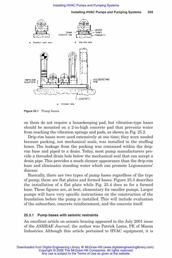
Installing HVAC Pumps and Pumping Systems 559
Figure 25.1 Pump bases.
on them do not require a housekeeping pad, but vibration-type basesshould be mounted on a 2-in-high concrete pad that prevents waterfrom reaching the vibration springs and pads, as shown in Fig. 25.2.
Drip-rim bases were used extensively at one time; they were neededbecause packing, not mechanical seals, was installed in the stuffingboxes. The leakage from the packing was contained within the drip-rim base and piped to a drain. Today, most pump manufacturers pro-vide a threaded drain hole below the mechanical seal that can accept adrain pipe. This provides a much cleaner appearance than the drip-rimbase and eliminates standing water which can promote Legionnaires’disease.
Basically, there are two types of pump bases regardless of the typeof pump; these are flat plates and formed bases. Figure 25.3 describesthe installation of a flat plate while Fig. 25.4 does so for a formedbase. These figures are, at best, elementary for smaller pumps. Largerpumps will have very specific instructions on the construction of thefoundation before the pump is installed. This will include evaluationof the subsurface, concrete reinforcement, and the concrete itself.
25.3.1 Pump bases with seismic restraints
An excellent article on seismic bracing appeared in the July 2001 issueof the ASHRAE Journal; the author was Patrick Lama, PE of MasonIndustries. Although this article pertained to HVAC equipment, it is
Rishel_CH25.qxd 20/4/06 6:53 PM Page 559
Downloaded from Digital Engineering Library @ McGraw-Hill (www.digitalengineeringlibrary.com)Copyright © 2006 The McGraw-Hill Companies. All rights reserved.
Any use is subject to the Terms of Use as given at the website.
Installing HVAC Pumps and Pumping Systems
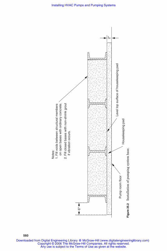
560
6"
2"
Pum
p ro
om fl
oor
Hou
seke
epin
g pa
d
Leve
l top
sur
face
of h
ouse
keep
ing
pad
Not
es:
1. F
ill v
oids
bet
wee
n st
ruct
ural
mem
bers
o
n op
en b
ases
with
ord
inar
y co
ncre
te.
2. F
ill c
lose
d ba
ses
with
non
-shr
ink
grou
t
if v
ibra
tion
occu
rs.
Fig
ure
25.
2In
stal
lati
on o
f pu
mpi
ng
syst
em b
ase.
Rishel_CH25.qxd 20/4/06 6:53 PM Page 560
Downloaded from Digital Engineering Library @ McGraw-Hill (www.digitalengineeringlibrary.com)Copyright © 2006 The McGraw-Hill Companies. All rights reserved.
Any use is subject to the Terms of Use as given at the website.
Installing HVAC Pumps and Pumping Systems
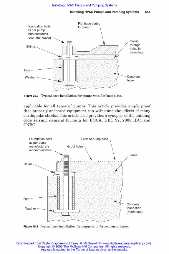
Installing HVAC Pumps and Pumping Systems 561
applicable for all types of pumps. This article provides ample proofthat properly anchored equipment can withstand the effects of manyearthquake shocks. This article also provides a synopsis of the buildingcode seismic demand formula for BOCA, UBC 97, 2000 IBC, andCNBC.
Pipe
Washer
Shims
Foundation boltsas per pumpmanufacturer’srecommendation
Concretebase
Groutthroughholes inbaseplate
Flat base platefor pump
Figure 25.3 Typical base installation for pumps with flat base plate.
Pipe
Washer
Shims
Foundation boltsas per pumpmanufacturer’srecommendation
Concretefoundation(reinforced)
Grout
Formed pump base
Grout holes
Figure 25.4 Typical base installation for pumps with formed, metal bases.
Rishel_CH25.qxd 20/4/06 6:53 PM Page 561
Downloaded from Digital Engineering Library @ McGraw-Hill (www.digitalengineeringlibrary.com)Copyright © 2006 The McGraw-Hill Companies. All rights reserved.
Any use is subject to the Terms of Use as given at the website.
Installing HVAC Pumps and Pumping Systems

562 Installing and Operating HVAC Pumps
The following figures are from this article:
Figure 25.5 Floor mounted equipment using Type HCF hole fillersor Type HG elastomeric grommets.
Figure 25.6 Installation of pumps. This article provides examples ofcalculation of the forces shown in this figure.
Most pump companies provide an installation diagram for connect-ing the steel pump base to the concrete. These diagrams include theuse of anchor bolts, shims, and nonshrink grout to properly install thepump on its concrete base. On large pumps, dowelling the pump andits driver to the steel base is a standard practice. These dowels areprovided to ensure that the pump and driver are kept in alignment.This really is not necessary for most HVAC pump applications. Also,variable-speed pumps operate at reduced speed and radial thrust sothat there seldom is any need to dowel them to the steel base. If dow-elling is necessary to keep the pump in alignment with its driver,there may be something wrong with the installation, such as pipingforce on the pump connections.
25.3.1 Pump bases with seismic restraints
The persistence of earthquakes has necessitated the installation ofmany pumps with seismic restraints built into their bases and othersupporting structures. The Uniform Building Code (UBC) has classi-fied the United States into zones and has provided lateral force levelsthat can be used for the design of pump bases and supporting equip-ment. Manufacturers of equipment that controls vibration, shock, andsound have computer programs that can develop the needed seismicrestraints for a specific application.
Figure 25.5 Seismic installation of floor bolts. (Copyright © 2001. American Society ofHeating, Refrigerating and Air-Conditioning Engineers, Inc. www.ashrae.org. Reprintedby permission from ASHRAE Journal, July 2001 Issue.)
Rishel_CH25.qxd 20/4/06 6:53 PM Page 562
Downloaded from Digital Engineering Library @ McGraw-Hill (www.digitalengineeringlibrary.com)Copyright © 2006 The McGraw-Hill Companies. All rights reserved.
Any use is subject to the Terms of Use as given at the website.
Installing HVAC Pumps and Pumping Systems

Installing HVAC Pumps and Pumping Systems 563
25.4 Connecting Piping to Pumps
There are two types of piping that impinge greatly on the efficiencyand maintenance levels of pumps. These are: (1) the fittings aroundthe pump itself and (2) the header or system piping. Either of themcan create energy waste and mechanical stress on the pump.
25.4.1 Pump fitting sizing
Pump fittings must be sized properly or there will be an appreciablewaste of energy. The friction losses through the pump fittings should be
Figure 25.6 Seismic installation of pump bases. (Copyright © 2001. American Society ofHeating, Refrigerating and Air-Conditioning Engineers, Inc. www.ashrae.org. Reprintedby permission from ASHRAE Journal, July 2001 Issue.)
Rishel_CH25.qxd 20/4/06 6:53 PM Page 563
Downloaded from Digital Engineering Library @ McGraw-Hill (www.digitalengineeringlibrary.com)Copyright © 2006 The McGraw-Hill Companies. All rights reserved.
Any use is subject to the Terms of Use as given at the website.
Installing HVAC Pumps and Pumping Systems
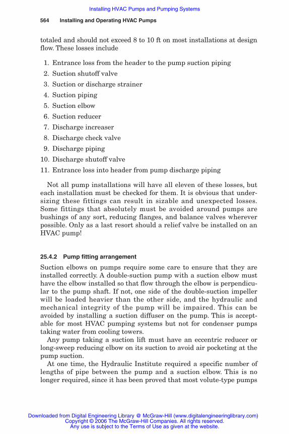
564 Installing and Operating HVAC Pumps
totaled and should not exceed 8 to 10 ft on most installations at designflow. These losses include
1. Entrance loss from the header to the pump suction piping
2. Suction shutoff valve
3. Suction or discharge strainer
4. Suction piping
5. Suction elbow
6. Suction reducer
7. Discharge increaser
8. Discharge check valve
9. Discharge piping
10. Discharge shutoff valve
11. Entrance loss into header from pump discharge piping
Not all pump installations will have all eleven of these losses, buteach installation must be checked for them. It is obvious that under-sizing these fittings can result in sizable and unexpected losses.Some fittings that absolutely must be avoided around pumps arebushings of any sort, reducing flanges, and balance valves whereverpossible. Only as a last resort should a relief valve be installed on anHVAC pump!
25.4.2 Pump fitting arrangement
Suction elbows on pumps require some care to ensure that they areinstalled correctly. A double-suction pump with a suction elbow musthave the elbow installed so that flow through the elbow is perpendicu-lar to the pump shaft. If not, one side of the double-suction impellerwill be loaded heavier than the other side, and the hydraulic andmechanical integrity of the pump will be impaired. This can beavoided by installing a suction diffuser on the pump. This is accept-able for most HVAC pumping systems but not for condenser pumpstaking water from cooling towers.
Any pump taking a suction lift must have an eccentric reducer orlong-sweep reducing elbow on its suction to avoid air pocketing at thepump suction.
At one time, the Hydraulic Institute required a specific number oflengths of pipe between the pump and a suction elbow. This is nolonger required, since it has been proved that most volute-type pumps
Rishel_CH25.qxd 20/4/06 6:53 PM Page 564
Downloaded from Digital Engineering Library @ McGraw-Hill (www.digitalengineeringlibrary.com)Copyright © 2006 The McGraw-Hill Companies. All rights reserved.
Any use is subject to the Terms of Use as given at the website.
Installing HVAC Pumps and Pumping Systems
can operate with elbows mounted on their suctions without damageor loss of efficiency. In fact, many pumps, such as in-line and somepetrochemical pumps, have the elbows integrated into their casings.
Hydraulic Institute standards are an excellent source for informa-tion on the proper arrangement of fittings around pumps. Manyexamples are provided by these standards that enhance the installa-tion of pumps.
25.4.3 Expansion provisions at pumps
Expansion of piping in HVAC systems consists of thermal expansionin the piping and expansion due to changes in the building due to set-tling or other movements. Both these possibilities must be recognizedin all HVAC systems.
One of the most damaging practices in the pump industry is notproviding adequate thermal expansion provisions around pumps. Thisis not very important for chilled water pumps because they operatenear 50°F and do not have much expansion in the piping. It is impor-tant for low-temperature hot water heating systems and particularlyso for medium- and high-temperature water systems to have the cor-rect expansion provisions.
Thermal expansion must be accounted for in both lateral and axialdirections. Installation of the system piping must be such that exces-sive expansion does not occur at the pumps. Long runs of piping mustinclude expansion provisions such as expansion joints, bellows assem-blies, or offset piping. Chapter 43 of the ASHRAE ApplicationsHandbook is an excellent source for evaluating complex piping sys-tems to determine the type and location of expansion provisions. Onecommon error in the pumping industry is to use flexible hose forpump connections; it can handle only lateral, not axial movement.
HVAC pumps must be installed without any thrust on the pumpconnections by the piping. After the installation is completed, theflange bolts on the pump connections should be removed. If the pipeflanges move at all, the piping should be redone. The worst practice isto have a gap between the pump and pipe flanges and then drawthem together with the flange bolts. Other conditions that must bewatched for are shifting of the pipe flange so that the flange holes donot line up or for the pipe flange to be at a slight angle from the pumpflange. All these conditions create stresses in the pump casing andwill, eventually, pull or push the pump out of alignment. Do not useflexible joints to eliminate these misalignments of the pipe flanges. Theexpansion joint and pump flanges must come together without anyforce or movement of any expansion provisions.
Installing HVAC Pumps and Pumping Systems 565
Rishel_CH25.qxd 20/4/06 6:53 PM Page 565
Downloaded from Digital Engineering Library @ McGraw-Hill (www.digitalengineeringlibrary.com)Copyright © 2006 The McGraw-Hill Companies. All rights reserved.
Any use is subject to the Terms of Use as given at the website.
Installing HVAC Pumps and Pumping Systems
25.5 Electrical Provisions for Pumps
Electrical provisions for pumps consist of connections to pump motorsand safety controls for pumps.
25.5.1 Electrical connections for pump motors
There are some simple rules for electrical connections for motors that,if followed, will result in trouble-free installations. Generally, the con-nection of power wiring to motor junction boxes should conform to theNational Electrical Code and any special provisions for a specificapplication. The power connections should be bolted to the motorleads; wire nuts should not be used. The final connection to the motormust be flexible to allow some movement between the electricalpower conduit and the motor.
A motor out of sight of or 50 ft from the electrical disconnectingmeans may require the installation of a manual switch at the motor.If there is a possibility that the motor can be stopped manually whilein operation, this disconnection switch should be equipped with a con-trol contact that opens the motor control circuit before the mainpower switch is disconnected.
Most HVAC pumps depend on the motor overloads to protect theirmotors. Larger motors should be equipped with temperature andvibration sensors that can be used to alarm the operators in event ofhigh temperature or excessive vibration.
25.5.2 Safety controls for pumps
Small HVAC pumps are often installed without any safety controls.Several inspection agencies are now requiring differential pressureswitches installed across the suction and discharge connections of thepumps. Such a switch proves that the pump has generated pressure;if this does not occur within a specific time period, the pump isstopped and an alarm signal is generated.
Larger pumps, like motors, should be equipped with temperatureand vibration sensors that alarm the operator in the event of hightemperature or excessive vibration.
25.6 Alignment of Pumps and Motors
Before attempting to start the pumps, the alignment of the pumpsand their motors or other drivers should be checked carefully. Allpump and flexible coupling manufacturers have alignment tolerancesthat must not be exceeded. Alignment should be checked for both off-set and angularity.
566 Installing and Operating HVAC Pumps
Rishel_CH25.qxd 20/4/06 6:53 PM Page 566
Downloaded from Digital Engineering Library @ McGraw-Hill (www.digitalengineeringlibrary.com)Copyright © 2006 The McGraw-Hill Companies. All rights reserved.
Any use is subject to the Terms of Use as given at the website.
Installing HVAC Pumps and Pumping Systems
Alignment by straight edge across the coupling was acceptable atone time. Today, alignment by means of an Ames dial or equivalentshould be accomplished for most HVAC pumps. Laser technology hasbeen applied to machinery alignment and is now available for cen-trifugal pumps.
25.7 Initial Operation of Pumps
Chapter 27 is devoted to the pump operation, which pertains to theefficiency of that operation. Initial operation of pumps is part of theinstallation process, since it tells quickly the quality of the actualinstallation.
The first operation of a pump and its driver will indicate manythings:
1. Unexpected noise will provide information on pump alignment,cavitation, or entrained air.
2. Pump speed on variable-speed pumps will provide information onthe adequacy of the pump control.
3. Heat in the motor or pump can be an indicator of problems withalignment or improper operation.
4. If wire-to-water efficiency indication is provided, it will furnishinformation on the adequacy of the pump control system andwhether the pumps, drivers, and pump fittings are of the qualityand size expected.
25.7.1 Rotation of pumps
Many unnecessary service trips could be averted if the rotation ofpumps was checked carefully at initial startup. A centrifugal pumpwill produce head with reverse rotation, but it will not perform to itsdesign condition. Rotation can be checked easily; also, on three-phasepower operations, the rotation can be changed by reversing two of thepower leads.
25.8 Summation
Proper installation of HVAC pumps will provide the long useful lifethat these pumps should have without much maintenance. Finally,pumping systems should be observed carefully during their firsthours of operation to ensure that the specifications have been met forthat installation.
Installing HVAC Pumps and Pumping Systems 567
Rishel_CH25.qxd 20/4/06 6:53 PM Page 567
Downloaded from Digital Engineering Library @ McGraw-Hill (www.digitalengineeringlibrary.com)Copyright © 2006 The McGraw-Hill Companies. All rights reserved.
Any use is subject to the Terms of Use as given at the website.
Installing HVAC Pumps and Pumping Systems

Rishel_CH25.qxd 20/4/06 6:53 PM Page 568
Downloaded from Digital Engineering Library @ McGraw-Hill (www.digitalengineeringlibrary.com)Copyright © 2006 The McGraw-Hill Companies. All rights reserved.
Any use is subject to the Terms of Use as given at the website.
Installing HVAC Pumps and Pumping Systems

Chapter
569
26Factory-Assembled
Pumping Systems
26.1 Introduction
Traditionally, pumping systems have been field erected in the HVACindustry. The development of digitally controlled pumping systemsalong with computer-aided drafting and manufacturing has made eco-nomical, the factory production of these systems.
Factory-assembled pumping systems have had the same naturaldevelopment as other equipment in the HVAC field, such as chillers,boilers, and air-handling units, as well as condensate pumps, deaera-tors, and boiler feed systems.
26.2 Types of Factory-Assembled Pumping Systems
There are a number of different pumping systems available for almostany HVAC pumping application. The principal limitation for thesesystems is size. Systems can be manufactured to the size limitsimposed by highway transportation or access into the building of finallocation. The principal applications in the HVAC field for factory-assembled equipment in addition to condensate return systems, boilerfeed systems, and deaerators are for chilled water, hot water, and con-denser water systems.
26.2.1 Chilled water systems
Pumping systems can be manufactured for chilled water in sizesfrom the simple primary pumping system (Fig. 26.1) to the large
Rishel_CH26.qxd 20/4/06 6:54 PM Page 569
Downloaded from Digital Engineering Library @ McGraw-Hill (www.digitalengineeringlibrary.com)Copyright © 2006 The McGraw-Hill Companies. All rights reserved.
Any use is subject to the Terms of Use as given at the website.
Source: HVAC Pump Handbook

570 Installing and Operating HVAC Pumps
Figure 26.1 Primary pumpingsystem.
variable-speed secondary pumping system (Fig. 26.2). Also, they canbe simple systems or very complete ones of secondary pumps withexpansion tanks and air separators (Fig. 26.3). Most HVAC pumpingsystems can utilize end-suction or double-suction pumps; larger systemsare equipped with either horizontally or vertically mounted double-suction pumps. A unit with vertically mounted double-suction pumpsis illustrated in Fig. 26.4. Axial flow pumps are seldom used on fac-tory-assembled chilled water systems.
A popular factory-assembled system has been one with primary andsecondary pumps, as shown in Fig. 26.5. This unit includes the pri-mary chiller pumps and secondary distribution pumps as well as the
Rishel_CH26.qxd 20/4/06 6:54 PM Page 570
Downloaded from Digital Engineering Library @ McGraw-Hill (www.digitalengineeringlibrary.com)Copyright © 2006 The McGraw-Hill Companies. All rights reserved.
Any use is subject to the Terms of Use as given at the website.
Factory-Assembled Pumping Systems

571
Fig
ure
26.
2L
arge
var
iabl
e-sp
eed
seco
nda
ry p
um
pin
g sy
stem
.
Rishel_CH26.qxd 20/4/06 6:54 PM Page 571
Downloaded from Digital Engineering Library @ McGraw-Hill (www.digitalengineeringlibrary.com)Copyright © 2006 The McGraw-Hill Companies. All rights reserved.
Any use is subject to the Terms of Use as given at the website.
Factory-Assembled Pumping Systems

572 Installing and Operating HVAC Pumps
Figure 26.3 Pumping system with expansion tank and heat exchanger.
chiller bypass; this ensures that the basic principles have been fol-lowed for good piping design for chillers.
26.2.2 Hot water systems
Factory-assembled hot water pumping systems are configured muchthe same as the chilled water systems described previously. They areavailable with primary, secondary, or primary-secondary pumps. Someboilers do not require primary or boiler pumps, so only distributionpumps are required. In many cases, the hot water pumps are furnished
Rishel_CH26.qxd 20/4/06 6:54 PM Page 572
Downloaded from Digital Engineering Library @ McGraw-Hill (www.digitalengineeringlibrary.com)Copyright © 2006 The McGraw-Hill Companies. All rights reserved.
Any use is subject to the Terms of Use as given at the website.
Factory-Assembled Pumping Systems

Factory-Assembled Pumping Systems 573
Figure 26.4 Pumping system with vertically mounteddouble-suction pumps.
on the same factory-assembled pumping system as the chilled waterpumps.
Steam-heated hot water systems are available in a number of con-figurations, such as units with constant- or variable-speed pumps.Figure 26.6 describes a steam-heated unit with dual heat exchangers,variable-speed pumps, and a three-way valve for control of systemtemperature. This system offers many advantages over the traditionalmethod of connecting steam-heated pumping systems. For example,
1. The control valve monitors steam pressure in the heat exchanger,not hot water system temperature. This ensures a positive pres-sure in the heat exchanger under all load variations in the hotwater system.
2. With constant steam pressure in the heat exchanger, it is difficultfor a vacuum to form in the heat exchanger under light loads.
3. The condensate flow through the steam trap is not erratic as withother steam-heated hot water systems. A steady flow of condensatethrough the steam trap ensures constant steam pressure in theheat exchanger.
4. Several different distribution loops with varying hot water supplytemperatures can be served from one heat exchanger system byproviding a three-way valve for each required temperature.
Rishel_CH26.qxd 20/4/06 6:54 PM Page 573
Downloaded from Digital Engineering Library @ McGraw-Hill (www.digitalengineeringlibrary.com)Copyright © 2006 The McGraw-Hill Companies. All rights reserved.
Any use is subject to the Terms of Use as given at the website.
Factory-Assembled Pumping Systems

574 Installing and Operating HVAC Pumps
26.2.3 Condenser and cooling tower systems
Factory-assembled pumping systems for cooling tower and condenserwater are similar to those for chilled water. They can range fromconstant-speed units like that in Fig. 26.1 to large pumping unitssimilar to that in Fig. 26.2. Others can be primary-secondary asdescribed in Fig. 26.5, where the primary pumps circulate the coolingtowers and provide a suction pressure to the variable-speed con-denser pumps.
The principal differences for cooling tower units are: (1) the pipingmust be designed for higher pipe roughness and (2) the elevation ofthe suction header must be checked to ensure that its elevation islower than the cooling tower sump.
Other special units for condenser water and cooling tower water arehot-well, cold-well systems and water source heat pump systems.
Figure 26.5 Primary-secondary pumping systems.
Rishel_CH26.qxd 20/4/06 6:54 PM Page 574
Downloaded from Digital Engineering Library @ McGraw-Hill (www.digitalengineeringlibrary.com)Copyright © 2006 The McGraw-Hill Companies. All rights reserved.
Any use is subject to the Terms of Use as given at the website.
Factory-Assembled Pumping Systems

Factory-Assembled Pumping Systems 575
Figure 26.6 Steam-heated hot water system with three-way valve control.
26.3 Advantages of Factory-AssembledHVAC Pumping Systems
26.3.1 First cost
For most new installations, the factory-assembled pumping systemoffers the lowest-cost procedure for designing, building, and installinga pumping system. Fewer personnel hours are required than indesigning a field installation and then actually installing the pumps,piping, and controls in the field. This, of course, is contingent on freeaccess to the equipment room; many rehabilitation projects do notoffer such access.
Factory-assembled pumping systems provide the production capabil-ities of a manufacturing plant and reduce the total cost of the whole
Rishel_CH26.qxd 20/4/06 6:54 PM Page 575
Downloaded from Digital Engineering Library @ McGraw-Hill (www.digitalengineeringlibrary.com)Copyright © 2006 The McGraw-Hill Companies. All rights reserved.
Any use is subject to the Terms of Use as given at the website.
Factory-Assembled Pumping Systems

576 Installing and Operating HVAC Pumps
process of design, manufacture, and installation of pumps. Followingare some detailed processes that are enhanced by such systems:
1. The consulting engineer can use a catalog or drawing that pro-vides a complete system of pumps, motors, piping, valving, controls,and switch gear all mounted on a single base. Figures 26.1 and 26.2provide typical general arrangement drawings for such pumpingsystems. Figure 26.1 is for a simple primary pumping system, whileFig. 26.2 describes a large variable-speed secondary chilled watersystem. This system demonstrates the ability to computerize suchcomplex systems for design and manufacture. This gives the pump-ing system manufacturer the same responsibility for detailed designof the pumping system as that of a manufacturer of a chiller or a boiler.All the contemporary electronic means of transmitting drawings canbe utilized in providing these drawings to HVAC system designers.
The designer/consulting engineer can depend on the expertise ofthe pumping system manufacturer to provide a properly configuredpumping system. The consultant can then devote more time to totalevaluation of the building’s environment and operation. This ensuresthat the client is getting the building services that are needed for thebuilding to function as desired.
2. The contractor can place one order for a factory-assembled pump-ing system instead of hundreds of little orders that may be required tocomplete a field-installed pumping system. There is only one set ofsubmittals to inspect and forward to the consulting engineer insteadof many submittals. The contractor depends on only one source for thepumping system startup and service.
3. The owner saves space, since factory-assembled pumping sys-tems usually reduce the space for the pumping equipment by around30 to 50 percent. The owner’s operating personnel have only onevendor to work with for service and adjustment after the consultingengineer and contractor have finished their work.
26.3.2 Time saving
Factory-assembled pumping systems offer savings in time duringdesign, construction, and installation:
1. In the design phase, the pumping system manufacturer can offerdrawings that enable the consulting engineer to select the completesystem without becoming involved in the detailed design of the pumpand piping details. On fast-track projects, this design procedurespeeds up the layout of other piping in the equipment room.
2. On accelerated construction programs, the pumping system canbe manufactured, tested, and prepared for installation long before the
Rishel_CH26.qxd 20/4/06 6:54 PM Page 576
Downloaded from Digital Engineering Library @ McGraw-Hill (www.digitalengineeringlibrary.com)Copyright © 2006 The McGraw-Hill Companies. All rights reserved.
Any use is subject to the Terms of Use as given at the website.
Factory-Assembled Pumping Systems

Factory-Assembled Pumping Systems 577
site is ready to receive it. When the proper time occurs, the pumpingsystem can be set in place. Much of the work delay, due to coordina-tion between various trades, is eliminated.
3. Startup and commissioning are accelerated due to preplanningbetween the pumping system manufacturer and other control compa-nies involved; the fact that one company is responsible for the operationof the complete pumping system also accelerates commissioning.
26.3.3 Unit responsibility
Factory-assembled pumping systems offer unit responsibility, asreferred to earlier. This should be emphasized because of the greatease offered by this singular responsibility. Only one entity is involvedwith the startup of the pumping system. The consulting engineer, con-tractor, and owner have only one company to deal with in solvingproblems and getting the pumping system to operate as specified.
The pumping system manufacturer has so much at stake in termsof marketing that it is imperative that an ongoing relationship beestablished with the ultimate owner. Following are some of the dutiesthat a pumping system manufacturer should carry out in commission-ing a pumping system:
1. Verify the capacities of the system in gallons per minute and headand ensure that they conform to the requirements of the consult-ing engineer or owner.
2. Inspect the equipment room and ensure that it is adequate andthat the ambient air is not hostile to the electronics of the pump-ing system.
3. Certify clearance around the system to ensure that adequatespace is available for proper operation of the system.
4. Inspect electrical service and ventilation provisions to ensure thatthey are adequate.
5. Check all field piping attached to the system to ensure that it isproperly supported and is not using the pumping system forsupport.
6. When the system is started, representatives of the owner, engi-neer, and contractor should be present to observe initial operationof the system.
7. The system should be run through all its capacities to verify thatit is conforming to the specifications. Owing to the light loads thatusually exist on HVAC systems at their initial operation, often itis impossible to achieve this in the field.
Rishel_CH26.qxd 20/4/06 6:54 PM Page 577
Downloaded from Digital Engineering Library @ McGraw-Hill (www.digitalengineeringlibrary.com)Copyright © 2006 The McGraw-Hill Companies. All rights reserved.
Any use is subject to the Terms of Use as given at the website.
Factory-Assembled Pumping Systems
578 Installing and Operating HVAC Pumps
8. All alarm and safety circuits should be tested and verified to theowner’s representative.
9. Complete operating instructions should be given to the operatorsof the system.
10. The service representative of the manufacturer of the systemshould establish a routine checkup procedure to ensure that thesystem is performing satisfactorily.
26.3.4 Less pump maintenance and repair
Factory-assembled pumping systems have demonstrated that there isless pump repair when the pump is assembled with a properlydesigned pumping system instead of mounting the pump in the field.This has been proved by years of operation of these factory-assembledpumping systems in the field. There are several reasons for thisreduction in pump repair:
1. The pumping system manufacturer is totally responsible for thepump’s environment.a. Suction and discharge piping is supported independently of the
pump connections. There are no pipe forces on these connections.b. The pumps are mounted on a heavy structural steel base that
does not shift as the building settles. This is not necessarilytrue for field-mounted pumps. There is little chance for thepump and motor to become misaligned after the pumping sys-tem is put into operation.
2. The pumping system manufacturer can evaluate the entire operat-ing range of a pump and ensure that it does not operate at pointsof poor efficiency or at high radial or axial thrust.
3. The pumping system manufacturer should include the installationof differential pressure switches on all pumps to ensure that pumpfailure is alarmed and that the pump does not run continuously ata dangerous condition.
A properly installed factory-assembled pumping system on HVACwater systems should provide many years of service without signifi-cant repair or failure.
26.4 Components of a Factory-AssembledPumping System
There is a variety of equipment that can be supplied with factory-assembled pumping systems. The principal components are listed
Rishel_CH26.qxd 20/4/06 6:54 PM Page 578
Downloaded from Digital Engineering Library @ McGraw-Hill (www.digitalengineeringlibrary.com)Copyright © 2006 The McGraw-Hill Companies. All rights reserved.
Any use is subject to the Terms of Use as given at the website.
Factory-Assembled Pumping Systems
Factory-Assembled Pumping Systems 579
as follows. Many special types of equipment are often furnished onthese systems to meet the requirements of particular installations.
26.4.1 Pumps
Pumps for factory-assembled systems usually consist of single-suctionand/or double-suction pumps. The number of pumps can vary fromone to a dozen. The only limitation to the number of pumps is theability to ship the pumping system.
The pumping systems can be a mixture of constant- and variable-speed pumps as long as constant- and variable-speed pumps are notdesigned to operate together in parallel.
Pump motor sizes vary from fractional horsepower up to 500 hp.Pumps with motors larger than this size are usually field installed.
26.4.2 Pumping system accessories
Following are standard accessories for these pumping systems:
1. Suction and discharge headers. Systems taking water from asump and utilizing vertical turbine pumps are not equipped withsuction headers.
2. Branch piping for each pump, including shutoff valves, checkvalves, and strainers. Some systems may include motorized valvesinstead of the check valves. Suction diffusers can be furnished inlieu of wye or basket strainers.
3. Chiller or boiler bypasses. These are furnished when both the pri-mary and secondary pumps are supplied on one system.
4. All piping should be supported by structural steel to remove anystress from the pump flanges. Supports must be equipped withsaddles and insulation spacers to reduce heat conductivity to andfrom the piping.
5. Hoists and rails can be furnished as an integral part of the pump-ing system for removing major components.
6. Heat exchangers, both shell and tube and plate and frame types.Steam-heated exchangers are furnished with steam controlvalves, steam traps, and water temperature control.
7. Expansion tanks with makeup water valves, including backflowpreventers.
8. Mechanical air eliminators.
9. Chemical feeders and control.
Rishel_CH26.qxd 20/4/06 6:54 PM Page 579
Downloaded from Digital Engineering Library @ McGraw-Hill (www.digitalengineeringlibrary.com)Copyright © 2006 The McGraw-Hill Companies. All rights reserved.
Any use is subject to the Terms of Use as given at the website.
Factory-Assembled Pumping Systems
580 Installing and Operating HVAC Pumps
10. Filters with control and piping.
11. Structural steel bases, standard and vibration types.
26.4.3 Electrical equipment
Factory-assembled pumping systems usually provide most of the electri-cal equipment required to integrate the pumping system into the rest ofthe water system. Following is a general listing of this equipment:
1. Switch geara. Power supply can include main disconnect, watt transmitter,
automatic transfer switch, and power feeders to variable-speeddrives and magnetic starters on the pumping system.
b. Combination starters for constant-speed pumps.c. Variable-speed drives.
2. Pump speed control and sequencing
3. Chiller or boiler sequencing
4. Instrumentation such as flowmeters, temperature transmitters,and pressure or differential pressure transmitters
5. Operator interfaces as well as information displays, alarms, andtotalizers
6. Energy calculations such as Btu, Btu/h, tons, ton-hours, kW/ton,coefficient of performance, and wire-to-water efficiency
7. Automation control interfacing. (This provides simple intercon-necting with building management system manufacturers withoutspecial software and field coordination. These systems can becomeBACnet compatible when BACnet standards are completed.)
26.4.4 Complete pump houses
The factory-assembled pumping system can be furnished in a com-plete pump house with the following equipment:
1. Base for installing the total assembly on a foundation in the field
2. Pumping system itself
3. Heating, ventilating, and air-conditioning equipment as required
4. Electrical switch gear for pumps as well as house lighting, heating,cooling, and ventilation equipment
The preceding is a brief synopsis of the equipment that can befurnished with a factory-assembled pumping system. Specificinstallations may require equipment not listed previously.
Rishel_CH26.qxd 20/4/06 6:54 PM Page 580
Downloaded from Digital Engineering Library @ McGraw-Hill (www.digitalengineeringlibrary.com)Copyright © 2006 The McGraw-Hill Companies. All rights reserved.
Any use is subject to the Terms of Use as given at the website.
Factory-Assembled Pumping Systems

Factory-Assembled Pumping Systems 581
On some applications, the installation of the pumps is away fromthe main building, or there is no room in the existing central energyplant for the installation of new pumps. In such situations, it may bemore economical to provide the pumps and switch gear in a separatehouse. A complete pumping system in its own house (Fig. 26.7) can befurnished with all wiring and internal piping completed and ready tobe set on a field foundation. The only connections are the power supply,information interface, makeup water, and supply and return piping.
Special equipment such as boilers, chillers, electric generators,emergency power transfer switches, and water conditioning equip-ment can be furnished in these houses.
Figure 26.7 Complete chiller plant. (Courtesy Flo-Pak Division of Patterson PumpCompany.)
Rishel_CH26.qxd 20/4/06 6:54 PM Page 581
Downloaded from Digital Engineering Library @ McGraw-Hill (www.digitalengineeringlibrary.com)Copyright © 2006 The McGraw-Hill Companies. All rights reserved.
Any use is subject to the Terms of Use as given at the website.
Factory-Assembled Pumping Systems

582 Installing and Operating HVAC Pumps
Figure 26.8 Variable-speed pumping control center.
26.4.5 Control centers for existing pumps
Often, on retrofit projects or on an installation with limited access tothe central energy plant, it is impossible to furnish a factory-assembledpumping system with pumps and piping all mounted on a structuralsteel base. In these cases, a complete control center (Fig. 26.8) canstill be furnished that offers many of the advantages of the factory-assembled pumping system. The supplier of these control centersshould be able to furnish the support services and commissioning nor-mally furnished by a manufacturer of pumping systems. The variable-speed drives for the pumps should be furnished by this manufacturer.This provides an assembly of the drives and pump controls that
CHANGE LIGHTS AND CONTROLLER
Rishel_CH26.qxd 20/4/06 6:54 PM Page 582
Downloaded from Digital Engineering Library @ McGraw-Hill (www.digitalengineeringlibrary.com)Copyright © 2006 The McGraw-Hill Companies. All rights reserved.
Any use is subject to the Terms of Use as given at the website.
Factory-Assembled Pumping Systems

Factory-Assembled Pumping Systems 583
ensures the best fit between the pumps and controls. Also, factorywiring and assembly eliminate much of the field coordination thatwould be required when the variable-frequency drives are furnishedby other suppliers.
The new procedures for controlling flow in chiller evaporators opena new field for the improvement of existing chilled water systems. Anintegrated control center providing all the necessary interfacing withchillers, chiller pumps, and any distribution pumps provides an eco-nomical and technical answer for achieving optimal operation of thechillers and pumps.
26.5 Testing Pumping Systems
The testing of factory-assembled pumping systems includes individ-ual testing of the pumps, as described in Chap. 24. Also, the flow andfriction loss tests of the entire pumping system should be completedto provide the designer or user of the pumping system with a totalevaluation of the pumping system’s performance. Test conditionsequal to the initial and ultimate system flows should be performed atthe factory test facility.
The flow test for a complete pumping system should include a wire-to-water efficiency evaluation, as described in Chap. 10 and Table 10.6.This enables the designer and ultimate user to have an overall evalu-ation of the pumping system before it leaves the manufacturer’splant. As with individual pumps described in Chap. 24, it is difficultto test pumping systems in the field due to the effort required toduplicate a factory test facility with its calibrated and properlyinstalled instrumentation.
26.6 Summation
Factory-assembled pumping systems, like boilers and chillers, providean economical answer for efficient pumping installations. They shouldbe used where entrance clearances and economic conditions allowtheir application.
Rishel_CH26.qxd 20/4/06 6:54 PM Page 583
Downloaded from Digital Engineering Library @ McGraw-Hill (www.digitalengineeringlibrary.com)Copyright © 2006 The McGraw-Hill Companies. All rights reserved.
Any use is subject to the Terms of Use as given at the website.
Factory-Assembled Pumping Systems

Rishel_CH26.qxd 20/4/06 6:54 PM Page 584
Downloaded from Digital Engineering Library @ McGraw-Hill (www.digitalengineeringlibrary.com)Copyright © 2006 The McGraw-Hill Companies. All rights reserved.
Any use is subject to the Terms of Use as given at the website.
Factory-Assembled Pumping Systems
Chapter
585
27Operating HVAC Pumps
27.1 Introduction
Good operation of HVAC pumps consists of efficient performancewithout undue wear of the pumps, motors, and appurtenances. Effi-cient operation has been stressed throughout this book and will besummarized here; much of this chapter is found in other parts of thebook. It is repeated here to emphasize the need for efficient operation,not just from an energy standpoint but also from a maintenance per-spective. Further, a review will be made of how pumps fit into theoverall energy conservation of HVAC water systems.
27.2 Checking for Efficient Selection of HVAC Pumps
Efficient operation begins with selecting the pump near the best effi-ciency point of its head-flow curve. It is difficult to imagine howpoorly pumps are often selected in the HVAC industry. Too manytimes pumps are selected far from the best efficiency point becauseone particular manufacturer does not have the proper sizes or typesof pumps to meet a system’s different pumping conditions. One pumpmanufacturer may have the best pump selections for the hot waterpumps but not for the chilled and condenser pumps. On another pro-ject, one pump manufacturer may have the best selections for the single-suction pumps, while another may have better pumps for the double-suction applications.
The failure of the HVAC designer to realize that one pump manu-facturer cannot truly meet all the various pump design conditions for
Rishel_CH27.qxd 20/4/06 7:37 PM Page 585
Downloaded from Digital Engineering Library @ McGraw-Hill (www.digitalengineeringlibrary.com)Copyright © 2006 The McGraw-Hill Companies. All rights reserved.
Any use is subject to the Terms of Use as given at the website.
Source: HVAC Pump Handbook

586 Installing and Operating HVAC Pumps
a complex project, results in poor selection of pumps. The designershould evaluate several manufacturers’ pumps to ensure that themost efficient pump is selected for each pump duty. Too much empha-sis is placed on having all the pumps from the same manufacturer.
In the past, great emphasis was placed on pump maintenance.Pump maintenance was high because of the use of constant-speedpumps and letting them operate at points of high radial thrust. Pumpbearings and mechanical seals wore out rapidly and required continu-ous maintenance. Today, with proper selection and the use of variable-speed pumps, maintenance of HVAC pumps should be minimal. If anHVAC pump needs continuous maintenance, its application should bechecked to ensure that the pump is operating near its best efficiencypoint. As has been mentioned throughout this book, HVAC pump dutyis not difficult duty. Therefore, these pumps should run continuouslywithout excessive wear. There should be little noise, no vibration, andno heat (except with hot water pumps). Evidence of any of these fac-tors should be of concern and require inspection of the pumps todetermine the cause. More on pump maintenance will be presented inChap. 28.
Throughout this book, the emphasis has been on operating pumpsnear their best efficiency point to avoid radial thrust and resultingfailure. Manufacturers of mechanical seals recognize this fact morethan any other equipment manufacturer. A recent article in PlantEngineering Magazine estimated that 85 percent of mechanical sealsreplaced in pumps had failed and were not worn out. These failureswere due to improper operation of the pumps, not the seals them-selves. This article also pointed out the importance of operatingpumps within �20 percent of the flow at the best efficiency point.Further, this article provided additional information on extending theuseful life of mechanical seals and centrifugal pumps.
27.3 Constant- or Variable-Speed Pumps
As was emphasized earlier, constant-speed pumps should be operatedon constant-volume systems and variable-speed pumps should beoperated on variable-volume systems. When investigating the opera-tion of existing pumps, great concern should be given to ensuring thatconstant-speed pumps are not operated at the left side of the pumphead-flow curve. On most hot and chilled water systems, constant-speed pumps should not be operated on variable-volume systems. Onlight loads, this causes the pumps to run up their head-flow curvesand operate where the radial thrust is high. Radial thrust wears cas-ing rings, bearings, and mechanical seals!
Rishel_CH27.qxd 20/4/06 7:37 PM Page 586
Downloaded from Digital Engineering Library @ McGraw-Hill (www.digitalengineeringlibrary.com)Copyright © 2006 The McGraw-Hill Companies. All rights reserved.
Any use is subject to the Terms of Use as given at the website.
Operating HVAC Pumps

Operating HVAC Pumps 587
Variable-volume systems should be equipped with variable-speedpumps for energy conservation and prolonged useful life. This appliesto most HVAC water systems, including hot, chilled, condenser, andcooling tower installations. The cost differential between variable-and constant-speed pumps has been dropping with the reduction inthe cost of variable-speed drives. In fact, with the knowledge that wehave today of properly designed variable-volume systems, a variable-speed system should be less expensive than a constant-volume,constant-speed system with the valving that is required to overcomethe overpressure of the constant-speed pump.
27.4 Proper Selection and Operation of Variable-Speed Pumps
Contrary to many who look at any pump as a simple thing that justproduces pressure, the proper selection and operation of variable-speed pumps provide great savings in energy and maintenance. Fol-lowing is a brief resumé on these two important subjects.
27.4.1 Selection
1. Select the pumps just to the right of the best efficiency point.
2. Determine the optimal number of pumps. Remember that threepumps, each with a capacity equal to 50 percent of system capacity,is often the best number of pumps.
3. Determine the system head area of the proposed HVAC water sys-tem, from minimum to maximum load.
4. Run a wire-to-water efficiency calculation from minimum tomaximum system flow to determine the acceptability of thepump selection.
27.4.2 Operation
1. Verify the actual maximum and minimum flow in gallons perminute of the system. So often systems are designed for futureloads; if so, the pumping program should be adjusted to the initialoperation.
2. Confirm the system heads in feet at both the maximum and mini-mum flow rates. They should be taken into consideration whenadjusting the initial pump operation.
3. If a wire-to-water efficiency calculation has been completed and wire-to-water efficiency indication and control are available, compare the
Rishel_CH27.qxd 20/4/06 7:37 PM Page 587
Downloaded from Digital Engineering Library @ McGraw-Hill (www.digitalengineeringlibrary.com)Copyright © 2006 The McGraw-Hill Companies. All rights reserved.
Any use is subject to the Terms of Use as given at the website.
Operating HVAC Pumps

588 Installing and Operating HVAC Pumps
actual operation with that projected in the calculations. If a calcu-lation has not been made, depending on the instrumentation avail-able, the following equation can be used to determine the efficiencyof the system operation.
Wire-to-water efficiency � (10.2)
The pump flow can be measured from a flowmeter, the pump headfrom a differential pressure transmitter as installed in Fig. 10.8,and the pump kilowatts from a watt transmitter.
The control of variable-speed pumps includes programming boththe number of pumps that should be operating and the speed of thepumps. Too often only speed is considered in the operation of variable-speed pumps.
27.5 Control Signals for Speed Control
Various methods of speed control have been tried for HVAC variable-speed pumps. The most successful has been the differential pressuretransmitter for hot and chilled water distribution systems, as well asfor condenser water systems. In the latter case, the differential pres-sure transmitter measures the lift pressure of the chiller.
Controlling pump speed with temperature, differential tempera-ture, level, or flow signals can create problems because of the rate ofresponse of the system itself. These signals can be used on systemsthat do not change such conditions such as temperature level, or flowrate rapidly.
27.6 Sequencing and Alternation
Two of the most neglected control procedures for HVAC pumps areproper sequencing and alternation of pumps operating in parallel.Here again, with digital electronics, it is so easy to write the correctprogram for these two procedures.
27.6.1 Sequencing
Pump sequencing for variable-speed pumps has been discussed atseveral points in this book. The point at which this takes placedepends on the load characteristics of the system. This is operationalsequencing; sequencing under failure of an operating pump has notbeen discussed.
flow (gal/min) � pump head����
53.08 � pump kW
Rishel_CH27.qxd 20/4/06 7:37 PM Page 588
Downloaded from Digital Engineering Library @ McGraw-Hill (www.digitalengineeringlibrary.com)Copyright © 2006 The McGraw-Hill Companies. All rights reserved.
Any use is subject to the Terms of Use as given at the website.
Operating HVAC Pumps
Operating HVAC Pumps 589
In the past, when a pump failed, an alarm was sounded, and thestandby pump did not start until the system conditions detected areduction in flow or pressure. With digital electronics, the programcan be written to start the standby pump immediately on failure of apump and not waiting for system conditions to deteriorate. Also, analarm should be initiated at pump failure. These procedures protectthe system and give the operator earlier notice that a pump hasfailed.
27.6.2 Alternation
Pump alternation is the selection of lead and lag pumps. For example,if three pumps are operating in parallel, there are several sequences,such as no. 1, no. 2, and no. 3 or no. 3, no. 2, and no. 1, and so on.There are a number of different methods of sequencing pumps.Following is a description of most of them:
1. Manual. The operator selects the lead pump and the sequence ofthe lag pumps.
2. Duty alternation. Whenever a pump is stopped, the program index-es down one pump so that there is an automatic change in the leadpump. This is called first on, first off, which means that the leadpump is stopped instead of the last pump started.
3. Timed alternation. With this method, the pumps are alternatedwith a time clock, such as daily or weekly.
4. Equal run time. The pumps are equipped with elapsed-time cir-cuits, and the pumps are sequenced so that equal run times areachieved for all the pumps.
The three automatic alternation methods listed previously aredesigned to achieve equal wear on the pumps. Alternation in HVACpumps is not as an important issue as it was in the past becausethere should be little wear in them. Also, it has been found that “equalwear” is a dangerous practice. If pumps are to wear, it should beknown which pump should wear out first. If all the pumps have equalwear, they all should wear out at the same time!
None of these automatic alternation procedures should be used onany HVAC pumps, even those on condensate return systems. Manualalternation is the best procedure for operating HVAC pumps.
1. The operator should change the lead pump every month or so andshould be there when the pump that has been at rest is brought onthe line. This provides observation of the pump as it comes up to
Rishel_CH27.qxd 20/4/06 7:37 PM Page 589
Downloaded from Digital Engineering Library @ McGraw-Hill (www.digitalengineeringlibrary.com)Copyright © 2006 The McGraw-Hill Companies. All rights reserved.
Any use is subject to the Terms of Use as given at the website.
Operating HVAC Pumps

590 Installing and Operating HVAC Pumps
speed. Any unexpected noise, vibration, or heat can be detectedimmediately, not after the pump has been operating for some time.
2. Larger pumps or those supplying critical processes should beequipped with elapsed-time meters, and the operator should man-ually select the pumps so that a difference of 2000 to 4000 hoursis maintained between the pump running times. If wear is occur-ring, the pump with the most hours should be the first to requiremaintenance.
27.7 Summary
Too often HVAC pumps are looked on as simple devices that requireno thought about their operation. If you need some more flow or pres-sure, just turn on another pump. It should be remembered that underload-shedding procedures such as use of energy storage, the pumpsand fans of an HVAC system comprise the remaining load. In the caseof chiller operation, the pump horsepower can equal that of thechillers under reduced-load conditions. Pump energy consumptionshould be given serious consideration under any load condition.
Typical wire-to-water efficiencies are provided throughout thisbook. Actual wire-to-water efficiencies for operating HVAC systemsshould be in the same general ranges.
27.8 Bibliography
William “Doc” Burke, Extending seal and pump maintenance intervals, PlantEngineering Magazine, July 10, 1995, p. 83.
ANSI/HI 1.1-15-1994, American National Standard for Centrifugal Pumps, HydraulicInstitute, N.J., 1994.
Rishel_CH27.qxd 20/4/06 7:37 PM Page 590
Downloaded from Digital Engineering Library @ McGraw-Hill (www.digitalengineeringlibrary.com)Copyright © 2006 The McGraw-Hill Companies. All rights reserved.
Any use is subject to the Terms of Use as given at the website.
Operating HVAC Pumps
Chapter
591
28Maintaining HVAC Pumps
28.1 Introduction
If all HVAC pumps were installed and operated properly, this wouldbe the shortest chapter in this book. Also, anyone reading the previ-ous chapters may wonder if HVAC pumps require any maintenance.Compared with other pump fields such as industrial pumping, verylittle repair should be required by HVAC pumps. Actual cases existwhere variable-speed pumps have operated on chilled water for over20 years with no maintenance other than changing the mechanicalseals that were damaged by the chemistry of the water.
There are certain maintenance procedures that should be performedand which are outlined by most pump manufacturers. They are pro-vided with the pumps in the form of installation, operation, and main-tenance instructions.
Pump maintenance should consist of (1) sustaining the perfor-mance of the pump, its driver, and accessories at a high level of effi-ciency, and (2) providing the lubrication and servicing specified in thepump manufacturer’s instructions.
28.2 Maintaining the Pumping Equipment at High Efficiency
So often, pump maintenance means just making sure that the pump ispumping water without concern for the efficiency of its operation.There are a great many procedures that can be followed to ensure thatthe pump or pumping system is operating at the expected efficiency.
The ability to check a pump or a pumping system’s performancedepends on the instrumentation that was provided with the pumping
Rishel_CH28.qxd 20/4/06 6:56 PM Page 591
Downloaded from Digital Engineering Library @ McGraw-Hill (www.digitalengineeringlibrary.com)Copyright © 2006 The McGraw-Hill Companies. All rights reserved.
Any use is subject to the Terms of Use as given at the website.
Source: HVAC Pump Handbook

592 Installing and Operating HVAC Pumps
system. This instrumentation can vary from nothing to overall wire-to-water efficiency indication and control. It can be expected that apumping system without instrumentation does not have a very highcontinuing wire-to-water efficiency. Reiterating, wire-to-water effi-ciency is not an esoteric thing that is hard to understand. It is merelythe ratio of energy imparted to the water divided by the energy inputto the pump driver or variable-speed drive for variable-speed pumps.
If the installation is not equipped with wire-to-water indication buthas a flowmeter that registers in gallons per minute, wire-to-waterefficiency can be developed by installing a watt meter on the powersupply to the system along with a differential pressure indicatoracross the pumping system connections, as shown in Fig. 10.8. If thewatt transmitter reads in kilowatts and the differential pressure indi-cator in feet, Eq. 10.2 provides the wire-to-water efficiency, and it isrepeated here:
Wire-to-water efficiency � (10.2)
For example, if the flowmeter is reading 600 gal/min, the differen-tial pressure indicator 80 ft, and the watt transmitter 14 kW, then
Wire-to-water efficiency � � 64.6%
Periodic readings can be taken from this instrumentation to ensurethat an adequate pumping efficiency is being maintained. Obviously,with today’s digital computer technology, it would be better to readthe three values of flow, head, and wattage as analogs and input theminto a computer where the wire-to-water efficiency could be read con-tinuously.
The advantage of the wire-to-water efficiency technology is that thesingle value of efficiency can be watched or recorded to provide a con-tinuous record of pumping efficiency. Any decay in this efficiency indi-cates one of the following problems:
1. The wrong number of pumps may be in operation. Too many or toofew pumps will cause operation at low wire-to-water efficiency.
2. Dirt or debris may be in a pump impeller, reducing the efficiency ofthat pump.
3. A pump’s casing rings may have opened, allowing greater bypass-ing and therefore creating poor pump efficiency.
4. The pump may have air in it, or it may be cavitating.
600 � 80��53.08 � 14
flow (gal/min) � pump head����
53.08 � pump kW
Rishel_CH28.qxd 20/4/06 6:56 PM Page 592
Downloaded from Digital Engineering Library @ McGraw-Hill (www.digitalengineeringlibrary.com)Copyright © 2006 The McGraw-Hill Companies. All rights reserved.
Any use is subject to the Terms of Use as given at the website.
Maintaining HVAC Pumps

Maintaining HVAC Pumps 593
5. A pump isolation valve may be partially closed, or a check valvemay not be operating properly.
6. If the pump is a variable-speed pump, there may be problems withthe variable-speed drive, although this has seldom been the case inactual operation.
Thus wire-to-water efficiency can be a watchdog on pumping systemoperation.
28.3 Checking the Pump Itself
There are several procedures that can be completed to determine apump’s condition. The first check is to listen to the pump. If it is noisy,it could have air in it, or it could be cavitating. Moving the dischargeisolating valve to 90 percent closed will differentiate between the two.If the noise persists with this valve nearly closed, the problem is air;if the noise goes away with the valve nearly closed, the problem isprobably cavitation. As indicated before, efforts should be made toensure that there is no air entrainment. If the pump is cavitating, thenet positive suction head (NPSH) required by the pump should bechecked, and the NPSH available should be recalculated. If there isno flowmeter to verify flow, cavitation may be developing by the pumprunning out to the right-hand part of its head-flow curve where theNPSH required is high.
Suction and discharge gauges are invaluable in checking pump per-formance. If the pump is not noisy, the pump should achieve shutoffhead if it is in good condition. The casing wear rings can be checkedby again moving the discharge isolation valve to around 90 percentclosed. If the pump produces the shutoff head that is indicated on itshead-flow curve, the casing rings probably are in good shape. A secondcheck on the casing rings is to operate the pump at design flow andverify that the design head has been achieved.
If the wire-to-water efficiency is low or the pump is not achievingdesign flow, the interior of the pump should be checked for dirt ordebris. This is very easy to do with a double-suction pump with anaxially-split casing. It is not as easy with other types of pumps.
Other parameters to check are the pump’s speed and the amperageor kilowatt input to the pump motor. If the pump’s speed meets thespecification, the power input to the motor will indicate the amount ofenergy being consumed by the pump. If there is an accurate flowme-ter that can be used to check the pump’s performance, a total diagno-sis can be made of the pump through use of the pump gauges, powerinput, and the flowmeter.
Rishel_CH28.qxd 20/4/06 6:56 PM Page 593
Downloaded from Digital Engineering Library @ McGraw-Hill (www.digitalengineeringlibrary.com)Copyright © 2006 The McGraw-Hill Companies. All rights reserved.
Any use is subject to the Terms of Use as given at the website.
Maintaining HVAC Pumps

594 Installing and Operating HVAC Pumps
28.4 Checking the Pump Installation
As mentioned earlier, the installation of the pump has much to do withits maintenance. Following are some conditions that should be checked:
1. Is the base sturdy and supporting the pump and its driver properlywithout vibration? Is it strong enough that the piping is not dis-turbed? Does the pump or its driver require periodic realignment?
2. Are any vibration isolators on the pump or base operating properly?Have the isolators been selected properly, and are any axial thrustsbeing imposed on isolators that are not designed for such thrusts?
3. Are ambient conditions conducive to good pump, motor, and switch-gear operation, namely, proper air temperature, humidity, andcleanliness?
4. Are any water leaks apparent? If so, they should be repaired assoon as possible due to the possibility of resulting in Legionnaires’disease. Likewise, leakage from packing or mechanical sealsshould be piped to floor drains, not run in open gutters.
5. Has the water being pumped been checked for proper chemistry?Bad water is the source of many mechanical seal failures. Are nec-essary filters, air vents, and chemical feeders installed to preventerosion and corrosion?
28.5 Checking the Electrical Conduit andPiping Installation
The attachment of electrical conduit to the pump motor obviouslyshould not impair the pump movement of any vibration isolators. Aflexible connection should be provided on the electrical conduit thatwill eliminate any such interference and any abrading of the conduitor fittings.
The piping should not impose any forces on the pump connections.On flanged pumps, this is easy to check by closing the shutoff valves onthe pump suction and discharge and removing the flange bolts. If themating pipe flanges gap, shift, or move to an angular position, the flexi-ble connectors on the piping should be reevaluated or the pipe hangersshould be adjusted. Forces imposed on the pump flanges by the pipingcan accelerate the wear of bearings, sleeves, and mechanical seals.
28.6 Maintenance Observations and Scheduling
Although HVAC pumps should be relatively free of maintenance, con-tinuous evaluation of parameters such as wire-to-water efficiency
Rishel_CH28.qxd 20/4/06 6:56 PM Page 594
Downloaded from Digital Engineering Library @ McGraw-Hill (www.digitalengineeringlibrary.com)Copyright © 2006 The McGraw-Hill Companies. All rights reserved.
Any use is subject to the Terms of Use as given at the website.
Maintaining HVAC Pumps
Maintaining HVAC Pumps 595
guarantees that a pumping system is operating at optimal efficiency.Data on wire-to-water efficiency can be fed into computer memoryand recalled to verify if current operation is similar to that when thesystem was commissioned. Load increases, due to system changes,may dictate the need to reset the points of addition and subtraction ofpumps. Wire-to-water efficiency degradation indicates systemchanges, improper operation, or dirty equipment.
Many rigid, real-time maintenance schedules are unnecessarywhen operational parameters such as wire-to-water efficiency areused to provide a running evaluation of the pumping equipment. Withsuch information on a computer screen, it will advise the operatorwhen pumps should be serviced or repaired. Usually, it is unnecessaryto periodically disassemble an HVAC pump on some theoretical main-tenance schedule when computer data on the pump’s operation isavailable to the operator.
28.7 Summation
As with any mechanical equipment, good housekeeping always pro-motes longer life for pumps, motors, and electrical switchgear. Thepreceding practices, along with the pump operation recommended inChap. 28, should provide long pump and motor operation with a mini-mum of maintenance.
The pump or pumping system manufacturer’s installation, operation,and maintenance instructions should be reread to ensure compliance.Are these instructions located at a known place in the maintenanceoffices?
Noise, heat, vibration, and continual speed changes have no place ina well-designed and properly controlled pumping system. The qualityof pumping equipment and operational procedures available todayshould provide HVAC pumping systems that are relatively free ofmaintenance.
Rishel_CH28.qxd 20/4/06 6:56 PM Page 595
Downloaded from Digital Engineering Library @ McGraw-Hill (www.digitalengineeringlibrary.com)Copyright © 2006 The McGraw-Hill Companies. All rights reserved.
Any use is subject to the Terms of Use as given at the website.
Maintaining HVAC Pumps

Rishel_CH28.qxd 20/4/06 6:56 PM Page 596
Downloaded from Digital Engineering Library @ McGraw-Hill (www.digitalengineeringlibrary.com)Copyright © 2006 The McGraw-Hill Companies. All rights reserved.
Any use is subject to the Terms of Use as given at the website.
Maintaining HVAC Pumps
Chapter
597
29Retrofitting Existing
HVAC Water Systems
29.1 Introduction
There are so many HVAC water systems in operation and designed tothe old constant-speed mechanical control procedures that it is impor-tant that a chapter of this book be devoted to retrofit of these existingsystems. Some of this chapter will be a reprise of other chapters andwill utilize the information provided in them.
There have been earlier discussions of energy waste in existing sys-tems, for example, the reference to the system with balance valves onpump discharges that wasted over 900,000 kWh per year. Any watersystem with a preponderance of balance valves should be studied forenergy savings by eliminating them through the use of the varioussystem analyses offered herein.
29.2 System Evaluation
This chapter will try to develop a systematic evaluation of existingsystems in the hope that the systems with the greatest potential forsavings in energy and maintenance will be highlighted.
29.2.1 Evaluating existing systems
Water systems will be evaluated first by the number of mechanicaldevices used to control water flow and pressure in these older sys-tems. Most of these systems will be found in the distribution of chilledand hot water; chilled water is usually the best candidate because ofthe higher flows, heads, and energy consumption.
Rishel_CH29.qxd 20/4/06 6:57 PM Page 597
Downloaded from Digital Engineering Library @ McGraw-Hill (www.digitalengineeringlibrary.com)Copyright © 2006 The McGraw-Hill Companies. All rights reserved.
Any use is subject to the Terms of Use as given at the website.
Source: HVAC Pump Handbook
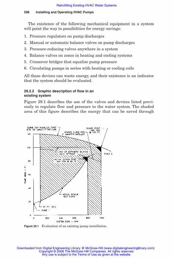
598 Installing and Operating HVAC Pumps
The existence of the following mechanical equipment in a systemwill point the way to possibilities for energy savings:
1. Pressure regulators on pump discharges
2. Manual or automatic balance valves on pump discharges
3. Pressure-reducing valves anywhere in a system
4. Balance valves on zones in heating and cooling systems
5. Crossover bridges that equalize pump pressure
6. Circulating pumps in series with heating or cooling coils
All these devices can waste energy, and their existence is an indicatorthat the system should be evaluated.
29.2.2 Graphic description of flow in anexisting system
Figure 29.1 describes the use of the valves and devices listed previ-ously to regulate flow and pressure to the water system. The shadedarea of this figure describes the energy that can be saved through
Figure 29.1 Evaluation of an existing pump installation.
Rishel_CH29.qxd 20/4/06 6:57 PM Page 598
Downloaded from Digital Engineering Library @ McGraw-Hill (www.digitalengineeringlibrary.com)Copyright © 2006 The McGraw-Hill Companies. All rights reserved.
Any use is subject to the Terms of Use as given at the website.
Retrofitting Existing HVAC Water Systems
Retrofitting Existing HVAC Water Systems 599
proper system analysis of a chilled water system and replacement ofthese mechanical devices with proper pump control.
The system head curve in Fig. 29.1 is typical for a variable-volumehot or chilled water system. The perfect pumping and control systemwould be one that tracks this curve at any load on the water system;in other words, there would be no overpressure at all.
The procedure for evaluating existing hot and chilled water systemscan best be demonstrated by setting up a typical system, generating thesystem head curve, and establishing the ways through which energy canbe saved. First, a typical chilled water system should be established.Assume:
1. The system is served by only one pump. This simplifies the proce-dures that follow. (Actual systems would normally be equippedwith two 500 gal/min pumps.) Original design for the pump was1000 gal/min at 100 ft with a 10-in-diameter impeller operating at1770 rev/min.
2. A flowmeter is available to read actual system flow in gallons perminute. (Note: If a flowmeter is not installed, an insertion-typeflowmeter could be hot tapped into the piping without draining thesystem.) A flowmeter is an essential instrument for monitoringsystem performance and should be part of the permanent instru-mentation.
3. Two-way valves are installed on all cooling coils.
The system head curve can be calculated by:
1. Determining the maximum pressure loss of the cooling coils, theircontrol valves, and associated piping. Usually this loss is in therange of 15 to 30 ft. This is point 1 in Fig. 29.1, or 20 ft, and is at ano-flow condition for the system.
2. Developing the maximum flow and head of the system (point 2).This can be achieved by reading the flowmeter for maximum flowunder full-load conditions. Suction and discharge pressures at thepump headers can be read to secure the head of the system at fullload. Existing pressure gauges should be checked for accuracy. Ifpressure gauges are not installed, new calibrated pressure gaugesshould be installed. On larger systems where wire-to-water effi-ciency is to be checked, a differential pressure transmitter shouldbe installed, as shown in Fig. 10.13a. The flow and head of point 2are assumed to be 800 gal/min and 85 ft, as shown in Fig. 29.1.
3. Determining the minimum flow for the system. In this case, it is100 gal/min.
Rishel_CH29.qxd 20/4/06 6:57 PM Page 599
Downloaded from Digital Engineering Library @ McGraw-Hill (www.digitalengineeringlibrary.com)Copyright © 2006 The McGraw-Hill Companies. All rights reserved.
Any use is subject to the Terms of Use as given at the website.
Retrofitting Existing HVAC Water Systems

600 Installing and Operating HVAC Pumps
4. If it is difficult to accomplish the measurements of point 2, a recal-culation of the system flow and head loss can be made based onactual operation of the system and known cooling loads.
5. Once points 1 and 2 are known, an approximate system head curvecan be developed from Eq. 9.3:
Ha � H1 � ��QQ
a
2
��1.9
� (H2�H1) (9.3)
where Ha � head at any point a on the system head curveH1 � head at point 1 on the curve (the maximum pressure loss
for any coil, its valve, and piping)H2 � head at point 2 on the curve (the maximum head of the
water system)Qa � flow at any point a on the system head curveQ2 � flow at point 2 (the maximum flow in the water system)
Note: The exponent 1.9 follows the Darcy-Wiesbach equation closerthan does an exponent of 2.0.
Although the system head curve thus generated does not representthe system head area of a water system as developed in Chap. 9, itcan be used as recommended in Chap. 9 to develop the approximatesystem head area.
29.2.3 Evaluation of existing pumps and motors
Just because HVAC pumps look dirty and beat up on the outside doesnot mean they should be replaced. As mentioned so often, HVACpump duty is easy duty. Before considering the replacement of exist-ing pumps, the pumps should be opened and the impellers and casingrings should be inspected. The inside diameter of the casing ringsshould checked to ensure that they are near their original diameter. Ifnot, they should be replaced. Their cost is much less than the cost ofnew pumps!
The great advances that have been made in electric motors requiresthat existing motors on pumps be checked very carefully. The princi-pal motor manufacturers and other companies have programs, includ-ing actual testing that provide accurate checking of these motors. Theamortization evaluation can be provided to demonstrate the value ofreplacing existing motors on an energy basis.
Do not change existing electric motors just because the pumps arebeing changed to variable speed. Most existing motors will operatevery well with contemporary variable-speed drives. This includes old
Rishel_CH29.qxd 20/4/06 6:57 PM Page 600
Downloaded from Digital Engineering Library @ McGraw-Hill (www.digitalengineeringlibrary.com)Copyright © 2006 The McGraw-Hill Companies. All rights reserved.
Any use is subject to the Terms of Use as given at the website.
Retrofitting Existing HVAC Water Systems
Retrofitting Existing HVAC Water Systems 601
T-frame, U-frame, and even wound rotor motors converted to induc-tion type by shorting the rotor windings. The variable-speed drivemanufacturers can verify the suitability of these old motors operatingwith their drives. The question is usually energy, not mechanical con-ditions, that favors the installation of new motors.
It must be remembered that variable-speed drives are current-rated devices, so their selection for existing motors must take intoconsideration the full-load ampere rating of these motors.
29.2.4 Evaluation of the number of pumps
Too often existing HVAC water systems, particularly chilled watersystems, are equipped with oversized pumps. In many cases, the sys-tems are equipped with pumps with 100 percent system capacity. Anyevaluation of existing pumps must include a review of the system’srequirements. The overall wire-to-water efficiency can be improvedin many cases by replacing these larger pumps with three 50 percentcapacity pumps. The wire-to-water efficiency evaluation that has beenprovided in this book is an excellent procedure to determine the valueof changing to multiple smaller pumps.
29.2.5 Control of existing pumps
This is one of the most overlooked tasks and sometimes the most diffi-cult task in evaluating an existing system. The type of pump controlmust be determined, from manual to the most complete control suchas wire-to-water efficiency.
Manual control of HVAC pumps is a holdover from the past andusually indicates possibilities of improving energy conservationthrough programming of the pump to match the system’s require-ments. Constant-speed pumps should be programmed on and off tomatch the system head curve or area as closely as possible. This willreduce the overpressure at lower loads on the water systems.
Variable-speed pumps must be programmed on and off as well andhave their speed controlled to achieve the highest wire-to-water effi-ciency. Most of this work has been covered in previous chapters.Existing systems, when retrofitted to variable speed, can be every bitas efficient as new systems with the correct approach to pump sizingand control.
Following are some system characteristics that should be observedwith the proper control of variable-speed pumps:
1. There should be very little overpressure on the system at mini-mum to 50 percent of total load on the water system.
Rishel_CH29.qxd 20/4/06 6:57 PM Page 601
Downloaded from Digital Engineering Library @ McGraw-Hill (www.digitalengineeringlibrary.com)Copyright © 2006 The McGraw-Hill Companies. All rights reserved.
Any use is subject to the Terms of Use as given at the website.
Retrofitting Existing HVAC Water Systems

602 Installing and Operating HVAC Pumps
2. There should be no discernible fluctuation in pump speed. If anoperator can hear or see HVAC variable-speed pumps changetheir speed, there are pump control problems. The rate of responsefor the control system may be too slow.
3. All equal-sized pumps should be operating within 15 rev/min ofeach other. If not, there again are control problems.
4. The controlling differential pressure transmitter should hold thedifferential pressure at this transmitter to within �1⁄2 to 1 ft ofhead. Fluctuation of the pressure beyond 1 ft from the set pointindicates insufficient control.
29.3 Evaluation of Existing Procedures
Once the system head curve or area is developed, a figure similar toFig. 29.1 can be developed for the system. If the shaded area is appre-ciable, there exist possibilities for energy savings. The engineers forsystem design and operation should then continue their evaluation ofthe water system to determine actual energy savings by several pro-cedures; some systems may require several such procedures:
1. Eliminate some or all of the existing mechanical devices such asbalancing or pressure-reducing valves.
2. Trim existing pump impellers.
3. Change to variable-speed pumps.
4. Determine if the pump programming is correct. Are the rightnumber of pumps being operated at all system loads?
The amount of overpressure that is occurring at the minimum flowpoint will help determine what procedure should be used. In Fig. 29.1,this overpressure is 120�21, or 99 ft. The existing balance or pressure-regulating valves may have been used to control this overpressure.Removing them may cause operating problems without correcting thepumps as well.
29.3.1 Trimming the pump impeller
The first step that should be considered is to trim the pump impellerto provide the maximum flow and head of 800 gal /min at 85 ft ofhead. The dotted curve in Fig. 29.1 describes the resulting head-flowcurve for the pump.
Care should be taken in trimming the pump impeller. The affinitylaws cannot be taken for granted in trimming this impeller, since the
Rishel_CH29.qxd 20/4/06 6:57 PM Page 602
Downloaded from Digital Engineering Library @ McGraw-Hill (www.digitalengineeringlibrary.com)Copyright © 2006 The McGraw-Hill Companies. All rights reserved.
Any use is subject to the Terms of Use as given at the website.
Retrofitting Existing HVAC Water Systems
Retrofitting Existing HVAC Water Systems 603
system contains 20 ft of constant head across its cooling coils andtheir control valves and associated piping. Equation 10.1 should beused to compute the impeller diameter. This is done by finding theequivalent operating point on the present pump curve.
Q3 ����� H�3� (10.1)
where Q2 and H2 � maximum flow and head conditions of 800 gal/minand 85 ft
Q3 and H3 � unknown equivalent points on the pump head-flowcurve
By trial and error, values of H3 are inserted in the preceding equa-tion until Q3 and H3 fall on the known pump head-flow curve for the10-in-diameter impeller operating at 1770 rev/min. The equivalentoperating point, after several trials, is determined from the equationto be Q3 � 889 gal/min and H3 � 105 ft.
Since the diameter varies directly with the flow, the new diameteris 800 � 889 10, or 9.0 in. If the affinity laws had been used directlywithout recognition of the system head curve, the impeller diameterwould be 800 � 1000 10, or 8.0 in. The impeller would therefore beundercut and would not have sustained the desired point of 800gal/min at 85 ft of head.
Equation 10.1 should always be used for trimming impellers, not theratio of flows in gallons per minute from the affinity laws themselves.Also, it must be remembered that the trimmed impeller must bereplaced if the original design condition of 1000 gal/min at 100 ft isever reached by the system in the future.
Trimming the impeller reduces the pressure from 120 ft at shutoffto 98 ft. At minimum flow of 100 gal/min, the head will be 98 ft and theoverpressure 98�21, or 77 ft. This may still be too much overpressurefor the coil control valves. The trimmed impeller has saved energy, butmuch is still to be saved by the use of a variable-speed pump. All theshaded area below the dotted curve for the trimmed pump can be savedby changing the original 10-in-diameter impeller to variable speed.
29.3.2 Changing to a variable-speed pump
The trimming of the impeller requires some careful calculations toensure that the correct impeller diameter is selected. The variable-speed pump requires none of these calculations. Instead of cutting theimpeller, the pump will run at a lesser speed to maintain the desired
Q22
�H2
Rishel_CH29.qxd 20/4/06 6:57 PM Page 603
Downloaded from Digital Engineering Library @ McGraw-Hill (www.digitalengineeringlibrary.com)Copyright © 2006 The McGraw-Hill Companies. All rights reserved.
Any use is subject to the Terms of Use as given at the website.
Retrofitting Existing HVAC Water Systems
604 Installing and Operating HVAC Pumps
condition of 800 gal/min at 85 ft. At this point, from the preceding cal-culations, the pump speed will be 800 � 889 1770, or 1593 rev/min.
There are several advantages for the variable-speed pump overtrimming the impeller.
1. The original 10-in impeller can be retained.
2. Since the 10-in impeller is retained, future conditions of 1000gal/min at 100 ft can be achieved.
3. No overpressure will occur at any load on the system because thepump will merely slow down to the needed speed to maintain thehead required by the system head curve.
4. If the system has a broad system head area that is difficult tocompute, the variable-speed pump, if properly controlled, willautomatically adjust to this variable-head condition.
5. All the energy shown by the shaded area in Fig. 29.1 will be saved.Additional energy will be saved because the wire-to-water efficiencyof the variable-speed pump will be much greater than that for theconstant-speed pump.
It is up to the designer to run the calculations and determine theenergy and maintenance savings for the variable-speed pump as com-pared with a pump with a trimmed impeller.
Many public utilities in the United States are offering rebates forprograms aimed at energy savings. Often, the installation of variable-speed drives qualifies the owner for these rebates. These rebates mustbe factored into the costs for the conversion to the variable-speedpump.
There are other conditions in the system that must be considered,whether the pump impeller is trimmed or the pump is converted tovariable speed. For example,
1. All three-way valves on heating or cooling coils should be convertedto two-way valves. Three-way valves should not be converted totwo-way valves by shutting off their bypasses without a very care-ful evaluation of the maximum pump head that can be imposed onthem. The valves should be checked to ensure that they will oper-ate satisfactorily as two-way valves.
2. Differential pressure-control transmitters should be installed inaccordance with Chap. 8 to control the variable-speed pump.
3. Adequate instrumentation should be provided in the new systemto ensure that projected energy savings are achieved.
Rishel_CH29.qxd 20/4/06 6:57 PM Page 604
Downloaded from Digital Engineering Library @ McGraw-Hill (www.digitalengineeringlibrary.com)Copyright © 2006 The McGraw-Hill Companies. All rights reserved.
Any use is subject to the Terms of Use as given at the website.
Retrofitting Existing HVAC Water Systems

Retrofitting Existing HVAC Water Systems 605
29.3.3 Control and drives for modified systems
When variable-speed drives are added to existing pumps on a watersystem, some care must be taken in evaluating the electrical powerinstallation. For example,
1. A study of the power feeds to each motor should be made to ensurethat they are physically adequate for any new motors. An appre-ciable savings can be made if they can be reused, particularly ifthey are buried in the cement slab.
2. Existing magnetic starters should be evaluated for use as emer-gency standby in event of variable-speed drive failure. This couldeliminate the need for new standby starters.
3. Since there is some power loss in the variable-speed drives withtheir approximate efficiency of 95 percent, the total power con-sumption of the drives should be checked against the capacity ofthe existing power supply. The maximum ampere rating for thedrives should be considered in this evaluation.
A completely integrated control and power center as described inFig. 26.8 should be considered for existing pumps. This provides aconcentrated location of all the switchgear and controls needed forproper functioning of the variable-speed pumps.
29.4 System Configuration Modification
Too often boilers or chillers are added because there is a lack of suffi-cient hot or chilled water. Inefficient water distribution systems canbe the cause, not boiler or chiller capacity. Before such equipment isadded,
1. The heating and cooling loads imposed on these systems should berecalculated to verify that actual boiler or chiller capacity is trulyneeded.
2. The return water temperatures of these systems should be checkedto see how close they are to the design return temperatures. Forexample, assume that a chilled water system was designed for44°F supply and 56°F return temperatures, and the actual returntemperature is 52°F. The pumping rate from Eq. 9.2 should be24 � 12, or 2 gal/min per ton; instead, it is 24 � 8, or 3 gal/min perton. This indicates that work should be done to improve the waterdistribution system before additional chiller capacity is considered.
Rishel_CH29.qxd 20/4/06 6:57 PM Page 605
Downloaded from Digital Engineering Library @ McGraw-Hill (www.digitalengineeringlibrary.com)Copyright © 2006 The McGraw-Hill Companies. All rights reserved.
Any use is subject to the Terms of Use as given at the website.
Retrofitting Existing HVAC Water Systems
606 Installing and Operating HVAC Pumps
Correcting or changing central pumps may be an easy task com-pared with changing system piping to achieve the best possiblearrangement with the lowest energy consumption. Many existing sys-tems for hot and chilled water have three-way valves and are there-fore constant-volume systems that may have great waste in pumpingenergy. Changing the three-way valves to two-way valves makes thesystem variable volume, not constant volume. Boilers and chillersthat require constant flow through them must be taken care of withthe proper type and location of a bypass.
29.4.1 Changing constant-volume systemsto variable volume
Existing systems that are changed from constant volume with three-way coil control valves to variable volume with two-way coil valvesmust accommodate chillers or boilers that may require constant flowthrough them. One procedure is to install new primary pumps for thechillers and make the existing constant-speed pumps into secondarypumps by converting them to variable speed. This procedure is oftendifficult due to lack of space for the new pumps and the amount ofrepiping that must be done to produce a primary-secondary pumpingsystem.
An alternative design for making the system variable volume is toconvert the existing pumps to variable speed and provide the meansto ensure adequate flow through the chillers or boilers. This is doneby adding a bypass with a control valve in it, as described in Fig. 15.4.This works most effectively on systems with three or more chillers. Allthe coils should be equipped with two-way control valves, and differ-ential pressure transmitters should be located as recommended inChap. 10.
Following is a description of the operation of this system:
1. The speed of the chiller pumps is controlled by the differentialpressure transmitters, maintaining the desired differential pres-sure required by the cooling coils.
2. Minimum flow in the chillers is maintained.
Contemporary chillers with digital control of their chilled watertemperature may allow variable flow in their evaporators. The pipingarrangement in Fig. 15.3b can be utilized; the only difference is thatthe flow set point for the bypass is reduced to the minimum allowableflow for the evaporator. This procedure has some significant advan-tages over primary-secondary pumping because space, first cost, andpossibly energy are usually saved with such installations.
Rishel_CH29.qxd 20/4/06 6:57 PM Page 606
Downloaded from Digital Engineering Library @ McGraw-Hill (www.digitalengineeringlibrary.com)Copyright © 2006 The McGraw-Hill Companies. All rights reserved.
Any use is subject to the Terms of Use as given at the website.
Retrofitting Existing HVAC Water Systems

Retrofitting Existing HVAC Water Systems 607
29.4.2 Changing pumped coil systems to variable-speed pumping
Some existing systems may have been designed with coil pumps withbypasses, as shown in Figs. 8.5b and 8.6b. This is a very inefficientarrangement because of the piping losses and the efficiency of thepump and motor themselves. So often, such pumps are small circulatorswith very low wire-to-water efficiencies for the pump and motor. Suchpumped coil systems can be converted to variable speed by installingtwo-way valves on the coils and using variable-speed pumps at a cen-tral or building location. The work in redesign and retrofit is usuallyworthwhile in energy savings. To verify this effort, the energy con-sumption of the small circulators should be checked along with theirmaintenance record.
Pumped coils with circulators in the bypass, as described in Fig. 8.7,should not be confused with the preceding pumped coil systems. If thecirculator is in the bypass, it was installed there for freeze protectionor for eliminating laminar flow in the coil.
29.4.3 Variable-volume systems with bypass valves
Many chilled and hot water systems were installed with constant-speed pumps and utilized bypass valves to accommodate the chillerflow and to achieve some form of variable volume. The problem withthis type of system, in terms of energy, is that all the water must bepumped at a head equal to or greater than the design head.
These bypass valve systems should be changed to variable primarypumping, as described in Chap. 15.
29.4.4 Adding variable-volume systems to existing systems
The retrofit of existing systems, particularly large, multiple-buildinginstallations, can be prohibitive in cost to convert to contemporarypumping and control systems. These systems require a great amountof thought and evaluation to achieve the most economical plan ofoperation. This does not mean that additions to these older systemscannot be made that utilize efficient variable-speed pumping.
There are several rules that can be followed that may help theplanning for such complex installations:
1. Do not install variable-speed pumps centrally with constant-speedpumps operating on their discharges unless the constant-speedpumps are located in chiller or building bypasses.
Rishel_CH29.qxd 20/4/06 6:57 PM Page 607
Downloaded from Digital Engineering Library @ McGraw-Hill (www.digitalengineeringlibrary.com)Copyright © 2006 The McGraw-Hill Companies. All rights reserved.
Any use is subject to the Terms of Use as given at the website.
Retrofitting Existing HVAC Water Systems

608 Installing and Operating HVAC Pumps
2. Variable-speed pumps can be installed in the discharge pipingfrom existing constant-speed pumps if (a) the variable-speedpumps are controlled properly with differential pressure con-trollers, and (b) a bypass is provided around the variable-speedpumps to accommodate the constant-speed pumps under reducedload conditions as shown in Fig. 15.6c.
29.4.5 Converting to distributed pumping
Some existing campus systems that contain tertiary pumping can beconverted to distributed pumping by eliminating existing secondarypumps. This requires extensive evaluation, but it may pay off in greatsavings in energy and may eliminate the need for additional chillersthat are required because of greater system flows but not because ofadditional tonnage on the system.
If the coil control valves are to be converted at the same time fromthree-way to two-way design, a sizable amount of money may be savedby the reduction in maximum differential pressure across these valvesthat is achieved by distributed pumping.
29.4.6 Combining multiple-chiller plants
There are a number of small colleges and other campus-type installa-tions that have chillers in individual buildings with a total tonnagemuch greater than that required by the entire system. By combiningthe chiller plants into one system, better standby capacity will beprovided, and the running chillers will operate at a much higher effi-ciency. A study should be made to consider combining the chillers, aswas described in Fig. 14.10. Appreciable energy savings may beachieved, along with greater flexibility in the selection of operatingchillers.
29.5 Summation
A great amount of energy can be saved through the use of contempo-rary digital electronic procedures on existing HVAC water systems.The preceding examples cover only a small part of all the existingchilled and hot water systems that should be retrofitted. Reiterating,systems should be evaluated if they depend on any of the mechanicaldevices listed earlier to control system pressure or to move waterthrough the various components of the system.
At present, the program for changing refrigerants in chillers offersopportunities to update and improve the pumping efficiency of thesesystems. When an analysis is made of the pumping programs, it is
Rishel_CH29.qxd 20/4/06 6:57 PM Page 608
Downloaded from Digital Engineering Library @ McGraw-Hill (www.digitalengineeringlibrary.com)Copyright © 2006 The McGraw-Hill Companies. All rights reserved.
Any use is subject to the Terms of Use as given at the website.
Retrofitting Existing HVAC Water Systems

Retrofitting Existing HVAC Water Systems 609
often found that reprogramming the chillers will achieve a lower kilo-watt per ton figure that yields great energy savings. Older chillerinstallations accommodated chilled water pumping systems thatreduced the efficiency of the chillers as well as the pumping. The effortto improve overall system efficiency should, therefore, include evalua-tion of the chiller operation as well as that of the pumping system.
29.6 Bibliography
Peterson, K., Variable Primary Flow, Central Plant Conversion, HPAC Magazine, March 2004.Avery, G., Improving the Efficiency of Chilled Water Plants, ASHRAE Journal, May 2001.
Rishel_CH29.qxd 20/4/06 6:57 PM Page 609
Downloaded from Digital Engineering Library @ McGraw-Hill (www.digitalengineeringlibrary.com)Copyright © 2006 The McGraw-Hill Companies. All rights reserved.
Any use is subject to the Terms of Use as given at the website.
Retrofitting Existing HVAC Water Systems

Rishel_CH29.qxd 20/4/06 6:57 PM Page 610
Downloaded from Digital Engineering Library @ McGraw-Hill (www.digitalengineeringlibrary.com)Copyright © 2006 The McGraw-Hill Companies. All rights reserved.
Any use is subject to the Terms of Use as given at the website.
Retrofitting Existing HVAC Water Systems

Chapter
611
30Summary of HVAC
Energy Evaluations
30.1 Review of Efficiencies
Much has been offered here in the design and operation of HVACwater systems. Configuration of these systems as well as methods ofoperation that have been provided should aid in achieving optimalenergy consumption for them. Although no final design can be offeredfor a specific system, a number of equations have been delineated forthe various efficiencies of an HVAC water system. These equationshave been kept at the level of algebra, not higher mathematics, inorder to render easily the conversion of this information to personalcomputer programs that fit the language and format most familiar tothe reader. As mentioned in Chap. 1, computer programs are nowavailable that will accommodate almost any equation.
It is obvious that this book is but a guidepost in the endeavor toproduce more efficient HVAC water systems. Some of the efficiencyequations included are for equipment, whereas others are for part orall of a water system. The individual equipment efficiencies are forboilers, chillers, motors, pumps, and variable-speed drives. All theactual efficiencies for this equipment are determined, to a largeextent, by their manufacturers.
30.2 System Efficiencies
Two efficiencies are included that are composites of equipment effi-ciencies; these are wire-to-water efficiency for pumping systems andoverall kilowatts per ton for chilled water plants. The equations arerepeated here:
Rishel_CH30.qxd 20/4/06 6:58 PM Page 611
Downloaded from Digital Engineering Library @ McGraw-Hill (www.digitalengineeringlibrary.com)Copyright © 2006 The McGraw-Hill Companies. All rights reserved.
Any use is subject to the Terms of Use as given at the website.
Source: HVAC Pump Handbook

612 Installing and Operating HVAC Pumps
Wire-to-water efficiency � �53.
Q08
�
�
HkW
� (10.2)
Chiller plant kW/ton � (14.4)
One other system efficiency is for the use of energy in a hot orchilled water system, and this is explained in Chap. 8:
System efficiency WS�
� �Ke �
K10
i
0%� (8.3)
Alternate pumping efficiencies that may be easier to use in systemanalysis are as follows. For chilled water:
kW/100 tons � (8.4)
or
kW/100 tons � (8.5)
For hot water:
kW/1000 mbh � (8.6)
or
kW/1000 mbh � (8.7)
The actual equations that should be used on a specific installationdepend on the instrumentation that is available to provide the neededanalog signals.
30.3 Purpose of Efficiencies
All these equations have two purposes: (1) to aid the designer in thedevelopment of efficient water systems and (2) to provide the managerof HVAC systems with operating tools that ensure optimal systemoperation.
The most important efficiency in this book for chilled water systemsis that for chiller plant kilowatts per ton (Eq. 14.4). This efficiency givesplant operators and managers an overall insight about the efficiency of
124,700 � �pump kW���gal/min � �T (°F) � �
23.48 � H���P
�� E
�� �T (°F) � �
2400 � �pump kW���gal/min � �T (°F)
0.452 � H��P
�� E� � �T (°F)
�equipment kW���tons of cooling on system
Rishel_CH30.qxd 20/4/06 6:58 PM Page 612
Downloaded from Digital Engineering Library @ McGraw-Hill (www.digitalengineeringlibrary.com)Copyright © 2006 The McGraw-Hill Companies. All rights reserved.
Any use is subject to the Terms of Use as given at the website.
Summary of HVAC Energy Evaluations
Summary of HVAC Energy Evaluations 613
plant operation. The cost of this instrumentation is relatively smallfor medium and large chiller plants. More can be gained from thisefficiency than from any other system or equipment efficiency forchilled water operations.
Not all these equations will be useful for every HVAC water sys-tem. The size and economics of each application will determine theirvalue. Systems with high energy costs will justify their use more thansystems with low energy costs. It is in the province of the designer todetermine which of them will aid in the design and operation of spe-cific HVAC water systems. Obviously, the first cost of the instrumen-tation and electronics will have a bearing on which efficiencies areutilized for a particular installation.
Generally, it is not feasible to have one overall efficiency for anHVAC water system, since there are several uses of energy in such asystem. At this date, there does not appear to be any interest in suchan efficiency. Also, some systems use several sources of energy, whichmakes difficult the development of an overall efficiency. The objectiveof the designer now should be to determine which of these expressionsof efficiency will establish and sustain the operating efficiency ofHVAC water systems.
30.4 Sustained System and EquipmentEfficiencies
Sustaining operating efficiency is as important as the original equip-ment or system efficiencies. In the past, the difficulty in maintaininganalog instrumentation often resulted in loss of the equipment thatindicated efficiency of operation. Sometimes the instrumentation wasnot operator friendly, so it was neglected and not maintained. Contem-porary digital instrumentation is relatively maintenance-free; withproper instructions at the beginning, this instrumentation should pro-vide continued indication of operating conditions for the operatorsand managers of HVAC energy plants. The great amount of data stor-age capacity of contemporary computer systems enables operators tomaintain detailed records on operating parameters such as coefficientof performance, kilowatts per ton, and wire-to-water efficiency; sus-tained high efficiencies are now achievable through the interpretationof this information.
30.5 Summary
The emphasis in this book has been on making available the variousexpressions of efficiency in a form useable to the designer and system
Rishel_CH30.qxd 20/4/06 6:58 PM Page 613
Downloaded from Digital Engineering Library @ McGraw-Hill (www.digitalengineeringlibrary.com)Copyright © 2006 The McGraw-Hill Companies. All rights reserved.
Any use is subject to the Terms of Use as given at the website.
Summary of HVAC Energy Evaluations
614 Installing and Operating HVAC Pumps
operator. The elimination of older types of water system flow controlsuch as balance valves, pressure-regulating valves, and most cross-over bridges should be urged continuously to direct the designertoward the use of digital processes that aid in the rapid design ofhigh-quality HVAC water systems. It is obvious from all these simplealgebraic equations that they are tools that can be inserted easily intocomputer programs to aid the efficient design and operation of HVACwater systems.
Every energy-consuming device that is proposed for an HVACwater system should be evaluated to see if it can be eliminated bychanging the water system design. The information, software, designexpertise, and equipment are now available to achieve highly efficientwater systems for the HVAC industry.
Rishel_CH30.qxd 20/4/06 6:58 PM Page 614
Downloaded from Digital Engineering Library @ McGraw-Hill (www.digitalengineeringlibrary.com)Copyright © 2006 The McGraw-Hill Companies. All rights reserved.
Any use is subject to the Terms of Use as given at the website.
Summary of HVAC Energy Evaluations

Chapter
615
31The Modern Two-Pipe
Heating and Cooling System
Chapters 31 and 32 on two-pipe heating and cooling systems andadvanced heat recovery procedures were the last chapters written inorder to secure the latest information on these subjects and to empha-size their importance in energy conservation during the years tocome. Both of these chapters should be reviewed by anyone concernedabout energy in schools and larger facilities in general.
Although pumps are not the major topic in these chapters, theseenergy-saving procedures would be difficult without properly con-trolled, variable-speed pumps.
31.1 Introduction
The two-pipe concept uses the same distribution network for heatingin the winter and cooling in the summer. It is an old idea, almost asold as hydronic cooling. It is simple, cost effective, and logical. As thename implies, there is a single supply line and a single return linethat run hot water in the winter and chilled water in the summer, asopposed to a four-pipe system that has two dedicated hot water linesand two dedicated chilled water lines. The two-pipe system uses thesame lines to “changeover” from heating to cooling and vice-versa tomeet the demands of the building. It was a common system in the for-ties, fifties, and sixties but was generally relegated to the scrap heapof history due to inflexibility and chronic complaints about occupantcomfort. The most troublesome times would be spring and fall when“warm days, cool nights” is a common scenario, and when the out-side temperature is around 60°F, not really warm enough to run air-conditioning or cool enough to run the heating. When two-pipe sys-tems were used, it was generally on projects with limited budgets.
Rishel_CH31.qxd 20/4/06 6:58 PM Page 615
Downloaded from Digital Engineering Library @ McGraw-Hill (www.digitalengineeringlibrary.com)Copyright © 2006 The McGraw-Hill Companies. All rights reserved.
Any use is subject to the Terms of Use as given at the website.
Source: HVAC Pump Handbook
616 Installing and Operating HVAC Pumps
The traditional two-pipe paradigm called for a seasonal changeover.Cooling would operate all summer, changing over to heating in thefall, and changing back to cooling again in the spring. Changeoverwas typically a time and energy intensive effort. So once a cooling orheating mode was “on”, it was on continuously until the next season.If there was a warm winter day or a cool summer night, the buildingoccupants suffered. Usually, when an idea gets relegated to thescrap heap of history, it is for valid reasons. In this case, the conceptof seasonal changeover was just not compatible with the expecta-tions of a modern, comfortable building environment.
Other concerns about two-pipe systems were (are):
• How do you design for load variations?
• When does the system changeover? How long does it take and howcomplex is the process?
• Is the safety and longevity of the boilers and chillers impacted bywater temperatures, especially during changeover?
• Isn’t energy wasted during changeover?
• How do two-pipe systems control humidity, since there is no oppor-tunity to reheat?
The first cost benefit of two-pipe versus four-pipe is about $3 persquare foot (2006 dollars). Given the average cost of new school con-struction in the Midwest at around $120 per SF ($30 per SF HVAC),most engineers and many building owners, operating under the old par-adigm, would contend that the operational difficulties and potentialcomfort issues are not worth the savings. But, the assumed two-pipeproblems can be solved, raising room comfort to meet the expectations ofmodern educational spaces, and realizing significant first cost savings.
31.2 The Renaissance
The “modern two-pipe system” originated in New Albany, Indiana, in1993. New Albany-Floyd County Consolidated School Corporation oper-ates 20 buildings, serving about 11,000 students in grades kindergartenthrough 12. In 1993, 17 of the buildings were air conditioned, which isgenerally considered an educational necessity in the hot, humid OhioRiver Valley. Parents of students from the three non–air-conditionedbuildings petitioned the school board for “environmental equity.”Emergency funding generated insufficient dollars to install a traditionalfour-pipe system. The owner accepted the idea of a two-pipe solution, butchallenged their engineer, Tom Durkin, to solve the age-old problems.
Rishel_CH31.qxd 20/4/06 6:58 PM Page 616
Downloaded from Digital Engineering Library @ McGraw-Hill (www.digitalengineeringlibrary.com)Copyright © 2006 The McGraw-Hill Companies. All rights reserved.
Any use is subject to the Terms of Use as given at the website.
The Modern Two-Pipe Heating and Cooling System
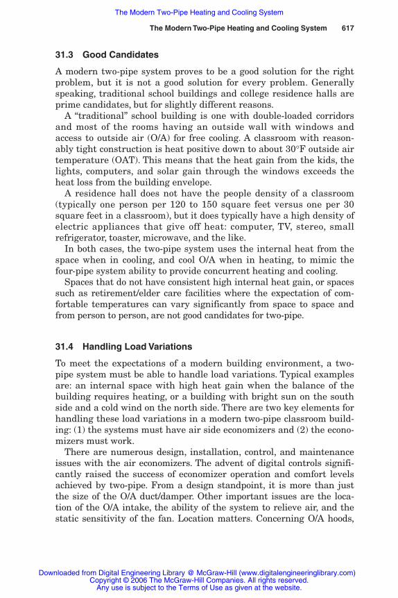
The Modern Two-Pipe Heating and Cooling System 617
31.3 Good Candidates
A modern two-pipe system proves to be a good solution for the rightproblem, but it is not a good solution for every problem. Generallyspeaking, traditional school buildings and college residence halls areprime candidates, but for slightly different reasons.
A “traditional” school building is one with double-loaded corridorsand most of the rooms having an outside wall with windows andaccess to outside air (O/A) for free cooling. A classroom with reason-ably tight construction is heat positive down to about 30°F outside airtemperature (OAT). This means that the heat gain from the kids, thelights, computers, and solar gain through the windows exceeds theheat loss from the building envelope.
A residence hall does not have the people density of a classroom(typically one person per 120 to 150 square feet versus one per 30square feet in a classroom), but it does typically have a high density ofelectric appliances that give off heat: computer, TV, stereo, smallrefrigerator, toaster, microwave, and the like.
In both cases, the two-pipe system uses the internal heat from thespace when in cooling, and cool O/A when in heating, to mimic thefour-pipe system ability to provide concurrent heating and cooling.
Spaces that do not have consistent high internal heat gain, or spacessuch as retirement/elder care facilities where the expectation of com-fortable temperatures can vary significantly from space to space andfrom person to person, are not good candidates for two-pipe.
31.4 Handling Load Variations
To meet the expectations of a modern building environment, a two-pipe system must be able to handle load variations. Typical examplesare: an internal space with high heat gain when the balance of thebuilding requires heating, or a building with bright sun on the southside and a cold wind on the north side. There are two key elements forhandling these load variations in a modern two-pipe classroom build-ing: (1) the systems must have air side economizers and (2) the econo-mizers must work.
There are numerous design, installation, control, and maintenanceissues with the air economizers. The advent of digital controls signifi-cantly raised the success of economizer operation and comfort levelsachieved by two-pipe. From a design standpoint, it is more than justthe size of the O/A duct/damper. Other important issues are the loca-tion of the O/A intake, the ability of the system to relieve air, and thestatic sensitivity of the fan. Location matters. Concerning O/A hoods,
Rishel_CH31.qxd 20/4/06 6:58 PM Page 617
Downloaded from Digital Engineering Library @ McGraw-Hill (www.digitalengineeringlibrary.com)Copyright © 2006 The McGraw-Hill Companies. All rights reserved.
Any use is subject to the Terms of Use as given at the website.
The Modern Two-Pipe Heating and Cooling System
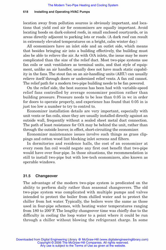
618 Installing and Operating HVAC Pumps
location away from pollution sources is obviously important, and loca-tions that yield cool air for economizers are equally important. Avoidlocating hoods on dark-colored roofs, in small enclosed courtyards, or inareas directly adjacent to parking lots or roads. (A dark roof can resultin extremely elevated temperatures on a bright, calm winter day.)
All economizers have an inlet side and an outlet side, which meansthat besides bringing air into a building effectively, the building mustalso be able to relieve the air. As with O/A inlets, the issue may be morecomplicated than the size of the relief duct. Most two-pipe systems usefan coils or unit ventilators as terminal units, and that style of equip-ment, unlike an air handler, usually does not have much static capabil-ity in the fans. The stout fan on an air-handling units (AHU) can usuallyrelieve itself through doors or undersized relief vents. A fan coil cannot.The relief path for a modern two-pipe building needs to be fan powered.
On the relief side, the best success has been had with variable-speedrelief fans controlled by average economizer position rather thanbuilding pressure. Pressure needs to be less than 0.05 in wc in orderfor doors to operate properly, and experience has found that 0.05 in isjust too low a number to try to control to.
Economizer installation details are very important, especially withunit vents or fan coils, since they are usually installed directly against anoutside wall, frequently without a sealed sheet metal duct connection.The path of least resistance for O/A may be behind the unit, rather thanthrough the outside louver, in effect, short-circuiting the economizer.
Economizer maintenance issues involve such things as grass clip-pings and cotton wood lint blocking inlet screens and filters.
In dormitories and residence halls, the cost of an economizer atevery room fan coil would negate any first cost benefit that two-pipewould have over four-pipe. In those situations, the recommendation isstill to install two-pipe but with low-tech economizers, also known asoperable windows.
31.5 Changeover
The advantage of the modern two-pipe system is predicated on theability to perform daily rather than seasonal changeovers. The oldtwo-pipe system was complicated with multiple pumps and valvesintended to protect the boiler from chilled water and to protect thechiller from hot water. Typically, the boilers were the same as thoseused in four-pipe schemes, with heating water temperatures rangingfrom 180 to 200°F. The lengthy changeover time was chiefly due to thedifficulty in cooling the loop water to a point where it could be runthrough a chiller without blowing the refrigerant charge. In some
Rishel_CH31.qxd 20/4/06 6:58 PM Page 618
Downloaded from Digital Engineering Library @ McGraw-Hill (www.digitalengineeringlibrary.com)Copyright © 2006 The McGraw-Hill Companies. All rights reserved.
Any use is subject to the Terms of Use as given at the website.
The Modern Two-Pipe Heating and Cooling System
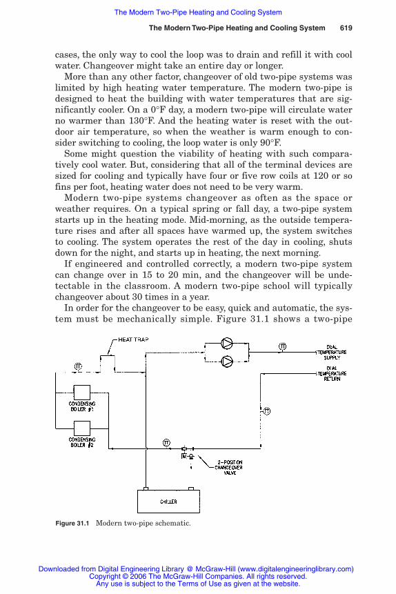
cases, the only way to cool the loop was to drain and refill it with coolwater. Changeover might take an entire day or longer.
More than any other factor, changeover of old two-pipe systems waslimited by high heating water temperature. The modern two-pipe isdesigned to heat the building with water temperatures that are sig-nificantly cooler. On a 0°F day, a modern two-pipe will circulate waterno warmer than 130°F. And the heating water is reset with the out-door air temperature, so when the weather is warm enough to con-sider switching to cooling, the loop water is only 90°F.
Some might question the viability of heating with such compara-tively cool water. But, considering that all of the terminal devices aresized for cooling and typically have four or five row coils at 120 or sofins per foot, heating water does not need to be very warm.
Modern two-pipe systems changeover as often as the space orweather requires. On a typical spring or fall day, a two-pipe systemstarts up in the heating mode. Mid-morning, as the outside tempera-ture rises and after all spaces have warmed up, the system switchesto cooling. The system operates the rest of the day in cooling, shutsdown for the night, and starts up in heating, the next morning.
If engineered and controlled correctly, a modern two-pipe systemcan change over in 15 to 20 min, and the changeover will be unde-tectable in the classroom. A modern two-pipe school will typicallychangeover about 30 times in a year.
In order for the changeover to be easy, quick and automatic, the sys-tem must be mechanically simple. Figure 31.1 shows a two-pipe
The Modern Two-Pipe Heating and Cooling System 619
Figure 31.1 Modern two-pipe schematic.
Rishel_CH31.qxd 20/4/06 6:58 PM Page 619
Downloaded from Digital Engineering Library @ McGraw-Hill (www.digitalengineeringlibrary.com)Copyright © 2006 The McGraw-Hill Companies. All rights reserved.
Any use is subject to the Terms of Use as given at the website.
The Modern Two-Pipe Heating and Cooling System
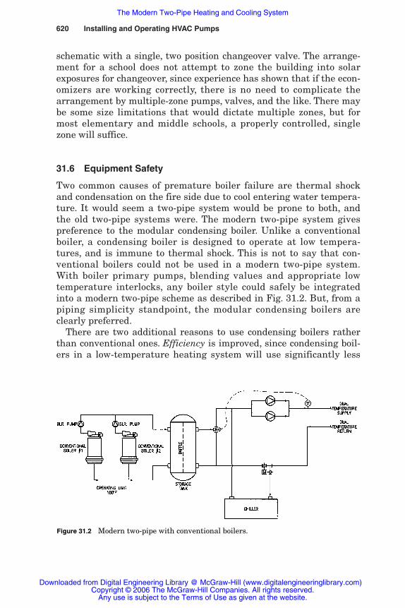
schematic with a single, two position changeover valve. The arrange-ment for a school does not attempt to zone the building into solarexposures for changeover, since experience has shown that if the econ-omizers are working correctly, there is no need to complicate thearrangement by multiple-zone pumps, valves, and the like. There maybe some size limitations that would dictate multiple zones, but formost elementary and middle schools, a properly controlled, singlezone will suffice.
31.6 Equipment Safety
Two common causes of premature boiler failure are thermal shockand condensation on the fire side due to cool entering water tempera-ture. It would seem a two-pipe system would be prone to both, andthe old two-pipe systems were. The modern two-pipe system givespreference to the modular condensing boiler. Unlike a conventionalboiler, a condensing boiler is designed to operate at low tempera-tures, and is immune to thermal shock. This is not to say that con-ventional boilers could not be used in a modern two-pipe system.With boiler primary pumps, blending values and appropriate lowtemperature interlocks, any boiler style could safely be integratedinto a modern two-pipe scheme as described in Fig. 31.2. But, from apiping simplicity standpoint, the modular condensing boilers areclearly preferred.
There are two additional reasons to use condensing boilers ratherthan conventional ones. Efficiency is improved, since condensing boil-ers in a low-temperature heating system will use significantly less
620 Installing and Operating HVAC Pumps
Figure 31.2 Modern two-pipe with conventional boilers.
Rishel_CH31.qxd 20/4/06 6:58 PM Page 620
Downloaded from Digital Engineering Library @ McGraw-Hill (www.digitalengineeringlibrary.com)Copyright © 2006 The McGraw-Hill Companies. All rights reserved.
Any use is subject to the Terms of Use as given at the website.
The Modern Two-Pipe Heating and Cooling System

gas than a conventional boiler. The other is size, since condensing boil-ers are much smaller and require a boiler room about half the size ofa conventional boiler.
Another important boiler longevity requirement is to preventchilled water from entering the boiler circuit when the system is incooling. While the condensing boilers are made to handle cold waterwhen they are firing, and while condensing boilers are insulated, theinsulation does not have a vapor barrier. If chilled water at any tem-perature were to get into the boilers, the boilers will sweat and ruston the outside. In Figure 31.1, the single changeover valve isolatesthe boilers on the inlet side, and a “heat trap” isolates the boilers onthe outlet side. The heat trap is a vertical piece of pipe that uses thedifferential densities of cold and warm water to act like an isolationvalve. Care must be exercised in layout of the piping to avoid turbu-lence-induced flow backwards into the boilers. The boiler pipingneeds to be on the branch of the tee, and the tee should be located inthe same way a flowmeter would be, with straight pipe both up anddownstream.
The safety of chillers in a modern two-pipe scheme is also of lessconcern than in a traditional two-pipe, primarily because the maxi-mum heating water temperature is much lower, 130°F vs. 180°F. Thelower temperatures equate to refrigerant pressures comfortably belowchiller relief device settings. Boiler operating and high limit settingsmust reflect this line of thinking.
Newer chillers have their own digital controllers, both to protect theequipment from damage and to load the chillers smoothly and slowly.This is important because, at changeover, the chiller will receive warmwater, and if unchecked, it may exceed its allowable power input.
Another important equipment safety question is: What happens ifcontrol power is lost? Since the most important equipment safetyissues are cold water in the boilers and hot water in the chillers, thechangeover valve (or valves) must never be spring driven. Since it isimpossible to predict what mode the system will be in when powerfails, a “fail safe” position cannot be defined. Changeover valves mustbe “last position fail (power to open, power to close).”
31.7 Energy Concerns
ASHRAE Standard 90.1 (2001) states:
6.3.2.2.2: Two-Pipe Changeover System. Systems that use a commondistribution system to supply both heated and chilled water isacceptable provided all of the following are met:
The Modern Two-Pipe Heating and Cooling System 621
Rishel_CH31.qxd 20/4/06 6:58 PM Page 621
Downloaded from Digital Engineering Library @ McGraw-Hill (www.digitalengineeringlibrary.com)Copyright © 2006 The McGraw-Hill Companies. All rights reserved.
Any use is subject to the Terms of Use as given at the website.
The Modern Two-Pipe Heating and Cooling System

a. The system is designed to allow a deadband betweenchangeover from one mode to the other of at least 15°F outsideair temperature.
b. The system is designed to operate and is provided with con-trols that will allow operation in one mode for at least fourhours before changing over to the other mode.
c. Reset controls are provided that allow heating and coolingsupply temperatures at the changeover point to be no morethan 30°F apart.
The operating conditions dictated by Standard 90.1 reflect “old”rather than “modern” two-pipe thinking. If a building were to be oper-ated in such a fashion, the result is assuredly going to be comfortcomplaints. Presumably, ASHRAE Standard 90.1’s concerns have todo with energy wasted during changeover, since the owner has paid toheat up the water and then has to pay a second time to cool the samewater.
But, using “wasted energy during changeover” as justification forspending an additional $3 per square foot to install a four-pipe, sys-tem in lieu of two-pipe, ignores the payback. Consider the following:
• A 100,000 square foot school with a 200T air-cooled chiller at1.25 kW/ton at 95°F OAT, 0.7 kW/ton at 70°F OAT (changeovertemperature)
• Electricity at $0.10/kwh
• Fifty changeovers per year (actual will be about 30)
• Changeover time of 30 min (actual will be 15 to 20 min)
• Cost per changeover $7 (worst case)
• Changeover cost per year = $350
• Payback four-pipe versus two-pipe = 857 years
No combination of factors will get the payback down to a reasonablelevel.
While wasted energy at changeover may be seen as an energy nega-tive, there are enough energy positives to more than compensate. Themain one is heating energy.
In numerous “before and after” case studies, two-pipe systems withhigh-efficiency condensing boilers typically use half as much naturalgas as conventional hot water boiler systems, and one-third as muchas low-pressure steam systems. This level of energy savings is morerelated to heating system design and boiler operation than two-pipe
622 Installing and Operating HVAC Pumps
Rishel_CH31.qxd 20/4/06 6:58 PM Page 622
Downloaded from Digital Engineering Library @ McGraw-Hill (www.digitalengineeringlibrary.com)Copyright © 2006 The McGraw-Hill Companies. All rights reserved.
Any use is subject to the Terms of Use as given at the website.
The Modern Two-Pipe Heating and Cooling System
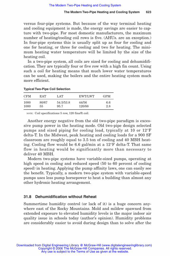
versus four-pipe systems. But because of the way terminal heatingand cooling equipment is made, the energy savings are easier to cap-ture with two-pipe. For most domestic manufacturers, the maximumnumber of heating/cooling coil rows is five. (AHUs. are an exception.)In four-pipe systems this is usually split up as four for cooling andone for heating, or three for cooling and two for heating. The mini-mum heating water temperature will be limited by the size of theheating coil.
In a two-pipe system, all coils are sized for cooling and dehumidifi-cation. They are typically four or five row with a high fin count. Usingsuch a coil for heating means that much lower water temperaturescan be used, making the boilers and the entire heating system muchmore efficient.
Typical Two-Pipe Coil Selection
CFM EAT LAT EWT/LWT GPM
1000 80/67 54.5/53.8 44/56 6.61000 55 95.7 120/88 2.8
NOTE: Coil specifications 5 row, 120 fins/ft coil.
Another energy negative from the old two-pipe paradigm is exces-sive pump power in the heating mode. Old two-pipe design selectedpumps and sized piping for cooling load, typically at 10 or 12°Fdelta-T. In the Midwest, peak heating and cooling loads for a 900 SFclassroom are roughly equal to 3.5 ton of cooling and 40 MBH heat-ing. Cooling flow would be 6.6 gal/min at a 12°F delta-T. That sameflow in heating would be significantly more than necessary todeliver 40 MBH.
Modern two-pipe systems have variable-sized pumps, operating athigh speed in cooling and reduced speed (50 to 60 percent of coolingspeed) in heating. Applying the pump affinity laws, one can easily seethe benefit. Typically, a modern two-pipe system with variable-speedpumps uses less pump horsepower to heat a building than almost anyother hydronic heating arrangement.
31.8 Dehumidification without Reheat
Summertime humidity control (or lack of it) is a huge concern any-where east of the Rocky Mountains. Mold and mildew spawned fromextended exposure to elevated humidity levels is the major indoor airquality issue in schools today (author’s opinion). Humidity problemsare considerably easier to avoid during design than to solve after the
The Modern Two-Pipe Heating and Cooling System 623
Rishel_CH31.qxd 20/4/06 6:58 PM Page 623
Downloaded from Digital Engineering Library @ McGraw-Hill (www.digitalengineeringlibrary.com)Copyright © 2006 The McGraw-Hill Companies. All rights reserved.
Any use is subject to the Terms of Use as given at the website.
The Modern Two-Pipe Heating and Cooling System
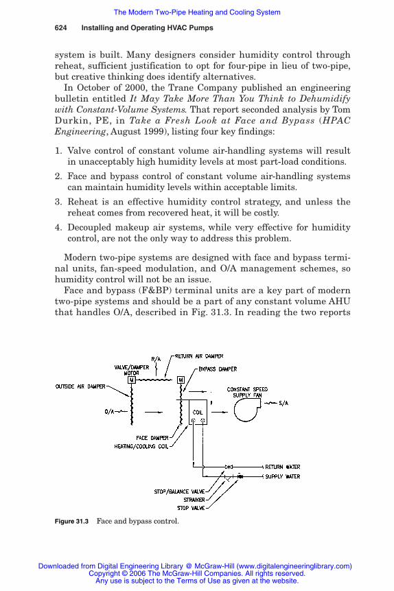
system is built. Many designers consider humidity control throughreheat, sufficient justification to opt for four-pipe in lieu of two-pipe,but creative thinking does identify alternatives.
In October of 2000, the Trane Company published an engineeringbulletin entitled It May Take More Than You Think to Dehumidifywith Constant-Volume Systems. That report seconded analysis by TomDurkin, PE, in Take a Fresh Look at Face and Bypass (HPACEngineering, August 1999), listing four key findings:
1. Valve control of constant volume air-handling systems will resultin unacceptably high humidity levels at most part-load conditions.
2. Face and bypass control of constant volume air-handling systemscan maintain humidity levels within acceptable limits.
3. Reheat is an effective humidity control strategy, and unless thereheat comes from recovered heat, it will be costly.
4. Decoupled makeup air systems, while very effective for humiditycontrol, are not the only way to address this problem.
Modern two-pipe systems are designed with face and bypass termi-nal units, fan-speed modulation, and O/A management schemes, sohumidity control will not be an issue.
Face and bypass (F&BP) terminal units are a key part of moderntwo-pipe systems and should be a part of any constant volume AHUthat handles O/A, described in Fig. 31.3. In reading the two reports
624 Installing and Operating HVAC Pumps
Figure 31.3 Face and bypass control.
Rishel_CH31.qxd 20/4/06 6:58 PM Page 624
Downloaded from Digital Engineering Library @ McGraw-Hill (www.digitalengineeringlibrary.com)Copyright © 2006 The McGraw-Hill Companies. All rights reserved.
Any use is subject to the Terms of Use as given at the website.
The Modern Two-Pipe Heating and Cooling System

referenced earlier, it is evident that the F&BP arrangement willalso impact the ability of the system to dehumidify. In every AHU,there are four air streams: O/A, return air, mixed air, and supplyair. In arranging the F&BP, the engineer can bypass any of the firstthree air streams. To control humidity, the stream to run throughthe coil is O/A, and the stream to bypass is return air, since that hasalready been dehumidified. That line of thinking will dictate drawthrough units in lieu of blow through, and units without airblenders. This arrangement works best if the air streams stratify,rather than mix.
One might ask, “why would someone bypass O/A?” The answer is “byaccident.” The standard arrangement of air handlers for roof installa-tion has the coil on the bottom of the box, return air through the floorof the unit, and O/A coming in the back. Figure 31.4 shows the affect of
The Modern Two-Pipe Heating and Cooling System 625
a. Incorrect.
b. Correct.
Figure 31.4 Orientation of face and bypass control.
Rishel_CH31.qxd 20/4/06 6:58 PM Page 625
Downloaded from Digital Engineering Library @ McGraw-Hill (www.digitalengineeringlibrary.com)Copyright © 2006 The McGraw-Hill Companies. All rights reserved.
Any use is subject to the Terms of Use as given at the website.
The Modern Two-Pipe Heating and Cooling System

stratified air going through a standard penthouse style AHU. A customunit with the coil raised so that return air can bypass will be a veryminor first cost addition, but significantly more effective.
Fan-speed modulation is an important component of modern two-pipe, and an inexpensive way to enhance humidity control and alsoreduce classroom noise levels. Since terminal units are selected forthe hottest day of the year with the class full of kids and the suncoming in the windows, and since one of the major causes of highhumidity is oversized air side equipment, fan speed modulationallows the terminal unit to better match the space load. It becomes,in effect, a mini variable air-volume unit. Along with slowing thefan, an increase in outside air damper position may be required toensure adequate ventilation to meet ASHRAE Standard 62. Mosttemperature control contractors and unit ventilator manufacturerscan accomplish the fan speed modulation with standard applicationspecific controllers.
Managing O/A is another key humidity and energy control strat-egy, since O/A will be at least 35 percent of the cooling load, 70 per-cent of the heating load, and 95 percent of potential humidity prob-lems. Outside air is a necessary component of a healthy andeffective learning environment, but in a school, the mentality shouldbe to ventilate only when there are kids in the building. Outside-airmanagement schemes must be integrated into the building controlsystem so that it is possible to operate only those parts of the build-ing that are being used. For example, do not turn the whole buildingto “Occupied” because there is basketball practice in the gym. Do notventilate the cafeteria as if it were full unless it is full.
31.9 Piping Arrangements
Figure 31.3 shows the recommended terminal unit piping arrange-ments for modern two-pipe systems. There are no control valves, sinceall are face and bypass. In addition to aiding dehumidification, faceand bypass makes the units almost freeze proof.
Balancing is done with manual flow control valves rather thanautomatic flow limiters. This means the system can turn down pro-portionately as pump speed changes from high speed in cooling tolow speed in heating. True proportional balancing means that whenthe pumps slow down, all units see the same reduction. For exam-ple, 10 units balanced at 10 gal/min in cooling with the pumps at100 percent speed, will all see 6 gal/min in heating when the pumpsgo to 60 percent speed. Proportional balancing is not possible withcontrol valves or automatic flow limiters on the terminal units.
626 Installing and Operating HVAC Pumps
Rishel_CH31.qxd 20/4/06 6:58 PM Page 626
Downloaded from Digital Engineering Library @ McGraw-Hill (www.digitalengineeringlibrary.com)Copyright © 2006 The McGraw-Hill Companies. All rights reserved.
Any use is subject to the Terms of Use as given at the website.
The Modern Two-Pipe Heating and Cooling System
(Note: the use of balance valves on these relatively constant- or two-flow systems is consistent with the general belief of this book thatbalance valves are for constant-flow systems and not for variable-flowinstallations.)
A related benefit to the “face and bypass, no control valve” arrange-ment goes back to the question of equipment safety. With the faceand bypass arrangement, there will never be pockets of warm waterthat might slug a chiller, or cold water that might thermally shock aboiler, as there might be in a valve-controlled system when thevalves are closed.
The modern two-pipe is arranged for ease of balancing in almost allareas. Multiple modular boilers are arranged in reverse return, andwhere the geometry of the building allows, the building loop will alsobe laid out reverse return for ease of balancing and lowering overallpump head.
Related to the piping arrangement is the way that a modern two-pipe system addresses the question of load diversity. Since two-pipeflow does not vary much, changes in load show up as variations inthe system delta-T. The opposite would be a valve-controlled systemwhere changes in load show up as changes in flow, with the delta-Tbeing (theoretically) constant. Typically, two-pipe terminal units willbe selected for 12°F temperature rise (44 to 56°F). But, since the unitwill only develop 12°F at full load, most of the time system delta-Twill be significantly less. A typical design day might show only 8°Fdelta-T at the chiller. Some might see this as overpumping the evapo-rator, but it is completely normal in a face and bypass system.
Good reasons for using F&BP in lieu of valve control have alreadybeen highlighted (humidity control and freeze protection). Anothervery good reason for not using control valves in two-pipe is the diffi-culty (impossibility?) of selecting a valve that would perform ade-quately from full cooling mode to partial heating load.
31.10 Variations
The 4 × 2 pipe system combines the need for four-pipe variable airvolume system (VAV) with two-pipe where it is applicable. A commonscenario is a college dormitory with offices, restaurants, book store,and the like, on the lower floors being served by VAV air handlers.The upper floors are resident rooms and, as discussed before, goodtwo-pipe candidates. Figure 31.5 shows how the 4 × 2 might be piped,so that the owner can reap the first cost benefit of two-pipe over muchof the building. Two two-position, three-way changeover valves arerequired. The modulating valve at the two-pipe pump inlet allows for
The Modern Two-Pipe Heating and Cooling System 627
Rishel_CH31.qxd 20/4/06 6:58 PM Page 627
Downloaded from Digital Engineering Library @ McGraw-Hill (www.digitalengineeringlibrary.com)Copyright © 2006 The McGraw-Hill Companies. All rights reserved.
Any use is subject to the Terms of Use as given at the website.
The Modern Two-Pipe Heating and Cooling System

variations in supply water to the two-pipe side versus the 4-pipe side.The modulating valve can also be used to slowly regulate thechangeover to ensure safe water temps at the chiller or boiler. In acouple of cases where chilled water delta-T was a concern of theowner, a temperature transmitter in the return line was used to con-trol pump speed. That arrangement will work if the building is pro-portionally balanced, but it assumes that all spaces served by thetwo-pipe are relatively equally loaded.
The two-pipe geothermal system is recent synthesis of three technolo-gies that separately have proven to be very effective. From two-pipecomes economy and simplicity for school designs, and the proven abilityto heat large buildings with low temperature water. From geothermalcomes a very efficient heating and cooling sink. And from heat recov-ery chillers comes a proven machine that can be programmed to make44°F cooling water and 130°F heating water. Natural gas energyprices post–Hurricane Katrina (2005 super storm) may finally be thetipping point that will offset what has been an unjustifiably high costof the geothermal well field.
It is important to note that this arrangement is not a heat pump.Heat pumps cannot handle cold winter air or humid summer aireffectively, and most are equipped with a decoupled makeup air sys-tem, a big first cost penalty. Because they cannot handle outside air,heat pumps cannot run economizer cooling, which is a severe operat-ing cost penalty in a school. Two-pipe geothermal can operate air sideeconomizers and it can use the ground temperature to cool the build-ing when the ground temperature and dew point allow. Figure 31.6shows the three water flow arrangements.
628 Installing and Operating HVAC Pumps
Figure 31.5 4 × 2 Pipe changeover.
Rishel_CH31.qxd 20/4/06 6:58 PM Page 628
Downloaded from Digital Engineering Library @ McGraw-Hill (www.digitalengineeringlibrary.com)Copyright © 2006 The McGraw-Hill Companies. All rights reserved.
Any use is subject to the Terms of Use as given at the website.
The Modern Two-Pipe Heating and Cooling System
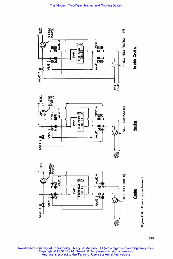
629
Fig
ure
31.
6T
wo-
pipe
geo
ther
mal
.
Rishel_CH31.qxd 20/4/06 6:58 PM Page 629
Downloaded from Digital Engineering Library @ McGraw-Hill (www.digitalengineeringlibrary.com)Copyright © 2006 The McGraw-Hill Companies. All rights reserved.
Any use is subject to the Terms of Use as given at the website.
The Modern Two-Pipe Heating and Cooling System

31.11 Conclusions
Over 150 successful installations have shown that for the right appli-cation, a properly designed modern two-pipe system will be lessexpensive to build, less expensive to operate, and easier to maintainthan any other HVAC option. If designed and operated properly, therewill be no compromises in indoor air quality, occupant comfort, orhumidity control.
630 Installing and Operating HVAC Pumps
Rishel_CH31.qxd 20/4/06 6:58 PM Page 630
Downloaded from Digital Engineering Library @ McGraw-Hill (www.digitalengineeringlibrary.com)Copyright © 2006 The McGraw-Hill Companies. All rights reserved.
Any use is subject to the Terms of Use as given at the website.
The Modern Two-Pipe Heating and Cooling System
Chapter
631
32Advanced Heat Recovery
32.1 Introduction
There are several references to heat recovery herein, but a detailedreview of the latest activities in this field is provided in this chapterwhere it can be discussed extensively.
The largest source of heat for recovery in the HVAC industry is theheat rejection from chillers. Another source of heat is flue gases ema-nating from all types of boilers. The development of the condensing-type boiler has all but eliminated the hot water boiler as a source ofheat for recovery since much of the water vapor from combustion iscondensed already. Steam boilers can be sources of heat recovery fromflue gases, and the cost of fuels may provide the impetus to evaluatethe economics of economizers on the stack connections of them. Forthe most part, this chapter will be devoted to the evaluation of heatrejection from chillers. It is recognized that there are other possibili-ties outside the HVAC industry.
As was calculated in Chap. 11, there is a sizeable amount of heat tobe recovered from chiller condensers. The costs of heat recovery werenot conducive to do so in the past. New equipment, digital control,and sensible selection of operating temperatures have resulted inheat recovery that does make economic sense. No longer is it viewedas necessary to have 180 to 200°F water to heat 78°F air.
The use of 130°F water for heating will increase the size and cost ofthe heating coil on a four-pipe heating and cooling system. However,the ability to use a condensing boiler with thermal efficiencies above90 percent usually amortizes this extra cost within an acceptableperiod of operation. Such a cost analysis should be conducted on a job-to-job basis to confirm the amortization period. Standard proceduresare available for making these cost analyses.
Rishel_CH32.qxd 20/4/06 7:03 PM Page 631
Downloaded from Digital Engineering Library @ McGraw-Hill (www.digitalengineeringlibrary.com)Copyright © 2006 The McGraw-Hill Companies. All rights reserved.
Any use is subject to the Terms of Use as given at the website.
Source: HVAC Pump Handbook
632 Installing and Operating HVAC Pumps
32.2 The Logic of Heat Recovery
Is it logical to have a source of heat injected into a building when anappreciable amount of heat is being rejected from that building? Wehave to find a way to use the Second Law of Thermodamics to moveheat from a warmer source to a cooler receiver. In the past, the neededheat requirements were too high in temperature and the waste heatwas too low. Now that we are correcting this imbalance, we can pro-ceed to develop systems that will enable us to recover the heat fromchiller condensers and reduce appreciably the needed heat from boil-ers or direct fired air heaters. The basic rule of heat recovery then isto use recovered heat wherever economically possible before consum-ing electricity or fossil fuels.
32.3 Types of Heat Recovery Chillers
There are three types of water-cooled chillers when classifying themas to the configuration of their condensers. Most of the contemporarychillers are designed to reject their heat at temperatures around95°F; others are dedicated to be heat recovery chillers with condenserwater leaving temperatures of around 130°F, and the third type havedouble bundle condensers with one tube bundle designed to providethe heat recovery. The coefficient of performance (COP) of the heatrecovery chiller, when counting the cooling only, is not as high as thevery efficient chillers now operating with standard leaving condenserwater temperatures. The problem with the double-bundle condenseris the inability to provide a correct ratio between the conventionalcondenser and the needed amount of heat recovery. The result is theemergence of the dedicated heat recovery chiller (DHRC) that isavailable in a number of sizes and can be furnished in modules asneeded for heat recovery load. Typical construction of the DHRC isshown in Figs. 32.1 and 32.2.
32.4 Heat Available from Chillers
The heat available from a chiller is the 12,000 Btu per ton-hour plusthe thermal equivalent of the energy consumed which, for electricity,is 3412 Btu/kW. Equation 32.1 provides this.
Heat available for recovery
� 12,000 + (kW/ton ⋅ 3412) Btu/ton-hour (32.1)
The ton-hour is equivalent to 12,000 Btu; the current kilowatts perton for contemporary water-cooled chillers is around 0.6 or
Rishel_CH32.qxd 20/4/06 7:03 PM Page 632
Downloaded from Digital Engineering Library @ McGraw-Hill (www.digitalengineeringlibrary.com)Copyright © 2006 The McGraw-Hill Companies. All rights reserved.
Any use is subject to the Terms of Use as given at the website.
Advanced Heat Recovery

Advanced Heat Recovery 633
approximately 2000 Btu. For general calculation purposes, the heatavailable per ton from the water-cooled chiller would be 14,000 Btuper ton-hour. For precise calculation, the actual kilowatts per ton forthe chiller should be determined for the operating range of the chillerwhen heat is being recovered.
Figure 32.1 Exterior view of DHRC. (Courtesy of Multistack, WestSalem, WI.)
Rishel_CH32.qxd 20/4/06 7:03 PM Page 633
Downloaded from Digital Engineering Library @ McGraw-Hill (www.digitalengineeringlibrary.com)Copyright © 2006 The McGraw-Hill Companies. All rights reserved.
Any use is subject to the Terms of Use as given at the website.
Advanced Heat Recovery
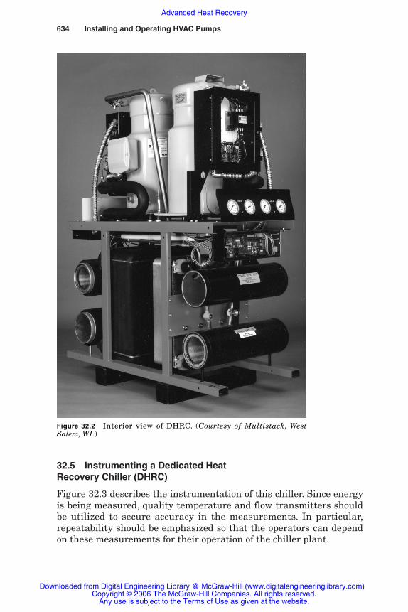
634 Installing and Operating HVAC Pumps
32.5 Instrumenting a Dedicated HeatRecovery Chiller (DHRC)
Figure 32.3 describes the instrumentation of this chiller. Since energyis being measured, quality temperature and flow transmitters shouldbe utilized to secure accuracy in the measurements. In particular,repeatability should be emphasized so that the operators can dependon these measurements for their operation of the chiller plant.
Figure 32.2 Interior view of DHRC. (Courtesy of Multistack, WestSalem, WI.)
Rishel_CH32.qxd 20/4/06 7:03 PM Page 634
Downloaded from Digital Engineering Library @ McGraw-Hill (www.digitalengineeringlibrary.com)Copyright © 2006 The McGraw-Hill Companies. All rights reserved.
Any use is subject to the Terms of Use as given at the website.
Advanced Heat Recovery

The flow and temperature measurements are as follows:
Chilled water flow, gal/min f1
Condenser water flow, gal/min f2
Chilled water return temperature °F t2
Chilled water supply temperature °F t1
Condenser entrance temperature °F t3
Condenser leaving temperature °F t4
It should be noted that the condenser entrance temperature and flowtransmitters are installed before any return water from the coolingtower is mixed with the water from the heat recovery processes.
32.6 Typical Piping for the DHRC
Figure 32.4 provides the typical piping for DHRC; the use of the heatrecovery will be shown in other figures. The DHRC can be piped inseries or parallel with the other chillers. Valve V1 can be furnished ifthere may be a reason for both series and parallel operation. Valve V2provides connection to a cooling tower, heat exchanger or closed-circuitcooler in event that the condenser heat is greater than that needed forthe heat recovery processes.
The pumping requirements for operating the DHRC in parallel withother chillers can vary from no pump needed to one with sizeable
Advanced Heat Recovery 635
t2
t1t4
f1
t3f2
C
kW
Con
dens
er
Eva
pora
tor
FromHX
Returnchilledwater
From heatrecovery
To heatrecovery
Supplychilled water
DHRC
Figure 32.3 Instumentation for dedicated heat recov-ery chiller.
Rishel_CH32.qxd 20/4/06 7:03 PM Page 635
Downloaded from Digital Engineering Library @ McGraw-Hill (www.digitalengineeringlibrary.com)Copyright © 2006 The McGraw-Hill Companies. All rights reserved.
Any use is subject to the Terms of Use as given at the website.
Advanced Heat Recovery
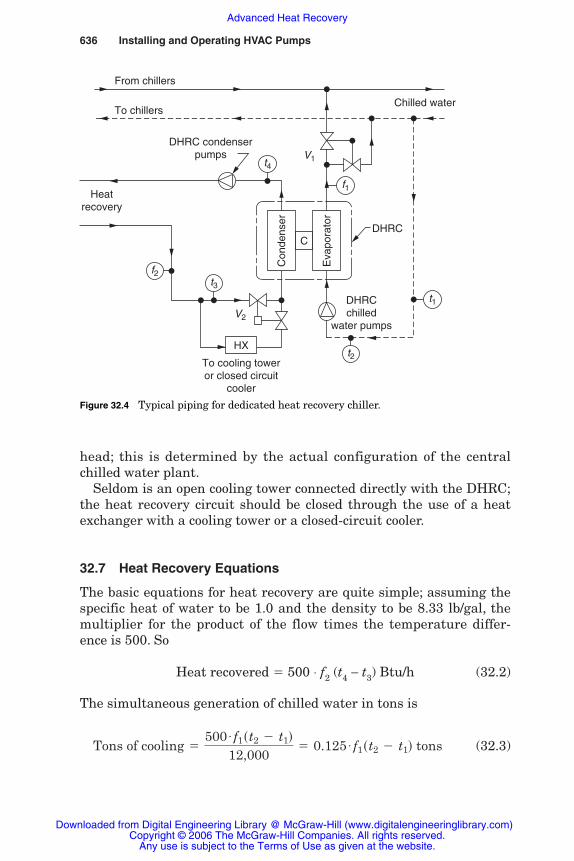
head; this is determined by the actual configuration of the centralchilled water plant.
Seldom is an open cooling tower connected directly with the DHRC;the heat recovery circuit should be closed through the use of a heatexchanger with a cooling tower or a closed-circuit cooler.
32.7 Heat Recovery Equations
The basic equations for heat recovery are quite simple; assuming thespecific heat of water to be 1.0 and the density to be 8.33 lb/gal, themultiplier for the product of the flow times the temperature differ-ence is 500. So
Heat recovered � 500 ⋅ f2 (t4 − t3) Btu/h (32.2)
The simultaneous generation of chilled water in tons is
(32.3)Tons of cooling 5500 # f1st2 2 t1d
12,0005 0.125 # f1st2 2 t1d tons
636 Installing and Operating HVAC Pumps
C
Con
dens
er
Eva
pora
tor
HX
From chillers
To chillersChilled water
V1
V2
t3
t2
f2
DHRC condenserpumps
Heatrecovery
To cooling toweror closed circuit
cooler
DHRCchilled
water pumps
DHRC
t4
t1
f1
Figure 32.4 Typical piping for dedicated heat recovery chiller.
Rishel_CH32.qxd 20/4/06 7:03 PM Page 636
Downloaded from Digital Engineering Library @ McGraw-Hill (www.digitalengineeringlibrary.com)Copyright © 2006 The McGraw-Hill Companies. All rights reserved.
Any use is subject to the Terms of Use as given at the website.
Advanced Heat Recovery

The total COP for the electric motor driven, heat recovery chiller isa sum of the above two equations in British thermal unit per hourdivided by the thermal equivalent of the kW input to the chiller.
(32.4)
Following is actual data derived from a 50-ton DHRC:
Chilled water flow f1 � 100 gal/min; condenser flow f2 � 81 gal/min
Chilled water temperatures: t2 � 56°F; t1 � 44°FCondenser water temperatures: t4 � 130°F; t3 � 110°FkW input � 62 kW
Inserting these values in Eq. 32.4 provides the total COP for thechiller.
These are the basic equations for heat recovery from chillers. Theycan be adapted to the various uses of recovered heat.
32.8 The Uses of Recovered Heat
Recovered heat from chillers can be used for (1) domestic water heat-ing, (2) space heating, (3) heat recovery reheat in VAV boxes or air-handling units, and (4) any other process where the heat receiver islower in temperature than the leaving temperature t4 of the DHRC.The use that has the lowest temperature will be the most economicalsince the leaving water temperature, t4, of the chiller condenser willalso be the lowest for any of these uses. Usually, this is domesticwater heating.
32.8.1 Domestic water heating
Domestic water heating is an excellent use for recovered heat due toits relatively low supply temperatures, namely, 45 to 55°F. This is thefirst use that should be considered for recovered heat. Heat recoveryfor domestic water heating can reduce substantially the operation ofhot water boilers in the summertime. Figure 32.5 describes the typical
Total COP 50.147[100s56 2 44d 1 81s130 2 110d]
625 6.7
5 0.147 [f2st4 2 t3d 1 f1st2 2 t1d]
Total COP 5500 [f2 st4 2 t3d 1 f1 st2 2 t1d]
kW # 3412
Advanced Heat Recovery 637
Rishel_CH32.qxd 20/4/06 7:03 PM Page 637
Downloaded from Digital Engineering Library @ McGraw-Hill (www.digitalengineeringlibrary.com)Copyright © 2006 The McGraw-Hill Companies. All rights reserved.
Any use is subject to the Terms of Use as given at the website.
Advanced Heat Recovery
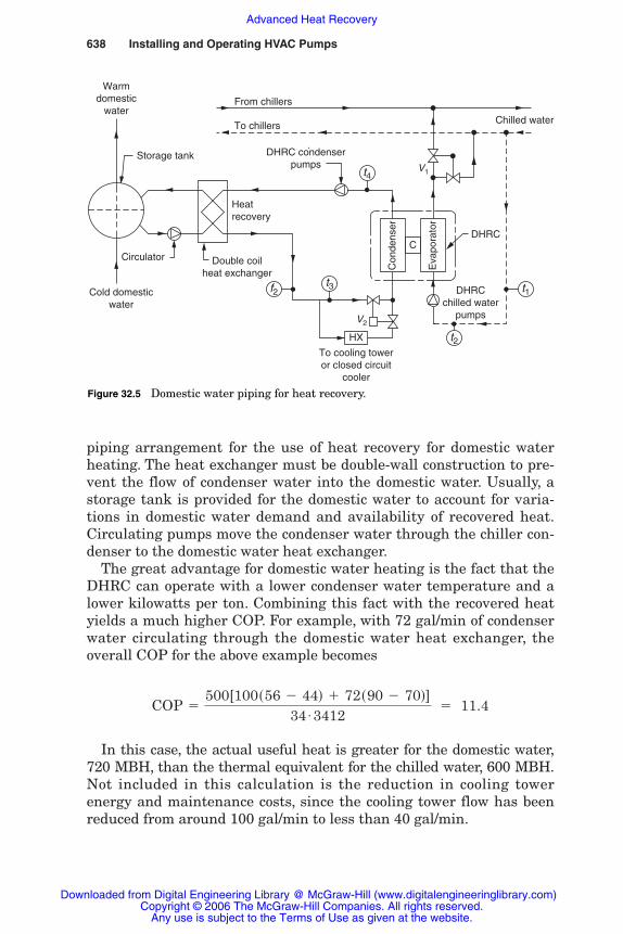
piping arrangement for the use of heat recovery for domestic waterheating. The heat exchanger must be double-wall construction to pre-vent the flow of condenser water into the domestic water. Usually, astorage tank is provided for the domestic water to account for varia-tions in domestic water demand and availability of recovered heat.Circulating pumps move the condenser water through the chiller con-denser to the domestic water heat exchanger.
The great advantage for domestic water heating is the fact that theDHRC can operate with a lower condenser water temperature and alower kilowatts per ton. Combining this fact with the recovered heatyields a much higher COP. For example, with 72 gal/min of condenserwater circulating through the domestic water heat exchanger, theoverall COP for the above example becomes
In this case, the actual useful heat is greater for the domestic water,720 MBH, than the thermal equivalent for the chilled water, 600 MBH.Not included in this calculation is the reduction in cooling towerenergy and maintenance costs, since the cooling tower flow has beenreduced from around 100 gal/min to less than 40 gal/min.
COP 5500[100s56 2 44d 1 72s90 2 70d]
34 # 3412 5 11.4
638 Installing and Operating HVAC Pumps
C
Con
dens
er
Eva
pora
tor
HX
V1
Warmdomestic
water
Storage tank
Circulator Double coilheat exchanger
Cold domesticwater
From chillers
To chillers Chilled water
DHRC condenserpumps
To cooling toweror closed circuit
cooler
´
DHRCchilled water
pumps
DHRC
Heatrecovery
V2
f2t3 t1
t4
t2
Figure 32.5 Domestic water piping for heat recovery.
Rishel_CH32.qxd 20/4/06 7:03 PM Page 638
Downloaded from Digital Engineering Library @ McGraw-Hill (www.digitalengineeringlibrary.com)Copyright © 2006 The McGraw-Hill Companies. All rights reserved.
Any use is subject to the Terms of Use as given at the website.
Advanced Heat Recovery
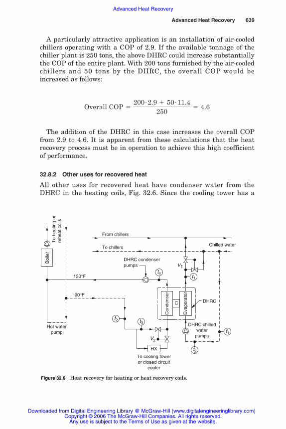
A particularly attractive application is an installation of air-cooledchillers operating with a COP of 2.9. If the available tonnage of thechiller plant is 250 tons, the above DHRC could increase substantiallythe COP of the entire plant. With 200 tons furnished by the air-cooledchillers and 50 tons by the DHRC, the overall COP would beincreased as follows:
The addition of the DHRC in this case increases the overall COPfrom 2.9 to 4.6. It is apparent from these calculations that the heatrecovery process must be in operation to achieve this high coefficientof performance.
32.8.2 Other uses for recovered heat
All other uses for recovered heat have condenser water from theDHRC in the heating coils, Fig. 32.6. Since the cooling tower has a
Overall COP 5200 # 2.9 1 50 # 11.4
2505 4.6
Advanced Heat Recovery 639
C
Con
dens
er
Eva
pora
tor
V1
V2
To cooling toweror closed circuit
cooler
DHRC condenserpumps
´Boi
ler
HX
To
heat
ing
orre
heat
coi
ls
Hot waterpump
90°F
130°F
From chillers
To chillers Chilled water
DHRC
DHRC chilledwater
pumps
f2
f1
t1
t3
t2
t4
Figure 32.6 Heat recovery for heating or heat recovery coils.
Rishel_CH32.qxd 20/4/06 7:03 PM Page 639
Downloaded from Digital Engineering Library @ McGraw-Hill (www.digitalengineeringlibrary.com)Copyright © 2006 The McGraw-Hill Companies. All rights reserved.
Any use is subject to the Terms of Use as given at the website.
Advanced Heat Recovery

heat exchanger or is a closed-circuit cooler, there is no difference inthe chemistry of the DHRC condenser water and the hot water for heat-ing. Therefore, this condenser water can be used in the heating coils.
These heating coils include those for space heating as well as forreheat. Another application of recovered heat is in natatorium airhandling units. Since natatoriums require dehumidification yearround, the latent heat can be recovered for reheat and heating thepool water or other parts of the building.
32.9 Sizing the DHRC
How large should the DHRC be, in comparison to the regular chillerson a particular installation? The heat recovery chiller should bedesigned to accommodate as much of the heating load as economicallypossible. Remember that for every ton of cooling, 14,000 Btu is avail-able for heating. The basic rule for sizing the DHRC is as follows.
32.9.1 Prevent boilers from running in thesummer and main chillers in the winter
The first step is to make a detailed analysis of the summer heatingloads, which in most cases, are domestic water heating and reheat inair-handling units and VAV boxes. The instantaneous domestic waterheating load can be reduced through the installation of a hot waterstorage tank. The sizing of this tank must take in to consideration theavailability of space for it and the need to keep it warm when there isneither heating nor cooling loads in the building. A very careful studyshould be made of both domestic water and reheat requirements inthe sizing of the DHRC.
Winter cooling requirements of the building should determine thesize of the DHRC. In this case, the heat from the condenser can beused to heat partially the domestic water load or to reduce the heat-ing load on the boilers.
It is obvious that this is a complex problem needing great care in itssolution. One characteristic that the DHRC has is the ability to beinstalled in modules so that it is not difficult to install additional ton-nage if the initial installation proves to be inadequate. The space pro-vided for the DHRC should be adequate in event that this addition isrequired.
32.10 Control of DHRC
It is obvious that the control of heat recovery chillers is different fromthat for ordinary chillers. The control of the condenser heat becomes
640 Installing and Operating HVAC Pumps
Rishel_CH32.qxd 20/4/06 7:03 PM Page 640
Downloaded from Digital Engineering Library @ McGraw-Hill (www.digitalengineeringlibrary.com)Copyright © 2006 The McGraw-Hill Companies. All rights reserved.
Any use is subject to the Terms of Use as given at the website.
Advanced Heat Recovery
the principal objective of the control system as well as the needed pro-duction of a specific number of tons of cooling or a chilled water sup-ply temperature.
For example, several of the piping configurations discussed earlierassume that no heat is being rejected to a cooling tower or other heatabsorbing equipment. How can this be done? With many applicationsof these chillers, the desire is to produce a specific amount of heatfrom the condenser, and the cooling effect is secondary. To achievethis, it is necessary to control the chiller operation by the amount ofheat that is derived from the chiller. This can be done by maintaininga particular water temperature for the water leaving the condenser.Other applications may require the control of the water temperatureentering the condenser.
As has been stated repeatedly, the DHRC makes sense when there isa simultaneous need for heating and cooling, and it must run as manyhours as possible. Further to that point, when the DHRC is operatingto satisfy the facility’s hot water requirements, there must be a chilledwater requirement in the building that meets or exceeds the hot waterdemand. If this is not the case, the heat recovery system will subcoolthe chilled water loop and eventually shut down automatically on a lowtemperature fault. Similarly, if the DHRC is operating to satisfy thefacility’s chilled water requirement, there must be a hot water require-ment in the building that meets or exceeds the chilled water demand.
It has been discovered that the best way to operate the DHRC is toalways set the control point (hot water or chilled water) to the side ofthe system that has the lowest demand. In doing this, we are alwaysassured of operating the heat recovery system during the maximumavailable hours for maximum economic impact on the facility.
This can be done by simply monitoring the temperatures on theside of the system (hot water or chilled water) that is not beingactively controlled by the DHRC. That is, if the chiller is controlling toa leaving hot water temperature, thus producing chilled water as aby-product, then the control system must monitor the entering chilledwater temperature. If this temperature drops below a predeterminedset point, indicating a lack of chilled water load, the control point ofthe DHRC is changed over to the chilled waterside of the system. Thiswill ensure that the heat recovery system will only produce theamount of heat that can safely be absorbed from the facility’s chilledwater system. This logic would then be applied similarly when in thechilled water control mode. This control may be easily accomplishedby the building control system or can come prepackaged within theDHRC control system. Such chillers are being produced now withautomatic switchover from control of the amount of cooling to theamount of heat recovered.
Advanced Heat Recovery 641
Rishel_CH32.qxd 20/4/06 7:03 PM Page 641
Downloaded from Digital Engineering Library @ McGraw-Hill (www.digitalengineeringlibrary.com)Copyright © 2006 The McGraw-Hill Companies. All rights reserved.
Any use is subject to the Terms of Use as given at the website.
Advanced Heat Recovery
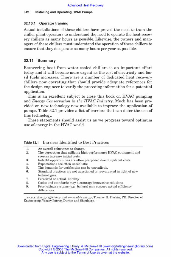
32.10.1 Operator training
Actual installations of these chillers have proved the need to train thechiller plant operators to understand the need to operate the heat recov-ery chillers as many hours as possible. Likewise, the owners and man-agers of these chillers must understand the operation of these chillers toensure that they do operate as many hours per year as possible.
32.11 Summary
Recovering heat from water-cooled chillers is an important efforttoday, and it will become more urgent as the cost of electricity and fos-sil fuels increases. There are a number of dedicated heat recoverychillers now operating that should provide adequate references forthe design engineer to verify the preceding information for a potentialapplication.
This is an excellent subject to close this book on HVAC pumpingand Energy Conservation in the HVAC Industry. Much has been pro-vided on new technology now available to improve the application ofpumps. Table 32.1 provides a list of barriers that can deter the use ofthis technology.
These statements should assist us as we progress toward optimumuse of energy in the HVAC world.
642 Installing and Operating HVAC Pumps
Table 32.1 Barriers Identified to Best Practices
1. An overall reluctance to change.2. The perception that utilizing high-performance HVAC equipment and
sources increase initial costs.3. Retrofit opportunities are often postponed due to up-front costs.4. Expectations are often unrealistic.5. The demands for verification can be unrealistic.6. Standard practices are not questioned or reevaluated in light of new
technologies.7. Perceived or actual liability.8. Codes and standards may discourage innovative solutions.9. Poor ratings systems (e.g., boilers) may obscure actual efficiency
differences.
SOURCE: Energy efficiency and renewable energy, Thomas H. Durkin, PE. Director ofEngineering, Veazey Parrott Durkin and Shoulders.
Rishel_CH32.qxd 20/4/06 7:03 PM Page 642
Downloaded from Digital Engineering Library @ McGraw-Hill (www.digitalengineeringlibrary.com)Copyright © 2006 The McGraw-Hill Companies. All rights reserved.
Any use is subject to the Terms of Use as given at the website.
Advanced Heat Recovery