arX

iv:g

r-qc

/980

3043

v1 1

2 M

ar 1

998

The Husain-Kuchar Model:

Time Variables and Non-degenerate Metrics

J. Fernando Barbero G., Alfredo Tiemblo and

Romualdo Tresguerres

Centro de Fısica “Miguel Catalan”,Instituto de Matematicas

y Fısica Fundamental, C.S.I.C.Serrano 113 bis, 28006 Madrid, Spain

November 26, 1997

ABSTRACT

We study the Husain-Kuchar model by introducing a new action principle similar

to the self-dual action used in the Ashtekar variables approach to Quantum Gravity.

This new action has several interesting features; among them, the presence of a scalar

time variable that allows the definition of geometric observables without adding new

degrees of freedom, the appearance of a natural non-degenerate four-metric and the

possibility of coupling ordinary matter.

PACS number(s): 04.20.Cv, 04.20.Fy

I Introduction

In the long quest to understand General Relativity (G.R.) the use of toy models has a

long tradition. This is especially true in Quantum Gravity and Quantum Cosmology

where they have allowed to obtain some, otherwise very difficult to get, information.

However, this does not come without a price because one is usually forced to introduce

very strong simplifying assumptions and, quite often, some of the key features of the

theory are lost. Though a final judgement on the success of this approach can only be

made once a consistent Quantum Gravity theory is found, it is possible, in principle,

to get some clues on how well one is doing by considering widely different toy models.

Bianchi models (see, for example, [1]) are obtained by imposing homogeneity

conditions on the gravitational variables. Their high symmetry has the consequence

of killing most of the degrees of freedom of the full theory leaving only a finite number

of them. They have been widely used in Quantum Cosmology mainly because the

equations obtained upon quantization are more or less tractable.

There are other (less known) toy models that achieve the goal of simplifying the

theory by going in the opposite direction: adding degrees of freedom. Chief among

them is the Husain-Kuchar model [2] (H-K in the following). This model is quite

interesting because it has some of the features that make G.R. so difficult to deal with

in the quantum regime, in particular diffeomorphism invariance, but is significantly

simpler because it lacks the Hamiltonian constraint (another important source of

difficulties in full G.R.). This has the effect of increasing the number of degrees of

freedom per space point from two to three.

To illustrate with a picture the different and complementary roles played by these

two approaches one can make the following analogy: Portray G.R. as a complicated,

knotted, two-dimensional-surface Σ embedded in IR3. Working with Bianchi models

is something akin to trying to get information about Σ by looking at a finite number

of points on it. The H-K model, on the other hand, is like trying to gather information

by studying the whole IR3. Clearly some crucial features are lost in both approaches

1

but, still, they provide useful and complementary views about Σ.1

The H-K model, in its usual formulation (see [3] for some alternative descriptions),

can be conveniently derived from an action principle very close to the self-dual action

[4] from which the Ashtekar approach to classical and quantum G.R. [5] can be found.

The phase space of the Hamiltonian description of both theories is the same: it is

coordinatized by a SO(3) connection and a densitized (inverse) triad canonically

conjugate to it. Their crucial difference is the absence of a Hamiltonian constraint in

the H-K model. The usual interpretation of this lack of “dynamics” is the following:

By using the frame field in terms of which the H-K action is written2 one can build a

degenerate four-metric gab and a densitized vector field na (that can be de-densitized

by means of an auxiliary space-time foliation). The lack of dynamics can be seen as

the fact that the Lie derivative of gab in the direction of na is zero.

The four-dimensional metric that we can build from the frame field in the H-

K action is degenerate. This can lead to the erroneous conclusion that the model

describes only degenerate four-metrics; a fact that has induced some authors to claim,

for example, that ordinary matter cannot be coupled to the model. We will show that

this is not the case in due time but at this point we urge the reader to think about the

following paradoxical situation: The fact that the Hamiltonian constraint is missing

from the H-K model means that the constraint hypersurface of G.R. in the Ashtekar

formulation is contained in the H-K one, hence, every solution to G.R (for example

Minkowski space-time) is a solution to the H-K model. How can we then describe

these G.R. solutions in terms of the fields present in the H-K action if we only have

a 4 × 3 frame field available?

The solution to this problem that we give in the paper has some unexpected

implications that make it quite attractive. On one hand it provides an elegant way

to define quantum geometric observables (such as areas and volumes) without having

to resort to increasing the number of physical degrees of freedom as in previous

approaches [6],[7]. On the other, it allows the introduction of a kind of time variable in

1This analogy is, actually, a little bit more than that because the Hamiltonian formulation ofG.R. can be understood as the study, in phase space, of the hypersurface defined by the constraints.

2Being a 4 × 3 matrix it is neither a tetrad nor a triad!

2

the double sense that dynamics can be referred to it and also that the scalar constraint

(that we need now in order to get the correct counting of degrees of freedom) is

linear in its canonically conjugate momentum (so that, upon quantization it gives a

Schrodinger type of equation).

The main result of the paper is that it is possible to obtain the H-K model from

an action principle (also related to the self-dual action) that admits an interpretation

in terms of non-degenerate four dimensional metrics. This is achieved by introducing

a scalar field that can be interpreted, in a sense that will be made more precise later,

as the time variable mentioned before. This will not only solve the paradox presented

above but also will provide a means to couple ordinary matter thus enhancing the

usefulness of H-K as a toy model. We hope that the possible interpretation of this

scalar field as time will help to shed some light on the problem of time in full G.R.

The paper is organized as follows. This introduction is followed by section II

where the usual formulation of the Husain-Kuchar model is briefly reviewed. The new

action principle, that is the object of this paper, is introduced in section III where we

derive it from the well known self-dual action for G.R. The details of the Hamiltonian

formulation of our model are spelled out in section IV. There we thoroughly study

the derivation of the constraints of the theory and discuss their interpretation. In

section V we compare the field equations in both the usual and the new formulation

for the H-K model in order to show that they are not in contradiction (a non-trivial

fact as the number of equations is different in both cases). Section VI gives a different

proof of the equivalence of our “non-degenerate” formulation and the usual one at the

Lagrangian level. We also show that the addition of a cosmological constant (made

possible in our scheme by the availability of a non-degenerate four-metric) does not

lead us beyond the H-K model. We end the paper with section VII, where we give

our conclusions and general comments, and an appendix that contains some details

of the computations needed to disentangle the constraints in our formulation.

3

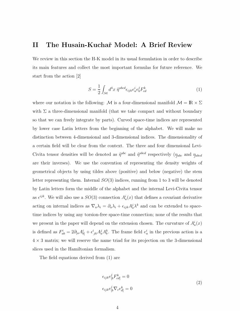
II The Husain-Kuchar Model: A Brief Review

We review in this section the H-K model in its usual formulation in order to describe

its main features and collect the most important formulas for future reference. We

start from the action [2]

S =1

2

∫

M

d4x ηabcdǫijkeiae

jbF

kcd (1)

where our notation is the following: M is a four-dimensional manifold M = IR × Σ

with Σ a three-dimensional manifold (that we take compact and without boundary

so that we can freely integrate by parts). Curved space-time indices are represented

by lower case Latin letters from the beginning of the alphabet. We will make no

distinction between 4-dimensional and 3-dimensional indices. The dimensionality of

a certain field will be clear from the context. The three and four dimensional Levi-

Civita tensor densities will be denoted as ηabc and ηabcd respectively (˜ηabc and

˜ηabcd

are their inverses). We use the convention of representing the density weights of

geometrical objects by using tildes above (positive) and below (negative) the stem

letter representing them. Internal SO(3) indices, running from 1 to 3 will be denoted

by Latin letters form the middle of the alphabet and the internal Levi-Civita tensor

as ǫijk. We will also use a SO(3) connection Aia(x) that defines a covariant derivative

acting on internal indices as ∇aλi = ∂aλi + ǫijkAjaλ

k and can be extended to space-

time indices by using any torsion-free space-time connection; none of the results that

we present in the paper will depend on the extension chosen. The curvature of Aia(x)

is defined as F iab = 2∂[aA

ib] + ǫijkA

jaA

kb . The frame field ei

a in the previous action is a

4 × 3 matrix; we will reserve the name triad for its projection on the 3-dimensional

slices used in the Hamiltonian formalism.

The field equations derived from (1) are

ǫijkej[bF

kcd] = 0

ǫijkej[b∇ce

kd] = 0

(2)

4

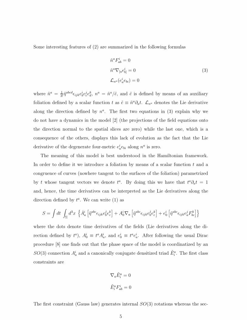
Some interesting features of (2) are summarized in the following formulas

naF iab = 0

na∇[aeib] = 0 (3)

Lna(eiaebi) = 0

where na = 13!ηabcdǫijke

ibe

jce

kd, n

a = na/e, and e is defined by means of an auxiliary

foliation defined by a scalar function t as e ≡ na∂at. Lna denotes the Lie derivative

along the direction defined by na. The first two equations in (3) explain why we

do not have a dynamics in the model [2] (the projections of the field equations onto

the direction normal to the spatial slices are zero) while the last one, which is a

consequence of the others, displays this lack of evolution as the fact that the Lie

derivative of the degenerate four-metric eiaebi along na is zero.

The meaning of this model is best understood in the Hamiltonian framework.

In order to define it we introduce a foliation by means of a scalar function t and a

congruence of curves (nowhere tangent to the surfaces of the foliation) parametrized

by t whose tangent vectors we denote ta. By doing this we have that ta∂at = 1

and, hence, the time derivatives can be interpreted as the Lie derivatives along the

direction defined by ta. We can write (1) as

S =∫

dt∫

Σd3x

{

Aia

[

ηabcǫijkejbe

kc

]

+ Ai0∇a

[

ηabcǫijkejbe

kc

]

+ ei0

[

ηabcǫijkejaF

kbc

]}

where the dots denote time derivatives of the fields (Lie derivatives along the di-

rection defined by ta), Ai0 ≡ taAi

a, and ei0 ≡ taei

a. After following the usual Dirac

procedure [8] one finds out that the phase space of the model is coordinatized by an

SO(3) connection Aia and a canonically conjugate densitized triad Ea

i . The first class

constraints are

∇aEai = 0

Eai F

iab = 0

The first constraint (Gauss law) generates internal SO(3) rotations whereas the sec-

5

ond (known as vector constraint) generates spatial diffeomorphisms3. As we can see

there is no scalar constraint so that we have three degrees of freedom per space point.

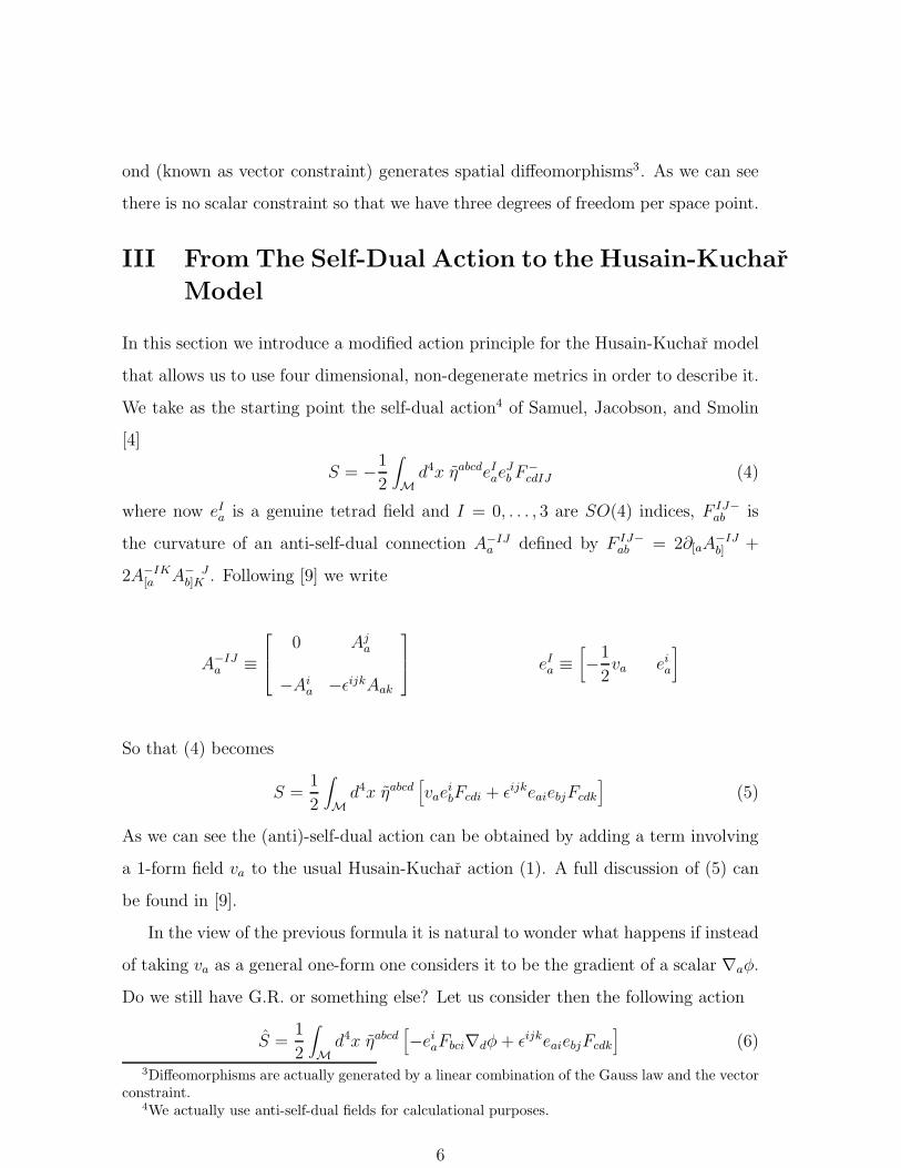
III From The Self-Dual Action to the Husain-Kuchar

Model

In this section we introduce a modified action principle for the Husain-Kuchar model

that allows us to use four dimensional, non-degenerate metrics in order to describe it.

We take as the starting point the self-dual action4 of Samuel, Jacobson, and Smolin

[4]

S = −1

2

∫

M

d4x ηabcdeIae

JbF

−

cdIJ (4)

where now eIa is a genuine tetrad field and I = 0, . . . , 3 are SO(4) indices, F IJ−

ab is

the curvature of an anti-self-dual connection A−IJa defined by F IJ−

ab = 2∂[aA−IJb] +

2A−IK[a A− J

b]K . Following [9] we write

A−IJa ≡

0 Aja

−Aia −ǫijkAak

eI

a ≡[

−1

2va ei

a

]

So that (4) becomes

S =1

2

∫

M

d4x ηabcd[

vaeibFcdi + ǫijkeaiebjFcdk

]

(5)

As we can see the (anti)-self-dual action can be obtained by adding a term involving

a 1-form field va to the usual Husain-Kuchar action (1). A full discussion of (5) can

be found in [9].

In the view of the previous formula it is natural to wonder what happens if instead

of taking va as a general one-form one considers it to be the gradient of a scalar ∇aφ.

Do we still have G.R. or something else? Let us consider then the following action

S =1

2

∫

M

d4x ηabcd[

−eiaFbci∇dφ+ ǫijkeaiebjFcdk

]

(6)

3Diffeomorphisms are actually generated by a linear combination of the Gauss law and the vectorconstraint.

4We actually use anti-self-dual fields for calculational purposes.

6

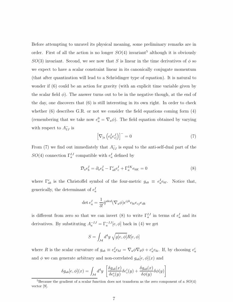
Before attempting to unravel its physical meaning, some preliminary remarks are in

order. First of all the action is no longer SO(4) invariant5 although it is obviously

SO(3) invariant. Second, we see now that S is linear in the time derivatives of φ so

we expect to have a scalar constraint linear in its canonically conjugate momentum

(that after quantization will lead to a Schrodinger type of equation). It is natural to

wonder if (6) could be an action for gravity (with an explicit time variable given by

the scalar field φ). The answer turns out to be in the negative though, at the end of

the day, one discovers that (6) is still interesting in its own right. In order to check

whether (6) describes G.R. or not we consider the field equations coming form (4)

(remembering that we take now e0a = ∇aφ). The field equation obtained by varying

with respect to A−

IJ is[

∇[a

(

eIbe

Jc]

)]−

= 0 (7)

From (7) we find out immediately that A−

IJ is equal to the anti-self-dual part of the

SO(4) connection ΓIJa compatible with eI

a defined by

DaeIb = ∂ae

Ib − Γc

abeIc + ΓIK

a ebK = 0 (8)

where Γcab is the Christoffel symbol of the four-metric gab ≡ eI

aebI . Notice that,

generically, the determinant of eIa

det eIa =

1

3!ηabcd(∇aφ)ǫijkebiecjedk

is different from zero so that we can invert (8) to write ΓIJa in terms of eI

a and its

derivatives. By substituting A−IJa = Γ−IJ

a [e, φ] back in (4) we get

S =∫

M

d4y√

g[e, φ]R[e, φ]

where R is the scalar curvature of gab ≡ eIaebI = ∇aφ∇bφ + ei

aebi. If, by choosing eia

and φ we can generate arbitrary and non-correlated gab[e, φ](x) and

δgab[e, φ](x) =∫

M

d4y

[

δgab(x)

δeic(y)

δeic(y) +

δgab(x)

δφ(y)δφ(y)

]

5Because the gradient of a scalar function does not transform as the zero component of a SO(4)vector [9].

7

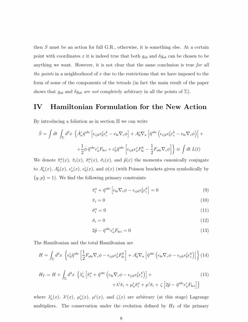
then S must be an action for full G.R., otherwise, it is something else. At a certain

point with coordinates x it is indeed true that both gab and δgab can be chosen to be

anything we want. However, it is not clear that the same conclusion is true for all

the points in a neighborhood of x due to the restrictions that we have imposed to the

form of some of the components of the tetrads (in fact the main result of the paper

shows that gab and δgab are not completely arbitrary in all the points of Σ).

IV Hamiltonian Formulation for the New Action

By introducing a foliation as in section II we can write

S =∫

dt∫

Σd3x

{

Aiaη

abc[

ǫijkejbe

kc − ebi∇cφ

]

+ Ai0∇a

[

ηabc(

ǫijkejbe

kc − ebi∇cφ

)]

+

+1

2φ ηabcei

aFbci + ei0η

abc[

ǫijkejaF

kbc −

1

2Fabi∇cφ

]}

≡∫

dt L(t)

We denote πai (x), πi(x), σ

ai (x), σi(x), and p(x) the momenta canonically conjugate

to Aia(x), A

i0(x), e

ia(x), e

i0(x), and φ(x) (with Poisson brackets given symbolically by

{q, p} = 1). We find the following primary constraints

πai + ηabc

[

ebi∇cφ− ǫijkejbe

kc

]

= 0 (9)

πi = 0 (10)

σai = 0 (11)

σi = 0 (12)

2p− ηabceiaFbci = 0 (13)

The Hamiltonian and the total Hamiltonian are

H =∫

Σd3x

{

ei0η

abc[

1

2Fabi∇cφ− ǫijke

jaF

kbc

]

+ Ai0∇a

[

ηabc(

ebi∇cφ− ǫijkejbe

kc

)]

}

(14)

HT = H +∫

Σd3x

{

λia

[

πai + ηabc

(

ebi∇cφ− ǫijkejbe

kc

)]

+ (15)

+λiπi + µiaσ

ai + µiσi + ζ

[

2p− ηabceiaFbci

]}

where λia(x), λ

i(x), µia(x), µ

i(x), and ζ(x) are arbitrary (at this stage) Lagrange

multipliers. The conservation under the evolution defined by HT of the primary

8

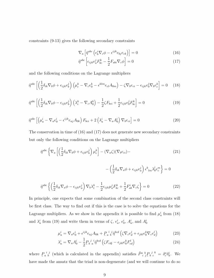
constraints (9-13) gives the following secondary constraints

∇a

[

ηabc(

eib∇cφ− ǫijkebjeck

)]

= 0 (16)

ηabc[

ǫijkejaF

kbc −

1

2Fabi∇cφ

]

= 0 (17)

and the following conditions on the Lagrange multipliers

ηabc[(

1

2δik∇bφ+ ǫijke

jb

)

(

µkc −∇ce

k0 − ǫklmeclA0m

)

− ζ∇beci − ǫijkej0∇be

kc

]

= 0 (18)

ηabc[(

1

2δik∇bφ− ǫijke

jb

)

(

λkc −∇cA

k0

)

−1

2ζFbci +

1

2ǫijke

j0F

kbc

]

= 0 (19)

ηabc[(

µia −∇ae

i0 − ǫijkeajA0k

)

Fbci + 2(

λia −∇aA

i0

)

∇beci

]

= 0 (20)

The conservation in time of (16) and (17) does not generate new secondary constraints

but only the following conditions on the Lagrange multipliers

ηabc{

∇a

[(

1

2δik∇bφ+ ǫijke

jb

)

µkc

]

− (∇aζ)(∇beci)− (21)

−(

1

2δik∇aφ+ ǫijke

ja

)

ǫklmλlbe

mc

}

= 0

ηabc{(

1

2δik∇aφ− ǫijke

ja

)

∇bλkc −

1

2ǫijkµ

jaF

kbc +

1

2F i

ab∇cζ}

= 0 (22)

In principle, one expects that some combination of the second class constraints will

be first class. The way to find out if this is the case is to solve the equations for the

Lagrange multipliers. As we show in the appendix it is possible to find µia from (18)

and λia from (19) and write them in terms of ζ , ei

a, ei0, A

ia, and Ai

0

µia = ∇ae

i0 + ǫijkeajA0k +

˜P i j

a b ηbcd

(

ζ∇cejd + ǫjkle

k0∇ce

ld

)

(23)

λia = ∇aA

i0 −

1

2˜P j i

b a ηbcd

(

ζFcdj − ǫjklek0F

lcd

)

(24)

where˜P i j

a b (which is calculated in the appendix) satisfies P a bi j

˜P j k

b c = δac δ

ik. We

have made the ansatz that the triad is non-degenerate (and we will continue to do so

9

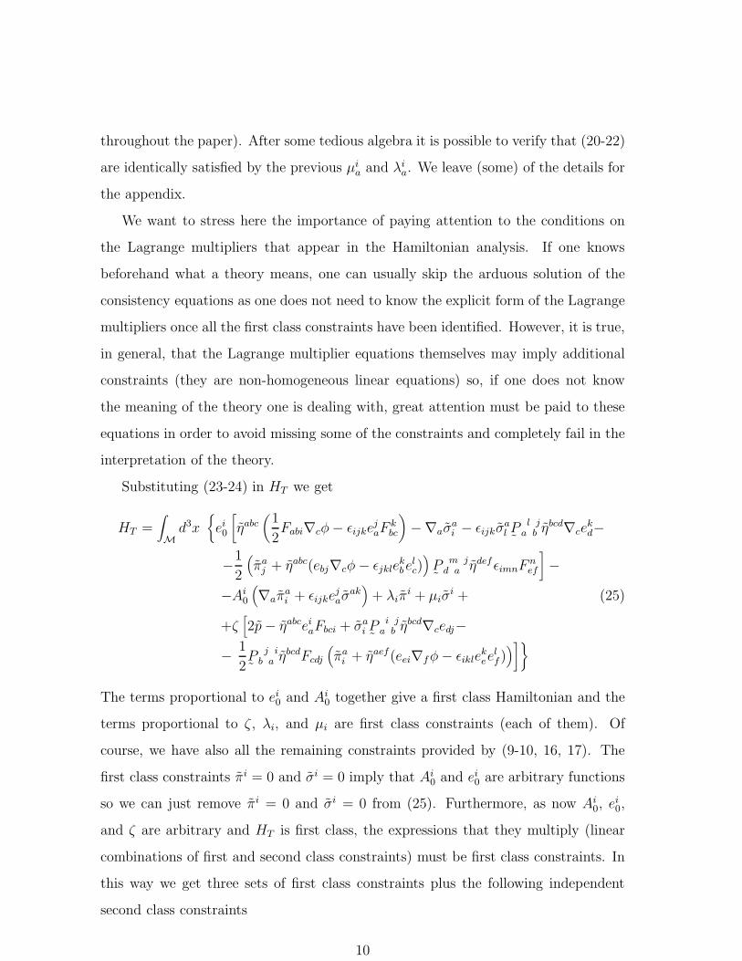
throughout the paper). After some tedious algebra it is possible to verify that (20-22)

are identically satisfied by the previous µia and λi

a. We leave (some) of the details for

the appendix.

We want to stress here the importance of paying attention to the conditions on

the Lagrange multipliers that appear in the Hamiltonian analysis. If one knows

beforehand what a theory means, one can usually skip the arduous solution of the

consistency equations as one does not need to know the explicit form of the Lagrange

multipliers once all the first class constraints have been identified. However, it is true,

in general, that the Lagrange multiplier equations themselves may imply additional

constraints (they are non-homogeneous linear equations) so, if one does not know

the meaning of the theory one is dealing with, great attention must be paid to these

equations in order to avoid missing some of the constraints and completely fail in the

interpretation of the theory.

Substituting (23-24) in HT we get

HT =∫

M

d3x{

ei0

[

ηabc(

1

2Fabi∇cφ− ǫijke

jaF

kbc

)

−∇aσai − ǫijkσ

al˜P l j

a b ηbcd∇ce

kd−

−1

2

(

πaj + ηabc(ebj∇cφ− ǫjkle

kbe

lc)

)

˜P m j

d a ηdef ǫimnFnef

]

−

−Ai0

(

∇aπai + ǫijke

jaσ

ak)

+ λiπi + µiσ

i + (25)

+ζ[

2p− ηabceiaFbci + σa

i˜P i j

a b ηbcd∇cedj−

−1

2˜P j i

b a ηbcdFcdj

(

πai + ηaef(eei∇fφ− ǫikle

kee

lf )

)

]}

The terms proportional to ei0 and Ai

0 together give a first class Hamiltonian and the

terms proportional to ζ , λi, and µi are first class constraints (each of them). Of

course, we have also all the remaining constraints provided by (9-10, 16, 17). The

first class constraints πi = 0 and σi = 0 imply that Ai0 and ei

0 are arbitrary functions

so we can just remove πi = 0 and σi = 0 from (25). Furthermore, as now Ai0, e

i0,

and ζ are arbitrary and HT is first class, the expressions that they multiply (linear

combinations of first and second class constraints) must be first class constraints. In

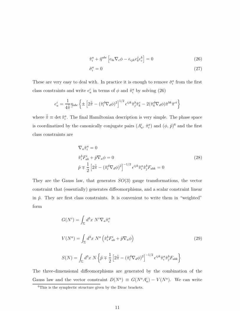
this way we get three sets of first class constraints plus the following independent

second class constraints

10

πai + ηabc

[

ebi∇cφ− ǫijkejbe

kc

]

= 0 (26)

σai = 0 (27)

These are very easy to deal with. In practice it is enough to remove σai from the first

class constraints and write eia in terms of φ and πa

i by solving (26)

eia =

1

4˜π˜ηabc

{

±[

2˜π − (πdl ∇dφ)2

]1/2ǫijkπb

j πck − 2(πd

k∇dφ)πbkπci}

where ˜π ≡ det πai . The final Hamiltonian description is very simple. The phase space

is coordinatized by the canonically conjugate pairs (Aia, π

ai ) and (φ, p)6 and the first

class constraints are

∇aπai = 0

πbiF

iab + p∇aφ = 0 (28)

p∓1

2

[

2˜π − (πdl ∇dφ)2

]−1/2ǫijkπa

i πbjFabk = 0

They are the Gauss law, that generates SO(3) gauge transformations, the vector

constraint that (essentially) generates diffeomorphisms, and a scalar constraint linear

in p. They are first class constraints. It is convenient to write them in “weighted”

form

G(N i) =∫

Σd3x N i∇aπ

ai

V (Na) =∫

Σd3x Na

(

πbiF

iab + p∇aφ

)

(29)

S(N) =∫

Σd3x N

{

p∓1

2

[

2˜π − (πdl ∇dφ)2

]−1/2ǫijkπa

i πbjFabk

}

The three-dimensional diffeomorphisms are generated by the combination of the

Gauss law and the vector constraint D(Na) ≡ G(NaAia) − V (Na). We can write

6This is the symplectic structure given by the Dirac brackets.

11

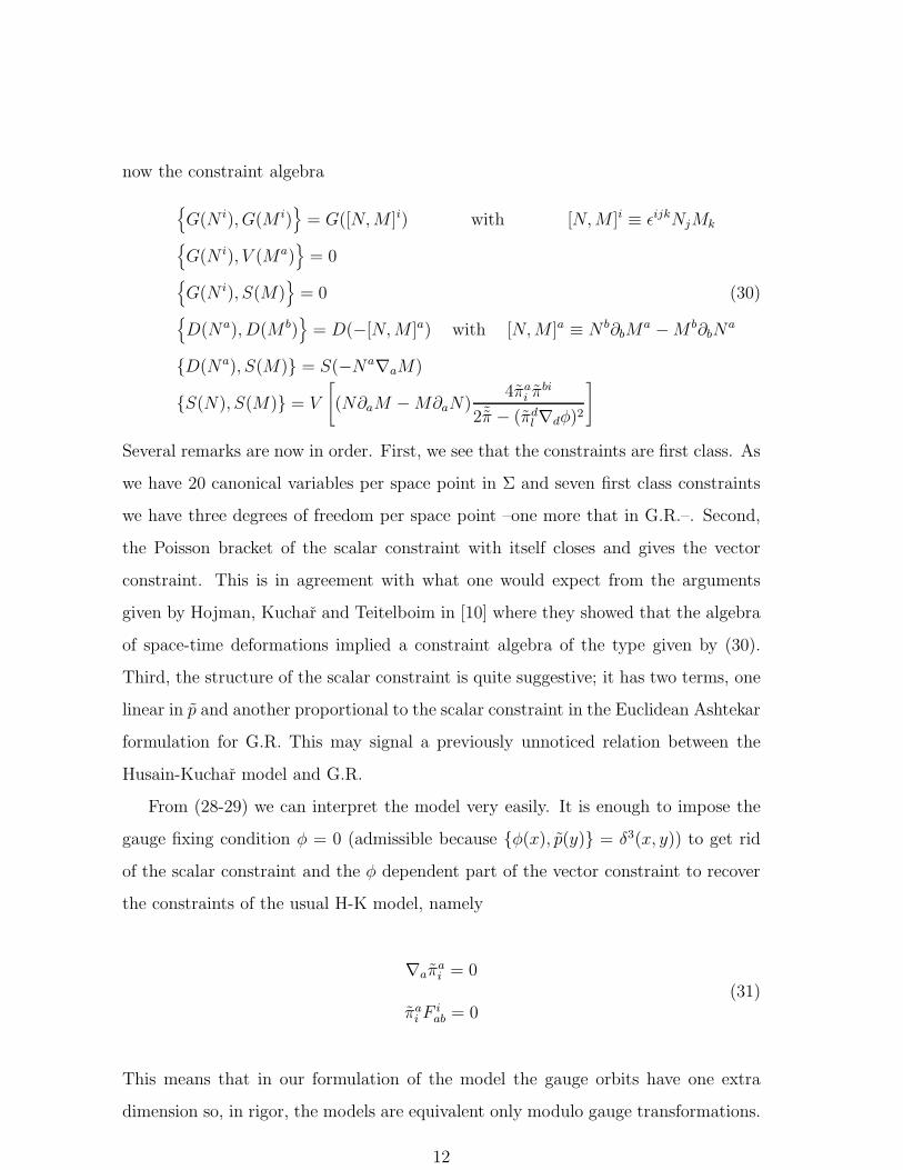
now the constraint algebra

{

G(N i), G(M i)}

= G([N,M ]i) with [N,M ]i ≡ ǫijkNjMk

{

G(N i), V (Ma)}

= 0{

G(N i), S(M)}

= 0 (30){

D(Na), D(M b)}

= D(−[N,M ]a) with [N,M ]a ≡ N b∂bMa −M b∂bN

a

{D(Na), S(M)} = S(−Na∇aM)

{S(N), S(M)} = V

[

(N∂aM −M∂aN)4πa

i πbi

2˜π − (πdl ∇dφ)2

]

Several remarks are now in order. First, we see that the constraints are first class. As

we have 20 canonical variables per space point in Σ and seven first class constraints

we have three degrees of freedom per space point –one more that in G.R.–. Second,

the Poisson bracket of the scalar constraint with itself closes and gives the vector

constraint. This is in agreement with what one would expect from the arguments

given by Hojman, Kuchar and Teitelboim in [10] where they showed that the algebra

of space-time deformations implied a constraint algebra of the type given by (30).

Third, the structure of the scalar constraint is quite suggestive; it has two terms, one

linear in p and another proportional to the scalar constraint in the Euclidean Ashtekar

formulation for G.R. This may signal a previously unnoticed relation between the

Husain-Kuchar model and G.R.

From (28-29) we can interpret the model very easily. It is enough to impose the

gauge fixing condition φ = 0 (admissible because {φ(x), p(y)} = δ3(x, y)) to get rid

of the scalar constraint and the φ dependent part of the vector constraint to recover

the constraints of the usual H-K model, namely

∇aπai = 0

πai F

iab = 0

(31)

This means that in our formulation of the model the gauge orbits have one extra

dimension so, in rigor, the models are equivalent only modulo gauge transformations.

12

At this point the reader may have the temptation to think that, after all, it is trivial

to add a scalar constraint to (31) in order to have a time variable (just take p = 0

and add the term necessary to generate diffeomorphisms on φ and p to the vector

constraint). The formulation thus obtained is, obviously, equivalent to ours (and can

be derived from the action (6) by removing the derivatives of φ with an integration

by parts). However, it is much less obvious (and less trivial) the fact that with a

suitable choice of a scalar constraint one gets, not only a time variable, but also a

way to interpret the H.K model as a theory for non-degenerate four-metrics at the

Lagrangian level.

V The four-dimensional Picture: Non-degenerate

4-metrics

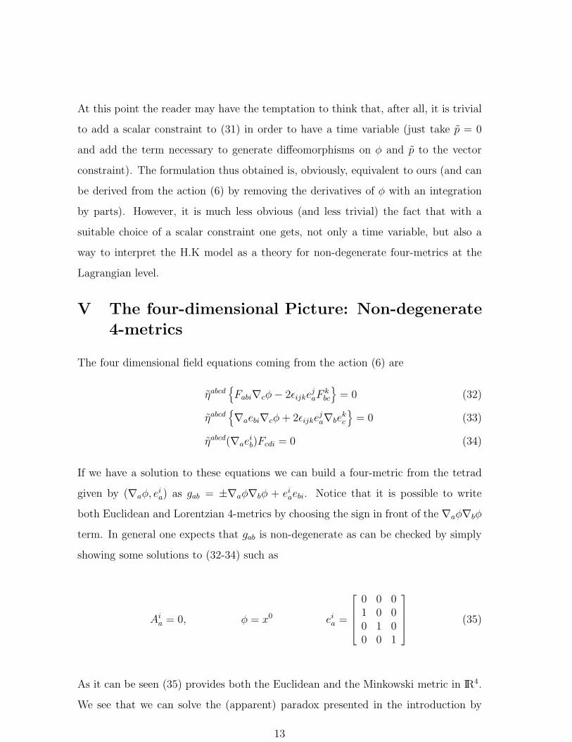
The four dimensional field equations coming from the action (6) are

ηabcd{

Fabi∇cφ− 2ǫijkejaF

kbc

}

= 0 (32)

ηabcd{

∇aebi∇cφ+ 2ǫijkeja∇be

kc

}

= 0 (33)

ηabcd(∇aeib)Fcdi = 0 (34)

If we have a solution to these equations we can build a four-metric from the tetrad

given by (∇aφ, eia) as gab = ±∇aφ∇bφ + ei

aebi. Notice that it is possible to write

both Euclidean and Lorentzian 4-metrics by choosing the sign in front of the ∇aφ∇bφ

term. In general one expects that gab is non-degenerate as can be checked by simply

showing some solutions to (32-34) such as

Aia = 0, φ = x0 ei

a =

0 0 01 0 00 1 00 0 1

(35)

As it can be seen (35) provides both the Euclidean and the Minkowski metric in IR4.

We see that we can solve the (apparent) paradox presented in the introduction by

13

using the scalar field that is present now in the field equations to build non-degenerate

four-metrics.

It is interesting at this point to compare the new equations (32-34) with the old

ones (2). For starters we seem to have one more equation now that we had before;

however, as we show below, this equation is not independent of the others and, also,

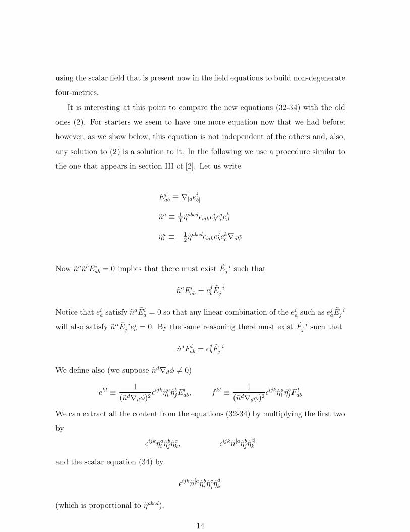
any solution to (2) is a solution to it. In the following we use a procedure similar to

the one that appears in section III of [2]. Let us write

Eiab ≡ ∇[ae

ib]

na ≡ 13!ηabcdǫijke

ibe

jce

kd

ηai ≡ −1

2ηabcdǫijke

jbe

kc∇dφ

Now nanbEiab = 0 implies that there must exist E i

j such that

naEiab = ej

bEi

j

Notice that eia satisfy naEi

a = 0 so that any linear combination of the eia such as ej

aEi

j

will also satisfy naE ij e

ja = 0. By the same reasoning there must exist F i

j such that

naF iab = ej

bFi

j

We define also (we suppose nd∇dφ 6= 0)

ekl ≡1

(nd∇dφ)2ǫijkηa

i ηbjE

lab, fkl ≡

1

(nd∇dφ)2ǫijkηa

i ηbjF

lab

We can extract all the content from the equations (32-34) by multiplying the first two

by

ǫijkηai η

bj η

ck, ǫijkn[aηb

j ηc]k

and the scalar equation (34) by

ǫijkn[aηbi η

cj η

d]k

(which is proportional to ηabcd).

14

The result that we obtain from (32) is that F ij = −12

(

f ij − 12δijf

)

and f ij is

symmetric and from (33) that Eij = 12

(

eij − 12δije

)

and eij is symmetric, where e

and f are the traces of eij and fij respectively. In terms of eij , f ij, Eij , and F ij the

scalar equation (34) gives eijFij +f ijEij = 0; we see now that all the solutions to (32)

and (33) are solutions to the scalar equation and, hence, it is redundant.

If we consider now the standard H-K equations we see that there is no scalar

equation there. It is possible to extract the content of (2) by using the procedure

introduced above. The only difference now is that we need an auxiliary scalar function

(for example the one that gives the foliation used in the passage to the Hamiltonian

formulation) to define ηai . We immediately find the result that appears in [2] e[ij] = 0,

f [ij] = 0, Eij = 0, and F ij = 0, so that now it is also true that the scalar equation

(34) is satisfied. In order to compare the solutions to (2) and (32-34) one must take

into account the new symmety present in the model due to the introduction of φ.

VI From the Old to the New Husain-Kuchar Model:

Equivalence at the Lagrangian Level.

Although we have seen from the Hamiltonian analysis that the new and all formula-

tions of the H-K model are strictly equivalent it is instructive to understand this from

an independent point of view because the actions (1) and (6) look quite different (in

fact one could claim that (6) is really “closer” to the self-dual action for G.R. than

to the H-K action).

The key idea to show this equivalence is the last result of the previous section,

i.e. the fact that every solution to the ordinary H-K equations (2) also satisfies (34).

This means that nothing changes if we add this condition to the action (1) with a

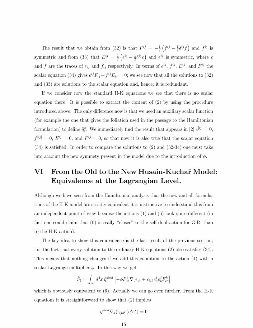
scalar Lagrange multiplier φ. In this way we get

S1 =∫

M

d4x ηabcd[

−φF iab∇cedi + ǫijke

iae

jbF

kcd

]

which is obviously equivalent to (6). Actually we can go even further. From the H-K

equations it is straightforward to show that (2) implies

ηabcd∇a(ǫijkeibe

jce

kd) = 0

15

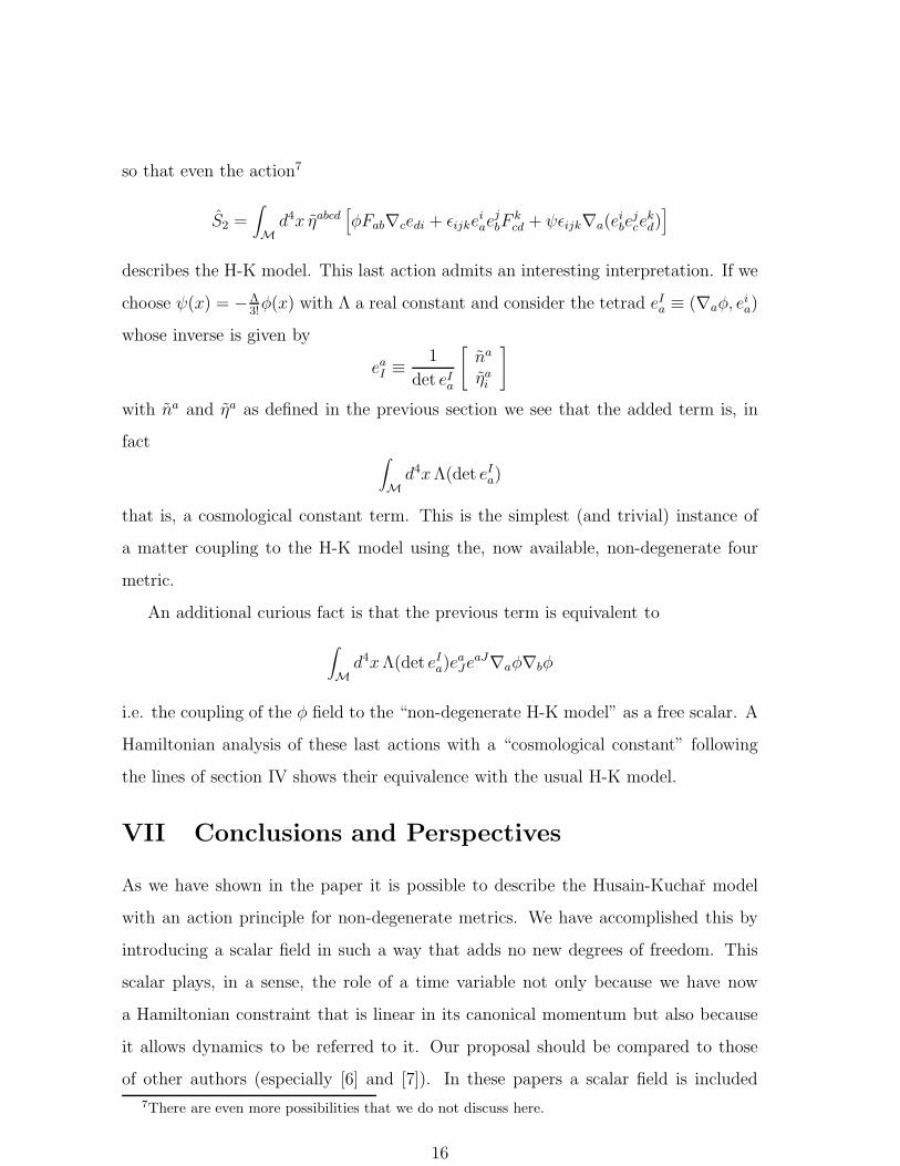
so that even the action7

S2 =∫

M

d4x ηabcd[

φFab∇cedi + ǫijkeiae

jbF

kcd + ψǫijk∇a(e

ibe

jce

kd)

]

describes the H-K model. This last action admits an interesting interpretation. If we

choose ψ(x) = −Λ3!φ(x) with Λ a real constant and consider the tetrad eI

a ≡ (∇aφ, eia)

whose inverse is given by

eaI ≡

1

det eIa

[

na

ηai

]

with na and ηa as defined in the previous section we see that the added term is, in

fact∫

M

d4xΛ(det eIa)

that is, a cosmological constant term. This is the simplest (and trivial) instance of

a matter coupling to the H-K model using the, now available, non-degenerate four

metric.

An additional curious fact is that the previous term is equivalent to

∫

M

d4xΛ(det eIa)e

aJe

aJ∇aφ∇bφ

i.e. the coupling of the φ field to the “non-degenerate H-K model” as a free scalar. A

Hamiltonian analysis of these last actions with a “cosmological constant” following

the lines of section IV shows their equivalence with the usual H-K model.

VII Conclusions and Perspectives

As we have shown in the paper it is possible to describe the Husain-Kuchar model

with an action principle for non-degenerate metrics. We have accomplished this by

introducing a scalar field in such a way that adds no new degrees of freedom. This

scalar plays, in a sense, the role of a time variable not only because we have now

a Hamiltonian constraint that is linear in its canonical momentum but also because

it allows dynamics to be referred to it. Our proposal should be compared to those

of other authors (especially [6] and [7]). In these papers a scalar field is included

7There are even more possibilities that we do not discuss here.

16

as a means to define quantum gauge invariant observables, quoting Rovelli “matter

observables which can be used to dynamically determine surfaces, the areas of which,

we can measure”. Our contribution in this respect is that we have managed to achieve

this goal without introducing new degrees of freedom in the model. We find it quite

appealing that in this process we get a nice interpretation of the scalar φ as time. Not

only can we do this but also, as a side result, we have now the possibility of coupling

ordinary matter to the model. This provides a type of theories that lie in between

those that have a matter evolving in a non-dynamical background and full G.R. We

think that a lot can be learned from looking at these theories; we plan to study them

in the future. Notice, by the way, that we have the choice of coupling the matter

fields to Euclidean or Lorentzian metrics, depending on the choice of the sign in the

first term of the four-metric gab = ±∇aφ∇bφ+ eiaebi.

We want to remark at this point that not knowing beforehand what the meaning

of the action (6) is, one should be very careful in order to avoid missing constraints

crucial for the interpretation of the theory. That is why we have paid so much

attention to the solution of the equations for the Lagrange multipliers. Also, we

emphasize again the contradiction in claiming that the Husain-Kuchar model only

allows for the existence of degenerate four-metrics whereas it is obviously an extension

of both Euclidean and Lorentzian G.R. We believe that we have clearly solved this

seemingly paradoxical fact in the paper.

VIII Appendix

As we have said in the main text of the paper we have paid special attention to the

solution of the Lagrange multiplier equations (18-22). The strategy that we have

followed is simple. First solve (18) for µia and (19) for λi

a and plug the result in the

remaining ones. The result that we have obtained (for non-degenerate triads) shows

that once we write these Lagrange multipliers in terms of ζ , A0i, e0i, Aai, eai, and φ

the remaining equations are identically satisfied.

In order to solve (18) and (19) we need to compute the inverses (that we denote

17

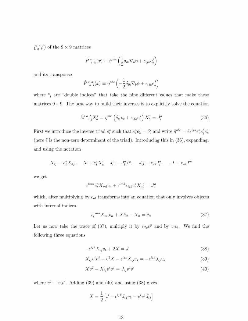
˜P i j

a b ) of the 9 × 9 matrices

P a ci k(x) ≡ ηabc

(

1

2δik∇bφ+ ǫijke

jb

)

and its transponse

P c ak i(x) ≡ ηabc

(

−1

2δik∇bφ+ ǫijke

jb

)

where ai are “double indices” that take the nine different values that make these

matrices 9×9. The best way to build their inverses is to explicitly solve the equation

M a bi jX

jb ≡ ηabc

(

δijvc + ǫijkekc

)

Xjb = Ja

i (36)

First we introduce the inverse triad eai such that ea

i eja = δj

i and write ηabc = eǫijkeai e

bje

ck

(here e is the non-zero determinant of the triad). Introducing this in (36), expanding,

and using the notation

Xij ≡ eaiXaj , X ≡ ea

iXia Ja

i ≡ Jai /e, Jij ≡ eaiJ

aj , , J ≡ eaiJ

ai

we get

ǫlmnealXmivn + ǫlmkǫijke

alX

jm = Ja

i

which, after multiplying by eal transforms into an equation that only involves objects

with internal indices.

ǫ mnl Xmivn +Xδil −Xil = jli (37)

Let us now take the trace of (37), multiply it by ǫilpvp and by vivl. We find the

following three equations

−ǫijkXijvk + 2X = J (38)

Xijvivj − v2X − ǫijkXijvk = −ǫijkJijvk (39)

Xv2 −Xijvivj = Jijv

ivj (40)

where v2 ≡ vivi. Adding (39) and (40) and using (38) gives

X =1

2

[

J + ǫijkJijvk − vivjJij

]

18

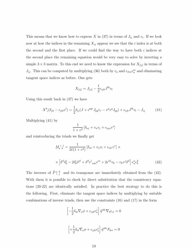
This means that we know how to express X in (37) in terms of Jij and vi. If we look

now at how the indices in the remaining Xij appear we see that the i index is at both

the second and the first place. If we could find the way to have both i indices at

the second place the remaining equation would be very easy to solve by inverting a

simple 3× 3 matrix. To this end we need to know the expression for X[ij] in terms of

Jij. This can be computed by multiplying (36) both by va and ǫilmema and eliminating

tangent space indices as before. One gets

X[ij] = J[ij] −1

2ǫijkJ

lkvl

Using this result back in (37) we have

Xki(δjk − ǫjklv

l) =1

2δij(J + ǫpqrJpqvr − vpvqJpq) + ǫijkJ

lkvl − Jij (41)

Multiplying (41) by1

1 + v2[δnj + vnvj + ǫnjsv

s]

and reintroducing the triads we finally get

˜M i j

a b =1

2e(1 + v2)[δnl + vnvl + ǫnlrv

r] ×

×[

δilδjk − 2δi

kδjl + δilǫjmkv

m + 2ǫiljvk − vkvjδil

]

enae

kb (42)

The inverses of P a bi j and its transponse are immediately obtained from the (42).

With them it is possible to check by direct substitution that the consistency equa-

tions (20-22) are identically satisfied. In practice the best strategy to do this is

the following. First, eliminate the tangent space indices by multiplying by suitable

combinations of inverse triads, then use the constraints (16) and (17) in the form

[

−1

2δik∇aφ+ ǫijke

ja

]

ηabc∇beci = 0

[

+1

2δik∇aφ+ ǫijke

ja

]

ηabcFbci = 0

19

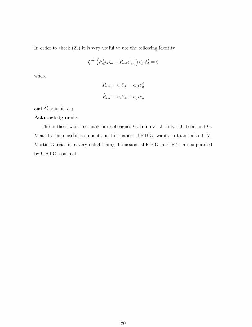
In order to check (21) it is very useful to use the following identity

ηabc(

P kaiǫklm − Paklǫ

kmi

)

emc Λl

b = 0

where

Paik ≡ vaδik − ǫijkeja

Paik ≡ vaδik + ǫijkeja

and Λlb is arbitrary.

Acknowledgments

The authors want to thank our colleagues G. Immirzi, J. Julve, J. Leon and G.

Mena by their useful comments on this paper. J.F.B.G. wants to thank also J. M.

Martın Garcıa for a very enlightening discussion. J.F.B.G. and R.T. are supported

by C.S.I.C. contracts.

20

References

[1] M. P. Ryan Jr. and L. C. Shepley, Homogeneous Relativistic Cosmologies (Prince-

ton University Press 1975).

[2] V. Husain and K. Kuchar, Phys. Rev. D42 (1990) 4070.

[3] J. F. Barbero G., Int. J. Mod. Phys. D3 (1994) 379.

[4] J. Samuel, Pramana J. Phys. 28 (1987) L429.

T. Jacobson and L. Smolin, Phys. Lett. B196, (1987) 39.

[5] A. Ashtekar, Phys. Rev. Lett. 57 (1986) 2244.

A. Ashtekar, Phys. Rev. D36 (1987) 1587.

A. Ashtekar Non Perturbative Canonical Gravity (Notes prepared in collabora-

tion with R. S. Tate) (World Scientific Books, Singapore, 1991).

[6] V. Husain, Phys. Rev. D47 (1993) 5394.

[7] C. Rovelli, Nucl. Phys. B405 (1993) 797.

[8] P.A.M. Dirac, Lectures on Quantum Mechanics, Belfer Graduate School of Sci-

ence Monograph Series number Two, Yeshiva University, New York, 1964.

[9] J. F. Barbero G. Phys. Rev. D51 (1995) 5498.

[10] S. Hojman, K. Kuchar, and C. Teitelboim, Annals Phys. 96 (1976) 88.

21