Human population history and its interplay with natural selection
361
Human population history and its interplay with natural selection Veronika Siska Department of Zoology University of Cambridge This dissertation is submitted for the degree of Doctor of Philosophy Trinity College 2018 September
-
Upload
khangminh22 -
Category
Documents
-
view
6 -
download
0
Transcript of Human population history and its interplay with natural selection
Human population history and its
interplay with natural selection
Veronika Siska
Department of Zoology
University of Cambridge
This dissertation is submitted for the degree of
Doctor of Philosophy
Trinity College 2018 September
ii
Human population history and its
interplay with natural selection
Veronika Siska
Summary
The complex demographic changes that underlie the expansion of anatomically modern humans out of Africa have important consequences on the dynamics of natural selection and our ability to detect it. In this thesis, I aimed to refine our knowledge on human population history using ancient genomes, and then used a climate-informed, spatially explicit framework to explore the interplay between complex demographies and selection.
I first analysed a high-coverage genome from Upper Palaeolithic Romania from ~37.8 kya, and demonstrated an early diversification of multiple lineages shortly after the out-of-Africa expansion (Chapter 2). I then investigated Late Upper Palaeolithic (~13.3ky old) and Mesolithic (~9.7 ky old) samples from the Caucasus and a Late Upper Palaeolithic (~13.7ky old) sample from Western Europe, and found that these two groups belong to distinct lineages that also diverged shortly after the out of Africa, ~45-60 ky ago (Chapter 3). Finally, I used East Asian samples from ~7.7ky ago to show that there has been a greater degree of genetic continuity in this region compared to Europe (Chapter 4).
In the second part of my thesis, I used a climate-informed, spatially explicit demographic model that captures the out-of-Africa expansion to explore natural selection. I first investigated whether the model can represent the confounding effect of demography on selection statistics, when applied to neutral part of the genome (Chapter 5). Whilst the overlap between different selection statistics was somewhat underestimated by the model, the relationship between signals from different populations is generally well-captured. I then modelled natural selection in the same framework and investigated the spatial distribution of two genetic variants associated with a protective effect against malaria, sickle-cell anaemia and β0 thalassemia (Chapter 6). I found that although this model can reproduce the disjoint ranges of different variants typical of the former, it is incompatible with overlapping distributions characteristic of the latter. Furthermore, our model is compatible with the inferred single origin of sickle-cell disease in most regions, but it can not reproduce the presence of this disorder in India without long-distance migrations.
iii
Declaration
This dissertation is the result of my own work and includes nothing which is the outcome of
work done in collaboration except as declared in the Preface and specified in the text.
It is not substantially the same as any that I have submitted, or, is being concurrently
submitted for a degree or diploma or other qualification at the University of Cambridge or
any other University or similar institution except as specified in the text.
I further state that no substantial part of my dissertation has already been submitted, or, is
being concurrently submitted for any such degree, diploma or other qualification at the
University of Cambridge or any other University or similar institution.
The main text does not exceed the prescribed word limit for the relevant Degree Committee
(School of Biology).
Veronika Siska
2018 September

iv
Acknowledgements
I would like to give my thanks to the many people in many countries who I met through my
PhD journey and without whom the work presented in this thesis would not have been
possible.
First and foremost, I would like to thank my supervisor, Andrea Manica. Thank you for your
continuous support, your understanding and your advice in both academic matters and
regarding general life issues. Thank you also for your trust and for giving me the freedom to
explore my ideas. I am also grateful for the continuous support of the postdocs in our group –
without them, this PhD would have been a very lonely experience. Thank you, Eppie, for
your guidance on ancient DNA, for my first, fully positive experience about collaborative
research, and for your incredible support when I was searching for my path. I also want to
thank Anders for creating the model I could build on; Pier for his warm support (especially in
the last, frantic period) and the many useful discussions and Mario and Robert for their effort
on modelling. I would like to also thank my advisors, Chris Jiggins and John Welch for
insightful comments on my project. Another warm thank goes to those who have given their
time to read through my thesis and make sure it is actually in English: to Philipp, Eppie, Pier,
Anne-Sophie and Riva.
I am also grateful for all of the organisations who supported me. The Gates Cambridge Trust
provided the financial basis that enabled me to conduct this research and attend conferences.
Even more importantly, the Trust provided a stimulating environment through workshops on
general humanitarian and personal development topics and by acting as a platform to meet
with like-minded scholars. I also would like to thank the Cambridge Philosophical Society for
their financial help in the last year of my PhD studies. Lastly, living in Cambridge would not
have been such an incredible, unique experience without my college, Trinity, who not only
helped me financially, but was also my home for over three years. In particular, the support
of my college tutor, David Spring, the lively discussions over dinner on the Trinity Biology
Seminars and the warmth and helpfulness of every member of the college staff made me feel
welcome in Cambridge and at Trinity College.
The Department of Zoology and the Evolutionary Ecology Lab provided the basis of all of
my academic work. The frequent coffee breaks, happy hours, talks showcasing various
animals and the odd lunch meeting created a lovely working space. I am grateful for the staff

v
to make all of our work possible and feel honoured to have met so many incredible people at
Zoology: Riva, Anne-Sophie, Eppie, Pier, Anahit, Robert, Mario, Tim, Anders, Maddie,
Maanasa, Lizzie, Alison, James, Jim, Arne and so many others. Such an environment made it
possible to keep focused and bounce back at the inevitable downs - I will miss everyone!
I also would like to thank my friends who had my back through these exciting, but often
challenging years. In Cambridge, Anne-Sophie helped me manage my own expectations and
demonstrated that work-life balance is possible, Riva showed what being passionate about a
research topic really is like and Young Mi was always there when things were not going
according to plan. Another warm thanks goes to David for his support; Konrad for helping
me find a job; Daniel, Tim and Lawrence, my climbing companions, and to all the friendly
Trinitarians, Zoologists and other Cambridge residents I’ve met. Special thanks to all of my
friends in Budapest who made the effort to keep in touch with me through my ever-changing
life, visited me and met with me at home: Péter, Szilvi, Laura, Bence and Bálint kept me in
touch with “real life” beyond Cambridge. Finally, I am eternally grateful for my family for
supporting me in a foreign environment and for giving me the strong roots that I could rely
on.
This PhD was an incredible journey leading to new destinations. I would like to dedicate my
thesis to those closest to me who helped me find my own way: to my parents, Éva and Péter,
and to my partner, Philipp.
vi
Contents
Contents .................................................................................................................................... vi
Chapter 1 General introduction .......................................................................................... 11
1.1 History of anatomically modern humans .................................................................. 11
1.1.1 Evolution of anatomically modern humans ....................................................... 11
1.1.2 The expansion of anatomically modern humans out of Africa .......................... 13
1.1.3 Neolithic transition............................................................................................. 15
1.2 Genome sequencing .................................................................................................. 16
1.2.1 Introduction to genome sequencing ................................................................... 16
1.2.2 Ancient DNA ..................................................................................................... 17
1.3 Modelling .................................................................................................................. 19
1.3.1 Demography ....................................................................................................... 19
1.3.2 Genetics.............................................................................................................. 20
1.4 Natural selection ........................................................................................................ 22
1.4.1 Introduction to natural selection ........................................................................ 22
1.4.2 Confounding effects ........................................................................................... 23
1.5 Bibliography .............................................................................................................. 24
Chapter 2 Palaeolithic Oase genome implies diversification and extinction events across
Eurasia 32
2.1 Abstract ..................................................................................................................... 32
2.2 Contribution .............................................................................................................. 33
2.3 Introduction ............................................................................................................... 33
2.4 Results ....................................................................................................................... 36
2.4.1 DNA extraction, sequencing and authentification ............................................. 36
2.4.2 Mitochondrial haplogroup assignment .............................................................. 38
2.4.3 Comparison of Oase 1 and Oase 2 ..................................................................... 39
2.4.4 Neanderthal ancestry .......................................................................................... 42
2.4.5 Comparison of Oase 2 and other modern and ancient samples ......................... 44
2.4.6 African origins ................................................................................................... 45
vii
2.4.7 Demographic analysis on high-quality Upper Palaeolithic genomes ................ 47
2.5 Conclusions ............................................................................................................... 50
2.6 Methods ..................................................................................................................... 52
2.6.1 DNA extraction and library preparation ............................................................ 52
2.6.2 Processing and mapping of NGS data ............................................................... 54
2.6.3 Mitochondrial DNA ........................................................................................... 55
2.6.4 Authenticity of ancient DNA molecules ............................................................ 55
2.6.5 SNP calling and merging with reference panel .................................................. 56
2.6.6 Calculating statistics .......................................................................................... 56
2.6.7 G-PhoCS analysis for Oase ................................................................................ 58
2.7 Bibliography .............................................................................................................. 63
Chapter 3 Upper Palaeolithic genomes reveal deep roots of modern Eurasians ................ 69
3.1 Abstract ..................................................................................................................... 69
3.2 Contribution .............................................................................................................. 70
3.3 Introduction ............................................................................................................... 70
3.4 Results ....................................................................................................................... 72
3.4.1 Samples, sequencing and authenticity ............................................................... 72
3.4.2 Continuity across the Palaeolithic-Mesolithic boundary ................................... 72
3.4.3 Deep coalescence of early Holocene lineages ................................................... 75
3.4.4 Caucasus hunter-gatherer contribution to subsequent populations .................... 80
3.4.5 CHG origins of migrating Early Bronze Age herders ....................................... 82
3.4.6 Modern impact of CHG ancestry ....................................................................... 84
3.5 Conclusions ............................................................................................................... 84
3.6 Methods ..................................................................................................................... 86
3.6.1 Sample preparation and DNA sequencing ......................................................... 86
3.6.2 Sequence processing and alignment .................................................................. 86
3.6.3 Authenticity of results ........................................................................................ 87
3.6.4 Molecular sex and uniparental haplogroups ...................................................... 90
3.6.5 Merging ancient data with published data ......................................................... 92
3.6.6 Population genetic analyses ............................................................................... 95
3.6.7 Dating split times using G-PhoCS. .................................................................. 100
3.6.8 Runs of homozygosity ..................................................................................... 105
3.6.9 Phenotypes of interest ...................................................................................... 107
3.7 Bibliography ............................................................................................................ 109
viii
Chapter 4 Genome-wide data from two early Neolithic East Asian individuals dating to
7,700 years ago ...................................................................................................................... 119
4.1 Abstract ................................................................................................................... 119
4.2 Contribution ............................................................................................................ 120
4.3 Introduction ............................................................................................................. 120
4.4 Results ..................................................................................................................... 121
4.4.1 Samples, sequencing and authenticity ............................................................. 121
4.4.2 Relation to modern populations ....................................................................... 123
4.4.3 Relation to ancient genomes from Asia ........................................................... 128
4.4.4 Continuity between Devil’s Gate and the Ulchi .............................................. 128
4.4.5 Southern and Northern genetic material in the Japanese and the Korean........ 130
4.4.6 Phenotypic prediction ...................................................................................... 133
4.5 Conclusions ............................................................................................................. 133
4.6 Methods ................................................................................................................... 134
4.6.1 Experimental Design ........................................................................................ 134
4.6.2 Statistical Analysis ........................................................................................... 137
4.7 Bibliography ............................................................................................................ 144
Chapter 5 Behaviour of selection statistics in a spatially explicit, neutral demographic
model 153
5.1 Abstract ................................................................................................................... 153
5.2 Contribution ............................................................................................................ 154
5.3 Introduction ............................................................................................................. 154
5.4 Methods ................................................................................................................... 157
5.4.1 Spatially explicit demographic model ............................................................. 157
5.4.2 Refitting the model .......................................................................................... 160
5.4.3 Overlap between different statistics ................................................................. 169
5.5 Results ..................................................................................................................... 173
5.5.1 Refitting the model .......................................................................................... 173
5.5.2 Overlap between different statistics and populations ...................................... 175
5.6 Discussion ............................................................................................................... 183
5.7 Bibliography ............................................................................................................ 184
Chapter 6 Explaining spatial patterns of adaptation against malaria................................ 188
6.1 Abstract ................................................................................................................... 188
6.2 Contribution ............................................................................................................ 189
6.3 Introduction ............................................................................................................. 189
ix
6.3.1 Malaria and protective genetic disorders ......................................................... 189
6.3.2 Variants of protective disorders ....................................................................... 190
6.3.3 Aim of this study .............................................................................................. 191
6.4 Methods ................................................................................................................... 192
6.4.1 Model ............................................................................................................... 192
6.4.2 Data .................................................................................................................. 195
6.4.3 Inferring haplotype origins .............................................................................. 202
6.4.4 Single-origin hypothesis of sickle-cell disease ................................................ 203
6.5 Results ..................................................................................................................... 204
6.5.1 Inferring haplotype origins .............................................................................. 204
6.5.2 Qualitative spatial patterns ............................................................................... 209
6.5.3 Single-origin hypothesis of sickle-cell anaemia .............................................. 212
6.6 Discussion ............................................................................................................... 213
6.6.1 Results .............................................................................................................. 213
6.6.2 Limitations ....................................................................................................... 214
6.6.3 Perspectives...................................................................................................... 216
6.6.4 Summary .......................................................................................................... 216
6.7 Bibliography ............................................................................................................ 217
Chapter 7 Epilogue ........................................................................................................... 222
7.1 Introduction ............................................................................................................. 222
7.2 aDNA and its use in uncovering demographic processes ....................................... 223
7.2.1 Introduction ...................................................................................................... 223
7.2.2 Broad and deep sampling ................................................................................. 223
7.2.3 Increase in data volume and issues of compatibility ....................................... 225
7.2.4 Data-driven projects ......................................................................................... 225
7.3 Continuity and extinctions in human evolution ...................................................... 226
7.3.1 Introduction ...................................................................................................... 226
7.3.2 Extinctions and lineages .................................................................................. 226
7.3.3 Definition of continuity.................................................................................... 227
7.4 Importance of space in modelling ........................................................................... 228
7.4.1 Advantages ....................................................................................................... 228
7.4.2 Disadvantages .................................................................................................. 228
7.5 Concluding remarks ................................................................................................ 229
7.6 Bibliography ............................................................................................................ 230
x
Appendix A Appendix for Chapter 2 ................................................................................ 234
A.1 NGS sequencing statistics ....................................................................................... 234
A.2 Mitochondrial genome ............................................................................................ 237
A.3 Outgroup f3 statistics for Oase 1 using modern populations ................................... 238
A.4 Outgroup f3 statistics for Oase 2 on SNPs called in Oase 1 .................................... 239
A.5 African origins......................................................................................................... 241
A.6 Comparison of Upper Palaeolithic genomes using D statistics............................... 248
A.7 Convergence of G-PhoCS Monte Carlo chains....................................................... 250
A.8 Detailed G-PhoCS results........................................................................................ 254
Appendix B Appendix for Chapter 3 ................................................................................ 260
B.1 Archaeological context ............................................................................................ 260
B.1.1 Kotias Klde ...................................................................................................... 260
B.1.2 Satsurblia.......................................................................................................... 262
B.1.3 Grotte du Bichon .............................................................................................. 263
B.2 Supplementary figures............................................................................................. 265
B.3 Supplementary tables .............................................................................................. 272
Appendix C Appendix for Chapter 4 ................................................................................ 292
C.1 Osteology ................................................................................................................ 292
C.2 Archaeology ............................................................................................................ 293
C.3 Phenotypic prediction .............................................................................................. 294
C.4 Supplementary figures............................................................................................. 297
C.5 Supplementary tables .............................................................................................. 311
Appendix D Appendix for Chapter 5 ................................................................................ 346
D.1 Relationship between potential ABC summary statistics ....................................... 346
Appendix E Appendix for Chapter 6 ................................................................................ 353
E.1 Fit using SSE for thalassemia.................................................................................. 353
E.2 Sensitivity analysis .................................................................................................. 356
E.2.1 Selection coefficient......................................................................................... 357
E.2.2 Demographic parameters ................................................................................. 358
E.2.3 Starting time of selection ................................................................................. 360
Chapter 1 General introduction
11
Chapter 1 General introduction
1.1 History of anatomically modern humans
1.1.1 Evolution of anatomically modern humans
Anatomically modern humans evolved through a long and non-linear process, starting with
the separation of the hominins (species closer to humans than to the closest relative, the
chimpanzee). The current, widely accepted model of hominin origins is termed “Out of
Asia”: according to this, apes evolved in Africa and then dispersed over Eurasia in the Middle
Miocene, once a landbridge was established. Climate change then lead to the disappearance
of primitive apes from Africa (by roughly 9 million years ago), until its recolonization in the
Late Miocene (roughly 4-8 million years ago)1,2. These modern apes then evolved into
diverse groups through a so-called adaptive dispersal, since they were faced with a new,
heterogeneous environment following climate change (e.g. forest cover breaking up)3. In this
view, hominins were just one of the resulting groups, together with other African apes like
gorillas or chimpanzees.
A combination of fossil evidence, genetics and paleoclimate reconstructions support this “Out
of Asia” model of hominin origins1,2. Palaeontology provides evidence for when different
clades appeared and how they were related morphologically, genetics establishes their
phylogenetic relation, and past climate dates when the necessary land-bridge existed and
when the climate changed. Genetics was crucial to disentangle the relationship between
hominins and African apes, supporting that hominins and chimpanzees form a clade, as
Chapter 1 General introduction
12
opposed to earlier models that placed all non-hominin apes into one clade based on their
morphology.
However, the timing and process of the separation of hominins and other apes is far from
clear. Palaeontology struggles with a combination of sparsity and unclear classification of
fossil specimens, carrying a mosaic of archaic and modern morphological features. Regarding
genetics, we can only rely on the difference between living species due to a lack of genetic
data from ancient hominins1,2. Based on modern genetic data, the separation occurred around
6 million years ago, but a large variation of estimated divergence times between humans and
chimpanzees across the genome and a shorter divergence time on the X chromosome was
inferred4. This could be due to incomplete lineage sorting
5, the different mutation rate of the
X chromosome5,6
and/or natural selection acting differentially6, but could also be the sign of a
complex speciation-hybridisation process as opposed to a clean split4 ().
After the separation of the hominin clade, a long and winding evolutionary road leads to the
genus Homo, following the same pattern of complex relationships among different taxa.
There is no clear definition of the genus Homo, but broadly speaking, members of the family
are those either ancestral to or closely related to modern humans. There is an observed,
continual increase in cranial capacity throughout the evolution of the genus, which is also
associated with the advent of tool use2. These signs separate them from their ancestors, the
early hominins and Australopithecines, as well as the robust Australopithecines who took an
alternative evolutionary path and did not leave any present-day descendants.
Classification of the Homo genus into species and subspecies is challenging, due to
incomplete information and complex relationships within the genus; I here present the
summary of a widely accepted view1,2. The first accepted species is Homo habilis, the
initiators of tool use, with an evolutionary history in Africa. This species is followed by the
more human-like Homo ergaster in Africa and the Homo erectus inside and outside Africa,
with even more derived features. According to the currently most accepted view, Homo
erectus evolved through a radiation out of Africa, where Homo ergaster was its ancestral or
Chapter 1 General introduction
13
sister species. Homo erectus then spread over Eurasia and separated into diverse groups with
different variants inhabiting different areas, from Spain and Georgia all the way to South-East
Asia. However, the classification of these variants is still debated: whether they are separate
species, ancestral to each other, or simply regional variants originating from the same
dispersal event remains unclear. What we know for certain is that they represent a wide range
of morphological variation, but due to the limited number of remains in each group, it is
difficult to judge the level of differentiation.
Homo heidelbergensis appeared around 700kya2. They reached the range of cranial capacity
of anatomically modern humans and possessed material culture hardly distinguishable from
that of early Homo sapiens, including tool use and even signs of social structures, such as
care of the old or infirm or interpersonal violence. The evolution and classification of Homo
heidelbergensis mimic that of Homo erectus, with unclear boundaries between groups, a
plausible origin in Africa, a successive spread over Eurasia and divergent evolution in
geographically different areas. Neanderthals and Denisovans in Eurasia, and Homo sapiens,
also called anatomically modern humans (AMHs) in Africa are all thought to have evolved
from Homo heidelbergensis, with African and Eurasian groups possibly separated due to
climatic changes (an arid phase in the Near East)2.
1.1.2 The expansion of anatomically modern humans out of Africa
Evidence for the African origin of Homo sapiens comes from a combination of archaeology
and genetics. The earliest fossils classified as Homo sapiens all originate from Africa Omo
Valley, Ethiopia ~190kya7, Herto, Ethiopia ~160kya
8 and Pinnacle Point, South Africa
~164kya9). However, the recent dating to ~300kya of a Homo sapiens fossil from Jebel
Irhoud, Morocco10,11
, implies that modern humans may have evolved earlier and could have
had a wider distribution than previously thought. In contrast, the earliest fossils outside
Africa is only 92kya (Skuhl & Quafzeh, Israel2), but even those have archaic features and are
regarded by many scholars as not directly ancestral to present-day non-Africans. The first
Chapter 1 General introduction
14
finding from outside the Near East is from China (Daoxian teeth ~80kya12
), followed by
archaeological and palaeontological evidence showing that anatomically modern humans
spread out from Africa from 60kya onwards, reaching all corners of Eurasia by about
45kya13–15
and crossing into the Sahul somewhere between 60kya and 40kya14
.
Genetics played a crucial role in establishing the African origin of anatomically modern
humans. The first line of evidence comes from the present-day diversity of uniparental
haplotypes (mtDNA16,17
and Y-chromosome17,18
), which date last common ancestor to
between 200 and 130kya, before the appearance of modern human fossils outside Africa.
These dates rely heavily on estimates of the mutation rate, which provide the conversion
between mutational distance and time. However, by now, accurate estimates are available
using Next-Generation Sequencing data for the Y chromosome19
and ancient data for
mtDNA20
. Second, the modern-day non-African genetic diversity lies within that of Africans,
both regarding uniparental markers and the nuclear genome. Therefore, populations within
Africa carry the deepest separations, with the oldest (more than 100kya) separating the South
African Khoe San people from all other populations19
. Last, genetic diversity on mtDNA21
and nuclear markers22,23
, but even phenotypic diversity estimated based on cranial
metrics22,24
, decreases with distance from Africa. This pattern of decreasing diversity with
distance from the origin is typical after the expansion of a species.
Many aspects of the exit out of Africa are well understood. The most commonly accepted
timing is around 50-60 kya, supported by the appearance of unambiguously classified Homo
sapiens fossils outside of Africa2, the times to the common origin of non-African mtDNA
25
haplogroups, as well as estimated exit times based on modelling using nuclear genetic
diversity26,27
. Furthermore, this period coincides with a window of climate favourable for
humans in the otherwise arid and impassable Arabian peninsula around 60-70kya27
.
However, there are also several aspects of the so-called Out-of-Africa event that remain
unclear. First, there is a possibility of earlier exit(s) out of Africa, which are difficult to detect
Chapter 1 General introduction
15
if they were overwhelmed by a subsequent larger wave. There was a favourable climatic
window about 130kya, accompanied by a similarity in lithics inside and outside of Africa28
and some genetic studies also point to a small amount of genetic material from such an early
wave in Papuans29
. However, other studies, also including samples from the same region,
failed to reject the single-wave scenario30,31
, and the broad pattern of diversity in non-African
populations is also consistent with a single expansion wave22,27
. This implies that
anatomically modern humans (AMHs) mainly originate from a single wave, which could
have been preceded by a smaller one. Chapter 2 explores the diversity of AMHs in Eurasia
shortly after the main wave out of Africa in light of a ~37.8 ky old genome from present-day
Romania.
The relationship between modern and archaic humans (Neanderthals and Denisovans, the
latter only known by its DNA) is an additional debated point in the early evolution of AMHs.
Certain modern-day non-Africans show an increased affinity to Neanderthals32,33
and
Denisovans34
. Neanderthal ancestry is estimated at roughly 1.5-2.1 in all non-Africans33
,
whereas Denisovan ancestry is estimated at around 2-4% in Oceania35
and Melanesia36
.
However, it is also possible that substructure within Africa37
or a difference in mutation rates
between modern Africans and non-Africans38
can explain at least part of this signal.
1.1.3 Neolithic transition
After the spread of humans out of Africa, a structured population of hunter-gatherers existed
all over Eurasia. In addition to their cultural relations from archaeological studies, we are
now starting to understand their genetic composition, with the help of ancient genomes.
There is genetic material available from Eurasia in the Upper Paleolithic, the period
stretching from the dispersal of anatomically modern humans out of Africa until the advent of
the Holocene roughly 10 kya. Some samples are associated with different groups of modern
populations (e.g. Europeans39–41
, East Asians42
, Native Americans43
or Central Asians from
the Caucasus40
), but others did not seem to contribute substantially to extant populations
Chapter 1 General introduction
16
(Ust’Ishim from Asia44
and several European samples from 40-30,000 years ago41,45
).
Chapter 3 explores data from one of the early European lineages that appear to be a dead end,
whereas Chapter 4 presents an Upper Paleolithic lineage that left its footprint on modern
populations across Eurasia.
The next large shift in the history of anatomically modern humans was brought by the so-
called Neolithic transition, coinciding with the beginning of the Holocene in West Eurasia
and characterised by the advent of agriculture, industrial developments (pottery, textile) and a
sedentary lifestyle. The transition is well-studied in archaeology, but genetic data is necessary
to determine the extent to which the Neolithic spread through cultural transmission or the
movement of people. Ancient genomes have revealed a major population replacement in
West Eurasia during the transition from hunting-gathering to agriculture from ~10.5 kya
onwards, followed by a progressive “resurgence” of local hunter-gatherer population ancestry
and later, coinciding with the advent of the Bronze age ~5.5 kya, a major contribution from
the Asian Steppe39,46
. The process in Asia is less well-known: archaeology shows multiple
origins of the Neolithic and a lack of the strong association between its components (pottery,
farming and animal husbandry) that was observed in Europe, but ancient DNA is still missing
from the relevant time period in the region. In Chapter 5, I analyse such data and explore its
implications on the Neolithic transition on the northern periphery of East Asia.
1.2 Genome sequencing
1.2.1 Introduction to genome sequencing
One of the main sources of information on human population history is genetic data. The
genetic data used in this thesis is mainly the sequence of DNA from the 22 nuclear
chromosomes, the sex chromosomes and the mitochondrial chromosome, encoded in a four-
letter alphabet of base pairs. In the case of whole-genome sequencing, we are interested in all
Chapter 1 General introduction
17
positions, but one can also focus on only single nucleotides at given polymorphic positions
(single nucleotide polymorphisms or SNPs).
The process of determining the DNA sequence is called sequencing. The most common
technology used nowadays is Next-Generation Sequencing (NGS)47
, where the target
sequence is broken up into pieces and then amplified before the base pairs are determined (in
other words, the sequence is read). These short, generally 50-100 base pair long segments
(reads) are then mapped (aligned) to the sequence of the organism in question (the reference
sequence), according to where they fit well. Finally, the bases that the sample most likely had
at locations of interest (genotypes) can be determined.
1.2.2 Ancient DNA
Sequencing ancient DNA (aDNA), that is, DNA from specimens not preserved for DNA
analysis (e.g. bones from archaeological sites, mummies, hair, tissues from the permafrost) is
technologically challenging. The first such study in 1984 reported DNA traces from an
ancient horse species, the Quagga, sampled over 150 years after the organism’s death48
.
Unfortunately several early ancient DNA studies proved to be only contamination, including
claims of obtaining DNA from a dinosaur49
. These false positives, together with the laborious
process of sequencing DNA at the time before NGS, hindered advances in the field50–52
.
However, with technological progress and rigorous laboratory procedures, it became possible
to routinely sequence ancient DNA; first from the abundantly available mitochondria and
later also from the nuclear genome. The age of sequenced samples is continuously pushed
back: the oldest sequenced sample to date is a horse from the permafrost that lived over half a
million years ago53
, but several modern44
and ancient33,35
hominins over 40,000 years-old
have also been sequenced.
There are three main families of problems that make the sequencing of ancient DNA
challenging50–52
. First, as DNA breaks down, the segments get shorter. With NGS, these
segments can be sequenced, but the difficulty of alignment increases with decreasing segment
Chapter 1 General introduction
18
length. Even intermediate read lengths make de novo assembly impossible, and parts of the
genome that are particularly difficult to align to (e.g. repetitive regions) become inaccessible.
At even shorter read lengths, any kind of alignment becomes infeasible. Second, chemical
processes, deamination in particular, can change the sequence and cause spurious mutations,
especially at the end of the fragments. Third, contamination leads to only a small proportion
of the DNA originating from the ancient specimen. Including these fragments in the analysis
can lead to erroneous conclusions, and they are especially difficult to filter out if the ancient
sample is contaminated by modern DNA of the same or similar species.
There are several ways to assess the quality of ancient genomes and to deal with the
challenges described above. Both fragment length and the presence of deaminated bases at
the end of fragments can be used to assess the authenticity of the sample. Afterwards, a
minimum read length is usually imposed and the (likely damaged) ends are clipped before
further processing. It is also possible to chemically reverse deamination, in which case a
small portion of the DNA is kept in its original form for authenticity assessment. Regarding
contamination, sequences from organisms different from the sample (e.g. soil bacteria on a
human sample) can be separated during alignment on the basis of their low similarity to the
target reference sequence. Contamination from modern sources of the same or closely related
organism (e.g. humans handling an ancient human sample) is more challenging to handle. In
addition to authenticity based on damage patterns, the level of such contamination can be
estimated using uniparental markers (by looking at the proportion of sequencing not matching
the consensus haplotype) or, for male specimens, using the X chromosome (by looking at
polymorphisms).
Chapter 1 General introduction
19
1.3 Modelling
1.3.1 Demography
The goal of demographic modelling is to provide a simplified framework of demographic
processes, such as natural birth and death or population admixture. Such models track the size
of populations over time, given the rules governing its change. These models can be discrete
or continuous in how they represent population size, space and time. Discrete and continuous
models can be each other’s approximation and the choice of framework depends on the
system studied and the features of its behaviour that one is trying to capture. For instance, a
discrete-time model is more suited for a system with separate generations, whereas one with
overlapping generations with incremental changes is easier to represent using a continuous-
time framework.
Deterministic and stochastic demographic models are fundamentally different in terms of
their mathematics, but can be used to model similar systems. Just like with continuous and
discrete models, deterministic and stochastic models can be equivalent under certain
conditions, and the choice between them depends on the system. Deterministic models are
usually easier to handle mathematically and often have a smaller computational footprint, but
the effects of stochasticity can be important for certain systems. Natural systems are usually
stochastic by nature, but in the case of large systems, where fluctuations even out, a
deterministic approximation can be sufficient. However, when the population sizes are low or
changes are abrupt (e.g. large fluctuations or small subpopulations), stochastic effects have to
be taken into account explicitly.
Population substructure can further complicate demographic models. Real systems are
usually not completely homogeneous, but it depends on the level of inhomogeneity whether
such substructure can be neglected. There are numerous ways to represent substructure, from
toy models consisting of a few separate populations through metapopulation models where
populations are connected in a network all the way to complex, spatially explicit frameworks
Chapter 1 General introduction
20
that attempt to capture geographical substructure. However, in addition to the obvious trade-
off between simplicity and computational time, fitting the model to the real system also has to
be considered. Often there is not enough data to set all parameters in a structured model, even
if it is clear that the structure exists. In such cases there are two possibilities: one can either
use a simplified model (e.g. only a few populations) or make assumptions about the
underlying structure (e.g. assume that inhomogeneities and/or connectivity are a function of a
measurable quantity). Simple tree-like models (Chapters 2 and 3) are examples for the
former, whereas spatially explicit models with environment-dependent carrying capacities
and connectivity (Chapters 5 and 6) for the latter.
1.3.2 Genetics
Once we have a demographic model, we can use it to also study the genetic composition of
samples from the population, that is, the DNA sequences of each sample. Depending on the
organism, a single individual can contain one (haploid) or two (diploid) sequences, which can
change from generation to generation through mutation and recombination. Tracking a
certain variant or sequence is equivalent to differentiating between different types of
individuals in the population. In addition to the sequences, the relationship between different
samples can also be relevant. For instance, for analysis based on genealogical trees (the
ancestry tree of sampled genetic markers), we need to track the ancestry of individuals in our
demographic model.
The simplest genetic models assume that there are no new mutations and individuals
randomly mate with each other (no selection) in an infinite population, with non-overlapping
generations. A diploid organism with two alleles in such a model is described by the Hardy-
Weinberg model, where frequencies of the three possible diploid genotypes will be constant
and only dependent on the frequencies of the two alleles54.
One of the simplest deviations from the above model is to relax the assumption of an infinite
population and instead work with a finite number of discrete individuals. Such a system can
Chapter 1 General introduction
21
be described in a simple stochastic framework, where individuals are still mating randomly
within a population, with each offspring originating from two randomly chosen ancestors in
the previous generation54. The case with non-overlapping populations is described by the
Wright-Fisher model, where the whole population is replaced by a new set of individuals in
each generation. The other extreme is the Moran model, where generations overlap and only
a single individual is replaced by a new one in each step. In both of these models, the change
in the number of alleles from generation to generation can be described by a random walk on
a bounded interval, and the corresponding mathematical results (time to fixation, diffusion
approximation, etc.) apply.
Once we have a model to describe the dynamics of different alleles in a population and a set
of samples we are interested in at a given generation, we can build the ancestral relationship
between these (genealogical tree). The genealogy can then be used to calculate when the most
recent common ancestor between any two samples lived, or to track where a certain mutation
occurred and which samples it affects. Observed data generally comes in the form of a set of
samples, which can be used to estimate the corresponding genealogies and through that, to
make inferences about past population history.
A further complication in a diploid population comes from recombination. Recombination is
when the two ancestral sequences are combined to form a diploid sample in the next
generation, but with both sequences in the new sample containing material from both of the
two ancestral sequences. The process mixes up the genealogical trees from the sequences,
resulting in a genealogical network. Furthermore, since recombination only occurs through a
set of breakpoints along a sequence, it takes time to de-couple nearby section of the sequence.
As a consequence, mutations close to each other on the sequence will occur more frequently
together, forming linked sections or haplotypes. Patterns of such haplotypes can also be used
to infer the population history of the sample, and are particularly informative on the timing
and extent of admixture events between populations55,56
.
Chapter 1 General introduction
22
1.4 Natural selection
1.4.1 Introduction to natural selection
Natural selection is the main process behind evolution, where individuals better adapted to
their environment tend to be more successful in survival and reproducing, thus changing the
distribution of heritable biological traits in the population. By studying the dynamics of
adaptation to different environments, it is possible to uncover population history, speciation
and demonstrate evolution at work (e.g. spread of lactase persistence in humans in response
to consuming dairy products57
or change in pigmentation of peppered moths in response to
industrial development58
). Detecting signals of selection also has important implications for
medical applications. Since selection acts on the phenotype, segments under selection are
often of functional importance, associated for instance with resistance against pathogens or
genetic diseases (e.g. sickle cell trait offering partial protection against malaria59
, deleterious
mutation in Siberians originally providing an advantage to a high-fat diet or cold
environment60
). Strong signals of selection in the genome thus have the potential to guide
association studies looking for the underlying genetic causes of medical conditions.
There are several different modes in which selection can act. It can be simply directional,
where an allele is either advantageous and increases in frequency (positive selection) or the
opposite (negative selection). Most new mutations are disadvantageous, leading to constant
negative selection against new variants, called background or purifying selection. In non-
haploid organisms, selection can also act in more complex ways. Balancing selection favours
intermediate frequencies of multiple alleles, for example when the heterozygote is favoured
in a diploid organism. The signature of selection in the genome also depends on whether a
newly arisen mutation is quickly increasing in frequency (hard sweep) or whether it is an
existing variant, part of standing variation, that is becoming favoured (soft sweep). In
humans, the spread of lactase persistence in humans in response to pastorialism57
is a typical
Chapter 1 General introduction
23
example of a sweep, while the HLA locus has long been shown to be under balancing
selection61
.
The availability of dense genetic data has made it possible to detect signals of natural
selection. Selection can be studied either by directly investigating the time series of
occurrence of traits and/or genetic composition (e.g. from experiments or ancient DNA),
looking for associations with certain environments, or by studying signatures of past selection
in the genome. For humans, long-term experiments are unavailable and the quantity and
quality of ancient DNA is just now becoming sufficient to study selection. Two successful
examples for the study of selection using ancient DNA are the detection of derived immune
and ancestral pigmentation alleles in a single 7,000 year old European hunter-gatherer62
and
direct evidence for selection acting on pigmentation in Europeans during the last 5,000
years63
. Associations with the environment provide strong indicators (e.g. between latitude
and skin pigmentation in humans64
), but require assumptions about what the important
environmental factors are, as well as about past climate and the selected population’s history.
Furthermore, spatial boundaries between different genetically incompatible variants (alleles
neutral on the native background, but disadvantageous when occurring together) tend to
become trapped by environmental boundaries even without any kind of selection65
.
Therefore, for humans, most effort has been dedicated to the indirect method of looking for
signals of past selection in the genomes from present-day genomes.
1.4.2 Confounding effects
Interpreting the results of indirect methods can be challenging, as they are influenced by the
demographic history of the studied populations, including changes in population size,
population substructure or admixture66
. Neutral demographic events can create signals similar
to those left by natural selection, making it difficult to assess the significance of any given
finding. There are two strategies commonly adopted to deal with this issue: to use a simple
demographic model to define the null distribution of the signal of interest in the absence of
Chapter 1 General introduction
24
selection57,63
or to focus on a fixed quantile (e.g. top 1%) of the loci with strongest signal60,67–
70. Each of these solutions can be problematic, since simple demographic models often fail to
fully capture the confounding processes of interest, and defining a quantile of how much of
the genome is under strong selection is arbitrary (and does not really solve the confounding
effect of demography). A strong warning of the lack of precision in these methods comes
from the low congruence in the sites detected as under selection by different methods –
although we also have to keep in mind that some methods are sensitive for different kinds of
selection and/or on different timescales than others.
To mitigate the confounding effects, some researchers combine multiple metrics into
composite measures to look for regions consistently scoring highly using different methods
(e.g. composite likelihood ratio71
). However, without knowing the correlations between the
individual measures and how they relate to different cases of selection, statistical significance
still cannot be calculated. In order to disentangle signals of selection from false positives
caused by demographic events and assess significance, we would ideally need a more
realistic demographic model.
1.5 Bibliography
1. Boyd, R. & Silk, J. B. How Humans Evolved: Seventh Edition. (W. W. Norton &
Company, 2014).
2. Foley, R. A. & Lewin, R. Principles of Human Evolution. (John Wiley & Sons,
2013).
3. Kürschner, W. M., Kvaček, Z. & Dilcher, D. L. The impact of Miocene atmospheric
carbon dioxide fluctuations on climate and the evolution of terrestrial ecosystems. Proc. Natl.
Acad. Sci. U. S. A. 105, 449–453 (2008).
Chapter 1 General introduction
25
4. Patterson, N., Richter, D. J., Gnerre, S., Lander, E. S. & Reich, D. Genetic evidence
for complex speciation of humans and chimpanzees. Nature 441, 1103–1108 (2006).
5. Barton, N. H. Evolutionary Biology: How Did the Human Species Form? Curr. Biol.
16, R647–R650 (2006).
6. Wakeley, J. Complex speciation of humans and chimpanzees. Nature 452, E3 (2008).
7. McDougall, I., Brown, F. H. & Fleagle, J. G. Stratigraphic placement and age of
modern humans from Kibish, Ethiopia. Nature 433, 733–736 (2005).
8. White, T. D. et al. Pleistocene Homo sapiens from Middle Awash, Ethiopia. Nature
423, 742–747 (2003).
9. Marean, C. W. et al. Early human use of marine resources and pigment in South
Africa during the Middle Pleistocene. Nature 449, 905 (2007).
10. Hublin, J.-J. et al. New fossils from Jebel Irhoud, Morocco and the pan-African origin
of Homo sapiens. Nature 546, 289 (2017).
11. Richter, D. et al. The age of the hominin fossils from Jebel Irhoud, Morocco, and the
origins of the Middle Stone Age. Nature 546, 293 (2017).
12. Liu, W. et al. The earliest unequivocally modern humans in southern China. Nature
526, 696 (2015).
13. Mellars, P. Why did modern human populations disperse from Africa ca. 60,000 years
ago? A new model. Proc. Natl. Acad. Sci. 103, 9381 (2006).
14. Mellars, P. Going East: New Genetic and Archaeological Perspectives on the Modern
Human Colonization of Eurasia. Science 313, 796–800 (2006).
Chapter 1 General introduction
26
15. Barker, G. et al. The ‘human revolution’ in lowland tropical Southeast Asia: the
antiquity and behavior of anatomically modern humans at Niah Cave (Sarawak, Borneo). J.
Hum. Evol. 52, 243–261 (2007).
16. Cann, R. L., Stoneking, M. & Wilson, A. C. Mitochondrial DNA and human
evolution. Nature 325, 31–36 (1987).
17. Poznik, G. D. et al. Sequencing Y Chromosomes Resolves Discrepancy in Time to
Common Ancestor of Males Versus Females. Science 341, 562–565 (2013).
18. Francalacci, P. et al. Low-Pass DNA Sequencing of 1200 Sardinians Reconstructs
European Y-Chromosome Phylogeny. Science 341, 565–569 (2013).
19. Helgason, A. et al. The Y-chromosome point mutation rate in humans. Nat. Genet. 47,
453 (2015).
20. Rieux, A. et al. Improved Calibration of the Human Mitochondrial Clock Using
Ancient Genomes. Mol. Biol. Evol. 31, 2780–2792 (2014).
21. Balloux, F., Handley, L.-J. L., Jombart, T., Liu, H. & Manica, A. Climate shaped the
worldwide distribution of human mitochondrial DNA sequence variation. Proc. R. Soc. Lond.
B Biol. Sci. 276, 3447–3455 (2009).
22. Manica, A., Amos, W., Balloux, F. & Hanihara, T. The effect of ancient population
bottlenecks on human phenotypic variation. Nature 448, 346–348 (2007).
23. Prugnolle, F., Manica, A. & Balloux, F. Geography predicts neutral genetic diversity
of human populations. Curr. Biol. 15, R159–R160 (2005).
24. Betti, L., Balloux, F., Amos, W., Hanihara, T. & Manica, A. Distance from Africa,
not climate, explains within-population phenotypic diversity in humans. Proc Biol Sci 276,
809–14 (2009).
Chapter 1 General introduction
27
25. Soares, P. et al. Correcting for Purifying Selection: An Improved Human
Mitochondrial Molecular Clock. Am. J. Hum. Genet. 84, 740–759 (2009).
26. Liu, H., Prugnolle, F., Manica, A. & Balloux, F. A Geographically Explicit Genetic
Model of Worldwide Human-Settlement History. Am. J. Hum. Genet. 79, 230–237 (2006).
27. Eriksson, A. et al. Late Pleistocene climate change and the global expansion of
anatomically modern humans. Proc. Natl. Acad. Sci. 109, 16089–16094 (2012).
28. Groucutt, H. S. et al. Rethinking the dispersal of Homo sapiens out of Africa. Evol.
Anthropol. Issues News Rev. 24, 149–164 (2015).
29. Pagani, L. et al. Genomic analyses inform on migration events during the peopling of
Eurasia. Nature 538, 238–242 (2016).
30. Malaspinas, A.-S. et al. A genomic history of Aboriginal Australia. Nature 538,
nature18299 (2016).
31. Mallick, S. et al. The Simons Genome Diversity Project: 300 genomes from 142
diverse populations. Nature 538, 201–206 (2016).
32. Green, R. E. et al. A Draft Sequence of the Neandertal Genome. Science 328, 710–
722 (2010).
33. Prüfer, K. et al. The complete genome sequence of a Neanderthal from the Altai
Mountains. Nature 505, 43–49 (2014).
34. Meyer, M. et al. A High-Coverage Genome Sequence from an Archaic Denisovan
Individual. Science 338, 222–226 (2012).
35. Meyer, M. et al. A High-Coverage Genome Sequence from an Archaic Denisovan
Individual. Science 338, 222–226 (2012).
Chapter 1 General introduction
28
36. Vernot, B. et al. Excavating Neandertal and Denisovan DNA from the genomes of
Melanesian individuals. Science 352, 235–239 (2016).
37. Eriksson, A. & Manica, A. Effect of ancient population structure on the degree of
polymorphism shared between modern human populations and ancient hominins. Proc. Natl.
Acad. Sci. 109, 13956–13960 (2012).
38. Amos, W. The quantity of Neanderthal DNA in modern humans: a reanalysis relaxing
the assumption of constant mutation rate. bioRxiv 065359 (2016). doi:10.1101/065359
39. Lazaridis, I. et al. Ancient human genomes suggest three ancestral populations for
present-day Europeans. ArXiv13126639 Q-Bio (2013).
40. Jones, E. R. et al. Upper Palaeolithic genomes reveal deep roots of modern Eurasians.
Nat. Commun. 6, 8912 (2015).
41. Fu, Q. et al. The genetic history of Ice Age Europe. Nature 534, 200–205 (2016).
42. Yang, M. A. et al. 40,000-Year-Old Individual from Asia Provides Insight into Early
Population Structure in Eurasia. Curr. Biol. 27, 3202–3208.e9 (2017).
43. Raghavan, M. et al. Upper Palaeolithic Siberian genome reveals dual ancestry of
Native Americans. Nature 505, 87–91 (2014).
44. Fu, Q. et al. Genome sequence of a 45,000-year-old modern human from western
Siberia. Nature 514, 445–449 (2014).
45. Fu, Q. et al. An early modern human from Romania with a recent Neanderthal
ancestor. Nature 524, 216–219 (2015).
46. Haak, W. et al. Massive migration from the steppe was a source for Indo-European
languages in Europe. Nature 522, 207–211 (2015).
Chapter 1 General introduction
29
47. Schuster, S. C. Next-generation sequencing transforms today’s biology. Nature
Methods (2007). Available at: https://www.nature.com/articles/nmeth1156. (Accessed: 21st
April 2018)
48. Wilson, A. C., Bowman, B., Freiberger, M., Ryder, O. A. & Higuchi, R. DNA
sequences from the quagga, an extinct member of the horse family. Nature 312, 282 (1984).
49. Woodward, S. R., Weyand, N. J., Bunnell, M. & others. DNA sequence from
Cretaceous period bone fragments. Sci.-N. Y. THEN Wash.- 1229–1229 (1994).
50. Poinar, H. N. & Cooper, A. Ancient DNA: do it right or not at all. Science 5482, 416
(2000).
51. Ancient DNA Comes of Age. Available at:
http://journals.plos.org/plosbiology/article?id=10.1371/journal.pbio.0030056#pbio-0030056-
b2. (Accessed: 21st December 2017)
52. Hagelberg, E., Hofreiter, M. & Keyser, C. Ancient DNA: the first three decades. Phil
Trans R Soc B 370, 20130371 (2015).
53. Velazquez, A. M. V. et al. Recalibrating Equus evolution using the genome sequence
of an early Middle Pleistocene horse. Nature 499, 74 (2013).
54. Hartl, D. L., Clark, A. G. & Clark, A. G. Principles of population genetics. 116,
(Sinauer associates Sunderland, 1997).
55. Li, H. & Durbin, R. Inference of human population history from individual whole-
genome sequences. Nature 475, 493–496 (2011).
56. Lawson, D. J., Hellenthal, G., Myers, S. & Falush, D. Inference of Population
Structure using Dense Haplotype Data. PLOS Genet. 8, e1002453 (2012).
57. Tishkoff, S. A. et al. Convergent adaptation of human lactase persistence in Africa
and Europe. Nat. Genet. 39, 31–40 (2007).
Chapter 1 General introduction
30
58. Cook, L. M. The Rise and Fall of the Carbonaria Form of the Peppered Moth. Q. Rev.
Biol. 78, 399–417 (2003).
59. Hanchard, N. et al. Classical sickle beta-globin haplotypes exhibit a high degree of
long-range haplotype similarity in African and Afro-Caribbean populations. BMC Genet. 8,
52 (2007).
60. Clemente, F. J. et al. A Selective Sweep on a Deleterious Mutation in CPT1A in
Arctic Populations. Am. J. Hum. Genet. (2014). doi:10.1016/j.ajhg.2014.09.016
61. Hedrick, P. W. & Thomson, G. Evidence for Balancing Selection at Hla. Genetics
104, 449–456 (1983).
62. Olalde, I. et al. Derived immune and ancestral pigmentation alleles in a 7,000-year-
old Mesolithic European. Nature 507, 225–228 (2014).
63. Wilde, S. et al. Direct evidence for positive selection of skin, hair, and eye
pigmentation in Europeans during the last 5,000 y. Proc. Natl. Acad. Sci. 111, 4832–4837
(2014).
64. Norton, H. L. et al. Genetic Evidence for the Convergent Evolution of Light Skin in
Europeans and East Asians. Mol. Biol. Evol. 24, 710–722 (2007).
65. Bierne, N., Welch, J., Loire, E., Bonhomme, F. & David, P. The coupling hypothesis:
why genome scans may fail to map local adaptation genes. Mol. Ecol. 20, 2044–2072 (2011).
66. Li, J. et al. Joint analysis of demography and selection in population genetics: where
do we stand and where could we go? Mol. Ecol. 21, 28–44 (2012).
67. Scheinfeldt, L. B. et al. Genetic adaptation to high altitude in the Ethiopian highlands.
Genome Biol. 13, R1 (2012).
68. Xu, S. et al. A Genome-Wide Search for Signals of High-Altitude Adaptation in
Tibetans. Mol. Biol. Evol. 28, 1003–1011 (2011).
Chapter 1 General introduction
31
69. Tekola-Ayele, F. et al. Novel genomic signals of recent selection in an Ethiopian
population. Eur. J. Hum. Genet. 23, 1085–1092 (2015).
70. Metspalu, M. et al. Shared and Unique Components of Human Population Structure
and Genome-Wide Signals of Positive Selection in South Asia. Am. J. Hum. Genet. 89, 731–
744 (2011).
71. Kim, Y. & Nielsen, R. Linkage Disequilibrium as a Signature of Selective Sweeps.
Genetics 167, 1513–1524 (2004).
Chapter 2 Palaeolithic Oase genome implies diversification and extinction
events across Eurasia
32
Chapter 2 Palaeolithic Oase genome implies
diversification and extinction events across Eurasia
2.1 Abstract
We sequenced to high coverage (~20X) the genome of Oase 2, a ~34-38 ky old individual
from the Pestera cu Oase cave in Romania, where a specimen (Oase 1) with a recent
Neanderthal ancestor was found. Oase 2 has a lower Neanderthal contribution than
Oase 1, and is from a related, but not identical population. Oase 2 is highly divergent
from modern day populations, but more related to modern and ancient East Asian and
Native American populations than to Western Eurasians. A joint analysis with other
high-quality Upper Palaeolithic samples from Eurasia (~32ky old Sunghir and ~45ky
old Ust’Ishim from Siberia) shows that the genetic affinity of these populations does not
follow present-day geographical patterns. Furthermore, coalescent modelling implies
that the populations that these three genomes belong to separated around the same
time, around 45-60ky ago. This is consistent with temporally close diversifications
between early Upper Palaeolithic populations across Eurasia shortly after the exit out of
Africa, followed by population extinctions and the establishment of structured genetic
landscape seen in modern-day populations only later on.
Chapter 2 Palaeolithic Oase genome implies diversification and extinction
events across Eurasia
33
2.2 Contribution
I performed all population genetics analysis and wrote the manuscript, except for the sections
detailed below. Gloria González Fortes conducted DNA extraction, sequencing, mapping and
mitochondrial haplogroup analysis and wrote the corresponding sections (2.4.1, 2.4.2 and
2.6.1 to 2.6.4). Michi Hofreiter helped provide the archaeological context and also
contributed to the writing process. Serena Tucci gave comments on the text. Neutral windows
for the G-PhoCS analysis were extracted using a modified version of scripts written by
Anders Eriksson for Jones et al. 20151.
2.3 Introduction
The dynamics of how anatomically modern humans expanded out of Africa and colonised
Eurasia is still highly debated2. Genetic evidence, such as the age of the most recent common
ancestor of non-African mtDNA3 haplogroups and estimated exit times from models using
nuclear genetic diversity4,5
, point to a relatively recent out of Africa expansion around 50-
60kya. This timing is supported by the appearance of morphologically distinct Homo sapiens
fossils outside of Africa6, and it coincides with a window of favourable climate around 60-
70kya in the otherwise arid and impassable Arabian peninsula5. Based on early fossil remains
from the Arabian Peninsula and China, an earlier exit has also been suggested, possibly
taking advantage of a favourable climatic window about 130kya. This early exit is also
supported by the similarity of lithics inside and outside of Africa5 during this period. Whilst
some genetic studies have found signals compatible with a small amount of genetic material
from such an early wave in Papuans7, other studies, also including samples from the same
region, failed to reject the single-wave scenario8,9
. Whilst the extent of this earlier wave is
unclear, all genetic lines of evidence point to a major expansion wave about 50-60kya, from
which all modern populations derive the majority or entirety of their ancestry.
Chapter 2 Palaeolithic Oase genome implies diversification and extinction
events across Eurasia
34
After the spread of humans out of Africa during this recent exit, a structured population of
hunter-gatherers existed all over Eurasia by about 50-40kya10–12
. Based on the nearly
synchronous appearance of fossils all over Eurasia, stretching from Europe to South-East
Asia and Australia, archaeologists postulated a fast expansion in all directions2. The sparsity
of the fossil record, however, prevents us from reconstructing the dynamics of expansion in
any detail. Genetic data from this era are also limited to a handful of anatomically modern
humans, mostly captured rather than shotgun-sequenced (thus preventing accurate timing of
the splits among these populations). Some, such as 40kya Tianyuan13
from China, samples
from 37kya onwards in Europe14
or 13kya Satsurblia1 from Georgia are associated with
modern populations of the same region. Other, especially older, samples, are either not
directly related to any modern population (37-42kya Oase 115
and 45kya Ust’Ishim16
from
Central Siberia) or their closest relationship is not to populations currently living in the same
area (24kya MA117
from Central Siberia). In modern genetic data, there is a clear separation
into a European and an Asian major lineage18
, with estimated split times shortly after the exit
out of Africa7,9
. However, the origin of these lineages and how they became so diverged is
unclear, since there is no clear geographic barrier leading to such a separation.
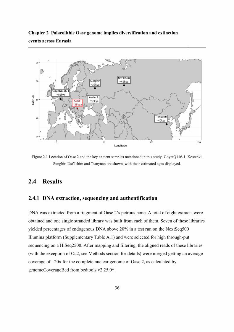
To shed light on the population history of anatomically modern humans in Eurasia in the
Upper Palaeolithic and their relationship to modern lineages, we sequenced to high coverage
(~20X, Figure 2.2) an anatomically modern human (Oase 2) from the Upper Palaeolithic
(~34-38 ky old, based on association with directly dated finds from the site19–21
) from Pestera
cu Oase in Romania19–21
. A sample from the same cave and of a similar age (Oase 1), dated to
~37.8kya20
was captured using an enrichment strategy with a panel of ~2.2 million SNPs
(2.2M panel), to extract information on sites informative about its relationship to
Neanderthals and present-day humans15
. However, the low coverage and high contamination
of this sample did not allow for detailed demographic analysis. The high quality of Oase 2
enabled us to conduct haplotype-based demographic analysis and to compare it to other high-
quality Upper Palaeolithic genomes. I also conducted a SNP-based analysis using a panel
Chapter 2 Palaeolithic Oase genome implies diversification and extinction
events across Eurasia
35
consisting of modern populations from the Human Origins panel14
, as well as ancient
African22
and Eurasian16,17,14,13
samples (Figure 2.1 for key ancient samples).
Upper Palaeolithic genomes also inform us on the extent of Neanderthal admixture.
Neanderthal ancestry in modern living individuals has been mostly ascribed to one pulse of
admixture at a very early stage of the out of Africa expansion, with possible minor events
later on. The observed relationship of decreasing Neanderthal ancestry with time is attributed
to negative selection acting on such genetic segments14,16
, although the topic is still debated.
So far, Oase 1 is the only sample that stands out in this regard: it had an unusually high
proportion of its genome derived from Neanderthals DNA: 6-9%, more than expected given
its age (up to ~6%)15
. Furthermore, this ancestry was distributed in very long segments,
indicative of a Neanderthal ancestor as recent as 4-6 generations back15
. Whether Oase 2 is
also special in this extent can inform us on the dynamics of Neanderthal interbreeding in
early humans.
Chapter 2 Palaeolithic Oase genome implies diversification and extinction
events across Eurasia
36
Figure 2.1 Location of Oase 2 and the key ancient samples mentioned in this study. GoyetQ116-1, Kostenki,
Sunghir, Ust’Ishim and Tianyuan are shown, with their estimated ages displayed.
2.4 Results
2.4.1 DNA extraction, sequencing and authentification
DNA was extracted from a fragment of Oase 2’s petrous bone. A total of eight extracts were
obtained and one single stranded library was built from each of them. Seven of these libraries
yielded percentages of endogenous DNA above 20% in a test run on the NextSeq500
Illumina platform (Supplementary Table A.1) and were selected for high through-put
sequencing on a HiSeq2500. After mapping and filtering, the aligned reads of these libraries
(with the exception of Oa2, see Methods section for details) were merged getting an average
coverage of ~20x for the complete nuclear genome of Oase 2, as calculated by
genomeCoverageBed from bedtools v2.25.023.
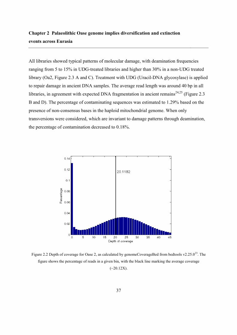
Chapter 2 Palaeolithic Oase genome implies diversification and extinction
events across Eurasia
37
All libraries showed typical patterns of molecular damage, with deamination frequencies
ranging from 5 to 15% in UDG-treated libraries and higher than 30% in a non-UDG treated
library (Oa2, Figure 2.3 A and C). Treatment with UDG (Uracil-DNA glycosylase) is applied
to repair damage in ancient DNA samples. The average read length was around 40 bp in all
libraries, in agreement with expected DNA fragmentation in ancient remains24,25
(Figure 2.3
B and D). The percentage of contaminating sequences was estimated to 1.29% based on the
presence of non-consensus bases in the haploid mitochondrial genome. When only
transversions were considered, which are invariant to damage patterns through deamination,
the percentage of contamination decreased to 0.18%.
Figure 2.2 Depth of coverage for Oase 2, as calculated by genomeCoverageBed from bedtools v2.25.023
. The
figure shows the percentage of reads in a given bin, with the black line marking the average coverage
(~20.12X).
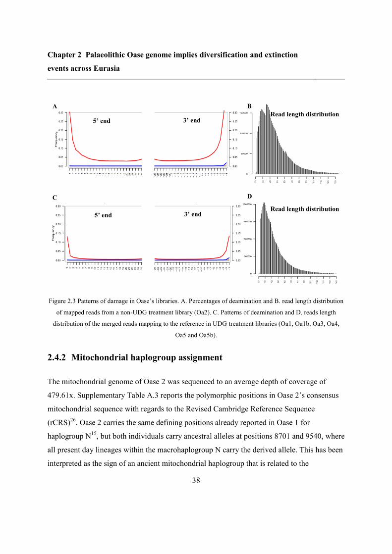
Chapter 2 Palaeolithic Oase genome implies diversification and extinction
events across Eurasia
38
Figure 2.3 Patterns of damage in Oase’s libraries. A. Percentages of deamination and B. read length distribution
of mapped reads from a non-UDG treatment library (Oa2). C. Patterns of deamination and D. reads length
distribution of the merged reads mapping to the reference in UDG treatment libraries (Oa1, Oa1b, Oa3, Oa4,
Oa5 and Oa5b).
2.4.2 Mitochondrial haplogroup assignment
The mitochondrial genome of Oase 2 was sequenced to an average depth of coverage of
479.61x. Supplementary Table A.3 reports the polymorphic positions in Oase 2’s consensus
mitochondrial sequence with regards to the Revised Cambridge Reference Sequence
(rCRS)26
. Oase 2 carries the same defining positions already reported in Oase 1 for
haplogroup N15
, but both individuals carry ancestral alleles at positions 8701 and 9540, where
all present day lineages within the macrohaplogroup N carry the derived allele. This has been
interpreted as the sign of an ancient mitochondrial haplogroup that is related to the
C
A
5’ end 3’ end
3’ end 5’ end
Read length distribution
Read length distribution
B
D
Chapter 2 Palaeolithic Oase genome implies diversification and extinction
events across Eurasia
39
macrohaplogroup N, which nowadays includes all Eurasian mitochondrial diversity, but
diverged from its base15
. The fact that Oase 1 and Oase 2 belong to the same, previously
unobserved mtDNA haplogroup also implies a relatively close relationship between these
samples on the maternal line.
2.4.3 Comparison of Oase 1 and Oase 2
Oase 1 and Oase 2 appear to be from related, but not identical populations. Their outgroup f3
profiles are different: they are closest to each other, but Oase 1 shows a similarity to
European Ice Age genomes that is absent from Oase 2, whereas the increased similarity to
Asian populations is slightly more pronounced in Oase 2 than in Oase 1 (Figure 2.4 and
Supplementary Figure A.1), even when only positions called in Oase 1 are considered
(Supplementary Figure A.2 and Supplementary Figure A.3). A further peculiarity is the close
relatedness between Muierii2 and Oase 1, which is missing in Oase 2. Muierii2 is a ~33ky
old sample from Romania, not assigned to any lineage that contributed to later European
hunter-gatherers. This also supports the differences between Oase 1 and Oase 2, and points to
a complicated genetic landscape in Upper Palaeolithic Eurasia with multiple, differentially
related populations, many of which did not contribute to modern-day diversity.
A formal test of whether the two samples from Pestera cu Oase form a clade, using D
statistics27
with an African outgroup of the form D(Oase 1, Oase 2; X, Yoruba), is also
violated (absolute value of Z scores up to 4.2). However, this signal appears to be dominated
by the unusually high Neanderthal proportion in Oase 1: Oase 1 is significantly closer to
ancient hominids and Oase 2 to most modern populations; only deeply divergent populations
from sub-Saharan Africa are neutral (Figure 2.5 and Figure 2.6). This suggests that the two
samples are probably from related, but not identical populations, but we need to control for
the difference in Neanderthal ancestry to be able to reach a firm conclusion.
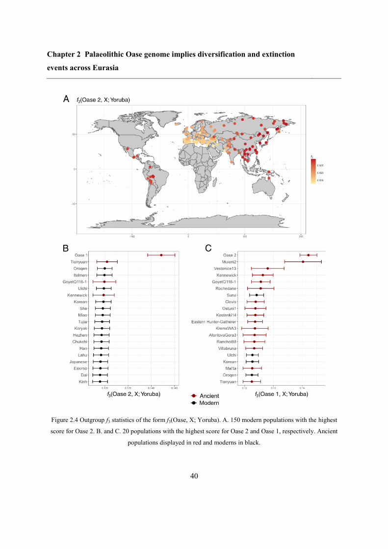
Chapter 2 Palaeolithic Oase genome implies diversification and extinction
events across Eurasia
40
Figure 2.4 Outgroup f3 statistics of the form f3(Oase, X; Yoruba). A. 150 modern populations with the highest
score for Oase 2. B. and C. 20 populations with the highest score for Oase 2 and Oase 1, respectively. Ancient
populations displayed in red and moderns in black.
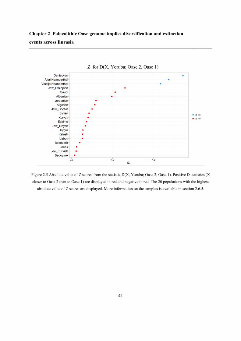
Chapter 2 Palaeolithic Oase genome implies diversification and extinction
events across Eurasia
41
Figure 2.5 Absolute value of Z scores from the statistic D(X, Yoruba; Oase 2, Oase 1). Positive D statistics (X
closer to Oase 2 than to Oase 1) are displayed in red and negative in red. The 20 populations with the highest
absolute value of Z scores are displayed. More information on the samples is available in section 2.6.5.
|Z| for D(X, Yoruba; Oase 2, Oase 1)
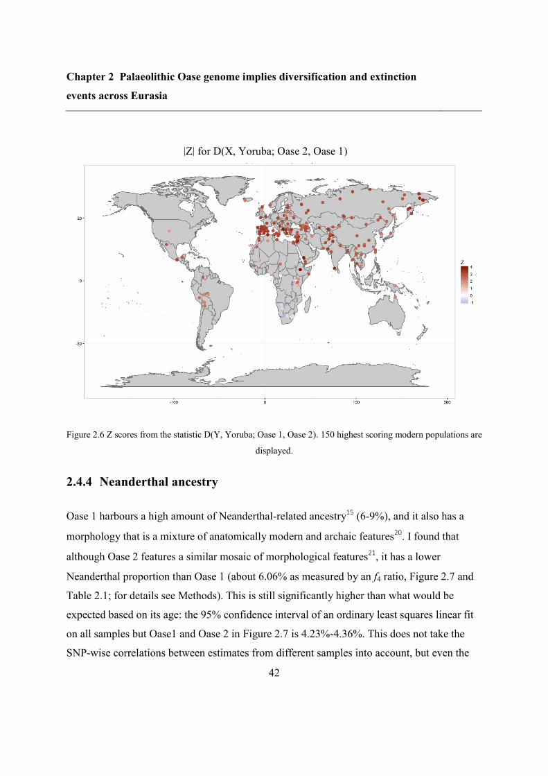
Chapter 2 Palaeolithic Oase genome implies diversification and extinction
events across Eurasia
42
Figure 2.6 Z scores from the statistic D(Y, Yoruba; Oase 1, Oase 2). 150 highest scoring modern populations are
displayed.
2.4.4 Neanderthal ancestry
Oase 1 harbours a high amount of Neanderthal-related ancestry15
(6-9%), and it also has a
morphology that is a mixture of anatomically modern and archaic features20
. I found that
although Oase 2 features a similar mosaic of morphological features21
, it has a lower
Neanderthal proportion than Oase 1 (about 6.06% as measured by an f4 ratio, Figure 2.7 and
Table 2.1; for details see Methods). This is still significantly higher than what would be
expected based on its age: the 95% confidence interval of an ordinary least squares linear fit
on all samples but Oase1 and Oase 2 in Figure 2.7 is 4.23%-4.36%. This does not take the
SNP-wise correlations between estimates from different samples into account, but even the
|Z| for D(X, Yoruba; Oase 2, Oase 1)
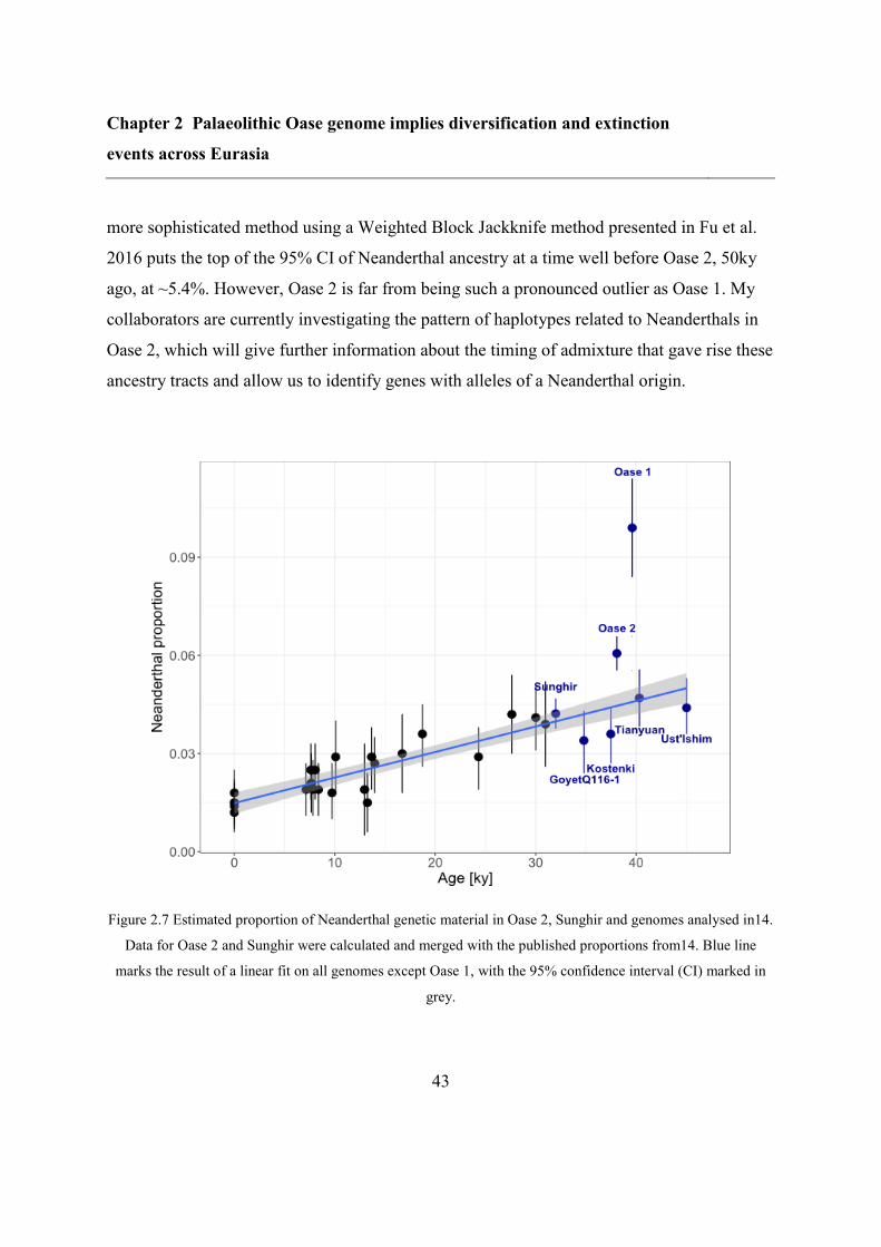
Chapter 2 Palaeolithic Oase genome implies diversification and extinction
events across Eurasia
43
more sophisticated method using a Weighted Block Jackknife method presented in Fu et al.
2016 puts the top of the 95% CI of Neanderthal ancestry at a time well before Oase 2, 50ky
ago, at ~5.4%. However, Oase 2 is far from being such a pronounced outlier as Oase 1. My
collaborators are currently investigating the pattern of haplotypes related to Neanderthals in
Oase 2, which will give further information about the timing of admixture that gave rise these
ancestry tracts and allow us to identify genes with alleles of a Neanderthal origin.
Figure 2.7 Estimated proportion of Neanderthal genetic material in Oase 2, Sunghir and genomes analysed in14.
Data for Oase 2 and Sunghir were calculated and merged with the published proportions from14. Blue line
marks the result of a linear fit on all genomes except Oase 1, with the 95% confidence interval (CI) marked in
grey.
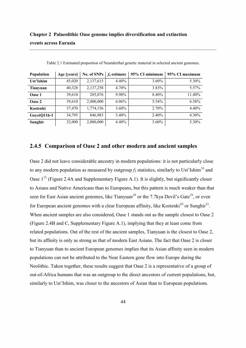
Chapter 2 Palaeolithic Oase genome implies diversification and extinction
events across Eurasia
44
Table 2.1 Estimated proportion of Neanderthal genetic material in selected ancient genomes.
Population Age [years] No. of SNPs f4 estimate 95% CI minimum 95% CI maximum
Ust’Ishim 45,020 2,137,615 4.40% 3.60% 5.30%
Tianyuan 40,328 2,137,258 4.70% 3.83% 5.57%
Oase 1 39,610 285,076 9.90% 8.40% 11.40%
Oase 2 39,610 2,000,000 6.06% 5.54% 6.58%
Kostenki 37,470 1,774,156 3.60% 2.70% 4.40%
GoyetQ116-1 34,795 846,983 3.40% 2.40% 4.30%
Sunghir 32,000 2,000,000 4.40% 3.60% 5.30%
2.4.5 Comparison of Oase 2 and other modern and ancient samples
Oase 2 did not leave considerable ancestry in modern populations: it is not particularly close
to any modern population as measured by outgroup f3 statistics, similarly to Ust’Ishim16
and
Oase 115
(Figure 2.4A and Supplementary Figure A.1). It is slightly, but significantly closer
to Asians and Native Americans than to Europeans, but this pattern is much weaker than that
seen for East Asian ancient genomes, like Tianyuan28
or the 7.7kya Devil’s Gate29
, or even
for European ancient genomes with a clear European affinity, like Kostenki30
or Sunghir31
.
When ancient samples are also considered, Oase 1 stands out as the sample closest to Oase 2
(Figure 2.4B and C, Supplementary Figure A.1), implying that they at least come from
related populations. Out of the rest of the ancient samples, Tianyuan is the closest to Oase 2,
but its affinity is only as strong as that of modern East Asians. The fact that Oase 2 is closer
to Tianyuan than to ancient European genomes implies that its Asian affinity seen in modern
populations can not be attributed to the Near Eastern gene flow into Europe during the
Neolithic. Taken together, these results suggest that Oase 2 is a representative of a group of
out-of-Africa humans that was an outgroup to the direct ancestors of current populations, but,
similarly to Ust’Ishim, was closer to the ancestors of Asian than to European populations.
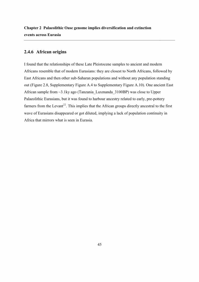
Chapter 2 Palaeolithic Oase genome implies diversification and extinction
events across Eurasia
45
2.4.6 African origins
I found that the relationships of these Late Pleistocene samples to ancient and modern
Africans resemble that of modern Eurasians: they are closest to North Africans, followed by
East Africans and then other sub-Saharan populations and without any population standing
out (Figure 2.8, Supplementary Figure A.4 to Supplementary Figure A.10). One ancient East
African sample from ~3.1ky ago (Tanzania_Luxmanda_3100BP) was close to Upper
Palaeolithic Eurasians, but it was found to harbour ancestry related to early, pre-pottery
farmers from the Levant22
. This implies that the African groups directly ancestral to the first
wave of Eurasians disappeared or got diluted, implying a lack of population continuity in
Africa that mirrors what is seen in Eurasia.
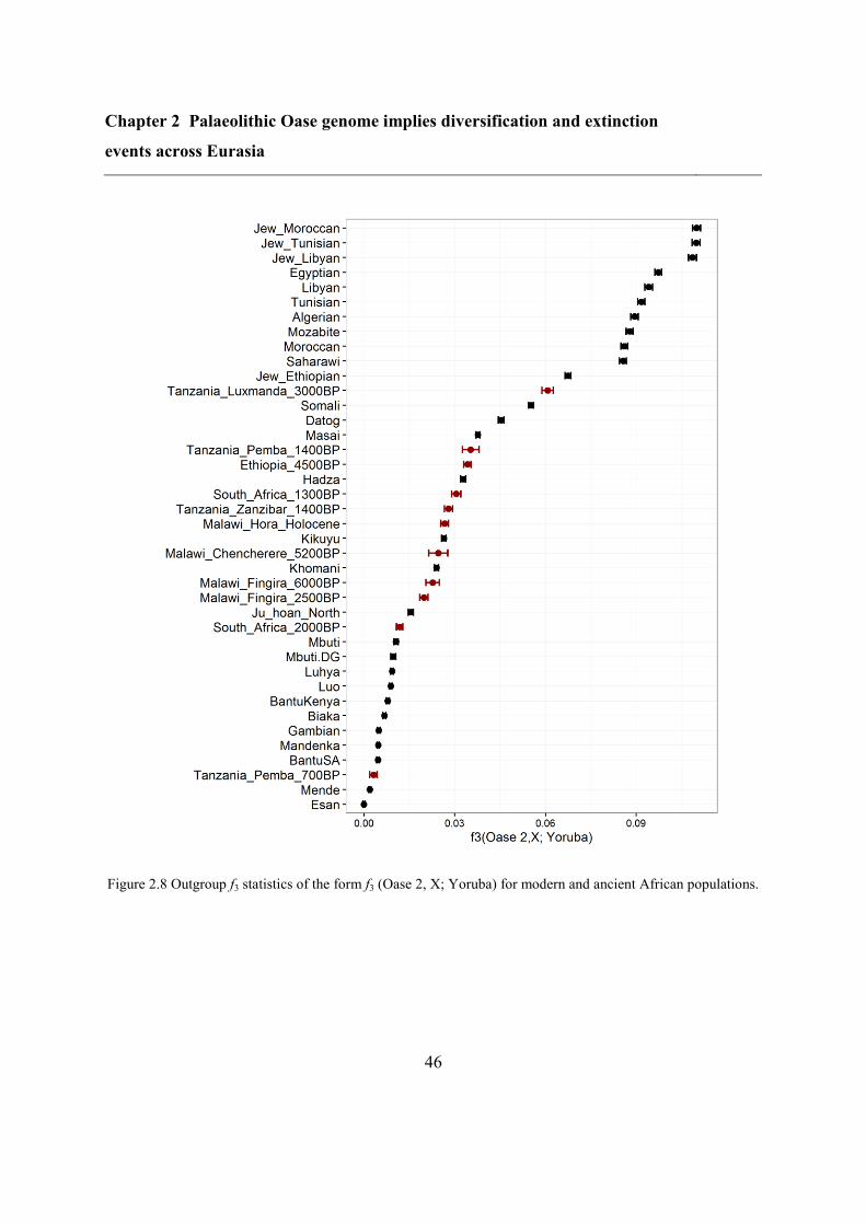
Chapter 2 Palaeolithic Oase genome implies diversification and extinction
events across Eurasia
46
Figure 2.8 Outgroup f3 statistics of the form f3 (Oase 2, X; Yoruba) for modern and ancient African populations.
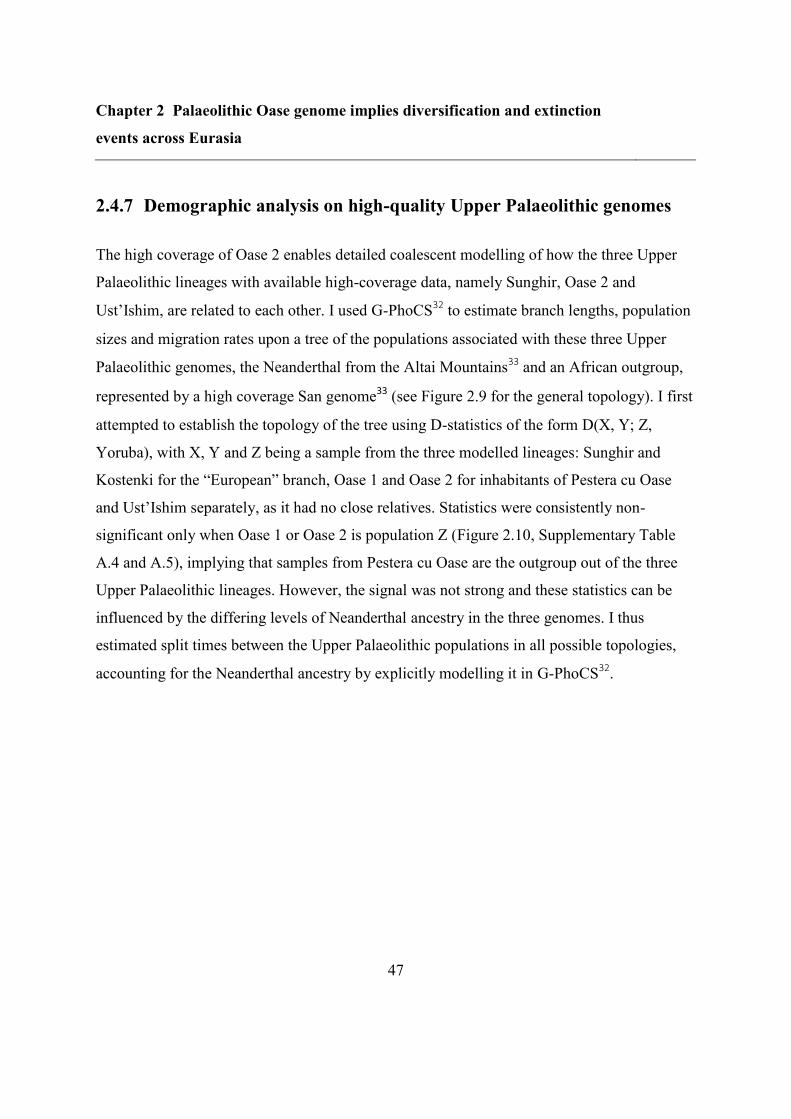
Chapter 2 Palaeolithic Oase genome implies diversification and extinction
events across Eurasia
47
2.4.7 Demographic analysis on high-quality Upper Palaeolithic genomes
The high coverage of Oase 2 enables detailed coalescent modelling of how the three Upper
Palaeolithic lineages with available high-coverage data, namely Sunghir, Oase 2 and
Ust’Ishim, are related to each other. I used G-PhoCS32
to estimate branch lengths, population
sizes and migration rates upon a tree of the populations associated with these three Upper
Palaeolithic genomes, the Neanderthal from the Altai Mountains33
and an African outgroup,
represented by a high coverage San genome33
(see Figure 2.9 for the general topology). I first
attempted to establish the topology of the tree using D-statistics of the form D(X, Y; Z,
Yoruba), with X, Y and Z being a sample from the three modelled lineages: Sunghir and
Kostenki for the “European” branch, Oase 1 and Oase 2 for inhabitants of Pestera cu Oase
and Ust’Ishim separately, as it had no close relatives. Statistics were consistently non-
significant only when Oase 1 or Oase 2 is population Z (Figure 2.10, Supplementary Table
A.4 and A.5), implying that samples from Pestera cu Oase are the outgroup out of the three
Upper Palaeolithic lineages. However, the signal was not strong and these statistics can be
influenced by the differing levels of Neanderthal ancestry in the three genomes. I thus
estimated split times between the Upper Palaeolithic populations in all possible topologies,
accounting for the Neanderthal ancestry by explicitly modelling it in G-PhoCS32
.
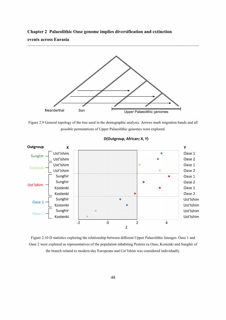
Chapter 2 Palaeolithic Oase genome implies diversification and extinction
events across Eurasia
48
Figure 2.9 General topology of the tree used in the demographic analysis. Arrows mark migration bands and all
possible permutations of Upper Palaeolithic genomes were explored.
Figure 2.10 D statistics exploring the relationship between different Upper Palaeolithic lineages. Oase 1 and
Oase 2 were explored as representatives of the population inhabiting Pestera cu Oase, Kostenki and Sunghir of
the branch related to modern-day Europeans and Ust’Ishim was considered individually.
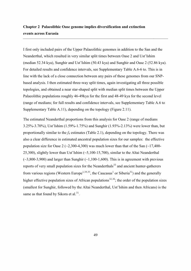
Chapter 2 Palaeolithic Oase genome implies diversification and extinction
events across Eurasia
49
I first only included pairs of the Upper Palaeolithic genomes in addition to the San and the
Neanderthal, which resulted in very similar split times between Oase 2 and Ust’Ishim
(median 52.34 kya), Sunghir and Ust’Ishim (50.43 kya) and Sunghir and Oase 2 (52.86 kya).
For detailed results and confidence intervals, see Supplementary Table A.6-6 to. This is in
line with the lack of a close connection between any pairs of these genomes from our SNP-
based analysis. I then estimated three-way split times, again investigating all three possible
topologies, and obtained a near star-shaped split with median split times between the Upper
Palaeolithic populations roughly 46-49kya for the first and 48-49 kya for the second level
(range of medians; for full results and confidence intervals, see Supplementary Table A.6 to
Supplementary Table A.11), depending on the topology (Figure 2.11).
The estimated Neanderthal proportions from this analysis for Oase 2 (range of medians
3.25%-3.70%), Ust’Ishim (1.59%-1.75%) and Sunghir (1.93%-2.13%) were lower than, but
proportionally similar to the f4 estimates (Table 2.1), depending on the topology. There was
also a clear difference in estimated ancestral population sizes for our samples: the effective
population size for Oase 2 (~2,300-4,300) was much lower than that of the San (~17,400-
25,300), slightly lower than Ust’Ishim (~5,100-15,700), similar to the Altai Neanderthal
(~3,800-3,900) and larger than Sunghir (~1,100-1,600). This is in agreement with previous
reports of very small population sizes for the Neanderthals33
and ancient hunter-gatherers
from various regions (Western Europe1,34,35
, the Caucasus1 or Siberia
31) and the generally
higher effective population sizes of African populations32,36
; the order of the population sizes
(smallest for Sunghir, followed by the Altai Neanderthal, Ust’Ishim and then Africans) is the
same as that found by Sikora et al.31.
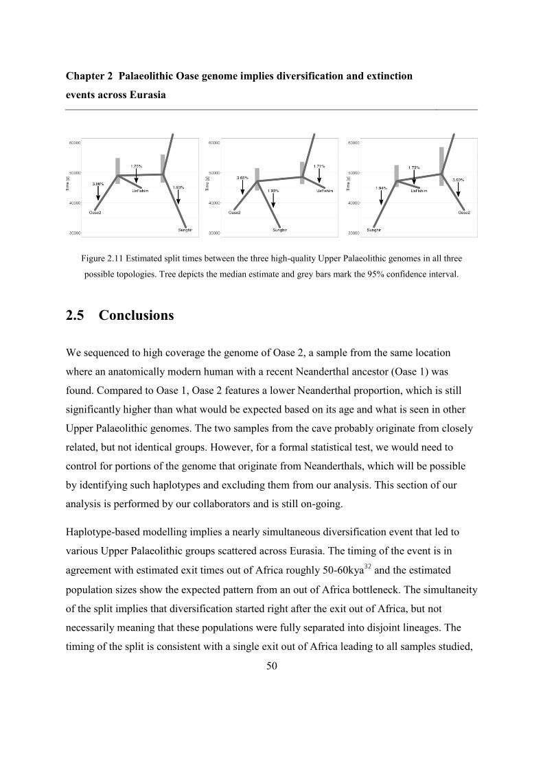
Chapter 2 Palaeolithic Oase genome implies diversification and extinction
events across Eurasia
50
Figure 2.11 Estimated split times between the three high-quality Upper Palaeolithic genomes in all three
possible topologies. Tree depicts the median estimate and grey bars mark the 95% confidence interval.
2.5 Conclusions
We sequenced to high coverage the genome of Oase 2, a sample from the same location
where an anatomically modern human with a recent Neanderthal ancestor (Oase 1) was
found. Compared to Oase 1, Oase 2 features a lower Neanderthal proportion, which is still
significantly higher than what would be expected based on its age and what is seen in other
Upper Palaeolithic genomes. The two samples from the cave probably originate from closely
related, but not identical groups. However, for a formal statistical test, we would need to
control for portions of the genome that originate from Neanderthals, which will be possible
by identifying such haplotypes and excluding them from our analysis. This section of our
analysis is performed by our collaborators and is still on-going.
Haplotype-based modelling implies a nearly simultaneous diversification event that led to
various Upper Palaeolithic groups scattered across Eurasia. The timing of the event is in
agreement with estimated exit times out of Africa roughly 50-60kya32
and the estimated
population sizes show the expected pattern from an out of Africa bottleneck. The simultaneity
of the split implies that diversification started right after the exit out of Africa, but not
necessarily meaning that these populations were fully separated into disjoint lineages. The
timing of the split is consistent with a single exit out of Africa leading to all samples studied,
Chapter 2 Palaeolithic Oase genome implies diversification and extinction
events across Eurasia
51
but the reason why we do not see signs of an earlier exit in the form of an older split time,
despite favourable climatic conditions, is not known. Competition with archaic hominins
could have been a preventive factor, but the sparsity of ancient data does not yet allow for a
formal test of such a hypothesis.
Oase 2 did not leave its ancestry in modern populations, similarly to some samples of a
similar age, such as Oase 115
, Ust’Ishim16
and multiple early Upper Palaeolithic European
samples14
, but unlike others that are related to modern populations from their respective
regions (e.g. Tianyuan28
, Kostenki30
, Sunghir31
and numerous other European samples14
).
The varying affinities of early Eurasian populations show a restructuring of genetic diversity
between the Upper Palaeolithic and present day, including several extinction events.
Numerous factors could play a role in such changes, such as climate affecting areas
differentially (e.g. harsh conditions in Europe and Siberia only leaving few survivors, but not
in East Asia), or geographic connectivity affecting how easily different areas can be
repopulated. Furthermore, I did not find any particular pattern of similarity between Upper
Palaeolithic samples and modern Africans, which could be a sign of similar extinction events
in Africa and/or successive admixture within the continent. There is a wide range of evidence
for the latter, for example through the admixed ancestry of most modern African
populations22
.
The lineages leading to modern populations could originate from the surviving groups all
over Eurasia, but could also be a result of large-scale movements from refugia with
favourable conditions, such as the Near East or southern parts of Asia. Although genetic data
from the period directly following the exit out of Africa is sparse, given that many of the
observed Upper Paleolithic samples did not leave considerable ancestry, it is reasonable to
suppose that this disappearance of an observable genetic trace (through extinction and/or
admixture) was not a rare, special event. Consequentially, the signatures of events we can
infer based on their signature in modern genomes (e.g. genes obtained via introgression,
Chapter 2 Palaeolithic Oase genome implies diversification and extinction
events across Eurasia
52
population bottlenecks) are probably only a subset of all such events and only give insight
into the history of the fittest, or, more likely, the luckiest populations that contributed their
genetic material to modern human diversity.
2.6 Methods
2.6.1 DNA extraction and library preparation
All decontamination steps and laboratory procedures before PCR amplification were carried
out in ancient DNA dedicated facilities at the University of Potsdam. All tools used in these
stages were decontaminated with bleach, DNA-ExitusPlusTM and UV radiation.
DNA was extracted from a fragment of petrous bone sampled in Bucharest (Romania) in
2013. Before extraction, the bone fragment was exposed to UV radiation for 10 minutes on
each side. Afterwards, the bone surface was physically removed using a dental drill attached
to a dremel saw. A new drill was then used to remove all the porous parts until we got to the
dense walls forming the inner ear channels. After cleaning, two fragments of compact bone,
172 mg and 212 mg respectively, were obtained. Both fragments were ground to fine bone
powder using mortars and pestles.
Six DNA extracts were prepared from a starting amount of 50 mg of bone powder each (from
now onwards we are referring to these extracts as: Oa1, Oa2, Oa3, Oa4, Oa5 and Oa6). We
followed the DNA extraction protocol described in Dabney et al (2013)37
, which is specially
optimized to recover short DNA fragments (from 30-40 bp length). In extracts Oa1 and Oa5,
the bone powder was not completely digested after overnight incubation with proteinase K
(PK), thus we add new digestion buffer with PK and performed a secondary extraction (Oa1b
and Oa5b). Finally, we obtained eight DNA extracts, each in 25 µl of elution buffer.
Chapter 2 Palaeolithic Oase genome implies diversification and extinction
events across Eurasia
53
One single stranded library was built from each extract following the protocol described by
Gansauge and Meyer (2013)38
. This protocol includes UDG treatment before library building
in order to reduce the presence of uracils in aDNA molecules. We applied these treatments to
all our extracts with the exception of Oa2, in order to accurately measure the deamination
patterns in Oase’s DNA molecules and thus support the authenticity of the sequences.
The number of cycles for the amplification of each library was estimated based on qPCR. We
used Accuprime Pfx (InvitrogenTM
) for the amplification of the UDG treated libraries, while
Oa2 was amplified using Accuprime SM (InvitrogenTM
), which is able to read over uracils. A
different index sequence was incorporated during this amplification of each library, in order
to be able to pool them for sequencing. Finally, each library was amplified in four parallel
reactions with 4 µl of template and 16 µl of master mix each. PCR amplification conditions
were as specified by the manufacture.
The amplified libraries were purified using a MinElute kit (Qiagen) and quantified using a
2200 TapeStation (Agilent Technologies). The libraries were pooled in equimolar quantities
and sequenced on an Illumina NextSeq500 platform in 75PE mode. The output from this run
(around 20 to 50 million reads per library) was used to estimate the percentage of endogenous
DNA in each library. After this test, libraries Oa4 and Oa2a were discarded from further
sequencing because of high duplication levels in Oa4 and the presence of uracils in Oa2a. All
the other libraries showed percentages of endogenous DNA higher than 20% and low
clonality, and they were selected for high through-put sequencing.
High throughput sequencing was carried out at TheragenEtex (Suwon, South Korea), using
four whole flow cells of an Illumina HiSeq2500 platform. Two of the sequencing runs were
set to 50 cycles in single end mode (50SE) and another two to 50 cycles in paired end mode
(50PE). Libraries were selected for these runs based on their performance in the test
NextSeq500 run, but also on the availability of enough library volume left to fill the
flowcells.
Chapter 2 Palaeolithic Oase genome implies diversification and extinction
events across Eurasia
54
2.6.2 Processing and mapping of NGS data
After sequencing, the raw BCL files were converted to fastq format following the Illumina
base-calling pipeline (Illumina Pipeline v1.4). Raw reads were assigned to the corresponding
libraries based on the barcode sequences, no mismatches were allowed in the first base of the
barcode and a single mismatch was allowed at any other position. The software SeqPrep
(https://github.com/jstjohn/SeqPrep) was used to trim and merge the forward (R1) and
reverse (R2) reads from pair end (PE) runs, while cutadapt-1.339
was used to trim SE reads.
In both cases, a minimum length of 25 bases was set as threshold after trimming.
The trimmed and merged reads were aligned to the human reference genome (GRCh37 build)
using the software Burrows-Wheeler Aligner (BWA) version 0.7.5a-r40540
, with default
parameters and seed option disabled (-l 1000). Prior to the alignment, the mitochondrial
sequences in the GRCh37 reference were replaced by the Revised Cambridge Reference
Sequence (NC_01292026
).
After mapping, clonal sequences were removed from the alignment using the
MarkDuplicates.jar tool in picards-1.98 (http://broadinstitute.github.io/picard/). Also, reads
were realigned around indels using the RealignerTargetCreator and IndelRealigner tools in
GATK-3.0-041
. The resulting bam files were filtered for mapping quality of 30 using
Samtools-0.1.1940
. Finally, we used Mapdamage42
to downscale the quality score of bases at
the end of the reads, in order to diminish possible errors when calling SNPs at likely damaged
positions.
The mapped reads from the downscaled alignments were merged in a single bam file using
picards-1.98. This merged file was used to estimate the whole genome coverage, as well as
for SNP calling and downstream analysis described below.
Chapter 2 Palaeolithic Oase genome implies diversification and extinction
events across Eurasia
55
2.6.3 Mitochondrial DNA
The mitochondrial genome of Oase 2 was reconstructed from the NGS output of the first run
on the HiSeq2500 (Supplementary Table A.2). Seven libraries (Oa1a, Oa1b, Oa2, Oa3, Oa4,
Oa5a, Oa5b and Oa6) were sequenced in 50PE mode and the output reads were processed as
described in the previous section, with the only difference that the Revised Cambridge
Reference Sequence (rCRS, NC_01292026
) was used at the mapping stage.
Polymorphic positions with regards to the reference were called using the samtools-0.1.19
mpileup function40
. Mapping and base quality scores equal to or higher than 30 were required
for the base calling. The identified polymorphic positions were directly checked by
visualizing the mitochondrial alignment in Tablet43
. Finally, the confirmed polymorphisms
were uploaded to Haplogrep44
, which bases the identification of the haplogroup on the
updated mitochondrial phylogeny of PhyloTree (http://www.phylotree.org/). The resulting
mitochondrial haplogroup was N, but in fact Oase 2 carried the ancestral allele at positions
7801 and 9540 instead of the defining derived alleles.
2.6.4 Authenticity of ancient DNA molecules
Negative controls were included during the extraction and library building procedures, and
sequenced together with the libraries in the NextSeq500 run (Supplementary Table A.1). The
percentage of reads mapping to the reference in these blanks ranged from 0.2 to 2.3%.
Also, we used MapDamage42
to assess the patterns of molecular damage in Oase 2’s libraries.
Finally, the percentage of modern human contamination was estimated by measuring the
frequency of non-consensus calls at haplogroup defining positions in Oase 2’s mitochondrial
DNA (mtDNA) sequences.
Chapter 2 Palaeolithic Oase genome implies diversification and extinction
events across Eurasia
56
2.6.5 SNP calling and merging with reference panel
To compare our sample to modern and ancient human genetic variation, I called SNPs from
the BAMfiles of Oase 2 and Sunghir using SAMtools 1.640
and the hg19 reference FASTA
file. I only called positions overlapping with the ~600k SNPs from the Human Origins
panel45
, also part of the 2.2M panel used in the study of Oase 115
and the genetic history of
Ice Age Europe14
. Bases were required to have a minimum mapping quality of 30 and base
quality of 20. The resulting SNP data was then merged using Plink1.946
with the panels used
in Fu et al. 201614
, Lazaridis et al. 201747
and Skoglund et al. 201722
, as well as with a
version of the Tianyuan genome28
called on the same 2.2M SNP panel as in Fu et al. 201614
,
kindly sent by the authors( 2423 individuals in total). SNPs were restricted to triallelic SNPs,
which resulted in 587,247 SNPs (133,069 called in Oase 1).
2.6.6 Calculating statistics
2.6.6.1 D and outgroup f3 statistics
D statistics27
and f3 statistics48,49
were used to formally assess the relationships between the
samples using the qpDstat (D statistics) and qp3PopTest (f3 statistics) programs from the
ADMIXTOOLS package49
. Significance was assessed by these programs using a block
jackknife over 5-centimorgan chunks of the genome, and statistics were considered
significant if their Z score was of magnitude greater than 2, or, for admixture f3 scores, if they
were smaller than −2. These correspond approximately to P values of 0.046 and 0.023,
respectively. Outgroup f3 scores were filtered to include populations with at least 20,000
SNPs overlapping; 10,000 SNPs when the low coverage Oase 1 was the focal sample.
D statistics of the form D(X, Y; Z, Yoruba) were used first to formally assess the relationship
between the three Upper Palaeolithic lineages that I later used in our demographic analysis:
Chapter 2 Palaeolithic Oase genome implies diversification and extinction
events across Eurasia
57
Oase (Oase 1 or Oase 2), Ust’Ishim and Upper Palaeolithic Europeans (Kostenki14 or
Sunghir).
2.6.6.2 Estimating the proportion of Neanderthal ancestry
f4 ratios were used to estimate the proportion of Neanderthal ancestry in our samples,
following 14
. I used the equation below:
𝑄(𝑥) = 1 −𝑓4(𝑊𝑒𝑠𝑡 𝑎𝑛𝑑 𝐶𝑒𝑛𝑡𝑟𝑎𝑙 𝐴𝑓𝑟𝑖𝑐𝑎𝑛𝑠,𝐶ℎ𝑖𝑚𝑝;𝑋,𝐴𝑟𝑐ℎ𝑎𝑖𝑐)
𝑓4(𝑊𝑒𝑠𝑡 𝑎𝑛𝑑 𝐶𝑒𝑛𝑡𝑟𝑎𝑙 𝐴𝑓𝑟𝑖𝑐𝑎𝑛𝑠,𝐶ℎ𝑖𝑚𝑝;𝐷𝑖𝑛𝑘𝑎 𝐴𝑟𝑐ℎ𝑎𝑖𝑐)
I computed allele frequencies by pooling data from each of the following sets of samples:
West and Central Africans: a pool of 9 samples from the Mbuti, Yoruba and Mende
populations (S_Mbuti-1, S_Mbuti-2, S_Mbuti-3, B_Mbuti-4, S_Yoruba-1, S_Yoruba-
2, S_Yoruba-3, S_Mende-1, S_Mende-2)
Dinka: a pool of 3 samples (S_Dinka-1, S_Dinka-2, B_Dinka-3)
Archaic: a pool of 2 samples (Altai Neanderthal and the Siberian Denisova)
This data was acquired from the Simons Genome Diversity Project (SGDP,
https://www.simonsfoundation.org/simons-genome-diversity-project/)9. I downloaded v3 of
the compressed SGDP-lite version and used Ctools to query the samples in question. I then
merged these samples with Oase 2, Sunghir and ancient genomes used in 14
, subsetting to the
~2.2 million SNPs used in 14
to stay directly comparable to those estimates. I finally merged
the resulting proportions with those calculated using the same method from Fu et al. 201614
.
For Oase 1, estimates using multiple methods and either using all SNPs or only transversions,
were available from the original publication15
. However, I decided to use the values
recalculated in Fu et al. 201514
to be consistent in the method of estimating Neanderthal
ancestry proportions.
Chapter 2 Palaeolithic Oase genome implies diversification and extinction
events across Eurasia
58
2.6.7 G-PhoCS analysis for Oase
I used G-PhoCS 1.2.350
to reconstruct the joint demographic history of high-coverage Upper
Palaeolithic samples from Europe. In addition to the three available high-coverage samples
(Oase 2, Ust’Ishim and Sunghir), I also included the Altai Neanderthal33
for information on
Neanderthal admixture and a modern African as a reference sample largely free from the
Neanderthal admixture51
. I chose to use a high-quality San genome from the same publication
as the Altai Neanderthal33
(HGDP01037 from Panel B). This analysis estimates split times,
population sizes and migration rates on a tree with a given topology, given sequence data
from short, homologous windows from (some) samples at the leaves of the tree.
2.6.7.1 Topology of the tree
G-PhoCS represents the demographic history of a collection of samples by a binary tree in
which each branch is a population, with each sample belonging to a different leaf branch and
interior branches corresponding to (unsampled) ancestral populations. In addition, the
sampling time of leaves and unidirectional migration bands between any two branches can be
defined. I based the topology of our tree (Figure 2.9) on the literature and our previous
analysis, the former showing that Neanderthals are an outgroup to anatomically modern
humans and the San Pygmies are an outgroup to Eurasians. In order to establish the
relationship between our three Upper Palaeolithic genomes, I first tried topologies with each
pair of them, before running the final tree with all three genomes.
I set the sample ages to zero for the modern San Pygmy, to the age estimated using G-PhoCS
for the Altai Neanderthal50
and to the mean estimates from the radiocarbon dating of
Sunghir31
and Ust’Ishim16
(Table 2.2). The radiocarbon dating for Oase 2 failed and since the
human remains in Pestera cu Oase are a palaeo-surface find, stratigraphic dating is also not
possible19
. However, the morphological similarities point to contemporaneity between Oase 1
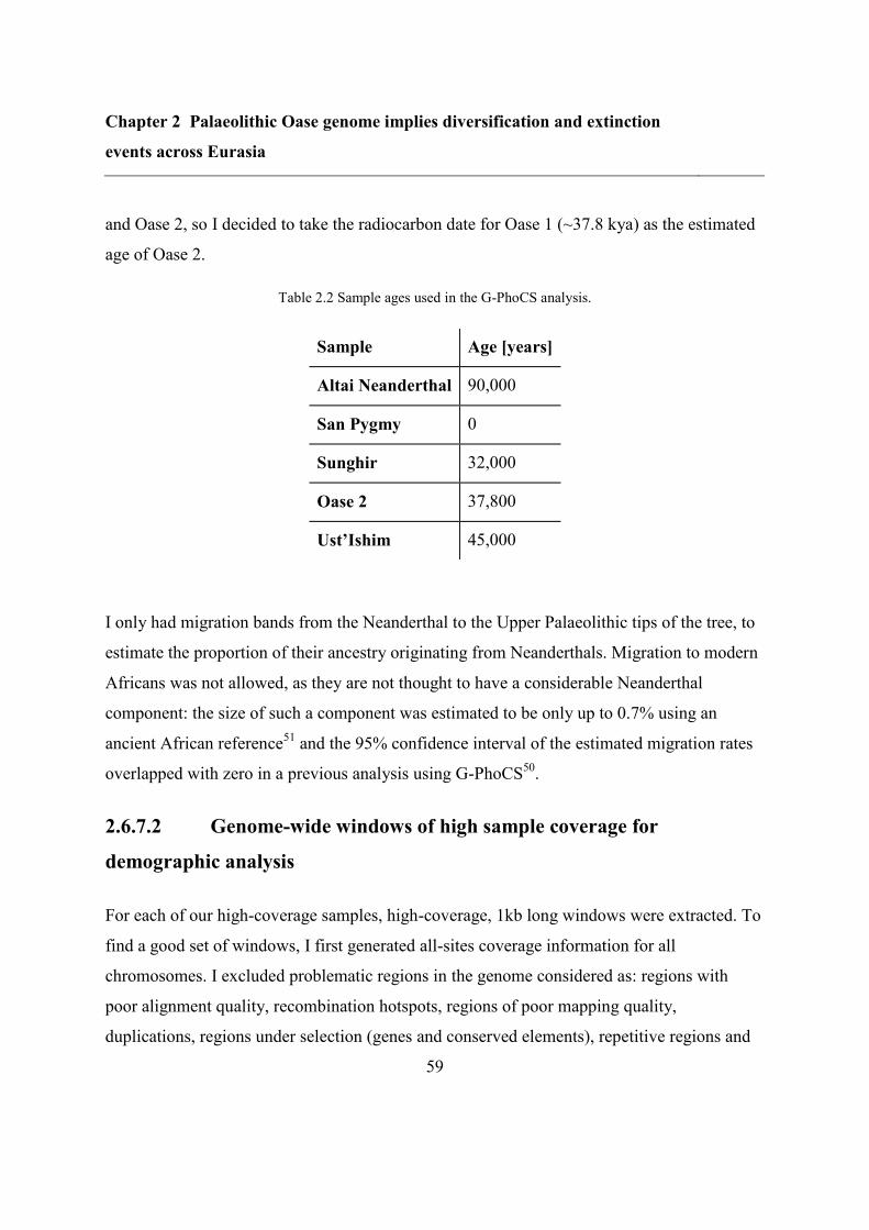
Chapter 2 Palaeolithic Oase genome implies diversification and extinction
events across Eurasia
59
and Oase 2, so I decided to take the radiocarbon date for Oase 1 (~37.8 kya) as the estimated
age of Oase 2.
Table 2.2 Sample ages used in the G-PhoCS analysis.
Sample Age [years]
Altai Neanderthal 90,000
San Pygmy 0
Sunghir 32,000
Oase 2 37,800
Ust’Ishim 45,000
I only had migration bands from the Neanderthal to the Upper Palaeolithic tips of the tree, to
estimate the proportion of their ancestry originating from Neanderthals. Migration to modern
Africans was not allowed, as they are not thought to have a considerable Neanderthal
component: the size of such a component was estimated to be only up to 0.7% using an
ancient African reference51
and the 95% confidence interval of the estimated migration rates
overlapped with zero in a previous analysis using G-PhoCS50
.
2.6.7.2 Genome-wide windows of high sample coverage for
demographic analysis
For each of our high-coverage samples, high-coverage, 1kb long windows were extracted. To
find a good set of windows, I first generated all-sites coverage information for all
chromosomes. I excluded problematic regions in the genome considered as: regions with
poor alignment quality, recombination hotspots, regions of poor mapping quality,
duplications, regions under selection (genes and conserved elements), repetitive regions and
Chapter 2 Palaeolithic Oase genome implies diversification and extinction
events across Eurasia
60
positions with systematic sequencing errors, using the following filters from Kuhlwilm et al.
201650
, sent kindly by Ilan Gronau:
filter_hotspot1000g: Recombination hotspots
filter_Map20: Sites with poor mapping quality
filter_rmsk20: Recent duplications
filter_segDups: Recent segmental duplications
filter_selection_10000_100: Gene exons together with the 1 kbp flanking regions in
each direction and conserved non-coding sequences corresponding to PhastCons
elements
filter_simpleRepeat: Simple repeats
filter_SysErrHCB and filter_SysErr: Positions with systematic sequencing errors
For more details, see Supplementary SI 8 in Kuhlwilm et al. 201650
.
I then extracted the depth information using a custom code written in C, again filtering for
sites with read depth between 10 and twice the average coverage of the sample:.
samtools-0.1.19 mpileup -C50 -uRID -f $FASTA -r chr$CHR -l Beds/chr${CHR}.bed
$FILES $DINKA_DIR/chr$CHR.dedup.realign.recal.bam
$SAN_DIR/chr$CHR.dedup.realign.recal.bam $ALTAI_NEA.$CHR.dq.chr.bam
2>Genotypes/log.geno.chr$CHR.txt | bcftools-0.1.19 view -gc -
2>>Genotypes/log.geno.chr$CHR.txt | ./get_genotypes dpMin=10 maxDpProp=2.0
1>Genotypes/geno.chr$CHR.txt 2>>Genotypes/log.geno.chr$CHR.txt
Sites with very low and very high coverage were avoided because alignment and genotyping
can be problematic52
– for example, heterozygous calls are unreliable if coverage is too low,
whereas a coverage unusually high given the average sample coverage can signal repetitive
regions and spurious alignment.
Chapter 2 Palaeolithic Oase genome implies diversification and extinction
events across Eurasia
61
I then scanned each chromosome for good windows, using a simple heuristic to maximise the
sample coverage. I start by finding the first 1kb window with at least 80% coverage. I then
search locally for a window within the next 10 kb for the 1kb window with the highest
coverage. Finally, I jump 5 kb forward from the chosen location and repeat the process until I
reach the end of the chromosome. For the whole genome, this yielded a total of 45759
windows. I then used SAMtools/BCFtools 0.1.19 40
(using flags as above) and custom
programs written in C and MATLAB to extract genotypes or the windows and converted the
genotypes into FASTA files for G-PhoCS. To deal with DNA damage in ancient samples, I
“in vitro” deaminated all our sequences, as already done for previous analyses of aDNA27
.
2.6.7.3 G-PhoCS setup
Gamma distributed priors were used for all observables. The shape parameter was set to an
intermediate value of 1 for both population sizes and split times, to obtain a mean to standard
deviation ratio of unity and allow sufficient exploration of the parameter space without an
overly long convergence time. The rate parameter was set to result in means in the correct
range, based on previous knowledge on population sizes of hunter-gatherers and the split
times between Neanderthals and modern humans, Africans and non-Africans and within
Eurasia. I also ran initial exploratory runs with a variety of starting values, using a single
MCMC chain with 200,000 iterations, out of which, the first 100,000 were discarded as burn-
in. Furthermore, it was shown that the initial value for MCMC chains in G-PhoCS hardly
affects the resulting means, it only slows down convergence32
. The rate parameters used are
shown in Table 2.3.
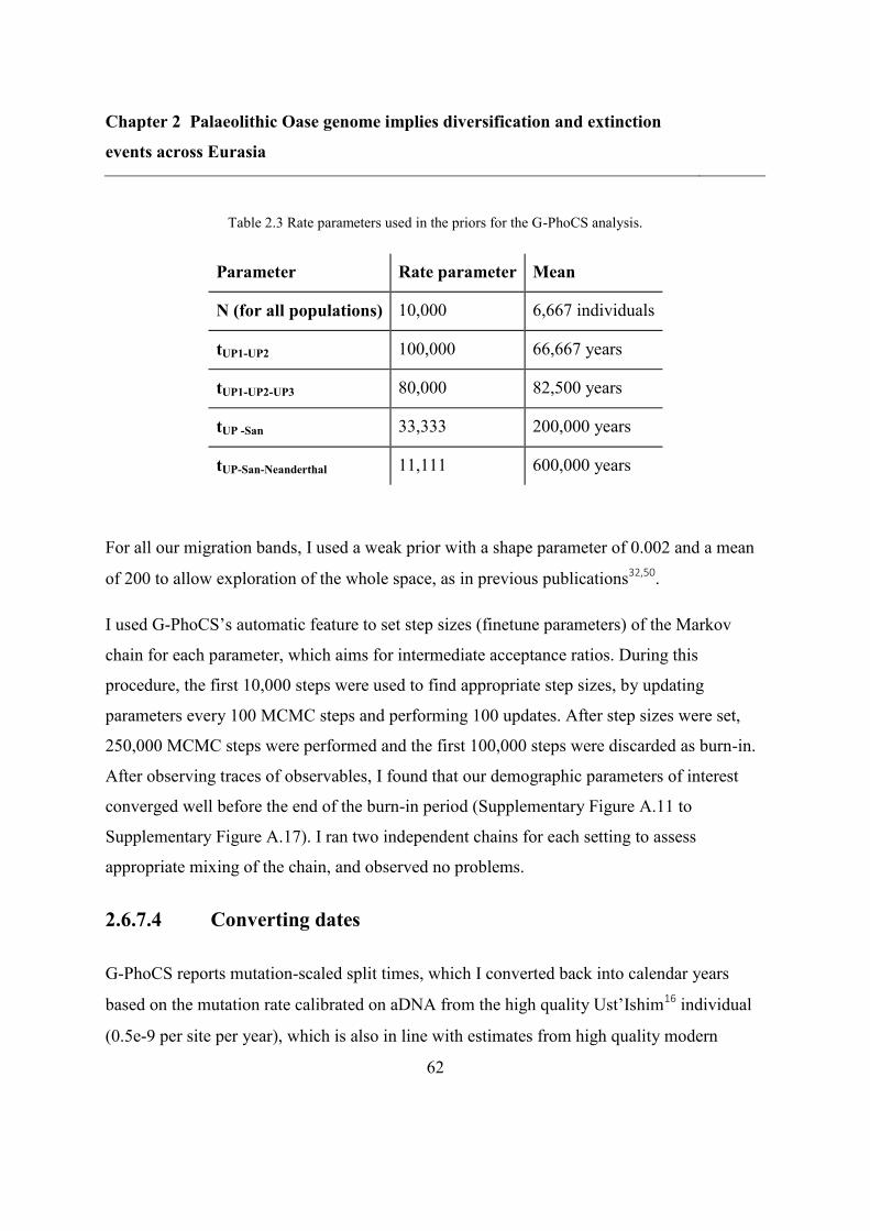
Chapter 2 Palaeolithic Oase genome implies diversification and extinction
events across Eurasia
62
Table 2.3 Rate parameters used in the priors for the G-PhoCS analysis.
Parameter Rate parameter Mean
N (for all populations) 10,000 6,667 individuals
tUP1-UP2 100,000 66,667 years
tUP1-UP2-UP3 80,000 82,500 years
tUP -San 33,333 200,000 years
tUP-San-Neanderthal 11,111 600,000 years
For all our migration bands, I used a weak prior with a shape parameter of 0.002 and a mean
of 200 to allow exploration of the whole space, as in previous publications32,50
.
I used G-PhoCS’s automatic feature to set step sizes (finetune parameters) of the Markov
chain for each parameter, which aims for intermediate acceptance ratios. During this
procedure, the first 10,000 steps were used to find appropriate step sizes, by updating
parameters every 100 MCMC steps and performing 100 updates. After step sizes were set,
250,000 MCMC steps were performed and the first 100,000 steps were discarded as burn-in.
After observing traces of observables, I found that our demographic parameters of interest
converged well before the end of the burn-in period (Supplementary Figure A.11 to
Supplementary Figure A.17). I ran two independent chains for each setting to assess
appropriate mixing of the chain, and observed no problems.
2.6.7.4 Converting dates
G-PhoCS reports mutation-scaled split times, which I converted back into calendar years
based on the mutation rate calibrated on aDNA from the high quality Ust’Ishim16
individual
(0.5e-9 per site per year), which is also in line with estimates from high quality modern
Chapter 2 Palaeolithic Oase genome implies diversification and extinction
events across Eurasia
63
genomes53
. I converted this mutation rate for our in vitro deaminated sequences by
multiplying it with a factor of 0.3, based on the ratio of average levels of polymorphism
before and after deamination on our modern genomes.
2.7 Bibliography
1. Jones, E. R. et al. Upper Palaeolithic genomes reveal deep roots of modern Eurasians.
Nat. Commun. 6, 8912 (2015).
2. Groucutt, H. S. et al. Rethinking the dispersal of Homo sapiens out of Africa. Evol.
Anthropol. Issues News Rev. 24, 149–164 (2015).
3. Soares, P. et al. Correcting for Purifying Selection: An Improved Human
Mitochondrial Molecular Clock. Am. J. Hum. Genet. 84, 740–759 (2009).
4. Liu, H., Prugnolle, F., Manica, A. & Balloux, F. A Geographically Explicit Genetic
Model of Worldwide Human-Settlement History. Am. J. Hum. Genet. 79, 230–237 (2006).
5. Eriksson, A. et al. Late Pleistocene climate change and the global expansion of
anatomically modern humans. Proc. Natl. Acad. Sci. 109, 16089–16094 (2012).
6. Foley, R. A. & Lewin, R. Principles of Human Evolution. (John Wiley & Sons,
2013).
7. Pagani, L. et al. Genomic analyses inform on migration events during the peopling of
Eurasia. Nature 538, 238–242 (2016).
8. Malaspinas, A.-S. et al. A genomic history of Aboriginal Australia. Nature 538,
nature18299 (2016).
Chapter 2 Palaeolithic Oase genome implies diversification and extinction
events across Eurasia
64
9. Mallick, S. et al. The Simons Genome Diversity Project: 300 genomes from 142
diverse populations. Nature 538, 201–206 (2016).
10. Mellars, P. Why did modern human populations disperse from Africa ca. 60,000 years
ago? A new model. Proc. Natl. Acad. Sci. 103, 9381 (2006).
11. Mellars, P. Going East: New Genetic and Archaeological Perspectives on the Modern
Human Colonization of Eurasia. Science 313, 796–800 (2006).
12. Barker, G. et al. The ‘human revolution’ in lowland tropical Southeast Asia: the
antiquity and behavior of anatomically modern humans at Niah Cave (Sarawak, Borneo). J.
Hum. Evol. 52, 243–261 (2007).
13. Yang, M. A. et al. 40,000-Year-Old Individual from Asia Provides Insight into Early
Population Structure in Eurasia. Curr. Biol. 27, 3202–3208.e9 (2017).
14. Fu, Q. et al. The genetic history of Ice Age Europe. Nature 534, 200–205 (2016).
15. Fu, Q. et al. An early modern human from Romania with a recent Neanderthal
ancestor. Nature 524, 216–219 (2015).
16. Fu, Q. et al. Genome sequence of a 45,000-year-old modern human from western
Siberia. Nature 514, 445–449 (2014).
17. Raghavan, M. et al. Upper Palaeolithic Siberian genome reveals dual ancestry of
Native Americans. Nature 505, 87–91 (2014).
18. Rosenberg, N. A. et al. Genetic Structure of Human Populations. Science 298, 2381–
2385 (2002).
19. Trinkaus, E., Milota, Ş., Rodrigo, R., Mircea, G. & Moldovan, O. Early modern
human cranial remains from the Peştera cu Oase, Romania. J. Hum. Evol. 45, 245–253
(2003).

Chapter 2 Palaeolithic Oase genome implies diversification and extinction
events across Eurasia
65
20. Trinkaus, E. et al. An early modern human from the Peştera cu Oase, Romania. Proc.
Natl. Acad. Sci. 100, 11231–11236 (2003).
21. Rougier, H. et al. Peştera cu Oase 2 and the cranial morphology of early modern
Europeans. Proc. Natl. Acad. Sci. 104, 1165–1170 (2007).
22. Skoglund, P. et al. Reconstructing Prehistoric African Population Structure. Cell 171,
59–71.e21 (2017).
23. Quinlan, A. R. & Hall, I. M. BEDTools: a flexible suite of utilities for comparing
genomic features. Bioinformatics 26, 841–842 (2010).
24. Green, R. E. et al. The Neandertal genome and ancient DNA authenticity. EMBO J.
28, 2494–2502 (2009).
25. Ginolhac, A., Rasmussen, M., Gilbert, M. T. P., Willerslev, E. & Orlando, L.
mapDamage: testing for damage patterns in ancient DNA sequences. Bioinformatics 27,
2153–2155 (2011).
26. Andrews, R. M. et al. Reanalysis and revision of the Cambridge reference sequence
for human mitochondrial DNA. Nat. Genet. 23, 147 (1999).
27. Green, R. E. et al. A Draft Sequence of the Neandertal Genome. Science 328, 710–
722 (2010).
28. Fu, Q. et al. DNA analysis of an early modern human from Tianyuan Cave, China.
Proc. Natl. Acad. Sci. 110, 2223–2227 (2013).
29. Siska, V. et al. Genome-wide data from two early Neolithic East Asian individuals
dating to 7700 years ago. Sci. Adv. 3, e1601877 (2017).
30. Seguin-Orlando, A. et al. Paleogenomics. Genomic structure in Europeans dating
back at least 36,200 years. Science 346, 1113–1118 (2014).
Chapter 2 Palaeolithic Oase genome implies diversification and extinction
events across Eurasia
66
31. Sikora, M. et al. Ancient genomes show social and reproductive behavior of early
Upper Paleolithic foragers. Science (2017). doi:10.1126/science.aao1807
32. Gronau, I., Hubisz, M. J., Gulko, B., Danko, C. G. & Siepel, A. Bayesian inference of
ancient human demography from individual genome sequences. Nat Genet 43, 1031–1034
(2011).
33. Prüfer, K. et al. The complete genome sequence of a Neanderthal from the Altai
Mountains. Nature 505, 43–49 (2014).
34. Morin, E. Evidence for declines in human population densities during the early Upper
Paleolithic in western Europe. Proc Natl Acad Sci U A 105, 48–53 (2008).
35. Gamba, C. et al. Genome flux and stasis in a five millennium transect of European
prehistory. Nat. Commun. 5, 5257 (2014).
36. Li, H. & Durbin, R. Inference of human population history from individual whole-
genome sequences. Nature 475, 493–496 (2011).
37. Dabney, J. et al. Complete mitochondrial genome sequence of a Middle Pleistocene
cave bear reconstructed from ultrashort DNA fragments. Proc Natl Acad Sci U A 110,
15758–15763 (2013).
38. Gansauge, M.-T. & Meyer, M. Single-stranded DNA library preparation for the
sequencing of ancient or damaged DNA. Nat. Protoc. 8, 737–748 (2013).
39. Martin, M. Cutadapt removes adapter sequences from high-throughput sequencing
reads. EMBnet J 17, 10–12 (2011).
40. Li, H. et al. The Sequence Alignment/Map format and SAMtools. Bioinformatics 25,
2078–2079 (2009).
Chapter 2 Palaeolithic Oase genome implies diversification and extinction
events across Eurasia
67
41. McKenna, A. et al. The Genome Analysis Toolkit: a MapReduce framework for
analyzing next-generation DNA sequencing data. Genome Res 20, 1297–1303 (2010).
42. Jónsson, H., Ginolhac, A., Schubert, M., Johnson, P. L. F. & Orlando, L.
mapDamage2.0: fast approximate Bayesian estimates of ancient DNA damage parameters.
Bioinformatics 29, 1682–1684 (2013).
43. Milne, I. et al. Using Tablet for visual exploration of second-generation sequencing
data. Brief. Bioinform. 14, 193–202 (2013).
44. Kloss‐Brandstätter Anita et al. HaploGrep: a fast and reliable algorithm for automatic
classification of mitochondrial DNA haplogroups. Hum. Mutat. 32, 25–32 (2010).
45. Lazaridis, I. et al. Ancient human genomes suggest three ancestral populations for
present-day Europeans. ArXiv13126639 Q-Bio (2013).
46. Purcell, S. et al. PLINK: a tool set for whole-genome association and population-
based linkage analyses. Am J Hum Genet 81, 559–575 (2007).
47. Lazaridis, I. et al. Genomic insights into the origin of farming in the ancient Near
East. Nature 536, 419–424 (2016).
48. Reich, D., Thangaraj, K., Patterson, N., Price, A. L. & Singh, L. Reconstructing
Indian population history. Nature 461, 489–494 (2009).
49. Patterson, N. et al. Ancient Admixture in Human History. Genetics 192, 1065–1093
(2012).
50. Kuhlwilm, M. et al. Ancient gene flow from early modern humans into Eastern
Neanderthals. Nature 530, 429–433 (2016).
51. Llorente, M. G. et al. Ancient Ethiopian genome reveals extensive Eurasian
admixture throughout the African continent. Science 350, 820–822 (2015).
Chapter 2 Palaeolithic Oase genome implies diversification and extinction
events across Eurasia
68
52. Rasmussen, M. et al. The genome of a Late Pleistocene human from a Clovis burial
site in western Montana. Nature 506, 225–229 (2014).
53. Kong, A. et al. Rate of de novo mutations and the importance of father’s age to
disease risk. Nature 488, 471–475 (2012).
Chapter 3 Upper Palaeolithic genomes reveal deep roots of modern Eurasians
69
Chapter 3 Upper Palaeolithic genomes reveal deep
roots of modern Eurasians
3.1 Abstract
We extend the scope of European palaeogenomics by sequencing the genomes of Late
Upper Palaeolithic (13,300-year-old, 1.4-fold coverage) and Mesolithic (9,700-year-old,
15.4-fold) males from western Georgia in the Caucasus and a Late Upper Palaeolithic
(13,700-year-old, 9.5-fold) male from Switzerland. While we detect genomic continuity
from the Late Palaeolithic to the Mesolithic in both regions, we find that Caucasus
hunter-gatherers (CHG) belong to a distinct ancient clade that split from western
hunter-gatherers ~45 kya, shortly after the expansion of anatomically modern humans
into Europe and from Neolithic farmers ~25 kya, around the Last Glacial Maximum.
Relatives of the CHG genomes significantly contributed to the Yamnaya steppe herders
who migrated into Europe ~3,000 BC, supporting a formative Caucasus influence on
this important Early Bronze age culture. CHG-related populations also left their
imprint on modern populations from the Caucasus and also central and south Asia,
possibly marking the arrival of Indo-Aryan languages.
Chapter 3 Upper Palaeolithic genomes reveal deep roots of modern Eurasians
70
3.2 Contribution
This study was published as part of Jones et al., 20161. I was responsible for performing the
model-based clustering analysis and the coalescent-based modelling using the softwares
ADMIXTURE and G-PhoCS, respectively.
3.3 Introduction
Ancient genomes from Eurasia have revealed three ancestral populations that contributed to
contemporary Europeans in varying degrees2. Mesolithic individuals, sampled from Spain all
the way to Hungary2–4
, belong to a relatively homogenous group, termed western hunter-
gatherers (WHG). The expansion of early farmers (EF) out of South-West Asia during the
Neolithic transition led to major changes in the European gene pool, with almost complete
replacement in the south and increased mixing with local WHG further north and west2–6
.
Finally, a later wave represented by the Early Bronze Age Yamnaya from the Pontic steppe,
carrying partial ancestry from ancient north Eurasians (ANE) and from a second,
undetermined source, arrived from the east, profoundly changing populations and leaving a
cline of admixture in Eastern and Central Europe2,4,7
. This view, which was initially based on
a handful of genomes, was recently confirmed by extensive surveys of Eurasian samples from
the Holocene6,8
.
Since the publication that forms the basis of this chapter, additional data from the Near East
and South-West Asia has become available, which expanded our views on the spread of
farming in Western Eurasia. First, ancient genomes from the European and Asian sides of the
Aegan uncovered a line of ancestry stretching from the Near East to early farmers from
Europe9. Then, Early Neolithic genomes from Iran revealed an eastern group of farmers that
was genetically different from their early European counterparts and was related more
(although not directly descendant) to the samples from the Caucasus presented here10,11
.
Chapter 3 Upper Palaeolithic genomes reveal deep roots of modern Eurasians
71
Finally, data from the southern Caucasus (Armenia), northwestern Anatolia (Turkey), Iran,
and the southern Levant (Israel and Jordan) including hunter-gatherers, early farmers and
samples from later ages12
confirmed that the first farmers were highly differentiated and
related to local hunter-gatherers. This study also validated the link between early farmers
from northwestern Anatolia and Europe and showed that relatives of Iranian farmers
expanded north, towards the Eurasian steppe and contributed to the steppe herders. Together,
these studies showed that pre-agricultural populations in the Near East were highly
structured, and that the earliest farmers were related to local hunter-gatherers, thus preserving
this structure. These distinct ancestries were then spread by the expansion of early farmers,
but then mixed again through subsequent migrations, such as those during the Bronze Age. I
will reflect on these results and on how they relate to the presented body of work in the
discussion of this chapter.
In this study, we extended our view of the genetic makeup of early Europeans by both
looking further back in time and sampling from the crossroads between the European and
Asian continents. We sequenced a Late Upper Palaeolithic (‘Satsurblia’ from Satsurblia cave,
13,300-year-old, 1.4-fold coverage) and a Mesolithic genome (‘Kotias’ from Kotias Klde
cave, 9,700-year-old, 15.4-fold) from western Georgia, at the very eastern boundary of
Europe. We term these two individuals Caucasus hunter-gatherers (CHG). To extend our
overview of WHG to a time depth similar to the one available for our samples from the
Caucasus, we also sequenced a western European Late Upper Palaeolithic genome, ‘Bichon’
(13,700-year-old, 9.5-fold) from Grotte du Bichon, Switzerland. These new genomes,
together with already published data, provide us with a much-improved geographic and
temporal coverage of genetic diversity across Europe after the Last Glacial Maximum
(LGM)13
. We show that CHG belong to a new, distinct ancient clade that split from WHG
~45kya and from Neolithic farmers ~25kya. In our panel, this clade represents the best
surrogate for the previously undetermined source of ancestry to the Yamnaya, and its
relatives contributed to modern populations from the Caucasus all the way to Central Asia.
Chapter 3 Upper Palaeolithic genomes reveal deep roots of modern Eurasians
72
3.4 Results
3.4.1 Samples, sequencing and authenticity
Recent excavations of Satsurblia cave in western Georgia yielded a human right temporal
bone, dated to the Late Upper Palaeolithic 13,132-13,380 cal. BP. Following the approach of
Gamba et al.4, extractions from the dense part of the petrous bone yielded sequencing
libraries comprising 13.8% alignable human sequence which were used to generate 1.4-fold
genome coverage. A molar tooth sampled from a later Mesolithic (9,529-9,895 cal. BP)
burial in Kotias Klde, a rock shelter also in western Georgia showed excellent preservation,
with endogenous human DNA content of 76.9%. This was sequenced to 15.4-fold genome
coverage. Grotte du Bichon is a cave situated in the Swiss Jura Mountains where a skeleton
of a young male of Cro-magnon type was found and dated to the late Upper Palaeolithic
13,560- 13,770 cal. BP. A petrous bone sample extraction from this also gave excellent
endogenous content at 71.5% and was sequenced to 9.5-fold coverage. The sequence data
from each genome showed sequence length and nucleotide misincorporation patterns which
were indicative of post-mortem damage and contamination estimates, based on X
chromosome and mitochondrial DNA tests (see methods), were less than 1%; comparable to
those found in other ancient genomes 3,4,13
.
3.4.2 Continuity across the Palaeolithic-Mesolithic boundary
Kotias and Satsurblia, the two Caucasus hunter gatherer genomes (CHG), are genetically
different from all other early Holocene (i.e. Mesolithic and Neolithic) ancient genomes2–7,13–
15, while Bichon is similar to other younger WHG. The distinctness of CHG can be clearly
seen on a principal component analysis (PCA) plot16
where ancient samples were projected
on contemporary Eurasian populations2. CHG genomes fall between modern Caucasian and
South-Central Asian populations in a region of the graph separated from both other hunter
gatherer and early farmer samples (Figure 3.1A). Clustering using ADMIXTURE software17
Chapter 3 Upper Palaeolithic genomes reveal deep roots of modern Eurasians
73
confirms this pattern, with CHG forming their own homogenous cluster (Figure 3.1B). The
close genetic proximity between Satsurblia and Kotias is also formally supported by D-
statistics18
, indicating the two CHG genomes form a clade to the exclusion of other pre-
Bronze Age ancient genomes (Supplementary Table B.3), suggesting continuity across the
Late Upper Palaeolithic and Mesolithic periods. This result is mirrored in western Europe as
Bichon: i) is close to other WHG on the first two dimensions in the PCA space (Figure 3.1A)
and outgroup f3 analysis (Supplementary Figure B.1), ii) belongs to the same cluster as other
WHG in ADMIXTURE analysis (Figure 3.1B) and iii) forms a clade with other WHG to the
exclusion of other ancient genomes based on D-statistics (Supplementary Table B.4). Thus,
these new data indicate genomic persistence between the Late Upper Palaeolithic and
Mesolithic both within western Europe and, separately, within the Caucasus.
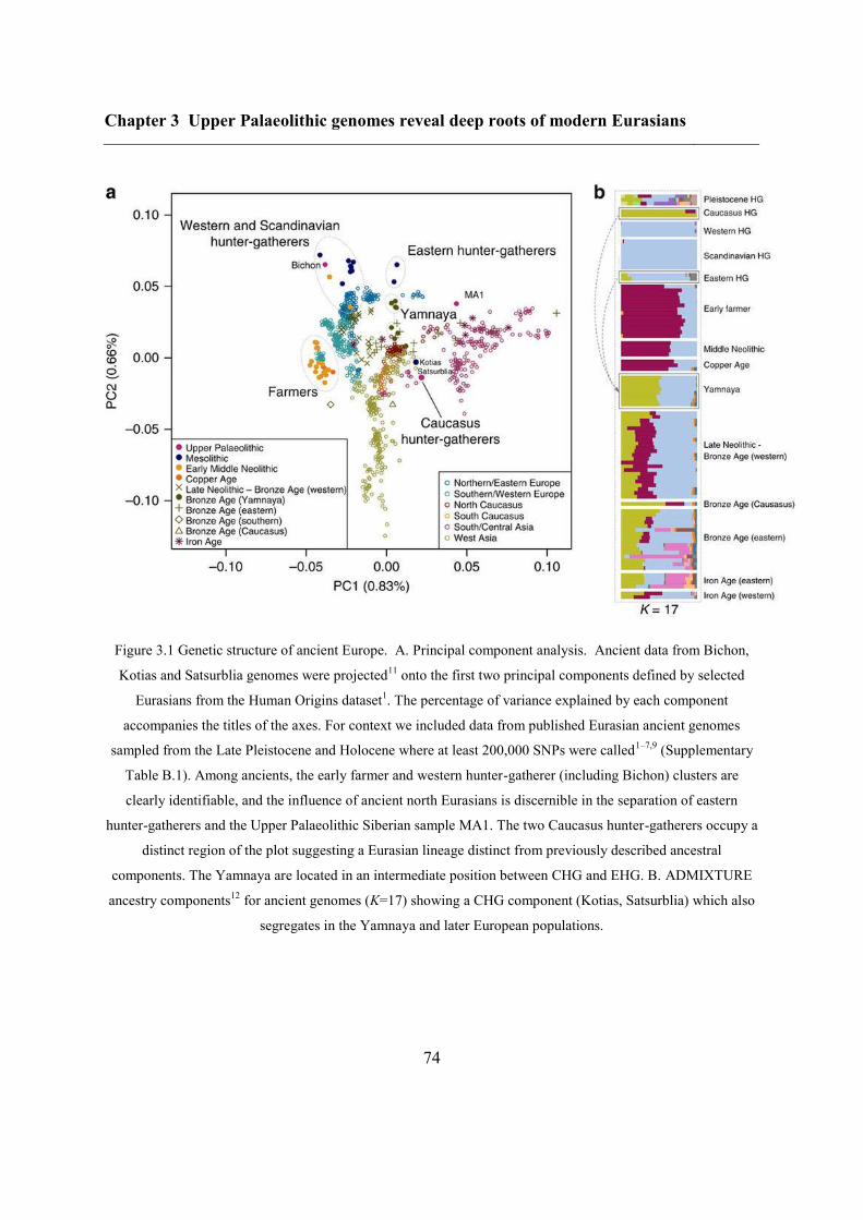
Chapter 3 Upper Palaeolithic genomes reveal deep roots of modern Eurasians
74
Figure 3.1 Genetic structure of ancient Europe. A. Principal component analysis. Ancient data from Bichon,
Kotias and Satsurblia genomes were projected11
onto the first two principal components defined by selected
Eurasians from the Human Origins dataset1. The percentage of variance explained by each component
accompanies the titles of the axes. For context we included data from published Eurasian ancient genomes
sampled from the Late Pleistocene and Holocene where at least 200,000 SNPs were called1–7,9
(Supplementary
Table B.1). Among ancients, the early farmer and western hunter-gatherer (including Bichon) clusters are
clearly identifiable, and the influence of ancient north Eurasians is discernible in the separation of eastern
hunter-gatherers and the Upper Palaeolithic Siberian sample MA1. The two Caucasus hunter-gatherers occupy a
distinct region of the plot suggesting a Eurasian lineage distinct from previously described ancestral
components. The Yamnaya are located in an intermediate position between CHG and EHG. B. ADMIXTURE
ancestry components12
for ancient genomes (K=17) showing a CHG component (Kotias, Satsurblia) which also
segregates in the Yamnaya and later European populations.
Chapter 3 Upper Palaeolithic genomes reveal deep roots of modern Eurasians
75
3.4.3 Deep coalescence of early Holocene lineages
The geographical proximity of the southern Caucasus to the Levant begs the question of
whether CHG might be related to early Neolithic farmers with Near Eastern heritage. To
formally address this question, we reconstructed the relationship among WHG, CHG and EF
using available high quality ancient genomes2–4
. Outgroup f3-statistics19
were used to
compare the three possible topologies, with the correct relationship being characterised by the
largest amount of shared drift between the two groups that form a clade with respect to the
outgroup (Figure 3.2A; Supplementary Table B.5). A scenario in which the population
ancestral to both CHG and EF split from WHG receives the highest support, implying that
CHG and EF form a clade with respect to WHG. A scenario in which CHG and WHG form a
distinct clade with respect to EF can be rejected. The known admixture of WHG with EF2,4–6
(WHG component in our EF samples) implies that some shared drift is found between WHG
and EF with respect to CHG, but this is much smaller than the shared drift between CHG and
EF. Thus, WHG split first, with CHG and EF separating only at a later stage.
I next dated the splits among WHG, CHG and EF using a coalescent model implemented in
G-PhoCS20
, based on the high coverage genomes in our dataset (Figure 3.2B for a model
using the German farmer Stuttgart2 to represent EF; Supplementary Table B.6 for models
using the Hungarian farmer NE14) and taking advantage of the mutation rate recently derived
from Ust’-Ishim15
. G-PhoCS dates the split between WHG and the population ancestral to
CHG and EF at ~40-50 kya (range of best estimates depending on which genomes are used;
see Supplementary Table B.6 for details), implying that they diverged early on during the
colonisation of Europe21
, and well before the LGM. On the WHG branch, the split between
Bichon and Loschbour2 is dated to ~16-18 kya (just older than the age of Bichon), implying
continuity in western Europe, which supports the conclusions from our previous analyses.
The split between CHG and EF is dated at ~20-30 kya, emerging from a common basal
Eurasian lineage2 (Supplementary Figure B.2) and suggesting a possible link with the LGM,
although the broad confidence intervals require some caution with this interpretation. Overall,
Chapter 3 Upper Palaeolithic genomes reveal deep roots of modern Eurasians
76
the sharp genomic distinctions between these post-LGM populations contrasts with the
comparative lack of differentiation between the earlier Eurasian genomes, e.g. as visualised
in the ADMIXTURE analysis (Figure 3.1A), and it seems likely that this structure could have
emerged as a result of ice age habitat restriction. WHG and CHG also carry different markers
with known links to their phenotypes. For example, like EF, but in contrast to WHG, CHG
carry a variant of the SLC24A5 gene22
associated with light skin pigmentation (rs1426654,
see Supplementary Information). This trait, which is believed to have risen to high frequency
during the Neolithic expansion23
, may thus have a relatively long history in Eurasia, with its
origin probably predating the LGM, if the variant in EF and CHG has a common origin.
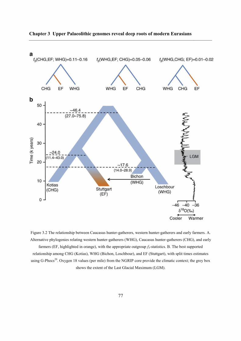
Chapter 3 Upper Palaeolithic genomes reveal deep roots of modern Eurasians
77
Figure 3.2 The relationship between Caucasus hunter-gatherers, western hunter-gatherers and early farmers. A.
Alternative phylogenies relating western hunter-gatherers (WHG), Caucasus hunter-gatherers (CHG), and early
farmers (EF, highlighted in orange), with the appropriate outgroup f3-statistics. B. The best supported
relationship among CHG (Kotias), WHG (Bichon, Loschbour), and EF (Stuttgart), with split times estimates
using G-Phocs20
. Oxygen 18 values (per mile) from the NGRIP core provide the climatic context; the grey box
shows the extent of the Last Glacial Maximum (LGM).
Chapter 3 Upper Palaeolithic genomes reveal deep roots of modern Eurasians
78
We also investigated the relationship between a partial genome from a 24,000 year old
individual (MA1) from Mal’ta, Siberia7 and CHG. MA1 had been shown to be divergent
from other ancient samples and to have more shared alleles with nearly all modern Europeans
than with an EF genome by Lazaridis et al.2. This allowed inference of an ancient north
Eurasian (ANE) component in European ancestry, which was subsequently shown to have an
influence in later eastern hunter gatherers and to have spread into Europe via incoming
Steppe herders beginning ~4,500 years ago6,8
. Several analyses indicate that CHG genomes
are not a subset of this ANE lineage. First, MA1 and CHG fall in distinct regions of the PCA
plot and also have very different profiles in the ADMIXTURE analysis (Figure 3.1). Second,
when we test if CHG shows any evidence of excess allele sharing with MA1 or with EHG
relative to western hunter gatherers using tests of the form D(Yoruba, CHG; MA1, WHG),
no combinations were significantly positive (Supplementary Table B.7). Although such a test
loses power when the number of overlapping SNPs is low, in this case, we had a high number
of markers for the comparison (over 200,000 for MA1 and over 100,000 for EHG). Last, we
also tested whether the ancestral component inferred in modern Europeans from MA1 was
distinct from any that may have been donated from CHG using tests of the form D(Yoruba,
MA1; CHG, modern north European population) (Supplementary Table B.8). All northern
Europeans showed a significant amount of shared alleles with MA1 separate to any they
shared with CHG.
We have shown that WHG and CHG are the descendants of two ancient populations that
appear to have persisted in Europe since the mid Upper Palaeolithic and survived the LGM
separately. We looked at runs of homozygosity (ROH: Figure 3.3) which inform on past
population size or inbreeding4,24,25
. Both WHG and CHG have a high frequency of ROH and
in particular, the older CHG, Satsurblia, shows signs of recent consanguinity, with a high
frequency of longer (>4Mb) ROH. In contrast, EF are characterised by lower frequency of
ROH of all sizes, suggesting a less constricted population history with larger population sizes
and/or less inbreeding25,26
, perhaps associated with a more benign passage through the LGM
than the more northern populations.
Chapter 3 Upper Palaeolithic genomes reveal deep roots of modern Eurasians
79
Figure 3.3 Distribution of ROH. A. The total length of short ROH (<1.6Mb) plotted against the total length of
long ROH (≥1.6 Mb) and B. mean total ROH length for a range of length categories. ROH were calculated
using a panel of 199,868 autosomal SNPs. For Kotias we analysed both high-coverage genotypes and genotypes
imputed from down-sampled data (marked in italics; see Supplementary Information). Diploid genotypes
imputed from low-coverage variant calls were used for Satsurblia and high coverage genotypes were used for all
other samples. A clear distinction is visible between both WHG and CHG who display an excess of shorter
ROH, akin to modern Oceanic and Onge populations, and EF who resemble other populations with sustained
larger ancestral population sizes.
Chapter 3 Upper Palaeolithic genomes reveal deep roots of modern Eurasians
80
3.4.4 Caucasus hunter-gatherer contribution to subsequent
populations
We next explored the extent to which Bichon and CHG contributed to contemporary
populations using outgroup f3(African; modern, ancient) statistics, which measure the shared
genetic history between an ancient genome and a modern population since they diverged
from an African outgroup. Bichon, like younger WHG, shows strongest affinity to northern
Europeans (Supplementary Figure B.3), whilst contemporary southern Caucasus populations
are the closest to CHG (Figure 3.4A & Supplementary Figure B.3), thus implying a degree of
continuity in both regions stretching back at least 13,000 years to the late Upper Palaeolithic.
Continuity in the Caucasus is also supported by the mitochondrial and Y-chromosomal
haplogroups of Kotias (H13c and J2a respectively) and Satsurblia (K3 and J), which are all
found at high frequencies in Georgia today27–29
(see Supplementary Information for further
details).
EF share greater genetic affinity to populations from southern Europe than to those from
northern Europe with an inverted pattern for WHG2–6
. Surprisingly, we find that CHG
influence is stronger in northern than southern Europe (Figure 3.4A & Supplementary Figure
B.3) despite the closer relationship between CHG and EF compared to WHG, suggesting an
increase of CHG ancestry in western Europeans subsequent to the early Neolithic period. We
investigated this further using D-statistics of the form D(Yoruba, Kotias; EF, modern western
European population), which confirmed a significant introgression from CHG into modern
northern European genomes after the early Neolithic period (Supplementary Figure B.4).
Chapter 3 Upper Palaeolithic genomes reveal deep roots of modern Eurasians
81
Figure 3.4 The relationship of Caucasus hunter-gatherers to modern populations. A. Genomic affinity of modern
populations2 to Kotias, quantified by the outgroup f3-statistics of the form f3(Kotias, modern population;
Yoruba). Kotias shares the most genetic drift with populations from the Caucasus with high values also found
for northern Europe and central Asia. B. Sources of admixture into modern populations: semicircles indicate
those that provide the most negative outgroup f3 statistic for that population. Populations for which a
significantly negative statistic could not be determined are marked in white. Populations for which the ancient
Caucasus genomes are best ancestral approximations include those of the southern Caucasus and interestingly,
south and central Asia. Western Europe tends to be a mix of early farmers and western/eastern hunter-gatherers
while Middle Eastern genomes are described as a mix of early farmers and Africans.
Chapter 3 Upper Palaeolithic genomes reveal deep roots of modern Eurasians
82
3.4.5 CHG origins of migrating Early Bronze Age herders
We investigated the temporal stratigraphy of CHG influence by comparing these data to
previously published ancient genomes. We find that CHG, or a population close to them,
contributed to the genetic make-up of individuals from the Yamnaya culture, which have
been implicated as vectors for the profound influx of Pontic steppe ancestry that spread
westwards into Europe and east into central Asia with metallurgy, horse-riding and possibly
Indo-European languages in the third millenium BC6,8
. CHG ancestry in these groups is
supported by ADMIXTURE analysis (Figure 3.1B) and admixture f3-statistics19,30
(Figure
3.5), which best describe the Yamnaya as a mix of CHG and Eastern European hunter-
gatherers.
The Yamnaya were semi-nomadic pastoralists, mainly dependent on stock-keeping but with
some evidence for agriculture, including incorporation of a plow into one burial31
. As such,
it is interesting that they lack an ancestral component of the EF genome (Figure 3.1B), which
permeates through western European Neolithic and subsequent agricultural populations.
During the Early Bronze Age, the Caucasus was in communication with the steppe,
particularly via the Maikop culture32
, which emerged in the first half of the fourth millennium
BC. The Maikop culture predated and, possibly with earlier southern influences, contributed
to the formation of the adjacent Yamnaya culture that emerged further to the north and may
be a candidate for the transmission of CHG ancestry. In the ADMIXTURE analysis of later
ancient genomes (Figure 3.1B) the Caucasus component gives a marker for the extension of
Yamnaya admixture, with substantial contribution to both western and eastern Bronze Age
samples. However, this is not completely coincident with metallurgy; Copper Age genomes
from Northern Italy and Hungary show no contribution and neither does the earlier of two
Hungarian Bronze Age individuals.
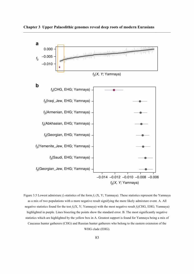
Chapter 3 Upper Palaeolithic genomes reveal deep roots of modern Eurasians
83
Figure 3.5 Lowest admixture f3-statistics of the form f3 (X, Y; Yamnaya). These statistics represent the Yamnaya
as a mix of two populations with a more negative result signifying the more likely admixture event. A. All
negative statistics found for the test f3(X, Y; Yamnaya) with the most negative result f3(CHG, EHG; Yamnaya)
highlighted in purple. Lines bisecting the points show the standard error. B. The most significantly negative
statistics which are highlighted by the yellow box in A. Greatest support is found for Yamnaya being a mix of
Caucasus hunter gatherers (CHG) and Russian hunter gatherers who belong to the eastern extension of the
WHG clade (EHG).
Chapter 3 Upper Palaeolithic genomes reveal deep roots of modern Eurasians
84
3.4.6 Modern impact of CHG ancestry
In modern populations, the impact of CHG also stretches beyond Europe to the east. Central
and south Asian populations received genetic input from CHG (or a population close to
them), as indicated by a prominent CHG component in ADMIXTURE (Supplementary
Figure B.5) and admixture f3-statistics, which represent many samples as a mix of CHG and
another south Asian population (Figure 3.4B; Supplementary Table B.10). It has been
proposed that modern Indians are a mixture of two ancestral components, an Ancestral North
Indian (ANI) component related to modern west Eurasians and an Ancestral South Indian
component related more distantly to the Onge30
. Kotias provides the majority best surrogate
for the former33,34
(Supplementary Table B.11): it has the highest D(Yoruba,ANI; Onge,
Indian population) score for 5 out of the 9 Indian populations in our panel. However, samples
from the Afanasievo culture, relatives of the Early Bronze Age Yamnaya, are also a good
proxy: they score highest for 3 populations, with Z scores higher than that for Kotias. A third
population, the South Indian Mala is the best ANI proxy for the Kharia, but the Kharia tends
to differ from other Indian populations on genetic analysis (e.g. ADMIXTURE). It is
estimated that this admixture in the ancestors of Indian populations occurred relatively
recently, 1,900-4,200 years BP, and is possibly linked with migrations introducing Indo-
European languages and Vedic religion to the region33
.
3.5 Conclusions
Given their geographic origin, it seems likely that CHG and EF are the descendants of early
colonists from Africa who stopped south of the Caucasus, in an area stretching south to the
Levant and possibly east towards central and south Asia. WHG, on the other hand, are likely
the descendants of a wave that expanded further into Europe. The separation of these
populations is one that stretches back before the Holocene as indicated by local continuity
through the Late Palaeolithic/Mesolithic boundary and deep coalescence estimates which date
Chapter 3 Upper Palaeolithic genomes reveal deep roots of modern Eurasians
85
to around the LGM and earlier. Several analyses indicate that CHG are distinct from another
inferred minority ancestor, ANE, making them a divergent fourth strand of Eurasian ancestry
that expands the model of human colonisation of Europe.
The separation between CHG and both EF and WHG ended during the Early Bronze Age
when a major ancestral component linked to CHG was carried west by migrating herders
from the Eurasian Steppe. The foundation group for this seismic change was the Yamnaya,
who we estimate to owe half of their ancestry to CHG-linked sources. These sources may be
linked to the Maikop culture, which predated the Yamnaya and was located further south,
closer to the Southern Caucasus. Through the Yamanya, the CHG-related ancestral strand
contributed to most modern European populations, especially in the northern part of the
continent. The link we found between CHG and the Yamnaya also agrees with Broushaki et
al.10
and Lazaridis et al.12
, where the the Yamnaya is modelled as a mixture of two sources,
one of which is related to EHG and the other to a population from the western Near East.
Although Broushaki et al. 10
found that the CHG was a better proxy than early Iranian
farmers for this second component, additional, younger Iranian samples from the
Chalcolithic, published by Lazaridis et al. 12
were an even better surrogate than the CHG.
Finally, we found that CHG-related ancestry was also carried east to become a major
contributor to the Ancestral North Indian component found in the Indian subcontinent. The
additional genomes from the Near East also failed to pinpoint the direct source of the ANI
component, but found that it was related to both Iranian farmers and to populations from the
Eurasian steppe10,12
. Given that these two populations are both also related to the CHG, the
similarity we found between CHG and ANI was not surprising. Exactly when the eastwards
movement related to the ANI component occurred is unknown, but it likely included
migration around the same time as their contribution to the western European gene pool and
may be linked with the spread of Indo-European languages. However, earlier movements
associated with other advancements, such as cereal farming and herding, are also plausible.
Chapter 3 Upper Palaeolithic genomes reveal deep roots of modern Eurasians
86
The discovery of CHG as a fourth ancestral component of the European gene pool
underscores the importance of a dense geographical sampling of human palaeogenomes,
especially among diverse geographical regions. Its separation from other European ancestral
strands ended dramatically with the extensive population, linguistic and technological
upheavals of the Early Bronze Age resulting in a wide impact of this ancestral strand on
contemporary populations, stretching from the Atlantic to Central and South Asia.
3.6 Methods
3.6.1 Sample preparation and DNA sequencing
DNA was extracted from three samples: two from Georgia (Kotias and Satsurblia) and one
from Switzerland (Bichon; Supplementary Figure B.6). Sample preparation, DNA extraction
and library construction were carried out in dedicated ancient DNA facilities at Trinity
College Dublin (Kotias and Satsurblia) and at the University of York, England (Bichon).
DNA was extracted from Kotias and Satsurblia following a silica column based protocol3
based on Yang et al.35
and libraries were prepared and amplified with AccuPrimeTM
Pfx
Supermix (Life Technology), using a modified version of 36
as outlined in 3. For the ancient
Swiss sample Bichon, DNA was extracted following 37
and libraries were built as described
above with the exception that enzymatic end-repair was arrested using heat inactivation rather
than a silica-column purification step38,39
. Libraries were first screened to assess their human
DNA content on an Illumina MiSeq platform at TrinSeq, Dublin using 50 base pair (bp)
single-end sequencing (Supplementary Table B.12). Selected libraries were further sequenced
on a HiSeq 2000 platform using 100 bp single-end sequencing (Supplementary Table B.13).
3.6.2 Sequence processing and alignment
To reduce the effects of post-indexing contamination, raw reads were retained if the
Hamming distance for the observed index was within 1 base of the expected index. Adapter
Chapter 3 Upper Palaeolithic genomes reveal deep roots of modern Eurasians
87
sequences were trimmed from the 3’ ends of reads using cutadapt version 1.340
, requiring an
overlap of 1 bp between the adapter and the read. As ancient DNA damage is more apparent
at the ends of sequences41,42
, the first and last two base pairs of all reads from the deep
sequencing phase of analysis (Supplementary Table B.13) were removed using SeqTK
(https://github.com/lh3/seqtk). A minimum read length of 30 bp was also imposed.
Sequences were aligned using Burrows-Wheeler Aligner (BWA) version 0.743
, with the seed
region disabled, to the GRCh37 build of the human genome with the mitochondrial sequence
replaced by the revised Cambridge reference sequence (NCBI accession number
NC_012920.1). Sequences from the same sample were merged using Picard MergeSamFiles
(http://picard.sourceforge.net/) and duplicate reads were removed using SAMtools version
0.1.1944
. Average depth of coverage was calculated using genome analysis toolkit (GATK)
Depth of Coverage and indels were realigned using RealignerTargetCreator and
IndelRealigner from the same suite of tools45
. Reads with a mapping quality of at least 30
were retained using SAMtools39
, and mapDamage 2.046
was used with default parameters to
downscale the quality scores of likely damaged bases, reducing the influence of nucleotide
misincorporation on results. Only data from the deep sequencing phase of the project (100 bp
single-end sequencing on a HiSeq 2,000) were used in the subsequent analyses.
Alignment data are available through the Sequence Read Archive (SRA) under the project
accession number PRJNA284219.
3.6.3 Authenticity of results
Rigorous measures were taken during laboratory work in an effort to minimize DNA
contamination4 and negative controls were processed in parallel with samples. The
authenticity of the data was further assessed in silico in a number of ways. The data were
examined for the presence of short average sequence length and nucleotide misincorporation
patterns which are characteristic of aDNA41,42
(Supplementary Figure B.7 and Supplementary
Chapter 3 Upper Palaeolithic genomes reveal deep roots of modern Eurasians
88
Figure B.8). The degree of mitochondrial DNA contamination4,47
(Supplementary Table
B.14) and X chromosome contamination in male samples3 (Supplementary Table B.15 to 16)
was also assessed.
3.6.3.1 Estimation of molecular damage and sequence length
Ancient DNA molecules are subject to post-mortem degradation typified by short sequence
length and an over-representation of nucleotide misincorporation sites at the ends of
reads41,42
. Using a subsample of 500,000 reads per sample, which had been processed as
described in the methods section with the SeqTK step omitted, we examined the sequence
length distribution of our reads (Supplementary Figure B.7) and patterns of molecular
damage using mapDamage 2.046
(Supplementary Figure B.8). Only bases with a minimum
quality of 30 were considered when running mapDamage.
Endogenous DNA sequences from ancient samples tend to have an average sequence length
of less than 100 bp48
and for Kotias and Satsurblia a peak in DNA sequence length was
observed at 47 bp and 48 bp respectively, with a second peak at 100bp (Supplementary
Figure B.7A&B). As 100 bp sequencing was performed, all sequences greater than this length
are truncated, inflating the count of 100 bp reads. The peaks at < 50 bp are more likely an
accurate reflection of the modal sequence length of the molecules. Bichon shows a large peak
at 100 bp with a longer, flatter distribution of reads than that from the Georgian samples
(Supplementary Fig. 7C). A different extraction protocol was used for Bichon37
compared to
Satsurblia and Kotias4. Different extraction protocols can result in distinctive sequence length
distributions for ancient next-generation sequencing data49
and this, along with variation in
DNA preservation, may have contributed to the observed differences in the length of
sequences between the Caucasus hunter-gatherers (CHG) samples and Bichon.
For each sample a clear increase in C to T and G to A transitions can be seen at the 5’ and 3’
ends of molecules respectively (Supplementary Figure B.8), a typical hallmark of aDNA41,42
.
Chapter 3 Upper Palaeolithic genomes reveal deep roots of modern Eurasians
89
Misincorporation frequencies at the start and end of reads (>20% for the Georgian samples
and >7% for Bichon) are consistent with levels present in other similarly aged specimens2–4,6
.
Bichon may have less damage at the 5’ ends of molecules (the 3’ ends were not always
completely sequenced) than CHG because DNA fragments retrieved from Bichon tended to
be longer (Supplementary Figure B.7) and thus better preserved.
3.6.3.2 Mitochondrial DNA contamination
Mitochondrial DNA contamination was evaluated by assessing the proportion of secondary
(non-consensus) bases at haplogroup defining positions in our ancient samples4,50
.
Haplogroup defining positions determined using HAPLOFIND51
were called in our samples
using GATK Pileup45
and filtered to remove bases with a quality < 30. The contamination
rate (“C + MD”) was determined by calculating the secondary base count as a fraction of the
total base count at all haplogroup-defining positions4,47
. Because of the possible influence of
residual molecular damage on estimates, this was also repeated omitting sites where the
secondary base could be explained by deamination (“C”) 4,47
. We found low contamination
rates of ≤ 0.62% for all samples (Supplementary Table B.14).
3.6.3.3 X-chromosomal contamination estimates
As all our samples were male (Supplementary Table B.18), we were able to assess the level
of X chromosome contamination in our samples as described in 4 which was based on
52. The
X chromosome is found in single copy in males and therefore two or more different alleles
found at a given site along this chromosome may be due to contamination, damage, sequence
error or mismapping. Assuming a similar background site error rate, it is expected that
contamination will be more conspicuous at polymorphic sites than at neighbouring
monomorphic sites due to the increased propensity for allelic diversity at these sites in
contaminating populations. We examined discordance in the rate of heterozygous calls
between known polymorphic sites on the non-pseudoautosomal region of the X chromosome
Chapter 3 Upper Palaeolithic genomes reveal deep roots of modern Eurasians
90
reported in the 1,000 Genomes Project53
and their adjacent sites. Genotypes in the 1,000
Genomes dataset and ancient samples were called and filtered according to 4 with a minimum
sequence depth of 5 required for genotypes called in Kotias and Bichon and 3 for loci called
in Satsurblia (a lower threshold was used for Satsurblia due to its comparatively lower
coverage). Two tests, which employ a maximum likelihood based approach, were performed
to evaluate the rate of contamination. “Test 1” uses all high quality reads provided per sample
while “test 2” removes the assumption of independent error rates by only sampling a single
read per site (Supplementary Table B.15 & 16)52
. A very low contamination rate of 0.99% (p-
value < 2.2 × 10⁻¹⁶
) was found for Kotias with similarly low levels of 0.56-0.58% (p-value =
0.001) for Satsurblia and 0.45-0.54% (p-value < 2.2 × 10⁻¹⁶
) for Bichon (Supplementary
Table B.17).
3.6.4 Molecular sex and uniparental haplogroups
Genetic sex was determined by examining the ratio of Y chromosome reads to reads aligning
to both sex chromosomes54
(Supplementary Table B.18). Mitochondrial haplogroups were
assigned following 5 with coverage determined using GATK Depth of Coverage
45
(Supplementary Table B.19). YFitter55
, which employs a maximum likelihood based
approach, was used to determine Y-chromosomal haplogroups for our ancient male samples
(Supplementary Table B.20).
3.6.4.1 Mitochondrial haplogroups
Kotias (425x-fold coverage of the mitochondria) was assigned to haplogroup H13c.
Mitochondrial haplogroup H, the most prevalent and diverse haplogroup found in west
Eurasia, peaks in frequency in western Europe, accounting for more than 40% of total
mtDNA diversity with a decreasing yet still appreciable frequency towards the Near East, the
Caucasus and Central Asia (10-30%)50
. Coalescence age estimates are considerably older for
H in the Near East (23-28 kya) than in Europe (19-21 kya) and it has been proposed that H
Chapter 3 Upper Palaeolithic genomes reveal deep roots of modern Eurasians
91
may have evolved in the southern Caucasus and northern part of the Near East where the
most ancient clades of H are present28,50,56
. Sub-haplogroup H13 is most common in the Near
East and Caucasus reaching highest frequencies in Georgia and Daghestan28
. Interestingly
this sub-haplogroup has been found in individuals from the Late Neolithic Bell Beaker
culture in Germany and the Early Bronze Age Yamnaya culture from the Pontic Steppe6.
Individuals from these cultures are proposed to have a component of Near Eastern ancestry
distinct from that of Early European farmers6. H13 has an estimated coalescence time of 20-
24 kya (17-24 kya for H13c) thus placing the origin of this subclade during the LGM or even
before28
.
Satsurblia (144x -fold coverage) was assigned to haplogroup K3. Satsurblia lacked 5 of the
11 mutations associated with the K3 haplogroup (Supplementary Table B.19)51,57
. These
"missing" mutations (all sites had a minimum of 119x coverage) are all on the branch leading
from K to K3 suggesting that the haplotype of Satsurblia could represent an early
manifestation of the K3 haplogroup. Haplogroup K is found at about 11% frequency in
Georgia today with similarly high level found in the Near East58
. Its average European
frequency is 5.6%58
however it has been a found at higher frequencies in Early European
Neolithic farmers and its diffusion in Europe has been associated with the Neolithic
transition59
. Haplogroup K was found to be the predominant haplogroup among samples from
Pre-Pottery Neolithic B sites in Syria60
. This culture is thought to represent one of the
original Near Eastern Neolithic communities.
Bichon (314x) belongs to haplogroup U5b1h. The U branch, especially haplogroup U5, has
been found to be a dominant mitochondrial haplogroup among European hunter-gatherer
communities2,3,5,6,38,47,61
.
Chapter 3 Upper Palaeolithic genomes reveal deep roots of modern Eurasians
92
3.6.4.2 Y-chromosomal haplogroups
Both Georgian hunter-gatherer samples were assigned to haplogroup J with Kotias belonging
to the subhaplogroup J2a. Haplogroup J is estimated to have arisen 31.7 kya in the Middle
East and is widely distributed in Eurasia, the Middle East and North Africa27,29
. Patterns of
haplogroup frequency are consistent with an expansion from the Middle East towards Europe
which has been suggested to have accompanied the Neolithic transition in Europe27,62,63
. In a
study exploring J haplogroups in 445 individuals from Eurasia, J2a was found at highest
frequency in Georgia and Iraq27
. It is intriguing that the mitochondrial haplogroup of
Satsurblia and the Y-chromosomal haplogroups of both our ancient Georgian samples have
been associated with the Neolithization of Europe. This tentatively suggests a genetic link
between Georgian hunter-gatherers and early European migrants from the Near East.
Bichon belongs to Y haplogroup I2a (see methods). Haplogroup I has been found at high
frequencies in Europe but is virtually absent elsewhere64
. This haplogroup is suggested to
have a European pre-LGM origin65
and has been found in ancient samples with hunter-
gatherer backgrounds from central and northern Europe2,4–6
.
3.6.5 Merging ancient data with published data
3.6.5.1 Modern reference dataset
Genotype calls from Kotias, Satsurblia, Bichon and selected Eurasian samples
(Supplementary Table B.1) were merged with modern genotype calls from the Human
Origins dataset2
using PLINK66
. This dataset was first filtered to exclude genotypes which
had a minor allele frequency of zero in the modern populations, non-autosomal sites and
modern populations with less than 4 individuals. Genotypes where neither allele was
consistent with the GRCh37 orientation of the human genome were also removed.
Chapter 3 Upper Palaeolithic genomes reveal deep roots of modern Eurasians
93
3.6.5.2 Ancient reference dataset
3.6.5.2.1 Data sources and pre-processing
Hungarian ancient data: MapDamage 2.046
was used to rescale selected high coverage
BAM files (Supplementary Table B.1) from Hungary4 using default parameters.
Swedish Samples, Loschbour and Stuttgart: BAM files with genome-level coverage
(Supplementary Table B.1) from 5 and
2 were realigned to the human genome as outlined
before. MapDamage rescaling46
was not performed on data from 2 as these samples had been
molecularly treated to remove deaminated cytosines, reducing DNA damage associated
errors.
Mal’ta (MA1) and La Braña: FASTQ files from 7 and
3 were aligned to the GRCh37 build
of the human genome with the mitochondrial sequence removed. For MA1, mapDamage
rescaling46
was omitted due to the low deamination rates found in this sample7.
Ust’-Ishim: A BAM file containing sequences from the Ust’-Ishim genome15
was filtered to
remove reads with mapping quality of less than 30. This sample had been molecularly treated
to remove deaminated cytosines so mapDamage rescaling46
was not performed.
Kostenki: A BAM file containing sequences from the Kostenki genome was downloaded
from 13
and duplicate reads were removed. Sequences had already been filtered to have
mapping quality > 30 and the first and last 5 bp of all reads had been soft-clipped to a base
quality of zero. As terminal bases had been soft-clipped and the sample had been molecularly
treated to remove deaminated cytosines, mapDamage rescaling46
was not carried out.
Otzi the Tyrolean Iceman: Forward FASTQ files were downloaded from 14
and realigned to
the GRCh37 build of the human genome with the mitochondrial sequence removed. Reads
were not rescaled using mapDamage as the substitution frequencies were outside the bounds
of the posterior predictive distribution intervals set by the mapDamage model46
.
Chapter 3 Upper Palaeolithic genomes reveal deep roots of modern Eurasians
94
Haak ancient data: Genotypes for Eurasian ancient samples (Supplementary Table B.1)
which overlapped the Human Origins array2 were downloaded from
6. Only samples with at
least 200,000 called genotypes were used, in-keeping with the level of data from other
samples used in analyses. Genotypes had not been called in the first and last two bases of
sequence reads and all samples had been UDG-treated (molecularly treated to remove
deaminated cytosines) to reduce the influence of deaminated cytosines on analyses6.
Allentoft ancient data: Genotypes for Bronze and Iron Age ancient samples published in 8
were kindly provided by GeoGenetics, Copenhagen. Only samples with at least 200,000
called genotypes were used (Supplementary Table B.1).
3.6.5.2.2 Genotype calling
For ancient samples with > 8x genome-wide coverage (namely Kotias, Bichon, Ust’-Ishim,
Loschbour, Stuttgart, NE1 and BR2 (Supplementary Table B.1)) genotypes were determined
using GATK Unified Genotyper45
. Genotypes were called at SNP positions observed in the
Human Origins dataset using sequencing data with a base quality ≥ 30, depth ≥ 8 and
genotype quality ≥ 20. The resulting VCF files were converted to PLINK format using
VCFtools67
.
For lower coverage samples genotypes were called at positions that overlapped with the
Human Origins dataset using GATK Pileup45
. Bases were required to have a minimum
quality of 30 and all triallelic SNPs were discarded. For SNP positions with more than one
base call, one allele was randomly chosen with a probability equal to the frequency of the
base at that position. This allele was duplicated to form a homozygous diploid genotype
which was used to represent the individual at that SNP position68
. This merged dataset was
used for PCA, ADMIXTURE, f3-statistics, D-statistics and ROH analysis. This number of
SNPs per sample for those ancient samples that were recalled is shown in Supplementary
Table B.2.

Chapter 3 Upper Palaeolithic genomes reveal deep roots of modern Eurasians
95
3.6.5.2.3 Soft-clipping ancient data
Due to the SeqTK step carried out prior to alignment (see methods), Kotias, Satsurblia, and
Bichon had the first and last two bases of all reads removed. To mirror this step in published
ancient data which had not been trimmed in this way, the first and last 2 bp of all sequences
were soft-clipped to a base quality of two before genotypes were called (with the exception of
data from 6 and
8 for which genotypes were already called).
3.6.6 Population genetic analyses
PCA was performed by projecting selected ancient Eurasian data onto the first two principal
components defined by a subset of the filtered Human Origins dataset (Fig. 1A). This
analysis was carried out using EIGENSOFT 5.0.1 smartpca16
with the lsqproject option on
and the outlier removal option off. One SNP from each pair in linkage disequilibrium with r2
> 0.2 was removed68
.
A clustering analysis was performed using ADMIXTURE version 1.2317
. Genotypes were
restricted to those that overlapped with the SNP capture panel described in 6
. SNPs in linkage
disequilibrium were thinned using PLINK (v1.07)
66 with parameters --indep-pairwise 200 25
0.56 resulting in a set of 229,695 SNPs for analysis. 2 to 20 clusters (K) were explored using
10 runs with 5-fold cross validation at each K with different random seeds (Supplementary
Figure B.5). The minimal cross-validation error was found at K=17, but the error already
starts plateauing from roughly K=10, implying little improvement from this point onwards.
(Supplementary Figure B.9).
D-statistics18
and f3-statistics19,30
were used to formally assess the relationships between
samples. Statistics were computed using the qpDstat (D-statistics) and 3PopTest (f3-statistics)
programs from the ADMIXTOOLS package19
. Significance was assessed using a block
jackknife over 5cM chunks of the genome19
and statistics were considered significant if their
Chapter 3 Upper Palaeolithic genomes reveal deep roots of modern Eurasians
96
Z-score was of magnitude greater than 330
corresponding approximately to a p-value of less
than 0.001. For f3-statistics where the test population was ancient the inbreed:YES option was
used.
3.6.6.1 ADMIXTURE analysis
The admixture proportions are shown on Supplementary Figure B.5 for all samples and in
Figure 3.1 for ancient individuals at K=17 (the minimal cross validation error;Supplementary
Figure B.9). In Supplementary Figure B.5, samples are hierarchically clustered by region (as
on the PCA plot) and population. For better visibility, ancient samples are positioned on the
left side of the figure and represented as bars with a width corresponding to five individuals.
There are no clear outliers in any population, suggesting that they were well-defined and that
the number of SNPs was sufficient to correctly define the clusters, even after LD-based
pruning.
The cluster membership of published modern and ancient samples is similar to previous
analyses6. Modern individuals harbour components as expected from their location and
history, and ancient samples have components similar to those seen in 7 and other studies.
European hunter-gatherers from the Mesolithic form a distinct component (“light blue”),
which is also present in most Europeans and many populations from Western Asia. Early
European farmers as well as modern European and West Asian groups additionally harbour a
component dominant in the Middle East (“magenta”), appearing at K=9, in agreement with a
Middle Eastern source of early Neolithic farmers. European groups from the late Neolithic
onwards and many West Asian groups also possess a component prevalent in South Asia, as
soon as this appears at K=7. This component is at first the same one that is prevalent in India
(“dark purple”), but is later replaced by the Caucasus-related component (“lime green”).
Bichon, our Upper Palaeolithic hunter-gatherer from Switzerland, harbours mainly the
European Mesolithic hunter-gatherer component, in agreement with our PCA analysis while
the Caucasus hunter-gatherers look unlike any other modern or ancient group. From K=9 to
Chapter 3 Upper Palaeolithic genomes reveal deep roots of modern Eurasians
97
K=14, when both the South Asian “dark purple” and the Near Eastern “magenta” are present,
they mainly consist of those two components, with a small fraction of Western hunter-
gatherer related ancestry. Modern populations from the Caucasus and West Asia harbour the
same components, but with an increased fraction of the Near Eastern “magenta” component.
From K=15 onwards, a new cluster nearly completely describing CHG (“lime green”)
appears. Out of the two CHG samples, the older Satsurblia is fully assigned to the “lime
green” cluster, whereas the later sample Kotias also features minor (<10%) Near Eastern
ancestry. This new CHG-related component also appears in modern populations in west
Eurasia, but no modern population belongs purely to this cluster. Even modern populations
from the Caucasus continue to harbour a large amount (close to 50%) of the Near Eastern
“magenta” component.
Both Kotias and Satsurblia show a certain similarity to the early European Farmers (EF) and
the Yamnaya, in that they feature both the Middle Eastern component of the EF and the
South Asian of the Yamnaya. However, in contrast to EF and the Yamnaya and in agreement
with a deep CHG-WHG split, they only harbour a minor proportion (<10%) of the European
hunter-gatherer ancestry. Also from K=15 onwards, the new CHG-related component
replaces the South Asian “dark purple” and reduces the Near Eastern “magenta” component
in the Yamnaya and all Neolithic and later European populations.
The components characteristic of Native American populations (“dark green”, “light brown”,
“dark grey” and “dark blue”) are also worth noting. These components are present in MA1
and eastern hunter-gatherers, in agreement with previous studies6,7
, but are at very low levels
in the Yamnaya and virtually absent from our samples from the Caucasus. These components
may point to the presence of the Ancient North Eurasian ancestry of both Native Americans
and eastern hunter-gatherers. Their absence in Caucasus hunter-gatherers is in agreement
with their southern geographical position and their separation from northern Eurasia by the
Caucasus mountain range.
Chapter 3 Upper Palaeolithic genomes reveal deep roots of modern Eurasians
98
3.6.6.2 Relationship of Satsurblia, Kotias and Bichon to other samples
D-statistics of the form D(Yoruba, OA; Satsurblia, Kotias) and D(Yoruba, OA; Bichon,
WHG) were used to assess whether the pairs of samples (Kotias, Satsurblia) and (Bichon,
WHG) are compatible with forming a clade in an unrooted tree with respect to an African
outgroup and other ancient samples (OA). For the test D(Yoruba, OA; Satsurblia, Kotias) we
found most statistics to have non-significant (zero) values (Supplementary Table B.3) which
support Kotias and Satsurblia forming a clade to the exclusion of other branches of ancient
ancestry. The only population for which a positive value was observed was the Sintasha
Bronze Age culture. These Uralic people are genetically similar to Corded Ware populations8
and this result could be explained by the temporally closer Kotias representing a better donor
for CHG ancestry than the older Satsurblia for this population. These D-statistics confirm
inferences from PCA and ADMIXTURE that Kotias and Satsurblia are genetically distinct
from other broadly contemporaneous ancient genomes. When we performed the tests
D(Yoruba, Satsurblia; OA, Kotias) and D(Yoruba, Kotias; OA, Satsurblia) we found positive
values of 0.07 to0.16 with associated Z-scores of 9.66 to 24.18, depending on the CHG
sample and the other ancient (OA) population. This shows that there is enough power to
detect signals of admixture using this dataset and that the zero values found above are not due
to paucity of data.
The test D(Yoruba, OA; Bichon, WHG) (where WHG were represented by the highest
coverage WHG genomes, Loschbour2 and La Braña
4) resulted in non-significant values for
95% of tests consistent with Bichon having more recent shared ancestry with WHG than with
most other ancient lineages (Supplementary Table B.4). We consistently found zero-values
when the OA involved was an eastern hunter-gatherer (EHG), a CHG or a Pleistocene hunter-
gatherer showing that Bichon forms a clade with WHG to the exclusion of these other hunter-
gatherer groups. However, we did not always find zero-values when we let OA be a
Scandinavian hunter-gatherer (SHG; Supplementary Table B.4). WHG are proposed to be
part of a hunter-gatherer metapopulation, which also encompasses SHG and EHG and ranges
Chapter 3 Upper Palaeolithic genomes reveal deep roots of modern Eurasians
99
over northern Europe from as far west as Spain to as far east as Russia7. These three hunter-
gatherer groups cannot be related by a simple tree as there are signals of admixture between
these groups7. This explains why Bichon does not always form a clade with other WHG to
the exclusion of SHG.
When we inverted the statistics and evaluated D(Yoruba, Bichon; OA, WHG) and D(Yoruba,
WHG; OA, Bichon) we consistently found statistically significant values (Z >3). This shows
that admixture can be detected for the genotype coverage found in this dataset. We also found
similar results when we let the Hungarian sample KO14 represent WHG. It is interesting to
note that Bichon, as well as other WHG, form a clade with both MA1 and EHG to the
exclusion of CHG (Supplementary Table B.7). This suggests the Ancient North Eurasian
(ANE) ancestry and WHG ancestry may have shallower roots and diverged subsequent to
splitting from CHG (Supplementary Figure B.2). This is consistent with ADMIXTURE
analysis and the geographic range of these groups - CHG were separated from these North
Eurasian hunter-gatherers by the Caucasus mountain range.
We also explored the relationships between ancient samples by performing outgroup f3-
statistics of the form f3(X, OA; Yoruba) where we let X be Kotias, Satsurblia and Bichon in
turn and OA be all other ancient groups in the dataset (Supplementary Fig. 1). These statistics
are informative as their magnitude is proportional to the amount of shared genetic history
between the ancient individuals (X and OA) since they diverged from an African (in this case
Yoruba) outgroup.
We found that CHG share the most drift with each other and the least drift with the
Pleistocene sample Ust’-Ishim (Supplementary Figure B.1A&B). Other ancient samples
share an intermediate amount of drift with no obvious pattern to the distribution of allele
sharing. Bichon shares the most genetic drift with other western hunter-gatherers, followed
by Scandinavian and eastern hunter-gatherers (Supplementary Figure B.1C). The fact that
Bichon is closest to other WHG, and not equally close to SHG and EHG, suggests that there
Chapter 3 Upper Palaeolithic genomes reveal deep roots of modern Eurasians
100
may have already been sub-structure between these hunter-gatherer groups 13,700 years ago
when Bichon was alive.
3.6.7 Dating split times using G-PhoCS.
A coalescent model implemented with G-PhoCS20
was used to reconstruct the joint
demographic history of western and Caucasus hunter -gatherers (WHG and CHG
respectively) and early farmers (EF). This analysis requires (1) the topology of the underlying
population tree; (2) sequence data from short, homologous windows; and (3) specified
directional gene flow between branches (migration bands).
3.6.7.1 Topology of population tree
G-PhoCS represents the demographic history of a collection of samples by a (binary) tree in
which each branch is a population, with each sample belonging to a different leaf branch and
interior branches corresponding to ancestral populations. To find the most likely topology of
this tree, we used f3 analysis to determine the most likely ordering of the population splits
(see Figure 3.2B for a graphical representation). For the G-PhoCS analyses, we considered
both a tree with only the ancient genomes, and a tree with an African San Pygmy69
as the
outgroup.
To explore the topology between CHG, WHG and early farmers (EF) we used available high
coverage data and performed f3-statistics (see methods), attempting all possible triplet
combinations for these three groups (Figure 3.2A; Supplementary Table B.5). When we did
this we presumed that two samples form a clade and the other sample is the outgroup to this
clade. For the correct topology we would expect f3 > 0, as the two correctly grouped samples
will have shared drift since they diverged from the outgroup. For incorrect topologies we
would expect f3 = 0 as the incorrectly grouped samples will not have shared drift exclusive to
themselves. We found that f3(WHG, CHG; EF) tended to equal zero, depending on the
representing samples used and gave the smallest values of all our tests. This makes it unlikely
Chapter 3 Upper Palaeolithic genomes reveal deep roots of modern Eurasians
101
that WHG and CHG are sister groups to the exclusion of EF. The largest values were found
for f3(CHG, EF; WHG) (Z > 14.4) suggesting that CHG and EF form a clade to the exclusion
of WHG. However, we did also find positive statistics for the test f3(WHG, EF; CHG) (Z >
8.5) but these were not as significant as for the former topology. WHG introgression into EF
has been previously proposed2,4,7,13
and positive statistics for f3(WHG, EF; CHG) could be a
function of this admixture (admixture is also suggested by D-statistics of the form D(Yoruba,
WHG; CHG, EF) (Supplementary Table B.9) and ADMIXTURE analysis (Figure 3.1B)). As
the signal for EF and CHG forming a clade is much stronger than for the other two topologies
we consider the most parsimonious scenario to be that farmers and CHG are sister groups that
diverged from each other after splitting from WHG.
Unfortunately we did not have a high coverage diploid sample representing ANE to include
in this approach. Analyses using D-statistics (Supplementary Table B.7) revealed however
that ANE and WHG group together to the exclusion of CHG. It therefore seems likely that an
ancient south (Neolithic farmers and CHG) divergence from the ancient North (WHG and
ANE) was the earliest split for these groups. This is shown in Supplementary Figure B.2
which extends the model proposed in 2 to include CHG. To fit this proposed model, CHG and
EF should form a clade to the exclusion of Eastern non-Africans which is indeed supported
by zero values for D(Yoruba, eastern non-African, CHG, EF) (Supplementary Table B.9).
CHG and EF also form a clade to the exclusion of ANE as represented by MA1
(Supplementary Table B.9).
3.6.7.2 Genome-wide windows of high sample coverage for
demographic analyses
Since this analysis requires sequence data from all genomes in short (1 kilobase (kb))
homologous windows, we chose high-coverage genomes to represent each group: Bichon and
Loschbour to represent WHG, Kotias to represent CHG, and either Stuttgart or NE1 to
represent EF. In addition, we used a high-quality San Pygmy genome69
as an outgroup. To
Chapter 3 Upper Palaeolithic genomes reveal deep roots of modern Eurasians
102
find the best set of windows, we first generated all-sites coverage information from
chromosomes 1 to 22, restricted to regions classified as “neutral” according to the filters in20
(using UCSC liftOver tool to translate coordinates from hg18 to hg19), and extracted the
depth information using a program written in C, again filtering for sites with read depth
between 10 and 35 (we avoid sites with very low and very high coverage because alignment
and genotyping is problematic (for more details see70
):
samtools mpileup -C50 -uDI -f <reference.fa> -r <chromosome> \
-l <bedfile with accepted regions> <bamfiles> | bcftools view -gc – \
| get_depth_intervals minCover=10 maxCover=35
interval_file=<chromosome>
We then scanned each chromosome for windows satisfying the previous criteria, using a
simple heuristic approach to maximise the sample coverage. We start by finding the first 1 kb
window with at least 80% coverage. We then search within the next 10 kb to find the 1 kb
window with the highest coverage. Finally, we jump 5 kb forward from the chosen location
and repeat the process until we reach the end of the chromosome. For the whole genome, this
search yielded a total of 152,883 high-quality windows. We then used SAMtools/BCFtools44
(using flags as above) and custom programs written in C and MATLAB to extract genotypes
for the windows and converted the genotypes into fasta files for G-PhoCS. To deal with DNA
damage in ancient samples, we “in vitro” deaminated all our sequences, as already done for
previous studies18
.
3.6.7.3 Directional gene flow between branches
Because our WHG samples predate the arrival of farming to central and northern Europe21
,
any gene flow creating shared drift between EF and WHG must be from WHG to EF. Ideally,
we would like our model to only allow gene flow between WHG and EF after the arrival of
farming to the WHG locations. However, G-PhoCS requires migration to start or stop at time
Chapter 3 Upper Palaeolithic genomes reveal deep roots of modern Eurasians
103
where populations split. Fortunately, our analysis puts the split between the two WHG,
Bichon and Loschbour, at around 14k years ago, just a few thousand years prior to farming.
We therefore allow gene flow between WHG and EF only after this split. Because Loschbour
is temporally and geographically closer than Bichon to the EF, we allow only gene flow from
Loschbour to the EF.
3.6.7.4 G-PhoCS set up
Gamma distributed priors were used for all observables (split times, population sizes and
migration rates). The shape parameter 𝛼 was set to an intermediate value of 1 for both
population sizes and split times, to obtain a mean to standard deviation ratio of unity and
allow sufficient exploration of the parameter space without an overly long convergence time.
The rate parameter 𝛽 was set to result in means in the correct range, based on initial
exploratory runs with a variety of starting values (running two MCMC chains of 1,000,000
steps for each set of starting values, which is enough to get an order of magnitude estimate of
variables of interest; see below for details of how chains were set up). For 𝜃, the effective
population sizes, we set 𝛽=2,500 for the San (i.e. for 𝜃San), and 𝛽=10,000 for all other
populations, corresponding to mean effective population sizes of 26,667 and 6,667,
respectively. The rate parameters were 𝛽=1,000,000 (mean split time of 6,667 years) for the
Bichon-Loschbour and Stuttgart-Kotias splits, 𝛽=250,000 (mean split time of 26,667 years)
for the (Bichon-Loschbour)-(Stuttgart-Kotias split) and 𝛽=30,000 (mean split time of 222,222
years) for the San and ancient genomes.
With regards to migration from Loschbour to Stuttgart, we explored three different settings:
no migration and migrations bands with either a strong or a weak prior. In the case of a weak
prior, the shape parameter was set to 0.002 and the mean to 200, to allow exploration of the
whole space. With such a broad distribution, the value of the mean hardly influenced our
results, based on exploratory runs. As for the strong prior, the shape parameter was set to 1
and the mean to 20,000, corresponding to ~18% of the genealogies sampled as Stuttgart
Chapter 3 Upper Palaeolithic genomes reveal deep roots of modern Eurasians
104
actually originating from Loschbour, with a Loschbour-Bichon split time of 6,666 years (the
prior mean). Migration had a negligible effect on split times. The only exception was the split
between EF and Caucasus Hunter Gatherers, which was approximately 4-10 thousand year
younger without migration; however, the confidence interval for this split was similar, and
very broad, for levels of migration, suggesting that this split is difficult to date with the
current data. In this supplementary, we present the results with the strong prior, since
previous studies1,7,46
have pointed to mixing between hunter-gatherers and early farmers. We
also explored models with migration going in the opposite direction or bidirectional, but this
did not affect the results (as already noted in the original paper describing G-Phocs54
, the
direction of migration tends not to be captured by this method).
We used G-PhoCS's automatic feature to set step sizes (finetune parameters) of the Markov
chain for each parameter, which aims for intermediate acceptance ratios. During this
procedure, the first 10,000 steps were used to find appropriate step sizes, by updating the
parameters every 100 MCMC steps and performing 100 updates. After the step sizes were
set, 3,000,000 MCMC steps were performed, with the first 100,000 steps discarded as burn-
in. After observing traces of observables, we found that our demographic parameters of
interest converged well before the end of the burn-in period. We started two independent
chains for each setting in order to assess appropriate mixing of the chain, and observed no
problems in any setting.
3.6.7.5 Converting dates from ancient genomes
The available version of G-PhoCS assumed samples to be contemporaneous. The ages of our
ancient genomes all fell within a range of about 6 thousand years (about 7 thousand years for
the youngest, EF, to about 13 thousand years for the oldest, Bichon). This discrepancy is
relatively small compared to the ages of the splits of interest, and will not affect estimates in a
qualitative way (especially given the size of the confidence interval of this type of analysis).
To convert split times for a given node as computed by G-PhoCS into calendar dates, we
Chapter 3 Upper Palaeolithic genomes reveal deep roots of modern Eurasians
105
added the mean of the ages of the samples that defined that node. The only modern genome is
the San, which is only used as an outgroup; as such, the age of that split between the San and
the ancient genomes is not of interest (and given how old that split is, a difference of 10k
years in age of the genomes has negligible consequences on the estimates).
Split times estimates from G-PhoCS have to be converted into calendar years based on a
mutation rate. Recent work on the high quality genome from Ust’Ishim3 provides a mutation
rate calibrated on ancient DNA, (0.5 × 10⁻⁹ per site per year) which is also in line with
estimates from high quality modern genomes71
. We converted this mutation rate into an
appropriate substitution rate for our in vitro deaminated sequences.
3.6.7.6 G-PhoCS Results
If we consider the model with Stuttgart to represent EF, and San as an outgroup, we find that
the split between WHG and the population ancestral to CHG and EF is dated at around ~46
kya, implying an early divergence at the time of, or shortly after, the colonisation of Europe.
On the WHG branch, the split between Bichon and Loschbour is dated to ~18 kya (just older
than the age of Bichon), implying continuity in western Europe. The split between CHG and
EF is dated at ~24 kya, thus suggesting a possible link with the LGM, although the broad
confidence intervals require some caution with this interpretation.
Our conclusions are qualitatively similar for other models, irrespective of which genome
(Stuttgart or NE1) was used to represent EF, nor whether we used an outgroup (San) or not.
In the main text and in Figure 3.2B, we report the dates from the model including Stuttgart
and San, but details of the other models are available in Supplementary Table B.6.
3.6.8 Runs of homozygosity
To gain an insight into past population structure we examined runs of homozygosity (ROH)
in our ancient samples. ROH occur when identical extended regions of the genome are
Chapter 3 Upper Palaeolithic genomes reveal deep roots of modern Eurasians
106
inherited from both parents and their distribution can be informative about past population
demography4,25,26,72
. Long homozygous genomic stretches provide evidence for recent
endogamy because recombination has not acted to break down these long tracts which are
identical by descent. In contrast short runs can be indicative of an ancient population
bottleneck. After such a constrictive event a population will experience a period of increased
inbreeding creating long homozygous haplotypes but these segments can be broken up by
recombination over time as the population expands, creating short homozygous runs.
Examination of ROH requires dense diploid genotypes. We used imputation to maximise the
information content of our most ancient sample, Satsurblia, which was sequenced to 1.44x,
following the procedure described in15
. Imputation allows the inference of missing genotypes
by comparing surrounding haplotypes in the sample to those found in a phased reference
panel and has been shown to be a valid method for leveraging palaeogenomic data4. We were
concerned that the haplotypes present in Satsurblia may not be well represented by
haplogroups in our modern dataset. To test if CHG genotypes could be accurately imputed
we down-sampled our high coverage genome Kotias to ~1x and compared 546,625 imputed
genotypes which overlapped with our confidently called high coverage genotypes for the
filtered Human Origins dataset (Supplementary Figure B.10). When we imposed a genotype
probability of 0.99 we found that 85% of loci were retained and of those 99.41% (97.91% of
heterozygotes) matched our high coverage calls (Supplementary Figure B.8). This high
concordance rate supports the use of imputed CHG data in our analyses.
Imputed data for Satsurblia and downsampled-Kotias, implementing a genotype probability
threshold of 0.99 (Supplementary Figure B.10), was merged with high confidence diploid
calls for selected ancient samples (namely Bichon, Loschbour, NE1, Stuttgart and Kotias) as
well as with SNP data from modern samples using PLINK66
. This resulted in 199,868
overlapping high-quality diploid loci for ROH analysis which was carried out using PLINK66
as described in15
. When we plotted short ROH (<1.6 Mb) against long ROH (≥ 1.6
Mb) (Figure 3.3A)4,26
we found that our three hunter-gatherer samples, Satsurblia, Kotias
Chapter 3 Upper Palaeolithic genomes reveal deep roots of modern Eurasians
107
and Bichon locate with other hunter-gatherer samples in a region of the plot with a relative
excess of both short and long ROH compared to Neolithic farmers. These short runs suggest
an ancestrally restricted population size for CHG as well as WHG which could reflect the
effect of a reduced population size in glacial refugia. This contrasts with the relatively low
frequency ROH found for Neolithic samples, perhaps because the ancestors of these people
resided in a location further south with a more moderate climate during the LGM, permissive
of a larger effective population size. Longer runs of ROH found in hunter-gatherer samples
are compatible with more recent consanguinity in their family lines than that experienced by
Neolithic farmers.
Kotias, Bichon and Loschbour all overlap with individuals from America with the former two
samples also overlapping Oceanic individuals. Both American and Oceanic populations have
experienced a population bottleneck during their histories25
. Of all the ancient samples
Satsurblia has the most long ROH and lies closest to the Onge, indigenous people from the
Andaman islands. This island population has experienced long term isolation resulting in a
small ancestral population size30
and recent population reduction after colonisation by the
British in 185873
.
We also placed our ROH into size bins25
(Figure 3.2B) and found Neolithic farmers to have a
ROH distribution that follows a similar pattern to modern Eurasian groups. In contrast
hunter-gatherers had a relative excess of ROH <4 Mb in size, a signature of a small ancestral
population size. Compared to other hunter-gatherer samples, Satsurblia has an excess of long
ROH 4-16 Mb in size suggestive of a more recent interbreeding event in the family history of
this individual.
3.6.9 Phenotypes of interest
We called genotypes in Bichon, Kotias and Satsurblia using GATK Unified Genotyper45
. For
each position under investigation we only called alleles which were present in the 1,000
Genomes dataset53
, using bases with a quality ≥ 30 in positions with a depth ≥ 4. Due to the
Chapter 3 Upper Palaeolithic genomes reveal deep roots of modern Eurasians
108
low average coverage of Satsurblia (1.44x) we also used imputed genotypes for this sample
(see above) imposing a genotype probability cut-off of 0.854. We used the 8-plex
74 and
Hirisplex75
prediction models to predict hair, eye and skin colour for our samples. Other loci
investigated are discussed in the Supplementary Information.
To get a picture of the phenotypic characteristics of our samples, we examined genes which
have been associated with particular phenotypes in modern populations, including some loci
which have been subject to selection in European populations. To investigate skin tone in our
samples we began by using the 8-plex prediction model74
, a tool developed for forensic
applications. We found the skin colour results for Kotias, Satsurblia and Bichon to be
inconclusive (Supplementary Table B.21). To explore further we looked at genotypes in two
pigmentation genes proposed to have been strongly selected in the ancestors of modern
Europeans, namely SLC45A2 and SLC24A522,76,77,77–79
. Skin colour tends to get progressively
paler with increasing distance from the equator80
and this pattern is thought be the result of
natural selection. In higher latitudes, with restricted ultraviolet radiation exposure, lighter
skin colour confers a selective advantage as it allows increased dermal vitamin D
synthesis81,82
. Selected SNPs in the SLC45A2 and SLC24A5 genes (rs16891982 and
rs1426654 respectively) contribute to lightening of skin and are almost fixed in modern
Europeans22,76,77,77–79
. We found that Kotias and Satsurblia have the ancestral version of the
SLC45A2 (rs16891982) variant but both CHG have the selected version of the SLC24A5
(rs1426654) gene (Supplementary Table B.22) encompassed by the most commonly
associated haplotype (C11) found in modern populations76
. Bichon on the other hand has the
ancestral version of both genes suggesting that our Caucasus hunter-gatherers may have had
lighter skin than our western hunter-gatherer, Bichon (Supplementary Table 20).
We used the Hirisplex online tool to predict hair and eye colour for our samples75
. We found
it most likely that Bichon, Kotias and Satsurblia had dark/black hair and brown eyes (
Chapter 3 Upper Palaeolithic genomes reveal deep roots of modern Eurasians
109
Supplementary Table B.23 & 24). It is unlikely that any of our samples was able to drink
milk into adulthood as all samples had the ancestral genotype at two positions (rs4988235
and rs182549) upstream of the LCT locus where the derived genotype is associated in
Europeans with the ability to process lactose. The ability to digest milk is thought to have
been driven to high frequencies in Europe subsequent to the introduction of farming4,83
.
3.7 Bibliography
1. Jones, E. R. et al. Upper Palaeolithic genomes reveal deep roots of modern Eurasians.
Nat. Commun. 6, 8912 (2015).
2. Lazaridis, I. et al. Ancient human genomes suggest three ancestral populations for
present-day Europeans. Nature 513, 409–413 (2014).
3. Olalde, I. et al. Derived immune and ancestral pigmentation alleles in a 7,000-year-
old Mesolithic European. Nature 507, 225–228 (2014).
4. Gamba, C. et al. Genome flux and stasis in a five millennium transect of European
prehistory. Nat. Commun. 5, 5257 (2014).
5. Skoglund, P. et al. Genomic Diversity and Admixture Differs for Stone-Age
Scandinavian Foragers and Farmers. Science 344, 747–750 (2014).
6. Haak, W. et al. Massive migration from the steppe was a source for Indo-European
languages in Europe. Nature 522, 207–211 (2015).
7. Raghavan, M. et al. Upper Palaeolithic Siberian genome reveals dual ancestry of
Native Americans. Nature 505, 87–91 (2014).
8. Allentoft, M. E. et al. Population genomics of Bronze Age Eurasia. Nature 522, 167–
172 (2015).
Chapter 3 Upper Palaeolithic genomes reveal deep roots of modern Eurasians
110
9. Hofmanová, Z. et al. Early farmers from across Europe directly descended from
Neolithic Aegeans. Proc. Natl. Acad. Sci. 113, 6886–6891 (2016).
10. Broushaki, F. et al. Early Neolithic genomes from the eastern Fertile Crescent.
Science aaf7943 (2016). doi:10.1126/science.aaf7943
11. Gallego-Llorente, M. et al. The genetics of an early Neolithic pastoralist from the
Zagros, Iran. Sci. Rep. 6, (2016).
12. Lazaridis, I. et al. Genomic insights into the origin of farming in the ancient Near
East. Nature 536, 419–424 (2016).
13. Seguin-Orlando, A. et al. Paleogenomics. Genomic structure in Europeans dating
back at least 36,200 years. Science 346, 1113–1118 (2014).
14. Keller, A. et al. New insights into the Tyrolean Iceman’s origin and phenotype as
inferred by whole-genome sequencing. Nat Commun 3, 698 (2012).
15. Fu, Q. et al. Genome sequence of a 45,000-year-old modern human from western
Siberia. Nature 514, 445–449 (2014).
16. Patterson, N., Price, A. L. & Reich, D. Population Structure and Eigenanalysis. PLOS
Genet 2, e190 (2006).
17. Alexander, D. H., Novembre, J. & Lange, K. Fast model-based estimation of ancestry
in unrelated individuals. Genome Res. (2009). doi:10.1101/gr.094052.109
18. Green, R. E. et al. A Draft Sequence of the Neandertal Genome. Science 328, 710–
722 (2010).
19. Patterson, N. et al. Ancient Admixture in Human History. Genetics 192, 1065–1093
(2012).
Chapter 3 Upper Palaeolithic genomes reveal deep roots of modern Eurasians
111
20. Gronau, I., Hubisz, M. J., Gulko, B., Danko, C. G. & Siepel, A. Bayesian inference of
ancient human demography from individual genome sequences. Nat Genet 43, 1031–1034
(2011).
21. Pinhasi, R., Thomas, M. G., Hofreiter, M., Currat, M. & Burger, J. The genetic history
of Europeans. Trends Genet 28, 496–505 (2012).
22. Lamason, R. L. et al. SLC24A5, a putative cation exchanger, affects pigmentation in
zebrafish and humans. Science 310, 1782–1786 (2005).
23. Mathieson, I. et al. Eight thousand years of natural selection in Europe. bioRxiv
(2015).
24. Morin, E. Evidence for declines in human population densities during the early Upper
Paleolithic in western Europe. Proc Natl Acad Sci U A 105, 48–53 (2008).
25. Kirin, M. et al. Genomic runs of homozygosity record population history and
consanguinity. PLoS One 5, e13996 (2010).
26. Pemberton, T. J. et al. Genomic patterns of homozygosity in worldwide human
populations. Am J Hum Genet 91, 275–292 (2012).
27. Semino, O. et al. Origin, diffusion, and differentiation of Y-chromosome haplogroups
E and J: inferences on the neolithization of Europe and later migratory events in the
Mediterranean area. Am J Hum Genet 74, 1023–1034 (2004).
28. Derenko, M. et al. Complete mitochondrial DNA diversity in Iranians. PLoS One 8,
e80673 (2013).
29. Balanovsky, O. et al. Parallel evolution of genes and languages in the Caucasus
region. Mol Biol Evol 28, 2905–2920 (2011).
30. Reich, D., Thangaraj, K., Patterson, N., Price, A. L. & Singh, L. Reconstructing
Indian population history. Nature 461, 489–494 (2009).
Chapter 3 Upper Palaeolithic genomes reveal deep roots of modern Eurasians
112
31. Mallory, J. P. Yamna Culture. Encycl. Indo-Eur. Cult. (1997).
32. Kohl, P. L. The Making of Bronze Age Eurasia. (Cambridge University Press, 2007).
33. Moorjani, P. et al. Genetic evidence for recent population mixture in India. Am J Hum
Genet 93, 422–438 (2013).
34. Metspalu, M. et al. Shared and Unique Components of Human Population Structure
and Genome-Wide Signals of Positive Selection in South Asia. Am. J. Hum. Genet. 89, 731–
744 (2011).
35. Yang, D. Y., Eng, B., Waye, J. S., Dudar, J. C. & Saunders, S. R. Technical note:
improved DNA extraction from ancient bones using silica-based spin columns. Am J Phys
Anthr. 105, 539–543 (1998).
36. Meyer, M. & Kircher, M. Illumina sequencing library preparation for highly
multiplexed target capture and sequencing. Cold Spring Harb Protoc 2010, db.prot5448
(2010).
37. Rohland, N., Siedel, H. & Hofreiter, M. A rapid column-based ancient DNA
extraction method for increased sample throughput. Mol Ecol Resour 10, 677–683 (2010).
38. Bollongino, R. et al. 2000 Years of Parallel Societies in Stone Age Central Europe.
Science 342, 479–481 (2013).
39. Fortes, G. G. & Paijmans, J. L. A. Analysis of whole mitogenomes from ancient
samples. (2015).
40. Martin, M. Cutadapt removes adapter sequences from high-throughput sequencing
reads. EMBnet J 17, 10–12 (2011).
41. Briggs, A. W. et al. Patterns of damage in genomic DNA sequences from a
Neandertal. Proc Natl Acad Sci U A 104, 14616–14621 (2007).
Chapter 3 Upper Palaeolithic genomes reveal deep roots of modern Eurasians
113
42. Brotherton, P. et al. Novel high-resolution characterization of ancient DNA reveals C
> U-type base modification events as the sole cause of post mortem miscoding lesions.
Nucleic Acids Res 35, 5717–5728 (2007).
43. Li, H. & Durbin, R. Fast and accurate short read alignment with Burrows-Wheeler
transform. Bioinformatics 25, 1754–1760 (2009).
44. Li, H. et al. The Sequence Alignment/Map format and SAMtools. Bioinformatics 25,
2078–2079 (2009).
45. McKenna, A. et al. The Genome Analysis Toolkit: a MapReduce framework for
analyzing next-generation DNA sequencing data. Genome Res 20, 1297–1303 (2010).
46. Jónsson, H., Ginolhac, A., Schubert, M., Johnson, P. L. F. & Orlando, L.
mapDamage2.0: fast approximate Bayesian estimates of ancient DNA damage parameters.
Bioinformatics 29, 1682–1684 (2013).
47. Sánchez-Quinto, F. et al. Genomic Affinities of Two 7,000-Year-Old Iberian Hunter-
Gatherers. Curr. Biol. 22, 1494–1499 (2012).
48. Shapiro, B. & Hofreiter, M. Analysis of ancient human genomes. Bioessays 32, 388–
391 (2010).
49. Dabney, J. et al. Complete mitochondrial genome sequence of a Middle Pleistocene
cave bear reconstructed from ultrashort DNA fragments. Proc Natl Acad Sci U A 110,
15758–15763 (2013).
50. Roostalu, U. et al. Origin and Expansion of Haplogroup H, the Dominant Human
Mitochondrial DNA Lineage in West Eurasia: The Near Eastern and Caucasian Perspective.
Mol Biol Evol 24, 436–448 (2007).
51. Vianello, D. et al. HAPLOFIND: a new method for high-throughput mtDNA
haplogroup assignment. Hum Mutat 34, 1189–1194 (2013).
Chapter 3 Upper Palaeolithic genomes reveal deep roots of modern Eurasians
114
52. Rasmussen, M. et al. An Aboriginal Australian genome reveals separate human
dispersals into Asia. Science 334, 94–98 (2011).
53. 1000 Genomes Project Consortium et al. An integrated map of genetic variation from
1,092 human genomes. Nature 491, 56–65 (2012).
54. Skoglund, P., Stor\a a, J., Götherström, A. & Jakobsson, M. Accurate sex
identification of ancient human remains using DNA shotgun sequencing. J Archaeol Sci 40,
4477–4482 (2013).
55. Jostins, L. et al. YFitter: Maximum likelihood assignment of Y chromosome
haplogroups from low-coverage sequence data. (2014).
56. Richards, M. et al. Tracing European founder lineages in the Near Eastern mtDNA
pool. Am J Hum Genet 67, 1251–1276 (2000).
57. Van Oven, M. & Kayser, M. Updated comprehensive phylogenetic tree of global
human mitochondrial DNA variation. Hum Mutat 30, E386–94 (2009).
58. Simoni, L., Calafell, F., Pettener, D., Bertranpetit, J. & Barbujani, G. Geographic
patterns of mtDNA diversity in Europe. Am J Hum Genet 66, 262–278 (2000).
59. Brandt, G. et al. Ancient DNA reveals key stages in the formation of central European
mitochondrial genetic diversity. Science 342, 257–261 (2013).
60. Fernández, E. et al. Ancient DNA analysis of 8000 B.C. near eastern farmers supports
an early neolithic pioneer maritime colonization of Mainland Europe through Cyprus and the
Aegean Islands. PLoS Genet 10, e1004401 (2014).
61. Bramanti, B. et al. Genetic discontinuity between local hunter-gatherers and central
Europe’s first farmers. Science 326, 137–140 (2009).
62. Cinnioğlu, C. et al. Excavating Y-chromosome haplotype strata in Anatolia. Hum
Genet 114, 127–148 (2004).
Chapter 3 Upper Palaeolithic genomes reveal deep roots of modern Eurasians
115
63. Jobling, M. A. & Tyler-Smith, C. The human Y chromosome: an evolutionary marker
comes of age. Nat Rev Genet 4, 598–612 (2003).
64. Rootsi, S. et al. Phylogeography of Y-chromosome haplogroup I reveals distinct
domains of prehistoric gene flow in europe. Am J Hum Genet 75, 128–137 (2004).
65. Semino, O. et al. The genetic legacy of Paleolithic Homo sapiens sapiens in extant
Europeans: a Y chromosome perspective. Science 290, 1155–1159 (2000).
66. Purcell, S. et al. PLINK: a tool set for whole-genome association and population-
based linkage analyses. Am J Hum Genet 81, 559–575 (2007).
67. Danecek, P. et al. The variant call format and VCFtools. Bioinformatics 27, 2156–
2158 (2011).
68. Skoglund, P. et al. Origins and Genetic Legacy of Neolithic Farmers and Hunter-
Gatherers in Europe. Science 336, 466–469 (2012).
69. Prüfer, K. et al. The complete genome sequence of a Neanderthal from the Altai
Mountains. Nature 505, 43–49 (2014).
70. Rasmussen, M. et al. The genome of a Late Pleistocene human from a Clovis burial
site in western Montana. Nature 506, 225–229 (2014).
71. Kong, A. et al. Rate of de novo mutations and the importance of father’s age to
disease risk. Nature 488, 471–475 (2012).
72. McQuillan, R. et al. Runs of homozygosity in European populations. Am J Hum
Genet 83, 359–372 (2008).
73. Sharma, A. N. Tribal Development in Andaman Islands. (Sarup & Sons, 2003).
74. Hart, K. L. et al. Improved eye- and skin-color prediction based on 8 SNPs. Croat
Med J 54, 248–256 (2013).
Chapter 3 Upper Palaeolithic genomes reveal deep roots of modern Eurasians
116
75. Walsh, S. et al. The HIrisPlex system for simultaneous prediction of hair and eye
colour from DNA. Forensic Sci Int Genet 7, 98–115 (2013).
76. Canfield, V. A. et al. Molecular phylogeography of a human autosomal skin color
locus under natural selection. G3 3, 2059–2067 (2013).
77. Sturm, R. A. & Duffy, D. L. Human pigmentation genes under environmental
selection. Genome Biol. 13, 248 (2012).
78. Basu Mallick, C. et al. The Light Skin Allele of SLC24A5 in South Asians and
Europeans Shares Identity by Descent. PLoS Genet 9, e1003912 (2013).
79. Wilde, S. et al. Direct evidence for positive selection of skin, hair, and eye
pigmentation in Europeans during the last 5,000 y. Proc. Natl. Acad. Sci. 111, 4832–4837
(2014).
80. Relethford, J. H. Hemispheric difference in human skin color. Am J Phys Anthr. 104,
449–457 (1997).
81. Loomis, W. F. Skin-pigment regulation of vitamin-D biosynthesis in man. Science
157, 501–506 (1967).
82. Jablonski, N. G. & Chaplin, G. The evolution of human skin coloration. J Hum Evol
39, 57–106 (2000).
83. Itan, Y., Powell, A., Beaumont, M. A., Burger, J. & Thomas, M. G. The Origins of
Lactase Persistence in Europe. PLoS Comput Biol 5, e1000491 (2009).
84. Meshveliani, T. et al. Anthromorphic Figurine from Kotias Klde Cave Bulletin of the
Georgian National Museum. Bull. Georgian Natl. Mus. IV (49-B):11-17, (2013).
85. Liubin, V. Pervye svedeija o mezolite gornogo Kavkaza (Osetija) (First evidence
concerning the Mesolithic of the Caucasus Highlands (Ossetia)). . In: Gurnia N, editor. U
istokov drevnikh kul’tur: epokha mezolita (At the Dawn of the Ancient Cultures: The
Chapter 3 Upper Palaeolithic genomes reveal deep roots of modern Eurasians
117
Mesolithic Period). Mosc. LeningradNakua Mater. Issled. Po Arkheologii SSSR 155–163
(1966).
86. Grigolia, G. K. Centraluri Kolhetis neoliti Paluri [The Neolithic of Central Colchis:
Paluri]. Tbilisi. Metsniereba (1977).
87. Arimura, M., Chataigner, C. & Gasparyan, B. Kmlo 2. An Early Holocene site in
Armenia. Neo-Lithics 2/2009:17-19., (2009).
88. Nebieridze, L. Darkvetis mravalpeniani ekhi. (The Darkveti Multilayer Rockshelter).
Tbilisi: Metsniereba, (1978).
89. Meshveliani, T. et al. Mesolithic Hunters at Kotias Klde, Western Georgia:
Preliminary Results. paleo 33, 47–58 (2007).
90. Kalandadze, A. N. & Kalandadze. Archaeological Research of Karstic Caves in
Tskaltubo region (in Georgian, with Russian summary). Caves Ga. 116–136 (1978).
91. Kalandadze, K. S., Bugianishvili, T., Ioseliani, N., Jikia, M. & Kalandadze, N.
Tskaltubo Expedition. The short reports of the archaeological expedition of 1989-1992. (in
Georgian with Russian summary). Tbil Math J (2004).
92. Pinhasi, R. et al. Satsurblia: new insights of human response and survival across the
Last Glacial Maximum in the southern Caucasus. PLoS One 9, e111271 (2014).
93. Morel, P. Une chasse à l’ours brun il y a 12’000 ans: nouvelle découverte à la grotte
du Bichon (La Chaux-de-Fonds). Archéologie Suisse 16, 110–117 (1993).
94. Chauviere, F. La grotte du Bichon : un site préhistorique des montagnes
neuchâteloises.
95. Simon, C. & Formicola, V. Anatomie générale de l’homme du Bichon. In: Chauvière
F-X, editor. La grotte du Bichon: un site préhistorique des montagnes neuchâteloises:
Archéologie neuchâteloise, 42. (2008).
Chapter 3 Upper Palaeolithic genomes reveal deep roots of modern Eurasians
118
96. Holt, B. & Churchill, S. Anatomie fonctionnelle du squelette post-crânien de l’homme
du Bichon. Chauvière F-X Dir Grotte Bichon Un Site Préhistorique Mont. Neuchâtel.
Archéologie Neuchâtel. 42 (2008).
97. Iacumin, P. Étude des isotopes stables : détermination du régime alimentaire de
l’homme du Bichon. In: Chauvière F-X, editor. La grotte du Bichon: un site préhistorique des
montagnes neuchâteloises: Archéologie neuchâteloise, 42. (2008).
98. Behar, D. M. et al. A ‘Copernican’ reassessment of the human mitochondrial DNA
tree from its root. Am J Hum Genet 90, 675–684 (2012).
Chapter 4 Genome-wide data from two early Neolithic East Asian individuals
dating to 7,700 years ago
119
Chapter 4 Genome-wide data from two early
Neolithic East Asian individuals dating to 7,700
years ago
4.1 Abstract
Ancient genomes have revolutionized our understanding of Holocene prehistory and,
particularly, the Neolithic transition in western Eurasia. In contrast, East Asia has so
far received little attention, despite representing a core region at which the Neolithic
transition took place independently ~3 millennia after its onset in the Near East. I
report genome-wide data from two hunter-gatherers from Devil’s Gate, an early
Neolithic cave site (dated to ~7.7 thousand years ago) located in East Asia, on the border
between Russia and Korea. Both of these individuals are genetically most similar to
geographically close modern populations from the Amur Basin, all speaking Tungusic
languages, and in particular to the Ulchi. The similarity to nearby modern populations
and the low levels of additional genetic material in the Ulchi imply a high level of
genetic continuity in this region during the Holocene, a pattern that markedly contrasts
with that reported for Europe.
Chapter 4 Genome-wide data from two early Neolithic East Asian individuals
dating to 7,700 years ago
120
4.2 Contribution
This study was published in Siska et al. 20171. I was responsible for the computational
population genetics analysis of the nuclear genome, for coordinating the project and for
writing the manuscript. Sequencing, the analysis of uniparental markers, and predicting
phenotypes were conducted by my collaborators. All co-authors gave their input on the
manuscript.
4.3 Introduction
Ancient genomes from western Asia have revealed a degree of genetic continuity between
preagricultural hunter-gatherers and early farmers 12 to 8 thousand years ago (ka)2,3
. In
contrast, studies on southeast and central Europe indicate a major population replacement of
Mesolithic hunter-gatherers by Neolithic farmers of a Near Eastern origin during the period
8.5 to 7 ka4. This is then followed by a progressive “resurgence” of local hunter-gatherer
lineages in some regions during the Middle/Late Neolithic and Eneolithic periods and a major
contribution from the Asian Steppe later, ~5.5 ka, coinciding with the advent of the Bronze
Age4–6
.
Compared to western Eurasia, for which hundreds of partial ancient genomes have already
been sequenced, East Asia has been largely neglected by ancient DNA studies to date. The
only exceptions are the Siberian Arctic belt, which has received attention in the context of the
colonization of the Americas7,8
and a 40,000 year-old Chinese sample (Tianyuan) which was
more similar to modern Asians and South Americans than to ancient or modern
Europeans9,10
. However, East Asia represents an extremely interesting region as the shift to
reliance on agriculture appears to have taken a different course from that in western Eurasia.
In the latter region, pottery, farming, and animal husbandry were closely associated. In
contrast, Early Neolithic societies in the Russian Far East, Japan, and Korea started to
Chapter 4 Genome-wide data from two early Neolithic East Asian individuals
dating to 7,700 years ago
121
manufacture and use pottery and basketry 10.5 to 15 ka, but domesticated crops and livestock
arrived several millennia later11,12
. Because of the current lack of ancient genomes from East
Asia, we do not know the extent to which this gradual Neolithic transition, which is generally
considered to have happened independently from the one taking place in western Eurasia,
reflected actual migrations, as found in Europe, or cultural diffusion associated with a higher
level of population continuity.
4.4 Results
4.4.1 Samples, sequencing and authenticity
To fill this gap in our knowledge about the Neolithic in East Asia, we sequenced to low
coverage five genomes (DevilsGate1, 0.059-fold coverage; DevilsGate2, 0.023-fold
coverage; and DevilsGate3, DevilsGate4 and DevilsGate5 under 0.001-fold coverage) of five
early Neolithic burials from a single occupational phase at Devil’s Gate (Chertovy Vorota)
Cave in the Russian Far East, close to the border with China and North Korea (see Suppl.
Mat.). This site dates back to 9.4-7.2 kya, with the human remains dating to ~7.7 kya, and
includes some of the world’s earliest evidence of ancient textiles13
. The people inhabiting
Devil’s Gate were hunter-fisher-gatherers with no evidence of farming, and even the main
raw material for textile production were fibres of wild plants13
.
I focus the analysis on the two samples with the highest coverage, DevilsGate1 and
DevilsGate2, both of which were female. DevilsGate1’s sex is in accordance with that
inferred from archaeology, but DevilsGate2 was thought to be male based on its skull.
DevilsGate1 was directly radiocarbon dated to 6756±37 uncalibrated bp (OxA 27678) and
DevilsGate2 to 6765±40 uncalibrated before present (OxA 27677). The calibrated range of
both dates is 5726-5622 cal BC (2 SD. 95.4% confidence interval range, Supplementary
Figure C.1).
Chapter 4 Genome-wide data from two early Neolithic East Asian individuals
dating to 7,700 years ago
122
The mitochondrial DNA (mtDNA) of the individual with higher coverage (DevilsGate1,
coverage of the mtDNA ~9.76-fold) could be assigned to haplogroup D4. DevilsGate1 has
one of the two mutations which define haplogroup D (T16362C, 13-fold coverage; the other
position had no spanning sequence data) and all three mutations which are associated with
haplogroup D4 (G3010A, 2-fold coverage; C8414T, 3-fold coverage; C14668T, 6-fold
coverage). Haplogroup D4 is found in present day populations in East Asia14
, and has also
been found in Jomon skeletons in northern Japan15,16
. The other individual with lower
coverage (DevilsGate2, coverage of the mtDNA ~2.75-fold), had three of the four mutations
which define haplogroup M (T489C, 7-fold coverage; C10400T, 3-fold coverage; T14783C,
2 -fold coverage), to which D4 belongs. DevilsGate2 was assigned with equal likelihood to
subhaplogroups M9 and M13’46’61; suggesting that this sample may not be accurately
assigned to a subhaplogroup due to low sequence coverage.
Contamination, estimated from the number of discordant calls in the mtDNA on non-
consensus bases at haplogroup-defining positions, was low: 0.87% [95% confidence interval
(CI), 0.28 to 2.37%] and 0.59% [95% CI, 0.03 to 3.753%] for DevilsGate1 and DevilsGate2,
respectively. These were reduced to 0% for both samples when non-consensus base calls
which could be explained by deamination were omitted from the analysis. Using schmutzi17
on the higher-coverage genome, DevilsGate1, also gives low contamination levels (1% [95%
CI, 0 to 2%]). As a further check against the possible confounding effect of contamination,
we made sure that our most important analyses, outgroup f3 scores and principal components
analysis (PCA), were qualitatively replicated using only reads showing evidence of
postmortem damage18
(see Supplementary Figure C.4, Supplementary Figure C.5 and
Supplementary Figure C.7), although these latter results had a high level of noise due to the
low coverage (0.005X for DevilsGate1 and 0.001X for DevilsGate2).
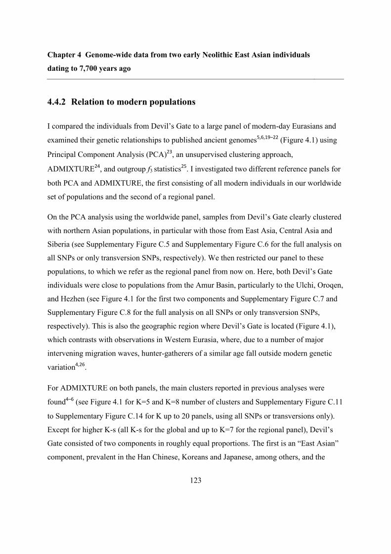
Chapter 4 Genome-wide data from two early Neolithic East Asian individuals
dating to 7,700 years ago
123
4.4.2 Relation to modern populations
I compared the individuals from Devil’s Gate to a large panel of modern-day Eurasians and
examined their genetic relationships to published ancient genomes5,6,19–22
(Figure 4.1) using
Principal Component Analysis (PCA)23
, an unsupervised clustering approach,
ADMIXTURE24
, and outgroup f3 statistics25
. I investigated two different reference panels for
both PCA and ADMIXTURE, the first consisting of all modern individuals in our worldwide
set of populations and the second of a regional panel.
On the PCA analysis using the worldwide panel, samples from Devil’s Gate clearly clustered
with northern Asian populations, in particular with those from East Asia, Central Asia and
Siberia (see Supplementary Figure C.5 and Supplementary Figure C.6 for the full analysis on
all SNPs or only transversion SNPs, respectively). We then restricted our panel to these
populations, to which we refer as the regional panel from now on. Here, both Devil’s Gate
individuals were close to populations from the Amur Basin, particularly to the Ulchi, Oroqen,
and Hezhen (see Figure 4.1 for the first two components and Supplementary Figure C.7 and
Supplementary Figure C.8 for the full analysis on all SNPs or only transversion SNPs,
respectively). This is also the geographic region where Devil’s Gate is located (Figure 4.1),
which contrasts with observations in Western Eurasia, where, due to a number of major
intervening migration waves, hunter-gatherers of a similar age fall outside modern genetic
variation4,26
.
For ADMIXTURE on both panels, the main clusters reported in previous analyses were
found4–6
(see Figure 4.1 for K=5 and K=8 number of clusters and Supplementary Figure C.11
to Supplementary Figure C.14 for K up to 20 panels, using all SNPs or transversions only).
Except for higher K-s (all K-s for the global and up to K=7 for the regional panel), Devil’s
Gate consisted of two components in roughly equal proportions. The first is an “East Asian”
component, prevalent in the Han Chinese, Koreans and Japanese, among others, and the
Chapter 4 Genome-wide data from two early Neolithic East Asian individuals
dating to 7,700 years ago
124
second is a “Siberian” component, typical for the Nganasan. Other populations from the
Amur Basin, but also the Koreans and the Japanese, had the same components, but with a
higher proportion of “East Asian” ancestry, and, for the Koreans and Japanese, also a small
amount from a different component which is common in South-East Asia. On the regional
panel from K=8 onwards, a new component corresponding to Devil’s Gate appeared. It also
contributed to various other East Asian populations, including those from the Amur Basin
(especially the Ulchi), and from modern-day China, Japan and Korea.
I further confirmed the affinity between Devil’s Gate and modern-day Amur Basin
populations by using outgroup f3 statistics in the form, f3(African; DevilsGate, X), which
measures the amount of shared genetic drift between a Devil’s Gate individual and X, a
modern or ancient population, since they diverged from an African outgroup. Modern
populations that live in the same geographic region as Devil’s Gate have the highest genetic
affinity to our ancient genome (Figure 4.2), with a progressive decline in affinity with
increasing geographic distance (R2 = 0.756, F1,96=301, p < 0.001,Figure 4.3), in agreement
with neutral drift leading to a simple isolation-by-distance pattern. The Ulchi, traditionally
fishermen who live geographically very close to Devil’s Gate, are the genetically most
similar samples in our panel. Other populations that show high affinity to Devil’s Gate are
Oroqen and Hezhen, also from the Amur Basin, as well as Koreans and Japanese. Given their
geographic distance from Devil’s Gate (Figure 4.3), Amerindian populations are unusually
genetically close to samples from this site; in agreement with their previously reported
relationship to Siberian and other north Asian populations.
Chapter 4 Genome-wide data from two early Neolithic East Asian individuals
dating to 7,700 years ago
125
Figure 4.1 Regional reference panel, Principal Component analysis and ADMIXTURE analysis. (A) Map of
Asia showing the location of Devil’s Gate (black triangle) and of modern populations forming the regional panel
of our analysis. (B) Plot of the first two Principal Component Analysis as defined by our regional panel of
modern populations from East and Central Asia shown on panel (A), with the two samples from Devil’s Gate
(black triangles) projected upon them23. (C) ADMIXTURE analysis24 performed on Devil’s Gate and our
regional panel, for k=5 (lowest cross-validation error) and k=8 (appearance of Devil’s Gate-specific cluster).
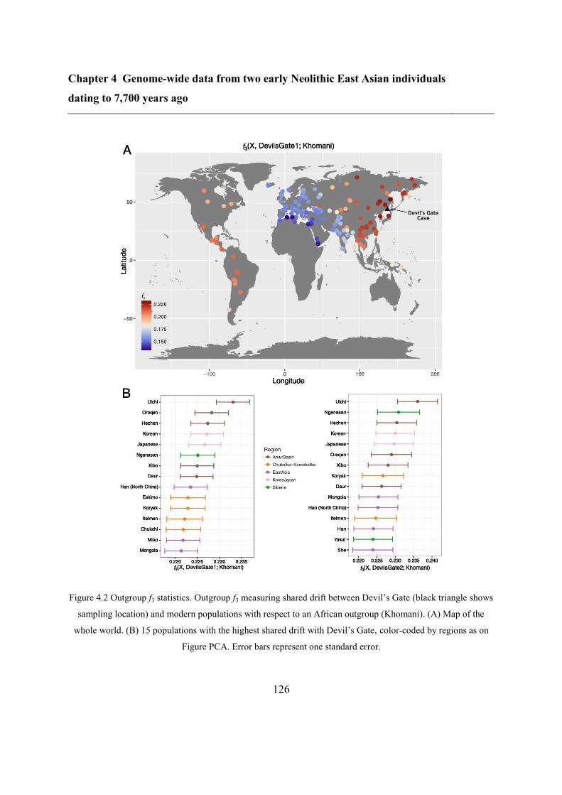
Chapter 4 Genome-wide data from two early Neolithic East Asian individuals
dating to 7,700 years ago
126
Figure 4.2 Outgroup f3 statistics. Outgroup f3 measuring shared drift between Devil’s Gate (black triangle shows
sampling location) and modern populations with respect to an African outgroup (Khomani). (A) Map of the
whole world. (B) 15 populations with the highest shared drift with Devil’s Gate, color-coded by regions as on
Figure PCA. Error bars represent one standard error.
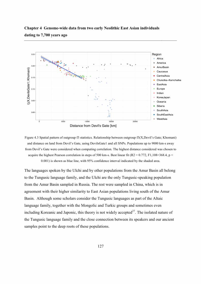
Chapter 4 Genome-wide data from two early Neolithic East Asian individuals
dating to 7,700 years ago
127
Figure 4.3 Spatial pattern of outgroup f3 statistics. Relationship between outgroup f3(X,Devil’s Gate; Khomani)
and distance on land from Devil’s Gate, using DevilsGate1 and all SNPs. Populations up to 9000 km-s away
from Devil’s Gate were considered when computing correlation. The highest distance considered was chosen to
acquire the highest Pearson correlation in steps of 500 km-s. Best linear fit (R2 = 0.772, F1,108=368.4, p <
0.001) is shown as blue line, with 95% confidence interval indicated by the shaded area.
The languages spoken by the Ulchi and by other populations from the Amur Basin all belong
to the Tungusic language family, and the Ulchi are the only Tungusic-speaking population
from the Amur Basin sampled in Russia. The rest were sampled in China, which is in
agreement with their higher similarity to East Asian populations living south of the Amur
Basin. Although some scholars consider the Tungusic languages as part of the Altaic
language family, together with the Mongolic and Turkic groups and sometimes even
including Koreanic and Japonic, this theory is not widely accepted27
. The isolated nature of
the Tungusic language family and the close connection between its speakers and our ancient
samples point to the deep roots of these populations.

Chapter 4 Genome-wide data from two early Neolithic East Asian individuals
dating to 7,700 years ago
128
4.4.3 Relation to ancient genomes from Asia
No previously published ancient genome shows marked genetic affinity to Devil’s Gate: the
top 50 populations in our outgroup f3 statistic were all modern, an unsurprising result given
that all other ancient genomes are either geographically or temporally very distant from
Devil’s Gate. Amongst these ancient genomes, the closest to Devil’s Gate are from Steppe
populations dating from the Bronze onwards and mesolithic European hunter-gatherers, but
they are at most as close as modern populations from the same regions (e.g. Tuvinian,
Kalmyk, Russian, Finnish). The two ancient genomes geographically closest to Devil’s Gate,
Mal’ta (MA1) and Ust’-Ishim, also do not show high genetic affinity, probably due to them
both dating to a much earlier time period. MA1 is genetically closer to Devil’s Gate, but it is
equally distant from Devil’s Gate and from other East Asians (Supplementary Figure C.15-
17). A similar pattern is found for Ust’Ishim, which is basal to all Eurasians, including
Devil’s Gate (Supplementary Figure C.18-20).
At the time of this work, only a very limited amount of data (chromosome 21 and an
additional ~3000 polymorphic sites) was available from the single sequenced ancient genome
with clear affinities to East Asians, Tianyuan9; which did not allow a direct comparison with
the Devil’s Gate samples. In 2017, the whole genome of this individual was published10
, but
it revealed no particular similarities with the samples from Devil’s Gate, or even with modern
populations close to them (Ulchi and the other Amur Basin populations).
4.4.4 Continuity between Devil’s Gate and the Ulchi
As Devil’s Gate falls within the range of modern variability in a number of analyses and
shows a high genetic affinity to the Ulchi, I investigated the extent of genetic continuity
within this region. I modelled the Ulchi as a mixture of Devil’s Gate and other modern
populations, using admixture f3 statistics. Despite a large panel of possible modern sources,
the Ulchi are best represented by Devil’s Gate alone without any further contribution (no
Chapter 4 Genome-wide data from two early Neolithic East Asian individuals
dating to 7,700 years ago
129
admixture f3 gave a significant negative result, Supplementary Table C.20-21). In contrast,
European populations gave significantly negative f3 statistics with numerous pairs of
populations even on our smallest SNP panel consisting of those called in DevilsGate2. (e.g.
Lithuanians, the population with the highest hunter-gatherer-related component:
Supplementary Table C.23 and Sardinians, harbouring the highest early farmer-related
component: Supplementary Table C.22).
Since admixture f3 can be affected by demographic events such as bottlenecks, I also tested
whether Devil’s Gate formed a clade with the Ulchi using a D statistic in the form D(African
outgroup, X; Ulchi, Devil’s Gate). A number of primarily modern populations worldwide
gave significantly non-zero results (|Z| > 2), which, together with the additional components
for the Ulchi in the ADMIXTURE analysis implies that the continuity is not perfect.
Populations from Central Asia scored highest, but for DevilsGate1 on the total SNP panel
(the case with the highest power), a very wide range of populations from all over the world
also gave smaller, but still significantly non-zero scores, in the direction indicating that they
are closer to the Ulchi than to Devil’s Gate. The high-scoring Central Asian populations are
in agreement with the Central Asian-related ADMIXTURE ancestry components in the
Ulchi, but the wide variety of the rest of the populations is difficult to explain. Possible
contributors to this result could be the large uncertainty in SNP calling due to our very low
coverage (even data from SNPs covered only originate from a single read in most cases), and
errors from DNA degradation, which can also decrease the inferred level of continuity.
To compare the inferred level of continuity between the Ulchi and inhabitants of Devil’s Gate
to that between modern Europeans and European hunter-gatherers, I compared the sizes of
ancestry proportions as inferred by ADMIXTURE. I found that the proportion of Devil’s
Gate-related ancestry in the Ulchi was significantly higher than that for the local hunter-
gatherer related ancestry in any European population (t=3.10, df=27.23, p=0.002 using all
SNPs for modern Lithuanians who have the largest European hunter-gatherer component and
Chapter 4 Genome-wide data from two early Neolithic East Asian individuals
dating to 7,700 years ago
130
p < 0.001 for all other populations, Supplementary Table C.6-11). Even when not only the
hunter-gatherer-related components were considered, the difference was significant for every
comparison except for the early European farmer-related component in the Sardinians
(Supplementary Table C.7 and Supplementary Table C.10), a pair where a high level of
continuity was observed in other analysis already.
These results suggest a relatively high degree of population continuity in this region; the
Ulchi are likely descendants of Devil’s Gate or a population genetically very close to it, but
connectivity among populations in the region means that this modern population also shows
increased association with related modern populations. Compared to Europe, these results
suggest a higher level of genetic continuity in this region of northern East Asia over the last
~7.7 ky, without any major population turnover since the early Neolithic.
4.4.5 Southern and Northern genetic material in the Japanese and the
Korean
The high genetic affinity between Devil’s Gate and modern Japanese and Koreans, who live
further south, is also of interest. Japanese have been argued, based on archaeology28
and
genetic analyses29–32
, to have a dual origin, descending from an admixture event between
hunter-gatherers of the Jomon culture (16 kya – 3 kya) and migrants of the Yayoi culture (3
kya – 1.7 kya), who brought wet rice agriculture from the Yangtze estuary in southern China
through Korea. The few ancient mtDNA samples available from Jomon sites on the northern
Hokkaido island show an enrichment of particular haplotypes (N9b and M7a, with D1, D4,
and G1 also detected) present in modern Japanese populations, particularly the Ainu and
Ryukyuans, and also in southern Siberians (for example, Udegey and Ulchi)15,16
. Recently,
nuclear genetic data from two Jomon samples also confirmed the dual origin hypothesis and
implied that the Jomon diverged before the diversification of present-day East Asians33
. The
mtDNA haplogroups of our samples from Devil’s Gate (D4 and M) are also present in Jomon
Chapter 4 Genome-wide data from two early Neolithic East Asian individuals
dating to 7,700 years ago
131
samples, although they are not the most common ones (N9b and M7a). Unfortunately the low
coverage of both our and the Jomon samples did not allow for a direct comparison of nuclear
genetic data.
I investigated whether it was possible to recover these two components by modelling modern
Japanese as a mixture of all possible pairs of sources, including modern Asian populations
and Devil’s Gate, using admixture f3 statistics. The clearest signal was given by a
combination of Devil’s Gate and aboriginal populations from Taiwan, southern China and
Vietnam (Figure 4.4), which could represent hunter-gatherer and agriculturalist components,
respectively. However, it is important to note that these scores were just about significant (-3
< Z < -2) and that some modern pairs also gave negative scores, even if not reaching our
significance threshold (Z scores as low as -1.9, see Supplementary Table C.28-31). The
origin of Koreans has received less attention, and, because of their location on the mainland,
they likely experienced a greater degree of contact with neighbouring populations through
history. However, they show similar characteristics to the Japanese on genome-wide SNP
data34
(Supplementary Table C.24-27) and are also shown to harbour mtDNA35
and Y
chromosomal haplogroups35,36
common in both northern and southern Asian populations.
Unfortunately our coverage and sample size from Devil’s Gate was not enough to reliably
estimate mixture coefficients or to use linkage disequilibrium-based methods to investigate
whether the components originate from secondary contact (admixture) or continuous
differentiation, and if the former is the case, to date the admixture event.
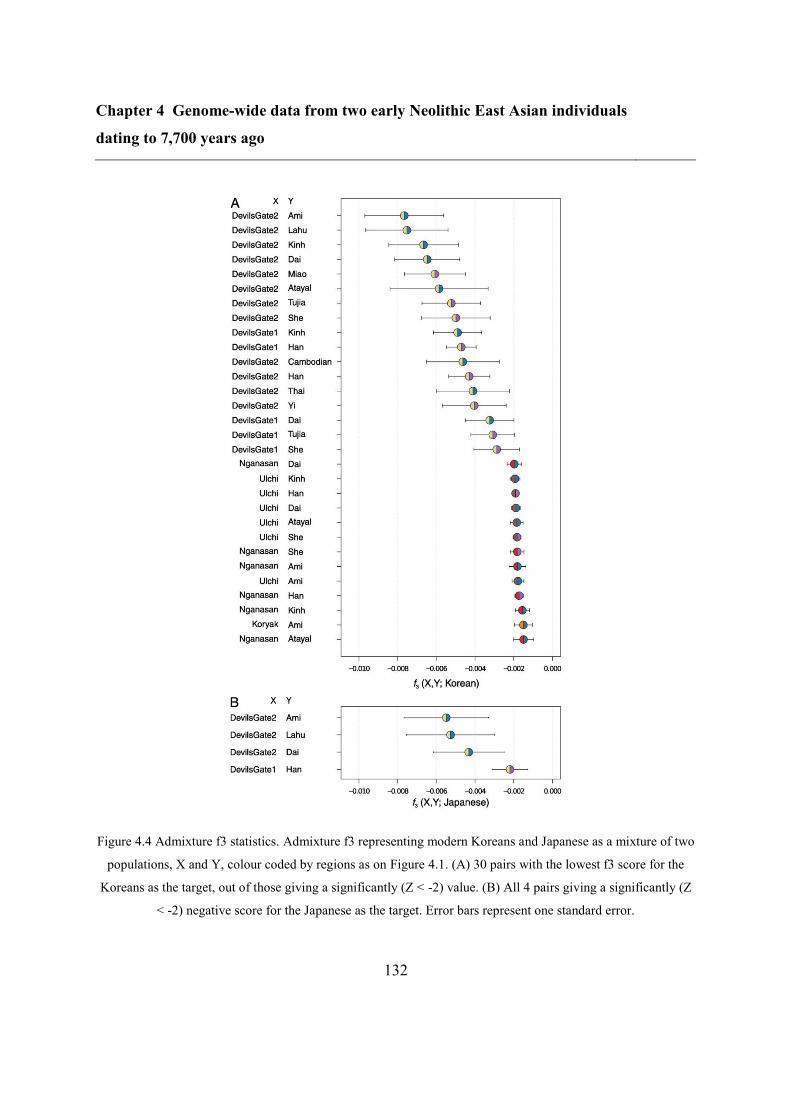
Chapter 4 Genome-wide data from two early Neolithic East Asian individuals
dating to 7,700 years ago
132
Figure 4.4 Admixture f3 statistics. Admixture f3 representing modern Koreans and Japanese as a mixture of two
populations, X and Y, colour coded by regions as on Figure 4.1. (A) 30 pairs with the lowest f3 score for the
Koreans as the target, out of those giving a significantly (Z < -2) value. (B) All 4 pairs giving a significantly (Z
< -2) negative score for the Japanese as the target. Error bars represent one standard error.
Chapter 4 Genome-wide data from two early Neolithic East Asian individuals
dating to 7,700 years ago
133
4.4.6 Phenotypic prediction
The low coverage of our sample does not allow for direct observation of most SNPs linked to
phenotypic traits of interest, but imputation based on modern-day populations can provide
some information (although locations under selection can still be problematic). I focussed on
the genome with the highest coverage, DevilsGate1, using the same imputation approach that
has previously been used to estimate genotype probabilities (GP) for ancient European
samples6,21,22
. For the detailed results, see Supplementary Table C.32. DevilsGate1 likely had
brown eyes (rs12913832 on HERC2; GP=0.905) and, where it could be determined, had
pigmentation-associated variants which are common in East Asia37
. She appears to have had
at least one copy of the derived EDAR allele (rs3827760, GP = 0.865) common in East Asia,
which gives increased odds of straight, thick hair38,39
as well as shovel-shaped incisors 40
. She
almost certainly lacked the most common Eurasian allele for lactase persistance41
(rs4988235, LCT gene, GP>0.999), and was unlikely to have suffered from alcohol flush42
(rs671, ALDH2 gene; GP=0.847). Thus, at least with regard to those phenotypic traits for
which the genetic basis is known, there also seems to have been some degree of phenotypic
continuity.
4.5 Conclusions
By sequencing two ancient East Asians who lived at the beginning of the Neolithic period in
this region, I was able to demonstrate a high level of genetic continuity over the last ~7.7 ky
in the northern part of this region, both demographically and phenotypically. The cold
climate experienced in this area, where modern populations still rely on a number of hunter-
gatherer-fishing practices, likely played a role in preventing major settlements of migrating
Neolithic food-producers. Thus, it seems plausible that the local hunter-gatherers
progressively added food-producing practices to their original lifestyle. However, it is
Chapter 4 Genome-wide data from two early Neolithic East Asian individuals
dating to 7,700 years ago
134
interesting to note that in Europe, even at very high latitudes where hunter-gathering practices
were still similarly important until very recent times, the Neolithic expansion left a significant
genetic signature in modern populations, albeit attenuated when compared to the southern
part of the continent. Our ancient genomes thus provide evidence for a qualitatively different
population prehistory during the Neolithic transition in this part of East Asia compared to
Western Eurasia, suggesting stronger genetic continuity in the former region. These results
encourage further study of the East Asian Neolithic, which would greatly benefit from
genetic data from early agriculturalists (ideally from areas near the origin of wet rice
cultivation and other types of agriculture in southern East Asia), as well as higher coverage
hunter-gatherer samples from different regions in order to quantify population structure
before intensive agriculture.
4.6 Methods
4.6.1 Experimental Design
4.6.1.1 Radiocarbon dates
Direct AMS radiocarbon dates were obtained at the Oxford AMS Radiocarbon Laboratory for
the two highest-coverage individuals, DevilsGate1 and DevilsGate2.
4.6.1.2 Sample preparation and sequencing
Molecular analyses were carried out in dedicated ancient DNA facilities at Trinity College
Dublin, Ireland. Samples were prepared and DNA extracted using a silica column based
protocol following Gamba et al.22
which was based on Yang et al.43
. DNA extracted from
both the first and second lysis buffers22
were used for library preparation which was carried
out using a modified version of Meyer & Kircher44
as described in Gamba et al.22
. Libraries
Chapter 4 Genome-wide data from two early Neolithic East Asian individuals
dating to 7,700 years ago
135
were sequenced on either an Illumina MiSeq or HiSeq platform (for further details and
sequencing statistics see Supplementary Table C.1).
4.6.1.3 Data processing and alignment
For single-end sequencing data (Supplementary Table C.1), adapter sequences were trimmed
from the ends of reads using cutadapt45
allowing an overlap of only 1 base pair (bp) between
the adapter and the read. For paired end data (Supplementary Table C.1), adapters were
trimmed using leeHom46
. This was run using the --ancientdna option and paired end reads
which overlapped were merged. For paired end reads that could not be overlapped only data
from read 1 were used in downstream analyses. Reads were aligned using BWA47
, with the
seed region disabled, to the GRCh37 build of the human genome with the mitochondrial
sequence replaced by the revised Cambridge reference sequence (National Centre for
Biotechnology Information (NCBI) accession number NC_012920.1). Reads from different
sequencing experiments were merged using Picard MergeSamFiles
(http://picard.sourceforge.net/) and clonal reads were removed using SAMtools48
. A
minimum read length of 30 bp was imposed and for the higher coverage (above 0.01X)
samples, DevilsGate1 and DevilsGate2, indels were realigned using RealignerTargetCreator
and IndelRealigner from the Genome Analysis Toolkit (GATK49
). SAMtools48
was used to
filter out reads with a mapping quality of less than 30 and reads were rescaled using
mapDamage 2.050
to reduce the qualities of likely damaged bases, therefore lessening the
effects of ancient DNA damage associated errors on analysis50
. Average genomic depth of
coverage was calculated using the genomecov function of bedtools51
.
4.6.1.4 Authenticity of results
Patterns of molecular damage and the length distribution of reads were assessed using all
reads for DevilsGate3, DevilsGate4, and DevilsGate5. As a portion of the reads from
Chapter 4 Genome-wide data from two early Neolithic East Asian individuals
dating to 7,700 years ago
136
DevilsGate1 and DevilsGate2 derived from 50 bp single end sequencing, only reads
sequenced with 150 bp paired end sequencing were considered in the following analyses in
order to avoid using truncated reads (library ID MOS5A.E1 for DevilsGate1 and MOS4A.E1
for DevilsGate2). MapDamage 2.050
was used to assess patterns of molecular damage which
are typical of ancient DNA. Only reads with mapping quality ⩾ 20 were considered. An
increased rate (up to 11%) of C to T misincorporations was found at the 5’ ends of reads with
reciprocal patterns of G to A misincorporations at the 3’ read termini (Supplementary Figure
C.2). The sequence length distribution was analysed as in 52
. For all samples a peak in DNA
sequence length is visible at <70 bp, consistent with the short fragment length expected for
ancient molecules53
(Supplementary Figure C.3).
Low coverage data like ours often does not provide sufficient information to distinguish the C
to T mutations on the sample relative to the reference sequence, which appear close to the 5’
terminus, from damage. Thus, such positions can be downscaled in quality and dropped,
which can lead to a bias pulling the ancient sample closer to the human reference genome. On
the other hand, not applying MapDamage can lead to the opposite bias due to damage. Thus,
I also replicated our analysis on versions of Devil’s Gate samples without MapDamage
rescaling, to confirm that neither of these biases affect our conclusions.
4.6.1.5 Contamination estimates
The rate of mitochondrial contamination was assessed for our highest coverage samples,
DevilsGate1 and DevilsGate2. This was calculated by evaluating the percentage of non-
consensus bases at haplogroup-defining positions (haplogroup D4 for DevilsGate1 and M for
DevilsGate2) using bases with quality ⩾ 2022,26
.
Schmutzi, a tool which employs a Bayesian maximum a posteriori algorithm17
, was also used
to estimate the mitochondrial contamination for DevilsGate1 (the contamination rate for
DevilsGate2 was not estimated using this tool, as it estimates a contamination prior using
Chapter 4 Genome-wide data from two early Neolithic East Asian individuals
dating to 7,700 years ago
137
deamination frequencies at read termini and as 99% of reads from DevilsGate2 derive from
50 bp sequencing, its read termini are likely truncated). For DevilsGate1 only reads from
>=100bp sequencing were used in the analysis. The contDeam.pl script was run using the --
library double option followed by the schmutzi.pl script with default parameters, using a
dataset of putative contaminants provided with the schmutzi package. It should be noted that
this program will underestimate the contamination rate if the contaminating molecules are
deaminated or if there are multiple contaminating sources.
Since other ways of estimating contamination were not possible (e.g. based on the X-
chromosome), I also attempted to replicate our main results using only reads with evidence of
postmortem damage. I applied PMDtools (9), a framework assigning likelihood scores to
degraded sequences that are unlikely to originate from modern contamination. In this part of
the analysis, I restricted our reads to those with a PMD score of at least 3. This greatly
decreased our coverage, to 0.0050X for DevilsGate1 and 0.0012X for DevilsGate2, but it was
still enough to perform two of our most robust analysis: the outgroup f3 statistics
(Supplementary Figure C.4) and a Principal Component Analysis (Supplementary Figure C.5
and Supplementary Figure C.7 using the world-wide or the reginal panel, respectively).
4.6.2 Statistical Analysis
4.6.2.1 Mitochondrial Haplogroup Determination
Mitochondrial consensus sequences were generated for DevilsGate1 and DevilsGate2 using
ANGSD54
. Called positions were required to have a depth of coverage ⩾ 3 and only bases
with quality ⩾ 20 were considered. The resulting FASTA files were uploaded to
HAPLOFIND55
for haplogroup determination. Mutations defining the assigned haplogroup
were also manually checked. Coverage was calculated using GATK DepthOfCoverage49
.
Chapter 4 Genome-wide data from two early Neolithic East Asian individuals
dating to 7,700 years ago
138
4.6.2.2 Sex determination
Sex was assigned using the script described by Skoglund et al.56
. The observed fraction of Y
chromosome alignments compared to the total number of alignments to the X and Y
chromosome and it’s estimated 95% confidence interval was RY = 0.0057 (0.0053-0.0061)
and RY = 0.0059 (0.0054-0.0064) for DevilsGate1 and DevilsGate2, respectively, implying
that both of them were females.
4.6.2.3 SNP calling and merging with reference panel
In order to compare our sample to modern and ancient human genetic variation, we called
SNPs using the hg19 reference FASTA file at positions overlapping with the Human Origins
(HO) reference panel (591,356 positions)25
, using Samtools 1.248
. Bases were required to
have a minimum mapping quality of 30, base quality of 20, and all triallelic SNPs were
discarded. Then, a read was chosen uniformly at random, since our low coverage does not
provide sufficient information to infer diploid genotypes. This allele was duplicated to form a
homozygous diploid genotype which was used to represent the individual at that SNP
position56
. This method of SNP calling, referred to as the proportional method from now on,
will artificially increase the appearance of drift on the lineage leading to the ancient
individual; however, this drift is not expected to be in any particular direction and therefore
should not bias inferences about population relationships 4. A total of 35,903 positions in
DevilsGate1 and 14,739 in DevilsGate2 were covered by at least one high-quality read.
The resulting SNP data for Devil’s Gate 1 and 2 were then merged with a reference panel
containing modern genomes from the HO panel and selected ancient genomes (this dataset
was described in 6) as well as an additional 45 Korean genomes from the Personal Genome
Project Korea (http://opengenome.net/) using PLINK 1.0757
. Additional sample information
is available in Supplementary Table C.2 to Supplementary Table C.5, including sample ID-s,
Chapter 4 Genome-wide data from two early Neolithic East Asian individuals
dating to 7,700 years ago
139
populations and groupings used throughout the manuscript. Finally, a transversion-only
version of all the above data was created, by converting all T-s to C-s and G-s to A-s and
keeping only SNPs still polymorphic. This alternative dataset was used to confirm that biases
originating from ancient DNA damage do not influence our conclusions.
In the later analyses (outgroup and admixture f3 statistics, Principal Component Analysis and
ADMIXTURE analysis), results from the two different calling methods were qualitatively
equivalent. Results using all mutations or only transversions were also qualitatively similar,
apart from increased noise in the transversion-only data due to the reduced information
content. Thus, in the main text, I will only report results using all mutations and the default
calling method, referred to as the proportional method (choosing a read uniformly at random
from the reads covering any given position). I present results using the Khomani San as our
African outgroup for outgroup f3 and D statistics, but other populations (the Yoruba, the
Mbuti and the Dinka) gave equivalent results.
4.6.2.4 Affinities of the samples from Devil’s Gate
a. Principal Component Analysis
In order to explore where our samples from Devil’s Gate are placed in the context of the main
axes defining modern genetic variation, I performed a Principal Component Analysis (PCA)
with two different reference panels, both subset of the worldwide panel of contemporary and
ancient individuals from 6. The analysis was carried out using EIGENSOFT 6.0.1 smartpca
23
with the lsqproject and normalisation options on, the outlier removal option off and one SNP
from each pair in linkage disequilibrium with r2>0.2 removed. Ancient samples were
projected onto the Principal Components defined by modern populations.
Chapter 4 Genome-wide data from two early Neolithic East Asian individuals
dating to 7,700 years ago
140
b. ADMIXTURE analysis
A clustering analysis was performed using ADMIXTURE version 1.2324
SNPs in linkage
disequilibrium were thinned using PLINK 1.07 with parameters –indep-pairwise 200 25 0.5
resulting in a set of 334,359 SNPs for analysis (91,379 transversions). K=2-20 clusters were
explored for the global panel and K=1-10 for the regional panel, using 10 independent runs
with fivefold cross-validation at each K with different random seeds. The minimal cross-
validation error was found at K=17 for the global panel (Supplementary Figure C.9) and K=5
for the regional (East & Central Asian) panel (Supplementary Figure C.10), but the error
already started plateauing around K=9 for the global, suggesting little improvement.
I further used the ADMIXTURE results to compare the levels of Devil’s Gate-related
ancestry in the Ulchi to hunter-gatherer, Early European Farmer and Bronze Age steppe-
related ancestries in modern Europeans. Supplementary Table C.6-11 shows the p-values
from T-tests for each European population in our panel. I investigated both K=8, where the
Devil’s Gate-specific cluster first. For the Europeans, I used k=18, where cross-validation
error is the lowest (although the proportions hardly change once the three main European
clusters corresponding to hunter-gatherers, Neolithic farmers and steppe ancestry are all
present).
The proportion of Devil’s Gate-related ancestry depends on the choice of K for the
ADMIXTURE analysis. However, K=8, which was chosen (lowest k with a defined Devil’s
Gate cluster on both all SNPs and transversion only SNPs) results in the lowest Devil’s Gate-
related ancestry components in the Ulchi. Therefore, higher K-s would only increase the
significance in the difference from European proportions.
Chapter 4 Genome-wide data from two early Neolithic East Asian individuals
dating to 7,700 years ago
141
c. Outgroup f3 statistics
I used outgroup f3-statistics to estimate the amount of shared drift between inhabitants of
Devil’s Gate and a range of modern-day and ancient populations. I computed f3(X,
DevilsGate; Khomani), where X was a population from our panel, and the Khomani
(Khoisan) acted as our outgroup. f3 statistics were calculated with the 3PopTest tool from the
AdmixTools25
. Figure 2 shows results using all SNP-s and MapDamage treatment,
Supplementary Figure C.4 those using PMD-filtered data and all other results are shown on
Supplementary Table C.12-15.
4.6.2.5 Relation to MA1 and Ust’Ishim
d. Outgroup f3
Outgroup f3 with MA1
First, I used the outgroup f3-statistics to investigate if the inhabitants of Devil’s Gate were
related to the ancient lineages represented by MA1 and Ust’Ishim. I considered all modern-
day and ancient populations in our panel, including the two new samples from Devil’s Gate. I
computed f3(X, MA1; Khomani), where X was a population from our panel, and the Khomani
(Khoisan) acted as outgroup. f3 statistics were calculated with the 3PopTest tool from the
AdmixTools package25
.
e. D statistics
Next, I used D statistics to investigate how MA1 and Ust’Ishim and Devil’s Gate are related
to modern populations. I considered all modern-day and ancient populations in our panel,
including the two new samples from Devil’s Gate. I computed D(X, Khomani; MA1,
Chapter 4 Genome-wide data from two early Neolithic East Asian individuals
dating to 7,700 years ago
142
DevilsGate1), where X was a population from our panel, and the Khomani (Khoisan) acted as
outgroup. D-statistics were calculated with the qpDstat tool from the AdmixTools package25
.
4.6.2.6 Searching for signals of admixture in the Ulchi
f. Admixture f3 shows no signal of admixture
In order to search for signals of admixture in the Ulchi, I first used the admixture f3-statistics
in the form f3(X, Y; Ulchi), using the pq3Pop tools from the AdmixTools package25
. I scanned
every possible pair of populations X and Y, taken from our global panel of modern and
ancient populations and Devil’s Gate. Only considered pairs with at least 1000 SNPs in
common were considered. This statistic can be significantly negative if the target population
(in this case, the Ulchi) has genetic material from both populations X and Y.
In order to test for signals of admixture in the Ulchi, I tested the statistics of the form f3(X, Y;
Ulchi), scanning every possible pair of populations X and Y in our global panel (including
Devil’s Gate). Pairs of populations with Z<-1 and at least 1000 SNPs covered are
Supplementary Table C.20 and Supplementary Table C.21, using all SNPs or transversions
only. As a comparison, I conducted the same analysis for the Lithuanians (Supplementary
Table C.23), who harbour the highest hunter-gatherer component on ADMIXTURE and the
Sardinians (Supplementary Table C.22) who are closest to Early European Farmers on
numerous analysis.
g. D statistics can’t reject a breach of continuity
I then tested if the samples from Devil’s Gate and the Ulchi form a clade against other
populations by examining D statistics of the form D(Khomani, X; Ulchi, Devil’s Gate). This
statistic deviates from zero if the Ulchi or Devil’s Gate are not symmetrically related to
population X when compared to an outgroup population (I used the African Khomani San).
Chapter 4 Genome-wide data from two early Neolithic East Asian individuals
dating to 7,700 years ago
143
For both DevilsGate1 and DevilsGate2, populations with a significantly non-zero score (|Z| >
2) are shown on Supplementary Table C.16-19).
4.6.2.7 Dual origin of the Koreans and the Japanese
In order to search for signals of multiple components in the Koreans and the Japanese, I again
used the admixture f3-statistics in the form f3(X, Y; Target) for the Japanese and the Koreans
as target populations, using the pq3Pop tools from the AdmixTools package25
. I scanned
every possible pair of populations X and Y, taken from our global panel of modern and
ancient populations and Devil’s Gate. Only pairs with at least 1000 SNPs in common were
considered. This statistic can be significantly negative if the target population has genetic
material from both populations X and Y (this does not exclude additional populations also
contributing to the target population). In order to investigate the origin of the northern
component and whether it is related to the occupants of Devil’s Gate, I calculated admixture
f3 statistics of the form f3 (X, Y; Korean) and f3 (X, Y; Japanese). Pairs giving significantly
negative admixture f3 statistics at a significance level of Z<-2 and at least 1000 SNPs are
included on Supplementary Table C.24-31.
4.6.2.8 Phenotypic prediction
Phenotypes of interest were investigated in our highest coverage sample, DevilsGate1,
including some loci known to have been under selection in Eurasian populations. Due to the
low quality of our samples, BEAGLE58
was used to impute genotypes using a reference panel
containing phased genomes from the 1,000 Genomes Project (26 different populations).
Following 22
, GATK Unified genotyper49
was used to call genotype likelihoods at SNP sites
in Phase 3 of the 1,000 Genomes Project. Equal likelihoods were set for positions with no
spanning sequence data as well as positions where the observed genotype could be explained
by deamination22
. At least 1Mb upstream and downstream from the loci of interest was
Chapter 4 Genome-wide data from two early Neolithic East Asian individuals
dating to 7,700 years ago
144
imputed, using 10 iterations to estimate genotypes at ungenotyped markers. The only position
covered by a read was rs74653330 SNP on the OCA2 gene. It had 1x coverage of a C allele
(the allele predicted using imputation). The summary of our results is shown in
Supplementary Table C.32.
4.7 Bibliography
1. Siska, V. et al. Genome-wide data from two early Neolithic East Asian individuals
dating to 7700 years ago. Sci. Adv. 3, e1601877 (2017).
2. Lazaridis, I. et al. Genomic insights into the origin of farming in the ancient Near
East. Nature 536, 419–424 (2016).
3. Gallego-Llorente, M. et al. The genetics of an early Neolithic pastoralist from the
Zagros, Iran. Sci. Rep. 6, (2016).
4. Lazaridis, I. et al. Ancient human genomes suggest three ancestral populations for
present-day Europeans. Nature 513, 409–413 (2014).
5. Haak, W. et al. Massive migration from the steppe was a source for Indo-European
languages in Europe. Nature 522, 207–211 (2015).
6. Jones, E. R. et al. Upper Palaeolithic genomes reveal deep roots of modern Eurasians.
Nat. Commun. 6, 8912 (2015).
7. Raghavan, M. et al. The genetic prehistory of the New World Arctic. Science 345,
1255832 (2014).
8. Raghavan, M. et al. Genomic evidence for the Pleistocene and recent population
history of Native Americans. Science 349, aab3884 (2015).
Chapter 4 Genome-wide data from two early Neolithic East Asian individuals
dating to 7,700 years ago
145
9. Fu, Q. et al. DNA analysis of an early modern human from Tianyuan Cave, China.
Proc. Natl. Acad. Sci. 110, 2223–2227 (2013).
10. Yang, M. A. et al. 40,000-Year-Old Individual from Asia Provides Insight into Early
Population Structure in Eurasia. Curr. Biol. 27, 3202–3208.e9 (2017).
11. Kuzmin, Y. The Paleolithic-to-Neolithic transition and the origin of pottery
production in the Russian Far East: a geoarchaeological approach. Archaeol. Ethnol.
Anthropol. Eurasia 4, 16–26 (2003).
12. Chi, Z. & Hsiao-chun, H. 26 Eastern Asia: archaeology. in The Encyclopedia of
Global Human Migration (Blackwell Publishing Ltd, 2013).
13. Kuzmin, Y. V., Keally, C. T., Jull, A. J. T., Burr, G. S. & Klyuev, N. A. The earliest
surviving textiles in East Asia from Chertovy Vorota Cave, Primorye Province, Russian Far
East. Antiquity 86, 325–337 (2012).
14. Tanaka, M. et al. Mitochondrial Genome Variation in Eastern Asia and the Peopling
of Japan. Genome Res. 14, 1832–1850 (2004).
15. Adachi, N., Shinoda, K., Umetsu, K. & Matsumura, H. Mitochondrial DNA analysis
of Jomon skeletons from the Funadomari site, Hokkaido, and its implication for the origins of
Native American. Am. J. Phys. Anthropol. 138, 255–265 (2009).
16. Adachi, N. et al. Mitochondrial DNA analysis of Hokkaido Jomon skeletons:
Remnants of archaic maternal lineages at the southwestern edge of former Beringia. Am. J.
Phys. Anthropol. 146, 346–360 (2011).
17. Renaud, G., Slon, V., Duggan, A. T. & Kelso, J. Schmutzi: estimation of
contamination and endogenous mitochondrial consensus calling for ancient DNA. Genome
Biol. 16, 224 (2015).
Chapter 4 Genome-wide data from two early Neolithic East Asian individuals
dating to 7,700 years ago
146
18. Skoglund, P. et al. Separating endogenous ancient DNA from modern day
contamination in a Siberian Neandertal. Proc. Natl. Acad. Sci. 111, 2229–2234 (2014).
19. Fu, Q. et al. Genome sequence of a 45,000-year-old modern human from western
Siberia. Nature 514, 445–449 (2014).
20. Raghavan, M. et al. Upper Palaeolithic Siberian genome reveals dual ancestry of
Native Americans. Nature 505, 87–91 (2014).
21. Allentoft, M. E. et al. Population genomics of Bronze Age Eurasia. Nature 522, 167–
172 (2015).
22. Gamba, C. et al. Genome flux and stasis in a five millennium transect of European
prehistory. Nat. Commun. 5, 5257 (2014).
23. Patterson, N., Price, A. L. & Reich, D. Population Structure and Eigenanalysis. PLOS
Genet 2, e190 (2006).
24. Alexander, D. H., Novembre, J. & Lange, K. Fast model-based estimation of ancestry
in unrelated individuals. Genome Res. (2009). doi:10.1101/gr.094052.109
25. Patterson, N. et al. Ancient Admixture in Human History. Genetics 192, 1065–1093
(2012).
26. Sánchez-Quinto, F. et al. Genomic Affinities of Two 7,000-Year-Old Iberian Hunter-
Gatherers. Curr. Biol. 22, 1494–1499 (2012).
27. Pereltsvaig, A. in Languages of the world: An introduction 211–216 (Cambridge
University Press, 2017).
28. Imamura, K. Prehistoric Japan: New Perspectives on Insular East Asia. (University
of Hawaii Press, 1996).
Chapter 4 Genome-wide data from two early Neolithic East Asian individuals
dating to 7,700 years ago
147
29. Jinam, T. A., Kanzawa-Kiriyama, H. & Saitou, N. Human genetic diversity in the
Japanese Archipelago: dual structure and beyond. Genes Genet. Syst. 90, 147–152 (2015).
30. Rasteiro, R. & Chikhi, L. Revisiting the peopling of Japan: an admixture perspective.
J. Hum. Genet. 54, 349–354 (2009).
31. He, Y., Wang, W. R., Xu, S., Jin, L. & Consortium, P.-A. S. Paleolithic Contingent in
Modern Japanese: Estimation and Inference using Genome-wide Data. Sci. Rep. 2, 355
(2012).
32. Jinam, T. A. et al. Unique characteristics of the Ainu population in Northern Japan. J.
Hum. Genet. 60, 565–571 (2015).
33. Kanzawa-Kiriyama, H. et al. A partial nuclear genome of the Jomons who lived 3000
years ago in Fukushima, Japan. J. Hum. Genet. (2016). doi:10.1038/jhg.2016.110
34. Consortium, T. H. P.-A. S. Mapping Human Genetic Diversity in Asia. Science 326,
1541–1545 (2009).
35. Jin, H.-J., Tyler-Smith, C. & Kim, W. The Peopling of Korea Revealed by Analyses
of Mitochondrial DNA and Y-Chromosomal Markers. PLoS ONE 4, (2009).
36. Jin, H.-J. et al. Y-chromosomal DNA haplogroups and their implications for the dual
origins of the Koreans. Hum. Genet. 114, 27–35 (2003).
37. Sturm, R. A. & Duffy, D. L. Human pigmentation genes under environmental
selection. Genome Biol. 13, 248 (2012).
38. Fujimoto, A. et al. A scan for genetic determinants of human hair morphology: EDAR
is associated with Asian hair thickness. Hum. Mol. Genet. 17, 835–843 (2008).
Chapter 4 Genome-wide data from two early Neolithic East Asian individuals
dating to 7,700 years ago
148
39. Fujimoto, A. et al. A replication study confirmed the EDAR gene to be a major
contributor to population differentiation regarding head hair thickness in Asia. Hum. Genet.
124, 179–185 (2008).
40. Park, J.-H. et al. Effects of an Asian-specific nonsynonymous EDAR variant on
multiple dental traits. J. Hum. Genet. 57, 508–514 (2012).
41. Itan, Y., Powell, A., Beaumont, M. A., Burger, J. & Thomas, M. G. The Origins of
Lactase Persistence in Europe. PLoS Comput Biol 5, e1000491 (2009).
42. Crabb, D. W., Edenberg, H. J., Bosron, W. F. & Li, T. K. Genotypes for aldehyde
dehydrogenase deficiency and alcohol sensitivity. The inactive ALDH2(2) allele is dominant.
J. Clin. Invest. 83, 314–316 (1989).
43. Yang, D. Y., Eng, B., Waye, J. S., Dudar, J. C. & Saunders, S. R. Technical note:
improved DNA extraction from ancient bones using silica-based spin columns. Am. J. Phys.
Anthropol. 105, 539–543 (1998).
44. Meyer, M. & Kircher, M. Illumina Sequencing Library Preparation for Highly
Multiplexed Target Capture and Sequencing. Cold Spring Harb. Protoc. 2010, pdb.prot5448
(2010).
45. Martin, M. Cutadapt removes adapter sequences from high-throughput sequencing
reads. EMBnet.journal 17, pp. 10–12 (2011).
46. Renaud, G., Stenzel, U. & Kelso, J. leeHom: adaptor trimming and merging for
Illumina sequencing reads. Nucleic Acids Res. 42, e141 (2014).
47. Li, H. & Durbin, R. Fast and accurate short read alignment with Burrows-Wheeler
transform. Bioinforma. Oxf. Engl. 25, 1754–1760 (2009).
Chapter 4 Genome-wide data from two early Neolithic East Asian individuals
dating to 7,700 years ago
149
48. Li, H. et al. The Sequence Alignment/Map format and SAMtools. Bioinforma. Oxf.
Engl. 25, 2078–2079 (2009).
49. McKenna, A. et al. The Genome Analysis Toolkit: a MapReduce framework for
analyzing next-generation DNA sequencing data. Genome Res. 20, 1297–1303 (2010).
50. Jónsson, H., Ginolhac, A., Schubert, M., Johnson, P. L. F. & Orlando, L.
mapDamage2.0: fast approximate Bayesian estimates of ancient DNA damage parameters.
Bioinforma. Oxf. Engl. 29, 1682–1684 (2013).
51. Quinlan, A. R. & Hall, I. M. BEDTools: a flexible suite of utilities for comparing
genomic features. Bioinforma. Oxf. Engl. 26, 841–842 (2010).
52. Llorente, M. G. et al. Ancient Ethiopian genome reveals extensive Eurasian
admixture throughout the African continent. Science 350, 820–822 (2015).
53. Shapiro, B. & Hofreiter, M. A Paleogenomic Perspective on Evolution and Gene
Function: New Insights from Ancient DNA. Science 343, 1236573 (2014).
54. Korneliussen, T. S., Albrechtsen, A. & Nielsen, R. ANGSD: Analysis of Next
Generation Sequencing Data. BMC Bioinformatics 15, 356 (2014).
55. Vianello, D. et al. HAPLOFIND: a new method for high-throughput mtDNA
haplogroup assignment. Hum. Mutat. 34, 1189–1194 (2013).
56. Skoglund, P. et al. Genomic Diversity and Admixture Differs for Stone-Age
Scandinavian Foragers and Farmers. Science 344, 747–750 (2014).
57. Purcell, S. et al. PLINK: a tool set for whole-genome association and population-
based linkage analyses. Am. J. Hum. Genet. 81, 559–575 (2007).
58. Browning, B. L. & Browning, S. R. Genotype Imputation with Millions of Reference
Samples. Am. J. Hum. Genet. 98, 116–126 (2016).
Chapter 4 Genome-wide data from two early Neolithic East Asian individuals
dating to 7,700 years ago
150
59. Balueva, T. S. . Kraniologicheskij material neoliticheskogo sloya peshchery
«Chertovy Vorota» (Primor’e) (Cranial samples from a Neolithic layer from Devil’s Gate
Cave, Primorye). Vopr. Antropol. 58, 184–187 (1978).
60. Andreeva, Z. V. & Tatarnikov, V. Peshera «Chertovy Vorota» v Primor’e. Arheol.
Otkrytiya 1973 Goda Cave Devils Gate Primorye 1973 Excav. Seas. Mosc. 180–181 (1974).
61. Zhushchikhovskaya, IS. Neolithic of the Primorye. in .), Archaeology of the Russian
Far East: essays in Stone Age prehistory (eds. S.M. Nelson, A.P. Derevianko, Y.V. Kuzmin
& R.L. Bland) 101–122 (Archaeopress, 2006).
62. Kuznecov, A. Drevnee poselenie v peshchere Chertovy Vorota i nekotorye problemy
neolita Primor’ya (The ancient settlement in a cave Devil’s Gate and some problems of the
Neolithic of Primorye ). Ross. Arheol. 2, 17–19 (2002).
63. Lamason, R. L. et al. SLC24A5, a Putative Cation Exchanger, Affects Pigmentation
in Zebrafish and Humans. Science 310, 1782–1786 (2005).
64. Sturm, R. A. Molecular genetics of human pigmentation diversity. Hum. Mol. Genet.
18, R9–R17 (2009).
65. Canfield, V. A. et al. Molecular Phylogeography of a Human Autosomal Skin Color
Locus Under Natural Selection. G3 GenesGenomesGenetics 3, 2059–2067 (2013).
66. Basu Mallick, C. et al. The Light Skin Allele of SLC24A5 in South Asians and
Europeans Shares Identity by Descent. PLoS Genet 9, e1003912 (2013).
67. Wilde, S. et al. Direct evidence for positive selection of skin, hair, and eye
pigmentation in Europeans during the last 5,000 y. Proc. Natl. Acad. Sci. 111, 4832–4837
(2014).
Chapter 4 Genome-wide data from two early Neolithic East Asian individuals
dating to 7,700 years ago
151
68. Norton, H. L. et al. Genetic Evidence for the Convergent Evolution of Light Skin in
Europeans and East Asians. Mol. Biol. Evol. 24, 710–722 (2007).
69. Donnelly, M. P. et al. A global view of the OCA2-HERC2 region and pigmentation.
Hum. Genet. 131, 683–696 (2011).
70. Hider, J. L. et al. Exploring signatures of positive selection in pigmentation candidate
genes in populations of East Asian ancestry. BMC Evol. Biol. 13, 150 (2013).
71. Yuasa, I. et al. Distribution of Two Asian-Related Coding SNPs in the MC1R and
OCA2 Genes. Biochem. Genet. 45, 535–542 (2007).
72. Yuasa, I. et al. OCA2*481Thr, a hypofunctional allele in pigmentation, is
characteristic of northeastern Asian populations. J. Hum. Genet. 52, 690–693 (2007).
73. Yuasa, I. et al. Distribution of OCA2∗481Thr and OCA2∗615Arg, associated with
hypopigmentation, in several additional populations. Leg. Med. 13, 215–217 (2011).
74. Ramos, E. M. et al. Phenotype–Genotype Integrator (PheGenI): synthesizing genome-
wide association study (GWAS) data with existing genomic resources. Eur. J. Hum. Genet.
22, 144–147 (2014).
75. Kamberov, Y. G. et al. Modeling Recent Human Evolution in Mice by Expression of
a Selected EDAR Variant. Cell 152, 691–702 (2013).
76. Goedde, H. W. et al. Distribution of ADH2 and ALDH2 genotypes in different
populations. Hum. Genet. 88, 344–346 (1992).
77. Li, H. et al. Refined Geographic Distribution of the Oriental ALDH2*504Lys (nee
487Lys) Variant. Ann. Hum. Genet. 73, 335–345 (2009).

Chapter 4 Genome-wide data from two early Neolithic East Asian individuals
dating to 7,700 years ago
152
78. Matsuo, K. et al. Gene–environment interaction between an aldehyde dehydrogenase-
2 (ALDH2) polymorphism and alcohol consumption for the risk of esophageal cancer.
Carcinogenesis 22, 913–916 (2001).
79. Cusi, D. et al. Polymorphisms of α-adducin and salt sensitivity in patients with
essential hypertension. The Lancet 349, 1353–1357 (1997).
80. Van den Wildenberg, E. et al. A functional polymorphism of the mu-opioid receptor
gene (OPRM1) influences cue-induced craving for alcohol in male heavy drinkers. Alcohol.
Clin. Exp. Res. 31, 1–10 (2007).
81. Haerian, B. S. & Haerian, M. S. OPRM1 rs1799971 polymorphism and opioid
dependence: evidence from a meta-analysis. Pharmacogenomics 14, 813–824 (2013).
82. Rodriguez, S., Steer, C. D., Farrow, A., Golding, J. & Day, I. N. M. Dependence of
Deodorant Usage on ABCC11 Genotype: Scope for Personalized Genetics in Personal
Hygiene. J. Invest. Dermatol. 133, 1760–1767 (2013).
83. Yoshiura, K. et al. A SNP in the ABCC11 gene is the determinant of human earwax
type. Nat. Genet. 38, 324–330 (2006).
84. Cho, Y. S. et al. Meta-analysis of genome-wide association studies identifies eight
new loci for type 2 diabetes in east Asians. Nat. Genet. 44, 67–72 (2012).
Chapter 5 Behaviour of selection statistics in a spatially explicit, neutral
demographic model
153
Chapter 5 Behaviour of selection statistics in a
spatially explicit, neutral demographic model
5.1 Abstract
Natural selection is the main driving process behind adaptive evolution. Detecting
signals of selection in the genome is not only useful for medical genetics, but can also
uncover key processes in the dynamics of speciation and the population histories of
species. However, complex demographic processes can confound signals and are one of
the likely causes of the commonly observed contradicting results between different
studies. Here I made use of a paleoclimate-informed, spatially explicit demographic
model to explore the behaviour of commonly used selection statistics. I investigated how
different statistics behave when the confounding effects of space and population history
are taken into account. I focused on three statistics: allele frequency spectrum-based
Tajima’s D, population differentiation-based FST and linkage disequilibrium-based iHS.
To investigate which statistics are linked to similar processes and to what extent purely
demographic signals in different populations are correlated, I measured the amount of
overlap between signals from different statistics or different populations and compared
them to those from the 1000 Genomes Phase 3 dataset. I found that different statistics
overlap to a smaller extent in the neutral simulations than in observed data, but the
relationships between signals from different populations were better captured by our
model.
Chapter 5 Behaviour of selection statistics in a spatially explicit, neutral
demographic model
154
5.2 Contribution
The base demographic model that generated recombining and non-recombining genealogies
and TMRCA-s was created by Anders Eriksson. The non-recombining version was used in
publications concerning the spread of anatomically modern humans1 and the population
history of the Americas2, but this chapter is the first use case for the model including
recombination. I implemented modules in this existing C++ modelling framework for
sequence generation upon both non-recombining (tree-like) and recombining (network-like)
genealogies, as well as to calculate Tajima’s D. I also performed the complete analysis
outside the modelling framework: processed the observed data, calculated selection statistics
on both observed and simulated data, compared them to each other and created this
manuscript.
5.3 Introduction
The availability of high-resolution genetic datasets made it possible to detect signals of
natural selection in observed data. For humans, most efforts have been dedicated to the
indirect method of looking for signals of past selection in present-day genomes by scanning
the whole genomes for outlier segments on the basis of different statistics. Such outliers can
arise from a scenario where a single, new allele has a beneficial effect (positive selection) and
rapidly spreads to high frequencies or fixation in a population (a hard sweep). As a
consequence, diversity in the region surrounding the beneficial allele’s locus is reduced, until
mutation and recombination together restore it to values typical of neutral variation.
Additionally, in the case of localised selection pressures, the target population becomes
unusually differentiated from others around the selected locus. There are three basic families
of methods to detect signals of positive selection that exploit these signatures: allele
frequency spectrum-, population differentiation- and linkage disequilibrium-based methods3.
Chapter 5 Behaviour of selection statistics in a spatially explicit, neutral
demographic model
155
The first family, based on the allele frequency spectrum, uses the distribution of alleles in a
population to detect deviations from neutral expectation. For instance, Tajima’s D4 looks for
a departure from neutrality as reflected by the difference between low-frequency and
intermediate frequency variants, and Fay and Wu’s H5 focuses on differences between high
and intermediate frequency variants whilst also using ancestral state information.
The second family, based on population differentiation, focuses on population-specific
selection pressures and looks for loci where allele frequencies differ between populations to a
greater extent than expected. As a result, population differentiation-based statistics have the
highest power to detect selection in variants that are fixed in a given population – in contrast
to the previous measures comparing different variants at a given locus and thus suitable only
for incomplete sweeps. Typical examples of this family are statistical tests based on Wright’s
fixation index (FST)6. This index measures the proportion of genetic variance contained in a
subpopulation, relative to the total population: 𝐹𝑆𝑇 =𝜎𝑆
2
𝜎𝑇2, where 𝜎𝑆
2 is the variance in the
frequency of an allele between different subpopulations, weighted by the sizes of the
subpopulations and 𝜎𝑇2 is the variance of the allelic state in the total population.
The third family, based on linkage disequilibrium (LD), looks for regions of strong LD
surrounding the beneficial allele; in other words, it focuses on the low diversity around a
given allele at a specific location (long linked regions, also called haplotypes). Two common
examples of such tests are the integrated Haplotype Score7 (iHS) and the number of
Segregating sites by Length8 (nSL), with the only difference being in the distance measure
they use. Both statistics begin by calculating the probability that any two haplotypes carrying
a chosen allele at a chosen, focal SNP are identical up to a certain distance away from the
focal SNP. This probability is then integrated over all possible distances and compared to the
integral from other variants at the same locus as a baseline. iHS, the most commonly used
LD-based selection test, measures distance in the metric 4Nr, where N is the effective
population size and r is the recombination rate per generation. nSL is a more recent statistic; it
Chapter 5 Behaviour of selection statistics in a spatially explicit, neutral
demographic model
156
uses the number of alleles in the remaining haplotypes in the data set in the same region as a
distance measure. Therefore, nSL does not require a fine estimation of recombination rates
and was shown to be more robust to recombination rate variation8. A third LD-based statistic
is the cross-population extended haplotype homozygosity9 (XP-EHH), which is similar to
iHS but compares integrated haplotype homozygosities between variants in different
populations instead of different variants in the same set of individuals. Therefore, XP-EHH
does not require the presence of alternative alleles at the focal locus and can work also for
fixed variants, similarly to population differentiation-based statistics.
A strong warning that using different methods together is not without problems comes from
the low congruence in the loci they detect as under selection. Some researchers combine
multiple metrics to look for regions that consistently score highly, either through composite
measures (e.g. composite likelihood ratio10
), or by applying the methods separately, and
focusing on shared outlier windows3,11,12
. Both of these approaches are based on the
assumption that false signals would be correlated to a lesser extent than those arising from
selection, and thus false positives would be excluded from shared signals. However, the
extent to which signals become more correlated under different cases of selection is not well
known, and different statistics are sensitive for different kinds of selection and/or selection
acting on different timescales. Furthermore, a complete lack of correlation would not be
expected even in genomic regions that are completely neutral. In fact, multiple populations
are likely to be influenced by the same confounding demographic processes and, from the
signal side, different statistics can be sensitive to similar confounding effects. In order to
disentangle signals of selection from false positives caused by demographic events and assess
significance, we need a realistic demographic model to explore the null distributions of these
quantities.
Chapter 5 Behaviour of selection statistics in a spatially explicit, neutral
demographic model
157
5.4 Methods
5.4.1 Spatially explicit demographic model
Here I applied an individual-based, climate-driven, spatially explicit demographic model
(Figure 5.1) created in C++, which was previously used to investigate the effect of climate on
human dispersal1 (using data from microsatellite markers) and the peopling of the Americas
2
(based on SNP-data).
In the model, the Earth was divided into hexagons that could be inhabited by separate
populations (Figure 5.1A). Each hexagon was roughly 100km wide and was characterised by
the maximum number of individuals it could sustain (carrying capacity), with local
population growth following a simple logistic growth model. Palaeoclimate reconstructions
based on the Hadley Centre model HadCM3 were used to determine sea level (defining
which hexagons were above water at any point in time), ice coverage (which made some land
hexagons uninhabitable), and vegetation. Vegetation was quantified in terms of Net Primary
Productivity (NPP), which was used as a measure of available resources. The local carrying
capacities were then scaled by a saturating function (Figure 5.1B) of the local NPP. The
relationship between carrying capacity and NPP was a continuous, piecewise linear function:
zero below a lower habitability threshold, the maximal carrying capacity above an upper NPP
threshold and linearly increasing in-between.
Migration was allowed between neighbouring hexagons, with empty hexagons potentially
colonised from inhabited neighbours if the neighbours’ carrying capacity was reached (Figure
5.1C). The simulation was initiated with a population in a single hexagon in East Africa,
spreading by the successive colonisation of neighbouring.
The parameters determining the conversion between NPP and carrying capacity (threshold
NPP values for inhabitability and for reaching maximal carrying capacity), as well as
Chapter 5 Behaviour of selection statistics in a spatially explicit, neutral
demographic model
158
unknown demographic parameters (growth, migration and colonisation rates), the length of
the simulation and the global maximal carrying capacity were fitted based on genetic data
(see section 5.4.2). The resulting demography was simulated in a stochastic, individual-based
framework.
While running the demography forward, reconstructing the last 120k years of human
demographic history and the major expansion out of Africa, time-series of population sizes
and migration events were recorded. Using these time-series, genealogies were simulated
backwards based on the Fisher-Wright coalescent model, with or without recombination.
Non-recombining sequences were used to fit the model and recombining ones to calculate the
amount of overlap between statistics/populations. Finally, sequences of fixed length were
generated by distributing mutations along the genealogies with a constant rate and inferring
the resulting alleles at the tips of the genealogies.
The whole simulation framework was coded in C++. The modules for sequence generation
upon both non-recombining (tree-like) and recombining (network-like) genealogies were
developed as part of the work for this chapter, while the upstream part of the framework
(demographic simulation and genealogy generation) were developed by Anders Eriksson for
previous projects1,2
.
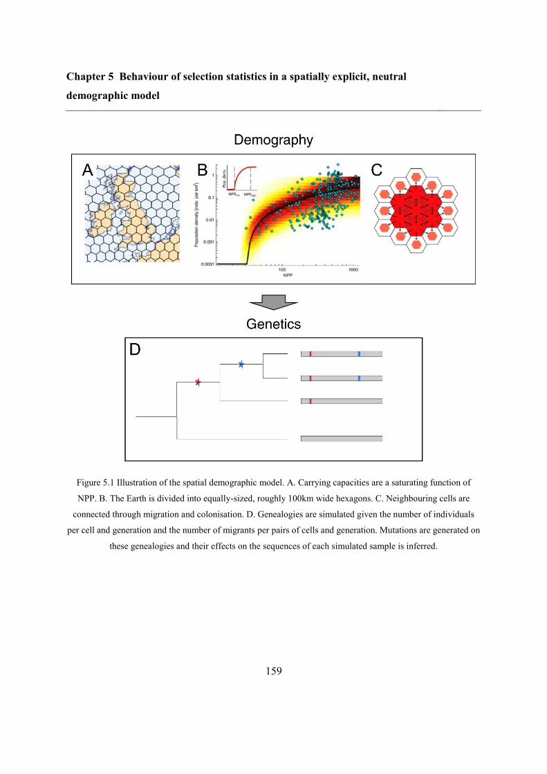
Chapter 5 Behaviour of selection statistics in a spatially explicit, neutral
demographic model
159
Figure 5.1 Illustration of the spatial demographic model. A. Carrying capacities are a saturating function of
NPP. B. The Earth is divided into equally-sized, roughly 100km wide hexagons. C. Neighbouring cells are
connected through migration and colonisation. D. Genealogies are simulated given the number of individuals
per cell and generation and the number of migrants per pairs of cells and generation. Mutations are generated on
these genealogies and their effects on the sequences of each simulated sample is inferred.
Chapter 5 Behaviour of selection statistics in a spatially explicit, neutral
demographic model
160
5.4.2 Refitting the model
5.4.2.1 Rationale and comparison to previous versions
To make the existing model suitable for the study of selection, a few adjustments had to be
made to the original framework1,2
: we had to use a different dataset and an additional
summary statistic during the fitting procedure. Given these changes, I needed to refit our
model to acquire realistic demographic parameter sets.
Selection scans are generally based on a large number of whole genomes. However, in the
previous model versions, only microsatellite1 and SNP-based
2 panels were used, mostly with
small sample sizes per population (down to a single representative diploid sample). To enable
direct comparison between data and model output, I chose to use the 1000 Genomes Phase 3
dataset13,14
instead, which includes whole-genome data from a high number of samples per
population. Furthermore, this dataset has previously been used to study selection15–17
, and
consists of populations covering most large geographic areas (with the exception of Oceania
and Australia).
Furthermore, our initial investigations showed that although I acquired well-fitting values for
FST and iHS using demographic parameters fitted through TMRCA values only1,2
, in that the
model output was within the variation seen in data, I generally did not get realistic Tajima’s
D values. Although the general trend of increasing mean D values with distance from Africa
was present to a similar extent in both observed data and our simulations, the mean values
were higher in the former, with the exception of a subset of parameter values associated with
stronger bottlenecks. Therefore, I supplemented the TMRCA-based summary statistics
previously used to fit the model1,2
with continental-level means of Tajima’s D.
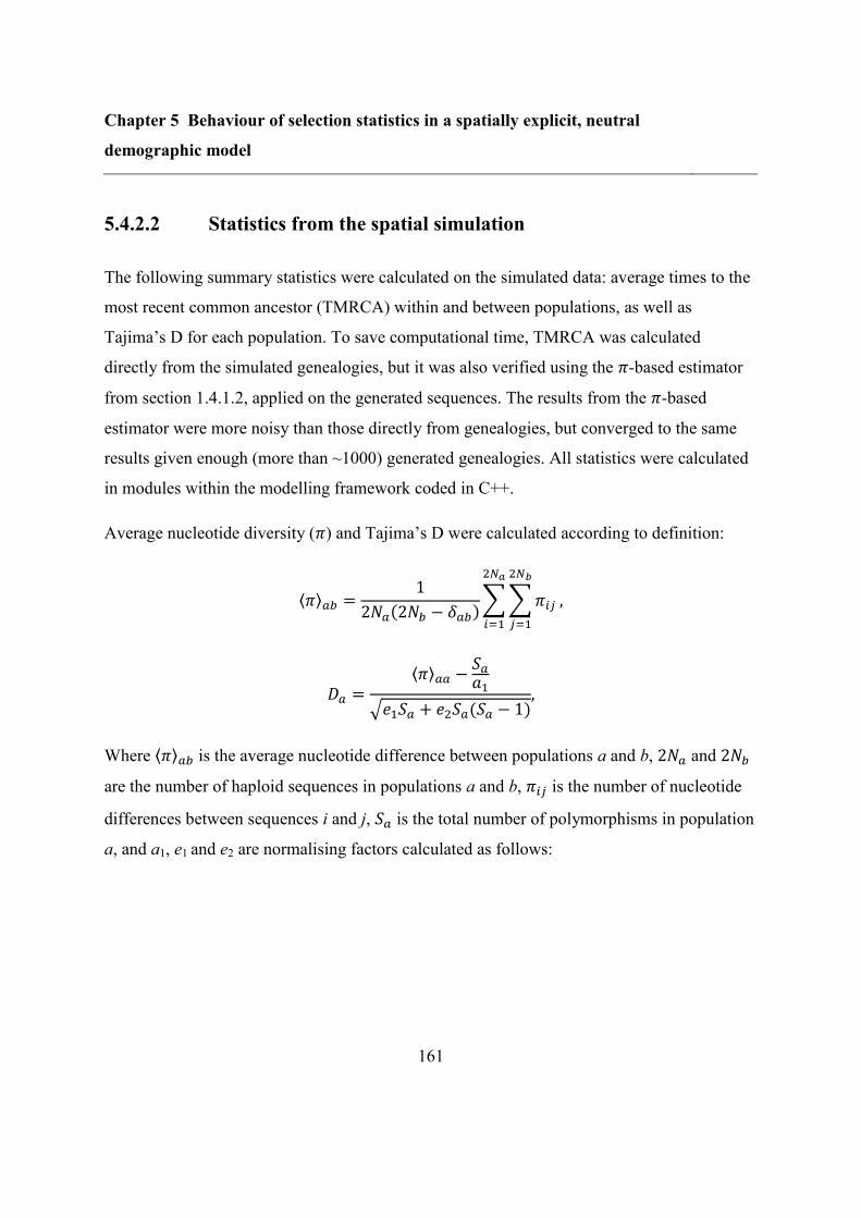
Chapter 5 Behaviour of selection statistics in a spatially explicit, neutral
demographic model
161
5.4.2.2 Statistics from the spatial simulation
The following summary statistics were calculated on the simulated data: average times to the
most recent common ancestor (TMRCA) within and between populations, as well as
Tajima’s D for each population. To save computational time, TMRCA was calculated
directly from the simulated genealogies, but it was also verified using the 𝜋-based estimator
from section 1.4.1.2, applied on the generated sequences. The results from the 𝜋-based
estimator were more noisy than those directly from genealogies, but converged to the same
results given enough (more than ~1000) generated genealogies. All statistics were calculated
in modules within the modelling framework coded in C++.
Average nucleotide diversity (𝜋) and Tajima’s D were calculated according to definition:
⟨𝜋⟩𝑎𝑏 =1
2𝑁𝑎(2𝑁𝑏 − 𝛿𝑎𝑏)∑ ∑ 𝜋𝑖𝑗
2𝑁𝑏
𝑗=1
,
2𝑁𝑎
𝑖=1
𝐷𝑎 =⟨𝜋⟩𝑎𝑎 −
𝑆𝑎
𝑎1
√𝑒1𝑆𝑎 + 𝑒2𝑆𝑎(𝑆𝑎 − 1),
Where ⟨𝜋⟩𝑎𝑏 is the average nucleotide difference between populations a and b, 2𝑁𝑎 and 2𝑁𝑏
are the number of haploid sequences in populations a and b, 𝜋𝑖𝑗 is the number of nucleotide
differences between sequences i and j, 𝑆𝑎 is the total number of polymorphisms in population
a, and a1, e1 and e2 are normalising factors calculated as follows:
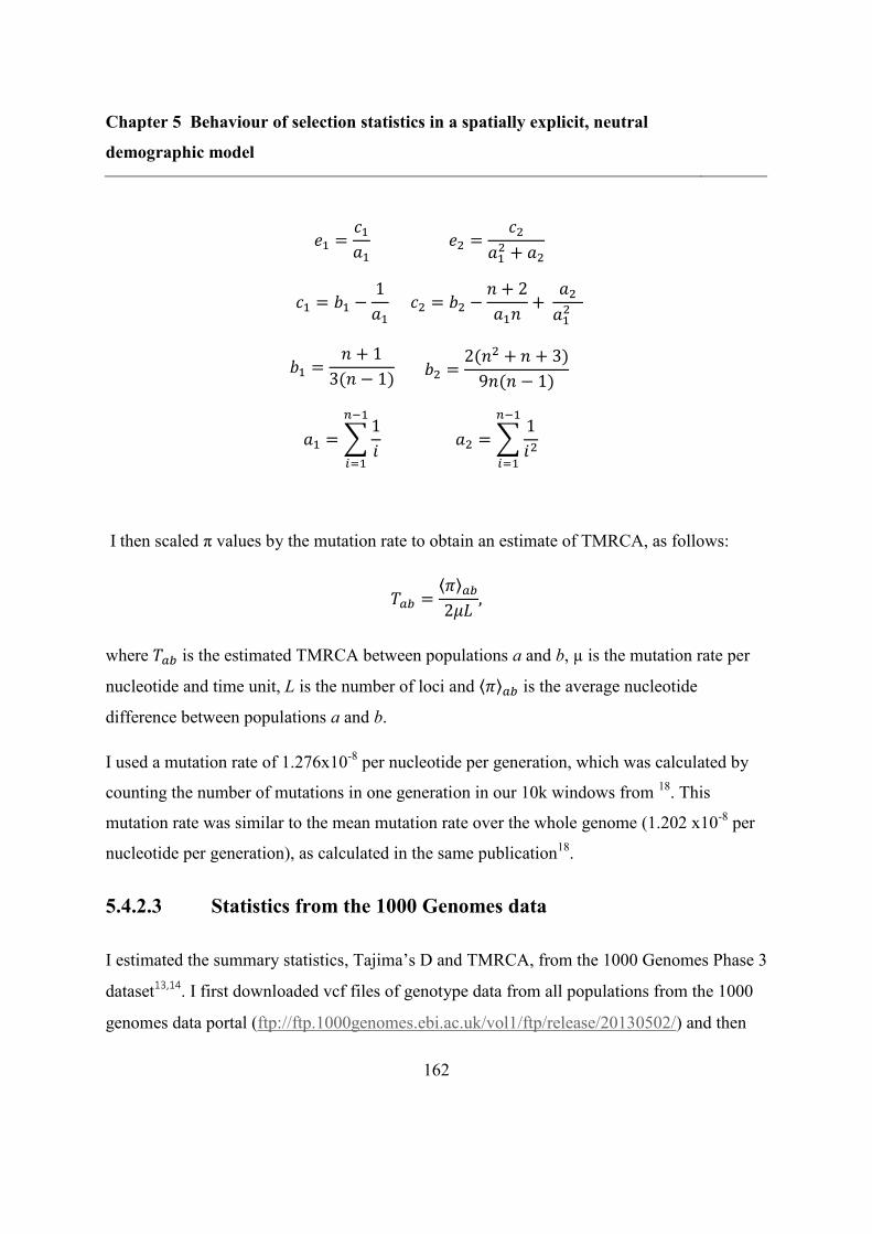
Chapter 5 Behaviour of selection statistics in a spatially explicit, neutral
demographic model
162
𝑒1 =𝑐1
𝑎1 𝑒2 =
𝑐2
𝑎12 + 𝑎2
𝑐1 = 𝑏1 −1
𝑎1 𝑐2 = 𝑏2 −
𝑛 + 2
𝑎1𝑛+
𝑎2
𝑎12
𝑏1 =𝑛 + 1
3(𝑛 − 1) 𝑏2 =
2(𝑛2 + 𝑛 + 3)
9𝑛(𝑛 − 1)
𝑎1 = ∑1
𝑖
𝑛−1
𝑖=1
𝑎2 = ∑1
𝑖2
𝑛−1
𝑖=1
I then scaled π values by the mutation rate to obtain an estimate of TMRCA, as follows:
𝑇𝑎𝑏 =⟨𝜋⟩𝑎𝑏
2𝜇𝐿,
where 𝑇𝑎𝑏 is the estimated TMRCA between populations a and b, µ is the mutation rate per
nucleotide and time unit, L is the number of loci and ⟨𝜋⟩𝑎𝑏 is the average nucleotide
difference between populations a and b.
I used a mutation rate of 1.276x10⁻⁸
per nucleotide per generation, which was calculated by
counting the number of mutations in one generation in our 10k windows from 18
. This
mutation rate was similar to the mean mutation rate over the whole genome (1.202 x10⁻⁸
per
nucleotide per generation), as calculated in the same publication18
.
5.4.2.3 Statistics from the 1000 Genomes data
I estimated the summary statistics, Tajima’s D and TMRCA, from the 1000 Genomes Phase 3
dataset13,14
. I first downloaded vcf files of genotype data from all populations from the 1000
genomes data portal (ftp://ftp.1000genomes.ebi.ac.uk/vol1/ftp/release/20130502/) and then
Chapter 5 Behaviour of selection statistics in a spatially explicit, neutral
demographic model
163
filtered both genetic positions and populations before extracting windows from which to
calculate the statistics.
○ Filtering samples
I excluded populations of African origin that were sampled in the Americas (ASW and
ACB), due to their mixed origin within Africa and the presence of European admixture in
their genomes13
. I also excluded the Finnish samples because they had an unusually high
Tajima’s D value compared to other European populations, likely because they are
genetically isolated with severe bottlenecks in their history, experienced an unusually low
amount of admixture and could have less internal structure than other, larger populations19
. I
also excluded highly admixed Native American populations (CLM, PUR and MXL), as seen
on the ADMIXTURE analysis13
. I kept the least admixed Native American population in the
dataset, the Peruvians (PEL), but I only considered data with Native American ancestry on
both chromosomes. Ancestry was inferred using RFMix in Martin et al. 201720
, and the data
was provided by Alicia Martin. I selected the 10,000 windows (for details, see “Filtering
positions”) in regions with the highest amount of Peruvian samples with purely Native
American ancestry available, which increased the number of such samples available at all of
our windows to 45. The selected populations, their size and their assignment to continental-
level groupings are shown in Table 5.1.
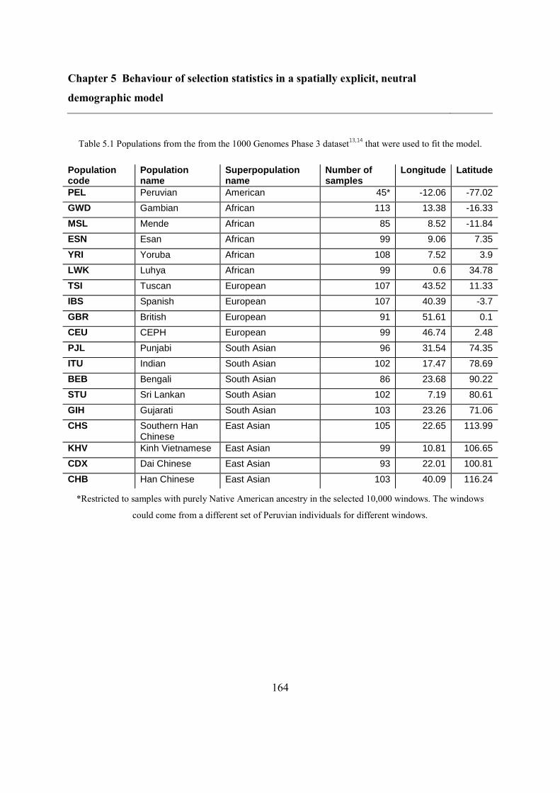
Chapter 5 Behaviour of selection statistics in a spatially explicit, neutral
demographic model
164
Table 5.1 Populations from the from the 1000 Genomes Phase 3 dataset13,14
that were used to fit the model.
Population code
Population name
Superpopulation name
Number of samples
Longitude Latitude
PEL Peruvian American 45* -12.06 -77.02
GWD Gambian African 113 13.38 -16.33
MSL Mende African 85 8.52 -11.84
ESN Esan African 99 9.06 7.35
YRI Yoruba African 108 7.52 3.9
LWK Luhya African 99 0.6 34.78
TSI Tuscan European 107 43.52 11.33
IBS Spanish European 107 40.39 -3.7
GBR British European 91 51.61 0.1
CEU CEPH European 99 46.74 2.48
PJL Punjabi South Asian 96 31.54 74.35
ITU Indian South Asian 102 17.47 78.69
BEB Bengali South Asian 86 23.68 90.22
STU Sri Lankan South Asian 102 7.19 80.61
GIH Gujarati South Asian 103 23.26 71.06
CHS Southern Han Chinese
East Asian 105 22.65 113.99
KHV Kinh Vietnamese East Asian 99 10.81 106.65
CDX Dai Chinese East Asian 93 22.01 100.81
CHB Han Chinese East Asian 103 40.09 116.24
*Restricted to samples with purely Native American ancestry in the selected 10,000 windows. The windows
could come from a different set of Peruvian individuals for different windows.
Chapter 5 Behaviour of selection statistics in a spatially explicit, neutral
demographic model
165
○ Filtering positions
I excluded the following regions in the genome considered as problematic: regions with poor
alignment quality, recombination hotspots, regions of poor mapping quality, duplications,
regions under selection (genes and conserved elements), repetitive regions and positions with
systematic sequencing errors. I applied the following filters from Kuhlwilm et al. 201621
,
provided by Ilan Gronau:
filter_hotspot1000g: Recombination hotspots
filter_Map20: Sites with poor mapping quality
filter_rmsk20: Recent duplications
filter_segDups: Recent segmental duplications
filter_selection_10000_100: Gene exons together with the 1 kbp flanking regions in
each direction and conserved non-coding sequences corresponding to PhastCons
elements
filter_simpleRepeat: Simple repeats
filter_SysErrHCB and filter_SysErr: Positions with systematic sequencing errors
For more details, see Supplementary SI 8 in Kuhlwilm et al. 201621
.
I then considered windows containing 10kb unfiltered sites with at most 30% of the sites
missing. I did not impose a minimal separation between the windows, but my previous
investigation on 1kb windows with/without 10kb separation showed no change in the
resulting statistics. This procedure yielded in 12,662 windows.
Last, I pruned our windows to increase the number of available Peruvian individuals with
purely Native American diploid ancestry tracts at all of our windows. At keeping the 10,000
windows with the highest number of available such tracts, I could acquire data from 45
individuals (down from the original 85 diploid samples). For each window, I choose 45
Chapter 5 Behaviour of selection statistics in a spatially explicit, neutral
demographic model
166
individuals at random out of those with Native American ancestry on both chromosomes,
thus potentially using different sets of individuals for different windows. This procedure
generated diploid individuals that were a mosaic of Native American tracts from different
samples. I then treated these generated diploid individuals in the same way as the rest of our
samples.
I also attempted to keep Mexican individuals, but I only managed to keep 18 of them out of
the original 64, even with a strong pruning down to 5000 windows. Such a low number of
windows resulted in an unequal distribution of windows across chromosomes, and reduced
the number of available Peruvians down to 37. I thus decided to keep only the Peruvians in
the final dataset. I also attempted to allow a mix of individuals within a single window, but
the Native American ancestry tracts were long enough in comparison to our window size so
that this would not have increased the number of retained samples.
○ Calculating statistics
I extracted the chosen 10,000 windows from the filtered population set, applied the above
mentioned filters and considered only biallelic sites; using vcftools 0.1.1522
. I then calculated
counts of the two alleles per population and chromosome, also using vcftools 0.1.1522
. For
the Peruvians, I first created per-individual filters, including only those windows where that
particular individual was chosen. I then used these allele counts to calculate average pairwise
π within and between populations, as well as Tajima’s D within populations, using custom
scripts in Python based on their definitions (for the formulas, see Section 5.4.2.2).
In the final step, I calculated mean TMRCA-s and Tajima’s D for our continental groups:
Africa, Europe, Asia and America. I pooled South Asian and East Asian population, since
their corresponding summary statistics were linearly dependent on each other. I chose a
subset of the summary statistics for fitting the model, to exclude statistics linearly dependent
on each other (Supplementary Figure D.1-7 in Appendix D.1). In particular, TMRCA within
Chapter 5 Behaviour of selection statistics in a spatially explicit, neutral
demographic model
167
Africa was determined by TMRCA between African and Europe and TMRCA-s between
non-neighbouring continental groups were determined by neighbouring ones (Africa – Asia
by Africa – Europe, Africa – America by Asia – America, etc.). Finally, the statistics I used
were mean Tajima’s D from all four continental groups, mean TMRCA from all groups
except Africa and mean between-population TMRCA between neighbouring groups (Africa –
Europe, Europe – Asia and Asia – America). The observed summary statistics are shown in
Table 5.2.
Table 5.2 Observed summary statistics from the 1000 genomes data.
Summary statistic Acronym Value
Tajima’s D within Africa D_AF -0.6195
Tajima’s D within Europe D_EU -0.0974
Tajima’s D within Asia D_AS -0.1433
Tajima’s D within America D_AM 0.5654
TMRCA between Africa and Europe T_AF_EU [years] 57791.69
TMRCA within Europe T_EU_EU [years] 43545.74
TMRCA between Europe and Asia T_EU_AS [years] 51362.65
TMRCA within Asia T_AS_AS [years] 44450.85
TMRCA between Asia and America T_AS_AM [years] 48151.22
TMRCA within America T_AM_AM [years] 34784.69
Chapter 5 Behaviour of selection statistics in a spatially explicit, neutral
demographic model
168
5.4.2.4 Fitting procedure
To fit the model, I sampled 100,000 input parameter sets, performed a single demographic
run and simulated 200x10kb sequences along independent (non-recombining) genealogies for
each. I first sampled the input parameters from wide prior distributions (Table 5.3) for the
demographic input parameters and recorded TMRCA-s and Tajima’s D at the population-
level for all simulations. Due to problems with the resulting posterior distribution of
parameters, I also sampled parameter sets from the central 99% of the posterior distributions
of each parameter from Raghavan et al.2 (Table 5.4), which was obtained through fitting to a
panel of genomes more densely and homogeneously distributed across the globe but with a
lower sample size per population, up to only 2 diploid genomes per population. This latter,
narrow posterior is what I used for further investigations.
Table 5.3 Wide parameter ranges for ABC sampling. Generation time is assumed to be 25 years1.
Parameter Acronym Low limit High limit Sampling
Simulation time [generation] tSim 1000 8000 Linear
Migration rate [1/generation] m 0.0001 0.166666 Logarithmic
Colonisation number c 10.0 5000.0 Logarithmic
Growth rate [1/generation] r 0.3 1.00 Logarithmic
Maximal carrying capacity K 1000 100000 Logarithmic
Low NPP offset npp_offs_low 0.001 0.1 Linear
High NPP offset npp_offs_high 0.001 0.5 Linear
Ancestral carrying capacity Ka 1000 100000 Logarithmic
Initial carrying capacity K0 22000 30000 Logarithmic
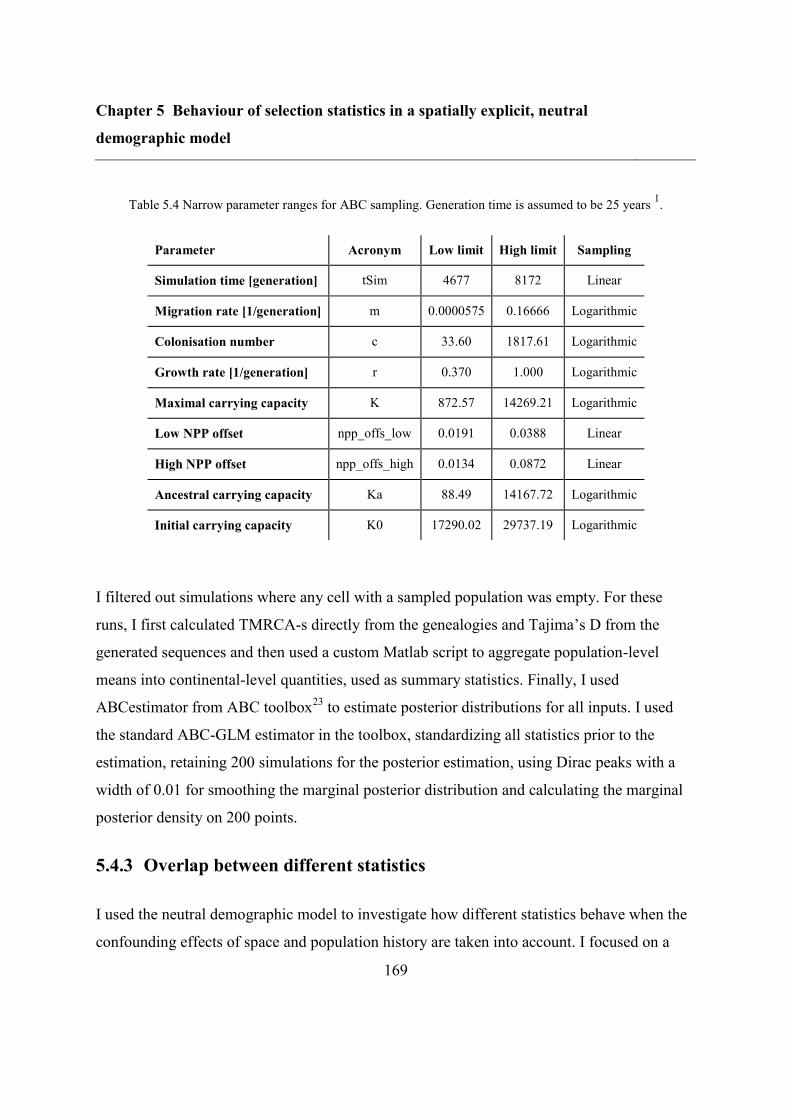
Chapter 5 Behaviour of selection statistics in a spatially explicit, neutral
demographic model
169
Table 5.4 Narrow parameter ranges for ABC sampling. Generation time is assumed to be 25 years 1.
Parameter Acronym Low limit High limit Sampling
Simulation time [generation] tSim 4677 8172 Linear
Migration rate [1/generation] m 0.0000575 0.16666 Logarithmic
Colonisation number c 33.60 1817.61 Logarithmic
Growth rate [1/generation] r 0.370 1.000 Logarithmic
Maximal carrying capacity K 872.57 14269.21 Logarithmic
Low NPP offset npp_offs_low 0.0191 0.0388 Linear
High NPP offset npp_offs_high 0.0134 0.0872 Linear
Ancestral carrying capacity Ka 88.49 14167.72 Logarithmic
Initial carrying capacity K0 17290.02 29737.19 Logarithmic
I filtered out simulations where any cell with a sampled population was empty. For these
runs, I first calculated TMRCA-s directly from the genealogies and Tajima’s D from the
generated sequences and then used a custom Matlab script to aggregate population-level
means into continental-level quantities, used as summary statistics. Finally, I used
ABCestimator from ABC toolbox23
to estimate posterior distributions for all inputs. I used
the standard ABC-GLM estimator in the toolbox, standardizing all statistics prior to the
estimation, retaining 200 simulations for the posterior estimation, using Dirac peaks with a
width of 0.01 for smoothing the marginal posterior distribution and calculating the marginal
posterior density on 200 points.
5.4.3 Overlap between different statistics
I used the neutral demographic model to investigate how different statistics behave when the
confounding effects of space and population history are taken into account. I focused on a
Chapter 5 Behaviour of selection statistics in a spatially explicit, neutral
demographic model
170
commonly used statistic from each group: allele frequency spectrum-based Tajima’s D,
population differentiation-based FST and linkage disequilibrium-based iHS. I measured the
amount of overlap between different statistics and different populations and compared our
estimates to the relevant quantities computed for neutral genomic windows from the 1000
Genomes Phase 3 dataset13,14
, in order to investigate which statistics suggest similar
processes and to what extent purely demographic signals in different populations are
correlated.
5.4.3.1 1000 Genomes data
For the 1000 genomes data, I used the same windows as used for fitting TMRCAs and
Tajima’s D. I estimated FST using vcftools 0.1.1522
, implementing Weir and Cockerham’s
estimator24
and used Tajima’s D as calculated when fitting the model.
To calculate iHS7, I first estimated genetic distances in these windows. To acquire data for all
our SNP-s, I linearly interpolated the genetic map generated by the HapMap 2 Project25
. This
map, which is an average over recombination rates in the CEU, YRI, and ASN populations,
was lifted over to hg19 by Adam Auton and is available at ftp://ftp-
trace.ncbi.nih.gov/1000genomes/ftp/technical/working/20110106_recombination_hotspots/. I
then calculated iHS scores on the vcf-formatted data from the chosen populations and
windows using selscan26
, a multi-threaded program capable of calculating linkage-based
selection statistics efficiently. I finally calculated the proportion of significant (|Z| > 2) iHS
scores in each 10kb-long window, as suggested by Voight et al.7 and following Clemente et
al.11
.
Chapter 5 Behaviour of selection statistics in a spatially explicit, neutral
demographic model
171
5.4.3.2 Simulation
I used our spatial model to generate data equivalent to the windows from the 1000 genomes
data. To simulate recombining sequences needed for linkage disequilibrium-based statistics
like iHS, I used a modified version of our spatial framework, which generated a network of
recombining genealogies instead of separate trees. I generated sequences upon these
networks, which could then be analysed in the same way as for the 1000 Genomes data.
Generating such sequences is computationally expensive, therefore I used only the 5 best-
fitting demographic parameter sets (Table 5.5). For each parameter set, I simulated five
4Mbp-long recombining sequences either with a constant or a variable recombination rate. In
order to set recombination rates, I estimated the mean recombination rate in each 10kb
window by summing the genetic distances within that window from the HapMap 2 Project25
,
linearly interpolating the distance at the border of the windows, and scaled genetic distances
back to recombination rates. I used the mean recombination rate over all 10kb windows,
0.7961 cM/Mbp, as our constant recombination rate.
Since a study found that the effect of a varying recombination rate was necessary to reach
realistic levels of signal-sharing27
, I also generated equivalent data with a non-uniform
recombination rate in our model. For this investigation, I chose a recombination rate
uniformly at random for each simulated window from the 10,000 mean recombination rates
from the windows used for fitting the model, calculated as detailed before.
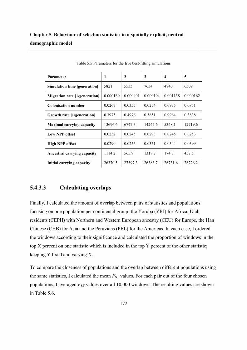
Chapter 5 Behaviour of selection statistics in a spatially explicit, neutral
demographic model
172
Table 5.5 Parameters for the five best-fitting simulations
Parameter 1 2 3 4 5
Simulation time [generation] 5821 5533 7634 4840 6309
Migration rate [1/generation] 0.000160 0.000401 0.000104 0.001138 0.000162
Colonisation number 0.0267 0.0355 0.0254 0.0935 0.0851
Growth rate [1/generation] 0.3975 0.4976 0.5851 0.9964 0.3838
Maximal carrying capacity 13696.6 6747.3 14245.6 5348.1 12719.6
Low NPP offset 0.0252 0.0245 0.0293 0.0245 0.0253
High NPP offset 0.0290 0.0256 0.0351 0.0344 0.0399
Ancestral carrying capacity 1114.2 565.9 1318.7 174.3 457.5
Initial carrying capacity 26370.5 27397.3 26383.7 26731.6 26726.2
5.4.3.3 Calculating overlaps
Finally, I calculated the amount of overlap between pairs of statistics and populations
focusing on one population per continental group: the Yoruba (YRI) for Africa, Utah
residents (CEPH) with Northern and Western European ancestry (CEU) for Europe, the Han
Chinese (CHB) for Asia and the Peruvians (PEL) for the Americas. In each case, I ordered
the windows according to their significance and calculated the proportion of windows in the
top X percent on one statistic which is included in the top Y percent of the other statistic;
keeping Y fixed and varying X.
To compare the closeness of populations and the overlap between different populations using
the same statistics, I calculated the mean FST values. For each pair out of the four chosen
populations, I averaged FST values over all 10,000 windows. The resulting values are shown
in Table 5.6.
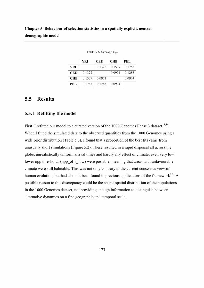
Chapter 5 Behaviour of selection statistics in a spatially explicit, neutral
demographic model
173
Table 5.6 Average FST
YRI CEU CHB PEL
YRI 0.1322 0.1539 0.1765
CEU 0.1322 0.0971 0.1283
CHB 0.1539 0.0971 0.0974
PEL 0.1765 0.1283 0.0974
5.5 Results
5.5.1 Refitting the model
First, I refitted our model to a curated version of the 1000 Genomes Phase 3 dataset13,14
.
When I fitted the simulated data to the observed quantities from the 1000 Genomes using a
wide prior distribution (Table 5.3), I found that a proportion of the best fits came from
unusually short simulations (Figure 5.2). These resulted in a rapid dispersal all across the
globe, unrealistically uniform arrival times and hardly any effect of climate: even very low
lower npp thresholds (npp_offs_low) were possible, meaning that areas with unfavourable
climate were still habitable. This was not only contrary to the current consensus view of
human evolution, but had also not been found in previous applications of the framework1,2
. A
possible reason to this discrepancy could be the sparse spatial distribution of the populations
in the 1000 Genomes dataset, not providing enough information to distinguish between
alternative dynamics on a fine geographic and temporal scale.
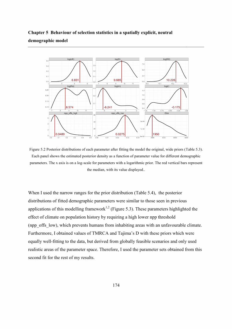
Chapter 5 Behaviour of selection statistics in a spatially explicit, neutral
demographic model
174
Figure 5.2 Posterior distributions of each parameter after fitting the model the original, wide priors (Table 5.3).
Each panel shows the estimated posterior density as a function of parameter value for different demographic
parameters. The x axis is on a log-scale for parameters with a logarithmic prior. The red vertical bars represent
the median, with its value displayed..
When I used the narrow ranges for the prior distribution (Table 5.4), the posterior
distributions of fitted demographic parameters were similar to those seen in previous
applications of this modelling framework1,2
(Figure 5.3). These parameters highlighted the
effect of climate on population history by requiring a high lower npp threshold
(npp_offs_low), which prevents humans from inhabiting areas with an unfavourable climate.
Furthermore, I obtained values of TMRCA and Tajima’s D with these priors which were
equally well-fitting to the data, but derived from globally feasible scenarios and only used
realistic areas of the parameter space. Therefore, I used the parameter sets obtained from this
second fit for the rest of my results.
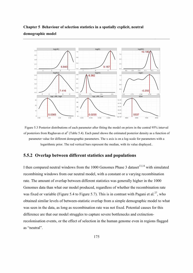
Chapter 5 Behaviour of selection statistics in a spatially explicit, neutral
demographic model
175
Figure 5.3 Posterior distributions of each parameter after fitting the model on priors in the central 95% interval
of posteriors from Raghavan et al2 (Table 5.4). Each panel shows the estimated posterior density as a function of
parameter value for different demographic parameters. The x axis is on a log-scale for parameters with a
logarithmic prior. The red vertical bars represent the median, with its value displayed..
5.5.2 Overlap between different statistics and populations
I then compared neutral windows from the 1000 Genomes Phase 3 dataset13,14
with simulated
recombining windows from our neutral model, with a constant or a varying recombination
rate. The amount of overlap between different statistics was generally higher in the 1000
Genomes data than what our model produced, regardless of whether the recombination rate
was fixed or variable (Figure 5.4 to Figure 5.7). This is in contrast with Pagani et al.27
, who
obtained similar levels of between-statistic overlap from a simple demographic model to what
was seen in the data, as long as recombination rate was not fixed. Potential causes for this
difference are that our model struggles to capture severe bottlenecks and extinction-
recolonisation events, or the effect of selection in the human genome even in regions flagged
as “neutral”.
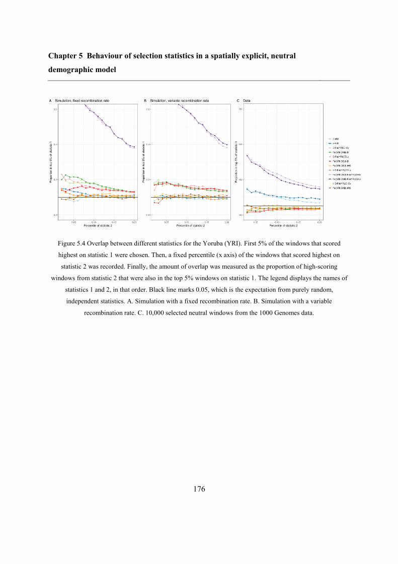
Chapter 5 Behaviour of selection statistics in a spatially explicit, neutral
demographic model
176
Figure 5.4 Overlap between different statistics for the Yoruba (YRI). First 5% of the windows that scored
highest on statistic 1 were chosen. Then, a fixed percentile (x axis) of the windows that scored highest on
statistic 2 was recorded. Finally, the amount of overlap was measured as the proportion of high-scoring
windows from statistic 2 that were also in the top 5% windows on statistic 1. The legend displays the names of
statistics 1 and 2, in that order. Black line marks 0.05, which is the expectation from purely random,
independent statistics. A. Simulation with a fixed recombination rate. B. Simulation with a variable
recombination rate. C. 10,000 selected neutral windows from the 1000 Genomes data.
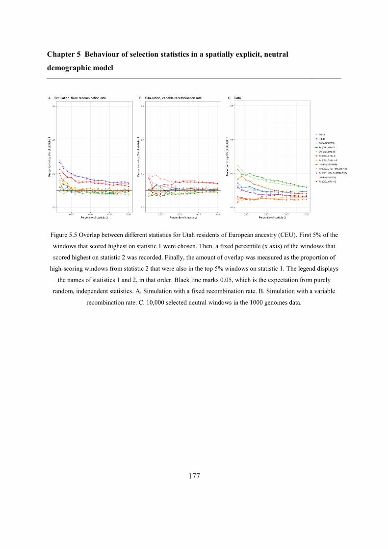
Chapter 5 Behaviour of selection statistics in a spatially explicit, neutral
demographic model
177
Figure 5.5 Overlap between different statistics for Utah residents of European ancestry (CEU). First 5% of the
windows that scored highest on statistic 1 were chosen. Then, a fixed percentile (x axis) of the windows that
scored highest on statistic 2 was recorded. Finally, the amount of overlap was measured as the proportion of
high-scoring windows from statistic 2 that were also in the top 5% windows on statistic 1. The legend displays
the names of statistics 1 and 2, in that order. Black line marks 0.05, which is the expectation from purely
random, independent statistics. A. Simulation with a fixed recombination rate. B. Simulation with a variable
recombination rate. C. 10,000 selected neutral windows in the 1000 genomes data.
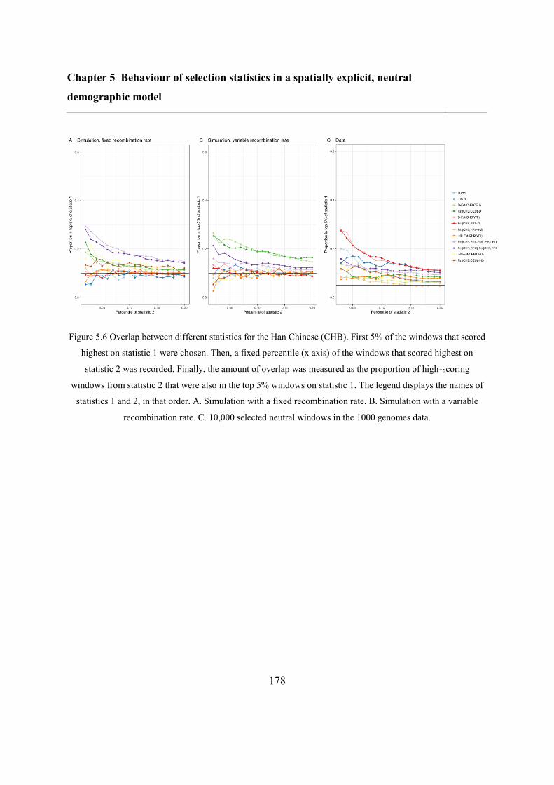
Chapter 5 Behaviour of selection statistics in a spatially explicit, neutral
demographic model
178
Figure 5.6 Overlap between different statistics for the Han Chinese (CHB). First 5% of the windows that scored
highest on statistic 1 were chosen. Then, a fixed percentile (x axis) of the windows that scored highest on
statistic 2 was recorded. Finally, the amount of overlap was measured as the proportion of high-scoring
windows from statistic 2 that were also in the top 5% windows on statistic 1. The legend displays the names of
statistics 1 and 2, in that order. A. Simulation with a fixed recombination rate. B. Simulation with a variable
recombination rate. C. 10,000 selected neutral windows in the 1000 genomes data.
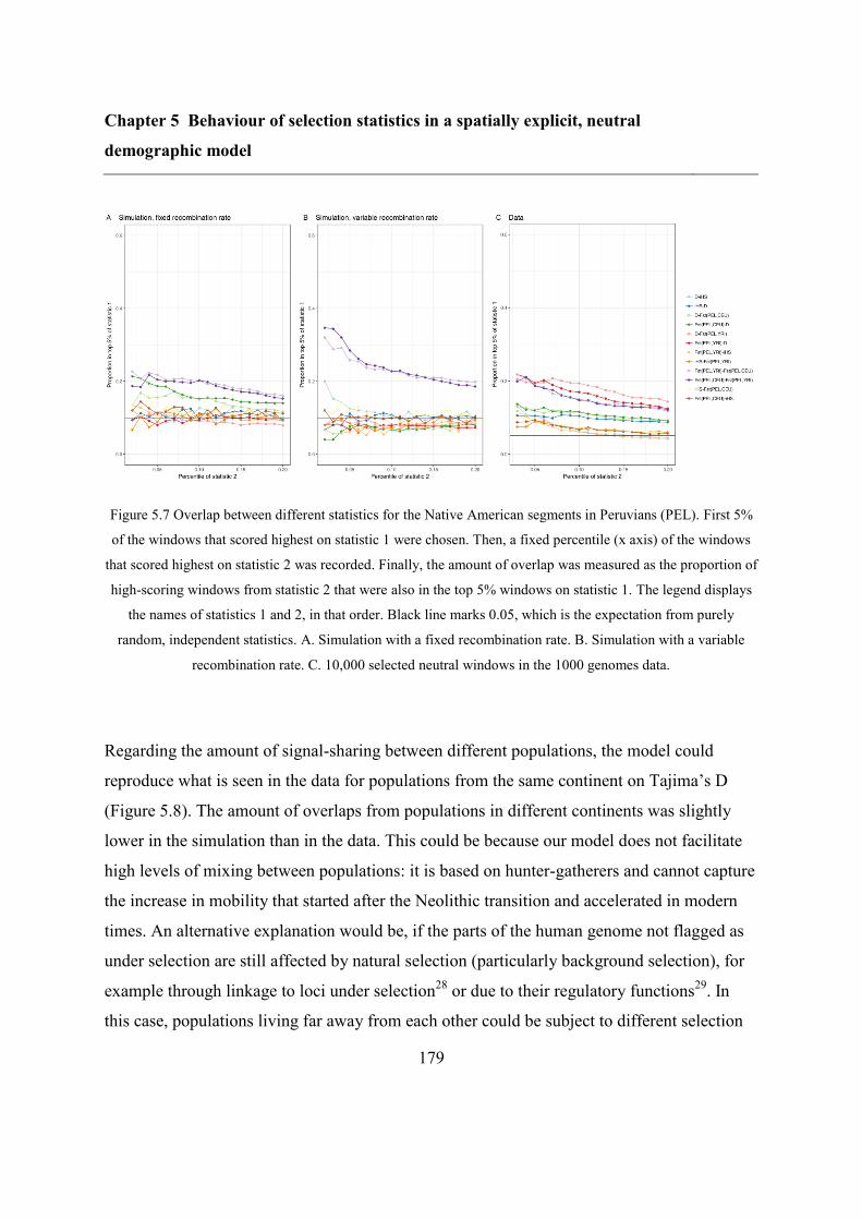
Chapter 5 Behaviour of selection statistics in a spatially explicit, neutral
demographic model
179
Figure 5.7 Overlap between different statistics for the Native American segments in Peruvians (PEL). First 5%
of the windows that scored highest on statistic 1 were chosen. Then, a fixed percentile (x axis) of the windows
that scored highest on statistic 2 was recorded. Finally, the amount of overlap was measured as the proportion of
high-scoring windows from statistic 2 that were also in the top 5% windows on statistic 1. The legend displays
the names of statistics 1 and 2, in that order. Black line marks 0.05, which is the expectation from purely
random, independent statistics. A. Simulation with a fixed recombination rate. B. Simulation with a variable
recombination rate. C. 10,000 selected neutral windows in the 1000 genomes data.
Regarding the amount of signal-sharing between different populations, the model could
reproduce what is seen in the data for populations from the same continent on Tajima’s D
(Figure 5.8). The amount of overlaps from populations in different continents was slightly
lower in the simulation than in the data. This could be because our model does not facilitate
high levels of mixing between populations: it is based on hunter-gatherers and cannot capture
the increase in mobility that started after the Neolithic transition and accelerated in modern
times. An alternative explanation would be, if the parts of the human genome not flagged as
under selection are still affected by natural selection (particularly background selection), for
example through linkage to loci under selection28
or due to their regulatory functions29
. In
this case, populations living far away from each other could be subject to different selection
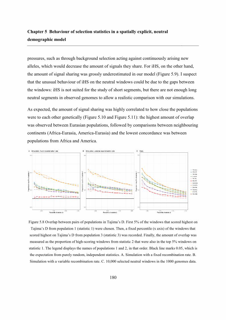
Chapter 5 Behaviour of selection statistics in a spatially explicit, neutral
demographic model
180
pressures, such as through background selection acting against continuously arising new
alleles, which would decrease the amount of signals they share. For iHS, on the other hand,
the amount of signal sharing was grossly underestimated in our model (Figure 5.9). I suspect
that the unusual behaviour of iHS on the neutral windows could be due to the gaps between
the windows: iHS is not suited for the study of short segments, but there are not enough long
neutral segments in observed genomes to allow a realistic comparison with our simulations.
As expected, the amount of signal sharing was highly correlated to how close the populations
were to each other genetically (Figure 5.10 and Figure 5.11): the highest amount of overlap
was observed between Eurasian populations, followed by comparisons between neighbouring
continents (Africa-Eurasia, America-Eurasia) and the lowest concordance was between
populations from Africa and America.
Figure 5.8 Overlap between pairs of populations in Tajima’s D. First 5% of the windows that scored highest on
Tajima’s D from population 1 (statistic 1) were chosen. Then, a fixed percentile (x axis) of the windows that
scored highest on Tajima’s D from population 3 (statistic 3) was recorded. Finally, the amount of overlap was
measured as the proportion of high-scoring windows from statistic 2 that were also in the top 5% windows on
statistic 1. The legend displays the names of populations 1 and 2, in that order. Black line marks 0.05, which is
the expectation from purely random, independent statistics. A. Simulation with a fixed recombination rate. B.
Simulation with a variable recombination rate. C. 10,000 selected neutral windows in the 1000 genomes data.
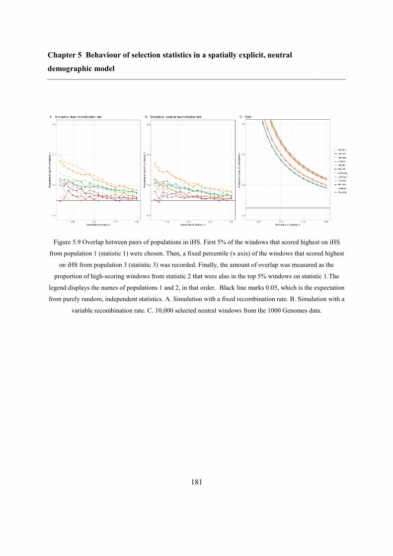
Chapter 5 Behaviour of selection statistics in a spatially explicit, neutral
demographic model
181
Figure 5.9 Overlap between pairs of populations in iHS. First 5% of the windows that scored highest on iHS
from population 1 (statistic 1) were chosen. Then, a fixed percentile (x axis) of the windows that scored highest
on iHS from population 3 (statistic 3) was recorded. Finally, the amount of overlap was measured as the
proportion of high-scoring windows from statistic 2 that were also in the top 5% windows on statistic 1.The
legend displays the names of populations 1 and 2, in that order. Black line marks 0.05, which is the expectation
from purely random, independent statistics. A. Simulation with a fixed recombination rate. B. Simulation with a
variable recombination rate. C. 10,000 selected neutral windows from the 1000 Genomes data.
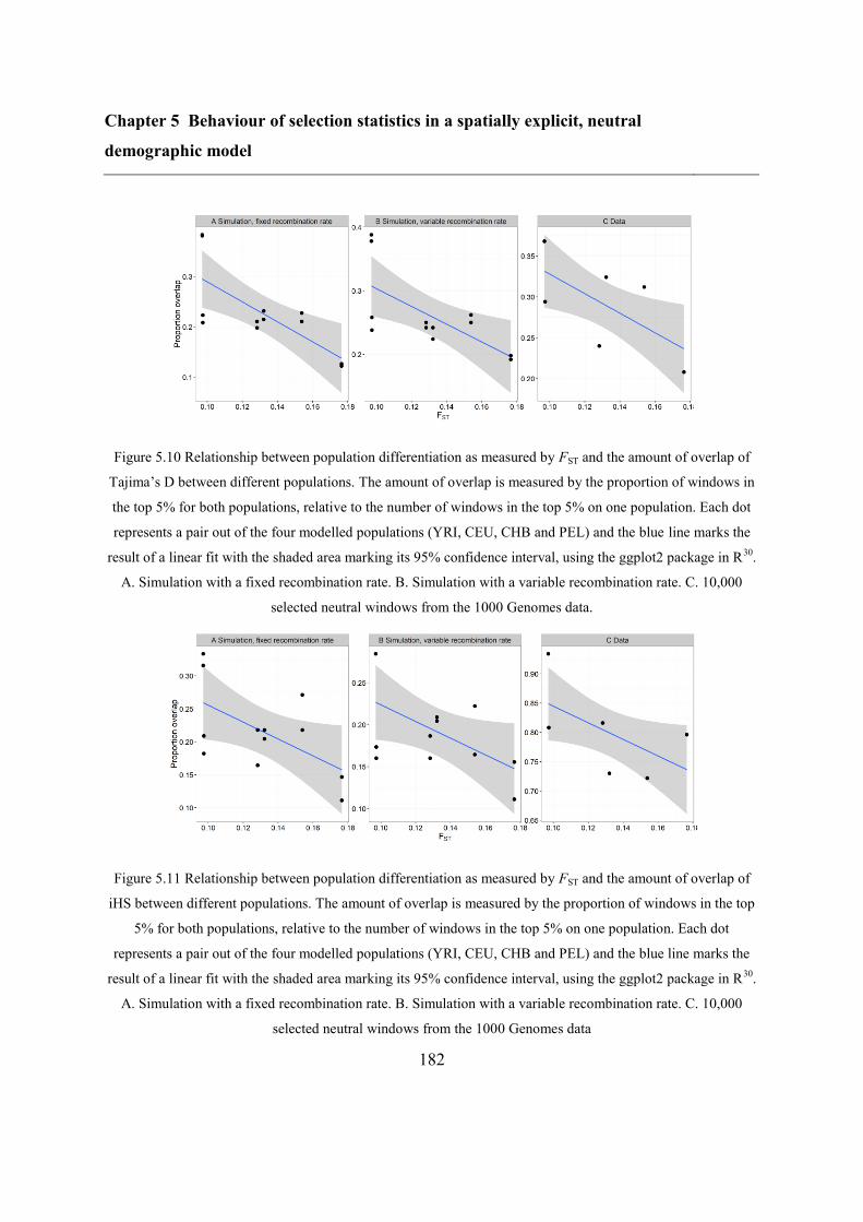
Chapter 5 Behaviour of selection statistics in a spatially explicit, neutral
demographic model
182
Figure 5.10 Relationship between population differentiation as measured by FST and the amount of overlap of
Tajima’s D between different populations. The amount of overlap is measured by the proportion of windows in
the top 5% for both populations, relative to the number of windows in the top 5% on one population. Each dot
represents a pair out of the four modelled populations (YRI, CEU, CHB and PEL) and the blue line marks the
result of a linear fit with the shaded area marking its 95% confidence interval, using the ggplot2 package in R30
.
A. Simulation with a fixed recombination rate. B. Simulation with a variable recombination rate. C. 10,000
selected neutral windows from the 1000 Genomes data.
Figure 5.11 Relationship between population differentiation as measured by FST and the amount of overlap of
iHS between different populations. The amount of overlap is measured by the proportion of windows in the top
5% for both populations, relative to the number of windows in the top 5% on one population. Each dot
represents a pair out of the four modelled populations (YRI, CEU, CHB and PEL) and the blue line marks the
result of a linear fit with the shaded area marking its 95% confidence interval, using the ggplot2 package in R30
.
A. Simulation with a fixed recombination rate. B. Simulation with a variable recombination rate. C. 10,000
selected neutral windows from the 1000 Genomes data
Chapter 5 Behaviour of selection statistics in a spatially explicit, neutral
demographic model
183
5.6 Discussion
We used a uniquely realistic, neutral demographic model and showed that it could produce
selection statistics similar to what is seen in neutral parts of the genome. The advantages of
this model derive from its mechanistic nature: assumptions are only made regarding the
underlying demographic processes, such as isotropic migration and colonisation and linear
population growth up to the carrying capacity. Furthermore, the resulting spatial
reconstruction of human population history can be used to simulate genetic data for any
chosen population. However, in addition to sufficient computational capacity, the model
requires detailed geographical and climate data to infer the ecology and therefore the local
carrying capacities. Furthermore, it only captures the effect of climate, but might miss other
factors such as cultural or linguistic differences that could also influence population
demography. Therefore, this model works best for events occurring during the early parts of
the out-of-Africa expansion, rather than for recent processes such as the Neolithic expansion.
Even though our model could produce realistic selection statistics, we first had to adjust it to
the statistics we aimed to reproduce. Some statistics, such as Tajima’s D, were very sensitive
to demographic parameters: without fitting the model accordingly, we could not obtain values
similar to those observed. It was also difficult to capture fine-scale geographic patterns: using
the only dataset available with large enough population sizes, the 1000 Genomes dataset, the
signal was still not strong enough to distinguish populations from the same continent.
The quality of our fit could have been improved by using a larger dataset, or by combining
multiple sources. Unfortunately the latter is particularly problematic, due to incompatibilities
in the bioinformatics pipeline between different commonly used datasets. For example, the
1000 Genomes data was treated with a custom pipeline that does not allow for integration
with other datasets. In the future, such datasets should be reanalysed using a standard pipeline
and combined with different datasets that provide more spatial breadth in sampling, to
Chapter 5 Behaviour of selection statistics in a spatially explicit, neutral
demographic model
184
compile a reference set with both a high spatial resolution and high enough samples sizes that
allow scans for natural selection.
Finally, we found that the amount of signal sharing between different populations within the
same continent was closely matched between observed and simulated data. However, the
level of overlap between high-scoring regions for populations from different continents was
lower in the data than in the simulation, which could be due to the high level of mixing in
historical times. Signals from different statistics were shared to a lower extent in the
simulation than in the data, which could point to either our model not capturing certain
demographic events or that regions of the human genomes that are flagged as “neutral” are
still affected by natural selection. The latter is also not unreasonable given that signals of
purifying selection have been detected even in non-coding regions31
. In this case, populations
in different continents would be subject to different selection pressures, decreasing signal
sharing, whereas different selection statistics in the same populations could pick up the same
signal, thus increasing overlaps.
5.7 Bibliography
1. Eriksson, A. et al. Late Pleistocene climate change and the global expansion of
anatomically modern humans. Proc. Natl. Acad. Sci. 109, 16089–16094 (2012).
2. Raghavan, M. et al. Genomic evidence for the Pleistocene and recent population
history of Native Americans. Science 349, aab3884 (2015).
3. Vitti, J. J., Grossman, S. R. & Sabeti, P. C. Detecting Natural Selection in Genomic
Data. Annu. Rev. Genet. 47, 97–120 (2013).
4. Tajima, F. Statistical method for testing the neutral mutation hypothesis by DNA
polymorphism. Genetics 123, 585–595 (1989).
Chapter 5 Behaviour of selection statistics in a spatially explicit, neutral
demographic model
185
5. Fay, J. C. & Wu, C.-I. Hitchhiking Under Positive Darwinian Selection. Genetics 155,
1405–1413 (2000).
6. Holsinger, K. E. & Weir, B. S. Genetics in geographically structured populations:
defining, estimating and interpreting FST. Nat. Rev. Genet. 10, 639–650 (2009).
7. Voight, B. F., Kudaravalli, S., Wen, X. & Pritchard, J. K. A Map of Recent Positive
Selection in the Human Genome. PLoS Biol 4, e72 (2006).
8. Ferrer-Admetlla, A., Liang, M., Korneliussen, T. & Nielsen, R. On Detecting
Incomplete Soft or Hard Selective Sweeps Using Haplotype Structure. Mol. Biol. Evol. 31,
1275–1291 (2014).
9. Sabeti, P. C. et al. Detecting recent positive selection in the human genome from
haplotype structure. Nature 419, 832–837 (2002).
10. Kim, Y. & Nielsen, R. Linkage Disequilibrium as a Signature of Selective Sweeps.
Genetics 167, 1513–1524 (2004).
11. Clemente, F. J. et al. A Selective Sweep on a Deleterious Mutation in CPT1A in
Arctic Populations. Am. J. Hum. Genet. (2014). doi:10.1016/j.ajhg.2014.09.016
12. Sabeti, P. C. et al. Genome-wide detection and characterization of positive selection
in human populations. Nature 449, 913–918 (2007).
13. 1000 Genomes Project Consortium et al. A global reference for human genetic
variation. Nature 526, 68–74 (2015).
14. Sudmant, P. H. et al. An integrated map of structural variation in 2,504 human
genomes. Nature 526, 75–81 (2015).
15. Hider, J. L. et al. Exploring signatures of positive selection in pigmentation candidate
genes in populations of East Asian ancestry. BMC Evol. Biol. 13, 150 (2013).
Chapter 5 Behaviour of selection statistics in a spatially explicit, neutral
demographic model
186
16. Pybus, M. et al. 1000 Genomes Selection Browser 1.0: a genome browser dedicated
to signatures of natural selection in modern humans. Nucleic Acids Res. 42, D903–D909
(2014).
17. Nédélec, Y. et al. Genetic Ancestry and Natural Selection Drive Population
Differences in Immune Responses to Pathogens. Cell 167, 657–669.e21 (2016).
18. Kong, A. et al. Rate of de novo mutations and the importance of father’s age to
disease risk. Nature 488, 471–475 (2012).
19. Arcos-Burgos, M. & Muenke, M. Genetics of population isolates. Clin. Genet. 61,
233–247 (2002).
20. Martin, A. R. et al. Human Demographic History Impacts Genetic Risk Prediction
across Diverse Populations. Am. J. Hum. Genet. 100, 635–649 (2017).
21. Kuhlwilm, M. et al. Ancient gene flow from early modern humans into Eastern
Neanderthals. Nature 530, 429–433 (2016).
22. Danecek, P. et al. The variant call format and VCFtools. Bioinformatics 27, 2156–
2158 (2011).
23. Wegmann, D., Leuenberger, C., Neuenschwander, S. & Excoffier, L. ABCtoolbox: a
versatile toolkit for approximate Bayesian computations. BMC Bioinformatics 11, 116
(2010).
24. Weir B. S. & Cockerham C. Clark. Estimating f‐statistics for the analysis of
population structure. Evolution 38, 1358–1370 (2017).
25. The International HapMap Consortium. A second generation human haplotype map of
over 3.1 million SNPs. Nature 449, 851 (2007).
Chapter 5 Behaviour of selection statistics in a spatially explicit, neutral
demographic model
187
26. Szpiech, Z. A. & Hernandez, R. D. selscan: An Efficient Multithreaded Program to
Perform EHH-Based Scans for Positive Selection. Mol. Biol. Evol. 31, 2824–2827 (2014).
27. Pagani, L. et al. Genomic analyses inform on migration events during the peopling of
Eurasia. Nature 538, 238–242 (2016).
28. Lohmueller, K. E. et al. Natural Selection Affects Multiple Aspects of Genetic
Variation at Putatively Neutral Sites across the Human Genome. PLOS Genet. 7, e1002326
(2011).
29. Dermitzakis, E. T., Reymond, A. & Antonarakis, S. E. Conserved non-genic
sequences — an unexpected feature of mammalian genomes. Nat. Rev. Genet. 6, 151–157
(2005).
30. Wickham, H. ggplot2: Elegant Graphics for Data Analysis. (Springer-Verlag New
York, 2009).
31. Miller, W., Makova, K. D., Nekrutenko, A. & Hardison, R. C. Comparative
Genomics. Annu. Rev. Genomics Hum. Genet. 5, 15–56 (2004).
Chapter 6 Explaining spatial patterns of adaptation against malaria
188
Chapter 6 Explaining spatial patterns of
adaptation against malaria
6.1 Abstract
Malaria is a widespread disease that placed one of the highest selective pressures on the
human genome over the last 5-10 ky. Numerous alleles provide a level of genetic
resistance, most of which are associated with blood disorders and thus lead to an
evolutionary trade-off. These alleles have different spatial distributions, some global
and some present only in certain populations, with disjoint or overlapping distributions
between different variants of the same genetic disorder, and the reason for these
dissimilarities is not well understood. I use a spatially explicit, climate-conditioned
demographic framework and an empirical map of malaria presence to study the
dynamics of variants offering genetic resistance against the disease. I aim to infer the
likely origins of the different variants and to determine which factors are necessary to
explain the main characteristics of their spatial distribution. I find that our framework
is incompatible with a single origin for sickle-cell disease and that it can reproduce the
spatial distribution of variants for sickle-cell disease (disjoint ranges) but not for β0
thalassemia (overlapping pattern). The ability to recover the observed distribution for
sickle-cell variants show the power of a spatially explicit framework, but the
incompatibilities with thalassemia highlight the importance of additional mechanisms
not represented in our model, such as long-distance and/or large-scale migrations and
differences in the time of appearance of different variants and selection pressures.
Chapter 6 Explaining spatial patterns of adaptation against malaria
189
6.2 Contribution
I conducted the analysis and wrote the manuscript for this chapter, with the exception of the
following two points. The map for the spatial distribution of malaria endemicity was
digitalised by Michela Leonardi and the base of the demographic model was created by
Anders Eriksson (for the description and contributions to the model, see Chapter 5).
6.3 Introduction
6.3.1 Malaria and protective genetic disorders
Malaria is linked to one of the strongest selection pressures in the population history of
anatomically modern humans and multiple alleles are associated with a protective effect
against it. Due to this strong environmental connection, malaria also lead to one of the
earliest hypothesis about the relationship between an infection and a genetic disease,
proposed by Haldane in 19481,2
. Protective alleles most commonly affect the hemoglobin or
other molecules that are essential for red blood cell function and are associated with a
negative effect on fitness in malaria-free regions through the corresponding blood disorders.
Balancing selection maintains these alleles despite their deleterious effect and they appear at
high frequencies in regions where malaria is endemic3. The selection pressure associated with
malaria is thought to be recent (last 5-10k years or less)3,4
and linked to the lifestyle changes
and increased population density following the Neolithic transition.
Sickle cell disease (βS) and the severe form of β
.thalassemia, β
0 thalassemia, are two
particularly well-studied, classical examples of genetic disorders that increase resistance to
malaria. In the heterozygous form, these alleles offer a protective effect against malaria with
hardly any negative effects, whereas homozygote mutants suffer from the associated severe
blood disorders. In the absence of early diagnosis and treatment, these disorders generally
lead to death within the first few years of life. Both sickle cell disease and β0 thalassemia are
Chapter 6 Explaining spatial patterns of adaptation against malaria
190
inherited through a set of different haplotypes, i.e. a set of genetic alleles, including the
variant under selection, that are located on the same chromosome within close proximity and
are inherited together. Sickle-cell disease is caused by a single mutation (HBB c. 20 A → T;
p. Glu6-Val) and is associated with five “classical” restriction fragment length polymorphism
haplotypes5,6
named Bantu, Benin, Arab-Indian, Senegal and Cameroon haplotypes after the
areas where they were first discovered. β0
thalassemia, on the other hand, can be caused by
any mutation that completely eliminates protein production from the β-globin gene. As a
result, there are many more β0 thalassemia variants than sickle-cell disease variants: 163
different mutations are reported (as queried from http://globin.bx.psu.edu/cgi-
bin/hbvar/query_vars3 on 22 April 2018), and many of them can appear on multiple
haplotypes.
6.3.2 Variants of protective disorders
The origins of the different variants are still not well-understood, even though this is a crucial
piece of information for modelling studies. Most variants offering resistance to malaria are
thought to be the result of recent mutations that arose at most 5-10k years ago3. For sickle-
cell disease, the five “classical” haplotypes were traditionally thought to be the result of
independent mutations5. However, a recent study by Shriner & Rotimi
7, based on the analysis
of whole-genome sequence data and a systematic identification of haplotypes, points to a
single origin roughly 259 generations ago (~6,5ky ago using a generation time of 25 years).
This would then be followed by a spatial expansion and diversification and finally an increase
in frequency due to the appearance of the strong malaria-related selection pressure. The
authors inferred that the single original mutation arose in West or Central Africa 395-123
generations ago, possibly linked to the last Green Sahara phase in the middle of the Holocene
Wet Phase that lasted from 9,500-9,000 years ago until 5,500-5,000 years ago.
Different causal mutations for the β0 haplotypes, on the other hand, are clearly independent,
but different haplotypes with the same causal mutation are thought to be the result of gene
Chapter 6 Explaining spatial patterns of adaptation against malaria
191
conversion8. Since gene conversion is not represented in our framework, we modelled
haplotypes as variants for sickle-cell disease, but different causal mutations, regardless of the
haplotype background, as variants for β0 thalassemia.
The spatial distributions of different variants for these two disorders are remarkably different.
Neither of them is present globally, but both have a wide distribution: sickle-cell disease is
prevalent all over Africa, the Near East and in India, and β0 thalassemia is found throughout
Eurasia9. The five “classical” sickle-cell haplotypes have largely disjoint spatial
distributions10
(Table 6.2 and Figure 6.1), but β0 thalassemia shows an overlapping
distribution, with multiple variants present in any studied region10
(Table 6.4, Table 6.5 and
Figure 6.2). Previous modelling work using a homogeneous metapopulation model inferred
that the prerequisites of a disjoint, sickle cell-like pattern were high population subdivision,
low migration rate and the absence of long-distance migration, whereas the opposite was true
for overlapping, thalassemia-like patterns.
6.3.3 Aim of this study
In this chapter, I explore whether a discrete-time, spatially explicit model can explain these
two contrasting patterns. I aim to answer three questions: where different variants of the same
disorder originated from, whether our model can produce realistic variant distributions (both
disjoint sickle-cell-like and overlapping thalassemia-like patterns) and if a single origin for
sickle-cell disease is plausible even in the absence of long-distance migrations.
Chapter 6 Explaining spatial patterns of adaptation against malaria
192
6.4 Methods
6.4.1 Model
6.4.1.1 Base model
The model in this chapter is based on the climate-informed, spatially explicit framework
introduced in Chapter 5. Only its demographic module was used, but with multiple layers of
populations to represent the different genetic variants. In the original model, the demographic
processes were fitted using genetic data (SNP-data) to produce a realistic structure of genetic
diversity11,12
, and thus population subdivision and migration rates were constant. The spatial
structure of populations was explicitly taken into account, but long-distance migrations were
not included.
For the main results, I used the best-fitting parameter set from Raghavan et al12
(Table 6.1).
These parameters were fitted using world-wide genetic data and represent the demographic
parameters suitable to describe human populations in general. The hexagon where the whole
human population originated from was still the same as in Chapter 5, located at -9.23°
latitude and 33.25° longitude. For a sensitivity analysis on parameters that were pre-defined
using previous results (selection coefficient, demographic parameters and the starting time of
selection), see Appendix E.2.
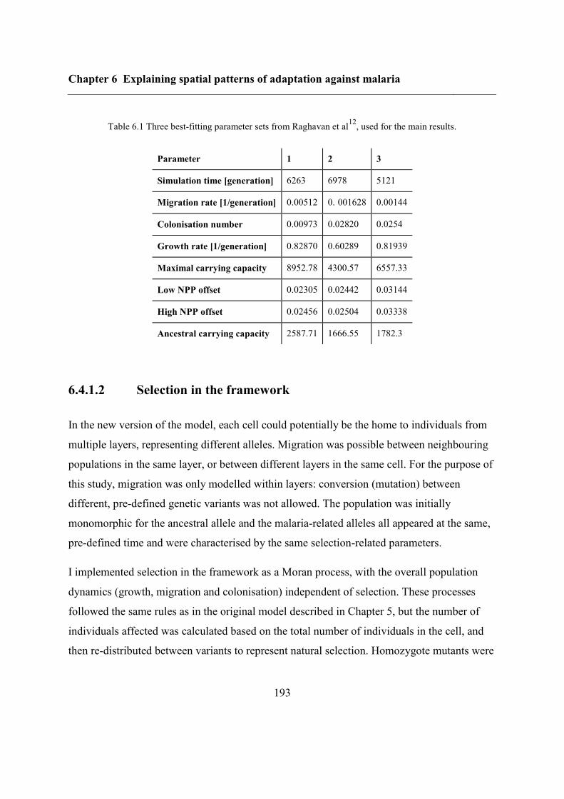
Chapter 6 Explaining spatial patterns of adaptation against malaria
193
Table 6.1 Three best-fitting parameter sets from Raghavan et al12
, used for the main results.
Parameter 1 2 3
Simulation time [generation] 6263 6978 5121
Migration rate [1/generation] 0.00512 0. 001628 0.00144
Colonisation number 0.00973 0.02820 0.0254
Growth rate [1/generation] 0.82870 0.60289 0.81939
Maximal carrying capacity 8952.78 4300.57 6557.33
Low NPP offset 0.02305 0.02442 0.03144
High NPP offset 0.02456 0.02504 0.03338
Ancestral carrying capacity 2587.71 1666.55 1782.3
6.4.1.2 Selection in the framework
In the new version of the model, each cell could potentially be the home to individuals from
multiple layers, representing different alleles. Migration was possible between neighbouring
populations in the same layer, or between different layers in the same cell. For the purpose of
this study, migration was only modelled within layers: conversion (mutation) between
different, pre-defined genetic variants was not allowed. The population was initially
monomorphic for the ancestral allele and the malaria-related alleles all appeared at the same,
pre-defined time and were characterised by the same selection-related parameters.
I implemented selection in the framework as a Moran process, with the overall population
dynamics (growth, migration and colonisation) independent of selection. These processes
followed the same rules as in the original model described in Chapter 5, but the number of
individuals affected was calculated based on the total number of individuals in the cell, and
then re-distributed between variants to represent natural selection. Homozygote mutants were
Chapter 6 Explaining spatial patterns of adaptation against malaria
194
modelled as deleterious, while heterozygotes had an advantage in malarious regions
(selection coefficient, 𝑠 ≈ 0.1523) and were neutral otherwise.
The implemented steps in each generation were therefore as follows, in order of execution:
1. Count the total number of individuals per cell.
2. Apply the same rules as in the original model (Chapter 5) to the total number of
individuals per cell to determine the new population sizes and the number of colonists
and exchanged migrants.
3. Re-distribute the number of individuals per layer (including colonists) to represent the
effect of diploid natural selection with deleterious homozygote mutants:
𝑝𝑖′ =
𝑝𝑖(1 − ∑ 𝑝𝑗𝑗 )𝑤𝑖
(1 − ∑ 𝑝𝑗𝑗 )2
𝑤0 + 2 ∑ 𝑝𝑗𝑗 (1 − ∑ 𝑝𝑘𝑘 )𝑤𝑗
,
where 𝑝𝑖 is the frequency of variant i at the previous generation, 𝑝𝑖′ is the frequency of
variant i at the current (new) generation, 𝑤𝑖 is the fitness of variant i and the ancestral
variant is indexed 0.
4. Distribute the number of migrants such that the ratio of the different variants is the
same as that in the source node at the current (new) generation.
The selection coefficient 𝑤𝑖 was the same for all variants (ancestral and derived) in areas
where malaria is not present and 0.868 for the ancestral allele and 1.0 for all derived alleles in
malarious areas3. However, our model was not sensitive to its exact value (see Appendix
E.2.1 for sensitivity analysis).
I modelled the variants only after the “turn-on” of malaria-related selection pressure when I
studied the dynamics of multiple sickle-cell haplotypes and thalassemia variants, which
means that their origin represented the centre of their area of presence at that time. Therefore,
variants were modelled in the same way regardless of whether they were the result of
diversification after a common origin (sickle-cell trait) or independent mutations (β0
Chapter 6 Explaining spatial patterns of adaptation against malaria
195
thalassemia). For sickle-cell disease, this corresponds to a soft sweep, where the alleles on
different haplotype backgrounds are part of standing variation. For all of our analysis on
multiple variants, a selection turn-on time of 200 generations (5000 years) ago was imposed,
roughly coinciding with the beginning of the migrations of Bantu-speaking populations3 (for
a sensitivity analysis, see Appendix E.2.3).
6.4.2 Data
6.4.2.1 Malaria distribution
To represent the range of malaria, we used a pre-control map of malaria endemicity that was
previously used to confirm the malaria hypothesis for the sickle-cell trait13
. This map is based
on a review from the 1960s by a team of Russian researchers who synthesised historical
records, documents and maps of several malariometric indices used to record malaria
endemicity14
. Combined with expert opinion and data on temperature and rainfall, a unique
global map of the pre-control distribution of malaria could then be reconstructed at the peak
of its hypothesized distribution15
. This map was digitalised using Figure 1C in Piel et al.13
by
Michela Leonardi, which was then converted to a Boolean presence-absence mask for the
cells of our model, based on the hypoendemic regions of the map.
6.4.2.2 Variant distributions
To examine the distribution of variants, I used country-level data assembled from multiple
sources by Hockham et al10
. For countries with multiple data sources available, I used the
mean of the proportions from all sources. The data for sickle-cell disease in Saudi Arabia
showed a conflicting picture, one study showing an overwhelming majority of the Benin
haplotype, and the other the same for the Arab-Indian haplotype. The cause of this
inconsistency in Saudi Arabia is probably due to its large spatial extent that allows different
modal (most common) sickle-cell haplotypes in different areas16,17
: Benin in the west and
Arab-Indian in the east. However, there was no available data on the exact boundary between
Chapter 6 Explaining spatial patterns of adaptation against malaria
196
these regions or on the spatial origin of the ancestors of the individuals from these studies and
we also had data available from another country on the Arabian Peninsula (Kuwait), so we
did not use Saudi Arabia for our error estimates. Furthermore, we pooled all Italian studies
(two from Sardinia and one from Sicily), since our coarse spatial resolution is not capable of
representing such small scales accurately.
Due to computational limitations, I only considered the ancestral variant and those that
reached a frequency of at least 25% in at least one country in the assembled country-level
frequency data in Hockham et al.10
. This resulted in four haplotypes for sickle-cell disease
(Bantu, Benin, Arab-Indian and Senegal) and three mutations for β0 thalassemia (Cd39, IVS-
I-1 and FSC-6). I then scaled the proportions of these variants to amount to unity.
The original data for all variants is shown in Table 6.2 and Figure 6.1 (sickle-cell disease)
and Table 6.4, Table 6.5 and Figure 6.2 (β0 thalassemia), while the resulting proportions of
modelled variants are in Table 6.3 (sickle-cell disease) and Table 6.6 (β0 thalassemia).
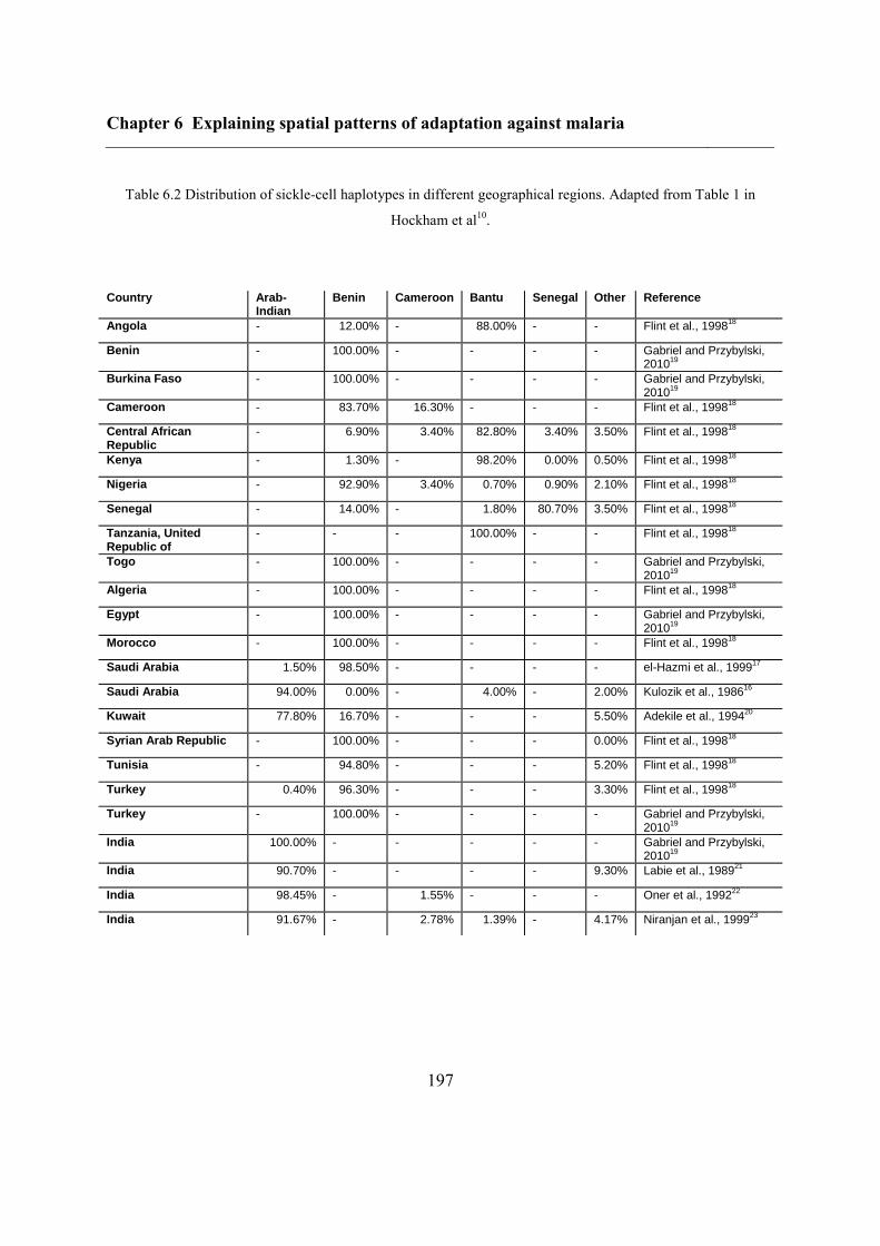
Chapter 6 Explaining spatial patterns of adaptation against malaria
197
Table 6.2 Distribution of sickle-cell haplotypes in different geographical regions. Adapted from Table 1 in
Hockham et al10
.
Country Arab-Indian
Benin Cameroon Bantu Senegal Other Reference
Angola - 12.00% - 88.00% - - Flint et al., 199818
Benin - 100.00% - - - - Gabriel and Przybylski, 2010
19
Burkina Faso - 100.00% - - - - Gabriel and Przybylski, 2010
19
Cameroon - 83.70% 16.30% - - - Flint et al., 199818
Central African Republic
- 6.90% 3.40% 82.80% 3.40% 3.50% Flint et al., 199818
Kenya - 1.30% - 98.20% 0.00% 0.50% Flint et al., 199818
Nigeria - 92.90% 3.40% 0.70% 0.90% 2.10% Flint et al., 199818
Senegal - 14.00% - 1.80% 80.70% 3.50% Flint et al., 199818
Tanzania, United Republic of
- - - 100.00% - - Flint et al., 199818
Togo - 100.00% - - - - Gabriel and Przybylski, 2010
19
Algeria - 100.00% - - - - Flint et al., 199818
Egypt - 100.00% - - - - Gabriel and Przybylski, 2010
19
Morocco - 100.00% - - - - Flint et al., 199818
Saudi Arabia 1.50% 98.50% - - - - el-Hazmi et al., 199917
Saudi Arabia 94.00% 0.00% - 4.00% - 2.00% Kulozik et al., 198616
Kuwait 77.80% 16.70% - - - 5.50% Adekile et al., 199420
Syrian Arab Republic - 100.00% - - - 0.00% Flint et al., 199818
Tunisia - 94.80% - - - 5.20% Flint et al., 199818
Turkey 0.40% 96.30% - - - 3.30% Flint et al., 199818
Turkey - 100.00% - - - - Gabriel and Przybylski, 2010
19
India 100.00% - - - - - Gabriel and Przybylski, 2010
19
India 90.70% - - - - 9.30% Labie et al., 198921
India 98.45% - 1.55% - - - Oner et al., 199222
India 91.67% - 2.78% 1.39% - 4.17% Niranjan et al., 199923
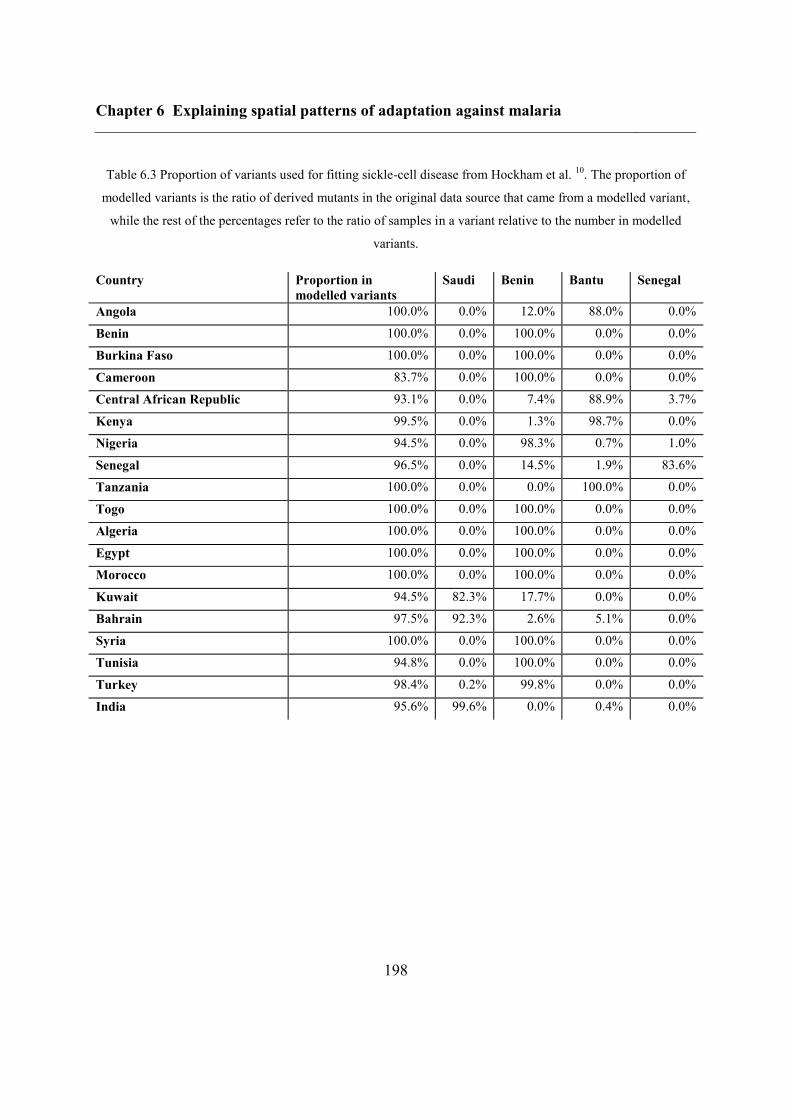
Chapter 6 Explaining spatial patterns of adaptation against malaria
198
Table 6.3 Proportion of variants used for fitting sickle-cell disease from Hockham et al. 10
. The proportion of
modelled variants is the ratio of derived mutants in the original data source that came from a modelled variant,
while the rest of the percentages refer to the ratio of samples in a variant relative to the number in modelled
variants.
Country Proportion in
modelled variants
Saudi Benin Bantu Senegal
Angola 100.0% 0.0% 12.0% 88.0% 0.0%
Benin 100.0% 0.0% 100.0% 0.0% 0.0%
Burkina Faso 100.0% 0.0% 100.0% 0.0% 0.0%
Cameroon 83.7% 0.0% 100.0% 0.0% 0.0%
Central African Republic 93.1% 0.0% 7.4% 88.9% 3.7%
Kenya 99.5% 0.0% 1.3% 98.7% 0.0%
Nigeria 94.5% 0.0% 98.3% 0.7% 1.0%
Senegal 96.5% 0.0% 14.5% 1.9% 83.6%
Tanzania 100.0% 0.0% 0.0% 100.0% 0.0%
Togo 100.0% 0.0% 100.0% 0.0% 0.0%
Algeria 100.0% 0.0% 100.0% 0.0% 0.0%
Egypt 100.0% 0.0% 100.0% 0.0% 0.0%
Morocco 100.0% 0.0% 100.0% 0.0% 0.0%
Kuwait 94.5% 82.3% 17.7% 0.0% 0.0%
Bahrain 97.5% 92.3% 2.6% 5.1% 0.0%
Syria 100.0% 0.0% 100.0% 0.0% 0.0%
Tunisia 94.8% 0.0% 100.0% 0.0% 0.0%
Turkey 98.4% 0.2% 99.8% 0.0% 0.0%
India 95.6% 99.6% 0.0% 0.4% 0.0%
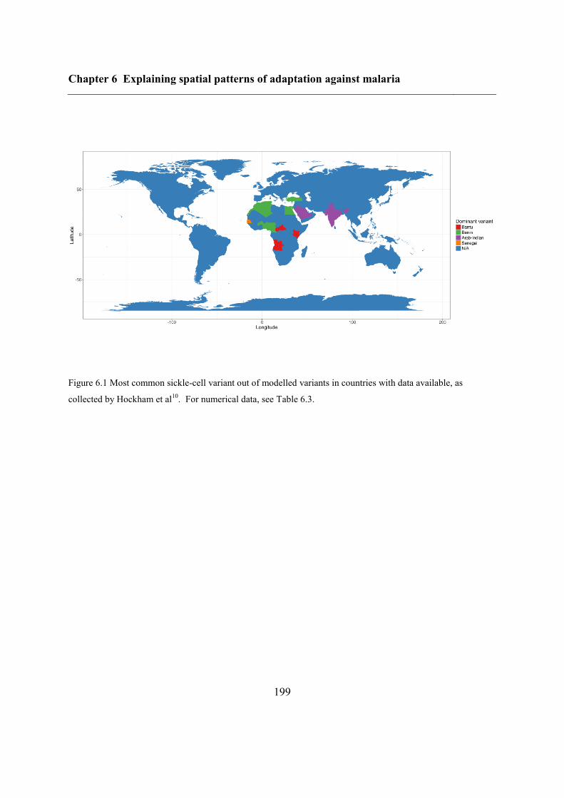
Chapter 6 Explaining spatial patterns of adaptation against malaria
199
Figure 6.1 Most common sickle-cell variant out of modelled variants in countries with data available, as
collected by Hockham et al10
. For numerical data, see Table 6.3.

Chapter 6 Explaining spatial patterns of adaptation against malaria
200
Table 6.4 Distribution of β0 thalassemia variants in North Africa and the Middle East. Adapted from Table 2 in
Hockham et al. Haplotype definitions are given in Antonarakis et al24
.
Cd37 (G->A)
Cd39 (C->T)
IVS-I-1 (G->A)
IVS-I-2 (T->C)
IVS2-1 (G->A)
FSC-8 (-AA)
FSC-6 (-A)
IVS-I-2 (T->G)
Other Reference
Algeria - 44.59% 18.91% 5.40% - - 27.70% - 3.37% Bennani et al., 1994
25
Algeria - 50.00% 11.90% 19.05% - - 16.67% - 2.38% Bouhass et al., 1994
26
Morocco 4.67% 39.26% 7.48% 7.48% 3.74% 20.56% 8.41% 4.67% 3.74% Agouti et al., 2008
27
Morocco 3.51% 24.56% 21.05% 5.26% 1.75% 24.56% 15.79% 0.78% 3.51% Lemsaddek et al., 2003
28
Morocco 1.55% 37.98% 12.40% 3.10% - 13.95% 19.38% 3.45% 10.85% Lemsaddek et al., 2004
29
Tunisia - 62.07% - - - 3.45% 3.45% 3.45% 27.59% Fattoum et al., 1991
30
Table 6.5 Distribution of β0 thalassemia in Europe. Adapted from Table 2 in Hockham et al. Haplotype
definitions are given in Antonarakis et al24
.
Cd39 (C->T) IVS-I-1 (G->A) IVS-I-2 (T->C) IVS2-1 (G->A) Cd6 (-A) Other Reference
Albania 65.00% 15.00% - 5.00% - 15.00% Boletini et al., 199431
Greece 50.86% 39.66% - 6.03% - 3.45% Boletini et al., 199431
Macedonia 21.43% 59.52% - 7.14% - 11.90% Boletini et al., 199431
Sardinia 97.80% 0.04% - 0.04% 2.13% - Cao et al., 199132
Sicily 79.35% 20.65% - - - - Schiliro et al., 199733
Sicily 71.92% 18.72% 3.45% 3.94% 1.23% 0.74% Schiliro et al., 199534
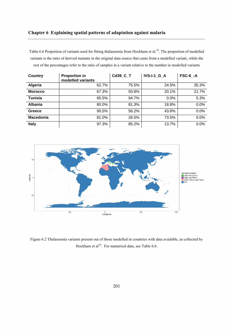
Chapter 6 Explaining spatial patterns of adaptation against malaria
201
Table 6.6 Proportion of variants used for fitting thalassemia from Hockham et al.10
. The proportion of modelled
variants is the ratio of derived mutants in the original data source that came from a modelled variant, while the
rest of the percentages refer to the ratio of samples in a variant relative to the number in modelled variants
Country Proportion in modelled variants
Cd39_C_T IVS-I-1_G_A FSC-6_-A
Algeria 62.7% 75.5% 24.5% 35.3%
Morocco 67.3% 50.8% 20.1% 21.7%
Tunisia 65.5% 94.7% 0.0% 5.3%
Albania 80.0% 81.3% 18.8% 0.0%
Greece 90.5% 56.2% 43.8% 0.0%
Macedonia 81.0% 26.5% 73.5% 0.0%
Italy 97.3% 85.2% 13.7% 0.0%
Figure 6.2 Thalassemia variants present out of those modelled in countries with data available, as collected by
Hockham et al10
. For numerical data, see Table 6.6.
Chapter 6 Explaining spatial patterns of adaptation against malaria
202
6.4.3 Inferring haplotype origins
6.4.3.1 Sampling origins
To find the most likely geographic origin of variants, I ran the model with five layers for
sickle-cell disease (ancestral allele and Bantu, Benin, Senegal and India-Arab haplotypes)
and with four layers for thalassemia (ancestral allele and Cd39, IVS-I-1 and FSC-6 variants).
I sampled 2500 sets of random origins for sickle-cell disease and 3500 for thalassemia,
chosen uniformly at random out of those possible for each variant (the choice of possible
origins is detailed below). After running the simulation, I recorded the count of each variant
at the final time-step for all countries present in our data and calculated error terms as
detailed in Section 6.4.3.3.
6.4.3.2 Possible origins
For sickle-cell disease, I chose the possible origins per variant according to the following
procedure:
1. Determine the cells belonging to countries where the variant is the most common one.
2. Add a 10-cell buffer around this region
3. Assign cells between -25 and 110 in longitude and -40 and 55 in latitude that are not
yet in the set of possible origins to the haplotype with the closest already assigned cell
The only country with available data where the Senegal haplotype was most common was
Senegal, but initial runs pointed to areas north of Senegal to also be plausible origins. We
therefore included Western Sahara as an additional core country for the Senegal haplotype.
Since the dominance of haplotypes for thalassemia was not well-defined, we adapted a
different procedure, considering all cells lying between -25 and 60 in longitude and 15 and 60
in latitude and choosing the three origins for the derived haplotypes independently and
uniformly at random out of these. This sampling region contained most of Europe, North
Chapter 6 Explaining spatial patterns of adaptation against malaria
203
Africa and the Middle East and therefore also all countries with data that we considered. We
focused only on Europe and North Africa, because of the large spatial gap to the other
available regions (India and the Maldives). When calculating the error function, all possible
permutations of the assignment of modelled variants to the three observed variants were
considered.
6.4.3.3 Error function
For sickle-cell disease, a mean squared error-based error function was used. I first calculated
the mean of squared errors between the proportion of different haplotypes from the
simulation and the data over all countries per haplotype and then calculated the mean of the
haplotype-specific errors, which served as my error term for that particular simulation.
For thalassemia, this error function generally lead to a very good fit to the two common
variants, Cd39 and IVS-I-1, at the cost of the complete absence of the rare FSC-6 (Appendix
E.1), probably because its absence was not penalised enough due to its low frequencies in the
observed data. However, the characteristic of the distribution that we aimed to capture was
the presence of multiple variants. I therefore decided to use a different error function,
commonly used for multi-class classification: the count of the number of variants with
mismatching presence-absence values between the data and simulation.
6.4.4 Single-origin hypothesis of sickle-cell disease
I only modelled the ancestral variant and a single derived allele in the study of the single-
origin hypothesis of sickle-cell disease. I considered three appearance times: the estimated
age by Shriner & Rotimi7 (259 generations), as well as the bottom and the top of its 95%
confidence interval (123 and 395 generations). They deem starting points in East to Central
Africa possible, and mention the Green Sahara as their primary hypothesis and the equatorial
rainforest as an alternative. Therefore, I also examined two starting points: one in the eastern
part of this region, in the Green Sahara (longitude 2°, latitude 20°) and one in Central Africa
Chapter 6 Explaining spatial patterns of adaptation against malaria
204
in the equatorial rainforest (longitude 22°, latitude 12°), as close to the centre of the present-
day range as possible.
For the main results, I present two settings: the primary hypothesis with our best-fitting
demographic parameter set and a second setting that maximises the range reached by sickle-
cell disease in the simulation. The latter corresponds to the earliest possible appearance time,
the origin in Central Africa and the demographic parameter set with the quickest spread out
of those we examined (Table 6.1), namely parameter set 2 (see sensitivity analysis in
Appendix E.2.2).
6.5 Results
6.5.1 Inferring haplotype origins
6.5.1.1 Sickle cell
In the data, the Bantu haplotype is wide-spread all over sub-Saharan Africa and the Benin
haplotype in North Africa and the Middle East. The Arab-Indian and Senegal haplotypes
have narrower distributions: in our dataset, the former is modal only on the Arabian
Peninsula and in India, and the latter in Senegal (Table 6.4, Table 6.5 and Figure 6.2 ). The
inferred distribution of most likely origins for sickle-cell disease looked realistic for each
haplotype (Figure 6.3 to Figure 6.6). The Benin haplotype had its origin near Benin, the
Arab-Indian haplotype in India and the Senegal haplotype somewhat north of Senegal, close
to the coast. The Bantu haplotype had a wide range of plausible origins: most cells in Sub-
Saharan Africa were good candidates, as long as they were not too close to the Benin
haplotype.
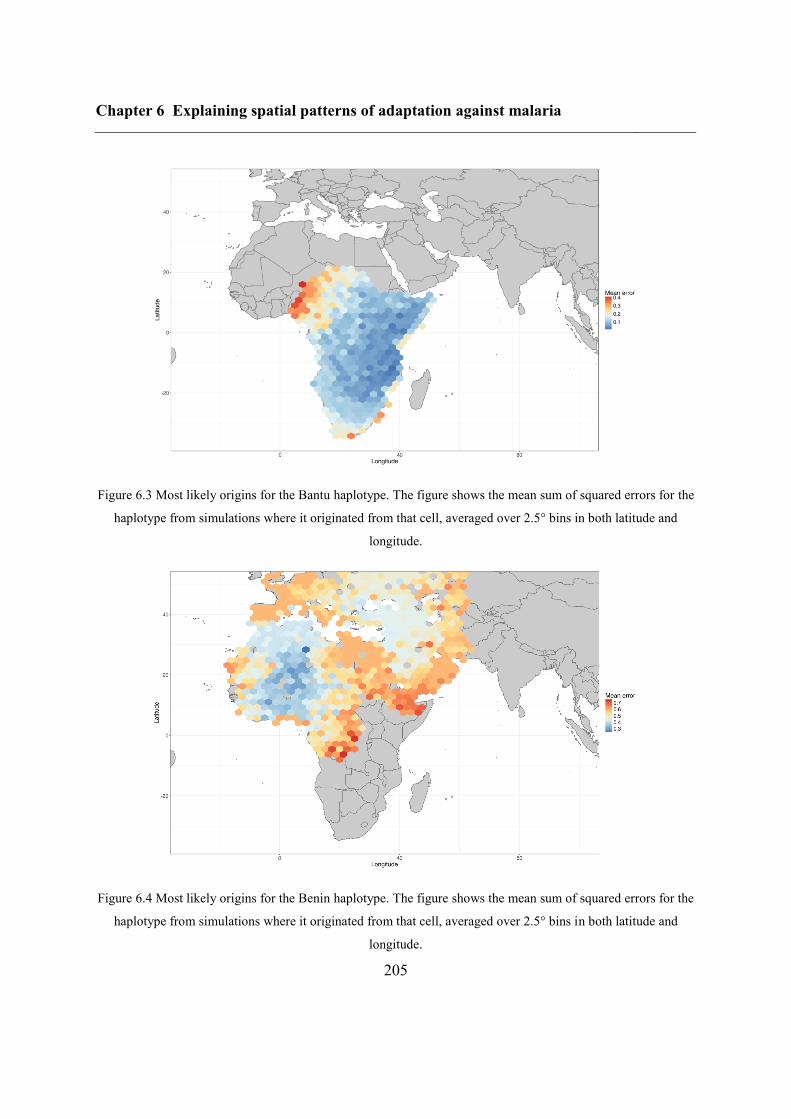
Chapter 6 Explaining spatial patterns of adaptation against malaria
205
Figure 6.3 Most likely origins for the Bantu haplotype. The figure shows the mean sum of squared errors for the
haplotype from simulations where it originated from that cell, averaged over 2.5° bins in both latitude and
longitude.
Figure 6.4 Most likely origins for the Benin haplotype. The figure shows the mean sum of squared errors for the
haplotype from simulations where it originated from that cell, averaged over 2.5° bins in both latitude and
longitude.
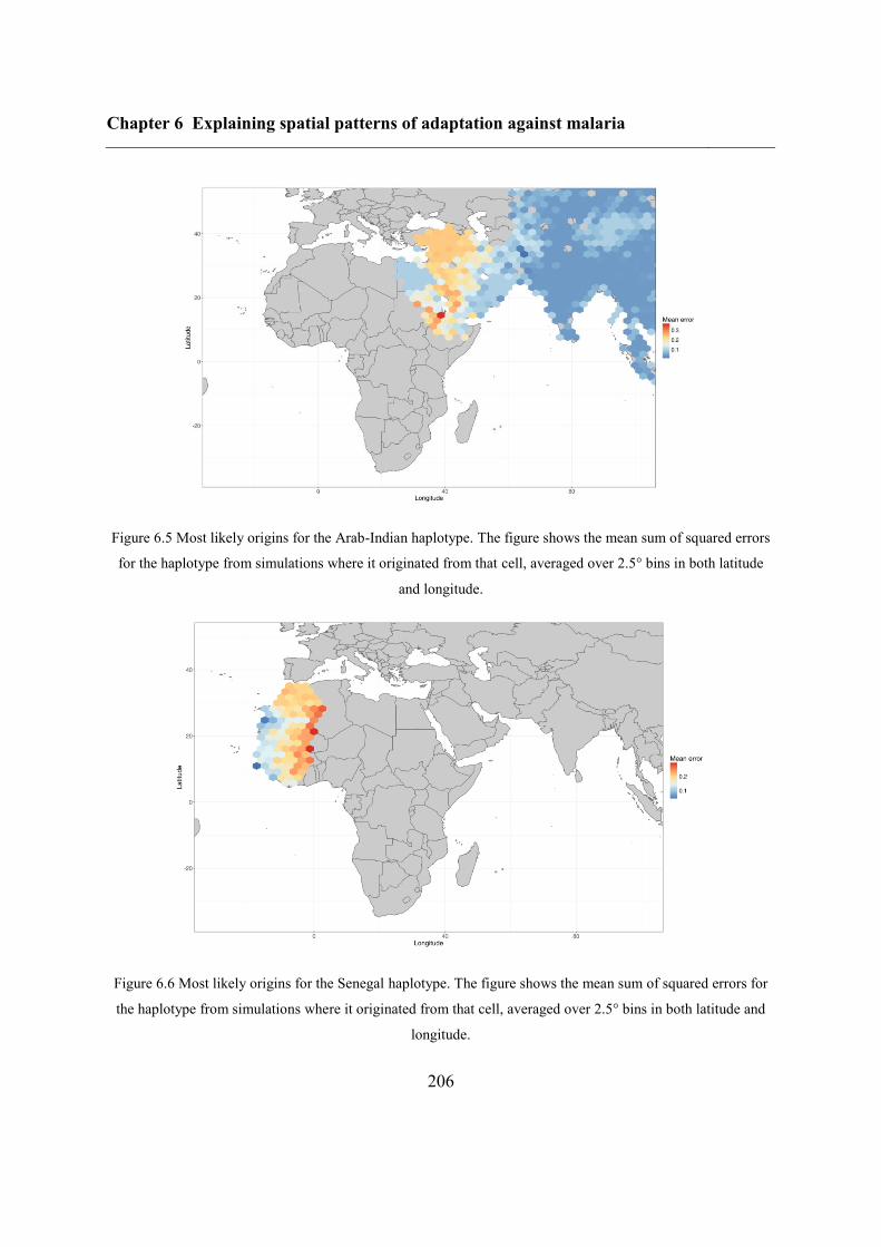
Chapter 6 Explaining spatial patterns of adaptation against malaria
206
Figure 6.5 Most likely origins for the Arab-Indian haplotype. The figure shows the mean sum of squared errors
for the haplotype from simulations where it originated from that cell, averaged over 2.5° bins in both latitude
and longitude.
Figure 6.6 Most likely origins for the Senegal haplotype. The figure shows the mean sum of squared errors for
the haplotype from simulations where it originated from that cell, averaged over 2.5° bins in both latitude and
longitude.
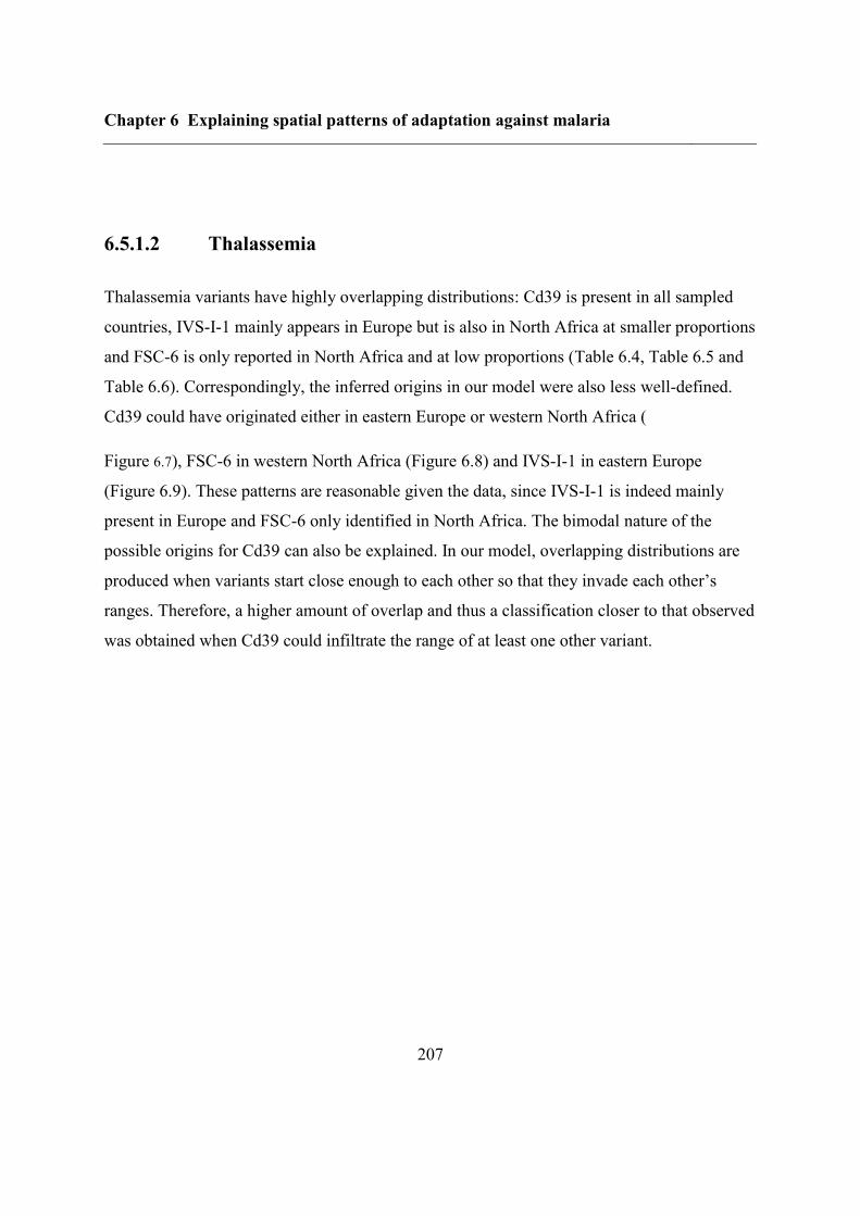
Chapter 6 Explaining spatial patterns of adaptation against malaria
207
6.5.1.2 Thalassemia
Thalassemia variants have highly overlapping distributions: Cd39 is present in all sampled
countries, IVS-I-1 mainly appears in Europe but is also in North Africa at smaller proportions
and FSC-6 is only reported in North Africa and at low proportions (Table 6.4, Table 6.5 and
Table 6.6). Correspondingly, the inferred origins in our model were also less well-defined.
Cd39 could have originated either in eastern Europe or western North Africa (
Figure 6.7), FSC-6 in western North Africa (Figure 6.8) and IVS-I-1 in eastern Europe
(Figure 6.9). These patterns are reasonable given the data, since IVS-I-1 is indeed mainly
present in Europe and FSC-6 only identified in North Africa. The bimodal nature of the
possible origins for Cd39 can also be explained. In our model, overlapping distributions are
produced when variants start close enough to each other so that they invade each other’s
ranges. Therefore, a higher amount of overlap and thus a classification closer to that observed
was obtained when Cd39 could infiltrate the range of at least one other variant.
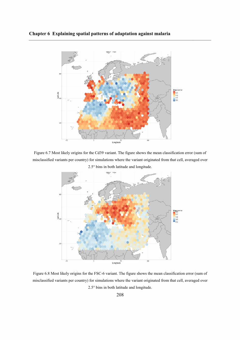
Chapter 6 Explaining spatial patterns of adaptation against malaria
208
Figure 6.7 Most likely origins for the Cd39 variant. The figure shows the mean classification error (sum of
misclassified variants per country) for simulations where the variant originated from that cell, averaged over
2.5° bins in both latitude and longitude.
Figure 6.8 Most likely origins for the FSC-6 variant. The figure shows the mean classification error (sum of
misclassified variants per country) for simulations where the variant originated from that cell, averaged over
2.5° bins in both latitude and longitude.
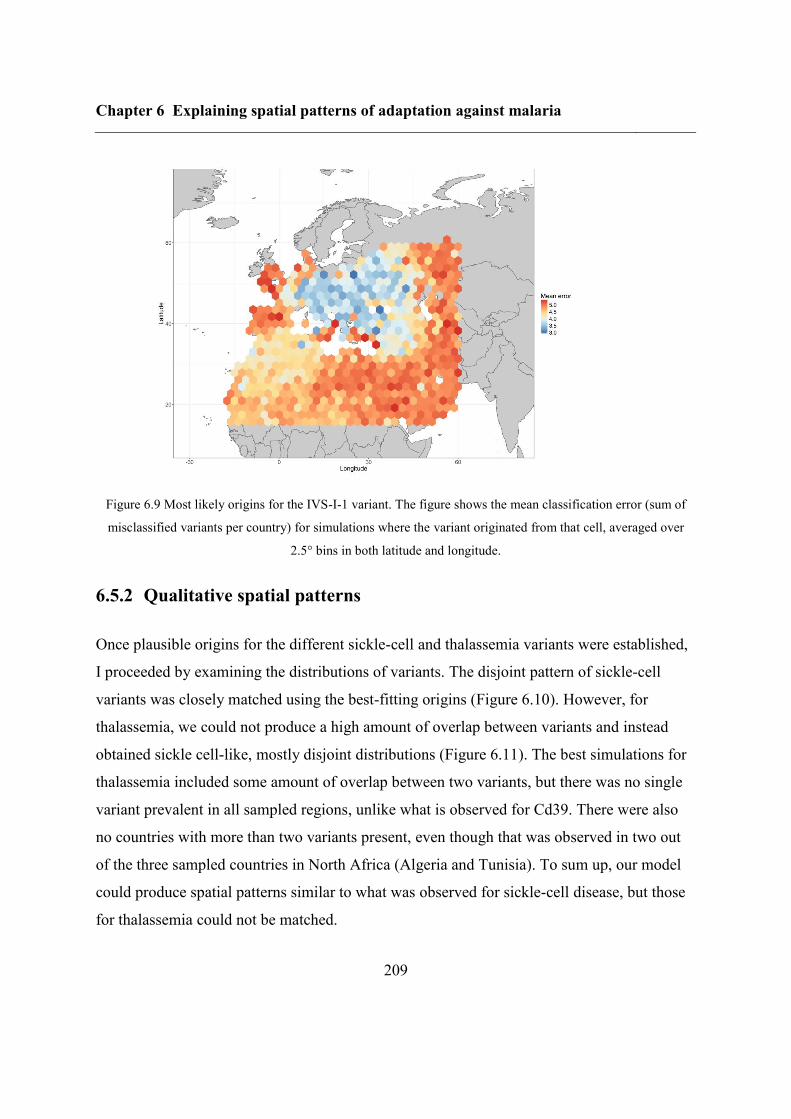
Chapter 6 Explaining spatial patterns of adaptation against malaria
209
Figure 6.9 Most likely origins for the IVS-I-1 variant. The figure shows the mean classification error (sum of
misclassified variants per country) for simulations where the variant originated from that cell, averaged over
2.5° bins in both latitude and longitude.
6.5.2 Qualitative spatial patterns
Once plausible origins for the different sickle-cell and thalassemia variants were established,
I proceeded by examining the distributions of variants. The disjoint pattern of sickle-cell
variants was closely matched using the best-fitting origins (Figure 6.10). However, for
thalassemia, we could not produce a high amount of overlap between variants and instead
obtained sickle cell-like, mostly disjoint distributions (Figure 6.11). The best simulations for
thalassemia included some amount of overlap between two variants, but there was no single
variant prevalent in all sampled regions, unlike what is observed for Cd39. There were also
no countries with more than two variants present, even though that was observed in two out
of the three sampled countries in North Africa (Algeria and Tunisia). To sum up, our model
could produce spatial patterns similar to what was observed for sickle-cell disease, but those
for thalassemia could not be matched.
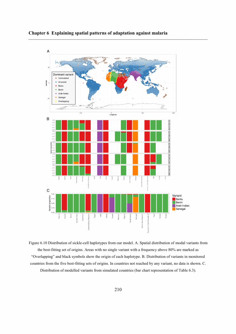
Chapter 6 Explaining spatial patterns of adaptation against malaria
210
Figure 6.10 Distribution of sickle-cell haplotypes from our model. A. Spatial distribution of modal variants from
the best-fitting set of origins. Areas with no single variant with a frequency above 80% are marked as
“Overlapping” and black symbols show the origin of each haplotype. B. Distribution of variants in monitored
countries from the five best-fitting sets of origins. In countries not reached by any variant, no data is shown. C.
Distribution of modelled variants from simulated countries (bar chart representation of Table 6.3).
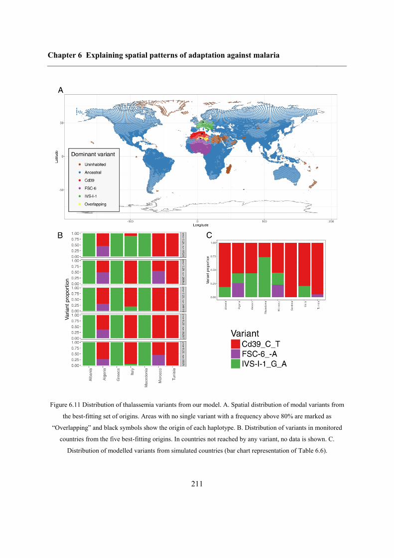
Chapter 6 Explaining spatial patterns of adaptation against malaria
211
Figure 6.11 Distribution of thalassemia variants from our model. A. Spatial distribution of modal variants from
the best-fitting set of origins. Areas with no single variant with a frequency above 80% are marked as
“Overlapping” and black symbols show the origin of each haplotype. B. Distribution of variants in monitored
countries from the five best-fitting origins. In countries not reached by any variant, no data is shown. C.
Distribution of modelled variants from simulated countries (bar chart representation of Table 6.6).
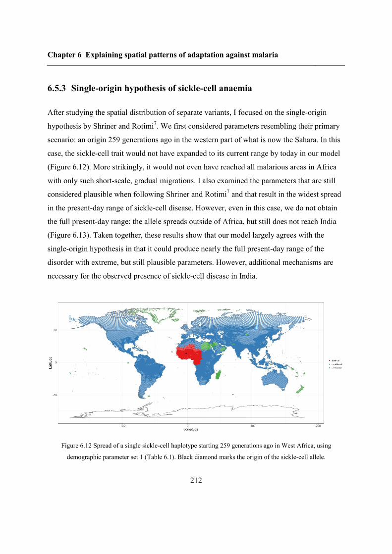
Chapter 6 Explaining spatial patterns of adaptation against malaria
212
6.5.3 Single-origin hypothesis of sickle-cell anaemia
After studying the spatial distribution of separate variants, I focused on the single-origin
hypothesis by Shriner and Rotimi7. We first considered parameters resembling their primary
scenario: an origin 259 generations ago in the western part of what is now the Sahara. In this
case, the sickle-cell trait would not have expanded to its current range by today in our model
(Figure 6.12). More strikingly, it would not even have reached all malarious areas in Africa
with only such short-scale, gradual migrations. I also examined the parameters that are still
considered plausible when following Shriner and Rotimi7 and that result in the widest spread
in the present-day range of sickle-cell disease. However, even in this case, we do not obtain
the full present-day range: the allele spreads outside of Africa, but still does not reach India
(Figure 6.13). Taken together, these results show that our model largely agrees with the
single-origin hypothesis in that it could produce nearly the full present-day range of the
disorder with extreme, but still plausible parameters. However, additional mechanisms are
necessary for the observed presence of sickle-cell disease in India.
Figure 6.12 Spread of a single sickle-cell haplotype starting 259 generations ago in West Africa, using
demographic parameter set 1 (Table 6.1). Black diamond marks the origin of the sickle-cell allele.

Chapter 6 Explaining spatial patterns of adaptation against malaria
213
Figure 6.13 Spread of a single sickle-cell haplotype starting 395 generations ago in Central Africa, using
demographic parameter set 2 (Table 6.1). Black diamond marks the origin of the sickle-cell allele.
6.6 Discussion
6.6.1 Results
Our mechanistic, spatially explicit model with only short-distance migrations could
reproduce the spatial distribution of variants for sickle-cell disease, but not for β0
thalassemia:
overlapping, β0
thalassemia-like patterns were not possible given the processes and
parameters considered. Furthermore, the model was also not completely in agreement with
the single-origin hypothesis for sickle-cell disease. In both cases, the short-distance
migrations explored were insufficient to produce enough mixing: the single, original sickle-
cell allele was not carried far enough and the different thalassemia variants could not invade
each other’s ranges.
It should be noted that the migration rates in the three demographic parameter sets explored
(~0.005 per generation and individual) are relatively low compared to the high end of the
Chapter 6 Explaining spatial patterns of adaptation against malaria
214
95% credible interval of possible migration rates (~0.167 per generation and individual) from
Raghavan et al.12
It would be interesting to explore such higher migration rates, as they might
be sufficient to produce the overlapping patterns of β0
thalassemia and be compatible with the
expansion of a single haplotype of sickle cell anaemia. Furthermore, it is possible that
migration rates might have increased in recent time, as reported for Europe35
, but the model
currently does not allow for such time-dependent changes in migration rate.
Long distance movements are another possible mechanism that could produce a higher
amount of mixing. There is ample evidence for long-distance, large-scale migrations in the
time range considered here, from about 10,000 years ago until today. For example, the
Neolithic transition36
and the Bronze Age migrations37
both left their signatures in European
genetic diversity, evidence of an expansion wave into India has also been described on the
basis of genetic data38
and high levels of mixed genetic ancestry amongst Africans also point
to a high level of admixture in that continent39
. Furthermore, these dynamics have previously
been suggested to facilitate the spread of sickle-cell haplotypes: the migrations of Bantu-
speaking people have been postulated as a cause for the wide distribution within Africa7 and
long-distance overseas connections for the presence of the same haplotype in India and the
Near East40
.
6.6.2 Limitations
There are multiple limitations to this approach. First, the simultaneous appearance of malaria-
related selection pressure and the identity of haplotypes regarding selection strength and the
level of deleteriousness is an oversimplification. Estimates for the ages of the different
haplotypes differ3,41
and there are also signs for a diversity in clinical effects between
different sickle-cell haplotypes42
, but the model outcomes were reasonably robust to the
corresponding parameters. I also did not account for variability in selection pressure and only
used a binary representation of the presence of malaria. However, our results were also not
Chapter 6 Explaining spatial patterns of adaptation against malaria
215
sensitive to changes in selection coefficient and I therefore do not expect a non-binary profile
of the strength of selection to make a substantial difference.
This model also represented a simplified view of the origin of variants by starting in just a
single deme. If the alleles were already part of standing variation at the start of selection, as it
likely was the case for at least the sickle-cell trait, they could have been present over a wider
range. This would accelerate the spread of both the overall trait and the different variants and
our range estimates can thus only be considered as lower boundaries. Furthermore, standing
variation could also influence our incapability of producing the highly overlapping patterns
characteristic of thalassemia: if the variants were already present in a wide range, they could
have spread further and had more time to invade each other’s ranges. In particular, if alleles
with a wider geographic distribution (e.g. Cd39) were already present when the other variants
(e.g. IVS-I-1, FSC-6 and the less common, not modelled variants) appeared, the observed
overlapping distribution would have been more likely. Since β0
thalassemia can be caused by
any mutation that completely eliminates protein production from the β -globin gene and as
many such mutations have already been reported, it is likely that new mutations continuously
occur. In the future, our model could easily be adapted to account for such a scenario.
An additional limitation of our model is the lack of epistatic interactions. These can lead to a
diminishing advantage offered by one variant where another is already present13
, or even to
negative epistasis. For example, both the sickle-cell trait and α thalassemia offer some level
of protection, but individuals heterozygous for both are just as vulnerable to malaria as the
controls43
. The boundaries between the current distributions of different disorders, such as the
relatively low incidence of sickle-cell disease in the Mediterranean44
, has been attributed to
epistatic interaction between different genetic disorders13
. Since these effects were not
represented in our model, it is no surprise that the overall extent of the simulated range of all
variants is only bounded by malaria endemicity. For example, if the system is simulated long
enough, the sickle-cell trait would become common also outside of Africa.
Chapter 6 Explaining spatial patterns of adaptation against malaria
216
Lastly, but perhaps most importantly, our model did not include migration waves or long-
distance connections, despite their likely effect in the spread of protective variants. In the
current framework, such events would have to have been pre-defined using other, non-genetic
lines of evidence. However, this made it possible to test the importance of such events and
showed that they indeed could be necessary to explain the present-day extent of sickle-cell
anaemia and possibly also the overlapping distribution of β0 thalassemia.
6.6.3 Perspectives
A considerable advantage of this layer-based modelling framework is that it is very easy to
generalise to other cases of selection and beyond. Different protective variants and their
interactions, or other types of selection (e.g. haploid and diploid selection; additive, dominant
and recessive traits; epistatic interactions) can all be modelled by simply changing the
corresponding term in the population growth step. The spatial aspect also provides a
convenient way to represent space- and time-dependent selection pressures, or even a link to
climatic variables. Last, the layer-based framework can even be used for arbitrary types of
interacting individuals, such as hunter-gatherers and farmers over the Neolithic transition or
anatomically modern humans and Neanderthals in Europe.
6.6.4 Summary
This chapter presented a spatially explicit model for selection and its application to sickle-cell
disease and β0 thalassemia, two well-studied traits with a protective effect against malaria. It
showed the importance of modelling spatial effects and the limitations of such a framework
when applied to recent events when long-distance migrations were probably already common
for humans. The exact cause of our model’s inability to capture the quick spread of malaria-
resistant traits and the contrast between the spatial distributions of variants of these traits
remains to be determined, but this application highlighted the power of a spatially explicit
model and paved the way for its future applications.
Chapter 6 Explaining spatial patterns of adaptation against malaria
217
6.7 Bibliography
1. Bengtsson, B. O. & Tunlid, A. The 1948 International Congress of Genetics in
Sweden: People and Politics. Genetics 185, 709–715 (2010).
2. Haldane J. B. S. The rate of mutation of human genes. Hereditas 35, 267–273 (2010).
3. Hedrick, P. W. Population genetics of malaria resistance in humans. Heredity 107,
283 (2011).
4. Carter, R. & Mendis, K. N. Evolutionary and Historical Aspects of the Burden of
Malaria. Clin. Microbiol. Rev. 15, 564–594 (2002).
5. Pagnier, J. et al. Evidence for the multicentric origin of the sickle cell hemoglobin
gene in Africa. Proc. Natl. Acad. Sci. 81, 1771–1773 (1984).
6. Lapouniéroulie, C. et al. A novel sickle cell mutation of yet another origin in Africa:
the Cameroon type. Hum. Genet. 89, 333–337 (1992).
7. Shriner, D. & Rotimi, C. N. Whole-Genome-Sequence-Based Haplotypes Reveal
Single Origin of the Sickle Allele during the Holocene Wet Phase. Am. J. Hum. Genet. 102,
547–556 (2018).
8. Chen, J.-M., Cooper, D. N., Chuzhanova, N., Férec, C. & Patrinos, G. P. Gene
conversion: mechanisms, evolution and human disease. Nat. Rev. Genet. 8, 762–775 (2007).
9. Cao, A. & Galanello, R. Beta-thalassemia. Genet. Med. 12, 61–76 (2010).
10. Hockham, C., Piel, F. B., Gupta, S. & Penman, B. S. Understanding the contrasting
spatial haplotype patterns of malaria-protective β-globin polymorphisms. Infect. Genet. Evol.
36, 174–183 (2015).
Chapter 6 Explaining spatial patterns of adaptation against malaria
218
11. Eriksson, A. et al. Late Pleistocene climate change and the global expansion of
anatomically modern humans. Proc. Natl. Acad. Sci. 109, 16089–16094 (2012).
12. Raghavan, M. et al. Genomic evidence for the Pleistocene and recent population
history of Native Americans. Science 349, aab3884 (2015).
13. Piel, F. B. et al. Global distribution of the sickle cell gene and geographical
confirmation of the malaria hypothesis. Nat. Commun. 1, 104 (2010).
14. Lysenko, A. & Semashko, I. Geography of malaria. A medico-geographic profile of
an ancient disease. Itogi Nauki Med. Geogr. 25–146 (1968).
15. Hay, S. I., Guerra, C. A., Tatem, A. J., Noor, A. M. & Snow, R. W. The global
distribution and population at risk of malaria: past, present, and future. Lancet Infect. Dis. 4,
327–336 (2004).
16. Kulozik, A. E. et al. Geographical survey of βS-globin gene haplotypes: Evidence for
an independent Asian origin of the sickle-cell mutation. Am. J. Hum. Genet. 39, 239–244
(1986).
17. El Hazmi, M. A. et al. Haplotypes of the beta-globin gene as prognostic factors in
sickle-cell disease. (1999).
18. Flint, J., Harding, R. M., Boyce, A. J. & Clegg, J. B. 1 The population genetics of the
haemoglobinopathies. Baillières Clin. Haematol. 11, 1–51 (1998).
19. Gabriel, A. & Przybylski, J. Sickle-cell anemia: a look at global haplotype
distribution. (2010).
20. Adekile, A. D. et al. Molecular Characterization of α-Thalassemia Determinants, β-
Thalassemia Alleles, and βs Haplotypes among Kuwaiti Arabs. Acta Haematol. 92, 176–181
(1994).
Chapter 6 Explaining spatial patterns of adaptation against malaria
219
21. LABIE, D. et al. Haplotypes in Tribal Indians Bearing the Sickle Gene: Evidence for
the Unicentric Origin of the β s Mutation and the Unicentric Origin of the Tribal Populations
of India. Hum. Biol. 61, 479–491 (1989).
22. Öner, C. et al. β<Superscript>s</Superscript> Haplotypes in various world
populations. Hum. Genet. 89, 99–104 (1992).
23. NIRANJAN, Y., CHANDAK, G. R., VEERRAJU, P. & SINGH, L. Some Atypical
and Rare Sickle Cell Gene Haplotypes in Populations of Andhra Pradesh, India. Hum. Biol.
71, 333–340 (1999).
24. Antonarakis, S. E., Kazazian, H. H. & Orkin, S. H. DNA polymorphism and
molecular pathology of the human globin gene clusters. Hum. Genet. 69, 1–14 (1985).
25. BENNANI, C. et al. Anthropological Approach to the Heterogeneity of ß-
Thalassemia Mutations in Northern Africa. Hum. Biol. 66, 369–382 (1994).
26. Bouhass, R., Perrin, P. & Trabuchet, G. The spectrum of β-thalassemia mutations in
the oran region of algeria. Hemoglobin 18, 211–219 (1994).
27. Agouti, I., Badens, C., Abouyoub, A., Levy, N. & Bennani, M. Molecular Basis of β-
Thalassemia in Morocco: Possible Origins of the Molecular Heterogeneity. Genet. Test. 12,
563–568 (2008).
28. Lemsaddek, W. et al. Spectrum of β thalassemia mutations and HbF levels in the
heterozygous Moroccan population. Am. J. Hematol. 73, 161–168 (2003).
29. Lemsaddek, W. et al. The β‐Thalassemia Mutation/Haplotype Distribution in the
Moroccan Population. Hemoglobin 28, 25–37 (2004).
30. Fattoum, S. et al. β-Thalassemia, HB S-β-Thalassemia and Sickle Cell Anemia
Among Tunisians. Hemoglobin 15, 11–21 (1991).
Chapter 6 Explaining spatial patterns of adaptation against malaria
220
31. Boletini, E. et al. Sickle cell anemia, sickle cell β-thalassemia, and thalassemia major
in Albania: characterization of mutations. Hum. Genet. 93, 182–187 (1994).
32. Cao, A., Rosatelli, C., Pirastu, M. & Galanello, R. Thalassemias in Sardinia:
molecular pathology, phenotype-genotype correlation, and prevention. Am. J. Pediatr.
Hematol. Oncol. 13, 179–188 (1991).
33. Schilirò, G., Mirabile, E., Testa, R., Russo-Mancuso, G. & Dibenedetto, S. P.
Presence of hemoglobinopathies in Sicily: A historic perspective. Am. J. Med. Genet. 69,
200–206 (1997).
34. Schilirò, G. et al. Genetic heterogeneity of β-thalassemia in southeast sicily. Am. J.
Hematol. 48, 5–11 (1995).
35. Loog, L. et al. Estimating mobility using sparse data: Application to human genetic
variation. Proc. Natl. Acad. Sci. 201703642 (2017). doi:10.1073/pnas.1703642114
36. Lazaridis, I. et al. Ancient human genomes suggest three ancestral populations for
present-day Europeans. ArXiv13126639 Q-Bio (2013).
37. Haak, W. et al. Massive migration from the steppe was a source for Indo-European
languages in Europe. Nature 522, 207–211 (2015).
38. Reich, D., Thangaraj, K., Patterson, N., Price, A. L. & Singh, L. Reconstructing
Indian population history. Nature 461, 489–494 (2009).
39. Tishkoff, S. A. et al. The Genetic Structure and History of Africans and African
Americans. Science 324, 1035–1044 (2009).
40. Stuart, M. J. & Nagel, R. L. Sickle-cell disease. Lancet Lond. Engl. 364, 1343–1360
(2004).
Chapter 6 Explaining spatial patterns of adaptation against malaria
221
41. Modiano, D. et al. Haemoglobin S and haemoglobin C: ‘quick but costly’ versus
‘slow but gratis’ genetic adaptations to Plasmodium falciparum malaria. Hum. Mol. Genet.
17, 789–799 (2008).
42. Loggetto, S. R. Sickle cell anemia: clinical diversity and beta S-globin haplotypes.
Rev. Bras. Hematol. E Hemoter. 35, 155–157 (2013).
43. Williams, T. N. et al. Negative epistasis between the malaria-protective effects of α+-
thalassemia and the sickle cell trait. Nat. Genet. 37, 1253–1257 (2005).
44. Penman, B. S., Pybus, O. G., Weatherall, D. J. & Gupta, S. Epistatic interactions
between genetic disorders of hemoglobin can explain why the sickle-cell gene is uncommon
in the Mediterranean. Proc. Natl. Acad. Sci. 106, 21242–21246 (2009).
Chapter 7 Epilogue
222
Chapter 7 Epilogue
7.1 Introduction
In this thesis, I explored human evolutionary history and its interplay with natural selection
on the basis of ancient DNA and spatially explicit modelling. Chapters 2, 3 and 4 studied
important episodes in the history of anatomically modern humans through the analysis of
novel ancient genetic data. Chapter 2 focussed on early anatomically modern humans in
Europe and highlights their diversification shortly after their exit out of Africa, but also that
many of the resulting populations did not manage to contribute significantly to modern
genetic diversity. Chapter 3 introduced a separate, divergent lineage of hunter-gatherers in the
Caucasus, and Chapter 4 pointed to a high level of continuity in northern East Asia
throughout the Neolithic transition. Chapters 5 and 6 used a climate-driven, spatially explicit
modelling framework: the former explored the effect of space on selection statistics in a
neutral model, and the latter focussed on selection for variants providing resistance against
malaria.
In this last chapter, I first discuss the use of ancient DNA in uncovering demographic
processes. I compare two main data acquisition strategies: broad sampling of many genomes
and deep sampling, focussing on a few, high-quality genomes. I also touch on the teething
problems and future directions in the field, as well as on the issue of compatibility of datasets
from different sources. I then continue with the discussion of continuity and extinction in
human evolution, particularly the signals of these processes in ancient and modern genetic
data and the different definitions of continuity. I then finish this epilogue with a few remarks
on complex spatial models, including advantages, disadvantages, and technical challenges.
Chapter 7 Epilogue
223
7.2 aDNA and its use in uncovering demographic processes
7.2.1 Introduction
Genetic data from ancient samples is a relatively new source in the study of human evolution.
Not only does it give access to individual ancient samples, giving a chance to examine extinct
species (e.g. the quagga1), subspecies (e.g. Neanderthals
2) or populations (e.g. the ancestors
of early European farmers3), but it also broadens our sampling domain in time and space. The
additional time dimension enables a direct estimation of the mutation rate4 and the direct
study of temporal processes, such as changes in allele frequencies (e.g. alleles influencing
skin pigmentation5) or the appearance of alleles (e.g. lactase persistence in the Bronze Age
instead of the Neolithic3,6,7
). However, the imputation of unobserved alleles can be
problematic, especially if the locus in focus has risen rapidly in allele frequency, as is the
case for many variants under selection. Furthermore, we can pinpoint the location of events in
evolutionary history by observing changes through samples from a known location and time.
Common examples are the study of the origin and extent of expansion waves (e.g. Bronze
Age migrations in Europe6 or the spread of eskimo cultures in North America
8) or admixture
events (e.g. sources of European genetic diversity9 or back-migration to North Africa
10).
However, aDNA is still a developing field and has a number of limitations. Protocols in data
generation and analysis are still under development, and although the amount of available
data has drastically increased, jointly using these datasets is very problematic. Furthermore,
projects are sometimes driven by the availability of data instead of a scientific question or
hypothesis, and the quality of analysis sometimes suffers from the time-pressure for high-
profile publications that are based on the novelty of the data.
7.2.2 Broad and deep sampling
There are two main strategies in the use of ancient genetic data. First, one can focus on a few
high-quality samples and sequence those to high coverage, which I will refer to as deep
Chapter 7 Epilogue
224
sampling. Alternatively, a large number of individuals can be studied in parallel, but are then
usually sequenced to only low coverage and/or at selected genetic loci. I will refer to this
latter strategy as broad sampling. The high-quality samples presented in Chapters 2 and 3 are
cases of deep sampling, while Chapter 4 belongs to neither of these strategies: it is based on
only a few low-coverage samples as sample availability was limited and the samples were not
well preserved.
The ancient DNA community seems to move more towards broad sampling, but certain
characteristics of samples and processes can only be studied through deep sampling. A broad
sample is more suited to study large-scale changes in evolution that affect multiple
populations, such as the space- and time-dependent, complex details of the Bronze Age
migrations in Eurasia6 or the definition of and the interplay between different genetic groups
in Ice Age Europe11
. However high-quality samples are necessary to study haplotype patterns
or diploid genotypes12–14
. Detailed demographic inference through the assignment of sections
of the genomes to different ancestries is only possible in the knowledge of diploid
haplotypes; for example, the distribution of the length of such ancestries can give information
about changes in past population size or the timing of admixture events. Haplotypes can also
be analysed to extract genetic data from the source populations of admixture, such as
Neanderthal and Denisovan ancestry in Melanesians15
or Native American segments in the
1000 Genomes populations16
(Chapter 5). Furthermore, high-confidence diploid genotype
calls are necessary to reliably study particular locations in the genome17
, such as those
associated with phenotypic changes – although broad sampling is still needed for population-
level information18
. Last, a practical consideration regarding these two sampling strategies is
that a large number of samples is not always within reach. Therefore, we are often restricted
to extract as much information as possible from those few sample(s) that are available and
sufficiently preserved.
Chapter 7 Epilogue
225
7.2.3 Increase in data volume and issues of compatibility
Although the ancient DNA field is still new, a large amount of data has already been
generated. Technological advances enable us to sequence samples in a worse preservation
state and using a smaller quantity of the ancient material than ever before. In addition, the
increasing credibility of the field after the initial lack of confidence facilitates the acquisition
of samples: archaeologists and anthropologists are naturally more willing to give up a piece
of their sample when they can expect to receive reliable information in exchange.
Furthermore, ethical issues are now more carefully considered. For example, clear guidelines
along with personal connections help build long-term relations with indigenous people and
gain their support to conduct analysis on the remains of their ancestors19
.
The increase in data quantity also highlights problems around the compatibility of different
datasets, where samples that went through different processing pipelines share similarities
independent from their actual genetic relationship. Researchers are still exploring best
practices and protocols for sequencing and bioinformatics pipelines and each lab has its own
standards. Such differences are difficult to take into account after the processing has been
done, although some considerations are generally taken, such as the reproduction of results
on a reduced set of markers which are highly invariant to the differences (e.g. transversions
only for differences in how damaged bases are handled). However, such checks do not
guarantee an unbiased analysis and also usually lead to a reduction in data quantity. Ideally,
all samples should be processed in exactly the same way from the very beginning, but given
that that is rarely feasible, the sequenced data should at least be reprocessed using a
standardised bioinformatics pipeline if different datasets are merged.
7.2.4 Data-driven projects
Even with the increase in availability, many ancient DNA studies are still purely data-driven
and the directed collection of samples to study a hypothesis is rare. In addition, the main
determinant of the success of a publication can often be the novelty of the data and not the
Chapter 7 Epilogue
226
quality of the research. The resulting rush for the first publication in an area or time period
creates a time pressure that can increase the chances of errors. However, there are promising
signs to address this concern: the push for open data enables such errors to be discovered by
the scientific community10
, leading to high-quality, reproducible ancient DNA studies.
Furthermore, as the field matures and low-hanging fruits disappear, high-quality analysis
with a well-defined goal will become more important and simply possessing novel data is no
longer sufficient for a high-profile paper.
7.3 Continuity and extinctions in human evolution
7.3.1 Introduction
The notions of continuity and extinction are strongly linked in human evolution. Current
knowledge points to a series of expansion events, followed by continuous diversification20
. In
contrast, we often see lineages in genetic data, but what processes generated these deep splits
is still unclear. A further complication is coming from the unclear and arbitrary definitions of
continuity, especially considering human populations which are characterised by a high level
of contact and a lack of reproductive isolation.
7.3.2 Extinctions and lineages
The division between lineages in ancient genetic diversity is often unclear and/or does not
correspond to modern genetic diversity. Chapter 2 showcases such a situation in Europe, but
there are also cases in other regions, like the affinities of the Siberian Mal’ta boy to both
Native Americans and North Europeans21
or the lack of continuity on the Eurasian steppes18
.
The notion of lineages can also become obscured as more data is analysed, especially for
ancient data. For example, the initial view of Neanderthals mixing into anatomically modern
humans (AMHs)22
became increasingly complex. Additional Neanderthal samples indicated
structure within their population and identified the Neanderthal group closest to that which
Chapter 7 Epilogue
227
contributed to modern humans23
; the discovery of Denisovans added a sister group of
Neanderthals to the picture24
, and further modelling even showed signals of gene flow into
Neanderthals from a different archaic hominin and from an early AMH group25
. This is just
one simple example, but it illustrates the general trend of tree-like models becoming
increasingly complex as new data is incorporated, implying that many apparent ancient
“lineages” could just be artifacts due to limited sampling.
However, for modern populations in large reference datasets, a lack of spatial sampling is less
of a problem. Therefore, the presence of well-supported lineages in modern genetic data, such
as deeply divergent populations in Africa (e.g. the San or the Mbuti) or the clearly separated
European and East Asian continental groups, need a different explanation. The extinction of
the original intermediate populations, such as what was found in Upper Palaeolithic Europe
(as discussed in Chapter 2 using novel and published4,11,26
data), seems like a good candidate.
7.3.3 Definition of continuity
The other point that needs discussing with regards to the notion of lineages is population
continuity. In its purest definition, continuity means that a population evolves in complete
isolation, without any genetic exchange with other populations. In this case, samples from
different times that originate from the same, continuous population only differ due to genetic
drift27
. However, for a species where migration and admixture are as common as in humans,
such perfect continuity is highly improbable. For uniparental markers, haplogroup
membership has been used to infer continuity and admixture28,29
, but such analysis, based on
a single locus, is sensitive to stochastic effects. For nuclear genetic data, formal tests can be
used to detect admixture (as in multiple papers investigating, for example, the origins of
Europeans3,6,9,18
or South Asians3,30,31
, but also Chapters 312
and 432
), but since a complete
lack of such signal cannot be expected, the threshold level for “continuity” must be chosen
carefully. The level of continuity can also be compared to that between other pairs of
populations on the basis of inferred admixture proportions, such as in the analysis performed
Chapter 7 Epilogue
228
in Chapter 4. However, just like for any hypothesis test, the lack of a clear signal of
admixture does not necessarily imply continuity, as it might simply be due to the lack of
power33
.
7.4 Importance of space in modelling
7.4.1 Advantages
Spatial models have multiple advantages and disadvantages, as mentioned in Chapter 1. They
are capable of representing gradual changes and complex population structure without the
constraints of lineages for tree-like models. Continuous processes are natural in such models:
admixture and expansion are the consequence of mechanistic processes and do not need to be
pre-defined. Spatial models are also capable of providing a different view on continuity: we
can consider a population continuous if it is in contact with its geographic neighbours at a
level typical for the model and is not affected by any major expansion wave or extinction
event27
. Thus, there is no need for a lineage-based continuity definition or arbitrary levels of
acceptable admixture. Spatial models are also a natural choice in the study of selection, as
selection pressures are inherently linked to the environment (e.g. presence of pathogens34
)
and space-dependent demographic processes interact with natural selection (Chapters 5 and
6).
7.4.2 Disadvantages
Spatial models also have some obvious disadvantages, as already mentioned in Chapters 1, 5
and 6. They have high computational costs, are challenging to develop from a coding
perspective, and are intensive in terms of data - although the latter is mitigated in a
mechanistic model where only a few free parameters are sufficient to explore the model. A
further limitation is that it is difficult to represent sudden and/or large-scale changes
(migrations, expansions or extinctions) in such models, although such events are common in
Chapter 7 Epilogue
229
human evolutionary history (e.g. the Neolithic transition3 or the Bantu expansion
35) and are
often triggered by cultural or technological changes and not just by external environmental
variables36
. Since their origin is highly stochastic, difficult to predict and often not well-
understood, this limitation is particularly hard to address without using other lines of
evidence (e.g. from archaeology or linguistics). Our spatial framework certainly represents a
more spatio-temporally continuous view of human population history than the reality, and we
can only incorporate large-scale events through pre-defined effects (e.g. selection-related
processes in Chapter 6) or by changing the interaction with environmental variables (as is
currently explored in our group).
7.5 Concluding remarks
This thesis explored fundamental aspects of human evolutionary history - patterns of
continuity and admixture and phases of stagnation and sudden changes - through the use of
modelling and data analysis. The abundance of modern and ancient genetic data in today’s
“genomics era” enable the usage of not only simple, tree-like models, but also of complex,
spatially explicit frameworks. The contrasting results from different areas and time periods
highlighted key processes from the origins of our species’ remarkable diversity, and have
opened further questions to serve as the topic of future research.
Chapter 7 Epilogue
230
7.6 Bibliography
1. Wilson, A. C., Bowman, B., Freiberger, M., Ryder, O. A. & Higuchi, R. DNA
sequences from the quagga, an extinct member of the horse family. Nature 312, 282 (1984).
2. Green, R. E. et al. Analysis of one million base pairs of Neanderthal DNA. Nature
444, 330–336 (2006).
3. Lazaridis, I. et al. Genomic insights into the origin of farming in the ancient Near
East. Nature 536, 419–424 (2016).
4. Fu, Q. et al. Genome sequence of a 45,000-year-old modern human from western
Siberia. Nature 514, 445–449 (2014).
5. Wilde, S. et al. Direct evidence for positive selection of skin, hair, and eye
pigmentation in Europeans during the last 5,000 y. Proc. Natl. Acad. Sci. 111, 4832–4837
(2014).
6. Haak, W. et al. Massive migration from the steppe was a source for Indo-European
languages in Europe. Nature 522, 207–211 (2015).
7. Mathieson, I. et al. Genome-wide patterns of selection in 230 ancient Eurasians.
Nature 528, 499–503 (2015).
8. Raghavan, M. et al. Genomic evidence for the Pleistocene and recent population
history of Native Americans. Science 349, aab3884 (2015).
9. Lazaridis, I. et al. Ancient human genomes suggest three ancestral populations for
present-day Europeans. ArXiv13126639 Q-Bio (2013).
10. Gallego-Llorente, M. et al. Ancient Ethiopian genome reveals extensive Eurasian
admixture throughout East Africa. Science 350, 820–822 (2015).
Chapter 7 Epilogue
231
11. Fu, Q. et al. The genetic history of Ice Age Europe. Nature 534, 200–205 (2016).
12. Jones, E. R. et al. Upper Palaeolithic genomes reveal deep roots of modern Eurasians.
Nat. Commun. 6, 8912 (2015).
13. Broushaki, F. et al. Early Neolithic genomes from the eastern Fertile Crescent.
Science aaf7943 (2016). doi:10.1126/science.aaf7943
14. Hofmanová, Z. et al. Early farmers from across Europe directly descended from
Neolithic Aegeans. Proc. Natl. Acad. Sci. 113, 6886–6891 (2016).
15. Vernot, B. et al. Excavating Neandertal and Denisovan DNA from the genomes of
Melanesian individuals. Science 352, 235–239 (2016).
16. Martin, A. R. et al. Human Demographic History Impacts Genetic Risk Prediction
across Diverse Populations. Am. J. Hum. Genet. 100, 635–649 (2017).
17. Olalde, I. et al. Derived immune and ancestral pigmentation alleles in a 7,000-year-
old Mesolithic European. Nature 507, 225–228 (2014).
18. Allentoft, M. E. et al. Population genomics of Bronze Age Eurasia. Nature 522, 167–
172 (2015).
19. Callaway, E. Aboriginal genome analysis comes to grips with ethics. Nature 477,
522–523 (2011).
20. Foley, R. A. & Lewin, R. Principles of Human Evolution. (John Wiley & Sons,
2013).
21. Raghavan, M. et al. Upper Palaeolithic Siberian genome reveals dual ancestry of
Native Americans. Nature 505, 87–91 (2014).
22. Green, R. E. et al. A Draft Sequence of the Neandertal Genome. Science 328, 710–
722 (2010).
Chapter 7 Epilogue
232
23. Prüfer, K. et al. The complete genome sequence of a Neanderthal from the Altai
Mountains. Nature 505, 43–49 (2014).
24. Reich, D. et al. Genetic history of an archaic hominin group from Denisova Cave in
Siberia. Nature 468, 1053–1060 (2010).
25. Kuhlwilm, M. et al. Ancient gene flow from early modern humans into Eastern
Neanderthals. Nature 530, 429–433 (2016).
26. Fu, Q. et al. An early modern human from Romania with a recent Neanderthal
ancestor. Nature 524, 216–219 (2015).
27. Silva, N. M., Rio, J. & Currat, M. Investigating population continuity with ancient
DNA under a spatially explicit simulation framework. BMC Genet. 18, 114 (2017).
28. Brandt, G. et al. Ancient DNA Reveals Key Stages in the Formation of Central
European Mitochondrial Genetic Diversity. Science 342, 257–261 (2013).
29. Ghirotto, S. et al. Inferring Genealogical Processes from Patterns of Bronze-Age and
Modern DNA Variation in Sardinia. Mol. Biol. Evol. 27, 875–886 (2010).
30. Reich, D., Thangaraj, K., Patterson, N., Price, A. L. & Singh, L. Reconstructing
Indian population history. Nature 461, 489–494 (2009).
31. Moorjani, P. et al. Genetic evidence for recent population mixture in India. Am J Hum
Genet 93, 422–438 (2013).
32. Siska, V. et al. Genome-wide data from two early Neolithic East Asian individuals
dating to 7700 years ago. Sci. Adv. 3, e1601877 (2017).
33. Patterson, N. et al. Ancient Admixture in Human History. Genetics 192, 1065–1093
(2012).
Chapter 7 Epilogue
233
34. Piel, F. B. et al. Global distribution of the sickle cell gene and geographical
confirmation of the malaria hypothesis. Nat. Commun. 1, 104 (2010).
35. Patin, E. et al. Dispersals and genetic adaptation of Bantu-speaking populations in
Africa and North America. Science 356, 543–546 (2017).
36. Ammerman, A. J. & Cavalli-Sforza, L. L. The Neolithic Transition and the Genetics
of Populations in Europe. (Princeton University Press, 2014).
Appendix A Appendix for Chapter 2
234
Appendix A Appendix for Chapter 2
A.1 NGS sequencing statistics
Supplementary Table A.1 NGS data ouput from the test and HiSeq sequencing runs of Oase’s libraries.
“Rmdup” stands for results after the removal of clonal sequences and “rmdup30” after the removal of clonal
sequencing and filtering for a mapping quality of at least 30. For more details, see section 2.6.2
Test sequencing run: NextSeq500 75PE
Library Index Pairs
processed
Pairs
merged
Mapped Mapped
rmdup
Mapped
rmdup30
%
endogenous
%
duplicate
Bl004 4 833555 90192 26909 19998 14450 2.39 99.74
Bl288 288 1427469 902205 39728 8319 5945 0.58 99.71
eBb440 440 2382154 1608042 65978 11716 7856 0.49 82.24
eB200 200 3363366 2071394 82522 26945 18967 0.80 67.34
Oa1 220 23178331 17636104 8578143 8350749 6323583 36.02 2.65
Oa1b 610 40844664 28871250 15960082 15392302 11747066 37.68 3.55
Oa2 625 30550222 25577980 8511774 8315297 5644337 27.22 2.30
Oa3 687 51178692 36425021 17406697 16871246 12850859 32.96 3.07
Oa4 702 42278773 23253547 10360615 5558135 3488379 13.14 46.35
Oa5a 256 18453200 13055325 6153955 5999221 4519979 32.51 2.51
Oa5b 179 39033310 24724703 10894541 10446189 7788599 26.76 4.11
Oa6 475 6051604 4574323 2178206 2130496 1610837 35.20 2.19
1st sequencing run: HiSeq2500 50PE
Oa1 220 218694705 166017467 81852475 76877139 61173573 35.15 6.07
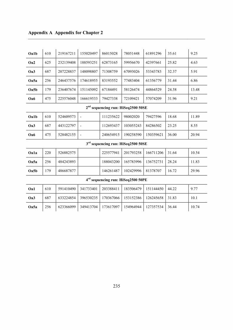
Appendix A Appendix for Chapter 2
235
Oa1b 610 219167211 155020497 86015028 78051448 61891296 35.61 9.25
Oa2 625 232139408 188593251 62873165 59956670 42397661 25.82 4.63
Oa3 687 207228837 148098807 71308759 67093026 53343783 32.37 5.91
Oa5a 256 246437576 174618955 83193552 77483404 61356779 31.44 6.86
Oa5b 179 236407674 151145092 67184491 58126474 44864529 24.58 13.48
Oa6 475 225576048 166619533 79427338 72109421 57074209 31.96 9.21
2nd
sequencing run: HiSeq2500 50SE
Oa1b 610 524609573 - 111235622 98002020 79427596 18.68 11.89
Oa3 687 443122797 - 112693437 103055243 84286502 23.25 8.55
Oa6 475 528482155 - 240654915 190258590 150359621 36.00 20.94
3rd
sequencing run: HiSeq2500 50SE
Oa1a 220 526882575 225577941 201793258 166711206 31.64 10.54
Oa5a 256 484243893 188043200 165783996 136752731 28.24 11.83
Oa5b 179 486687877 146261487 102429996 81378707 16.72 29.96
4rd
sequencing run: HiSeq2500 50PE
Oa1 610 591410490 341733401 203388411 183506479 151144450 44.22 9.77
Oa3 687 633224854 396530235 170367066 153152386 126245658 31.83 10.1
Oa5a 256 623366099 349413704 173617097 154964944 127357534 36.44 10.74
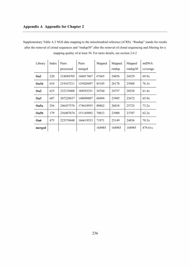
Appendix A Appendix for Chapter 2
236
Supplementary Table A.2 NGS data mapping to the mitochondrial reference (rCRS). “Rmdup” stands for results
after the removal of clonal sequences and “rmdup30” after the removal of clonal sequencing and filtering for a
mapping quality of at least 30. For more details, see section 2.6.2
Library Index Pairs
processed
Pairs
merged
Mapped Mapped
rmdup
Mapped
rmdup30
mtDNA
coverage
Oa1 220 218694705 166017467 67665 24856 24529 69.9x
Oa1b 610 219167211 155020497 85185 26178 25968 76.3x
Oa2 625 232139408 188593251 54760 24757 20528 61.4x
Oa3 687 207228837 148098807 60494 23985 23672 65.9x
Oa5a 256 246437576 174618955 80862 26018 25725 73.2x
Oa5b 179 236407674 151145092 70813 23900 23707 62.2x
Oa6 475 225576048 166619533 71971 25149 24856 70.5x
merged 168985 168985 168985 479.61x
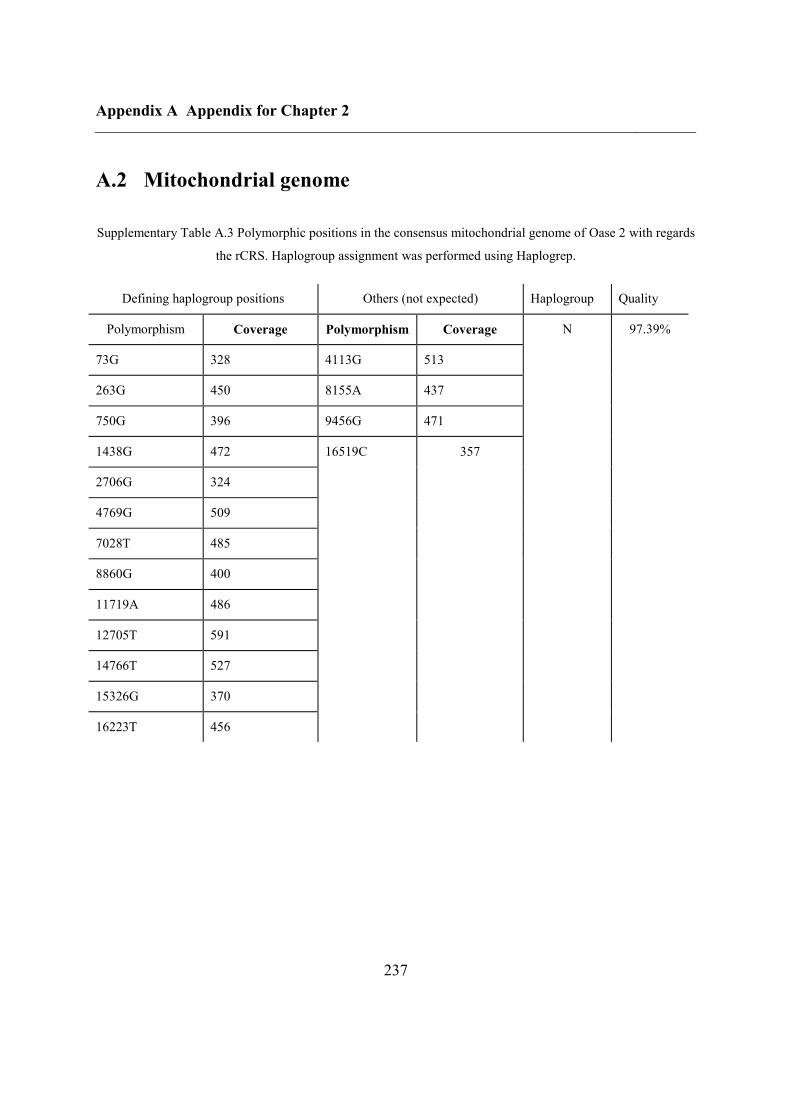
Appendix A Appendix for Chapter 2
237
A.2 Mitochondrial genome
Supplementary Table A.3 Polymorphic positions in the consensus mitochondrial genome of Oase 2 with regards
the rCRS. Haplogroup assignment was performed using Haplogrep.
Defining haplogroup positions Others (not expected) Haplogroup Quality
Polymorphism Coverage Polymorphism Coverage N 97.39%
73G 328 4113G 513
263G 450 8155A 437
750G 396 9456G 471
1438G 472 16519C 357
2706G 324
4769G 509
7028T 485
8860G 400
11719A 486
12705T 591
14766T 527
15326G 370
16223T 456
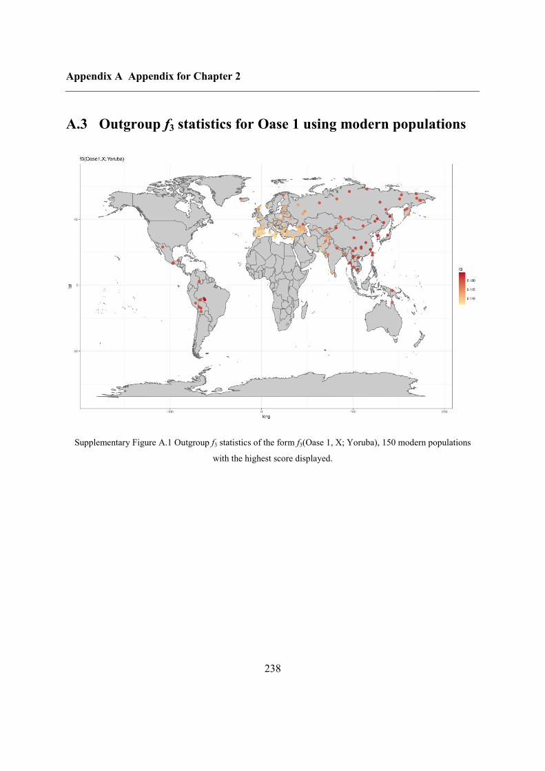
Appendix A Appendix for Chapter 2
238
A.3 Outgroup f3 statistics for Oase 1 using modern populations
Supplementary Figure A.1 Outgroup f3 statistics of the form f3(Oase 1, X; Yoruba), 150 modern populations
with the highest score displayed.
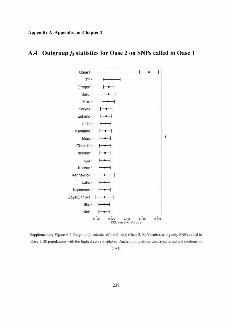
Appendix A Appendix for Chapter 2
239
A.4 Outgroup f3 statistics for Oase 2 on SNPs called in Oase 1
Supplementary Figure A.2 Outgroup f3 statistics of the form f3 (Oase 2, X; Yoruba), using only SNPs called in
Oase 1. 20 populations with the highest score displayed. Ancient populations displayed in red and moderns in
black.
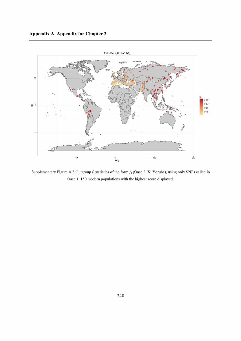
Appendix A Appendix for Chapter 2
240
Supplementary Figure A.3 Outgroup f3 statistics of the form f3 (Oase 2, X; Yoruba), using only SNPs called in
Oase 1. 150 modern populations with the highest score displayed.
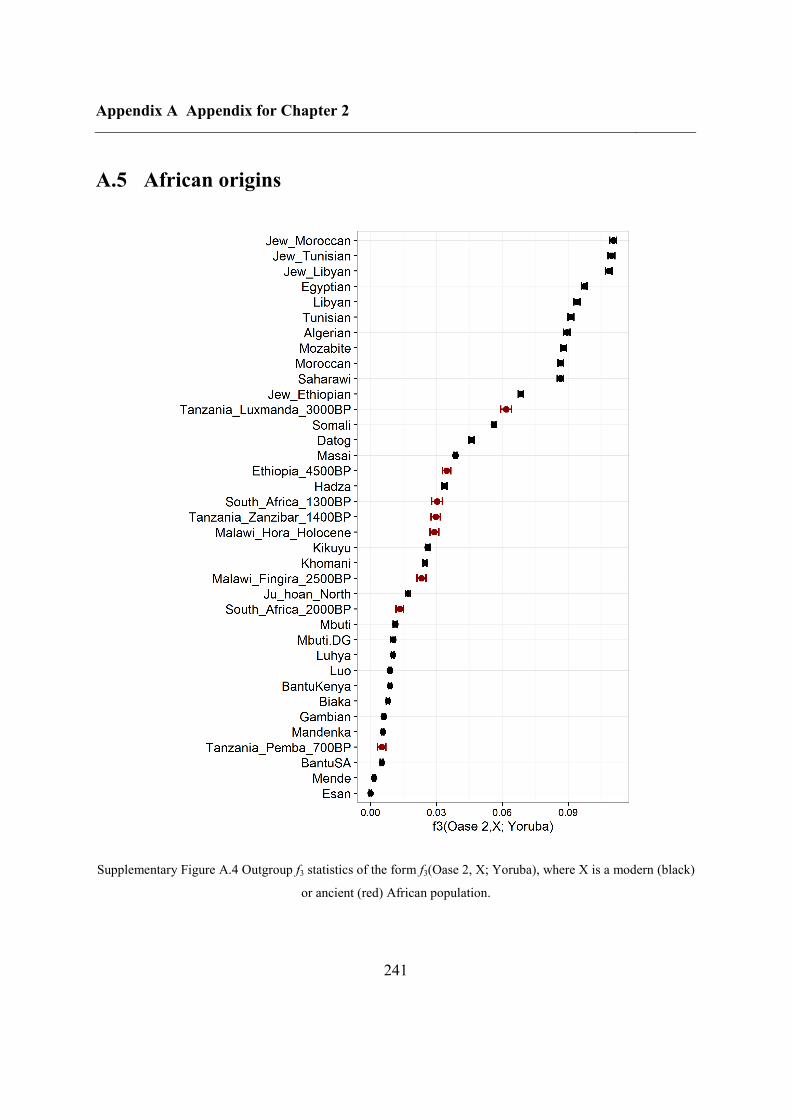
Appendix A Appendix for Chapter 2
241
A.5 African origins
Supplementary Figure A.4 Outgroup f3 statistics of the form f3(Oase 2, X; Yoruba), where X is a modern (black)
or ancient (red) African population.

Appendix A Appendix for Chapter 2
242
Supplementary Figure A.5 Outgroup f3 statistics of the form f3(Kostenki, X; Yoruba), where X is a modern
(black) or ancient (red) African population.
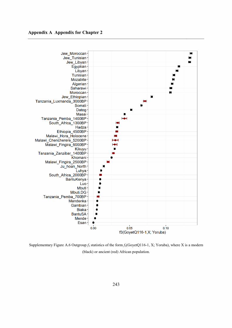
Appendix A Appendix for Chapter 2
243
Supplementary Figure A.6 Outgroup f3 statistics of the form f3(GoyetQ116-1, X; Yoruba), where X is a modern
(black) or ancient (red) African population.
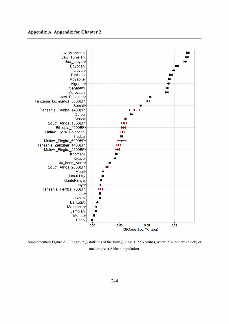
Appendix A Appendix for Chapter 2
244
Supplementary Figure A.7 Outgroup f3 statistics of the form f3(Oase 1, X; Yoruba), where X a modern (black) or
ancient (red) African population.
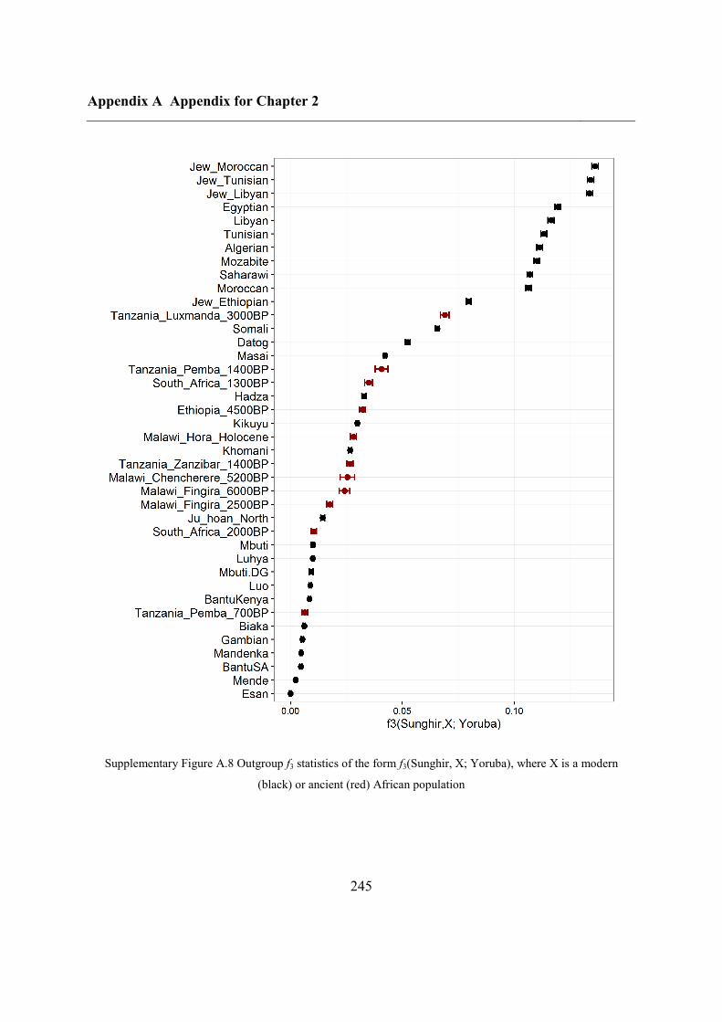
Appendix A Appendix for Chapter 2
245
Supplementary Figure A.8 Outgroup f3 statistics of the form f3(Sunghir, X; Yoruba), where X is a modern
(black) or ancient (red) African population
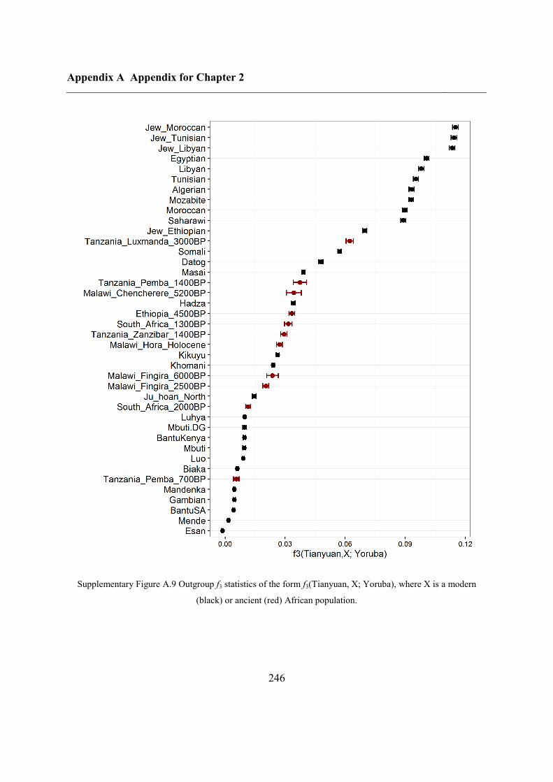
Appendix A Appendix for Chapter 2
246
Supplementary Figure A.9 Outgroup f3 statistics of the form f3(Tianyuan, X; Yoruba), where X is a modern
(black) or ancient (red) African population.
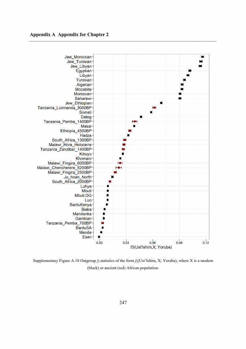
Appendix A Appendix for Chapter 2
247
Supplementary Figure A.10 Outgroup f3 statistics of the form f3(Ust’Ishim, X; Yoruba), where X is a modern
(black) or ancient (red) African population.
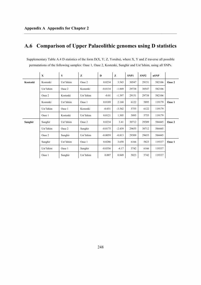
Appendix A Appendix for Chapter 2
248
A.6 Comparison of Upper Palaeolithic genomes using D statistics
Supplementary Table A.4 D statistics of the form D(X, Y; Z, Yoruba), where X, Y and Z traverse all possible
permutations of the following samples: Oase 1, Oase 2, Kostenki, Sunghir and Ust’Ishim, using all SNPs.
X Y Z D Z SNP1 SNP2 nSNP
Kostenki Kostenki Ust’Ishim Oase 2 0.0234 3.543 30547 29151 582106 Oase 2
Ust’Ishim Oase 2 Kostenki -0.0134 -1.849 29738 30547 582106
Oase 2 Kostenki Ust’Ishim -0.01 -1.397 29151 29738 582106
Kostenki Ust’Ishim Oase 1 0.0189 2.168 6122 5895 119179 Oase 1
Ust’Ishim Oase 1 Kostenki -0.031 -3.542 5755 6122 119179
Oase 1 Kostenki Ust’Ishim 0.0121 1.305 5895 5755 119179
Sunghir Sunghir Ust’Ishim Oase 2 0.0234 3.41 30712 29309 584445 Oase 2
Ust’Ishim Oase 2 Sunghir -0.0175 -2.439 29655 30712 584445
Oase 2 Sunghir Ust’Ishim -0.0059 -0.813 29309 29655 584445
Sunghir Ust’Ishim Oase 1 0.0286 3.658 6166 5823 119337 Oase 1
Ust’Ishim Oase 1 Sunghir -0.0356 -4.17 5742 6166 119337
Oase 1 Sunghir Ust’Ishim 0.007 0.849 5823 5742 119337
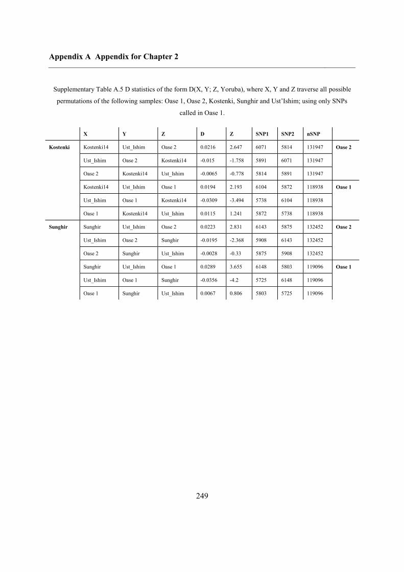
Appendix A Appendix for Chapter 2
249
Supplementary Table A.5 D statistics of the form D(X, Y; Z, Yoruba), where X, Y and Z traverse all possible
permutations of the following samples: Oase 1, Oase 2, Kostenki, Sunghir and Ust’Ishim; using only SNPs
called in Oase 1.
X Y Z D Z SNP1 SNP2 nSNP
Kostenki Kostenki14 Ust_Ishim Oase 2 0.0216 2.647 6071 5814 131947 Oase 2
Ust_Ishim Oase 2 Kostenki14 -0.015 -1.758 5891 6071 131947
Oase 2 Kostenki14 Ust_Ishim -0.0065 -0.778 5814 5891 131947
Kostenki14 Ust_Ishim Oase 1 0.0194 2.193 6104 5872 118938 Oase 1
Ust_Ishim Oase 1 Kostenki14 -0.0309 -3.494 5738 6104 118938
Oase 1 Kostenki14 Ust_Ishim 0.0115 1.241 5872 5738 118938
Sunghir Sunghir Ust_Ishim Oase 2 0.0223 2.831 6143 5875 132452 Oase 2
Ust_Ishim Oase 2 Sunghir -0.0195 -2.368 5908 6143 132452
Oase 2 Sunghir Ust_Ishim -0.0028 -0.33 5875 5908 132452
Sunghir Ust_Ishim Oase 1 0.0289 3.655 6148 5803 119096 Oase 1
Ust_Ishim Oase 1 Sunghir -0.0356 -4.2 5725 6148 119096
Oase 1 Sunghir Ust_Ishim 0.0067 0.806 5803 5725 119096
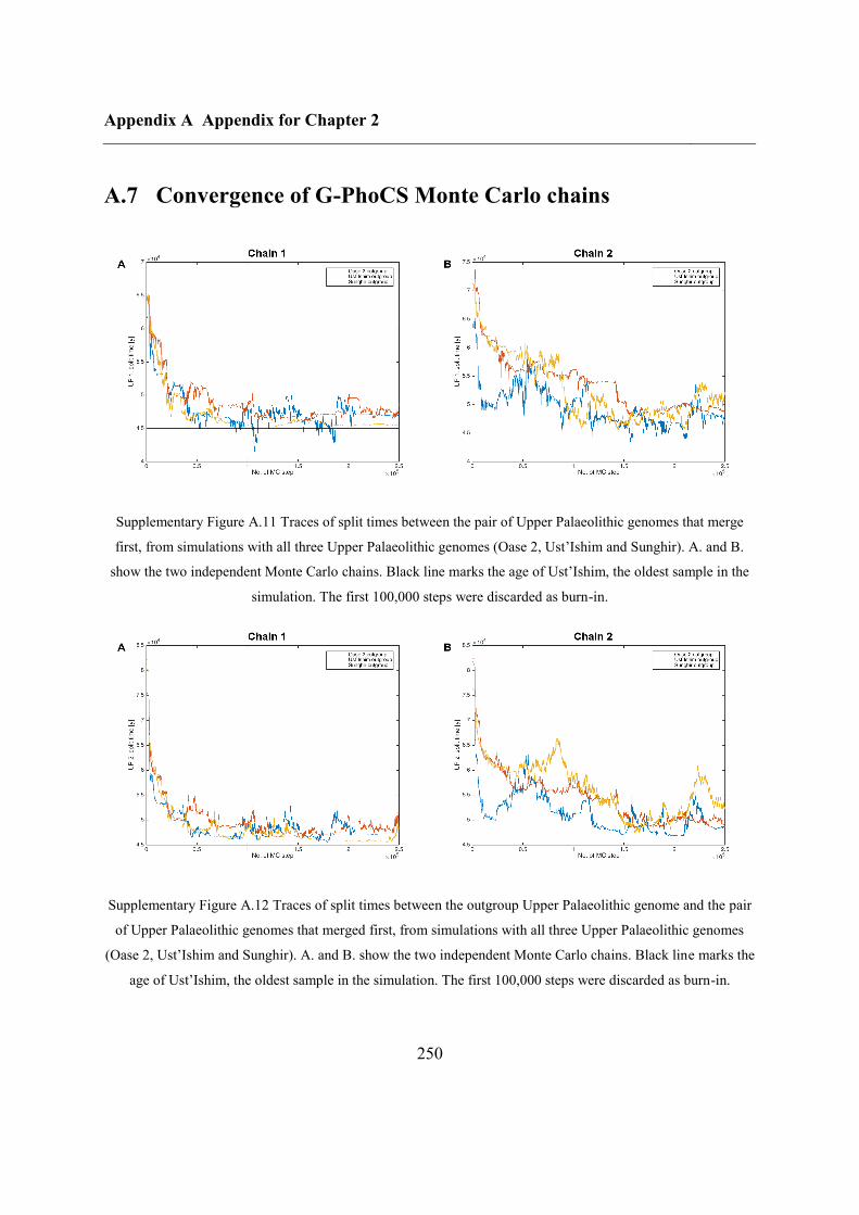
Appendix A Appendix for Chapter 2
250
A.7 Convergence of G-PhoCS Monte Carlo chains
Supplementary Figure A.11 Traces of split times between the pair of Upper Palaeolithic genomes that merge
first, from simulations with all three Upper Palaeolithic genomes (Oase 2, Ust’Ishim and Sunghir). A. and B.
show the two independent Monte Carlo chains. Black line marks the age of Ust’Ishim, the oldest sample in the
simulation. The first 100,000 steps were discarded as burn-in.
Supplementary Figure A.12 Traces of split times between the outgroup Upper Palaeolithic genome and the pair
of Upper Palaeolithic genomes that merged first, from simulations with all three Upper Palaeolithic genomes
(Oase 2, Ust’Ishim and Sunghir). A. and B. show the two independent Monte Carlo chains. Black line marks the
age of Ust’Ishim, the oldest sample in the simulation. The first 100,000 steps were discarded as burn-in.
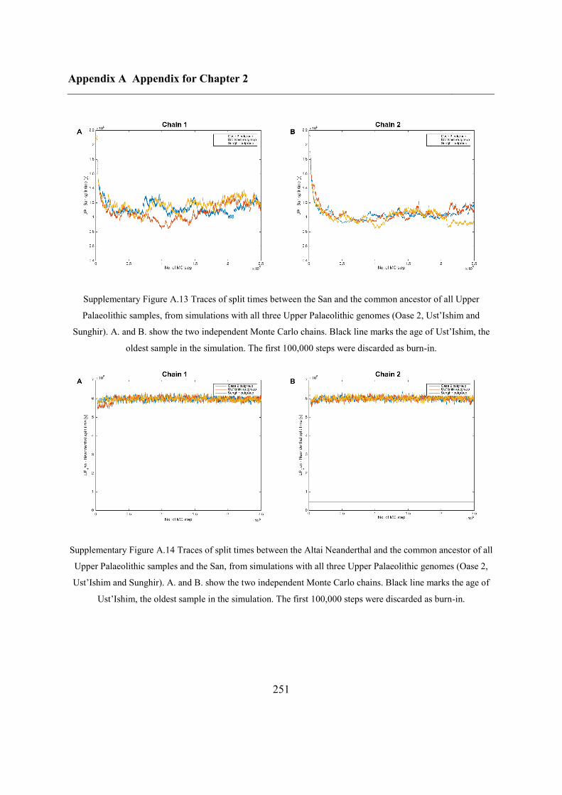
Appendix A Appendix for Chapter 2
251
Supplementary Figure A.13 Traces of split times between the San and the common ancestor of all Upper
Palaeolithic samples, from simulations with all three Upper Palaeolithic genomes (Oase 2, Ust’Ishim and
Sunghir). A. and B. show the two independent Monte Carlo chains. Black line marks the age of Ust’Ishim, the
oldest sample in the simulation. The first 100,000 steps were discarded as burn-in.
Supplementary Figure A.14 Traces of split times between the Altai Neanderthal and the common ancestor of all
Upper Palaeolithic samples and the San, from simulations with all three Upper Palaeolithic genomes (Oase 2,
Ust’Ishim and Sunghir). A. and B. show the two independent Monte Carlo chains. Black line marks the age of
Ust’Ishim, the oldest sample in the simulation. The first 100,000 steps were discarded as burn-in.
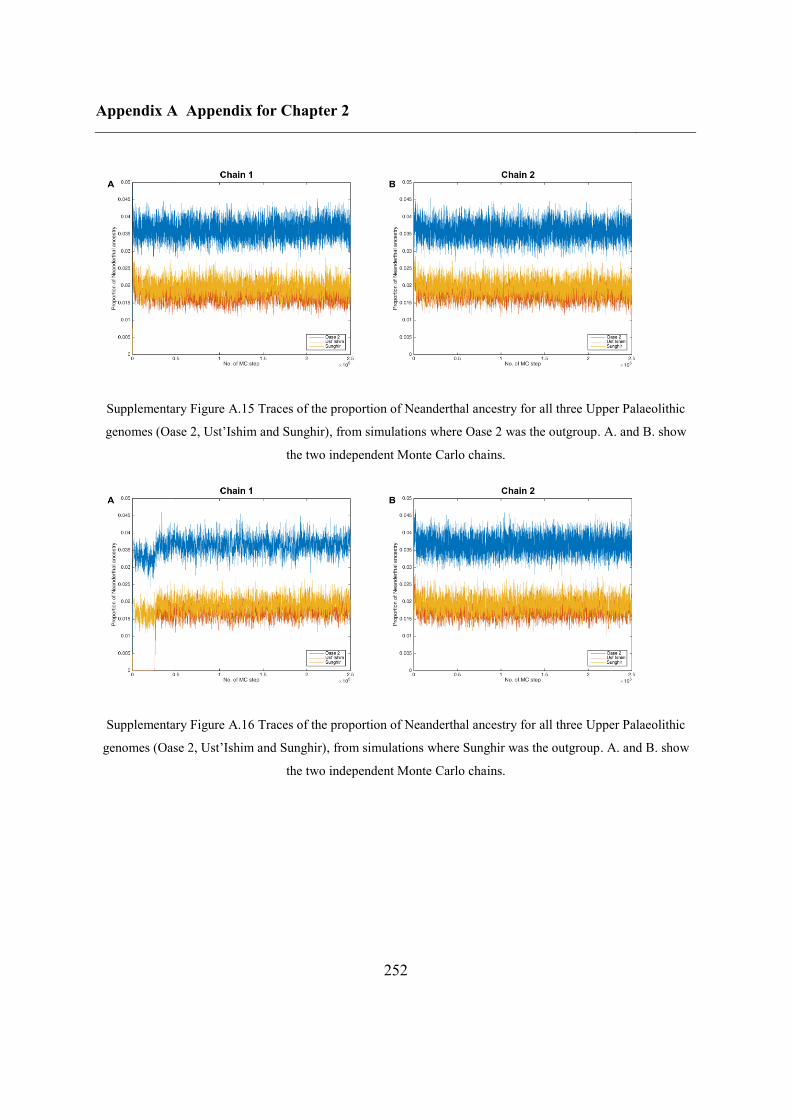
Appendix A Appendix for Chapter 2
252
Supplementary Figure A.15 Traces of the proportion of Neanderthal ancestry for all three Upper Palaeolithic
genomes (Oase 2, Ust’Ishim and Sunghir), from simulations where Oase 2 was the outgroup. A. and B. show
the two independent Monte Carlo chains.
Supplementary Figure A.16 Traces of the proportion of Neanderthal ancestry for all three Upper Palaeolithic
genomes (Oase 2, Ust’Ishim and Sunghir), from simulations where Sunghir was the outgroup. A. and B. show
the two independent Monte Carlo chains.
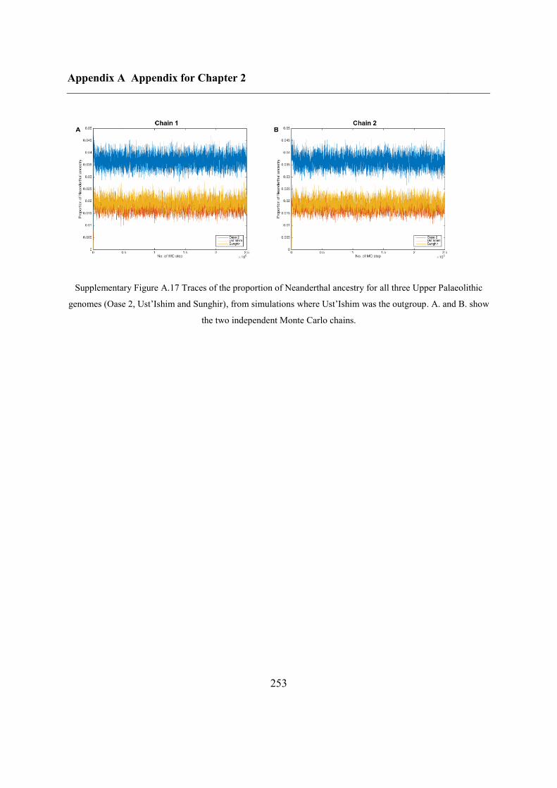
Appendix A Appendix for Chapter 2
253
Supplementary Figure A.17 Traces of the proportion of Neanderthal ancestry for all three Upper Palaeolithic
genomes (Oase 2, Ust’Ishim and Sunghir), from simulations where Ust’Ishim was the outgroup. A. and B. show
the two independent Monte Carlo chains.
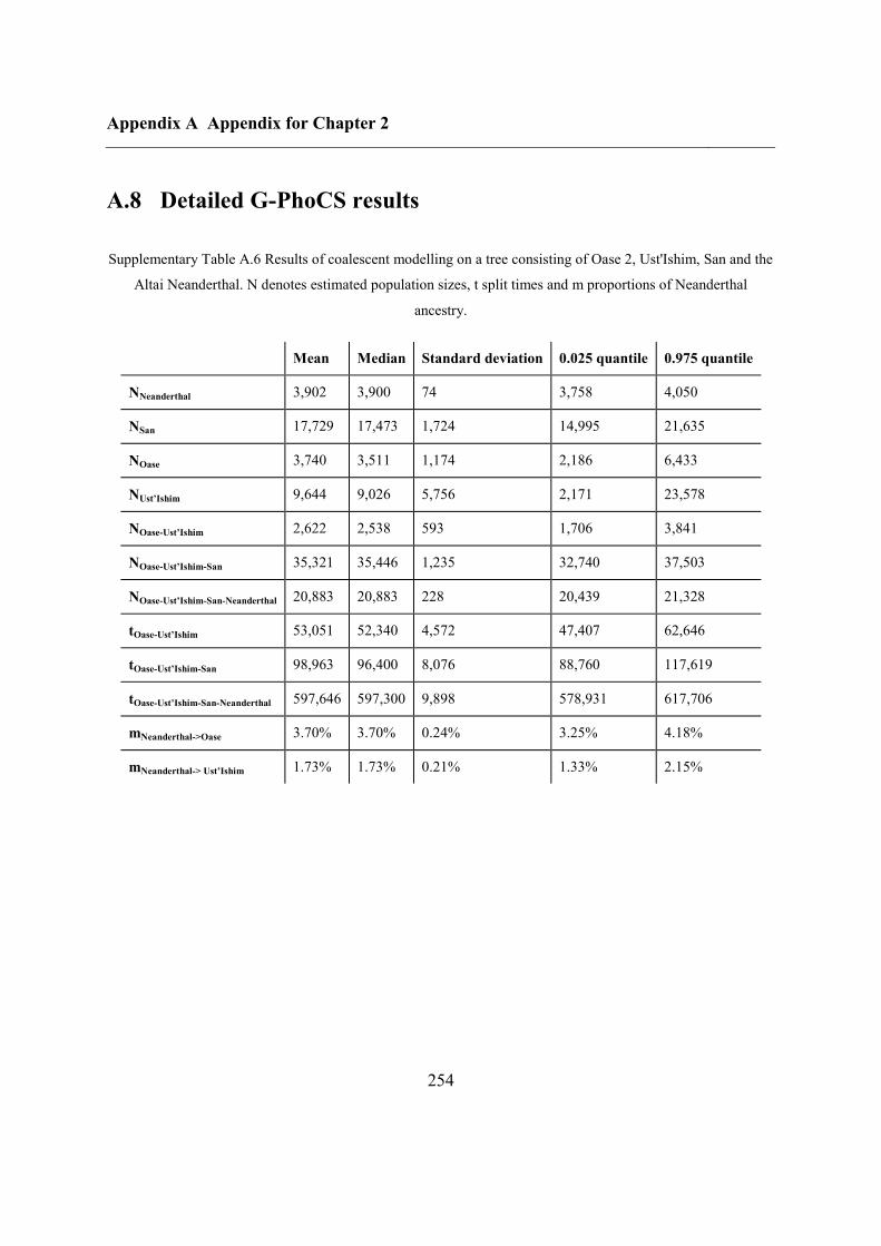
Appendix A Appendix for Chapter 2
254
A.8 Detailed G-PhoCS results
Supplementary Table A.6 Results of coalescent modelling on a tree consisting of Oase 2, Ust'Ishim, San and the
Altai Neanderthal. N denotes estimated population sizes, t split times and m proportions of Neanderthal
ancestry.
Mean Median Standard deviation 0.025 quantile 0.975 quantile
NNeanderthal 3,902 3,900 74 3,758 4,050
NSan 17,729 17,473 1,724 14,995 21,635
NOase 3,740 3,511 1,174 2,186 6,433
NUst’Ishim 9,644 9,026 5,756 2,171 23,578
NOase-Ust’Ishim 2,622 2,538 593 1,706 3,841
NOase-Ust’Ishim-San 35,321 35,446 1,235 32,740 37,503
NOase-Ust’Ishim-San-Neanderthal 20,883 20,883 228 20,439 21,328
tOase-Ust’Ishim 53,051 52,340 4,572 47,407 62,646
tOase-Ust’Ishim-San 98,963 96,400 8,076 88,760 117,619
tOase-Ust’Ishim-San-Neanderthal 597,646 597,300 9,898 578,931 617,706
mNeanderthal->Oase 3.70% 3.70% 0.24% 3.25% 4.18%
mNeanderthal-> Ust’Ishim 1.73% 1.73% 0.21% 1.33% 2.15%
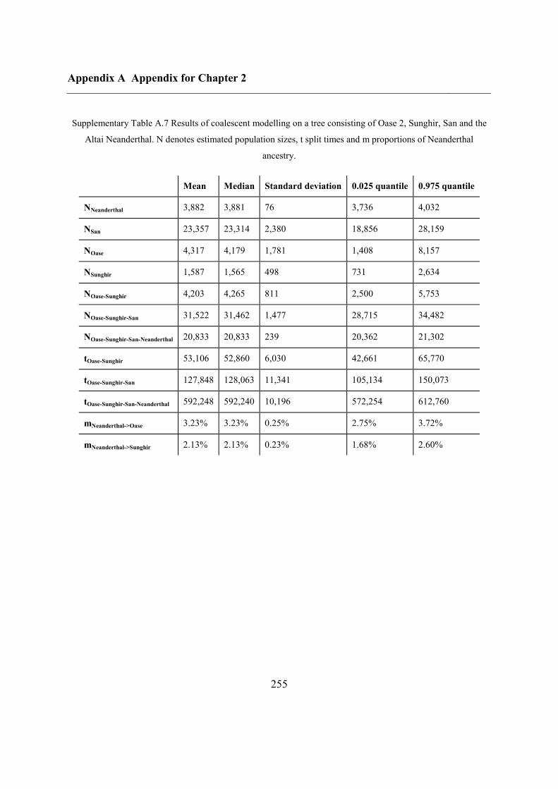
Appendix A Appendix for Chapter 2
255
Supplementary Table A.7 Results of coalescent modelling on a tree consisting of Oase 2, Sunghir, San and the
Altai Neanderthal. N denotes estimated population sizes, t split times and m proportions of Neanderthal
ancestry.
Mean Median Standard deviation 0.025 quantile 0.975 quantile
NNeanderthal 3,882 3,881 76 3,736 4,032
NSan 23,357 23,314 2,380 18,856 28,159
NOase 4,317 4,179 1,781 1,408 8,157
NSunghir 1,587 1,565 498 731 2,634
NOase-Sunghir 4,203 4,265 811 2,500 5,753
NOase-Sunghir-San 31,522 31,462 1,477 28,715 34,482
NOase-Sunghir-San-Neanderthal 20,833 20,833 239 20,362 21,302
tOase-Sunghir 53,106 52,860 6,030 42,661 65,770
tOase-Sunghir-San 127,848 128,063 11,341 105,134 150,073
tOase-Sunghir-San-Neanderthal 592,248 592,240 10,196 572,254 612,760
mNeanderthal->Oase 3.23% 3.23% 0.25% 2.75% 3.72%
mNeanderthal->Sunghir 2.13% 2.13% 0.23% 1.68% 2.60%
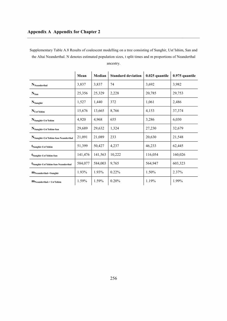
Appendix A Appendix for Chapter 2
256
Supplementary Table A.8 Results of coalescent modelling on a tree consisting of Sunghir, Ust’Ishim, San and
the Altai Neanderthal. N denotes estimated population sizes, t split times and m proportions of Neanderthal
ancestry.
Mean Median Standard deviation 0.025 quantile 0.975 quantile
NNeanderthal 3,837 3,837 74 3,692 3,982
NSan 25,356 25,329 2,228 20,785 29,753
NSunghir 1,527 1,440 372 1,061 2,486
NUst’Ishim 15,676 13,665 8,766 4,153 37,374
NSunghir-Ust’Ishim 4,920 4,968 655 3,286 6,030
NSunghir-Ust’Ishim-San 29,689 29,632 1,324 27,230 32,679
NSunghir-Ust’Ishim-San-Neanderthal 21,091 21,089 233 20,630 21,548
tSunghir-Ust’Ishim 51,399 50,427 4,237 46,233 62,445
tSunghir-Ust’Ishim-San 141,476 141,563 10,222 116,054 160,026
tSunghir-Ust’Ishim-San-Neanderthal 584,077 584,003 9,765 564,947 603,323
mNeanderthal->Sunghir 1.93% 1.93% 0.22% 1.50% 2.37%
mNeanderthal-> Ust’Ishim 1.59% 1.59% 0.20% 1.19% 1.99%
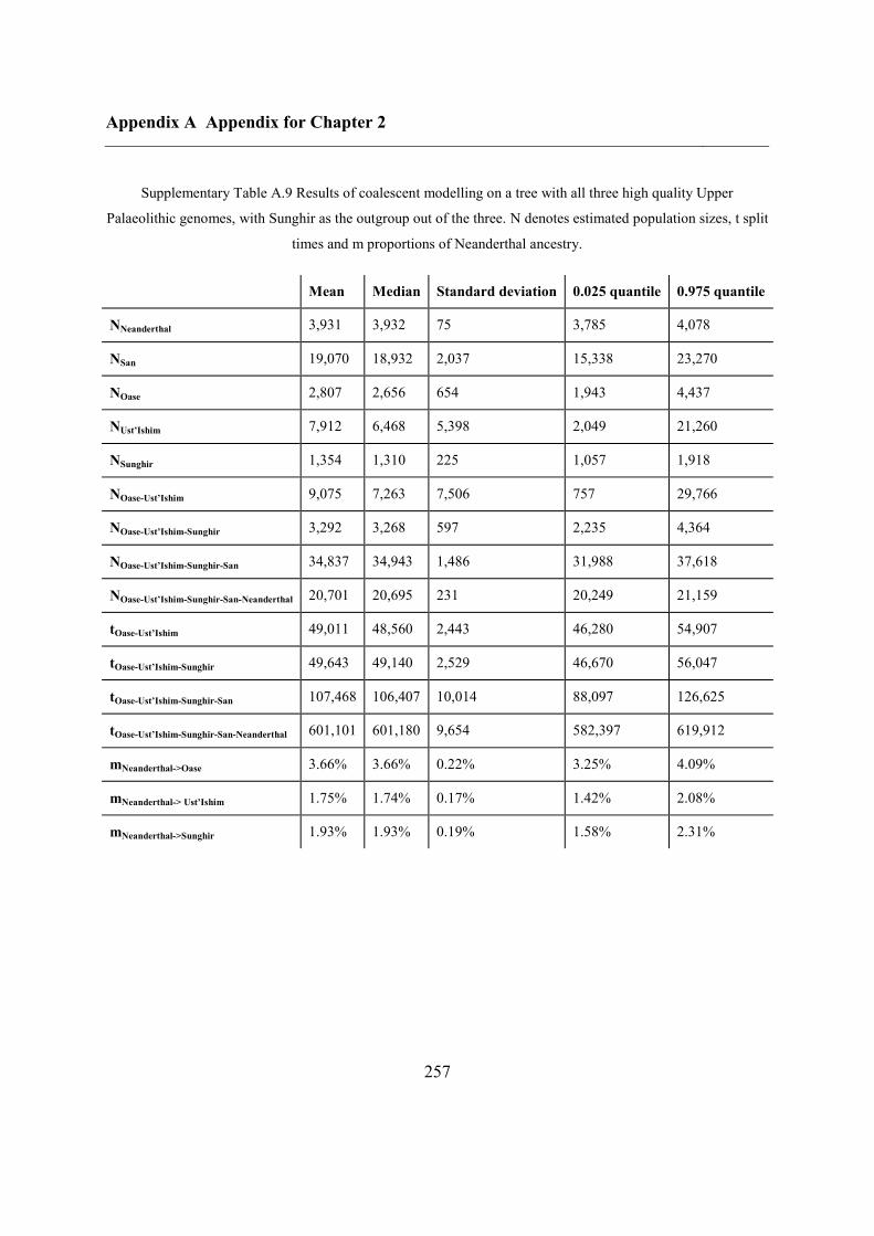
Appendix A Appendix for Chapter 2
257
Supplementary Table A.9 Results of coalescent modelling on a tree with all three high quality Upper
Palaeolithic genomes, with Sunghir as the outgroup out of the three. N denotes estimated population sizes, t split
times and m proportions of Neanderthal ancestry.
Mean Median Standard deviation 0.025 quantile 0.975 quantile
NNeanderthal 3,931 3,932 75 3,785 4,078
NSan 19,070 18,932 2,037 15,338 23,270
NOase 2,807 2,656 654 1,943 4,437
NUst’Ishim 7,912 6,468 5,398 2,049 21,260
NSunghir 1,354 1,310 225 1,057 1,918
NOase-Ust’Ishim 9,075 7,263 7,506 757 29,766
NOase-Ust’Ishim-Sunghir 3,292 3,268 597 2,235 4,364
NOase-Ust’Ishim-Sunghir-San 34,837 34,943 1,486 31,988 37,618
NOase-Ust’Ishim-Sunghir-San-Neanderthal 20,701 20,695 231 20,249 21,159
tOase-Ust’Ishim 49,011 48,560 2,443 46,280 54,907
tOase-Ust’Ishim-Sunghir 49,643 49,140 2,529 46,670 56,047
tOase-Ust’Ishim-Sunghir-San 107,468 106,407 10,014 88,097 126,625
tOase-Ust’Ishim-Sunghir-San-Neanderthal 601,101 601,180 9,654 582,397 619,912
mNeanderthal->Oase 3.66% 3.66% 0.22% 3.25% 4.09%
mNeanderthal-> Ust’Ishim 1.75% 1.74% 0.17% 1.42% 2.08%
mNeanderthal->Sunghir 1.93% 1.93% 0.19% 1.58% 2.31%
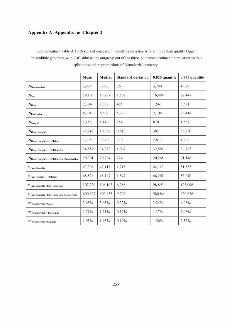
Appendix A Appendix for Chapter 2
258
Supplementary Table A.10 Results of coalescent modelling on a tree with all three high quality Upper
Palaeolithic genomes, with Ust’Ishim as the outgroup out of the three. N denotes estimated population sizes, t
split times and m proportions of Neanderthal ancestry.
Mean Median Standard deviation 0.025 quantile 0.975 quantile
NNeanderthal 3,929 3,928 76 3,780 4,079
NSan 19,103 18,987 1,507 16,494 22,447
NOase 2,394 2,337 485 1,547 3,581
NUst’Ishim 8,391 6,608 5,778 2,108 23,418
NSunghir 1,158 1,146 154 870 1,557
NOase- Sunghir 12,243 10,366 9,613 382 36,830
NOase- Sunghir –Ust’Ishim 3,375 3,320 379 2,813 4,262
NOase- Sunghir –Ust’Ishim-San 34,857 34,928 1,067 32,507 36,765
NOase- Sunghir –Ust’Ishim-San-Neanderthal 20,701 20,704 224 20,265 21,146
tOase- Sunghir 47,306 47,113 1,718 44,113 51,583
tOase-Sunghir –Ust’Ishim 48,526 48,167 1,847 46,207 53,670
tOase- Sunghir –Ust’Ishim-San 107,739 106,103 6,288 98,893 123,096
tOase- Sunghir –Ust’Ishim-San-Neanderthal 600,627 600,653 9,799 580,864 620,076
mNeanderthal->Oase 3.65% 3.65% 0.22% 3.24% 4.08%
mNeanderthal-> Ust’Ishim 1.71% 1.71% 0.17% 1.37% 2.06%
mNeanderthal->Sunghir 1.93% 1.93% 0.19% 1.56% 2.32%

Appendix A Appendix for Chapter 2
259
Supplementary Table A.11 Results of coalescent modelling on a tree with all three high quality Upper
Palaeolithic genomes, with Oase 2 as the outgroup out of the three. N denotes estimated population sizes, t split
times and m proportions of Neanderthal ancestry.
Mean Median Standard deviation 0.025 quantile 0.975 quantile
NNeanderthal 3,925 3,925 74 3,780 4,072
NSan 19,390 19,425 2,356 15,101 23,872
NOase 2,944 2,618 1,036 1,716 5,261
NUst’Ishim 6,621 5,150 5,478 717 20,249
NSunghir 1,170 1,092 198 942 1,638
NSunghir-Ust’Ishim 8,486 6,933 6,993 438 26,946
NSunghir-Ust’Ishim-Oase 3,417 3,456 875 1,791 4,817
NSunghir-Ust’Ishim-Oase-San 34,641 34,640 1,739 31,398 38,027
NSunghir-Ust’Ishim-Oase-San-Neanderthal 20,707 20,707 235 20,239 21,158
tSunghir-Ust’Ishim 47,319 46,120 2,208 45,260 52,553
tSunghir-Ust’Ishim-Oase 49,739 48,487 4,015 45,660 58,516
tSunghir-Ust’Ishim-Oase-San 109,563 109,013 12,290 87,337 131,259
tSunghir-Ust’Ishim-Oase-San-Neanderthal 600,336 600,047 9,837 581,384 619,811
mNeanderthal->Oase 3.60% 3.60% 0.22% 3.18% 4.03%
mNeanderthal-> Ust’Ishim 1.73% 1.73% 0.18% 1.39% 2.08%
mNeanderthal->Sunghir 1.94% 1.94% 0.19% 1.57% 2.33%
Appendix B Appendix for Chapter 3
260
Appendix B Appendix for Chapter 3
B.1 Archaeological context
B.1.1 Kotias Klde
Kotias Klde (Supplementary Figure B.6) is a rockshelter located at 707 m above sea level
(a.s.l.) on a limestone plateau above the Kvirila River in western Georgia. Excavations took
place from 2003-2006 and in 2010. The exposed stratigraphy showed four layers without
attaining bedrock. Below we provide a description of the stratigraphy from top to bottom.
Layer A1 was 30 cm deep and contained the remains of a shallow pit-house, 2.5/3.0 m in
diameter, which was dug into the underlying layers (A2 and B). Though there were a few
pottery shards of Bronze Age and later periods, most of the material at the base of the layer
belonged to the local Late Neolithic period, generally referred to as ‘Eneolithic’. These finds
included a clay figurine84
with nearby charcoal dated to 5,820 ± 40 uncal. BP (OS-90616).
Layer A2 contained a distinct lithic industry with transverse, trapezoid arrowheads. Special
forms of denticulates known as "Lekalo" or "Kmlo" tools85–87
, often retouched on the ventral
face, were represented in this assemblage. Flake scrapers, including the thumb-nail type, were
also found. Blade cores and some production waste (debitage) reflect on-site blade reduction
for secondary shaping of tools. A similar industry was reported in Neolithic sites of the
region such as the Darkveti rockshelter, ca. 5 km away in the Kvirila river gorge88
, and
Appendix B Appendix for Chapter 3
261
Paluri, which is situated further away on the Enguri river86
. Charcoal from this layer was
dated to 7,430 ± 40 uncal. BP (OS-63263).
Layer A2 contained the grave of a complete skeleton from a young adult male (ca. 30-35
years old) whom we have called “Kotias”. The grave was dug from this layer into layer B.
The skeleton was laid in supine position and stones were placed over certain parts of the
skeleton which crushed the skull and covered the knees and lower limb bones. The skull was
angled with the right side facing upwards. Both the right and left hands, which lay along the
side of the skeleton, covered the groin area. A 15 cm long bone splinter was found in the
chest cavity of the specimen below the cervical vertebrae and above the clavicle on the right
side. It cannot be affirmed, however, that this splinter was the cause of death. It appears that
there were some pathological lesions on the right first rib. Other traumatic and degenerative
pathological conditions were evident on the left calcaneus and talus. Attrition of the teeth was
intense, especially when taking the relatively young age of the specimen into consideration.
Two superimposed shallow hearths were exposed some 20 cm above the skeleton’s legs
probably either indicating the sealing of the grave or a later occupation. A sample from one
of the hearths was dated to 8,370 ± 55 uncal. BP (RTT 5220). A tibia from the skeleton was
directly dated to 8,665 ± 65 uncal. BP (RTT 5246) and a mandibular fragment to 8,745 ± 40
uncal. BP (OxA-28256). A combined calibrated plot provided an interval of 9,529-9,895 cal.
BP (95.4%, 2 s.d.).
Layer B, interspersed with limestone fragments, was 50-60cm thick and subdivided into three
sub-layers (B1-B3) all of which contained evidence of Mesolithic industry and animal bones.
A total of nine radiocarbon dates from animal bones and charcoal of this layer yielded a
calibrated interval range of 10,300-13,000 cal. BP. Artefacts were made of flint, radiolarite,
rare crystal rock, and obsidian (the latter was obtained from exposures some 80 km away).
The main tool groups were backed and retouched bladelets. Numerous scalene triangles
shaped by bi-polar retouch from blades and bladelets define the Mesolithic industry89
. In
Appendix B Appendix for Chapter 3
262
addition, a few bone tools were recovered, including a handle made of a red deer antler
hollowed for hafting a tool, as well as several point tips.
Layer C, consisting of yellow, compact clay/loamy sediment, was exposed to a very limited
extent. The lithic industry was of Upper Palaeolithic age characterized by blade production
and the presence of end-scrapers and burins. A total of 9 radiocarbon dates from animal
bones and charcoal of this layer yielded a calibrated interval range of 22,200-23,600 cal. BP.
The time gap between these two occupations (Layers B and C) indicates that the cave was not
inhabited during the Last Glacial Maximum (LGM) and for quite some time after the LGM
until the Younger Dryas and the first millennium of the Holocene.
B.1.2 Satsurblia
Satsurblia cave in western Georgia (Supplementary Figure B.6) was discovered in 1975 by A.
N. Kalandadze90
who excavated it sporadically during 1976, 1985–88 and 1990-199391
. A
second series of excavations was conducted during 2008–2010, directed by Tengiz
Meshveliani.
Further excavations in Satsurblia (2012-2013), directed by Tengiz Meshveliani and Ron
Pinhasi, were conducted in two areas. Area A was situated in the north-western part of the
cave, near the entrance (squares R−T 20−24) and Area B was to the rear of the cave (squares
T−Z 4−7), adjacent to a trench excavated by K. Kalandadze in the 1980s. Both areas revealed
stratigraphic sequences comprising Pleistocene (Upper Palaeolithic) and Holocene
(Eneolithic and later) deposits. Excavations in 2012 and 2013 focused on Areas A and B with
both yielding in situ Upper Palaeolithic layers that were extremely rich in finds (a circular
fireplace, large quantities of charcoal and brunt bones, lithics, bone tools, shell ornaments,
yellow ochre) and which continued to unknown depth. The Upper Palaeolithic sequence of
Area A was divided into two main units: A/I and A/II. A/II contained a sequence of living
surfaces which were dated (surface II and III) to 17,000-18,000 cal. BP and as such are the
first well-dated evidence for human occupation in the southern Caucasus at the end of the
Appendix B Appendix for Chapter 3
263
LGM. This fills a gap in the Upper Palaeolithic sequence, namely that between Unit C and
Unit B in Dzudzuana Cave (western Georgia), dated to 27,000-24,000 cal. BP and 16,000 cal.
BP - 13,200 cal. BP respectively.
Preliminary analyses of lithics from Satsurblia cave reveal a cultural variant which resembles
Eastern Epi-Gravettian industries, dominated by bladelets and including varieties of
microgravette points and bigger gravette points. A rectangular tool type was novel to
excavations from the region and differed from the geometric trapezoid-rectangle tools of the
proceeding Mesolithic cultures in size, shape and retouch92
Direct AMS dating of human
remains from Area B yielded the first securely dated Upper Palaeolithic human remains from
the Caucasus. “Satsurblia” was sampled from a right temporal bone which was recovered in
2013 from square Y5 and dated to 11,415 ± 50 uncal. BP (OxA-34632). A combined
calibrated plot provided an interval of 13,132-13,380 cal. BP (95.4%, 2 s.d.).
B.1.3 Grotte du Bichon
The small cave “Grotte du Bichon” is situated in the Swiss Jura Mountains, a few kilometres
north of the city of La Chaux-de-Fonds (canton Neuchâtel), at an altitude of 845 m a.s.l.
(Supplementary Figure B.6). During its first excavation, undertaken by speleologists in 1956,
bones of a young man were discovered intermingled with the remains of a female brown bear
(Ursus arctos) and nine flint projectile points, apparently stemming from the hunter’s
weapons.
Both skeletons as well as the flints were located about 15 m from the entrance, at a recess of
the cave, and were associated with charcoal concentrations but with no other archaeological
material. Although a hunting accident was already envisioned at that time, without further
indications the remains of the bear were considered not to be related to the human skeleton
and therefore stored at the natural history museum of La Chaux-de-Fonds, while the human
bones and the flints were kept in the archaeology museum of Neuchâtel (Laténium).
Appendix B Appendix for Chapter 3
264
Only in 1991, during re-examination of the animal bone material, archaeozoologist Philippe
Morel discovered an impact trace and two flint chips (probably a broken tip of an arrowhead)
in a cervical vertebra of the bear, thus establishing a clear connection between the animal and
the man93
. This discovery prompted new excavations that were carried out between 1991 and
1995. During these new investigations, using modern excavation techniques (including water
sieving), all of the missing long bones from the two skeletons were recovered, together with
some more flint artefacts. The small lithic assemblage now contained 10 backed points, 16
backed bladelets and one retouched blade fragment, characteristic of final (Azilian)
Palaeolithic industries. It seems that the cave was never used as a camp site as unretouched
debitage products were not recovered. Four radiocarbon measurements performed on the
bones from the bear and the man (two on each) and eight dates obtained from charcoal, from
willow (Salix sp.) and from pine (Pinus sylvestis) ranged from 10,950 to 11,760 uncal. BP94
.
A new direct date on the human skeleton 11,855 ± 50 uncal. BP (OxA-27763) or 13,560-
13,770 cal. BP (95.4% CI, previously unpublished) is in agreement with the dates of the
charcoal and pine.
The human skeleton was determined to be of a young male, 20-23 years of age, of the Cro-
magnon type. According to the cranio-facial architecture, it was characterized by classical
cranio-facial disharmony, i.e. a relatively long skull associated with a low face and sub-
rectangular eye-sockets, which are quite typical of the time period. The young man weighed a
little over 60 kg and stood 1.64 m tall. Although of a relatively slender build, muscle
attachments showed him to have been a strong runner and well adapted to mountainous
terrain95
. His upper limbs show a high degree of asymmetry, indicative of preferential use of
the right arm96
. Isotopic studies of carbon and nitrogen fractionations indicated a largely meat
based terrestrial diet97
.
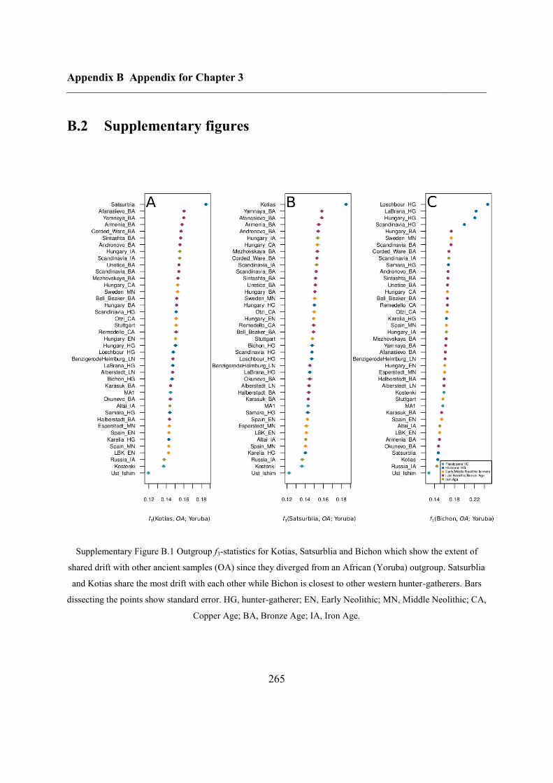
Appendix B Appendix for Chapter 3
265
B.2 Supplementary figures
Supplementary Figure B.1 Outgroup f3-statistics for Kotias, Satsurblia and Bichon which show the extent of
shared drift with other ancient samples (OA) since they diverged from an African (Yoruba) outgroup. Satsurblia
and Kotias share the most drift with each other while Bichon is closest to other western hunter-gatherers. Bars
dissecting the points show standard error. HG, hunter-gatherer; EN, Early Neolithic; MN, Middle Neolithic; CA,
Copper Age; BA, Bronze Age; IA, Iron Age.
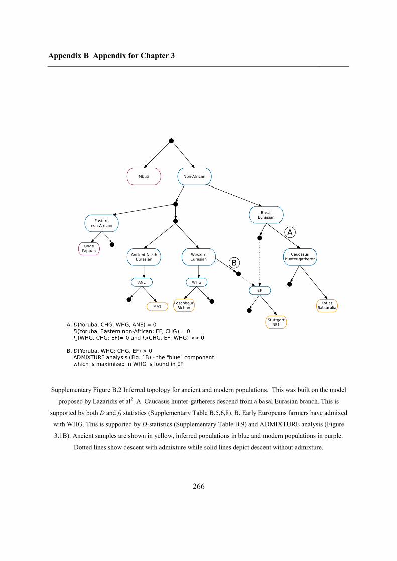
Appendix B Appendix for Chapter 3
266
Supplementary Figure B.2 Inferred topology for ancient and modern populations. This was built on the model
proposed by Lazaridis et al2. A. Caucasus hunter-gatherers descend from a basal Eurasian branch. This is
supported by both D and f3 statistics (Supplementary Table B.5,6,8). B. Early Europeans farmers have admixed
with WHG. This is supported by D-statistics (Supplementary Table B.9) and ADMIXTURE analysis (Figure
3.1B). Ancient samples are shown in yellow, inferred populations in blue and modern populations in purple.
Dotted lines show descent with admixture while solid lines depict descent without admixture.
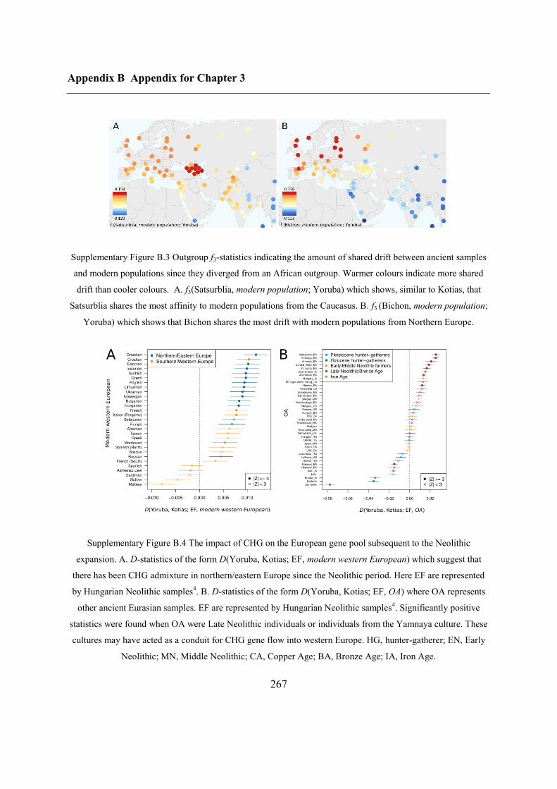
Appendix B Appendix for Chapter 3
267
Supplementary Figure B.3 Outgroup f3-statistics indicating the amount of shared drift between ancient samples
and modern populations since they diverged from an African outgroup. Warmer colours indicate more shared
drift than cooler colours. A. f3(Satsurblia, modern population; Yoruba) which shows, similar to Kotias, that
Satsurblia shares the most affinity to modern populations from the Caucasus. B. f3 (Bichon, modern population;
Yoruba) which shows that Bichon shares the most drift with modern populations from Northern Europe.
Supplementary Figure B.4 The impact of CHG on the European gene pool subsequent to the Neolithic
expansion. A. D-statistics of the form D(Yoruba, Kotias; EF, modern western European) which suggest that
there has been CHG admixture in northern/eastern Europe since the Neolithic period. Here EF are represented
by Hungarian Neolithic samples4. B. D-statistics of the form D(Yoruba, Kotias; EF, OA) where OA represents
other ancient Eurasian samples. EF are represented by Hungarian Neolithic samples4. Significantly positive
statistics were found when OA were Late Neolithic individuals or individuals from the Yamnaya culture. These
cultures may have acted as a conduit for CHG gene flow into western Europe. HG, hunter-gatherer; EN, Early
Neolithic; MN, Middle Neolithic; CA, Copper Age; BA, Bronze Age; IA, Iron Age.
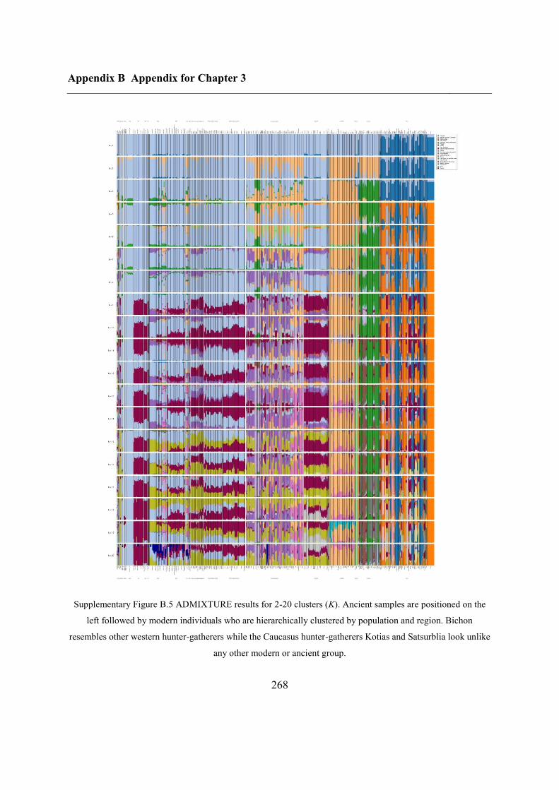
Appendix B Appendix for Chapter 3
268
Supplementary Figure B.5 ADMIXTURE results for 2-20 clusters (K). Ancient samples are positioned on the
left followed by modern individuals who are hierarchically clustered by population and region. Bichon
resembles other western hunter-gatherers while the Caucasus hunter-gatherers Kotias and Satsurblia look unlike
any other modern or ancient group.
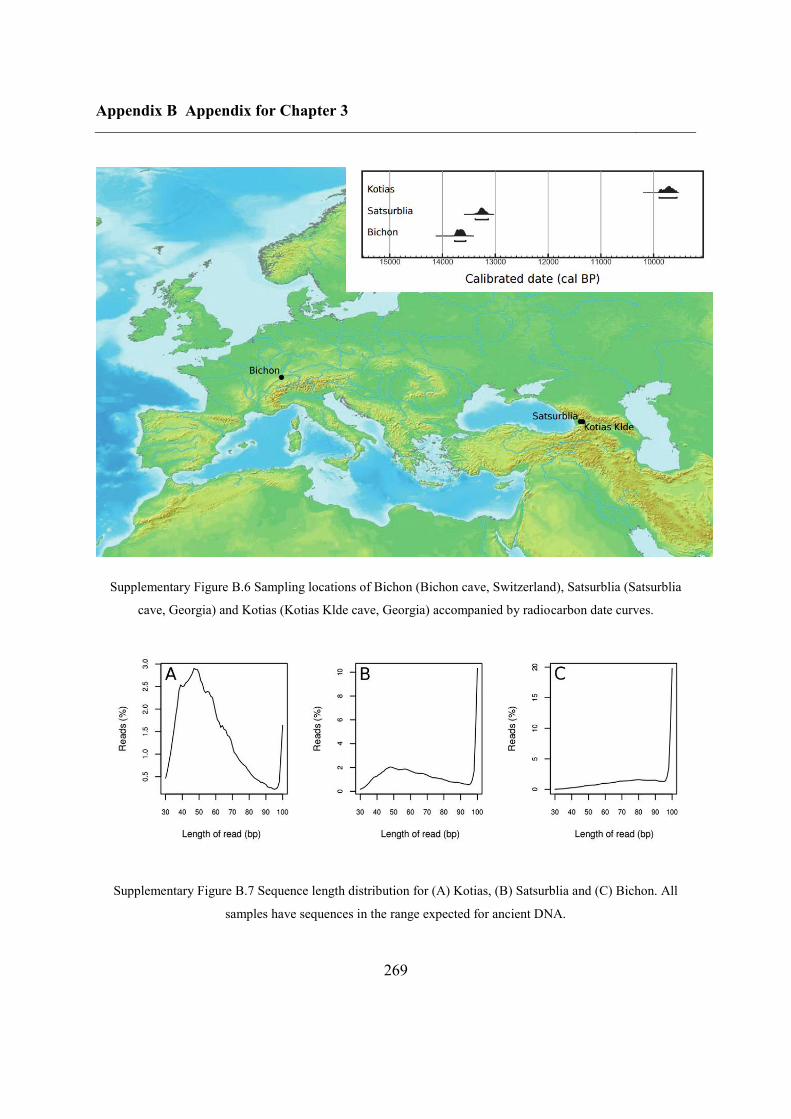
Appendix B Appendix for Chapter 3
269
Supplementary Figure B.6 Sampling locations of Bichon (Bichon cave, Switzerland), Satsurblia (Satsurblia
cave, Georgia) and Kotias (Kotias Klde cave, Georgia) accompanied by radiocarbon date curves.
Supplementary Figure B.7 Sequence length distribution for (A) Kotias, (B) Satsurblia and (C) Bichon. All
samples have sequences in the range expected for ancient DNA.
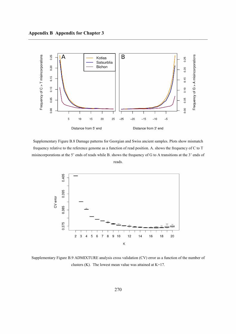
Appendix B Appendix for Chapter 3
270
Supplementary Figure B.8 Damage patterns for Georgian and Swiss ancient samples. Plots show mismatch
frequency relative to the reference genome as a function of read position. A. shows the frequency of C to T
misincorporations at the 5’ ends of reads while B. shows the frequency of G to A transitions at the 3’ ends of
reads.
Supplementary Figure B.9 ADMIXTURE analysis cross validation (CV) error as a function of the number of
clusters (K). The lowest mean value was attained at K=17.
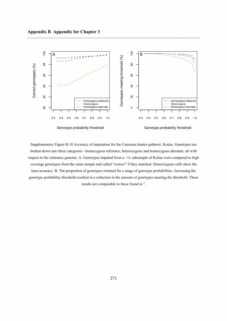
Appendix B Appendix for Chapter 3
271
Supplementary Figure B.10 Accuracy of imputation for the Caucasus hunter-gatherer, Kotias. Genotypes are
broken down into three categories - homozygous reference, heterozygous and homozygous alternate, all with
respect to the reference genome. A. Genotypes imputed from a ~1x subsample of Kotias were compared to high
coverage genotypes from the same sample and called “correct” if they matched. Heterozygous calls show the
least accuracy. B. The proportion of genotypes retained for a range of genotype probabilities. Increasing the
genotype probability threshold resulted in a reduction in the amount of genotypes meeting the threshold. These
results are comparable to those found in 2.
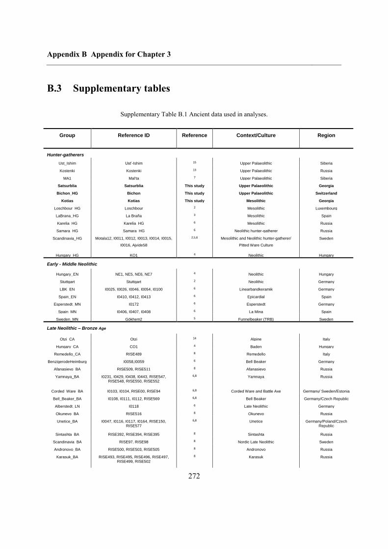
Appendix B Appendix for Chapter 3
272
B.3 Supplementary tables
Supplementary Table B.1 Ancient data used in analyses.
Group Reference ID Reference Context/Culture Region
Hunter-gatherers Ust_Ishim Ust’-Ishim 15
Upper Palaeolithic Siberia Kostenki Kostenki 13
Upper Palaeolithic Russia MA1 Mal'ta 7
Upper Palaeolithic Siberia Satsurblia Satsurblia This study Upper Palaeolithic Georgia
Bichon_HG Bichon This study Upper Palaeolithic Switzerland Kotias Kotias This study Mesolithic Georgia
Loschbour_HG Loschbour 2 Mesolithic Luxembourg
LaBrana_HG La Braña 3 Mesolithic Spain
Karelia_HG Karelia_HG 6 Mesolithic Russia
Samara_HG Samara_HG 6 Neolithic hunter-gatherer Russia
Scandinavia_HG Motala12, I0011, I0012, I0013, I0014, I0015,
I0016, Ajvide58 2,5,6
Mesolithic and Neolithic hunter-gatherer/
Pitted Ware Culture Sweden
Hungary_HG KO1 4 Neolithic Hungary
Early - Middle Neolithic
Hungary_EN NE1, NE5, NE6, NE7 4 Neolithic Hungary
Stuttgart Stuttgart 2 Neolithic Germany
LBK_EN I0025, I0026, I0046, I0054, I0100 6 Linearbandkeramik Germany
Spain_EN I0410, I0412, I0413 6 Epicardial Spain
Esperstedt_MN I0172 6 Esperstedt Germany
Spain_MN I0406, I0407, I0408 6 La Mina Spain
Sweden_MN Gökhem2 5 Funnelbeaker (TRB) Sweden
Late Neolithic – Bronze Age
Otzi_CA Otzi 14 Alpine Italy
Hungary_CA CO1 4 Baden Hungary
Remedello_CA RISE489 8 Remedello Italy
BenzigerodeHeimburg_LN
I0058,I0059 6 Bell Beaker Germany
Afanasievo_BA RISE509, RISE511 8 Afanasievo Russia
Yamnaya_BA I0231, I0429, I0438, I0443, RISE547, RISE548, RISE550, RISE552
6,8 Yamnaya Russia
Corded_Ware_BA I0103, I0104, RISE00, RISE94 6,8 Corded Ware and Battle Axe Germany/ Sweden/Estonia
Bell_Beaker_BA I0108, I0111, I0112, RISE569 6,8 Bell Beaker Germany/Czech Republic
Alberstedt_LN I0118 6 Late Neolithic Germany
Okunevo_BA RISE516 8 Okunevo Russia
Unetice_BA I0047, I0116, I0117, I0164, RISE150, RISE577
6,8 Unetice Germany/Poland/Czech
Republic Sintashta_BA RISE392, RISE394, RISE395 8
Sintashta Russia Scandinavia_BA RISE97, RISE98 8
Nordic Late Neolithic Sweden Andronovo_BA RISE500, RISE503, RISE505 8
Andronovo Russia Karasuk_BA RISE493, RISE495, RISE496, RISE497,
RISE499, RISE502 8 Karasuk Russia
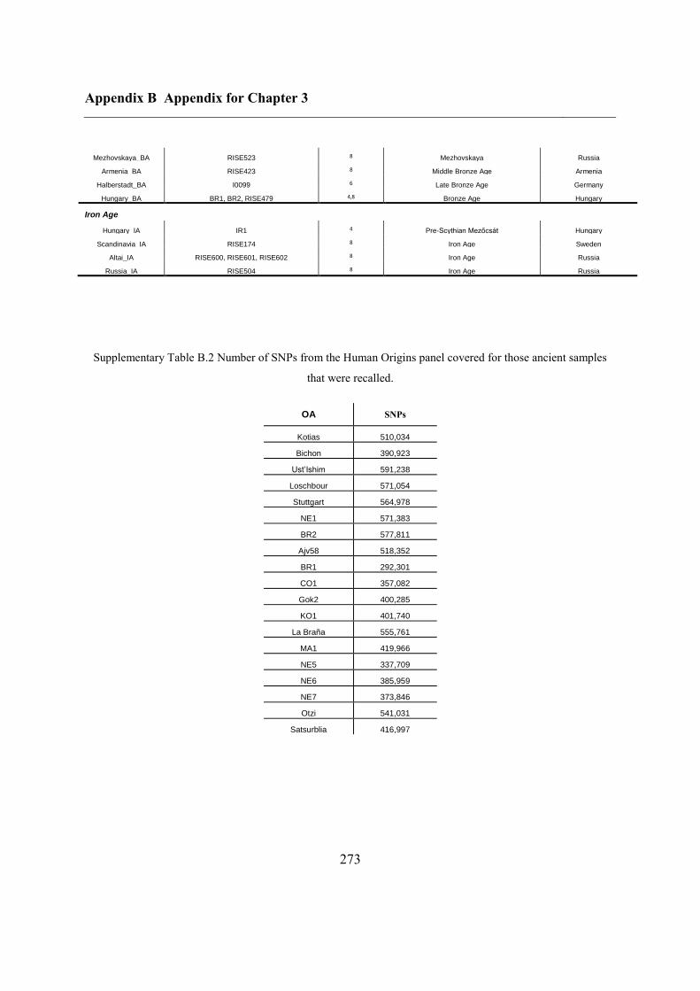
Appendix B Appendix for Chapter 3
273
Mezhovskaya_BA RISE523 8 Mezhovskaya Russia
Armenia_BA RISE423 8 Middle Bronze Age Armenia
Halberstadt_BA I0099 6 Late Bronze Age Germany
Hungary_BA BR1, BR2, RISE479 4,8 Bronze Age Hungary
Iron Age Hungary_IA IR1 4
Pre-Scythian Mezőcsát Hungary Scandinavia_IA RISE174 8
Iron Age Sweden Altai_IA RISE600, RISE601, RISE602 8
Iron Age Russia Russia_IA RISE504 8
Iron Age Russia
Supplementary Table B.2 Number of SNPs from the Human Origins panel covered for those ancient samples
that were recalled.
OA SNPs
Kotias 510,034
Bichon 390,923
Ust’Ishim 591,238
Loschbour 571,054
Stuttgart 564,978
NE1 571,383
BR2 577,811
Ajv58 518,352
BR1 292,301
CO1 357,082
Gok2 400,285
KO1 401,740
La Braña 555,761
MA1 419,966
NE5 337,709
NE6 385,959
NE7 373,846
Otzi 541,031
Satsurblia 416,997
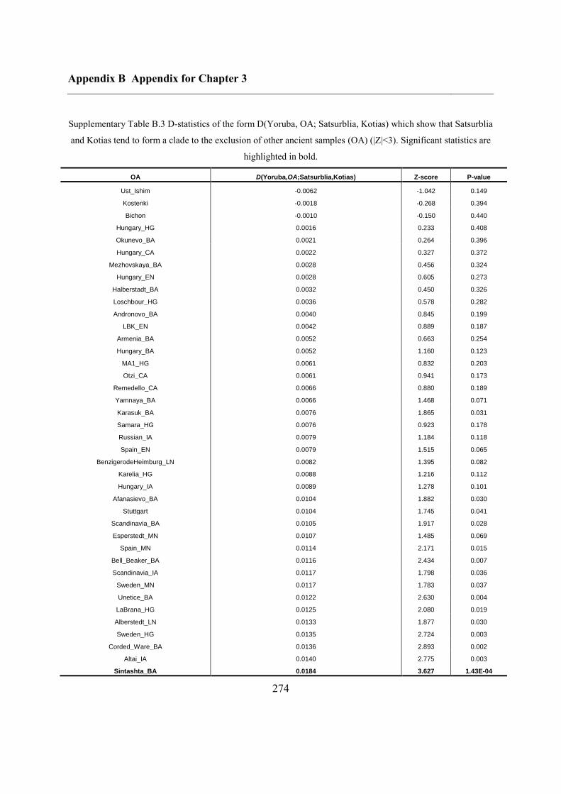
Appendix B Appendix for Chapter 3
274
Supplementary Table B.3 D-statistics of the form D(Yoruba, OA; Satsurblia, Kotias) which show that Satsurblia
and Kotias tend to form a clade to the exclusion of other ancient samples (OA) (|Z|<3). Significant statistics are
highlighted in bold.
OA D(Yoruba,OA;Satsurblia,Kotias) Z-score P-value
Ust_Ishim -0.0062 -1.042 0.149 Kostenki -0.0018 -0.268 0.394 Bichon -0.0010 -0.150 0.440
Hungary_HG 0.0016 0.233 0.408 Okunevo_BA 0.0021 0.264 0.396 Hungary_CA 0.0022 0.327 0.372
Mezhovskaya_BA 0.0028 0.456 0.324 Hungary_EN 0.0028 0.605 0.273
Halberstadt_BA 0.0032 0.450 0.326 Loschbour_HG 0.0036 0.578 0.282 Andronovo_BA 0.0040 0.845 0.199
LBK_EN 0.0042 0.889 0.187 Armenia_BA 0.0052 0.663 0.254 Hungary_BA 0.0052 1.160 0.123
MA1_HG 0.0061 0.832 0.203 Otzi_CA 0.0061 0.941 0.173
Remedello_CA 0.0066 0.880 0.189 Yamnaya_BA 0.0066 1.468 0.071 Karasuk_BA 0.0076 1.865 0.031 Samara_HG 0.0076 0.923 0.178 Russian_IA 0.0079 1.184 0.118 Spain_EN 0.0079 1.515 0.065
BenzigerodeHeimburg_LN 0.0082 1.395 0.082 Karelia_HG 0.0088 1.216 0.112 Hungary_IA 0.0089 1.278 0.101
Afanasievo_BA 0.0104 1.882 0.030 Stuttgart 0.0104 1.745 0.041
Scandinavia_BA 0.0105 1.917 0.028 Esperstedt_MN 0.0107 1.485 0.069
Spain_MN 0.0114 2.171 0.015 Bell_Beaker_BA 0.0116 2.434 0.007 Scandinavia_IA 0.0117 1.798 0.036
Sweden_MN 0.0117 1.783 0.037 Unetice_BA 0.0122 2.630 0.004
LaBrana_HG 0.0125 2.080 0.019 Alberstedt_LN 0.0133 1.877 0.030 Sweden_HG 0.0135 2.724 0.003
Corded_Ware_BA 0.0136 2.893 0.002 Altai_IA 0.0140 2.775 0.003
Sintashta_BA 0.0184 3.627 1.43E-04
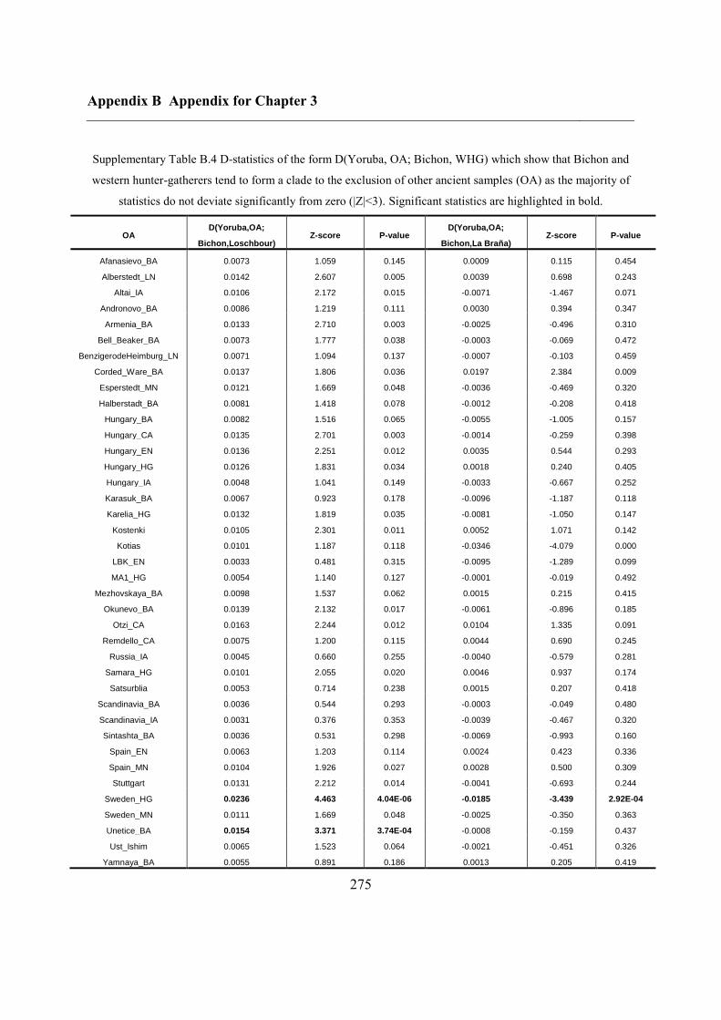
Appendix B Appendix for Chapter 3
275
Supplementary Table B.4 D-statistics of the form D(Yoruba, OA; Bichon, WHG) which show that Bichon and
western hunter-gatherers tend to form a clade to the exclusion of other ancient samples (OA) as the majority of
statistics do not deviate significantly from zero (|Z|<3). Significant statistics are highlighted in bold.
OA D(Yoruba,OA;
Bichon,Loschbour) Z-score P-value
D(Yoruba,OA; Bichon,La Braña)
Z-score P-value
Afanasievo_BA 0.0073 1.059 0.145 0.0009 0.115 0.454 Alberstedt_LN 0.0142 2.607 0.005 0.0039 0.698 0.243
Altai_IA 0.0106 2.172 0.015 -0.0071 -1.467 0.071 Andronovo_BA 0.0086 1.219 0.111 0.0030 0.394 0.347 Armenia_BA 0.0133 2.710 0.003 -0.0025 -0.496 0.310
Bell_Beaker_BA 0.0073 1.777 0.038 -0.0003 -0.069 0.472 BenzigerodeHeimburg_LN 0.0071 1.094 0.137 -0.0007 -0.103 0.459
Corded_Ware_BA 0.0137 1.806 0.036 0.0197 2.384 0.009 Esperstedt_MN 0.0121 1.669 0.048 -0.0036 -0.469 0.320 Halberstadt_BA 0.0081 1.418 0.078 -0.0012 -0.208 0.418
Hungary_BA 0.0082 1.516 0.065 -0.0055 -1.005 0.157 Hungary_CA 0.0135 2.701 0.003 -0.0014 -0.259 0.398 Hungary_EN 0.0136 2.251 0.012 0.0035 0.544 0.293 Hungary_HG 0.0126 1.831 0.034 0.0018 0.240 0.405 Hungary_IA 0.0048 1.041 0.149 -0.0033 -0.667 0.252 Karasuk_BA 0.0067 0.923 0.178 -0.0096 -1.187 0.118 Karelia_HG 0.0132 1.819 0.035 -0.0081 -1.050 0.147
Kostenki 0.0105 2.301 0.011 0.0052 1.071 0.142 Kotias 0.0101 1.187 0.118 -0.0346 -4.079 0.000
LBK_EN 0.0033 0.481 0.315 -0.0095 -1.289 0.099 MA1_HG 0.0054 1.140 0.127 -0.0001 -0.019 0.492
Mezhovskaya_BA 0.0098 1.537 0.062 0.0015 0.215 0.415 Okunevo_BA 0.0139 2.132 0.017 -0.0061 -0.896 0.185
Otzi_CA 0.0163 2.244 0.012 0.0104 1.335 0.091 Remdello_CA 0.0075 1.200 0.115 0.0044 0.690 0.245
Russia_IA 0.0045 0.660 0.255 -0.0040 -0.579 0.281 Samara_HG 0.0101 2.055 0.020 0.0046 0.937 0.174 Satsurblia 0.0053 0.714 0.238 0.0015 0.207 0.418
Scandinavia_BA 0.0036 0.544 0.293 -0.0003 -0.049 0.480 Scandinavia_IA 0.0031 0.376 0.353 -0.0039 -0.467 0.320 Sintashta_BA 0.0036 0.531 0.298 -0.0069 -0.993 0.160
Spain_EN 0.0063 1.203 0.114 0.0024 0.423 0.336 Spain_MN 0.0104 1.926 0.027 0.0028 0.500 0.309 Stuttgart 0.0131 2.212 0.014 -0.0041 -0.693 0.244
Sweden_HG 0.0236 4.463 4.04E-06 -0.0185 -3.439 2.92E-04 Sweden_MN 0.0111 1.669 0.048 -0.0025 -0.350 0.363 Unetice_BA 0.0154 3.371 3.74E-04 -0.0008 -0.159 0.437 Ust_Ishim 0.0065 1.523 0.064 -0.0021 -0.451 0.326
Yamnaya_BA 0.0055 0.891 0.186 0.0013 0.205 0.419
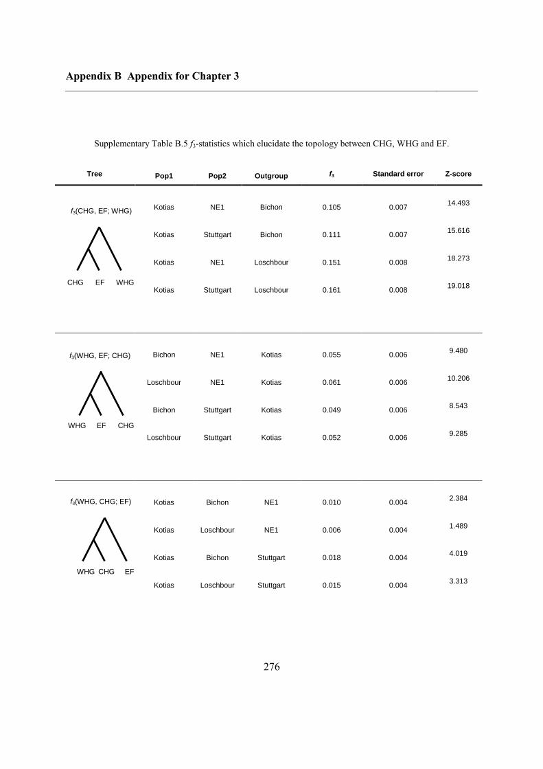
Appendix B Appendix for Chapter 3
276
Supplementary Table B.5 f3-statistics which elucidate the topology between CHG, WHG and EF.
Tree Pop1 Pop2 Outgroup f3 Standard error Z-score
Kotias NE1 Bichon 0.105 0.007 14.493
Kotias Stuttgart Bichon 0.111 0.007 15.616
Kotias NE1 Loschbour 0.151 0.008 18.273
Kotias Stuttgart Loschbour 0.161 0.008 19.018
Bichon NE1 Kotias 0.055 0.006 9.480
Loschbour NE1 Kotias 0.061 0.006 10.206
Bichon Stuttgart Kotias 0.049 0.006 8.543
Loschbour Stuttgart Kotias 0.052 0.006 9.285
Kotias Bichon NE1 0.010 0.004 2.384
Kotias Loschbour NE1 0.006 0.004 1.489
Kotias Bichon Stuttgart 0.018 0.004 4.019
Kotias Loschbour Stuttgart 0.015 0.004 3.313
f3(CHG, EF; WHG)
f3(WHG, EF; CHG)
f3(WHG, CHG; EF)
CHG EF WHG
WHG EF CHG
WHG CHG EF
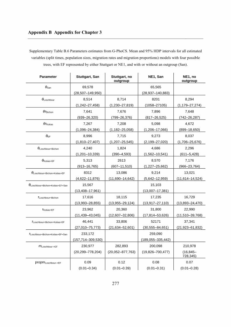
Appendix B Appendix for Chapter 3
277
Supplementary Table B.6 Parameters estimates from G-PhoCS. Mean and 95% HDP intervals for all estimated
variables (split times, population sizes, migration rates and migration proportions) models with four possible
trees, with EF represented by either Stuttgart or NE1, and with or without an outgroup (San).
Parameter Stuttgart, San Stuttgart, no outgroup
NE1, San NE1, no outgroup
θSan 69,578
(28,507–149,950) 65,565
(28,937–140,883)
θLoschbour 8,514
(1,242–27,458)
8,714
(1,230–27,819)
8201
(1058–27105)
8,294
(1,179–27,274)
θτBichon 7,641
(939–26,320)
7,676
(799–26,376)
7,896
(817–26,525)
7,648
(742–26,287)
θτKotias 7,267
(1,096–24,384)
7,208
(1,182–25,058)
5,098
(1,206–17,066)
4,672
(899–18,650)
θEF 8,996
(1,810–27,407)
7,715
(1,207–25,545)
9,273
(2,199–27,020)
8,037
(1,706–25,676)
θLoschbour+Bichon 4,240
(1,201–10,339)
1,824
(390–4,593)
4,686
(1,562–10,541)
2,296
(611–5,428)
θKotias+EF 5,313
(913–16,765)
2613
(607–11,510)
8,570
(1,227–25,662)
7,176
(966–23,764)
θLoschbour+Bichon+Kotias+EF 8312
(4,622–11,876)
13,086
(11,690–14,642)
9,214
(5,642–12,959)
13,021
(11,614–14,524)
θLoschbour+Bichon+Kotias+EF+San 15,567
(13,408–17,961) 15,103
(13,007–17,381)
τLoschbour+Bichon 17,616
(13,993–28,855)
18,115
(13,955–29,124)
17,235
(13,917–27,110)
16,729
(13,893–24,470)
τKotias+EF 23,962
(11,439–43,045)
20,360
(12,607–32,806)
31,800
(17,814–53,626)
22,990
(11,510–39,768)
τLoschbour+Bichon+Kotias+EF 46,441
(27,010–75,773)
33,806
(21,634–52,601)
52171
(30,555–84,651)
37,341
(21,923–61,832)
τLoschbour+Bichon+Kotias+EF+San 233,172
(157,714–309,530) 259,090
(189,055–335,442)
mLoschbour->EF 230,977
(20,299–778,204)
282,893
(20,052–877,763)
200,098
(19,826–700,477)
210,978
(16,845–728,345)
propmLoschbour->EF 0.09
(0.01–0.34)
0.12
(0.01–0.39)
0.08
(0.01–0.31)
0.07
(0.01–0.28)
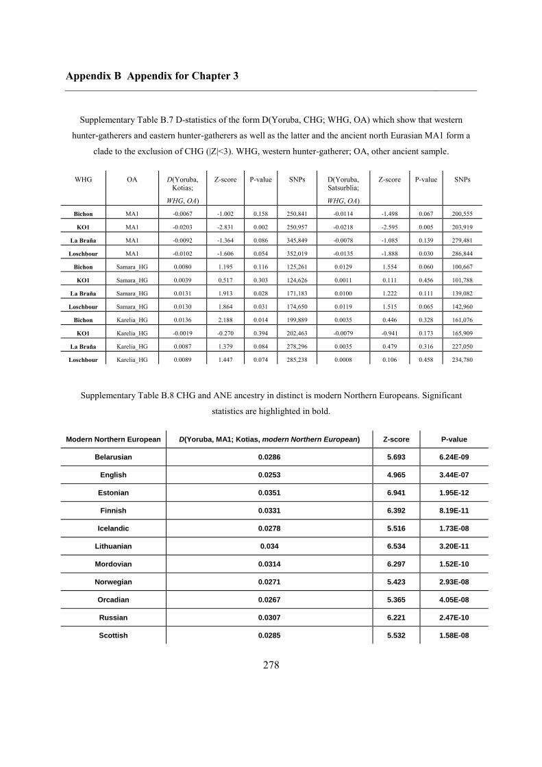
Appendix B Appendix for Chapter 3
278
Supplementary Table B.7 D-statistics of the form D(Yoruba, CHG; WHG, OA) which show that western
hunter-gatherers and eastern hunter-gatherers as well as the latter and the ancient north Eurasian MA1 form a
clade to the exclusion of CHG (|Z|<3). WHG, western hunter-gatherer; OA, other ancient sample.
WHG OA D(Yoruba, Kotias;
WHG, OA)
Z-score P-value SNPs D(Yoruba, Satsurblia;
WHG, OA)
Z-score P-value SNPs
Bichon MA1 -0.0067 -1.002 0.158 250,841 -0.0114 -1.498 0.067 200,555
KO1 MA1 -0.0203 -2.831 0.002 250,957 -0.0218 -2.595 0.005 203,919
La Braña MA1 -0.0092 -1.364 0.086 345,849 -0.0078 -1.085 0.139 279,481
Loschbour MA1 -0.0102 -1.606 0.054 352,019 -0.0135 -1.888 0.030 286,844
Bichon Samara_HG 0.0080 1.195 0.116 125,261 0.0129 1.554 0.060 100,667
KO1 Samara_HG 0.0039 0.517 0.303 124,626 0.0011 0.111 0.456 101,788
La Braña Samara_HG 0.0131 1.913 0.028 171,183 0.0100 1.222 0.111 139,082
Loschbour Samara_HG 0.0130 1.864 0.031 174,650 0.0119 1.515 0.065 142,960
Bichon Karelia_HG 0.0136 2.188 0.014 199,889 0.0035 0.446 0.328 161,076
KO1 Karelia_HG -0.0019 -0.270 0.394 202,463 -0.0079 -0.941 0.173 165,909
La Braña Karelia_HG 0.0087 1.379 0.084 278,296 0.0035 0.479 0.316 227,050
Loschbour Karelia_HG 0.0089 1.447 0.074 285,238 0.0008 0.106 0.458 234,780
Supplementary Table B.8 CHG and ANE ancestry in distinct is modern Northern Europeans. Significant
statistics are highlighted in bold.
Modern Northern European D(Yoruba, MA1; Kotias, modern Northern European) Z-score P-value
Belarusian 0.0286 5.693 6.24E-09
English 0.0253 4.965 3.44E-07
Estonian 0.0351 6.941 1.95E-12
Finnish 0.0331 6.392 8.19E-11
Icelandic 0.0278 5.516 1.73E-08
Lithuanian 0.034 6.534 3.20E-11
Mordovian 0.0314 6.297 1.52E-10
Norwegian 0.0271 5.423 2.93E-08
Orcadian 0.0267 5.365 4.05E-08
Russian 0.0307 6.221 2.47E-10
Scottish 0.0285 5.532 1.58E-08
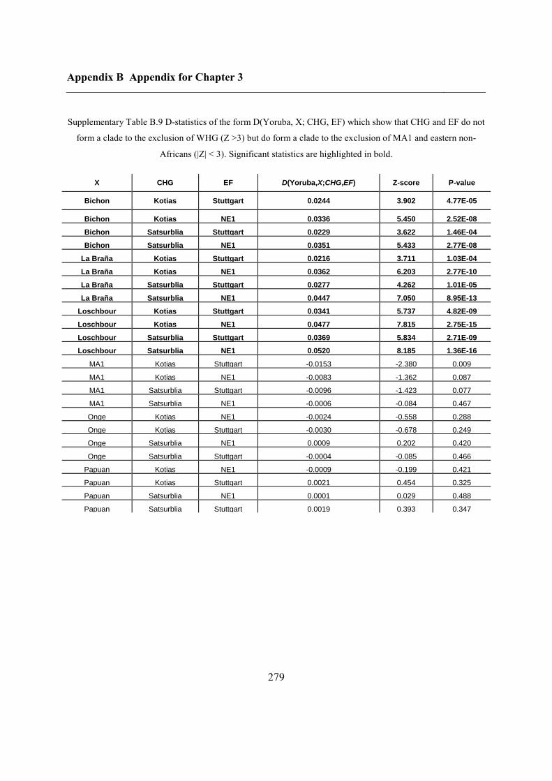
Appendix B Appendix for Chapter 3
279
Supplementary Table B.9 D-statistics of the form D(Yoruba, X; CHG, EF) which show that CHG and EF do not
form a clade to the exclusion of WHG (Z >3) but do form a clade to the exclusion of MA1 and eastern non-
Africans (|Z| < 3). Significant statistics are highlighted in bold.
X CHG EF D(Yoruba,X;CHG,EF) Z-score P-value
Bichon Kotias Stuttgart 0.0244 3.902 4.77E-05
Bichon Kotias NE1 0.0336 5.450 2.52E-08
Bichon Satsurblia Stuttgart 0.0229 3.622 1.46E-04
Bichon Satsurblia NE1 0.0351 5.433 2.77E-08
La Braña Kotias Stuttgart 0.0216 3.711 1.03E-04
La Braña Kotias NE1 0.0362 6.203 2.77E-10
La Braña Satsurblia Stuttgart 0.0277 4.262 1.01E-05
La Braña Satsurblia NE1 0.0447 7.050 8.95E-13
Loschbour Kotias Stuttgart 0.0341 5.737 4.82E-09
Loschbour Kotias NE1 0.0477 7.815 2.75E-15
Loschbour Satsurblia Stuttgart 0.0369 5.834 2.71E-09
Loschbour Satsurblia NE1 0.0520 8.185 1.36E-16
MA1 Kotias Stuttgart -0.0153 -2.380 0.009
MA1 Kotias NE1 -0.0083 -1.362 0.087
MA1 Satsurblia Stuttgart -0.0096 -1.423 0.077
MA1 Satsurblia NE1 -0.0006 -0.084 0.467
Onge Kotias NE1 -0.0024 -0.558 0.288
Onge Kotias Stuttgart -0.0030 -0.678 0.249
Onge Satsurblia NE1 0.0009 0.202 0.420
Onge Satsurblia Stuttgart -0.0004 -0.085 0.466
Papuan Kotias NE1 -0.0009 -0.199 0.421
Papuan Kotias Stuttgart 0.0021 0.454 0.325
Papuan Satsurblia NE1 0.0001 0.029 0.488
Papuan Satsurblia Stuttgart 0.0019 0.393 0.347
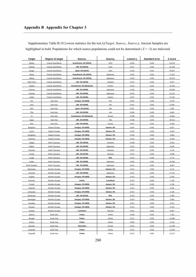
Appendix B Appendix for Chapter 3
280
Supplementary Table B.10 Lowest statistics for the test f3(Target; Source1, Source2). Ancient Samples are
highlighted in bold. Populations for which source populations could not be determined ( Z > -3) are italicized.
Target Region of target Source1 Source2 Lowest f3 Standard error Z-score Altaian Central Asia/Siberia Scandinavia_HG (I0013) Ulchi -0.020 0.001 -23.378 Kalmyk Central Asia/Siberia LBK_EN (I0054) Ulchi -0.017 0.001 -22.109 Kyrgyz Central Asia/Siberia Spain_EN (I0410) Ulchi -0.025 0.001 -30.837 Mansi Central Asia/Siberia Scandinavia_HG (I0015) Nganasan -0.021 0.001 -17.357 Selkup Central Asia/Siberia Scandinavia_HG (I0015) Nganasan -0.023 0.001 -20.470
Tajik Pomiri Central Asia/Siberia LBK_EN (I0026) Karitiana -0.012 0.001 -8.257 Tubalar Central Asia/Siberia Scandinavia_HG (Motala12) Korean -0.012 0.001 -12.045
Turkmen Central Asia/Siberia LBK_EN (I0046) Nganasan -0.025 0.001 -20.594 Tuvinian Central Asia/Siberia LBK_EN (I0046) Nganasan -0.012 0.001 -12.131 Uzbek Central Asia/Siberia LBK_EN (I0046) Hezhen -0.027 0.001 -27.451
Dai East Asia Hungary_EN (NE6) Ami 0.000 0.001 -0.074 Lahu East Asia LBK_EN (I0046) Dai 0.014 0.001 13.381 Naxi East Asia Spain_EN (I0410) She 0.001 0.001 1.429 Thai East Asia LBK_EN (I0026) Ami -0.005 0.001 -4.801 Tu East Asia Scandinavia_HG (Motala12) Korean -0.009 0.001 -10.881
Uygur East Asia LBK_EN (I0046) She -0.028 0.001 -30.514 Xibo East Asia LBK_EN (I0025) Korean -0.007 0.001 -6.628
Bulgarian Eastern Europe Hungary_EN (NE6) Samara_HG -0.015 0.002 -6.927 Czech Eastern Europe Hungary_EN (NE6) Samara_HG -0.016 0.002 -6.924
Hungarian Eastern Europe Hungary_EN (NE6) Samara_HG -0.015 0.002 -6.804 Ukrainian Eastern Europe Hungary_EN (NE6) Samara_HG -0.015 0.002 -6.339
Adygei North Caucasus LBK_EN (I0026) Karitiana -0.008 0.002 -5.094 Balkar North Caucasus LBK_EN (I0046) Nganasan -0.012 0.001 -9.455
Chechen North Caucasus LBK_EN (I0100) Karitiana -0.007 0.001 -4.741 Kumyk North Caucasus LBK_EN (I0100) Karitiana -0.013 0.001 -8.589 Lezgin North Caucasus LBK_EN (I0046) MA1 -0.010 0.002 -4.737 Nogai North Caucasus LBK_EN (I0046) Nganasan -0.024 0.001 -21.062
North Ossetian North Caucasus LBK_EN (I0046) Nganasan -0.011 0.001 -8.067 Belarusian Northern Europe Hungary_EN (NE6) Samara_HG -0.014 0.002 -6.121 Chuvash Northern Europe LBK_EN (I0046) Nganasan -0.021 0.001 -17.147 English Northern Europe Hungary_EN (NE6) Samara_HG -0.015 0.002 -6.330
Estonian Northern Europe Kotias Loschbour -0.012 0.002 -7.432 Finnish Northern Europe Hungary_EN (NE6) Samara_HG -0.012 0.002 -4.709
Icelandic Northern Europe Hungary_EN (NE6) Samara_HG -0.013 0.002 -5.491 Lithuanian Northern Europe Hungary_EN (NE6) Samara_HG -0.012 0.002 -5.106 Mordovian Northern Europe LBK_EN (I0100) MA1 -0.013 0.002 -5.958 Norwegian Northern Europe Hungary_EN (NE6) Samara_HG -0.013 0.002 -5.562 Orcadian Northern Europe Hungary_EN (NE6) Samara_HG -0.013 0.002 -5.527 Russian Northern Europe Hungary_EN (NE6) Samara_HG -0.013 0.002 -6.125 Scottish Northern Europe Loschbour Iraqi Jew -0.011 0.001 -8.567 Balochi South Asia Kotias Kharia -0.006 0.001 -7.351 Bengali South Asia Kotias Kharia -0.011 0.001 -13.990 Brahui South Asia Kotias Kharia -0.004 0.001 -5.154
Burusho South Asia Satsurblia Korean -0.012 0.001 -11.349 GujaratiA South Asia Kotias Kharia -0.011 0.001 -12.005 GujaratiB South Asia Kotias Kharia -0.012 0.001 -12.427
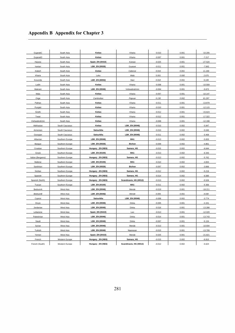
Appendix B Appendix for Chapter 3
281
GujaratiC South Asia Kotias Kharia -0.010 0.001 -10.205 GujaratiD South Asia Kotias Kharia -0.007 0.001 -7.217 Hazara South Asia Spain_EN (I0410) Korean -0.025 0.001 -27.520 Iranian South Asia LBK_EN (I0026) Guarani -0.011 0.001 -7.943 Kalash South Asia Kotias Cabecar 0.016 0.001 11.166 Kharia South Asia Lahu Mala 0.001 0.000 2.675
Kusunda South Asia LBK_EN (I0054) Naxi 0.010 0.001 9.149 Lodhi South Asia Kotias Kharia -0.008 0.001 -10.559
Makrani South Asia LBK_EN (I0046) Vishwabrahmin -0.004 0.001 -5.672 Mala South Asia Kotias Kharia -0.007 0.001 -10.147 Onge South Asia Cambodian Papuan 0.130 0.002 61.297
Pathan South Asia Kotias Kharia -0.011 0.001 -13.879 Punjabi South Asia Kotias Kharia -0.010 0.001 -12.115 Sindhi South Asia Kotias Kharia -0.012 0.001 -15.623 Tiwari South Asia Kotias Kharia -0.012 0.001 -17.322
Vishwabrahmin South Asia Kotias Kharia -0.008 0.001 -12.198 Abkhasian South Caucasus Kotias LBK_EN (I0046) -0.010 0.002 -5.847 Armenian South Caucasus Satsurblia LBK_EN (I0046) -0.010 0.002 -5.040 Georgian South Caucasus Satsurblia LBK_EN (I0046) -0.011 0.002 -5.469 Albanian Southern Europe LBK_EN (I0046) MA1 -0.013 0.002 -5.833 Basque Southern Europe LBK_EN (I0026) Bichon -0.009 0.002 -4.861 Croatian Southern Europe Hungary _EN (NE6) Samara_HG -0.015 0.002 -6.644 Greek Southern Europe LBK_EN (I0100) MA1 -0.013 0.002 -6.343
Italian (Bergamo) Southern Europe Hungary _EN (NE6) Samara_HG -0.013 0.002 -5.762 Maltese Southern Europe LBK_EN (I0100) MA1 -0.010 0.002 -4.834
Sardinian Southern Europe LBK_EN (I0026) Bichon -0.007 0.002 -3.666 Sicilian Southern Europe Hungary _EN (NE6) Samara_HG -0.012 0.002 -5.216 Spanish Southern Europe Hungary _EN (NE6) Samara_HG -0.014 0.002 -6.580
Spanish (North) Southern Europe Hungary _EN (NE6) Scandinavia_HG (I0012) -0.013 0.002 -5.526 Tuscan Southern Europe LBK_EN (I0100) MA1 -0.011 0.002 -5.366
BedouinA West Asia LBK_EN (I0046) Mende -0.019 0.001 -18.211 BedouinB West Asia LBK_EN (I0046) Mende 0.005 0.001 4.030
Cypriot West Asia Satsurblia LBK_EN (I0046) -0.008 0.002 -3.774 Druze West Asia LBK_EN (I0046) Dinka -0.005 0.001 -4.151
Jordanian West Asia LBK_EN (I0046) Dinka -0.016 0.001 -13.288 Lebanese West Asia Spain_EN (I0410) Luo -0.013 0.001 -12.029 Palestinian West Asia LBK_EN (I0046) Dinka -0.014 0.001 -13.743
Saudi West Asia LBK_EN (I0046) Dinka -0.007 0.001 -5.134 Syrian West Asia LBK_EN (I0046) Mende -0.013 0.001 -10.934 Turkish West Asia LBK_EN (I0046) Nganasan -0.015 0.001 -13.709 Yemen West Asia Spain_EN (I0410) Mende -0.025 0.001 -21.821 French Western Europe Hungary _EN (NE6) Samara_HG -0.015 0.002 -6.810
French (South) Western Europe Hungary _EN (NE6) Scandinavia_HG (I0012) -0.012 0.002 -5.624
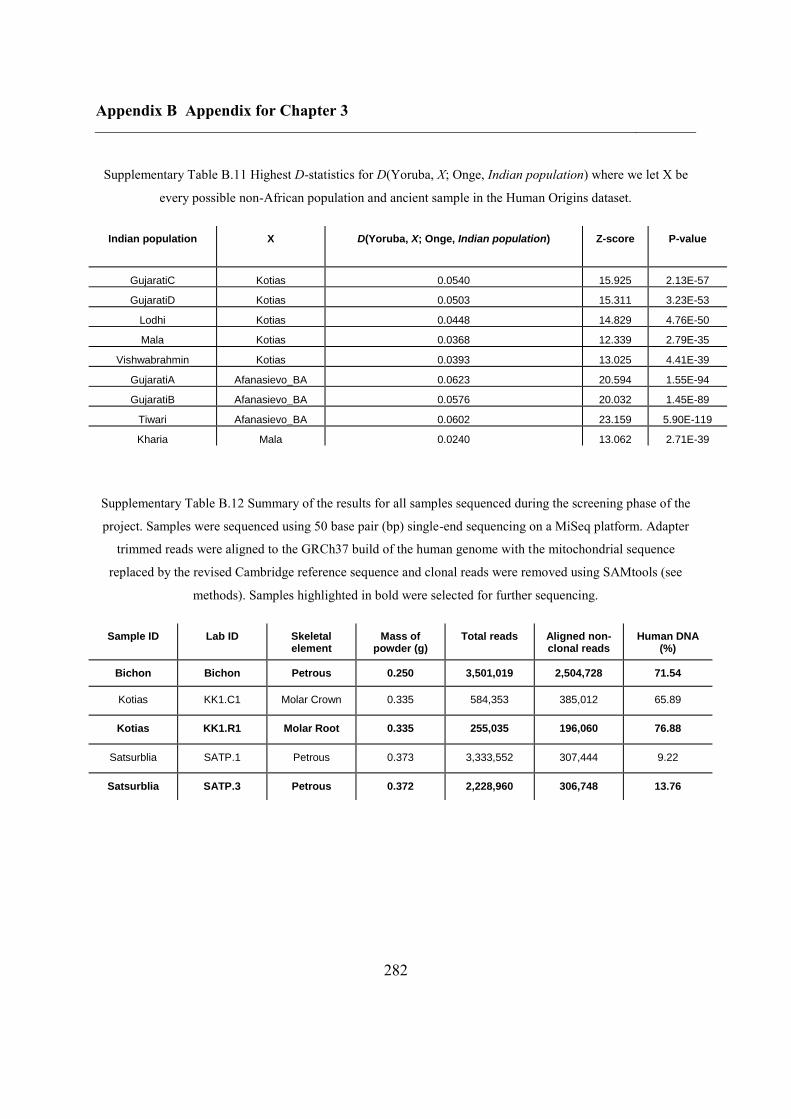
Appendix B Appendix for Chapter 3
282
Supplementary Table B.11 Highest D-statistics for D(Yoruba, X; Onge, Indian population) where we let X be
every possible non-African population and ancient sample in the Human Origins dataset.
Indian population X D(Yoruba, X; Onge, Indian population) Z-score P-value
GujaratiC Kotias 0.0540 15.925 2.13E-57
GujaratiD Kotias 0.0503 15.311 3.23E-53
Lodhi Kotias 0.0448 14.829 4.76E-50
Mala Kotias 0.0368 12.339 2.79E-35
Vishwabrahmin Kotias 0.0393 13.025 4.41E-39
GujaratiA Afanasievo_BA 0.0623 20.594 1.55E-94
GujaratiB Afanasievo_BA 0.0576 20.032 1.45E-89
Tiwari Afanasievo_BA 0.0602 23.159 5.90E-119
Kharia Mala 0.0240 13.062 2.71E-39
Supplementary Table B.12 Summary of the results for all samples sequenced during the screening phase of the
project. Samples were sequenced using 50 base pair (bp) single-end sequencing on a MiSeq platform. Adapter
trimmed reads were aligned to the GRCh37 build of the human genome with the mitochondrial sequence
replaced by the revised Cambridge reference sequence and clonal reads were removed using SAMtools (see
methods). Samples highlighted in bold were selected for further sequencing.
Sample ID Lab ID Skeletal element
Mass of powder (g)
Total reads Aligned non-clonal reads
Human DNA (%)
Bichon Bichon Petrous 0.250 3,501,019 2,504,728 71.54
Kotias KK1.C1 Molar Crown 0.335 584,353 385,012 65.89
Kotias KK1.R1 Molar Root 0.335 255,035 196,060 76.88
Satsurblia SATP.1 Petrous 0.373 3,333,552 307,444 9.22
Satsurblia SATP.3 Petrous 0.372 2,228,960 306,748 13.76
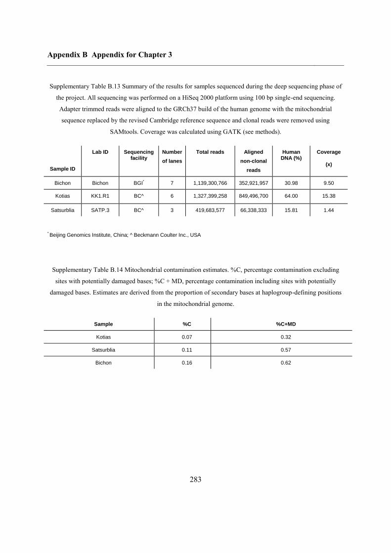
Appendix B Appendix for Chapter 3
283
Supplementary Table B.13 Summary of the results for samples sequenced during the deep sequencing phase of
the project. All sequencing was performed on a HiSeq 2000 platform using 100 bp single-end sequencing.
Adapter trimmed reads were aligned to the GRCh37 build of the human genome with the mitochondrial
sequence replaced by the revised Cambridge reference sequence and clonal reads were removed using
SAMtools. Coverage was calculated using GATK (see methods).
Sample ID
Lab ID Sequencing facility
Number
of lanes
Total reads Aligned
non-clonal
reads
Human DNA (%)
Coverage
(x)
Bichon Bichon BGI* 7 1,139,300,766 352,921,957 30.98 9.50
Kotias KK1.R1 BC^ 6 1,327,399,258 849,496,700 64.00 15.38
Satsurblia SATP.3 BC^ 3 419,683,577 66,338,333 15.81 1.44
* Beijing Genomics Institute, China; ^ Beckmann Coulter Inc., USA
Supplementary Table B.14 Mitochondrial contamination estimates. %C, percentage contamination excluding
sites with potentially damaged bases; %C + MD, percentage contamination including sites with potentially
damaged bases. Estimates are derived from the proportion of secondary bases at haplogroup-defining positions
in the mitochondrial genome.
Sample %C %C+MD
Kotias 0.07 0.32
Satsurblia 0.11 0.57
Bichon 0.16 0.62
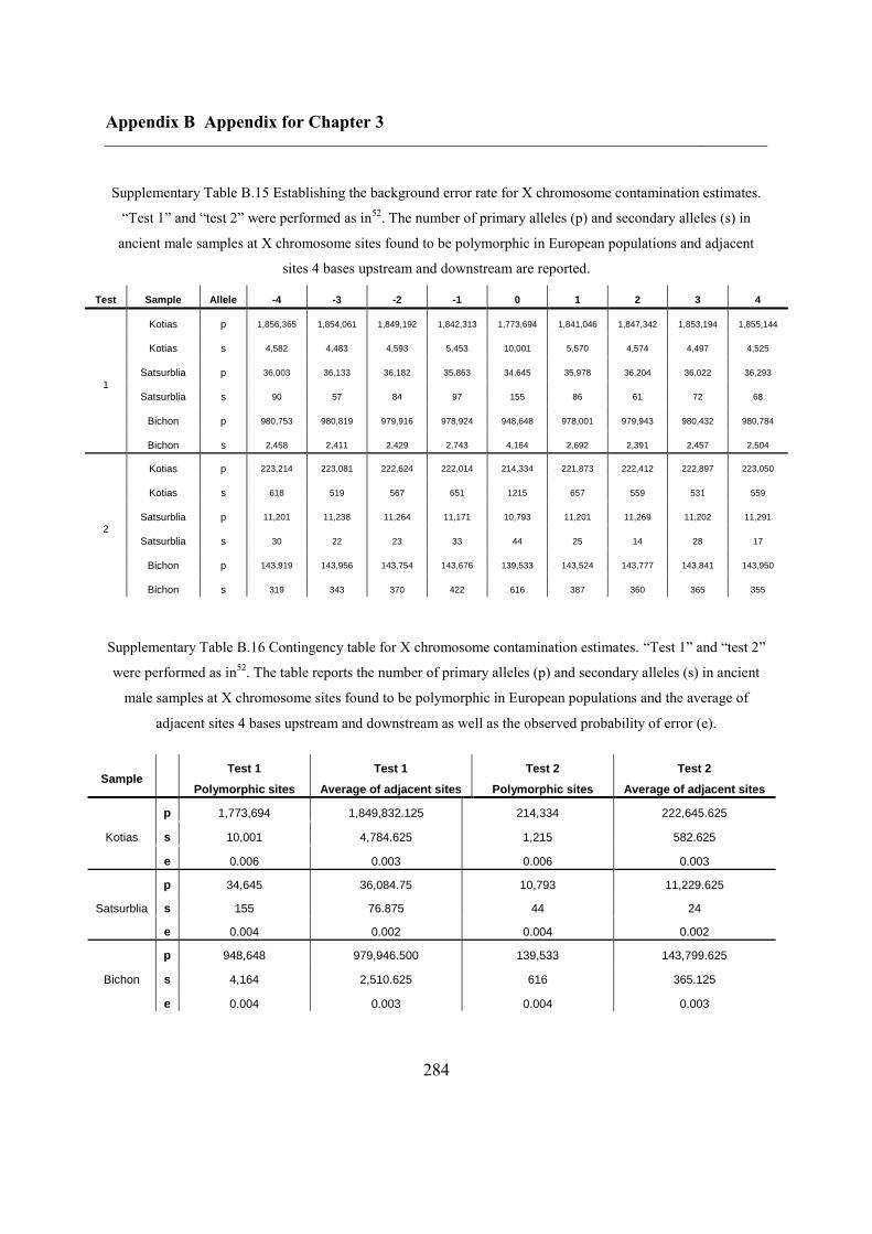
Appendix B Appendix for Chapter 3
284
Supplementary Table B.15 Establishing the background error rate for X chromosome contamination estimates.
“Test 1” and “test 2” were performed as in52
. The number of primary alleles (p) and secondary alleles (s) in
ancient male samples at X chromosome sites found to be polymorphic in European populations and adjacent
sites 4 bases upstream and downstream are reported.
Test Sample Allele -4 -3 -2 -1 0 1 2 3 4
1
Kotias p 1,856,365 1,854,061 1,849,192 1,842,313 1,773,694 1,841,046 1,847,342 1,853,194 1,855,144
Kotias s 4,582 4,483 4,593 5,453 10,001 5,570 4,574 4,497 4,525
Satsurblia p 36,003 36,133 36,182 35,863 34,645 35,978 36,204 36,022 36,293
Satsurblia s 90 57 84 97 155 86 61 72 68
Bichon p 980,753 980,819 979,916 978,924 948,648 978,001 979,943 980,432 980,784
Bichon s 2,458 2,411 2,429 2,743 4,164 2,692 2,391 2,457 2,504
2
Kotias p 223,214 223,081 222,624 222,014 214,334 221,873 222,412 222,897 223,050
Kotias s 618 519 567 651 1215 657 559 531 559
Satsurblia p 11,201 11,238 11,264 11,171 10,793 11,201 11,269 11,202 11,291
Satsurblia s 30 22 23 33 44 25 14 28 17
Bichon p 143,919 143,956 143,754 143,676 139,533 143,524 143,777 143,841 143,950
Bichon s 319 343 370 422 616 387 360 365 355
Supplementary Table B.16 Contingency table for X chromosome contamination estimates. “Test 1” and “test 2”
were performed as in52
. The table reports the number of primary alleles (p) and secondary alleles (s) in ancient
male samples at X chromosome sites found to be polymorphic in European populations and the average of
adjacent sites 4 bases upstream and downstream as well as the observed probability of error (e).
Sample Test 1
Polymorphic sites
Test 1
Average of adjacent sites
Test 2
Polymorphic sites
Test 2
Average of adjacent sites
Kotias
p 1,773,694 1,849,832.125 214,334 222,645.625
s 10,001 4,784.625 1,215 582.625
e 0.006 0.003 0.006 0.003
Satsurblia
p 34,645 36,084.75 10,793 11,229.625
s 155 76.875 44 24
e 0.004 0.002 0.004 0.002
Bichon
p 948,648 979,946.500 139,533 143,799.625
s 4,164 2,510.625 616 365.125
e 0.004 0.003 0.004 0.003
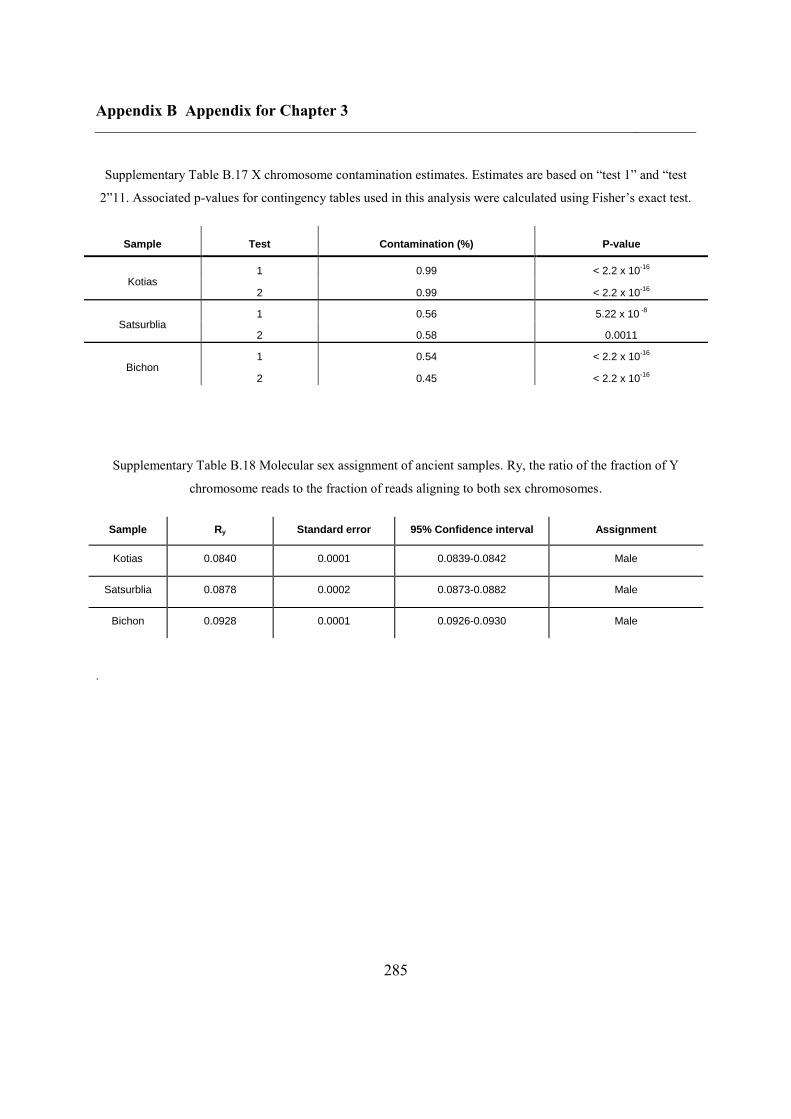
Appendix B Appendix for Chapter 3
285
Supplementary Table B.17 X chromosome contamination estimates. Estimates are based on “test 1” and “test
2”11. Associated p-values for contingency tables used in this analysis were calculated using Fisher’s exact test.
Sample Test Contamination (%) P-value
Kotias 1 0.99 < 2.2 x 10
-16
2 0.99 < 2.2 x 10⁻¹⁶
Satsurblia 1 0.56 5.22 x 10
-8
2 0.58 0.0011
Bichon 1 0.54 < 2.2 x 10
-16
2 0.45 < 2.2 x 10⁻¹⁶
Supplementary Table B.18 Molecular sex assignment of ancient samples. Ry, the ratio of the fraction of Y
chromosome reads to the fraction of reads aligning to both sex chromosomes.
Sample Ry Standard error 95% Confidence interval Assignment
Kotias 0.0840 0.0001 0.0839-0.0842 Male
Satsurblia 0.0878 0.0002 0.0873-0.0882 Male
Bichon 0.0928 0.0001 0.0926-0.0930 Male
.
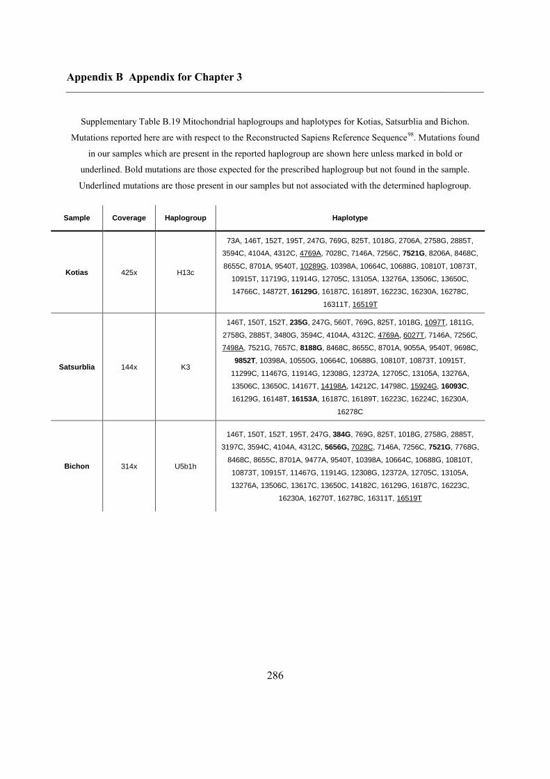
Appendix B Appendix for Chapter 3
286
Supplementary Table B.19 Mitochondrial haplogroups and haplotypes for Kotias, Satsurblia and Bichon.
Mutations reported here are with respect to the Reconstructed Sapiens Reference Sequence98
. Mutations found
in our samples which are present in the reported haplogroup are shown here unless marked in bold or
underlined. Bold mutations are those expected for the prescribed haplogroup but not found in the sample.
Underlined mutations are those present in our samples but not associated with the determined haplogroup.
Sample Coverage Haplogroup Haplotype
Kotias 425x H13c
73A, 146T, 152T, 195T, 247G, 769G, 825T, 1018G, 2706A, 2758G, 2885T,
3594C, 4104A, 4312C, 4769A, 7028C, 7146A, 7256C, 7521G, 8206A, 8468C,
8655C, 8701A, 9540T, 10289G, 10398A, 10664C, 10688G, 10810T, 10873T,
10915T, 11719G, 11914G, 12705C, 13105A, 13276A, 13506C, 13650C,
14766C, 14872T, 16129G, 16187C, 16189T, 16223C, 16230A, 16278C,
16311T, 16519T
Satsurblia 144x K3
146T, 150T, 152T, 235G, 247G, 560T, 769G, 825T, 1018G, 1097T, 1811G,
2758G, 2885T, 3480G, 3594C, 4104A, 4312C, 4769A, 6027T, 7146A, 7256C,
7498A, 7521G, 7657C, 8188G, 8468C, 8655C, 8701A, 9055A, 9540T, 9698C,
9852T, 10398A, 10550G, 10664C, 10688G, 10810T, 10873T, 10915T,
11299C, 11467G, 11914G, 12308G, 12372A, 12705C, 13105A, 13276A,
13506C, 13650C, 14167T, 14198A, 14212C, 14798C, 15924G, 16093C,
16129G, 16148T, 16153A, 16187C, 16189T, 16223C, 16224C, 16230A,
16278C
Bichon 314x U5b1h
146T, 150T, 152T, 195T, 247G, 384G, 769G, 825T, 1018G, 2758G, 2885T,
3197C, 3594C, 4104A, 4312C, 5656G, 7028C, 7146A, 7256C, 7521G, 7768G,
8468C, 8655C, 8701A, 9477A, 9540T, 10398A, 10664C, 10688G, 10810T,
10873T, 10915T, 11467G, 11914G, 12308G, 12372A, 12705C, 13105A,
13276A, 13506C, 13617C, 13650C, 14182C, 16129G, 16187C, 16223C,
16230A, 16270T, 16278C, 16311T, 16519T
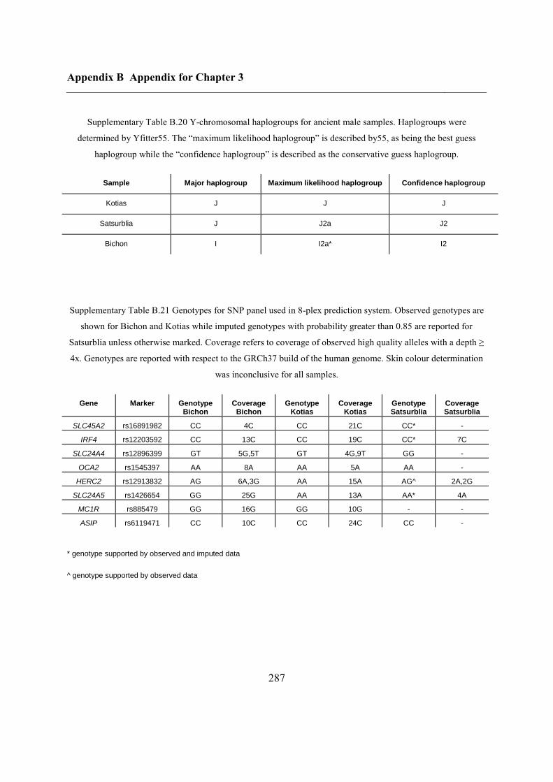
Appendix B Appendix for Chapter 3
287
Supplementary Table B.20 Y-chromosomal haplogroups for ancient male samples. Haplogroups were
determined by Yfitter55. The “maximum likelihood haplogroup” is described by55, as being the best guess
haplogroup while the “confidence haplogroup” is described as the conservative guess haplogroup.
Sample Major haplogroup Maximum likelihood haplogroup Confidence haplogroup
Kotias J J J
Satsurblia J J2a J2
Bichon I I2a* I2
Supplementary Table B.21 Genotypes for SNP panel used in 8-plex prediction system. Observed genotypes are
shown for Bichon and Kotias while imputed genotypes with probability greater than 0.85 are reported for
Satsurblia unless otherwise marked. Coverage refers to coverage of observed high quality alleles with a depth ≥
4x. Genotypes are reported with respect to the GRCh37 build of the human genome. Skin colour determination
was inconclusive for all samples.
Gene Marker Genotype Bichon
Coverage Bichon
Genotype Kotias
Coverage Kotias
Genotype Satsurblia
Coverage Satsurblia
SLC45A2 rs16891982 CC 4C CC 21C CC* -
IRF4 rs12203592 CC 13C CC 19C CC* 7C
SLC24A4 rs12896399 GT 5G,5T GT 4G,9T GG -
OCA2 rs1545397 AA 8A AA 5A AA -
HERC2 rs12913832 AG 6A,3G AA 15A AG^ 2A,2G
SLC24A5 rs1426654 GG 25G AA 13A AA* 4A
MC1R rs885479 GG 16G GG 10G - -
ASIP rs6119471 CC 10C CC 24C CC -
* genotype supported by observed and imputed data
^ genotype supported by observed data
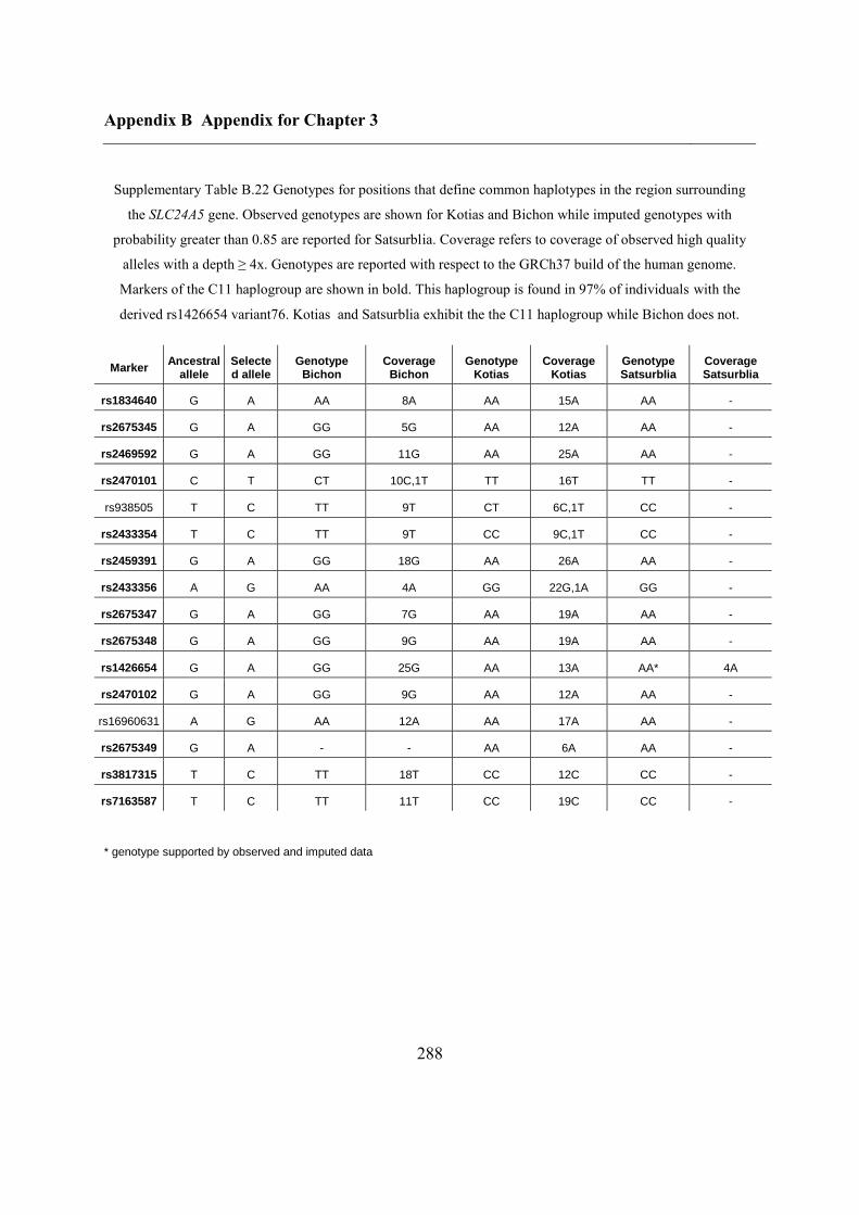
Appendix B Appendix for Chapter 3
288
Supplementary Table B.22 Genotypes for positions that define common haplotypes in the region surrounding
the SLC24A5 gene. Observed genotypes are shown for Kotias and Bichon while imputed genotypes with
probability greater than 0.85 are reported for Satsurblia. Coverage refers to coverage of observed high quality
alleles with a depth ≥ 4x. Genotypes are reported with respect to the GRCh37 build of the human genome.
Markers of the C11 haplogroup are shown in bold. This haplogroup is found in 97% of individuals with the
derived rs1426654 variant76. Kotias and Satsurblia exhibit the the C11 haplogroup while Bichon does not.
Marker Ancestral allele
Selected allele
Genotype Bichon
Coverage Bichon
Genotype Kotias
Coverage Kotias
Genotype Satsurblia
Coverage Satsurblia
rs1834640 G A AA 8A AA 15A AA -
rs2675345 G A GG 5G AA 12A AA -
rs2469592 G A GG 11G AA 25A AA -
rs2470101 C T CT 10C,1T TT 16T TT -
rs938505 T C TT 9T CT 6C,1T CC -
rs2433354 T C TT 9T CC 9C,1T CC -
rs2459391 G A GG 18G AA 26A AA -
rs2433356 A G AA 4A GG 22G,1A GG -
rs2675347 G A GG 7G AA 19A AA -
rs2675348 G A GG 9G AA 19A AA -
rs1426654 G A GG 25G AA 13A AA* 4A
rs2470102 G A GG 9G AA 12A AA -
rs16960631 A G AA 12A AA 17A AA -
rs2675349 G A - - AA 6A AA -
rs3817315 T C TT 18T CC 12C CC -
rs7163587 T C TT 11T CC 19C CC -
* genotype supported by observed and imputed data
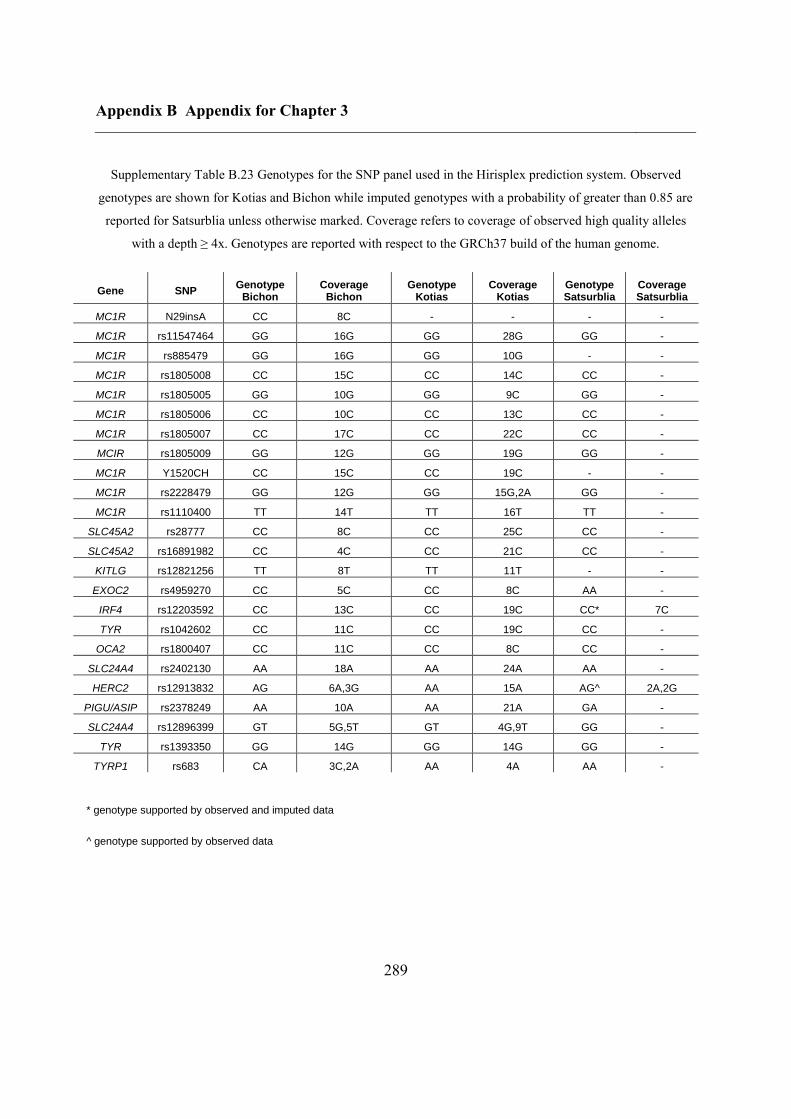
Appendix B Appendix for Chapter 3
289
Supplementary Table B.23 Genotypes for the SNP panel used in the Hirisplex prediction system. Observed
genotypes are shown for Kotias and Bichon while imputed genotypes with a probability of greater than 0.85 are
reported for Satsurblia unless otherwise marked. Coverage refers to coverage of observed high quality alleles
with a depth ≥ 4x. Genotypes are reported with respect to the GRCh37 build of the human genome.
Gene SNP Genotype Bichon
Coverage Bichon
Genotype Kotias
Coverage Kotias
Genotype Satsurblia
Coverage Satsurblia
MC1R N29insA CC 8C - - - -
MC1R rs11547464 GG 16G GG 28G GG -
MC1R rs885479 GG 16G GG 10G - -
MC1R rs1805008 CC 15C CC 14C CC -
MC1R rs1805005 GG 10G GG 9C GG -
MC1R rs1805006 CC 10C CC 13C CC -
MC1R rs1805007 CC 17C CC 22C CC -
MCIR rs1805009 GG 12G GG 19G GG -
MC1R Y1520CH CC 15C CC 19C - -
MC1R rs2228479 GG 12G GG 15G,2A GG -
MC1R rs1110400 TT 14T TT 16T TT -
SLC45A2 rs28777 CC 8C CC 25C CC -
SLC45A2 rs16891982 CC 4C CC 21C CC -
KITLG rs12821256 TT 8T TT 11T - -
EXOC2 rs4959270 CC 5C CC 8C AA -
IRF4 rs12203592 CC 13C CC 19C CC* 7C
TYR rs1042602 CC 11C CC 19C CC -
OCA2 rs1800407 CC 11C CC 8C CC -
SLC24A4 rs2402130 AA 18A AA 24A AA -
HERC2 rs12913832 AG 6A,3G AA 15A AG^ 2A,2G
PIGU/ASIP rs2378249 AA 10A AA 21A GA -
SLC24A4 rs12896399 GT 5G,5T GT 4G,9T GG -
TYR rs1393350 GG 14G GG 14G GG -
TYRP1 rs683 CA 3C,2A AA 4A AA -
* genotype supported by observed and imputed data
^ genotype supported by observed data
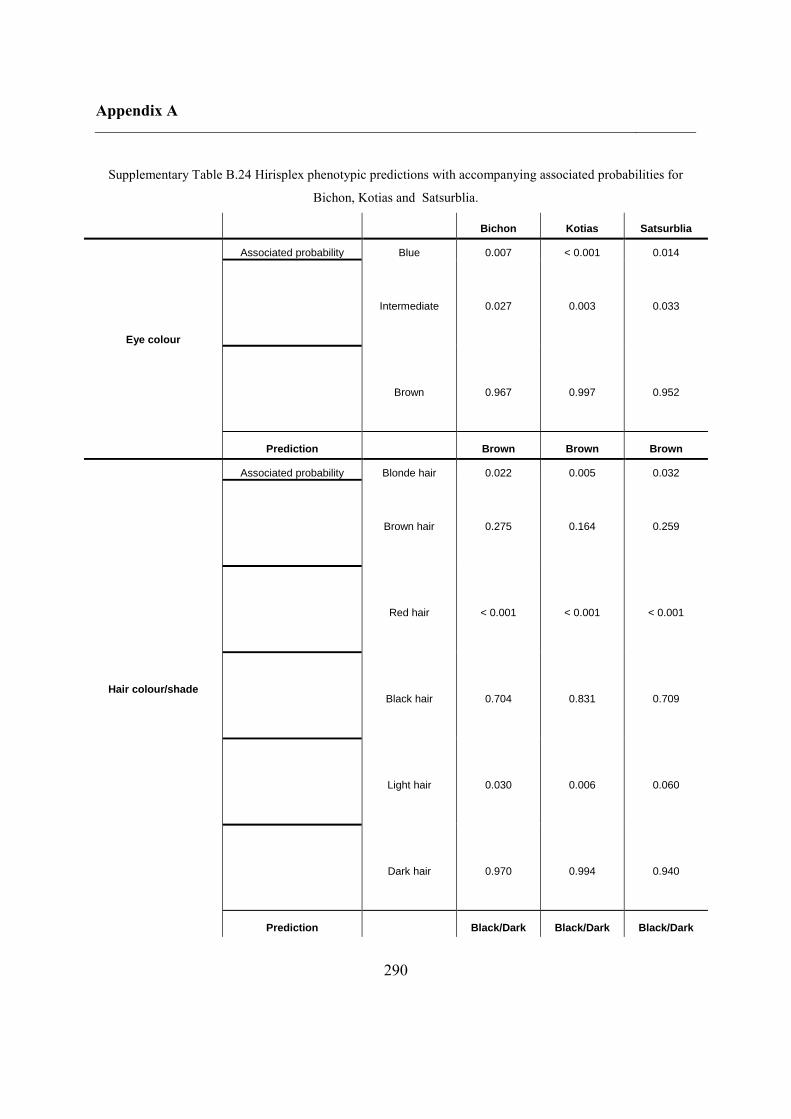
Appendix A
290
Supplementary Table B.24 Hirisplex phenotypic predictions with accompanying associated probabilities for
Bichon, Kotias and Satsurblia.
Bichon Kotias Satsurblia
Eye colour
Associated probability Blue 0.007 < 0.001 0.014
Intermediate 0.027 0.003 0.033
Brown 0.967 0.997 0.952
Prediction Brown Brown Brown
Hair colour/shade
Associated probability Blonde hair 0.022 0.005 0.032
Brown hair 0.275 0.164 0.259
Red hair < 0.001 < 0.001 < 0.001
Black hair 0.704 0.831 0.709
Light hair 0.030 0.006 0.060
Dark hair 0.970 0.994 0.940
Prediction Black/Dark Black/Dark Black/Dark

Appendix A
291
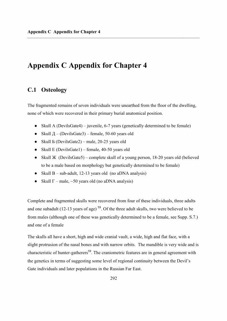
Appendix C Appendix for Chapter 4
292
Appendix C Appendix for Chapter 4
C.1 Osteology
The fragmented remains of seven individuals were unearthed from the floor of the dwelling,
none of which were recovered in their primary burial anatomical position.
● Skull A (DevilsGate4) – juvenile, 6-7 years (genetically determined to be female)
● Skull Д – (DevilsGate3) – female, 50-60 years old
● Skull Б (DevilsGate2) – male, 20-25 years old
● Skull Е (DevilsGate1) – female, 40-50 years old
● Skull Ж (DevilsGate5) – complete skull of a young person, 18-20 years old (believed
to be a male based on morphology but genetically determined to be female)
● Skull В – sub-adult, 12-13 years old (no aDNA analysis)
● Skull Г – male, ~50 years old (no aDNA analysis)
Complete and fragmented skulls were recovered from four of these individuals, three adults
and one subadult (12-13 years of age) 59
. Of the three adult skulls, two were believed to be
from males (although one of these was genetically determined to be a female, see Supp. S.7.)
and one of a female
The skulls all have a short, high and wide cranial vault, a wide, high and flat face, with a
slight protrusion of the nasal bones and with narrow orbits. The mandible is very wide and is
characteristic of hunter-gatherers59
. The craniometric features are in general agreement with
the genetics in terms of suggesting some level of regional continuity between the Devil’s
Gate individuals and later populations in the Russian Far East.
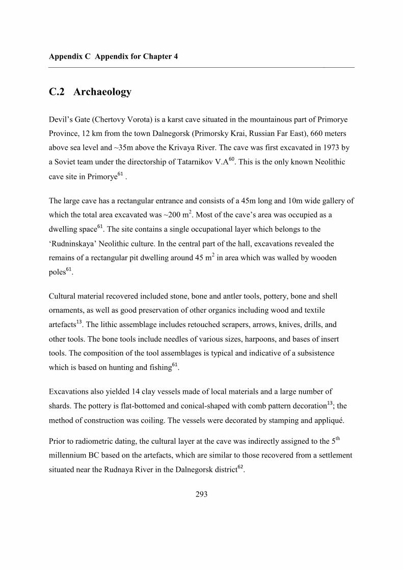
Appendix C Appendix for Chapter 4
293
C.2 Archaeology
Devil’s Gate (Chertovy Vorota) is a karst cave situated in the mountainous part of Primorye
Province, 12 km from the town Dalnegorsk (Primorsky Krai, Russian Far East), 660 meters
above sea level and ~35m above the Krivaya River. The cave was first excavated in 1973 by
a Soviet team under the directorship of Tatarnikov V.A60
. This is the only known Neolithic
cave site in Primorye61
.
The large cave has a rectangular entrance and consists of a 45m long and 10m wide gallery of
which the total area excavated was ~200 m2. Most of the cave’s area was occupied as a
dwelling space61
. The site contains a single occupational layer which belongs to the
‘Rudninskaya’ Neolithic culture. In the central part of the hall, excavations revealed the
remains of a rectangular pit dwelling around 45 m2 in area which was walled by wooden
poles61
.
Cultural material recovered included stone, bone and antler tools, pottery, bone and shell
ornaments, as well as good preservation of other organics including wood and textile
artefacts13
. The lithic assemblage includes retouched scrapers, arrows, knives, drills, and
other tools. The bone tools include needles of various sizes, harpoons, and bases of insert
tools. The composition of the tool assemblages is typical and indicative of a subsistence
which is based on hunting and fishing61
.
Excavations also yielded 14 clay vessels made of local materials and a large number of
shards. The pottery is flat-bottomed and conical-shaped with comb pattern decoration13
; the
method of construction was coiling. The vessels were decorated by stamping and appliqué.
Prior to radiometric dating, the cultural layer at the cave was indirectly assigned to the 5th
millennium BC based on the artefacts, which are similar to those recovered from a settlement
situated near the Rudnaya River in the Dalnegorsk district62
.
Appendix C Appendix for Chapter 4
294
The excavations yielded fragments of textiles, fishing nets, cords and mats made of plant
fabrics and wooden artefacts made of birch bark. A large number of bones of animals, acorns,
fruits and birch bark were found in the center62
. The assemblage also includes numerous
ornaments including bone pendants from boar canines and beads made of shell, bone and
stone.
Animal bones belong mostly to brown and black bears, wild boar, red deer, and badger. The
fauna also comprises of the remains of birds (grouse, ptarmigan, dove and duck) and
freshwater and anadromous fish (salmon)60
. The assemblage does not include any domestic
plant or faunal remains which suggests that the inhabitants of the site belonged to a hunter-
gatherer-fisher population who manufactured utilitarian low-quality domestic pottery.
C.3 Phenotypic prediction
To explore pigmentation, we first looked at the genes SLC45A2 and SLC24A5, contributing
to light skin pigmentation in modern-day Europeans37,63–67
. Selected genotypes in these two
genes (rs16891982 and rs1426654 for SLC45A2 and SLC24A5, respectively) are known to
have been under strong positive selection in Europeans and are almost fixed in modern
populations in the region. Our results imply that DevilsGate1 was unlikely to have been
homozygous for either of the selected alleles, as is typical for non-Europeans. The
rs12913832 variant of the HERC2 gene was also investigated, where a mutation is found in
nearly all people with blue eyes. Our sample was likely homozygous for the ancestral allele,
implying brown eyes.
A variant of the LCT gene (rs4988235), where the derived genotype is associated with
lactose tolerance in adult Europeans41
, was examined. We found that DevilsGate1 was
unlikely to possess the derived genotype similar to modern-day East Asian populations.
Appendix C Appendix for Chapter 4
295
A number of mutations associated with phenotypes in East Asians were also looked at, first
two locations within the OCA2 gene (rs1800414 and rs74653330) that give signals of positive
selection68–70
and are wide-spread and associated with decreased melanin levels in East
Asians71–73
. The results for the variant rs1800414 were inconclusive, but DevilsGate1 likely
did not carry the derived variant at rs74653330. We also looked at two loci with a high
frequency differentiation between East Asians and non-East Asians and showing signals of
positive selection (rs12821256, rs1407995, rs885479 on the KITLG, DCT and SLC24A2
genes, respectively)37
or otherwise associated with pigmentation (rs1042602, rs1834640,
rs26722 on the TYR, RPL7AP62/SLC24A5 and SLC24A2 genes, respectively)74
.
DevilsGate1 was most likely homozygous for the East Asian variant at both rs12821256 and
rs1407995 and did not possess the alleles rare in East Asia at rs885479, rs1042602,
rs1834640 and rs26722.
Our next target was the EDAR gene. This region also shows signals of positive selection in
East Asian populations, with the selected allele linked to certain phenotypic changes (e.g. in
tooth morphology40
, hair thickness38,39
and sweat gland density75
), also confirmed using a
mouse model. The haplotype with the selected allele is very common in East Asian,
Northeast Asian and Native American populations and is estimated to have emerged in
central China around 30,000 years ago75
. Our sample likely carried at least one copy of the
derived allele, giving increased odds of straight, thick hair as well as shovel-shaped incisors.
The mutation rs671 on ALDH2 was also studied. The derived variant, of intermediate
frequencies (roughly up to 50%) in various East Asian populations76,77
, is associated with
alcohol flush and increased risk of hangovers, alcoholism and Esophageal Cancer42,78
. Our
sample probably did not carry the derived allele.
Then, three East Asian phenotypic traits were investigated. DevilsGate1 most likely had at
least one copy of the risk allele for common salt-sensitive hypertension79
at rs4961 on the
ADD1 gene, common in Asia. She was most likely not homozygous for the risk allele at
Appendix C Appendix for Chapter 4
296
rs1799971 on the OPRM1 gene, associated with increased craving and stronger effects for
alcohol80
and for opioids81
in Asian populations, although the results from association studies
on this marker are mixed. The derived variant at rs17822931 on the ABCC11 gene is
associated with weaker than usual body odour82
and dry ear wax type83
(for the latter, when
homozygous) in East Asians and is indicative of east Asian ancestry. DevilsGate1’s genotype
could not be determined but she most likely possessed at least one copy of the derived allele.
Finally, eight loci associated with an increased risk for Type 2 diabetes in East Asian
populations was studied (rs1535500, rs6017317, rs6467136, rs9470794, rs3786897,
rs6815464, rs7041847, rs831571)84
. She was likely heterozygous at two loci associated with
increased susceptibility to Type 2 diabetes in East Asians (rs1535500 and rs9470794) and
had at least one copy of the disease-associated variant at a third location (rs6815464). Our
results at rs3786897 were completely uninformative and at other locations, she most likely
had at least one copy of the normal variant.
Detailed results of the phenotypic inference are shown in Supplementary Table C.32..
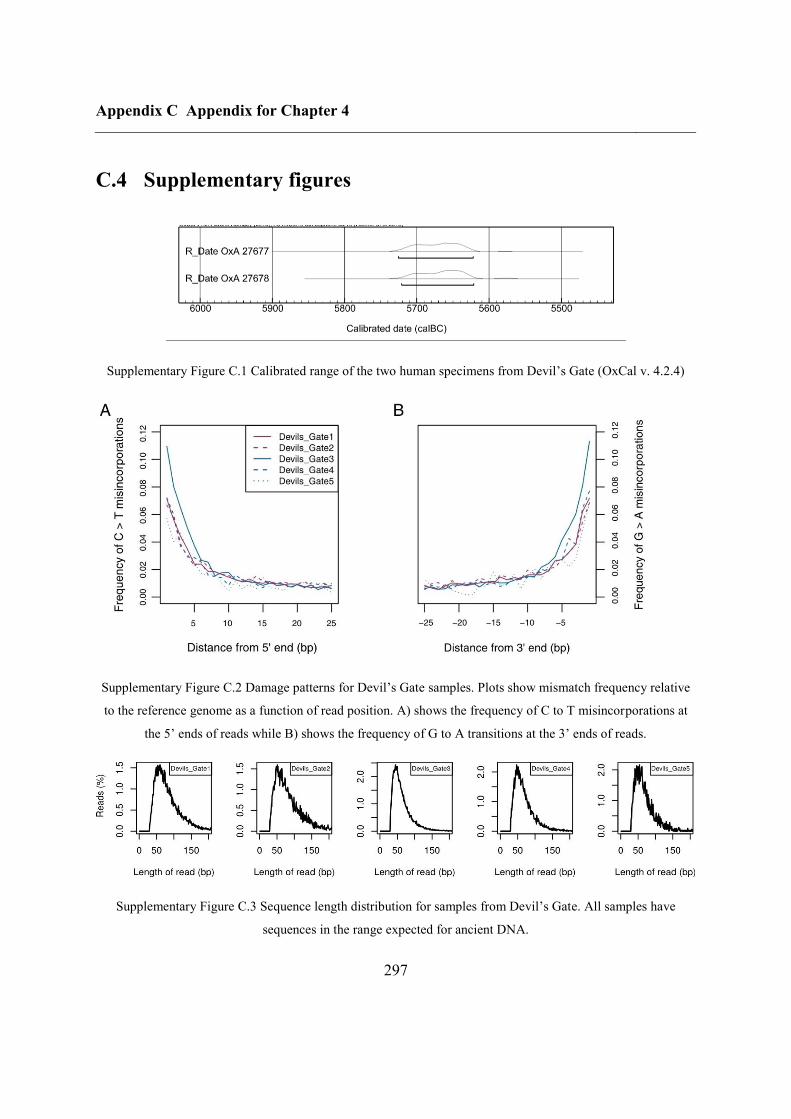
Appendix C Appendix for Chapter 4
297
C.4 Supplementary figures
Supplementary Figure C.1 Calibrated range of the two human specimens from Devil’s Gate (OxCal v. 4.2.4)
Supplementary Figure C.2 Damage patterns for Devil’s Gate samples. Plots show mismatch frequency relative
to the reference genome as a function of read position. A) shows the frequency of C to T misincorporations at
the 5’ ends of reads while B) shows the frequency of G to A transitions at the 3’ ends of reads.
Supplementary Figure C.3 Sequence length distribution for samples from Devil’s Gate. All samples have
sequences in the range expected for ancient DNA.
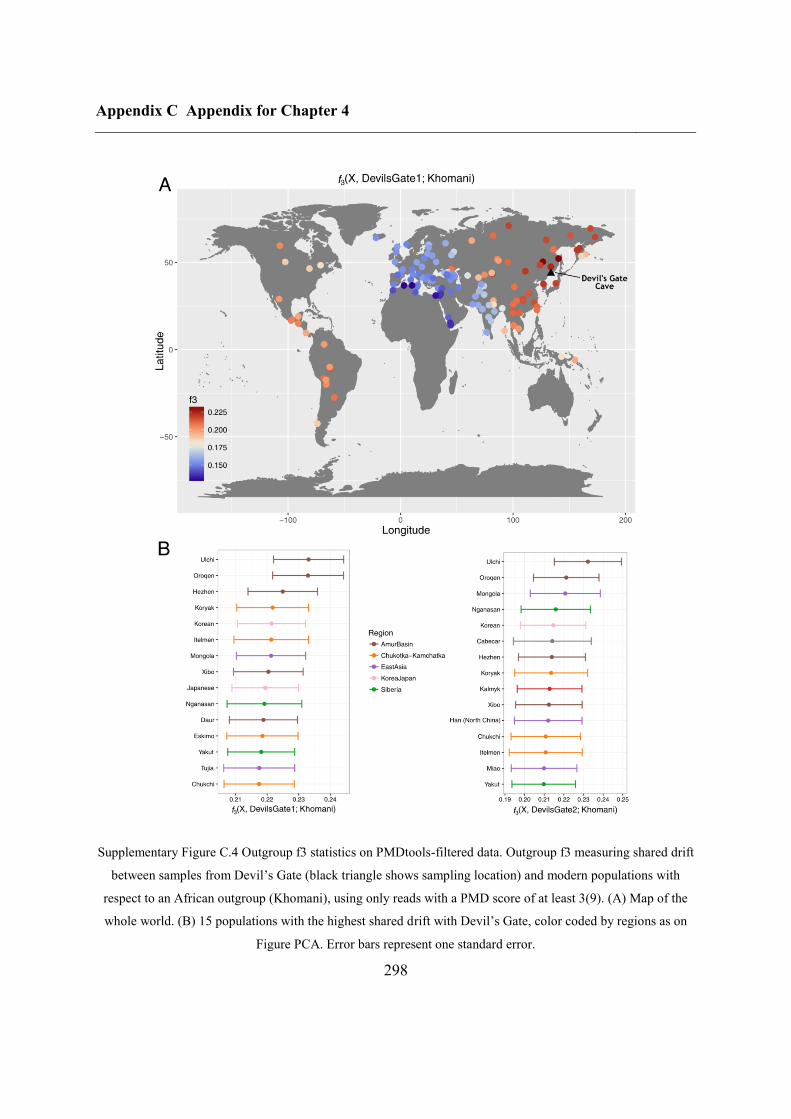
Appendix C Appendix for Chapter 4
298
Supplementary Figure C.4 Outgroup f3 statistics on PMDtools-filtered data. Outgroup f3 measuring shared drift
between samples from Devil’s Gate (black triangle shows sampling location) and modern populations with
respect to an African outgroup (Khomani), using only reads with a PMD score of at least 3(9). (A) Map of the
whole world. (B) 15 populations with the highest shared drift with Devil’s Gate, color coded by regions as on
Figure PCA. Error bars represent one standard error.
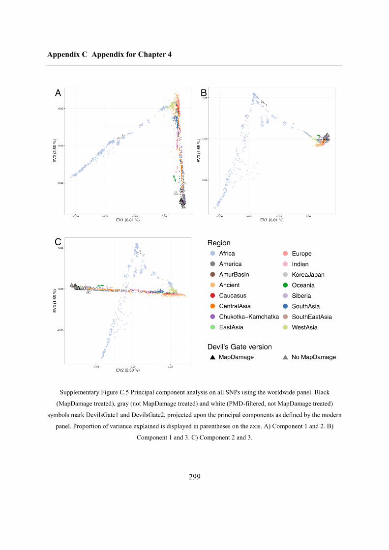
Appendix C Appendix for Chapter 4
299
Supplementary Figure C.5 Principal component analysis on all SNPs using the worldwide panel. Black
(MapDamage treated), gray (not MapDamage treated) and white (PMD-filtered, not MapDamage treated)
symbols mark DevilsGate1 and DevilsGate2, projected upon the principal components as defined by the modern
panel. Proportion of variance explained is displayed in parentheses on the axis. A) Component 1 and 2. B)
Component 1 and 3. C) Component 2 and 3.
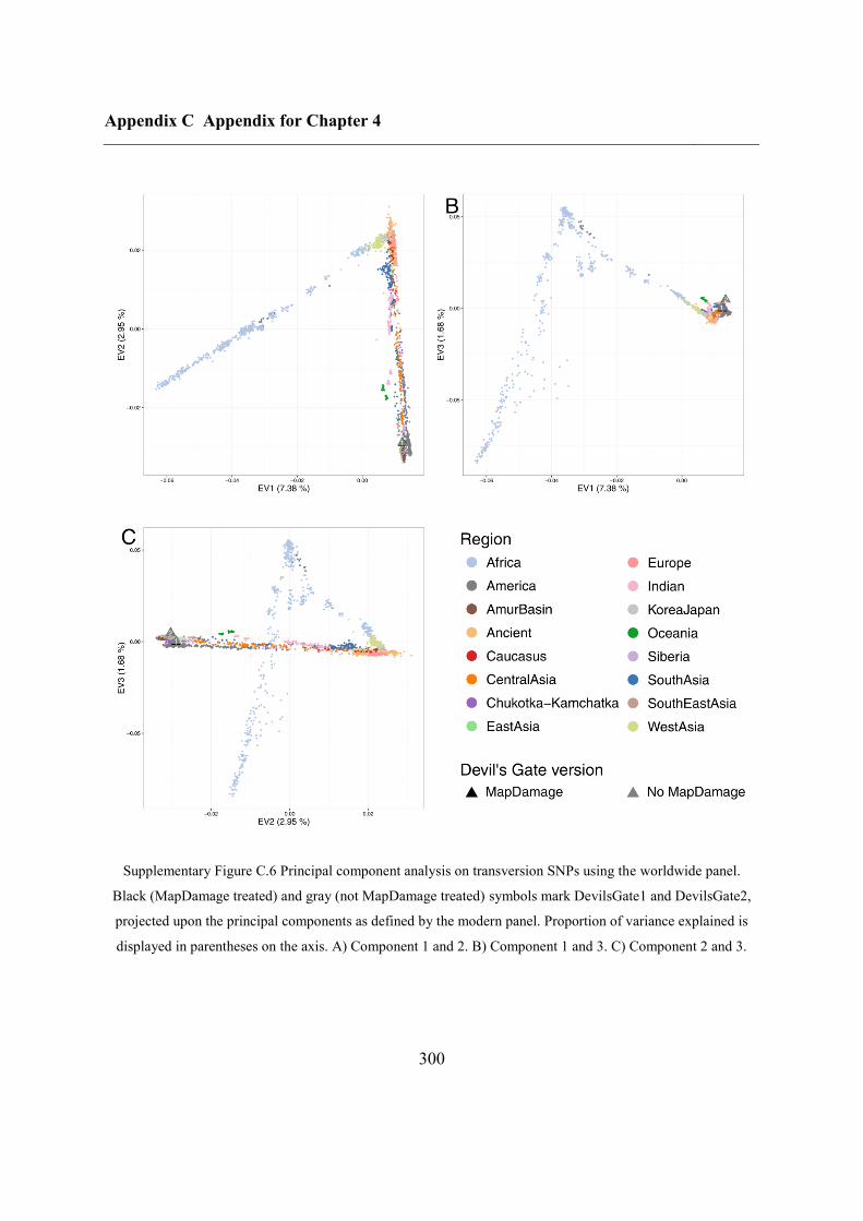
Appendix C Appendix for Chapter 4
300
Supplementary Figure C.6 Principal component analysis on transversion SNPs using the worldwide panel.
Black (MapDamage treated) and gray (not MapDamage treated) symbols mark DevilsGate1 and DevilsGate2,
projected upon the principal components as defined by the modern panel. Proportion of variance explained is
displayed in parentheses on the axis. A) Component 1 and 2. B) Component 1 and 3. C) Component 2 and 3.
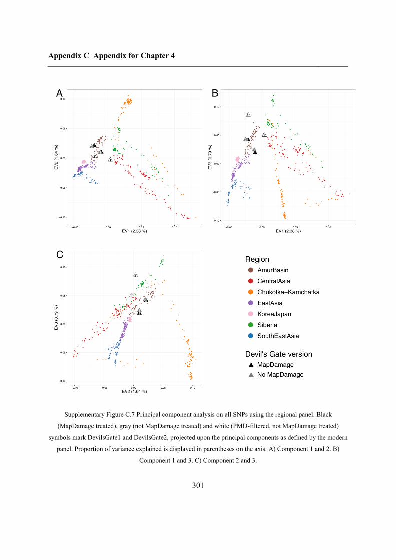
Appendix C Appendix for Chapter 4
301
Supplementary Figure C.7 Principal component analysis on all SNPs using the regional panel. Black
(MapDamage treated), gray (not MapDamage treated) and white (PMD-filtered, not MapDamage treated)
symbols mark DevilsGate1 and DevilsGate2, projected upon the principal components as defined by the modern
panel. Proportion of variance explained is displayed in parentheses on the axis. A) Component 1 and 2. B)
Component 1 and 3. C) Component 2 and 3.
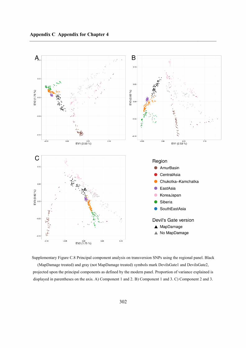
Appendix C Appendix for Chapter 4
302
Supplementary Figure C.8 Principal component analysis on transversion SNPs using the regional panel. Black
(MapDamage treated) and gray (not MapDamage treated) symbols mark DevilsGate1 and DevilsGate2,
projected upon the principal components as defined by the modern panel. Proportion of variance explained is
displayed in parentheses on the axis. A) Component 1 and 2. B) Component 1 and 3. C) Component 2 and 3.
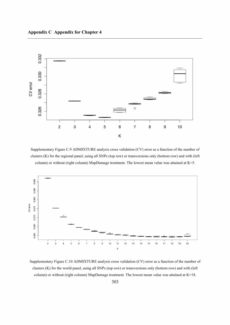
Appendix C Appendix for Chapter 4
303
Supplementary Figure C.9 ADMIXTURE analysis cross validation (CV) error as a function of the number of
clusters (K) for the regional panel, using all SNPs (top row) or transversions only (bottom row) and with (left
column) or without (right column) MapDamage treatment. The lowest mean value was attained at K=5.
Supplementary Figure C.10 ADMIXTURE analysis cross validation (CV) error as a function of the number of
clusters (K) for the world panel, using all SNPs (top row) or transversions only (bottom row) and with (left
column) or without (right column) MapDamage treatment. The lowest mean value was attained at K=18.
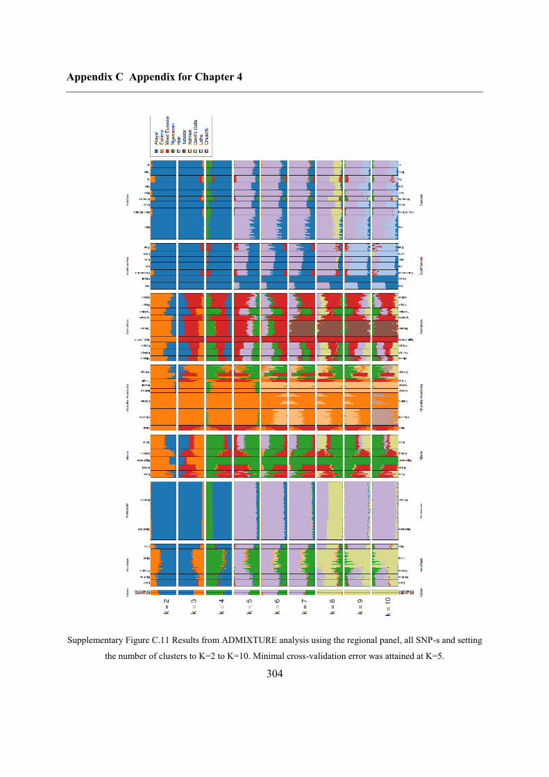
Appendix C Appendix for Chapter 4
304
Supplementary Figure C.11 Results from ADMIXTURE analysis using the regional panel, all SNP-s and setting
the number of clusters to K=2 to K=10. Minimal cross-validation error was attained at K=5.
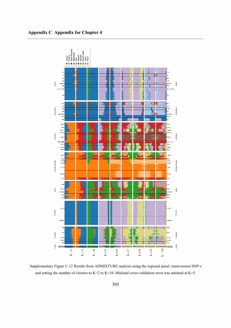
Appendix C Appendix for Chapter 4
305
Supplementary Figure C.12 Results from ADMIXTURE analysis using the regional panel, transversion SNP-s
and setting the number of clusters to K=2 to K=10. Minimal cross-validation error was attained at K=5.
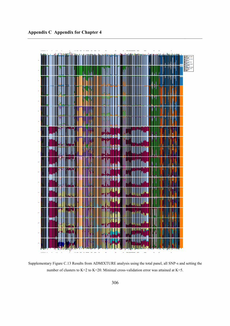
Appendix C Appendix for Chapter 4
306
Supplementary Figure C.13 Results from ADMIXTURE analysis using the total panel, all SNP-s and setting the
number of clusters to K=2 to K=20. Minimal cross-validation error was attained at K=5.

Appendix C Appendix for Chapter 4
307
Supplementary Figure C.14 Results from ADMIXTURE analysis using the total panel, transversion SNP-s and
setting the number of clusters to K=2 to K=20. Minimal cross-validation error was attained at K=5.
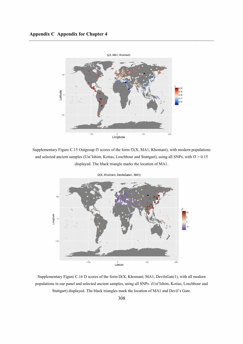
Appendix C Appendix for Chapter 4
308
Supplementary Figure C.15 Outgroup f3 scores of the form f3(X, MA1; Khomani), with modern populations
and selected ancient samples (Ust’Ishim, Kotias, Loschbour and Stuttgart), using all SNPs, with f3 > 0.15
displayed. The black triangle marks the location of MA1.
Supplementary Figure C.16 D scores of the form D(X, Khomani; MA1, DevilsGate1), with all modern
populations in our panel and selected ancient samples, using all SNPs. (Ust’Ishim, Kotias, Loschbour and
Stuttgart) displayed. The black triangles mark the location of MA1 and Devil’s Gate.
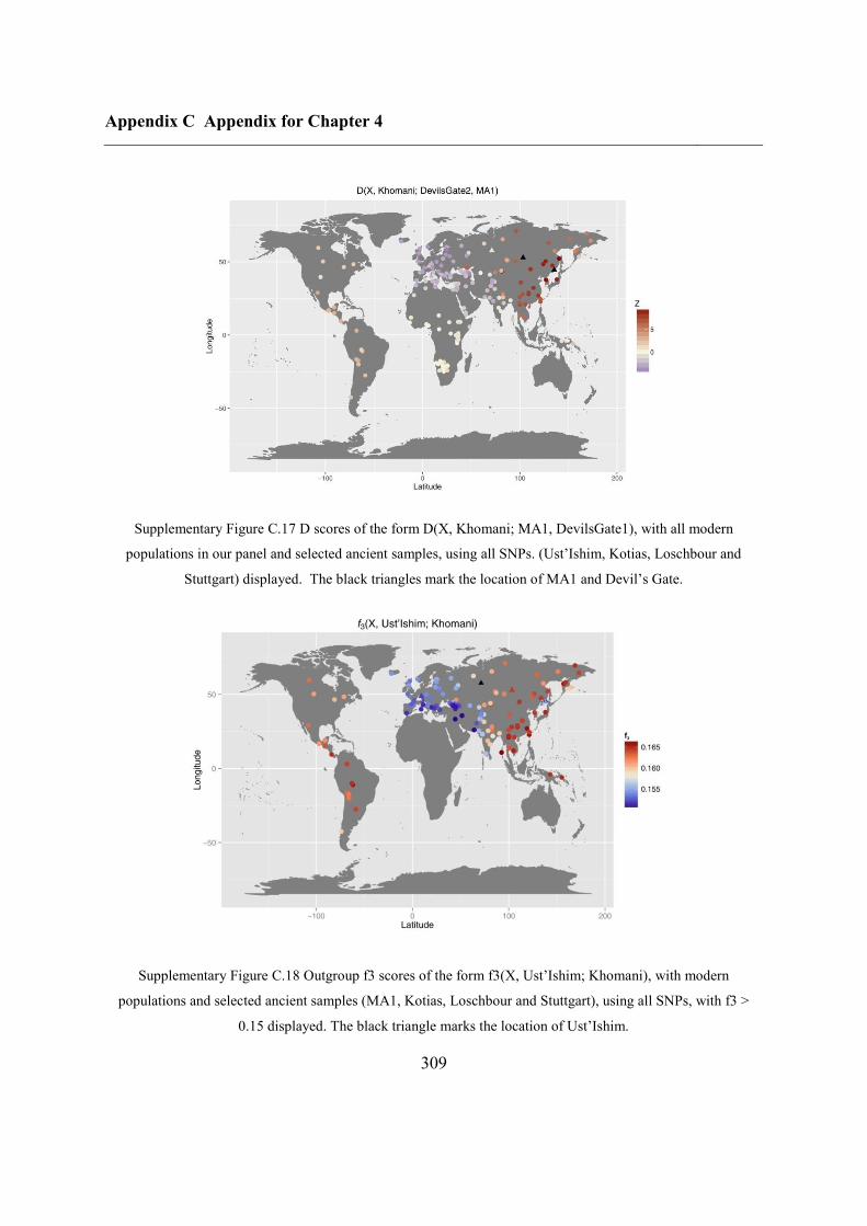
Appendix C Appendix for Chapter 4
309
Supplementary Figure C.17 D scores of the form D(X, Khomani; MA1, DevilsGate1), with all modern
populations in our panel and selected ancient samples, using all SNPs. (Ust’Ishim, Kotias, Loschbour and
Stuttgart) displayed. The black triangles mark the location of MA1 and Devil’s Gate.
Supplementary Figure C.18 Outgroup f3 scores of the form f3(X, Ust’Ishim; Khomani), with modern
populations and selected ancient samples (MA1, Kotias, Loschbour and Stuttgart), using all SNPs, with f3 >
0.15 displayed. The black triangle marks the location of Ust’Ishim.
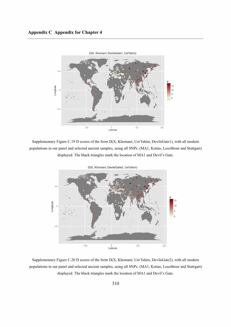
Appendix C Appendix for Chapter 4
310
Supplementary Figure C.19 D scores of the form D(X, Khomani; Ust’Ishim, DevilsGate1), with all modern
populations in our panel and selected ancient samples, using all SNPs. (MA1, Kotias, Loschbour and Stuttgart)
displayed. The black triangles mark the location of MA1 and Devil’s Gate.
Supplementary Figure C.20 D scores of the form D(X, Khomani; Ust’Ishim, DevilsGate2), with all modern
populations in our panel and selected ancient samples, using all SNPs. (MA1, Kotias, Loschbour and Stuttgart)
displayed. The black triangles mark the location of MA1 and Devil’s Gate.
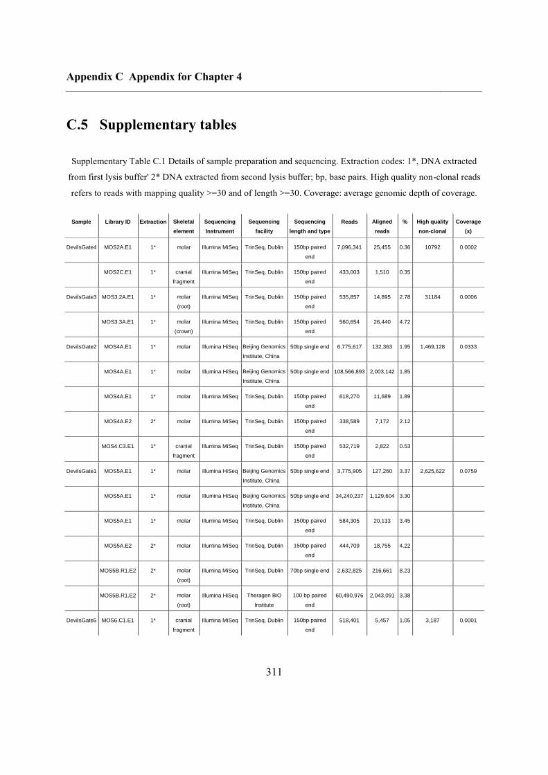
Appendix C Appendix for Chapter 4
311
C.5 Supplementary tables
Supplementary Table C.1 Details of sample preparation and sequencing. Extraction codes: 1*, DNA extracted
from first lysis buffer' 2* DNA extracted from second lysis buffer; bp, base pairs. High quality non-clonal reads
refers to reads with mapping quality >=30 and of length >=30. Coverage: average genomic depth of coverage.
Sample Library ID Extraction Skeletal
element
Sequencing
Instrument
Sequencing
facility
Sequencing
length and type
Reads Aligned
reads
% High quality
non-clonal
reads
Coverage
(x)
DevilsGate4 MOS2A.E1 1* molar Illumina MiSeq TrinSeq, Dublin 150bp paired
end
7,096,341 25,455 0.36 10792 0.0002
MOS2C.E1 1* cranial
fragment
Illumina MiSeq TrinSeq, Dublin 150bp paired
end
433,003 1,510 0.35
DevilsGate3 MOS3.2A.E1 1* molar
(root)
Illumina MiSeq TrinSeq, Dublin 150bp paired
end
535,857 14,895 2.78 31184 0.0006
MOS3.3A.E1 1* molar
(crown)
Illumina MiSeq TrinSeq, Dublin 150bp paired
end
560,654 26,440 4.72
DevilsGate2 MOS4A.E1 1* molar Illumina HiSeq Beijing Genomics
Institute, China
50bp single end 6,775,617 132,363 1.95 1,469,128 0.0333
MOS4A.E1 1* molar Illumina HiSeq Beijing Genomics
Institute, China
50bp single end 108,566,893 2,003,142 1.85
MOS4A.E1 1* molar Illumina MiSeq TrinSeq, Dublin 150bp paired
end
618,270 11,689 1.89
MOS4A.E2 2* molar Illumina MiSeq TrinSeq, Dublin 150bp paired
end
338,589 7,172 2.12
MOS4.C3.E1 1* cranial
fragment
Illumina MiSeq TrinSeq, Dublin 150bp paired
end
532,719 2,822 0.53
DevilsGate1 MOS5A.E1 1* molar Illumina HiSeq Beijing Genomics
Institute, China
50bp single end 3,775,905 127,260 3.37 2,625,622 0.0759
MOS5A.E1 1* molar Illumina HiSeq Beijing Genomics
Institute, China
50bp single end 34,240,237 1,129,604 3.30
MOS5A.E1 1* molar Illumina MiSeq TrinSeq, Dublin 150bp paired
end
584,305 20,133 3.45
MOS5A.E2 2* molar Illumina MiSeq TrinSeq, Dublin 150bp paired
end
444,709 18,755 4.22
MOS5B.R1.E2 2* molar
(root)
Illumina MiSeq TrinSeq, Dublin 70bp single end 2,632,825 216,661 8.23
MOS5B.R1.E2 2* molar
(root)
Illumina HiSeq Theragen BiO
Institute
100 bp paired
end
60,490,976 2,043,091 3.38
DevilsGate5 MOS6.C1.E1 1* cranial
fragment
Illumina MiSeq TrinSeq, Dublin 150bp paired
end
518,401 5,457 1.05 3,187 0.0001
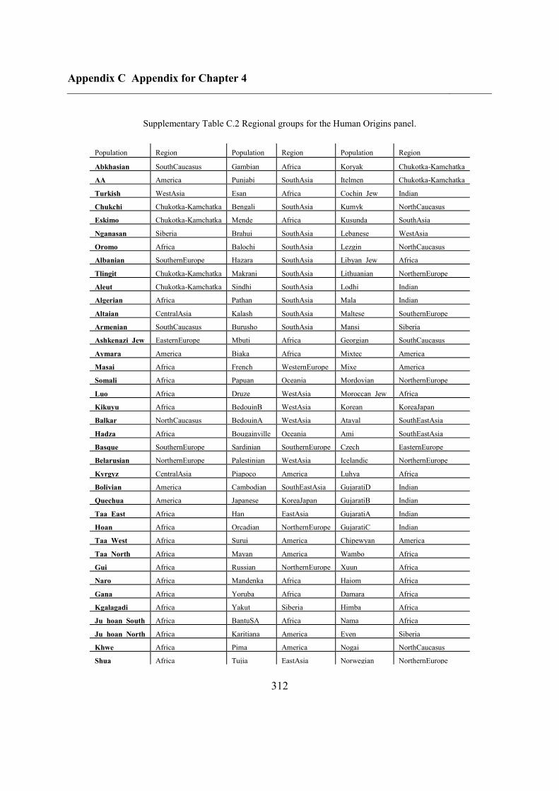
Appendix C Appendix for Chapter 4
312
Supplementary Table C.2 Regional groups for the Human Origins panel.
Population Region Population Region Population Region
Abkhasian SouthCaucasus Gambian Africa Koryak Chukotka-Kamchatka
AA America Punjabi SouthAsia Itelmen Chukotka-Kamchatka
Turkish WestAsia Esan Africa Cochin_Jew Indian
Chukchi Chukotka-Kamchatka Bengali SouthAsia Kumyk NorthCaucasus
Eskimo Chukotka-Kamchatka Mende Africa Kusunda SouthAsia
Nganasan Siberia Brahui SouthAsia Lebanese WestAsia
Oromo Africa Balochi SouthAsia Lezgin NorthCaucasus
Albanian SouthernEurope Hazara SouthAsia Libyan_Jew Africa
Tlingit Chukotka-Kamchatka Makrani SouthAsia Lithuanian NorthernEurope
Aleut Chukotka-Kamchatka Sindhi SouthAsia Lodhi Indian
Algerian Africa Pathan SouthAsia Mala Indian
Altaian CentralAsia Kalash SouthAsia Maltese SouthernEurope
Armenian SouthCaucasus Burusho SouthAsia Mansi Siberia
Ashkenazi_Jew EasternEurope Mbuti Africa Georgian SouthCaucasus
Aymara America Biaka Africa Mixtec America
Masai Africa French WesternEurope Mixe America
Somali Africa Papuan Oceania Mordovian NorthernEurope
Luo Africa Druze WestAsia Moroccan_Jew Africa
Kikuyu Africa BedouinB WestAsia Korean KoreaJapan
Balkar NorthCaucasus BedouinA WestAsia Atayal SouthEastAsia
Hadza Africa Bougainville Oceania Ami SouthEastAsia
Basque SouthernEurope Sardinian SouthernEurope Czech EasternEurope
Belarusian NorthernEurope Palestinian WestAsia Icelandic NorthernEurope
Kyrgyz CentralAsia Piapoco America Luhya Africa
Bolivian America Cambodian SouthEastAsia GujaratiD Indian
Quechua America Japanese KoreaJapan GujaratiB Indian
Taa_East Africa Han EastAsia GujaratiA Indian
Hoan Africa Orcadian NorthernEurope GujaratiC Indian
Taa_West Africa Surui America Chipewyan America
Taa_North Africa Mayan America Wambo Africa
Gui Africa Russian NorthernEurope Xuun Africa
Naro Africa Mandenka Africa Haiom Africa
Gana Africa Yoruba Africa Damara Africa
Kgalagadi Africa Yakut Siberia Himba Africa
Ju_hoan_South Africa BantuSA Africa Nama Africa
Ju_hoan_North Africa Karitiana America Even Siberia
Khwe Africa Pima America Nogai NorthCaucasus
Shua Africa Tujia EastAsia Norwegian NorthernEurope
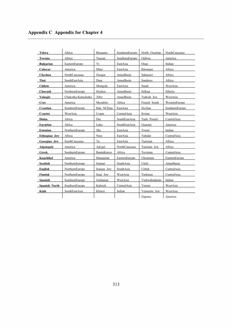
Appendix C Appendix for Chapter 4
313
Tshwa Africa Bergamo SouthernEurope North_Ossetian NorthCaucasus
Tswana Africa Tuscan SouthernEurope Ojibwa America
Bulgarian EasternEurope Yi EastAsia Onge Indian
Cabecar America Miao EastAsia Khomani Africa
Chechen NorthCaucasus Oroqen AmurBasin Saharawi Africa
Thai SouthEastAsia Daur AmurBasin Sandawe Africa
Chilote America Mongola EastAsia Saudi WestAsia
Chuvash NorthernEurope Hezhen AmurBasin Selkup Siberia
Yukagir Chukotka-Kamchatka Xibo AmurBasin Turkish_Jew WestAsia
Cree America Mozabite Africa French_South WesternEurope
Croatian SouthernEurope Han_NChina EastAsia Sicilian SouthernEurope
Cypriot WestAsia Uygur CentralAsia Syrian WestAsia
Dinka Africa Dai SouthEastAsia Tajik_Pomiri CentralAsia
Egyptian Africa Lahu SouthEastAsia Guarani America
Estonian NorthernEurope She EastAsia Tiwari Indian
Ethiopian_Jew Africa Naxi EastAsia Tubalar CentralAsia
Georgian_Jew SouthCaucasus Tu EastAsia Tunisian Africa
Algonquin America Adygei NorthCaucasus Tunisian_Jew Africa
Greek SouthernEurope BantuKenya Africa Tuvinian CentralAsia
Kaqchikel America Hungarian EasternEurope Ukrainian EasternEurope
Scottish NorthernEurope Iranian SouthAsia Ulchi AmurBasin
English NorthernEurope Iranian_Jew SouthAsia Uzbek CentralAsia
Finnish NorthernEurope Iraqi_Jew WestAsia Turkmen CentralAsia
Spanish SouthernEurope Jordanian WestAsia Vishwabrahmin Indian
Spanish_North SouthernEurope Kalmyk CentralAsia Yemen WestAsia
Kinh SouthEastAsia Kharia Indian Yemenite_Jew WestAsia
Zapotec America
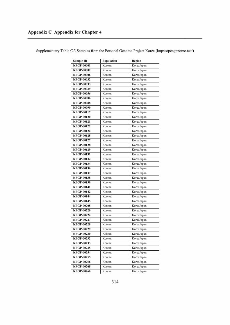
Appendix C Appendix for Chapter 4
314
Supplementary Table C.3 Samples from the Personal Genome Project Korea (http://opengenome.net/)
Sample ID Population Region
KPGP-00001 Korean KoreaJapan
KPGP-00002 Korean KoreaJapan
KPGP-00006 Korean KoreaJapan
KPGP-00032 Korean KoreaJapan
KPGP-00033 Korean KoreaJapan
KPGP-00039 Korean KoreaJapan
KPGP-00056 Korean KoreaJapan
KPGP-00086 Korean KoreaJapan
KPGP-00088 Korean KoreaJapan
KPGP-00090 Korean KoreaJapan
KPGP-00117 Korean KoreaJapan
KPGP-00120 Korean KoreaJapan
KPGP-00121 Korean KoreaJapan
KPGP-00122 Korean KoreaJapan
KPGP-00124 Korean KoreaJapan
KPGP-00125 Korean KoreaJapan
KPGP-00127 Korean KoreaJapan
KPGP-00128 Korean KoreaJapan
KPGP-00129 Korean KoreaJapan
KPGP-00131 Korean KoreaJapan
KPGP-00132 Korean KoreaJapan
KPGP-00134 Korean KoreaJapan
KPGP-00136 Korean KoreaJapan
KPGP-00137 Korean KoreaJapan
KPGP-00138 Korean KoreaJapan
KPGP-00139 Korean KoreaJapan
KPGP-00141 Korean KoreaJapan
KPGP-00142 Korean KoreaJapan
KPGP-00144 Korean KoreaJapan
KPGP-00145 Korean KoreaJapan
KPGP-00205 Korean KoreaJapan
KPGP-00220 Korean KoreaJapan
KPGP-00224 Korean KoreaJapan
KPGP-00227 Korean KoreaJapan
KPGP-00228 Korean KoreaJapan
KPGP-00229 Korean KoreaJapan
KPGP-00230 Korean KoreaJapan
KPGP-00232 Korean KoreaJapan
KPGP-00233 Korean KoreaJapan
KPGP-00235 Korean KoreaJapan
KPGP-00254 Korean KoreaJapan
KPGP-00255 Korean KoreaJapan
KPGP-00256 Korean KoreaJapan
KPGP-00265 Korean KoreaJapan
KPGP-00266 Korean KoreaJapan
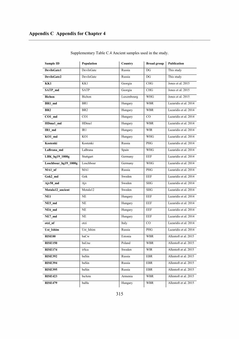
Appendix C Appendix for Chapter 4
315
Supplementary Table C.4 Ancient samples used in the study.
Sample ID Population Country Broad group Publication
DevilsGate1 DevilsGate Russia DG This study
DevilsGate2 DevilsGate Russia DG This study
KK1 KK1 Georgia CHG Jones et al. 2015
SATP_md SATP Georgia CHG Jones et al. 2015
Bichon Bichon Luxembourg WHG Jones et al. 2015
BR1_md BR1 Hungary WBR Lazaridis et al. 2014
BR2 BR2 Hungary WBR Lazaridis et al. 2014
CO1_md CO1 Hungary CO Lazaridis et al. 2014
HDma1_md HDma1 Hungary WBR Lazaridis et al. 2014
IR1_md IR1 Hungary WIR Lazaridis et al. 2014
KO1_md KO1 Hungary WHG Lazaridis et al. 2014
Kostenki Kostenki Russia PHG Lazaridis et al. 2014
LaBrana_md LaBrana Spain WHG Lazaridis et al. 2014
LBK_hg19_1000g Stuttgart Germany EEF Lazaridis et al. 2014
Loschbour_hg19_1000g Loschbour Germany WHG Lazaridis et al. 2014
MA1_nf MA1 Russia PHG Lazaridis et al. 2014
Gok2_md Gok Sweden EEF Lazaridis et al. 2014
Ajv58_md Ajv Sweden SHG Lazaridis et al. 2014
Motala12_ancient Motala12 Sweden SHG Lazaridis et al. 2014
NE1 NE Hungary EEF Lazaridis et al. 2014
NE5_md NE Hungary EEF Lazaridis et al. 2014
NE6_md NE Hungary EEF Lazaridis et al. 2014
NE7_md NE Hungary EEF Lazaridis et al. 2014
otzi_nf otzi Italy CO Lazaridis et al. 2014
Ust_Ishim Ust_Ishim Russia PHG Lazaridis et al. 2014
RISE00 baCw Estonia WBR Allentoft et al. 2015
RISE150 baUne Poland WBR Allentoft et al. 2015
RISE174 irSca Sweden WIR Allentoft et al. 2015
RISE392 baSin Russia EBR Allentoft et al. 2015
RISE394 baSin Russia EBR Allentoft et al. 2015
RISE395 baSin Russia EBR Allentoft et al. 2015
RISE423 baArm Armenia WBR Allentoft et al. 2015
RISE479 baHu Hungary WBR Allentoft et al. 2015
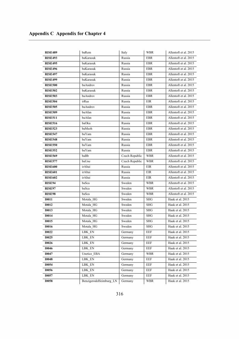
Appendix C Appendix for Chapter 4
316
RISE489 baRem Italy WBR Allentoft et al. 2015
RISE493 baKarasuk Russia EBR Allentoft et al. 2015
RISE495 baKarasuk Russia EBR Allentoft et al. 2015
RISE496 baKarasuk Russia EBR Allentoft et al. 2015
RISE497 baKarasuk Russia EBR Allentoft et al. 2015
RISE499 baKarasuk Russia EBR Allentoft et al. 2015
RISE500 baAndrov Russia EBR Allentoft et al. 2015
RISE502 baKarasuk Russia EBR Allentoft et al. 2015
RISE503 baAndrov Russia EBR Allentoft et al. 2015
RISE504 irRus Russia EIR Allentoft et al. 2015
RISE505 baAndrov Russia EBR Allentoft et al. 2015
RISE509 baAfan Russia EBR Allentoft et al. 2015
RISE511 baAfan Russia EBR Allentoft et al. 2015
RISE516 baOku Russia EBR Allentoft et al. 2015
RISE523 baMezh Russia EBR Allentoft et al. 2015
RISE547 baYam Russia EBR Allentoft et al. 2015
RISE548 baYam Russia EBR Allentoft et al. 2015
RISE550 baYam Russia EBR Allentoft et al. 2015
RISE552 baYam Russia EBR Allentoft et al. 2015
RISE569 baBb Czech Republic WBR Allentoft et al. 2015
RISE577 baUne Czech Republic WBR Allentoft et al. 2015
RISE600 irAltai Russia EIR Allentoft et al. 2015
RISE601 irAltai Russia EIR Allentoft et al. 2015
RISE602 irAltai Russia EIR Allentoft et al. 2015
RISE94 baSca Sweden WBR Allentoft et al. 2015
RISE97 baSca Sweden WBR Allentoft et al. 2015
RISE98 baSca Sweden WBR Allentoft et al. 2015
I0011 Motala_HG Sweden SHG Haak et al. 2015
I0012 Motala_HG Sweden SHG Haak et al. 2015
I0013 Motala_HG Sweden SHG Haak et al. 2015
I0014 Motala_HG Sweden SHG Haak et al. 2015
I0015 Motala_HG Sweden SHG Haak et al. 2015
I0016 Motala_HG Sweden SHG Haak et al. 2015
I0022 LBK_EN Germany EEF Haak et al. 2015
I0025 LBK_EN Germany EEF Haak et al. 2015
I0026 LBK_EN Germany EEF Haak et al. 2015
I0046 LBK_EN Germany EEF Haak et al. 2015
I0047 Unetice_EBA Germany WBR Haak et al. 2015
I0048 LBK_EN Germany EEF Haak et al. 2015
I0054 LBK_EN Germany EEF Haak et al. 2015
I0056 LBK_EN Germany EEF Haak et al. 2015
I0057 LBK_EN Germany EEF Haak et al. 2015
I0058 BenzigerodeHeimburg_LN Germany WBR Haak et al. 2015
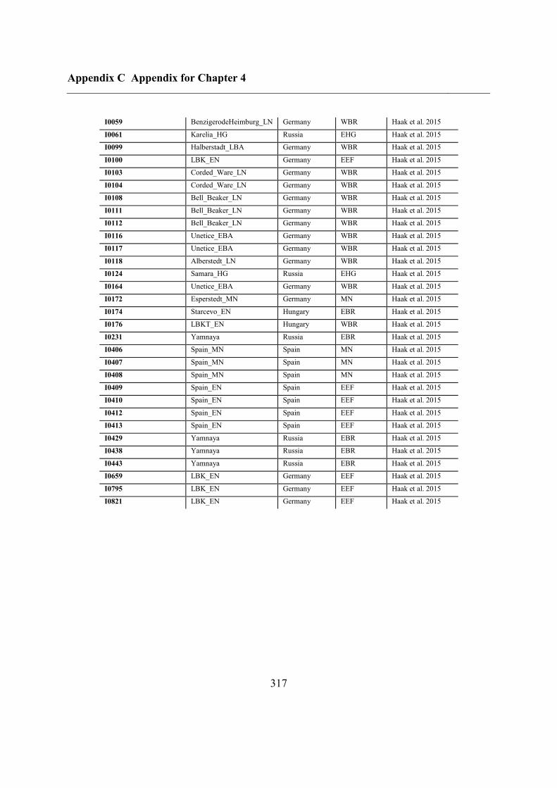
Appendix C Appendix for Chapter 4
317
I0059 BenzigerodeHeimburg_LN Germany WBR Haak et al. 2015
I0061 Karelia_HG Russia EHG Haak et al. 2015
I0099 Halberstadt_LBA Germany WBR Haak et al. 2015
I0100 LBK_EN Germany EEF Haak et al. 2015
I0103 Corded_Ware_LN Germany WBR Haak et al. 2015
I0104 Corded_Ware_LN Germany WBR Haak et al. 2015
I0108 Bell_Beaker_LN Germany WBR Haak et al. 2015
I0111 Bell_Beaker_LN Germany WBR Haak et al. 2015
I0112 Bell_Beaker_LN Germany WBR Haak et al. 2015
I0116 Unetice_EBA Germany WBR Haak et al. 2015
I0117 Unetice_EBA Germany WBR Haak et al. 2015
I0118 Alberstedt_LN Germany WBR Haak et al. 2015
I0124 Samara_HG Russia EHG Haak et al. 2015
I0164 Unetice_EBA Germany WBR Haak et al. 2015
I0172 Esperstedt_MN Germany MN Haak et al. 2015
I0174 Starcevo_EN Hungary EBR Haak et al. 2015
I0176 LBKT_EN Hungary WBR Haak et al. 2015
I0231 Yamnaya Russia EBR Haak et al. 2015
I0406 Spain_MN Spain MN Haak et al. 2015
I0407 Spain_MN Spain MN Haak et al. 2015
I0408 Spain_MN Spain MN Haak et al. 2015
I0409 Spain_EN Spain EEF Haak et al. 2015
I0410 Spain_EN Spain EEF Haak et al. 2015
I0412 Spain_EN Spain EEF Haak et al. 2015
I0413 Spain_EN Spain EEF Haak et al. 2015
I0429 Yamnaya Russia EBR Haak et al. 2015
I0438 Yamnaya Russia EBR Haak et al. 2015
I0443 Yamnaya Russia EBR Haak et al. 2015
I0659 LBK_EN Germany EEF Haak et al. 2015
I0795 LBK_EN Germany EEF Haak et al. 2015
I0821 LBK_EN Germany EEF Haak et al. 2015
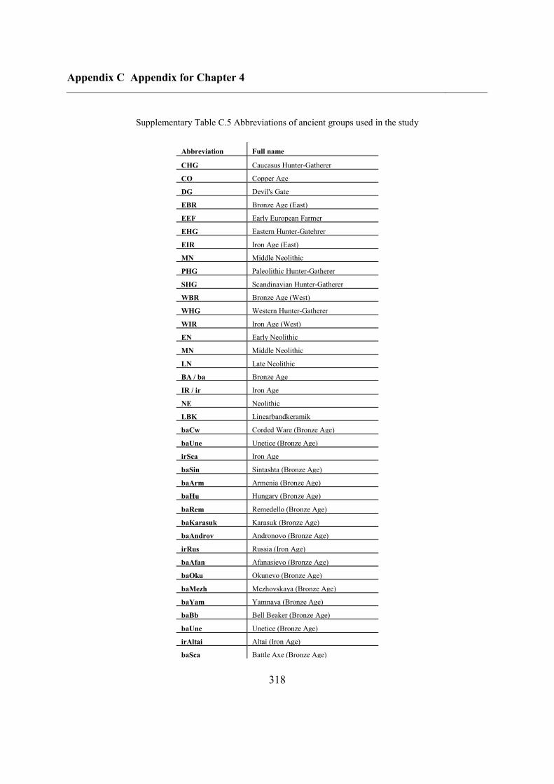
Appendix C Appendix for Chapter 4
318
Supplementary Table C.5 Abbreviations of ancient groups used in the study
Abbreviation Full name
CHG Caucasus Hunter-Gatherer
CO Copper Age
DG Devil's Gate
EBR Bronze Age (East)
EEF Early European Farmer
EHG Eastern Hunter-Gatehrer
EIR Iron Age (East)
MN Middle Neolithic
PHG Paleolithic Hunter-Gatherer
SHG Scandinavian Hunter-Gatherer
WBR Bronze Age (West)
WHG Western Hunter-Gatherer
WIR Iron Age (West)
EN Early Neolithic
MN Middle Neolithic
LN Late Neolithic
BA / ba Bronze Age
IR / ir Iron Age
NE Neolithic
LBK Linearbandkeramik
baCw Corded Ware (Bronze Age)
baUne Unetice (Bronze Age)
irSca Iron Age
baSin Sintashta (Bronze Age)
baArm Armenia (Bronze Age)
baHu Hungary (Bronze Age)
baRem Remedello (Bronze Age)
baKarasuk Karasuk (Bronze Age)
baAndrov Andronovo (Bronze Age)
irRus Russia (Iron Age)
baAfan Afanasievo (Bronze Age)
baOku Okunevo (Bronze Age)
baMezh Mezhovskaya (Bronze Age)
baYam Yamnaya (Bronze Age)
baBb Bell Beaker (Bronze Age)
baUne Unetice (Bronze Age)
irAltai Altai (Iron Age)
baSca Battle Axe (Bronze Age)
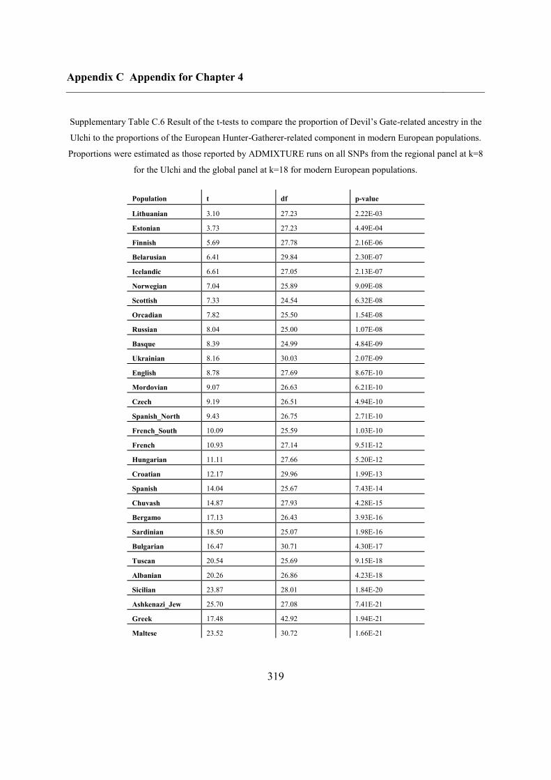
Appendix C Appendix for Chapter 4
319
Supplementary Table C.6 Result of the t-tests to compare the proportion of Devil’s Gate-related ancestry in the
Ulchi to the proportions of the European Hunter-Gatherer-related component in modern European populations.
Proportions were estimated as those reported by ADMIXTURE runs on all SNPs from the regional panel at k=8
for the Ulchi and the global panel at k=18 for modern European populations.
Population t df p-value
Lithuanian 3.10 27.23 2.22E-03
Estonian 3.73 27.23 4.49E-04
Finnish 5.69 27.78 2.16E-06
Belarusian 6.41 29.84 2.30E-07
Icelandic 6.61 27.05 2.13E-07
Norwegian 7.04 25.89 9.09E-08
Scottish 7.33 24.54 6.32E-08
Orcadian 7.82 25.50 1.54E-08
Russian 8.04 25.00 1.07E-08
Basque 8.39 24.99 4.84E-09
Ukrainian 8.16 30.03 2.07E-09
English 8.78 27.69 8.67E-10
Mordovian 9.07 26.63 6.21E-10
Czech 9.19 26.51 4.94E-10
Spanish_North 9.43 26.75 2.71E-10
French_South 10.09 25.59 1.03E-10
French 10.93 27.14 9.51E-12
Hungarian 11.11 27.66 5.20E-12
Croatian 12.17 29.96 1.99E-13
Spanish 14.04 25.67 7.43E-14
Chuvash 14.87 27.93 4.28E-15
Bergamo 17.13 26.43 3.93E-16
Sardinian 18.50 25.07 1.98E-16
Bulgarian 16.47 30.71 4.30E-17
Tuscan 20.54 25.69 9.15E-18
Albanian 20.26 26.86 4.23E-18
Sicilian 23.87 28.01 1.84E-20
Ashkenazi_Jew 25.70 27.08 7.41E-21
Greek 17.48 42.92 1.94E-21
Maltese 23.52 30.72 1.66E-21

Appendix C Appendix for Chapter 4
320
Supplementary Table C.7 Results of t-tests to compare the proportion of Devil’s Gate-related ancestry in the
Ulchi to the proportions of the Early European Farmer-related component in modern European populations.
Proportions were estimated as those reported by ADMIXTURE runs on all SNPs from the regional panel at k=8
for the Ulchi and the global panel at k=18 for modern European populations.
Population t df p-value
Sardinian 0.47 25.16 0.32
Sicilian 8.76 24.57 2.49E-09
Maltese 8.29 29.30 1.79E-09
Ashkenazi_Jew 9.18 26.53 5.07E-10
Tuscan 10.18 27.07 4.68E-11
Bergamo 11.24 25.77 9.81E-12
Albanian 10.70 28.22 9.60E-12
Greek 10.97 29.28 3.46E-12
Spanish 12.16 24.71 3.20E-12
Basque 12.26 24.86 2.44E-12
French_South 12.24 26.65 9.55E-13
Spanish_North 12.46 26.26 7.78E-13
Bulgarian 15.18 27.67 3.02E-15
Croatian 18.20 25.98 1.31E-16
French 16.43 30.71 4.60E-17
Hungarian 20.15 25.25 2.23E-17
English 20.51 25.55 1.09E-17
Orcadian 22.06 25.16 2.78E-18
Scottish 21.76 26.53 9.55E-19
Czech 21.23 27.43 7.37E-19
Norwegian 22.93 25.60 6.86E-19
Icelandic 23.01 26.05 3.89E-19
Belarusian 24.98 26.71 2.34E-20
Mordovian 28.00 24.66 1.65E-20
Ukrainian 22.60 30.61 5.94E-21
Russian 28.15 25.76 3.57E-21
Estonian 27.67 26.50 2.19E-21
Finnish 24.83 29.43 1.36E-21
Lithuanian 26.52 28.89 3.94E-22
Chuvash 30.50 26.10 3.04E-22

Appendix C Appendix for Chapter 4
321
Supplementary Table C.8 Result of the t-tests to compare the proportion of Devil’s Gate-related ancestry in the
Ulchi to the proportions of the Bronze Age Steppe-related component in modern European populations.
Proportions were estimated as those reported by ADMIXTURE runs on all SNPs from the regional panel at k=8
for the Ulchi and the global panel at k=18 for modern European populations.
Population t df p-value
Scottish 23.15 23.08 8.92E-18
Ashkenazi_Jew 22.34 27.59 1.65E-19
Russian 25.40 25.02 1.10E-19
Bulgarian 23.54 26.73 1.06E-19
Mordovian 23.92 26.36 1.06E-19
Sicilian 24.60 26.09 7.05E-20
Chuvash 24.31 26.63 5.18E-20
Czech 25.60 25.80 3.63E-20
Ukrainian 24.14 27.17 3.40E-20
Hungarian 25.63 25.87 3.23E-20
Orcadian 26.85 24.98 3.02E-20
Albanian 23.04 28.56 2.71E-20
Estonian 25.97 25.95 2.12E-20
Norwegian 26.71 25.42 2.01E-20
Belarusian 24.71 27.39 1.46E-20
Lithuanian 25.61 26.58 1.44E-20
Croatian 25.15 27.16 1.19E-20
Maltese 22.09 30.95 8.29E-21
English 26.72 26.16 8.12E-21
Finnish 26.47 26.74 5.18E-21
Tuscan 24.51 28.68 4.39E-21
Bergamo 27.72 26.10 3.41E-21
Icelandic 26.04 27.68 2.62E-21
Spanish 31.43 25.01 6.37E-22
French 27.48 27.97 4.39E-22
Greek 19.81 38.63 3.91E-22
French_South 33.93 25.61 4.07E-23
Basque 36.02 25.09 1.98E-23
Sardinian 37.91 24.56 1.30E-23
Spanish_North 32.79 27.71 5.22E-24
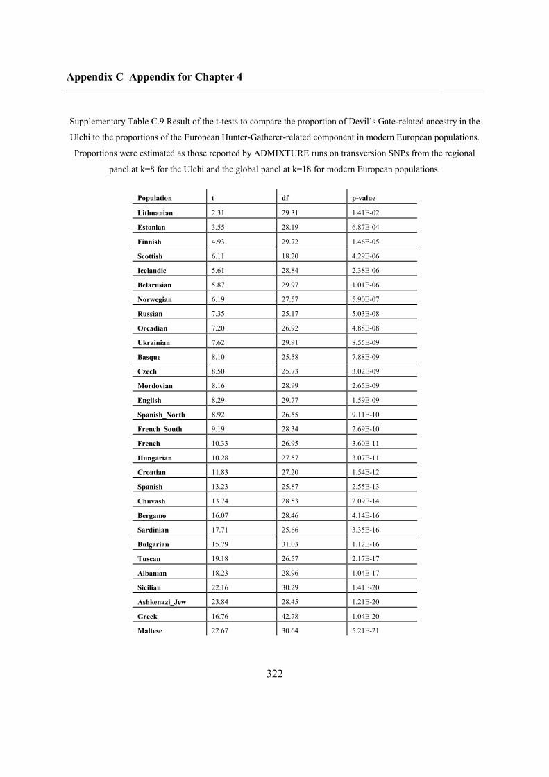
Appendix C Appendix for Chapter 4
322
Supplementary Table C.9 Result of the t-tests to compare the proportion of Devil’s Gate-related ancestry in the
Ulchi to the proportions of the European Hunter-Gatherer-related component in modern European populations.
Proportions were estimated as those reported by ADMIXTURE runs on transversion SNPs from the regional
panel at k=8 for the Ulchi and the global panel at k=18 for modern European populations.
Population t df p-value
Lithuanian 2.31 29.31 1.41E-02
Estonian 3.55 28.19 6.87E-04
Finnish 4.93 29.72 1.46E-05
Scottish 6.11 18.20 4.29E-06
Icelandic 5.61 28.84 2.38E-06
Belarusian 5.87 29.97 1.01E-06
Norwegian 6.19 27.57 5.90E-07
Russian 7.35 25.17 5.03E-08
Orcadian 7.20 26.92 4.88E-08
Ukrainian 7.62 29.91 8.55E-09
Basque 8.10 25.58 7.88E-09
Czech 8.50 25.73 3.02E-09
Mordovian 8.16 28.99 2.65E-09
English 8.29 29.77 1.59E-09
Spanish_North 8.92 26.55 9.11E-10
French_South 9.19 28.34 2.69E-10
French 10.33 26.95 3.60E-11
Hungarian 10.28 27.57 3.07E-11
Croatian 11.83 27.20 1.54E-12
Spanish 13.23 25.87 2.55E-13
Chuvash 13.74 28.53 2.09E-14
Bergamo 16.07 28.46 4.14E-16
Sardinian 17.71 25.66 3.35E-16
Bulgarian 15.79 31.03 1.12E-16
Tuscan 19.18 26.57 2.17E-17
Albanian 18.23 28.96 1.04E-17
Sicilian 22.16 30.29 1.41E-20
Ashkenazi_Jew 23.84 28.45 1.21E-20
Greek 16.76 42.78 1.04E-20
Maltese 22.67 30.64 5.21E-21
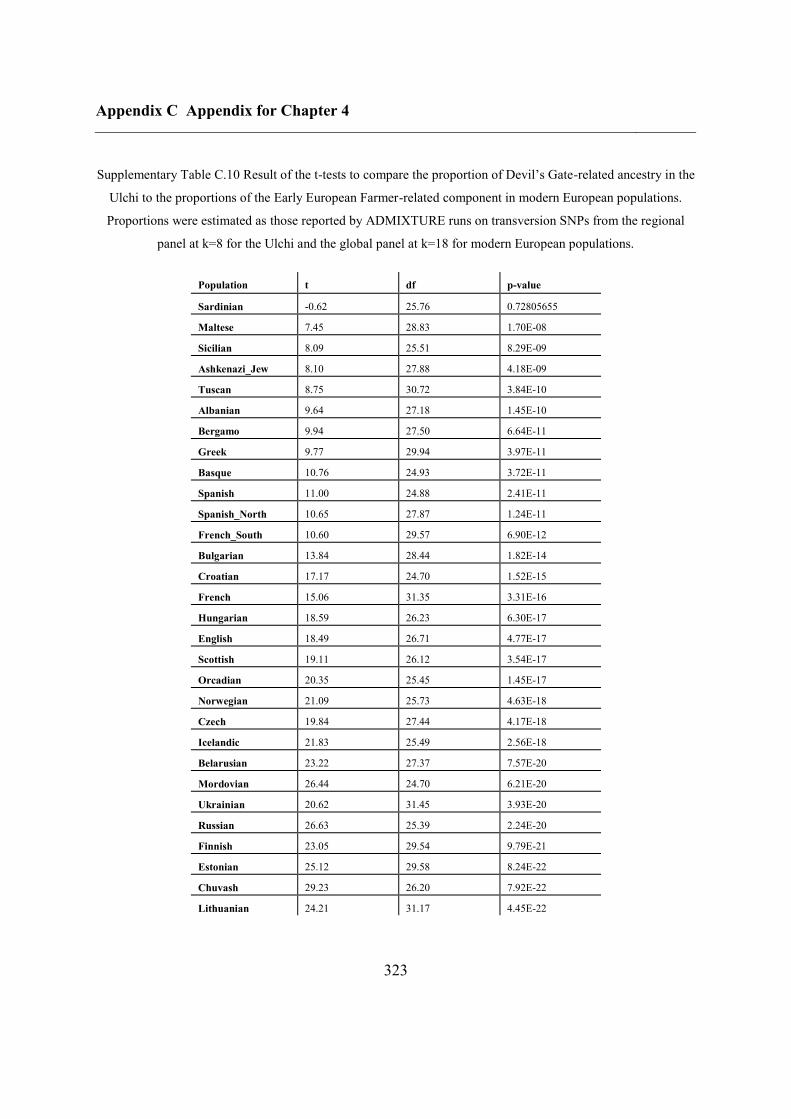
Appendix C Appendix for Chapter 4
323
Supplementary Table C.10 Result of the t-tests to compare the proportion of Devil’s Gate-related ancestry in the
Ulchi to the proportions of the Early European Farmer-related component in modern European populations.
Proportions were estimated as those reported by ADMIXTURE runs on transversion SNPs from the regional
panel at k=8 for the Ulchi and the global panel at k=18 for modern European populations.
Population t df p-value
Sardinian -0.62 25.76 0.72805655
Maltese 7.45 28.83 1.70E-08
Sicilian 8.09 25.51 8.29E-09
Ashkenazi_Jew 8.10 27.88 4.18E-09
Tuscan 8.75 30.72 3.84E-10
Albanian 9.64 27.18 1.45E-10
Bergamo 9.94 27.50 6.64E-11
Greek 9.77 29.94 3.97E-11
Basque 10.76 24.93 3.72E-11
Spanish 11.00 24.88 2.41E-11
Spanish_North 10.65 27.87 1.24E-11
French_South 10.60 29.57 6.90E-12
Bulgarian 13.84 28.44 1.82E-14
Croatian 17.17 24.70 1.52E-15
French 15.06 31.35 3.31E-16
Hungarian 18.59 26.23 6.30E-17
English 18.49 26.71 4.77E-17
Scottish 19.11 26.12 3.54E-17
Orcadian 20.35 25.45 1.45E-17
Norwegian 21.09 25.73 4.63E-18
Czech 19.84 27.44 4.17E-18
Icelandic 21.83 25.49 2.56E-18
Belarusian 23.22 27.37 7.57E-20
Mordovian 26.44 24.70 6.21E-20
Ukrainian 20.62 31.45 3.93E-20
Russian 26.63 25.39 2.24E-20
Finnish 23.05 29.54 9.79E-21
Estonian 25.12 29.58 8.24E-22
Chuvash 29.23 26.20 7.92E-22
Lithuanian 24.21 31.17 4.45E-22
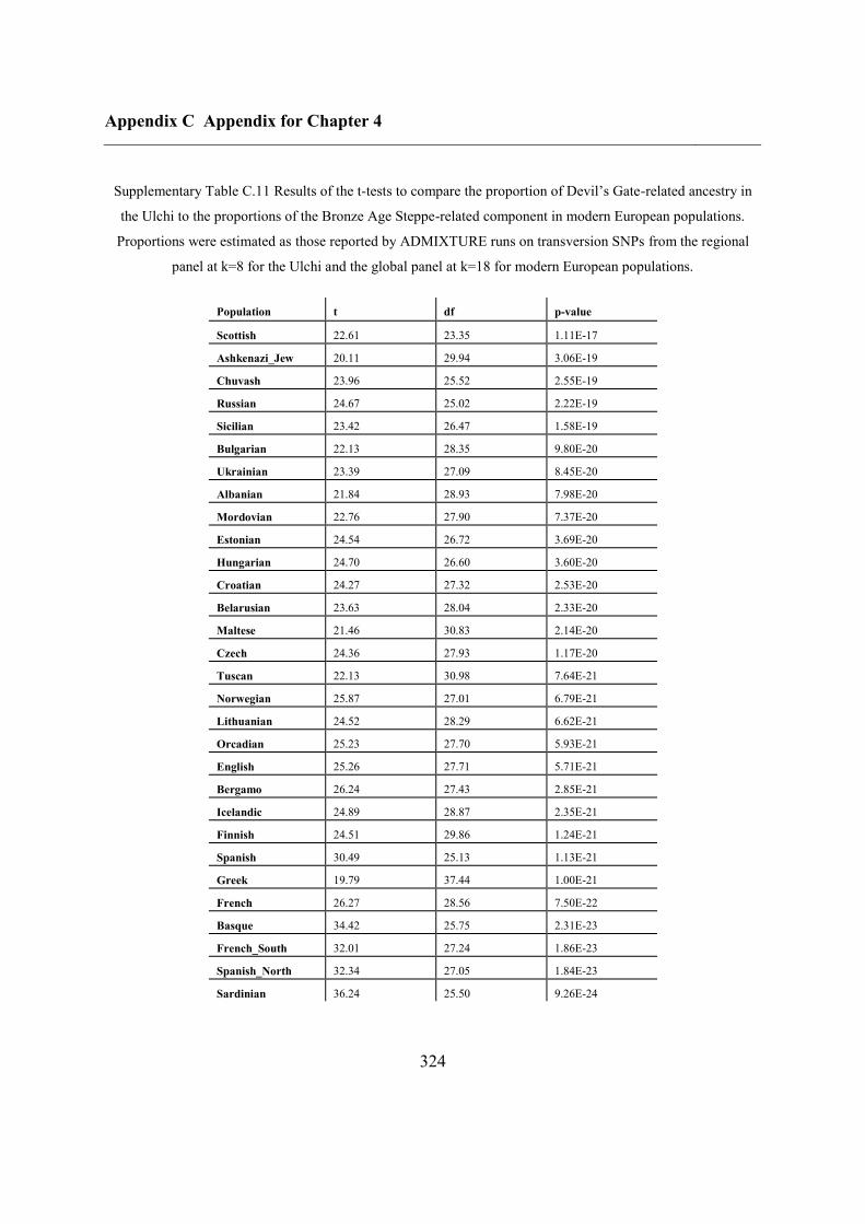
Appendix C Appendix for Chapter 4
324
Supplementary Table C.11 Results of the t-tests to compare the proportion of Devil’s Gate-related ancestry in
the Ulchi to the proportions of the Bronze Age Steppe-related component in modern European populations.
Proportions were estimated as those reported by ADMIXTURE runs on transversion SNPs from the regional
panel at k=8 for the Ulchi and the global panel at k=18 for modern European populations.
Population t df p-value
Scottish 22.61 23.35 1.11E-17
Ashkenazi_Jew 20.11 29.94 3.06E-19
Chuvash 23.96 25.52 2.55E-19
Russian 24.67 25.02 2.22E-19
Sicilian 23.42 26.47 1.58E-19
Bulgarian 22.13 28.35 9.80E-20
Ukrainian 23.39 27.09 8.45E-20
Albanian 21.84 28.93 7.98E-20
Mordovian 22.76 27.90 7.37E-20
Estonian 24.54 26.72 3.69E-20
Hungarian 24.70 26.60 3.60E-20
Croatian 24.27 27.32 2.53E-20
Belarusian 23.63 28.04 2.33E-20
Maltese 21.46 30.83 2.14E-20
Czech 24.36 27.93 1.17E-20
Tuscan 22.13 30.98 7.64E-21
Norwegian 25.87 27.01 6.79E-21
Lithuanian 24.52 28.29 6.62E-21
Orcadian 25.23 27.70 5.93E-21
English 25.26 27.71 5.71E-21
Bergamo 26.24 27.43 2.85E-21
Icelandic 24.89 28.87 2.35E-21
Finnish 24.51 29.86 1.24E-21
Spanish 30.49 25.13 1.13E-21
Greek 19.79 37.44 1.00E-21
French 26.27 28.56 7.50E-22
Basque 34.42 25.75 2.31E-23
French_South 32.01 27.24 1.86E-23
Spanish_North 32.34 27.05 1.84E-23
Sardinian 36.24 25.50 9.26E-24
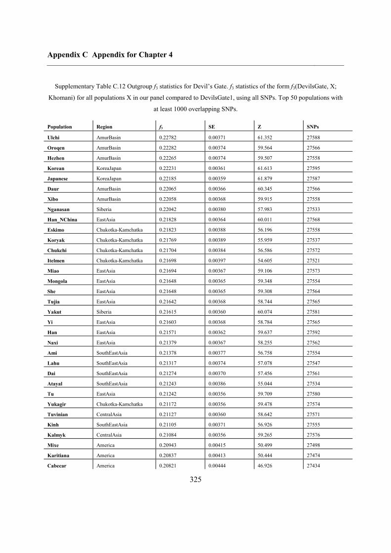
Appendix C Appendix for Chapter 4
325
Supplementary Table C.12 Outgroup f3 statistics for Devil’s Gate. f3 statistics of the form f3(DevilsGate, X;
Khomani) for all populations X in our panel compared to DevilsGate1, using all SNPs. Top 50 populations with
at least 1000 overlapping SNPs.
Population Region f3 SE Z SNPs
Ulchi AmurBasin 0.22782 0.00371 61.352 27588
Oroqen AmurBasin 0.22282 0.00374 59.564 27566
Hezhen AmurBasin 0.22265 0.00374 59.507 27558
Korean KoreaJapan 0.22231 0.00361 61.613 27595
Japanese KoreaJapan 0.22185 0.00359 61.879 27587
Daur AmurBasin 0.22065 0.00366 60.345 27566
Xibo AmurBasin 0.22058 0.00368 59.915 27558
Nganasan Siberia 0.22042 0.00380 57.983 27533
Han_NChina EastAsia 0.21828 0.00364 60.011 27568
Eskimo Chukotka-Kamchatka 0.21823 0.00388 56.196 27558
Koryak Chukotka-Kamchatka 0.21769 0.00389 55.959 27537
Chukchi Chukotka-Kamchatka 0.21704 0.00384 56.586 27572
Itelmen Chukotka-Kamchatka 0.21698 0.00397 54.605 27521
Miao EastAsia 0.21694 0.00367 59.106 27573
Mongola EastAsia 0.21648 0.00365 59.348 27554
She EastAsia 0.21648 0.00365 59.308 27564
Tujia EastAsia 0.21642 0.00368 58.744 27565
Yakut Siberia 0.21615 0.00360 60.074 27581
Yi EastAsia 0.21603 0.00368 58.784 27565
Han EastAsia 0.21571 0.00362 59.637 27592
Naxi EastAsia 0.21379 0.00367 58.255 27562
Ami SouthEastAsia 0.21378 0.00377 56.758 27554
Lahu SouthEastAsia 0.21317 0.00374 57.078 27547
Dai SouthEastAsia 0.21274 0.00370 57.456 27561
Atayal SouthEastAsia 0.21243 0.00386 55.044 27534
Tu EastAsia 0.21242 0.00356 59.709 27580
Yukagir Chukotka-Kamchatka 0.21172 0.00356 59.478 27574
Tuvinian CentralAsia 0.21127 0.00360 58.642 27571
Kinh SouthEastAsia 0.21105 0.00371 56.926 27555
Kalmyk CentralAsia 0.21084 0.00356 59.265 27576
Mixe America 0.20943 0.00415 50.499 27498
Karitiana America 0.20837 0.00413 50.444 27474
Cabecar America 0.20821 0.00444 46.926 27434
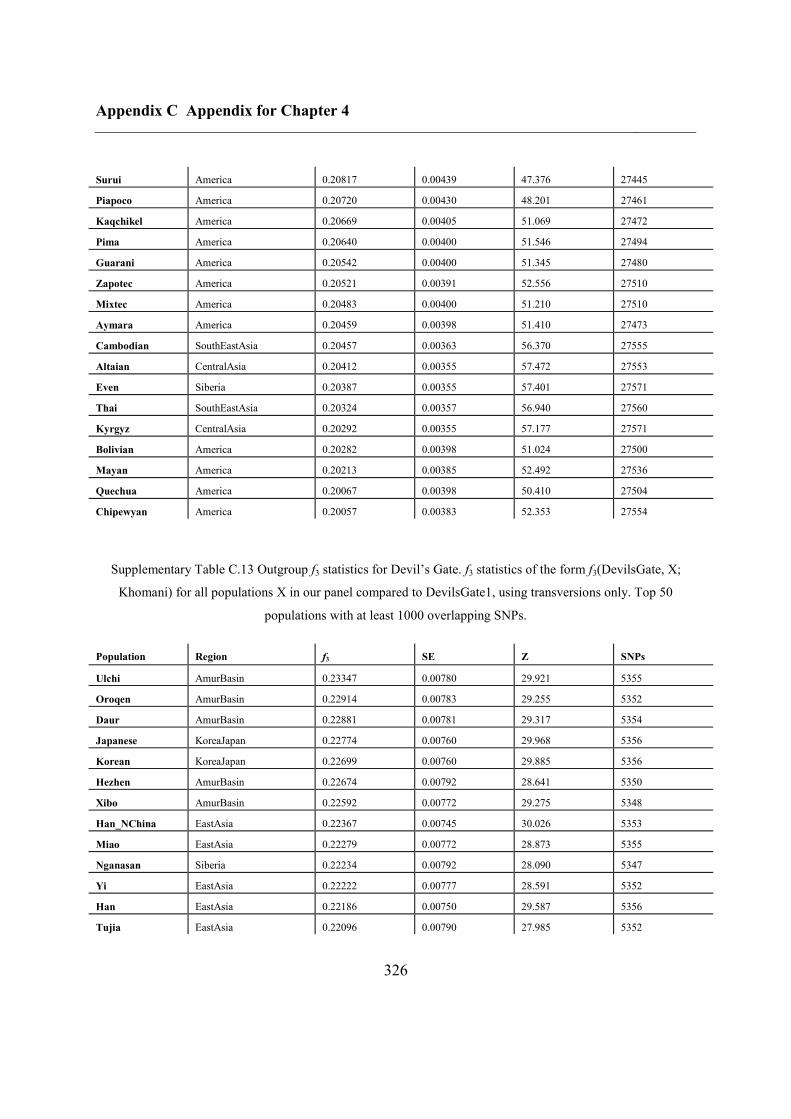
Appendix C Appendix for Chapter 4
326
Surui America 0.20817 0.00439 47.376 27445
Piapoco America 0.20720 0.00430 48.201 27461
Kaqchikel America 0.20669 0.00405 51.069 27472
Pima America 0.20640 0.00400 51.546 27494
Guarani America 0.20542 0.00400 51.345 27480
Zapotec America 0.20521 0.00391 52.556 27510
Mixtec America 0.20483 0.00400 51.210 27510
Aymara America 0.20459 0.00398 51.410 27473
Cambodian SouthEastAsia 0.20457 0.00363 56.370 27555
Altaian CentralAsia 0.20412 0.00355 57.472 27553
Even Siberia 0.20387 0.00355 57.401 27571
Thai SouthEastAsia 0.20324 0.00357 56.940 27560
Kyrgyz CentralAsia 0.20292 0.00355 57.177 27571
Bolivian America 0.20282 0.00398 51.024 27500
Mayan America 0.20213 0.00385 52.492 27536
Quechua America 0.20067 0.00398 50.410 27504
Chipewyan America 0.20057 0.00383 52.353 27554
Supplementary Table C.13 Outgroup f3 statistics for Devil’s Gate. f3 statistics of the form f3(DevilsGate, X;
Khomani) for all populations X in our panel compared to DevilsGate1, using transversions only. Top 50
populations with at least 1000 overlapping SNPs.
Population Region f3 SE Z SNPs
Ulchi AmurBasin 0.23347 0.00780 29.921 5355
Oroqen AmurBasin 0.22914 0.00783 29.255 5352
Daur AmurBasin 0.22881 0.00781 29.317 5354
Japanese KoreaJapan 0.22774 0.00760 29.968 5356
Korean KoreaJapan 0.22699 0.00760 29.885 5356
Hezhen AmurBasin 0.22674 0.00792 28.641 5350
Xibo AmurBasin 0.22592 0.00772 29.275 5348
Han_NChina EastAsia 0.22367 0.00745 30.026 5353
Miao EastAsia 0.22279 0.00772 28.873 5355
Nganasan Siberia 0.22234 0.00792 28.090 5347
Yi EastAsia 0.22222 0.00777 28.591 5352
Han EastAsia 0.22186 0.00750 29.587 5356
Tujia EastAsia 0.22096 0.00790 27.985 5352
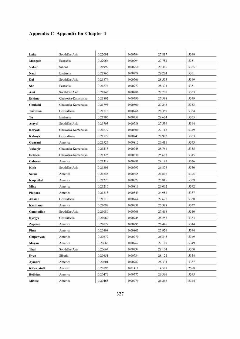
Appendix C Appendix for Chapter 4
327
Lahu SouthEastAsia 0.22091 0.00794 27.817 5349
Mongola EastAsia 0.22066 0.00794 27.782 5351
Yakut Siberia 0.21992 0.00750 29.306 5355
Naxi EastAsia 0.21966 0.00779 28.204 5351
Dai SouthEastAsia 0.21876 0.00766 28.555 5349
She EastAsia 0.21874 0.00772 28.324 5351
Ami SouthEastAsia 0.21843 0.00786 27.790 5353
Eskimo Chukotka-Kamchatka 0.21802 0.00790 27.598 5349
Chukchi Chukotka-Kamchatka 0.21793 0.00800 27.243 5353
Tuvinian CentralAsia 0.21713 0.00766 28.357 5354
Tu EastAsia 0.21705 0.00758 28.624 5355
Atayal SouthEastAsia 0.21703 0.00788 27.539 5344
Koryak Chukotka-Kamchatka 0.21677 0.00800 27.113 5349
Kalmyk CentralAsia 0.21529 0.00743 28.992 5353
Guarani America 0.21527 0.00815 26.411 5343
Yukagir Chukotka-Kamchatka 0.21513 0.00748 28.761 5355
Itelmen Chukotka-Kamchatka 0.21325 0.00830 25.693 5345
Cabecar America 0.21318 0.00881 24.185 5326
Kinh SouthEastAsia 0.21305 0.00793 26.878 5350
Surui America 0.21245 0.00855 24.847 5325
Kaqchikel America 0.21225 0.00822 25.815 5339
Mixe America 0.21216 0.00816 26.002 5342
Piapoco America 0.21213 0.00849 24.981 5337
Altaian CentralAsia 0.21110 0.00764 27.625 5350
Karitiana America 0.21098 0.00831 25.398 5337
Cambodian SouthEastAsia 0.21080 0.00768 27.468 5350
Kyrgyz CentralAsia 0.21062 0.00745 28.255 5353
Zapotec America 0.21027 0.00795 26.446 5344
Pima America 0.20808 0.00803 25.926 5344
Chipewyan America 0.20677 0.00770 26.845 5349
Mayan America 0.20666 0.00762 27.107 5349
Thai SouthEastAsia 0.20664 0.00734 28.174 5350
Even Siberia 0.20651 0.00734 28.122 5354
Aymara America 0.20601 0.00782 26.334 5337
irRus_atoft Ancient 0.20595 0.01411 14.597 2598
Bolivian America 0.20476 0.00777 26.366 5345
Mixtec America 0.20465 0.00779 26.268 5344
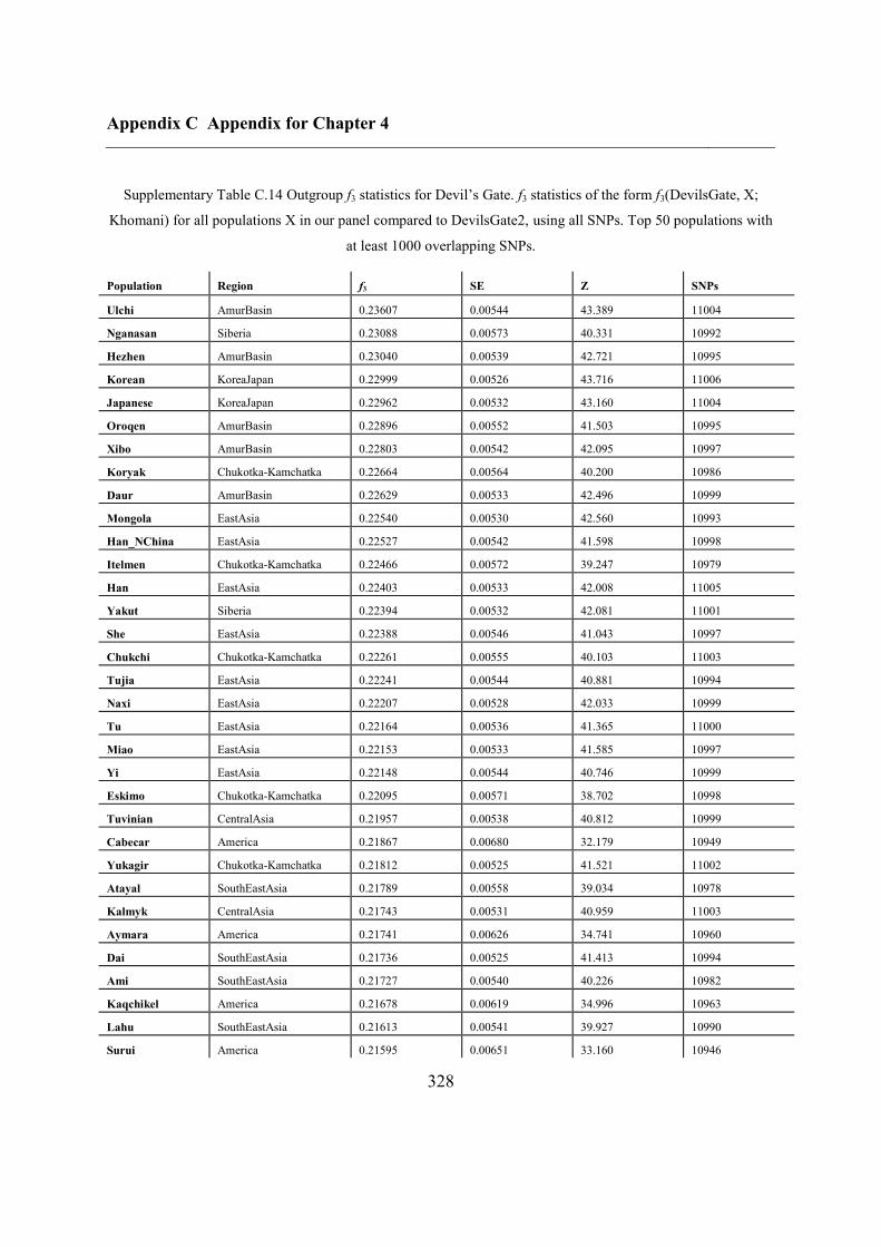
Appendix C Appendix for Chapter 4
328
Supplementary Table C.14 Outgroup f3 statistics for Devil’s Gate. f3 statistics of the form f3(DevilsGate, X;
Khomani) for all populations X in our panel compared to DevilsGate2, using all SNPs. Top 50 populations with
at least 1000 overlapping SNPs.
Population Region f3 SE Z SNPs
Ulchi AmurBasin 0.23607 0.00544 43.389 11004
Nganasan Siberia 0.23088 0.00573 40.331 10992
Hezhen AmurBasin 0.23040 0.00539 42.721 10995
Korean KoreaJapan 0.22999 0.00526 43.716 11006
Japanese KoreaJapan 0.22962 0.00532 43.160 11004
Oroqen AmurBasin 0.22896 0.00552 41.503 10995
Xibo AmurBasin 0.22803 0.00542 42.095 10997
Koryak Chukotka-Kamchatka 0.22664 0.00564 40.200 10986
Daur AmurBasin 0.22629 0.00533 42.496 10999
Mongola EastAsia 0.22540 0.00530 42.560 10993
Han_NChina EastAsia 0.22527 0.00542 41.598 10998
Itelmen Chukotka-Kamchatka 0.22466 0.00572 39.247 10979
Han EastAsia 0.22403 0.00533 42.008 11005
Yakut Siberia 0.22394 0.00532 42.081 11001
She EastAsia 0.22388 0.00546 41.043 10997
Chukchi Chukotka-Kamchatka 0.22261 0.00555 40.103 11003
Tujia EastAsia 0.22241 0.00544 40.881 10994
Naxi EastAsia 0.22207 0.00528 42.033 10999
Tu EastAsia 0.22164 0.00536 41.365 11000
Miao EastAsia 0.22153 0.00533 41.585 10997
Yi EastAsia 0.22148 0.00544 40.746 10999
Eskimo Chukotka-Kamchatka 0.22095 0.00571 38.702 10998
Tuvinian CentralAsia 0.21957 0.00538 40.812 10999
Cabecar America 0.21867 0.00680 32.179 10949
Yukagir Chukotka-Kamchatka 0.21812 0.00525 41.521 11002
Atayal SouthEastAsia 0.21789 0.00558 39.034 10978
Kalmyk CentralAsia 0.21743 0.00531 40.959 11003
Aymara America 0.21741 0.00626 34.741 10960
Dai SouthEastAsia 0.21736 0.00525 41.413 10994
Ami SouthEastAsia 0.21727 0.00540 40.226 10982
Kaqchikel America 0.21678 0.00619 34.996 10963
Lahu SouthEastAsia 0.21613 0.00541 39.927 10990
Surui America 0.21595 0.00651 33.160 10946
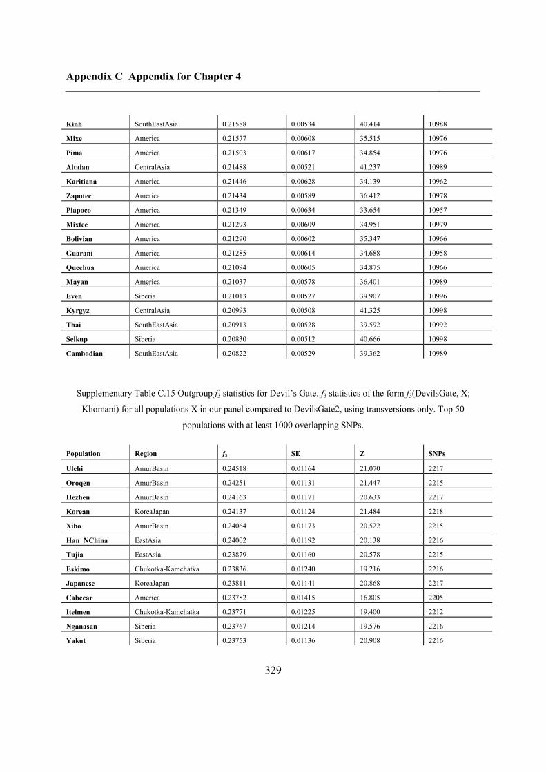
Appendix C Appendix for Chapter 4
329
Kinh SouthEastAsia 0.21588 0.00534 40.414 10988
Mixe America 0.21577 0.00608 35.515 10976
Pima America 0.21503 0.00617 34.854 10976
Altaian CentralAsia 0.21488 0.00521 41.237 10989
Karitiana America 0.21446 0.00628 34.139 10962
Zapotec America 0.21434 0.00589 36.412 10978
Piapoco America 0.21349 0.00634 33.654 10957
Mixtec America 0.21293 0.00609 34.951 10979
Bolivian America 0.21290 0.00602 35.347 10966
Guarani America 0.21285 0.00614 34.688 10958
Quechua America 0.21094 0.00605 34.875 10966
Mayan America 0.21037 0.00578 36.401 10989
Even Siberia 0.21013 0.00527 39.907 10996
Kyrgyz CentralAsia 0.20993 0.00508 41.325 10998
Thai SouthEastAsia 0.20913 0.00528 39.592 10992
Selkup Siberia 0.20830 0.00512 40.666 10998
Cambodian SouthEastAsia 0.20822 0.00529 39.362 10989
Supplementary Table C.15 Outgroup f3 statistics for Devil’s Gate. f3 statistics of the form f3(DevilsGate, X;
Khomani) for all populations X in our panel compared to DevilsGate2, using transversions only. Top 50
populations with at least 1000 overlapping SNPs.
Population Region f3 SE Z SNPs
Ulchi AmurBasin 0.24518 0.01164 21.070 2217
Oroqen AmurBasin 0.24251 0.01131 21.447 2215
Hezhen AmurBasin 0.24163 0.01171 20.633 2217
Korean KoreaJapan 0.24137 0.01124 21.484 2218
Xibo AmurBasin 0.24064 0.01173 20.522 2215
Han_NChina EastAsia 0.24002 0.01192 20.138 2216
Tujia EastAsia 0.23879 0.01160 20.578 2215
Eskimo Chukotka-Kamchatka 0.23836 0.01240 19.216 2216
Japanese KoreaJapan 0.23811 0.01141 20.868 2217
Cabecar America 0.23782 0.01415 16.805 2205
Itelmen Chukotka-Kamchatka 0.23771 0.01225 19.400 2212
Nganasan Siberia 0.23767 0.01214 19.576 2216
Yakut Siberia 0.23753 0.01136 20.908 2216
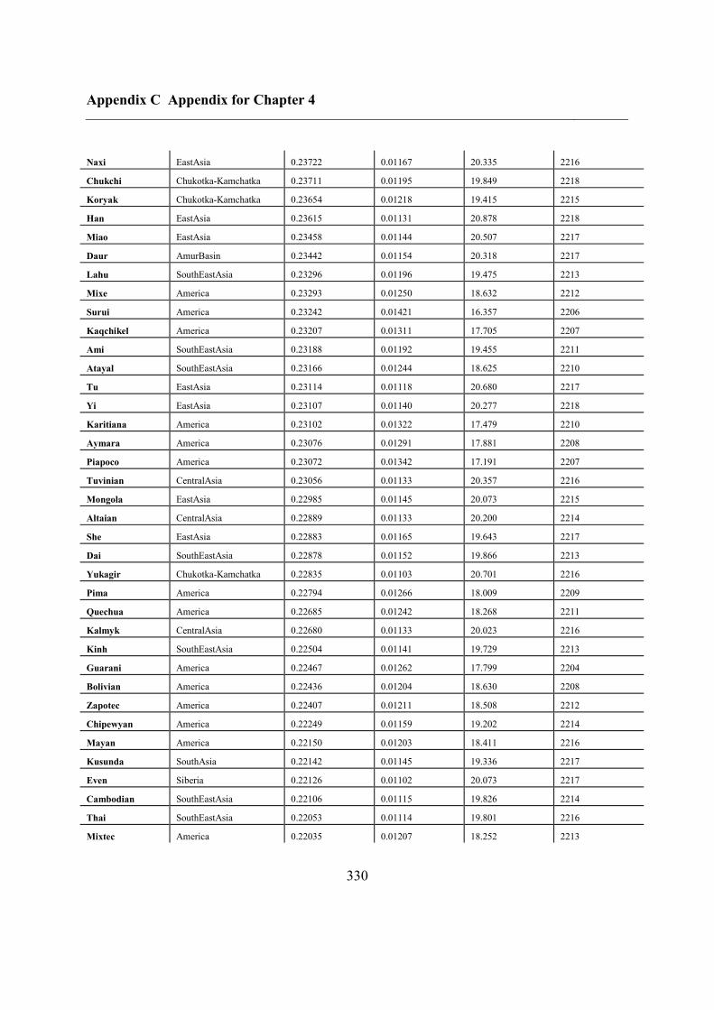
Appendix C Appendix for Chapter 4
330
Naxi EastAsia 0.23722 0.01167 20.335 2216
Chukchi Chukotka-Kamchatka 0.23711 0.01195 19.849 2218
Koryak Chukotka-Kamchatka 0.23654 0.01218 19.415 2215
Han EastAsia 0.23615 0.01131 20.878 2218
Miao EastAsia 0.23458 0.01144 20.507 2217
Daur AmurBasin 0.23442 0.01154 20.318 2217
Lahu SouthEastAsia 0.23296 0.01196 19.475 2213
Mixe America 0.23293 0.01250 18.632 2212
Surui America 0.23242 0.01421 16.357 2206
Kaqchikel America 0.23207 0.01311 17.705 2207
Ami SouthEastAsia 0.23188 0.01192 19.455 2211
Atayal SouthEastAsia 0.23166 0.01244 18.625 2210
Tu EastAsia 0.23114 0.01118 20.680 2217
Yi EastAsia 0.23107 0.01140 20.277 2218
Karitiana America 0.23102 0.01322 17.479 2210
Aymara America 0.23076 0.01291 17.881 2208
Piapoco America 0.23072 0.01342 17.191 2207
Tuvinian CentralAsia 0.23056 0.01133 20.357 2216
Mongola EastAsia 0.22985 0.01145 20.073 2215
Altaian CentralAsia 0.22889 0.01133 20.200 2214
She EastAsia 0.22883 0.01165 19.643 2217
Dai SouthEastAsia 0.22878 0.01152 19.866 2213
Yukagir Chukotka-Kamchatka 0.22835 0.01103 20.701 2216
Pima America 0.22794 0.01266 18.009 2209
Quechua America 0.22685 0.01242 18.268 2211
Kalmyk CentralAsia 0.22680 0.01133 20.023 2216
Kinh SouthEastAsia 0.22504 0.01141 19.729 2213
Guarani America 0.22467 0.01262 17.799 2204
Bolivian America 0.22436 0.01204 18.630 2208
Zapotec America 0.22407 0.01211 18.508 2212
Chipewyan America 0.22249 0.01159 19.202 2214
Mayan America 0.22150 0.01203 18.411 2216
Kusunda SouthAsia 0.22142 0.01145 19.336 2217
Even Siberia 0.22126 0.01102 20.073 2217
Cambodian SouthEastAsia 0.22106 0.01115 19.826 2214
Thai SouthEastAsia 0.22053 0.01114 19.801 2216
Mixtec America 0.22035 0.01207 18.252 2213

Appendix C Appendix for Chapter 4
331
Supplementary Table C.16 D scores for the Ulchi. D statistics of the form D(Ulchi, DevilsGate1; X, Khomani)
for all populations X in our panel, using all SNPs, sorted by |Z| and top 30 populations displayed.
Population D Z SNPs1 SNPs2 SNPs
Nganasan -0.0466 -6.658 1485 1630 34815
Yukagir -0.0413 -6.448 1478 1605 34815
Koryak -0.0475 -6.412 1481 1628 34815
Selkup -0.0410 -6.172 1462 1587 34815
Itelmen -0.0463 -6.089 1477 1620 34815
Even -0.0365 -5.699 1471 1583 34815
Tuvinian -0.0372 -5.680 1486 1601 34815
Chukchi -0.0407 -5.655 1485 1611 34815
Oroqen -0.0380 -5.604 1500 1619 34815
Altaian -0.0357 -5.488 1477 1586 34815
Han -0.0353 -5.457 1496 1605 34815
Hezhen -0.0370 -5.403 1501 1616 34815
Yakut -0.0343 -5.331 1492 1598 34815
Naxi -0.0355 -5.261 1491 1601 34815
Kinh -0.0360 -5.203 1489 1600 34815
Tubalar -0.0323 -5.179 1462 1560 34815
Kharia -0.0322 -5.068 1451 1547 34815
MA1 -0.0668 -5.020 978 1118 24644
Kalmyk -0.0337 -5.012 1488 1592 34815
Tu -0.0335 -5.004 1494 1597 34815
Sindhi -0.0291 -4.963 1424 1509 34815
Thai -0.0327 -4.955 1481 1581 34815
Tujia -0.0328 -4.857 1498 1600 34815
Xibo -0.0337 -4.773 1504 1608 34815
Daur -0.0330 -4.745 1502 1605 34815
Mongola -0.0331 -4.733 1498 1601 34815
Dai -0.0323 -4.718 1493 1593 34815
GujaratiA -0.0310 -4.668 1420 1511 34815
Lodhi -0.0287 -4.666 1433 1518 34815
Mansi -0.0313 -4.658 1464 1559 34815
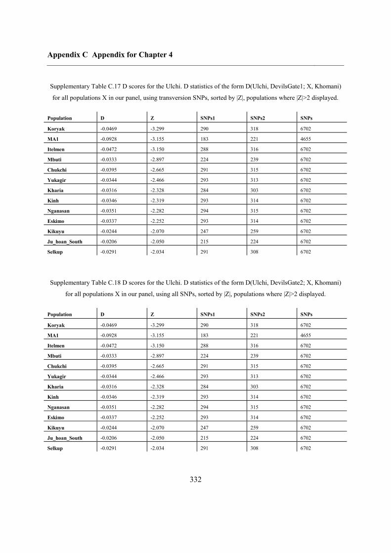
Appendix C Appendix for Chapter 4
332
Supplementary Table C.17 D scores for the Ulchi. D statistics of the form D(Ulchi, DevilsGate1; X, Khomani)
for all populations X in our panel, using transversion SNPs, sorted by |Z|, populations where |Z|>2 displayed.
Population D Z SNPs1 SNPs2 SNPs
Koryak -0.0469 -3.299 290 318 6702
MA1 -0.0928 -3.155 183 221 4655
Itelmen -0.0472 -3.150 288 316 6702
Mbuti -0.0333 -2.897 224 239 6702
Chukchi -0.0395 -2.665 291 315 6702
Yukagir -0.0344 -2.466 293 313 6702
Kharia -0.0316 -2.328 284 303 6702
Kinh -0.0346 -2.319 293 314 6702
Nganasan -0.0351 -2.282 294 315 6702
Eskimo -0.0337 -2.252 293 314 6702
Kikuyu -0.0244 -2.070 247 259 6702
Ju_hoan_South -0.0206 -2.050 215 224 6702
Selkup -0.0291 -2.034 291 308 6702
Supplementary Table C.18 D scores for the Ulchi. D statistics of the form D(Ulchi, DevilsGate2; X, Khomani)
for all populations X in our panel, using all SNPs, sorted by |Z|, populations where |Z|>2 displayed.
Population D Z SNPs1 SNPs2 SNPs
Koryak -0.0469 -3.299 290 318 6702
MA1 -0.0928 -3.155 183 221 4655
Itelmen -0.0472 -3.150 288 316 6702
Mbuti -0.0333 -2.897 224 239 6702
Chukchi -0.0395 -2.665 291 315 6702
Yukagir -0.0344 -2.466 293 313 6702
Kharia -0.0316 -2.328 284 303 6702
Kinh -0.0346 -2.319 293 314 6702
Nganasan -0.0351 -2.282 294 315 6702
Eskimo -0.0337 -2.252 293 314 6702
Kikuyu -0.0244 -2.070 247 259 6702
Ju_hoan_South -0.0206 -2.050 215 224 6702
Selkup -0.0291 -2.034 291 308 6702
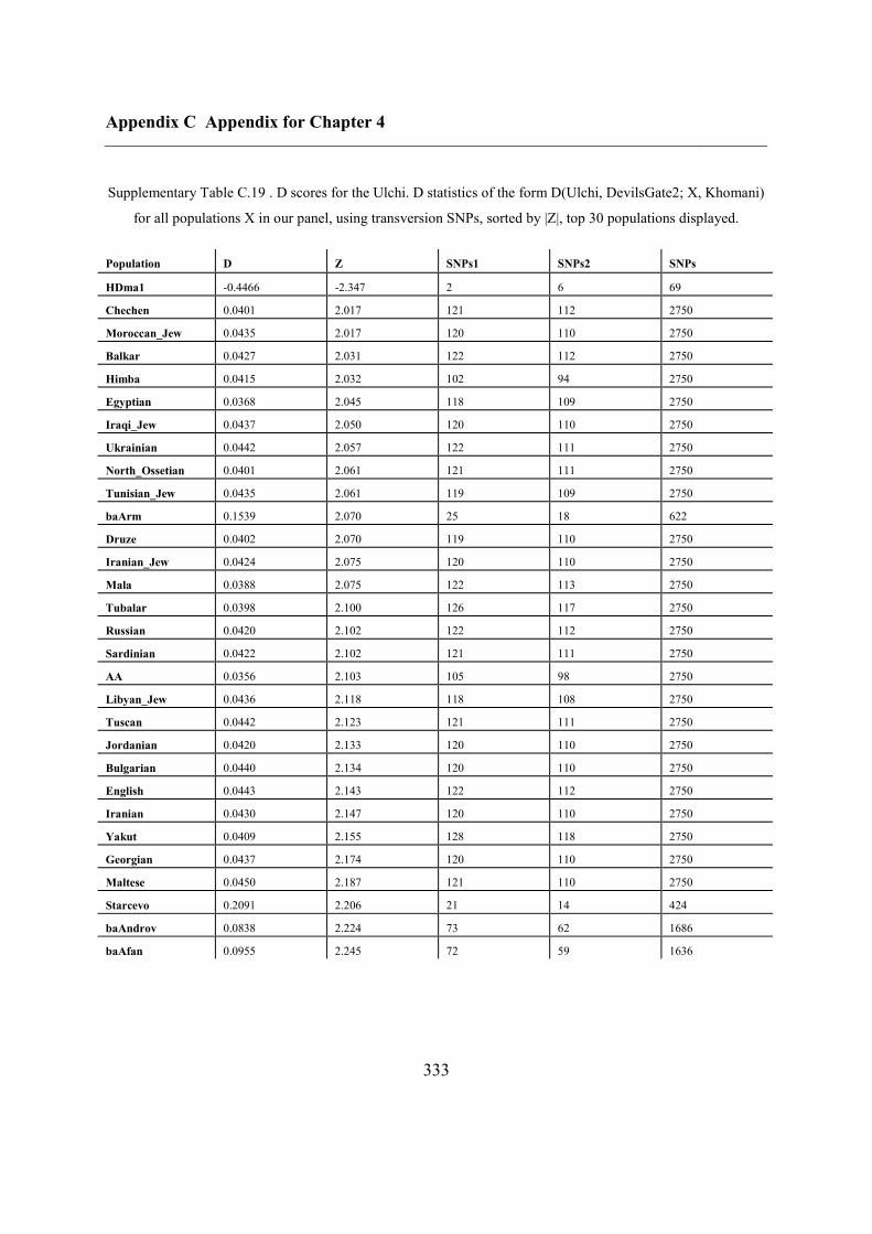
Appendix C Appendix for Chapter 4
333
Supplementary Table C.19 . D scores for the Ulchi. D statistics of the form D(Ulchi, DevilsGate2; X, Khomani)
for all populations X in our panel, using transversion SNPs, sorted by |Z|, top 30 populations displayed.
Population D Z SNPs1 SNPs2 SNPs
HDma1 -0.4466 -2.347 2 6 69
Chechen 0.0401 2.017 121 112 2750
Moroccan_Jew 0.0435 2.017 120 110 2750
Balkar 0.0427 2.031 122 112 2750
Himba 0.0415 2.032 102 94 2750
Egyptian 0.0368 2.045 118 109 2750
Iraqi_Jew 0.0437 2.050 120 110 2750
Ukrainian 0.0442 2.057 122 111 2750
North_Ossetian 0.0401 2.061 121 111 2750
Tunisian_Jew 0.0435 2.061 119 109 2750
baArm 0.1539 2.070 25 18 622
Druze 0.0402 2.070 119 110 2750
Iranian_Jew 0.0424 2.075 120 110 2750
Mala 0.0388 2.075 122 113 2750
Tubalar 0.0398 2.100 126 117 2750
Russian 0.0420 2.102 122 112 2750
Sardinian 0.0422 2.102 121 111 2750
AA 0.0356 2.103 105 98 2750
Libyan_Jew 0.0436 2.118 118 108 2750
Tuscan 0.0442 2.123 121 111 2750
Jordanian 0.0420 2.133 120 110 2750
Bulgarian 0.0440 2.134 120 110 2750
English 0.0443 2.143 122 112 2750
Iranian 0.0430 2.147 120 110 2750
Yakut 0.0409 2.155 128 118 2750
Georgian 0.0437 2.174 120 110 2750
Maltese 0.0450 2.187 121 110 2750
Starcevo 0.2091 2.206 21 14 424
baAndrov 0.0838 2.224 73 62 1686
baAfan 0.0955 2.245 72 59 1636
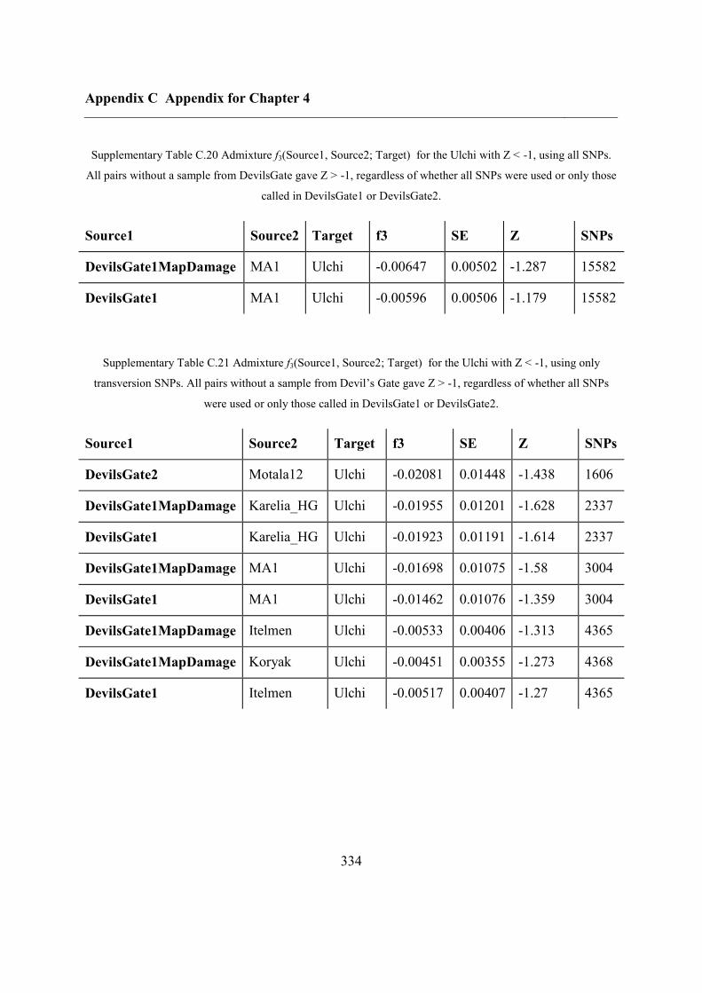
Appendix C Appendix for Chapter 4
334
Supplementary Table C.20 Admixture f3(Source1, Source2; Target) for the Ulchi with Z < -1, using all SNPs.
All pairs without a sample from DevilsGate gave Z > -1, regardless of whether all SNPs were used or only those
called in DevilsGate1 or DevilsGate2.
Source1 Source2 Target f3 SE Z SNPs
DevilsGate1MapDamage MA1 Ulchi -0.00647 0.00502 -1.287 15582
DevilsGate1 MA1 Ulchi -0.00596 0.00506 -1.179 15582
Supplementary Table C.21 Admixture f3(Source1, Source2; Target) for the Ulchi with Z < -1, using only
transversion SNPs. All pairs without a sample from Devil’s Gate gave Z > -1, regardless of whether all SNPs
were used or only those called in DevilsGate1 or DevilsGate2.
Source1 Source2 Target f3 SE Z SNPs
DevilsGate2 Motala12 Ulchi -0.02081 0.01448 -1.438 1606
DevilsGate1MapDamage Karelia_HG Ulchi -0.01955 0.01201 -1.628 2337
DevilsGate1 Karelia_HG Ulchi -0.01923 0.01191 -1.614 2337
DevilsGate1MapDamage MA1 Ulchi -0.01698 0.01075 -1.58 3004
DevilsGate1 MA1 Ulchi -0.01462 0.01076 -1.359 3004
DevilsGate1MapDamage Itelmen Ulchi -0.00533 0.00406 -1.313 4365
DevilsGate1MapDamage Koryak Ulchi -0.00451 0.00355 -1.273 4368
DevilsGate1 Itelmen Ulchi -0.00517 0.00407 -1.27 4365
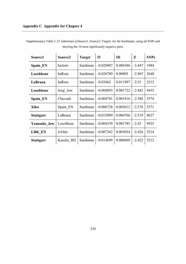
Appendix C Appendix for Chapter 4
335
Supplementary Table C.22 Admixture f3(Source1, Source2; Target) for the Sardinians, using all SNPs and
showing the 10 most significantly negative pairs.
Source1 Source2 Target f3 SE Z SNPs
Spain_EN baArm Sardinian -0.028907 0.008386 -3.447 1984
Loschbour baRem Sardinian -0.026789 0.00903 -2.967 2648
LaBrana baRem Sardinian -0.03462 0.011897 -2.91 2512
Loschbour Iraqi_Jew Sardinian -0.004893 0.001722 -2.842 9435
Spain_EN Chuvash Sardinian -0.004701 0.001816 -2.588 5574
Xibo Spain_EN Sardinian -0.006728 0.002612 -2.576 5571
Stuttgart LaBrana Sardinian -0.012009 0.004766 -2.519 8627
Yemenite_Jew Loschbour Sardinian -0.004339 0.001785 -2.43 9435
LBK_EN irAltai Sardinian -0.007362 0.003034 -2.426 5214
Stuttgart Karelia_HG Sardinian -0.014699 0.006069 -2.422 5212
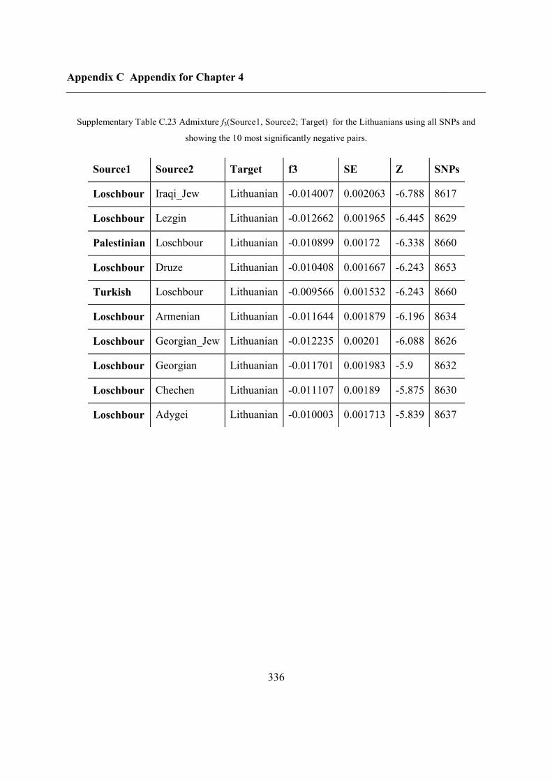
Appendix C Appendix for Chapter 4
336
Supplementary Table C.23 Admixture f3(Source1, Source2; Target) for the Lithuanians using all SNPs and
showing the 10 most significantly negative pairs.
Source1 Source2 Target f3 SE Z SNPs
Loschbour Iraqi_Jew Lithuanian -0.014007 0.002063 -6.788 8617
Loschbour Lezgin Lithuanian -0.012662 0.001965 -6.445 8629
Palestinian Loschbour Lithuanian -0.010899 0.00172 -6.338 8660
Loschbour Druze Lithuanian -0.010408 0.001667 -6.243 8653
Turkish Loschbour Lithuanian -0.009566 0.001532 -6.243 8660
Loschbour Armenian Lithuanian -0.011644 0.001879 -6.196 8634
Loschbour Georgian_Jew Lithuanian -0.012235 0.00201 -6.088 8626
Loschbour Georgian Lithuanian -0.011701 0.001983 -5.9 8632
Loschbour Chechen Lithuanian -0.011107 0.00189 -5.875 8630
Loschbour Adygei Lithuanian -0.010003 0.001713 -5.839 8637
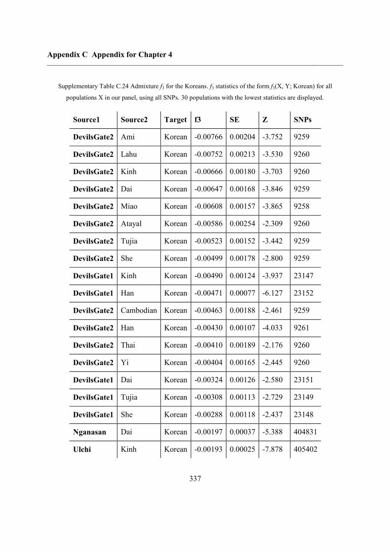
Appendix C Appendix for Chapter 4
337
Supplementary Table C.24 Admixture f3 for the Koreans. f3 statistics of the form f3(X, Y; Korean) for all
populations X in our panel, using all SNPs. 30 populations with the lowest statistics are displayed.
Source1 Source2 Target f3 SE Z SNPs
DevilsGate2 Ami Korean -0.00766 0.00204 -3.752 9259
DevilsGate2 Lahu Korean -0.00752 0.00213 -3.530 9260
DevilsGate2 Kinh Korean -0.00666 0.00180 -3.703 9260
DevilsGate2 Dai Korean -0.00647 0.00168 -3.846 9259
DevilsGate2 Miao Korean -0.00608 0.00157 -3.865 9258
DevilsGate2 Atayal Korean -0.00586 0.00254 -2.309 9260
DevilsGate2 Tujia Korean -0.00523 0.00152 -3.442 9259
DevilsGate2 She Korean -0.00499 0.00178 -2.800 9259
DevilsGate1 Kinh Korean -0.00490 0.00124 -3.937 23147
DevilsGate1 Han Korean -0.00471 0.00077 -6.127 23152
DevilsGate2 Cambodian Korean -0.00463 0.00188 -2.461 9259
DevilsGate2 Han Korean -0.00430 0.00107 -4.033 9261
DevilsGate2 Thai Korean -0.00410 0.00189 -2.176 9260
DevilsGate2 Yi Korean -0.00404 0.00165 -2.445 9260
DevilsGate1 Dai Korean -0.00324 0.00126 -2.580 23151
DevilsGate1 Tujia Korean -0.00308 0.00113 -2.729 23149
DevilsGate1 She Korean -0.00288 0.00118 -2.437 23148
Nganasan Dai Korean -0.00197 0.00037 -5.388 404831
Ulchi Kinh Korean -0.00193 0.00025 -7.878 405402
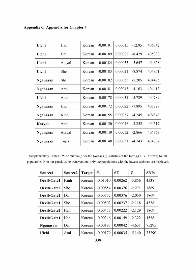
Appendix C Appendix for Chapter 4
338
Ulchi Han Korean -0.00191 0.00015 -12.951 406842
Ulchi Dai Korean -0.00189 0.00022 -8.429 405330
Ulchi Atayal Korean -0.00184 0.00033 -5.647 404628
Ulchi She Korean -0.00183 0.00021 -8.874 404851
Nganasan She Korean -0.00182 0.00035 -5.205 404475
Nganasan Ami Korean -0.00181 0.00043 -4.163 404413
Ulchi Ami Korean -0.00178 0.00031 -5.789 404789
Nganasan Han Korean -0.00172 0.00022 -7.895 405829
Nganasan Kinh Korean -0.00155 0.00037 -4.245 404849
Koryak Ami Korean -0.00150 0.00046 -3.252 404317
Nganasan Atayal Korean -0.00149 0.00052 -2.866 404368
Nganasan Tujia Korean -0.00148 0.00031 -4.743 404802
Supplementary Table C.25 Admixture f3 for the Koreans. f3 statistics of the form f3(X, Y; Korean) for all
populations X in our panel, using transversions only. 30 populations with the lowest statistics are displayed.
Source1 Source2 Target f3 SE Z SNPs
DevilsGate1 Kinh Korean -0.01010 0.00262 -3.856 4538
DevilsGate2 She Korean -0.00854 0.00376 -2.271 1869
DevilsGate2 Dai Korean -0.00772 0.00376 -2.050 1869
DevilsGate1 She Korean -0.00502 0.00237 -2.118 4538
DevilsGate2 Han Korean -0.00473 0.00222 -2.129 1869
DevilsGate1 Han Korean -0.00346 0.00149 -2.322 4538
Nganasan Dai Korean -0.00193 0.00042 -4.631 75295
Ulchi Ami Korean -0.00179 0.00035 -5.140 75290
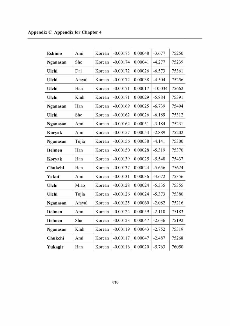
Appendix C Appendix for Chapter 4
339
Eskimo Ami Korean -0.00175 0.00048 -3.677 75250
Nganasan She Korean -0.00174 0.00041 -4.277 75239
Ulchi Dai Korean -0.00172 0.00026 -6.573 75361
Ulchi Atayal Korean -0.00172 0.00038 -4.504 75256
Ulchi Han Korean -0.00171 0.00017 -10.034 75662
Ulchi Kinh Korean -0.00171 0.00029 -5.884 75391
Nganasan Han Korean -0.00169 0.00025 -6.739 75494
Ulchi She Korean -0.00162 0.00026 -6.189 75312
Nganasan Ami Korean -0.00162 0.00051 -3.184 75231
Koryak Ami Korean -0.00157 0.00054 -2.889 75202
Nganasan Tujia Korean -0.00156 0.00038 -4.141 75300
Itelmen Han Korean -0.00150 0.00028 -5.319 75370
Koryak Han Korean -0.00139 0.00025 -5.548 75437
Chukchi Han Korean -0.00137 0.00024 -5.656 75624
Yakut Ami Korean -0.00131 0.00036 -3.672 75356
Ulchi Miao Korean -0.00128 0.00024 -5.335 75355
Ulchi Tujia Korean -0.00126 0.00024 -5.373 75380
Nganasan Atayal Korean -0.00125 0.00060 -2.082 75216
Itelmen Ami Korean -0.00124 0.00059 -2.110 75183
Itelmen She Korean -0.00123 0.00047 -2.636 75192
Nganasan Kinh Korean -0.00119 0.00043 -2.752 75319
Chukchi Ami Korean -0.00117 0.00047 -2.487 75268
Yukagir Han Korean -0.00116 0.00020 -5.763 76050
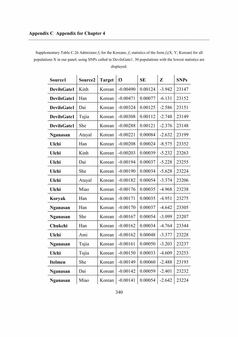
Appendix C Appendix for Chapter 4
340
Supplementary Table C.26 Admixture f3 for the Koreans. f3 statistics of the form f3(X, Y; Korean) for all
populations X in our panel, using SNPs called in DevilsGate1. 30 populations with the lowest statistics are
displayed.
Source1 Source2 Target f3 SE Z SNPs
DevilsGate1 Kinh Korean -0.00490 0.00124 -3.942 23147
DevilsGate1 Han Korean -0.00471 0.00077 -6.131 23152
DevilsGate1 Dai Korean -0.00324 0.00125 -2.586 23151
DevilsGate1 Tujia Korean -0.00308 0.00112 -2.748 23149
DevilsGate1 She Korean -0.00288 0.00121 -2.376 23148
Nganasan Atayal Korean -0.00221 0.00084 -2.632 23199
Ulchi Han Korean -0.00208 0.00024 -8.575 23352
Ulchi Kinh Korean -0.00203 0.00039 -5.232 23263
Ulchi Dai Korean -0.00194 0.00037 -5.228 23255
Ulchi She Korean -0.00190 0.00034 -5.628 23224
Ulchi Atayal Korean -0.00182 0.00054 -3.374 23206
Ulchi Miao Korean -0.00176 0.00035 -4.968 23238
Koryak Han Korean -0.00171 0.00035 -4.951 23275
Nganasan Han Korean -0.00170 0.00037 -4.642 23305
Nganasan She Korean -0.00167 0.00054 -3.099 23207
Chukchi Han Korean -0.00162 0.00034 -4.764 23344
Ulchi Ami Korean -0.00162 0.00048 -3.377 23228
Nganasan Tujia Korean -0.00161 0.00050 -3.203 23237
Ulchi Tujia Korean -0.00150 0.00033 -4.609 23253
Itelmen She Korean -0.00149 0.00060 -2.488 23193
Nganasan Dai Korean -0.00142 0.00059 -2.401 23232
Nganasan Miao Korean -0.00141 0.00054 -2.642 23224
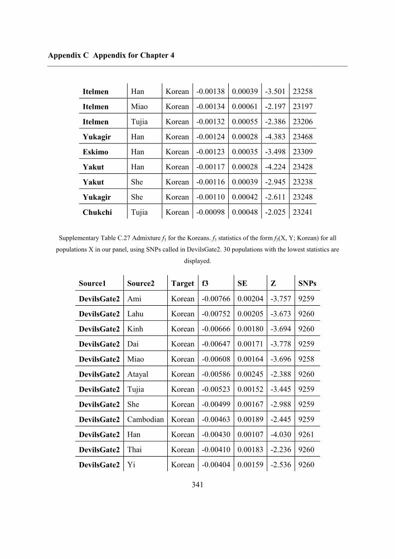
Appendix C Appendix for Chapter 4
341
Itelmen Han Korean -0.00138 0.00039 -3.501 23258
Itelmen Miao Korean -0.00134 0.00061 -2.197 23197
Itelmen Tujia Korean -0.00132 0.00055 -2.386 23206
Yukagir Han Korean -0.00124 0.00028 -4.383 23468
Eskimo Han Korean -0.00123 0.00035 -3.498 23309
Yakut Han Korean -0.00117 0.00028 -4.224 23428
Yakut She Korean -0.00116 0.00039 -2.945 23238
Yukagir She Korean -0.00110 0.00042 -2.611 23248
Chukchi Tujia Korean -0.00098 0.00048 -2.025 23241
Supplementary Table C.27 Admixture f3 for the Koreans. f3 statistics of the form f3(X, Y; Korean) for all
populations X in our panel, using SNPs called in DevilsGate2. 30 populations with the lowest statistics are
displayed.
Source1 Source2 Target f3 SE Z SNPs
DevilsGate2 Ami Korean -0.00766 0.00204 -3.757 9259
DevilsGate2 Lahu Korean -0.00752 0.00205 -3.673 9260
DevilsGate2 Kinh Korean -0.00666 0.00180 -3.694 9260
DevilsGate2 Dai Korean -0.00647 0.00171 -3.778 9259
DevilsGate2 Miao Korean -0.00608 0.00164 -3.696 9258
DevilsGate2 Atayal Korean -0.00586 0.00245 -2.388 9260
DevilsGate2 Tujia Korean -0.00523 0.00152 -3.445 9259
DevilsGate2 She Korean -0.00499 0.00167 -2.988 9259
DevilsGate2 Cambodian Korean -0.00463 0.00189 -2.445 9259
DevilsGate2 Han Korean -0.00430 0.00107 -4.030 9261
DevilsGate2 Thai Korean -0.00410 0.00183 -2.236 9260
DevilsGate2 Yi Korean -0.00404 0.00159 -2.536 9260
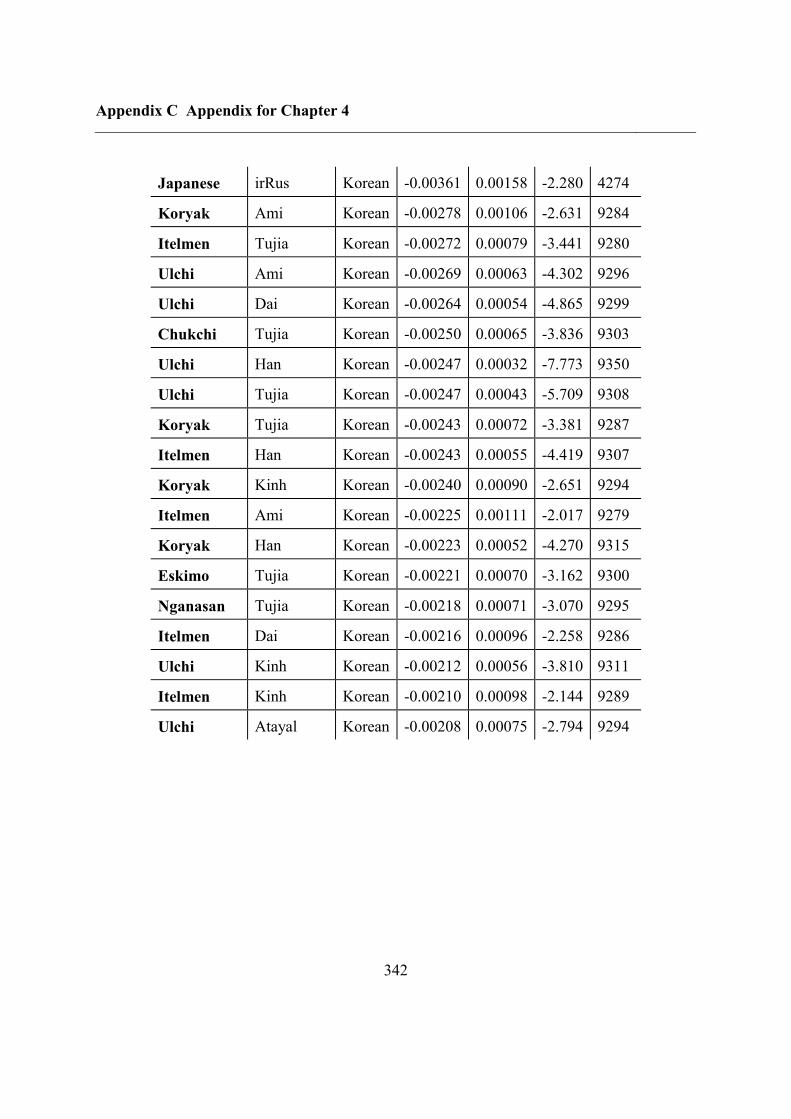
Appendix C Appendix for Chapter 4
342
Japanese irRus Korean -0.00361 0.00158 -2.280 4274
Koryak Ami Korean -0.00278 0.00106 -2.631 9284
Itelmen Tujia Korean -0.00272 0.00079 -3.441 9280
Ulchi Ami Korean -0.00269 0.00063 -4.302 9296
Ulchi Dai Korean -0.00264 0.00054 -4.865 9299
Chukchi Tujia Korean -0.00250 0.00065 -3.836 9303
Ulchi Han Korean -0.00247 0.00032 -7.773 9350
Ulchi Tujia Korean -0.00247 0.00043 -5.709 9308
Koryak Tujia Korean -0.00243 0.00072 -3.381 9287
Itelmen Han Korean -0.00243 0.00055 -4.419 9307
Koryak Kinh Korean -0.00240 0.00090 -2.651 9294
Itelmen Ami Korean -0.00225 0.00111 -2.017 9279
Koryak Han Korean -0.00223 0.00052 -4.270 9315
Eskimo Tujia Korean -0.00221 0.00070 -3.162 9300
Nganasan Tujia Korean -0.00218 0.00071 -3.070 9295
Itelmen Dai Korean -0.00216 0.00096 -2.258 9286
Ulchi Kinh Korean -0.00212 0.00056 -3.810 9311
Itelmen Kinh Korean -0.00210 0.00098 -2.144 9289
Ulchi Atayal Korean -0.00208 0.00075 -2.794 9294
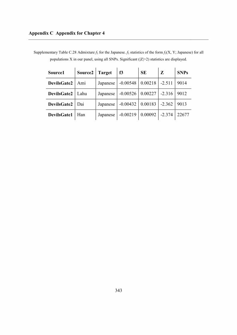
Appendix C Appendix for Chapter 4
343
Supplementary Table C.28 Admixture f3 for the Japanese. f3 statistics of the form f3(X, Y; Japanese) for all
populations X in our panel, using all SNPs. Significant (|Z|>2) statistics are displayed.
Source1 Source2 Target f3 SE Z SNPs
DevilsGate2 Ami Japanese -0.00548 0.00218 -2.511 9014
DevilsGate2 Lahu Japanese -0.00526 0.00227 -2.316 9012
DevilsGate2 Dai Japanese -0.00432 0.00183 -2.362 9013
DevilsGate1 Han Japanese -0.00219 0.00092 -2.374 22677
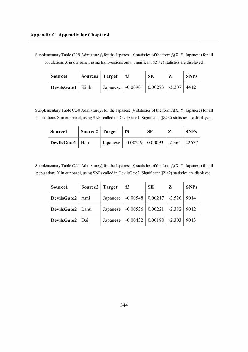
Appendix C Appendix for Chapter 4
344
Supplementary Table C.29 Admixture f3 for the Japanese. f3 statistics of the form f3(X, Y; Japanese) for all
populations X in our panel, using transversions only. Significant (|Z|>2) statistics are displayed.
Source1 Source2 Target f3 SE Z SNPs
DevilsGate1 Kinh Japanese -0.00901 0.00273 -3.307 4412
Supplementary Table C.30 Admixture f3 for the Japanese. f3 statistics of the form f3(X, Y; Japanese) for all
populations X in our panel, using SNPs called in DevilsGate1. Significant (|Z|>2) statistics are displayed.
Source1 Source2 Target f3 SE Z SNPs
DevilsGate1 Han Japanese -0.00219 0.00093 -2.364 22677
Supplementary Table C.31 Admixture f3 for the Japanese. f3 statistics of the form f3(X, Y; Japanese) for all
populations X in our panel, using SNPs called in DevilsGate2. Significant (|Z|>2) statistics are displayed.
Source1 Source2 Target f3 SE Z SNPs
DevilsGate2 Ami Japanese -0.00548 0.00217 -2.526 9014
DevilsGate2 Lahu Japanese -0.00526 0.00221 -2.382 9012
DevilsGate2 Dai Japanese -0.00432 0.00188 -2.303 9013
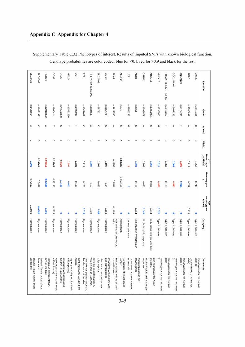
Appendix C Appendix for Chapter 4
345
Supplementary Table C.32 Phenotypes of interest. Results of imputed SNPs with known biological function.
Genotype probabilities are color coded: blue for <0.1, red for >0.9 and black for the rest.
SL
C24
A5
SL
C45
A2
HE
RC
2
OC
A2
OC
A2
KIT
LG
DC
T
TY
R
RP
L7
AP
62
, SL
C24
A5
SL
C24
A2
MC
1R
ED
AR
AL
DH
2
LC
T
AD
D1
OP
RM
1
AB
CC
11
KN
CK
16
FIT
M2
-R3H
DM
L-H
NF
4A
GC
C1
-PA
X4
ZN
FA
ND
3
PE
PD
MA
EA
Ide
ntifie
r
rs1
42
66
54
rs1
68
91
98
2
rs1
29
13
83
2
rs1
80
04
14
rs7
46
53
33
0
rs1
28
21
25
6
rs1
40
79
95
rs1
04
26
02
rs1
83
46
40
rs2
67
22
rs8
85
47
9
rs3
82
77
60
rs6
71
rs4
98
82
35
rs4
96
1
rs1
79
99
71
rs1
78
22
93
1
rs1
53
55
00
rs6
01
73
17
rs6
46
71
36
rs9
47
07
94
rs3
78
68
97
rs6
81
54
64
Ge
ne
A
C
A
T
C
T
T
C
A
C
G
A
G
G
G
A
C
G
T
A
T
A
C Alle
le0
G
G
G
C
T
C
C
A
G
T
A
G
A
A
T
G
T
T
G
G
C
G
G Alle
le1
0.0
02
0.3
93
41
0.9
05
11
0.2
39
43
0.9
82
1
0.9
97
0.8
39
0.7
22
0.0
07
0.5
08
0.1
92
0.1
35
6
0.8
47
35
1
0.0
01
0.3
05
0.0
68
0.0
24
0.8
68
0.0
63
0.9
99
0.1
12
0.2
57
GP
H
om
ozy
go
us
Alle
le0
0.7
75
12
0.5
43
8
0.0
95
89
0.5
31
35
0.0
18
9
0.0
03
0.1
61
0.2
62
0.6
7
0.4
32
0.6
4
0.7
54
6
0.1
53
16
5
0
0.1
85
0.6
52
0.3
88
0.9
55
0.1
31
0.9
37
0.0
01
0.7
49
0.7
43
GP
H
ete
rozy
go
u
s
0.2
24
86
0.0
59
2
0.0
01
0.2
32
3
0
0
0
0.0
15
0.3
23
0.0
6
0.1
68
0.1
15
9
0
0
0.8
14
0.0
43
0.5
44
0.0
22
0
0
0
0.1
39
0
GP
H
om
ozy
go
us
Alle
le1
Pig
me
nta
tion
Pig
me
nta
tion
Pig
me
nta
tion
Pig
me
nta
tion
Pig
me
nta
tion
Pig
me
nta
tion
Pig
me
nta
tion
Pig
me
nta
tion
Pig
me
nta
tion
Pig
me
nta
tion
Pig
me
nta
tion
Hair a
nd
oth
er p
he
no
typ
ic
traits
Alc
oh
ol flu
sh
La
cto
se
tole
ran
ce
Sa
lt-se
nsitiv
e h
yp
erte
nsio
n
Alc
oh
ol / o
pio
id re
sp
on
se
Bo
dy o
do
ur a
nd
ear w
ax ty
pe
Typ
e II d
iab
ete
s
Typ
e II d
iab
ete
s
Typ
e II d
iab
ete
s
Typ
e II d
iab
ete
s
Typ
e II d
iab
ete
s
Typ
e II d
iab
ete
s
Cate
go
ry
Unlik
ely
to b
e h
om
ozyg
ou
s
de
rived
. Th
is is
typ
ical o
f no
n-
Eu
rop
ea
ns.
Unlik
ely
to b
e h
om
ozyg
ou
s
de
rived
. Th
is is
typ
ical o
f no
n-
Eu
rop
ea
ns.
Bro
wn e
ye
pig
mm
en
tatio
n,
80
% o
f the
time
Und
ete
rmin
ed
(SN
P
asso
cia
ted
with
me
lan
in le
ve
ls
in E
ast A
sia
ns)
Sa
mp
le d
oe
s n
ot h
ave th
e
de
rived
alle
le w
hic
h h
as b
ee
n
asso
cia
ted
with
de
cre
ase
d
me
lan
in in
Ea
st A
sia
ns.
Sa
mp
le h
ad
the
va
rian
t mo
st
co
mm
on
ly fo
un
d in
Ea
st
Asia
ns (C
is a
sso
cia
ted
with
a
hig
he
r pro
ba
bility
of b
lon
d h
air
in E
uro
pe
an
s)
Sa
mp
le h
ad
the
va
rian
t T,
mo
st c
om
mo
nly
foun
d in
Ea
st
Asia
ns.
Sa
mp
le m
ost lik
ely
did
no
t
ha
ve
the
Eu
rop
ea
n d
eriv
ed
alle
le A
, asso
cia
ted
with
ligh
t
skin
an
d h
air p
igm
en
tatio
n a
nd
the
ab
sce
nce
of fre
ckle
s.
Sa
mp
le m
ost lik
ely
did
no
t h
ave
the
an
ce
stra
l alle
le A
,
whic
h is
rare
in E
ast A
sia
.
Sa
mp
le m
ost lik
ely
did
no
t
ha
ve
the
de
rived
alle
le T
,
asso
cia
ted
with
da
rder e
ye
,
ha
ir an
d s
kin
pig
men
taitio
n
(Ea
st A
sia
n p
op
ula
tion
s a
re
po
lym
orp
hic
)
Und
ete
rmin
ed
(SN
P
asso
cia
ted
with
red
ha
ir an
d
skin
pig
me
nta
tion
)
Incre
ase
d o
dd
s o
f stra
igh
ter,
thic
ker h
air a
s w
ell a
s s
ho
ve
l-
sh
ap
ed
incis
ors
Alc
oh
ol F
lush
: Norm
al, d
oe
sn
't
flush
. Norm
al h
an
go
ve
rs.
Norm
al ris
k o
f Alc
oh
olis
m.
Norm
al ris
k o
f Eso
ph
ag
ea
l
Can
ce
r.
Lik
ely
to b
e la
cto
se
into
lera
nt
as a
n a
du
lt
Sa
mp
le m
ost lik
ely
ha
d th
e ris
k
alle
le fo
r com
mo
n s
alt-
se
nsitiv
e h
yp
erte
nsio
n (E
ast
Asia
n p
op
ula
tion
s a
re
po
lym
orp
hic
).
Sa
mp
le w
as m
ost lik
ely
no
t
ho
mo
zyg
ou
s fo
r the
risk a
llele
asso
cia
ted
with
cra
vin
gs fo
r
alc
oh
ol / o
pio
id a
nd
a s
trong
er
resp
on
se
.
Sa
mp
le m
ost lik
ely
did
no
t
ha
ve
a s
tron
g b
od
y o
dou
r (CC
)
an
d h
ad
eith
er c
ou
ld h
ave
ha
d
dry
ea
rwax (T
T). T
he
T a
llele
is
als
o a
n in
dic
ato
r for A
sia
n
an
ce
stry
.
Sa
mp
le w
as m
ost lik
ely
h
ete
rozygo
us fo
r the
risk a
llele
T.
Sa
mp
le w
as m
ost lik
ely
ho
mo
zyg
ou
s fo
r the
norm
al
alle
le
Sa
mp
le w
as m
ost lik
ely
he
tero
zygo
us fo
r the
risk a
llele
G.
Sa
mp
le w
as m
ost lik
ely
h
om
ozyg
ou
s fo
r the
norm
al
alle
le T
.
Und
ete
rmin
ed
(A is
the
risk
alle
le)
Sa
mp
le w
as m
ost lik
ely
no
t
ho
mo
zyg
ou
s fo
r the
norm
al
alle
le G
.
Co
mm
en
ts
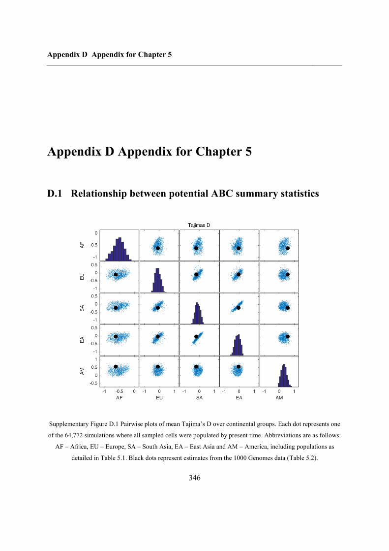
Appendix D Appendix for Chapter 5
346
Appendix D Appendix for Chapter 5
D.1 Relationship between potential ABC summary statistics
Supplementary Figure D.1 Pairwise plots of mean Tajima’s D over continental groups. Each dot represents one
of the 64,772 simulations where all sampled cells were populated by present time. Abbreviations are as follows:
AF – Africa, EU – Europe, SA – South Asia, EA – East Asia and AM – America, including populations as
detailed in Table 5.1. Black dots represent estimates from the 1000 Genomes data (Table 5.2).
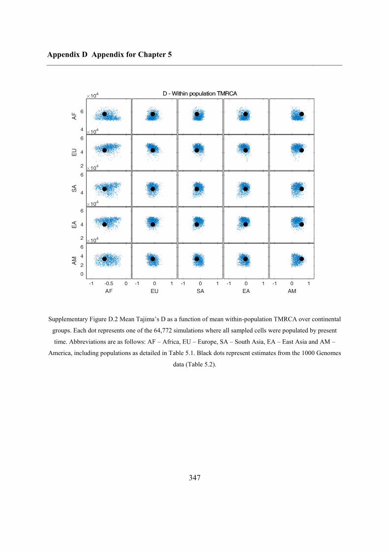
Appendix D Appendix for Chapter 5
347
Supplementary Figure D.2 Mean Tajima’s D as a function of mean within-population TMRCA over continental
groups. Each dot represents one of the 64,772 simulations where all sampled cells were populated by present
time. Abbreviations are as follows: AF – Africa, EU – Europe, SA – South Asia, EA – East Asia and AM –
America, including populations as detailed in Table 5.1. Black dots represent estimates from the 1000 Genomes
data (Table 5.2).
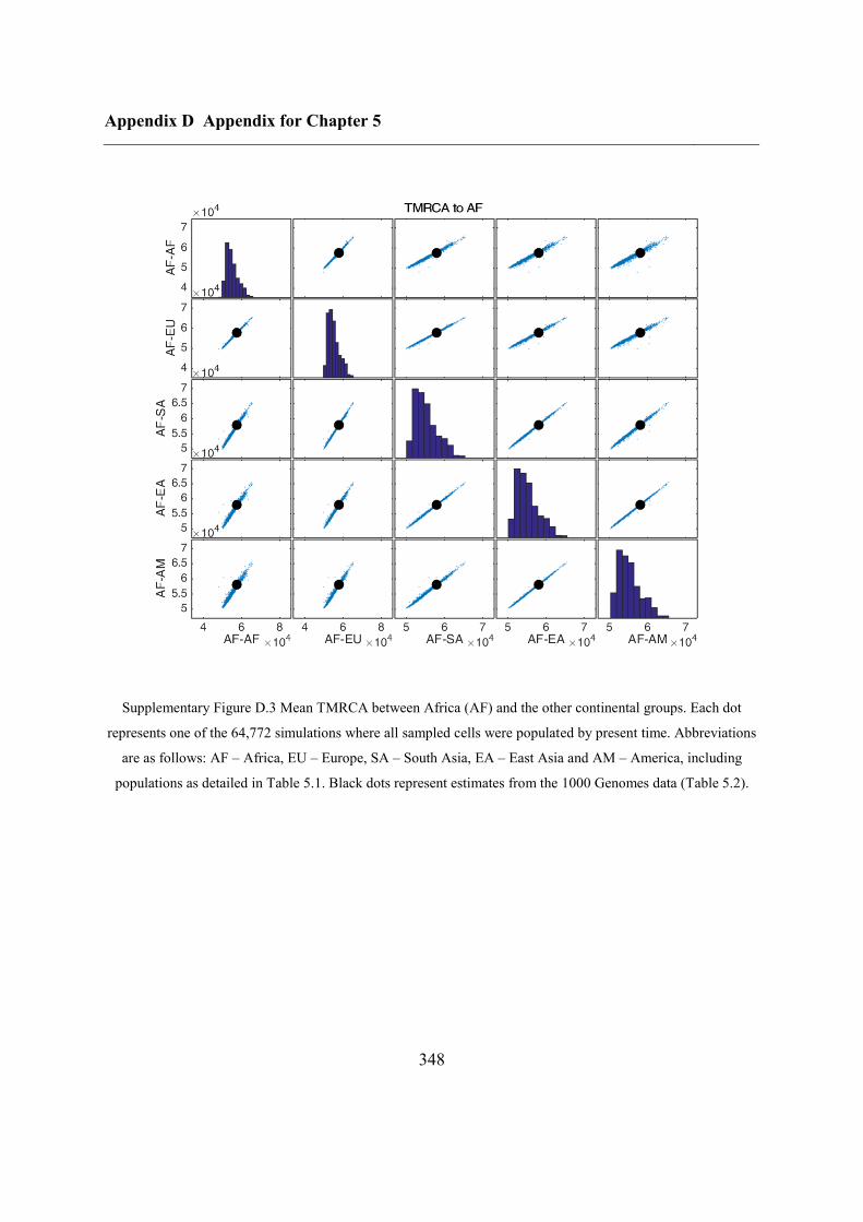
Appendix D Appendix for Chapter 5
348
Supplementary Figure D.3 Mean TMRCA between Africa (AF) and the other continental groups. Each dot
represents one of the 64,772 simulations where all sampled cells were populated by present time. Abbreviations
are as follows: AF – Africa, EU – Europe, SA – South Asia, EA – East Asia and AM – America, including
populations as detailed in Table 5.1. Black dots represent estimates from the 1000 Genomes data (Table 5.2).
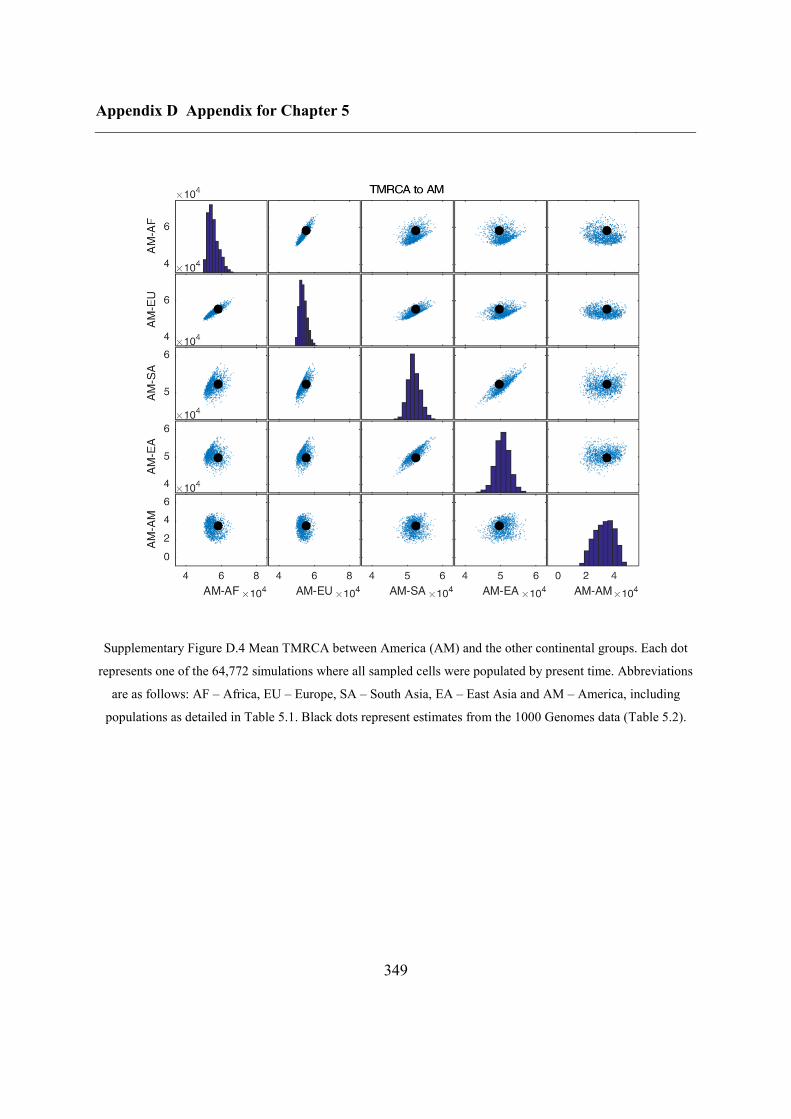
Appendix D Appendix for Chapter 5
349
Supplementary Figure D.4 Mean TMRCA between America (AM) and the other continental groups. Each dot
represents one of the 64,772 simulations where all sampled cells were populated by present time. Abbreviations
are as follows: AF – Africa, EU – Europe, SA – South Asia, EA – East Asia and AM – America, including
populations as detailed in Table 5.1. Black dots represent estimates from the 1000 Genomes data (Table 5.2).
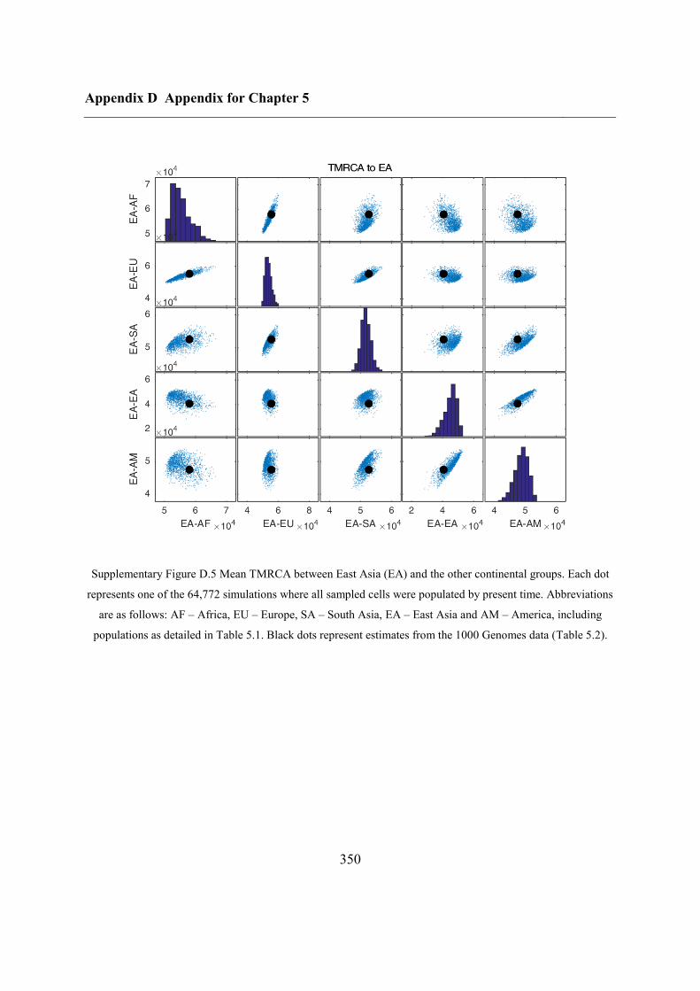
Appendix D Appendix for Chapter 5
350
Supplementary Figure D.5 Mean TMRCA between East Asia (EA) and the other continental groups. Each dot
represents one of the 64,772 simulations where all sampled cells were populated by present time. Abbreviations
are as follows: AF – Africa, EU – Europe, SA – South Asia, EA – East Asia and AM – America, including
populations as detailed in Table 5.1. Black dots represent estimates from the 1000 Genomes data (Table 5.2).
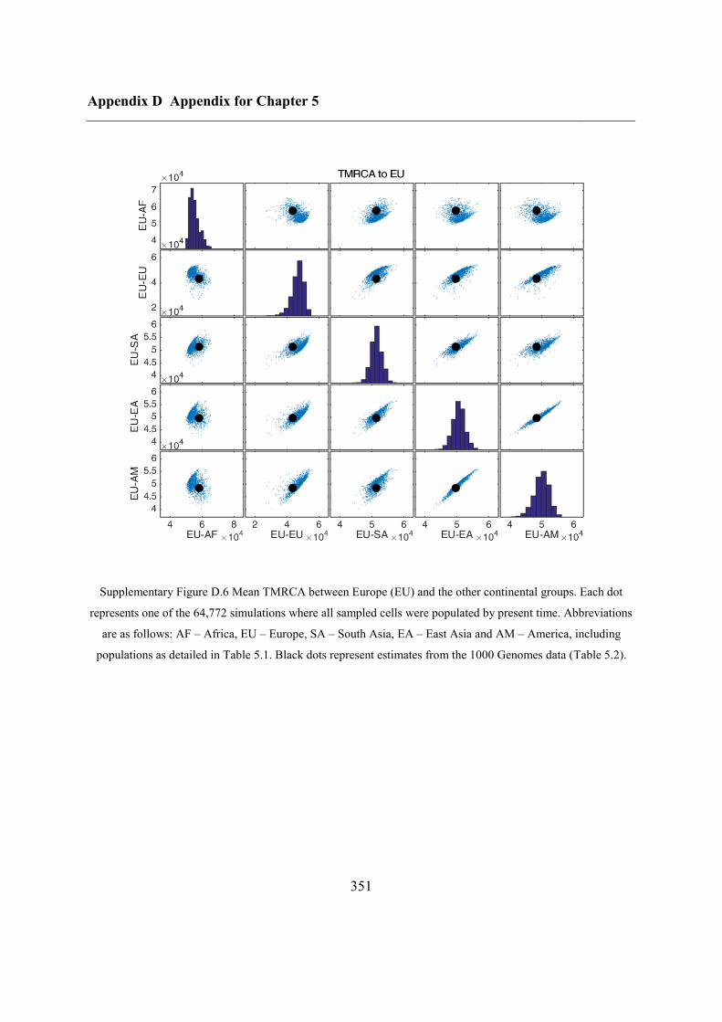
Appendix D Appendix for Chapter 5
351
Supplementary Figure D.6 Mean TMRCA between Europe (EU) and the other continental groups. Each dot
represents one of the 64,772 simulations where all sampled cells were populated by present time. Abbreviations
are as follows: AF – Africa, EU – Europe, SA – South Asia, EA – East Asia and AM – America, including
populations as detailed in Table 5.1. Black dots represent estimates from the 1000 Genomes data (Table 5.2).
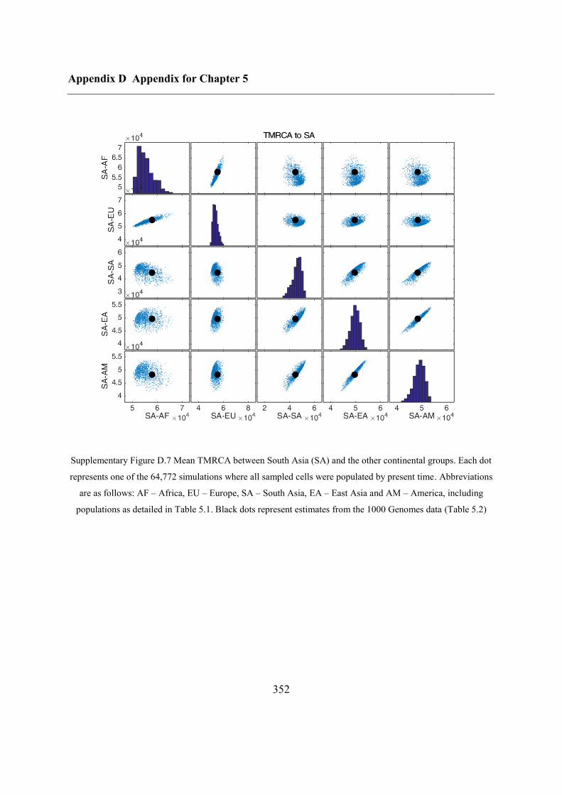
Appendix D Appendix for Chapter 5
352
Supplementary Figure D.7 Mean TMRCA between South Asia (SA) and the other continental groups. Each dot
represents one of the 64,772 simulations where all sampled cells were populated by present time. Abbreviations
are as follows: AF – Africa, EU – Europe, SA – South Asia, EA – East Asia and AM – America, including
populations as detailed in Table 5.1. Black dots represent estimates from the 1000 Genomes data (Table 5.2)
Appendix E Appendix for Chapter 6
353
Appendix E Appendix for Chapter 6
E.1 Fit using SSE for thalassemia
We initially investigated fitting the distribution of thalassemia variants using the same,
frequency-based error function as for sickle-cell disease (6.4.3.1). The resulting origins for
Cd39 (Supplementary Figure E.2) were similar to, but noisier than those inferred using the
classification error presented in the main text. Furthermore, since the Cd39 frequencies were
higher in North Africa than in Southern Europe (Table 6.6), the former was a more likely
origin than the latter. For FSC-6, on the other hand, the obtained distribution was
fundamentally different, the complement of that inferred for Cd39 (Supplementary Figure
E.3). It was absent in Europe and western North Africa, near the sampled regions, as opposed
to the North African origin inferred using classification error. After observing the
frequencies, we found that this behaviour was driven by the low frequencies of the variant in
the data, which lead to the complete absence of FSC-6 in sampled countries appear as an
outcome favoured over frequencies that were too high (Supplementary Figure E.1). For IVS-
I-1, we also obtained fundamentally different distributions using the two error functions.
Classification error implied an origin in Eastern Europe, whereas the frequency-based error
function was undetermined, apart from showing that the origin should not be in North Africa
(Supplementary Figure E.4). Again this is due to the low frequencies of the variant which
resulted in a marginal change between its presence or absence in Europe; only the very low
frequencies in North Africa were picked up.
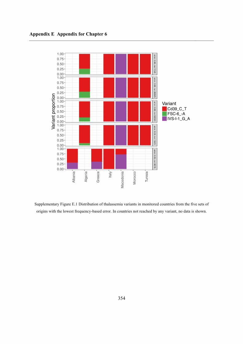
Appendix E Appendix for Chapter 6
354
Supplementary Figure E.1 Distribution of thalassemia variants in monitored countries from the five sets of
origins with the lowest frequency-based error. In countries not reached by any variant, no data is shown.
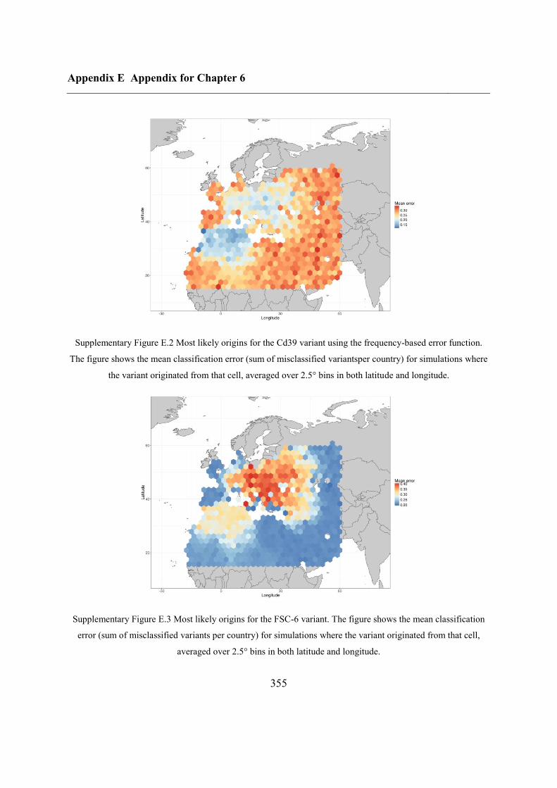
Appendix E Appendix for Chapter 6
355
Supplementary Figure E.2 Most likely origins for the Cd39 variant using the frequency-based error function.
The figure shows the mean classification error (sum of misclassified variantsper country) for simulations where
the variant originated from that cell, averaged over 2.5° bins in both latitude and longitude.
Supplementary Figure E.3 Most likely origins for the FSC-6 variant. The figure shows the mean classification
error (sum of misclassified variants per country) for simulations where the variant originated from that cell,
averaged over 2.5° bins in both latitude and longitude.
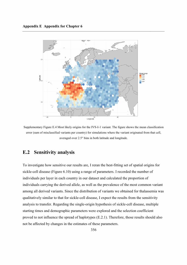
Appendix E Appendix for Chapter 6
356
Supplementary Figure E.4 Most likely origins for the IVS-I-1 variant. The figure shows the mean classification
error (sum of misclassified variants per country) for simulations where the variant originated from that cell,
averaged over 2.5° bins in both latitude and longitude.
E.2 Sensitivity analysis
To investigate how sensitive our results are, I reran the best-fitting set of spatial origins for
sickle-cell disease (Figure 6.10) using a range of parameters. I recorded the number of
individuals per layer in each country in our dataset and calculated the proportion of
individuals carrying the derived allele, as well as the prevalence of the most common variant
among all derived variants. Since the distribution of variants we obtained for thalassemia was
qualitatively similar to that for sickle-cell disease, I expect the results from the sensitivity
analysis to transfer. Regarding the single-origin hypothesis of sickle-cell disease, multiple
starting times and demographic parameters were explored and the selection coefficient
proved to not influence the spread of haplotypes (E.2.1). Therefore, those results should also
not be affected by changes in the estimates of these parameters.
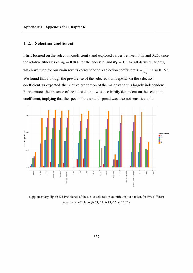
Appendix E Appendix for Chapter 6
357
E.2.1 Selection coefficient
I first focused on the selection coefficient s and explored values between 0.05 and 0.25, since
the relative fitnesses of 𝑤0 = 0.868 for the ancestral and 𝑤1 = 1.0 for all derived variants,
which we used for our main results correspond to a selection coefficient 𝑠 =1
𝑤1− 1 ≈ 0.152.
We found that although the prevalence of the selected trait depends on the selection
coefficient, as expected, the relative proportion of the major variant is largely independent.
Furthermore, the presence of the selected trait was also hardly dependent on the selection
coefficient, implying that the speed of the spatial spread was also not sensitive to it.
Supplementary Figure E.5 Prevalence of the sickle-cell trait in countries in our dataset, for five different
selection coefficients (0.05, 0.1, 0.15, 0.2 and 0.25).
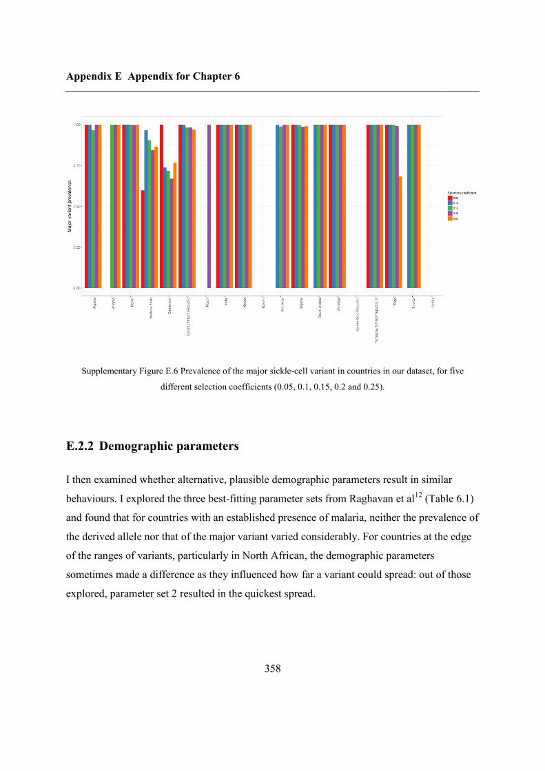
Appendix E Appendix for Chapter 6
358
Supplementary Figure E.6 Prevalence of the major sickle-cell variant in countries in our dataset, for five
different selection coefficients (0.05, 0.1, 0.15, 0.2 and 0.25).
E.2.2 Demographic parameters
I then examined whether alternative, plausible demographic parameters result in similar
behaviours. I explored the three best-fitting parameter sets from Raghavan et al12
(Table 6.1)
and found that for countries with an established presence of malaria, neither the prevalence of
the derived allele nor that of the major variant varied considerably. For countries at the edge
of the ranges of variants, particularly in North African, the demographic parameters
sometimes made a difference as they influenced how far a variant could spread: out of those
explored, parameter set 2 resulted in the quickest spread.
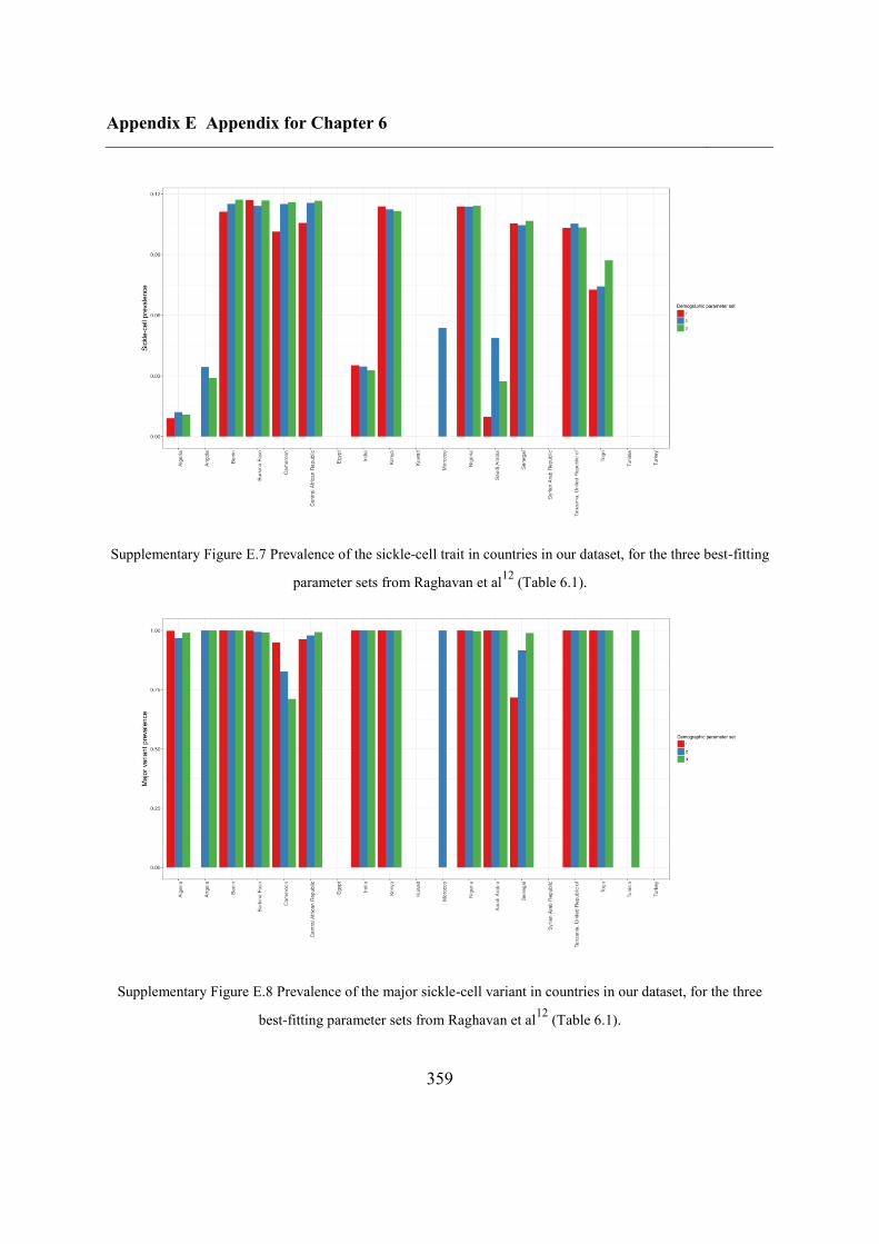
Appendix E Appendix for Chapter 6
359
Supplementary Figure E.7 Prevalence of the sickle-cell trait in countries in our dataset, for the three best-fitting
parameter sets from Raghavan et al12
(Table 6.1).
Supplementary Figure E.8 Prevalence of the major sickle-cell variant in countries in our dataset, for the three
best-fitting parameter sets from Raghavan et al12
(Table 6.1).
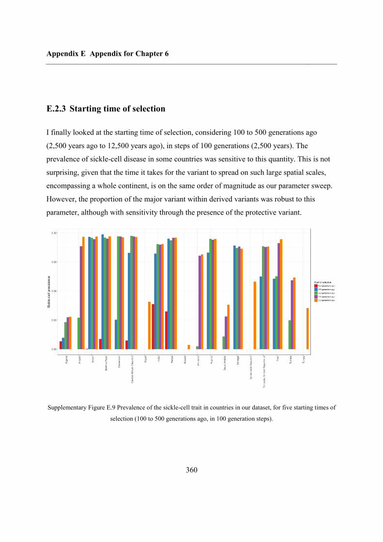
Appendix E Appendix for Chapter 6
360
E.2.3 Starting time of selection
I finally looked at the starting time of selection, considering 100 to 500 generations ago
(2,500 years ago to 12,500 years ago), in steps of 100 generations (2,500 years). The
prevalence of sickle-cell disease in some countries was sensitive to this quantity. This is not
surprising, given that the time it takes for the variant to spread on such large spatial scales,
encompassing a whole continent, is on the same order of magnitude as our parameter sweep.
However, the proportion of the major variant within derived variants was robust to this
parameter, although with sensitivity through the presence of the protective variant.
Supplementary Figure E.9 Prevalence of the sickle-cell trait in countries in our dataset, for five starting times of
selection (100 to 500 generations ago, in 100 generation steps).
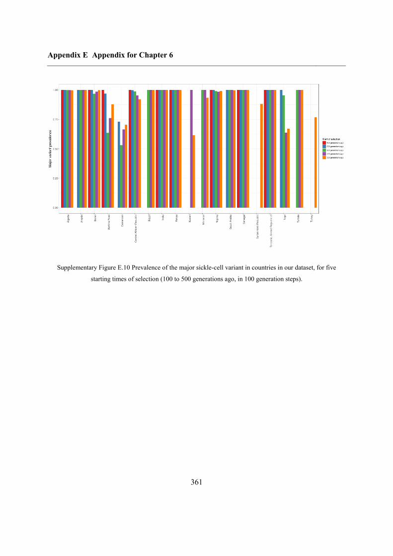
Appendix E Appendix for Chapter 6
361
Supplementary Figure E.10 Prevalence of the major sickle-cell variant in countries in our dataset, for five
starting times of selection (100 to 500 generations ago, in 100 generation steps).