HStellakis 2 - Propagation & Link Budget - eClass ΕΚΠΑ
32
Δρ. Χάρης Μ. Στελλάκης 1 Παρουσιάσεις για το Μάθημα Ασύρματων και Κινητών Τηλεπικοινωνιών του ΔΜΠΣ στο ΕΚΠΑ Δρ. Χάρης Μ. Στελλάκης [email protected] Αθήνα, 2019
-
Upload
khangminh22 -
Category
Documents
-
view
7 -
download
0
Transcript of HStellakis 2 - Propagation & Link Budget - eClass ΕΚΠΑ

Δρ. Χάρης Μ. Στελλάκης1
Παρουσιάσεις για το Μάθημα
Ασύρματων και Κινητών Τηλεπικοινωνιών
του ΔΜΠΣ στο ΕΚΠΑ
Δρ. Χάρης Μ. Στελλάκης
Αθήνα, 2019

Δρ. Χάρης Μ. Στελλάκης2
Radio Signal Propagation

Δρ. Χάρης Μ. Στελλάκης3
Radio Signal Propagation
Unlike wired communication channels that are stationary and predictable, wireless channels are extremely random and do not offer easy analysis.
Radio Signal Propagation analysis has been focusing on predicting
— the average signal strength at a given distance from the Tx , as well as (large scale propagation modeling)
— The variability of the signal strength in close spatial proximity to a particular location (small scale propagation or fading modeling)

Δρ. Χάρης Μ. Στελλάκης4
Free Space Propagation Modeling
The Received Signal Level (RSL) varies
— Proportionally to Tx power, antenna gains and wavelength
— Inversely proportionally to the distance between the {Tx, Rx}, and other miscellaneous losses in the communication system hardware
Ld
GGPP rtt
r 22
2
)4(~
MHzKmdB FDFSL log20log2045.32
MHzmi FD log20log2058.36
fcA
G /,4
2
A: Effective aperture related to antenna physical size
L: Miscellaneous losses in communication system
FSL: Free Space Loss

Δρ. Χάρης Μ. Στελλάκης5
Path Loss
Path Loss (PL) represents signal attenuation as a positive quantity, usually measured in dB(i.e. 10log(x))
)log(10)()()(r
trt
P
PdBPdBPdBPL
Due to the large dynamic range of received power levels, often dBm or dBW units are used to express received power levels in milliwattsor watts respectively
dBmmWdBWWW 30)1000log(100)1log(101

Δρ. Χάρης Μ. Στελλάκης6
Path Loss Analysis - Example
Example:In a wireless system, the Tx produces 50 watts of power, the antenna at
900 MHz carrier frequency, and both antennas have a unity gain.
— What is the transmit power in (a) dBm or (b) dBW?
— What is received power in dBm at a free space distance of 100m from the antenna?
Answers:— Pt = 50W = 47.0 dBm = 17.0 dBW
— Pr(dBm@100m) = -24.5 dBm

Δρ. Χάρης Μ. Στελλάκης7
Mechanisms affecting Free-Space Propagation
Reflection: Occurs when the e-m wave impinges upon an object with very large dimensions (wrt λ)
Diffraction: Occurs when the radio line-of-sight (LOS)path (between the Tx and Rx) is obstructed by a surface with sharp edges, leading to «wave bending»
Scattering: Due to many and small obstacles (Foliage, Street signs, lamp posts, etc)

Δρ. Χάρης Μ. Στελλάκης8
Path Loss Modeling
n
d
ddPLavg
0
Measured signal levels (in dB) have a Gaussian
distribution
(log-normal shadowing)
)log(10)(0
0d
dndPLavgdBPLavg
A reference distance
close to Tx

Δρ. Χάρης Μ. Στελλάκης9
Fresnel Zones
Fresnel zones represent successive regions where secondary waves have a path length from Tx to Rx greater from LOS path by n*λ/2, n=1,2,3,…
Successive Fresnel zones alternatively provide constructive and destructive interference to the received signal
Fresnel zone radii get max when the obstruction is in the middle of Tx-Rx path
Rule of thumb: 1st Fresnel zone should be at least 55% clear
1d 2d
21
21
dd
ddnrn
nrrh
th h

Δρ. Χάρης Μ. Στελλάκης10
Fresnel Zones cont’d
Fresnel Diffraction parameter (v) may be used to determine the loss due to edge diffraction
21
21 )(2
dd
ddhv
• h: the obstructing object
height above LOS
(positive or negative)

Δρ. Χάρης Μ. Στελλάκης11
Propagation Modeling
The objective is to predict/ estimate the path loss statistics over an irregular terrain
Outdoor models— Okumura
— Hata
— COST-231 (Hata @ PCS frequencies)
— Walfisch & Bertoni, Longley-Rice, Durkin
Indoor models— Same floor soft/ hard partitions
— Intra-floor partitions
— Log-distance path loss
— Ericsson multiple breakpoint

Δρ. Χάρης Μ. Στελλάκης12
Okumura Model
3log~)(
200log20)(
)()(),()(
rere
tete
AreareteFreeSpacemed
hhG
hhG
GhGhGdfALdBLMedian Attenuation Environment specific
Correction Factor
{Tx, Rx} Antenna Height
Gain Factors
Median path Loss:
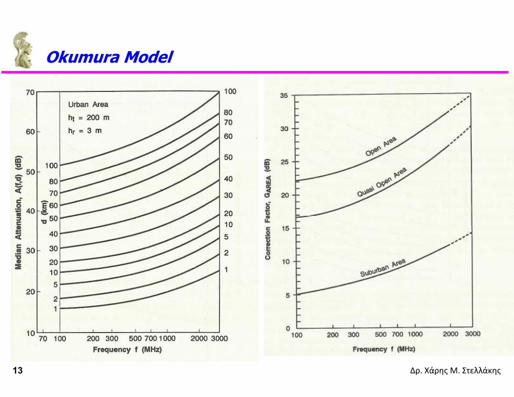
Δρ. Χάρης Μ. Στελλάκης13
Okumura Model

Δρ. Χάρης Μ. Στελλάκης14
Walfisch & Bertoni Model
nmultiscreeeetRooftopStrFreeSpace LLLdBL )(
{1,2} {3,4}

Δρ. Χάρης Μ. Στελλάκης15
Indicative Average Loss Measurements

Δρ. Χάρης Μ. Στελλάκης16
Average Floor Attenuations

Δρ. Χάρης Μ. Στελλάκης17
Average Floor Attenuations

Δρ. Χάρης Μ. Στελλάκης18
Propagation Loss inside Buildings
),0(~)(
log10)()(0
0
NdBX
Xd
dndPLdBPL

Δρ. Χάρης Μ. Στελλάκης19
Ericsson Multiple Breakpoint Model
As MS moves further from the BS,
the path loss change increases

Δρ. Χάρης Μ. Στελλάκης20
Small Scale Fading and Multipath
Small scale fading (or simply fading) is used to describe the rapid fluctuation of the signal amplitude over a short period of time so that large-scale path loss effects may be ignored
Fading is caused by interference between two or more version of the transmitted signal which arrive at the Rx at slightly different times. These waves are called multipath
Multipath is combined at the Rx to produce the resultant signal that may vary widely in amplitude and phase, depending on the individual characteristics of every multipath components
Factors influencing fading:— Multipath propagation
— Speed of mobile (Doppler effect)
— Speed of surrounding objects
— The transmission bandwidth of the signal

Δρ. Χάρης Μ. Στελλάκης21
Doppler Shift
Movement of MS relative to BS, leads to change in frequency
Example:
A Tx radiates a signal at 1850 MHz
For a vehicle moving at 60mph:— Directly towards Tx, then new
frequency received by MS is 1850.00016 MHz
— Directly away from Tx, then new frequency received by MS is 1849.999834 MHz
— Perpendicular to Tx, then there in no change in received Frequency
cosv
fd
dprevnew fff

Δρ. Χάρης Μ. Στελλάκης22
Multipath Propagation
Multiple components/ rays of the Tx signal arrive at the Rx end, with different amplitudes and phases
Time availability = The % of time, RSL is above the required level
Outage = The % of time, RSL is below the required level = 1-Time availability

Δρ. Χάρης Μ. Στελλάκης23
Signal Fading Statistics
In mobile environments— Rayleigh Fading distribution
When there is a strong / non fading signal component (ex. LOS). This a typical case for Wireless Fixed Access Environments
— Rician fading distribution
0,2
exp)(2
2
2
r
rrrp
0,,2
)(exp)(
202
22
2
rA
ArI
Arrrp

Δρ. Χάρης Μ. Στελλάκης24
Level Crossing and Fading Statistics
Level Crossing Rate (LCR) is the expected rate at which the Rayleigh fading signal, normalized to its mean value, falls below a pre-specified threshold “p”
The number of level crossings per second is Nr
Average Fade Duration, (τ) is the average period of time for which the received signal remains below a pre-specified level, relative to its mean value
Both parameters depend on MS speed (i.e. a function of maximum Doppler Frequency “fm”)
“τ” helps estimating the average number of bits that may be lost during a fade
2
2 efN mr
2
12
mf
e

Δρ. Χάρης Μ. Στελλάκης25
Link Budget Analysis

Δρ. Χάρης Μ. Στελλάκης26
Link Budget Analysis
It provides the Radio network designer with the necessary equipment parameters to
— Prepare a block diagram of the terminal or repeater configuration
— Determine equipment technical specifications
EIRPIRL
RSL

Δρ. Χάρης Μ. Στελλάκης27
Link Budget Analysis
The Effective Isotropic Radiated Power
The Isotropic Received Level
The Received Signal level (at the Rx input)
10 GLPEIRP tdBW
airdBdBW LFSLEIRPIRL
rLGIRLRSL 2
Example:— Tx output power = 750mW
— Line losses = (-) 3.4dB
— Tx – Rx distance = 17 mi
— Operating Frequency = 7.1 GHz
— Antenna Gains = 30.5dB each
— Air Loss = 0.3 dB
dBWRSL 56.85
dBWWmW 30)001,0log(101
dbW

Δρ. Χάρης Μ. Στελλάκης28
Digital Link Budget Analysis
In digital links, the received Eb/No (instead of RSL) is a key parameter
— Eb: Received information energy per bit
— No: Noise spectral density
— No ~ f(Temperature)
)log(10)( bdBWdBWb RRSLE
dBNFdBWN 2040
Receiver
QoS (BER)Eb/No RSL EIRP Tx Specs
Receiver
QoS (BER)Eb/No RSL EIRP Tx Specs
FSLSystem
Coverage
Thermal noise level
of perfect Rx over 1Hz

Δρ. Χάρης Μ. Στελλάκης29
Link Budget Analysis In Fading
Link Availability denotes the time period during which a specified QoS (ex. BER) is met or exceeded
Fade margin denotes the extra signal level required so that a specified link availability is attained
Example:
Assume, minimum (unfaded) C/N = 20dB
Then, min C/N = 53dB for 99.95% availability, ie
Outage is 0.05%
C/N < 20 dB for 262.8 min/yr

Δρ. Χάρης Μ. Στελλάκης30
Example of WCDMA Radio Link Budget

Δρ. Χάρης Μ. Στελλάκης31
Η ανάλυση «Link Budget» αποτελεί θεμελιώδες βήμα στη σχεδίαση και
ανάπτυξη ασύρματων δικτύων!

Δρ. Χάρης Μ. Στελλάκης32
Βιβλιογραφία
T. Rappaport, Wireless Communications – Principles & Practice, Prentice Hall PTR
R. Freeman, Radio System Design for Telecommunications, Wiley Series in Telecommunications
M. Clark, Wireless Access Networks, Wiley
J. Laiho & A. Wacker & T. Novosad, Radio Network Planning and Optimization for UMTS, Wiley
A. Viterbi, CDMA – Principles of Spread Spectrum Communication, Addison-Wesley Wireless Communications Series
J. Sam Lee & L.E. Miller, CDMA Systems Engineering Handbook, Artech House
V. Garg & K. Smolik & J. Wilkes, Applications of CDMA in Wireless / Personal Communications, Prentice Hall PTR
S. Glisic & B. Vucetic, Spread Spectrum CDMA Systems for Wireless Communications, Artech House
T. Ojanpera & R. Prasad, Wideband CDMA for 3rd Generation Mobile Communications, Artech House
W. Webb, Introduction to Wireless Local Loop, Artech House
D. Roddy, Satellite Communications, Mc Graw Hill
S. Ohmori & H. Wakana & S. Kawase, Mobile Satellite Communications, Artech House