How the Dark-Matter Sheet Stretches and Folds up to Form Cosmic Structures

Mark Neyrinck Johns Hopkins University

!

!

ICTP, May 15, 2015

Mark Neyrinck, JHU

Outline

• Stretching the dark matter sheet: Multiscale spherical collapse: muscling particles into place

• Folding it: Origami approximation: toy model to understand velocities, spins in the cosmic web

Pattern, printed on the spatial “sheet,” gives a blueprint for the structures that form

A billion light years

Mark Neyrinck, JHU

Mark Neyrinck, JHU

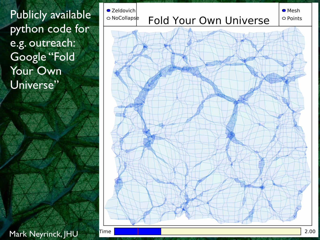
Publicly available python code for e.g. outreach: Google “Fold Your Own Universe”

- 2LPT, 3LPT:

Mark Neyrinck, JHU

2 F. S. Kitaura and Steffen Heß

2LPT

LPT/ZeldovichSC

3LPT ALPT: 2LPT-SC

ψf≡

∇·Ψ

(q,z

=0)

ψi ≡ −D1δ(q, z = 100) ψi ≡ −D1δ(q, z = 100) ψi ≡ −D1δ(q, z = 100)

Figure 1. Cell-to-cell correlation between the linear initial overdensity field D1δ(q, z = 100) and the corresponding approximations for the divergence ofthe displacement field for the 10th realisation of our set of simulations. The solid black line represents the LPT/Zeldovich approximation and the green curvethe local SC model, which approximately fits the mean N -body relation. The nonlocal relations are given by the contours for various approximations: leftpanel: 2LPT (quadratic relation). middle panel: 3LPT (cubic relation) and right panel: combined 2LPT-SC with rS = 4 Mpc/h. The dark colour-codeindicates a high number and the light colour-code a low number of cells.

timations from large scale structure surveys has raised the inter-est in approximate efficient structure formation models, which canbe massively used. See Scoccimarro & Sheth (2002); Monaco et al.(2002); Manera et al. (2012) for generation of mock galaxy cata-logues; and Schneider et al. (2011) to increase the volume of a setof N -body simulations with smaller volumes. An improvement tolinear LPT is given by second order LPT (2LPT) including non-local tidal field corrections. However, this is known to be a poor es-timator in high and low density regions, being strongly limited byshell crossing (Sahni & Shandarin 1996; Neyrinck 2013). Recently,local fits based on the spherical collapse model have been proposed(Mohayaee et al. 2006; Neyrinck 2013), which better match themean stretching parameter (divergence of the displacement field)of N -body simulations. We propose in this work to combine thesuperiority of 2LPT on large scales with the more accurate treat-ment of the spherical collapse (SC) model on small scales includ-ing a collapse truncation of the stretching parameter, which acts asa viscosity term. Our algorithm splits the displacement field into along-range and a short-range component, the first one being givenby 2LPT and the second one by the truncated SC model. Both arecombined by using a Gaussian filter with smoothing scales of 4-5Mpc/h radii, being this scale the only free parameter in our model.

2 THEORY

Let us define the positions of a set of test particles at an initial timeti by q and call them the Lagrangian positions. The final comovingpositions x (called Eulerian positions) corresponding to the sameset of test particles at a final time tf are related to the Lagrangianpositions q through the displacement field,Ψ:

x = q +Ψ . (1)

Hence, the displacement field encodes the whole action of gravityduring cosmic evolution. An approximation is to consider that thedisplacement field is a function of the initial conditions only, andcan be described by straight paths. The various models considerthe relation between the divergence of the displacement field andthe linear initial field: ψ = ψ(δ(1)) ≡ ∇ · Ψ(δ(1)), where ψ isthe so-called stretching parameter. Let us call the previous equationthe stretching parameter relation. Lagrangian perturbation theory to

third order yields the following expression for curl-free fields (seeBuchert 1994; Bouchet et al. 1995; Catelan 1995):

ψ3LPT ≡ ∇ ·Ψ3LPT (2)= −D1δ

(1) +D2δ(2) +D3aδ

(3)a +D3bδ

(3)b ,

where D1 is the linear growth factor, D2 the second order growthfactor, D3a, D3b, D3c are the 3rd order growth factors corre-sponding to the gradient of two scalar potentials (φ(3)

a ,φ(3)b ). Partic-

ular expressions can be found in Bouchet et al. (1995) and Catelan(1995): D2 = −3/7Ω−1/143D2

1 , D3a = −1/3Ω−4/275D31 ,

D3b = 1/4 · 10/21Ω−269/17875D31 . The term δ(2)(q) represents

the ‘second-order overdensity’ and is related to the linear overden-sity field by the following quadratic expression:

δ(2)(q) =!

i>j

"

φ(1),ii (q)φ

(1),jj (q)− [φ(1)

,ij (q)]2#

, (3)

The potentials φ(1) and φ(2) are obtained by solving a pair of Pois-son equations: ∇2

qφ(1)(q) = δ(1)(q), where δ(1)(q) is the linear

overdensity, and ∇2qφ

(2)(q) = δ(2)(q). The first term is cubic inthe linear potential

δ(3)a ≡ µ(3)(φ(1)) = det"

φ(1),ij

#

, (4)

and the second term is the interaction term between the first- andthe second-order potentials:

δ(3)b ≡ µ(2)(φ(1),φ(2)) =12

!

i=j

"

φ(2),ii φ

(1),jj − φ(2)

,ij φ(1),ji

#

, (5)

(see Buchert 1994; Bouchet et al. 1995; Catelan 1995). Keepingterms only to first order is called the Zeldovich approximation(Zel’dovich 1970) and keeping terms to second order yields the2LPT approximation.

Based on the nonlinear spherical collapse approximation, de-veloped by Bernardeau (1994), Mohayaee et al. (2006) found a lo-cal nonlinear expression for the stretching parameter relation:

ψSC ≡ ∇ ·ΨSC = 3

$

%

1−23D1δ

(1)

&1/2

− 1

'

. (6)

This analytic formula has been recently found to fit very well themean stretching parameter relation from an N -body simulation

c⃝ 0000 RAS, MNRAS 000, 000–000

(Kitaura & Heß 2013)

-“stretching” ψ≡∇L⋅ψ, - Zel’dovich (1970): ψ = -δlinear. - ψ = -3: halo formation, where ∇L⋅xf = 0.

How does the dark-matter sheet really stretch?

(MN 2013)

Mark Neyrinck, JHU

Pjnonlinear ≡ ΣGijPiPjnonlinear ≡ ΣGijPi

Interpolating between 2LPT and Spherical Collapse

Mark Neyrinck, JHU

Multiscale Spherical Collapse

Alternative solution: apply spherical collapse on many scales. Gaussian*-smooth the field at scales 2nc, where c = cell size, where n < ~5 !

If δlin>3/2 at any scale, set ψ=-3. Apply spherical collapse formula at c, otherwise. !

*- Top-hat smoothing didn’t work as well. Other multiscale prescriptions possible.

Mark Neyrinck, JHU

How does the dark-matter sheet really stretch?

!- Approaches based on the “stretch parameter” ψ≡∇L⋅ψ directly from initial conditions (Lagrangian divergence of the displacement field)

← perturbative

← Non-perturbative: MUltiscale Spherical ColLapse Evolution

Mark Neyrinck, JHU

!- Approaches based on the “stretch parameter” ψ≡∇L⋅ψ directly from initial conditions (Lagrangian divergence of the displacement field)

How does the dark-matter sheet really stretch?

perturbative ->Non-perturbative: MUltiscale Spherical ColLapse Evolution

!- Large scale structure simpler than often imagined on quasilinear scales!

← perturbative

How does the dark-matter sheet really stretch?

(N-body)

← Non-perturbative: MUltiscale Spherical ColLapse Evolution

Mark Neyrinck, JHU

Quantitatively:

Simple Python Code for quick N-body realizations & IC’s at http://skysrv.pha.jhu.edu/~neyrinck/muscle

Mark Neyrinck, JHU

How does it fold?

http://skysrv.pha.jhu.edu/~neyrinck/muscle

Folding in a 1D universe

Mark Neyrinck, JHU

Mark Neyrinck, JHU

- Tools needed to understand phase-space geometry of haloes and subhaloes necessary — difficult to distinguish substructures in crowded environments !

- Easy to visualize in 1D, but 2D? 3D?

2

FIG. 1: The phase space of a one-dimensional halo simulatedfrom random but smooth initial condition. The individualsubhaloes are shown by di↵erent colors

tively. Topologically, this mapping, referred to as the La-grangian submanifold, is a three-dimensional sheet in thethe six-dimensional (q,x) space. The method is based ona concept of a DM sheet in phase space v = v(x, t) suc-cessfully employed to improve accuracy of the estimatesof the density, velocity and other parameters in standardcosmological N -body simulations [16, 17]. The major dif-ference between this concept and the conventional one isin the di↵erent interpretation of the role of the particlesin the simulations of the evolution of the continuous DMmedium. Instead of the common interpretation of parti-cles as carriers of mass, it was suggested to treat themas massless markers of the vertices in a tessellation ofthe three-dimensional DM sheet in six-dimentional phasespace. The particles’ mass is uniformly distributed insideeach tetrahedra of the tessellation [16, 17]. Once the tes-sellation is built in the initial state of the simulation, itmust remain intact through the whole evolution becauseof the Liouville’s theorem, as long as the thermal veloci-ties of the DM particles are vanishing. This requirementresults in a significant di↵erence between this approachand Delaunay tessellation suggested in [18] for estimatingthe density from particle distributions.

The particles being the vertices of the tetrahedra de-scribe all deformations occurred to the geometry of the

FIG. 2: Fields x(q) and n↵(q) are plotted in the top andbottom panels respectively for the halo shown in fig. 1.

tessellation. However it remains continuous in both six-dimensional phase space (x,v) and in (q,x) space. Inparticular, the variations of tetrahedra volumes resultin the corresponding change of the tetrahedra densities.This property is especially valuable because it makesthe tessellation self-adaptive to the growth of densityperturbations with time. We stress that whereas both(x,v) and (q,x) spaces contain all the information abouta dynamical system, the latter is a metric space andhence superior to the non-metric phase space. More-over, the Lagrangian submanifold mapping, q = q(x),is a single-valued function, unlike the phase-space map-pings v = v(x) or x = x(v) which are multivalued.We now illustrate the main idea of the proposed La-

grangian submanifold technique with a halo formed inone-dimensional N -body simulation of a collisionless coldDM medium in an expanding universe.Figure 1 shows the phase space of the halo evolved in

the universe from smooth random initial condition. Thehalo can be naturally defined as the region in Eulerianspace where the number of streams is greater than one.The number of stream changes by two at caustics wherethe tangent to the phase space curve becomes verticaland the density in the corresponding stream becomesformally infinite. One can see a complicated substruc-ture that consists of a number of subhaloes and streams

(Shandarin & Medvedev 2014)

Eric Gjerde, origamitessellations.com

Rough analogy to origami: initially flat (vanishing bulk velocity) 3D sheet folds in 6D phase space.

The Universe’s crease pattern

Crease pattern before folding

After folding

(Neyrinck 2012)

!!!

Schematic, based on the VIPERS survey

.

. .

Currently on display in the JHU physics dept:

New Scientist article (Dec 2014) “The Origami Code” Documentary

Mark Neyrinck, JHU

Origami mathematics: Helps in art, engineering, biology.

Can it help to understand structure formation? Let’s see …

Dr. Robert J. Lang

Origami approximation to large-scale structure

• creases = reflections • 1D: Nodes form between “void centers.” Squashed pile of string • 2D: Extrude — make sure single-stream/layer regions don’t rotate

• 2D voids from 1D voids • 2D filaments from 1D nodes • 2D nodes new (can twist!)

• 1D cosmic web:

!

• Filaments that form together • In (?), >1 reflection → rotation • Called a “twist fold” by origamists • “Triangular collapse” by cosmologists?

Mark Neyrinck, JHU

Cosmological Origami!!!

?

θ

θθ

θ

2θ

Tetrahedral Twist Folds/Tetrahedral collapse

Unless the central node has no rotation, filaments will twist, giving a correlation

between adjacent halo spins

1230 A. Slosar et al.

Figure 3. This figure shows the constrains on the binned correlation func-tion c for angular (top panel), redshift (middle panel) and projected (bottompanel) spaces. Two lines correspond to our best-fitting exponential (solidred) and Gaussian (dashed green) fits.

5 R ESULTS

In Fig. 3, we plot the results of our binned estimation of c(r). Fromthe two figures, it is immediately clear that there is a hint of anexcess at low values of r. The statistical significance of this excessis marginal, at about !χ 2 of 7.5, 14.2 and 5.6 for angular, real andprojected distances with six extra degrees of freedom associatedwith six bins. This corresponds to 2σ–3σ detection in the redshiftspace but a non-detection in other spaces.

To understand this excess better, we calculate the probability con-tours on the a − b plane using exponential and Gaussian likelihoods.These are plotted in Fig. 4 and the relevant numbers are given inTable 1. How significant are these detections? The improvementin χ 2 is between nine and 12 with respect to zero correlation inangular and redshift cases with two free parameters. Within a fre-quentist approach, this is significant at 2σ–3σ level. The excessat low redshift is not significant in the case of projected distances,although visually, the low-distance points are not incompatible withan excess.

A more appropriate statistical procedure is the Bayesian evidence(Slosar et al. 2003; Beltran et al. 2005; Trotta 2007) which wecalculate for all our two model parametrizations and are also shownin Table 1. These can be calculated exactly for a simple problemlike ours. Evidence depends weakly on the prior size, and in this wechose the prior on a between 0 and 1/1.5 for Gaussian/exponentialcase and b between 0 and 1000 arcsec or 1 or 0.5 Mpc h−1 projected.Regardless of the exact number employed, the evidence ratio isbetween a few and a few tens units implying a weak evidence or ahint for angular and redshift spaces, but not for the projected space.This is consistent with results from the frequentist approach above.

Figure 4. This figure shows the constrains on the a–b plane for all datasets and models under consideration. Thick lines enclose 68.3, 99.4 and99.8 per cent likelihood volume for the weighted sample. Thin lines are thesame for unweighted sample. The top and bottom rows show results in realand angular spaces, respectively. The left- and right-hand columns are theexponential and the Gaussian fittings exponentially.

Finally, we acknowledge the fact that the exponential and Gaus-sian forms were chosen a posteriori after seeing the data, and hencethe improvements in fits contain a subjective a posteriori factor.

5.1 Systematics

We can now briefly discuss some of the main systematic effect thatmight affect our measurements.

Rogue pairs. As discussed in Section 4.1, we manually lookedat all pairs in the clean sample and discarded rogue pairs. It isan important systematic check, because we have at the same timeconvinced ourselves that manually classifying a small subset (80galaxies) of the total sample gave consistent results.

Weighting. Repeating our measurements with unweighted data,changes result by less than 5 per cent.

Cleanliness level. We have repeated the analysis with the su-perclean sample. There are many fewer galaxies in the supercleansample (Lintott et al. 2008) and so the statistical significance de-creases considerably. We have no significant detection in any of thespaces considered. The error bars increase by a factor of 2 to 2.5,but the central values in individual bins remain consistent. While

C⃝ 2008 The Authors. Journal compilation C⃝ 2008 RAS, MNRAS 392, 1225–1232

at Milton S. Eisenhow

er Library/ Johns Hopkins U

niversity on April 1, 2015

http://mnras.oxfordjournals.org/

Dow

nloaded from

Chirality correlation observed in SDSS (Slosar et al. 2008)

Tetrahedral Twist Fold

Before folding After folding

8 MARK C. NEYRINCK

Figure 6. Tetrahedral-collapse models. Filament creases (green) are indicated by trian-gular tubes, intersecting at the central node. Wall creases (blue), extend from filamentedges through the thin lines drawn between filaments. Node creases are in red. Left:Pre-folding/collapse (Lagrangian). Right: Post-folding/collapse (Eulerian). Top: An ir-rotational model (↵1 = /2). Each filament vector fi ? a face of the central tetrahedron.Walls, filaments, and the node invert along their central planes, axes, and point, but re-main connected as before. Void regions simply move inward. All 15 initial regions over-lap at the center. Bottom: A rotational model (↵1 = /6). The top filament rotatescounter-clockwise by /3, while the smaller, bottom filaments rotate clockwise by 2/3. Seehttp://skysrv.pha.jhu.edu/

~

neyrinck/TetCollapse for an interactive model.

Many of the results given here, particularly in 3D, were numerical. This is fine for comparison tocosmological simulations, as we plan to do. But there is much room for further rigorous mathematical studyof polyhedral collapse, both of isolated nodes, and of how networks of collapsed polyhedra behave together.

Irrotational (~ spherical collapse)

Rotational

Mark Neyrinck, JHU

Conclusions

• Stretching the dark matter sheet: Multiscale spherical collapse: muscling particles into place

• Folding it: Origami approximation: toy model to understand velocities, spins in the cosmic web