Wright meets Markowitz:How standard portfolio theory changes when assets

are technologies following experience curves

Rupert Way ∗a, b, François Lafond †a, b, c, Fabrizio Lillo ‡d, e, ValentynPanchenko §f and J. Doyne Farmer ¶a, g, h, i

aInstitute for New Economic Thinking at the Oxford Martin School,University of Oxford, Oxford OX2 6ED, UK

bSmith School of Enterprise and the Environment, University of Oxford,Oxford, OX1 3QY

cOxford Martin School Programme on Technological and EconomicChange, University of Oxford, OX1 3BD

dScuola Normale Superiore, Piazza dei Cavalieri 7, 56126 Pisa, ItalyeCADS, Center for Analysis, Decisions, and Society, Human Technopole,

Milano, 20156, ItalyfSchool of Economics, UNSW Business School, Sydney NSW 2052,

AustraliagMathematical Institute, University of Oxford, Oxford OX1 3LP, UKhDepartment of Computer Science, University of Oxford, Oxford OX1

3QD, UKiSanta-Fe Institute, Santa Fe, NM 87501, USA

August 28, 2018

∗rupert.way@smithschool.ox.ac.uk†francois.lafond@inet.ox.ac.uk‡fabrizio.lillo@sns.it§v.panchenko@unsw.edu.au¶doyne.farmer@inet.ox.ac.uk

1

arX

iv:1

705.

0342

3v3

[q-

fin.

EC

] 2

6 A

ug 2

018

Abstract

We consider how to optimally allocate investments in a portfolio of compet-ing technologies using the standard mean-variance framework of portfolio theory.We assume that technologies follow the empirically observed relationship known asWright’s law, also called a “learning curve” or “experience curve”, which postulatesthat costs drop as cumulative production increases. This introduces a positive feed-back between cost and investment that complicates the portfolio problem, leadingto multiple local optima, and causing a trade-off between concentrating investmentsin one project to spur rapid progress vs. diversifying over many projects to hedgeagainst failure. We study the two-technology case and characterize the optimal di-versification in terms of progress rates, variability, initial costs, initial experience,risk aversion, discount rate and total demand. The efficient frontier framework isused to visualize technology portfolios and show how feedback results in nonlineardistortions of the feasible set. For the two-period case, in which learning and uncer-tainty interact with discounting, we compare different scenarios and find that thediscount rate plays a critical role.

2

1 IntroductionThere is a fundamental trade-off, encountered throughout life, between investing enougheffort in any one activity to make rapid progress, and diversifying effort over many projectssimultaneously to hedge against failure. On the one hand, by focusing on a single task onecan quickly accumulate experience, become an expert, and reap rewards more efficiently.But on the other, unforeseen circumstances can impede progress or make the rewardsless valuable, so it may be wise to maintain progress on several fronts at once, even ifindividually slower. This brings to mind the familiar adage “don’t put all your eggs inone basket”, and at first glance appears very similar to the question of how diversified aportfolio of financial investments should be. However there is a key difference betweenthe financial portfolio setting and the type of problem considered in this paper, which isthat here learning is involved: the more effort we invest in one area, the more effectivethat effort becomes — so we may want to put all our eggs in one basket after all.

The dilemma is ubiquitous, and is understood intuitively by us all as we learn newskills, engage in new projects, and attempt to plan for the future. For example, considertrying to decide how many courses to take in university; or how many languages, musicalinstruments, sports, or web application frameworks to learn. Focusing on one, or justa few, allows us to gain expertise and reach a more rewarding phase of activity sooner.Or at the organisational level, firms and governments must decide how many, and which,strategic and technological capabilities to develop. We present a simple model for under-standing this trade-off, and show how it is related to the optimal diversification problemfor financial assets.

The reason this decision framework is of particular interest is that, despite its simplic-ity, it shares several important features with the question of how to allocate investmentsamong competing technologies. This is because often, in the long run, scientific advancesand knowledge gains mean that performance-weighted technology investment costs de-crease as cumulative deployment increases. Put simply, in such cases the more we investin a technology (whether at the R&D, deployment or any other stage) the more effec-tive the technology becomes at delivering the same output, so future investment costsare lower, per unit of output1. Hence, in order to achieve certain long term technologi-cal goals, understanding the correct allocation of investments among available substitutetechnologies is vital. The specific question we have in the back of our minds is how toallocate funding over potential clean energy technologies to accelerate the transition to anet zero carbon economy — should we invest in solar photovoltaics, or offshore wind, ornext generation nuclear, or carbon capture and storage, or a little bit in each?

Despite this high-level motivation, here we focus in on a very simple conceptual modelrepresenting the underlying trade-off. The key assumption we make is that increased cu-mulative investment in a technology leads to reduced investment costs (but with somedegree of uncertainty). In reality this causal mechanism is not so straightforward, andthere are many other complicating factors, such as correlations between projects andspillovers (incoming and outgoing) of various kinds. However, while stating the caveatsclearly, we set aside these issues for now and just focus on the core problem, which isto find the optimal risk-averse investment in competing technologies following experi-ence curves. This setting brings together the specialization incentives of the learning

1Though note that many technologies do not exhibit such decreasing costs at all, and also that theeffect (when it exists) is far less evident in mature technologies since so much experience has alreadyaccrued.

3

curve model with the diversification incentives of modern portfolio theory, allowing us tocharacterize the optimal solution to the trade-off between diversifying and specializing.

Our approach is to consider multiple independent technologies (two), increasing re-turns to investment (through experience curves), uncertainty (cost is a stochastic process),and a risk-averse decision maker (who minimizes a mean-variance value function). Sincethe two technologies follow stochastic processes, diversification tends to reduce the risks,but at the same time increasing returns tend to favour specialization. Investing in oneoption drives down its marginal cost, making it more and more attractive, but ex-anteuncertainty in future benefits from learning suggests that diversifying can limit the riskof over-investing in a technology that eventually shows a poor performance. We charac-terize optimal investment as a function of learning characteristics (rate and uncertaintyof learning), initial conditions (cost competitiveness and accumulated experience), riskaversion, discount rate and the level of demand. We focus primarily on the one-periodinvestment decision, but also consider the extension to two periods.

In classical (Markowitz) portfolio theory, the optimal allocation of investments isunique. In general, the further a portfolio is from the optimum, the worse is its value. Incontrast, when the positive feedback of endogenous technological progress is strong, it isbetter to invest mostly in either of the two options than to split investment more evenly.Except in some knife-edge cases, one of the two specialized portfolios is better than theother, but which one is best depends on the parameters. As a result, a small change inone of the parameters can result in the optimal portfolio being completely different.

In general we characterize three different regimes. In the first regime, one technology isso much better than the other that it dominates the portfolio entirely. This happens eitherbecause there is no risk aversion (so we revert to the classic deterministic learning curvewinner-takes-all scenario) or because the relative advantage of one technology in termsof initial conditions or speed and uncertainty of learning is very strong. In the secondregime, the optimal portfolio features unambiguous diversification, that is, the objectivefunction has a unique optimum corresponding to a balanced mix of technologies. In thethird regime, there are two local optima of similar value, corresponding to quite differentinvestment policies. As parameters change, the transition of the global optimum fromone local optimum to the other is abrupt. In other words, in this critical region, a smallchange in a parameter causes a large change in the optimal policy.

We show what this finding implies for the theory of path-dependence and lock-in,and characterize lock-in as a situation where investing in a fast-learning technology is notcurrently optimal, but it would be if a higher level of demand existed. Intuitively, whetheror not one should attempt to bring a technology down its learning curve depends on thesize of the market. For some parameter values though, the transition is sharp – thereexists a critical level of demand below which investment in the fast-learning technologyis limited, and above which it becomes dominant (i.e. the global optimum switches fromone local optimum to the other).

We show analytically that a Markowitz-like case may be recovered in two differentways. First, when there is no learning increasing returns are absent and it becomeshighly unlikely that one would want to specialize entirely. (Specialization is still possible,but only because one technology is currently much better than the other, not becauseinvesting in it makes it better.) Second, when future demand is very small, comparedto the current level, the potential for learning is insignificant and therefore investment isnever enough for increasing returns to really matter.

Our results relate to several different branches of literature. First of all we are moti-

4

vated by the optimal energy systems, energy transition and climate change literatures. Itis now clear that to avoid a rise in temperatures that would have “dangerous” effects wemust attain net zero carbon emissions, and one of the main factors involved in this is aswitch to a clean energy system. However, dirty energy technologies are currently consid-ered to be both cheap and convenient (in some ways due to legacy energy system designand infrastructure, and societal embeddedness), whereas alternatives are still expensive,even though their cost is falling, sometimes very fast. In this context the questions ariseof what costs will be in the future, which decisions affect these costs, and what is thebest investment or tax/subsidy policy. Energy systems are highly complex2 and energyexperts generally rely on highly detailed models of the energy production and consump-tion mix. To include endogenous technological change in these models, a simple solutionwhich has been widely adopted (and criticized) is that of experience curves (Gritsevskyi& Nakićenović 2000, Barreto & Kypreos 2004, Alberth & Hope 2007, Criqui et al. 2015,Webster et al. 2015). However, these models end up being very complex so that optimalpolicies are very hard to determine and understand. Numerical methods have to be used,and it is not always the case that the global optimum is found. Analytical approaches forthese complex models generally have to assume a deterministic setting, so that the in-creasing returns induced by the learning curve lead to full specialization, see for instanceWagner (2014). In this paper we only wish to understand the fundamental trade-offinvolved in technology investment: diversification against specialization, and the risk oflock-in in systems with path dependent, self-reinforcing dynamics. Therefore, we do notattempt to provide a realistic model of the energy system or a direct empirical applicationof our results, and instead focus on a theoretical contribution at the intersection of thelearning-by-doing and portfolio literatures.

To model technological progress, we use a very specific parametric model. Techno-logical progress is not perfectly predictable, but in many detailed empirical cases it hasbeen found that unit costs tend to decrease by a constant percentage every time cumu-lative production doubles. Subject to some uncertainty about future shocks, the cost ofa technology follows an experience curve which is technology-specific. This relationshipbetween unit cost and cumulative investment has been observed for a long time (Wright1936, Alchian 1963, Thompson 2012) and is generally explained by the fact that duringproduction learning-by-doing takes place3. Starting with Arrow (1962), a large literaturehas developed to analyse the consequences of this relationship for pricing and outputdecisions (Rosen 1972, Spence 1981, Mazzola & McCardle 1997). Learning-by-doing de-creases marginal cost, which gives an advantage to size and may encourage predatorypricing (Cabral & Riordan 1994) or legitimize the protection of infant industry from in-ternational competition (Dasgupta & Stiglitz 1988). When one considers a single firmoperating a single technology, learning-by-doing generates irreversibilities and creates anincentive to delay investment. The optimal investment dynamics can be characterized

2Each energy source has specific infrastructure building time (e.g. nuclear takes a long time), can beintermittent or not (e.g. solar energy is not produced at night), has specific transport, storage and safetyconditions, etc.

3While learning-by-doing often refers to labour force or organisational learning in particular, twoother related and noteworthy sources of increasing returns include economies of scale, which depend onlyon current (not cumulative) production levels, and network externalities, which depend on the numberof consumers or other producers joining or using the same network or technology. The key featureof experience curves, however, is that performance increases depend on the growth of total experience(cumulative production), not on the growth of production. We think of experience curves as capturingall experience-related effects, including, but not limited to learning-by-doing.

5

using the theory of real options (Brueckner & Raymon 1983, Majd & Pindyck 1989,Della Seta et al. 2012). In general, the literature does not study multiple technologies atthe same time; and when it does, for instance when characterizing the social optimum fora multi-firm sector, it is generally in the absence of uncertainty. Given our motivation tounderstand optimal investment in energy technologies, which are very diverse and uncer-tain, we turn to another branch of literature which has dealt in detail with investment inmultiple uncertain assets, that is modern portfolio theory (Markowitz 1952).

Modern portfolio theory considers a risk-averse decision maker who wishes to investin financial assets. The key result of portfolio theory is that there exists an optimal wayof combining assets in a portfolio such that expected returns are maximized, conditionalon a given level of risk (or that risk is minimized, conditional on a given level of ex-pected returns). We argue that this idea is well suited for thinking about technologyinvestment, and we borrow from portfolio theory the mean-variance value function (inour case, both expected costs and variance of the portfolio have to be minimized). Forsimplicity, however, we generally assume that technologies are uncorrelated. As opposedto a “learning curve technology”, a key property of a financial asset is that investing init does not change its value, although there are some important exceptions4. We recovera classical portfolio setup when the learning parameter is zero or when the total marketsize is very small compared to the initial production.

Besides our general motivation (energy systems) and the two major ingredients ofour model (experience curves and mean-variance portfolio theory), our setup relates toa large literature dealing with optimal control of stochastic processes, which goes wellbeyond economics and operation research. Of more direct interest are the applications totechnology, R&D and innovation problems, where the questions of increasing returns andlock-in are more salient. When investing in an option makes it better and better, historymatters. Atkinson & Stiglitz (1969) already pointed out that localized technologicalprogress, an important source of which is learning-by-doing, would justify investing ina technology that is not yet the cheapest. In the technology choice literature, it iswell known that increasing returns and uncertainty may result in situations where poortechnological options dominate (David 1985). In a model of two competing standardsoperating under network externalities, Arthur (1989) showed that if chance favors anintrinsically worse option early on, this option’s accumulated experience gives it an edgefor obtaining the marginal consumer. As this advantage accumulates, it may foreverexceed the benefits from switching to the intrinsically better option. In this context apolicy maker is interested in a policy that optimally explores the merit of different optionsbefore making a final choice. Cowan (1991) characterized a social planner’s optimaldecision in a two arm bandit framework, where there is a choice between one of twotechnologies at every period. In this model, there exists an optimal policy known as theGittins index, but according to this policy eventually a single technology will be chosen.Thus early bad luck may induce the social planner to lock in the wrong technology. While

4One is the situation in which market impact is considered. Market impact acknowledges that tradinglarge quantities simply violates the atomicity assumption, so that one’s choice of quantities demandedor supplied affects the price. In this case, this is a negative feedback and the literature has focused onfinding optimal liquidation strategies (Almgren & Chriss 2001, He & Mamaysky 2005). Another situationin which financial portfolios incorporate feedback effects is when learning about an asset is taken intoaccount. An investor who is familiar with a particular asset makes more precise estimates of expectedreturns, so that this asset is relatively more valuable than other assets (Boyle et al. 2012). In turn,holding a lot of a particular asset makes information acquisition about that asset more valuable, whichcan generate a positive feedback that encourages specialization (Van Nieuwerburgh & Veldkamp 2010).

6

this theoretical literature often refers to learning-by-doing5, it attempts to model otherforms of increasing returns all at once and therefore does not model more explicitly howcost decreases with investment. Zeppini (2015) considered learning curves for clean anddirty technologies in a discrete choice framework, with social interactions as an additionalsource of increasing returns to adoption and lock-in. He found that policies inducing theclean technology to progress down its learning curve faster have greater potential to inducesmooth technological transitions, as opposed to traditional policies such as a pollutiontax which can work only by being large enough to induce an equilibrium shift. Finally,another branch of literature has contrasted the benefits of increasing returns againstthe benefits of technological diversity by assuming that further technological progresstakes place through recombination. This implies that there is some value in giving up onincreasing returns from specialization and keeping a range of diverse technologies availablefor further re-combination (Van den Bergh 2008, Zeppini & Van den Bergh 2013).

The paper is organized as follows. Section 2 defines the stochastic process for theexperience curves and the optimization problem in the one-period case, and shows how itrelates to Markowitz portfolios. Section 3 presents the main results of the optimizationand shows under which conditions diversification is optimal. It also analyzes in detail theobjective function by characterizing how the number and nature of optima changes withunderlying parameter values, and studies the effect of total demand. Section 4 returns tothe comparison of financial and technology portfolios and shows how the efficient frontierchanges when technologies are introduced. Section 5 establishes conditions to escape lock-in by studying the case where a mature, cheap but slow-learning technology dominatesthe market but faces competition from a young, expensive but fast-learning challenger.Section 6 introduces the multi-period model and explores how discounting interacts withrisk aversion and learning in a two-period setting. Finally, Section 7 concludes.

2 One-period modelConsider the development of a single technology over one time period. The unit costof the technology at time t is ct (measured in $/unit), and its cumulative production6

(measured in units) is zt. Let t = 0 be the present time and t = 1 be some given futuretime. The current unit cost is c0 and current cumulative production is z0. Productionduring the period is q, and the cumulative production at t = 1 is z1 = z0 + q. We firstpresent the stochastic model for a single technology then consider a portfolio of two suchtechnologies.

2.1 Wright’s law

The standard form of the experience curve is

ct ∝ zt−α, (1)

where the constant α is the experience exponent (or Wright exponent) for this technology.This leads to two related concepts often used in the literature: the “progress ratio” is

5When increasing returns are from the consumer side, typically as in Arthur (1989), they are generallymotivated as learning-by-using following Rosenberg (1982).

6We use the terms investment and production interchangeably throughout the one-period modelpresentation. Generally the literature considers production, although the original paper by Arrow (1962)used investment. Here we are looking only one step ahead so this is not an important difference.

7

defined as the relative cost level seen after each doubling of cumulative production, PR =2−α, while the “learning rate” is defined as the relative cost reduction seen after each suchdoubling, LR = 1 − 2−α. Dutton & Thomas (1984) report learning rates from differentstudies and find that the vast majority lie between 5% and 40%, corresponding to valuesof α lying approximately within the range (0.07, 0.7). However, commodities such asminerals and fossil fuels mostly have α ≈ 0 since they do not exhibit a significant costdecrease over the long run (Newbold et al. 2005, McNerney et al. 2011). The power lawrelationship between cost and cumulative production was first noted by Wright (1936)in the context of the production of airplanes, so we call it Wright’s law. Since then ithas been found to describe the available evidence for a number of technologies fairly well(Nagy et al. 2013). In contrast to a large part of the theoretical literature on experiencecurves, which deals only with the deterministic form, we model uncertainty explicitly. Todo this we make the future cost stochastic by assuming additive noise η on the log-first-difference version of Eq. (1):

log(c1)− log(c0) = −α[

log(z1)− log(z0)]

+ η. (2)

This equation models a situation where, over the course of one period, an underlyinglinear trend in log-log space advances according to Wright’s law, but then is hit by arandom shock. It is one of the simplest possible ways of incorporating uncertainty in theexperience curve model, chosen here specifically for its clarity and simplicity7. The costof production at t = 1, interpreted as the average (or constant) within-period cost, isthen given by

c1 = c0

(z0z1

)αeη = c0

(z0

z0 + q

)αeη. (3)

So there is a distribution of possible future costs c1, and Eq. (3) shows clearly how itdepends on: i) the current state, c0, z0, of the technology8, ii) the technology’s experienceexponent α, iii) the choice of production q over the period, and iv) the noise distributionη.

Next, we suppose that the shock is normally distributed with mean zero9 and varianceσ2, η ∼ N (0, σ2). This noise model is known to be a reasonable assumption for financialassets with lognormal returns, but some justification is required when considering tech-nologies. Lafond et al. (2018) found that this model gave a reasonably good fit to dataon 51 technology time series, in the sense of predicting theoretical forecast errors in linewith realised forecast errors, although their preferred model allows for autocorrelation.

Thus cost is log-normally distributed, and by standard log-normal properties its ex-pectation and variance are given by

E [c1] = c0

(z0

z0 + q

)αeσ

2/2, (4)

Var (c1) = c20

(z0

z0 + q

)2α

eσ2(eσ

2 − 1). (5)

7Another way would be to make the learning rate α stochastic, instead of the cost. Mazzola &McCardle (1996) considered how a Bayesian learner benefits from more production not only by decreasingcosts, but also by improved estimates of the learning parameter.

8Note that it is the presence of z0 here that distinguishes between learning effects and increasingreturns to scale.

9Nonzero mean noise is discussed in Section 6.

8

These two properties of the stochastic experience curve, specified uniquely by the fourparameters c0, z0, α, σ, will now be used to construct the portfolio model.

2.2 The optimization

Consider two independent technologies, A and B, each evolving according to the form ofWright’s law proposed above, with their own technology-specific parameters. We labelvariables and parameters with superscripts (e.g. qA, cA0 , zA0 , αA, σA). Suppose the technolo-gies are perfect substitutes10 and that there is a fixed, exogenous demand K, which mustbe satisfied exactly by some combination of production of the two technologies11, i.e. thereis a production constraint K = qA + qB. Production is non-negative, so qA, qB ∈ [0, K],and choosing qA also determines qB = K − qA. We use qA as the control variable in thefollowing optimization and present results in terms of the share of total production intechnology A, qA/K. Let the total cost of production during the period be V (qA). Thisis just the sum of unit costs times units produced

V (qA) =∑i=A,B

ci1qi, (6)

where stochastic costs ci1 depend nonlinearly on productions qi, as in Eq. (3). Thus for afixed, known set of technology parameters {ci0, zi0, αi, σi}i=A,B and total demand K, eachchoice of production qA maps to a distribution of total costs V . The tools for addressingthis type of problem are well developed, see for example Krey & Riahi (2013). The goalhere is to understand how the parameters and the choice of production together generatethe total system cost distribution, from which an optimal production portfolio may beidentified. We perform a mean-variance analysis on V because it is simple, intuitive andillustrates clearly the key features of the system12. Let λ ≥ 0 be a risk aversion parameterand f be the mean-variance objective function. The optimization problem is then

minimize:qA

f(qA) = E[V (qA)

]+ λVar

(V (qA)

)(7)

subject to: qA ∈ [0, K].

The aim therefore is to find the production mix which, while meeting the productionconstraint, minimizes the expected total cost of production, plus an additional termcharacterizing the spread of the distribution of possible outcomes. The risk aversionparameter λ scales the contribution of the variance term in f , reflecting the extent to

10While the perfect substitutability assumption is essential in this model, in reality technologies areoften not continuously varying substitutes, and it may not be possible to adopt just a bit of severaldifferent technologies. Indeed, many technology adoption decisions are entirely binary, such as thechoice of firm-wide software systems. This is a limitation of the model, and the domain of applicationshould therefore be chosen carefully.

11Since demand and total production are assumed equal throughout we use the terms interchangeably.It is assumed that the demand is inelastic and prices are determined competitively (as is typical in energymarkets). Under these conditions cost minimization is equivalent to profit maximization.

12Since empirical technology cost noise shocks are found to fit a lognormal distribution fairly well, asdiscussed previously, standard results from the finance literature apply here. In particular, use of themean-variance decision framework in the one-period setting is justified as it provides a good approxi-mation to all commonly used utility functions (Pulley (1981), Kroll et al. (1984)). However, the choiceof utility function in a multi-period setting (as we consider in Section 6) is much more subtle, and adifferent objective function may be preferable.

9

which the decision maker prefers to minimize exposure to cost uncertainty. In the risk-neutral case (λ = 0) the variance term has zero weight so the optimization just discoversthe production mix with lowest expected total cost (in this case just a single technology).Conversely, in the high risk aversion case (λ� 1) the second term in f dominates the firstand so the optimization discovers the production mix with lowest total cost uncertainty,regardless of its expectation. In the intermediate regime both terms play a significantrole in determining the outcome of the optimization. Using Eqs. (4), (5) and (6) theobjective function in problem (7) may be written explicitly as

f(qA) =∑i=A,B

ci0

(zi0

zi0 + qi

)αi

e(σi)2/2qi

+λ

(ci0

(zi0

zi0 + qi

)αi

qi

)2

e(σi)2(e(σ

i)2 − 1). (8)

Thus f is just the sum of one cost-expectation-based component and one cost-variance-based component for each technology; covariance terms are zero due to the technologyindependence assumption (i.e. ηA and ηB are uncorrelated). (The case of correlated noiseis considered in Section 3.5.)

This is a non-convex optimization problem so it may have more than one local min-imum. Since there is only one free variable though, qA, it is relatively quick to solve bybrute force optimization. Denote the optimum by qA∗

Despite the simplicity of the model, the scope for understanding its behaviour viastandard analytical techniques is rather limited. This is because the product terms (zi0 +qi)−α

iqi in the objective function mean that differentiation of f just generates more and

more similar product terms, which makes closed-form expressions for optima or othersystem properties only possible in a few restricted cases. Most of our results and analysisare therefore based on numerical optimization (and so were checked extensively to ensurethey are representative of the whole parameter space).

2.3 Technological maturity and the no-learning limit

2.3.1 Markowitz portfolios

Consider briefly the topic of Markowitz portfolio analysis for standard financial assets(Markowitz 1952). Let r = (r1, . . . , rn)T be a vector of stochastic returns (possiblycorrelated) and w = (w1, . . . , wn)T be a vector of portfolio weights. The portfolio returndistribution is V (w) = wT r, on which a mean-variance optimization is carried out, withw as control variable. The classic form of the problem is

maximize:w

f(w) = E [V (w)]− λVar (V (w)) (9)

subject to:∑

j=1,...,n

wj = 1.

Since this is a mean-variance optimization it looks very similar to our technology port-folio problem (7). There are several differences though; three are superficial but one isfundamental.

First, in the Markowitz case the decision maker seeks high expected portfolio returnand low variance, while in the technology case they seek low expected portfolio cost

10

and low variance13 — hence the sign difference of the variance terms in (7) and (9).Second, short-selling is in general allowed, so portfolio weights wj are not restricted tobeing non-negative. Third, returns are generally assumed to be correlated, and a lot ofattention is paid to understanding these correlations. Finally though, the fundamentaldifference between the two problems is that in the Markowitz case asset returns are purelystochastic, so portfolio weights do not affect asset performance, while in the experiencecurve model the stochastic costs depend explicitly on production, so portfolio weights doaffect technology performances. The more one invests in a given technology the better itgets, on average; there is nonlinear feedback in the technology portfolio model but not inthe Markowitz model.

2.3.2 Comparing financial and technology portfolios

To better understand the differences between the two portfolio types, we make a moreaccurate comparison by using a restricted version of the Markowitz model: the no short-selling, enforced budget, uncorrelated, two-asset model. This is a direct equivalent of ourtechnology portfolio problem in a standard financial setting. It eliminates the second andthird superficial differences listed above, making it easier to observe feedback effects.

Suppose there are two assets, A and B, with uncorrelated normal returns rA ∼N (µA, (sA)2) and rB ∼ N (µB, (sB)2). Then let qA and qB = (1− qA) be the proportionof wealth invested in A and B respectively, with qA, qB ∈ [0, 1] (the no short-selling con-dition). The portfolio return distribution is then V (qA) =

∑i=A,B r

iqi, and the objectivefunction to be maximized is

f(qA) = E[V (qA)

]− λVar

(V (qA)

)(10)

=∑i=A,B

µiqi − λ(siqi)2. (11)

Note that this is quadratic in portfolio weights qi. Then returning to the technology port-folio problem and considering the role of demand K and initial cumulative productionszA0 and zB0 in the objective function, a simple calculation reveals the connection betweenthe financial and technology models. Observe that the technologies objective function,Eq. (8), may be written

f(qA) =∑i=A,B

ci0qi

(1 + qi

zi0)αie(σ

i)2/2 + λ

ci0qi

(1 + qi

zi0)αi

2

e(σi)2(e(σ

i)2 − 1). (12)

When qi/zi0 is small we can approximate this in a simpler form. If the maximum futureproduction of technology i is much less than its current cumulative production (K � zi0),then qi/zi0 � 1, and the binomial series representation

(1 +qi

zi0)−α

i

= 1− αi qi

zi0+ αi(αi + 1)

(qi

zi0

)2

+ . . . (13)

may be used. Thus if K � zi0 for both technologies then to zeroth order the objectivefunction may be approximated as

f(qA) ≈∑i=A,B

ci0e(σi)2/2qi + λ

(ci0)2e(σ

i)2(e(σ

i)2 − 1)

(qi)2, (14)

13This is also the case in the optimal liquidation problem, see e.g. Almgren & Chriss (2001).

11

which no longer includes the experience exponents αi. Appendix A shows details ofthe expansion, plus higher order terms. Apart from the sign difference of the variancecomponent, this has the same form as the Markowitz model (Eq. (11)), i.e. it is quadraticin production14. In this limit learning plays no part, and there is no feedback processby which production affects future costs (since this is represented by the higher orderterms). Hence a Markowitz-like portfolio problem is the limiting case of the Wright’s lawportfolio problem as learning effects tend to zero.

Eq. (13) shows that a low-learning regime can exist in two ways for a given technol-ogy: first, if its learning rate is intrinsically small, and second, if its initial cumulativeproduction is very large compared to the total demand. The latter condition is problem-specific, since it depends on K, not just on the technology itself. All else being equal, asK → 0 technologies behave increasingly like standard financial assets, as noise increas-ingly dominates learning effects. Furthermore, very mature technologies automaticallybehave like standard financial assets in the model (since the incremental gains due tolearning decrease with maturity by definition in Wright’s law). Note that this analysisrelies on the assumption that model parameters are static, e.g. experience exponents areconstant and do not depend on the size of K. This assumption would require justificationin any practical application, and indeed is closely related to the question of whether asingle- or multi-period framework is more appropriate (the latter could allow for a morefine-grained approach to modelling technological maturity, for example). Neverthelessthe simple analytical connection between the two portfolio systems shown here is of note,as it reveals an interesting perspective on technological maturity in a portfolio setting.

Within any given problem then, each technology lies somewhere on a spectrum be-tween more technology-like and more asset-like, depending on the entire set of parameters.We use “asset-like” simply to mean that learning effects are negligible relative to noise,as with standard financial assets.

Finally, consider how the learning and non-learning portfolio problems differ analyt-ically at lowest orders. As shown in Appendix A, the approximation to f including thelowest order “learning” terms (i.e. terms in −αi qi

zi0) is

f(qA) ≈∑i=A,B

ci0e(σi)2/2

(1− αi q

i

zi0

)qi + λ

(ci0)2e(σ

i)2(e(σ

i)2 − 1)(

1− 2αiqi

zi0

)(qi)2.

(15)Thus the most straightforward effect of learning is to reduce both the expectation andvariance components linearly in αi, so that the technology with higher αi will performrelatively better in the optimization. In addition though, observe that while the zeroth-order approximation to f (Eq. (14)) is quadratic in qA, and hence always has just onesingle minimum, the first-order approximation to f is cubic in qA, and may thereforehave two local minima inside the optimization range (depending on parameters). Theintroduction of learning therefore corresponds to the introduction of multiple local optimaof the objective function.

14Note that the σi terms remain in the expectation component here due to the particular noise modelused (Eq. (4)). They are fixed and independent of qi (and indeed could be avoided with a different choiceof noise), so do not affect the argument.

12

3 Optimization resultsThe goal here is to understand how the optimal allocation of production between thetwo competing technologies depends on the technology-specific learning parameters (ex-perience exponent α and volatility σ) and the initial conditions (cost competitiveness c0and cumulative production z0) under varying levels of risk aversion λ, for fixed demandK. To do this we first hold all model parameters constant, then vary technology B ex-perience exponent αB and risk aversion λ. This generates a grid of tuples (αB, λ). Ateach point of this grid the optimization (7) is performed, and the resulting collection ofoptima is plotted, giving the surface of optimal production of technology A as a share oftotal production, qA∗ /K. The whole process may then be repeated for each of the othertechnology parameters σB, cB0 and zB0 .

3.1 Effects of experience exponents α

We set the initial conditions and parameter values to those shown in Table 1. Almostidentical technologies are used here as this allows us to understand the effects of varyingdifferent parameters most effectively. (Asymmetrical technologies are considered in Sec-tion 5.) Note that the total demand is twice the initial cumulative production of eachtechnology. Hence the technologies are relatively immature, in the sense that there isplenty of potential left for learning to take place relative to how much has occurred in thepast. As shown above, this is necessary since if both technologies are sufficiently maturea nearly-Markowitz scenario emerges.

Fig. 1 shows the surface of optimal technology A production share, qA∗ /K, over a gridof αB and λ values. This shows how risk aversion and relative experience exponents affectthe composition of the optimal portfolio.

Symbol Description Tech A Tech Bz0 Technology maturity 1 1c0 Initial cost 2 2α Experience exponent 0.5 [0-1]σ Technology volatility 1.0 1.1K Demand 2λ Risk aversion [0-1]

Table 1: Parameter values for the case of two almost identical technologies, as used in Fig. 1

13

Figure 1: Surface of the optimal production in technology A as a share of total production.This shows how the optimal portfolio varies with risk aversion λ and technology B experienceexponent αB (with αA fixed at 0.5). Red areas correspond to higher production of technologyA being optimal, and blue areas to higher production of technology B being optimal. Lowrisk aversion leads to more specialized portfolios and greater parameter sensitivity (representedby the surface discontinuity), while high risk aversion leads to greater diversification and lowerparameter sensitivity. Parameter values are shown in Table 1.

When risk aversion is low the optimal strategy is to concentrate production entirely ineither A or B (the dark red and blue plateau regions), depending on relative experienceexponents. When risk aversion is high portfolios are diversified over both technologies.This is consistent with a general understanding of both deterministic experience curves(in which specialization is always optimal) and standard portfolio theory (in which di-versification reduces portfolio risk). However, the nature of the transitions between theseregimes depends on model parameters and is of great interest. For low to moderate riskaversion there is a discontinuity in the surface, indicating a region of extreme sensitivityto model parameters. In this region an incremental change in either experience exponentor risk aversion can lead to a large change in the optimal portfolio. In contrast, for highrisk aversion the surface is smooth, so the optimal portfolio is robust to small changes inparameters. As we shall see (in Section 3.3.2), this is caused by the existence of multiplelocal minima of the objective function in the low risk aversion regime, and a single globalminimum in the high risk aversion regime.

On the λ = 0 boundary, variance terms do not feature in the optimization so produc-tion is concentrated in the technology with the best expected outcome. As risk aversionincreases, up to around 0.2, the asymmetry in noise variance becomes apparent and thethreshold for switching from 100% A to 100% B gradually shifts to larger αB values. Thepreference for the higher experience exponent technology (B in this region) is traded off

14

Asset B expected returnµ B

0.00.2

0.40.6

0.81.0

Risk aversion λ0.0 0.2 0.4 0.6 0.8 1.0

Ass

etA

shar

eqA

0.0

0.2

0.4

0.6

0.8

1.0

Figure 2: The Markowitz portfolio analogue of the technology portfolio surface shown in Fig.1. This is the surface of optimal investment share in asset A for varying values of risk aversionand asset B expected return. Portfolios are more diversified for high risk aversion and morespecialized for low risk aversion as before, and there still exist regions of full specialization, inwhich one technology sufficiently outperforms the other. However, in contrast to the case oftechnologies the surface is continuous ∀λ > 0, due to the convexity of the objective function.

against a preference for the less noisy technology (A), since the optimization penalizeshigher noise variance. As risk aversion increases further portfolios become increasinglybalanced. The surface discontinuity becomes less pronounced as the two local optima oneither side of it approach a common value. Eventually the discontinuity disappears, anda single stable global optimum exists thereafter. (Only λ = 0 is a strict boundary in themodel, and the surface extends in the other directions beyond the bounds shown.)

Therefore some combinations of technologies and risk preferences are more robustthan others: in some regions the solution is not particularly sensitive to changes in theunderlying parameters, while for others it is extremely sensitive. In the unstable regions,a parameter estimation error could lead to a mix of technologies being chosen that is veryfar from the true optimal mix.

3.2 Comparison with Markowitz portfolios

To illustrate how nonlinearities in the technology portfolio affect the optimization resultsrelative to the financial assets case, we plot the corresponding surface of optimal portfolioweights for the equivalent Markowitz system, Eq. (10). With model parameters in Eq.(11) set to µA = 0.5, sA = 1.0, sB = 1.1, Fig. 2 shows the surface of optima over agrid of varying asset B expected return µB, and risk aversion λ. The usual patterns arepresent: portfolios are more diversified for higher risk aversion and more specialized for

15

lower risk aversion. Full specialization occurs when one asset sufficiently outperforms theother, again giving the dark red and blue plateau regions. However the crucial differenceis that now the surface is continuous everywhere except at the single point on the λ = 0boundary where µA = µB. There are no positive values of risk aversion at which portfoliostransition instantaneously from one state to another; portfolios vary continuously withboth risk aversion and model parameters. This is because the Markowitz problem isconvex. Without the Wright’s law nonlinearity in f there do not exist multiple localminima for portfolios to instantaneously switch between as parameters vary, and henceno unstable regions of parameter space.

3.3 Analysis

Next we present some analytical observations which help in understanding the characterof the problem and the shape of the surface in Fig. 1.

3.3.1 Corner and interior solutions

Since the optimization domain is bounded (qA ∈ [0, K]), solutions are either cornersolutions or interior solutions. Corner solutions (qA∗ = 0 or K) satisfy f ′(qA∗ ) 6= 0 almosteverywhere in parameter space, while interior solutions (qA∗ ∈ (0, K)) always satisfyf ′(qA∗ ) = 0. Corner solutions form both the dark red horizontal plateau with qA∗ = K onthe left of Fig. 1 and the dark blue horizontal floor section with qA∗ = 0 at the front ofthe plot (plus the equivalent areas on Fig. 2). All other points of the surface are interiorsolutions, at which optimal portfolios are diversified.

3.3.2 Local and global minima of the objective function

The nonlinearity in the model generates interesting behaviour because in some regionsof parameter space the objective function has multiple local optima. Fig. 3 shows howthe objective function varies along one particular line in parameter space: risk aversionis fixed at λ = 0.25 and technology B experience exponent is varied (so this correspondsto a section through Fig. 1). The objective function is plotted for three different valuesof αB, showing how distinct local minima emerge and disappear. As αB varies the globalminimum switches from one local minimum to another, and very different portfolios ofapproximately equal objective value exist simultaneously. When the surface discontinuityin Fig. 1 is crossed the global minimum switches from one local minimum to the other.This means that a parameter estimation error could lead to a portfolio significantlydifferent to the correct optimal portfolio being chosen. Fig. 4 plots the locations of thedifferent optima against αB. This shows how, if the measured value of αB is, for example,0.7±0.02, then the optimal production share is roughly a 20:80 split, but either technologycould be the dominant one, depending on what the true value really is.

Finally, since Fig. 4 is just the λ = 0.25 section through Fig. 1, it is apparent thatif all optima were plotted on Fig. 1, not just the global minima, the surface woulddouble back under itself in a fold, smoothly connecting the upper and lower edges of thediscontinuity. This type of geometry is well-known from the cusp catastrophe bifurcation(see e.g. Zeeman (1976), Poston & Stewart (2014)). Although our setting is different, sinceparameters here are not dynamic, the similarity is worth noting; both involve plotting thezeros of an underlying nonlinear system, resulting in a multivalued surface representing

16

0.0 0.2 0.4 0.6 0.8 1.0Tech A production share qA/K

9.7

9.8

9.9

10.0

f(q

A,α

B)

αB = 0.70

αB = 0.71

αB = 0.72

Figure 3: The objective function for three different technology B experience exponents (empha-sized by writing αB as an argument of f here). Minima are shown in red, risk aversion is fixedat λ = 0.25 and all other parameters are as before. For smaller αB there is a single interior localminimum with production concentrated mainly in A. As αB increases a second local minimumappears, which then becomes the global minimum, and production switches to being mainlyconcentrated in B. This is what happens as the surface discontinuity in Fig. 1 is crossed —highly differentiated portfolios of approximately equal objective value exist simultaneously.

0.68 0.70 0.72 0.74 0.76 0.78 0.80 0.82Tech B experience exponent αB

0.0

0.2

0.4

0.6

0.8

1.0

Tech

Apr

oduc

tion

shar

eqA

/K

Optimization boundsInterior local minimumInterior local maximumGlobal minimum

Figure 4: Locations of the optima of the objective function for varying αB, corresponding toFig. 3. This is the λ = 0.25 section through Fig. 1. Distinct local minima emerge and disappearas αB varies. At the critical value αBswitch ≈ 0.71 the global optimum switches instantaneouslybetween the two minima.

17

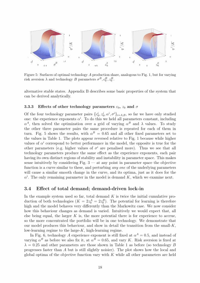
Figure 5: Surfaces of optimal technology A production share, analogous to Fig. 1, but for varyingrisk aversion λ and technology B parameters σB, cB0 , zB0 .

alternative stable states. Appendix B describes some basic properties of the system thatcan be derived analytically.

3.3.3 Effects of other technology parameters c0, z0 and σ

Of the four technology parameter pairs {ci0, zi0, αi, σi}i=A,B, so far we have only studiedone: the experience exponents αi. To do this we held all parameters constant, includingαA, then solved the optimization over a grid of varying αB and λ values. To studythe other three parameter pairs the same procedure is repeated for each of them inturn. Fig. 5 shows the results, with αB = 0.65 and all other fixed parameters set tothe values in Table 1. The plots appear reversed relative to Fig. 1 because while highervalues of αi correspond to better performance in the model, the opposite is true for theother parameters (e.g. higher values of σi are penalised more). Thus we see that alltechnology parameters produce the same effect as the experience exponents, each pairhaving its own distinct regions of stability and instability in parameter space. This makessense intuitively by considering Fig. 3 — at any point in parameter space the objectivefunction is a curve similar to these, and perturbing any one of the underlying parameterswill cause a similar smooth change in the curve, and its optima, just as it does for theαi. The only remaining parameter in the model is demand K, which we examine next.

3.4 Effect of total demand; demand-driven lock-in

In the example system used so far, total demand K is twice the initial cumulative pro-duction of both technologies (K = 2zA0 = 2zB0 ). The potential for learning is thereforehigh and the model behaves very differently than the Markowitz case. We now considerhow this behaviour changes as demand is varied. Intuitively we would expect that, allelse being equal, the larger K is, the more potential there is for experience to accrue,so the more concentrated the portfolio will be in one technology. We demonstrate thatour model produces this behaviour, and show in detail the transition from the small-K,low-learning regime to the large-K, high-learning regime.

In Fig. 6, technology A experience exponent is still fixed at αA = 0.5, and instead ofvarying αB as before we also fix it, at αB = 0.65, and vary K. Risk aversion is fixed atλ = 0.25 and other parameters are those shown in Table 1 as before (so technology Bprogresses faster than A but is still slightly noisier). The plot shows how the local andglobal optima of the objective function vary with K while all other parameters are held

18

0 2 4 6 8 10 12Total production K

0.0

0.2

0.4

0.6

0.8

1.0Te

chA

prod

uctio

nsh

areqA

/K

Optimization boundsInterior local minimumInterior local maximumGlobal minimumMarkowitz approximation minimum

Figure 6: Plot showing how optima of the objective function vary with total production K. Theminimum of the Markowitz approximation to f (Eq. 14) is also shown for comparison. AsK goesfrom approximately 0 to 1 the system transitions from a Markowitz-like, low-learning regimeto a technology-like, learning regime. When demand is small (approximately K < 4) the morecertain, slower progressing technology A (αA = 0.5) dominates the portfolio, but when demandis high there is enough scope for progress to occur that the noisier, faster progressing technologyB (αB = 0.65) becomes optimal. The transition between these states is instantaneous as theglobal optimum switches between different local minima of equal objective value. Risk aversionis fixed at λ = 0.25 and other parameter values are those shown in Table 1 as before.

constant — it is the analogue of Fig. 4, but with K as the independent variable. As wellas the maximum and minima of f , the plot also shows the minimum of the Markowitzapproximation to f for comparison.

Again we observe instantaneous switching between portfolio states as demand varies.As K goes from approximately 0 to 1 the share of technology A in the optimal portfolio(dashed black line) initially decreases sharply then reverses direction and increases again,due to the increased potential for learning. Here the technologies transition from behavingin a more “asset-like” way to a more “technology-like” way, as more higher order terms inthe series expansion of f start to have an impact (see Eq. (15)). Indeed, for very smallK, the minimum of f and the minimum of the Markowitz approximation to f roughlycoincide (i.e. the black and yellow dashed lines), and the solution for technologies isalmost the same as for financial assets. But as K increases the two curves diverge due tothe increasing impact of the nonlinearities in f , eventually resulting in the appearance ofa second minimum when K is just over 3.

When K is between approximately 1 and 4, despite technology B having a largerexperience exponent, demand is still too low for it to make enough progress along itsexperience curve to outweigh its higher variability, so technology A dominates. But as Kincreases a threshold is crossed (K ≈ 4), and production suddenly switches to B. Thuswe observe a demand-driven unlocking of technological lock-in, in the sense that if only asmall amount of future demand is considered then it is optimal to continue investing inthe slower progressing, less uncertain technology, but if market size is large enough thenit is optimal to switch to the noisier, faster progressing technology now.

19

0.0 0.2 0.4 0.6 0.8 1.0Tech A production share qA/K

9.6

9.8

10.0

10.2

f(q

A,ρ)

ρ = −0.1

ρ = 0.0

ρ = 0.1

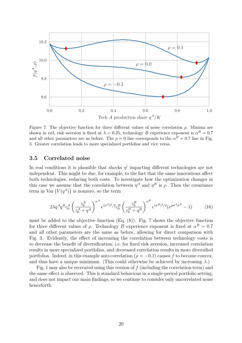
Figure 7: The objective function for three different values of noise correlation ρ. Minima areshown in red, risk aversion is fixed at λ = 0.25, technology B experience exponent is αB = 0.7and all other parameters are as before. The ρ = 0 line corresponds to the αB = 0.7 line in Fig.3. Greater correlation leads to more specialized portfolios and vice versa.

3.5 Correlated noise

In real conditions it is plausible that shocks ηi impacting different technologies are notindependent. This might be due, for example, to the fact that the same innovations affectboth technologies, reducing both costs. To investigate how the optimization changes inthis case we assume that the correlation between ηA and ηB is ρ. Then the covarianceterm in Var

(V (qA)

)is nonzero, so the term

2λqAqBcA0

(zA0

zA0 + qA

)αA

e(σA)2/2cB0

(zB0

zB0 + qB

)αB

e(σB)2/2(eρσ

AσB − 1) (16)

must be added to the objective function (Eq. (8)). Fig. 7 shows the objective functionfor three different values of ρ. Technology B experience exponent is fixed at αB = 0.7and all other parameters are the same as before, allowing for direct comparison withFig. 3. Evidently, the effect of increasing the correlation between technology costs isto decrease the benefit of diversification; i.e. for fixed risk aversion, increased correlationresults in more specialized portfolios, and decreased correlation results in more diversifiedportfolios. Indeed, in this example anti-correlation (ρ = −0.1) causes f to become convex,and thus have a unique minimum. (This could otherwise be achieved by increasing λ.)

Fig. 1 may also be recreated using this version of f (including the correlation term) andthe same effect is observed. This is standard behaviour in a single-period portfolio setting,and does not impact our main findings, so we continue to consider only uncorrelated noisehenceforth.

20

4 The efficient frontierTechnology portfolios can also be viewed in the efficient frontier framework. This tech-nique is well-known in portfolio theory, and involves plotting each portfolio as a pointin expected-return/variance space. We first describe the approach for the restrictedMarkowitz problem introduced earlier, then show how it applies for technologies (thoughnote that we only consider the no risk-free asset case.)

4.1 Financial assets

In the Markowitz system defined above (Eq. (10)) there are two assets, with known returndistributions. The portfolio weight of asset A, qA, is the single free control variable.Each qA ∈ [0, 1] describes a unique portfolio and as qA varies from 0 to 1 all feasibleportfolios are spanned. For a given value of risk aversion only one of these portfolios isoptimal. Each portfolio has a return distribution V (qA), the expectation and varianceof which may be used to plot a single point in expectation-variance space representingthe portfolio. This gives the well-known Markowitz diagram: the x-axis is the portfoliovariance, Var

(V (qA)

), and the y-axis is the expected return, E

[V (qA)

]. The feasible set

of portfolios is the curve traced out on these axes as qA varies from 0 to 1. Fig. 8 showsthe feasible set for two assets with fixed parameters µA = 0.5, µB = 0.65, sA = 1.0 andsB = 1.1 (cf. Section 3.2). This horizontal parabola is known as the Markowitz bullet.The colour scheme is the same as before (cf. Fig. 2) so dark red corresponds to 100%asset A and dark blue to 100% asset B.

From the definition of f (Eq. (10)) we have E [V ] = f(V ) + λVar (V ), so on theseaxes the isolines of f (i.e. level sets of f), for any fixed value of risk aversion, are justthe straight lines of gradient λ. The value of f for each portfolio lying on a given isoline(i.e. the points of intersection with the feasible set) is given by the y-axis intercept. Thensince we want to maximise f in this problem, the optimal portfolio for this λ is theunique point of intersection of the feasible set and the isoline of gradient λ with highesty-axis intercept. The efficient frontier is defined as the set of all portfolios which areoptimal for some value of λ. Therefore, since λ ∈ [0,∞), the efficient frontier here isthe segment of the feasible set furthest into the upper-left-most quadrant of the diagram.These elements are all shown on Fig. 8.

4.2 Technologies

In contrast to the Markowitz model, in the technologies model we want to minimize boththe variance and the expected cost, so the sign of the variance part of the objectivefunction is reversed. The isolines of f are therefore now the downward -sloping straightlines, of gradient −λ ∈ (−∞, 0]. And since lower f is now better, an optimal portfoliois a point of intersection of the feasible set with the isoline of lowest y-axis intercept.The efficient frontier therefore consists of the part of the feasible set furthest into thelower-left-most quadrant of the diagram. We demonstrate these differences between theMarkowitz and technology models by first plotting the expectation-variance diagram fortwo technologies in a low-learning regime, and then for the same two technologies in ahigh-learning regime. These are shown in Figs. 9 and 10, and are analogous to Fig. 8.

In Fig. 9, technology B has experience exponent αB = 0.65 and other parametersare those shown in Table 1 as before, except for demand, which is set to K = 0.1. By

21

Figure 8: The feasible set of portfolios for the Markowitz system Eq. (10), with µA = 0.5,µB = 0.65, sA = 1.0 and sB = 1.1. This is the path of portfolios traced out as the proportionof asset A in the portfolio varies from 0% (dark blue, qA = 0) to 100% (dark red, qA = 1). Todemonstrate how risk aversion and optimality are related geometrically, an isoline of f for riskaversion λ = 0.25 is plotted. The black dot at the point of tangency with the feasible set is theunique optimal portfolio for this λ. The two other black dots represent the two full specializationportfolios.

22

Figure 9: The feasible set of portfolios for two technologies in a low-learning regime. This isthe path of portfolios traced out as the proportion of technology A production in the portfoliovaries from 0% (dark blue, qA = 0) to 100% (dark red, qA = K). The technologies here haveαA = 0.5, αB = 0.65, and other parameters are those shown in Table 1, except demand, whichis set to K = 0.1. This severely limits the potential for learning, so the problem is nearly-Markowitz and hence the feasible set is almost parabolic. Isolines of f now slope downward andthe efficient frontier is the lower-left-most portion of the feasible set. An isoline correspondingto risk aversion λ = 0.25 is plotted. The black dot at the point of tangency with the feasible setis the unique optimal portfolio for this λ.

23

Figure 10: The feasible set of portfolios for technologies analogous to Fig. 9, but with demandnow set at the higher value K = 2. The technologies are no longer in a low-learning regime,and nonlinear feedback causes the feasible set to be stretched and tilted. Isolines for four valuesof risk aversion are plotted, showing how the transformed geometry of the feasible set causesthe efficient frontier to now consist of two disconnected components. There is a critical valueof risk aversion (0.02 < λswitch < 0.1) at which two optimal portfolios exist simultaneously(100% tech A and 100% tech B). This is how instantaneous optimum switching is manifestedin expectation-variance space.

24

restricting production in this way, learning effects are very small, so we are in a nearly-Markowitz regime, and hence the feasible set is almost parabolic. The figure makes clearhow the efficient frontier and isolines differ in the technologies problem, as compared tothe Markowitz problem (Fig. 8). In Fig. 10 all parameters are identical to Fig. 9, exceptdemand, which is now returned to the value in Table 1, K = 2, so that the technologiesare no longer in a low-learning regime.

As these plots show, there are two significant differences between how technologiesand financial assets appear in this framework. First, for technologies the feasible set istilted and stretched. This is because the objective function is highly nonlinear in portfolioweights, not just quadratic. Second, as a direct consequence of this, the efficient frontiermay now be split into two disconnected components. This is the case in Fig. 10, wherethe efficient frontier consists of both the long red segment on the left (mainly technologyA) and the isolated end-point on the right (100% technology B). This splitting of theefficient frontier is how instantaneous optimum switching is manifested in expectation-variance space: as risk aversion goes from λ = 0 to ∞ the optimal portfolio traverses theefficient frontier from one end to the other, jumping from one component to the other atthe critical value λ = λswitch. At the point of the discontinuity f has two distinct minimaof equal value, and there are two optimal portfolios, both of which lie on the same isoline,of gradient −λswitch. In this case these are the 100% A and 100% B portfolios.

Note that since αB = 0.65 in Fig. 10, the efficient frontier shown corresponds to theαB = 0.65 section through the surface in Fig. 1. Hence the change in the optimal portfolioas risk aversion varies can be traced out equivalently on both diagrams. The closed-formexpression for λswitch is given in Appendix B.2.

Viewing the problem in the expectation-variance framework shows how optimal tech-nology portfolios of equal value can coexist simultaneously (unlike in financial portfolios).Similar value portfolios may have either large expectation and small variance, or viceversa, or some combination in between. And since the feasible set is no longer parabolic(due to Wright’s law nonlinearities), there may be many very different portfolios lyingnear the optimal isoline. For example, in Fig. 10 all portfolios with around 60-90% tech-nology A (red) lie very near to the optimal λ = 0.25 isoline, because the feasible set hasvery low curvature here.

This is suggestive of the behaviour we would expect to see in a multi-technology model.The increasing returns dynamic allows many different ways of generating portfolios ofsimilar value, using different combinations of the various technologies’ expectations andvariances. This would result in a highly non-convex optimization problem with manylocal minima.

4.3 Effect of demand on the efficient frontier

Fig. 11 shows in more detail the effect of total demand on the feasible set and optimalportfolios. The technologies are fixed, and are the same as in Figs. 9 and 10. K is theonly parameter which varies. Although the scales on the axes differ in each plot, the ratiobetween them is constant. Indeed, the dashed lines all have gradient λ = −0.25; they arethe isolines corresponding to the optimal portfolio for λ = 0.25 in each case.

When K is tiny there is very little potential for learning so the technologies behavein an “asset-like” way, and the feasible set is almost a parabolic Markowitz bullet. Heretechnology A (red) dominates the optimal portfolio for all values of risk aversion. As Kincreases the potential for learning increases, so the nonlinearities in f start to have an

25

Figure 11: Feasible portfolios for αA = 0.5, αB = 0.65 and varying K, with other parametersfixed as before (Table 1). Again, dark blue corresponds to 0% technology A (qA = 0) and darkred to 100% (qA = K). The dashed lines are λ = 0.25 isolines of f , and the black dots are theoptimal portfolio for this risk aversion. The axes scales have been omitted for clarity (they aredifferent for each plot). These plots show how the problem transitions from a Markowitz-like,low-learning regime when K is small, to a highly nonlinear high-learning regime when K is large.

26

impact and the feasible set starts to become distorted. At around K = 1 the blue armdrops below the red arm, splitting the efficient frontier in two and indicating the presenceof two equal value portfolios for the first time. Here, for λ ≤ λswitch 100% technologyB (blue) is optimal, but for λ ≥ λswitch technology A (red) is dominant. At aroundK = 4 the two arms cross and large portions of the feasible set are very close to theλ = 0.25 isoline. Hence there are many different nearly-optimal portfolios in this case.After this point the two arms of the feasible set cross over completely so that technologyB is dominant for all values of risk aversion. As K gets very large (> 10) the potential forlearning is so great that near full specialization in the fastest-learning technology (B) isoptimal for all levels of risk aversion. Fig. 11 may be related back to Fig. 6 (though notethat distance increments along the feasible set do not correspond linearly to incrementsin qA/K).

Clearly this analysis relies on the assumption that noise is independent of total pro-duction K, so that more production, and hence learning, can take place without affectingthe size of the shocks.

5 Asymmetrical technologies and escaping lock-inThe paper so far has focused on the case of two almost symmetrical technologies, studyingthe behaviour of the optimal portfolio as one parameter is changed, while all others areheld constant. We now consider a more realistic and interesting example in which anestablished technology is challenged by a newcomer15. Suppose the setting is one where acheap, mature, slow-learning technology A is challenged by a costly, young, fast-learningtechnology B. Table 2 shows the parameter values used here.

Symbol Description Tech A Tech Bz0 Technology maturity 100 1c0 Initial cost 1 2α Experience exponent 0.15 0.2σ Technology volatility 0.1 0.1K Demand [0-100]λ Risk aversion [0-1.2]

Table 2: Parameter values for the case where a young expensive technology competes with anold cheap technology.

15The limiting case of this is when one technology is a ‘safe’ technology, with constant cost (αA =σA = 0). Then, in the nearly-Markowitz regime (K � zB0 ), the objective function reduces to

f ≈ cA0(K − qB

)+ cB0 e

(σB)2/2qB + λ(cB0)2e(σ

B)2(e(σ

B)2 − 1)(qB)2 (17)

(cf. Eq. (14)). This is a convex parabola with minimum

qB∗ =cA0 − cB0 e(σ

B)2/2

2λ(cB0)2e(σB)2

(e(σB)2 − 1

) , (18)

and the condition for the optimal solution to be diversified between the safe and the new technologyis 0 < qB∗ < K. This is analogous to the Markowitz portfolio problem with a safe asset and a riskyasset. Outside of this low-learning regime though, the safe technology simplification does not result inincreased analytical tractability, so the numerical solution approach is still applicable.

27

Figure 12: Optimal share of production of incumbent technology A (red) when in competitionwith challenger technology B (blue), for varying demand K and risk aversion λ. Parametervalues are shown in Table 2. Technology A has such a strong initial cost advantage that whendemand is low (and hence the potential for learning is low), it is optimal to specialize fully inA, for all values of risk aversion shown. As demand increases, so does the potential for learning,and in order exploit the faster-learning challenger the global optimum switches to a new localminimum, in which technology B dominates.

Repeating the demand-driven lock-in analysis of Section 3.4, Fig. 12 shows the op-timal portfolio surface over total demand and risk aversion axes. Technology A’s initialcost advantage is so strong that a demand of at least 20 times the initial cumulativeproduction of technology B is required to prevent full specialization in A, even for highrisk aversion. We observe the familiar optimum switching as demand increases, demon-strating again how important the role of anticipated future demand is in determiningthe optimal production mix. In this case, the K-λ parameter space separates into threequalitatively different regimes: i) for low K 100% technology A is optimal, ii) for highK but low risk aversion 100% technology B is optimal, and iii) for high K and at leastmoderate risk aversion, the optimal proportion of technology A is around 0-40%. Resultslike this could be very useful in applications, where often the key challenge is simplyreducing the dimension of the decision space.

For large K there is a qualitative change in the surface at λ ≈ 0.4. Here the globaloptimum of the objective function moves from the boundary to the interior of the opti-mization range (the value of λ at which this transition occurs may be found analyticallyas shown in Appendix B.1). This is similar to the situation in Fig. 3, where as αB in-creases from 0.71 to 0.72 up to, say 0.9 (not shown), the global minimum moves towardsthe boundary, then sticks on it (and in fact the function minimum over R continues tomove further outside the optimization range, but this is not a valid solution).

28

For comparison, Appendix C shows the same demand-risk surface for the case of thetwo almost identical technologies of Section 3.

To summarise the behaviour of the model, note the direction in which each of theparameters would need to move in order to escape lock-in to an incumbent technology.All things being equal, avoiding lock-in to technology A would require: decreased B ma-turity, decreased B initial cost, increased B experience exponent, decreased B volatility,increased demand K, or increased risk aversion λ.

6 Two-period modelHaving analysed the model in the simplest, single-period case, we now consider the ex-tension to two periods. This allows us to introduce discounting and investigate its effecton optimal production timing. This is especially relevant for experience curves since theyexemplify the concept of investing effort now to unlock future benefits, so the relativevalue of present and future benefits is critical. Moving to a multi-period setting allows usto investigate the conditions under which we should plan to invest in a technology now,or in future (or neither), given current knowledge about the present state of technologiesand their likely development under various investment scenarios. We briefly discuss somefeatures and limitations of our approach.

The extension we consider is static, in the sense that the model schedules productionnow, for all future periods, in the optimal manner as defined by the objective function.This static analysis relies on current estimates of technology parameters, which are inturn based on empirical data about the technologies in question. But as time progresseswe observe realisations of the noise, thereby gaining new information about technologycosts and parameters. Therefore performing the same optimization procedure in futuremay yield different results, and we are faced with the possibility of time-inconsistency.This is a limitation of the static model16. In support of the static approach however, notethat portfolio adjustment costs could be very high for technologies, which may result inhigh levels of commitment for future periods anyway.

In this model, technological progress only occurs via the stochastic experience curvemechanism, there is no exogenous progress trend. This is due to our choice of zero meannoise, η ∼ N (0, σ2), which we use because it is close to the model tested empirically byLafond et al. (2018). By using normal noise with nonzero mean instead it is possible tomodel an exogenous progress trend. For η ∼ N (µ, σ2), the standard lognormal distribu-tion has expectation eµ+σ2/2, so if µ < −σ2/2 then the expected cost of a technology canin fact decrease between periods under zero production (cf. Eq. (4)). This is especiallyimportant in the multi-period setting (although it also applies in the single-period case).If a technology is initially very expensive, and µ is very negative, then waiting for thetechnology to improve may indeed be a viable strategy. However, while waiting for thisimprovement in the expectation, the cost variance may become less favourable (relativeto that of the other technology), counteracting any benefit in the objective function.

16The dynamic mean-variance portfolio problem is difficult even in the case of standard financialreturns, see e.g. Gârleanu & Pedersen (2013). In our case the complexities are increased by the nonlin-earities and time dependencies in costs. One way to approach the problem would be to discretize thedecision space and the random event space, then apply backward induction to the resulting “scenariotree”. See, e.g., Edirisinghe & Patterson (2007) for an application of this method to the standard mean-variance portfolio problem. However, even for rough discretization the resulting tree would grow veryquickly. Hence, we do not pursue this analysis here, but leave it for future research.

29

Generally, increasing experience in one technology comes at the expense of the other,and if it is optimal to “delay production” in one technology then this is due only to thecomplex interplay of all model parameters in the objective function, not because of somesimple background improvement in a technology. Here though we continue to use zeromean noise.

For simplicity, as in the one-period case, we use technology production, not invest-ment, as a proxy for experience. In the single period case the distinction is not significant,but when considering multiple periods it is, due to capital depreciation. Thus our multi-period framework does not model investment strategies, only production strategies. Aproper treatment of investment would need to model the relationship between productionand investment, which would require at least one extra parameter to represent deprecia-tion. We prefer not to complicate the model further, and instead just consider production,while highlighting this discrepancy.

6.1 Optimization

We use the same first-difference Wright’s law model as before (Eq. (2)), with subscriptsnow denoting distinct periods, and separate noise shocks impacting each period:

log(cit)− log(cit−1) = −αi[

log(zit)− log(zit−1)]

+ ηit , i = A,B, t = 1, 2. (19)

Production of each technology accumulates in the obvious way: zit = zi0 +∑t

k=1 qik.

We retain the assumption that each technology has its own specific noise distribution,ηi ∼ N (0, (σi)2), and now assume that in each period there is a new draw from thisdistribution, ηit. For simplicity we assume shocks are uncorrelated over both time andtechnologies (though clearly correlated noise has the potential to play an important rolein a multi-period setting). Average unit costs in the second period are then given by:

ci2 = ci1

(z1z2

)αi

eηi2 = ci0

(z0z2

)αi

eηi1+η

i2 . (20)

This makes it clear how successive shocks impact cost in the two-period setting: fromperiod to period costs fall according to Wright’s law, but the periodic shocks accumulate,potentially driving the cost far from the deterministic experience curve trend. In contrastto standard experience curve implementations, this has the advantage that costs are notguaranteed to fall in the long run due to experience effects, and instead admits thepossibility that uncertain exogenous events may dominate.

While it is possible to allow any of the parameters to vary over the periods in thissetup (e.g. experience exponents, noise distributions), here we keep them all fixed, againfor simplicity and clarity. Total production is set to K per period, so there are now twoproduction constraints: qAt + qBt = K for t = 1, 2. The above choices are made becausethe model gets unwieldy very quickly, so it is preferable to use the simplest possibleformulation that captures the key features of interest.

We implement exponential discounting with discount rate r and consider the presentdiscounted cost of the total system:

V (qA1 , qA2 ) =

∑t=1,2

∑i=A,B

e−r(t−1)citqit. (21)

30

In contrast to the one-period total cost (Eq. (6)), this is now a function of productionin both periods. We use the same mean-variance objective function as before, details ofwhich are given in Appendix D17. The optimization problem is then

minimize:qA1 ,q

A2

f(qA1 , qA2 ) = E

[V (qA1 , q

A2 )]

+ λVar(V (qA1 , q

A2 ))

(22)

subject to: qA1 ∈ [0, K], qA2 ∈ [0, K].

6.2 Results

To show how discount rate r and risk aversion λ interact to influence optimal productionover the two periods we fix all other technology parameters and production constraints,then plot the objective function for a range of r-λ pairs. Since f is now a function of thetwo control variables, qA1 and qA2 , we plot its values as a contour-/heat-map over theseaxes.

Fig. 13 shows the results for nine pairs of low, medium and high discount rate andrisk aversion: r = 0.1, 1.0, 3.0, λ = 0.1, 0.5, 3.0.18 The two technologies used here arethe same as in the asymmetrical case of Section 5 (Table 2), and total production Kis set to 30 units per period, as this allows results to be related directly back to theone-period case in Fig. 12. (Production is shown here in units instead of percentages foreasier comparison.) Darker blue corresponds to lower values of f and darker red to highervalues, though the scale is different for each plot. The global minimum, again obtainedby brute force optimization, is shown as a black dot (though this sometimes forms partof a valley of nearly identical values).

6.3 Discussion

We observe the same kind of phenomena as in the one-period case: highly specializedsolutions for low risk aversion (due to deterministic learning feedback), greater diversi-fication for high risk aversion (due to the counteracting effects of variance terms in f),multiple optima of the objective function, and discontinuities in the global optimum asparameters vary.

First note that as the discount rate increases the two-period problem reduces to theone-period problem. Plots in the r = 3.0 column are nearly uniform in the qA2 direction,since second period costs are discounted so heavily that the choice of second periodproduction makes little difference to f . The global optima here correspond to the globaloptima shown at the relevant points on Fig. 12.

To observe the presence of multiple optima and instantaneous switching of the globalminimum, consider the two left-most plots of the top and middle rows of Fig. 13. In thetop row (λ = 0.1), the two plots are formed of concentric oval isolines, with a maximum off at their centres. All four corners are local minima, reflecting the fact that strong feed-back in the deterministic experience curve setting discourages any diversification at all.

17As mentioned earlier, the choice of objective function in a multi-period setting is more subtle andimportant than for a single period; we leave this consideration for future research.

18These values are picked for illustrative purposes only, in order to display various features clearly.However, to justify these discount rates, it is useful to think about the length of one period being about30-40 years. This could be motivated by long horizons in the energy sector; for instance, thermal powerplants are designed for a life of 30 to 40 years.

31

0 10 20 30

0

10

20

30

qA 2

r =0.1

λ =0.1

0 10 20 30

0

10

20

30

r =1.0

0 10 20 30

0

10

20

30

r =3.0

0 10 20 30

0

10

20

30

qA 2λ =0.5

0 10 20 30

0

10

20

30

0 10 20 30

0

10

20

30

0 10 20 30qA1

0

10

20

30

qA 2λ =3.0

0 10 20 30qA1

0

10

20

30

0 10 20 30qA1

0

10

20

30

Figure 13: Heat-maps showing the value of the two-period objective function for a range of riskaversion and discount values, as a function of first and second period production in technologyA (qA1 , qA2 ). Blue corresponds to lower values of f , red to higher values, and the global optimumis shown as a black dot. The technologies used here are the asymmetrical technologies of Section5: A is a cheaper, mature, incumbent technology and B is a young, fast-learning challenger.

32

As r goes from 0.1 to 1.0, the global optimum switches from (0, 0) to (30, 30) (similarly toFig. 3). This is because when second period costs are only weakly discounted, technologyB’s higher experience exponent has the potential to generate sufficiently low expectedsecond period cost that it is worth concentrating production in B in the first period,then reaping the rewards in the second. But when second period costs are moderatelydiscounted, this second period ‘reward’ has lower overall value in f , so it is not worthproducing any technology B at all in either period. (This is just standard deterministicexperience curve behaviour with discounting.)

In the middle row (λ = 0.5) we again observe optimum switching behaviour, butthe situation is more nuanced. f is now a saddle, with opposite corners forming distinctminima and maxima as the different expectation and variance components of f contributeand interact in complex ways. In comparison with the top row though, the central areasof these plots are generally less unattractive, since risk aversion allows more balancedportfolios. As r varies from 0.1 to 1.0, the global optimum switches from around (0, 23)to (30, 0). When discounting is very weak the optimal strategy is again to concentrateproduction in technology B initially in order to bring the cost down, but then to diversifyslightly in period two in order to lower the variance. When discounting is moderatethough, the expected cost reduction in technology B is not valuable enough to overridethe initial cost advantage of A, so first period production is concentrated in A. Thenhowever, production switches to being entirely concentrated in technology B in the secondperiod. This is likely due to the fact that the covariance term in f (see Eq. (52)) containsthe product qA1 qA2 , so there is a benefit to setting one of these terms equal to zero, and inthis particular case the effect is large enough to produce the bang-bang solution shown.However, since all 10 components of f (see Appendix D) are being traded off againsteach other in this moderate risk aversion/ moderate discounting regime, the relative sizeof any specific effect is not clear (without further analysis).

Finally, in the bottom row (λ = 3.0), risk aversion is strong and hence diversificationis optimal. Whole regions of the solution space generate identical or similar values of f .This is because, as in the one-period case, expected progress is being traded off againstthe certainty in this progress, and the same objective function value may be achieved bymany different combinations of first and second period production.

As in the one-period problem, due to the functional form of the objective function, theinstantaneous optimum-switching behaviour demonstrated here with the r and λ param-eters can also occur when any one of the underlying parameters is varied continuously.

6.4 Effects of discounting and risk aversion in scenario compari-son

While optimization over the entire solution space is essential for understanding the basicproperties of the model, there are situations in which this is either undesirable or impos-sible, and it is better simply to compare the performance of a restricted set of portfolios.We refer to this as scenario comparison (as this captures better the idea of comparingworlds characterised by different technology mixes). This can be useful either if thereare additional system constraints, or if the solution space is very large, for the followingreasons.

First, in practise technologies are not perfect substitutes, so although they may beconsidered substitutes in terms of some primary characteristic (i.e. “production”), other,secondary characteristics may require portfolios to be constrained in additional ways. For

33

0 1 2 3

Discount rate, r

35

40

45

50

55

60

65

f(q

A 1,q

A 2,r)

λ = 0.1

0 1 2 3

Discount rate, r

40

50

60

70

λ = 0.5

0 1 2 3

Discount rate, r

60

80

100

120

140

160

λ = 3.0

95% A both periods50-50 both periods95% B both periods

Figure 14: Plots showing how the objective function varies with the discount rate for eachof three different technology scenarios, in low, moderate and high risk aversion regimes. Thetechnologies are the same as in Fig. 13. For low and moderate risk aversion there is a criticaldiscount rate separating regimes in which different scenarios are preferred.

example, solutions that vary wildly from period to period may be impractical in manyreal world situations. Or as another example, consider a portfolio of energy technologieson an electric power grid. While they may be considered substitutes in terms of, say,total annual energy production, many other engineering and physical constraints mustbe met in order to ensure grid stability19. This would place extra restrictions on suchtechnology portfolios; these constraints could of course be modelled explicitly and a morecomplicated objective function constructed, but this is outside the scope (and spirit) ofthe work here.

Second, consider extending the model to include more technologies and/or periods.As the number of control variables increases, brute force optimization quickly becomescomputationally intractable, and since the problem is non-convex (due to the experiencecurve feedback), local optimization methods are not guaranteed to find the global opti-mum. It may therefore be necessary to use heuristic arguments to specify a restricted setof available portfolios, and compare these directly.

Now, since portfolios are fixed in the scenario comparison setting, this allows for analternative perspective on the effects of discounting and risk aversion. We demonstratethis with an example, using the same two-period model and asymmetrical technologiesas earlier in this section.

Suppose that due to extra system constraints, only three scenarios are available: 95%technology A in both periods, 50% technology A in both periods and 95% technology Bin both periods. Fig. 14 shows three different risk aversion regimes (λ = 0.1, 0.5, 3.0),and in each regime the objective function is shown as a function of discount rate, for eachscenario. This shows how the discount rate affects the preference ordering of the threeavailable scenarios in each risk aversion regime. These plots are readily related back toFig. 13 above.

When risk aversion is low the preferred scenario is 95% technology B in both peri-ods for mild discounting, but as discounting increases this becomes less advantageous,and there is a critical discount rate above which the preferred scenario becomes 95%technology A in both periods. When risk aversion is moderate, 50% A in both periods

19E.g. if large shares of intermittent renewable technologies are present then large quantities of energystorage or other backup technologies may also be required, depending on daily and seasonal demandpatterns.

34

is preferred for low discounting, all three scenarios are roughly equal when discountingis moderate, and 95% A in both periods is preferred when discounting is high. Whenrisk aversion is high a 50-50 mix of technologies in both periods is the preferred scenarioregardless of discount rate.

The same arguments and explanations given in Section 6.3 apply here. Clearly this isonly a stylized model, with limited scenarios, but the key point is that in some circum-stances a critical discount rate exists separating regimes in which different scenarios arepreferred. While this type of result is well known in deterministic situations, and seemstrivial in a low dimensional stochastic model such as this, in a multi-technology, multi-period setting this technique could provide essential insight into preference orderings ofdifferent technology scenarios.

7 ConclusionIn this paper we considered two technologies following stochastic experience curves andwe characterised the optimal investment (or production) strategies. We used an objectivefunction that accounts for total portfolio cost and uncertainty. The optimal investmentdepends on risk-aversion, initial conditions (relative technology maturity and initial cost),progress characteristics (mean progress rate and uncertainty of future shocks) and marketsize; and in the multi-period case also the discount rate.

In contrast to classical Markowitz portfolios, in our setting investment lowers marginalcost, creating a larger and larger incentive to continue investing in the same option. Butcontrary to the deterministic case, in which these self-reinforcing effects lead to completespecialization, we find that accounting for uncertainty and risk aversion promotes diver-sification even if one option has better intrinsic technological characteristics. Our resultstherefore show how the choice of specializing or diversifying depends on the underlyingparameters and initial conditions. Crucially, we find that the nonlinearity of the problemleads to multiple local optima, so that very different optimal portfolios can exist simulta-neously, and the global optimum switches instantaneously between them as parameterschange. This means that inside a critical region of parameter space a small change in oneof the parameters can lead to a very significant change in the optimal portfolio.

We established an analytical connection between portfolios of technologies and port-folios of financial assets. The Wright’s law model of endogenous technological changemay be expanded in a series approximation, the leading terms of which are equivalent tothose found in the Markowitz model for financial assets. Only the higher order nonlinearterms contribute towards the learning feedback, and hence the Markowitz model may beregarded as the no-learning limit of the technology portfolio model. We also showed thatthe strength of learning feedback in the model depends on the complete set of modelparameters, but in particular on technologies’ previous cumulative production and thelevel of total future demand. As a result, each technology may be viewed as existingsomewhere on a spectrum between more asset-like and more technology-like, dependingon the specific set of parameters present.

We also considered the two-period case and found that in a scenario comparisonsetting (i.e. when comparing a limited number of available portfolios, as would be typicalin higher-dimensional applications), the discount rate plays a critical role. For a givenlevel of risk aversion, the discount rate determines which of the available portfolios ispreferred.

35

These findings help establish a theoretical basis for understanding how technologiesbehave in a simple mean-variance framework, and give insight into how multiple optimacan arise in the context of uncertain endogenous technological change.

AcknowledgementsThis project was primarily supported by Partners for a New Economy. The projectalso received funding from the European Union’s Horizon 2020 research and innovationprogramme under grant agreement No. 730427 (COP21 RIPPLES), and from the Eu-ropean Research Council under the European Union’s Seventh Framework Programme(FP7/2007-2013)/ ERC grant agreement No. 611272 (GROWTHCOM). The authorsgratefully acknowledge all these sources of financial support, and additionally the Insti-tute for New Economic Thinking at the Oxford Martin School for its continuing support.We would also like to thank Cameron Hepburn, Alex Teytelboym, Torsten Heinrich,Jessika E. Trancik and Béla Nagy for helpful comments and discussions.

Appendix

A Series expansion approximation to fThe standard Maclaurin series expansion for (1 + x)α is

(1 + x)α =∞∑n=0

(α

n

)xn for |x| < 1 (23)

= 1 + αx+α(α− 1)

2!x2 +

α(α− 1)(α− 2)

3!x3 + . . . (24)

where(αn

)are the generalized binomial coefficients(

α

n

)=α(α− 1) . . . (α− n+ 1)

n!, α ∈ C. (25)

Setting x to qi/zi0 (with qi < zi0) and α to −αi gives(1 +

qi

zi0

)−αi

= 1− αi(qi

zi0

)+α(α + 1)

2

(qi

zi0

)2

− α(α + 1)(α + 2)

6

(qi

zi0

)3

+ . . . . (26)

Then from Eq. (12) we have

f =∑i=A,B

ci0qi

(1 +

qi

zi0

)−αi

e(σi)2/2 + λ(ci0q

i)2(

1 +qi

zi0

)−2αi

e(σi)2(e(σ

i)2 − 1),

and hence

f =∑i=A,B

ci0qi

(1− αi

(qi

zi0

)+α(α + 1)

2

(qi

zi0

)2

− . . .)e(σ

i)2/2 (27)

+ λ(ci0qi)2(

1− 2αi(qi

zi0

)+ . . .

)e(σ

i)2(e(σ

i)2 − 1).

36

Thus if qi is much smaller than zi0, then the approximation formed by discarding every-thing except the zero order terms in the series expansions will be reasonable. This givesthe lowest order approximation to f ,

f ≈∑i=A,B

ci0qie(σ

i)2/2 + λ(ci0q

i)2e(σ

i)2(e(σ

i)2 − 1), (28)

which has the same form as the Markowitz objective function, with ci0e(σi)2/2 playing

the role of expected return and (ci0)2e(σ

i)2(e(σ

i)2 − 1)

the role of the variance. Notethat although the series expansion Eq. (26) converges provided qi < zi0, and is itselfreasonably approximated by its zero order term (i.e. 1) provided qi � zi0, the lowestorder approximation to f (Eq. (28)) involves discarding the (qi)2

zi0term in the expectation

part of Eq. (27), so is reasonable only when (qi)2 � zi0. Thus the correct conditionfor the full optimization problem to be Markowitz-like is K2 � zi0 ∀i. Higher orderapproximations to f , and the corresponding conditions for validity, may be computedsimilarly. See e.g. Kraus & Litzenberger (1976) for further details on portfolio selectioninvolving preferences over skewness.

B Analytical points to accompany Section 3.3

B.1 Onset of diversification

For a given pair of technologies the risk neutral portfolio (λ = 0) always concentratesproduction entirely in one technology due to increasing returns, while for sufficiently largerisk aversion the portfolio is diversified over both technologies. The value of risk aversionat which the transition between these two regimes occurs (i.e. the onset of diversification)may be found analytically by calculating the intersection of corner and interior solutions.This is done by substituting the relevant boundary condition (qA = 0 or qA = K) in thefirst-order condition equation (f ′(qA) = 0), and solving for λ.

For example, consider what happens when αB ≈ 0.8 in Fig. 1. For low risk aversion theoptimal portfolio is 100% technology B, but as λ increases there is a value, λdiversification,at which technology A first enters the portfolio. Setting f ′(0) = 0 (with f given by Eq.(8)) and solving for λ gives

λdiversification(αB) =cA0 e

(σA)2/2 − cB0(

zB0zB0 +K

)αB

e(σB)2/2

(1− αBK

zB0 +K

)2K(cB0 )2

(zB0

zB0 +K

)2αB

e(σB)2(e(σB)2 − 1

) (1− αBK

zB0 +K

) (29)

=E[cA1 (0)

]− E

[cB1 (K)

] (1− αBK

zB0 +K

)2KVar (cB1 (K))

(1− αBK

zB0 +K

) . (30)

Inserting the parameter values from Table 1 in this expression and setting αB = 0.8yields the value λdiversification = 0.255, which is of course consistent with Fig. 1. Notethat this expression is independent of αA, and only has the interpretation given (onsetof diversification) in the specific region of parameter space stated — it does not in itselfdetermine whether qA = 0 is a global minimum in the first place; that must be verifiedseparately. There is an equivalent expression for the onset of diversification starting from

37

the 100% technology A portfolio, computed in precisely the same way. Having foundanalytical expressions for these two major features of the surface, this just leaves thesurface discontinuity itself, which we consider next.

B.2 Location of the discontinuity

Observe that in Fig. 3 the value of the global minimum varies continuously with αB.This follows from the smoothness of the objective function. In fact the global minimumvaries continuously with all the underlying parameters, in particular over the entire αB-λgrid of Fig. 1. Hence the value that f attains at the surface discontinuity in Fig. 1 isthe same when approached from both sides, so we have f(qA∗ ) = f(K − qA∗ ). This meansthat near the discontinuity, portfolios on either side of it are symmetric about a 50%production share. For example, in Figs. 3 and 4 the neighbouring portfolios either side ofthe discontinuity (i.e. the point at which the optimum switches) are seen to be symmetricabout 50%, at approximately 20% and 80% shares. Additionally, in the case where qA∗is known exactly (i.e. in the small-λ, full specialization region, where qA∗ = 0 or K), thisinsight allows the location of the discontinuity to be calculated analytically.

For example, consider what happens for fixed αB = 0.65. As risk aversion increasesfrom zero the optimal portfolio switches from 0 to 100% technology A. The critical valueat which this switch occurs, λswitch, is found by solving f(0) = f(K) for λ, which gives

λswitch =cA0

(zA0

zA0 +K

)αA

e(σA)2/2 − cB0

(zB0

zB0 +K

)αB

e(σB)2/2

K

[(cB0 )2

(zB0

zB0 +K

)2αB

e(σB)2(e(σB)2 − 1)− (cA0 )2(

zA0zA0 +K

)2αA

e(σA)2(e(σA)2 − 1)

]=

E[cA1 (K)

]− E

[cB1 (K)

]K [Var (cB1 (K))− Var (cA1 (K))]

. (31)

Again though, note that this expression only has the interpretation given (location ofthe discontinuity) in the specific region of parameter space stated — it does not in itselfdetermine whether qA = 0, K are global minima; this must be verified separately.

The same technique may also be used along the αB axis, to compute the value αBswitchat which the discontinuity occurs, for fixed λ. There is no elementary closed-form solutionfor this in general, though there is for the special case λ = 0: solving f(0) = f(K) forαB, with λ = 0, gives

αBswitch|λ=0 =log(cA0cB0

)+ 1

2

[(σA)2 − (σB)2

]+ αA log

(zA0

zA0 +K

)log(

zB0zB0 +K

) . (32)

Inserting the relevant parameters we find αBswitch|λ=0 = 0.596 in Fig. 1. For other valuesof λ the solution may be computed numerically. For example, fixing λ = 0.1 and solvingf(0) = f(K) for αB yields the value αBswitch = 0.681, which again matches Fig. 1.

C Demand-risk surface for similar technologiesIn order to provide some comparison with the case of the two asymmetrical technologies(Fig. 12), Fig. 15 shows the analogous surface for the two almost identical technologies of

38

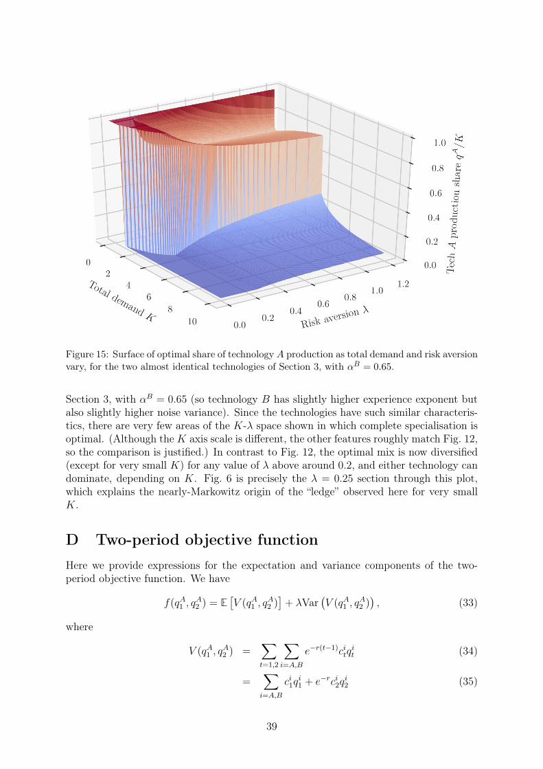
Figure 15: Surface of optimal share of technology A production as total demand and risk aversionvary, for the two almost identical technologies of Section 3, with αB = 0.65.

Section 3, with αB = 0.65 (so technology B has slightly higher experience exponent butalso slightly higher noise variance). Since the technologies have such similar characteris-tics, there are very few areas of the K-λ space shown in which complete specialisation isoptimal. (Although the K axis scale is different, the other features roughly match Fig. 12,so the comparison is justified.) In contrast to Fig. 12, the optimal mix is now diversified(except for very small K) for any value of λ above around 0.2, and either technology candominate, depending on K. Fig. 6 is precisely the λ = 0.25 section through this plot,which explains the nearly-Markowitz origin of the “ledge” observed here for very smallK.

D Two-period objective functionHere we provide expressions for the expectation and variance components of the two-period objective function. We have

f(qA1 , qA2 ) = E

[V (qA1 , q

A2 )]

+ λVar(V (qA1 , q

A2 )), (33)

where

V (qA1 , qA2 ) =

∑t=1,2

∑i=A,B

e−r(t−1)citqit (34)

=∑i=A,B

ci1qi1 + e−rci2q

i2 (35)

39

is the total system present discounted cost, and first and second period technology costsare given by

ci1 = ci0

(z0z1

)αi

eηi1 and ci2 = ci0

(z0z2

)αi

eηi1+η

i2 (36)

respectively. The noise shocks, ηA1 , ηA2 ∼ N (0, (σA)2) and ηB1 , ηB2 ∼ N (0, (σB)2), are allindependent. Now, in the one period problem independence of technologies means thereis no covariance term in Var (V ), but here, even though technologies are still independent,the second period cost of each technology depends on its own first period cost, so thereare nonzero covariance terms to consider. To simplify notation write

c̄it = ci0

(z0zt

)αi

(37)

so thatci1 = c̄i1e

ηi1 and ci2 = c̄i2eηi1+η

i2 . (38)

The following results are then required:

E[eη

i1

]= e(σ

i)2/2 (39)

E[eη

i1+η

i2

]= e(σ

i)2 (40)

Var(eη

i1

)= e(σ

i)2(e(σ

i)2 − 1)

(41)

Var(eη

i1+η

i2

)= e2(σ

i)2(e2(σ

i)2 − 1)

(42)

Cov(eη

i1 , eη

i1+η

i2

)= e3(σ

i)2/2(e(σ

i)2 − 1). (43)

The expectation component of f is thus given by

E [V ] = E

[ ∑i=A,B

ci1qi1 + e−rci2q

i2

](44)

=∑i=A,B

E[ci1q

i1

]+ E

[e−rci2q

i2

](45)

=∑i=A,B

E[c̄i1q

i1eηi1

]+ E

[e−rc̄i2q

i2eηi1+η

i2

](46)

=∑i=A,B

c̄i1qi1e

(σi)2/2 + e−rc̄i2qi2e

(σi)2 , (47)

40

and the variance component by

Var (V ) = Var

(∑i=A,B

ci1qi1 + e−rci2q

i2

)(48)

=∑i=A,B

Var(ci1q

i1 + e−rci2q

i2

)(49)

=∑i=A,B

Var(c̄i1q

i1eηi1 + e−rc̄i2q

i2eηi1+η

i2

)(50)

=∑i=A,B

(c̄i1q

i1

)2 Var(eηi1)+(e−rc̄i2q

i2

)2 Var(eηi1+ηi2)+ 2e−rc̄i1c̄

i2qi1qi2Cov

(eη

i1 , eη

i1+η

i2

)(51)

=∑i=A,B

(c̄i1q

i1

)2e(σ

i)2(e(σ

i)2 − 1)

+(e−rc̄i2q

i2

)2e2(σ

i)2(e2(σ

i)2 − 1)

+ 2e−rc̄i1c̄i2qi1qi2e

3(σi)2/2(e(σ

i)2 − 1). (52)

ReferencesAlberth, S. & Hope, C. (2007), ‘Climate modelling with endogenous technical change:Stochastic learning and optimal greenhouse gas abatement in the PAGE2002 model’,Energy Policy 35(3), 1795–1807.

Alchian, A. (1963), ‘Reliability of progress curves in airframe production’, Econometrica31(4), 679–693.

Almgren, R. & Chriss, N. (2001), ‘Optimal execution of portfolio transactions’, Journalof Risk 3, 5–40.

Arrow, K. J. (1962), ‘The economic implications of learning by doing’, The Review ofEconomic Studies pp. 155–173.

Arthur, W. B. (1989), ‘Competing technologies, increasing returns, and lock-in by his-torical events’, The Economic Journal pp. 116–131.

Atkinson, A. B. & Stiglitz, J. E. (1969), ‘A new view of technological change’, TheEconomic Journal 79(315), 573–578.

Barreto, L. & Kypreos, S. (2004), ‘Endogenizing R&D and market experience in the“bottom-up” energy-systems ERIS model’, Technovation 24(8), 615–629.

Boyle, P., Garlappi, L., Uppal, R. & Wang, T. (2012), ‘Keynes meets Markowitz: Thetrade-off between familiarity and diversification’, Management Science 58(2), 253–272.

Brueckner, J. K. & Raymon, N. (1983), ‘Optimal production with learning by doing’,Journal of Economic Dynamics and Control 6, 127–135.

Cabral, L. M. & Riordan, M. H. (1994), ‘The learning curve, market dominance, andpredatory pricing’, Econometrica: Journal of the Econometric Society pp. 1115–1140.

41

Cowan, R. (1991), ‘Tortoises and hares: choice among technologies of unknown merit’,The Economic Journal pp. 801–814.

Criqui, P., Mima, S., Menanteau, P. & Kitous, A. (2015), ‘Mitigation strategies andenergy technology learning: an assessment with the poles model’, Technological Fore-casting and Social Change 90, 119–136.

Dasgupta, P. & Stiglitz, J. (1988), ‘Learning-by-doing, market structure and industrialand trade policies’, Oxford Economic Papers pp. 246–268.

David, P. A. (1985), ‘Clio and the economics of QWERTY’, The American EconomicReview 75(2), 332–337.

Della Seta, M., Gryglewicz, S. & Kort, P. M. (2012), ‘Optimal investment in learning-curve technologies’, Journal of Economic Dynamics and Control 36(10), 1462–1476.

Dutton, J. M. & Thomas, A. (1984), ‘Treating progress functions as a managerial oppor-tunity’, Academy of Management Review 9(2), 235–247.

Edirisinghe, N. C. P. & Patterson, E. I. (2007), ‘Multi-period stochastic portfolio opti-mization: Block-separable decomposition’, Annals of Operations Research 152(1), 367–394.

Gârleanu, N. & Pedersen, L. H. (2013), ‘Dynamic trading with predictable returns andtransaction costs’, The Journal of Finance 68(6), 2309–2340.

Gritsevskyi, A. & Nakićenović, N. (2000), ‘Modeling uncertainty of induced technologicalchange’, Energy policy 28(13), 907–921.

He, H. & Mamaysky, H. (2005), ‘Dynamic trading policies with price impact’, Journal ofEconomic Dynamics and Control 29(5), 891–930.

Kraus, A. & Litzenberger, R. H. (1976), ‘Skewness Preference and the Valuation of RiskAssets’, Journal of Finance 31(4), 1085–1100.

Krey, V. & Riahi, K. (2013), Risk Hedging Strategies Under Energy System and ClimatePolicy Uncertainties, Springer US, Boston, MA, pp. 435–474.

Kroll, Y., Levy, H. & Markowitz, H. M. (1984), ‘Mean-variance versus direct utilitymaximization’, The Journal of Finance 39(1), 47–61.

Lafond, F., Bailey, A. G., Bakker, J. D., Rebois, D., Zadourian, R., McSharry, P. &Farmer, J. D. (2018), ‘How well do experience curves predict technological progress?a method for making distributional forecasts’, Technological Forecasting and SocialChange 128, 104–117.

Majd, S. & Pindyck, R. S. (1989), ‘The learning curve and optimal production underuncertainty’, The Rand Journal of Economics 20(3), 331–343.

Markowitz, H. (1952), ‘Portfolio selection’, The Journal of Finance 7(1), 77–91.

Mazzola, J. B. & McCardle, K. F. (1996), ‘A bayesian approach to managing learning-curve uncertainty’, Management Science 42(5), 680–692.

42

Mazzola, J. B. & McCardle, K. F. (1997), ‘The stochastic learning curve: Optimal produc-tion in the presence of learning-curve uncertainty’, Operations Research 45(3), 440–450.

McNerney, J., Farmer, J. D. & Trancik, J. E. (2011), ‘Historical costs of coal-fired elec-tricity and implications for the future’, Energy Policy 39(6), 3042–3054.

Nagy, B., Farmer, J. D., Bui, Q. M. & Trancik, J. E. (2013), ‘Statistical basis for pre-dicting technological progress’, PLOS ONE 8(2), e52669.

Newbold, P., Pfaffenzeller, S. & Rayner, A. (2005), ‘How well are long-run commodityprice series characterized by trend components?’, Journal of International Development17(4), 479–494.

Poston, T. & Stewart, I. (2014), Catastrophe theory and its applications, Courier Corpo-ration.

Pulley, L. B. (1981), ‘A general mean-variance approximation to expected utility for shortholding periods’, The Journal of Financial and Quantitative Analysis 16(3), 361–373.

Rosen, S. (1972), ‘Learning by experience as joint production’, The Quarterly Journal ofEconomics pp. 366–382.

Rosenberg, N. (1982), Inside the black box: technology and economics, Cambridge Uni-versity Press.

Spence, A. M. (1981), ‘The learning curve and competition’, The Bell Journal of Eco-nomics pp. 49–70.

Thompson, P. (2012), ‘The relationship between unit cost and cumulative quantity andthe evidence for organizational learning-by-doing’, The Journal of Economic Perspec-tives 26(3), 203–224.

Van den Bergh, J. C. (2008), ‘Optimal diversity: increasing returns versus recombinantinnovation’, Journal of Economic Behavior & Organization 68(3), 565–580.

Van Nieuwerburgh, S. & Veldkamp, L. (2010), ‘Information acquisition and under-diversification’, The Review of Economic Studies 77(2), 779–805.

Wagner, F. (2014), Optimal investment strategy for competing learning technologies: Ananalytical approach, in ‘Renewables in Future Power Systems’, Springer, pp. 75–129.

Webster, M., Fisher-Vanden, K., Popp, D. & Santen, N. (2015), Should we give up afterSolyndra? Optimal technology R&D portfolios under uncertainty, Technical report,National Bureau of Economic Research.

Wright, T. P. (1936), ‘Factors affecting the cost of airplanes’, Journal of the AeronauticalSciences 3(4), 122–128.

Zeeman, E. (1976), ‘Catastrophe theory’, Scientific American 234, 65–83.

Zeppini, P. (2015), ‘A discrete choice model of transitions to sustainable technologies’,Journal of Economic Behavior & Organization 112, 187–203.

Zeppini, P. & Van den Bergh, J. C. (2013), ‘Optimal diversity in investments with re-combinant innovation’, Structural Change and Economic Dynamics 24, 141–156.

43