��� ���� �� �� ����� �� ������������� ����� �������� �������� ��� !��"������

#������ $%%��

&������ %�%�� �'((

)����*�� +������ ,���%

�� �� &����� -����"���

��"����� .(((

!�� ������� %�%�� %�"����� �� �� ���� ��%������ �����/ %������ �%����� ��� �� �� ��������� ������ �� ����� �� &����� -����"���0

Deutsche Bundesbank, Wilhelm-Epstein-Strasse 14, 60431 Frankfurt am Main,

P.O.B. 10 06 02, 60006 Frankfurt am Main, Federal Republic of Germany

Telephone (0 69) 95 66-1

Telex within Germany 4 1 227, telex from abroad 4 14 431, fax (0 69) 5 60 10 71

Internet: http://www.bundesbank.de

Please address all orders in writing to: Deutsche Bundesbank,

Press and Public Relations Division, at the above address, or by fax No. (0 69) 95 66-30 77

Reproduction permitted only if source is stated.

ISBN 3–933747–36–8

�������

The turbulences in the international financial markets during the summer and autumn of

1998 put the price formation and liquidity provision mechanism in many markets under

severe strain. As part of the large-scale portfolio rebalancing that took place, investors

shifted a large part of their holdings into cash and into instruments that were perceived as

having a low risk and being highly liquid. One of these "safe havens" was the market for

German government securities. The paper examines the liquidity of the secondary market

for four German benchmark government bonds during this period. The analysis is based on

a unique dataset provided by the German securities’ regulator, which covers every single

transaction of the four bonds in Germany. This feature is particularly attractive for the bond

market, where OTC transactions account for most trading.

The volatility of yields of the four bonds more than doubled in the wake of the Russian

devaluation on August 17th, 1998, and experienced a further peak in early October. It was

accompanied by a widening in the yield spread between the individual bonds, which soared

to more than twenty basis points from less than five basis points during the first half of the

year. The cost of trading, as measured by the effective spread, increased even in a "safe

haven" like the market for ten year German government bonds, indicating a reduction in

liquidity. Nevertheless, the market was able to handle a statistically significantly higher

than usual number of transactions and turnover. In this sense, liquidity provision has been

remarkably effective in dealing with the turbulences.

Effective bid-ask spreads are positively related to unexpected trading volume, which

should reflect the amount of private information in the market. Nevertheless, surprises

volume cannot explain the surge in spreads that occurred during the turbulences.

'��&&�������

Die Turbulenzen auf den internationalen Finanzmärkten im Sommer und Herbst 1998

führten zu wesentlichen Beeinträchtigungen bei der Preisbildung und zu

Liquiditätsengpässen auf mehreren Wertpapiermärkten. Im Rahmen umfangreicher

Vermögensumschichtungen wurde ein wesentlicher Teil des Anlagevermögens entweder

als Barreserve gehalten oder in solchen Wertpapieren investiert, die als besonders

risikoarm und hochliquide angesehen wurden. Einer dieser „sicheren Häfen” war der Markt

für Bundeswertpapiere. Die vorliegende Arbeit analysiert die Liquidität des Marktes für

vier zehnjährige Bundesanleihen während dieses Zeitraums. Sie basiert auf einem bisher

nicht ausgewerteten Datensatz des Bundesamts für den Wertpapierhandel, der jede einzelne

Transaktion dieser vier Anleihen in Deutschland umfasst. Dies ist besonders für Arbeiten

über den Rentenmarkt von großem Interesse, auf dem außerbörsliche Transaktionen einen

Großteil des Handelsvolumens ausmachen.

Die Renditevolatilität der vier Anleihen stieg nach der russischen Abwertung am

17. August 1998 zunächst auf mehr als das Doppelte an und erreichte Anfang Oktober

weitere Höchstwerte. Gleichzeitig weitete sich der Renditeabstand zwischen den einzelnen

Papieren von weniger als fünf Basispunkten im ersten Halbjahr auf mehr als zwanzig

Basispunke aus. Die Handelskosten – gemessen an der effektiven Geld-Brief-Spanne –

stiegen auch in einem „sicheren Hafen” wie der Markt für Bundesanleihen an, was auf eine

Reduzierung der Marktliquidität hindeutet. Trotzdem war der Markt in der Lage, ein

statistisch signifikant höhere Anzahl von Transaktionen und Volumina zu handeln. In

diesem Sinne war die Bereitstellung von Marktliquidität während der Turbulenzen

außergewöhnlich effektiv.

Das Verhältnis zwischen der effektiven Geld-Brief-Spanne und dem unerwarteten

Handelsvolumen ist positiv und statistisch signifikant, was auf die Existenz von

nichtöffentlichen Informationen hindeutet. Den Anstieg der Geld-Briefspannnen während

der Turbulenzen kann allerdings nicht durch überraschend hohe Umsätze erklärt werden.

!�"������#����

1. Introduction 1

2. The 1998 Turbulences in International Financial Markets 5

3. Liquidity Measurement 6

3.1. The four dimensions of market liquidity 6

3.2. Measures for market liquidity 8

4. The Market for German Government Bonds 10

5. Data 11

5.1. Description 11

5.2. Intra-day patterns of trading activity 17

5.3. Construction of equally-spaced time series 19

6. Yields of Bunds in 1998 20

7. Market Liquidity in 1998 23

7.1. Activity indicators 24

7.2. Effective spreads 26

7.3. Did banks destabilise the market? 31

8. Conclusions 32

9. References 35

�����������������!�"��

������

Figure 1: Dimensions of Market Liquidity 7

Figure 2(a): Distribution of Trade Size (all trades) 14

Figure 2(b): Distribution of Trade Size (client and inter-dealer trades) 15

Figure 3: End-of-day Inventories 16

Figure 4(a): Intra-day Distribution of Number of Trades 17

Figure 4(b): Intra-day Distribution of Trading Volume 18

Figure 4(c): Intra-day Distribution of Average Trade Size 18

Figure 5: Construction of an Equally Spaced Time Series 19

Figure 6: Yields to Maturity 20

Figure 7: Intra-day Volatility of Yields 23

Figure 8: Daily Number of Trades 24

Figure 9: Daily Turnover 25

Figure 10: Effective Spreads (Roll measure) 28

Figure 11: Unexpected Volume and Effective Spreads 31

!�"��

Table 1: The 1998 Financial Market Turbulences 5

Table 2: Summary Statistics 13

Table 3: Correlation of Yields 22

Table 4: Trading Activity During the 1998 Turbulences 26

Table 5: Effective Bid-Ask Spreads 27

Table 6: Daily Effective Spreads During the 1998 Turbulences 29

Table 7: Effective Spreads and Trading Volume 30

Table 8: Changes in Inventories and Prices 32

- 1 -

����������������������� ������������������������������������������ �!��"������

�(�)���������

The turbulences in the international financial markets during the summer and autumn of

1998 put the price formation and liquidity provision mechanism in many markets under

severe strain. Both the International Monetary Fund and the Bank for International

Settlements1 cite anecdotal evidence that "market liquidity dried up temporarily even in the

deepest and most liquid markets as risks were repriced and positions deleveraged"(IMF

[1998]). As part of the large-scale portfolio rebalancing that took place, investors shifted a

large part of their holdings into cash and into instruments that were perceived as having a

low risk and being highly liquid. One of these "safe havens" was the market for German

government securities. The purchases of German debt securities by non-residents, which

had averaged some of 11.4 billion DM per month during the first half of 1998, soared to

34.5 billion DM in July and remained close to this level in August. Most of this increase

went into bonds issued by the Federal government, in particular those with maturities

around ten years, whose yields fell accordingly.2 The safe-haven effect disappears from the

data as the turbulences reached their climax in early October. Purchases of German bonds

by non-residents fell back to 8.6 billion DM in September and were actually negative in

October, when foreign investors reduced their holdings of German bonds by 10 billion

DM.

This paper analyses the evolution of prices and indicators for market liquidity during 1998

for four benchmark 10 year Bundesanleihen. These securities represent the most liquid and

actively traded segment of the German fixed income market, and were the main beneficiary

of the flight into quality. In particular, I focus on the question of how the turbulences

affected market liquidity and price formation. In other words, how did the safe haven

weather the storm? Beyond this immediate question, the paper intends to further our

understanding of the mechanisms for the provision of liquidity in securities markets more

generally, especially in periods of stress.

1 IMF (1998) and BIS (1999a).2 As a consequence, the spread between the benchmark government bonds and bonds issued by other

institutions widened significantly. See Deutsche Bundesbank (1998).

- 2 -

The market for Government debt is of particular concern to central banks for a number of

reasons.3 Firstly, the prices of government securities provide important indicators for

monetary policy, e.g. through the yield curve, and serve as benchmarks for the pricing of

other securities. Such indicators will only be accurate if prices are efficient, i.e. if they

accurately reflect all available information. If markets are not liquid enough, then this may

not be the case.

Secondly, government bonds are important hedging vehicles for market participants. A

breakdown in market liquidity turns tradable assets turn into non-marketable loans or at

least induces large changes in prices. This can lead to substantial losses for those market

participants who rely on the ability to turn over positions quickly and at a low price. Upper

bounds for the cost of a temporary interruption of tradability have been derived using an

options pricing approach by Longstaff (1995). Such costs arise from investors not being

able to optimally time their trades. The upper bounds are concave in the time during which

the asset cannot be sold, indicating that the cost of illiquidity may be very high even if the

period of non-tradability lasts only a short period of time.

In addition, continuous liquidity is the key assumption of standard option pricing and risk

management models, which are based on dynamic hedging strategies. If the underlying

assets cannot easily be traded, then options can no longer be priced correctly and the

riskiness of a portfolio cannot be assessed. While this does not directly impose a cost on

investors, it contributes to a rise in uncertainty about their financial health and may trigger

off massive sales or runs that could possibly call into question the stability of the financial

system. The prevention of such periods of illiquidity should therefore be of serious concern

to policymakers and central banks in their quest to safeguard financial stability.

A third reason for why central banks should be interested in the market for government

bonds lies in their role as fiscal agents. If secondary markets are not very liquid, then this

may add to the borrowing costs of the government. This cost of illiquidity can be

substantial. For example, Amihud & Mendelson (1991) find that, after accounting for

brokerage fees, the yield of US-Treasury Bills was on average 39 basis points lower than

that of Treasury Notes of the same residual maturity but with a bid-ask spread about four

times as high4.

3 This has been pointed out by several papers in BIS (1999b).4 They argue that the larger spread of the T-Notes is the result of a large proportion of the securities being

buried in investors’ portfolios as a consequence of buy-and-hold strategies.

- 3 -

Market microstructure theory has identified three factors which affect liquidity in financial

markets: order processing costs, inventory control considerations and adverse selection

problems.5 Order processing costs include exchange fees and taxes as well as the more

immediate costs of handling transactions. They should be fairly constant over time unless

changes in the microstructure of the market or in technology take place, and are therefore

an unlikely candidate when it comes to explaining variations in market liquidity.

Inventory and adverse selection effects are much more likely to vary even in the short run.

The former arise from uncertainty about the order flow and thus the size of the inventory as

well as from uncertainty about future prices and hence the valuation of the portfolio.6

Adverse selection problems arise when a group of investors has private information on the

value of the asset and will want to trade only if the current ask price is below, or the bid

price above the fundamental value of the asset. In either case, the market maker would

make a loss, which he has to recoup from other investors by charging a positive bid-ask

spread. This idea, which goes back to Bagehot (1971), has been formalised in a dynamic

setting by Glosten & Milgrom (1985) and Kyle (1985), who analyse the pricing strategy of

a risk-neutral market maker facing a sequence of informed traders (Glosten & Milgrom)

and a strategically acting information monopolist (Kyle). In their models, market liquidity

is a decreasing function of the precision of private information relative to the information

available to the market maker. If the degree of asymmetric information increases beyond a

threshold, then market makers would have to widen their bid-ask spreads by an extent that

would drive away liquidity traders (Glosten & Milgrom) or would make prices infinitely

sensitive to volume (Kyle). In either case, an equilibrium of the continuous trading

involving a market maker would not exist. But even if continuous trading may not be

feasible in equilibrium, Madhavan (1992) shows that it may still be possible to trade in

auctions that take place at discrete time intervals over which all trades are aggregated and

executed at a single price. They may even work if market makers withdraw from trading

altogether.

There is by now a large literature on the importance of inventory control and adverse

selection effects in the price formation process.7 However, with the exception of the work

of Proudman (1995) and Vitale (1998) on the UK gilt market, so far mainly equity markets

have been looked at. This may be due to the fact that data is more easily available for

equities, which tend to be traded on organised exchanges, than for bonds, which are mostly

5 A survey of the theoretical literature on market microstructure is O’Hara (1995).6 Models of inventory control include, among others, Ho & Stoll (1981, 1983) and O’Hara & Oldfield

(1986).7 A good example is Huang & Stoll (1997), which also contains a comprehensive review of the literature.

- 4 -

traded over the counter. Also, existing models of adverse selection are based on the

assumption that some investors have superior information on the payoff of the asset. This

is unlikely to be the case for government bonds, where cash flows are perfectly known.

Private information may nevertheless play a role in these markets since some investors may

know more about short term supply and demand conditions, e.g. on trading strategies of

institutional investors.

Proudman (1995) estimated the importance of asymmetric information in the market for

UK government bonds, using the VAR approach of Hasbrouck (1991). He finds no

indication for either asymmetric information or inventory control. This is partly in contrast

with the results obtained by Vitale (1998), who finds that while customer orders do not

seem to provide any information to market makers, this is not the case for inter-dealer

transactions, which do seem to carry information. This is exactly what we would expect

from the modified adverse selection story informally set out in the previous paragraph.

Vitale finds no indication for inventory effects, and comes to the conclusion that the market

for gilts is very deep.

Both the inventory and the adverse selection models give hints at why market liquidity may

dry up, but they don’t actually model this explicitely. Instead, they assume that the factors

driving the degree of liquidity (volatility of the underlying price process, behaviour of

noisy traders, precision of private information) are exogenous and constant over time. If we

allow these factors to vary over time, possibly even endogenously, then the equilibria of the

models may be different or may not even exist. There simply is, at least to my knowledge,

no satisfactory theory of liquidity breakdowns. The same applies to the empirical literature,

which assumes that spreads, and hence liquidity, is constant over time.

The present paper loosens this assumption and allows liquidity to vary across days,

although not within a day. I find that while liquidity is relatively constant over time when

markets operate in normal conditions, this is not the case during periods of stress. During

the financial market turbulences of August to October, 1998, the effective bid-ask spreads

in the market for German government bonds more than doubled, indicating a significant

worsening of liquidity.

The paper is structured as follows: Section 2 reviews the literature on the 1998 turbulences

in the international financial markets and presents a dating scheme that is used in the

remainder of the paper. In the following section, I discuss the concept of market liquidity

before turning to the issue of how to measure it. Section 4 gives an overview of the

institutional structure of the market for Bunds and section 5 describes the data. Empirical

- 5 -

results are presented in sections 6 and 7, which focus on yields and indicators for liquidity,

respectively. A final section concludes.

*(�!������ �!��"����������)��������������������������

In the summer and autumn of 1998, many international financial markets experienced a

period of severe stress which provoked fear of a worldwide recession and deflation. Asset

prices became very volatile, the bid-ask spreads in many, but not all, markets increased

dramatically, and hitherto stable pricing relationships between different assets broke

down.8 Episodes of collapsing liquidity in securities markets are nothing new, but few if

any have affected markets as important as the US bond market or the dollar-yen market.9

This section gives a brief outline of the events associated with the turbulences. It is largely

based on the report of the Committee on the Global Financial System (BIS [1999c]), whose

narrative-historic dating scheme, which informally draws on a large number of statistics, is

presented in table 1.

!�"�����+�!������ �����������������!��"��������� , ��I. July 6th – Aug.14th July 6th: Salomon Brothers arbitrage desk disbanded

July 20th: First Wall Street Journal on LTCM lossesJuly 23rd: Japanese sovereign debt placed under review

II. Aug.17th – Sept. 22nd Aug.17th: Russian effective default and rouble devaluationSept.2nd: LTCM shareholder letter issued

III. Sept.23rd – Oct. 15th Sept.23rd: LTCM recapitalisationSept.29th: Federal Reserve interest rate cutearly Oct.: Interest rate cuts in Spain, UK, Portugal and IrelandOct. 7/8th: Large appreciation of Yen relative to US dollar related toclosing of "yen carry trades”.Oct.12th: Japanese Diet approves bank reform legislationOct. 14th: BankAmerica reports 78% fall in earningsOct. 15th: Federal Reserve cuts rate between meetings

IV. Oct.16th – 31st Dec. Nov. 5th: Bank of England cuts ratesNov. 13th: Brazil formally requests IMF programmeNov. 17th: Federal Reserve cuts rates, Japanese sovereign debtdowngradedDec. 2nd: IMF Board approves programme for BrazilDec.3rd: Coordinated rate cut by European central banksDec.10th: Bank of England cuts rates

Source: BIS (1999c)

8 See data appendix of BIS (1999c) for details.9 Davies (1999) compares the 1998 turbulences to previous episodes.

- 6 -

While it is tempting to date back the start of turbulences in the international financial

markets to the Thai devaluation in July 1997, it was not until after the Russian default on

August 17th 1998 that the turbulences spread to the markets of the developing economies.

But even before, in July and the first half of August, there had been signs that strategies of

relative value arbitrage, which involve buying an asset that is perceived to be undervalued

and simultaneously selling a similar asset that is expected to fall in price, had led to losses

at several large investors. Consequently, the BIS dating begins with a period of mounting

tensions, ranging from 6 July to 14 August. Nevertheless, asset price and exchange rate

volatility as well as bid-ask spreads were relatively low during this subperiod.

The Russian devaluation and effective default on its short term debt on August 17th caused

sizeable losses to some investors and led to a general deleveraging of positions. This

affected primarily the yield spreads of non-benchmark securities relative to the benchmarks

and, to a lesser extend, price volatility and bid-ask spreads. The recapitalization of LTCM,

a large hedge fund, on September 23rd, marked the beginning of the third, most turbulent,

subperiod, where yield spreads, volatility and bid-ask spreads soared to record levels. The

turbulences began to subside after the inter-meeting rate cut by the Federal Reserve on

October 15th, which marks the beginning of the fourth and final period, although yield

spreads, volatility and bid-ask spreads remained high until the end of the year.

-(����������������&��

-(�(�!����������&���������&�������������

The liquidity of a secondary market refers to the "ease" with which securities can be traded.

As is so often the case, liquidity is in general easy to recognise but difficult to define. Four

dimensions of liquidity have been mentioned in the literature: tightness, depth, resiliency

and immediacy.

A market is ����� if there are enough limit orders or quotes in the vicinity of the last trading

price such that new buy and sell orders can be executed without great discontinuities in

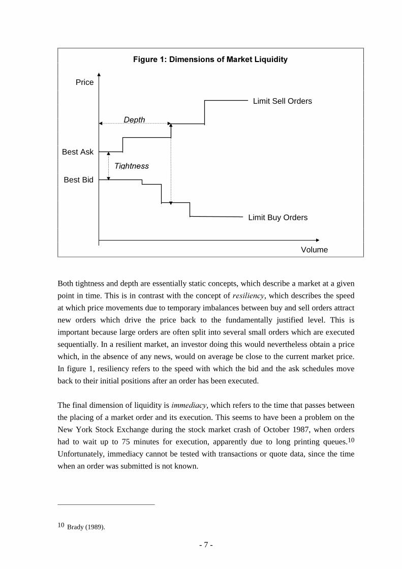
prices. Tightness is directly measured by the bid-ask spread, which in figure 1 corresponds

to the vertical distance between the lowest ask and the highest bid prices. A market is ����

if large orders can be executed without much effect on prices. In figure 1, market depth is

given by order size, measured on the horizontal axis, and the relevant spread for that

amount, measured on the vertical axis.

- 7 -

Both tightness and depth are essentially static concepts, which describe a market at a given

point in time. This is in contrast with the concept of ������� , which describes the speed

at which price movements due to temporary imbalances between buy and sell orders attract

new orders which drive the price back to the fundamentally justified level. This is

important because large orders are often split into several small orders which are executed

sequentially. In a resilient market, an investor doing this would nevertheless obtain a price

which, in the absence of any news, would on average be close to the current market price.

In figure 1, resiliency refers to the speed with which the bid and the ask schedules move

back to their initial positions after an order has been executed.

The final dimension of liquidity is �������� , which refers to the time that passes between

the placing of a market order and its execution. This seems to have been a problem on the

New York Stock Exchange during the stock market crash of October 1987, when orders

had to wait up to 75 minutes for execution, apparently due to long printing queues.10

Unfortunately, immediacy cannot be tested with transactions or quote data, since the time

when an order was submitted is not known.

10 Brady (1989).

���������

���

Price

Volume

Limit Sell Orders

Limit Buy Orders

������������� ��� ��������������������

Best Ask

Best Bid

- 8 -

-(*(������������&�������������

Market liquidity has traditionally been proxied by indicators for market activity like the

number of trades, trading volume or the spacing between trades.11 These measures have

the advantage that they are immediately available or at least easy to compute, but

unfortunately are not directly related to any of the four dimensions of liquidity presented in

the previous subsection. Market liquidity is only one, and not necessarily the most

important, factor affecting trading activity. For example, if traders have sufficiently large

hedging needs, then they may trade even if market liquidity, in terms of tightness, depth,

resiliency and immediacy, is relatively low.

Nevertheless, even though there is not a one to one relationship between trading activity

and liquidity, indicators such as turnover or the intervals between trades do show that

markets are sufficiently liquid to sustain a given amount of trading. The converse is not the

case, however. The absence of transactions does not necessarily imply that markets are not

liquid but may be due to the agents not wanting to trade at the market clearing prices. Such

no-trade equilibria are common in theoretical models with homogenous agents. So, while

we should not discard activity indicators altogether, it would be preferable to have

measures that are linked to at least one of the four dimensions of market liquidity.

A measure for liquidity that is both easily available and in line with one of the four

dimensions mentioned before is the ������ bid-ask spread, which indicates the tightness of

a market. In quote-driven markets such as the over-the-counter market for German

government bonds quoted spreads can be observed by traders at any point in time.12

Unfortunately, quoted� spreads may not represent the true cost of trading since many

transactions take place at prices inside the quoted bid-ask bracket. In addition, they apply to

transactions up to a specified amount only, which, furthermore, varies over time. E.g., if

market participants cut this amount in periods of stress, then this would leave the quoted

spread unchanged.

We can overcome the problems associated with ������� spreads by computing ���������

spreads. In contrast to the former, effective spreads refer to the average transaction and thus

captures not only the tightness but also the depth of a market. They are computed from

11 For examples, see BIS (1999b).12 Since there is no commitment to market making in the OTC market for Bundesanleihen, quoted spreads

are merely indicative, i.e. agents do not have to honour the prices they promise. While this should notmatter in normal times, it may be a problem in periods of stress.

- 9 -

transactions data and thus reflect the price actually ���� by traders and not the price

��������� by dealers.

The computation of the effective spread goes back to the seminal work of Roll (1984), who

uses the negative first order autocorrelation in transaction prices that results from

transactions being undertaken alternately at bid and ask prices. Assuming that buy and sell

orders arrive with equal probability and that the bid-ask spread effectively paid by the

traders remains constant over the estimation period, he shows that the spread is given by

( ) ��� � �W W

= − −2 1∆ ∆, .

Unfortunately, there are a number of problems associated with the Roll measure. First of

all, as is shown in Stoll (1989), in the presence of adverse selection or inventory effects it

may underestimate the actual spread. Secondly, a bias may be induced by the fact that the

number of bid and offer transactions may not be balanced.13 Nevertheless, its simplicity

and the ease with which it is implemented make the Roll measure a good starting point

when measuring liquidity, although its limitations have to be borne in mind.14

More recently, several other ways for computing spreads from transactions data have been

developed.15 Their computation is more involved than that of the Roll measure, which is

why they have not been included in this paper.

13 See Choi et al (1988) on how to adjust Roll’s estimator for this.14 Two practical difficulties may arise when implementing Roll’s method. Firstly, the estimate for

( )��� � �W W

∆ ∆, −1 may be negative. In this case, I drop the observation from the sample. Secondly, the fact

that the autocovariance of prices is not known but has to be estimated from the data induces a smallsample bias. This can become a problem when estimating the effective spread over short time intervalslike individual days. However, Roll (1984) argues that the bias is relatively small, e.g. for a sample of 60observations it would amount to about two percent of the spread, which would seem acceptable. I dealwith the problem dropping all intervals with less than 50 observations.

15 They are surveyed in Huang & Stoll (1997), who also present their own measure for estimating anddecomposing the spread into the components due to order-processing, inventory control and adverseselection costs.

- 10 -

.(�!�������������/��&���/� ���&���0���16

This section describes the trading arrangements in the market for German government

bonds. As is generally the case in the microstructure literature, the institutional structure of

a market is of great importance since it conditions the availability of data and is important

for the interpretation of the results. A description of the structure of the market for German

government securities is also of interest in its own right, since it differs from that of other

securities markets.

The market for German 10 year Bundesanleihen (Bunds) represents the most liquid

segment of the European bond market and provides a benchmark for the pricing of long

maturity bonds throughout Europe. German government bonds are traded both on

organised exchanges and over the counter (OTC), with the latter accounting for the bulk of

trading. This is especially true for the inter-dealer market, where trading takes place either

directly between banks or through inter-dealer brokers (Freimakler). These act as

intermediaries, but have no obligation to provide firm quotes. While the academic literature

would suggest that dealers use brokers mainly in order to obtain anonymity17,

conversations with market participants have hinted at a more mundane reason: Brokers

seem to be more efficient in matching counterparties because of their more active

participation in the market.

While there is a trend towards electronic trading, this stage had not yet been reached during

1998, when brokers posted their quotes on screen but the actual transactions took place

over the phone. Electronic trading is more important in the client market. Large banks run

proprietary trading systems, where they provide quotes for their customers. Recently,

electronic trading systems as the Euro-MTS have become more important also in the inter-

dealer market, but in 1998 their role was negligible.

The OTC market seems to be rather opaque. Participants observe quotes but do not receive

timely information on other traders’ past transactions beyond anecdotal evidence. In

principle, it would be possible to obtain this information from clearing data, but it would

arrive with a delay of up to three days and would be expensive to collect.

16 The description of the market for Bunds draws from conversations with Gerhard Klopf and Uwe Ullrich,of the trading desks of the Bundesbank and Deutsche Bank, respectively. I focus the market for Bunds asit was in 1998 and ignore many recent developments.

17 At least temporarily, as the banks receive details on their counterparty for clearing purposes. Only veryrecently did brokers act as a counterparty, thus preserving anonymity even after clearing.

- 11 -

The role of exchanges is minor in comparison to the OTC market, even though all issues

are listed. Trading takes place almost exclusively on the Frankfurt Stock Exchange, the role

of regional exchanges is negligible. In 1998, German government bonds traded more or

less entirely by open outcry since the computerised trading system XETRA did not permit

traders to link their quotes to the price of the Bund future.18 Prices are formed by a

specialist broker (Kursmakler), who has to ensure price continuity. If the potential market

clearing price lies outside a pre-specified corridor, he interrupts trading for five minutes

and calls for new quotes. He may undertake some trading on his own account, but this

occurs mainly to offset imbalances in order size and does not seem to play a big role in

providing market liquidity.

1(����

1(�(������%���

The data covers all transactions in Germany during 1998 of four government bonds

(Bunds) with a residual maturity of 8 to 10 years. It includes all ������������ (long term

bonds issued by the federal government) with an original maturity of 10 years that were

issued between January 1997 and July 1998. Details on the individual bonds are given in

table 2. The securities have been selected because they were delivered for the Eurex Bund

future in 1998.

Bundesanleihen are usually first issued in January and July, and the size of the issue is

increased during the following months. The autumn of 1998 marked an exception to this

rule, as in the wake of falling interest rates a new issue with a lower coupon was brought to

the market outside the normal issuing schedule in November. As a consequence, the 4.75

% bond first issued in July 1998 has a volume outstanding of only 17 billion DM compared

to 30 billion DM for the other three bonds in our sample.

The data has been provided by the German securities’ regulator ����������������� ���

���� ���������������� ������, which receives notice of ���� � ���� transaction in

Germany, irrespective of whether or not it takes place on an exchange. This feature is

particularly attractive for work on the bond market, where OTC transactions account for

most trading.

18 This possibility has been provided in the summer of 1999, but it remains to be seen whether this will shiftmore activity onto XETRA.

- 12 -

Bunds are also traded abroad, in particular in London. Unfortunately, we do not have any

information on transactions outside Germany, although there is anecdotal evidence that the

market share of London has fallen in recent years, albeit by a lesser extent than the one in

the market for Bund futures.

In principle, we should have two observations for each trade: one concerning the final

buyer and another for the final seller of the security. An exception are trades with

intermediaries that reside outside Germany and are therefore not subject to the reporting

requirement. For each observation, we have a date and time stamp, price, volume, as well

as indicators for whether it is the sale or the purchase leg of a transaction, whether the

reporting bank’s inventory is affected, whether the reporting bank acts as an agent for a

customer or on its own account, and whether trade takes place over the counter or on an

exchange.

Some observations on the quality of the data are in order. Firstly, the precision of the time

stamps (up to the nearest second) may be more apparent than real. It is probably high for

trades that take place on an exchange, but may be low for OTC-transactions. An indication

for this is that many trades are reported as taking place outside normal office hours, often at

midnight sharp or at prices that seem out of date. Inaccurate time stamps represent a severe

problem since the reliability of most indicators for liquidity crucially depend on the correct

sequence, although not so much the timing, of trades. Secondly, other variables may have

been reported incorrectly. While most of such errors have been eliminated by the BAWe

using supplementary information, some mistakes especially in prices or volume may

remain.

Matching the buy and sell legs of transactions and filtering the data can reduce the

severeness of these problems. Unfortunately, matching the two legs is not straightforward,

in part because of errors in the data and in part because of missing notifications. I have

matched all purchases and sales that occurred on the same day at the same price and with

the same volume. If the time stamps of these pairs of ‘matched’ observations do not

coincide, I have used the earlier one. Of a total of 145 thousand observations in our raw

data, only about half could be matched in this way.�19 Since the remaining ‘unmatched’

observations account for a large proportion of market activity, I have decided to keep them

in the data. After matching, we are left with 109 thousand observations, which further

19 The BAWe successfully matches the various notices for more than three quarters of the trades but usessupplemental data to achieve this. They use the matches in order to hunt down missing notifications and toeliminate contra-trades. Since the matches are stored in a different database, using this information in thepresent study would have incurred computational costs that seemed out of proportion to the limitedbenefits of doing so.

- 13 -

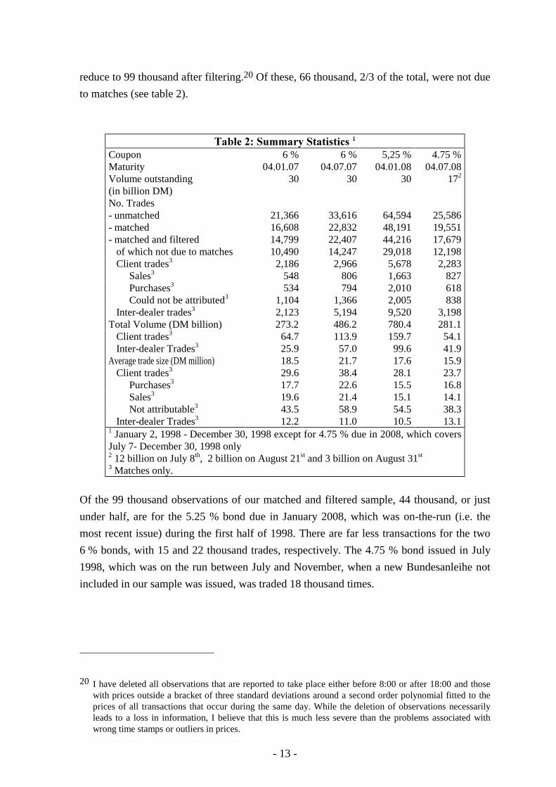
reduce to 99 thousand after filtering.20 Of these, 66 thousand, 2/3 of the total, were not due

to matches (see table 2).

!�"���*+���&&�����������

Coupon 6 % 6 % 5,25 % 4.75 %Maturity 04.01.07 04.07.07 04.01.08 04.07.08Volume outstanding(in billion DM)

30 30 30 172

No. Trades- unmatched 21,366 33,616 64,594 25,586- matched 16,608 22,832 48,191 19,551- matched and filtered 14,799 22,407 44,216 17,679 of which not due to matches 10,490 14,247 29,018 12,198 Client trades3 2,186 2,966 5,678 2,283 Sales3 548 806 1,663 827 Purchases3 534 794 2,010 618 Could not be attributed3 1,104 1,366 2,005 838 Inter-dealer trades3 2,123 5,194 9,520 3,198Total Volume (DM billion) 273.2 486.2 780.4 281.1 Client trades3 64.7 113.9 159.7 54.1 Inter-dealer Trades3 25.9 57.0 99.6 41.9Average trade size (DM million) 18.5 21.7 17.6 15.9 Client trades3 29.6 38.4 28.1 23.7 Purchases3 17.7 22.6 15.5 16.8 Sales3 19.6 21.4 15.1 14.1 Not attributable3 43.5 58.9 54.5 38.3 Inter-dealer Trades3 12.2 11.0 10.5 13.11 January 2, 1998 - December 30, 1998 except for 4.75 % due in 2008, which coversJuly 7- December 30, 1998 only2 12 billion on July 8th, 2 billion on August 21st and 3 billion on August 31st

3 Matches only.

Of the 99 thousand observations of our matched and filtered sample, 44 thousand, or just

under half, are for the 5.25 % bond due in January 2008, which was on-the-run (i.e. the

most recent issue) during the first half of 1998. There are far less transactions for the two

6 % bonds, with 15 and 22 thousand trades, respectively. The 4.75 % bond issued in July

1998, which was on the run between July and November, when a new Bundesanleihe not

included in our sample was issued, was traded 18 thousand times.

20 I have deleted all observations that are reported to take place either before 8:00 or after 18:00 and thosewith prices outside a bracket of three standard deviations around a second order polynomial fitted to theprices of all transactions that occur during the same day. While the deletion of observations necessarilyleads to a loss in information, I believe that this is much less severe than the problems associated withwrong time stamps or outliers in prices.

- 14 -

As was mentioned before, our dataset contains information on whether the sale or purchase

leg was an agency trade or on the intermediary’s own account. In the case of ‘matched’

observations, this allows us to distinguish inter-dealer trades, where banks appear on both

sides, from client trades, which cover the remainder. A transaction is classified as a client

sale (purchase) if the sale (purchase) involved a client and the counterparty was a bank. If

both the purchase and the sale are agency trades, then the transaction is counted as non-

attributable client trades. Unfortunately, this classification is not possible for ‘unmatched’

trades.

Client trades account for less than 40 % of the ‘matched’ transactions, and inter-dealer

trades for the remainder. Of the former, about 30 % were identified as purchases and

approximately the same number as sales, the remaining client transactions could not be

attributed.

<5 10 15 20 25 30 45 50 >500

20

40

60

6 % (Jan)

%

<5 10 15 20 25 30 45 50 >500

20

40

60

6 % (July)

%

<5 10 15 20 25 30 45 50 >500

20

40

60

5.25 %

%

<5 10 15 20 25 30 45 50 >500

20

40

60

4.75 %

%

Size Category (million DM)

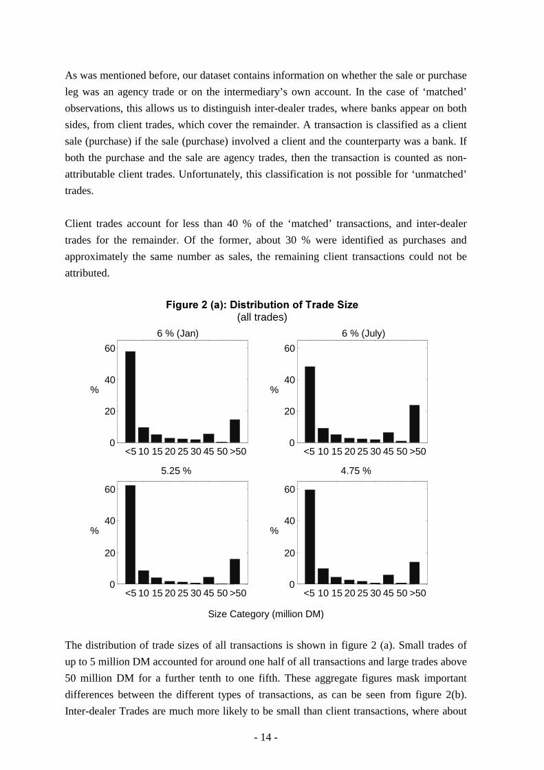
�������������� �����������������������(all trades)

The distribution of trade sizes of all transactions is shown in figure 2 (a). Small trades of

up to 5 million DM accounted for around one half of all transactions and large trades above

50 million DM for a further tenth to one fifth. These aggregate figures mask important

differences between the different types of transactions, as can be seen from figure 2(b).

Inter-dealer Trades are much more likely to be small than client transactions, where about

- 15 -

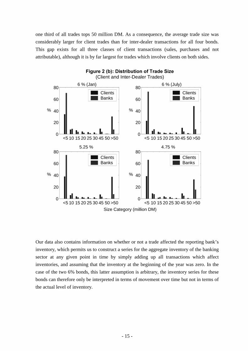
one third of all trades tops 50 million DM. As a consequence, the average trade size was

considerably larger for client trades than for inter-dealer transactions for all four bonds.

This gap exists for all three classes of client transactions (sales, purchases and not

attributable), although it is by far largest for trades which involve clients on both sides.

<5 10 15 20 25 30 45 50 >500

20

40

60

806 % (Jan)

%

ClientsBanks

<5 10 15 20 25 30 45 50 >500

20

40

60

806 % (July)

%

ClientsBanks

<5 10 15 20 25 30 45 50 >500

20

40

60

805.25 %

%

ClientsBanks

<5 10 15 20 25 30 45 50 >500

20

40

60

804.75 %

%

Size Category (million DM)

ClientsBanks

�������������� �����������������������(Client and Inter-Dealer Trades)

Our data also contains information on whether or not a trade affected the reporting bank’s

inventory, which permits us to construct a series for the aggregate inventory of the banking

sector at any given point in time by simply adding up all transactions which affect

inventories, and assuming that the inventory at the beginning of the year was zero. In the

case of the two 6% bonds, this latter assumption is arbitrary, the inventory series for these

bonds can therefore only be interpreted in terms of movement over time but not in terms of

the actual level of inventory.

- 16 -

1 2 3 4 5 6 7 8 9 101112

-200

-100

0

100

200

3006% (January)

1 2 3 4 5 6 7 8 9 101112

-200

-100

0

100

200

3006% (Jul)

1 2 3 4 5 6 7 8 9 101112

-200

-100

0

100

200

3005.25%

Month 1 2 3 4 5 6 7 8 9101112

-200

-100

0

100

200

3004.75%

Month

��������� ��!��!����"�#�������

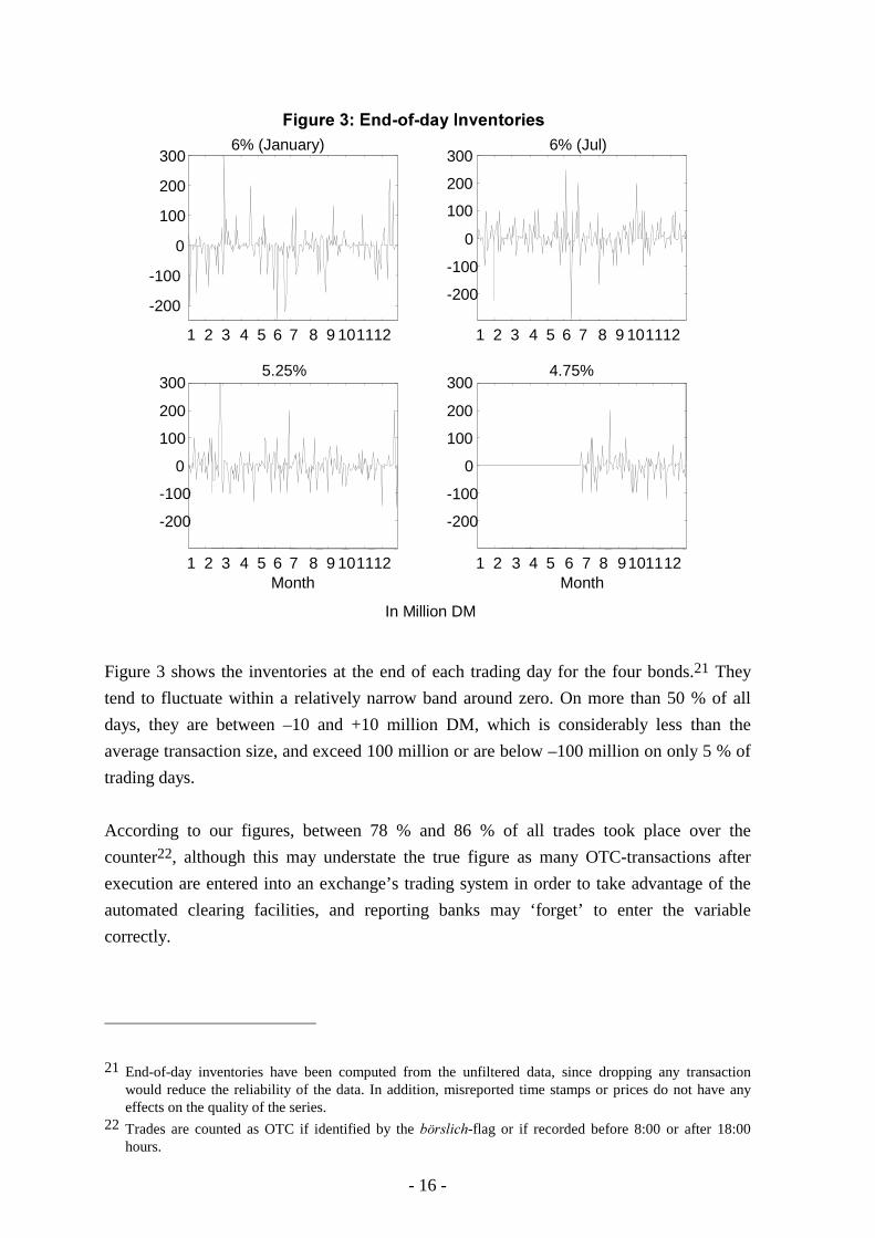
In Million DM

Figure 3 shows the inventories at the end of each trading day for the four bonds.21 They

tend to fluctuate within a relatively narrow band around zero. On more than 50 % of all

days, they are between –10 and +10 million DM, which is considerably less than the

average transaction size, and exceed 100 million or are below –100 million on only 5 % of

trading days.

According to our figures, between 78 % and 86 % of all trades took place over the

counter22, although this may understate the true figure as many OTC-transactions after

execution are entered into an exchange’s trading system in order to take advantage of the

automated clearing facilities, and reporting banks may ‘forget’ to enter the variable

correctly.

21 End-of-day inventories have been computed from the unfiltered data, since dropping any transactionwould reduce the reliability of the data. In addition, misreported time stamps or prices do not have anyeffects on the quality of the series.

22 Trades are counted as OTC if identified by the � ����-flag or if recorded before 8:00 or after 18:00hours.

- 17 -

1(*(�)���2����%������������������ ��

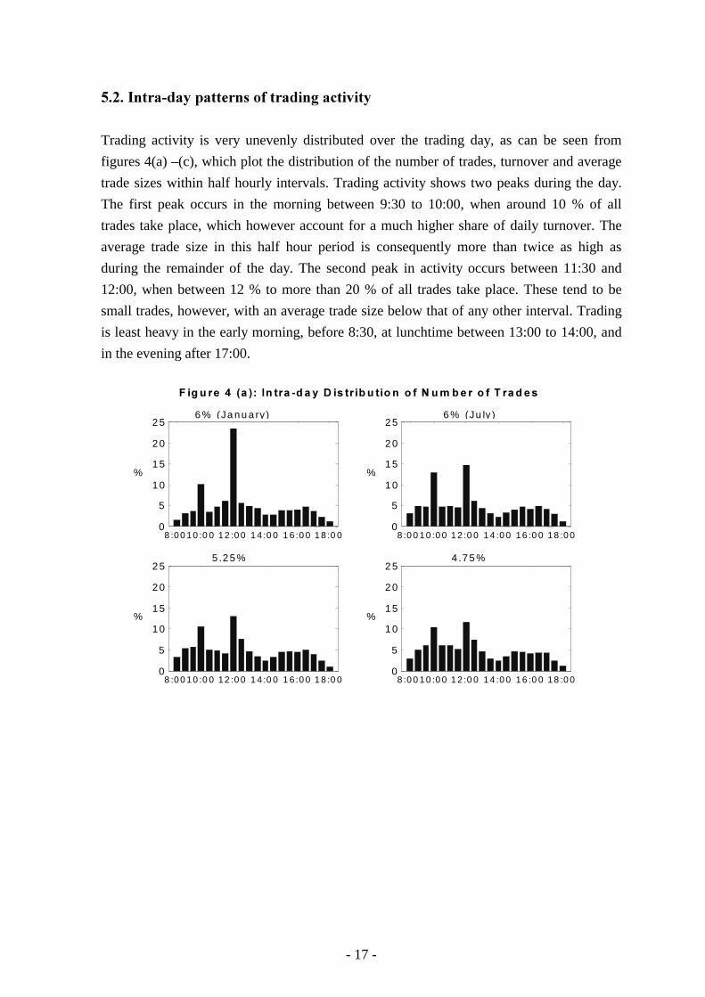
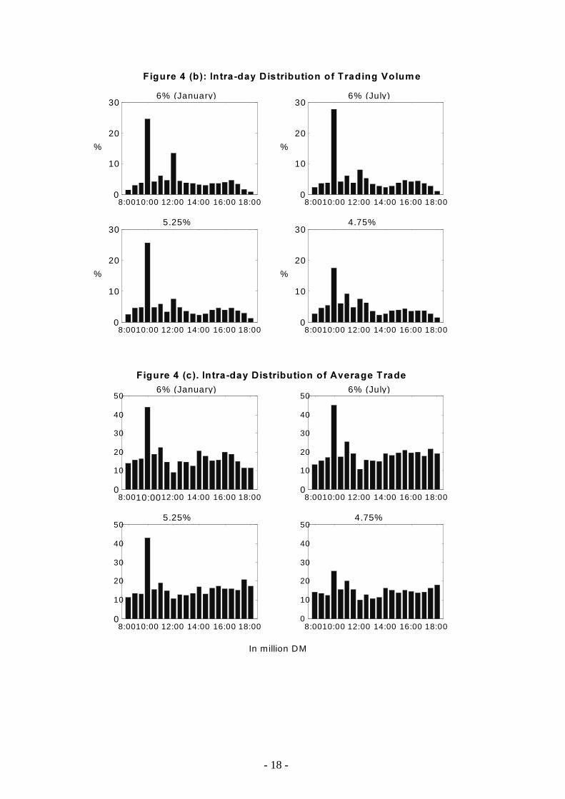
Trading activity is very unevenly distributed over the trading day, as can be seen from

figures 4(a) –(c), which plot the distribution of the number of trades, turnover and average

trade sizes within half hourly intervals. Trading activity shows two peaks during the day.

The first peak occurs in the morning between 9:30 to 10:00, when around 10 % of all

trades take place, which however account for a much higher share of daily turnover. The

average trade size in this half hour period is consequently more than twice as high as

during the remainder of the day. The second peak in activity occurs between 11:30 and

12:00, when between 12 % to more than 20 % of all trades take place. These tend to be

small trades, however, with an average trade size below that of any other interval. Trading

is least heavy in the early morning, before 8:30, at lunchtime between 13:00 to 14:00, and

in the evening after 17:00.

8 :00 10 :0 0 12 :0 0 1 4 :0 0 1 6 :0 0 1 8 :0 00

5

1 0

1 5

2 0

2 5

%

6 % (Ja n u a ry)

8 :0 0 1 0 :0 0 1 2 :0 0 1 4 :0 0 16 :0 0 1 8 :0 00

5

1 0

1 5

2 0

2 5

%

6 % (Ju ly )

8 :00 10 :0 0 12 :0 0 1 4 :0 0 1 6 :0 0 1 8 :0 00

5

1 0

1 5

2 0

2 5

%

5 .2 5 %

8:0 0 1 0 :0 0 1 2 :0 0 1 4 :0 0 16 :0 0 1 8 :0 00

5

1 0

1 5

2 0

2 5

%

4 .7 5 %

� ��� �� �$ ��� ��"� ��� !� � � � � �� �� � ��� � �� ��% �� �� ��� ��� ����

- 18 -

8:0010:00 12:00 14:00 16:00 18:000

10

20

30

%

6% (January)

8:0010:00 12:00 14:00 16:00 18:000

10

20

30

%

6% (July)

8:0010:00 12:00 14:00 16:00 18:000

10

20

30

%

5.25%

8:0010:00 12:00 14:00 16:00 18:000

10

20

30

%

4.75%

�������$�����"����!����� ���������������������&�'���

8:0010:0012:00 14:00 16:00 18:000

10

20

30

40

506% (January)

8:0010:00 12:00 14:00 16:00 18:000

10

20

30

40

506% (July)

8:0010:00 12:00 14:00 16:00 18:000

10

20

30

40

505.25%

8:0010:00 12:00 14:00 16:00 18:000

10

20

30

40

504.75%

�������$��(�)�"����!����� �������������*#�����������

In million DM

- 19 -

1(-(�#�������������������2%������&������

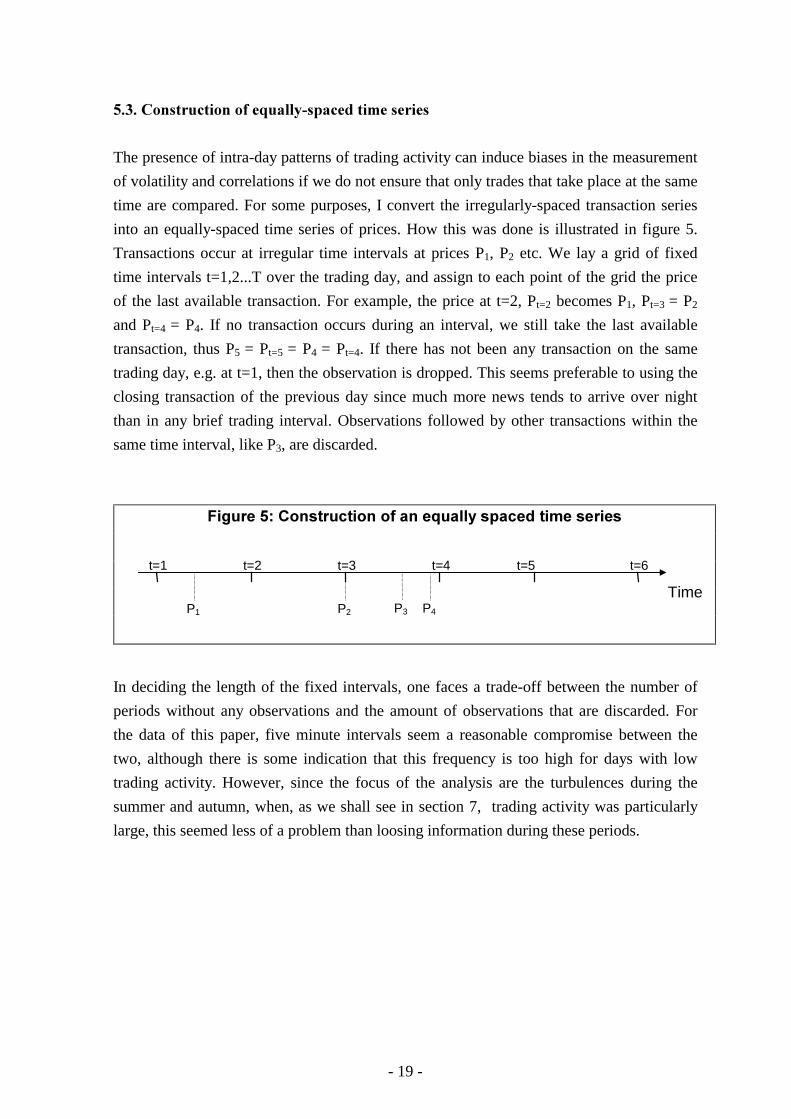
The presence of intra-day patterns of trading activity can induce biases in the measurement

of volatility and correlations if we do not ensure that only trades that take place at the same

time are compared. For some purposes, I convert the irregularly-spaced transaction series

into an equally-spaced time series of prices. How this was done is illustrated in figure 5.

Transactions occur at irregular time intervals at prices P1, P2 etc. We lay a grid of fixed

time intervals t=1,2...T over the trading day, and assign to each point of the grid the price

of the last available transaction. For example, the price at t=2, Pt=2 becomes P1, Pt=3 = P2

and Pt=4 = P4. If no transaction occurs during an interval, we still take the last available

transaction, thus P5 = Pt=5 = P4 = Pt=4. If there has not been any transaction on the same

trading day, e.g. at t=1, then the observation is dropped. This seems preferable to using the

closing transaction of the previous day since much more news tends to arrive over night

than in any brief trading interval. Observations followed by other transactions within the

same time interval, like P3, are discarded.

In deciding the length of the fixed intervals, one faces a trade-off between the number of

periods without any observations and the amount of observations that are discarded. For

the data of this paper, five minute intervals seem a reasonable compromise between the

two, although there is some indication that this frequency is too high for days with low

trading activity. However, since the focus of the analysis are the turbulences during the

summer and autumn, when, as we shall see in section 7, trading activity was particularly

large, this seemed less of a problem than loosing information during these periods.

�������+�,�� ���(���������������''�� -�(�������� ����

Time

t=1 t=2 t=3 t=4 t=5 t=6

P1 P2 P3 P4

- 20 -

3(�4��������0����������

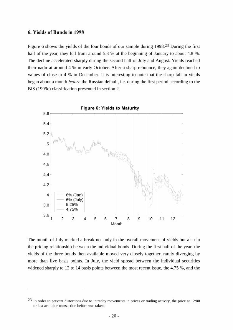
Figure 6 shows the yields of the four bonds of our sample during 1998.23 During the first

half of the year, they fell from around 5.3 % at the beginning of January to about 4.8 %.

The decline accelerated sharply during the second half of July and August. Yields reached

their nadir at around 4 % in early October. After a sharp rebounce, they again declined to

values of close to 4 % in December. It is interesting to note that the sharp fall in yields

began about a month ������ the Russian default, i.e. during the first period according to the

BIS (1999c) classification presented in section 2.

1 2 3 4 5 6 7 8 9 10 11 123.6

3.8

4

4.2

4.4

4.6

4.8

5

5.2

5.4

5.6�������.�/��'� ������������

Month

6% (Jan)6% (July)5.25%4.75%

The month of July marked a break not only in the overall movement of yields but also in

the pricing relationship between the individual bonds. During the first half of the year, the

yields of the three bonds then available moved very closely together, rarely diverging by

more than five basis points. In July, the yield spread between the individual securities

widened sharply to 12 to 14 basis points between the most recent issue, the 4.75 %, and the

23 In order to prevent distortions due to intraday movements in prices or trading activity, the price at 12:00or last available transaction before was taken.

- 21 -

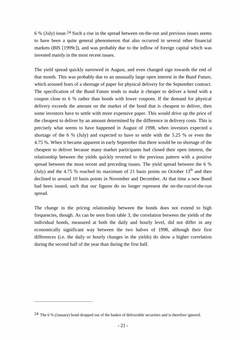
6 % (July) issue.24 Such a rise in the spread between on-the-run and previous issues seems

to have been a quite general phenomenon that also occurred in several other financial

markets (BIS [1999c]), and was probably due to the inflow of foreign capital which was

invested mainly in the most recent issues.

The yield spread quickly narrowed in August, and even changed sign towards the end of

that month. This was probably due to an unusually large open interest in the Bund Future,

which aroused fears of a shortage of paper for physical delivery for the September contract.

The specification of the Bund Future tends to make it cheaper to deliver a bond with a

coupon close to 6 % rather than bonds with lower coupons. If the demand for physical

delivery exceeds the amount on the market of the bond that is cheapest to deliver, then

some investors have to settle with more expensive paper. This would drive up the price of

the cheapest to deliver by an amount determined by the difference in delivery costs. This is

precisely what seems to have happened in August of 1998, when investors expected a

shortage of the 6 % (July) and expected to have to settle with the 5.25 % or even the

4.75 %. When it became apparent in early September that there would be no shortage of the

cheapest to deliver because many market participants had closed their open interest, the

relationship between the yields quickly reverted to the previous pattern with a positive

spread between the most recent and preceding issues. The yield spread between the 6 %

(July) and the 4.75 % reached its maximum of 21 basis points on October 13th and then

declined to around 10 basis points in November and December. At that time a new Bund

had been issued, such that our figures do no longer represent the on-the-run/of-the-run

spread.

The change in the pricing relationship between the bonds does not extend to high

frequencies, though. As can be seen from table 3, the correlation between the yields of the

individual bonds, measured at both the daily and hourly level, did not differ in any

economically significant way between the two halves of 1998, although their first

differences (i.e. the daily or hourly changes in the yields) do show a higher correlation

during the second half of the year than during the first half.

24 The 6 % (January) bond dropped out of the basket of deliverable securities and is therefore ignored.

- 22 -

!�"���-+�#�������������4������ �� ��������������

1. Daily 5.25 % 4.75 % 5.25 % 4.75 %a) 01.01.99 – 30.12.99 6 % (July) 0.994 n/a 0.932 n/a 5.25 % n/a n/ab) 01.01.99 – 30.06.99 6 % (July) 0.981 n/a 0.884 n/a 5.25 % n/a n/ac) 07.07.99 – 30.12.99 6 % (July) 0.986 0.980 0.951 0.947 5.25 % 0.994 0.970*(�������a) 01.01.99 – 30.12.99 6 % (July) 0.993 n/a 0.313 n/a 5.25 % n/a n/ab) 01.01.99 – 30.06.99 6 % (July) 0.973 n/a 0.234 n/a 5.25 % n/a n/ac) 07.07.99 – 30.12.99 6 % (July) 0.984 0.976 0.363 0.447 5.25 % 0.993 0.436

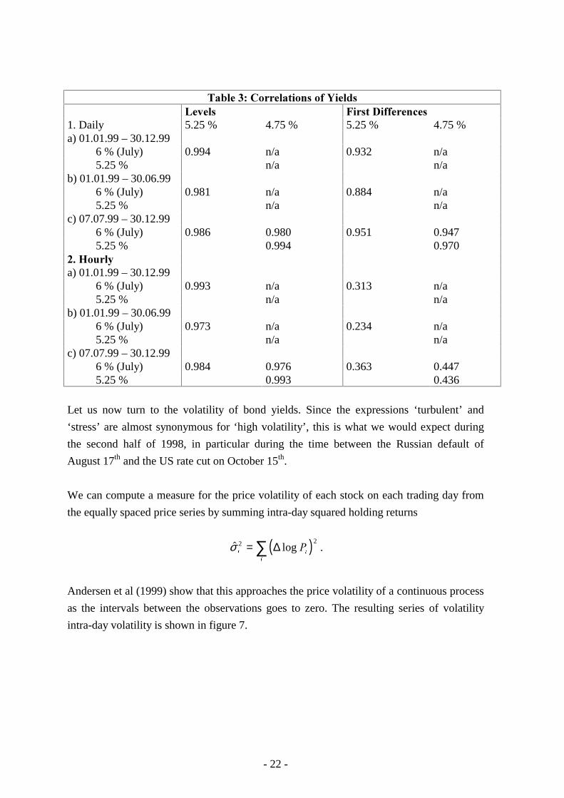
Let us now turn to the volatility of bond yields. Since the expressions ‘turbulent’ and

‘stress’ are almost synonymous for ‘high volatility’, this is what we would expect during

the second half of 1998, in particular during the time between the Russian default of

August 17th and the US rate cut on October 15th.

We can compute a measure for the price volatility of each stock on each trading day from

the equally spaced price series by summing intra-day squared holding returns

( )� logσW L

L

�2 2= ∑ ∆ .

Andersen et al (1999) show that this approaches the price volatility of a continuous process

as the intervals between the observations goes to zero. The resulting series of volatility

intra-day volatility is shown in figure 7.

- 23 -

1 2 3 4 5 6 7 8 9 10 11120

2

4

6

8

6% (January)

Month 1 2 3 4 5 6 7 8 9 10 1112

0

2

4

6

8

6% (July)

Month

1 2 3 4 5 6 7 8 9 10 11120

2

4

6

8

5.25%

Month 1 2 3 4 5 6 7 8 9 10 1112

0

2

4

6

8

4.75%

Month

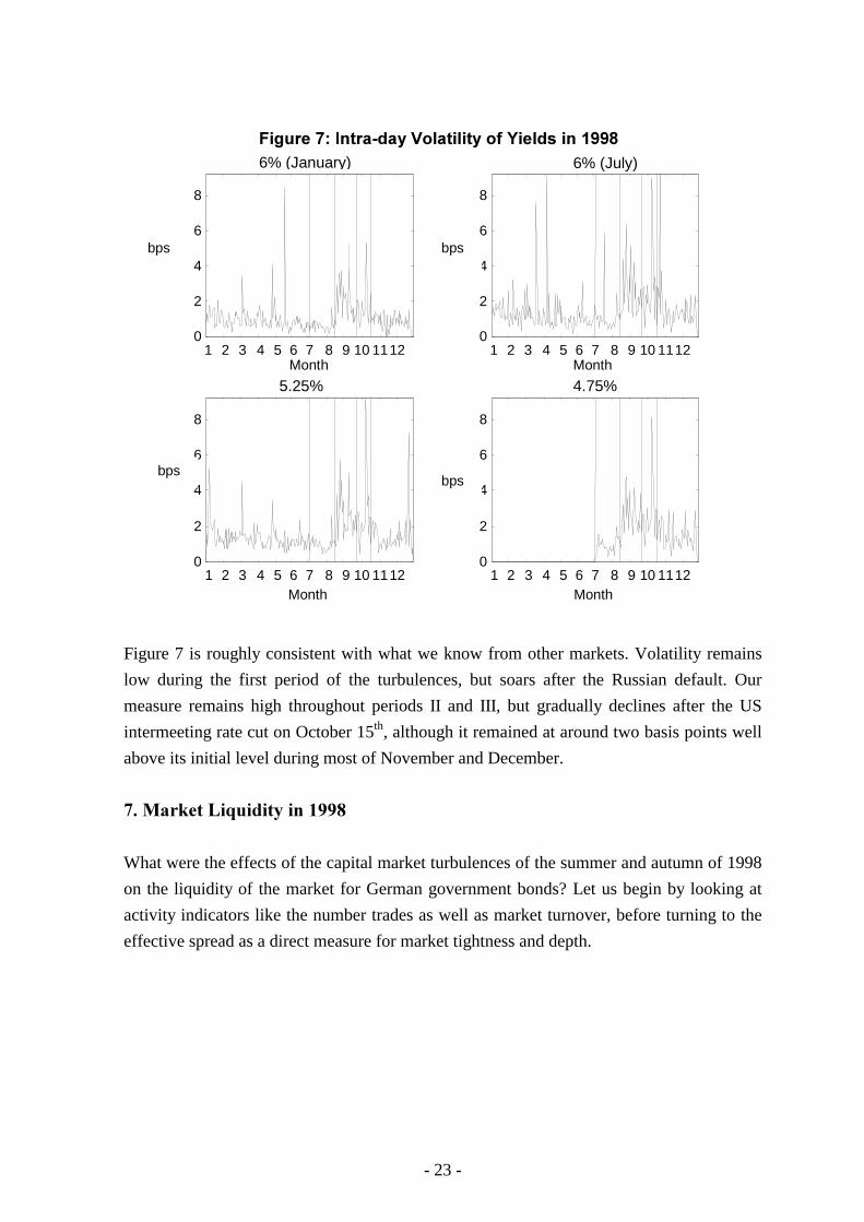
�������0�"����!����&�'���'�������/��'� �����112

bps bps

bpsbps

Figure 7 is roughly consistent with what we know from other markets. Volatility remains

low during the first period of the turbulences, but soars after the Russian default. Our

measure remains high throughout periods II and III, but gradually declines after the US

intermeeting rate cut on October 15th, although it remained at around two basis points well

above its initial level during most of November and December.

5(����������������������

What were the effects of the capital market turbulences of the summer and autumn of 1998

on the liquidity of the market for German government bonds? Let us begin by looking at

activity indicators like the number trades as well as market turnover, before turning to the

effective spread as a direct measure for market tightness and depth.

- 24 -

5(�(�6�� �����������

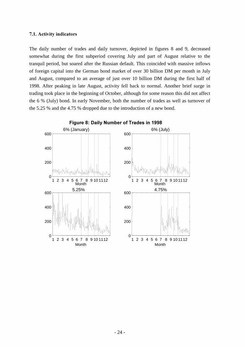
The daily number of trades and daily turnover, depicted in figures 8 and 9, decreased

somewhat during the first subperiod covering July and part of August relative to the

tranquil period, but soared after the Russian default. This coincided with massive inflows

of foreign capital into the German bond market of over 30 billion DM per month in July

and August, compared to an average of just over 10 billion DM during the first half of

1998. After peaking in late August, activity fell back to normal. Another brief surge in

trading took place in the beginning of October, although for some reason this did not affect

the 6 % (July) bond. In early November, both the number of trades as well as turnover of

the 5.25 % and the 4.75 % dropped due to the introduction of a new bond.

1 2 3 4 5 6 7 8 9 10 11120

200

400

6006% (January)

Month 1 2 3 4 5 6 7 8 9 10 1112

0

200

400

6006% (July)

Month

1 2 3 4 5 6 7 8 9 10 11120

200

400

6005.25%

Month 1 2 3 4 5 6 7 8 9 10 1112

0

200

400

6004.75%

Month

�������2���'��%�������������� �����112

- 25 -

1 2 3 4 5 6 7 8 9 10 11120

5

10

6% (January)

Month 1 2 3 4 5 6 7 8 9 10 1112

0

5

10

6% (Jul)

Month

1 2 3 4 5 6 7 8 9 10 11120

5

10

5.25%

Month 1 2 3 4 5 6 7 8 9 10 1112

0

5

10

4.75%

Month(in billion DM)

�������1���'�������#�������112

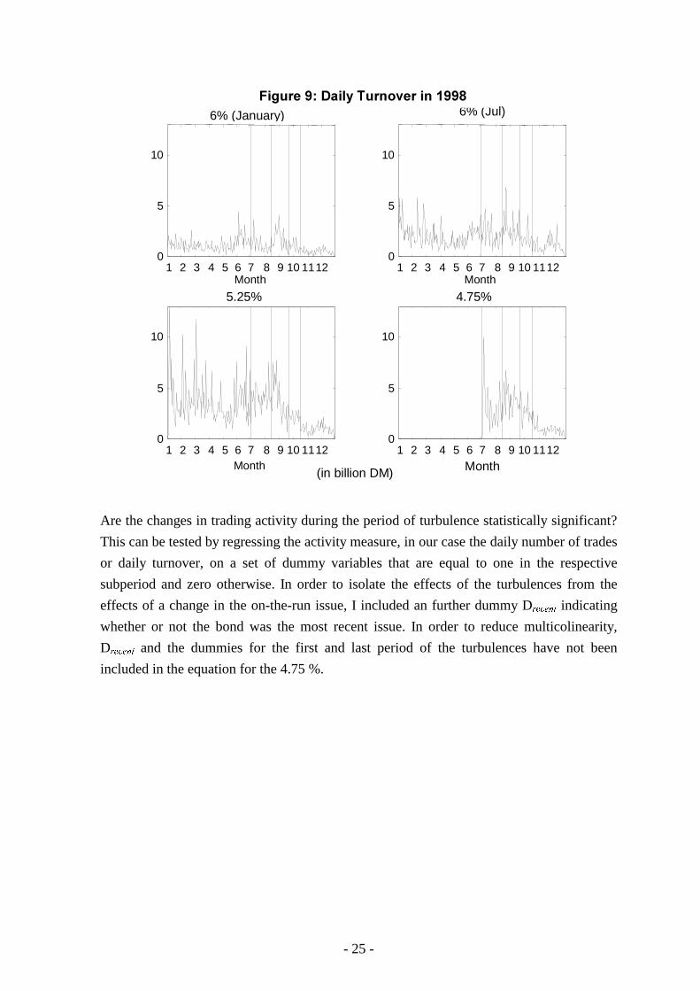
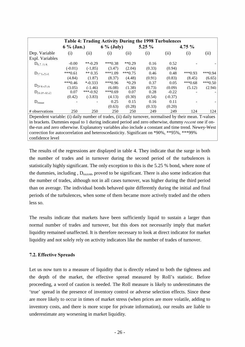
Are the changes in trading activity during the period of turbulence statistically significant?

This can be tested by regressing the activity measure, in our case the daily number of trades

or daily turnover, on a set of dummy variables that are equal to one in the respective

subperiod and zero otherwise. In order to isolate the effects of the turbulences from the

effects of a change in the on-the-run issue, I included an further dummy DUHFHQW indicating

whether or not the bond was the most recent issue. In order to reduce multicolinearity,

DUHFHQW and the dummies for the first and last period of the turbulences have not been

included in the equation for the 4.75 %.

- 26 -

!�"���.+�!�������6�� ���������������� �!��"������3�7�89��(: 3�7�89���: 1(*1�7 .(51�7

Dep. Variable (i) (ii) (i) (ii) (i) (ii) (i) (ii)Expl. Variables D���������� -0.00

(-0.01)**-0.29

(-1,85)***0.38

(3.47)**0.29

(2.04)0.16

(0.33)0.52

(0.94)- -

D����������� ***0.61(4.84)

** 0.35(1.87)

***1.09(8.37)

***0.75(4.48)

0.46(0.91)

0.48(0.83)

***0.93(8.45)

***0.94(6.65)

D������������

***0.46(3.05)

*-0.333(-1.46)

***0.96(6.08)

*0.29(1.38)

0.37(0.73)

0.05(0.09)

***0.68(5.12)

***0.50(2.94)

D������������� 0.07(0.42)

***-0.92(-3.83)

***0.69(4.13)

0.07(0.30)

0.28(0.54)

-0.22(-0.37)

- -

DUHFHQW - - 0.25(0.63)

0.15(0.28)

0.16(0.33)

0.11(0.20)

- -

# observations 250 250 250 250 249 249 124 124Dependent variable: (i) daily number of trades, (ii) daily turnover, normalised by their mean. T-valuesin brackets. Dummies equal to 1 during indicated period and zero otherwise, dummy �������one if on-the-run and zero otherwise. Explanatory variables also include a constant and time trend. Newey-Westcorrection for autocorrelation and heteroscedasticity. Significant on *90%, **95%, ***99%confidence level

The results of the regressions are displayed in table 4. They indicate that the surge in both

the number of trades and in turnover during the second period of the turbulences is

statistically highly significant. The only exception to this is the 5.25 % bond, where none of

the dummies, including , DUHFHQW, proved to be significant. There is also some indication that

the number of trades, although not in all cases turnover, was higher during the third period

than on average. The individual bonds behaved quite differently during the initial and final

periods of the turbulences, when some of them became more actively traded and the others

less so.

The results indicate that markets have been sufficiently liquid to sustain a larger than

normal number of trades and turnover, but this does not necessarily imply that market

liquidity remained unaffected. It is therefore necessary to look at direct indicator for market

liquidity and not solely rely on activity indicators like the number of trades of turnover.

5(*(�,����� ���%����

Let us now turn to a measure of liquidity that is directly related to both the tightness and

the depth of the market, the effective spread measured by Roll’s statistic. Before

proceeding, a word of caution is needed. The Roll measure is likely to underestimates the

‘true’ spread in the presence of inventory control or adverse selection effects. Since these

are more likely to occur in times of market stress (when prices are more volatile, adding to

inventory costs, and there is more scope for private information), our results are liable to

underestimate any worsening in market liquidity.

- 27 -

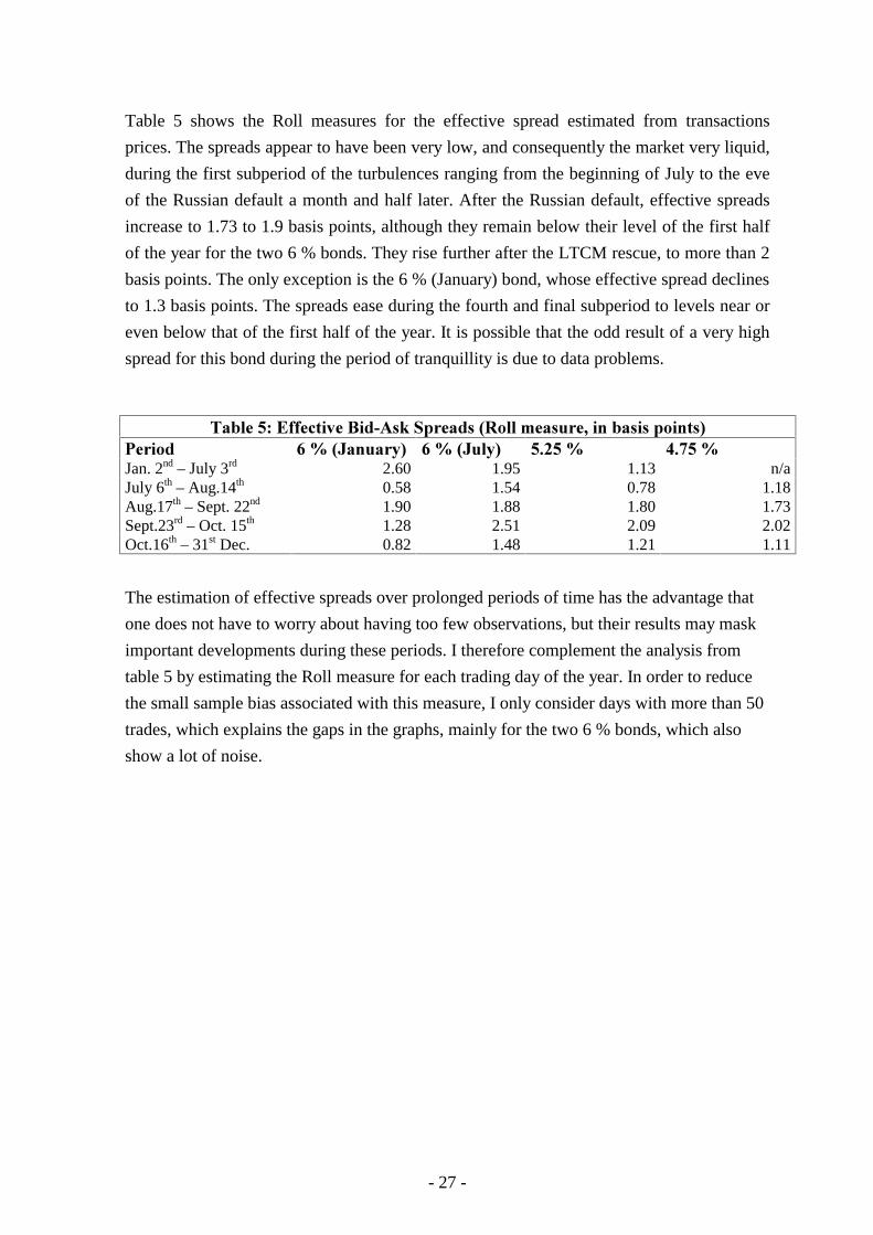
Table 5 shows the Roll measures for the effective spread estimated from transactions

prices. The spreads appear to have been very low, and consequently the market very liquid,

during the first subperiod of the turbulences ranging from the beginning of July to the eve

of the Russian default a month and half later. After the Russian default, effective spreads

increase to 1.73 to 1.9 basis points, although they remain below their level of the first half

of the year for the two 6 % bonds. They rise further after the LTCM rescue, to more than 2

basis points. The only exception is the 6 % (January) bond, whose effective spread declines

to 1.3 basis points. The spreads ease during the fourth and final subperiod to levels near or

even below that of the first half of the year. It is possible that the odd result of a very high

spread for this bond during the period of tranquillity is due to data problems.

!�"���1+�,����� ��0��26���%�����8;����&�����<����"���%���:=����� 3�7�89������: 3�7�89���: 1(*1�7 .(51�7Jan. 2nd – July 3rd 2.60 1.95 1.13 n/aJuly 6th – Aug.14th 0.58 1.54 0.78 1.18Aug.17th – Sept. 22nd 1.90 1.88 1.80 1.73Sept.23rd – Oct. 15th 1.28 2.51 2.09 2.02Oct.16th – 31st Dec. 0.82 1.48 1.21 1.11

The estimation of effective spreads over prolonged periods of time has the advantage that

one does not have to worry about having too few observations, but their results may mask

important developments during these periods. I therefore complement the analysis from

table 5 by estimating the Roll measure for each trading day of the year. In order to reduce

the small sample bias associated with this measure, I only consider days with more than 50

trades, which explains the gaps in the graphs, mainly for the two 6 % bonds, which also

show a lot of noise.

- 28 -

1 2 3 4 5 6 7 8 9 10 11120

1

2

3

4

5

6% (January)

Month 1 2 3 4 5 6 7 8 9 10 1112

0

1

2

3

4

5

6% (July)

Month

1 2 3 4 5 6 7 8 9 10 11120

1

2

3

4

5

5.25%

Month 1 2 3 4 5 6 7 8 9 10 1112

0

1

2

3

4

5

4.75%

Month

��������3� ���(��#���-���� ��4�''���� ���������112

(in basis points of yields)

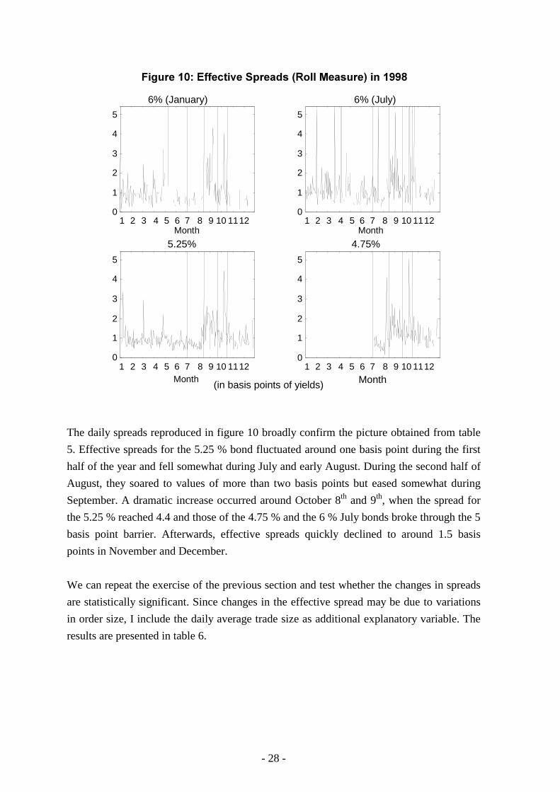
The daily spreads reproduced in figure 10 broadly confirm the picture obtained from table

5. Effective spreads for the 5.25 % bond fluctuated around one basis point during the first

half of the year and fell somewhat during July and early August. During the second half of

August, they soared to values of more than two basis points but eased somewhat during

September. A dramatic increase occurred around October 8th and 9th, when the spread for

the 5.25 % reached 4.4 and those of the 4.75 % and the 6 % July bonds broke through the 5

basis point barrier. Afterwards, effective spreads quickly declined to around 1.5 basis

points in November and December.

We can repeat the exercise of the previous section and test whether the changes in spreads

are statistically significant. Since changes in the effective spread may be due to variations

in order size, I include the daily average trade size as additional explanatory variable. The

results are presented in table 6.

- 29 -

!�"���3+�������,����� ���%������������������ �!��"������

3�7�89��(: 3�7�89���: 1(*1�7 .(51�7Expl. Variables D���������� **-1.294

(-1.77)0.114(0.31)

-0.206(-0.44)

-

D����������� -0.664(-0.88)

*0.584(1.35)

*0.754(1.54)

***0.461(3.51)

D������������ -1.069(-1.17)

**0.935(1.73)

*0.800(1.59)

***0.530(3.39)

D������������� *-1.531(-1.44)

0.635(1.08)

0.249(0.49)

-

DUHFHQW - -0.293(-0.24)

-0.165(-0.35)

-

Av.Trade Size *0.522(1.33)

**0.447(1.73)

0.065(0.70)

-0.010(-0.05)

# observations 250 250 249 124Dependent variable: Roll measure for the effective spread, normalised by their mean. T-values inbrackets. Dummies equal to 1 during indicated period and zero otherwise, dummy �������one if on-the-run and zero otherwise. Explanatory variables also include a constant and time trend. Newey-Westcorrection for autocorrelation and heteroscedasticity. Significant on *90%, **95%, ***99%confidence level

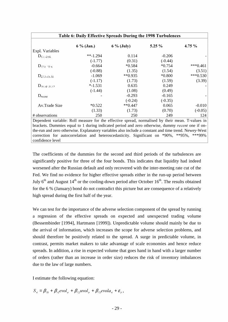
The coefficients of the dummies for the second and third periods of the turbulences are

significantly positive for three of the four bonds. This indicates that liquidity had indeed

worsened after the Russian default and only recovered with the inter-meeting rate cut of the

Fed. We find no evidence for higher effective spreads either in the run-up period between

July 6th and August 14th or the cooling-down period after October 16th. The results obtained

for the 6 % (January) bond do not contradict this picture but are consequence of a relatively

high spread during the first half of the year.

We can test for the importance of the adverse selection component of the spread by running

a regression of the effective spreads on expected and unexpected trading volume

(Bessembinder [1994], Hartmann [1999]). Unpredictable volume should mainly be due to

the arrival of information, which increases the scope for adverse selection problems, and

should therefore be positively related to the spread. A surge in predictable volume, in

contrast, permits market makers to take advantage of scale economies and hence reduce

spreads. In addition, a rise in expected volume that goes hand in hand with a larger number

of orders (rather than an increase in order size) reduces the risk of inventory imbalances

due to the law of large numbers.

I estimate the following equation:

LWLWLLWLLWLLLW����������! εββββ ++++= 3210 ,

- 30 -

where expected volume ����LW of bond ��is proxied with the (in-sample) fitted values from a

standard ARMA model25, and unexpected volume ����LW with the corresponding residuals.

In order to control for variations in the inventory holding costs, I control for the expected

price volatility �����LW, also obtained from an ARMA model. Since unexpected volume may

be determined by the bid-ask spread, we face a problem of endogeneity that could induce a

bias in our estimation results (Hartmann [1999]). Unfortunately, our dataset does not

contain any variable that is exogenous and could be used as an instrument for ����LW.26 We

therefore have to live with the endogeneity problem, although we have to interpret the

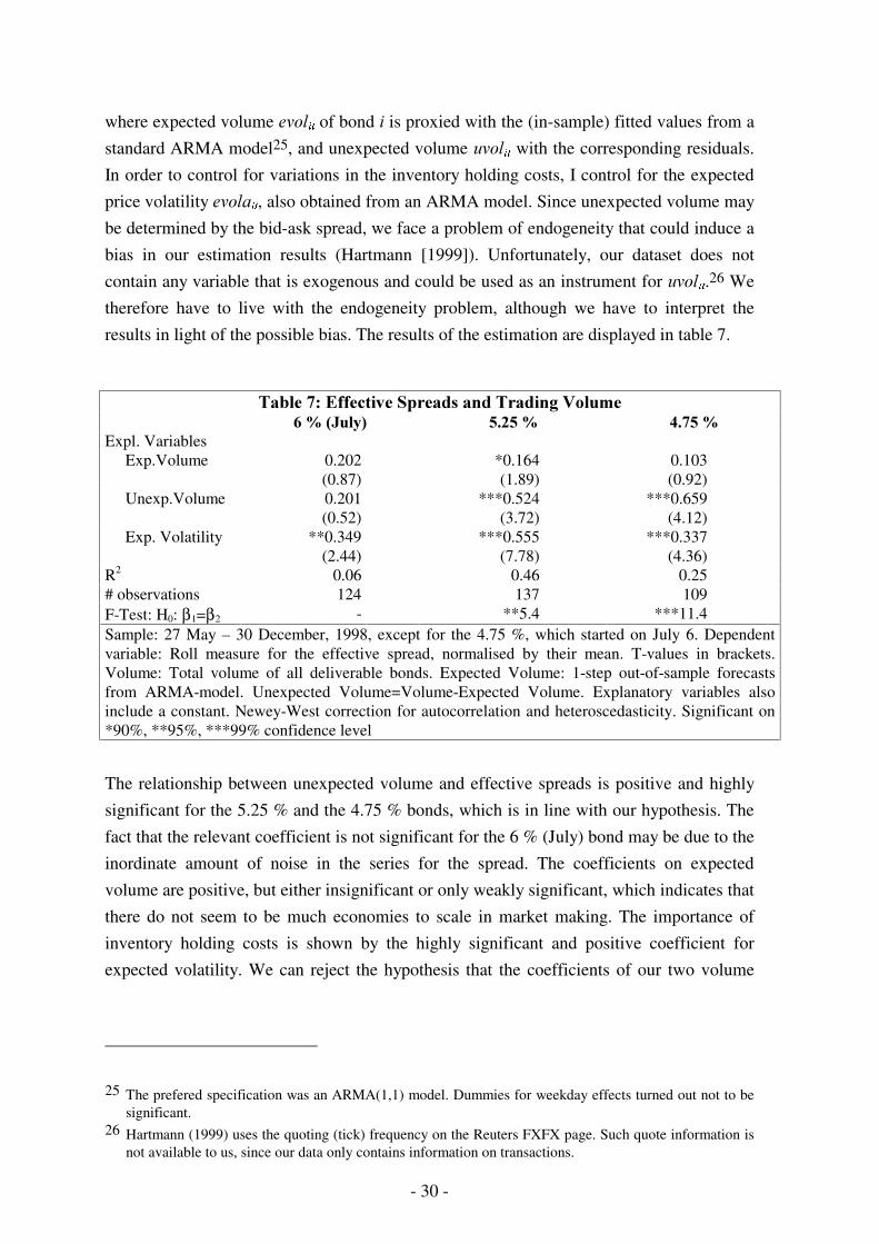
results in light of the possible bias. The results of the estimation are displayed in table 7.

������������ ������������������� ������������������� !" �� #!� ��

Expl. Variables Exp.Volume 0.202

(0.87)*0.164(1.89)

0.103(0.92)

Unexp.Volume 0.201(0.52)

***0.524(3.72)

***0.659(4.12)

Exp. Volatility **0.349(2.44)

***0.555(7.78)

***0.337(4.36)

R2 0.06 0.46 0.25# observations 124 137 109F-Test: H0: β1=β2 - **5.4 ***11.4Sample: 27 May – 30 December, 1998, except for the 4.75 %, which started on July 6. Dependentvariable: Roll measure for the effective spread, normalised by their mean. T-values in brackets.Volume: Total volume of all deliverable bonds. Expected Volume: 1-step out-of-sample forecastsfrom ARMA-model. Unexpected Volume=Volume-Expected Volume. Explanatory variables alsoinclude a constant. Newey-West correction for autocorrelation and heteroscedasticity. Significant on*90%, **95%, ***99% confidence level

The relationship between unexpected volume and effective spreads is positive and highly

significant for the 5.25 % and the 4.75 % bonds, which is in line with our hypothesis. The

fact that the relevant coefficient is not significant for the 6 % (July) bond may be due to the

inordinate amount of noise in the series for the spread. The coefficients on expected

volume are positive, but either insignificant or only weakly significant, which indicates that

there do not seem to be much economies to scale in market making. The importance of

inventory holding costs is shown by the highly significant and positive coefficient for

expected volatility. We can reject the hypothesis that the coefficients of our two volume

25 The prefered specification was an ARMA(1,1) model. Dummies for weekday effects turned out not to besignificant.

26 Hartmann (1999) uses the quoting (tick) frequency on the Reuters FXFX page. Such quote information isnot available to us, since our data only contains information on transactions.

- 31 -

measures are equal for two of the bonds, which is in accordance with the results obtained

for the forex market (see Hartmann [1999] and references therein).

1 2 3 4 5 6 7 8 9 10 11 12

0

2

4

6

Month

bps

5.25 %

1 2 3 4 5 6 7 8 9 10 11 12

0

2

4

6

Month

bps

4.75 %

������������� ��������������������������� �����

Effective Spread

Explained by unexpected volume

The strong statistical relationship between unexpected volume and bid-ask spreads cannot

explain the rise in the latter that occured from August to October. Figure 11 plots thespreads and the proportion that can be explained by unexpected volume (

LWL����2β ).

Spreads seem to be related to surprises in volume only in the very short run (a day) but not

over prolonged periods of time. When the effective bid-ask spreads surged after the

Russian devaluation and later during the uncertainty about the yen-carry-trades, unexpected

volume remained essentially flat. This is not consistent with the hypothesis that the fear of

adverse selection caused market makers to widen their spreads.

�!$!�% ��&��'��%����� � ����(��)��'��*

More generally, did market makers on average play a stabilising or a destabilising role

during the turbulences? In particular, did they buy when prices were falling and sell when

- 32 -

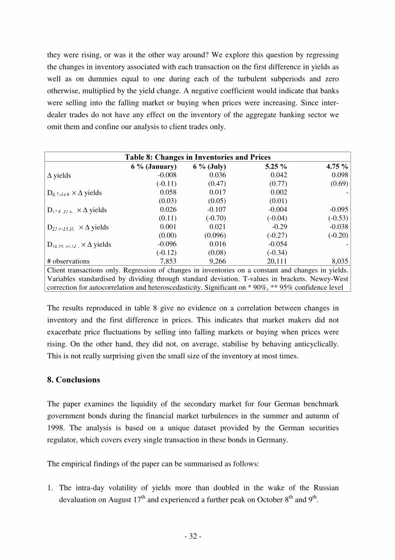
they were rising, or was it the other way around? We explore this question by regressing

the changes in inventory associated with each transaction on the first difference in yields as

well as on dummies equal to one during each of the turbulent subperiods and zero

otherwise, multiplied by the yield change. A negative coefficient would indicate that banks

were selling into the falling market or buying when prices were increasing. Since inter-

dealer trades do not have any effect on the inventory of the aggregate banking sector we

omit them and confine our analysis to client trades only.

������+��,(������ ��-������� �������.� ���������������� ���������� !" �� #!� ��

∆ yields -0.008(-0.11)

0.036(0.47)

0.042(0.77)

0.098(0.69)

D���������� × ∆ yields 0.058(0.03)

0.017(0.05)

0.002(0.01)

-

D������������� × ∆ yields 0.026(0.11)

-0.107(-0.70)

-0.004(-0.04)

-0.095(-0.53)

D�������������� × ∆ yields 0.001(0.00)

0.021(0.096)

-0.29(-0.27)

-0.038(-0.20)

D��������������� × ∆ yields -0.096(-0.12)

0.016(0.08)

-0.054(-0.34)

-

# observations 7,853 9,266 20,111 8,035Client transactions only. Regression of changes in inventories on a constant and changes in yields.Variables standardised by dividing through standard deviation. T-values in brackets. Newey-Westcorrection for autocorrelation and heteroscedasticity. Significant on * 90%, ** 95% confidence level

The results reproduced in table 8 give no evidence on a correlation between changes in

inventory and the first difference in prices. This indicates that market makers did not

exacerbate price fluctuations by selling into falling markets or buying when prices were

rising. On the other hand, they did not, on average, stabilise by behaving anticyclically.

This is not really surprising given the small size of the inventory at most times.

+!�,������ ���

The paper examines the liquidity of the secondary market for four German benchmark

government bonds during the financial market turbulences in the summer and autumn of

1998. The analysis is based on a unique dataset provided by the German securities

regulator, which covers every single transaction in these bonds in Germany.

The empirical findings of the paper can be summarised as follows:

1. The intra-day volatility of yields more than doubled in the wake of the Russian

devaluation on August 17th and experienced a further peak on October 8th and 9th.

- 33 -

2. The yield spread between the individual bonds of our sample soared from less than five

basis points during the first half of the year to more than twenty basis points in early

October. No equivalent breakdown in the pricing relationship can be found at daily or

hourly level, however. This indicates that the bonds remained close substitutes for

hedging purposes even during periods of stress.

3. The surge in volatility and the building up of the yield spread occurred at a time of

heavy trading activity. For three of the four bonds, both the number of trades and daily

turnover were statistically significantly higher between August 17th and October 15th

than during the first half of the year.

4. The effective bid-ask spreads (measured by Roll’s [1984] approach) on the two most

heavily traded bonds increased from just over one basis point to 1.8 basis points after

the Russian de-facto default on August 17th, and rose above two basis points after the

LTCM rescue operation. They peaked around October 8th and 9th at around five basis

points. This rise is statistically significant even after controlling for changes in the

average transaction size.

5. Effective bid-ask spreads are positively related to unexpected trading volume, which

should reflect the amount of private information in the market. Nevertheless, surprises

volume cannot explain the surge in spreads that occurred during the turbulences.

How does this answer our initial question on "how did the ‘safe-haven’ weather the

storm”? The finding that the effective spread increased considerably during the turbulences

clearly indicates that the market suffered from a reduction in liquidity. This result is even

more clear cut if we consider that our estimates for the effective spread based on the Roll

[1984] measure are downward biased in the presence of inventory control and adverse

selection effects, which are likely to be important particularly in times of great volatility.

Nevertheless, while agents may have faced a higher cost of trading, they were still able to

trade. Our data does not tell us whether individual agents were able to turn over their

position as quickly as they would have liked, but the fact that the market has been able to

sustain a significantly higher than normal number of trades and volume suggests that such

problems were not widespread, if they occurred at all. In this sense, liquidity provision has

been remarkably effective in dealing with the turbulences, especially when seen in contrast

to what happened in the US bond market.

Apart from the issue of financial stability, I mentioned two other reasons for why a central

bank should monitor the liquidity in the secondary market for government bonds: the

- 34 -

quality of indicators and the borrowing costs of government. Indicator quality clearly

suffers if it becomes more costly to trade. Hence our findings provide further evidence for

the already widely known fact that indicators are the least likely to be accurate at times

when they are most needed.

The present paper considers only a small, albeit important, segment of the market. It would

be interesting to extend the analysis to a) the futures market, which is far more active than

the spot market, and b) bonds from other issuers. It would also be of interest to compute a

measure of liquidity that is more robust to the presence of inventory control and adverse

selection effects than the Roll measure. Both extensions are left for future work.

- 35 -

�(�;��������

Amihud, Y. & H. Mendelson (1991) "Liquidity, Maturity and the Yields on U.S. Treasury

Securities", "���������#������, 66: 1411-25

Andersen, T.G. , T. Bollerslev, F.X. Diebold & P. Labys (1999) "The Distribution of

Exchange Rate Volatility", $�%&����'����������()(*

Bagehot, W. [pseud.] (1971) "The Only Game in Town", #����������� ��"�����, 27:

12-4

Bank for International Settlements (1999a) "International Banking and Financial Markets

Developments", ��+!�,������ �&����-, March

Bank for International Settlements (1999b) .��'��� /������� 0� &������� #������� ���

!����������� � +���������, Report of a Study Group established by the Committee

on the Global Financial System of the central banks of the Group of Ten countries,

May

Bank for International Settlements (1999c) �� &����-� ��� #�������� .��'��� %����� ��

�������*))1, Committee on the Global Financial System , October

Bessembinder, H. (1994) "Bid-Ask Spreads in the Interbank Foreing Exchange Markets",

"���������#��������%�������, 35: 317-48

Brady, N. (1989) &������������������������2�'�#��������.��'���.�������, January,

Washington, D.C.: Government Printing Office Choi, J.Y., D. Salandro & K. Shastri

(1988) "On the Estimation of Bid-Ask Spreads: Theory and Evidence", "������ ��

#������������,��������������� �, 23(2): 245-69

Davis, E.P. (1999) "A Reappraisal of Market Liquidity Risk in the Light of the

Russia/LTCM Global Securities Market Crisis", Paper presented to the workshop on

"Empirical Research on bank supervision and Structure", Bank for International

Settlements, June 1999

Deutsche Bundesbank (1998) .���� �&�����, December

- 36 -

Glosten, L. & P. Milgrom (1985) "Bid, Ask, and Transaction Prices in a Specialist Market

with Heterogeneously Informed Traders", "���������#��������%�������, 13: 71-100

Hartmann, P.(1999) "Trading Volumes and Transaction Costs in the Foreign Exchange

Market: Evidence from Daily Dollar-Yen Spot Data", "������������'��������#������,

23: 801-24

Hasbrouck, J. (1991) "Measuring the Information Content of Stock Trades", "������ ��

#������, 46: 178-208

Ho, T. & H.R. Stoll (1981) "Optimal Dealer Pricing under Transactions and Return

Uncertainty", "���������#��������%�������, 9: 47-73

Ho, T. & H. Stoll (1983) "The Dynamics of Dealer Markets under Competition", "�����

���#������, 38: 1053-74

Huang, R.D. & H.R. Stoll (1997) "The Components of the Bid-Ask Spread: A General

Approach", &����-����#��������!�����310(4):

International Monetary Fund (1998) �����%��������4����'� ���� +������������������

.��'���+�������������, December

Kyle, A.S. (1985) "Continuous Auctions and Insider Trading", %�����������, 53(6): 1315-

35

Longstaff, F.A. (1995) "How Much Can Marketability Affect Security Values?", "��������

#������, 50(5): 1767-74

Madhavan, A. (1992) "Trading Mechanisms in Securities Markets", "������ ��� #������,

47: 607-42

O’Hara, M. (1995) .��'���.�������������2���� , Cambridge MA & Oxford: Blackwell

O’Hara, M. & G. Oldfield (1986) "The Microeconomics of Market Marking", "��������

#������������,��������������� �3 21, December: 361-76

Proudman, J. (1995) "The Microstructure of the UK Gilt Market", Bank of England,

���'����������51

- 37 -

Roll, R. (1984) "A Simple Implicit Measure of the Effective Bid-Ask Spread in an

Efficient Market", "���������#������, 39: 1127-40

Stoll, H.R. (1989) "Inferring the Components of the Bid-Ask Spread: Theory and Empirical

Tests", "���������#������, 44(1): 115-34

Vitale, P. (1998) "Two Months in the Life of Several Gilt-Edged Market Makers on the

London Stock Exchange", "���������+������������#��������.��'��3�+�������������

.��� 3�10�6))�567

- 38 -

������������� ������ ������� ���������������

May 1995 The Circulation of

Deutsche Mark Abroad Franz Seitz

June 1995 Methodology and technique

for determining structural

budget deficits Gerhard Ziebarth

July 1995 The information content of derivatives

for monetary policy – Implied vola-

tilities and probabilities Holger Neuhaus

August 1995 Das Produktionspotential

in Ostdeutschland * Thomas Westermann

January 1996 Sectoral Disaggregation

of German M3 Vicky Read

March 1996 Monetary aggregates with special

reference to structural changes in the

financial markets Michael Scharnagl

March 1996 The impact of interest rates on

private consumption in Germany Hermann-Josef Hansen

May 1996 Market Reaction to Changes

in German Official Interest Rates Daniel C. Hardy

May 1996 The role of wealth

in money demand Dieter Gerdesmeier

� Available in German only.

- 39 -

August 1996 Intergenerational redistribution through

the public sector – Methodology of

generational accounting and its empirical

application to Germany Stephan Boll

August 1996 The impact of the exchange rate

on Germany’s balance of trade Jörg Clostermann

October 1996 Alternative specifications of the

German term structure and its informa-

tion content regarding inflation Sebastian T. Schich

November 1996 Enterprises’ financing structure and their

response to monetary policy stimuli

An analysis based on the Deutsche Bundes-

bank’s corporate balance sheet statistics Elmar Stöss

January 1997 Reserve Requirements

and Economic Stabilization Ulrich Bindseil

June 1997 Direct investment

and Germany as a business location Thomas Jost

July 1997 Price Stability versus

Low Inflation in Germany Karl-Heinz Tödter

An Analysis of Costs and Benefits Gerhard Ziebarth

October 1997 Estimating the German

term structure Sebastian T. Schich

October 1997 Inflation and Output in Germany:

The Role of Inflation Expectations Jürgen Reckwerth

- 40 -

February 1998 Problems of

Inflation Measurement in Germany Johannes Hoffmann

March 1998 Intertemporal Effects

of Fiscal Policy

in an RBC-Model Günter Coenen

September 1998 Macroeconomic determinants

of currency turbulences

in emerging markets Bernd Schnatz

January 1999 Die Geldmenge und ihre bilanziellen

Gegenposten: Ein Vergleich zwischen

wichtigen Ländern der Europäischen

Währungsunion * Dimut Lang

February 1999 Die Kapitalmarktzinsen in Deutschland

und den USA: Wie eng ist der Zinsverbund?

Eine Anwendung der multivariaten

Kointegrationsanalyse * Manfred Kremer

April 1999 Zur Diskussion über den Verbraucher-

preisindex als Inflationsindikator –

Beiträge zu einem Workshop in der

Deutschen Bundesbank *

July 1999 Monitoring Fiscal Adjustments

in the European Union and EMU Rolf Strauch

October 1999 Cyber money as a medium of exchange Gabriele Kabelac

� Available in German only.

- 41 -

December 1999 Implicit Government Guarantees

and Bank Herding Behavior Rasmus Rüffer

December 1999 Implications of the new sesonal

adjustment method Census

X-12-ARIMA for current

economic analysis in Germany Robert Kirchner

February 2000 How Save Was the “Safe Haven“?

Financial Market Liquidity during

the 1998 Turbulences Christian Upper