This article appeared in a journal published by Elsevier. The attachedcopy is furnished to the author for internal non-commercial researchand education use, including for instruction at the authors institution

and sharing with colleagues.

Other uses, including reproduction and distribution, or selling orlicensing copies, or posting to personal, institutional or third party

websites are prohibited.

In most cases authors are permitted to post their version of thearticle (e.g. in Word or Tex form) to their personal website orinstitutional repository. Authors requiring further information

regarding Elsevier’s archiving and manuscript policies areencouraged to visit:

http://www.elsevier.com/copyright

Author's personal copy

How much influence does landscape-scale physiography have on air temperaturein a mountain environment?

Solomon Z. Dobrowski a,*, John T. Abatzoglou b, Jonathan A. Greenberg c, S.G. Schladow d

a Department of Forest Management, University of Montana, Missoula, MT, United Statesb Department of Geography, University of Idaho, Moscow, ID, United Statesc Center for Spatial Technologies and Remote Sensing, University of California, Davis, Davis, CA, United Statesd Tahoe Environmental Research Center, University of California, Davis, Davis, CA, United States

1. Introduction

1.1. Overview

Air temperature is arguably the single most importantcomponent of mountain climate (Barry, 1992; Lookingbill andUrban, 2003), influencing a broad range of ecosystem processesincluding, evapotranspiration, photosynthesis, respiration, decom-position, and carbon fixation, among others (Coughlan andRunning, 1997; Running et al., 1987). Through these processes,

temperature affects vegetation dynamics and the distribution ofbiota in space and time. Consequently, temperature shifts and theirconcomitant ecological effects are increasingly a focal point ofclimate change impact assessment studies and resource decision-making processes (Millar et al., 2007).

Given critical temperature thresholds for many ecological andhydrologic processes [e.g. snow melt, degree-day accumulation,bud burst, frost tolerance (Cayan et al., 2001; Gutschick andBassirRad, 2003; Inouye, 2000; Saxe et al., 2001; Stewart et al.,2004)], it is vital to be able to accurately represent temperatureacross the landscape both today, and under future climatescenarios. Modeling of temperature fields is conducted using amultitude of approaches varying from simple linear transforms ofelevation to mechanistic approaches. Datasets and modeling

Agricultural and Forest Meteorology 149 (2009) 1751–1758

A R T I C L E I N F O

Article history:

Received 26 February 2009

Received in revised form 2 June 2009

Accepted 8 June 2009

Keywords:

Temperature modeling

Terrain analysis

Lapse rate

Physiography

Lake Tahoe

Mountain climate

A B S T R A C T

Spatio-temporal patterns of temperature in mountain environments are complex due to both regional

synoptic-scale and landscape-scale physiographic controls in these systems. Understanding the nature

and magnitude of these physiographic effects has practical and theoretical implications for the

development of temperature datasets used in ecosystem assessment and climate change impact studies

in regions of complex terrain. This study attempts to quantify the absolute and relative influence of

landscape-scale physiographic factors in mediating regional temperatures and assess how these

influences vary in time. Our approach was to decompose the variance in in situ temperature

measurements into components associated with regional free-air temperature estimates and local

physiographic effects. Near-surface air temperature data, collected between 1995 and 2006 from 16

meteorological stations in the Lake Tahoe region of California, USA were regressed against free-air

temperature (North American Regional Reanalysis dataset) for the same period. Residuals from this fit

represent spatial deviations from the regional mean and were modeled as a function of physiographic

position on the landscape using variables derived from terrain analysis techniques. Linear models

relating temperature residuals to physiographic variables explained roughly 10–90% of the variance in

temperature residuals and had root mean squared error of 1.2–2.0 8C, depending upon the type of

measurement and time of year. Results demonstrate that: (1) regional temperature patterns were the

principle driver of surface temperatures explaining roughly 70–80% of the variance in in situ

measurements; (2) the remaining variance was largely explained by spatial variability in landscape-

scale physiographic variables; (3) the influence of physiographic drivers varied seasonally and was

influenced by regional conditions. Periods of well-mixed atmospheric conditions lend themselves to the

use of simple elevation-based lapse rate models for temperature estimation whereas other

physiographic effects become more prominent during periods of enhanced atmospheric stability;

and lastly (4) small differences in temperature due to landscape position, when integrated over time, can

have a prominent effect on water balance and thus hydrologic and ecologic processes.

� 2009 Elsevier B.V. All rights reserved.

* Corresponding author.

E-mail address: solomon.dobrowski@cfc.umt.edu (S.Z. Dobrowski).

Contents lists available at ScienceDirect

Agricultural and Forest Meteorology

journal homepage: www.e lsev ier .com/ locate /agr formet

0168-1923/$ – see front matter � 2009 Elsevier B.V. All rights reserved.

doi:10.1016/j.agrformet.2009.06.006

Author's personal copy

approaches have assumptions, inherent spatial and temporalresolutions and domains, as well as strengths and weaknesseswhen applied to specific applications (Beniston et al., 1997; Daly,2006). In particular, the adequacy of a given dataset becomesincreasingly uncertain as spatial resolution becomes finer andterrain becomes more complex (Daly, 2006; Lookingbill and Urban,2003).

Spatio-temporal patterns of temperature in mountain environ-ments are particularly complex due to both regional andlandscape-scale physiographic controls in these systems. Byregional controls, we are referring to the combined influence ofdaily synoptic-scale circulation patterns and large-scale physio-graphic features such as proximity to oceans, and latitudinalposition. This is in contrast to landscape-scale influences ontemperature which are mediated by fine-scale physiographicfeatures resolved at the scale of individual watersheds. Theseinclude elevation, slope and aspect effects on solar insolation,topographic convergence, and others. Much work has highlightedthe influence of regional-scale physiography on climate patterns(Daly, 2006; Daly et al., 2008). Similarly, landscape-scale studieshave highlighted the influence of local physiography on tempera-ture patterns (Chung et al., 2002; Chung and Yun, 2004; Lookingbilland Urban, 2003). There has been less work that tries to link thetwo by quantifying the proportion of the spatial and temporalvariance in temperature that can be attributed to local vs. regionaldrivers, and how these influences vary in time. To these ends, weask a basic yet fundamental question: How much influence does

landscape-scale physiography have on air temperature? If thesephysiographic effects are large, then failing to account for themwill result in a discrepancy between the scale of support of in situ

ecological data and climate data used in a given analysis. Incontrast, if these physiographic effects are small, then coarser-scaled climate data should adequately characterize local condi-tions and prove useful in ecological studies.

1.2. Topoclimate

Topoclimatic modeling refers to spatial estimates of climatethat take into account topographic position in the landscape(Lookingbill and Urban, 2003). Physiographic factors such aselevation, slope, aspect, and landscape position influence meteor-ological elements such as air temperature, precipitation, wind,solar insolation, evapotranspiration, surface flow, snow accumula-tion and melt, among others (Coughlan and Running, 1997;Thornthwaite, 1953; Weiss et al., 1988). Primary topoclimaticeffects include the influence of elevation, hillslope angle andaspect, while secondary effects include terrain effects on windsand cold-air drainage (Barry, 1992; Bolstad et al., 1998). There havebeen notable efforts at modeling topoclimatic effects. For example,at the watershed scale Lookingbill and Urban (2003) and Chunget al. (2002) showed that minimum temperature estimates couldbe improved by using distance to streams and flow accumulationas predictor variables to capture the effect of cold-air drainage. Atregional scales, the Parameter-elevation Regression on Indepen-dent Slopes Model [PRISM—(Daly et al., 2008)] uses a two-layeratmospheric model to stratify stations into those below and aboveinversion layers. Additionally, modeled estimates of solar insola-tion have been used effectively as predictors in estimatingtemperature in complex terrain (Chung and Yun, 2004; Lookingbilland Urban, 2003). Many of these landscape-scale studies haverelied on the use of dense networks of portable micro-loggers. Theavailability of these sensors has provided valuable insights intofine-scale spatial variability in temperature but they also tend tolimit analysis periods to short temporal extents [e.g. Julytemperatures—(Lookingbill and Urban, 2003)] which can obscurelinkages between local temperature patterns and regional drivers.

1.3. Objectives

The primary goal of this study is to quantify the absolute andrelative influence of landscape-scale physiographic factors on airtemperature in an area of complex terrain. Topoclimatic effectsoperate against a backdrop of regional circulation patterns thatvary in time. Hence, a second objective is to examine how theinfluence of local physiography varies temporally. Understandingthe nature and magnitude of these physiographic effects haspractical and theoretical implications for the development oftemperature datasets used in ecosystem assessment and climatechange impact studies in regions of complex terrain.

2. Methods

2.1. Study area

The Lake Tahoe region spans both states of California andNevada, USA between the Carson and Sierra Nevada mountainranges (Fig. 1). The total land area in our study area isapproximately 2752 km2 (273,000 ha). The region is ideally suitedfor this type of research given its diverse physiography, and thepresence of a dense network of long-term meteorological stations.The elevation of the region ranges between 1500 m (a.s.l.) to3400 m (a.s.l.) at the highest peaks. The mean winter temperatureat lake level is �6 8C; the mean summer temperature is 24 8C.Annual precipitation ranges from 500 to 1500 mm depending onelevation and location, two-thirds of which falls betweenDecember and March as snow (Rogers, 1974). The majority ofthe region spans the montane and subalpine elevation ranges.Vegetation types are diverse and include conifer dominatedforests, both evergreen and deciduous shrublands, as well asdiverse meadow and fen habitats.

2.2. Data

Daily near-surface (2 m) temperature means, minima, andmaximums were acquired from 16 permanent meteorologicalstations (14 SNOTEL sites, National Resource Conservation Service;2 National Weather Service’s Cooperative Observer Program sites;Fig. 1). The period of record for the stations varied. For 12 of thesites, a continuous 11-year series was extracted between 1995 and2006 whereas the remaining stations had a 4-year record (2003–2006). Subsequent analysis was conducted on monthly climatenormals (see below); thus, we assume that potential biasintroduced by inter-annual variability in station records will occurindependent of station physiographic setting (the focus of thisstudy). Extreme outliers were screened by identifying observationsthat were >3 standard deviations from the means of allobservations across all sites. Topographic data used in the analysiswas derived from a 30 m USGS digital elevation model (DEM).

2.3. Decomposing temperature variance into synoptic and local effects

Our overall approach is to decompose the variance in in situ

temperature measurements into components associated withregional free-air temperature and local physiographic effects.

We employ the following general model (Lundquist et al.,2008):

Tðx;y;tÞ ¼ T 0ðtÞ þ T̃ðx;y;tÞ þ e (1)

where T(x, y, t) is the temperature (min, max, average) at a givenlocation x, y over a time basis t; T 0ðtÞ is the regional free-airtemperature over time basis t within the study domain (principallycapturing fluctuations associated with seasonal and synoptic

S.Z. Dobrowski et al. / Agricultural and Forest Meteorology 149 (2009) 1751–17581752

Author's personal copy

weather effects); T̃ðx;y;tÞ are local spatial deviations driven bytopoclimatic effects that vary with time, and e is instrument andmodel error.

The first term in Eq. (1) accounts for temporal fluctuations inregional-scale temperatures. We characterize T 0ðtÞ using free-airestimates from the North American Regional Reanalysis (NARR)dataset. NARR provides model ‘‘observations’’ of temperature byassimilating observations from radiosondes and satellites toprovide high temporal (3 h) and coarse spatial (32 km) resolutiondata (Mesinger et al., 2006). As free-air temperature lapse ratesmay depart significantly from near-surface lapse rates within theboundary layer (Harlow et al., 2004), we consider free-airtemperatures to provide an independent dataset for the analysisof surface observations. For the study area of interest, a single datapoint from NARR encompasses the entire domain. Daily averaged(8� daily) free-air temperatures were further interpolated to afixed elevation of 2200 m, the median elevation of the stations.

To decompose the influence of local topoclimatic effects fromregional-scale control, we first regressed daily temperatureobservations of average temperature (Tavg), minimum temperature(Tmin), and maximum temperature (Tmax) at all sites against thecorresponding daily free-air temperature for the region (Fig. 3). Theresiduals of this fit represent unexplained variance in observedtemperature not accounted for by the regional-scale predictor.These residuals can be attributed to the second and third terms ofEq. (1); the first of which characterizes spatial deviations from theregional mean that are a function of physiographic position on thelandscape:

T̃ðx;y;tÞ ¼ f ðZðx;yÞ þ Iðx;yÞ þ Cðx;yÞÞ (2)

where Z(x, y) is the elevation at location x, y; I(x, y), is the meanannual daily clear sky irradiance at location x, y. This represents the

effects of slope and aspect on the amount of irradiance of a surfaceby considering hillshading effects caused by variations in solarangle, ground slope, and aspect, as well as shadowing effects ofadjacent topographic features. Clear sky irradiance (MJ m�2 day�1)was computed at a 30 m spatial resolution and a daily time stepusing the r.sun algorithm (Hofierka and Suri, 2002) running underGRASS GIS 6.1 (GRASS Development Team 2005).

C(x, y) is a measure of topographic convergence and is a proxy oflocal convective forcings, specifically cold-air drainage at locationx, y. C(x, y) is represented by the topographic convergence index (tci)for cell (x, y) and was calculated as ln(a/tan u) where a is theupslope watershed area flowing through cell (x, y) and u is thehillslope angle of the cell (Wolock and McCabe, 1995). tci values areunitless and ranged from 1 to 20 with high tci values representingconvergent environments such as concave surfaces at the base ofhillslopes and with low tci values representing less convergentenvironments such as ridge tops. We assume that cold, dense airmasses will act in a manner similar to surface water andaccumulate in areas with high tci values under stable atmosphericconditions.

We estimated the spatial anomalies described in Eq. (2) usingboth linear (LM) and linear mixed effects models (LME) that relatetemperature residuals to the physiographic predictors describedabove. For LME models, a separate model was fit to daily datasubset by month. Physiographic predictors were treated as fixedeffects. Station ID was treated as a random effect. For LM models, aseparate model was fit to data subset by month and aggregated tomonthly climate normals (i.e. 16 sites by 12 months for 192observations). For each monthly model, we examined parameterestimates and effect tests (t-test) over time. Parameter estimatesand effect tests were nearly identical between the LME and LMapproaches. Consequently, we opted to use the LM approach givenits simplicity.

Analysis of variance (ANOVA) was used with each LM model topartition variance explained by each of the model terms and theresidual error (e; Eq. (1)). The proportion of the variance explainedby each model term was calculated by dividing the sum of squaresattributed to each term by the total sum of squares across allterms.

Model validation was conducted using general cross-validation.Data from a single meteorological station was withheld from thetraining data, LM models were fit using a step-wise modelselection procedure based on the Aikaki information criterion(AIC), and selected model predictions were compared againstmeasured temperature residuals. Root mean squared error (RMSE)was calculated. This procedure was repeated for each of the 16stations and the average RMSE across all folds (k = 16) wasdetermined. All statistical analysis was conducted using R (R

Foundation for Statistical Computing).

3. Results

The 16 meteorological stations span a broad range of elevations,exposures, and landscape positions (Fig. 2). Elevation for thestation sites varied from approximately 1800 to 2680 m, topo-graphic convergence values varied from roughly 2 to 12, meanclear sky irradiance estimates varied from approximately 20–28 MJ m�2 day�1.

3.1. Station temperature vs. free-air

The relationship between station temperature measurementsand free-air estimates is summarized in Fig. 3. The percentage ofthe variance in measured temperature explained by free-airestimates (R2) was 82%, 70%, and 80% for Tavg, Tmin, and Tmax,respectively. The residuals for Tavg, Tmin and Tmax appeared

Fig. 1. Location of study site and 16 meteorological stations used in the analysis.

S.Z. Dobrowski et al. / Agricultural and Forest Meteorology 149 (2009) 1751–1758 1753

Author's personal copy

normally distributed based on examinations of normal-quantileplots.

3.2. Deviations explained by physiography

LM models relating temperature residuals to physiographicvariables explained roughly 10–90% (adjusted R2 values) of thevariance in temperature residuals (Fig. 4). RMSE estimates forthese models ranged from 1.2 to 2.0 8C, depending upon the typeof temperature measurement and time of year (Fig. 4). For Tavg,the highest R2 values and inversely, the lowest error, occurredduring the spring months. Similarly, minimum temperature R2

values were highest during the spring months and lowest duringthe fall. Maximum temperature R2 values were greatest duringthe summer months and decreased sharply during the wintermonths.

Tavg, Tmin, and Tmax temperature residuals show varyingtemporal sensitivity to physiographic drivers. Regression coeffi-cients for each predictor variable and associated effect test resultsare shown in Fig. 5. Average temperature residuals decreased withincreasing elevation and topographic convergence, and increasedwith increasing clear sky irradiance. These results reveal thatcooler conditions prevail in areas of high topographic convergenceunder the influence of cold-air drainage, at high elevations given asteep lapse rate, and in shaded areas in the presence of lowerinsolation.

While such results are consistent with expectation, we furthershow that the influence of these variables varies significantly overthe course of the year. For instance, Tavg showed a greatersensitivity (larger negative values) to elevation (lapse rate) duringthe spring months as compared to the winter months. The meanmonthly environmental lapse rate for Tavg was 5.3 8C km�1, withthe steepest lapse rates in late spring (6.5 8C km�1) and theshallowest lapse rates in winter (3.9 8C km�1). Additionally, theinfluence of topographic convergence and irradiance on Tavg waspredominantly limited to the winter months. Elevation lapse ratesfor Tmin deviations were steepest in March and April and werenegligible in summer and fall. In contrast, topographic conver-gence had influence on Tmin over most of the year, the effect beingmost pronounced in July and August. Irradiance had little influenceon Tmin deviations. Maximum temperature deviations showedsensitivity to elevation and no other physiographic variable. Lapserates for Tmax were steepest during the summer months andshallowest during the winter months.

3.3. Variance decomposed by model terms

We further partitioned the variance in temperature residualsby each of the physiographic predictors and error terms (Fig. 6).Elevation explained the majority of the residual variancefor Tavg and Tmax. In contrast, elevation explained little of theresidual variance in Tmin. tci was the strongest predictor for

Fig. 2. Summary of physiographic variables for 16 meteorological stations found within the study area.

Fig. 3. Daily in situ temperature measurements (for average, minimum, and maximum temperatures between 1995 and 2006) by daily free-air temperature estimates over

the same period. The solid line represents a simple linear regression fit. Residuals of the fits are used in subsequent analysis.

S.Z. Dobrowski et al. / Agricultural and Forest Meteorology 149 (2009) 1751–17581754

Author's personal copy

minimum temperature exerting influence over most of theyear. tci also explained a moderate amount of the residualvariance in average temperature, the values being the greatest inthe fall and winter months. Clear sky irradiance had limitedinfluence on the residual variance for average temperatures, theeffect being limited to the winter months. The remainingunaccounted for variance was attributed to error and variedseasonally between 10–20% for Tavg, 40–70% for Tmin, and10–40% for Tmax.

4. Discussion

4.1. Spatial and temporal variance in temperature

Temporal variability in regional conditions (i.e. free-airtemperature) is the primary driver of temperatures for thestations in our study area. The combined influence of regional-scale climate and synoptic-scale weather from daily free-airtemperatures explained 70–80% of the variability in in situ

temperature measurements. Free-air temperatures alone lackthe ability to describe spatio-temporal temperature patterns onboth weather timescales and climate timescales (Pepin andLosleben, 2002; Pepin and Norris, 2005; Pepin and Seidel, 2005).Differences between free-air temperatures and surface observa-tions accounted for 20–30% of the total temperature variance.These differences can principally be attributed to spatialvariance in physiographic features. This finding provides anempirical basis for estimating the maximum amount of

temperature variance that can be attributed to local physio-graphy of the landscape. Given the magnitude of temporalvariance in temperature due to seasonality and weather(approximately 60 8C), spatial variance of 20–30% is a sub-stantive figure.

4.2. Elevation as a predictor of temperature

The use of elevation as a surrogate for temperature iswidespread. Elevation-based lapse rates within our models differsubstantially from the standard atmosphere environmental lapserate of 6.5 8C km�1, varying between being close to the dry-adiabatic lapse rate (9.8 8C km�1) for summer maximum tem-peratures, and isothermal (0 8C km�1) for minimum temperatures.Significant diurnal and seasonal differences in environmental lapserates limit their utility in estimating temperatures (Blandford et al.,2008). Moreover, our findings demonstrate that the explanatorypower of elevation varies substantially over the course of the year.For average temperature, elevation explains the majority of thespatial variability in temperature residuals during the springmonths but its explanatory power drops sharply in the summer,fall, and winter months. For minimum temperatures, elevation haslittle explanatory power during most of the year (except thespring) due to the prevalence of temperature inversions. Ananalysis by the authors (Dobrowski et al., 2007) of dailyenvironmental lapse rates for the region showed that minimumtemperature lapse rates were positive in 37% of the dailyobservations within the study period primarily during thesummer, fall and to a lesser extent, winter months. This value isconsistent with other estimates of inversion frequency found inmountainous regions globally (Bolstad et al., 1998; Iijima andShinoda, 2000).

4.3. Secondary topoclimatic effects

Secondary topoclimatic effects are prevalent during periodsof the year that elevation loses its explanatory power. Forexample, convergent areas (high tci values) tend to have morenegative residuals given that these landscape positions supportthe formation and maintenance of cold-air pools (Colette et al.,2003; Whiteman, 1982; Whiteman et al., 2004). Similar resultshave been demonstrated empirically by other investigators(Chung et al., 2002; Lookingbill and Urban, 2003). Our resultsexpand on this and show that the effect of topographicconvergence varies temporally becoming increasingly importantduring periods of enhanced atmospheric stability during thesummer, fall, and winter months. These are periods of theyear in which regional weather patterns in the western USpromote cold-air pool formation (Lundquist and Cayan, 2007;Lundquist et al., 2008). Similarly, solar insolation has beenshown to exert a positive influence on measured temperatures(Chung and Yun, 2004). Our results suggest that the radiationeffect is principally relegated to the winter months. Low solarzenith angles during winter months tend to accentuatedifferences in solar insolation experienced on varying slopefacets whereas high solar angles, terrain winds, and boundary-layer mixing during the summer months will tend to diminishsensible temperature differences. However, our meteorologicalstation sites do not span a large gradient in irradiance values.SNOTEL stations are placed in areas that are representative ofthe water producing regions of a watershed as well as beingaccessible and protected. Consequently, sites are generallylocated on slopes void of strong aspect differences. This willtend to diminish strong radiation gradients between sites, thuspotentially explaining why radiation had a minimal impact onthe results presented.

Fig. 4. Proportion of variance explained (R2) and cross-validated estimates of

root mean squared error (RMSE) for linear models relating temperature

residuals to physiographic variables. Points represent values from separate

models fit to monthly normals. Lines are produced using a smoothing spline

(df = 6).

S.Z. Dobrowski et al. / Agricultural and Forest Meteorology 149 (2009) 1751–1758 1755

Author's personal copy

Fig. 5. Summary of regression coefficients for monthly models relating temperature residuals to physiographic variables. Results for average temperature, minimum

temperature, and maximum temperature are displayed in rows 1, 2, and 3, respectively. Starred symbols denote months with significant (t-test; p < 0.05) effect tests. The

smoothed lines are fitted using a smoothing spline (df = 6).

Fig. 6. Proportion of residual variance explained by each model term (including an error term). Model parameters are described in Fig. 5. Lines are produced using a smoothing

spline (df = 6).

S.Z. Dobrowski et al. / Agricultural and Forest Meteorology 149 (2009) 1751–17581756

Author's personal copy

4.4. Topoclimate and spatial scale

Climate datasets used operationally often do not utilize, or donot resolve many terrain-based predictors of climate (Daly, 2006).A noted consequence of this it that there is often a disparitybetween the scale of many climate modeling efforts, and thebiological scale at which montane organisms experience theirenvironment. For example, modeling in climate change scienceusing regional climate models (RCMs) and global climate models(GCMs) is conducted at scales of tens to hundreds of kilometers,while plants in mountainous regions experience their environmentat a much finer scale (Urban et al., 2000). GCMs and RCMs are morelikely to accurately simulate free-air temperatures than surfacetemperatures. The inability of these models to directly simulatefeatures in the boundary layer (instead relying on parameteriza-tion techniques) is problematic when trying to directly use suchoutputs in a real world context. These discrepancies becomeincreasingly important in the presence of terrain features, assurface temperatures are often decoupled from free-air tempera-tures (Grotch and MacCracken, 1991; Pepin and Seidel, 2005).Decoupling such as this is present not only on daily timescales, butalso on long-term climate trend timescales (Pepin and Losleben,2002; Pepin and Seidel, 2005; Seidel and Free, 2003).

Thus, an important issue for the development of temperaturefields is determining the spatial scale at which physiographymediates regional temperature. This is analogous to assessing thescale at which physiography varies in mountain environments. Toour knowledge, there has been surprisingly little research in thisarea. An exception to this is provided by Urban et al. (2000) whocharacterized the spatial grain of elevation, transformed aspect (ameasure of solar insolation), and topographic convergence (tci)over three spatial extents in the Sierra Nevada using variogramanalysis. They showed that at the largest spatial extent (90,000 ha),elevation showed no obvious grain, transformed aspect varied onthe scales of 800–1000 m, while tci varied at roughly 200 m inscale. When examined at smaller spatial extents, both aspect andtci showed even finer spatial grain. These findings coupled with ourresults and previous landscape-scale research on air temperaturein mountain environments (Chung et al., 2002; Chung and Yun,2004; Lookingbill and Urban, 2003) suggest that significantvariation in temperature is occurring at scales of less than 1 km.In particular, minimum temperature, with its strong sensitivity tocold-air drainage, is likely to vary at scales less than 200 m.

4.5. Practical implications

Our findings have practical implications for the use oftemperature data in landscape-scale research efforts. First, ourapproach is functionally a means to statistically downscale outputsof regional climate estimates to local scales. GCM or RCM outputscould be used instead of the NARR data within our modelingframework, thus allowing for forecasting capabilities underclimate change scenarios. Combining GCM/RCM outputs andtopographic data in this fashion will lead to improved datasetsin climate change impact studies.

Second, the magnitude and timing of topoclimatic effects iscontingent upon regional-scale circulation patterns. For instance,periods of mixed atmospheric conditions lend themselves to theuse of simple elevation-based lapse rate models. Model fit foraverage temperature was highest during the spring months andwas principally driven by elevation as a predictor. This suggeststhat for our study area, simple lapse rate estimates of temperatureare best applied during the spring, a useful finding given the stronginfluence of spring temperatures on hydrologic and phenologicprocesses [e.g. snow melt, bud burst, frost tolerance—(Cayan et al.,2001; Gutschick and BassirRad, 2003; Inouye, 2000; Saxe et al.,

2001; Stewart et al., 2004)]. Conversely, secondary topoclimaticeffects (e.g. cold-air drainage) become more prominent duringperiods of enhanced atmospheric stability (Whiteman, 1982;Whiteman et al., 2004). For example, the sensitivity of minimumtemperature to tci was greatest during the summer and fallmonths, periods with clear and dry conditions often associatedwith high pressure systems. Consistent results were shown byLundquist et al. (2008) in the Sierras and (Blandford et al., 2008) inthe northern Rockies. Relating projected changes in regionalcirculation patterns through their influence on fine-scale physio-graphic factors may provide an additional means to estimatetemperature changes at scales relevant for ecological assessment.

4.6. Ecological implications

Temperature fields are used widely in ecological research andare particularly critical to climate change impact assessments.Although temperature is commonly used to predict the distribu-tion of species, temperature is not likely to directly constrainmontane species distributions except at the highest elevations(Koerner, 1998). Instead, temperature principally affects waterbalance which has a dramatic influence on species distributions(Stephenson, 1998), particularly in the arid western US.

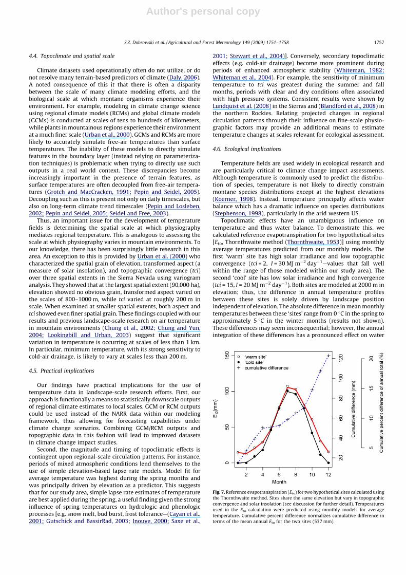
Topoclimatic effects have an unambiguous influence ontemperature and thus water balance. To demonstrate this, wecalculated reference evapotranspiration for two hypothetical sites[Eto, Thornthwaite method (Thornthwaite, 1953)] using monthlyaverage temperatures predicted from our monthly models. Thefirst ‘warm’ site has high solar irradiance and low topographicconvergence (tci = 2, I = 30 MJ m�2 day�1—values that fall wellwithin the range of those modeled within our study area). Thesecond ‘cool’ site has low solar irradiance and high convergence(tci = 15, I = 20 MJ m�2 day�1). Both sites are modeled at 2000 m inelevation; thus, the difference in annual temperature profilesbetween these sites is solely driven by landscape positionindependent of elevation. The absolute difference in mean monthlytemperatures between these ‘sites’ range from 0 8C in the spring toapproximately 5 8C in the winter months (results not shown).These differences may seem inconsequential; however, the annualintegration of these differences has a pronounced effect on water

Fig. 7. Reference evapotranspiration (Eto) for two hypothetical sites calculated using

the Thornthwaite method. Sites share the same elevation but vary in topographic

convergence and solar insolation (see discussion for further detail). Temperatures

used in the Eto calculation were predicted using monthly models for average

temperature. Cumulative percent difference normalizes cumulative difference in

terms of the mean annual Eto for the two sites (537 mm).

S.Z. Dobrowski et al. / Agricultural and Forest Meteorology 149 (2009) 1751–1758 1757

Author's personal copy

balance. Our hypothetical sites vary in Eto by approximately120 mm, a value that is over 22% of the mean annual total of thesites (Fig. 7). It should be noted that this estimate is likely to beconservative. The Thornthwaite method of Eto calculation onlyutilizes monthly average temperatures. Evapotranspiration is alsoinfluenced by solar insolation, wind speed, and other variables thatwill further emphasize differences between sites. Simply stated,subtle differences in temperature associated with landscapeposition, can result in large differences in water balance, whichare manifest in a host of hydrologic and ecologic processes.

4.7. Conclusions

The results we presented in this study are applicable to thenarrow range of physiographic and climatic conditions found inthe study area. With any empirically based statistical model,caution should be used when trying to extrapolate findings beyondthe domain of the analysis. Despite this, our results put some initialbounds on describing the spatial and temporal influence oflandscape-scale physiography on temperature patterns. Further,they highlight the ability of simple terrain analysis techniques toimprove temperature estimates in areas of complex terrain.

In summary, we demonstrate that for our study area: (1)regional temperature patterns are the principle driver of localtemperatures. (2) After removing the effect of regional temporalpatterns, the remaining variance (20–30%) can be largely explainedby spatial variability in landscape-scale physiography. Variablesderived from terrain modeling techniques can be used to describethis spatial variability and link regional free-air temperatures to in

situ measurements. (3) The influence of physiographic driversvaries temporally and is influenced by regional conditions. Periodsof well-mixed atmospheric conditions lend themselves to the useof simple lapse rate models for temperature estimation. Con-versely, secondary topoclimatic effects become most prominentduring periods of enhanced atmospheric stability. This isparticularly relevant when modeling minimum temperatures inareas of complex terrain. (4) Lastly, cumulative differences intemperature due to landscape position can have a prominent effecton water balance, and as a result, hydrologic and ecologicprocesses.

References

Barry, R.G., 1992. Mountain Weather and Climate. Routledge, London.Beniston, M., Diaz, H.F., Bradley, R.S., 1997. Climatic change at high elevation sites:

an overview. Climatic Change 36, 233–251.Blandford, T.R., Humes, K.S., Harshburger, B.J., Moore, B.C., Walden, V.P., 2008.

Seasonal and synoptic variations in near-surface air temperature lapse ratesin a mountainous basin. Journal of Applied Meteorology and Climatology 47,249–261.

Bolstad, P.V., Swift, L., Collins, F., Regniere, J., 1998. Measured and predicted airtemperatures at basin to regional scales in the southern Appalachian moun-tains. Agricultural and Forest Meteorology 91, 161–176.

Cayan, D.R., Kammerdiener, S.A., Dettinger, M.D., Caprio, J.M., Peterson, D.H., 2001.Changes in the onset of spring in the western United States. Bulletin of theAmerican Meteorological Society 82 (3), 399–415.

Chung, U., Seo, H.H., Hwang, K.H., Hwang, B.S., Yun, J.I., 2002. Minimum temperaturemapping in complex terrain based on calculation of cold air accumulation.Korean Journal of Agricultural and Forest Meteorology 4, 133–140.

Chung, U., Yun, J.I., 2004. Solar irradiance corrected spatial interpolation of hourlytemperature in complex terrain. Agricultural and Forest Meteorology 126, 129–139.

Colette, A., Chow, F.K., Street, R.L., 2003. A numerical study of inversion layerbreakup and the effects of topographic shading in idealized valleys. Journalof Applied Meteorology 42, 1255–1272.

Coughlan, J.C., Running, S.W., 1997. Regional ecosystem simulation: a generalmodel for simulating snow accumulation and melt in mountainous terrain.Landscape Ecology 12, 119–136.

Daly, C., 2006. Guidelines for assessing the suitability of spatial climate data sets.International Journal of Climatology 26, 707–721.

Daly, C., Halbleib, M., Smith, J.I., Gibson, W.P., Dogget, M.K., Taylor, G.H., Curtis, J.,Pasteris, P.P., 2008. Physiographically sensitive mapping of climatologicaltemperature and precipitation across the conterminous United States. Inter-national Journal of Climatology.

Dobrowski, S.Z., Greenberg, J.A., Schladow, G., 2007. Air temperature, cold airdrainage, and topoclimatic effects in the Lake Tahoe Basin. In: Proceedingsof Pacific Climate Workshop (PACLIM), Pacific Grove, CA, 13–16 May.

Grotch, S.L., MacCracken, M.C., 1991. The use of general circulation models topredict climatic change. Journal of Climate 4, 283–303.

Gutschick, V.P., BassirRad, H., 2003. Tansley review—extreme events as shapingphysiology, ecology, and evolution of plants: toward a unified definition andevaluation of their consequences. New Phytologist 160, 21–42.

Harlow, C., Burke, E., Scott, R.L., Shuttleworth, W.J., Brown, C., Petti, J., 2004.Derivation of temperature lapse rates in semi-arid southeastern Arizona.Hydrology and Earth System Sciences 8 (6), 1179–1185.

Hofierka, J., Suri, M., 2002. The solar radiation model for open source GIS: imple-mentation and applications. In: Proceedings of the Open Source GIS-GRASSUsers Conference, Trento, Italy, September.

Iijima, Y., Shinoda, M., 2000. Seasonal changes in the cold-air pool formation in asubalpine hollow, central Japan. International Journal of Climatology 20,1471–1483.

Inouye, D.W., 2000. The ecological and evolutionary significance of frost in thecontext of climate change. Ecology Letters 3, 457–463.

Koerner, C., 1998. A re-assessment of high elevation treeline positions and theirexplanation. Oecologia 115, 445–459.

Lookingbill, T.R., Urban, D.L., 2003. Spatial estimation of air temperature differencesfor landscape scale studies in montane environments. Agricultural and ForestMeteorology 114, 141–151.

Lundquist, J.D., Cayan, D.R., 2007. Surface temperature patterns in complex terrain:daily variations and long-term change in the central Sierra Nevada, California.Journal of Geophysical Research 112, D11124.

Lundquist, J.D., Pepin, N.C., Rochford, C., 2008. Automated algorithm for mappingregions of cold-air pooling in complex terrain. Journal of Geophysical Research113, D22107.

Mesinger, F., DiMego, G., Kalnay, E., Mitchell, K., Shafran, P.C., Ebisuzaki, W., Jovic, D.,Woolen, J., 2006. North American regional reanalysis. Bulletin of the AmericanMeteorological Society 87, 343–360.

Millar, C.I., Stephenson, N.L., Stephens, S.L., 2007. Climate change and forests of thefuture: managing in the face of uncertainty. Ecological Applications 17 (8),2145–2151.

Pepin, N.C., Losleben, M., 2002. Climate change in the Colorado Rocky Mountains:free-air versus surface temperature trends. International Journal of Climatology22, 311–329.

Pepin, N.C., Norris, J.R., 2005. An examination of the differences between surface andfree-air temperature trend at high elevation sites: relationships with cloudcover, snow cover, and wind. Journal of Geophysical Research 110, D24112.

Pepin, N.C., Seidel, D.J., 2005. A global comparison of surface and free-air tempera-tures at high elevations. Journal of Geophysical Research 110, D03104.

Rogers, J.H., 1974. Soil Survey of the Tahoe Basin Area, California and Nevada. USDASoil Conservation Service and Forest Service, Washington DC.

Running, S.W., Nemani, R.R., Hungerford, R.D., 1987. Extrapolation of synopticmeteorological data in mountainous terrain and its use for simulating forestevapotranspiration and photosynthesis. Canadian Journal of Forest Research 17,472–483.

Saxe, H., Cannell, M.G.R., Johnsen, O., Ryan, M.G., Vourlitis, G., 2001. Tansley Reviewno 123: tree and forest functioning in response to global warming. NewPhytologist 149, 369–400.

Seidel, D.J., Free, M., 2003. Comparison of lower-tropospheric temperature climatol-ogies and trends at low and high elevation radiosonde sites. Climatic Change 59,53–74.

Stephenson, N.L., 1998. Actual evapotranspiration and deficit: biologically mean-ingful correlates of vegetation distribution across spatial scales. Journal ofBiogeography 25, 855–870.

Stewart, I.T., Cayan, D., Dettinger, M.D., 2004. Changes toward earlier streamflowtiming across western North America. Journal of Climate 18, 1136–1155.

Thornthwaite, C.W., 1953. A charter for climatology. World Meteorological Orga-nization Bulletin 2 (2.).

Urban, D.L., Miller, C., Halpin, P.N., Stephenson, N.L., 2000. Forest gradient responsein Sierran landscapes: the physical template. Landscape Ecology 15, 603–620.

Weiss, S.B., Murphy, D.D., White, R.R., 1988. Sun, slope, and butterflies: topographicdeterminants of habitat quality for Euphydryas editha bayensis. Ecology 69,1486–1496.

Whiteman, D.C., 1982. Breakup of temperature inversions in deep mountain valleys.Part I. Observations. Journal of Applied Meteorology 21, 270–289.

Whiteman, D.C., Pospichal, B., Eisenbach, S., Weihs, P., Clements, C.B., Steinacker, R.,Mursch-Radlgruber, E., Dorninger, M., 2004. Inversion breakup in small RockyMountain and alpine basins. Journal of Applied Meteorology 43, 1069–1082.

Wolock, D.M., McCabe, J., 1995. Comparison of single and multiple flow directionalgorithms for computing topographic parameters in TOPMODEL. WaterResources Research 31, 1315–1324.

S.Z. Dobrowski et al. / Agricultural and Forest Meteorology 149 (2009) 1751–17581758