Household Energy Demand and the Equity and Efficiency Aspects of Subsidy Reform in Indonesia

Household Energy Demand and the Equity and EfficiencyAspects of Subsidy Reform in Indonesia

Susan Olivia* and John Gibson**

The proper design of price interventions in energy markets requiresconsideration of equity and efficiency effects. In this paper, budget survey datafrom 29,000 Indonesian households are used to estimate a demand system forfive energy sources, which is identified by the spatial variation in unit values(expenditures divided by quantities). We correct for the various quality andmeasurement error biases that result when unit values are used as proxies formarket prices. The price elasticities are combined with tax and subsidy rates tocalculate the marginal social cost of price changes for each item. The resultssuggest that even with high levels of inequality aversion there is a case forreducing the large subsidies on kerosene in Indonesia, supporting the reformsthat have been announced recently.

1. INTRODUCTION

Energy demand is rising rapidly in developing countries. The energy pric-ing policies of those countries are therefore increasingly important to the efficientuse of the world's energy supply. Some developing country energy markets arehighly distorted by consumer subsidies (IEA, 1999). For example, the Governmentof Indonesia spent over US$13 billion dollars on consumer fuel subsidies in 2005.These subsidies have a major effect on the overall energy balance in Indonesia be-cause households account for about 45 percent of total energy consumption. Therealso are large fiscal effects, with about one-quarter of the government budget (andabout five percent of GDP) going on fuel subsidies (Sen and Steer, 2005).

The Energy Journal, Vol. 29, No. 1. Copyright ©2008 by the IAEE. All rights reserved.

* University of California, Davis. E-mail: [email protected].** Corresponding author. Department of Economics, LTniversity of Waikato, Private Bag 3105,

Hamilton, 3240, New Zealand. Fax: (64-7) 838-4331. E-mail: [email protected].

We are grateful to Catherine Morrison Paul and seminar audiences at the University of California,Davis and the 2006IAAE conference on the Gold Coast and three anonymous referees for their helpfulcomments. All remaining errors are our responsibility.

21

22 / The Energy Journal

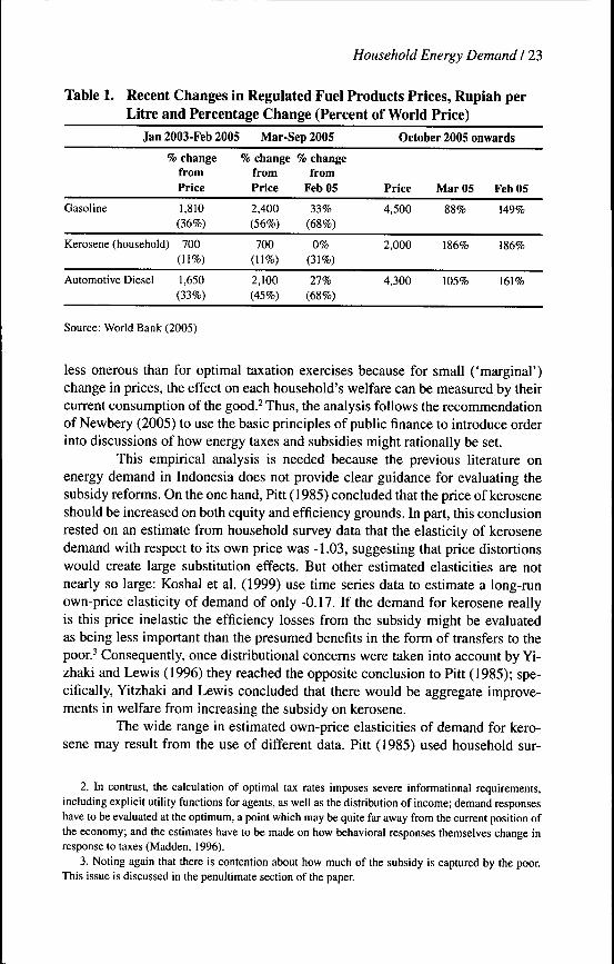
Dramatic reforms have been attempted by the Indonesian government inresponse to this escalating cost of fuel subsidies. In October 2005 the subsidisedprice of kerosene was raised 186 percent, from Rp 700 per litre (US 7 cents) toRp 2000 per litre (US 19 cents). The prices for diesel and gasoline were raisedby approximately 90 percent, following on from increases of 30 percent in March2005 (Table 1). These earlier price increases did not apply to kerosene. Moreover,fuel subsidies were timetabled for a complete phase out by either the end of 2006(gasoline and diesel) or the end of 2007 (kerosene). These energy subsidies aremeant to be replaced with a set of targeted subsidies, whose benefits are to bedesigned so that they are restricted to low-income groups (Kompas, 2005; JakartaPost, 2005).

It is unclear whether these ambitious plans for reform will be realised.First, despite the substantial price rises enacted in 2005, there is still a long wayto go if Indonesian fuel prices are to be set at world levels. The kerosene price inOctober 2005 was only 31 percent of the world price, while gasoline and dieselprices were about two-thirds of the world level (Table 1). Second, many previousattempts at reforming energy price policy in Indonesia have failed because ofthe resulting political difficulties. Attempted reforms in 2003 were reversed afterwidespread protests while the price rises in 1998 are believed to have precipitatedthe downfall of the Suharto regime (BBC, 2005; Economist, 2005). Moreover,these subsidies have been long-term features of the Indonesian economy, datingback to the mid-1970s (Dick, 1980). The subsidization of especially kerosene hasbeen seen as one feasible way of meeting equity objectives, because the poor arepresumed to use kerosene as their main cooking fuel.' However there are debatesabout whether the poor are the main beneficiaries of kerosene subsidies (Sumartoand Saryahadi, 2001). Indeed, even though there was early evidence that a dispro-portionate share of the subsidy was being captured by richer urban households,the subsidy policy continued to be strengthened and kerosene prices were heldbelow one-fifth of the world level as far back as 1980 (Pitt, 1985).

The aim of this paper is to provide empirical evidence to help assesswhether the proposed reforms of energy price policy in Indonesia are likely to bewelfare-enhancing. Specifically, the equity and efficiency effects of price changesin the household energy sector are analysed. To achieve this aim, the marginalsocial costs of indirect taxes and subsidies are calculated for five fuels and house-hold energy sources: kerosene, gasoline, oil, LPG, and electricity. These marginalsocial costs depend on the rate at which household welfare falls as prices increase,and on the rate at which net public revenue rises (Ahmad and Stem, 1984). If a re-form is optimally designed, the costs in terms of social welfare of the last Rupiahof government expenditure saved by cutting subsidies (or raising taxes) on eachgood should be equal. To obtain the two required parameters - the welfare deriva-tive and the revenue derivative - information is needed on tax and subsidy rates,consumption patterns, and aggregate demand responses. These requirements are

1. This reliance on energy subsidies reflects the limited capacity for income transfers, which is afeature of many developing countries.

Household Energy Demand 123

Table 1. Recent Changes in Regulated Fuel Products Prices, Rupiah perLitre and Percentage Change (Percent of World Price)

Jan 2003-Feb 2005

% change ^fromPrice

Gasoline 1,810(36%)

Kerosene (household) 700(11%)

Automotive Diesel 1,650(33%)

Mar-Sep 2005

% changefromPrice

2,400(56%)

700(11%)

2,100(45%)

% changefrom

FehO5

33%(68%)

0%(31%)

27%(68%)

October 2005 onwards

Price

4,500

2,000

4,300

Mar 05

88%

186%

105%

FebO5

149%

186%

161%

Source: World Bank (2005)

less onerous than for optimal taxation exercises because for small ('marginal')change in prices, the effect on each household's welfare can be measured by theircurrent consumption of the good.^ Thus, the analysis follows the recommendationof Newbery (2005) to use the basic principles of public finance to introduce orderinto discussions of how energy taxes and subsidies might rationally be set.

This empirical analysis is needed because the previous literature onenergy demand in Indonesia does not provide clear guidance for evaluating thesubsidy reforms. On the one hand, Pitt (1985) concluded that the price of keroseneshould be increased on both equity and efficiency grounds. In part, this conclusionrested on an estimate from household survey data that the elasticity of kerosenedemand with respect to its own price was -1.03, suggesting that price distortionswould create large substitution effects. But other estimated elasticities are notnearly so large: Koshal et al. (1999) use time series data to estimate a long-runown-price elasticity of demand of only -0.17. If the demand for kerosene reallyis this price inelastic the efficiency losses from the subsidy might be evaluatedas being less important than the presumed benefits in the form of transfers to thepoor.-' Consequently, once distributional concems were taken into account by Yi-zhaki and Lewis (1996) they reached the opposite conclusion to Pitt (1985); spe-cifically, Yitzhaki and Lewis concluded that there would be aggregate improve-ments in welfare from increasing the subsidy on kerosene.

The wide range in estimated own-price elasticities of demand for kero-sene may result from the use of different data. Pitt (1985) used household sur-

2. In contrast, the calculation of optimal tax rates imposes severe informational requirements,including explicit utility functions for agents, as well as the distribution of income; demand responseshave to be evaluated at the optimum, a point which may be quite far away from the current position ofthe economy; and the estimates have to be made on how behavioral responses themselves change inresponse to taxes (Madden, 1996).

3. Noting again that there is contention about how much of the subsidy is captured by the poor.This issue is discussed in the penultimate section of the paper.


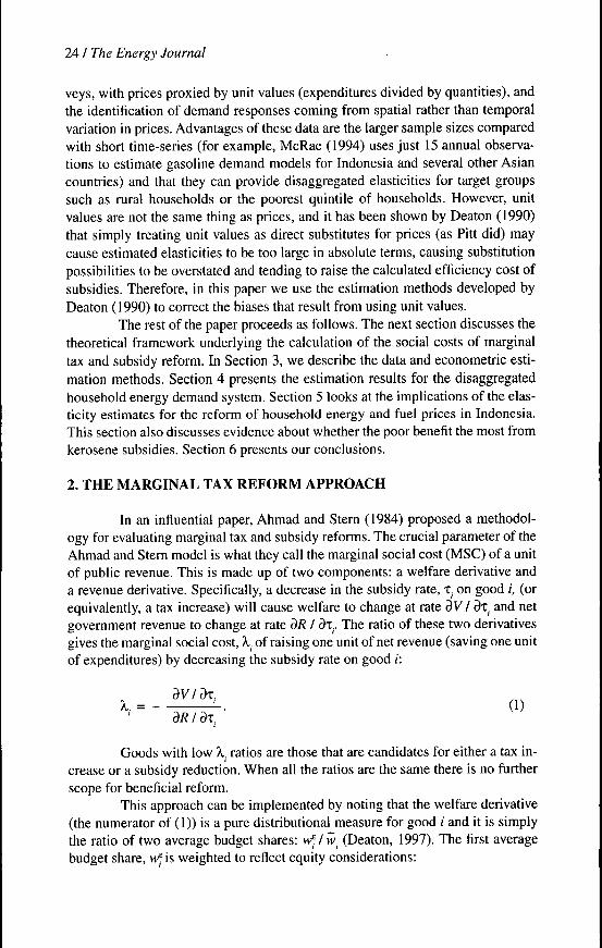
veys, with prices proxied by unit values (expenditures divided by quantities), andthe identification of demand responses coming from spatial rather than temporalvariation in prices. Advantages of these data are the larger sample sizes comparedwith short time-series (for example, McRae (1994) uses just 15 annual observa-tions to estimate gasoline demand models for Indonesia and several other Asiancountries) and that they can provide disaggregated elasticities for target groupssuch as rural households or the poorest quintile of households. However, unitvalues are not the same thing as prices, and it has been shown by Deaton (1990)that simply treating unit values as direct substitutes for prices (as Pitt did) maycause estimated elasticities to be too large in absolute terms, causing substitutionpossibilities to be overstated and tending to raise the calculated efficiency cost ofsubsidies. Therefore, in this paper we use the estimation methods developed byDeaton (1990) to correct the biases that result from using unit values.

The rest of the paper proceeds as follows. The next section discusses thetheoretical framework underlying the calculation of the social costs of marginaltax and subsidy reform. In Section 3, we describe the data and econometric esti-mation methods. Section 4 presents the estimation results for the disaggregatedhousehold energy demand system. Section 5 looks at the implications of the elas-ticity estimates for the reform of household energy and fuel prices in Indonesia.This section also discusses evidence about whether the poor benefit the most fromkerosene subsidies. Section 6 presents our conclusions.

2. THE MARGINAL TAX REFORM APPROACH

In an infiuential paper, Ahmad and Stern (1984) proposed a methodol-ogy for evaluating marginal tax and subsidy reforms. The crucial parameter of theAhmad and Stem model is what they call the marginal social cost (MSC) of a unitof public revenue. This is made up of two components: a welfare derivative anda revenue derivative. Specifically, a decrease in the subsidy rate, x. on good (, (orequivalently, a tax increase) will cause welfare to change at rate dV / 3T. and netgovernment revenue to change at rate dR I 3x.. The ratio of these two derivativesgives the marginal social cost, X. of raising one unit of net revenue (saving one unitof expenditures) by decreasing the subsidy rate on good ;:

"•• - -

Goods with low X. ratios are those that are candidates for either a tax in-crease or a subsidy reduction. When all the ratios are the same there is no furtherscope for beneficial reform.

This approach can be implemented by noting that the welfare derivative(the numerator of (1)) is a pure distributional measure for good / and it is simplythe ratio of two average budget shares: w^lw. (Deaton, 1997). The first averagebudget share, w is weighted to reflect equity considerations:


w'== [E (x / n )- x w. ] / E X (2)

where w. is the budget share for good / in household m, x and n are the total ex-penditure and size of household m, and e is the coefficient of inequality aversion."* Arange of values of e between zero (no inequality aversion) and two (a high degreeof inequality aversion) are commonly used to see whether tax reform recommen-dations are robust to particular ethical judgements (Ahmad and Stem, 1984). Interms of the calculation of equation (2), the larger is 8 the closer the average budgetshare will be to budget shares of the poorest households in the sample. The sec-ond average budget share is the so-called 'plutocratic budget share' (Prais, 1957)which is based on ratios of total expenditure (rather than averages of ratios) andgives the biggest weights to the richest households:^

M M

w. = E X w. / E X . (3)m=l

The denominator of the A,-ratio represents the efficiency aspect of tax-and subsidy-induced price changes. A given price change will produce a largernet revenue effect, the greater is the total consumption of the good and the less thesubstitution away from taxed goods:

w'r/w.h ^ • (4)T.

1-l-t.e.. 1

1 + X, W.

The total consumption of the good is shown by w., while the substitu-tion effects are shown by 0 ,., the derivative of the budget share for good k withrespect to the (log) price of good /. The tax factor gives the share of tax in the finalprice. For example, in Indonesia household purchases of oil face a VAT rate of10 percent, so the tax factor is 0.10/(1 + 0.10) - 0.09 while subsidies meant thatkerosene prices since October 2005 are only 31 percent of the world price, so thetax factor is -0.69/(1 - 0.69) = 2.23.

The first term of the denominator in equation (4) measures the own-pricedistortionary effect ofthe tax or subsidy. If it is large and positive, as would be thecase for a heavily subsidised and price elastic good, the term will contribute to asmall X. and would indicate the low social cost of raising net revenue by decreas-

4. Consider judgements about the effect of taking RplOOO from someone to give some of it toa person with half the income and destroying the rest (e.g., due to efficiency losses). When 8=0 thejudge would approve of this transfer only if the poorer person received all RplOOO. But when e takesthe values of 1 (or 2) the amount the poorer person receives has to be only Rp500 (or Rp250 if e=2)in order for the resulting distribution to be judged as giving the same level of social welfare as beforethe transfer (Creedy, 1996).

5. The plutocratic budget share is widely used in Consumer Price Index calculations. According tocalculations by Deaton (1998) the "average consumer" according to plutocratic budget shares in theUnited States was located at about the 75* percentile of the distribution of household expenditures.

26 / The Energy Joumai

ing the subsidy on this good. The last term is the sum of the tax factors multipliedby the cross price elasticities, and captures the effects on other goods (and theresulting net revenue changes) from the change in the tax on good i.

3. DATA AND ESTIMATION METHODS

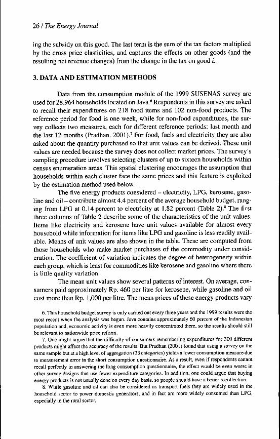
Data from the consumption module of the 1999 SUSENAS survey areused for 28,964 households located on Java.' Respondents in this survey are askedto recall their expenditures on 218 food items and 102 non-food products. Thereference period for food is one week, while for non-food expenditures, the sur-vey collects two measures, each for different reference periods: last month andthe last 12 months (Pradhan, 2001).' For food, fuels and electricity they are alsoasked about the quantity purchased so that unit values can be derived. These unitvalues are needed because the survey does not collect market prices. The survey'ssampling procedure involves selecting clusters of up to sixteen households withincensus enumeration areas. This spatial clustering encourages the assumption thathouseholds within each cluster face the same prices and this feature is exploitedby the estimation method used below.

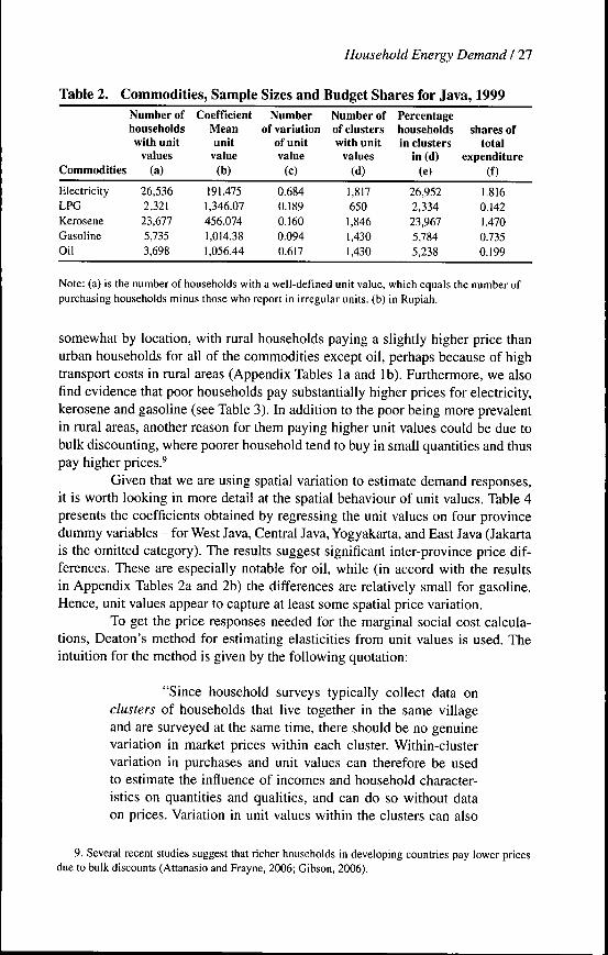
The five energy products considered - electricity, LPG, kerosene, gaso-line and oil - contribute almost 4.4 percent of the average household budget, rang-ing from LPG at 0.14 percent to electricity at 1.82 percent (Table 2).^ The firstthree columns of Table 2 describe some of the characteristics of the unit values.Items like electricity and kerosene have unit values available for almost everyhousehold while information for items like LPG and gasoline is less readily avail-able. Means of unit values are also shown in the table. These are computed fromthose households who make market purchases of the commodity under consid-eration. The coefficient of variation indicates the degree of heterogeneity withineach group, which is least for commodities like kerosene and gasoline where thereis little quality variation.

The mean unit values show several patterns of interest. On average, con-sumers paid approximately Rp. 460 per litre for kerosene, while gasoline and oilcost more than Rp. 1,000 per litre. The mean prices of these energy products vary

6. This household budget survey is only carried out every three years and the 1999 results were themost recent when the analysis was begun. Java contains approximately 60 percent of the Indonesianpopulation and, economic activity is even more heavily concentrated there, so the results should stillbe relevant to nationwide price reform,

7. One might argue that the difficulty of consumers remembering expenditures for 300 differentproducts might affect the accuracy of the results. But Pradhan (2001) found that using a survey on thesame sample but at a high level of aggregation (23 categories) yields a lower consumption measure dueto measurement error in the short consumption questionnaire. As a result, even if respondents cannotrecall perfectly in answering the long consumption questionnaire, the effect would be even worse inother survey designs that use fewer expenditure categories. In addition, one could argue that buyingenergy products is not usually done on every day basis, so people should have a better recollection.

8. While gasoline and oil can also be considered as transport fuels they are widely used in thehousehold sector to power domestic generators, and in fact are more widely consumed than LPG,especially in the rural sector.

Household Energy Demand I 27

Tahle 2. Commodities, Sample Sizes and Budget Shares for Java, 1999

Commodities

ElectricityLPGKeroseneGasolineOil

Number ofhouseholdswith unit

values(a)

26,5362,32123,6775,7353,698

CoefficientMeanunit

value(b)

191.4751,346.07456.0741,014.381,056.44

Numberof variation

of unitvalue

(c)

0.6840.1890.1600.0940.617

Number ofof clusterswith unit

values(d)

1,817650

1,8461,4301,430

Percentagehouseholdsin clusters

in(d)(e)

26,9522,33423,9675,7845,238

shares oftotal

expenditure(f)

1.8160.1421.4700.7350.199

Note: (a) is the number of households with a well-defined unit value, which equals the number ofpurchasing households minus those who report in irregular units, (b) in Rupiah.

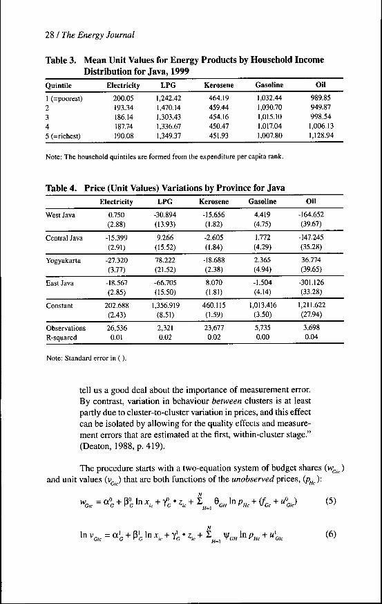
somewhat by location, with rural households paying a slightly higher price thanurban households for all of the commodities except oil, perhaps because of hightransport costs in rural areas (Appendix Tables la and lb). Furthermore, we alsofind evidence that poor households pay substantially higher prices for electricity,kerosene and gasoline (see Table 3). In addition to the poor being more prevalentin rural areas, another reason for them paying higher unit values could be due tobulk discounting, where poorer household tend to buy in small quantities and thuspay higher prices.'

Given that we are using spatial variation to estimate demand responses,it is worth looking in more detail at the spatial behaviour of unit values. Table 4presents the coefficients obtained by regressing the unit values on four provincedummy variables - for West Java, Central Java, Yogyakarta, and East Java (Jakartais the omitted category). The results suggest significant inter-province price dif-ferences. These are especially notable for oil, while (in accord with the resultsin Appendix Tables 2a and 2b) the differences are relatively small for gasoline.Hence, unit values appear to capture at least some spatial price variation.

To get the price responses needed for the marginal social cost calcula-tions, Deaton's method for estimating elasticities from unit values is used. Theintuition for the method is given by the following quotation:

"Since household surveys typically collect data onclusters of households that live together in the same villageand are surveyed at the same time, there should be no genuinevariation in market prices within each cluster. Within-clustervariation in purchases and unit values can therefore be usedto estimate the influence of incomes and household character-istics on quantities and qualities, and can do so without dataon prices. Variation in unit values within the clusters can also

9. Several recent studies suggest that richer households in developing countries pay lower pricesdue to bulk discounts (Attanasio and Frayne, 2006; Gibson, 2006).


Table 3. Mean Unit Values for Energy Products by Household IncomeDistribution for Java, 1999

Quintile

1 (=poorest)2345 (=richest)

Electricity

200.05193.34186.14187.74190.08

LPG

1,242.421,470.141,303.431,336.671,349.37

Kerosene

464.19459.44454.16450.47451.93

Gasoline

1,032.441,030.701,015.101,017.041,007.80

Oil

989.85949.87998.541,006.131,128.94

Note: The household quintiles are formed from the expenditure per capita rank.

Table 4. Price (Unit Values) Variations by Province for Java

West Java

Central Java

Yogyakarta

East Java

Constant

ObservationsR-squared

Electricity

0.750(2.88)

-15.399(2.91)

-27.320(3.77)

-18.567(2.85)

202.688(2.43)

26,5360.01

LPG

-30.894(13.93)

9.266(15.52)

78.222(21.52)

-66.705(15.50)

1,356.919(8.51)

2,3210.02

Kerosene

-15.656(1.82)

-2.605(1.84)

-18.688(2.38)

8.070(1.81)

460.115(1.59)

23,6770.02

Gasoline

4.419(4.75)

1.772(4.29)

2.365(4.94)

-1.504(4.14)

1,013.416(3.50)

5,7350.00

Oil

-164.652(39.67)

-147.245(35.28)

36.774(39.65)

-301.126(33.28)

1,211.622(27.94)

3,6980.04

Note: Standard error in ( ) .

tell us a good deal about the importance of measurement error.By contrast, variation in behaviour between clusters is at leastpartly due to cluster-to-cluster variation in prices, and this effectcan be isolated by allowing for the quality effects and measure-ment errors that are estimated at the first, within-cluster stage."(Deaton, 1988, p.419).

The procedure starts with a two-equation system of budget sharesand unit values (v . ) that are both functions of the unobserved prices, (p^_.):

M ' . = I fa (5)

= « (6)


the G indicates goods, i indicates households and the c indexes clusters. Amongstthe explanatory variables, x. is total expenditure of household i, p^ are the unob-served prices, z. is a vector of other household characteristics,/^^ is a cluster fixed-effect in the budget share for good G and M'J,. and M' . , are idiosyncratic errors.

In the first stage, the procedure removes the household-specific effectsof income and other demographic characteristics from the budget shares and unitvalues. To do so, equations (5) and (6) are estimated using OLS, where in additionto X. and z., the specification also controls for all cluster fixed effects, includingthose due to unohserved prices, so that the P^, 7^, |3J,, and yj, parameters can beestimated consistently, even in the absence of market price data. These four pa-rameters are used to create adjusted budget shares and unit values that have thequality effects due to income and other factors removed. For example, if richerhouseholds huy higher grade oil (which will have a higher unit value) the firststage regression can account for this and the adjusted unit value is more like aprice, which does not vary across households in the same community.

The first stage regressions also produce the residuals needed in the sec-ond stage for estimating the covariances to correct for the effect of any measure-ment error in unit values and budget shares. The error terms, e" . . and e' . , fromequations (5) and (6) contain all the variability in w^^ and v ^ not explained by x,z, or the cluster fixed effects. Assuming a single price per cluster, the unexplainedvariation around the cluster mean can indicate measurement error. Hence, a be-tween-clusters errors-in-variables regression is applied to the (adjusted) averagebudget shares and unit values, which have heen purged of household characteris-tics at the first stage. If it were not for the effect of prices on cluster-wide qualityvariation, the parameters estimated at the second stage would he sufficient forcalculating the price responses. Instead, a separability theory of quality (Deaton1988) has to be used to identify the price effects at the third and final stage.'" Fur-ther details of the estimation method can be found in Deaton (1997).

One feature of the procedure is that the budget share equation (5) pays nospecial attention to non-purchasing households, who have budget shares of zero.Since subsidy hudgets do not depend on whether demand changes take place atthe extensive or intensive margins, when studying tax and subsidy reform oneneeds to include all households, whether they purchase or not (Deaton, 1990).Therefore, equation (5) is simply viewed as a linear approximation to the regres-sion function of the budget share conditional on the right-hand-side variables,averaging over both zeros and non-zeros in much the same way that an aggregatedemand function does (Deaton, 1997)." Including non-purchasing households in

10. Intuitively, there is an identification problem that comes from working with three magnitudes:quaiity, quantity and price, with data on oniy two of them. Hence, quality downgrading accompanyinga rise in price is treated as an income effect, such that an increase in say oii prices would causessuhstitution toward lower grades in the same way that wouid follow from a decrease in income.Consequently, if we know how the quality of oil changes with changes in income, we can predict theeffects of changes in prices on the unit value.

11. Other studies applying Deaton's method to household survey data also follow the samespecification and include households with budget shares of zero. See, for example, Nicita (2004),


the analysis is needed because the effect of tax and subsidy changes on publicrevenue depends on total demand which is affected by both changes in the inten-sity of purchase by those who continue to purchase and by switching betweenpurchasing and non-purchasing.

4. ECONOMETRIC RESULTS

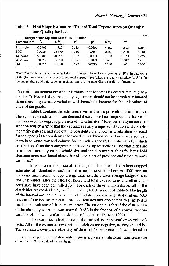
Table 5 contains results from the first stage (within-cluster) estimationof the budget share and unit value equations. The coefficients reported are forthe effects of log total expenditures on budget shares, P" and on log unit values,P' plus summary statistics for each equation. The tables also include the elas-ticity of quantity demanded with respect to total expenditures, which dependson coefficients from both the budget share and unit value equations.'^ The other(unreported) variables used at the first stage include (log) household size, a set ofdemographic variables (the number of household members in each of thirteen ageand sex categories as a ratio of household size), and nine educational dummies."These variables are based on those used by Deaton (1990) in his study of fooddemand from the same survey in an earlier year. As can be seen from Table 5, thefirst stage estimation of the budget share equations explains from 27 percent of thevariation for oil to 47 percent for kerosene. More of the variation in unit values isexplained, ranging from 31 percent for gasoline to 66 percent for oil.

LPG, gasoline and oil attract positive p° coefficients - indicating luxurygoods whose budget shares rise more than proportionally as household expendi-ture rises. The total expenditure elasticity for kerosene is 0.44; similar to previousestimates indicating that kerosene is a necessity. Appendix Tables 2a and 2b showthat rural households tend to have higher expenditure elasticities; for example,3.08 and 4.08 for gasoline and LPG compared with 2.38 and 2.36 for urban house-holds. These results imply that rural households are likely to have larger propor-tionate increases in demand for these products as their income rises.

The quality elasticities, p' are estimated from the effect of changes inthe logarithm of total expenditure on the log of the unit value. With the exceptionof kerosene and oil, all of the quality elasticities are negative although none arevery large. Thus, richer households seem to pay less per unit, possibly becauseof bulk purchases or more favourable electricity tariffs than are available to thepoor. However, the magnitude of these effects is small, and it is only for the unitvalue of oil, where the quality elasticity is 0.07, that there would appear to beany significant within-cluster variation in unit values. The small response of unitvalues to total expenditure occurs in both urban and rural Java (Appendix Tables2a and 2b). The small size of these quality effects is consistent with other studiesusing the Deaton method and so it is the ability of this method to also mitigate the

12. See equation 5.36 of Deaton (1997) for a derivation.13. The gender and age composition of the household is likely to be reflected in the consumption

basket of the household, so is the educational level of the head of the household. The unreported resultsfor these variables support their inclusion.

Household Energy Demand / 31

Table 5. First Stage Estimates: Effect of Total Expenditures on Quantityand Quality for Java

Budget Share EquationUnit Value EquationCommodities


P»-0.00030.0025-0.00830.01230.0037

-1.32025.660-36.79037.60028.020

0.3130.3100.4670.3260.273

P'-0.0302-0.01500.0004-0.01210.0745

tm-4.460-0.9500.110-1.6003.580

0.5930.5000.3440.3120.661

£

1.1042.7400.4352.6912.800

Note: (3° is the derivative of the budget share with respect to log total expenditures, p' is the derivativeof the (log) unit value with respect to log total expenditures (a.k.a. the 'quality elasticity'), R^ is forthe budget share and unit value regressions, and e is the expenditure elasticity of quantity.

effect of measurement error in unit values that becomes its crucial feature (Dea-ton, 1997). Nevertheless, the quality adjustment should not be completely ignoredsince there is systematic variation with household income for the unit values ofthree of the goods.

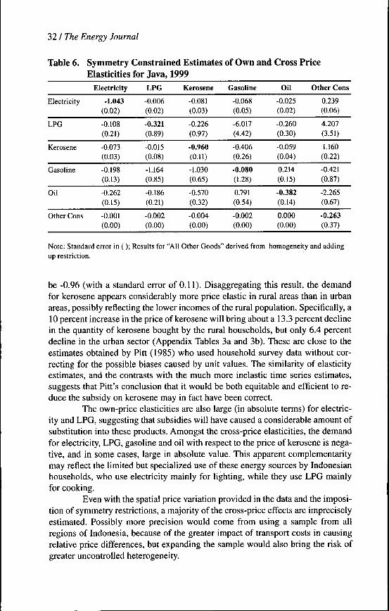
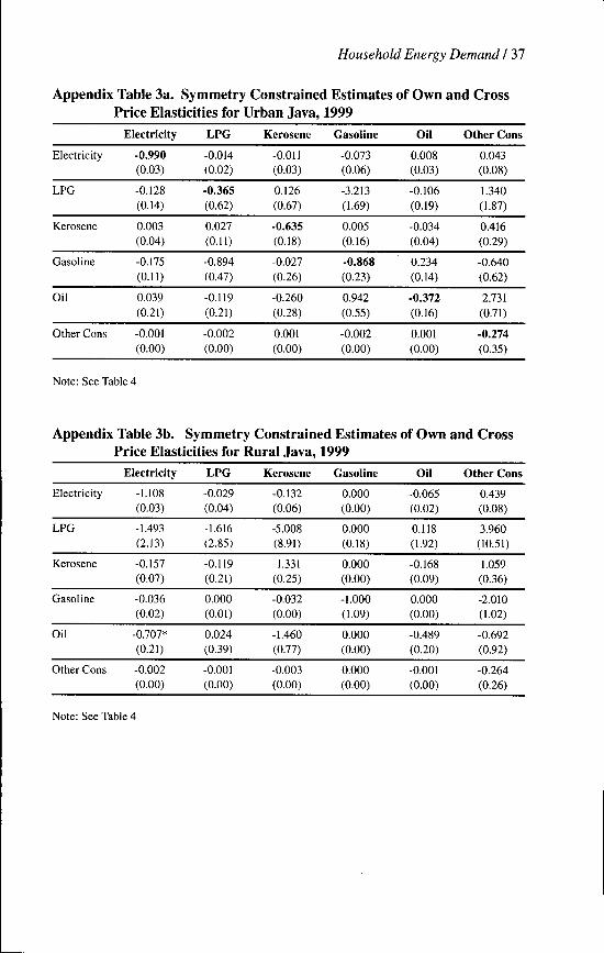
Table 6 contains the estimated own- and cross-price elasticities for Java.The symmetry restrictions from demand theory have been imposed on these esti-mates in order to improve precision of the estimates. Moreover, the symmetry re-striction will guarantee that the estimates satisfy unique substitution and comple-mentarity pattems, and rule out the possibility that good / is a substitute for goodi when goody is a complement for good /. In addition to the five energy sources,there is an extra row and column for "all other goods", the estimates for whichare obtained from the homogeneity and adding-up restrictions. The elasticities areconditional not only on household size and the dummy variables for householdcharacteristics mentioned above, but also on a set of province and urban dummyvariables.'''

In addition to the price elasticities, the table also includes bootstrappedestimates of "standard errors". To calculate these standard errors, 1000 randomdraws are taken from the second stage data (i.e., the cluster average budget sharesand unit values, after the effect of household total expenditures and other char-acteristics have been controlled for). For each of these random draws, all of theelasticities are recalculated, in effect creating 1000 versions of Table 6. The lengthof the interval around the mean of each bootstrapped elasticity that contains 68.3percent of the bootstrap replications is calculated and one-half of this interval isused as the estimate of the standard error. The rationale is that if the distributionof the elasticity estimates was nonnal, 0.683 is the fraction of a normal randomvariable within two standard deviations of the mean (Deaton, 1997).

The own-price effects are well determined as are several cross-price ef-fects. All of the estimated own-price elasticities are negative, as they should be.The estimated own-price elasticity of demand for kerosene in Java is found to

14. It is not possible to add these regional effects at the first (within-cluster) stage because thecluster fixed effects would obliterate them.


Table 6. Symmetry Constrained Estimates of Own and Cross PriceElasticities for Java, 1999

Electricity

LPG

Kerosene

Gasoline

Oil

Other Cons

Eiectricity

-1.043(0.02)

-0.108(0.21)

-0.073(0.03)

-0.198(0.13)

-0.262(0.15)

-0.001(0.00)

LPG

-0.006(0.02)

-0.321(0.89)

-0.015(0.08)

-1.164(0.85)

-0.186(0.21)

-0.002(0.00)

Kerosene

-0.081(0.03)

-0.226(0.97)

-0.960(0.11)

-1.030(0.65)

-0.570(0.32)

-0.004(0.00)

Gasoline

-0.068(0.05)

-6.017(4.42)

-0.406(0.26)

-0.080(1.28)

0.791(0.54)

-0.002(0.00)

Oil

-0.025(0.02)

-0.260(0.30)

-0.059(0.04)

0.214(0.15)

-0.382(0.14)

0.000(0.00)

Other Cons

0.239(0.06)

4.207(3.51)

1.160(0.22)

-0.421(0.87)

-2.265(0.67)

-0.263(0.37)

Note: Standard error in ( ) ; Results for "All Other Goods" derived from homogeneity and addingup restriction.

be -0.96 (with a standard error of 0.11). Disaggregating this result, the demandfor kerosene appears considerably more price elastic in rural areas than in urbanareas, possibly reflecting the lower incomes of the rural population. Specifically, a10 percent increase in the price of kerosene will bring about a 13.3 percent declinein the quantity of kerosene bought by the rural households, but only 6.4 percentdecline in the urban sector (Appendix Tables 3a and 3b). These are close to theestimates obtained by Pitt (1985) who used household survey data without cor-recting for the possible biases caused by unit values. The similarity of elasticityestimates, and the contrasts with the much more inelastic time series estimates,suggests that Pitt's conclusion that it would be both equitable and efficient to re-duce the subsidy on kerosene may in fact have been correct.

The own-price elasticities are also large (in absolute terms) for electric-ity and LPG, suggesting that subsidies will have caused a considerable amount ofsubstitution into these products. Amongst the cross-price elasticities, the demandfor electricity, LPG, gasoline and oil with respect to the price of kerosene is nega-tive, and in some cases, large in absolute value. This apparent complementaritymay reflect the limited but specialized use of these energy sources by Indonesianhouseholds, who use electricity mainly for lighting, while they use LPG mainlyfor cooking.

Even with the spatial price variation provided in the data and the imposi-tion of symmetry restrictions, a majority of the cross-price effects are impreciselyestimated. Possibly more precision would come from using a sample from allregions of Indonesia, because of the greater impact of transport costs in causingrelative price differences, but expanding the sample would also bring the risk ofgreater uncontrolled heterogeneity.

Household Energy Demand / 33

5. MARGINAL SOCIAL COST CALCULATIONS

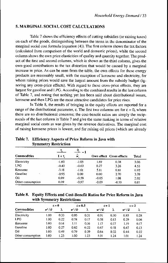
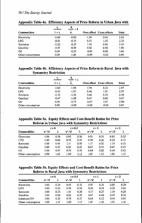
Table 7 shows the efficiency effects of cutting subsidies (or raising taxes)on each of the goods, distinguishing between the terms in the denominator of themarginal social cost formula (equation (4)). The first column shows the tax factors(calculated from comparison of the world and domestic prices), while the secondcolumn shows the own price elasticities of quality and quantity together. The prod-uct of the first and second columns, which is shown as the third column, gives theown-good contributions to the tax distortion that would be caused by a marginalincrease in price. As can be seen from the table, the own effects for these energyproducts are reasonably small, with the exception of kerosene and electricity, forwhom raising prices would save the largest amount from the subsidy budget (ig-noring any cross-price effects). With regard to these cross-price eifects, they arelargest for gasoline and LPG. According to the combined results in the last columnof Table 7, and noting that nothing yet has been said about distributional issues,kerosene and then LPG are the most attractive candidates for price rises.

In Table 8, the results of bringing in the equity effects are reported for arange of the distributional parameter, 8. The first two columns are for e = 0, wherethere are no distributional concerns; the cost-benefit ratios are simply the recip-rocals of the last column in Table 7 and give the same ranking in terms of relativemarginal social costs as was given by the revenue derivatives. The marginal costof raising kerosene prices is lowest, and for raising oil prices (which are already

Table 7. Efficiency Aspects of Price Reform in Java withSymmetry Restriction

Commodities

ElectricityLPGKeroseneGasolineOilOther consumption

T.

1 + T.

-1.60-0.43-3.18-0.950.090.09

-1.05-0.63-1.610.00-0.59-0.97

Own effect

1.690.275.110.00-0.05-0.09

Cross effects

0.383.260.812.701.08

-0.10

Total

3.064.536.923.702.020.81

Table 8. Equity Effects and Cost-Benefit Ratios for Price Reform in Javawith Symmetry Restrictions

Commodities


w' tiv

1.001.001.001.001.001.00

e = 0X

0.330.220.140.270.491.23

e=w'^ /w

0.950.781.110.820.791.00

0.5X

0.310.170.160.220.391.23

e=w' tw

0.910.581.170.670.641.01

1X

0.300.130.170.180.321.24

E =

w'^ /iv

0.850.291.190.470.441.01

2X

0.280.060.170.130.221.24


taxed) is highest amongst the energy sources. However, all of the X. for the energysources are much lower than for "other consumption" indicating the general desir-ability of removing all energy subsidies.

Moving across to the right in Table 8, the e parameter increases, givinglarger values to the goods most heavily consumed by the poor and relatively smallervalues to those consumed by households that are better off. For e = 0.5, kerosenereceives the highest social weight, with w* / vv greater than unity. Consequently, as eincreases further, kerosene loses its place as the most attractive candidate for a pricerise, becoming the third most attractive when e = 1 and the fourth most attractivewhen £-2. Indeed, with an inequality aversion parameter of e = 2 the lowest socialcost of reduced govemment expenditure (or equivalently additional revenue) wouldcome from raising LPG prices, followed by raising gasoline prices.

When the results are disaggregated into the rural and urban sector the rec-ommendations are largely the same. In the rural sector kerosene is the best candidatefor price increases when inequality aversion levels are low, with LPG becoming thebest candidate at higher inequality aversion levels (Appendix Table 5b). In the urbansector LPG is consistently ranked as the commodity with the lowest social costof price increases and the attractiveness of raising kerosene prices diminishes asinequality aversion rises.

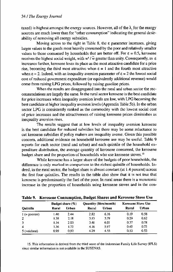
The results suggest that at low levels of inequality aversion keroseneis the best candidate for reduced subsidies but there may be some reluctance tocut kerosene subsidies if policy makers are inequality averse. Given this possibleconcern, additional evidence on household kerosene use may be useful. Table 9reports for each sector (rural and urban) and each quintile of the household ex-penditure distribution, the average quantity of kerosene consumed, the kerosenebudget share and the proportion of households who use kerosene stoves."

While kerosene has a larger share of the budgets of poor households, the

difference is only marked in comparison to the richest quintile of households. In-

deed, in the rural sector, the budget share is almost constant (at 1.4 percent) across

the first four quintiles. The results in the table also show that it is not true that

kerosene is predominantly the fuel of the poor. In rural areas there is a monotonic

increase in the proportion of households using kerosene stoves and in the con-

Table 9. Kerosene Consumption, Budget Shares and Kerosene Stove Use

Quintile

1 (= poorest)2345 (=richest)

Budget share (%)Rural

1.401.381.341.360.99

Urban

2.442.182.031.730.92

Quantity (litre/month)Rural

2.823.133.414.164.29

Urban

6.165.796.015.974.53

Kerosene Stove UseRural

0.190.290.370.450.53

Urban

0.580.620.780.750.53

15. This information is derived from the third wave of the Indonesian Family Life Survey (IFLS)since similar information is not available in the SUSENAS.


sumption level of kerosene when moving from poorer to richer quintiles. In urbanareas the three middle quintiles all have higher rates of kerosene stove usage thanthe poorest quintile and the consumption level of kerosene is roughly constantacross quintiles. Thus, a majority of the kerosene subsidies will not be capturedby the poor, especially in rural areas, and the replacement of energy subsidies withtargeted income subsidies is likely to be both more efficient and more equitable.

6. CONCLUSIONS

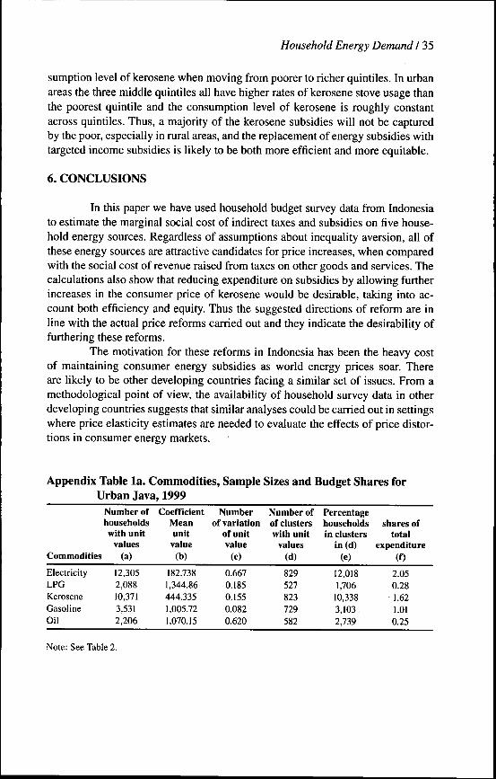
In this paper we have used household budget survey data from Indonesiato estimate the marginal social cost of indirect taxes and subsidies on five house-hold energy sources. Regardless of assumptions about inequality aversion, all ofthese energy sources are attractive candidates for price increases, when comparedwith the social cost of revenue raised from taxes on other goods and services. Thecalculations also show that reducing expenditure on subsidies by allowing furtherincreases in the consumer price of kerosene would be desirable, taking into ac-count both efficiency and equity. Thus the suggested directions of reform are inline with the actual price reforms carried out and they indicate the desirability offurthering these reforms.

The motivation for these reforms in Indonesia has been the heavy costof maintaining consumer energy subsidies as world energy prices soar. Thereare likely to be other developing countries facing a similar set of issues. From amethodological point of view, the availability of household survey data in otherdeveloping countries suggests that similar analyses could be carried out in settingswhere price elasticity estimates are needed to evaluate the effects of price distor-tions in consumer energy markets.

Appendix Table la. Commodities, Sample Sizes and Budget Shares forUrban Java, 1999

Commodities



values(a)

12,3052,08810,3713,5312,206

CoefficientMeanunit

value(b)

182.7381,344.86444.3351,005.721,070.15

Numberof variation

of unitvalue

(c)

0.6670.1850.1550.0820.620


values(d)

829527823729582


in(d)(e)

12,0181,70610,3383,103 .2,739

shares oftotal

expenditure(f)

2.050.28

• 1.621.010.25

Note: See Table 2.


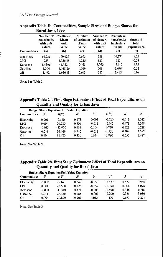
Appendix Table lb. Commodities, Sample Sizes and Budget Shares forRural Java, 1999

Commodities



values(a)

14,231233

13,3062,2041,492

CoefficientMeanunitvalue

(b)

199.0291,356.88465.2241,028.261,036.18

Numberof variation

of unitvalue

(c)

0.6930.2250.1610.1090.613


values(d)

988123

1,023701567


in(d)(e)

14,574627

13,6162,6762,493

shares oftotal

expenditure(f)

1.630.031.350.520.16

Note: See Table 2.

Appendix Table 2a. First Stage Estimates: Effect of Total Expenditures onQuantity and Quality for Urban Java



P»0.0010.004-0.0130.0140.004

'(P°)2.120

20.980-42.97026.46018.480

R'

0.2750.3010.4940.3400.320

P'-0.005-0.0120.004-0.0120.074

'(P')-0.620-0.7400.770-1.4502.880

R'

0.6120.4780.3230.3040.655

e

1.0422.3580.2182.3822.427

Note: See Table 3.

Appendix Table 2b. First Stage Estimates: Effect of Total Expenditures onQuantity and Quality for Rural Java



p»-0.0020.001-0.0040.0110.004

'(P°)-6.14012.660-11.51026.15020.890

R'

0.3420.2260.4710.2860.209

P'-0.058-0.357-0.003-0.0030.053

-5.570-0.350-0.490-0.2001.470

R'

0.5770.6660.3460.3410.677

e

0.9524.0760.7183.0803.271

Note: See Table 3.


Appendix Table 3a. Symmetry Constrained Estimates of Own and CrossPrice Elasticities for Urban Java, 1999

Electricity

LPG

Kerosene

Gasoline

Oil

Other Cons

Electricity

-0.990(0.03)

-0.128(0.14)

0.003(0.04)

-0.175(0.11)

0.039(0.21)

-0.001(0.00)

LPG

-0.014(0.02)

-0.365(0.62)

0.027(0.11)

-0.894(0.47)

-0.119(0.21)

-0.002(0.00)

Kerosene

-0.011(0.03)

0.126(0.67)

-0.635(0.18)

-0.027(0.26)

-0.260(0.28)

0.001(0.00)

Gasoline

-0.073(0.06)

-3.213(1.69)

0.005(0.16)

-0.868(0.23)

0.942(0.55)

-0.002(0.00)

Oil

0.008(0.03)

-0.106(0.19)

-0.034(0.04)

0.234(0.14)

-0.372(0.16)

0.001(0.00)

Other Cons

0.043(0.08)

1.340(1.87)

0.416(0.29)

-0.640(0.62)

-2.731(0.71)

-0.274(0.35)

Note: See Table 4

Appendix Table 3b. Symmetry Constrained Estimates of Own and CrossPrice Elasticities for Rural Java, 1999

Electricity

LPG

Kerosene

Gasoline

Oil

Other Cons

Electricity

-1.108(0.03)

-1.493(2.13)

-0.157(0.07)

-0.036(0.02)

-0.707*(0.21)

-0.002(0.00)

LPG

-0.029(0.04)

-1.616(2.85)

-0.119(0.21)

0.000(0.01)

0.024(0.39)

-0.001(0.00)

Kerosene

-0.132(0.06)

-5.008(8.91)

-1.331(0.25)

-0.032(0.00)

-1.460(0.77)

-0.003(0.00)

Gasoline

0.000(0.00)

0.000(0.18)

0.000(0.00)

-1.000(1.09)

0.000(0.00)

0.000(0.00)

Oil

-0.065(0.02)

0.118(1.92)

-0.168(0.09)

0.000(0.00)

-0.489(0.20)

-0.001(0.00)

Other Cons

0.439(0.08)

3.960(10.51)

1.059(0.36)

-2.010(1.02)

-0.692(0.92)

-0.264(0.26)

Note: See Table 4


Appendix Table 4a. Efficiency Aspects of Price Reform in Urban Java witb

Commodities


T,

-1.60-0.43-2.23-0.470.090.09

w.

-0.99-0.35-0.53-0.89-0.53-1.00

Own effect

1.580.151.180.42-0.05-0.09

Cross effects

0.041.100.060.480.08-0.02

Totai

2.622.252.241.901.040.89

Appendix Table 4b. Efficiency Aspects of Price Reform in Rural Java witbSymmetry Restriction

Commodities


T.

1 + T,

-1.60-0.43-2.23-0.470.090.09

-1.09-1.07-1.36-1.00-0.75-0.99

Own effect

1.740.463.040.47-0.07-0.09

Cross effects

0.221.510.250.001.97

-0.04

Totai

2.972.974.281.472.900.87

Appendix Table 5a. Equity Effects and Cost-Benefit Ratios for PriceReform in Urban Java witb Symmetry Restrictions

Commodities


e =

1.001.001.001.001.001.00

0X

0.380.440.450.530.971.12

E =

w^lw

0.950.781.110.820.791.00

0.5X

0.360.350.500.430.761.12

e =w'^ Iw

0.910.581.170.670.641.01

1X

0.350.260.520.350.621.13

£=2w^ Iw

0.850.291.190.470.441.01

X

0.320.130.530.250.421.13

Appendix Table 5b. Equity Effects and Cost-Benefit Ratios for PriceReform in Rural Java witb Symmetry Restrictions

Commodities

ElectricityLPGKeroseneGasolineLubricant OilOther consumption

w' Iw

1.001.001.001.001.001.00

e = 0X

0.340.340.230.680.351.15

E =w' Iw

0.950.781.110.820.791.00

0.5X

0.320.260.260.550.271.15

e=w' Iw

0.910.581.170.670.641.01

1X

0.310.190.270.460.221.16

e=w^lw

0.850.291.190.470.441.01

2X

0.290.100.280.320.151.16

Household Energy Demand I 39

REFERENCES

Ahmad, E. and Stern, N. (1984). "The theory of reform and Indian indirect taxes" Journal of PublicEconomics 25 (3): 259 - 298.

Attanasio, O. and Frayne, C. (2006). "Do the poor pay more?" Paper presented at the Eighth BREADConference, Cornell University, May 2006.

BBC News (2005). "Indonesia clashes over fuel hike" [On-line] Available http://news.bbc.co.Uk/l/hi/world/asia-pacific/4296320.stm

Creedy, J. (1996). "Measuring income inequality"/4«ifra/(an Economic Review 29(2): 236-246.Deaton, A. (1988). "Quality, quantity, and spatial variation of price" American Economic Review

78(3): 418-430.Deaton, A. (1990). "Price elasticities from survey data: Extensions and Indonesian results" Journal of

Econometrics 44(3): 281 -309.Deaton, A. (1997). The Analysis of Household Surveys: A Microeconometric Approach to Develop-

ment Policy. Baltimore: The John Hopkins University Press.Deaton, A. (1998). "Getting prices right: what should be done?" Journal of Economic Perspectives

12(1): 37-46.Dick, H. (1980). "The oil price subsidy, deforestation and equity" Bulletin of Indonesian Economic

Studies 16(3): 32-60.Economist (2005). "Indonesia's ropey Rupiah" September I". [On-line] Available http://www.

economist.com/displaystory.cfm?story_id=4355717Gibson, J. (2006). "A simple test of liquidity constraint and whether the poor pay more" Paper pre-

sented at the NEUDC 2006 Conference, Cornell University, September 2006.International Energy Agency (1999). World Energy Outlook: Looking at Energy Subsidies, Getting the

Prices Right. International Energy Agency: Paris.Jakarta Post (2005). "Indonesia may cut fuel subsidies by as much as 60 percent by November" [On-

line] Available http://www.thejakartapost.com/detaillatestnews.asp?fileid=20050908120004&irec=6Kompas (2005). "Dana kompensasi BBM: 40 juta orang dapat subsidi secara langsung" [On-line]

Available http://www.kompas.com/utama/news/0507/27/011328.htmKoshal, R., Koshal, M., Boyd, R., and Rachmany, H. (1999). "Demand for kerosene in developing

countries: a case of Indonesia" Journal of Asian Economics 10(3): 329-336.Madden, D. (1996). "Marginal tax reform and the specification of consumer demand systems" Oxford

Economic Papers 48(4): 556 - 567.Newbery, D. (2005) "Why tax energy? Towards a more rational policy" The Energy Journal 26(3):

1-40.Nicita, A. (2004). "Efficiency and equity of a marginal tax reform: income, quality and price elastici-

ties for Mexico" World Bank Policy Working Paper No. 3266, World Bank, Washington DC.Pitt, M. (1985). "Equity, externalities and energy subsidies: The case of kerosene in Indonesia" Jour-

nal of Development Economics 17 (3): 201 -217.Pradhan, M. (2001). "Welfare analysis with a proxy consumption measure: Evidence from a repeated

experiment in Indonesia" Cornell Food and Nutrion Policy Program Working Paper No. 126.Prais, S. (1958). Whose cost of living? Review of Economic Studies 26(1): 126-134.Sen, K. and Steer, L. (2005). "Survey of recent developments" Bulletin of Indonesian Economic Stud-

ies 4\(?,): 213-204.Sumarto, S. and Suryahadi, A. (2001). "Kerosene: Government subsidies and household consump-

tion" SMERU Newsletter No. 2, March-April, 2001, pp 1-4 <http://smeru.orid/newslet/2001/ed02/200102data.htm>

Yitzhaki, S. and Lewis, J. (1996). "Guidelines on searching for a Dalton-improving tax reform: Anillustration with data from Indonesia" World Bank Economic Review 10(3): 541-562.

World Bank (2005). Indonesia: Economic and Social Update, October. World Bank, Jakarta.

Household Energy Demand and the Equity and Efficiency Aspects of Subsidy Reform in Indonesia

Documents

Transcript of Household Energy Demand and the Equity and Efficiency Aspects of Subsidy Reform in Indonesia