Household Characteristics and Calorie Intake in RuralIndia: A Quantile Regression Approach∗

Kompal SinhaThe Australian National University

January 2005

Abstract

The present paper investigates the nutrition demand pattern for rural householdsin India. The non-parametric approach of quantile regression is applied to character-ize the entire distribution of calorie consumption. This technique has an advantageover the traditional ordinary least square technique. It relaxes the assumption ofa constant effect of the explanatory variables over the entire distribution of the de-pendent variable. These effects are allowed to vary over the entire distribution ofdependent variable i.e., in this case the distribution of calorie consumption. The re-sults show that indeed, the responsiveness of calorie consumption to various factorsdiffers across different levels of calorie consumption. A comparison of the quantileregression results with OLS results suggests conclusions and policy suggestions basedon OLS results are unlikely to be ideal. Some further light is also shed on the debateon calorie income elasticity as the magnitude is observed to be different for the un-dernourished and the over nourished households.

∗I thank Prof. R. Jha and Prof. Anil. B. Deolalikar for comments on earlier drafts of this paper.The UK Department for International Development (DFID) supports policies, programmes and projectsto promote international development. DFID provided funds for this study as part of that objective butthe views and opinions expressed are those of the author(s) alone.

1 Introduction

Access to adequate food and proper nutrition is one of humanity’s basic needs. One fifth

of the population of developing countries i.e., around 800 million people, were reported to

be suffering from chronic undernutrition by the FAO (1992). Malnourishment creates a

vicious circle - without regular adequate food an individual is not able to live a healthy

and active life. Without such a life the individual will be unable to efficiently produce or

procure food or perform well in the labour market. Thus, it is very important to provide

people with adequate food availability or in other words “food security”. Food security is

broadly defined by the Food and Agriculture Organization of the United Nations (FAO)

as access to enough food for a healthy, active lifestyle. Although national food security is

important it is only effective if measures are taken at the household level. At that level

“food security” is defined as ‘access to food that is adequate in terms of quality, quantity,

safety and cultural acceptability for all household members’ (FAO 1992). In economics,

the importance of health and nutrition has been widely accepted. Health and nutrition

have both demand and supply side effects. On the demand side, people require health and

nutrition to stay fit as they derive satisfaction from feeling healthy. Health and nutrition

have an effect on the fertility and mortality of the population which has a direct effect on

development of the economy. On the supply side, health and nutrition affect individual

productivity, thereby having an effect on human-capital formation. These factors affect

the efficient functioning of an economy. Thus a healthy nutritional population status is

vital for economic growth. There is great interest around the world in improving nutrition

in developing countries though measures such as price subsidies and income generation

policies. In order to actually “improve nutrition” it is important to define the meaning

of an adequate and balanced diet for different groups of individuals within a society and

design economic policies in a manner which caters to their needs. “A large variation exists

in defining ‘adequate’ nutrition, ranging between 1400 and 2800 Kilo Calories (Kcal) and is

therefore subject to value judgement” FAO (1992). In India, the Indian Council of Medical

Research (ICMR) sets up the Nutrition Advisory Committee and recommends the “dietary

allowances” of the various nutrients for the various age groups within the population. As

per the ICMR report a daily energy intake is recommended of 2400 Kcal per person in

2

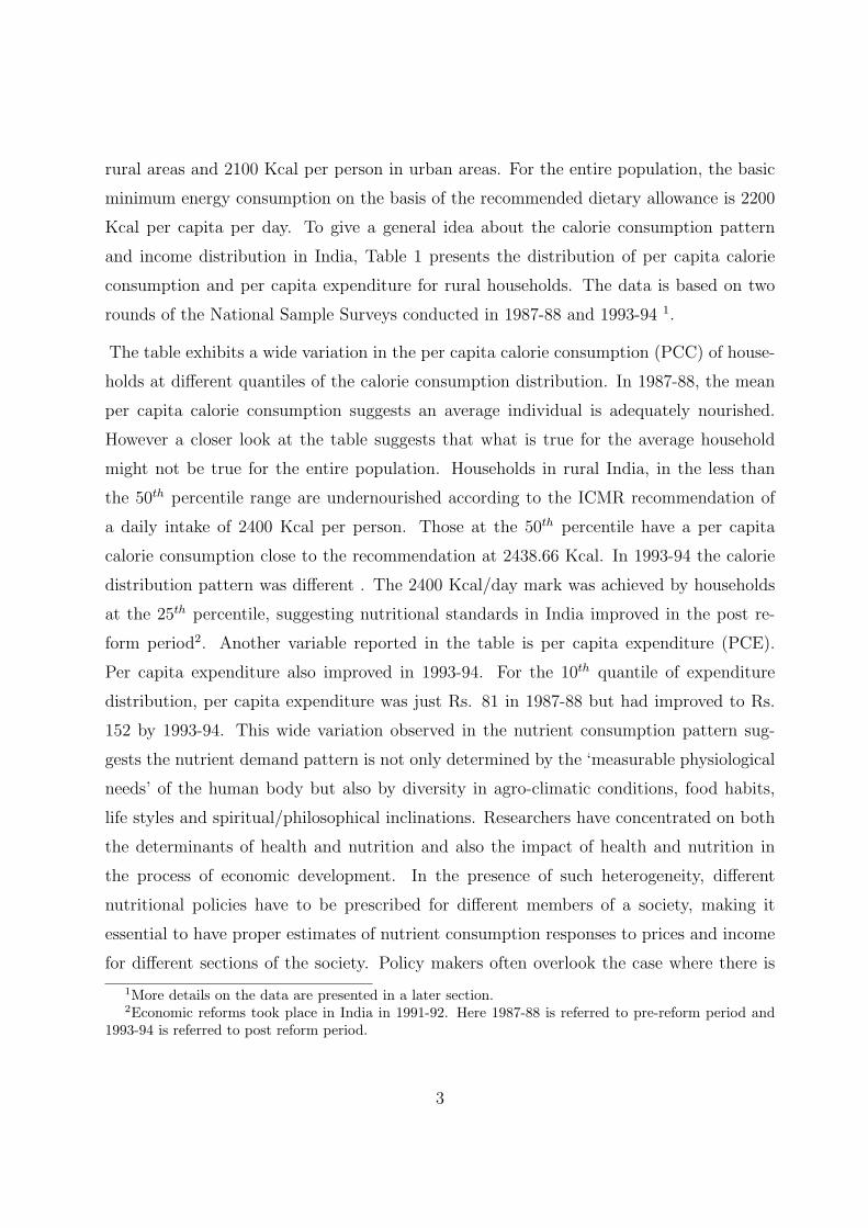
rural areas and 2100 Kcal per person in urban areas. For the entire population, the basic

minimum energy consumption on the basis of the recommended dietary allowance is 2200

Kcal per capita per day. To give a general idea about the calorie consumption pattern

and income distribution in India, Table 1 presents the distribution of per capita calorie

consumption and per capita expenditure for rural households. The data is based on two

rounds of the National Sample Surveys conducted in 1987-88 and 1993-94 1.

The table exhibits a wide variation in the per capita calorie consumption (PCC) of house-

holds at different quantiles of the calorie consumption distribution. In 1987-88, the mean

per capita calorie consumption suggests an average individual is adequately nourished.

However a closer look at the table suggests that what is true for the average household

might not be true for the entire population. Households in rural India, in the less than

the 50th percentile range are undernourished according to the ICMR recommendation of

a daily intake of 2400 Kcal per person. Those at the 50th percentile have a per capita

calorie consumption close to the recommendation at 2438.66 Kcal. In 1993-94 the calorie

distribution pattern was different . The 2400 Kcal/day mark was achieved by households

at the 25th percentile, suggesting nutritional standards in India improved in the post re-

form period2. Another variable reported in the table is per capita expenditure (PCE).

Per capita expenditure also improved in 1993-94. For the 10th quantile of expenditure

distribution, per capita expenditure was just Rs. 81 in 1987-88 but had improved to Rs.

152 by 1993-94. This wide variation observed in the nutrient consumption pattern sug-

gests the nutrient demand pattern is not only determined by the ‘measurable physiological

needs’ of the human body but also by diversity in agro-climatic conditions, food habits,

life styles and spiritual/philosophical inclinations. Researchers have concentrated on both

the determinants of health and nutrition and also the impact of health and nutrition in

the process of economic development. In the presence of such heterogeneity, different

nutritional policies have to be prescribed for different members of a society, making it

essential to have proper estimates of nutrient consumption responses to prices and income

for different sections of the society. Policy makers often overlook the case where there is

1More details on the data are presented in a later section.2Economic reforms took place in India in 1991-92. Here 1987-88 is referred to pre-reform period and

1993-94 is referred to post reform period.

3

Tab

le1:

Dis

trib

uti

onof

Cal

orie

Con

sum

ption

and

Expen

diture

for

Rura

lH

ouse

hol

ds

inIn

dia

,19

87-8

8an

d19

93-9

4.

Per

centi

le—

——

——

——

——

——

——

——

——

——

——

—-

1025

5075

90M

ean

Std

Dev

.Ske

wnes

sK

urt

osis

1987-8

8C

alor

ie(K

cal/

day

)16

16.9

920

07.8

924

77.7

530

51.8

537

75.6

626

52.4

012

70.7

77.

9917

1.88

Expen

dit

ure

(Rs.

/m

onth

)80

.93

105.

9414

5.93

210.

7531

1.88

185.

2623

6.06

52.6

951

03.8

8

1993-9

4C

alor

ie(K

cal/

day

)14

11.6

122

72.7

431

39.9

841

98.0

955

27.3

4134

16.3

119

69.0

93.

6946

.92

Expen

dit

ure

(Rs.

/mon

th)

144.

0418

7.56

260.

3737

0.43

529.

4431

7.67

303.

2927

.92

1599

.27

All

the

vari

able

sare

inper

capita

term

s.

Note

:T

he

2400

KC

al/

day

daily

requir

em

ent

was

att

ain

ed

at

46

thpercenti

lein

1987-8

8,th

eactu

alvalu

ew

as

2401.1

6K

Cal/

day

Note

:T

he

2400

KC

al/

day

daily

requir

em

ent

was

att

ain

ed

at

28.5

thpercenti

lein

1993-9

4,th

eactu

alvalu

ew

as

2403.4

3K

Cal/

day

Sourc

e:N

ationalSam

ple

Surv

ey43

rd

Round

and

50

thR

ound

4

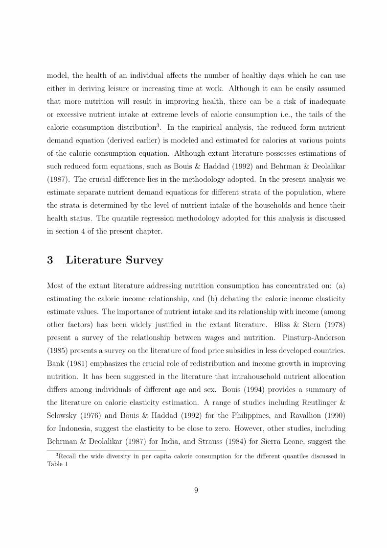
a risk of inadequate or excess intake. Such inadequacy prevails at the tails of the nutri-

ent intake distribution i.e., situations where calorie consumption is either very low ( the

left tail) or very high (the right tail) than at the mean (or the average). Thus in issues

involving the public health and nutrition perspective it is important to characterize the

population at the tails of nutrient intake distribution. Given the wide variation in calorie

consumption at various points of the distribution a single policy measure depending on

the average calorie consumption would be unrealistic and unable to reach the expected

goals. An individual’s demand for nutrition of an individual will depend on his present

level of nutrition. An overnourished person might demand a lesser amount of nutrient

vis-a-vis a person who is undernourished. Thus in designing nutrition policy it is neces-

sary to take into account the “level of healthiness” of the population. With various policy

measures taken by the government, the individuals at different points of a nutrient intake

distribution might respond differently so that focusing the implication just on the mean

would give an incomplete picture of the response. Thus, empirically, it is important to

look for such behaviour by studying the whole distribution. Therefore, in focusing only

on the conditional mean, a parametric approach such as the OLS would give an incom-

plete picture of the various factors promoting healthier diet behaviour. The present paper

models the entire distribution of calorie consumption and is organized as follows. Section

2, theoretically models farm household behaviour and derives the reduced form demand

equations for various commodities, one of which is nutrient demand. Section 3 presents a

literature survey of past research pertaining to nutrient demand. Section 4 gives a detailed

overview of the quantile regression technique used in the analysis. Section 5 explains the

data used in the analysis. On the basis of the reduced form equations obtained in Section

2, Section 6 empirically models the demand of nutrients - calories - at the various points

of the calorie consumption distribution and analyzes the results. The interpretation of the

results concentrates on where the risks of inadequacy is higher i.e., undernourished and

overnourished households. Section 7 discusses the conclusions.

5

2 Theoretical Model

An individual’s health and nutrition status and the demand thereof are dependent on

the household he belongs to and therefore, it is important to model the behaviour of the

household in relation to nutritional intake. There are two main approaches to modeling

such household behaviour Behrman & Deolalikar (1988). One is the Becker (1965) approach

of household production and the other the farm household model of Nakajima (1969).

Grossman (1972) developed a household production model considering health as a form of

human capital. Nutrition is an important determinant of the health and well being of an

individual and hence has important consequences for household behaviour. To explain the

relationship between market factors, health, production and consumption the model of a

farm household is considered in the presence of health effects. The model is very similar

to the one designed by Pitt & Rosenzweig (1986) and Behrman & Deolalikar (1988). The

household maximizes its preference function subject to a set of constraints. For simplicity

a single period model under certainty or certainty equivalence is considered.

The rural household under consideration is assumed to maximize the following utility

function.

Household utility function :

U = U(χa, χm, χl, χH ; ξ) (1)

where,

χa : Agriculture output produced at level Q by the household,

χm : Market purchased commodity,

χl : Leisure,

χH : Level of health of the household,

ξ : Environmental factors out of control of the household.

1. Time Constraint: The constraints to maximize this utility function are as follows:

χl + F = T ' Ω(χH) (2)

where,

T : total time,

6

F : labour input of family.

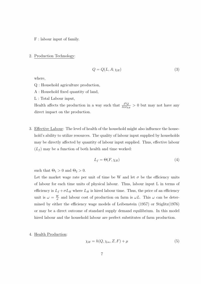
2. Production Technology:

Q = Q(L, A; χH) (3)

where,

Q : Household agriculture production,

A : Household fixed quantity of land,

L : Total Labour input,

Health affects the production in a way such that δ2QδLδχH

> 0 but may not have any

direct impact on the production.

3. Effective Labour: The level of health of the household might also influence the house-

hold’s ability to utilize resources. The quality of labour input supplied by households

may be directly affected by quantity of labour input supplied. Thus, effective labour

(Lf ) may be a function of both health and time worked:

Lf = Θ(F, χH) (4)

such that Θ1 > 0 and Θ2 > 0.

Let the market wage rate per unit of time be W and let σ be the efficiency units

of labour for each time units of physical labour. Thus, labour input L in terms of

efficiency is Lf +σLH where LH is hired labour time. Thus, the price of an efficiency

unit is ω = Wσ

and labour cost of production on farm is ωL. This ω can be deter-

mined by either the efficiency wage models of Leibenstein (1957) or Stiglitz(1976)

or may be a direct outcome of standard supply demand equilibrium. In this model

hired labour and the household labour are perfect substitutes of farm production.

4. Health Production:

χH = h(Q,χm, Z, F ) + µ (5)

7

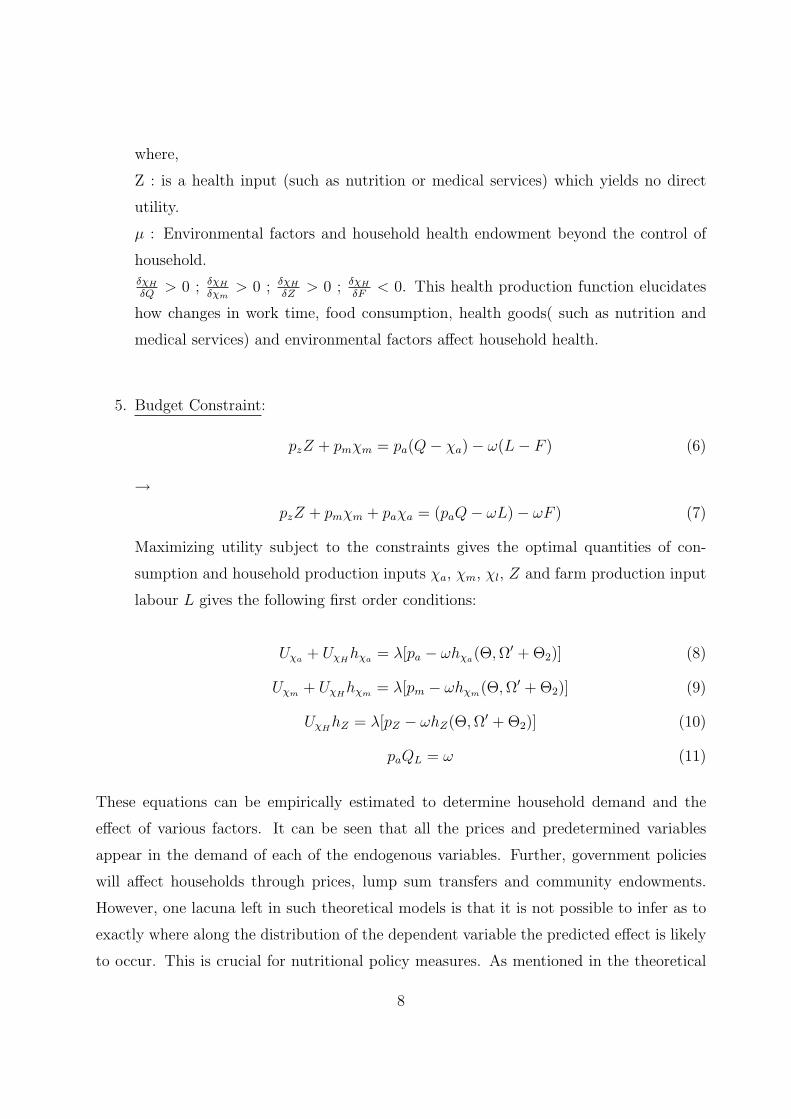
where,

Z : is a health input (such as nutrition or medical services) which yields no direct

utility.

µ : Environmental factors and household health endowment beyond the control of

household.δχH

δQ> 0 ; δχH

δχm> 0 ; δχH

δZ> 0 ; δχH

δF< 0. This health production function elucidates

how changes in work time, food consumption, health goods( such as nutrition and

medical services) and environmental factors affect household health.

5. Budget Constraint:

pzZ + pmχm = pa(Q− χa)− ω(L− F ) (6)

→pzZ + pmχm + paχa = (paQ− ωL)− ωF ) (7)

Maximizing utility subject to the constraints gives the optimal quantities of con-

sumption and household production inputs χa, χm, χl, Z and farm production input

labour L gives the following first order conditions:

Uχa + UχHhχa = λ[pa − ωhχa(Θ, Ω′ + Θ2)] (8)

Uχm + UχHhχm = λ[pm − ωhχm(Θ, Ω′ + Θ2)] (9)

UχHhZ = λ[pZ − ωhZ(Θ, Ω′ + Θ2)] (10)

paQL = ω (11)

These equations can be empirically estimated to determine household demand and the

effect of various factors. It can be seen that all the prices and predetermined variables

appear in the demand of each of the endogenous variables. Further, government policies

will affect households through prices, lump sum transfers and community endowments.

However, one lacuna left in such theoretical models is that it is not possible to infer as to

exactly where along the distribution of the dependent variable the predicted effect is likely

to occur. This is crucial for nutritional policy measures. As mentioned in the theoretical

8

model, the health of an individual affects the number of healthy days which he can use

either in deriving leisure or increasing time at work. Although it can be easily assumed

that more nutrition will result in improving health, there can be a risk of inadequate

or excessive nutrient intake at extreme levels of calorie consumption i.e., the tails of the

calorie consumption distribution3. In the empirical analysis, the reduced form nutrient

demand equation (derived earlier) is modeled and estimated for calories at various points

of the calorie consumption equation. Although extant literature possesses estimations of

such reduced form equations, such as Bouis & Haddad (1992) and Behrman & Deolalikar

(1987). The crucial difference lies in the methodology adopted. In the present analysis we

estimate separate nutrient demand equations for different strata of the population, where

the strata is determined by the level of nutrient intake of the households and hence their

health status. The quantile regression methodology adopted for this analysis is discussed

in section 4 of the present chapter.

3 Literature Survey

Most of the extant literature addressing nutrition consumption has concentrated on: (a)

estimating the calorie income relationship, and (b) debating the calorie income elasticity

estimate values. The importance of nutrient intake and its relationship with income (among

other factors) has been widely justified in the extant literature. Bliss & Stern (1978)

present a survey of the relationship between wages and nutrition. Pinsturp-Anderson

(1985) presents a survey on the literature of food price subsidies in less developed countries.

Bank (1981) emphasizes the crucial role of redistribution and income growth in improving

nutrition. It has been suggested in the literature that intrahousehold nutrient allocation

differs among individuals of different age and sex. Bouis (1994) provides a summary of

the literature on calorie elasticity estimation. A range of studies including Reutlinger &

Selowsky (1976) and Bouis & Haddad (1992) for the Philippines, and Ravallion (1990)

for Indonesia, suggest the elasticity to be close to zero. However, other studies, including

Behrman & Deolalikar (1987) for India, and Strauss (1984) for Sierra Leone, suggest the

3Recall the wide diversity in per capita calorie consumption for the different quantiles discussed inTable 1

9

elasticity is closer to 1. Papers studying farm productivity and calorie intake include

Strauss (1986), who estimates a significant output calorie elasticity.

Gibson & Rozelle (2002) study the urban areas of Papua New Guinea and seek evidence

of the elasticity of calorie demand with respect to household resources. The authors find

the relationship between per capita calorie consumption and per capita expenditure is

consistent with the assertion that income changes have a negligible effect on nutrient intake.

The results are not seen to alter when parametric and semiparametric estimation is done

to control for other influences on calorie consumption.

Tiffin & Dawson (2002) examine the long run relationship between per capita calorie

intake, per capita income and food prices for Zimbabwe. The authors identify strong

evidence of a long-run relationship between calorie and income and their feedback effects.

Therefore, calorie intake is determined by income and simultaneously nutritional status

constrains income. Impulse responses suggest a shock to calorie (income) increases income

(calorie) permanently and these effects are complete in four years. Thus, income growth

can act as a catalyst in alleviating inadequate calorie intake and income can increase with

improvements in nutritional status - supporting the efficiency wage hypothesis.

Few studies on the nutrient demand in India have been done such as the ones by Behrman

& Deolalikar (1989, 1990). Behrman & Deolalikar (1989) explore the quantifiable expla-

nation of the assertion that calorie elasticity are substantially less than food expenditure

elasticity. This implies people prefer food variety. As income increases households purchase

a variety of food even though this might not result in altering calorie intake. The esti-

mates suggest that as income and total expenditures on food increase consumers display

a behaviour of increasingly preferring food variety. This suggests the income elasticity of

calorie intakes is less than food expenditure elasticities with respect to income at lower

levels of per capita income.

Behrman & Deolalikar (1987) investigate the relatively poor population of rural south

India. The authors introduce the concept of ‘direct’ and ‘indirect’ calorie -income elasticity

estimation. Direct elasticity estimation is the conversion of food group quantities into

aggregate calories before estimation and indirect elasticity estimation is when food group’s

expenditure elasticities are calculated and a weighted average computed. The authors

10

calculate calorie-income elasticities for the same households from two different data sources,

viz., calorie intake as a function of predicted total expenditure (this is from a two hourly

recall of 120 foods) and food group expenditure as a function of predicted total expenditure

in a non system framework (for only 6 aggregate food groups). Their results thereby

infer direct nutrient elasticities are not significantly different from zero whereas indirect

nutrient elasticities are close to one. Similar results for developing countries are reported

in: Knudsen & Scandizzo (1982) for Sri Lanka, India and Morocco, Ravallion (1988) for

Indonesia, Greer & Thorbecke (1986) for Kenya, and Alderman (1986) for Sri Lanka,

Thailand, Egypt, Sudan, Indonesia, Nigeria, Malaysia, Brazil, Bangladesh and Morocco.

All these studies indicate that relatively poor individuals give importance to food attributes

other than calorie content when making their marginal food choices in response to an

income change.

Behrman et al. (1997) take a panel data of farm households in rural Pakistan and calculate

the calorie response to different components of income. In particular the authors take into

account the sequential nature of agricultural production, labour and capital market imper-

fections, heterogeneity and productive effects of calories. A theoretical model is considered

taking into account the aforementioned conditions. The analysis suggests that to under-

stand the impact of income on calorie consumption it is critical to distinguish between the

stages of agricultural production. This is due to the differential cost of consumption in

calorie’s consumed in the planting stages. Thus the authors infer calorie-income elasticity

is not only affected by the wealth class but also by the stages of production within class.

In his study of wages and nutrition in rural India Deolalikar (1988) was unable to trace

any evidence of nutrition determining wages.

Dawson & Tiffin (1998) use annual data for India for 1961-1992 and examine the long

run relationship between calories and income using a cointegration approach. The authors

do not make any assumptions regarding the direction of causality ex ante. The results

show calorie intake to be Granger caused by income and food prices were observed to be

constant.

Bouis & Haddad (1992) discuss the calorie income elasticities estimated in the extant liter-

ature. The authors attempt to address the question: “what effect do increases in the income

11

levels of the poor in developing countries have on their level of calorie consumption?” This

question is crucial to nutrition policy analysis because sound nutrition policy must have

an accurate calorie income elasticity measurement. The authors suggest that there is a

wide variation in the calorie income elasticities calculated in the ex ante literature. This

variation is due to the particular calorie and income variables used by economists in their

econometric analysis. To see this, the paper compares elasticities across four estimation

techniques and four calorie-income variable pairs for a sample of Philippine farm house-

holds. The four possible pairs of dependent and independent variables considered in the

analysis are: calorie availability, calorie intake (this is an alternative dependent variable

considered), total expenditure and current income (this is an alternative dependent vari-

able). Considering the calorie availability and total expenditure pair the authors observe

that both variables are affected by measurement errors - the random error in measuring

food purchases is transferred both to calorie availability and total expenditure. Therefore,

there is correlation between the measurement errors for these two variables. This results in

the coefficient of total expenditure estimator to be biased upwards. The other observation

is that the residual difference between family calorie intake and household calorie availabil-

ity will often increase as a percentage of total food expenditure as income increases. With

this, the underestimate of meals served to non-family members will be positively correlated

with any income variable which in turn will result in an overestimate of the true elastic-

ity. Analysing the past literature the authors note that larger elasticities are derived from

calorie availability and total expenditure. They observe that on disaggregation by expen-

diture quantile, there is a clear pattern well below the family calorie intake for low-income

households and for family calorie availability to be well above calorie intake for high income

households. Finally, the authors conclude the calorie intake and total expenditure variable

pair gives a reliable elasticity estimate and is important for the policy debate to take into

account the absolute change in income as against the percentage change in income.

Majority of the extant literature has concentrated on an average household i.e., a represen-

tative household assuming that behaviour of all households in the society is homogenous

because the analysis in these studies is mostly done at the mean. However, policy measures

taken according to these results are not likely to be equally effective for all members of

the society. Therefore, it is important to take account of the heterogeneity of the popula-

12

tion. Various policy measures taken by the government affect the behaviour of the various

strata of the population differently. Thus, policy has to be tailored differently for different

sections of the society. When deciding on an adequate dietary intake and policies for its

enhancement policymakers often overlook the case where there is a risk of inadequate or

excess intake. Only one study by Variyam et al. (2002) has dealt with this issue. The

next section will empirically analyse the issue of nutritional status taking into account the

heterogeneity in nutrient consumption.

4 Methodology

Recent empirical research has provided evidence to show that for data having outliers, the

traditional conditional mean estimates do not give an efficient outcome. Yu et al. (2003)

mention the “sample median is more robust to outliers than a sample mean for estimating

the average location of population” and hence quantile regression is more stable than mean

regression for analysing data with outlying observation.

In the classical least square regression methodology it is only necessary to know the con-

ditional mean function i.e., the function that describes how the mean of y changes with

the vector of covariates x. Simply said, it is the true value around which y fluctuates

due to an accidental error. The error is assumed to have exactly the same distribution

irrespective of the values taken by the components of the vector x. This is known as a pure

location shift model as it assumes the x vector affects only the location of the conditional

distribution of y, neither its shape nor any other aspect of its distribution shape. With

the additional assumption that the error terms are normally distributed, the least square

methods give the maximum likelihood estimates of the conditional mean functions. It has

been argued in the econometric literature that the covariates may influence the conditional

distribution of the response variable in ways other than just the location. These factors are

: induce multimodality, expand the dispersion of the response variable as in the models of

heteroskedasticity, stretch one tail of the distribution and/or compress the other tail of the

distribution. All these issues can be addressed by performing quantile regressions. Quan-

tile regression models possess certain features that make this technique a better alternative

than the ordinary least square model:

13

• Quantile regression models can be used to characterize the entire distribution of a

dependent variable for a given set of regressors.

• A quantile regression model has a linear programming representation which makes

estimation easy.

• The objective function for quantile regression is the weighted sum of absolute devia-

tions. This gives a robust measure of location and thereby the estimated coefficient

is not sensitive to outlier observations of the dependent variable.

• Quantile regression estimators are more efficient than least square estimators if the

distribution of the error term is non-normal.

• Potential different solutions at distinct quantiles may be inferred as differences in the

response of the dependent variable to changes in the regressors at various points in

the distribution of the dependent variable.

• Quantile regression is more stable than mean regression for analysing contaminated

data. 4 Yu & Jones (1998) established that the variance of a typical kernel smoother

is greater than the variance of a smooth quantile regression curve.

In the present analysis nutrient demand equations will be estimated using the quantile

regression methodology. The quantile regression estimates will also be compared with the

OLS regression estimates and inferences drawn.

4If a pair (xi, yi) is bad with probability π and good with probability (1−π) and (xi, yi) are distributedas

(X, Y ) =∼ N(0, 0, 1, 1) if (xi, yi) is goodN(0, 0, k, k) (xi, yi) is bad

where N(µ1, µ2, r , σ12, σ2

2) is a bivariate normal distribution with correlation coefficient r , means µ1, µ2

and variances σ12 and σ2

2. Then (xi, yi) are independent realization from the underlying contaminateddensity

f(x, y) = (1− π)f1(x, y) + πf2(x, y) (12)

where f1 and f2 are density functions for N(0,0,r,1,1) and N(0,0,r,k,k) respectively.

14

4.1 Quantile Regression

The Basic Model: Before formally defining quantile regression the elementary definition

of a sample quantile is explained. The word quantile is a synonym for percentile or fractiles

and refers to the general case of dividing the the reference population into four segments, a

quintile divides the reference population into five parts and a decile divides the population

into 10 segments. The median divides the population into two parts. In a sense, quantiles

are related to the process of ordering and sorting. As a sample population mean is defined

as a solution of minimizing the sum of squared residuals, the median is defined as the

solution to minimizing a sum of absolute residuals. Suppose that the θth quantile of a

population is mθ where 0 < θ < 1 and FN is the cumulative distribution function, in the

population, of y then mθ is defined as:

θ = Pr[y ≤ mθ] = FN(mθ) (13)

For a sample the analogous expression for defining mθ is:

mθ = inf[y : FN(y) ≥ θ] (14)

Thus, for example, these equations say that in a class of pupils, a pupil scores at the θth

quantile of an exam if he or she performs better than the proportion θ of the reference

group of students and worse than the proportion (1−θ) of the reference group of students.

The median is the case when θ = 1/2.

4.1.1 Quantile Regression Empirical Literature

A nice update on the quantile regression technique is provided in Yu et al. (2003).

There has been considerable use of the quantile regression technique in labour economics.

Chamberlain (1994) on the basis of his quantile regression model infers that for manufac-

turing workers, the union wage premium, which is at 28 percent at first decile, declines

continuously to 0.3 percent at the upper decile. The author suggests that the location shift

model estimate(least square estimate) which is 15.8 percent, gives a misleading impression

of the union effect. In fact, this mean union premium of 15.8 percent is captured primarily

by the lower tail of the conditional distribution. The labour market issues addressed using

15

quantile regression include a number of studies by Buchinsky (for example, see Buchinsky

(1994) and Buchinsky (2001)) among others.

Machado & Mata (2001) estimate the earning function for Portugal for the period 1982-

1994. The objective of the analysis is to analyse the structure and evolution of the re-

turns to education and their relationship with increased wage inequality. The authors use

quantile regression technique to document the heterogeneity in the way wages respond to

variations in the variables - gender, human capital, firm attributes and industry indica-

tors. Unlike meas square regression these techniques allow the study of the effect of each of

the covariates along the whole distribution and, consequently, the estimation of the effect

of employers and workers heterogeneity upon wages. The authors observe that despite

substantial improvement in the level of education of the working population, returns to

secondary education increased at all quantiles, however the effect was more prominent at

the top of the wage distribution. It was observed that the returns to education were higher

at higher quantiles and the difference in returns at the top and the bottom of the wage

distribution had widened over the time period.

Min & Kim (2004) compare the parametric and nonparametric quantile regression meth-

ods using Monte Carlo simulations. The authors suggest “... over a wide-class of non

Gaussian error, with asymmetric and fat tail distribution, the simple mean regression can-

not satisfactorily capture the stylized facts on the data. Also, dependent variables in the

household survey data, under these circumstances, the conditional mean estimator and

thus can be misleading.” The authors conclude that the nonparametric quantile regression

approach proves to be more appropriate when the underlying model is nonlinear or when

the error term follows a non-normal distribution. Abrevaya (2001) investigates the impact

of various demographic characteristics and maternal behaviour on the birth weight of the

infants born in the U.S.

Eide & Showalter (1998) and Levin (2001) have addressed school quality issues. Levin

(2001) studies a panel survey of the performance of Dutch school children. The author

finds some evidence of positive peer effects in the lower tail of the achievement distribution.

However, there seems to be little support for the claim that student outcomes are improved

by reducing class size.

16

Nguyen et al. (2003) attempt to examine the source of inequality in rural and urban

Vietnam. The urban rural gap has been an important feature of Vietnam and the authors

attempt to address this gap by employing quantile regression. The paper uses the Machado

& Mata (2000) quantile regression decomposition technique. The marginal effects of the

covariates calculated at each quantile are considered to be the returns to household charac-

teristics at that quantile. The authors use the Vietnam Living Standard Surveys of 1992-93

and 1997-98 which is a country wide stratified clustered household survey. The authors use

real per capita household expenditure as a proxy for household welfare. Other authors us-

ing this as a proxy are Liu (2001) and de Walle & Gunewardena (2001). The choice of real

per capita consumption expenditure instead of real income rests on two principal grounds.

Firstly, the expenditure data are less likely to be subject to measurement error vis-a-vis

the income data. Questions regarding expenditure are easier, less invasive to respondents

as compared to questions regarding income and more straightforward. Other than this, in

developing countries agriculture is important and self employment and home production

are common sources of income, income sources may be missed and hence social welfare

may be estimated. Second, consumption can be smoothed and this is a better measure of

welfare than current income. The urban-rural log per capita consumption expenditure gap

is decomposed into two components i.e., gap due to differences in household characteristics

and gap due to differences in returns to those characteristics. These two effects are named

the covariate effect and the return effect respectively. The authors thereby infer that the

covariates effect dominates at the bottom of the distributions and the returns effects dom-

inate the top of the distribution. Alternatively, for the poor section of the people urban

households are better off than their rural counterparts. This is due to the difference be-

tween rural and urban household characteristics. For the high welfare households, on the

other hand, the difference is due to urban and rural rewards for their characteristics. Sec-

ondly, the authors suggest that of all the covariates education appears to be particularly

important and its effect is significantly positive. The effect of education on the urban-

rural gap is more significant in the south than in the north. Also, the marginal effect of

agriculture is large and increased in the second survey - both in the north and the south.

In an attempt to study the wage structure in West Germany Fitzenberger et al. (2001)

investigate the uniformity of wage trends for male full time workers. The authors employ

17

quantile regression technique for their study. The data are grouped into cells defined by

education, age, and year of observations and then the empirical cell medians and quantile

differences are explained by weighted least squares regressions - polynomials in year, age

and cohort taking into account the identification issue. This kind of analysis is done for

all the quantiles except the highest education group. For the highest education group a

censored quantile regression model is estimated. the paper puts forth a new framework

to describe trends in the entire wage distribution across age groups and education. It is

observed that each education group wage are uniform across cohorts and wage inequality

within age education group stayed constant. The authors also observed that although

the wage distribution in West Germany was fairly constant, the wage of workers with

intermediate education level (especially for young workers) deteriorated slightly.

Buchinsky (1998) attempts to clarify ambiguous literature and clarify important ideas

and fill certain gaps in the quantile regression literature. The paper provides some guide-

lines for the practical use of semi parametric quantile regression giving special attention to

applications to cross sectional data. The author provides an empirical example for the esti-

mation of a logarithmic wage regression at five quantiles. The derivatives of the conditional

quantiles with respect to education at various points of logarithmic wage distribution are

investigated. Thereby defining the basic model of quantile regression the author explains

the interpretation, efficient estimation and equivariance properties of quantile regression.

Therefore, Buchinsky addresses the alternative estimators for the covariance matrix of the

quantile regression estimates. These estimators hold under different assumptions about

the nature of dependence between the error term and the regressors. Other than this the

paper also discusses the various procedures for testing homoskedasticity and symmetry of

the error distribution using the minimum distance framework. Finally, an extension of the

censored quantile regression model is discussed. This paper is an important contribution

in the quantile regression literature.

Nahm (2001) investigates the innovative firm size relationships for Korean firms. A data

set taken form Financial Statement Analysis files of the Bank of Korea comprises of 1400

manufacturing firms for the period of 1987-1988. A statistical analysis of the data on R &

D of the firms it is observed that the underlying distribution is asymmetric and hence the

18

mean regression would be unable to capture the stylized facts of R & D behaviour and give

an underestimate of sales elasticity. Comparing the parametric and nonparametric esti-

mates suggest that there is evidence of a nonlinear relationship between R & D expenditure

and sales. The author divides the data into three groups according to the sales volume

and observe that doing this division was fruitful. It is observed that in the subsample of

scientific firms the sales elasticity is the biggest for medium sized firms. In other words,

R & D expenditure increases faster than firm size up to a point and thereby moves at a

lower rate among larger firms. For non scientific firms, the R & D expenditure increases

steadily, suggesting increasing returns to scale in innovative activity in large firms.

Viscusi & Born (1995) consider liability reform effects on medical malpractice. Viscusi &

Hamilton (1999) consider public decision making on hazardous waste cleanup. Manning

et al. (1995) study the demand for alcohol using survey data from National Health Inter-

view Study. They report considerable heterogeneity in the price and income elasticity over

the entire range of conditional distribution. Quantile regression are frequently applied to

earnings inequality and mobility. Conley & Galenson (1998) investigate wealth accumula-

tion in U.S cities during mid 19th century. In the empirical finance literature Taylor (1999)

and others address the issue of value -at - risk using quantile regression methods.

4.2 The Model

The concept of quantile regression was introduced by Koenker & Bassett (1978). Quantile

regression is the generalization of the concept of ordinary quantiles in a location model.

Consider a sample (yi, xi), i = 1...n from a population where xi is an K X 1 vector of

regressors. Then it is assumed that:

yi = x′iβθ + uθi(15)

where uθiis the error term such that Quantθ(uθi

|xi) = 0. Thus,

Quantθ[yi|xi] = x′

iβθ (16)

Where Quantθ(yi|xi) represents the conditional quantile of yi conditional upon the set of

independent variables vector xi. The assumption that Quantθ(uθi|xi) = 0 implies that only

19

the distribution term uθisatisfies the assumption that the θth quantile of uθi

i.e., yi− x′iβθ

conditional upon the vector of regressors is equal to zero. This can be expressed in terms

of statistical probability theory for a given scalar τ as:

Pr[yi ≤ τ |xi] = Pr[x′

iβ ≤ τ + uθi|xi] = Pr[uθi

≤ τ − x′

iβθ|xi] = Fuθ[τ − x

′

iβθ|xi] (17)

No assumption is made regarding the distribution of the error term uθi. The only assump-

tion made in this model is that the θth quantile of yi−x′iβθ conditional upon the regressor

vector xi equals zero. This assumption is made simply to identify the intercept term in βθ.

The θth quantile regression result is the solution to the following minimization problem:

minβ

1

n[

∑i:yi≥x

′iβ

θ|yi − x′

iβ|+∑

i:yi<x′iβ

(1− θ)|yi − x′

iβ|] (18)

The parameter space for β is Bθ and Bθ ⊆ <k. The above minimization problem can be

written alternatively as:

1

nmin

β[

n∑i=1

(θ − 1/2 + 1/2sgn(yi − x′

iβ))(yi − x′

iβ)] (19)

where, sgn(u) = I(u ≥ 0)−I(u ≤ 0). The first order condition corresponding to the above

minimization problem is:

1

n

n∑i=1

(θ − 1/2 + 1/2sgn(yi − x′

iβθ))xi = 0 (20)

This minimization problem suggests the presence of a moment function g(xi, yi; β) = (θ −1/2 + 1/2sgn(yi − x

′iβθ))xi

Koenker & Bassett (1978) have proved that the following asymptotic properties are proved

to hold :

1. Dropping the i subscript it can be shown that:

E[g(x, y; β)] = 0 (21)

This equation suggests that g(.) is a moment function.

20

2. Define the asymptotic covariance matrix as:

Λθ = θ(1− θ)(E[fuθ(0|xi)x

′

i])−1E(xix

′

i)(E[fuθ(0|xi)x

′

i])−1 (22)

If fuθ(0|x) = fuθ

(0) for all x with probability 1 i.e. the density of the error term uθ

evaluated at 0 is independent of x then:

Λθ =θ(1− θ)E(xix

′i)

f 2uθ

(0)(23)

which implies√

n(βθ − βθ) → N(0, Λθ)

This result implies that for any error distribution for which the median is a more efficient

estimator of location than the mean, the quantile regression estimator at the median i.e.,

the Least Absolute Deviation (LAD) estimator is more efficient than the least square (OLS)

estimator in the linear model.

The quantile regression problem can be represented in a linear programming framework and

can be solved by applying the simplex algorithm. The linear programming representation is

very important as it has some implicit implications (Buchinsky 1998). Firstly, the quantile

regression estimator will be achieved in a finite number of simplex iterations. Secondly,

due to the duality theorem a feasible solution is guaranteed. Thirdly, unlike the ordinary

least square estimator the parameter estimate is robust to outliers. That is, if yi−x′iβθ > 0

then y is increased towards ∞ ; however if yi − x′iβθ < 0 then y is decreased towards −∞

and thus the solution βθ remains unaltered.

4.2.1 Asymptotic Covariance Matrix

The asymptotic covariance matrix ((22) and (23)) of the quantile regression estimate can

be calculated using various methods as suggested by Buchinsky (1998). However, on the

basis of his Monte Carlo study Buchinsky (1995) suggests that the design matrix bootstrap

estimator provides a consistent estimator for the covariance matrix of a quantile regression

estimate. The present analysis uses the design matrix bootstrap method for calculating

the standard errors.

Design Matrix Bootstrap: The bootstrap method was proposed by Efron (1979) and

21

offers several options for computing confidence intervals and standard errors. The method is

also known as the (x, y) - pair bootstrap. Under an independent but identical distributed

setup, this method starts by randomly drawing a sample (y∗i , x∗i ), i = 1...n from the

empirical distribution Fnxy. For the quantile regression model, equation (11) - (12), this

translates into saying that y∗ = x∗βθ + uθ∗iwhere y∗ = (y∗ = y∗1....y

∗n)′ and x∗ = (x∗1....x

∗n)′.

On applying the simplex algorithm to this model we get the bootstrap estimate as β∗θ .

The process is repeated B times to get the bootstrap estimates β∗θ1, ...β

∗θB. The bootstrap

estimate of the asymptotic variance covariance matrix (Λθ) is thus calculated by:

ΛBθ =

n

B

B∑j=1

(β∗θj − β∗

θ )(β∗θj − β∗

θ )′ (24)

where ΛBθ is the bootstrap estimate of the variance covariance matrix; β∗

θ = 1B

∑Bj=1 β∗

θj is

the pivotal value, an alternative pivotal value can be βθ. This estimate of the asymptotic

covariance matrix of βθ is consistent as the conditional distribution of√

n(β∗θ − βθ) weakly

converges to the unconditional distribution of√

n(βθ − βθ).

4.2.2 Hypothesis Testing

According to Buchinsky (1998) the equality of slope coefficients of a given dependent

variable can be tested using the minimum distance (MD) method. This method has been

used to test for the equality of coefficients.

In the minimum distance distance framework, first the slope coefficients are estimated from

quantile regression at P quantiles. The unrestricted parameter vector estimates thereby

obtained is a KP X 1 vector:

βθ = (β′θ1

....β′θp

)KPX1 (25)

If βRθ = (βθ11....βθp1, β2....βk)

′ is a (K + P − 1)X1 vector comprising P unrestricted inter-

cepts and (K − 1) restricted slope quantile regression at P quantiles. Then the restricted

coefficients vector minimizes,

minβR

Q(βR) = (βθ −RβR)′A−1(βθ −RβR) (26)

where A is a positive definite weight matrix and the restriction matrix R is given by:

R′ = (R1...Rp) (27)

22

and

Rj =

[ej 0n

0V IK−1

];

where ej is a pX1 vector of zeros except for 1 in the jth place, 0V is a (K − 1)X1 vector of

zeros, 0m is a pX(K− 1) vector of zeros and I(K−1) is the identity matrix of order (K− 1).

The optimal minimum distance estimator βRθ has the asymptotic distribution given by

√n(βR

θ − βRθ ) → N(0, ΛR

θ ) where ΛRθ = (R′ΛθR)−1. The test statistic from the minimum

distance fraomework under the null hypothesis of equality of slope coefficient is :

n(βθ −RβRθ )′A−1(βθ −RβR

θ ) → χ2(pK − p−K + 1) (28)

In the present analysis we get the quantile regression parameter estimates by estimating

a separate equation for various quantiles of calorie consumption. The variance covariance

matrix for θ quantiles is obtained by design matrix bootstrap. Λθ was calculated to obtain

the standard error of coefficient estimates and thereby the equality tests are conducted.

5 Data

Data for the present study is drawn from the National Sample Survey (NSS) for rural

households in India. The National Sample Survey Organization of India (NSSO) has had a

program of quinquennial survey on Consumer Expenditure and Employment since 1972-73.

The present data is taken from the 43rd and 50th rounds of this survey conducted in June

1987 to July 1988 and June 1993 to July 1994, respectively. The survey covered the total

population of the rural and urban areas of India and has detailed information about the

expenditure incurred by the sample household for the purpose of domestic consumption.

The present paper concentrates on the rural areas of India.

5.1 Data Extraction

One long and tedious process of the present paper has been the data extraction. The NSS

data is available in the form of strings of 105 numbers and each number of a row represents

some variable such as the sample number, sub-sample number, etc. On the basis of the

information provided in the NSS documentation a 16 digit household ID is constructed.

23

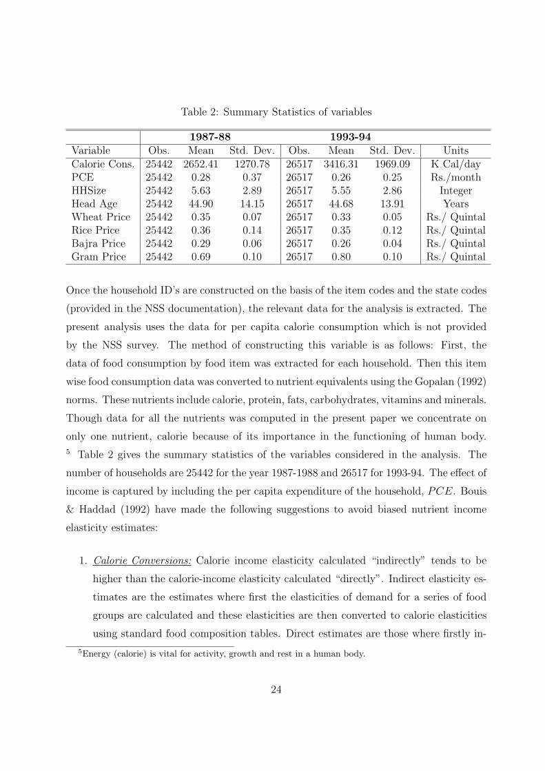
Table 2: Summary Statistics of variables

1987-88 1993-94Variable Obs. Mean Std. Dev. Obs. Mean Std. Dev. UnitsCalorie Cons. 25442 2652.41 1270.78 26517 3416.31 1969.09 K Cal/dayPCE 25442 0.28 0.37 26517 0.26 0.25 Rs./monthHHSize 25442 5.63 2.89 26517 5.55 2.86 IntegerHead Age 25442 44.90 14.15 26517 44.68 13.91 YearsWheat Price 25442 0.35 0.07 26517 0.33 0.05 Rs./ QuintalRice Price 25442 0.36 0.14 26517 0.35 0.12 Rs./ QuintalBajra Price 25442 0.29 0.06 26517 0.26 0.04 Rs./ QuintalGram Price 25442 0.69 0.10 26517 0.80 0.10 Rs./ Quintal

Once the household ID’s are constructed on the basis of the item codes and the state codes

(provided in the NSS documentation), the relevant data for the analysis is extracted. The

present analysis uses the data for per capita calorie consumption which is not provided

by the NSS survey. The method of constructing this variable is as follows: First, the

data of food consumption by food item was extracted for each household. Then this item

wise food consumption data was converted to nutrient equivalents using the Gopalan (1992)

norms. These nutrients include calorie, protein, fats, carbohydrates, vitamins and minerals.

Though data for all the nutrients was computed in the present paper we concentrate on

only one nutrient, calorie because of its importance in the functioning of human body.

5 Table 2 gives the summary statistics of the variables considered in the analysis. The

number of households are 25442 for the year 1987-1988 and 26517 for 1993-94. The effect of

income is captured by including the per capita expenditure of the household, PCE. Bouis

& Haddad (1992) have made the following suggestions to avoid biased nutrient income

elasticity estimates:

1. Calorie Conversions: Calorie income elasticity calculated “indirectly” tends to be

higher than the calorie-income elasticity calculated “directly”. Indirect elasticity es-

timates are the estimates where first the elasticities of demand for a series of food

groups are calculated and these elasticities are then converted to calorie elasticities

using standard food composition tables. Direct estimates are those where firstly in-

5Energy (calorie) is vital for activity, growth and rest in a human body.

24

formation on the quantities of each food consumed is gathered and calorie conversions

are done and the relationship with income calculated.

In the present paper the “direct” method is adopted. The calorie conversions for the

food consumed is done using the Gopalan (1992) conversion equivalent tables.

2. Measuring Income: Measuring income is crucial and, in some household surveys this

is not reported clearly. In such cases a common equivalent of income is the expen-

diture. However it has been shown that calorie-income elasticities calculated using

current income are lower than calorie-income elasticities based on expenditure.

Some studies have assumed that income is endogenous. If increased nutrient in-

take results in increased productivity and/or labour supply, especially in low income

households, estimated calorie income elasticities will be biased upwards and this bias

might be greater for lower income households. In addition, the unobserved tastes for

work might be correlated with taste for nutrients. Expenditure, which is a function

of income, might be considered to be jointly determined with income (Strauss &

Thomas 1995). In the present chapter, per capita expenditure is taken as a proxy

for household income, and income is not assumed to be endogenous.

3. Measurement Error: There might be a measurement error problem which results in

a biased calorie-income elasticity. The nutrient consumption data collection method

might result in measurement error. There are two methods of nutrient data collec-

tion. One is to infer households nutrient ‘availability’ from the information on food

purchases and imputed values based on the consumption of part of own production

or wages received in kind. A second method is the information on nutrient ‘intake’

where actual meals consumed is used. Elasticities based on availability tend to be

higher than those based on intakes.

In the NSS surveys the nutrient consumption ‘availability’ data is collected, hence

the elasticities estimates here might be biased upwards.

Given all these reasons for biased estimates and the limitations of data the calorie-income

elasticities estimates in the present analysis might be biased upwards. However it has been

suggested by Strauss & Thomas (1995) that the bias with these limitations is not very

large.

25

Along with per capita expenditure of the household the farm harvest prices for various food

items is included as the data is for rural agricultural households in India and households

are likely to be affected by the farm harvest price. In order to take into account the effect

of various food prices the prices of wheat and rice have been considered as superior goods.

Apart from this, the price of bajra is considered to take into account the effect of the

price of an inferior good and the price of gram is taken to take into account the effect of

the price of a normal good. In addition to these variables certain variables accounting for

household characteristics and environmental factors are also included. These variables are

household size, age of household head, sex of household head, literacy of household head,

whether the household owns land or not, occupation of the household, social background

of the household, type of employment, religion of the household and various interaction

terms. A brief summary of all these variables is presented in Table 3.

Household size, HHSize is included to take account of economies of scale and congestion

effects. Next, these dummy variables are defined. As the financial status of the household

is of importance in determining the quality of food consumed the variable LandOwned is

considered. This variable is defined as: Land owned by the household and can give some

indication about household’s financial situation. A household possessing land is obviously

better off than a household not possessing land. Therefore, the variable captures whether

there is some effect of owning land on the calorie consumption of household members. Base

case is that the household owns land.

The sex and literacy of the household head is represented by the variables, FemaleHead

and HeadLit. FemaleHead aims to capture the effect of the sex of the household head

on per capita calorie consumption of the household. HeadLit, captures the effect of a

household head who is literate beyond primary level education rather than being illiterate

or educated below primary standard. The base case is that the household head is either

not educated or educated below primary level.

The occupation of the household is also considered, as the type of occupation can have

an effect on calorie consumption. The dummy variable considers four types of occupa-

tions: Self employed in non agricultural activities (SEmpNon−Ag.), Agricultural Labour

(Ag.Lab), Other Labour (OthLab) and Self Employed in Agriculture (SelfEmpAg). The

base case is being Self Employed in Agriculture (SelfEmpAg).

26

Another dummy variable taken into account is the social group affiliation of the household.

If the household belongs to a backward social group i.e., Scheduled Castes, Scheduled tribe

or other backward castes (OBC) then the variable takes the value one i.e., The base case

is that SC/ST = 1 thus implying that the effect of a household ‘not’ belonging to SC/ST

vis-a-vis a group belonging to SC/ST.

The religion of the household is also taken into account as an indicator of the household’s

ethnic background. The religion categories considered are, Hinduism, Islam, Christianity,

Sikhism and Other religion (OtherRel) such as Jainism, Buddhism, Zoroastrianism etc.

The base case is Hinduism.

The analysis takes into account the state dummies for 15 states to get rid of the state

effects. These states are Assam, Bihar, Gujarat, Karnataka, Kerela, Madhya Pradesh,

Maharashtra, Orissa, Punjab, Rajasthan, Tamil Nadu, West Bengal and Uttar Pradesh.

The base state is Punjab. For any state Si, the dummy variable takes the value 1 and zero

otherwise. Having explained the variables and their meaning, next we present the results

of the analysis.

6 Estimation and Results

As mentioned earlier, the analysis is done for two rounds of NSS data i.e., the 43rd and

50th Round corresponding to the years 1987-88 and 1993-94 respectively. Table 4 and 5

display the results of the analysis. In addition, the quantile regression plots are shown

in Figures 1, 2, 3 and 4. These plots compare the coefficients of the quantile and OLS

regressions for a particular variable. The results are discussed by considering the effect of

one independent variable at various levels of calorie consumption at a time.

Responsiveness to Income: From Table 1, showing the distribution of the calorie con-

sumption of rural households in India, it is observed that people at the 10th-30th quantile of

the calorie consumption distribution have less than 2400KCal/day per capita consumption,

so that a larger proportion of people are undernourished. The quantile regression results

for the 43rd Round show that the effect of an increase in income on the per capita calorie

consumption is low at the lower quantiles and high at the higher quantiles. For the highly

undernourished people at the 10th and 25th percentiles, a one percent increase in the income

27

of the household increases per capita calorie consumption by 0.29 percent and 0.32 percent,

respectively. However, beyond the median quantile the effect is greater, suggesting that

well nourished households i.e., those with a per capita calorie consumption of greater than

2400 KCal/day, spend a higher proportion of additional income on calorie consumption.

For the year 1993-94, the robust OLS regression suggests that a one percent increase in the

income of households increases calorie consumption by around 0.57 percent. The quan-

tile regression results show that for households with very low levels of nutritional status

i.e., between the 10th and 25th percentiles, a one percent increase in income increases per

capita calorie consumption by 0.51 percent. These people are the undernourished strata

of the sample with a per capita calorie intake of 1723.469 KCal/day (Table 1). The effect

of income on the per capita calorie consumption is progressive and rising over the quan-

tiles. For people with larger quantities of per capita calorie consumption an increase in

per capita income increases per capita calorie consumption by a larger proportion. At the

90th quantile a one percent increase in income means a 0.59 percent increase in calorie

consumption. These results are different and statistically significant (Table 5 - 6).

The debate on the responsiveness of household nutrient intake to income is large, some

surveys are presented in Behrman & Deolalikar (1990) and Bouis & Haddad (1992). Re-

searchers have argued households have a special preference for tastes and thereby, for even

the poorest of households an increase in income results in an increase in the purchase of

tasty foods which might not be rich in nutrients. This analysis sheds further light on this

view and it is observed that the effect of an income increase is not uniform for all house-

holds and responsiveness also depends on the existing nutritional status of the household.

A undernourished household will respond differently to an income increase compared with

an adequately nourished or over nourished household. Thus, it will be an incomplete state-

ment to suggest that an income increase results in people diverting consumption towards

tasty food (Behrman & Deolalikar 1987). It is necessary to take into consideration the fact

that the responsiveness of calorie consumption to income is contingent upon the nutritional

status of the households.

However, the results in this analysis are not indicative of the actual magnitude of the

calorie-income elasticity. Our analysis emphasizes that the elasticity varies across the

quantiles. The Extant literature has examined the calorie income elasticity and pointed

28

out certain reasons for biased calorie-income elasticity estimates. Responsiveness to

Household Size: The effect of household size on calorie consumption indicates scale and

congestion effects. The results in the present chapter show that an additional household

member has a positive and significant effect on per capita calorie consumption. The OLS

result for 1987-88 suggests an additional member in the household will increase the per

capita calorie consumption by 0.02 percent. On the other hand the quantile regression

result paints a different picture. At the lower quantiles i.e.,between the 10th and 25th per-

centiles, an additional household member will increase per capita calorie consumption by

0.02 and 0.03 percent respectively. This effect is negative for higher quantiles. At the me-

dian quantile, where the unconditional per capita calorie consumption as shown in Table 1

is around 2438.60 KCal/day, an additional household member decreases per capita calorie

consumption by just 0.008 percent. However, this result is to be viewed with caution as the

coefficient is not statistically significant at 5 percent level of significance. The over nour-

ished households (at the 75th and 90th quantiles) reduce per capita calorie consumption for

an additional household member. A similar pattern is observed in the post reform period,

i.e., 1993-94. The effect of an additional household member is descending across the quan-

tiles. It becomes statistically insignificant at the 75th quantile and negative and significant

at the 90th quantile. This result suggests that in poorly nourished households an additional

member results in an increase in calorie consumption because this member is a potential

income earner and it is beneficial to increase the calorie consumption of the household. For

the higher quantiles, the households are overnourished so an additional member does not

require an increase in calorie consumption as an intra household reallocation of calories is

done without severely affecting the nutritional status of existing household members.

Responsiveness to Household Head Age: In Indian rural households, the household

head is a dominant decision maker and hence has an effect on the nutritional status of

the household members. The age of the household head could also influence his or her

decisions. Extant literature, such as the seminal work of Grossman (1972), suggests that

an older individual demands more health inputs- such as medical care and nutrition. The

OLS results show responsiveness of per capita calorie consumption to the age of the house-

hold decision maker was positive (0.01) in 1987-88 and negative (-0.02) in 1993-94. This

effect was very small but statistically significant at 5 percent level of significance. The

29

quantile regression results estimates suggest that the responsiveness of per capita calorie

consumption of the household to the age of the household head in 1987-88 was around 0.02

percent for undernourished households (i.e., 10th to 50th quantiles) and even smaller for

higher quantiles (75th to 90th quantiles). In contrast, in the post reform period (i.e., 1993-

94), the percapita calorie consumption reduced with higher age of the household head for

all the quantiles. However, these results are statistically insignificant for undernourished

households.

Responsiveness to Food Prices: As per the theoretical model framework the effect of

prices should be such that own price effects are negative and cross price effects positive.

Since there is no clear price of calories to account for the price effect we have taken the

price of four food items. The effect of prices of various food items is of crucial importance

as calorie consumption might be directly affected by the prices. The effect of prices is

mixed in both the OLS and quantile regression results, for both the pre-reform and the

post reform period. The OLS results for the 43rd Round show that the price of wheat had

a positive and significant effect while that of bajra and gram had a negative effect. The

quantile regression results show the effect of the price of different types of food commodities

has a varied effect across quantiles. In the pre-reform period an increase in the price of

wheat by one percent increases per capita calorie consumption at all quantiles. However,

this effect varies algebraically across quantiles. The effect of the price of rice, gram and

bajra is negative and varies across quantiles. The price effect on the undernourished popu-

lation is the most negative or less positive than for adequately nourished or over nourished

households. Thus, our results show there was asymmetric behaviour of undernourished

households to price change such that when food prices change the nutrient consumption

of undernourished households is reduced more than for overnourished households. For un-

dernourished households (at the 10th and 25th percentile) in 1987-88 the per capita calorie

consumption increases as the price of wheat increases. The effect of the prices of gram

and rice is statistically significant for the 25th quantile. In the post reform period i.e., in

1993-94, OLS results suggest the effect of the price of wheat and bajra was negative and

that of the price of rice and gram positive. According to the quantile regression results the

price effect of wheat is negative at all the quantiles, however this effect is least negative

for the undernourished households. Suggesting that as the price of wheat increases the

30

calorie consumption for undernourished households reduces by a lesser amount than of an

overnourished household.

The positive price effect implies there is strong substitution among various foods with

changing prices. This result is similar to that of Behrman & Deolalikar (1989). The results

obtained in the analysis suggest that subsidies on certain foods such as gram, rice can affect

the individual nutrient intakes for undernourished households by a larger amount vis-a-vis

an overnourished household. Hence, a revenue neutral method of improving calorie intake

for undernourished households should be designed.

Literate Household Head Effect: The effect of education on the demand for nutrition

and thereby health has been well documented in the extant literature. Education has both

demand side and supply side effects on household behaviour. There is a positive associa-

tion between education and labour market returns. Education can improve the efficiency

of an individual both in terms of producing investment in health and labour market pro-

ductivity. There is very high correlation between the demand for health and nutrition

and education. From the demand side, educated people recognize the benefits of improved

health and would have a better taste for health and nutrition.

In the 43rd round ( the pre reform period), the literacy of household head had a negative

effect on the per capita calorie consumption of the household on the lower quantiles. In the

post reform period, the OLS results suggest a literate household head will have a positive

effect on the per capita calorie consumption. The quantile regression results show that in

the pre-reform period a literate household head does not influence the percapita calorie con-

sumption at median quantiles. Similarly, in the post reform period for the overnourished

households at the 90th percentile the per capita calorie consumption is not significantly af-

fected by literacy of household head.

Responsiveness of Land Owned by Household: If the household owns land there are

possibilities for home production that can be indicative of the asset status of the household.

Both, the OLS and quantile regression results indicate that owning land had a positive but

statistically insignificant effect on per capita calorie consumption. The per capita calorie

consumption of the household is not affected by the land ownership of the households.

Responsiveness to Literate Household Head and Land Ownership: If the house-

hold head is literate and the household owns land then the OLS results suggest per capita

31

calorie consumption is not affected significantly. The quantile regression results show a

similar result except for the 90th percentile in the pre reform period. The result indicates

that if the household head is literate and the household owns land per capita calorie con-

sumption of households corresponding 90th percentile will decrease by 0.36 percent. This

result suggests that if the household has assets and the household head is also literate then

they indulge in consuming tasty foods and might be less concerned about the nutritional

content of their diet.

Responsiveness to Social Group: This variable captures the effect of the household’s

social background on preferences for nutritious food. The background variable include a

Non-Schedule Caste/ Schedule Tribe household i.e., belonging to a upper caste. The regres-

sion results at the mean, i.e., robust OLS regression, show that if the household belonged

to a non-SC/ST social group rather than to a backward social group, per capita calorie

consumption increased in the pre-reform period and decreased in the post reform period.

On the other hand the quantile regression results suggest that belonging to an upper caste

reduced the demand for calorie consumption in 1987-88. At the lowest quantile the calorie

consumption was not significantly affected by the social group affiliation of households.

However, for the 25th - 90th quantiles, belonging to a non-SC/ST increased per capita calo-

rie consumption by 0.02 units at the 25th percentile and by 0.04 at the 90th quantile. In

the post reform period, belonging to an upper caste decreased calorie consumption of un-

dernourished people by a larger amount than for the households at the 50th percentile. For

overnourished households at 90th percentile, the social group did not affect calorie demand

significantly. Thus, belonging to an upper caste affects calorie consumption differently in

pre-reform period and the post reform period. The calorie consumption was seen to improve

in 1987-88 if the household belonged to non SC-ST social group. however in the 1993-94

the calorie consumption was seen to fall if the household belonged to a non SC-ST social

group, suggesting that the backward household’s calorie consumption improved in the post

reform period.

Responsiveness to Occupation of the Household: The occupation type of the house-

hold can also affect calorie demand. The OLS result for 1987-88 shows that a household

belonging to Agricultural labourers or Self Employed in non agriculture occupation, rather

than belonging to Self Employed Agriculture had a negative effect on the calorie consump-

32

tion of the household. In 1993-94, belonging to any of the occupations type decreased

the per capita calorie demand of the households. The effect however was smaller for the

pre reform period. the quantile regression results show that in the pre-reform period the

occupation of the household had a negative influence on the calorie consumption of the

households. In the post reform period the effect of occupation was mixed. Belonging to

aggriculturer labourer and other labour occupation categories rather than being self em-

ployed in agriculture had a negative and statistically significant influence on the calorie

consumption. This result was positive but not statistically significant for households self

employed in non agriculture category.

Responsiveness to Literate Household Head and Occupation Type: For almost

all the occupation types the category literate household head as against an illiterate house-

hold head belonging to the occupation of ‘agriculture labourer’ does not significantly affect

the calorie consumption of the household, at any quantile other than the 10th percentile

in 1987-88. The effect is negative and declining over the quantiles for a household self

employed in non-agriculture with a literate household head. At the 90th quantile the effect

is insignificant. In the post reform period none of these variables had a statistically signif-

icant effect.

Responsiveness to Female Household Head: If the household head is a female per

capita calorie consumption is higher than for a household where the head is a male. The

OLS results suggest calorie consumption is positively affected by a female household head

and the effect is algebraically consistent for 1987-88 and 1993-94. In 1987-88 the effect

was increasing across all the quantiles whereas in 1993-94 it was declining across the quan-

tiles. This effect was higher in absolute terms for 1993-94.

Responsiveness to Occupation and Land Owned: For all occupation types the OLS

results suggest that if the household also owned land per capita calorie consumption de-

creased significantly in the pre reform period and in the post reform period this was sig-

nificant only for households belonging to other than agricultural labour category. The

quantile regression results throw further light on the impact of this interaction variable and

suggest that the effect was generally negative and numerically different for all the quantiles

in 1987-88. In 1993-94 per capita calorie consumption increased only for households own-

ing land and belonging to the occupation category ‘other labourer’. This effect was largest

33

at the 10th quantile and smallest for the 50th quantile.

Responsiveness to Religion Effect: According to the OLS and quantile regression re-

sults for 1987-88, the percapita calorie consumption is affected significantly if the household

is a Muslim rather than being a Hindu. In the post reform period, the result suggest that if

the household is a Muslim or a Sikh rather than being a Hindu, then the per capita calorie

consumption will be higher by 0.03 percent. Quantile regression result show that belonging

to any religion does not effect the per capita calorie consumption for the undernourished

households at the 25th and 50th quantiles, however the effect is positive and significant for

Muslims and negative for Christians. The calorie consumption of overnourished households

at the 90th percentile is again not affected by the religion of the households. Hence we can

conclude that the severely undernourished and over nourished people do not show any sign

of religion effect on the household’s calorie consumption.

6.1 Hypothesis Tests Results

Table 7 and 8 show the results for hypothesis testing. Wald test is applied to test the

equality of slope coefficients across the quantiles for the independent variables 6. The diag-

onal matrix consists of the F-statistic with (1, N −K) degrees of freedom. The associated

p-values are reported in parentheses. Since the sample size is large F is distributed as χ2q/q.

The large sample critical values of χ2q/q for q = 1 is 3.84. Hence the decision rule is that

an F value greater than 3.84 rejects Ho. Alternatively if the p-value is very small then we

reject the hypothesis of equality of slope coefficients. These test results show that the slope

coefficients indeed vary across the quantiles. In 1987-88 the slopes were significantly dif-

ferent from each other between the 10th and 90th quantiles for per capita expenditure and

household size and between 25th and 75th percentile for per capita expenditure, household

size, bajra price and gram price. These test results confirm the argument that the income

and the size of the households along with the food prices affect the calorie consumption

differently across the quantiles. It is also suggested that the prices of normal goods and

inferior goods affect the calorie consumption differently for undernourished and over nour-

6The results for the categorical variables are not included

34

ished population.

Although the null hypothesis of equality of slope coefficients can not be rejected for the

age of the household head and the prices of wheat and rice in 1987 -88. In 1993-94 the

null is seen to be rejected for all of these variables too. Suggesting that the responsiveness

of calorie consumption to the prices and the household characteristics has become more

varied in the post reform period.

35

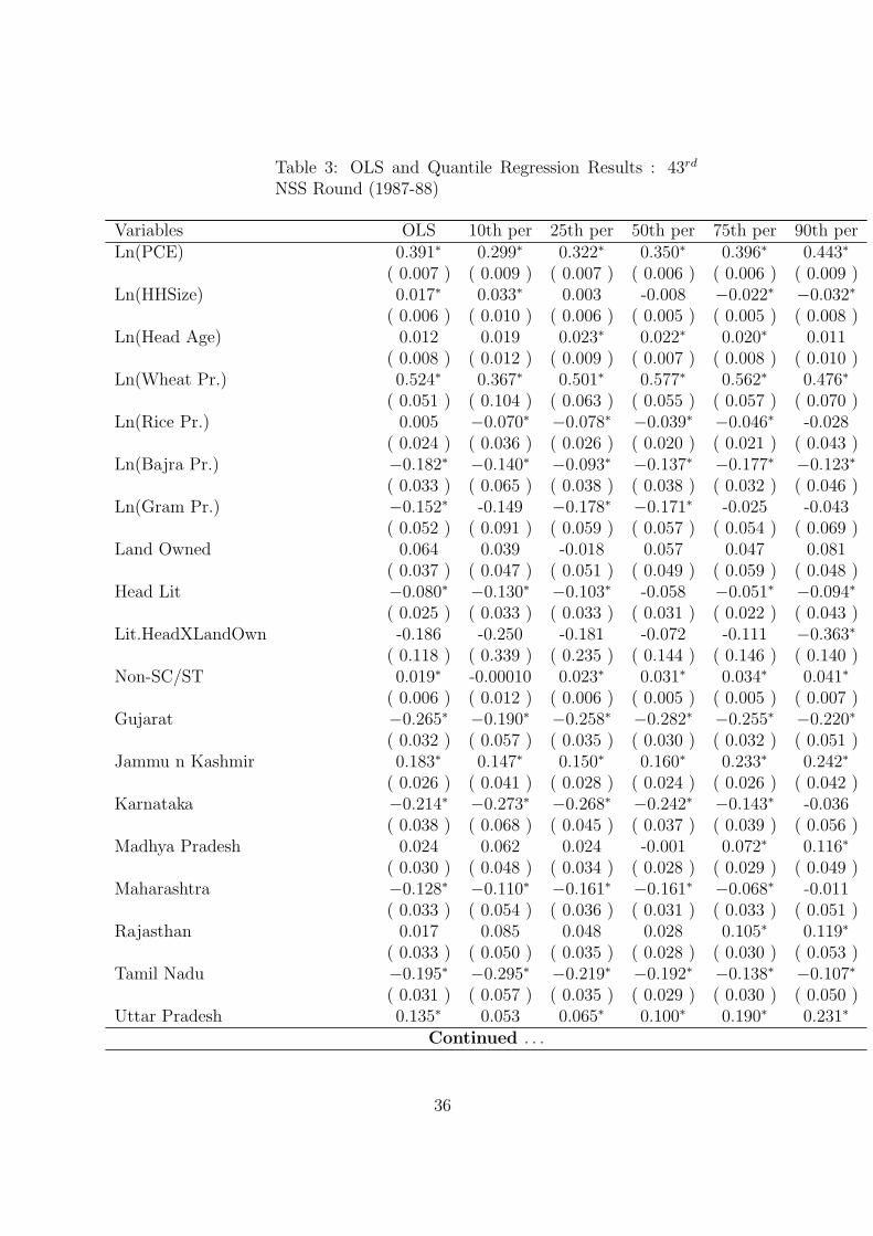
Table 3: OLS and Quantile Regression Results : 43rd

NSS Round (1987-88)

Variables OLS 10th per 25th per 50th per 75th per 90th perLn(PCE) 0.391∗ 0.299∗ 0.322∗ 0.350∗ 0.396∗ 0.443∗

( 0.007 ) ( 0.009 ) ( 0.007 ) ( 0.006 ) ( 0.006 ) ( 0.009 )Ln(HHSize) 0.017∗ 0.033∗ 0.003 -0.008 −0.022∗ −0.032∗

( 0.006 ) ( 0.010 ) ( 0.006 ) ( 0.005 ) ( 0.005 ) ( 0.008 )Ln(Head Age) 0.012 0.019 0.023∗ 0.022∗ 0.020∗ 0.011

( 0.008 ) ( 0.012 ) ( 0.009 ) ( 0.007 ) ( 0.008 ) ( 0.010 )Ln(Wheat Pr.) 0.524∗ 0.367∗ 0.501∗ 0.577∗ 0.562∗ 0.476∗

( 0.051 ) ( 0.104 ) ( 0.063 ) ( 0.055 ) ( 0.057 ) ( 0.070 )Ln(Rice Pr.) 0.005 −0.070∗ −0.078∗ −0.039∗ −0.046∗ -0.028

( 0.024 ) ( 0.036 ) ( 0.026 ) ( 0.020 ) ( 0.021 ) ( 0.043 )Ln(Bajra Pr.) −0.182∗ −0.140∗ −0.093∗ −0.137∗ −0.177∗ −0.123∗

( 0.033 ) ( 0.065 ) ( 0.038 ) ( 0.038 ) ( 0.032 ) ( 0.046 )Ln(Gram Pr.) −0.152∗ -0.149 −0.178∗ −0.171∗ -0.025 -0.043

( 0.052 ) ( 0.091 ) ( 0.059 ) ( 0.057 ) ( 0.054 ) ( 0.069 )Land Owned 0.064 0.039 -0.018 0.057 0.047 0.081

( 0.037 ) ( 0.047 ) ( 0.051 ) ( 0.049 ) ( 0.059 ) ( 0.048 )Head Lit −0.080∗ −0.130∗ −0.103∗ -0.058 −0.051∗ −0.094∗

( 0.025 ) ( 0.033 ) ( 0.033 ) ( 0.031 ) ( 0.022 ) ( 0.043 )Lit.HeadXLandOwn -0.186 -0.250 -0.181 -0.072 -0.111 −0.363∗

( 0.118 ) ( 0.339 ) ( 0.235 ) ( 0.144 ) ( 0.146 ) ( 0.140 )Non-SC/ST 0.019∗ -0.00010 0.023∗ 0.031∗ 0.034∗ 0.041∗

( 0.006 ) ( 0.012 ) ( 0.006 ) ( 0.005 ) ( 0.005 ) ( 0.007 )Gujarat −0.265∗ −0.190∗ −0.258∗ −0.282∗ −0.255∗ −0.220∗

( 0.032 ) ( 0.057 ) ( 0.035 ) ( 0.030 ) ( 0.032 ) ( 0.051 )Jammu n Kashmir 0.183∗ 0.147∗ 0.150∗ 0.160∗ 0.233∗ 0.242∗

( 0.026 ) ( 0.041 ) ( 0.028 ) ( 0.024 ) ( 0.026 ) ( 0.042 )Karnataka −0.214∗ −0.273∗ −0.268∗ −0.242∗ −0.143∗ -0.036

( 0.038 ) ( 0.068 ) ( 0.045 ) ( 0.037 ) ( 0.039 ) ( 0.056 )Madhya Pradesh 0.024 0.062 0.024 -0.001 0.072∗ 0.116∗

( 0.030 ) ( 0.048 ) ( 0.034 ) ( 0.028 ) ( 0.029 ) ( 0.049 )Maharashtra −0.128∗ −0.110∗ −0.161∗ −0.161∗ −0.068∗ -0.011

( 0.033 ) ( 0.054 ) ( 0.036 ) ( 0.031 ) ( 0.033 ) ( 0.051 )Rajasthan 0.017 0.085 0.048 0.028 0.105∗ 0.119∗

( 0.033 ) ( 0.050 ) ( 0.035 ) ( 0.028 ) ( 0.030 ) ( 0.053 )Tamil Nadu −0.195∗ −0.295∗ −0.219∗ −0.192∗ −0.138∗ −0.107∗

( 0.031 ) ( 0.057 ) ( 0.035 ) ( 0.029 ) ( 0.030 ) ( 0.050 )Uttar Pradesh 0.135∗ 0.053 0.065∗ 0.100∗ 0.190∗ 0.231∗

Continued . . .

36

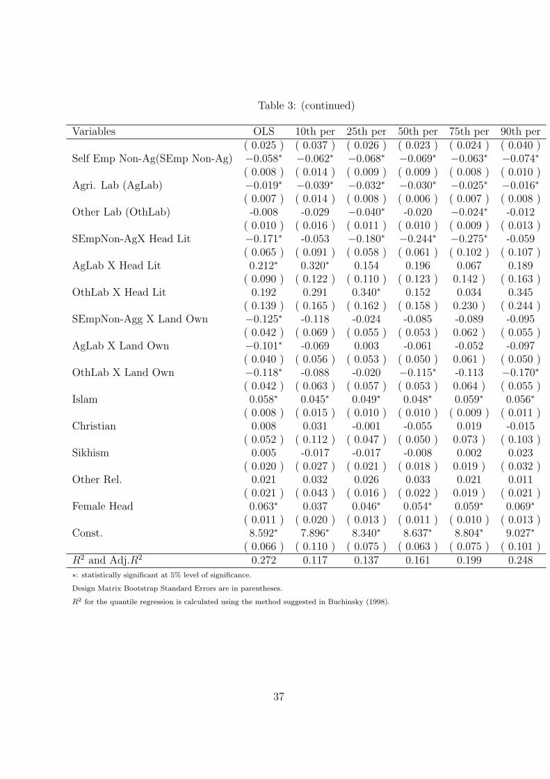
Table 3: (continued)

Variables OLS 10th per 25th per 50th per 75th per 90th per( 0.025 ) ( 0.037 ) ( 0.026 ) ( 0.023 ) ( 0.024 ) ( 0.040 )

Self Emp Non-Ag(SEmp Non-Ag) −0.058∗ −0.062∗ −0.068∗ −0.069∗ −0.063∗ −0.074∗

( 0.008 ) ( 0.014 ) ( 0.009 ) ( 0.009 ) ( 0.008 ) ( 0.010 )Agri. Lab (AgLab) −0.019∗ −0.039∗ −0.032∗ −0.030∗ −0.025∗ −0.016∗

( 0.007 ) ( 0.014 ) ( 0.008 ) ( 0.006 ) ( 0.007 ) ( 0.008 )Other Lab (OthLab) -0.008 -0.029 −0.040∗ -0.020 −0.024∗ -0.012

( 0.010 ) ( 0.016 ) ( 0.011 ) ( 0.010 ) ( 0.009 ) ( 0.013 )SEmpNon-AgX Head Lit −0.171∗ -0.053 −0.180∗ −0.244∗ −0.275∗ -0.059

( 0.065 ) ( 0.091 ) ( 0.058 ) ( 0.061 ) ( 0.102 ) ( 0.107 )AgLab X Head Lit 0.212∗ 0.320∗ 0.154 0.196 0.067 0.189

( 0.090 ) ( 0.122 ) ( 0.110 ) ( 0.123 ) 0.142 ) ( 0.163 )OthLab X Head Lit 0.192 0.291 0.340∗ 0.152 0.034 0.345

( 0.139 ) ( 0.165 ) ( 0.162 ) ( 0.158 ) 0.230 ) ( 0.244 )SEmpNon-Agg X Land Own −0.125∗ -0.118 -0.024 -0.085 -0.089 -0.095

( 0.042 ) ( 0.069 ) ( 0.055 ) ( 0.053 ) 0.062 ) ( 0.055 )AgLab X Land Own −0.101∗ -0.069 0.003 -0.061 -0.052 -0.097

( 0.040 ) ( 0.056 ) ( 0.053 ) ( 0.050 ) 0.061 ) ( 0.050 )OthLab X Land Own −0.118∗ -0.088 -0.020 −0.115∗ -0.113 −0.170∗

( 0.042 ) ( 0.063 ) ( 0.057 ) ( 0.053 ) 0.064 ) ( 0.055 )Islam 0.058∗ 0.045∗ 0.049∗ 0.048∗ 0.059∗ 0.056∗

( 0.008 ) ( 0.015 ) ( 0.010 ) ( 0.010 ) ( 0.009 ) ( 0.011 )Christian 0.008 0.031 -0.001 -0.055 0.019 -0.015

( 0.052 ) ( 0.112 ) ( 0.047 ) ( 0.050 ) 0.073 ) ( 0.103 )Sikhism 0.005 -0.017 -0.017 -0.008 0.002 0.023

( 0.020 ) ( 0.027 ) ( 0.021 ) ( 0.018 ) 0.019 ) ( 0.032 )Other Rel. 0.021 0.032 0.026 0.033 0.021 0.011

( 0.021 ) ( 0.043 ) ( 0.016 ) ( 0.022 ) 0.019 ) ( 0.021 )Female Head 0.063∗ 0.037 0.046∗ 0.054∗ 0.059∗ 0.069∗

( 0.011 ) ( 0.020 ) ( 0.013 ) ( 0.011 ) ( 0.010 ) ( 0.013 )Const. 8.592∗ 7.896∗ 8.340∗ 8.637∗ 8.804∗ 9.027∗

( 0.066 ) ( 0.110 ) ( 0.075 ) ( 0.063 ) ( 0.075 ) ( 0.101 )R2 and Adj.R2 0.272 0.117 0.137 0.161 0.199 0.248∗: statistically significant at 5% level of significance.

Design Matrix Bootstrap Standard Errors are in parentheses.

R2 for the quantile regression is calculated using the method suggested in Buchinsky (1998).

37

Table 4: OLS and Quantile Regression Results : 50th

NSS Round (1993-94)

Variables OLS 10th per 25th per 50th per 75th per 90th perLn(PCE) 0.575∗ 0.519∗ 0.534∗ 0.549∗ 0.575∗ 0.599∗

( 0.009 ) ( 0.013 ) ( 0.010 ) ( 0.008 ) ( 0.009 ) ( 0.010 )Ln(HHSize) 0.010 0.052∗ 0.040∗ 0.025∗ -0.013 −0.055∗

( 0.007 ) ( 0.011 ) ( 0.008 ) ( 0.007 ) ( 0.008 ) ( 0.009 )Ln(Head Age) −0.023∗ -0.008 -0.007 −0.029∗ −0.045∗ −0.047∗

( 0.010 ) ( 0.015 ) ( 0.012 ) ( 0.008 ) ( 0.010 ) ( 0.012 )Ln(Wheat Pr.) −0.771∗ −0.668∗ −0.449∗ −0.586∗ −0.817∗ −1.225∗

( 0.093 ) ( 0.177 ) ( 0.146 ) ( 0.105 ) ( 0.106 ) ( 0.126 )Ln(Rice Pr.) 0.593∗ 0.727∗ 0.550∗ 0.246∗ 0.144∗ 0.106

( 0.063 ) ( 0.119 ) ( 0.095 ) ( 0.066 ) ( 0.057 ) ( 0.066 )Ln(Bajra Pr.) −0.237∗ −0.356∗ −0.300∗ -0.031 0.083 0.216∗

( 0.053 ) ( 0.092 ) ( 0.075 ) ( 0.053 ) ( 0.050 ) ( 0.061 )Ln(Gram Pr.) 0.880∗ 0.332 1.116∗ 1.135∗ 1.237∗ 1.011∗

( 0.116 ) ( 0.213 ) ( 0.157 ) ( 0.117 ) ( 0.119 ) ( 0.155 )Land Owned 0.0002 -0.024 0.007 0.021 -0.042 -0.026

( 0.025 ) ( 0.038 ) ( 0.047 ) ( 0.023 ) ( 0.025 ) ( 0.038 )Head Litracy 0.039∗ 0.035∗ 0.034∗ 0.034∗ 0.032∗ 0.015

( 0.008 ) ( 0.015 ) ( 0.011 ) ( 0.008 ) ( 0.009 ) ( 0.011 )Lit. Head X Land Own -0.033 -0.050 -0.016 -0.043 0.007 0.001

( 0.019 ) ( 0.030 ) ( 0.026 ) ( 0.023 ) ( 0.019 ) ( 0.025 )Non- SC/ST −0.047∗ −0.075∗ −0.055∗ −0.029∗ −0.014∗ -0.016

( 0.007 ) ( 0.013 ) ( 0.009 ) ( 0.007 ) ( 0.007 ) ( 0.008 )Bihar 0.518∗ 0.471∗ 0.457∗ 0.418∗ 0.486∗ 0.550∗

( 0.025 ) ( 0.046 ) ( 0.034 ) ( 0.024 ) ( 0.026 ) ( 0.034 )Gujarat −0.237∗ −0.307∗ −0.504∗ −0.281∗ -0.101 0.193∗

( 0.067 ) ( 0.136 ) ( 0.100 ) ( 0.071 ) ( 0.078 ) ( 0.097 )Jammu n Kashmir −0.547∗ −0.703∗ −0.582∗ −0.275∗ −0.142∗ -0.044

( 0.061 ) ( 0.110 ) ( 0.088 ) ( 0.066 ) ( 0.061 ) ( 0.069 )Karnataka −0.210∗ −0.551∗ −0.576∗ −0.219∗ 0.094 0.415∗

( 0.055 ) ( 0.112 ) ( 0.082 ) ( 0.058 ) ( 0.064 ) ( 0.078 )Madhya Pradesh -0.082 −0.502∗ −0.184∗ 0.147∗ 0.325∗ 0.425∗

( 0.049 ) ( 0.090 ) ( 0.069 ) ( 0.049 ) ( 0.051 ) ( 0.060 )Maharashtra -0.030 −0.562∗ −0.280∗ 0.078 0.398∗ 0.576∗

( 0.052 ) ( 0.088 ) ( 0.061 ) ( 0.054 ) ( 0.058 ) ( 0.070 )Rajasthan −0.384∗ −1.009∗ −0.652∗ −0.099∗ 0.140∗ 0.313∗

( 0.049 ) ( 0.083 ) ( 0.067 ) ( 0.050 ) ( 0.050 ) ( 0.060 )Tamil Nadu 0.455∗ 0.312∗ 0.436∗ 0.482∗ 0.558∗ 0.569∗

Continued . . .

38

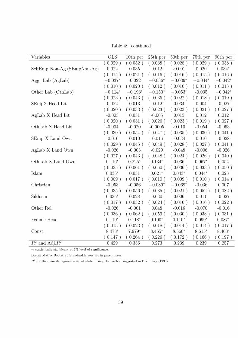
Table 4: (continued)

Variables OLS 10th per 25th per 50th per 75th per 90th per( 0.029 ) ( 0.052 ) ( 0.038 ) ( 0.028 ) ( 0.029 ) ( 0.038 )

SelfEmp Non-Ag.(SEmpNon-Ag) 0.022 0.035 0.012 -0.001 0.020 0.034∗

( 0.014 ) ( 0.021 ) ( 0.016 ) ( 0.016 ) ( 0.015 ) ( 0.016 )Agg. Lab (AgLab) −0.037∗ -0.022 −0.036∗ −0.039∗ −0.044∗ −0.042∗

( 0.010 ) ( 0.020 ) ( 0.012 ) ( 0.010 ) ( 0.011 ) ( 0.013 )Other Lab (OthLab) −0.114∗ −0.193∗ −0.150∗ −0.053∗ -0.035 −0.042∗

( 0.023 ) ( 0.043 ) ( 0.035 ) ( 0.022 ) ( 0.018 ) ( 0.019 )SEmpX Head Lit 0.022 0.013 0.012 0.034 0.004 -0.027

( 0.020 ) ( 0.033 ) ( 0.023 ) ( 0.023 ) ( 0.021 ) ( 0.027 )AgLab X Head Lit -0.003 0.031 -0.005 0.015 0.012 0.012

( 0.020 ) ( 0.031 ) ( 0.026 ) ( 0.023 ) ( 0.019 ) ( 0.027 )OthLab X Head Lit -0.004 -0.020 -0.0005 -0.010 -0.054 -0.053

( 0.030 ) ( 0.054 ) ( 0.047 ) ( 0.035 ) ( 0.030 ) ( 0.041 )SEmp X Land Own -0.016 0.010 -0.016 -0.034 0.010 -0.028

( 0.029 ) ( 0.045 ) ( 0.049 ) ( 0.028 ) ( 0.027 ) ( 0.041 )AgLab X Land Own -0.026 -0.003 -0.029 -0.048 -0.006 -0.026

( 0.027 ) ( 0.043 ) ( 0.048 ) ( 0.024 ) ( 0.026 ) ( 0.040 )OthLab X Land Own 0.116∗ 0.225∗ 0.134∗ 0.036 0.067∗ 0.054

( 0.035 ) ( 0.061 ) ( 0.060 ) ( 0.036 ) ( 0.033 ) ( 0.050 )Islam 0.035∗ 0.031 0.021∗ 0.043∗ 0.044∗ 0.023

( 0.009 ) ( 0.017 ) ( 0.010 ) ( 0.009 ) ( 0.010 ) ( 0.014 )Christian -0.053 -0.056 −0.089∗ −0.069∗ -0.036 0.007

( 0.035 ) ( 0.056 ) ( 0.035 ) ( 0.021 ) ( 0.052 ) ( 0.082 )Sikhism 0.035∗ 0.028 0.030 0.006 0.011 -0.027

( 0.017 ) ( 0.032 ) ( 0.024 ) ( 0.016 ) ( 0.016 ) ( 0.022 )Other Rel. -0.026 -0.001 0.048 -0.016 -0.070 -0.016

( 0.036 ) ( 0.062 ) ( 0.059 ) ( 0.030 ) ( 0.038 ) ( 0.031 )Female Head 0.110∗ 0.118∗ 0.100∗ 0.110∗ 0.099∗ 0.087∗

( 0.013 ) ( 0.023 ) ( 0.018 ) ( 0.014 ) ( 0.014 ) ( 0.017 )Const. 8.473∗ 7.979∗ 8.465∗ 8.560∗ 8.615∗ 8.463∗

( 0.147 ) ( 0.264 ) ( 0.226 ) ( 0.172 ) ( 0.166 ) ( 0.197 )R2 and Adj.R2 0.429 0.336 0.273 0.239 0.239 0.257∗: statistically significant at 5% level of significance.

Design Matrix Bootstrap Standard Errors are in parentheses.

R2 for the quantile regression is calculated using the method suggested in Buchinsky (1998).

39

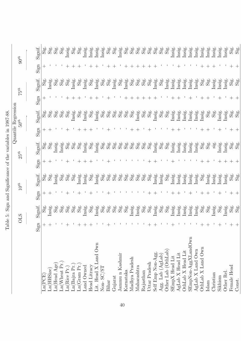
Tab

le5:

Sig

nan

dSig

nifi

cance

ofth

eva

riab

les

in19

87-8

8.

Quan

tile

Reg

ress

ion

OLS

10th

25th

50th

75th

90th

——

–—

——

——

—–

——

—-

——

——

——

——

-

Sig

nSig

nif.

Sig

nSig

nif.

Sig

nSig

nif.

Sig

nSig

nif.

Sig

nSig

nif.

Sig

nSig

nif.

Ln(P

CE

)+

Sig

.+

Sig

.+

Sig

.+

Sig

.+

Sig

.+

Sig

.Ln(H

HSiz

e)+

Insi

g.+

Sig

.+

Sig

.+

Sig

.-

Insi

g.-

Sig

.Ln(H

ead

Age

)-

Sig

.-

Insi

g.-

Insi

g.-

Sig

.-

Sig

.-

Sig

.Ln(W

hea

tP

r.)

-Sig

.-

Sig

.-

Insi

g.-

Sig

.-

Sig

.-

Sig

.Ln(R

ice

Pr.

)+

Sig

.+

Sig

.+

Sig

.+

Sig

.+

Sig

.+

Insi

g.Ln(B

ajr

aP

r.)

-Sig

.-

Sig

.-

Sig

.-

Insi

g.+

Insi

g.+

Sig

.Ln(G

ram

Pr.

)+

Sig

.+

Insi

g.+

Sig

.+

Sig

.+

Sig

.+

Sig

.Lan

dO

wned

+In

sig.

-In

sig.

+In

sig.

+In

sig.

-In

sig.

-In

sig.

Hea

dLit

racy

+Sig

.+

Sig

.+

Sig

.+

Sig

.+

Sig

.+

Insi

g.Lit

.H

ead

XLan

dO

wn

-In

sig.

-In

sig.

-In

sig.

-In

sig.

+In

sig.

+In

sig.

Non

-SC

/ST

-Sig

.-

Sig

.-

Sig

.-

Sig

.-

Sig

.-

Insi

g.B

ihar

+Sig

.+

Sig

.+

Sig

.+

Sig

.+

Sig

.+

Sig

.G

uja

rat

-Sig

.-

Sig

.-

Sig

.-

Sig

.-

Insi

g.+

Sig

.Jam

mu

nK

ashm

ir-

Sig

.-

Sig

.-

Sig

.-

Sig

.-

Sig

.-

Insi

g.K

arnat

aka

-Sig

.-

Sig

.-

Sig

.-

Sig

.+

Insi

g.+

Sig

.M

adhya

Pra

des

h-

Insi

g.-

Sig

.-

Sig

.+

Sig

.+

Sig

.+

Sig

.M

ahar

ashtr

a-

Insi

g.-

Sig

.-

Sig

.+

Insi

g.+

Sig

.+

Sig

.R

aja

sthan

-Sig

.-

Sig

.-

Sig

.-

Sig

.+

Sig

.+

Sig

.U

ttar

Pra

des

h+

Sig

.+

Sig

.+

Sig

.+

Sig

.+

Sig

.+

Sig

.Sel

fE

mp

Non

-Agg

.+

Insi

g.+

Insi

g.+

Insi

g.-

Insi

g.+

Insi

g.+

Sig

.A

gg.

Lab

(AgL

ab)

-Sig

.-

Insi

g.-

Sig

.-

Sig

.-

Sig

.-

Sig

.O

ther

Lab

(Oth

Lab

)-

Sig

.-

Sig

.-

Sig

.-

Sig

.-

Insi

g.-

Sig

.SE

mpX

Hea

dLit

+In

sig.

+In

sig.

+In

sig.

+In

sig.

+In

sig.

-In

sig.

AgL

abX

Hea

dLit

-In

sig.

+In

sig.

-In

sig.

+In

sig.

+In

sig.

+In

sig.

Oth

Lab

XH

ead

Lit

-In

sig.

-In

sig.

-In

sig.

-In

sig.

-In

sig.

-In

sig.

SE

mpN

on-A

ggX

Lan

dO

wn

-In

sig.

+In

sig.

-In

sig.

-In

sig.

+In

sig.

-In

sig.

AgL

abX

Lan

dO

wn

-In

sig.

-In

sig.

-In

sig.

-In

sig.

-In

sig.

-In

sig.

Oth

Lab

XLan

dO

wn

+Sig

.+

Sig

.+

Sig

.+

Insi

g.+

Sig

.+

Insi

g.Is

lam

+Sig

.+

Insi

g.+

Sig

.+

Sig

.+

Sig

.+

Insi

g.C

hri

stia

n-

Insi

g.-

Insi

g.-

sig.

-Sig

.-

Insi

g.+

Insi

g.Sik

his

m+

Sig

.+

Insi

g.+

Insi

g.+

Insi

g.+

Insi

g.-

Insi

g.O

ther

Rel

.-

Insi

g.-

Insi

g.+

Insi

g.-

Insi

g.-

Insi

g.-

Insi

g.Fem

ale

Hea

d+

Sig

.+

Sig

.+

Sig

.+

Sig

.+

Sig

.+

Sig

.C

onst

.+

Sig

.+

Sig

.+

Sig

.+

Sig

.+

Sig

.+

Sig

.

40

Tab

le6:

Sig

nan

dSig

nifi

cance

ofth

eva

riab

les

in19

93-9

4.

Quan

tile

Reg

ress

ion

OLS

10th

25th

50th

75th

90th

——

–—

——

——

—–

——

—-

——

——

——

——

-

Sig

nSig

nif.

Sig

nSig

nif.

Sig

nSig

nif.

Sig

nSig

nif.

Sig

nSig

nif.

Sig

nSig

nif.

Ln(P

CE

)+

Sig

.+

Sig

.+

Sig

.+

Sig

.+

Sig

.+

Sig

.Ln(H

HSiz

e)+

Insi

g.+

Sig

.+

Sig

.+

Sig

.-

Insi

g.-

Sig

.Ln(H

ead

Age

)-

Sig

.-

Insi

g.-

Insi

g.-

Sig

.-

Sig

.-

Sig

.Ln(W

hea

tP

r.)

-Sig

.-

Sig

.-

Insi

g.-

Sig

.-

Sig

.-

Sig

.Ln(R

ice

Pr.

)+

Sig

.+

Sig

.+

Sig

.+

Sig

.+

Sig

.+

Insi

g.Ln(B

ajr

aP

r.)

-Sig

.-

Sig

.-

Sig

.-

Insi

g.+

Insi

g.+

Sig

.Ln(G

ram

Pr.

)+

Sig

.+

Insi

g.+

Sig

.+

Sig

.+

Sig

.+

Sig

.Lan

dO

wned

+In

sig.

-In

sig.

+In

sig.

+In

sig.

-In

sig.

-In

sig.

Hea

dLit

racy

+Sig

.+

Sig

.+

Sig

.+

Sig

.+

Sig

.+

Insi

g.Lit

.Hea

dX

Lan

dO

wn

-In

sig.

-In

sig.

-In

sig.

-In

sig.

+In

sig.

+In

sig.

Non

-SC

/ST

-Sig

.-

Sig

.-

Sig

.-

Sig

.-

Sig

.-

Insi

g.B

ihar

+Sig

.+

Sig

.+

Sig

.+

Sig

.+

Sig

.+

Sig

.G

uja

rat

-Sig

.-

Sig

.-

Sig

.-

Sig

.-

Insi

g.+

Sig

.Jam

mu

nK

ashm

ir-

Sig

.-

Sig

.-

Sig

.-

Sig

.-

Sig

.-

Insi

g.K

arnat

aka

-Sig

.-

Sig

.-

Sig

.-

Sig

.+

Insi

g.+

Sig

.M

adhya

Pra

des

h-

Insi

g.-

Sig

.-

Sig

.+

Sig

.+

Sig

.+

Sig

.M

ahar

ashtr

a-

Insi

g.-

Sig

.-

Sig

.+

Insi

g.+

Sig

.+

Sig

.R

aja

sthan

-Sig

.-

Sig

.-

Sig

.-

Sig

.+

Sig

.+

Sig

.U

ttar

Pra

des

h+

Sig

.+

Sig

.+

Sig

.+

Sig

.+

Sig

.+

Sig

.Sel

fE

mp(S

Em

p)

+In

sig.

+In

sig.

+In

sig.

-In

sig.

+In

sig.

+Sig

.A

gg.

Lab

(AgL

ab)

-Sig

.-

Insi

g.-

Sig

.-

Sig

.-

Sig

.-

Sig

.O

ther

Lab

(Oth

Lab

)-

Sig

.-

Sig

.-

Sig

.-

Sig

.-

Insi

g.-

Sig

.SE

mpX

Hea

dLit

+In

sig.

+In

sig.

+In

sig.

+In

sig.

+In

sig.

-In

sig.

AgL

abX

Hea

dLit

-In

sig.

+In

sig.

-In

sig.

+In

sig.

+In

sig.

+In

sig.

Oth

Lab

XH

eadLit

-In

sig.

-In

sig.

-In

sig.

-In

sig.

-In

sig.

-In

sig.

SE

mpX

Lan

dO

wn

-In

sig.

+In

sig.

-In

sig.

-In

sig.

+In

sig.

-In

sig.

AgL

abX

Lan

dO

wn

-In

sig.

-In

sig.

-In

sig.

-In

sig.

-In

sig.

-In

sig.

Oth

Lab

XLan

dO

wn

+Sig

.+

Sig

.+

Sig

.+

Insi

g.+

Sig

.+

Insi

g.Is

lam

+Sig

.+

Insi

g.+

Sig

.+

Sig

.+

Sig

.+

Insi

g.C

hri

stia

n-

Insi

g.-

Insi

g.-

sig.

-Sig

.-

Insi

g.+

Insi

g.Sik

his

m+

Sig

.+

Insi

g.+

Insi

g.+

Insi

g.+

Insi

g.-

Insi

g.O

ther

Rel

.-

Insi

g.-

Insi

g.+

Insi

g.-

Insi

g.-

Insi

g.-

Insi

g.Fem

ale

Hea

d+

Sig

.+

Sig

.+

Sig

.+

Sig

.+

Sig

.+

Sig

.C

onst

.+

Sig

.+

Sig

.+

Sig

.+

Sig

.+

Sig

.+

Sig

.

41

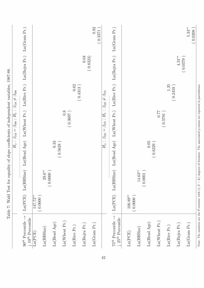
Tab

le7:

Wal

dTes

tfo

req

ual

ity

ofsl

ope

coeffi

cien

tsof

indep

enden

tva

riab

les,

1987

-88.

Ho

:β

i10

=β

i90

;H

1:

βi1

06=

βi9

0

——

——

——

——

——

——

——

——

——

——

–90

thPer

centi

le→

Ln(P

CE

)Ln(H

HSiz

e)Ln(H

ead

Age

)Ln(W

hea

tP

r.)

Ln(R

ice

Pr.)

Ln(B

ajr

aP

r.)

Ln(G

ram

Pr.)

↓10

thPer

centi

leLn(P

CE

)14

7.72

∗∗

(0.

0000

)Ln(H

HSiz

e)29

.6∗∗

(0.

0000

)Ln(H

ead

Age

)0.

33(

0.56

28)

Ln(W

hea

tP

r.)

0.8

(0.

3697

)Ln(R

ice

Pr.

)0.

62(

0.43

13)

Ln(B

ajr

aP

r.)

0.04

(0.

8323

)Ln(G

ram

Pr.

)0.

92(

0.33

71)

Ho

:β

i25

=β

i75

;H

1:

βi2

56=

βi7

5

——

——

——

——

——

——

——

——

——

——

–75

thPer

centi

le→

Ln(P

CE

)Ln(H

HSiz

e)Ln(H

ead

Age

)Ln(W

hea

tP

r.)

Ln(R

ice

Pr.)

Ln(B

ajr

aP

r.)

Ln(G

ram

Pr.)

↓25

thPer

centi

le

Ln(P

CE

)10

0.89

∗∗

(0.

0000

)Ln(H

HSiz

e)14

.63∗

∗

(0.

0001

)Ln(H

ead

Age

)0.

05(

0.82

29)

Ln(W

hea

tP

r.)

0.77

(0.

3791

)Ln(R

ice

Pr.

)1.

35(

0.24

59)

Ln(B

ajr

aP

r.)

4.31

∗∗

(0.

0379

)Ln(G

ram

Pr.

)5.

34∗∗

(0.

0208

)N

ote

:T

he

num

ber

sare

the

F-s

tatist

icw

ith

(1,N

−K

)deg

rees

offr

eedom

.T

he

ass

oci

ate

dp-v

alu

esare

report

edin

pare

nth

eses

.

42

Tab

le8:

Wal

dTes

tfo

req

ual

ity

ofsl

ope

coeffi

cien

tsfo

rth

ein

dep

enden

tva

riab

les,

1993

-94.

Ho

:β

i10

=β

i90

;H

1:

βi1

06=

βi9

0

——

——

——

——

——

——

——

——

——

——

–90

thPer

centi

le→

Ln(P

CE

)Ln(H

HSiz

e)Ln(H

ead

Age

)Ln(W

hea

tP

r.)

Ln(R

ice

Pr.)

Ln(B

ajr

aP

r.)

Ln(G

ram

Pr.)

↓10

thPer

centi

le

Ln(P

CE

)30

.00∗

∗

(0.

0000

)Ln(H

HSiz

e)64

.41∗

∗

(0.

0000

)Ln(H

ead

Age

)4.

60∗∗

(0.

0319

)Ln(W

hea

tP

r.)

7.37

∗∗

(0.

0066

)Ln(R

ice

Pr.

)22

.36∗

∗

(0.

0000

)Ln(B

ajr

aP

r.)

31.0

7∗∗

(0.

0000

)Ln(G

ram

Pr.

)6.

92∗∗

(0.

0086

)H

o:

βi2

5=

βi7

5;H

1:

βi2

56=

βi7

5

——

——

——

——

——

——

——

——

——

——

–75

thPer

centi

le→

Ln(P

CE

)Ln(H

HSiz

e)Ln(H

ead

Age

)Ln(W

hea

tP

r.)

Ln(R

ice

Pr.)

Ln(B

ajr

aP

r.)

Ln(G

ram

Pr.)

↓25

thPer

centi

le

Ln(P

CE

)16

.64∗

∗

(0.

0000

)Ln(H

HSiz

e)33

.55∗

∗

(0.

0000

)Ln(H

ead

Age

)8.

39∗∗

(0.

0038

)Ln(W

hea

tP

r.)

6.19

∗∗

(0.

0128

)Ln(R

ice

Pr.

)19

.45∗

∗

(0.

0000

)Ln(B

ajr

aP

r.)

24.9

1∗∗

(0.

0000

)Ln(G

ram

Pr.

)0.

54(

0.46

45)

Note

:T

he

num

ber

sare

the

F-s

tatist

icw

ith

(1,N

−K

)deg

rees

offr

eedom

.T

he

ass

oci

ate

dp-v

alu

esare

report

edin

pare

nth

eses

.

43

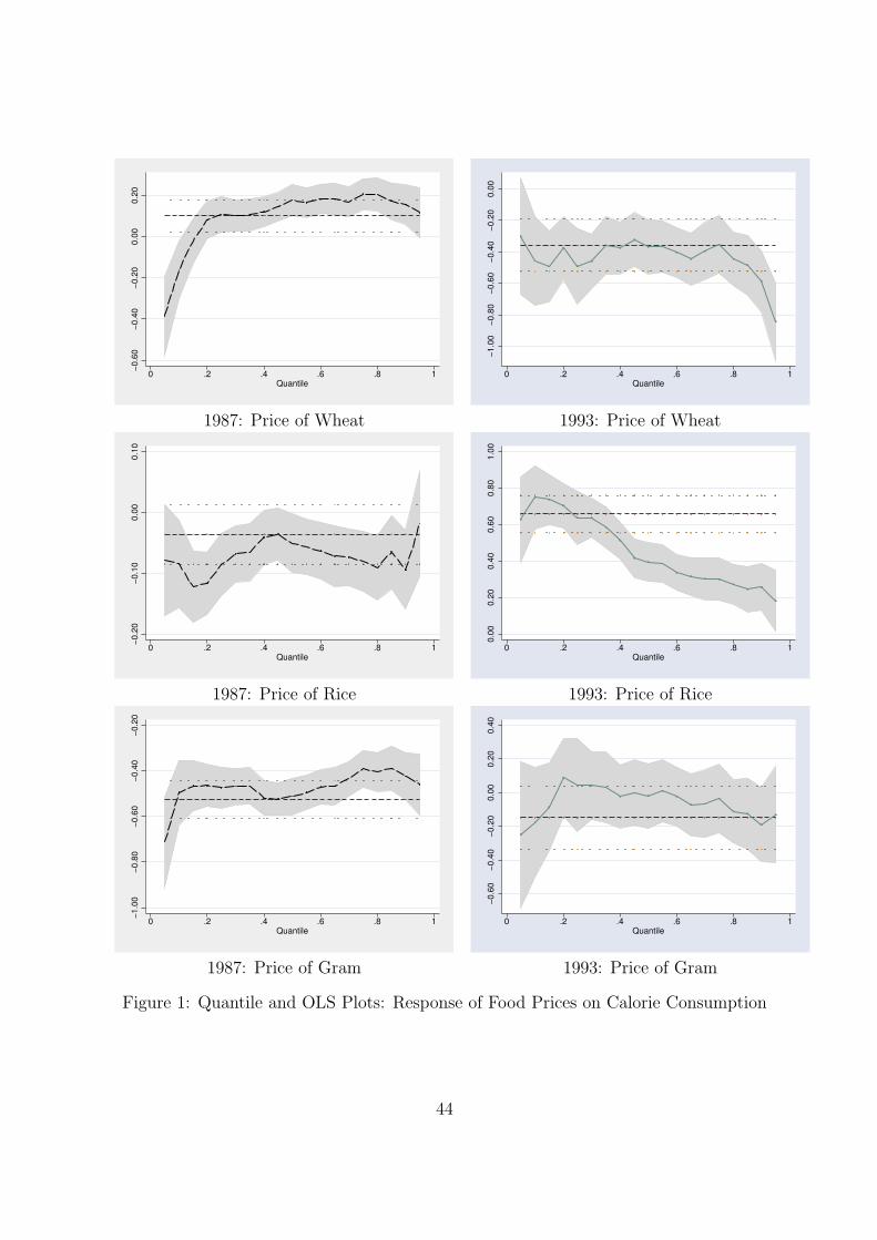
−0

.60

−0

.40

−0

.20

0.0

00

.20

0 .2 .4 .6 .8 1

Quantile

−1

.00

−0.8

0−

0.6

0−

0.4

0−

0.2

00

.00

0 .2 .4 .6 .8 1

Quantile

1987: Price of Wheat 1993: Price of Wheat

−0

.20

−0

.10

0.0

00

.10

0 .2 .4 .6 .8 1

Quantile

0.0

00

.20

0.4

00

.60

0.8

01

.00

0 .2 .4 .6 .8 1

Quantile

1987: Price of Rice 1993: Price of Rice

−1

.00

−0

.80

−0

.60

−0

.40

−0

.20

0 .2 .4 .6 .8 1

Quantile

−0

.60

−0

.40

−0

.20

0.0

00

.20

0.4

0

0 .2 .4 .6 .8 1

Quantile

1987: Price of Gram 1993: Price of Gram

Figure 1: Quantile and OLS Plots: Response of Food Prices on Calorie Consumption

44

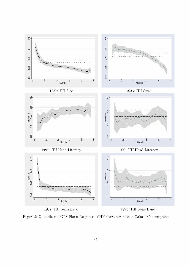
−0

.05

0.0

00

.05

0.1

00

.15

0 .2 .4 .6 .8 1

Quantile

−0

.10

−0.0

50

.00

0.0

50

.10

0 .2 .4 .6 .8 1

Quantile

1987: HH Size 1993: HH Size

−0

.60

−0

.40

−0

.20

0.0

00

.20

lith

ea

d=

=1

0 .2 .4 .6 .8 1

Quantile

−0

.10

0.0

00

.10

0.2

0

lith

ea

d=

=1

0 .2 .4 .6 .8 1

Quantile

1987: HH Head Literacy 1993: HH Head Literacy

0.0

00

.20

0.4

00

.60

lan

d=

=1

0 .2 .4 .6 .8 1

Quantile

−0

.10

0.0

00

.10

0.2

0

lan

d=

=1

0 .2 .4 .6 .8 1

Quantile

1987: HH owns Land 1993: HH owns Land

Figure 2: Quantile and OLS Plots: Response of HH characteristics on Calorie Consumption

45

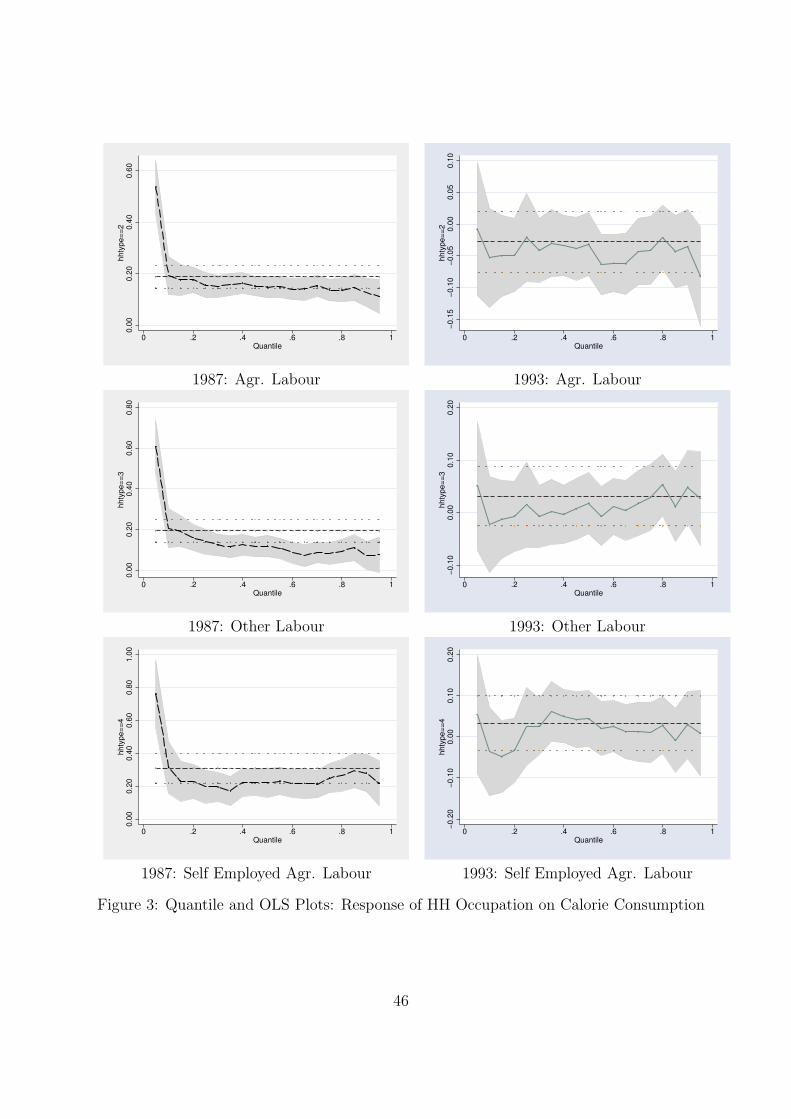
0.0

00

.20

0.4

00

.60

hh

typ

e=

=2

0 .2 .4 .6 .8 1

Quantile

−0

.15

−0

.10

−0.0

50.0

00

.05

0.1

0

hh

typ

e=

=2

0 .2 .4 .6 .8 1

Quantile

1987: Agr. Labour 1993: Agr. Labour

0.0

00

.20

0.4

00

.60

0.8

0

hh

typ

e=

=3

0 .2 .4 .6 .8 1

Quantile

−0

.10

0.0

00

.10

0.2

0

hh

typ

e=

=3

0 .2 .4 .6 .8 1

Quantile

1987: Other Labour 1993: Other Labour

0.0

00

.20

0.4

00

.60

0.8

01

.00

hh

typ

e=

=4

0 .2 .4 .6 .8 1

Quantile

−0

.20

−0

.10

0.0

00

.10

0.2

0

hh

typ

e=

=4

0 .2 .4 .6 .8 1

Quantile

1987: Self Employed Agr. Labour 1993: Self Employed Agr. Labour

Figure 3: Quantile and OLS Plots: Response of HH Occupation on Calorie Consumption

46

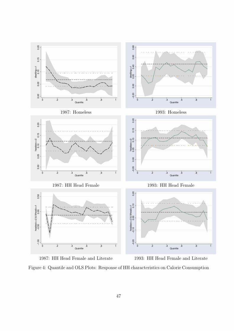
0.0

00

.05

0.1

00

.15

0.2

0

dw

ellin

g=

=1

0 .2 .4 .6 .8 1

Quantile

−0.2

00

.00

0.2

00

.40

0.6

00

.80

dw

ellin

g=

=1

0 .2 .4 .6 .8 1

Quantile

1987: Homeless 1993: Homeless

0.0

00

.05

0.1

00

.15

0.2

0

he

ad

se

x=

=2

0 .2 .4 .6 .8 1

Quantile

−0

.05

0.0

00

.05

0.1

00

.15

0.2

0

he

ad

se

x=

=2

0 .2 .4 .6 .8 1

Quantile

1987: HH Head Female 1993: HH Head Female

−1

.00

−0

.50

0.0

00

.50

he

ad

se

x=

=2

& lith

ea

d=

=1

0 .2 .4 .6 .8 1

Quantile

−0

.20

−0

.10

0.0

00

.10

0.2

0

he

ad

se

x=

=2

& lith

ea

d=

=1

0 .2 .4 .6 .8 1

Quantile

1987: HH Head Female and Literate 1993: HH Head Female and Literate

Figure 4: Quantile and OLS Plots: Response of HH characteristics on Calorie Consumption

47

7 Conclusion

This paper has been an attempt to model the effect of income and certain household char-

acteristics affect the per capita calorie consumption in rural India. The main conclusions

are:

There is much heterogeneity in the marginal effect of income and household characteristics

on calorie consumption. The distribution for calorie consumption is affected differently at

different levels depending on the household characteristics and the nutritional status of the

household. The effect of income is not uniform across the conditional calorie consumption

distribution. It is higher for individuals at higher positions in the calorie consumption dis-

tribution. Thus, OLS analysis does not give a complete picture of the effect of income and

other household characteristics on the calorie consumption of the household’s behaviour.

The distribution of calorie consumption differs across households. The implications of price

and income effects for a particular level of calorie consumption differs substantially from

the effects at the mean. The price elasticities for nutrient consumption are substantially

different for undernourished than for overnourished households. The behaviour at the

average, as suggested by the OLS results, thus misrepresents the substantial nutritional

status differences in adjustment to price changes of different commodities. The positive

price elasticities for different quantiles has been justified by Behrman & Deolalikar (1988)

in saying that there is strong substitution among various foods for price changes. The

positive effect of prices is suggestive of the fact that the households do not always consume

the diet which the can afford in minimum cost. In deciding upon the food choice the

households also take into account other attributes of foods which might be non-nutritive

in nature such as aroma, tastes, quality etc. The price elasticity results have important

policy implications. The results suggests that while providing food subsidy, the nature of

the food subsidized is also important. A subsidy on certain commodities might actually

reduce the nutritional level of the households. Not only this, in designing the subsidy

the policy maker has to take into account the actual “healthiness of the households”. A

subsidy on a less nutritious food might not be effective in improving the nutrition of the

under nourished households whereas it might provide over nutrition for the over nourished

households!

48

The analysis in this paper suggest that the ordinary least square method gives an incom-

plete picture of the responsiveness of the calorie consumption for various households. This

is very important for policy design attempting to improve nutrition of the people in the

economy.

8 Appendix

The dummy variables are defined as:

References

Abrevaya, J. (2001), ‘The Effects of Demographics and Maternal Behavior on the Distri-

bution of Birth Outcomes’, Empirical Economics 26(1), 247–57.

Alderman, H. (1986), ‘The effect of food prices and income changes on the acquisition of

food by low income households’, International Food Policy Research Institute .

Bank, W. (1981), ‘World development report’.

Becker, G. (1965), ‘A theory of the allocation of time’, Economic Journal 75, 493–517.

Behrman, J. & Deolalikar, A. B. (1988), Health and Nutrition, in H. Chenery & T. N.

Srinivasan, eds, ‘Handbook of Development Economics Volume’, Elsevier Science Publi-

cation, North-Holland, pp. 631–704.

Behrman, J. R. & Deolalikar, A. (1989), ‘Is Variety the Spice of Life? Implications for

Calorie Intake’, The Review of Economics and Statistics 71, 666–72.

Behrman, J. R. & Deolalikar, A. B. (1990), ‘The Intrahousehold Demand for Nutrients in

Rural South India: Individual Estimates, Fixed Effects, and Permanent Income’, The

Journal of Human Resources 25, 665–96.

Behrman, J. R. & Deolalikar, A. K. (1987), ‘Will Developing Country Nutrition Improve

with Income? A case study of rural South India’, Journal of Political Economy 95, 108–

38.

49

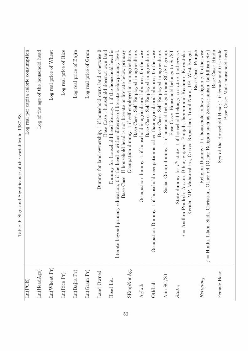
Tab

le9:

Sig

nan

dSig

nifi

cance

ofth

eva

riab

les

in19

87-8

8.

Ln(P

CE

)Log

real

per

capita

calo

rie

consu

mpti

on

Ln(H

eadA

ge)

Log

ofth

eag

eof

the

hou

sehol

dhea

d

Ln(W

hea

tP

r)Log

real

pri

ceof

Whea

t

Ln(R

ice

Pr)

Log

real

pri

ceof

Ric

e

Ln(B

ajr

aP

r)Log

real

pri

ceof

Bajr

a

Ln(G

ram

Pr)

Log

real

pri

ceof

Gra

m

Lan

dO

wned

Dum

my

for

land

owner

ship

;1

ifhou

sehol

dow

ns

land

other

wis

e0

Bas

eC

ase

:hou

sehol

ddoes

not

own

land

Hea

dLit

.D

um

my

for

hou

sehol

dhea

dlite

racy

.1

ifth

ehou

sehol

dhea

dis

lite

rate

bey

ond

prim

ary

educa

tion

;0

ifth

ehea

dis

wit

her

illite

rate

oflite

rate

bel

owpri

mar

yle

vel.

Bas

eC

ase:

Ifhou

sehol

dhea

dis

not

lite

rate

orlite

rate

bel

owpri

mar

ySE

mpN

onA

g.O

ccupat

ion

dum

my.

1if

self

emplo

yed

innon

agri

cult

ure

.B

ase

Cas

e:Sel

fE

mplo

yed

inag

ricu

lture

.A

gLab

Occ

upat

ion

dum

my.

1if

hou

sehol

dis

agricu

ltura

lla

bou

rer,

0ot

her

wis

eB

ase

Cas

e:Sel

fE

mplo

yed

inag

ricu

lture

.O

thLab

Occ

upat

ion

Dum

my.

1if

hou

sehol

docc

upat

ion

isot

her

than

agri

cult

ura

lla

bou

rer,

0ot

her

wis

eB

ase

Cas

e:Sel

fE

mplo

yed

inag

ricu

lture

.N

onSC

/ST

Soci

alG

roup

dum

my.

1if

hou

sehol

dbel

ongs

tonon

SC

/ST

grou

p.

Bas

eC

ase:

Hou

sehol

dbel

ongs

toSc/

ST

Sta

tei

Sta

tedum

my

for

ithst

ate.

1if

hou

sehol

dbel

ongs

tost

ate

i0

other

wis

e.i=

Andhra

Pra

des

h,A

ssam

,B

ihar

,gu

jara

t,P

unja

b,Jam

mu

and

Kas

hm

ir,K

arnat

aka.

Ker

ala,

MP,M

ahar

ashtr

a,O

riss

a,R

aja

sthan

,Tam

ilN

adu,U

P,W

est

Ben

gal.

Bas

eC

ase:

Punja

bR

elig

ion

jR

elig

ion

Dum

my:

1if

hou

sehol

dfo

llow

sre

ligi

onj,

0ot

her

wis

ej

=H

indu,Is

lam

,Sik

h,C

hri

stia

n,O

ther

rel(O

ther

Rel

igio

nsu

chas

Zor

astr

ianis

m,buddhis

met

c.)

Bas

eC

ase:

Hin

du

Fem

ale

Hea

dSex

ofth

eH

ouse

hol

dH

ead;1

iffe

mal

ean

d0

ism

ale

Bas

eC

ase:

Mal

ehou

sehol

dhea

d

50

Behrman, J. R., Foster, A. D. & Rosenzweig, M. R. (1997), ‘The Dynamics of Agricultural

Production and The Calorie-Income Relationship: Evidence from Pakistan’, Journal of

Econometrics 77, 187–207.

Bliss, C. & Stern, N. (1978), ‘Productivity, Wages and Nutrition: Part I and II: The

Theory’, Journal of Development Economics 5, 331–398.

Bouis, H. E. (1994), ‘The Effect of Income on Demand for Food in Poor Countries: Are our

databases giving reliable estimates’, Journal of Developmental Economics 44, 199–226.

Bouis, H. E. & Haddad, L. J. (1992), ‘Are Estimates of Calorie-Income Elasticities too

High?’, Journal of Development Economics 39, 333–64.

Buchinsky, M. (1994), ‘Changes in U.S wage structure 1963-87 : An application of quantile

regression’, Econometrica 62, 405–458.

Buchinsky, M. (1995), ‘Estimating the covariance matrix for quantile regression models :

A monte carlo study’, Journal of Econometrics 68, 303–38.

Buchinsky, M. (1998), ‘Recent Advances in Quantile Regression Models - A Practical Guide

for Empirical Research’, The Journal of Human Resources 33, 88–126.

Buchinsky, M. (2001), ‘Quantile Regression with Sample Selection: Estimating womens

returns to education in the U.S’, Empirical Economics 26(1), 87–113.

Chamberlain, G. (1994), Quantile Regression, Censoring and the Structure of Wages, El-

sevier, New York.

Conley, T. & Galenson, D. (1998), ‘Nativity and Wealth in Mid-Nineteenth Century Cities’,

Journal of Economic History 58, 468–93.

Dawson, P. J. & Tiffin, R. (1998), ‘Estimating the Demand for Calorie in India’, American

Journal of Agricultural Economics 80, 474–81.

de Walle, D. V. & Gunewardena, D. (2001), ‘Sources of ethnic inequality in Vietnam’,

Journal of Development Economics 65, 177–207.

51

Deolalikar, A. B. (1988), ‘Nutrition and Labour Productivity in Agriculture: Estimates for

Rural India’, Review of Economic and Statistics 7, 406–13.

Efron, B. (1979), ‘Bootstraping method: Another look at the jackknife’, Annals of Statistics

7, 1–26.

Eide, E. & Showalter, M. H. (1998), ‘The Effect of School Quality on Student Performance:

A Quantile Regression Approach’, Economic Letters 58(3), 345–50.

FAO (1992), Www.fao.org, Technical report, Food and Agriculture Organization of the

United Nations.

Fitzenberger, B., Hujer, R., MaCurdy, T. E. & Schnabel, R. (2001), ‘Testing for uniform

wage trends in West-Germany: A cohort analysis using quantile regressions for censored

data’, Empirical Economics 26(1), 41–86.

Gibson, J. & Rozelle, S. (2002), ‘How elastic is calorie demand? Parametric, Nonparametric

and Semiparametric results for Papua New Guinea’, Journal of Development Studies

38(6), 23.

Gopalan (1992), Nutrition and Poverty, Oxford University Press., Delhi, chapter Under-

nutrition: Measurement and Implications, p. S. Osmani.

Greer, J. & Thorbecke, E. (1986), ‘A Methodology for Measuring Food Poverty Applied

to Kenya’, Journal of Development Economics 24(1), 59–74.

Grossman, M. (1972), ‘On the concept of health capital and the demand for health’, Journal

of Political Economy 80, 223–55.

Knudsen, O. K. & Scandizzo, P. L. (1982), ‘The Demand for Calories in Developing Coun-

tries’, American Journal of Agricultural Econmics 64(1), 80–86.

Koenker, R. & Bassett, G. (1978), ‘Regression Quantiles’, Econometrica 46, 33–50.

Levin, J. (2001), ‘For Whom the Reduction Counts : A Quantile Regression Analysis of

Class size on Scholastic Achievement’, Empirical Economics 26(1), 221–46.

52

Liu, A. Y. C. (2001), ‘Markets ineqality and poverty in Vietnam’, Asian Economic Journal

15(2), 217–35.

Machado, J. A. F. & Mata, J. (2000), ‘Counterfactual decomposition of changes in wage

distribution using quantile regression’, mimeo .

Machado, J. A. & Mata, J. (2001), ‘Earning Functions in Portugal 1982-1994: Evidence

from Quantile Regressions’, Empirical Economics 26, 115–34.

Manning, W., Blumberg, L. & Moulton, L. (1995), ‘The demand of alcohol the differential

response to price’, Journal of Health Economics 14, 123–148.

Min, I. & Kim, I. (2004), ‘A Monte Carlo Comparison of Parametric and Nonparametric

Quantile Regressions’, Applied Economic Letters 11, 71–74.

Nahm, J.-W. (2001), ‘Nonparametric Quantile Regression Analysis of R&D Sales REla-

tionship for Korean Firms’, Empirical Economics 26, 259–70.

Nakajima, C. (1969), Subsistence and commercial family farms: Some theoretical models

of objective equilibrium, in C. Wharton, ed., ‘Subsistence Agriculture and Economic

Development’, Chicago: Aldine.

Nguyen, B. T., Albrecht, J. W., Vroman, S. B. & Westbrook, M. D. (2003), ‘A Quantile

Regression Decomposition of Urban Rural Poverty in Vietnam’, Working Paper .

Pinsturp-Anderson, P. (1985), ‘Food Policies and Poor in Developing Countries’, European

Rwview of Agricultural Economics 12(1/2).

Pitt, M. M. & Rosenzweig, M. R. (1986), Agricultural prices, food consumption, and the

health and productivity of indonesian farmers, in I. Singh, L. Squire & J. Strauss, eds,

‘Agricultural Household Models’, The World Bank, The John Hopkins University Press,

Baltimore and London.

Ravallion, M. (1988), ‘Income Effects on Calorie Undernutrition : A Case Study of East

Java’, Australia National University mimeo.

53

Ravallion, M. (1990), ‘Income effects on Undernutrition’, Economic Development and Cul-

tural Change pp. 489–515.

Reutlinger, S. & Selowsky, M. (1976), Malnutrition and Poverty: Magnitude and Policy

Options, World Bank/John Hopkins University Press, Baltimore.

Strauss, J. (1984), ‘Joint Determination of Food Consumption and Production in Rural

Sierra Leone:Estimates of a Household-Firm Model’, Journal of Development Studies

14, 77–103.

Strauss, J. (1986), ‘Does Better Nutrition Raise Farm Productivity’, Journal of Political

Economy 94, 297–320.

Strauss, J. & Thomas, D. (1995), Human resources: Empirical modeling of household and

family decisions, in J. Behrman & T. N. Srinivasan, eds, ‘Handbook of Development

Economics, Volume 3A’, Elsevier Science Publishers, North-Holland, p. Chapter 34.

Taylor, J. (1999), ‘A Quantile Regression Approach to Estimating the Distribution of

Multiperiod Returns’, Journal of Derivatives pp. 64–78.

Tiffin, R. & Dawson, P. J. (2002), ‘The Demand for Calorie : Some further estimates from

Zimbabwe’, Journal of Agricultural Economics 53(2), 221–232.

Variyam, J. N., Blaylock, J. & Smallwood, D. (2002), ‘Characterizing the Distribution of

Macronutrient Intake among U.S. Adults: A Quatile Regression Approach’, American

Journal of Agriculural Economics 84(2), 454–66.

Viscusi, W. & Born, P. (1995), ‘Medical Malpractice Insurance in the Wake of Liability

Reform’, Journal of Legal Studies 24, 463–90.

Viscusi, W. & Hamilton, J. (1999), ‘Are Risk Regulators Rational ? Evidence from Haz-

ardous Waste Cleanup Decisions’, American Economic Review 89, 1010–27.

Yu, K. & Jones, M. C. (1998), ‘Local linear regression quantile estimation’, Journal of

American Statistical Association 93, 228–238.

54

Yu, K., Lu, Z. & Stander, J. (2003), ‘Quantile Regression : applications and current

research areas’, The Statistician 52(3), 331–350.

55