HONG KONG INSTITUTE FOR MONETARY AND FINANCIAL RESEARCH

Max Breitenlechner, Georgios Georgiadis and Ben Schumann

HKIMR Working Paper No.16/2021 August 2021

WHAT GOES AROUND COMES AROUND: HOW LARGE ARE SPILLBACKS FROM US MONETARY POLICY?

Hong Kong Institute for Monetary and Financial Research 香港貨幣及金融研究中心 (a company incorporated with limited liability)

All rights reserved.

Reproduction for educational and non-commercial purposes is permitted provided that the source is acknowledged.

* Email: Breitenlechner: max.breitenlechner@uibk.ac.at, Georgiadis: georgios.georgiadis@ecb.int and Schumann: benschumann91@gmail.com

* The authors would like to thank, without implying endorsement, Dimitris Georgarakos, Marek Jarocinski, Silvia Miranda-Agrippino, GernotMüller, Ivan Petrella, Michele Piffer, Martin Schmitz, Andrej Sokol, and Fabrizio Venditti, seminar participants at the ECB, Bank of Lithuania,University of Innsbruck, University of Tübingen, and Hong Kong Institute for Monetary and Financial Research as well as conferenceparticipants at the 28th European Summer Symposium in International Macroeconomics (ESSIM), the 2021 BoE/BIS/ECB/IMF SpilloverConference, the 21st IWH-CIREQ-GW Macroeconometric Workshop, the 13th FIW Research Conference on International Economics, the 25th

ICMAIF, the 11th RCEA Money-Macro-Finance Conference, the 27th International Conference on Computing in Economics and Finance, and the2021 Conference on Economic Measurement. Helena Le Mezo provided excellent research assistance. Georgios Georgiadis gratefullyacknowledges financial support from Hong Kong Institute for Monetary and Financial Research. This paper represents the views of the authors,which are not necessarily the views of the Hong Kong Monetary Authority, Hong Kong Institute for Monetary and Financial Research, or itsBoard of Directors or Council of Advisers. The above-mentioned entities except the authors take no responsibility for any inaccuracies oromissions contained in the paper. The views expressed in the paper do also not reflect those of the ECB, the Eurosystem and should not bereported as such.

What Goes Around Comes Around: How Large Are Spillbacks From US Monetary Policy?

Max BreitenlechnerUniversity of Innsbruck

Georgios GeorgiadisEuropean Central Bank

Ben SchumannFree University of Berlin

August 2021

We quantify spillbacks from US monetary policy based on structural scenario analysis and minimum relative

entropy methods applied in a Bayesian proxy structural vector-autoregressive model estimated on data for the

time period from 1990 to 2019. We find that spillbacks account for a non-trivial share of the overall slowdown in

domestic real activity in response to a contractionary US monetary policy shock. Our analysis suggests that

spillbacks materialise as Tobin’s q/cash flow and stock market wealth effects impinge on US investment and

consumption. Contractionary US monetary policy depresses foreign sales of US firms, which reduces their

valuations/cash flows and thereby induces cutbacks in investment. Similarly, as contractionary US monetary

policy depresses US and foreign equity prices, the value of US households’ portfolios is reduced, which triggers

a drop in consumption. Net trade does not contribute to spillbacks because US monetary policy affects exports

and imports similarly. Finally, spillbacks materialise through advanced rather than emerging market economies,

consistent with their relative importance in US firms’ foreign demand and US foreign equity holdings.

Keywords: US monetary policy, spillovers, spillbacks, Bayesian proxy structural VAR models.

JEL classification: F42, E52, C50.

1 Introduction

Much empirical work as well as prominent policy debates suggest that US monetary policy

spillovers are large and an important driver of business cycles and financial conditions in the

global economy (Banerjee et al., 2016; Dedola et al., 2017; Brauning and Sheremirov, 2019;

Iacoviello and Navarro, 2019; Vicondoa, 2019; Degasperi et al., 2020). At the same time,

it has been argued that the Federal Reserve has exhibited “benign neglect” regarding its

international effects (Eichengreen, 2013, p. 87). For example, after the Global Financial Crisis

some policymakers complained that US monetary policy measures aimed at stabilising the

domestic economy elicited waves of capital flows and accentuated financial market volatility

in the rest of the world (Rajan, 2013). Some have even argued that the global effects of

US monetary policy inhibit control of fundamentals by monetary policy in small open and

emerging market economies and jeopardise local financial stability (Rey, 2016; Miranda-

Agrippino and Rey, 2020).

Against this background, some policymakers have argued that the Federal Reserve should take

into account its effects on the rest of the world in the calibration of its monetary policy (Rajan,

2016a,b). The Federal Reserve has responded that it already does so implicitly, as spillovers

spill back to the US economy: “Actions taken by the Federal Reserve influence economic

conditions abroad. Because these international effects in turn spill back on the evolution

of the US economy, we cannot make sensible monetary policy choices without taking them

into account” (Fischer, 2014); similarly: “The Fed recognizes that its own policies do have

international spillovers, and, in turn because they affect global performance, they are going to

have spillbacks to US economic performance” (Yellen, 2019). Carney (2019) exemplifies the

view that large monetary policy spillbacks are not confined to the Federal Reserve: “Advanced

economies’ monetary policies will increasingly need to take account of spillbacks”. Similarly,

Shin (2015) notes: “There is much talk of ‘headwinds’ from emerging markets buffeting

advanced economies, [which] are the result of monetary policy actions taken some time ago

(...) by precisely those advanced economies”. However, to the best of our knowledge, no

rigorous analysis of spillbacks from US monetary policy exists in the literature. In this paper

we fill this gap.

We define spillbacks from US monetary policy as the difference between the actual domestic

effects of US monetary policy and a counterfactual in which the spillovers to rest-of-the-world

real activity are nil. Our analysis suggests that spillbacks are large: When spillovers to the

rest of the world in response to a contractionary US monetary policy shock are precluded, the

slowdown in domestic real activity and the drop in domestic consumer prices is substantially

smaller.

1

Regarding economic transmission channels our analysis suggests that spillbacks materialise

through Tobin’s q/cash flow and stock market wealth effects. In particular, contractionary

US monetary policy depresses US firms’ valuations/cash flows as their foreign sales decline,

inducing them to cut back investment. Similarly, as contractionary US monetary policy

depresses US and also foreign equity prices, the value of US households’ portfolios is reduced,

which triggers a drop in consumption; that wealth effects contribute to the domestic effects

of monetary policy is consistent with recent work on heterogeneous-agent New Keynesian

models (Kaplan et al., 2018; Alves et al., 2020). In contrast to consumption and investment,

net exports do not contribute to spillbacks because US monetary policy affects exports and

imports to a similar degree. Finally, spillbacks to US consumer prices materialise primarily

as a US monetary policy contraction puts downward pressure on global commodity prices

and thereby reduces US import prices.

Regarding geographic transmission channels our analysis suggests that spillbacks materialise

through advanced economies (AEs) rather than through emerging market economies (EMEs).

Specifically, we find that we can replicate the counterfactual in which US monetary policy

spillovers to real activity in the entire rest of the world are nil by precluding spillovers only

to AEs. In contrast, when only spillovers to EMEs are precluded we replicate the baseline

under which spillovers are unconstrained. We argue this finding is consistent with the relative

exposure of US firms’ sales and US holdings’ of foreign equity across AEs and EMEs. An

important caveat to this finding is that it reflects the average properties of the data over

our sample period from 1990 to 2019. As the importance of EMEs has been growing over

time, their contribution to spillbacks from US monetary policy may be larger at the current

juncture. We leave the assessment of time variation in spillbacks to future research.

Our finding that spillbacks from US monetary policy are large but that these materialise pri-

marily through AEs and not EMEs suggests there may be a case for international monetary

policy coordination (Engel, 2016; Ostry and Ghosh, 2016; Egorov and Mukhin, 2020). In par-

ticular, we find that while real activity spillovers from US monetary policy are contractionary

in both AEs and EMEs, consumer prices fall in AEs but rise in EMEs. Thus, while US mon-

etary policy spillovers do not induce welfare-reducing trade-offs between output and inflation

stabilisation in AEs, they do so in EMEs. This implies that global welfare could benefit

if spillovers to EMEs were internalised by playing a role in the calibration of US monetary

policy that is independent from spillbacks. Interestingly, there is evidence that the Federal

Reserve is doing precisely that already. Ferrara and Teuf (2018) construct an indicator that

measures the number of references to the international environment in FOMC minutes. They

then estimate a Taylor-rule with domestic variables augmented with their international envi-

ronment indicator, and find that the Federal Reserve responds to global developments even

2

conditional on US real activity and inflation. Hence, our finding that spillbacks from US

monetary policy hardly materialise through EMEs may be a rationalisation for the observed

behaviour of the Federal Reserve.

It should be noted upfront that quantifying spillbacks from US monetary policy is not straight-

forward even conceptually.1 On the one hand, it is unlikely that any existing structural

model in the literature can be expected to encompass all empirically relevant monetary policy

spillover transmission channels (see for example Brauning and Sheremirov, 2019; Degasperi

et al., 2020, for opposing views regarding the relative importance of trade vs. financial

channels). As a result, a structural model is likely to impose a dogmatic prior that unduly

constrains the range of possible spillback assessments (for a similar argument see Bachmann

and Sims, 2012; Rostagno et al., 2021). Moreover, as spillovers can be shut down in vari-

ous ways there is not a unique ‘no-spillovers’ counterfactual structural model; and in general,

precluding spillovers in a structural model in different ways results in different spillback assess-

ments. On the other hand, an empirical approach that defines the counterfactual benchmark

in terms of the outcome that spillovers are absent without being explicit about the trans-

mission channels that are being shut down may be more difficult to interpret economically.

Notwithstanding these conceptual challenges, the lack of existing analysis coupled with the

prominence spillbacks from US monetary policy have assumed (Fischer, 2014; Shin, 2015;

Yellen, 2019; Carney, 2019) dictate an urgency for study. It is against this background that

we attempt to inject more rigour in the debate about spillbacks with this paper.

Considering these conceptual challenges, we opt for an empirical instead of a structural

approach. This avoids imposing dogmatic priors and frees us from taking a stand on the

specification of the ‘no-spillovers’ counterfactual structural model. In particular, we carry

out counterfactual analyses in two-country vector-autoregressive (VAR) models for the US

and the rest of the world. We adopt the Bayesian proxy structural VAR framework of Arias

et al. (2018, forthcoming). We identify a US monetary policy shock using the high-frequency

interest rate surprises on FOMC meeting dates of Gurkaynak et al. (2005) as in Gertler

and Karadi (2015) as well as Caldara and Herbst (2019), additionally cleansed from central

bank information effects as in Jarocinski and Karadi (2020). We consider two approaches

to construct counterfactual impulse responses in which the real activity spillovers from US

monetary policy to the rest of the world are nil: (i) Structural scenario analysis (SSA) and

(ii) minimum relative entropy (MRE).

In SSA we identify two additional shocks that represent a convolution—but together capture

the universe—of rest-of-the-world structural shocks by combinations of zero, sign and magni-

tude restrictions. We use combinations of these two rest-of-the-world shocks to offset the real

1We discuss these issues in more detail in Section 2.

3

activity spillovers from US monetary policy to obtain the counterfactual. Technically, SSA

indicates how US variables would evolve if current and future shocks materialised along the

impulse response horizon that happened to offset the effect of the US monetary policy shock

on rest-of-the-world real activity. Intuitively, SSA is similar to the assessment of direct and

indirect effects in mediation analysis, in which simulated interventions are invoked in order

to keep the value of the mediating variable at its baseline (Pearl et al., 2016). SSA is a point

of contact with existing literature and provides a natural methodological benchmark (Kilian

and Lewis, 2011; Bachmann and Sims, 2012; Wong, 2015; Epstein et al., 2019; Rostagno

et al., 2021). We also consider a more general version of SSA in which we do not restrict the

set of structural shocks we use to undo the real activity spillovers from US monetary policy

to obtain the counterfactual (Antolin-Diaz et al., 2021).

In MRE we determine the minimum ‘tilt’ of the posterior distribution of the baseline impulse

responses to a US monetary policy shock that satisfies the counterfactual constraint that

the mean real activity spillovers are nil. Intuitively, MRE indicates how US variables would

evolve in a counterfactual world in which the spillovers from US monetary policy to rest-of-

the-world real activity are nil but which is otherwise minimally different from the actual world

in an information-theoretic sense (Cogley et al., 2005; Robertson et al., 2005; Giacomini and

Ragusa, 2014). We argue SSA and MRE are conceptually complementary, which strengthens

our analysis given the challenges involved in defining the counterfactual benchmark.

The rest of the paper is organised as follows. Section 2 provides a brief discussion of the

conceptual challenges in the analysis of spillbacks. Section 3 provides a short description of

the Bayesian proxy SVAR model. Section 4 lays out our specification of the Bayesian proxy

SVAR model. Section 5 explains how we construct counterfactuals and presents our results.

Section 6 concludes.

2 Monetary policy spillbacks: conceptual considerations

Consider a two-country New Keynesian dynamic stochastic general equilibrium (NK DSGE)

model for the US and the rest of the world. To illustrate the conceptional challenges in the

analysis of spillbacks, we consider a model that incorporates multiple transmission channels

for spillovers from US monetary policy. Specifically, the model features cross-border bank

lending as in Akinci and Queralto (2019) as well as trade in final goods under producer-

currency pricing.2 The black solid lines with circles in Figure 1 depict the impulse responses

to a contractionary US monetary policy shock: Rest-of-the-world output rises on impact as

depreciation against the dollar stimulates net exports through expenditure switching; the

2A detailed model description is available upon request.

4

output spillover turns negative with some delay when the deterioration of the net worth

of rest-of-the-world banks that, given their stock of US dollar liabilities, results from the

appreciation of the dollar induces a contraction in local lending.

In the spirit of Fischer (2014) and Yellen (2019) we define spillbacks as the part of the overall

domestic effect of US monetary policy that arises because of spillovers to the rest of the world.

Intuitively, if the rest of the world was not affected by US monetary policy, nothing would

spill back to the US economy. Based on this definition, spillbacks are given by the difference

between the domestic effects of US monetary policy in the ‘true’ model in Figure 1 and in

some counterfactual model in which there are no spillovers to the rest of the world.

An intuitive ‘no-spillover’ counterfactual model is a version of the ‘true’ model in which cross-

border bank lending and trade are shut down. The impulse responses for this counterfactual

model are shown by the orange lines with squares in Figure 1. As a result of the absence of

spillovers, the domestic output effects of US monetary policy are weaker. Based on this ‘no-

spillover’ counterfactual model we conclude that in the ‘true’ model spillbacks—the difference

between the black lines with circles and the orange lines with squares—amplify the domestic

output effects of US monetary policy.3

However, in practice it is unlikely that the ‘true’ model and all spillover transmission channels

are known. Arguably, any existing model studied in the literature incorporates only a subset

of all empirically relevant spillover transmission channels and is thereby mis-specified. For

example, the impulse responses shown by the blue lines with triangles in Figure 1 show the

effects of a US monetary policy shock when the model does not feature cross-border bank

lending but still features trade.4 It is not surprising that in this mis-specified model the

effects of US monetary policy are different from those in the ‘true’ model. Accordingly, the

spillback assessment we obtain when we use this mis-specified model as baseline does not

recover the one we obtain when we use the ‘true’ model as baseline: The difference between

the blue lines with triangles and the orange lines with squares (the spillbacks assessed using

the mis-specified model as baseline) differs from the difference between the black lines with

circles and the orange lines with squares (the ‘true’ spillbacks). The bias in the assessment of

3There also exist counterfactual models in which there are no spillbacks while spillovers from US monetarypolicy are not precluded. For example, we could assume the US is large relative to the rest of the world.However, especially against the background of the debate about the implications of spillovers from US monetarypolicy discussed in the Introduction it seems more natural and intuitive to benchmark spillbacks based oncounterfactual models in which spillovers are absent. Furthermore, the absence of spillovers constitutes asufficient condition for the absence of spillbacks.

4The parametrisation in this model coincides with that in the ‘true’ model, which could be interpreted asreflecting the researcher’s tight priors centred around the true values of the corresponding deep parameters. Ofcourse, when the mis-specified model is confronted with the data with looser priors the estimated parameters ingeneral do not recover their true values and thereby lose their structural interpretation (Fernandez-Villaverdeand Rubio-Ramirez, 2008). This is an additional practical challenge when structural models are used to assessspillbacks.

5

the spillbacks results from a dogmatic prior imposed on the structure of the model in terms

of the spillover transmission channels the researcher decides to consider.

Another conceptual challenge in the analysis of spillbacks is that even if the ‘true’ model was

known, the ‘no-spillover’ counterfactual benchmark model is not unique. For example, the

green lines with crosses show that specifying the US as a small open economy mutes spillovers

to rest-of-the-world domestic variables, even when cross-border bank lending and trade are

not shut down. However, it can also be seen that the spillback assessment implied by using

this small open economy counterfactual model as the ‘no-spillover’ benchmark (black lines

with circles vs. green lines with crosses) is different from the one implied by using the ‘true’

model with cross-border bank lending and trade shut down as ‘no-spillover’ benchmark (black

lines with circles vs. orange lines with squares). Unfortunately, there is no metric that could

be used to determine which of these two ‘no-spillover’ counterfactual benchmarks—shutting

down cross-border bank lending and trade or assuming the US is a small open economy—is

conceptually more appropriate or intuitive for assessing spillbacks.

In sum, two conceptual challenges afflict the analysis of spillbacks from US monetary policy

based on a structural model: (i) the risk of imposing a dogmatic prior that biases the range of

possible spillback assessments; (ii) the lack of a unique structural ‘no-spillover’ counterfactual

benchmark. Against this background, we adopt an empirical approach that avoids imposing

dogmatic priors and considers an entire class of counterfactual models in which spillovers

from US monetary policy to rest-of-the-world output are nil as ‘no-spillover’ benchmark.

The disadvantage of an empirical approach is that it is not straightforward to disentangle

the transmission channels through which spillbacks materialise. To address this shortcoming,

we later extend our analysis and explore the behaviour of variables that reflect a range of

possible transmission channels of spillbacks in the counterfactual.

3 The Bayesian proxy SVAR framework

We provide a description of the Bayesian proxy SVAR (BPSVAR) framework of Arias et al.

(forthcoming) before discussing our model specification and identifying assumptions. Because

we identify a global uncertainty shock in addition to a US monetary policy shock using proxy

variables, we discuss the BPSVAR model for the general case with k proxy variables.

Following the notation of Rubio-Ramirez et al. (2010), consider without loss of generality the

structural VAR model with one lag and without deterministic terms

y′tA0 = y′t−1A1 + ε′t, ε ∼ N(0, In), (1)

6

where yt is an n × 1 vector of endogenous variables and εt an n × 1 vector of structural

shocks. The BPSVAR framework builds on the following assumptions in order to identify k

structural shocks of interest: There exists a k × 1 vector of proxy variables mt that are (i)

correlated with the k structural shocks of interest ε∗t , and (ii) orthogonal to the remaining

structural shocks εot . Formally, the identifying assumptions are

E[ε∗tm′t] = V

(k×k), (2a)

E[εotm′t] = 0

((n−k)×k), (2b)

and represent the relevance and the exogeneity condition, respectively.

Denote by y′t ≡ (y′t,m′t) the vector of endogenous variables augmented with the k× 1 vector

of proxy variables, by A` the corresponding coefficient matrices of dimension n × n with

n = n + k, by ε ≡ (ε′t,v′t)′ ∼ N(0, In+k), where vt is a k × 1 vector of measurement errors

(see below). The augmented model is then given by

y′tA0 = y′t−1A1 + ε′t. (3)

To ensure that augmenting the model with these equations does not affect the dynamics of

the endogenous variables, restrictions are imposed on the matrices A` such that

A` =

A`(n×n)

Γ`,1(n×k)

0(k×n)

Γ`,2(k×k)

, ` = 0, 1. (4)

The zero restrictions on the lower left-hand side block imply that the proxy variables do not

enter the equations of the endogenous variables. The reduced form of the model is

y′t = y′t−1A1A0−1

+ εt′A0

−1. (5)

Because the inverse of A0 is given by

A0−1

=

(A−10 −A−10 Γ0,1Γ

−10,2

0 Γ−10,2

), (6)

the last k equations of the augmented model in Equation (5) read as

m′t = y′t−1A1

(−A−10 Γ0,1Γ

−10,2

Γ−10,2

)− ε′tA−10 Γ0,1Γ

−10,2 + v′tΓ

−10,2, (7)

which shows that the proxy variables may be serially correlated and affected by past values

7

of the endogenous variables, and measurement error.

Ordering the structural shocks so that εt = (εo′t , ε∗′t )′ we have

E[εtm

′t

]= −A−10 Γ0,1Γ

−10,2 =

0((n−k)×k)

V(k×k)

, (8)

where the first equality is obtained using Equation (7) and because the structural shocks

εt are by assumption orthogonal to yt−1 and vt, and the second equality is due to the

exogeneity and relevance conditions in Equations (2a) and (2b). Equation (8) shows that

the identifying assumptions imply restrictions on the last k columns of the contemporaneous

structural impact coefficients in A0−1

. In particular, if the exogeneity condition in Equation

(2b) holds, the first n − k columns of the upper right-hand side sub-matrix A−10 Γ0,1Γ−10,2 of

A0−1

in Equation (6) are zero. From Equation (5) it can be seen that this implies that the

first n−k structural shocks do not impact contemporaneously the proxy variables. In turn, if

the relevance condition in Equation (2a) holds, the last k columns of the upper right-hand side

sub-matrixA−10 Γ0,1Γ−10,2 of A0

−1are different from zero. From Equation (5) it can be seen that

this implies that the last k structural shocks impact the proxy variables contemporaneously.

The Bayesian estimation algorithm of Arias et al. (forthcoming) determines the estimates of

A0 and Γ0,` such that the restrictions on A0−1

implied by Equations (2a) and (2b) as well

as on A` in Equation (4) are simultaneously satisfied, and hence the estimation identifies the

structural shocks ε∗t .

If the number of structural shocks identified by the proxy variables is larger than one, the

BPSVAR model is set identified, as rotations of the structural shocksQε∗t satisfy the exogene-

ity and relevance conditions in Equations (2a) and (2b). In this case, additional restrictions

are needed in order to point-identify the structural shocks in ε∗t . An important advantage of

the BPSVAR over the traditional frequentist proxy SVAR framework is that the additional

identifying assumptions can be imposed on the relevance condition in Equation (2a) reflected

in the matrix V rather than on the contemporaneous relationships between the endogenous

variables in the structural impact matrix A−10 . One may, for example, impose the restriction

that a particular structural shock in ε∗t does not affect a particular proxy variable in mt.

Restrictions on the relationship between structural shocks and proxy variables are arguably

less controversial than exogeneity restrictions between the endogenous variables in A−10 , such

as for example those imposed in Mertens and Ravn (2013).

Another appealing feature of the BPSVAR model is that it allows to incorporate a prior

belief about the strength of the proxy variables as instruments are based on the notion

that “researchers construct proxies to be relevant” (Caldara and Herbst, 2019, p. 165). A

8

convenient metric is the ‘reliability matrix’ R derived in Mertens and Ravn (2013) given by

R =(Γ−1

′

0,2 Γ0,2 + V V ′)−1

V V ′. (9)

Intuitively, R indicates the share of variance of the proxy variables that is accounted for by

the structural shocks ε∗t (see Equation (7)). Specifically, the minimum eigenvalues of R can

be interpreted as the share of the variance of (any linear combination of) the proxy variables

explained by the structural shocks ε∗t (Gleser, 1992).

Yet another appealing feature of the BPSVAR model is that it allows to additionally iden-

tify some of the structural shocks in εot using zero, sign and magnitude restrictions. These

additional restrictions are imposed on the contemporaneous structural impact matrix A−10 .

Importantly, the BPSVAR framework of Arias et al. (forthcoming) allows coherent infer-

ence for specifications in which identification is achieved using zero, sign, and magnitude

restrictions as well as proxy variables.

Finally, a last appealing feature of the BPSVAR framework—especially relative to the tradi-

tional frequentist proxy SVAR framework—is that it allows exact finite sample inference, even

in settings in which the proxy variables are weak instruments and only set rather than point

identification is achieved with a combination of sign, magnitude and zero restrictions (see

Moon and Schorfheide, 2012; Caldara and Herbst, 2019; Arias et al., forthcoming). In partic-

ular, note that traditional proxy SVAR models are typically estimated following a three-step

procedure (Mertens and Ravn, 2013; Gertler and Karadi, 2015): (i) estimate the reduced-form

VAR model by least squares; (ii) regress the reduced-form residuals on the proxy; and (iii)

impose the restrictions derived in (ii) to identify the structural parameters. This three-stage

procedure makes only limited use of the information contained in the proxy. For example,

the estimation of the reduced-form VAR model is not informed by the proxy variable. In

contrast, the joint likelihood of the endogenous variables and the proxy variables based on

Equation (3) allows the proxy to inform the estimation of both reduced form and structural

parameters in the BPSVAR model and therefore entails a coherent modelling of all sources of

uncertainty. Furthermore, in a Bayesian setting, weak identification does not pose a problem

per se; as long as the prior distribution is proper, inference is possible (Poirier, 1998). By

contrast, traditional frequentist proxy SVAR models require an explicit theory to deal with

weakly informative instruments (Olea et al., forthcoming), either to derive the asymptotic

distributions of estimators or to ensure satisfactory coverage in bootstrap procedures.5

5To the best of our knowledge, there is no clear consensus yet on how to conduct inference in frequentistproxy SVAR models, even in a setting with only a single proxy variable (Jentsch and Lunsford, 2016, 2019).

9

4 Empirical framework

4.1 VAR model specification

Our point of departure is the closed-economy US VAR model in Gertler and Karadi (2015),

which includes as endogenous variables monthly (log) US industrial production (IP), the

(log) US consumer-price index (CPI), the excess bond premium (EBP) and the one-year

US Treasury Bill (TB) rate as a monetary policy indicator. We augment the model with

the VXO, (log) rest-of-the-world (non-US) real industrial production, and the (log) nominal

effective exchange rate (NEER) of the US dollar. Variable descriptions and data sources are

provided in Table 1. The sample spans the time period from February 1990 to June 2019.

4.2 Identifying assumptions

We identify a US monetary policy shock using a proxy variable and—for the purpose of SSA

counterfactuals—two rest-of-the-world shocks using a mixture of sign, magnitude and zero

restrictions. In addition, we identify a global uncertainty shock to preclude that the two

rest-of-the-world shocks are contaminated by shocks that are common to the US and the rest

of the world. We identify the global uncertainty shock using a second proxy variable.

4.2.1 US monetary policy and global uncertainty shocks

As in Gertler and Karadi (2015) as well as Caldara and Herbst (2019) we consider the

intra-daily interest rate surprises around narrow time windows on FOMC meeting days of

Gurkaynak et al. (2005) as proxy variable for the US monetary policy shock. We cleanse these

surprises from central bank information effects using the ‘poor-man’s’ approach of Jarocinski

and Karadi (2020): When the interest rate surprise has the same sign as the equity price

surprise, we classify it as a central bank information effect; when the interest rate and the

equity price surprises have opposite signs, we classify it as a ‘pure’ monetary policy surprise.

We consider the intra-daily gold price surprises of Piffer and Podstawski (2018) around narrow

time windows on narratively selected days as proxy variable for the global uncertainty shock.

Specifically, Piffer and Podstawski (2018) first extend the list of dates selected by Bloom

(2009) on which the VXO increased arguably due to exogenous uncertainty shocks. Then,

they calculate the change in the price of gold between the last auction before and the first

auction after the news about the event representing the uncertainty shock became available

to markets. The original data on gold price surprises of Piffer and Podstawski (2018) cover

the time period until 2015; we use the update of Bobasu et al. (2020) that spans until 2019.

10

Consider the notation from Section 3 and define ε∗t ≡ (εmpt , εut )′, where εmpt denotes the

US monetary policy shock and εut the global uncertainty shock. Furthermore, define mt ≡(pε,mpt , pε,ut )′ as the vector containing the proxy variables for the US monetary policy and the

global uncertainty shocks. Our identifying assumptions are

E[ε∗tm′t] =

(E[pε,mpt εmpt ] E[pε,ut εmpt ]

E[pε,mpt εut ] E[pε,ut εut ]

)= V

(2×2), (10a)

E[εotm′t] =

(E[pε,mpt εot ] E[pε,ut ε

ot ])

= 0((n−2)×2)

. (10b)

First, in the relevance condition in Equation (10a) we assume that US monetary policy

shocks drive the interest rate surprises on FOMC meeting days, E[pε,mpt εmpt ] 6= 0. This is the

standard instrument relevance assumption maintained in the literature (Gertler and Karadi,

2015; Caldara and Herbst, 2019). The exogeneity condition E[pε,mpt εot ] = 0 in Equation (10b)

cannot be tested as none of the other structural shocks εot is observed, but it seems plausible

that in a narrow time window around FOMC meetings monetary policy shocks are the only

systematic drivers of interest rate surprises purged from central bank information effects.

Second, in the relevance condition in Equation (10a) we assume that global uncertainty shocks

drive the gold price surprises on the narratively selected dates, E[pε,ut εut ] 6= 0. Intuitively, as

gold is widely seen as a safe haven asset, demand increases when uncertainty rises (Baur and

McDermott, 2010, 2016). Piffer and Podstawski (2018) provide evidence that gold price sur-

prises are relevant instruments for uncertainty shocks based on F -tests and Granger causality

tests with the VXO and the macroeconomic uncertainty measure constructed in Jurado et al.

(2015). Ludvigson et al. (forthcoming) also use gold price changes as a proxy variable for un-

certainty shocks. Regarding the exogeneity condition E[pε,ut εot ] = 0 in Equation (10b), Piffer

and Podstawski (2018) document that gold price surprises are uncorrelated with a range of

non-uncertainty shocks.

As discussed in Section 3, when multiple proxy variables are used to identify multiple struc-

tural shocks, the relevance and exogeneity conditions are not sufficient for point identification.

In this case, additional restrictions need to be imposed on the structural impact matrix A−10

that reflects the contemporaneous relationships between the endogenous variables yt or—

arguably less restrictive and an important advantage of the BPSVAR over the traditional

frequentist proxy SVAR framework—on V in Equation (10a). A natural idea is to impose

that V is a diagonal matrix, implying that US interest rate surprises on FOMC meeting days

purged from central bank information effects are not driven by global uncertainty shocks, and

that gold price surprises on days with prominent global economic, political or natural events

are not systematically driven by US monetary policy shocks. Technically, these additional

restrictions imply an over-identified system, which cannot be handled by the algorithm of

11

Arias et al. (forthcoming). We therefore impose a weaker set of additional restrictions on V ,

namely only that US interest rate surprises on FOMC meeting days are not driven by global

uncertainty shocks, E[pε,mpt εut ] = 0. Note that this assumption is implicitly maintained and

crucial for the validity of much work in the literature. For example, if this assumption was

not satisfied then the prominent analyses of Gertler and Karadi (2015), Caldara and Herbst

(2019) as well as Jarocinski and Karadi (2020) would be invalid as the identified US monetary

policy shocks would be contaminated by global uncertainty shocks.

Finally, it is worthwhile pointing out that when two proxy variables are used to identify two

structural shocks, a single additional zero restriction imposed on V is sufficient for point-

identification (Giacomini et al., forthcoming).6

4.2.2 Rest-of-the-world shocks

Existing literature using SSA has considered offsetting shocks that are as ‘close’ as possible

to the transmission channel being evaluated (Kilian and Lewis, 2011; Bachmann and Sims,

2012; Wong, 2015; Epstein et al., 2019; Rostagno et al., 2021). For example, Bachmann

and Sims (2012) assess the role of the confidence channel in the transmission of fiscal policy

shocks. To do so, in the counterfactual they use a confidence shock to offset the effect of a

fiscal policy shock on the confidence measure in the VAR model.

To establish a point of contact with this literature, we use rest-of-the-world shocks to offset

the real activity spillovers from US monetary policy. In particular, we ‘identify’ two rest-

of-the-world ‘depreciating’ and ‘appreciating’ shocks. Our identification implies these two

shocks only have a reduced-form interpretation. However, this is sufficient for our purposes

as the two rest-of-the-world ‘depreciating’ and ‘appreciating’ shocks nest the universe of rest-

of-the-world structural shocks.

While using specific offsetting shocks that are as ‘close’ as possible to the transmission channel

of interest may seem intuitive and a useful point of contact with existing literature, we argue

below in Section 5.1 that it is not compelling from a conceptual point of view. We therefore

also consider a more general version of SSA in which we do not restrict the set of structural

shocks we use to offset the real activity spillovers from US monetary policy.

Table 2 presents the sign and relative magnitude restrictions we impose in order to identify

the two rest-of-the-world shocks. We normalise both shocks so that rest-of-the-world real

activity decelerates on impact. We impose the restriction that real activity slows down more

6This is appealing also because under set-identification results may depend on the choice of the priordistribution for the construction of the rotation matrices in the estimation (Baumeister and Hamilton, 2015).

12

at home than abroad in order to distinguish US and rest-of-the-world shocks.7

For the ‘depreciating’ rest-of-the-world shock we assume that it appreciates the US dollar

NEER and that it slows down rest-of-the-world and US real activity. We assume US real

activity slows down as expenditure reducing and expenditure switching effects in the US point

in the same direction: In response to a rest-of-the-world ‘depreciating’—e.g. a contractionary

demand—shock US exports decline as rest-of-the-world real activity slows down. Moreover,

because the US dollar NEER appreciates the rest-of-the-world switches away from imports

from the US towards domestically produced goods, also slowing down US real activity.

For the ‘appreciating’ rest-of-the-world shock we assume that it depreciates the US dollar

NEER. We do not assume that US real activity slows down, as expenditure reducing and

expenditure switching effects in the US move in opposite directions: While demand for US

exports declines as rest-of-the-world real activity slows down in response to a rest-of-the-world

‘appreciating’—e.g. a contractionary monetary policy—shock, in the US the depreciation of

the US dollar NEER induces expenditure switching away from imports towards domestically

produced goods; the overall effect on US net exports and hence US real activity is ambiguous.8

Finally, note that as we need to offset the effect of a US monetary policy shock on only one

variable (rest-of-the-world real activity), we could identify just a single instead of two rest-of-

the-world shocks. However, as it offers sharper identification with only negligible additional

computational cost we identify two rest-of-the-world shocks.

4.3 Priors

We use flat priors for the VAR parameters. We follow Caldara and Herbst (2019) as well

as Arias et al. (forthcoming) and impose a ‘relevance threshold’ to express our prior belief

that the proxy variables are relevant instruments: We require that at least a share γ = 0.1

of the variance of the proxy variables is accounted for by the US monetary policy and global

uncertainty shocks, respectively; this is weaker than the relevance threshold of γ = 0.2 used by

Arias et al. (forthcoming), and—although not directly comparable conceptually—lies below

the ‘high-relevance prior’ of Caldara and Herbst (2019).

7Consistent with the exogeneity restriction in Equation (10b) we also assume that the proxy variables arenot systematically driven by the rest-of-the-world shocks using zero restrictions.

8While we do not take a stand on the response of the exchange rate to rest-of-the-world productivity,financial and fiscal policy shocks, it should be clear that they are subsumed in one of the two rest-of-the-worldreduced-form shocks.

13

4.4 Baseline impulse responses

Figure 2 presents the posterior mean of the baseline impulse responses together with 68%

credible sets (as is common when using uninformative priors, see Arias et al., 2018, forthcom-

ing).9 Our findings are consistent with the literature (see Gertler and Karadi, 2015; Caldara

and Herbst, 2019). A contractionary US monetary policy shock is accompanied by a rise in

the one-year Treasury Bill rate, tightens financial conditions by raising the excess bond pre-

mium, increases the VXO, appreciates the dollar NEER, temporarily reduces US industrial

production and persistently US consumer prices. Our findings are also consistent with the

literature on the spillovers from US monetary policy (see, e.g., Banerjee et al., 2016; Geor-

giadis, 2016; Dedola et al., 2017; Iacoviello and Navarro, 2019; Vicondoa, 2019; Degasperi

et al., 2020; Dees and Galesi, 2021): Rest-of-the-world real activity slows down considerably,

essentially mirroring developments in the US.

The second and third columns in Figure 2 show that the ‘depreciating’ and ‘appreciating’

rest-of-the-world—e.g. a contractionary demand and monetary policy—shocks slow down

real activity globally. That rest-of-the-world shocks have a non-trivial impact on the US

suggests that spillovers from US monetary policy may entail non-trivial spillbacks.

Finally, the last column in Figure 2 shows that the global uncertainty shock appreciates the

US dollar NEER, raises the VXO and the excess bond premium, causes a slowdown in global

real activity, lowers US consumer prices, and is followed by a fall in the one-year Treasury

Bill rate. Overall, the impulse responses of the global uncertainty shock are consistent with

the literature on the importance of US safe assets and the implications for the US dollar

exchange rate (Bianchi et al., 2020; Jiang et al., 2021) as well as the global economy and

financial markets (Epstein et al., 2019).

Before we move to the counterfactual analysis, Figure E.1 documents that our results for

the effects of US monetary policy shocks are robust in several important dimensions. First,

we consider an alternative specification in which we drop interest rate surprises on non-

scheduled FOMC meetings (‘intermeetings’) when constructing the monetary policy shock

proxy variable as suggested by Caldara and Herbst (2019). Second, instead of the approach

of Gertler and Karadi (2015) for temporal aggregation of the interest rate and gold price

surprises from daily to monthly frequency we take the simple average in a given month as

in Jarocinski and Karadi (2020). Third, we do not consider the ‘poor-man’s’ approach of

Jarocinski and Karadi (2020) to cleanse the daily interest rate surprises from central bank

information effects but instead follow Miranda-Agrippino and Ricco (2021) and purge the

9While Caldara and Herbst (2019) show 90% credible sets in a BPSVAR model estimation, it should benoted that they use informative Minnesota-type priors.

14

surprises from information contained in Greenbook projections. Fourth, we include additional

variables in the VAR model, namely rest-of-the-world consumer prices and policy rates, US

exports and imports as well as global equity prices; in this case we follow Giannone et al.

(2015) and use informative priors in order to deal with the high dimensionality of the model.

Fifth, we additionally identify US demand and supply shocks using standard sign restrictions.

Sixth, we additionally identify an oil supply shock as a second global shock that is common

to the US and the rest of the world using the proxy variable constructed by Kanzig (2021).

And seventh, we do not impose a ‘relevance threshold’ for the proxy variables and set γ to

zero.

5 Quantifying spillbacks from US monetary policy

The VAR model in Equation (1) can be iterated forward and re-written as

yT+1,T+h = bT+1,T+h +M ′εT+1,T+h, (11)

where the nh× 1 vector yT+1,T+h ≡ [y′T+1,y′T+2, . . . ,y

′T+h]′ denotes the future values of the

endogenous variables, bT+1,T+h an autoregressive component that is due to initial conditions

as of period T , and the nh× 1 vector εT+1,T+h ≡ [ε′T+1, ε′T+2, . . . , ε

′T+h]′ future values of the

structural shocks; the nh× nh matrix M reflects the impulse responses and is a function of

the structural VAR parameters ψ ≡ vec(A0,A1).

Assume for simplicity of exposition but without loss of generality that the VAR model in

Equation (1)—which does not have deterministic components—is stationary and in steady

state in period T so that bT+1,T+h = 0. In this setting, an impulse response to the i-th

structural shock over a horizon of h periods coincides with the forecast yT+1,T+h conditional

on εT+1,T+h = [e′i,01×n(h−1)]′, where ei is an n × 1 vector of zeros with unity at the i-th

position. For example, for the impulse response to a US monetary policy shock we have

εmpT+1 = 1, εmpT+s = 0 for s > 1 and ε`T+s = 0 for s > 0, ` 6= mp.

As in Section 2, we define spillbacks as the difference between the impulse responses of domes-

tic variables to a US monetary policy shock in the baseline denoted by yT+1,T+h (displayed

in Figure 2) and in a counterfactual denoted by yT+1,T+h. In the counterfactual, the impulse

response of rest-of-the-world real activity to a US monetary policy shock is nil. We consider

two approaches for constructing the counterfactual impulse response yT+1,T+h: SSA and

MRE.

15

5.1 SSA counterfactuals

5.1.1 Conceptual considerations

In SSA the VAR model is unchanged in the counterfactual in terms of the structural parame-

ters ψ and hence M in Equation (11). Therefore, in order for the impulse response yT+1,T+h

to satisfy counterfactual constraints we must allow for additional shocks in εT+1,T+h to ma-

terialise over horizons T + 1, T + 2, . . . , T + h. In our application of SSA these additional

shocks and their magnitude are chosen such that they offset the effect of the US monetary

policy shock on rest-of-the-world real activity. Intuitively, SSA analyses causal contributions

to an overall effect in a similar way as mediation analysis does in structural causal models

(see Pearl et al., 2016, chpt. 3): To assess the direct and indirect effects of a variable of

interest X on an outcome variable Y a mediating variable Z is held constant by simulated

interventions.

Building on Waggoner and Zha (1999), Antolin-Diaz et al. (2021) describe how to obtain

yT+1,T+h subject to constraints on the paths of a subset of the endogenous variables repre-

sented by

CyT+1,T+h = CM ′εT+1,T+h ∼ N(fT+1,T+h,Ωf ), (12)

where C is a ko × nh selection matrix, fT+1,T+h is a ko × 1 vector and Ωf a ko × ko matrix,

and subject to constraints on the structural shocks represented by

ΞεT+1,T+h ∼ N(gT+1,T+h,Ωg), (13)

where Ξ is a ks × nh selection matrix, gT+1,T+h a ks × 1 vector, and Ωg a ks × ks matrix.

In our context, Equation (12) imposes the counterfactual constraint that the real activity

spillovers from US monetary are nil, and Equation (13) the constraint that some structural

shocks may not be in the set of offsetting shocks that enforce the counterfactual constraint.

Antolin-Diaz et al. (2021) show how to obtain the SSA solution in terms of εT+1,T+h which

satisfies both the counterfactual constraint on the endogenous variables in Equation (12) and

the constraint on the offsetting shocks in Equation (13). The SSA counterfactual impulse

response is then given by yT+1,T+h = M ′εT+1,T+h.10,11

10Note that because at every horizon we have two rest-of-the-world shocks to impose one constraint (thatrest-of-the-world real activity does not respond to a US monetary policy shock), there is a multiplicity ofsolutions. Antolin-Diaz et al. (2021) show that the solution chosen minimises the Frobenius norm of thedeviation of the distribution of the structural shocks under the counterfactual from the baseline. Intuitively,this means the counterfactual shocks chosen are those that are minimally different in terms of mean andvariance from their baseline analogues.

11See Appendix C for further technical details and the specification of the matrices C, fT+1,T+h, Ξ,

gT+1,T+h, Ωg and Ωf under the baseline and the counterfactual conditional forecast for our application.

16

5.1.2 Results from SSA

The left-hand side panel in Figure 3 presents the baseline impulse response of domestic in-

dustrial production to the US monetary policy shock from Figure 2 (black solid line) and

the SSA counterfactual in which rest-of-the-world shocks materialise so that real activity

spillovers are offset (green line with squares). Because we estimate the unknown VAR pa-

rameters by Bayesian methods, we present results in terms of the posterior distribution of

the counterfactual impulse responses. In the counterfactual in which real activity spillovers

are precluded the drop in US industrial production is reduced substantially compared to

the baseline. This implies that spillbacks amplify the domestic effects of US monetary pol-

icy. Quantitatively, spillbacks account for almost 50% of the overall domestic effect of US

monetary policy on industrial production.

From a conceptual perspective it is intuitive to consider rest-of-the-world shocks to offset

real activity spillovers from US monetary policy shocks in line with earlier literature using

SSA (Kilian and Lewis, 2011; Bachmann and Sims, 2012; Wong, 2015; Epstein et al., 2019;

Rostagno et al., 2021). At the same time, one could argue there should not be any con-

straint on the set of shocks that may materialise to offset the real activity spillovers in the

counterfactual. A collateral benefit of this alternative is that it does not require identifying

assumptions for the rest-of-the-world shocks. The middle panel in Figure 3 presents the re-

sults for this more general SSA specification. The results are very similar to those based only

on rest-of-the-world shocks in the left-hand side panel.

Figure 4 presents the posterior distribution of the difference between the response of domestic

industrial production to a US monetary policy shock in the baseline and the SSA counterfac-

tuals from Figure 3. Our estimation assigns a high probability to spillbacks being different

from zero. The posterior distribution of the SSA spillback estimates is tighter if the set of

offsetting shocks is not constrained. This is because in this case only the US monetary policy

shock needs to be identified, and hence uncertainty stemming from the set identification of

the rest-of-the-world shocks based on sign restrictions is absent.12

The validity of SSA depends on the characteristics of the offsetting shocks, i.e. εT+1,T+h in

Equation (13). In particular, if these are exceptionally large or persistent, then agents may

update their beliefs about the policy regime and the structure of the economy more gen-

erally; recall that the rest-of-the-world shocks include—even if we do not disentangle them

12As our two rest-of-the-world shocks are set identified inference on the identified set may depend on thechoice of our prior over the rotation matrix as we sample from the set of orthonormal matrices using theuniform prior discussed in Rubio-Ramirez et al. (2010). As pointed out by Baumeister and Hamilton (2015)this uniform prior might influence the posterior of the impulse responses, although the practical relevance ofthis concern is still debated (Inoue and Kilian, 2020).

17

explicitly—policy shocks. Consequently, SSA might be subject to the Lucas critique. How-

ever, the results for the ‘modesty statistic’ of Leeper and Zha (2003) displayed in the top row

in Figure 5 indicate that the offsetting shocks are not unusually large or persistent; the test

statistic has a standard normal distribution under the null of ‘modest’ interventions. Simi-

larly, the q-divergence proposed by Antolin-Diaz et al. (2021) and displayed in the bottom

row in Figure 5 does not indicate that the distribution of shocks in the counterfactual is no-

tably different from the baseline; the q-divergence indicates how strongly the distributions of

the offsetting shocks in the counterfactual deviate from their baseline distributions expressed

in terms of a bias of the ‘heads’ probability of a coin toss.

One may wonder if our results for the counterfactual in Figure 3 suggest that without the

rest of the world and without spillbacks US monetary policy would be ineffective. We return

to this important question below in Section 5.5.4 after discussing the transmission channels

through which the spillbacks materialise.

5.2 MRE counterfactuals

5.2.1 Conceptual considerations

In the existing literature MRE is used to incorporate restrictions derived from economic

theory in order to improve a forecast. For example, Robertson et al. (2005) improve their

forecasts of the Federal Funds rate, US inflation and the output gap by imposing the con-

straint that the mean three-year-ahead inflation forecast must equal 2.5% through MRE.13

Similar in spirit, we use MRE to generate a counterfactual conditional forecast based on our

baseline conditional forecast in Equation (11) that represents the impulse responses to a US

monetary policy shock.

As in SSA conceive of an impulse response as—again assuming for simplicity of exposition

the VAR model is stationary and in steady state in period T so that bT+1,T+h = 0—the

conditional forecast yT+1,T+h, where in case of a US monetary policy shock we have εmpT+1 = 1,

εmpT+s = 0 for s > 1 and ε`T+s = 0 for s > 0, ` 6= mp. Our posterior belief about the actual

effects of a US monetary policy shock after h periods based on the data is given by

f(yT+h|y1,T , Ia, εT+1,T+h) ∝ p(ψ)× `(y1,T |ψ, Ia)× ν, (14)

where p(ψ) is the prior about the structural VAR parameters, Ia our identifying assumptions,

and ν the volume element of the mapping from the posterior distribution of the structural

VAR parameters to the posterior distribution of the impulse response yT+h; the mean of f

13See Cogley et al. (2005) and Giacomini and Ragusa (2014) for similar applications.

18

is plotted in the first column in Figure 2. MRE determines the posterior beliefs about the

effects of a US monetary policy shock yT+h in a counterfactual VAR model with structural

parameters ψ by

MinψD(f∗||f) s.t.∫

f∗(y)yip∗dy = E(yip

∗) = 0,

∫f∗(y)dy = 1, f∗(y) ≥ 0, (15)

where D(·) is the Kullback-Leibler divergence—the ‘relative entropy’—between the counter-

factual and baseline posterior beliefs (we drop the subscripts in yip∗T+h/yT+h in Equation (15)

for simplicity). In general, there is an infinite number of counterfactual beliefs f∗ that satisfy

the constraint E(yip∗

T+h) = 0. The MRE approach in Equation (15) disciplines the choice of

the counterfactual posterior beliefs f∗ by requiring that they are minimally different from the

baseline posterior beliefs f in an information-theoretic sense.14 Intuitively, MRE determines

the counterfactual VAR model in which real activity spillovers from US monetary policy

are nil but whose dynamic properties in terms of impulse responses are otherwise minimally

different from those of the actual VAR model.15

It turns out that in order to determine the posterior beliefs f∗ in Equation (15) MRE updates

the baseline posterior beliefs f by incorporating the information represented by the constraint

that real activity spillovers from US monetary policy are nil in the counterfactual VAR model

according to

f∗(yT+h|y1,T , Ia, εT+1,T+h, y

ip∗

T+h = 0)∝

f(yT+h|y1,T , Ia, εT+1,T+h)× τ(yip∗

T+h(ψ)), (16)

where τ is a ‘tilt’ function (see Robertson et al., 2005). Intuitively, τ down-weights the baseline

posterior for values of the VAR parameters ψ that are associated with large deviations from

the counterfactual constraint that real activity spillovers from US monetary policy shall be

nil. In practice, Robertson et al. (2005) as well as Giacomini and Ragusa (2014) show

14The structural parameters ψ of the counterfactual VAR model could in principle be obtained from thecounterfactual impulse responses y based on the mapping between impulse responses and structural VARparameters (see Arias et al., 2018, Appendix B).

15Brute force alternatives for carrying out counterfactual analysis in VAR models are to set to zero au-toregressive parameters after or before estimation (see, for example, Ramey, 1993; Vicondoa, 2019; Degasperiet al., 2020; Dees and Galesi, 2021). However, setting to zero VAR coefficients before estimation impliesa mis-specified empirical model and induces biased estimates; in general, the bias is not informative aboutthe strength of the channel that is being shut down (Georgiadis, 2017). In turn, setting to zero VAR coeffi-cients after estimation may be understood similarly as the MRE approach in the sense that it reflects somecounterfactual VAR model. However, while the MRE approach determines a counterfactual VAR model thatis—roughly speaking—minimally different from the actual VAR model, setting to zero some VAR coefficientdoes not impose any intuitively plausible discipline on the choice of the counterfactual VAR model (for adiscussion see Benati, 2010).

19

that MRE boils down to adjusting the weights of the draws of the approximated baseline

posterior distribution.16 Once the counterfactual weights are obtained, importance sampling

techniques can be used to estimate the mean and percentiles of the counterfactual posterior

distribution.17

Before turning to the MRE results, it is worthwhile highlighting the conceptual difference

between SSA and MRE counterfactuals. In particular, the SSA posterior of the counter-

factual impulse response is given by f(yT+h|y1,T , Ia, εT+1,T+h), whereas the MRE posterior

is given by f∗(yT+h|y1,T , Ia, εT+1,T+h, yip∗

T+h = 0). This makes clear that SSA and MRE

are conceptually different approaches to counterfactual analysis: While SSA holds the VAR

model in terms of structural parameters ψ constant and produces the counterfactual impulse

responses by allowing for some of the structural shocks εT+1,T+h to be non-zero over horizons

T + 1, T + 2, . . . , T +h, MRE retains the assumption that only the US monetary policy shock

in T + 1 is non-zero but determines beliefs about impulse responses in a counterfactual VAR

model with structural parameters ψ 6= ψ.

5.2.2 Results from MRE counterfactuals

The right-hand side column in Figure 3 presents the baseline impulse response of US industrial

production to the contractionary US monetary policy shock (black solid line) together with

the MRE counterfactual (blue line with triangles). The results are very similar to those from

SSA: When real activity spillovers are precluded, US industrial production drops by much

less following a contractionary US policy shock.18

5.3 Spillbacks to US consumer prices

The first panel in Figure 6 presents results for US consumer prices.19 Similar to industrial

production, in the counterfactual in which real activity spillovers from US monetary policy

16See appendix D for details on the implementation of MRE.17Importance sampling is only feasible and efficient if the baseline density—in our case the posterior distri-

bution of the impulse responses—spans the target density. As shown in Arias et al. (2018) the posterior of theimpulse responses follows a Normal-Generalized-Normal distribution, which (in theory) has infinite support.Hence, theoretically any counterfactual posterior distribution of impulse responses can be obtained using MREupdating. However, in practice when the posterior distribution is approximated by a finite number of drawsand when the target density is very different from the baseline density, importance sampling might performpoorly. In this case, other samplers can be used, for instance the one-block tailored Metropolis–Hastingsalgorithm of Chib et al. (2018).

18While SSA produces a distribution of differences, MRE produces a different distribution. Therefore, wecannot report a statistic for the MRE counterfactual that corresponds to those for SSA depicted in Figure 4.

19Figure E.2 presents the posterior distribution of the spillbacks to US consumer prices as well as the‘modesty statistic’ of Leeper and Zha (2003) analogous to Figures 4 and 5 for industrial production. Therelevant q-divergence is the same as in Figure 5.

20

are precluded, US consumer prices fall by less. Hence, spillbacks again account for almost

50% of the overall domestic effect of US monetary policy on consumer prices.

5.4 Placebo tests

As a placebo test for our counterfactual analysis, we check what we obtain when we estimate

spillbacks from US monetary policy through some small open economy (SOE) rather than

through the entire rest of the world. We expect the counterfactual in which we preclude only

spillovers to individual SOEs to be very similar to the baseline, if at all different.

The top row in Figure 7 presents results for estimations in which we constrain real activity

spillovers from US monetary policy to some individual SOEs to be nil while those to the rest

of the world to be identical to our baseline (dark blue crossed lines). The impulse responses

of US industrial production from this alternative counterfactual are very different from the

counterfactual in which real activity spillovers to the entire rest of the world are constrained

to be nil (light blue lines with triangles). In fact, the impulse responses of US industrial

production from this alternative counterfactual in which only spillovers to individual SOEs

are precluded are very similar to the unconstrained baseline (black solid lines). SSA and

MRE thus indicate that the spillbacks from US monetary policy that materialise through

individual SOEs alone are essentially zero. This is plausible.

A related check for the plausibility of SSA and MRE counterfactuals is to explore how large

spillbacks from US monetary policy are assessed if we constrain spillovers to the rest of the

world to be nil but leave those to individual SOEs unconstrained. The impulse responses

of US industrial production for this specification (dark blue crossed lines) in the bottom

row in Figure 7 are hardly distinguishable from the counterfactual in which spillovers to the

entire rest of the world are precluded (light blue lines with triangles. This suggests that

the contribution of individual SOEs to the overall spillbacks from US monetary policy are

negligible. Again, this is plausible.

Overall, the results from these exercises bolster the plausibility of our counterfactual analysis

based on SSA and MRE.20

5.5 Transmission channels

To shed light on the channels through which spillbacks from US monetary policy materialise

we first examine the responses of US GDP components. To do so we augment the VAR model

by one additional endogenous variable at a time, unless otherwise mentioned.

20Figures E.3 and E.4 provide results for SSA with rest-of-the-world shocks and for MRE.

21

5.5.1 GDP components

Figure 8 displays the responses of US real exports, imports, investment and consumption

to a monetary policy shock in the baseline and the counterfactual in which real activity

spillovers from US monetary policy are precluded.21 All GDP components decline in response

to a contractionary US monetary policy shock in the baseline. In the counterfactual the

decline is weaker for all GDP components. The results in the first two rows suggest that

net exports cannot account for spillbacks to the US: Exports and imports decline by less in

the counterfactual to roughly the same degree. The panels in the last two rows suggest that

spillbacks instead arise through consumption and in particular investment. We next explore

the underlying mechanisms in more detail.

5.5.2 Investment

From a theoretical perspective a key determinant of investment is Tobin’s q, i.e. the ratio of

the market price of capital—a firm’s stock market valuation—and its replacement price. A

slowdown in rest-of-the-world real activity in response to a contractionary US monetary policy

shock might reduce US firms’ foreign sales, their profits, and hence their valuations. Moreover,

much work has documented that contrary to the prediction from standard Tobin’s q theory,

firm investment is additionally determined by cash flow (for references and a discussion see

Cao et al., 2019).

Indeed, Figure 9 documents that US equity prices fall by less in the counterfactual when

spillovers from US monetary policy are precluded. And somewhat more clearly, also US

firms’ cash flows measured by earnings expectations falls by less in the counterfactual.

That US firms’ valuations and cash flows fall by less in the counterfactual in which real

activity spillovers are precluded is consistent with their substantial exposure to the rest of

the world: More than 40% (30%) of total sales (revenues) of S&P 500 firms are accounted

for by the rest of the world (Brzenk, 2018; Silverblatt, 2019). Moreover, Figure 9 documents

that valuations of sectors which are more exposed to the rest of the world exhibit greater

differences in their responses to a US monetary policy shock across the baseline and the

counterfactual than sectors which are less exposed.

Overall, our results are consistent with spillbacks from US monetary policy arising through

cutbacks in investment by US firms whose valuations and cash flows fall as they experience

21The results for investment are based on quarterly data interpolated to monthly frequency. Figure E.5documents that results are very similar if we use quarterly data interpolated to monthly frequency also forconsumption, exports and imports.

22

a decline in foreign demand. Figure E.7 documents that other possible channels—through

probabilities of default, risk premia and uncertainty—may also contribute to the spillbacks

to investment, although their quantitative contributions seems to be marginal.

5.5.3 Consumption

The main channel through which monetary policy affects consumption in the traditional

representative-agent NK (RANK) model centres on interest rates and inter-temporal substi-

tution. However, Figure 10 documents that the one-year ahead ex ante real interest rate

responds very similarly in the baseline and the counterfactual. The evidence thus suggests

real interest rates and inter-temporal substitution do not play a role in the transmission of

spillbacks from US monetary policy.

Recent research highlights that indirect channels may be quantitatively much more impor-

tant for monetary transmission than direct channels centred on inter-temporal substitution as

laid out in RANK models. Kaplan et al. (2018) propose a heterogeneous-agent NK (HANK)

framework in which the effect of monetary policy on consumption that materialises through

indirect channels involving labour demand, wages and wealth is large relative to direct chan-

nels. Alves et al. (2020) generalise the model of Kaplan et al. (2018) by accounting for

aggregate capital adjustment costs and inertia in the monetary policy rule and show that

this entails substantial marginal propensities to consume out of illiquid equity wealth; also,

these propensities turn out to be rather similar across the income distribution. Alves et al.

(2020) show that these wealth effects play a quantitatively important role in the transmission

of monetary policy.22

Recall that Figure 9 already documents that US equity prices fall by less in the counterfactual,

and that this is plausibly related to spillovers and hence spillbacks due to a weaker fall in US

firms’ drop in foreign sales. Analogously, Figure 10 documents that global equity prices also

fall considerably less in response to a US monetary policy shock in the counterfactual. As

they are denominated in foreign currency, the smaller drop in foreign equity prices is further

cushioned by the somewhat weaker appreciation of the US dollar NEER in the counterfactual

(see Figure 6 and Georgiadis and Mehl, 2016). Overall, the responses of domestic and foreign

equity prices are qualitatively consistent with stock market wealth effects accounting for the

spillbacks to US consumption.

Estimates of the elasticity of US aggregate consumption to equity prices in the literature are

22In the 1979 movie “Manhattan” Woody Allen’s character laments:My stocks are down. I’m cash poor or something. I got no cash flow. I’m not liquid, something’s not flowing.(...) You know, I gotta cut down. I’ll have to give up my apartment. I’m not gonna be able to play tennis, pickchecks up at dinner, or take the Southampton house. Plus I’ll probably have to give my parents less money.

23

broadly consistent with the implied stock market wealth effects that account for spillbacks

to US consumption. In particular, in the counterfactual consumption declines less by about

0.02pp and US/non-US equity prices decline less by about 0.25pp/0.6pp in US dollar terms

given Figures 6, 9, and 10; given that foreign equity accounts for about one third of the overall

US equity portfolio (see Figure E.6), the dampening in the drop in the overall portfolio is

about 0.37pp. Therefore, for stock market wealth effects to fully account for the spillbacks

from US monetary policy, we would need an elasticity of aggregate consumption to equity

prices of about 5.5% (0.02/(0.25 × 2/3 + 0.6 × 1/3)). This is not too far from estimates in

the literature. For example, using US county-level data Chodorow-Reich et al. (2021) find

an elasticity of about 3.2%. Similarly, in the calibrated HANK model of Alves et al. (2020)

the implied marginal propensity to consume out of illiquid equity averages around 3% across

the income distribution.23

Figure E.7 documents that other possible channels—through precautionary savings related

to variation in consumer confidence and wealth effects through house price variation—do not

appear to account for spillbacks to consumption.

Of course we need to note that our analysis of the channels through which spillbacks mate-

rialise is reduced form and thereby remains suggestive. In particular, it does not allow us

to perfectly decompose the overall spillbacks into the contributions accounted for by Tobin’s

q/cash flow and stock market wealth effects, respectively. In practice, these channels interact

and amplify each other to produce the overall spillbacks. For example, a decline in US in-

vestment due to Tobin’s q/cash flow effects induces a slowdown in real activity, which in turn

induces a drop in employment and wages, which eventually induces a drop in consumption

independently of stock market wealth effects.

5.5.4 Would US monetary policy be ineffective domestically if it wasn’t for

spillbacks?

In the counterfactual in Figure 3 a non-trivial posterior probability mass of the domestic real

activity effects of US monetary policy is not below zero. One might be tempted to interpret

this as suggesting that US monetary policy would be ineffective domestically if there were no

spillbacks. However, especially given our findings for the role of US foreign equity holdings

and US firms’ sales/cash flow from the rest of the world for the transmission of spillbacks,

this interpretation is not warranted.

23Using aggregate data Lettau and Ludvigson (2004) estimate an elasticity of about 5%. In the contextof the interaction between US monetary policy and stock prices Bjornland and Leitemo (2009) estimate anelasticity of the output gap to exogenous equity price changes of about 10%.

24

In particular, in a counterfactual thought experiment in which spillbacks are nil we would

have that US holdings of foreign equity were zero as well; but then holdings of domestic

equity would be commensurately higher. As a result, stock market wealth effects would not

play out through spillbacks on foreign equity holdings, but instead through domestic equity

holdings; a similar argument applies to the spillbacks that materialise through the exposure

of US firms to the rest of the world through sales/cash flow. In other words, rather than

assessing how large the overall domestic effects would be in a counterfactual world without

spillbacks, our analysis decomposes the actual overall domestic effect of US monetary policy

into the components that materialise through domestic channels and spillbacks.

5.5.5 Transmission channels for spillbacks to US consumer prices

Figure 6 documents that in the counterfactual US domestic prices exhibit a reduction in the

drop in response to a monetary policy shock that is very similar to that in consumer prices.

Hence, spillbacks to US consumer prices are to a large extent accounted for by spillbacks

to US real activity, which put downward pressure on domestic prices. At the same time,

spillbacks to US consumer prices also materialise in a more direct way. In particular, Figure

6 shows that also US import prices drop by less in the counterfactual.24 Given that US

import prices are largely invoiced and sticky in US dollar (Gopinath et al., 2010), the weaker

appreciation of the US dollar NEER in the counterfactual likely only plays a limited role.

Instead, the weaker drop in US import prices seems to be primarily due to a weaker fall in

oil prices in the counterfactual. Indeed, the reduction in the drop in import prices excluding

petroleum in the counterfactual is much smaller than for overall import prices.

5.6 Spillbacks through AEs vs. EMEs

Finally, we explore if spillbacks materialise through spillovers to AEs or EMEs, or both. To

this end, we re-estimate the VAR model replacing rest-of-the-world industrial production

with the corresponding AE and EME analogues. We then repeat the counterfactual analysis,

imposing that the real activity spillovers to AEs and EMEs are nil. In order to assess the

contribution of spillovers to AEs and EMEs for the overall spillbacks to the US, we consider

two variations of the counterfactual: First we only preclude spillovers from US monetary

policy to AEs while constraining spillovers to EMEs to coincide with those in the baseline;

24The hump-shaped pattern in the response of import prices contrasts with the predictions from producer-currency pricing (PCP) but is consistent with dominant-currency pricing (DCP; Gopinath et al., 2020): UnderPCP import prices fall on impact essentially one-to-one with the exchange rate; under DCP, import prices arestable in the short run, and are adjusted only gradually along with US domestic prices as rest-of-the-worldexporters vary their mark-ups in order to preserve market shares due to strategic complementarities.

25

hence, in this variation we shut down spillbacks through AEs but allow spillbacks through

EMEs. Second, we do the reverse.

The left-hand side panel in Figure 11 presents the results for the variation of the counter-

factual in which we shut down spillovers to AEs but not to EMEs. The light blue line with

triangles depicts the domestic real activity response to a US monetary policy shock when

spillovers to the entire rest of the world—i.e. both AEs and EMEs—are precluded, and the

dark blue line with crosses when only spillovers to AEs are precluded. The domestic effect

of a US monetary policy shock is estimated to be almost identical when spillovers to the

entire rest of the world or only to AEs are precluded. This suggests that spillbacks from US

monetary policy arise much more through AEs rather than EMEs. Indeed, the right-hand

side panel shows that the domestic effect of a US monetary policy shock is almost identical

when spillovers to the entire rest of the world are unconstrained (black solid line) and when

only spillovers to EMEs are precluded (dark blue line with crosses). An important caveat to

this finding is that it reflects the average properties of the data over the entire time period

from 1990 to 2019; as the importance of EMEs has been growing over time, their contribution

to the overall spillbacks may be larger at the current juncture.

One may wonder if the relative importance of AEs and EMEs is consistent with our findings

on the transmission channels in Section 5.5. Recall that the evidence suggests spillbacks

materialise through stock market wealth effects and Tobin’s q/cash flow effects rooted in

the exposure of US firms’ to foreign demand and holdings of foreign equity. The top panel

in Figure 12 documents that since 2003 the share of US foreign portfolio investment equity

accounted for by AEs and EMEs on average amounted to about 63% and 26%, respectively.

Because the share accounted for by AEs has been falling over time along with the integration

of EMEs in global financial markets, the dominant role of AEs as a destination for US foreign

portfolio investment equity over our sample period would stand out even more prominently

if data prior to 2003 was available. 25 Finally, using the country composition of exports

as a proxy for the share of US firms’ revenues/sales accounted for by AEs and EMEs in

the bottom panel in Figure 12 again suggests a more important role for AEs. Overall, the

country composition of the exposure of US foreign equity holdings and exports in Figure 12

is consistent with our interpretation of Figure 11 that spillbacks from US monetary policy

have materialised primarily through AEs over our sample period.

These findings have important implications for the notion that the existence of large spillbacks

from US monetary policy weakens the case for more extensive forms of international monetary

policy coordination (Fischer, 2014; Yellen, 2019). Figure 13 presents estimates of the spillovers

25Figure E.9 documents that differences in spillovers to AEs and EMEs equity prices across the baselineand the counterfactual are very similar.

26

from US monetary policy to consumer prices and policy rates in AEs and EMEs. While real

activity spillovers are negative both in AEs and EMEs, consumer prices fall in AEs but tend

to rise in EMEs. The latter is a common finding usually ascribed to greater exchange rate

pass-through to consumer prices in EMEs (Hausmann et al., 2001). Indeed, our estimates

suggest that consistent with fear-of-floating EME monetary policy is tightened in response

to a contractionary US monetary policy shock (Calvo and Reinhart, 2002); the latter could

also point to trade-offs between output stabilisation and financial stability due to foreign-

currency exposures on EME balance sheets (Georgiadis and Zhu, 2021). The tightening in

EME monetary policy may contain exchange rate depreciation and hence prevent spikes in

import prices as well as risks to financial stability but comes at the cost of exacerbating the

slowdown in real activity.

Thus, while US monetary policy spillovers do not induce welfare-reducing trade-offs between

output and inflation stabilisation in AEs, they do so in EMEs. This implies that global wel-

fare could benefit if spillovers to EMEs were internalised by playing a role in the calibration

of US monetary policy that is independent from spillbacks.26 Interestingly, there is evidence

that the Federal Reserve is doing precisely that already. Specifically, Ferrara and Teuf (2018)

construct an indicator that measures the number of references to the international environ-

ment in FOMC minutes. They then estimate a Taylor-rule with standard domestic variables

augmented with their international environment indicator and find that the Federal Reserve

responds to global developments even conditional on US real activity and inflation. Our

finding that spillbacks from US monetary policy hardly materialise through EMEs may be a

rationalisation for the observed behaviour of the Federal Reserve.

6 Conclusion

In this paper we quantify spillbacks from US monetary policy using SSA and MRE in a state-

of-the-art BPSVAR model. Our results suggest that spillbacks are large as they account

for a substantial fraction of the overall domestic effects of US monetary policy. We find

that spillbacks materialise through stock market wealth and Tobin’s q/cash flow effects. In

particular, contractionary US monetary policy depresses valuations and cash flows of US

firms through declines in foreign sales, inducing them to cut back investment. Moreover,

as contractionary US monetary policy depresses US and global equity prices, stock market

wealth effects impinge on consumption. Net trade does not contribute to spillbacks because

26It is not clear if AE monetary policy does not offset spillovers from the US due to the presence of trade-offsbeyond output and inflation stabilisation or simply due to interest rate smoothing. In any case, given that wefind there are spillbacks through AEs it is possible that US monetary policy indeed internalises its spilloversat least to AEs as claimed by (Fischer, 2014).

27

US monetary policy affects exports and imports similarly.

We also find that spillbacks materialise through AEs rather than through EMEs, consistent

with the composition of US foreign equity holdings and exports. This suggests that US

monetary policy only internalises a part of the spillovers it emits to the rest of the world

through spillbacks. Moreover, our evidence also suggests that while US monetary policy

spillovers do not give rise to trade-offs between output stabilisation on the one hand and

inflation stabilisation as well as financial stability on the other hand in AEs, they may do

so in EMEs. Against this background, our results suggest global welfare could benefit if

spillovers to EMEs were internalised by playing an independent role in the calibration of US

monetary policy.

A natural extension of this paper would consider spillbacks from monetary policy in other

systemic economies such as the euro area (Draghi, 2018; Coeure, 2019) and time variation in

spillbacks.

28

References

Akinci, O., Queralto, A., 2019. Exchange Rate Dynamics and Monetary Spillovers withImperfect Financial Markets. Federal Reserve Bank of New York Staff Reports 849.

Alves, F., Kaplan, G., Moll, B., Violante, G., 2020. A Further Look at the Propagation ofMonetary Policy Shocks in HANK. Journal of Money, Credit and Banking 52 (S2), 521–559.

Antolin-Diaz, J., Petrella, I., Rubio Ramirez, J., 2021. Structural Scenario Analysis withSVARs. Journal of Monetary Economics 117, 798–815.

Arias, J., Rubio-Ramirez, J., Waggoner, D., 2018. Inference Based on Structural Vector Au-toregressions Identified with Sign and Zero Restrictions: Theory and Applications. Econo-metrica 86 (2), 685–720.

Arias, J., Rubio Ramırez, J., Waggoner, D., forthcoming. Inference in Bayesian Proxy-SVARs.Journal of Econometrics.

Bachmann, R., Sims, E., 2012. Confidence and the Transmission of Government SpendingShocks. Journal of Monetary Economics 59 (3), 235–249.

Banerjee, R., Devereux, M., Lombardo, G., 2016. Self-Oriented Monetary Policy, GlobalFinancial Markets and Excess Volatility of International Capital Flows. Journal of Inter-national Money and Finance 68, 275–297.

Baumeister, C., Hamilton, J., 2015. Sign Restrictions, Structural Vector Autoregressions, andUseful Prior Information. Econometrica 83 (5), 1963–1999.

Baur, D., McDermott, T., 2010. Is Gold a Safe Haven? International Evidence. Journal ofBanking & Finance 34 (8), 1886–1898.

Baur, D., McDermott, T., 2016. Why is Gold a Safe Haven? Journal of Behavioral andExperimental Finance 10, 63–71.

Benati, L., 2010. VAR Policy Counterfactuals Based on Structural VARs Reliable. ECBWorking Paper 1188.

Bertaut, C., Bressler, B., Curcuru, S., 2019. Globalization and the Geography of CapitalFlows. FEDS Notes September.

Bianchi, J., Bigio, S., Engel, C., 2020. Banks, Dollar Liquidity, and Exchange Rates. mimeo.

Bjornland, H., Leitemo, K., 2009. Identifying the Interdependence Between US MonetaryPolicy and the Stock Market. Journal of Monetary Economics 56 (2), 275–282.

Bloom, N., 2009. The Impact of Uncertainty Shocks. Econometrica 77 (3), 623–685.

Bobasu, A., Geis, A., Quaglietti, L., Ricci, M., 2020. Tracking Global Economic Uncertainty:Implications for Global Investment and Trade. ECB Economic Bulletin 1.

Brzenk, P., 2018. The Impact of the Global Economy on the S&P 500. S&P Global EquityResearch March.

Brauning, F., Sheremirov, V., 2019. Output Spillovers from U.S. Monetary Policy: The Roleof International Trade and Financial Linkages. Federal Reserve Bank of Boston WorkingPaper 19-15.

29

Caldara, D., Herbst, E., 2019. Monetary Policy, Real Activity, and Credit Spreads: Evidencefrom Bayesian Proxy SVARs. American Economic Journal: Macroeconomics 11 (1).

Calvo, G., Reinhart, C., 2002. Fear of Floating. Quarterly Journal of Economics 117 (2),379–408.

Cao, D., Lorenzoni, G., Walentin, K., 2019. Financial frictions, investment, and Tobin’s q.Journal of Monetary Economics 103 (C), 105–122.

Carney, M., 2019. The Growing Challenges for Monetary Policy in the Current InternationalMonetary and Financial System. Speech held at the Federal Reserve Bank of Kansas CityJackson Hole Symposium, 23 August.

Chib, S., Shin, M., Simoni, A., 2018. Bayesian Estimation and Comparison of Moment Con-dition Models. Journal of the American Statistical Association 113 (524), 1656–1668.

Chodorow-Reich, G., Nenov, P., Simsek, A., 2021. Stock Market Wealth and the Real Econ-omy: A Local Labor Market Approach. American Economic Review 111 (5), 1613–1657.

Coeure, B., 2019. The Euro’s Global Role in a Changing World: A Monetary Policy Perspec-tive. Speech held at the Council on Foreign Relations, New York City, 15 February.

Cogley, T., Morozov, S., Sargent, T., 2005. Bayesian Fan Charts for UK Inflation: Fore-casting and Sources of Uncertainty in an Evolving Monetary System. Journal of EconomicDynamics and Control 29 (11), 1893–1925.

Dedola, L., Rivolta, G., Stracca, L., 2017. When the Fed Sneezes, Who Gets a Cold? Journalof International Economics S1 (108), S23–S41.

Dees, S., Galesi, A., 2021. The Global Financial Cycle and US Monetary Policy in an Inter-connected World. Journal of International Money and Finance 115, 102395.

Degasperi, R., Hong, S. S., Ricco, G., 2020. The Global Transmission of US Monetary Policy.Warwick Economics Research Paper 1257.

Draghi, M., 2018. The International Dimension of the ECB’s Asset Purchase Programme: AnUpdate. Speech held at the Conference on “Exiting Unconventional Monetary Policies”,organised by the Euro 50 Group, the CF40 forum and CIGI, Paris, 26 October.

Egorov, K., Mukhin, D., 2020. Optimal Policy under Dollar Pricing. CESifo Working Paper8272.

Eichengreen, B., 2013. Does the Federal Reserve Care about the Rest of the World? Journalof Economic Perspectives 27 (4), 87–104.

Engel, C., 2016. International Coordination of Central Bank Policy. Journal of InternationalMoney and Finance 67 (C), 13–24.

Epstein, B., Finkelstein Shapiro, A., Gonzalez Gomez, A., 2019. Global Financial Risk, Ag-gregate Fluctuations, and Unemployment Dynamics. Journal of International Economics118 (C), 351–418.

Favara, G., Gilchrist, S., Lewis, K., Zakrajsek, E., 2016. Updating the Recession Risk andthe Excess Bond Premium. FEDS Notes October.

30

Fernandez-Villaverde, J., Rubio-Ramirez, J., September 2008. How Structural Are Struc-tural Parameters? In: NBER Macroeconomics Annual 2007. Vol. 22 of NBER Chapters.National Bureau of Economic Research, pp. 83–137.

Ferrara, L., Teuf, C.-E., 9 2018. International Environment and US Monetary Policy: ATextual Analysis. Banque de France Eco Notepad Blog, posted September 25.

Fischer, S., 2014. The Federal Reserve and the Global Economy. Per Jacobsson FoundationLecture, Annual Meetings of the IMF and the World Bank Group, Washington D.C., 11October.

Georgiadis, G., 2016. Determinants of Global Spillovers from US Monetary Policy. Journalof International Money and Finance 67, 41–61.

Georgiadis, G., 2017. To Bi, or Not to Bi? Differences in Spillover Estimates from Bilateraland Multilateral Multi-country Models. Journal of International Economics 107 (C), 1–18.

Georgiadis, G., Mehl, A., 2016. Financial Globalisation and Monetary Policy Effectiveness.Journal of International Economics 103 (C), 200–212.

Georgiadis, G., Zhu, F., 2021. Foreign-currency Exposures and the Financial Channel ofExchange Rates: Eroding Monetary Policy Autonomy in Small Open Economies? Journalof International Money and Finance 110 (C).

Gertler, M., Karadi, P., 2015. Monetary Policy Surprises, Credit Costs, and Economic Ac-tivity. American Economic Journal: Macroeconomics 7 (1), 44–76.

Giacomini, R., Kitagawa, T., Read, M., forthcoming. Robust Bayesian Inference in ProxySVARs. Journal of Econometrics.

Giacomini, R., Ragusa, G., 2014. Theory-coherent Forecasting. Journal of Econometrics182 (1), 145–155.

Giannone, D., Lenza, M., Primiceri, G., 2015. Prior Selection for Vector Autoregressions.Review of Economics and Statistics 97 (2), 436–451.

Gleser, L., 1992. The Importance of Assessing Measurement Reliability in Multivariate Re-gression. Journal of the American Statistical Association 87 (419), 696–707.

Gopinath, G., Boz, E., Casas, C., Diez, F., Gourinchas, P.-O., Plagborg-Moller, M., 2020.Dominant Currency Paradigm. American Economic Review 110 (3), 677–719.

Gopinath, G., Itskhoki, O., Rigobon, R., 2010. Currency Choice and Exchange Rate Pass-Through. American Economic Review 100 (1), 304–336.

Gurkaynak, R., Sack, B., Swanson, E., 2005. The Sensitivity of Long-Term Interest Ratesto Economic News: Evidence and Implications for Macroeconomic Models. American Eco-nomic Review 95 (1), 425–436.

Haubrich, J., Pennacchi, G., Ritchken, P., 2012. Inflation Expectations, Real Rates, and RiskPremia: Evidence from Inflation Swaps. Review of Financial Studies 25 (5), 1588–1629.

Hausmann, R., Panizza, U., Stein, E., 2001. Why Do Countries Float the Way They Float?Journal of Development Economics 66 (2), 387–414.

31

Iacoviello, M., Navarro, G., 2019. Foreign Effects of Higher US Interest Rates. Journal ofInternational Money and Finance 95, 232–250.

Inoue, A., Kilian, L., 2020. The Role of the Prior in Estimating VAR Models with SignRestrictions. CEPR Discussion Paper 15545.

Jarocinski, M., Karadi, P., 2020. Deconstructing Monetary Policy Surprises: The Role ofInformation Shocks,. American Economic Journal: Macroeconomics 12 (2), 1–43.

Jentsch, C., Lunsford, K., 2016. Proxy SVARs: Asymptotic Theory, Bootstrap Inference, andthe Effects of Income Tax Changes in the United States. Federal Reserve Bank of ClevelandWorking Paper 16-19.

Jentsch, C., Lunsford, K. G., July 2019. The Dynamic Effects of Personal and CorporateIncome Tax Changes in the United States: Comment. American Economic Review 109 (7),2655–78.

Jiang, Z., Krishnamurthy, A., Lustig, H., 2021. Foreign Safe Asset Demand and the DollarExchange Rate. Journal of Finance 76 (3), 1049–1089.

Jurado, K., Ludvigson, S., Ng, S., 2015. Measuring Uncertainty. American Economic Review105 (3), 1177–1216.

Kanzig, D. R., 2021. The Macroeconomic Effects of Oil Supply News: Evidence from OPECAnnouncements. American Economic Review 111 (4), 1092–1125.

Kaplan, G., Moll, B., Violante, G.-L., 2018. Monetary Policy According to HANK. AmericanEconomic Review 108 (3), 697–743.

Kilian, L., Lewis, L., 2011. Does the Fed Respond to Oil Price Shocks? Economic Journal121 (555), 1047–1072.

Leeper, E., Zha, T., 2003. Modest Policy Interventions. Journal of Monetary Economics50 (8), 1673–1700.

Lettau, M., Ludvigson, S., 2004. Understanding Trend and Cycle in Asset Values: Reevalu-ating the Wealth Effect on Consumption. American Economic Review 94 (1), 276–299.

Ludvigson, S., Ma, S., Ng, S., forthcoming. Uncertainty and Business Cycles: ExogenousImpulse or Endogenous Response? American Economic Journal: Macroeconomics.

Martinez-Garcia, E., Grossman, V., Mack, A., 2015. A Contribution to the Chronology ofTurning Points in Global Economic Activity (1980–2012). Journal of Macroeconomics 46,170–185.

Mertens, K., Ravn, M., 2013. The Dynamic Effects of Personal and Corporate Income TaxChanges in the United States. American Economic Review 103 (4), 1212–1247.

Miranda-Agrippino, S., Rey, H., 2020. US Monetary Policy and the Global Financial Cycle.Review of Economic Studies 87 (6), 2754–2776.

Miranda-Agrippino, S., Ricco, G., 2021. The Transmission of Monetary Policy Shocks. Amer-ican Economic Journal: Macroeconomics 13 (3), 74–107.

32

Moon, H., Schorfheide, F., 2012. Bayesian and Frequentist Inference in Partially IdentifiedModels. Econometrica 80 (2), 755–782.

Olea, M., Stock, J., Watson, M., forthcoming. Inference in Structural Vector AutoregressionsIdentified with an External Instrument. Journal of Econometrics.

Ostry, J., Ghosh, A., 2016. On the Obstacles to International Policy Coordination. Journalof International Money and Finance 67 (C), 25–40.

Pearl, J., Glymour, M., Jewell, N., 2016. Causal Inference in Statistics - A Primer. JohnWiley & Sons.

Piffer, M., Podstawski, M., 2018. Identifying Uncertainty Shocks Using the Price of Gold.Economic Journal 128 (616), 3266–3284.

Poirier, D., 1998. Revising Beliefs In Nonidentified Models. Econometric Theory 14 (4), 483–509.

Rajan, R., 2013. A Step in the Dark: Unconventional Monetary Policy After the Crisis.Speech at The Andrew Crockett Memorial Lecture, Bank for International Settlements,Basel, 23 June.

Rajan, R., 2016a. Rethinking the Global Monetary System. Speech held at the London Schoolof Economics, May 10.

Rajan, R., 2016b. Towards Rules of the Monetary Game. Speech held at the IMF/Governmentof India Conference on Advancing Asia: Investing for the Future, New Delhi, 12 March.

Ramey, V., 1993. How Important Is the Credit Channel in the Transmission of MonetaryPolicy? Carnegie-Rochester Conference Series on Public Policy 39 (1), 1–45.

Rey, H., 2016. International Channels of Transmission of Monetary Policy and the MundellianTrilemma. IMF Economic Review 64 (1), 6–35.

Robertson, J., Tallman, E., Whiteman, C., 2005. Forecasting Using Relative Entropy. Journalof Money, Credit and Banking 37 (3), 383–401.

Rostagno, M., Altavilla, C., Carboni, G., Lemke, W., Motto, R., Saint Guilhem, A., 2021.Combining Negative Rates, Forward Guidance and Asset Purchases: Identification andImpacts of the ECB’s Unconventional Policies. ECB Working Paper 2564.

Rubio-Ramirez, J., Waggoner, D., Zha, T., 2010. Structural Vector Autoregressions: Theoryof Identification and Algorithms for Inference. Review of Economic Studies 77 (2), 665–696.

Shin, H.-S., 2015. Remarks. Held the Board of Governors of the Federal Reserve Systemconference “Monetary Policy Implementation and Transmission in the Post-crisis Period”,Washington, D.C., 13 November.

Silverblatt, H., 2019. S&P 500 2018: Global Sales. S&P Global Equity Research August.

Vicondoa, A., 2019. Monetary News in the United States and Business Cycles in EmergingEconomies. Journal of International Economics 117 (C), 79–90.

Waggoner, D., Zha, T., 1999. Conditional Forecasts in Dynamic Multivariate Models. Reviewof Economics and Statistics 81 (4), 639–651.

33

Wong, B., 2015. Do Inflation Expectations Propagate the Inflationary Impact of Real OilPrice Shocks?: Evidence from the Michigan Survey. Journal of Money, Credit and Banking47 (8), 1673–1689.

Yellen, J., 2019. On Monetary Policy, Currencies, and Manipulation. Podcast recorded forThe Brookings Institution, 19 February.

34

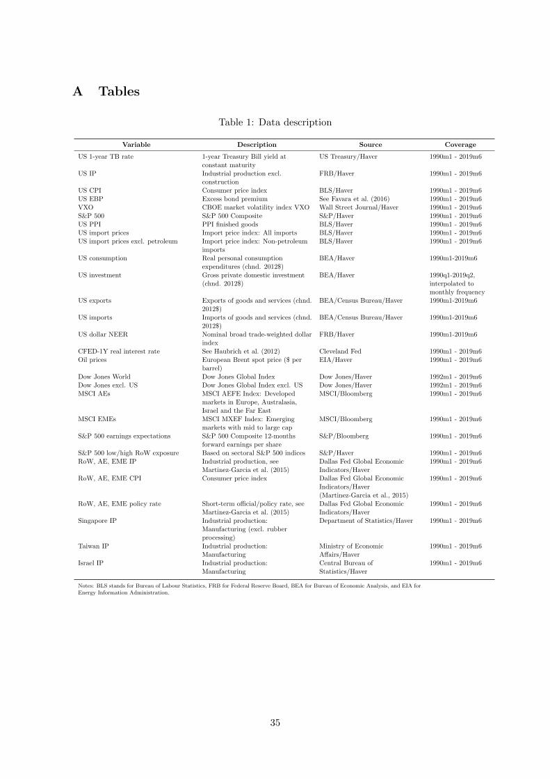
A Tables

Table 1: Data description

Variable Description Source Coverage

US 1-year TB rate 1-year Treasury Bill yield atconstant maturity

US Treasury/Haver 1990m1 - 2019m6

US IP Industrial production excl.construction

FRB/Haver 1990m1 - 2019m6

US CPI Consumer price index BLS/Haver 1990m1 - 2019m6US EBP Excess bond premium See Favara et al. (2016) 1990m1 - 2019m6VXO CBOE market volatility index VXO Wall Street Journal/Haver 1990m1 - 2019m6S&P 500 S&P 500 Composite S&P/Haver 1990m1 - 2019m6US PPI PPI finished goods BLS/Haver 1990m1 - 2019m6US import prices Import price index: All imports BLS/Haver 1990m1 - 2019m6US import prices excl. petroleum Import price index: Non-petroleum

importsBLS/Haver 1990m1 - 2019m6

US consumption Real personal consumptionexpenditures (chnd. 2012$)

BEA/Haver 1990m1-2019m6

US investment Gross private domestic investment(chnd. 2012$)

BEA/Haver 1990q1-2019q2,interpolated tomonthly frequency

US exports Exports of goods and services (chnd.2012$)

BEA/Census Bureau/Haver 1990m1-2019m6

US imports Imports of goods and services (chnd.2012$)

BEA/Census Bureau/Haver 1990m1-2019m6

US dollar NEER Nominal broad trade-weighted dollarindex

FRB/Haver 1990m1-2019m6

CFED-1Y real interest rate See Haubrich et al. (2012) Cleveland Fed 1990m1 - 2019m6Oil prices European Brent spot price ($ per

barrel)EIA/Haver 1990m1 - 2019m6

Dow Jones World Dow Jones Global Index Dow Jones/Haver 1992m1 - 2019m6Dow Jones excl. US Dow Jones Global Index excl. US Dow Jones/Haver 1992m1 - 2019m6MSCI AEs MSCI AEFE Index: Developed

markets in Europe, Australasia,Israel and the Far East

MSCI/Bloomberg 1990m1 - 2019m6

MSCI EMEs MSCI MXEF Index: Emergingmarkets with mid to large cap

MSCI/Bloomberg 1990m1 - 2019m6

S&P 500 earnings expectations S&P 500 Composite 12-monthsforward earnings per share

S&P/Bloomberg 1990m1 - 2019m6

S&P 500 low/high RoW exposure Based on sectoral S&P 500 indices S&P/Haver 1990m1 - 2019m6RoW, AE, EME IP Industrial production, see

Martinez-Garcia et al. (2015)Dallas Fed Global EconomicIndicators/Haver

1990m1 - 2019m6

RoW, AE, EME CPI Consumer price index Dallas Fed Global EconomicIndicators/Haver(Martinez-Garcia et al., 2015)

1990m1 - 2019m6

RoW, AE, EME policy rate Short-term official/policy rate, seeMartinez-Garcia et al. (2015)

Dallas Fed Global EconomicIndicators/Haver

1990m1 - 2019m6

Singapore IP Industrial production:Manufacturing (excl. rubberprocessing)

Department of Statistics/Haver 1990m1 - 2019m6

Taiwan IP Industrial production:Manufacturing

Ministry of EconomicAffairs/Haver

1990m1 - 2019m6

Israel IP Industrial production:Manufacturing

Central Bureau ofStatistics/Haver

1990m1 - 2019m6

Notes: BLS stands for Bureau of Labour Statistics, FRB for Federal Reserve Board, BEA for Bureau of Economic Analysis, and EIA forEnergy Information Administration.

35

Table 2: Identification restrictions of the rest-of-the-world shocks

Variable / Shock RoW ‘depreciating’ shock RoW ‘appreciating’ shock

US 1-year T-Bill rateUS industrial production < 04 ♦

US CPIUS excess bond premiumUS dollar NEER > 0 < 0VXORoW industrial production < 0 & <4 < 0 & <♦

Notes: The table presents the sign and magnitude restrictions we impose in order to identify the rest-of-the world shocks. We additionally impose the exogeneity restrictions E[pε,mpt εot ] = 0 in Equation(10b) that the proxy variables are not driven by the rest-of-the-world shocks.

36

B Figures

Figure 1: Impulse responses to a US monetary policy shock in a structural two-countrymodel

5 10 15

-0.05

0

0.05

0.1

0.15

0.2

5 10 15

-0.4

-0.3

-0.2

-0.1

0

5 10 15

-0.2

-0.15

-0.1

-0.05

0

5 10 15

-5

0

5

10

15

2010

-3

5 10 15

-0.04

-0.02

0

0.02

0.04

5 10 15

-0.08

-0.06

-0.04

-0.02

0

0.02

Notes: The figure displays the responses of policy rates and output in the US and the rest of the world as wellas US exports and imports to a contractionary US monetary policy shock in the structural two-countrymodel. The black solid lines with circles show the impulse responses for the baseline specification withinternational banks and home bias below unity, the orange lines with squares for a specification withoutinternational banks and with home bias equal to unity, the blue solid lines with triangles for a specificationwithout international banks, and the green lines with crosses for a specification with international banksand home bias below unity but in whic hthe US is assumed to be small relative to the rest of the world.Interest rates are plotted in percentage-point deviations from steady state, output in percent deviations fromsteady state, and exports/imports in absolute deviations from steady state (in order to avoid complicationsin specifications in which their steady-state values are zero).

37

Figure 2: Baseline impulse responses to US monetary policy, rest-of-the-world ‘appreciating’and ‘depreciating’, and global uncertainty shocks

US monetary policyshock

RoW ‘depreciating’shock

RoW ‘appreciating’shock

Global uncertaintyshock

US

1Y

TB

R

0 6 12 18 24-0.1

0

0.1

0.2

0 6 12 18 24-0.1

0

0.1

0.2

0 6 12 18 24-0.1

0

0.1

0.2

0 6 12 18 24-0.1

0

0.1

0.2

US

IP

0 6 12 18 24-0.5

0

0.5

0 6 12 18 24-0.5

0

0.5

0 6 12 18 24-0.5

0

0.5

0 6 12 18 24-0.5

0

0.5

US

CP

I

0 6 12 18 24-0.2

-0.1

0

0.1

0.2

0 6 12 18 24-0.2

-0.1

0

0.1

0.2

0 6 12 18 24-0.2

-0.1

0

0.1

0.2

0 6 12 18 24-0.2

-0.1

0

0.1

0.2

US

EB

P

0 6 12 18 24-0.1

0

0.1

0.2

0 6 12 18 24-0.1

0

0.1

0.2

0 6 12 18 24-0.1

0

0.1

0.2

0 6 12 18 24-0.1

0

0.1

0.2

VX

O

0 6 12 18 24-2

0

2

0 6 12 18 24-2

0

2

0 6 12 18 24-2

0

2

0 6 12 18 24-2

0

2

US

NE

ER

0 6 12 18 24-1

0

1

0 6 12 18 24-1

0

1

0 6 12 18 24-1

0

1

0 6 12 18 24-1

0

1

RoW

IP

0 6 12 18 24-0.5

0

0.5

0 6 12 18 24-0.5

0

0.5

0 6 12 18 24-0.5

0

0.5

0 6 12 18 24-0.5

0

0.5

Notes: The figure shows the point-wise posterior means of the impulse responses (black solid lines) and 68%centered point-wise probability bands (grey areas) obtained from the BPSVAR model. ‘1YTBR’ stands forthe one-year Treasury Bill rate, ‘IP’ for industrial production, ‘CPI’ for the consumer-price index, ‘EBP’ forexcess bond premium, ‘VXO’ for the S&P 500 stock market volatility index, and ‘NEER’ for the nominaleffective exchange rate.

38

Figure 3: Baseline and counterfactual impulse responses of US industrial production to aUS monetary policy shock

SSA with RoW shocks SSA with all shocks MRE

0 6 12 18 24-0.3

-0.15

0

0.15

0.3

0 6 12 18 24-0.3

-0.15

0

0.15

0.3

0 6 12 18 24-0.3

-0.15

0

0.15

0.3

Notes: The black solid lines depict the baseline impulse responses of US industrial production to a USmonetary policy shock and the coloured solid lines with markers the counterfactual impulse responses basedon point-wise posterior mean SSA with rest-of-the-world shocks (left column, green lines with squares),based on point-wise posterior mean SSA with all shocks (middle column, blue lines with triangles), andbased on point-wise posterior mean MRE (right column, red lines with circles). The grey shaded areasrepresent 68% centered point-wise probability bands for the baseline impulse responses, and the light-coloured dotted lines represent 68% centered point-wise probability bands for the counterfactual impulseresponses.

Figure 4: Distribution of SSA spillback estimates

SSA with RoW shocks SSA with all shocks

0 6 12 18 24-0.4

-0.2

0

0.2

0 6 12 18 24-0.2

0

0.2

Notes: The figure presents the point-wise mean of the differences between the baseline and the counterfactualeffects of US monetary policy on US industrial production together with 68% centered point-wise probabilitybands.

39

Figure 5: Modesty statistic of Leeper and Zha (2003) and distribution of the q-divergence ofAntolin-Diaz et al. (2021) for SSA counterfactuals

SSA with RoW shocks SSA with all shocks

0 6 12 18 24-2

-1

0

1

2

0 6 12 18 24-2

-1

0

1

2

0.5 0.6 0.70

0.2

0.4

mea

n=0.

54

0.51 0.515 0.52 0.5250

0.05

0.1

0.15

mea

n=0.

51Notes: The top panels show the ‘modesty statistic’ of Leeper and Zha (2003) for the implied offsettingshocks that impose the counterfactual constraint for rest-of-the-world industrial production; the black solidline depicts the point-wise mean and the grey shaded areas the 68% centered point-wise probability bands.The offsetting shocks are ‘modest’—meaning their materialisation is unlikely to induce agents to adjusttheir expectation formation and beliefs about the structure of the economy—if the statistic is smaller thantwo in absolute value. The bottom panels show the distribution of the q-divergence of Antolin-Diaz et al.(2021) for the SSA; the left-hand side panel presents results for the case in which only the rest-of-the-worldshocks are used as offsetting shocks, while the right-hand side panel for the case in which all shocks areused. The q-divergence indicates how unlikely a conditional forecast is in terms of comparing the implieddistributions of shocks with their unconditional distributions, translated into a comparison of the binomialdistributions of a fair and a biased coin. See Appendix C.1 for a description how we implement the q-divergence in the context of our paper. We drop SSA counterfactuals when the offsetting shocks increaseover time (εT+1 < εT+h) or if the offsetting shocks are particularly large on impact (εT+1 lies above the99th percentile in absolute terms).

40

Figure 6: Spillbacks for US consumer prices

CPI Import prices US dollar NEERBaseline and counterfactual impulse responses

0 6 12 18 24-0.15

-0.1

-0.05

0

0 6 12 18 24-0.6

-0.4

-0.2

0

0 6 12 18 240

0.5

1

Distribution of spillback estimates (SSA with all shocks)

0 6 12 18 24

-0.06

-0.04

-0.02

0

0 6 12 18 24

-0.2

0

0.2

0 6 12 18 24-0.2

0

0.2

PPI (final products) Import prices excl. petrol. Oil pricesBaseline and counterfactual impulse responses

0 6 12 18 24

-0.2

-0.1

0

0 6 12 18 24

-0.2

-0.1

0

0 6 12 18 24-4

-2

0

2

Distribution of spillback estimates (SSA with all shocks)

0 6 12 18 24-0.2

-0.1

0

0.1

0 6 12 18 24-0.1

-0.05

0

0.05

0 6 12 18 24-2

-1

0

1

0 6 12 18 24

-0.2

0

0.2

SSA with RoW shocks SSA with all shocks MRE

Notes: In the first and third row the figure shows the baseline and counterfactual impulse responses based onSSA with rest-of-the-world shocks (green lines with squares), SSA with all shocks (blue lines with triangles)and MRE (red lines with circles) for US CPI, import prices with and without petroleum, PPI, the USdollar NEER and oil prices to a US monetary policy shock. The grey shaded areas represent 68% centeredpoint-wise probability bands for the baseline impulse responses. In the second and fourth row the figureshows the point-wise mean of the differences between the baseline and the counterfactual effects togetherwith 68% centered point-wise probability bands.

41

Figure 7: Placebo-test impulse responses of US industrial production

Spillbacks through SOE shut down, but allowed through RoWSingapore Taiwan Israel

0 6 12 18 24-0.2

0

0.2

0 6 12 18 24-0.4

-0.2

0

0.2

0 6 12 18 24

-0.2

0

0.2

0 6 12 18 24

-0.2

0

0.2

SOE set to zero and RoW IP set to unconstrained IRF RoW IP set to zero

Spillbacks through SOE allowed, but shut down through RoWSingapore Taiwan Israel

0 6 12 18 24-0.2

0

0.2

0 6 12 18 24-0.4

-0.2

0

0.2

0 6 12 18 24

-0.2

0

0.2

0 6 12 18 24

-0.2

0

0.2

SOE set to unconstrained IRF and RoW IP set to zero RoW IP set to zero

Notes: The black solid lines depict the response of US industrial production from VAR models in which SOEindustrial production is added to the vector of observables and their impulse responses to a US monetarypolicy shock are not constrained, and the grey shaded areas represent the associated 68% centered point-wise probability bands. The light blue lines with triangles depict the counterfactual impulse response inwhich spillovers to rest-of-the-world and SOE industrial production are precluded. In the top row, thedark blue lines with crosses depict the counterfactual response of US industrial production when SOEindustrial production is constrained to not respond to a US monetary policy shock, and rest-of-the-worldindustrial production is constrained to respond as in the unconstrained case. In the bottom row, thedark blue lines with crosses depict the response of US industrial production when the response of SOEindustrial production is constrained to respond as in the unconstrained case, and rest-of-the-world industrialproduction is constrained to not respond to a US monetary policy shock. Figure E.3 and Figure E.4document the placebo tests based on SSA with rest-of-the-world shocks and MRE.

42

Figure 8: Responses of monthly GDP components to US monetary policy shock for thebaseline and the counterfactual

Exports ImportsBaseline and counterfactual impulse responses

0 6 12 18 24-0.6

-0.4

-0.2

0

0 6 12 18 24

-0.4

-0.2

0

Distribution of spillback estimates (SSA with all shocks)

0 6 12 18 24-0.4

-0.2

0

0.2

0 6 12 18 24-0.4

-0.2

0

0.2

Investment ConsumptionBaseline and counterfactual impulse responses

0 6 12 18 24

-0.5

0

0.5

0 6 12 18 24

-0.1

-0.05

0

Distribution of spillback estimates (SSA with all shocks)

0 6 12 18 24-0.4

-0.2

0

0.2

0 6 12 18 24

-0.06

-0.04

-0.02

0

0 6 12 18 24

-0.2

0

0.2

SSA with RoW shocks SSA with all shocks MRE

Notes: In the first and third row the figure shows the baseline and counterfactual impulse responses based onSSA with rest-of-the-world shocks (green lines with squares), SSA with all shocks (blue lines with triangles)and MRE (red lines with circles) for real exports, real imports, real private gross fixed capital investmentand real private consumption expenditures to a US monetary policy shock. The grey shaded areas represent68% centered point-wise probability bands for the baseline impulse responses. In the second and fourth rowthe figure shows the point-wise mean of the differences between the baseline and the counterfactual effectstogether with 68% centered point-wise probability bands.

43

Figure 9: Channels of transmission for spillbacks from US monetary policy to investment

S&P 500 S&P 500 earnings expectationsBaseline and counterfactual impulse responses

0 6 12 18 24-2

-1

0

0 6 12 18 24-1

-0.5

0

0.5

Distribution of spillback estimates (SSA with all shocks)

0 6 12 18 24-0.5

0

0.5

0 6 12 18 24

-0.4

-0.2

0

0.2

S&P 500 low RoW exposure S&P 500 high RoW exposureBaseline and counterfactual impulse responses

0 6 12 18 24-2

-1

0

1

0 6 12 18 24

-2

-1

0

Distribution of spillback estimates (SSA with all shocks)

0 6 12 18 24

-0.5

0

0.5

0 6 12 18 24-1

0

1

0 6 12 18 24

-0.2

0

0.2

SSA with RoW shocks SSA with all shocks MRE

Notes: In the first and third row the figure shows the baseline and counterfactual impulse responses basedon SSA with rest-of-the-world shocks (green lines with squares), SSA with all shocks (blue lines withtriangles) and MRE (red lines with circles) for the S&P 500 Composite, the 12-months forward S&P 500’searnings per share, and the S&P 500 index for low and high rest-of-the-world exposures. The latter two areconstructed as market-capitalisation-weighted averages of sectoral S&P indices. The low rest-of-the-worldexposure sectors are utilities, telecommunication services, health care and financials, and the high rest-of-the-world exposure sectors are energy, materials, industrials and information technology; see Brzenk (2018)for data and a discussion of rest-of-the-world exposures in the S&P 500. The grey shaded areas represent68% centered point-wise probability bands for the baseline impulse responses. In the second and fourth rowthe figure shows the point-wise mean of the differences between the baseline and the counterfactual effectstogether with 68% centered point-wise probability bands.

44

Figure 10: Channels of transmission for spillbacks from US monetary policy to consumption

1Y-CFED real rate Dow Jones excl. USBaseline and counterfactual impulse responses

0 6 12 18 24

0

0.1

0.2

0 6 12 18 24

-2

-1

0

Distribution of spillback estimates (SSA with all shocks)

0 6 12 18 24-0.05

0

0.05

0 6 12 18 24-1

-0.5

0

0 6 12 18 24

-0.2

0

0.2

SSA with RoW shocks SSA with all shocks MRE

Notes: In the first row the figure shows the baseline and counterfactual impulse responses based on SSAwith rest-of-the-world shocks (green lines with squares), SSA with all shocks (blue lines with triangles) andMRE (red lines with circles) for the Cleveland Fed/Haubrich et al. (2012) interest rate-term structure-basedone-year real rate and the Dow Jones World excl. US index. The grey shaded areas represent 68% centeredpoint-wise probability bands for the baseline impulse responses. In the second row the figure shows thepoint-wise mean of the differences between the baseline and the counterfactual effects together with 68%centered point-wise probability bands.

45

Figure 11: Spillbacks from US monetary policy through AEs and EMEs

Spillbacks through AEs shut down, Spillbacks through AEs allowed,but allowed through EMEs but shut down through EMEs

0 6 12 18 24

-0.2

0

0.2

0 6 12 18 24

-0.2

0

0.2

0 6 12 18 24

-0.2

0

0.2

AEs or EMEs IP set to zero AEs and EMEs IP set to zero

Notes: The black solid lines depict the response of US industrial production to a US monetary policy shockfrom VAR models in which rest-of-the-world industrial production is replaced with separate measures forAEs and EMEs industrial production and their impulse responses to a US monetary policy shock are notconstrained; the grey shaded areas represent the associated 68% centered point-wise probability bands.The light blue lines with triangles depict counterfactual impulse responses in which spillovers to the rest-of-the-world are precluded, meaning that both AEs and EMEs industrial production are constrained tonot respond to a US monetary policy shock. In the left-hand side panel the dark blue line with crossesdepicts the counterfactual impulse response of US industrial production when AEs industrial production isconstrained to not respond while EMEs industrial production is set to respond as in the unconstrained case.In the right-hand side panel the dark blue line with crosses depicts the counterfactual impulse response whenAEs industrial production is constrained to respond as in the unconstrained case while EMEs industrialproduction is constrained to not respond to a US monetary policy shock. All counterfactual impulseresponses shown are based on SSA with all shocks. Figure E.8 presents the counterfactual impulse responsesbased on SSA with rest-of-the-world shocks and MRE.

46

Figure 12: Country composition of US foreign portfolio investment equity holdings and USexports

US foreign portfolio investment equity0

.2.4

.6.8

1

Share

2003 2004 2005 2006 2007 2008 2009 2010 2011 2012 2013 2014 2015 2016 2017 2018 2019

Fin. centers EME AE

US exports

0.2

.4.6

.81

Share

in tota

l

1990−94 1995−99 2000−04 2005−09 2010−14 2015−19

EME AE

Notes: The top panel shows the country composition of US foreign portfolio equity holdings throughcommon stocks and mutual funds based on the analysis in Bertaut et al. (2019), which accountsfor measurement problems related to multinationals, financial centres and mutual funds. The totalunderlying the shares does not include cross-border equity of firms that primarily operate in the US(for details see Bertaut et al., 2019). The list of financial centres is taken from Bertaut et al. (2019).The bottom panel shows the country composition of US exports of goods obtained from the IMFDirection of Trade Statistics as a proxy for the composition of US firms’ sales to the rest of the world.

47

Figure 13: US monetary policy spillovers to AEs and EMEs

AE IP AE CPI AE policy rate

0 6 12 18 24

-0.2

0

0.2

0 6 12 18 24-0.06

-0.04

-0.02

0

0 6 12 18 24-0.01

0

0.01

EME IP EME CPI EME policy rate

0 6 12 18 24-0.2

0

0.2

0 6 12 18 24-0.1

0

0.1

0.2

0 6 12 18 24-0.02

0

0.02

0.04

0.06

Notes: The figure shows point-wise posterior mean impulse responses (black solid lines) and 68% centeredpoint-wise probability bands (grey areas). The impulse responses are estimated from a VAR model in whichthe variables are added at once to the vector of endogenous variables.

48

C The SSA framework of Antolin-Diaz et al. (2021)

Building on the work of Waggoner and Zha (1999), the SSA framework of Antolin-Diaz

et al. (2021, henceforth ADPRR) provides a rigorous and general treatment on how to

impose specific paths on observables in a VAR model as conditional forecasts with and

without constraints on the set of offsetting—or ‘driving’—shocks. Denoting by y′T+1,T+h ≡[y′T+1,y

′T+2, . . . ,y

′T+h] the 1×nh vector that stacks the future values of the observables over

an horizon of h periods, the SSA framework of ADPRR consists of obtaining the distribution

of the observables

yT+1,T+h ∼ N(µy,Σy), (C.1)

where the nh×1 vector vector yT+1,T+h contains the values of all observables—i.e. both those

whose paths are constrained and those whose paths are unconstrained—under the conditional

forecast. The nh × 1 vector µy contains the corresponding means of the distribution of the

observables in yT+1,T+h under the conditional forecast, and the nh × nh matrix Σy the

associated uncertainty.

In the framework of ADPRR, structural scenarios involve

(i) ‘conditional-on-observables forecasting’, i.e. specifying paths for a subset of observables

in yT+1,T+h that depart from their unconditional forecast, and/or

(ii) ‘conditional-on-shocks forecasting’, i.e. specifying the subset of (and potentially a path

for) the structural shocks εT+1,T+h that are allowed to depart from their unconditional

distribution to produce the specified path of the observables in (i);

Both the case in which the path of observables under (i) and the case in which the path of

structural shocks under (ii) is constrained can be laid out based on Equation (C.1). The

goal is to determine µy and Σy such that the constraints under (i) and (ii) are satisfied

simultaneously.

Assume the structural parameters of the VAR model are known. The future values of the

observables are given by

yT+1,T+h = bT+1,T+h +M ′εT+1,T+h, (C.2)

where the nh × 1 vector bT+1,T+h represents the deterministic component due to initial

conditions and the autoregressive dynamics of the VAR model, and the nh× nh matrix M ′

the impact of future structural shocks.

Under (i), ‘conditional-on-observables forecasting’ can be written as

CyT+1,T+h = CbT+1,T+h +CM ′εT+1,T+h ∼ N(fT+1,T+h,Ωf ). (C.3)

49

whereC is a ko×nh selection matrix, the ko×1 vector fT+1,T+h is the mean of the distribution

of the observables constrained under the conditional forecast and the ko × ko matrix Ωf the

associated uncertainty. In turn, under (ii), ‘conditional-on-shocks forecasting’ can be written

as

ΞεT+1,T+h ∼ N(gT+1,T+h,Ωg), (C.4)

where Ξ is a ks×nh selection matrix, the ks×1 vector gT+1,T+h the mean of the distribution

of the shocks constrained under the conditional forecast and the ks × ks matrix Ωg the

associated uncertainty.27 Under invertibility we have

M ′−1yT+1,T+h = M ′−1bT+1,T+h + εT+1,T+h,

ΞM ′−1yT+1,T+h = ΞM ′−1bT+1,T+h + ΞεT+1,T+h, (C.5)

CyT+1,T+h = CbT+1,T+h + ΞεT+1,T+h, (C.6)

and hence

CyT+1,T+h = CbT+1,T+h + ΞεT+1,T+h ∼ N(fT+1,T+h

,Ωf ), (C.7)

with Ωf = Ωg.

Based on Equations (C.3) and (C.7), we can combine the ko constraints on the observables

under ‘conditional-on-observables forecasting’ and the ks constraints on the structural shocks

under ‘conditional-on-shocks forecasting’ by defining the k × nh, k = ko + ks, matrices C ≡[C′,C ′]′ and D ≡ [MC

′,Ξ′]′ to write

CyT+1,T+h = CbT+1,T+h +DεT+1,T+h ∼ N(fT+1,T+h,Ωf ), (C.8)

where the k × 1 vector fT+1,T+h ≡ [f′T+1,T+h,f

′T+1,T+h

]′ stacks the means of the distri-

butions under the ‘conditional-on-observables forecasting’ (fT+1,T+h = CbT+1,T+h) and the

‘conditional-on-shocks forecasting’ (fT+1,T+h

= CbT+1,T+h+gT+1,T+h), and the k×k matrix

Ωf ≡ diag(Ωf ,Ωf ).28

Based on the combination of ‘conditional-on-observables forecasting’ and ‘conditional-on-

shocks forecasting’ in Equation (C.8), we can derive the solutions for µy and Σy. Define

εT+1,T+h ∼ N(µε,Σε), Σε = I + Ψε, (C.9)

27For the conditional forecast that underlies an impulse response function to the i-th shock in period T + 1we have

Ξ = Inh, gT+1,T+h = [e′i,0′n(h−1)×1]′nh×1, Ωg = 0nh×nh,

where ei is an n× 1 vector of zeros with unity at the i-th position.28Note that f

T+1,T+hrefers to the mean of CyT+1,T+h = ΞM ′−1yT+1,T+h and hence not just of a path of

some observable(s). Instead, ΞM ′−1yT+1,T+h are the values of the observables that are implied by a specificpath of the structural shocks assumed under ‘conditional-on-shocks forecasting’.

50

so that the nh× 1 vector µε and the nh× nh matrix Ψε represent the deviation of the mean

and the variance of the structural shocks under the conditional forecast from their values in

the unconditional forecast. Given Equations (C.8) and (C.9), we have

fT+1,T+h = CbT+1,T+h +Dµε, (C.10)

Ωf = D(I + Ψε)D′. (C.11)

The solutions for µε and Σε are given by

µε = D∗(fT+1,T+h −CbT+1,T+h), (C.12)

Σε = D∗ΩfD∗′ + (I −D∗DD′D∗′), (C.13)

where the nh×k matrix D∗ is the Moore-Penrose inverse of D.29 Equation (C.12) shows that

the path of the implied future structural shocks under the conditional forecast depends on its

deviation from the unconditional forecast. In turn, Equation (C.13) shows that the variance

of the implied future structural shocks depends on the uncertainty the researcher attaches to

the conditional forecast; if the uncertainty is zero, then Ωf = 0 as Ωf = Ωf = Ωg = 0, and

hence Σε = 0, meaning that a unique, certain path µε for the structural shocks is implied by

the conditional forecast.30

Finally, as

yT+1,T+h = bT+1,T+h +M ′εT+1,T+h, (C.14)

and given Equations (C.12) and (C.13) we have that

µy = bT+1,T+h +M ′D∗(fT+1,T+h −CbT+1,T+h), (C.15)

Σy = M ′M −M ′D∗(Ωf −DD′)D∗′M . (C.16)

Again, when Ωf = 0 then Σy = 0, and there is no uncertainty about the path of the

observables under the conditional forecast.

It is useful to discuss how the framework of ADPRR is parsed in the context of our paper.

Recall that we constrain the effect of a US monetary policy shock on rest-of-the world real

activity to be zero, and we assume this occurs due to two offsetting rest-of-the world shocks.

Ordering rest-of-the-world output last in yt, the US monetary policy shock first and the two

rest-of-the-world shocks last in εt, and denoting by ei a n × 1 vector of zeros with unity at

29ADPRR discuss the properties of the solutions under different values for k relative to nh.30As discussed in ADPRR, the researcher could impose that the uncertainty under the conditional forecast

is identical to that of the unconditional forecast, i.e. set Ωf = DD′.

51

the i-th position, for ‘conditioning-on-observables forecasting’ we have

C = Ih ⊗ e′n, (C.17)

fT+1,T+h = 0h×1, (C.18)

Ωf = 0h×h. (C.19)

The intuition underlying Equations (C.17) and (C.18) is that in the conditional forecast that

underlies the impulse response we constrain rest-of-the-world output (ordered at the n-th

position in yt) to be zero over all horizons T + 1, T + 2, . . . , T + h, and Equation (C.19)

indicates that we do not allow for any uncertainty. In turn, for ‘conditioning-on-shocks

forecasting’ we have

Ξ =

e′1 01×n(h−1)

(0n−3×1, In−3,0n−3×2) 0n−3×n(h−1)

0(h−1)(n−2)×n Ih−1 ⊗ (In−2,0n−2×2)

h(n−2)×nh

(C.20)

fT+1,T+h

= gT+1,T+h = [1,01×n−3,01×(n−2)(h−1)]′, (C.21)

Ωf = Ωg = 0h(n−2)×h(n−2). (C.22)

The first row in Equation (C.20) selects the US monetary policy shock ordered first in εt and

the first row in Equation (C.21) constrains it to be unity in the impact period T + 1; the

second row in Equation (C.20) selects the non-US monetary policy and the non-rest-of-the-

world shocks ordered from position 2 to n− 3 in εt and the second entry in Equation (C.21)

constrains them to be zero in the impact period T + 1; the third row in Equation (C.20)

selects the US monetary policy and the non-rest-of-the-world shocks and Equation (C.21)

constrains them to be zero over horizons T + 2, T + 3, . . . , T +h. It is furthermore interesting

to consider—recalling that C ≡ ΞM ′−1—the stacked matrices C and D in Equation (C.8)

C =

[Ch×hn

Ch(n−2)×hn

]h(n−1)×hn

, D =

[CM ′

Ξ

]h(n−1)×nh

. (C.23)

Note that the fact that C and D are not square and full rank reflects that at every horizon

we have two rest-of-the-world shocks to impose one constraint (the absence of a rest-of-

the-world real activity response to a US monetary policy shock), implying a multiplicity of

solutions. ADPRR show that the solution chosen in this case—obtained using the Moore-

Penrose inverse of D—minimises the Frobenius norm of the deviation of the distribution of

the structural shocks under the conditional forecast from the baseline, i.e. µε from 0 and

Σε from I. Note that C and D become square and full rank if h additional constraint are

imposed. For example, we could impose that the two rest-of-the-world shocks we use for the

52

offsetting of the effects of the US monetary policy shock on rest-of-the-world output are of

equal size. To do so, we would stack below Ξ in Equation (C.20) an h× nh matrix

Ξadd = Ih ⊗ [0, 0, . . . , 0, 1,−1]1×n, (C.24)

and below fT+1,T+h

in Equation (C.21) an h× 1 vector

faddT+1,T+h

= 0h×1. (C.25)

C.1 How plausible is the counterfactual?

When constructing a counterfactual using SSA it might be that the implied shocks are so

“unusual” that the analysis becomes subject to the Lucas critique. Against this background,

ADPRR propose to use the Kullback-Leibler (KL) divergence D(Fbl||Fcf ) between the dis-

tributions of the implied shocks in the conditional forecasts in the baseline Fbl and in the

counterfactual Fcf . While it is straightforward to compute D(Fbl||Fcf ), it is difficult to grasp

intuitively whether a given numerical value for the KL divergence is large or small. In other

words, the KL divergence can be easily used to rank scenarios, but it is hard to understand

how far away they are from the unconditional forecast. To allow an intuitive interpreta-

tion of the KL divergence, ADPRR “calibrate” it based on two generic distributions Q to

P , using the KL divergence between two easily interpretable distributions. In particular,

ADPRR suggest comparing D(Fbl||Fcf ) with the KL divergence between two binomial dis-

tributions Q and P , one with probability q and the other with probability p = 0.5. ADPRR

suggest calibrating the KL divergence from Q to P to a parameter q that would solve the

following equation D(B(nh; 0.5)||B(nh; q)) = D(Fbl||Fcf ). The solution to the equation is

q = 0.5(1 +√

1− exp(−2z/nh)), where z = D(Fbl||Fcf ). Intuitively, the value for the KL

divergence D(Fbl||Fcf ) is translated into a comparison between the flip of a fair and a bi-

ased coin. For example, a value of q = 0.501 suggests that the distribution of the shocks

under the counterfactual is not at all far from the distribution under the baseline, so that the

counterfactual can be considered as quite realistic relative to the baseline.

It is worthwhile noting that this measure of plausibility is similar in spirit to the concept of

“modest” policy interventions proposed by Leeper and Zha (2003). In particular, the measure

proposed by Leeper and Zha (2003) reports how unusual the path for a set of policy shocks

needed to achieve some conditional forecast. For example, if the counterfactual implies a

sequence of shocks close to their unconditional mean, the policy intervention is considered

“modest”, in the sense that the shocks are unlikely to induce agents to revise their beliefs

about policy rules and the structure of the economy. Instead, if the counterfactual involves

53

an unlikely sequence of shocks the analysis is likely to be subject to the Lucas critique. In

contrast to the “modesty” statistic of Leeper and Zha (2003) the q-divergence of ADPRR

compares the entire distribution rather than only the path of the shocks and generalises to

counterfactuals that use more than a single driving shock.

ADPRR propose the KL divergence to assess the plausibility of a conditional forecast relative

to an unconditional forecast. In the context of our paper, we need to slightly adjust their

proposed KL divergence. In particular, while in the case of ADPRR the baseline is given by

an unconditional forecast and the counterfactual by a conditional forecast both afflicted by

uncertainty, in our case the baseline and the counterfactual are given by conditional forecasts

both of which are not subject to any uncertainty. Obviously, the KL divergence is not defined

in case the baseline and the counterfactual do not feature any uncertainty. For the purpose

of assessing the plausibility of the shocks that materialise to produce our counterfactual, we

therefore consider the following exercise. As baseline we consider a conditional forecast in

which we assume that a US monetary policy shock of size 1 occurs in period T + 1 with

certainty, while all other non-US monetary policy shocks in period T + 1 as well as all shocks

in periods T +2, T +3, . . . , T +h follow their unconditional distributions. For the conditional

forecast under the counterfactual, we impose the mean constraint from our main exercise (i.e.

that rest-of-the-world output stays at zero and that there is a US monetary policy shock in

period T + 1) but we also allow for uncertainty.

Formally, this exercise involves setting for the baseline and the counterfactual ` ∈ bl, cfC` = I and

f bl = µy,bl = M ′(e′i,0n(h−1)×1)′, (C.26)

f cf = µy,cf , (C.27)

where i is the position of the US monetary policy shock, Equation (C.26) states that the

observables on average shall follow the impulse response to a US monetary policy shock in

period T + 1 under the baseline, and Equation (C.26) that they shall follow the path we

obtained in the SSA counterfactual. Moreover, we set Ξ` = 0 and C` = 0 so that D` = M ′,

54

Ψε,` = 0 as we allow the shocks to have their unconditional variance. Hence we have

Ωf,` = D`D′` = M ′M , (C.28)

Σε,` = D∗`Ωf,`D∗′` = D−1` Ωf,`D

−1′` = M ′−1M ′MM−1 = I, (C.29)

µε,` = D∗`f ` = D−1` f ` = M ′−1f `, (C.30)

Σy,` = M ′M −M ′D∗` (Ωf,` −D`D′`)D

∗′` M

= M ′M −M ′D−1` (Ωf,` −D`D′`)D

−1′` M

= M ′M −M ′M ′−1(Ωf,` −M ′M)M−1M

= M ′M − (Ωf,` −M ′M)

= M ′M . (C.31)

Note that µε,bl equals a vector of zeros with unity at the ith position, where i is the position

of the US monetary policy shock. The KL divergence between the distribution of the shocks

under the baseline εT+1,T+h,bl and the counterfactual εT+1,T+h,cf is then given by

D(Fbl||Fcf ) =1

2

[tr(Σ−1ε,cfΣε,bl

)+(µε,cf − µε,bl

)′Σ−1ε,cf

(µε,cf − µε,bl

)− nh+ log

(|Σε,cf ||Σε,bl|

)].

(C.32)

55

D Implementation of the MRE approach

The posterior distribution of the impulse responses f(·) is approximated by N draws obtained

from a Bayesian estimation algorithm. Following the importance sampling procedure of Arias

et al. (2018, forthcoming), the re-sampled draws from the BPSVAR for yT+1,T+h constitute

an unweighted and independent sample from the posterior distribution f(·), and as such are

assigned a weight of wi = 1/N , i = 1, 2, . . . , N . The counterfactual posterior distribution

f?(·) can be approximated by assigning different weights w∗i to the draws from the baseline

posterior.

The relative entropy (or distance) between the approximated posterior distributions is mea-

sured by

D(f∗, f) =

N∑i=1

w?i log

(w?iwi

). (D.1)

The goal of the MRE approach is to determine the counterfactual weights w∗ that minimise

D(·) subject to

w?i ≥ 0, ∀ i = 1, 2, ..., N, (D.2)

N∑i=1

w∗i = 1, (D.3)

N∑i=1

w∗i g(y(i)T+1,T+h) = g, (D.4)

where y(i)T+1,T+h are the impulse responses to a US monetary policy shock as defined in Section

5. Equations (D.2) and (D.3) reflect that the weights are probabilities, and Equation (D.4)

that the counterfactual posterior distribution shall satisfy some constraint.

In particular, in our application for Equation (D.4) we have

N∑i=1

y(i)ip∗,T+hw

∗i,h = 0, (D.5)

where y(i)ip∗,T+h denotes the impulse response of rest-of-the-world real activity to a US mone-

tary policy shock at horizon h associated with the i-th draw. Notice that—consistent with

the baseline posterior for which we report point-wise means in Figure 2 and elsewhere in the

paper as well as in line with Giacomini and Ragusa (2014)—we apply the MRE approach

separately at each impulse response horizon T + 1, T + 2, . . . , T + h.

As shown by Robertson et al. (2005) and Giacomini and Ragusa (2014), the weights of the

counterfactual posterior distribution w∗h can be obtained numerically by tilting the weights

56

of the baseline posterior distribution wh using the method of Lagrange. In particular, the

weights of the counterfactual posterior distribution are given by

w∗i,h =wi,h exp

[λhg(y

(i)ip∗,T+h)

]N∑i=1

wi,h exp[λhg(y

(i)ip∗,T+h)

] , i = 1, 2, . . . , N, (D.6)

where λh is the Lagrange multiplier associated with the constraint g(y(i)ip∗,T+h) = y

(i)ip∗,T+h = 0.

It can be shown that the Lagrange multiplier can be obtained numerically as

λh = arg minλh

N∑i=1

wi,h expλh

[g(y

(i)ip∗,T+h)

]. (D.7)

57

E Additional figures

Figure E.1: Impulse responses to US monetary policy shocks from alternative BPSVARspecifications

US 1YTBR US IP US CPI

0 6 12 18 24

0

0.1

0.2

0 6 12 18 24

-0.2

0

0.2

0 6 12 18 24

-0.1

-0.05

0

US EBP VXO US NEER

0 6 12 18 24

0

0.05

0.1

0 6 12 18 24

0

1

2

0 6 12 18 24

0

0.5

1

RoW IP

0 6 12 18 24

-0.2

0

0.2

0 6 12 18 24-5

0

5

10

10-3

No intermeetings Average Greenbook Large VARAdd. US shocks Add. oil shock Gamma Zero

Notes: The figure shows point-wise posterior mean impulse responses from our baseline specification (blacksolid lines) and 68% centered point-wise probability bands (grey areas) and various robustness checks(coloured solid lines with markers). ‘1YTBR’ stands for the one-year Treasury Bill rate, ‘IP’ for industrialproduction, ‘CPI’ for consumer-price index, ‘EBP’ for excess bond premium, ‘VXO’ is the S&P 500 stockmarket volatility index, and ‘NEER’ the nominal effective exchange rate. In the specification labelled ‘Nointermeetings’ we exclude FOMC announcements on unscheduled, ‘inter-meeting’ dates; in ‘Average’ wetemporally aggregate to monthly frequency the interest rate and gold price surprises originally available atdaily frequency by taking monthly averages rather than as in Gertler and Karadi (2015); in ‘Greenbook’ wepurge the interest rate surprises from Green Book forecast as suggested in Miranda-Agrippino and Ricco(2021) instead of applying the ‘poor-man’s’ approach of Jarocinski and Karadi (2020); in ‘Large VAR’ weadd rest-of-the-world consumer prices, AEs policy rate, US imports and exports, and the MSCI world stockprice index to the vector of endogenous variables in the VAR model; in ‘Add. US shocks’ we additionallyidentify US demand and supply shocks with standard sign restrictions (we impose: negative demand shocksaffect US IP, CPI, NEER, and 1YTBR negatively and US EBP positively; negative supply shocks affectUS IP negatively and US CPI and EBP positively; the restrictions hold on impact); in ‘Add. oil shock’ weadditionally identify global oil supply shocks using the high-frequency proxy variable of Kanzig (2021); andin ‘Gamma Zero’ we set γ—the ‘relevance threshold’ of the proxy variables—to zero.

58

Figure E.2: Distribution of SSA spillback estimates to US CPI and ‘modesty statistic’ ofLeeper and Zha (2003) for SSA counterfactuals

SSA with RoW shocks SSA with all shocks

0 6 12 18 24-0.4

-0.2

0

0.2

0 6 12 18 24-0.2

0

0.2

0 6 12 18 24-2

-1

0

1

2

0 6 12 18 24-2

-1

0

1

2

Notes: The top panels show the differences between the baseline and counterfactual effects of US monetarypolicy on domestic consumer prices. The bottom panels show the ‘modesty statistic’ of Leeper and Zha(2003) for the implied offsetting shocks needed to impose the counterfactual path of rest-of-the-worldindustrial production. The offsetting shocks are‘modest’—meaning they would be unlikely to induce agentsto adjust their expectation formation—if the statistic is smaller than two in absolute value. The black solidlines depict the point-wise mean and the grey shaded areas represent 68% centered point-wise probabilitybands.

59

Figure E.3: SSA with RoW shocks placebo-test responses of US industrial production

Spillbacks through SOE shut down, but allowed through RoWSingapore Taiwan Israel

0 6 12 18 24-0.2

0

0.2

0 6 12 18 24-0.4

-0.2

0

0.2

0 6 12 18 24

-0.2

0

0.2

0 6 12 18 24

-0.2

0

0.2

SOE set to zero and RoW IP set to unconstrained IRF RoW IP set to zero

Spillbacks through SOE allowed, but shut down through RoWSingapore Taiwan Israel

0 6 12 18 24-0.2

0

0.2

0 6 12 18 24-0.4

-0.2

0

0.2

0 6 12 18 24

-0.2

0

0.2

0 6 12 18 24

-0.2

0

0.2

SOE set to unconstrained IRF and RoW IP set to zero RoW IP set to zero

Notes: See the notes to Figure 7.

Figure E.4: MRE placebo-test responses of US industrial production

Spillbacks through SOE shut down, but allowed through RoWSingapore Taiwan Israel

0 6 12 18 24-0.2

0

0.2

0 6 12 18 24-0.4

-0.2

0

0.2

0 6 12 18 24

-0.2

0

0.2

0 6 12 18 24

-0.2

0

0.2

SOE set to zero and RoW IP set to unconstrained IRF RoW IP set to zero

Spillbacks through SOE allowed, but shut down through RoWSingapore Taiwan Israel

0 6 12 18 24-0.2

0

0.2

0 6 12 18 24-0.4

-0.2

0

0.2

0 6 12 18 24

-0.2

0

0.2

0 6 12 18 24

-0.2

0

0.2

SOE set to unconstrained IRF and RoW IP set to zero RoW IP set to zero

Notes: See the notes to Figure 7.

60

Figure E.5: Responses of GDP components to US monetary policy shock for the baselineand the counterfactual

Exports ImportsBaseline and counterfactual impulse responses

0 6 12 18 24-0.4

-0.2

0

0.2

0 6 12 18 24-0.4

-0.2

0

0.2

Distribution of spillback estimates (SSA with all shocks)

0 6 12 18 24-0.2

0

0.2

0 6 12 18 24-0.2

0

0.2

Investment ConsumptionBaseline and counterfactual impulse responses

0 6 12 18 24

-0.5

0

0.5

0 6 12 18 24

-0.2

-0.1

0

Distribution of spillback estimates (SSA with all shocks)

0 6 12 18 24-0.4

-0.2

0

0.2

0 6 12 18 24-0.2

-0.1

0

0.1

0 6 12 18 24

-0.2

0

0.2

SSA with RoW shocks SSA with all shocks MRE

See the notes to Figure 8. The responses are based on quarterly data interpolated to monthly frequency,except for investment.

61

Figure E.6: US stock market capitalisation and US foreign portfolio investment equityassets and liabilities

025

50

75

100

125

% o

f U

S G

DP

2006 2009 2012 2015 2018

(1) US stock market cap

(2) US foreign portfolio investment equity liabilities

(1)−(2)

US foreign portfolio investment equity assets

Notes: The figure shows the evolution of US (New York Stock Exchange) stock market capitalisationdepicted by the black solid line as well as US foreign portfolio investment equity assets and liabilitiesdepicted by the solid red and dashed blue lines, respectively; the black dashed line depicts US stockmarket capitalisation less US foreign portfolio investment equity liabilities. All variables are depictedas a percentage of US nominal annual GDP. The data on stock market capitalisation are obtainedfrom the World Federation of Exchanges, those on US foreign equity assets and liabilities from theBureau of Economic Analysis.

62

Figure E.7: Channels of transmission for spillbacks from US monetary policy: Additionalvariables

VXO EBP GZ spreadBaseline and counterfactual impulse responses

0 6 12 18 24

0

1

2

0 6 12 18 24

0

0.05

0.1

0 6 12 18 24-0.1

0

0.1

Distribution of spillback estimates (SSA with all shocks)

0 6 12 18 24-0.5

0

0.5

0 6 12 18 24

-0.02

0

0.02

0 6 12 18 24-0.05

0

0.05

House prices Macro uncertainty Consumer confidenceBaseline and counterfactual impulse responses

0 6 12 18 24

-0.2

0

0.2

0 6 12 18 24-2

0

2

10-3

0 6 12 18 24-2

-1

0

1

Distribution of spillback estimates (SSA with all shocks)

0 6 12 18 24

0

0.05

0.1

0 6 12 18 24

-1

0

110-3

0 6 12 18 24-1

0

1

0 6 12 18 24

-0.2

0

0.2

SSA with RoW shocks SSA with all shocks MRE

Notes: In the first and third row the figure shows the baseline and counterfactual impulse responses based onSSA with rest-of-the-world shocks (green lines with squares), SSA with all shocks (blue lines with triangles)and MRE (red lines with circles) for the VXO, the excess bond premium, the Gilchrist-Zakrajsek (GZ)spread, the S&P CoreLogic Case-Shiller home price index, the macroeconomic uncertainty index of Juradoet al. (2015), and the Conference Board consumer confidence index. The grey shaded areas represent 68%centered point-wise probability bands for the baseline impulse responses. In the second and fourth rowthe figure shows the point-wise mean of the differences between the baseline and the counterfactual effectstogether with 68% centered point-wise probability bands.

63

Figure E.8: Spillbacks from US monetary policy through AEs and EMEs (SSA RoW shocksand MRE counterfactuals)

SSA with RoW shocksSpillbacks through AEs shut down, Spillbacks through AEs allowed,

but allowed through EMEs but shut down through EMEs

0 6 12 18 24

-0.2

0

0.2

0 6 12 18 24

-0.2

0

0.2

0 6 12 18 24

-0.2

0

0.2

AEs or EMEs IP set to zero AEs and EMEs IP set to zero

MRESpillbacks through AEs shut down, Spillbacks through AEs allowed,

but allowed through EMEs but shut down through EMEs

0 6 12 18 24

-0.2

0

0.2

0 6 12 18 24

-0.2

0

0.2

0 6 12 18 24

-0.2

0

0.2

AEs or EMEs IP set to zero AEs and EMEs IP set to zero

Notes: See the notes to Figure 11.

64

Figure E.9: US monetary policy spillovers to AE and EME equity prices

MSCI AEs MSCI EMEsBaseline and counterfactual impulse responses

0 6 12 18 24-2

0

2

0 6 12 18 24-4

-2

0

Distribution of spillback estimates (SSA with all shocks)

0 6 12 18 24-1

0

1

0 6 12 18 24-1

0

1

0 6 12 18 24

-0.2

0

0.2

SSA with RoW shocks SSA with all shocks MRE

Notes: In the first row the figure shows the baseline and counterfactual impulse responses based on SSAwith rest-of-the-world shocks (green lines with squares), SSA with all shocks (blue lines with triangles) andMRE (red lines with circles) for the MSCI AEs index (excluding US stocks) and the MSCI EME index. Thegrey shaded areas represent 68% centered point-wise probability bands for the baseline impulse responses.In the second row the figure shows the point-wise mean of the differences between the baseline and thecounterfactual effects together with 68% centered point-wise probability bands.

65