Holocene paleohydrology from Lake of the Woods and Shoal Lake cores

using ostracodes, thecamoebians and sediment properties

by

Trevor Mellors

A Thesis submitted to the Faculty of Graduate Studies of

The University of Manitoba

in partial fulfilment of the requirements of the degree of

MASTER OF SCIENCE

Department of Geological Sciences

University of Manitoba

Winnipeg

Copyright © 2010 by Trevor Mellors

Library and Archives Canada

Bibliothèque et Archives Canada

Published Heritage Branch

Direction du Patrimoine de l’édition

395 Wellington Street Ottawa ON K1A 0N4 Canada

395, rue Wellington Ottawa ON K1A 0N4 Canada

Your file Votre référence ISBN: 978-0-494-70174-4Our file Notre référence ISBN: 978-0-494-70174-4

NOTICE: The author has granted a non-exclusive license allowing Library and Archives Canada to reproduce, publish, archive, preserve, conserve, communicate to the public by telecommunication or on the Internet, loan, distribute and sell theses worldwide, for commercial or non-commercial purposes, in microform, paper, electronic and/or any other formats. .

AVIS: L’auteur a accordé une licence non exclusive permettant à la Bibliothèque et Archives Canada de reproduire, publier, archiver, sauvegarder, conserver, transmettre au public par télécommunication ou par l’Internet, prêter, distribuer et vendre des thèses partout dans le monde, à des fins commerciales ou autres, sur support microforme, papier, électronique et/ou autres formats.

The author retains copyright ownership and moral rights in this thesis. Neither the thesis nor substantial extracts from it may be printed or otherwise reproduced without the author’s permission.

L’auteur conserve la propriété du droit d’auteur et des droits moraux qui protège cette thèse. Ni la thèse ni des extraits substantiels de celle-ci ne doivent être imprimés ou autrement reproduits sans son autorisation.

In compliance with the Canadian Privacy Act some supporting forms may have been removed from this thesis. While these forms may be included in the document page count, their removal does not represent any loss of content from the thesis.

Conformément à la loi canadienne sur la protection de la vie privée, quelques formulaires secondaires ont été enlevés de cette thèse. Bien que ces formulaires aient inclus dans la pagination, il n’y aura aucun contenu manquant.

i

ABSTRACT

Ten sediment cores (2.0-8.5 m long) from various locations in Lake of the Woods

(LOTWs) and Shoal Lake (SL) were recovered in August 2006, using a Kullenberg

piston corer. From the study of the macrofossils (primarily ostracodes and

thecamoebians) and the sediments in six processed cores, variations in paleoconditions

were observed both spatially and temporally, and the timing of these changes were

identified in over 10,000 years of postglacial history. Ostracodes disappeared from the

LOTWs record from about 9000 to 7600 calendar years before present (BP) (about 5800

in SL), after LOTWs became isolated from glacial Lake Agassiz. Thecamoebians

appeared in many cores around 2000 calendar years BP, with the earliest appearance at

9200. Buried paleosols in three cores indicate portions of the lake dried on several

occasions during the Hypsithermal, perhaps indicating the region’s future climate

response. One core contained a pink clay bed indicative of the Marquette readvance

about 11,300 years (BP), and the subsequent input of water from the Superior basin.

ii

ACKNOWLEDGEMENTS

I would like to thank my advisor, James T. Teller (University of Manitoba) for the

opportunity to undertake this very interesting project enroute to a Master of Science

degree in Geological Sciences. The project was very different from my Engineering

background, and in light of my vintage I appreciate him accepting me as a student. I

would also like to thank him for his patience as I asked a lot of sedimentological

questions while I tried to come to grips with the intricacies of glacial Lake Agassiz and

its deposits. Thank you for the financial support and all the fun. Thanks to Brandon

Curry (Illinois Geological Survey) for giving his valuable time to help me to process the

Lake of the Woods and Shoal Lake sediments and extract the ostracode record. I would

also like to thank him for taking me into his home while I was in Champaign; I felt like I

was one of the family during my brief but very enjoyable stay. Also thanks to Kristina

Brady, Amy Mybro, Anders Noren and Mark Shapley of the Limnological Research

Center at the University of Minnesota, for providing coring equipment and leading our

effort to recover sediment cores from Lake of the Woods and Shoal Lake, their good

company, and their patience and expertise in their lab as we sub-sampled the cores.

Thanks to Jim McPhee for escorting us and loaning his equipment during our SL core

recovery operations. I would also like to thank Alice Telka of Paleotec Services for her

help in processing and picking macrofossils for radiocarbon dating. Thanks to my wife

Joyce for putting up with me during my quest for a Master’s degree in Geology, at this

rather late stage in my continuing pursuit for knowledge.

iii

ABSTRACT........................................................................................................................ iACKNOWLEDGEMENTS ............................................................................................. iiLIST OF TABLES ......................................................................................................... viiiLIST OF FIGURES ....................................................................................................... viiiLIST OF COPYRIGHTED MATERIAL PERMISSIONS ......................................... xi

CHAPTER 1 INTRODUCTION........................................................................................11.1 OBJECTIVES..........................................................................................................11.2 GENERAL PALEOHISTORY OF NORTH AMERICA SINCE THE LAST

GLACIAL MAXIMUM ..........................................................................................11.2.1 Introduction..............................................................................................................21.2.2 Glacial History of the Laurentide Ice Sheet.............................................................41.2.3 Climatic Changes since the Last Glacial Maximum................................................81.2.4 General Overview of Glacial Lake Agassiz...........................................................111.3 GENERAL HOLOCENE HISTORY OF LAKE OF THE WOODS AND SHOAL

LAKE.....................................................................................................................161.3.1 General ...................................................................................................................161.3.2 Isolation of Lake of the Woods and Shoal Lake from Lake Agassiz ....................201.4 MODERN LAKE OF THE WOODS AND SHOAL LAKE WATERSHED.......231.4.1 Introduction............................................................................................................231.4.2 Description of the LOTWs and SL and their Watersheds .....................................241.4.3 Geology of the Modern Lake of the Woods and Shoal Lake Watershed/Region..301.5 HOLOCENE PALEOCLIMATE HISTORY BASED ON OTHER STUDIES ...331.5.1 General ...................................................................................................................331.5.2 Early Holocene Climate.........................................................................................351.5.3 Mid-Holocene Climate...........................................................................................371.5.4 Late Holocene Climate ..........................................................................................451.5.5 Mid-Holocene Climate: An Analogue to the Currently Warming Climate? .........48

CHAPTER 2 FIELD AND LAB METHODOLOGY, AND DESCRIPTION OFSAMPLING SITES ...................................................................................52

2.1 INTRODUCTION TO CORING...........................................................................522.2 CORING SITE SELECTION................................................................................532.2.1 Introduction............................................................................................................532.2.2 Site Access Requirements......................................................................................552.2.3 Kullenberg Rig Operational Restrictions...............................................................562.2.4 Site Selections in LOTWs......................................................................................562.2.5 Site Selection in Shoal Lake ..................................................................................602.2.6 Core Recovery Operations.....................................................................................612.3 DETAILED DESCRIPTIONS OF CORING LOCATIONS ................................652.3.1 General ...................................................................................................................652.3.2 LOTWs Southern Basin.........................................................................................662.3.3 LOTWs Northern Northwest Angle Channel Coring Sites ...................................682.3.4 LOTWs Northwest Angle Basin Coring Sites .......................................................702.3.5 LOTWs Northern Outlets - Kenora Coring Sites ..................................................72

iv

2.3.6 SL Coring Sites ......................................................................................................732.4 CORE PROCESSING AND SUBSAMPLING.....................................................752.4.1 Removal of Sediment from Core Barrel ................................................................752.4.2 Subsampling Strategy ............................................................................................762.4.3 Macrofossil Processing Strategy and Methodology ..............................................802.4.3.1 Ostracodes...........................................................................................................802.4.3.2 Thecamoebian Subsampling ...............................................................................862.4.3.3 Macrofossil and Lithic Materials Subsampling ..................................................882.4.4 XRD Analysis ........................................................................................................892.4.5 Moisture Analysis ..................................................................................................90

CHAPTER 3 RELATIONSHIPS OF STUDIED PROXIES TO ENVIRONMENTALCONDITIONS ...........................................................................................92

3.1 GENERAL.............................................................................................................923.2 USE OF OSTRACODES IN PALEOENVIRONMENT

RECONSTRUCTIONS…………………………………………………………. 953.2.1 General ...................................................................................................................953.2.2 Using Ostracodes as Paleoenvironmental Indicators.............................................973.2.3 Chemical Influences on the Presence of Ostracodes ...........................................1013.2.4 The Influences of Environmental Conditions on LOTWs Ostracode Populations

..............................................................................................................................1043.3 USE OF THECAMOEBIANS IN PALEOENVIRONMENT

RECONSTRUCTIONS .......................................................................................1113.3.1 General .................................................................................................................1113.3.2 Thecamoebians as Paleoenvironmental Indicators ..............................................1133.4 USE OF OTHER PROXIES IN LOTWs AND SL PALEOENVIRONMENT

RECONSTRUCTION..........................................................................................1163.4.1 General .................................................................................................................1163.4.2 Plant Materials .....................................................................................................1163.4.3 Paleosol or Burried Soil Indicators ......................................................................1183.4.4 Charcoal ...............................................................................................................1193.4.6 Lithic Grains ........................................................................................................1213.4.6 Other Organic Materials ......................................................................................121

CHAPTER 4 CORE DESCRIPTIONS, DATA AND OBSERVATIONS ...................1234.1 GENERAL...........................................................................................................1234.2.1 South Basin Site - WOO06-1A............................................................................1234.2.1.1 General ..............................................................................................................1234.2.1.2 General Stratigraphic Description.....................................................................1244.2.1.3 Ostracodes.........................................................................................................1284.2.1.4 Thecamoebians .................................................................................................1294.2.1.5 Other Macrofossils............................................................................................1304.2.1.6 Lithic Grains .....................................................................................................1314.2.1.7 Moisture Analysis .............................................................................................1324.2.1.8 Radiocarbon Dates ............................................................................................133

v

4.2.2 Northwest Angle Site - WOO06-3A....................................................................1354.2.2.1 General ..............................................................................................................1354.2.2.2 General Stratigraphic Description.....................................................................1364.2.2.3 Ostracodes.........................................................................................................1364.2.2.4 Thecamoebians .................................................................................................1364.2.2.5 Other Macrofossils............................................................................................1364.2.2.6 Lithic Grains .....................................................................................................1374.2.2.7 Radiocarbon Dates ............................................................................................1374.2.3 Northwest Angle Site - WOO06-4A....................................................................1374.2.3.1 General ..............................................................................................................1374.2.3.2 General Stratigraphic Description.....................................................................1384.2.3.3 Ostracodes.........................................................................................................1424.2.3.4 Thecamoebians .................................................................................................1434.2.3.5 Other Macrofossils............................................................................................1444.2.3.6 Lithic Grains .....................................................................................................1464.2.3.7 Radiocarbon Dates ............................................................................................1474.2.4 Northwest Angle Site - WOO06-5A....................................................................1484.2.4.1 General ..............................................................................................................1484.2.4.2 General Stratigraphic Description.....................................................................1494.2.4.3 Ostracodes.........................................................................................................1564.2.4.4 Thecamoebians .................................................................................................1574.2.4.5 Other Macrofossils............................................................................................1584.2.4.6 Lithic Grains .....................................................................................................1594.2.4.7 Moisture Analysis .............................................................................................1604.2.4.8 Radiocarbon Dates ............................................................................................1614.2.5 Northwest Angle Site - WOO06-6A....................................................................1644.2.5.1 General ..............................................................................................................1644.2.5.2 General Stratigraphic Description.....................................................................1644.2.5.3 Ostracodes.........................................................................................................1694.2.5.4 Thecamoebians .................................................................................................1704.2.5.5 Other Macrofossils............................................................................................1714.2.5.6 Lithic Grains .....................................................................................................1724.2.5.7 Radiocarbon Dates ............................................................................................1724.2.6 Kenora Site - WOO06-7A ...................................................................................1744.2.6.1 General ..............................................................................................................1744.2.6.2 General Stratigraphic Description.....................................................................1744.2.6.3 Ostracodes.........................................................................................................1804.2.6.4 Thecamoebians .................................................................................................1824.2.6.5 Other Macrofossils............................................................................................1834.2.6.6 Lithic Grains .....................................................................................................1844.2.6.7 Moisture Analysis .............................................................................................1854.2.6.8 XRD Analysis ...................................................................................................1864.2.6.9 Radiocarbon Dates ............................................................................................1864.2.7 Shoal Lake Site - SHO06-2A...............................................................................1894.2.7.1 General ..............................................................................................................189

vi

4.2.7.2 General Stratigraphic Description.....................................................................1894.2.7.3 Ostracodes.........................................................................................................1964.2.7.4 Thecamoebians .................................................................................................1984.2.7.5 Other Macrofossils............................................................................................1984.2.7.6 Lithic Grains .....................................................................................................2014.2.7.7 Radiocarbon Dates ............................................................................................201

CHAPTER 5 INTERPRETATIONS OF SITE DATA..................................................2045.1 Overview..............................................................................................................2045.1.1 Low Abundance and Number of Species of Ostracodes in LOTWs and SL.......2045.1.2 Radiocarbon Date Inconsistencies. ......................................................................2085.2 Coring Site Interpretations General .....................................................................2105.2.1 South Basin Site - WOO06-1A............................................................................2115.2.1.1 Ostracodes.........................................................................................................2125.2.1.2 Thecamoebians .................................................................................................2155.2.1.3 Other Macrofossils............................................................................................2165.2.1.4 Lithic Grains .....................................................................................................2165.2.1.5 Sedimentation Rates..........................................................................................2185.2.1.6 Discussion and Interpretation of Coring Site Data ...........................................2195.3.1 Northwest Angle Site - WOO06-3A....................................................................2245.3.1.1 Ostracodes.........................................................................................................2255.3.1.2 Thecamoebians .................................................................................................2255.3.1.3 Other Macrofossils............................................................................................2255.3.1.4 Lithic Grains .....................................................................................................2255.3.1.5 Sedimentation Rates..........................................................................................2255.3.1.6 Core Chronology...............................................................................................2265.2.1.7 Discussion and Interpretation of Coring Site Data ...........................................2265.4.1 Northwest Angle Site - WOO06-4A....................................................................2275.4.1.1 Ostracodes.........................................................................................................2285.4.1.2 Thecamoebians .................................................................................................2295.4.1.3 Other Macrofossils............................................................................................2305.4.1.4 Lithic Grains .....................................................................................................2315.4.1.5 Core Chronology...............................................................................................2315.4.1.6 Sedimentation Rates..........................................................................................2325.4.1.7 Discussion and Interpretation of Coring Site Data ...........................................2335.5.1 Northwest Angle Site - WOO06-5A....................................................................2395.5.1.1 Ostracodes.........................................................................................................2405.5.1.2 Thecamoebians .................................................................................................2435.5.1.3 Other Macrofossils............................................................................................2445.5.1.4 Lithic Grains .....................................................................................................2465.5.1.5 Core Chronology...............................................................................................2465.5.1.6 Sedimentation Rates..........................................................................................2495.5.1.7 Discussion and Interpretation of Coring Site Data ...........................................2505.6.1 Northwest Angle Site - WOO06-6A....................................................................2555.6.1.1 Ostracodes.........................................................................................................256

vii

5.6.1.2 Thecamoebians .................................................................................................2585.6.1.3 Other Macrofossils............................................................................................2585.6.1.4 Lithic Grains .....................................................................................................2605.6.1.5 Core Chronology...............................................................................................2615.6.1.6 Sedimentation Rates..........................................................................................2635.6.1.7 Discussion and Interpretation of Coring Site Data ...........................................2635.7.1 Kenora Site - WOO06-7A ...................................................................................2675.7.1.1 Ostracodes.........................................................................................................2685.7.1.2 Thecamoebians .................................................................................................2725.7.1.3 Other Macrofossils............................................................................................2735.7.1.4 Lithic Grains .....................................................................................................2755.7.1.5 XRD Analysis ...................................................................................................2755.7.1.6 Core Chronology...............................................................................................2765.7.1.7 Sedimentation Rates..........................................................................................2775.7.1.8 Discussion and Interpretation of Coring Site Data ...........................................2785.8.1 Shoal Lake Site - SHO06-2A...............................................................................2825.8.1.1 Ostracodes.........................................................................................................2845.8.1.2 Thecamoebians .................................................................................................2865.8.1.3 Other Macrofossils............................................................................................2875.8.1.4 Lithic Grains .....................................................................................................2905.8.1.5 Core Chronology...............................................................................................2915.8.1.6 Sedimentation Rate ...........................................................................................2915.8.1.7 Discussion and Interpretation of Coring Site Data ...........................................292

CHAPTER 6 CORE DATA INTEGRATION AND INTERPRETATION .................2986.1 GENERAL...........................................................................................................2986.2 OSTRACODE DATA – INTEGRATION AND INTERPRETATIONS ...........3026.2.1 General .................................................................................................................3026.2.2 Possible Reasons for the Disappearance of Ostracodes.......................................3046.2.3 Ostracode Populations; the Transition from Lake Agassiz to LOTWs ...............3076.2.4 Integrating and Interpreting the Ostracode Record..............................................3096.2.5 Summary of Ostracode Data Interpretations and Integrations.............................3146.3 THECAMOEBIAN DATA – INTEGRATION AND INTERPRETATIONS ...3146.4 CHARCOAL MACROFOSSIL DATA – INTEGRATION AND

INTERPRETATIONS .........................................................................................3186.5 SEDIMENTATION RATE DATA – INTEGRATION AND

INTERPRETATIONS .........................................................................................3226.6 PALEOSOL DATA – INTEGRATION AND INTERPRETATIONS ...............3256.7 OTHER DATA – INTEGRATION AND INTERPRETATIONS ......................328

CHAPTER 7 SUMMARY AND CONCLUSIONS......................................................3307.1 SUMMARY.........................................................................................................3307.1.1 Stratigraphic Correlations and Summary of Core Data Interpretations and

Integration ............................................................................................................3307.1.2 History of LOTWs and SL...................................................................................336

viii

7.1.3 Summary of LOTWs and SL Regional Paleoclimate ..........................................3407.1.4 Mid-Holocene Climate; Analogy to Current Warming Climate? .......................3427.2 CONCLUSIONS ………………………………………………………………346

REFERENCES...............................................................................................................349

APPENDICES ................................................................................................................375APPENDIX A: Core Subsample Data and Core Images.................................................375APPENDIX B: Radiocarbon Analysis Reports ...............................................................420APPENDIX C: XRD Analysis........................................................................................440APPENDIX D: Moisture Analysis Data.........................................................................446

LIST OF TABLES

Table 1: Evolution of Aerial Extent, Bathymetry and Volume of LOTWs.......................22Table 2: Environmental Ranges for Modern Otracodes ..................................................107Table 3: Summary of LOTWs and SL Core Dates and Sedimentation Rates .................310

LIST OF FIGURES

Figure 1. Early Holocene Configuration of Land, Ice and Water in North America........2Figure 2. Configuration of the Land, Ice and Water in North America at Beginning of

Mid-Holocene Warm Period..............................................................................3Figure 3. Fluctuations in the Retreating Red River Des Moines Lobe of the LIS ............5Figure 4. Depiction of the Maximum Extent of Lake Agassiz ........................................6Figure 5. Wind Directions Related to Glacial Limits and Proglacial Lakes ...................10

Figure 7. Map of Glacial Lake Agassiz Region Indicating Isobase Lines ......................18Figure 8. Paleomaps of the LOTWs Region at 11.0 cal ka BP, 10.5 cal ka BP, and 10.0

cal ka BP .........................................................................................................19Figure 9. Paleomap of the LOTWs Region after Lake Agassiz Separated from LOTWs

at about 9.0 cal ka BP .....................................................................................20Figure 10. Paleomap of the LOTWs Region after Separation from Lake Agassiz...........21Figure 11. Winnipeg River Watershed Including LOTWs and Rainy River Watersheds ....

..........................................................................................................................26Figure 12. Aerial Photo of LOTWs and SL .....................................................................27Figure 13. Winnipeg River Outlets from LOTWs into Winnipeg River Near Kenora.....28Figure 14. Biomes at 1000 yrs BP in the LOTWs Region................................................30Figure 15. Western Wabigoon Subprovince Simplified Bedrock Geology......................31Figure 16. Quaternary Geologic Map of LOTWs.............................................................32Figure 17. North American Biomes at 9 and 8 14C ka BP...............................................36Figure 18. Mean Annual Temperature, Mean Annual Precipitation and

Evapotranspiration Versus Time Based on Ostracode Analogs. ....................39Figure 19. Location of Modern January and July Air Masses Over North America........41

ix

Figure 20. Eastern Portion of Lake Winnipeg Watershed Including LOTWs, IndicatingLocation of Modern and Mid-Holocene Grassland and Parkland Borders.....43

Figure 21. Map of Minnesota, Southern Manitoba and LOTWs Region of NorthwestOntario Indicating Modern Major Modern Vegetative Biomes. .....................44

Figure 22. Location of ELA Lake 239..............................................................................44Figure 23. Figure Indicating Periodic Greater Than Century Scale Wet/Dry Climate

Cycles in Central North America During Holocene . .....................................51Figure 24. Regional Aerial Photo of LOTWs and SL Indicating the Approximate

Locations of Coring Sites in LOTWs and SL.................................................58Figure 25. LRC Kullenberg Rig in the Southern Basin of LOTWs, August 2006. ..........61Figure 26. LRC Kullenberg Rig Trailer and SUV Preparing for Rig Assembly..............62Figure 27. Kullenberg Gravity Piston Corer Schematic. ..................................................63Figure 28. Core Recovery Operations Using the LRC Kullenberg Rig ...........................64Figure 29. Recovered Cores in the Polycarbonate Liners.................................................65Figure 30. Core Subsampling at the LRC.........................................................................77Figure 31. Subsampling Data Sheet..................................................................................82Figure 32. Modern Ostracode Data in the Continental U.S. Database Indicating the

Calcite Branch Point. ....................................................................................103Figure 33. Plot of Ostracode Diversity and Abundance, Against Salinity. ....................104Figure 34. Fabaeformiscandona rawsoni Ostracode Solute Space Distribution............109Figure 35. Limnocythere friabilis Ostracode Species Solute Space Distribution...........110Figure 36. Diagnostic Thecamoebian Species for Typical Forest-Lake-Wetland

Environments. ...............................................................................................115Figure 37. Photographic Record and Description of WOO06-1A-1K1. .........................125Figure 38. Photographic Record and Description of WOO06-1A-1K2. .........................126Figure 39. Photographic Record and Description of WOO06-1A-1K3. .........................127Figure 40. Ostracode Population Variation for WOO06-1A-1K. ...................................129Figure 41. Plots of Lithic Materials and Macrofossils for WOO06-1A-1K. ..................130Figure 42. Plot of Moisture Loss from Freeze Drying of Sample WOO06-1A-1K .......133Figure 43. Radiocarbon Dates for WOO06-1A-1K Showing the Ostracode and

Thecamoebian Intervals ................................................................................134Figure 44. Photographic Record and Description of WOO06-4A-1K1. ........................140Figure 45. Photographic Record and Description of WOO06-4A-1K2. ........................141Figure 46. Ostracode Population Variation for WOO06-4A-1K....................................142Figure 47. Plots of Lithic Materials and Macrofossils for WOO06-4A-1K...................144Figure 48. Radiocarbon Dates for WOO06-4A-1K Showing the Ostracode and

Thecamoebian Intervals. ...............................................................................148Figure 49. Photographic Record and Description of WOO06-5A-1K1. ........................152Figure 50. Photographic Record and Description of WOO06-5A-1K2. ........................152Figure 51. Photographic Record and Description of WOO06-5A-1K3. ........................153Figure 52. Photographic Record and Description of WOO06-5A-1K4. ........................154Figure 53. Photographic Record and Description of WOO06-5A-1K5. ........................155Figure 54. Ostracode Population Variation for WOO06-5A-1K....................................157Figure 55. Plots of Lithic Materials and Macrofossils for WOO06-5A-1K. ..................159Figure 56. Plot of Moisture Loss from Freeze Drying of Sample WOO06-5A-1K .......161

x

Figure 57. Radiocarbon Dates for WOO06-5A-1K Showing the Ostracode andThecamoebian Intervals. ...............................................................................163

Figure 58. Photographic Record and Description of WOO06-6A-1K1. ........................166Figure 59. Photographic Record and Description of WOO06-6A-1K2. ........................167Figure 60. Photographic Record and Description of WOO06-6A-1K3. ........................168Figure 61. Ostracode Population Variation for WOO06-6A-1K....................................170Figure 62. Plots of Lithic Materials and Macrofossils for WOO06-6A-1K. ..................171Figure 63. Radiocarbon Dates for WOO06-6A-1K Showing the Ostracode and

Thecamoebian Intervals. ...............................................................................175Figure 64. Photographic Record and Description of WOO06-7A-1P1 ..........................176Figure 65. Photographic Record and Description of WOO06-7A-1P2 ..........................177Figure 66. Photographic Record and Description of WOO06-7A-1P3 ..........................178Figure 67. Photographic Record and Description of WOO06-7A-1P4 ..........................179Figure 68. Ostracode Population Variation for WOO06-7A-1P. ...................................181Figure 69. Plots of Lithic Materials and Macrofossils for WOO06-7A-1......................184Figure 70. Plot of Moisture Loss from Freeze Drying of Sample WOO06-7A-1P........185Figure 71. Radiocarbon Dates for WOO06-7A-1P Showing the Ostracode and

Thecamoebian Intervals …. ..........................................................................188Figure 72. Photographic Record and Description of SHO06-2A-1K1 ...........................191Figure 73. Photographic Record and Description of SHO06-2A-1K2 ...........................192Figure 74. Photographic Record and Description of SHO06-2A-1K3 ...........................193Figure 75. Photographic Record and Description of SHO06-2A-1K4 ...........................194Figure 76. Photographic Record and Description of SHO06-2A-1K5 ...........................195Figure 77. Ostracode Population Variation for SHO06-2A-1K. ....................................197Figure 78. Plots of Lithic Materials and Macrofossils for SHO06-2A-1K.....................199Figure 79. Radiocarbon Dates for SHO06-2A-1K Showing the Ostracode and

Thecamoebian Intervals. ...............................................................................203Figure 80. Ostracode Population Variation with the Approximate Locations of Paleosols

Identified .......................................................................................................242Figure 81. Schematic Stratigraphic Sections of LOTWs and SL Cores Indicating

Radiocarbon Ages and Locations of Paleosols. ............................................301Figure 82. Location of Ostracode and Thecamoebian Intervals of LOTWs and SL Cores

Superimposed on the Schematic Stratigraphic Sections. ..............................303Figure 83. Charcoal Abundance of LOTWs and SL Cores Superimposed on the

Schematic Stratigraphic Sections..................................................................319Figure 84. Estimated Stratigraphic Correlations Superimposed on the Schematic

Stratigraphic Sections. ..................................................................................331

xi

List of Copyrighted Material for which Permission was Obtained

The following is a list of figures for which copyright approvals were obtained from the

copyright owners or the agencies tasked with granting approvals on their behalf. Each

figure in the thesis including those used with permission of the copyright owner provides

the reference source for the figure, and page number where the figure is located within

the reference as appropriate. The specific reference source is provided in the References

section of the thesis. Photos used in this thesis which were not taken by the author are

used with permissions as noted. Copyright approvals for the macrofossil photos in the

figures of Appendix B, Section 4, were provided by Alice Telka of Paleotec Services.

The copyright approval for the modern counterpart photos as part of Figures B-2, B-3,

and B-4 in Appendix B, Section 4, were provided separately as noted in the Figure listing

below.

Figure 1. Early Holocene Configuration of Land, Ice and Water in North America, p.2,(Dean et al., 2002) approval obtained on July 04, 2010.

Figure 2. Configuration of the Land, Ice and Water in North America at Beginning ofMid-Holocene Warm Period, p. 3, (Dean et al., 2002) approval obtained onJuly 04, 2010.

Figure 3. Fluctuations in the Retreating Red River Des Moines Lobe of the LIS, p. 5,(Teller 1985) approval obtained on July 04, 2010.

Figure 4. Depiction of the Maximum Extent of Lake Agassiz, p. 6, (Leverington andTeller, 2003) approval obtained July, 2010.

Figure 5. Wind Directions Related to Glacial Limits and Proglacial Lakes, p. 10,(Wolfe et al., 2004) approval obtained on July 23, 2010.

and Leveringon, 2004) approval obtained July, 2010.

xii

Figure 7. Map of Glacial Lake Agassiz Region Indicating Isobase Lines, p. 18, (Yangand Teller, 2005) approval obtained on July 11, 2010.

Figure 8. Paleomaps of the LOTWs Region at 11.0 cal ka BP, 10.5 cal ka BP, and 10.0cal ka BP, p. 19, (Teller et al., 2008) approval obtained on July 11, 2010.

.Figure 9. Paleomap of the LOTWs Region after Lake Agassiz Separated from LOTWs

at about 9.0 cal ka BP, p. 20, (Yang and Teller, 2005) approval obtained onJuly 11, 2010.

Figure 10. Paleomap of the LOTWs Region after Separation from Lake Agassiz, p. 21,(Yang and Teller, 2005) approval obtained on July 11, 2010.

Figure 11. Winnipeg River Watershed Including LOTWs and Rainy River Watersheds,p. 26, (LWCB Brochure, 2002) approval obtained Aug, 2010.

Figure 12. Aerial Photo of LOTWs and SL, p. 28, (http://www.virtualnorth.net/satimp/)approval obtained on July 12, 2010.

Figure 13. Winnipeg River Outlets from LOTWs into the Winnipeg River Near Kenora,p. 28, (LWCB Brochure, 2002) approval obtained Aug, 2010.

Figure 14. Biomes at 1000 yrs BP in the LOTWs Region, p. 30, (Dyke 2005) approvalobtained on July 23, 2010.

Figure 15. Western Wabigoon Subprovince Simplified Bedrock Geology, p. 31,(Minning et al., 1994) approval obtained on July 11, 2010.

Figure 16. Quaternary Geologic Map of LOTWs, p. 32, (Sado et al., 1995) approvalobtained on July 18, 2010.

Figure 17. North American Biomes at 9 and 8 14C ka BP, p. 36, (Dyke 2005) approvalobtained on July 23, 2010.

Figure 18. Mean Annual Temperature, Mean Annual Precipitation andEvapotranspiration Versus Time Based on Ostracode Analogs, p. 39,(Forrester et al., 1987) approval obtained on (Dyke 2005) approvalobtained on July 27, 2010.

Figure 19. Location of Modern January and July Air Masses over North America, p. 41,(Harrison and Metcalf, 1985) approval obtained on July 23, 2010.

xiii

Figure 20. Eastern Portion of Lake Winnipeg Watershed Including LOTWs, IndicatingLocation of Modern and Mid-Holocene Grassland and Parkland Borders,p. 43, (Lewis et al., 2001) approval obtained July, 2010.

Figure 21. Map of Minnesota, Southern Manitoba and LOTWs Region of NorthwestOntario Indicating Modern Major Modern Vegetative Biomes, p. 44,(St. Jacques et al., 2009) approval obtained July, 2010.

Figure 22. Location of ELA Lake 239, p. 44, (Laird and Cumming, 2008) approvalobtained on July 17, 2010.

Figure 23. Figure Indicating Periodic Greater Than Century Scale Wet/Dry ClimateCycles in Central North America During Holocene, p. 51, (Clark et al.,2002) approval obtained on July 19, 2010.

Figure 24. Regional Aerial Photo of LOTWs and SL Indicating the ApproximateLocations of Coring Sites in LOTWs and SL, p. 58,(http://www.virtualnorth.net/satimp/) approval obtained on July 12, 2010.

Figure 27. Kullenberg Gravity Piston Corer Schematic, p. 63,(http://esp.cr.usgs.gov/info/lacs/piston.htm) approval obtained onAug 05, 2010).

Figure 28. Core Recovery Operations Using the LRC Kullenberg Rig, p. 64, (Photo byJ. Teller, 2006) approval obtained on Aug.16, 2010.

Figure 30. Core Subsampling at the LRC, p. 77, (Photo by J. Teller, 2006) approvalobtained on Aug.16, 2010.

Figure 32. Modern Ostracode Data in the Continental U.S. Database Indicating theCalcite Branch Point, p. 103, (Curry, 1999) approval obtained on July 18,2010.

Figure 33. Plot of Ostracode Diversity and Abundance, Against Salinity, p. 108,( Holmes, 2001) approval obtained on July 27, 2001.

Figure 34. Fabaeformiscandona rawsoni Ostracode Solute Space Distribution, p. 109,(Forrester et al., 2005) approval obtained on July 18, 2001.

Figure 35. Limnocythere friabilis Ostracode Species Solute Space Distribution, p. 110,(Forrester et al., 2005) approval obtained on July 18, 2001.

Figure 36. Diagnostic Thecamoebian Species for Typical Forest-Lake-WetlandEnvironments, p. 115, approval obtained on July 21, 2010.

xiv

Appendix B, Section 4:

Figure B-1. LOW 1A-1K-3, 99-101 cm; five curlytop knotweed (Polygonumlapathifolium) achenes, weighing 2.86 mg, (Telka, Paleotec Services)approval obtained on Aug.17, 2010.

Figure B-2. Left: image of curlytop knotweed, Polygonum lapathifolium; Right: LOW1A-1K-3, 99-101 cm macrofossil achene of Polygonum lapathifolium,(Telka, Paleotec Services) approval obtained on Aug.17, 2010 andmodern analogue (http://www.delawarewildflowers.org/plant.php?id=1534)approval obtained on Aug 18, 2010.

Figure B-3. LOW 1A-1K-3, 141-144 cm (inset); macrofossil achene of curlytopknotweed (Polygonum lapathifolium). Background photo: Curlytopknotweed, an annual herb of moist meadows and wet shorelines, approvalobtained on Aug.17, 2010 and modern analogue(http://luirig.altervista.org:80/photos-int/polygonum-lapathifolium---persicaria-mayor.htm) approval obtained on Aug 18, 2010.

Figure B-4. LOW 4A-1K-1, 7-9 cm, (inset); macrofossil achene of bulrush (Scirpus sp.).Background: Photo of Scirpus validus, approval obtained on Aug.17, 2010,and modern analogue (http://plants.ifas.ufl.edu/images/scival/scival01.jpg)approval obtained on Aug 18, 2010.

Figure B-5. LOW 4A-1K-2, 22-23 cm; a wood fragment, weighing 28.2 mg, approvalobtained on Aug.17, 2010.

Figure B-6. LOW 4A-1K-2, 42-43 cm; a wood fragment, weighing 33.7 mg. Bottom:opposite view of same wood fragment, approval obtained on Aug.17, 2010.

Figure B-7. LOW 4A-1K-2, 99-100 cm; three macrofossil bulrush (Scirpus sp.) achenesweighing 11.81 mg, approval obtained on Aug.17, 2010.

Figure B-8. LOW 5A-1K-4, 45-47 cm; two golden dock (Rumex maritimus) macrofossilcalyx and achenes, approval obtained on Aug.17, 2010.

Figure B-9. LOW 5A-1K-4, 45-47 cm; left: golden dock (Rumex maritimus) macrofossilachene. right: goosefoot (Chenopodium sp.) macrofossil seed, approvalobtained on Aug.17, 2010.

xv

Figure B-10. LOW 5A-1K-4, 75-77 cm; two bulrush achenes (Scirpus sp.) weighing2.23 mg, Aug.17, 2010.

Figure B-11. LOW 7A-1P-2, 75 cm; one twig weighing 15.04 mg. Bottom: oppositeview of twig, Aug.17, 2010.

Figure B-12. LOW 7A-1P-3, 86-90 cm; charred conifer remains weighing 0.89 mg,Aug.17, 2010.

Figure B-13. SHO 2A-1K-1, 102-104 cm; lateral bud and two birch (Betula) nutletsweighing 0.86 mg. Right: LOW 7A-1P-3, 14-16 cm. A small twig weighing0.68 mg, Aug.17, 2010.

Figure B-14. SHO 2A-1K-5, 65-66 cm; Drepanocladius sp. moss fragments weighing19.85 mg, Aug.17, 2010.

1

CHAPTER 1 INTRODUCTION

1.1 OBJECTIVES

The objective of this thesis is to reconstruct the Holocene paleohydrological history of

Lake of the Woods and Shoal Lake (LOTWs and SL), and relate this to changes in

regional paleoclimate. To achieve this objective, sediment cores were retrieved from key

areas of LOTWs and in SL, and subsamples were obtained and processed to extract the

ostracodes. Subsample processing was expanded to encompass other macrofossils such

as insect and plant materials including charcoal, and rock and mineral lithic fragments.

The physical nature and stratigraphy of the sediments were also studied to interpret the

sedimentology of the processed cores. Interpreting the data also required consideration

of the effects of differential isostatic rebound. Due to the limited numbers (and the

disappearance) of ostracodes from the fossil record in upper portions of the cored

sequence, the study was expanded to include the other paleoecological and paleoclimate

proxies noted above, and thecamoebians. All of this was combined with 35 new

radiocarbon dates to establish a history of hydrological change in LOTWs and SL during

the past 9000 to 10,000 years BP (9-10 cal ka BP).

2

1.2 GENERAL PALEOHISTORY OF NORTH AMERICA SINCE THELAST GLACIAL MAXIMUM

1.2.1 Introduction

The retreat of the Laurentide Ice sheet (LIS) started in the late Quaternary about 23 cal ka

BP during the Late Wisconsinan (Dyke, 2005) following the last glacial maximum, and

in due course led to the formation of large proglacial lakes along the ice margin, starting

about 11.7 cal ka BP (Teller, 1985). Eventually amalgamation of some of these lakes led

to the formation of very large proglacial lakes including Lake Agassiz and Lake Ojibway

(Figure 1).

Figure 1. Early Holocene configuration of land, ice and water in North America showing the locations ofLake Agassiz and Lake Ojibway at about 10 cal ka BP (Dean, et al., 2002, p.1764).

The LIS and these very large proglacial lakes dominated the northern portions of North

America for thousands of years until Lake Agassiz finally drained northward into Hudson

3

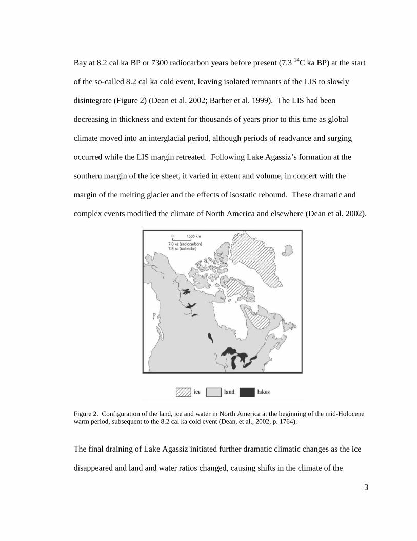
Bay at 8.2 cal ka BP or 7300 radiocarbon years before present (7.3 14C ka BP) at the start

of the so-called 8.2 cal ka cold event, leaving isolated remnants of the LIS to slowly

disintegrate (Figure 2) (Dean et al. 2002; Barber et al. 1999). The LIS had been

decreasing in thickness and extent for thousands of years prior to this time as global

climate moved into an interglacial period, although periods of readvance and surging

occurred while the LIS margin retreated. Following Lake Agassiz’s formation at the

southern margin of the ice sheet, it varied in extent and volume, in concert with the

margin of the melting glacier and the effects of isostatic rebound. These dramatic and

complex events modified the climate of North America and elsewhere (Dean et al. 2002).

Figure 2. Configuration of the land, ice and water in North America at the beginning of the mid-Holocenewarm period, subsequent to the 8.2 cal ka cold event (Dean, et al., 2002, p. 1764).

The final draining of Lake Agassiz initiated further dramatic climatic changes as the ice

disappeared and land and water ratios changed, causing shifts in the climate of the

4

interior of North America (Haskell et al., 1996; Alley and Augustsdottir, 2005; Dean et

al., 2002). Subsequently an unstable warm period established itself and dominated the

region during the warm and unstable Hypsithermal interval of the mid-Holocene (Laird

and Cumming, 2008; Clark et al., 2002). The polar air which had dominated the centre of

North America shifted its location northward, and a region where the atmosphere flowed

from the west began to interact with air from the Gulf of Mexico, and with the arctic air

mass. This eventually established the more modern climatic conditions prevalent today

(Dean et al. 2002; Laird et al., 2003; Dyke, 2005). As the transition to these more

modern conditions took place, rapid variation in climate occurred creating periods of

increased and reduced moisture, and temperature (Haskell et al., 1996). Following this

transition period, the modern more stable climatic conditions were established, although

climate variations continued to occur, including the Medieval Warm Period and the Little

Ice Age intervals of the past millennium (Adam et al., 1999).

1.2.2 Glacial History of the Laurentide Ice Sheet

The retreat of the Laurentide Ice Sheet (LIS) began at about 23 cal ka BP (Dyke, 2005).

Some of the proglacial lakes that formed along the south western side of the LIS

amalgamated into Lake Agassiz (Teller, 1985; Leverington and Teller, 2003). As the ice

margin slowly receded northward, glacial surges occurred at times, causing LIS lobes to

readvance relatively rapidly (greater than 2 km/yr) (Figure 3) (Teller, 1985; Teller and

Leverington, 2004). The surges and rapid calving off the glacier into Lake Agassiz

5

would have created very dynamic conditions in Lake Agassiz (Leverington and Teller,

2003).

Figure 3. Fluctuations in the retreating Red River Des Moines Lobe of the LIS, indicating the growth ofLake Agassiz (Teller, 1985, p. 4).

The LIS ice margin also underwent a number of retreats and readvances responding to

changes in climate, and large proglacial lakes next to the retreating ice margin

correspondingly fluctuated in areal extent and depth as their outlets were covered or

uncovered, and as differential isostatic rebound affected the elevation of their outlet

channels (Teller and Thorleifson,1983; Teller, 1985). The geographic location of the

outlets and the inputs from the LIS had major impacts on the extent and depth of Lake

Agassiz (Teller and Leverington, 2003). Ice margin fluctuations and differential isostatic

rebound opened and closed the overflow drainage pathways, resulting in variable routing

of overflow, specifically down the Mississippi River to the south, the Saint Lawrence

6

River to the east, and to the northwest down the Mackenzie River drainage channel

(Figure 4) (Leverington and Teller, 2003; Teller et al., 2005).

Figure 4. Depiction of the maximum extent of Lake Agassiz during its 5.0 ka cal yr history, indicating thethree major outlets before the lake finally drained north into Hudson Bay. Main routes of overflow areindicated by arrows and letters; NW = northwestern outlet, S = southern outlet, K = eastern outlets throughThunder Bay area, E = eastern outlets through Nipigon basin, KIN = Kinojevis outlet, HB = Hudson Bayroute of final drainage (Leverington and Teller, 2003, p. 1261).

The location of the discharge pathways not only affected the area and depth of Lake

Agassiz (Teller and Leverington, 2003), it also affected the local and regional climate in

the northern portions of North America, and more globally (Alley, 2000). Specifically,

catastrophic Lake Agassiz discharges into the Arctic and/or North Atlantic oceans (Clark

et al., 2001) affected ocean currents by interfering with ocean surface currents and deep

ocean currents (Teller et al., 2005). This influenced the ocean conveyor belt circulation

7

which is associated with the Earth’s heat distribution mechanism, and in turn affected

global climate by reducing heat flow into the high (North Atlantic) latitudes (Teller et al.,

2005).

As the ocean currents stalled or were dramatically reduced, climate cooled and in some

areas, the ice margin readvanced southward (Teller et al., 2002). On one occasion, the

rerouting of Lake Agassiz overflow prolonged the duration of the end of the last glacial

period for about 1000 years around 11 14C ka BP (~ 12.9 cal ka BP) until about 10 14C ka

BP (~ 11.5 cal ka BP) and initiated the Younger Dryas (Broecker et al., 1989). In the

Superior basin this resulted in a lobe of the LIS moving south (the Marquette glacial

readvance), covering the eastern Lake Agassiz outlets from about 10.1 to 9.4 14C ka BP

( 11.7 to 10.6 cal ka BP) (Teller and Leverington, 2004; Teller et al., 2005). After about

9.4 14C ka BP (10.6 cal ka BP) the ice margin withdrew far enough to once again permit

flow out the eastern outlets (Teller and Thorleifson, 1983; Teller and Clayton, 1983;

Teller and Leverington, 2004; Teller et al., 2005). The almost simultaneous changes in

the local, regional, and broader paleoclimate indicators, which correspond with those in

the Greenland ice cores, demonstrate that much of the Earth underwent abrupt nearly

synchronous climate changes at this time (within a few decades) (Dyke, 2005).

The continued retreat of the ice margin down slope into Hudson Bay led to the merger of

glacial Lake Agassiz and Ojibway (Figure 1) and eventually these lakes breached the ice

margin and drained northward below the LIS ice sheet at about 8.2 cal ka BP (7.3 14C ka

BP) (Barber et al., 1999; Dean et al., 2002). This event not only changed the routing of

8

overflow from Lake Agassiz and dramatically altered North American hydrology, it also

had an impact on ocean circulation and climate, causing the so-called 8.2 ka cooling

(Barber et al., 1999). The decay of the LIS continued for a short period after Lake

Agassiz drained, and while portions of the ice sheet remained farther north (Figure 2), the

major impact of the LIS and its dominating influence on the climate of North America

was over (Dean et al., 2002).

1.2.3 Climatic Changes Since the Last Glacial Maximum

Until the end of the last glacial maximum about 23 cal ka BP (Dyke, 2005), the large

anticyclone positioned over the ice sheet had dominated conditions south of the ice

margin, as strong winds from the west developed from the Pacific to the Atlantic along

the ice margin, in conjunction with katabatic winds blowing down slope off the ice sheet

and across the thermal gradient between ice and terrestrial terrains (Dyke, 2005; Wolfe et

al., 2004; Fisher, 1996). As the LIS margin slowly retreated northward the direct affects

of the anticyclone would have moved northward, and would have shrunk in radius, likely

dissipating over the region with the deglaciation of Hudson Bay about 7.6 cal ka BP (6.7

14C ka BP) (Dyke, 2005). The western portion of the continent was deglaciated earlier

than the eastern portion, which affected the shape of the jet stream over the continent

(Dyke, 2005).

Retreat of the LIS was interrupted during the Younger Dryas, as climate cooled as a

result of a massive discharge of Lake Agassiz’s fresh water about 12.9 cal ka BP (11.0

9

14C ka BP) which altered ocean currents (Broecker et al., 1989). In places, the LIS

readvanced as climate cooled for about 1300 calendar years (Teller and Leverington).

After this, the LIS began its northward withdrawal and once again allowed the

anticyclone to shift northward. The magnitude, extent and rapidity of the Younger Dryas

climatic change has not been duplicated since this paleoclimatic change (Alley, 2000;

Shuman et al., 2002), although several smaller cooling events did result from other

influences of fresh water discharges into the oceans (Clark et al., 2001; Teller et al.,

2002).

Factors beyond the direct influence of the proximity of the LIS and Lake Agassiz were

also likely at play in shaping the atmospheric circulations in the northern portions of

North America. The influence of the global climate changes, from glacial to interglacial,

would have influenced the climate over central North America as the Pacific air mass

became more influential, replacing the cold strong anticyclone winds to the south of the

LIS margin, which retreated northwards with the ice sheet margin (Dyke, 2005). The

west and northwest winds generated by the influence of Pacific air mass became more

dominant (Dyke, 2005), however there were additional localized effects related to the

location of the LIS. Katabatic winds across the margin of the ice sheet combined with

the strong anticyclone winds circulating over the ice sheet and would have had strong

influences over wind direction, frequently bringing winds out of the southeast (Wolfe, et

al., 2004). These anticyclonic winds, which extended up to 200 km from the ice sheet,

were prevalent up to about 9.0 cal ka BP in western North America and are reflected by

the orientations of eolian dune fields (Figure 5) (Wolfe, et al., 2004). As the LIS

10

retreated to the northeast, the anticyclonic winds would have retreated with it. As the

southeast wind reduced in frequency the prevalent direction of the winds of the central

plains of North America became those of the more modern winds (i.e. from the west and

northwest) (Wolfe, et al., 2004). This complex interrelationship between the changing

climate, the retreating LIS, and changes in Lake Agassiz would have resulted in many

changes in wind direction and climatic conditions in the region.

Figure 5. Wind directions, based on dune orientations, related to glacial limits and proglacial lakes for “A”15.6 cal ka BP and “B” between 13.0 and 9.0 cal ka BP in Alberta and Saskatchewan, Canada. Winddirection is indicated by solid arrows with known timing, and dashed arrows with inferred timing. Glaciallakes are identified (P = Peace, L = Leduc, DV = Drayton Valley and M = McConnell). The limit ofanticyclonic winds are identified in “B (Wolfe et al., 2004, p. 232).

The general early Holocene change in atmospheric circulation and its associated

anticyclone continued until about 7 cal ka BP (~ 6.1 14C ka BP) and this climatic

influence was reflected in the type and sequences in the biomes (i.e. vegetation and

animal assemblages) (Dyke, 2005). These changes in ice margin position in conjunction

with the development and fluctuations in margins of developing proglacial lakes, and the

11

fluctuating climate, resulted in limnological changes in the proglacial lakes (Dean et al.

2002). For example, lakes changed from well-stratified conditions surrounded by the

developing boreal forests, to well-mixed open prairie lakes during the drier periods of the

mid-Holocene (Dean et al. 2002). The lakes were subject to the more modern north

westerly winds, and with the disappearance of forests in the region the exposed lakes

were subject to increased mixing (Dean et al. 2002). Winds deposited eolian sediments

from the west were recorded in the lacustrine sediments of the region (Dean et al. 2002;

Fisher, 1996).

The 8.2 cal ka cold event was recorded in Greenland ice cores and other records on both

sides of the Atlantic Ocean (Alley and Augustsdottir, 2005) when a fundamental change

in atmospheric circulation occurred after Lake Agassiz drained into Hudson Bay.

Following this was the mid-Holocene dry period (Hypsithermal), whose maximum was

centred around 5.5 cal ka BP (4.8 14C ka BP) in central North America (Dean et al. 2002).

The end of this unstable warm period marked the beginning of modern atmospheric

circulation conditions (Dean et al. 2002).

1.2.4 General Overview of Glacial Lake Agassiz

The retreat of the LIS, discussed in Section 1.2.2, led to formation of a very large

proglacial lake, Lake Agassiz, which during its maximum extent connected eastward

through Lake Ojibway and discharged to the St. Lawrence River until about 8.5 cal ka BP

(7.7 14C ka BP). Lake Agassiz stretched from the Northwest Territories into Ontario

12

(Figure 4) at various times in its 5000 year history along the melting glacial margin

starting about 13.4 cal ka BP (11.7 14C ka BP) (Teller and Clayton, 1983; Teller 1985;

Teller and Leverington, 2004). The lake was contained in a watershed of approximately

2 million km2 with the lake’s maximum extent (not occupied simultaneously) covering an

area of 1 million km2, primarily controlled by the location of the glacial ice margin and

the location of its outlets (Teller and Thorleifson, 1983; Teller, 1985).

The changing climate discussed in Section 1.2.3, in conjunction with differential isostatic

rebound and the location of changing outlets, brought about dramatic changes in extent

and depth of Lake Agassiz. Five Lake Agassiz phases were identified based on changes

in routing of overflow, which variably occurred to the south, northwest, east and north

(Figure 4) (Fenton et al., 1983; Teller and Clayton, 1983; Teller, 1985). Many of these

changes resulted in relatively rapid falls in lake level.

The fluctuations in this large lake resulted in a very challenging environment for the biota

which were trying to establish themselves in these constantly changing conditions.

Severe conditions were imposed on the biota such as icebergs, a short ice-free season,

and large waves. High volume influxes of water from the west (Kehew and Teller, 1994)

and rapid drawdowns of the lake resulting from breaches of the rebounding ice margin

(Teller et al., 2002), further perturbed the environment of Lake Agassiz. The relatively

rapidly changing extent and depth of the lake was repeated numerous times (Bajc et al.,

2000; Teller and Leverington, 2004), adding further challenges to the biota’s ability to

adapt to the dramatically changing environment, especially at the margins of the lake.

13

Life did prevail however, and its signatures can be traced in sediments within modern

lakes of the region.

Deglaciation of the Rainy River basin near LOTWs occurred during the Lockhart Phase,

somewhere between about 11.7 and 10.8 14C ka BP (13.6 - 12.8 cal ka BP) when Lake

Agassiz was at the Herman level (Bajc, 2000). Following deglaciation, water remained at

the Herman level until the ice retreated north of the position of the Eagle-Finlayson

Moraine to the east of LOTWs (Bajc, 2000). During the Lockhart Phase sediments were

deposited in generally less than 100 m of water, while in the subsequent low water

Moorehead phase of Lake Agassiz, much of the LOTWs basin was sub aerially exposed

(Bajc, 2000; Yang and Teller, 2005). Deposition of Emerson Phase sediments began

when the Marquette readvance occurred and the eastern outlets of the Superior Basin

were dammed causing water levels to rise until at least 9.5 14C ka BP (10.7 cal ka BP) in

the Rainy River watershed (Bajc, 2000). When the ice margin retreated to the north the

eastern outlets again were exposed and the Lake Nipigon Phase of Lake Agassiz began

(Figure 6) with the overflow directed eastward, first to Lake Superior, and then North of

Lake Superior into Lake Ojibway and the Ottawa River (Teller and Leverington, 2005).

The final low-water phase of Lake Agassiz resulted in the isolation of the LOTWs basin,

ending their common paleohydrology and subsequently initiated climatic changes in the

LOTWs and SL watershed (Dean et al. 2002; Yang and Teller, 2005). The final drainage

of Lake Agassiz was into Hudson Bay at 8.2 cal. ka B.P. (~ 7.3 14C ka BP) (Dean et al.

2002; Barber et al. 1999) which initiated the final phase of climatic change in the

14

Northern Great Plains and LOTWs region (Dean et al., 2002), which had separated from

Lake Agassiz at about 9.0 cal ka BP (8.1 14C ka BP) (Yang and Teller, 2005).

18O record in GISP2 cores plotted against cal kadates. The five Lake Agassiz phases are indicated and catastrophic outbursts from Lake Agassiz are notedas A-R. Negative isotopic responses to the Younger Dryas, Preboreal Oscillation, and the 8.2 ka event areidentified. Lake Agassiz outbursts were interpreted to occur over a 1 yr period and are depicted by a barwith its height related to total outburst volume, with the final outburst of 163,000 km3 indicated by anarrow (Teller and Leverington, 2004, p. 739).

The final draining of Lake Agassiz initiated a dramatic change in climate of the north

central portion of North America (Clarke et al., 2004; Dean et al. 2002), as the ice sheet

15

disintegrated and Lake Agassiz disappeared completely leaving only isolated remnants of

the proglacial lake. A global climate perturbation once again rapidly occurred somewhat

similar to the Younger Dryas event, as freshwater flooded into Hudson Bay and the North

Atlantic, affecting thermohaline circulation (Figure 6) (Alley and Augustsdottir, 2005).

This cooling event however was relatively short lived (Figure 6) as return to glacial

conditions, in the absence of the large LIS, would no longer be likely with the ice sheet

essentially gone. The cooling influences of the ice sheet and proglacial lake, and the

associated influences of the large anticyclonic winds, were no longer at play. The

cooling effect from the introduction of fresh water through Hudson Bay would likely be

insufficient to allow the climate to cool significantly although other regions around North

Atlantic do record a cooling for up to a century or two (Alley and Augustsdottir, 2005).

The final draining of Lake Agassiz occurred about 1000 years after Lake Agassiz and

LOTWs were estimated to have separated at 9.0 cal ka BP (8.1 14C ka BP) (Yang and

Teller, 2005). This ended the influence of both Lake Agassiz and the LIS on the climate

of North America and the LOTWs region. The influence of the lake would have slowly

declined in the LOTWs region as the remnants of Lake Agassiz slowly drained due to the

influences of differential rebound, and the warming climate affected the hydrological

budget of the remaining remnants of the lake such as LOTWs and SL. The climate

continued to warm and moved through the unstable warm interval of the Hypisthermal,

and finally reached the relatively stable modern climatic conditions.

16

1.3 GENERAL HOLOCENE HISTORY OF LAKE OF THE WOODSAND SHOAL LAKE

1.3.1 General

The LIS withdrew from LOTWs region before 11.0 cal ka BP (10 14C ka BP) (McMillan

et al., 2003) and proglacial Lake Agassiz then dominated the region for the next thousand

or so years. At about 11 cal ka BP (9.6 14C ka BP) Lake Agassiz was at its deepest (~

132 m) in the LOTWs region (Yang and Teller, 2005). Lake Agassiz continued its

complex hydrologic history and overflowed through the eastern outlets at times as

significant outbursts above a baseline flow (Figure 6). As early as 10 cal ka BP LOTWs

was barely linked to Lake Agassiz, and by about 9.0 cal ka BP (8.1 14C ka BP) LOTWs

and SL became hydrologically independent from Lake Agassiz (Yang and Teller, 2005;

Teller and Leverington, 2004).

The late Quaternary history of the LOTWs region slowly changed from being buried

under the thick ice of the LIS to being part of the bathymetry of Lake Agassiz. When

LOTWs became isolated from Lake Agassiz, it was already reacting to regional

differential isostatic rebound from the withdrawal of the LIS to the northeast. This

rebound, and the influences of the warming post glacial climate during the unstable warm

climate of the Hypsithermal in the mid-Holocene, about 9.5 - 4.5 cal ka BP (8.4 - 4 14C ka

BP) (Teller and Last, 1982; Laird and Cumming, 2008; Clark et al., 2002), affected the

hydrology of LOTWs. The late Holocene environment progressively moved toward the

slightly cooler modern environment of the past millennium (Teller et al., 2005). All of

17

these changes would have had a significant influence on the hydrologic budget of both

LOTWs and SL.

Differential isostatic rebound would have resulted in a southward movement of the

shoreline, as the LOTWs outlets into the Winnipeg River at the north end of the lake rose

relative to the main body of the lake to the south. This generally increased the depth of

LOTWs and SL south of the overflow outlet, and resulted in a southward transgression of

the shoreline (Figure 10), assuming the hydraulic budget was positive (Yang and Teller,

2005). The relationship of SL with LOTWs would most likely be primarily driven by

climate change influences alone, as the isostatic rebound between the Winnipeg River

outlets and the shallow interconnecting channel sill to SL, at Ash rapids, would be

minimal since it is at or near the same isobase on the northern portion of LOTWs (Figure

7).

From the spatial variation in the elevation of the beaches of Lake Agassiz and an

empirical formula developed by Lewis and Thorleifson (2003), the isostatic rebound of

both the Lake Agassiz period and later stages in the LOTWs region can be determined

(Yang and Teller, 2005). Based on this information the reconstructions of the

paleotopography of the region and the paleobathymetry of the LOTWs and a portion of

SL were made showing their extent and depth (Figure 8, Figure 9 and Figure 10) (Yang,

and Teller, 2005), and are presented below.

18

Figure 7. Map of glacial Lake Agassiz region with isobase lines (lines of equal uplift) indicated in bold andproglacial lakes Agassiz and Ojibway indicated in grey. Watershed limits are indicated by dashed lines andthe location of the major outlets indicated (NW = northwest; K = eastern; and S = southern) (NW), the east(K) and the southern (S) outlets). The locations of SL and LOTWs are indicated in red. (After Yang andTeller, 2005, p. 485).

The isolation of LOTWs from Lake Agassiz was nearly complete by 10.0 cal ka BP (9.6

14C ka BP) resulting from the opening of the lower eastern outlets, which lowered the

level of Lake Agassiz (Teller et al., 2008). This isolation allowed LOTWs and SL to

operate within their own hydrologic systems (Yang and Teller, 2005).

SL

LOTWs

19

Figure 8. Paleomaps of the LOTWs region indicating the changes in topography and bathymetry as LakeAgassiz regressed from the region at (a) 11.0 cal ka BP, (b) 10.5 cal ka BP, and (c) 10.0 cal ka BP. Bluecolours = water with depth in m, and white to dark brown = elevation at or above the water surface in m(Teller et al., 2008, p. 681).

20

1.3.2 Isolation of Lake of the Woods and Shoal Lake from Lake Agassiz

Following isolation of LOTWs and SL from Lake Agassiz, terrestrial inputs from the

drying of former Lake Agassiz sediments surrounding LOTWs (Figure 9), would

continue into the new hydrologically independent LOTWs and SL and their watershed,

providing inputs of sediments containing CaCO3 into the lakes. This persisting input of

former Lake Agassiz sediments would likely continue prolonging the influence of Lake

Agassiz over LOTWs and SL, until the newly exposed Lake Agassiz watershed was

stabilized with the developing vegetative cover (Dean et al., 2002).

After the complete separation of Lake of the Woods from Lake Agassiz estimated at 9000

cal ka BP (8.1 14C ka BP) (Figure 9), LOTWs occupied the isostatically depressed

northern part of the basin (Figure 10) (Yang and Teller, 2005).

Figure 9. Paleomap of the LOTWs region indicating the topography and bathymetry of LOTWs after LakeAgassiz separated from LOTWs at about 9.0 cal ka BP. Blue colours = water with depth in m, and white todark orange = elevation at or above the water surface in m (Yang and Teller, 2005, p. 493).

21

Figure 10. Paleomap of the LOTWs region indicating the topography and bathymetry of LOTWs afterseparation from Lake Agassiz and its transgression to the south; (b) 8.0 cal ka BP (c) 7.0 cal ka BP, (d) 6.0cal ka BP, (e) 5.0 cal ka BP, (f) 4.0 cal ka BP, (g) 3.0 cal ka BP, (h) 2.0 cal ka BP, and (i)1.0 cal ka BP.Blue colours = water with depth in m, and white to dark orange = elevation at or above the water surface inm (Yang and Teller, 2005, p. 493).

The areal expansion of the lake shown in Figure 10 and Table 1, was controlled by the

elevation of the northern outlets (overflow spilled into the Winnipeg River watershed and

22

subsequently into the Lake Winnipeg basin), and runoffs into LOTWs, with the main

runoff into the modern lake from the Rainy River watershed.

Table 1: Evolution of Aerial Extent, Bathymetry and Volume of LOTWs

Periods Cal yrs BP MaximumDepth (m)

MeanDepth (m)

Area(km2)

Volume(km3)

LOTWs Period Present 66.9 8.1 4524 371000 67.0 7.6 4415 342000 67.0 7.4 4292 323000 66.0 6.9 4052 284000 66.0 6.3 3676 235000 65.0 5.8 3227 196000 65.0 5.6 2857 167000 64.0 6.1 1822 118000 63.0 8.3 1061 99000 61.0 8.5 858 7

Lake Agassiz Period 10,000 89.0 14.7 - -10,500 116.0 31.4 - -11,000 132.0 43.8 - -

From Yang and Teller, 2005, p. 494.

Depending on the overall hydrologic budget, which would be strongly affected by the

changing climate, the stabilizing effects of flora on the watershed’s runoff, and the

mechanics of the differential isostatic rebound, LOTWs either occupied the full extent of

the new configuration of the lake basin, or a subset of the full extent of the basin based on

the hydrologic budget (Figure 10) (Yang and Teller 2005).

The regional climate variability, in conjunction with the differential isostatic rebound,

would have significant impacts on shallower portions of the LOTWs and on the

interconnection into SL. Compartmentalization of portions of the shallow southern basin

and disconnection of the northern and southern parts of the LOTWs basin would have

been likely during lake lowstands. Deeper channels connecting the compartments and

23

the northern and southern basins would permit Rainy River input and overflow into the

Winnipeg River. These flows would have decreased/ceased during negative water budget

intervals. SL with its generally deeper basin would likely be less affected aerially,

however would have become independent from LOTWs whenever the level of LOTWs

fell below the shallow ledge in the interconnecting channel.

1.4 MODERN LAKE OF THE WOODS AND SHOAL LAKEWATERSHED

1.4.1 Introduction

The location of LOTWs along the international border between Canada and the U.S.

makes it an international body of water. It is subject to a special treaty between the two

countries, which was negotiated through the International Joint Commission’s (IJC).

Since 1925 this required the Canadian Lake of the Woods Control Board to regulate the

outflows from the lake to maintain lake levels within specified limits. SL was also

included in the IJC jurisdiction due to its interconnection with LOTWs and the city of

Winnipeg’s use of this body of water for its water supply.

LOTWs spans the border of the provinces of Manitoba and Ontario, as well as that of the

state of Minnesota, and as such is subject to the laws of three state/provincial

governments, and two federal jurisdictions. This multi-jurisdiction environment can

make access to the lake complicated, especially due to the unusual border configuration

24

of the U.S./Canada border north of the 49th parallel and to the east of the Manitoba border

with Ontario. This means this part of Minnesota (known as the Northwest Angle) cannot

be reached by land directly from the rest of the state, requiring a border crossing between

Minnesota and Manitoba, or alternately it can be reached directly by a water route from

Minnesota, without a formal border crossing point.

1.4.2 Description of the LOTWs and SL and their Watersheds

LOTWs and SL are located at a latitude of about 49-50o and a longitude of about 95o,

with LOTWs located at the conjunction of the Canadian provinces of Manitoba and

Ontario, and the northern boundary of the U.S. state of Minnesota. LOTWs is a highly

irregular body of water about 110 km long by 95 km wide, with a complex bathymetry

ranging from a relatively shallow southern basin typically 10 m in depth, to much deeper

bays in the north and northeast which range to over 70 m in depth. The lake covers

approximately 386,000 ha (3860 km2) and is composed of numerous and distinct basins,

with more than 14,500 islands (Pla et al., 2005). The main inflow into LOTWs is from

the Rainy River which supplies about 70-75% of the stream inflow (Pla et al., 2005;

Yang and Teller, 2005). The inflow interconnects through the southern part of the basin

to multiple deep and mostly narrow channels in the Northwest Angle area, into the deeper

northern portions of the lake, discharging 13.59 km3/yr (431 m3/yr) into the Winnipeg

River System (Yang and Teller, 2005). Overall watershed runoff is estimated to be

16.78 km3/yr including 2.69 km3/yr of precipitation directly onto the lake, with

evaporation from the lake surface of 2.5 km3/yr, just below the rate of precipitation (Yang

25

and Teller, 2005). Groundwater inflow and outflow is estimated to result in a net outflow

of groundwater of 3.38 km3/yr (Yang and Teller, 2005). Most of the lake lies on the

granitic bedrock of the Precambrian Shield (Figure 15), however the Rainy River

watershed and the southern part of LOTWs watershed (Figure 11) overlie the lake

sediments of glacial Lake Agassiz (Figure 16) (Pla et al., 2005).

The LOTWs (including SL) watershed is part of a broader watershed which feeds the

Winnipeg River joining other Winnipeg River watersheds (Figure 11) and ultimately

feeds 45 % of Lake Winnipeg’s total inflow into its southern basin (St. George, 2006).

On average, about 50% of this total Winnipeg River inflow to Lake Winnipeg comes

from LOTWs (LWCB, 2002).

26

Figure 11. Winnipeg River watershed including the LOTWs and Rainy River watersheds (Lake of theWoods Control Board brochure, 2002, p. 10).

The lake is primarily separated into two zones by the Aulneau Peninsula which lies in an

approximately east/west orientation and separates the shallow southern basin from the

deeper basins in the north and northeast. The lake is a complex network of islands,

channels, broad expanses of open water, and deep bays, many of which are almost

independent of the main open portions of the lake (Figure 12).

27

Figure 12. Aerial photo of LOTWs and SL indicating the location of Kenora and the nearby outlets to theWinnipeg River (after http://www.virtualnorth.net/satimp/).

There are three natural outlets in the northern portion of the lake into the Winnipeg River.

Only two channels are currently operational as the third shallower intermittent channel

was filled in (Figure 13) (LWCB, 2002). The third natural channel at Portage Bay

operated during high water conditions (Figure 13) (LWCB, 2002). LOTWs outflow is

now controlled through the jurisdiction of the Lake of the Woods Control Board, which

regulates the flow through the enlarged eastern and western outlets (enlarged for power

generation with the ability to permit compliance with international agreements for

LOTWs level control) (LWCB, 2002). Lake levels typically fluctuate between 0.9 and

1.2 m (Pla et al., 2005).

Lake of the

Shoal Lake

Kenora

AulneauPeninsula

© satellite impressions.com 1992

28

Figure 13. Winnipeg River outlets from LOTWs into the Winnipeg River near Kenora, Ontario. Site 1(Kenora powerhouse) and Site 2 (Norman dam and powerhouse) are in the two main outlets into theWinnipeg River, with the Site 2 so-called Western channel taking about 75% of the flow. The third naturalchannel is through Portage Bay but only a small flow (3 m3/s) can occur at Site 3 (gated culvert), with Site5 (the old mill) no longer receiving any flow due to the filling of the channel to the mill at Site 4 (Lake ofthe Woods Control Board brochure, 2002, p. 7).

SL is located to the northwest of the main body of LOTWs straddling the Manitoba-

Ontario Border at about 49.5 °N latitude and has a surface area of 260 km² which lies

within a relatively small 960 km² watershed (Shoal Lake Watershed Management Plan,

2001). It receives inflow from the smaller Falcon Lake via High Lake watersheds

through the Falcon River (Shoal Lake Watershed Management Plan, 2001). It generally

has the same typically deep characteristics as the northern portions of LOTWs, with the

exception of the interconnecting channel at Ash Rapids, which narrows and shallows.

This interconnection was deepened around the turn of the 20th century, to its current 10 m

width and 1.5 m depth (at the centre of the channel at the low level datum), subsequent to

dams being constructed on the LOTWs Winnipeg River outlets (Shoal Lake Watershed

Management Plan, 2001). The controls established in LOTWs in conjunction with the

use of water from SL for the City of Winnipeg water supply, and variations in watershed

runoff between the small SL watershed and much larger LOTWs watershed now causes

29

the natural inflow into LOTWs to reverse at times (Shoal Lake Watershed Management

Plan, 2001).

The LOTWs and SL watershed, and the Rainy River watershed flowing into LOTWs

from the south, are all currently near the western limit of the LOTWs Boreal Wetland

Region (Figure 14) which is dominated by continental air masses (Bajc et al., 2000). The

location of the air masses produce July mean air temperatures of 18 °C and January mean

air temperatures of minus 15 °C, with ~ 710 mm of annual precipitation, two-thirds of

which occurs as rain during summer (Bajc et al., 2000).

The high degree of complexity of LOTWs extends to its physical geography (Figure 12),

bathymetry and ecological systems, and this produces highly variable biotic systems (Pla

et al., 2005). LOTWs is an unusual Precambrian Shield lake influenced by glacial Lake

Agassiz deposits, with relatively hard water and with a pH between 7-8 (Molot et al.,

1987; Pla et al., 2005). LOTWs pH values vary from a low of 7.5 in Rainy River and 7.8

near Kenora with the south east portions of the lake lower, and the deeper northern bays

such as Clearwater Bay ranging up to a pH of 7.9 (Molot, 1987; Pla et al., 2005). Big

Traverse Bay in the south basin had a relatively uncharacteristic value of pH of 8.0

(Molot, 1987). Shoal Lake values are even higher at a pH of 8.2 (Molot, 1987). These

variations across LOTWs including the Rainy River and SL are indicative of the

complexity of LOTWs (Pla, et al., 2005) and its watershed. These variations in

conditions are reflected in modern and historical ecology (Laird and Cumming, 2008).

30

Figure 14. Biomes at 1000 yrs BP in the LOTWs region. This biome has remained relatively unchangedfor the past millennium (after Dyke, 2005 p. 244).

1.4.3 Geology of the Modern Lake of the Woods and Shoal LakeWatershed/Region

LOTWs is underlain by Precambrian granite-greenstone of the Wabigoon Subprovince

consisting of metavolcanic and metasedimentary rocks with granitoid intrusions

(Minning et al., 1994) (Figure 15). The predominant underlying geology of the LOTWs

watershed is a pink granodiorite, with overlying thin moss soils in places (Schindler et

al., 1996). Quaternary deposits include glacial deposits consisting of tills, sands and

gravels (with a few locations containing Paleozoic rocks), and include lacustrine silts and

clays which occur in various locations within the LOTWs watershed and within the lake

31

basin (Figure 16), with generally thin and patchy Quaternary sediments with thicker

glaciolacustrine deposits south of the Aulneau Peninsula and south of SL (Minning et al.,

1994).

Figure 15. Western Wabigoon subprovince simplified bedrock geology including the LOTWs region(Minning et al., 1994, 2005 p. 11).

32

Figure 16. Quaternary geologic map of LOTWs. Note al unit not mapped in Ontario where a differentalluvium is defined (after Sado et al., 1995, from map NM-15).

Thick deep water sediments (from 1-75 m) of laminated to varved clay, silt and fine sand,

are found in depressions and are found throughout the watershed (Maps 1770A through

1175A; Minning et al., 1994). Calcareous components reportedly occur only rarely in

hp

50 km

List of map unitsHolocene:al - alluviumhp - peat and muckHolocene & Late Wisconsin Sandy Tillts - ground morainetsr - discontinuous sandy tillke - kame moraine depositgg – outwash sandlca – lake clay & siltlsa – sand & gravellu – lake clay, silt, sand & gravelLate Wisconsintku – loamy tilltlg - ground morainetdr – discontinuous sandy loamy tilltlr – discontinuous loamy till

tsr

33

these thin widely spaced sediments based on Map 1771A (Surficial Geology Northwest

Angle), although specifically sampled sediments and clasts in LOTWs reacted to dilute

hydrochloric acid and are believed to be calcareous till and reworked till from Paleozoic

bedrock carbonate debris, possibly from the Manitoba lowlands and Hudson Bay

(Minning et al., 1994). A number of the units identified in Figure 16 include calcareous

components (Sado et al., 1995). Unit “al” along the Rainy River is described as

containing pebbles cobbles and boulders of limestone and dolomite while the Holocene

and Wisconsin sandy till units (gg, lca, and lsa) contain non calcareous to weakly

calcareous components, while the Late Wisconsin loamy till (tku) which likely underlies

the peat and muck to the west of LOTWs and SL (unit hp) (Teller and Fenton, 1980) is

described as having a very calcareous matrix with up to 50% carbonate (Sado et al.,

1995). Additionally, Schindler et al., 1996, report Paleozoic carbonate rocks in the

glacial drift are a source of carbonates to LOTWs and SL with further inputs from Lake

Agassiz sediments. The availability of these calcareous components is important to any

biota which develop CaCO3 shells.

1.5 HOLOCENE PALEOCLIMATE HISTORY BASED ON OTHERSTUDIES

1.5.1 General

Since the last glacial maximum, the climate of the LOTWs region has undergone

dramatic changes. Proximity of the ice margin and extent of proglacial lakes, particularly

Lake Agassiz, were major climate driving forces during the early post glacial period.

34

LOTWs region eventually emerged from the direct influence of the LIS and Lake

Agassiz, however it remained closely linked to these influences as the local climate

reacted to the katabatic winds, prevailing winds blowing off Lake Agassiz or the

anticyclonic winds circulating above and beyond the margins of the glacier farther to the

north. As the LIS continued its retreat, the influence of the ice to the northeast, and Lake

Agassiz’s large cold surface, diminished and the position of the jet stream slowly shifted

to the north (Dyke, 2005). The large anticyclone over the ice sheet weakened and finally

lost its influence as the position of the jet stream moved to its modern location sometime

after the 8.2 ka cold event (Dyke, 2005; Dean et al. 2002).

Based on the electrical conductivity measurements in Greenland ice cores, rapid

(decadal) changes in deposition of loess were identified at the glacial-interglacial

transition, implying the relatively slow changes in solar insolation were also unlikely to

have been the direct cause of the unstable climatic conditions in the Hypsithermal (Taylor

et al., 1993). It is more likely changes in atmospheric circulation and temperature

gradients between the high and mid-latitudes of North America increased, or decreased

wind speeds, and affected the loess data in the Greenland cores (Taylor et al., 1993).

Mid to late Holocene paleoclimate proxies in the LOTWs region indicate significant

variation in the location of climatic zones across the region (Dyke, 2005). These

variations have been related to changes in the location of convergence zones of the air

masses and the record of these changes has been identified in the study of the ecotones

(Haskell et al., 1996; Dyke, 2005). The relatively dry westerlies driven by the Pacific air

35

mass, the outflow of the cold Arctic air mass, and the warm moist tropical Gulf air mass,

all converge in the LOTWs region (Haskell et al., 1996; Dyke, 2005). Changes in the

location of the convergence of these air masses can result in rapid changes in climate and

can causing considerable variability in local climatic conditions (Haskell et al., 1996).

1.5.2 Early Holocene Climate

From about 18 to 7 cal ka BP (14.7 - 6.1 14C ka BP) the changing atmospheric circulation

resulting from the changing geographical position of the convergence of the Pacific,

Arctic and tropical air masses, were reflected in the sequencing of biome changes (Dyke,

et al., 2005). Deglaciation of the Rainy River basin occurred between 11.7 and 10.8 cal

ka BP (10.8 to 9.5 14C ka BP) (Bajc, 2000) with LOTWs becoming ice-free around 12.9

cal ka BP (11.0 14C ka BP) (Teller et al., 2000). Lake Agassiz followed the retreating ice

and by about 10.2 cal ka BP (9 14C ka BP) the terrain around LOTWs slowly emerged

from under the lake (Bajc, 2000). The emergent terrain was primarily covered by boreal

forest (Bajc, 2000). As the climate continued to moderate, grasslands replaced the boreal

forest in part of the LOTWs basin (Figure 17) by 8.9 cal ka BP (~8 14C ka BP) (Dyke et

al., 2005).

36

Figure 17. North American Biomes at 9 (upper) and 8 (lower) 14C ka BP indicating locations of borealforest and grassland biomes near LOTWs region and the position of the LIS and Lake Agassiz/Ojibway.The legend at the right provides the biome legend (stars = macrofossil, triangles = mammal, and circles =pollen sites) (after Dyke, 2005, p. 230 and p. 233).

37

Variations between boreal forest and grassland biomes followed the climate fluctuations

in the early Holocene in the north central portions of North America (Dyke et al., 2005).

Biome and climatic reconstructions in the Rainy River watershed, and nearby pollen

profiles in northern Minnesota and northwestern Ontario, indicate that from about 11.5

cal ka BP (10.0 14C ka BP) until at least 10.7 cal ka BP (9.5 14C ka BP), biomes were

similar to modern assemblages (Bajc, 2000). However, a distinct component from much

farther north and west was present, making this assemblage similar to the mixed

community sites in the mid-continent (Bajc, 2000).

Farther to the east in the Great Lakes it has been hypothesized these large lakes were

hydrologically closed during the early to mid-Holocene, due to the drier climate (Lewis et

al., 2001). This implies LOTWs and SL were also likely below their outlets at this time.

1.5.3 Mid-Holocene Climate

The mid-Holocene in central North America, about 8.0 - 4.0 cal ka BP (7.1 - 3.7 14C ka

BP), was generally warmer and drier than today with rapid variations in temperature and

precipitation occurring, similar to today (Forester et al., 1987). Ostracode studies in Elk

Lake, Minnesota, about 300 km to the south of LOTWs, however, indicate portions of

this period were colder and drier than today, notably in the interval from 7.8 - 6.7 cal ka

BP (~ 6.9 - 5.9 14C ka BP) (Forester et al., 1987). Overall, the interval from 6.7 - 4.0 cal

ka BP (5.9- 3.7 14C ka BP) had temperatures approaching the modern average mean (3.7

oC), with warm summers from 6.7 - 5.8 cal ka BP (~ 5.9 - 5.1 14C ka BP) and only

38

periodic warm summers in the interval from 5.8 - 4.0 cal ka BP (~ 5.1- 3.7 14C ka BP)

(Figure 18) (Forester et al., 1987).

Sediments in lakes in the Experimental Lakes Area (ELA) near LOTWs, specifically

Lake 239, indicate a drier climate with lake levels varying as much as 8 m from the early

to the mid-Holocene from about 8.9 - 4.4 cal ka BP (8.0 - 4.0 14C ka BP) (Laird and

Cumming, 2008). The sedimentary record in West Hawk Lake, a small deep lake 40 km

to the northwest of LOTWs, indicates a drier interval between 7.1- 4.5 cal ka BP (~ 6.2 -

4.0 14C ka BP) (Teller at al., 2008). These low moisture conditions are also reflected

farther west in Lake Winnipeg, and at the Wampum site just to the west of the south

basin of LOTWs (Lewis et al., 2001; Teller et al., 2000). As the Wampum, Manitoba site

became a lagoon with Lake Agassiz falling below the Upper Campbell beach level about

10.5 cal ka BP (9.3 14C ka BP), only minor hydrologic fluctuations (possibly due to

groundwater inputs) were noted, except for a possible dry interval between 7.1 to 4.5 cal

ka BP (6.2 - 4.0 14C ka BP); after this, peat accumulation began (Teller et al., 2000). The

southern basin of Lake Winnipeg reflects this regional mid-Holocene aridity and Lewis et

al., (2001) concluded the basin was desiccated for most of the mid-Holocene from about

8.2 - 4.3 cal ka BP (7.5 - 4.0 14C ka BP), as a result of this regional aridity and the effects

of differential isostatic rebound. Yang and Teller, 2005 proposed that the mid-Holocene

warming in the LOTWs region, in conjunction with the effects of differential isostatic

rebound, caused the LOTWs to fall below its northern outlets.

Mid-Holocene aridity has

the U.S. and Canada, from

Cumming, 2008). Based

precipitation and higher t

al., 2008). Increasing pin

4.4 14C ka BP) indicates d

evident after this, based o

(Teller et al., 2008).

Figure 18. Mean annual tempversus time (cal ka BP), based

Conditions farther to the w

and 8 cal ka BP (9.3 - 7.1

4.5 cal ka BP (~ 6.6 to 4

1996). The presence of s

s been interpreted from lake level data in the nor

m about 8.3 - 4.5 cal ka BP (~ 7.5 - 4 14C ka BP)

on pollen, diatoms, and carbon and oxygen isot

temperatures were detected in nearby West Haw

ne versus spruce pollen between 9.5 and 5.0 cal k

drier conditions in the region, with cooler and w

on increased organic vs. mineral lithics in the lak

erature (left), and mean annual precipitation and evapotrad on ostracode analogs (Forester et al., 1987, p. 266).

west in Devils Lake, indicated saline conditions

1 14C ka BP) with saline conditions reoccurring b

14C ka BP), but at a lesser frequency and duratio

struvite (hydrous Mg-ammonium-phosphate) in n

39

rthern prairies of

) (Laird and

tope data, low

wk Lake (Teller et

ka BP (~ 8.4 -

wetter conditions

ke sediments

anspiration (right)

s between 10.5

between 7.5 to

on (Haskell et al.,

northern North

40

Dakota lakes during dry periods, deposited by high concentrations of migrating

waterfowl, have been detected and related to the end of dry periods in the region

(Donovan and Grimm, 2007). These arid periods range from 8.7 to 4.7 cal ka BP (~ 7.9 -

4.1 14C ka BP) and indicate frequent arid intervals in the early Holocene from about 8.7

to 8.1 cal ka BP (~ 7.9 - 7.2 14C ka BP) into the mid-Holocene, with the youngest

identified in the late Holocene at 2.7 cal ka BP (~ 2.6 14C ka BP) (Donovan and Grimm,

2007).

The general location of major modern atmospheric circulation features, including the air

masses and prevailing winds, are depicted in Figure 19 for the winter/summer

atmospheric circulation patterns; these conditions may have been established in the late

Holocene at about 3.0 cal ka BP (~ 2.9 14C ka BP) (Harrison and Metcalfe, 1985), or a

little later (Forester et al., (1987). The location of these main atmospheric circulation

features were much different in the past, and the mean westerly storm tracks associated

with the late glacial period 18 cal ka BP (~ 14.7 14C ka BP) likely were centred much

farther south than at present, at around 35° - 36° N latitude (Harrison and Metcalfe,

1985). Interestingly, the mid-Holocene location of these atmosphere features at about 6.0

ka BP (5.2 14C ka BP), reached their northernmost location at around 56° N latitude,

which is much farther north of their modern location (Harrison and Metcalfe, 1985).

Figure 19. Location of the mo1985 p. 142).

The dominant pre 7.0 cal

dry summers) fluctuated

meridional patterns were

1987). The location of th

reason for the much warm

the atmospheric condition

Overall, the mid-Holocen

occurring rapidly (in less

(Forester et al., 1987).

The variations in Holocen

odern January and July air masses over North America (H

ka BP (6.1 14C ka BP) zonal pattern (long dry w

and decreased in intensity, until the modern seas

established around 4.0 cal ka BP (3.7 14C ka BP

he air masses farther north in the Hypsithermal is

mer and drier conditions, and perhaps its variabil

ns migrated north and south (Harrison and Metc

ne climate was drier and warmer, with changes in

than 50 years) between the main intervals of the

ne climate are reflected in the regional boreal fo

41

Harrison and Metcalf,

winters and cool

sonal zonal and

P) (Forester et al.,

s likely the

lity resulted as

alfe, 1985).

n climate

e mid-Holocene

rest during the

42

mid-Holocene as indicated by pollen data (Laird and Cumming, 2008). Vegetative cover

changed to accommodate the drier and warmer climate as the prairie expanded farther

eastward (Laird and Cumming, 2008). ELA lake pollen data imply an open grassy jack

pine and poplar region, with junipers on the arid/windy hilltops during the mid-Holocene

about 7-8 cal ka BP (7.1 - 6.1 14C ka BP). Interestingly there was little vegetative change

during this period even though there were large lake level changes in Lake 239 associated

with lower effective moisture (Laird and Cumming, 2008). These low moisture

conditions are also reflected farther west in Lake Winnipeg (Lewis et al., 2001). The

transition zone between the prairie and parkland boundaries of the northern plains

including LOTWs and SL, is described as more humid than the prairie zone, with the

Winnipeg River watershed flowing through a well forested region (Figure 20) (Lewis et

al., 2001). Mid-Holocene conditions would likely have differed somewhat as the biome

boundary responded to climate changes, however based on Lake 239 data, the prairie and

parkland biome boundary does not appear to be dramatically different from that of today.

Consistency in the location of biomes from the mid-Holocene to present has been noted

by others (Williams et al., 2000), although within a biome, shifts in importance of

functional plant types would have occurred due to climate changes. Nonetheless, the

east/west boundary of the biomes of 6.8 cal ka BP (~ 6.0 14C ka BP) were approximately

in the same position as they are today (Williams et al., 2000), although they extended

farther north (Figure 20) (Laird and Cumming, 2008; St. Jacques et al., 2008).

Figure 20. Eastern portion ofindicating the location of the glocation of the parkland borderLOTWs, Winnipeg River, RedWinnipeg watershed (after Lew

As can be seen in Figure

border farther to the north

2008) than the modern bo

parkland-boreal forest bo

to the east of LOTWs (Fi

confirmed from studies o

of LOTWs (Figure 22) (L

the Lake Winnipeg watershed including the Lake of the Wgrassland border between 0 and 6.5 cal ka BP (solid greenr farther east at 6.5 cal ka BP (dashed green line). The yed River, and Lakes Winnipeg and Manitoba represents thewis et al., 2001, p. 744).

20, mid-Holocene data from U.S. sites locates th

heast of the modern boundary (Figure 21) (Laird

oundary which brings the prairie region close to

oundary during the mid-Holocene was interpreted

gure 17 and Figure 20) (Lewis et al., 2001); this

f ELA Lake 239, which lies to the about 50 km

Laird and Cumming, 2008).

43

Woods region,n line) and theellow area arounde extent of the Lake

he grassland

d and Cumming,

LOTWs. The

d to have moved

s appears to be

to the northeast

44

Figure 21. Map of Minnesota, Southern Manitoba and Lake of the Woods region of Northwest Ontario,indicating modern major modern vegetative biomes with the prairie forest border marked by a dotted line(after St. Jacques et al., 2009, p. 538).

Figure 22. Location of ELA Lake 239 (Laird and Cumming, 2008, p. 294).

45

Although the changes in biomes in this region would have been slow to respond to

variations in mid-Holocene climate, they do “average” the effects of the larger and longer

changes in climate, and confirm the trends in the climate fluctuations of the mid-

Holocene in this region. The biomes in the LOTWs region further confirm the location

of the LOTWs near the contact zone of the Arctic, Pacific and maritime tropical air

masses (Laird et al., 2003). This means the LOTWs region was likely subject to many

climatic fluctuations in the mid-Holocene.

1.5.4 Late Holocene Climate

Overall, late Holocene climate in the northern plains regions of Canada and the U.S., in

the past couple of thousands years, has been categorized as having periods of stability

interspersed with large shifts between wet and dry (Laird et al., 2003; Clark et al., 2002).

The timing of drought shifts is location specific, and is related to changes in the position

of the jet stream and the associated storm tracks (Laird et al., 2003). Minor shifts in the

position of the polar high pressure vortex have been hypothesised to be the driving force

for spatial climate variations in the region and century-scale climatic variability have

been tracked through climate proxies in small prairie lakes (Clark et al., 2002; Laird et

al., 2003). Abrupt changes in the Northern Hemisphere climate condition have been

detected through the late Holocene such as the transition from the Medieval Warm Period

to the Little Ice Age, which corresponds to the beginning of a period of drought starting

about 0.7 cal ka BP (Adam et al., 1999; Laird et al., 2003; Cook et al., 2007; St. Jacques

et al., 2008). Looking backwards from this point in time, a 1200 yr cycle of drought has

46

been detected in British Columbia, with some sites correlating well with periods of

increased fire frequency in the prairies (Laird et al., 2003). Other investigators associate

increased fire frequency in grassland regions with increased charcoal in the sediments,

which correspond with periods of increased precipitation which in turn produced an

increase in vegetation, particularly grasses that provide fuel for fires (Clark et al., 2002;

Brown et al., 2005). These opposing interpretations of high charcoal levels in sediments

can complicate interpretations. Nonetheless, in both studies mid-Holocene century scale

droughts and the late Holocene decadal scale droughts have been detected.

Cycles of extreme drought lasting about a century, in the northern U.S. plains and

Canadian prairies have been linked to the proximity of this region to the polar vortex, and

its associated ability to block or enable moist air from the Gulf of Mexico from reaching

the region (Laird et al., 2003). The blocking of maritime tropical air masses from the

south, by the drier and cooler Pacific air masses, has also been identified as a mechanism

that may reduce precipitation (Lewis et al., 2001; St George, 2006). Late Holocene

intervals of aridity, however, were not as pronounced as mid-Holocene droughts, and

their durations were typically less than a century, unlike 600 year drought experienced

around 8.0 cal ka BP (Clark et al., 2002).

Bog moisture variability studies using thecamoebians, peat humification, pollen, leaf

stomata and plant macrofossils (Booth and Jackson, 2003) have found that over the past

2000 years in sites in southern Michigan and north-central Minnesota, there were

intervals of extreme drought in both regions (Booth et al., 2006). These correlate with

47

large droughts identified much farther west in the Northern Great Plains and the Rockies

(Booth et al., 2006).

Conditions in the late Holocene in the northern Great Plains region at Devils Lake, North

Dakota, were wet from 4.5 to 3.5 cal ka BP with dry conditions (indicated by more saline

lake conditions) returning at about 3 cal ka BP (Haskell et al., 1996). These conditions

also occurred in lakes in the Canadian prairies where many basins were subject to drying

conditions (Fritz et al., 2000). Farther east in Minnesota, nearly synchronous droughts

are recorded (Haskell et al., 1996). At ELA Lake 239, the unstable and intermittent arid

period of the mid-Holocene was reflected by large fluctuations in lake level, which

stabilized in the last 3000 years (Laird and Cummings, 2008).

The droughts of the past few centuries including the more recent and well recorded 20th

century climatic variabilities recorded in tree ring data (St. George and Nielson, 2002),

are indicative of climatic variabilities. However, they are less intense and shorter in

duration than those of the past several thousand years (Laird and Cumming, 2008; Cook

et al., 2007). These shorter duration droughts occurred in relatively stable climatic

conditions (Laird et al., 2003) and differ considerably from the intense century-scale mid-

Holocene droughts during the instabilities of the Hypsithermal (Laird and Cumming,

2008; Clark et al., 2002).

Today’s mixed forest, boreal parkland, boreal forest, and grasslands all converge in the

LOTWs region. This is a change from the boreal forest and grasslands locations of the

48

early and mid-Holocene respectively (Figure 17 and Figure 20), and reflects the change in

the climate (Dyke et al., 2005).

1.5.5 Mid-Holocene Climate: An Analogue to the Currently Warming Climate?

The unstable and warm mid-Holocene climate is frequently used as an analogue for

future climate change, although modern warming appears to be driven by increasing CO2

levels, whereas mid-Holocene warming is mainly related to earth-sun relationships (i.e.

Milankovitch orbital relationships) (Ruddiman, 2002). This section briefly reviews the

mid-Holocene in the LOTWs region and considers whether this analog can be used to

predict the effects of current climate change.

There is agreement that prediction of climate changes through the development of climate

models is indeed very complex, and using these models to predict regional climate is

difficult (IPCC, 2007). However, the recent projections from the IPCC Report (IPCC,

2007) predicts a 1-2 oC increase in temperature for this region due to increases in CO2,

which is close to the increased temperatures inferred from the climate proxies used to

establish the mid-Holocene climate (Laird and Cumming, 2008). The periodic century

drought cycles of the mid-Holocene due to insolation driven climate variability implies

that we may be faced with similar intense century scale droughts in the future (Clark et

al., 2002).

49

Based on Clark’s studies, mid-Holocene droughts were also more intense and longer in

duration than those of the late Holocene, and the current climate warming may result in

similar drought conditions to those of the mid-Holocene (Clark et al., 2002). However,

the complexity of climatic change mechanisms will make it difficult to predict future

climate changes, and there is considerable disagreement (Mitchell, 1990) as to whether

the mid-Holocene climate variability can be used as a means to predict future climate

changes, as past climate was likely driven by increased insolation and not increasing

atmospheric CO2 levels (Clark et al., 2002; Laird and Cumming, 2008).

In the case of the LOTWs region, the increasing temperatures in central North America

due to climate change are likely to result in a drier climate (Clark et al., 2002) with

reduced precipitation, ground water levels, stream flow and lake levels in the LOTWs

region (Laird and Cumming, 2008). According to Clark, the future patterns of decadal-

century climate fluctuations may actually be more intense that those predicted by General

Circulation Models (GCMs), and much more intense than those droughts of the past

century (Clark et al., 2002). It is suggested the mid-Holocene climate aridity and lower

lake levels recorded in ELA Lake 239 in the mid-Holocene may be indicative of what

may be in store for us as a result of future climate warming (Laird and Cumming, 2008).

It appears the mid-Holocene conditions from Figure 23, and its periodic century intervals

of drought and non drought intervals, may be an analogue of the greenhouse driven future

climate changes currently underway.

50

Predicting where and when climate changes will occur, as well as the magnitude of the

change, depends on the regions position with respect to the location of the contact zone of

the Arctic, Pacific and maritime tropical air masses (Laird et al., 2003). The location of

LOTWs near the edge of the interplay of these air masses likely means this region will be

subjected to climate shifts in the future because slight movements in the boundary

location can shift the region from one climate regime to another.

There is however a significant difference between the paleoclimate changes of the mid-

Holocene and those that could occur due to future climate changes, which will further

hinder the predictions based on these paleoclimate conditions (Dyke, 2005). In the past,

climate warmings were associated with changing of the axial tilt of the Earth producing

warmer summers and cooler winters, which were amplified in the mid to high latitudes

(Dyke, 2005). The expectations for CO2 forced climate warming are that summers and

winters will both be warmer and once again amplified in the higher latitudes, this time by

the more readily warmed land surfaces versus those of the LIS (Dyke, 2005). The

reduced seasonality of a CO2 induced climate change represents a major departure from

the climate changes related to axial tilt (Dyke, 2005). Future climate change may not

follow the same pattern as those in the past.

51

Figure 23. Periodic greater than century scale wet/dry climate cycles in central North America. “A”provides sedimentary evidence tracking a mid-Holocene periodic drought, characterized by dry intervalsassociated with accumulations of quartz and low levels of precipitated aragonite, low grass and highAmbrosia pollen levels. Wet and dry cycles are additionally tracked by benthic and saline diatoms. “B”indicates late Holocene humid conditions, tracked by mineralogy, with the high charcoal levels (inset)indicating intervals when the flora is sufficiently productive to support fires (Clark et al., 2002, p. 597).

52

CHAPTER 2 FIELD AND LAB METHODOLOGY, ANDDESCRIPTION OF SAMPLING SITES

2.1 INTRODUCTION TO CORING

Personnel from the Limnological Research Center (LRC) at the University of Minnesota

in Minneapolis, Minnesota, were contracted to perform lacustrine core recovery

operations from LOTWs and SL in August 2006, using the LRC Kullenberg Rig. The

LRC field team of 4 individuals, Kristina Brady, Amy Mybro, Anders Noren and Mark

Shapley, was supplemented by personnel from the University of Manitoba, Trevor

Mellors and James Teller.

The coring program was based on the need to provide paleohydrologic and paleoclimate

data from LOTWs. Alternate sites were selected to ensure the resources of the LRC team

were maximized and would not be unduly affected should adverse weather conditions be

encountered. This preparation included an extensive review of available

accommodations, including availability and flexibility during the busy tourist period, to

ensure the field team could be accommodated should adverse weather require changes to

the sequencing of the coring operations. Pre-scouting of the potential launching sites was

carried out to ensure the Kullenberg Rig could access the sites and be assembled and

launched. The suitability of accommodations and availability of food at the access sites,

and access to a support/safety boat were also evaluated at each potential site. The

availability of guiding services was also established for those portions of the lake where

53

shoals were of particular concern, or where remoteness of the coring site could increase

the consequences of potential accidents during coring operations.

Border crossings to/from Minnesota to Manitoba and to/from Minnesota to Ontario for

both Canadian and U.S. citizens, and the U.S.-owned LRC equipment required special

attention to ensure delays were not encountered. Preapproved authorizations were

obtained from U.S. and Canadian Customs for both Canadian and U.S. citizens, the LRC

equipment and the retrieved cores. Complexities in these jurisdictional issues influenced

site selections or affected the priority given to potential coring sites.

Taking the constraining conditions into account, the key criteria chosen for the core

recovery program were related to deciding where to core on LOTWs and SL, and at what

depths core retrieval should be conducted in order to obtain sufficient data for

interpretation of past conditions in the lakes. A deep/shallow strategy was employed in

order to help to track changes in bathymetry from climate fluctuations (described below).

2.2 CORING SITE SELECTION

2.2.1 Introduction

The basic requirements of the coring program were to sample in areas representative of

the paleohydrological conditions in the various regions of LOTWs, the need to sample

near the inlet and outlet of its major fluvial connections, and the decision to use a

54

companion core deep/shallow site coring strategy to try and track major hydrological

changes due to changing paleohydrological conditions. The site selection process in

LOTWs and SL were constrained by potential meteorological factors, factors related to

the geographical/hydrological complexity of the lakes themselves (principally LOTWs),

distance to sites from shore access points, and the numerous shoals which appeared as a

consequence of the unusually low lake levels in 2006. Lake levels were approximately

1.7 m (5-6 feet) below the normal level of 322.7 m (1058.7 feet) (Yang and Teller, 2005).

Due to the above considerations plans for alternate coring site selections were made and

differing coring sequencing strategies were developed.

The selection of a lake for paleoclimate studies is very important. Small lakes are ideal,

however they must be of sufficient depth to retain a minimum depth sufficient to ensure

the biota for the selected climate proxy remains viable, and population and species

signals remain. The Digerfeldt method which tracks shoreline positions and hence lake

level, requires lakes be small (<50 ha) and relatively shallow (max depth 10 m), with a

catchment to lake area of < 5:1 (Digerfeldt, 1986; Digerfeldt et al., 1992). Similarly,

ideal plant macrofossil data sites are smaller bodies of water or bays (500 m in diameter

and up to 10 m deep) since plant macrofossils do not easily reach beyond the littoral zone

into the deeper portions of the lake basin (Birks, 2001). In temperate zones, steep sided

small lakes with an overhanging forest or, in non forested regions small lakes with active

inflow or slope washes, provide the preferred conditions (Birks, 2001). In addition

groundwater inputs into lakes can interfere with climate signals, delaying or interfering

with the signal, and therefore the ideal lake would have limited or constant groundwater

55

flows (Laird et al., 2003; Yansa et al., 2007). In addition, to the size of lakes, a thorough

understanding of the ecology of modern species being used as proxies, is fundamental to

most ecological studies.

Unfortunately LOTWs and SL do not meet these requirements due to the size and

complexity of these lakes, and many proxies in the cores do not appear to be present

and/or preserved over the core interval, increasing the complexity of interpretations.

Specifically, thecamoebians are primarily found in about the top metre of most of the

examined cores, and ostracodes, are absent in the top sediments of the cores. Although

these shortcomings exist, LOTWs and SL still provide sufficient data to track hydrologic

and climate signals through the use of multiproxies.

2.2.2 Site Access Requirements

Lake access for the Kullenberg Rig requires a large laydown area to facilitate rig

assembly and disassembly. Additionally, the assembly/disassembly area must have either

an available docking area, or a sandy beach area free of any rocks that could interfere

with the assembly or launching of the rig. These minimum rig assembly and launch

requirements also needed to be in relative close proximity to the coring site due to the

relatively slow travel speed (~ 5 km/hr) of the rig platform. An accompanying motorized

boat was employed as a safety boat to provide faster egress from the platform to shore in

the event of medical emergencies and provided the ability to shuttle personnel in the case

56

of adverse weather. It additionally supported rig navigation in complex lake passages

and/or shallow water locations essentially providing a pilotage service.

2.2.3 Kullenberg Rig Operational Restrictions

For the shallower of the deep/shallow companion coring sites, there were limitations on

the length of core that could be retrieved, due to restrictions in the minimum depth in

which the Kullenberg Rig can be operated. For safety reasons the core assembly length

cannot exceed the depth of water below the Kullenberg Rig platform. This ensures the

weight assembly at the top of the core barrel, remains below the rig decking, and avoids

the hazards that could occur to the field personnel and equipment when the core barrel

and weight assembly are released.

Kullenberg Rig operations are also somewhat affected by unknowns with respect to the

lake bottom substrate. Ideally, the depth and nature of the bottom substrate are known

through prior seismic profiling of the area, to help determine the stratigraphic

characteristics sediments and to avoid possible damage to the core assembly and the rig

itself should a hard substrate be encountered when the core barrel is released.

Unfortunately, detailed knowledge of the substrate was not available.

2.2.4 Site Selections in LOTWs

Three primary areas were chosen in LOTWs based on availability of suitable lake access

locations for the Kullenberg Rig while taking into account the potential weather related

57

risks and time required for the rig to traverse to the selected sites. These locations and

the final coring sites are shown in Figure 24: (1) a southern basin location near the inlet

from the Rainy River, (2) a northern location near the exit of the Winnipeg River from

LOTWs and (3) two mid-lake locations in the northern part of the southern basin and

nearby main channels connecting the shallow southern basin and the deep northern basin.

Deep and shallow water cores were retrieved at each of the LOTWs locations and in SL,

to ensure changes in lake depth could be tracked. The optimum deep site was designated

as about 50 ft (~ 15 m) with the shallow companion site about 25 ft (~ 7.5 m). These

nominal depths were adjusted as necessary at each site to suit local conditions, while

taking into account the Kullenberg Rig restrictions.

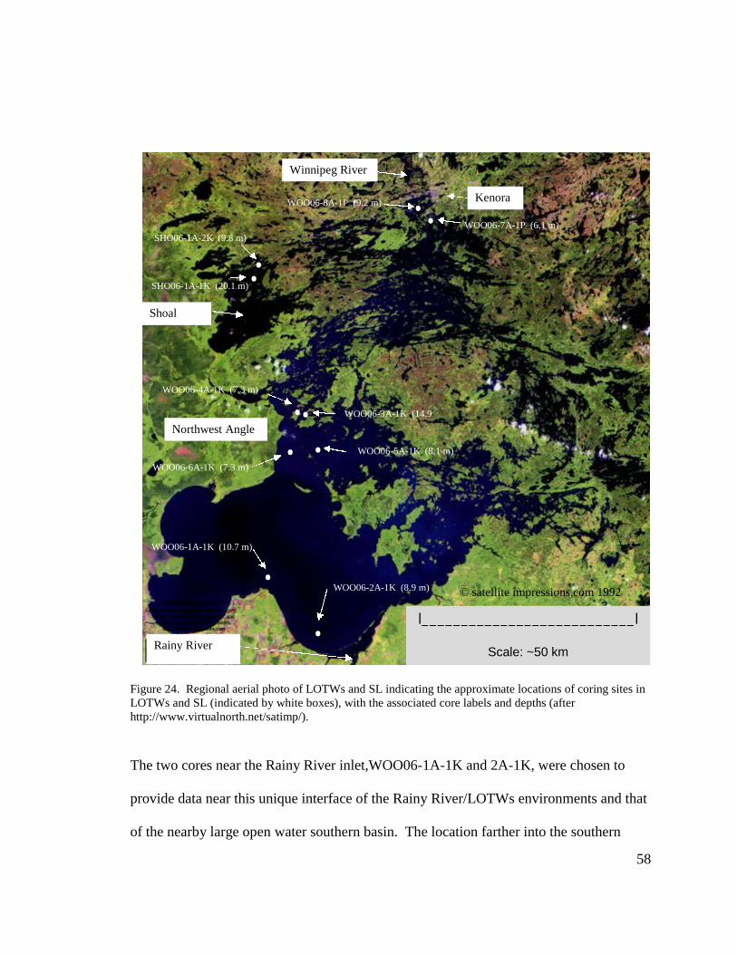
58

Figure 24. Regional aerial photo of LOTWs and SL indicating the approximate locations of coring sites inLOTWs and SL (indicated by white boxes), with the associated core labels and depths (afterhttp://www.virtualnorth.net/satimp/).

The two cores near the Rainy River inlet,WOO06-1A-1K and 2A-1K, were chosen to

provide data near this unique interface of the Rainy River/LOTWs environments and that

of the nearby large open water southern basin. The location farther into the southern

....

..

l___________________________l

Scale: ~50 km

..

..

Rainy River

Northwest Angle

Shoal

Kenora

Winnipeg River

WOO06-7A-1P (6.1 m)

WOO06-8A-1P (9.2 m)

SHO06-1A-2K (9.8 m)

WOO06-3A-1K (14.9)

SHO06-1A-1K (20.1 m)

WOO06-4A-1K (7.3 m)

WOO06-5A-1K (8.1 m)

WOO06-6A-1K (7.3 m)

WOO06-2A-1K (8.9 m)

WOO06-1A-1K (10.7 m)

© satellite impressions.com 1992

59

basin (WOO06-1A-1K) should provide information more closely related to the timing of

the southward lake transgression due to differential isostatic rebound. Although the

WOO06-1A-1K site is located farther to the west, it should still be representative of both

the southern basin paleoenvironment and the paleoenvironment associated with the inputs

from the nearby Rainy River.

The four mid-lake sites in the Northwest Angle area, two in the open expanse at the top

of the southern basin (WOO06-5A-1K and 6A-1K), and two additional sites in a deep but

narrow channel leading to the deeper northern basin of the LOTWs (WOO06-3A-1K and

4A-1K) likely represent an intermediate time in the history of LOTWs when the

southward LOTWs transgression entered the region (Yang and Teller, 2005). They

should provide a differing set of data due to their likely distinct paleoenvironments from

the southern basin.

The third LOTWs coring area near the northern outlets into the Winnipeg River drainage

system is in the deep and oldest portion of the lake and the cores (WOO06-7A-1P and

8A-1P), should provide another unique set of paleoecological and paleohydrologic

conditions. This location is near the outlets into the Winnipeg River and is in a deep

portion of the LOTWs which formed in the deep basin at the edge of the receding ice

sheet. This portion of the lake retained its relatively deep hydrology throughout the post

isolation history of LOTWs (Figure 9 and Figure 10).

60

2.2.5 Site Selection in Shoal Lake

The deep/shallow coring strategy was also applied in SL with the restrictions/limitations

related to rig operation and weather restrictions still applicable to the site selection

process. The two coring sites were separated somewhat (Figure 24) due to the generally

rocky shoreline and sharp offshore drop-offs in the lake in the selected coring area, and

concerns related to encountering a rocky substrate should the shallower coring operation

be conducted too close to shore. In addition a site too close to shore was undesirable due

to the potential for subaqueous slumping of materials on the steep near shore slope of the

lake bottom. This required some adjustments in final site selection. The SL coring

locations (SHO06-1A-1K and 2A-1K) are located in the northern portion of a broad open

expanse of the lake. SL provides data from a distinct paleoenvironment, and therefore

should provide the means to compare changes with those in LOTWs. Based on its

slightly higher elevation and location near the same differential isostatic rebound isobase,

SL would have operated independently from LOTWs for most of its history.

The lack of bathymetric data for SL required some preliminary rough bathymetric data to

be obtained prior to final site selection. Using a simple depth finder, several short

transects were run near the chosen coring area.

2.2.6 Core Recovery O

The Kullenberg Rig from

for sediment core recover

composed of the masts of

the core barrel assembly,

consisting of two hulls w

is transported using a larg

for assembly and launchin

polycarbonate liners, the

Kullenberg Rig platform,

mechanisms are all transp

Figure 25. LRC Kullenberg R

Operations

m the LRC at the University of Minnesota (Figure

ry operations in LOTWs and SL. The Kullenber

f the superstructure, pulleys and hydraulic devic

which is then assembled on a floating mobile pl

ith outboard motors bolted to the platform. The

ge SUV and trailer (Figure 26) to a shoreline loc

ng. A supply of core barrels of various lengths

necessary tools for field assembly and disassem

, and the core barrel suspension superstructure an

ported with the SUV and trailer.

Rig in the Southern basin of LOTWs, August 2006.

61

e 25) was used

rg Rig is

es, weights, and

latform

e Kullenberg Rig

cation suitable

and associated

mbly of the

nd hoisting

Figure 26. LRC Kullenberg RLOTWs August 2006.

The Kullenberg coring pr

core within a polycarbona

contained within the steel

cutter and core catcher as

(Figure 27) which rises w

water interface and is driv

core barrel. The vacuum

liner, in addition to the co

Rig trailer and SUV, preparing for rig assembly in the sout

rocess is a gravity coring system which recovers

ate (plastic) tube about 3 ½ inches (~ 9 cm) in d

l core barrel assembly. The core barrel assembl

ssembly on the lead end of the core barrel, and a

within the core barrel when it is released above th

ven downward by the weight assembly attached

created by the entry of the sediments into the po

ore catcher, ensures the sediments are retrieved w

62

thern basin of

s a single long

iameter

y includes a

a vacuum piston

he sediment

to the top of the

olycarbonate

when the core is

63

lifted to the rig platform using the hydraulic driven pulley assembly. The cross-shaped

slot (“moon pool”) in the platform allows the recovered core barrel to be manipulated

onto the platform (Figure 28). A “muck core” is also positioned beside the core barrel on

a trip lever, which is used to trigger the release of the core barrel assembly and to recover

the sediments across the water-sediment interface where pore water content is very high

(Figure 27) (Leroy and Colman, 2001). This short approximately 1 m core was

concurrently collected with the longer core.

Figure 27. Kullenberg gravity piston corer schematic showing the major core barrel assembly componentsand the operation of the sliding vacuum piston used to help retain the sediments (fromhttp://esp.cr.usgs.gov/info/lacs/piston.htm).

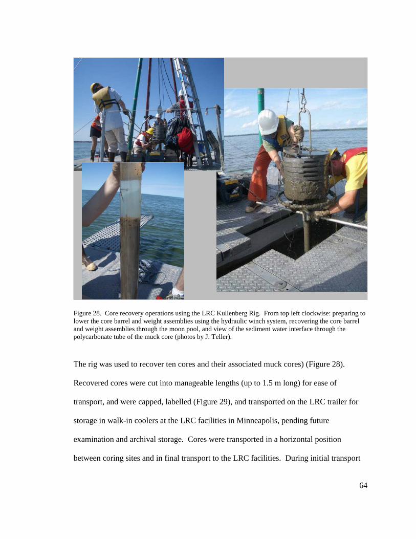
64

Figure 28. Core recovery operations using the LRC Kullenberg Rig. From top left clockwise: preparing tolower the core barrel and weight assemblies using the hydraulic winch system, recovering the core barreland weight assemblies through the moon pool, and view of the sediment water interface through thepolycarbonate tube of the muck core (photos by J. Teller).

The rig was used to recover ten cores and their associated muck cores) (Figure 28).

Recovered cores were cut into manageable lengths (up to 1.5 m long) for ease of

transport, and were capped, labelled (Figure 29), and transported on the LRC trailer for

storage in walk-in coolers at the LRC facilities in Minneapolis, pending future

examination and archival storage. Cores were transported in a horizontal position

between coring sites and in final transport to the LRC facilities. During initial transport

65

cores were stored in ambient conditions, and were not placed into coolers until they

arrived at the LRC.

Figure 29. Recovered cores in the polycarbonate liners cut and labeled in preparation for transport.

2.3 DETAILED DESCRIPTIONS OF CORING LOCATIONS

2.3.1 General

Coring location (Figure 24) details related to core recovery were recorded and are

provided in the following sections. Longitudes and latitudes of the coring sites are also

provided which are based on the readings from the LRC GPS unit on the Kullenberg Rig.

Water depths at the coring site are also provided along with the length of the recovered

core. It should be noted the normal water depths at the sites would be 5-6 feet (~2 m)

66

deeper than those recorded by the depth finder on the Kullenberg Rig, due to the

unusually low water levels. UTM coordinates (unofficial reading taken near the

Kullenberg Rig) were also taken using readings from a hand held GPS unit, or those

provided from the guide boat for Northwest Angle sites, and have been included where

available (for convenience). Similarly, unofficial water depth readings were taken, but

have not been included.

Subsequent to the coring operations, seven LOTWs cores were split, examined, scanned,

core logged and subsampled at the LRC Core Lab (WOO06-2A-1K and WOO06-8A-1P

were not examined). In SL only the SHO06-2A-1K core was processed.

2.3.2 LOTWs Southern Basin

Two cores (WOO06-1A-1K and WOO06-2A-1K) were recovered from the southern

basin (Figure 24) but only WOO06-1A-1K was processed at the LRC Core Lab. Access

to the coring site was made from Long Point which had a sheltered docking facility and a

wide sandy beach to facilitate Kullenberg Rig assembly/disassembly and had access to

nearby accommodations.

67

WOO06-1A-1K: latitude 48.99229o; longitude -94.92356o

This site is the deeper of two companion coring sites located in the southern basin near

the inlet from the Rainy River. It is directly off Long Point Resort, in the Minnesota

portion of Big Traverse Bay of LOTWs, about 2.5 km offshore and 17 km to the

northwest of the inlet of the Rainy River. Water depth at the site was ~ 10.7 m (35.1

feet), which was deemed suitable as the deep coring site, since the southern basin is

relatively flat and the depth at this site was reasonably close to the common basin depth.

Adjacent UTM coordinates (taken from the support boat), for this site were Zone 15;

E359287; N5428381. The recovered 3.3 m long core was cut into three core intervals

(1A-1K-1, 1A-1K-2, and 1A-1K-3), and 80 cm of sediment in the muck core was also

recovered.

WOO06-2A-1K: latitude 48.89121o longitude -94.82602o

This site is the shallower of two companion cores located in the southern basin near the

inlet from the Rainy River, about 3.25 km directly off Zipple Bay. Water depth at the site

was ~ 8.9 m (29.2 feet) which is only ~ 2 m shallower than the deeper companion core

but is closer to the mouth of the Rainy River and is located about 12 km to the west

northwest of the Rainy River inlet.

Adjacent UTM coordinates (taken from the support boat) were Zone 15; E366171;

N5416751. The recovered 3.6 m long core was cut into three core intervals (2A-1K-1,

68

2A-1K-2, and 2A-1K-3), and 80 cm of sediment in the muck core was also recovered.

This core was not processed and resides at the LRC core Lab.

2.3.3 LOTWs Northern Northwest Angle Channel Coring Sites

Two cores were recovered from Northwest Angle channel sites WOO06-3A-1K and

WOO06-4A-1K (Figure 24), with both coring sites located about 10 km to the east of a

sheltered docking facility at Young’s Resort, which is located on the southern shore near

the entrance to the Northwest Angle Inlet. Young’s Resort provided a sheltered docking

facility which accommodated the Kullenberg Rig assembly/disassembly and dockage,

and provided access to nearby accommodations. It also provided official access to

Canadian waters through a customs telephone service when access to the Ontario portion

of the lake was necessary.

Site WOO06-3A-1K: latitude 49.34714o; longitude -94.84379o

This site is the deeper of two companion cores with both located in the northeast trending

deep channel near Cyclone Island, to the east of the Northwest Angle Inlet. Water depth

at the site was ~ 14.9 m (48.9 feet) which closely approximated the nominal 50 foot core

depth for the deeper of the two companion LOTWs northern Northwest Angle channel

cores.

The released core barrel hit a hard object in the substrate causing the coring platform to

shake violently. The core was very difficult to retrieve but eventually was successfully

69

recovered to the deck of the Kullenberg Rig. The core barrel had been bent into a curve

and the core cutter on the end of the core barrel sustained damage from the impact with a

boulder or possibly bedrock. The weight stacker at the top of the core barrel assembly

was also bent and required a return to the launch area to obtain a spare before the

shallower companion core could be obtained. The polycarbonate liner was eventually

recovered from the bent core barrel and processed at the LRC Core Lab.

Adjacent UTM coordinates (taken from the support boat) were Zone 15; E366107;

N5467466. The 14.9 m long core was cut into six core intervals (3A-1K-1, 3A-1K-2,

3A-1K-3, 3A-1K-4, 3A-1K-5, and 3A-1K-6). Approximately 10 cm of core length were

lost, with about 5 cm bagged when removing the polycarbonate liner between 3A-1K-2

and 1K-3. Similarly about 5.5 cm were lost between 3A-1K-4 and 1K-5. Overall about

7.5 m of core were recovered along with 57 cm of sediment in the muck core.

Site WOO06-4A-1K: latitude 49.33830o; longitude -94.85979o

This site is the shallower of two companion cores located in the channel near Cyclone

Island. A slight current was noted in the channel. Water depth at the site was ~ 7.3 m

(24 feet) which closely approximated the nominal 25 foot shallow site criteria.

Adjacent UTM coordinates (taken from the support boat) were Zone 15; E3664908;

N5466509. The recovered 2 m long core was cut into two core intervals (4A-1K-1, and

4A-1K-2). The muck core material was lost during retrieval. A granular, possibly

70

pedogenic, greenish grey sediment was observed through the polycarbonate liner about

20 cm from the bottom of the core, overlain by 15 cm of dark grey sediment, with the

interval above a grey clay like sediment.

2.3.4 LOTWs Northwest Angle Basin Coring Sites

Two cores (WOO06-5A-1K and WOO06-6A-1K) were recovered from the open basin to

the south of the Northwest Angle (Figure 24) and processed at the LRC Core Lab. Shore

access to these sites was the same as the two northern Northwest Angle channel coring

sites.

Site WOO06-5A-1K: latitude 49.27928o; longitude -94.82007o

This site is the deeper of two companion cores located in a relatively open portion of the

northern part of the southern basin, to the west of Massacre Island and about 13 km to the

southeast of the entrance to the Northwest Angle Inlet. Water depth at the site was ~ 8.1

m (26.6 feet) which is much less than the proposed nominal depth for the deeper

companion core site strategy (50 ft), but was the deepest water in this part of the lake.

Adjacent UTM coordinates (taken from the support boat) were Zone 15; E367641;

N5459872. The recovered 5.5 m long core was cut into five core intervals (5A-1K-1,

5A-1K-2, 5A-1K-3, 5A-1K-4, and 5A-1K-5), with 60 cm of sediment in the muck core

also recovered. Additionally, 6 cm within the core catcher were retrieved and 7 cm

within the core bit. Bottom clays were noted half way up the weights at the top of the

71

core barrel, indicating that the top of the core may have penetrated a few tens of cms

below the floor of the lake.

Site WOO06-6A-1K: latitude 49.28098o longitude -94.89926o

This site is the shallower of two companion cores located in a relatively open portion of

the northern part of the southern basin, about 6 km farther to the west of the Massacre

Island deeper coring site. Water depth at the site was ~ 5.9 m (19.4 feet) which although

not close to the nominal depth for the shallow companion core site (25 ft), was as deep as

possible in this part of the lake while remaining within the restrictions of the Kullenberg

Rig.

Adjacent UTM coordinates (taken from the support boat) were Zone 15; E361907;

N5460214. The recovered 3.8 m long core was cut into three core intervals (6A-1K-1,

6A-1K-2, and 6A-1K-3). The muck core failed to recover any sediment and manual

actions were taken to recover about 45 cm of material from the sediment water interface.

72

2.3.5 LOTWs Northern Outlets - Kenora Coring Sites

Access to this portion of the lake was made using a docking facility at Anicinabe Park in

the southern most portion of the town of Kenora, Ontario. Rig assembly was complicated

somewhat by the relatively high volume of users at the docking facility. Two cores were

recovered from the northern outlet Kenora region WOO06-7A-1P and WOO06-8A-1P

(Figure 24), with only the WOO06-7A-1P core processed at the LRC Core Lab.

Site WOO06-7A-1P latitude 49.72984o longitude -94.51310o

This site is the deeper of the two companion cores located near the outlets to the

Winnipeg River just south of the town of Kenora, Ontario, amidst a complex series of

channels connecting to deeper portions of the deep northern basin. Water depth at the

site was ~ 6.1 m (20 feet) which although not close to the targeted depth for the shallow

core (25 ft) was reasonably close and as deep as possible in this part of the lake, under the

low water conditions encountered during coring.

UTM coordinates (from the LRC GPS) for the site were Zone 15; E390931; N5509911.

The recovered 4.6 m long core was cut into four core intervals (7A-1P-1, 7A-1P-2, 7A-

1P-3 and 7A-1P-4) and about 80 cm of sediment in the muck core was also recovered.

73

Site WOO06-8A-1P: latitude 49.74471o longitude -94.52096o

This site is the deeper of two companion cores located in the northern basin near the

outlets to the Winnipeg River and was located just to the south of Kenora on the south

side of Coney Island, about 3 km to the south of the Winnipeg River outlets. Water depth

at the site was ~ 9.2 m (30.2 feet) which is about 3 m deeper than the companion core.

Adjacent UTM coordinates (taken from the support boat) were Zone 15; E390423;

N5511358. The recovered ~ 4.25 m long core was cut into three core intervals (8A-1P-1,

8A-1P-2, and 8A-1P-3) with 60 cm of sediments in the muck core also recovered. A dark

grey interval was noted at the top of the core down to about 77 cm before a distinct

change to a lighter grey was noted; the dark colour may be due to anthropogenic inputs

when the island was in heavy use as a cottage area. A rhythmically bedded sequence was

noted in WOO06-8A-1P 2 and a distinct contact was noted about 0.5 m from the bottom

of the core in between what appears to be clay, and a sandy silt. This core was not

processed and resides at the LRC core Lab.

2.3.6 SL Coring Sites

Two cores were recovered from SL, SHO06-1A-1K and SHO06-2A-1K (Figure 24), with

only SHO06-2A-1K processed at the LRC Core Lab. Access to the sites was made from

a resort on the north shore about a 1 km to the west of Clytie Bay, which provided

docking facilities.

74

Site SHO06-1A-1K: latitude 49.59605o longitude -95.03322o

This site is the deeper of two companion cores located in the northern part of an open

basin of SL about 4 km from the north shore to the west of Clytie Bay. Water depth at

the site was ~ 20.1 m (65.9 feet) which is considerably deeper than the nominal depth of

50 feet for the deep coring site.

Adjacent UTM coordinates (taken from the support boat) were Zone 15; E356323;

N5497880 (using University of Manitoba GPS). The recovered 6.9 m long core was cut

into six core intervals (SHO-1A-1K-1, SHO-1A-1K-2, SHO-1A-1K-3, SHO-1A-1K-4,

SHO-1A-1K-5 and SHO-1A-1K-6) with 60 cm of sediments in the muck core also

recovered. Difficulty was experienced in removing the polycarbonate liner from the core

barrel as the liner had collapsed. Significant hammering was required to remove the core

and as a result, this core was not processed but remains at the LRC core facility.

Site SHO06-2A-1K: latitude 49.59796o longitude -95.03353o

This site is the shallower of two companion cores located near the northern part of the

open basin of SL, with this site about 1 km from the north shore near Clytie Bay in a

narrowing part of the lake. Water depth at the site was ~ 9.8 m (32.2 feet) which is a

little deeper than the targeted depth (25 ft) for the shallow core site.

Adjacent UTM coordinates (taken from the support boat) were Zone 15; E353057;

N5495918. The recovered 6.8 m long core was cut into six core intervals (SHO-2A-1K-

75

1, SHO-2A-1K-2, SHO-2A-1K-3, SHO-2A-1K-4, SHO-2A-1K-5 and SHO-2A-1K-6)

with about 50 cm of sediments in the muck core also recovered.

2.4 CORE PROCESSING AND SUBSAMPLING

2.4.1 Removal of Sediment from Core Barrel

Transported cores were recovered from the temporary storage coolers at the LRC and

prepared for examination. The ~ 6.5 cm diameter polycarbonate liners of the cores were

split using small vibrating cutters in a special core cutting machine at the LRC, which cut

most of the way through the liner. A utility knife was then used to complete the cutting

of the liner and care was taken to ensure that polycarbonate fragments were not

introduced into the sediments within the liner. A long thin blade was placed along the cut

length of the polycarbonate core liner and pressed through the sediments to separate the

core into two halves. Alternately, when the consistency of the sediment within the liner

was deemed sufficiently stiff, a fishing line was pulled along the length of the core to cut

the core into two halves. The fishing line provides a cleaner cut but can only be used

when the sediment is stiff enough to ensure the two halves remain apart.

One half of the split core was further processed, with the other half covered with a plastic

wrap and scanned using a Geotek multi-sensor core logger. This core logger records

density and magnetic susceptibility values along the core. Subsequently both core halves

were carefully wrapped in a plastic wrap, inserted into a heavier plastic sleeve, sealed,

76

inserted into a hard plastic core storage box specially designed for core protection and

efficient long term storage, and labelled. Half of the core was retained by the LRC in

their long term archive facility.

The other half of the core was used for visual examination, core logging and

subsampling. The split core was smoothed to enhance the visibility of stratigraphic

features along the length of the core, using glass slides pulled carefully across the core

until a smooth surface is obtained. The core was then scanned using a core scanning

facility to obtain a permanent photographic image, which was subsequently used as part

of a core logging and description process, and provides an undisturbed visual record of

the core stratigraphy.

2.4.2 Subsampling Strategy

Core subsampling was conducted using the non-archive half of the split core, following

core logging and description (Figure 30). Core subsample size was set at 15 mL, which

corresponds with the plastic sampling containers available at the LRC, and seemed to be

of a reasonable size to allow an ostracode population analysis. The objective was to

obtain a minimum of 20 ostracode tests for species population studies in each sample.

The 15 mL sample size spanned about 2 cm along the length of the half core and

consumed about one half of that half (i.e. one quarter of the full core diameter) (Figure

30). Some sample sizes were based on the size of the targeted materials (e.g. wood

fragments).

77

The initial core subsampling process was based on a number of factors, including the

need to obtain a relatively consistent ostracode sample interval along the core, extraction

of any observed biological carbon materials suitable for radiocarbon dating, and the time

available for subsampling at the LRC facilities. These initial sampling intervals were

later modified during subsequent resampling programs, based on the need for additional

material for radiocarbon dating, the need to characterize or date additional stratigraphic

intervals, and the need for additional biostratigraphic data (e.g. ostracodes and

thecamoebians).

Figure 30. Core subsampling at the LRC of the non-archive half of the split core, using one quarter of thecore diameter and the typical subsampling span along the core length of about 2 cm. The subsample plasticsampling containers are shown on the right (photos by J. Teller).

78

The initial sampling of the cores was based on a relatively wide sampling interval

(typically every 20 cm) which tried to capture ostracode biostratigraphic information

along the core length. Shorter sampling intervals and specific sample locations along the

core were also selected based on the observations from the core logging and description

process. These adjustments to the initial sampling interval or the decision to include

specific sample locations were based on identification of specific stratigraphic features of

interest, or the identification of locations which appeared to contain materials suitable for

radiocarbon dating. The unexpected presence of paleosols in some cores required an

immediate adjustment to the core sampling intervals in these regions.

When the subsample analysis of the initial set of sampled cores was completed, the

sampling strategy was adjusted as required to obtain additional data. Specifically, the

lack of ostracodes in the upper portions of the first cores studied (WOO06-5A-1K,

WOO06-6A-1K, and SHOO06-2A-1K); indicated ostracodes were not present along the

entire core length and hence could not provide a complete paleoenvironmental record of

the entire core sequence as was initially anticipated. Subsequently, it was decided to add

thecamoebians to the study as a means to add paleoenvironment information, particularly

in the upper cores where ostracodes were not present. To obtain this additional

thecamoebian data, sample intervals were adjusted in previously subsampled cores. In

effect, the sampling program was iterative, and sampling was carried out in progressive

steps as it became evident additional data was required.

79

Subsamples for radiocarbon dating were selected in order to establish the time frame of

the stratigraphic sequences in each core. In some cases identifiable vegetative fragments

and organic rich laminae were observed at the surface of the split core and were removed

for dating. In other cases samples at specific intervals were taken and sent to Alice Telka

of Paleotec Services in Ottawa, to pick suitable macrofossils that were likely to provide

an unambiguous date (i.e. material that had not been reworked from older sediment). In

addition, it was important to date the beginning and end of ostracode sequences, and

beginning of the thecamoebian intervals. For certain cases, further subsamples were

taken for radiocarbon dating to determining the beginning and end of paleosols identified

in the WOO06-5A-1K, WOO06-6A-1K and WOO06-4A-1K cores. Samples were also

taken to date pollen in those parts of the cores (primarily at the bottom of the cores),

where there are very limited macrofossils with suitable organic materials available for

radiocarbon analysis.

Further intensive sampling was undertaken in the Kenora and SL cores (WOO06-7A-1P

and SHO06-2A-1K) to provide materials to permit a thecamoebian species analysis by a

thecamoebian specialist. Unfortunately this analysis is not available at the time of the

writing of this thesis. Similarly, samples were taken to permit a diatom study in the

Kenora core (WOO06-7A-1P) by the Paleoecological Environmental Assessment and

Research Laboratory (PEARL) at Queens University, Ontario Canada, but it is only

partially complete at the time of the writing this thesis.

80

In addition, samples were taken to perform a moisture analysis on several cores,

especially near the paleosol horizons in the deeper water of the southern Northwest Angle

core (WOO06-5A-1K). Samples were also obtained from the Kenora core (WOO06-7A-

1P) to perform a broad qualitative XRD analysis at the northern outlet, to see if there

were any significant changes in the mineralogy at this location. Moisture Data is

provided in Appendix D.

2.4.3 Macrofossil Processing Strategy and Methodology

2.4.3.1 Ostracodes

Sample processing was conducted using the techniques employed for studying ostracodes

by Dr. Brandon Curry of the Illinois Geological Survey at the University of Illinois. This

technique was subsequently used for all macrofossil sample processing, except those used

by external contractors. Although this sample processing was developed for ostracode

studies, the other macrofossils recovered using this methodology did not appear to have

been adversely affected. As the core sampling program evolved to include

thecamoebians, the same sample processing method for separating the clay and silt

fractions was retained. Some sieving operations (discussed later) were modified

somewhat, and examinations of the macrofossils broadened to identify the other

macrofossils and record the data they provided.

Data was initially recorded on subsampling data sheets, primarily designed to facilitate

the recovery of ostracode data, and relevant additional data such as those provided by

81

other macrofossils and sediment characteristics including mineralological lithics. These

data sheets were revised following the processing and data extraction of the initial

subsamples, to facilitate recording of observations including notes and sketches of

observed macrofossils (Figure 31). This revised data sheet was used for most of the

processed subsamples, with a similar though less structured sample form used to record

the data of the initial processing campaign for the Northwest Angle open basin cores and

the SL core (WOO06-5A-1K, WOO06-6A-1K, and SHO06-2A-1K).

The sampling intervals in the cores were initially selected to obtain a consistent sample

interval along the core and hence the means to trend any changes in the ostracode

populations. The core sampling intervals were modified in subsequent sampling

campaigns for a number of reasons, with the sampling interval often supplemented in

certain regions to obtain additional data to improve discrimination in regions deemed to

be of particular interest (Figure 30). Additionally, the core sample interval was shortened

to permit further discrimination near the point of disappearance of ostracodes and first

appearance of thecamoebians. The data from the subsample data sheets are presented in

Appendix A, Section 2 for each core.

82

Figure 31. Subsampling data sheet used to capture information related to ostracode populations andsubsequently to gather the available data related to thecamoebians and other macrofossil data, including theabundance of lithics, plant material, charcoal, and insect material.

#MOMOS WOO06

Sample # ___________________Depth in Core _______________Date _________________________________

Colour ____________ Consistency _______________________________Moisture Content ____________________

Petri Dish View:Lithics Type ___________________________________________________________

Size ___________________________________________________________Roundness _________________________________________________________Sample Proportion ____%

Organics Plant Mat'l ____________________________________________________________________________________________________________________________________________________________________datable ?____leaves ___ Stems ___ Wood Frgmts ___ Seeds___ Others ________Sample Proportion ____%

Charcoal __________________________________________________________________________________________________________datable ?____Sample Proportion ____%

Insect Mat'l _______________________________________________________________________________________________________________________________________________________________________________exoskeleton ____ larvae cases ____Sample Proportion ____%

Thecamoebans _____________________________________________________

Other organics _____________________________________________________

Datable Material Yes____ Description: ______________________________

Ostracodes _____Type _________Prelim. Count _________________________

Sieve # 35

Sieve # 60

Sieve # 80

Pan

Adults A-1 TotalOstracode Totals sub triangulata

friabilisrawsonisharpei

sketches

Lake of the Woods Core Samples

Sample Description

83

To reduce microbial growth in the sediment samples, the subsample containers were

stored in a cooler whenever possible. Prior to processing of each sample, a rough

estimate of the moisture content in each sample was made, and its general colour was

noted. The amount of material in the sample container was also noted and recorded on

the subsampling data sheets, since some containers were not completely full due to

variabilities in sample consistency and difficulties in extracting samples. The consistency

of each sample (i.e. how well the material held its shape) was also recorded.

The material was extracted from the sample containers and placed in a 500 mL beaker,

and 1 g of baking soda and about 0.1 g of commercial Calgon (sodium carbonate, and

sodium hexametaphosphate) were added to facilitate disaggregation of the clay to silt

sized sediments (i.e. to deflocculate and disperse the material) and assist in the separation

of the macrofossils from this material. About 150 mL of distilled water, heated to boiling

in a microwave oven, was poured over the sediment, and the samples were allowed to

disaggregate for several hours. The disaggregated sediment was then washed through a

12 inch # 100 mesh (150 micron) U.S. standard brass sieve (ASTM E-11 specification),

using hot tap water sprayed onto the sample material using a flexible water spray hose.

Care was taken during sieving to ensure material was not lost over the sieve edge. The

sieve was tilted back and forth under the spray to separate sand-sized and coarser

material, with the clay and silt fractions washing through the sieve and down the drain.

In some cases, particularly in gyttja deposits, the sample had to be left overnight in the

Calgon solution, or occasionally the process had to be repeated, before disaggregation

occurred.

84

The disaggregated materials on the sieve were transferred to a petri dish using distilled

water from a spray bottle, where a preliminary viewing of the recovered material was

conducted using an optical (non-polarizing) microscope. Descriptions and sketches of

the macrofossils were then recorded in the subsample data sheet. The petri dish was then

placed in a fume hood, and allowed to dry at room temperature.

The > 150 micron dried materials were subsequently dry sieved. The dried materials in

the petri dish were carefully transferred using a stiff brush into a nested set of three, 8

cm-diameter U.S. standard brass sieves [(ASTM E-11 specification) (#35, #60 and # 80

mesh; 500, 250 and 180 ) and a catch pan]. The sieve set was then covered and tapped

on a flat surface to complete the sieving process.

The materials from each sieve were transferred to a counting tray by tapping the contents

of the sieve into a 9 x 5 cm black counting tray with 1 cm grids. The dark colour and

grids facilitated identification and counting of the ostracode macrofossils using an optical

binocular, non-polarizing microscope (Kyowa model FBO 99-001; 0.7 - 4.5

magnification). Sieve contents which were not released by tapping were brushed into the

tray to ensure all the materials were transferred. This process was repeated for each of

the three sieves, plus the catch pan. Ostracode species and their instars vary in size and

are captured on the various sieves. The capture location of the ostracode shell on the

various sieves assists in identification of the ostracode species and in identifying the adult

and A-1 (last instar) shells. Both the adult and A-1 instars were counted and recorded.

85

All the ostracode macrofossils were then transferred to 3 x 1 inch (7.5 x 2.5 cm)

microslides to permit storage of the materials and re-examination if necessary. The

microslides have a 3.6 x 1.6 cm storage area with 4mm x 4mm grids and a glass cover

which can be opened, permitting materials to be removed (e.g. for adding to radiocarbon

samples).

Ostracode tests and other macrofossils, plus selected representative mineral rock

fragments (lithics), charcoal and various organic materials, were transferred to the

microslide with a picking brush (# 3/0). The picking brush was dipped in demineralized

water to facilitate material transfer (the surface tension of the water causes any material

the brush contacts to adhere to the brush). Additionally, most of the charcoal and datable

organic materials collected on the sieves, and some of the larger pieces from the

collection pan which captures materials which pass through the nested sieves, were also

transferred to the microslide. Representative lithics, insect carapace fragments and larvae

cases, and other materials including bones, teeth, fish scales and thecamoebians were

transferred. In some cases where there were large amounts of organic materials (other

than ostracodes) and only representative samples were transferred to the microslides.

The remaining material from the counting tray and catch tray were then transferred back

to the original 15 mL sample container and stored. The data from the observations made

in the counting tray were transferred to the subsample data sheet and sketches were made

of the biota. Ostracode species were identified using publications by Delorme (Delorme,

1970a; Delorme, 1970b; Delorme, 1970c; Delorme, 1970d; and Delorme, 1971a) and

86

through application of the training provided by Dr. Brandon Curry of the Illinois

Geological Survey.

Following the sieving processes, the dry sieves were vigorously tapped to release all

materials trapped in the sieves and the stiff brush was used to release and remove trapped

materials to ensure cross contamination between various dry sieving operations were

eliminated. Similarly the counting tray was tapped, brushed and cleaned with

demineralised water and wiped with a lint free wipe (Kimwipe). The wet tray used to

wash the sample was reverse flushed between sample processing operations to remove all

visible materials. The picking brush and stiff brush were both visually inspected to

ensure dried materials were not captured within the bristles.

2.4.3.2 Thecamoebian Subsampling

Thecamoebians were noted in the materials removed from the clay and silt fraction of the

sediments during the initial sampling campaign for ostracodes. Although thecamoebian

macrofossils are typically much more fragile than ostracodes, they did not appear to have

been damaged by the processing, although transferring the thecamoebians after

processing did result in some of them disintegrating, so special care was needed to

transfer these tests intact. It is also likely some thecamoebians may have been damaged

during the initial dry sieving operations to remove ostracode shells.

87

The subsampling process developed for ostracodes was used for extracting

thecamoebians from the clay and silt sediment fractions. Once the subsample was

processed and washed into the petri dish, preliminary observations were made and

recorded. The objective of the thecamoebian sampling was only to identify their

presence; hence there was no requirement to dry sieve the processed and dried subsample

in non ostracode bearing intervals. After the initial sampling campaign if no ostracodes

were observed in the petri dish, dry sieving was not conducted. In rare cases, a small

number of ostracode tests were observed in the same sample as thecamoebians, and full

processing was carried out including dry sieving to facilitate the capture of the ostracode

data.

For the thecamoebian intervals the dried contents of the petri dish were transferred to the

counting tray, and more thorough observations of macrofossils, were made to facilitate

data recovery. Transfer of macrofossils to microslides was completed using the same

process used for ostracodes.

88

2.4.3.3 Macrofossil and Lithic Materials Subsampling

Macrofossils were extracted when ostracode or thecamoebian samples were processed.

Following wet sieving and drying of subsamples in a petri dish, and either dry sieving

(ostracode samples), or direct transfer of dried materials (thecamoebian samples), the

material was transferred to the counting tray. From here, all larger fragments of charcoal

> 180 were transferred to the microslide including some of the charcoal fragments from

the dry sieve catch tray (150-180 ). Additionally, typical macrofossils and lithics were

transferred to the microslide. These data were then recorded on subsample data sheets

and sketches made. Observations related to the abundance of the macrofossils as well as

the recording of the presence of other macrofossil materials such as bones, teeth, fish

scales, seeds etc. were recorded on the data sheets. Additionally, the presence of

potentially datable organic materials, based on the quantity of the material and whether

fragile appendages were retained by the organic fragments, were recorded to assist in

selecting materials and intervals suitable for future radiocarbon dating.

Initially, exposed organic materials were extracted from the split core for radiocarbon

dating during the macrofossil subsampling process at the LRC. Subsequently, selected

organic materials from processed subsamples which had been transferred to the

microslides were sent to Paleotec Services along with additional core subsamples.

Paleotec Services selected suitable materials from these sources for AMS dating and in

some cases combined these materials if appropriate, to obtain sufficient material for

radiocarbon dating. The selected organic materials were subsequently sent to the Keck

89

Carbon Cycle AMS Facility at University of California, Irvine. Through the iterative

core sampling process, additional subsamples were also obtained, and sent directly to

Paleotec Services. In addition, Paleotec Services identified selected flora and fauna, and

used these data for ecological interpretations which are used to help assess

paleoecological conditions in LOTWs.

The separated lithic materials were also observed. Their mineralogy and general physical

attributes (size, roundness, and abundance) were recorded. Additionally, charcoal

fragments were observed and noted when processing the subsamples, and their size and

abundance in the sample were recorded.

2.4.4 XRD Analysis

Only a very qualtitative assessment from bulk sediment X-ray diffraction (XRD) samples

was completed at several broadly spaced intervals in the Kenora core (WOO06-7A-1P).

The objective was to see if any significant mineralogical changes through time could be

identified in the LOTWs sediments near the outlet to the Winnipeg River. Five samples

were taken in what appeared to be diverse sections of the core. Two samples were taken

in the upper core, one near the top and the other mid-core. Additionally, one was taken

near and above a pink clay unit; one in the pink clay unit; and one was taken below the

pink clay unit near the bottom of the core. The bottom two samples were taken in what

appeared to be Lake Agassiz sediment.

90

The XRD samples were obtained from freeze dried samples which had been used for

moisture analysis. These were crushed to a fine powder, and then a paste was made and

smeared onto slides. These slides were loaded into a Phillips PW1710 Powder

Diffractometer using Cu radiation and scanned. The powder diffraction pattern produced

was then read into MDI Jade 6.1 Pattern Processing Software to identify the major

mineralogical components. The Jade XRD plots are located in Appendix C.

2.4.5 Moisture Analysis

To assess changes in sediment moisture content a series of subsamples were taken in

several cores. Samples were prepared and processed by James Teller using the LRC

freeze drying equipment and procedures. The wet subsamples were weighed in their

original 15 mL sample containers and placed on a metal tray and frozen. They were then

placed in the freeze drier and a vacuum was applied overnight or until the vacuum gauge

read about 10-1 mbar. The dry subsamples were then weighed and the data was

processed.

In the Northwest Angle core (WOO06-5A-1K), which contained a number of paleosols,

extensive sampling was performed extracting 10 mL samples at 10 cm intervals, with

shorter sample intervals near the buried soil horizons.

Other cores studied for moisture content include the southern basin core (WOO06-1A-

1K), the deeper of the Northwest Angle channel area sites (WOO06-3A-1K), and the

91

Kenora core (WOO06-7A-1P). The latter was sampled along the entire core using a 10

cm sampling interval. A broad moisture profile was also taken in the SL core (SHO06-

2A-1K); only the last two segments of this core were sampled with intervals 15-50 cm

apart. All samples were processed at the LRC using LRC freeze drying equipment, and

data is located in Appendix D.

92

CHAPTER 3 RELATIONSHIPS OF STUDIED PROXIES TOENVIRONMENTAL CONDITIONS

3.1 GENERAL

Cores from LOTWs and SL provide evidence of changing paleohydrology and

paleochemistry in the lake. For shell building biota the availability of CaCO3 is essential.

Carbonate is mainly derived from Paleozoic rocks, which are found in glacial erosional

deposits and in subsequent aqueous transport and deposition in the LOTWs region, and in

generally thicker glaciolacustrine deposits (Minning et al., 1994) (see Figure 16 and

discussion in Section 1.4.3). This would have supplied bicarbonates and calcium ions to

Lake Agassiz as well as LOTWs and SL. The shell building organisms within the

LOTWs lacustrine cores, including those specifically adapted to the cold deep waters of

Lake Agassiz, such as certain species of ostracodes, are markers and are useful in

differentiating Lake Agassiz from the subsequent and more modern lake conditions.

Interpretations of the timing of the climatic responses and magnitude are however

dependant on lake morphology, and the geological and hydrological settings (Laird et al.,

2003). Influences from the groundwater inflows have been determined to be substantial

in prairie lakes and affect the biota making it difficult to extract climate proxy data

normally derived from evaporation and precipitation cycles (Laird et al., 2003). In larger

complex lakes local inflows (surface and groundwater) can influence the chemistry in a

region of the lake, or within a local bay (Laird et al., 2003). The groundwater inflows in

the southern basin glacial and lacustine deposits of LOTWs may have had an influence

93

which differs from the groundwater inflows from other parts of LOTWs, which are

located in Precambrian Shield topography (Figure 16). Groundwater influences on

paleochemistry were noted in the Wampum site very near the western part of the southern

basin of LOTWs.

Ostracode macrofossils and the nature of the sediment were studied in this thesis as the

primary means to identify changes in paleohydrology and paleoenvironments. It is

important however when attempting to extract climate signals from sediments that other

means be used to confirm and enhance interpretations. Many proxies are available, and

climatic interpretations are best made through the use of a multi-proxy approach (Booth

and Jackson, 2003).

Thecamoebians were also used to gain insight into changing conditions. The presence of

thecamoebians was noted and radiocarbon dates obtained to establish the timing of their

appearance. A cursory thecamoebian species analysis was performed in some cores.

Additionally, macrofossils of plant and insect biota, vertebrate bones, fish scales, and

charcoal, were recovered as useful proxies for assessing changing paleoenvironmental

conditions within the lakes (Birks, 2001; Booth and Jackson, 2003), as well as the means

to obtain materials for radiocarbon dating.

The macrofossils within the sediments not only provide an indication of the ecological

conditions within the lake, but also within the watershed of the lake, and in the case of

many microfossils such as pollen, beyond the watershed (Birks, 2001). Macrofossil

populations (including datable organic materials) are typically much lower than

94

microfossil populations, making sediment studies dependant on the availability of the

macrofossil proxy (Birks, 2001), which forces a multiple proxy approach in order to

understand paleoclimate conditions. This was encountered in LOTWs where the

ostracode proxy populations were often limited, and in the upper portions of the cores

unavailable in the record. Furthermore, in the case of larger lakes macrofossil dispersion

can be limited, and their presence can indicate a more local lacustrine condition or nearby

watershed terrestrial conditions (Birks, 2001), and hence can be better suited for

establishing the local environmental.

Sediment data were also obtained from the study of core sediment structures and textures,

including paleosols, moisture analysis, and a qualitative XRD analysis. The properties of

the lithics in processed subsamples were also observed and recorded, including the

physical and mineralogical properties of various large lithic grains, which provided

further information on changes in the depositional environments.

In summary, a multiproxy approach was used, including available macrofossil,

microfossil and sedimentological data from the cores, and was used to relate these data to

the changing paleoclimate in the LOTWs region and the changing paleohydrology of

LOTWs and SL.

95

3.2 USE OF OSTRACODES IN PALEOENVIRONMENTRECONSTRUCTIONS

3.2.1 General

Ostracodes are typically benthic or epi-benthic, and crawl or weakly swim to feed on the

available detritus (which is a prime factor in their existence) (Cohen, 2003). Ostracodes

undergo ecdysis (molting) and typically have up to eight instars in their juvenile stages

before the adult stage (Horne et al., 2002). Ostracodes usually reproduce sexually but

can reproduce by parthenogenesis when stressful environmental conditions are

encountered (Curry and Yansa, 2004). Their eggs can remain viable for years up to

decades, should they desiccate (Horne et al., 2002). Life spans range from a few months

to up four years (Horne et al., 2002).

Ostracodes are aquatic crustaceans of the class Ostracoda with adults typically ranging

from 0.5 to 3.0 mm. They mainly occupy marine and non-marine environments such as

lakes, ponds and streams, although some species occupy moist terrestrial regimes such as

those in mosses, soils and leaf litter (Holmes, 2001; Horne et al., 2002). Their bivalve

carapaces are strongly calcified and preserve well, with their fossils ranging in age from

the present to as far back as 500 million years (Horne et al., 2002). The ostracodes of

interest for Holocene studies are Subclass Podocopa, Order Podocopida, which is well

represented in Quaternary sediments (Horne et al., 2002), as long as the pH of the water

is above 8.3, otherwise their calcite shells may not be produced because calcite saturation

is inhibited, or their preservation made unlikely (Delorme, 1989; De Decker, 2002).

96

Ostracode bivalves enclose the body and 5-8 appendages which the organism uses for

locomotion in crawling over the substrate or swimming (Horne et al., 2002; De Decker,

2002). Ostracodes are restricted to certain ecological conditions determined by available

habitats and climate, and can be limited by the physical and chemical conditions of the

habitat (Delorme and Zoltai, 1984; Curry, 1999).

Ostracodes can provide information about and trends in water chemistry, physical habitat,

and paleoclimate from fossil records because they can be related to modern fauna

ecological conditions (Delorme, 1989). The presence of certain ostracode species can

also be used to try and identify paleoecological conditions, based simply on the presence

and absence of the ostracode species (Curry and Yansa, 2004). Paleoecological analyses

have been used to develop ecological models to indicate the environmental ranges of

ostracodes (Smith and Horne, 2002).

The calcite ostracode shells preserve well and record the chemistry in the aquatic

environments they occupied (Chivas et al., 1986). Ostracode shell geochemistry,

including Sr/Ca and Mg/Ca ratios, have been used as a means to establish

paleotemperatures and paleosalinity of lakes and this is then related to paleoclimate

(Chivas et al., 1986). In some northern U.S. prairie lakes, paleoclimates have been

reconstructed through salinity studies (Fritz et al., 2000; Haskell et al., 1996). Studies

based on ostracode shell trace elements and sediment bulk-carbonates, compare well with

the diatom-based salinity proxy (Fritz et al., 2000). These analyses have been

97

successfully used to identify and establish durations of drought sequences in regional

climates although a multi-proxy approach is required (such as pollen) (Haskell et al.,

1996; Ito, 2002). The best lakes for these studies are in simple closed-basins, with

catchment areas that have not changed over the time interval of the study (Chivas et al.,

1986).

3.2.2 Using Ostracodes as Paleoenvironmental Indicators

Ostracodes have been successfully used in many paleoenvironment reconstructions. An

autecological method has been used to relate modern ostracode population data from

specific bodies of water to fossil ostracode assemblages, by using a best match process to

assess the paleo conditions (Delorme, 1969; Smith et al., 1992; Curry and Delorme,

2003). This, in conjunction with an understanding of the environmental tolerances of

species, can provide a means to interpret the environments of the fossil ostracode

assemblages (Delorme, 1969; Curry, 1999), although the farther back in time from the

modern ostracode environments the greater the uncertainty (Smith, 1991).

Environmental Tolerance Indices (ETIs) have been produced to assist in relating

ostracodes species to specific environments (Curry, 1999; Smith and Horne, 2002; Davis

et al., 2003).

Unlike terrestrial organisms, ostracodes do not rapidly respond to many climatic changes

due to their isolation within the hydrosphere; they do however, respond to longer term

climate variability, particularly precipitation/evaporation balance (Curry, 2003). This

98

balance affects the hydrochemistry of lakes and strongly influences ostracode populations

(De Deckker and Forester, 1988) (see next section). Water temperatures also affect

ostracodes but to a lesser degree (Curry, 2003).

Hydrochemical influences include basin overflows, groundwater inflows, and water

residence times, as well as climate and the underlying geology of the lake and watershed

(Curry, 2003). Even the surrounding overlying organic terrestrial materials can leach

carbonates or other elements into the lake, due to the acidity of the organic litter

(Delorme 1969).

Ostracode populations, both the species and their abundance, can be used to track

changes in lake depth (Curry, 2003). Mobile ostracode species populations tend to

increase in shallower conditions, due to the additional sunlight reaching the bottom which

increases vegetation, and therefore the ostracodes (Curry, 2003). Shallow water

environments are thermally variable and subject to wave action, and ostracode species

living in this ecological zone need to be tolerant to a wide range of conditions including

waves and wind induced currents (Curry, 1999). In deepening periods, benthic

burrowing species increase in the dark and muddy water/sediment interface (Curry,

2003). The absence of ostracodes can also mean the shells were leached from the

sediments due to diagenetic conditions, even if they originally lived in the lake; this is

most likely to occur under low pH conditions (Delorme, 1969).

99

Variations in water energy regimes can be tracked by differing abundance of ostracode

instars and adult shells (De Deckker, 2002). A complete spectrum from the relatively

small instars to the larger adults implies a low energy regime where no sorting occurs.

The presence of only adults indicates higher energy conditions (De Deckker, 2002). The

presence of only adults can also be interpreted as a possible rapid change in oxic state,

temperature or salinity, eliminating the juveniles before they progress to adults, leaving

only adults for a short period of time (De Deckker, 2002). The shells of freshwater

ostracodes do not have complex hinges (Holmes, 2001) and presence of articulated shells

can be used as a measure of the degree of post mortem transport, or presence of high

sedimentation rates (Holmes, 2001; Cohen, 2003).

In the case of LOTWs and SL, ostracodes were found in the bottom portions of all of the

cores, but none were found in the uppermost portions of the cores. A spot check of

modern LOTWs near shore environments did not produce any ostracodes and subsequent

data from examined cores supported this as no ostracode shells were observed in

uppermost core sediments. In addition, in a diatom study of LOTWs by PEARL in 2006,

it was noted there were no ostracode shells present from short cores of the modern lake

sediments (Ruhland, 2006).

The complexity of the bathymetry and topography of LOTWs during the Holocene would

likely have resulted in considerable ostracode population variability due to the many

different ecological niches, particularly as LOTWs evolved from its separation from Lake

Agassiz, to its modern configuration. LOTWs would likely have had a very complex

100

response to climate changes, due to its large size and interconnections to other watersheds

(Curry, 2006, personal communication). Of course the absence of ostracodes in the upper

portions of the cores limits the use of this proxy in interpreting the entire environmental

history of LOTWs. However, the ETIs do provide insight into the major

paleohydrological and paleochemical conditions in those portions of the core which do

contain ostracode populations, such as the presence and dominance of Candona

subtriangulata ostracodes which are a prime indicator of deep, cold and low TDS levels

(Burke, 1987), which are typical of Lake Agassiz waters, or near Lake Agassiz conditions

(A. Breckinridge, 2007, personal communication).

LOTWs is not an ideal candidate for establishing and tracking of hydrological and

hydrochemical changes. Normally, smaller bodies of water with limited or simple

watersheds, and limited or well-understood groundwater inputs, are required to ensure

climatic signals can be extracted from variations in ostracode populations (B. Curry,

2006, personal communication; Ito, 2002; Smith 1991). The added complexity of the

regional differential isostatic rebound of LOTWs must also be taken into account when

trying to extract a climate signal. Due to the size and complexity of LOTWs the

discrimination available for identifying changes in climate based on variations in

ostracode populations in is only qualitative. However, ostracodes do provide a broad

indication of climatic variability and changes in lacustrine conditions.

101

3.2.3 Chemical Influences on the Presence of Ostracodes

The ecological niches preferred by different species of ostracodes may result in changes

through time and space in the species present and the ostracode population mix. These

variations provide a paleoclimatic/paleohydrologic signal. Even the absence of

ostracodes in a core sequence can indicate changes in the paleochemistry of the lake.

Additionally, specific species of ostracodes are favoured by hydrochemical (solute)

conditions within the lacustrine environment. The ETIs which were developed for

ostracode species provide the means to assess which paleoenvironmental conditions

existed at the time the sediments were deposited (Davis et al., 2003).

Low pH conditions are unfavourable to the development the calcite shells of ostracodes,

or their preservation (Benson et al., 2003). The thin shells of adult ostracodes produced

by low pH levels are subject to post mortem bacterial destruction of their carapaces both

on and within the sediment, as the thin protective organic sheath on the calcite shell is

eaten by the bacteria exposing the calcite to chemical destruction (De Deckker, 2002).

Ostracode shells can be eliminated by dissolution at the time of deposition, especially

those with thin shells, including instar moults (Delorme and Zoltai, 1984; Holmes 2001;

De Deckker, 2002). Alternately, fossil ostracode shells can be thinned by diagenetic

processes.

Preservation of the ostracode tests is best in alkaline lakes, and their distribution is

strongly tied to the balance of bicarbonates, calcium, and sulphates (Smith, 1991). This

102

solute balance is affected by climatic conditions (the precipitation and evaporation

balance), the underlying mineralogy, watershed runoff, fluvial system throughput, and

any inputs from groundwater (Smith, 1991).

The initial conditions of the lake, the underlying mineralogy of the lake and watershed,

and the groundwater inputs, all interact with the climatic conditions in a very complex

manner, to determine overall chemical composition of the lake and the levels of

bicarbonate and calcite ions in the water. This chemical composition subsequently

strongly affects the makeup of the ostracode population and the production of their shells

(Ito, 2002; Smith, 1991), and their preservation (Benson et al., 2003). Inputs from river

systems, and hence the chemistry of distant watersheds, can further influence the ionic

balance (Smith, 1991).

Calcium and bicarbonate are the most common dissolved ions from the dissociation of

carbonates and carbonic acid, and CaCO3 typically precipitates either through the effects

of algal photosynthesis within the water column, or as a result of reaching the calcite

branch point (Figure 32) (Curry, 1999; Smith, 1991). If precipitation and runoff decrease

and evaporation increases, mineralogical precipitation of CaCO3 would continue until

either Ca or CO3 is depleted, enriching the lake in either Ca (if CO3 depletes first) or CO3

producing one of two types of saline lakes, which strongly influence ostracode

populations (Smith, 1991).

103

Figure 32. Modern ostracode data from 341 sampling locations in the continental U.S. database, plottedagainst the log of TDS of the water, indicating the calcite branch point at a TDS of 325 mg/L; bicarbonateenriched environments are locate above the dark line and more saline conditions to the right, with in filledboxes indicating where ostracodes were present at sample locations (Curry, 1999, p. 53). The red arrowindicates a TDS of 100, which is typical of Lake Agassiz (Curry, 1997), with the green arrow to the leftindicating the estimated modern LOTWs TDS of about 50 mg/L (Pla et al., 2005).

Large changes in Ca or HCO3 can occur depending on the source of the ionic inputs, with

HCO3 increasing with respect to Ca if evaporation exceeds precipitation (Curry, 1999;

Mann, 1999). The diversity (number of species of ostracodes) is highest centred on the

calcium branch point, which is often considered as the dividing line between fresh and

saline waters (about a salinity of 0.3 g/L) (Figure 32) (Smith, 1991). The major ions in

the water beyond the calcite branch point are key in determining which species are

present however, not salinity (Figure 33) (Smith and Horne, 2002). Beyond this point

the abundance of ostracodes continues to rise with increasing TDS until the non marine

ostracode upper tolerance limit of about 100 g/L is reached (Holmes, 2001; Smith and

Horne, 2002). The presence of ostracode species and their abundance is dependant on

these complex relationships, with high bicarbonate conditions favouring ostracode

presence (Curry, 1999). Establishing the specific reasons for the ostracode species and

population changes, and u

difficult, and requires a g

not currently available fo

Figure 33. Plot of ostracode denvironments (Holmes, 2001,

3.2.4 The Influences oPopulations

Maps of modern ostracod

populations follow the cli

ecotones established for p

used to locate the paleo b

diversity of ostracode spe

understanding the role of different hydrochemic

good understanding of the modern system (Ito, 20

r LOTWs.

diversity and abundance, against salinity in lacustrine nonp. 131).

f Environmental Conditions on LOTWs Ostr

de populations have been prepared which indicat

imatic boundaries between the major air masses

plant biomes in North America, and this relation

boundaries of air masses (Smith and Horne, 2002

ecies respond to increasing nutrient levels and th

104

al conditions is

002), which is

marine

racode

te ostracode

similar to the

nship has been

2). Increases in

heir availability

105

during increases in erosion, and due to increases in salinity due to a warmer and drier

climate (Burke, 1987).

A statistical analysis using a large database of sites in the U.S., the North American Non-

Marine Ostracode Database (NANODe) has been completed which relates ostracodes to

hydrochemical conditions and climate (Davis et al., 2003). It was consulted to help

interpret paleoclimate conditions in LOTWs.

De Deckker and Forester (1988) hypothesized that ostracode diversity, as expressed by

the number of species present, increases and then subsequently decreases as TDS

increases (Figure 33). In the regional context, the initial low salinity hydrochemistry of

Lake Agassiz estimated as having a TDS < 100 mg/L (Curry 1997), appears to have

dropped to about half of this value over the period since isolation from Lake Agassiz (Pla

et al., 2005), and is still well below the calcite branch point (Figure 32). The species

richness of LOTWs and SL ostracode populations, in the ostracode interval of the

examined cores of LOTWs and SL, were all relatively low, with only 4 ostracode species

identified. This implies LOTWs and SL had mostly been quite fresh.

Four ostracode species were identified in LOTWs and SL; Candona subtriangulata,

Cyclocypris sharpei, Fabaeformiscandona rawsoni, and Limnocythere friabilis. The

following environmental relationships are associated with these species and are related to

environmental conditions in LOTWs.

106

Candona subtriangulata ostracodes are benthic and prefer a low mean bottom

temperature of about 5.5 oC within its broader tolerance range of 3-19 oC (Delorme

2001). This species is commonly found at depths of 45-305 m in modern Lakes Superior,

Huron and Ontario, where bottom temperatures do not vary significantly (Delorme,

2001). This species is more restricted than most ostracodes to pristine, low salinity

(including SO4) conditions (Delorme, 2001) which restricts its modern geographic range

(Delorme, 2001). The presence of C. subtriangulata alone, implies deep cold waters were

always present (Dettman, 1995). This species is one of few benthic species which could

have tolerated the cold and oligotrophic conditions of proglacial lake such as Lake

Agassiz (Burke, 1987), including the comparatively low dissolved solute levels (Table 2)

(Curry, 2003).

The presence of this species in the lower (older) portions of all LOTWs and SL cores

indicates the waters were generally cold and deep like those that existed in Lake Agassiz

(Curry, 2006 personal communication; A. Breckinridge, 2007, personal communication),

or alternately the early stages of LOTWs and SL when the water was still cold and deep

in certain regions of these lakes providing suitable conditions for C. Subtriangulata.

After LOTWs separated from Lake Agassiz, terrestrial inputs and a rapidly eroding new

shoreline and would continue to provide a source of CaCO3 in LOTWs and SL suitable

for the production of shells. The abundant and available chemical and organic nutrients

washing into the basin would essentially retain similar hydrochemical conditions to those

of Lake Agassiz and result in an increasing food supply. Overall the cold and deep

portions of the lakes in conjunction with continuing favourable chemical conditions and

107

improved supplies of nutrients input from the watershed would continue to favour C.

Subtriangulata. Ostracode diversity would have eventually increased as the nutrient

levels remained high and salinity increased following the effects of drier climates,

eventually giving preference to other ostracode species (Burke, 1987).

Table 2: Modern Environmental Ranges of Ostracodes which were Observed inLOTWs and SL CoresOstracode TDS Range

(mg/L)approximat

e

pH Range BottomWaterTemp

ToleranceRange oC

Habitat% Probability

Lake (L), Pond (P),or Stream (S)

Candona subtriangulata 20-100 6-8 3-19 L-100

Cyclocypris sharpei 15-9000 5-11 3-24 L-20; P-60; S-20

Fabaeformiscandona rawsoni 50-11000 6.8 – 11.5 5-20 L-60; P-15; S-25

Limnocythere friabilis *

* Modern data for Limnocythere friabilis is very limited and is not presented, however, this ostracode appears toprefer cold near tundra conditions similar to Candona subtriangulata and is an indicator of glacial conditionsand has been associated with tundra like climatic conditions (Curry, 2003).

Modern environmental ranges of ostracodes observed in LOTWs and SL cores. Prepared fromdata in (Delorme, 2001, p. 821-825).

Cyclocypris sharpei are benthic ostracodes that occupy a broad range of TDS levels and a

very broad pH range (Table 2). They have been recovered from lakes as well as very

low dissolved oxygen level stream environments, and have the ability to survive broad

temperature ranges forced by shallow water conditions, including flowing and standing

water environments (Delorme, 2001).

108

Fabaeformiscandona rawsoni (formerly Candona rawsoni (Forester et al., 2005,

www.kent.edu/NANODe) are benthic ostracodes (Xia et al., 1995) which prefer fresh to

oligohaline water (0.5-5 0/00) with enriched bicarbonate levels. This species prefers lake

and wetland habitats, with springs and streams and bicarbonate levels sufficient to allow

this ostracode to become established (Davis et al., 2003). As noted in Table 2 this

species can tolerate an extreme range of salinities, from 50-10,000 mg/L. Other authors

note F. rawsoni is eurytrophic and can be found in both enriched and bicarbonate

depleted environments in sulphate dominated regimes. However, it prefers and is most

abundant in relatively low salinity oligohaline lakes (Smith, 1993; Smith 1991). F.

rawsoni are often observed in cold environments in ephemeral lakes, as well as in

permanent bodies of water (Table 2) including the Great Lakes and have been found in

association with C. subtriangulata (Delorme 1969; Mann, 1999). They are noted to be

highly tolerant of a variety of chemical conditions and salinities (Figure 34) (Table 2)

(Curry, 1999). The change from an environment dominated by C. subtriangulata to one

dominated by F. rawsoni, implies waters changed from fresh to the more saline waters

tolerated by F. rawsoni (Dettman, 1995); because both species are tolerant of cold

conditions (Table 2).

This ostracode was not abundant in LOTWs and SL. F. rawsoni has been correlated to

the position and duration of the major air masses, and is currently restricted within the

eastern boundary of the relatively dry Pacific air mass, and below the summer extent of

the Arctic air mass (Pfaff, 2004). Its presence generally infers that precipitation is greater

than evaporation as reflected in increasing but still relatively low salinity (Smith, 1991).

109

Figure 34. Fabaeformiscandona rawsoni ostracode species solute space distribution based on solutes; xaxis TDS in mg/L, and y axis the ratio of bicarbonate and carbonate to calcium in mg/L (both shown on alog scale). Red circles are sites with living species, and white triangles are all NANODe sampled sites.sampled for ostracodes (NANODe Version 1, Species List, Fabaeformiscandona rawsoni) (Forester et al.,2005, www.kent.edu/NANODe).

Limnocythere friabilis is often present in ice marginal and supraglacial lake sediments

(Curry and Yansa, 2004). Very few modern Canadian lakes still contain these

ostracodes, but modern Lake Michigan and Lake Erie have populations at depths between

30 and 75 m, and below 15 m respectively, which are near or below the thermocline

(Curry and Yansa, 2004). These relatively shallow depths imply that Limnocythere

friabilis favoured paleoenvironments supplied with meltwaters or cold groundwater

inputs (Curry and Yansa, 2004). Since major ions of water beyond the calcite branch

point are critical in determining which species are present, not salinity (Figure 35), the

110

Limnocythere ostracode species exhibit a hydrochemical partitioning, and waters of the

same salinity produce different ostracode populations, depending on the major ions

available (Smith and Horne, 2002). This species is an indication of glacial conditions,

cold water, low TDS, and near tundra conditions in surrounding terrain (Curry, 2003;

Delorme 1971). A change from the deep cold species C. subtriangulata to L. friabilis

implies the deep cold waters changed to shallower conditions, and slightly more saline

conditions exceeding the abilities of C. subtriangulata to survive (Dettman, 1995).

Figure 35. Limnocythere friabilis ostracode species solute space distribution based on solutes; x axis TDSin mg/L, and y axis the ratio of bicarbonate and carbonate to calcium in mg/L both shown on a log scale.Red circles are sites with living species, and white triangles are all NANODe sampled sites sampled forostracodes (NANODe Version 1, Species List, Limnocythere friabilis) (Forester et al., 2005,www.kent.edu/NANODe).

111

3.3 USE OF THECAMOEBIANS IN PALEOENVIRONMENTRECONSTRUCTIONS

3.3.1 General

Thecamoebians are part of a group of testate rhizopods which include foraminifera, and

are also known as testate amoebae (Scott et al., 2001). They are single celled protozoan

organisms enclosed in a test which typically has a single aperture from which the

organism extends its pseudopodium (extended foot); it primarily feeds on diatoms and

bacteria (Scott et al., 2001). Thecamoebians are typically benthic detritus feeders which

are sensitive to the quality and quantity of particulate organic matter, and hence can be

related to the trophic state of their environment, with modern thecamoebians correlating

with pH, specifically higher acidity environments typically have lower thecamoebian

concentrations, especially in those taxa that are less acid tolerant (Cohen, 2003; Wall et

al., 2008).

Their tests are made by the secretions from the organism (autogenous) or are constructed

by the agglutination of foreign particles (xenogenous), or both, and are typically < 0.5

mm (Scott et al., 2001; Medioli and Scott, 1988). The size of the test is primarily related

to the availability of food prior to reproduction which affects the size of the cytoplasm,

with some influence from accessible suitable xenosomes for production of the test

(Medioli and Scott, 1988). Thecamoebian morphology can be broadly categorized into

three groups; beret-shaped, sack-shaped and others (Scott et al., 2001). These general

112

morphologies can be somewhat affected in the xenogenous thecamoebians, by the nature

of the particles they incorporate into their tests, and by environmental conditions

(Medioli and Scott, 1988).

Thecamoebians reproduce asexually by binary fission but can reproduce sexually, and

can form cysts when stressful environmental conditions are encountered, allowing them

to withstand desiccation, freezing, extreme pH, etc. (Scott et al., 2001). These cysts can

be transported by the wind, and either on migratory birds or within their guts (Scott et al.,

2001). Thecamoebians do not grow after initial fission and their tests are essentially

made to cover and protect the amoeba at the time of fission (Scott et al., 2001).

The taxonomy of thecamoebians is very confused and has caused the development of a

highly disorganized terminology and nomenclature, with multiple synonyms being used

in the literature such as rhizopods, testate amoebae, and arcellaceans (Medioli et al.,

2003). The confusion occurred as a result of studies from a global spectrum of

researchers with differing perspectives and regional interests (Medioli et al., 2003).

Over-splitting of thecamoebian taxa at the species level in European studies and others,

has led to many of these studies becoming almost impossible to use by other researchers

(Medioli et al., 2003).

Classifications at the higher taxonomic levels are based on the nature of their

pseudopodia (lobose, recticulose, or filose) with a species level classification now

developed based on test morphology (Medioli et al., 2003; Scott et al., 2001). Variations

113

in the species morphology can occur as a result of environmental conditions, creating a

high morphological variability (Medioli and Scott, 1988). Despite this variability, a

system of classification has been applied successfully to freshwater taxa (Sarcodina)

(Medioli et al., 2003; Scott et al., 2001; Patterson and Kumar, 2002).

Modern thecamoebians have been associated with specific pH levels, preferring low

acidity conditions (Cohen, 2003; Wall et al., 2008). The tests are preserved in most

freshwater sediments including those with low pH (Scott et al., 2001; Limaye et al.,

2007).

3.3.2 Thecamoebians as Paleoenvironmental Indicators

In LOTWs and SL thecamoebians have been identified in sediments in the upper portions

of all examined cores. In some cores the thecamoebian interval, as sampled, is

continuous, whereas in others there are gaps where they are not present. It is not

surprising to find gaps in observed thecamoebians within the sediments, as they rapidly

respond to changing paleoclimate or paleohydrology due to their high reproduction rates

(Scott et al., 2001). Changes in thecamoebian populations can be associated with

changes in climatic conditions, or to increases in nutrient levels (Patterson and Kumar,

2000; Wall et al., 2008). Thecamoebians are also sensitive to the presence of suspended

organic matter and they respond when organic materials are transported from watersheds

into the lake (Wall et al., 2008). Increased runoff, or as runoff containing organic

materials increases in the surrounding watershed as the quantities of surrounding

114

vegetation increases, causes an associated increase in lake and thecamoebian productivity

(Wall et al., 2008).

Species such as Centropyxis aculeate, Difflugia oblonga, Difflugia proteiformis, Difflugia

(Nebela) numata, Difflugia urceolata, and Difflugia globulus, were identified in LOTWs

(Figure 36). Difflugia have been related to eutrophic conditions while Centropyxis are

associated with oligotophic and eutrophic conditions (Tolonen, 1986; Scott et al., 2001).

D. oblonga in one study have been associated with pH levels as low as 6.2 (Scott et al.,

2001). In another study, D. oblonga is associated with warm periods, and C. aculeate

with cooler intervals (Patterson and Kumar, 2002).

A detailed thecamoebian analysis to the species level was not undertaken in the examined

cores of LOTWs and SL. Species were identified however, and the number of different

species were recorded.

Figure 36. Diagnostic thecam2001, p. 98).

moebian species for typical forest-lake-wetland environmen

115

nts. (Scott et al.,

116

3.4 USE OF OTHER PROXIES IN LOTWs AND SLPALEOENVIRONMENT RECONSTRUCTION

3.4.1 General

Detailed studies of other macrofossils were not undertaken. However during examination

of the subsamples for ostracodes, notes were taken when other macrofossils were

observed including plant, insect, and charcoal fragments. Additionally, observations

were made and recorded related to the lithics encountered in the subsamples. Although

detailed studies of lithics and macrofossils other than ostracodes were not undertaken,

these potential paleoclimate proxies were roughly quantified to see if a hydrologic or

climatic signal could be extracted.

3.4.2 Plant Materials

Detailed paleoenvironmental information can be obtained form plant macrofossils and

they have been used in numerous paleoenvironmental studies (Birks, 2001; Warner,

1990). They can also be used to assess whether the microfossil plant materials are from

local plant ecosystems (Birks, 2001). When pollen microfossil studies are undertaken,

larger organic macrofossils can be used to assess whether the pollen is from local sources

or, as is often in the case in post glacial studies, from long distance refugia sources

(Birks, 2001). The aquatic plants in a lacustrine environment and the surrounding

terrestrial plants operate on different time scales, with changes in aquatic plants

somewhat tempered by their environments (Cohen, 2003). Terrestrial plants respond

117

much more slowly due to their relatively long lifetimes, providing a time averaged

climatic response (Cohen, 2003). Variations in the abundance of aquatic and terrestrial

plants in lacustrine sediments, and the type of terrestrial plant materials and seeds

washing into lacustrine basins, can provide a rough indication of the magnitude and

duration of changing conditions in the lake, as well as in the surrounding watersheds.

The organic materials directly deposited into the basin are ideal materials for radiocarbon

analysis and dating of the sediments (Birks, 2001). However, some aquatic plants

incorporate non atmospheric carbon (“old” carbon) from the geological substrates,

skewing the radiocarbon dates away from the date the plants lived (Birks, 2001).

Terrestrial plant materials are not subject to the hardwater effect that some aquatic

organisms are subject to (Birks, 2001). Plant materials are also subject to reworking from

older deposits, and care must be taken to select the “right” macrofossils for dating to

ensure organic materials from older terrestrial deposits are not selected. Reworking and

incorporation in contemporary sediments can result in dates that do not reflect the age of

deposition of the bed in which they are found, leading to difficulties in interpretation

(Nambudiri et al., 1980; Warner, 1990).

LOTWs and SL are not ideal locations for the study of plant macrofossils, the littoral

zone of small round lakes with limited throughputs are deemed ideal (Birks, 2001; Curry

2003). LOTWs in particular with its large open expanses, complex and highly variable

bathymetry and shape (with numerous islands), and the input from the Rainy River

watershed make it particularly challenging to interpret. However, plant macrofossils

118

were observed in all cores and are useful in association with other proxies in interpreting

the paleoenvironment. Fossil seeds were recovered from many cores providing materials

for radiocarbon dating and the means to identify the specific plants growing in the

watershed (Wasylikowa, 1986) and, in turn the means to interpret paleoclimatic

conditions. Plant macrofossils, especially seeds that retain their ornate and fragile

structures, are good indicators of a low degree of transport, and therefore reflect nearby

environmental conditions. These data are presented in the subsample data tables in

Appendix A, Subsection 2 for each core.

3.4.3 Paleosol or Buried Soil Indicators

Paleosols in a lacustrine sequence are a clear indicator of major paleohydraulic changes

that may be linked to climatic variations (Teller and Last, 1982). Low water lake

conditions or dry lake floors may be identified in lake sediments, and have been linked to

drier conditions experienced in the northern Great Plains, notably to those during the

Hypsithermal between 9.5 to 4.5 cal ka BP (~ 8.4 to 4 14C ka BP) in Lake Manitoba

(Teller and Last, 1982). Buried soils may be recognized by pedogenic features such as

soil structures, low moisture zones produced by desiccation of exposed lake muds,

secondary mineral occurrences, increased organic content related to roots, and various

aspects related to weathering such as progressive upward changes in mineralogy. Pellets

derived from the soil structural peds may be present at the top of a soil, and are also good

indicators of subaerial exposure (Teller and Last, 1982).

119

3.4.4 Charcoal

The presence of charcoal in sediments can be related to the proximity and frequency of

occurrence of fires, which in turn can be related to regional climate aridity (McMillan et

al., 2003). Other factors can influence the quantity and size of the charcoal such as fire

intensity and duration, the type of vegetative cover, and hydrologic processes which may

wash charcoal into the basin (McMillan et al., 2003). The relative sizes of the charcoal

fragments can be related to the intensity of the fires (burning more material and

dispersing larger fragments) and their proximity to the site, however interpretations can

be difficult (McMillan et al., 2003).

In grasslands, the presence of charcoal can be related to the abundance of the grass itself,

with more precipitation producing more grass and hence fuel, which shorter term dry

weather conditions can then ignite and burn (Clark et al., 2002; Camill et al., 2003). In

very dry conditions the grass biota may not be present and although the fire frequency

may increase, the lack of fuel would limit the amount of charcoal transported (Clark et

al., 2002). The use of charcoal abundance and size to interpret climatic changes is a

useful proxy but other proxies are needed to extract the climatic signal (Camill et al.,

2003).

Grassland fires are low intensity fires and dispersal of the charcoal fragments are

typically charred herbaceous fragments, and usually indicate relatively wetter conditions

which tend to result in the growth of prairie grasses (Whitlock and Larsen, 2001; Clark et

120

al., 2002). The quantities of non eolian charcoal, referred to as secondary charcoal, are

related to the subsequent time delayed deposition of the charcoal from the watershed.

These overland deposits of charcoal can often be associated with increases in magnetic

susceptibility in the sediment which are related to the increased clastic inputs washed into

the lake from the geological substrate (Whitlock and Larsen, 2001).

Charcoal fragments smaller than 150 would have been washed through the sieve during

subsample processing leaving only larger fragments for subsequent viewing, so fine

grains are not part of the sample population evaluated in LOTWs. The 2 cm subsample

interval along the core length typically represents at least several decades, within the

interval between samples (nominally 10 cm) representing at least 100 years, both

depending on the sedimentation rate at the time the sediments accumulated, and the

amount of subsequent compaction the sediments underwent. Subsamples with high

quantities of charcoal in consecutive samples, could indicate long term trends in fire

incidence, providing a climate signal. The presence of larger fragments should provide a

qualitative assessment of long term trends in regional fire frequency within the LOTWs

and SL watersheds. The relative amount of charcoal fragments, including notes related to

their size, and if possible its source biota, were noted on the subsample data sheet and are

presented in the subsample data tables in Appendix A, Subsection 2 for each core.

121

3.4.5 Lithic Grains

The relative quantity and type of lithic fragments within the sediments may provide

information related to paleoenvironmental conditions within the watershed or reflect

changes in shoreline erosion. These lithics (all > 150 due to lab methodology) could

reflect unstable (possibly low vegetation) conditions in the watershed associated with a

nearby recent fire, or a dry climate, unstable conditions along the shoreline leading to

subaqueous gravity flows, wave action, or rafting by winter ice. In some cases these

lithics are concentrated in laminae and consist of pedogenic fragments derived from soils

and clay balls, so may correlate with erosional events associated with increasing lake

levels and flooding of previously dry former lake floors.

Lithic particles were observed and noted on the subsample data sheets. The presence of

carbonate lithics in some subsamples were also noted and recorded providing evidence of

paleochemical conditions. Sediment lithics from LOTWs and SL cores were obtained

using the same process as was used for sieving ostracodes from the sediments and are

presented in the subsample data tables in Appendix A, Subsection 2 for each core.

Observing and recording the characteristics of the lithics in the subsamples provides

additional evidence of changing conditions within the lakes.

3.4.6 Other Organic Macrofossils

Other organic macrofossils can provide valuable information related to environmental

conditions which can complement the data provided by other available macrofossils, such

122

as ostracodes and thecamoebians. In LOTWs and SL sediment macrofossils contained

aquatic invertebrate fossils including the shells of calcareous organisms (periostracum),

and vertebrate fossils including vertebrae and fish scales, all of which can provide useful

data (Birks, 2001; Booth and Jackson, 2003). Terrestrial vertebrate remains were also

noted including small mammalian teeth. Due to limited macrofossil dispersion in larger

lakes, such as LOTWs, the presence of these macrofossils tend to indicate a more local

condition (Birks, 2001). These data are presented in the subsample data tables in

Appendix A, Subsection 2 for each core.

In addition insect macrofossils were also observed in the recovered sediments.

Paleoentomology studies have been used by others to establish paleoclimatic effects

(Morgan and Morgan, 1990). Insects have chitinous exoskeletons that preserve well and

provide a direct indication of the ecological conditions in lake sediments (Morgan and

Morgan, 1990). For LOTWs and SL variations in the deposits of aquatic insect

macrofossils were recorded which in conjunction with plant macrofossils, provides a

means to identify oligotrophic/eutrophic trends within the LOTWs and SL. Additionally,

terrestrial insects were identified which provide indications of the nearby terrestrial

environment.

123

CHAPTER 4 CORE DESCRIPTIONS, DATA ANDOBSERVATIONS

4.1 GENERAL

The following sections provide the descriptions of the core, and the data and observations

from each of the examined cores. The data recovered from the cores is quite variable due

to the complex paleoecology within the LOTWs. Appendix A contains additional data

retrieved from the examined cores including the subsample data and observations, and

scanned core images. Additionally, a number of specific vegetation and insect

macrofossils were identified by Paleotec Services and are included Appendix B, Table B-

1 with selected photos in Appendix B, Section 4.

4.2.1 South Basin Site - WOO06-1A

4.2.1.1 General

The WOO06-1A-1K coring location, latitude 48.89121o; longitude -94.82602o, in the

south basin of LOTWs (Figure 24) is described in Section 2.3.2. The retrieved data is

presented in Appendix A, Subsections 1.1 and 1.2, with detailed photographic images in

Appendix A, Subsection 1.3. The WOO06-1A-1K core is located in the southern portion

of the broad flat basin of the southern LOTWs about 2.5 km offshore, in 10.7 m (35.1 ft)

of water. The retrieved length is about 3.3 m.

124

4.2.1.2 General Stratigraphic Description

The stratigraphy for the WOO06-1A core is described for the three sections of the core

WOO06-1A-1K1, 1K2 and 1K3 in

Figure 37, Figure 38, and Figure 39. In this core there are two primary stratigraphic units.

Unit 1 is a relatively low moisture unit, primarily a slightly sandy silty clay, with distinct

laminations and occasional black organics near the top of the unit at about 2.65 m (at

about 83 cm in Figure 39) , including a thin (~ 0.3 cm) organic bearing interval at the top.

Unit 2 from about 2.65 m to the top of the core, trends from a low moisture content to a

relatively high moisture content upwards. It also trends from distinctly laminated silty

clay to a very silty clay with faint laminations becoming less distinct upwards and

disappearing near the top.

125

Figure 37. Photographic Record and description of WOO06-1A-1K1.

126

Figure 38. Photographic record and description of WOO06-1A-1K2.

127

Figure 39. Photographic record and description of WOO06-1A-1K3.

128

4.2.1.3 Ostracodes

An Ostracode population graph for this core is shown in (Figure 40), with the associated

data located in Appendix A, Subsection 1.1, with additional ostracode observations

included in Subsection 1.2. There is an exclusively C. Subtriangulata interval at the

bottom of the core, with a later co-occurrence of L. friabilis, overlain by a thin zone near

2.8 m depth containing both L. friabilis with F. rawsoni near 2.8 m. The shells of all

species were noted to be coated (Appendix A, Subsection 1.2) with thin shells in other

nearby intervals. There is a rapid upward decrease in ostracode numbers at ~ 2.7 m

without a preceding trend in shell thinning. Subsequently ostracodes disappear from the

record in this core above 2.7 m.

129

WOO06-1A-1K

Number of C. subtriangulataostracodes

0 5 10 15 20 25 30

Cor

eD

epth

(m)

-3

-2

-1

0

Number of L. friabilisostracodes

0 1 2 3 4 5

-3

-2

-1

0

Number of F. rawsoniostracodes

0 1 2 3 4 5 6 7

-3

-2

-1

0

Figure 40. Ostracode population variation for WOO06-1A-1K; from the top of the core to the bottom at3.4 m. The small crosses indicate sample locations. Note the scale for the number of ostracodes varies,with the C. subtriangulata ostracode population much higher than the others.

4.2.1.4 Thecamoebians

The locations where thecamoebians are present in the core are identified in (Figure 41)

with detailed thecamoebian observations included in Appendix A, Subsection 1.2.

Thecamoebians first appear above 1.4 m, corresponding with an increase in plant material

and generally high abundance of insect macrofossils (Figure 41), possibly indicating an

increase in productivity towards more eutrophic conditions in the lake at this time.

130

Up to five species of thecamoebians were observed in some intervals including Difflugia

oblonga and Centropyxis aculeate which have been associated with warmer and cooler

conditions respectively (Section 3.3.2).

WOO06-1A-1K

lithics

0 2 4 6 8 10

Cor

eD

epth

(m)

-3.5

-3.0

-2.5

-2.0

-1.5

-1.0

-0.5

0.0

plant materials

0 2 4 6 8 10

Charcoal

0 2 4 6 8 10

Insect Material

0 2 4 6 8 10Presence ofCarbonates

Presence ofThecamoebians

Figure 41. Plots of thecamoebians lithic materials and various macrofossils for WOO06-1A-1K. Sampledlocations are the same as those in Figure 40. Lithics, plant, charcoal, and insect material are indicated by abar reflecting their abundance in the sample on a scale of 0 (absent) to 10 (abundant) and were recoveredfrom the subsamples after wet sieving. Presence of thecamoebians and carbonates in a sample are shownonly by a bar, and do not imply any quantity.

4.2.1.5 Other Macrofossils

Figure 41 includes macrofossil data plots generated from the subsample data. Detailed

data and observations are located in Appendix A, Subsection 1.2.

There is a relatively high abundance of charcoal and a similar relatively high abundance

of plant materials in the lower portion of the core which falls to generally lower levels in

the mid-core regions before becoming abundant near the top of the core. The charcoal

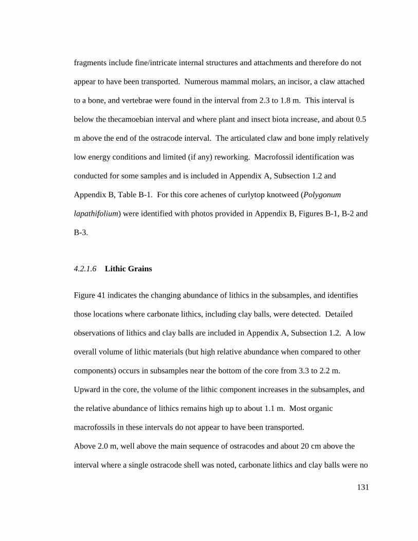
131

fragments include fine/intricate internal structures and attachments and therefore do not

appear to have been transported. Numerous mammal molars, an incisor, a claw attached

to a bone, and vertebrae were found in the interval from 2.3 to 1.8 m. This interval is

below the thecamoebian interval and where plant and insect biota increase, and about 0.5

m above the end of the ostracode interval. The articulated claw and bone imply relatively

low energy conditions and limited (if any) reworking. Macrofossil identification was

conducted for some samples and is included in Appendix A, Subsection 1.2 and

Appendix B, Table B-1. For this core achenes of curlytop knotweed (Polygonum

lapathifolium) were identified with photos provided in Appendix B, Figures B-1, B-2 and

B-3.

4.2.1.6 Lithic Grains

Figure 41 indicates the changing abundance of lithics in the subsamples, and identifies

those locations where carbonate lithics, including clay balls, were detected. Detailed

observations of lithics and clay balls are included in Appendix A, Subsection 1.2. A low

overall volume of lithic materials (but high relative abundance when compared to other

components) occurs in subsamples near the bottom of the core from 3.3 to 2.2 m.

Upward in the core, the volume of the lithic component increases in the subsamples, and

the relative abundance of lithics remains high up to about 1.1 m. Most organic

macrofossils in these intervals do not appear to have been transported.

Above 2.0 m, well above the main sequence of ostracodes and about 20 cm above the

interval where a single ostracode shell was noted, carbonate lithics and clay balls were no

132

longer identified. The presence of carbonates corresponds with the intervals where

ostracode shells were noted to have been coated, and includes the 70 cm above the

ostracode interval.

Typically maximum lithic size is around 4 mm throughout the core decreasing in size

somewhat to 2-3 mm in the uppermost metre of the core. Lithics were consistently

abundant and represented a high relative proportion of the sample volume until a depth of

about 1.4 m, when plant and insect macrofossils increased upward in abundance and the

number of thecamoebians increased, indicating more productive conditions in the lake

(Figure 41).

4.2.1.7 Moisture Analysis

Moisture data is plotted below in Figure 42. The increase in moisture levels around 2.8

m corresponds with the end of the interval where ostracodes were abundant (Figure 40).

It is unclear why there is a sharp increase sediment moisture at 1.7 m.

133

Figure 42. Plot of % moisture loss based on freeze drying of samples, against depth in the WOO06-1A-1Kcore, with the bottom of the core to the right.

4.2.1.8 Radiocarbon Dates

Two radiocarbon dates near the bottom of the core (Figure 43) were primarily obtained

from seed materials, refer to Appendix B, Section 2, Table B-1 and Section 3, and

Appendix B, Section 4, Figures B-1, B-2 and B-3. The lowermost and younger date of

7.140 14C ka BP (7.973 cal ka BP) at 3.2 m is about 0.4 m below the older date of 7.375

14C ka BP (8.228 cal ka BP). An articulated ostracode shell was identified between these

intervals possibly implying little reworking occurred. Pollen was dated at 12.260 14C ka

BP (14.365 cal ka BP) 0.4 m above the 7.375 14C ka BP (8.228 cal ka BP) date at a core

depth of 2.4 m. This pollen date is rejected, because the region is known to have been

covered by the LIS at this time; almost certainly the pollen has been reworked from older

materials.

WOO06-1A-1K

0.010.0

20.030.0

40.050.060.0

70.080.0

90.0100.0

0.0 0.4 0.9 1.4 1.9 2.4 2.9

Core depth (m)

Moi

stur

eLo

ss(%

)

134

The two upper core radiocarbon dates are in sequence, with the lower of these dated at

1.675 14C ka BP (1.579 cal ka BP) defining the beginning of the thecamoebian sequence

at about 1.4 m.

Figure 43. Radiocarbon dates for WOO06-1A-1K showing the ostracode and thecamoebian intervals.Sampled locations are the same as those in Figure 40. The yellow bars represent the presence ofthecamoebians. All dates are from the radiocarbon analysis reports in Appendix B. The total number ofostracodes includes all species as are reported in the details of Figure 40

WOO06-1A-1K

Number of Ostracodes

0 5 10 15 20 25 30-3.5

-3.0

-2.5

-2.0

-1.5

-1.0

-0.5

0.0C. subtriangulataL. friabilisF. rawsonipresence of thecamoebians

1460 (1358) BP

1675 (1579) BP

7375 (8228) BP

12260 (14365)

Radiocarbon Dates14C (cal) years BP

7140 (7973) BP

Cor

eD

epth

(m)

135

4.2.2 Northwest Angle Site - WOO06-3A

4.2.2.1 General

The WOO06-3A-1K coring location, latitude 49.34714o; longitude -94.84379o in a

narrow deep channel (Figure 24) is described in Section 2.3.3. WOO06-3A-1K is located

in the northeast trending channel near Cyclone Island about 10 km to the east of the

Northwest Angle Inlet and is in about 14.9 m (48.9 feet) of water. The retrieved length is

about 7.5 m.

During the coring operation the WOO06-3A-1K core deflected and the core barrel was

permanently bent. The liner containing the sediment was recovered after considerable

force was applied to extract the liner from the bent core barrel, and the core was

subsampled and processed similar to the other cores. It was noted the split core was

essentially devoid of the sedimentary structures observed in the other cores, possibly as a

result of the core deflection or hammering forces applied to remove the liner. Initially,

the core data appeared relatively normal. Due to the deviation of the core from the

vertical when dropped into the sediments, data in this core is suspect and have not been

included, although general observations have been provided where deemed appropriate.

136

4.2.2.2 General Stratigraphic Description

The stratigraphic data in this core were not suitable for assessment due to the core

deflection from the vertical.

4.2.2.3 Ostracodes

No ostracodes were observed in this core.

4.2.2.4 Thecamoebians

Thecamoebians were observed throughout most of the top portion of the core and were

found near the core bottom with an apparent hiatus in between. The thecamoebian hiatus

appeared to be quite extensive (i.e. from about 7 m to 1.4 m) although the deflection of

the core sideways is possibly responsible for the long hiatus. These uncertainties make

interpretation of the data from this core very difficult and there is little confidence in the

thecamoebian data from this core.

4.2.2.5 Other Macrofossils

Macrofossils including fish scales and typical plant, insect and charcoal components were

observed throughout the cored sequence. Due to the uncertainties in these data due to the

core deflection, a detailed assessment of processed macrofossils was not completed.

137

4.2.2.6 Lithic Grains

Intervals of abundant granitic and quartz lithics were observed throughout the core.

4.2.2.7 Radiocarbon Dates

Only one radiocarbon sample was sent for analysis. The analysed sample at about 7.3 m

in this very long core (7.47 m) indicated an unusually young radiocarbon date for this

length of core. A sample of organic materials at 7.34 m including a birch and Verbena

(flowering plant) seed, and an ant mandible, and a small weevil elytron was dated at

2.915 14C ka BP (3.070 cal ka BP).

4.2.3 Northwest Angle Site - WOO06-4A

4.2.3.1 General

The WOO06-4A-1K coring location, latitude 49.33830o; longitude -94.85979o, in a

narrow deep northeast trending channel near Cyclone Island in the North West Angle

area of LOTWs (Figure 24) is described in Section 2.3.3. The retrieved data is presented

in Appendix A, Subsections 2.1 and 2.2, with detailed photographic images in Appendix

A, Subsection 2.3. The WOO06-4A-1K core is located in the interconnecting channels

between the large southern basin and the deep portion of LOTWs to the north (Figure

24), in 7.3 m (24 feet) of water. The retrieved length is about 2 m.

138

It was anticipated the sediments in the channel sites might be somewhat different from

the open Northwest Angle basin sites to the south and that a different paleoenvironment

may be present. This shallower of the two companion channel site cores does have

considerable organic accumulation and the development of pedogenic blocky structures

in an indistinct possible paleosol just below 70 cm from the top of the core (Figure 45).

4.2.3.2 General Stratigraphic Description

The stratigraphy of the WOO06-4A core is described for the two sections of the core

WOO06-4A-1K1 and 1K2, in Figure 44 and Figure 45. In this core there are four

primary stratigraphic units.

Unit 1 below about 1.55 m (about 100 cm in Figure 45) is a silty clay grading downward

to a slightly sandy clayey silt, with a low moisture content. It is dramatically different

from those units directly above (Figure 45). Near the bottom of the core there are “root-

like” structures.

Unit 2 starts at a depth of 1.55 m and ends at a depth of about 0.7 m (about 23 cm in

Figure 45). The lower boundary is indistinct with a dark 5 cm thick organic rich bed of

silty clay overlying the unit below. Organic laminations appear above the bed upwards

from a depth of about 1.3 m, to a depth of about 0.9 m. Above a depth of 1.55 m the unit

changes upwards from a primarily well laminated to poorly laminated silty clay,

including occasional zones of organic laminae. The top portion of Unit 2 contains a

139

crumbly fine angular blocky pedogenic zone, decreasing downward to a depth of 1.3 m.

Two distinct black beds and other black laminae occur in this unit. Abundant plant and

charcoal fragments are prevalent throughout the unit, with clay balls and ball fragments

near the top at about 0.9 m. The microscope observations of the processed subsamples

generally confirm the visual core descriptions in this unit.

Unit 3 is a silty clay grading downward to a clayey silt, with no visible laminae from 0.1

m to the gradual lower boundary at a depth of about 0.7 m (about 10 cm in Figure 44 and

2.3 cm Figure 45). From observations of the subsamples prior to processing, Unit 3 is a

relatively high moisture content unit when compared to the units below.

Unit 4, the uppermost unit above a core depth 0.1 m, is a non-laminated interval of high

moisture sandy gyttja, with a distinct lower boundary (Figure 44).

140

Figure 44. Photographic record and description of WOO06-4A-1K1.

141

Figure 45. Photographic record and description of WOO06-4A-1K2.

142

4.2.3.3 Ostracodes

An ostracode population graph is shown in (Figure 46), with the data located in Appendix

A, Subsection 2.1 with additional ostracode observations in Section 2.2. The C.

subtriangulata ostracode species is the only ostracode identified in the core. The

ostracode interval ends about 0.2 m above the bottom of the core at ~ 1.8 m. In addition

to the presence of C. subtriangulata at the bottom of the core, a high quartz lithics

component and a low plant, insect and charcoal macrofossil abundances were noted.

There are a limited number of ostracode shells within the ostracode interval, with the

most abundant concentration at the bottommost sampled interval. The ostracode shells

are thin and mostly broken with light deposits on the shells, but do not have a corroded

appearance.

Number of C. subtriangulataostracodes

0 2 4 6 8 10 12 14

Cor

eD

epth

(m)

0.0

0.5

1.0

1.5

2.0

Figure 46. Ostracode population variation for the WOO06-4A-1K core from the top of the core to thebottom at about 2 m. The small crosses indicate sample locations.

WOO06-4A-1K

143

4.2.3.4 Thecamoebians

The locations where thecamoebians are present are identified in (Figure 47) with detailed

thecamoebian observations included in Appendix A, Subsection 2.2. The first

thecamoebian interval which includes two species is located at about 0.77 m, between

intervals that have abundant large plant and charcoal fragments. A hiatus appears above

this point with the next interval continuing upwards of 0.31 m, which contains relatively

abundant thecamoebians with four species identified.

The uppermost appearance of thecamoebians occurs within a zone of high relative

abundance of plant and charcoal fragments, and insect macrofossils. The plant material

includes abundant seeds, including terrestrial and near shore plants, and abundant large

charcoal fragments, all indicating a near shore paleoenvironment, which corresponds with

the modern configuration of this narrow channel. Observed thecamoebian species

include both Difflugia oblonga and Centropyxis aculeate.

144

Lithics

0 2 4 6 8 10

Cor

eD

epth

(m)

0.0

0.5

1.0

1.5

2.0

PlantMaterial

0 2 4 6 8 10

Charcoal

0 2 4 6 8 10

InsectMaterial

0 2 4 6 8 10

Thecamoebians

0 1 2 3

Presence ofCarbonates

Figure 47. Plots of lithic materials and macrofossils for WOO06-4A-1K. Sampled locations are the sameas those in Figure 46. Lithics, plant, charcoal, and insect material are indicated by a bar reflecting theirabundance in the sample on a scale of 0 (absent) to 10 (abundant) and were recovered from the subsamplesafter wet sieving. Presence of thecamoebians and carbonates in a sample are shown only by a bar, and donot imply any quantity.

4.2.3.5 Other Macrofossils

Figure 47 includes macrofossil data plots generated from the subsample data. Data and

observations are located in Appendix A, Subsection 2.2.

Fish vertebrae and scales occur between 0.6 to 0.3 m in an interval where thecamoebians

underwent a hiatus. High abundance of plant and charcoal macrofossils, and increased

insects material, all begin above a black organic rich interval at about 1.5 m, indicating a

145

change in conditions at this site. The proportion of lithics also decreases above the same

interval. The scanned split core (Figure 45) clearly shows these dramatic changes across

this contact.

A gradational lower boundary at the base of the 5 cm thick black interval and a sharp

boundary at the top, marks the beginning of a transition from a low organic material

interval below this the black interval, to a zone of abundant plant and seed macrofossils

with large charcoal fragments within and above. This black organic interval includes

terrestrial and near shore plants, such as curlytop knotweed (Polygonum lapathifolium)

and bulrush (Scirpus validus) (Appendix B, Section 4, Figures B-1, B-2, B-3, and B-4),

with the insect materials also increasing somewhat in the interval.

The insect component remains low throughout most of the middle portion of the core

(except in the black organic layer), and starts rising to a maximum after the first

thecamoebian interval. The relative proportion of insects then continues at a high level

through the highest thecamoebian population interval (Figure 47), and then falls to low

levels as the thecamoebian population also starts to drop to a low level near the top of the

core. A reduction was noted in overall volume (but high relative abundance when

compared to other components) of organic and large charcoal components in the

processed samples above 0.74 m.

146

4.2.3.6 Lithic Grains

Abundant quartz, mica, and carbonate lithics, are present in the bottom ~ 0.4 m of the

core below the distinct black boundary located at about 1.5 m. This boundary lies below

an interval of non-laminated to weakly laminated sediments at about 0.9 to 1.5 m (Figure

45).

The abundance of lithics changes dramatically upward at about 1.5 m over a short

interval at the black organic interval. The bottom two subsample intervals in the core

include non disaggregated clay balls which tested positive for carbonates (using dilute

HCl), with the interval above including a carbonate grain. Interestingly, the lithics in the

portion of the core containing ostracodes (Figure 46) are dominated by quartz. Other

intervals above this point at about 1.3 m (Figure 47) had some carbonate rich clay balls

(Appendix A, Subsection 2.2). Some of these clay balls may have been eliminated if the

subsamples were processed father, but hard carbonate rich pellets were also observed in

one interval near the bottom of the core, indicating carbonate pellets/balls were relatively

common in this lower portion of the core.

Although there are variations in the observed lithology in the core above 1.5 m, the

processed samples have a limited variability in the type of lithics except at the second

pedogenic-like interval at about 0.74 m. At this point carbonate grains reappear, and then

disappear above.

147

4.2.3.7 Radiocarbon Dates

The four radiocarbon dates (Figure 48) were obtained from large macrofossils

(Appendix B, Section 2, Table B-1 and Section 3), the top and bottom dated samples

come from multiple Scirpus validus (bulrush) achenes ad are shown in Appendix B,

Section 4, Figures B-5 and B-6. These achenes did not have attached bristles and some of

the achenes were split open. The uppermost date of 2.495 14C ka BP (2.604 cal ka BP)

was obtained from a sample very near the top of the recovered core at 0.08 m. The lower

dated samples at 0.74 and 0.92 m, 6.370 14C ka BP (7.319 cal ka BP) and 6.955 14C ka

BP (7.787 cal ka BP) are from twigs up to one cm long (Appendix B, Section 4, Figures

B-7). Both of these dated intervals also have high abundances of plant and charcoal

macrofossils above and below. The interval between a depth of about 0.9 and 1.3 m

(Figure 45) contained an angular blocky crumbly textured slightly sandy silty clay, which

appears to be near pedogenically altered.

The distinct black interval at 1.5 m, was radiocarbon dated at 7.655 14C ka BP (8.443 cal

ka BP) using a Scirpus validus (bulrush) seed. The processing of this subsample revealed

a heavily matted organic residue composed of terrestrial plant components such as leaves,

stems and seeds.

148

6370 (7319) BP

2495 (2604) BP

6955 (7787) BP

7655 (8443) BP

Number of Ostracodes

0 2 4 6 8 10 12 14

0.0

0.5

1.0

1.5

2.0

Cor

eD

epth

(m)

C. SubtriangulataRelative Proportion of Thecamoebians

1 2

Relative Proportion

30

Figure 48. Radiocarbon dates for WOO06-4A-1K showing the ostracode and thecamoebian intervals.Sampled locations are the same as those in Figure 46. The yellow bars represent the presence ofthecamoebians. All dates are from the radiocarbon analysis reports in Appendix B.

4.2.4 Northwest Angle Site - WOO06-5A

4.2.4.1 General

The WOO06-5A-1K coring location, latitude 49.27928o; longitude -94.82007o, in the

northern portion of the southern basin (Figure 24) is described in Section 2.3.4. The

retrieved data is presented in Appendix A, Subsections 3.1 and 3.2, with detailed

photographic images in Appendix A, Subsection 3.3. The WOO06-5A-1K core is

located at the north/south mid-point of the modern extent of LOTWs, beyond the broad

open southern basin in a large partially sheltered broad bay just to the south of the

149

Northwest Angle Inlet. This core is located about 7 km from the western shore near

Massacre Island, adjacent to the U.S./Canada border, in 8.1 m (26.6 feet) of water. The

retrieved length is about 5.48 m.

4.2.4.2 General Sratigraphic Description

The stratigraphy for the WOO06-5A core is described for the five sections of the core

WOO06-5A-1K1, 1K2, 1K3, 1K4 and 1K5, in Figure 49, Figure 50, Figure 51, Figure 52,

and Figure 53. In this core there are eight primary stratigraphic units, including three

paleosols.

Unit 1 is the lowermost unit from the bottom of the core at about 5.47 m to about 4.0 m

(about 150 to 0 cm Figure 53). It is a very silty clay with a relatively low moisture

content in the upper 50 cm. Below this it becomes a silty clay with more distinct

laminations and organic streaks downward with a lower moisture content. It becomes

softer below 4.6 m, with more distinct laminations and a higher moisture content. The

results of a moisture analysis are presented in Section 5.2.4.7 with the trends in moisture

also observed in the subsamples (Appendix A, Subsection 3.2). A fault was noted at

about 4.9 m.

Unit 2 is the first paleosol which extends from about 3.9 to 3.33 m (about 150 to 85 cm

Figure 52) and contains a crumbly very dry fine texture with all peds < 2 mm. The top 9

cm includes fine organics between granular peds, and includes shell fragments including

150

bivalves and gastropods, which were also observed during subsampling and noted in

Appendix A, Subsection 3.2. The subsample observations also reflect paleosol

conditions and closely correlate with the top surface of the unit, with the lower surface

extending farther downward about 20 cm to 3.9 m. Unit 3 is located above the first

paleosol surface at about 3.33 m, extends upwards to about 3.1 m (about 85 to 54 cm

Figure 52), and is a poorly laminated silty clay with decreasing moisture upward. Unit 4

is the 2nd paleosol which is weakly granular and about 5 cm thick, with an upper

boundary at about 2.97 m (about 54 to 48 cm Figure 52). The location of the top

boundary of the 2nd paleosol, based on the core description, is also confirmed by

observations from the subsamples. The lower boundary as identified in the core

description, appears to extend downward a further 15 cm to about 3.2 m from the

observations of the subsample (this observation is similar to those observed in other

paleosols), although the lowermost boundary appears to be most distinct around 3.1 m.

Unit 5 extends from the bottom of the top paleosol at about 2.8 m, down to about 2.97 m

(30 to 48 cm Figure 52) where the 2nd paleosol is located. Unit 5 is a poorly laminated

silty clay with an abrupt increase in organics about 10 cm below the top of the unit. The

lower boundary is variable between the non-granular components of this unit and

granular components of the paleosol of Unit 4 at about 3 m. Unit 6 from 2.4 to 2.67 m

(about 140 cm Figure 51 to about 20 cm Figure 52) is a paleosol. The top 10 cm have

about 80% hard (some round) granules, some > 5mm in diameter, in a dark grey silty clay

matrix, which appears infiltrated from above. The granules appear to be detrital and

some appear bluish, possibly containing vivianite. The blocky structures above decrease

151

and disappear downward about 18 cm below the top of the unit. A moisture minimum

occurs about this point (refer to Section 5.2.4.7). Subsample data (Appendix A,

Subsection 3.2), closely corresponds with this paleosol interval, although extends the

apparent boundary downward slightly (10 cm) to about 2.8 m.

Unit 7 starts at about 2.4 m (about 140 cm Figure 51) and is a very silty clay with

occasional faint laminae, with a 10 cm darker interval (more organic rich) starting about

0.5 m from the top of the unit at about 0.7 m (about 55 cm Figure 50). Moisture

gradually decreases downward, and in the lower 10 cm, abundant angular granules

increase to abundant and the unit changes from a very silty clay to a matrix increasing in

silt and very fine grained sand content. The lower boundary is defined by an abrupt

increase to very abundant dry granules, which help define the end of the last soil horizon.

The lower 10 cm includes hard and dry granules increasing to abundant at the base of the

unit. Unit 8 is the uppermost unit, and is 0.7 m (starting about 55 cm Figure 50) of a high

moisture silty clay with occasional light laminae, and an irregular lower boundary.

152

Figure 49. Photographic record and description of WOO06-5A-1K1.

Figure 50. Photographic record and description of WOO06-5A-1K2.

153

Figure 51. Photographic record and description of WOO06-5A-1K3.

154

Figure 52. Photographic record and description of WOO06-5A-1K4.

155

Figure 53. Photographic record and description of WOO06-5A-1K5.

156

4.2.4.3 Ostracodes

The ostracode sequence identified from the bottom of the core at 5.47 m to about 4.6 m is

composed of an exclusive C. subtriangulata interval, changing to a more mixed sequence

including L. friabilis from 4.5 to 4.1 m. C. subtriangulata disappear at 3.7 m with L.

friabilis dominant in an interval from 3.8-3.4 m, which also contains C. sharpei and F.

rawsoni (Figure 54). Above 3.4 m ostracodes again disappear completely for a period of

time until they reappear at about 3.0 m, and finally disappear above 2.7 m. Above the

mid-point of the first paleosol C. subtriangulata disappear, except for one interval within

the last paleosol which includes rare appearances of other ostracodes. The absence of

ostracodes in the upper portions of the core repeats a similar pattern in other cores.

Ostracode shells near observed paleosol horizons appear crushed. Deeper ostracode

shells are mostly broken and thin and have a corroded appearance (particularly below the

first soil horizon). Articulated ostracode shells were observed within the first paleosol

horizon. The lowermost (3.7 - 3.3 m) and uppermost (2.7 - 2.4 m) paleosol horizons

include intervals with ostracodes present. The 2nd thin paleosol around 3.1 m does not

have any ostracode shells within it.

157

C. subtriangulata

0 20 40 60 80

Cor

eD

epth

(m)

0

1

2

3

4

5

L. friabilis

0 2 4 6 8 10 12 14 16 18

C. sharpei

0 2 4 6 8 101214161820

F. rawsoni

0 2 4 6 8 10 12 14 16

Figure 54. Ostracode population variation for WOO06-5A-1K from the top of the core to the bottom at5.47 m. The crosses indicate sample locations. Note the number of ostracodes scale varies, with the C.subtriangulata ostracode population much higher than the others.

4.2.4.4 Thecamoebians

Thecamoebians appear at about 0.8 m (Figure 55) in an interval which was already

relatively abundant in plant and insect materials. A detailed thecamoebian species

analysis was not conducted for this core, however up to four species were noted when

subsamples were re-examined subsequent to the initial ostracode examinations

(Appendix A, Subsection 3.2).

Number of ostracode shells

WOO06-5A-1K

158

4.2.4.5 Other Macrofossils

Figure 55 includes macrofossil data plots generated from the subsample data. Data and

observations are included in Appendix A, Subsection 3.2.

Relatively large volumes of plant and charcoal were observed in the lower portion of the

core (Figure 55). Higher concentrations of plant material, particularly seeds and charcoal

materials, were also noted near paleosol horizons with high volumes of organic material

observed within the paleosols (Appendix A, Subsection 3.2). Within and near the second

paleosol horizon, seeds of shallow water plants including Scirpus sp (bulrush), and other

terrestrial seeds such as Rumex maritimus (golden dock) and Chenopodium sp

(goosefoot) (Appendix B, Section 4, Figures B-8, B-9, and B-10), are found in

abundance. The uppermost soil horizon includes birch nutlets. The zones between the

paleosol horizons include seeds and twigs, rare ostracode shells, abundant gastropod and

pelecypod shells, indicating an overall shallow water environment. The middle soil

horizon contains abundant matted plant material and charcoal.

159

WOO06-5A-1K

Lithics

0 2 4 6 8 10

Cor

eD

epth

(m)

0

1

2

3

4

5

PlantMaterial

0 2 4 6 8 10

Charcoal

0 2 4 6 8 10

InsectMaterial

0 2 4 6 8 10

Presence ofCarbonates

Thecamoebians

0 1 2 3

Figure 55. Plots of thecamoebians lithic materials and various macrofossils for WOO06-5A-1K. Sampledlocations are the same as those in Figure 54. Lithics, plant, charcoal, and insect material are indicated by abar reflecting their abundance in the sample on a scale of 0 (absent) to 10 (abundant) and were recoveredfrom the subsamples after wet sieving. Presence of thecamoebians and carbonates in a sample are shownonly by a bar, and do not imply any quantity.

4.2.4.6 Lithic Grains

Quartz lithics are abundant from the bottom of the core upwards to the beginning of the

first soil horizon (Figure 55). Included in the bottommost 0.5 m of this core are iron

stained lithic grains ranging from brown to black carbonate pellets (i.e. react to dilute

HCl), and carbonate clay pellets and balls (Appendix A, Subsection 3.2). Above this,

quartz lithics become the dominant lithic up to the first paleosol horizon. Within the

160

paleosol horizons quartz becomes rare, with clay balls and pellets becoming the

predominant lithics. Above the last paleosols horizon lithics are predominantly quartz,

but overall are primarily in low relative concentrations.

4.2.4.7 Moisture analysis

Moisture data is plotted below in Figure 56. Moisture levels start to drop above about 4.4

m and then start to rise again above 2.4 m, with two distinct low moisture zones between

about 4.4 and 3.4 m and about 3.2 and 2.6 m with an intervening high moisture zone

between them. These changes in moisture levels are also reflected in the moisture

estimates performed during the subsample processing (Appendix A, Subsection 3.2). The

lowermost soil horizon between about 3.9 to 3.3 m, ocurrs near the top of the lower low

moisture zone. The two upper observed paleosol horizons at about 2.8 to 2.4 m, and

around 3.2 to 3.0 m occur within the upper low moisture zone between about 3.2 and 2.6

m. This further supports the classification of these intervals in the core as paleosols.

161

Figure 56. Plot of % moisture loss based on freeze dried samples, against depth in the WOO06-5A-1Kcore, with the bottom of the core to the right.

4.2.4.8 Radiocarbon Dates

Six of the nine radiocarbon dates for this core were obtained from dating of macrofossils

including seeds and terrestrial plant materials (Appendix B, Section 2, Table B-1). These

six dates all fell in a normal chronological sequence. A well rounded twig at about 4.3 m

was dated at 15.62 14C ka BP (18.8 cal ka BP). This twig was within the C.

subtriangulata ostracode sequence. There are also two pollen dates bounding this

interval, 17.56 14C ka BP (20.97 cal ka BP) and 17.04 14C ka BP (20.36 cal ka BP).

One of the key objectives in the dating strategy for this core was to obtain radiocarbon

dates for the paleosol intervals in the core. Six samples were taken within the paleosol

horizons. Two of these samples, 8.245 and 8.405 14C ka BP, were from the same interval

WOO06-5A-1K

010

2030

405060

7080

90100

0.2 0.6 1.1 1.6 2.1 2.5 2.7 3.2 3.4 3.9 4.4 4.9

Core depth (m)

Moi

stur

eLo

ss%

162

at 3.3 m; when averaged the age of that interval is 8.345 14C ka BP (9.377 cal ka BP).

Figure 57 presents the radiocarbon dates for the core but does not include two old pollen

dates [(1.7040 14C ka BP (20.236 cal ka BP) and 1.7560 14C ka BP (20.970 cal ka BP)]

which were rejected. The radiocarbon dated twig of 15.62 14C ka BP (18.8 cal ka BP)

was also rejected.

The end of the lower paleosol closely corresponds with a radiocarbon date of 8.345 14C

ka BP (9.377 cal ka BP), with a nearby (0.6 cm higher) sequential date of 8.065 14C ka

BP. The 7.630 14C ka BP (8.419 cal ka BP) radiocarbon date corresponds with the top of

the 2nd paleosol, with a nearby (0.5 cm higher) sequential date of 7.510 14C ka BP. The

uppermost date of 7.510 14C ka BP (8.308 cal ka BP) at 2.9 m is close to what appears to

be the bottom of the top paleosol (at about 2.8 m).

163

Figure 57. Radiocarbon dates for WOO06-5A-1K showing the ostracode and thecamoebian intervals.Sampled locations are the same as those in Figure 54. The light yellow area is the interval wherethecamoebian are present. The positions of the three paleosol intervals are shown as brown bars on the leftscale. The total number of ostracodes includes all species as are reported in the details of Figure 54. Alldates are from the radiocarbon analysis reports in Appendix B.

WOO06-5A-1K

Total Number of Ostracodes

0 20 40 60 80

Cor

eD

epth

(m)

0

1

2

3

4

5

Presence of Thecamoebians

2080 (2071)

3910 (4343)

7510 (8308)

15620 (18802) BP

7630 (8419)

8065 (9008)8345 (9377)

Radiocarbon Dates14C (cal) years BP

164

4.2.5 Northwest Angle Site - WOO06-6A

4.2.5.1 General

The WOO06-6A-1K coring location, latitude 49.28098o longitude -94.89926o, in the

northern portion of the southern basin (Figure 24) is described in Section 2.3.4. The

retrieved data are presented in Appendix A, Subsections 4.1 and 4.2, with detailed

photographic images in Appendix A, Subsection 4.3. The WOO06-6A-1K core is

located at the approximate north/south mid-point of the modern extent of LOTWs,

beyond the broad open southern basin in a large partially sheltered broad bay just to the

south of the Northwest Angle Inlet. This coring site is located about 1.5 km from the

western shore about 6 km to the west of the companion core (WOO06-5A-1K), in 5.9 m

(19.4 feet) of water. The retrieved length is about 3.8 m.

4.2.5.2 General Stratigraphic Description

The stratigraphy for the WOO06-6A core is described for WOO06-6A-1K1, 1K2, and

1K3, in Figure 58, Figure 59 and Figure 60. In this core there are three primary

stratigraphic units, including one paleosol.

Unit 1 extends upwards from the bottom of the core at about 3.8 m (Figure 58) and ends

at the paleosol at about 2.0 m (about110 cm in Figure 59). It is a well laminated silty

clay to clayey silt, with the lighter coloured silty laminae typically a 1-5 mm thick and 1-

3 mm darker silty laminae, with some laminae about 8 mm thick. These structures are

165

repetitive within this unit from the bottom of the core upwards. Unit 2 is a paleosol with

a distinct top boundary at about 1.8 m (about 90 cm in Figure 59), and appears to be

about 20 cm thick based on the core description and from the subsample observations

(Appendix A, Subsection 4.2). The top very silty clay portion has an 8 cm interval of

hard and abundant 1-3 mm granules in a clayey matrix. The lower boundary appears to

extend downward to about 2.0 m based on the 3mm clay pellets observed in the

subsamples. A 3.2 cm rounded piece of mafic bedrock was noted in upper part of the

unit (possibly ice rafted). Near the bottom of the interval containing granules, a

decomposed bivalve was observed and the bivalve and nearby shell debris, were

radiocarbon dated at 6.760 14C ka BP (7.616 cal ka BP). Unit 3 (starting at about 90 cm

in Figure 59) is the uppermost unit and is a poorly laminated, very clayey and very fined

grained silt, grading downward to slightly more clayey around 0.9 m. Darker banding

occurs below 0.62 m which becomes lighter downward. Near the bottom of the unit at

1.8 m, about 4 cm above the obvious colour difference, hard granules were noted and

increase in number downward indicating the presence of a paleosol below.

166

Figure 58. Photographic record and description of WOO06-6A-1K1.

167

Figure 59. Photographic record and description of WOO06-6A-1K2.

168

Figure 60. Photographic record and description of WOO06-6A-1K3.

169

4.2.5.3 Ostracodes

The ostracode sequence identified in the bottom of the core at 3.8 m to about 2.8 m

(Figure 61) is composed of two ostracode species C. subtriangulata and L. friabilis. C.

subtriangulata is the dominant species in the core and they extend from the bottom to

about 1.8 m. One rare interval of C. sharpei occurs at about 3.1 m when both C.

subtriangulata and L. Friabilis populations disappear.

The end of the ostracode interval in this core at about 1.9 m, is very close (8 cm below)

the radiocarbon dated interval 6.760 14C ka BP (7.616 cal ka BP) near the end of the

paleosol. The absence of ostracodes in the upper portions of the core repeats a similar

pattern present in other cores.

C. subtriangulata shells are typically broken and thin and have a corroded appearance.

Two intervals with articulated ostracode shells were observed and some L. friabilis shells

appeared to be crushed. The ostracode shells at the bottom of the core (~ 0.4 m from the

bottom) do not have the same mechanical damage or corroded appearance as those above.

170

no. C. subtriangulata

0 10 20 30 40

Cor

eD

epth

(m)

0

1

2

3

no. L. friabilis

0 2 4 6 8 10

no. C. shapei

0 2 4 6 8 10

Figure 61. Ostracode population variation for WOO06-6A-1K from the top of the core to the bottom at 3.8m. The crosses indicate sample locations. Note the number of ostracodes scale varies, with the C.subtriangulata ostracode population much higher than the others.

4.2.5.4 Thecamoebians

Thecamoebians appear at about 1.3 m in an interval below which there was already a

relatively abundant zone of lithics, plant, insect and charcoal materials (Figure 62). A

detailed thecamoebian species analysis was not conducted for this core, however up to

four species of thecamoebians were noted. This thecamoebian interval is about 0.5 m

above the end of the paleosol zone (Appendix A, Subsection 4.2).

Number of ostracode shells

WOO06-6A-1K

171

4.2.5.5 Other Macrofossils

Relatively large volumes of plant and charcoal in the lower portion of the core in

conjunction with C. subtriangulata ostracodes are observed in a zone below the observed

paleosol interval, at about 1.9 m (Figure 62). This interval contains high volumes of

plant materials, including large fragments of charcoal, and gastropod shells (Appendix A,

Subsection 4.2). Above the paleosol, plant materials, charcoal and insect materials

increase dramatically.

Lithics

0 2 4 6 8 10

Cor

ede

pth

(m)

0.0

0.5

1.0

1.5

2.0

2.5

3.0

3.5

PlantMaterial

0 2 4 6 8 10

Charcoal

0 2 4 6 8 10

InsectMaterial

0 2 4 6 8 10

Thecamoebians

0 1 2 3

Presence ofCarbonates

Figure 62. Plots of lithic materials and macrofossils for WOO06-6A-1K from the top to the bottom of thecore at 3.8 m. Sampled locations are the same as those in Figure 61. Lithics, plant, charcoal, and insectmaterial are indicated by a bar reflecting their abundance in the sample on a scale of 0 (absent) to 10(abundant) and were recovered from the subsamples after wet sieving. Presence of thecamoebians andcarbonates in a sample are shown only by a bar, and do not imply any quantity.

WOO06-6A-1K

172

4.2.5.6 Lithic Grains

Quartz lithics are present in conjunction with clay pellets from near the bottom of the

core upwards to the end of paleosol horizon (Figure 62), where quartz becomes the

dominant lithic (Appendix A, Subsection 4.2). Quartz lithics decrease in relative quantity

to the top of the core, while clay pellets disappear completely. Quartz lithics dominate in

the bottommost ~ 0.3 m. Iron stained carbonate rich pellets are present from near the

bottom of the core to the top of the paleosol, and they are often in conjunction with

coated ostracode shells.

4.2.5.7 Radiocarbon Dates

Three radiocarbon dates were obtained for this core (Figure 62) from available

macrofossils (Appendix B, Section 2, Table B-1). Near the top of the paleosol at a depth

of about 1.9 m a mollusc shell was dated at 6.760 14C ka BP (7.616 cal ka BP). This date

is very near to the top of the interval where ostracodes disappeared. A date of 2.11 14C ka

BP (2.091 cal ka BP) was obtained above the paleosol from blackened organic material at

1.0 m and is located above the beginning of the thecamoebians at 1.3 m. A date of 3.245

14C ka BP (3.481 cal ka BP) was obtained from beetle parts at 1.5 m. This date is below

the beginning of the thecamoebian interval.

173

Figure 63. Radiocarbon dates for WOO06-6A-1K showing the ostracode and thecamoebian intervals.Sampled locations are the same as those in Figure 61. The yellow bars represent the presence ofthecamoebians. The brown bar on the left scale indicates the location of a paleosol. The total number ofostracodes includes all species as are reported in the details of Figure 61. All dates are from theradiocarbon analysis reports in Appendix B.

WOO06-6A-1K

Number of Ostracodes

0 10 20 30 40 50

Cor

eD

epth

(m)

0.0

0.5

1.0

1.5

2.0

2.5

3.0

3.5

C. subtriangulataL. friabilisC. Sharpei

Presence of Thecamoebians

2110 (2091) BP

3245 (3481) BP

6760 (7616) BP

174

4.2.6 Kenora Site - WOO06-7A

4.2.6.1 General

The WOO06-7A-1P coring location, latitude 49.72984o longitude -94.51310o, in a

complex channel system south of the outlets to the Winnipeg River and the town of

Kenora, Ontario (Figure 24), is described in Section 2.3.5. The retrieved data is

presented in Appendix A, Subsections 5.1 and 5.2, with detailed photographic images in

Appendix A, Subsection 5.3. The WOO06-7A-1P core is located in a complex channel

system connecting to more open waters to the south, in about 6.1 m (20 feet) of water.

The retrieved length is about 4.65 m.

4.2.6.2 General Stratigraphic Description

The stratigraphy for the WOO06-7A core is described for the four sections of the core

WOO06-7A-1P1, 1P2, 1P3, and 1P4, in

Figure 64, Figure 65, Figure 66, and Figure 67. In this core there are three primary units.

Unit 1 ends at about 3.85 m (about 75 cm in Figure 67) at a distinct colour boundary. It

is a laminated sandy silty clay becoming a weakly laminated silty clay upward from the

bottom of the core at 4.65 m, to a pink clay bed occurring at about 4.0 m. Above this it

becomes a weakly laminated slightly sandy silty clay. The lowermost portion of Unit 1

has common 2-10 mm sand laminae with the laminae thinning to < 2mm upwards. The

175

pink clay has an underlying silty clay 0.5 cm interval of tan coloured clay. These clay

intervals are smoother and contain less silt, and no sand.

Unit 2 is a sandy silty clay with weakly to distinct sandy clayey silt laminae, which are

increasingly sandy downward. A distinct colour change occurs at the lower boundary at

3.85 m, and the upper boundary at about 2.9 m (at about 130 cm in Figure 66) is

distinguished by the transition to the non-laminated unit above.

Unit 3 is the uppermost unit (Figure 64 and Figure 65) and is a non-laminated, high

moisture, gelatinous and slightly sandy silty clay, trending to more sandy below, down to

about 2.9 m.

176

Figure 64. Photographic record and description of WOO06-7A-1P1

177

Figure 65. Photographic record and description of WOO06-7A-1P2

178

Figure 66. Photographic record and description of WOO06-7A-1P3

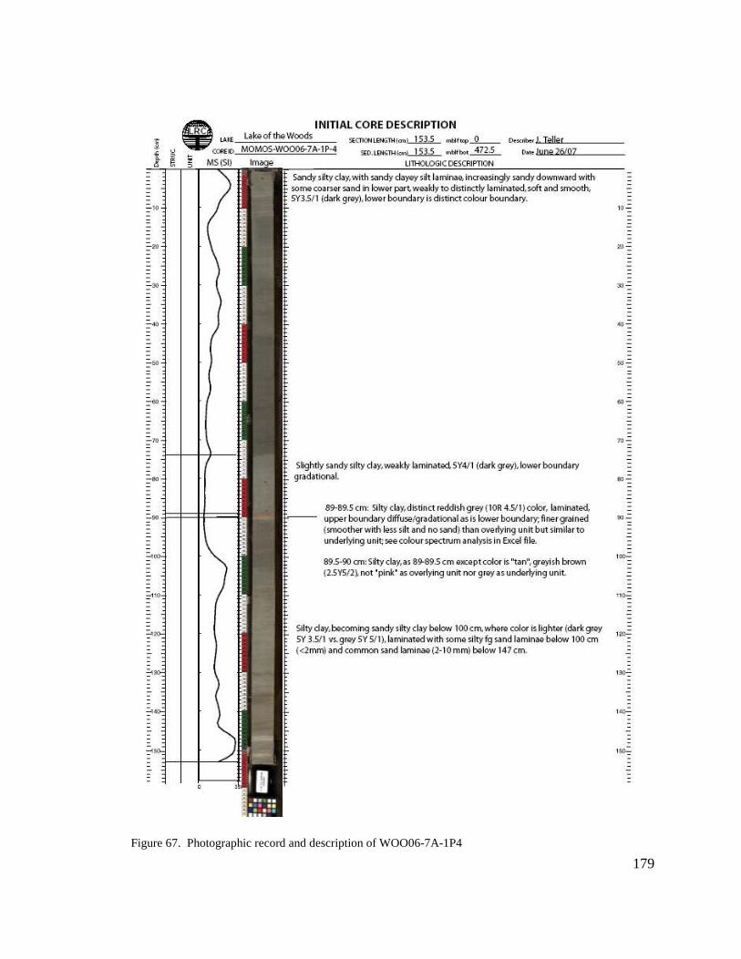
179Figure 67. Photographic record and description of WOO06-7A-1P4

180

4.2.6.3 Ostracodes

The ostracode sequence identified in the bottom of the core is composed of an almost

exclusive C. subtriangulata interval in the bottom ~ 0.8 m of the core, to about 3.9 m

(Figure 68). Subsequent ostracode populations are atypical from the other observed cores

in that there are primarily only two ostracode species present, C. subtriangulata and C.

sharpei, with one short interval with low population numbers of L. friabilis and F.

rawsoni near the bottom of the core, above a pink clay layer at 4.0 m. The C.

subtriangulata and C. sharpei intervals are separated in time and do not overlap.

Additionally, there are four ostracode intervals with three distinct hiatuses, before the last

ostracode interval ends at about 1.2 m (Figure 68), which is within the first appearance of

thecamoebians. This overlap of ostracode and thecamoebian intervals in the top portion

of the core is unique to this core. The C. subtriangulata ostracode dominates near and

below the pink clay layer in the two ostracode sequences near the bottom of the core, and

it briefly reappears in low numbers at about 2.7 m, and then disappears from the record.

The C. sharpei ostracode appears in low population numbers by itself, above the last

incidence of C. subtriangulata, and subsequently goes through a hiatus, and then

disappears above about 2.2 m.

181

no. C. subtriangulata

0 10 20 30 40

Cor

eD

epth

(m)

0

1

2

3

4

no. L. friabilis

0 1 2 3 4 5

no. C. sharpei

0 1 2 3 4 5

no. F. rawsoni

0 1 2 3 4 5

Figure 68. Ostracode population variation from the top of the core to the bottom at 4.65 m. The crossesindicate sample locations. Note the number of ostracodes scale varies, with the C. subtriangulata ostracodepopulation much higher than the others.

The last interval of ostracodes begins near an interval dated at 8.310 14C ka BP (9.350 cal

ka BP) (from a twig macrofossil) at about 1.2 m. A date at about 1.1 m just above the

end of the ostracodes and below the beginning of the thecamoebians was dated at 6.775

14C ka BP (7.630 cal ka BP).

Ostracode shells throughout the core are coated, fragile looking, and many are broken.

One interval above the pink clay layer had heavily coated shells, and was associated with

WOO06-7A-1P

Number of ostracode shells

182

the presence of clay balls which appeared in the 20 cm directly above the pink clay. The

presence of an articulated ostracode shell was noted near the pink clay bed, indicating

reworking near this interval is unlikely.

The lowermost ostracode sequence near and below the pink clay bed which has been

associated with the Marquette readvanced, is clearly within the Lake Agassiz period. A

hiatus in ostracodes occurred from about 4.4 to 4.1 m after a decline in ostracodes

starting from the bottom of the core at 4.65 m, which was followed by a rapid rise in the

ostracode population to a maximum at the pink clay bed, at about 4 m.

4.2.6.4 Thecamoebians

The early appearance of thecamoebians at 1.5 m, just above the interval dated at 8.265

14C ka BP (9.235 cal ka BP) is preceded by high insect and plant macrofossils (Figure

69), and is very near the point where LOTWs was estimated to have isolated from Lake

Agassiz (Yang and Teller, 2005). The thecamoebians subsequently disappear before

reappearing at about 1.0 m, in an interval preceded and followed by relatively high plant,

insect and charcoal levels. The appearance of thecamoebians is prior to the end of the

last ostracode horizon, which is near a radiocarbon dated interval at 1.1 m of 6.775 14C ka

BP (7.630 cal ka BP).

183

4.2.6.5 Other Macrofossils

Plant and insect macrofossils remained very low until plant material sharply increase

about 1.5 m from the bottom of the core at about 3.1 m (about 0.8 m above the pink clay),

which is followed by a sharp increase in insects at about 2.6 m (Figure 69). A similar

increase in charcoal is noted about the same time as the increase in insects. From the

bottom of the core to above the pink clay, there are rare quantities of these biological

components to about 3.6 m, where the relative proportion of plant materials increases.

Relatively low biotic components continue upwards to about 3.0 m, where plant materials

become relatively abundant and insect populations increase.

An insect wing and a grass-like terrestrial plant macrofossil were found at about 3.6 m

(Appendix A, Subsection 5.2). High abundance of plant and insect volumes were found

below the two radiocarbon dated intervals at about 1.6 m of 8.265 14C ka BP (9.235 cal

ka BP) and 8.310 14C ka BP (9.350 cal ka BP) (Figure 69). A pelecypod hinge was found

at 4.2 m (below the pink clay). Increasing charcoal levels were noted at 2.8 m which

become abundant at about 2.5 m (dated nearby at 8.780 14C ka BP (9.804 cal ka BP).

184

Lithics

0 2 4 6 8 10

Cor

eD

epth

(m)

0

1

2

3

4

PlantMaterial

0 2 4 6 8 10

Charcoal

0 2 4 6 8 10

InsectMaterial

0 2 4 6 8 10

Thecamoebians

0 1 2 3Presence ofCarbonates

Figure 69. Plots of lithic materials and macrofossils for WOO06-7A-1K from the top to the bottom of thecore at 4.65 m. Sampled locations are the same as those in Figure 68. Lithics, plant, charcoal, and insectmaterial were recovered from the subsamples after wet sieving; the high numbers reflect greaterabundances in a subsample interval. Presence of thecamoebians and carbonates in a sample are shown by abar, but do not imply any quantity.

4.2.6.6 Lithic Grains

Non disaggregated clay balls occur throughout the core but are most prevalent just above

the pink clay. Abundant quartz lithics occur from the bottom of the core to 2.7 m where

they drop from abundant to common for most of the remainder of the core, sometimes

reaching rare levels (Figure 69). Carbonate lithics and clay balls are noted at and just

above the pink clay and at a short interval between about 2.9-3.3 m.

WOO06-7A-1P

Pink Clay

185

4.2.6.7 Moisture Analysis

Moisture data is plotted below in Figure 70. Moisture levels remain relatively consistent

throughout the lower portion of the core with moisture levels trending upwards about 1 m

from the top of the core. An increase in moisture levels occurs starting above 4 m and

corresponds with a dramatic decrease in the ostracodes population and their subsequent

disappearance (Figure 68), the presence of carbonate lithics (Figure 69), and a pink clay

layer. The increase in moisture at a depth of 1 m also corresponds with the end of the last

ostracode interval and the beginning of a continuous zone of thecamoebians in the upper

core.

Figure 70. Plot of % moisture loss based on freeze drying of samples, against depth in the WOO06-7A-1Pcore, with the bottom of the core to the right.

WOO06-7A-1P

0.010.0

20.030.0

40.050.060.0

70.080.0

90.0100.0

0.0 0.5 1.0 1.5 2.1 2.6 3.1 3.6 4.0 4.3

Core depth (m)

Moi

stur

eLo

ss%

186

4.2.6.8 XRD Analysis

Five broadly spaced samples were taken in the core (refer to Appendix C). Only a very

qualitative sampling and data extraction was undertaken in this thesis. Further work

including closer sampling intervals and a quantitative assessment of the data would need

to be performed to gain further insights. The samples did not appear to show any

significant deviation in the general mineralogy of the sediments based on the outputs

provided by the Jade program. There was some general variation noted however in the

Lake Agassiz sequence above and below the pink clay bed and the lowermost sample

appeared unique.

4.2.6.9 Radiocarbon Dates

There are two radiocarbon dates at 1.6 m, 8.265 14C ka BP (9.235 cal ka BP) and 8.310

14C ka BP (9.350 cal ka BP) in correct chronological sequence. The dates were obtained

from twigs (Appendix B, Section 4, Figures B-11 and B-13). One twig did not have bark,

and both appeared smooth, however one had the nub of small branch. Subsequently,

additional radiocarbon dating from intervals above and below 1.6 m confirmed the

stratigraphic sequence was appropriate (Figure 71) with a date from a twig, birch seed,

insect parts at about 1.2 m dated to 6.775 14C ka BP (7.630 cal ka BP) and a date at about

2.4 m on charred conifer needle fragments dated to 8.800 14C ka BP (9.804 cal ka BP)

(Appendix B, Section 5, Figure B-12) and a woody herb tissue 2 cm above at 8.780 14C

ka BP.

187

A radiocarbon date of 6.060 14C ka BP (6.930 cal ka BP) from pollen at about 3.3 m and

below the older dates from macrofossils appears to be incorrect. A possible sampling or

labelling error may have occurred. It did not follow the chronological sequencing of the

dated macrofossil materials and is not considered valid.

188

Figure 71. Radiocarbon dates for WOO06-7A-1P showing the ostracode and thecamoebian intervals.Sampled locations are the same as those in Figure 68. The light yellow bars represent the presence ofthecamoebians. The unusual radiocarbon date at about 3.3 m is not logical and was not used in coreanalysis. The total number of ostracodes includes all species as are reported in the details of Figure 68. Alldates are from the radiocarbon analysis reports in Appendix B.

WOO06-7A-1P

Number of Ostracodes

0 10 20 30 40

Cor

eD

epth

(m)

0

1

2

3

4

C. subtriangulataL. friabilisC. sharpeiF. rawsoni

Presence of Thecamoebians

6775 (7630) BP

8265 (9235) BP

8310; 9350 BP

8780 (9800) BP

6060 (6930) BP

Radiocarbon Dates14C (cal) years BP

Pink Clay

189

4.2.7 Shoal Lake Site - SHO06-2A

4.2.7.1 General

The SHO06-2A-1K coring location, latitude 49.74471o longitude -94.52096o, in the

northern portion of SL (Figure 24), is described in Section 2.3.6. The retrieved data are

presented in, Subsections 6.1 and 6.2, with detailed photographic images in Appendix A,

Subsection 6.3. The SHO06-2A-1K core is located in the narrowing portion of a long

bay leading to the northwest portion of the SL about 1 km off shore, in about 9.2 m (30.2

feet) of water. The retrieved length is about 6.85 m.

4.2.7.2 General Stratigraphic Description

The stratigraphy for the WOO06-7A core is described for SHO06-2A-1K1, 1K2, 1K3,

1K4 and 1K5, in Figure 72, Figure 73, Figure 74, Figure 75, and Figure 76. In this core

there are two primary stratigraphic units.

Unit 1 is a thinly laminated slightly silty clay with alternating dark and light laminations,

from the bottom of the core at 6.84 m, to the top of the unit at about 5.7 m (30 cm in

Figure 76), where the laminations disappear and there is a distinct colour change. The

unit includes extremely fine organic/algal matter i.e. it is a slightly silty clay gyttja. Unit

1 occurs about 10 cm below the radiocarbon dated interval in Unit 2 dated at 6.685 14C ka

BP (7.554 cal ka BP). Unit 2 starts at about 5.7 m and is a non-laminated clayey silty

gyttja with a high moisture content which decreases downward, becoming very soft and

190

gelatinous. There is an increase in clay content downward from the top of the core to

about 2.55 m, where it becomes a smooth soft silty clay. At about 3.75 m it slowly

transitions to silty clay with fine organic algal matter below, with intervals of organic

detritus along horizontal planes. The silty clay oxidized to a greyer colour over 12 hours

implying sulphides are present from here to the bottom of the unit at about 5.7 m.

191

Figure 72. Photographic record and description of SHO06-2A-1K1

192

Figure 73. Photographic record and description of SHO06-2A-1K2

193

Figure 74. Photographic record and description of SHO06-2A-1K3

194

Figure 75. Photographic record and description of SHO06-2A-1K4

195

Figure 76. Photographic record and description of SHO06-2A-1K5

196

4.2.7.3 Ostracodes

The ostracode sequence in this core is like all other cores and ostracodes disappear

towards the top of the core (Figure 77). C. subtriangulata are present throughout the

entire ostracode sequence at the bottom of the core, but are not dominant. Nor do they

disappear towards the top of the ostracode sequence as they do in other cores, and

actually undergo a peak in population in the top ~ 0.5 m of the ostracode sequence. All

four of the ostracode species which were found in the other LOTWs cores are found in

the ostracode sequence of this core. This sequence starts at the bottom of the core at 6.84

m to about 3.5 m, with C. sharpei dominant. The other two ostracodes L. friabilis and F.

rawsoni are also present in significant numbers with L. friabilis more prevalent and

spanning a greater range from 6.1 to 3.6 m, with one shell found at the bottom of the core

before L. friabilis undergoes a long hiatus of about 0.5 m. The upper portion of the L.

friabilis sequence starts to trend to its final disappearance starting at 3.9 m, at the same

time a maximum occurs in C. subtriangulata. F. rawsoni is much less prevalent, and is

intermittently present from about 5.3 to 3.5 m when it disappears with the other ostracode

species. Ostracodes disappear about a metre below an interval dated at 7.130 14C ka BP

(7.963 cal ka BP) at about 3 m, however this date does not appear in sequence with other

dates and is not likely correct.

The condition of the ostracode shells in this core are quite variable (Appendix A,

Subsection 6.2) and range from all species intact, at the bottom intervals of the core, to all

mostly intact except C. subtriangulata. Articulated ostracode shells are present in

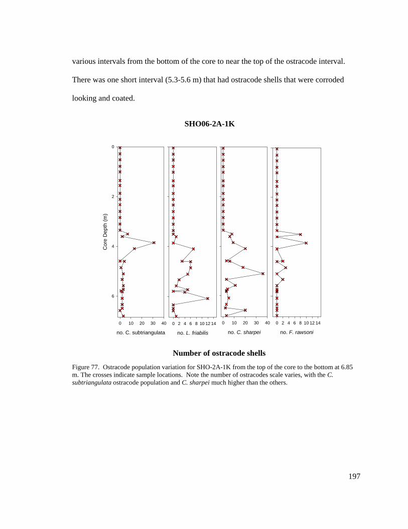
197

various intervals from the bottom of the core to near the top of the ostracode interval.

There was one short interval (5.3-5.6 m) that had ostracode shells that were corroded

looking and coated.

no. C. subtriangulata

0 10 20 30 40

Cor

eD

epth

(m)

0

2

4

6

no. L. friabilis

0 2 4 6 8 10 12 14

no. C. sharpei

0 10 20 30 40

no. F. rawsoni

0 2 4 6 8 10 12 14

Figure 77. Ostracode population variation for SHO-2A-1K from the top of the core to the bottom at 6.85m. The crosses indicate sample locations. Note the number of ostracodes scale varies, with the C.subtriangulata ostracode population and C. sharpei much higher than the others.

SHO06-2A-1K

Number of ostracode shells

198

4.2.7.4 Thecamoebians

Thecamoebians appear at about 6.8-6.6 m and above 2.8 m (Figure 78). The appearance

of thecamoebians at the bottom of the core, even in the limited number encountered, is

unlike any other core. Additionally, the thecamoebians at the top of the core are

continuous within the sampling sequence, and are typically common to abundant in this

interval with up to five species identified which are relatively abundant in the interval

(Appendix A, Subsection 6.2). The lowermost interval included three species of

thecamoebians. Thecamoebians appear above a nearby interval dated at 5.630 14C ka BP

(6.452 cal ka BP), however this date does not appear to be in sequence.

4.2.7.5 Other Macrofossils

Plant and insect macrofossils remained relatively high throughout the length of the core

(Figure 78). Plant levels were continuously high starting at the bottom of the core, and

started decreasing just above the thecamoebian interval at 2.6 m and increased to

common and abundant levels at about 1.0 m.

Insect macrofossil abundances were relatively high in the lower portion of the core, and

decreased thought the middle portions and then rose to relatively high abundance in the

top of the core. Overall insect levels in the core are relatively high, but cycle a number of

times from a minimum, rapidly rising to a maximum in the bottom third of the core, then

falling to a minimum just before the beginning of thecamoebians before finally rising in

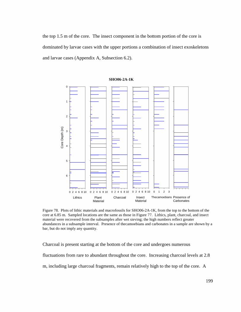
199

the top 1.5 m of the core. The insect component in the bottom portion of the core is

dominated by larvae cases with the upper portions a combination of insect exoskeletons

and larvae cases (Appendix A, Subsection 6.2).

Lithics

0 2 4 6 8 10

Cor

eD

epth

(m)

0

1

2

3

4

5

6

PlantMaterial

0 2 4 6 8 10

Charcoal

0 2 4 6 8 10

InsectMaterial

0 2 4 6 8 10

Thecamoebians

0 1 2 3

Presence ofCarbonates

Figure 78. Plots of lithic materials and macrofossils for SHO06-2A-1K, from the top to the bottom of thecore at 6.85 m. Sampled locations are the same as those in Figure 77. Lithics, plant, charcoal, and insectmaterial were recovered from the subsamples after wet sieving; the high numbers reflect greaterabundances in a subsample interval. Presence of thecamoebians and carbonates in a sample are shown by abar, but do not imply any quantity.

Charcoal is present starting at the bottom of the core and undergoes numerous

fluctuations from rare to abundant throughout the core. Increasing charcoal levels at 2.8

m, including large charcoal fragments, remain relatively high to the top of the core. A

SHO06-2A-1K

200

minimum charcoal interval occurs at about 2.3 m after the interval of charcoal abundance

and above the first appearance of thecamoebians at 2.8 m. Charcoal levels then rise

somewhat before rising to the more abundant levels with large fragments common

(Appendix A, Subsection 6.2). Small amorphous charcoal fragments were also noted in

some intervals between intervals of large fragments. Large charcoal fragments were

noted near the bottom of the core including what appear to be bark fragments. A large (1

cm) charcoal leaf fragment was found at 5.6 m with the interval dated at 6.685 14C ka BP

(7.554 cal ka BP).

Evidence of fish biota is present throughout the core, including the bottom intervals in the

core which have a higher incidence. What appear to be fish vertebrae, miscellaneous

bones, teeth and scales, are relatively common and significantly more abundant than in

LOTWs cores. A gastropod shell at 6.1 m and pelecypod shell at 3.4 m (just beyond the

end of ostracodes) were also noted. The pelecypod beyond the ostracode interval

correlates with the carbonate lithic evidence found in this interval. This interval is just

before the upper thecamoebian interval.

Seeds were present starting at about 2.8 m and became common to about 0.5 m from the

top of the core. The seed macrofossils started to appear at the same interval as the

beginning of the upper thecamoebian interval. The presence of birch nutlets were noted

(Appendix B, Section 4, Figure B-13) at about 1 m, and were dated at 2.525 14C ka BP

(2.636 cal ka BP).

201

4.2.7.6 Lithic Grains

The lithic materials are generally at low levels of abundance although there are some

intervals with elevated lithics grains (Figure 78). These are however, primarily non

disaggregated clay balls, with only two intervals with elevated quartz lithics (Appendix

A, Subsection 6.2). One interval with higher quartz is near the bottom of the core at 6.4

m, and one is near the top (0.3 m). Other than these two intervals, quartz concentrations

in this core essentially range from rare to none. An extended interval where carbonate

lithic grains including clay balls were observed occurs from about 4.6 to 2.6 m (includes

the interval where a pelecypod was observed), with other carbonate grains are

interspersed through the core from the bottom to about 1.6 m from the top of the core

where they disappear.

4.2.7.7 Radiocarbon Dates

Five radiocarbon dates were obtained in this core and are spaced relatively evenly over

the length of the core (Figure 79). One date, 7.130 14C ka BP (7.963 cal ka BP), at 3.0 m,

appears to be out of sequence with respect to the adjacent radiocarbon dates, and has been

rejected as being too old (by about 3.0 14C ka). An additional date at the bottom of the

core at about 6.8 m which was obtained from a large bulk sample (over a 12 cm interval)

was dated at 5.630 14C ka BP (6.452 cal ka BP) and appears suspect as it is much

younger than radiocarbon dates above this interval. The remaining dates are logically

sequenced and were used in making the subsequent assessments.

202

The youngest date 2.525 14C ka BP (2.636 cal ka BP) at 1 m, was obtained from two

birch nutlets and an insect head (Helodidae) (Appendix B, Section 5, Figure B-13). This

date helps define the beginning of thecamoebians and sedimentation rates in the upper

core.

The second oldest valid date of 6.170 14C ka BP (7.082 cal ka BP) at about 4.5 m was

obtained from an aquatic moss (Drepanocladus sp) (Appendix B, Section 5, Figure B-14)

which can be affected by the hard water effect. It does however appear to

chronologically sequenced reasonably well. The lowermost and oldest available valid

date at about 5.6 m, was dated at 6.685 14C ka BP (7.554 cal ka BP) and is the closest

viable date to the bottom of the core.

203

Figure 79. Radiocarbon dates for SHO06-2A-1K showing the ostracode and thecamoebian intervals.Sampled locations are the same as those in Figure 77. The yellow bars represent the presence ofthecamoebians at the top of the core and their sample locations; the yellow box indicates the location of thebottom two sample intervals of the lower thecamoebian sequence. The total number of ostracodes includesall species as are reported in the details of Figure 77. All dates are from the radiocarbon analysis reports inAppendix B.

SHO06-2A-1K

Number of Ostracodes

0 10 20 30 40 50 60

Cor

eD

epth

(m)

0

1

2

3

4

5

6

C. subtriangulataL. friabilisC. sharpeiF. rawsoni

Presence thecamoebians2525 (2636) BP

6170 (7082) BP

7130 (7963) BP

6685 (7554) BP

5630 (6452) BP

Radiocarbon Dates14C (cal) years BP

204

CHAPTER 5 INTERPRETATIONS OF SITE DATA

5.1 Overview

This chapter interprets the data from each individual core in order to assess the

paleoconditions at each of the relatively diverse coring sites. In Chapter 6, the

interpretations and data from each coring site are then integrated to provide a broader

interpretation for the LOTWs and SL region. Some common characteristics became

evident while interpreting the data for each coring location and are noted where

appropriate, to assist in interpreting data from each coring location. These common

characteristics are described in detail in Chapter 6.

5.1.1 Low Abundance and Number of Species of Ostracodes inLOTWs and SL

Only four species of ostracodes were identified in the LOTWs and SL cores, specifically,

Candona subtriangulata, Cyclocypris sharpei, Fabaeformiscandona rawsoni, and

Limnocythere friabilis. The abundance of ostracodes in the cores was relatively low in

many ostracode intervals, with typical concentrations from about 10-25 shells per 15 mL

sample, although many samples only had 1-3 shells. Ostracodes were not present

throughout the entire length of any of the cores. They were absent in the top portions of

all the cores and in most cores generally reduced in overall numbers moving upwards.

The lack of modern LOTWs and SL ostracode population analogues makes it difficult to

interpret paleo conditions.

205

The limited number of species may be related to water chemistry within LOTWs and SL.

The relatively fresh waters (low TDS) of Lake Agassiz (~ 100 mg/L) (Curry, 1997) are

well below the calcite branch point (Figure 33) where ostracode species richness reaches

a maximum. Ostracode diversity (species present) increases with increasing TDS levels

(De Deckker and Forester, 1988). There was an upwards increase in ostracode diversity

in most LOTWs and SL cores (e.g. Figure 68) before the ostracodes disappear from the

record. As water TDS level increases above the calcite branch point, ostracode species

richness (diversity) drops, but the abundance of the remaining species usually increases

as they adapt to these conditions (Smith and Horne, 2002). The low number of ostracode

species and their relatively low abundance in most intervals of the LOTWs and SL

sequences may reflect low salinity, and non-optimum concentrations of calcium and

bicarbonate ions in the water (Smith and Horne, 2002). The specific ostracode species

present reflects the available solutes in the water, and are specific to the physical

lacustrine conditions at the time (Smith and Horne, 2002).

Decreases in diversity of ostracode species can also be related to decreasing organic

nutrient levels and their availability (Burke, 1987), however the presence of

thecamoebians in the upper portions of the LOTWs and SL cores, which increases with

increasing nutrient levels (Wall et al., 2008), are generally indicative of an increase in

primary productivity (movement to more eutrophic conditions). Similarly, increased

plant and insect macrofossils were observed in the upper portions of the cores reflecting

increases in nutrient levels. This means nutrient levels should have been favourable for

206

ostracodes toward the top of the core, therefore, lack of sufficient nutrients can be

eliminated as a reason for the disappearance of ostracodes.

The chemical conditions in the Lake Agassiz sequence of LOTWs and SL were reflected

in the TDS levels and the specific chemical components, which were further reflected by

the low diversity of ostracodes in the bottom core sequences, and the dominance of C.

subtriangulata. These chemical conditions were retained somewhat in the early phases

of modern LOTWs and SL due to the input of Lake Agassiz sediments from the new

LOTWs and SL watersheds. Since the LOTWs and SL remains relatively low in TDS in

the modern lake, the disappearance of ostracodes was not likely caused by changes in

TDS, but possibly from the low availability of calcium and bicarbonate ions. However,

there may have been intervals when TDS levels fluctuated due to changes in the basin or

due to climate induced effects, so some of the ostracode intervals above the basal Lake

Agassiz zone may be related to fluctuations in TDS as well as Ca and HCO3.

The LOTWs watershed slowly evolved towards the modern vegetated watershed as Lake

Agassiz disconnected from LOTWs (Figure 8). The overall progression to the modern

vegetated LOTWs watershed, likely affected TDS levels. Once the terrestrial terrain

stabilized, inputs to the lake would trend away from the Lake Agassiz sediment inputs,

and have been influenced by organic rich runoff. Variations in terrestrial conditions

around LOTWs and SL, due to isostatic rebound and vegetative response would have

influenced the LOTWs generally and perhaps more so at specific sites. Climate change

could additionally increase solute through increased precipitation and watershed runoff,

207

or alternately in drier climatic intervals by increasing evaporation at the lake surface

resulting in lower lake levels and increasing proportions of solutes.

Climate induced changes resulting from increases in precipitation and the increased

runoff affect acidification of the lakes due to the increased levels of humic acid input and

changes in buffering. These climate related changes in pH are another factor affecting

ostracode populations and may lead to post diagenetic destruction of carbonate shells.

Although the water chemistry, particularly low bicarbonate levels are important to

ostracodes, from the core subsample observations it was noted intervals of carbonate-

bearing sediments, and the presence of gastropods and pelecypods, were found near and

above the end of the ostracode intervals in the cores. Their presence above these

intervals and the lack of any observed trend in damage to their shells, implies low

bicarbonate levels and post mortem or post diagenic loss of shell material due to low pH,

may not be the primary reasons for ostracodes disappearing from the record.

208

5.1.2 Radiocarbon Date Inconsistencies

A number of inconsistencies were encountered in radiocarbon dates obtained from the

cores, although the dated macrofossil samples were generally consistent and provided a

logical and sequential chronology in the cores. AMS radiocarbon dating of pollen was

undertaken on a number of cores when limited macrofossil content was encountered in

certain intervals, particularly near the bottom of the cores. Some rather large aberrations

in radiocarbon dates were encountered when the pollen samples were dated, with the

pollen dating from a time when the region was buried deep by the LIS (McMillan et al.,

2003; Teller et al., 2008). Pollen intervals, including increased charcoal deposits in

nearby WHL, were estimated to have begun from nearby watershed biota about 7.0 cal ka

BP (~ 6.1 14C ka BP), well after Lake Agassiz receded from the region (Teller et al.,

2008), hence local pollen should have been relatively young.

Pollen and resuspended microfossils from outside the region can be transported long

distances, especially over recently deglaciated terrain with low vegetative cover, and

were particularly susceptible to eolian transport including during the Younger Dryas

(Birks, 2001; Curry and Yansa, 2004). Long distance transport of pollen causing

discrepancies in radiocarbon dates is a well known phenomenon (Bajc et al., 2000).

Transported pollen can create circumstances where pollen and macrofossil radiocarbon

dates are not in close agreement due to biasing of the sample towards older dates due to

209

contamination from older pollen deposits (Bajc et al., 2000), or due to incorporation of

older carbon (Nambudiri et al., 1980) in the pollen samples, or in some cases transport or

reworking of macrofossils. In view of this, and the possible incorporation of older fine

grained carbon into pollen reworked from older sediments (Nambudiri et al., 1980), all

the pollen dates were rejected based on their anomalously old ages.

Terrestrial plant macrofossil radiocarbon dates are often considered more reliable than

pollen especially if the pollen is degraded (Curry and Yansa, 2004), and more reliable

than aquatic macrofossils which can be subject to the hardwater effect. However, in

LOTWs, one macrofossil date on a wood fragment (WOO06-5A-1K5 at 37.5 cm) was

noted to have been much older than the others and was dated at 15.6 14C ka BP (18.8 cal

ka BP) (Appendix B, Section 2). In this core the abnormally old wood fragment

macrofossil is located between two older pollen samples dated at 17.040 14C ka BP

(20.386 cal ka BP) and 17.560 14C ka BP (20.970 cal ka BP), implying it may have

eroded from older sediments and/or had been transported into the region. This

radiocarbon date was also rejected.

The macrofossils selected for dating were examined using an optical microscope during

processing of the subsamples, or by Paleotec Services during selection of suitable organic

materials from additional subsamples (i.e. their appendages were relatively intact).

Paleotec Services rejected any macrofossils that indicated they may have been

transported, before sending them to the Keck Carbon Cycle AMS Facility for radiocarbon

dating. Nonetheless, the possibility exists some macrofossils may have been reworked

210

from lower (older) Wisconsinian deposits (such as the WOO06-5A-1K5 sample at 37.5

cm), since Wisconsinian deposits have been reported to be close to the surface (< 10 m)

in south eastern Manitoba (Matile, 2001), or at the surface due to Lake Agassiz wave

actions in regions to the east of the Red River Lowlands (Fenton and Teller, 1980).

Other than the rejected WOO06-5A-1K5 sample radiocarbon dated at 37.5 cm, other

macrofossil dates were reasonable and were accepted.

5.2 Coring Site Interpretations General

The interpretation of the individual LOTWs and SL cores provides the means to track

paleohydrologic and paleoecologic conditions. However, differential isostatic rebound

must also be considered to help in understanding the changing conditions at the coring

sites. Seven of the ten cores recovered from LOTWs and SL were examined and

subsampled. These cores are the basis for the interpretations of the paleoecological,

paleoclimatic and paleohydrological conditions noted in the following sections.

The WOO06-3A-1K core was determined to have deflected sideways and only very

limited data was extracted from this core, although its shallower companion core

WOO06-4A-1K has provided data suitable for interpretation. The stratigraphic data and

the scanned image and core description presented in Chapter 4 are complemented by the

data provided in Appendix A for each core. The following paleoecologic and

paleohydrologic interpretations are based on those data.

211

5.2.1 South Basin Site - WOO06-1A

Differential isostatic rebound in this portion of the lake over the interval since LOTWs

separated from Lake Agassiz, resulted in the southern basin initially loosing its water

(Figure 9). Subsequently, the lake transgressed southward from the northern region near

Kenora (Figure 10). The elevation of the northern outlets to the Winnipeg River

ultimately controlled the bathymetry of the southern basin. Differential isostatic rebound

over time resulted in the northern outlet rising farther above the southern basin elevation,

ponding additional water in the large southern basin, and creating a transgression of

LOTWs to the south.

The southward transgression into the southern basin would have resulted result in

reworking of Lake Agassiz and glacial deposits. This, and the close proximity of the

sediment influx from the Rainy River, would likely increase the quantity of lithics in this

portion of the LOTWs. The slowly increasing water depths in the south and the

proximity to the inflowing Rainy River, would likely result in a unique paleoecology in

the southern basin coring site locations, which are about 40 km farther south of the North

West Angle area sites, and 90 km farther south of the Kenora outlets. It was anticipated

that Lake Agassiz deposits would not be encountered at the WOO06-1A-1K site,

however, there is contrary evidence based on the ostracode species identified (Figure 40).

In this area, an unconformity likely overlies the Lake Agassiz deposits, as a result of the

212

southward transgression of LOTWs and reworking of the sediments. This may account

for the appearance of the Lake Agassiz type ostracodes (Figure 43) in this core.

Alternately, the nearby Rainy River entrance into the southern basin may have created

localized compartments of deeper water or deep channels, as the water ponded in the area

and supported biota characteristic of Lake Agassiz.

5.2.1.1 Ostracodes

The exclusive C. subtriangulata interval at the bottom of the core, with a later co-

occurrence of L. friabilis, implies these sediments were deposited in deep, cold and low

salinity (TDS) waters such as those in Lake Agassiz. The later occurrence of F. rawsoni

implies a transition to higher salinities was underway just before the ostracode record

ends. The increase to three species in the core near 2.8 m is an additional indicator of

increasing but still relatively low salinity. The presence of carbonate coated shells of all

species implies there was sufficient carbonate in the sediments, however thin shells in

other nearby intervals may imply these conditions were not consistent. The rapid

decrease in ostracode numbers above ~ 2.7 m, without a preceding trend in shell thinning

and fragmentation in response to changing environmental conditions may mean a rapid

change in paleochemistry may have occurred. This either made the hydrochemistry

unsuitable for shell formation, or resulted in dissolution of the shells on the lake floor or

within the sediments, which then continued from this point to the top of the core.

Alternately, or in conjunction with changing hydrochemistry, a change in food supply

may have resulted in the apparent population crash and subsequent end of ostracodes in

213

LOTWs. A rapid drop in relative abundance of plant materials occurs above ~2.6 m

(Figure 43), with a continued low insect proportion, and may be an indication the

available food supply became limited, stressing the ostracode population. Interestingly,

the first occurrence of thecamoebians occurs at about 1.5 m, and the abundance of plant

macrofossils increases, followed by higher abundance of insect macrofossils, indicating

the availability of food likely increased at this time. Similarly the increase in plant and

insect macrofossils indicates increased lake productivity, supporting changes to more

eutrophic conditions as the reason for the increase of thecamoebians in the upper core.

The reason for the disappearance of ostracodes therefore is not likely to be the

unavailability of food supply.

The ostracode interval identified in the bottom of the core (Figure 40) includes a

radiocarbon date of 7.14 14C ka BP (~ 8.0 cal ka BP) at 3.3 m, with the ostracodes

appearing to be a typical Lake Agassiz sequence of ostracodes with an exclusive C.

subtriangulata interval at the bottom, similar to those observed in the more northerly

cores. However, the two radiocarbon dates near the bottom of the core are well after the

estimated date Lake Agassiz isolated from LOTWs. An interval further upwards dates to

7.375 14C ka BP (~ 8.2 cal ka BP) implying this older date above the younger date may be

from reworked materials, even though bristles on the dated Polygonum lapathifolium

seed were intact (Appendix B, Section 2, Table B-1, South Basin Site - WOO06-1A),

implying reworking was minimal. Macrofossils in nearby core intervals similarly imply

reworking was not significant. Since it is unclear which date is correct, the average of

these dates, 7.26 14C ka BP (8.05 cal ka BP), is used to estimate the end of the ostracode

214

interval. Nonetheless, both dates are after the date estimated by Yang and Teller for

isolation from Lake Agassiz (8.1 14C ka BP (9.0 cal ka BP)) and do not correspond with

the estimated calculated elevation from the paleotopographic maps (Yang and Teller,

2005), which indicate this portion of LOTWs should have been dry at this time (Figure

9).

The ostracode sequence changes to a more mixed population including L. friabilis and F.

rawsoni at about 3.0 to 2.7 m, with ostracode shells disappearing completely at 2.7 m,

near the radiocarbon dated sample at 2.9 m, dated at 7.375 14C ka BP (~ 8.2 cal ka BP).

One C. subtriangulata shell fragment appears above this point at 2.2 m, which may imply

reworking, however, an articulated claw on a bone in this interval, indicates reworking is

unlikely.

As noted in Section 5.2.1, there is a strong possibility the sediments in the southern basin

were reworked. The ostracode sequence from the cold, deep and low salinity ostracodes

species of C. subtriangulata and L. friabilis evolves upward to the more salinity- tolerant

F. rawsoni, and is a logical sequence for the hydrochemical evolution of the lake once it

became independent from Lake Agassiz. The presence of sub-adult instars in this

interval implies the sequence probably was not unduly reworked. Fragmented shells

could be an indication some reworking occurred, however, an articulated ostracode shell

at 3.0 m and the articulated claw on a bone at 2.2 m, are evidence that reworking in these

intervals did not occur or was limited.

215

Based on the ostracode sequence observed, cold water conditions like that of Lake

Agassiz, appear to have existed in the southern basin around 7.3 14C ka BP (8.1 cal ka

BP). Based on the estimated extent of LOTWs and Lake Agassiz by Yang and Teller

(2005), and the timing of the isolation of LOTWs from Lake Agassiz this suggests deep

compartments existed at this location in the southern basin.

5.2.1.2 Thecamoebians

The locations where thecamoebians are present are identified in Figure 41 and detailed

thecamoebian observations can be found in Appendix A, Subsection 1.2. Thecamoebians

first appear at 1.4 m, corresponding with a high proportion of plant material and generally

high abundance of insect macrofossils, suggesting productive lake conditions existed at

this time. A radiocarbon date at 1.37 m indicates this first appearance of thecamoebians

and the change to more eutrophic conditions at this location occurred at about 1.685 14C

ka BP (1.579 cal ka BP). This is the youngest date for the appearance of thecamoebians

in all processed cores (see Chapter 6).

Numerous species of thecamoebians were observed with up to five noted in some

intervals (Appendix A, Subsection 1.2), indicating an abundance of food was likely

available in this interval. Thecamoebian species including Difflugia oblonga and

Centropyxis aculeate which have been associated with warmer and cooler conditions

respectively, indicate thecamoebians may be responding to a changing climate.

216

5.2.1.3 Other Macrofossils

Abundant charcoal in the lower portion of the core and high abundance of plant materials

were observed in what would appear to be Lake Agassiz intervals based on the ostracode

record. High charcoal and plant abundances in a Lake Agassiz sequence are not typical.

This may be an indicator of reworking, but the charcoal does not appear to have been

transported based on the many fine fragile looking structures present in the fragments.

Numerous mammal molars, an incisor, a claw attached to a bone, and vertebrae were

found in the interval from 2.3 to 1.8 m. This is below the thecamoebian zone which was

interpreted to be the start of more eutrophic conditions, and about 0.5 m above the end of

the ostracode interval. The terrestrial vertebrate macrofossils and presence of terrestrial

plant macrofossils are possible indicators of near shore conditions, the articulated claw

and bone imply relatively low energy conditions and limited reworking appears to have

occurred in this interval. It is possible this interval is either terrestrial, or in a swampy

location with the low energy condition implying a swamp-like condition may have

existed at this time.

5.2.1.4 Lithic Grains

Figure 41 indicates the abundance of lithic grains in the sequence and indicates those

locations where carbonate grains were detected. Detailed observations of these lithic

grains including presence of clay balls are included in Appendix A, Subsection 1.2. A

low volume but high relative abundance of lithic grains is present in the subsamples near

the bottom of the core, from 3.3 to 2.2 m. This is similar to Lake Agassiz sequences

217

observed in the other cores (see Chapter 6). Upward in the core, higher volumes of

primarily quartz lithics occur in the subsamples and the abundance of lithics remains high

up to 1.1 m. This could possibly be an indication of reworked shorelines as LOTWs

transgressed southward, although most organic macrofossils in these intervals do not look

to have been transported (Appendix A, Subsection 1.2).

Above 2.0 m, well above the main sequence of ostracodes and about 20 cm above the

interval where a single ostracode shell was noted, carbonate lithics were no longer

identified. This may indicate a time when a significant hydrological change possibly

occurred in this portion of the lake, perhaps due to changes in the drainage basin of the

lake, or a time of hydrological/hydrochemical changes. The presence of carbonates

corresponds with the intervals where coated ostracode shells were noted, and also

includes the 70 cm interval above the ostracode interval. It is possible this may indicate a

change to more acidic conditions may have occurred, preventing ostracode shells that

may have formed from being preserved with post depositional leaching and destruction of

ostracode shells on the lake floor and within the upper sedimentary sequence occurring

(Teller, 2009, personal communication).

Lithics were consistently the highest relative proportion of the sieved materials in the

lower part of the sequence until about 1.4 m, when conditions in the lake became more

productive (Figure 41), as indicated by the increasing macrofossil content including

thecamoebians. Maximum lithics sizes were around 4 mm throughout the core

decreasing somewhat in the uppermost metre of the core to 2-3 mm. This would be

218

expected as the initial transgression period probably would have reworked more sediment

from the underlying surface.

5.2.1.5 Sedimentation Rates

The radiocarbon dates in the core provide the means to estimate sedimentation rates. As

discussed previously there are some aberrant dates and these are not included in the

sediment rate calculations. The two lower core dates were averaged when the

sedimentation rates were estimated. Assuming no losses from the top of the core during

recovery, produces an overall sedimentation rate of 0.4 mm/yr [3.0 m / (8228+7973 cal

yrs at 3.0 m) / 2) = 0.38 mm/cal yr].

The two upper core radiocarbon dates are in sequence, with the lower date of 1.675 14C

ka BP (1.579 cal ka BP) defining the beginning of the thecamoebian sequence at about

1.4 m. The uppermost radiocarbon date of 1.460 14C ka BP (1.358 cal ka BP) at about 0.9

m, in conjunction with the lower date, imply two sedimentation rates may have been in

effect in the upper part of the core, or some material may have been lost from the top part

of the core during recovery.

A sedimentation rate in the top 1.37 m of the core is estimated to be 0.9 mm/yr [(1.37 m /

(1579-0) yrs = 0.87 mm/cal yr]. This sedimentation rate corresponds well with modern

rates reported by Molot (Molot et al., 1987) of 0.7 mm/yr. In contrast a low overall

sedimentation rate of 0.25 mm/yr was observed in the much smaller West Hawk Lake

219

(Teller et al., 2008) in the 10,000 year period after isolation from Lake Agassiz. This

sedimentation rate is consistent with those identified in the Experimental Lakes Area

(ELA) since about 8.2 cal ka BP (7.3 14C ka BP) (Laird and Cumming, 2008). Laird and

Cumming reported sedimentation rates as being relatively consistent and based on data

from the paper the rate appears to be about 0.16mm/yr over the entire length of the core

(ignoring compaction).

In the interval between the upper and lower portions of the core, the sedimentation rate is

0.3 mm/yr [(3.0-1.37 m) / ((8228+7973 yrs) / 2)-1579 yrs) = 0.25 mm/yr]. This

sedimentation rate in the intermediate interval of the core is close to those reported others

in the LOTWs region.

5.2.1.6 Discussion and Interpretation of Coring Site Data

There are a number of conflicting interpretations possible from the data from this core.

Initially, based on ostracode sequences, it appears this core extended into Lake Agassiz

sediments. However, there are unusually large proportions of charcoal compared to Lake

Agassiz sequences in other cores. Perhaps the charcoal is from encroachment of post

glacial forests in the region from the south which washed into LOTWs through the Rainy

River after Lake Agassiz drained from this area. Mid-core intervals containing terrestrial

vertebrate molars and other skeletal components, are noteworthy (Appendix A,

Subsection 1.2). Perhaps they indicate a lake had formed in this location of the southern

basin, and this coring site was near shore or close to swampy area as discussed earlier.

220

The uncharacteristically high lithics volume and increased abundance when compared to

other cores (see Chapter 6) in the mid-core intervals, and the plant and larger charcoal

fragments, including seeds near the bottom of the core in what appears to be a possible

Lake Agassiz sequence (Figure 43), are problematic. Based on the other cores, Lake

Agassiz sequences typically have low lithics volumes (although a high relative

abundance compared to other materials). The lithics volume in this core may be

indicative of shoreline erosion, due the subsequent differential isostatic rebound induced

southward transgression. The two dates from the lower core indicate the sediments were

deposited well after the LOTWs and Lake Agassiz isolation, despite the presence of the

deep and cold water C. subtriangulata ostracode. Furthermore, the lowermost

radiocarbon dates place the associated sediments in an interval where lacustrine

conditions should not have existed in this area (Figure 10). This leads to the possible

interpretation of these apparently conflicting data that this part of the LOTWs basin

contained small lakes, disconnected from the main body of LOTWs that formed after

Lake Agassiz fell below the level of the lake floor.

The sedimentation rate estimates do show some significant changes and the overall

sedimentation rate is relatively high at about 0.4 mm/yr, which is about twice the rates

from the lake 239 of the ELA, and most of the other cores (see Chapter 6). The upper

core sedimentation rate of 0.9 mm/yr is closer to those reported by Molot, but compared

to other LOTWs coring sites, it is very high (Molot et al,. 1987).

221

The relatively high sedimentation rate calculated for the top of the core is of course

partially due to less dewatering in the upper core and hence less compaction. The

sedimentation rate in the middle core region of about 0.3 mm/yr is close to the overall

sedimentation rate and closely reflects the observed ELA and WHL rates, although these

lakes are in substantially different watersheds. There is no reliable means to estimate the

lower core sedimentation rate with the available radiocarbon dates.

There is some variability in the stratigraphy within the core, with the lower ~ 1.7 m

distinctly laminated. A sharp contact at ~ 2.8 m separates a lower moisture interval

below with a distinct colour change at this point, from dark grey below, to a dark grey-

brown interval above. This point is at the end of the ostracode interval (Figure 40). In

view of the distinct contact it is possible that this may be an erosional surface on which a

weak soil may have developed (Figure 39). Since the Rainy River inflow is nearby, some

of the coarser grains and organics may have been brought into this portion of LOTWs.

The question remains, are the sediments near the bottom of the core either Lake Agassiz

or near Lake Agassiz sediments? The ostracode sequence, especially the presence of C.

subtriangulata and L. friabilis indicate that deep, cold, and low TDS paleohydrological

conditions existed at least until about 7.3 14C ka BP (~ 8.1 cal ka BP) at around 3 m (from

the averaged two lower dates), shortly above which the ostracode interval ended. The

radiocarbon dates however are much later than the estimated separation of LOTWs from

Lake Agassiz, and furthermore, this part of the lake should have been dry land according

to the paleotopographical data (Figure 9 and Figure 10) from Yang and Teller, 2005. It is

222

unclear why deep and cold water would have existed at the time the radiocarbon dates

suggest, although the dates do appear to be at the beginning of the Hypsithermal possibly

prior to the onset of warmer and drier conditions in the region. One possible

interpretation is that the inflowing cold Rainy River water flowed into a deep sub-basin

within the generally dry southern basin at this coring location.

This independent lake within the southern basin would have remained independent until

isostatic rebound caused the main lake to transgress into the southern basin. If this were

the case this location would have had a distinctly different history and paleoenvironment

than the deep basins to the north, and would have been strongly influenced by the

inflowing Rainy River just to the east.

The onset in increased more eutrophic conditions occurred at about 1.685 14C ka BP

(1.579 cal ka BP), with the appearance of thecamoebians above at about 1.4 m. Multiple

thecamoebian species are evident throughout most of this part of the sequence, included

D. oblonga and C. aculeate. The appearance of thecamoebians corresponds with

increasing plant and insect macrofossils (Figure 41), supporting the interpretation that the

appearance of thecamoebians correspond with the onset of more eutrophic conditions in

this part of the southern basin.

223

Summary

The ostracode populations only occur in the bottom portion of the core and they reflect

deep, cold, and low TDS conditions typical of Lake Agassiz based on the presence of

both C. subtriangulata and L. friabilis. The radiocarbon dates of 7.140 14C ka BP (7.973

cal ka BP) and 7.375 14C ka BP (8.228 cal ka BP) near the bottom of the core are too

young however, for these to be Lake Agassiz sediments, so this part of the sequence is

interpreted to have been deposited in this location after Lake Agassiz drained from this

area about 9-10 cal ka BP. The ostracode species imply there may have been a deep cold

compartment in this area, which then trended to more saline conditions during the

Hypsithermal.

There is conflicting evidence with respect to reworking of the sediments of the core

(Appendix A, Subsection 1.2), making interpretation of paleoconditions challenging.

However, a low moisture zone (Figure 39 and Figure 42) at the top of the ostracode

bearing sequence at about 2.8 m, suggests that the southern basin may have become dry

sometime after about 7 14C ka BP ( ~ 7.8 cal ka BP). There is evidence of an erosional

surface at 2.8 m and a potential paleosol above. The mid-core sediments above this

interval up to the beginning of thecamoebians appear to reflect a nearby low energy

shoreline or swampy area existed near this site. The possibility of an erosional surface at

the top of the ostracode interval may mean the ostracode bearing sediments were

reworked, affecting the ostracode signal and the associated radiocarbon dates which were

not sequenced chronologically.

224

An increase in lake productivity is estimated at 1.685 14C ka BP (1.579 cal ka), at a point

where plant abundance in the lake increases, insect materials increase, and where

thecamoebians became part of the record. These data all seem to reflect higher nutrient

conditions were established at this time, and have continued to today.

5.3.1 Northwest Angle Site - WOO06-3A

The WOO06-3A-1K coring site is located near an intermediate point in the lake which

would have been subject to the long term southward transgression from the more rapidly

rebounding northern part of the lake, and would have provided the pathway to the

northern outlets from the northward flow of draining waters from the Rainy River

watershed and southern basin watershed inflows (Figure 10). The draining of this excess

water northward to the Winnipeg River would be through relatively narrow channels in

this portion of LOTWs (Figure 24). The Northwest Angle sites are located to the east of

a large emerging island within Lake Agassiz (Figure 8) which resulted in a topographic

high after separation of Lake Agassiz (Figure 9).

225

5.3.1.1 Ostracodes

No ostracodes were observed in this core.

5.3.1.2 Thecamoebians

The uncertainties introduced by the deflection of the core make interpretation of

thecamoebian data from this core impossible.

5.3.1.3 Other Macrofossils

The uncertainties introduced by the deflection of the core make interpretation of

macrofossil data from this core impossible.

5.3.1.4 Lithic Grains

Intervals of abundant granitic and quartz lithics were observed throughout the core;

however, the uncertainties introduced by the deflection of the core make interpretation of

lithic grain data from this core impossible.

5.3.1.5 Sedimentation Rates

The uncertainties introduced by the deflection of the core make interpretation data from

this core impossible.

226

5.3.1.6 Core Chronology

Only one radiocarbon sample was sent for analysis and it indicated an unusually young

radiocarbon date at ~ 7.3 m near the bottom of this 7.47 m core, of 2.915 14C ka BP

(3.070 cal ka BP) (Appendix B, Section 2, Table B-1, NWA - Channel Site WOO06-3A).

Establishing a core chronology based on this single radiocarbon date, especially

considering the deflection of the core, is not possible.

5.3.1.7 Discussion and Interpretation of Coring Site Data

The unusually young date of 2.915 14C ka BP (3.070 cal ka BP) at about 7.3 m, indicates

the WOO06-3A-1K core did not maintain a vertical orientation in the sediments and was

significantly deflected when it encountered a hard substrate during its penetration of the

sediments. The interpretation that the core underwent a significant deflection is further

supported by the processed subsample results. By combining the unusually young date

near the bottom of this long core, the observations of thecamoebians at the bottom of the

core and their long hiatus from ~ 7 to 1.4 m, and the absence of any ostracodes in the

core, it is evident the core barrel had deflected significantly from the vertical. This would

also explain the significant difficulty in recovering the core from the sediments to the

Kullenberg platform during the core recovery operation.

227

5.4.1 Northwest Angle Site - WOO06-4A

The WOO06-4A-1K coring site is located near an intermediate point in the lake which

would have been subject to the long term southward transgression from the more rapidly

rebounding northern part of the lake, and would have provided the pathway to the

northern outlets from the northward flow of any water draining from the Rainy River

watershed and southern basin watershed inflows (Figure 10). The draining of this excess

water northward to the Winnipeg River would be through relatively narrow channels in

this portion of LOTWs (Figure 24). The Northwest Angle sites are located to the east of

a large emerging island within Lake Agassiz (Figure 8) which resulted in a topographic

high after separation of Lake Agassiz (Figure 9).

This LOTWs location is relatively unique in that it is located in a relatively deep narrow

channel and would likely have been subject to currents throughout most of its history. It

was anticipated sediments in the channel may have differed somewhat from the open

basin and that a different paleoenvironment may have prevailed. There is evidence of an

indistinct paleosol development (Figure 45) containing pedogenic blocky structures in the

sediments of this site and the sediments contain considerable organic accumulations,

including evidence of near shore conditions (Appendix A, Subsection 2.2).

This core is the shortest of all cores (about 2 m) however, despite this limited penetration

it appears Lake Agassiz sediments may have been encountered. Subsamples from the

228

bottom of the core have a high relative proportion of lithics, appear relatively barren with

low plant and insect contents, and include C. subtriangulata ostracodes.

5.4.1.1 Ostracodes

Only the C. subtriangulata ostracode is found in this core which implies these sediments

were deposited in deep, cold, and low salinity (TDS) waters, such as those in Lake

Agassiz. The ostracode interval in this core ends about 0.2 m above the bottom of the

core at about 1.8 m. The nearby radiocarbon date of 7.655 14C ka BP (8.443 cal ka BP)

from bulrush achenes (Scirpus validus), at 1.5 m can be extrapolated downwards to 1.8 m

based on a rough estimate of the overall sedimentation rate of 0.23 mm/cal yr (see

Section 5.4.1.6). This rough estimate places the end of the ostracode interval in this core

at about 8.8 14C ka BP (9.8 cal years BP) [0.23 mm/yr X (1800 -1500 mm + 8443 = 9747

cal years BP or ~ 8.8 14C ka BP]. It is important to note this is a very rough estimate as

sedimentation rates below the paleosol are not know due to the lack of two available

radiocarbon dates below the paleosol, nonetheless it places the end of ostracodes into a

Lake Agassiz interval and corresponds reasonably well with the isostatic rebound

calculations of Yang and Teller. The presence of the C. subtriangulata ostracode species,

in conjunction with the high quartz lithics component, and low plant, insect, and charcoal

macrofossils, further supports the conclusion the bottom sediments in this core are from

Lake Agassiz.

229

5.4.1.2 Thecamoebians

In the first of two thecamoebian intervals in the core at about 0.77 m, two species of

thecamoebians were identified. They appear between two lower radiocarbon dated

intervals at 0.74 m (6.330 14C ka BP (7.319 cal ka BP)) and 0.92 m (6.955 14C ka BP

(7.787 cal ka BP)), and therefore, assuming a constant sedimentation rate, the date of first

appearance of thecamoebians can be estimated at 6.5 14C ka BP (7.4 cal ka BP) [(0.77-

0.74 m) / (0.92-0.74 m) X (6955-6370 14C yrs) + 6370 14C BP = 6.468 14C ka BP]. This

date is the earliest date for the presence of thecamoebians found in the examined LOTWs

cores in this area of LOTWs (see Chapter 6), and indicated an early more eutrophic

interval in this channel location. This thecamoebian zone is within intervals with

abundant large plant and charcoal fragments (Figure 47) (Appendix A, Subsection 2.2).

The second thecamoebian interval at 0.31 m follows a thecamoebian hiatus, and contains

four species possibly indicating more eutrophic conditions. The date for this uppermost

interval assuming a constant sedimentation rate and using the nearest radiocarbon dated

intervals is 3.8 ka BP (4.2 cal ka BP) [(0.31-0.08 m) / (0.74-0.08) X (6370-2495 14C yrs)

+ 2495 = 3.845 14C yrs], which still predates most of the other thecamoebian intervals

(see Chapter 6, Table 3). The uppermost appearance of thecamoebians occurs within a

zone of high plant and insect macrofossils, and charcoal fragments, which supports the

interpretation that the upper portion of the core was productive and hence more eutrophic

since about 3.8 ka BP (4.2 cal ka BP).

230

5.4.1.3 Other Macrofossils

Significant changes in environmental conditions are evident in the macrofossil data from

this site (Figure 47). The occurrence of fish vertebrae and scales between 0.6 to 0.3 m in

the thecamoebian hiatus, and high abundance of plant and charcoal macrofossils, and

increased insects material, upward from the black organic rich interval at about 1.5 m, are

evidence of these changes (Appendix A, Subsection 2.2). These changes in

environmental conditions across the black bed are clearly reflected in Figure 45.

A gradational lower boundary and a sharp boundary at the top of the 5 cm thick distinct

black interval, marks the beginning of a transition from a low organic material interval

below this point, to a zone of abundant plant and seed macrofossils, and large charcoal

fragments within and above this interval. This black organic interval includes an

abundance of seeds of terrestrial and near shore plants, such as curlytop knotweed

(Polygonum lapathifolium) and bulrush (Scirpus validus) (Appendix B, Section 4,

Figures B-2, B-3 and B-4) and also Scirpus validus. These organic rich sediments

include insect macrofossils and abundant large charcoal fragments, and are consistent

with a near shore paleoenvironment, which reflects the modern configuration of this

narrow channel.

231

5.4.1.4 Lithic Grains

Figure 47 indicates the changes in the abundance of lithics within the core, and indicates

those subsamples where carbonate lithics were detected. Abundant quartz and mica, and

carbonate lithics, in the bottom ~ 0.4 m of the core are similar to the Lake Agassiz

sequences observed in the other cores. High abundances of lithic grains including clay

balls occur below the distinct black boundary (Figure 45), and are present in conjunction

with carbonate lithics and ostracodes. These data appear to be consistent with Lake

Agassiz or near Lake Agassiz sediments. The available radiocarbon date confirms these

sediments were deposited close to the time estimated for separation of Lake Agassiz from

LOTWs. The dramatic appearance of the black organic rich sediments indicates a

significant change in the paleoenvironments after the lowermost lithic deposits were laid

down.

5.4.1.5 Core Chronology

All radiocarbon dates in this core are in chronological sequence (Figure 48) however, the

uppermost radiocarbon date of 2.495 14C ka BP (2.604 cal ka BP) is very near the top of

the recovered core at 0.08 m. The closeness of the uppermost radiocarbon dated sample

to the top of the core, and its relatively old date, indicates some material was likely lost

from the top of the core. The lowermost date of 7.655 14C ka BP (8.443 cal ka BP) using

a Scirpus validus (bulrush) seed implies this channel was vegetated shortly after Lake

Agassiz withdrew from the region. The two radiocarbon dated samples at 0.74 and 0.92

232

m of 6.370 14C ka BP (7.319 cal ka BP) and 6.955 14C ka BP (7.786 cal ka BP)

respectively, were obtained from an interval containing terrestrial plant components such

as leaves, stems and seeds, and a near pedogenic sediment (Figure 45). These dates

establish the chronology for an interval where this site may have been subject to climate

induced changes during a relatively dry interval in the Hypsithermal.

5.4.1.6 Sedimentation Rates

Lost material from the top of the core (based on the relatively old radiocarbon date at the

top) limits the ability to estimate sedimentation rates in this core. The muck core was

also lost at this site. Nonetheless, the overall sedimentation rate was estimated based on

the dates from close to the bottom at 1.5 m (7.655 14C ka BP (8.443 cal ka BP)) and the

uppermost radiocarbon date near the top of the recovered core (Figure 48), and is

estimated to be about 0.2 mm/yr [(1.5 - .08 m) / (8433 - 2604 cal yrs) = 0.23 mm/yr)].

The rate from the lower mid-core date (6.955 14C ka BP (7.786 cal ka BP)) to the lowest

mid-core date is about 0.9 mm/yr [(1.5 - .92 m) / (8443 - 7786 yrs) = 0.88 mm/yr]. The

rate from the upper mid-core date (6.370 14C ka BP (7.319 cal ka BP)) to the uppermost

radiocarbon date near the top of the core date is about 0.1 mm/yr [(.74 -. 08 m) / (7319 -

2604 cal yrs) = 0.14 mm/yr].

The estimated 0.1 mm/yr sedimentation rate in the upper portion of the core is consistent

with the overall relatively low sedimentation rate of 0.2 mm/yr, however is much lower

than the LOTWs sedimentation rate of 0.7 mm/yr (Molot et al., 1987) and some of those

233

observed in other cores (see Chapter 6). The loss of material from the top of the core

made it necessary to estimate the uppermost sedimentation rate by assuming the rate is

similar to the rate from the upper mid-core radiocarbon date to the available upper core

date. The higher rate in the mid-core region above the black organic rich bed at 1.5 m, of

0.9 mm/yr, is possibly related to the withdrawal of Lake Agassiz and a change to the arid

Hypsithermal climate conditions which caused the channel to shallow. This may have

created a higher sedimentation rate than average across the core in this interval.

5.4.1.7 Discussion and Interpretation of Coring Site Data

The C. subtriangulata ostracode species in the lowermost part of the core interval and

lack of any other ostracode species, implies the cold, deep and low TDS conditions of

Lake Agassiz existed in the bottom portion of the core. The C. subtriangulata

ostracodes, high relative proportion of quartz lithics, and presence of carbonates, all

imply Lake Agassiz conditions prevailed at the bottom of this core. The available

radiocarbon date of 7.655 14C ka BP (8.443 cal ka BP) confirms the bottom of the core is

likely within the Lake Agassiz sequence (Figure 48). The disappearance of ostracodes

roughly estimated at 8.8 14C ka BP (9.8 cal years BP) appears to be close to the time

when LOTWs became isolated from Lake Agassiz.

The observed change of lithology at the black organic rich bed at a sharp contact just

below 1.5 m (Figure 45) indicates a dramatic change in conditions above this interval.

Perhaps this contact marks the time when isostatic rebound and possibly a dry climate

234

markedly changed the environment within this channel completing the transition from a

Lake Agassiz dominated paleoenvironment, to a LOTWs influenced environment. A drop

in moisture content was also noted below 1.5 m. It is also possible the sharp upper

contact of organic materials may be indicative of a localized shallow fluvial deposit

within the channel creating an unconformity. Both possibilities indicate a fundamental

change occurred about this time.

The unit above the black organic rich bed to about 0.8 m which is dated at 6.955 14C ka

BP (7.786 cal ka BP), ranges from well laminated to poorly laminated, with a fine

angular blocky pedogenic like layer at the top of the interval (Figure 45). The inclusion

of two distinct black beds above the black organic bed at 1.5 m, and other smaller ones

within this sedimentary unit, imply a shallowing near shore environment, with blocky

structures indicating a near paleosol condition down to about 1.3 m. The processed

subsamples (Appendix A, Subsection 2.2) confirm the observations in the core

descriptions, with abundant plant and charcoal fragment intervals prevalent throughout

the unit, and with clay balls and ball fragments near the top at about 0.8 m.

Although there are variations in the observed lithology in the core above 1.5 m, the

processed samples have a limited variability except at about 0.74 m, where carbonate

lithics reappear and then disappear above (Figure 47). The abundance of insect material

drops at this interval, and the processed subsample is primarily a mat of plant materials,

including seeds and large charcoal fragments, which are continuous from the black

organic rich bed to this point. The pedogenic structures and large volumes of organics

235

imply a paleosol and/or terrestrial conditions occur from the black bed to just below 0.77

m, which is dated at 6.370 14C ka BP (7.319 cal ka BP). The first thecamoebians appear

at 0.77 m indicating a change in the environment in the channel at this point, and then

they disappear as they undergo a hiatus above to 0.31 m.

The pedogenic and near pedogenic lithology and terrestrial conditions, likely indicate arid

Hypsithermal paleoenvironmental conditions. Two dated samples, one dated at 6.370 14C

ka BP (7.319 cal ka BP) at 0.74 m, and the other at 6.955 14C ka BP (7.786 cal ka BP) at

0.92 m, were obtained from this pedogenic/terrestrial interval providing times when these

dry climatic conditions occurred. The thecamoebians indicate local eutrophic conditions

likely occurred within this channel perhaps as a result of reduced flows in the channel

due to dry conditions.

The reduction of overall volume of organic and large charcoal components in the

processed samples above 0.74 m and the thinly laminated interval above, which grade to

non-laminated at the boundary of the uppermost gyttja unit at 0.08 m, are likely in

response to increasing water depth. The presence of fish vertebrae and scales in the

uppermost portions of the core similarly may indicate increasing depth. The effects of

differential isostatic rebound may have slowly deepened the waters within the channel as

a result of the transgression, in conjunction with increased precipitation as the climate

eventually became less arid post Hypsithermal. The re-occurrence of multiple types of

thecamoebians near the top of the core may signal increased eutrophic conditions that are

236

prevalent within the LOTWs in the uppermost portions of all examined cores, including

the nearby cores in the open basin near the Northwest Angle (see Chapter 6).

The large amount of organic material and abundant charcoal at 1.5 m at the black organic

rich bed, suggest a period of shallow water conditions, or terrestrial conditions. The

abundant large charcoal fragments in this unit, implies the region was arid and fires were

nearby, similar to the other Northwest Angle sites. The fluvial conditions within this

channel in LOTWs may have resulted in higher concentrations of large charcoal deposits

at this site, as charcoal materials were transported by wind and wave action into this

channel from the dry basin sites of the Northwest Angle at this time. These materials

may have been amplified by shedding of materials from the large Lake Agassiz island

and subsequent highlands to the west (Figure 8 and Figure 9). This influx of materials

may be recorded as the black organic rich bed.

Dramatic increases in insect macrofossils at 0.74 m, above the last paleosol interval were

noted. These occurred just prior to the increased thecamoebian interval and the

subsequent drop in the insect component. This is similar to characteristics in both of the

Northwest Angle basin sites (discussed in Chapter 6). There appears to be an increase in

productivity in this part of the LOTWs, based on the plant and insect materials and

thecamoebian signals.

The short sediment length in this core (~ 1.5 m) from the top of the core to Lake Agassiz

sediments may have been the result of current flow through the channels in this region

237

and possibly erosion of sediments (note as indicated earlier some material was lost from

the top of this core).

Summary

Based on the radiocarbon dates of the paleosol intervals in this core, it appears these

intervals may have been associated with dry Hypsithermal conditions. The formation of

shallow water conditions and paleosols within the channel appear to have occurred

between the black bed dated at 7.655 14C ka BP (8.443 cal ka BP) at 1.5 m and 6.370 14C

ka BP (7.319 cal ka BP) at 0.74 m. Although the paleotopographic maps indicate this

region should have been terrestrial at 8.1 14C ka BP (9.0 cal ka BP) (Yang and Teller,

2005), this part of the LOTWs would have received transgressive waters from the north

basin of LOTWs due to differential isostatic rebound and have received the runoffs from

the ponding of waters in the south basin area supplied by the Rainy River. It appears this

channel site was in operation from the time of the retreat of Lake Agassiz, through the

period of time when this region of LOTWs was predicted to have been dry, however its

operation appears to have been interrupted as indicated by the formation of a paleosol

interval.

Based on the available radiocarbon date at the black bed at 1.5 m, the bottom of the core

appears to be well within the Lake Agassiz sequence. Ostracodes and these Lake Agassiz

like sediments continued to be deposited in this region at least up until the end of the

238

ostracode interval roughly estimated at 8.8 14C ka BP (9.8 cal years BP) which

corresponds well with the paleotopographic maps.

Thecamoebians appeared in two separate intervals (Figure 47); the first one at about

6.468 14C ka BP (7.397 cal years BP) is earlier than most of the other processed cores

(see Chapter 6). The second interval 3.845 14C ka BP (4.247 cal ka BP) is still much

earlier than most of the other LOTWs sites. An increased insect component noted even

earlier than this thecamoebian date appears to indicate an increase in productivity,

possibly due to localized conditions within this narrow channel. The high charcoal and

plant macrofossil contents in these sediments from the black organic rich bed at 1.5 m to

the gyttja interval at the very top of the recovered core, implies nearby surrounding

terrestrial biota and possibly the introduction of terrestrial materials from the nearby

Northwest Angle basin area which may have been dry at his time from differential

isostatic rebound and possibly due to drying climatic conditions at this time. The

presence of terrestrial and near shore plants in the sediments of the channel would likely

be strongly influenced by the narrowness of the channel, making it difficult to use these

indicators to assess paleohydrologic conditions. Nonetheless, there appears to be a

consistent signal from the various proxies in this area which reflect the changing

paleohydrologic conditions since Lake Agassiz isolated, including changes introduced by

differential isostatic rebound, drying conditions in the Hypsithermal, and the changes

from increasingly productive conditions in the modern lake in this region.

239

5.5.1 Northwest Angle Site - WOO06-5A

The WOO06-5A-1K coring site is located at the north/south mid-point of modern

LOTWs (Figure 24) and would have been subject to the long term southward

transgression from the more rapidly rebounding northern part of the lake (Figure 10).

Differential isostatic rebound in this northern part of the southern LOTWs basin, resulted

in this basin accumulating water flowing in from the main inlet from the Rainy River and

the LOTWs watershed, with the elevation of the northern outlet to the Winnipeg River

ultimately controlling the bathymetry of the southern basin (Figure 10). The Northwest

Angle sites are located to the east of a large emerging island within Lake Agassiz (Figure

8) which resulted in a topographic high after separation of Lake Agassiz (Figure 9).

The relative shallowness of this part of the northern basin region and distance from the

Rainy River inlet, would likely make this region more responsive to aridity during

climate warming cycles and due to the effects of differential isostatic rebound.

Sedimentary evidence and macrofossil evidence from this core provide evidence of

paleosol formation from the early Holocene through the mid-Holocene. Sediments at the

bottom of the core appear to have been deposited during a phase of Lake Agassiz. This

core was extensively subsampled and radiocarbon dated.

240

5.5.1.1 Ostracodes

An exclusively C. subtriangulata interval in the bottom metre of the core implies these

sediments were deposited in deep, cold and low salinity waters (TDS), such as those in

Lake Agassiz. Changes to a more mixed ostracode sequence (Figure 54), including the L.

friabilis interval from 4.5 to 4.1 m, continues to be consistent with deep, cold and low

TDS conditions. The disappearance of C. subtriangulata at about 3.8 m, with L. friabilis

dominating in an interval from about 3.9 - 3.4 m, which also contains C. sharpei and F.

rawsoni is consistent with increasing TDS levels and warmer water conditions.

The presence of ostracodes within the paleosol does not at first appear reasonable (Figure

80), however, it is possible these ostracodes were present in the overlying lacustrine

environment, and then were incorporated into the paleosol when it formed. Paleosol

horizons form downward (personal communication J. Teller) and the presence of

ostracodes within the upper and lower paleosols may have resulted from the paleosol

working downward into the lake sequence deposits (and the associated ostracode bearing

sediment). It appears these ostracode intervals within the paleosol were not significantly

reworked based on the articulated ostracode shells in the first soil horizon. Above 3.4 m,

dated at about 8.3 - 8.4 14C ka BP (9.3 - 9.5 cal ka BP) near the end of the lowermost

paleosol (PS3), C. sharpei and F. rawsoni reappear (at about 3.3 m) in a lacustrine

interval between the 2nd (PS2) and the uppermost paleosol (PS3) (Figure 57 and 80).

241

This lacustrine interval appears to occur near the two dated intervals (Figure 57), at about

7.4 to 7.6 14C ka BP (~ 8.2 to 8.4 cal ka BP). The dominance of C. sharpei indicates this

lacustrine interval was shallower, warmer and had higher TDS levels. Ostracodes then

reappear in a lacustrine sequence above the PS2 paleosol interval which is dominated by

L. friabilis and F. rawsoni. The ostracode sequence ends above 2.7 m within the

uppermost paleosol, with L. friabilis disappearing, but with the other three ostracode

species present including C. subtriangulata. In the preceding lacustrine interval C.

sharpie disappears and F. rawsoni reappears joined by L. friabilis, possibly implying

there was a deepening sequence between the PS2 paleosol and the PS3 paleosol, and less

saline waters. However, the large percentages of plant, charcoal and insect material

(Figure 55) in this interval implies relatively shallow conditions occurred at this time,

although these materials may have been washed into the basin from the elevated terrain to

the west.

242

C. subtriangulata

0 20 40 60 80

Cor

eD

epth

(m)

0

1

2

3

4

5

L. friabilis

0 2 4 6 8 10 12 14 16 18

C. sharpei

0 2 4 6 8 101214161820

F. rawsoni

0 2 4 6 8 10 12 14 16

4.7 (5.5)

8.0 (8.9)8.4 (9.5)

7.0 (7.8)

7.7 (8.5)

PS3

PS2

PS1

Figure 80. Ostracode population variation (from Figure 54) from the top of the core to the bottom at 5.49m with the approximate locations of paleosols (PS1, PS2 and PS3) indicated by brown hachured lines. Theestimated time (see Section 5.5.1.5) for the beginning and end of the paleosols are indicted in ka 14C BP(calendar years in brackets). The crosses indicate sample locations. Note the number of ostracodes scalevaries, with the C. subtriangulata ostracode population much higher than the others.

The appearance and domination of C. subtriangulata within the PS3 paleosol in

conjunction with the reappearance of L. friabilis in the lake sequence just below, suggests

there was a possible deepening trend before the PS3 paleosol formed. This occurred

sometime after about 7.4 - 7.6 14C ka BP (8.2 - 8.4 cal ka BP) near the beginning of the

Hypsithermal.

WOO06-5A Ostracode Populationsand Locations of Paleosols

243

Estimating the date for the end of the ostracode interval is difficult due to their

disappearance within the PS3 paleosol. Nonetheless, the top of the paleosol is estimated

at 4.7 14C ka BP (5.5 cal ka BP) (refer to Section 5.5.1.5 below). Using the dates from

the lacustrine interval below, the disappearance of ostracodes within and near the bottom

of the last paleosol would be after the date estimated for the bottom of the paleosol,

which was estimated at 7 14C ka BP (7.8 cal ka BP) (refer to Section 5.5.1.5 below). The

disappearance of ostracodes in the upper portions of the core repeats a similar pattern

found in other cores reflecting ecological and chemical changes within the basin.

The condition of the ostracode shells in this core appear to have been affected by

paleochemical conditions, diagenetic changes and/or paleosol formation. Ostracode

shells near the paleosol horizons appear crushed implying freeze/thaw conditions

occurred, in shallow water or in soils. Below the first soil horizon ostracode shells are

mostly broken and thin and have a corroded appearance, possibly reflecting chemical

conditions in the lake or sediments, or perhaps a combination of mechanical stresses

associated with sediment reworking or paleosol formation.

5.5.1.2 Thecamoebians

The appearance of thecamoebians at about 0.8 m in an interval already abundant in plant

and insects macrofossils (Figure 55) indicates an increase in lake productivity occurred

about this time in this part of the core. The closest available radiocarbon date of 2.080

244

14C ka BP (2.071 cal ka BP) is 0.1 m above the interval where thecamoebians first

appeared. The date of first appearance is roughly estimated to be about 2.3 14C ka BP (~

2.3 cal ka BP) based on the nearby date.

5.5.1.3 Other Macrofossils

Relatively large volumes of plant and the presence of charcoal were observed in the

lower portion of the core (Figure 55) within what otherwise appears to be a typical cold

and deep water Lake Agassiz sequence based on the lithics and ostracode sequences.

This apparent Lake Agassiz interval should have been a relatively barren ecological zone.

The emerging island to the west and subsequent topographic high may be the source of

these plant macrofossils and charcoal materials.

The macrofossils and lithics in processed subsamples (Appendix A, Subsection 3.2)

confirmed the existence paleosols which were evident from the blocky and granular

appearance of the sediments in the split core (Figure 51, Figure 52 and Figure 53). The

subsample observations helped to constrain the paleosol locations identified in the visual

examinations of the core. The presence of well endurated clay pellets, and a high

abundance of plant material, particularly seeds and charcoal materials, are indicative of

terrestrial, or near terrestrial shallow water conditions, and were also used to identify the

location of the paleosol. Thick mats of organic material in the subsamples were noted in

paleosol locations.

245

The abundant seeds within and near the second (the thinnest) paleosol horizon, include

the shallow water plant Scirpus validus, and near shore terrestrial plants such as Rumex

maritimus and Chenopodium sp., all indicating shallow water and likely near shore

terrestrial conditions were present, and support the observations of paleosols in the split

core. Based on the type of seeds in the interval between the lowermost and uppermost

paleosols, the environment between the lower and upper paleosols were not likely deep

water environments. The birch nutlets in the uppermost paleosol (PS3) suggest terrestrial

conditions at this time. The zones between the paleosol horizons include seeds, twigs,

and abundant gastropod and pelecypod shells, and indicate an overall shallow water

environment. The interval between the PS2 to the uppermost PS3 paleosol horizon also

contains abundant charcoal, implying arid conditions existed.

Below and within the PS1 paleosol, there appears to be considerable sediment reworking

in some intervals. The presence of deep and cold water C. subtriangulata ostracodes

within abundant plant material zones, and horizons containing charcoal are somewhat

problematic. The aberrant radiocarbon dates below the first paleosol horizon imply that

much older macro and microfossil components are present, and also imply the

sedimentary inputs to this area may have experienced considerable reworking and

possibly subaerial exposure before re-deposition. Terrestrial sediments shed from the

topographical high to the west, or redeposition of eolian deposits from this nearby

landform, may explain the aberrant radiocarbon dates in the lower portions of the core

and what appear to be an unusually high organic components in Lake Agassiz vintage

sediments.

246

5.5.1.4 Lithic Grains

Quartz lithics are abundant from the bottom of the core (Figure 55) upwards to the

beginning of the first soil horizon (PS1) at about 3.9 m. This dominance of quartz lithics

in this interval is interpreted as being due to the deposition of sediments from Lake

Agassiz. The presence of C. subtriangulata provides evidence of the cold and deep

conditions in the glacial lake existed at the time of deposition of these sediments.

In this core iron stained carbonate lithics, and carbonate clay pellets and balls, dominate

the bottom 0.5 m of the core above which quartz lithics become the dominant lithic up to

the first paleosol horizon. The reason(s) for this unique characteristic in this core is not

clear. The high abundance of carbonate lithics may be the result of deposits from a

region of Lake Agassiz rich in carbonates, possibly from wave driven erosion along the

eastern shore of Lake Agassiz and/or shed deposits from the emerging Lake Agassiz

island and subsequent high topography (Figure 8).

5.5.1.5 Core Chronology

Generally the radiocarbon dates of the macrofossil seeds and terrestrial plants resulted in

dates that were well sequenced (Figure 57). The radiocarbon date of a well rounded twig

however, appeared to have been reworked and transported, as it dated at 15.62 14C ka BP

(18.8 cal ka BP), which is long before Lake Agassiz formed at the melting glacial front

247

around 11.7 14C ka BP (13.6 cal ka BP) (Teller and Leverington, 2004). This twig was

within the C. subtriangulata ostracode sequence which means it should have dated to an

interval within the Lake Agassiz period. Subsequent pollen analysis bounding this

interval also indicated unusually old dates 17.56 14C ka BP (20.97 cal ka BP) and 17.04

14C ka BP (20.36 cal ka BP). This confirms there are older than Lake Agassiz period

components in the sediments. The pollen samples imply the pollen was from a period

after the last glacial maximum 23.0 cal ka BP, or that old carbon components were not

separated from the pollen samples, and contaminated the pollen samples, resulting in

older and erroneous radiocarbon dates (Nambudiri, et al., 1980; Mybro, A.E., 2009). All

three of these unusually old radiocarbon dates were rejected and not used to establish

core chronology.

A radiocarbon date of 7.510 14C ka BP (8.308 cal ka BP) at 2.9 m was obtained between

the middle paleosol (PS2) and the upper paleosol (PS3) (Figure 80). This date is close to

what appears to be the bottom of the upper paleosol (at about 2.8 m). Based on this date

an estimated date for the bottom of the uppermost paleosol of about 7 14C ka BP (7.8 cal

ka BP) seems reasonable. To establish the date for the top the upper paleosol, the

sedimentation rate between the upper available radiocarbon dates (3.910 and 2.080 14C ka

BP at 1.78 m and 0.66 m respectively) was used and extrapolated downward to the top of

the paleosol at 2.38 m (i.e. 0.5 m below interval at 3.910 14C ka BP). A date for the top

of the upper paleosol of about 4.7 14C ka BP (5.5 cal ka BP) was estimated [(3910-2080) /

(1.78-0.66) X (2.28-1.78) = 1634 X 0.5 = 817 yrs; 3910 + 817 = 4.726 14C ka BP].

248

The lacustrine interval between the PS3 and PS2 paleosols based on the nearby

radiocarbon dates appears to be from about 7.7 to 7 14C ka BP (8.5 to 7.8 cal ka BP). The

lacustrine interval after the first paleosol (PS1) started near the radiocarbon dated interval

at about 3.3 m and is dated at 8.405 14C ka BP (9.437 cal ka BP) and lasted until

sometime after the dated interval at 3.25 m of 8.065 14C ka BP (9.008 cal ka BP). This is

very near the estimated time for LOTWs isolation from Lake Agassiz based on

differential isostatic rebound calculations (Yang and Teller, 2005).

249

5.5.1.6 Sedimentation Rates

Calculating lacustrine sedimentation rates within or across the paleosol intervals would

need to account for these interruptions and hence it was not possible to determine

sedimentation rates in the interval between the lower and upper paleosols. The two sets

of dates within lake sequences between paleosols may provide some information but they

are close together in the core, and errors would be difficult to quantify, and therefore

sedimentation rate estimates were not undertaken. The rate above the two uppermost

dates, which are above the last paleosol (Figure 57) are suitable dates for estimating

sedimentation rates, assuming a relatively consistent sedimentation rate, and recognising

the compaction of older/deeper sediments would give lower sedimentation rates than the

upper non compacted (i.e. dewatered) sediments.

The sedimentation rate from the top to the deeper of the two radiocarbon dates dated at

3.91 14C ka BP, at 1.78 m (above the last paleosol) is 0.4 mm/yr (1780 mm / 4343 cal yrs

= 0.41 mm/yr). The rate between the two dated intervals at 4.343 and 2.071 cal ka BP at

1.78 m and 0.66 m respectively is 0.5 mm/yr [(1780-660 mm / (4343-2071 yrs) = 0.49

mm/yr]. These sedimentation rates are comparable and therefore increase the confidence

that the estimated sedimentation rates are reasonable.

250

5.5.1.7 Discussion and Interpretation of Coring Site Data

The C. subtriangulata shells below the lowermost paleosol had thin and broken shells

with a corroded appearance, implying they may have been subject to reworking and/or

diagenetic changes. Broken and crushed ostracode shells appear within the intervals of

the core at about 3.7 to 3.3 m, and through the other paleosol horizons, suggesting

reworking of these paleosols may have taken place, and/or freeze thaw cycles may have

occurred. Contrary to these data, the presence of articulated ostracode shells leads to the

conclusion reworking was not significant if it occurred at all. Nonetheless the presence

of ostracodes within the lowermost (PS1) and uppermost paleosol (PS3) horizons (Figure

80) implies reworking of these sediments may have taken place as a result of shallowing

waters.

Below the uppermost paleosol (PS3) the ostracode population was mostly dominated by

L. friabilis and F. rawsoni. The presence of C. subtriangulata and L. friabilis in and near

the paleosol implies the water may have been deepening somewhat before the formation

of the last paleosol, with C. sharpei and F. rawsoni inferring a period of increasing TDS

levels and warming/shallowing waters. This interval was also noted to have contained

significant quantities of seeds leading to the interpretation that shallow water conditions

or near shore conditions existed. The presence of these conflicting data near the same

interval may be rationalized based on the possibility that the paleosol was reworked,

bringing the former lake intervals to near the same paleosol horizon as a result of initial

reworking as the water shallowed.

251

The large amount of organic material and abundant charcoal in the short interval between

the lowermost PS1 and PS2 paleosols (Figure 80), indicate a short period of near shore

very shallow water conditions occurred. These high relative abundances of charcoal

throughout the paleosol interval and within the sediments in the lake interval between

paleosols, imply the region was arid with nearby fires. Large charcoal fragments in these

intervals (Appendix a, Subsection 3.2) lead to the conclusion nearby fires existed during

the early Hypsithermal, both near the time of withdrawal of Lake Agassiz from this

location, sometime between the PS1 and PS2 paleosols (8.405 14C ka BP (9.437 cal ka

BP) to 8.065 14C ka BP (9.008 cal ka BP), and subsequently after the withdrawal of Lake

Agassiz from the Northwest Angle region of LOTWs in the PS2 to PS3 uppermost

paleosol intervals around 7.7 to 7 14C ka BP (8.5 to 7.8 cal ka BP).

The formation of a paleosol in what appears to be a Lake Agassiz period is noteworthy.

The rising Lake Agassiz island to the west due to isostatic rebound is likely the reason for

paleosol formation (Figure 8 and Figure 9), causing this region to rise above the lake

level within Lake Agassiz before 8.405 14C ka BP (9.437 cal ka BP). The coring site then

appears to have returned to a shallow lake sequence before a second paleosol formed

(Figure 80). This time the driving force for the paleosol formation and duration may

have been strongly influenced by a drying climate, sometime during the early

Hypsithermal after 8.405 14C ka BP (9.437 cal ka BP). The abundant and large charcoal

fragments present in the sediments (Figure 55 and Appendix A, Subsection 3.2) support

this as a possibility. A further climate change appears to have returned the site to

252

lacustrine conditions before a last paleosol period occurred sometime after 7.0 14C ka BP

(7.8 cal ka BP), possibly due to drying climatic conditions in conjunction with

differential isostatic rebound. The site finally returned to lacustrine conditions sometime

around 4.7 14C ka BP (5.5 cal ka BP) and continued as a lake sequence to the present.

This change may have occurred as a result of a wetter climate.

Above the last paleosol horizon there are intervals of common to abundant charcoal

which generally reduces to rare in the top ~ 0.5 m of the core (Figure 55). An interval of

common to abundant charcoal with relatively large charcoal fragments from about 1.0 to

0.5 m (Appendix A, Subsection 3.2), implies nearby fires existed at this time (about 2.2

to 1.5 cal ka BP), and the climate in the region was likely dry.

Dramatic increases in insect macrofossils above the last soil horizon are evident, with

abundant to common insect intervals throughout the upper part of the core (Figure 55).

Only one interval dropped to rare levels, which interestingly corresponds to an interval

with no thecamoebians around 0.5 m. The apparent change to more oligotrophic

conditions in this portion of the core is clear, but the reasons for this change are not

apparent, although the subsequent drop in charcoal levels also implies wetter conditions

may have become prevalent.

The lack of insect macrofossils in the core prior to the first paleosol supports the

interpretation that Lake Agassiz conditions prevailed at this time. The abundance of

plant macrofossils however at the same time is problematic. It is possible however the

253

abundant plant material may have resulted from materials been shed into the lake from

the large island / high topography to the west, and/or eolian transport may have taken

place. The relatively shallow and protected LOTWs configuration as LOTWs became

independent (Figure 8), may however also have been a factor.

Summary

The lowermost paleosol in this core appears to correspond with the withdrawal phase of

Lake Agassiz. The lowermost radiocarbon date of 8.405 14C ka BP (9.437 cal ka BP) is

very close to the top of the lowermost paleosol (Figure 80), which indicates its initial

formation must have been even earlier and much earlier than anticipated for terrestrial

conditions in this region. An initial formation date for this paleosol is not available.

Shed sediments from the large emerging Lake Agassiz island and subsequent elevated

topography to the west may have in-filled the basin, and differential isostatic rebound

may have combined with this effect to form this early paleosol in this region of LOTWs.

It is also possible the paleosol formation may have been influenced by an early arid

Hypsithermal interval.

Isostatic rebound in the northern portion of LOTWs at the outlets to the Winnipeg River

in conjunction with a wetter climate may have caused an interval of deeper water in the

Northwest Angle area, interrupting the initial paleosol formation. The return of colder

water ostracode species such as L. friabilis, support the interpretation that deeper water

conditions returned. This deeper water interval may have been interrupted by drier

254

conditions in the unstable Hypsithermal period, forming two further paleosols and

subsequent returns to lacustrine conditions, as climate varied between wet and dry

conditions and as LOTWs continued to experience the effects of differential isostatic

rebound. The last paleosol started forming sometime after 7.0 14C ka BP (7.8 cal ka BP)

(Figure 80). The transgression of waters from the north due to differential isostatic

rebound, in conjunction with a wetter climate likely reflooded this region ending the

formation of the uppermost paleosol at around 4.7 14C ka BP (5.5 cal ka BP). The

lacustrine interval above the last paleosol includes indications of changing ecological

conditions, such as changes in abundance of plant and insect macrofossils, and the

abundance of charcoal (Figure 55).

The end of ostracodes in this core was estimated to be about at about 7 14C ka BP (7.8 cal

ka BP) at 3.3 m within the last paleosol. Thecamoebians appeared at about 2300 cal

years BP (Figure 57) which is very close to the date estimated for the shallow water

companion site of about 2400 cal years (see next section). This places the beginning of a

more eutrophic interval at about 2300 cal years BP. A peak in plant material at this time

and continued high insect levels supports this timing for the beginning of more

productive lake conditions. The high charcoal contents in these sediments up to and

above this interval, including the presence of large charcoal fragments just prior to the

interval, implies nearby surrounding terrestrial biota may have been subject to the dry

climatic conditions.

255

5.6.1 Northwest Angle Site - WOO06-6A

The WOO06-6A-1K coring site is located at the north/south mid-point of the modern

LOTWs (Figure 24) and would have been subject to the long term southward

transgression from the more rapidly rebounding northern part of the lake (Figure 10).

Differential isostatic rebound in this northern part of the southern LOTWs basin, resulted

in this basin accumulating water flowing in from the main inlet from the Rainy River and

the LOTWs watershed, with the elevation of the northern outlet to the Winnipeg River

ultimately controlling the bathymetry of the southern basin. The Northwest Angle sites

are located to the east of a large emerging island within Lake Agassiz (Figure 8) which

resulted in a topographic high after separation of Lake Agassiz (Figure 9).

The relative shallowness of this part of the northern basin region and distance from the

Rainy River inlet would likely make this region more likely to form paleosols during

periods of aridity and due to the effects of differential isostatic rebound. Sedimentary

evidence and macrofossil evidence from this core and its companion core (WOO06-5A-

1K) provide evidence of paleosol formation in the early Holocene. Sediments at the

bottom of the core provide evidence these lowermost sediments were deposited during a

phase of Lake Agassiz.

256

5.6.1.1 Ostracodes

C. subtriangulata dominate at the bottom of the core (~ 2m) to about 1.8 m from the top

of the core where a transition from the well laminated to weakly laminated sediments,

and the observed paleosol occurs (based on hard 1-3 mm granules). The ostracode

sequence identified in the bottom of this core implies these sediments were deposited in

deep, cold and low TDS conditions, such as those in Lake Agassiz. In this core however,

there is a mixed sequence of ostracodes from the bottom of the core to about 2.8 m

including L. friabilis and one rare interval of C. sharpei, although C. subtriangulata was

dominant. The presence of L. friabilis in conjunction with C. subtriangulata in the

deepest parts of the core, confirms deep cold conditions with low TDS levels existed,

which is consistent with a Lake Agassiz sequence. The short interval of C. Sharpei in

conjunction with the decrease in C. subtriangulata and L. friabilis ostracode populations

implies a short interval of possibly shallower and higher TDS conditions may have

existed before conditions returned to deeper, cooler and perhaps lower TDS conditions.

This change in conditions may indicate a change in conditions within Lake Agassiz

occurred, and/or the emergence of the large island to the west which appears at about

10.0 cal ka BP (Figure 8), was influencing local conditions with possible additional

affects from an arid climatic condition.

The end of the ostracode interval in this core at about 1.9 m, is very close (8 cm below)

the radiocarbon dated interval of 6.760 14C ka BP (7.616 cal ka BP). The absence of

257

ostracodes in the upper portions of the core repeats a similar pattern present in other

cores.

Ostracode shells within the paleosol horizon appear crushed which suggests freeze/thaw

periods occurred in shallow water conditions or in exposed soils. C. subtriangulata

shells are typically broken and thin and have a corroded appearance, possibly reflecting

chemical conditions at the time, or perhaps a combination of mechanical stresses

associated with sediment reworking and/or post diagenetic chemical changes. However,

the presence of two intervals below the paleosol with articulated ostracode shells implies

the shells were not transported or significantly disturbed despite the crushed appearance

of some L. friabilis ostracodes. This may mean they may have undergone a freeze/thaw

process near a paleosol or in shallow low energy water and not have been significantly

reworked.

The lack of mechanical damage or corroded appearance of ostracode shells in the bottom

~ 0.4 m provides evidence of what appears to be a different paleoenvironment in the

bottom portion of the core. Perhaps this interval is closer to the deep and cold Lake

Agassiz environment, although the relatively high population of L. friabilis in the

ostracode sequence implies a somewhat shallower condition existed, perhaps as a result

of the emerging western island.

258

5.6.1.2 Thecamoebians

The appearance of thecamoebians at about 1.3 m follows an interval of increasing

abundance of plant, insect and charcoal materials (Figure 62), and confirms productivity

was increasing towards more eutrophic conditions in LOTWs. Although a detailed

thecamoebian species analysis was not performed, up to four species were noted

(Appendix A, Subsection 4.2). This thecamoebian interval is about 0.6 m above the end

of the paleosol. Nearby radiocarbon dates of 3.245 14C ka BP (3.481 cal ka BP) at about

1.5 m, and a second dated interval at 1.0 m of 2.11 14C ka BP (2.091 cal ka BP), provide

the means to estimate the first appearance of thecamoebians. Assuming the

sedimentation rate was relatively constant, appearance of thecamoebians is estimated to

be about 2.8 14C ka BP (2.9 cal ka BP) [(3245-2110) X (1.3-1.0)/ (1.5-1.0) +2110 = 2796

14C years BP (2899 cal ka BP)].

5.6.1.3 Other Macrofossils

Relatively large volumes of plant and charcoal (Figure 62) in the lower portion of the

core, within what appears to be a Lake Agassiz sequence, based on the available

radiocarbon date and presence of the cold and deep water C. subtriangulata ostracode

species, are problematic. The same characteristics, however, occurred in the deeper

companion site (WOO06-5A-1K). The presence of large plant and charcoal

macrofossils, along with the presence of a C. sharpie ostracode while the C.

subtriangulata population fell dramatically and L. friabilis was falling around 3.3-3.2 m,

may reflect a shallowing was underway in this portion of Lake Agassiz. At 10.0 cal ka

259

BP a large island within Lake Agassiz had been rebounding (Figure 8 and Figure 9) such

that this portion of LOTWs was dry land about 1000 years before Lake Agassiz fully

withdrew from the LOTWs basin. This leads to the conclusion that the Northwest Angle

sites were terrestrial or shallow, before Lake Agassiz fully withdrew from LOTWs (see

Section 5.5.1.7). This could have affected the type of Lake Agassiz sediments in this

location as Lake Agassiz became shallower. This may explain why the lower core

interval in this core does not reflect what should be a relatively barren Lake Agassiz

interval and instead includes relatively abundant plant, charcoal, and insect macrofossils

possibly shed from the large Lake Agassiz island to the west, and from the subsequent

presence of shallow water environmental conditions.

A paleosol horizon was identified during core logging (Figure 59) and this was supported

by observations from the associated subsamples (Appendix A, Subsection 4.2). The

location of the paleosol horizon in this core appears to be between 2.0 and 1.8 m based on

visual observations and the data from processed subsamples. Large quantities of plant

materials were present throughout the paleosol horizon and helped to constrain the extent

of the paleosol. A shallow water zone below the observed paleosol interval is evident in

this core, with high volumes of plant materials, large fragments of charcoal, and

gastropod shells, all supporting an interpretation that a shallow near shore condition

prevailed prior to the formation of the paleosol. The presence of C. subtriangulata in this

zone may be due to reworking of earlier deeper water sediments in a higher energy

shallow water environment. The presence of carbonate lithic components at the soil

horizon is consistent with the presence of a bivalve in this paleosol interval. Above the

260

paleosol plant materials, charcoal and insect materials increased dramatically, indicating

shallow water conditions may have prevailed for some time after the end of the paleosol.

The presence of a bivalve within the soil horizon indicates the reason for the end of the

ostracode interval was not likely related to the availability of carbonate. It is interpreted

that the disappearance of ostracodes is more likely due to a changing paleoclimate and

the effects of differential isostatic rebound, which changed the paleoecological conditions

within Lake Agassiz.

5.6.1.4 Lithic Grains

In the deeper portions of the core the dominant lithic component is quartz, which is

typical of the deep sediments in other cores, but this dominance only occurs in the

bottommost ~ 0.3 m of the core. Based on the type of lithics and the available

radiocarbon date of 6.760 14C ka BP (7.616 cal ka BP) these lowermost sediments are

interpreted as being from Lake Agassiz.

Iron stained carbonate rich pellets are common from near the bottom of the core and

through the paleosol (Appendix A, Subsection 4.2). The frequent occurrence of clay

pellets and balls above these Lake Agassiz deposits up to the paleosol and above it, is

another indication of changing depositional and diagenetic conditions in this core. The

presence of C. subtriangulata ostracodes and coated ostracode shells may indicate these

pellets are products of diagenesis and reworking of Lake Agassiz deposits. It is unclear

261

why some of the pellets appear to be iron stained but these pellets are typically composed

of carbonates, whereas non stained pellets are not. Nonetheless, the presence of these

pellets and the carbonates, appear to be associated with Lake Agassiz sediments, in this

case likely reworked, as this region shallowed and dried from the effects of differential

isostatic rebound and possibly a drying climate.

5.6.1.5 Core Chronology

The radiocarbon date at 1.9 m of 6.760 14C ka BP (7.616 cal ka BP) is very near the top

of the paleosol at 1.8 m and may be a possible means to establish a date for the top of this

paleosol, and additionally provides a date shortly after the ostracode interval (Figure 63).

Although it is the closest date to the bottom of the core it is still almost 2 m above the

bottom of the core, and hence does not provide the means to accurately date the bottom

of the core, especially since it is within the paleosol and the core may be missing material

due to the paleosol formation and reworking below the paleosol. It is likely however, the

bottom of the core is within a Lake Agassiz sequence based on this date and other

observations.

The two other radiocarbon dates are above the paleosol; 2.11 14C ka BP (2.091 cal ka

BP), at 1.0 m and 3.245 14C ka BP (3.481 cal ka BP), at 1.5 m. These dates provide the

means to estimate the beginning of the thecamoebians at 1.3 m which is estimated to be

about 2.8 14C ka BP (2.9 cal ka BP). This estimated date places the beginning of a more

eutrophic condition within this part of the lake, at about 2.8 14C ka BP (2.9 cal ka BP),

262

when thecamoebians first appeared, although more productive conditions were already

underway based on the sharp increase in insects and plant macrofossils just below the

radiocarbon date of 3.245 14C ka BP (3.481 cal ka BP).

Based on the available radiocarbon dates above the paleosol and extrapolating downward,

the date for the top of the paleosol is 4.4 14C ka BP (4.9 cal ka BP) [(1.5-1.0 m) / (3245-

2110 14C yrs) = 0.27 mm/yr; 0.27 X (3245-2110) + 3245 = 4355 14C years BP]. This is a

much later date than the date indicated within the paleosol. This indicates considerable

reworking or erosion took place in the paleosol, which is supported by broken ostracode

fragments near this interval.

From Figure 9, the drying of the terrain at this location would have initiated prior to 10

cal ka BP and should have remained dry until sometime between 6-7 cal ka BP

depending on the type of climate (Figure 10). The infilling of the Northwest Angle

region with shed deposits form the emerging landform to the west may have made this

occur even earlier, especially if the climate was arid. The estimated date for the end of

the paleosol of 4.4 14C ka BP (4.9 cal ka BP) indicates a return to lake conditions

occurred much later, possibly as a result of the infilling of sediments and an arid climate

at the end of the paleosol interval.

263

5.6.1.6 Sedimentation Rates

The overall sedimentation rate from the paleosol upwards is about 0.21 mm/yr [1.86 m /

4900 cal yrs = 0.21 mm/yr]. The rate between the two upper radiocarbon dates (Figure

63) is also about 0.2 mm/yr [(1.32 -1.01 m) / (3481-2091 cal yrs) = 0.22]. This rate is

about half of the sedimentation rate observed in its companion core (WOO06-5A-1K).

The sedimentation rate below the paleosol is indeterminate since the available

radiocarbon date of 6.760 14C ka BP (7.616 cal ka BP) is within the paleosol and cannot

be accurately extrapolated downward.

5.6.1.7 Discussion and Interpretation of Coring Site Data

The ostracodes species in the lower part of the core interval infer cold Lake Agassiz

conditions existed, however their thin and broken shells and corroded appearance imply

they may have been subject to reworking and/or diagenetic changes, that differ from the

deep core intervals of other sites. They look very similar to the WOO06-5A-1K

companion site ostracode shells. The crushed/distorted appearance of some ostracode

shells near the paleosol implies these shells may have been exposed to freeze/thaw cycles

in shallow water or have been subjected to drying in the paleosol. Broken and crushed

ostracode shells appear from the intervals of the core below the paleosol horizon,

implying reworking of soil horizons may have taken place, and/or freeze thaw cycles may

have occurred.

264

The ostracode horizon (Figure 61) includes a transition from deep water C.

subtriangulata and L. friabilis, and very rarely C. sharpie indicating a possible

shallowing interval and movement to higher TDS conditions. The ostracode interval

extends from the bottom of the core into the paleosol zone. The presence of C.

subtriangulata and L. friabilis ostracodes implies a deeper and colder environment at the

bottom of the core. Nonetheless, the disappearance of the last ostracode horizon at the

paleosol (Figure 63) seems to be reasonable, as the soil horizon may have worked

downward into the underlying lake sequence and the associated ostracode sediments,

without significantly reworking the sediments, as indicated by the articulated ostracodes

near the upper soil horizon. The presence of a bivalve in the soil horizon is noteworthy.

This means the conditions in the lake had changed, but the chemistry still favoured the

development of CaCO3 shells, hence the reason for disappearance of the ostracodes was

not likely related to paleochemistry, but rather paleoenvironmental changes, that no

longer favoured the ostracodes, particularly C. subtriangulata.

The radiocarbon date at 1.9 m of 6.760 14C ka BP (7.616 cal ka BP) near the top of the

paleosol (near 1.8 m) (Figure 63) is much earlier than the date estimated by extrapolating

downward 4.4 14C ka BP (4.9 cal ka BP), using the two dated intervals above the paleosol

(Section 5.6.1.5). This much earlier date than the date within the paleosol indicates

considerable reworking may have taken place within the paleosol which is also indicated

by broken ostracode fragments within the paleosol. The 4.4 14C ka BP (4.9 cal ka BP)

estimated date for the top of the paleosol seems more appropriate.

265

The sediment after the last paleosol interval indicates this is a continuous lake sequence,

with variations productivity evident through variations in the plant and insect components

and the occurrence of thecamoebians in the upper portion of the core (Figure 62). The

high abundance of charcoal after the paleosol interval starting at about 1.6 m to about 1.4

m implies the region was dry, and based on the presence of large charcoal fragments

(Appendix A, Subsection 4.2) suggests fires were nearby. An estimated start date for this

dry interval, is close to the radiocarbon dated interval at 1.5 m of about 3.245 14C ka BP

(3.481 cal ka BP), which lasts until the thecamoebians appeared at 2.8 14C ka BP (2.9 cal

ka BP). Intervals of common to abundant charcoal, generally reduces above this point to

rare, in the top ~ 0.5 m of the core indicating conditions may have become wetter.

Dramatic increases in insect macrofossils above the soil horizon are evident with

abundant to common insect intervals to about 1.2 m, where they trend lower (Figure 62).

These characteristics are similar to the WOO06-5A-1K companion core. Plant materials

in the core above the paleosol, increase and remain abundant to the top of the core. The

change to more productive conditions in this portion of the LOTWs is clear, based on the

plant and insect materials, and ultimately the appearance of thecamoebians.

The primarily low levels of insect macrofossils in the core prior to the paleosol, suggests

Lake Agassiz conditions or similar conditions may have prevailed up to this time. The

associated higher than expected plant macrofossils, similar to the WOO06-5A-1K core,

may have been shed, or eolian transport may have taken place, from the large island to

the west. This may be the reason for the high relatively high plant content of the

266

sediments below the paleosol. The very bottom of the core has less plant material and

may be closer to Lake Agassiz conditions. The subsample plant materials observed in

these lower intervals, were primarily aquatic suggesting non Lake Agassiz conditions

prevailed in this interval.

Summary

A radiocarbon date within the paleosol in this core of 6.760 14C ka BP (7.616 cal ka BP)

provides a reasonable estimate for the date where ostracodes disappeared. This

disappearance occurred when there was evidence of carbonates in the paleosol indicating

a lack of carbonates was not the reason for the end of the ostracode interval.

It appears the paleosol was formed into Lake Agassiz sediments as a result of differential

isostatic rebound and remained considerably later than would have been predicted by the

paleotopographic maps (Figure 10). The delayed return of lake conditions in this area

may be due to sediment in-filling of the region from the large rebounding Lake Agassiz

island to the west of the Northwest Angle area and possibly due to a dry interval in the

Hypsithermal. Similarly, this part of LOTWs may have isolated earlier from the

influences of Lake Agassiz, but the unavailability of radiocarbon dates in the lower parts

of the core means this cannot be verified. The sediments in the lacustrine interval above

the last paleosol indicate some variability in paleoenvironment which is reflected by plant

and insect macrofossils, and charcoal signals (Figure 62). The estimated date for the top

of the paleosol obtained by extrapolating downward from the two dated intervals above

267

the paleosol indicates the top of the paleosol and hence the return to lacustrine conditions

occurred at about 4.4 14C ka BP (4.9 cal ka BP) at 1.8 m.

Thecamoebians appeared at about 2900 cal years BP, which is earlier than, but

comparable to the deeper water companion site (dated at about 2300 cal years BP).

Indications of increasing productivity preceded the beginning of thecamoebians

(increasing plant and insect materials) with the beginning of thecamoebians at about 2.8

14C ka BP (2.9 cal ka BP) possibly signalling a shift to more eutrophic conditions (Figure

62). The high charcoal contents in these sediments from the paleosol to the

thecamoebian interval, implies nearby surrounding terrain may have been subject to

drying conditions. The age for the start of this dry interval which begins at about 1.6 m,

is provided by the nearby dated interval at 1.5 m of 3.245 14C ka BP (3.481 cal ka BP).

This interval extends to around 1.3 m when the thecamoebians appeared at 2.8 14C ka BP

(2.9 cal ka BP).

5.7.1 Kenora Site - WOO06-7A

This coring site is located near the location where LOTWs drains into the Winnipeg

River system in a complex channel connecting to more open waters to the south (Figure

24). Differential isostatic rebound in this area over the interval since Lake Agassiz

separated from LOTWs, resulted in this deep northern basin being initially depressed

even further with respect to the modern elevations of LOTWs, due to its more recent

268

proximity to the retreating LIS ice margin. The relatively rapid isostatic rebound

compared to the remainder of the lake to the south, and southeast, raised the northern

outlets and caused a transgression to the south. This part of LOTWs had always been

relatively deep (Figure 9) and water level variations would not likely have been as

significant to the lacustrine paleoenvironment in this location, as those in the shallow

portions of the modern lake. This makes the paleoenvironment generally less subject to

change and less responsive to climatic variations. Nonetheless, since this portion of the

lake receives inputs from the Rainy River basin and inputs from the surrounding LOTWs

watershed, paleoenvironment changes in the LOTWs basins and the drainage basin may

be visible in the changes in lake productivity and chemical conditions. The presence of a

pink clay bed at about 4 m in this core reflects significant change in Lake Agassiz

paleohydrology.

5.7.1.1 Ostracodes

The almost exclusive C. subtriangulata interval in the bottom of the core, to about 3.9 m

(Figure 68) is similar to Lake Agassiz sequences observed in most of the cores. The

appearance of a dominant albeit low population of C. sharpei upwards of about 2.1 m is

atypical compared to other cores. This trend from the cold, deep, and low TDS preferring

C. subtriangulata to the higher TDS and water temperature tolerant C. sharpei tracks a

dramatic change in conditions at this site even prior to the estimated time when Lake

Agassiz separated from LOTWs (Yang and Teller, 2005).

269

The one short interval with low population numbers of L. friabilis and F. rawsoni near

the bottom of the core above a pink clay bed at 4.0 m, in an otherwise exclusively C.

subtriangulata interval, may reflect the changing conditions at the time of deposition of

the pink clay bed in Lake Agassiz, including conditions shortly thereafter when the

ostracode population entered a hiatus for about 1 m in the core. It is possible the hiatus

was related to a deepening sequence, which was less favourable to ostracodes in this part

of Lake Agassiz and disrupted the lacustrine niche preferred by these ostracodes.

The three distinct ostracode hiatuses in the core are clear indicators of dramatic changes

occurring in the coring area, before a final environmental change at about 1.2 m resulted

in the disappearance of ostracodes from the record. Within the last ostracode sequence

thecamoebians appear providing further evidence of a dramatic change in conditions.

This overlap of ostracode and thecamoebian intervals in the top portion of the core is

unique to this core.

The deep and cold water C. subtriangulata ostracode dominated near and below the pink

clay layer in the two ostracode sequences near the bottom of the core, and it briefly

reappears in low numbers at ~ 2.7 m, and then disappears from the record. At the bottom

of the core, dropping population numbers for C. subtriangulata indicate conditions were

becoming unfavourable possibly due to shallowing water levels in Lake Agassiz, before

they began to rise below the pink clay, with L. friabilis and F. rawsoni ostracodes

appearing with them before they all disappeared above the pink clay bed. The C. sharpei

ostracode appears in low population numbers by itself, above the last incidence of C.

270

subtriangulata, and subsequently goes through a hiatus, before reappearing in low

numbers and then finally disappearing above about 1.2 m, following the appearance of

thecamoebians.

The coated, fragile looking, and broken ostracode shells (Appendix A, Subsection 5.2)

appear to reflect changing paleoconditions in the region of this core and possibly changes

in preservation conditions. The heavily coated shells in an interval above the pink clay

bed were associated with the presence of clay balls. An articulated ostracode shell noted

near the pink clay bed indicates reworking near this interval was not significant and was

not likely the reason for broken ostracode shells nearby.

The lowermost ostracode sequence is unusual, in that it is clearly within a Lake Agassiz

period, as reflected by their presence near and below the pink clay bed. This pink clay

bed is estimated by others to have been deposited between about 10.1 to 9.4 14C ka BP as

a result of the Marquette readvance over the eastern Lake Agassiz outlets which flooded

water westward over the height of land and into the LOTWs region (Teller and

Leverington, 2004; Teller et al., 2005). The hiatus in ostracodes from about 4.4 to 4.1 m

may have been due to changes in Lake Agassiz, and the location of the ice margin prior

to the Marquette readvance, possibly due to the Younger Dryas climatic changes at 10.9

14C ka BP (12.8 cal ka BP), and changes in Lake Agassiz during the Herman, Norcross

and Tintah stages (Teller et al., 2005).

271

The rapid rise in the ostracode population to a maximum at the pink clay layer is also

noteworthy. It appears conditions in the region became optimal for ostracodes during the

time when Lake Agassiz received inputs from the transgression initiated by the Marquette

readvance. This may have been due to a change in chemistry, hydrology, or a change to

increased productivity within Lake Agassiz due to increased food supply from flooded

terrain.

The last interval of ostracodes begins about 20 cm below the sample at about 1.7 m, dated

at 8.310 14C ka BP (9.350 cal ka BP). This is just before the time when LOTWs was

estimated to have disconnected from Lake Agassiz (Figure 9), at about 8.1 14C ka BP (9.0

cal ka BP), based on differential isostatic rebound calculations assuming LOTWs

hydrology was at the level of the northern outlets. The final disappearance of ostracodes

occurs after the separation of Lake Agassiz from LOTWs. The exclusive C. sharpie

ostracodes in this portion of the core at this time, when deep Lake Agassiz conditions

should still have prevailed, implies changing water chemistry may have been a factor,

along with other paleoenvironmental conditions that may also have changed. However,

the disappearance of C. subtriangulata well before the independence of LOTWs suggests

the reason for disappearance of ostracodes in this area was not likely water chemistry but

perhaps other paleoenvironmental conditions. The change to the warmer and shallower

water and higher TDS tolerant C. sharpie ostracodes may reflect significant changes in

the local environment even prior to the complete isolation from Lake Agassiz. These

changes in the ostracode populations are very different from the other cores.

272

Conditions at the time of the exclusive C. sharpie ostracode interval would appear to

have favoured deep and cold water species. Closer examination of Figure 8 however,

shows an emerging large Lake Agassiz island to the west, and a nearby complex island to

the north of this coring site. These rebounding terrains possibly changed the local

ecological conditions due to changes in the hydrology at this location, affecting the

bathymetry and possibly creating strong local currents as the LOTWs watershed flowed

towards the receding Lake Agassiz. This coring location is near the northern outlets and

the modern configuration is in a complex channel system supporting this possibility.

5.7.1.2 Thecamoebians

The early appearance of thecamoebians at 1.5 m, just above the interval dated at 8.265

14C ka BP (9.235 cal ka BP) at 1.6 m, is preceded by high insect and plant macrofossils

(Figure 69), and indicates an early change to more productive conditions in this core. This

thecamoebian presence appears to be within or very near the point where LOTWs was

estimated to have become isolated from Lake Agassiz based on isostatic rebound

calculations. The associated presence of large charcoal fragments, prior to and following

the first thecamoebians, indicates drier conditions existed at this time, likely from the

climatic variations of the early Hypsithermal. The appearance was short lived and they

only appeared in small numbers, before they reappeared at 1.0 m, above the interval at

1.2 m dated at 6.775 14C ka BP (7.630 cal ka BP), and then continued to the top of the

core.

273

This second interval of thecamoebians appeared prior to the end of the last ostracode

horizon shortly after ostracodes disappeared after 6.775 14C ka BP (7.630 cal ka BP).

The relatively early date for appearance of thecamoebians places the onset of more

productive ecological conditions before the arid Hypsithermal period, but close to a time

when emerging islands to the west and north were appearing, implying these rebounding

nearby terrains were having significant effects on the paleoecology of this site.

5.7.1.3 Other Macrofossils

The Lake Agassiz phase of this core in the lower metre of the core, except for a sharp

increase in plant material just prior to the pink clay bed, has very limited abundances or

no observed quantities of plant, insect, and charcoal. This short lived spike may be due

to the influx of waters from the east, which transported aquatic plant materials and wood

fragments from the flooded shoreline due to the blocking of the eastern outlets. A

pelecypod hinge at 4.2 m (below the pink clay) may indicate a shallowing in Lake

Agassiz in this region before the influx of the waters from the Marquette readvance.

The increases in plant and insect macrofossils from these very low levels until plant

materials sharply increase at about 3.1 m, and the subsequent sharp increase in insects

and charcoal at about 2.5 m (Figure 69), reflect significant changes in Lake Agassiz from

the typically low levels of biota. A short increase of plant and charcoal at an interval near

3.6 m within the Lake Agassiz sequence reflects additional short duration changes in

Lake Agassiz or its environs. Moving upwards in the core to about 3.3 m, plant and

274

insect components increase becoming even more uncharacteristic of Lake Agassiz

sediments. The insect wing and a grass-like terrestrial plant macrofossil found at about

3.6 m (Appendix A, Subsection 5.2) implies changing conditions were underway in

nearby terrestrial environments, with the increasing plant components also increasing

above this interval to abundant above 3 m. From here upwards plant and insect

abundances fluctuate somewhat but remain generally high. The same general

characteristic also applies to charcoal levels which start at about 2.8 m. A notable change

in the lithics indicates the presence of carbonates starting about 3.3 m corresponds with

this interval of increasing macrofossils. The high abundances of plant, insect and

charcoal below the two radiocarbon dated intervals at about 1.6 m, of 8.265 14C ka BP

(9.235 cal ka BP) and 8.310 14C ka BP (9.350 cal ka BP), does not seem consistent with

the estimated isolation date of LOTWs from Lake Agassiz based on isostatic rebound.

The presence of high abundances of carbon macrofossils starting around 3.0 m, well

below an interval dated at 8.780 14C ka BP (9.804 cal ka BP) and which appear to be well

within the Lake Agassiz interval, all indicate the conditions within Lake Agassiz at this

location had become more productive which is uncharacteristic of the relatively sterile

conditions of a large proglacial lake.

Increasing charcoal levels at 2.8 m which become abundant at about 2.5 m (dated nearby

at 8.780 14C ka BP (9.804 cal ka BP), possibly indicate increasing aridity in the region

particularly locally, as large fragments of charcoal are common, indicating nearby fires.

This increase in charcoal fragments is prior to the unstable warm climate of the

Hypsithermal. However, Figure 8 and Figure 9 indicate the appearance of an emerging

275

island to the west, and a larger and closer one to the north and east of the site, and these

rising terrains may provide a source of charcoal relatively near to this coring site.

5.7.1.4 Lithic Grains

The occurrence of carbonate lithics within and just above the pink clay bed, are another

indication of the dramatic changes in conditions at this time in Lake Agassiz (Figure 69)

(Appendix A, Subsection 5.2).

The abundance of quartz lithics remains high from the bottom of the core to 2.7 m where

they drop from abundant to common for most of the remainder of the core, sometimes

reaching rare levels, as the biota become the major component in the subsamples. The

decrease in abundance of the quartz lithic component above 2.7 m is about 0.3 m below

the dated interval of 8.780 14C ka BP (9.804 cal ka BP) at 2.4 m. This change in the

abundance of lithics may reflect changes in the configuration of Lake Agassiz at this

location, which is also supported by subsequent increases in plant, insect and charcoal

macrofossils. The nearby emerging Lake Agassiz islands Figure 8 indicate significant

topographic changes were underway near this location within Lake Agassiz.

5.7.1.5 XRD Analysis

Although the broadly spaced qualitative XRD sampling and analyses did not appear to

show any significant deviation in the mineralogical signatures of the sediments (refer to

276

Appendix C), there was a variation noted in the mineralogy across the pink clay bed in

the Lake Agassiz sequence. The sample nearest to and above the bed was unique with

conditions above this sample returning to the same general signature observed below the

bed. This variation likely reflects the different source of sediments that were input into

the LOTWs region of Lake Agassiz by the damming of the eastern outlets and the

movement of sediments westward as a result of the flooding produced by the Marquette

glacial readvance at about 10.1 to 9.4 14C ka BP (Teller and Leverington, 2004; Teller et

al., 2005). The qualitative XRD sampling and analysis further confirms what is evident

from the core descriptions and from the observed subsample biota.

The relatively consistent XRD plots in Appendix C, other than above and below the pink

clay, imply the Lake Agassiz sediments and LOTWs sediments were similar over the

entire period when the sediments were deposited (within the limitations of the sampling

program). It seems the Lake Agassiz depositions and subsequent transportation of these

sediments from terrestrial locations surrounding the lake basin, after LOTWs isolated

from Lake Agassiz, continued to dominate the sediments of LOTWs. A reason for the

lack of ostracode macrofossils in the upper portions of the core was not evident from the

qualitative XRD analysis.

5.7.1.6 Core Chronology

The two Radiocarbon dates of 8.265 14C ka BP (9.235 cal ka BP) and 8.310 14C ka BP

(9.350 cal ka BP) at approximately 1.6 m, which are near the top of the core and it

277

appears that some material may be missing or that these dates are too old. Additionally, a

pollen date at about 3.3 m of 6.060 14C ka BP (6.930 cal ka BP) brought these dates into

question. It was noted however the dates are chronologically sequenced and two dated

samples above and below are also chronologically sequenced (Figure 71) restoring

confidence that these dates are appropriate. The pollen date was rejected based on the

series of four macrofossil dates which are chronologically correct, and noting the pollen

dated interval at 3.3 m was relatively near the pink clay bed which is estimated to have

been deposited much earlier and well within a Lake Agassiz sequence.

With this aberrant pollen date removed from the sequence, the overall chronological

sequence appears logical, although the late date of 6.775 14C ka BP (7.630 cal ka BP) at

1.1 m is close to the top of the core. Nonetheless the upper date provides an estimate for

both the disappearance of the ostracodes and the beginning of the thecamoebians.

5.7.1.7 Sedimentation Rates

The overall sedimentation rate from the oldest date to the top of the core is about 0.2

mm/yr [2.4 m / 9804 cal yrs = 0.245 mm/yr]. The uppermost sedimentation rate is

estimated at 0.1 mm/yr [1.1 m / 7630 cal yrs = 0.144].

The sedimentation rate in the middle portions of the core, from the lowest radiocarbon

date at 2.4 m dated at 8.780 14C ka BP (9.804 cal ka BP) to the uppermost date of 6.775

14C ka BP (7.630 cal ka BP) at 1.1 m, is estimated as 0.6 mm/yr [(2.4 - 1.1 m) / (9804 -

278

7630 cal yrs) = 0.598 mm/yr]. Based on the assumption the pink clay layer is around

10.1 to 9.4 14C ka BP, the sedimentation rate to the lowest radiocarbon date at 8.780 14C

ka BP, is similar to the higher rate observed between the upper and lowermost

radiocarbon date, of approximately 0.6 mm/yr.

5.7.1.8 Discussion and Interpretation of Coring Site Data

The pink clay bed appears to be associated with the inflows over the height of land from

the Superior Basin caused by the Marquette readvance and the associated covering of the

eastern outlets by the LIS. Unfortunately, there are insufficient macrofossils near this

interval, and the LOTWs pollen samples have proven to be unreliable. Projecting down

in the core from 2.4 m, assuming the sedimentation rate between the uppermost and

lowermost dates is constant, an estimate of the date for deposition of the pink clay can be

made. Using the 0.598 mm/yr sedimentation rate over the core interval from the pink

clay at 4.0 m to the dated interval at 2.4 m, provides an estimated date of 12.5 cal ka BP

(10.5 14C ka BP) [(4.0 - 2.4 m) / 0.598 mm/yr + 9800 cal yrs = 2675 + 9800 = 12476 cal

yrs]. This date is somewhat older than the estimated time of the Marquette readvance,

but is sufficiently close to the estimated deposition dates of between about 10.1 to 9.4 14C

ka BP (Zoltai, 1963; Teller and Thorleifson, 1983; Teller and Leverington, 2004; Teller

et al., 2005), to confirm the lowermost macrofossil radiocarbon date used for this

estimate is reasonable.

279

The reasons for the ostracode hiatus intervals, which initially appear to be within the

Lake Agassiz sequence, are unclear. Similarly, the reason for the end of C.

subtriangulata just above the pink clay layer within a Lake Agassiz sequence is not clear.

Although the overall characteristics of C. subtriangulata sequence in the lower portion of

the core is similar to the other cores, the early disappearance of C. subtriangulata in this

core sequence is very different than all the other cores. This part of the core is, however,

in an earlier Lake Agassiz sequence, and temporally is very different from the other

cores. The lack of C. subtriangulata in what should have been the beginning of the

LOTWs sequence however is also somewhat problematic. This portion of the LOTWs

should have been the deepest part of LOTWs and its environment should have been

conducive to both C. subtriangulata and L. friabilis. C. subtriangulata did reappear in

small numbers for a short time at about 2.6 m, but the sequence died out. The re-

emergence of C. sharpie in an intermittent population and in small numbers around 2.0

m, well within what should have been a Lake Agassiz sequence, implies conditions in the

coring site were not deep or cold at the time. The emerging nearby islands and landforms

in this complex portion of the connection between Lake Agassiz and LOTWs would

appear to have been dominant factors in the environment at this coring site at this time.

From Figure 8, it appears this portion of the LOTWs had shallowed somewhat to 0 to 40

m, and the connection to Lake Agassiz through this portion of LOTWs at 10,000 cal yrs

BP was a winding narrow, although deep channel. The emerging terrain near this Kenora

site and the narrowing channel may have effectively isolated LOTWs at this time from

the influences of Lake Agassiz. The deep cold conditions preferred by the C.

280

subtriangulata ostracode may have been terminated prior to the complete isolation of

LOTWs from Lake Agassiz. This would explain the ostracode sequence and their

disappearance before Lake Agassiz fully isolated sometime around 9000 cal years BP

(Figure 9). The uplift of the surrounding terrain in the region, would also account for the

early rise in plant, insect and thecamoebians, as well as high charcoal levels due to a

relatively early establishment of terrestrial biota nearby.

From the macrofossil data around 3 m (Figure 69), a shallowing sequence appears to be

underway, although this is long before the isolation from Lake Agassiz. The insect wing

and apparent grass macrofossil around 3.6 m may indicate shallower conditions in Lake

Agassiz in this region. An earlier pelecypod macrofossil at 4.2 m, from below the pink

clay layer, may reflect the shallowing sequence in this portion of Lake Agassiz before the

Marquette readvance. The emerging Lake Agassiz islands and terrain near this Kenora

coring site (Figure 8) may be the source of the apparent shallowing and subsequent

changing paleoenvironmental conditions reflected in the sediments.

Similarly, charcoal increases at 2.8 m, becoming abundant at about 2.5 m (Figure 69),

possibly indicate increasing local aridity at a time when Lake Agassiz conditions should

have been present. Once again the specific location of this site within Lake Agassiz may

have been affected by the emerging islands and terrain near the coring site. The presence

of large charcoal fragments prior to and following the first thecamoebians at about 1.6 m

dated at 8.265 14C ka BP (9.235 cal ka BP), may indicate drier conditions, possibly from

281

the early climatic variations of the Hypsithermal. This may also mean LOTWs may have

operated below the sill of the northern outlets at this time.

Similarly the very early appearance of thecamoebians at 1.5 m just above the dated

interval at 1.6 m, of 8.265 14C ka BP (9.235 cal ka BP), which is preceded by high insect

and plant macrofossils, all indicate a very early change to more productive ecological

conditions in this core, and point to the emerging terrain as the likely source of significant

paleoecological changes. The onset of these conditions occurred prior to the end of the

last ostracode horizon, which is near to a radiocarbon dated interval of 6.775 14C ka BP

(7.630 cal ka BP) at 1.1 m.

Summary

The paleoenvironmental conditions of this core are very different from the other LOTWs

cores and the lower portions of this core reaches the furthest into the Lake Agassiz

sequence, which is confirmed by the appearance of a pink clay bed about 0.9 m above the

bottom of the core. The core contains the earliest evidence of thecamoebians at

approximately 8.2 14C ka BP (9.2 cal ka BP) which significantly precedes the ultimate

ostracode disappearance at 6.8 14C ka BP (7.6 cal ka BP). Variability in paleoconditions

is evident from the early presence of thecamoebians and subsequent hiatus, a number of

hiatuses of ostracodes, and the relatively high abundances of charcoal and insect

macrofossils in what should be Lake Agassiz period sediments. The proximity of this

location to the complex interconnections between LOTWs and Lake Agassiz and the

282

emerging landforms, likely resulted in materials being washed from the emerging islands

and nearby terrain, through the interconnecting channels (Figure 8). This complexity and

the variability in environments at this site make it more difficult to interpret the data from

this core.

The early appearance of thecamoebians and disappearance of ostracodes in conjunction

with early increases in abundance of plant and insect macrofossils and charcoal

Figure 69, may reflect dry conditions in the region and operation of LOTWs below the

nearby northern outlets to the Winnipeg River.

5.8.1 Shoal Lake Site - SHO06-2A

This coring site is located in SL in a narrowing portion of a long bay leading to the

northwest portion of the SL, in 9.8 m (32.2 ft) of water (Figure 24). Differential isostatic

rebound in this area over the interval since LOTWs separated from Lake Agassiz, would

be very similar to the deep northern basin near Kenora as it is close to the same line of

equal isostatic rebound (Figure 7).

The SL connection to LOTWs is to the southwest of the Kenora outlets so a minor

difference in differential rebound of the Shoal Lake connection to LOTWs would occur,

but overall the northern basin in LOTWs and Kenora would share a very similar isostatic

rebound history. The effect of any difference in the differential isostatic rebound

283

between the SL to LOTWs interconnection at the shallow Ash Rapids sill, would be a rise

in the SL sill elevation, increasing its relative elevation to the LOTWs northern basin

(Figure 10) and its interconnection to the Winnipeg River sill. This elevation difference

would have reduced due to the slowly equalizing effects of differential isostatic rebound.

The modern interconnect was subject to anthropogenic changes which deepened and

widened the narrow interconnecting channel, essentially equalizing the lake levels (Shoal

Lake Watershed Management Plan, 2001).

SL and the northern LOTWs basin have always been relatively deep (Figure 8), and

water level variations since the isolation from Lake Agassiz, would not likely have been

as significant to the lacustrine paleoenvironment, as those in the shallow portions of the

modern LOTWs (note: the bathymetry data for SL in Figure 10 was not fully available

and the paleotopographic maps for this lake should show a bathymetry history similar to

the deep northern basin of LOTWs). Its relatively deep bathymetry and its limited

connectivity to LOTWs may make the paleoenvironment in SL less subject to change and

less responsive to the regional climatic variations than much of LOTWs. Variations in

regional evaporation and precipitation were likely the primary means to change the

paleohydrology, since its watershed is limited and there are no major fluvial inputs, as

there are in the LOTWs. Since SL was, and is today, at a slightly higher elevation than

LOTWs it has essentially operated independently and would have different

paleoecological conditions after it was essentially separated from LOTWs by its narrow

and shallow connection, with only conditions of extreme high water levels in the LOTWs

resulting in any exchange of water from LOTWs. Overall the water budget would be

284

much simpler and more subject to the climatic variations of the evaporation/precipitation

balance than LOTWs.

5.8.1.1 Ostracodes

The ostracode sequence identified in the bottom of the core does not have the dominant

C. subtriangulata sequence observed in LOTWs cores although, like the other cores,

ostracodes do disappear towards the top of the core (Figure 79). L. friabilis and C.

sharpei populations trend downward starting at 4.1 m to their final disappearance from

the record around 3.4 m, at the same time a maximum occurs in C. Subtriangulata at 3.9

m. This implies conditions may have moved away from the more saline and warmer

conditions preferred by C. sharpei, to the deeper, cooler and lower TDS condition

preferred by C. subtriangulata and usually tolerated by L. friabilis. Why L. friabilis

disappear while C. subtriangulata were increasing is not clear, but the disappearance of

C. subtriangulata and all ostracodes by 3.4 m after a brief increase in all ostracodes

indicates conditions were changing at this time. Using a radiocarbon date at 4.5 m of

6.170 14C ka BP (7.082 cal ka BP) and the date at 1.0 m of 2.525 14C ka BP (2.636 cal ka

BP), the end of ostracodes can be estimated as 5.1 14C ka BP (5.8 cal ka BP) [(3.5-1.0) /

(4.5-1.0 m) X (6170-2525) + 2525 = 5113 14C BP]. The oldest dated ostracode sequence

at about 5.8 m is dated at 6.685 14C ka BP (7.554 cal ka BP). This estimated date for the

disappearance of ostracodes places this interval within the unstable climate conditions of

the Hypsithermal and is very much later than other LOTWs sites.

285

Other fluctuations in ostracode populations occur throughout the ostracode intervals

indicated by numerous trends sometimes simultaneous, or out of sequence, or in opposite

directions. Clearly there are changing environmental conditions but there is not a clear

signal, other than environmental changes were occurring within the lake during the

Hypsithermal. The presence of carbonate lithics immediately below and above the last

ostracode sequence (Appendix A, Subsection 6.2) implies that chemical changes related

to lack of carbonate in the water, was not likely responsible for the disappearance of

ostracodes.

The variability in the condition of the C. subtriangulata ostracode shells may also

represent an indirect climate signal as TDS levels in the lake may have been fluctuating

with climate aridity cycles (Appendix A, Subsection 6.2). The other ostracode shells

vary from all intact at the bottom, to mostly intact. The fluctuations in C. subtriangulata

shell conditions throughout most of the core from thin and often broken, to intact may be

related to this ostracode being close to its ecological limit, while the other ostracodes are

apparently flourishing.

The presence of articulated ostracode shells in various intervals from the bottom of the

core to near the top of the ostracode interval, suggest sediments throughout most of the

ostracode range were not reworked. The lowermost ostracode sequence does not appear

to be within a Lake Agassiz sequence based on the radiocarbon date of 6.685 14C ka BP

(7.554 cal ka BP) at 5.6 m, and the presence of the warmer and shallow water C. sharpei

286

ostracode near the bottom of the core along with low levels of C. subtriangulata and L.

friabilis.

5.8.1.2 Thecamoebians

The two thecamoebians intervals, one at the bottom of the core between 6.8-6.6 m and

another larger interval above at about 2.8 m, differ from most other LOTWs cores which

generally only have thecamoebians in the upper parts of the core. The beginning of the

upper interval in this core at about 2.8 m, is estimated to be at about 4.4 14C ka BP (4.9

cal ka BP) [(2.8-1.0) / 4.5-1.0)] x (6170-2525) + 2525 = 4384]. It was noted the upper

thecamoebian interval is preceded by an almost continuously high plant levels although

plant materials fell after the beginning of thecamoebians until they returned nearer the top

of the core (Figure 78). Insect macrofossils increased after the first thecamoebians were

observed. The increasing plant macrofossils indicate the lake was becoming more

productive, with the appearance of thecamoebians and subsequent increase in insect

macrofossils supporting this interpretation. The high abundance of thecamoebians in the

subsamples of the upper interval (Appendix A, Subsection 6.2) and presence of five

species may indicate increasingly eutrophic conditions towards the top of the core

reflecting a similar pattern observed in the LOTWs cores.

The presence of thecamoebians in two sampled intervals at the bottom of the core is

unique to this examined SL core. The lower portion of the core is undated due to lack of

suitable macrofossils and an invalid date near the bottom of the core, however based on

287

the lowermost viable dated sample (6.685 14C ka BP (7.082 cal ka BP), it appears to be

about 7.2 14C ka BP (8.0 cal ka BP) (see Section 5.8.1.5). The lowermost interval

included three types of thecamoebians with a relatively rare abundance level.

Nonetheless, their appearance suggests productivity at this time was relatively high.

High plant and insect levels at this time confirm this interpretation.

5.8.1.3 Other Macrofossils

The relatively high levels of plant and insects in the core and the presence of

thecamoebians starting at the bottom, indicates this lake has been productive throughout

most of the cored length. The high abundance of both plant and insect macrofossils prior

to, and through, the upper thecamoebian interval starting at 2.6 m (Figure 78) support the

interpretation that the lake was becoming more eutrophic. The decrease in plant

materials after the interval when the upper thecamoebian interval occurred seems

somewhat contrary to what would be expected with increasing eutrophication, however

the subsequent general increase in abundance of the insect component and abundant

thecamoebians seems to infer shallower water and productive environment existed.

The insect component in the bottom portion of the core is dominated by larvae cases with

the uppermost portions a combination of insect exoskeletons and larvae cases (Appendix

A, Subsection 6.2). It is not clear why this characteristic exists, other than perhaps

indicating slightly deeper conditions when only larvae cases are noted, which may have

288

been washed into the deeper water due to their relatively small size or floated over and

sank in deeper water.

Increasing charcoal levels, including larger charcoal fragments starting at the beginning

of the upper thecamoebian level, may be an indicator of more arid conditions in the SL

and LOTWs region, which may also have created lower lake levels and possibly more

eutrophic conditions at this location in the lake. The sharp increase in charcoal levels at

2.8 m dated at about 4.4 14C ka BP (4.9 cal ka BP) which remain relatively high to the top

of the core, include large charcoal fragments. These large charcoal fragments infer

nearby fires and indicate drier climatic conditions may have prevailed at various times.

The trend in charcoal abundance seems to correspond with apparent increases in the lake

productivity. The minimum charcoal interval at about 2.3 m above the first appearance

of thecamoebians then rises somewhat before falling and once again rising to the more

abundant levels which may be indicative of a change in climatic to drier conditions

(Figure 78). Large charcoal fragments in the upper core interval (Appendix A,

Subsection 6.2) indicate nearby fires and possibly increasing aridity in the region. Small

amorphous charcoal fragments in some intervals, indicate the fires were more distal, and

several intervals varying from distal to more proximal locations were noted. Large

charcoal fragments near the bottom of the core, including what appear to be bark

fragments, imply there was a nearby forest at this time. This further confirms the bottom

of this core was not in a Lake Agassiz sequence along with the large (1 cm) charcoal leaf

fragment found at 5.6 m which was dated at 6.685 14C ka BP (7.554 cal ka BP). High

289

aquatic plant levels were also noted in the earliest parts at the bottom of the core

providing additional evidence of non Lake Agassiz conditions.

The presence of fish macrofossils throughout the core, including high incidence of these

biota in bottom intervals of the core, in conjunction with high plant and insect

components at this time, imply the paleolacustrine conditions may have been more

productive throughout the period represented by this core. The presence of these

vertebrate macrofossils throughout the core further confirms the bottom of the core is not

a Lake Agassiz sequence.

The gastropod shell at 6.1 m and pelecypod shell at 3.4 m (just beyond the end of

ostracodes) in conjunction with carbonate lithic evidence found in this interval, confirms

the existence of appropriate chemical conditions for ostracode shell development, after

the interval in which they disappeared. The presence of these macrofossils and carbonate

lithics as noted earlier, implies changes in paleochemistry related to CaCO3 levels, were

not responsible for the disappearance of ostracodes.

The presence of seeds starting at about 2.8 m with levels becoming increasingly more

common to about 0.5 m, implies changes in the nearby surrounding terrestrial conditions

were underway. The birch nutlets found at 1 m and dated to 2.525 14C ka BP (2.636 cal

ka BP) indicates modern deciduous forests were present at this time.

290

5.8.1.4 Lithic Grains

Lithic grains in this core are generally in low abundance (Figure 78), with some intervals

elevated in the abundance of non disaggregated clay balls, and only two intervals with

elevated quantities of quartz lithics. This is very different from the LOTWs cores.

Perhaps the relatively small watershed including the lack of a major river system running

through it, are responsible for this characteristic. Additionally, it is unlikely any

significant reworking of glacial deposits occurred in SL, as this lake was not subject to

the differential isostatic rebound induced transgression evident in the southern basin of

LOTWs.

The high levels of clay balls in certain intervals, primarily occurring near the bottom and

close to the top, may be due to difficulties experienced in disaggregating subsamples in

this core, although one interval at 5.1 m did have high levels of large clay pellets with

deep blue staining (possibly viviantite). This implies the presence of carbonate clay balls

were not just a result of difficulties in processing the subsamples. The extended interval

of carbonate lithics from 4.6 to 2.6 m encompasses the interval where a pelecypod was

found. As noted earlier, the presence of carbonate lithics immediately below and above

the last ostracode sequence, and the pelecypod (Appendix A, Subsection 6.2), further

supports the premise that chemical changes related to lack of carbonate in the water, were

not likely responsible for the ostracode sequence ending.

291

5.8.1.5 Core Chronology

Of the five radiocarbon dates obtained in this core two were rejected. The chronology is

based on the remaining three dates and all are well sequenced (Figure 79). The youngest

date of 2.525 14C ka BP (2.636 cal ka BP) at 1 m, is used in conjunction with the next

lower valid date to estimate the beginning of thecamoebians at about 4.4 14C ka BP (4.9

cal ka BP) and was used to estimate sedimentation rates in the upper portion of the core.

The two oldest valid dates of 6.170 14C ka BP (7.082 cal ka BP) at about 4.5 m and the

date closest to the core bottom 6.685 14C ka BP (7.554 cal ka BP) at 5.6 m, are well

within the estimated LOTWs (SL) isolation date from Lake Agassiz. Extrapolating from

the lowermost date, the bottom of the core is estimated to be about 7.2 14C ka BP (8.0 cal

ka BP) [(6685 - 6170 14C yrs) / (5.6 - 4.5 m) = 468 14C yrs x 6.9 - 5.6 m = 562 yrs + 6685

= 7247 14C yrs BP (8032 cal yrs BP)].

The validity of the estimated date for the bottom of the core is supported by the

macrofossils in this portion of the core, specifically the higher plant and insect

macrofossils, and high charcoal levels including large charcoal fragments (Appendix A,

Subsection 6.2). Additionally, the bottom ostracode interval of the core is not dominated

by C. subtriangulata, and thecamoebians are present at the bottom of the core.

5.8.1.6 Sedimentation Rates

The overall sedimentation rate based on the oldest radiocarbon date available of 6.685

14C ka BP (7.554 cal ka BP) at 5.6 m, to the top of the core, is about 0.7 mm/yr [5.6 m /

292

7554 cal yrs = 0.741 mm/yr]. The uppermost sedimentation rate is estimated at 0.4

mm/yr [1.0 m / 2636 cal yrs = 0.379 mm/yr].

The sedimentation rate in the middle portions of the core, from the lowest available

radiocarbon date of 6.685 14C ka BP (7.554 cal ka BP), to the uppermost date of 2.525

14C ka BP (2.636 cal ka BP) at 1.0 m, is estimated at 0.9 mm/yr [(5.6 - 1.0 m) / (7554 -

2636 cal yrs) = 0.935 mm/yr]. The sedimentation rate in the middle portion of the core

is high, but comparable to some other LOTWs mid-core sedimentation rates, however, it

has a relatively high overall rate of 0.7 mm/yr. The reasons for such a high sedimentation

rate when compared to LOTWs and other regional lakes such as ELA Lake 239, are not

immediately evident. It is possible the relatively small modern SL watershed, may have

been larger in the past, with possible inflows through Falcon Creek from the Falcon and

High Lake watersheds may have input sediments but the relatively few quartz lithics

intervals do not seem to support this. Based on the long gyttja sequences observed in the

core, it is possible the biota within SL including high levels of cyanobacteria, may have

resulted in high sedimentation rates, especially during climate induced eutrophic

intervals.

5.8.1.7 Discussion and Interpretation of Coring Site Data

The ostracodes species in the lower part of the core (Figure 77) do not correspond with

the typical Lake Agassiz sequence dominated by the C. subtriangulata ostracode that

were observed in the other cores, indicating the bottom of this core is not into Lake

293

Agassiz sediments. This is confirmed by the extrapolation downward from the

lowermost valid radiocarbon date to obtain an estimated date of about 7.2 14C ka BP (8.0

cal ka BP) for the bottom of the core (Section 5.8.1.5). The low quartz lithic, high

charcoal abundances including large fragments, abundant plant and insect components,

and presence of thecamoebians (Appendix A, Subsection 6.2), all indicate the bottom of

the core is not a Lake Agassiz sequence (Figure 78). The bark fragments and a leaf

fragment in conjunction with abundant charcoal in subsamples near the bottom of the

core, also suggest there was a nearby vegetated terrain and arid conditions, which in

combination with evidence of fish, provide further evidence these sediments are not

likely Lake Agassiz sediments.

The fluctuations in the ostracode species populations up until they disappear at about

3.5 m at about 5.1 14C ka BP (5.8 cal ka BP) appear to be related to changing bathymetric

and climatic conditions during the unstable Hypsithermal period. Their abrupt

disappearance at 3.5 m may be related to a significant environmental change at this time,

which is also reflected in the plant and insect macrofossils (Figure 78). The presence of

carbonate lithics immediately below and above the last ostracode sequence and the

presence of a pelecypod shell at 3.4 m (Appendix A, Subsection 6.2), directly above the

end of the ostracodes, implies that chemical changes related to lack of carbonate in the

water, was not likely responsible for the ostracode sequence ending.

The presence of C. subtriangulata throughout most of the lower part of the, core although

mostly in low numbers, implies conditions in the lake were relatively deep, cold and had

294

low TDS levels. Variations in temperature and TDS levels are indicated by changes in

the other ostracodes. A peak in C. subtriangulata near the top of the ostracode interval

indicates a possible deepening and with cooler water conditions still available in a deeper

water environment, likely below the thermocline. Decreasing plant and insect levels at

this time appear to support the possibility conditions could have been cooling.

The higher levels of more saline tolerant ostracodes at the bottom of the core (C. sharpie

and F. rawsoni) indicate the initial phase of the core, may have had relatively high TDS

levels. The limited number of insect exoskeleton fragments at the bottom of the core,

while larvae cases remain high, may also be an indicator of deeper waters near the bottom

of the core although both of the deeper colder ostracodes (C. subtriangulata and L.

friabilis) were in decline. Fragile and broken C. subtriangulata shells near the bottom

imply this species of ostracode may have be at its ecological limit in this interval, perhaps

responding to warming, shallowing and higher trending TDS levels. The presence of

articulated ostracode shells near broken C. subtriangulata shell intervals, and intact shells

of other ostracode species, confirms shell damage is not due to transport or reworking of

ostracode shells.

The almost continuously high plant levels prior to the upper thecamoebian interval

(Figure 78), implies conditions were becoming more eutrophic, with the appearance of

thecamoebians supporting this interpretation. The high abundance of thecamoebians in

the subsamples of the upper interval and presence of five species (Appendix A,

Subsection 6.2), also indicates an increase to more eutrophic conditions towards the top

295

of the core. There is a decrease in plant materials after the initiation of the upper

thecamoebian interval contradicting the interpretation of increases in productivity,

however the increase in insect levels above the thecamoebian interval does support a

shallower water and more productive environment interpretation. Towards the top of the

core an increase plant macrofossils indicates lake productivity was increasing.

Conditions from the end of the ostracode interval at about 5.1 14C ka BP (5.8 cal ka BP)

appear to be trending to a shallower, or a warmer water interval, based on the beginning

of thecamoebians at 2.8 m dated at about 4.4 14C ka BP (4.9 cal ka BP), and the generally

increasing plant and insect levels. The increase in charcoal at the beginning of

thecamoebians at 2.8 m also provides evidence of a drier local climate at this time. The

trend in charcoal abundance to a minimum after the interval of charcoal abundance

possibly indicates a short wetter interval occurred at this time before charcoal levels

increased indicating a return to drier climate conditions in the upper part of the core. A

simultaneous maximum in plant, insect, charcoal and thecamoebians at 0.3 m indicates a

relatively recent dry period occurred before a return to a lower level of productivity at the

top of the core. Using the uppermost radiocarbon date and assuming a constant

sedimentation rate, this arid interval can be estimated to have occurred at 0.8 14C ka BP

(0.7 cal ka BP [0.3 / 1.0 X 2525 14C BP = 757.5 14C BP (~ 687 cal BP)] which appears to

correspond with the end of Medieval Warm Period.

The presence of fish biota and the high plant and insect components, throughout the core,

imply the paleolacustrine conditions may have been more productive in SL than LOTWs.

296

This is further supported by the sedimentology of the core. The long 5.75 m sedimentary

unit of the top unit of the core which is primarily a clayey silty gyttja, and the lower

slightly laminated slightly silty clay, are very different from LOTWs cores. The

unusually high sedimentation rates in the SL are also very different than LOTWs and

may have been influenced by the high productivity in the lake including periods where

cyanobacteria were abundant which may have further increased sedimentation rates and

the formation of gyttja deposits. The high productivity in SL throughout the history of

this core indicates the connection to LOTWs was either not a significant interconnection,

or perhaps not in play at all over long intervals, allowing Shoal Lake to be more or less

independent from LOTWs for most of its lifetime.

Summary

Evidence from the bottom of this core, including the presence of ostracode species not

normally found in Lake Agassiz sediments, a low quartz component in the sediments,

high plant and insect components, high charcoal levels, presence of thecamoebians, and

common fish macrofossils, all indicate that this core does not extend into Lake Agassiz

sediments despite it being the longest examined core. This is further confirmed by

radiocarbon dating which places the bottom of the core at about 7.2 14C ka BP (8.0 cal ka

BP) (Section 5.8.1.5).

Throughout the core, the relatively high incidence of aquatic plant, insect and fish

macrofossils, and the sedimentology, all indicate the sediments in this core were

297

deposited during relatively eutrophic conditions compared to LOTWs, and the lake likely

operated independently from LOTWs.

298

CHAPTER 6 CORE DATA INTEGRATION ANDINTERPRETATION

6.1 GENERAL

In Chapter 5 the interpretation of the history at each coring site in LOTWs and SL

(Figure 24) was performed based on the data from each specific core, while the effects of

differential isostatic rebound at each site were considered. The various regions

(subbasins) in LOTWs (southern basin, Northwest Angle basin, Northwest Angle channel

and the outflow sites at Kenora) and SL, each experienced somewhat different histories

due to their topography, elevation, and the effects of differential isostatic rebound. Many

of these subbasins of LOTWs were not always connected during the Holocene because

lake levels (due to isostatic rebound and/or climate) did not always rise over thresholds

separating one basin from another. Studying the coring sites individually, provided the

means to establish the paleohydrology at each site and more easily differentiate climate

driven changes from those of differential isostatic rebound, without unduly complicating

the interpretations due to spatial and temporal variations in this complex lake. To more

fully understand the paleohydrology of LOTWs and SL and the paleoclimate of the

LOTWs region, data from the six available cores now need to be integrated.

Additionally, the data from the two Northwest Angle companion cores (WOO06-5A and

WOO06-6A), come from two different nearby locations and can be compared to help

trend the changing water depths in this region of LOTWs. To a limited degree site

comparisons were made to assist in individual site interpretation in Chapter 5, however, a

broader examination is required and is presented in this Chapter.

299

Data from the coring sites are integrated and discussed in the following sections based on

ostracode, thecamoebian, charcoal macrofossil, and sedimentation rate data, while

considering the nature and composition of the sediment, radiocarbon dates and variations

of the macrofossils and lithic grains identified in the subsamples. Once these data are

integrated, broader interpretations can be made to help to develop an overall history of

LOTWs and SL which is summarized in Chapter 7.

In order to integrate the data from the cores, a number of figures have been developed.

Figure 81 is a composite of stratigraphic sections of LOTWs and SL cores and includes

radiocarbon dates. The locations of paleosols, an important organic-rich bed inWOO06-

4A, and a pink clay bed in WOO07-7P are indicated. Figure 82 builds on Figure 81 and

includes the ostracode and thecamoebian data. Figure 83 overlays abundance of charcoal

data.

Some broad observations and conclusions are reached which were common to most

cores. The ostracode and thecamoebian macrofossils do not range the entire core length

and the timing of their appearance and disappearance provides important markers within

the cores. In addition variations in the charcoal content and the size of the charcoal

fragments may reflect climatic changes in the region. Variations in plant and insect biota

also provide the means to track changes in the lake ecosystems and help to identify

changes in lake productivity due to warming climatic conditions. The abundance and

types of lithic grains in the cores also provided information on changing sedimentary

300

conditions in the cores, and helped to further discriminate the locations of paleosols in

some cores, identify the transition from Lake Agassiz to LOTWs, and identify potential

changes in the availability of carbonates. All of these data provided the means to identify

hydrologic changes in the lakes and changes in regional climatic and are located in

Appendix A, Subsection 2 for each core (i.e. Appendix A, Subsections 1.2, 2.2, 3.2, 4.2,

5.2 and 6.2).

Figure 81 shows the overall core stratigraphy including the location of the paleosols and

indicates the location of the radiocarbon dates which were obtained for the cores. Not all

radiocarbon dates were used, with suspect dates rejected for various reasons as discussed

earlier.

301

Figure 81. Schematic stratigraphic sections of LOTWs and SL cores. Radiocarbon dates are indicated[aberrant dates in square brackets]. Locations of paleosols, an organic-rich bed (WOO06-4A), and a pinkclay bed (WOO06-7A) are shown. Ages between paleosols in WOO06-5A are averaged. A scale withmetre intervals is provided on the right. LOTWs cores are arranged starting on left from south to north.

1675 (1579) BP

7375 (8228) BP

7140 (7973) BP

1460 (1358) BP

WO

O06

-5A

WO

O06

-6AWO

O06

-1A

2110 (2091) BP

3245 (3481) BP

6760 (7616) BP

6775 (7630) BP

8265 (9235) BP8310 (9350) BP

8780 (9800) BP

[6060 (6930) BP]

[5630 (6452) BP]

6685 (7554) BP

6170 (7082) BP

7130 (7963) BP

2525 (2636) BP

WO

O06

-7A

WO

O06

-4A

SHO

06-2

A

7655 (8443) BP

6955 (7787) BP6370 (7319) BP

8155 (9190) BP

2080 (2071) BP

3910 (4343) BP

~7570 (8363) BP

[15620 (18802) BP]gy

ttja

2495 (2604) BP

[[12260 (14365)]

Radiocarbon ages (cal ka BP)

Pink bed[17040 (20386) BP]

[17560 (20970) BP]

Cor

ele

ngth

6.8

m

Cla

yey

silt

Silty

clay

Ver

ySi

ltycl

ay

gyttj

a

pale

osol

laminae present

faint laminaepresent

Organic richbedPink claybed

302

6.2 OSTRACODE DATA – INTEGRATION AND INTERPRETATIONS

6.2.1 General

The ostracode populations in LOTWs cores are highly variable, reflecting the ecological

complexity in LOTWs as it separated from Lake Agassiz, and the effects of differential

isostatic rebound and the changing climate exerted their influence. The most notable

characteristic is that ostracodes disappear in the upper portions of the cores (Figure 82).

Ostracode populations also become more diverse upward in the sequence before

disappearing, except in WOO06-4A where only C. subtriangulata is present, and in

SHO06-2A which has a relatively diverse population throughout the ostracode interval.

The increase in diversity upwards may reflect increasing TDS levels (Figure 33). The

lowermost part of the ostracode zone is almost exclusively C. subtriangulata in most

cores, inferring deep, cold, and low TDS conditions. The exception is in the SHO06-2A

core where C. subtriangulata doesn’t become dominant until close to the top of the

ostracode interval (Figure 77), indicating a significantly different paleoenvironment in

SL. SL appears to have moved from relatively shallower and warmer conditions near the

bottom to a deeper phase with C. subtriangulata, suggesting they were possibly living in

colder water environments below the thermocline.

303

Figure 82. Location of ostracode and thecamoebian intervals of LOTWs and SL cores. The intervals aresuperimposed on the schematic stratigraphic sections with key radiocarbon ages indicated and aberrantdates removed for clarity; note the two radiocarbon dates between the paleosols in WOO06-5A arepresented here as an average. A scale with metre intervals is provided on the right.

1675 (1579) BP

7375 (8228) BP

7140 (7973) BP

WO

O06

-5A

WO

O06

-6AW

OO

06-1

A

2110 (2091) BP

3245 (3481) BP

6760 (7616) BP

6775 (7630) BP

8265 (9235) BP8310 (9350) BP

6685 (7554) BP

6170 (7082) BP

2525 (2636) BP

WO

O06

-7A

WO

O06

-4A

SHO

06-2

A

7655 (8443) BP

6955 (7787) BP6370 (7319) BP

8155 (9190) BP

2080 (2071) BP

3910 (4343) BP

7570 (8363) BP

8780 (9800) BP

ostracode interval

thecamoebian interval

Radiocarbon ages (cal ka BP)

Pink bed

Cor

ele

ngth

6.8

m

Cla

yey

silt

Silty

clay

gyttj

a

pale

osol

laminae

faint laminaepresent

Organic richbedPink claybed

Ver

ysi

ltycl

a y

304

6.2.2 Possible Reasons for the Disappearance of Ostracodes

The disappearance of ostracodes (Figure 82) and other organisms with CaCO3 shells in

the upper parts of all cores, probably reflects a change in the chemistry of the lakes, and

may be related to the lack of the bicarbonate or calcium ions necessary for shell

production. Furthermore, low levels of Ca and CO3 may result in re-solution of carbonate

shells through diagenetic changes on the lake floor or within the sediments. The presence

of well preserved pelecypods and gastropods above the end of the ostracode intervals,

and the presence of carbonate lithics and calcareous clay balls within and above these

intervals in a number of cores, imply that this chemical change is an unlikely candidate to

explain the disappearance of ostracodes from the record, since Ca and CO3 were clearly

available. Additionally, although in some cores the ostracode shells (particularly C.

subtriangulata) appeared broken and thin near the time they disappeared, some C.

subtriangulata and other species in the same interval were observed to be intact and

showed no sign they were thinning due to chemical re-sorption (Appendix A, Subsections

1.2, 2.2, 3.2, 4.2, 5.2 and 6.2). No specific trend indicating decreasing shell thickness

was observed in the cores as the ostracode interval terminated.

In some cores, ostracode shells seemed to be coated with what appeared to be carbonate

deposits. It is possible a leaching process could have occurred within the sediments and

have been related to increasing acidity in the lakes. However, no coatings were observed

on the ostracode shells in SL or in the WOO06-5A-1K core, while in other LOTWs cores

like the Kenora core (WOO06-7A-1P), coatings spanned much of the ostracode interval.

It seems more likely lower pH levels may have interfered with the production of

305

ostracode shells, although some shells could have been eliminated from the record due to

post diagenetic changes as was discussed in Section 3.2.3 (Chemical Influences on the

Presence of Ostracodes). The presence of more acid-tolerant thecamoebians in the upper

part of the cores, which generally increase in abundance upward, seems to support the

idea that pH in the lakes may have been increasing, making ostracode shell production

and preservation more difficult. Increasing acidity may have been due to the continued

terrestrial inputs into the LOTWs basin, including an increasing humic acid component

from the influences of post glacial terrestrial biota. This, and the reduction of inputs of

some incoming ions such as bicarbonate, as the watershed became more stable and as soil

production reduced carbonate availability by erosion of glacial drift, may also have

contributed to increased acidity (J. Teller, 2009, personal communication).

The presence of ostracode species in the lower portions of all six of the cores implies

paleochemical conditions were similar in the various coring locations around LOTWs.

As discussed above, the disappearance of ostracodes in the upper portions of all cores

indicates there was a change in conditions throughout the LOTWs region that affected the

viability and/or the preservation of ostracodes. From the radiocarbon ages in Figure 82

this indicates the chemical conditions in LOTWs suitable for ostracodes changed

somewhere between 6.8 and 7.3 14C ka BP (7.6 and 8.0 cal ka BP) (Sections 5.5.1.1 and

5.6.1.1), with the WOO06-4A-1K Northwest Angle core occurring much earlier at 8.8

14C ka BP (9.8 cal ka BP) (5.4.1.1) and SL much later at 5.1 14C ka BP (5.8 cal ka BP)

(Section 5.8.1.1). The underlying geology of the region of course did not change, but

overland inputs from the watershed would have changed due to the warming post-glacial

306

climate and the stabilizing effect of the colonizing terrestrial biota. In addition, the

availability of the calcareous component from Lake Agassiz sediments would reduce

over time as the watershed vegetated, and carbonate availability was primarily limited to

those carbonate bearing components within LOTWs. The increased terrestrial cover in

the region and an associated increase in humic acidic inputs and subsequent reduction in

bicarbonates in the lakes, were likely a primary driving force for the disappearance of

ostracodes in LOTWs and SL in the upper cores.

Over time, the input from calcareous drift and Lake Agassiz deposits in the watershed

and reworked Lake Agassiz deposits slowly decreased as the watershed was stabilized by

vegetation and exposed deposits at the shoreline were no longer available. This could

have further reducing the availability of these inputs, and subsequently changed the

chemical conditions in the lakes until these conditions no longer supported ostracodes.

The 990,000 year sediment sequence in nearby West Hawk Lake does not have suitable

conditions for production and preservation of ostracode and bivalve shells, due to the

slightly basic conditions and low alkalinity of ~ 24 mg/L (CaCO3) (Teller et al., 2008).

Mean alkalinity in LOTWs today is about double at 44.5 mg/L (CaCO3) and is also

slightly basic with a mean pH of 7.8 (Pla et al., 2005), and remains well below the calcite

branch point (typically ~ 250 mg/L (Forester, 1987). TDS levels are estimated to have

been typically about 100 mg/L in Lake Agassiz (Curry, 1997) implying there have been

significant changes from the historical periods of the LOTWs. These changes and the

movement to more acidic conditions induced by the influx of humic acid runoff into the

LOTWs basin, may have tipped the balance and changed the niche the ostracodes had

307

occupied to less favourable conditions, and decreased the probability that survivors

would be preserved in the sediments.

6.2.3 Ostracode Populations; The Transition From Lake Agassiz to LOTWs

The lacustrine paleochemical conditions may have slowly changed after LOTWs became

isolated from Lake Agassiz and fresher meteoric sourced inputs replaced the turbid

glacial-melt input. The Lake Agassiz sediments consist of fine grain sediments

suspended in the turbid melt waters coming from the LIS and from wave resuspension of

those previously-deposited lacustrine and glacial sediments (Teller et al., 2008). The

paleochemistry in LOTWs and SL continued to be strongly influenced by Lake Agassiz

through its reworked sediments in LOTWs and its watershed, even after the lakes became

isolated from Lake Agassiz. Reworking of previously deposited sediments, including

calcareous lacustrine sediment and glacial drift, within the smaller LOTWs basin and

along the shorelines, as well as erosional inputs from the Rainy River watershed would

have continued to contribute ions to the lake, including bicarbonate, although this

contribution would have diminished as the watershed and water levels became more

stable. This means hydrochemical conditions in the LOTWs basin may have remained

similar during the early post Lake Agassiz period, continuing to provide a suitable

environment for ostracodes.

Variability in climate during the unstable Hypsithermal would induce further changes

beyond the general trend from the warming post glacial climate and the waning effects of

Lake Agassiz. Changes in groundwater, fluvial, and the overland inputs into the basin

308

would probably induce periodic changes in water chemistry impacting ostracodes.

Aridity, which was documented just to the west of LOTWs in the bordering grasslands,

would have influenced the LOTWs region, affecting the evaporation/precipitation ratios

and resulting in higher TDS levels in LOTWs and SL. Drier periods caused decreases in

terrestrial plant biota (see Teller et al., 2008) and forest fires in forested areas, and would

change watershed erosional inputs further increasing TDS beyond those which are

induced as a result of increased evaporation. Exposure of lake sediments in periods of

low water levels would also result in re-suspension of the minerals laid down in an earlier

time (Risberg et al., 1999) reintroducing calcareous sediments from earlier deposits and

also increase TDS levels. The introduction these sediments would contribute to increased

TDS levels and may change the percentage of calcium and bicarbonate, and calcite may

even precipitate if it exceeded the calcite branchpoint (Figure 32) (Curry, 1999; Smith

and Horne, 2002). The calcite branchpoint is fundamental to ostracode species diversity

and abundance (Figure 33).

The changes in the paleochemistry in conjunction with changes to paleoecological

conditions would result in changes in the ostracode species observed in LOTWs and SL

sediments as they progressed towards modern conditions. A fundamental change in

hydrochemistry appears to have resulted in ostracodes eventually disappearing as the

influences of Lake Agassiz and its sediments waned and the LOTWs and SL moved to

more modern conditions.

309

6.2.4 Integrating and Interpreting the Ostracode Record

The dates for the disappearance of ostracodes from the record are relatively consistent

throughout most of LOTWs given the inherently poor discrimination in interpolating and

extrapolating from the available radiocarbon dates, with most cores indicating a

disappearance of ostracodes (Refer to Sections 5.2.1.1, 5.4.1.1, 5.5.1.1, 5.6.1.1, 5.7.1.1

and 5.8.1.1) by about 6.8 to 7.3 14C ka BP (7.6 to 8.0 cal ka BP) (Figure 82). Table 3

summarizes these dates and for completeness provides additional data related to

thecamoebians and sedimentation rates. In the Northwest Angle core (WOO06-4A)

ostracode disappearance was much earlier at about 8.8 14C ka BP (9.8 cal ka BP)

indicating this channel site was very different from the open basin locations near this site.

The disappearance of ostracodes from the SHO06-2A core dated at about 5.1 14C ka BP

(5.8 cal ka BP), is much later than the others. This difference in timing for the end of the

ostracode interval and the characteristically different ostracode sequences in SL, are

prime indicators that this lake had a different and probably mainly isolated

paleoecological environment from that of LOTWs, despite its very similar bedrock

geology. However, the changing hydrological conditions around the LOTWs, was much

more complex due to the larger LOTWs watershed and effects of differential isostatic

rebound. The diversity of ostracode species in SL may have been affected by the

shedding of terrestrial materials from the Lake Agassiz island to the west (Figure 8)

which has a very different surface geology (Figure 16); the TDS levels and ionic

composition may therefore have been different than those in LOTWs.

310

Table 3. Interpretation Summary of Ages of Disappearance of Ostracodes and Appearance ofThecamoebians, and Estimated Sedimentation Rates in LOTWs and SL Cores

Core # Lastostracodeinterval

Firstappearance

thecamoebians

Sedimentation Rates(mm/yr)

Comments

overall mid-core upperWOO06-1A 7.3 (8.0) 1.7 (1.6) 0.4 0.3 0.9 This core is unique; has the latest

date for disappearance ofostracodes and latest appearanceof thecamoebians, and a highsedimentation rate including thehighest upper core rate.

WOO06-4A 8.8 (9.8) 6.5 (7.4) 0.2 0.9 0.1 Material was lost from the top ofthe core during core recovery sothis estimate does not include theuppermost part of core.

WOO06-5A <7.0 (7.8) 2.3 (2.3) 0.4 0.5 The presence of multiplepaleosols make estimates of theoverall sedimentation rate difficultand likely unreliable.

WOO06-6A 6.8 (7.6) 2.8 (2.9) 0.2 0.2 0.2 The presence of a paleosol andlack of radiocarbon dates belowthe paleosol, reduce the accuracyof the overall sedimentation rate.

WOO06-7A 6.8 (7.6) 8.2 (9.2) 0.2 0.6 0.1 The early appearance ofthecamoebians overlapping theostracode interval is unique.

SHO06-2A 5.1 (5.8) 4.4 (4.9)7.0 (7.8)

0.7 0.9 0.4 The two thecamoebian intervalsare unique to this core.

All dates are approximate, with some projected from the available radiocarbon dates, and are expressed as ka BP, with calendaryears following in brackets.

311

The lack of significant tributaries and the cul de sac morphology of SL with its historic

inflow into LOTWs (Shoal Lake Watershed Management Plan, 2001) means SL was not

likely influenced by changes in fluvial inputs or overland inflow changes, as much as the

much larger LOTWs watershed. Perhaps for this reason, ostracodes do not disappear in

SL for more than 1500 years after they disappeared from LOTWs. The

evaporation/precipitation ratio would be the same in both of these essentially

hydrologically independent lakes, so the difference in the size of the two basins may have

helped determine the viability of ostracodes in these lakes and accounts for the

differences observed between SL and LOTWs.

The ostracode interval in the southern basin WOO06-1A core is dominated by C.

subtriangulata which infers cold, deep and low TDS conditions existed up until about 7.3

14C ka BP (8.0 cal ka BP) (Figure 43) when the ostracodes disappeared, however, lake

reconstructions based on isostatic rebound indicate this location would have emerged

from Lake Agassiz by about 10.0 cal ka BP and not yet have become part of the

expanding LOTWs water body (Figure 9). As can be seen from Figure 9, the WOO06-

1A site would have been inundated by expanding LOW by 6000-7000 years ago,

suggesting that an independent lake existed in the southern part of the basin during the

early post-Agassiz period. In fact, in this core ostracodes were present at the bottom of

the core and were estimated to have disappeared at around 7.3 14C ka BP (8.0 cal ka BP),

which is the 2nd earliest time of disappearance and 500 years before their disappearance

in other locations (Table 3). One explanation for this discrepancy may be that a deep

compartment (lake) within the southern basin in this region was supplied by the Rainy

312

River drainage system. A wetter climate in the Rainy River watershed and LOTWs

watershed may also have maintained deep lakes in the southern basin of LOTWs.

The ostracode signals all show a similar upward increase in the number of species

indicating a similar overall change to higher TDS conditions which were likely driven by

a drier climate. Support for the interpretation that the change in TDS level was driven by

a drier climate is provided by paleosol formation in the cores of the Northwest Angle at

this time. The multiple paleosols in the WOO06-5A indicates there may have been a

number of dry climate periods, although other factors may have been at play in the

formation of the earliest paleosol. One possibility may be that sediments shed from the

emerging island to the west (Figure 8) caused associated infilling of the Northwest Angle

area and/or a low level phase occurred in Lake Agassiz due to a change in an outflow

location at the eastern outlets. The shed materials may also have influenced timing of the

formation of the other paleosols based on Figure 8 and Figure 9 as this part of the basin

infilled and shallowed.

The unique exclusive C. subtriangulata population in the WOO06-4A core and the

available radiocarbon date supports the interpretation this ostracode interval was within a

Lake Agassiz sequence at this site. A rough estimate for disappearance of ostracodes at

this site is about 8.8 14C ka BP (9.8 cal ka BP), and is well within a late Lake Agassiz

sequence (Figure 8) for this location and is the earliest date identified for ostracode

disappearance. Figure 9 predicts this area was dry at about 8.1 14C ka BP (9.0 cal ka BP)

which is much later than the disappearance date. It is unclear why C. subtriangulata

313

ostracodes disappeared at his time, but may have been influenced by the factors noted

above.

Ostracodes are present in sediments below the uppermost paleosol in the nearby

Northwest Angle basin site WOO06-5A core, and are roughly estimated to have

continued until they disappear at about 7.0 14C ka BP (7.8 cal ka BP) (Figure 80),

although ostracodes within the above paleosol indicates they continued sometime after

this. Ostracodes in the WOO06-6A core are estimated to have disappeared at 6.8 14C ka

BP (7.6 cal ka BP) (Section 5.6.1.1). This confirms the presence of lake conditions until

about this time. In WOO06-4A, a shallowing sequence above the ostracode interval at

7.655 14C ka BP (8.443 cal ka BP) indicated by the black organic rich bed and subsequent

paleosol, corresponds reasonably well with the beginning of the upper paleosol in nearby

WOO05-5A and the paleosol in WOO06-6A (Figure 82) which ended this lake sequence

in the Northwest Angle region of LOTWs. This indicates the timing of the terrestrial

conditions indicted in Figure 9 does not correspond with the paleohydrology in this part

of LOTWs at this time. Lake conditions at the Northwest Angle basin sites appear to

have continued about 1000 years after the indicated terrestrial conditions from the

isostatic rebound calculations. Wetter climatic conditions and operation above the

outflow elevation prior to this time may be the reason for this non correlation.

The ostracode interval in the Kenora core (WOO06-7A) core disappears at about 6.8 14C

ka BP (7.6 cal ka BP) (Section 5.7.1.1). This is similar to most other cores but in this

case extends well into the thecamoebian interval (Figure 71) which is unique in the

314

examined cores.

6.2.5 Summary of Ostracode Data Interpretations and Integrations

Complications from the differential isostatic rebound and the very complex morphology

and ecology of LOTWs, and the differing ostracode data encountered in the various cored

regions of LOTWs, some possibly related to unconformities, makes it very difficult to

extract both paleoclimate and paleohydrologic signals. Furthermore, the limited number

of radiocarbon dates in some cores and uncertainties due to aberrant dates, make it

difficult to correlate with the paleotopographic maps of Lake Agassiz and LOTWs

produced by Yang and Teller (2005). Despite the uncertainties and the gaps in the

radiocarbon dating of the cores, and the incomplete ostracode record in the upper portions

of the cores, a pattern of the paleohydrology was extracted. Not unexpectedly, in order to

gain additional discrimination in both the paleohydrology and paleoclimate signals, other

proxies need to be considered in addition to ostracodes.

6.3 THECAMOEBIAN DATA – INTEGRATION ANDINTERPRETATIONS

Thecamoebians occur primarily in the upper portions of all cores. The SL core is unique

as it has thecamoebians present at the bottom of the core (Figure 79) which then

underwent a subsequent long hiatus, with the upper sequence then following a pattern and

timing somewhat similar to the other sites. The Kenora core was also unique with an

overlapping of the thecamoebian and ostracode intervals (Figure 71). The appearance of

315

thecamoebians in the upper parts of the cores is interpreted as being associated with

increasing productivity in LOTWs and SL and may also be linked to increasing acidity

and the ability of thecamoebians to tolerate more acidic conditions. However, the

overlap of ostracode and thecamoebian intervals in the Kenora core implies they both

were able to occupy a similar hydrochemical niche in LOTWs at this time. This implies

the ultimate disappearance of ostracodes may not be related to low pH conditions alone.

Thecamoebians in the southern basin site (WOO06-1A) (Section 5.2.1.2) and Northwest

Angle basin coring sites (WOO06-5A and 6A) (Sections 5.5.1.2 and 5.6.1.2) appeared

relatively late around 2 14C ka BP (2 cal yrs BP) (Table 3). These three sites appeared to

have shared a relatively similar set of ecological and hydrological conditions at this time.

Any earlier records containing the fragile tests of thecamoebians may have been

eliminated in these regions of LOTWs during the differential isostatic rebound induced

transgression, paleosol formation and reworking of the southern shoreline.

The first appearance of thecamoebians in the Northwest Angle channel (WOO06-4A)

(Section 5.4.1.2), the SL (SHO06-2A) (Section 5.8.1.2), and Kenora (WOO06-7A)

(Section 5.7.1.2) coring sites all had a much earlier appearance of thecamoebians in the

sedimentary record than the other sites (Figure 82) (Table 3). The Kenora core

thecamoebians appear at 8.2 14C ka BP (9.2 cal ka BP), which is near the estimated time

of isolation from Lake Agassiz based on differential isostatic rebound estimates. It

appears this early appearance of thecamoebians may indicate LOTWs operated below the

sill to the Winnipeg River creating lower and warmer water conditions which increased

the productivity. Other observed data from this core, including ostracode data, do not

316

support the conclusion that Lake Agassiz or near Lake Agassiz conditions still existed at

the estimated time of separation of Lake Agassiz from LOTWs of about 8.1 14C ka BP

(9.0 cal ka BP). The complexities of the hydrologic interconnections to Lake Agassiz

and increasing complexities in this area induced by differential isostatic rebound in

conjunction with climatic induced operation below the sills to the Winnipeg River, likely

produced conditions very different from those of Lake Agassiz which is evident in the

sediments. The sedimentary record including both ostracodes and thecamoebians, and

other proxies discussed below indicate the isolation effectively occurred earlier.

Similarly, the early appearance of thecamoebians in WOO06-4A, and SHO06-2A of 6.5

14C ka BP (7.4 cal ka BP) and 7.0 14C ka BP (7.8 cal ka BP), indicate warm Hypsithermal

conditions had affected the paleohydrology and paleoenvironmental in the channel

WOO06-4A site, and in the SL basin near the same time (Table 3) (Figure 82). This

likely caused lower water levels and warmer water environments conducive to increased

productivity and higher populations of thecamoebians. The early presence of

thecamoebians at the bottom of the SL core estimated at about 7.0 14C ka BP (7.8 cal ka

BP) (Section 5.8.1.2), implies the sediments below the core, may also have contained

thecamoebians, with a first appearance possibly similar to the Kenora core which is

estimated to have occurred after 8.2 14C ka BP (9.2 cal ka BP) (Section 5.7.1.2). This

early appearance of thecamoebians in this northern deep part of the LOTWs watershed

supports the interpretation that the lakes in this interval were relatively productive at this

time, and this may be related to a dry climate interval and operation below the outlets to

the Winnipeg River. The atypical long hiatus in thecamoebians in the SL core (Section

317

5.8.1.2) once again indicates the SHO06-2A coring site is unlike the others, although

short hiatuses in the WOO06-7A and WOO06-4A cores are noteworthy (Sections 5.5.1.2

and 5.6.1.2) and possibly related. The hiatus interval may be a climate signal, and

indicate a possible deepening in the SL core with a return to more productive conditions

at about 4.4 14C ka BP (4.9 cal ka BP) with the WOO06-4A channel site returning to

more eutrophic conditions about 3.8 14C ka BP (4.2 cal ka BP) (Section 5.4.1.2), and the

Kenora site returning to these conditions sometime after 6.8 14C ka BP (7.6 cal ka BP)

(Section 5.7.1.2). This may mean the WOO06-7A core higher productivity conditions

may have been related to other than climatic driven changes, with the isostatic rebound

and the elevation of the Winnipeg River sill a complicating factor.

Overall the more northerly sites all indicate more productive conditions existed well

before the southern basin sites (Table 3) with the deep channel Northwest Angle site

(WOO06-4A) the youngest of this grouping possibly reflecting the reintroduction of

waters from the transgression into the south basin, and the role of this channel in

interconnecting the deep northern basin and the deepening south basin. There appears to

be an anomaly in the thecamoebian record for the Northwest Angle basin and southern

basin sites. This region would have shallowed during the initial phases of the withdrawal

of Lake Agassiz from the region, and shallow and warm conditions should have existed

for a period of time, especially in the Northwest Angle basin sites. This shallowing

would have been conducive to the development of a thecamoebian population. However,

as was noted earlier, fragile thecamoebian tests may not have been preserved in the

sedimentary record as this region was subject to paleosol formation in the Northwest

318

Angle sites and reworking from the subsequent transgression. This portion of the

thecamoebian record shortly after Lake Agassiz became isolated and conditions

shallowed appears to be missing.

6.4 CHARCOAL MACROFOSSIL DATA – INTEGRATION ANDINTERPRETATIONS

Figure 83 provides an indication of the abundance of charcoal observed in LOTWs and

SL cores, superimposed on the stratigraphic, ostracode, thecamoebian and radiocarbon

dating data. These charcoal signals provide additional information to assist in

interpreting the paleoclimate conditions in the core.

In the Kenora core (WOO06-7A), an unusually high charcoal signal (Figure 69) was

noted at about 2.4 m which dated to 8.8 14C ka BP (9.8 cal ka BP) (Section 5.7.1.3), in an

interval that should be in the Lake Agassiz sequence. The occurrence of high levels of

charcoal in the relatively sterile sediments of a proglacial lake seems very anomalous.

However, from Figure 8, it is apparent the hydrological interconnections between

LOTWs and Lake Agassiz were very complex. The source of the charcoal may be from

emerging land to the west, east and north of the Kenora core area. The high abundance

of charcoal at a time when Lake Agassiz was in the region confirms this area had a

complex paleoenvironment at this time.

319

Figure 83. Charcoal relative abundance in LOTWs and SL cores; indicated by the length of the small barsto the left of cores (from Appendix A, Subsample Data table for each core). Stratigraphic sections,ostracode and thecamoebian data, and important radiocarbon ages are indicated (including rejected datesenclosed in square brackets. A scale with metre intervals is provided on the right.

1460(1358)

WO

O06

-5A

WO

O06

-6AW

OO

06-1

A2110(2091)

3245(3481)

6760(7616)

8265(9235)8310(9350)

2525(2636)

WO

O06

-7A

WO

O06

-4A

SHO

06-2

A

6955(7787)6370(7319)

8155(9190)

2080(2071)

3910(4343)

7570(8363)

2495(2604)

thecamoebian interval

ostracode interval

Radiocarbon ages (cal ka BP)

[17560 (20970) BP]

[15620(18802) BP]

[17040(20386]BP] Pink bed

6685(7554)

6170(7082)

[5630(6452)]

7655(8443)

8780(9800)

6775(7630)

[6060(6930)]

7375(8228)

7140(7973)

1675(1579)

Cor

ele

ngth

6.8

m

Cla

yey

silt

Silty

clay

Ver

ySi

ltycl

ay

Gyt

tja

Pale

osol

Laminae

faint laminae

Organic richbedPink claybed

320

The WOO06-4A core (at 1.5 m) and WOO06-5A and 6A cores include intervals

containing large and abundant charcoal fragments (Appendix A, Subsection 3.2 and 4.2)

(Figure 83) which has been interpreted by others (McMillan et al., 2003) to indicate fires

were located nearby. These intervals of abundant and large charcoal, start near the

beginning of the first paleosol in WOO06-5A, and extend part way into the upper

paleosol after 7.5 14C ka BP (8.4 cal ka BP). Similarly in WOO06-6A, high relative

charcoal levels (Figure 83) were noted around the paleosol about 6.8 14C ka BP (7.6 cal

ka BP) with high charcoal levels appearing in WOO06-4A about 7.7 14C ka BP (8.4 cal

ka BP). These estimated dates of high relative charcoal levels are similar in age and

suggest warmer and drier conditions in the Northwest Angle area during the mid-

Holocene Hypsithermal period. The rising terrain around these sites may also have

introduced charcoal into the sediments from runoff in addition to aerial inputs of charcoal

from nearby forests which would have recently colonized the area as the land emerged

from Lake Agassiz. This terrain would then have been subject to forest fires particularly

during drier climatic conditions.

A similar interval of high charcoal abundance and large charcoal fragments (Appendix A,

Subsection 5.2), dated to about 6.8 14C ka BP (7.6 cal ka BP) at about 1.2 m in the

WOO06-7A core (Figure 83), further supports the interpretation of relatively dry climate

conditions at that time with nearby fires. Incidences of high relative amounts of charcoal

were also present in the SL core with two intervals dating to about 6.2 14C ka BP (7.1 cal

ka BP) and 6.7 14C ka BP (7.6 cal ka BP) (Figure 83); these also contained abundant and

321

large charcoal fragments (Appendix A, Subsection 6.2). The 6.7 14C ka BP (7.6 cal ka

BP) date in SL closely corresponds with the WOO06-7A core dates, and is reasonably

close although somewhat later than the other cores.

The incidence of relatively high charcoal abundance and the presence of large charcoal

fragments in LOTWs cores between 6.8 and 6.2 14C ka BP (7.6 to 7.1 cal ka BP) (Figure

83) indicate the LOTWs region was undergoing a dry climate interval around this time.

This is further supported by the timing of the beginning of the paleosol horizons in the

Northwest Angle area core paleosols of WOO06-4A and WOO06-6A, and the upper

paleosol of WOO06-5A which indicate the paleosols formed sometime around 7.7 to 6.7

14C ka BP (8.4 to 7.6 cal ka BP) (Figure 80 and Figure 83). The apparent dry intervals in

WOO06-7A and SL cores, which corresponds reasonably close to the beginning of the

Northwest Angle paleosols, suggests a climatic component in addition to the effects of

differential isostatic rebound may have been in play at this time (see Section 6.6).

Other intervals of relatively abundant charcoal in the WOO06 5A and WOO06-6A cores

(Figure 83) (Appendix A, Subsections 3.2 and 4.2) occur prior to the thecamoebian

interval, indicating there were fires in the region after the last paleosol interval ended in

the WOO06-5A core about 4.8 14C ka BP (5.5 cal ka BP) (Figure 80) to about 2.8 14C ka

BP (2.9 cal ka BP) when the first thecamobians appeared in this core (Table 3). In the

WOO06-6A core large charcoal fragments (Appendix A, Subsection 4.2) indicates

nearby region fires occurred about 3.2 14C ka BP (3.5 cal ka BP) (Section 5.6.1.5). In the

WOO06-5A core near the radiocarbon dated interval at 1.8 m dated at 3.910 14C ka BP

322

(4.343 cal ka BP) (Figure 80), intervals of relatively high charcoal levels also occur

(Appendix A, Subsection 3.2). The SL core contains high charcoal, plant, and insect

components which vary in abundance throughout the core (Appendix A, Subsection 6.2),

indicating variable climatic conditions occurred within this relatively stable basin. An

interval of charcoal in the SL core just prior to the beginning of thecamoebians around

4.4 14C ka BP (4.9 cal ka BP) included a burnt twig (Appendix A, Subsection 6.2).

Although the SL sampled intervals were broadly spaced in this part of the core, short

increases in charcoal indicate varying and sometimes dry climatic conditions. From these

cores, the data suggests dry climate conditions at around 4.0 14C ka BP (4.5 cal ka BP).

Based on charred seed pods and wood fragments (Appendix A, Subsection 6.2) near the

radiocarbon dated interval of about 2.5 14C ka BP (2.6 cal ka BP) at 1m in the SL core

(Figure 83), another dry climate interval appears to have occurred. High abundance of

charcoal including a charred needle in WOO06-5A at about the same time, in conjunction

with common charcoal and blackened stems in WOO06-6A all support the interpretation

that relatively dry conditions prevailed around 2.5 14C ka BP (2.6 cal ka BP) (Figure 80).

6.5 SEDIMENTATION RATE DATA – INTEGRATION ANDINTERPRETATIONS

Sedimentation rates were roughly estimated from the available radiocarbon dates with

some rates estimated by extrapolating or interpolating the available dates. Estimates of

the sedimentation rates were made for the overall rate, a mid-core rate and upper rate, in

most cores (Sections 5.2.1.5, 5.4.1.6, 5.5.1.6, 5.6.1.6, 5.7.1.7, and 5.8.1.6). Lower core

323

sedimentation rates were mostly unavailable due to a lack of reliable radiocarbon dates in

the lower portions of the cores and only overall, mid-core and upper core sedimentation

rates were estimated and are summarized in (Table 3). The effects of sediment

compaction were ignored, but qualitative sedimentation rate comparisons between cores

over similar locations in the cores, should be reasonably comparable. The overall rate

from the WOO06-5A core could not be obtained due to the numerous paleosols.

Sedimentation rates in the cores are variable and range from about 0.1 to a maximum of

0.9 mm/yr (Table 3). The available estimated rates in the WOO06-5A core (Section

5.5.1.6) were more than double those of its companion core WOO06-6A (Section

5.6.1.6), likely reflecting its position deeper in the basin. The highest sedimentation rate

cores were the SL core (SHO06-2A) (Section 5.8.1.6), and the southern basin core

(WOO06-1A) (5.2.1.5). The SL core is the only coring site that likely had relatively

unchanging lake basin paleoconditions, with its sedimentation rates remaining relatively

high throughout its history. The high rates in the southern basin site (WOO06-1A) are

likely related to the transgression onto the southern basin shoreline, with the highest rates

in the upper part of the core possibly reflecting the continuing erosion along the southern

shoreline and addition of that sediment to the offshore record as the south basin waters

deepened and transgressed to the southwest. The Northwest Angle channel site

(WOO06-4A) (Section 5.4.1.6) and the Kenora (WOO06-7A) (Section 5.7.1.7) sites both

had high mid-core sedimentation rates, while overall and upper core sedimentation rates

were the lowest (0.1 mm/yr). The lower upper core rates may reflect deep channels and

high currents at these locations during these intervals, reducing sediment deposition.

324

Caution is required when considering the data collected from the cores. Based on the

typical subsample length along the core of 2 cm, and the deposition rates from Table 3,

the subsamples represent intervals that vary between 10 to 100 years of sedimentation.

This does not take into account the effect of increased compaction of sediments at the

bottom of the core, which increases the time period represented by the subsample. The

discrimination available for the data therefore generally varies from the top to the bottom

of the core, and decreases downward based on compaction. The typical inter-sample

interval of between 10 to 20 cm, can represent a range of 100 to 1000 years, or 200 to

2000 years, respectively. The discrimination available from the subsamples and their

sample intervals is therefore limited. The accuracy of the interpretations from the climate

and hydrologic proxies therefore varies considerably and must be kept in mind.

The data available from each core is affected by the differing sample intervals, with some

cores sampled extensively such as the WOO06-5A core, while others were only broadly

sampled such as the SL core. Additionally, sampling intervals along the core were not

consistent, with the sampling frequency increasing around stratigraphic features of

interest, such as the paleosols in WOO06-5A. The sampling intervals and variabilities in

sedimentation rates between and within the cores, introduces uncertainties. Despite these

uncertainties, the general trend in the changing sedimentation rates in the cores can be

discerned and interpretations related to the paleohydrology and paleoclimate were made.

To improve inter-core sedimentation rate comparability a different sampling strategy

325

would be required accounting for the highly variable sedimentation rates, and additional

radiocarbon dates would be required.

6.6 PALEOSOL DATA – INTEGRATION AND INTERPRETATIONS

Paleosol horizons within the cores are key markers for low water levels at those sites and

indirectly possibly reflect drier climatic conditions. The first two of three paleosol

horizons within WOO06-5A are however likely to have appeared for differing reasons.

The radiocarbon dates place the first paleosol (PS1) (Figure 80) within a Lake Agassiz

timeframe with this paleosol ending around 8.4 14C ka BP (9.5 cal ka BP) and may have

been influenced at this time by isostatic rebound, in particular the influence of the rising

terrain associated with the large Lake Agassiz island to the west (Figure 8) and associated

sediment transport and basin infilling. Alternately, or in cojunction with high

sedimentation into the Northwest Angle area, it is possible a low level phase in Lake

Agassiz occurred from opening of lower elevation Lake Agassiz outlets to the east, with a

possible subsequent higher level phase prior to LOTWs occupying the region.

The reasons for the formation of the second paleosol (PS2) (Figure 80) may be a mixture

of the continuing rebound and shedding of sediments, plus early Hypsithermal climatic

variations since this paleosol ended at about 7.7 14C ka BP (8.5 cal ka BP). The paleosol

may have formed when drying conditions occurred when the terrain was uplifting and

lake sediments including materials which were previously shed from the island the west,

were exposed. The timing and possibly duration of this paleosol may have been

326

influenced by the uplifting terrain and the shed sediments. The formation of the upper

paleosol (PS3) (Figure 80) was possibly more strongly influenced by a drying climate

than the PS2 since the age of the paleosol of about 7.0 14C ka BP (7.8 cal ka BP) to about

4.7 14C ka BP (5.5 cal ka BP), spans the relatively warm and dry Hypsithermal period.

The corresponding abundant charcoal intervals with large charcoal fragments in the

WOO06-7A and SL cores near the time when the paleosols formed around 6.8 to 6.2 14C

ka BP (7.6 to 7.1 cal ka BP) (Section 6.4), indicate the LOTWs region was undergoing a

drier climate around this time possibly significantly influencing paleosol timing and

duration.

The estimated termination of the upper PS3 paleosol of 4.7 14C ka BP (5.5 cal ka BP)

(Figure 80) signals the return to lacustrine conditions and corresponds closely with the

date for return to these conditions in its shallower companion core WOO06-6A estimated

at about 4.4 14C ka BP (4.9 cal ka BP) (see section 5.6.1.5). The correlation is even

closer when taking into consideration that the shallower coring site would not see the

return to lake conditions until sometime after its deeper companion core. The return of

lake conditions corresponds well with the paleotopographic maps of Yang and Teller,

2005 (Figure 10) including about a 600 year delay in the return of water to the WOO06-

6A site.

The radiocarbon date from sediment overlying the upper paleosol in the WOO06-4A

channel site of 6.955 14C ka BP (7.787 cal ka BP) does not correlate well with the end of

paleosols of the Northwest Angle basin sites (Figure 80). This much older date indicates

327

a return to lacustrine conditions at this site would be about 2300 to 2900 years earlier

than the end of the uppermost paleosol in nearby Northwest Angle sites. The estimated

date of formation of this paleosol just below the paleosol of 7.655 14C ka BP (8.443 cal

ka BP) (Figure 82) does however correspond reasonably well with the estimated date of

formation of the upper paleosol in the WOO06-5A core of 7.0 14C ka BP (7.8 cal ka BP)

(Figure 80) and the formation of the paleosol in the WOO06-6A core of sometime prior

to the dated interval within the paleosol of 6.760 14C ka BP (7.616 cal ka BP) (Figure 82).

The WOO06-4A paleosol horizon is not distinct and hence the associated ages of

formation and termination are not well constrained. The paleosol likely formed at a time

when lake levels in this region of LOTWs were primarily shallow. The intervals of

pedogenic structures, hard gray pellets, abundant plant materials and charcoal (Appendix

A, Subsection 2.2) within sediment that is part of this paleosol horizon, may be

interpreted as a reflection of drier intervals immediately prior to when the lake began to

form the main paleosol. Alternately, the soil formation may have formed in the interval

following independence of the basin from Lake Agassiz when it became dry, but before

differential isostatic rebound caused the site to be reflooded (Figure 10). Similar to the

upper paleosol interpretations for the Northwest Angle basin sites, the reasons for the

paleosol formation in this channel may reflect dry climatic conditions during the

Hypsithermal or possibly.

328

6.7 OTHER DATA – INTEGRATION AND INTERPRETATIONS

Other macrofossil and lithic data from the subsamples were used in developing the

paleohydrology and paleoclimate interpretations in LOTWs and SL. Much of these data

have been incorporated in the interpretations in the above sections, and were presented in

the lithic materials and macrofossil plots for each core in Chapter 5. In addition to these

supporting lithic and macrofossil data, other macrofossil data from the subsamples

(Appendix A, Subsections 1.2, 2.2, 3.2, 4.2, 5.2 and 6.2) were used to assist in the

interpretations. These data included the presence of pelecypods and gastropods,

identification of seeds in many cores which indicated terrestrial or near shore conditions,

the presence of aquatic/terrestrial plants and insects, and other information such as fish

scales and vertebrae (in addition to providing material to obtain radiocarbon dates).

These data and radiocarbon dates were used to support individual core interpretations and

were extensively used with the final integration of these interpretations presented in this

chapter. Since most of the data from macrofossils and lithic grains were used in the core

by core interpretations, this detailed information is not repeated here. These data assisted

in integrating and interpreting the sediment data necessary to develop the history of the

LOTWs and SL, which is presented in Chapter 7.

The lithic grain data from the subsamples helped to assess the paleolacustrine conditions,

with clay pellets used to help in further defining the end of paleosol horizons. The

presence of carbonate rich clay balls and carbonate lithics were used to define core

intervals where carbonates were present, and hence were used in investigating the reasons

329

for disappearance of ostracodes. The pink clay bed in the WOO06-7A core was also

confirmed through the examination of lithics, with carbonate lithics appearing within and

directly above the bed (Appendix A, Subsection 5.2).

There were no other pink sediments such as those in the WOO06-7A core in any of the

other cores, and this is interpreted to mean that no other cores penetrated as deeply as the

Kenora core. Based on the interpretation of others (Zoltai, 1963; Teller and Thorliefson,

1983; Teller and Leverington, 2004) this pink bed was deposited in other places in

Northwestern Ontario about 9.9 14C ka BP (11.3 cal ka BP), as a result of overflow into

Lake Agassiz from the Superior basin where red coloured bedrock and glacial drift is

found. In the WOO06-7A core a rough estimate extrapolated from the available

radiocarbon dates, indicates this clay was deposited about 10.5 14C ka BP (12.5 cal ka

BP), which is somewhat older than the date established by others. In view of the

uncertainties in the radiocarbon dates and variabilities in the sedimentations rates in

LOTWs cores, the relatively close proximity of this roughly estimated date to the

estimates of others is remarkable and confirms the available radiocarbon dates in the

lower part of the WOO06-7A core are valid.

The abundance of SL macrofossil data (Appendix A, Subsection 6.2) and their primarily

lacustrine nature throughout the length of the core is distinct and unlike many others does

not contain paleosols. The SL macrofossil data is discussed in detail in Section 5.8.1.3.

330

CHAPTER 7 SUMMARY AND CONCLUSIONS

7.1 SUMMARY

7.1.1 Stratigraphic Correlations and Summary of Core Data Interpretations andIntegration

This section summarizes many of the interpretations and subsequent integrations from the

previous chapter. Figure 84 proposes stratigraphic correlations for ostracodes, paleosols,

and thecamoebian intervals which are superimposed on the stratigraphic sections, and

show the interpreted age for the end of ostracodes, end of the uppermost paleosol, and the

beginning of thecamoebians which were discussed extensively in Chapter 6. The

approximate chronological dates associated with these stratigraphic events were

estimated, when necessary, by extrapolating or interpolating, and using the roughly

calculated sedimentation rates (refer to Chapters 5 and 6).

The end of the ostracode intervals correlate reasonably well for most of the LOTWs

coring sites with most locations ending about 6.8 to 7.0 14C ka BP (7.6 to 7.8 cal ka BP)

(Figure 84). The southern basin ostracodes disappeared earlier at about 7.3 14C ka BP (8.1

cal ka BP) (Section 5.2.1.1). Ostracodes in the WOO06-4A channel site differ

significantly and disappear much earlier at about 8.8 14C ka BP (9.8 cal ka BP) while in

SL the ostracode interval ends much later at about 5.1 14C ka BP (5.8 cal ka BP) (Section

5.8.1.1), reflecting the generally differing paleoenvironment in SL.

331

Figure 84. Estimated stratigraphic correlations superimposed on the schematic stratigraphic sections forthe end of ostracode intervals (green dotted lines), beginning and end of the upper paleosol (brown dashedlines), and beginning of upper thecamoebian intervals (red dashed lines). Dates for beginning of the firstthecamoebian interval are also shown. The dates are based on estimates from available radiocarbon dates.

1.7 (1.6)

7.3 (8.1)

WO

O06

-5A

WO

O06

-6A

WO

O06

-1A

2.8 (2.9)

6.8 (7.6)

8.2 (9.2)

5.1 (5.8)

4.4 (4.9)

WO

O06

-7A

WO

O06

-4A

SHO

06-2

A

8.8 (9.8)

6.5 (7.4)

7.0 (7.8)

2.3 (2.3)

4.7 ( 5.5)

ostracode interval

thecamoebian interval

Estimated dates; 14C ka BP (cal ka BP)

10.5 (12.5)

4.4 (4.9)

<6.8 (7.6)

3.8 (4.2)

7.2 (8.0)

7.0 (7.8)

7.7 (8.4)

Cor

ele

ngth

6.8

m

Cla

yey

silt

Silty

clay

gyttj

a

pale

osol

laminae

faint laminaepresent

Organic richbedPink claybed

Ver

ySi

ltycl

ay

332

The end of the paleosol horizons in the companion cores WOO06-5A and WOO06-6A

appropriately reflect the 600 cal yr chronological offset in the return to lacustrine

conditions in the higher elevation WOO06-6A core, and correlate well with the

paleotopographic map reconstructions (Figure 10). The paleosol within the narrow

WOO06-4A channel site is dated from about 7.655 14C ka BP (8.443 cal ka BP) to 6.955

14C ka BP (7.787cal ka BP), based on these available radiocarbon dates near the end and

beginning of the paleosol, and corresponds reasonably well with the beginning of the

upper paleosol of WOO06-5A which occurs sometime after 7.0 14C ka BP (7.8 cal ka BP)

and the WOO06-6A paleosol starting sometime before about 6.8 14C ka BP (7.6 cal ka

BP) (Figure 84).

The end of the WOO06-4A paleosol, however, does not correlate well with the end of the

paleosols in the basin sites. It occurs about 2300 years earlier than the WOO06-5A core

and 2900 years earlier than the WOO06-6A core. This is possibly due to the nature of

this channel site which helps to direct the northward flow from the Rainy River towards

the northern outlets near Kenora, and also provides part of the pathway for the

differential isostatic rebound induced transgression which reflooded the southern basin.

These factors, the narrowness of the channel and the relatively near shore location of this

core could result in temporal differences in the paleosol formation and its termination,

when compared to the paleosols in the nearby Northwest Angle basin sites.

From the radiocarbon dating of LOTWs and SL cores (Figure 81 and Figure 82) some

significant differences were noted when comparing these to the paleotopographic maps

333

prepared by Yang and Teller, in 2005 (Figure 9 and Figure 10) which were generated

from differential isostatic rebound calculations. Specifically, deep lacustrine conditions

were identified at the southern basin WOO06-1A site prior to the estimated end of the

ostracode interval at about 7.26 14C ka BP (8.05 cal ka BP) near the bottom of the core

(Figure 84), whereas the paleotopographic maps indicate this portion of the LOTWs

should have been terrestrial at this time. Lacustrine conditions were also observed in the

Northwest Angle area WOO06-5A core between 8.4 to 8.0 14C ka BP (9.5 to 8.9 cal ka

BP) after the end of an earlier paleosol, and at about 7.7 to 7.0 14C ka BP (8.5 to 7.8 cal

ka BP) (Figure 80 and Figure 82), whereas Figure 9 and Figure 10 indicate terrestrial

conditions started at about 9000 years BP and continued until about 6000 years BP.

However, the return to lacustrine conditions after the upper paleosol in the WOO06-5A

core and at the end of the paleosol in the WOO06-6A core, which are estimated at about

4.7 and 4.4 14C ka BP respectively (5.5 and 4.9 cal ka BP) (Figure 84), correlates very

well with the paleotopographic map (Figure 10).

The lacustrine conditions in the southern basin and Northwest Angle basin sites at a time

when the paleotopographic map predicted terrestrial conditions may have been the result

of climatic effects which caused LOTWs to operate at or above above the sill to the

Winnipeg River at this time. This may have created lake conditions in small

compartments around an otherwise relatively dry lake basin which may have been

connected from Rainy River inflows and/or as differential isostatic rebound reflooded

this region. The southern basin and Northwest Angle sites may have been particularly

susceptible to the formation of small lakes or development of channels in the lake, either

334

due to the proximity to of the WOO06-1A core to the Rainy river inlet, or due to the

location of WOO06-5A and WOO06-6A cores near the interconnecting region between

the southern basin and deep northern basin. This may account for the spatial and

temporal differences between the paleotopographic maps produced by isostatic rebound

calculations and the observations and interpretations based on the core sediments.

The timing of the Lake Agassiz isolation from LOTWs based on the paleotopographic

maps, does not appear to be reflected in the Kenora core sedimentary data and by the

available radiocarbon dates. Both an early thecamoebian interval and abundant quantities

of charcoal, predate the isolation of LOTWs from Lake Agassiz (Figure 8 and Figure 9),

and suggest these sediments may not have been deposited during a Lake Agassiz phase.

The high abundance of charcoal may reflect the forest cover developing on the nearby

uplifted terrain and possibly a dry climate induced by the warming post Lake Agassiz

climate. The sediments in the lower part of the Kenora core do not appear to be the

typical deep water Lake Agassiz sediments and indicate LOTWs may have started

isolating from Lake Agassiz earlier. This may also indicate LOTWs had effectively been

isolated earlier and operated below the Winnipeg River outlets shortly after separation,

creating more productive conditions at the WOO06-7A coring site than would be possible

in Lake Agassiz.

The SHO06-2A core, although the longest of the recovered cores, did not reach Lake

Agassiz sediments with the bottom of the core estimated to be about 7.2 14C ka BP (8.0

cal ka BP) (Figure 84). The paleotopographic maps (Figure 9 and Figure 10) do not

335

reflect the lacustrine conditions found in the SHO06-2A core sediments, with these maps

indicating the lake should have been dry, starting about 9000 cal years BP and should

have remained dry until around 4000 cal years BP.

In SL a charcoal interval at about 2.5 m (Figure 83) included a burnt twig (Appendix A,

Subsection 6.2) near an interval estimated to be about 4.4 14C ka BP (4.9 cal ka BP) near

the beginning of thecamoebians, corresponds well with other climate proxies in LOTWs

cores (refer to Section 6.4), indicating dry climate conditions occurred between about 4.5

to 4.0 14C ka BP. In addition charred seed pods and wood fragments about 2.5 14C ka BP

(2.6 cal ka BP) in the SL core, correspond well with WOO06-5A and WOO06-6A cores

(refer to Section 6.4), indicating another dry climatic interval at about this time.

The differing ecological conditions within LOTWs and its morphological complexities

make comparisons between LOTWs and SL difficult. The timing of the disappearance of

ostracodes and appearance of thecamoebians (Figure 84) in the SL core does not correlate

well with LOTWs cores (Table 3), however, some of the later Hypsithermal dry cycles

noted above, are reasonably consistent with those in the nearby Northwest Angle area of

LOTWs. Additionally, there also appears to be some similarities in the timing of

charcoal abundances and large charcoal fragments between the SL and Kenora WOO06-

7A cores and the Northwest Angle WOO06-4A channel site during the early

Hypsithermal with the SL and Kenora cores closely corresponding at about 6.7 14C ka BP

(7.6 cal ka BP) and 6.8 14C ka BP (7.6 cal ka BP) respectively (refer to Section 6.4). The

WOO06-4A Northwest Angle channel site charcoal abundances and fragment size also

336

correlate somewhat with these cores, although it dates somewhat earlier around 7.7 14C

ka BP (8.4 cal ka BP). These similarities are possibly related to the common

paleoclimate conditions in these LOTWs and SL cores.

7.1.2 History of LOTWs and SL

Based on the studied proxies and radiocarbon dates from the southern basin core

(WOO06-1A), this location was in a lacustrine environment from about 7.3 14C ka BP

(8.1 cal ka BP) up to the present (see Section 5.2.1.1), although there is evidence that an

erosional surface may have existed with a possible paleosol above, perhaps indicating

this coring location may have been exposed and dried for a period of time. Based on the

effects of isostatic rebound depicted in the paleotopographic maps (Figure 9 and Figure

10), the region should have been dry from around 9.0 cal ka BP to 6.0 cal ka BP, and

LOTWs should not have been present here at this time. There are however lacustrine

sediments in this core that dated earlier than this and they aren’t all glacial Lake Agassiz

sediments. This suggests the coring location may have been in a local lacustrine

compartment (lake) supplied by the nearby Rainy River, which was suitably cold and

deep enough to continue to sustain a Lake Agassiz like ecological environment. This

entire region then eventually flooded as a result of the southward transgression in

LOTWs, although the date for this transition could not be determined from the

characteristics of the sediments.

337

The Northwest Angle basin sites on the north side of the southern basin, indicate the

bottom of these cores reached Lake Agassiz sediments. The Lake Agassiz sequence and

subsequent LOTWs sequence were interrupted by paleosol formation. In the deeper

WOO06-5A core, the first paleosol formed during the Lake Agassiz phase prior to 8.4

14C ka BP (9.5 cal ka BP) and then three lacustrine intervals with two intervening

paleosols formed (Figure 80). The formation of these later paleosols, particularly the

uppermost one, appears to have been primarily caused by dry Hypsithermal intervals with

the last paleosol interval ending with the return to lacustrine conditions about 4.7 14C ka

BP (5.5 cal ka BP) (Figure 84). The isostatically-driven transgression (Figure 10) and

likely wetter climatic conditions as the dry Hypsithermal period waned, were likely the

reason for the timing of this return to lacustrine conditions. The shallower companion

site returned to lacustrine conditions about 600 years later at 4.4 14C ka BP (4.9 cal ka

BP) as the transgression and possibly wetter climate flooded this site located closer to the

edge of the basin.

The Northwest Angle channel site (WOO06-4A) appears to have been occupied by Lake

Agassiz as late as 8.1 14C ka BP (9.0 cal ka BP). The lacustrine/riverine sequence was

interrupted by an interval of paleosol formation between about 7.7 to 7 14C ka BP (8.4 to

7.8 cal ka BP), then the channel appears to have been flooded around 7 14C ka BP (7.8 cal

ka BP) (Figure 84). This ended the paleosol forming episode in WOO06-4A which

corresponds with the lacustrine interval in the deeper Northwest Angle basin site core

(WOO06-5A) (Figure 80), with WOO06-4A appearing to have remained in a flooded

state throughout the uppermost paleosol interval in the WOO06-5A and in the WOO06-

338

6A cores, although it was likely subject to low water level intervals. The span of the

paleosol of about 7.7 to 7 14C ka BP (8.4 to 7.8 cal ka BP) also indicates WOO06-4A

may have been subject to the effects of drying climates during dry periods of the early

Hypsithermal at this time. However, the location of this channel in the interconnecting

channels between the south basin and north basin may be the reason for what appears to

be mostly riverine conditions in this channel site, in an apparently otherwise dry portion

of LOTWs. This part of the lake would have received the inputs from the Rainy River to

the south as its waters flowed northwards and would have been subject to the deepening

effects of the differential isostatic rebound induced transgression from the rising northern

outlets.

The Kenora core (WOO06-7A) appears to have been in a highly complex environment in

both its late Lake Agassiz and LOTWs phases. This core was clearly well within the

Lake Agassiz sequence which is reflected by the pink clay bed marker bed (Figure 67)

introduced from the Marquette readvance. The complexity of the ostracode and

thecamoebian proxies, the presence of abundant charcoal and plant materials in Lake

Agassiz vintage sediments, and the complexity of the interconnection to Lake Agassiz

(Figure 8) make interpretations from this core difficult. However, it appears this location

in the northern portion of the LOTWs had high charcoal levels (Figure 83) about 8.8 14C

ka BP (9.8 cal ka BP) well before the time when LOTWs became isolated from Lake

Agassiz (based on the paleotopographic maps). However, the early appearance of

thecamoebians (Figure 84) at 8.2 14C ka BP (9.2 cal ka BP) and already abundant plant

and insect macrofossils (Appendix A, Subsection 5.2) and charcoal (Figure 83) all imply

339

an earlier separation from Lake Agassiz occurred somewhere around 9.0 14C ka BP (10.0

cal ka BP). This may have resulted from a drop in Lake Agassiz as a result of opening of

an eastern outlet and/or operation below the Winnipeg River sills. Subsequently it

appears the north basin may have operated below these outlets until about 6.8 14C ka BP

(7.6 cal ka BP) (Figure 83 and Figure 84 ) when abundant and large charcoal fragments

occurred (Appendix A, Subsection 5.2), and dry conditions were observed in the region

with paleosols present in the Northwest Angle basin sites (Figure 84), implying possibly

drier climatic conditions.

If the deep northern basin in LOTWs did operate below the northern outlets and/or

effectively became isolated around 9.0 14C ka BP (10.0 cal ka BP) possibly due to a low

water Lake Agassiz phase, then why is there evidence of Lake Agassiz sediments in the

Northwest Angle area after this time? From Figure 8 it appears a connection to Lake

Agassiz through the Northwest Angle inlet area could have been in operation after 9.0

14C ka BP (10.0 cal ka BP). If a connection existed this may be the source of the

apparent Lake Agassiz like conditions in the Northwest Angle area after the date when it

appears the Kenora location of LOTWs had isolated from Lake Agassiz. It may also

explain why the Southern Basin lakes may have existed beyond the time when the basin

was expected to be dry. A flow channel possibly ran from the Rainy River inlet through

the Northwest Angle region supplying water to maintain deep compartments in this

region. The channel may have then infilled with sediments after the southward

transgression erasing any obvious evidence of the existence of the channel. Clearly more

work is required to explore this possible explanation.

340

SL was lacustrine for the entire interval in the recovered core. The presence of

thecamoebians at the bottom of the core around 7.2 14C ka BP (8.0 cal ka BP) (Figure

84), in addition to high organic materials (Figure 83), supports the interpretation that an

early Hypsithermal dry period occurred which corresponds with a similar signal from the

Kenora core, indicating the LOTWs operated below the Winnipeg River outlet sills.

7.1.3 Summary of LOTWs and SL Regional Paleoclimate

Century-scale duration cycles of extreme drought occurred in the northern U.S. plains

and Canadian prairie (Laird et al., 2003), including 600 year droughts experienced around

7.2 14C yr BP (8.0 cal ka BP) (Clark et al., 2002). Studies of Lake Winnipeg, 240 km to

the northwest, indicate that a mid-Holocene drought from about 7.5 to 4.0 14C yr BP (8.4

to 4.5 cal ka BP) dramatically affected its level, and runoff was reduced such that the lake

stopped overflowing (Lewis et al. 2001). The Wampum lagoon site very near to the

south basin of LOTWs experienced a dry interval between about 6.2 to 4.0 14C ka BP (7.1

to 4.5 cal ka BP) (Teller et al., 2000). At Lake 239 about 50 km to the northeast of

LOTWs, lake levels fluctuated up to 8 m indicating an unstable and intermittent arid

period in the mid-Holocene about 8.0 to 4.0 14C ka BP (8.9 to 4.4 cal ka BP) (Laird and

Cummings, 2008).

These mid-Holocene dry conditions appear to correspond to some of the dry intervals

identified in the mid-Holocene portion of LOTWs. In particular they correspond to the

341

conditions noted in the WOO06-7A core after isolation from LOTWs and the apparent

operation below the Winnipeg River outlets. These reported dry conditions also align

reasonably well with the SL core thecamoebian and high charcoal intervals at the bottom

of the core. Additionally, they also correspond well with the dates of formation of the

upper Northwest Angle paleosol sites and charcoal intervals which indicated nearby fires.

The paleosol intervals appear around 7.7 to 6.8 14C ka BP (8.4 to 7.6 cal ka) (Figure 84).

A similar interval of high abundance of charcoal in the WOO06-7A core, around 6.8 14C

ka BP (7.6 cal ka BP) (Figure 83), contained large charcoal fragments (Appendix A,

Subsection 5.2), indicating relatively dry conditions and nearby fires may have existed

and correlates well with the Northwest Angle site data (Appendix A, Subsections 3.2 and

4.2), indicating a LOTWs regional aridity existed.

Late Holocene conditions in the northern Great Plains region at Devils Lake, North

Dakota, were determined to be wet from 4.5 to 3.5 cal ka BP with more saline lake (dry)

conditions returning at about 3 cal ka BP (Haskell et al., 1996). These drying conditions

were noted by Fritz et al., 2000, and were likely reflected in lakes just to the north on the

Canadian prairies. Farther east in Minnesota, nearly synchronous droughts are recorded

(Haskell et al., 1996). At Lake 239 conditions in the last 3000 years had become drier

and more stable (Laird and Cummings, 2008). Bog moisture variability studies have

found that over the past 2000 years in sites in southern Michigan and north central

Minnesota, intervals of extreme drought in both regions have occurred (Booth and

Jackson, 2003; Booth et al., 2006).

342

In LOTWs the Northwest Angle sites WOO06-6A indicates there were nearby fires from

about 4.8 14C ka BP (5.5 cal ka BP) to 2.8 14C ka BP (2.9 cal ka BP), with large charcoal

fragments indicating nearby fires around 3.2 14C ka BP (3.5 cal ka BP) (Section 6.4). In

the WOO06-5A core at approximately 3.9 14C ka BP (4.3 cal ka BP) intervals of

relatively high charcoal levels occur (Figure 83). An interval of charcoal in the SL core

around 4.4 14C ka BP (4.9 cal ka BP) (Section 5.8.1.3) indicates dry conditions occurred

at this time which corresponds well with the WOO06-6A site. A second interval about

2.5 14C ka BP (2.6 cal ka BP) in the SHO06-2a, WOO06-5A and WOO06-6A cores all

indicate that dry conditions occurred about this time (Section 6.4).

7.1.4 Mid-Holocene Climate; Analogy to Current Warming Climate?

Lake level variations back into the highly variable and often drier climatic conditions of

the mid-Holocene (Lewis et al., 2001; Laird and Cumming, 2008), infer similar future

unstable climate conditions could have dramatic effects on LOTWs and SL, and on the

regional watersheds. In the LOTWs the effects of differential isostatic rebound is now

much reduced (Yang and Teller, 2005) as the isostatic rebound slows and approaches

equilibrium, and the natural ability to raise the northern outlets and increase the holding

capacity of the LOTWs and SL is very much reduced. In the future, the southeastward

transgression within the LOTWs will no longer play a major role in preferentially

expanding the areal extent of the lake southwards. Any increase in the inventory of

LOTWs due to a wetter climate would be distributed evenly around the basin and flows

into the Winnipeg River would increase. Similarly, extended dry climate intervals would

343

result in levels falling in all basins of LOTWs without the compensating effects of

deepening in the southern basin from differential isostatic rebound.

LOTWs levels are now controlled by the power stations at the northern outlet channels,

and are subject to international regulation rather than those of natural processes.

However, prolonged wet intervals would increase shoreline erosion particularly in the

southern basin which is surrounded by glacial and older lacustrine deposits and is

susceptible to wind induced wave erosion particularly during storms. Prolonged droughts

would result in lower levels in LOTWs and an end to overflow into the Winnipeg River

from LOTWs. In SL, levels would increase in wetter climates with increasing LOTWs

levels above the elevation of the connection through the deepened Ash Rapids channel

which now ties these two lakes together as part of international regulation. In a

prolonged drier climate conditions SL would become independent should the level of the

LOTWs drop below the relatively shallow connecting ledge at Ash Rapids. From this

point onwards SL water levels would continue to fall with a prolonged drought. In

essence there would be little difference from the natural uncontrolled state with drought

duration determining whether lake level could be controlled.

It has been suggested that the effects of future climatic changes might be reflected by

those in the past (e.g. Alley and Augustsdottir, 2005). Past variations in LOTWs

hydrology have been very significant with some basins drying or flooding, however the

effects of differential isostatic rebound tended to mask or enhance the effects of climate

changes recorded in the sediments, making it difficult to determine which effect was

344

predominant. Nonetheless, climate variabilities have had dramatic impacts on lake levels

and the surrounding vegetation, which were identified in the sediments of LOTWs and

SL, and future climate fluctuations would induce changes that would likely be similar.

However, using the mid-Holocene Hypsithermal climate as an analog to predict future

climate instabilities in the LOTWs region, induced by the effects of increasing

anthropogenic CO2 emissions, needs to consider the moderating affects that the receding

and disintegrating LIS had on the past climate change. Future climate variabilities in this

region will not be influenced by an ice sheet to the north (Figure 1 and Figure 2) or Lake

Agassiz until it drained into Hudson Bay at about 8.2 cal ka BP (Figure 6). This could

mean, based on the same degree of climate forcing, future climate instabilities may be

more pronounced than those experienced in the Hypsithermal and the response of the

region to similar climate fluctuations to those of the early mid-Holocene, would not likely

be directly applicable.

Without the moderating effect of the LIS to the north which affects the location of the

Arctic high, the magnitude and frequency of climate variations may be significantly

different. In the past, the ice sheet tended to moderate changes until the ice sheet moved

sufficiently far from the region, or disintegrated sufficiently to reduce its climatic impact

(Forester et al., 1987). The moderating effect of Lake Agassiz would similarly have in

effect provided resistance in the climate system to climate fluctuations before it finally

drained. In the past some dramatic regional scale changes were induced by fluctuations

in the location of the zonal and meridional patterns in the region (Harrison and Metcalfe,

1985) which were strongly affected by the presence of the LIS and Lake Agassiz, and

345

they continued to be influenced even when these resistive components were far to the

north. Furthermore, regional climatic variabilities were influenced by more global

weather changes affecting the interplay of the Arctic high, Pacific and maritime tropical

air masses (Figure 19).

The climate instabilities in the Hypsithermal in North America were possibly the result of

the loss of these resistive climate influences over time, after the draining of Lake Agassiz

and as the ice sheet completed its retreat to its modern locations. An anthropogenic

induced CO2 forcing will not be restrained by the influence of these temperature-

moderating climate components. In addition, the impact of the rapid warming predicted

and being experienced in the far north due to the positive feedback from the melting

Arctic sea ice and subsequent dramatic decrease in albedo, was not in play during the

Hypsithermal. The effect of this temperature gradient on the location of the east-west

temperature line reflecting the collision between the Polar air mass with the Pacific and

maritime tropical air masses (Figure 19), will likely be that this line will be much farther

north. Predicting the location of the north/south line which reflects the collision zone of

the Pacific and maritime tropical air masses, will be even more difficult. The locations of

these two collision zones are very important to predicting the impact of any climate

warming. In the past the influences of the location of these collision zones on region

climate had significant impacts on the central portion of North America including the

LOTWs region.

346

In summary, the mid-Holocene climate fluctuations of the past and what appears to be the

current primarily anthropogenic induced warming may have very different

characteristics, however climate instability seems likely. In the past, the instabilities of

the Hypsithermal had dramatic impacts on the LOTWs and SL and the surrounding

terrain. Nothing less should be expected if the climate system becomes unstable.

7.2 CONCLUSIONS

Through the use of ostracode, thecamoebian and other macrofossil data from the

sediments of LOTWs and SL, and the study of the core stratigraphy, a picture of the

paleohydrology and paleoclimate of the LOTWs region was developed. The complex

morphology and watershed of LOTWs and additional complications introduced by

differential isostatic rebound, made the sedimentary data challenging to interpret.

Difficulties in obtaining radiocarbon dates, especially in the lowermost portions of the

LOTWs core sequences where organic materials were very limited or absent, created

further challenges. The two primary macrofossil proxies (ostracodes and thecamoebians)

which were used to interpret paleoclimate and paleohydrology, did not span the core

lengths and introduced uncertainties in the interpretations, although their disappearance

and appearance in certain portions of the core provided the means to interpret changing

conditions.

To overcome some of the difficulties in interpreting the ostracode and thecamoebian data,

other proxies were used. Additional observations from the subsamples related to the type

347

of lithic grains, plant materials, size and shape of charcoal fragments and presence of

vertebrate and invertebrate macrofossils were also used. Through the use of these proxies

the Holocene hydrologic history of LOTWs and SL was reconstructed and related to

changes in regional paleoclimate.

The presence of a pink clay bed in the Kenora core (WOO06-7A) provides evidence of

the intrusion of the Lake Agassiz sediments into the LOTWs region from the Superior

Basin as a result of the Marquette glacial readvance. This confirmed the lower portions

of the WOO06-7A core were well into Lake Agassiz sediments.

The LOTWs appears to have operated below its northern outlets during the early

Holocene indicating the LOTWs may have effectively isolated earlier from Lake Agassiz

at around 9.0 14C ka BP (10.0 cal ka BP) when compared to the predictions of the

paleotopographic maps generated from differential isostatic rebound calculations. This

may have been due to a drop in Lake Agassiz level through the opening of overflow

outlets to the east and possibly an early Holocene drier climate interval. Based on these

maps, variations in lake level in the cored regions of LOTWs were expected and the data

reflected these variations. Lake Agassiz like paleoecological conditions were evident

from macrofossils in the bottom of cores from the southern regions of the LOTWs, even

after the time the Kenora region of LOTWs appears to have become isolated from Lake

Agassiz, suggesting that Lake Agassiz may have been connected to these other locations

after the northern basin dropped below the modern northern outlets and isolated from

348

Lake Agassiz. It’s possible a connection through the Northwest Angle inlet to Lake

Agassiz may have been in operation.

The paleosols in the NW Angle region provide evidence of the affects of the changing

paleoclimate. SL remained immune from most of the effects of differential isostatic

rebound and provides a clearer picture of changes in the paleoclimate for the interval

covered by this core.

349

REFERENCES

Adams, J., Maslin, M., and Thomas, E., 1999. Sudden climate transitions during the

Quaternary, Progress in Physical Geography, vol. 23, no. 1, p. 1-36.

Alley, R.B., 2000. The Younger Dryas cold interval as viewed from central Greenland,

Quaternary Science Reviews, vol. 19, issues 1-5, pg. 213-226.

Alley, R.B., and Augustsdottir, A.M., 2005. The 8k event: cause and consequences of a

major Holocene abrupt climate change, Quaternary Science Reviews, vol. 24, p. 1123-

1149.

Barber, D.C., Dyke, A., Hillaire-Marcel, C., Jennings, A.E., Andrews, J.T., Kerwin, M.

W., Bilodeau, G., McNeely, R., Southon, J., Morehead, M.D., and Gagnon, J.M., 1999.

Forcing of the cold event of 8,200 years ago by catastrophic drainage of Laurentide lakes,

Nature, vol.400, no. 6742, p. 344-348.

Bajc, A.F., Schwert, D.P., Warner, B.G., Williams, N.E., 2000. A reconstruction

of Moorhead and Emerson Phase environments along the eastern margin of

glacial Lake Agassiz, Rainy River basin, northwestern Ontario, Canadian

Journal of Earth Sciences, vol. 37, p. 1335-1353.

Balch, D.P., Cohen, A.S., Schnurrenberger, D.W., Haskell, B.J., Valero Garces, B.L.,

350

Beck, J.L., Cheng, H., Edwards, R.L., 2005. Ecosystem and paleohydrological response

to Quaternary climate change in the Bonneville Basin, Utah, Palaeogeography,

Palaeoclimatology, Palaeoecology, vol. 221, p. 99-122.

Benson, R.H., 2003. The ontogeny of an ostracodologist, The Paleontological Society

Papers, vol. 9, p. 1-8.

Birks, H.H., 2001. Plant Macrofossils. In: Tracking environmental change using lake

sediments, Volume 3, Terrestrial, algal, and siliceous indicators, Smol, J.P., Birks,

H.J.B., and Last, W.M., (Eds.), Kluwer Academic Publishers, p. 49-74.

Booth, R.K., and Jackson, S.T., 2003. A high-resolution record of late-Holocene

moisture variability from a Michigan raised bog, U.S.A, The Holocene vol. 13, p. 863-

876.

Booth, R.K., Notaro, M., Jackson, S.T., and Kutzbach, J.E., 2006. Widespread drought

episodes in the western Great Lakes region during the past 2000 years: Geographic extent

and potential mechanisms, Earth and Planetary Science Letters, vol. 242, p. 415-427.

351

Broecker, W.S., Kennett, J., Flower, B., Teller, J.T., Trumbore, S., Bonani, G., and

Wolfli, W., 1989. Routing of meltwater from the Laurentide Ice Sheet during the

Younger Dryas cold episode, Nature vol. 341, p. 318–321.

Brown, K.J., Clark, J.S., Grimm, E.C., Donovan, J.J., Mueller, P.G., Hansen, B.C.S., and

Stefanova, I., 2005. Fire cycles in North American interior grasslands and their relation

to prairie drought, Proceedings of the National Academy of Sciences, vol. 102, no. 25, p.

8865-8870.

Burke, C.D., 1987. The effects of Late-Quaternary climatic changes and glacioisostatic

rebound on lake level fluctuations and benthos of Lake Michigan, Palaios, vol. 2, p. 514-

522.

Camill, P., Umbanhowar Jr., C.E., Teed, R., Geiss, C.E., Aldinger, J., Dvorak, L.,

Kenning, J., Limmer, J., and Walkup, K., 2003. Late-glacial and Holocene climatic

effects on fire and vegetation dynamics at the prairie–forest ecotone in south-central

Minnesota, Journal of Ecology, vol. 91, p. 822–836.

Chivas, A.R., De Decker, P., and Shelley, J.M.G., 1986. Magnesium and Strontium in

non-marine ostracode shells as indicators of paleosalinity and paleotemperature,

Hydrobiologia, vol. 143, p. 135-142.

352

Clark, P.U., Marshall, S.J., Clarke, G.K.C., Hostetler, S.W., Licciardi, J.M., and Teller,

J.T., 2001. Freshwater forcing of abrupt climate change during the last glaciation,

Science, vol. 293, issue 5528, p. 283-287.

Clark, J.S., Grimm, E.C., Donovan, J.J., Fritz, S.C., Engstrom, D.R., and Almendinger,

J.E., 2002. Drought cycles and landscape responses to past aridity on prairies of the

Northern Great Plains, U.S.A, Ecology, vol. 83(3), p. 595-601.

Clarke, G.K.C., Leverington, D.W., Teller, J.T., and Dyke, A.S., 2004. Paleohydraulics

of the last outburst flood from glacial Lake Agassiz and the 8200 BP cold event

Quaternary Science Reviews, vol. 23, no. 3-4, p. 389-407.

Cohen, A.S., 2003. Paleolimnology: The history and evolution of lake systems, Oxford

University Press, p. 1-448.

Cook, E.R., Seager, R., Cane, M.A., Stahle, D.W., 2007. North American drought:

Reconstructions, causes, and consequences, Earth-Science Reviews, vol. 81, p. 93-134.

Curry B.B., 1997. Paleochemistry of Lakes Agassiz and Manitoba based on ostracodes;

Canadian Journal of Earth Sciences, vol. 34, p. 699-708.

353

Curry B.B., 1999. An environmental tolerance index for ostracodes as indicators of

physical and chemical factors in aquatic habitats, Palaeogeography, Palaeoclimatology,

Palaeoecology vol. 148, p. 51-63.

Curry, B.B., 2003. Linking ostracodes to climate and landscapes in "Bridging the Gap:

Trends in the Ostracode Biological and Geological Sciences" ed. L. Park and A. J. Smith,

the Paleontological Society Papers, vol. 9, p. 223-246.

Curry, B.B., Delorme, D., 2003. Ostracode-based reconstruction from 23,300 to about

20,250 cal yr BP of climate, and paleohydrology of a groundwater-fed pond near St.

Louis, Missouri, Journal of Paleolimnology, vol. 29, p. 199–207.

Curry, B.B., and Yansa, C.H., 2004. Evidence for stagnation of the Harvard sublobe

(Lake Michigan lobe) in Northeastern Illinois, U.S.A., from 24000 to 17600 BP and

subsequent tundra-like ice-marginal paleoenvironments from 17600 to 15700 BP,

Geographie physique et Quaternaire, vol. 58, no. 2-3, p. 305-321.

Davis, J.W., Smith, A.J., Palmer, D.F., Forester, R.M., and Curry, B.B., 2003.

Environmental constraints on ostracode habitats in springs, wetlands, and streams of the

United States, 2003 Seattle, Annual Meeting (November 2–5, 2003) Paper No. 49-5.

Dean, W.E., 1997. Rates, timing, and cyclicity of Holocene eolian activity in north-

central United States: evidence from varved lake sediments, Geology, vol. 25, p. 331-

334.

354

Dean, W.E., Forester, R.M., and Bradbury J.P., 2002. Early Holocene change in

atmospheric circulation in the Northern Great Plains: an upstream view of the 8.2 ka cold

event, Quaternary Science Reviews, vol. 21, issues 16-17, p. 1763-1775.

De Deckker, P., and Forester, R.M., 1988. The use of ostracodes to reconstruct

continental paleoenvironmental records. In: Ostracoda in the Earth Sciences, De

Deckker, P., Colin, J.P., and Peypouquet, J.P., (Eds.), p. 175-199.

De Deckker, P., 2002. Ostracode paleoecology, in Ostracode. In: The Ostracoda,

Applications in Quaternary Research, Holmes, J.A., and Chivas, A.R., (Eds.),

Geophysical Monograph 131, American Geophysical Union, p. 125-132.

Delorme, L.D., 1969. Ostracodes as Quaternary paleoecological indicators, Canadian

Journal of Earth Science, no. 6, p. 1471-1476.

Delorme, L.D., 1970a. Freshwater ostracodes of Canada, Part III: family Candonidae;

Canadian Journal of Zoology, vol. 48, p. 1099-1127.

Delorme, L.D., 1970b. Freshwater ostracodes of Canada, Part II: subfamily

Cypridopsinae, and Herpetocypridinae, and farmily Cyclocyprididae; Canadian

Journal of Zoology, vol. 48, p. 253-266.

355

Delorme, L.D., 1970c. Freshwater ostracodes of Canada, Part I: subfamily Cypridinae;

Canadian Journal of Zoology, vol. 48, p. 153-168.

Delorme, L.D., 1970d. Freshwater ostracodes of Canada, Part IV: families

Ilyocyprididae, Notodromadidae, Darwinulidae, Cytherideidae, and

Entocytheridae; Canadian Journal of Zoology, vol. 48, p. 1251-1259.

Delorme, L.D., 1971a. Freshwater ostracodes of Canada, Part V; families

Limnocytheridae, Loxoconchidae; Canadian Journal of Zoology, vol. 49, p. 43-64.

Delorme, L.D., 1971b. Paleoecology of Holocene sediments from Manitoba using

freshwater ostracodes, Geological Association of Canada, Special Paper, no. 9, p. 301-

304.

Delorme, L.D., 1971c. Paleoecological determinations using freshwater ostracodes,

Bulletin, Centre Rech., Pau-SNPA 5 supplement, p. 341-347.

Delorme, L.D., and Zoltai, S.C., 1984. Distribution of an Arctic ostracode fauna in space

and time, Quaternary Research, vol. 21, p. 65-73.

Delorme, L.D., 1989. Freshwater ostracodes. In: Methods in Quaternary ecology,

Warner, B.G., (Ed), Geoscience Canada, Reprint Series 5. 1990, p. 93-100.

Delorme, L.D., 2001. Chapter 20 Ostracodes, In Thorp, J.H., and Covich, A.P., (Eds.)

356

Ecology and Classification of North American Freshwater Invertebrates, 2nd Edition,

Academic Press, p. 811-848.

Dettman, D.L., Smith, A.J., and Lohmann, K.C., 1995. Glacial meltwater in Lake Huron

during early postglacial time as inferred from single-valve analysis of oxygen isotopes in

ostracodes, Quaternary Research, vol. 43, p. 297-310.

Digerfeldt, G., 1986. Studies on past lake-level fluctuations, in Berglund, B.E.

(Ed.), Handbook of Holocene Palaeoecology and Palaeohydrology, John

Wiley & Sons Ltd., p. 127-143.

Digerfeldt, G., Almendinger, J.E., Björck, S., 1992. Reconstruction of past lake

levels and their relation to groundwater hydrology in the Parkers Prairies

sandplain, west-central Minnesota, Palaeogeography, Palaeoclimatology,

Palaeoecology vol. 94, p. 99-118.

Donovan, J.J., and Grimm, E.C., 2007. Episodic struvite deposits in a Northern Great

Plains flyway lake: indicators of mid-Holocene drought?, The Holocene, 17, 8 (2007), p.

1155-1169.

357

Donovan, J.J., Smith, A.J., Panek, V.A., Engstrom, D.R., and Emi, I., 2002. Climate-

driven hydrologic transients in lake sediment records: calibration of groundwater

conditions using 20th Century drought, Quaternary Science Reviews, vol. 21, issues 4-6,

p. 605-624.

Dyke, A.S., 2005. Late Quaternary vegetation history of northern North America

based on pollen, macrofossil, and faunal remains, Géographie Physique et

Quaternaire vol. 59, p. 211-262.

Fisher, T.G., 1996. Sand-wedge and ventifact palaeoenvironmental indicators in North-

West Saskatchewan, Canada, 11 ka to 9.9 ka BP, Permafrost and Periglacial Processes,

vol. 7, p. 391-408.

Forester, R.M., Delorme, D.D., and Bradbury, J.P., 1987. Mid-Holocene climate in

Northern Minnesota, Quaternary Research, vol. 28 p. 263-273.

Forester, R.M., Smith, A.J., Palmer, D.F. and Curry, B.B., 2005. NANODe: North

American Non-marine Ostracode Database, v. 1, (www.kent.edu/NANODe, Kent State

University, Kent, Ohio, USA).

358

Fritz, S.C., Engstrom, D.R., and Haskell, B.J., 1994. “Little Ice Age” aridity in the North

American Great Plains: a high-resolution reconstruction of salinity fluctuations from

Devils Lake, North Dakota, U.S.A, The Holocene, vol. 4, no. 1, p. 69-73.

Fritz, S.C., Ito, E., Yu, Z., Laird, K.R., and Engstrom, D.R., 2000. Hydrologic variation

in the Northern Great Plains, Quaternary Research vol. 53, p. 175-184.

Grimm, E.C., 2001. Trends and palaeoecological problems in the vegetation and climate

history of the Northern Great Plains, U.S.A, Biology and Environment: Proceedings of

the Royal Irish Academy, vol. 101b, no. 1-2, p. 47-64.

Harrison, S.P., and Metcalfe, S.E., 1985. Variations in lake levels during the Holocene in

North America: an indicator of changes in atmospheric circulation patterns, Géographie

Physique et Quaternaire, vol. 34, no. 2, p. 141-150.

Haskell, B.J., Engstrom, D.R., and Fritz, S.C., 1996. Late Quaternary paleohydrology in

the North American Great Plains inferred from the geochemistry of endogenic carbonate

and fossil ostracodes from Devils Lake, North Dakota, U.S.A, Palaeogeography,

Palaeoclimatology, Palaeoecology vol. 124, p. 179-193.

359

Holmes, J.A., 2001. Ostracoda. In: Tracking Environmental Change Using Lake

Sediments, vol. 4, Zoological Indicators, J.P., Birks, H.J.B., and Last, W.M., 2001 (Eds.),

Kluwer Academic Publishers, Dordrecht, the Netherlands, p. 125-151.

Horne, D.J., Cohen, C., and Martens, K., 2002. Taxonomy, morphology and Biology of

Quaternary and Living ostracodes. In: The Ostracoda, Holmes, J.A., and Chivas, A.R.,

(Ed.), Applications in Quaternary Research, Geophysical Monograph 131, American

Geophysical Union, p. 5-36.

Hostetler, S.W., Bartlein, P.J., Clark, P.U., Small, E.E., and Solomon, A.M., 2000.

Simulated influences of Lake Agassiz on the climate of central North America 11,000

years ago, Nature vol. 405, p. 334-337.

Hu, F.S., Ito, E., Brown, T.A., Curry, B.B., and Engstromi, D.R., 2001. Pronounced

climatic variations in Alaska during the last two millennia, PNAS, vol. 98, no. 19, p.

10552-10556.

IPCC, 2007. Summary for policy makers. In: The physical science basis, Contribution

of Working Group I to the Fourth Assessment Report of the Intergovernmental Panel on

Climate Change, Climate change 2007, Solomon, S., Qin, D., Manning, M., Chen, Z.,

Marquis, M., Averyt, K.B., Tignor, M., Miller, H.L (Eds.), Cambridge University Press,

Cambridge, United Kingdom and New York, New York, U.S.A.

360

Ito, E., 2002. Mg/Ca, Sr/Ca and 13C chemistry of Quaternary lacustrine Ostracode shells

from the North American continental interior. In: The Ostracoda, Applications in

Quaternary Research, Holmes, J.A., and Chivas, A.R., (Ed.), Geophysical Monograph

131, American Geophysical Union, p. 267-278.

Kehew A.E., and Teller J.T., 1994. History of late glacial runoff along the southwest

margin of the Laurentide Ice Sheet, Quaternary Science Reviews, vol. 13, p. 859-877.

Kennett, D.J., West, A., Mercer, C., Que Hee, S.S., Bement, L., Bunch, T.E., Sellers, M.,

and Wolbach, W.S., 2009. Nanodiamonds in the Younger Dryas boundary sediment

layer, Science, vol. 323, p. 94.

Laird, K.R., Cumming, B.F., Wunsam, S., Rusak, J.A., Oglesby, R.J., Fritz, S.C., and

Leavitt. P.R., 2003. Lake sediments record large-scale shifts in moisture regimes across

northern prairies of North America during the past two millennia, Proceedings of the

National Academy of Sciences, vol. 100, p. 2483-2488.

Laird, K.R., and Cumming, B.F., 2007. Reconstruction of Holocene lake level from

diatoms, chrysophytes and organic matter in a drainage lake from the Experimental Lakes

Area (northwestern Ontario, Canada), Quaternary Research, vol. 69, p. 292-305.

361

Last, W.M., Teller, J.T., and Forester, R.M., 1994. Paleohydrology and paleochemistry

of Lake Manitoba, Canada: the isotope and ostracode records, Journal of Paleolimnology

vol. 12, p. 269-282.

Leroy S.A.G., and Coleman, S.M., 2001. Coring and drilling equipment and procedures

for recovery of long lacustrine sequences. In: Tracking Environmental Change Using

Lake Sediments, vol. 1, Basin Analysis Coring, and Chronological Tecniques, Last,

W.M., and Smol, J.P., 2001 (Eds.), Kluwer Academic Publishers, Dordrecht, the

Netherlands, p. 107-136.

Leverington, D.W., and Teller, J.T., 2003. Paleotopographic reconstructions

of the eastern outlets of glacial Lake Agassiz. Canadian Journal Earth Sciences, vol. 40,

p. 1259-1278.

Lewis, C.F.M., Forbes, D.L., Todd, B.J., Nielsen, E., Thorleifson, L.H., Henderson,

P.J., McMartin, I., Anderson, T.W., Betcher, R.N., Buhay, W.M., Burbidge, S.M.,

Schröder-Adams, C.J., King, J.W., Moran, K., Gibson, C., Jarrett, C.A., Kling, H.J.,

Lockhart, W.L., Last, W.M., Matile, G.L.D., Risberg, J., Rodrigues, C.G., Telka, A.M.,

Vance, R.E., 2001. Uplift-driven expansion delayed by middle Holocene desiccation in

Lake Winnipeg, Manitoba, Canada. Geology, vol. 29, p. 743-746.

362

Lewis, C.F.M., and Thorleifson, L.H., 2003. Empirical modeling of regional glacio-

isostatic warping for evaluating drainage system development in Red River valley and

Lake Winnipeg basin, In Brooks, G.R., George, S.S., Lewis, C.F.M., Medioli B.E.,

Nielsen, E., Simpson, E., and Thorleifson, L.H., 2003 Geoscience insights into Red River

flood hazards in Manitoba, The final report of the Red River flood project. Natural

Resources Canada.

Limaye, R.B., Kumaran K.P.N., Nair K. M., and Padmalal, D., 2007. Non-pollen

palynomorphs as potential palaeoenvironmental indicators in the Late

Quaternary sediments of the West coast of India, Current Science, vol. 92, no. 10,

p. 1370-1382.

LWCB Brochure, 2002. Managing the water resources of the Winnipeg River drainage

basin, Lake of the Woods Control Board, 2002/11, p. 1-20.

Manitoba Hydro Brochure, ~ 1991. Lake Winnipeg Erosion and Water Levels.

Mann, J.D., 1999. Using ostracodes and sediments in paleolagoons Behind the Upper

Campbell Beach of glacial Lake Agassiz to reconstruct its History during the Emerson

Phase, master of science thesis, University of Manitoba, p. 1-293.

Matile, G., 2001. Email communication Matile, G., to Teller, J.T., August 27, 2001.

363

McMillan, K., Boyd, M., Teller, J., King, J., and Schnurrenberger, D., 2003. Physical

sedimentology of West Hawk Lake, Manitoba –implications for paleohydrology and

paleoclimate, CANQUA annual meeting, 2003, Halifax, Nova Scotia, poster.

Medioli, F.S., and Scott, D.B., 1988. Lacustrine thecamoebians (mainly Arcellaceans) as

potential tools for palaeolimnological interpretations. Paleogeography,

Paleoeclimatology, Paleoecology, vol. 62, p. 361-386.

Medioli, F.S.L., Scott, D.B., and Medioli, B.E., 2003. The Thecamoebian Bibliography,

2nd, Palaeontologia Electronica 6(5): 107,

(http://palaeo-electronica.org/paleo/2003_1/biblio/issue1_03.htm).

McAndrews, J.H., 1982. Holocene environment of a fossil bison from Kenora,

Ontario. Ontario Archaeology, vol. 37, p. 41-51.

Minning, G.V., Cowan, W.R., Sharpe, D.R., and Warman, T.A., 1994. Quaternary

geology and drift composition, Lake of the Woods region, Northwestern Ontario,

Geological Survey of Canada, Memoir 436, p. 1-239.

Mitchell, J.F.B., 1990. Greenhouse warming: is the Mid-Holocene a good analogue?,

Journal of Climate, vol. 3, p. 1177-1192.

364

Molot, L., 1987. Re: Lake of the Woods Progress Report, B.A.R. Environmental letter to

Nicholls, K., Water Resources Branch, Ontario Ministry of Environment, April 15, 1987,

p. 1-15.

Molot, L.A., Trick, C.G., and Zimmerman, A.P., 1987. A paleolimnological

investigation of algal pigments in Lake-of-the-Woods: recent changes in trophic status

near Donald Duck and Smith Islands, Report for Ontario Ministry of Environment and

Energy, p. 1-40.

Morgan, A.V., and Morgan, A., 1990. Beetles. In: Methods in Quaternary Ecology,

Warner, B.G., (Ed.), Geoscience Canada, Reprint Series 5, p. 113-126.

Mybro, A.E, 2009. Personal email communication Mybro, A.E, to Teller, J.T., re LOW

pollen ages, March 09, 2009.

Nambudiri, E.M.V., Teller, J.T., and Last, W.M., 1980. Pre-Quaternary microfossils a

guide to errors in radiocarbon dating, Geology, vol. 8, p. 123-126.

Pair, D.L., and Rodrigues, C.G., 1993. Late Quaternary deglaciation of the southwestern

St. Lawrence Lowland, New York and Ontario; with Suppl. Data 9321, GSA Bulletin,

vol. 105, no. 9, p. 1151-1164.

365

Parent, M., and Occhietti, S., 1999. Late Wisconsinan deglaciation and glacial lake

development in the Appalachians of southeastern Québec, Géographie physique et

Quaternaire, vol. 53, no. 1, p. 117-135.

Patterson, R.T., and Kumar A., 2000. Assessment of arcellacean (thecamoebian)

assemblages, species, and strains as contaminant indicators in James Lake, Northeastern

Ontario, Canada, Journal of Foraminiferal Research, vol. 30, no. 4, p. 310-320.

Patterson, R.T., and Kumar A., 2002. A review of current testate rhizopod

(thecamoebian) research in Canada, Palaeogeography, Palaeoclimatology, Palaeoecology

vol. 180, p. 225-251.

Pla, S., Paterson, M., Smol, J.P., Clark, B.J., and Ingram, R., 2005. Spatial variability in

water quality and surface sediment diatom assemblages in a complex lake basin: Lake of

the Woods, Ontario, Canada, International Association Great Lakes Resources, vol. 31,

2005, p. 253-266.

Pfaff, L.J., 2004. Using non-marine ostracodes to reconstruct Quaternary

plaeoenvironments, Emporia University, Kansas, p. 1-7,

(http://www.emporia.edu/earthsci/student/pfaff2/ostracode.htm).

366

Risberg, J., Sandren, P., Teller, J.T., and Last, W.M., 1999. Siliceous microfossils and

mineral magnetic characteristics in a sediment core from Lake Manitoba: Canada a

remnant of glacial Lake Agassiz, Canadian Journal of Earth Sciences, vol. 36, no. 8, p.

1299-1314.

Ruddiman, W.F., 2002, Earth’s Climate Past and Future, New York, W. H. Freeman and

Company, p.1-465.

Ruhland, K., 2006. Personal email communication Ruhland, K., to Teller, J.T., re Lake

of the Woods carbonate, April 17, 2006.

Sado, E.V., Fullertton, D.S., Goebel, J.E., and Ringrose, S.M., 1995. Quaternary

Geologic Map of the Lake of the Woods 4o x 6o Quadrangle, United States and Canada,

Quaternary Geologic Atlas of the United States, Miscellaneous Investigations Series Map

I-1420, NM-15, U.S Department of the Interior, U.S. Geologic Survey.

Schindler, D.W., 1997. Widespread effects of climatic warming on freshwater

ecosystems in North America. Hydrological Processes, vol. 11, p. 1043-1067.

367

Schindler, D.W., Bayley, S.E., Parker, B.R., Beaty, K.G., Cruikshank, D.R., Fee,

E.J., Schindler, E.U., Stainton, M.P., 1996. The effects of climatic warming on the

properties of boreal lakes and streams at the Experimental Lakes Area, northwestern

Ontario, Limnology and Oceanography, vol. 41, p. 1004-1017.

Scott, D.B., Medioli, F.S., and Schafer, C.T., 2001. Monitoring in coastal environments

using foraminifera and thecamoebian indicators, New York, Cambridge University Press,

p. 94-168.

Shoal Lake Watershed Management Plan, 2001. A report to governments by the

Shoal Lake Watershed Working Group, final working group draft prepared for public

review, p. 1-145.

Shuman, B., Webb, T., Bartlein, P., and Williams, J.W., 2002. The anatomy of a climatic

oscillation: vegetation change in eastern North America during the Younger Dryas

chronozone, Quaternary Science Reviews, vol. 21, p. 1777-1791.

Smith, A.J., 1991. Lacustrine ostracodes as hydrochemical indicators in Holocene lake

records of the north-central United States, Brown University, thesis, 1991, p. 1-306.

Smith, A.J., 1993. Lacustrine ostracodes as hydrochemical indicators in lakes of the

north-central United States, Journal of Paleolimnology, vol. 8, p. 121-134.

368

Smith, A.J., Delorme, L.D., and Forester, R.M., 1992. A lake’s solute history from

ostracodes: comparison of methods. In: Proceedings of the 7th International Symposium

on Water-Rock Interaction, Kharaka, Y.K., and Maest, A.S., WRI-7 / Park City, Utah,

U.S.A, July 1992, p. 677-680.

Smith, A.J., and Horne, 2002. Ecology of marine, marginal marine, and non marine

ostracodes. In: The Ostracoda, Applications in Quaternary Research, Holmes, J.A., and

Chivas, A.R., (Ed.), Geophysical Monograph 131, American Geophysical Union, p. 37-

64.

St. George, S., and Nielsen, E., 2002. Hydroclimatic changes in southern Manitoba

since A.D. 1409 inferred from tree rings. Quaternary Research, vol. 58, p. 103-111.

St. George, S., 2006. Streamflow in the Winnipeg River basin, Canada: Trends, extremes

and climate linkages, Journal of Hydrology, p. 1-16.

St. Jacques, J., Cumming, B.F., and Smol, J.P., 2008. A 900-year pollen-inferred

temperature and effective moisture record from varved Lake Mina, west-central

Minnesota, U.S.A, Quaternary Science Reviews, vol. 27, p. 781-196.

St. Jacques, J., Cumming, B.F., and Smol, J.P., 2009. A 900-yr diatom and chrysophyte

record of spring mixing and summer stratification from varved Lake Mina, west-central

Minnesota, USA, The Holocene, 19, 4, p. 537-547.

369

Taylor, K.C., Lamorey, G.W., Doyle, G.A., Alley, R.B., Grootes, P.A., Mayewski, P.A.,

White, J.W.C., and Barlow, L.K., 1993. The “flickering” switch of the late Pleistocene

climate change, Nature, vol. 361, p. 432-436.

Teller, J.T., 1985. Glacial Lake Agassiz and its influence on the Great Lakes, Quaternary

Evolution of the Great Lakes, Geological association of Canada, paper 30, p. 1-12.

Teller J.T., and Fenton, M.M., 1980. Late Wisconsinan glacial stratigraphy and history

of southeastern Manitoba, Canadian Journal of Earth Science, vol. 17, p. 19-35.

Teller J.T., and Last, W.M., 1982. Pedogenic zones in postglacial sediment of Lake

Manitoba, Canada, Earth surface processes and landforms, vol. 7, p. 367-379.

Teller, J.T., and Clayton, L., 1983. An introduction to glacial Lake Agassiz. In: Glacial

Lake Agassiz, Teller, J.T., Clayton, L. (Eds.), Geological Association of Canada, St

John’s, Newfoundland, p. 3-5.

Teller, J.T., and Thorleifson, L.H., 1983. The Lake Agassiz-Lake Superior connection.

In: Glacial Lake Agassiz, Teller, J.T., Clayton, L. (Eds.), Geological Association of

Canada, Special Paper 26, p. 261-290.

370

Teller, J.T., Risberg, J., Matile, G., and Zoltai, S., 2000. Postglacial history and

Paleoecology of Wampum, Manitoba, a former lagoon in the Lake Agassiz basin, GSA

Bulletin 112, p. 943-958.

Teller, J.T., Leverington, D.W., and Mann, J.D., 2002. Freshwater outbursts to the

oceans from glacial Lake Agassiz and their role in climate change during the last

deglaciation. Quaternary Science Reviews 21, p. 879-887.

Teller J.T., and Leverington D.W., (2004) Glacial Lake Agassiz: a 5000-year history of

change and its relationship to delta 18O record of Greenland. Bulletin, American

Geological Society, vol. 116, p. 729-742

Teller, J.T., Boyd, M., Yang, Z., Kor, P.S.G., Fard, A.M., 2005. Alternative routing of

Lake Agassiz overflow during the Younger Dryas: new dates, paleotopography, and a re-

evaluation, Quaternary Science Reviews vol. 24 p. 1890-1905.

Teller, J.T., Yang, Z., Boyd, M., Buhay, W.M., McMillan, K., Kling, H.J., and Telka,

A.M., 2008. Postglacial sedimentary record and history of West Hawk Lake crater,

Manitoba, Journal of Paleolimnology, vol. 40, p. 661-688.

371

Tolonen, K., 1986. Chapter 31, Rhizopod analysis. In: Handbook of Holocene

Palaeoecology and Palaeohydrology, Berglund, B.E., (Ed.), John Wiley & Sons Ltd., p.

645-666.

Von Grafenstein, U., Eicher, U., Erlenkeuser, H., Ruch, P., Schwander, J., and Ammann,

B., 2000. Isotope signature of the Younger Dryas and two minor oscillations at

Gerzensee (Switzerland): palaeoclimatic and palaeolimnologic interpretation based on

bulk and biogenic carbonates, Palaeogeography, Palaeoclimatology, Palaeoecology, vol.

159, p. 215-229.

Wall, A., Magny, M., Gilbert, D., Millet, L., Vannière, B., and Ruffaldi, P., 2008.

Subfossil thecamoebians response to climate variations during the transition lateglacial /

Holocene: a case study from Lake Lautrey (Jura, France), EGU General Assembly 2008,

Geophysical Research Abstracts, vol. 10, EGU2008-A-00755, SRef-ID: 1607-

7962/gra/EGU2008-A-00755.

Warner, B.G., 1990. Plant Macrofossils. In: Methods in Quaternary Ecology, Warner,

B.G., (Ed.), Geoscience Canada, Reprint Series 5, p. 53-63.

Williams, J.W., Webb, T., Richard, P.H, and Newby, P., 2000. Late Quaternary biomes

of Canada and the eastern United States, Journal of Biogeography, vol. 27, no. 3, p. 585-

607.

372

Yang, Z., and Teller, J.T., 2005. Modeling the history of Lake of the Woods since

11,000 cal yr B.P. using GIS. Journal of Paleolimnology, vol. 33, p. 483-498.

Yansa, C.H., Dean, W.E., and Murphy, E.C., 2007. Late Quaternary paleoenvironments

of an ephemeral wetland in North Dakota, U.S.A, Journal of Paleolimnology, vol. 38,

no. 3, p. 441-457.

Wasylikowa, K., 1986. Analysis of fossil fruit and seeds. In: Handbook of Holocene

Palaeoecology Palaeohydrology, Berglund, B., (Ed.), John Wiley & Sons Ltd., p. 571-

590.

Whitlock, C., and Larsen, C., 2001. Charcoal as a fire proxy. In: Tracking

environmental change using lake sediments, Volume 3, Terrestrial, algal, and siliceous

indicators, Smol, J.P., Birks, H.J.B., and Last, W.M., (Eds.), Kluwer Academic

Publishers, p. 75-97.

Willard, D.A., Bernhardt, C.E., Brooks, G.R., Cronin, T.M., Edgar, T., and Larson, R.,

2007. Deglacial climate variability in central Florida, U.S.A, Palaeogeography,

Palaeoclimatology, Palaeoecology, vol. 251, p. 366-382.

Wolfe, S.A., Huntley D.J., and Ollerhead, J., 2004. Relict Late Wisconsinan dune fields

of the northern Great Plains, Canada, Geographie physique et Quaternaire, vol. 58, no. 2-

3, p. 323-336.

373

Woodhouse, C.A., 2004. A paleo perspective on hydroclimatic variability in the

western United States. Aquatic Sciences 66, 346-356.

Xia, J., Haskell, B.J., Engstrom, D.R., and Ito, E., 1995. Holocene climate

reconstructions from tandem trace-element and stable isotope composition of ostracodes

from Coldwater Lake, North Dakota, U.S.A, Journal of Paleolimnology, vol. 17, p. 85-

100.

Zoltai, S.C. 1961. Glacial history of part of northwestern Ontario, Proceedings of

Geological Association of Canada, vol. 13, p. 61-83.

Zoltai, S.C., 1963. Glacial features of the Canadian Lakehead area.

Canadian Geographer 7, p. 101–115.

374

INTERNET SITES

Aber, J.S., Ostracode morphology, web page, Earth Science 767, Quaternary Geology,Emporia State University, Emporia, Kansas,http://images.google.com/imgres?imgurl=http://www.emporia.edu/earthsci/student/pfaff2/ostracode_morphology.jpg&imgrefurl=http://www.emporia.edu/earthsci/student/pfaff2/ostracode.htm&h=459&w=800&sz=60&hl=en&start=1&usg=__TSO5XhI2h8Zk5d1xvzqVEWTMEdg=&tbnid=i9StRbTXrPE_tM:&tbnh=82&tbnw=143&prev=/images%3Fq%3Dsite:www.emporia.edu%2BCandona%2Brawsoni%26hl%3Den

CalPal-2007online, 2009, software by Danzeglocke, U., Jöris, O., Weninger, B.,http://www.calpal-online, calibration data set CalPal-2007Hulu.

NANODe Version 1, www.kent.edu/NANODe,(http://www.kent.edu/CAS/Geology/nanode/).

Illustration of Piston Corer, (http://esp.cr.usgs.gov/info/lacs/piston.htm).

Satellite Image of Lake of the Woods, (http://www.virtualnorth.net/satimp/).

Appendix B, Section 4 modern analogue images in following figures:

Figure B-2 (www.delawarewildflowers.org).

Figure B-3(http://search.creativecommons.org/?q=Polygonum+lapathifolium+images&sourceid=Mozilla-search).

Figure B-4 (http://plants.ifas.ufl.edu/images/scival/sciva101.jpg)..

375

APPENDICES

APPENDIX A: Core Subsample Data and Core Images

1. WOO06-1A-1K

1.1 WOO06-1A-1K: Subsample Ostracode Data:

Table A-1: Ostracode Data - Lake of the Woods South Basin Site 1A (WOO06-1A-1K)

sample codeCore

Length (m) C. subtriangulata L. friabilis C. sharpei F. rawsonitop of core 0.00 0 0 0 01K1 09-10 0.06 0 0 0 01K1 19-21 0.16 0 0 0 01K1 39-41 0.36 0 0 0 01K1 49-51 0.46 0 0 0 01K1 59-61 0.56 0 0 0 01K-2 2-4 0.68 0 0 0 0

1K-2 19-21 0.85 0 0 0 01K-2 29-31 0.95 0 0 0 01K-2 31-33 0.97 0 0 0 01K-2 39-41 1.05 0 0 0 01K-2 51-53 1.17 0 0 0 01K-2 59-61 1.25 0 0 0 01K-2 69-71 1.35 0 0 0 01K-2 79-81 1.45 0 0 0 01K-2 89-91 1.55 0 0 0 0

1K-2 99-101 1.65 0 0 0 01K-2 109-111 1.75 0 0 0 0

1K-3 3-4 1.86 0 0 0 01K-3 9-11 1.92 0 0 0 01K-3 19-21 2.02 0 0 0 01K-3 29-31 2.12 0 0 0 01K-3 39-41 2.22 1 0 0 01K-3 49-51 2.32 0 0 0 01K-3 59-61 2.42 0 0 0 01K-3 69-71 2.52 0 0 0 01K-3 79-81 2.62 0 0 0 01K-3 89-91 2.72 1 1 0 0

1K-3 99-101 2.82 18 4 0 61K-3 109-111 2.92 25 0 0 01K-3 119-121 3.02 17 1 0 01K-3 129-131 3.12 24 0 0 01K-3 139-141 3.22 26 0 0 01K-3 147-149 3.30 23 0 0 0

376

1.2 WOO06-1A-1K Subsample Lithic and Macrofossil Data, and Observations

Table A-2: WOO06-1A-1K Subsample DataSampleCode

depth(m)

Note 1

Lithic

Note 1

plantmat'l.Note 1

charcoal*

Note 1

insectmat'l.Note 1

carbonates(presence)

Note 2

Thecam.(presence)

Note 2

moistureestimate

**

Samplevolume

estimate**

Observations

top of core 0.0 no sample1K1 09-10 0.1 1 10 3 2 sample missing.1K1 19-21 0.2 5 10 5 5 0 1 3 2 lith-com, qtz to 3mm, rre mica; insect-com.(exoskel &

larvae cases, abn daphnia); charc-com, wood frags,misc frags. incl lves. to 5mm incl spruce needle, stems;pln't mat'l-abn, lves, stems, wood frags; theca-abn, 4types incl spiney & cannon-like.

1K1 39-41 0.4 10 10 5 1 0 1 1 2 lith-com, qtz to 4mm, fibrous white min; insect-com.(exoskel & larvae cases, mostly daphnia); charc-com, lves & stems; pln't mat'l-abn, aquatic; theca-com, 5types incl spiney, cannon-like & flat.

1K1 49-51 0.5 1 10 1 10 0 1 2 2 lith-rre, qtz to 2mm; insect-com.(exoskel & larvae cases,mostly daphnia); charc-rre, stems&amorphous; pln'tmat'l-abn, aquatic; theca-abn, 5 types incl spiney, & 2varieties of flat.

1K1 59-61 0.6 5 10 1 5 0 1 2 2 lith-rre, qtz to 3mm; insect-com.(exoskel & larvae cases,mostly daphnia); charc-rre, lge frags; pln't mat'l-abn,aquatic + seed pods; theca-abn, 2 types of spiney vases(short and tall).

1K-2 2-4 0.7 1 10 1 5 0 1 2 3 lith-rre-com (2%), qtz to 2mm; insect-com.(exoskel &larvae cases); charc-rre (1%), stems(not transptd) & terr.lves; pln't mat'l-abn, aquatic & terr + seed; theca-abn, 5types incl spiney & 2 flat varieties + brn vase).

1K-2 19-21 0.9 5 10 5 1 0 1 3 2 lith-com, qtz to 4mm, fibrous wht min; insect-rre.(exoskel & larvae cases); charc-rre-com(1-2%), thinstems(not transptd) & terr. lves; pln't mat'l-abn, aquatic?Lge lves to 2 cm; theca-rre-com, 2 types short/tall vase+ brn vase); periostracum bivalve frag. dated 1460(1358) C14 (Cal) yrs. BP.

1K-2 29-31 1.0 5 10 10 5 0 0 3 2 lith-com, mostly non deaggr. clay, qtz to 1mm; insect-com. (exoskel & larvae cases); charc-abn, terr. largefrags to 1cm, fenestral frags; pln't mat'l-abn, long hollowstem (grass?); theca-none.

377

SampleCode

depth(m)

Note 1

Lithic

Note 1

plantmat'l.Note 1

charcoal*

Note 1

insectmat'l.Note 1

carbonates(presence)

Note 2

Thecam.(presence)

Note 2

moistureestimate

**

Samplevolume

estimate**

Observations

1K-2 31-33 1.0 1 10 10 1 0 1 2 2 lith-rre, qtz to 2mm; insect-rre. (exoskel & larvae cases);charc-abn, terr. Lve frags, hollow stems to 8mm, nontransported; pln't mat'l-abn, aquatic + darkenedlves/stems to 1cm x 1mm; theca-abn, 2 varieties inclwith rim spikes, various sizes.

1K-2 39-41 1.1 10 1 5 1 0 1 3 2 lith-abn, qtz to 4mm; insect-rre. (exoskel & larvaecases); charc-rre-com (1-2%), leaf frags 5-7mm, nontransported; pln't mat'l-rre, aquatic; theca-rre, vase, brnvase, larvae encasement 5 mm.

1K-2 51-53 1.2 10 10 10 5 0 1 2 2 lith-abn, qtz to 3mm rre darker min; insect-com. (exoskel& larvae cases); charc-abn, twigs & bark (nottransported), pieces of wood to 4mm, fenestral frags;pln't mat'l-abn, aquatic; theca-com, common vasevariable sizes, 1 elongate, + brn. vase.

1K-2 59-61 1.3 10 1 10 10 0 1 2 1 lith-abn, qtz to 3mm, fibrous wht min; insect-abn.(exoskel & larvae cases); charc-abn, thin stems, lves,large frags. (not transported); pln't mat'l-rre, aquatic;theca-rre-com, 4 vase variable sizes incl flat, flat spiny,& brn. vase, 6mm insect frag (leg)?.

1K-2 69-71 1.4 10 5 5 5 0 1 3 1.5 lith-abn, qtz to 3mm; insect-com. (exoskel & larvaecases); charc-rre-com(1-2%), stems, leaf frags to 4mm;pln't mat'l-com, aquatic; theca-rre-com, 1 type (vase), +brn. vase. One conifer seed wing (no seed) & beetleelytron (1) nearby at 69-71 cm, processed at Paleotec &dated. 1675 (1579) C14 (Cal) yrs. BP.

1K-2 79-81 1.5 10 1 5 1 0 1 3 2 lith-abn, qtz to 3mm; insect-rre. (exoskel & larvaecases); charc-rre-com (2%), twigs, stems, wood, & leaffrags, datable; pln't mat'l-rre; theca vase shaped rre, &brn vase.

1K-2 89-91 1.6 10 1 5 1 0 0 3 2 lith-abn, qtz to 4mm; insect-rre. (exoskel & larvaecases); charc-rre-com (2%), twigs, leaf frags, seedcases (to 3mm), datable; pln't mat'l-rre, aquatic; notheca.

1K-2 99-101

1.7 10 1 10 1 0 0 3 2 lith-abn, qtz to 3mm, fibrous wht min; insect-rre. (exoskel& larvae cases); charc-abn, twigs, leaf frags (to 4mm),stems, datable; pln't mat'l-rre, aquatic; no theca exceptbrn vase.

378

SampleCode

depth(m)

Note 1

Lithic

Note 1

plantmat'l.Note 1

charcoal*

Note 1

insectmat'l.Note 1

carbonates(presence)

Note 2

Thecam.(presence)

Note 2

moistureestimate

**

Samplevolume

estimate**

Observations

1K-2 109-111

1.8 10 1 5 1 0 0 2 2 lith-abn, qtz to 4mm, fibrous wht min; insect-rre. (exoskel& larvae cases); charc-rre-com (3%), stems, lge. leaffrags. & wood frags, fenestral; frags, datable; pln't mat'l-rre, aquatic + wood frag; molar 3-4 mm blk.

1K-3 3-4 1.9 10 1 5 1 0 0 2 2 lith-abn, qtz to 4mm, fibrous wht min; insect-rre. (exoskel& larvae cases); charc-rre-com (2%), stems, lge. frags,seeds & cases, leaf frags; datable; pln't mat'l-rre, aquaticincl spiral leaf & stem; brn vase.

1K-3 9-11 1.9 10 1 5 1 0 0 3 2 lith-abn, qtz to 3mm, wht fluffy min; insect-rre. (exoskel& rre. larvae cases); charc-rre-com (2%), stem & leaffrags, wood frags; look transported; pln't mat'l-rre,aquatic.

1K-3 19-21 2.0 10 1 5 1 1 0 3 3 lith-abn, qtz to 5mm, carbonates; insect-rre. (exoskel &rre. larvae cases); charc-com (3%), stem, wood & leaffrags; not transptd; pln't mat'l-rre, aquatic; vertebrae,molars.

1K-3 29-31 2.1 10 1 5 1 1 0 3 0.5 lith-abn, qtz to 3mm, fibrous wht min (carbonate); insect-rre. (larvae cases only); charc-com, sml stems, wood &amorphous frags; not transptd; pln't mat'l-rre, aquatic;insect appendage.

1K-3 39-41 2.2 10 1 10 5 0 0 3 0.5 lith-abn, qtz to 3mm, fibrous wht min; insect-com (2%),(exoskel & larvae cases); charc-abn, sml frags stems,wood & lves; not transptd; pln't mat'l-rre, aquatic;molars, 1 broken ostra (ST) possible outlier orreworked?, incisor and molar?, claw attached to bone(implies no reworking).

1K-3 49-51 2.3 10 1 10 10 1 0 3 2 lith-abn, qtz to 4mm, wht snow flake min (carbonate);insect-rre, (exoskel & larvae cases); charc-abn, lge. leaf,stem, wood frags, seed (4mm, shiny blk); not transptd;pln't mat'l-rre, aquatic;

1K-3 59-61 2.4 10 1 10 1 1 0 3 1 lith-abn, qtz to 4mm, wht fibrous min (carbonate); insect-rre, (exoskel & larvae cases); charc-abn, lge. woodfrags to 5mm, lves, stems not transptd; pln't mat'l-rre,aquatic. Radiocarbon date using pollen at 2.45 m.12260 (14365) C14 (Cal) yrs. BP.

1K-3 69-71 2.5 10 1 10 1 1 0 2 1 lith-abn, qtz to 3mm, rre calcarious min; insect-rre,(exoskel & larvae cases); charc-abn, wood, stems, leaffrags, not transptd; pln't mat'l-rre, aquatic.

379

SampleCode

depth(m)

Note 1

Lithic

Note 1

plantmat'l.Note 1

charcoal*

Note 1

insectmat'l.Note 1

carbonates(presence)

Note 2

Thecam.(presence)

Note 2

moistureestimate

**

Samplevolume

estimate**

Observations

1K-3 79-81 2.6 10 5 10 5 1 0 1 0.5 lith-abn, qtz to 3mm, rre opaque wht. Min, carbonates;insect-rre, (exoskel (incl. leg parts, & larvae cases);charc-abn (40%), sml. amorphous gry/blk frags, woodfrags (not transptd); pln't mat'l-abn, aquatic.

1K-3 89-91 2.7 10 10 10 1 1 0 1 0.5 lith-abn, qtz/fsp to 3mm, some rust coloured, rre fibrouswht. min. & carbonate min; insect-rre, (exoskel & larvaecases); charc-abn (70%), sml frags ) sml. amount wood,stems, leaf frags (not transptd); pln't mat'l-rre, seed;aquatic; ostra (ST,F) coated. two 89-91 samplesprocessed.

1K-3 99-101

2.8 10 5 10 0 1 0 1 1 lith-abn, qtz/fsp to 3mm, abn carbonate; insect-none;charc-abn (10%), leaf frags 6mm seeds Polygonallapathifolium (not transptd); pln't mat'l-rre, non char leaf& wood frags; frag. gastropod; ostra ((ST, F, & R) oftencoated, some frags. 7375 (8228) C14 (Cal) yrs. BP.

1K-3 109-111

2.9 10 5 10 0 1 0 1 1 lith-abn, qtz to 4mm, calcarious min, lge abn nondisaggr. gry clay; insect-none; charc-abn, wood, stems,leaf frags, not transptd, seeds (appear burnt) Polygonallapathifolium; pln't mat'l-abn, aquatic & seeds; ostra (ST)thin shelled & coated, possible vertebrae.

1K-3 119-121

3.0 10 1 5 0 1 0 1 1.5 lith-abn, qtz to 4mm, turquoise min, carbonate min, abn.non disaggr. clay; v rre. Insect (larvae case); charc-com,stems, leaf frags, not transptd; pln't mat'l-rre, aquatic &seeds, Polygonal lapathifolium; ostra (ST, F) coated,one articulated.

1K-3 129-131

3.1 10 1 10 1 1 0 1 1 lith-abn, qtz to 4mm, wht. opaque min, carbonates; rre.Insect (larvae cases); charc-com, stems, lge to 8mm leaf& wood frags, not transptd; pln't mat'l-rre, aquatic; ostra(ST, F) thin & coated. Two samples processed.

1K-3 139-141

3.2 10 10 10 1 1 0 1 1 lith-abn, qtz to 4mm, wht. opaque min, carbonates; rre.Insect (exoskel & larvae cases); charc-abn, seeds, lves& stem frags, not transptd; pln't mat'l-rre, aquatic; ostra(ST) coated, some broken. 2 139-141 samplesprocessed. Polygonum lapathifolium seeds (4) foundnearby (141-144) at 3.25 m and dated. 7140 (7973) C14

(Cal) yrs. BP:

380

SampleCode

depth(m)

Note 1

Lithic

Note 1

plantmat'l.Note 1

charcoal*

Note 1

insectmat'l.Note 1

carbonates(presence)

Note 2

Thecam.(presence)

Note 2

moistureestimate

**

Samplevolume

estimate**

Observations

1K-3 147-149

3.3 10 5 1 0 1 0 1 1 lith-abn, qtz to 3mm, com blk & red min, non deagrreg.clay granules to 5mm,clear min, carbonates; Insect,none; charc-rre, leaf frags; pln't mat'l-rre, aquatic; ostra(ST) coated, some broken.

Note 1: For lithics, plant material, charcoal, and insect material: 1=rare; 5=common; 10=abundant.Note 2: For carbonates and thecamoebians; 1=present, 0=not present (relative % were not estimated).* note abundance of charcoal of 10, means its subsample volume was > 5%** volume of material and moisture estimates based on scale 1=low (rare); 2=common; 3=highostra = ostracodes; ST=C. subtriangulata, F=L. friabilis; S=C. sharpie; R=F. rawsoni.

381

1.3 WOO06-1A-1K Scanned Core Images and Core Lithologic Descriptions

The following scanned core images WOO06-1A-1K1, 1K2, and 1K3; provide a view of the sedimentology in the core. The coloured

bars at the bottom of the scanned core are each 10 cm long. Core Lithologic descriptions of these scanned images are provided on the

following 3 pages.

1K1

1K2

1K3

382

2. WOO06-4A-1K

2.1 WOO06-4A-1K: Subsample Ostracode Data:

Table A-3: Ostracode Data - LOTWs Northwest Angle Channel Site 4A (WOO06- 4A-1K)

sample codeCore

Length (m) C. subtriangulata L. friabilis C. sharpei F. rawsonitop core 0.001K1 7-9 0.08 0 0 0 01K1 15-17 0.16 0 0 0 01K1 30-32 0.31 0 0 0 01K1 45-47 0.46 0 0 0 01K2 10-12 0.62 0 0 0 01K2 22-23 0.741K2 25-27 0.77 0 0 0 01K2 40-42 0.92 0 0 0 01K2 55-57 1.07 0 0 0 01K2 70-72 1.22 0 0 0 01K2 85-87 1.37 0 0 0 01K2 99-100 1.50 0 0 0 01K2 115-117 1.67 0 0 0 01K2 130-132 1.82 2 0 0 01K2 145-147 1.97 12 0 0 01K-2 99-101 2.01

383

2.2 WOO06-4A-1K: Subsample Lithic and Macrofossil Data, and Observations

Table A-4: WOO06-4A-1K Subsample DataSampleCode

depth(m)

Lithic

Note 1

plantmat'l.Note 1

charcoal*

Note 1

insectmat'l.Note 1

carbonates(presence)

Note 2

Thecam.(presence)

**

moistureestimate

**

Samplevolume

estimate**

Observations

top of core 0.001K1 7-9 0.08 Paleotec sample, dated; bulrush Scirpus validus

seeds, no attached bristles, some opened. 2495(2604) C14 (Cal) yrs. BP.

1K1 15-17 0.16 5 10 10 1 0 1 2 3 lith-com, qtz typically <0.5mm; insect-rre (larvaecases); charc-abn, abn lge wood frags to 3mm, +sml frags wood and amorphous; pln't mat'l-abn, lves,stems, wood frags, seeds (multiple types, includingbulrush (Scirpus validus) to 7-8 mm, pine conefrags?; theca-rre, 3 types incl flat spiney.

1K1 30-32 0.31 1 10 10 10 0 3 3 2 lith-rre, qtz & mica to 3mm; insect-com.(exoskel &larvae cases); charc-abn, abn lge. wood frags; pln'tmat'l-abn (75%), lves, stems, wood frags, seeds to3mm (2 types, incl (Polygonumlapathifolium)curlytop knotweed)); theca-abn, 4types incl mostly flat, & rimless.

1K1 45-47 0.46 1 10 10 10 0 0 2 1.5 lith-rre, qtz, micas, grn min. to 3mm; insect-abn.(exoskel & larvae cases); charc-abn, stems incl.branch to 6mm, long fenestral frags; pln't mat'l-abn,aquatic rre seeds; theca-none, fish bone? larvaeencasement; not transpt'd.

1K2 10-12 0.62 5 10 10 5 0 0 2 2.5 lith-com, qtz & abn. micas to 3mm; insect-com.(exoskel & larvae cases); charc-abn, lge fragsincl blk. seeds 5mm, stems (2-3mm); pln't mat'l-abn,multiple variety of stems, lves, etc, 3 types seeds to8mm, some blackn'd, possible pine cone frag; theca-none, fish scale frag; org. not transpt'd.

1K2 22-23 0.74 Paleotec sample, dated, wood fragment 1 cm long.6370 (7319) C14 (Cal) yrs. BP.

384

SampleCode

depth(m)

Lithic

Note 1

plantmat'l.Note 1

charcoal*

Note 1

insectmat'l.Note 1

carbonates(presence)

Note 2

Thecam.(presence)

**

moistureestimate

**

Samplevolume

estimate**

Observations

1K2 25-27 0.77 5 10 5 1 1 1 1.5 3 lith-com, qtz & micas 1-2mm, carbonate lithics;insect-com.(exoskel & rre. larvae cases); charc-com,wood & twig frags; pln't mat'l-abn (80%) thick mat,lves, stems, lge. wood pieces (one lge transprt'd to1cm), seeds & seed pods, pine cone frags?, to8mm; theca-rre, 2 types incl. flat type, larvaeencasement, org. mostly not transpt'd.

1K2 40-42 0.92 1 10 10 1 0 0 1.5 3 Paleotec sample (42-43), dated 1 cm wood frag: lith-rre (<1%), qtz to 2mm; insect-com.(rre-exoskel &larvae cases); charc-abn (50%), stems, seeds,amorphous frags; pln't mat'l-abn (50%), seeds lge &sml, lge wood frags. to 5x4mm; theca-none visiblecould not sieve due to matted plant mat; nottranspt'd. Dated 4 wood frags to 1 cm long 6955(7787) C14 (Cal) yrs. BP.

1K2 55-57 1.07 5 10 10 1 0 0 1.5 3 lith-com, qtz typically 1 mm + non deaggr. clay balls,insect-rre. (exoskel & larvae cases); charc-rre-abn(5%), charc frags long (some look transpt'd; pln'tmat'l-abn (90%), lge frgmts wood & lves, some woodnot transpt'd; thick organic mat not sieved.

1K2 70-72 1.22 1 10 10 1 0 0 2 3 lith-rre, mostly hard gry clay pellets to 4mm; insect-rre. (v-rre-exoskel & larvae cases); charc-abn (5%),sml twigs & wood frags not transptd; pln't mat'l-abn(95%), lves, stems, wood frags, lge. & sml. seeds to5mm, 2 types (incl. bullrush & curlytop knotweed);long hollow wood frag.

1K2 85-87 1.37 1 10 10 1 0 0 0.5 3 lith-rre, qtz to 5mm; insect-rre. (exoskel, incl. dapnia,& larvae cases); charc-abn (5%), lge plant mat'ls in amat, blackened seeds, sml. amorphous charc; pln'tmat'l-abn (90%), aquatic & terr. all types plant mat'l,sml-lge. seeds to 5mm (incl. bullrush), dark and lightcoloured, not transpt'd.

1K2 99-100

1.50 0.5 10 10 3 0 0 0.5 3 lith-v-rre; insect-com. (exoskel & larvae cases);charc-abn (25%), lge pieces of wood to 10mm; pln'tmat'l-abn (70%), terr. & aquatic, seeds and seedcases to 8 mm, 2 types (incl. bulrush & curlytopknotweed), stems & lves; org. not transpt'd. Datedscirpus achenes 7655 (8443) C14 (Cal) yrs. BP.

385

SampleCode

depth(m)

Lithic

Note 1

plantmat'l.Note 1

charcoal*

Note 1

insectmat'l.Note 1

carbonates(presence)

Note 2

Thecam.(presence)

**

moistureestimate

**

Samplevolume

estimate**

Observations

1K2 115-117

1.67 10 1 1 1 1 0 1 1.5 lith-abn, qtz & micas/granitic to 1mm, rre carbonates;insect-rre (exoskel & larvae cases); charc-rre, smlfrags, (transported); pln't mat'l-rre, aquatic.

1K2 130-132

1.82 10 1 0 1 1 0 1.5 1 lith-abn, qtz & micas, rre carbonates, some clay balls(react to HCl) to 2; mm, opaque min; insect-rre(exoskel & larvae cases); charc-none; pln't mat'l-rre,aquatic; ostra (ST), lightly coated, broken.

1K2 145-147

1.97 10 0.5 0.5 0.5 1 0 0.5 3 lith-abn, qtz, non deaggr. clay balls to 3mm, brn min,carbonate; insect-v-rre. (exoskel & larvae cases);charc-v-rre; pln't mat'l-abn (aquatic), long thin stems;ostra (ST), thin & fragmnt'd.

Note 1: For lithics, plant material, charcoal, and insect material: 1=rare; 5=common;10=abundant.Note 2: For carbonates and thecamoebians; 1=present, 0=not present (relative % were notestimated).* note abundance of charcoal of 10, means its subsample volume was > 5%** volume of material and moisture estimates based on scale 1=low (rare); 2=common; 3=highostra = ostracodes; ST=C. subtriangulata, F=L. friabilis; S=C. sharpie; R=F. rawsoni.

386

2.3 WOO06-4A-1K Scanned Core Images and Core Lithologic Descriptions

The following scanned core images WOO06-4A-1K1 and 1K2 provide a view of the sedimentology in the core. The coloured bars at

the bottom of the scanned core are each 10 cm long. Core lithologic descriptions of these scanned images are provided on the

following 2 pages.

1K1

1K2

387

3. WOO06-5A-1K

3.1 WOO06-5A-1K: Subsample Ostracode Data:

Table A-5: Ostracode Data - LOTWs Northwest Angle Basin Site 5A (WOO06- 5A-1K)

sample codeCore

Length (m) C. subtriangulata L. friabilis C. sharpei F. rawsonitop core 0.00

1K1 12-14 0.02 0 0 0 01K1 22-24 0.13 0 0 0 01K2 2-4 0.02 0 0 0 01K2 09-11 0.26 0 0 0 01K-2 19-21 0.36 0 0 0 01K-2 29-31 0.46 0 0 0 01K-2 39-41 0.56 0 0 0 01K-2 49-51 0.66 0 0 0 01K-2 59-61 0.76 0 0 0 01K-2 69-71 0.86 0 0 0 01K-2 78-80 0.94 0 0 0 01K-3 9-11 1.08 0 0 0 01K-3 19-21 1.18 0 0 0 01K-3 29-31 1.28 0 0 0 01K-3 39-41 1.38 0 0 0 01K-3 49-51 1.48 0 0 0 01K-3 55-57 1.55 0 0 0 01K-3 59-61 1.58 0 0 0 01K-3 69-71 1.68 0 0 0 01K-3 79-81 1.78 0 0 0 01K-3 89-91 1.88 0 0 0 01K-3 99-101 1.98 0 0 0 01K-3 109-111 2.08 0 0 0 01K-3 119-121 2.18 0 0 0 01K-3 129-131 2.28 0 0 0 01K-3 139-141 2.38 0 0 0 01K-3 147-149.5 2.45 0 0 0 01K-4 9-11 2.59 0 0 0 01K-4 20-22 2.70 16 0 2 31K-4 25-27 2.75 2 0 0 01K-4 29-31 2.79 0 0 0 01K-4 35-37 2.85 0 0 0 81K-4 39-41 2.89 0 16 0 151K-4 45-47 2.95 0 0 0 8

388

sample codeCore

Length (m) C. subtriangulata L. friabilis C. sharpei F. rawsoni1K-4 49-51 2.99 0 0 0 01K-4 59-61 3.09 0 0 0 01K-4 69-71 3.19 0 0 0 01K-4 75-77 3.251K-4 79-81 3.29 0 0 0 01K-4 82-83 3.311K-4 82-83 3.311K-4 89-91 3.39 0 0 18 81K-4 99-101 3.49 0 5 0 01K-4 109-111 3.59 0 11 0 01K-4 119-121 3.69 0 1 0 01K-4 129-131 3.79 2 8 0 01K-4 139-141 3.89 6 4 0 01K-4 147-149 3.97 4 0 2 41K-5 9-11 4.09 3 2 0 01K-5 19-21 4.19 11 0 0 01K-5 29-31 4.29 17 0 0 01K5-5-37.5 4.361K-5 39-41 4.39 2 2 0 01K-5 49-51 4.49 10 2 0 01K-5 59-61 4.59 8 0 0 01K-5 69-71 4.69 22 0 0 01K-5 79-81 4.79 7 0 0 01K-5 89-91 4.89 7 0 0 01K-5 99-101 4.99 67 0 0 01K-5 109-111 5.09 74 0 0 01K-5 119-121 5.19 48 0 0 01K-5 129-131 5.29 26 0 0 01K-5 139-141 5.39 49 0 0 01K-5 147-149 5.47 30 0 0 0

bottom core 5.48

389

3.2 WOO06-5A-1K Subsample Lithic and Macrofossil Data, and Observations

Table A-6: WOO06-5A-1K Subsample DataSampleCode

depth(m)

Lithic

Note 1

plantmat'l.Note 1

charcoal*

Note 1

insectmat'l.Note 1

carbonates(presence)

Note 2

Thecam.(presence)

**

moistureestimate

**

Samplevolume

estimate**

Observations

top of core 0.00

Sample core depths adjusted tocompensate for 10 cm of foam to obtaintop of recovered core.

1K1 12-14 0.02 5 1 1 5 0 1 3 2

lith-com, qtz; insect-com. (rre exoskel;com larvae cases); charc-rre; org pln'tmat'l-com; theca-rre.

1K1 22-24 0.13 1 1 3 10 0 2 3 2

lith-com, qtz; com insect-com (rreexoskel); charc-rre; org pln't mat'l-com;theca-com (2 types).

1K2 2-4 0.02 1 5 1 5 0 1 3 1

lith-rre, qtz; insect-com (rre exoskel);charc-rre; pln't mat'l.- rre; theca-rre (1type, flat rimless), brn vase.

1K2 09-11 0.26 3 5 1 5 1 1 3 2

lith- rre-com, qtz, carbonate lithics; insect-com (rre exoskel;); charc-rre; pln't mat'l-rre; theca-rre (vase), brn vase.

1K-2 19-21 0.36 1 1 1 5 0 1 3 2

lith-rre, qtz to 2mm; insect-com. (rreexoskel) plnt-com (rre seeds); charc-com(some lge frags); theca-rre (vase).

1K-2 29-31 0.46 1 1 5 1 0 0 3 0.5

lith-rre qtz (com non disaggr. clay balls);insect-rre (I lge piece 3mm; larvae cases);charc-com; pln't mat'l-rre (rre seed); notheca; fish bone.

1K-2 39-41 0.56 1 5 1 1 1 0 3 1

lith-rre, qtz, carbonate lithics; insect-rre.(exoskel & larvae cases); charc-rre;org pln't mat'l-com; no theca, brn vase.

1K-2 49-51 0.66 5 1 5 5 0 2 3 1

lith-com, qtz; insect-com.(exoskel & larvaecases); charc-com (8mm blk needle,larch); org pln't mat'l-rre; theca-com (shortvase). C14 date from 49-61 (conifer seedwing, beetle elytron. Ant mandible) 2080(2071) C14 (Cal) yrs. BP.

390

SampleCode

depth(m)

Lithic

Note 1

plantmat'l.Note 1

charcoal*

Note 1

insectmat'l.Note 1

carbonates(presence)

Note 2

Thecam.(presence)

**

moistureestimate

**

Samplevolume

estimate**

Observations

1K-2 59-61 0.76 7.5 10 5 7.5 0 1 3 1

lith-com/abn, qtz; insect-com.(exoskel &larvae cases); charc-com (up to lge 3mm);pln't mat'l-abn; theca-rre (vase), brnvases; org mat'l not tranpt'd. 2 samplesprocessed, one FD.

1K-2 69-71 0.86 1 5 5 10 0 0 3 0.5

lith -rre, opaque min.; insect-abn.(exoskel& larvae cases); char-com. to 2mm; plantmat'l-com; no theca; mat'ls not transpt'd.

1K-2 78-80 0.94 5 1 5 5 0 0 3 0.5

lith-com, qtz; insect-com. (exoskel &larvae cases); charc-com (to 2-3 mm) pln'tmat'l-rre; no theca.

1K-3 9-11 1.08 1 1 1 10 0 0 3 1

lith-rre, qtz, opq. min; insect-com.(exoskel& larvae cases); charc-rre; pln't mat'l-rre (1sml seed, birch nutlet); no theca; fishtooth?

1K-3 19-21 1.18 1 5 7.5 10 1 0 3 0.5

lith-rre, qtz, opaque min (carbonate);insect-abn.(exoskel & larvae cases);charc-com/abn (not transpt'd); pln't mat'l-com (blk lichen?); brn vase frag, 1 ST(contam? not counted).

1K-3 29-31 1.28 1 5 5 5 0 0 3 1lith-rre, qtz; insect-com.(exoskel & rrelarvae cases); charc-com; pln't mat'l-com.

1K-3 39-41 1.38 1 1 1 10 0 0 3 1lith-com, qtz; insect-abn.(exoskel & larvaecases); charc-rre; pln't mat'l-rre.

1K-3 49-51 1.48 5 5 5 5 0 0 3 1lith-com, qtz & fsp; insect-com.( exoskel &larvae cases); charc-com; pln't mat'l-com.

1K-3 55-57 1.55 0.5 1 5 10 0 0 1

FD sample; lith-v rre; qtz, amorphouswhite min.; insect-abn (exoskel & larvaecases); charc-com (not transpt'd); pln'tmat'l-rre.

1K-3 59-61 1.58 0.5 1 5 10 0 0 3 1

porcessed in Champaign, Ill; samplemissing (refer to nearby sample above)used same values with moisture and vol.est. from below.

1K-3 69-71 1.68 5 1 5 5 0 0 3 1

lith-com, qtz; insect-com.(exoskel & rrelarvae cases); charc-com; pln't mat'l-rre;no theca, brn vase - 2mm.

391

SampleCode

depth(m)

Lithic

Note 1

plantmat'l.Note 1

charcoal*

Note 1

insectmat'l.Note 1

carbonates(presence)

Note 2

Thecam.(presence)

**

moistureestimate

**

Samplevolume

estimate**

Observations

1K-3 79-81 1.78 1 1 10 10 0 0 3 1

lith-rre, qtz; insect-abn.(exoskel & larvaecases); charc-abn; pln't mat'l-rre. C14 datefrom 78-90 Dated grass seed and miscinsect parts 3910 (4343) C14 (Cal) yrs.BP.

1K-3 89-91 1.88 5 1 10 5 0 0 3 1lith-com, qtz; insect-com.(exoskel & larvaecases); charc-abn; pln't mat'l-rre.

1K-3 99-101 1.98 1 1 5 10 0 0 3 2

lith-rre, qtz (opaque min.); insect-abn.(exoskel & larvae cases); charc-com;pln't mat'l-rre; ostra. broken ST, contam?

1K-3 109-111 2.08 1 3 5 5 0 0 3 1

lith-rre, qtz (opaque min.); insect-com.(rreexoskel, & com. larvae cases); charc-com;pln't mat'l-rre/com.

1K-3 119-121 2.18 1 3 3 10 0 0 3 1

lith-rre, qtz, com non disaggr. clay balls;insect-abn.(exoskel & larvae cases);charc-rre (1-2 mm blk lichen); pln't mat'l-rre (common sml seeds); organics nottranspt'd; supplmt FD sample (1K-3 115-117) indicted carbonate & char leaf &twigs; + coated F(1) ostrac? (not counted),contam?

1K-3 129-131 2.28 1 5 5 5 0 0 3 2

lith-rre, qtz; insect-com.(rre exoskel & comlarvae cases); charc-com; pln't mat'l-com(rre sml seeds) larvae encasement.

1K-3 139-141 2.38 10 3 1 3 0 0 3 1.5

lith-abn pellets (blk/red-up to 5-6mm), rreqtz; opaque min; insect-rre. (exoskel &larvae cases); charc-rre; pln't mat'l-rre/com (aquatic); suppl FD sample 136-137 also used.

1K-3 147-149.5 2.45 10 0 0 0.5 1 0 2 2

lith-abn, clay pellets, blue -vivianite? lithics(most abn), opaque min. (carbonate), noqtz; insect-rre. (one larvae case); charc-0;pln't mat'l-0; fish bones.

1K-4 9-11 2.59 10 10 1 5 0 0 1 2

lith-abn clay pellets (brn exterior), rre-qtz;insect-com.(exoskel & larvae cases);charc-rre; pln't mat'l (aquatic leaves)-abn,+ numerous scirpus seeds (birch nutlets).

392

SampleCode

depth(m)

Lithic

Note 1

plantmat'l.Note 1

charcoal*

Note 1

insectmat'l.Note 1

carbonates(presence)

Note 2

Thecam.(presence)

**

moistureestimate

**

Samplevolume

estimate**

Observations

1K-4 20-22 2.70 5 5 1 10 0 0 1 3

lith-com, clay pellets blue (vivianite?) rreqtz; insect-abn.(exoskel & larvae cases);charc-rre; pln't mat'l-com (incl sml stems);ostra (ST,S,R): many broken & thin.

1K-4 25-27 2.75 10 10 10 5 1 0 1

FD sample: lith-abn, clay pellets, whtfibrous min. (carbonate); insect-com(exoskel & larvae cases); charc-com (2-3mm leaf frags & fenestral & amorphousfrags); pln't mat'l-abn aquatic; ostra (ST?),all thin & broken, ttl # est. from frags;organics not transpt'd; white feather-like2mm object?

1K-4 29-31 2.79 1 1 10 10 0 0 1 0.5

lith-very rre, qtz; insect-abn.(rre exoskel &com larvae cases); charc-abn; pln't mat'l-rre (seeds to 3 mm); v-rre ostra frags nottallied; suppl FD sample 25-27 included.

1K-4 35-37 2.85 1 10 5 10 0 0 1

FD sample: lith-rre, orange clay pelletsonly; insect-abn (exoskel & larvae cases);charc-com (1-2 mm non transpt'd twigs);pln't mat'l-abn aquatic; ostra (R), all thin &broken one distinct R, ttl # est. from frags.

1K-4 39-41 2.89 1 5 10 10 0 0 1

Processed at Champaign, Ill. (noadditional data); many Ostr (F) crushed…nearby soil? est.data from FD sample 35-37 above. 7510 (8308) C14 (Cal) yrs. BP.

1K-4 45-47 2.95 1.5 5 5 10 0 0 1

Date confirms above date. Nearby sample49-51 used to est. data. 7630 (8419) C14(Cal) yrs. BP.

1K-4 49-51 2.99 3 5 0 7.5 0 0 1 2

lith-com clay pellets, rre qtz; insect-com.(exoskel & larvae cases, eye cover);charc-0; pln't mat'l-com (com seeds to 4mm lves, stems, wood frags); no ostra.

393

SampleCode

depth(m)

Lithic

Note 1

plantmat'l.Note 1

charcoal*

Note 1

insectmat'l.Note 1

carbonates(presence)

Note 2

Thecam.(presence)

**

moistureestimate

**

Samplevolume

estimate**

Observations

1K-4 59-61 3.09 1 10 10 3 0 0 1 3

lith-com, clay pellets, opaque min, rre qtz;insect-rre/com.(exoskel & larvae cases);char-abn; pln't mat'l-abn. (leaves stems &seeds incl scirpus (bullrush-); no ostrac;wht. deposits on seeds; org mat'ls nottranspt'd.

1K-4 69-71 3.19 1 10 5 5 0 0 1 2

lith-rre, clay pellets, very rre qtz; insect-com.(exoskel & larvae cases); charc-com;pln't mat'l-abn (abn lge seeds to 4 mm,various types incl. Polygonumlapathifolium curlytop knotweed, & bannashaped seed), sml vertebrae; organics nottranspt'd.

1K-4 75-77 3.25Date confirms sequence. 8065 (9008) C14(Cal) yrs. BP.

1K-4 79-81 3.29 1 10 10 5 0 0 1 3

lith-rre, qtz; insect-com.(larvae cases);charc-abn; pln't mat'l-abn nearby fire?,(abn lrg & sml seeds; incl banannashaped & scirpus (bullrush-), organics nottranspt'd, not sieved due to organicmatting.

1K-4 82-83 3.31

This sample & below sample from sameinterval processed at Keck lab differentlywith 100 yr difference likely the process.8285 (9317) C14 (Cal) yrs. BP.

1K-4 82-83 3.31

This sample & above sample from sameinterval this 100 yr older uses sameprocess as all other samples. 8405 (9437)C14 (Cal) yrs. BP.

1K-4 89-91 3.39 1 10 10 1 1 0 1 3

lith-rre, clay pellets & qtz; insect-very rre;charc-abn; pln't mat'l-abn (abn lge seedsto 4 mm (bullrush-scirpus), & wood frags);gastropod & bivalve frags, abnt(carbonate), ostra R & S (somearticulated).

1K-4 99-101 3.49 1 10 5 0.5 1 0 1 2

lith-rre, non disaggr. clay balls & qtz,carbonate frags; insect v-rre; charc-com;pln't mat'l-abn (lge to 5mm, terr/aquatic?)ostra (F), etched; sample bubbledvigorously when boiling water added.

394

SampleCode

depth(m)

Lithic

Note 1

plantmat'l.Note 1

charcoal*

Note 1

insectmat'l.Note 1

carbonates(presence)

Note 2

Thecam.(presence)

**

moistureestimate

**

Samplevolume

estimate**

Observations

1K-4 109-111 3.59 5 5 5 1 1 0 1 1

lith-rre, opaque min. & qtz, carbonatefrag.; insect-very rre.(larvae case); charc-com; pln't mat'l-com; charc-com; ostra (F)distorted.

1K-4 119-121 3.69 1 5 5 1 0 0 1 2

lith-rre, sml brn fine grained clay & qtz;insect-rre.(larvae cases); charc-com (blkround fine, rre wood frags.); ostra (F) (1)distorted; Sample bubbled vigorouslywhen boiling water added. Pollen sample:17040 (20386)) C14 (Cal) yrs. BP.

1K-4 129-131 3.79 5 1 5 5 1 0 1 2

lith-com, clay balls opaque min. & qtz,carbonate; insect-com.(larvae cases);charc-com; pln't mat'l-rre; ostra. (F & instarST) (counted as adults).

1K-4 139-141 3.89 1 1 10 1 0 0 1 2

lith-rre, qtz; insect-rre.(larvae cases); char-abn (sml & round); pln't mat'l-rre; ostra (F(1 articulated) & ST (5 A-2 instar; count'das adult)), thin & corroded (white patchesand opaque), sample bubbled vigorouslywhen boiling water added

1K-4 147-149 3.97 5 1 0 1 0 0 1 0.5

lith-v-rre, qtz & fsp to 2mm; insect-rre.(1-exoskel); char-0; pln't mat'l-rre; ostra (thinshells, many broken) ST & R (mostly A-1;some A-2, not counted) & S.

1K-5 9-11 4.09 10 5 1 1 1 0 1 1

lith-abn, qtz, opaque min (carbonate);insect-rre. (larvae cases); char-rre (1,2mm piece); pln't mat'l-com (1 seed); ostra(ST & F, ST poor cond.)

1K-5 19-21 4.19 10 5 0 0 0 0 1 1

lith-abn, clay pellets, qtz & fsp; insect-0;char-0; pln't mat'l-com (datable); ostra ST(many broken).

1K-5 29-31 4.29 10 1 1 0 0 0 1 1

lith-abn, qtz, clay pellets; insect-0; char-rre; pln't mat'l-rre (aquatic); ostra (ST;many broken).

1K5-5-37.5 4.36Wood fragment; likely old carbon. 15620(18802) C14 (Cal) yrs. BP.

1K-5 39-41 4.39 10 5 1 1 0 0 1 1

lith-abn, qtz, opaque min.;insect-rre(larvae cases); charc-rre (sml amorphous);pln't mat'l-com (stem piece noted); ostraST eroded and corroded, crushed; F(intact); organics not transpt'd.

395

SampleCode

depth(m)

Lithic

Note 1

plantmat'l.Note 1

charcoal*

Note 1

insectmat'l.Note 1

carbonates(presence)

Note 2

Thecam.(presence)

**

moistureestimate

**

Samplevolume

estimate**

Observations

1K-5 49-51 4.49 5 1 1 1 1 0 1 1

lith-com, qtz & clay balls, carbonate;insect-rre (larvae cases).; charc-rre (smlamorphous); pln't mat'l-rre (aquatic);broken ostra shells (F,ST), F & sml STintact, large ones mostly broken.

1K-5 59-61 4.59 10 10 1 1 1 0 3 1

lith-abn, qtz, opaque min, carbonate;insect-rre.(larvae cases); charc-rre; pln'tmat'l-abn (aquatic); ostra ST, sml mostlyintact, large oned broken; organics nottranspt'd.

1K-5 69-71 4.69 10 1 1 1 1 0 2 1

lith-abn, qtz to 2 mm, carbonate; insect-0;charc-rre (sml amorphous); pln't mat'l-rre(aquatic); ostra ST, mostly intact.

1K-5 79-81 4.79 10 5 1 1 1 0 2 1Processed at Champaign Ill., assumedsimilar to below sample.

1K-5 89-91 4.89 10 5 1 1 1 0 2 1

lith-abn, qtz,fsp, wht opaque (carbonate);insect-rre (larvae case); charc-rre (smlamorphous); pln't mat'l-com (aquatic);ostra ST, (A and A-1 intact), adultsbroken.

1K-5 99-101 4.99 10 5 1 0 1 0 1 1

lith-abn, qtz, carbonate lithics; insect-0;charc-rre (sml amorphous); pln't mat'l-com(incl. 2-3 mm leaflets); ostra (ST) plentiful,gen. intact.

1K-5 109-111 5.09 10 10 1 0 1 0 2 1

lith-abn, qtz & iron stained clay pellets(react HCl), carbonate lithics; insect-0;charc-rre (one 3mm sq. bark?); pln't mat'l-abn (aquatic, 3mm leaflet); ostra. (ST)plentiful, gen. intact rre thin or corroded.

1K-5 119-121 5.19 10 5 0 0 1 0 3 1

lith-abn, qtz & iron stained/blk clay pellets(carbonate); insect-0; charc-0; pln't mat'l-com (aquatic leaflets and broad lves); fishtooth; moisture estimate missing.

1K-5 129-131 5.29 10 5 1 0 1 0 3 1

lith-abn, qtz & iron stained clay pellets(carbonate); insect-0; charc-rre (lge frags1-2 mm); pln't mat'l-com (aquatic leaves &stems); ostra A & A-1, + plentiful A-2's;shell thin but intact, some lge. broken.

396

SampleCode

depth(m)

Lithic

Note 1

plantmat'l.Note 1

charcoal*

Note 1

insectmat'l.Note 1

carbonates(presence)

Note 2

Thecam.(presence)

**

moistureestimate

**

Samplevolume

estimate**

Observations

1K-5 139-141 5.39 10 10 1 0 1 0 1 1

lith-abn, qtz & clay pellets (carbonate);insect-0; charc-rre (sml amorphous); pln'tmat'l-abn (aquatic); ostra ST, thin shells,some broken (lrg.) & corroded. Pollensample: 17560 (20970) C14 (Cal) yrs. BP.

1K-5 147-149 5.47 10 1 1 0 1 0 1 2

lith-abn, qtz & iron stained clay pellets(carbonate); insect-0; charc-rre (smlamorphous to 1 mm); pln't mat'l-rre(aquatic); ostra ST, thin shells.

bottom ofcore 5.48

Note 1: For lithics, plant material, charcoal, and insect material: 1=rare; 5=common; 10=abundant.Note 2: For carbonates and thecamoebians; 1=present, 0=not present (relative % were not estimated).* note abundance of charcoal of 10, means its subsample volume was > 5%** volume of material and moisture estimates based on scale 1=low (rare); 2=common; 3=highostra = ostracodes; ST=C. subtriangulata, F=L. friabilis; S=C. sharpie; R=F. rawsoni.

3.3 WOO06-5A-1K Scanned Core Image

The following scanned core images WOO06-5

the bottom of the scanned core are each 10 cm

following 5 pages.

1K1

es and Core Lithologic Descriptions

A-1K1 to 1K5 provide a view of the sedimentology in the cor

long. Core lithologic descriptions of these scanned images ar

1K2

397

re. The coloured bars at

re provided on the

1K3

1K4

1K5

398

4. WOO06-6A-1K

4.1 WOO06-6A-1K: Subsample Ostracode Data:

Table A-7: Ostracode Data - LOTWs Northwest Angle Basin Site 6A (WOO06-6A-1K)

sample codeCore

Length (m) C. subtriangulata L. friabilis C. sharpei F. rawsoniTop of Core 0

1K1 3-5 0.04 0 0 0 01K1 10-12 0.11 0 0 0 01K1 35-37 0.36 0 0 0 01K1 50-52 0.51 0 0 0 01K1 65-67 0.66 0 0 0 01K1 85-87 0.86 0 0 0 01K2 11-12 1.011K2 27-29 1.18 0 0 0 01K2 42-44 1.32 0 0 0 01K2 60-62 1.50 0 0 0 01K2 74-76 1.64 0 0 0 01K2 89-91 1.80 0 0 0 01K2-95-96 1.85 0 0 0 01K2-97 1.861K2 104-105 1.94 3 0 0 01K2 111-112 2.00 3 0 0 01K2 127-128 2.17 1 0 0 01K3 3-5 2.32 17 0 0 01K3 21-22 2.51 11 0 0 01K3 51-53 2.81 11 2 0 01K3 71-72 3.00 5 0 0 01K3 79-81 3.10 0 0 0 01K3 84-86 3.14 22 0 11K3 99-101 3.29 15 3 0 01K3 120-122 3.50 23 2 0 01K3 141-144 3.711K3 146-148 3.74 36 9 0 0Bottom of Core

399

4.2 WOO06-6A-1K: Subsample Lithic and Macrofossil Data, and Observations

Table A-8: WOO06-6A-1K Subsample DataSampleCode

depth(m)

Lithic

Note 1

plantmat'l.Note 1

charcoal*

Note 1

insectmat'l.Note 1

carbonates(presence)

Note 2

Thecam.(presence)

**

moistureestimate

**

Samplevolumeestimate

**

Observations

top core 0.0Sample core depths not adjusted to compensate for 1cm of foam (insignificant).

1K1 3-5 0.0 5 10 1 5 0 2 2 3

lith-com, qtz; insect-com.(exoskel; larvae cases ?);charc-rre; abn pln't mat'l; theca-com (2 types, narrowand broad mouth vase).

1K1 10-12 0.1 1 10 5 1 1 0 3 3

lith-rre, qtz to 2mm, clay balls, wht fibrous & opaquelithics (carbonates); insect-rre (exoskel & mostlylarvae cases); charc-rre (wood frags 10-15 mm, &coated stem pieces); pln't mat'l-abn (aquatic leaves).

1K1 35-37 0.4 1 10 5 5 0 2 2 3

lith-rre, qtz; insect-com (exoskel & larvae cases);charc-rre (sml frags); org pln't mat'l-abn (lves, stems(6-7mm), seed husk); theca-com (4 types, vase & flat,many in population sml); brn vase; organics nottranspt'd.

1K1 50-52 0.5 5 10 1 5 1 1 3 3

lith-com, qtz, carbonate lithics; insect-com (exoskel &larvae cases); charc-rre; pln't mat'l-abn; theca-rre (est.from nearby samples).

1K1 65-67 0.7 1 10 1 1 0 2 2 3

lith-rre, qtz & mica; insect-rre (exoskel & larvaecases); charc-rre (sml amorphous frags); org pln'tmat'l-abn (aquatic), (lves, stems, & wood frags);theca-com (2 types, flat & rimless); brn vase.

1K1 85-87 0.9 1 10 5 1 0 1 2 3

lith-rre, qtz & granitic; rre insect-com (exoskel &larvae cases, eye covers); charc-com (blackened stemsto 2mm, sml frags incl amorphous); pln't mat'l-abn(aquatic); theca rre/com (4 types, incl vase and flat);fish vertebrae; organics not transpt'd.

1K2 11-12 1.0

Within thecamoebian interval. Dated blackenedorganics 2110 (2091) C14 (Cal) yrs. BP.

400

SampleCode

depth(m)

Lithic

Note 1

plantmat'l.Note 1

charcoal*

Note 1

insectmat'l.Note 1

carbonates(presence)

Note 2

Thecam.(presence)

**

moistureestimate

**

Samplevolumeestimate

**

Observations

1K2 27-29 1.2 5 10 5 5 0 1 2 2

lith-com, qtz to 2 mm; insect-com (exoskel & larvaecases); charc-com (sml 2mm & stem to 4mm, smlamorphous frags); pln't mat'l-abn (aquatic leaves, &stems and wood frags); theca-rre some ornamented (4types).

1K2 42-44 1.3 7.5 10 10 5 0 1 2 1

lith-abn, qtz; insect-com.(exoskel & larvae cases);charc-abn (twig and amorphous frags); pln't mat'l-abn(aquatic lves & seed 2mm); theca-rre vase (1 type);organic mat'l not transpt'd.

1K2 60-62 1.5 10 5 10 5 0 0 3 2

Sample at Paleotec: lith-abn, qtz & clay balls; insect-com.(exoskel incl leg piece, & larvae cases); charc-abn (frags); pln't mat'l-abn (aquatic leaves). Datedbeetle parts 3245 (3481) C14 (Cal) yrs. BP.

1K2 74-76 1.6 10 10 10 10 0 0 2 1

lith-abn, qtz, orange pellets (not carbonate); insect-abn.(rre exoskel & abn larvae cases); charc-abn(stems, bark to 4 mm & amorphous frags); pln't mat'l-abn (aquatic leaves broad & seed 2mm); organics nottranspt'd.

1K2 89-91 1.8 10 1 1 1 1 0 2 3

lith-abn; qtz, abn red/orange clay pellets to 10mm(carbonate); insect-rre (exoskel & larvae cases);charc-rre; pln't mat'l-rre (aquatic).

1K2-95-96 1.9 10 1 0 1 1 0 1 2

lith-abn; qtz, brownish clay pellets to 4mm (react toHCl); insect-rre (larvae cases); charc-rre; pln't mat'l-rre; gastropod frag.

401

SampleCode

depth(m)

Lithic

Note 1

plantmat'l.Note 1

charcoal*

Note 1

insectmat'l.Note 1

carbonates(presence)

Note 2

Thecam.(presence)

**

moistureestimate

**

Samplevolumeestimate

**

Observations

1K3 3-5 2.3 10 10 3 0.5 1 0 1 1

lith-abn, clay pellets (rusty), carbonate lithics &qtz/micas; insect -v-rre (larvae case); charc-rre/com(sml frags); pln't mat'l-abn (aquatic plus dark brnmat'l & branched stems (not transpt'd, some coated),wood frags; ostra (ST), coated, Adults fragmt'dothers intact.

1K3 21-22 2.5 5 10 5 0 0 0 1 1

lith-com, qtz, opaque min. fibrous; insect-0; charc-com; pln't mat'l-abn; ostra ST incl. 2 A frags;moisture & quantity est. from nearby.

1K3 51-53 2.8 5 10 10 1 1 0 1 2

lith-com, clay pellets (rusty) react HCl, qtz; insect-rre(exoskel & larvae cases); charc-abn (stems & leaves);pln't mat'l-abn (aquatic leaves) ostra (F,ST), ST A'sbroken, F crushed & articilated, other tests intact;organics not trqanspt'd.

1K3 71-72 3.0 5 10 5 0 0 0 1 2

lith-com, clay pellets & qtz; insect-0; charc-com(including blackened needle, not transpt'd); pln'tmat'l-abn (aquatic leaflets); ostra (ST).

1K3 79-81 3.1 1 1 10 10 0 0 1 1

lith-very rre, qtz; insect-abn.(rre exoskel & comlarvae cases); charc-abn; pln't mat'l-rre (seeds to 3mm); v rre ostra frags not tallied.

1K3 84-86 3.1 10 10 5 1 1 0 1 1

lith-abn, clay pellets (blk & reddish brn), qtz, &carbonates; insect-rre (exoskel & larvae cases); charc-abn (lge frags & stems to 2mm); pln't mat'l-abn(aquatic leaves); ostra (S,ST), ST A's broken, somecoated and thin, instars mostly intact, 1 articulated.

1K3 99-101 3.3 5 10 5 0.5 1 0 1 1

lith-com, qtz, carbonate pellets; insect-rre (larvaecases); charc-com (frags not transported); pln't mat'l-abn (aquatic leaves, 3 mm stem with lves.) ostra(F,ST).

1K3 120-122 3.5 10 5 1 5 0 0 1 1lith-abn, qtz; insect-com (exoskel & larvae cases);charc-rre; pln't mat'l-abn; ostra (F,ST) good cond.

1K3 141-144 3.7Paleotec sample; no datable organics; 19 ostracodevalves (species not identified, likely ST).

402

SampleCode

depth(m)

Lithic

Note 1

plantmat'l.Note 1

charcoal*

Note 1

insectmat'l.Note 1

carbonates(presence)

Note 2

Thecam.(presence)

**

moistureestimate

**

Samplevolumeestimate

**

Observations

1K3 146-148 3.7 10 3 5 0.5 1 0 1 1

lith-abn, qtz/micas, carbonate lithic; insect-v-rre(larvae cases); charc-abn (stems not transported &bark frags); pln't mat'l-abn (aquatic leaves & stems)ostra (F,ST), lightly coated, thin, some broken.

Note 1: For lithics, plant material, charcoal, and insect material: 1=rare; 5=common; 10=abundant.Note 2: For carbonates and thecamoebians; 1=present, 0=not present (relative % were notestimated).* note abundance of charcoal of 10, means its subsample volume was > 5%** volume of material and moisture estimates based on scale 1=low (rare); 2=common; 3=highostra = ostracodes; ST=C. subtriangulata, F=L. friabilis; S=C. sharpie; R=F. rawsoni.

4.3 WOO06-6A-1K Scanned Core Imag

The following scanned core images WOO06-6

bars at the bottom of the scanned core are each

following 3 pages.

es and Core Lithologic Descriptions

A-1K1, 1K2 and 1K3, provide a view of the sedimentology in

h 10 cm long. Core lithologic descriptions of these scanned im

1K1

403

n the core. The coloured

mages are provided on the

1K2

1K3

404

5. WOO06-7A-1P

5.1 WOO06-7A-1P: Subsample Ostracode DataTable A-9: Ostracode Data - LOTWs Kenora site (WOO06-7A-1P)sample code depth subtriangulata friabilis sharpi rawsonitop core 01P-1 14-16 0.071P-1 24-27 0.17 0 0 0 01P-1 44-46 0.37 0 0 0 01P-1 54-56 0.47 0 0 0 01P-1 74-76 0.67 0 0 0 01P-2 4-6 0.87 0 0 0 01P-2 14-16 0.97 0 0 0 01P-2 34-36 1.17 0 0 1 01P-2 44-46 1.27 0 0 0 01P-2 64-66 1.47 0 0 2 01P-2 75 1.571P-3 4-6 1.63 0 0 0 01P-3 14-16 1.73 0 0 3 01P-3 24-26 1.83 0 0 0 01P-3 34-36 1.93 0 0 1 01P-3 54-56 2.13 0 0 0 01P-3 74-76 2.33 0 0 0 01P-3 84-86 2.43 0 0 0 01P-3 94-96 2.53 0 0 0 01P-3 104-106 2.63 0 0 2 01P-3 114-116 2.73 2 0 0 01P-3 124-126 2.83 0 0 0 01P-3 134-136 2.93 0 0 0 01P-3 144-146 3.03 0 0 0 01P-4 4-6 3.16 0 0 0 01P-4 14-16 3.26 0 0 0 01P-4 24-26 3.36 0 0 0 01P-4 34-36 3.46 0 0 0 01P-4 44-46 3.56 0 0 0 01P-4 54-56 3.66 0 0 0 01P-4 64-66 3.76 0 0 0 01P-4 74-76 3.86 0 0 0 01P-4 76-78 3.88 5 2 0 31P-4 81-83 3.93 20 0 0 01P-4 84-86 3.96 35 0 0 01P-4 96-98 4.08 13 0 0 01P-4 104-106 4.16 0 0 0 01P-4 114-116 4.26 0 0 0 01P-4 124-126 4.36 0 0 0 01P-4 134-136 4.46 4 0 0 01P-4 144-146 4.56 10 0 0 0

405

5.2 WOO06-7A-1P: Subsample Lithic and Macrofossil Data, and Observations

Table A-10: WOO06-7A-1P Subsample DataSampleCode

depth(m)

Lithic

Note 1

plantmat'l.Note 1

charcoal*

Note 1

insectmat'l.Note 1

carbonates(presence)

Note 2

Thecam.(presence)

**

moistureestimate

**

Samplevolumeestimate

**

Observations

top of core 0.0

406

SampleCode

depth(m)

Lithic

Note 1

plantmat'l.Note 1

charcoal*

Note 1

insectmat'l.Note 1

carbonates(presence)

Note 2

Thecam.(presence)

**

moistureestimate

**

Samplevolumeestimate

**

Observations

1P-2 14-16 1.0 5 10 10 5 0 1 3 0.5 2 samples: lith-com, qtz to 3mm, whitefibrous min; insect-com. (exoskel - mostlydaphnia & larvae cases); charc-abn (lge. Lves& stems); pln't mat'l-abn (aquatic and terr.)lves, stems (lge) wood frags. - to 1cm, seedhusks; theca-rre. 4 types; Paleotec samples:1/3 Rumex seed (12-14), birch seed (16-18).

1P-2 34-36 1.2 5 5 10 10 0 0 lith-com, qtz; insect-abn. (exoskel & larvaecases); charc-abn (plant frags incl. lves &datable twigs, seeds); pln't mat'l-com; ostra, 1(S?) Dated from 24-30 cm misc insect partsand org. frags. 6775 (7630) C14 (Cal) yrs. BP.

1P-2 44-46 1.3 5 5 10 5 0 0 3 2 lith-com, qtz & mica to 1-5mm; insect-com.(exoskel & larvae cases); charc-abn (lge. leaffrags to 2.5 cm & seed); pln't mat'l-com(aquatic & terr.) seeds (lge & partly burnt) lgeleaflets & hollow stem with lves.

1P-2 64-66 1.5 1 10 5 5 1 1 2 1 lith-rre, qtz & other min. <1mm, carbonategrn lithics; insect-com. (exoskel & larvaecases); charc-com (lge. leaf frags & lge seed5mm); pln't mat'l-abn (aquatic); theca v-rre(1); ostra (S), coated.

407

SampleCode

depth(m)

Lithic

Note 1

plantmat'l.Note 1

charcoal*

Note 1

insectmat'l.Note 1

carbonates(presence)

Note 2

Thecam.(presence)

**

moistureestimate

**

Samplevolumeestimate

**

Observations

1P-3 14-16 1.7 1 10 10 10 0 0 3 0.5 lith-rre, qtz & non deaggr. clay; insect-abn.(exoskel & larvae cases-some daphnia); charc-com (leaf incl delicate leaf structures & lgestem (1 cm) frags.); pln't mat'l-abn (aquatic &terr.), wood frags to 1cm, v sml seeds(dessicated?); ostra (S), thin shelled. Datedtwig: 8310 (9350) C14 (Cal) yrs. BP.

1P-3 24-26 1.8 5 10 10 10 0 0 2 0.5 lith-com, qtz & mica, white fibrous min;insect-abn. (exoskel & rre. larvae cases);charc-abn (lge leaf & bark frags. - 5-6mm,sml. char. frags.); pln't mat'l-abn (aquatic &terr. plant frags.).

1P-3 34-36 1.9 5 10 10 10 0 0 3 1 lith-com, qtz & mica, clay balls; insect-abn.(exoskel & larvae cases); charc-abn, (leaf &twigs, datable, frags to 2mm, & 3-4 mm blkseed); pln't mat'l-abn (aquatic & terr. stems);ostra (S), very thin with holes through shell.

1P-3 54-56 2.1 5 10 5 5 0 0 2 0.5 lith-com, qtz <1mm, fibrous min; insect-com.(exoskel & larvae cases); charc-com, (lves &twigs/stems - datable), sml. charc frags; pln'tmat'l-abn (aquatic with abn frags, & brn seed);2 fish teeth.

1P-3 74-76 2.3 5 10 5 10 0 0 3 0.5 lith-com, qtz & mica <1mm; insect-abn.(exoskel incl. daphnia & larvae cases); charc-com, (lves, twigs, wood frags. - datable &amorph. frags.); pln't mat'l-abn (aquatic &terr. twigs, & seed case); frag. hair?

408

SampleCode

depth(m)

Lithic

Note 1

plantmat'l.Note 1

charcoal*

Note 1

insectmat'l.Note 1

carbonates(presence)

Note 2

Thecam.(presence)

**

moistureestimate

**

Samplevolumeestimate

**

Observations

1P-3 84-86 2.4 5 10 10 10 0 0 3 0.5 lith-com, qtz & mica <1mm; insect-abn.(exoskel incl. daphnia & larvae cases); charc-abn, (lves, twigs, wood frags. - datable &amorph. frags.); pln't mat'l-abn (aquatic & terr.twigs, & seed - 2mm). Dated two samples: 86-88 cm woody herb tissue 8760 (9773) C14 (Cal)yrs. BP; and 86-88cm charred conifer needle8800 (9827) C14 (Cal) yrs. BP.

1P-3 94-96 2.5 5 5 10 5 0 0 3 0.5 lith-com, qtz & hornblende? to 4mm; insect-abn.(exoskel incl. daphnia & larvae cases); charc-abn, (leaf & wood frags to 4mm - datable, stems& amorph. frags.); pln't mat'l-com. (aquatic to4mm, & terr. twigs).

1P-3 104-106 2.6 5 10 5 5 0 0 2 0.5 lith-com, qtz & micas; insect-abn. (exoskel &larvae cases); charc-com, (lves, twigs, amorph.frags, blk seed - datable); pln't mat'l-abn.(aquatic & terr. twigs); ostra (S); frag. bivalve.1P3-106-108 sml potentilla seed; 104-106Chenopodium seed (1).

1P-3 114-116 2.7 10 5 1 5 0 0 3 1 lith-abn, qtz to 2mm; insect-abn. (exoskel & rrelarvae cases); charc-com, (leaf 4mm fragile,wood frags - datable); pln't mat'l-abn. (aquatic &terr. leaf frags & seed husk); ostra (ST).

1P-3 124-126 2.8 10 10 5 1 0 0 3 0.5 lith-abn, qtz to 2mm & non disaggr. clay; insect-rre. (exoskel & larvae cases); charc-com, (lves,stems, & amorph - datable); pln't mat'l-abn.(aquatic & terr. stem with leaflets).

1P-3 134-136 2.9 10 10 1 1 1 0 3 0.5 lith-abn, qtz to 3mm, & micas, carbonate lithics;insect-rre. (exoskel & larvae cases); charc-rre,(frags.incl leaf?); pln't mat'l-rre (aquatic, terr.leaf frags).

409

SampleCode

depth(m)

Lithic

Note 1

plantmat'l.Note 1

charcoal*

Note 1

insectmat'l.Note 1

carbonates(presence)

Note 2

Thecam.(presence)

**

moistureestimate

**

Samplevolumeestimate

**

Observations

1P-3 144-146 3.0 5 10 1 5 0 0 2 0.5 lith-com, qtz & micas < 1mm, white fibrousmineral; insect-com. (exoskel & larvae cases);charc-rre, (sml twigs); pln't mat'l-abn. (aquatic& terr. sml twigs).

1P-4 4-6 3.2 10 1 0 1 1 0 3 3 lith-abn, qtz, micas, granitic to 5mm, rrecarbonates; insect-rre. (exoskel & larvae cases);charc-none; pln't mat'l-rre. (aquatic); rre brnvase - theca?.

1P-4 14-16 3.3 10 5 1 10 1 0 3 1 lith-abn, qtz, micas, dark min, opaquegreen/wht, to 2mm (carbonate); insect-abn.(exoskel & larvae cases); charc-rre, 1-2 mm twigfrags; pln't mat'l-com (aquatic). Dated pollen at17-18 cm 6060 (6930) C14 (Cal) yrs. BP

1P-4 24-26 3.4 10 1 1 1 0 0 2 0.5 lith-abn, qtz, micas to 2mm, clay balls, 5mm;insect-rre. (exoskel & larvae cases); charc-rre,angular & fenestral; pln't mat'l-rre. (aquatic);1mm brn vase.

1P-4 34-36 3.5 10 5 1 1 0 0 2 1 lith-abn, qtz & micas to 3mm; insect-rre.(exoskel & larvae cases); charc-rre; pln't mat'l-com (aquatic).

1P-4 44-46 3.6 10 5 5 1 0 0 3 1 lith-abn, qtz, micas, 5mm; insect-rre. (exoskel &larvae cases); charc-rre to com, twigs, fenestral,to 1mm, & amorphous; pln't mat'l-rre to com.(aquatic & 3mm seed, 4mm hollow plant stem );4mm insect wing.

1P-4 54-56 3.7 10 1 1 1 0 0 2 1 lith-abn, qtz & biotite to 3mm, wht fibrous min;insect-rre. (exoskel & larvae cases); charc-rre;pln't mat'l-rre. (aquatic & terr., sml. twig(coated), blade of grass?).

1P-4 64-66 3.8 10 1 1 1 0 0 3 0.5 lith-abn, qtz & micas to 2mm, some non deaggr.clay; insect-rre. (exoskel incl daphnia & larvaecases); charc-rre, sml frags; pln't mat'l

410

rre.(aquat)

SampleCode

depth(m)

Lithic

Note 1

plantmat'l.Note 1

charcoal*

Note 1

insectmat'l.Note 1

carbonates(presence)

Note 2

Thecam.(presence)

**

moistureestimate

**

Samplevolumeestimate

**

Observations

1P-4 74-76 3.9 10 1 0 1 1 0 3 2 lith-abn, qtz & chlorite? to 3mm, somecarbonate lithics; insect-v rre. (larvae cases);charc-none; pln't mat'l-rre. (aquatic, 1.5 mmseed).

1P-4 76-78 3.9 10 1 1 1 1 0 2 1.5 lith-abn, qtz & micas to 3mm, abn non deaggr,clays balls, wht. opaque carbonate min; insect-none; charc-rre; pln't mat'l-com. (aquatic); ostra(ST,F,R) heavily coated.

1P-4 81-83 3.9 10 1 1 1 0 0 2 1 lith-abn, qtz & micas to 2mm, abn non deaggr,clays balls; insect-rre (larvae case); charc-rre,datable; pln't mat'l-rre. (aquatic); ostra (ST)some shells thin and broken, instars look robust,one articulated, represent 1-2 % of sample.

1P-4 84-86 4.0 10 1 1 1 1 0 3 2 Above pink clay: lith-abn, qtz to 3mm, whtdendritic min, carbonate frags; insect-rre (larvaecase); charc-v rre (1 frag.); pln't mat'l-rre.(aquatic); ostra (ST) shells fragile, many broken,some coated, some instars have holes.

1P-4 96-98 4.1 10 5 1 0 0 0 3 1 Below pink clay: lith-abn, qtz, micas, chlorite?to 2mm; insect-none; charc-rre; pln't mat'l-com.(aquatic & sml wood frags.); ostra (ST) shellsfragile, mostly broken, coated.

1P-4 104-106 4.2 10 1 1 0 0 0 2 2.5 lith-abn, qtz & micas, blk min. to 3mm, commonfibrous wht min (not carbonate); insect-none;charc-rre; pln't mat'l-rre. (aquatic & sml. stems);Chenopodium seed (1), pelecypod hinge frag.3mm.

1P-4 114-116 4.3 10 1 0 0 0 0 3 1 lith-abn, qtz & biotite to 2mm; insect-none;charc-none; pln't mat'l-v rre. (aquatic & smlwood frags.sml.).

411

1P-4 124-126 4.4 10 1 1 0 0 0 3 2 lith-abn, qtz & micas, to 1mm, fibrous wht min(not carbonate); insect-none; charc-rre; pln'tmat'l-v rre. (aquatic - threadlike; sml leaf frag).

SampleCode

depth(m)

Lithic

Note 1

plantmat'l.Note 1

charcoal*

Note 1

insectmat'l.Note 1

carbonates(presence)

Note 2

Thecam.(presence)

**

moistureestimate

**

Samplevolumeestimate

**

Observations

1P-4 134-136 4.5 10 1 0 1 0 0 3 2 lith-abn, qtz & biotite, to 3mm, fibrous wht min;insect-rre (exoskel); charc-none; pln't mat'l-v rre.(aquatic - threadlike only, looks coated); ostra(ST), all broken.

1P-4 144-146 4.6 10 1 0 0 0 0 2 2 lith-abn, qtz to 3mm some micas & drk min.;opaque min; insect-v rre (exoskel); charc-none;pln't mat'l-rre. (aquatic); ostra (ST) note conditionnot observed due to sample unavailability.

Bottom ofCore

4.64

Note 1: For lithics, plant material, charcoal, and insect material: 1=rare; 5=common; 10=abundant.Note 2: For carbonates and thecamoebians; 1=present, 0=not present (relative % were notestimated).* note abundance of charcoal of 10, means its subsample volume was > 5%** volume of material and moisture estimates based on scale 1=low (rare); 2=common; 3=highostra = ostracodes; ST=C. subtriangulata, F=L. friabilis; S=C. sharpie; R=F. rawsoni.

5.3 WOO06-7A-1P Scanned Core Image

The following scanned core images WOO06-7

coloured bars at the bottom of the scanned core

provided on the following 4 pages.

es and Core Lithologic Descriptions

A-1P1, 1P2, 1P3 and 1P4, provide a view of the sedimentolog

e are each 10 cm long. Core lithologic descriptions of these s

1P1

1P2

412

gy in the core. The

canned images are

1P3

1P4

413

6. SHO06-2A-1K

6.1 SHO06-2A-1K: Subsample Ostracode Data:

Table A-11: Ostracode Data – SL Site 2A (SHO06-2A-1K)

sample codeCore

Length (m) C. subtriangulata L. friabilis C. sharpei F. rawsonitop core

1K-1 3-4 0.0 0 0 0 01K-1 28-30 0.3 0 0 0 01K-1 52-54 0.5 0 0 0 01K-1 78-79 0.8 0 0 0 01K-1 102-104 1.0 0 0 0 01K-2 28-30 1.4 0 0 0 01K-2 52-54 1.6 0 0 0 01K-2 79-81 1.9 0 0 0 01K-3 22-24 2.1 0 0 0 01K-3 42-44 2.3 0 0 0 01K-4 23-25 2.6 0 0 0 01K-4 48-50 2.8 0 0 0 01K-4-69 3.01K-4 74-76 3.1 0 0 0 01K-4 99-101 3.4 0 0 0 01K-4 114-116 3.5 7 0 8 81K-4 124-126 3.6 2 1 6 01K-4 147-149 3.9 31 0 9 101K-5 23-25 4.1 13 7 20 01K-5 49-50 4.6 0 3 3 21K-5 65-66 4.51K-5 74-76 4.6 4 6 6 01K-5 99-101 4.9 1 6 18 31K-5 124-126 5.1 3 5 36 01K-5 147-149 5.3 2 2 3 21K-6 23-25 5.6 3 1 11 01K-6 32-33 5.61K-6 38-40 5.7 3 5 4 01K-6 44-46 5.8 1 0 3 01K-6 48-50 5.8 2 4 3 01K-6 74-76 6.1 2 12 5 01K-6 99-101 6.3 2 0 3 01K-6 114-116 6.5 2 0 2 01K-6 123-125 6.6 0 0 20 01K-6 145-147 6.8 3 1 3 0Bottom of Core

414

6.2 SHO06-2A-1K: Subsample Lithic and Macrofossil Data, and Observations

Table A-12: SHO06-2A-1K Subsample DataSampleCode

depth(m)

Lithic

Note 1

plantmat'l.Note 1

charcoal*

Note 1

insectmat'l.Note 1

carbonates(presence)

Note 2

Thecam.(presence)

**

moistureestimate

**

Samplevolumeestimate

**

Observations

415

SampleCode

depth(m)

Lithic

Note 1

plantmat'l.Note 1

charcoal*

Note 1

insectmat'l.Note 1

carbonates(presence)

Note 2

Thecam.(presence)

**

moistureestimate

**

Samplevolumeestimate

**

Observations

1K-2 79-81 1.9 1 1 1 1 0 1 3 2 processed Champaign Ill: assumed moist and vol.same as nearby; lith-rre, abn non deaggr. clay balls,yellow matted min.) rre qtz; insect-rre.(exoskel &larvae cases); charc-rre; pln't mat'l-rre; theca-rre (2types); fish tooth?

1K-3 22-24 2.1 5 5 5 5 0 2 2 1 lith-com, abn clay balls, com qtz; insect-rre.(exoskel & larvae cases); charc-com (up to 4mmwood frags.); pln't mat'l-com (incl leaf frag. & seedhusk); theca-com (brn vase & vase, cannon-like).Single ostra (S) noted but no others, misidentifiedmacrofossil? did not count.

1K-3 42-44 2.3 0 1 1 1 0 2 2 1 lith-none, abn non deaggr. clay balls, no qtz; insect-rre.(exoskel incl daphnia, & larvae cases); char-rre.(lrg frag 1-2 mm); plant mat'l-rre; theca-com (4types).

1K4-23-25 2.6 1 1 10 1 1 1 3 1 lith-rre, com non disaggr. clay balls (mild reactHCl), rre qtz, opaque min.; insect-rre. (exoskel &larvae cases); charc-abn (incl. 6 mm burnt twig)pln't mat'l-rre; theca rre (1 type) cannon-like.

1K-4 48-50 2.8 1 10 10 5 0 2 3 1 lith-rre, qtz; insect-com.(exoskel & larvae cases);charc-abn; pln't mat'l-abn (1 seed 2-3 mm, birchnutlet); theca-com cannon-like. Sample not avail.for carbonate test, at Paleotec.

416

SampleCode

depth(m)

Lithic

Note 1

plantmat'l.Note 1

charcoal*

Note 1

insectmat'l.Note 1

carbonates(presence)

Note 2

Thecam.(presence)

**

moistureestimate

**

Samplevolumeestimate

**

Observations

1K-4 114-116 3.5 1 10 5 1 0 0 2 1 lith-rre, qtz & micas, opaque min; insect-rre(exoskel & larvae cases); charc-com (sml woodfrags & amorph); pln't mat'l-abn (aquatic leaves &terrestrial leaf frags; fish scale frags; ostra(S,R,ST); many broken except S.

1K-4 124-126 3.6 0 1 5 3 1 0 2 1 lith-none, com non deaggr. clay (react HCl); insect-rre-com.(com. exoskel & rre. larvae cases); charc-com (lge wood frags); pln't mat'l-rre (aquatic); ostra(F,S,ST) lge ST fragile, S&F intact.

1K-4 147-149 3.9 1 10 3 5 1 0 2 1.5 lith-abn non deaggr. clay balls (react HCl); qtznone; insect-com (exoskel & larvae cases); charc-rre-com (sml frags & amorph.); pln't mat'l-abnaquatic (incl leaflets); insect leg; ostra (S,R,ST) Sintact, others mostly broken (adjusted countupwards by 25% to account for broken tests) .

1K-5 23-25 4.1 1 10 5 5 1 0 1 1.5 lith-abn non deaggr. clay balls (react to HCl); rreqtz; insect-com (exoskel & larvae cases); charc-com (sml frags & amorph.); pln't mat'l-abn aquatic(incl leaflets); ostra (S,R,F) S&F intact,1 Sarticulated, R many broken; fish vertebrae.

1K-5 49-50 4.6 1 10 10 5 1 0 1 1 lith-abn non deaggr.r clay balls; v rre qtz,carbonates; insect-com (exoskel & larvae cases);charc-abn (sml frags & amorph.); pln't mat'l-abnaquatic; ostra (S,R,F) all intact; unidentified ostra;fish scale.

417

1K-5 99-101 4.9 0 10 5 10 0 0 1 1 lith-abn non deaggr. clay balls; qtz none; insect-abn(exoskel & larvae cases); charc-com. (smlamorph.); pln't mat'l-com aquatic (incl leaflets);ostra (S,F,R,ST) mostly intact, some thin.

1K-5 124-126 5.1 10 10 5 5 0 0 1 1 lith-abn pellets gry/blk; rre qtz; insect-com (exoskel& larvae cases); charc-com. (sml amorph.); pln'tmat'l-com aquatic (incl leaflets & sml twigs); ostra(S,F,ST) mostly intact.

1K-5 147-149 5.3 0 10 10 5 0 0 2 1 lith-abn non disaggr. clay balls, qtz-none; insect-com (exoskel & larvae cases); charc-com. (smlamorph. & wood frags); pln't mat'l-abn aquatic;ostra (S,F,ST,R) mostly intact, 2 articulatedspecies(S,R), (each counted as 2 individuals), mostintact, some thin & crusted.

1K-6 23-25 5.6 10 10 10 1 1 0 1 1 lith-com non disaggr. clay balls, qtz-none, opaquewhite min.(carbonate); insect-rre (exoskel & larvaecases); charc-abn. (lge leaf frags to 1cm); pln'tmat'l-abn aquatic; ostra (S,F,ST) ST broken frag, 1corroded S others intact.

418

SampleCode

depth(m)

Lithic

Note 1

plantmat'l.Note 1

charcoal*

Note 1

insectmat'l.Note 1

carbonates(presence)

Note 2

Thecam.(presence)

**

moistureestimate

**

Samplevolumeestimate

**

Observations

1K-6 74-76 6.1 0 10 5 5 0 0 1 1 lith-rre non deaaggr. clay balls, qtz none; insect-rre.(larvae cases only); charc-com. (stems & smlamorph.); pln't mat'l-abn aquatic; ostra (F,S,ST)generally intact, 1 S articulated, some thin withholes; fish scale; gastropod shell frag.

1K-6 99-101 6.3 10 10 1 5 0 0 1 1 processed Champaign Ill.: assume moist and volsame as nearby; lith-abn, qtz; insect-com. (larvaecases only); charc-rre (sml amorph) pln't mat'l-abn(thin leaves to 1 cm); fish bone frag. Ostr (S,ST)thin shells ST broken.

1K-6 114-116 6.5 1 10 10 10 1 0 1 2 lith-rre, fsp, carbonate frags-com; insect-abn.(larvae cases only); charc-abn. (twigs, bark, sml-lgeamorph., to 3mm, coated carbonate); pln't mat'l-abnaquatic; ostra (S,ST) intact.

1K-6 123-125 6.6 0 5 5 5 0 1 2 1 lith-v. rre, qtz (1 lith); insect-com. (exoskel &larvae cases); charc-com. (sml frags & amorph.);pln't mat'l-com aquatic; ostra (S) 1 articulated; fishvertebrae & other bones.

1K-6 145-147 6.8 5 10 5 1 1 1 2 1 lith-abn, unconsolidated clay balls, com qtz & claypellets (carbonate); insect rre-com. (exoskel &larvae cases); charc-com. (incl lge 2mm bark?frag); pln't mat'l com-abn aquatic; ostra (S,ST,F) 1articulated; theca-com 3 species 2 ornamented.Additional sample; 143-146 had no theca but had 3S and 1 F ostra); abn plant mat'l including multipleseeds. Dated broad interval 135-147 cm tiny twigand moss stems. 5630 (6452) C14 (Cal) yrs. BP

End of Core

Note 1: For lithics, plant material, charcoal, and insect material: 1=rare; 5=common; 10=abundant.Note 2: For carbonates and thecamoebians; 1=present, 0=not present (relative % were notestimated).* note abundance of charcoal of 10, means its subsample volume was > 5%** volume of material and moisture estimates based on scale 1=low (rare); 2=common; 3=highostra = ostracodes; ST=C. subtriangulata, F=L. friabilis; S=C. sharpie; R=F. rawsoni.

6.3 SHO06-2A-1K: Scanned Core Images and Core Lithologic Descriptions

The following scanned core images SHO06-2A

the bottom of the scanned core are each 10 cm

A-1K1 to 1K6, provide a view of the sedimentology in the core

long. Core lithologic descriptions of scanned images are prov

1K1

1K2

1K3

419

e. The coloured bars at

vided on the next 6 pages.

1K4

1K5

1K6

420

APPENDIX B: RADIOCARBON ANALYSIS REPORTS

1. LOTWs and SL Radiocarbon Samples

This appendix includes a radiocarbon sample summary table (Table B-1), copies of the

Keck Carbon Cycle AMS Facility and the Lawrence Livermore National Laboratory

Laboratories Radiocarbon radiocarbon analysis sheets, and selected photos from Paleotec

Reports (Nov. 22, 2008 and May 02, 2009) which are associated with the KECK

Laboratory reports.

Most 14C dates were from organic fragments (i.e. macrofossils) picked by Alice Telka of

Paleotec Services from subsamples processed at the University of Manitoba, or from

subsamples processed at Paleotec Services, which were then dated at the Keck Carbon

Cycle AMS Facility. Photos of some of these macrofossils are provided below in

Appendix B, Section 4. Additional radiocarbon dates were obtained from pollen

microfossil samples which were processed by staff at the LRC, and then dated at the

Lawrence Livermore National Laboratory.

421

2. Radiocarbon Sample Summary Table

Table B-1: LOTWs and SL Radiocarbon Sample Summary

422

Note: Radiocarbon concentrations are given as fractions of the Modern standard, D14C, and conventionalradiocarbon age, following the conventions of Stuiver and Polach (Radiocarbon, v. 19, p.355, 1977).

423

3. Radiocarbon Analysis Reports

3.1 Keck Carbon Cycle AMS Facility Macrofossil Radiocarbon Reports

This section contains six radiocarbon dating reports from the Earth System Science

Department of Keck Carbon Cycle AMS Facility at University of California, Irvine from

the selected macrofossils provided by Paleotec Services.

The Keck Carbon Cycle AMS Facility reports are presented below and include the

reports issued on the following dates:

- March 19, 2007

- March 28, 2007

- May 17, 2008

- May 18, 2008

- November 19, 2008

- May 02, 2009

424

KECK CARBON CYCLE AMS FACILITYEARTH SYSTEM SCIENCE DEPT, UC IRVINE

14C results Teller Mar 19 2007

UCIAMS # Sample name Other ID 13C ± fraction ± D14C ± 14C age ±(‰) Modern (‰) (BP)

34146 LOW 6A-1K-2, 11-12 0.7688 0.0012 -231.2 1.2 2110 1534147 SHO 2A-1K-6, 32-33 0.4351 0.0008 -564.9 0.8 6685 2034148 SHO 2A-1K-4, 69 0.4117 0.0010 -588.3 1.0 7130 2034149 LOW 5A-1K-4, 39-41 .048mgC 0.3926 0.0031 -607.4 3.1 7510 7034150 LOW 5A-1K-4, 82-83 .2mgC 0.3513 0.0016 -648.7 1.6 8405 4034151 LOW 5A-1K-5,37.5 .027mgC 0.1430 0.0062 -857.0 6.2 15620 35034152 MPW1FG 0.8919 0.0014 -108.1 1.4 920 1534159 LOW 6A-1K-2, 97 shell debris 0.4312 0.0008 -568.8 0.8 6760 1534163 LOW 5A-1K-4, 82-83 (test, acid only) .36mgC 0.3566 0.0013 -643.4 1.3 8285 30

Radiocarbon concentrations are given as fractions of the Modern standard, D14C, and conventional radiocarbon age, followingthe conventions of Stuiver and Polach (Radiocarbon, v. 19, p.355, 1977).

Sample preparation backgrounds have been subtracted, based on measurements of 14C -free wood (organics) and calcite(carbonates).

All results have been corrected for isotopic fractionation according to the conventions of Stuiver and Polach (1977), with 13Cvalues measured on prepared graphite using the AMS spectrometer. These can differ from d13C of the original material, iffractionation occurred during sample graphitization or the AMS measurement, and are not shown.

Comments: The shell debris sample LOW 6A-1K-2, 97 was chalky material that contained no hard carbonate. The samplewas leached (50-75%) during pretreatment but there is still a possibility that exogenous carbonate was present in thematerial dated. The sample UCIAMS-34163 (silty clayey peat) was treated with acid only, whereas UCIAMS-34150 (and allof the other organic samples received the standard acid-base-acid treatment. The acid-only sample dates about 100 yearsyounger than the aliquot that received the full ABA treatment.

Note: sample # 34152 is not from LOTWs and SL

425

KECK CARBON CYCLE AMS FACILITYEARTH SYSTEM SCIENCE DEPT, UC IRVINE

14C results Paleotec/Teller Mar 28 2007

UCIAMS Sample name Other ID 13C ± fraction ± D14C ± 14C age ±# (‰) Modern (‰) (BP)

34412 LOW 5A-1K-4, 45-47cm .090mgC - - 0.3869 0.0012 -613.1 1.2 7630 2534413 LOW 5A-1K-4, 75-77cm .41mgC 25.8 0.1 0.3665 0.0008 -633.5 0.8 8065 2034414 SHO 2A-1K-5, 65-66cm 29.5 0.1 0.4639 0.0013 -536.1 1.3 6170 25

Radiocarbon concentrations are given as fractions of the Modern standard, D14C, and conventional radiocarbon age, following theconventions of Stuiver and Polach (Radiocarbon, v. 19, p.355, 1977).

Size-dependent sample preparation backgrounds have been subtracted based on measurements of 14C-free wood.

All results have been corrected for isotopic fractionation according to the conventions of Stuiver and Polach (1977), with 13C valuesmeasured on prepared graphite using the AMS spectrometer. These can differ from 13C of the original material, if fractionationoccurred during sample graphitization or the AMS measurement, and are not shown.

Comments: 13C values shown were measured to a precision of better than 0.1‰ on CO2 aliquots, using a Finnigan Delta Plus IRMSwith Gas Bench input.

One sample was too small to provide sufficient extra CO2 for 13C measurements.

KECK CARBON CYCLE AMS FACILITY

426

EARTH SYSTEM SCIENCE DEPT, UC IRVINE

14C results Paleotec/Teller May 17 2008

UCIAMS Sample name Other ID 13C ± fraction ± D14C ± 14C age ±# (‰) Modern (‰) (BP)

48217 LOW 1A-1K-3, 99-101-

29.8 0.1 0.3992 0.0009 -600.8 0.9 7375 2048218 SHO 2A-1K-1, 102-104 .14mgC 0.7302 0.0014 -269.8 1.4 2525 20

48219 LOW 7A-1P-2, 75-

28.5 0.1 0.3573 0.0009 -642.7 0.9 8265 2048220 LOW 7A-1P-3, 14-16 .16mgC 0.3554 0.0012 -644.6 1.2 8310 30

Radiocarbon concentrations are given as fractions of the Modern standard, D14C, and conventional radiocarbon age, following theconventions of Stuiver and Polach (Radiocarbon, v. 19, p.355, 1977).

Sample preparation backgrounds have been subtracted, based on measurements of 14C-free wood.

All results have been corrected for isotopic fractionation according to the conventions of Stuiver and Polach (1977), with 13C valuesmeasured on prepared graphite using the AMS spectrometer. These can differ from 13C of the original material, if fractionationoccurred during sample graphitization or the AMS measurement, and are not shown.

Comments:13C values shown above were measured to a precision of <0.1‰ relative to standards traceable to PDB, using a Thermo Finnigan

Delta Plus stable isotope ratio mass spectrometer (IRMS) with Gas Bench input. Two of these samples were too small to providethe extra CO2 aliquot for an IRMS 13C measurement.

427

KECK CARBON CYCLE AMS FACILITYEARTH SYSTEM SCIENCE DEPT, UC IRVINE

14C results Paleotec/Teller May 18 2008

UCIAMS Sample name Other ID 13C ± fraction ± D14C ± 14C age ±# (‰) Modern (‰) (BP)

48250 LOW 1A-1K-2 19-21 .028mgC 0.8339 0.0045 -166.1 4.5 1460 45

Radiocarbon concentrations are given as fractions of the Modern standard, D14C, and conventional radiocarbon age, following theconventions of Stuiver and Polach (Radiocarbon, v. 19, p.355, 1977).

Sample preparation backgrounds have been subtracted, based on measurements of 14C-free wood

All results have been corrected for isotopic fractionation according to the conventions of Stuiver and Polach (1977), with 13C valuesmeasured on prepared graphite using the AMS spectrometer. These can differ from 13C of the original material, if fractionation occurredduring sample graphitization or the AMS measurement, and are not shown.

Comments:This sample was too small to provide an extra CO2 aliquot for an IRMS 13C measurement.

428

KECK CARBON CYCLE AMS FACILITYEARTH SYSTEM SCIENCE DEPT, UC IRVINE

14C results Paleotec/Teller Nov 19 2008

UCIAMS Sample name Other ID 13C ± fraction ± D14C ± 14C age ±# (‰) Modern (‰) (BP)

54969 LOW 1A-1K-3, 141-144 cm -29.7 0.1 0.4112 0.0019 -588.8 1.9 7140 4054970 LOW 3A-1K-6, 107-110 cm .16mgC - - 0.6959 0.0024 -304.1 2.4 2915 3054971 LOW 4A-1K-1, 7-9 cm -25.0 0.1 0.7329 0.0022 -267.1 2.2 2495 2554972 LOW 4A-1K-2, 22-23 cm -24.9 0.1 0.4525 0.0014 -547.5 1.4 6370 3054973 LOW 4A-1K-2, 42-43 cm -26.3 0.1 0.4208 0.0013 -579.2 1.3 6955 30

Radiocarbon concentrations are given as fractions of the Modern standard, D14C, and conventional radiocarbon age, following theconventions of Stuiver and Polach (Radiocarbon, v. 19, p.355, 1977).

Sample preparation backgrounds have been subtracted, based on measurements of 14C-free wood.

All results have been corrected for isotopic fractionation according to the conventions of Stuiver and Polach (1977), with 13C valuesmeasured on prepared graphite using the AMS spectrometer. These can differ from 13C of the original material, if fractionation occurredduring sample graphitization or the AMS measurement, and are not shown.

Comments:13C values shown above were measured to a precision of <0.1‰ relative to standards traceable to PDB, using a Thermo Finnigan

Delta Plus stable isotope ratio mass spectrometer (IRMS) with Gas Bench input.

Sample LOW 3A-1K-6, 107-110 cm did not contain enough material for stable isotope analysis.

KECK CARBON CYCLE AMS FACILITY

429

EARTH SYSTEM SCIENCE DEPT, UC IRVINE

14C results Teller/Paleotec May 02 2009UCIAMS Sample name Other ID 13C ± fraction ± D14C ± 14C age ±

# (‰) Modern (‰) (BP)

61723 LOW 1A-1K-2, 69-74 cm .10mgC 0.8118 0.0020 -188.2 2.0 1675 2061724 SHO 2A-1K-6, 135-147 cm .029mgC 0.4963 0.0080 -503.7 8.0 5630 13061725 LOW 4A-1K-2, 99-100 cm 25.1 0.1 0.3856 0.0011 -614.4 1.1 7655 2561726 LOW 5A-1K-2, 49-61 cm .040mgC 0.7718 0.0072 -228.2 7.2 2080 8061727 LOW 6A-1K-2, 55-65 cm .063mgC 0.6677 0.0040 -332.3 4.0 3245 5061728 LOW 7A-1P-2, 24-30 cm .13mgC 0.4302 0.0016 -569.8 1.6 6775 3061729 LOW 5A-1K-3, 78-90 cm .029mgC 0.6147 0.0081 -385.3 8.1 3910 11061730 LOW 7A-1P-3, 86-88 cm 23.4 0.1 0.3360 0.0009 -664.0 0.9 8760 2561731 LOW 7A-1P-3, 86-90 cm 26.5 0.1 0.3343 0.0010 -665.7 1.0 8800 2561732 OFW-UPSTRM 2008 Basal Org-1 26.1 0.1 0.3699 0.0009 -630.1 0.9 7990 2061733 OFW-FRIDAY 2006 Upper Org-1 24.7 0.1 0.4496 0.0011 -550.4 1.1 6420 20

Radiocarbon concentrations are given as fractions of the Modern standard, D14C, and conventional radiocarbon age, following the conventions ofStuiver and Polach (Radiocarbon, v. 19, p.355, 1977).

Size-dependent sample preparation backgrounds have been subtracted based on measurements of 14C-free wood.All results have been corrected for isotopic fractionation according to the conventions of Stuiver and Polach (1977), with 13C values measured onprepared graphite using the AMS spectrometer. These can differ from 13C of the original material, if fractionation occurred during samplegraphitization or the AMS measurement, and are not shown.

Comments:13C values shown above were measured to a precision of <0.1‰ relative to standards traceable to PDB, using a Thermo Finnigan Delta Plus stable

isotope ratio mass spectrometer (IRMS) with Gas Bench input. The large uncertainties for some of these results are due to the very small samplesizes. Many of these samples were too small to provide sufficient extra CO2 for an IRMS 13C measurement.

Note: sample 61732 and 61733 are not samples from LOTWs and SL.

430

3.2 Lawrence Livermore National Laboratory Macrofossil Radiocarbon Reports

A report from the Center for Accelerator Mass Spectrometry at the Lawrence Livermore

National Laboratory, in Livermore, California, was obtained providing the radiocarbon

analysis from pollen subsamples selected by A. Mybro of the LRC.

431

CENTER FOR ACCELERATOR MASS SPECTROMETRYLawrence Livermore National Laboratory

14C resultsSubmitter: Myrbo DATE: February 10, 2009

CAMS # Sample Other 13C fraction ± D14C ± 14C age ±Name ID Modern

141463 Momos06 1A-1K-3 62-63 N86490 -25 0.2175 0.0021 -782.5 2.1 12260 80141464 Momos06 5A-1K-4 120-121 N86491 -25 0.1199 0.0032 -880.1 3.2 17040 220141465 Momos06 7A-1P-4 (A) 17-18 N86492 -25 0.4702 0.0111 -529.8 11.1 6060 190141466 Momos06 5A-1K-5 (A) 140-142 N86493 -25 0.1123 0.0012 -887.7 1.2 17560 90

1) 13C values are the assumed values according to Stuiver and Polach (Radiocarbon, v. 19, p.355, 1977) when givenwithout decimal places. Values measured for the material itself are given with a single decimal place.

2) The quoted age is in radiocarbon years using the Libby half life of 5568 years and following the conventions of Stuiver and Polach (ibid.).

3) Radiocarbon concentration is given as fraction Modern, D14C, and conventional radiocarbon age.

4) Sample preparation backgrounds have been subtracted, based on measurements of samples of 14C-free coal.Backgrounds were scaled relative to sample size.

432

4. Photos of Selected Dated Macrofossils (Paleotec Services)

All macrofossil images provided by Alice Telka of Paleotec Services.

Figure B-1. LOW 1A-1K-3, 99-101 cm; five curlytop knotweed (Polygonum lapathifolium) achenes,weighing 2.86 mg have been AMS dated by the Keck Carbon Cycle AMS Facility, University ofCalifornia, Irvine (May 17, 2008). An age of 7375 ± 20 yrs. BP (UCIAMS-48127) was obtained on the fiveachenes (expected age ~3.5 ka). Note that the achenes are well preserved with most having bristlesattached.

Figure B-2. Left: image of curlytop knotweed, Polygonum lapathifolium, an annual herb of moist meadowsand wet shorelines (www.delawarewildflowers.org). Right: LOW 1A-1K-3, 99-101 cm macrofossil acheneof Polygonum lapathifolium.

433

Figure B-3. LOW 1A-1K-3, 141-144 cm (inset); macrofossil achene of curlytop knotweed (Polygonumlapathifolium). Four achenes weighing 2.0 mg have been AMS radiocarbon dated by the Keck CarbonCycle AMS Facility, University of California, Irvine (Nov. 19/08). An age of 7140 ± 40 yrs BP (UCIAMS-54969) was obtained on the four knotweed achenes (expected age ~ 9 ka). Background photo: Curlytopknotweed, an annual herb of moist meadows and wet shorelines(http://search.creativecommons.org/?q=Polygonum+lapathifolium+images&sourceid=Mozilla-search).

Figure B-4. LOW 4A-1K-1, 7-9 cm, (inset); macrofossil achene of bulrush (Scirpus sp.). Six achenesweighing ~20 mg have been AMS radiocarbon dated by the Keck Carbon Cycle AMS Facility, Universityof California, Irvine (Nov. 19/08). An age of 2495 ± 25 yrs BP (UCIAMS-54971) was obtained on the sixbulrush achenes (expected age ~0.5 ka). Background: Photo of Scirpus validus growing in water up to 1 mdeep along sheltered lakeshores, ponds and marshes (http://plants.ifas.ufl.edu/images/scival/sciva101.jpg).

434

Figure B-5. LOW 4A-1K-2, 22-23 cm; a wood fragment, weighing 28.2 mg has been AMS radiocarbondated by the Keck Carbon Cycle AMS Facility, University of California, Irvine (Nov. 19/08). An age of6370 ± 30 yrs BP (UCIAMS-54972) was obtained on the wood fragment (estimated age ~6.5 ka). For scale,background white grid lines are ~ 4 mm by 4 mm.

435

Figure B-6. LOW 4A-1K-2, 42-43 cm; a wood fragment, weighing 33.7 mg has been AMS radiocarbondated by the Keck Carbon Cycle AMS Facility, University of California, Irvine (Nov. 19/08). An age of6955 ± 30 yrs BP (UCIAMS-54973) was obtained on the wood fragment (estimated age ~7 ka). For scale,background white grid lines are ~ 4 mm by 4 mm. Top: one view of wood fragment. Bottom: opposite viewof same wood fragment.

436

Figure B-7. LOW 4A-1K-2, 99-100 cm; three macrofossil bulrush (Scirpus sp.) achenes weighing 11.81mg have been AMS radiocarbon dated by the Keck Carbon Cycle AMS Facility, University of California,Irvine. An age of 7655 ± 25 yrs BP (UCIAMS-61725) was obtained on the bulrush achenes (May 2, 2009).

Figure B-8. LOW 5A-1K-4, 45-47 cm; two golden dock (Rumex maritimus) macrofossil calyx and achene(achene is inside), (see Figure B-9 (left): photo of a Rumex maritimus achene). Seeds of both golden dockand goosefoot (Figure B-9 (right),Chenopodium sp.) weighing 1.04 mg were submitted to the Keck CarbonCycle AMS facility, University of California, Irvine for AMS 14C radiocarbon dating. An age of 7630 ± 25yrs. BP (UCIAMS-34412) was obtained on the dated seeds (Mar. 28/07).

437

Figure B-9. LOW 5A-1K-4, 45-47 cm; left: golden dock (Rumex maritimus) macrofossil achene. right:goosefoot (Chenopodium sp.) macrofossil seed. Seeds of both golden dock and goosefoot weighing 1.04mg were submitted to the Keck Carbon Cycle AMS facility, University of California, Irvine for AMS 14Cradiocarbon dating. An age of 7630 ± 25 yrs. BP (UCIAMS-34412) was obtained on the dated seeds (Mar.28/07).

Figure B-10. LOW 5A-1K-4, 75-77 cm; two bulrush achenes (Scirpus sp.) weighing 2.23 mg weresubmitted to the Keck Carbon Cycle AMS facility, University of California, Irvine for AMS 14Cradiocarbon dating. The bulrush achenes yielded an age of 8065 ± 20 yrs. BP (UCIAMS-34413) (Mar.28/07).

438

Figure B-11. LOW 7A-1P-2, 75 cm; one twig weighing 15.04 mg has been AMS dated by the KeckCarbon Cycle AMS Facility, University of California, Irvine (May 17, 2008). An age of 8265 ± 20 yrs. BP(UCIAMS-48219) was obtained on the twig (expected age ~4 ka). Top: one view of twig. Bottom: oppositeview of twig.

Figure B-12. LOW 7A-1P-3, 86-90 cm; charred conifer remains weighing 0.89 mg have been AMSradiocarbon dated by the Keck Carbon Cycle AMS Facility, University of California, Irvine. An age of8800 ± 25 yrs BP (UCIAMS-61731) was obtained on the charred conifer remains (May 2, 2009).

439

Figure B-13. SHO 2A-1K-1, 102-104 cm; lateral bud and two birch (Betula) nutlets weighing 0.86 mg havebeen AMS dated by the Keck Carbon Cycle AMS Facility, University of California, Irvine (May 17, 2008).An age of 2525 ± 20 yrs. BP (UCIAMS-48218) was obtained from the bud and birch nutlets (expected age~2 ka). Right: LOW 7A-1P-3, 14 -16 cm. A small twig weighing 0.68 mg has also been AMS dated by theKeck Carbon Cycle AMS Facility, University of California, Irvine. An age of 8310 ± 30 yrs. BP(UCIAMS-48220) was obtained from the dated twig (expected age ~5 ka).

Figure B-14. SHO 2A-1K-5, 65-66 cm; Drepanocladius sp. moss fragments weighing 19.85 mg weresubmitted to the Keck Carbon cycle AMS facility, University of California, Irvine for AMS 14Cradiocarbon dating. An age of 6170 ± 25 yrs. BP (UCIAMS-34414) was obtained on the dated moss (Mar.28/07).

440

APPENDIX C: XRD ANALYSIS

Five broadly spaced XRD Samples were taken in the Kenora core (WOO06-7A-1P).

Jade generated diffractograms are provided for the following core sample intervals. A

quartz peak is noted in all cores but additional peaks were not investigated further

although they contain clay minerals. Only the samples at 2.8 m and 4.4 m both Lake

Agassiz sequences show significant deviation.

Summary of sample locations:

WOO06-7A-1P-2-60-61 at ~ 1.5

WOO06-7A-1P-3-20-21 at ~ 1.8 m

WOO06-7A-1P-3-120-121 at ~ 2.8 m

WOO06-7A-1P-4-89-89.5 at ~ 4.0

WOO06-7A-1P-4-130-131 at ~ 4.4 m

WOO06-7A-1P-2-60-61:

441

WOO06-7A-1P-3-20-21:

442

WOO06-7A-1P-3-120-121:

443

WOO06-7A-1P-4-89-89.5:

444

WOO06-7A-1P-4-130-131:

445

446

APPENDIX D: Moisture Analysis Data

Moisture samples were taken for the WOO06-1A, WOO06-3A, WOO06-5A, WOO06-

7A, and SHO06-2A cores. The WOO06-3A core was not suitable for analysis and was

not processed. The SHO06-2A core samples were very limited and were not processed

although are provided below for information. The other data are provided below and

were used to develop moisture profiles for the associated cores.

447

WOO06-1A

Top Depth(cm)

BottomDepth(cm)

Emptycontainer

WetSample &container

DrySample &container

Weightloss

% loss

MOMOS WOO05 1A 1K 1 4 5 6.9967 12.6048 7.5512 5.0536 90.1MOMOS WOO06 1A 1K 1 7 8 6.6307 14.1561 8.5512 5.6049 74.5MOMOS WOO06 1A 1K 1 14 15 6.6211 12.4366 7.9403 4.4963 77.3MOMOS WOO06 1A 1K 1 24 25 6.8092 13.5517 8.3274 5.2243 77.5MOMOS WOO06 1A 1K 1 34 35 6.8055 13.9292 8.4042 5.525 77.6MOMOS WOO06 1A 1K 1 44 45 6.6816 12.811 8.0856 4.7254 77.1MOMOS WOO06 1A 1K 1 54 55 6.6695 14.2116 8.5375 5.6741 75.2MOMOS WOO06 1A 1K 1 64 65 6.6336 13.579 8.3878 5.1912 74.7MOMOS WOO06 1A 1K 2 4 5MOMOS WOO06 1A 1K 2 4 5 6.6022 17.3779 9.6607 7.7172 71.6MOMOS WOO06 1A 1K 2 14 15 6.4898 14.2838 8.9708 5.313 68.2MOMOS WOO06 1A 1K 2 24 25 6.4163 15.3681 9.5296 5.8385 65.2MOMOS WOO06 1A 1K 2 34 35 6.6776 13.445 8.9765 4.4685 66.0MOMOS WOO06 1A 1K 2 44 45 6.6306 14.9565 9.722 5.2345 62.9MOMOS WOO06 1A 1K 2 54 55 7.0021 15.8856 10.7168 5.1688 58.2MOMOS WOO06 1A 1K 2 64 65 6.6815 15.9847 10.394 5.5907 60.1MOMOS WOO06 1A 1K 2 74 75 6.6578 14.4504 10.338 4.1124 52.8MOMOS WOO06 1A 1K 2 84 85 6.663 15.3419 11.0035 4.3384 50.0MOMOS WOO06 1A 1K 2 94 95 6.6654 14.7533 10.4467 4.3066 53.2MOMOS WOO06 1A 1K 2 104 105 6.4148 12.2865 8.7897 3.4968 59.6MOMOS WOO06 1A 1K 2 114 115 6.6003 12.2959 9.335 2.9609 52.0MOMOS WOO06 1A 1K 3 4 5 6.6624 18.9402 12.9904 5.9498 48.5MOMOS WOO06 1A 1K 3 14 15 6.4079 19.0877 13.8375 5.2502 41.4MOMOS WOO06 1A 1K 3 24 25 6.6736 17.6616 12.8031 4.8585 44.2MOMOS WOO06 1A 1K 3 34 35 6.4186 17.4532 12.953 4.5002 40.8MOMOS WOO06 1A 1K 3 44 45 6.6762 18.9379 13.9754 4.9625 40.5MOMOS WOO06 1A 1K 3 54 55 6.6064 15.4345 11.9125 3.522 39.9MOMOS WOO06 1A 1K 3 64 65 6.6707 16.1232 12.7332 3.39 35.9MOMOS WOO06 1A 1K 3 74 75 6.9869 19.0273 15.1049 3.9224 32.6MOMOS WOO06 1A 1K 3 90 91 6.4965 17.1571 13.8433 3.3138 31.1MOMOS WOO06 1A 1K 3 94 95 6.662 17.3967 14.7358 2.6609 24.8MOMOS WOO06 1A 1K 3 105 106 6.6575 15.7796 13.6092 2.1704 23.8MOMOS WOO06 1A 1K 3 115 116 6.4351 14.888 12.8821 2.0059 23.7MOMOS WOO06 1A 1K 3 125 126 6.6334 14.8821 13.0042 1.8779 22.8MOMOS WOO06 1A 1K 3 135 136 6.6637 15.4037 13.3443 2.0594 23.6MOMOS WOO06 1A 1K 3 145 146 6.5271 15.4655 13.518 1.9475 21.8

Core

448

WOO06-5A

Top Depth(cm)

BottomDepth(cm)

Emptycontainer

WetSample &container

DrySample &container

Weightloss

% loss

MOMOS WOO06 5A 1K 1 14 16 6.6 19.7249 11.24760 8.4773 64.6MOMOS WOO06 5A 1K 2 5 7 6.6 20.3708 11.08076 9.29004 67.5MOMOS WOO06 5A 1K 2 15 17 6.6 21.5935MOMOS WOO06 5A 1K 2 25 27 6.6 19.7412 11.09330 8.6479 65.8MOMOS WOO06 5A 1K 2 35 37 6.6 21.1728 11.73731 9.43549 64.7MOMOS WOO06 5A 1K 2 45 47 6.6 21.7162 11.98813 9.72807 64.4MOMOS WOO06 5A 1K 2 54 56 6.6 19.9837 11.63560 8.3481 62.4MOMOS WOO06 5A 1K 2 65 66 6.6 21.8278 12.65283 9.17497 60.3MOMOS WOO06 5A 1K 2 75 77 6.6 21.3501 12.35748 8.99262 61.0MOMOS WOO06 5A 1K 3 5 7 6.6 20.9325 12.59853 8.33397 58.1MOMOS WOO06 5A 1K 3 15 17 6.6 20.0944 11.26956 8.82484 65.4MOMOS WOO06 5A 1K 3 25 27 6.6 20.0803 11.70028 8.38002 62.2MOMOS WOO06 5A 1K 3 35 37 6.6 20.4073 11.86741 8.53989 61.9MOMOS WOO06 5A 1K 3 45 47 6.6 21.6447 12.30334 9.34136 62.1MOMOS WOO06 5A 1K 3 55 57 6.6 20.5025 11.71667 8.78583 63.2MOMOS WOO06 5A 1K 3 65 67 6.6 19.9775 11.78690 8.1906 61.2MOMOS WOO06 5A 1K 3 75 77 6.6 20.3953 12.27935 8.11595 58.8MOMOS WOO06 5A 1K 3 85 87 6.6 20.0464 12.30278 7.74362 57.6MOMOS WOO06 5A 1K 3 95 97 6.6 21.3317 12.62558 8.70612 59.1MOMOS WOO06 5A 1K 3 105 107 6.6 18.1743 11.25638 6.91792 59.8MOMOS WOO06 5A 1K 3 115 117 6.6 19.916 12.41534 7.50066 56.3MOMOS WOO06 5A 1K 3 125 127 6.6 21.6152 13.40092 8.21428 54.7MOMOS WOO06 5A 1K 3 135 137 6.6 19.7726 12.68991 7.08269 53.8MOMOS WOO06 5A 1K 3 143 145 6.6 19.8712 13.37605 6.49515 48.9MOMOS WOO06 5A 1K 3 145 146 6.6 17.5802 12.75813 4.82207 43.9MOMOS WOO06 5A 1K 3 148 149.5 6.6 21.3629 15.33285 6.03005 40.8MOMOS WOO06 5A 1K 4 2 4 6.6 19.5417 15.03707 4.50463 34.8MOMOS WOO06 5A 1K 4 5 7 6.6 21.6032 16.57198 5.03122 33.5MOMOS WOO06 5A 1K 4 8 9 6.6 17.9945 14.51282 3.48168 30.6MOMOS WOO06 5A 1K 4 13 15 6.6 24.0818 18.86778 5.21402 29.8MOMOS WOO06 5A 1K 4 18 20 6.6 21.5548 16.84242 4.71238 31.5MOMOS WOO06 5A 1K 4 25 27 6.6 25.3884 19.63695 5.75145 30.6MOMOS WOO06 5A 1K 4 35 37 6.6 23.3485 18.62601 4.72249 28.2MOMOS WOO06 5A 1K 4 49 51 6.6 21.1034 16.22381 4.87959 33.6MOMOS WOO06 5A 1K 4 55 57 6.6 21.4474 16.56080 4.8866 32.9MOMOS WOO06 5A 1K 4 65 67 6.6 22.4078 16.79619 5.61161 35.5MOMOS WOO06 5A 1K 4 81 82 6.6 16.1251 11.39121 4.73389 49.7MOMOS WOO06 5A 1K 4 82 83 6.6 10.6285 8.54157 2.08693 51.8MOMOS WOO06 5A 1K 4 83 85 6.6 17.4619 11.48892 5.97298 55.0MOMOS WOO06 5A 1K 4 87 89 6.6 17.6426 14.18718 3.45542 31.3MOMOS WOO06 5A 1K 4 95 97 6.6 20.3076 17.57615 2.73145 19.9MOMOS WOO06 5A 1K 4 105 107 6.6 19.4809 16.78522 2.69568 20.9MOMOS WOO06 5A 1K 4 115 117 6.6 20.3758 17.31013 3.06567 22.3MOMOS WOO06 5A 1K 4 125 127 6.6 20.4876 18.00463 2.48297 17.9MOMOS WOO06 5A 1K 4 135 137 6.6 19.7429 17.06453 2.67837 20.4MOMOS WOO06 5A 1K 4 145 147 6.6 21.5508 18.51329 3.03751 20.3MOMOS WOO06 5A 1K 5 5 7 6.6 23.2969 19.86609 3.43081 20.5MOMOS WOO06 5A 1K 5 15 17 6.6 24.1217 20.21665 3.90505 22.3MOMOS WOO06 5A 1K 5 25 27 6.6 22.3335 18.87914 3.45436 22.0MOMOS WOO06 5A 1K 5 35 37 6.6 25.2316 20.60171 4.62989 24.8MOMOS WOO06 5A 1K 5 45 47 6.6 22.1038 18.93827 3.16553 20.4MOMOS WOO06 5A 1K 5 55 57 6.6 24.5702 18.68617 5.88403 32.7MOMOS WOO06 5A 1K 5 85 87 6.6 28.6524 21.19523 7.45717 33.8MOMOS WOO06 5A 1K 5 95 97 6.6 27.3656 19.24561 8.11999 39.1MOMOS WOO06 5A 1K 5 105 107 6.6 26.3034 18.96231 7.34109 37.3MOMOS WOO06 5A 1K 5 115 117 6.6 26.0983 18.48994 7.60836 39.0MOMOS WOO06 5A 1K 5 125 127 6.6 28.4131 20.16898 8.24412 37.8MOMOS WOO06 5A 1K 5 135 137 6.6 28.5593 20.67443 7.88487 35.9MOMOS WOO06 5A 1K 5 145 147 6.6 28.7199 20.38837 8.33153 37.7

missing

Core

449

WOO06-7A

Top Depth(cm)

BottomDepth(cm)

Emptycontainer

WetSample &container

DrySample &container

Weightloss

% loss

MOMOS WOO06 7A 1P 1 10 11 6.6802 16.7185 9.0341 7.6844 76.6MOMOS WOO06 7A 1P 1 20 21 6.675 16.2898 8.8234 7.4664 77.7MOMOS WOO06 7A 1P 1 30 31 6.4178 17.1675 8.3142 8.8533 82.4MOMOS WOO06 7A 1P 1 40 41 6.5509 15.7427 8.1717 7.571 82.4MOMOS WOO06 7A 1P 1 50 51 6.4751 12.0779 7.556 4.5219 80.7MOMOS WOO06 7A 1P 1 60 61 6.6052 13.5111 8.0919 5.4192 78.5MOMOS WOO06 7A 1P 1 70 71 6.6532 14.3647 8.7403 5.6244 72.9MOMOS WOO06 7A 1P 1 80 81 6.994 14.9271 9.7382 5.1889 65.4MOMOS WOO06 7A 1P 2 1 2 6.812 13.1009 8.2741 4.8268 76.8MOMOS WOO06 7A 1P 2 10 11 6.811 14.3016 8.6956 5.606 74.8MOMOS WOO06 7A 1P 2 20 21 6.8087 14.4293 9.6522 4.7771 62.7MOMOS WOO06 7A 1P 2 30 31 6.4847 12.9689 9.0999 3.869 59.7MOMOS WOO06 7A 1P 2 40 41 6.4946 12.7098 8.7218 3.988 64.2MOMOS WOO06 7A 1P 2 50 51 6.642 13.0024 9.0042 3.9982 62.9MOMOS WOO06 7A 1P 2 60 61 6.406 12.3225 8.4411 3.8814 65.6MOMOS WOO06 7A 1P 2 70 71 6.4902 11.5777 8.2475 3.3302 65.5MOMOS WOO06 7A 1P 3 10 11 6.678 11.7925 8.4818 3.3107 64.7MOMOS WOO06 7A 1P 3 20 21 7.0053 12.2922 8.9432 3.349 63.3MOMOS WOO06 7A 1P 3 30 31 6.8088 11.7828 8.5486 3.2342 65.0MOMOS WOO06 7A 1P 3 40 41 6.4416 11.043 8.1461 2.8969 63.0MOMOS WOO06 7A 1P 3 50 51 6.6677 12.1642 8.6863 3.4779 63.3MOMOS WOO06 7A 1P 3 60 61 6.9848 13.3792 9.4968 3.8824 60.7MOMOS WOO06 7A 1P 3 70 71 6.6654 11.62 8.6417 2.9783 60.1MOMOS WOO06 7A 1P 3 80 81 6.8113 12.0844 8.981 3.1034 58.9MOMOS WOO06 7A 1P 3 90 91 6.4373 11.9535 8.7394 3.2141 58.3MOMOS WOO06 7A 1P 3 100 101 6.5434 11.6416 8.7412 2.9004 56.9MOMOS WOO06 7A 1P 3 110 111 6.8033 11.8425 8.9526 2.8899 57.3MOMOS WOO06 7A 1P 3 120 121 6.6346 12.1858 9.067 3.1188 56.2MOMOS WOO06 7A 1P 3 130 131 7.0033 12.2283 9.3648 2.8635 54.8MOMOS WOO06 7A 1P 3 140 141 6.673 12.5809 9.8234 2.7575 46.7MOMOS WOO06 7A 1P 3 150 151 6.4525 11.5048 9.1512 2.3536 46.6MOMOS WOO06 7A 1P 4 10 11 6.666 11.5914 9.4223 2.1691 44.0MOMOS WOO06 7A 1P 4 20 21 6.9972 13.2 9.9722 3.2278 52.0MOMOS WOO06 7A 1P 4 30 31 6.6673 12.5763 9.4924 3.0839 52.2MOMOS WOO06 7A 1P 4 40 41 6.6634 12.0559 9.5477 2.5082 46.5MOMOS WOO06 7A 1P 4 50 51 6.4849 11.2238 8.6758 2.548 53.8MOMOS WOO06 7A 1P 4 60 61 6.6696 11.6977 8.7212 2.9765 59.2MOMOS WOO06 7A 1P 4 70 71 6.6259 12.2237 8.973 3.2507 58.1MOMOS WOO06 7A 1P 4 80 81 6.403 14.3943 9.9343 4.46 55.8MOMOS WOO06 7A 1P 4 86 87 6.4093 12.8074 9.289 3.5184 55.0MOMOS WOO06 7A 1P 4 89 89.5 6.981 12.2346 9.2799 2.9547 56.2MOMOS WOO06 7A 1P 4 89.5 90 6.6658 10.9439 8.6377 2.3062 53.9MOMOS WOO06 7A 1P 4 95 96 6.4589 12.4578 9.3067 3.1511 52.5MOMOS WOO07 7A 1P 4 100 101 6.4906 12.1245 9.3067 2.8178 50.0MOMOS WOO06 7A 1P 4 110 111 6.6405 13.1893 10.1778 3.0115 46.0MOMOS WOO06 7A 1P 4 120 121 6.4933 12.6353 9.5208 3.1145 50.7MOMOS WOO06 7A 1P 4 130 131 6.6403 12.5541 9.6833 2.8708 48.5MOMOS WOO06 7A 1P 4 140 141 6.6715 14.1581 10.9862 3.1719 42.4MOMOS WOO06 7A 1P 4 150 151 6.8164 14.6625 11.9396 2.7229 34.7

Core

450

SHO06-2A

Top Depth(cm)

BottomDepth(cm)

Emptycontainer

WetSample &container

DrySample &container

Weightloss

% loss

MOMOS SHO06 2A 1K 5 6 8 22.6565 14.15218 8.50432 37.5MOMOS SHO06 2A 1K 5 56 58 20.8151 13.28125 7.53385 36.2MOMOS SHO06 2A 1K 5 65 67 23.7436 18.01250 5.7311 24.1MOMOS SHO06 2A 1K 5 75 77 24.9602 18.00580 6.9544 27.9MOMOS SHO06 2A 1K 5 106 108 21.2856 13.32639 7.95921 37.4MOMOS SHO06 2A 1K 6 16 18 20.4148 12.87187 7.54293 36.9MOMOS SHO06 2A 1K 6 66 68 20.7058 13.44676 7.25904 35.1MOMOS SHO06 2A 1K 6 126 128 22.5928 14.08227 8.51053 37.7

Core