Historical trends in occurrence and atmospheric inputs of halogenated volatile organic compounds in...

Science of the Total Environment 321(2004) 201–217

0048-9697/04/$ - see front matter� 2003 Elsevier B.V. All rights reserved.doi:10.1016/j.scitotenv.2003.09.007

Historical trends in occurrence and atmospheric inputs ofhalogenated volatile organic compounds in untreated ground water

used as a source of drinking water

Stephanie Dunkle Shapiro, Eurybiades Busenberg, Michael J. Focazio, L. Niel Plummer*

US Geological Survey, MS 432, 12201 Sunrise Valley Drive, Reston, VA 20192, USA

Received 31 May 2003; accepted 3 September 2003

Abstract

Analyses of samples of untreated ground water from 413 community-, non-community-(such as restaurants), anddomestic-supply wells throughout the US were used to determine the frequency of detection of halogenated volatileorganic compounds(VOCs) in drinking-water sources. The VOC data were compiled from archived chromatogramsof samples analyzed originally for chlorofluorocarbons(CFCs) by purge-and-trap gas chromatography with anelectron-capture detector(GC-ECD). Concentrations of the VOCs could not be ascertained because standards werenot routinely analyzed for VOCs other than trichloromonofluoromethane(CFC-11), dichlorodifluoromethane(CFC-12) and 1,1,2-trichloro-1,2,2-trifluoroethane(CFC-113). Nevertheless, the peak areas associated with the elution timesof other VOCs on the chromatograms can be classified qualitatively to assess concentrations at a detection limit onthe order of parts per quadrillion. Three or more VOCs were detected in 100%(percent) of the chromatograms, and77.2% of the samples contained 10 or more VOCs. The maximum number of VOCs detected in any sample was 24.Modeled ground-water residence times, determined from concentrations of CFC-12, were used to assess historicaltrends in the cumulative occurrence of all VOCs detected in this analysis, as well as the occurrence of individualVOCs, such as CFC-11, carbon tetrachloride(CCl ), chloroform and tetrachloroethene(PCE). The detection frequency4

for all of the VOCs detected has remained relatively constant from approximately 1940 to 2000; however, themagnitude of the peak areas on the chromatograms for the VOCs in the water samples has increased from 1940 to2000. For CFC-11, CCl , chloroform and PCE, small peaks decrease from 1940 to 2000, and large peaks increase4

from 1940 to 2000. The increase in peak areas on the chromatograms from analyses of more recently recharged wateris consistent with reported increases in atmospheric concentrations of the VOCs. Approximately 44% and 6.7% ofthe CCl and PCE detections, respectively, in pre-1940 water, and 68% and 62% of the CCl and PCE detections,4 4

respectively, in water recharged in 2000 exceed solubility equilibrium with average atmospheric concentrations. Theseexceedences can be attributed to local atmospheric enrichment or direct contaminant input to ground-water flowsystems. The detection of VOCs at concentrations indicative of atmospheric sources in 100% of the samples indicatesthat untreated drinking water from ground-water sources in the US recharged within the past 60 years has beenaffected by anthropogenic activity. Additional inputs from a variety of sources such as spills, underground injectionsand leaking landfills or storage tanks increasingly are providing additional sources of contamination to ground waterused as drinking-water sources.� 2003 Elsevier B.V. All rights reserved.

Keywords: Halogenated VOCs; Chlorofluorocarbons(CFCs); PCE; Carbon tetrachloride; Chloroform; Modeled ground-waterresidence times

*Corresponding author. Tel.:q1-703-648-5841; fax:q1-703-648-5832.E-mail address: [email protected](L.N. Plummer).

202 S.D. Shapiro et al. / Science of the Total Environment 321 (2004) 201–217

1. Introduction

Approximately 50%(percent) of the US popu-lation and 97% of the US population in rural areasrelies on ground water as a source of domesticsupply (Mlay, 1990). Ground water, however, issubject to many potential sources of contaminationin urban, suburban and rural areas. Contaminationof ground water with volatile organic compounds(VOCs) is of particular concern because manyVOCs are known or suspected carcinogens. Fed-eral drinking-water standards exist for only asubset of VOCs(US Environmental ProtectionAgency(USEPA) primary and secondary drinkingwater regulations). Other VOCs that are known tooccur in drinking water are unregulated but areincluded in the USEPA’s Contaminant CandidateList (CCL) for potential regulation under the SafeDrinking Water Act(SDWA), and still other VOCshave yet to be included in either category.

VOCs are used extensively in industrial appli-cations and consumer products, and are releasedinto the environment during their production, dis-tribution, storage, handling and use. In manyground-water flow systems, VOCs are mobile anddo not easily degrade(Dinicola et al., 2000; Harteet al., 1991; Jeffers et al., 1989; Stackelberg et al.,2000). In some highly contaminated ground-waterflow systems, degradation of VOC parent com-pounds to numerous daughter compounds is com-mon (Davis et al., 2003; Dinicola et al., 2000;Barrio-Lage et al., 1986; Bouwer and McCarty,1983a,b; Gupta et al., 1996; Parsons et al., 1984).Consequently, it is not uncommon to observedetectable concentrations of multiple VOCs inground water(Westrick, 1990; Bender et al., 1999;Moran et al., 1999; Squillace et al., 1999; Laphamet al., 2000; Rowe et al., 2001; Zogorski et al.,2001; Shapiro et al., 2002; Squillace et al., 2002;Stackelberg et al., 2000). The co-occurrence ofVOCs in ground water used for domestic supply,even at concentrations below the maximum con-taminant level(MCL), may have a negative long-term cumulative and synergistic effect on humanhealth(e.g. Carpenter et al., 1998, 2002; Colburnet al., 1996; Lappe, 1991; Squillace et al., 2002;´Thomas, 1990).

Recent surveys have focused on characterizingthe extent of VOC contamination in ground water(Westrick, 1990; Bender et al., 1999; Moran et al.,1999; Squillace et al., 1999; Lapham et al., 2000;Rowe et al., 2001; Zogorski et al., 2001; Shapiroet al., 2002; Moran et al., 2002; Squillace et al.,2002; Stackelberg et al., 2000). In a survey ofdrinking-water wells, including domestic and pub-lic supply wells, primarily in rural areas, Squillaceet al.(2002) detected at least one VOC or pesticideor anthropogenic nitrate in 70% of wells, with aminimum detection limit of 10 micrograms pery3

liter (mgyl), that is parts per billion(ppb), forconcentrations of VOCs and pesticides. With adetection limit of 10 mgyl (parts per quadril-y6

lion), Shapiro et al.(2002) reported that 98% ofthe samples from the untreated-drinking-water sitessurveyed contained at least one VOC. With alower detection limit, Shapiro et al.(2002) showedthat the percentage of the samples from these sitescontaining at least trace concentrations of oneVOC was substantially larger than previously rec-ognized (see, e.g. Mlay 1990; Squillace et al.,1999, 2002). The inverse relation between analyt-ical reporting limits and frequency of pesticidedetection reported by Kolpin et al.(1995) isapparently also applicable to the occurrence ofVOCs at drinking-water sites. Lapham et al.(2000) also noted this relation for VOCs at muchhigher concentrations, where detection frequency(for wells in which one or more VOCs weredetected) increased notably(from 22 to 54%) asthe reporting limit decreased(from 2 to 0.2mgyl).

Surveys of trace concentrations of VOCs arepotentially important to ground-water resourcemanagers because they offer an uncensored assess-ment of VOC occurrence. Detection of trace con-centrations of VOCs in ground water indicates thesource of water is susceptible to contamination(e.g. Shelton et al., 2001), and the potential mayexist for more severe deterioration in ground-waterquality. In addition the detection of VOCs at traceconcentrations provides recognition of the types ofVOCs that may need to be monitored with greaterfrequency.

This report evaluates the occurrence of selectedhalogenated VOCs at a detection limit of 10y6

203S.D. Shapiro et al. / Science of the Total Environment 321 (2004) 201–217

mgyl in water samples taken from community-,non-community-(such as restaurants), and domes-tic-supply wells throughout the US. A subset ofthe data compiled by Shapiro et al.(2002) is usedfor this report with additional interpretation oftrace concentrations of VOCs from the chromato-grams used in the compilation of those data onVOC occurrence. The data for this report can befound in Shapiro et al.(2003). This report alsouses modeled ground-water residence times, deter-mined from concentrations of dichlorodifluorome-thane(CFC-12), to assess historical trends in thedetection frequency and the magnitude of VOCconcentrations for all the VOCs combined, as wellas individual VOCs, such as carbon tetrachloride(CCl ), chloroform and tetrachloroethene(PCE).4

The VOC detections are assessed in terms of thepercentage that is due to equilibrium with averageatmospheric concentrations vs. the percentage thatis due to additional enhancements resulting fromlocal atmospheric enrichment or direct contaminantinput to ground-water flow systems. The occur-rence of VOCs is also evaluated with respect tofactors that may affect ground-water vulnerability,such as the type of well(community, non-com-munity, or domestic), well depth, hydrogeologicconditions, local land use and ground-water redoxconditions as inferred from measured concentra-tions of dissolved oxygen and methane.

2. Data selection

The data compiled by Shapiro et al.(2002)were obtained from archived chromatograms thatwere originally used to measure concentrations ofCFC-12, trichloromonofluoromethane(CFC-11)and 1,1,2-trichloro-1,2,2-trifluoroethane(CFC-113) in water samples by purge-and-trap gas chro-matography with an electron-capture detector(GC-ECD) at the US Geological Survey(USGS)Chlorofluorocarbon(CFC) Laboratory in Reston,VA. The water samples were collected over theperiod from 1997 to 2000, using metal tubing, andwere fused in borosilicate ampoules without con-tacting air (Busenberg and Plummer, 1992). Theanalytical detection limit for CFCs can varydepending on laboratory and sample conditions,but was typically in the range of 0.3 to 1.0 pgykg

of water (0.3 to 1.0=10 gykg or 0.3 to 1.0y12

parts per quadrillion). The CFC concentrations canbe converted to atmospheric partial pressures usingHenry’s Law and related to historic atmosphericconcentrations of CFCs to estimate the apparentyear a water sample was recharged to a ground-water flow system(see, for example, Busenbergand Plummer, 1992; Plummer and Friedman, 1999;Plummer and Busenberg, 2000; http:yywater.usgs.govylabycfc accessed on July 29,2003).

Because of the sensitivity of the GC-ECD tohalogenated VOCs, such as CFC-11, CFC-12 andCFC-113, the archived chromatograms from theUSGS CFC Laboratory include information on theoccurrence of a variety of other halogenated VOCs(such as CCl , chloroform and PCE) that can be4

used to assess their occurrence as well(Shapiro etal., 2002). The exact concentration of these VOCscannot be ascertained from the archived chromat-ograms because standards were not routinely ana-lyzed for VOCs other than CFC-11, CFC-12 andCFC-113. Nevertheless, the peak areas associatedwith the elution times of other VOCs on thechromatograms can be classified qualitatively toassess a range in the concentrations between thelower detection limit of parts per quadrillion andthe upper detection limit of parts per billion(10 mgyl); the exact range, however, dependsy3

on the specific VOC under consideration(seeShapiro et al., 2002, for a more detailed discus-sion). The USGS CFC Laboratory does not acceptsamples from wells that are known to be contam-inated with VOCs, because such samples wouldsaturate the GC-ECD system and disrupt measure-ments. Therefore, the archived chromatogramsfrom the USGS CFC Laboratory did not includemany samples with MCL violations, and the drink-ing-water samples used in this survey have notbeen affected by known accidental releases ofVOCs to the ground water.

In Shapiro et al.(2002), peak areas on the GC-ECD chromatograms were classified as ‘S’(small), ‘M’ (medium) or ‘L’ (large), correspond-ing to peak areas of 100 000–499 999 counts,500 000–999 999 counts and greater than1 000 000 counts, respectively. In this investiga-tion, the additional classification of ‘VS’(very


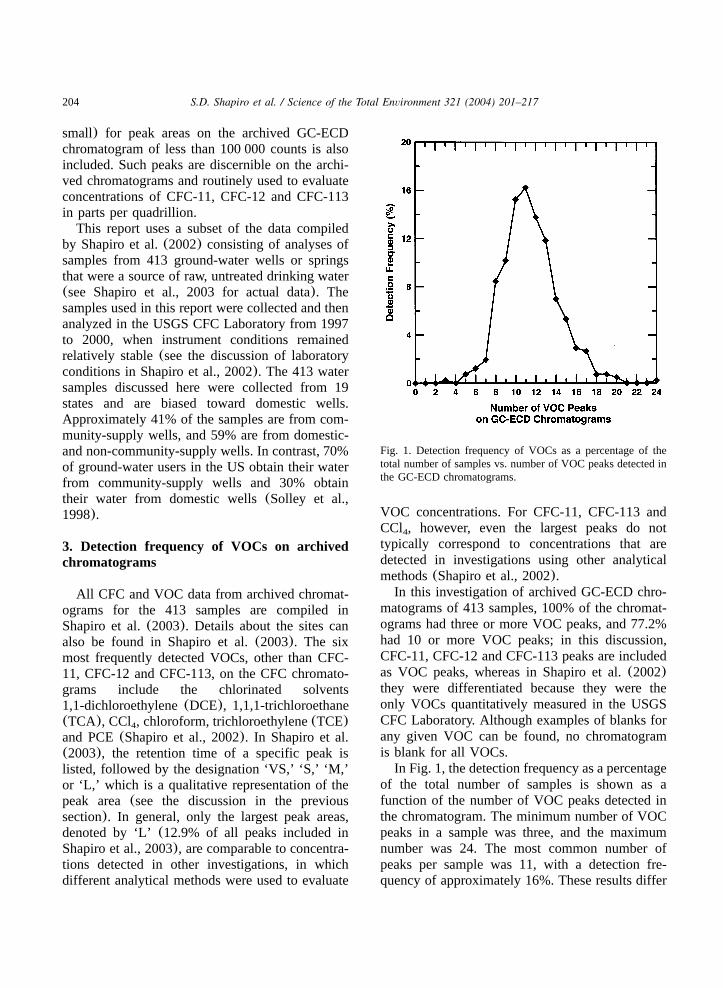
Fig. 1. Detection frequency of VOCs as a percentage of thetotal number of samples vs. number of VOC peaks detected inthe GC-ECD chromatograms.

small) for peak areas on the archived GC-ECDchromatogram of less than 100 000 counts is alsoincluded. Such peaks are discernible on the archi-ved chromatograms and routinely used to evaluateconcentrations of CFC-11, CFC-12 and CFC-113in parts per quadrillion.

This report uses a subset of the data compiledby Shapiro et al.(2002) consisting of analyses ofsamples from 413 ground-water wells or springsthat were a source of raw, untreated drinking water(see Shapiro et al., 2003 for actual data). Thesamples used in this report were collected and thenanalyzed in the USGS CFC Laboratory from 1997to 2000, when instrument conditions remainedrelatively stable(see the discussion of laboratoryconditions in Shapiro et al., 2002). The 413 watersamples discussed here were collected from 19states and are biased toward domestic wells.Approximately 41% of the samples are from com-munity-supply wells, and 59% are from domestic-and non-community-supply wells. In contrast, 70%of ground-water users in the US obtain their waterfrom community-supply wells and 30% obtaintheir water from domestic wells(Solley et al.,1998).

3. Detection frequency of VOCs on archivedchromatograms

All CFC and VOC data from archived chromat-ograms for the 413 samples are compiled inShapiro et al.(2003). Details about the sites canalso be found in Shapiro et al.(2003). The sixmost frequently detected VOCs, other than CFC-11, CFC-12 and CFC-113, on the CFC chromato-grams include the chlorinated solvents1,1-dichloroethylene(DCE), 1,1,1-trichloroethane(TCA), CCl , chloroform, trichloroethylene(TCE)4

and PCE(Shapiro et al., 2002). In Shapiro et al.(2003), the retention time of a specific peak islisted, followed by the designation ‘VS,’ ‘S,’ ‘M,’or ‘L,’ which is a qualitative representation of thepeak area(see the discussion in the previoussection). In general, only the largest peak areas,denoted by ‘L’ (12.9% of all peaks included inShapiro et al., 2003), are comparable to concentra-tions detected in other investigations, in whichdifferent analytical methods were used to evaluate

VOC concentrations. For CFC-11, CFC-113 andCCl , however, even the largest peaks do not4

typically correspond to concentrations that aredetected in investigations using other analyticalmethods(Shapiro et al., 2002).

In this investigation of archived GC-ECD chro-matograms of 413 samples, 100% of the chromat-ograms had three or more VOC peaks, and 77.2%had 10 or more VOC peaks; in this discussion,CFC-11, CFC-12 and CFC-113 peaks are includedas VOC peaks, whereas in Shapiro et al.(2002)they were differentiated because they were theonly VOCs quantitatively measured in the USGSCFC Laboratory. Although examples of blanks forany given VOC can be found, no chromatogramis blank for all VOCs.

In Fig. 1, the detection frequency as a percentageof the total number of samples is shown as afunction of the number of VOC peaks detected inthe chromatogram. The minimum number of VOCpeaks in a sample was three, and the maximumnumber was 24. The most common number ofpeaks per sample was 11, with a detection fre-quency of approximately 16%. These results differ


Fig. 2. Detection frequency for large VOC peaks as a percent-age of the total number of samples vs. number of VOC peaksdetected in the GC-ECD chromatograms.(‘Large’ peaks aredefined as those with peak areas greater than 1 000 000counts).

from those of previous investigations of the occur-rence of VOCs in drinking-water wells. For exam-ple, Moran et al.(2002) showed that the detectionfrequency decreased as the number of VOCsdetected increased. The present investigation, how-ever, shows a decrease in the detection frequencyas the number of VOCs increases for samplescontaining a large number of VOCs(greater than11), but an increase in the detection frequency forsamples containing a small number of VOCs(from3 to 11).

If only the peak areas from the archived GC-ECD chromatograms designated by ‘L’(large) areretained in a plot of detection frequency vs. thenumber of VOCs present in a ground-water sam-ple, the results of this investigation become moreconsistent with those of other surveys, such asMoran et al.(2002) and Squillace et al.(2002),in which different analytical methods of detectingVOCs were used. In this case, the detection fre-quency generally decreased as a function of thenumber of VOCs present in a sample(Fig. 2).

Using only the large peaks, approximately 34% ofthe samples would be classified with no VOCspresent, approximately 66% would have at leastone VOC present, and the maximum number ofVOCs in a sample would be nine. These valuesare more consistent with those of Shelton et al.(2001), with a detection frequency of 61% for atleast one VOC, and Squillace et al.(2002), witha detection frequency of 44% for at least oneVOC. The slightly higher detection frequency inthe present investigation than in these previousinvestigations for VOCs having peak areas denotedby ‘L’ is most likely the result of detecting CFC-11 and CCl more frequently with GC-ECD than4

with other analytical methods.

4. Historical trends in VOC occurrence inground water and in atmospheric sources ofVOCs to ground water

Previous investigators have found a high fre-quency of detection of anthropogenic compoundsin ground water recharged in the past 50 years(e.g. Kolpin et al., 1995; Bohlke and Denver,¨1995; Busenberg and Plummer, 1992; Plummerand Friedman, 1999; Plummer and Busenberg,2000; http:yywater.usgs.govylabycfc accessed onJuly 29, 2003; Kolpin et al., 1995; Fogg et al.,1999; Shelton et al., 2001; Stackelberg et al.,2000). For example, Kolpin et al.(1995) found acorrelation between tritium concentration and pes-ticide detections. They found that water rechargedprior to 1953 contained no pesticides because thefirst significant use of pesticides to control insectsin corn and soybeans occurred about the sametime as the advent of atmospheric testing of nucle-ar weapons. When Kolpin et al.(1995) accountedfor the age of the water(based on tritium concen-tration), their frequency of detection of pesticidesincreased to 70.3% in water recharged after 1953.Pankow et al.(1997) modeled the movement ofMTBE and other VOCs from atmospheric sourcesthrough shallow ground water and showed thatmodern urban air is a potentially significant non-point source of VOCs in ground water. The pres-ence of CFCs in ground water indicates that thewater was recharged during the past 60 years,when CFCs have been present in the atmosphere,


Fig. 3. Atmospheric growth curves for CFC-11, CFC-12, andCFC-113 (in pptv) from 1940 to present (fromhttp:yywater.usgs.govylabycfc accessed on July 29, 2003).

or is a mixture that contains a fraction of recentlyrecharged water(Busenberg and Plummer, 1992;Plummer and Friedman, 1999; Plummer and Bus-enberg, 2000; http:yywater.usgs.govylabycfcaccessed on July 29, 2003). Bohlke and Denver¨(1995), Fogg et al.(1999), Shelton et al.(2001)and Stackelberg et al.(2000), as well as manyothers, have utilized CFC and tritium concentra-tions to demonstrate that recently recharged waterhas an anthropogenic signature that can includehigh nitrate concentrations resulting from fertiliz-ers, pesticides, herbicides and VOCs.

The application of CFCs in developing modeledrecharge years is based on atmospheric growthcurves for CFC-11, CFC-12 and CFC-113 from1940 to present(Fig. 3). Atmospheric CFCs dis-solve in precipitation and become incorporated inthe Earth’s hydrologic cycle. The concentrationsof the CFCs in a water sample can be related tothe atmospheric concentrations associated with agiven year, or the water sample can be hypothe-sized to be a mixture that contains a fraction ofrecently recharged water(Busenberg and Plummer,1992; Plummer and Friedman, 1999; Plummer and

Busenberg, 2000. Recharge years modeled fromCFC concentrations in the ground-water samplesare correlated with the occurrence of VOCs andthe magnitude of VOC peaks on the chromato-grams. Such a correlation, however, can beobscured by CFC andyor VOC contamination,uncertainty in the recharge temperature which canaffect the modeled CFC recharge year, open-holemixing in the collection of water samples, CFCandyor VOC degradation due to the reducingconditions in the aquifer, mixing in fractured-rockor karst aquifers, and the fact that some VOCshave been in use longer than the 60-year time spanover which CFCs can be used to date ground-water samples(e.g. Doherty, 2000; Walker et al.,2000). Also, the recharge years associated withconcentrations of CFCs in ground water arederived from a piston-flow model that does notaccount for mixing, contamination, dispersion,sorption or other enhancement or attenuation pro-cesses(e.g. Plummer and Busenberg, 2000; http:yywater.usgs.govylabycfc accessed on July 29,2003). Samples with CFC-12 concentrations equalto zero were assigned a recharge year ofF1940for plotting purposes. Concentrations of CFC-12were used in this investigation to estimate themodeled recharge year because CFC-12 appears tothe most stable of the three CFC tracers used indating water (Busenberg and Plummer, 1992;Plummer and Friedman, 1999; Plummer and Bus-enberg, 2000; http:yywater.usgs.govylabycfcaccessed on July 29, 2003).

For the 413 samples used in this investigation,the number of sites with 3 to 8 VOCs presentdecreases from approximately 42.2% in the period1940–1944 to 0% in the period 1995–2000,whereas the number of sites with 9 to 10 VOCspresent is relatively constant, from 17.8 to 22.7%,for the same periods, and the number of sites with11 or more VOCs generally increases from 39.9to 77.3% during the same periods(Shapiro et al.,2003). At some sites that have low concentrationsof CFC-12, indicative of water recharged in the1940s, numerous VOCs are present. Conditions atmany of these sites are aerobic, precluding degra-dation as a rationale for low concentrations ofCFC-12. Furthermore, most of the VOCs presentother than the CFCs at these sites are CCl ,4


Fig. 4. (a) Number of VOC peaks in samples associated witha given CFC-12 recharge year divided by the number of sam-ples associated with that CFC-12 recharge year, 1940–2000,and(b) number of large VOC peaks in samples associated witha given CFC-12 recharge year divided by the number of sam-ples associated with that CFC-12 recharge year, 1940–2000.(‘Large’ peaks are defined as those with peak areas greaterthan 1 000 000 counts. The recharge year for samples denotedas ‘CFC-12 contaminated’ is unknown, but could be estimatedusing other dating techniques).

chloroform and PCE, which were in use wellbefore the 1940s and could be appearing in waterrecharged prior to and during the 1940s and 1950s.CCl can be produced naturally from marine algae,4

oceans and volcanoes(Gribble, 1994; Isidorov,1990). Additionally, CCl was first introduced in4

the US in 1898 and was produced in significantquantities starting approximately 1908(Doherty,2000; Walker et al., 2000). Chloroform is producednaturally from savanna fires(Keene et al., 1999;Khalil et al., 1999; Rudolph et al., 1995), marinealgae, hydrothermal sources, salt mines and vol-canoes(Gribble, 1994; Isidorov, 1990; Keene etal., 1999; Khalil et al., 1999), and in soils(Frankand Frank, 1990; Hoekstra et al., 1998; Keene etal., 1999; Khalil et al., 1999). Additionally, chlo-roform has been manufactured and used in numer-ous applications in significant quantities since1922(US Department of Health and Human Serv-ices, 2002). PCE can be produced naturally fromoceans and volcanoes(Gribble, 1994; Isidorov,1990; Keene et al., 1999; Khalil et al., 1999).Additionally, PCE was first synthesized in 1821,and was produced in significant quantities in theUS starting in the 1920s(Doherty, 2000).

The temporal trend in VOC occurrence as afunction of the CFC-12 recharge year is shown inFig. 4a and b as the total number of VOCs presentin samples associated with a given CFC-12recharge year, divided by the number of samplesassociated with that CFC-12 recharge year. Thiscalculation normalizes the data, because the num-ber of samples per recharge year is not constant.Fig. 4a shows substantial scatter, with the numberof VOCs detected increasing slightly from 1940to 2000. If only the peak areas on the GC-ECDchromatogram denoted by ‘L’ are used, the numberof VOCs detected per site increases over the 60-year period(Fig. 4b).

The number of VOC peaks detected on the GC-ECD chromatograms per sample for a givenrecharge year is relatively unchanged when all ofthe VOC peaks are included; however, the mag-nitude of the peak areas on the GC-ECD chromat-ograms appears to be increasing over time. Thisobservation can be demonstrated by examiningCFC-11, which has been found to have an atmos-pheric component that has increased over time in


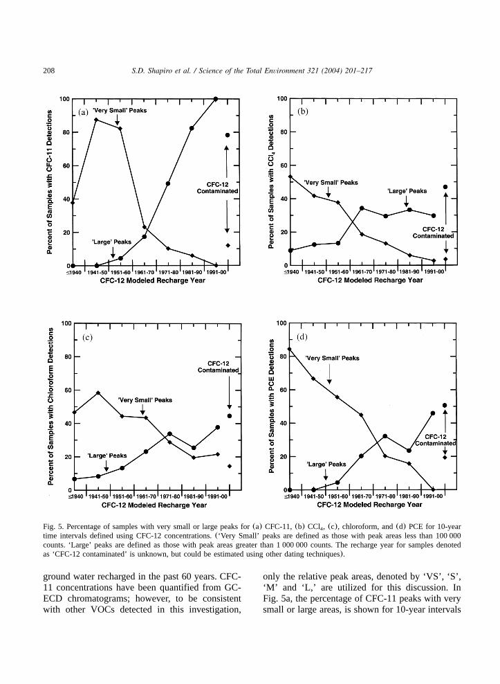
Fig. 5. Percentage of samples with very small or large peaks for(a) CFC-11,(b) CCl , (c), chloroform, and(d) PCE for 10-year4

time intervals defined using CFC-12 concentrations.(‘Very Small’ peaks are defined as those with peak areas less than 100 000counts. ‘Large’ peaks are defined as those with peak areas greater than 1 000 000 counts. The recharge year for samples denotedas ‘CFC-12 contaminated’ is unknown, but could be estimated using other dating techniques).

ground water recharged in the past 60 years. CFC-11 concentrations have been quantified from GC-ECD chromatograms; however, to be consistentwith other VOCs detected in this investigation,

only the relative peak areas, denoted by ‘VS’, ‘S’,‘M’ and ‘L,’ are utilized for this discussion. InFig. 5a, the percentage of CFC-11 peaks with verysmall or large areas, is shown for 10-year intervals


Fig. 6. Atmospheric growth curve for CCl for the northern4

hemisphere(in pptv) (from Walker et al., 2000).

as determined from the modeled recharge yearsfrom CFC-12 concentrations. The number of sam-ples with CFC-11 peak areas denoted by ‘VS’decreases from 1940 to present, whereas the num-ber of samples with CFC-11 peak areas denotedby ‘L’ increases from 1940 to present. The increasein the occurrence of large peaks over time isdirectly related to the increase in the atmosphericgrowth curve of CFC-11 over time(Fig. 3; e.g.Plummer and Busenberg, 2000 http:yywater.usgs.govylabycfc accessed on July 29, 2003.

Three VOCs(CCl , chloroform, PCE) that were4

routinely identified on the GC-ECD chromato-grams also show the same increase as CFC-11 inthe magnitude of their peak areas on GC-ECDchromatograms from 1940 to present. The exactconcentrations of CCl , chloroform, and PCE were4

not determined; however, the relative size(‘VS’,‘S’, ‘M’ and ‘L’ ) of the peak areas on the GC-ECD chromatograms can still be utilized. Thenumber of samples with CCl , chloroform, and4

PCE peaks denoted by ‘VS’ decreases from 1940to present, whereas the number of samples withCCl , chloroform, and PCE peaks denoted by ‘L’4

increases from 1940 to present(Fig. 5b, c and d,respectively).

With the detection limits achieved using theGC-ECD system in this investigation, atmosphericsignatures of CFC-11, CFC-12 and CFC-113 havebeen routinely identified and used for datingground water. Because of the sensitivity of theGC-ECD to halogenated VOCs, particularly CCl ,4

chloroform and PCE, an atmospheric signature forthese compounds is likely to be detected in watersamples as well, provided that the ground waterhas not been contaminated by local sources ofVOCs. As stated previously, samples with knowncontamination were not accepted for analysis forCFCs, as they would disrupt measurements. Thus,it is unlikely that the samples considered here werecontaminated by local releases of VOCs. Also, itis unlikely that the pervasive trace concentrationsof almost all of the VOCs detected can be attrib-uted to natural production of VOCs because thewater samples were collected from a wide rangeof hydrogeologic environments throughout the US.Atmospheric measurements of CCl and PCE can4

be correlated with peak areas on the GC-ECD

chromatograms to assess the relative importanceof the atmospheric source of VOCs vs. othercontaminant sources in the samples analyzed.

Historical atmospheric concentrations for CCl4

and PCE were compiled from numerous investi-gations(Butler et al., 1998, 1999; Fabian et al.,1996; Koppman et al., 1993; Lovelock, 1974;Prinn et al., 2000; Simmonds et al., 1996, 1998;Singh et al., 1977; Walker et al., 2000; Wang etal., 1995, 1998; Yokouchi et al., 1996). Althoughthere is some uncertainty in the historical atmos-pheric input, average concentrations for CCl and4

PCE in the Northern Hemisphere were used in thisinvestigation for the period from 1940 to 2000,when CFC-12 concentrations can be used fordating ground-water recharge. The CCl historical4

data for the Northern Hemisphere are relativelyuniform and well defined, with values rangingfrom 0 pptv(parts per trillion by volume) in 1900,to approximately 105 pptv in 1990, and back downto approximately 97 pptv in 2000(Fig. 6; Walkeret al., 2000). Atmospheric CCl concentrations4

higher than those tabulated by Walker et al.(2000)have been reported, particularly at urban monitor-ing stations(e.g. Singh et al., 1977); however, forCCl , concentrations at urban stations are only4


approximately 20% higher than those at remotestations(Singh et al., 1977). The maximum con-centration in the atmospheric curve occurs approx-imately 1990, whereas maximum productionoccurred approximately 1970(Doherty, 2000).

The historical concentration data for PCE forthe Northern Hemisphere have not been welldefined for the period from 1940 to the present;concentrations vary widely depending on proxim-ity to urban areas, and show a substantial seasonaleffect, with maximum concentrations occurringduring the winter, when most ground-waterrecharge would likely occur(Koppman et al.,1993; Singh et al., 1977; Wang et al., 1995, 1998;Yokouchi et al., 1996). Singh et al.(1977) deter-mined the PCE concentration ratio for urban air toclean air to be approximately 22. The amplitudeof the seasonal variation in atmospheric PCEconcentrations in the Northern Hemisphere isapproximately 15 pptv(Wang et al., 1995). Aver-age PCE concentrations utilized in calculations forthis investigation for the continental US for 1971–1980, 1981–1990, 1991–2000 and 2001 were 26,10, 14, 5 and 3 pptv, respectively(Hall et al.,2002; Koppman et al., 1993; Mohamed et al.,2002; Singh et al., 1977; Wang et al., 1998).Atmospheric concentrations prior to 1971 wereextrapolated back to zero approximately 1920,when substantial production of PCE first began.The maximum atmospheric concentration of PCEin the 1970s correlates well with the maximumproduction estimate for PCE between 1970 and1980(Doherty, 2000).

The air concentrations for CCl and PCE were4

converted to water concentrations by assumingequilibration at 128C (a reasonable temperaturefor many recharge waters). Values of the Henry’sLaw constant(K ) for CCl and PCE wereHenry 4

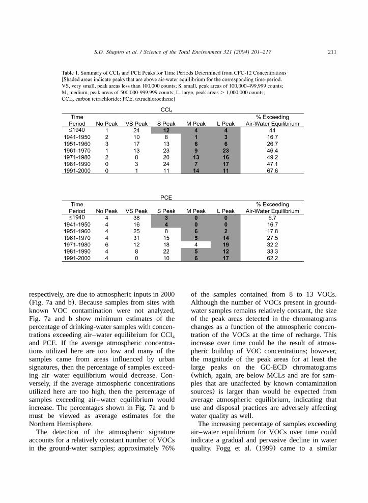
calculated from Bullister and Wisegarver(1998)and Sander(1999), respectively. The water con-centrations were then converted to peak areas onthe basis of calibration curves developed using alimited number of standards analyzed during thetime that the samples in this investigation wereanalyzed on the GC-ECD. The number of siteswith a given peak area for a time period deter-mined using CFC-12 concentrations is given inTable 1. The shaded areas of Table 1 indicate peak

areas exceeding air–water equilibrium for 10-yeartime intervals defined using CFC-12 concentra-tions and the atmospheric concentrations discussedabove. The peak areas that correlate with theatmospheric concentrations given for CCl are4

‘VS’ for the period through 1940, and ‘S’ for theperiods from 1941 to 2000. Therefore, those peaksdenoted by ‘S,’ ‘M’ and ‘L’ are considered to beabove air–water equilibrium for the period through1940, whereas those peaks denoted by ‘M’ and‘L’ are above air–water equilibrium for the periodsfrom 1941 to 2000(Table 1). The peak areas thatcorrelate with the atmospheric concentrations giv-en for PCE are ‘M’ for the period 1971 to 1980and ‘S’ for the periods from 1981 to 2001. There-fore, only those peaks that are denoted by ‘L’ areconsidered to be above air–water equilibrium forthe period 1971 to 1980, whereas those peaksdenoted by ‘M’ and ‘L’ are above air–waterequilibrium for the periods from 1981 to 2001(Table 1). For the periods before 1971, atmos-pheric concentrations were extrapolated back tozero approximately 1920, and the peak areas thatwould correlate with these atmospheric concentra-tions would be ‘VS’ for the periods from pre-1940to 1950 and ‘S’ for the periods from 1951 to 1970.Therefore, those peaks that are denoted by ‘S,’‘M’ and ‘L’ are considered to be above air–waterequilibrium for the periods from pre-1940 to 1950,whereas those peaks denoted by ‘M’ and ‘L’ areabove air–water equilibrium for the periods from1951 to 1970(Table 1).

Fig. 7a and b show the percentage of the CCl4

and PCE peaks, respectively, exceeding air–waterequilibrium for 10-year time intervals definedusing CFC-12 concentrations(also see Table 1).The percentage of peaks that exceed air–waterequilibrium generally increases from 1940 to thepresent for both CCl and PCE(Fig. 7a and b). A4

large percentage of the VOC detections on theGC-ECD result from atmospheric inputs; this isconsistent with the measurement of atmosphericCFC concentrations on the GC-ECD, which wasnecessary in order to use CFC concentrations todate ground-water recharge. For example, 56% and93% of the CCl and PCE detections, respectively,4

in 1940 were due to atmospheric inputs, whereasonly 32% and 38% of CCl and PCE detections,4


respectively, are due to atmospheric inputs in 2000(Fig. 7a and b). Because samples from sites withknown VOC contamination were not analyzed,Fig. 7a and b show minimum estimates of thepercentage of drinking-water samples with concen-trations exceeding air–water equilibrium for CCl4

and PCE. If the average atmospheric concentra-tions utilized here are too low and many of thesamples came from areas influenced by urbansignatures, then the percentage of samples exceed-ing air–water equilibrium would decrease. Con-versely, if the average atmospheric concentrationsutilized here are too high, then the percentage ofsamples exceeding air–water equilibrium wouldincrease. The percentages shown in Fig. 7a and bmust be viewed as average estimates for theNorthern Hemisphere.

The detection of the atmospheric signatureaccounts for a relatively constant number of VOCsin the ground-water samples; approximately 76%

of the samples contained from 8 to 13 VOCs.Although the number of VOCs present in ground-water samples remains relatively constant, the sizeof the peak areas detected in the chromatogramschanges as a function of the atmospheric concen-tration of the VOCs at the time of recharge. Thisincrease over time could be the result of atmos-pheric buildup of VOC concentrations; however,the magnitude of the peak areas for at least thelarge peaks on the GC-ECD chromatograms(which, again, are below MCLs and are for sam-ples that are unaffected by known contaminationsources) is larger than would be expected fromaverage atmospheric equilibrium, indicating thatuse and disposal practices are adversely affectingwater quality as well.

The increasing percentage of samples exceedingair–water equilibrium for VOCs over time couldindicate a gradual and pervasive decline in waterquality. Fogg et al.(1999) came to a similar


Fig. 7. Percentage of the samples in which air-water equilib-rium is exceeded for 10-year time intervals defined using CFC-12 concentrations for(a) CCl and (b) PCE. (The recharge4

year for samples denoted as ‘CFC-12 contaminated’ isunknown, but could be estimated using other datingtechniques).

conclusion utilizing nitrate and CFC concentrationsin conjunction with computer simulations for theSalinas Valley, California. The additional enhance-ments in VOCs that could cause deterioration of

water quality likely result from(1) local atmos-pheric enrichment, as is typical in urban environ-ments, or(2) direct contamination to an aquifer,such as from infiltration of stormwater runoff,septic water, or contaminated surface water. Thedetections of VOCs at concentrations indicative ofatmospheric sources in 100% of the samples indi-cates that drinking water has been affected byanthropogenic activity over the 60 years identifiedin this study, and that additional inputs from urbanair, spills, underground injections and leaking land-fills or storage tanks increasingly are providingadditional sources of ground-water contamination.

5. Assessment of aquifer vulnerability usingVOC data

Numerous investigators have considered the cor-relation between the occurrence of VOCs inground water and factors such as the hydrogeologicand physical setting, local land use, well type andgeochemical conditions(e.g. Lapham et al., 2000;Moran et al., 2001; Shelton et al., 2001; Squillaceand Moran, 2000; Squillace et al., 1999, 2002;Stackelberg et al., 2000). For example, Squillaceet al. (2002) found a higher detection frequencyfor VOCs in unconfined aquifers than in confinedaquifers. Unconfined aquifers may be affected bymore sources of contamination because they are inmore continuous contact with both point and non-point contaminant sources. Bruce and Oelsner(2001) and Squillace et al.(2002) and Stackelberget al. (2000) found that the number and totalconcentration of VOCs per sample were greaterfor samples from public-supply wells than forsamples from domestic or shallow and moderate-depth monitoring wells because the higher pump-ing rates and larger capture zones associated withpublic-supply wells make them more likely todraw water from sources of contamination. Inaddition, public-supply wells are generally nearerto large population centers than are domestic andmonitoring wells, and, therefore, are more likelyto intercept inputs from sources of contamination,just as urban wells have a higher frequency ofdetection of VOCs than rural wells(e.g. Squillaceet al., 1999). Also, Squillace et al.(2002) foundthat recently recharged ground water with gener-


ally higher dissolved—oxygen concentrations thanolder ground water, can carry anthropogenic con-taminants to shallow ground-water-flow systems.

Correlations between the detection of VOCs andother contaminants and physical, hydrogeologicand geochemical characteristics of the samplingsite are important because they may indicate thepotential for contamination with VOCs, and situ-ations where a greater degree of monitoring maybe warranted. Such correlations, however, may beoverly simplistic as they may be too general forspecific local conditions. Furthermore, detectionsof VOCs occurred at much higher concentrationsin previous investigations in which other analyticalmethods were used, than in the present investiga-tion in which the GC-ECD was used to analyzethe ground-water samples.

As discussed in the previous section, the detec-tion limit associated with VOCs determined withthe GC-ECD is on the order of air–water equilib-rium due to an atmospheric source of VOCs inground-water recharge. The presence of an atmos-pheric signature indicates that a component of theground-water sample was recharged within thetime period in which the VOC was manufactured.The detection of CFC-12 indicates that at least afraction of the water sample was recharged in thepast 60 years, even at sites classified as confined.The chromatograms associated with all of thesamples used in this analysis showed a detectionof at least three VOC peaks, indicating that all ofthe drinking-water wells in this analysis wereaffected by anthropogenic inputs of VOCs. Theanthropogenic input could be either from atmos-pheric sources in ground-water recharge, or froma combination of atmospheric sources in ground-water recharge and proximity to accidental releasesof VOCs into the ground-water system. In addition,although 100% of the sites have been affected byanthropogenic inputs of VOCs, these sites likelyhave been affected by inputs of many other typesof compounds that were not detected with the GC-ECD used in this investigation. For example,Squillace et al.(2002) found that anthropogenicnitrate co-occurs with VOCs and pesticides in 57%of samples.

The wells from which water samples were takenfor this analysis, were classified by Shapiro et al.

(2002, 2003) according to well type, local landuse, depth, hydrogeologic setting and geochemicalconditions. Correlations between the number ofVOCs detected and the site parameters associatedwith each sample are not quantifiable because theVOCs are pervasive due to the low detection limit.Detecting an atmospheric input does increase thenumber of VOCs detected for each of the siteparameters to 10 to 12 VOCs per sample. If,however, only those peaks denoted by ‘L’ areutilized to be more consistent with the detectionof VOCs from previous investigations, the averagenumber of VOCs detected decreases to 1 to 2VOCs per sample, and correlations between thenumber of VOCs detected and some of the siteparameters are similar to those found in previousinvestigations. For example, urban sites have morepeaks per site than rural sites, community-supplywells have more peaks per site than domesticwells, samples from fractured-rock and karst aqui-fers have more peaks per site than samples fromunconsolidated aquifers, wells in unconfined aqui-fers have more peaks per site than wells in con-fined aquifers, and samples with highdissolved-oxygen concentrations and no methanehave more peaks than samples with low dissolvedoxygen as well as methane(see Shapiro et al.(2003) for site parameters).

One final analysis involves classification accord-ing to well depth. The well depths ranged from 0to 2682 ft below land surface. In general, thenumber of VOC peaks decreases with well depth.Many wells are open to a substantial length of theaquifer, however, and likely mix multiple sourcesof water. Discharge from wells may also be affect-ed by leakage around the annulus. Recently-recharged water containing low concentrations ofone or more VOCs from a shallow portion of theaquifer could, therefore, mix with older water fromdeeper parts of the aquifer. In addition, the relationto well depth is further complicated by depth tothe water table in unconfined aquifers.

6. Summary and conclusions

Archived chromatograms from purge-and-trapGC-ECD analyses of drinking-water samples wereused to determine the frequency of detection of


halogenated VOCs in water samples from 413community-, non-community-(such as restau-rants), and domestic-supply wells throughout theUS. A subset of the data on VOC occurrencecompiled by Shapiro et al.(2002) is used in thisreport with additional interpretation of trace con-centrations of VOCs from the chromatograms usedin the compilation. When the detection frequencyof VOCs was assessed using a new detection limitof 10 mgyl, 100% of the chromatograms hady6

three or more VOC peaks, while 77.2% had 10 ormore VOC peaks. The maximum number of VOCsdetected in a sample was 24.

Modeled ground-water residence times, deter-mined from concentrations of CFC-12, were util-ized to assess historical trends in the cumulativeoccurrence of all VOCs detected in this analysis,as well as the occurrence of individual VOCs,such as CCl , chloroform and PCE. The total4

number of VOC peaks in ground water hasremained relatively constant from 1940 to 2000;however, concentrations of the VOCs haveincreased over this same period. This is clearlydemonstrated with CCl , chloroform and PCE, all4

of which show a decrease in small peaks and anincrease in large peaks on the GC-ECD chromat-ograms from 1940 to present. The CCl and PCE4

detections were assessed in terms of the percentagethat is due to equilibrium with average historicalatmospheric concentrations vs. the percentage thatis due to additional enhancements resulting fromlocal atmospheric enrichment or contaminationdirectly to ground-water flow systems. The per-centage of samples in which CCl concentrations4

exceed air–water equilibrium with average NorthAmerican air has increased from-20% in approx-imately 1940 to)60% in 2000. The percentageof samples in which PCE concentrations exceedair–water equilibrium with average North Ameri-can air has increased from-10% in approximately1940 to)60% in 2000.

The occurrence of VOCs was evaluated withrespect to factors that may affect ground-watervulnerability, such as the type of well(community,non-community, or domestic), well depth, hydro-geologic conditions, local land use, and ground-water redox conditions as inferred from measuredconcentrations of dissolved oxygen and methane.

With the low detection limit achieved in thisinvestigation, using all of the VOCs detected,regardless of peak areas, does not provide usefulcorrelations between the number of VOCs detectedand the site parameters associated with each sam-ple because the VOCs are pervasive. DetectingVOCs in parts per quadrillion increases the numberof VOCs detected for each of the site parametersto 10 to 12 VOCs per sample. If, however, onlylarge peaks are utilized to be more consistent withthe detection of VOCs from previous investiga-tions, the average number of VOCs detecteddecreases to 1 to 2 VOCs per sample, and corre-lations between the number of VOCs detected andsome of the site parameters are similar to thosefound in previous investigations. The detections ofVOCs at concentrations indicative of atmosphericsources in 100% of the samples indicates that thesedrinking-water sources have been affected byanthropogenic activity over the past 60 years, andthat additional inputs from spills, undergroundinjections and leaking landfills or storage tanksincreasingly are providing additional sources ofcontamination.

Acknowledgments

The authors gratefully acknowledge Jerry Casile(USGS, Reston, Va.) and Julian Wayland(USGS,Reston, Va.) for CFC analyses, and Allen M.Shapiro (USGS, Reston, Va.), Patricia Toccalino(Oregon Health and Science University, Beaverton,Ore.) and Michael Moran(USGS, Rapid City,S.D.) for their insightful reviews of the manuscript.This project was conducted in cooperation withthe US Environmental Protection Agency Officeof Ground Water and Drinking Water.

References

Barrio-Lage GA, Parsons RS, Nassar RS, Lorenzo PA. Sequen-tial dehalogenation of chlorinated ethenes. Environ SciTechnol 1986;20:96–99.

Bouwer EJ, McCarty PL. Transformations of 1- and 2-carbonhalogenated aliphatic organic compounds under methano-genic conditions. Appl Environ Microbiol 1983a;45:1286–1294.

Bouwer EJ, McCarty PL. Transformations of halogenatedorganic compounds under denitrification conditions. ApplEnviron Microbiol 1983b;45:1295–1299.


Bender DA, Zogorski JS, Halde MJ, Rowe BL. Selectionprocedure and salient information for volatile organic com-pounds emphasized in the National water-quality assessmentprogram. US Geological Survey Open-File Report 99-182,1999: 32 pp.

Bohlke JK, Denver JM. Combined use of groundwater dating,¨chemical and isotopic analyses to resolve the history andfate of nitrate contamination in two agricultural watersheds,Atlantic coastal plain, Maryland. Water Resour Res1995;31(9):2319–2339.

Bruce BW, Oelsner GP. Contrasting water quality from paireddomesticypublic supply wells, Central High Plains. J AmWater Resour Assoc 2001;37(5):1389–1403.

Bullister JL, Wisegarver DP. The solubility of carbon tetra-chloride in water and seawater. Deep-Sea Res 11998;45:185–1302.

Busenberg E, Plummer LN. Use of chlorofluorocarbons(CCl F and CCl F) as hydrologic tracers and age-dating3 2 2

tools: the alluvium and terrace system of Central Oklahoma.Water Resour Res 1992;28(9):2257–2283.

Butler JH, Battle M, Bender ML, Montzka SA, Clarke AD,Saltzman ES, Sucher CM, Severinghaus JP, Elkins JW. Arecord of atmospheric halocarbons during the twentiethcentury from polar firn air. Nature 1999;399:749–755.

Butler JH, Elkins JW, Montzka SA, Thompson TM, SwansonTH, Clarke AD, Moore FL, Hurst DF, Romashkin PA,Yvon-Lewis SA, Lobert JM, DiCorleto M, Dutton GS, LocLT, King DB, Dunn RE, Ray EA, Pender M, Wamsley PR,Volk CM ‘Nitrous Oxide and Halocarbons’. In: Hofman DJ,Peterson JT, Rosson RM(Eds.), Summary Report 1996–1997, Rep. No. 24, Climate Monitoring and DiagnosticsLab, US Department of Commerce, Boulder, CO, 1998, pp.91–121.

Carpenter DO, Arcaro KF, Spink DC. Understanding thehuman health effects of chemical mixtures. Environ HealthPerspect 2002;110(1):25–42 (Supplemental Volume).

Carpenter DO, Arcaro KF, Bush B, Niemi WD, Pang S,Vakharia DD. Human health and chemical mixtures: anoverview. Environ Health Perspect 1998;106(suppl.6):1263–1270.

Colburn T, Dumanoski D, Myers JP. Our stolen future. NewYork: Dutton, 1996. p. 316

Davis A, Fennemore GG, Peck C, Walker CR, McIlwraith J,Thomas S. Degradation of carbon tetrachloride in a reducinggroundwater environment: implications for natural attenua-tion. Applied Geochem 2003;18:503–525.

Dinicola RS, Cox SE, Bradley PM. Natural Attenuation ofChlorinated Volatile Organic Compounds in Ground Waterat Area 6, Naval Air Station Whidbey Island, Washington.US Geological Survey Water-Resources InvestigationsReport 00-4060, 2000: 86 pp.

Doherty RE. A history of the production and use of carbontetrachloride, tetrachloroethylene, trichloroethylene and1,1,1-trichloroethane in the United States: Part 1- historicalbackground; carbon tetrachloride and tetrachloroethylene. JEnviron Forensics 2000;1:69–81.

Fabian P, Borchers R, Schmidt U. Proposed reference modelsfor CO and halogenated hydrocarbons. Adv Space Res2

1996;18(9y10):145–153.Fogg GE, LaBolle EM, Weissmann GS. Groundwater vulner-

ability assessment: hydrogeologic perspective and examplefrom salinas valley, California’. In: Corwin DL, Loague K,Ellsworth TR (Eds.), Application of GIS, Remote Sensing,Geostatistical and Solute Transport Modeling. AGU Geo-physical Monograph 108, 1999; 45–61.

Frank W, Frank H. Concentrations of airborne C1 and C2halocarbons in forest areas in West Germany: results ofthree Campaigns in 1986, 1987 and 1988. Atmos Environ1990;24A:1735–1739.

Gribble GW. The natural production of chlorinated compounds.Environ Sci Technol 1994;28(7):310A–319.

Gupta M, Gupta A, Suidan MT, Sayles GD. Biotransformationrates of chloroform under anaerobic conditions-11. Sulfatereduction. Water Res. 1996;30:1387–1394.

Hall BD, Butler JH, Clarke AD, Dutton GS, Elkins JW, HurstDF, King DB, Kline ES, Lind J, Lock LT, Mondeel D,Montzka SA, Moore FL, Nance JD, Ray EA, RomashkinPA, Thompson TM Halocarbons and other AtmosphericTrace Species. In: King DB, Schnell RM, Rosson RM,Sweet C(Eds.), Climate Monitoring and Diagnostics Lab-oratory Summary Report No. 26, 2000–2001, Boulder, CO,2002; 26: pp. 106–134.

Harte J, Holdren C, Schneider R, Shirley C. Toxics A to Z: aguide to everyday pollution hazards. Berkeley: Universityof California Press, 1991. p. 479

Hoekstra EJ, De Leer EWB, Brinkman UAT. Natural formationof chloroform and brominated trihalomethanes in soil. Envi-ron Sci Technol 1998;32:3724–3729.

Isidorov VA. Organic chemistry of the earth’s atmosphere.Berlin: Springer-Verlag, 1990.

Jeffers PM, Ward LM, Woytowitch LM, Wolf NL. Homoge-neous hydrolysis rate constants for selected chlorinatedmethanes, ethanes, ethenes and propanes. Environ Sci Tech-nol 1989;23(8):965–969.

Keene WC, Khalil AK, Erickson DJ, McCulloch A, GraedelTE, Lobert JM, Aucott ML, Gong SL, Harper DB, KleimanG, Midgley P, Moore RM, Seuzaret C, Sturges WT, Ben-kovitz CM, Koropalov V, Barrie LA, Li YF. Compositeglobal emissions of reactive chlorine from anthropogenicand natural sources: reactive chlorine emissions inventory.J Geophys Res 1999;104(D7):8429–8440.

Khalil MAK, Moore RM, Harper DB, Lobert JM, EricksonDJ, Koropalov V, Sturges WT, Keene WC. Natural emissionof chlorine-containing gases: reactive chlorine emissionsinventory. J Geophys Res 1999;104(D7):8333–8346.

Kolpin DW, Goolsby DA, Thurman EM. Pesticides in near-surface aquifers: an assessment using highly sensitive ana-lytical methods and tritium. J Environ Quality1995;24:1125–1132.

Koppman R, Kohnen FJ, Plass-Dulmer C, Rudolph J. Distri-bution of methylchloride, dichloromethane, trichloroetheneand tetrachloroethene over the North and South Atlantic. JGeophys Res 1993;98(D11):20517–20526.


Lapham WW, Moran MJ, Zogorski JS. Enhancements of non-point-source monitoring programs to assess volatile organiccompounds in ground water of the United States. The AmWater Resour Assoc 2000;36(6):1321–1334.

Lappe M. Chemical deception, the toxic threat to health and´the environment. San Francisco: Sierra Club Books, 1991.p. 360

Lovelock JE. Atmospheric halocarbons and stratosphericozone. Nature 1974;252:292–294.

Mlay M. Management controls of volatile organic compoundsin groundwater protection. In: Ram NM, Christman RF,Cantor KP, editors. Significance and treatment of volatileorganic compounds in water suppliesLewis Publishers, Inc,1990. p. 15–36.

Mohamed MF, Kang D, Aneja VP. Volatile organic compoundsin some urban locations in United States. Chemosphere2002;47:86–882.

Moran MJ, Grady S, Zogorski J Occurrence and distributionof volatile organic compounds in drinking water suppliedby community water systems in the Northeast and Mid-Atlantic regions of the United States, 1993–1998. USGeological Survey Fact Sheet FS-089-01, 2001, 4.

Moran MJ, Lapham WW, Rowe BL, Zogorski JS Occurrenceand Status of Volatile Organic Compounds in Ground Waterfrom Rural, Untreated, Self-supplied Domestic Wells in theUnited States, 1986–1999. US Geological Survey Water-Resources Investigations Report 02-4085, 2002, 51 pp.

Moran MJ, Zogorski JS, Squillace PJ. MTBE in ground waterof the United States—occurrence, potential sources, andlong-range transport. In: Proceedings, of American WaterWorks Association, Norfolk, VA: American Water WorksAssociation, September 26–29, CD-ROM, 1999.

Pankow JF, Thomson NR, Johnson RL, Baehr AL, ZogorskiJS. The Urban atmosphere as a non-point source for thetransport of MTBE and other volatile organic compounds(VOCs) to shallow groundwater. Environ Sci Technol1997;31:2821–2828.

Parsons F, Wood PR, Dewitt JT. Transformations of tetrachlo-roethene and trichloroethene in microcosms and groundwa-ter. J Am Water Works Assoc 1984;76:56–59.

Plummer LN, Busenberg E. Chlorofluorocarbons. In: CookPG, Herzeg A, editors. Environmental tracers in subsurfacehydrology. Boston: Kluwer Academic Press, 2000. p. 441–478 (Chapter 15).

Plummer LN, Friedman LC. Tracing and dating young groundwater. US Geological Survey Fact Sheet 134-99, 1999, 4pp. (see http:yywater.usgs.govypubsyFSyFS-134-99y).

Prinn RG, Weiss RF, Fraser PJ, Simmonds PG, Cunnold DM,Alyea FN, O’Doherty S, Salameh P, Miller BR, Huang J,Wang RHJ, Hartley DE, Harth C, Steele LP, Sturrock G,Midgley PM, McCulloch A. A history of chemically andradiatively important gases in air deduced from ALEyGAGEyAGAGE. J Geophys Res 2000;105(D14):17751–17792.

Rowe B, Grady S, Zogorski J, Koch B, Tratnyek P. Nationalsurvey of MTBE, other ether oxygenates, and other VOCs

in community drinking-water sources. US Geological SurveyOpen File Report 01-399, 2001, 1 p.

Rudolph J, Khedim A, Koppmann R, Bonsang B. Field studyof the emissions of methyl chloride and other halocarbonsfrom biomass burning in western Africa. J Atmos Chem1995;22:67–80.

Sander R. Compilation of Henry’s Law constants for inorganicand organic species of potential importance in environmentalchemistry version 3. Accessed January 27, 2003, on theWorld Wide Web at URL http:yywww.mpch-mainz.mpg.dey;sanderyresyhenry.html, 1999.

Shapiro SD, Busenberg E, Plummer LN, Focazio, M. Datafrom archived chromatograms on halogenated volatile organ-ic compounds in untreated ground water used for drinkingwater. US Geological Survey Open-File Report 03-352,2003, 31 pp.

Shapiro SD, Plummer LN, Focazio M, Busenberg E, KirklandW, Fernandez M. VOC occurrence in drinking water fromthe United States: results from archived chromatograms andwater samples, 1989–2000. US Geological Survey Water-Resources Investigations Report 02-4173, 2002, 20 pp.

Shelton JL, Burow KR, Belitz K, Dubrovsky NM, Land M,Gronberg J. Low-level volatile organic compounds in activepublic supply wells as ground-water tracers in the LosAngeles physiographic basin, California, 2000. US Geolog-ical Survey Water-Resources Investigations Report 01-4188,2001, 29 pp.

Simmonds PG, Cunnold DM, Weiss RF, Prinn RG, Fraser PJ,McCulloch A, Alyea FN, O’Doherty S. Global trends andemission estimates of CCl from in situ background obser-4

vations from July 1978 to June 1996. J Geophys Res1998;103(D13):16017–16027.

Simmonds PG, Derwent RG, McCulloch A, O’Doherty S,Gaudry A. Long-term trends in concentrations of halocar-bons and radiatively active trace gases in Atlantic andEuropean air masses monitored at mace head, Ireland from1997–1994. Atmos Environ 1996;30(23):4041–4063.

Singh HB, Salas LJ, Shigeishi H, Crawford A. Urban-non-urban relationships of halocarbons, SF , N O, and other6 2

atmospheric trace constituents. Atmos Environ1977;11:819–828.

Solley WB, Pierce RR, Perlman HA Estimated Use of waterin the United States in 1995. US Geological Survey Circular1200, 1998, 71 pp.

Squillace PJ, Moran MJ. Estimating the Likelihood of MTBEOccurrence in Drinking Water Supplied By Ground-WaterSources in the Northeast and Mid-Atlantic Regions of theUnited States. U.S. Geological Survey Open-File Report 00-343, 2000, 10 pp.

Squillace PJ, Moran MJ, Lapham WW, Price CV, ClawgesRM, Zogorski JS. Volatile organic compounds in untreatedambient groundwater of the United States, 1985–1995.Environ Sci Technol 1999;33(23):4176–4187.

Squillace PJ, Scott JC, Moran MJ, Nolan BT, Kolpin DW.VOCs, pesticides, nitrate and their mixtures in groundwaterused for drinking water in the United States. Environ SciTechnol 2002;36(9):1923–1930.


Stackelberg PE, Kauffman LJ, Baehr AL, Ayers MA. Com-parison of Nitrate, Pesticides, and Volatile Organic Com-pounds in Samples from Monitoring and Public-SupplyWells, Kirkwood-Cohansey Aquifer System, Southern NewJersey. US Geological Survey Water-Resources Investiga-tions Report 00-4123, 2000, 51 pp.

Thomas RD. Evaluation of toxicity of volatile organic chemi-cals: general considerations. In: Ram NM, Christman RF,Cantor KP, editors. Significance and treatment of volatileorganic compounds in water supplies. Chelsea, Michigan:Lewis Publishers, Inc, 1990. p. 451–463.

US Department of Health and Human Services. Report onCarcinogens, Tenth Edition. US Department of Health andHuman Services, Public Health Service, National ToxicologyProgram, December 2002. Accessed May 15, 2003, on theWorld Wide Web at URL http:yyehp.niehs.nih.govyrocy.

Walker SJ, Weiss RF, Salameh PK. Reconstructed histories ofthe annual mean atmospheric mole fractions for the halo-carbons CFC-11, CFC-12, CFC-113 and carbon tetrachlo-ride. J Geophys Res 2000;105(C6):14 285–14 296.

Wang CJ-L, Blake DR, Rowland FS. Seasonal variations inthe atmospheric distribution of a reactive chlorine com-pound, tetrachloroethene(CCl sCCl ). Geophys Res Lett2 2

1995;22:1097–1100.Wang J-L, Chang C-J, Lin Y-H. Concentration distributions of

anthropogenic halocarbons over a metropolitan area. Che-mosphere 1998;36(10):2391–2400.

Westrick JJ. National surveys of volatile organic compoundsin ground and surface waters. In: Ram NM, Christman RF,Cantor KP, editors. Significance and treatment of volatileorganic compounds in water supplies. Chelsea, Michigan:Lewis Publishers, Inc, 1990. p. 103–125.

Yokouchi Y, Barrie LA, Toom D, Akimoto H. The seasonalvariation of selected natural and anthropogenic halocarbonsin the arctic troposphere. Atmos Environ 1996;30(10-11):1723–1727.

Zogorski J, Morgan MJ, Hamilton PA. MTBE and othervolatile organic compounds- new findings and implicationson the quality of source waters used for drinking-watersupplies. US Geological Survey Fact Sheet FS-105-01, 2001,2 pp.

Historical trends in occurrence and atmospheric inputs of halogenated volatile organic compounds in...

Documents

Transcript of Historical trends in occurrence and atmospheric inputs of halogenated volatile organic compounds in...