arX

iv:1

108.

0526

v5 [

mat

h.D

G]

14 D

ec 2

012

Higher order geometric flows on three dimensional

locally homogeneous spaces

Sanjit Das∗, Kartik Prabhu†, Sayan Kar‡

Department of Physics & Meteorology and Center for Theoretical Studies

Indian Institute of Technology, Kharagpur, 721302, India

Abstract

We analyse second order (in Riemann curvature) geometric flows (un-normalised) on locally ho-

mogeneous three manifolds and look for specific features through the solutions (analytic whereever

possible, otherwise numerical) of the evolution equations. Several novelties appear in the context

of scale factor evolution, fixed curves, phase portraits, approach to singular metrics, isotropisation

and curvature scalar evolution. The distinguishing features linked to the presence of the second

order term in the flow equation are pointed out. Throughout the article, we compare the results

obtained, with the corresponding results for un-normalized Ricci flows.

∗ Present address: The Institute of Mathematical Sciences, Chennai 600113, India; Electronic address:

sanjit@imsc.res.in,† Present address: Department of Physics, University of Chicago, 5640 S. Ellis Avenue, Chicago, IL 60637,

USA; Electronic address: kartikp@uchicago.edu‡Electronic address: sayan@phy.iitkgp.ernet.in

1

I. INTRODUCTION AND OVERVIEW

Ricci and other geometric flows [1, 2] were introduced in mathematics by Hamilton [3]

and in physics, by Friedan [4], around almost the same time, though with very different

motivations. More recently, such geometric flows have become popular, largely because

of Perelman’s work [5] which led to the proof of the well–known Poincare conjecture. In

physics, geometric flows have been investigated in varied contexts such as general relativity,

black hole entropy [6] and string theory [7, 8].

The unnormalised Ricci flow equation [1, 2] is given as,

∂gij∂t

= −2Rij (1)

where gij is the metric tensor, Rij the Ricci tensor and t denotes a time parameter (not the

physical time). For a normalised Ricci flow, the corresponding equation turns out to be:

∂gij∂t

= −2Rij +2

n〈R〉gij (2)

where 〈R〉 =∫RdV∫dV

. Thus the normalised flow ceases to be different from the unnormalised

one if we consider non–compact, infinite volume manifolds (with a finite value for∫RdV ). In

addition, for constant curvature manifolds, the second term in the normalised flow equation

reduces to 2nRgij .

Friedan’s early work showed how one may arrive at the vacuum Einstein field equations

of General Relativity from the Renormalisation Group (RG) analysis of a nonlinear σ-model

[4]. The RG β-function equations (after a α′ dependent scaling of the flow parameter) are

given (upto third order in the α′ parameter) as follows [9, 10].

∂g

∂t= −2Rc− α′Rc− 2α′2Rc− . . . (3)

where Rc is a symmetric 2-tensor defined as: Rc = RiklmRjabcgkaglbgmc and

Rc =

12RklmpRi

mlrRjkp

r− 3

8RikljR

ksprRlspr + ..... In component form, we have,

∂gij∂λ

= −2Rij − α′RiklmRjklm − . . . (4)

which may be considered as a higher order geometric flow equation for the metric on a given

manifold. We intend to continue our investigations [11] on such higher (mainly second)

order geometric flow equations, in this article. We mention that apart from a motivational

2

perspective, our work has no connection with RG flows and, in what follows, we will not

discuss any link with them anywhere. α′ is treated as a parameter without any link to the

RG flow equations. In other words, the higher order flows we talk about are treated as

geometric flows in their own right. Restricting to second order we mention a scaling feature

of this geometric flow. For Ricci flow a scaling of the metric gij → Ωgij′ can be compensated

by a scaling of t by t′ = tΩ. Since the Ricci is invariant under such scaling, flows for gij and t

are equivalent with those for g′ij and t′. For the second order flows, things are a bit different.

Here, we can see that flows for gij, t and α′ will be equivalent to flows for gij/Ω, t′ = t/Ω

and α′′ = α′/Ω. In our work, we have retained the α′ when we do analytic calculations

–however, for numerics we have chosen values of α′ = 0,±1– solutions for other values of α′

can be obtained using the scaling property mentioned above.

In this paper, we investigate higher (second) order flows on locally homogeneous three

manifolds. After the seminal work of Isenberg and Jackson [12] on the behavior of Ricci flow

on homogeneous three manifolds, several interesting papers on this topic have appeared in

the literature. Notable among them are the articles in [13], [14], [15], [16], [17]. In particular,

the authors in [13] discuss a new approach wherein the Ricci flow of left-invariant metrics on

homogeneous three manifolds is equivalently viewed as a flow of the structure constants of

the metric Lie algebra w.r.t. an evolving orthonormal frame. Consequences for some other

geometric flows on such three manifolds are available in [18],[19].

Homogeneous spaces are also known to play an important role in cosmology in the context

of the so–called Bianchi models ([20],[21]). It is worth mentioning that the Misner-Wheeler

minisuperspace deals with three dimensional homogeneous spaces in cosmology where dif-

ferent paths in superspace correspond to different evolution profiles for metrics. For more

details in this context see [12], [20], [22], [23]. Recently, a connection between self-dual

gravitational instantons and geometric flows of all Bianchi types has been shown in [24].

Our article is organised as follows. In Section II, we discuss some preliminaries. Section

III reviews the general theory of left invariant metrics. Section IV contains the main results

of the article–here we analyse the higher order flows for the various Bianchi classes. Finally,

in Section V we conclude with some remarks.

3

II. PRELIMINARIES ON HOMOGENEOUS THREE MANIFOLDS

Following Isenberg and Jackson[12] (to which we refer for details concerning the follow-

ing discussion), we take the view point that our original interest is in closed Riemannian

3-manifolds that are locally homogeneous. By a result of Singer [25], the universal cover of

a locally homogeneous manifold is homogeneous, i.e. its isometry group acts transitively.

Here we begin from the basic definition of homogeneous manifolds and give Thurston’s[26]

proposition for eight geometric structures. A homogeneous Riemannian space is a Rieman-

nian manifold (M, g) whose isometry group Isom(M, g) acts transitively on M , i.e given

x, y ∈ M there exists a φ ∈ Isom(M, g) such that φ(x) = y.

If G is a connected Lie group and H is a closed subgroup, G/H is the space of cosets

gH, π : G → G/H is defined by g → [gH ]. G/H is called a homogeneous space.

Let (M3, G,Gx) be a maximal model geometry i.e. the isotropy group Gx (g ∈ G|gx = x)

is maximal among all subgroups of the diffeomorphism group of M3 that have compact

isotropy groups. Depending on the isotropy group, there are eight possible manifestations

of the maximal model geometry which are also known as Thurston geometries. Here we

mention them briefly. If the isotropy group is SO(3) then the model geometry is any one

of the three, namely, SU(2), R3 or H3. On the other hand, if SO(2) is the isotropy group,

then it has four possibilities depending on whether M3 can be a trivial bundle over a two-

dimensional maximal model or not. The first possibility where M3 is a trivial bundle over a

2-dimensional maximal model, gives rise to S2 × R or H2 × R upto diffeomorphism and the

latter produces Nil or ˜SL(2,R) up to isomorphism. The last case where the isotropy group

is trivial, the Lie group is isomorphic to Sol.

III. GENERAL THEORY FOR LEFT INVARIANTS METRICS ON 3D UNIMOD-

ULAR LIE GROUPS

In studying curvature properties of left invariant metrics on a Lie group, many results

have been obtained in the past. Most of them are contained in a survey article by Milnor

[27]. For more details on Lie groups and homogeneous spaces we refer to [28], [29] and [30].

We review this work here largely because, later, we will use the results quoted here while

writing down the second order geometric flow equations.

4

The left invariant metric on M3 is taken as:

g(t) = A(t)η1 ⊗ η1 +B(t)η2 ⊗ η2 + C(t)η3 ⊗ η3

= π1 ⊗ π1 + π2 ⊗ π2 + π3 ⊗ π3(5)

and its inverse as,

g−1(t) =1

A(t)F1 ⊗ F1 +

1

B(t)F2 ⊗ F2 +

1

C(t)F3 ⊗ F3

= e1 ⊗ e1 + e2 ⊗ e2 + e3 ⊗ e3

(6)

where A(t), B(t), C(t) are positive. Here Fi3i=1 are the left invariant frame field (also

called Milnor’s frame) with dual coframe field ηi3i=1 . The Lie brackets w.r.t the left

invariant frames are of this form:

[Fi, Fj] = αijkFk (7)

Let us define an orthonormal frame field ei3i=1which will be of the form: e1 := 1√AF1. If

we let ζ1 := A, ζ2 := B, ζ3 := C and λ := α231, µ := α312, ν := α123 then Eq.(7) looks like

[ei, ej] =ζkαijk√ζiζjζk

ek (8)

The relevant components of the sectional curvature turn out to be

K(e1 ∧ e2) := 〈Rm(e1, e2)e2, e1〉 =(λA− µB)2

4ABC+

ν(2µB + 2λA− 3νC)

4AB(9)

K(e2 ∧ e3) := 〈Rm(e2, e3)e3, e2〉 =(µB − νC)2

4ABC+

λ(2νC + 2µB − 3λA)

4BC(10)

K(e3 ∧ e1) := 〈Rm(e3, e1)e1, e3〉 =(νC − λA)2

4ABC+

µ(2λA+ 2νC − 3µB)

4AC(11)

Recall that these are actually R1212, R2323, R3131, respectively, in the orthonormal frame.

We have to write them back in Milnor’s frame. Thus the Riemann tensor in the Milnor

frame will be

Rm(Fi, Fj , Fi, Fj) = ζiζjRm(ei, ej, ei, ej) (12)

From now on we would mean:〈Rm(ei, ej)ej, ei〉 = Rm(ei, ej, ei, ej). Similarly the Ricci and

Rc would look as :

Rc(Fi, Fi) =

3∑

k=1

Rm(Fi, Fk, Fi, Fk)1

ζk(13)

5

Rc(Fi, Fi) = 2

3∑

k=1

Rm(Fi, Fk, Fi, Fk)2 1

ζ2k

1

ζi(14)

Rc(F1, F1) =(λA)2 − (µB − νC)2

2BC(15)

Rc(F2, F2) =(µB)2 − (νC − λA)2

2CA(16)

Rc(F3, F3) =(νC)2 − (λA− µB)2

2AB(17)

Rc(F1, F1) =1

8AB2

[(λA− µB)2

C+ ν(2µB + 2λA− 3νC)

]2

+1

8AC2

[(νC − λA)2

B+ µ(2λA+ 2νC − 3µB)

]2(18)

Rc(F2, F2) =1

8BC2

[(µB − νC)2

A+ λ(2νC + 2µB − 3λA)

]2

+1

8BA2

[(λA− µB)2

C+ ν(2µB + 2λA− 3νC)

]2(19)

Rc(F3, F3) =1

8A2C

[(νC − λA)2

B+ µ(2λA+ 2νC − 3µB)

]2

+1

8B2C

[(µB − νC)2

A+ λ(2νC + 2µB − 3λA)

]2(20)

Using the above expressions, we can calculate the scalar curvature and the norm of the Ricci

tensor which are given as,

Scal =1

A(Rc(F1, F1)) +

1

B(Rc(F2, F2)) +

1

C(Rc(F3, F3)) (21a)

= −A2λ2 + (Bµ− Cν)2 − 2Aλ(Bµ+ Cν)

2ABC(21b)

‖Rc‖2 = 1

A2(Rc(F1, F1))

2 +1

B2(Rc(F2, F2))

2 +1

C2(Rc(F3, F3))

2 (22a)

=3A4λ4 − 4A3λ3(Bµ+ Cν)− 4Aλ(Bµ− Cν)2(Bµ+ Cν) + 2A2λ2(Bµ+ Cν)2

4A2 B2 C2

+(Bµ− Cν)2 (3B2µ2 + 2BCµν + 3C2ν2)

4A2 B2 C2(22b)

6

The higher order flow equations therefore turn out to be,

dA

dt= −

(2Rc(F1, F1) + α′ Rc(F1, F1)

)(23)

dB

dt= −

(2Rc(F2, F2) + α′ Rc(F2, F2)

)(24)

dC

dt= −

(2Rc(F3, F3) + α′ Rc(F3, F3)

)(25)

In the next section we analyze the flow equations in five different homogeneous spaces.

IV. EXAMPLES ON BIANCHI CLASSES

A. Computation on SU(2)

1. Flow equations

The canonical three sphere (S3) is topologically equivalent to the Lie group SU(2), which

is algebraically represented by

SU(2) =

z1 −z2

z2 z1

: z1, z2 ∈ C, |z1|2 + |z2|2 = 1

. (26)

All the structure constants are the same in the Milnor frame field. We assume λ = µ =

ν = −2. With these values of the structure constants, the 2nd order flow equations turn

out to be:

dA

dt=

4(B − C)2 − 4A2

BC− 2α′[

1

AB2(A− B)2

C

+(2B + 2A− 3C)2 + 1

AC2

(A− C)2

B+ (2C + 2A− 3B)

2

] (27)

dB

dt=

4(C − A)2 − 4B2

AC− 2α′[

1

BC2(C − B)2

A

+(2C + 2B − 3A)2 + 1

BA2(B −A)2

C+ (2B + 2A− 3C)2] (28)

dC

dt=

4(A− B)2 − 4C2

AB− 2α′[

1

CA2(A− C)2

B

+(2A+ 2C − 3B)2 + 1

CB2(C − B)2

A+ (2C + 2B − 3A)2] (29)

7

2. Analytical and numerical estimates

We first try and see if we can analytically estimate the nature of evolution for the scale

factors A, B, and C.

(a) Without any loss of generality, we can take the initial values of the scale factors in an

ordered way i.e. A0 > B0 > C0. Further, from Eqn.27 to 29 we can write the equations for

the differences (pairwise) of the scale factors as follows.

d(A−B)

dt= −4

(A− B) (A2 + 2AB +B2 − C2)

ABC− 4α′ (A−B) G1(A,B,C)

A2B2C2(30)

d(A− C)

dt= −4

(A− C) (A2 + 2AC + C2 −B2)

ABC− 4α′ (A− C) G2(A,B,C)

A2B2C2(31)

d(B − C)

dt= −4

(B − C) (B2 + 2BC + C2 −A2)

ABC− 4α′ (B − C) G3(A,B,C)

A2B2C2(32)

where G1(A,B,C), G2(A,B,C), G3(A,B,C) are, respectively

G1(A,B,C) =(A4 − 4A3B + 6A2B2 − 4AB3 +B4

+2A2C2 + 12ABC2 + 2B2C2 − 8AC3 − 8BC3 + 5C4)

(33)

G2(A,B,C) =(A4 + 2A2B2 − 8AB3 + 5B4 − 4A3C

+12AB2C − 8B3C + 6A2C2 + 2B2C2 − 4AC3 + C4)

(34)

G3(A,B,C) =(5A4 − 8A3B + 2A2B2 +B4 − 8A3C

+12A2BC − 4B3C + 2A2C2 + 6B2C2 − 4BC3 + C4)

(35)

From the above expressions for the differences, it can be inferred that A(t) > B(t) > C(t)

holds throughout the evolution, if the initial values satisfy A0 > B0 > C0. Note that each of

(30)-(32) may be formally solved. For example, if we consider (31), we have A(t)− C(t) =

(A0 − C0) exp[∫

K(t′)dt′].

(b) We now look at the evolution of B(t) for α′ = +1. We have, from Eqn.28,

dB

dt= 4

(A2 + C2)

AC−2 B2

AC+

P1

BC2+

P2

BA2+4 ≤ 4

(A2 + C2)

AC−2B

A+

P1

BC2+

P2

BA2+4 (36)

8

where P1 = (C−B)2

A+ (2C + 2B − 3A)2 and P2 = (A−B)2

C+ (2B + 2A− 3C)2 are strictly

positive. Choosing A0 = n+2, B0 = n, C0 = n−2 as the initial values of the scale factors, it

can be shown that dBdt

∣∣t=t0

is always negative (from the inequality above, it may be checked

that the negative term always dominates over the positive term). Further, it is easy to see

that for n > 4 and α′ = (0,+1), all the scale factors are decreasing.

(c) On the other hand, for α′ = −1 the upper bound on B(t) can be written as

dB

dt≤ −4

B

A+

4(A− C)2

AC+ 2

P1

BC2+ 2

P2

BA2(37)

Here we may note a difference with the α′ = +1 case. As before, let us choose A0 =

n + 2, B0 = n, C0 = n − 2 to estimate F1 = −4BA+ 4(A−C)2

AC+ 2 P1

BC2 + 2 P2

BA2 which turns

out to be, F1 = 4(256+n(−64+n(24+n(20−(−3+n)n))))

n(n2−4)2. It is easy to see that F1 is bounded below

(i.e.limn→∞ F1 = −4 and for any finite n, F1 is larger than −4.). Thus, the scale factor B(t)

can either decrease or increase depending on the choice of initial values.

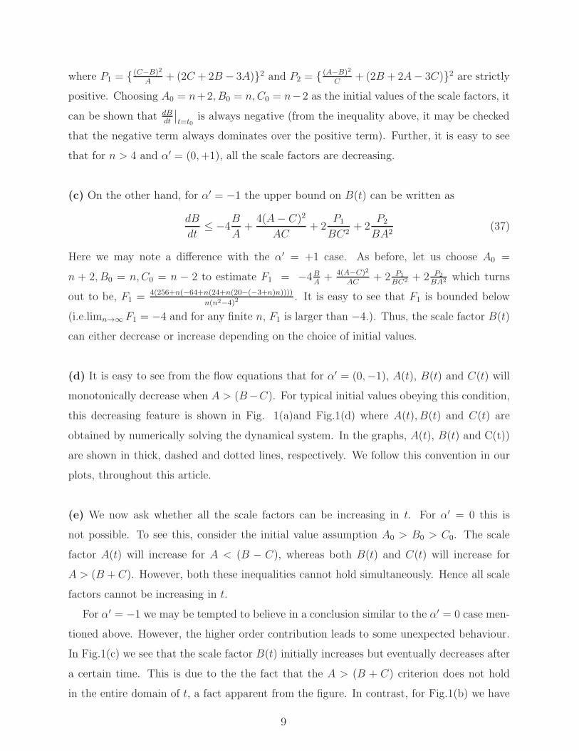
(d) It is easy to see from the flow equations that for α′ = (0,−1), A(t), B(t) and C(t) will

monotonically decrease when A > (B−C). For typical initial values obeying this condition,

this decreasing feature is shown in Fig. 1(a)and Fig.1(d) where A(t), B(t) and C(t) are

obtained by numerically solving the dynamical system. In the graphs, A(t), B(t) and C(t))

are shown in thick, dashed and dotted lines, respectively. We follow this convention in our

plots, throughout this article.

(e) We now ask whether all the scale factors can be increasing in t. For α′ = 0 this is

not possible. To see this, consider the initial value assumption A0 > B0 > C0. The scale

factor A(t) will increase for A < (B − C), whereas both B(t) and C(t) will increase for

A > (B + C). However, both these inequalities cannot hold simultaneously. Hence all scale

factors cannot be increasing in t.

For α′ = −1 we may be tempted to believe in a conclusion similar to the α′ = 0 case men-

tioned above. However, the higher order contribution leads to some unexpected behaviour.

In Fig.1(c) we see that the scale factor B(t) initially increases but eventually decreases after

a certain time. This is due to the the fact that the A > (B + C) criterion does not hold

in the entire domain of t, a fact apparent from the figure. In contrast, for Fig.1(b) we have

9

taken initial values which do not satisfy the aforesaid condition and though, initially, B(t) is

decreasing we find that after some time, B(t) increases. The reason behind this behaviour

is — the higher order contribution is much more positive and the net effect makes B(t)

increase after an initial decreasing phase.

0.0 0.1 0.2 0.3 0.4 0.5 0.6 0.70

1

2

3

4

5

6

7

(a)

A0 = 7, B0 = 5, C0 = 3, α′ = 1, Ts = 0.702

0 2 4 6 8 100

2

4

6

8

10

(b)A0 = 11, B0 = 9, C0 = 7, α′ = −1, Ts =

−1.09

0.0 0.2 0.4 0.6 0.8 1.0

2

3

4

5

(c)A0 = 5.5, B0 = 3.5, C0 = 1.5, α′ =

−1, Ts = −0.04

0.0 0.5 1.0 1.5 2.00

1

2

3

4

5

(d)

A0 = 7, B0 = 5, C0 = 3, α′ = 0, Ts = 2.76

Figure 1: A(t), B(t), C(t) vs t for α′ = 1, α′ = −1 and α′ = 0 for SU(2)

(f) recall that SU(2) admits round Einstein metrics and the Ricci flow converges. This

feature remains even when we include higher order terms with α′ = 1. If we change the

value of α′(from 1 to 0) a change appears only in the singularity time, though no difference

appears in the nature of the graph. On the other hand, when α′ = −1, we notice an

expansion of the scale factors – B(t) and A(t) appear to be expanding beyond the minimum

in Fig.[1(b)] at the same rate, whereas C(t) goes to zero asymptotically.

Let us now move on to some special cases.

10

3. Special Case: A 6= B = C

The flow equations, with this restriction (leading to the so-called Berger sphere metrics

[1]) become,dA

dt= −4

A2

B2− 4α′ A

3

B4(38)

dB

dt= −8 + 4

A

B− 4α′ [ 5

B(A

B− 1)2 +

3

B(1− 2A

3B)]

(39)

Let us first look at the case, α′ = 0. It is clear from Eqn. (38) that A(t) decreases with t and

has a upper bound, A(t) ≤ A0−4t. However, the same is not true for B(t). If A(t) < 2B(t)

then B(t) decreases with increasing t, otherwise it increases. B(t) does have a lower bound,

B(t) ≥ B0 − 8t. Depending on the sign of the R. H. S. of (39) B(t) can have an increasing,

stationary or decreasing behaviour during its evolution in t. From Eqns. (38), (39), one can

arrive at a second order equation for B(t) given as:

B(t)d2B

dt2+ 2

(dB(t)

dt

)2

+ 24dB(t)

dt= −64 (40)

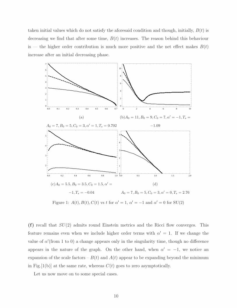
There are trivial solutions to this equation: dB(t)dt

= −8 (which corresponds to A(t) = 0)

and dB(t)dt

= −4 (which corresponds to A(t) = B(t)). If we define dBdt

= D(t) then we can

see the following: (i) At some t if D = 0 then dDdt

< 0 (maximum); (ii) If, over a range of

t, D > 0 then dDdt

< 0; (iii) If, over a range of t, D < 0 then dDdt

can be < 0, > 0 or = 0.

We note this behaviour in Fig.2(d). For example, the maximum occurs at the point where

D(t) = 0–substitute the values of A(t) and B(t) at the maximum as found in the graph,

into Eqn. (39) (with α′ = 0) and check that it is indeed zero.

Now we wish to note what happens to the rate of change of (A − B) and (A + B). We

show that (A− B) decreases faster than (A + B) which implies that as A and B decrease,

they approach each other. From the above equations for α′ = 0 we can write

d(A− B)

dt=

−4(A + 2B)

B2(A−B) ≤ −4A

B2(A2 + 3AB +B2) ≤ −20

A

B(41)

On the other hand,

d(A+B)

dt= − 4

B2(A2 + 2B2) + 4

A

B≤ −4

A

B(42)

It is easy to note that A − B decreases faster than A + B. Thus A and B approach each

other while decreasing. For α′ 6= 0 the analysis can be done following similar logic but we

prefer to solve the equations numerically and demonstrate our conclusions.

11

0.0 0.2 0.4 0.6 0.80

1

2

3

4

5

6

7

(a)A0 = 7, B0 = 5, α′ = 1, Ts = 0.914

0 1 2 3 4

2

3

4

5

6

7

(b)A0 = 7, B0 = 5, α′ = −1, Ts = −0.602

0 2 4 6 80.5

1.0

1.5

2.0

(c)A0 = 1, B0 = 0.5, α′ = −1, Ts = −0.004

-0.5 0.0 0.5 1.0 1.50

5

10

15

20

25

(d)A0 = 7, B0 = 5, α′ = 0, Ts = (−0.76)

Figure 2: A(t), B(t) vs t for α′ = 1, α′ = −1 and α′ = 0 for SU(2)

If we plot A(t) (thick line), B(t) (dashed line) treating the evolution equations as a

dynamical system, we see that both the scale factors converge to the origin (Fig.2(a),2(d))

for α′ = 0, 1. However, for α′ = −1 the evolution of the scale factors depend entirely on the

initial values of A,B,C– a fact shown in the two figures, Fig.2(b),2(c).

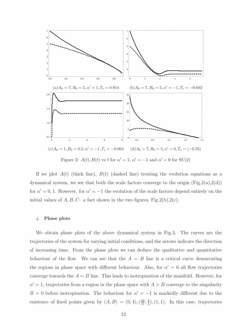
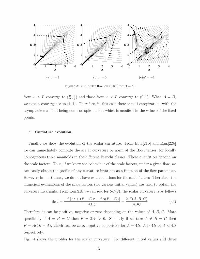
4. Phase plots

We obtain phase plots of the above dynamical system in Fig.3. The curves are the

trajectories of the system for varying initial conditions, and the arrows indicate the direction

of increasing time. From the phase plots we can deduce the qualitative and quantitative

behaviour of the flow. We can see that the A = B line is a critical curve demarcating

the regions in phase space with different behaviour. Also, for α′ = 0 all flow trajectories

converge towards the A = B line. This leads to isotropization of the manifold. However, for

α′ = 1, trajectories from a region in the phase space with A > B converge to the singularity

B = 0 before isotropization. The behaviour for α′ = −1 is markedly different due to the

existence of fixed points given by (A,B) = (0, 4), (169, 43), (1, 1). In this case, trajectories

12

0 1 2 3 40

1

2

3

4

A

B

(a)α′ = 1

0 1 2 3 40

1

2

3

4

A

B(b)α′ = 0

ææ

0 1 2 3 40

1

2

3

4

A

B

(c)α′ = −1

Figure 3: 2nd order flow on SU(2)for B = C

from A > B converge to (169, 43) and those from A < B converge to (0, 1). When A = B,

we note a convergence to (1, 1). Therefore, in this case there is no isotropization, with the

asymptotic manifold being non-isotropic - a fact which is manifest in the values of the fixed

points.

5. Curvature evolution

Finally, we show the evolution of the scalar curvature. From Eqn.[21b] and Eqn.[22b]

we can immediately compute the scalar curvature or norm of the Ricci tensor, for locally

homogeneous three manifolds in the different Bianchi classes. These quantitites depend on

the scale factors. Thus, if we know the behaviour of the scale factors, under a given flow, we

can easily obtain the profile of any curvature invariant as a function of the flow parameter.

However, in most cases, we do not have exact solutions for the scale factors. Therefore, the

numerical evaluations of the scale factors (for various initial values) are used to obtain the

curvature invariants. From Eqn.21b we can see, for SU(2), the scalar curvature is as follows

Scal =−2 [A2 + (B + C)2 − 2A(B + C)]

ABC=

2 F (A,B,C)

ABC(43)

Therefore, it can be positive, negative or zero depending on the values of A,B,C. More

specifically if A = B = C then F = 3A2 > 0. Similarly if we take A 6= B = C then

F = A(4B − A), which can be zero, negative or positive for A = 4B, A > 4B or A < 4B

respectively.

Fig. 4 shows the profiles for the scalar curvature. For different initial values and three

13

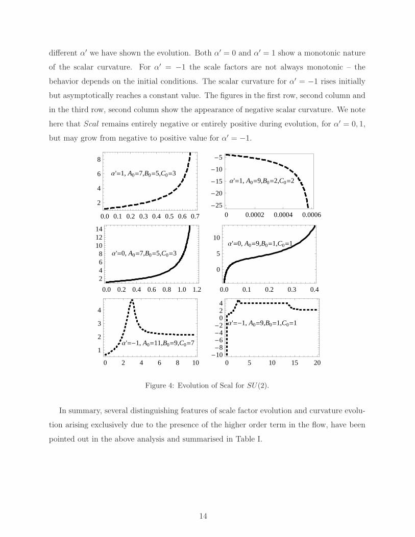
different α′ we have shown the evolution. Both α′ = 0 and α′ = 1 show a monotonic nature

of the scalar curvature. For α′ = −1 the scale factors are not always monotonic – the

behavior depends on the initial conditions. The scalar curvature for α′ = −1 rises initially

but asymptotically reaches a constant value. The figures in the first row, second column and

in the third row, second column show the appearance of negative scalar curvature. We note

here that Scal remains entirely negative or entirely positive during evolution, for α′ = 0, 1,

but may grow from negative to positive value for α′ = −1.

Α'=1, A0=7,B0=5,C0=3

0.0 0.1 0.2 0.3 0.4 0.5 0.6 0.7

2

4

6

8

Α'=1, A0=9,B0=2,C0=2

0 0.0002 0.0004 0.0006-25

-20

-15

-10

-5

Α'=0, A0=7,B0=5,C0=3

0.0 0.2 0.4 0.6 0.8 1.0 1.2

2468

101214

Α'=0, A0=9,B0=1,C0=1

0.0 0.1 0.2 0.3 0.4

0

5

10

Α'=-1, A0=11,B0=9,C0=7

0 2 4 6 8 10

1

2

3

4

Α'=-1, A0=9,B0=1,C0=1

0 5 10 15 20-10-8-6-4-2

024

Figure 4: Evolution of Scal for SU(2).

In summary, several distinguishing features of scale factor evolution and curvature evolu-

tion arising exclusively due to the presence of the higher order term in the flow, have been

pointed out in the above analysis and summarised in Table I.

14

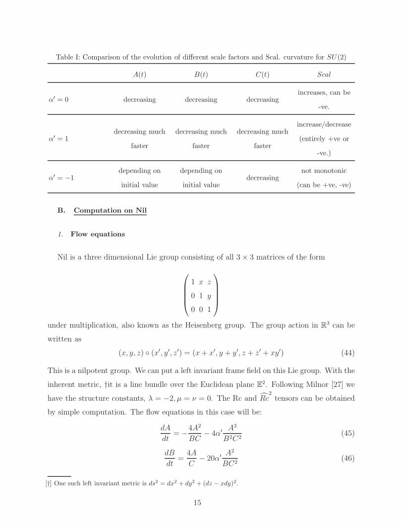
Table I: Comparison of the evolution of different scale factors and Scal. curvature for SU(2)

A(t) B(t) C(t) Scal

α′ = 0 decreasing decreasing decreasingincreases, can be

-ve.

α′ = 1decreasing much

faster

decreasing much

faster

decreasing much

faster

increase/decrease

(entirely +ve or

-ve.)

α′ = −1depending on

initial value

depending on

initial valuedecreasing

not monotonic

(can be +ve, -ve)

B. Computation on Nil

1. Flow equations

Nil is a three dimensional Lie group consisting of all 3× 3 matrices of the form

1 x z

0 1 y

0 0 1

under multiplication, also known as the Heisenberg group. The group action in R3 can be

written as

(x, y, z) (x′, y′, z′) = (x+ x′, y + y′, z + z′ + xy′) (44)

This is a nilpotent group. We can put a left invariant frame field on this Lie group. With the

inherent metric, †it is a line bundle over the Euclidean plane E2. Following Milnor [27] we

have the structure constants, λ = −2, µ = ν = 0. The Rc and Rc2tensors can be obtained

by simple computation. The flow equations in this case will be:

dA

dt= −4A2

BC− 4α′ A3

B2C2(45)

dB

dt=

4A

C− 20α′ A2

BC2(46)

[†] One such left invariant metric is ds2 = dx2 + dy2 + (dz − xdy)2.

15

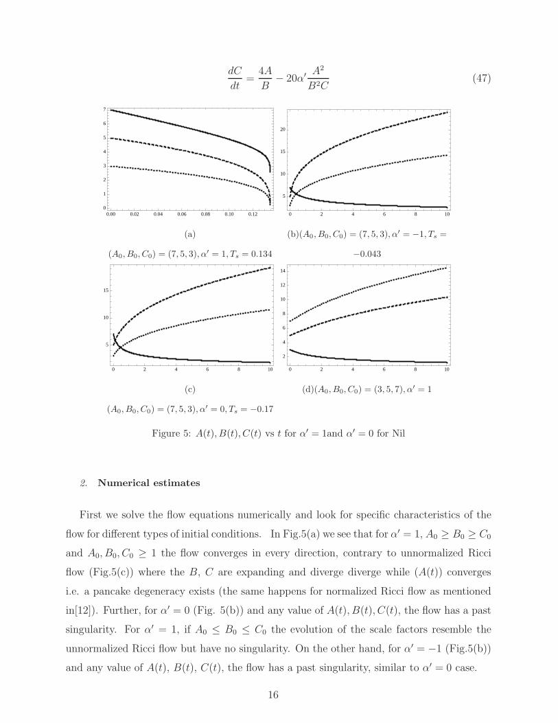
dC

dt=

4A

B− 20α′ A2

B2C(47)

0.00 0.02 0.04 0.06 0.08 0.10 0.120

1

2

3

4

5

6

7

(a)

(A0, B0, C0) = (7, 5, 3), α′ = 1, Ts = 0.134

0 2 4 6 8 10

5

10

15

20

(b)(A0, B0, C0) = (7, 5, 3), α′ = −1, Ts =

−0.043

0 2 4 6 8 10

5

10

15

(c)

(A0, B0, C0) = (7, 5, 3), α′ = 0, Ts = −0.17

0 2 4 6 8 10

2

4

6

8

10

12

14

(d)(A0, B0, C0) = (3, 5, 7), α′ = 1

Figure 5: A(t), B(t), C(t) vs t for α′ = 1and α′ = 0 for Nil

2. Numerical estimates

First we solve the flow equations numerically and look for specific characteristics of the

flow for different types of initial conditions. In Fig.5(a) we see that for α′ = 1, A0 ≥ B0 ≥ C0

and A0, B0, C0 ≥ 1 the flow converges in every direction, contrary to unnormalized Ricci

flow (Fig.5(c)) where the B, C are expanding and diverge diverge while (A(t)) converges

i.e. a pancake degeneracy exists (the same happens for normalized Ricci flow as mentioned

in[12]). Further, for α′ = 0 (Fig. 5(b)) and any value of A(t), B(t), C(t), the flow has a past

singularity. For α′ = 1, if A0 ≤ B0 ≤ C0 the evolution of the scale factors resemble the

unnormalized Ricci flow but have no singularity. On the other hand, for α′ = −1 (Fig.5(b))

and any value of A(t), B(t), C(t), the flow has a past singularity, similar to α′ = 0 case.

16

3. Analytical solution

It is possible to solve the flow equations analytically. Before working out the solutions,

we note from the flow equations that B/C = constant. Let us now choose a new variable

ξ = BC/A. It can be shown easily [31] that, with this choice and appropriate scaling of

the coordinates, the nature of the flow can be determined entirely by finding the evolution

of ξ. In other words, Nil has a one dimensional family of left invariant metrics which is

parametrised by ξ. The flow equations now take the form

ξ = 12− α′ 36

ξ(48a)

A

A= −4

ξ

(1 + α′ 1

ξ

)(48b)

B

B=

4

ξ

(1− α′ 5

ξ

)(48c)

where the ξ equation replaces the C equation and A, B are functions of ξ. So, effectively,

there is only one scale factor to worry about, i.e. ξ. The ξ equation is readily solved to give

two solutions–

ξ + 3α′ ln |ξ − 3α′| = 12t+ k (49a)

OR

ξ = 3α′ (49b)

The equations for A and B can then be solved to obtain A(ξ) and B(ξ)given as,

A

A0=

(ξ

ξ0

) 1

9

(ξ

3− α′

ξ03− α′

)−4

9

&B

B0=

(ξ

ξ0

) 1

45

(ξ

3− α′

ξ03− α′

) −2

225

(50a)

A = A0 exp

(− 16

3α′ t

)& B = B0 exp

(− 8

3α′ t

)(50b)

where (49a) is for the ξ given in (48a) and (49b) corresponds to the solution (48b). The

evolution of C can also be found using C = Aξ

B. In the case α′ = 1, and ξ = 3α′ we can

easily see that the scale factors A(t), B(t) and C(t) decrease. When α′ = 0, ξ = 12t and

A(t) ∼ t−1

3 , B(t) ∼ t1

3 , C(t) ∼ t1

3 . For α′ = −1, the solution ξ = 3α′ is not valid as long as

17

we are dealing with Riemannian manifolds and the evolution is determined from the other

solution.

Next we move on to a special case where B = C.

4. Special Case: A 6= B = C

The flow equations, under this assumption are

dAdt

= −4A2

B2 − 4α′A3

B4

dBdt

= 4AB

− 20α′A2

B3

(51)

It is obvious that the same analytical solutions mentioned above are valid here as long as

we define ξ = B2

A. However, we discuss some alternative ways of arriving at the nature of

scale factor evolution.

Let us look at the difference between the scale factors given as

d(A−B)

dt= −4

A

B2(A+B)−4α′(

A

B2)2(A−5B) ≤ −4

A

B2(A−B)−4α′(

A

B2)2(A−5B) (52)

It is easily seen that, for α′ = 0 (i.e. unnormalized Ricci flow) (A − B) decreases with

increasing t, but for other values of α′ different from zero the scale factors evolve differently.

The flow equation for B(t) is

dB

dt=

(4A

B2− 20(

A

B2)2)B (53)

If B2

A< 5 (or − A

B2 < −15) we have

dB

dt< 0 (54)

which explicitly shows that B(t) is decreasing in this region. We then move on to the case

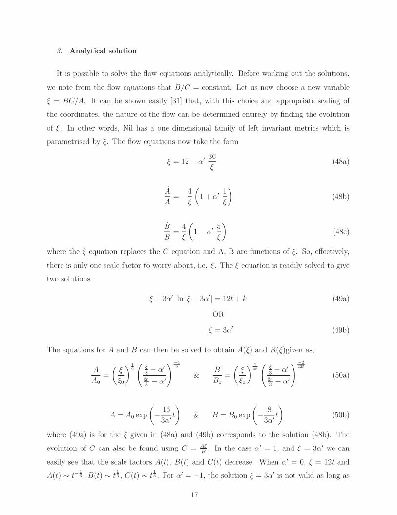
where B2

A> 5. Assume p = A

B2 . The quantity inside the bracket in Eq.53 is a polynomial

in p, f(p) = 4p − 20p2. f(p) represents a parabola (upside down) and its upper bound i.e

max[f(p)] = 15occurs at p = 1

10< 1

5. The parabola intersects the abscissa at p = 0, 1

5and

progressively increases in the negative direction of the ordinate (see Fig.6). Thus, f(p) is

positive in the region 0 < p < 15and, therefore B(t) increases with increasing t. Outside

this domain of t, B(t) decreases with increasing t. We now show the above-mentioned facts

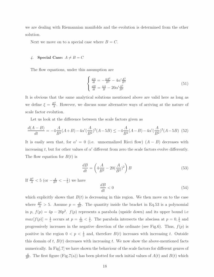
numerically. In Fig[.7] we have shown the behaviour of the scale factors for different genres of

AB2 . The first figure (Fig.7(a)) has been plotted for such initial values of A(t) and B(t) which

18

-0.2 0.2 0.4

-1.5

-1.0

-0.5

0.5

(a)f( A

B2 ) = 4( A

B2 )− 20( A

B2 )2 and ( A

B2 ) =1

3

Figure 6: f( AB2 ) vs (

AB2 ) for α

′ = 1

correspond to B2

A< 5, when both the scale factors are decreasing (see Eqn.[54], Fig. [7(b)]).

In Fig.7(b) we have shown an interesting turning behavior where B(t) initially decreases but

eventually increases. The initial condition has been chosen to satisfy AB2 > 1

5but during the

evolution A(t), B(t) decreases so that AB2 eventually becomes less than 1

5leading to growing

nature of B(t). On the other hand, for α′ = −1, 0, the evolution is easy to comprehend

from the equations (Eqn.[51]). The corresponding evolution of the scale factors is shown,

respectively in Fig[7(c)] and Fig[7(d)].

5. Phase plots

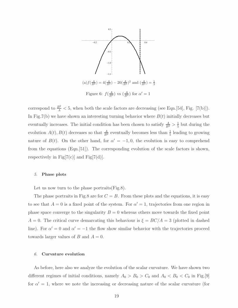
Let us now turn to the phase portraits(Fig.8).

The phase portraits in Fig.8 are for C = B. From these plots and the equations, it is easy

to see that A = 0 is a fixed point of the system. For α′ = 1, trajectories from one region in

phase space converge to the singularity B = 0 whereas others move towards the fixed point

A = 0. The critical curve demarcating this behaviour is ξ = BC/A = 3 (plotted in dashed

line). For α′ = 0 and α′ = −1 the flow show similar behavior with the trajectories proceed

towards larger values of B and A = 0.

6. Curvature evolution

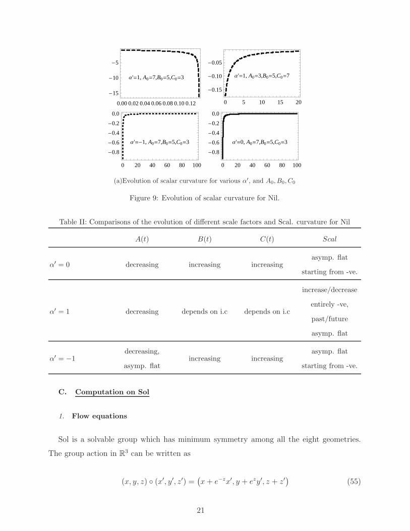
As before, here also we analyze the evolution of the scalar curvature. We have shown two

different regimes of initial conditions, namely A0 > B0 > C0 and A0 < B0 < C0 in Fig.[9]

for α′ = 1, where we note the increasing or decreasing nature of the scalar curvature (for

19

-1.0 -0.8 -0.6 -0.4 -0.2 0.00

10

20

30

40

50

60

(a)(A0, B0) = (7, 3), α′ = 1, Ts = 0.03

0 2 4 6 80.0

0.5

1.0

1.5

2.0

2.5

(b)(A0, B0) = (2, 2.45), α′ = 1

0 2 4 6 8 10

5

10

15

(c)(A0, B0) = (7, 1), α′ = −1, Ts = −0.0003

0 2 4 6 8 10

2

4

6

8

10

12

(d)(A0, B0) = (5, 3), α′ = 0, Ts = −0.15

Figure 7: A(t), B(t) vs t for α′ = 1, α′ = −1 and α′ = 0

0 1 2 3 4 5 60

1

2

3

4

5

6

A

B

(a)α′ = 1

0 1 2 3 4 5 60

1

2

3

4

5

6

A

B

(b)α′ = 0

0 1 2 3 4 5 60

1

2

3

4

5

6

A

B

(c)α′ = −1

Figure 8: 2nd order flow on Nil for B = C

different initial conditions). For α′ = 0 and α′ = −1 the scalar curvature monotonically

converges to zero asymptotically after beginning from a negative value.

We conclude this section by providing a comparison of the evolution of different scale

factors and Scal. curvature for Nil manifolds in tableII.

20

Α'=1, A0=7,B0=5,C0=3

0.000.020.040.060.080.100.12

-15

-10

-5

Α'=1, A0=3,B0=5,C0=7

0 5 10 15 20

-0.15

-0.10

-0.05

Α'=-1, A0=7,B0=5,C0=3

0 20 40 60 80 100

-0.8

-0.6

-0.4

-0.2

0.0

Α'=0, A0=7,B0=5,C0=3

0 20 40 60 80 100

-0.8

-0.6

-0.4

-0.2

0.0

(a)Evolution of scalar curvature for various α′, and A0, B0, C0

Figure 9: Evolution of scalar curvature for Nil.

Table II: Comparisons of the evolution of different scale factors and Scal. curvature for Nil

A(t) B(t) C(t) Scal

α′ = 0 decreasing increasing increasingasymp. flat

starting from -ve.

α′ = 1 decreasing depends on i.c depends on i.c

increase/decrease

entirely -ve,

past/future

asymp. flat

α′ = −1decreasing,

asymp. flatincreasing increasing

asymp. flat

starting from -ve.

C. Computation on Sol

1. Flow equations

Sol is a solvable group which has minimum symmetry among all the eight geometries.

The group action in R3 can be written as

(x, y, z) (x′, y′, z′) =(x+ e−zx′, y + ezy′, z + z′

)(55)

21

We can put left invariant vector fields¶ on the manifold, for which the structure constants

in the Milnor frame will be λ = −2, µ = 0, ν = +2. Sol really has a two parameter family of

metrics upto diffeomeorphism (obtained by scaling and redefinition of the coordinates, see

[31]). Using the values of the structure constants, we can find the components of Rc and

Rc2tensors. The 2nd order flow equations reduce to,

dA

dt=

−4(A2 − C2)

BC− 4α′ (A+ C)2(A2 − 2AC + 5C2)

AB2C2(56)

dB

dt= 4

(A+ C)2

AC− 4α′ (A+ C)2(5A2 − 6AC + 5C2)

A2BC2(57)

dC

dt= −4

(C2 − A2)

AB− 4α′ (A+ C)2(5A2 − 2AC + C2)

A2B2C(58)

2. Numerical and analytical estimates

(a) The behaviour of the scale factors for the above higher order flow are different from those

in unnormalized Ricci flow. From Fig.10(d) (unnormalized Ricci flow) we note that the scale

factors do not have a future singularity. In fact, we see the appearance of a cigar degeneracy.

The above behaviour can be predicted qualitatively from the equations themselves. We note

that A and C can be interchanged in the equations. So instead of three equations it is

enough to examine two of them. Further, without loss of generality, we may assume A > C.

For α′ = 1 the scale factors converge (see Fig 10 (a)). If α′ = 0 and A > C we find that B(t),

C(t) increase and A(t) decreases (more detail for α′ = 0 can be found in [1]). If α′ = −1 the

behaviour of the scale factors bear a resemblance with unnormalized Ricci flow, though the

singularity time (in the past) changes due to the higher order term ( Fig.10(c) illustrates

one such example for a particular set of initial values).

(b) We now consider the case α′ = 1 and analyze the evolution of the scale factor A(t) a

bit further. It can be shown that Eqn.56 can be written as

dA

dt≤ −4

A

C

A

B

(1− C

A

)2

− 2

B

A

B

(1− C

A

)2(1 +

A

C

)2

− 8

B

A

B

(1 +

C

A

)2

(59)

which shows that A(t) is decreasing in forward time. This is also true for C(t) where

the second term in Eq.58 dominates over the first term and, therefore, the net effect is a

[¶] it is easy to check that one such left invariant metric will be ds2 = e2zdx2 + e−2zdy2 + dz2

22

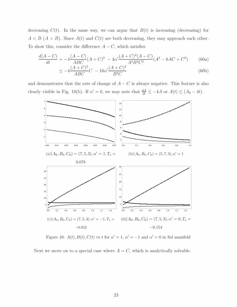
decreasing C(t). In the same way, we can argue that B(t) is increasing (decreasing) for

A < B (A > B). Since A(t) and C(t) are both decreasing, they may approach each other.

To show this, consider the difference A− C, which satisfies

d(A− C)

dt= −4

(A− C)

ABC(A+ C)2 − 4α′ (A+ C)2(A− C)

A2B2C2(A2 − 6AC + C2) (60a)

≤ −4(A + C)2

ABCC − 16α′ (A+ C)2

B2C(60b)

and demonstrates that the rate of change of A− C is always negative. This feature is also

clearly visible in Fig. 10(b). If α′ = 0, we may note that dAdt

≤ −4A or A(t) ≤ (A0 − 4t).

0.00 0.01 0.02 0.03 0.04 0.05 0.06 0.07

2

3

4

5

6

7

(a)(A0, B0, C0) = (7, 5, 3), α′ = 1, Ts =

0.078

0.0 0.2 0.4 0.6 0.8 1.0

2

4

6

8

10

12

14

(b)(A0, B0, C0) = (5, 7, 3), α′ = 1

0.0 0.2 0.4 0.6 0.8 1.0 1.2 1.4

5

10

15

20

25

30

(c)(A0, B0, C0) = (7, 5, 3), α′ = −1, Ts =

−0.052

0.0 0.2 0.4 0.6 0.8 1.0 1.2 1.4

5

10

15

20

25

30

(d)(A0, B0, C0) = (7, 5, 3), α′ = 0, Ts =

−0.154

Figure 10: A(t), B(t), C(t) vs t for α′ = 1, α′ = −1 and α′ = 0 in Sol manifold

Next we move on to a special case where A = C, which is analytically solvable.

23

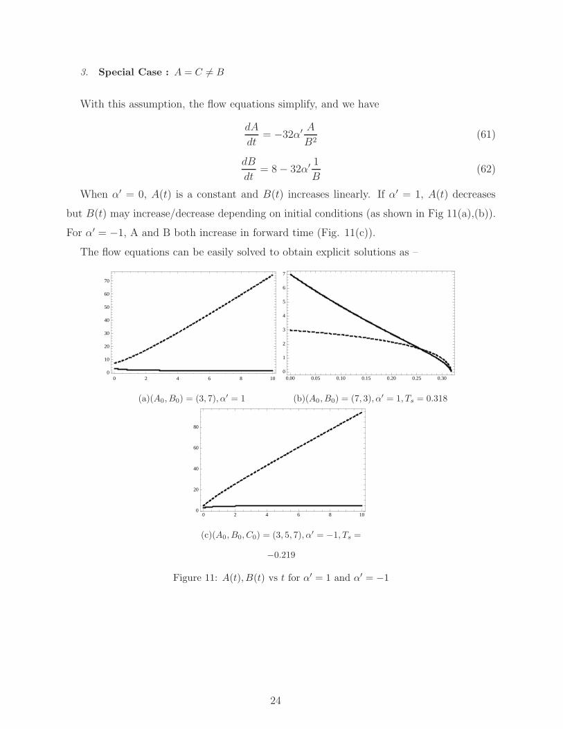
3. Special Case : A = C 6= B

With this assumption, the flow equations simplify, and we have

dA

dt= −32α′ A

B2(61)

dB

dt= 8− 32α′ 1

B(62)

When α′ = 0, A(t) is a constant and B(t) increases linearly. If α′ = 1, A(t) decreases

but B(t) may increase/decrease depending on initial conditions (as shown in Fig 11(a),(b)).

For α′ = −1, A and B both increase in forward time (Fig. 11(c)).

The flow equations can be easily solved to obtain explicit solutions as –

0 2 4 6 8 100

10

20

30

40

50

60

70

(a)(A0, B0) = (3, 7), α′ = 1

0.00 0.05 0.10 0.15 0.20 0.25 0.300

1

2

3

4

5

6

7

(b)(A0, B0) = (7, 3), α′ = 1, Ts = 0.318

0 2 4 6 8 100

20

40

60

80

(c)(A0, B0, C0) = (3, 5, 7), α′ = −1, Ts =

−0.219

Figure 11: A(t), B(t) vs t for α′ = 1 and α′ = −1

24

0 2 4 6 80

2

4

6

8

A

B

(a)α′ = 1

0 2 4 6 80

2

4

6

8

A

B(b)α′ = 0

0 2 4 6 80

2

4

6

8

A

B

(c)α′ = −1

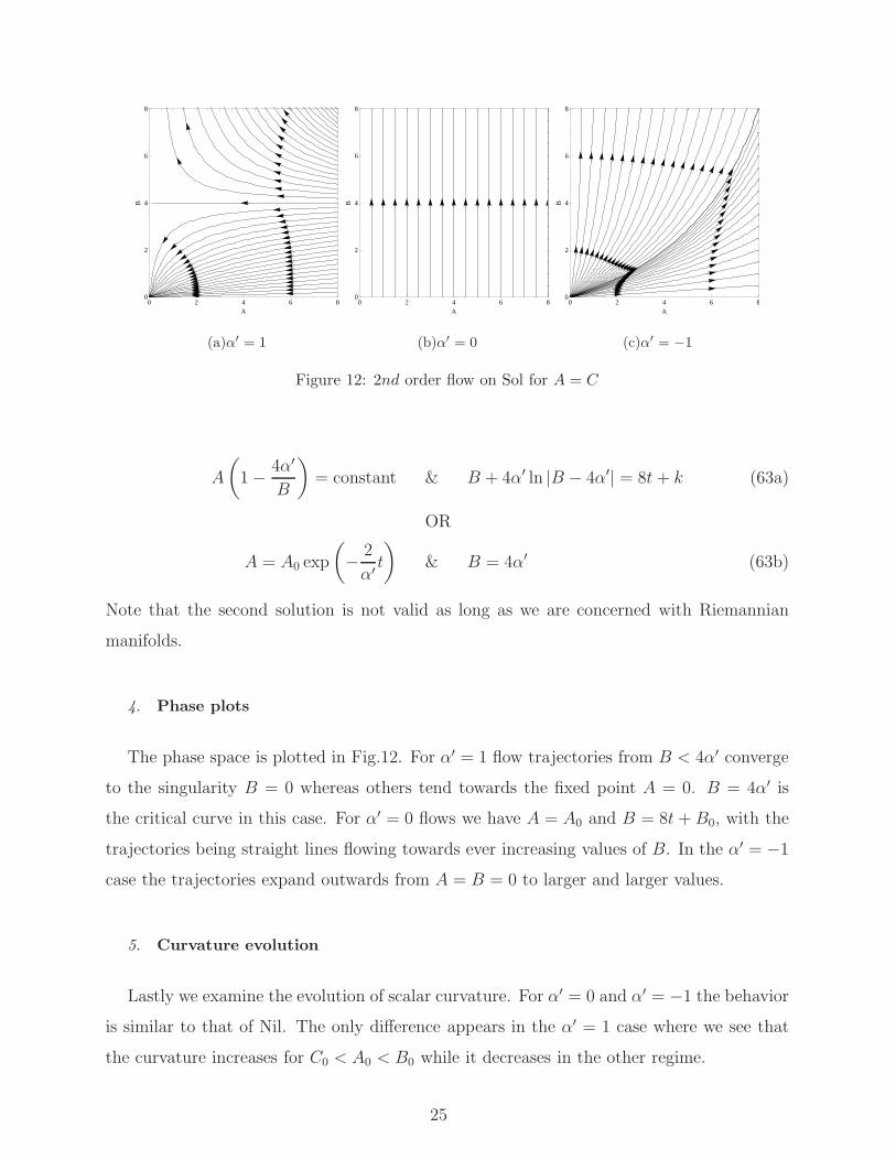
Figure 12: 2nd order flow on Sol for A = C

A

(1− 4α′

B

)= constant & B + 4α′ ln |B − 4α′| = 8t + k (63a)

OR

A = A0 exp

(− 2

α′ t

)& B = 4α′ (63b)

Note that the second solution is not valid as long as we are concerned with Riemannian

manifolds.

4. Phase plots

The phase space is plotted in Fig.12. For α′ = 1 flow trajectories from B < 4α′ converge

to the singularity B = 0 whereas others tend towards the fixed point A = 0. B = 4α′ is

the critical curve in this case. For α′ = 0 flows we have A = A0 and B = 8t +B0, with the

trajectories being straight lines flowing towards ever increasing values of B. In the α′ = −1

case the trajectories expand outwards from A = B = 0 to larger and larger values.

5. Curvature evolution

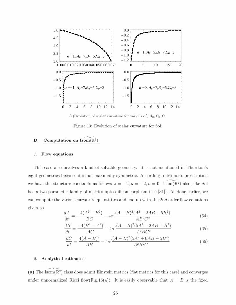
Lastly we examine the evolution of scalar curvature. For α′ = 0 and α′ = −1 the behavior

is similar to that of Nil. The only difference appears in the α′ = 1 case where we see that

the curvature increases for C0 < A0 < B0 while it decreases in the other regime.

25

Α'=1, A0=7,B0=5,C0=3

0.000.010.020.030.040.050.060.073.0

3.5

4.0

4.5

5.0

Α'=1, A0=5,B0=7,C0=3

0 5 10 15 20-1.2-1.0-0.8-0.6-0.4-0.2

0.0

Α'=-1, A0=7,B0=5,C0=3

0 2 4 6 8 10 12 14

-1.5

-1.0

-0.5

0.0

Α'=0, A0=7,B0=5,C0=3

0 2 4 6 8 10 12 14

-1.5

-1.0

-0.5

0.0

(a)Evolution of scalar curvature for various α′, A0, B0, C0

Figure 13: Evolution of scalar curvature for Sol.

D. Computation on ˜Isom(R2)

1. Flow equations

This case also involves a kind of solvable geometry. It is not mentioned in Thurston’s

eight geometries because it is not maximally symmetric. According to Milnor’s prescription

we have the structure constants as follows λ = −2, µ = −2, ν = 0. ˜Isom(R2) also, like Sol

has a two parameter family of metrics upto diffeomeorphism (see [31]). As done earlier, we

can compute the various curvature quantitites and end up with the 2nd order flow equations

given asdA

dt=

−4(A2 −B2)

BC− 4α′ (A−B)2(A2 + 2AB + 5B2)

AB2C2(64)

dB

dt=

−4(B2 − A2)

AC− 4α′ (A− B)2(5A2 + 2AB +B2)

A2BC2(65)

dC

dt=

4(A− B)2

AB− 4α′ (A− B)2(5A2 + 6AB + 5B2)

A2B2C(66)

2. Analytical estimates

(a) The ˜Isom(R2) class does admit Einstein metrics (flat metrics for this case) and converges

under unnormalized Ricci flow(Fig.16(a)). It is easily observable that A = B is the fixed

26

point of the flow irrespective of the presence of the higher order term. For α′ = 1 each of

the scale factors attain constant value asymptotically and they are seen to decrease initially.

(b) Let us check the evolution of each of the scale factors for α′ = 1. Using the fact that

(A2 + 2AB + 5B2) > (A +B)2 and Eqn.64 we can write the evolution of A(t) as

dA

dt≤ −4

(A− B)2

BC− 4

(A+B)2(A− B)2

AB2C2(67)

So the scale factor A(t) always decreases. Using the same kind of argument as earlier

(5A2 + 2AB +B2) > (A +B)2 we can rewrite Eq.65 as

dB

dt≤ 4

(A+B)2

AC− 4

(A+B)2(A−B)2

A2BC2≤ 4

(1− (A− B)2

ABC

)(A− B)2

AC(68)

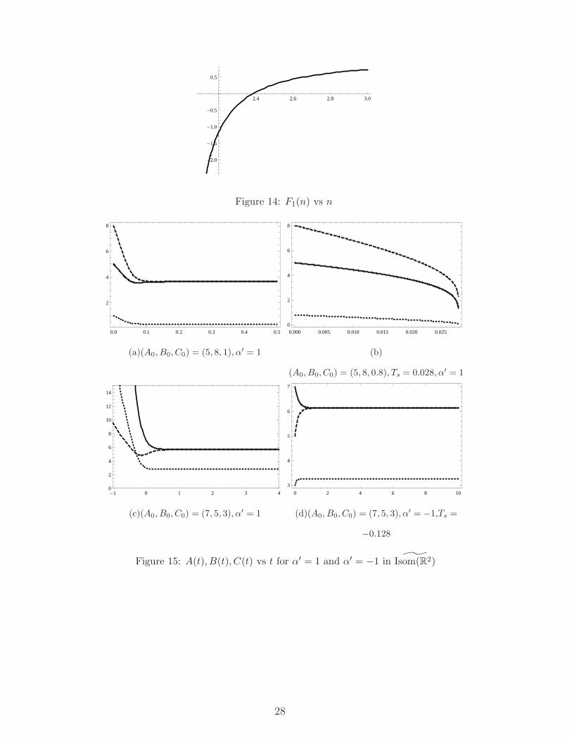
It can be easily shown that(1− (A−B)2

ABC

)(say F1) can be negative as well as positive. To

illustrate this we assume A = n + 2, B = n, C = n − 2 and calculate F1 which turns out

to be 1− 4(n−2)n(2+n)

. From the plot of F1 (Fig.14), we note that depending on the value of

n, F1 can be positive as well as negative. Obviously this holds for B(t) as well. Next, we

estimate the behavior of dCdt. From Eqn.66 it is easy to anticipate that (5A2 + 6AB + 5B2)

will be the deciding factor. Using the bound −(5A2 + 6AB + 5B2) < −(A − B)2 we can

recast the Eqn.66 asdC

dt≤ 4(

A

B− 1)2

(B

A− 16B

AC

)(69)

The behaviour for C(t) may be found by choosing A, B, C and calculating a quantity similar

to the F1 mentioned earlier. The evolution of C(t) is qualitatively similar to that of B(t).

3. Numerical estimates

In Fig.[15] we demonstrate our conclusions for certain specific inital values by numericaly

solving the dynamical system. The cases with α′ = 1 and different sets of initial values are

shown in Fig. 15(a)-(c). For α′ = −1 the flow develops a past singularity (Fig.15(d)). The

nature of the evolution of scale factors for α′ = 0 is similar to the case α′ = −1 except for

singularity time. These features appear in Fig. 16(a) and Fig.16(b).

4. Special case: B = ηA

Let us now choose B = ηA with 0 < η < 1. The flow equations become –

27

2.4 2.6 2.8 3.0

-2.0

-1.5

-1.0

-0.5

0.5

Figure 14: F1(n) vs n

0.0 0.1 0.2 0.3 0.4 0.5

2

4

6

8

(a)(A0, B0, C0) = (5, 8, 1), α′ = 1

0.000 0.005 0.010 0.015 0.020 0.0250

2

4

6

8

(b)

(A0, B0, C0) = (5, 8, 0.8), Ts = 0.028, α′ = 1

-1 0 1 2 3 40

2

4

6

8

10

12

14

(c)(A0, B0, C0) = (7, 5, 3), α′ = 1

0 2 4 6 8 10

3

4

5

6

7

(d)(A0, B0, C0) = (7, 5, 3), α′ = −1,Ts =

−0.128

Figure 15: A(t), B(t), C(t) vs t for α′ = 1 and α′ = −1 in ˜Isom(R2)

28

0 2 4 6 8 10

3

4

5

6

7

(a)(A0, B0, C0) = (7, 5, 3), α′ = 0, Ts = −0.3

0 2 4 6 8 10

3

4

5

6

7

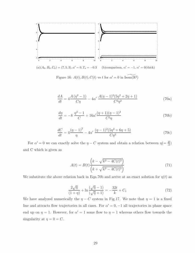
(b)comparison, α′ = −1, α′ = 0(thick)

Figure 16: A(t), B(t), C(t) vs t for α′ = 0 in ˜Isom(R2)

dA

dt= 4

A (η2 − 1)

Cη− 4α′ A(η − 1)2(5η2 + 2η + 1)

C2η2(70a)

dη

dt= −8

η2 − 1

C+ 16α′ (η + 1)(η − 1)3

C2η(70b)

dC

dt= 4

(η − 1)2

η− 4α′ (η − 1)2(5η2 + 6η + 5)

Cη2(70c)

For α′ = 0 we can exactly solve the η − C system and obtain a relation between η(= BA)

and C which is given as

A(t) = B(t)

(k −

√k2 − 4C(t)2

)

(k +

√k2 − 4C(t)2

) (71)

We substitute the above relation back in Eqn.70b and arrive at an exact solution for η(t) as

2√η

(1 + η)+ ln

(√η − 1)

(√η + 1)

= −32t

k+ C1 (72)

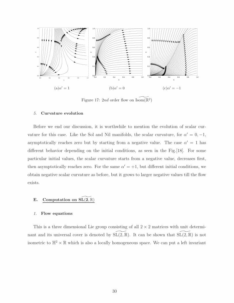
We have analyzed numerically the η − C system in Fig.17. We note that η = 1 is a fixed

line and attracts flow trajectories in all cases. For α′ = 0,−1 all trajectories in phase space

end up on η = 1. However, for α′ = 1 some flow to η = 1 whereas others flow towards the

singularity at η = 0 = C.

29

0.0 0.2 0.4 0.6 0.8 1.0

0.0

0.2

0.4

0.6

0.8

1.0

Η

C

(a)α′ = 1

0.0 0.2 0.4 0.6 0.8 1.00.0

0.2

0.4

0.6

0.8

1.0

Η

C(b)α′ = 0

0.0 0.2 0.4 0.6 0.8 1.00.0

0.2

0.4

0.6

0.8

1.0

Η

C

(c)α′ = −1

Figure 17: 2nd order flow on ˜Isom(R2)

5. Curvature evolution

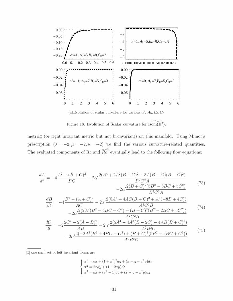
Before we end our discussion, it is worthwhile to mention the evolution of scalar cur-

vature for this case. Like the Sol and Nil manifolds, the scalar curvature, for α′ = 0,−1,

asymptotically reaches zero but by starting from a negative value. The case α′ = 1 has

different behavior depending on the initial conditions, as seen in the Fig.[18]. For some

particular initial values, the scalar curvature starts from a negative value, decreases first,

then asymptotically reaches zero. For the same α′ = +1, but different initial conditions, we

obtain negative scalar curvature as before, but it grows to larger negative values till the flow

exists.

E. Computation on ˜SL(2,R)

1. Flow equations

This is a three dimensional Lie group consisting of all 2× 2 matrices with unit determi-

nant and its universal cover is denoted by ˜SL(2,R). It can be shown that ˜SL(2,R) is not

isometric to H2 × R which is also a locally homogeneous space. We can put a left invariant

30

Α'=1, A0=5,B0=8,C0=2

0.0 0.1 0.2 0.3 0.4 0.5 0.6

-0.20

-0.15

-0.10

-0.05

0.00

Α'=1, A0=5,B0=8,C0=0.8

0.0000.0050.0100.0150.0200.025

-8

-6

-4

-2

Α'=-1, A0=7,B0=5,C0=3

0 1 2 3 4 5 6

-0.06

-0.04

-0.02

0.00

Α'=0, A0=7,B0=5,C0=3

0 1 2 3 4 5 6

-0.06

-0.04

-0.02

0.00

(a)Evolution of scalar curvature for various α′, A0, B0, C0

Figure 18: Evolution of Scalar curvature for ˜Isom(R2).

metric‡ (or right invariant metric but not bi-invariant) on this manifold. Using Milnor’s

prescription (λ = −2, µ = −2, ν = +2) we find the various curvature-related quantities.

The evaluated components of Rc and Rc2eventually lead to the following flow equations:

dA

dt= −4

A2 − (B + C)2

BC− 2α′2(A

4 + 2A2(B + C)2 − 8A(B − C)(B + C)2)

B2C2A

−2α′2(B + C)2(5B2 − 6BC + 5C2)

B2C2A

(73)

dB

dt= −4

B2 − (A + C)2

AC− 2α′2(5A

4 + 4AC(B + C)2 + A3(−8B + 4C))

A2C2B

−2α′2(2A2(B2 − 4BC − C2) + (B + C)2(B2 − 2BC + 5C2))

A2C2B

(74)

dC

dt= −2

2C2 − 2(A− B)2

AB− 2α′2(5A

4 − 4A3(B − 2C)− 4AB(B + C)2)

A2B2C

−2α′2(−2A2(B2 + 4BC − C2) + (B + C)2(5B2 − 2BC + C2))

A2B2C

(75)

[‡] one such set of left invariant forms are

π1 = dx + (1 + x2)2dy + (x − y − x2y)dz

π2 = 2xdy + (1− 2xy)dz

π3 = dx + (x2 − 1)dy + (x+ y − x2y)dz

31

2. Analytical and numerical estimates

(a) The abovementioned equations are very hard to solve, analytically, when α′ 6= 0. For

α′ = 0 we can see from Eqn.73 and Eqn.74 that the flow is symmetric in A and B. Assuming

A0 ≥ B0, without any loss of generality, we can show that A(t) ≥ B(t) throughout the

α′ = 0 flow. This may be inferred (for A > B > C) from the evolution of the difference of

(A− B) given as

d(A−B)

dt= − 4

ABC(A−B) (A+B − C) (A+B + C) ≤ 0 (76)

The evolution of C(t) is straightforward. We note that there exists a lower bound, in

the following sense,

dC

dt=

4

AB

((A− B)2 − C2

)

= 4((A

B+

B

A

)2

− C2

AB− 2)≥ −4 (77)

Eqn.77 shows that C(t)(= C0 − 4t) is monotonically decreasing –a point of difference from

what we find for normalised Ricci flow. Similarly, it is not difficult to show that B(t) is also

monotonically increasing, if we assume A0 > B0 > C0. However, the nature of the evolution

of A(t) shows an increase though it is not monotonic. This can be justified as follows. We

have

dA

dt=

4

BC(A+B + C) (B + C − A) (78)

Thus, A(t) will increase monotonically provided A < (B + C), otherwise it will decrease

initially and then increase. We further note that as A(t) and B(t) increase they approach

each other. This feature follows from Eqn.76, assuming A0 > B0 > C0. We can write

d(A− B)

dt= − 4

ABC(A−B) (A+B − C) (A +B + C)

≤ − 4

AB(A− B) (A+B − C)

≤ −12C

AB(A− B) (79)

All the above stated features for α′ = 0 are shown in Fig.19(e).

32

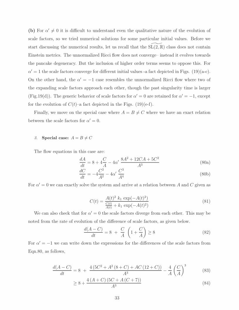
(b) For α′ 6= 0 it is difficult to understand even the qualitative nature of the evolution of

scale factors, so we tried numerical solutions for some particular initial values. Before we

start discussing the numerical results, let us recall that the ˜SL(2,R) class does not contain

Einstein metrics. The unnormalized Ricci flow does not converge– instead it evolves towards

the pancake degeneracy. But the inclusion of higher order terms seems to oppose this. For

α′ = 1 the scale factors converge for different initial values -a fact depicted in Figs. (19)(a-c).

On the other hand, the α′ = −1 case resembles the unnormalized Ricci flow where two of

the expanding scale factors approach each other, though the past singularity time is larger

(Fig.19(d)). The generic behavior of scale factors for α′ = 0 are retained for α′ = −1, except

for the evolution of C(t)–a fact depicted in the Figs. (19)(e-f).

Finally, we move on the special case where A = B 6= C where we have an exact relation

between the scale factors for α′ = 0.

3. Special case: A = B 6= C

The flow equations in this case are:

dA

dt= 8 + 4

C

A− 4α′ 8A

2 + 12CA+ 5C2

A3(80a)

dC

dt= −4

C2

A2− 4α′ C

3

A4(80b)

For α′ = 0 we can exactly solve the system and arrive at a relation between A and C given as

C(t) =A(t)2 k1 exp(−A(t)2)C(t)A(t)

+ k1 exp(−A(t)2)(81)

We can also check that for α′ = 0 the scale factors diverge from each other. This may be

noted from the rate of evolution of the difference of scale factors, as given below.

d(A− C)

dt= 8 +

C

A

(1 +

C

A

)≥ 8 (82)

For α′ = −1 we can write down the expressions for the differences of the scale factors from

Eqn.80, as follows,

d(A− C)

dt= 8 +

4 (5C2 + A2 (8 + C) + AC (12 + C))

A3− 4

A

(C

A

)3

(83)

≥ 8 +4 (A+ C) (5C + A (C + 7))

A3(84)

33

0 20 40 60 800

50

100

150

200

250

300

(a)(A0, B0, C0) = (9, 7, 5), α′ = 1

0.000 0.005 0.010 0.015 0.020 0.025 0.030

1

2

3

4

5

6

7

(b)

(A0, B0, C0) = (3, 5, 7), α′ = 1, Ts = 0.033

0.0 0.1 0.2 0.3 0.4 0.5 0.6

1

2

3

4

5

6

7

(c)(A0, B0, C0) = (7, 5, 3), α′ = 1, Ts = 0.6

0.0 0.2 0.4 0.6 0.8 1.0

5

10

15

20

(d)

(A0, B0, C0) = (7, 5, 3), α′ = −1, Ts = −0.07

0.0 0.2 0.4 0.6 0.8 1.0

4

6

8

10

12

14

(e)

(A0, B0, C0) = (7, 5, 3), α′ = 0, Ts = −0.24

0.0 0.2 0.4 0.6 0.8 1.0

5

10

15

20

(f)α′ = −1 and α′ = 0(thick)

Figure 19: A(t), B(t), C(t) vs t for α′ = 1, α′ = −1and α′ = 0 for ˜SL(2,R)

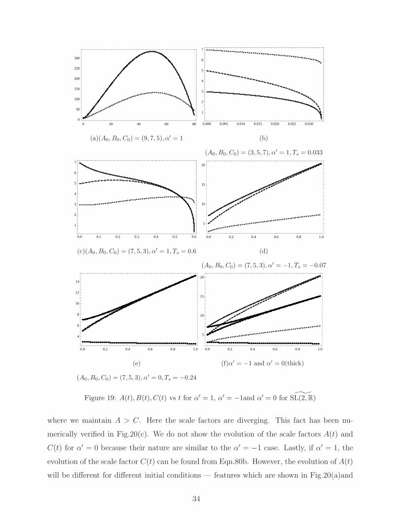
where we maintain A > C. Here the scale factors are diverging. This fact has been nu-

merically verified in Fig.20(c). We do not show the evolution of the scale factors A(t) and

C(t) for α′ = 0 because their nature are similar to the α′ = −1 case. Lastly, if α′ = 1, the

evolution of the scale factor C(t) can be found from Eqn.80b. However, the evolution of A(t)

will be different for different initial conditions — features which are shown in Fig.20(a)and

34

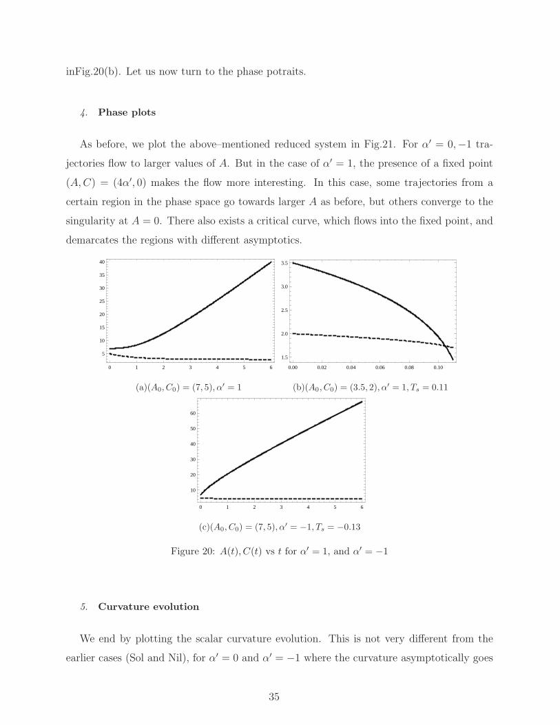
inFig.20(b). Let us now turn to the phase potraits.

4. Phase plots

As before, we plot the above–mentioned reduced system in Fig.21. For α′ = 0,−1 tra-

jectories flow to larger values of A. But in the case of α′ = 1, the presence of a fixed point

(A,C) = (4α′, 0) makes the flow more interesting. In this case, some trajectories from a

certain region in the phase space go towards larger A as before, but others converge to the

singularity at A = 0. There also exists a critical curve, which flows into the fixed point, and

demarcates the regions with different asymptotics.

0 1 2 3 4 5 6

5

10

15

20

25

30

35

40

(a)(A0, C0) = (7, 5), α′ = 1

0.00 0.02 0.04 0.06 0.08 0.10

1.5

2.0

2.5

3.0

3.5

(b)(A0, C0) = (3.5, 2), α′ = 1, Ts = 0.11

0 1 2 3 4 5 6

10

20

30

40

50

60

(c)(A0, C0) = (7, 5), α′ = −1, Ts = −0.13

Figure 20: A(t), C(t) vs t for α′ = 1, and α′ = −1

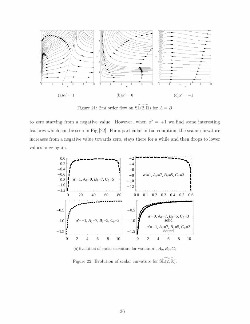
5. Curvature evolution

We end by plotting the scalar curvature evolution. This is not very different from the

earlier cases (Sol and Nil), for α′ = 0 and α′ = −1 where the curvature asymptotically goes

35

0 2 4 6 8 100

1

2

3

4

5

A

C

(a)α′ = 1

0 2 4 6 8 100

1

2

3

4

5

A

C(b)α′ = 0

0 2 4 6 8 100

1

2

3

4

5

A

C

(c)α′ = −1

Figure 21: 2nd order flow on ˜SL(2,R) for A = B

to zero starting from a negative value. However, when α′ = +1 we find some interesting

features which can be seen in Fig.[22]. For a particular initial condition, the scalar curvature

increases from a negative value towards zero, stays there for a while and then drops to lower

values once again.

Α'=1, A0=9, B0=7, C0=5

0 20 40 60 80-1.2-1.0-0.8-0.6-0.4-0.2

0.0

Α'=1, A0=7, B0=5, C0=3

0.0 0.1 0.2 0.3 0.4 0.5 0.6

-12-10-8-6-4-2

Α'=-1, A0=7, B0=5, C0=3

0 2 4 6 8 10

-1.5

-1.0

-0.5

Α'=0, A0=7, B0=5, C0=3solid

Α'=-1, A0=7, B0=5, C0=3dotted

0 2 4 6 8 10

-1.5

-1.0

-0.5

(a)Evolution of scalar curvature for various α′, A0, B0, C0

Figure 22: Evolution of scalar curvature for ˜SL(2,R).

36

V. CONCLUSIONS

Our overall aim in this work has been to study in detail the consequences of second

order (in Riemann curvature) geometric flows on three dimensional homogeneous spaces,

using analytical, semi-analytical and numerical methods. Through the analysis carried out,

we believe we have been able to obtain quite a few characteristics which seem to arise for

second order geometric flows on three dimensional homogeneous (locally) geometries. Here,

we briefly summarize our results and mention a few possibilities for the future.

From our results, we can say that for manifolds which do not contain Einstein metrics the

flow characteristics show new features essentially caused by the inclusion of the higher order

term. On the other hand, the class of group manifolds which admit metrics of Einstein class

(whether it is flat or round), results for second order flows appear to be refinements over

known results for Ricci flows. However, generic new characteristics do arise with varying

sign of α′ –in particular, a negative α′– and these have been noted in our work.

In several restricted cases (i.e. where two of the scale factors are related), we are able

to solve the flow equations exactly. We have obtained analytical solutions in such restricted

cases for Nil, Sol, ˜Isom(R2), ˜SL(2,R) manifolds. The exact solutions are instructive because

they help in obtaining analytical expressions for fixed points (curves) as well as in under-

standing the evolution of the scale factor. In addition, we also use them for checking our

numerics.

A generic observation is the fact that the singularity time changes due to the inclusion of

higher orders in the flow equations. This pattern is noticeable throughout in our numerical

work.

The results for α′ < 0 are, in quite a few cases, strikingly different from those for α′ = 0

or α′ > 0. Even the evolution of the scalar curvature exhibits a different behaviour in many

of the cases studied.

For SU(2) all the scale factors do not converge for α′ = −1 which is exactly opposite to

the characteristics for α′ = 1 and α′ = 0. Here, if α′ = 0, 1, the scalar curvature increases

but when α′ = −1 it increases first and then decreases. The appearance of negative scalar

curvature in SU(2) is also noted. In the case for Sol manifold the behavior of the scale

factors depend on different initial conditions for α′ = ±1—so does the evolution of the

scalar curvature.

37

In the case of ˜Isom(R2) all the scale factors converge for α′ = 1. When α′ = −1 one

scale factor decreases while the other two increase. In the last case, SL(2,R), we find that

for α′ = 1 all the scale factors may initially increase but they converge towards a singularity.

However, for α′ = −1 all the scale factors diverge.

In all cases we have obtained the phase portraits, which we feel, helps in visualising the

flow features as well as the fixed points. We also provide a summary of all our results in

several tables in the sections as well as, in the end.

Among possible future directions, we mention a few below.

• It would be interesting to pursue the approach presented in [13] for such higher order

flows.

• A more systematic and exhaustive analysis of the stability and classification of fixed

points, which is largely an algebraic problem, can be carried out for such second order

flows. This will surely shed more light on the behaviour of these flows from an analytical

perspective.

• Given the fact that such three manifolds do arise in various physically relevant contexts,

it will be nice to know whether our results on higher order flows can help us understand

such scenarios in any meaningful way.

• The relevance of our results in the context of renormalisation group flows of the bosonic

nonlinear σ-model deserve some attention.

• Since homogeneous four manifolds are already classified and studied with reference to

Ricci flows [32] it would be worthwhile extending our results to four manifolds.

We hope to address some of these issues in future articles.

38

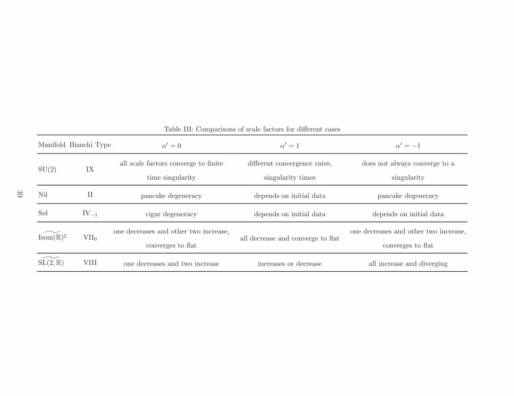
Table III: Comparisons of scale factors for different cases

Manifold Bianchi Type α′ = 0 α′ = 1 α′ = −1

SU(2) IXall scale factors converge to finite

time singularity

different convergence rates,

singularity times

does not always converge to a

singularity

Nil II pancake degeneracy depends on initial data pancake degeneracy

Sol IV−1 cigar degeneracy depends on initial data depends on initial data

˜Isom(R)2 VII0one decreases and other two increase,

converges to flatall decrease and converge to flat

one decreases and other two increase,

converges to flat

˜SL(2,R) VIII one decreases and two increase increases or decrease all increase and diverging

39

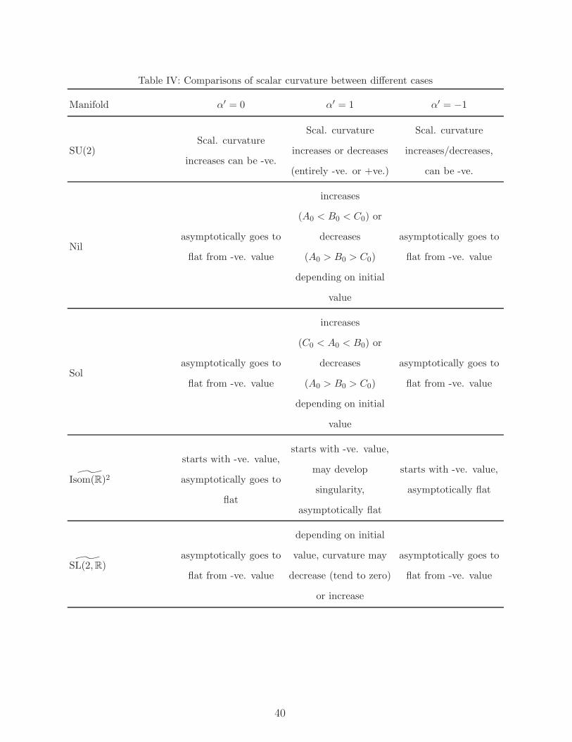
Table IV: Comparisons of scalar curvature between different cases

Manifold α′ = 0 α′ = 1 α′ = −1

SU(2)Scal. curvature

increases can be -ve.

Scal. curvature

increases or decreases

(entirely -ve. or +ve.)

Scal. curvature

increases/decreases,

can be -ve.

Nilasymptotically goes to

flat from -ve. value

increases

(A0 < B0 < C0) or

decreases

(A0 > B0 > C0)

depending on initial

value

asymptotically goes to

flat from -ve. value

Solasymptotically goes to

flat from -ve. value

increases

(C0 < A0 < B0) or

decreases

(A0 > B0 > C0)

depending on initial

value

asymptotically goes to

flat from -ve. value

˜Isom(R)2

starts with -ve. value,

asymptotically goes to

flat

starts with -ve. value,

may develop

singularity,

asymptotically flat

starts with -ve. value,

asymptotically flat

˜SL(2,R)asymptotically goes to

flat from -ve. value

depending on initial

value, curvature may

decrease (tend to zero)

or increase

asymptotically goes to

flat from -ve. value

40

Acknowledgments

SD acknowledges H. Seshadri, S. Panda for useful discusions and thanks the Institute of

Mathematical Sciences, Chennai, India, for support through a post-doctoral fellowship.

41

[1] B. Chow and D. Knopf, The Ricci flow: an introduction, Mathematical Surveys and Mono-

graphs Vol. 110, AMS, Providence, 2004.

[2] B. Chow et. al The Ricci flow: Techniques and Applications Part I: Geometric Aspects,

Mathematical Surveys and Monographs Vol. 135, AMS, Providence, 2007.

[3] R.S. Hamilton, Three manifolds with positive Ricci curvature, J. Diff. Geom. 17, 255 (1982).

[4] D. Friedan, Nonlinear Models in 2+ǫ Dimensions, Phys. Rev. Letts. 45 1057 (1980),

D. Friedan,Nonlinear Models in 2+ǫ Dimensions, Annals of Physics 163, 318 (1985).

[5] G. Perelman,The entropy formula for the Ricci flow and its geometric applications, Preprint

math.DG/0211159

[6] M. Headrick and T. Wiseman, Ricci flow and black holes, Class.Quant.Grav. 23, 6683 (2006);

E. Woolgar, Some applications of Ricci flow in Physics, arXiv:0708.2144; J. Samuel and S.

Roy Chowdhury, Energy, entropy and Ricci flow, Class.Quant.Grav. 25,035012 (2008) ibid.

Geometric flows and black hole entropy, Class.Quant.Grav.24:F47-F54 (2007); N. S. Manton,

One-vortex moduli space and Ricci flow, J.Geom.Phys.58,1772 (2008); M. Carfora and T.

Buchert, Ricci flow deformation of cosmological initial data sets. In ‘‘WASCOM 2007’’---14th

Conference on Waves and Stability in Continuous Media, N.Manganaro, R.Monaco,

S.Rionero (eds) World Scientific (2008), 118-127; V. Husain and S. S. Seahra, Ricci flows,

wormholes and critical phenomena, Class.Quant.Grav.25,222002 (2008)

[7] T. Oliynyk, V. Suneeta and E. Woolgar, Metric for gradient renormalization group flow of

the worldsheet sigma model beyond first order, Phys.Rev.D76:045001,2007; T. Oliynyk, The

second-order renormalization group flow for nonlinear sigma models in two dimensions, Class.

Quantum Grav. 26 105020, (2009); C. Guenther, and T. A. Oliynyk, Stability of the (Two-

Loop) Renormalization Group Flow for Nonlinear Sigma Models, Lett. Math. Phys. 84 (2008),

149-157.

[8] A. A. Tseytlin, On sigma model RG flow, central charge action and Perelman’s entropy, Phys.

Rev.D75, 064024 (2007)

[9] A. Sen, Equations of motion for the heterotic string theory from the conformal invariance of

the sigma model, Phys. Rev. Lett. 55, 1846 (1985); C. G. Callan, E. T. Martinec, M. T. Perry

and D. Friedan, Strings in background fields, Nucl. Phys. B262, 593 (1985)

42

[10] I. Jack, D. R. T. Jones, and N. Mohammedi, A four-loop calculation of the metric β-function

for the bosonic σ-model and the string effective action, Nuc. Phys. B322 (1989), 431-470.

[11] K. Prabhu, S. Das and S. Kar, Higher order geometric and renormalisation group flows, J.

Geom. and Phys. 61, 1854 (2011)

[12] J. Isenberg and M. Jackson, Ricci Flow of locally homogeneous geometries on closed

manifolds, J. Diff. Geom. 35 (1992), 723-741 ibid. Ricci Flow on Minisuperspaces and

the Geometry- Topology Problem. In Directions in general relativity:Vol1, Cambridge

University Press (1993), 166-181

[13] D. Glickenstein, T. L. Payne Ricci flow on three-dimensional, unimodular metric Lie algebras,

Comm. Anal. Geom. 18, 927 (2010)

[14] D. Knopf Quasi-convergence of the Ricci flow, Comm. Anal. Geom. 8, 375 (2000)

[15] J. Lauret Ricci flow of homogeneous manifolds and its soliton, arXiv:1112.5900v1

[16] X. Cao, J. Guckenheimer, L. Saloff-Coste The backward behavior of the Ricci and cross-

curvature flows on SL(2,R), Comm. Anal. Geom. 17, 777 (2009)

[17] X. Cao, L. Saloff-Coste Backward Ricci flow on locally homogeneous 3-manifolds, Comm. Anal.

Geom. 17, 305 (2009)

[18] A. U. O. Kisisel, O. Sarioglu, B. Tekin Cotton Flow, Class. Qunt. Grv.25, 165019 (2008)

[19] X. Cao, Y. Ni, L. Saloff-Coste Cross curvature flow on locally homogenous three-manifolds. I.,

Pacific J. Math.236, 263 (2008)

[20] M. Ryan and L. Shepley, Homogeneous relativistic cosmologies, Princeton University Press,

Princeton, NJ, 1975.

[21] L. Landau, Classical Theory of Fields, Butterworth-Heinemann, 1975

[22] J. A. Wheeler Our Universe: The Known and Unknown, Am. Scientist 56-1(1968)

[23] T. Koike, M. Tanimoto, A. Hosoya, Compact homogeneous universes, J. Math. Phys. 35, 4885

(1994)

[24] P.M. Petropoulos, V. Pozzoli, K. Siampos, Self-dual gravitational instantons and geometric

flows of all Bianchi types, arXiv:1108.0003.

[25] I. M. Singer Infinitesimally homogeneous spaces, Comm. Pure Appl. Math. 13, 685 (1960).

[26] W. Thurston, Three-dimensional geometry and topology. Vol. 1, Princeton University Press,

1997.

[27] J. Milnor, Curvature of the left invariants metrics on Lie Groups, Adv. Math. 21 (1976),

43

293-329

[28] A.L. Besse, Einstein Manifolds, Springer-Verlag (1987).

[29] J. Cheeger and D. Ebin, Comparison Theorems in Riemannian Geometry, North Holand,

1975.

[30] A. Arvanitoyeorgos, An Introduction to Lie Groups and the Geometry of Homogeneous Spaces,

AMS, 2003

[31] D. Glickenstein, Riemannian groupoids and solitons for three-dimensional homogeneous Ricci

and cross curvature flows, arXiv:0710.1276v2.

[32] J. Isenberg, M. Jackson and P. Lu, Ricci flow on locally homogeneous closed-4 manifolds,

Comm. Anal. Geom. 14(2006), 345-386

44