High-quality Image-based Interactive Exploration

of Real-World Environments1

Matthew Uyttendaele, Antonio Criminisi, Sing Bing Kang,

Simon Winder, Richard Hartley2, and Richard Szeliski

October, 2003

Technical Report

MSR-TR-2003-61

Microsoft Research

Microsoft Corporation

One Microsoft Way

Redmond, WA 98052

http://www.research.microsoft.com

1A shorter version of this article has been accepted for publication in IEEE Computer Graphics and

Applications.2Australian National University

(a) (b) (c)

Figure 1: The system described in this paper enables users to virtually explore large environments from the

comforts of their sofa (a). A standard wireless gamepad (b) allows the user to easily navigate through the

modeled environment which is displayed on a large wall screen (c). This results in a compelling experience

that marries the realism of high quality imagery acquired from real world locations together with the 3D

interactivity typical of computer games.

1 Introduction

Interactive scene walkthroughs have long been an important application area of computer graphics.

Starting with the pioneering work of Fred Brooks [1986], efficient rendering algorithms have been

developed for visualizing large architectural databases [Teller and Sequin, 1991,Aliaga et al., 1999].

More recently, researchers have developed techniques to construct photorealistic 3D architectural

models from real world images [Debevec et al., 1996, Coorg and Teller, 1999, Koch et al., 2000]. A

number of real-world tours based on panoramic images have also been developed (see the Previous

Work section). What all of these systems have in common is a desire to create a real sense of

being there, i.e., a sense of virtual presence that lets users experience a space or environment in an

exploratory, interactive manner.

In this paper, we present an image-based rendering system that brings us a step closer to a

compelling sense of being there. While many previous systems have been based on still photography

and/or 3D scene modeling, we avoid explicit 3D reconstruction in our work because this process

tends to be brittle. Instead, our approach is based directly on filming (with a set of high-resolution

cameras) an environment we wish to explore, and then using image-based rendering techniques to

replay the tour in an interactive manner. We call such experiences Interactive Visual Tours (Figure 1).

In designing this system, our goal is to allow the user to move freely along a set of predefined

tracks (cf. the “river analogy” in [Galyean, 1995]), choose between different directions of motion at

decision points, and look around in any direction. Another requirement is that the displayed views

should have a high resolution and dynamic range. The system is also designed to easily incorporate

1

Dem

osai

cing

Und

isto

rtio

n

De-

vign

etti

ng

Imagestitching

Featuretracking

Camera poseestimation

HDRstitching

Tonemapping

Com-pression Video

Objecttracking

Object poseestimation

Data forstabilization

Data for interactiveobject replacementD

ata

capt

ure

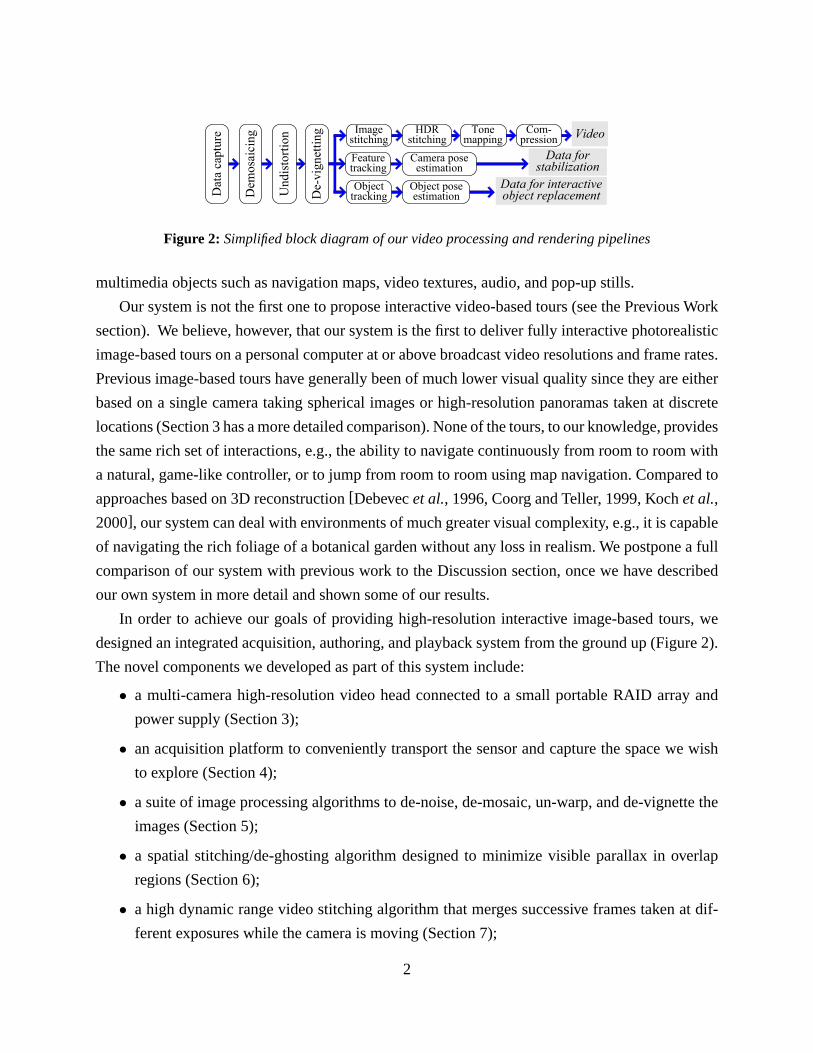
Figure 2: Simplified block diagram of our video processing and rendering pipelines

multimedia objects such as navigation maps, video textures, audio, and pop-up stills.

Our system is not the first one to propose interactive video-based tours (see the Previous Work

section). We believe, however, that our system is the first to deliver fully interactive photorealistic

image-based tours on a personal computer at or above broadcast video resolutions and frame rates.

Previous image-based tours have generally been of much lower visual quality since they are either

based on a single camera taking spherical images or high-resolution panoramas taken at discrete

locations (Section 3 has a more detailed comparison). None of the tours, to our knowledge, provides

the same rich set of interactions, e.g., the ability to navigate continuously from room to room with

a natural, game-like controller, or to jump from room to room using map navigation. Compared to

approaches based on 3D reconstruction [Debevec et al., 1996, Coorg and Teller, 1999, Koch et al.,

2000], our system can deal with environments of much greater visual complexity, e.g., it is capable

of navigating the rich foliage of a botanical garden without any loss in realism. We postpone a full

comparison of our system with previous work to the Discussion section, once we have described

our own system in more detail and shown some of our results.

In order to achieve our goals of providing high-resolution interactive image-based tours, we

designed an integrated acquisition, authoring, and playback system from the ground up (Figure 2).

The novel components we developed as part of this system include:

• a multi-camera high-resolution video head connected to a small portable RAID array and

power supply (Section 3);

• an acquisition platform to conveniently transport the sensor and capture the space we wish

to explore (Section 4);

• a suite of image processing algorithms to de-noise, de-mosaic, un-warp, and de-vignette the

images (Section 5);

• a spatial stitching/de-ghosting algorithm designed to minimize visible parallax in overlap

regions (Section 6);

• a high dynamic range video stitching algorithm that merges successive frames taken at dif-

ferent exposures while the camera is moving (Section 7);

2

• a feature tracking and pose estimation algorithm designed to stabilize the acquired video and

aid navigation (Section 8);

• a video compression scheme designed for selective (partial) decompression and random

access (Section 9);

• authoring tools for inserting branch points in the tour, adding sound sources, and augmenting

the video with synthetic and hybrid elements; and (Section 10).

• an interactive viewer that allows users to easily navigate and explore the space that has been

captured (Section 11).

Each of these components is described below in its own section. The overall complexity of the

system, however, is hidden from the end-user, who gets to intuitively navigate compelling interactive

tours of remote locations using a simple game control pad (Figure 1).

2 Previous work (panoramic photography)

Panoramic photography using mechano-optical means has a long history stretching back to the 19th

century [Malde, 1983, Benosman and Kang, 2001]. The stitching of photographs using computer

software has been around for a few decades [Milgram, 1975], but first gained widespread commercial

use with the release of Apple’s QuickTime VR system in 1995 [Chen, 1995]. Since then, a large

number of improvements have been made to the basic system, including constructing full-view

panoramas [Szeliski and Shum, 1997, Sawhney and Kumar, 1999], dealing with moving objects

[Davis, 1998], and using panoramas for image-based rendering [McMillan and Bishop, 1995]

and architectural reconstruction [Coorg and Teller, 1999]. (See [Benosman and Kang, 2001] for a

collection of some more recent papers in this area.) Most mid- to high-end digital cameras now ship

with image stitching software in the box, and there are over a dozen commercial stitching products

on the market today (http://www.panoguide.com/software lists a number of these).

Panoramic (360◦) movies were first introduced by Kodak at the World’s Fair in 1964 and are a

popular attraction in theme parks such as Disneyland. Interactive video tours were first demonstrated

by Andrew Lippman in his Movie Maps project, which stored video clips of the streets of Aspen

on an optical videodisc and allowed viewers to interactively navigate through these clips. In mobile

robotics, 360◦ video cameras based on reflecting curved mirrors (catadioptric systems [Baker and

Nayar, 1999]) have long been used for robot navigation [Ishiguro et al., 1992]. More recently,

such systems have also been used to present virtual tours [Boult, 1998, Aliaga and Carlbom, 2001,

3

Aliaga et al., 2002] and to build 3D image-based environment models [Coorg and Teller, 1999,

Taylor, 2002].

For example, Boult [Boult, 1998] developed a campus tour based on re-projecting catadioptric

spherical images streaming from a camcorder to give the user the ability to look around while

driving through campus. Teller et al. [Coorg and Teller, 1999] have built detailed 3D architectural

models of the MIT campus based on high-resolution still panoramic images taken from a specially

instrumented cart with a pan-tilt head. Aliaga et al. [Aliaga and Carlbom, 2001, Aliaga et al., 2002]

have built image-based interactive walkthrough of indoor rooms based on a dense sampling of

omnidirectional images taken from a mobile robot platform. Taylor’s VideoPlus system [Taylor,

2002] uses a similar setup but relies more on a sparse traversal of a set of connected rooms to

explore a larger region of interest. His paper also contains a nice review of previous work in the

area of environment modeling and visualization using catadioptric images.

Daniilidis’Omnidirectional Vision web page (//www.cis.upenn.edu/∼kostas/omni.html) lists al-

most 50 different research projects and commercial systems based on omnidirectional cameras. Of

the systems listed on his page, the majority employ curved mirrors and a single camera, while a few

employ multiple cameras. One clever design (http://www.fullview.com) uses mirrors to make the op-

tical centers coincident, which removes the parallax problems described in this paper (but results in

a slightly bulkier system). The system built by iMove (http://www.imoveinc.com) is the most similar

to ours, in that it uses a collection of outwardly pointing video cameras, but has a lower spatial resolu-

tion than the system built for us by Point Grey Research (http://www.ptgrey.com/products/ladybug/ ).

3 Omnidirectional camera design

The first step in achieving our goal of rendering full-screen, interactive walkthroughs is to design

a capture system. The system needs to efficiently capture full spherical environments at high res-

olution. One possible approach is to capture many high-resolution stills and to then stitch these

together. This step then has to be repeated at many locations throughout the environment [Coorg

and Teller, 1999]. While this yields very high resolution panoramas, it can require a long amount of

time, e.g., days instead of the few minutes that it takes us to digitize a home or garden. We decided

instead on omnidirectional capture at video rates.

A common approach to omnidirectional capture is to use catadioptric systems consisting of

mirrors and lenses. There are two major mirror based designs: those using curved mirrors with a

single lens and sensor, and those using multiple planar mirrors each with an associated camera.

These systems have the desirable feature that they capture a large cross section of a spherical

4

Camera 1

Camera 2

Camera 3

Camera 4

Camera 5

Camera 0

(a) (b)

Figure 3: Our six-sensor omnidirectional camera (a). The six images taken by our camera are arranged

horizontally around a pentagon, with a sixth sensor looking straight up. During processing, the overlapping

fields of view are merged and then re-sampled. During rendering, these images become the texture maps (b)

used in the 3D environment map.

environment and require no complex stitching, since they are designed to have a single optical

center. In order to enable full-screen experiences, our system needs to capture enough pixels to

provide at least a 640×480 resolution in any given 60◦ field of view. A curved mirror design would

need at least a 2K × 2K video rate sensor in order to approach these requirements, but the desired

resolution would only be within a fraction of its field of view. This is because these designs have

a non-uniform distribution of image resolution, which drops significantly towards the center of the

image. In addition, these designs have blind spots at the center of the image, where the field of view

is blocked by the camera itself.

Another class of omnidirectional sensors uses multiple individual cameras arranged in such a

way that they fully capture a scene. A disadvantage of this approach is that it is difficult to arrange

the cameras so that they share a common center of projection. The captured data must then be post-

processed with a more complex stitching and parallax compensation step to produce a seamless

panoramas (see our section on Image Stitching). However, parallax can be minimized by packing

the cameras very tightly together. On the plus side, such a system can capture most of a full viewing

sphere, can be made high-resolution using multiple sensors, and can be built in a rugged and compact

design. For these reasons, this was ultimately the design that we selected.

Since there was no commercially available system that met all of our requirements, we designed

our own multi-camera system, and contracted Point Grey Research to build it. The result is the

Ladybug camera (http://www.ptgrey.com/products/ladybug/ ) shown in Figure 3. The acquisition

system is divided into two parts: a head unit containing the cameras and control logic, and a storage

unit tethered to the head via a fiber optic link. The head unit contains six 768 × 1024 video-rate

5

sensors and associated lenses, with five pointing out along the equator, and one pointing up, giving

complete coverage from the North Pole to 50◦ below the equator. The lenses were chosen so that

there is a small overlap between adjacent cameras, allowing for stitching of the captured data.

The sensors run at a video rate of 15 frames/second and are synchronized. The storage unit is

a portable RAID array consisting of four 40GB hard drives, which allows us to store up to 20

minutes of uncompressed raw video. All components are powered by a small portable battery, and

the complete system can easily fit in a backpack or on a small robot (Figure 4), giving us a lot of

flexibility in terms of acquisition.

4 Data acquisition

Before we can capture large real-world scenes with our novel camera, we need to design a capture

platform to carry the sensor around, as well as a capture strategy to ensure that all the desirable data

gets collected. In this section we describe these two components.

4.1 Capture platform

To capture omnidirectional videos of scenes, we designed three different mobile platforms. Because

of the extremely wide field of view of our omnidirectional camera, each of our mobile platforms

was designed to avoid imaging itself and the camera person. (We considered using a steady-cam rig,

since it is capable of producing very smooth camera trajectories. Unfortunately, the person carrying

the steady-cam rig would always be visible to the omnidirectional camera, and so we rejected this

option.)

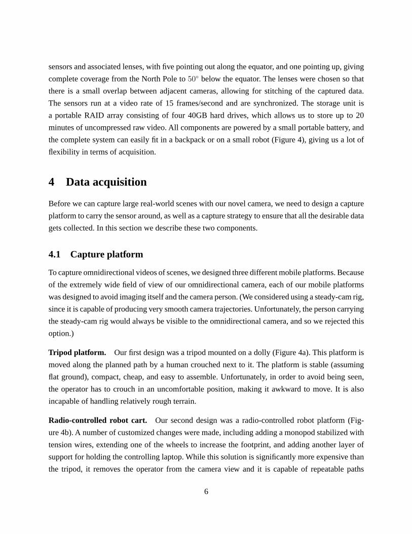
Tripod platform. Our first design was a tripod mounted on a dolly (Figure 4a). This platform is

moved along the planned path by a human crouched next to it. The platform is stable (assuming

flat ground), compact, cheap, and easy to assemble. Unfortunately, in order to avoid being seen,

the operator has to crouch in an uncomfortable position, making it awkward to move. It is also

incapable of handling relatively rough terrain.

Radio-controlled robot cart. Our second design was a radio-controlled robot platform (Fig-

ure 4b). A number of customized changes were made, including adding a monopod stabilized with

tension wires, extending one of the wheels to increase the footprint, and adding another layer of

support for holding the controlling laptop. While this solution is significantly more expensive than

the tripod, it removes the operator from the camera view and it is capable of repeatable paths

6

(a) (b) (c)

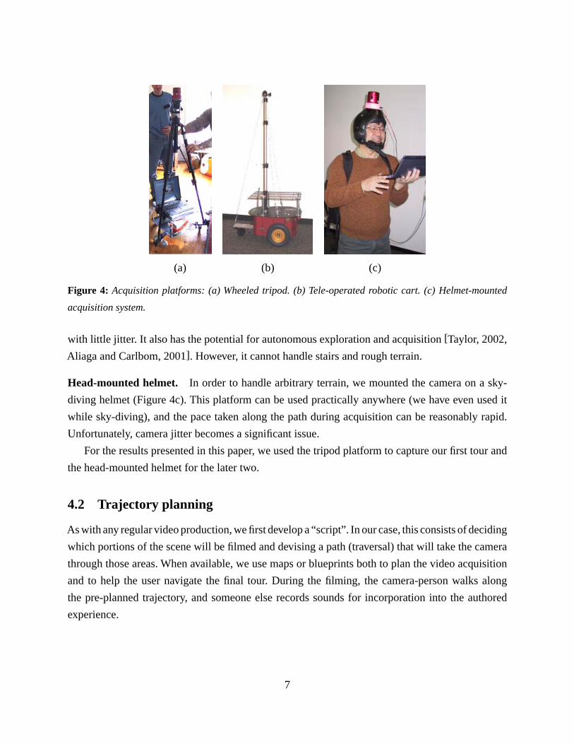
Figure 4: Acquisition platforms: (a) Wheeled tripod. (b) Tele-operated robotic cart. (c) Helmet-mounted

acquisition system.

with little jitter. It also has the potential for autonomous exploration and acquisition [Taylor, 2002,

Aliaga and Carlbom, 2001]. However, it cannot handle stairs and rough terrain.

Head-mounted helmet. In order to handle arbitrary terrain, we mounted the camera on a sky-

diving helmet (Figure 4c). This platform can be used practically anywhere (we have even used it

while sky-diving), and the pace taken along the path during acquisition can be reasonably rapid.

Unfortunately, camera jitter becomes a significant issue.

For the results presented in this paper, we used the tripod platform to capture our first tour and

the head-mounted helmet for the later two.

4.2 Trajectory planning

As with any regular video production, we first develop a “script”. In our case, this consists of deciding

which portions of the scene will be filmed and devising a path (traversal) that will take the camera

through those areas. When available, we use maps or blueprints both to plan the video acquisition

and to help the user navigate the final tour. During the filming, the camera-person walks along

the pre-planned trajectory, and someone else records sounds for incorporation into the authored

experience.

7

(a) (b) (c) (d) (e)

Figure 5: Radial distortion and vignetting correction: (a) image of calibration grid, (b) original photograph

of a building showing lens distortion, (c) corrected image, with straight lines converging on a vanishing

point; (d) original image showing vignetting effect, (e) image after vignetting correction.

5 Image pre-processing

The first step of our off-line processing pipeline is to perform some image processing tasks to

convert the raw video values coming from our sensor chip to color images and to correct for radial

distortion and vignetting.

5.1 De-mosaicing

Images are copied directly from the sensors onto the RAID array as raw Bayer color filter array

values (i.e., individual red, green, or blue samples arranged in a checkerboard array consisting of

50% G pixels and 25% R and B pixels) [Chang et al., 1999]. We use the algorithm described in

[Chang et al., 1999] to interpolate to full RGB images while preserving edge detail and minimizing

spurious color artifacts. We also undo the camera gamma so that the rest of the processing can be

done in a linear color space.

5.2 Radial distortion

Since the field of view of our cameras is large (∼ 100o), it introduces significant lens distortion. To

generate seamless mosaic images, the accuracy of the lens calibration is of paramount importance.

In fact, even a small degree of inaccuracy in the correction of the images will affect the quality of

the stitching in the regions where two images overlap.

We found that for our lenses, a parametric radial distortion model does not achieve sufficient

accuracy. We therefore developed a slightly more elaborate two-step correction algorithm. We start

8

from the standard plumb-line method where a parametric radial model is fitted to the image data

with the purpose of straightening up edges that appear to be curved [Brown, 1971, Devernay and

Faugeras, 1995]. Then, a second step is added to remove the small residual error by first finding

all corners of the image of a grid and mapping them back to their original locations. The output

displacements are then interpolated with a bilinear spline. The final result is a pixel-accurate lens

correction model (Figure 5). This technique is able to produce more accurate results than just fitting

a standard parametric radial distortion model.

5.3 Vignetting

Cameras with wide fields of view also suffer from a vignetting effect, i.e., an intensity drop-off away

from the center. This drop-off is due to both optical (off-axis illumination) and geometric (aperture)

factors. We compensate for these effects by first capturing an image within an integrating sphere

whose internal surface is almost perfectly Lambertian. We then fit a global function that accounts

for this effect. The function we use is of the form I(r) = I0(r)[1−αr]/[1+(r/f)2]2, where r is the

radial distance from the principal point (assumed to be the center of the image), I(r) is the sampled

image, I0(r) is the hypothesized un-attenuated intensity image, f is the camera focal length, and α

is the geometric attenuation factor. Details of extracting these parameters can be found in [Kang

and Weiss, 2000].

5.4 Geometric calibration

Once each camera has been unwarped to fit a linear perspective model, we need to compute the

linear transforms that relate camera pixels to world rays relative to the camera head. One way to

do this would be to track a large number of points while rotating the head and to then perform

a full bundle adjustment (structure from motion reconstruction [Hartley and Zisserman, 2000,

Triggs et al., 1999]. However, we have found that a simpler approach works well enough for our

purposes. We simply take an image of an outdoor scene where there is negligible parallax and use

an image stitching algorithm to compute the camera intrinsic parameters and rotations [Szeliski and

Shum, 1997]. We then estimate the inter-camera translations from the design specifications. While

these are not the exact displacements between the optical centers, they are close enough that we

can compensate for inter-camera parallax using the technique described in the next section.

9

… …

… …

C1 C2

I1 I2

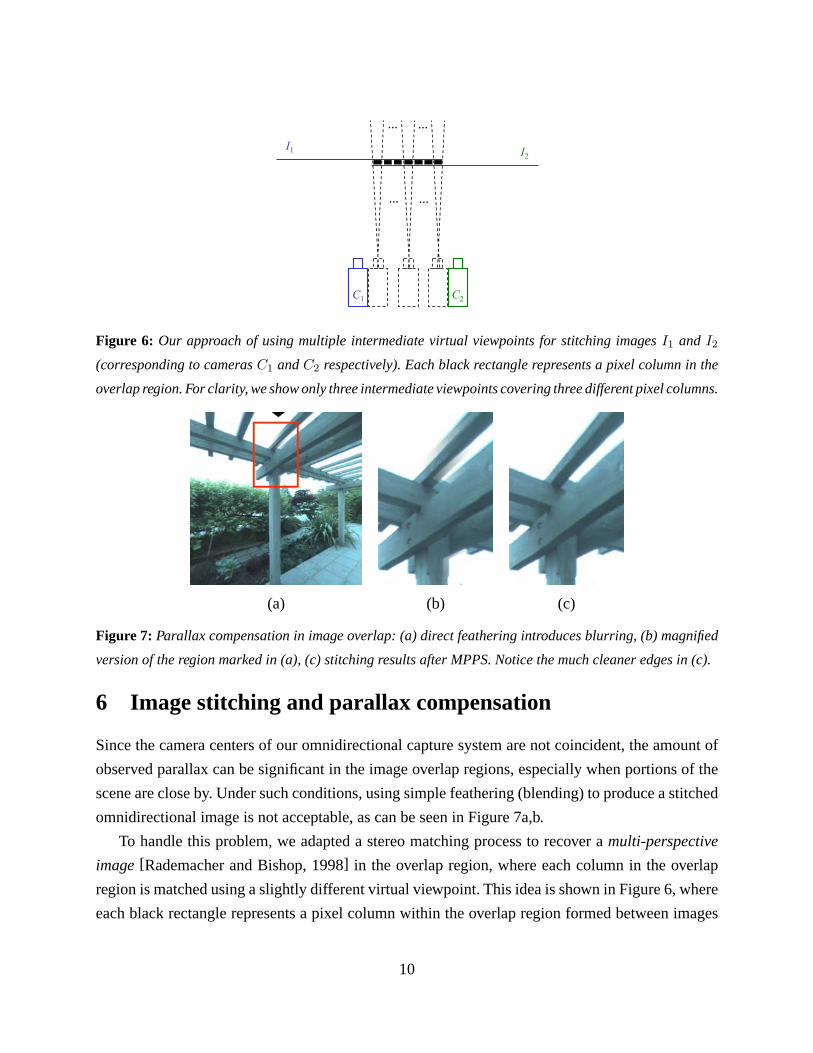
Figure 6: Our approach of using multiple intermediate virtual viewpoints for stitching images I1 and I2

(corresponding to cameras C1 and C2 respectively). Each black rectangle represents a pixel column in the

overlap region. For clarity, we show only three intermediate viewpoints covering three different pixel columns.

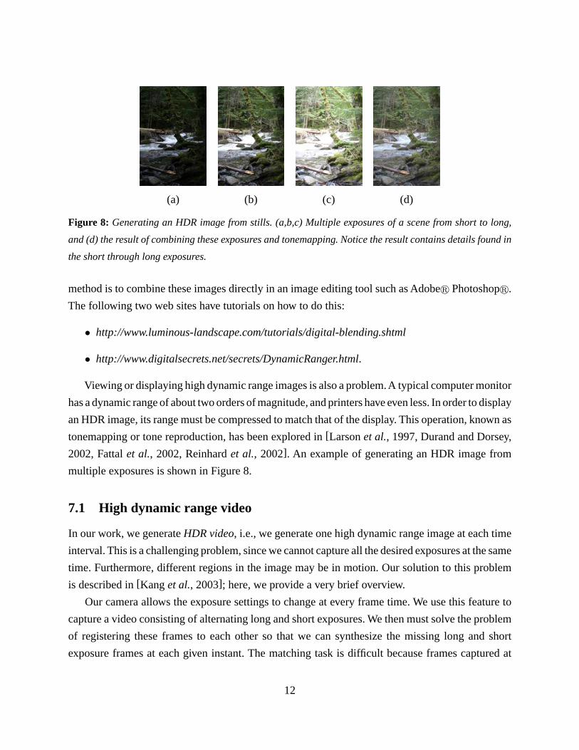
(a) (b) (c)

Figure 7: Parallax compensation in image overlap: (a) direct feathering introduces blurring, (b) magnified

version of the region marked in (a), (c) stitching results after MPPS. Notice the much cleaner edges in (c).

6 Image stitching and parallax compensation

Since the camera centers of our omnidirectional capture system are not coincident, the amount of

observed parallax can be significant in the image overlap regions, especially when portions of the

scene are close by. Under such conditions, using simple feathering (blending) to produce a stitched

omnidirectional image is not acceptable, as can be seen in Figure 7a,b.

To handle this problem, we adapted a stereo matching process to recover a multi-perspective

image [Rademacher and Bishop, 1998] in the overlap region, where each column in the overlap

region is matched using a slightly different virtual viewpoint. This idea is shown in Figure 6, where

each black rectangle represents a pixel column within the overlap region formed between images

10

I1 and I2. Each intermediate viewpoint (in black) covers a pixel column.

For a given intermediate viewpoint, stereo is applied to find the most photoconsistent appearance

given the two input images I1 and I2. This is accomplished by searching along a set of predetermined

depths (i.e., plane sweeping) and finding the minimum difference between projected local colors

from the input images at those depths.

We used the shiftable window technique [Kang et al., 2001] in our stereo algorithm to handle

occlusions in the overlap region. The size of the search window is 3 × 3. For a given hypothesized

depth at a pixel in the overlap region, the corresponding windows in the two input images are

first located. The match error is computed as sum-of-squared-differences (SSD) between these

windows. For a given depth, shifted versions of the corresponding windows that contain the central

pixel of interest are used in the computation. The most photoconsistent depth is the depth whose

shifted window pair produces the smallest matching error. Note that this operation is performed on

a per-pixel basis along each column. As a result, the final computed depths can vary along each

column.

Because these viewpoints vary smoothly between the two original camera viewpoints (C1 and C2

in Figure 6), abrupt visual discontinuities are eliminated in the stitched image. We call this technique

Multi-Perspective Plane Sweep, or MPPS for short. The results of applying this technique are shown

in Figure 7c. Details of MPPS can be found in [Kang et al., 2003].

7 High dynamic range capture and viewing

The real world contains a lot more brightness variation than can be captured by digital sensors

found in most cameras today. The radiance range of an indoor photograph can contain as many

as six orders of magnitude between the dark areas under a desk to the sunlit views seen through a

window. Typical CCD or CMOS sensors capture only two to three orders of magnitude. The effect

of this limited range is that details cannot be captured in both the dark areas and bright areas at the

same time. This problem has inspired many solutions in recent years.

One method of capturing greater dynamic range of still scenes is to shoot multiple exposures,

which appropriately capture tonal detail in dark and bright regions in turn. These images can then

be combined to create a high dynamic range (HDR) image. Automatically combining such images

requires a knowledge of the camera’s response curve as well as the camera settings used for each

exposure. See, for example, [Mann and Picard, 1995, Debevec and Malik, 1997, Mitsunaga and

Nayar, 1999] for details of techniques to create HDR images from multiple exposures. Each of

these techniques produces an HDR image with at least 16 bits per color component. An alternate

11

(a) (b) (c) (d)

Figure 8: Generating an HDR image from stills. (a,b,c) Multiple exposures of a scene from short to long,

and (d) the result of combining these exposures and tonemapping. Notice the result contains details found in

the short through long exposures.

method is to combine these images directly in an image editing tool such as Adobe� Photoshop�.

The following two web sites have tutorials on how to do this:

• http://www.luminous-landscape.com/tutorials/digital-blending.shtml

• http://www.digitalsecrets.net/secrets/DynamicRanger.html.

Viewing or displaying high dynamic range images is also a problem.A typical computer monitor

has a dynamic range of about two orders of magnitude, and printers have even less. In order to display

an HDR image, its range must be compressed to match that of the display. This operation, known as

tonemapping or tone reproduction, has been explored in [Larson et al., 1997, Durand and Dorsey,

2002, Fattal et al., 2002, Reinhard et al., 2002]. An example of generating an HDR image from

multiple exposures is shown in Figure 8.

7.1 High dynamic range video

In our work, we generate HDR video, i.e., we generate one high dynamic range image at each time

interval. This is a challenging problem, since we cannot capture all the desired exposures at the same

time. Furthermore, different regions in the image may be in motion. Our solution to this problem

is described in [Kang et al., 2003]; here, we provide a very brief overview.

Our camera allows the exposure settings to change at every frame time. We use this feature to

capture a video consisting of alternating long and short exposures. We then must solve the problem

of registering these frames to each other so that we can synthesize the missing long and short

exposure frames at each given instant. The matching task is difficult because frames captured at

12

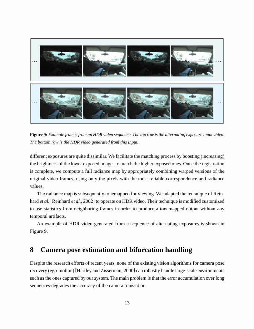
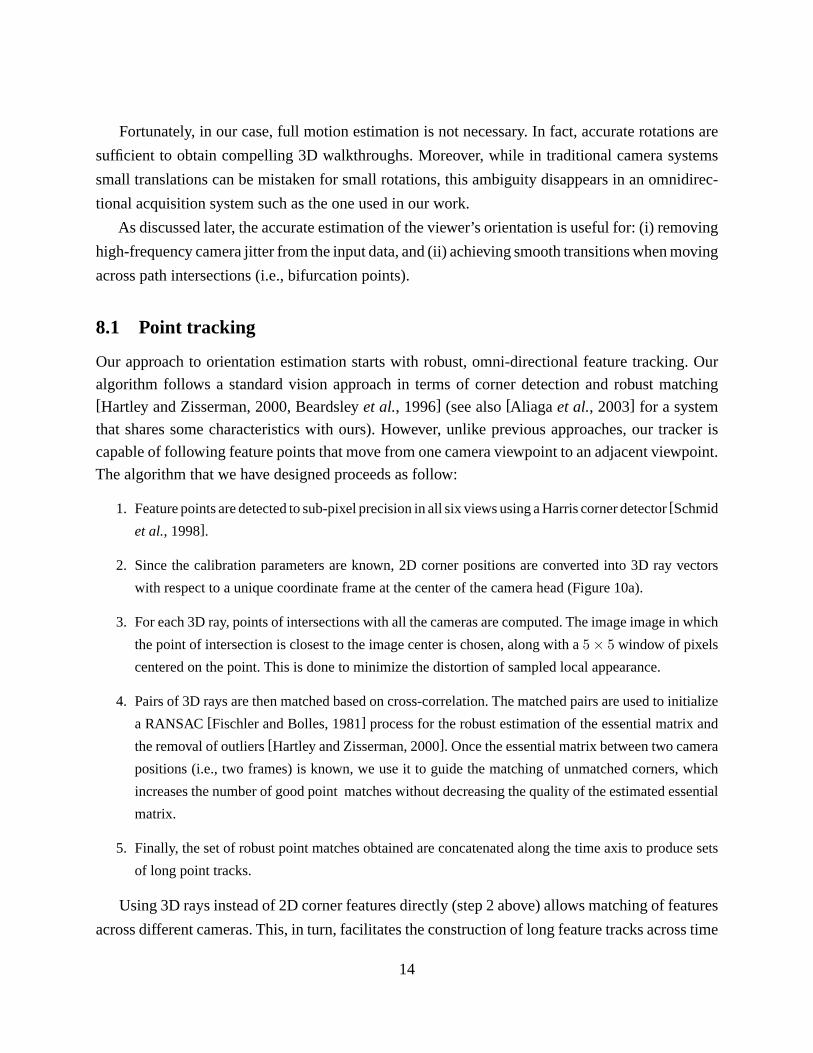
Figure 9: Example frames from an HDR video sequence. The top row is the alternating exposure input video.

The bottom row is the HDR video generated from this input.

different exposures are quite dissimilar. We facilitate the matching process by boosting (increasing)

the brightness of the lower exposed images to match the higher exposed ones. Once the registration

is complete, we compute a full radiance map by appropriately combining warped versions of the

original video frames, using only the pixels with the most reliable correspondence and radiance

values.

The radiance map is subsequently tonemapped for viewing. We adapted the technique of Rein-

hard et al. [Reinhard et al., 2002] to operate on HDR video. Their technique is modified customized

to use statistics from neighboring frames in order to produce a tonemapped output without any

temporal artifacts.

An example of HDR video generated from a sequence of alternating exposures is shown in

Figure 9.

8 Camera pose estimation and bifurcation handling

Despite the research efforts of recent years, none of the existing vision algorithms for camera pose

recovery (ego-motion) [Hartley and Zisserman, 2000] can robustly handle large-scale environments

such as the ones captured by our system. The main problem is that the error accumulation over long

sequences degrades the accuracy of the camera translation.

13

Fortunately, in our case, full motion estimation is not necessary. In fact, accurate rotations are

sufficient to obtain compelling 3D walkthroughs. Moreover, while in traditional camera systems

small translations can be mistaken for small rotations, this ambiguity disappears in an omnidirec-

tional acquisition system such as the one used in our work.

As discussed later, the accurate estimation of the viewer’s orientation is useful for: (i) removing

high-frequency camera jitter from the input data, and (ii) achieving smooth transitions when moving

across path intersections (i.e., bifurcation points).

8.1 Point tracking

Our approach to orientation estimation starts with robust, omni-directional feature tracking. Our

algorithm follows a standard vision approach in terms of corner detection and robust matching[Hartley and Zisserman, 2000, Beardsley et al., 1996] (see also [Aliaga et al., 2003] for a system

that shares some characteristics with ours). However, unlike previous approaches, our tracker is

capable of following feature points that move from one camera viewpoint to an adjacent viewpoint.

The algorithm that we have designed proceeds as follow:

1. Feature points are detected to sub-pixel precision in all six views using a Harris corner detector [Schmid

et al., 1998].

2. Since the calibration parameters are known, 2D corner positions are converted into 3D ray vectors

with respect to a unique coordinate frame at the center of the camera head (Figure 10a).

3. For each 3D ray, points of intersections with all the cameras are computed. The image image in which

the point of intersection is closest to the image center is chosen, along with a 5 × 5 window of pixels

centered on the point. This is done to minimize the distortion of sampled local appearance.

4. Pairs of 3D rays are then matched based on cross-correlation. The matched pairs are used to initialize

a RANSAC [Fischler and Bolles, 1981] process for the robust estimation of the essential matrix and

the removal of outliers [Hartley and Zisserman, 2000]. Once the essential matrix between two camera

positions (i.e., two frames) is known, we use it to guide the matching of unmatched corners, which

increases the number of good point matches without decreasing the quality of the estimated essential

matrix.

5. Finally, the set of robust point matches obtained are concatenated along the time axis to produce sets

of long point tracks.

Using 3D rays instead of 2D corner features directly (step 2 above) allows matching of features

across different cameras. This, in turn, facilitates the construction of long feature tracks across time

14

p

q

Camera center

r = r

p

q

a

ra

Camera 1

Ca

me

ra 2

(a) (b) (c)

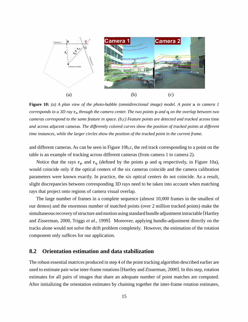
Figure 10: (a) A plan view of the photo-bubble (omnidirectional image) model. A point a in camera 1

corresponds to a 3D ray ra through the camera center. The two points p and q on the overlap between two

cameras correspond to the same feature in space. (b,c) Feature points are detected and tracked across time

and across adjacent cameras. The differently colored curves show the position of tracked points at different

time instances, while the larger circles show the position of the tracked point in the current frame.

and different cameras. As can be seen in Figure 10b,c, the red track corresponding to a point on the

table is an example of tracking across different cameras (from camera 1 to camera 2).

Notice that the rays rp and rq (defined by the points p and q respectively, in Figure 10a),

would coincide only if the optical centers of the six cameras coincide and the camera calibration

parameters were known exactly. In practice, the six optical centers do not coincide. As a result,

slight discrepancies between corresponding 3D rays need to be taken into account when matching

rays that project onto regions of camera visual overlap.

The large number of frames in a complete sequence (almost 10,000 frames in the smallest of

our demos) and the enormous number of matched points (over 2 million tracked points) make the

simultaneous recovery of structure and motion using standard bundle adjustment intractable [Hartley

and Zisserman, 2000, Triggs et al., 1999]. Moreover, applying bundle-adjustment directly on the

tracks alone would not solve the drift problem completely. However, the estimation of the rotation

component only suffices for our application.

8.2 Orientation estimation and data stabilization

The robust essential matrices produced in step 4 of the point tracking algorithm described earlier are

used to estimate pair-wise inter-frame rotations [Hartley and Zisserman, 2000]. In this step, rotation

estimates for all pairs of images that share an adequate number of point matches are computed.

After initializing the orientation estimates by chaining together the inter-frame rotation estimates,

15

we optimize the objective function∑

ij wijN (qiqijq−1j )2, where qi are the absolute orientation

quaternions, qij are the inter-frame rotation estimates, wij are weights based on the confidence in

each rotation estimate, and N is the norm of the vector component of the product quaternion (which

should be close to 0 when all frames are aligned). The resulting non-linear least squares problem is

solved using the standard Levenberg-Marquardt algorithm [Hartley and Zisserman, 2000].

Because of accumulated errors, rotation estimates will inevitably drift from their correct values.

We reduce this effect by: (i) correcting the drift at frames where the path self-intersects, and (ii) using

vanishing points, when possible, as constraints on the absolute orientation of each frame [Schaffal-

itzky and Zisserman, 2000, Antone and Teller, 2002].

The estimated absolute orientations are used to reduce the jitter introduced at acquisition time.

This is achieved by applying a low-pass filter to the camera rotations to obtain a smoother trajectory

(damped stabilization) and subtracting the original orientations (using quaternion division) to obtain

per-frame correction. The stabilization can be either performed at authoring time by resampling the

omni-camera mosaics onto a new set of viewing planes (which can potentially increase compression

efficiency), or at run-time, by simply modifying the 3D viewing transformation in the viewer. We

use the latter approach in our current system, since it results in less resampling of the imagery.

We have found that, with our current setup, compensating for only the rotational component

is enough to achieve satisfactory video stabilization, although a small amount of lower-frequency

up-and-down nodding (from the walking motion) remains. (Note that translational motion cannot

be compensated for without estimating 3D scene structure.) Furthermore, we decided not to use

additional hardware components for the detection and removal of jitter (e.g. accelerometers) in order

to keep the system simpler. A related technique for stabilizing regular, monocular video sequences

may be found in [Buehler et al., 2001].

9 Compression and selective decompression

During the playback of our video tour content, it is essential for the experience to be interactive.

Image data must therefore be fetched from the storage medium and rendered rapidly. For this

reason, we need a compression scheme that minimizes disk bandwidth while allowing for fast

decompression. There are two important requirements for such a scheme. First, it must allow for

temporal random access, i.e., it must be possible to play the content forward, backward, and to

jump to arbitrary frames with minimal delay. Second, it must support spatial random access so

that sub-regions of each frame can be decompressed independently. This is important because we

have six high resolution images and transferring this whole set at high frame rates over AGP to a

16

Disk

UserInterface

Disk Control(Prefetch)

YUV Cache

Renderer

RGB Cache

Decoder

XML Data

CompressedData Cache

Cached ReferenceTiles

Cache and Data Prefetch Control

Figure 11: Block diagram of playback engine showing decoder and caching configuration.

graphics card is impossible. Our solution was to develop our own compression scheme that allows

for selective decompression of only the currently viewed region and uses caching to support optimal

performance.

When rendering the interactive tour, we set up a six-plane Direct3D environment map that

matches the camera configuration (Figure 3b) and treat the processed video streams as texture maps.

To allow for spatial random access, we divide each view into 256×256 pixel tiles and compress these

independently. This choice of tile size is based on a compromise between compression efficiency (a

large tile allows for good spatiotemporal prediction) and granularity of random access. Our codec

uses both intra (I) and inter (B) coded tiles. The inter tiles are bidirectionally predicted and are similar

to MPEG’s B-frames. These tiles get their predictions from nearby past and future intra-coded

frames, where predictions can come from anywhere in a camera view, not just from the co-located

tile.Although this breaks the independence of the tile bitstreams, it increases compression efficiency,

and, with appropriate caching of intra coded tiles, it does not significantly affect performance. Our

use of B-tiles has some similarity to [Zhang and Li, 2003].

Tiles are divided into 16×16 macroblocks. For I-tiles, we use DCT coding with spatial prediction

ofAC and DC coefficients in a manner similar to MPEG-4. B-macroblocks can be forward, backward

or bidirectionally predicted. There are also two “skipped” modes which indicate that either the

forward or backward co-located macroblock is to be copied without requiring the transmission of

any motion vector or DCT information. Additionally, forward and backward motion vectors are

independently spatially predicted.

Our caching strategy (Figure 11) minimizes the amount of repeated decompression necessary

during typical viewing. Tiles are only decoded for the current viewpoint and are cached in case the

user is panning around. In additionYUV tiles from reference (intra) frames are cached because they

are repeatedly used during the decoding of consecutive predicted frames. When a B-tile is decoded,

17

30

32

34

36

38

40

42

44

0 100 200 300

Compression Ratio

SNR

(dB

) Intra only

1 B frame

2 B frames

3 B frames

JPEG

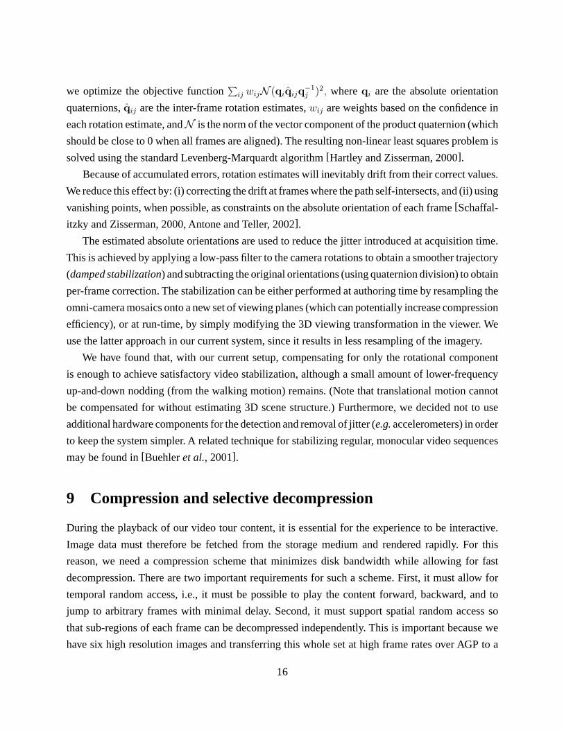
Figure 12: Rate-distortion curves comparing our codec with JPEG compression. We used a 500 frame home-

tour sequence and varied the number of B-frames between each I-frame. Compression ratio is the ratio of

the total bitstream size to the total number of bits in the sequence when using the uncompressed RGB format.

the decompressor determines which I-tiles are needed for motion compensation and requests these

from the cache. If they are not available, the cache may call upon the decoder to decompress

additional I-tiles.

In addition to the compression scheme described above, we have also implemented a tile-based

method that uses JPEG compression with no temporal prediction. This has a greater decoding speed

but a much lower compression efficiency than our new scheme. The rate-distortion curves for our

codec are plotted in Figure 12, showing the signal to noise ratio against the compression factor.

The JPEG compressed sequence has the worst performance as indicated by the fact that its curve is

lowest on the graph. Our intra codec performs quite well, but its performance is improved by adding

predicted B-frames, with two Bs for every intra frame being about optimal for this sequence. Using

bidirectional coding, we are able to obtain compression ratios of 60:1 with high visual quality.

With regard to performance, we are working to optimize our decoder so that the system can reach

a rate of thirty 768 × 1024 frames per second to support the required smoothness of interactivity.

Currently we maintain about ten frames per second with our new codec but can achieve the 30

fps target with the less space efficient JPEG compression. Since our codec enables playback from

media with lower data bandwidths, we are investigating the possibility of playing back our datasets

from standard DVD media.

18

(a) (b)

(c) (d)

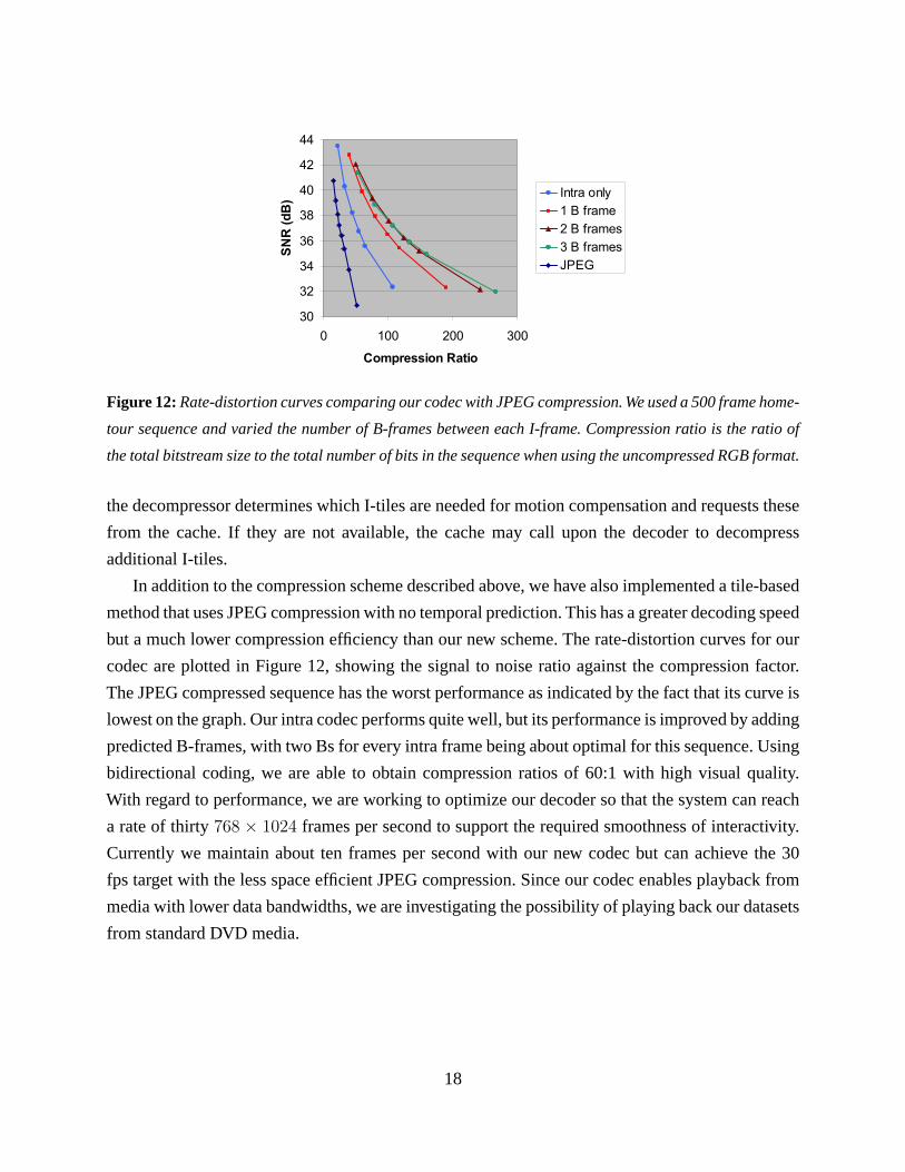
Figure 13: The use of maps to enhance the navigation experience: (a) Map of the botanical garden in Bellevue

(one of the demos shown in the results section). (b) The approximate camera path has been drawn in red.

(c) Some key frame numbers mapped to positions on the path. (d) Some audio sources captured in situ have

been placed on the map. The current viewer position and orientation is marked in green.

10 Multimedia experience authoring

In this section, we describe how the final walkthroughs are enhanced by adding multi-media elements

using simple semi-automatic authoring tools.

10.1 Bifurcation selection and map control

Whenever maps of the visited site are available, we incorporate them into our viewer to enhance

the user experience. For instance, to help the user navigate the space being visited, we display the

current location and orientation on a map (Figure 13).

19

fa

fa’ fb

fb’fi , fi’

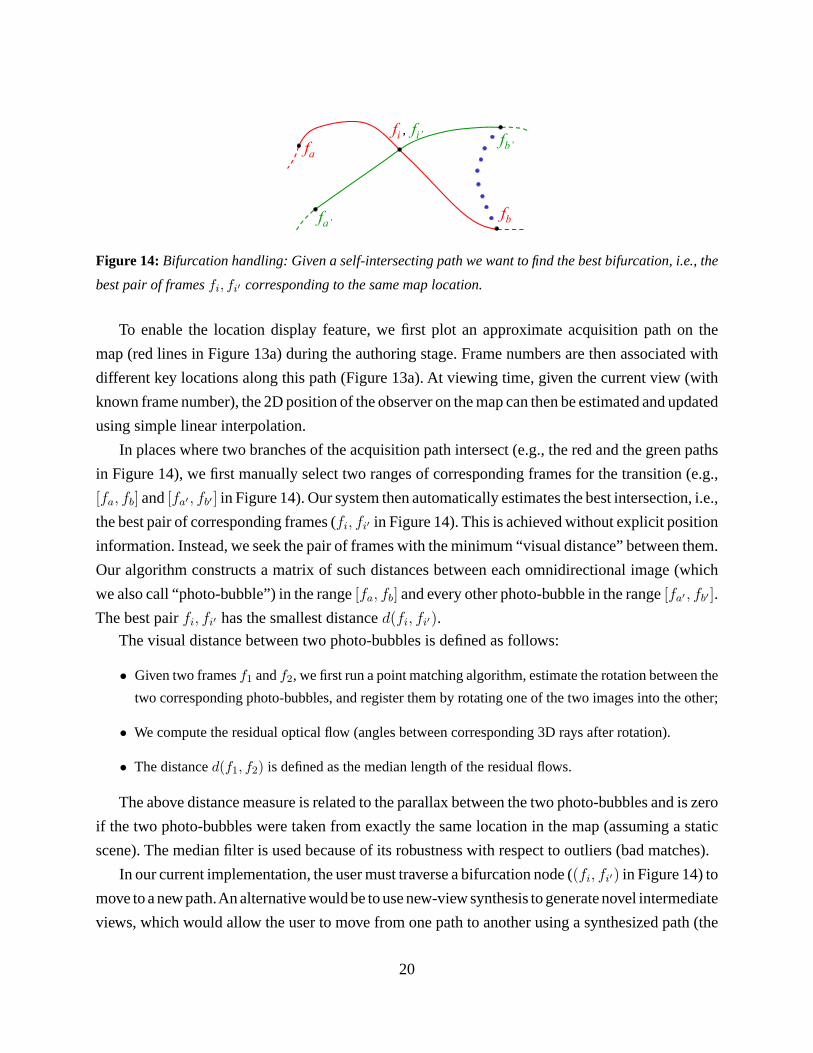
Figure 14: Bifurcation handling: Given a self-intersecting path we want to find the best bifurcation, i.e., the

best pair of frames fi, fi′ corresponding to the same map location.

To enable the location display feature, we first plot an approximate acquisition path on the

map (red lines in Figure 13a) during the authoring stage. Frame numbers are then associated with

different key locations along this path (Figure 13a). At viewing time, given the current view (with

known frame number), the 2D position of the observer on the map can then be estimated and updated

using simple linear interpolation.

In places where two branches of the acquisition path intersect (e.g., the red and the green paths

in Figure 14), we first manually select two ranges of corresponding frames for the transition (e.g.,

[fa, fb] and [fa′ , fb′ ] in Figure 14). Our system then automatically estimates the best intersection, i.e.,

the best pair of corresponding frames (fi, fi′ in Figure 14). This is achieved without explicit position

information. Instead, we seek the pair of frames with the minimum “visual distance” between them.

Our algorithm constructs a matrix of such distances between each omnidirectional image (which

we also call “photo-bubble”) in the range [fa, fb] and every other photo-bubble in the range [fa′ , fb′ ].The best pair fi, fi′ has the smallest distance d(fi, fi′).

The visual distance between two photo-bubbles is defined as follows:

• Given two frames f1 and f2, we first run a point matching algorithm, estimate the rotation between the

two corresponding photo-bubbles, and register them by rotating one of the two images into the other;

• We compute the residual optical flow (angles between corresponding 3D rays after rotation).

• The distance d(f1, f2) is defined as the median length of the residual flows.

The above distance measure is related to the parallax between the two photo-bubbles and is zero

if the two photo-bubbles were taken from exactly the same location in the map (assuming a static

scene). The median filter is used because of its robustness with respect to outliers (bad matches).

In our current implementation, the user must traverse a bifurcation node ((fi, fi′) in Figure 14) to

move to a new path.An alternative would be to use new-view synthesis to generate novel intermediate

views, which would allow the user to move from one path to another using a synthesized path (the

20

(a) (b) (c) (d)

Figure 15: Augmented reality in our surround models: (a,b) Different snapshots of our surround walkthrough

showing the living room being augmented with a video-textured fireplace and the TV set showing the program

of our choice. (c) A photograph of the TV set with the blue grid attached. (d) Another snapshot of our viewer

showing a different view of the living room. Notice how the occlusion of the TV set by the left wall is correctly

handled by our technique.

dotted blue path in Figure 14) and could result in a more seamless transition. (View interpolation

could also be used to compensate for the fact that paths may not exactly intersect in 3D.) However,

because it is difficult to avoid artifacts due to occlusions and non-rigid motions such as specularities

and transparency in new view synthesis, we have not yet investigated this alternative.

10.2 Object tracking and replacement

We have found that the richness and realism of real-world environment visualizations can be greatly

enhanced using interactive and dynamic elements. To support the insertion of such elements, during

the data capture process, a planar blue grid can be placed in strategic places, e.g., in front of

a TV screen or inside a fireplace (Figure 15c). During post-processing, our tracking algorithm

automatically estimates the position of the target together with an occlusion mask, and this data is

stored along with the video (in a separate alpha channel). During visualization, this allows us to

replace the selected object with other still images, streaming video, or video-textures (for repetitive

elements such as fire or waterfalls [Schodl et al., 2000]) while dealing correctly with possible

occlusion events. For example, we can replace the paintings in a room, or change the channel and

display live video on the television set (Figures 15a-b). Note that the blue grid is only necessary if

the surface may be partially occluded in some views (Figure 15d). In easier cases, we can track and

replace regular geometric objects such as picture frames, without the need for any special targets

in the scene.

21

10.3 Audio placement and mixing

The tour can also be made richer by adding spatialized sound.

Audio data is acquired in situ with a directional microphone, cleaned up using a standard audio

editing application, and then placed on the map to achieve a desired effect (Figure 13d).At rendering

time, the audio files are attenuated based on the inverse square distance rule and mixed together by

the audio card.

This simple technique increases the realism of the whole experience by conveying the feeling

of moving closer or farther away from objects such as waterfalls, swaying trees, or pianos. In future

work, we would like to investigate the use of true acoustic modeling for more realistic auralization

[Funkhouser et al., 1999].

11 Scene specification and rendering

The final component of our system is the interactive viewing software (viewer). This component

handles user input, the graphical user interface (visual overlays) and the rendering of video data.

For each walkthrough, the authoring stage outputs a file in our XML-based scene description

language (SDL). This file contains sound positions, stabilization information, bifurcation points,

object locations, map information, and object tracking data. The SDL was developed as a flexible

way of overlaying a user interface onto the raw video data. It allows us to rapidly prototype new

user interfaces as the project evolves.

The viewer takes user input from a mouse or gamepad as shown in Figure 1. The gamepad

controls are mapped in a similar way to driving games. The left joystick allows the user to pan

left/right/up/down, while the left and right trigger button move forwards and backwards respectively

along the path.The forward direction gets swapped as the user rotates180◦ from the forward direction

of capture. This causes the user to follow the original path backwards, but since we film only static

environments, it appears to be a valid forward direction.

The rendering process is completely done on the PC’s 3D graphics hardware. As shown in

Figure 3b, the environment model is a set of six texture-mapped planes corresponding to the six

camera focal planes. The positions of these six planes are specified through the SDL. This model

works well for our particular camera geometry; for other camera designs, a sphere or parabaloid

could be specified via the SDL. The virtual camera is placed at the center of this geometry and its

rotation is controlled via the joystick.

As the user navigates the environment, the viewer computes the appropriate data to request from

22

the selective decompressor. The input video is often traversed non-sequentially. In the case of fast

motion, the stride through the input frames can be greater than one. In the case of a bifurcation, the

next frame requested can be in a totally different section of the original video. To accommodate this,

we use a two stage pipeline. During a given display time, the next frame to display is computed and

requested from disk while the viewer decompresses and renders the frame already in the compressed

cache. The system loads all the compressed bits for a given surround frame into the compressed

cache. However, only a subset of these bits actually need to be decompressed and rendered for any

given view. Based on the user’s viewing direction, the viewer intersects the view frustum with the

environment geometry and computes the appropriate subset. Once the appropriate decompressed

tiles are in the RGB cache, the visible planes are texture mapped with those tiles.

At every frame, the viewer also applies the stabilization information in the SDL file. This is

accomplished through a simple transformation of the current view matrix. This could have been

done as a pre-process and doing so might improve compression efficiency. However, deferring this

to render time, where it is a very inexpensive operation, allowed us to fine tune the stabilizer without

re-processing the entire sequence.

The SDL also specifies additional user interface elements to display. The viewer monitors the

bifurcation points and displays the appropriate overlay as a user approaches one of these. Figure 16

is a screen shot of the UI for a home tour. Notice the navigation bar at the top indicating a branch

point: navigating to the left leads to the dining room and to the right leads to the living room.

Figure 17d shows an alternative UI in which arrows are overlaid on the environment. Figure 16

also shows an information bar at the bottom of the screen. Certain segments of the environment

(“hotspots”) get tagged as containing additional information. Here, the art case is in view, so icons

are displayed on the bottom bar indicating additional information about these art pieces. Selecting

one of the icons via the gamepad pops up a high resolution still image and an audio annotation.

This user interface also contains a map, indicating the current position within the tour. The gamepad

can be used to select a different room and the user is quickly transported to this new position. The

position and style of all these elements are easily specified via the SDL.

12 Results

This section describes the interactive visual tours that we created with our system. We captured

three different environments and built interactive experiences around each of these.

23

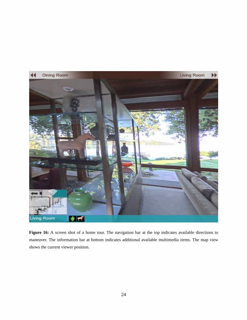
Figure 16: A screen shot of a home tour. The navigation bar at the top indicates available directions to

maneuver. The information bar at bottom indicates additional available multimedia items. The map view

shows the current viewer position.

24

(a) (b)

(c) (d)

(e) (f)

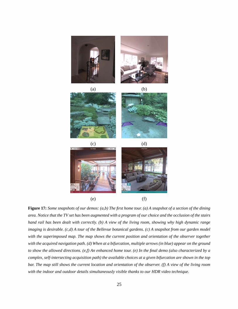
Figure 17: Some snapshots of our demos: (a,b) The first home tour. (a) A snapshot of a section of the dining

area. Notice that the TV set has been augmented with a program of our choice and the occlusion of the stairs

hand rail has been dealt with correctly. (b) A view of the living room, showing why high dynamic range

imaging is desirable. (c,d) A tour of the Bellevue botanical gardens. (c) A snapshot from our garden model

with the superimposed map. The map shows the current position and orientation of the observer together

with the acquired navigation path. (d) When at a bifurcation, multiple arrows (in blue) appear on the ground

to show the allowed directions. (e,f) An enhanced home tour. (e) In the final demo (also characterized by a

complex, self-intersecting acquisition path) the available choices at a given bifurcation are shown in the top

bar. The map still shows the current location and orientation of the observer. (f) A view of the living room

with the indoor and outdoor details simultaneously visible thanks to our HDR video technique.

25

A simple indoor environment. Our first demo was a basic home tour (Figure 17a,b). The data

was acquired along a single loop through the ground floor of the house. The final experience

contains some dynamic elements such as video playing on the TV and flames in the fireplace. To

do this, we placed blue grids in the environment at those locations. These were later tracked by our

authoring software. Once tracked, the renderer projects video onto these surfaces. Figure 15 shows

the resulting insertion. The setup process took approximately 45 minutes for path planning and

grid placement. The acquisition was done using our omnidirectional camera mounted on a rolling

tripod, as seen in Figure 4a. The entire capture process was done in one pass that took 80 seconds.

The processing time from raw data to the final compressed format took several hours.

For all demos described in this section, our interactive viewer was used to allow users to ex-

perience captured environments. The viewer was run on a 2GHz Pentium PC with an NVIDIA

GeForce2 graphics card in full-screen 1280 × 1024 mode with a horizontal field of view of about

80◦, and the compressed video data was streamed from the hard drive. Under these conditions,

we are able to maintain a rendering speed of 20 frames/sec during translation and 60 frames/sec if

rotating only. The difference in frame rates occurs because during translation, the system is fetching

frames from disk, while during rotation, the compressed frame is already in memory.

In this first demo, we observed that users did not need to arbitrarily navigate the environment

(away from the acquired path) to get a sense of the three-dimensional space. We did observe,

however, that users wanted to branch at obvious locations in the house, for example up the stairs or

down a hallway. Also, in this demo, many image areas are saturated. To enhance the realism of the

experience, we decided that high dynamic range imaging was essential.

A more complex outdoor environment. The next environment we captured was an outdoor

botanical garden (Figure 17c,d). Because of the more rugged nature of this location, we mounted

the camera on a helmet. This allowed us to navigate staircases as well as uneven paths. In this

case, we did more advanced planning and captured a large portion of the gardens. The planned path

crossed itself in several locations. At these positions, we placed small markers on the ground so that

the camera person could walk through these desired intersection points. The capture process was

again done in a single pass that took about 15 minutes. Audio data was also collected from various

locations in the garden.

Unfortunately, the helmet mount introduced much more jitter in the video. Therefore, in order

to remove much of this unwanted motion, we developed the stabilization technique described in this

paper. This increased the video processing time somewhat, which in this case took about 24 hours

unattended. There was also some manual authoring involved: video frames needed to be coarsely

26

registered to locations on the map and the position of audio sources needed to be indicated relative

to the same map (Figure 13). Another step of the authoring phase was to roughly indicate the branch

points. Our automated bifurcation selection system then computed the best branch near the user

selected point.

In order to indicate bifurcations to the user, arrows were rendered into the scene indicating the

available directions of travel (Figure 17d). Unfortunately, we found that this method of indicating

branches was somewhat confusing as the arrows were sometimes hard to find. The viewer application

also rendered a blend of distance-modulated sound sources. The addition of sound considerably

enhanced the feeling of presence in this virtual environment.

An enhanced home tour. Our final demo was a tour of a high-end home (Figure 17e,f). To capture

staircases and outside areas, we again used a head-mounted camera. The preparation time took about

45 minutes, which consisted mainly of planning the capture route and again placing small markers.

The capture was done in a single 15 minute pass.

For this tour, we also addressed the dynamic range issue by shooting with the omnidirectional

camera in HDR video mode as described in Section 7. Throughout the tour, the user can simulta-

neously see details inside and outside the home. The resulting imagery is much more pleasing than

the first demo where all the window regions were saturated.

In this tour, in order to alleviate the confusion around available branch points, we adopted a

heads up display user interface. As shown in Figure 17e, branch points are now indicated in a

separate area at the top of the display. We observed that users had an easier time navigating the

environment using this UI.

13 Discussion

Now that we have described our system in detail, let us discuss some of its advantages and disad-

vantages compared to other alternatives, as exemplified by previous work in this area.

Our system can be viewed as an extension of the idea first proposed in Andrew Lippman’s sem-

inal MovieMaps project [Lippman, 1980]. Because of the technology available at the time, viewers

of MovieMaps had to branch between a fixed number of video clips filmed in the streets of Aspen.

In our system, users have continuous control over both position and viewpoint, and the system is

lightweight and portable enough so that new content can be filmed in almost any location. Inter-

active tours based on catadioptric and multi-camera sensors similar to ours have previously been

demonstrated [Boult, 1998, Taylor, 2002]. However, the unique design of our capture and processing

27

steps makes our system the first to provide interactive video tours of sufficiently high resolution and

fidelity on a personal computer to make the experience truly compelling, i.e., to be comparable or

better than broadcast video. The capture system designed by iMove (http://www.imoveinc.com) has

a similar multi-camera design, but at a slightly lower resolution. Systems using multiple cameras

and planar reflectors, such as the one built by FullView (http://www.fullview.com) have no parallax

between the cameras, which is an advantage over our system, but result in bulkier (and hence less

portable) systems. We believe that our complete acquisition, post-processing, authoring, compres-

sion, and viewing system goes well beyond what has been demonstrated with such commercial

systems to date, especially in the areas of high dynamic range, ease of navigation, and interactivity.

Another line of research, exemplified by the work ofAliaga et al. [2001, 2002, 2003] uses a denser

sampling of viewpoints combined with new view interpolation to give the user greater freedom of

motion. While this is an advantage of their system, their approach requires fairly accurate geometric

impostors as well as beacons to locate the camera, and still sometimes leads to visible artifacts.

Moreover, the time required to scan a single room can be quite long. While our system constrains

the user to follow the original camera’s path, we believe this is a reasonable tradeoff, since a much

larger environment can be filmed (and therefore explored) in the same amount of time.

Another competing approach is to build full 3D models of the environment (see, for example

[Debevec et al., 1996, Koch et al., 2000, Coorg and Teller, 1999] and the articles in the IEEE

Computer Graphics andApplications Special Issue on 3D Reconstruction and Visualization of Large

Scale Environments, November/December 2003). The most ambitious of these efforts is Teller et

al.’s City Scanning Project at MIT (//city.lcs.mit.edu/city.html) [Teller et al., 2003], in which dozens

of buildings have been reconstructed from high-resolution, high dynamic range omnidirectional

panoramas. While these results allow the viewer to have unrestricted motion throughout the digitized

scene, they fail to capture beautiful visual effects such as reflections in windows, specularities, and

finely detailed geometry such as foliage. Our approach in this project has been to retain the best

possible visual quality, rather than trying to build more compact geometric models. In the next stage

of our project, we plan to reconstruct 3D surfaces and layered models wherever it is possible to do

so reliably and without the loss of visual fidelity, and to use these models to enable more general

movement, more sophisticated kinds of interactions, and to increase compression efficiency.

14 Conclusion

Compared to previous work in image-based visual tours, we believe that our system occupies a

unique design point, which makes it particularly suitable to delivering interactive high-quality visu-

28

alization of large real-world environments. Because our sensors combine high spatial and dynamic

range resolution (through the use of multiple exposures and temporal high dynamic range stitch-

ing), we can achieve visualization of remarkably high fidelity, while at the same time maintaining a

continuity of motion. Because we do not build 3D models or attempt to interpolate novel views by

merging pixels from different viewpoints, our rendered views are free from the artifacts that plague

geometric modeling and image-based rendering techniques whenever the geometry (or camera po-

sition) is inaccurately estimated. Our lightweight camera design makes it easy to film in locations

(such as gardens and complex architecture) that would be awkward for cart or mobile-robot based

systems. We compensate for the possible lack of smooth motion using stabilization techniques,

which also enable us to automatically jump among different video tracks without visual discontinu-

ities. To deal with the large amounts of visual data collected, we have developed novel compression

and selective decompression techniques that enable us to only decompress the information that the

user wants to see. Our flexible authoring system makes it easy to plan a tour, integrate the captured

video with map-based navigation, and add localized sounds to give a compelling sense of presence

to the interactive experience. Finally, our 3D graphics based rendering system, combined with a rich

and intuitive user interface for navigation, makes the exploration of large-scale visual environments

a practical reality on today’s personal computers.

References

[Aliaga and Carlbom, 2001] Daniel G. Aliaga and Ingrid Carlbom. Plenoptic stitching: A scalable

method for reconstructing 3D interactive walkthroughs. In Proceedings of ACM SIGGRAPH

2001, Computer Graphics Proceedings, Annual Conference Series, pages 443–450. ACM Press

/ ACM SIGGRAPH, August 2001. ISBN 1-58113-292-1.

[Aliaga et al., 1999] Daniel Aliaga et al. MMR: an interactive massive model rendering system

using geometric and image-based acceleration. In Proceedings of the 1999 symposium on Inter-

active 3D graphics, pages 199–206. ACM Press, 1999.

[Aliaga et al., 2002] D. G. Aliaga et al. Sea of images. In IEEE Visualization 2002, pages 331–338,

Boston, October 2002.

[Aliaga et al., 2003] D. G. Aliaga et al. Interactive image-based rendering using feature globaliza-

tion. In Symposium on Interactive 3D Graphics, pages 167–170, Monterey, April 2003.

29

[Antone and Teller, 2002] M. Antone and S. Teller. Scalable extrinsic calibration of omni-

directional image networks. International Journal of Computer Vision, 49(2-3):143–174,

September-October 2002.

[Baker and Nayar, 1999] S. Baker and S. Nayar. A theory of single-viewpoint catadioptric image

formation. International Journal of Computer Vision, 5(2):175–196, 1999.

[Beardsley et al., 1996] P. Beardsley, P. Torr, and A. Zisserman. 3D model acquisition from ex-

tended image sequences. In Fourth European Conference on Computer Vision (ECCV’96),

volume 2, pages 683–695, Cambridge, England, April 1996. Springer-Verlag.

[Benosman and Kang, 2001] R. Benosman and S. B. Kang, editors. Panoramic Vision: Sensors,

Theory, and Applications, New York, 2001. Springer.

[Boult, 1998] T. E. Boult. Remote reality via omni-directional imaging. In SIGGRAPH 1998

Technical Sketch, page 253, Orlando, FL, July 1998.

[Brooks, 1986] F. P. Brooks. Walkthrough - a dynamic graphics system for simulating virtual

buildings. In Workshop on Interactive 3D Graphics, pages 9–21, Chapel Hill, NC, 1986.

[Brown, 1971] D. C. Brown. Close-range camera calibration. Photogrammetric Engineering,

37(8):855–866, 1971.

[Buehler et al., 2001] C. Buehler, A. Bosse, and McMillan. Non-metric image-based rendering for

video stabilization. In Proc. CVPR, 2001.

[Chang et al., 1999] E. Chang et al. Color filter array recovery using a threshold-based variable

number of gradients. In SPIE Vol. 3650, Sensors, Cameras, and Applications for Digital Pho-

tography, pages 36–43. SPIE, March 1999.

[Chen, 1995] S. E. Chen. QuickTime VR – an image-based approach to virtual environment

navigation. Computer Graphics (SIGGRAPH’95), pages 29–38, August 1995.

[Coorg and Teller, 1999] S. Coorg and S. Teller. Extracting textured vertical facades from con-

trolled close-range imagery. In IEEE Computer Society Conference on Computer Vision and

Pattern Recognition (CVPR’99), volume 1, pages 625–632, Fort Collins, June 1999.

[Davis, 1998] J. Davis. Mosaics of scenes with moving objects. In IEEE Computer Society Confer-

ence on Computer Vision and Pattern Recognition (CVPR’98), pages 354–360, Santa Barbara,

June 1998.

[Debevec and Malik, 1997] Paul E. Debevec and Jitendra Malik. Recovering high dynamic range

radiance maps from photographs. Proceedings of SIGGRAPH 97, pages 369–378, August 1997.

ISBN 0-89791-896-7. Held in Los Angeles, California.

30

[Debevec et al., 1996] P. E. Debevec, C. J. Taylor, and J. Malik. Modeling and rendering archi-

tecture from photographs: A hybrid geometry- and image-based approach. Computer Graphics

(SIGGRAPH’96), pages 11–20, August 1996.

[Devernay and Faugeras, 1995] F. Devernay and O.D. Faugeras. Automatic calibration and removal

of distortion from scenes of structured environments. SPIE, 2567:62–72, July 1995.

[Durand and Dorsey, 2002] F. Durand and J. Dorsey. Fast bilateral filtering for the display of

high-dynamic-range images. ACM Transactions on Graphics (TOG), 21(3):257–266, 2002.

[Fattal et al., 2002] R. Fattal, D. Lischinski, and M. Werman. Gradient domain high dynamic range

compression. ACM Transactions on Graphics (TOG), 21(3):249–256, 2002.

[Fischler and Bolles, 1981] M.A. Fischler and R.C. Bolles. Random sample consensus:A paradigm

for model fitting with applications to image analysis and automated cartography. Communica-

tions of the ACM, 24(6):381–395, June 1981.

[Funkhouser et al., 1999] Thomas A. Funkhouser, Patrick Min, and Ingrid Carlbom. Real-time

acoustic modeling for distributed virtual environments. In Proceedings of SIGGRAPH 99, Com-

puter Graphics Proceedings, Annual Conference Series, pages 365–374, August 1999.

[Galyean, 1995] T. A. Galyean. Guided navigation of virtual environments. In ACM I3D’95

Symposium on Interactive 3D Graphics, pages 103–104, 1995.

[Hartley and Zisserman, 2000] R. I. Hartley and A. Zisserman. Multiple View Geometry. Cam-

bridge University Press, Cambridge, UK, September 2000.

[Ishiguro et al., 1992] H. Ishiguro, M. Yamamoto, and S. Tsuji. Omni-directional stereo. IEEE

Transactions on Pattern Analysis and Machine Intelligence, 14(2):257–262, February 1992.

[Kang et al., 2003] S. B. Kang et al. High dynamic range video. ACM Transactions on Graphics,

22(3):319–325, July 2003.

[Kang and Weiss, 2000] S. B. Kang and R. Weiss. Can we calibrate a camera using an image of a

flat, textureless Lambertian surface? In European Conference on Computer Vision (ECCV00),

volume II, pages 640–653, Dublin, Ireland, June/July 2000.

[Kang et al., 2001] S. B. Kang, R. Szeliski, and J. Chai. Handling occlusions in dense multi-view

stereo. In IEEE Computer Society Conference on Computer Vision and Pattern Recognition

(CVPR’2001), volume I, pages 103–110, Kauai, Hawaii, December 2001.

[Kang et al., 2003] S. B. Kang, R. Szeliski, and M. Uyttendaele. Seamless Stitching using Multi-

Perspective Plane Sweep. Microsoft Research Technical Report, 2003.

31

[Koch et al., 2000] R. Koch, M. Pollefeys, and L.J. Van Gool. Realistic surface reconstruction of

3d scenes from uncalibrated image sequences. Journal Visualization and Computer Animation,

11:115–127, 2000.

[Larson et al., 1997] G. W. Larson, H. Rushmeier, and C. Piatko. A visibility matching tone re-

production operator for high dynamic range scenes. IEEE Transactions on Visualization and

Computer Graphics, 3(4):291–306, 1997.

[Lippman, 1980] A. Lippman. Movie maps: An application of the optical videodisc to computer

graphics. Computer Graphics (SIGGRAPH’80), 14(3):32–43, July 1980.

[Malde, 1983] H. E. Malde. Panoramic photographs. American Scientist, 71(2):132–140, March-

April 1983.

[Mann and Picard, 1995] S. Mann and R. W. Picard. On being ‘undigital’ with digital cameras:

Extending dynamic range by combining differently exposed pictures. In IS&T’s 48th Annual

Conference, pages 422–428, Washington, D. C., May 1995. Society for Imaging Science and

Technology.

[McMillan and Bishop, 1995] L. McMillan and G. Bishop. Plenoptic modeling: An image-based

rendering system. Computer Graphics (SIGGRAPH’95), pages 39–46, August 1995.

[Milgram, 1975] D. L. Milgram. Computer methods for creating photomosaics. IEEE Transactions

on Computers, C-24(11):1113–1119, November 1975.

[Mitsunaga and Nayar, 1999] T. Mitsunaga and S. K. Nayar. Radiometric self calibration. In

IEEE Computer Society Conference on Computer Vision and Pattern Recognition (CVPR’99),

volume 1, pages 374–380, Fort Collins, June 1999.

[Rademacher and Bishop, 1998] P. Rademacher and G. Bishop. Multiple-center-of-projection im-

ages. In Computer Graphics Proceedings, Annual Conference Series, pages 199–206, Proc.

SIGGRAPH’98 (Orlando), July 1998. ACM SIGGRAPH.

[Reinhard et al., 2002] E. Reinhard et al. Photographic tone reproduction for digital images. ACM

Transactions on Graphics (TOG), 21(3):267–276, 2002.

[Sawhney and Kumar, 1999] H. S. Sawhney and R. Kumar. True multi-image alignment and its

application to mosaicing and lens distortion correction. IEEE Transactions on Pattern Analysis

and Machine Intelligence, 21(3):235–243, March 1999.

[Schaffalitzky and Zisserman, 2000] F. Schaffalitzky and A. Zisserman. Planar grouping for au-

tomatic detection of vanishing lines and points. Image and Vision Computing, 18:647–658,

2000.

32

[Schmid et al., 1998] C. Schmid, R. Mohr, and C. Bauckhage. Comparing and evaluating inter-

est points. In Sixth International Conference on Computer Vision (ICCV’98), pages 230–235,

Bombay, January 1998.

[Schodl et al., 2000] A. Schodl, R. Szeliski, D. H. Salesin, and I. Essa. Video textures. In Com-

puter Graphics (SIGGRAPH’2000) Proceedings, pages 489–498, New Orleans, July 2000.ACM

SIGGRAPH.

[Szeliski and Shum, 1997] R. Szeliski and H.-Y. Shum. Creating full view panoramic image mo-

saics and texture-mapped models. Computer Graphics (SIGGRAPH’97), pages 251–258,August

1997.

[Taylor, 2002] C. J. Taylor. Videoplus: a method for capturing the structure and appearance of im-

mersive environments. IEEE Transactions on Visualization and Computer Graphics, 8(2):171–

182, April-June 2002.

[Teller et al., 2003] S. Teller et al. Calibrated, registered images of an extended urban area. Inter-

national Journal of Computer Vision, 53(1):93–107, June 2003.

[Teller and Sequin, 1991] S. J. Teller and C. H. Sequin. Visibility preprocessing for interactive

walkthroughs. In Computer Graphics (Proceedings of SIGGRAPH 91), volume 25, pages 61–

69, Las Vegas, NV, July 1991. ISBN 0-201-56291-X.

[Triggs et al., 1999] B. Triggs et al. Bundle adjustment — a modern synthesis. In International

Workshop on Vision Algorithms, pages 298–372, Kerkyra, Greece, September 1999. Springer.

[Zhang and Li, 2003] C. Zhang and J. Li. Compression and rendering of concentric mosaics with

reference block codec (RBC). In SPIE Visual Communication and Image Processing (VCIP

2000), Perth, Australia, June 2003.

33