Journal of Multivariate Analysis 98 (2007) 852–872www.elsevier.com/locate/jmva

Hierarchical Bayes variable selection and microarrayexperiments

David J. Notta,b,∗, Zeming Yua, Eva Chanb, Chris Cotsapasb,Mark J. Cowleyb, Jeremy Pulversb, Rohan Williamsb, Peter Littleb

aDepartment of Statistics, University of New South Wales, Sydney 2052, AustraliabSchool of Biotechnology and Biomolecular Sciences, University of New South Wales, Sydney 2052, Australia

Received 12 July 2005Available online 21 November 2006

Abstract

Hierarchical and empirical Bayes approaches to inference are attractive for data arising from microarraygene expression studies because of their ability to borrow strength across genes in making inferences. Here wefocus on the simplest case where we have data from replicated two colour arrays which compare two samplesand where we wish to decide which genes are differentially expressed and obtain estimates of operating char-acteristics such as false discovery rates. The purpose of this paper is to examine the frequentist performanceof Bayesian variable selection approaches to this problem for different prior specifications and to examinethe effect on inference of commonly used empirical Bayes approximations to hierarchical Bayes procedures.The paper makes three main contributions. First, we describe how the log odds of differential expression canusually be computed analytically in the case where a double tailed exponential prior is used for gene effectsrather than a normal prior, which gives an alternative to the commonly used B-statistic for ranking genes insimple comparative experiments. The second contribution of the paper is to compare empirical Bayes pro-cedures for detecting differential expression with hierarchical Bayes methods which account for uncertaintyin prior hyperparameters to examine how much is lost in using the commonly employed empirical Bayesapproximations. Third, we describe an efficient MCMC scheme for carrying out the computations requiredfor the hierarchical Bayes procedures. Comparisons are made via simulation studies where the simulated dataare obtained by fitting models to some real microarray data sets. The results have implications for analysis ofmicroarray data using parametric hierarchical and empirical Bayes methods for more complex experimentaldesigns: generally we find that the empirical Bayes methods work well, which supports their use in the

∗ Corresponding author. Department of Statistics, University of New South Wales, Sydney 2052, Australia.Fax: +61 2 9385 7123.

E-mail address: D.Nott@unsw.edu.au (D.J. Nott).

0047-259X/$ - see front matter © 2006 Elsevier Inc. All rights reserved.doi:10.1016/j.jmva.2006.10.001

D.J. Nott et al. / Journal of Multivariate Analysis 98 (2007) 852–872 853

analysis of more complex experiments when a full hierarchical Bayes analysis would impose heavy compu-tational demands.© 2006 Elsevier Inc. All rights reserved.

AMS 2000 subject classification: 62F07; 62F15; 62P10

Keywords: Bayesian model selection; Hierarchical Bayes; Microarrays

1. Introduction

Empirical Bayes methods are attractive for inference for microarray experiments because oftheir ability to borrow strength across genes for making inferences. In this paper we considerthe simple case where we have replicated data from two colour microarrays for a comparison oftwo samples and where our interest lies in detecting differentially expressed genes and estimatingoperating characteristics such as false discovery rates. The problem here can be approachedby variable selection methods for linear models, and in this paper we consider empirical andhierarchical Bayes approaches. For the case of a constant known variance parameter an insightfuldiscussion of empirical Bayes variable selection methods for linear models was given by Georgeand Foster [9]. They consider a binomial prior for the number of active terms and a normal priorfor the coefficients of active terms and showed that for certain choices of the hyperparametersin their priors the ranking of models according to posterior probability agrees with ranking viavarious classical model selection criteria such as AIC [1], BIC [20] and RIC [8]. Estimating thehyperparameters results in a procedure able to adaptively approximate the best of these criteria.If prior hyperparameters are estimated conditional on the model, an explicit expression can begiven for the empirical Bayes criterion which is somewhat reminiscent of false discovery ratecontrolling procedures [3] in that the penalty for an additional term added decreases with thenumber of effects already discovered.

These observations suggest that empirical Bayes variable selection procedures represent apromising approach for the analysis of data from microarray experiments. For microarray data,parametric empirical Bayes model selection approaches have been considered by Baldi and Long[2], Kendziorski et al. [13], Lönnstedt and Speed [16], Newton and Kendziorski [18], Newtonet al. [19] and Smyth [21]. See also Broët et al. [4], Ibrahim et al. [11], Kauermann and Eilers [12]and Lönnstedt et al. [16]. Our approach is closest to that of Lönnstedt and Speed [17] who alsoconsidered replicated microarrays for simple comparative experiments. They consider a normalprior for effects of genes which are differentially expressed and an inverse gamma prior for genevariances. These priors allow an explicit expression for the log odds of differential expression tobe derived (the so-called B-statistic) after suitable values for the prior hyperparameters have beenobtained.

The present paper makes three main contributions. First, we consider an exponential powerprior for the effects of genes which are differentially expressed and in the special case of a doubletailed exponential prior are able to obtain an expression for the log odds of differential expres-sion similar to the B-statistic of Lönnstedt and Speed [17]. The double tailed exponential prioris more heavy tailed than the normal, which may be appropriate for many real data sets, andis related to the lasso of Tibshirani [22]. The second contribution of our paper is to compareempirical Bayes approaches to detection of differential expression with hierarchical Bayes ap-proaches which account for uncertainty in prior hyperparameters. One practical advantage of the

854 D.J. Nott et al. / Journal of Multivariate Analysis 98 (2007) 852–872

hierarchical Bayes approach over empirical Bayes approaches is that in the empirical Bayes meth-ods point estimates of hyperparameters such as the prior probability of differential expression maybe on the boundary of the parameter space, resulting in all genes having posterior probability ofdifferential expression of zero or one. Accounting for hyperparameter uncertainty in the hier-archical Bayes approach may result in more realistic inferences both in this situation and quitegenerally. Examining hierarchical Bayes procedures enables us to examine how much is lost viathe commonly used empirical Bayes approximations, which has lessons for the analysis of datafrom more complex experimental designs: it is interesting to know whether the computationaloverhead of a full hierarchical Bayes analysis is worth the effort. In general, we find that theempirical Bayes methods work well which supports their use in statistical practice. In addition,the comparison of results for different priors allows us to investigate questions of whether theresults of parametric empirical Bayes analyses are sensitive to the form of the prior. This alsohas implications for the analysis of data from more complex experiments. Our third contributionis to describe an efficient MCMC algorithm for implementing the computations required for thehierarchical Bayes approaches.

We do not consider in this paper the problem of normalization of microarray data, where sys-tematic sources of variation unrelated to genetic effects of interest are removed. For instance, it iswell known as the raw log expression ratios in microarray experiments vary with the spot intensity.Usually normalization is done prior to and independent of any assessment of significance of geneeffects which is what we do in the examples considered later. This ignores the uncertainty aboutthe normalization step in subsequent inference for gene effects. Recently there have been effortsto integrate normalization and assessments of significance: for a discussion of these approachesand of the problem of array specific intensity location and scale effects see Lewin et al. [14], Fanet al. [7] and Huang et al. [10].

The structure of the paper is as follows. In the next section we discuss empirical Bayes variableselection for microarrays and the prior specifications we consider. We also describe how to calcu-late the log odds of differential expression for a double tailed exponential prior on gene effects.In Section 3 we consider hierarchical Bayes approaches to the problem and describe our MCMCscheme for carrying out the computations required for inference in this case. In Section 4 wecompare the performance of different priors and the hierarchical and empirical Bayes proceduresin some simulation studies. Finally, Section 5 gives some discussion and conclusions.

2. Empirical Bayes variable selection for microarrays

2.1. Model and prior distributions

Let Mgj , g = 1, . . . , G, j = 1, . . . , n, be data from a replicated microarray experiment tocompare gene expression under two experimental conditions, where g indexes different genesand j indexes different arrays (replicates). For two colour microarrays the data come in the formof normalized log ratios of expression level measurements under the two conditions. We considerthe model

Mgj = �g + �gj ,

where �g is a gene specific mean and �gj ∼ N(0, �2g) where �2

g is a gene specific variance.The errors �gj are independent and if �g = 0 then gene g is not differentially expressed underthe two experimental conditions. In what follows, instead of interpreting differential expressionas meaning �g �= 0 we consider that a gene is differentially expressed if |�g| > k and not

D.J. Nott et al. / Journal of Multivariate Analysis 98 (2007) 852–872 855

differentially expressed if |�g|�k where k is some cutoff. In general, k might be chosen dependingon the purpose of the experiment and possible confounding sources of variation. It is often foundin microarray data that there are many small effects, and the genes most likely to be interestingfor further examination and experimentation are those with large effects. Hence our frameworkconsiders differential expression defined in this way, where of course we can set k = 0 if the sizeof the effect is not considered informative about which genes are of greatest biological interest.

We consider various priors on �g and �2g for doing Bayesian inference and our main interest

lies in the means �g . We summarize information about �g through the quantity

B(k) = logPr(|�g| > k|M)

Pr(|�g|�k|M), (1)

where we have written Pr(A|M) for the posterior probability of event A given the data M andk is the cutoff parameter described above. Lönnstedt and Speed [17] considered k = 0 and aprior on �g which allows �g to be exactly zero. For their prior on �g and a certain prior on �2

g

they were able to calculate B(0) explicitly, which they called the B-statistic. The B-statistic hasbeen generalized by Smyth [21] to a linear models framework. Both Lönnstedt and Speed [16]and Smyth [21] suggest that the B-statistic is of more interest as a way of ranking genes ratherthan for formal inferences. The attractiveness of Bayesian methods for ranking or inference liesin the ability to borrow strength across genes through the use of hierarchical priors on gene levelparameters.

The purpose of this paper is to compare the performance of hierarchical and empirical Bayesprocedures for detecting differential expression for different prior specifications on �g . We arealso interested in model based estimates of false discovery rates or other operating character-istics following a so-called direct posterior probability approach to inference [19]. Suppose wehave declared a certain set D ⊂ {1, . . . , G} of the genes as differentially expressed (by gene gbeing differentially expressed we mean |�g|�k). The posterior expected number of genes notdifferentially expressed among those declared differentially expressed is∑

g∈D

Pr(|�g|�k|M)

and dividing this by #D (where #A denotes the size of set A) gives a model based estimate of thefalse discovery rate.

Following the prior specification used in Smyth [21], we consider a prior specification on thegene variances �2

g which is inverse gamma,

�2g ∼ IG

(n0

2,n0s

20

2

),

where n0 and s20 are hyperparameters. The prior above can be thought of as information on �2

g ofa prior estimate s2

0 on n0 degrees of freedom. It remains to specify a prior on the means �g . Wehave p = Pr(�g �= 0) and given that �g �= 0, �g has an exponential power prior

p(�g|�2g, �g �= 0) = 1

2(2c�2g)

1b �(1 + 1

b

) exp

(−|�g|b

2c�2g

),

where b and c are hyperparameters. Setting b = 2 gives a normal prior (similar to [17,21]) andsetting b = 1 gives a double tailed exponential prior. Note that there is a certain dependence

856 D.J. Nott et al. / Journal of Multivariate Analysis 98 (2007) 852–872

between �g and �2g in the prior here. In some cases having the scale of the prior on �g dependent

on �2g may be natural (for instance, if prior information about �g were somehow based on a fixed

number of past observations) but the form of prior adopted here is primarily chosen for analyticalconvenience.

2.2. Log odds of differential expression

To evaluate (1), observe that

Pr(|�g| > k|M) = Pr(|�g| > k, �g �= 0|M)

= Pr(�g �= 0|M)Pr(|�g| > k|M, �g �= 0) (2)

and of course Pr(|�g|�k|M) = 1 − Pr(|�g| > k|M). We find an expression for Pr(�g �= 0|M)

and for the posterior distribution of �g given �g �= 0 which allows (2) to be calculated.We write Mg = (Mg1, . . . , Mgng )

T for the data for gene g. We allow the number of observationsto vary for each gene to allow for missing data. Now,

Pr(�g �= 0|M) = Pr(�g �= 0|Mg)

= p p(Mg|�g �= 0)

p p(Mg|�g �= 0) + (1 − p) p(Mg|�g = 0),

where p(Mg|�g �= 0) is the marginal likelihood of Mg given �g �= 0 and p(Mg|�g = 0) is themarginal likelihood of Mg given �g = 0. For convenience we have suppressed dependence onthe prior hyperparameters in our notation for the marginal likelihoods. We give expressions forthe marginal likelihoods now, which are derived in the Appendix.

First,

p(Mg|�g = 0) =�− ng

2 (n0s20 )

n02 �

(n0+ng

2

)�(

n02

)⎛⎝n0s

20 +

∑j

M2gj

⎞⎠− n0+ng2

.

In the case b = 2 (a normal prior for gene effects) we obtain

p(Mg|�g �= 0) =�− ng

2 (n0s20 )

n02 �

(n0+ng

2

)(cng + 1)

12 �(

n02

)⎛⎝n0s

20 +

∑j

M2gj − cng

1 + cng

ngM̄2g

⎞⎠− n0+ng2

which is the expression in Lönnstedt and Speed [17] and Smyth [21]. In the case b = 1 (a doubletailed exponential prior for gene effects) we obtain

p(Mg|�g �= 0) =∫

G(�g, 1, c, n0, s20 ) d�g

= K(1, c, n0, s20 )

∫ ⎛⎝n0s20 + |�g|

c+∑j

(Mgj − �g)2

⎞⎠− n0+ng+22

d�g,

where

K(1, c, n0, s20 ) =

�− ng2 (n0s

20 )

n02 �

(n0+ng+2

2

)2c�

(n02

) .

D.J. Nott et al. / Journal of Multivariate Analysis 98 (2007) 852–872 857

We can write the integral as I1 + I2 where

I1 =∫ ∞

0

⎛⎝n0s20 + �g

c+∑j

(Mgj − �g)2

⎞⎠− n0+ng+22

d�g

and

I2 =∫ 0

−∞

⎛⎝n0s20 − �g

c+∑j

(Mgj − �g)2

⎞⎠− n0+ng+22

d�g.

Write M̄g+ = M̄g + 1/(2cng), M̄g− = M̄g − 1/(2cng), T ∼ t�(�, �2) to denote that the randomvariable T has a t-distribution with � degrees of freedom, mean � and scale parameter �2, andB(·, ·) for the beta function. If

n0s20 +

∑j

M2gj − ngM̄

2g− > 0 and n0s

20 +

∑j

M2gj − ngM̄

2g+ > 0 (3)

we can show (see the Appendix)

I1 = n− 1

2g B

(1

2,n0 + ng + 1

2

)⎛⎝n0s20 +

∑j

M2gj − ngM̄

2g−

⎞⎠− n0+ng+12

Pr(T1 > 0),

where

T1 ∼ tn0+ng+1

(M̄g−,

n0s20 +∑

j M2gj − ngM̄

2g−

(n0 + ng + 1)ng

)and

I2 = n− 1

2g B

(1

2,n0 + ng + 1

2

)⎛⎝n0s20 +

∑j

M2gj − ngM̄

2g+

⎞⎠− n0+ng+12

Pr(T2 < 0),

where

T2 ∼ tn0+ng+1

(M̄g+,

n0s20 +∑

j M2gj − ngM̄

2g+

(n0 + ng + 1)ng

).

So if (3) holds we can explicitly write the marginal likelihood in terms of the distribution function ofcertain T random variables. While condition (3) is usually satisfied, if it does not then p(Mg|�g �=0) cannot be written in terms of distribution functions of T random variables as above, but therequired integrations can be done using some numerical integration method. Note that for thedouble exponential prior if we were to fix p = 1 (no variable selection) and if we estimate �g asthe posterior mode, then many of the estimates would still be exactly zero. In fact, the posteriormode for �g is

sign(M̄g)

(|M̄g| − 1

2cng

)+

,

858 D.J. Nott et al. / Journal of Multivariate Analysis 98 (2007) 852–872

where z+ = max(0, z) is the positive part of z and sign(M̄g) is 1 if M̄g is positive and −1otherwise. The use of the double tailed exponential prior is related to the lasso of Tibshirani [22].

So far we have described the evaluation of Pr(�g �= 0|M). We also need the posterior distri-bution of �g given �g �= 0 in order to calculate (2). When b = 2 (a normal prior) the distributionof �g|�g �= 0, M is a t-density (see the Appendix),

tn0+ng

(cng

1 + cng

M̄g,cng

1 + cng

n0s20 +∑

j M2gj − cng

1+cngngM̄

2g

ng(n0 + ng)

). (4)

So in this case we can easily calculate (2). In the case of b = 1 (the double tailed exponentialprior)

p(�g|Mg, �g �= 0) ∝�− ng

2 (n0s20 )

n02 �

(n0+ng+2

2

)2c�

(n02

)×⎛⎝n0s

20 + |�g|

c+∑j

(Mgj − �g)2

⎞⎠− n0+ng+22

.

If (3) holds, this density is a mixture of two constrained t-densities. With I1, I2, T1 and T2 definedas before, the density of �g|�g �= 0, M is the density of a random variable T where

T ={

Z1 with probability I1/(I1 + I2),

Z2 otherwise,

where Z1 = T1|T1 > 0 and Z2 = T2|T2 �0. Hence the required probability in (2) can be writtenin terms of distribution functions of certain t random variables if (3) holds, and the requiredprobability can be evaluated numerically from the above expression for the unnormalized densityotherwise. It is interesting to examine the mean and scale parameters for T1, T2 and those in thedistribution of �g|�g �= 0, M in the normal case—this shows the different kinds of shrinkageinduced by the two different priors.

2.3. Estimation of hyperparameters

In our prior distribution for the parameters (�g, �2g), g = 1, . . . , G, there are hyperparameters

(n0, s20 , p, c, b). Here we consider an empirical Bayes approach where we estimate these param-

eters from the data, with the exception of the parameter b which we fix at either b = 1 or b = 2(the double tailed exponential and normal priors, respectively, where some of the calculationscan be performed analytically). We do not estimate b since as noted by Smyth [21] estimatingmany parameters in the prior on �g|�g �= 0 may be difficult since only differentially expressedgenes contribute (perhaps only a small number) and there is an uncertainty about which genesare differentially expressed. Also, it is only in the case of b = 1 and 2 that substantial analyticsimplification is possible which allows convenient computations. For the estimation of n0 and s2

0we use the procedure outlined by Smyth [21]. Smyth [21] observes that n0 and s2

0 can be veryprecisely estimated because all genes contribute to the estimation of these parameters. The onlyremaining parameters to be estimated are p and c, which we estimate by maximum likelihood withb, n0 and s2

0 fixed. As noted above p and c can be more difficult to estimate than the parameters

D.J. Nott et al. / Journal of Multivariate Analysis 98 (2007) 852–872 859

n0 and s20 as they appear in the prior on �g for differentially expressed genes. The log marginal

likelihood here (where we suppress dependence on b, n0 and s20 in the notation) is

log p(M|p, c) =∑g

log p(Mg|p, c),

where

p(Mg|p, c) = (1 − p) p(Mg|�g = 0) + p p(Mg|�g �= 0).

Calculation of the marginal likelihoods in this expression was discussed in Section 2.2. Thechoice between b = 1 and 2 in applications can also be based on maximized marginal likelihoods(this is equivalent to the use of BIC applied with the marginal likelihood integrating out randomeffects, since the number of parameters is the same in the two models). It is often found that pointestimates of p can be on the boundary (that is, 0 or 1) which can result in the posterior probabilitiesof differential expression for all genes being zero or one. In empirical Bayes variable selection forlinear models George and Foster [9] observe a similar phenomenon and note that since mixturepriors like the one considered here do both variable selection (through the parameter p) andshrinkage (through the parameter c) then when there are many small effects the model mayeffectively give up on doing model selection and attempt to obtain good estimates of the means�g purely by doing shrinkage instead. The instability of estimation of p and c caused Lönnstedtand Speed [16] to abandon the idea of estimating both these parameters. Instead, they fix p andobserve that the value of p does not change the ranking of genes according to B(0) for fixed valuesof the other hyperparameters. In general, it is inadvisable to interpret the parameter p as being theproportion of genes differentially expressed. Rather, we should think of the prior on the �g’s witha point mass at zero as being a convenient and parsimonious approximation to a more continuousmixture prior with a low variance and high variance component. The problems associated withobtaining point estimates and ignoring uncertainty about prior hyperparameters by “plugging in”are avoided in the hierarchical Bayes approaches discussed next, where we consider posteriorprobabilities of differential expression obtained by averaging over the posterior distribution on pand c.

3. Hierarchical Bayesian procedures

In this section we extend the analysis of Section 2 to the consideration of hierarchical Bayesprocedures which attempt to account for uncertainty in the hyperparameters p and c. We estimateor fix n0, s2

0 and b in the same way as in Section 2 (as noted there, n0 and s20 can be very precisely

estimated so there is not too much loss in ignoring uncertainty about these parameters). In ourhierarchical Bayes approach we specify priors on p and c as follows. For p, we use a uniformprior on the range [0, 1]. For c, we use a uniform prior on the range [0.01, 100]. To get someintuition for this choice observe that for the case of a normal prior b = 2, the prior on �g|�g �= 0can be considered equivalent to the information obtained from observing 1/c observations at 0 sothat our hyperprior on c allows priors on �g varying from fairly noninformative to informative.It only remains to describe our computational approach for calculating (1) taking into accountour uncertainty about p and c. We use Markov chain Monte Carlo (MCMC) methods for thecalculation of the posterior probability Pr(|�g| > k|M) and the odds (1). For an introduction toMCMC methods see Liu [15].

860 D.J. Nott et al. / Journal of Multivariate Analysis 98 (2007) 852–872

Our sampling scheme generates dependent samples from the joint posterior distribution for pand c with all other parameters integrated out. We construct a Markov chain

C ={(p(j), c(j)), j �1

}which has the posterior distribution p(p, c|M) as its stationary distribution. Then after choosingsome initial values (p(1), c(1)) arbitrarily and simulating the chain C for a long time (B + S

iterations say) and discarding the first B iterations as a “burn in” sequence not typical of thestationary distribution then we obtain an approximate dependent sample from the posterior. Wecan estimate Pr(|�g| > k|M) by

1

S

B+S∑j=B+1

Pr(|�g| > k|M, p(j), c(j)).

Calculation of Pr(|�g| > k|M, p(j), c(j)) proceeds as for the empirical Bayes approaches ofSection 2 fixing (p, c) at (p(j), c(j)). Our MCMC sampling scheme is described below.

At step j for the chain C we generate (p(j+1), c(j+1)) from (p(j), c(j)) as follows.

1. Generate a proposal value (p∗, c∗) for (p(j+1), c(j+1)) from a proposal distribution q(p, c, |p(j), c(j)) (discussed further below).

2. Accept (p(j+1), c(j+1)) = (p∗, c∗) with probability min {1, �}, where

� = p(M|p∗, c∗)p(M|p(j), c(j))

q(p(j), c(j)|p∗, c∗)q(p∗, c∗|p(j), c(j))

I (p∗ ∈ [0, 1], c∗ ∈ [0.01, 100]).

Otherwise, (p(j+1), c(j+1)) = (p(j), c(j)).

To complete the specification of our sampling scheme we need to describe the proposal distributionin the above algorithm. For q(p, c|p(j), c(j)) we simply use a random walk proposal, a uniformdistribution on a rectangle centered at (p(j), c(j)), [p(j) − hp, p(j) + hp] × [c(j) − hc, c

(j) + hc]where in the examples later we set hp = hc = 0.05. In the simulation studies discussed nextit was observed that the posterior mean estimates of the parameters p and c obtained from theMCMC iterates were generally similar to the marginal maximum likelihood estimates employedin our empirical Bayes approach.

4. Simulation studies

We compare the performance of the procedures of Sections 2 and 3 in simulation studies.Four procedures are compared: the empirical Bayes procedures with normal or double tailedexponential priors and the hierarchical Bayes procedure with normal or double tailed exponentialpriors. We have taken two real data sets and estimated hyperparameters for both priors followingthe empirical Bayes methodology of Section 2. Then 50 simulated data sets were generated foreach of the two sets of hyperparameters where �g and �2

g are simulated from the prior and allvariable selection procedures are applied.

We consider the statistic B(k) for k = log 1.25, log 1.5, log 2. For each method and a givencutoff k, a gene is called differentially expressed if B(k) > 0 (that is, if Pr(|�g| > k|M) > 0.5).The threshold on the posterior probability of 0.5 is appropriate if false positive and false negativeresults are equally serious, but a different threshold can be used if this is not the case. For each

D.J. Nott et al. / Journal of Multivariate Analysis 98 (2007) 852–872 861

method we calculate the false discovery rate (FDR) which is the proportion of genes wronglydeclared differentially expressed, defined to be zero if no genes are declared differentially ex-pressed. We also calculate a model based estimate of the false discovery rate (F̂DR) as described inSection 2.1 as the posterior expected proportion of genes not differentially expressed among thosedeclared differentially expressed. Similarly, we calculate the false negative rate (FNR) which isthe proportion of genes which are differentially expressed among those which are not declareddifferentially expressed, defined to be zero if all genes are declared differentially expressed. Wecan also calculate a model based estimate of the false negative rate (F̂NR) for each method asthe posterior expected proportion of genes differentially expressed among those not declared dif-ferentially expressed. We also report the number actually differentially expressed at each cutoff(NDE), the number wrongly declared differentially expressed or number of false positives (NFP)and the number wrongly declared not differentially expressed or false negatives (NFN). Valuesreported in the tables for FDR, FDR–F̂DR, FNR, FNR–F̂NR and NDE are average values, av-eraging over the replicates in the simulation study for each case. The values NFP and NFN arederived as NFP=NDE×FDR and NFN = (G-NDE) × FNR, respectively. We stress once morethat our definitions of differential expression, of a false discovery and of a false negative dependon k so that it is very natural and expected that NDE, FDR and FNR will vary a lot betweendifferent k. Also, when comparing FDRs for the different priors, it must also be kept in mind thatthe FDRs are for different numbers of genes declared differentially expressed. In the results forthe hierarchical analyses below we took 1000 sampling iterations and 200 burn in iterations inthe MCMC scheme (s = 1000, b = 200). A lengthy burn in and sampling period is not requiredhere since we are sampling p and c with all other parameters integrated out analytically and wecan start the chains at the empirical Bayes estimates for p and c.

4.1. Swirl zebrafish data

The first real data set we consider concerns an experiment carried out using zebrafish as a modelorganism to study the early development in vertebrates. See Smyth [21] for a brief description ofthe data, which is available in the marrayInput package in R [6]. Swirl is a point mutant in theBMP2 gene that affects the dorsal/ventral body axis. The experiment compared the swirl mutantto wild type zebrafish in a four array experiment with two dye swap pairs. There were 8448 spotson each array including 768 control spots. Normalization was done as described in Smyth [21].Results are shown in Tables 1 and 2. Table 1 relates to simulations done from the normal prior(with c = 0.49, p = 0.81, the estimates obtained from the real data), and Table 2 to simulationsdone from the double exponential prior (with c = 0.82, p = 1.0, also obtained by fitting to thereal data). We note here that the maximized log marginal likelihood values indicate strong supportfor the normal prior (b = 2) as providing a better fit to the real data here. We obtain a maximizedmarginal log likelihood of −6982.7 for the normal prior and of −7154.7 for the double tailedexponential prior.

Looking first at Table 1, we note first that the empirical Bayes and hierarchical Bayes analysesare extremely similar. The FDR and FNR are similar for both priors at low thresholds. Also,model based estimates of false discovery rates perform well for both priors at the lowest threshold(k = log 1.25). The FDR rises as k increases which does not seem intuitive until one remembersthat the definition of differential expression is |�g|�k not �g �= 0 here. At high thresholds, themodel based estimate of the FDR performs well for the normal prior (which was the prior usedin simulating the data) but not for the alternative prior. This is sensible since the priors will differmost in the way they do shrinkage for larger effects. We also note that when using the normal

862 D.J. Nott et al. / Journal of Multivariate Analysis 98 (2007) 852–872

Table 1FDR, FDR–F̂DR, FNR, FNR–F̂NR, NFP, NFN and NDE for simulations based on fitted model with normal prior to swirlzebrafish data

EBN EBD HBN HBD

k = log 1.25 FDR 0.2832 0.2740 0.2826 0.2732NDE = 1648.6 (0.0026) (0.0027) (0.0026) (0.0027)

FDR–F̂DR −0.0061 0.0108 −0.0084 0.0099(0.0028) (0.0026) (0.0028) (0.0026)

FNR 0.1076 0.1116 0.1077 0.1117(0.0005) (0.0005) (0.0052) (0.0158)

FNR–F̂NR 0.0008 0.0210 −0.0021 0.0212(0.0005) (0.0005) (0.0007) (0.0005)

NFP,NFN 466.9,453.0 453.0,758.8 465.9,732.3 450.4,759.5

k = log 1.5 FDR 0.3053 0.3877 0.3039 0.3887NDE = 369.2 (0.0061) (0.0041) (0.0063) (0.0042)

FDR–F̂DR 0.0021 0.1245 −0.0001 0.1257(0.0061) (0.0040) (0.0063) (0.0040)

FNR 0.0277 0.0235 0.0278 0.0235(0.0003) (0.0003) (0.0003) (0.0033)

FNR–F̂NR 0.0002 −0.0072 −0.0005 −0.0072(0.0003) (0.0002) (0.0003) (0.0003)

NFP,NFN 112.7,223.8 143.1,189.9 112.2,224.6 143.5,189.9

k = log 2.0 FDR 0.3155 0.5028 0.3159 0.5024NDE = 63.5 (0.0132) (0.0099) (0.0133) (0.0099)

FDR–F̂DR 0.0002 0.2445 −0.0008 0.2440(0.0134) (0.0093) (0.0134) (0.0094)

FNR 0.0046 0.0031 0.0046 0.0031(0.0001) (0.0001) (0.0001) (0.0004)

FNR–F̂NR 0.0000 −0.0042 0.0000 −0.0042(0.0001) (0.0001) (0.0001) (0.0001)

NFP,NFN 20.0,38.6 31.9,26.0 20.1,38.6 31.9,26.0

The methods compared for the simulated data sets are EBN (empirical Bayes, normal prior), EBD (empirical Bayes,double exponential prior), HBN (hierarchical Bayes, normal prior) and HBD (hierarchical Bayes, double exponentialprior). Standard errors are shown in brackets.

prior more genes are declared differentially expressed at lower levels than for the double tailedexponential prior, whereas at high levels the situation is reversed. Again this is due to the differentways that the priors do shrinkage. Looking at Table 2, the conclusions are substantially similar,with the prior used in simulating the data (in this case the double exponential prior) performingbetter with respect to model based estimates of false discovery rates at high levels.

4.2. Inbred mice data

Our second example concerns an experiment to detect differential expression in brain tissuebetween two inbred strains of mice (C57BL/6J and DBA/2J). In this experiment we have 10 arrayscomparing expression in the two strains with 21764 spots on each array (after removal of controlspots). The experiment was part of a series of experiments to investigate the genetic control ofgene transcription [5]. We comment on an empirical Bayes analysis of the real data first before

D.J. Nott et al. / Journal of Multivariate Analysis 98 (2007) 852–872 863

Table 2FDR, FDR–F̂DR, FNR, FNR–F̂NR, NFP, NFN and NDE for simulations based on fitted model with double tailedexponential prior to swirl zebrafish data

EBN EBD HBN HBD

k = log 1.25 FDR 0.2572 0.2056 0.2558 0.2054NDE = 1261.1 (0.0023) (0.0024) (0.0023) (0.0023)

FDR–F̂DR 0.0499 0.0014 0.0476 0.0006(0.0021) (0.0021) (0.0021) (0.0021)

FNR 0.0795 0.0798 0.0796 0.0799(0.0005) (0.0004) (0.0005) (0.0004)

FNR–F̂NR 0.0069 0.0006 0.0058 0.0012(0.0007) (0.0004) (0.0008) (0.0004)

NFP,NFN 324.4,571.4 259.3,573.5 322.6,572.1 259.0,574.2

k = log 1.5 FDR 0.2404 0.1853 0.2400 0.1872NDE = 543.2 (0.0029) (0.0026) (0.0029) (0.0025)

FDR–F̂DR 0.0537 0.0059 0.0522 0.0049(0.0030) (0.0024) (0.0030) (0.0023)

FNR 0.0251 0.0274 0.0251 0.0271(0.0024) (0.0003) (0.0002) (0.0002)

FNR–F̂NR −0.0015 0.0000 −0.0021 −0.0001(0.0003) (0.0002) (0.0003) (0.0002)

NFP,NFN 112.7,223.8 143.1,189.9 112.2,224.6 143.5,189.9

k = log 2.0 FDR 0.1698 0.1627 0.1688 0.1640NDE = 223.6 (0.0041) (0.0041) (0.0040) (0.0041)

FDR–F̂DR 0.0048 0.0191 0.0035 0.0047(0.0041) (0.0049) (0.0040) (0.0039)

FNR 0.0086 0.0088 0.0086 0.0086(0.0002) (0.0002) (0.0002) (0.0002)

FNR–F̂NR 0.0009 0.0003 0.0007 0.0001(0.0002) (0.0001) (0.0002) (0.0001)

NFP,NFN 20.0,38.6 31.9,26.0 20.0,38.6 31.9,26.0

The methods compared for the simulated data sets are EBN (empirical Bayes, normal prior), EBD (empirical Bayes,double exponential prior), HBN (hierarchical Bayes, normal prior) and HBD (hierarchical Bayes, double exponentialprior). Standard errors are given in brackets.

proceeding to simulations. Fig. 1 shows a plot of log odds of differential expression versus averageM value with k = log 1.5 for normal and double exponential priors. Again maximized marginallikelihoods strongly indicate that the normal prior (b = 2) is more appropriate for the real data.The maximized marginal log likelihood for the normal prior is −246.6 and for the double tailedexponential prior is −375.4. In Fig. 1 for the normal prior there are 430 genes differentiallyexpressed (log odds of differential expression greater than zero). At k = log 1.25, on the otherhand, 2266 genes are declared differentially expressed which is biologically implausible. Forthe double exponential prior, there are 2261 and 541 genes differentially expressed at k valuesof log 1.25 and log 1.5, respectively. The large number of genes differentially expressed at k =log 1.25 occurs because of the estimated values of p of 0.85 and 1.0, respectively for the normaland double exponential priors. Although the data here have been normalized to remove put downtime, intensity and print tip effects, it is well known that array specific effects can interact with

864 D.J. Nott et al. / Journal of Multivariate Analysis 98 (2007) 852–872

-4 -3 -2 -1 0 1 2

-20

-15

-10

-5

0

5

10

15

Average M value

Log o

dds

-4 -3 -2 -1 0 1 2

-20

-10

0

10

20

Average M value

Log o

dds

Fig. 1. Plot of log odds of differential expression versus average M value for cutoff k = log 1.5 for normal prior (top) anddouble exponential prior (bottom).

gene effects and it is very difficult to completely adjust for this in normalization. In this example,there is evidence of a large number of small effects so that concentrating on genes with largeeffects is sensible if the interesting variation of genetic origin is thought to be large comparedto the variation of non-genetic origin remaining after normalization. The choice of k = log 1.5was based on prior expert opinion about the level of array specific variation of a non geneticorigin.

D.J. Nott et al. / Journal of Multivariate Analysis 98 (2007) 852–872 865

Table 3FDR, FDR–F̂DR, FNR, FNR–F̂NR, NFP, NFN and NDE for simulations based on fitted model with normal prior to inbredmice data

EBN EBD HBN HBD

k = log 1.25 FDR 0.2209 0.2194 0.2210 0.2194NDE = 3407.4 (0.0012) (0.0012) (0.0013) (0.0012)

FDR–F̂DR −0.0004 0.0077 −0.0003 0.0078(0.0014) (0.0013) (0.0014) (0.0013)

FNR 0.0573 0.0576 0.0573 0.0576(0.0002) (0.0002) (0.0002) (0.0002)

FNR–F̂NR 0.0001 0.0038 0.0000 0.0037(0.0002) (0.0002) (0.0002) (0.0002)

NFP,NFN 752.7,1051.9 747.6,1057.3 753.0,1051.9 747.6,1057.3

k = log 1.5 FDR 0.2560 0.3511 0.2561 0.3513NDE = 429.8 (0.0038) (0.0034) (0.0038) (0.0035)

FDR–F̂DR 0.0033 0.1192 0.0034 0.1192(0.0038) (0.0032) (0.0038) (0.0032)

FNR 0.0089 0.0069 0.0089 0.0069(0.0001) (0.0001) (0.0001) (0.0001)

FNR–F̂NR 0.0000 −0.0038 0.0000 −0.0038(0.0001) (0.0001) (0.0001) (0.0001)

NFP,NFN 110.0,189.9 150.9,147.2 110.1,189.9 151.0,147.2

k = log 2.0 FDR 0.2683 0.4903 0.2683 0.4911NDE = 18.3 (0.0190) (0.0154) (0.0190) (0.0152)

FDR–F̂DR −0.0162 0.2501 −0.0159 0.2489(0.0191) (0.0132) (0.0191) (0.0131)

FNR 0.0004 0.0003 0.0005 0.0003(0.0000) (0.0000) (0.0000) (0.0000)

FNR–F̂NR 0.0000 −0.0005 0.0000 −0.0005(0.0000) (0.0000) (0.0000) (0.0000)

NFP,NFN 4.9,8.7 9.0,6.5 4.9,10.9 9.0,6.5

The methods compared for the simulated data sets are EBN (empirical Bayes, normal prior), EBD (empirical Bayes,double exponential prior), HBN (hierarchical Bayes, normal prior) and HBD (hierarchical Bayes, double exponentialprior). Standard errors are given in brackets.

Results of our simulations are shown in Tables 3 and 4. Table 3 relates to the normal prior(with c = 0.51, p = 0.85, the estimates obtained from the real data), and Table 4 to the doubleexponential prior (with c = 1.09, p = 1.0, estimates also obtained from the real data). Looking atTable 3 first, we see that the results for different priors are substantially similar at low levels k. Athigher levels, the double exponential prior gives a higher FDR and lower FNR and the model basedestimate of the FDR performs poorly for the double exponential prior. Looking at the results whenthe data are simulated using the double exponential prior (Table 4) the conclusions are similar,with the prior used in simulating the data generally performing better. Once again there does notseem to be any great difference between the empirical and hierarchical Bayes analyses. It mightbe argued that in the two examples considered so far based on fitting to real data sets there seemsto be a large number of small effects so that with p large we can estimate the parameters p andc fairly well. Hence ignoring the uncertainty about these parameters does not result in any greatdifference between the empirical and hierarchical Bayes methods. With this in mind we consider

866 D.J. Nott et al. / Journal of Multivariate Analysis 98 (2007) 852–872

Table 4FDR, FDR–F̂DR, FNR, FNR–F̂NR, NFP, NFN and NDE for simulations based on fitted model with double tailedexponential prior to RI mice data

EBN EBD HBN HBD

k = log 1.25 FDR 0.2026 0.1623 0.2025 0.1620NDE = 2923.8 (0.0012) (0.0011) (0.0012) (0.0011)

FDR–F̂DR 0.0416 0.0020 0.0416 0.0017(0.0011) (0.0009) (0.0011) (0.0010)

FNR 0.0380 0.0442 0.0381 0.0442(0.0002) (0.0002) (0.0002) (0.0002)

FNR–F̂NR −0.0092 −0.0004 −0.0091 −0.0002(0.0002) (0.0002) (0.0002) (0.0002)

NFP,NFN 592.4,715.9 474.5,592.1 592.1,717.8 473.7,832.7

k = log 1.5 FDR 0.1432 0.1498 0.1430 0.1498NDE = 883.2 (0.0019) (0.0019) (0.0019) (0.0019)

FDR–F̂DR −0.0075 0.0021 −0.0078 0.0019(0.0018) (0.0017) (0.0018) (0.0017)

FNR 0.0111 0.0108 0.0111 0.0108(0.0001) (0.0001) (0.0001) (0.0001)

FNR–F̂NR 0.0002 −0.0002 0.0003 −0.0002(0.0001) (0.0001) (0.0001) (0.0001)

NFP,NFN 126.5,231.8 1323.3,225.5 126.3,231.8 132.3,225.5

k = log 2.0 FDR 0.0800 0.1306 0.0800 0.1305NDE = 212.8 (0.0027) (0.0033) (0.0028) (0.0033)

FDR–F̂DR −0.0605 −0.0015 −0.0605 −0.0018(0.0027) (0.0030) (0.0027) (0.0030)

FNR 0.0028 0.0021 0.0028 0.0021(0.0001) (0.0000) (0.0001) (0.0000)

FNR–F̂NR 0.0009 −0.0001 0.0009 −0.0001(0.0000) (0.0000) (0.0000) (0.0000)

NFP,NFN 17.0,60.3 27.8,45.3 17.0,60.3 27.8,45.3

The methods compared for the simulated data sets are EBN (empirical Bayes, normal prior), EBD (empirical Bayes,double exponential prior), HBN (hierarchical Bayes, normal prior) and HBD (hierarchical Bayes, double exponentialprior). Standard errors are given in brackets.

a further example where we fix p = 0.02 and estimate c for the swirl zebrafish data set for thetwo different priors and then simulate using these parameter values.

4.3. Swirl zebrafish data, p = 0.02

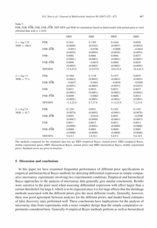
Results of simulations for the swirl zebrafish data set where we have fixed p = 0.02 are shownin Tables 5 and 6. Table 5 relates to simulations done from the normal prior (with c = 6.54, theestimate obtained from the real data), and Table 6 to simulations done from the double exponentialprior (with c = 0.82, also obtained by fitting to the real data). Conclusions of the hierarchicaland empirical Bayes analyses seem to be similar for the prior used in simulating the data for boththe cases considered, but not for the alternative prior. When there are few genes differentiallyexpressed and the prior not used in simulating the data is used then in general inference using thehierarchical approach seems to be more conservative.

D.J. Nott et al. / Journal of Multivariate Analysis 98 (2007) 852–872 867

Table 5FDR, FDR–F̂DR, FNR, FNR–F̂NR, NFP, NFN and NDE for simulations based on fitted model with normal prior to swirlzebrafish data with p = 0.02

EBN EBD HBN HBD

k = log 1.25 FDR 0.1641 0.1385 0.1660 0.0958NDE = 108.6 (0.0068) (0.0102) (0.0067) (0.0054)

FDR–F̂DR −0.0011 −0.0396 −0.0006 −0.0654(0.0059) (0.0095) (0.0059) (0.0054)

FNR 0.0066 0.0066 0.0066 0.0075(0.0001) (0.0001) (0.0001) (0.0001)

FNR–F̂NR 0.0000 −0.0019 0.0000 0.0029(0.0002) (0.0002) (0.0002) (0.0002)

NFP,NFN 17.8,55.0 15.0,55.0 18.0,55.0 10.4,62.5

k = log 1.5 FDR 0.1468 0.1128 0.1475 0.0935NDE = 77.4 (0.0062) (0.0092) (0.0063) (0.0055)

FDR–F̂DR −0.0037 −0.0461 −0.0036 −0.0580(0.0053) (0.0085) (0.0053) (0.0055)

FNR 0.0031 0.0033 0.0031 0.0037(0.0001) (0.0001) (0.0001) (0.0001)

FNR–F̂NR 0.0000 −0.0002 0.0000 0.0014(0.0001) (0.0001) (0.0001) (0.0001)

NFP,NFN 11.4,25.9 8.7,27.6 11.4,25.9 7.2,31.0

k = log 2.0 FDR 0.1356 0.0921 0.1362 0.1165NDE = 42.7 (0.0079) (0.0092) (0.0081) (0.0078)

FDR–F̂DR 0.0055 −0.0418 0.0051 −0.0500(0.0067) (0.0088) (0.0063) (0.0067)

FNR 0.0011 0.0012 0.0011 0.0013(0.0000) (0.0001) (0.0000) (0.0000)

FNR–F̂NR 0.0000 0.0001 0.0000 0.0004(0.0000) (0.0000) (0.0000) (0.0000)

NFP,NFN 5.8,9.2 3.9,10.1 5.8,9.2 5.0,10.9

The methods compared for the simulated data sets are EBN (empirical Bayes, normal prior), EBD (empirical Bayes,double exponential prior), HBN (hierarchical Bayes, normal prior) and HBD (hierarchical Bayes, double exponentialprior). Standard errors are given in brackets.

5. Discussion and conclusions

In this paper we have examined frequentist performance of different prior specifications inempirical and hierarchical Bayes methods for detecting differential expression in simple compar-ative microarray experiments involving two experimental conditions. Empirical and hierarchicalBayes approaches to the analysis of microarray data generally give similar conclusions. Resultswere sensitive to the prior used when assessing differential expression with effect larger than acertain threshold k for large k, which is to be expected since it is for large effects that the shrinkagemethods associated with the different priors give the most different results. Generally, however,there was good agreement between analyses for the different priors, and model based estimatesof false discovery rates performed well. These conclusions have implications for the analysis ofmicroarray data from experiments with a more complex design than the simple comparative ex-periments considered here. Generally if empirical Bayes methods perform as well as hierarchical

868 D.J. Nott et al. / Journal of Multivariate Analysis 98 (2007) 852–872

Table 6FDR, FDR–F̂DR, FNR, FNR–F̂NR, NFP, NFN and NDE for simulations based on fitted model with double tailedexponential prior to swirl zebrafish data with p = 0.02

EBN EBD HBN HBD

k = log 1.25 FDR 0.1878 0.2963 0.0000 0.2770NDE = 24.3 (0.0368) (0.0408) (0.0000) (0.0405)

FDR–F̂DR 0.0343 0.0671 −0.0178 0.0819(0.0288) (0.0382) (0.0011) (0.0367)

FNR 0.0029 0.0028 0.0032 0.0029(0.0001) (0.0001) (0.0001) (0.0001)

FNR–F̂NR 0.0007 −0.0010 0.0023 0.0000(0.0003) (0.0012) (0.0001) (0.0002)

NFP,NFN 4.6,24.4 7.2,23.6 0.0,27.0 6.7,24.4

k = log 1.5 FDR 0.1919 0.2807 0.0000 0.2858NDE = 10.4 (0.0369) (0.0396) (0.0000) (0.0418)

FDR–F̂DR 0.0388 0.0827 0.0000 0.0865(0.0286) (0.0351) (0.0000) (0.0384)

FNR 0.0004 0.0011 0.0013 0.0011(0.0001) (0.0001) (0.0001) (0.0001)

FNR–F̂NR 0.0002 −0.0002 0.0013 0.0001(0.0001) (0.0002) (0.0001) (0.0001)

NFP,NFN 2.0,3.4 2.9,9.3 0.0,11.0 3.0,9.3

k = log 2.0 FDR 0.1970 0.2451 0.0000 0.2387NDE = 4.1 (0.0382) (0.0398) (0.0000) (0.0413)

FDR–F̂DR 0.0566 0.0617 0.0000 0.0688(0.0283) (0.0347) (0.0000) (0.0356)

FNR 0.0004 0.0003 0.0005 0.0003(0.0000) (0.0000) (0.0000) (0.0000)

FNR–F̂NR 0.0002 0.0000 0.0005 0.0001(0.0000) (0.0001) (0.0000) (0.0000)

NFP,NFN 0.8,3.4 1.0,2.5 0.0,4.2 1.0,2.5

The methods compared for the simulated data sets are EBN (empirical Bayes, normal prior), EBD (empirical Bayes,double exponential prior), HBN (hierarchical Bayes, normal prior) and HBD (hierarchical Bayes, double exponentialprior). Standard errors are given in brackets.

Bayes methods as they do here then it may not be worth the computational overhead to implementthe more complex fully hierarchical method.

It would be possible to integrate the process of microarray normalization with as assessment ofsignificance as an extension of this work. Recent progress in this direction is described in Lewinet al. [14], Fan et al. [7] and Huang et al. [10]. However, such an approach demands a more complexmodelling in which revealing analytical expressions for the log odds of differential expressionsuch as those described in this paper are not available. The desirability of taking into accountuncertainty in normalization in subsequent inference for gene effects is undeniable, however.

We have focussed in this paper on priors for the gene specific mean parameters. However, alsoof interest would be further examination of alternative more flexible prior specifications for thegene variances �2

g as an alternative to the inverse gamma prior. One alternative prior would be aninverse gamma mixture, for which the kind of analytic calculations done in this paper could stillbe carried out. The estimation of prior hyperparameters is more complex, however. The priors

D.J. Nott et al. / Journal of Multivariate Analysis 98 (2007) 852–872 869

we have considered on the mean parameters could also be made more flexible. Some interestingrecent work in this direction is the semiparametric hierarchical mixture approach of Newton et al.[19]. However, simple parametric priors of the kind considered here may perform well and allowfor calculations to be done analytically.

Acknowledgments

This research was supported by an Australian Research Council grant. Chris Cotsapas wassupported by a School of Biotechnology and Biomolecular Sciences Genome Information Schol-arship, Rohan Williams by a National Health and Medical Research Council of Australia PeterDoherty Fellowship, and Mark Cowley and Eva Chan by Australian Postgraduate Awards.

Appendix

We derive the expressions for the marginal likelihoods given in Section 2 and the posteriordistribution for �g|�g �= 0, M . We have that

p(Mg|�g �= 0) =∫ ∫

p(Mg|�g, �2g)p(�g|�g �= 0, �2

g)p(�2g) d�2

g d�g

=∫

G(�g, b, c, n0, s20 ) d�g, (5)

where

G(�g, b, c, n0, s20 ) =

∫p(Mg|�g, �

2g)p(�g|�2

g)p(�2g) d�2

g

= K(b, c, n0, s20 )

⎛⎝n0s20 + |�g|b

c+∑j

(Mgj − �g)2

⎞⎠−(

n0+ng2 + 1

b

),(6)

where

K(b, c, n0, s20 ) =

�− ng2 (n0s

20 )

n02 �

(n0+ng

2 + 1b

)2c

1b �(1 + 1

b

)�(

n02

) .

The integral in (6) is easily done analytically here since the integrand is an unnormalized inversegamma density. A similar argument gives

p(Mg|�g = 0) =∫

p(Mg|�g = 0, �2g)p(�2

g) d�2g

=�− ng

2 (n0s20 )

n02 �

(n0+ng

2

)�(

n02

)⎛⎝n0s

20 +

∑j

M2gj

⎞⎠− n0+ng2

.

In general, the integral (5) can be done numerically in order to calculate Pr(�g �= 0|M).However, in the case where b = 2 (a normal prior) or b = 1 (a double tailed exponential prior)

870 D.J. Nott et al. / Journal of Multivariate Analysis 98 (2007) 852–872

some further analytic simplification is possible. For the normal case, we have

p(Mg|�g �= 0) =∫

G(�g, 2, c, n0, s20 ) d�g

=∫

K(2, c, n0, s20 )

⎛⎝n0s20 + �2

g

c+∑j

(Mgj − �g)2

⎞⎠− n0+ng+12

d�g,

where

K(2, c, n0, s20 ) =

�− ng2 (n0s

20 )

n02 �

(n0+ng+1

2

)√

�c�(

n02

) .

To evaluate the integral here and a similar integral for the case of the double tailed exponentialprior (b = 1) we use the following lemma.

Lemma 1. For constants f, g and h > 0 with f h > g2

∫A

(f − 2gt + ht2)−(�+1)

2 dt =(

f − g2

h

)− �2

h− 12 B

(1

2,�

2

)Pr(T ∈ A),

where B(·, ·) is the beta function and

T ∼ t�

(g

h,

1

�h

(f − g2

h

)),

where t�(�, �2) denotes the t-distribution with � degrees of freedom, mean � and scale parame-ter �2.

Proof. The proof is straightforward upon recognizing the integrand as an unnormalized t-density,

t�

(gh, 1

�h

(f − g2

h

)). �

Applying this lemma here for the b = 2 normal prior case gives

p(Mg|�g �= 0) =�− ng

2 (n0s20 )

n02 �

(n0+ng

2

)(cng + 1)

12 �(

n02

)⎛⎝n0s

20+

∑j

M2gj−

cng

1 + cng

ngM̄2g

⎞⎠− n0+ng2

,

which is the expression in Lönnstedt and Speed [13] and Smyth [21]. We can use Lemma 1 toobtain an expression for p(Mg|�g �= 0) also in the case where b = 1 (the double tailed exponentialprior). Here

p(Mg|�g �= 0) =∫

G(�g, 1, c, n0, s20 ) d�g

= K(1, c, n0, s20 )

∫ ⎛⎝n0s20 + |�g|

c+∑j

(Mgj − �g)2

⎞⎠− n0+ng+22

d�g,

D.J. Nott et al. / Journal of Multivariate Analysis 98 (2007) 852–872 871

where

K(1, c, n0, s20 ) =

�− ng2 (n0s

20 )

n02 �

(n0+ng+2

2

)2c�

(n02

) .

In the notation of Section 2 we write the integral as I1 + I2 and obtain the expressions forI1 and I2 given in Section 2 upon applying Lemma 1 if (3) holds. If (3) does not hold, thenp(Mg|�g �= 0) cannot be written in terms of distribution functions of T random variables, but therequired integrations can be done using some standard numerical integration method.

We also need the posterior distribution of �g given �g �= 0 in order to calculate (2). Note that

p(�g|Mg, �g �= 0) =∫

p(�g, �2g|Mg, �g �= 0) d�2

g

∝∫

p(�2g)p(�g|�2

g)p(Mg|�g, �2g) d�2

g

= G(�g, b, c, n0, s20 ).

When b = 2 (a normal prior) we have that G(�g, 2, c, n0, s20 ) is proportional to a t-density,

tn0+ng

(cng

1 + cng

M̄g,cng

1 + cng

n0s20 +∑

j M2gj − cng

1+cngngM̄

2g

ng(n0 + ng)

). (7)

In the case of b = 1 (the double tailed exponential prior)

p(�g|Mg, �g �= 0)

∝ G(�g, 1, c, n0, s20 )

=�− ng

2 (n0s20 )

n02 �

(n0+ng+2

2

)2c�

(n02

)⎛⎝n0s

20+|�g|

c+∑j

(Mgj−�g)2

⎞⎠− n0+ng+22

.

If (3) holds, this density is a mixture of two constrained t-densities as described in Section 2.

References

[1] H. Akaike, Information theory and an extension of the maximum likelihood principle, Second InternationalSymposium on Information Theory, 1973, pp. 267–281.

[2] P. Baldi, A.D. Long, A Bayesian framework for the analysis of microarray data: regularized t-test and statisticalinferences of gene changes, Bioinformatics 17 (2001) 509–519.

[3] Y. Benjamini,Y. Hochberg, Controlling the false discovery rate: a practical and powerful approach to multiple testing,J. Roy. Statist. Soc. B 57 (1995) 289–300.

[4] P. Broët, S. Richardson, F. Radvanyi, Bayesian hierarchical model for identifying changes in gene expression frommicroarray experiments, J. Comput. Biol. 9 (2002) 671–683.

[5] C. Cotsapas, E. Chan, M. Kirk, M. Tanaka, P. Little, Genetic variation in the control of transcription, Cold SpringHarbor Symposia on Quantitative Biology, vol. 68, 2003, pp. 109–114.

[6] S. Dudoit, Y.H. Yang, Bioconductor R packages for exploratory analysis and normalization of cDNA microarrayexperiments, in: G. Parmigiani, E.S. Garrett, R. Izirarry, S.L. Zeger (Eds.), The Analysis of Gene Expression Data:Methods and Software, Springer, New York, 2003, pp. 73–101.

[7] J. Fan, H. Peng, T. Huang, Semilinear high-dimensional model for normalization of microarray data: a theoreticalanalysis and partial consistency (with discussion), J. Amer. Statist. Assoc. 100 (2005) 781–813.

[8] D.P. Foster, E.I. George, The risk inflation criterion for multiple regression, Ann. Statist. 22 (1994) 1947–1975.[9] E.I. George, D.P. Foster, Calibration and empirical Bayes variable selection, Biometrika 87 (4) (2000) 731–747.

872 D.J. Nott et al. / Journal of Multivariate Analysis 98 (2007) 852–872

[10] J. Huang, D. Wang, C. Zhang, A two-way semilinear model for normalization and analysis of cDNA microarraydata, J. Amer. Statist. Assoc. 100 (2005) 814–829.

[11] J.G. Ibrahim, M. Chen, R.J. Gray, Bayesian models for gene expression with DNA microarray data, J. Amer. Statist.Assoc. 97 (2002) 88–99.

[12] G. Kauermann, P. Eilers, Modelling microarray data using a threshold mixture model, Biometrics 60 (2004)376–387.

[13] C.M. Kendziorski, M.A. Newton, H. Lan, M.N. Gould, On parametric empirical Bayes methods for comparingmultiple groups using replicated gene expression profiles, Statist. Med. 22 (2003) 3899–3914.

[14] A. Lewin, S. Richardson, C. Marshall, A. Glazier, T. Aitman, Bayesian modelling of differential gene expression,Biometrics 62 (2006) 10–18.

[15] J.S. Liu, Monte Carlo Strategies in Scientific Computing, Springer, New York, 2001.[16] I. Lönnstedt, S. Grant, G. Begley, T.P. Speed, Microarray analysis of two interacting treatments: a linear model

and trends in expression over time, Technical Report, Department of Mathematics, University, 2003. Available at〈www.math.uu.se/staff/pages/?uname-ingrid〉.

[17] I. Lönnstedt, T.P. Speed, Replicated microarray data, Statist. Sinica 12 (2002) 31–46.[18] M.A. Newton, C.M. Kendziorski, Parametric empirical Bayes methods for microarrays, in: G. Parmigiani, E.S.

Garrett, R. Izirarry, S.L. Zeger (Eds.), The Analysis of Gene Expression Data: Methods and Software, Springer, NewYork, 2003.

[19] M.A. Newton, A. Noueiry, D. Sarkar, P. Ahlquist, Detecting differential gene expression with a semiparametrichierarchical mixture method, Biostatistics 5 (2004) 155–176.

[20] G. Schwartz, Estimating the dimension of a model, Ann. Statist. 6 (1979) 461–464.[21] G.K. Smyth, Linear models and empirical Bayes methods for assessing differential expression in microarray

experiments, Statist. Appl. Genetics Molecular Biol. 3 (2004) 1–25.[22] R. Tibshirani, Regression shrinkage and selection via the lasso, J. Roy. Statist. Soc. B 58 (1996) 267–288.