An International Journal

computers & mathematics with applicationa

PERGAMON Computers and Mathematics with Applications 42 (2001) 1201-1216 www.elsevier.nl/locate/camwa

Heterogeneous Mathematical Models in Numerical Analysis of Structures

Y. H. SAVULA, I. I. DYYAK AND V. V. KREVS Department of Applied Mathematics and Informatics

Ivan Frank0 National University of L’viv Universitetska St., 1, L’viv, 79000, Ukraine

kpmQfranko.lviv.ua

Abstract-This paper presents a common approach to the numerical analysis of elasticity and heat conduction problems in compound structures. It is based on a combination of the linear elastic- ity theory with Timoshenko’s shell theory for elasticity problems, and of the classical heat conduction theory with a dimensionally reduced heat conduction model in thin bodies for heat conduction prob- lems. Parts of the compound structure, which are described by different theories, are joined by special interface boundary conditions. Variational statements are formulated and their properties are investigated. Numerical solution of the posed problems is performed by either coupled direct boundary element and finite element methods or domain decomposition method. The obtained re- sults demonstrate the effectiveness of the proposed techniques. @ 2001 Elsevier Science Ltd. All rights reserved.

Keywords-Heterogeneous models, Compound structures, Finite element method, Boundary el- ement method.

1. INTRODUCTION

In spite of the great progress of computers, numerical analysis of compound structures still

encounters significant difficulties. Such are the structures, which contain substructures of different

dimensionality (essentially three-dimensional, massive, substructures, plates, shells, rods, etc.) as

basic units. Several approaches to the analysis of compound structures are known in the literature.

Among them we would like to emphasize the approach developed in the papers [l-3]. It consists

of modelling the effect of the thin walled structure elements with special generalized boundary

conditions. As a result, one obtains nonclassical boundary-value problems, the numerical solution

of which encounters significant, difficulties. In the papers [4-61, a new class of mathematical models

was proposed, the so-called combined mathematical models. These models are described by the

equations of the elasticity theory and the equations of the classical, or asymptotic, shell theory that are joined by special nonclassical boundary conditions. Note that in the paper [6], such an

approach to mathematical modelling is called multifields model&g, and the models are called

heterogeneous. Numerical analysis of compound structures on the basis of such an approach

also encounters some difficulties, which originate in the difficulties of numerical analysis of the

classical and asymptotic shell theories (presence of high-order derivatives in the equations). In this paper, as in [7-lo], we consider an approach to numerical analysis of compound struc-

tures that is based on heterogeneous mathematical models that employ the equations of the

089%1221/01/$ - see front matter @ 2001 Elsevier Science Ltd. All rights reserved. Typeset by AM-T&X PII: SO898-1221(01)00233-4

1202 Y. H. SAVULA et al.

elasticity theory and the equations of the Timoshenko’s shell theory. The stress-strain state of

the massive structure part is described by the equations of the elasticity theory. The stress-strain

state of the shell structure part is described by the equations of the Timoshenko’s shell theory.

Problems of heat conduction in media with thin coatings and enclosures are also considered. In

numerical analysis of these problems, we also employ a heterogeneous model that combines both

the classical mathematical model of heat conduction and the lower-dimensional heat conduction

model (for thin coatings and enclosures). This model is a generalization of the models developed

in [11,12]. Here, the reduction of dimensionality is made on the basis of an assumption about

the temperature field behavior in the thin body and by employment of variational methods.

For the sake of simplicity, only two-dimensional problems are considered, but the obtained re-

sults can be readily generalized to three-dimensional problems. For the considered heterogeneous

mathematical models, boundary-value formulations and variational formulations are posed. A

special emphasis is made on the formulation of interface boundary conditions for the junction

of different dimensionality continua that are of nonclassical type. Properties of the BVP op-

erators of the considered heterogeneous mathematical models are investigated that provide for

uniqueness and existence of generalized solutions.

In order to obtain numerical solutions of the variational problems corresponding to heteroge-

neous models, we employ coupled direct boundary element and finite element methods for elas-

ticity problems [9,10] and a domain decomposition method for heat conduction problems [11,13].

The considered numerical examples demonstrate the effectiveness of the proposed techniques.

The results of the numerical analysis are given in tables and charts.

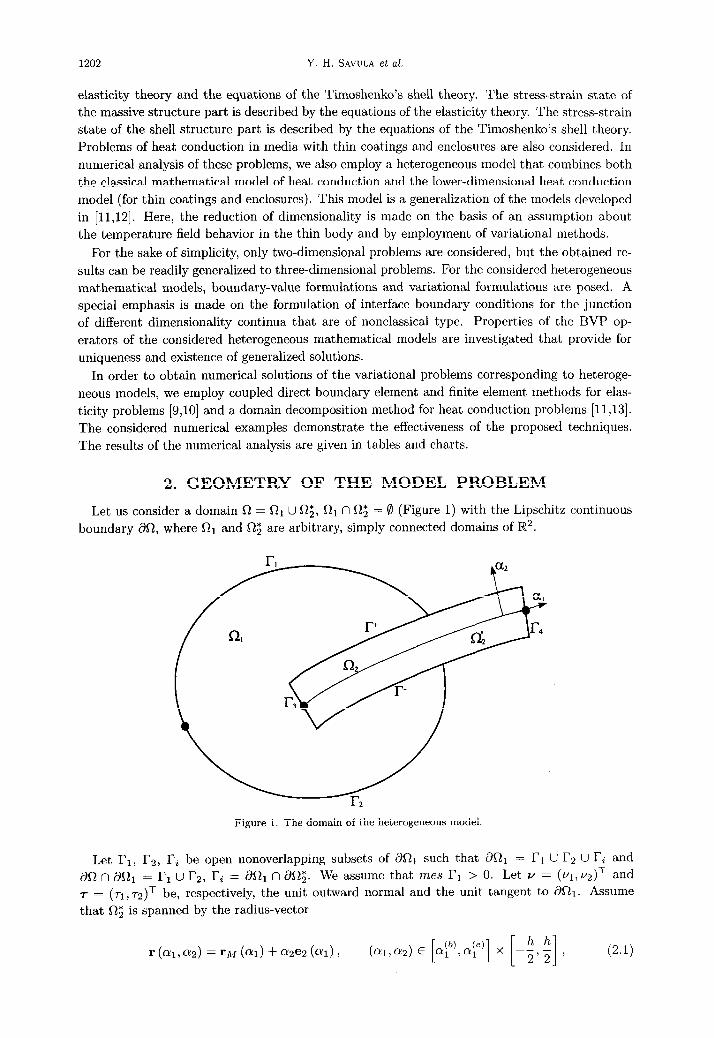
2. GEOMETRY OF THE MODEL PROBLEM

Let us consider a domain s2 = Ri U $, RI n 0; = 8 (Figure 1) with the Lipschitz continuous

boundary dR, where Ri and Cl; are arbitrary, simply connected domains of R2.

Figure 1. The domain of the heterogeneous model

Let Pi, P2, Pi be open nonoverlapping subsets of dRi such that dRr = I?r U r2 U ri and

80 n doi = rl u r2, ri = ml n 80;. We assume that mes Pi > 0. Let u = (ui,~2)~ and

7 = (ri, 7~)~ be, respectively, the unit outward normal and the unit tangent to 8Ri. Assume

that 0; is spanned by the radius-vector

r(al,a2)=r~(ol)+~2e2(CY1), (Q1,Q2) E [c&p] x [-;,;I , (2.1)

Heterogeneous Mathematical Models 1203

where rj,,I(cri) is the radius-vector of the piecewise smooth middle curve Rz, es(or) is the unit

normal, and ei(oi) is the unit tangent to s/2. This means that the domain 0; is referred to the

curvilinear orthogonal coordinate system (~1, ~2) and its Lame coefficients are [14]

Hi = Ai (1 + h~2), H2 = 1.

Here, Al = AI is the Lame parameter and ki = Ici(ai) is the curvature of the middle

curve R2. We assume that the thickness h of Rz is much smaller than the radius of curvature of R2. Let

Is, I’+, I-, I4 be open, nonoverlapping subsets of as2; such that Xl; = Is u I4 u l?+ u I-,

where

r3 = {

(al, a2) : a1 = I, -;Qc25; , 1 (2.2)

r4= ((Y~,cY~):cQ=$), --p25a , { h I (2.3)

rf = (~~4~) : (Y?) 1 (e) h < a1 <a, ) a2 = 5 )

>

(2.4)

r- = (~~4~) : c$) 1

< a1 < ap, a2 = -h I 2 . (2.5)

It follows from Figure 1 that Ii = I3 u I’+ u l?;, where I+ = Ii n I+, l?; = Ii n I?-, and that

there exists a point aim) E [a(lb),a(le)] such that

r+ = { (~~4~) : c$) < al < c@), a2 = $ 1 , r; = (~~4~) : c$)

{ < (Yl < cp, a!2 = -h

1 2

(2.6)

(2.7)

3. STATEMENT OF THE HETEROGENEOUS MODEL (I)

The stress-strain state of the elastic body in the domain Rr is described by the equations of

the linear elasticity theory [14] ( summation over repeated indices)

(3.1)

Here, aij are the components of the stress tensor given by

Oij = 2/&j + XekkSij, i,j = 1,2, (3.2)

where p, X are Lame constants, 6ij is Kronecker’s delta, and f = (fi, f~)~ is the body force

vector. The following Cauchy relations hold:

eij=i(z+g), i,j=1,2, (34

where U = (Ul, VZ)~ is the displacement vector of 521.

The stress-strain state of the elastic body in the domain 0; is described by the equations of

the Timoshenko’s shell theory [14]

(3.4)

1 dTl1

Al da1 - hTl2 = Pl,

-- ,: $$ +klTl1 =p2, 1 1

-$9$+T~2=m1, cp I a1 5 a1 . (e)

1 1

1204 Y. H. SAVULA et al.

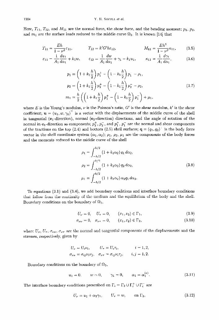
Here, Tll, Tl2, and Mii are the normal force, the shear force, and the bending moment; pl, par

and ml are the surface loads reduced to the middle curve 522. It is known [14] that

T12 = k’G’ha12, Eh3

A411 = - 1 _ $ Kl13 (3.5)

1 dul El1 = -- + klW,

1 dw

-41 dm El2 = -__ $71 - IClUl,

Al da

1 dyl

lcll = KG (3.6)

(3.7)

where E is the Young’s modulus, u is the Poisson’s ratio, G’ is the shear modulus, k’ is the shear

coefficient; u = (ui, w, 71) T is a vector with the displacements of the middle curve of the shell

in tangential (ei-direction), normal (ez-direction) directions, and the angle of rotation of the

normal in ei-direction as components; pi, p; , and pf , p; are the normal and shear components

of the tractions on the top (2.4) and bottom (2.5) shell surfaces; q = (q1,q2)T is the body force vector in the shell coordinate system (~1, a~); pi, ~2, pi are the components of the body forces and the moments reduced to the middle curve of the shell

s h/2 Pl = (I+ kla2) 41 do2,

-h/2

.I

h/2

P2 = (1 + kla2) q2 da2, (3.8) -h/2

s

h/2

111 = (1 + haa) wz,Ql dm. -h/2

To equations (3.1) and (3.4), we add boundary conditions and interface boundary conditions

that follow from the continuity of the medium and the equilibrium of the body and the shell. Boundary conditions on the boundary of Ri,

l_J,=o, u,=o, (Xl, x2) E r1, (3.9)

cl “” = 0, our = 0, (3h,22) E r2, (3.10)

where U,, UT, ovv, avT are the normal and tangential components of the displacements and the

stresses, respectively, given by

Boundary conditions on the boundary of R2,

Ul = 0, w = 0, 71 = 0, (e) a!1 =a1 .

The interface boundary conditions prescribed on l?i = l?a U r$ U ri are

(3.11)

UV = u1+ a2713 u, =w, on r3, (3.12)

Heterogeneous Mathematical Models 1205

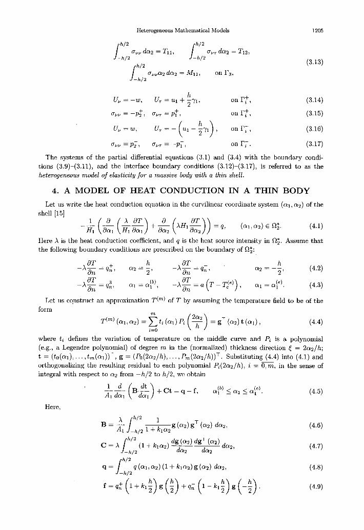
J h/2

J

h/2 0,” da2 = TII, avrda2 = 7'12,

-h/2 -h/2

J h/2 (3.13)

gvv~2 da2 = Mll, on r3, -h/2

u, = -w, on I?+, (3.14)

u VV = -P2f, our = Pf, on r+, (3.15)

u, =w, (ii=-(or--gyr), onr;, (3.16)

- ~vv = P, , 0 “7 = -Pl, on I?;. (3.17)

The systems of the partial differential equations (3.1) and (3.4) with the boundary condi-

tions (3.9)-(3.11), and the interface boundary conditions (3.12)-(3.17), is referred to as the

heterogeneous model of elasticity for a massive body with a thin shell.

4. A MODEL OF HEAT CONDUCTION IN A THIN BODY

Let us write the heat conduction equation in the curvilinear coordinate system ((;\I~, cr2) of the

shell [15]

-j$&&(&r~)+&(~~r~)) =q, (al,az)EQ;. (4.1)

Here X is the heat conduction coefficient, and q is the heat source intensity in aa. Assume that

the following boundary conditions are prescribed on the boundary of s2;:

h a2 = --)

2

h Q2 = -,

2

(6) a1 = Ql 9 --A: =a(7-Tie)), ~1 =LY~).

Let us construct an approximation T cm) of T by assuming the temperature field to be of the

form

+%1,~2)= -&adP, = gT (a2)t(crl),

i=O

(4.4

where ti defines the variation of temperature on the middle curve and Pi is a polynomial

(e.g., a Legendre polynomial) of degree m in the (normalized) thickness direction < = 2&2/h;

t = (to(m), . . . ,tm(m))T, g = (Po(%/h), . . . , P,(2az/h))T. Substituting (4.4) into (4.1) and

orthogonalizing the resulting residual to each polynomial Pi(2cx2/h), i = 0, m, in the sense of

integral with respect to ~2 from -h/2 to h/2, we obtain

Here,

B=$ J

h/2 1

-h/2 1 + kraz g (a2) gT (a2) dQ2,

J h/2 c=x &@z)dgT(w) da _h,2(1+k1a2+- da 27

2 2

J h/2 q= q (~1, ~2) (I+ ban) g ((~2) d&2, -h/2

f =q,+ (l+kl;)g(;) +q; (I-h;)g(-;).

(4.5)

(4.6)

(4.7)

(4.8)

(4.9)

1206 Y. H. SAWJLA et al

Similarly, employing the same orthogonalization procedure, we transform (4.3) and obtain the

following boundary conditions:

(4.10) F&g = q(b), 1

(b) al = “1 ; p =

./

h/2

4:g (02) da2, -h/2

(e). Ql = a1 1 tb”’ 1

J’

h/2

dz+)g (Q2) dcI2,

-h/2 c

(4.11)

s h/2

P= ag (Q2) gT (Q2) dQ2. (4.12) -h/2

5. STATEMENT OF THE HETEROGENEOUS MODEL (II)

Now we are in a position to write down the resulting heterogeneous model of heat conduction

in a body with a thin enclosure. The temperature field in Rr is described by the equation of

classical heat conduction theory [15] ( summation over repeated indices)

Here, X is the heat conduction coefficient, and q is the heat source intensity in Or.

The temperature field in 0; is described by (4.4), where t satisfies

(b) Qr (e) < Ql 501

(5.1)

To equations (5.1) and (5.2), we add boundary conditions and interface boundary conditions

that follow from the continuity of the temperature field and conservation of the heat flux. Bound-

ary conditions on the boundary of RI,

T = 0, (Zl,ZZ) E r1, (5.3)

-AZ =a(T-T,), (q, 22) E r2. (5.4)

Boundary conditions on the boundary of 02:

_B$ = pt - t?‘, (El al= cl1 .

1

The interface boundary conditions prescribed on I?? = l?s U I’+ U I’; are

T = gTt> on r3, (5.6)

.I h/2 dT _,~,2 X ay g (~2) da2 = d”), on h, (5.7)

T = gTt, on r;, (5.8)

-AE = -q;, on r;, (5.9)

T = gTt, on r;, (5.10)

-AE =-q,. o11 r;. (5.11)

The systems of partial differential equations (5.1) and (5.2) with the boundary conditions

(5.3)-(5.5), and the interface boundary conditions (5.G)-(5.11), . 1s referred to as the heterogeneous

model of heat conduction for a body with a thin enclosure.

Heterogeneous Mathematical Models 1207

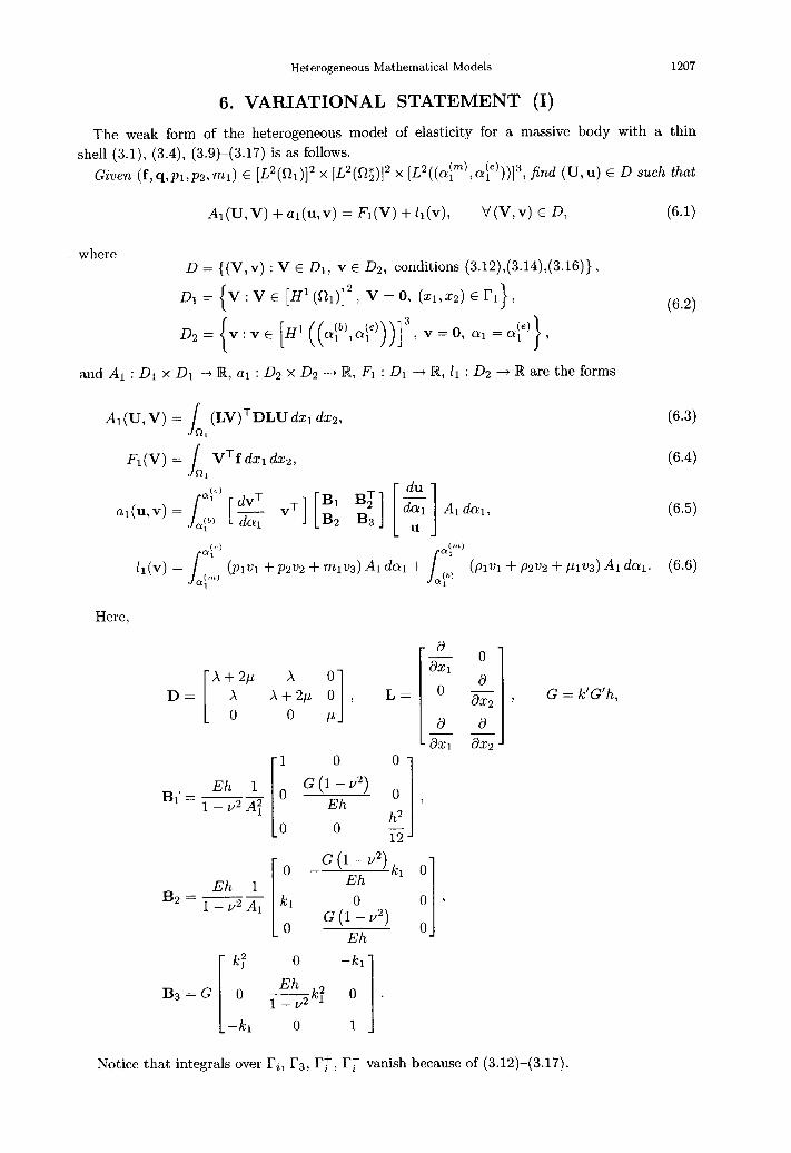
6. VARIATIONAL STATEMENT (I)

The weak form of the heterogeneous model of elasticity for a massive body with a thin

shell (3.1), (3.4), (3.9)-(3.17) is as follows.

Given (f,q,pr,ps,mr) E [L2(Rr)12 x [L2(s2z)12 x [L2((o~“‘,~(le)))]3, find (U,u) E D such that

Ar(U,V) + ar(u,v) = Fr(V) + II(V), Y(V,v) E D, (6-l)

where D={(V,v):VED r, v E Ds, conditions (3.12),(3.14),(3.16)},

D1 = V : V E [H’ (fl,)12, v = 0, (21,x2) E r1},

and Al : D1 x D1 -+ IR, al : Ds x Ds -+ R, Fr : D1 -+ R, 11 : Ds -+ R are the forms

Al (U, V) = s

(LV)TDLU dsl dx2, 01

Fl(V) = J’

VTf dxl dx2, RI

(6.2)

(6.3)

(6.4)

(6.5)

(1,)

ll(V) = .I a;,:Ll (Plwl + ~‘2 + ml4 Al da1 + /yty) (/awl + p2w2 + plug) Al dal. (f-3.6)

a1

Here,

J?- 0 1 8x1

, G = k’G’h,

a a -- -ax1 ax2 -

B1’= Eh 1

-- 1 - ~2 AT

Notice that integrals over J?i, rs, I’$, I’; vanish because of (3.12)-(3.17).

1208 Y. H. SAVULA et al.

7. VARIATIONAL STATEMENT (II)

The weak form of the heterogeneous model of heat conduction for a body with a thin enclo-

sure (5.1)-(5.11) is as follows.

Given (ql,q,f) E L2(0,) x [L2((~~),~(le)))]m+1 x [L2((~(lm),a~)))]mf1, find (T, t) E D such

that

where

A2 (T,V) +az(kv) = F2(V) +/2(v), ‘J(V,V)ED,

D = {(V,v) : V E D1, v E D 2, conditions (5.6),(5.8),(5.10)},

D1={V:V~H1(R1), V=O, (x~,z~)EI’I},

D2={v:vt [H’((aj”),a~)))]mtlJ,

(7.1)

(7.2)

and A2 : D1 x D1 -+ R, u2 : D2 x Dz -+ IR, FZ : DI -+ lit, 12 : D2 --+ IR are the forms

A2(T V) = s

Algz dxldxz+ J’

aTlV dr, 01 z z r2

F2(V) = s

qlV dxl dxz + J aT,V dr, 01 rz

(7.3)

(74

&’

a2(u,v) = J ( eB* + vTCt (*I da1 da1 >

A1 da1 + vTPtlaI=a(lpj , (7.5) 01 (cl a1

lz(v) = J (o) vTqA&l- ml J (cl a1

vTfAl da1 + vTtce) (-IL) C (7.6)

a1 ollC$)

Notice that, integrals over I’i, l?s, rt, I’; vanish because of (5.6)-(5.11).

8. PROPERTIES OF THE VARIATIONAL STATEMENTS

The following lemmas hold.

LEMMA 1. Let D be the space defined by (6.2). Then we have the following.

(1) Linear form F : D + IR defined by

F((V,v)) = FIW) +11(v)

is continuous on D.

(8.1)

(2) Bilinear form A : D x D -+ iR defined by

A((U,u),W,v)) =AlW,V)+al(u,v) (8.2)

is continuous and symmetric on D.

PROOF. Symmetry of A((U, u), (V, v)) f o 11 ows from the symmetry of Al(U,V) and al(u,v). a

LEMMA 2. Let D be the space defined by (7.2). Then we have the following.

(1) Linear form F : D + lR defined by

F((V,v)) = F2(V) +lz(v) (8.3)

is continuous on D. (2) Bilinear form A : D x D 4 IR defined by

A ((T, t), (V, v)) = MT, V) + az(t, v)

is continuous and symmetric on D.

(8.4)

PROOF. Symmetry of A((T,t),(V,v)) f o 11 ows from the symmetry of A2(T, V) and az(t, v). 1

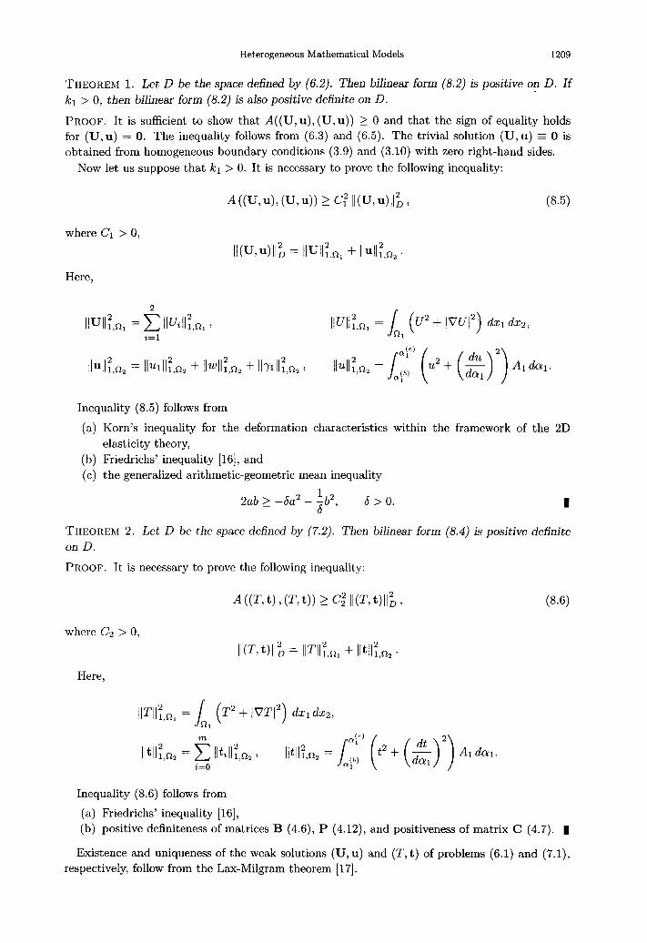
Heterogeneous Mathematical Models 1209

THEOREM 1. Let D be the space defined by (6.2). Then bilinear form (8.2) is positive on D. If

kl > 0, then bilinear form (8.2) is also positive definite on D.

PROOF. It is sufficient to show that A((U,u), (U,u)) 2 0 and that the sign of equality holds

for (U,u) = 0. The inequality follows from (6.3) and (6.5). The trivial solution (U,u) = 0 is obtained from homogeneous boundary conditions (3.9) and (3.10) with zero right-hand sides.

Now let us suppose that kl > 0. It is necessary to prove the following inequality:

A((U,u),(U,u)) 2 Cl” Il(U+)tl; 7 (3.5)

where Ci > 0,

II&J, u,ll”, = llull:.n, + Ilull:,% .

Here,

llull:,n, = 2 Ilw:,n, 7 IvJll:.r2, = i=l

s,, (U’ + lW12) dxl do,

Inequality (8.5) follows from

(a) Korn’s inequality for the deformation characteristics within the framework of the 2D

elasticity theory,

(b) Friedrichs’ inequality [16], and (c) the generalized arithmetic-geometric mean inequality

2ab 2 --da2 - ib2, 6 > 0. I

THEOREM 2. Let D be the space defined by (7.2). Then bilinear form (8.4) is positive definite

on D.

PROOF. It is necessary to prove the following inequality:

where C’s > 0,

IIKt)ll; = Il$n, + Iltll:,n,

Here,

IlW,r2, = J,, (T” + IW2) dxl dxz,

Ilt llT,s& = 5 IMl:,r2, 1 lltlf,n, i=o

= i,;&y (t2 + (g)‘) AIdal.

Inequality (8.6) follows from

(a) Friedrichs’ inequality [16], (b) positive definiteness of matrices B (4.6), P (4.12), and positiveness of matrix C (4.7). 1

Existence and uniqueness of the weak solutions (U, u) and (T, t) of problems (6.1) and (7.1), respectively, follow from the Lax-Milgram theorem [17].

1210 Y. H. SAVULA etal.

9. NUMERICAL IMPLEMENTATION

In the following, we describe two approaches for numerical solution of the discretized problems

corresponding to (6.1) and (7.1).

9.1. Numerical Solution of the Heterogeneous Model (I)

Here we will use a hybrid method based on simultaneous use of the direct boundary element

method (DBEM) for the problem of the theory of elasticity and finite element method (FEM)

for the problem of the Timoshenko’s shell theory elaborated in [9,10]. An advantage of this

technique is that we use approximations of the same order in the whole domain-quadratic ap-

proximation of displacements on the boundary of Ri and isoparametric quadratic approximations

of displacements and angles of rotations in 02.

Numerical approximation of the solution in Ri is obtained by means of the DBEM using

Galerkin method. The values of displacements and tractions on the boundary are obtained from

the following system of linear algebraic equations:

(9.1)

where x1 is the vector of degrees of freedom on the boundary dRi \ I’i, and xi is the vector of

degrees of freedom on interface boundary I’i.

Numerical approximation of the solution in QJ is obtained by minimization of the corresponding

Lagrangian functional. The values of displacements and angles of rotations are obtained from

the following system of linear algebraic equations:

where yi is the vector of degrees of freedom inside the domain (cry), crp’] and yi is the vector of

degrees of freedom corresponding to cyi = a?).

Matrices of (9.1) and (9.2) are rectangular. We supplement (9.1) and (9.2) by the discretized

relations on the interface boundary, which are obtained from (3.12))(3.17),

xi = sy,. (9.3)

Solution of system (9.1)-(9.3) . 1s complicated because of the different structure of BEM and

FEM matrices-nonsymmetric dense versus symmetric banded and because of the presence of

interface conditions (9.3). S ince the number of degrees of freedom on the interface boundary

is much less than the total number of degrees of freedom in each subdomain, we will use the

algorithm described in [8,10], which permits a separate solution of (9.1),(9.2). According to this

algorithm, the solutions are decomposed in the following way:

x = x0 + xlc, y=y’+Y’d. (9.4)

Here, x0, y” are the solutions of the problems with zero displacements on the interface boundary

and a given loading, and the columns of matrices (Xl),, (Y’)j are the solutions of (9.1),(9.2),

respectively, with unit displacements in the jth node on the interface boundary and zero external

loading. Vectors c, d are determined from (9.3).

9.2. Numerical Solution of the Heterogeneous Model (II)

Here we shall use a variant of the domain decomposition technique called iteration by sub-

domain based on an iterative solution of a sequence of mixed discretized subproblems in Ri

Heterogeneous Mathematical Models 1211

and & [11,13,18]. The heat conduction problem in Ri is solved by 3D FEM, and the dimension-

ally reduced heat conduction problem in !& is solved by 2D FEM. Advantages of this technique

are

(a) the discretized problems on subdomain can be solved by standard single-domain finite

element solvers, (b) no preconditioning is necessary, and (c) interface boundary conditions are easily imposed.

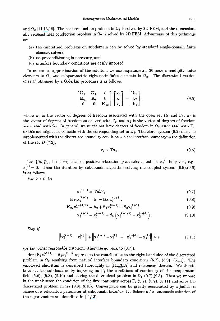
In numerical approximation of the solution, we use isoparametric 20-node serendipity finite elements in Ri and subparametric eight-node finite elements in flz. The discretized version of (7.1) obtained by a Galerkin procedure is as follows:

where xi is the vector of degrees of freedom associated with the open set Ri and I’z, xi is

the vector of degrees of freedom associated with l?i, and x:, is the vector of degrees of freedom associated with fiz. In general, we might not have degrees of freedom in 522 associated with ri, or this set might not coincide with the corresponding set in Ri. Therefore, system (9.5) must be

supplemented with the discretized boundary conditions on the interface boundary in the definition

of the set D (7.2),

xi = Tx2. (9.6)

Let -CPlc)El b e a sequence of positive relaxation parameters, and let xr) be given, e.g.,

x2 (‘I = 0. Then the iteration by subdomain algorithm solving the coupled system (9.5),(9.6)

is as follows.

For k > 0, let

xi ck+‘) = TX?),

Ki&+‘) = bi - Kiixl”+‘),

(9.7)

(9.8)

K22~p+1’2) = b2 + &x(,“+‘) + SzXik+‘),

x2 (k+l) = xp+l) + Pk (xplz) _ Xp+l)) _

(9.9)

(9.10)

stop if

II x(lk+l) _ xp + X!k+l) _ xy + xp+l) _ ,y < E I/ I/ 2 2 II II I/ - (9.11)

(or any other reasonable criterion, otherwise go back to (9.7)).

Here Six, (k+l) + s2x!“+i) represents the contribution to the right-hand side of the discretized problem in 522 resultiig from natural interface boundary conditions (5.7), (5.9), (5.11). The employed algorithm is described thoroughly in [11,13,18] and references therein. We iterate between the subdomains by imposing on I’i the conditions of continuity of the temperature field (5.6), (5.8), (5.10) and solving the discretized problem in Ri (9.7),(9.8). Then we impose in the weak sense the condition of the flux continuity across ri (5.7), (5.9), (5.11) and solve the discretized problem in Rz (9.9),(9.10). C onvergence can be greatly accelerated by a judicious choice of a relaxation parameter at subdomain interface I’i. Schemes for automatic selection of these parameters are described in [11,13].

1212 Y. H. SAVULA et&.

B* h ._._._._._._._I.

h b

’ x I

,/--_----__---______

-9

4

"II B1

b

1 4 b

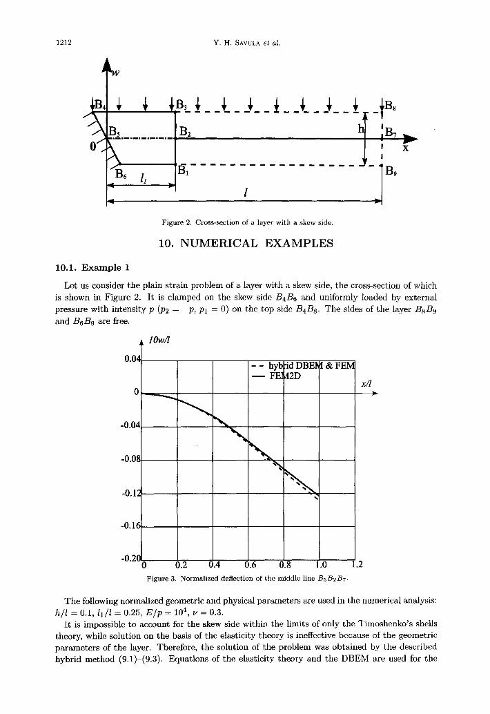
Figure 2. Cross-section of a layer with a skew side.

10. NUMERICAL EXAMPLES

10.1. Example 1

Let us consider the plain strain problem of a layer with a skew side, the cross-section of which

is shown in Figure 2. It is clamped on the skew side B4& and uniformly loaded by external pressure with intensity p (ps = -p, pi = 0) on the top side B&s. The sides of the layer BsBs

and B&J are free.

Figure 3. Normalized deflection of the middle line B5BzB7.

The following normalized geometric and physical parameters are used in the numerical analysis: h/l = 0.1, ii/l = 0.25, E/p = 104, v = 0.3.

It is impossible to account for the skew side within the limits of only the Timoshenko’s shells theory, while solution on the basis of the elasticity theory is ineffective because of the geometric parameters of the layer. Therefore, the solution of the problem was obtained by the described hybrid method (9.1)-(9.3). Equations of the elasticity theory and the DBEM are used for the

Heterogeneous Mathematical Models 1213

- - hybrid:>BEM & FEM

- FEM2D

l

-Q4 0 a4 08 B 1.2 B, 8

Figure 4. Normalized normal stresses along line B4Bs.

f

Z

Figure 5. Cross-section of a two-layer cylinder.

analysis of the part BlBsBdBc of the structure (domain RI). Equations of the Timoshenko’s

shell theory (for the case A = 0, ICI = 0) and FEM are used for the analysis of the part B1B9B8B3 of the structure (thin domain 0;). Segment BIBS is the interface boundary ri.

With the aim of comparison, we also present the results from a pure FEM analysis (bi-

quadratic 2D isoparametric elements), obtained on the basis of the plane strain model of the linear elasticity theory for the entire structure.

Figure 3 shows the normalized deflection w x 10/1 of the middle line BsBzB7 of the structure. As expected, the deflection obtained on the basis of the hybrid method is close to the one resulting from the 2D FEM.

Figure 4 illustrates the normalized stress aZ2/p along the line BdBsB8 of the structure as a function of x/l. Again, the results obtained by the hybrid method are close to the results from

the 2D FEM.

1214 Y. H. SAVULA etal.

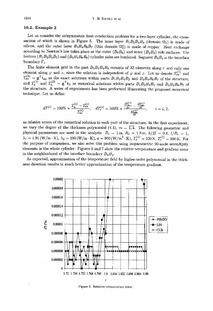
10.2. Example 2

Let us consider the axisymmetric heat conduction problem for a two-layer cylinder, the cross-

section of which is shown in Figure 5. The inner layer Bi&B& (domain fii) is made of silicon, and the outer layer BsBdBsB7 (thin domain 0;) is made of copper. Heat exchange

according to Newton’s law takes place at the outer (B7Bs) and inner (B1B2) side surfaces. The

bottom (B1 B3 B5 B7) and (Bz B4 B6 Bs) cylinder sides are insulated. Segment B3 B4 is the interface boundary I’i.

The finite element grid in the part BlBzBdBs consists of 32 elements along r and only one

element along ‘p and z, since the solution is independent of ‘p and z. Let us denote TLi) and

Tc2) = gTt,, as the exact solutions within parts BIB~B~Bs and B~B~BBB~ of the structure,

a: Ti’) and Ti2) = T g th as numerical solutions within parts BIB~B~B~ and BzBdBgB7 of

the structure. A series of experiments has been performed illustrating the proposed numerical

technique. Let us define

dTci) = 100% x

dT,I”) dT(‘)

dT,?) = 100% x dr dT(i) dr , i = 1,2, -

dr

as relative errors of the numerical solution in each part of the structure. In the first experiment,

we vary the degree of the thickness polynomial (4.4), m = 1,4. The following geometric and

physical parameters are used in the analysis: RI = lm, Rz = 1.8m, h/H = 0.1, l/R1 = 1,

X1 = 1.91 (W/m. K), X2 = 390 (W/m. K), a = 900 (W/m2 . K), T,(l) = 320K, T,(‘) = 900K. For

the purpose of comparison, we also solve this problem using isoparametric 20-node serendipity

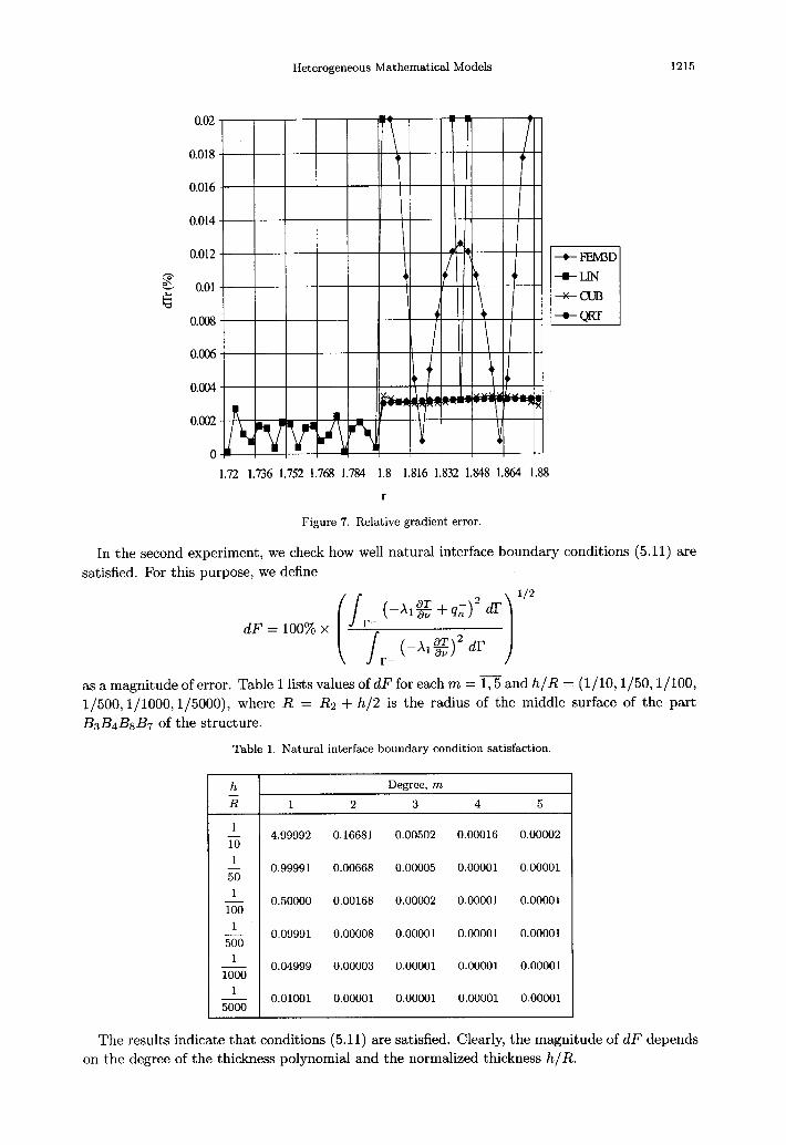
elements in the whole cylinder. Figures 6 and 7 show the relative temperature and gradient error

in the neighborhood of the interface boundary BsB4.

As expected, approximation of the temperature field by higher-order polynomial in the thick-

ness direction results in much better approximation of the temperature gradient.

1.72 1.736 1.752 1.768 1.784 1.8 1.816 1.832 1.848 1.864 1.88

r

Figure 6. Relative temperature error.

Heterogeneous Mathematical Models 1215

0.018

0.016

0.012

* G 0.01

6

0.008

-+-FEMD

-LIN

+cuEr

-QRT

1.72 1.736 1.752 1.768 1.784 1.8 1.816 1.832 1.848 1.864 1.88

r

Figure 7. Relative gradient error.

In the second experiment, we check how well natural interface boundary conditions (5.11) are

satisfied. For this purpose, we define

as a magnitude of error. Table 1 lists values of dF for each m = 1,5 and h/R = (1/10,1/50,1/100,

1/500,1/1000,1/5000), where R = R2 + h/2 is the radius of the middle surface of the part

BsBdBgB7 of the structure.

Table 1. Natural interface boundary condition satisfaction.

h Degree, m

x 1 2 3 4 5

1 lo 4.99992 0.16681 0.00502 0.00016 0.00002

1 50 0.99991 0.00668 0.00005 0.00001 0.00001

1 - 0.50000 0.00168 0.00002 0.00001 0.00001 100

1 - 0.09991 0.00008 0.00001 0.00001 0.00001 500

1 - 0.04999 0.00003 0.00001 0.00001 0.00001 1000

1 - 0.01001 0.00001 0.00001 0.00001 0.00001 5000

The results indicate that conditions (5.11) are satisfied. Clearly, the magnitude of dF depends on the degree of the thickness polynomial and the normalized thickness h/R.

1216 Y. H. SAVULA et al.

We also note that in all experiments, the number of iterations of the domain decomposition

method needed to obtain the numerical solution with a given number of correct digits was inde-

pendent of both m and h/R.

11. CONCLUSION

The considered heterogeneous models are an effective tool for analysis of compound structures,

because they allow us to employ the most suitable mathematical model and numerical method

in each substructure. The use of lower-dimensional models entails a significant reduction of

preprocessing, processing, and postprocessing time without significant losses of accuracy.

REFERENCES

1. Y.S. Pidstrygatch, Conditions of heat contact of solid bodies, Dop. Acad. Nauk. URSR 7, 872-874, (1963). 2. N.P. Phleishman, Mathematical models for heat coupling of media with thin foreign enclosures or coatings,

Vim. L’viv Un-tu, Ser. Mech.-Math. 39, 30-34, (1993). 3. V. Liantse and 0. Storoz, About one non-classic boundary value problem of the plate theory, Dop. Acad.

Nauk. URSR 2, 15-17, (1989). 4. P.G. Ciarlet, Plates and Junctions in Elastic Multi-Structures, Paris, (1990). 5. P.G. Ciarlet, H. Le Dret and R. Nzengwa, Junctions between three-dimensional and two-dimensional linearly

elastic structures, J. Math. Pures et Appl. 3, 261-295, (1989). 6. A. Quarteroni, Multifields modelling in numerical simulation of partial differential equations, GAMM-Mit-

teilungen 1, 45-63, (1996). 7. Y.H. Savula, Numerical analysis on the base of combined models of mechanical structures, In Proc. Szxth

Int. Conf Math. Meth. Eng., Volume 2, Czechoslovakia, pp. 521-526, (1991). 8. Y.H. Savula, 1.1. Dyyak and A.V. Dubovik, Application of the combined model for the stress analysis of

spatial structures, Prikladna Mekhanika 25 (9), 62-66, (1985). 9. Y.H. Savula, N.M. Pauk and 1.1. Dyyak, Boundary-finite-element analysis of combined models of 2-d problems

of elasticity, Dop. Nat. Acad. Nauk. Ukraine 5, 49-52, (1995). 10. Y.H. Savula and 1.1. Dyyak, D-adaptive model for the elasticity problem, Computer Assisted Mechanics and

Engineering Sciences 5, 65-74, (1998). 11. Y.H. Savula and V.V. Krevs, An application of the domain decomposition method to the heat conduction

problem for a body with a thin coating, Visn. L’viv Un-tu, Ser. Mech.-Math. 44, 3-10, (1996). 12. Y.H. Savula, I.M. Sypa and I.V. Strutynskiy, Mathematical models of heat conduction for bodies with thin

coatings, Vim. L’viv U&u, Ser. Mech.-Math. 37, 39-45, (1992). 13. L.D. Marini and A. Quarteroni, An iterative procedure for domain decomposition methods: A finite element

approach, In First International Symposium on Domain Decomposition Methods for Partial Differential Equations, (Edited by R. Glowinski et al.), pp. 129-143, SIAM, (1988).

14. S.P. Timoshenko, Course of the Theory of Elasticity, Naukova Dumka, Kyyiv, (1972). 15. N.M. Belyaev and A.A. Rysdno, Methods of the Heat Conduction Theory, Volume 1, Nauka, Moscow, (1982). 16. K. Rektorys, Variational Methods in Mathematics, Science and Engineering, Prague, (1980). 17. S.C. Brenner and L.R. Scott, The Mathematical Theory of Finite Element Methods, Springer-Verlag, New

York, (1994). 18. G.I. Marchuk, Methods of Computational Mathematics, Nauka, Moscow, (1989).