Health and “Poverty Traps” in Rural Developing Economies

Theresa K. Osborne� European University Institute

September 25, 2003

Abstract This paper tests for the presence of a positive convex relationship between individual consumption and productivity using data from rural Ethiopia. Such a convexity underlies the theory of efficiency wages and can create a low-consumption, low-productivity (“poverty”) “trap” operating through health status. I propose a test based on the predictions of a dynamic theoretical model of household consumption allocation which obviates the need to directly estimate the relationship between individual consumption and productivity directly. This is particularly advantageous, as at least one of these variables is typically not observed for individuals. Using semi-parametric estimation techniques, I find evidence of a convexity in the consumption-productivity relationship for households in the upper part of the land-per-worker distribution. Productivity incentives and the preference for equality appear to be in conflict for these rural households, who therefore face the possibility of a low-health, low-productivity steady state. Results also show that it is important to use a broad measure of an individual’s health or work capacity, as using a standard nutrition-based measure (body mass index) obscures these dynamics.

� Contact address: Department of Economics, EUI, Via della Piazzuola 43, 50133 Firenze (FI) Italy. Email: Theresa.Osborne@iue.it. I wish to thank Frank Vella for extremely valuable comments on the empirical approach, and participants in the EUI’s micro lunch for early feedback. I thank the Centre for the Study of African Economics (Oxford) for providing the data, as well as the survey funding organizations, the Economic and Social Research Council (ESRC), the Swedish International Development Agency (SIDA), and the Agency for International Development (USAID).

1

1. Introduction Ever since Leibenstein (1957) and Mirrlees (1975) advanced the notion of a link between

individuals’ consumption and productivity, there has been interest in studying this link. In

developing countries, interest has focused particularly on the prospect of dual causality

between nutrition and income. “Nutrition”- or “efficiency- wage” models (e.g., Stiglitz

[1976], Dasgupta and Ray [1986, 1987] and Ray and Streufert [1993]) posit a convexity in

this relationship in the low income and nutrition range. That is, for some range of nutritional

status the marginal productivity of consumption (or nutrition) is increasing in consumption.

If such a convexity is present, then a low nutrition-low productivity (“vicious”) circle can

produce an equilibrium with persistently under-employed and under-nourished workers (Ray

and Streufert [1993]). Yet a focus purely on nutrition may fail to fully capture the essential

linkages between consumption and productivity. Strauss and Thomas (1998) note that the

nature of work in low income economies tends to rely more heavily on strength and

endurance and, therefore, on good health generally. The body’s store of calories is only one

component of this. Yet in part due to a paucity of data, little research has been done using a

broader measure of health status.

Empirical studies focusing on nutritional status have found some support for a causal

linkage between nutrition and wages (see e.g. Berhman and Deolaker [1989], Foster and

Rosenzweig [1994], and Strauss [1986]) but on the whole cast doubt on the nutrition-

efficiency models (Binswanger and Rosenzweig [1984], Rosenzweig [1988]; for a review see

Strauss and Thomas [1998]). This could be at least in part because maintaining

recommended caloric intakes is cheap relative to wages, even in some poor economies such

as rural India (Subramian and Deaton [1996] and Swamy [1998]). Nonetheless, in many

countries nutritional sufficiency is a perennial issue. Moreover, the convexity between

2

consumption and work capacity posited by efficiency “wage” models may become more

realistic when consumption relates to all health inputs rather than merely to calories.

Consumption-productivity models are, of course, premised on the presence of dual

causality between income and health, and this makes the relationships difficult to identify

empirically. In particular, there are simultaneity issues not only between health and income,

but also with other important production inputs (see Smith [1999] for a survey of the health-

income literature). Moreover, income is measured with a great deal of error in agricultural

households. More importantly, often either individual income or individual consumption data

are not available. For these and other reasons, it has been extremely difficult to identify dual

causality in general, and in particular whether there is a convexity present in the relationship.

This paper tests for both of these phenomena using data from rural Ethiopian

households. It uses a broader measure of health which is likely to be more closely related to

productivity or work capacity than is nutritional status. An indirect estimation strategy is

proposed which avoids many of the difficulties of estimating the consumption-productivity

relationship directly, particularly as neither of these are observed for individuals.

While it is often supposed that health affects income in poor rural areas, one can

imagine circumstances in which this is not the case, at least in the short run. For example, if

household members are under-employed due to a lack of productive assets (and general

unemployment), then in the event one member falls ill, his or her work could be done by

another. Nonetheless, strenuous work is part of the life of most rural Ethiopians; thus health

is likely to affect income even in the short run. Income is also likely to affect health, as it can

help a household to command a healthier lifestyle – vegetables and fruits, meat and other

3

protein, warm clothing, soap, energy for boiling water, and medical care.1 At the same time,

if access to quality medical care is not affected by income (or if, as in some parts of rural

Ethiopia, it is not available at all) then a poor health shock may persist similarly for relatively

rich and poor households. Alternatively, if a household member contracts a chronic illness,

effective medical treatments may simply not be available at any price. Finally, if there is no

market for health inputs such as clean water or “clean” (non-toxic) energy, then there may be

little the better-off household can do to obtain these inputs. Nonetheless, it is clear at least in

the extreme that income and wealth affect health, as it is the poorest and landless who have

most suffered the persistent ill effects of famine (including death.) (See Webb et al. [1992]

for an analysis of the effects of famine in Ethiopia).

In this paper, I develop a dynamic intra-household allocation model which takes dual

causality as given. This model yields testable implications which would be unlikely to hold

in the absence of such causation. Moreover, it admits a test for the presence of a productivity

tradeoff with the households’ desire to equalize health outcomes across its members – that is,

a convexity in the consumption-productivity relationship. In particular, I estimate

movements in the relative health status of pairs of individuals within the same household with

respect to their initial health status. A finding that initial health status affects the degree of

equalization (or dispersion) in the pair’s subsequent health would support a general model in

which households weigh equality and productivity considerations in their intra-household

resource allocation. If initial health enters negatively in some range, then – as the theory

1Despite a burgeoning literature for the developed world, the exact mechanisms by which income “buys” better health are still in great need of study. There are also likely to be direct intra-household spillover effects from a poor income or health draw. If household members are too weak to carry fresh water in sufficient quantities, for instance, to take children for health checks, or to collect heating fuel, then other members of the household may suffer ill health.

4

shows – this is evidence that productivity incentives dominate for some range, and thus that a

convexity is present.

The results I obtain support the presence of dual causality. Households are generally

able to improve the health of their members as incomes improve. Thus even in areas, like

rural Ethiopia, with extremely poor health care provision it appears that resources matter. In

addition, I find evidence that households in the upper part of the distribution of landholdings

(per worker) confront an important productivity-equality tradeoff. This implies that health

also affects income (i.e., productivity). It also imples a convexity in the relationship between

consumption and productivity. Thus these households can neither maximize their

productivity nor fully invest in the recovery of the less healthy. Moreover, this convexity can

be a mechanism for multiple equilibria (“poverty trap”) in which low productivity and poor

health persist for some time.2

The next section presents the theoretical model and the propositions which form the

basis of the empirical tests. Section 3 describes the data and the necessary institutional

background. Section 4 describes the empirical strategy, and Section 5 reports the results.

Section 6 concludes.

2. Theoretical Model

I develop a model in which uncertainty is explicit with respect to both health status and

income, as such uncertainty is an important feature of poor rural economies. I begin with a

health transition equation, which relates health of individual i in period t to health in period

t+1:

11 1 1( ( (1 ))) ( )i i i i i

t t t t th f g f h f g� � ��

� � �� � � � � �� , (1)

5

where itg represents current consumption of all goods and services – food, warm clothing,

clean water, shelter, leisure, etc. – by the individual which contribute to health (“health

goods”). g� represents the (depreciated) “stock” of health goods stored in the body in the

prior period plus their current consumption. th denotes health status in period t, δ is the

systematic (natural) rate of deterioration of health from one period to the next with no

further g investment. it 1�� is a pure random shock to the health status of individual i which is

unrelated to his consumption and is centered at zero. Here I assume that the ( )f g� function

does not vary by individual, but this assumption could be relaxed without invalidating the

approach. I assume that ( ) 0f g� �� everywhere, as is commonly assumed for poor

populations. According to (1), health status is somewhat cumulative, but one can raise it

through greater consumption, and maintenance of health requires some ongoing investment.

It may not always be possible for physiological and other reasons to improve (chronically)

poor health through expenditure of resources, and in this case ( )f g� would contain a flat

segment.

In addition to (1), there is a household income production function in which the

lagged health status of all members of household H (1, 2,… HN ) enters:

1 21 1( , ,... ; , )

HH H N Ht t t t ty y h h h L �� �� � � (2)

where H indexes the household and HN denotes the number of working age members of

household H. L denotes the household’s landholdings. These can be taken as exogenous

given the lack of a legal market in rural land in Ethiopia. All land was redistributed by the

Revolutionary (Derg) government in 1975, with only slight adjustments since (with a

2A longer panel than that available here would be needed to pin down the long run dynamics

6

correlation of .99 between land reportedly held following this redistribution and that held

today). Ht 1�� represents a random shock to income which is not related to lagged health status

but could be correlated with 1t� � according to the joint distribution function ( , )F � � . One

can also write (2) from an individual productivity perspective, given other members’ health

( )ith� as follows:

1 1( | ; , )i i i i it t t ty y h h L �

�

� �� � � (3)

The exact shapes of functions (1) and (3) will of course depend upon the metric used

for health. Nonetheless, it is typically assumed that the functions are concave in their upper

ranges. That is, when health status is very good, it becomes more difficult to improve through

greater g consumption, and there is a natural upper bound for good health. Moreover, it is

reasonable to assume that health status exhibits decreasing returns at some point. However, it

is not clear a priori whether there will be a region of convexity at lower values of ith .3

Thus there are two general alternatives for the shapes of ( )y g� and ( )f g� , which are

familiar from Mirrlees (1975) and Dasgupta and Ray (D&R) (1986). Figure 1 represents

Hypothesis A, that )~(gf and ( )y g� are concave throughout the range relevant to the

population. Under this scenario, even at poor health states one may easily improve health

through a more diverse diet, simple hygienic practices, or basic medical interventions.

Moreover, individual production as a function of g consumption is concave due to the

concavity of either or both of (1) and (3). Hypothesis B is represented in Figure 2. According

to this hypothesis, it requires relatively more investment to bring a very low health individual

empirically or indeed to estimate the structural model with any confidence. 3Although each individual’s function (1) will vary somewhat due to genetic or historical factors, the basic shapes will depend upon common human physiology, as well as the price and availability of

7

to the point where he can perform physical tasks. More formally, if one or both of (1) and (3)

is sufficiently convex in some range, then the composite function, 1 1( ) ( )H it ty g y g� �

�� � , which

relates i’s g consumption in period t to income in t+2, would exhibit an S-shape, as shown.

D&R (1986) show that if such an S-shaped relationship (convexity) exists between

nutrition and productivity, then a vicious circle can arise wherein individuals remain

unemployed and undernourished. There are some important differences between their

framework and that used here, however. First, in the D&R model individuals can work for an

outside (equilibrium) wage as long as they are sufficiently productive, whereas here

production occurs at the household level. Thus a consumption-productivity circle could arise

for the individual only if he is employed (rather than unemployed) in the sense that the

household normally assigns him productive tasks.4 Being unable to perform such tasks

would lower household income. On the other hand, the marginal product of an individual

household member could be close to zero if the ratio of land (and other capital) to people is

low and if there are few outside income generation possibilities. In this case, a single

individual’s poor health status may have no effect on subsequent income. Moreover, if the

( )f g� curve is sufficiently steep, a temporarily ill individual may still be fed, clothed, and

cared for by the household and his or her illness may not affect household income beyond

one period.

In the dynamic version of the D&R model, Ray and Streufert (1993) have shown that

some individuals will remain malnourished and involuntarily unemployed indefinitely, even

health goods, and thus should be somewhat similar across individuals within the economy. Moreover, one can control for differences in (3) through individual, household, and village characteristics. 4 I will not consider the outside labor option formally, though this does represent a small portion of some households’ income.

8

with no missing markets.5 However, their model contains no uncertainty, a critical feature of

the environment considered here. Under uncertainty within a household-production system,

the likelihood of multiple steady states even in the presence of an S-shaped consumption-

productivity relationship is much less clear.

I assume that household utility is separable in individual utility and over time and

that the household H has the following optimization problem:

,0 1

max ( , , ),H

i it l t l

Nl i i i i

t l t l t lc gl i

tall i u c g hE � �� �

�

� � �

� �

� � (4)

where i� represents individual i’s pareto weight in household resource allocation and

1i

i H

�

�

�� . The variable g represents health goods and c represents consumption of goods

which do not affect health (such as, for example, coffee, spices, decorative items, or a second

pair of shoes).6 I ignore for simplicity the existence of goods that may damage health, such

as cigarettes, alcohol, and other non-medicinal drugs. In the empirical strategy, I am able to

take an agnostic view on which goods are to be considered c goods versus g goods, as I do

not use consumption data directly.

Household resources are denoted by tZ and follow the transition equation below,

where the safe return to liquid assets is denoted r :

1 11 1

( )(1 )H HN N

H H i i Ht t t t t

i i

Z Z g c r y� �

� �

� � � � �� � (5)

Carroll (1997) and Osborne (2002) show that in theory liquidity constraints do not

matter appreciably for households’ long run (steady state) consumption behavior. Risk

5 The ability to borrow would break the vicious circle in partial equilibrium with identical individuals, but not in general (dynamic) equilibrium where the labor market is explicitly modeled and individuals differ in their landholdings.

9

aversion alone will make perfect consumption smoothing over time sub-optimal.7 In general,

households will behave differently when they are at a low versus a high asset state relative to

their long run mean wealth, whether they can borrow or not. Thus, there is no compelling

reason to assume that households cannot borrow. A standard transversality condition can

ensure that all borrowings are repaid (or indefinitely serviced).

I assume that the utility function is concave in all its arguments and that households

strongly prefer to avoid catastrophic health (or death) of members:

0),,(

;0

,,0

���

�

���

hashcgu

u

hcgku

h

kk

k

(6)

Under standard regularity assumptions, one can write down a Bellman Equation as

follows:

1 2 1 21 1 1 1

, 1( , , ,... ) max ( , , ) ( , , ,... )

HH H

i it t

NN i i i i N

t t t t t t t t t t t tg c i i

V Z h h h u g c h EV Z h h h� �� � � �

��

� �� (7)

The First Order Conditions for itg (for all i) are:

1 1

1 1

(1 )i t tt ti i i

t t t t

u f V VE r Eg dg h Z

� � �� �

� �

� � � �� � � �� � �� � � �

� � �� � � (8)

This says that the pareto-weighted instantaneous marginal utility of g consumption

plus the discounted expected marginal value of future health (the investment value of g )

equals the discounted expected value of lost resources (Z) from the purchase of g .

Equating these conditions across all individuals ji � in the household results in:

6 These examples assume that the psychic (or stress-reducing) effects of possession or consumption of such items does not affect health appreciably. 7Households who know that they cannot borrow are considered “constrained,” even if in the current period they do not wish to borrow.

10

��

���

�

�

�

�

��

�

��

�

���

�

�

���

�

�

�

�

�

�

jt

ttj

tj

t

jit

tti

tit

i

hV

Egf

gu

hV

Egdf

gu

1

1

1

1~~ ���� (9)

The current marginal utility of consumption of g plus the discounted expected future marginal

value of health status multiplied by the “price” of marginal health will be equal across

individuals in the household. Noting also the following for all i H� :

1 1 1

1 1

(1 ) ,it t t tti i i i

t t t t t

V u V y VEh h Z h h

� � � �� � �

� �

� �� � � � �� � � �� �

� � � � � (10)

we see that the marginal value of individual i’s health is higher the more productive is his

future health status and the higher is his marginal utility of (future) health – under Hypothesis

A, that is, the lower is his future health.

To develop testable implications I must assume that allocative preferences within the

household are determined only by productivity and/or equality concerns, and therefore that

i j� �� for all ,i j H� . This is a strong assumption. However, one can deal with the

possible bias caused by unobserved pareto weights by controlling for observed

characteristics, as discussed below.

Given the theory presented above, one can draw upon results from similar models in

the precautionary savings and consumption literature (Deaton [1991], Carroll [1997]) to

argue that under Hypothesis A the household will have a preference for relative equality of

health outcomes:

Proposition 1:

If (1) and (3) are strictly increasing and concave (Hypothesis A) and 1i i� �

�

� for all i, i-1 such that 1i i

t th h �

� households will seek greater equality in 1ith�

and 11

ith �

� such

that :

1

1 111 1.

i it t

t t ti it t

h hE E Rh h

�

� �

��

� ��� �� �

��

11

Proof. See Appendix 1.

Moreover, the strength of the equalizing incentive will increase the lower is initial health: Proposition 2:

Under the Assumptions of Proposition 1, the degree of equalization will be

decreasing as health status improves in the sense that 1

1 11

i it t

t i it t

h hEh h

�

� �

�

� ��� �

�� � is rising in i

th

given the initial health dispersion, ith - 1i

th � . Proof: See Appendix 1.

The household will weigh each individual’s expected (marginal) contribution to

future resources through the term, 2 1 11

1 1

it k t k t k

t k i it k t k t k

V y hEZ h g

� � � � � �

� �

� � � � �

� � �

� � � �, which equals

2 11 1

1

( )it kt k t k

t k

VE y gZ

� � �

� � � �

� �

��

�� . If the ( )y g� curve is everywhere concave, then this will only

reinforce the equalizing incentive.8 Under Hypothesis A, therefore, [ ]E R is lower when

health status is low (and ( )y g� relatively more concave). In addition, under this hypothesis

relative equalization incentives will be greater (and [ ]E R lower) when ith and 1i

th � are

relatively far apart.

If the assumptions of the Propositions are not true, however – in particular, if there is

a convexity in ( )y g� , the household may prefer to equalize health outcomes less. A

8 Allowing for individually-varying curves, ( )i if g� and ( | )i iy h h� , one can generalize this framework

in terms of a household-level marginal productivity curve, denoted 1( ( (1 ))y f h ��

� � where each member of the household is arrayed along the horizontal axis in the order of his/her initial health status

12

“productivity effect” may produce a non-monotonic or negative relationship between [ ]E R

and h .9 This scenario (Hypothesis (B)) is illustrated in Figure 2. Here households will

allocate somewhat less to individual i-1 and more to individual i than would otherwise be the

case. These two individuals could even see their health status diverge in expectation so that

1 1t tE R�� , whereas individuals j and j-1 would tend to see theirs converge.

Equation (10) also shows that the productivity effect is “weighted” by the expected

marginal value of the household’s future resources, which will be high when resources are

relatively low. Thus households with low resources relative to their long run mean will need

to weight productivity considerations more heavily.

Dercon and Krishnan (2000) (D& K) use these same data to test for “perfect” sharing

of the risk of (unpredicted) illness within the household. They use a static model similar to

that used in the broader risk sharing literature (e.g., Chiappori 1992, Townsend 1994). The

model used here differs from theirs in that health goods consumption enters the utility

function directly, and this creates a source of persistence in intra-household inequality. In

addition, uncertainty is explicitly accounted for in the dynamic optimality conditions, since

households may wish (depending upon r and � ) to “save” more in lower health individuals

due to risk aversion. In the presence of these two factors pareto optimality (as in Equation

(9)) looks somewhat different than the standard model implies. Moreover, in deriving their

test, D&K do not allow for different “user costs” of improving nutritional status across

(or more precisely 1 ( (1 ))f h �

�

� . If this curve exhibits an upward sloping portion or inverted U-shape, then equalizing and productivity incentives come into conflict. 9 If only one of (1) or (3) exhibits a convexity, but ( )y g� does not, then there is no productivity tradeoff, and households will seek to equalize health of their members.

13

members over time, which here are represented by f

g

�

�

and y

h

�

�

. Testing for this type of

potential divergence is at the core of this exercise.10

The model as specified is fairly general, and without selecting parameters and

functional forms it can produce a variety of dynamic behaviors. Moreover, without solving it

numerically for given parameters and functional forms, the long run stationary distribution(s)

for health and income cannot be known. However, it is clear that for some combinations of

),( ttF �� , )~(gf , and ( )y h , multiple steady states (i.e., poverty traps) may arise. In a

similar, stochastic growth model with (capital) stock-dependent utility by Kurz (1968) and

Nyarko and Olson (1991, 1994), it is impossible to rule out a priori multiple steady states,

even with strictly concave functional forms. On the other hand, Nyarko and Olson (1994)

show that under further restrictions to the utility function and (their model’s analogue) to

( )y g� , if there is sufficient uncertainty, there will only be one limiting distribution – the

preferred steady state.11 Ruling out Hypothesis A in this model does not necessarily rule out

multiple steady states, just as rejecting it does not necessarily imply such multiplicity.

However, given that there is a great deal of uncertainty in the context of rural Ethiopian

agriculture, a multiplicity of steady states is particularly unlikely under Hypothesis A. The

strategy used here, therefore, is to use Propositions 1 and 2 to test the null of an everywhere

concave consumption-productivity relationship (Hypothesis A).

10 It is easy to show that under their model with CRRA utility, with no productivity issue in the sense

of different y

h

�

�

or fg�

� �

across individuals, even if pareto weights are unequal, households will attempt

to change all individuals’ health status by the same percentage. This would imply a constant R with respect to i

th .

14

3. The Data and the Measurement of Health

The data used are from the Ethiopian Rural Household Survey (1994-1995) (ERHS),

conducted by the Addis Ababa University and the Centre for the Study of African Economies

at Oxford University. There are 1476 households included in the survey and approximately

9,820 individuals. There are three rounds of data, collected in the first instance from May-

August 1994, in the second from January-March 1995, and finally from August-November

1995. Households were asked about the health of all individuals in the household in all three

rounds. There are generally two production cycles in the Ethiopian agricultural calendar – a

large main (meher) harvest, and small (belg) harvest. In the first round, households had

recently experienced (and reported on) a meher harvest. There had been another meher

harvest for some (6 out of 15) villages by Round 2, and by Round 3 for all villages. In

addition, there was a belg harvest between Rounds 1 and 2 for most villages. I will assume

that between each round households had an income draw, decided their consumption levels

( itg i� ), and experienced a new shock to their health, so that what one observes in the

survey is the resulting health status, ( 2 ( )i it th g�

� ). In terms of the model, that is, (at least) two

periods transpire between rounds.

Measuring health status is a non-trivial issue, as health measures are often of

necessity either categorical in nature or limited to measures of nutritional status (i.e., body

measurements). The ERHS contains each individual’s weight and height in each round, so

that a reasonable short run measure of nutritional status, the body mass (or Quetelet) index

11The model used here differs from theirs in that investment in health itself contributes to instantaneous utility.

15

can be calculated as weight in kilograms over height in meters squared. This has been found

to be a reliable (cardinal) measure of nutritional status. 12

The ERHS also contains data which capture various measures of health and work

capacity. In each round an informed household member was asked how easily each member

over the age of 7 could perform the following tasks: Stand up after sitting down; sweep the

floor; walk for 5 kilometers; carry 20 liters of water for 20 meters; and hoe a field for a

morning. I assigned a score of 4 to the answer of “easily,” 3 for “with a little difficulty”, 2

for “with a lot of difficulty” and 1 for “not at all.” Although these measures are somewhat

subjective, asking respondents to focus on specific tasks may make their answers less

subjective than a measure ranging, for example, from “poor” to “excellent” health.

Moreover, they are reasonable measures of work capacity and thus well suited to the issues

examined here. My point of departure is to assume that they contain some information on

health status which is not contained in the body mass index (bmi). Indeed, there is no clear

mapping from them to bmi in these data.13

As one might expect, the scores fall with the difficulty of the task, so that more

people had difficulty hoeing than, say, standing up.14 In addition, men were systematically

more able to perform all tasks, including those normally considered a woman’s task (such as

carrying water or sweeping). Health scores for women were, moreover, much more variable

than for men. Table 1 shows the means and standard deviations by sex of each individual

task-measure. All pregnant or breast-feeding women were excluded from the sample. In

addition, only “working age” adults from the ages of 16 to 64 are included. This is to avoid

12See James, Ferro-Luzzi, and Waterlow (1988). 13Unlike for the other capacity measures, for instance, bmi is decreasing in the score for the ability to stand up. 14To reduce the problem of missing data, if either walk, carry, or hoe were missing and the individual could not stand up after sitting down or sweep the floor, I assumed that they could not carry water or

16

the issues surrounding child physical development, which are somewhat distinct from health

status. Moreover, elderly individuals ( > 64 ) may respond less predictably to health

investments and are thus excluded.

As there is no clearly superior way to aggregate these individual task measures into a

single health measure, I begin by simply adding them together (and subtracting 4) to create a

health “index” (hlthindx) (on a 1-16 point scale). Thus impaired ability to stand up is rather

arbitrarily counted the same as impaired ability to hoe a field, and increasing impairment is

counted the same as milder impairment in performing more tasks. Nonetheless, if one cannot

stand up, one is not likely to be able to hoe a field either, and if one has severe impairment in

a less difficult task, one is likely to be severely impaired in more difficult tasks as well. The

survey responses are consistent in these respects. Thus, the aggregate measure (hlthindx)

should not be a bad measure of the true ranking of individuals’ health status. However, it will

blur distinctions in health status of individuals who have the same health score.

Note that health scores were on average significantly worse in the first round of the

survey. Hlthindx averaged 15.03 in Round 1 versus 15.32 and 15.38 in Rounds 2 and 3,

respectively. Round 1 corresponded to the “lean” season, when cash inflows are typically

lower and when plowing and preparing the land for the following main harvest are also done.

Moreover, the 1994 lean season was a relatively difficult one, as both the previous meher and

contemporaneous belg harvests were poor and food prices had risen dramatically. This

appears to have had an important effect on health status, an effect which is to some extent

reversed over the subsequent rounds.

Using this index as a measure of health status poses several difficulties. First, it is

highly skewed. Table 2 (Column 2) shows the distribution of hlthindx in the pooled (3-

hoe either. This mainly affected the “hoe” variable, as there were few examples of missing values for

17

round) sample. Over 80 percent of the sample has the top score of 16, and there are very few

observations in the lower part of the distribution. This makes inference somewhat difficult.

Nevertheless, deviations from 16 are likely to be quite meaningful, as are all differences

between health scores.

The second major issue in using hlthindx is its non-cardinality. Thus one cannot, for

example, compare the difference in true health status between the scores 2 and 3 with that

between 14 and 15. Thus one would like to transform this measure into a cardinal

(continuous) one. To do so I assume that there is an underlying latent measure of health, *h

which is generated by the following process:

*i i ir r rh W u�� � ,

where W is a vector of determinants of health status, � is a vector of coefficients, and u is an

error term distributed as a standard normal. Observations are indexed by individual (i) and

by round (r). The observed, or reported, health measure is generated as

*( ),hlthindx m h�

where m is a function mapping the latent measure into the ordinal outcomes j, j=1…J. I wish

to obtain the conditional expecation of *h given the reported value (hlthindx) and the W

vector. This is given as

* ˆ[ | , ] [ | , ],i i i i i i ir r r r r r rE h hlthindx W W E u W hlthindx�� � (11)

where ˆW� is the contribution due to the observables, �̂ is the orderd probit estimate of � ,

and [ | .]E u is the component due to unobservables. An estimate of this unobservable

component is known as the generalized residual (see Vella, 1993) and is constructed as:

“carry”.

18

1

1 1

ˆ ˆ ˆ ˆ( ) ( )ˆ ˆ ˆ ˆ( ) ( )

i iJj r j ri

j i ij j r j r

W WW W

� � � � � ��

� � � �

�

� �

� � �

� � �� �� (12)

where the �̂ represent the estimated cut points and 1j

i� � if individual i is in category j of

hlthindx and 0 otherwise. � and � represent the cumulative distribution function and the

density function of the standard normal distribution. (More details on the construction of

hlthhat are presented in Appendix 2.) Hlthhat can only be estimated up to scale and position,

but the variable of interest,1

1 11

i it t

i it t

h hRh h

�

� �

�

�

�

�

as defined in Proposition 1 is invariant to linear

transformations of the health status measure. Thus after estimation I also transform the

measures linearly to make them more comparable to the original hlthindx.

Table 2 (Column 3) shows the distribution for hlthhat for the full sample (pooled

rounds 1-3, for working age people.) This measure shows much less skewness than hlthindx

(Column 2), and as a continuous, cardinal measure of “true” health, avoids many of the

problems inherent in using hlthindx.15 The sample used in estimation is displayed in Table 2

(Column 4).16

Before proceeding to formal testing, it bears noting that the overall trend over the

three rounds is towards improvement in health status, as well as greater equalization across

the sampled population. To see this, I conducted a simple descriptive OLS regression of the

change in health on initial health as follows:

15There are other problems as well with using hlthindx. Frequently more than one individual in a household has the same health measure. Thus in pairing individuals, more than one may be matched to the same i-1 individual, and observations would not be strictly independent. In addition, a possible selectivity issue would arise in that individuals in households with no dispersion in hlthindx in a given round would have to be dropped from the analysis, as there is no way to pair them with a less healthy individual (though this problem is somewhat mitigated by the fact that these are almost uniquely cases where h=16). 16 These are those for which data are complete, for rounds 1 and 2 only, and after trimming (see below).

19

,1 1

i i ir r rh h� � �� �

� � � � (13)

where r indexes round, r=1,2, and where 1ir� �

is a random error term. The negative (and

statistically significant) coefficients on initial health of -.54 and -.34 for hlthindx and hlthhat,

respectively suggests that on average individuals who suffer from poor initial health, whether

due to a pure shock or to household allocation decisions, will on average see greater

improvements to their health over the medium run than those with better health. However,

this simple correlation masks some of the underlying intra-household dynamics.

4. Empirical Strategy and Issues

The purpose of the empirical estimation is twofold: (1) To test whether the dynamic health

distribution among household members is broadly consistent with the theory – that is,

whether current health status affects the implicit allocation of g, all else equal; and (2) To test

the null of Hypothesis A.

I define the convergence ratio R as in Proposition 1:

11 1

1 1

i ii r rr i i

r r

h hRh h

�

� �

� �

�

�

�

(14)

where 1ir kh �

�represents the r+k round health status of the person in individual i’s household

whose round r health was next-worst to his/hers among household members. This measure of

convergence is convenient as household-level (linear) shocks to health do not affect it.17 I

assume that the households’ target ratio and realized R are related in the data through the

following equation:

20

1

1 11 1 1 11( )

i ii i i i ir rr r r r r ri i

r r

R E R X ER eh h� �

�

� �

� � � ��

�� � � �

�

� (15)

where target R depends upon a set of conditioning variables X� which may include irh . 1

ire�

is a pure random error term of unknown distribution centered at zero. The average realization

of 1rR�

is thus a measure of the intensity of the household’s incentives to equalize versus

disperse target health of i and i-1 in r+1. Rewriting 1i ir rh h �

� henceforth as hlthdif, the

estimating equation can be written generally as:

1 11 1

1

( )( )

i ir r r

i i i i i i ir r r r r

R p h X ep h hlthdif x x z e

�

�

� �

� �

�

� � �

� � � � � �� �� �

(16)

where ( , , )X hlthdif x z� , x is a vector of individual characteristics and z represents

village-time effects and household characteristics. The x and z variables are included to

control for observable determinants of health and productivity as well as households’

constraints and opportunities. Since (as in Proposition 2) one must also control for the initial

dispersion in health to test Hypothesis A, I include hlthdif in the equation. ,� ,� and � are

unknown parameters, and ( )p h is some unknown function.

Given Proposition 2, if estimated ( )p h is increasing in some range this would be

consistent with the primacy of equalization incentives. A decreasing slope in some range

would, however, indicate the presence of a productivity tradeoff. Thus, one can test the null

hypothesis (A) by testing whether or not there is a decreasing range of ˆ ( )p h . In general, this

test is biased in favor of the null, since this tradeoff may still exist even if households’

17 Such shifts would affect a measures such as 1

1 1

1

i i

r r

i i

r r

h h

h h

�

� �

�

� , however. The latter measure also has the

disadvantage that a 1-unit improvement in health is in effect measured as a greater improvement the

21

equalizing incentives dominate for the applicable range of h . The hypothesis that

households do not weigh the factors considered in the model in deciding their short run health

investments would be consistent with their being no effect of current health status on the

household’s incentives to equalize (or dis-equalize) the health of its members. That is,

( ) 0.i

i

p hh

��

�

Since equalization and productivity effects may (under Hypothesis B) offset each

other in the determination of R, I split the sample according to households’ presumed

intensity of individual (own) labor demand on the farm, measured as landholdings per

working age person (denoted Landpbig). One might expect, given the paucity of outside

employment opportunities in rural Ethiopia, that households with relatively more land per

worker would utilize their own labor more intensively and would face stronger productivity

incentives in the allocation of goods across members. At the same time, they may be better

able to afford equality. Thus under Hypothesis A, they would seek to equalize health more

than would low Landpbig households. Under the alternative hypothesis, however, they may

show a greater tendency to dis-equalize. Therefore, all the estimations were done for “low”

Landpbig (< .05 hectares per person), and a relatively “high” Landpbig (> .05 hectares per

person) separately.18 As discussed above, land was largely allocated to households after the

1974 Revolution on the basis of political objectives, and landholdings are unlikely to be

correlated with unobserved health status. Landpbig itself may be correlated with such status

through the effect on fertility decisions made 16 years ago; however, these fertility decisions

lower is initial health. I do not wish to impose this assumption. 18 This split was done rather arbitrarily and no other splits were examined. Given the skewness of landholdings, this sample split did not result in equal proportions in each sample. Making a 50-50 split would have resulted in a threshold for Landpbig that seemed unreasonable low. Although the high landholdings group has a higher average health score (8.71 versus 8.50) its average R (1.11) is not statistically significantly different from that of the low landholdings group (1.10).

22

(and more recent in- and out- migration) are pre-determined as of the first round of the

survey. As such, they should not be correlated with recent unexplained shocks or

adjustments to health.

Clearly an important issue related to estimation of (16) is that of simultaneity

between irh , hlthdif, and R . In particular, R will tend to be negatively correlated with

1i ir r� �

�

� , as households will wish to offset these unplanned (random) shocks in period r+1.

In addition, if pareto weights across individuals are not equal (i.e., 1i i� �

�

� ), a source of bias

in the estimation of ( )p h could arise. That is, an individual with a high pareto weight will

tend to have a higher health status, and the household may also tend to see his status increase

vis-à-vis that of individual i-1.

Given that the form of ( )p h is unknown, and that the variables h and hlthdif are

endogenous, I use the semi-parametric instrumental variables estimator proposed by Newey,

Powell, and Vella (1999) (hereafter NPV). That is, one approximates the shape of p(h) by

polynomial series, and to account for the endogeneity of h and hlthdif one includes in the

main equation additional series approximations for the unknown functions ( )resid� using

the estimated residuals (resid) from two corresponding first stage regressions. Here

resid=(res, resdif) for irh and hlthdif, respectively. Although I use a linear term in hlthdif to

control for initial dispersion in health (Proposition 2), I will allow the endogeneity of this

term to enter non-linearly. The exact functional forms for ˆ ( )p h and ˆ ( )resid� are chosen

through the use of cross-validation (CV), where the sum of squared residuals is minimized

from the leave-one-out out-of-sample predictions (see Pagan and Ullah, 1999). The series

approximation to ( )p h is allowed to be of order 0 through 10, and for ( )resid� of order 0

23

through 3. Cross validation has been shown to provide the “best” estimate of the function in

the sense that mean squared error is minimized asymptotically.

For identification one must exclude at least one exogenous variable in each of the

first stage equations from the second stage (main) equation, and this excluded variable must

not be correlated with the errors in (16). In the first stage particularly I focus on parsimony.

Only variables which are significant, nearly significant, or which logically form part of a

group which is jointly significant (such as village-round effects or age and age squared) are

included in the equations. I select the included variables from a list of exogenous or

predetermined variables on the basis of these criteria. I then test the appropriateness of

excluding any of the selected variables by examining their individual significance in the

second stage regression once ( )p h and ( )resid� have been estimated. If any previously

excluded variable is marginally insignificant or significant, I update the specification to

include it in the second step (and re-do CV to update the chosen series specifications).

Candidate exogenous variables to be included in all steps as appropriate are as

follows: (1) variables capturing household-reported exogenous events during the prior main

(meher) production cycle, such as the incidence of cold temperatures (cold), excessive rain

(toomuch), flooding (flood) , an index of problems with the timing and amount of rainfall

(rainprob), and other weather-related occurences; the incidence of pests (pest), or destruction

of crop by livestock (trampled); (2) variables controlling for the asset position of the

household as of Round 1 of the survey, including household assets (totassets), the value of

livestock (SalVal), and Landpbig, again as a measure of both land wealth and the intensity of

individual labor demand on the farm. Also available is a measure of the quality of the

household’s landholdings (i.e., the percentage of landholdings of highest quality (Lem,

denoted pcLem).

24

Candidate controls ( rx ) for individual characteristics of both individual i and

individual i-1 may also be included if significant. These are age, age squared, sex (male),

whether both individuals are female (bothfem), and age and age squared interacted with male;

whether each individual is mainly engaged in farm work (farmer), whether he or she is head

of the family (head), whether he has a chronic condition (chronic), and height. The latter are

pre-determined measures of long-run health status, and although not strictly exogenous are

unlikely to be correlated with the errors in (16). Furthermore, it is important to control for the

presence of a chronic condition in those equations where appropriate, as the cost of

improving health can differ for those with such a condition.

Household and village characteristics that are candidates for inclusion ( z ) are village

dummies interacted with round dummies to control for village level shocks to production,

health, and prices; the educational level of the head of the household (eduhead), whether

there is anyone pregnant or breastfeeding in the family (preghhm), whether it is a female-

headed household (femhead), dummy variables for ethnicity, the number of teens and adults

(totbig), the number of children (totsmall) in the household, and the number of deaths in the

household due to illness in the past five years (Illdth). 19

Implementation of the NPV estimator involves two additional issues – overfitting and

trimming. First, as discussed in NPV (1999), theory requires overfitting so that the bias is

smaller than the variance asymptotically. However, since I do not wish to introduce more

fluctuations into ˆ ( )p h than are confirmed by CV, inference will be done using the model

chosen by CV, although I will show both the CV and the overfitted estimates.

19Fertility decisions are taken as pre-determined, although it may be the case that healthier couples have more children.

25

Second, NPV argue that trimming may be required to avoid issues associated with

outliers. Unfortunately, the trimming procedure one uses is unavoidably arbitrary. My

approach is therefore to use reasonable trimming rules and to test for the sensitivity of results

to these rules. In addition, I will exclude remaining outliers for which R is extremely large or

extremely negative, as these observations are most likely to reflect measurement error. A

small amount of trimming was done symmetrically on the basis of hlthhat.20 In addition,

since hlthhat is estimated, small differences in it – and therefore in irh and 1i

rh � – are

unlikely to be significant. I therefore trim (above and substantially more below) on the basis

of hlthdif.21 In addition, any remaining outliers in R (16 observations for which R < -3 and 16

for which R > 10) were excluded, again to reduce the possibility of outliers’ driving results.

While I find that the exact estimate of p(h) did appear somewhat sensitive to the trimming

procedure used, the major conclusions of the paper appear reasonably invariant to these

procedures.22

5. Results

I first estimated the relationships for the low Landpbig sub-sample. The first stage

estimations are shown in Table 3, Column 1. For the most part, the coefficients that were

significant had the anticipated sign. Taller people, as expected, had better health, as did those

with a more educated household head and no pregnant or breastfeeding household member.

Being male increased health status, as did being a farmer. Age increased health but at a

diminishing rate, and the positive effect of age is greater for males. In addition, having either

a chronic condition oneself or an i-1 counterpart with such a condition reduced one’s health

20 It is not strictly necessary to trim on the basis of hlthhat, since it is estimated using hlthindx, and this is defined over a compact domain. However, I opted for a conservative approach to outliers. 21Observations for which hlthdif < .15 or > 6 were trimmed.

26

score significantly. Having cold temperatures (cold) increased health (perhaps due to the

direct effect on tropical disease transmission.) Not shown are village-round dummies, most

of which were individually significant at the 5 percent level, as were two ethnicity dummies.

For the hlthdif equation, we see that cold temperatures and livestock damage to crops reduced

initial differences in health, whereas the incidence of pests increased it. An index counting

the number of problems in the timing and amount of rainfall (rainprob) increased the

difference, as did having a pregnant household member (albeit not significantly). Having

both members of the pair be female decreased initial dispersion. Individual i’s being a farmer

increased it (and i-1’s being a farmer decreased it, albeit not significantly), as would be

expected if farm work is more “productive” for the household. Finally, having the lower

health member of the pair have a chronic condition increased initial dispersion significantly,

as anticipated.

All second stage coefficients are reported in Table 4, column 1. The Table shows

that a quadratic term in both res and resdif were selected by CV, and each of these terms is

statistically significant. CV chose a fourth order polynomial in irh , all terms of which were

significant. In addition, having more livestock led to higher R, perhaps due to the labor input

involved. Finally, female headship reduced relative inequality, whereas having both

individuals in the pair be female increased it.23

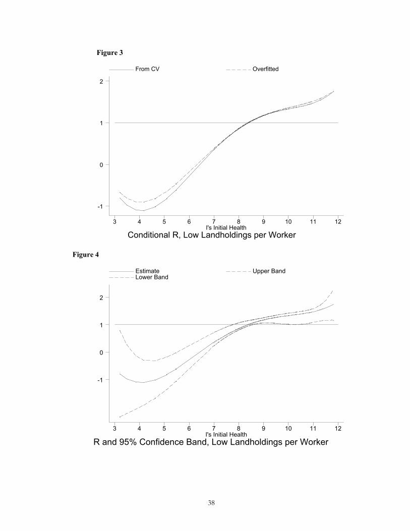
Figure 3 shows the estimate of ( )p h at mean ˆX � for this sub-sample. The

overfitted curve, also shown, is similar to that chosen by CV, but has a slightly lower slope.

22That is, as long as one trims with respect to hlthdif and eliminates at least a few of the outliers in R. 23 This result appears to somewhat contradict the first stage results, wherein initial dispersion is lowered by bothfem. A more complicated gender-based model (beyond the scope of this paper) may be able to explain why.

27

Figure 4 shows the estimate and 95 % confidence band. Clearly, the null that ˆ

0ph�

��

is

rejected. The estimated curve is mainly upward sloping, and one cannot reject that

ˆ0p

h�

��

everywhere (Hypothesis A.) Moreover, estimated R is for the most part less than or

equal to 1. Thus, the estimate of ( )p h provides no evidence that productivity concerns

affect the household’s intertemporal allocation of health goods. It appears that households do

respond, however, to equalizing preferences in allocating health goods within the household.

At the same time, the coefficient on hlthdif is positive and statistically significant, which

would not be the case under Hypothesis A. Thus, if evidence is found of a convex

consumption-productivity relationship in the other sub-sample, we may conclude that

productivity issues are important for this sub-sample as well, even if equality concerns

dominate for the shape of ˆ ( ).p h

I next estimate (16) for the “high” Landpbig households. The first stage equations

are shown in Table 3, Column 2. The effects of cold and flood on health are the same as in

the low land sub-sample. Greater height, higher total assets, and greater Landpbig are all

positively related to health. Here, having a pregnant household member is positively related

to health, as is having the other (i-1) individual be a farmer. The presence of a chronic

condition in the pair is negatively related to individual i’s initial health. Turning to initial

dispersion (hlthdif), greater height on the part of individual i increases this dispersion, as

expected. So do rainfall problems, the presence of a chronic condition, and having a pregnant

household member. In addition, initial dispersion in health was greater in Round 1, when

times were relatively bad. Once again sex and age matter in a complicated way through their

interaction terms.

28

The second stage coefficients of interest are shown in Table 4. As shown, cold

temperatures reduced R, (again perhaps due to the effect on disease transmission). In

addition, age of the individual i is negatively related to R (with age and age squared being

jointly significant), which would be consistent with older people being relatively less

productive. The presence of a chronic condition for the lower health individual made

equalization more unlikely, as would be expected if improving these peoples’ health is

relatively more costly. Table 4 also shows that movement towards greater equality was

greatest on average following Round 1, when initial dispersion was greatest and health was

poorest.24 Therefore, it appears that households were able to improve subsequent health by

allocating resources to less healthy individuals. Finally, the coefficients on the gender

variables defy a simple gender (anti-female) discrimination story: Having the better health

individual be male reduced R, while having both persons be female increased it.

The curve chosen by CV and the overfitted curve are shown in Figure 5, and the

estimate plus 95 % confidence band are shown in Figure 6. CV chooses a downward sloping

line, and once again the null hypothesis that ˆ

0ph�

��

can be rejected at the 5 percent level.

CV chose a quadratic in res and a cubic in resdif, so the endogeneity correction is once again

significant.

The downward sloping shapes shown in Figures 4-5, combined with the significant

portion for which [ ] 1E R � , lead to a rejection of the null of Hypothesis A for this group and

provide evidence of a convexity in the consumption-productivity relationship. Moreover, the

range spanned by R (from .27 to 2.5) is substantial. Thus households with moderate to high

landholdings per person allocated resources in a manner consistent with strong productivity

24Round-village effects were significant (and included) only for Round 1.

29

incentives, investing relatively more in the healthier individual than would be the case absent

such concerns.

For both groups, results (Figures 4 and 6) show that households invest differentially

in individuals according to their current health status, even when controlling for observable

characteristics which can affect productivity and health. Equalizing incentives are in

evidence particularly for low landholding households. However, given the findings for the

high landholding group and the coefficient on hlthdif (positive and statistically significant),

these households may also face a similar convexity in their consumption-productivity

relationship, which is nonetheless dominated by equality concerns.

Results using BMI I next re-estimate (16) using bmi to compare the results obtained for overall health to those for

nutritional status. Here it was necessary to drop individuals from age 16-19 to avoid

problems associated with differential growth patterns by gender.25 (This also reveals a

weakness of using this index as a health measure.) One could also normalize by the pooled

mean bmi by gender before ranking individuals’ health, since men in this age range tend to

have a higher bmi than women (with a 3-round pooled mean bmi of 20.05 versus 19.99 for

women). However, this is likely to also reflect the generally greater strength and work

capacity of males. So for this exercise I interpret this higher mean weight as better “health”

or work capacity, and do not normalize scores by their gender means.26

25When this group is included, females’ mean bmi is higher than males’. 26To obtain the sample, I trimmed the most extreme values obtained for body mass index in cases where the measured height or weight fluctuated unrealistically between rounds (9 observations out of 11 above 30). This was a general problem with these data, as heights for adults could vary from 50 to over 100 centimeters between rounds. This suggests either key coding errors or that different individuals presented themselves for measurement in different rounds. Where it was clear that a key coding error was present, I made the correction. Otherwise, I dropped the individual from the sample.

30

I first estimated (16) for the low Landpbig group. The first stage coefficients are

reported in Table 3, Column 3. Here, being a farmer reduces one’s body mass index,

presumably because of the physical labor involved. Having had too much rain lowered bmi

significantly but reduced initial dispersion. Landpbig shows a highly positive and statistically

significant coefficient for initial health, but raises the initial difference in bmi between the

individuals in the pair. The negative coefficient on chronic is what one would expect if these

individuals received less caloric investment relative to their i-1 counterpart.

The results for the second stage (which do not include a term in h) are shown in

Table 4, Column 3. The coefficient on hlthdif is negative and significant, as would be

predicted under Hypothesis A. In addition, having higher quality land increases target

inequality in bmi. Individual i’s being a farmer reduces this inequality, and her being female

increases it, which are not results that one would expect if one allocated net calories favoring

males, whether on the basis of productivity or simply gender preference. Farmers’ stores of

energy are drawn down over this period, due perhaps to the effect of greater caloric

expenditure, whereas females’ are increased, all else equal.

The results are similar for the high landholding sub-sample. Again, I cannot reject

the null that 0ph�

��

, and it appears that current nutritional status is not an important factor in

intra-household allocation of net caloric investment (all else equal). The coefficients for the

first stage are reported in Table 3, Column 4, and for the second in Table 4, Column 4.

These findings for bmi are consistent with those obtained by D&K (2000), who use

the same data to test whether unpredicted working days lost due to unexpected illness affect

subsequent changes in bmi. For most groups, they do not reject the null of no effect (i.e.,

In addition, I dropped observations for which hlthdif was less than .1 (numbering 17) or greater than 8 (14).

31

efficiency in their model of perfect risk sharing). According to the results obtained here,

households do not on average allocate net calories on the basis of initial bmi either (except

with regard to initial dispersion).27 These results do contrast somewhat with those of Pitt, et

al. (1990), however. Examining the intra-household allocation of net calories in Bangladesh,

they find that due to productivity complementarities with effort, people with intrinsically

higher weight-for-height are allocated more calories. But since these people also expend

more calories, they are in effect taxed to improve the nutritional status of others. Thus

equalization is preferred on average. In rural Ethiopia when nutritional status is measured as

bmi, however, initial bmi does not affect the subsequent allocation of calories. While farmers

(and possibly males) appear to be “taxed” in terms of net calories, on average equalization is

not preferred. Not only is ˆ ( )p h not increasing in bmi, but average R is not less than 1 (at

1.03).

6. Conclusion

The results of this paper lend support to a model of buffer health stocking with an important

equality-productivity tradeoff in the allocation of health investment, particularly for

households with relatively high landholdings per working age member. Under efficiency,

these households must weigh future productivity in their overall health investments. The

very desire to equalize health itself further reduces household income in the short run;

likewise, the desire to increase productivity will impede an ill-health person’s recovery.

Thus, the presence of a convexity in the consumption-productivity relationship means that

27The results for hlthhat may lead one to question one of D&K’s key identifying assumptions, however. As they point out, under optimality households must take account of productivity issues in their allocation of nutrition (or health status.) Here, even household (or village-) level shocks to health will affect individual productivity – and therefore the “user cost” of health – differently within the

32

adverse income and health shocks can reduce productivity for some time, possibly producing

a multiplicity of equilibria.

These results are based on a relatively short time frame, during which times were

initially difficult, albeit not disastrous for households possessing land, and then improved. In

times of greater distress or famine, the dynamics could be qualitatively different. Thus, a

longer panel would be needed to examine the extent to which the effects of poor health (or

income) shocks endure, particularly following a famine. As suggested by earlier work, such

downturns may have much more persistent effects on the long term health and work capacity

of children.

Finally, these results emphasize the importance of moving beyond pure body-mass -

based measures of health status if important dynamics are to be identified. Conducting the

test proposed here using such a measure would obscure important dynamics in the

relationship between consumption and productivity. These were uncovered in these data only

when a broader measure of health status was used.

household due to the non-linearities in ( )y g� . This may not be the case with nutrition, however. D&K must assume not for their test to be valid.

33

Table 1: Task Measures by Sex, Working Age (Pooled)

Male

Mean

St. Dev.

Female

Mean

Std. Dev.

Stand Up 3.957 .2739 3.924 .3555

Sweep 3.955 .3017 3.927 .3769

Walk 3.947 .3412 3.867 .5137

Carry

Hoe

3.889

3.886

.4901

.5061

3.753

3.506

.7057

.9874

Table 2: Distribution of Hlthindx, Hlthhat Hlthindx Full

Sample (1)

(%) Hlthhat Full

(3)

(%) Used

(%)

1 30 (.29) 0-1 13 (.17) 0 (0) 2 18 (.18) 1-2 60 (.76) 0 (0) 3 30 (.30) 2-3 159 (2.02) 0 (0) 4 34 (.33) 3-4 281 (3.58) 15 (1.04) 5 25 (.25) 4-5 418 (5.23) 40 (2.77) 6 44 (.43) 5-6 428 (5.45) 63 (4.36) 7 68 (.67) 6-7 43 (.55) 2 (.14) 8 68 (.67) 7-8 1242 (15.81) 204 (14.13) 9 62 (.61) 8-9 2378 (30.27) 548 (37.95)

10 123 (1.21) 9-10 1886 (24.01) 386 (26.73) 11 159 (1.56) 10-11 803 (10.26) 158 (10.94) 12 132 (1.29) 11-12 125 (1.59) 28 (1.94) 13 366 (3.59) 12-13 4 (.05) 0 (0) 14 221 (2.17) 13-14 4 (.05) 0 (0) 15 331 (3.25) 14-15 6 (.08) 0 (0) 16 8475 (83.20) 15-16 1 (.01) 0 (0)

10186

16-17 1

7855

(.01) 0

1444

(0)

34

Table 3: First Step Estimates (Robust Standard Errors in Parentheses) Measure: Hlthhat Low land

(1) Hlthhat High land

(2) Bmi Low land

(3) Bmi High Land

(4) i

rh 1i i

r rh h �

� irh

1i ir rh h �

�

irh

1i ir rh h �

� irh

1i ir rh h �

�

Totasset

-- -- .00001**(.00000)

.0001* (.0001)

-- -.00007** (.00002)/

-- .000024(.000016)

SalVal -- -- -- -- -- -.00001 (6.61e-6)

-- --

Height 2.75** (.347)

.608 (.508)

3.56** (.360)

1.26** (.638)

-- -- -- --

Too much -- -- --

-- -.705** (.223)

-.368** (.160)

-- .318 (.206)

Landpbig

-- --

.0038**(.0013)

-- 34.43**(16.05)

23.39* (13.15)

-- --

Rainprob -- .099** (.031)

-- .146** (.066)

-- -- -- .276 (.224)

Cold .621** (.112)

.659** (.216)

-- -- -- 1.37** (.584)

--

Flood -.279** (.119)

-.344* (.174)

-.312** (.108)

-- .451 (.278)

-- -1.03** (.354)

--

Pests

-- .216* (.126)

--

-- -- -- -- --

PcLem --

-- -- -.161 (.123)

-- -- -- -.640** (.219)

Preghhm -.121* (.064)

.143 (.089)

.149** (.061)

.188* (.111)

-- -- -- --

R1 --

--

-- .259** (.096)

-2.95** (.604)

-- -4.16** (.468)

--

Age .040** (.013)

.020** (.007)

-.049** (.004)

.025** (.007)

-.0097 (.0078)

-- .126** (.046)

.109** (.039)

Age2 -.0016** (.000)

.0009** (.0003)

-- -- -.0014**(.0005)

-- -.0016**(.0006)

-.001** (.0005)

Age 1i � --

-.028 (.019)

-- -.027 (.020)

.100** (.043)

-- .073* (.042)

.051 (.035

Age 1i � 2 --

.001** (.0002)

-- .0010**(.0003)

-.0015**(.0005)

-- -.001** (.0005)

-.0007 (.0004)

35

Male .365** (.164)

-- --

-- -- -- -- --

Bothfem

--

-1.25** (.210)

.371** (.129)

-.436* (.242)

-- -- -- --

Male*age .020** (.006)

-.025** (.012)

.068** (.007)

.004 (.014)

-- -.016** (.004)

-.055** (.019)

-.007* (.004)

Male*agei-1 --

-.012 (.011)

-.011* (.006)

-.031** (.005)

-- -- -- .0094 (.0065)

Male*age2 --

-.0004 (.0002)

-.0009**(.0001)

-.0007**(.0002)

-- -- .0007* (.0004)

--

Male*agei-12 --

-.0004** (.0002)

.0002**(.0001)

-.031** (.005)

-- -- -- --

Farmer .204** (.078)

.217* (.114)

-- .360** (.147)

-.725** (.218)

-- -- --

Farmeri-1 --

-.254 (.161)

.269** (.102)

.413** (.182)

-- -.371** (.146)

-.617** (.210)

-.914** (.281)

Head --

.378** (.136)

-- -- .806** (.269)

.946** (.206)

-- --

Headi-1 --

.326** (.136)

-- -- .788** (.255)

.772** (.182)

-- --

Totsmall .103** (.016)

-- -- -- .075* (.044)

-- .173** (.045)

--

Chronic -.185** (.086)

-- -.187** (.079)

.251* (.141)

-.395* (.232)

-.364** (.178)

.348 (.231)

--

Chronic 1i � -.184** (.074)

.444** (.098)

-.183** (.066)

.647** (.114)

-- -- -- --

Trampled --

-.321** (.153)

-- -- -- -- -- --

R2

.7526 .2830 .8225 .3138 .3348 .1343 .3203 .1942

N 843 843 601

601 669 669 468 468

Notes: Round interacted with village for a round included if jointly significant. Only individually significant ethnicity dummies included. *Significant at 10 percent. **Significant at 5 percent.

36

Table 4: Best Semi-Parametric Instrumental Variables Results for Equation (16) (Adjusted, White-Corrected Standard Errors in Parentheses)

Measure: Hlthhat Low Land (1)

Hlthhat High Land (2)

Bmi Low Land (3)

Bmi High Land (4)

2 3 4

/ / /i i i ir r r rh h h h

-7.74(4.74)/ 1.70*(.971)/ -.148*(.085)/ .0045*(.0027)

-.272**(.0996) -- -- --

-- --

1i ir rh h �

� .1038*(.058) .201** (.076)

-.285* (.155)

-.540** (.134)

Resdif Res i

-.608**/.105**

-.301**/.128**

-.618**/.049*

.311 / -.043 /- .014

.006/.044**

--

.228*/.177**/-.019**

--

SalVal

1.56xe-7** (6.99 xe-8)

--

-- .00001** (4.98e-6)

Totasset -- -- -- .0003**

(9.23e-6)

PcLem -- -- .358** (.176)

--

Cold -- -.364** (.132)

-- --

Age/agesq -- -.0237(.027)/-.0006(.0004)

-- -.015** (.007)

Round 1 -- -1.32** (.236)

-- --

Male -- -.769** (.306)

-.437* (.248)

--

Both Female .486** (.165)

.292 (.199)

-- .457 (.354)

Farmer -- -- -.470** (.225)

--

Farmeri-1 -- -- -- -.445** (.216)

Femhead -.813**

(.309) -.319 (.229)

-- -.445** (.216)

Totsmal

-- -.0388 (.0245)

-- --

Chronic -- -- -- .432** (.201)

Chronici-1 -- -.365** .282 --

37

(.146)

(.181)

Male*age -.002 .052** (.010)

.0087 (.0058)

--

Male*agei-1 -- -- -.006 (.004)

.040** (.014)

Male*agei-12 -- -- -- -.00047**

(.0002)

Illdth -- -- .161 (107)

--

N 843 610 669 468 See Notes, Table 3.

37

Figure 1

Hypothesis A

h y

( )f g�

( )y g�

g� g�

Figure 2

Hypothesis B

jh

1jh �

( )f g� ( )y g�

ih

1ih �

i-1 i j-1 j g� 1i � i 1j � j 1( (1 ))f h ��

�

38

Figure 3

Conditional R, Low Landholdings per WorkerI's Initial Health

From CV Overfitted

3 4 5 6 7 8 9 10 11 12

-1

0

1

2

Figure 4

R and 95% Confidence Band, Low Landholdings per WorkerI's Initial Health

Estimate Upper Band Lower Band

3 4 5 6 7 8 9 10 11 12

-1

0

1

2

39

Figure 5

Conditional R, High Landholdings per WorkerI's Initial Health

Estimate Overfitted

3 4 5 6 7 8 9 10 11 12

0

.5

1

1.5

2

2.5

3

Figure 6

R and 95% Confidence Band, High Landholdings per WorkerI's Initial Health

Estimate Upper Band Lower Band

3 4 5 6 7 8 9 10 11 12

0

.5

1

1.5

2

2.5

3

40

APPENDIX 1

Proof of Proposition 1.

First, note that according to standard results in Deaton (1991), given our assumptions on the

utility function (6), we know that:

(a) 0Vh

��

� and

2

2 0Vh

��

� .

We know also from (11) that V uh h

� ��

� � for all h . Thus, from (10 (a), we have that:

(b) 1 1t t

i i i it t t t

V Vu uh h h h� �

� �� �� � �

� � � �, which implies that

(c) 1 1 1 1 1 11 1

1 1 1 1

(1 ) (1 )t t t t t tt ti i i i

t t t t t t

V y V V y VE EX h h X h h

� �� � � � � �

� �

� � � �

� � � �� � � � � �� � � � �� � � �

� � � � � � .

Since 1 11

t ti it t

y yh h

� �

�

� ��

� � and 1

1

tt

t

VEh

�

�

�

� is monotonically decreasing in 1t tE h

�, there are two

possibilities. First, it could be the case that 11 1

i it t t tE h E h�

� �� . It must follow from this that

1i it tg g �

� . Alternatively, if 11 1

i it t t tE h E h�

� �� , and if 1i i

t t

f fg g �

� ��

� �� �then from (9) it must be the

case that 1i it tg g �

� . If 1i it t

f fg g �

� ��

� �� �, then it follows directly that 1i i

t tg g �

� . It follows from

1i it tg g �

� and the concavity of ( )f g� that 1

1 11 1

i it t

t i it t

h hEh h

�

� �

�

� ���� �

�� �.

Proof of Proposition 2:

Suppose that there are some individuals i,j such that j it th h� and their nearest neighbors in

the health distribution, i-1, j-1, are such that 1 1j j i it t t th h h h� �

� � � . Suppose that the

41

household wishes to set 1 1

1 1 1 11 1

j j i it t t t

t tj j i it t t t

h h h hE Eh h h h

� �

� � � �

� �

� � � �� ��� � � �

� �� � � �. This would imply that

1 1j j i ig g g g� �

� � � . Given proposition 1, we know that 1 1j j i ig g g g� �

� � � . These

conditions combined plus the concavity of the utility function imply

1 1'( ) '( ) '( ) '( ).j j i iu g u g u g u g� �

� � � This can be rewritten as

1 1'( ) '( ) '( ) '( ).j j i iu g u g u g u g� �

� � � From Equation (9) this implies that

1 11 11 11 1j j i i

t tt tj j i ih h h h

f f f fEV EV EV EVg g g g� �

� �� �� �

� � � �� � �

� � � �� � � �. As long as the household does not

wish to change the order of the health rankings, this violates the joint concavity of ( )f g� and

(., )V h . Thus, a contradiction arises, and it must be the case that the household wishes to set

1 11 1 1 1

1 1

j j i it t t t

t tj j i it t t t

h h h hE Eh h h h

� �

� � � �

� �

� � � �� ��� � � �

� �� � � �.

42

APPENDIX 2

The general form of the ordered model is well known. A latent continuous variable for

health, *h is assumed to underlie the discrete ordered measure, and the goal here is to

estimate the threshold points which determine the latent variable’s assignment to the discrete

values. For example, for which hlthindx=j where *1j jh� ��

� � . The estimated threshold

points are taken as estimates of the “true” distance between (upper) values for hlthindx. I

estimate the following model by ordered probit:

i i it t thlthindx W u� �� � � ,

where u and W are assumed to be independent. I use the pooled (3 rounds of) data for all

individuals from 16 to 64 for whom the data were complete. TheW variables were height (a

long run measure of health, age, age squared, sex, sex interacted with age, and this variable

squared, whether the individual was mainly engaged in farm work, the household’s

landholdings per working age person, the fraction of landholdings of highest quality, the

number of individuals having died of illness in the previous 5 years, the total number of

teenage and adult persons, the total number of children, the time it takes to collect water, the

total value of household assets as of Round 1, the education of the household head, dummy

variables for whether there was too little rain in the last main harvest season, whether there

was too much, whether the rains stopped late, and an index of other rainfall problems. In

addition, I included a set of dummies for other harvest related events, such as flooding, cold

temperatures, and insect infestation, and Round-village dummies for all village-round

combinations. There were 9298 observations, and the estimation had a Likelihood Ratio of

2106. The measures as constructed according to equation (12) (and transformed linearly by

multiplying by 2 and adding 4.148) produced values that preserved the original rankings,

43

except for where hlthindx=1 and hlthindx=16. The coefficients and threshold values are as

shown in Table A.

Table A: Results of Ordered Probit Estimation of Hlthindx

Coefficients (s.e.) Cut Points (s.e.)

Toolittle -.252** (.078) -1.65 (.472)Toomuch -.180** (.073) -1.45 (.470)Stoplate -.116* (.060) -1.22 (.468)Rainprob .106** (.046) -1.04 (.467)Cold Temp .253* (.084) -.933 (.467)Wind/Storm .072 (.064) -.827 (.466)Flood -.235** (.073) -.662 (.466)Pests -.069 (.059) -.522 (.466)Insects .029 (.070) -.416 (.466)Trampling .105 (.068) -.247 (.466)Landpbig .0022 (.0018) -.055 (.466)PcLem -.0002 (.0003) .076 (.466)Totasset .00005** (.00002) .395 (.466)Illdth -.007 (.025) .551 (.466)Preghhm .024 (.038) .761 (.466)Eduhead .014 (.010)Farmer .089 (.066)Age -.002 (.009)Age2 -.0004** (.0001)Male -.011 (.258)Male*age .029* (.015)Male*age2 -.0004* (.0002)Totbig -.002 (.008)Totsmall .037** (.010)Height 1.87** (.199)N 9298

44

REFERENCES

Carroll, Christopher (1997). “Buffer Stock Saving and the Life-Cycle/Permanent Income Hypothesis,” Quarterly Journal of Economics, Vol. CXII, Issue 1.

Chiappori, Pierre-Andre (1992). “Collective Labor Supply and Welfare,” Journal of Political

Economy 100 (June): 437-67. Dasgupta, Partha and Debraj Ray (1986). “Inequality as a Determinant of Malnutrition and

Unemployment: Theory,” The Economic Journal, Vol. 96, no. 384, 1011-1034. Deaton, Angus (1991). “Savings with Liquidity Constraints,” Econometrica, Vol. 59, No. 5

(September), 1221-1248. Dercon, Stefan and Pramila Krishnan (2000), In Sickness and in Health: Risk Sharing within

Households in Rural Ethiopia, Journal of Political Economy, vol. 108 no. 4. Foster, Andrew and Mark R. Rosenzweig (1993). “Information Flows and Discrimination in

Labor Markets in Rural Areas in Developing Countries,” Proceedings of the World Bank Annual Conference on Development Economics, March 1993, pp. 173-204.

_________________________________(1994). “A Test for Moral Hazard in the Labor

Market: Effort, Health and Calorie Consumption,” Review of Economic Statistics, May, 76(2), pp. 213-27.

James, W. P. T., Ferro-Luzzi, Anna, and J.C. Waterlow (1988). “Definition of Chronic

Dietary Energy Deficiency in Adults: Report of a Working Party of the International Diety Energy Consultative Group.” European Journal of Clinical Nutrition 42 (December).

Leibenstein, Harvey (1975). Economic Backwardness and Economic Growth, New York:

Wiley. Newey, Whitney, J. Powell and F. Vella (1999). “Nonparametric Estimation of Triangular

Simultaneous Equations Models,” Econometrica, 67(3), 565-603.

Nyarko, Yaw and Lars Olson (1994). “Stockastic growth when utility depends on both consumption and the stock level,” Economic Theory 4, 791-797.

Osborne, Theresa (2002). “On the Dynamic Effects of Credit under Uncertainty,” mimeo. Pagan, Adrian and Aman Ullah (1999). Nonparametric economics. Cambridge: Cambridge

University Press. Pitt, Mark, M.R.Rosenzweig, and M. N. Hassan (1990). “Productivity, Health, and

Inequality in the Intrahousehold Distribution of Food in Low-Income Countries,” American Economic Review, December.

45

Ray, Debraj and Peter Streufert (1993), “Dynamic equilibria with unemployment due to undernourishment,” Economic Theory 3, pp. 61-85.

Smith, James P. (1999). “Healthy Bodies and Thick Wallets: The Dual Relation Between

Health and Economic Status,” Journal of Economic Perspectives – Volume 13, No. 2, pp. 145-166.

Stiglitz, Joseph E. (1976). “The efficiency wage hypothesis, surplus labor, and the

distribution of income in LDC’s,” Oxford Economic Papers, 28, 185-207. Strauss, John and D. Thomas (1998). “Health, Nutrition, and Economic Development,”

Journal of Economic Literature, Vol. 36 (2). Subramanian, Shankar and A. Deaton (1996). “The Demand for Food and Calories,” Journal

of Political Economy, 104, 133-62. Swamy, Anand (1997). “ A Simple Test of the Nutrition-Based Efficiency Wage Model,”

Journal of Development Economics, 53, 85-98. Townsend, Robert M. (1994). “Risk and Insurance in Village India,” Econometrica 62 (May),

539-91. Vella, Francis (1993). A Simple Estimator for Simultaneous Models with Censored

Endogenous Regressors. International Economic Review (May); 34(2): 441-57. Webb, Patrick, Joachim von Braun and Yisehac Yohannes (1992). “Famine in Ethiopia:

Policy Implications of Coping Failure at National and Household Levels.” IFPRI Research Report 92.