Paper ID #22186

Have You Seen an Integral? Visual, intuitive and Relevant Explanations ofBasic Engineering-related Mathematical Concepts

Dr. Daniel Raviv, Florida Atlantic University

Dr. Raviv is a Professor of Computer & Electrical Engineering and Computer Science at Florida AtlanticUniversity. In December 2009 he was named Assistant Provost for Innovation and Entrepreneurship.

With more than 25 years of combined experience in the high-tech industry, government and academiaDr. Raviv developed fundamentally different approaches to ”out-of-the-box” thinking and a breakthroughmethodology known as ”Eight Keys to Innovation.” He has been sharing his contributions with profession-als in businesses, academia and institutes nationally and internationally. Most recently he was a visitingprofessor at the University of Maryland (at Mtech, Maryland Technology Enterprise Institute) and at JohnsHopkins University (at the Center for Leadership Education) where he researched and delivered processesfor creative & innovative problem solving.

For his unique contributions he received the prestigious Distinguished Teacher of the Year Award, theFaculty Talon Award, the University Researcher of the Year AEA Abacus Award, and the President’sLeadership Award. Dr. Raviv has published in the areas of vision-based driverless cars, green innovation,and innovative thinking. He is a co-holder of a Guinness World Record. His new book is titled: ”EveryoneLoves Speed Bumps, Don’t You? A Guide to Innovative Thinking.”

Dr. Daniel Raviv received his Ph.D. degree from Case Western Reserve University in 1987 and M.Sc. andB.Sc. degrees from the Technion, Israel Institute of Technology in 1982 and 1980, respectively.

c©American Society for Engineering Education, 2018

Have you seen an integral?

Visual, intuitive and relevant explanations of basic engineering-related mathematical concepts

Daniel Raviv

Department of Computer & Electrical Engineering and Computer Science

Florida Atlantic University Email: ravivd@fau.edu

Abstract Today’s students are exposed to information presented in visual, intuitive and concise ways. They expect explanations for why a subject is important and relevant, as well as for its potential use. In order to adapt to students’ learning preferences and styles, efforts must be made to further modify teaching methods to include relevance of the material to daily life experiences. The material should also be presented in easy-to-comprehend, visual, and intuitive ways. This is most relevant in math courses that are usually taught with little or no connection to other disciplines, and in particular engineering.

This paper focuses on introducing basic math concepts by linking them to daily experiences using relevant analogy-based examples, to be introduced prior to delving into purely mathematical explanations and proofs. The paper shows tangible physical explanations of concepts in calculus, specifically on topics such as:

(a) Integration and differentiation. To explain these concepts, the paper uses several examples such as (1) relations between steering wheel angle of a car and the physical angle of the car in world coordinates, (2) relations between water flow and its accumulation in a container, (3) elevator directional motion, and (4) energy and its temporal rate-of-change during running, walking, sitting, and sleeping. It also shows some unexpected examples that relay to very basic daily observations such as the relation between moving shadows to differentiation and integration.

(b) First order differential equation and time constant of first order system. Based on accumulated teaching experience, some helpful examples are: (1) battery charging a mobile phone at different initial charging values, and (2) cooling rate of coffee. There are of course many other examples, but less related to students’ everyday experiences (e.g., radioactive decay and carbon dating). These ideas are shared so that instructors can use them to enhance understanding of engineering-related math concepts, and to show their relevance.

We refer to this approach as “work in progress.” When using the above examples (and many others), students have demonstrated better, clearer understanding of difficult concepts. Even though this was not an official assessment, based on similar experience that was gained and assessed by the author multiple times in other engineering related subjects (Control Systems, Digital Signal Processing, Computer Algorithms, and Physics), it is believed that the approach has a great potential.

1 Introduction

This paper introduces some ideas for explaining engineering-related mathematical concepts by linking them to daily experiences. The focus is on visual and intuitive experience-based explanations in calculus, i.e., integration and differentiation, as well as on first order differential equations. Concepts are connected by analogy to real-life examples (other than the most common textbook examples that relate to the “relations between position, velocity and acceleration,” “area under a graph,” and “slope of a function”). The examples are meant to provide additional material for introductory purposes only, to allow students to see the relevance of math to their daily life. The examples intentionally use almost no equations. The sets of multi-faceted concept-based examples that are illustrated in this paper are meant to allow learners to not only recognize and appreciate the relevance of calculus to everyday life, but also tap on different learning styles and keep learners engaged, thereby allowing for multiple and diverse ways of comprehension. It is important to emphasize that the material presented in this paper is meant to be add-ons to existing calculus textbooks, and that is not meant to suggest competition, modifications or replacement of existing textbooks. The material is referred to as work in progress and is to be shared and discussed with multiple audiences. When these and many other examples were used, students have demonstrated better, clearer understanding of difficult concepts, and praised the approach. Even though this was not an official assessment, based on similar experience that was gained and assessed by the author in other engineering and science related subjects (Control Systems, Digital Signal Processing, Computer Algorithms, and Physics), it is believed that the approach has a great potential. Students not only have commended the approach, but they have demonstrated its effectiveness.

The rational for this this work stems from observations that the current generation of students learn differently: less textbook-reliance, and more dependence on web-based explanations, such as short videos, animations, and demonstrations. When it comes to concept comprehension, students repeatedly miss the Aha! moment, and ask for more hands-on, experiential, visual, intuitive, fun (e.g., game-based), and tech-based, web-based information. This is not new. For example, Tyler DeWitt [1] recognized this problem and taught isotopes to high school students using analogy to similar cars with minor changes to illustrate that isotopes are basically the same atom, i.e., have the same number of protons and electrons with varying

number of neutrons. By focusing on calculus there are some books that include visual explanations (see for example references [2-10]). Of a special interest is the work by Apostol and Mamikon from Caltech [11,12]. They were able to explain integration of some functions without the need for mathematical formulas. The author of this paper published papers on this topic [13-20] in addition to books [21,22], one for understanding concepts in “Control Systems” and the other for understanding the basics of “Newton’s Laws of Motion.” The bigger picture

This work is part of a multi-modal integrated project aimed at understanding concepts in STEM. The approach is meant to help both teachers and students, thereby allowing for more innovative teaching and comprehension-based learning. The project is catered towards appealing to learners in visual, intuitive, and interactive/engaging means. It uses daily-life and life-relevant experiences, as well as different STEM/STEAM examples and activities. The project targets a broad understanding and appreciation of basic concepts in STEM, currently involving Physics/Mechanics, Calculus, Statics, Control Systems, Digital Signal Processing (DSP), Probability, Estimation, and Computer Algorithms. Though the material can be used by teachers and learners in classroom settings, it is primarily designed to (eventually) be web-based, targeting those who prefer self-paced self-learning friendly environments. Simply put, the project is principally designed for a learner-centered e-based environment, making it ready for large scale dissemination. Examples of calculus concepts that the author and his team plan to develop and integrate include: (a) games, (b) puzzles and teasers, (c) animations, (d) visual and intuitive daily-experiences-based examples, (e) movies and short video clips, (f) demonstrations, (g) hands-on activities (including those based on virtual reality and augmented reality), (h) teaming and communication exercises, (i) small-scale inquiry-based research, (j) presentations, and peer-based teaching/learning, (k) visual click-based e-book, (l) community and social engagement, and (m) challenges beyond the basics.

2 Calculus Examples

The following is a set of examples for visualizing integration and differentiation and the relations between them. The examples are related to: (1) Water flow, (2) Driving and boating, (3) Garbage can and landfill, (4) Elevator motion, (5) Relation between power and energy, (6) Weight gain and weight loss, (7) Toilet paper rate of use, (8) Moving shadows, (9) Relationship between velocity and distance, (10) Output angle and angular velocity of a DC motor, (11) Mechanical integration in real life, and (12) Devices for calculating integration of functions.

2.1 Water flow example

The following snap shots (Figure 1) show a process of pouring water at a constant rate into a glass. At a certain point in time (second image from left) water is poured until the glass becomes full (right image). The graph shows the accumulation of water in the cup as indicated by arrows.

Clearly constant flow results in linearly growing amount of accumulated water, or simply integration.

Figure 1: Pouring water at constant rate

A related example (Figure 2) that is easier (less messy) can also be demonstrated using grains of rice. It is different only in the sense that “it is not as continuous” as the earlier example with the water flow. However, it has a visual advantage since the accumulation of rice can be better seen.

.

Figure 2: Pouring rice grains at constant rate

For animation or virtual reality demonstration purposes, one can use the following illustration (Figure 3).

The water level in the container is the integration (up to a scale factor) of the water flow. Note that when the faucet is turned off (i.e., the case of zero flow), the water level is constant (which is the result of integrating “zero”).

Figure 3: Accumulated water as a function of time

The next natural step is to expand the example to multiple rates of pouring as shown in Figure 4.

Figure 4: Effect of pouring water at different rates as a function of time

2.2 Driving and boating examples

Here are two related examples (Figure 5): (1) the relations between the angle of the front wheels of a car (relative to the car) and the physical angle of the car in world coordinates: a constant non-zero angle of the wheels results in linear performance of the car’s angle (θ) in world coordinates; (2) the relations between the angle of the boat’s rudder (α) (relative to the boat) and the physical angle of the boat (θ) in world coordinates. In a steady state ideal motion, a constant non-zero α results in linear behavior of θ.

Figure 5: Integration effect in driving and boating

2.3 Garbage can and landfill examples

Depends on the group a-priori knowledge or the age level of the audience, it may sometimes be advantegous to start with simpler examples (Figures 6 and 7). Even though they do not show pure integration, they can be used to develop some intution. Familiar examples are paper garbage can and landfill. The added amount of garbage is not a continuous, but its accumulation gives an idea of the nature and meaning of integration.

Figure 6: Accumulation of paper in a can

Figure 7: Accumulation of garbage in a landfill as a function of time

2.4 Elevator example

Elevator location as function of time can be used as a basic example to intuitively explain the concept of derivative. Observe the following two displays (Figure 8): the one on the left communicates that the elevator is located at the fourth floor, but there is no indication of its next move, i.e., up or down. However, even though the right image also communicates that the elevator is located at the fourth floor, the down pointing arrow provides additional information indicating the direction of motion. It is clear from the right image that the elevator is now moving down, meaning that the people on the first floor receive the information about the change in the elevator location, and that it is more likely that it will get to the first floor earlier.

Figure 8: Display of elevator location and its direction of motion

Now imagine yourself standing at the fifth floor of a building waiting for one of two elevators to arrive. You try to figure out which one will reach your floor first. If the displays (Figure 9) for both elevators show the same floor location (left image), you know that both elevators are stationary at the third floor, and there is no way for you to intelligently guess the likelihood of earlier arrival of one of them. In the second case (second image from left) the elevators are still near the third floor but you can also tell that both are moving up: in this case, you not only know the elevators’ locations, but also the general change in their locations (i.e., the sign of the “derivative”). In this case both elevators are moving up toward your location. Since both arrows are pointing up, it still does not help you in estimating which one will reach the fifth floor faster. In the third scenario (third image from left), even though both elevators are located at the third floor, only the one on the right is moving (in this case, up), indicating that the likelihood that it will get to your floor faster is higher. In this case, the up-pointing arrow in the display of the right elevator (i.e., the sign of the “derivative”) can help you become “more optimistic” about the arrival time of the right elevator. In the last scenario (right image), you can tell that the left elevator is moving away from you (due to an undesired sign of the “derivative”). You hope that the right elevator will start to move up soon and reach your floor faster.

The change is key to your estimation!

Figure 9: Two elevators at the 3rd floor: which one is expected to arrive earlier to the 5th floor?

2.5 Power and energy example

The following shows integration and differentiation in familiar situations: energy and energy rate-of-change as a function of time (aka power) during running, walking, sitting, and sleeping. A person spends a lot of energy during jogging, less in walking, even less in sitting, and very small amount while sleeping.

Figure 10 shows both the cumulative lost calories, and the change (the derivative) of this function during the different activities.

Figure 10: Calories and calories rate-of-change as function of time during running, walking, sitting, and sleeping.

2.6 Weight gain and weight loss example

Another example that can help in understanding integration is related to weight gain and weight loss as visualized in Figure 11.

Figure 11: Weight gain and weight loss as a function of time

To go beyond simple constant changes, other examples can be used and discussed. Figure 12 is a visual story of a penguin that gained, lost, and gained weight again. Both the weight and its change (derivative) are shown as a function of time.

Figure 12: Visualizing integration and differentiation: a story telling approach

2.7 Toilet paper example

The rate of change in the length of toilet paper is perhaps among the most basic examples that anyone at any age can relate to. Although it can be argued that it does not represent pure integration or differentiation due to its actual non-continuous use, it is certainly a very intuitive and visual example (Figure 13).

Figure 13: Visualizing total length of toilet paper as a function of time

2.8 Moving shadows example

This example illustrates how observing shadow edges over time (due to sun rise in early morning) can lead to understanding of differentiation. More specifically, it shows what can be learned from rate of change in shadows’ edges about the relative lengths of the shadows themselves (and obviously about the height of the objects that cast the shadows) even without knowing the angle of the light source and without knowing the absolute length of the shadows!

Observe the next set of 6 video snapshots of shadows on a horizontal surface (Figure 14; left to right, 1st row first). From the first image of two invisible objects (located on the right of the shadows) it is clear that there is neither information about the total length of the shadows, nor about the height of the objects that cast them. The location of the light source is also unknown. Now observe the set of the shadows in each of the other 5 images over time. The 2nd top image shows the shadows, top one being a longer one. This image by itself still does not tell us about the relative lengths of the 2 shadows. However, one notices that in the 3rd through 6th figures as time goes by, the rate of change of the shadow edges is different. In fact, a closer look at these

edges shows a ratio of exactly 2:1, i.e. the top shadow edge moves twice as fast as the lower shadow edge.

Now that we understand the effect of time on the motion of the shadows, we can say something about the objects that cast the shadows. If both objects have sharp top edges, the ratio of their relative heights is also 2:1. We can claim this even without knowing the total length of the shadows and also without knowing the direction (angle) of the light source! Amazingly this is true regardless of the rate of change of the light source!

So here the relative derivative of functions (relative change over time in the location of the shadows’ edges) tells us about the relative nature of the function itself (length of shadow), even though it is not possible to see the whole length of the shadows.

Figure 14: Partial shadows of two masked objects

To make the point even clearer, let’s look at the next six images (Figure 15) from which the above shadows were obtained. Two objects with a height ratio of 2:1 cast not only 2:1 ratio of shadows (obvious) but also a 2:1 ratio in the shadow derivatives which can be seen by observing the shadow edges!

Figure 15: Unmasked objects of different heights and their corresponding shadows

In the following example (Figure 16), video snapshots of a banana and an orange were taken every 10 minutes.

We can tell that the change in shadow length over time is proportional to the shadow itself. (A clarifying note: in this case it is “almost correct” due to the different curvatures of the 2 objects [23].)

Figure 16: Shadow behavior for two different objects

2.9 Velocity and distance example

Obviously one cannot escape the classic textbook example of integration and differentiation, i.e., the one that relates speed and distance traveled. Here (Figure 17) it is shown, using a constant rate of pedaling and the related accumulated distance travelled by a bicycle, in order to make it a bit more intuitive and visual. Two simple bicycle pedaling cases are illustrated: constant low rpm and constant high rpm referring to the actual number of rotations of the wheel and the corresponding accumulated distance. It is clear that the slope of the distance graph is proportional to the speed of the wheel. From here it may be easier to expand and talk about a more general case when the velocity changes, i.e., when both the speed and heading vary over time.

Figure 17: Distance and speed: a twist to the classical textbook example

2.10 DC motor example (refer to Figure 18)

Figure 18: Input output view of a DC motor

It is possible to use physics-based equations to relate the input voltage to the DC motor, 𝑣𝑣𝑎𝑎, to the angular velocity, 𝜔𝜔, as well as to the angle θ of the motor shaft. Since 𝜔𝜔 = 𝑑𝑑𝑑𝑑

𝑑𝑑𝑑𝑑 it means that

the relationship at all times between 𝜔𝜔 and θ is differentiation or integration depends on how we look at it.

By plotting the input voltage V𝑎𝑎, and the outputs ω, and θ of the DC motor we get a clear visualization of integration and differentiation (Figure 19).

Figure 19: Relation between angular velocity and angular position of a DC motor

After transforming the equations to the s-domain and then to block diagram we obtain (Figure 20):

Figure 20: Integrator block diagram – DC motor

To complement the understanding of the DC motor example, it is desirable to explain that the angular velocities and the angular position are measurable quantities, for example, using tachometer and potentiometer (Figure 21).

Figure 21: Measurement devices for angular velocity and angular position

2.11 Mechanical integration in real life practical examples

“Distance measuring wheels,” aka “footage wheels” or “rolling tape measure” are used to measure distances. They give excellent approximations when building lots need to be measured, for estimating length of a fence, etc. Figure 22 shows one such device.

Figure 22: Image of rolling tape measurement device

The display indicates the distance traveled. For example, if the wheel rotates 3 turns, the distance of the wheel traveled is the 3 times the circumference of the wheel. Simply put, the device measures the number of rotations of the wheel times a scale factor (which is the circumference of

the wheel = 2πr, where r is the radius of the wheel). Another way of looking at it is that the device integrates the angular velocity (up to a scale factor). For example, if it rotates at a constant rate of 2π rad/sec (i.e., one rotation per second) starting at t=0 then the angle after t seconds will be 2πt radians, i.e., a linear function of time. This result, if multiplied by the radius of the wheel, is identical to the traveled distance. Note that the result is invariant to the velocity, i.e., it works for varying directions and speeds as illustrated below (Figure 23).

Figure 23: Rolling tape measurement device in action

2.12 Devices for calculating integration of functions Just to complete the picture we briefly discuss some mechanical devices and an electric circuit that integrate. From a student’s point of view, it might be fun to observe, understand and appreciate mechanisms of some devices that can actually “compute without using a digital computer.” (a) Ball-and-disk integrator (refer to Figure 24)

Figure 24: Ball and disk integrator (images source: Wikipedia)

Refer to the left image in Figure 24. y is the radial distance from the center of the disc to the point where the ball touches the disc) and is the real variable to be integrated (as a function of x). Assume that the thin shaft rotates at a constant rate, one miniscule (“infinitesimal”) increment dx at a time. Then for a given non-zero value of the distance y the ball will rotate continuously,

resulting in a rate-of-rotation (i.e., angular velocity) that is proportional to the value of the distance y. This means that for a constant value of y, the ball will rotate continuously at a constant rate, resulting in a continuous and constant rate-of-rotation of the cylinder (or in other words, the angle of shaft of the cylinder will grow linearly). Also, for larger values of y, the rate-of-rotation of the cylinder’s shaft will be higher, and for smaller values of y the rate-of-rotation will be lower. Changes in the value of y will result in different values of the rate-of-rotation of the shaft, practically integrating y (up to a scale factor). The angle of the cylinder is the integration of y, i.e., ∫ 𝑦𝑦 𝑑𝑑𝑑𝑑 (again, up to a scale factor). (b) Planimeter [24] (refer to Figure 25) Planimeter is a mechanical analog integrator that can measure the area of a 2d arbitrary shape by tracing its perimeter. There are several kinds of planimeters, with 2 main types of mechanical planimeters: polar and linear.

As an example, the polar type consists of a two-bar linkage, with a pointer at the end of one link used to trace around the boundary of the shape to be measured. Near the intersection of the two links is a rotating measuring wheel. The number of turns of the wheel is a scale factor of the measured area. Schematics of the 2 major types is shown below [25,26]:

Figure 25: Linear (left) and polar (right) planimeters

The figures show the idea behind the tracing mechanisms of the linear and the polar planimeters. The pointer M follows the contour C of the shape to be measured. The linear planimeter traces the area by translating the elbow about the y-axis. For the polar planimeter there are two links that allow for 2 degrees of freedom motion. Accumulated angle as measured by a rotating wheel (not shown) is proportional to the area of the shape to be measured.

(c) Tannery mechanical surface integrator (refer to Figure 26)

The TANNERY mechanical surface integrator measures the area of 2d shape by counting the accumulated number of pins that are pointing up over time during the motion of the surface through the machine. The following are snapshots from a YouTube video [27].

Figure 26: Snapshots from YouTube video of TANNARY mechanical surface integrator

(d) Integrating op-amp circuit

One of the simplest electronic circuits that can integrate uses op-amp with a resistor R at its input and a capacitor C in its feedback as shown in Figure 27 (along with the transfer function in the s-domain). The values of R and C determine the scale factor K of the integration.

Figure 27: Op-amp-based integration arrangement

Visual summary (Figure 28)

Figure 28: Visual “summary” of the relation between integration and differentiation

3 First Order Differential Equation examples

The following is a set of examples that shows first order systems and behaviors. We show only a few, but obviously there are many other examples from many disciplines. The examples are related to: (1) Cell phone battery, (2) Cooling rate of hot coffee, (3) Toilet mechanism, (4) Diffusion, (5) Car dynamics, and (6) Transient response of a DC motor.

3.1 Cell phone battery example

The voltage function during the battery charging process of a mobile phone is illustrated in Figure 29. It is basically a “resistor capacitor” (RC) circuit that can be described using first order differential equation.

Figure 29: Charging a mobile phone – first order system

Let’s observe (Figure 30) different initial charging values and at different stages of the battery’s life. Say someone wants to charge his or her phone in three phases, unplugging the charger and quickly plugging it back in, stopping at a certain time, say at the so called time constant τ, and its multiples, as depicted here. This is an experience-based example: We all know that cell phone charges faster in the beginning and slower later: the change (the derivative) is different at each point in time.

Figure 30: Charging mobile phone in three steps

The charging is broken down to three phases look like the following (Figure 31). Note the different derivatives of the graphs at different points in time: they are instants of exponentially decaying function.

Figure 31: Charging mobile phone in three steps

It should be noted that at any point in time the tangent line of the graph touches the line of the final value exactly τ seconds later. This property of a first order system was used by Mamikon and Apostol [11] to compute the area under the graph without using integration!

3.2 Coffee cooling example

Cooling rate of coffee is proportional to the difference between the coffee temperature and the room temperatures. The following is a brain teaser (followed by a solution) that can help in understanding the concept.

Puzzler

Question:

One day, two brothers had a dispute. The first brother, Joe, claimed that coffee stays hotter if one pours cold creamer ten minutes after initially pouring the coffee. The second brother, Moe, claimed that it would stay hotter after 10 minutes if cold creamer is added right away. Based on what you know about time constants: which brother is correct?

Answer:

Since the first cup of coffee starts at a hotter temperature, the initial slope is greater. This causes the temperature of the first cup to decay more rapidly. Therefore, when Joe adds the creamer to the first cup, the temperature spike drops it below the temperature of cup two. This makes Moe correct. Simply put, pouring cold creamer first and then waiting guarantees hotter coffee. This is depicted in the following qualitative graph.

Zooming in on the initial time:

3.3 Toilet mechanism example (refer to Figure 32)

Figure 32: Visualization of toilet mechanism – a mechanical first order system

The water level after flushing the toilet rises following a response that is very similar to a step response of first order system (i.e., the change in water level is proportional to the difference between the actual water level and the max water level, due to the continuous decrease in water flow through the valve).

3.4 Diffusion example

Diffusion occurs at an exponential rate. This is when molecules from a region of high concentration move to a region of lower concentration. It occurs naturally as molecules randomly bounce off each other, and they are more likely to fill open space then continue to bounce off each other in close quarters. For example, assume there are two compartments separated by a wall, one filled with gas molecules and the other is just a vacuum (Figure 33).

Figure 33: Diffusion: before and after

Several factors affect the diffusion process, including the initial concentration/pressure, the ongoing pressure difference between the two chambers, and the size of the opening. Eventually the concentrations of molecules in the two chambers will reach the same value (Figure 34). It happens at an exponentially decaying rate.

Figure 34: Diffusion: concentration as a function of time

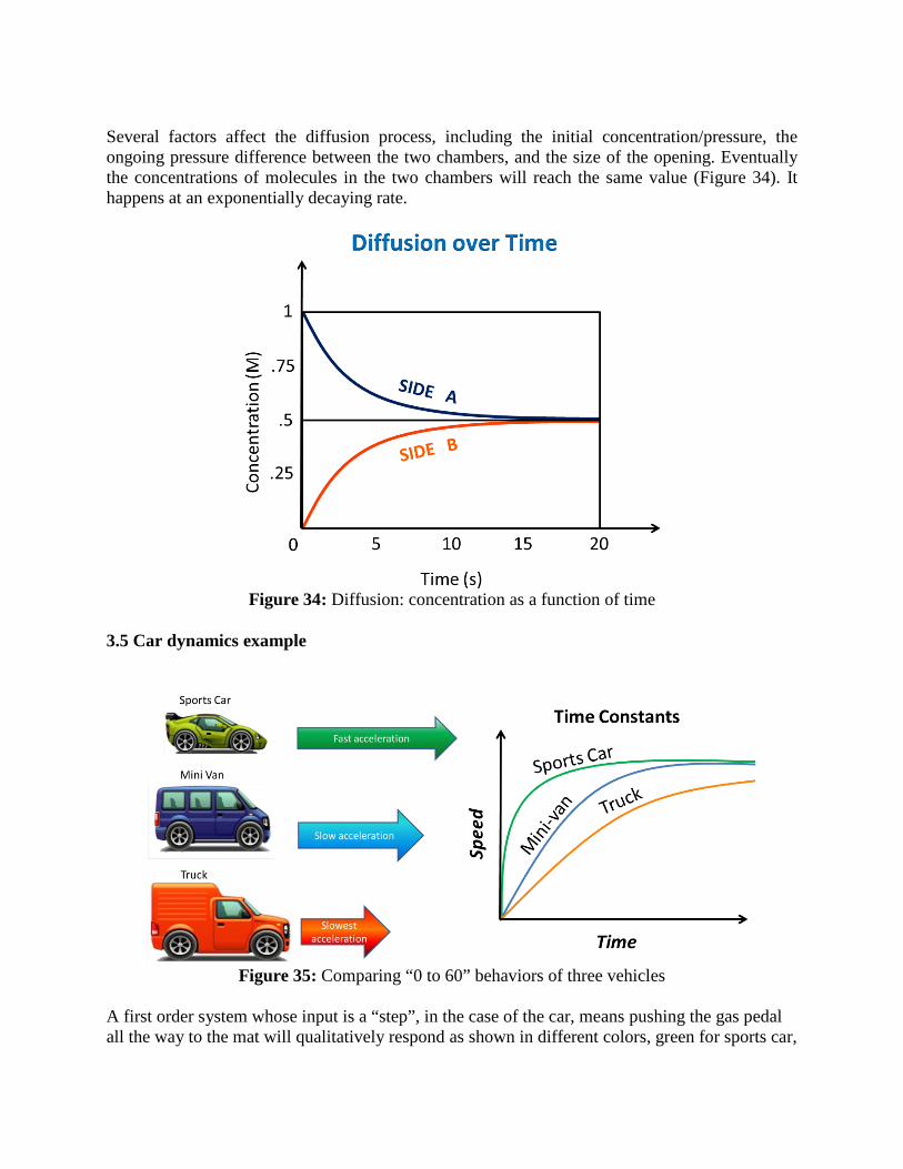
3.5 Car dynamics example

Figure 35: Comparing “0 to 60” behaviors of three vehicles

A first order system whose input is a “step”, in the case of the car, means pushing the gas pedal all the way to the mat will qualitatively respond as shown in different colors, green for sports car,

blue for mini-van and orange for truck. This is a behavior that is similar to a first order system (Figure 35).

3.6 DC motor example (refer to Figure 36)

A DC motor has a dominant (slow) time constant, aka the mechanical time constant. Because of this constant, the response to a step function can be approximated by a first order linear differential equation. (Note that the integration relation between ω and θ of a DC motor is always pure integration and is independent of the time constant.)

Figure 36: DC motor: effect of mechanical time constant

Refer to Figure 19. Note the angular speed 𝜔𝜔(𝑡𝑡) and the angular position 𝜃𝜃(𝑡𝑡) of the motor as a function of time. When an armature voltage is applied (as a step function), the angular speed, 𝜔𝜔(𝑡𝑡), first increases quickly then plateaus to a constant value. On the other hand, the angular position of the motors, 𝜃𝜃(𝑡𝑡), continues to increase. This makes sense because as the motor keeps spinning with a constant angular speed, the motor position will keep increasing as well.

Conclusion The illustrated sets of examples attempt to introduce basic math concepts, i.e., integration, differentiation and first order differential equation, by linking them to daily experiences using relevant analogy-based examples. The idea is to introduce math-less visual and intuitive examples so that students understand and comprehend basic concepts and their importance and relevance. It is important to emphasize that the material presented in this paper is meant to be add-ons to existing calculus textbooks, and is not meant to suggest competition, modifications or replacement of existing textbooks. The presented material is referred to as work in progress and can be shared and discussed with multiple audiences. We hope that the reader will use some of the examples, as well as suggesting new ideas and/or sharing his/her own.

Acknowledgements The author thanks Venturewell.org (formerly NCIIA.org), for the support of the development of innovative and entrepreneurial teaching and learning methods, and Michael R. Levine and Last Best Chance, LLC, for the continuous support. Special thanks to Professors Moshe Barak, Miri Barak, Nancy Romance, and Nahum Shimkin for the very fruitful discussions on enhancing the teaching and learning of concepts in STEM. Special thanks to George Roskovich and Pamela Noguera for providing some of the excellent illustrations. Moises Levy, Md Kabir, and the Center for Writing at Florida Atlantic University provided very valuable feedback as well. References [1] https://www.youtube.com/watch?v=EboWeWmh5Pg [2] Adams, Colin Conrad. Zombies & Calculus. State- Massachusetts: Princeton, 2014. Print. [3] Amdahl, Kenn, and Jim Loats. Calculus for Cats. Broomfield, CO: Clearwater Pub., 2001. Print. [4] Ghrist, Robert. Funny Little Calculus Text. U of Pennsylvania, 2012. Print. [5] Herge" The Calculus Affair: The Adventures of Tintin. London: Methuen Children's, 1992. Print. [6] Kelley, W. The Complete Idiot's Guide to Calculus, 2nd Edition. S.l.: DK, 2006. Print. [7] Pickover, Clifford A. Calculus and Pizza: A Cookbook for the Hungry Mind. Hoboken, NJ: John Wiley, 2003. [8] Averbach, Bonnie, and Orin Chein.Problem Solving through Recreational Mathematics. Mineola, N.Y.: Dover Publications, 2000. [9] Azad, Kalid. Math, Better Explained, 2014. [10] Fernandez, Oscar E. Everyday Calculus: Discovering the Hidden Math All around Us. Princeton: Princeton UP, 2014. [11] Tom Apostol, A Visual Approach to Calculus Problems, ENGINEERING & SCIENCE NO. 3, 2000 http://www.mamikon.com/VisualCalc.pdf

[12] www.mamikon.com [13] D. Raviv, P. Reyes and J. Baker, “A Comprehensive Step-by-Step Approach for Introducing Design of Control Systems,” ASEE National Conference, Columbus, Ohio, June 2017. [14] D. Raviv, and J. Jimenez, “A Visual, Intuitive, and Experienced-Based Approach to Explaining Stability of Control Systems,” ASEE National Conference, Columbus, Ohio, June 2017. [15] D. Raviv, L. Gloria, Using Puzzles for Teaching and Learning Concepts in Control Systems,” ASEE Conference, New Orleans, June 2016. [16] D. Raviv, P. Benedict Reyes, and G. Roskovich, A Visual and Intuitive Approach to Explaining Digitized Controllers,” ASEE Conference, New Orleans, June 2016. [17] D. Raviv and J. Ramirez, “Experience-Based Approach for Teaching and Learning Concepts in Digital Signal Processing,” ASEE National Conference, Seattle, WA, June 2015. [18] D.Raviv, Y. Nakagawa and G. Roskovich, “A Visual and Engaging Approach to Learning Computer Algorithms,” ASEE National Conference, Indianapolis, Indiana, June 2014. [19] D.Raviv and G. Roskovich, An intuitive approach to teaching key concepts in Control Systems, ASEE Conference, Indianapolis, Indiana, June 2014. [20] D.Raviv and G. Roskovich, “ An Alternative Method to Teaching Design of Control Systems,” LACCEI, Latin American and Caribbean Engineering Institutions, Guayaquil, Ecuador, July 22-24, 2014. [21] D. Raviv and Megan Geiger, Math-less Physics! A Visual Guide to Understanding Newton’s Laws of Motion, Create Space Publishers, 2016. [22] D. Raviv and George Roskovich, Understood! A Visual and Intuitive Approach to Teaching and Learning Control Systems: Part 1, Create Space Publishers, 2014.

[23] D. Raviv, Y.H.Pao and K.Loparo, “Reconstruction of three-dimensional surfaces from two-dimensional binary images,” IEEE Transactions on Robotics and Automation Volume: 5, Issue: 5, Oct 1989, Pp: 701 – 710.

[24] Tanya Leise, As the Planimeter’s Wheel Turns: Planimeter Proofs for Calculus Class, https://tleise.people.amherst.edu/HomePage/LeisePlanimeter.pdf, 2013

[25] https://en.wikipedia.org/wiki/Planimeter

[26] H. Shaw, Mechanical Integrators Including the Various Forms of Plnimeters, Reprinted from the Proceedings of the Institution of Civil Engineers, D. Van Nostrand

Publishers, New York, 1886. [27] https://www.youtube.com/watch?v=u3vHZqsY9Qg