HAS EGYPT’S MONETARY POLICY CHANGED AFTER THE FLOAT?

Hoda Selim

Working Paper 543

September 2010

I am very grateful to Dr. Alaa El-Shazly, professor of economics, at the Faculty of Economics and Political Science, Cairo University for help and substantive comments throughout the paper. I would also like to thank Dr. Tarek Moursi and Mai Mossallamy at the Faculty of Economics and Political Science, Cairo University for sharing their data on monthly output. Special thanks goes to Dr. Simon Naieme, discussant of the paper at the ERF conference as well as Dr. Bassem Kamar at the International Monetary Fund for productive discussions.

Send correspondence to: Hoda Selim The World Bank, Cairo, Egypt hselim@worldbank.org

First published in 2010 by The Economic Research Forum (ERF) 7 Boulos Hanna Street Dokki, Cairo Egypt www.erf.org.eg Copyright © The Economic Research Forum, 2010 All rights reserved. No part of this publication may be reproduced in any form or by any electronic or mechanical means, including information storage and retrieval systems, without permission in writing from the publisher. The findings, interpretations and conclusions expressed in this publication are entirely those of the author(s) and should not be attributed to the Economic Research Forum, members of its Board of Trustees, or its donors.

1

Abstract

After maintaining a currency peg to the US$ for more than 40 years, Egypt announced the float of its exchange rate in 2003. Yet, the somewhat stable exchange rate suggests that it continues to be managed by the Central Bank of Egypt. The objective of this paper is to assess whether monetary policy significantly changed after the float. It first applies cointegration methodology using monthly data from 1981 to 2008 to show that there is a long-run relationship between the LE/US$ exchange rate and monetary fundamentals. A vector error-correction model shows that the speed of exchange rate adjustment to long-run equilibrium is slow suggesting that exchange rate misalignments are persistent. The model also shows that there has not been a significant change in exchange rate determination after the float. Second, the paper attempted to provide a de facto classification for Egypt’s exchange rate regime and could not classify it as a float.

ملخص

ات سعر . 2003عام، أعلنت مصر تعويم الجنيه المصرى فى عام 40بعد المحافظة على نظام سعر الصرف الثابت لمدة وحى ثب د ي ق

ر . المرآزىالصرف منذ هذا التاريخ بأن ذلك نتاج تدخل البنك اك تغيي ان هن ا إذا آ ة م ى معرف ذا البحث إل وى ( ولذلك، يهدف ه معن

ويم ) إحصائيا د التع ة التكامل وبإستخدام . فى السياسة النقدية فى مصر بع ذا البحث من خالل منهجي ائج الجزء األول من ه تشير نت

ية إلى وجود عالقة ساآنة طويلة األجل بين 2008-1981بيانات شهرية للفترة ا . سعر الصرف والمتغيرات النقدية األساس تشير . آم

أن ) VEC( نتائج متجه تصحيح الخطأ وحى ب ا ي وازن مم ذا الت ه اذا انحرف عن ه ى مستوى توازن إلى بطء عودة سعر الصرف إل

د . اختالالت سعر الصرف مستمرة د سعر الصرف بع وى فى تحدي ويم آذلك يدلل النموذج على أنه ال يوجد اختالف معن الجزء . التع

اره نظام ذا النظام ال يمكن اعتب ى أن ه ى فى مصر ويخلص إل الثاني من هذا البحث يعد محاولة لتصنيف نظام سعر الصرف الفعل

".تعويم"

2

Introduction

Egypt’s exchange rate has been historically characterized by a large degree of rigidity, and only in January 2003 did the Central Bank of Egypt (CBE) announce a float of the Egyptian Pound (LE). This decision followed the persistence of pressures on the nominal exchange rate resulting from adverse external shocks and a domestic liquidity crunch. Although this move meant that the exchange rate should cease to be the explicit nominal anchor for monetary policy, there has been no announcement of any other. Even more, there is an increasing public perception that it remains an implicit target of monetary policy.

The aim of this paper is twofold. The first is to empirically assess whether there has been any significant change in exchange rate determination after the announcement of the float. The second is to provide a de facto classification for Egypt’s exchange rate regime. Both contributions were not addressed in previous empirical work. They are also timely since the CBE has announced in 2005 the move to an inflation targeting framework in the medium term.1 Should the CBE decide to move in this direction, exchange rate concerns should only be addressed if they are not in conflict with price stability.

To these ends, the paper undertakes an empirical investigation of the LE/US$ exchange rate behavior since the early eighties until the present. It applies cointegration methodology to test the long-run (flexible) monetary model of exchange rate determination for the LE/US$ exchange rate using monthly data from 1981 to 2008. A vector error-correction model (VECM) is also estimated to investigate the adjustment process to the long-run monetary equilibrium. The VECM is also used to test for significant change in exchange rate determination since the announcement of the float. The analysis shows the following. First, recent stability of the exchange rate has been achieved at the expense of large and sustained sterilization with possible implications on the inflation level. Second, cointegration analysis indicate that there exists a long-run stationary relationship between the LE/US$ exchange rate and monetary fundamentals. Third, the results of the VECM imply that when deviations from the long-run equilibrium occur, the exchange rate adjusts to restore long-run equilibrium. However, the speed of adjustment is very slow suggesting that shocks to the exchange rate are persistent. Fourth, there has not been any significant change in exchange rate determination after the float. Finally, Egypt?s de facto exchange rate regime cannot be classified as a float.

The paper is divided into four sections. The first section sketches some of the ideas that motivate the analysis on the absence of flexibility of the exchange rate. The second section presents the model and reviews previous empirical findings. The third section deals with data issues and presents estimation results for both the long and short-run dynamics of the relationship between the exchange rate and monetary fundamentals. It also tests for significant change in exchange rate determination associated with the announced float of the LE. The last section attempts to provide a de facto classification of Egypt’s exchange rate regime.

1. Long-Run Flexibility of the Exchange Rate Regime 1.1. Exchange rate trends Egypt maintained a peg of its currency to the US$ for over forty years (since the sixties until FY03). During this period, the exchange rate has been relatively stable over time, except for periods where devaluations occurred to reflect a more competitive value for the exchange rate (Figure 1). More accurately, it behaved like a “fixed adjustable peg”, regardless of its official classification. The nominal exchange rate also exhibited very limited volatility (a coefficient 1 Central Bank of Egypt 2005.

3

of variation of only 3 percent). After the float it declined to 2.8 percent from 3.6 percent before.

The announcement of the float in January 2003 was followed by a depreciation until October 2004 to LE/US$ 6.23 (by 15.6 percent). Since then and until August–08, the exchange rate continued to appreciate and reached LE/US$ 5.32. The substantial increases in foreign exchange earnings (increase in oil prices, Suez Canal revenues and surges in FDI inflows) led to an unprecedented accumulation of international reserves (from US$15 billion to US$35 billion) between FY05 and FY08. However, the LE/US$ has only nominally appreciated by 8.4 percent but at a much quicker pace in real terms, by about 14 percent. In the aftermath of the global crisis (between September–08 and March–09) and contrary to what happened in most emerging market economies (EMEs), the exchange rate fell by just 3.3 percent. This slight depreciation was surprising given the sharp fall in Egypt’s external demand on goods and services as well as the occurrence of a sudden stop in capital flows. In fact, portfolio outflows were significant (down by 5 percentage points of GDP), the stock market plunged by 63 percent and the foreigner’s holdings of T-Bills fell from LE 32 billion to LE 11 billion. Also, foreign direct investment inflows fell by more than 50 percent. The depreciation of the currency has been mitigated by central bank intervention in the foreign exchange market. And starting March–09 until May–09, the exchange rate stabilized at LE/US$ 5.62 and started appreciating afterwards. Moreover, official international reserves which continued to accumulate (although marginally) until October–08 started to decline afterwards, though slightly (by 8 percent between October and March 2009) and stood at US$ 31.3 billion in June–08 (down by almost US$ 3 billion).

Because the lack of exchange rate volatility between FY05 and FY08 could equally reflect an absence of shocks or an active intervention policy, the next section respectively looks at the behavior of Egypt’s other exchange rates and the following one examines the impact of CBE sterilized intervention policy on the exchange rate.

1.2. Egypt’s other exchange rates An exchange rate target implies that the domestic currency is fixed to some anchor currency and this makes it normal for this local currency to follow the same movements of the anchor currency vis-à-vis other currencies.

With the adoption of the Economic Reform and Structural Adjustment Program (ERSAP), the LE became officially pegged to the US$ in one unified market. Figure 2(a) below shows that, between FY96 and mid-FY03 (the date of the announcement of the float), the exchange rate of the LE/GBP followed the same movements as that of the US$ against the GBP. The same thing can be noticed with respect to the movement of the LE/Euro exchange rate against the movement of the US$/Euro (Figure 2b).

Figures for the post-float years show that the exchange rate of the LE vis-à-vis the British Pound (GBP) and the Euro have been reflecting the movements of these currencies vis-à-vis the US$. Figure 3(a) shows a quasi stable rate of the LE to the US$ but that the rate of LE/GBP has been following the same movements of the rate of the US$/GBP. Figure 3(b) shows the same thing for the Euro. When the US$/GBP exchange rate appreciates the LE/GBP also appreciates and vice versa. These observations indicate that despite the announcement of the float, the LE does not have independent movements against the GBP and the Euro and that these movements mimic the movements of the US$ against these currencies, suggesting that the LE remains pegged to the US$.

1.3. Reserve accumulation, sterilized intervention and the exchange rate The de jure float allows the CBE to intervene in the foreign exchange market only to counter major imbalances and sharp swings in the exchange rate. However, the stability of the

4

exchange rate raises the question whether it is the outcome of sustained intervention to resist appreciation.

In fact, to prevent exchange rate appreciation, the monetary authorities may engage in sterilized intervention to prevent overshooting while keeping inflation low. Foreign exchange assets are purchased with LE-denominated currency, with a countervailing sale of LE bonds to absorb the addition in the domestic money supply. This operation would only alter the relative supplies of available LE and dollar assets but would have a neutral impact on domestic interest rate, money supply and inflation. One simple way to know if sterilization operations have been taking place is to look at the balance sheet of the central bank. On the liability side, there is reserve money (comprising both currency in circulation and reserve deposits of commercial banks) and on the asset side, there are Net Foreign Assets (NFA) (official reserves) and Net Domestic Assets (NDA) (dominated by government securities). At all times, any change in reserve money must be reflected in changes in NDA or NFA. Sterilization essentially consists of the central bank offsetting changes in NFA (reserve accumulation) by either changing NDA (selling bonds) or adjusting its reserve deposits. Open Market Operations is a common sterilization technique that consists of the central bank selling bonds to commercial banks or to the public to reduce the liquidity in foreign-currency denominated assets. However, broader sterilization measures are approximated by the following ratios:

NFANDARD ΔΔ−Δ /)( or NFACCNFA ΔΔ−Δ /)( 2

Typically, these ratios are between 0 (no sterilization) and 1 (complete sterilization). The purpose of this section is thus to examine recent trends in sterilized intervention in Egypt, to determine its size and possible impact on inflation.

As mentioned in the previous section, the Egyptian economy benefited from significant capital inflows during the period FY05-FY08, allowing the CBE to accumulate US$ 19.7 in international reserves from US$14.7 billion in June-04 to US$34.6 in June-08. Meanwhile, the CBE’s balance sheet shows that NFA started to accumulate significantly since FY05 (when they posted a triple digit growth) and started to exceed NDA since FY06. Meanwhile, open market operations surged from -1.5 percent of GDP in FY03 to -20.4 percent of GDP in FY08. Sterilization operations in the foreign exchange market were estimated at an annual cost close to 1 percent of GDP in 2007 IMF (2007). We also calculate the sterilization measures explained above.

Following the dramatic increase in the change of net foreign assets since FY05 (5.1 percent of GDP), the pace of CBE sterilization activities picked up to reach 71.5 percent of the change in net foreign assets (Figure 4). These trends continued until FY08 with the CBE sterilizing between 53 and 77 percent of its net foreign assets growth and with sterilization being the highest in FY08 (Figure 5). As ratios to GDP, sterilization operations also increased from 2 percent of GDP in 2006 to almost 7.4 percent in 2008.

Over the whole period FY05-FY08, the CBE accumulated 16 percent of GDP in net foreign assets, but it offset about 69 percent of this amount with sterilization operations. This situation is very comparable to the period FY91-FY97 when the exchange rate was officially pegged.

Part of the sterilization occurred largely via the banking sector, which became flooded with sterilization debt. Indeed, T-Bills holdings of the banking sector drastically increased from 56.5 percent of total holdings in June-05 to 68.3 percent in June-08, reaching more than 80 percent in some instances.

2 Lavigne (2008) and Mohanty and Turner (2006)

5

However, if the sterilization of capital inflows is not complete and the appreciation pressures persist, liquidity can become excessive and may translate into money growth and inflation. A simple way to know if sterilization operations were sufficient or not is to look at a central bank’s operating target. When the latter is explicit, excess day-to-day liquidity (arising from inadequate sterilization) would allow the relevant market interest rate to fall and stay below the targeted level. Egypt is thus a difficult case to interpret because the CBE’s operating targets (short-term interest rates) are not explicitly stated. Nevertheless, a good indication would be to look at the growth rate of reserve money against that of net foreign assets (Figure 6). Up until January-05, reserve money growth had outpaced NFA growth. Afterwards, reserve money growth began to lag behind NFA growth since mid-FY05 until FY08, suggestive of a conscious effort to control liquidity associated with foreign exchange purchases.

More generally, there was a clear acceleration in M1 growth starting in 2003 and 2004 to 12 percent and 15 percent, a rate that was already inconsistent with price stability. The situation was worse in 2006, when it increased to 20 percent and close to 35 percent in 2008. M2 growth also peaked to 24 percent and most of this growth was accounted for through the expansion in NFA.

Also, inflation which remained high since FY04, had three spikes to the double-digit levels. Inflation first rose from 3.2 percent in FY03 to an average close to 20 percent in FY04 and mid FY05 to reflect lagged pass-through pressures. It picked up and remained in the double-digit level since FY07 and was propelled to the mid-twenties range in mid-2008 following the food crisis. Such high inflation was not the case for other economies, even those where the share of food in the overall basket of consumption is as high as Egypt3. Despite the reserve accumulation, increasing monetary expansion and rising inflation, the exchange rate remained surprisingly stable (Figure 7).

Moreover, the inflation and exchange rate objectives became in conflict with the inflation shocks since FY07. Higher interest rates, which were necessary to control inflation, sustained the reserve accumulation and exacerbated the upward pressure on the exchange rate. Monetary policy tightening led to a vicious circle through which higher interest rates continued to attract foreign inflows, which exerted pressure on the exchange rate, thus forcing the CBE to resist such pressures. And as foreign inflows remained partially unsterilized, they fuelled monetary growth and inflation, which required further policy tightening.

This section has shown that despite the announced float, the official exchange rate continued to be rigid. The analysis has also presented some preliminary evidence suggesting that the exchange rate continues to be managed. Recent movements of the LE/GBP and LE/Euro still mirror the movements of the exchange rate of these respective currencies with respect to the US$. Significant capital inflows since FY05 led to a huge reserve accumulation and to pressure on the exchange rate. However, as reserve accumulation was of a large scale and persistent, sterilization operations were insufficient and the unsterilized capital inflows contributed to money growth and exacerbated inflation. Monetary policy tightening, necessary to curb inflationary pressures, sustained the reserve accumulation and the pressure on the exchange rate, which was not subject to any significant movements.

There is one caveat to this analysis. The absence of explicit targets (both for inflation and the interest rate) makes it difficult to judge conclusively whether efforts to resist currency appreciation were fully responsible for the rise in inflation. High inflation could be the

3 Emerging economies such as Guatemala, Honduras, Nigeria, Lithuania, Indonesia or Armenia, saw inflation increase to 15 percent.

6

outcome of many factors and not only the rigidity of the exchange rate such as excess demand pressures, the fiscal stance and a looser-than-warranted monetary stance. But had the exchange rate been more flexible and able to adjust to external shocks, would inflation have remained high since 2004 and would it have risen to the mid-twenty range and persisted in the double-digit level?

2. The Monetary Approach to Exchange Rate Determination The theory of exchange rate determination was introduced in the middle of the last century. Ever since, many models have been developed including the monetary model, the portfolio balance, and the balance of payments approaches...etc. The monetary approach to exchange rate determination can assume that prices are either flexible or sticky. This section describes the main features of the monetary approach to exchange rate determination in its flexible-price formulation. It then reviews the literature attempting to use these models to forecast exchange rates.

2.1. The model We assume that there are two countries—a domestic country (Egypt) and a foreign country the (United States)—which both produce a good that is assumed to be a perfect substitute between them. With the exception of the nominal interest rate, all variables are expressed in logarithmic forms. Asterisks denote foreign variables. A number of relationships underlie the flexible-price monetary model.

First, in the absence of restrictions to trade, the Purchasing Power Parity (PPP) holds. *ttt pps −= , (1)

where ts , tp and *tp are the exchange rate (the number of units of LE per US$), domestic

prices and foreign prices. This parity implies that arbitrage in the goods market will tend to move the exchange rate to equalize prices in the two countries.

Second, money is not substitutable but bonds are assumed to be perfect substitutes. Since it is further assumed that asset holders can adjust their portfolios instantly after a shock and thus capital is mobile, uncovered interest rate parity must hold.

)( *1 iie

t −=Δ + (2)

Where et 1+Δ denotes the expected change in the exchange rate one period ahead, and i denotes

interest rates.

Third, stable money demand functions are assumed for the domestic and foreign countries.

tttDt iypm 21 αα −=− 02,1 fαα (3)

*2

*1

**ttt

Dt iypm αα −=− (3a)

Where Dtm is money demand and y is real national income. Thus ,1α is the income elasticity

of the demand for money.

Fourth, the money supply is exogenously determined by the monetary authorities and equilibrium prevails, thus

tst

Dt mmm == (4)

***t

st

Dt mmm == (4a)

7

By substituting (4) into (3) and subtracting the resulting foreign demand money relationship from the domestic expression and solving the relative price level, we obtain

tttttt iiyymmpp )()()( *2

*1

** −+−−−=− αα (5)

Equation (5) can be substituted into equation (1) in order to obtain the reduced form equation

)()()( *2

*1

*ttttttt iiyymms −+−−−= αα (6)

This basic form of the monetary model establishes a long-run relationship between the nominal exchange rate, money, income and interest rates, all expressed in the difference between domestic and foreign variables. The simplified version of the model assumes that income elasticities and interest rate elasticities of money demand are the same for the domestic and foreign countries. Equation (6) assumes a number of relationships. First, an increase in the domestic money supply (relative to foreign money supply) leads to a depreciation in the exchange rate. Second, an increase in income leads to an exchange rate appreciation. This is because increased income increases the transactions’ demand for money, and with a constant money supply the money market equilibrium can only be maintained if the domestic price level falls, this in turn can only occur, given a strict PPP assumption, if the exchange rate appreciates. Third, an increase in the domestic interest rate leads to exchange rate depreciation. This again reflects the effect of interest rates on money demand. A rise in the domestic interest rate reduces the demand for money which requires a rise in the domestic price level to maintain the equilibrium in the money market. However, given that PPP holds, the domestic price level can only rise if the exchange rate depreciates. This relationship is clear through the Fisher parity equation

ettt pri 1+Δ+= (7)

*1

** ettt pri +Δ+= (7a)

Where tr is the real interest rate and etp 1+Δ is the expected inflation rate over the maturity

horizon of the underlying bond. Assuming that the real interest rate are equalized across countries, we can rewrite equation (7)

1*

2*

1* )()( +Δ−Δ+−−−= t

eetttt ppyymms αα (8)

Thus an increase in the domestic interest rate reflects an increase in expected inflation and a desire to reduce real money balances. Given that fixed money supply is exogenous, the price level changes by exchange rate depreciation in order to alter the real money balance.

2.2. Empirical literature review Following the abandoned gold standard in 1973, estimation of exchange rate empirical models has been relatively successful using US$ and DM exchange rate or UK pound for relatively short time periods (Hodrick, 1978 and Bilson, 1978). 4 Nevertheless, estimation attempts beyond 1978 and for other currencies have not been particularly successful. The major problem of the estimation is the consistently wrong sign of the coefficient on the relative money supply term, which is hypothesized to be positive or equal to unity in all monetary models. The second problem is the presence of serial correlation, suggesting that the monetary model is misspecified (Tawadros, 2001).

In their seminal paper, Meese and Rogoff (1983) explain that in an out-of-sample forecasting context, the monetary model fails to outperform a simple random walk model of the 4 Neely and Sarno (2002) provide a comprehensive review of empirical studies on the monetary approach for exchange rate determination.

8

exchange rate. Smith and Wickens (1986) also suggest that the breakdown of the PPP assumption in the short term and the misspecification of the money demand function are the main causes of the failure of the monetary model.

By introducing some modifications on the basic model, a number of studies were relatively successful. Frankel (1982) substitutes real income by real financial wealth and the interest rate differential by the differential of expected inflation. Somanath (1986) found that a monetary model with a lagged endogenous variable forecasts better than either a monetary model by itself or the lagged endogenous variable by itself (i.e., better than the random walk).

More progress was made in the nineties. Mark (1995) found supportive results of the long-run predictability of exchange rates using quarterly data on exchange rates of US dollar with Canada, Germany, Japan and Switzerland over the 1981–1991 period. Using an expression relating the change in the exchange rate to its deviation from a linear combination of relative money and relative output, he showed that there was greater power to predict exchange rates at long horizons than at short ones. His conclusions were largely buttressed by those of Chinn and Meese (1995), who used a wider variety of explanatory variables, including trade balance, the relative price of tradeables/nontradeables, interest rates and inflation, as well as nonparametric methods. Chinn and Meese (1995) found that their fundamental-based error-correction models outperformed the random walk model for long-term prediction horizons. Nonetheless, both studies were unable to document short-run exchange rate predictability. However, Berkowitz and Giorgianni (2001) show that Mark’s (1995) findings depend critically on the assumption of a stable cointegration relationship among nominal exchange rates, relative money supplies, and relative output levels.

With the emergence of the work of Engle and Granger in the late eighties, many studies have tested the long-run properties of the monetary model using cointegration techniques. Like Mark (1995), they find little evidence of cointegration among nominal exchange rates and monetary fundamentals during the post-Bretton Woods float, Baillie and Selover (1987), McNown and Wallace (1989), Baillie and Pecchenino (1991) and Sarantis (1994). However, MacDonald and Taylor (1994) were able to find strong evidence of co-integration – using the cointegration methods of Johansen - between the GBP/US$ exchange rate and fundamentals between 1976 and 1990. They argue that this method is superior to that of Engle-Granger because it fully captures the underlying properties of the data, provides estimates of all the distinct cointegrating vectors that may exist and generates test statistics with exact distributions for the number of cointegrating vectors. MacDonald and Taylor (1994) are thus able to estimate a VEC model, capturing both the short-run and long-run cointegrating relationships. They show that this model outperforms the random walk forecasting as well as the basic monetary model. Recent supportive evidence can be found in Islam and Hassan (2006), Zhang and Lowinger (2005), Tawadros (2001) and Hwang (2001).

Successful estimation of the model was carried out using either panel or long-span data, as a way to increase the span of the sample, which in individual cases was limited to only 25 years— the lifetime of the post-Bretton Woods float. According to Shiller and Perron (1985) and Hakkio and Rush (1991), this should increase the power of unit root tests (and Engle-Granger cointegration tests) to reject the hypothesis of non-stationarity or non-cointegration. Panel studies include those of Groen (2000) and Mark and Sul (2001). Rapach and Wohar (2001) successfully estimate the long-run model using a century-old data for eight out of 14 industrial countries.

Work on EMEs has been increasingly growing since the early 2000s. Empirical evidence include Loria, Sanchez and Salgado (2009) and Garces-Diaz (2004) for Mexico, Baharumshah et al. (2009) and Chin et al. (2007) for Malaysia, and Makrydakis (1998) and Miyakoshi (2000) for Korea. One study on Turkey fails to find evidence for the validity of

9

the flexible monetary model (Civcir, 2003). However, the author is able to provide empirical support for the sticky version of the model. Two papers use panel cointegration tests and are able to explain the long-run exchange rate dynamics for Central and Eastern European and Asia/Pacific economies by Crespo-Cuaresma and MacDonald (2003) and Husted and MacDonald (1999) respectively.

On Egypt, work by Fayed (2005) applies unit root and cointegration analysis to test the validity of the flexible price monetary model using quarterly data from 1973 and 2003. This work establishes a long-run relationship between the LE/US$ exchange rate with two cointegrating relationships. The author then uses impulse response function and variance decomposition analysis and shows that monetary fundamentals can explain very little of short-term exchange rate volatility.

To sum up, attempts to forecast exchange rates using the monetary model prior to Mark (1995) were unsuccessful, except for a few studies using data before 1978. Yet, many authors criticized the underlying assumption of this work with respect to the stationarity of data. And while the use of the Engle-Granger method did not always give results that were supportive of a long-term cointegrating relationship between the exchange rate and fundamentals, the use of the Johansen cointegration technique has proved to be more successful. Panel data and long-time series analysis are supportive of the model. Empirical evidence in EMEs has mostly been done using the Johansen technique and successfully validated the monetary model of exchange rate determination.

3. Has Monetary Policy Changed with the Announcement of the Float? This section explores empirical evidence in order to assess whether the announcement of the float

was associated with a significant change in exchange rate determination. To do this, the monetary model of exchange rate determination is considered for the LE/US$ exchange rate. We include a dummy variable to distinguish between the float and fixed months. The dummy variable takes the value of 0 for all the months before January 2003 and the value of 1afterwards. As mentioned in the previous section, only one empirical study on exchange rate determination models was conducted for Egypt but could not establish a short-run relationship between the variables. This paper could thus contribute to the empirical literature. 3.1. Methodology We need to test whether the exchange rate is cointegrated with domestic and foreign money supplies, domestic and foreign income as well as domestic interest rates (equation 6). As a first step, we perform unit root tests to determine the order of integration and then we use the Johanson cointegration method. If we are able to reject the null hypothesis of no cointegrating vector, this indicates that the exchange rate and its monetary fundamentals have a stable long-run relationship. The finding of cointegration allows an examination of the short-term monetary model using an error-correction model.

3.2. Data and description of variables The data used in the analysis is monthly covering the period January-81 to December-08. All data is from the IFS database except for the proxy for Egyptian monthly output, which is interpolated using several indicator variables. All variables are logged except interest rates. The dependent variable is the nominal exchange rate (LE/US$). Explanatory variables include:

(i) the relative domestic and foreign money supplies. M2 aggregates in LE billions for Egypt and US$ billion for the United States (seasonally adjusted from IFS) are differenced.

(ii) the real relative income differential. Due to the absence of monthly real GDP series for Egypt, this variable was interpolated using six high frequency indicator

10

variables.5 These series are transformed into an industrial production index with a base year January 1981 and then they were seasonally adjusted in e-views. For the US, the (IFS seasonally adjusted) real production index was rebased to January 1981. The two series are differenced to obtain the income differential.

(iii)the interest rate differential is the spread between the LE 3-month deposit rate and the US$ 3-month treasury-bills rate.

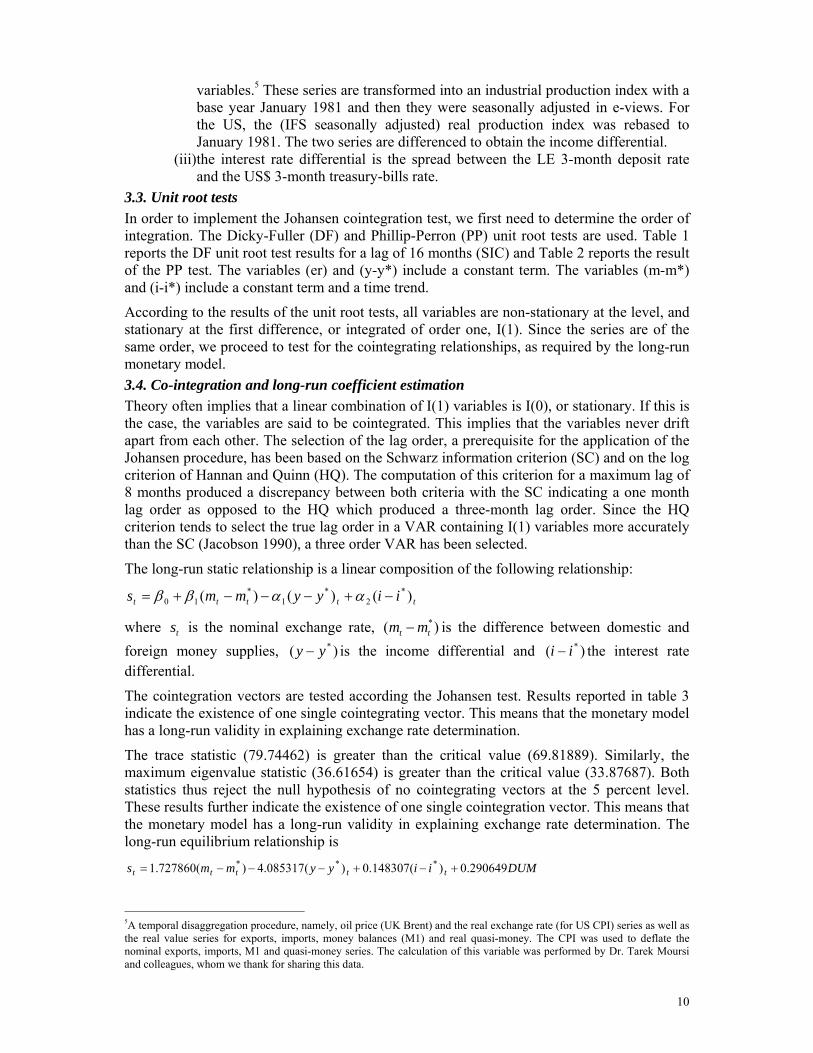
3.3. Unit root tests In order to implement the Johansen cointegration test, we first need to determine the order of integration. The Dicky-Fuller (DF) and Phillip-Perron (PP) unit root tests are used. Table 1 reports the DF unit root test results for a lag of 16 months (SIC) and Table 2 reports the result of the PP test. The variables (er) and (y-y*) include a constant term. The variables (m-m*) and (i-i*) include a constant term and a time trend.

According to the results of the unit root tests, all variables are non-stationary at the level, and stationary at the first difference, or integrated of order one, I(1). Since the series are of the same order, we proceed to test for the cointegrating relationships, as required by the long-run monetary model. 3.4. Co-integration and long-run coefficient estimation Theory often implies that a linear combination of I(1) variables is I(0), or stationary. If this is the case, the variables are said to be cointegrated. This implies that the variables never drift apart from each other. The selection of the lag order, a prerequisite for the application of the Johansen procedure, has been based on the Schwarz information criterion (SC) and on the log criterion of Hannan and Quinn (HQ). The computation of this criterion for a maximum lag of 8 months produced a discrepancy between both criteria with the SC indicating a one month lag order as opposed to the HQ which produced a three-month lag order. Since the HQ criterion tends to select the true lag order in a VAR containing I(1) variables more accurately than the SC (Jacobson 1990), a three order VAR has been selected.

The long-run static relationship is a linear composition of the following relationship:

ttttt iiyymms )()()( *2

*1

*10 −+−−−+= ααββ

where ts is the nominal exchange rate, )( *tt mm − is the difference between domestic and

foreign money supplies, )( *yy − is the income differential and )( *ii − the interest rate differential.

The cointegration vectors are tested according the Johansen test. Results reported in table 3 indicate the existence of one single cointegrating vector. This means that the monetary model has a long-run validity in explaining exchange rate determination.

The trace statistic (79.74462) is greater than the critical value (69.81889). Similarly, the maximum eigenvalue statistic (36.61654) is greater than the critical value (33.87687). Both statistics thus reject the null hypothesis of no cointegrating vectors at the 5 percent level. These results further indicate the existence of one single cointegration vector. This means that the monetary model has a long-run validity in explaining exchange rate determination. The long-run equilibrium relationship is

DUMiiyymms ttttt 290649.0)(148307.0)(085317.4)(727860.1 *** +−+−−−=

5A temporal disaggregation procedure, namely, oil price (UK Brent) and the real exchange rate (for US CPI) series as well as the real value series for exports, imports, money balances (M1) and real quasi-money. The CPI was used to deflate the nominal exports, imports, M1 and quasi-money series. The calculation of this variable was performed by Dr. Tarek Moursi and colleagues, whom we thank for sharing this data.

11

These results show that the estimated coefficients of money, income and interest rate differentials have the anticipated signs.

3.5. The vector error correction model According to the Granger Representation Theorem, if a cointegrating relationship exists between a series of I(1) variables, then a dynamic error-correction model also exists. The latter is an equilibrium model which uses the lagged residual from the cointegrating relationships in combination with short-run dynamics to adjust the model towards long-run equilibrium. This suggests that there should exist an exchange rate equation of the form:

ttitit

n

iiit

n

iitiitit

n

ii

n

iitit uziiyymmss ++−+−Δ+−Δ+Δ+=Δ −−−

=−

=−−−

==−− ∑∑∑∑ 1

*

0

*

0

*

001 )()()( ρλθβγα

Where tu denotes a disturbance term, tz represents the cointegrating vector normalized on

ts and tρ captures the adjustment of the exchange rate towards its long-run equilibrium value. Using the estimated cointegrating vector, a dynamic error correction model was estimated.

Table 4 reports the estimates of the VECM. The coefficient of the error correction in the exchange rate equation is negative and statistically significant. Its size (-0.015184) shows that 1.5 percent of the adjustment towards the long-run equilibrium takes place per month. In other words, when deviations from the long-run equilibrium occur, the exchange rate adjusts to restore long-run equilibrium. Also, the coefficient of the dummy variable is insignificant and close to 0, suggesting that there has not been any significant change in exchange rate determination.

In this section, the monetary model of exchange rate determination was examined for the LE/US$ using monthly data over the period 1981-2008. A single long-run relationship between the exchange rate, money supplies, output and short-term interest rates was found. Using the single cointegrating vector, a dynamic error correction model was estimated to verify the short-run effects of the variables on the nominal exchange rate. The latter also supports the short-run relationships. Does this mean that Egypt’s exchange rate is still fixed? The following section looks with more depth into this question

4. Estimating Egypt’s De Facto Exchange Rate Regime In this section, we attempt to provide an alternative de facto classification of the regime.

4.1. Literature review Determining the de facto exchange rate regime is not an end to itself, but rather the means to identify the impact of the exchange rate policy on macroeconomic outcomes, especially growth and inflation, as well as the limitation it imposes on monetary policy. For instance in the case of Egypt, if the CBE adopts an inflation targeting framework, as announced, it must introduce more flexibility in the exchange rate regime, in order not to compromise the objective of price stability. This section thus seeks to determine Egypt’s exchange rate regime.

A de jure classification was compiled and published in the International Monetary Fund’s (IMF) Annual Report on Exchange Rate Arrangements and Exchange Rate Restrictions. It distinguished between two types of regimes, fixed and “other”. Later, the classification expanded to three, then four regimes (including a peg, limited flexibility, more flexible arrangements and independently floating), the latter prevailing through most of the 1980s and 1990s (Reinhart and Rogoff, 2002). This de jure classification—relying on self-declarations—was considered to be comprehensive in terms the coverage of economies, observations over time and frequency of updating (Bubula and Otker-Robe, 2002). It thus

12

became the main reference on countries’ exchange rate regimes. Nevertheless, it was not very reflective of the actual exchange rate regime in the case where a country exhibits fear of floating behavior.

In light of these deficiencies, empirical work emerged to estimate the de facto exchange rate classification.6 Some classifications are entirely independent of the official country announcements and are based on the actual behavior of the exchange rate. These methodologies look at exchange rate volatility, the changes in foreign reserves and/or nominal interest rates. The last two variables help provide information on intervention during the occurrence of shocks.7 Some authors remain skeptical about the addition of these two variables. De Grauwe and Schnabl (2008) argue that (percentage) changes of foreign reserves tend to be biased by the stock of foreign reserves, i.e. a large stock of reserves would tend to exhibit low percentage changes and vice versa. Also, Ghosh, Gulde and Wolf (2002) argue that information on intervention data may not always be available because central banks treat them as confidential. Further, they explain that the existence of a variety of off-balance sheet instruments make the use of reserves less pertinent. Furthermore, movements in central bank reserves, particularly in low income countries, could be influenced by servicing of foreign debt or payments for bulky purchases which have little to do with intentional foreign exchange intervention but result in large movements in reported reserves.

Meanwhile, interest

rate changes may not reflect exchange rate policies because in many emerging markets they could be set administratively and because financial and money markets are highly underdeveloped, fragmented, and isolated from international financial markets.

An early de facto classification can be found in Bofinger and Wollmershäuser (2001) who rank officially floating regimes based on changes in foreign reserves as a (i) ratio to the economy’s external sector (being exports and imports) and (ii) as percentage change of the level of reserves at the beginning of the period. Floating regimes are divided into: pure floats (no intervention in the foreign exchange market), independent floats (intervention to stabilize the exchange rate around its market-determined trend) and managed floats (which follow an unannounced target path). Poirson (2001) constructed a rigidity index on the basis of the ratio of exchange volatility to reserves for a sample of 93 countries during 1990–1998. Shambaugh (2003) divided 100 regimes between 1973-2000 into pegs and non-pegs based on whether exchange rate changes were within pre-specified bands.

In their proposed de facto classification, Levy-Yeyati and Sturzenegger (LYS) (2005) use cluster analysis to classify regimes for 183 countries between 1974–20008. To assess the volatility of the exchange rate, they look at the behavior of two variables: changes in the nominal exchange rate and the volatility of these changes. To measure intervention in the foreign market, they measure the volatility of international reserves relative to the monetary base. They use this last measure in countries where low monetization implies a larger relative intervention in foreign exchange markets. They do not include interest rates in their classification process for several reasons. First, most of the changes in interest rates in small open economies are the response to unsterilized intervention by monetary authorities.9 But they argue that interest rate policy is taken into account through the changes that unsterilized reserve flows induce on monetary aggregates. Second, they further argue that the scope for interest rate changes to alter exchange market conditions without a concomitant movement in reserves is quite limited, both in duration and strength. 6 For a comprehensive literature review, please see Tavlas, Dellas and Stockman (2008). 7 Very early work focusing on currency crisis used these two variables. Edwards (2001) used the international reserves to build an index of exchange rate pressures. Eichengreen, Rose and Wyplosz (1994) added the interest rate. 8 Cluster analysis means that all volatilities are compared to their sample averages. 9 If a central bank wants to defend its currency by raising interest rates, it simply has to leave unsterilized the reserve outflows, by doing so the money supply contracts, raising interest rates.

13

LYS (2005) classify exchange rate regimes into 4 types: (i) fixed when the exchange rate does not move while reserves are allowed to fluctuate, (ii) flexible when there is little intervention together with unlimited volatility of the nominal exchange rate, (iii) a crawling peg when changes in the nominal exchange rates occur with stable increments (i.e. low volatility in the rate of change of the exchange rate) while active intervention keeps the exchange rate along a path, (iv) a dirty float when volatility is relatively high across all variables, with intervention only partially smoothing the exchange rate. They subsequently classify some inconclusive countries as pegs when both the exchange rate and international reserves are stable. However, they do not distinguish between conventional fixed pegs and hard pegs.

Other empirical work has at starting point the self-declared regimes and are adjusted based on judgment, statistical algorithms and developments in parallel markets [see for instance the work of Ghosh, Gulde, Ostry and Wolf (1997) and (2002), Bailliu, Lafrance and Perrault (2002) and Reinhart and Rogoff (2002)].

The International Monetary Fund itself revised its assessment of “official regimes” in 1999 by correcting declared regimes for the observed behavior of nominal exchange rates and official reserves. Using this methodology, Bubula and Ötker-Robe (2002) reclassified regimes over the 1990– 2001 period for all IMF members. Since 2003, the IMF’s “de Facto Classification of Exchange Rate Regimes and Monetary Policy Frameworks” replaced the older de jure classification. Exchange rate arrangements are ranked on the basis of their degree of flexibility and the existence of formal or informal commitments to exchange rate paths. It distinguishes among 8 forms of exchange rate arrangements (see appendix table 1). According to this classification, there are 84 countries with a floating exchange rate, of which 44 are managed floaters and 40 are pure floaters.

With the move towards intermediate regimes, a main thrust of recent research tries to estimate basket weights in the case when economies claim to be following transparent intermediate regimes (a basket peg or a basket with a band) but keep the weights in the basket secret. This branch of the literature is outside the scope of this study as it is not the case for Egypt.

Ghosh, Gulde and Wolf (2002) observe that de facto classifications have one main drawback, related to their backward-looking nature. They explain that the stated regime in principle conveys information about future policy intentions, observed actions necessarily pertain to the past. However, we believe that even if this is true, the identification of the de facto exchange rate regime helps to know the constraints and/or effectiveness of monetary policy with respect to what it can or cannot do.

In the next section, we use the LYS methodology to classify Egypt’s de facto exchange rate regime. We choose this methodology because it does not rely on any official declarations by the government or any other entity. It is also simple while taking into account several variables that are closely related to the behavior of the exchange rate.

4.2. A de facto classification of Egypt’s exchange rate regime According to the IMF’s de jure classification, Egypt’s exchange rate regime moved from being a fixed adjustable peg between 1960 and 1991 to a managed floating regime as announced by the government between 1991 and 1998. In 1998, realizing that the exchange rate was still fixed, the IMF revised its classification and ranked Egypt as having a conventional fixed peg arrangement (Kamar and Bakardzhieva, 2005). Under the IMF de facto classification, the regime has been classified as a managed float with a pre-determined path for the exchange rate since 2003. It has been labeled as a conventional fixed peg

14

arrangement in 2006 and then in a mark of gradually increasing exchange rate flexibility, was reclassified as a managed float with pre-determined path for the exchange rate (IMF, 2007).

Two papers provide alternative classifications to exchange rate regimes in Egypt. Kamar and Bakardzhieva (2005) assume that the exchange rate is fixed when its volatility is confined to a 3 percent band and it is a float when the band is larger than 15 percent. Another paper by El-Refaie (2002) used the LYS methodology with some modifications to one of the classification variables (volatility of reserves) and concludes that Egypt had a fixed exchange rate between 1992 and 2000.

Based on the LYS methodology, the exchange rate regime will be defined according to the behavior of three variables (the exchange rate volatility, the volatility of exchange rate changes and the volatility of international reserves relative to the monetary base).

Exchange rate volatility )( eσ is measured as the average of the absolute monthly percentage changes in the nominal exchange rate during a calendar year.

The volatility of exchange rate changes )( eΔσ is computed as the standard deviation of the monthly percentage changes in the exchange rate.

The volatility of reserves )( rtσ is calculated as follows

t

tttt e

sitsermentDepoCentralGovbilitiesForeignLiaetsForeignAssR

−−=

1

11

−

−

−−=

tetsemonetaryba

tRtRtr

)( rtσ is thus the average of the absolute monthly change in r.

Our analysis relies on monthly data for the period from 1982 to 2008. We divide this period into two sub-periods. The first, until 2003 corresponds to an official exchange rate peg while the second starts with the announcement of the float since January 2003. The currency of reference is the US$ over the whole period because the LE was de jure pegged to it. Monthly data was obtained from the IFS. We compute a yearly figure for each of the variables for the period of FY82-FY08 and compare the yearly figure with the sample average in order to label the exchange rate regime. If the two measures of exchange rate volatility are lower than the sample average and if the measure of the volatility of international reserves is higher, then the exchange rate regime would be classified as a fixed regime and vice versa. We consider this classification to be completely independent of the official regime stated by the government. The calculations are reported in Table 5.

Most striking about this analysis is that, in general, both the volatility of the nominal exchange rate and that of international reserves are low, 0.9 percent and 4.5 percent respectively. The volatility was higher before 2003, probably reflecting recurring devaluations and continuous attempts of policy intervention using official reserves. After the float, both variables have a volatility that is less than the sample averages. Concerning the exchange rate, this is a bit puzzling. Had the exchange rate been de facto floating, shouldn’t it have exhibited more volatility, with the surge in capital inflows between FY05-FY08? International reserves have been most volatile in FY91 when several devaluations occurred within the year. They also had higher volatility during the nineties period of the official peg (5.1 percent), when the CBE resorted to them to defend the peg. However, after the float, they have been less volatile (2.4 percent).

15

The exchange rate is classified as a float for one year, FY03, when the de jure float was announced because the exchange rate was subject to significant depreciation. It is classified as fixed (a dirty float) in four out of 26 years. Most of the dirty float years reflect political devaluations. For the rest of the years, the exchange rate regime is inconclusive because the exchange rate stability coexisted with rather low international reserve volatility. These results differ from those of El-Refaie (2002) who classifies the exchange rate as fixed until 2000. However, the author also reports very low volatility of reserves, with no further explanations.

We repeat the exercise one more time using the volatility of reserves (not as a ratio to the monetary base), we get the same results. We repeat the same exercise using other foreign currency assets, instead of international reserves. These assets are reported by the CBE but are not calculated as part of the CBE’s total official reserves. This data has only been available since December-04. We find that the stability of the exchange rate coexisted with enormous reserve volatility since 2005. This suggests that the CBE could be resorting to these foreign currency assets to control the exchange rate.

This section provided an attempt to classify Egypt’s exchange rate regime using the LYS methodology. Based on the first two criteria measuring exchange rate volatility, one would tend to classify Egypt’s exchange rate regime as fixed. However, the third criteria which measures intervention through reserves has been relatively stable over time and never exhibited any significant volatility, except for the year when the LE was devalued. This suggests that the CBE does not frequently and transparently resort to official reserves to defend the peg. We are thus unable to classify Egypt’s exchange rate as a float for recent years according to the LYS methodology.

Conclusion The motivation behind this paper was the intuition that the exchange rate continues to be managed by the CBE, despite the de jure float. The first aim of this paper was thus to empirically assess whether there has been any significant change in exchange rate determination with the announcement of the float. To this end, the first section has shown that the stability of the exchange rate persisted after the announcement of the float. Since FY05, significant capital inflows led to a huge reserve accumulation but as sterilization operations have only been partial, the unsterilized capital inflows could have contributed to money growth and inflation.

In the second section, the monetary model of exchange rate determination was tested for the LE/US$ using monthly data over the period 1981-2008. A single long-run relationship was found. Using the single cointegrating vector, the estimated VEC model shows that the exchange rate adjusts to restore long-run equilibrium, albeit at a slow rate. There does not seem to be any significant change in the exchange rate regime after the announcement of the float.

Policy Recommendations and Further research A main question that naturally rises after this research is how to determine the role of the exchange rate in monetary policy and what exchange rate regime would be best suited for Egypt.

Unlike in industrial economies, the exchange rate plays an important role in EMEs, even for those adopting an explicit inflation target. In the case of Egypt, it is becoming a risky implicit anchor because it remained quasi-fixed for a number of years in an environment in which the persistence of inflation led to a worrisome real appreciation of the currency.

16

There are several key factors to look at when determining the weight of the exchange rate in monetary policy: the impact of exchange rate movements on domestic inflation, the source of shocks, the volatility of capital flows and the credibility of the monetary authorities.

First, it is clear that a weakening exchange rate pass-through in an environment of low and stable inflation could provide a good argument for more flexibility and allow a shift towards interest rate channels to control inflation. A second key factor, which is partly related to the role of pass-through, is the nature of shocks that hit the exchange rate and which require policy intervention. The latter must be based on the belief that that the exchange rate is becoming misaligned. In general, movements in the exchange rate that respond to adjustments in the equilibrium real exchange rate will have smaller inflationary effects than movements that are not a response to changes in fundamentals.

A third key factor is the vulnerability to volatile or sudden stops of capital flows. Such volatility, together with the size of the economy, its degree of openness to trade and capital flows should determine the role of exchange rate in monetary policy.

A fourth factor is the level of central bank credibility, and, conversely, the potential impact of any actions on it. Some have argued that there is greater room for monetary policy to pay attention to the exchange rate over and above inflation when its anti-inflation credentials are beyond doubt. This can only be possible with a strong institutional setup, which includes credible price stability, fiscal discipline, strong prudential system based on openness and transparency and well-developed financial markets.

Based on the above, based on some IMF work, econometric tests showed that the exchange pass-through to domestic CPI inflation following the 2003 devaluation was low and slow. Future work is required to determine how the pass-through has evolved in the post-float years. Other IMF work has shown that the LE/US$ exchange rate is not misaligned from fundamentals, which presents a strong argument against continued policy intervention. With respect to credibility, it must be admitted that a lot of reforms within the CBE have taken place that helped to improve its credibility. Nevertheless, the lack of transparency about explicit and operating targets and monetary stance in general may be undermining the CBE’s credibility and its control of price stability. Moreover, a credible monetary policy goes hand in hand with fiscal discipline and coordination which implies a low fiscal deficit and debt ratio. Other arguments in favor of floating the exchange rate is that Egypt’s vulnerability to a sudden stop is also low, unlike other EMEs, because “capital inflows have not been intermediated through the financial system and official reserve levels are comfortable”. Also, capital inflows are geographically well diversified and only a small part of inflows is portfolio investment while the rest is foreign direct investment, (IMF, 2007).

Finally, it is important to have an exit strategy for the exchange rate policy. In this respect, the CBE has announced its intention to move to an inflation targeting (IT) framework over the medium term. However, other options could also be explored. For an economy that maintains an underlying inflation in the low two digits, Kamar and Bakardzhieva (2005) made a case for managed bands or crawling pegs. Such regime allows the exchange rate to fluctuate within a band and thus could accommodate short-term fluctuations. Naturally, the band must be periodically reviewed to ensure that it remains consistent with the underlying fundamentals of the economy. A crawling peg system could also accommodate exchange rate fluctuations and also neutralize the inflation differential and reflect the real adjustment of the economy. Kamar and Bakardzhieva (2005) recommend that the currency be related to a weighted basket of currencies that constitute Egypt’s main trading partners.

We would also like to suggest the targeting of the real exchange rate since it will allow monetary policy to focus both on inflation and the exchange rate. Frenkel and Taylor (2006)

17

suggest a real targeting approach to maintain a stable and competitive real exchange rate. This policy avoids fluctuations in the exchange rate (both nominal and real), thus signaling the stability of the real exchange rate over the medium term. This should provide Egypt with the option to focus on employment and growth, the exchange rate and inflation which should maintain macroeconomic stability and still be consistent with financial globalization.

In the meantime, in order to ensure the credibility of success of any monetary policy framework that focuses on price stability, a more flexible exchange rate is called for. The exchange rate cannot be in conflict with the goal of price stability.

18

References

Baharumshah, Ahmad Zubaidi, Siti Hamizah Mohd and Sung K. Ahn. 2009. “On the Predictive Power of Monetary Exchange Rate Model: The Case of the Malaysian Ringgit: US dollar Rate”. Applied Economics. Vol. 41, N. 14, pp. 1761–1770.

Baillie, Richard T. and Pecchenino, A. Rowena. 1991. “The Search for Equilibrium Relationships in International Finance: The Case of the Monetary Model”. Journal of International Money and Finance. Vol. 10, N. 4, pp. 582–593.

Baillie, Richard T. and David D. Selover. 1987. “Cointegration and Models of Exchange Rate Determination”. International Journal of Forecasting. Vol. 3, N. 1, pp. 43–51.

Bailliu, Jeannine; Robert Lafrance and Jean-François Perrault. 2002. “Does Exchange Rate Policy Matter for Growth?”. Working Paper 2002–17. Ottawa: Bank of Canada.

Berkowitz, Jeremy and Lorenzo Giorganni. 2001. “Long-Horizon Exchange Rate Predictability?”. Review of Economics and Statistics. Vol. 83, N. 1, pp. 81–91.

Bilson, John F.O. 1978. “Rational Expectations and the Exchange Rate”. In “The Economics of Exchange Rates: Selected Studies”, eds. Jacob A. Frenkel, and Harry G. Johnson. Reading, MA: Addison-Wesley Publishing Co.

Bofinger, Peter and Timo Wollmershaeuser. 2001. “Managed Floating: Understanding the New International Monetary Order”. Discussion Paper Series 3064. London: Center for Economic Policy Research.

Bubula, A. and Inci Ötker-Robe. 2002. “The Evolution of Exchange Rate Regimes since 1990: Evidence from De Facto Policies”. International Monetary Fund Working Paper 02/155. 07/380. Washington, D.C.

Central Bank of Egypt. 2005. “Monetary Policy Statement”. Cairo: Central Bank of Egypt. Available on http://www.cbe.org.eg/public/MONETARY%20POLICY%20STATEMENT.pdf

Chinn, Menzie D. and Richard A. Meese. 1995. “Banking on Currency Forecasts: How Predictable is Change in Money?. Journal of International Economics. Vol. 38, N. 1/2, pp. 161–178.

Chin, Lee, M. Azali and K.G. Mathews. 2007. “The Monetary Approach to Exchange Rate Determination for Malaysia”. Applied Financial Economics Letters. Vol. 3, N. 2, pp. 91–94.

Civicir, Irfan. 2003. “The Monetary Models of the Turkish/US Dollar Exchange Rate: Long-run Relationships, Short-run Dynamics and Forecasting”. Eastern European Economics. Vol.41, N. 6, pp. 43–69.

Crespo-Cuaresma, Jesus, Jarko Fidrmuc and Ronald McDonald. 2003. “The Monetary Approach to Exchange Rates in the CEEs”. Discussion Paper 14/2003. Institute for Economies in Transition, Bank of Finland.

De Grauwe, Paul and Gunther Schnabl. 2008. “Exchange Rate Stability, Inflation, and Growth in South Eastern and Central Europe”. Review of Development Economics. Vol. 12, N. 3, pp. 530–549.

19

Edwards, Sebastian. 2001. “Does the Current Account Matter?”. Working Paper Series 8275. Cambridge, Mass.: National Bureau of Economic Investigation.

El-Refaie, Faika. 2002. “The Coordination of Monetary Policy and Fiscal Policies in Egypt”. In “Monetary Policy and Exchange Rate Regimes: Options for the Middle East”, eds. Cardoso and Galal. Cairo: The Egyptian Centre for Economic Studies.

Eichengreen, Barry; Andrew K. Rose and Charles Wyplosz. 1994. “Speculative Attacks on Pegged Exchange Rates: An Empirical Exploration with Special Reference to the European Monetary System”. Working Paper Series 4898. Cambridge, Mass: National Bureau of Economic Investigation.

Fayed, Mona, Esam. 2005. “An Empirical Investigation of Exchange Rate Behaviour in Egypt 1973 – 2001”. MA dissertation submitted to the Department of Economics at the Faculty of Economics and Political Science, Cairo University.

Frankel, Jeffrey. 1982. “The Mystery of the Multiplying Marks: A Modification of the Monetary Model”. The Review of Economics and Statistics. Vol. 64, N. 3, pp. 515–519.

Frenkel, Roberto and Lance Taylor. 2006. “Real Exchange Rate, Monetary Policy and Employment”. Working Paper 19. United Nations Department of Social Affairs.

Garces-Diaz, Daniel. 2004. “How Does the Monetary Model of Exchange Rate Determination Look when it Really Works?”. Econometric Society, North American Winter Meetings 60.

Ghosh, Atish R., Anne-Marie Gulde, Jonathan D. Ostry and Holger C. Wolf. 1997. “Does the Nominal Exchange Rate Regime Matter?”. Working Paper Series 5874. Cambridge, Mass: National Bureau of Economic Investigation.

Ghosh, Atish R., Anne-Marie Gulde and Holger C. Wolf. 2002. “Exchange Rate Regimes: Choices and Consequences”. Cambridge, Mass: MIT Press.

Groen, Jan J.J. 2000. “The Monetary Exchange Rate Model as a Long-run Phenomenon”. Journal of International Economics. Vol. 52, N. 2, pp. 299–319.

Hakkio, C.S. and M. Rush. 1991. “Cointegration: How Short is the Long-Run?”. Journal of International Money and Finance. Vol. 10, N. 4, pp. 321–355.

Hodrick, R.J. 1978. “An Empirical Analysis of the Monetary Approach to the Determination of the Exchange Rate”. In “The Economics of Exchange Rates”, eds. Jacob A. Frenkel and Harry G. Johnson. Reading, MA: Addison-Wesley Publishing Co.

Husted, Steven and Ronald MacDonald. 1999. “The Asian Currency Crash: Were Badly Driven Fundamentals to Blame?”. Journal of Asian Economics, Vol. 10, N. 4, pp. 537–550.

Hwang, Jae-Kwang. 2001. “Dynamic Forecasting of Monetary Exchange Rate Models: Evidence from Cointegration”. International Advances in Economic Research. Vol. 7, N. 1, pp. 51–64.

International Monetary Fund. 2007. Article IV Consultation—Staff Report. International Monetary Fund Country Report 07/380. Washington, D.C.

20

________IMF. 2008. “De Facto Classification of Exchange Rate Regimes and Monetary Policy Frameworks”. Available on http://www.imf.org/external/np/mfd/er/2008/eng/0408.htm

Islam, M. Faizul and Mohammad S. Hassan. 2006. “The Monetary Model of the Dollar-Yen Exchange Rate Determination: A Cointegration Approach”. International Journal of Business and Economics. Vol. 5, N. 2, pp. 129-145

Jacobson, T. 1990. “On the Determination of the Order of Lag Order in Vector Autoregressions of Cointegrated Systems”. Mimeo. Sweden: Department of Statistics, University of Uppsala.

Kamar, Bassem and Damyana Bakardzhieva 2005. “Economic Trilemma and Exchange Rate Management in Egypt”. Review of Middle East Economics and Finance. Vol. 3, N. 2, pp. 91–114.

Lavigne, Robert. 2008. “Sterilized Intervention in Emerging-Market Economies: Trends, Costs, and Risks”. Banque du Canada Discussion Paper 2008–4.

Levy-Yeyati, Eduardo and Federico Sturzenegger. 2005. “Classifying Exchange Rate Regimes: Deeds vs. Words”. European Economic Review. Vol. 49, N. 3, pp. 1603–1635.

Loria, Eduardo, Armando Sanchez and Uberto Salgado. 2009. “New Evidence on the Monetary Approach of Exchange Rate Determination in Mexico 1994 –2007: A Cointegrated SVAR Model”. Journal of International Money and Finance. pp. 1–15.

Mohanty, M.S. and Philip Turner. 2006. “Foreign Exchange Reserve Accumulation in Emerging Markets: What are the Domestic Implications?”. Bank for International Settlements Quarterly Review-September.

Mark, Nelson C. 1995. “Exchange Rates and Fundamentals: Evidence on Long-Horizon Predictability”. American Economic Review. Vol. 85, N. 1, pp. 201–218.

Mark, Nelson C. and Donggyu Sul. 2001. “Nominal Exchange Rates and Monetary Fundamentals: Evidence from a Small Post-Bretton Woods Panel”. Journal of International Economics. Vol. 53, N. 1, pp. 29–52.

MacDonald, R. and Mark P. Taylor. 1994. “The Monetary Model of the Exchange Rate: Long-Run Relationships, Short-Run Dynamics, and How to Beat a Random Walk”. Journal of International Money and Finance. Vol. 13, N. 3, pp. 276–290.

Makrydakis, Stelios. 1998. “Testing the Long-Run Validity of the Monetary Approach to the Exchange Rate: the Won-US dollar case”. Applied Economic Letters. Vol. 5, N. 8, pp. 507–511.

Miyakoshi, Tatsuyoshi. 2000. “The Monetary Approach to the Exchange Rate: Empirical Observations from Korea”. Applied Economic Letters. Vol. 7, N. 12, pp. 791–794.

McNown, R.A. and M. Wallace. 1989. “Cointegration Tests for Long-run Equilibrium in the Monetary Exchange Rate Model”. Economic Letters. Vol. 31, N. 3, pp. 263–267.

Meese, Richard A. and Kenneth Rogoff. 1983. “Empirical Exchange Rate Models of the Seventies: Do They Fit Out of sample?”. Journal of International Economics. Vol. 14, N. 1/2, pp. 3–24.

21

Neely, Christopher J. and Lucio Sarno. 2002. “How Well Do Monetary Fundamentals Forecast Exchange Rates?”. The Federal Reserve Bank of Saint Louis Review. Vol. 84, N. 5, pp. 51–74.

Poirson, Hélène. 2001. “How Do Countries Choose Their Exchange Rate Regime?”. International Monetary Fund Working Paper WP/01/46. Washington, D.C.

Rapach, David E. and Mark E. Wohar. 2002. “Testing the Monetary Model of Exchange Rate Determination: New Evidence from a Century of Data”. Journal of International Economics. Vol. 58, N. 2, pp. 359–385.

Reinhart, C. and Kenneth S. Rogoff. 2002. “The Modern History of Exchange Rate Arrangements: a Reinterpretation”. Working Paper Series 8963. Cambridge, Mass: National Bureau of Economic Investigation.

Sarantis, N. 1994. “The Monetary Exchange Rate Model in the Long-Run: An Empirical Investigation”. Review of World Economics. Vol. 130, N. 4, pp. 698–711.

Shambaugh. Jay C. 2004. “The Effect of Fixed Exchange Rates on Monetary Policy”. Quarterly Journal of Economics. Vol. 119, N. 1, pp. 300–351.

Shiller, R. and Pierre Perron. 1985. “Testing the Random Walk Hypothesis: Power versus Frequency of Observation”. Economic Letters. Vol. 18, N. 4, pp. 381–386.

Smith, P.N. and M.R. Wickens. 1986. “An Empirical Investigation into the Causes of Failure of the Monetary Model of the Exchange Rate”. Journal of Applied Econometrics. Vol. 1, N. 2, pp. 143–162.

Somanath, V.S. 1986. “Efficient Exchange Rate Forecasts”. Journal of International Money and Finance. Vol. 5, N. 2, pp. 195–220.

Tavlas, George, Harris Dellas and Alan C. Stockman. 2008. “The Classification and Performance of Alternative Exchange Rate Systems”. European Economic Review. Vol. 52, N. 6, pp. 941– 963.

Tawadros, Georges B. 2001. “The Predictive Power of the Monetary Model of Exchange Rate Determination”. Applied Financial Economics. Vol. 11, N. 2, pp. 279–286.

Zhang, Shidong and Thomas C. Lowinger. 2005. “Cointegration in a Monetary Model of Exchange Rate Determination”. American Society of Business and Behavioral Sciences (ASBBS) E-Journal. Vol. 1, N. 1. Available at www.asbbs.org/files/2005/PDF/Zhang.pdf

22

Figure 1: Nominal Exchange Rate

Figure 2: Egypt’s other Exchange Rates Before 2003

(a)The British Pound

0.0

1.0

2.0

3.0

4.0

5.0

6.0

7.0

8.0

Nov

-95

May

-96

Nov

-96

May

-97

Nov

-97

May

-98

Nov

-98

May

-99

Nov

-99

May

-00

Nov

-00

May

-01

Nov

-01

May

-02

Nov

-02

0.00.20.40.60.8

1.01.21.41.61.8

LE/US$ LE/GBP US$/GBP

(b) The Euro

0.0

0.5

1.0

1.5

2.0

2.5

3.0

3.5

4.0

4.5

5.0

0

0.2

0.4

0.6

0.8

1

1.2

LE/US$ LE/EUR US$/Euro

23

Figure 3: Egypt’s other Exchange Rates After 2003

(a) The British Pound

(b) The Euro

Figure 4: NFA and Reserve Money Growth

24

Figure 5: Change in NFA and Sterilization

Figure 6: Growth Rate of Reserve Money and Net Foreign Assets

Figure 7: Money Growth, Inflation and the Exchange Rate

25

Table 1: The Augmented Dicky-Fuller Test The Augmented Dicky-Fuller test

Variable ADF statistic

Order of integration

McKinnon critical values for rejection of hypothesis of a unit root

1 percent 5 percent 10 percent Log levels (except interest rates)

er -1.440381 I(1) -3.450381 -2.870247 -2.571478 y-y* -2.396807 I(1) -3.449917 -2.870057 -2.571377 m-m* -1.323367 I(1) -3.986026 -3.423459 -3.134688i-i* -3.259100¹ I(1) -3.986636 -3.423755 -3.134863

First differences Δer -2.810054¹ I(0) -3.450348 -2.870247 -2.571478Δy-y* -13.91567 I(0) -3.449917 -2.870057 -2.571377 Δm-m* -16?58893 I(0) -3.986112 -3.423501 -3.134713 Δi-i* -14.09124 I(0) -3.986636 -3.423755 -3.134863

The null hypothesis of a unit root is rejected if the t-statistic is greater than the critical values. ¹Significant only at the 1 and 5 percent levels.

Table 2: The Phillips-Perron Test

The Phillips-Perron test

Variable PP statistic Order of integration

McKinnon critical values for rejection of hypothesis of a unit root

1 percent 5 percent 10 percent Log levels (except interest rates)

er -0.908123 I(1) -3.449679 -2.869952 -2.571321 y-y* -2.314739 I(1) -3.449679 -2.869952 -2.571321 m-m* -1.3581767 I(1) -3.986026 -3.423459 -3.134688 i-i* -3.581767¹ I(1) -3.986284 -3.423585 -3.134762

First differencesΔer -16.68953 I(0) -3.449738 -2.869978 -2.571335 Δy-y* -35.94809 I(0) -3.449738 -2.869978 -2.571335Δm-m* -16.67403 I(0) -3.986112 -3.423501 -3.134713 Δi-i* -14.09391 I(0) -3.986636 -3.423715 -3.134863

The null hypothesis of a unit root is rejected if the t-statistic is greater than the critical values. ¹ Significant only at the 1 percent level.

26

Table 3: Results of the Johansen Cointegration Test

Unrestricted Cointegration Rank Test (Trace)Hypothesized Trace 0.05No. of CE(s) Eigenvalue Statistic Critical Value Prob.**None * 0.110736 79.74462 69.81889 0.0065At most 1 0.082923 43.12809 47.85613 0.1295At most 2 0.041812 16.12024 29.79707 0.7038At most 3 0.008703 2.794439 15.49471 0.9754At most 4 0.000215 0.067221 3.841466 0.7954 Trace test indicates 1 cointegrating eqn(s) at the 0.05 level * denotes rejection of the hypothesis at the 0.05 level **MacKinnon‐Haug‐Michelis (1999) p‐values

Unrestricted Cointegration Rank Test (Maximum Eigenvalue)Hypothesized Max‐Eigen 0.05No. of CE(s) Eigenvalue Statistic Critical Value Prob.**None * 0.110736 36.61654 33.87687 0.0229At most 1 0.082923 27.00785 27.58434 0.0591At most 2 0.041812 13.3258 21.13162 0.4227At most 3 0.008703 2.727219 14.2646 0.9632At most 4 0.000215 0.067221 3.841466 0.7954 Max‐eigenvalue test indicates 1 cointegrating eqn(s) at the 0.05 level * denotes rejection of the hypothesis at the 0.05 level **MacKinnon‐Haug‐Michelis (1999) p‐values Table 4: Results from the VECM Variable Coefficient Standard Error t-statistic Error Correction Term -0.015184 0.00723 -2.10147

1−Δ ts 0.062836 0.05764 1.09024

2−Δ ts -0.014104 0.05747 -0.24542

3−Δ ts -0.004929 0.05711 -0.08630 )( *

11 −− −Δ tt mm 0.546755 0.21496 2.54356

)( *22 −− −Δ tt mm 0.315641 0.21638 1.45870

)( *33 −− −Δ tt mm 0.010983 0.21509 0.05106

)( *11 −− −Δ tt yy 0.111590 0.07894 1.41363

)( *22 −− −Δ tt yy 0.112266 0.08545 1.31379

)( *33 −− −Δ tt yy -0.022840 0.07286 -0.31346

)( *11 −− − tt ii 0.005473 0.00600 0.91150

)( *22 −− − tt ii 0.002294 0.00607 0.37810

)( *33 −− − tt ii 0.007370 0.00595 1.123863

DUM -0.000838 0.00674 -0.12424

27

Table 5: A De Facto Classification of Egypt’s Exchange Rate Regime According to LYS Methodology

Absolute ER Monthly Volatility

Volatility of Exchange Rate

Changes

Volatility of Reserves

LYS Classification

Sample Average 0.9% 5.9% 4.5% na FY82-FY03 1.0% 6.6% 5.1% na FY04-FY08 0.5% 0.9% 2.4% na FY82 0.0% 0.0% 3.4% inconclusive FY83 0.0% 0.0% 3.0% inconclusive FY84 0.0% 0.0% 0.8% inconclusive FY85 0.0% 0.0% 1.7% inconclusive FY86 0.0% 0.0% 1.5% inconclusive FY87 0.0% 0.0% 2.7% inconclusive FY88 0.0% 0.0% 2.3% inconclusive FY89 0.0% 0.0% 2.2% inconclusive FY90 4.2% 10.2% 5.7% dirty float FY91 11.8% 26.6% 36.9% dirty float FY92 0.2% 0.3% 3.3% inconclusive FY93 0.2% 0.2% 6.7% fixed FY94 0.1% 0.1% 8.9% fixed FY95 0.1% 0.1% 5.7% fixed FY96 0.1% 0.0% 4.8% fixed FY97 0.1% 0.1% 4.4% inconclusive FY98 0.0% 0.0% 2.7% inconclusive FY99 0.0% 0.1% 4.9% fixed FY00 0.1% 0.2% 3.0% inconclusive FY01 0.9% 1.6% 1.9% inconclusive FY02 1.3% 2.9% 3.0% inconclusive FY03 2.6% 5.5% 1.0% float FY04 0.3% 0.5% 2.1% dirty float FY05 0.7% 1.5% 3.3% dirty float FY06 0.1% 0.1% 3.1% inconclusive FY07 0.1% 0.1% 1.4% inconclusive FY08 0.7% 1.5% 2.2% inconclusive

28

Appendix 1 Exchange Rate Arrangement (No. of Countries)

Exchange Rate Anchor U.S. dollar (66) Euro (27) Composite (15) Other (7)

Exchange arrangement with no separate legal

The currency of another country circulates as the sole legal tender (formal dollarization), or the member belongs to a monetary or currency union in which the same legal tender is shared by the members of the union. Adopting such regimes implies the complete surrender of the monetary authorities' control over domestic monetary policy.

Currency board arrangement (13) There is explicit legislative commitment to exchange domestic currency for a specified foreign currency at a fixed exchange rate, combined with restrictions on the issuing authority to ensure the fulfillment of its legal obligation. This implies that domestic currency will be issued only against foreign exchange and that it remains fully backed by foreign assets, leaving little scope for discretionary monetary policy and eliminating traditional central bank functions.

Other conventional fixed peg arrangement (68)

The country pegs its currency within margins of ±1 percent or less vis-à-vis another currency; a cooperative arrangement, such as the ERM II; or a basket of currencies.

Pegged exchange rate within horizontal bands (3)

The value of the currency is maintained within certain margins of fluctuation of more than ±1 percent around a fixed central rate or the margin between the maximum and minimum value of the exchange rate exceeds 2 percent.

Crawling peg (8) The currency is adjusted periodically in small amounts at a fixed rate or in response to changes in selective quantitative indicators, such as past inflation differentials vis-à-vis major trading partners, differentials between the inflation target and expected inflation in major trading partners.

Crawling band (2) The currency is maintained within certain fluctuation margins of at least ±1 percent around a central rate—or the margin between the maximum and minimum value of the exchange rate exceeds 2 percent—and the central rate or margins are adjusted periodically at a fixed rate or in response to changes in selective quantitative indicators.

Managed floating with no pre-determined path for the exchange rate (44)

The monetary authority attempts to influence the exchange rate without having a specific exchange rate path or target. Indicators for managing the rate are broadly judgmental (e.g., balance of payments position, international reserves, parallel market developments), and adjustments may not be automatic. Intervention may be direct or indirect.

Independently floating (40) The exchange rate is market-determined, with any official foreign exchange market intervention aimed at moderating the rate of change and preventing undue fluctuations in the exchange rate, rather than at establishing a level for it.