Happiness and personality types

How different personality types affect happiness levels

(Words: 4150)

In submitting this assignment:

1. We declare that this written assignment is our own work and does not include (i) material

from

published sources used without proper acknowledgment or (ii) material copied from the work

of other students.

2. We declare that this assignment has not been submitted for assessment in any other course

at any university.

3. We have a photocopy and electronic version of this assignment in our possession.

Tudor Carstoiu 1408558

MariaVittoria Fava 1315720

Li Li 1408905

Ruxandra Turturean 1411222

Summary

Using data taken from the European Social Survey round 4(ESS from now onwards), this

project aims to identify a link between different personality types across Europe and their

implication on happiness levels.

We argue that personality types and happiness are somewhat linked and we investigate how

does each personality type found by us affect happiness. To do this, we picked the ESS

variables that are about personality traits (mainly from G Section) and we created factors

representing different personality types. The three personality types found are: Self-confident

type, Conventional type and Self-sacrificing type.

In the end, we used multiple regression techniques, first without any control variables and

second controlling for income, age, education, and health and find that the two personality

types (self-confident and self-sacrificing) positively affect happiness levels and the middle

one, the conventional type, affects happiness negatively. When other things are kept

controlled, a person with self-sacrificing personality traits tends to feel happier.

The paper consists of four sections. Section 1: Introduction. We introduced our research

question and initial hypothesis. Section 2: Data description. Two stages are covered: Stage 1

is about selecting variables for factor analysis and regression analysis; Stage 2 deals with

preliminary testing on variables for factor analysis. Section 3: Mutiple analysis. Two parts

are included: Part 1 is about factor analysis, and Part 2 discusses regression analysis. Section

4: Conclusion.

Section 1:

Introduction

We have chosen this topic because we think that happiness is the ultimate goal in most

people's lives and it is a better measure of wellbeing than income. Although income and

consumption expenditure are the traditional ways of measuring wellbeing, an intriguing

finding of the literature is that the correlation between happiness and income is not always

very strong (Easterlin, 2001).

One popular hypothesis is that well-being is primarily determined by personality traits and

other genetic factors and highly stable over the life course (Easterlin, 2003; Easterlin 2005;

Behrman, Kohler, Skytthe, 2005). This view is known as the set point theory and predicts that

a substantial part of variation in well-being is due to social or biological endowments that are

unobserved in social surveys, which thus explains why happiness does not necessarily follow

closely observed income levels (Oswald, 1997).

In our paper we try to extract those questions that could highlight some social or biological

endowments expressed throgh people's opinions about different personality traits. After doing

explanatory factor analysis and deleting the variables that, for various reasons didn't fit well

with one of the factors, we find three meaningful factors that highlight three different

personality types: Self-confident type, Conventional type and Self-sacrificing type.

Our objective is not to explain happiness through personality types. Variables like income,

education, age and healh cleary have an important impact, but we still think that different

personality types can affect happiness in different, even opposite, ways.

Section 2:

Data Description In carrying out our analysis we used secondary data provided by the Round 4 (2008) of the

ESS, an academically-driven multi-country survey, which has been administrated in over 30

countries to date. All the variables used by the 3 factors are ordered categorical variables.

They are measured on an anchor scale going from “1” (Very much like me) to a maximum of

“6” (Not like me at all). The missing values are registered in the following way: “7” (Refusal),

“8” (Don’t know) and “9” (No answer).

Stage 1: Selecting variables:

1. Composition of the factors:

Factor 1: Self-confident personality

The factor denominated “ Self-confident personality” includes the following variables:

Gb - it is important to her/him to be rich, wants to have a lot of money and

expensive things ( IMPRICH)

Gd - it is important to her/him to show his/her abilities, wants people to admire

what she/he does ( IPSHABT)

Gf - she/he likes surprises and is always looking for new things to do, thinks

it is important to do a lots of different things in life ( IMPDIFF)

Gj - having a good time is important to her/him, she/he likes to “spoil”

herself/himself ( IPGDTIM )

Gm - being very successful is important to her/him, she/he hopes people will

recognise her/his achievements (IPSUCES )

Go - she/he looks for adventures and likes to take risks, she/he wants to have

an exciting life (IPADVNT )

Gu - she/he seeks every chance she/he can to have fun, it is important to

her/him to do things that give her/him pleasure ( IMPFUN )

Self-confident: The following seem to be the core value beliefs of the Self-Confident type.

These beliefs give primary value to external things, things not 'in our power'. Achievement

and talents are good. Personal importance is good. Success, power, brilliance, beauty, and

ideal love are good. Being "special" and unique are good. Having association with other

special or high-status people (or institutions) is good. Favorable treatment or automatic

compliance with his or her expectations is good. Others are good when they can be used to

achieve his or her own ends. Empathy is bad. The feelings and needs of others are bad. Being

envied by others is good.

Factor 2: Conventional personality

The factor denominated “Conventional personality” includes the following variables:

Ge - it is important to her/him to live in secure surroundings, she/he avoids anything

that might endanger her/his safety ( IMPSAFE )

Gg - she/he believes that people should do what they're told, she/he thinks people

should follow rules at all times, even when no-one is watching ( IPFRULE )

Gn - it is important to her/him that the government ensures her/his safety against all

threats, she/he wants the state to be strong so it can defend its citizens (IPSTRGV )

Gp - it is important to her/him always to behave properly, she/he wants to avoid doing

anything people would say is wrong( IPBHPRP)

Conventional: A conventional personality type likes to work with data and numbers, carry out

tasks in detail and follow through on the instructions of others. They are quiet, careful,

responsible, well organized and task oriented. These individuals use their mind, eyes and

hands to carry out tasks. This personality type solve problems by appealing to and following

rules. They are task oriented and prefer to carry out tasks initiated by others, rather than being

in a position of authority. Because of the attention to detail that a conventional personality

type has, these individuals keep the world's records and transmit its messages.

Factor 3: Self-sacrificing personality

The factor denominated “Self-sacrificing personality” includes the following variables:

Gc - she/he thinks it is important that every person in the world should be treated

equally, she/he believes everyone should have equal opportunities in life( IPEQOPT )

Gh - it is important to her/him to listen to people who are different from her/him, even

when she/he disagrees with them, she/he still wants to understand them ( IPUDRST )

Gl - it's very important to her/him to help the people around her/him, she/he wants to

care for their well-being ( IPHLPPL )

Gr - it is important to her/him to be loyal to her/his friends, she/he wants to devote

herself/himself to people close to her/him (IPLYLFR )

Self-sacrificing:

1. Generosity. Individuals with the Self-Sacrificing personality style will give you the shirts

off their backs if you need them. They do not wait to be asked.

2. Service. Their "prime directive" is to be helpful to others. Out of deference to others, they

are noncompetitive and unambitious, comfortable coming second, even last.

3. Consideration. Self-Sacrificing people are always considerate in their dealings with

others. They are ethical, honest, and trustworthy.

4. Acceptance. They are nonjudgmental, tolerant of others' foibles, and never harshly

reproving. They'll stick with you through thick and thin.

5. Humility. They are neither boastful nor proud, and they're uncomfortable being fussed

over. Self-Sacrificing men and women do not like being the center of attention; they are

uneasy in the limelight.

6. Endurance. They are long-suffering. They prefer to shoulder their own burdens in life.

They have much patience and a high tolerance for discomfort.

7. Artlessness. Self-Sacrificing individuals are rather naive and innocent. They are unaware

of the often deep impact they make on other people's lives, and they tend never to suspect

deviousness or underhanded motives in the people to whom they give so much of

themselves.

2. Control variables:

C15 – HEALTH - Subjective general health. This variable is measured on a anchor

scale from "1" (very good) until “5” (very bad), while the missing values are

registered as “7” (refusal), “8” (don't know), “9” (no answer)

F 33 – HINCFEL – feeling about household's income nowadays. This variable is

measured on an anchor scale from "1" (living comfortably on present income) until

“4” (finding it very difficult on present income), while the missing values are

registered as “7” (refusal), “8” (don't know), “9” (no answer). We used this

subjective income variable instead of the absolute one, because in our opinion, this is

more correlated with happiness as having enough money to sustain a good standard

of living is more important than having an excessive amount of money.

(However, we acknowledge the fact that it is better to use continuous variable for

regression analysis and the direction of the causal mechanism may not be so clear

when both dependent and independent variables are about subjective opinions.

Without learning more techniques, we keep this problem as known but unsolved.)

F 3 1b – AGEA – age of respondent. This variable is measured as the current year

minus the year of birth.

F 7 – EDUYRS – years of full-time education completed. This variable is measured in

integer positive numbers, while the missing values are registered as “77” (refusal),

“88” (don't know), “99” (no answer).

3. Independent variable:

C1 – Happy – How happy are you? This variable is measured on a anchored scale

ranging from “0” (extremely unhappy) to “10” (extremely happy).

We restrict our attention to those individuals whose age is equal or higher than 20

because we consider that only after 20 people start to have a well defined personality.

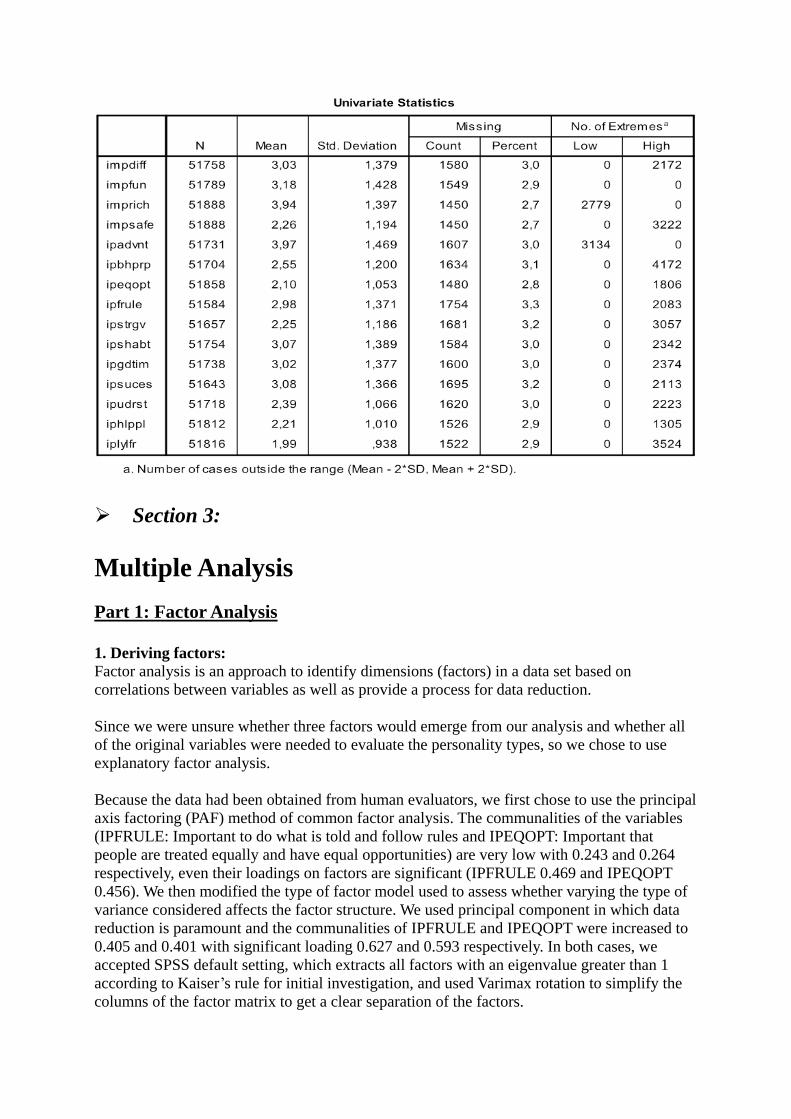
Stage 2: Preliminary testing on variables for factor analysis

Before using our variables for statistical research, it was necessary to run a data analysis.

Developing a descriptive statistic, by summarizing the data in hand computing mean, standard

deviation, skewness and kurtosis, allowed us to test the adequacy of our variables. The table

below displays our outcomes, starting from the condition that in order to carry out a factor

analysis, data has to be approximately normally distributed; our data highlights two variables

that do not respect this condition. Some of our variables are slightly leptokurtic, kurtosis

greater than zero, and some are slightly platykurtic, kurtosis lower than zero; while from the

skewness standpoint the majority of our variables are mildly right skewed, except for two that

are mildly left skewed.

The two variables “important that people are treated equally and have equal opportunities”

and “important to be loyal to friends and devote to people close” arise some concerns, they

have skewness greater than 1 i.e. have a tail that extends to the right, and a kurtosis greater

than 1 which means they are leptokurtic i.e. with a higher peak and more concentration

around the mean and thinner tails. However, even if some variables cannot be exactly defined

as normal, the Central Limit Theorem states that “as the sample size gets large enough (in our

case N exceeds 50 000), the sampling distribution become almost normal regardless of the

shape of the population.

Using the second table, we analyzed missing values and number of extremes. The number of

missing values was not particularly high, in fact it is never higher than 5% of observations,

and therefore we decided to implement the listwise deletion from SPSS, which completely

deletes the cases that present missing values in one of the relevant variables, but still allows

us to maintain a valid N (49183), more than 90% of the survey. Ultimately, in our analysis we

did not encounter an excessively high number of extreme values that could damage our

analysis.

Section 3:

Multiple Analysis

Part 1: Factor Analysis

1. Deriving factors:

Factor analysis is an approach to identify dimensions (factors) in a data set based on

correlations between variables as well as provide a process for data reduction.

Since we were unsure whether three factors would emerge from our analysis and whether all

of the original variables were needed to evaluate the personality types, so we chose to use

explanatory factor analysis.

Because the data had been obtained from human evaluators, we first chose to use the principal

axis factoring (PAF) method of common factor analysis. The communalities of the variables

(IPFRULE: Important to do what is told and follow rules and IPEQOPT: Important that

people are treated equally and have equal opportunities) are very low with 0.243 and 0.264

respectively, even their loadings on factors are significant (IPFRULE 0.469 and IPEQOPT

0.456). We then modified the type of factor model used to assess whether varying the type of

variance considered affects the factor structure. We used principal component in which data

reduction is paramount and the communalities of IPFRULE and IPEQOPT were increased to

0.405 and 0.401 with significant loading 0.627 and 0.593 respectively. In both cases, we

accepted SPSS default setting, which extracts all factors with an eigenvalue greater than 1

according to Kaiser’s rule for initial investigation, and used Varimax rotation to simplify the

columns of the factor matrix to get a clear separation of the factors.

During the analysis process, we dropped variables that based on three criteria: 1) a variable

has on significant loadings; 2) even with a significant loading, a variable’s communality is

deemed to be low; 3) a variable has a cross-loading.

They were all dropped for cross-loading reasons:

IPCRTIV (Important to think new ideas and being creative)

IMPFREE (Important to make own decisions and be free)

IPMODST (Important to be humble and modest, not draw attention)

IMPTRAD (Important to follow traditions and customs)

IPRSPOT (Important to get respect from others)

IMPENV (Important to care for nature and environment)

Three factors were extracted, they account for a total variance of 52.908% in the 15 variables.

In social sciences, where information is often less precise, 60% of the total variance is

satisfactory. Since no absolute threshold is adopted for all applications, we accepted our result.

From the rotated solution in the next page table, we can see that all the three factors contain at

least four variables. With a cutoff for display of 0.4, almost all variables have factor loadings

above 0.6, except IPEQOPT (Important that people are treated equally and have equal

opportunities) loads below 0.6 on Factor 3. The three factor solution looks feasible and

interpretable. We name Factor 1 as self-confident personality, Factor 2 conventional

personality and Factor 3 self-sacrifacing personality.

Rotated Component Matrixa

Component

1 2 3

Important to seek adventures and have an exiting life ,750

Important to have a good time ,702

Important to seek fun and things that give pleasure ,700

Important to be successful and that people recognise achievements ,679

Important to try new and different things in life ,663

Important to be rich, have money and expensive things ,638

Important to show abilities and be admired ,628

Important to live in secure and safe surroundings ,719

Important that government is strong and ensures safety ,674

Important to behave properly ,641

Important to do what is told and follow rules ,627

Important to help people and care for others well-being ,718

Important to be loyal to friends and devote to people close ,700

Important to understand different people ,692

Important that people are treated equally and have equal opportunities ,593

Extraction Method: Principal Component Analysis.

Rotation Method: Varimax with Kaiser Normalization.

a. Rotation converged in 7 iterations.

2. Assessing overall fit:

It is important to check the extraction of the factors that were created and if their soundness is

good enough to be accepted.

Determinant refers to the determinant of correlation matrix of the

variables. Here we find a positive determinant 0.017, which means

there is some correlation between variables. We do not want a

determinant that is exactly zero, as this would suggest perfect

collinearity.

The KMO MSA (a measure

of sampling analysis) is a

measure of variance among

all the variables relative to

other sources of shared

variance and, for the factor

to be accepted, the result

should be at least 0.5, an optimal level is higher than 0.7. Our result is higher than 0.8, which

is very good. Bartlett’s Test of Sphericity tests the null hypothesis that there are no significant

correlations in the data set. Since we have significance p<0.05, we accept the alternative

hypothesis and conclude that there is sufficient correlation within the correlation matrix to

proceed with factor analysis.

The MSA for each variable is shown in the diagonal of the anti-image correlation matrix.

Here, all values were high (all above 0.8), indicating that each variable has the potential to

contribute to a factor in the initial solution.

We include those variables for which the extracted factors explain an adequate amount of

variance (40% common variance is sufficient). Two varialbes have communality slightly

above 0.4.

Communalities

Initial Extraction

Important to be rich, have money and expensive things 1.000 .603

Important that people are treated equally and have equal opportunities 1.000 .401

Important to show abilities and be admired 1.000 .535

Important to live in secure and safe surroundings 1.000 .554

Important to try new and different things in life 1.000 .522

Important to do what is told and follow rules 1.000 .405

Important to understand different people 1.000 .509

Important to have a good time 1.000 .544

Important to help people and care for others well-being 1.000 .573

Important to be successful and that people recognize achievements 1.000 .593

Important that government is strong and ensures safety 1.000 .515

Important to seek adventures and have an exciting life 1.000 .588

Important to behave properly 1.000 .499

Important to be loyal to friends and devote to people close 1.000 .541

Important to seek fun and things that give pleasure 1.000 .555

Extraction Method: Principal Component Analysis.

Correlation Matrixa

a. Determinant = .017

KMO and Bartlett's Test

Kaiser-Meyer-Olkin Measure of Sampling Adequacy. .845

Bartlett's Test of Sphericity Approx. Chi-Square 199550.360

df 105

Sig. .000

Part 2: Regression Analysis Regression without control variables:

The three types of personality

explain only 6.4% variance of

happiness in the model with

only three factors included as

independent variables.

HAPPY= 6.939 – 0.207*Self-confident + 0.261*Conventional –0.416*Self-sacrificing

Regression with control variables:

1. Data description

Descriptive Statistics

N Mean Std. Deviation Skewness Kurtosis

Statistic Statistic Statistic Statistic Std. Error Statistic Std. Error

How happy are you 52870 6.91 2.140 -.838 .011 .507 .021

Subjective general

health

53263 2.32 .949 .453 .011 -.145 .021

Feeling about

household's income

nowadays

52902 2.21 .913 .404 .011 -.610 .021

Age of respondent,

calculated

53338 49.35 17.455 .195 .011 -.910 .021

Years of full-time

education completed

52880 12.02 4.248 -.099 .011 .744 .021

REGR factor score 1

for analysis 1

49183 .000 1.000 .183 .011 -.274 .022

REGR factor score 2

for analysis 1

49183 .000 1.000 .541 .011 .343 .022

REGR factor score 3

for analysis 1

49183 .000 1.000 .458 .011 .513 .022

Valid N (listwise) 48188

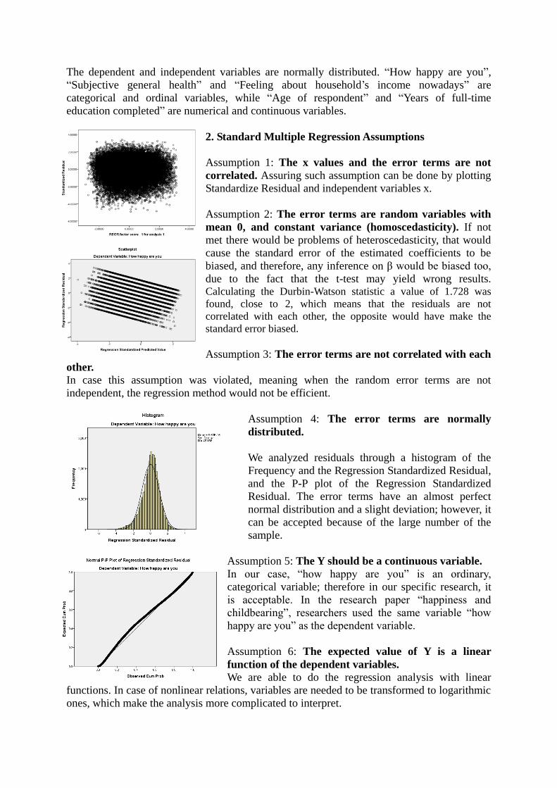
The dependent and independent variables are normally distributed. “How happy are you”,

“Subjective general health” and “Feeling about household’s income nowadays” are

categorical and ordinal variables, while “Age of respondent” and “Years of full-time

education completed” are numerical and continuous variables.

2. Standard Multiple Regression Assumptions

Assumption 1: The x values and the error terms are not

correlated. Assuring such assumption can be done by plotting

Standardize Residual and independent variables x.

Assumption 2: The error terms are random variables with

mean 0, and constant variance (homoscedasticity). If not

met there would be problems of heteroscedasticity, that would

cause the standard error of the estimated coefficients to be

biased, and therefore, any inference on β would be biased too,

due to the fact that the t-test may yield wrong results. Calculating the Durbin-Watson statistic a value of 1.728 was

found, close to 2, which means that the residuals are not

correlated with each other, the opposite would have make the

standard error biased.

Assumption 3: The error terms are not correlated with each

other.

In case this assumption was violated, meaning when the random error terms are not

independent, the regression method would not be efficient.

Assumption 4: The error terms are normally

distributed.

We analyzed residuals through a histogram of the

Frequency and the Regression Standardized Residual,

and the P-P plot of the Regression Standardized

Residual. The error terms have an almost perfect

normal distribution and a slight deviation; however, it

can be accepted because of the large number of the

sample.

Assumption 5: The Y should be a continuous variable.

In our case, “how happy are you” is an ordinary,

categorical variable; therefore in our specific research, it

is acceptable. In the research paper “happiness and

childbearing”, researchers used the same variable “how

happy are you” as the dependent variable.

Assumption 6: The expected value of Y is a linear

function of the dependent variables.

We are able to do the regression analysis with linear

functions. In case of nonlinear relations, variables are needed to be transformed to logarithmic

ones, which make the analysis more complicated to interpret.

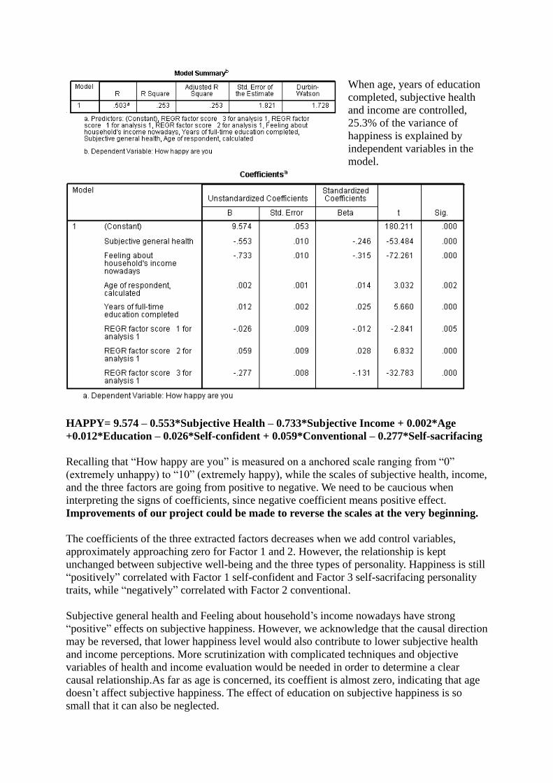
When age, years of education

completed, subjective health

and income are controlled,

25.3% of the variance of

happiness is explained by

independent variables in the

model.

HAPPY= 9.574 – 0.553*Subjective Health – 0.733*Subjective Income + 0.002*Age

+0.012*Education – 0.026*Self-confident + 0.059*Conventional – 0.277*Self-sacrifacing

Recalling that “How happy are you” is measured on a anchored scale ranging from “0”

(extremely unhappy) to “10” (extremely happy), while the scales of subjective health, income,

and the three factors are going from positive to negative. We need to be caucious when

interpreting the signs of coefficients, since negative coefficient means positive effect.

Improvements of our project could be made to reverse the scales at the very beginning.

The coefficients of the three extracted factors decreases when we add control variables,

approximately approaching zero for Factor 1 and 2. However, the relationship is kept

unchanged between subjective well-being and the three types of personality. Happiness is still

“positively” correlated with Factor 1 self-confident and Factor 3 self-sacrifacing personality

traits, while “negatively” correlated with Factor 2 conventional.

Subjective general health and Feeling about household’s income nowadays have strong

“positive” effects on subjective happiness. However, we acknowledge that the causal direction

may be reversed, that lower happiness level would also contribute to lower subjective health

and income perceptions. More scrutinization with complicated techniques and objective

variables of health and income evaluation would be needed in order to determine a clear

causal relationship.As far as age is concerned, its coeffient is almost zero, indicating that age

doesn’t affect subjective happiness. The effect of education on subjective happiness is so

small that it can also be neglected.

Section 4:

Conclusion

Does having a particular personality types make us more predisposed for being more happier

or less happier? Well, the only fact we can infere from our results is that, all else equal, a

person that has a personality close to the self-sacrificng type can be positively affected in

his/her happiness level. Cleary this should be interpreted only qualitatively and we are not

able to establish any causal link due to the cross-sectional nature of our data. It is still possible

that a person who in general is happier may be inclined to embrace personality traits that are

characteristic for the self-sacrificing personality type.

Our research confirms that happiness is a very complex and sensitive variable to measure and

there are many other factors that affect it, factors that are quite hard to be captured in a survey.

Bibliography:

Happiness and childbearing, A. Aassve, A. Goisis, M. Sironi

Statistics for Business and Economics, P. Newbold, W.L. Carlson, B. Thorne. 2007

Prentice Hall;

Applied Statistics: From Bivariate through Multivariate Techniques, R. Warner. Los

Angeles: Sage;

Multivariate Data Analysis, J. F. Hair, R. L. Tatham, R. E. Anderson, W. Black. Pearson

Education.

Lost in trust - reasons and fields of action, students’ project report

Lecture slides of bocconi course 30050, “Applications for Economics, Management and

Finance” 2011

www.ptypes.com/self-confident-values.html

www.123test.com/conventional-personality-type

www.ptypes.com/self-sacrificing.html