
Handbook for Economic analysis of on-farm trials
23
1 | Page Economic analysis of on-farm trials By: Leykun Birhanu Handbook for Economic Analysis of on-farm Trials By: Leykun Birhanu 15.1 Introduction Evaluation of on-farm trials is done to determine the impact of the technology/intervention. It may be ex-ante, on-going as well as ex-post. Traditionally experimental results are assessed using statistical techniques only. Over the years it has been demonstrated that the criteria used by farmers to evaluate and adopt technologies may be totally different to that of researchers. Very often socio-economic considerations play a major role in accepting or rejecting a technology. Assessment of trials is, therefore, one of the important stages of an on-farm research programme. The main elements of such an assessment are farmer assessment, agronomic evaluation, statistical analysis and economic analysis. In this module various socio-economic criteria and simple techniques used to assess economic performance of a technology are discussed. The economic analysis helps researchers: to look at the results from the farmers’ view point; to decide which treatments merit further investigation, and to decide on the recommendations to make to farmers. On-farm data upon which the recommendations are based must be relevant to the farmers’ own agro-ecological conditions, and the evaluation of those data must be consistent with the farmers’ goals and socio-economic circumstances. 15.2 The need for socio-economic evaluation Traditionally, agronomic trials are evaluated by biological scientists using statistical techniques and the dominant evaluation criteria used is yield per unit area. The primary objective here is the maximum exploitation of the biological potential and the test used often is statistical significance. Normally the experiments/treatments are tested at 0.01, 0.05, 0.10 percent level. If they do not pass this test they are not considered any further. This approach has many limitations in deriving recommendations in a systems context: (a) Evaluation criteria that a farmer may use are varied, location specific and depend greatly on the degree of market orientation. The appropriateness of any technology should always be evaluated in relation to their priority objectives and resource use pattern. The relevant criteria for the target group should be identified and used in the design and interpretation of the experiment. A number of physical, biological and socio-economic variables influence the farmers' choice of a technology. Very often the socio-economic factors such as lack of marketing, shortage of labour, clash with food priority etc., determine these choices. (b) Agronomic data only establishes the technical relationships that can be used to determine the technical optimum. It should be complemented with market information in order to establish the economic optimum. The 'economic optimum' for any input is always lower than the 'technical optimum'. If the treatment means are not significantly different but an economic analysis shows that one treatment is a better recommendation than the others then we need to have a more careful analysis. Examples of situations
Transcript of Handbook for Economic analysis of on-farm trials
1 | P a g e
Economic analysis of on-farm trials By: Leykun Birhanu
Handbook for Economic Analysis of on-farm Trials
By: Leykun Birhanu
15.1 Introduction
Evaluation of on-farm trials is done to determine the impact of the technology/intervention. It
may be ex-ante, on-going as well as ex-post. Traditionally experimental results are assessed
using statistical techniques only. Over the years it has been demonstrated that the criteria used
by farmers to evaluate and adopt technologies may be totally different to that of researchers.
Very often socio-economic considerations play a major role in accepting or rejecting a
technology. Assessment of trials is, therefore, one of the important stages of an on-farm
research programme. The main elements of such an assessment are farmer assessment,
agronomic evaluation, statistical analysis and economic analysis.
In this module various socio-economic criteria and simple techniques used to assess economic
performance of a technology are discussed. The economic analysis helps researchers:
to look at the results from the farmers’ view point;
to decide which treatments merit further investigation, and
to decide on the recommendations to make to farmers.
On-farm data upon which the recommendations are based must be relevant to the farmers’ own
agro-ecological conditions, and the evaluation of those data must be consistent with the
farmers’ goals and socio-economic circumstances.
15.2 The need for socio-economic evaluation
Traditionally, agronomic trials are evaluated by biological scientists using statistical techniques
and the dominant evaluation criteria used is yield per unit area. The primary objective here is
the maximum exploitation of the biological potential and the test used often is statistical
significance. Normally the experiments/treatments are tested at 0.01, 0.05, 0.10 percent level.
If they do not pass this test they are not considered any further. This approach has many
limitations in deriving recommendations in a systems context:
(a) Evaluation criteria that a farmer may use are varied, location specific and depend
greatly on the degree of market orientation. The appropriateness of any technology
should always be evaluated in relation to their priority objectives and resource use
pattern. The relevant criteria for the target group should be identified and used in the
design and interpretation of the experiment. A number of physical, biological and
socio-economic variables influence the farmers' choice of a technology. Very often the
socio-economic factors such as lack of marketing, shortage of labour, clash with food
priority etc., determine these choices.
(b) Agronomic data only establishes the technical relationships that can be used to
determine the technical optimum. It should be complemented with market information
in order to establish the economic optimum. The 'economic optimum' for any input is
always lower than the 'technical optimum'. If the treatment means are not significantly
different but an economic analysis shows that one treatment is a better recommendation
than the others then we need to have a more careful analysis. Examples of situations
2 | P a g e
Economic analysis of on-farm trials By: Leykun Birhanu
where farmers choose technologies even without significant differences in yield may
be:
varietal means may not be different but one could observe differences in
palatability (preference), prices, storability, early maturing etc;
technology may not increase the yield/profit, but may reduce the labour
requirement at the critical period;
A new technology may provide possibility of introducing a second crop i.e.
increasing the total production of the systems;
The intervention may reduce malnutrition in the target group.
It should be remembered that these variable attributes are also valid even in situations where
there is significant difference in yield between treatments. It is important to remember that a
farmer is managing a system and he/she is interested in improving the total production of the
system without creating serious contradictions to his/her priority objectives and resource use
patterns.
c) Farm level decisions are made and actions are taken in an attempt to reach goals in a
world of uncertainty and scarcity of resources. These two elements are therefore crucial
in assessing the impact of any technology. Thus it is necessary for the biological
scientist to conduct economic analysis in a similar manner, as they are responsible for
the statistical analysis of their trials. The usefulness of the result of many bio-physical
research experiments can be greatly enhanced if relevant economic analysis can be
applied to the results. In this regard, therefore it makes sense for biological scientists
and agricultural economists to jointly evaluate experiments to establish both biological
and economic viability.
The majority of economic analysis with reference to on-farm trial work is in three categories:
1. Average Returns Analysis. This analysis consists of a listing of the average costs of
producing a particular product and the average value of the product for each technology
being compared. The cost-and-returns analysis requires information on both variable
and fixed inputs. A more limited average variable cost-and-returns analysis is often
used to compare different technologies that used the same fixed inputs. This
information can be used to compare the average returns above variable costs (RAVC)
(i.e., sometimes called gross margin analysis) for different technologies and the returns
to other production factors such as total labour or labour for a single operation e.g.
weeding. The process of valuing inputs and commodities is of particular importance in
making realistic cost-and-return analyses.
The average returns (gross margin) analysis allows a comparison between various
technologies being tested based on the inputs the farmer must provide. The procedure is as
follows:
Calculate an average yield or an average amount of product for each separate
technology.
Calculate average inputs -- often with particular emphasis on labour inputs -- for
each technology separately.
Calculate the gross return (i.e., gross total value product), which is the adjusted
yield times the appropriate field price for the product, or products, if there are
more than one.
Calculate the variable costs associated with each technology. The variable costs
for a crop trial usually include labour, seed, draught hire (i.e., if hired draught is
used), and a charge for equipment depreciation.
The average return above variable cost (RAVC) -- also called gross margin -- is
then calculated by subtracting the variable costs from the gross total value product.
3 | P a g e
Economic analysis of on-farm trials By: Leykun Birhanu
These average net returns can then be compared between technologies. According
to Norman, et. al. (1994) some scientists believe that the return for a new
technology must be at least 30 percent higher than that for the traditional
technology before farmers will be willing to consider adopting the new
technology.
This analysis is generally on a per hectare basis, and the return calculated is a return to
management, assuming that land is fixed and that labour has been valued at the price of its best
alternative use (i.e., opportunity cost). In order to maximise profits, it is necessary to maximise
returns to the most limiting resource. For example, the most limiting resource may labour for
weeding. When the most limiting resource is known, it is possible to calculate an average net
return to that resource for the different technologies being compared and choose the most
favourable technology.
Measures of return are calculated as follows:
(a) Return above variable cost (RAV) i.e. Gross Margin (GM)
= Gross Return - Total Variable Costs
(GR) (TVC
(b) Returns to Factor A.
The general equation for the rate of return to Factor A is:
Rate of Return to A
= GR - all costs other than Costs of A
Costs of A
Therefore:
(i) Return to TVC = GR
TVC
(ii) Return to labour and power Cost = GR - Material Cost
Labour and power cost
(iii) Return to material Cost = GR - Labour and power cost
Material Cost
2. Budget Analysis. There are several types of budget analysis. The enterprise budget is
statement of costs-and-returns (i.e., both variable and fixed) for a particular enterprise
or technology. This type of budget can be used as a building block in making whole
farm budgets. The partial budget, on the other hand, is a direct comparison of the
elements within enterprise budgets that change between technologies. This type of
budget requires fewer data than the enterprise budget and offers the advantage of direct
comparison. Finally, whole farm budgets can be used to look at allocation of resources
between enterprises and at the impact of a new technology on the allocation of
resources to other enterprises on a farm. The partial budget technique is used most
frequently in FSR.
3. Risk Analysis. When a farmer undertakes a crop or livestock enterprise she/he always
faces the risk of failure and loss of their time, cash or other inputs invested in the
enterprise. When farmers consider a new technology, they are concerned about the risk

4 | P a g e
Economic analysis of on-farm trials By: Leykun Birhanu
involved in the new technology compared to the risk of their present technology.
Measuring risk is difficult and is of somewhat limited value because different farmers
look at risk differently. Risk analysis needs to be kept as simple as possible. Some
indications of risk can be obtained from doing sensitivity analysis with partial budgets.
5 | P a g e
Economic analysis of on-farm trials By: Leykun Birhanu
15.3 The partial budget
The first step in doing an economic analysis of on-farm experiments is to calculate the costs
that vary for each treatment. In developing a partial budget all outputs and inputs are measured
in currency units, as a common denominator. This is necessary because otherwise it would be
impossible, for example, to add hours of labour to litres of herbicide and compare these with
kilograms of grain. The use of currency units does not, however, necessarily imply that farmers
spend money on inputs or receive money for the outputs. Neither does it imply that farmers are
concerned only with money. It is simply a device to represent the process that farmers go
through when comparing the value of the things gained and the value of the things given up.
In a partial budget not all costs (e.g. family labour) necessarily represent the exchange of cash.
An important concept used in the calculation of such cost items is that of opportunity cost. This
cost is defined as the value of any resource in its best alternative use. In partial budgeting one
has to be concerned with the differences in costs and benefits between experimental treatments.
Preparation of a good partial budget requires:
1. A detailed understanding of farmers objectives, practices, resource use pattern,
constraints etc.
2. Some understanding of the fundamental concepts and principles of economic theory
e.g. profitability, risk, opportunity cost, scarcity of resources, marginal concepts etc.
3. Good judgement and common sense. Educated guesses are always better than ignoring
a cost or a benefit. It should be remembered that:
a. all source of benefits and costs to farmers are included in the analysis.
b. the realism of the costs and yield assumptions are as important as the type of
analysis chosen.
c. a partial budget does not give the net effect of a technology/production process. It
only gives the change in NET BENEFITS. It does not show the profitability of the
enterprise or the farm. In order to get this one has to do an enterprise/whole farm
budget.
In order to construct a Partial Budget one should calculate:
A. benefits of different treatments
B. costs that vary across treatments
A. Estimation of benefits
1. Identify the sources of benefits
(a) Direct Benefits - main products
- by products
(b) Indirect benefits - often difficult to identify and quantify if the
systems interaction is not known.
2. Quantify the benefits derived from the technology or treatment
(a) Estimate the yield
(b) Estimate the yield adjustment coefficient
(c) Calculate the adjusted yield
(d) Determine the field price of the product (and by-products).
3. Calculate the Gross Field Benefit (GFB)
GFB = Adjusted Yield X Field Price
B. Estimation of Costs
6 | P a g e
Economic analysis of on-farm trials By: Leykun Birhanu
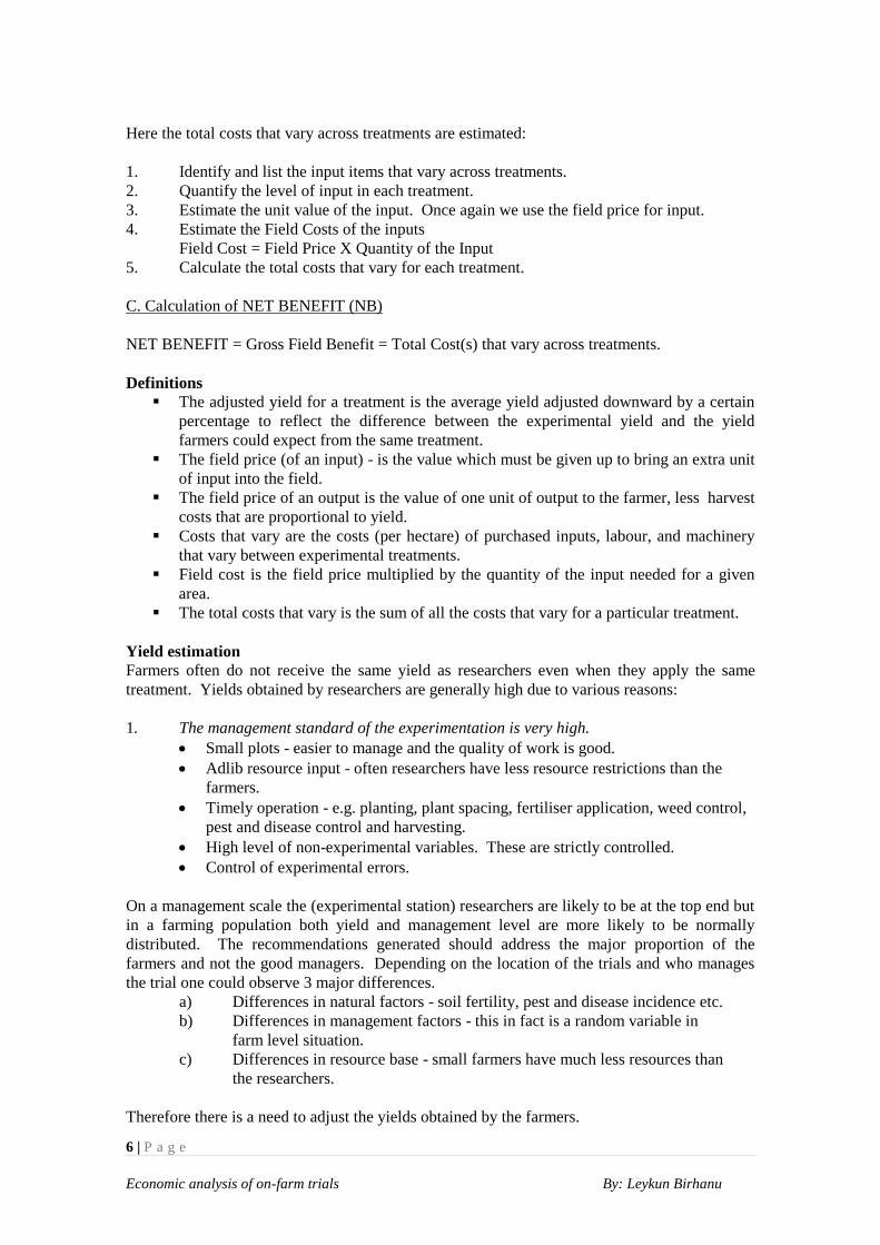
Here the total costs that vary across treatments are estimated:
1. Identify and list the input items that vary across treatments.
2. Quantify the level of input in each treatment.
3. Estimate the unit value of the input. Once again we use the field price for input.
4. Estimate the Field Costs of the inputs
Field Cost = Field Price X Quantity of the Input
5. Calculate the total costs that vary for each treatment.
C. Calculation of NET BENEFIT (NB)
NET BENEFIT = Gross Field Benefit = Total Cost(s) that vary across treatments.
Definitions
The adjusted yield for a treatment is the average yield adjusted downward by a certain
percentage to reflect the difference between the experimental yield and the yield
farmers could expect from the same treatment.
The field price (of an input) - is the value which must be given up to bring an extra unit
of input into the field.
The field price of an output is the value of one unit of output to the farmer, less harvest
costs that are proportional to yield.
Costs that vary are the costs (per hectare) of purchased inputs, labour, and machinery
that vary between experimental treatments.
Field cost is the field price multiplied by the quantity of the input needed for a given
area.
The total costs that vary is the sum of all the costs that vary for a particular treatment.
Yield estimation
Farmers often do not receive the same yield as researchers even when they apply the same
treatment. Yields obtained by researchers are generally high due to various reasons:
1. The management standard of the experimentation is very high.
Small plots - easier to manage and the quality of work is good.
Adlib resource input - often researchers have less resource restrictions than the
farmers.
Timely operation - e.g. planting, plant spacing, fertiliser application, weed control,
pest and disease control and harvesting.
High level of non-experimental variables. These are strictly controlled.
Control of experimental errors.
On a management scale the (experimental station) researchers are likely to be at the top end but
in a farming population both yield and management level are more likely to be normally
distributed. The recommendations generated should address the major proportion of the
farmers and not the good managers. Depending on the location of the trials and who manages
the trial one could observe 3 major differences.
a) Differences in natural factors - soil fertility, pest and disease incidence etc.
b) Differences in management factors - this in fact is a random variable in
farm level situation.
c) Differences in resource base - small farmers have much less resources than
the researchers.
Therefore there is a need to adjust the yields obtained by the farmers.
7 | P a g e
Economic analysis of on-farm trials By: Leykun Birhanu
2. Use of Different Techniques
Researchers often use different harvesting and drying techniques which minimises
the field loses.
3. Storage losses
Some of the local varieties store better than the improve varieties. If farmers store
improved varieties for late sale or house hold consumption then they incur heavy
storage losses. Therefore the effective production for the farmer is less than the actual
harvest.
4. Abandoning of treatments
Very often researchers abandon some sites or some treatments due to drought, floods,
insect attack etc. This may inflate the yield of the experiment, but the farmers will have
to face these situations. Therefore it is important to include them in analysing the
experiments.
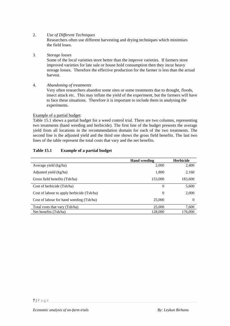
Example of a partial budget:
Table 15.1 shows a partial budget for a weed control trial. There are two columns, representing
two treatments (hand weeding and herbicide). The first line of the budget presents the average
yield from all locations in the recommendation domain for each of the two treatments. The
second line is the adjusted yield and the third one shows the gross field benefits. The last two
lines of the table represent the total costs that vary and the net benefits.
Table 15.1 Example of a partial budget
Hand weeding Herbicide
Average yield (kg/ha) 2,000 2,400
Adjusted yield (kg/ha) 1,800 2,160
Gross field benefits (Tsh/ha) 153,000 183,600
Cost of herbicide (Tsh/ha) 0 5,600
Cost of labour to apply herbicide (Tsh/ha) 0 2,000
Cost of labour for hand weeding (Tsh/ha) 25,000 0
Total costs that vary (Tsh/ha) 25,000 7,600
Net benefits (Tsh/ha) 128,000 176,000
8 | P a g e
Economic analysis of on-farm trials By: Leykun Birhanu
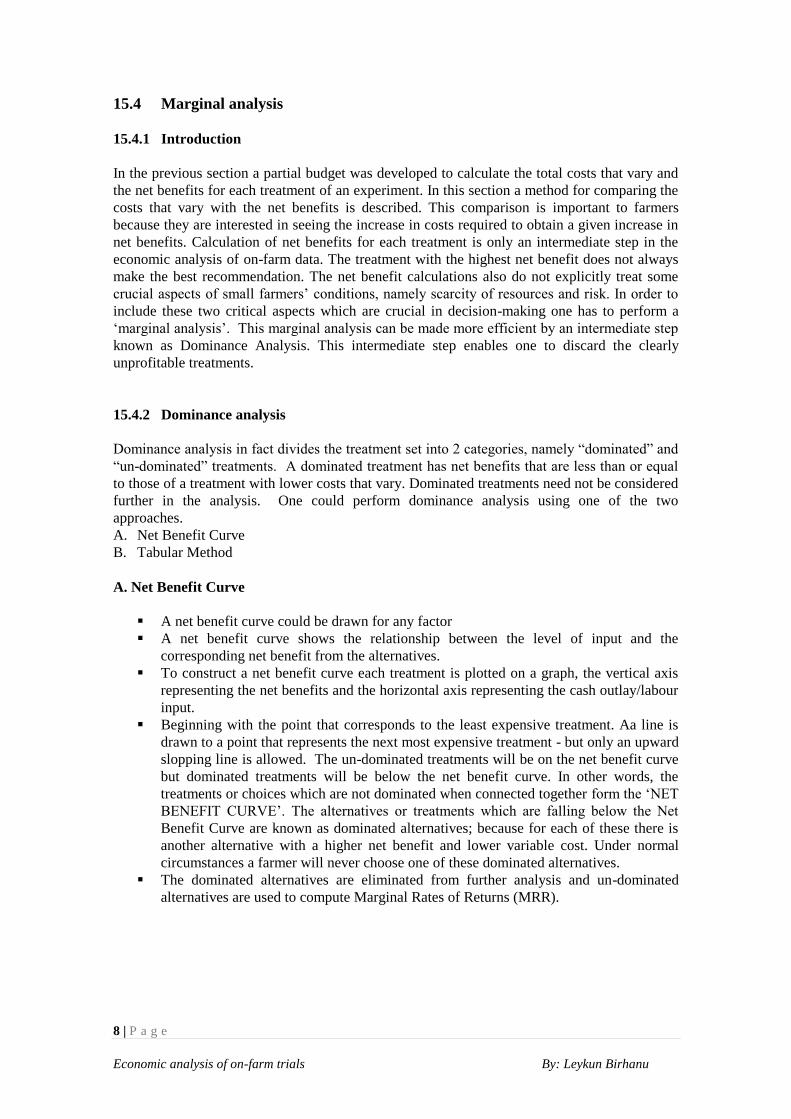
15.4 Marginal analysis
15.4.1 Introduction
In the previous section a partial budget was developed to calculate the total costs that vary and
the net benefits for each treatment of an experiment. In this section a method for comparing the
costs that vary with the net benefits is described. This comparison is important to farmers
because they are interested in seeing the increase in costs required to obtain a given increase in
net benefits. Calculation of net benefits for each treatment is only an intermediate step in the
economic analysis of on-farm data. The treatment with the highest net benefit does not always
make the best recommendation. The net benefit calculations also do not explicitly treat some
crucial aspects of small farmers’ conditions, namely scarcity of resources and risk. In order to
include these two critical aspects which are crucial in decision-making one has to perform a
‘marginal analysis’. This marginal analysis can be made more efficient by an intermediate step
known as Dominance Analysis. This intermediate step enables one to discard the clearly
unprofitable treatments.
15.4.2 Dominance analysis
Dominance analysis in fact divides the treatment set into 2 categories, namely “dominated” and
“un-dominated” treatments. A dominated treatment has net benefits that are less than or equal
to those of a treatment with lower costs that vary. Dominated treatments need not be considered
further in the analysis. One could perform dominance analysis using one of the two
approaches.
A. Net Benefit Curve
B. Tabular Method
A. Net Benefit Curve
A net benefit curve could be drawn for any factor
A net benefit curve shows the relationship between the level of input and the
corresponding net benefit from the alternatives.
To construct a net benefit curve each treatment is plotted on a graph, the vertical axis
representing the net benefits and the horizontal axis representing the cash outlay/labour
input.
Beginning with the point that corresponds to the least expensive treatment. Aa line is
drawn to a point that represents the next most expensive treatment - but only an upward
slopping line is allowed. The un-dominated treatments will be on the net benefit curve
but dominated treatments will be below the net benefit curve. In other words, the
treatments or choices which are not dominated when connected together form the ‘NET
BENEFIT CURVE’. The alternatives or treatments which are falling below the Net
Benefit Curve are known as dominated alternatives; because for each of these there is
another alternative with a higher net benefit and lower variable cost. Under normal
circumstances a farmer will never choose one of these dominated alternatives.
The dominated alternatives are eliminated from further analysis and un-dominated
alternatives are used to compute Marginal Rates of Returns (MRR).
9 | P a g e
Economic analysis of on-farm trials By: Leykun Birhanu
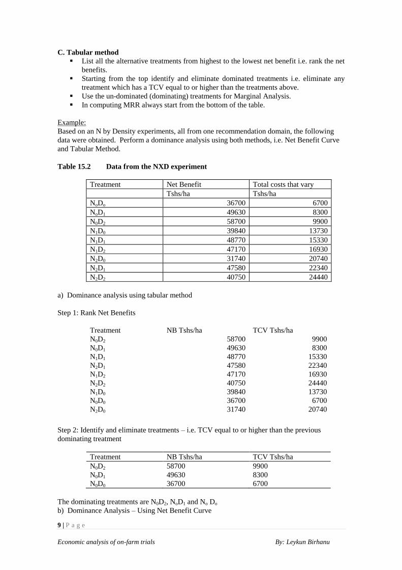
C. Tabular method
List all the alternative treatments from highest to the lowest net benefit i.e. rank the net
benefits.
Starting from the top identify and eliminate dominated treatments i.e. eliminate any
treatment which has a TCV equal to or higher than the treatments above.
Use the un-dominated (dominating) treatments for Marginal Analysis.
In computing MRR always start from the bottom of the table.
Example:
Based on an N by Density experiments, all from one recommendation domain, the following
data were obtained. Perform a dominance analysis using both methods, i.e. Net Benefit Curve
and Tabular Method.
Table 15.2 Data from the NXD experiment
Treatment Net Benefit Total costs that vary
Tshs/ha Tshs/ha
NoDo 36700 6700
NoD1 49630 8300
N0D2 58700 9900
N1D0 39840 13730
N1D1 48770 15330
N1D2 47170 16930
N2D0 31740 20740
N2D1 47580 22340
N2D2 40750 24440
a) Dominance analysis using tabular method
Step 1: Rank Net Benefits
Treatment NB Tshs/ha TCV Tshs/ha
N0D2 58700 9900
N0D1 49630 8300
N1D1 48770 15330
N2D1 47580 22340
N1D2 47170 16930
N2D2 40750 24440
N1D0 39840 13730
N0D0 36700 6700
N2D0 31740 20740
Step 2: Identify and eliminate treatments – i.e. TCV equal to or higher than the previous
dominating treatment
Treatment NB Tshs/ha TCV Tshs/ha
N0D2 58700 9900
N0D1 49630 8300
N0D0 36700 6700
The dominating treatments are N0D2, NoD1 and No Do
b) Dominance Analysis – Using Net Benefit Curve
10 | P a g e
Economic analysis of on-farm trials By: Leykun Birhanu
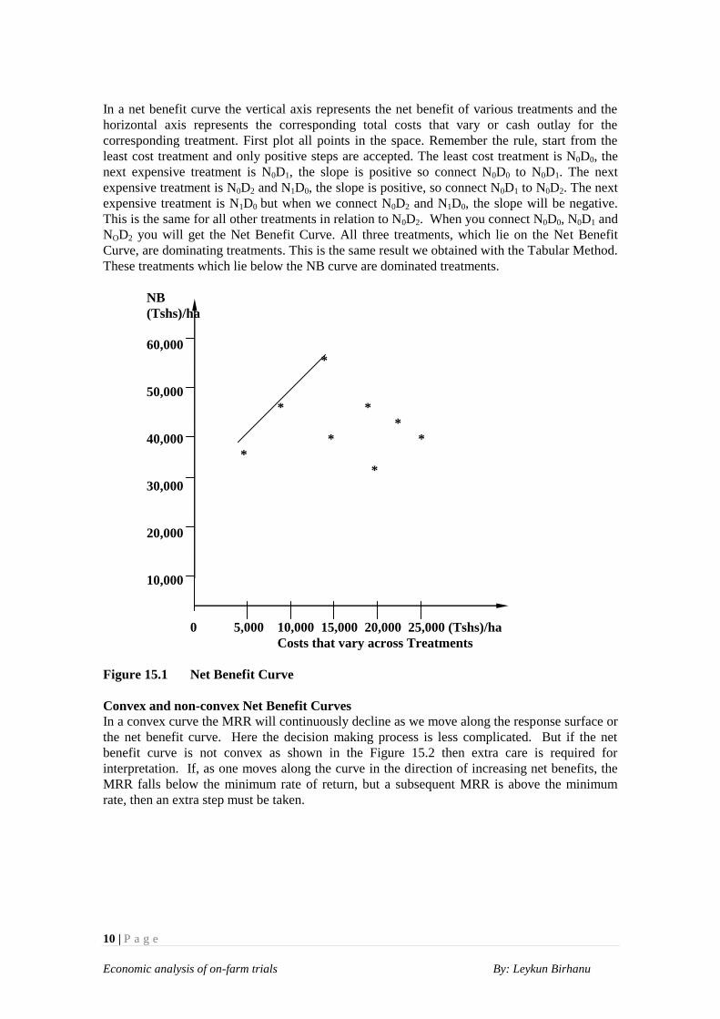
In a net benefit curve the vertical axis represents the net benefit of various treatments and the
horizontal axis represents the corresponding total costs that vary or cash outlay for the
corresponding treatment. First plot all points in the space. Remember the rule, start from the
least cost treatment and only positive steps are accepted. The least cost treatment is N0D0, the
next expensive treatment is N0D1, the slope is positive so connect N0D0 to N0D1. The next
expensive treatment is N0D2 and N1D0, the slope is positive, so connect N0D1 to N0D2. The next
expensive treatment is N1D0 but when we connect N0D2 and N1D0, the slope will be negative.
This is the same for all other treatments in relation to N0D2. When you connect N0D0, N0D1 and
NOD2 you will get the Net Benefit Curve. All three treatments, which lie on the Net Benefit
Curve, are dominating treatments. This is the same result we obtained with the Tabular Method.
These treatments which lie below the NB curve are dominated treatments.
NB
(Tshs)/ha
60,000
*
50,000
* *
*
40,000 * *
*
*
30,000
20,000
10,000
0 5,000 10,000 15,000 20,000 25,000 (Tshs)/ha
Costs that vary across Treatments
Figure 15.1 Net Benefit Curve
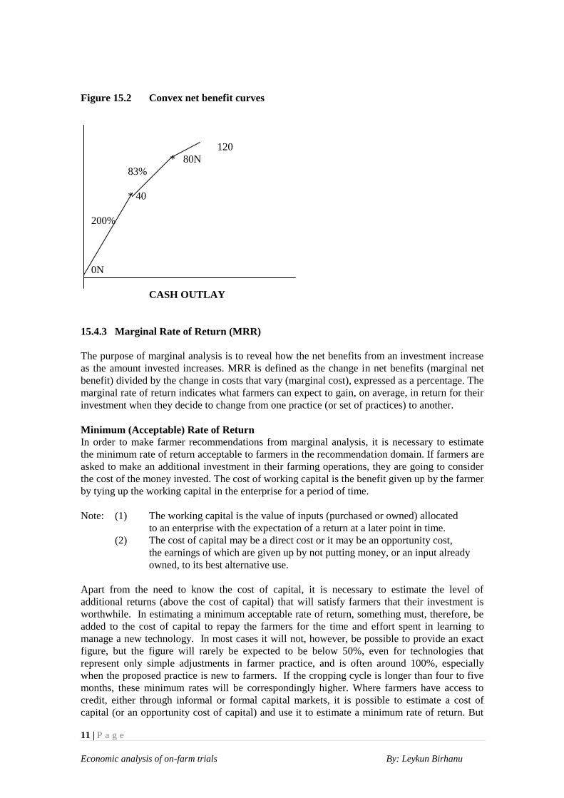
Convex and non-convex Net Benefit Curves
In a convex curve the MRR will continuously decline as we move along the response surface or
the net benefit curve. Here the decision making process is less complicated. But if the net
benefit curve is not convex as shown in the Figure 15.2 then extra care is required for
interpretation. If, as one moves along the curve in the direction of increasing net benefits, the
MRR falls below the minimum rate of return, but a subsequent MRR is above the minimum
rate, then an extra step must be taken.
11 | P a g e
Economic analysis of on-farm trials By: Leykun Birhanu
Figure 15.2 Convex net benefit curves
120
* 80N
83%
* 40
200%
0N
CASH OUTLAY
15.4.3 Marginal Rate of Return (MRR)
The purpose of marginal analysis is to reveal how the net benefits from an investment increase
as the amount invested increases. MRR is defined as the change in net benefits (marginal net
benefit) divided by the change in costs that vary (marginal cost), expressed as a percentage. The
marginal rate of return indicates what farmers can expect to gain, on average, in return for their
investment when they decide to change from one practice (or set of practices) to another.
Minimum (Acceptable) Rate of Return
In order to make farmer recommendations from marginal analysis, it is necessary to estimate
the minimum rate of return acceptable to farmers in the recommendation domain. If farmers are
asked to make an additional investment in their farming operations, they are going to consider
the cost of the money invested. The cost of working capital is the benefit given up by the farmer
by tying up the working capital in the enterprise for a period of time.
Note: (1) The working capital is the value of inputs (purchased or owned) allocated
to an enterprise with the expectation of a return at a later point in time.
(2) The cost of capital may be a direct cost or it may be an opportunity cost,
the earnings of which are given up by not putting money, or an input already
owned, to its best alternative use.
Apart from the need to know the cost of capital, it is necessary to estimate the level of
additional returns (above the cost of capital) that will satisfy farmers that their investment is
worthwhile. In estimating a minimum acceptable rate of return, something must, therefore, be
added to the cost of capital to repay the farmers for the time and effort spent in learning to
manage a new technology. In most cases it will not, however, be possible to provide an exact
figure, but the figure will rarely be expected to be below 50%, even for technologies that
represent only simple adjustments in farmer practice, and is often around 100%, especially
when the proposed practice is new to farmers. If the cropping cycle is longer than four to five
months, these minimum rates will be correspondingly higher. Where farmers have access to
credit, either through informal or formal capital markets, it is possible to estimate a cost of
capital (or an opportunity cost of capital) and use it to estimate a minimum rate of return. But
12 | P a g e
Economic analysis of on-farm trials By: Leykun Birhanu
even in such cases, it must be remembered that the figure will be approximate. In summary, if
the estimated MRR for cash is less than the Minimum Acceptable Rate for Return (MARR)
then reject the technology.
This minimum rate of return should cover:
Direct cost of cash;
Risk premium, and;
Provide some incentive (management) for the producer/farmer.
The maximum economic limit on input use is more meaningful to a farmer with abundant
capital or credit. At this level the farmer makes more net income even though the efficiency
with which (s) he is using his/her capital and inputs is less than the maximum possible.
To be acceptable, a new technology needs to be:
At a cost which the target group of farmers can handle
Competitive with the present options that the farmers have for spending their cash
Low risk of losing the cash investment
Using Marginal Analysis to make recommendations
The procedure involves comparing the marginal rates of return (MRR) between treatments with
the minimum rate of return acceptable to farmers. It should be noted that this type of analysis is
useful both for making recommendation to farmers, where there is sufficient experimental
evidence, and for helping select treatments for further experimentation. Farmers should be
willing to change from one treatment to another if the MRR of that change is greater than the
minimum rate of return.
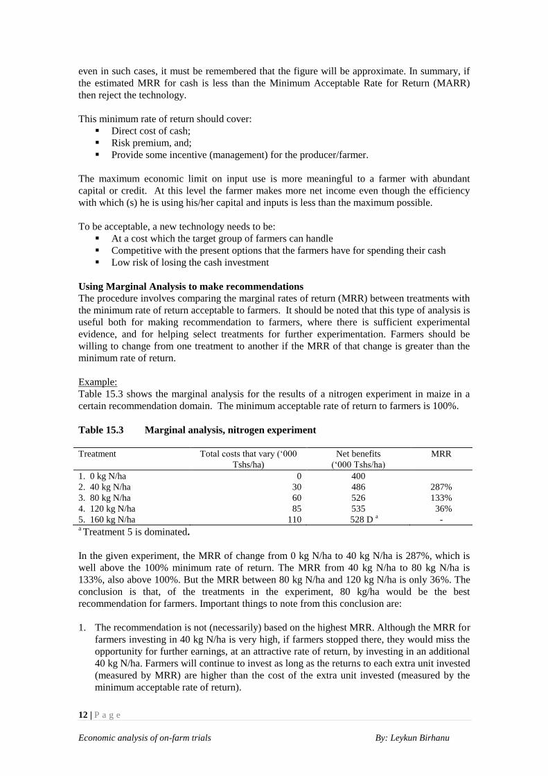
Example:
Table 15.3 shows the marginal analysis for the results of a nitrogen experiment in maize in a
certain recommendation domain. The minimum acceptable rate of return to farmers is 100%.
Table 15.3 Marginal analysis, nitrogen experiment
Treatment Total costs that vary (‘000
Tshs/ha)
Net benefits
(‘000 Tshs/ha)
MRR
1. 0 kg N/ha 0 400
2. 40 kg N/ha 30 486 287%
3. 80 kg N/ha 60 526 133%
4. 120 kg N/ha 85 535 36%
5. 160 kg N/ha 110 528 D a -
a Treatment 5 is dominated.
In the given experiment, the MRR of change from 0 kg N/ha to 40 kg N/ha is 287%, which is
well above the 100% minimum rate of return. The MRR from 40 kg N/ha to 80 kg N/ha is
133%, also above 100%. But the MRR between 80 kg N/ha and 120 kg N/ha is only 36%. The
conclusion is that, of the treatments in the experiment, 80 kg/ha would be the best
recommendation for farmers. Important things to note from this conclusion are:
1. The recommendation is not (necessarily) based on the highest MRR. Although the MRR for
farmers investing in 40 kg N/ha is very high, if farmers stopped there, they would miss the
opportunity for further earnings, at an attractive rate of return, by investing in an additional
40 kg N/ha. Farmers will continue to invest as long as the returns to each extra unit invested
(measured by MRR) are higher than the cost of the extra unit invested (measured by the
minimum acceptable rate of return).

13 | P a g e
Economic analysis of on-farm trials By: Leykun Birhanu
2. The recommendation is not (necessarily) the treatment with the highest net benefits (in this
case 120 kg N/ha). If instead of a step-by-step marginal analysis, an average analysis is
carried out, the rate of return looks attractive (i.e. (535-400)/(85-0) = 159%), but this is
misleading because the average rate of return of 159% hides the fact that most of the
benefits were already earned from lower levels of investment.
In conclusion, therefore, it should be noted that the recommendation is not necessarily the
treatment with the highest MRR compared to that of next lowest cost, nor the treatment with
the highest net benefit. The identification of a recommendation requires careful marginal
analysis using an appropriate minimum rate of return.
14 | P a g e
Economic analysis of on-farm trials By: Leykun Birhanu
15.5 Dealing with risk in on-farm research
15.5.1 Need for risk analysis
Whenever a specific action may give different outcomes when repeated at a different time,
there is said to be risk attached to that action. In other words where the outcome of an action
cannot be predicted with complete certainty, there is risk. Farming is a particularly risky
activity. For example, climate, diseases and prices are all unpredictable and affect the outcome
of any farming activity. When farmers evaluate one action (practice) against another they will
take account of the outcome variability (risk) attached to each action.
Risk is present when the outcome of the intervention (result) is not known with certainty. For
example, experimental results indicate a range (distribution) of yield obtained from various
sites (locations) at different time periods (year to year variation). Not all farmers obtain the
same yield in all sites at all times. There is not one yield level (single value) to realise but
rather a range of yields, but we do not know for sure which will be realised at the farmer level
of output. The marginal analysis discussed in the previous section uses an average of those
yields to calculate the Net Benefits.
From experience we know that some treatments lead to larger yields on average but are highly
variable (more risky and less stable). Other treatments may result in lower yields on average
but with smaller range of variation (less risky or more stable). If farmers do not care about risk
(risk neutral) then variability in yields does not matter. However, small holder farmers
generally care about stability and level of returns. They are risk averse and they prefer less risk
as well as higher returns. Therefore, in the minds of the farmers, a treatment that combines
both desirable properties (less risky or stable as well as higher returns) dominates. Most of the
times there is a trade off between higher returns and risk. The choice then depends on the
degree of risk aversion of the farmers. The basic questions are:
How much risk can a farmer accept in exchange for larger benefits on average?
Or
How much gain in average benefits is he/she is willing to give up for more stable or assured
returns?
It is difficult to measure (remember that there are techniques) the degree of risk aversion or
farmers' attitude towards the risk, but we need to provide for variability (risk) in our analysis as
risk matters to the farmers.
15.5.2 Risk decision theory
There are two major elements to decision theory under risk. The first deals with the
PROBABILITIES of outcome from a specific action. That is the extent of outcome variability.
This is a function of a particular technology in a given environment. The other element deals
with farmer response to variability of outcomes, often referred to as risk aversion. This is a
personal characteristic of the farmer, or group of farmers and has to do with RISK
PREFERENCES and CERTAINTY EQUIVALENTS.
A. Subjective probabilities
For any action that gives variable outcomes, it will be possible for farmers to attach
probabilities of obtaining different outcomes. For example a farmer’s current technology set
for growing maize (A) may give Tsh. 100,000 net value of output per hectare 50% of the time
15 | P a g e
Economic analysis of on-farm trials By: Leykun Birhanu
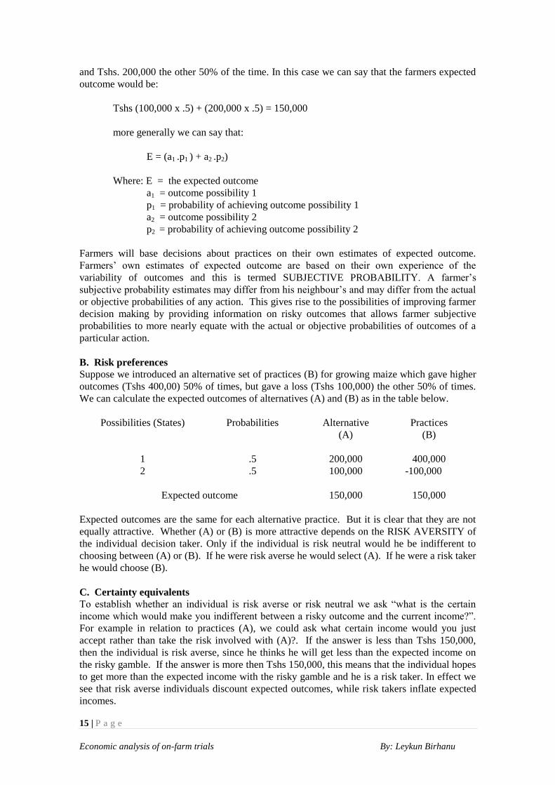
and Tshs. 200,000 the other 50% of the time. In this case we can say that the farmers expected
outcome would be:
Tshs (100,000 x .5) + (200,000 x .5) = 150,000
more generally we can say that:
E = (a1 .p1 ) + a2 .p2)
Where: E = the expected outcome
a1 = outcome possibility 1
p1 = probability of achieving outcome possibility 1
a2 = outcome possibility 2
p2 = probability of achieving outcome possibility 2
Farmers will base decisions about practices on their own estimates of expected outcome.
Farmers’ own estimates of expected outcome are based on their own experience of the
variability of outcomes and this is termed SUBJECTIVE PROBABILITY. A farmer’s
subjective probability estimates may differ from his neighbour’s and may differ from the actual
or objective probabilities of any action. This gives rise to the possibilities of improving farmer
decision making by providing information on risky outcomes that allows farmer subjective
probabilities to more nearly equate with the actual or objective probabilities of outcomes of a
particular action.
B. Risk preferences
Suppose we introduced an alternative set of practices (B) for growing maize which gave higher
outcomes (Tshs 400,00) 50% of times, but gave a loss (Tshs 100,000) the other 50% of times.
We can calculate the expected outcomes of alternatives (A) and (B) as in the table below.
Possibilities (States) Probabilities Alternative
(A)
Practices
(B)
1
.5
200,000
400,000
2 .5 100,000 -100,000
Expected outcome
150,000
150,000
Expected outcomes are the same for each alternative practice. But it is clear that they are not
equally attractive. Whether (A) or (B) is more attractive depends on the RISK AVERSITY of
the individual decision taker. Only if the individual is risk neutral would he be indifferent to
choosing between (A) or (B). If he were risk averse he would select (A). If he were a risk taker
he would choose (B).
C. Certainty equivalents
To establish whether an individual is risk averse or risk neutral we ask “what is the certain
income which would make you indifferent between a risky outcome and the current income?”.
For example in relation to practices (A), we could ask what certain income would you just
accept rather than take the risk involved with (A)?. If the answer is less than Tshs 150,000,
then the individual is risk averse, since he thinks he will get less than the expected income on
the risky gamble. If the answer is more then Tshs 150,000, this means that the individual hopes
to get more than the expected income with the risky gamble and he is a risk taker. In effect we
see that risk averse individuals discount expected outcomes, while risk takers inflate expected
incomes.
16 | P a g e
Economic analysis of on-farm trials By: Leykun Birhanu
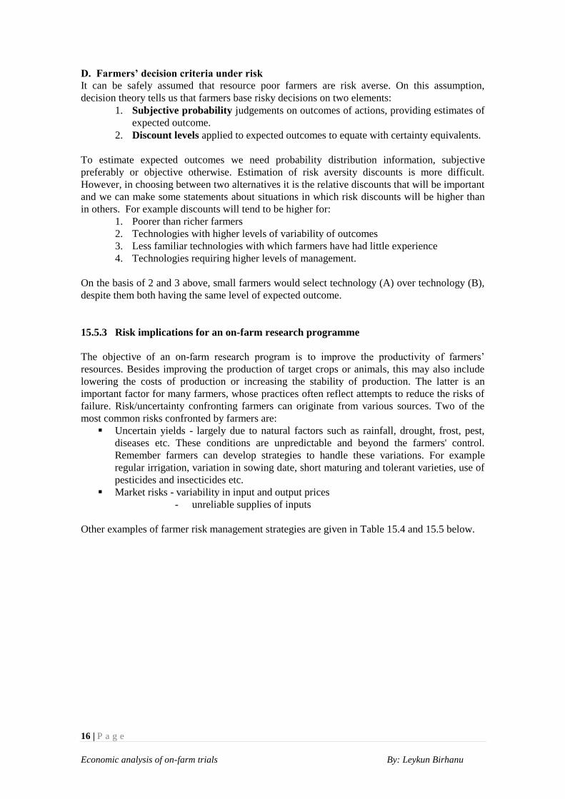
D. Farmers’ decision criteria under risk
It can be safely assumed that resource poor farmers are risk averse. On this assumption,
decision theory tells us that farmers base risky decisions on two elements:
1. Subjective probability judgements on outcomes of actions, providing estimates of
expected outcome.
2. Discount levels applied to expected outcomes to equate with certainty equivalents.
To estimate expected outcomes we need probability distribution information, subjective
preferably or objective otherwise. Estimation of risk aversity discounts is more difficult.
However, in choosing between two alternatives it is the relative discounts that will be important
and we can make some statements about situations in which risk discounts will be higher than
in others. For example discounts will tend to be higher for:
1. Poorer than richer farmers
2. Technologies with higher levels of variability of outcomes
3. Less familiar technologies with which farmers have had little experience
4. Technologies requiring higher levels of management.
On the basis of 2 and 3 above, small farmers would select technology (A) over technology (B),
despite them both having the same level of expected outcome.
15.5.3 Risk implications for an on-farm research programme
The objective of an on-farm research program is to improve the productivity of farmers’
resources. Besides improving the production of target crops or animals, this may also include
lowering the costs of production or increasing the stability of production. The latter is an
important factor for many farmers, whose practices often reflect attempts to reduce the risks of
failure. Risk/uncertainty confronting farmers can originate from various sources. Two of the
most common risks confronted by farmers are:
Uncertain yields - largely due to natural factors such as rainfall, drought, frost, pest,
diseases etc. These conditions are unpredictable and beyond the farmers' control.
Remember farmers can develop strategies to handle these variations. For example
regular irrigation, variation in sowing date, short maturing and tolerant varieties, use of
pesticides and insecticides etc.
Market risks - variability in input and output prices
- unreliable supplies of inputs
Other examples of farmer risk management strategies are given in Table 15.4 and 15.5 below.
17 | P a g e
Economic analysis of on-farm trials By: Leykun Birhanu
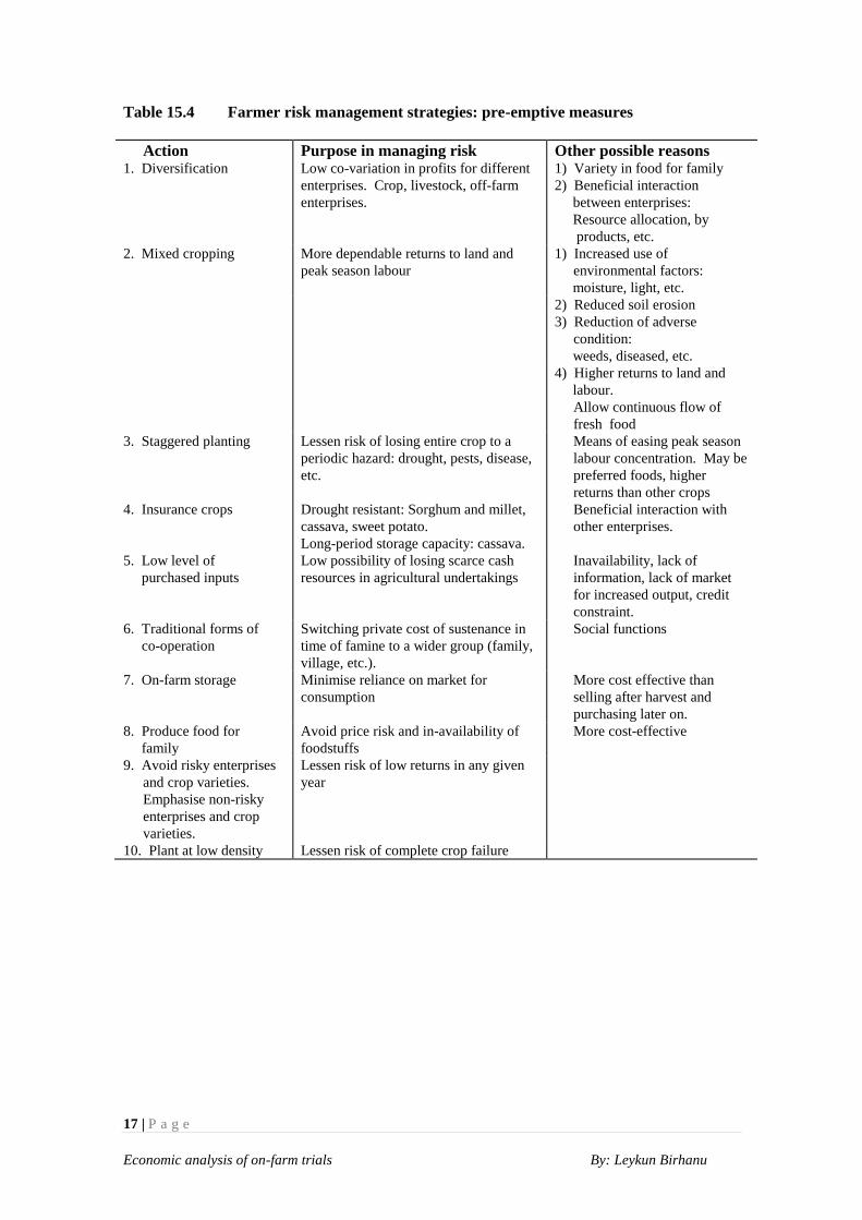
Table 15.4 Farmer risk management strategies: pre-emptive measures
Action Purpose in managing risk Other possible reasons 1. Diversification Low co-variation in profits for different
enterprises. Crop, livestock, off-farm
enterprises.
1) Variety in food for family
2) Beneficial interaction
between enterprises:
Resource allocation, by
products, etc.
2. Mixed cropping More dependable returns to land and
peak season labour
1) Increased use of
environmental factors:
moisture, light, etc.
2) Reduced soil erosion
3) Reduction of adverse
condition:
weeds, diseased, etc.
4) Higher returns to land and
labour.
Allow continuous flow of
fresh food
3. Staggered planting Lessen risk of losing entire crop to a
periodic hazard: drought, pests, disease,
etc.
Means of easing peak season
labour concentration. May be
preferred foods, higher
returns than other crops
4. Insurance crops Drought resistant: Sorghum and millet,
cassava, sweet potato.
Long-period storage capacity: cassava.
Beneficial interaction with
other enterprises.
5. Low level of
purchased inputs
Low possibility of losing scarce cash
resources in agricultural undertakings
Inavailability, lack of
information, lack of market
for increased output, credit
constraint.
6. Traditional forms of
co-operation
Switching private cost of sustenance in
time of famine to a wider group (family,
village, etc.).
Social functions
7. On-farm storage Minimise reliance on market for
consumption
More cost effective than
selling after harvest and
purchasing later on.
8. Produce food for
family
Avoid price risk and in-availability of
foodstuffs
More cost-effective
9. Avoid risky enterprises
and crop varieties.
Emphasise non-risky
enterprises and crop
varieties.
Lessen risk of low returns in any given
year
10. Plant at low density Lessen risk of complete crop failure
18 | P a g e
Economic analysis of on-farm trials By: Leykun Birhanu
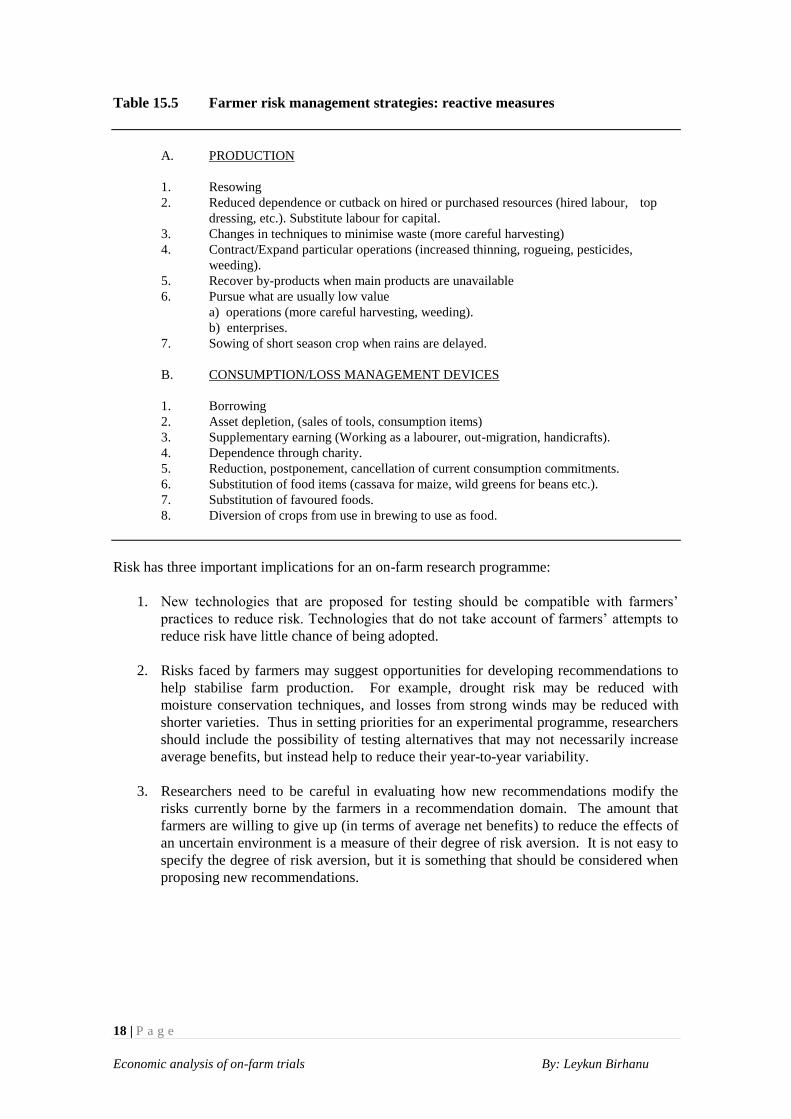
Table 15.5 Farmer risk management strategies: reactive measures
A. PRODUCTION
1. Resowing
2. Reduced dependence or cutback on hired or purchased resources (hired labour, top
dressing, etc.). Substitute labour for capital.
3. Changes in techniques to minimise waste (more careful harvesting)
4. Contract/Expand particular operations (increased thinning, rogueing, pesticides,
weeding).
5. Recover by-products when main products are unavailable
6. Pursue what are usually low value
a) operations (more careful harvesting, weeding).
b) enterprises.
7. Sowing of short season crop when rains are delayed.
B. CONSUMPTION/LOSS MANAGEMENT DEVICES
1. Borrowing
2. Asset depletion, (sales of tools, consumption items)
3. Supplementary earning (Working as a labourer, out-migration, handicrafts).
4. Dependence through charity.
5. Reduction, postponement, cancellation of current consumption commitments.
6. Substitution of food items (cassava for maize, wild greens for beans etc.).
7. Substitution of favoured foods.
8. Diversion of crops from use in brewing to use as food.
Risk has three important implications for an on-farm research programme:
1. New technologies that are proposed for testing should be compatible with farmers’
practices to reduce risk. Technologies that do not take account of farmers’ attempts to
reduce risk have little chance of being adopted.
2. Risks faced by farmers may suggest opportunities for developing recommendations to
help stabilise farm production. For example, drought risk may be reduced with
moisture conservation techniques, and losses from strong winds may be reduced with
shorter varieties. Thus in setting priorities for an experimental programme, researchers
should include the possibility of testing alternatives that may not necessarily increase
average benefits, but instead help to reduce their year-to-year variability.
3. Researchers need to be careful in evaluating how new recommendations modify the
risks currently borne by the farmers in a recommendation domain. The amount that
farmers are willing to give up (in terms of average net benefits) to reduce the effects of
an uncertain environment is a measure of their degree of risk aversion. It is not easy to
specify the degree of risk aversion, but it is something that should be considered when
proposing new recommendations.
19 | P a g e
Economic analysis of on-farm trials By: Leykun Birhanu
15.5.4 Techniques used in handling risk
If the probability of occurrence of each state of nature or incidence of changing factors is
known, then the risk factor can be incorporated in the quantitative analysis. Unfortunately in
most cases this information is not available. One can use subjective probabilities for some
events. Once again we are looking for some simple techniques. In performing economic
analysis of technologies very often one of the following approaches can be used to handle risk.
Minimum returns analysis
Sensitivity analysis
Risk discounting
These simple techniques are discussed in the following sections.
A. Minimum Returns Analysis
A minimum returns analysis (MRA) is a way of screening data from on-farm experiments in
order to give farmers (and researchers) additional information about the variability in returns
implicit in a proposed recommendation in comparison with the farmers’ practice. A minimum
returns analysis compares the average of the lowest net benefits for each non-dominated
treatment. The MRA presented below is not strictly speaking, a method of risk analysis, but
rather a way of assessing the variability due to unpredictable and at times unexplained causes.
The MRA is done to look at variability the way that farmers do. Looking at across-location and
across-year variability is one way of estimating the risks for farmers associated with the
proposed recommendation. The careful definition of recommendation domains attempts to
eliminate across-location variability as much as possible. Across-year variability, on the other
hand, is estimated based on the results of several years. A careful minimum returns analysis is
therefore a useful way of examining the variability associated with different technological
alternatives.
It should be noted that farmers are more interested in variability in benefits than variability in
yields. A minimum returns analysis looks at variability in net benefits. If the results of a set of
on-farm experiments show that two treatments have the same average net benefits, but one
treatment’s results are more variable than the other’s, it is likely that farmers will prefer the
treatment that is more consistent, rather than the one that sometimes gives very high net
benefits but at other times gives very low net benefits.
Pre-requisites for a Minimum Returns Analysis
For the MRA to be relevant, several prerequisites must be met:
1. The marginal analysis must have been done on all locations for a given experiment and for
all years.
2. A minimum returns analysis should be done only on experimental treatments that are being
considered for recommendation. That may include not only the farmers’ practice and the
treatment that has been judged acceptable on the average by marginal analysis, but also
other non-dominated treatments that may provide alternatives if the tentative
recommendation proves unsatisfactory.
3. Minimum returns analysis presumes that researchers have tried to explain the reasons for
the variability they observe. The more precise an idea of the sources of observed
variability, the more useful the information from the minimum returns analysis will be for
farmers.
4. Minimum returns analysis is relevant when done on the results of several locations and
years. The results should be from enough locations and years to fairly represent the
variability that farmers in the recommendation domain are likely to face.
20 | P a g e
Economic analysis of on-farm trials By: Leykun Birhanu
Minimum Returns Analysis: procedure
The steps involved in the minimum returns analysis are:
1. To calculate the net benefits at each one of the locations for each one of the treatments.
2. To select the (approximately) 25% lowest benefits for one treatment and compare their
average with that of the 25% lowest benefits for the alternative.
3. If the average of the lowest net benefits for the tentative recommendation is higher than the
average of the lowest net benefits for the farmers’ practice, then the recommendation
should be made, because even in the worst cases the recommendation does better than the
farmers’ practice.
4. If the average for the tentative recommendation is lower than that for the farmers’ practice,
then one should be more careful in making the recommendation. The absolute value of the
net benefits has little meaning but the difference between the two should be examined. If
the difference is small, then farmers will probably be willing to accept this risk, knowing
that over the long run they will benefit. If, on the other hand, the difference is large, then it
would be best to reconsider the recommendation by taking an alternative less risky
recommendation. If this is not available, then the farmers’ practice is to be preferred.
It is important to note that:
MRA assumes that all locations are representative of a single recommendation domain,
and that there is nothing special about any individual location.
MRA is done with actual location by location data.
The key to MRA is a common sense examination of the data from the farmers’ point of
view.
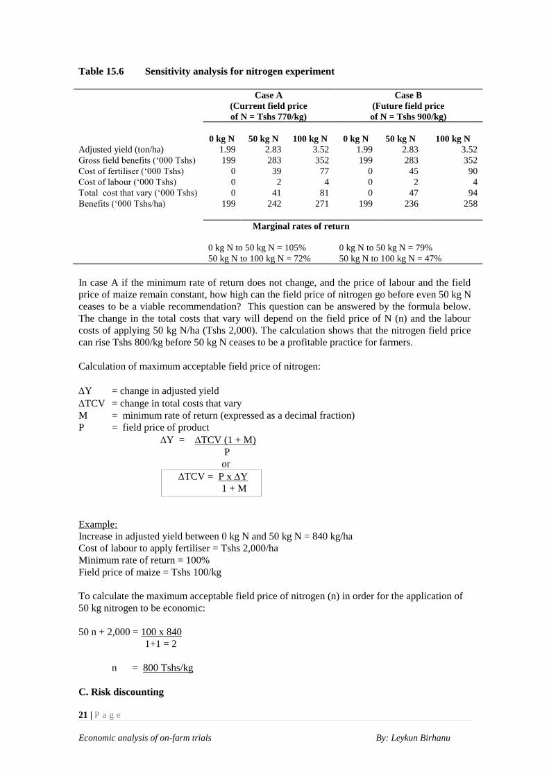
B. Sensitivity analysis
Experimental yields are not the only element of the partial budget that is likely to change. Input
and product prices are also subject to change. The best way to test a recommendation for its
ability to withstand price changes is through sensitivity analysis. This simply implies redoing a
marginal analysis with alternative prices. If, for instance, a fertiliser recommendation is made
using current fertiliser prices, but there are indications that those prices may increase a
reasonable estimate of the new prices may be substituted in the analysis. Table 3 illustrates
such a situation. In the original analysis (case A), a field price for nitrogen of Tsh 770/kg was
used. The recommendation of 50 kg N was made, assuming a minimum rate of return of 100%.
If the field price of nitrogen increases to Tshs. 900/kg would the same recommendation hold?
Redoing the partial budget (case B) with the higher price of nitrogen shows that the
recommendation of 50 kg N is now inappropriate because the marginal rate of return from
application of 50 kg N is less than the minimum rate of return (100%). Any higher nitrogen
prices would necessitate lowering the fertiliser recommendation.
21 | P a g e
Economic analysis of on-farm trials By: Leykun Birhanu
Table 15.6 Sensitivity analysis for nitrogen experiment
Case A
(Current field price
of N = Tshs 770/kg)
Case B
(Future field price
of N = Tshs 900/kg)
0 kg N
50 kg N
100 kg N
0 kg N
50 kg N
100 kg N
Adjusted yield (ton/ha) 1.99 2.83 3.52 1.99 2.83 3.52
Gross field benefits (‘000 Tshs) 199 283 352 199 283 352
Cost of fertiliser (‘000 Tshs) 0 39 77 0 45 90
Cost of labour (‘000 Tshs) 0 2 4 0 2 4
Total cost that vary (‘000 Tshs) 0 41 81 0 47 94
Benefits (‘000 Tshs/ha) 199 242 271 199 236 258
Marginal rates of return
0 kg N to 50 kg N = 105% 0 kg N to 50 kg N = 79%
50 kg N to 100 kg N = 72% 50 kg N to 100 kg N = 47%
In case A if the minimum rate of return does not change, and the price of labour and the field
price of maize remain constant, how high can the field price of nitrogen go before even 50 kg N
ceases to be a viable recommendation? This question can be answered by the formula below.
The change in the total costs that vary will depend on the field price of N (n) and the labour
costs of applying 50 kg N/ha (Tshs 2,000). The calculation shows that the nitrogen field price
can rise Tshs 800/kg before 50 kg N ceases to be a profitable practice for farmers.
Calculation of maximum acceptable field price of nitrogen:
Y = change in adjusted yield
TCV = change in total costs that vary
M = minimum rate of return (expressed as a decimal fraction)
P = field price of product
Y = TCV (1 + M)
P
or
TCV = P x Y
1 + M
Example:
Increase in adjusted yield between 0 kg N and 50 kg N = 840 kg/ha
Cost of labour to apply fertiliser = Tshs 2,000/ha
Minimum rate of return = 100%
Field price of maize = Tshs 100/kg
To calculate the maximum acceptable field price of nitrogen (n) in order for the application of
50 kg nitrogen to be economic:
50 n + 2,000 = 100 x 840
1+1 = 2
n = 800 Tshs/kg
C. Risk discounting
22 | P a g e
Economic analysis of on-farm trials By: Leykun Birhanu
This is simply a matter of discounting the rate of return for risk. This is done by adding a risk
premium to the cost of capital in estimating the minimum acceptable rate of returns (MARR)
for the farmer. The risk premium depends on the nature of the technology, which depends on
the subjective judgement of the research team. If the anticipated risk is high, then the benefits
are highly discounted by adding a much higher risk premium in MARR. As a rule of thumb, the
average acceptable rate of return should be at least 20 percent above the direct cost of capital.
Remember, the cost of capital may vary from farmer to farmer and may also depend on the
source of capital.
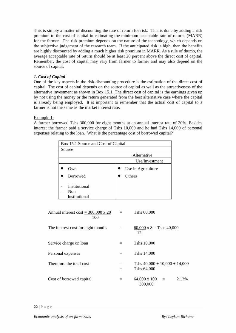
1. Cost of Capital
One of the key aspects in the risk discounting procedure is the estimation of the direct cost of
capital. The cost of capital depends on the source of capital as well as the attractiveness of the
alternative investment as shown in Box 15.1. The direct cost of capital is the earnings given up
by not using the money or the return generated from the best alternative case where the capital
is already being employed. It is important to remember that the actual cost of capital to a
farmer is not the same as the market interest rate.
Example 1:
A farmer borrowed Tshs 300,000 for eight months at an annual interest rate of 20%. Besides
interest the farmer paid a service charge of Tshs 10,000 and he had Tshs 14,000 of personal
expenses relating to the loan. What is the percentage cost of borrowed capital?
Box 15.1 Source and Cost of Capital
Source
Alternative
Use/Investment
Own
Borrowed
- Institutional
- Non
Institutional
Use in Agriculture
Others
Annual interest cost = 300,000 x 20 = Tshs 60,000
100
The interest cost for eight months = 60,000 x 8 = Tshs 40,000
12
Service charge on loan = Tshs 10,000
Personal expenses = Tshs 14,000
Therefore the total cost = Tshs 40,000 + 10,000 + 14,000
= Tshs 64,000
Cost of borrowed capital = 64,000 x 100 = 21.3%
300,000
23 | P a g e
Economic analysis of on-farm trials By: Leykun Birhanu
2. Minimum Acceptable Rate of Returns (MARR)
MARR is only an estimate and it must be inferred from an estimate of the cost of borrowed
capital. We need to be very realistic in making such estimation. The MARR should include the
direct cost of capital, plus some allowance for risk (not to mention management). The MARR is
influenced by three factors:
1. The type of technology under consideration
Whether it involves a major/minor change from the current practice
Likelihood of failure (e.g. loosing a crop) and frequency
Amount of cash involved
2. The cost of borrowed capital. This again depends on the source and alternative use as
discussed earlier.
3. The length of the enterprise cycle.
These factors should be carefully considered in estimating the MARR.
References
Amir, P. and H. C. Knipscheer (1989). Conducting on-farm animal research: Procedures and
economic analysis. Winrock International Arkansas, USA.
Anderson, J. R. and J. L. Dillon (1992). Risk analysis in dryland farming systems. FAO, Rome.
Anandajayasekeram, P. (n.d.). Teaching Notes: Experimental Evaluation. CIMMYT, Eastern
African Economics Programme, Nairobi, Kenya.
CIMMYT (1988A). From Agronomic Data to Farmer Recommendations: An Economics
Training Manual. Completely revised edition. Mexico, D.F.
CIMMYT (1988B). From Agronomic Data to Farmer Recommendations: An Economics
Workbook. Mexico, D.F.
Low, A. (1989). Application of Risk Decision Theory to Net Benefit and MRR Analysis.
Teaching Notes for the Experimental and Other Data Analysis Workshop for Social Scientists,
October 15-27, 1989, Njoro, Kenya.
Norman, D.W., J.D. Siebert, E. Modiakgotla and F.D. Worman (1994). Farming Systems
Research Approach: A Primer for Eastern and Southern Africa. Regional Farming Systems
Programme.
Perrin, R. K., D. L. Winkelmann, E. R. Moscardi and J. R. Anderson (1976). From agronomic
data to farmer recommendations: An economics training manual. Information Training Bulletin
21. CIMMYT, Mexico.
Worman, F., D. Norman and J. Ware-Snyder (Eds) (1990). Farming Systems Research
Handbook for Botswana. ATIP RP 3. Agricultural Technology Improvement Project.
Department of Agricultural Research Ministry of Agriculture, Botswana.