Habitat area trumps fragmentation effects on arthropods in an experimental landscape system

RESEARCH ARTICLE

Habitat area trumps fragmentation effects on arthropodsin an experimental landscape system

Kimberly A. With • Daniel M. Pavuk

Received: 11 February 2011 / Accepted: 21 June 2011 / Published online: 7 July 2011

� Springer Science+Business Media B.V. 2011

Abstract The effects of habitat area and fragmen-

tation are confounded in many studies. Since a

reduction in habitat area alone reduces patch size and

increases patch isolation, many studies reporting

fragmentation effects may really be documenting

habitat-area effects. We designed an experimental

landscape system in the field, founded on fractal

neutral landscape models, to study arthropod com-

munity responses to clover habitat in which we

adjusted the level of fragmentation independently of

habitat area. Overall, habitat area had a greater and

more consistent effect on morphospecies richness

than fragmentation. Morphospecies richness doubled

between 10 and 80% habitat, with the greatest

increase occurring up to 40% habitat. Fragmentation

had a more subtle and transient effect, exhibiting an

interaction at intermediate levels of habitat only at the

start of the study or in the early-season (June) survey.

In these early surveys, morphospecies richness was

higher in clumped 40–50% landscapes but higher in

fragmented landscapes at 60–80% habitat. Rare or

uncommon species are expected to be most sensitive

to fragmentation effects, and we found a significant

interaction with fragmentation at intermediate levels

of habitat for these types of morphospecies in early

surveys. Although the effects of fragmentation are

expected to amplify at higher trophic levels, all

trophic levels exhibited a significant fragmentation

effect at intermediate levels of habitat in these early

surveys. Predators/parasitoids were more sensitive to

habitat area than herbivores, however. Thus, our

results confirm that habitat area is more important

than fragmentation for predicting arthropod commu-

nity responses, at least in this agricultural system.

Keywords Agroecosystems � Edge effects �Insects � Patch size � Patch isolation � Scaling effects �Species–area relationship � Trophic responses

Introduction

Studies on the effects of habitat fragmentation have

been an active area of research in ecology for two

decades now. As Fahrig (2003) has pointed out,

however, many of these studies do not distinguish

between habitat loss and the effects of fragmentation

per se. Habitat fragmentation refers to the degree to

which habitat is subdivided on the landscape (i.e., the

pattern of habitat on the landscape). Because habitat

Electronic supplementary material The online version ofthis article (doi:10.1007/s10980-011-9627-x) containssupplementary material, which is available to authorized users.

K. A. With (&)

Division of Biology, Kansas State University, Manhattan,

KS 66506, USA

e-mail: [email protected]

D. M. Pavuk

Department of Biological Sciences, Bowling Green State

University, Bowling Green, OH 43403, USA

123

Landscape Ecol (2011) 26:1035–1048

DOI 10.1007/s10980-011-9627-x

Author's personal copy

http://dx.doi.org/10.1007/s10980-011-9627-x

fragmentation usually occurs as a result of habitat

loss, however, the effects of habitat loss and

fragmentation are likely to be confounded unless

care is taken to control for habitat area. In most of the

studies surveyed, many of the effects attributed to

fragmentation were really an effect of habitat area

(Fahrig 2003). Further, many of these fragmentation

studies were patch-based rather than landscape-based,

such that it was the attributes of the individual habitat

patches (patch size or isolation) rather than the

overall landscape (percent habitat cover or degree of

fragmentation) that were the object of study (see also

McGarigal and Cushman 2002). Although some

inferences about the effects of habitat loss and

fragmentation can be made from patch-based studies,

these effects are more properly studied at the

landscape scale, especially if landscape context (such

as the overall amount of habitat on the landscape) has

an overriding effect on ecological responses within

patches (Tscharntke et al. 2002; Fahrig 2003;

Collinge 2009).

Traditionally, the design of fragmentation studies

has been heavily influenced by island biogeography

and metapopulation theory, in which patch area and

isolation are assumed to govern species’ responses to

the loss and fragmentation of habitat: small isolated

patches are expected to have fewer species (owing to

greater extinction rates and lower rates of recoloni-

zation) than large patches or small patches that are

not isolated. Subsequently, most studies seek to

identify or create patches of various sizes and degrees

of isolation to test these effects on species richness or

some other ecological response (e.g., Kruess and

Tscharntke 1994; Golden and Crist 1999; Collinge

2000; Haynes and Crist 2009). However, because of

the inevitable trade-offs between patch size, inter-

patch distances and replication in most studies, only a

limited number of patch configurations can ultimately

be explored (Debinski and Holt 2000). Further,

although both habitat loss and fragmentation may

reduce habitat patch area, it is unclear that fragmen-

tation necessarily increases patch isolation. In fact,

habitat fragmentation could decrease isolation if the

pattern of fragmentation results in smaller gaps

between remaining patches that facilitate dispersal

across the landscape (Fahrig 2003). Thus, patch

isolation is more a measure of the amount of habitat

on the landscape than an index of fragmentation

(Bender et al. 2003).

One alternative to the patch-based approach to the

study of fragmentation effects is to consider the

overall structure or connectivity of the landscape,

rather than of individual patches. Neutral landscape

models, developed in the field of landscape ecology,

offer a simple way of generating complex landscape

patterns across a range of habitat abundance and

fragmentation (Gardner et al. 1987; With 1997). By

tuning two parameters, it is possible to create

complex landscape patterns that vary in both the

amount (p) and spatial autocorrelation (H) of habitat

using fractal algorithms. Patch structure (the distri-

bution of patch sizes and distances among patches)

thus emerges depending upon the specific combina-

tion of landscape parameters (p and H, With and King

1999a; Fig. 1). This then gives us the opportunity to

tease apart the relative effects of habitat amount

(p) from fragmentation (H) on ecological responses to

landscape structure. Further, the structural connec-

tivity of the landscape (whether habitat spans the

landscape) is predicted to become disrupted at a

critical level of habitat (pc) that is dependent on the

pattern of habitat fragmentation (H). Thresholds in

landscape structure may presage other ecological

thresholds, such as in dispersal, colonization or

extinction (With and King 1999a, b). Given that the

number of species on a landscape represents a

tradeoff between species’ colonization abilities and

extinction rates, a disruption in landscape structure or

connectivity may well affect species diversity and

community composition.

We devised an experimental model landscape

system (EMLS) in the field, founded on neutral

landscape models, to explore the relative effects of

habitat area versus fragmentation on arthropod

diversity in an agroecosystem. Experimental model

systems are useful tools in ecology (Lawton 1995),

and EMLSs in particular are a cornerstone of

experimental landscape ecology for testing the effects

of spatial pattern on ecological processes (Wiens

et al. 1993; With et al. 1999, 2002). As McGarigal

and Cushman (2002) pointed out, strong inferences

about the relative effects of habitat area and frag-

mentation can only be obtained from carefully

designed experiments conducted at the landscape

scale. However, ‘‘landscape scale’’ need not imply a

broad spatial extent (e.g., km-wide scale); rather, the

‘‘landscape’’ must be scaled to the organism or

process under investigation (Wiens et al. 1993).

1036 Landscape Ecol (2011) 26:1035–1048

123


Arthropods are particularly good subjects for exper-

imental landscape studies because they are small-

bodied and have short generation times, and thus

might reasonably be expected to exhibit responses to

habitat area and fragmentation at scales commensu-

rate to the relatively small size and short duration of

most fragmentation experiments (Debinski and Holt

2000). Agricultural systems are also ideal for the

experimental study of fragmentation effects because

they are relatively simple (e.g., monocultures) and are

thus easy to construct and maintain (McGarigal and

Cushman 2002).

We thus sought to address the following questions

with our EMLS study: (1) How does habitat

fragmentation, apart from habitat area, affect species

richness? If fragmentation exacerbates the effects of

habitat area (e.g., through edge effects, such as

increased predation or competition), then species

richness should be lower in fragmented landscapes,

particularly in those with limited habitat where

fragmentation effects are generally expected to be

greatest (e.g., \30% habitat; Andren 1994; Fahrig

1997); (2) Are different types of species differentially

affected by fragmentation? Life-history traits related

to dispersal, establishment, and persistence may all

influence a species’ vulnerability to fragmentation

(Davies et al. 2000; Steffan-Dewenter and Tscharntke

2002; Ewers and Didham 2006; Ockinger et al.

2010). Rare or uncommon species, given their lower

density or patch occupancy, are likely to suffer higher

extinction rates and are therefore expected to be more

sensitive to habitat loss and fragmentation than more

common or widespread species (Davies et al. 2000;

Summerville and Crist 2001). The negative effects of

fragmentation may also amplify at higher trophic

levels (van Nouhuys 2005), with predators and

parasitoids expected to be more sensitive to habitat

loss and fragmentation than herbivores (Kruess and

Tscharntke 1994, 2000; Roland and Taylor 1997;

Zabel and Tscharntke 1998); and, (3) How is species

richness at the local scale influenced by landscape

context, in terms of the overall amount or fragmen-

tation of habitat on the landscape? If fragmented

landscapes have fewer species than clumped land-

scapes, then local-scale richness may also be

affected, perhaps comprising only the most abundant

or widespread species (e.g., Golden and Crist 1999).

Study area and methods

Experimental model landscape system

We established our EMLS on a 4-ha site at the

Bowling Green State University Ecology Research

Station, located 2 km northeast of campus in

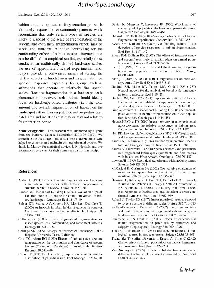
Fig. 1 Design of EMLS.

Red clover (Trifoliumpratense) was planted

within each plot

(16 9 16 m) as a fractal

distribution (C clumped:

H = 1.0; F fragmented:

H = 0.0) at different levels

of habitat area (10, 20, 40,

50, 60 and 80%). Each

landscape type (e.g., 10%

C) has three replicates

Landscape Ecol (2011) 26:1035–1048 1037

123


northwest Ohio, USA (41�23044.8300N, 83�37044.

1200W). Prior to our study, this site had been used

for rowcrop agriculture for many years, and thus had

been plowed repeatedly and was devoid of native

vegetation. Our EMLS comprised a replicated series

of plots (36, 16-m 9 16-m plots) that were seeded to

red clover (Trifolium pratense) in May 1997 (Fig. 1;

see also Fig. 1 in With et al. 2002). The plots

(‘‘landscapes’’) varied in both the total area (10, 20,

40, 50, 60 and 80% cover) and fragmentation

(clumped vs. fragmented) of clover habitat. In the

context of our experiment, ‘‘fragmentation’’ refers to

the spatial contagion or arrangement of habitat, and

not the process by which habitat is lost (since habitat

is in fact being created in this EMLS). We selected

these habitat levels because previous analysis indi-

cated that structural connectivity was disrupted in the

40–60% range (clumped pc = 0.45, fragmented

pc = 0.54), but other research on dispersal and

animal movement suggested that thresholds in dis-

persal success or movement parameters may occur at

B20% habitat (With and King 1999a; With et al.

1999), whereas extinction thresholds may occur

across a range of habitat depending on the demo-

graphic potential of the species (With and King

1999b); we therefore bracketed these habitat ranges

in the design of our EMLS. Landscape patterns were

first computer-generated as a fractal distribution of

habitat (fragmented: H = 0.0, clumped: H = 1.0; see

With et al. 2002 for details) to produce individual

landscape maps with the specified amount and degree

of habitat fragmentation (6 levels of habitat 9 2

levels of fragmentation = 12 landscape patterns).

Three replicate maps were produced for each land-

scape pattern (12 landscape patterns 9 3 repli-

cates = 36 maps). These landscape patterns were

then duplicated in the field by randomly assigning

fractal landscape maps to plots. Each plot was laid

out as a 16-m 9 16-m grid (256, 1-m2 cells) and was

separated from neighboring plots by 16 m (Fig. 1).

The scale of our EMLS thus exceeds most other

experimental fragmentation studies of arthropods in

grassland or agricultural systems (e.g., 169-m2 plots

separated by 11 m, Golden and Crist 1999; 1–100-m2

plots separated by 10 m, Collinge 2000; 225-m2 plots

separated by 9 m, Summerville and Crist 2001).

Clover seed was obtained from a commercial supplier

and planted within plots according to the specified

fractal pattern. Each plot was maintained throughout

the growing season (May–September) through a

combination of hand-weeding (clover cells) and

herbicide application (non-clover cells) as required

to maintain uniform habitat and a bare soil matrix,

respectively. The area between plots was also plowed

periodically to keep it weed-free and reduce the

potentially confounding effects of matrix heteroge-

neity or species ‘‘spillover’’ from other habitats.

Arthropod surveys

Arthropods colonized plots via natural dispersal and

immigration from the surrounding landscape, which

was dominated by rowcrop agriculture (e.g., corn,

soybean, winter wheat). Plots were surveyed by one of

us (DMP) one to three times per growing season, for a

total of six surveys over 3 years: (1) 8–27 July 1997

(hereafter, July-Year1); (2) 25 August–27 September

1997 (August-Year1); (3) 1–14 June 1998 (June-

Year2); (4) 28 June–12 July 1998 (July-Year2); (5) 31

July–19 August 1998 (August-Year2); and (6) 23

June–9 July 1999 (July-Year3). Surveys were con-

ducted during favorable weather conditions (i.e., no

precipitation, winds \32–40 kph, 10.0–32.2�C

[�x = 24.1 ± 3.02(SD)�C, n = 6 surveys]). Plots were

surveyed by visiting each clover cell (1 m2) for

*1 min and recording the occurrence of all arthro-

pods visible within that cell, including below the

canopy. We thus standardized our survey time with

respect to the spatial grain of our landscape (i.e., 1-m2

cells) since this represented the finest scale of

sampling (data from individual clover cells were

ultimately aggregated across plots). The advantage of

visual surveys was that we were able to conduct a

comprehensive survey of the entire system: we

censused more than 3,960 cells (i.e., every clover

cell) each survey, resulting in a total of *23,760

individual cell-censuses over the six surveys. Survey

time per plot ranged from 20 min for 10% landscapes

(*20 clover cells) to 3.5–4 h for 80% landscapes

(*205 clover cells). Non-clover cells were not

surveyed because the bareground matrix was inhos-

pitable to arthropods in this system. Given that

arthropods were not collected, it was not possible to

identify every arthropod to species. We thus use the

term ‘‘morphospecies’’ hereafter to refer to the

number of taxonomically distinct units (species, genus

or family) observed within cells or plots, similar to

other studies that have documented arthropod

1038 Landscape Ecol (2011) 26:1035–1048

123


responses to fragmentation (e.g., Bolger et al. 2000).

Morphospecies were additionally assigned to a tro-

phic guild (herbivores vs. predators/parasitoids). For

some morphospecies, different life stages may belong

to different trophic guilds (e.g., lacewing larvae are

predators but adults feed on pollen, nectar and aphid

honeydew) and thus were considered different ‘‘tro-

phic morphospecies.’’ Each survey was completed

within a two- to three-week period to minimize

possible changes in community composition across

the study site during the survey period.

Morphospecies richness (S) was assayed at two

scales within plots: local scale (SC), the number of

morphospecies within an individual clover cell; and

landscape scale (SL), the total number of morpho-

species observed across all clover cells within a plot.

Average local-scale richness SC

� �was obtained for

each plot as SC ¼Pn

i¼1 SC

� �=n, where n is the

number of clover cells in a given plot (which varied

from about 25 to 205, depending on habitat area). In

addition, we quantified the relative richness of

herbivores and predators/parasitoids, as well as the

number of ‘‘widespread’’ morphospecies (occupying

C50% plots in a given survey) versus those that were

encountered less frequently (‘‘uncommon’’) at the

landscape scale (SL).

Statistical analysis

Because individual plots were sampled repeatedly

over the course of the study, we examined the effect

of habitat area and fragmentation on plot-level

richness (SL) within a repeated measures analysis of

variance (SAS PROC GLM), in which the within-

subject effects of survey were tested against the

between-subject effects of cover, fragmentation and

their interaction. We used Mauchly’s sphericity test

(based on orthogonal components) to test for com-

pound symmetry in the variance–covariance matrix.

In the event that the assumption of sphericity was

violated, we used the Huynh–Feldt adjusted proba-

bilities for testing within-subject effects. Similar

analyses were also performed for each trophic level

(herbivores vs. predators/parasitoids) and level of

occurrence (widespread vs. uncommon morphospe-

cies), and thus we applied the Bonferroni correction

and interpreted tests with P B 0.01 (a = 0.05/5) as

statistically significant. Because there was always a

strong survey effect (see ‘‘Results’’ section), we also

conducted a series of post-hoc analyses to aid our

interpretation of main results by examining habitat

area and fragmentation effects for each survey

individually (two-factor ANOVA) to determine

whether patterns were consistent among surveys,

followed by post-hoc comparisons of significant

treatment effects (Tukey tests). For each survey, we

also tested for non-linear trends in the relationship

between morphospecies richness and habitat area

through orthogonal polynomial contrasts (6 levels of

habitat—1 = 5-degree polynomial), in which we

retained the highest-order polynomial that was

significant. A finding that a higher-order polynomial

is significant (e.g., quartic or quintic) means that there

is a high degree of non-linearity, with one or more

inflection points (2 for quartic, 3 for quintic) in which

the relationship changes direction. Because of non-

linearities in the relationship (see ‘‘Results’’ section),

we took the logs of both richness and habitat area and

fit a linear regression to the transformed data to

obtain the slope and examine the rate at which

morphospecies increased per unit habitat area.

The broader landscape context (habitat area or degree

of fragmentation) might influence richness at the local

scale (cell) within plots. We therefore performed a

repeated measures ANOVA on average cell morpho-

species richness within plots SC

� �, complete with

sphericity test. Again, there was a strong survey effect

(see ‘‘Results’’ section) and so we highlight the results

of post-hoc tests for individual surveys. The relation-

ship between cell richness and plot richness was further

explored through partial correlation analysis, in which

the effect of survey was removed to determine whether

plots with high morphospecies richness also have high

richness at a local scale.

Results

We recorded more than 100 arthropod morphospecies

(S = 129) in this EMLS during our three-year study,

averaging 65 morphospecies per survey (summed

across all plots; Table 1). Overall, plots averaged about

19 morphospecies (SL = 18.6 ± 5.80 SD, n = 216

plot-survey-years). There were about 25–33% fewer

morphospecies per plot at the beginning of the study

(July-Year1: 16.7 ± 5.76, n = 36 plots) or early in the

season (June-Year2: 15.1 ± 3.98), than at the end of the

Landscape Ecol (2011) 26:1035–1048 1039

123


study (July-Year3: 21.4 ± 6.02) or later in the season

(August-Year1: 22.7 ± 5.52). Herbivores made up

half of the arthropod community in this system,

with predators/parasitoids comprising 40% (Table 1).

Among surveys, 12–21 morphospecies (15.3 ± 3.50,

n = 6 surveys) were widespread in occurrence (C50%

plots in a given survey), which represents 25% of all

morphospecies found in our EMLS (Table 1). Potato

leafhoppers (Empoasca fabae), pea aphids (Acyrthos-

piphon pisum), tarnished plant bugs (Lygus lineolaris),

spittlebugs (Cercopidae), and grasshoppers (Acrididae)

were some of the most frequently encountered herbi-

vores; braconid wasps (Braconidae), spiders (Araneae),

damsel bugs (Nabis spp.), spotted lady beetles (Coleo-

megilla maculata) and Asian lady beetles (Harmonia

axyridis) were among the most common parasitoids/

predators found within our clover plots (Supplemental

Table 1).

Effect of landscape structure on arthropod

richness

Morphospecies richness at the plot level (SL) was

only affected by habitat area (Table 2). In general,

plots with 80% cover had 29 more morphospecies

than plots with 10% cover, amounting to a difference

of about 12 morphospecies (10%: 11.6 ± 3.22, n =

36 plot-survey-years; 80%: 23.1 ± 5.34, n = 36

plot-survey-years; Fig. 2). Morphospecies richness

scaled as z = 0.33 with an increase in habitat area

(fitted double-log plot; S = cAZ = 0.75A0.33, R2 =

0.982).

Morphospecies richness differed among surveys

(Table 2). Habitat area still had the greatest influence

on plot-level richness in all surveys (P B 0.001),

although a weak-to-moderate interaction between

habitat area and fragmentation was observed in the

first surveys of both the first and second years (July-

Year1: F5,24 = 2.51, P = 0.058; June-Year2: F5,24 =

4.26, P = 0.007; Fig. 3). In these surveys, morpho-

species richness was higher in the clumped landscape

plots at 40–50% habitat, but became greater in the

fragmented plots at 60% habitat (total, Fig. 3). These

early surveys also averaged 5–7 fewer morphospecies

than surveys conducted either later in the season

(August-Year1) or later in the study (July-Year3;

compare horizontal lines in Supplemental Fig. 1).

The complexity of the morphospecies–area relation-

ship was evident in the higher-order polynomial that

best described these trends (quartic or quintic,

Table 3). In general, the morphospecies–area rela-

tionship was a non-linear one; only the relationship

for August-Year1 was linear.

Trophic responses to landscape structure

Herbivore morphospecies richness was affected by

the amount of habitat cover, although there was a

significant survey by cover interaction (Table 2;

Supplemental Fig. 2). Among surveys, there was a

Table 1 Number and proportion (in parentheses) of arthropod morphospecies encountered within experimental clover landscapes

(n = 36 plots)

Survey Widespread morphospeciesa Uncommon morphospeciesa Herbivores Predators/parasitoids Totalb

July-Year1 13 (0.186) 54 (0.771) 35 (0.500) 30 (0.429) 70

August-Year1 21 (0.284) 51 (0.689) 39 (0.527) 28 (0.378) 74

June-Year2 12 (0.214) 43 (0.768) 26 (0.464) 22 (0.393) 56

July-Year2 13 (0.188) 55 (0.797) 35 (0.507) 26 (0.377) 69

August-Year2 18 (0.419) 25 (0.581) 22 (0.511) 16 (0.372) 43

July-Year3 15 (0.192) 63 (0.808) 43 (0.551) 32 (0.410) 78

Average 15.3 (0.247) 48.5 (0.736) 33.3 (0.510) 25.7 (0.393) 65

SD 3.50 (0.092) 13.20 (0.086) 7.92 (0.029) 5.85 (0.022) 13.08

The total number of morphospecies encountered in a given survey (total) is divided into species groups (widespread vs. uncommon;

herbivores vs. predators/parasitoids), both of which may contain fewer species than the totala Widespread morphospecies are those occupying C50% plots in a given survey; uncommon morphospecies occupied\50% plots in

that surveyb Total morphospecies richness includes nectarivores and morphospecies that do not feed as adults (e.g., Ephemeroptera), and thus

exceeds total sum of herbivores and predators/parasitoids

1040 Landscape Ecol (2011) 26:1035–1048

123


significant cover by fragmentation effect at the start

of the study (July-Year1: F5,24 = 2.81, P = 0.039);

herbivore richness was higher in clumped landscapes,

except in 60% landscapes where richness was greater

in fragmented landscapes (Herbivores, Fig. 3). Over-

all, herbivore richness was almost twice as high

(1.89) in 80% plots as in 10% plots, resulting in a

gain of more than five morphospecies in the former

(Fig. 2). Herbivore richness scaled as z = 0.27 with

an increase in habitat area (S = 1.34A0.27, R2 =

0.994). Herbivore richness generally exhibited a non-

linear relationship with habitat area, however (67% of

surveys; Table 3).

Table 2 Repeated measures analysis of variance of habitat

area and fragmentation effects on morphospecies richness in

experimental clover landscapes. Survey is the within-subjects,

repeated measures variable

Source of variation DF MS F P

Morphospecies richness (SL)

Habitat area 5 655.69 78.20 \0.0001

Fragmentation 1 0.02 0.00 0.963

Habitat

area 9 fragmentation

5 6.73 0.80 0.559

Error 24 8.38

Survey 5 302.68 25.99 \0.0001

Survey 9 habitat area 25 14.51 1.25 0.215

Survey 9 fragmentation 5 4.32 0.37 0.868

Survey 9 habitat


25 16.67 1.43 0.104

Error (survey) 120 11.65

Herbivores

Habitat area 5 150.06 47.04 \0.0001


Habitat


5 1.97 0.62 0.687

Error 24 3.19

Survey 5 242.75 68.60 \0.0001



Survey 9 habitat


25 4.38 1.24 0.220


Predators/parasitoids*

Habitat area 5 132.05 52.34 \0.0001


Habitat


5 2.09 0.83 0.541

Error 24 2.52

Survey 5 75.3 13.06 \0.0001



Survey 9 habitat


25 6.70 1.16 0.289


Widespread morphospecies

Habitat area 5 92.86 37.99 \0.0001


Habitat


5 1.52 0.62 0.685

Error 24 2.44

Survey 5 206.29 108.26 \0.0001

Table 2 continued

Source of variation DF MS F P



Survey 9 habitat


25 2.12 1.11 0.343


Uncommon morphospecies

Habitat area 5 250.54 76.76 \0.0001


Habitat


5 11.69 3.58 0.015

Error 24 3.26

Survey 5 91.46 11.26 \0.0001



Survey 9 habitat


25 10.38 1.28 0.192


Cell morphospecies richness SC

� �*

Habitat area 5 0.13 0.40 0.843


Habitat


5 0.69 2.22 0.086

Error 24 0.31

Survey 5 50.57 90.37 \0.0001



Survey 9 habitat


25 0.65 1.17 0.301


* Huynh–Feldt adjusted probabilities used in these within-

subjects tests

Landscape Ecol (2011) 26:1035–1048 1041

123


For predators/parasitoids, habitat area also had a

significant effect on richness, although again there

were differences among surveys (Table 2). Habitat

cover had a significant effect on predator/parasitoid

richness in five of six surveys (there were no

significant effects of cover or fragmentation on

predator/parasitoid richness in August-Year1; Sup-

plemental Fig. 3). There was a significant cover by

fragmentation interaction for the first survey (July-

Year1: F5,24 = 8.91, P \ 0.001) and for the first

survey in the second year of the study (June-Year2:

F5,24 = 3.66, P = 0.013). In the first survey, preda-

tor/parasitoid richness was initially greater in

clumped landscapes before switching to higher

richness in 60 and 80% fragmented landscapes;

predator richness was nearly 29 (1.79) greater in

80% fragmented than clumped landscapes (predators/

parasitoids; Fig. 3). The relationship was more com-

plex in the first survey of the second year (June-

Year2), with higher predator/parasitoid richness in 40

and 60% fragmented landscapes, but lower richness

in 50% fragmented landscapes, than in clumped

landscapes (Fig. 3). Overall, plots with 80% habitat

tended to have 2.29 more predators/parasitoids than

10% plots, resulting in a gain of about five morpho-

species in the former (Fig. 2). Predator/parasitoid

richness thus scaled as z = 0.37 as a function of

habitat area (S = 0.63A0.37, R2 = 0.980); predator

richness by itself scaled as z = 0.41 with habitat area

(S = 0.31A0.41, R2 = 0.972). The above treatment

effects remained unchanged when only predators

were analyzed (i.e., when parasitoids were omitted

from analysis). In general, predators/parasitoids

exhibited non-linear morphospecies–area relation-

ships in half of the surveys (Table 3).

Landscape effects on widespread

versus uncommon morphospecies

Despite the fact that uncommon morphospecies

outnumbered widespread morphospecies 3:1 in this

EMLS (Table 1), plots averaged twice as many

widespread morphospecies (12.8 ± 3.01) as uncom-

mon morphospecies (5.7 ± 3.94, n = 216 plot-sur-

vey-years). For widespread morphospecies, there

was a significant survey (within-subjects effects:

F5,120 = 108.26, P \ 0.0001) and survey by cover

interaction (F25,120 = 1.91, P = 0.01; Supplemental

Fig. 4). Habitat area had a significant effect on the

richness of widespread morphospecies (Table 2),

with a third fewer morphospecies in 10% than 80%

plots (a difference of four morphospecies, Fig. 2).

Widespread morphospecies scaled as z = 0.17

with an increase in habitat area (S = 1.94A0.17,

R2 = 0.937), although the relationship reached an

asymptote at 40% with 13–14 morphospecies

(Fig. 2). Thus, the morphospecies–area relationship

was non-linear in all surveys (quadratic or cubic;

Table 3).

Fig. 2 Effect of habitat area (% red clover) on arthropod

morphospecies richness (mean ± 2 SE) within experimental

landscape plots (SL) for (top) all morphospecies combined,

(center) different trophic groups (herbivores vs. predators/

parasitoids), and (bottom) different levels of occurrence

(widespread vs. uncommon morphospecies; widespread:

C50% plot occupancy in a given survey). In each group,

means (n = 36 plot-surveys) with the same letter are not

significantly different (P [ 0.05, Tukey test)

1042 Landscape Ecol (2011) 26:1035–1048

123


For uncommon morphospecies, survey also had a

significant effect, and there were significant habitat

area and habitat area by fragmentation effects

(Table 2). There were 5.49 more uncommon mor-

phospecies in 80% than 10% plots, resulting in a

difference of about seven morphospecies (Fig. 2).

Both the first (July-Year1) and early-season (June-

Year2) surveys exhibited significant interactions

between habitat area and fragmentation (July-Year1:

F5,24 = 3.32, P = 0.02; June-Year2: F5,24 = 5.03,

P = 0.003). Uncommon morphospecies exhibited

greater richness in the clumped landscape plots at

40-50% habitat, but became greater in the fragmented

plots at 60% habitat (Supplemental Fig. 5). Uncom-

mon morphospecies scaled as z = 0.79 with increas-

ing habitat area (S = -1.21A0.79, R2 = 0.970),

although the morphospecies–area relationship was

non-linear in two-thirds of surveys (Table 3).

Relationship between local- and landscape-scale

richness

Average local richness SC

� �was unaffected by

landscape context, such as the amount or fragmen-

tation of habitat within the plot (Table 2). Other than

at the start of the experiment (July-Year1), SC was

significantly greater in July (mid-season) surveys

than all other surveys (July-Year2: 5.5 ± 0.47,

n = 36 plots; July-Year3: 5.1 ± 0.42, n = 36; July-

Year1A = August-Year1A = August-Year2A \ June-

Year2B \ July-Year3C = July-Year2C; Tukey test).

Local richness was 29 higher in these mid-season

surveys than the lowest level encountered at the start

of the study (July-Year1: 2.7 ± 0.68, n = 36). Over-

all, clover cells averaged four morphospecies (SC =

4.0 ± 1.29, n = 216 plot-survey-years) regardless of

habitat area or level of fragmentation. There was no

correlation between local and landscape richness

(Pearson partial correlation coefficient = 0.09,

P = 0.188, n = 216; Supplemental Fig. 6). Thus,

plots with higher morphospecies richness did not

have a greater local richness than plots with fewer

morphospecies.

Discussion

Habitat area had a far greater—and more consis-

tent—effect than fragmentation on arthropod mor-

phospecies richness within these clover landscapes.

Fig. 3 Interaction between habitat area and fragmentation for

arthropod morphospecies (mean ± SE) within experimental

clover plots (SL) for ‘‘early’’ surveys at the beginning of the

study (Year1-July) and early in the season (Year2-June).

Horizontal line in each panel is the average morphospecies

richness for that survey

Landscape Ecol (2011) 26:1035–1048 1043

123


Our study thus adds to the growing body of evidence

that it is the overall amount of habitat on the

landscape rather than how that habitat is arrayed that

is ultimately most important for understanding com-

munity responses to landscape pattern (Fahrig 2003).

Overall, morphospecies richness in 80% plots (205-

m2 total habitat area) was double that found in 10%

plots (26-m2 total habitat area). This gain in mor-

phospecies richness was not a linear function of

increasing habitat area, however. Morphospecies

richness increased by 72% from 10 to 40% habitat,

but only by about 16% (15.7%) between 40 and 80%

habitat (Fig. 2). Given that our experimental land-

scapes were clover monocultures in fixed-sized plots,

an increase in richness with habitat area obviously

cannot be explained by an increase in habitat diversity,

which is one of the explanations usually given for the

species–area relationship (e.g., Holt et al. 1999). The

fact that morphospecies richness at the local level SC

� �

was unaffected by the amount of habitat within the plot

( SC

� �* 4.0 morphospecies; Supplemental Fig. 6),

however, suggests that plots with more habitat cells are

effectively ‘‘sampling’’ the regional source pool to a

greater degree than plots with less habitat area, and

thus tend to accumulate more morphospecies at the

plot level. Thus, this is essentially equivalent to a

rarefaction analysis, in which we have standardized

samples by some minimum area (1 m2) rather than

number of individuals, since we only have presence-

absence data available.

The effects of fragmentation on arthropod richness

in this system were at best subtle and transient, in that

they were evident only in ‘‘early’’ surveys either at

the start of the study (July-Year1) or early in the

season (June-Year2). Here again, the effect was

Table 3 Significant trend that best described the relationship

between morphospecies richness and habitat area in experi-

mental clover landscapes by survey, based on an analysis of all

orthogonal polynomial contrasts (n = 5)

Survey Trend F1,24 P

Morphospecies richness (SL)

Year 1

July Quartic 5.28 0.031

August Linear 52.68 \0.0001

Year 2

June Quintic 8.01 0.009

July Quadratic 9.50 0.005

August Quadratic 13.41 0.001

Year 3


Herbivores

Year 1

July Cubic 6.76 0.016


Year 2




Year 3

July Linear 23.43 \0.0001

Predators/parasitoids

Year 1


August Linear 6.79 0.016

Year 2


July Linear 16.22 0.0005


Year 3


Widespread morphospecies

Year 1

July Cubic 5.09 0.033


Year 2

June Quadratic 5.26 0.031



Year 3


Uncommon morphospecies

Year 1

Table 3 continued

Survey Trend F1,24 P

July Quartic 4.24 0.051


Year 2



August Quartic 4.70 0.040

Year 3


1044 Landscape Ecol (2011) 26:1035–1048

123


decidedly non-linear in that richness was higher in

clumped 40–50% landscapes but higher in frag-

mented landscapes at 60–80% habitat. The reason for

the crossover is unclear. Neutral landscape theory

predicts a threshold in structural connectivity in the

domain between 40 and 60% habitat, depending upon

the specific fractal configuration (clumped: H = 1.0,

pc = 0.45; fragmented, H = 0.0, pc = 0.54). It is

therefore interesting that this is the domain where

fragmentation effects occur, when they do. In some

contexts, a disruption of landscape connectivity has

actually been used to define when landscapes become

fragmented (e.g., With 1997). Clumped landscapes

should therefore maintain connectivity at lower levels

of habitat abundance, and thus might support higher

richness below this threshold relative to more frag-

mented landscapes. This would not explain why

morphospecies richness is greater in fragmented

landscapes above the threshold, however.

Rather than overall connectivity, morphospecies

responses to fragmentation might be affected by some

other aspect of landscape structure, such as the

amount or complexity of patch edges (e.g., Ewers and

Didham 2007). The amount of edge exhibits a

parabolic distribution with increasing habitat cover,

peaking at intermediate habitat densities, and frag-

mented fractal landscapes certainly have more edge

than clumped fractal landscapes (With and King

1999a). Some species may benefit from intermediate

levels of habitat loss and fragmentation because of

greater resource diversity or more favorable micro-

climates along habitat edges (Crist and Ahern 1999).

This sort of response might increase morphospecies

richness at intermediate habitat levels, particularly in

fragmented landscapes (i.e., another manifestation of

the intermediate disturbance hypothesis). However,

habitat edges negatively affect patch quality for other

species, resulting in lower survival or reproduction if

predation or parasitism is greater along edges,

especially in small patches or patches with high edge

contrast (e.g., Kruess and Tscharntke 1994; Thies and

Tscharntke 1999; Cronin 2003). Although the patch-

size distribution in fragmented fractal landscapes is

shifted toward smaller patches at low habitat levels,

patch sizes are pretty equivalent between fragmented

and clumped fractal landscapes at higher habitat

abundances (i.e., above the connectivity threshold;

With and King 1999a). Fragmented fractal land-

scapes may thus afford suitably large patches beyond

the connectivity threshold, but nevertheless have

more edge habitat and thus greater microhabitat

diversity that can support more morphospecies than

clumped landscapes at this level. Changes in land-

scape structure—either in terms of structural connec-

tivity, amount of edge or both—might thus be

responsible for altering the effect of habitat fragmen-

tation on morphospecies richness at intermediate

habitat densities.

Higher trophic levels are expected to be most

sensitive to the effects of habitat fragmentation

(Tscharntke et al. 2002; van Nouhuys 2005). For

example, parasitism rates are often lower in frag-

mented landscapes (Roland and Taylor 1997; van

Nouhuys 2005). To the extent that patch isolation is

related to habitat fragmentation (and it may not be, see

Fahrig 2003), then parasitoids are affected more by

isolation than their herbivorous hosts (Kruess and

Tscharntke 1994, 2000). For example, small (1.2 m2)

isolated clover patches (separated 500 m from the

nearest meadow) had 2–69 fewer species of parasit-

oids and 19–60% lower rates of parasitism than clover

patches within meadows (Kruess and Tscharntke

1994). Recall that in our study, fragmentation effects

were evident only in ‘‘early’’ surveys and manifest as a

crossover effect in which morphospecies richness was

alternately higher in clumped landscapes up to about

40–50% habitat, and then in fragmented landscapes

beyond 50–60% habitat. Although predators/parasit-

oids exhibited this sort of crossover effect at the start of

the survey (July-Year1), and early in the season (June-

Year2), herbivores also exhibited a crossover in the

relative importance of fragmentation on diversity

(Fig. 3). Thus, our findings do not provide unequivocal

support for the idea that higher trophic levels (preda-

tors/parasitoids) are necessarily more sensitive to

habitat fragmentation than lower trophic levels

(herbivores).

Predators/parasitoids in our EMLS were more

sensitive to habitat area than herbivores, however, in

that predators/parasitoids had a steeper species–area

relationship (z = 0.37 vs. 0.27, respectively; Fig. 2).

Most of the gain in predator/parasitoid morphospe-

cies occurred between 10 and 40%: morphospecies

richness increased by 89% across this range, com-

pared to only a 17% increase in morphospecies

richness between 40 and 80% habitat. For herbivores,

the increase between 10 and 40% habitat was 53%,

compared to only a 16% gain in morphospecies

Landscape Ecol (2011) 26:1035–1048 1045

123


between 40 and 80% habitat. The size of clover

patches has previously been shown to affect herbi-

vore densities and levels of herbivory, especially by

the potato leafhopper Empoasca fabae (Haynes and

Crist 2009). This is a ubiquitous herbivore in our

EMLS as well, which was found in almost every cell

of every plot, thus swamping any habitat area or

fragmentation effect for this species at the landscape

scale (Supplemental Table 1).

Given that morphospecies richness increased

throughout the season and over the course of the

study (Fig. 3), it is possible that fragmentation effects

were simply being swamped, especially by wide-

spread and common morphospecies like the potato

leafhopper. In our EMLS, widespread morphospecies

showed only a strong effect of habitat area, not

fragmentation (Fig. 2). Because of their widespread

distribution, these morphospecies will likely drive

community responses to landscape structure, espe-

cially in terms of the relative importance of habitat

area versus fragmentation (Haynes and Crist 2009).

Rare or less-widespread morphospecies might there-

fore be expected to show a greater sensitivity to

habitat area and fragmentation (e.g., Golden and Crist

1999; Kruess and Tscharntke 2000; Summerville and

Crist 2001). Widespread morphospecies in our EMLS

exhibited a significant effect of habitat area, but only

up to about 40% habitat, at which point richness

leveled off to an average 13–14 morphospecies per

plot. Overall, the richness of widespread morphospe-

cies increased 41% between 10 and 80%, with half of

that increase (21%) occurring between 10 and 20%.

Morphospecies that were less frequently encountered

showed the most rapid accumulation of morphospe-

cies with increasing habitat area: a fivefold increase

between 10 and 80%, with the number of morpho-

species doubling between 10 and 20% and again

between 20 and 40%. These morphospecies were also

influenced by fragmentation, at least in some surveys

(the ‘‘early’’ surveys), showing crossover effects at

around 40–50% habitat and 60% (Supplemental

Fig. 5). Because uncommon or rare species tend to

occur at low density or occupancy and have greater

spatial variability, they are expected to have higher

extinction rates (Kruess and Tscharntke 2000), and

thus if fragmentation effects are ultimately driven by

the extinction or absence of these rare or uncom-

mon species, then it would be difficult to detect

such effects when more-common or widespread

morphospecies are also included in the analysis

(Golden and Crist 1999).

Although our plot dimensions were larger than

many other experimental fragmentation studies that

have studied arthropods in agricultural or grassland

habitats, our plots no doubt represented foraging

patches for many morphospecies in this agricultural

system, rather than discrete landscapes in which they

completed their entire life-cycle. For example, indi-

vidual ladybird beetles were observed to fly among

plots while foraging for pea aphids (With et al. 2002).

The scale of habitat fragmentation can always be

expected to have a differential effect on species,

however. Rare or less-widespread species with lim-

ited vagility are sensitive to patch isolation even at

the scales studied here (e.g., Golden and Crist 1999),

whereas more-mobile species that have no difficulty

colonizing plots might nevertheless avoid smaller

patches because of their perceived low resource

abundance or quality (Summerville and Crist 2001).

Even at more traditionally defined landscape scales

(km-wide), broad-scale population processes such as

local extinction and patch colonization may ulti-

mately manifest through the collective response of

individual patch-selection and foraging dynamics

(Golden and Crist 1999; van Nouhuys 2005). It is

precisely because of these sorts of species-specific

responses to patch structure, where different types of

responses occur simultaneously across a range of

scales, which make fragmentation effects so difficult

to isolate experimentally (McGarigal and Cushman

2002). Further, over short time-scales (e.g., among

surveys within a season or over a few years),

responses by individual species can generate idio-

syncratic patterns, in which the effect of fragmenta-

tion may well be transient (Grez et al. 2004). Highly

mobile species in particular, whose individual or

population-level responses may encompass a spatial

domain much larger than a single landscape or plot,

likely contribute to such transient dynamics (Debin-

ski and Holt 2000). Finally, some species are

themselves ‘‘transient’’ or early-successional species,

thus adding an additional idiosyncratic component to

the community’s response to landscape structure.

In conclusion, community responses to habitat

area and fragmentation will always represent the

collective response of species that are responding in

individual ways and at different scales to landscape

pattern. The important distinction is to what extent

1046 Landscape Ecol (2011) 26:1035–1048

123


habitat area, as opposed to fragmentation per se, is

ultimately responsible for community patterns, while

recognizing that only certain types of species are

likely to respond to the scale of fragmentation of the

system, and even then, fragmentation effects may be

subtle and transient. Although controlling for the

confounding effects of habitat area and fragmentation

can be difficult in empirical studies, especially those

conducted at traditionally defined landscape scales,

the use of appropriately scaled experimental land-

scapes provide a convenient means of testing the

relative effects of habitat area and fragmentation on

species’ responses, especially for groups such as

arthropods that operate at relatively fine spatial

scales. Because fragmentation is a landscape-scale

phenomenon, however, such studies should ideally

focus on landscape-based attributes (i.e., the total

amount and overall fragmentation of habitat on the

landscape) rather than on patch-based properties (i.e.,

patch area and isolation) that may or may not relate to

fragmentation per se.

Acknowledgments This research was supported by a grant

from the National Science Foundation (DEB-9610159). We

appreciate the assistance of the dozen or so undergraduates who

helped to establish and maintain this experimental system. We

thank L. Murray for statistical advice, J. R. Nechols and two

anonymous reviewers for their comments on the manuscript.

References

Andren H (1994) Effects of habitat fragmentation on birds and

mammals in landscapes with different proportions of

suitable habitat: a review. Oikos 71:355–366

Bender DJ, Tischendorf L, Fahrig L (2003) Evaluation of patch

isolation metrics for predicting animal movement in bin-

ary landscapes. Landscape Ecol 18:17–39

Bolger DT, Suarez AV, Crooks KR, Morrison SA, Case TJ

(2000) Arthropods in urban habitat fragments in southern

California: area, age and edge effects. Ecol Appl 10:

1230–1248

Collinge SK (2000) Effects of grassland fragmentation on

insect species loss, colonization, and movement patterns.

Ecology 81:2211–2226

Collinge SK (2009) Ecology of fragmented landscapes. Johns

Hopkins University Press, Baltimore

Crist TO, Ahern RG (1999) Effects of habitat patch size and

temperature on the distribution and abundance of ground

beetles (Coleoptera: Carabidae) in an old field. Environ

Entomol 28:681–689

Cronin JT (2003) Patch structure, oviposition behavior, and the

distribution of parasitism risk. Ecol Monogr 73:283–300

Davies K, Margules C, Lawrence JF (2000) Which traits of

species predict population declines in experimental forest

fragments? Ecology 81:1450–1461

Debinski DM, Holt RD (2000) A survey and overview of habitat

fragmentation experiments. Conserv Biol 14:342–355

Ewers RM, Didham RK (2006) Confounding factors in the

detection of species responses to habitat fragmentation.

Biol Rev 81:117–142

Ewers RM, Didham RK (2007) The effect of fragment shape

and species’ sensitivity to habitat edges on animal popu-

lation size. Conserv Biol 21:926–936

Fahrig L (1997) Relative effects of habitat loss and fragmen-

tation on population extinction. J Wildl Manag

61:603–610

Fahrig L (2003) Effects of habitat fragmentation on biodiver-

sity. Annu Rev Ecol Syst 34:487–515

Gardner RH, Milne BT, Turner MG, O’Neill RV (1987)

Neutral models for the analysis of broad-scale landscape

pattern. Landscape Ecol 1:19–28

Golden DM, Crist TO (1999) Experimental effects of habitat

fragmentation on old-field canopy insects: community,

guild and species responses. Oecologia 118:371–380

Grez A, Zaviezo T, Tischendorf L, Fahrig L (2004) A transient,

positive effect of habitat fragmentation on insect popula-

tion densities. Oecologia 141:444–451

Haynes KJ, Crist TO (2009) Insect herbivory in an experimental

agroecosystem: the relative importance of habitat area,

fragmentation, and the matrix. Oikos 118:1477–1486

Holt RD, Lawton JH, Polis GA, Martinez ND (1999) Trophic rank

and the species–area relationship. Ecology 80:1495–1504

Kruess A, Tscharntke T (1994) Habitat fragmentation, species

loss and biological control. Science 264:1581–1584

Kruess A, Tscharntke T (2000) Species richness and parasitism

in a fragmented landscape: experiments and field studies

with insects on Vicia sepium. Oecologia 122:129–137

Lawton JH (1995) Ecological experiments with model systems.

Science 269:328–331

McGarigal K, Cushman SA (2002) Comparative evaluation of

experimental approaches to the study of habitat frag-

mentation effects. Ecol Appl 12:335–345

Ockinger E, Schweiger O, Crist TO, Debinski DM, Krauss J,

Kuussaari M, Petersen JD, Poyry J, Settele J, Summerville

KS, Bommarco R (2010) Life-history traits predict spe-

cies responses to habitat area and isolation: a cross-con-

tinental synthesis. Ecol Lett 13:969–979

Roland J, Taylor PD (1997) Insect parasitoid species respond

to forest structure at different scales. Nature 386:710–713

Steffan-Dewenter I, Tscharntke T (2002) Insect communities

and biotic interactions on fragmented calcareous grass-

lands—a mini review. Biol Conserv 104:275–284

Summerville KS, Crist TO (2001) Effects of experimental

habitat fragmentation on patch use by butterflies and

skippers (Lepidoptera). Ecology 82:1360–1370

Thies C, Tscharntke T (1999) Landscape structure and bio-

logical control in agroecosystems. Science 285:893–895

Tscharntke T, Steffan-Dewenter I, Kruess A, Thies C (2002)

Characteristics of insect populations on habitat fragments:

a mini-review. Ecol Res 17:229–239

Van Nouhuys S (2005) Effects of habitat fragmentation at

different trophic levels in insect communities. Ann Zool

Fennici 42:433–447

Landscape Ecol (2011) 26:1035–1048 1047

123


Wiens JA, Stenseth NC, Van Horne B, Ims RA (1993) Eco-

logical mechanisms and landscape ecology. Oikos 66:

369–380

With KA (1997) The application of neutral landscape models

in conservation biology. Conserv Biol 11:1069–1080

With KA, King AW (1999a) Dispersal success in fractal

landscapes: a consequence of lacunarity thresholds.

Landscape Ecol 14:73–82

With KA, King AW (1999b) Extinction thresholds in fractal

landscapes. Conserv Biol 13:314–326

With KA, Cadaret SJ, Davis C (1999) Movement responses to

patch structure in experimental fractal landscapes. Ecol-

ogy 80:1340–1353

With KA, Pavuk DM, Worchuck JL, Oates RK, Fisher JL

(2002) Threshold effects of landscape structure on bio-

logical control in agroecosystems. Ecol Appl 12:52–65

Zabel J, Tscharntke T (1998) Does fragmentation of Urticahabitats affect phytophagous and predatory insects dif-

ferentially? Oecologia 116:419–425

1048 Landscape Ecol (2011) 26:1035–1048

123


Supplemental Table 1. The most widespread arthropods encountered within experimental

landscapes of red clover (Trifolium pratense), ordered by their relative occurrence (proportion of

plots occupied, n = 36 plots) within each survey over a three-year period (1997-1999). Only

morphospecies with plot occupancy >0.5 are presented (i.e., widespread morphospecies). Cell

occupancy is the average proportion of cells occupied across all plots occupied ( cells/plot +

SD).

Morphospecies

Cell occupancy

Plot occupancy

July-Year1

Empoasca fabae 0.99 (0.008) 1.00

Acrididae 0.53 (0.296) 1.00

Syrphidae (adult) 0.14 (0.137) 1.00

Leafminers 0.29 (0.129) 0.97

Nabis sp. 0.07 (0.045) 0.89

Lygus lineolaris 0.05 (0.054) 0.86

Coleomegilla maculata 0.07 (0.038) 0.83

Araneae 0.10 (0.110) 0.81

Acyrthosiphon pisum 0.22 (0.282) 0.78

Gryllidae 0.07 (0.074) 0.75

Cercopidae 0.04 (0.043) 0.69

Systena blanda 0.04 (0.044) 0.67

Braconidae 0.04 (0.034) 0.61

Morphospecies

Cell occupancy

Plot occupancy

August-Year1



Nabis sp. 0.24 (0.154) 1.00


Chaetocnema sp. 0.20 (0.123) 0.97

Araneae 0.10 (0.058) 0.97

Braconidae 0.08 (0.061) 0.97

Gryllidae 0.39 (0.161) 0.94

Chaetocnema pulicaria 0.11 (0.096) 0.92


Harmonia axyridis 0.10 (0.117) 0.89

Acrididae 0.08 (0.057) 0.89

Leafminers 0.11 (0.097) 0.72


Diabrotica virgifera 0.03 (0.032) 0.64

Hypera sp. 0.03 (0.017) 0.61

Hippodamia parenthesis 0.04 (0.046) 0.56

Aleyrodidae 0.04 (0.045) 0.56

Cercopidae 0.02 (0.010) 0.56

Morphospecies

Cell occupancy

Plot occupancy

Cerotoma trifurcate 0.06 (0.071) 0.53

Popillia japonica 0.02 (0.016) 0.50

June-Year2


Braconidae 0.90 (0.168) 1.00

Cercopidae 0.24 (0.126) 1.00






Hypera sp. 0.10 (0.067) 0.89

Araneae 0.05 (0.066) 0.69

Chauliognathus

pennsylvanicus

0.05 (0.051) 0.67

Acrididae 0.03 (0.042) 0.61

July-Year2


Braconidae 0.95 (0.164) 1.00

Acrididae 0.45 (0.178) 1.00

Morphospecies

Cell occupancy

Plot occupancy


Cercopidae 0.45 (0.104) 0.97

Tetranychidae 0.97 (0.164) 0.94

Araneae 0.27 (0.150) 0.94



Nabis sp. 0.05 (0.038) 0.78



Euschistus servus 0.02 (0.014) 0.56

August-Year2


Araneae 0.22 (0.152) 0.97

Chaetocnema sp. 0.15 (0.090) 0.97

Braconidae 0.41 (0.282) 0.94


Gryllidae 0.15 (0.125) 0.94

Cercopidae 0.28 (0.253) 0.92

Acrididae 0.29 (0.233) 0.86

Nabis sp. 0.04 (0.032) 0.78

Aleyrodidae 0.19 (0.111) 0.72

Morphospecies

Cell occupancy

Plot occupancy





Miridae 0.02 (0.014) 0.61

Chaetocnema pulicaria 0.03 (0.028) 0.58


Phalangidae 0.03 (0.032) 0.56

July-Year3


Braconidae 0.83 (0.174) 1.00





Acrididae 0.41 (0.243) 0.97

Araneae 0.15 (0.110) 0.94

Cercopidae 0.09 (0.070) 0.92

Nabis sp. 0.05 (0.038) 0.86


Chaetocnema sp. 0.05 (0.039) 0.75

Morphospecies

Cell occupancy

Plot occupancy

Orius insidiosus 0.04 (0.041) 0.69

Leptopterna dolabrata 0.10 (0.211) 0.58

Popillia japonica 0.04 (0.034) 0.50

SUPPLEMENTAL FIGURE CAPTIONS

Supplemental Figure 1. Effect of habitat fragmentation on total morphospecies richness (mean

+ SE) within experimental landscape plots by survey. Horizontal lines represent the mean

richness for that survey. Survey means were significantly different (P < 0.05) as June-Year2A <

July-Year1AB < August-Year2B = July-Year2B < July-Year3C = August-Year1C (Tukey test).

Supplemental Figure 2. Effect of habitat fragmentation on herbivore morphospecies richness

(mean + SE) within experimental landscape plots by survey. Horizontal lines represent the mean

richness for that survey. Survey means were significantly different (P < 0.05) as June-

Year2A<July-Year1B=July-Year2B=August-Year2B<July-Year3C<August-Year1D (Tukey test).

Note the y-axis is scaled differently in each panel.

Supplemental Figure 3. Effect of habitat fragmentation on predator/parasitoid morphospecies

richness (mean + SE) within experimental landscape plots by survey. Horizontal lines represent

the mean richness for that survey. Survey means were significantly different (P < 0.05) as

August-Year2A=July-Year1A=June-Year2A<July-Year2AB<July-Year3BC<August-Year1C (Tukey

test).

Supplemental Figure 4. Effect of habitat fragmentation on the diversity of widespread

morphospecies (mean + SE), arthropods encountered in >50% plots for a given survey, within

experimental landscape plots by survey. Horizontal lines represent the mean richness for that

survey. Survey means were significantly different (P < 0.05) as June-Year2A=July-

Year1A=July-Year2A<July-Year3B<August-Year2C<August-Year1D (Tukey test). Note the y-

axis is scaled differently in each panel.

Supplemental Figure 5. Effect of habitat fragmentation on the diversity of uncommon

morphospecies (mean + SE), arthropods encountered in <50% plots for a given survey, within

experimental landscape plots by survey. Horizontal lines represent the mean richness for that

survey. Survey means were significantly different (P < 0.05) as August-Year2A<June-

Year2AB<July-Year1B=August-Year1B<July-Year2BC<July-Year3C (Tukey test). Note the y-axis

is scaled differently in each panel.

Supplemental Figure 6. Relationship between average local (cell)- and individual landscape

(plot)-level richness of arthropods within experimental landscape plots. Data points are the

individual scores for each plot (n = 36), which was surveyed six times over three years (n = 216

plot-survey-years). Line represents a linear fit to the data.

5

10

15

20

25

30

35

0 20 40 60 80 100

5

10

15

20

25

30

35

5

10

15

20

25

30

35

0 20 40 60 80 100

5

10

15

20

25

30

35

5

10

15

20

25

30

35

5

10

15

20

25

30

35

0 20 40 60 80 100

Habitat amount (%)

Morph

ospeciesrichness

Year 1 Year 2 Year 3

June

July

August

ClumpedFragmentedAverage

Total MorphospeciesRichness

468

1012141618

0 20 40 60 80 100

4

6

8

10

12

14

16

0 20 40 60 80 100

4

6

8

10

12

14

164

5

6

7

8

9

10

468

101214161820

0 20 40 60 80 100

4567891011121314

Habitat amount (%)

Morph

ospeciesrichness


June

July

August


Herbivore MorphospeciesRichness

0246810121416

02468

10121416

0 20 40 60 80 100

02468

10121416

0 20 40 60 80 100

02468

101214160246810121416

02468

10121416

0 20 40 60 80 100

Habitat amount (%)

Morph

ospeciesrichness


June

July

August


Predator/Parasitoid MorphospeciesRichness

5

10

15

20

25

30

35

40

1.0 1.5 2.0 2.5 3.0 3.5 4.0 4.5 5.0 5.5 6.0 6.5 7.0

Plot richn

ess (S

L)

Average cell richness (Sc)

Habitat area trumps fragmentation effects on arthropods in an experimental landscape system

Documents

Transcript of Habitat area trumps fragmentation effects on arthropods in an experimental landscape system