Guidelines for the use of mathematics in operational area ...

This guideline attempts to assist managers in the use of mathematics in area-wide Integrated Pest Management (AW-IPM) programmes using the Sterile Insect Technique (SIT). It describes mathematical tools that can be used at different stages of suppression/eradication programmes. For instance, it provides simple methods for calculating the various quantities of sterile insects required in the intervention area so that more realistic sterile: fertile rates to suppress pest populations can be achieved. The calculations, for the most part, only involve high school mathematics and can be done easily with small portable computers or calculators.

The guideline is intended to be a reference book, to be consulted when necessary. As such, any particular AW-IPM programme using the SIT will probably only need certain sections, and much of the book can be ignored if that is the case.

SIT have produced over many years a vast amount of every-day data from the field operations and from the mass rearing facility and packing and sterile insect releasing centres. With the help of this guideline, that information can be used to develop predictive models for their particular conditions to better plan control measures.

I5573E/1/04.16

ISBN 978-92-5-109190-6

9 7 8 9 2 5 1 0 9 1 9 0 6

Guidelines for the use of mathematics in operational area-wide integrated pest management programmes using the sterile insect technique with a special focus on Tephritid fruit flies

16-08331

Guidelines for the use of mathematics in

operational area-wide integrated pest

management programmes using the sterile

insect technique with a special focus on

Tephritid fruit flies

Hugh J. Barclay 928 Old Esquimalt Road, Victoria, B.C., Canada V9A 4X3 Walther Enkerlin H. Co-Director México, Programa Regional Moscamed, 16 Calle 3-38 zona 10, Guatemala, CA

Nicholas C. Manoukis Agricultural Research Service, US Dept. of Agriculture, US Pacific Basin Agricultural Research Center, Hilo, Hawaii, USA.

Jesus Reyes Flores Insect Pest Control Section, Joint FAO/IAEA Division of Nuclear Techniques in Food and Agriculture, International Atomic Energy Agency, Vienna, Austria

The proper citation for this document is: FAO/IAEA. 2016. Guidelines for the Use of Mathematics in Operational Area-Wide Integrated Pest Management Programmes Using the Sterile Insect Technique with a Special Focus on Tephritid Fruit Flies. Barclay H.L., Enkerlin W.R., Manoukis, N.C. Reyes-Flores, J. (eds.), Food and Agriculture Organization of the United Nations. Rome, Italy. 95 pp.

The designations employed and the presentation of material in this information product do not imply the expression of any opinion whatsoever on the part of the Food and Agriculture Organization of the United Nations (FAO) concerning the legal or development status of any country, territory, city or area or of its authorities, or concerning the delimitation of its frontiers or boundaries. The mention of specific companies or products of manufacturers, whether or not these have been patented, does not imply that these have been endorsed or recommended by FAO in preference to others of a similar nature that are not mentioned.

The views expressed in this information product are those of the author(s) and do not necessarily reflect the views or policies of FAO.

ISBN 978-92-5-109190-6

© FAO, 2016

FAO encourages the use, reproduction and dissemination of material in this information product. Except where otherwise indicated, material may be copied, downloaded and printed for private study, research and teaching purposes, or for use in non-commercial products or services, provided that appropriate acknowledgement of FAO as the source and copyright holder is given and that FAO’s endorsement of users’ views, products or services is not implied in any way.

All requests for translation and adaptation rights, and for resale and other commercial use rights should be made via www.fao.org/contact-us/licence-request or addressed to [email protected].

FAO information products are available on the FAO website (www.fao.org/publications) and can be purchased through [email protected].

Foreword


The guideline is intended to be a reference book, to be consulted when necessary. As such, any particular AW-IPM programme using the SIT will probably only need certain sections, and much of the book can be ignored if that is the case. For example, if the intervention area is relatively small and well isolated, then the section on dispersal can safely be ignored, as the boundedness of the area means that dispersal should not be a problem, and so the section on diffusion equations can be ignored. An overview is given in each chapter to try to let the programme manager make a decision about where to put the programme efforts.

On the other hand, most SIT programmes have an information system (many of them based on GIS) that produces reliable profiles of historic information. Based on the results of past activities they describe what has happened in the last days or weeks but usually do not explain, or barely explain, what is expected in the following days or weeks. Current AW-IPM progammes using the SIT have produced over many years a vast amount of every-day data from the field operations and from the mass rearing facility and packing and sterile insect releasing centres. With the help of this guideline, that information can be used to develop predictive models for their particular conditions to better plan control measures.

v

Contents

1. Introduction ........................................................................................................................................ 1

2. Requirements of a sterile insect release programme .......................................................................... 3

3. Sampling insect populations for surveys............................................................................................ 5

3.1 Why sample? ................................................................................................................................ 5

3.2 Why assess pest distribution? ....................................................................................................... 5

3.3 Sampling methods ........................................................................................................................ 6

3.3.1 Sampling designs and associated analyses ............................................................................ 6

3.3.2 Examples ............................................................................................................................. 10

3.4 Sampling distributions................................................................................................................ 12

3.4.1 The Poisson Distribution ..................................................................................................... 13

3.4.2 The Negative Binomial Distribution ................................................................................... 13

3.4.3 The Binomial Distribution ................................................................................................... 15

4. Population estimation ....................................................................................................................... 15

4.1 Absolute estimation of population Size: Mark-recapture methods ............................................ 16

4.1.1 General features of mark-recapture methods: ...................................................................... 16

4.1.2 Lincoln (Peterson) Index ..................................................................................................... 16

4.1.3 Jolly-Seber Index ................................................................................................................. 17

4.1.4 Joint Hypergeometric Estimator .......................................................................................... 20

4.2 Relative estimation of population size: Monitoring and detection ............................................. 22

4.2.1 Trapping for monitoring ...................................................................................................... 22

4.2.2 Trapping for detection ......................................................................................................... 22

4.2.3 The “Fly per Trap per Day” Index. ..................................................................................... 23

4.2.4 Fruit sampling...................................................................................................................... 24

vi

4.2.4.1 The larvae/fruit as an index of population ........................................................................ 24

4.2.5 Converting Relative estimates to absolute estimates ........................................................... 25

5. Forecasting populations ................................................................................................................... 26

5.1 Detecting population change ...................................................................................................... 27

5.2 Prediction of life history events.................................................................................................. 27

5.2.1 Developmental time for the stages: Degree-days ................................................................ 27

5.2.2. Curves of developmental rate vs. temperature .................................................................... 30

5.2.3 Population growth................................................................................................................ 30

6. Population and demographic models ............................................................................................... 31

6.1. Population processes ................................................................................................................. 31

6.1.1. Fertility and fecundity ........................................................................................................ 31

6.1.2 Mortality and survivorship .................................................................................................. 32

6.1.3 Pest dispersal. ...................................................................................................................... 32

6.1.4 Correlated Random Walks. ................................................................................................. 35

6.2 Features of population models ................................................................................................... 36

6.2.1 Population growth ............................................................................................................... 36

6.2.2 Overlapping or non-overlapping generations ...................................................................... 37

6.2.3 Age-specific mortality and fecundity .................................................................................. 38

6.3 Demographic models ................................................................................................................. 39

6.3.1 Leslie Matrix Models .......................................................................................................... 39

6.3.2 Life Tables........................................................................................................................... 41

6.3.3 Procedures for construction of Life Tables ......................................................................... 41

7. Models of SIT .................................................................................................................................. 42

7.1 Models of Population dynamics using SIT ................................................................................ 42

7.1.1 Knipling’s original model .................................................................................................... 42

vii

7.1.2 Population aggregation ........................................................................................................ 43

7.1.3 Polygamy vs monogamy ..................................................................................................... 43

7.1.4 Release of males-only vs both sexes ................................................................................... 44

7.1.5 Residual fertility of released males and females ................................................................. 44

7.1.6 Sterile male competitive ability ........................................................................................... 45

7.1.7 Immigration ......................................................................................................................... 45

7.1.8 Age structure ....................................................................................................................... 45

7.1.9 Effect of interval between sterile releases ........................................................................... 47

7.1.10 The fertility factor ............................................................................................................. 50

Knipling’s original model ................................................................................................................ 51

Density-dependence...................................................................................................................... 51

Discrete vs continuous .................................................................................................................. 51

Lekking behavior .......................................................................................................................... 51

Dispersal and diffusion ................................................................................................................. 51

Immigration .................................................................................................................................. 52

Equilibrium models ...................................................................................................................... 52

8. Estimation of SIT parameters .......................................................................................................... 52

8.1 Population size ........................................................................................................................... 52

8.2 Population growth rate ............................................................................................................... 52

8.3 Daily sterile survivorship ........................................................................................................... 53

8.4 Density-dependence ................................................................................................................... 53

8.5 Sterile dispersal ability ............................................................................................................... 53

8.6 Estimation of percent residual fertility ....................................................................................... 54

8.7 Estimation of sterile competitive ability .................................................................................... 54

8.8 Over-flooding ratios used to suppress insect populations with SIT ........................................... 55

viii

8.8.1 SIT without initial knockdown: Equilibrium population..................................................... 55

8.8.2 SIT Without initial knockdown: Increasing population as a resource becomes available ........................................................................................................................................................56

8.8.3 Initial knockdown followed by SIT .....................................................................................57

8.8.4 Stopping a growing population ............................................................................................ 58

9. Suppressing Fruit fly populations with bait sprays .......................................................................... 59

9.1 Factors affecting bait spray effectiveness ................................................................................... 59

9.1.1 Percent kill of each spray .................................................................................................... 59

9.1.2 Intervals between sprays...................................................................................................... 59

9.1.3 Number of sprays ................................................................................................................ 59

9.2 Optimizing spray interval ........................................................................................................... 59

9.2.1 Age at first oviposition ........................................................................................................ 59

9.2.2 Temperature......................................................................................................................... 62

10. Suppressing fruit flies with sterile insect releases .......................................................................... 63

10.1 Sampling sterile fly populations.............................................................................................. 63

10.1.1 Sterile fly distribution and abundance after releases or dispersal of sterile flies .............. 63

10.1.2 Sex ratio ............................................................................................................................ 64

10.1.3 Sterile: Fertile ratio ............................................................................................................ 65

10.1.4 Aggregation ....................................................................................................................... 65

10.1.5 Dispersal and immigration ................................................................................................ 66

11. An intervention model: Fixed-area model. .................................................................................... 66

11.1 The biological component: Width of the buffer area ............................................................... 67

11.2 An approximate method ........................................................................................................... 69

12. Assessing eradication status and reinfestation ............................................................................... 69

12.1 Probability models ................................................................................................................... 70

ix

12.1.1 Local sampling with one or a few traps ............................................................................ 70

12.1.2 Sampling fraction of the population .................................................................................. 71

12.1.3 Area of attraction ............................................................................................................... 71

12.1.4 Trapping effectiveness....................................................................................................... 71

12.1.5 Area-wide sampling of an established population ............................................................. 72

12.1.6 Incipient non-detectable populations ................................................................................. 73

References ............................................................................................................................................ 74

Tables ................................................................................................................................................... 81

Appendix 1. Overflooding Ratio for age-structured populations with SIT .......................................... 86

Appendix 2. Equations of SIT models ................................................................................................. 91

Appendix 3. Software .......................................................................................................................... 92

Appendix 4. Glossary .......................................................................................................................... 94

1

1. Introduction Managers of the area-wide insect pest management (AW-IPM) programmes that include the

sterile insect technique (SIT) can benefit from using mathematical approaches, particularly models, when implementing control programmes especially when these are used to calculate required rates of sterile insect releases needed to achieve suppression or eradication of pest populations. The benefit and the difficulty of a mathematical approach is evident when one considers the large number of models that have been proposed and analyzed in order to deal with complicating factors that affect the outcome of control measures.

Recognition of the need for more ecological realism led to the development of many models for the use of the SIT that incorporated more biological features as well as, in some cases, climatic and ecological factors not present in the original SIT model produced by E. F. Knipling (1955). Some of the additional factors pertain to the quality of the sterile insects released (survivorship, residual fertility, mating competitiveness, etc.), others are part of the wild population to be controlled (age structure, reproduction capacity, dispersal rate, etc.), and some others are related to the environment (number and host distribution, seasonal weather, presence/absence of human settlements, etc.). These models have been summarized by Barclay (2005) and provide one view of the population dynamics of pests under control by SIT implementation as well as assessing the importance of each of the biological features modeled. The generalizations in Barclay (2005) were reinforced and extended by Itǒ and Yamamura (2005) in their chapter on the dynamics of populations under control by the SIT.

Many mathematical methods are available that can be used as tools to increase the technical efficiency or to foresee likely outcomes under certain conditions in SIT programmes; however, many people not specifically trained in mathematics might have trouble interpreting symbolic equations. In addition some field biologists have traditionally distrusted the use of mathematics in biology because of the simplification required (or imposed) by mathematics when describing systems that are complex and variable. However, developments in modeling and computation have enabled ever more realistic models. One example is the inclusion of spatial variation, which is very apparent to field biologists, and has only recently been included in SIT models by means of statistics and Geographic Information Systems (GIS).

A recurring feature of early models of the SIT has been that predicted sterile insect release levels required for eradication of a pest population (critical release rates) have been greatly below those that were found to be necessary in control measures in the field. The reasons for this underestimation of critical control rates have not been immediately apparent, though some have been elucidated by new SIT models that incorporate biological and ecological features not previously considered. Other likely causes for underestimation the result are complications not foreseen by the AW-IPM programme managers (efficiency of devices to measure pest populations, role of marginal and urban areas in the intervention areas, sterile insect quality). Yet other causes are still elusive, as those related to the logistics of the field activities.

The critical sterile insect release rate (i.e., the release rate that separates success from failure of the control measures), is addressed in section 8.8. Based on the number of generations the target pest completes per year, there are two approaches to estimating the critical sterile insect release rate; one is for univoltine species with one relatively short reproductive period each year and in which generations do not overlap; the other is for multivoltine species that reproduce more or less

2

continuously during the growing season. The distinction between them is that for univoltine species, the existing sterile insect population following a release is exactly the size of the release (assuming the released individuals all survive) whereas in the case of continuous growth, each daily or weekly release simply adds to the population of sterile males that are still alive from previous releases.

The next chapter gives a list of features for which knowledge is required for the success of an AW-IPM programme using the SIT together with the relevant chapters of the guide.

3

2. Requirements of a sterile insect release programme The requirements for mathematical approaches to any SIT programme can be inferred by

the equations for SIT that have been published over the years. For example, the Knipling equation (Knipling 1955) is

Nt+1 = λNt (Nt / (S + Nt)) (1) It contains only three kinds of quantities: the population size N, the sterile release rate S, and the rate of population increase per generation λ. At equilibrium (i.e., steady state, which in this case is unstable), one can solve for S and find that S = (λ-1)N. Thus, λ, S and N are part of the equations of the simplest SIT model.

The mathematics useful for SIT programmes is used to solve particular aspects of the SIT requirements. Some of the chapters contain background mathematical material for understanding the population dynamics of SIT while others contain techniques for performing the necessary estimations. The following is a list of SIT requirements together with the appropriate chapters to go to in order to satisfy each requirement.

1. Population size:

• Sampling for estimation outlined in Chapter 3

• Estimates outlined in Chapters 4 and 8 • Equations outlined in Appendix 2

2. Fecundity:

• Outlined in Chapter 6

3. Survivorship:

• Outlined in Chapters 6

4. Sterile male competitive ability:


5. Residual fertility after sterilization:

• Outlined Chapter 7

6. Population aggregation:

• Outlined in Chapters 3 and 7

7. Immigration and dispersal:

• Outlined in Chapters 6, 7 and 10

8. Age structure:

4

• Outlined in Chapters 5, 6 and 7 and Appendix 1

9. Overflooding ratio:

• Outlined in Chapter 7 and 8 and Appendix 1

10. Forecasting populations:


11. Buffers around control areas:


12. Assessing eradication status:


5

3. Sampling insect populations for surveys 3.1 Why sample?

In order to obtain information on the size of a pest population or any other information that is required for planning the control measures, the population must be sampled. Beyond the size of the pest population, information obtained from such a sample might allow the programme managers to assess the sex ratio, spatial distribution, determine if there are ‘hot spots’ where the insects congregate, estimate the age structure of the population, etc. This information will be useful in planning the control measures to be applied, and even in determining the type of these measures.

There are many possible methods of sampling insects and the ecology and habits of the species will help determine which methods are most appropriate. It is also important to note that most commonly used statistical tests rely on random sampling, so the analysis of the sampled data will depend on the sampling design used. Sampling designs are dependent on pest distribution, as discussed below.

3.2 Why assess pest distribution?

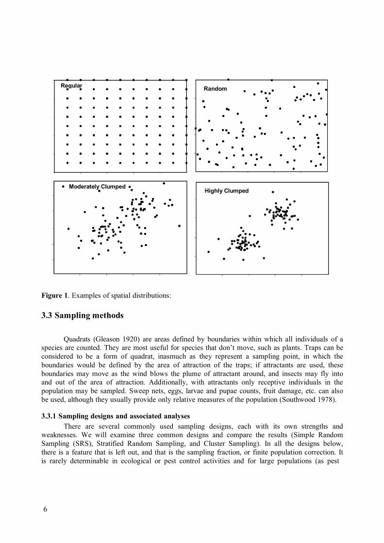
If pest spatial distribution is regular (uniform) or random, monitoring is relatively easy. Traps can be placed anywhere and results can be expected to be typical of the entire area. The sample size can be small because the pest situation is nearly the same throughout the entire intervention area. However, if the spatial distribution of insect pests is aggregated (clumped), then if only a few traps are used, it might be that few or none of them are in a cluster, and thus very biased results could be obtained. This means that more traps have to be used to make sure that all conditions within the intervention area are sampled and that trapping results can be trusted.

If the spatial distribution of pests is regular or random (Fig. 1), then the results of models such as those of Knipling and others, that assume spatial homogeneity, are directly applicable in SIT programs. On the other hand, if the spatial distribution is aggregated (clumped, Fig. 1), then the sterile release rate resulted from these models will have to be adjusted to meet the requirements of the density of the clumps.

6

Figure 1. Examples of spatial distributions: 3.3 Sampling methods

Quadrats (Gleason 1920) are areas defined by boundaries within which all individuals of a species are counted. They are most useful for species that don’t move, such as plants. Traps can be considered to be a form of quadrat, inasmuch as they represent a sampling point, in which the boundaries would be defined by the area of attraction of the traps; if attractants are used, these boundaries may move as the wind blows the plume of attractant around, and insects may fly into and out of the area of attraction. Additionally, with attractants only receptive individuals in the population may be sampled. Sweep nets, eggs, larvae and pupae counts, fruit damage, etc. can also be used, although they usually provide only relative measures of the population (Southwood 1978).

3.3.1 Sampling designs and associated analyses

There are several commonly used sampling designs, each with its own strengths and weaknesses. We will examine three common designs and compare the results (Simple Random Sampling (SRS), Stratified Random Sampling, and Cluster Sampling). In all the designs below, there is a feature that is left out, and that is the sampling fraction, or finite population correction. It is rarely determinable in ecological or pest control activities and for large populations (as pest

Regular Random

Moderately Clumped Highly Clumped

7

populations tend to be) and it has very little effect and will thus be ignored. Those interested in further details on sampling designs may consult Green (1979) and Krebs (1999).

Simple Random Sampling. SRS is a common design for sampling items in which the probability of sampling all items in the population is the same and they are easily available for sampling. This is useful for monitoring surveys where the aim is to understand population dynamics. Ideally, each individual would be identified and tagged with a unique number, and then random numbers would be used to identify which individuals would be included in the sample. This may be feasible for some political or sociological surveys where the population size is known, but it is seldom possible with animals that move, especially with large populations, most of which are not visible to the people doing the sampling. In these cases the best approach may be to conduct “pseudo-random” sampling, where sampling is not mathematically random, but is generally undirected (somewhat haphazard) and not obviously biased. Most people feel that sweep nets, traps, and egg, larvae and pupae counts can be adequate when care is taken to avoid bias during haphazard sampling. For example, true simple random sampling may require sampling in areas in which it is obvious that there are no insects present. Often judgement is needed to justify whether or not a sample can be considered sufficiently representative of the study area.

Means and variances of the samples form unbiased estimates of means and variances for the

population. The mean is the simple average; the variance is a measure of the variability of the data and is the mean of the squared deviations from the sample mean, the standard deviation is the square root of the variance; the standard error is a measure of the standard deviation of the sample mean and is estimated by dividing the standard deviation of the data by the square root of the sample size. If many samples were taken (all of the same size) and the mean was computed for each sample, then the standard error is the standard deviation of these sample mean values. Strictly speaking, the population does not have a standard error, as standard error depends on the sample size. Thus, the unbiased estimate of the mean of a population is the sample mean, i.e., the sum of the observations divided by the sample size

y = ∑yi / n (2)

where y is the sample mean, yi is the value of the ith observation and n is the sample size (i.e. the number of observations used in computing the mean). The variance of the data is

Var(y) = ∑ (yi – y)2/(n-1) = (∑y2 – (∑y)2/n )/(n-1) (3)

and the standard deviation of the data is the square root of the variance:

SD = √(Var(y)) (4)

The variance of the estimate of the mean is

Var(y) = (∑y

2 – (∑y)2/n )/(n-1) / n (5)

where n is the number of means. The standard error is the square root of the variance of the mean:

8

S.E. = √Var(y) (6)

Thus, for example, suppose a sample of insects has been taken and the egg production measured in the laboratory; the egg production for six females was 24, 27, 43, 56, 33 and 17. The mean of these data is then

y = (24 + 27 + 43 + 56 + 33 + 17) / 6 = 200 / 6 = 33.3 eggs per female. The variance is Var (y) =

((242 + 272 + 432 + 562 + 332 + 172) – (200)2/6) /5 = 200.27 The standard deviation is SD = √200.27

= 14.15, and the standard error is S.E. = 14.15/√6 = 14.15 / 2.45 = 5.78.

These measures describe the average value of eggs per female and the variability of the data around the mean, and the standard error shows how much the average may vary by chance from one sample to another.

Stratified Random Sampling. Stratified random sampling (StRS) is done by splitting the population into identifiable subpopulations (strata) and then doing simple random sampling within each stratum. This is particularly useful for detection and delimiting surveys. For example, if one wants to determine the abundance of a particular insect species in a given area, and if the abundance of the species is known to vary among land use zones, it would make sense to partition the area into zones such as commercial orchards, abandoned orchards, human settlements, urban areas, forest, etc. Sampling would then be done in each of these zones separately and then the results analyzed together taking into account the sampling scheme.

Usually simple random sampling would be done within each zone and the sample size would be proportional to the surface of the zone (or the number of individuals available for sampling in the zone). If the sample size is not known, then an intelligent guess is usually better than no information at all. Many fruit flies species infest different species or varieties of fruits and vegetables, so it makes sense, when sampling them on their hosts, to sample each host species separately and tabulate the results for the various host species separately. This is especially useful if the variability in insect numbers between host species is greater than the variability within each host species, and, in this case, the standard errors of the estimates are smaller than for simple random sampling without stratification.

In sampling fruit fly populations it is common practice, before a SRS, to implement a sequential stratification starting from partitioning the area, selecting host species based on host preference, selecting fruit based on infestation symptoms and then finally a SRS of fruit with infestation symptoms. An example is using fruit sampling as a detection tool for the Mediterranean fruit fly. Before applying an SRS on coffee berries with infestation symptoms, sequential stratification is implemented by directing sampling to the primary host (in this case coffee berries), sampling fully ripened berries and sampling during the time of the year when availability of berries is scarce. This procedure greatly improves the likelihood of detection by reducing randomness. Under certain conditions, this procedure has been used in the medfly eradication programme as the preferred detection tool, often detecting the pest as larvae infesting coffee berries prior to detecting adults in traps (Programa Moscamed, 2012).

9

This design lends itself to analysis of the data by means of random blocks analysis of variance. Estimators for the population mean and variance of the mean are as follows.

The population mean, µ is estimated by:

y = Σ(L) ni xi / n (7)

where y is the sample overall mean, Σ(L) is the sum over the L strata that were sampled, ni is the number of individuals sampled in the ith stratum, xi is the mean of the individuals sampled in the ith

stratum, and n is the total number of insects sampled from all the strata. It is assumed that the numbers, ni, of insects sampled from the various strata are proportional to the total numbers existing in each of the strata. If that is the case, then the sample mean for StRS will be the same as for SRS. Generally, however, it will not be known how many insects are in any of the strata, so judgement will be needed in determining the sample sizes, ni, for each of the L strata. There are formulas for computing the mean for non-proportional sampling, but these require the total numbers in each stratum, so they are not presented here (but see Cochran (1977) for more information on these).

The variance of the estimate of the mean is estimated by

Var(y) = (1/n2) Σ(L) (ni)2 (si)2 (8)

where (si)2 = Σ(ni) (xij – xi)2 / (ni -1), (i.e., the sample variance of the ith stratum)

Then the standard error is

√ [(1/n2) Σ(L) (ni)2 (si)2] (9) Cluster sampling. Cluster sampling consists of concentrating samples in units that are easily sampled, such as sampling fruits on trees, each tree representing a cluster of fruit. In this case several, or all, individuals within each cluster are included in the sample. For example, if a programme manager wanted to sample fruit fly larvae in each of several fruits of host trees being attacked by a particular species, she or he could first randomly choose several trees from the orchard, and then randomly choose several fruits from each tree for examination; in this case the numbers of larvae per fruit would be the data collected, so the total number of larvae found in a given fruit would be recorded. For pest detection purposes this is much easier than trying to sample the fruits completely at random from all the trees in the orchard. The distinction between cluster sampling and stratified sampling is that the strata together cover the whole population and sampling is done on each stratum; on the other hand the clusters are easily identifiable and easy to sample, but only some of the clusters (trees) are sampled. For example, strata might consist of tree species of hosts, whereas clusters might consist of individual host trees. If the trees of different species are intermixed, then trees of a given species would not be any easier to sample than trees chosen randomly, whereas sampling branches from a single tree may be much easier than randomly sampling branches from several trees.

10

Cluster sampling works best if the variability of larval counts among fruits within a tree is greater than the variability among trees; however, this is seldom the case, as there are many factors that tend to make individuals within a cluster more similar to each other than they are to those on other trees. One such factor is that insects may attack trees at random, but once within a tree, most of the fruits in the tree are attacked and most of the insects within a fruit may be related. We consider here only the case of equal sized clusters and equal sized samples from each cluster. The appropriate analysis design for data using cluster sampling is nested analysis of variance in which replicate samples are taken from a common source (Sokal and Rohlf 2012).

For a single level of nesting of clusters, assume there are N clusters in the population and we sample n of them. Also, each cluster consists of M individuals and we sample m of them from each cluster.

The population mean, µ is estimated by y, where y is:

y = (Σ(n) (Σ(m) n yij)/m) / n (10)

here, i goes from one to n and j goes from 1 to m, and yi,j is the value of the jth observation in the ith

cluster. The variance of the estimate of the mean is estimated by adding two components of variance. The variance of the cluster means is

s12 = Σ(n) (yi – y)2 / n-1 (11)

where yi is the mean of the ith cluster, y stands for grand mean, and i goes from 1 to n. The variance within clusters is

s22 = Σ(n) Σ(m) (yij – yi)2 / n(m-1) (12)

where j goes from 1 to m, i goes from 1 to n and yi is the mean of the ith cluster. Finally, the

variance of the estimate of the grand mean, ygm, is

Var(y) = s12/n + s2

2/mn (13) 3.3.2 Examples These three sampling designs are illustrated by computing the mean and variance of the mean for each of simple random sampling, stratified random sampling and cluster sampling using the data set in Table 1. Table 1 consists of hypothetical numbers of larvae in fruit in fruit trees that were constructed so that there would be a similarity of numbers of larvae in fruits within each tree, as there normally would be in nature. To compare the calculations of the three designs, we will calculate the mean and variance for each one.

Simple random sampling: Here we calculate the mean and the variance as if the data were collected using simple random sampling from throughout the orchard, while recognizing that the data were not really gathered randomly. Given this assumption, the mean is the sum of all the larval numbers divided by the number of fruit:

y = ∑y / n = 824/80 = 10.3 (14)

11

The variance of the mean is given by

Var(y) = [(∑y2 – (∑y)2/n )/(n-1)] / n = [(12752 – (824)2/80) / 79] / 80 = 0.675 (15)

and the standard error of the mean (se) is then √0.675 = 0.822. Stratified random sampling: Here we assume that the eight trees are the only trees in the orchard, so that each tree becomes a stratum, and that the ten fruit are sampled randomly throughout each tree. The distinctive feature here is that all the trees are sampled and each fruit has an equal chance of being sampled. The mean under StRS is

y = Σ(n) ni xi / n = (10/80)(11.9 + 3.3 + … + 4.6) = 82.4/8 = 10.3 (16)

The variance of the mean is

Var(y) = Σ(n) (ni/n) (si2/n) = Σ(8) (10/80) (49.21+8.68+ … +16.93) / 80 = 0.367 (17)

and the standard error is √0.367 = 0.606.

Cluster Sampling: Here we assume that the eight trees were sampled at random from an orchard containing many trees, and that the ten fruit per tree were sampled at random from within each tree once they had been selected. In this case, each fruit had an equal chance of being selected before the trees were selected, but after the trees were selected, only fruit on those eight trees could be selected. Thus, in for the formula below, mi = 10 for all clusters, and n = 8.

The mean is

y = (Σ(n) (Σ(m) yij / m) / n = Σ(n) (11.9 + 3.3 + 10.1 + … + 4.6) / 8 = 10.3 (18)

where y is the grand mean, yij is the jth observation in the ith cluster, m is the number of observations in each cluster, n is the number of clusters and nm is the total number of observations.

The variance of y = s12/n + s2

2/mn, where s12 is the variance among the i cluster means, s1

2 = Σ(n) (yi

– y)2 / (n-1), so

s12 = [(11.9 - 10.3)2 + (3.3 - 10.3)2 + (10.1 - 10.3)2 + … + (4.6 - 10.3)2] / 7 = 215.04/7 = 30.72

and s2

2 is the variance among subunits within clusters, s22 = Σ(n) (Σ(m) (yij – y)2) / n(m-1), so

s22 = [ (21 – 11.9)2 + (14 – 11.9)2 + (0 – 11.9)2 + … + (10 – 11.9)2

+ (5 - 3.3)2 + (3 - 3.3)2 + (0 - 3.3)2 + … + (3 - 3.3)2

+ (14 - 10.1)2 + (10 - 10.1)2 + (9 - 10.1)2 + … + (11 - 10.1)2 + …

12

+ (4 – 4.6)2 + (0 – 4.6)2 + (0 – 4.6)2 + … + (13 – 4.6)2 ] / 8(9) = 29.37. Then the variance of the estimate of the mean is y = s1

2/n + s22/mn,

Var(y) = 30.72 / 8 + 29.37 / 72 = 3.84 + 0.408 = 4.21

and the standard error of the mean is √4.21 = 2.05

We can see from this that in this example, most of the contribution to the Var(y) is in the variability of the cluster means as a result of differing numbers of larvae in different trees..

Calculations using these three designs yield the same mean, and that will always be true if the sample sizes of the strata and clusters are equal. However, the variances of the mean are different. The lowest variance of the mean, and therefore the most precise estimate, comes from stratified random sampling. This will usually be true, especially if the strata are quite different in their mean values of the observed variable and the variation within a stratum is less than the variation among strata, as is the case in Table 1. The calculation of the variance of the mean under SRS does not take into account the variation among strata, as the strata cover the whole population of interest, at least locally. Cluster sampling produced the highest variance of the mean (i.e., the least precise estimate) and thus it might seem that cluster sampling should be avoided. However, the apparently higher precision using SRS or StRS when clusters are really being used is an illusion; it is false precision because the design really calls for calculations appropriate to cluster sampling. Also, the reduced cost of cluster sampling might compensate for the lowered precision. Since the number of units in a cluster are often more similar to each other than to units in other clusters, the precision is lowered by reduction in the effective sample size. However, this is a justified reduction in the sample size because the units in a cluster are not really independent, but are correlated with each other.

In general, the variance of the mean using cluster sampling is larger than the other two because the variation among clusters is usually much greater than the variation within clusters. This may be because of properties of the cluster (e.g., differing resistance of the trees to infestation by larvae) or simply to chance (the tree just happened to be found by an ovipositing female), or perhaps because of other factors. The calculation of the variance of the grand mean for clustered data takes account of this variation among clusters; calculation by the formula for SRS does not take this into account and it is therefore inappropriate if cluster sampling was used.

The biological and logistical situation of the study should dictate which sampling design and method of calculation to use. To calculate the variance of the mean using the calculations for simple random sampling when the sampling really was done by cluster sampling ignores the real design and the results of the calculations, although mathematically correct, are misleading because they are not appropriate. The variance calculated by the wrong method is less likely to contain the true value being estimated and so can’t be trusted.

3.4 Sampling distributions When we sample fruit fly adults using traps whose locations are spatially identifiable, the

traps in locations where there happen to be a high density of individuals would be expected to catch

13

more individuals than those traps located where individuals are scarce. If we count the adults caught in traps in a given day, we can graph the counts and get a frequency distribution of counts. For example, we might have found 22 cases where the trap count was zero, 37 cases where the trap count was one, 44 cases with two flies, 26 cases with three flies, 12 cases with four flies, 1 case with six flies and none with more than six flies (Table 2). We can describe the resulting graph by one of several theoretical distributions. Such a graphic representation of the frequencies of trap counts is called a frequency distribution of trap counts. The distribution can tell us something about the spatial distribution and density of the individuals, although not in much detail unless the counts are also related to a map of the area sampled.

3.4.1 The Poisson Distribution If the spatial arrangement of the individuals is random, then the distribution of counts will conform to a theoretical sampling distribution called the Poisson distribution (Sokal and Rohlf 2012). The Poisson distribution is specified by the formula:

P(x) = λx e

–λ / x! (19)

Here x is the number of individuals found in the trap, P(x) means the probability of a trap or other sampling device having x insects in it, λ is the mean number of flies found per trap, and λ is also the variance (this is a definitional property of a Poisson distribution), and x! (called “x factorial”) represents x(x-1)(x-2) … (1). If x = 1, then x! = 1; if x = 0, then x! is defined to be 1. This leads to the expression for the zero term of the Poisson distribution; if x = 0, then both λx and x! are 1.0, so that P(0) = e

–λ, meaning that a proportion e–λ of traps would be empty on the basis that the mean

trap catch was λ and that the empty traps would represent the probability that no insects encounter and are caught by the trap, if flies encounter traps randomly. A collection of trap results can be tested against the Poisson distribution by means of a χ

2 statistical test using the observed trap results and the theoretical predictions of the Poisson distribution (Sokal & Rohlf 2012). However, a simpler way is outlined below.

3.4.2 The Negative Binomial Distribution If the spatial arrangement is aggregated (i.e., clumped), then the frequency distribution of the trap samples will not generally follow a Poisson distribution, but usually will approximately follow the Negative Binomial distribution (NBD). The NBD is specified by the formula:

P(x) = [(k+x-1)(k+x-2) ….(k) / x!] [Px / (1+P)k+x] (20) The mean of the NBD is µ = kP, where k and P are the two parameters that define a given NBD. A decrease in k results in an increase in the frequency of larger numbers (aggregation). Thus the parameter k can be used as a measure of the degree of aggregation. As the population becomes more aggregated, the value of k decreases towards zero. As the population becomes less aggregated and approaches random placement of individuals, the value of k increases towards infinity. The value of k for a given NDB may be calculated by the methods outlined by Bliss & Fisher (1953), which will give a measure of the degree of clumping.

Another way of estimating whether a species has a random or clumped distribution is to calculate a statistic known as the Coefficient of Dispersion (CD), which is the sample variance divided by the sample mean (Southwood, 1978). If the insects are randomly located in space, then

14

the CD will be close to 1.0, because the mean is equal to the variance in the Poisson distribution; if the insect population is clumped, then CD > 1.0, and the variance will be greater than the mean; if the population is more uniformly distributed than random, then CD < 1.0. It is not the best index, but it is the simplest and usually works well except in sparse populations. In sparse populations, the CD is usually near 1.0 even for clumped populations. The decision of whether the spatial arrangement of a population is random or clumped is made by comparing the n-1 times the CD with a χ2 goodness-of-fit statistic with n-1 degrees of freedom, where n is the number of trap samples being analyzed.

Using the data provided in Table 2, the mean is calculated using X = ∑ X / n

X = (26(0) + 7(1) + 2(2) + 13(3) + 25(4) + 6(5) + 1(6)) / 80 = 186 / 80 = 2.325

The variance is calculated using Var(X) = (∑ X2 – (∑X)2 / n) / (n-1) Var(X) = [(26(02) + 7(12) + 2(22) + 13(32) + 25(42) + 6(52) + 1(62) – (186)2/80] / 79

= [(0 + 7 + 8 + 117 + 400 + 150 + 36) – 34596/80] / 79

= [718.0 – 432.5] / 79 = 3.61

In this case the coefficient of dispersion is

CD = Var(X) / X = 3.61 / 2.325 = 1.55

and n-1 times the CD is a form of computed χ2 statistic, where n is the number of quadrats or traps (here n-1 = 79).

Then we compare the computed value of χ2 (79x1.55 = 122.45) with a χ2 statistic with ν = 79 degrees of freedom; this is found in a table of χ2 statistics (Table A1) under χ2

0.05,79 and it is 100.75 If the value of the χ2 that is computed from the data is bigger than the χ2 found in the table, then we reject the idea that the dispersion is random and conclude that the population is aggregated because the computed χ2 (i.e. the (n-1)CD) is bigger than the tabled χ2. In that case, it is useful to plot the trap results on a map of the area and discover where the clumps are. Table A1 gives values of χ2

0.05,ν for degrees of freedom (ν) of 1 to 80. For higher values, an approximate value of the critical value of χ2 can be found from the formula: χ2

0.05,ν = (1.645 + √(2ν – 1))2 / 2. Thus, for example, if we wanted to find a value of χ2

0.05,ν for ν (= n-1) = 150, then we get χ20.05,150 = (1.645 + √(300 –

1))2 / 2 = (1.645 + 17.292)2 / 2 = 179.305.

If the CD is much greater than 1.0, then we may want to estimate the parameter k to characterize the population. Southwood (1978) gives three methods of estimating k. The simplest method is to use

k = x2 / (s2 – x) (21)

15

although it is only accurate for sparse populations. However, sparse populations are where the CD fails to discriminate between aggregated and random dispersion, so that this estimator of k will be useful where the Coefficient of Dispersion is not. The other two methods of estimating k require iterative solutions, involving guessing values and continuing until an equality is satisfied, whereas the estimator given above is easy to compute. If we apply the last formula to the data above, we get

k = 2.3252 / (3.61 - 2.325) = 5.41 / 1.285 = 4.21. Thus, according to the parameter k, the spatial distribution of the population is somewhat clumped.

We could also apply the CD and k to the data in Table 1. It is clumped in columns (which represent trees). For Table 1 the mean is 10.3 and the SRS variance is 80(0.675) = 54.0, so that the CD = 5.24 and the estimate of k is k = 10.32 / (54.0 – 10.3) = 2.43. Thus it appears that the population is clumped, but we have no indication of where the clumping is unless we plot the trap catches on a map (see textbooks such as Chiles and Delfiner (1999), Wackernagel (2003), for use of geostatistics as a tool for assessing spatial distribution of insect populations).

3.4.3 The Binomial Distribution The binomial distribution has also been used for insect numbers, and is appropriate when the

spatial distribution is more uniform than random. This is probably not often the case for insects, although it is useful for animal species with territorial behaviour. Also, it is only useful for population units that have an upper limit in number (such as insect larvae on leaves, where there is only space for a certain number). The binomial distribution assumes that each space for an insect on a leaf has a given probability of being occupied. The formula for the binomial distribution is

P(x) = (n!/(n-x)!x!) px (1-p)n-x (22) where P(x) is the probability of x occurrences (in this example larvae on the leaf) and n-x empty spaces, p is the probability of a space being filled and 1-p is the probability of the space not being filled. Again, n! is n(n-1)(n-2)(n-3) … (1).

The binomial distribution applies to data in which there are only two possible states and a finite number of cases. For example, the number of girls (or boys) in families with six children is binomially distributed. If the probability of a child being a girl or a boy at birth is 0.5 for each, then the probability of a family with six children having 5 girls is:

P(5) = [6! / (1!)(5!)] (0.55) (0.51) = [(720)/(1)(120)] (0.03125)(0.5) = 0.09375

Note that P(0) + P(1) + P(2) + P(3) + P(4) + P(5) + P(6) = 1.0 because these are the only possibilities for the numbers of girls in families of size six. Since the probability of a newborn child being a girl or a boy is 0.5 for each outcome, the probabilities for boys are the same as for girls.

4. Population estimation The estimation of pest population size is of value in planning control activities because the

release of sterile males relies on knowing population size in order to assess the amount of control to be imposed. It is also of value in calibrating the various relative methods of population estimation, such as observing infestation levels, the use of trapping measures such as flies per trap per day, and observing egg masses, or fruit punctures in order to be able to use them as estimates of actual

16

population size. It is also of use in assessing the progress of a control programme (see also the trapping guidelines of the IAEA (IAEA 2003)).

4.1 Absolute estimation of population size: Mark-recapture methods This method of estimation will be most useful for longer lived insects, such as species of

fruit flies, especially tephritids, and less useful for shorter lived species, such as Drosophilids, whose life expectancy is only a few weeks. In addition it may not be logistically possible to capture wild flies in sufficient numbers to mark them, release them, and then recapture them in sufficient numbers to obtain reliable estimates by this method. For fruit flies, the conventional method of estimation is by releasing a known number of marked sterile males and then recapturing them in lower numbers together with wild flies. An exhaustive and useful description of Mark-Recapture methods is given by Service (1993).

4.1.1 General features of mark-recapture methods: (1) Two or more samples of individuals are taken at distinct times. After all except the last capture, the captured individuals are marked and then released. Also, for each capture after the first one, individuals are checked for marking before marking and releasing.

(2) The length of time between samples is sufficient to allow mixing of the marked individuals with the wild population, but not long enough that a sizeable portion of the population dies. The marked (and released) individuals are assumed to completely intermix with the rest of the population before the next capture.

(3) The marked individuals are assumed not to be affected by marking; being captured does not affect the probability of being recaptured.

(4) All individuals have the same probability of surviving to the next time period.

(5) All samples are taken randomly; all individuals have an equal probability of capture.

(6) Marks are not lost; all marked individuals remain marked.

Mark-recapture methods yield estimates of absolute population size, rather than just being indices of relative abundance, such as would be the case with sticky traps or egg, larval or pupal counts.

4.1.2 Lincoln (Peterson) Index The Lincoln index is the oldest and simplest of the mark-recapture methods (Le Cren, 1965). It

uses two samples: an initial sample, with subsequent marking and release, and then one more sample for counting the marked and unmarked individuals. In addition to the assumptions listed above, the Lincoln index assumes that there are no births, deaths, immigration or emigration of individuals in the population between the two sampling periods. This index is based on the assumption that the ratio of the total population to the number caught (and then marked) in the first sample is the same as the ratio of the size of the second sample to the number that are found to be marked. In symbols:

N / M = n / m (23)

17

so that the estimate of population size is

N = n M / m (24)

where N is the unknown total population size to be estimated, M is the number of individuals in the first sample (all of which were marked before release), n is the size of the second sample and m is the number of marked individuals in the second sample. The variance of the estimate of population size is

Var (N) = M2 n (n-m) / m3 (25)

Thus, if the initial trapping sample yielded 105 adult flies all of which were marked and

then released, and if a second sample of 99 adult flies yielded 17 marked individuals and 82 unmarked individuals, then the Lincoln estimate of population size would be N = (99)(105) / 17 = 611 individuals and the variance of the estimate of N would be Var(N) = (1052)(99)(82)/173 = 18217. This estimate is easy to obtain, but it is biased. The bias is negligible for large sample sizes, but serious for small samples. In addition, for many insect species, life expectancy is not long and individuals move freely out of and into the sampling area, violating the assumptions of no births, deaths, immigration or emigration. However, for short-lived insect species, other estimation methods requiring more recaptures may not be feasible. The bias can be reduced or eliminated by use of the estimator:

N* = M (n+1) / (m+1) (26)

And the bias of the variance is similarly reduced by the estimator

Var(N*) = M2 (n+1) (n-m) / (m+1)2 (m+2) (27)

(Service 1993). In the example above, the less biased estimate of the mean would be (105)(100) / 18 = 583 and of the variance of the estimate of N would be (105)2(100)(82)/(182)(19) = 14686. Notice that both the estimates of N and variance of N are overestimated by the original formulae. It is recommended that the m be greater than 10 for the estimates to be satisfactory. For a description of methods of marking insects, see Southwood (1978), Service (1993) and Hagler and Jackson (2001) and Guillen (1984) (specifically for tephritid fruit flies).

4.1.3 Jolly-Seber Index The full Jolly-Seber method (Jolly 1965; Seber 1965) is a stochastic approach that uses multiple releases and recaptures and can allow births, deaths, immigration and emigration of individuals. Thus the restrictions are fewer, but the data requirements are greater compared with the Lincoln Index. The Jolly-Seber method is better suited to species that are relatively long-lived and survive well in the field (i.e., with a life expectancy greater than one month), such as with many species of Anastrepha and Bactrocera. For this method to work, we need at least three captures: one initial capture at which insects are marked and released, and then at least two recaptures at which marking and releases are made at all except the last recapture. The recaptures should be sufficiently long after the releases that random mixing of the population occurs. From these we can estimate population size as well as birth rate, death rate and emigration.

18

The Jolly-Seber index allows deaths and emigration, but it also assumes that if they occur, both are permanent. Although deaths are permanent, emigration often is not. However, if the amount of emigration is relatively small, this assumption is not a big problem. Many insect species have a relatively low daily survivorship, so we only present here the case for five captures and four releases. Having more than five capture periods provides little extra information, except to increase overall sample size and precision. Those interested in mark-recapture experiments with more than five capture periods should consult Seber (1982).

One important requirement of the Jolly-Seber index is that it requires unique marking of individuals captured at each sample, so that recaptures can be identified with respect to when they were previously caught. Thus, the first sample might be marked with red dye, the second with blue dye, etc. Since we are dealing with five capture samples, and only four of them need to be marked, four unique marking schemes are required. Any marked individual from the first marked release that is caught again in the second capture will be marked again and thus have two different marks, and similarly for subsequent recaptures. Thus in the fifth capture sample the capture history of each insect in the sample will be evident from the marks it carries. If four distinct marking schemes are not possible, then fewer sampling periods could be used. In practical use, almost no insects will carry four different markings, unless a large proportion of the population is being captured and they are quite long-lived.

The following variables must be evaluated by observation or calculation (notation from Seber (1982)) for the Jolly-Seber index. In what follows, the word “insect” is taken to mean “insect of the species being estimated”.

ti – time when the ith sample is taken (t will probably be in days or weeks). Ni – total number in the population just before time ti.

Mi – total number of marked individuals in the population just before time ti.

ni – total number of insects caught in the ith sample.

mi – number of marked insects caught in the ith sample. Ri – number of marked insects released after the ith sample (any damaged insects are not marked

and released.

ri – number of marked insects from the release of Ri insects which are subsequently recaptured.

φi – proportion of insects that die or emigrate from time i to time i+1.

zi – the number of insects caught before the ith sample which are not caught in the ith sample but are

caught subsequently where i is any sampling day after the first and before the last one.

19

Bi – the number of births in the ith time period. There is no direct estimate of N1. The estimators are as follows:

Mi = Ri zi / ri + mi (28)

Ni = Mi ni / mi (29)

φi = Mi+1 / (Mi - mi + Ri) (30)

Bi Ni+1 - φi (Ni - ni + Ri) (31)

The estimate of most interest will usually be Ni = ni Mi / mi at each time i, which is of the same form as that in the Lincoln estimate. However, we also have estimates of the death rate, φi, and birth rate, Bi which will be important in constructing life tables. With more capture samples estimates of both of these quantities become more accurate. One common confounding factor is that the population size may change over the course of the measurements.

Table 3 shows the steps taken in the calculation of the final estimates. Detailed calculations of these steps are shown here to illustrate. In Table 3a are listed the numbers captured last at time h

of the marked insects captured at time i, for any h < i and any i > 1. These are summed for each row and the sums printed at the right, and these are the number from the release Rh that are subsequently recaptured, where the initial time of capture, h, is listed down the left column and times, i, of subsequent recaptures are listed at the top. The columns are also summed and the sums listed at the bottom, these being mi, the number of marked insects in sample i. The numbers captured at each time, i, are listed at the top together with the numbers marked and released, Ri.

Table 3b shows the numbers, chi, caught in the ith sample that were last caught in or before the hth sample. These are also summed by rows and the sums listed in the right hand column, denoted zi+1. These values are then used to compute the estimates of M, ρ, N, φ and B as above seen in Table 3c. Using the data in Tables 3a and 3b, we compute the following.

M2 = (143)(10)/60 + 10.0 = 33.83 M 3 = (164)(33)/46 + 37 = 154.65 M 4 = (202)(23)/30 + 56 = 210.87 N2 = 33.83/0.0685 = 493.87 N3 = 154.65/0.2189 = 706.49 N4 = 210.87/0.2679 = 787.12 φ2 = 154.65/(33.83 – 10.0 + 143.0) = 0.9270 φ3 = 210.87/(154.65 – 37.0 + 164.0) = 0.7487 B2 = 706.49 – 0.9270(493.87 – 146.0 + 143.0) = 251.45 B3 = 787.12 – 0.7487(706.49 – 169.0 + 164.0) = 261.91

These are seen in Table 3c. The differences over time partly reflect sampling error and partly changes in the parameters themselves.

20

i

∏

These estimates are also biased, as are the Lincoln estimates, and the bias can be mostly corrected by using the modified estimators. It is recommended that both the mi and ri be greater than 10 for the estimates to be satisfactory. More accurate estimators (Seber 1982) are:

Mi* = (Ri + 1) zi / (ri + 1) + mi (32)

Ni* = Mi

* (ni + 1) / (mi + 1) (33) *

φi* = Mi+1

* = / (Mi

Bi* = Ni+1

* - φi (N *

- mi + Ri) (34) - ni + Ri) (35)

In the study on the black-kneed capsid (Jolly 1965) there were 13 sampling events; we have only considered the first five of the 13. The estimates using 13 sampling events were all about 10- 20% higher than using only the first five samplings. This may be because of the fact that the population was increasing during the sampling period and some of the data from later samplings were used in the computations of the earlier estimates. Obviously, a greater number of sampling events is desirable, but practical considerations often restrict what one can do in practice.

4.1.4 Joint Hypergeometric Estimator

A large class of population size estimators has been developed for wildlife management (Seber 1982; Pollock 1990; White and Burnham 1999). Many of these methods assume that marked animals may be sighted multiple times after release, such as the widely used Cormack-Jolly-Seber method (Cormack 1964; Lebreton 1992). Several other more recent methods have been developed for the general purpose of estimating population size, individual daily survival and a range of other parameters on animals larger than insects and are built around powerful statistical models (Lebrenton et al 2012; Pollock 1990).

One of the newer methods that apply to insects is the Joint Hypergeometric Estimator, or JHE (Bartmann et al 1987). JHE uses numerical iteration to maximize a likelihood function based on the hypergeometric distribution, a discrete distribution of the number of successes (recaptures) in a finite population (size N) containing a maximum number of successes (marked individuals) without replacement. Thus this estimator is appropriate for situations where a known number of marked individuals are released into a natural population and then recaptured over multiple occasions and not replaced, such as when marked insects are released and recaptured over several days in traps. The likelihood function that is maximized (N-|Mi , ni , mi) is equal to

K

i

m n m

-

n

(36)

where N- is the estimated population size, Mi is the number of marked individuals that are in the population on sampling occasion i, ni is the total number captured on occasion i,mi is the number of marked individuals recaptured on occasion i and i=1 to k total capture occasions.

The JHE includes fewer assumptions than those in the methods already discussed: no movement out of the area, marks that are not lost and no failure to identify marked individuals. Requiring fewer assumptions comes with requiring more parameters. Importantly, the probability of sighting any given individual, marked or unmarked, is assumed to be equal, though the probabilities don’t have to be equal between sampling sessions (Neal et al 1993). Since the number of individuals available for recapture Mi can vary, it is possible to consider mortality and/or

21

movement out of the study area in this variable. For most practical studies mortality will have to be estimated and included in the analysis.

Currently the JHE can be estimated via the program MARK (White and Burnham 1999) or via the older program NOREMARK (White 1996). Baber et al 2010 use the JHE in a study on mosquitoes during the wet and dry seasons in Mali (see following Table B), and also calculate the estimated population size using the simpler Lincoln Index approach for each of their multiple releases and recaptures (see following Table C). Their results are a useful numerical example showing how the methods compare.

Table B. Estimated population sizes for Fourda from the study of Baber et al 2010 using the joint hypergeometric maximum likelihood estimator from the program NOREMARK with varying daily survival rates.

March 2008 July 2008

Daily Survival Estimate 95% CI a Estimate 95% CI a

0.6 1687 1191-2537 10507 7608-15156

0.8 3659 2556-5547 21450 15484-31015

0.9 5378 3746-8172 30293 21849-43830

a CI, confidence interval.

Table C. Instantaneous Population Size Estimated via Lincoln Index in the study of Baber et al 2010, calculated via equations (25) and (26).

Recapture date M n M N* SD(N*)

17 March 2008 101 75 4 1535 606

18 March 2008 85 120 5 1715 632

19 March 2008 79 74 3 1481 645

03 July 2008 148 160 7 2979 968

04 July 2008 126 166 2 7014 3475

22

05 July 2008 144 187 4 5414 2181

06 July 2008 157 385 1 30301 17449

07 July 2008 299 235 3 17641 5700

4.2 Relative estimation of population size: Monitoring and detection

4.2.1 Trapping for monitoring Trapping is commonly used to monitor pest populations. This simply gives general

information on the seasonal abundance, spatial distribution and host sequence but does not usually yield information on the absolute size of the pest population unless mark-recapture methods are also used, or a connection is made between the usual trapping and mark-recapture estimates (see below). Initially, for population monitoring, simple random sampling is the recommended sampling method (see section 3.3.1). If the trapping technique for the insect being monitored is powerful (i.e. capable of detecting low numbers in a large area), then lower trap densities may be used, as a single capture will signal the presence of the pest species. This is in contrast to trapping for evaluating effectiveness of suppression and eradication measures, where a higher trap density is usually required. Based on the initial results obtained from population monitoring, trapping should be more like a stratified random sampling where traps are placed in locations where the pest is known to occur.

4.2.2 Trapping for detection

Detection trapping is done to determine if a pest is present or absent in an area. For this purpose the sampling need not to be completely random and a sequential stratification would be applied before a SRS, to increase probability of capture (see section 3.3.1). Traps would usually be placed where the highest probability of detecting the insect in question is anticipated. One procedure that may be used to increase the likelihood of detection is through identifying risk factors (presence of primary hosts, human settlements, human migratory routes, etc.) in a given area and assessing the probability for each factor and the overall probability. If this procedure is applied systematically in the area of interest (country, region, etc), a mosaic of levels of risk can be plotted in a map which can then be used as the basis for establishing a trapping network (Enkerlin et al. 2012).

The results will be affected by several factors. In addition to placement of the traps, mentioned above, the area of attraction of traps is an important consideration. If the pest species has a long distance pheromone (e.g. over 500 meters), then the area of attraction might be many hectares; if the species has no long-distance pheromone (e.g. only a few metres), then the area of attraction would probably be less than one hectare or a group of trees. The condition of the habitat would also affect this; if the area is heavily vegetated, then detection of the traps either visually or by odour may be significantly impaired. This will affect the probability of the traps catching insects and will therefore also affect the interpretation of the trapping results.

Trap effectiveness is a third factor of interest that relates to the area of attraction, but more specifically refers to the ability of traps to capture insects within their areas of attraction. Trap

23

effectiveness will depend on features of both the traps and the insects themselves. If pheromone can be used as an attractant, then the trap effectiveness is usually greatly enhanced. If the habitat is relatively open, then visual cues may be very effective. If the prevailing winds are strong, then trapping may not yield good results, and rain is also often a deterrent to trapping. Rain affects the rate of attractant release by reducing the temperature and increasing relative humidity and also physically reduces mobility of insects thus preventing adult flies from encountering traps.

Finally, trap density will affect the total number of captures. Usually, trap captures will increase with trap density up to the point at which the traps start to interfere with each other. If pheromone is being used, then there may be an upper limit to the density of trapping that will yield good results. Above that density, the pheromone will cause the insects to lose their ability to detect the direction of the traps or otherwise interfere with the trapping. If pheromone is not being used (e.g. food attractant), then this limiting density is likely to be higher.

4.2.3 The “Fly per Trap per Day” Index

One measure of success in trapping insects is the number of insects caught each day by each trap, on average. This is called “flies per trap per day” (or FTD) in the context of trapping fruit flies. It makes no assumptions on trap efficiency or other factors affecting trapping success, except that all insects of the target species are equally attracted, and is simply an index of trapping success. The FTD is commonly used in fruit fly area-wide integrated control programmes as an operational index in multiple ways: 1) As an action threshold for aerial and ground insecticide-bait sprays (some programs use a fertile FTD above 0.1) and for release of sterile insects (fertile FTD below 0.1); 2) to monitor sterile insect temporal and spatial distribution in the field as well as relative abundance; 3) to assess required sterile insect density by computing sterile to fertile ratios and adjusting sterile fly release densities based on the ratios required to achieve suppression and/or eradication (FAO, 2007); and 4) to assess the progress of a program by measuring the relative size of the population, as it may be reasonable that an FTD of eight flies per trap represents a population twice the size of one that yields four flies per trap, and in that case one can follow the progress of a control programme by noting in a time-line the trend of the observed FTD.

Some care must be used in the interpretation of FTD data if the number of fertile insects is small, as sampling error can give very misleading results. If the density of flies is very low, then the probabilities of FTD being one or two or three are about the same, but the estimates derived from these FTD’s will be very different; the variability of results in determining FTD will be considerable, and the variability of the estimates will be even greater. For example, estimates derived from numbers such as 1, 2, 4, 2, and 5 will be much more variable that estimates from numbers such as 41, 42, 44, 42, and 45. Also, an estimate of population size based on an FTD of two would be twice that of an FTD of one, but the difference would probably be simply a result of sampling error. It is important also not to include both sexes in a single calculation of FTD. For instance, with medfly sexing strains it is possible to produce only males for use in SIT programmes. To measure the medfly population we could use two different attractants, trimedlure that attracts mostly males (over 99%) and the food attractant biolure which attracts males and females (approximately 40 to 60%, respectively). If the male specific trimedlure baited trap is being used to compute the FTD to estimate the ratio between the release sterile insects and the wild populations, then the FTD is computed separately for the sterile and wild males for the total traps and the sterile to wild ratio is then assessed by dividing the FTD´s. However, in the case of traps baited with

24

biolure, it is common to record and count only sterile and wild males to assess the respective FTD´s leaving out the wild female counts as no sterile females would be caught in traps.

The specific case of Medfly is interesting because there are often released sterile males involved and multiple lures might be used. Trimedlure captures mostly males, but if traps baited with trimedlure are used, they may become completely full of sterile flies and it is difficult to find a wild male among such a massive number of sterile males. On the other hand, if a very good female attractant that captures 90% females and 10% males existed it would be very useful because low numbers of sterile and wild males will be captured with higher number of females. Because it is easy to distinguish females from males, and because no sterile females are being released, records of females would be very precise. If we assume a sex distribution of 1:1, and a uniform age structure, these female records can be used to assess the respective wild male FTD´s.

4.2.4 Fruit sampling

Fruit sampling involves collecting fruits in those areas where fruit bearing host trees are present in the programme’s working area. Fruit sampling can be used to detect the presence or absence of fruit flies, to verify the phytosanitary condition of an area as a complement to trapping or simply to monitor the population fluctuations, host preference and sequence and relative infestation levels. It may or may not be necessary to destroy the fruit in the process of sampling it. Fruit may be cut open to count the larval inhabitants or it may be left for few days in holding cages to allow larvae to fully develop, leave the fruit and pupate.

In AW-IPM programmes, as in the case of trapping, initially fruit sampling is usually done using simple random sampling when applied for population monitoring and a stratified random sampling when applied as a detection tool. Given the amount and diversity of fruit hosts normally present in the field, stratification is critical to improve the probability of detecting an immature stage of the pest. The factors that are usually considered for stratification include: fruit preference (usually efforts are directed towards primary hosts), availability of fruits (fewer fruit present at the beginning and at the end of the ripening season), fruit ripeness (unripened and over-ripe fruits are discarded), sites with historical profile of pest presence, and fruits with infestation symptoms (e.g. oviposition punctures). Fruit samples are collected on a weekly basis. Results are usually compiled in the same way as for trapping, presenting the number of larvae/number of fruits of the same host or number of larvae/kilogram of the same host as well as, in the case of the need to assess damage levels, the number of infested fruits which is transformed into percent infested fruit.

If there is a strong correlation between infestation and fruits within a tree, only a few samples need be taken from each tree. On the other hand, if infestation of fruits are independent of each other (both within and among trees), then stratified cluster sampling can be used to advantage, as it is easier and will allow a greater sample size for a given amount of expense (see Section 3.1.1). This means that a few trees will be intensively sampled, and most trees do not need to be sampled, as the few that are sampled will be representative of the rest.

4.2.4.1 The larvae/fruit as an index of population

There are important differences between using trapping and fruit sampling as a way of measuring fruit fly population size. In trapping of adults, it is possible to distinguish between male and female, so the index can be sex-related (FTDm or FTDf); in fruit sampling however, inmature

25

insects found cannot easily be separated by sex, so in practice a sex distribution of 1:1 is often assumed.

The movement and changes of the adult populations can be more easily traced by traps, and estimates of adult populations based on number of larvae are likely to be less precise than estimates based on trap captures. In addition, assessing the size of the population of a pest based on fruit sampling requires much more effort per unit than traps, thus, the cost per fruit sample is normally substantially greater than the cost per trap. On the other hand, if the objective of fruit sampling is to assess presence or absence of the pest (i.e. fruit sampling for detection), then it may be a cost- effective tool, especially when stratification is used (see Section 3.3.1 b).

An additional difference between fruit and trap sampling is that a sampled fruit usually contain a certain number of larvae and that number may be stable for several days until they pupate and emerge as adults. In the case of the traps, the captures are likely to vary from day to day. Additionally, the traps only capture a fraction of all the adults nearby, so the counts from the fruits and from the traps cannot be compared, except to say that both are indices of the relative size of the wild population, but neither can provide direct estimates of the population size unless prior sampling has established a relationship between the two that can be applied at later dates. Also, if males and females are computed separately, then the sex ratio must be known before any comparison between the trap counts and the fruit counts can be made. If larvae within a given fruit are all or mostly from the eggs of one female, then numbers per infested fruit will not correlate well with population size; in that case the number of infested fruits per tree would be a better measure of population size.

4.2.5 Converting relative estimates to absolute estimates

For this conversion we use a statistical technique called least-squares linear regression. This is a technique, familiar to most readers, for constructing a relationship (a straight line) between two or more variables by minimizing the squares of the deviations between the data and a straight line relating the independent (predictor) and dependent (response) variables. It can be done by hand, but is best done on a computer using a program such as SPSS, SigmaStat, SAS or R.

Relative estimates can be converted to absolute estimates by taking subsamples from populations at different population densities, computing the relative estimates based on the subsamples and simultaneously conducting mark-recapture to obtain estimates of absolute population size. A regression is then computed between the relative estimates and the mark- recapture estimates of population size obtained at the same times. With this relationship, one can use the relative estimates to get estimates of the absolute population size. As with any measurement, the more paired estimates of relative and absolute population sizes generated for a given area, the more confidence we can have in the relationship derived by regression. Since the fit of data to the straight line is never perfect, and all measures include some error, the estimates one gets from this technique are never as good as doing mark-recapture on the whole sample, but it is better than simply using the relative estimates.

An example will illustrate this approach. Consider a population of a defoliating species of insect that lays egg masses in the lower branches of trees. The egg masses are easy to count and will serve as an index of relative population size. Mark-recapture studies have been done each year and the collection of egg masses has been done at the same season as the mark-recapture

26

estimations. The results are presented in Table 4 below. Table 4 contains one estimate of total population size and one collection of egg masses for each year. From these data, a regression can be calculated. The regression is of the form:

Nt = a + bNe (37) where Nt is the number of individuals per ha and Ne is the number of egg masses per ha. The parameters a and b are estimated by regression, called the intercept and slope respectively, and they turned out to be: a = -7.459, b = 10.057. The equation predicting total numbers is then

Nt = -7.459. + 10.057*Ne (38) Now one can estimate the total population size by simply counting the total number of egg masses and then putting that number into eq. (38).

When using this method of converting relative to absolute estimates of population size, one must be aware that other things besides the egg mass density will affect the total population size, and also that the relationship obtained may actually change over time and with differing circumstances. This means that the estimates obtained should be treated as tentative. Also, it may vary from one location to another, but may be a useful starting point. It helps to have more than one relative measure related to the total population size, and then each can serve as a check on the others.

In Table 4, the relationship between total population size and egg mass density was linear. Other relationships are often found, and it may be useful to include other terms in the regression, such as the square of egg mass density and the reciprocal of egg mass density. Adding in both these terms would lead to a modified regression equation which would take the form:

Nt = a + bNe + c Ne2 + d/Ne (39)

In general squared, reciprocal or other terms would be added through some biological

consideration. The improvement of the fit of the overall model could be evaluated with an ANOVA or by the regression equation itself. For an examination of these issues plus the question of statistical significance testing any number of introductory statistics text books could be consulted such as Sokal and Rohlf (2012).

5. Forecasting populations In order to plan for control activities, it is necessary to have some idea of the size of the

population and also, if possible, whether the population is increasing or decreasing in size. It would be useful also to know the spatial distribution of the population. These can be estimated from noting the populations found in previous years, but it is especially useful to know the timing of events as they occur in the current year, such as the emergence of adults from overwintering pupae or the massive dispersal of adult fruit flies after fruit harvest or in response to a prolonged drought. The emergence of the first adults after winter can be forecast by knowing the heat requirements of the species and using meteorological forecasts of temperatures for the next few weeks. Such meteorological forecasts are often not very reliable, but they are usually better than having no information. Useful computer based programs to forecast timing and spatial distribution of events

27

based on temperature are available. One frequently used to forecast fruit fly populations is CLIMEX and the FAO Locust Watch forecast based on seasonal weather predictions. See Appendix 3 for details on these software programmes.

5.1 Detecting population change Mark-recapture. Mark-recapture analysis can be used to determine whether the wild population is increasing, decreasing or staying relatively constant (see section 4.1). In order to separate a trend from sampling error and other errors, at least three determinations of population size should be made and at time intervals that would allow detectable change to occur between readings.

Age structure. The age structure of an increasing population will have a preponderance of young age classes, whereas a declining population will have mostly older age classes. From life table analysis, these characteristics can be assessed and inferences made about the change of the population size.

Indirect indices. Other methods involve sightings of flying insects, resting or mating; number of individuals captured trying to obtain a blood meal per night; net sweeps, counting egg masses, fruit punctures and evidence of damage to host plants, etc. It is usually useful to use more than one method of detection, as often a given method may work well under certain conditions or at certain times, and not otherwise. The use of several detection methods usually ensures that the weak areas of one method are covered by other methods.

5.2 Prediction of life history events Development in insects is governed by chemical and biochemical processes, and these are

temperature-dependent. Chemical processes usually occur more quickly at higher temperatures than at lower temperatures and the rate of change of the speed of reaction is often nearly a linear function of temperature within normally encountered temperature ranges. In species with synchronized breeding, or a sharp increase in breeding in response to a seasonal resource suddenly becoming available, it is useful to predict when the first larvae will appear, to aid in the timing of the use of the appropriate suppression measures (e.g. fruit stripping, release of parasitoids, application of bait sprays or residual spraying, etc.); the time of emergence of adults will be important in the timing of the application of bait sprays or the release of sterile males. In continuously breeding species, prediction of developmental events may be of less interest, as generations are overlapping and all stages may be present at any one time.

5.2.1 Developmental time for the stages: degree-days

If early season temperatures are lower than the temperature required for physiological development of the overwintering stage, then there will be some threshold (or base) temperature, τ, at which development starts. Any temperature above this threshold will allow development to occur and the difference between the threshold and the ambient temperature will determine the rate of development. This model underpins the most widely used approach to estimating development in insects, the thermal accumulation model, which we will refer to here as “Degree days” (for degree- day requirements for many insect species see: http://ccesuffolk.org/assets/Horticulture- Leaflets/Using-Growing-Degree-Days-for-Insect-Pest-Management.pdf ).

Calculation of degree days typically involves calculating the mean temperature, Tm, for each day and then adding Tm – τ to a daily running total for the season. Thus a single degree day may be

28

thought of as 24 hours where the temperature is 1 degree above τ. Any days where the temperatures are all below the threshold do not contribute to the degree-day total and Tm – τ is taken to be zero. From experimental measurements in the laboratory we have estimates of τ and the number of degree days required for transitions from each developmental stage for a number of economically important species (Magarey et al 2007; Nietshcke et al 2007), so the sum described above can continue until enough degree days have accumulated for transformation of individuals into another life stage (e.g., eggs hatch into larvae, larvae molt and progress to another instar, etc.). If degree-day requirements for development are known, then predictions of the occurrence of each life stage can be made by tabulating the daily accumulations of degree-days. It is important to note also that the degrees in question may be C or F and also that the time unit does not have to be days; in the egg stage of C. capitata, for example, the accumulations are often measured in hours (e.g. Duyck and Quilici 2002).

There are various methods for calculating Tm from daily minimum/maximum temperatures, commonly available from meteorological services and weather stations; one of the simplest is given by Snyder (1985). If both the maximum and the minimum temperatures for the day are above the threshold, then a simple average of the maximum and minimum temperatures for the day can be used. If the maximum is above the threshold but the minimum is below the threshold, then the method of Baskerville and Emin (1969) would be more appropriate. The temperature curve during a 24-hour period can be approximated by a sine curve and this can be used to calculate the mean value above the threshold (see also Allen 1976).

If hourly temperatures are available, then these can be added to get the sum over the 24 hour period and divided by 24 to get Σ (Th – τ) / 24, i.e., the mean hourly temperature contribution to the degree-day total, where Th is the temperature at hour h. Thus, if hourly temperatures are available and the threshold for development was 8oC, then the degree-day component for the day illustrated is calculated as follows. Suppose the hourly temperatures from one o’clock in the morning until midnight of the same day are as in Table 5. The degree-day value for that day would be 26/24 = 1.08.

If hourly measurements are not available and only minimum and maximum temperatures for each day are available, then a method similar to that of Baskerville and Emin (1969) can be used together with Table A2 to approximate the area under a sine curve that is above the threshold. To use Table A2, we need to know three numbers: the minimum, Tmin, and maximum, Tmax, temperatures for the day as well as the threshold temperature, Tthr, for development to occur. We then calculate

f = (Tthr - Tmin) / (Tmax - Tmin) (40)

and enter Table A2 with it to find p, the proportion of the area below the sine curve and above the threshold. Here the maximum is 12o and the minimum is 5o, while the threshold is 8o; thus we calculate f = (8 – 5) / (12 – 5) = 0.43. Using Table A2 with f = 0.43, we obtain p = 0.392. We then multiply 0.392 by (Tmax - Tmin) / 2. Applying this table to the minimum and maximum in Table 5 gives degree-days = 0.392 (12 – 5) / 2 = 1.372. This is more than the amount calculated by hourly temperatures (1.08), but the numbers shown in Table 5 do not closely follow a sine curve, so that the discrepancy is not surprising. In this case the hourly temperatures are the better ones to use, if they are available, as they are more accurate than the approximation by a sine curve.

29

A slightly more sophisticated approach to calculating degree-days when only minimum- maximum daily temperatures are available for some or all days is to generate estimated hourly temperatures using the empirical formulae described by Campbell and Norman (1997):

Γ(t) = 0.44 − 0.46sin(ωt+ 0.9) + 0.11sin(2ωt+ 0.9) (41)

where ω = π/12, and t is time of day in hours, with t = 12 at solar noon. The temperature for any time of a day i can be estimated as follows:

T (t) = Tx,i−1Γ(t) + Tn,i[1 − Γ(t)] for 0 < t ≤ 5,

Tx,iΓ(t) + Tn,i[1 − Γ(t)] for 5 < t ≤ 14 (42)

Tx,iΓ(t) + Tn,i+1[1 − Γ(t)] for 14 < t < 24

where Tx is the daily maximum temperature Tn is the daily minimum.

The method above involves using two terms of a Fourier series fitted to a longer term hourly

average, and is superior to the more commonly used sine method because it does not necessarily generate diurnally symmetrical temperature curves. An example of this method in practice for studying insect phenology can be seen in Manoukis and Hoffmann (2013); A similar approach, validated for use in California, is given in Cesaraccio et al (2001), who also discuss other relevant approaches. Additional methods for calculating degree days not discussed here include those in the “triangle” method (Lindsay and Newman, 1956) family, outlined in Roltsch et al (1999).

In terms of forecasting development, precise estimates of the actual degree-day values for given days are only possible as the days pass, but if approximate daily temperatures are available in weekly forecasts, then some predictions can be made and resources be made available at appropriate times for the stages subject to control. It is also common practice to use historical average temperatures to forecast the length of development.

As an example, the degree-day requirements for the Mediterranean fruit fly –medfly- (Ceratitis capitata) were calculated from times to finish the egg, larval and pupal stages at various temperatures given by Shoukry and Hafez (1979). It was found that the degree-day requirements were approximately constant over temperatures for thresholds of 10oC for eggs, 6oC for larvae and 13oC for pupae. Using these thresholds, their medflies had heat requirements for eggs of 32.7 degree-days, for larvae of 178 degree-days and for pupae of 132 degree-days. In another example, in the trilateral Moscamed Programme (USA-Guatemala-Mexico) a degree-days model was used to calculate the generation time and number of generations that the medfly can produce based on the different climatic zones in Guatemala. Fruit fly outbreak eradication protocols indicate that the time required to declare eradication should be equivalent to three biological cycles of the pest (ISPM No. 26, FAO 2006). Degree day models are then used to determine the generation time and the total time required for completion of three life cycles which will depend on the environmental conditions present in the area.

30

5.2.2. Curves of developmental rate vs. temperature Another approach is used in a model of tsetse for purposes of assessing the usefulness of

various control measures and how much of each would be required for eradication (Barclay & Vreysen 2011). Instead of degree days, the length of the pupal developmental period and the time until first larviposition are estimated from empirical curves. For tsetse, the pupal developmental period is given by

pd = [1.0 + exp(5.4 + 0.25T)] / 0.55 (43) and the time until first larviposition is given (data from J. Hargrove) by

lt = [1.0 + exp(1.63 – 0.063T)] / 0.130 (44)

Functions such as these may be especially useful in cases where the relationships between temperature and development are nonlinear. They have to be developed by experimental manipulation of temperature, usually in the laboratory.

5.2.3 Population growth

The extent to which a population exhibits synchronous changes from one stage to another probably depends mostly on the extent to which there is a clearly defined inactive period for part of the year, and this will be most apparent at high latitudes and least apparent in tropical and subtropical latitudes. If breeding is synchronous, then the change from one stage to another (egg hatch, pupation, etc.) will be predictable on the basis of degree-day accumulations and these changes will be of assistance in planning control operations. If the various stages of the population overlap appreciably, then predicting changes of these stages will also overlap and be blurred.

There are many examples of published models of phenology based on degree days. One of these was done by Judd and Gardiner (1997) and is summarized here. Orthosia hibisci is a pest of apple and pear trees in British Columbia, Canada. The species has one generation per year and overwinter as pupae, emerging as adults in late February or early March. O. hibisci has six larval instars and most of the damage to fruit is done by later larval instars. Eggs are laid shortly after adult emergence and larvae hatch to coincide with fruit bud development in the fruit trees. This is when controls should begin (Table 6).

Bacillus thuringiensis is used to control O. hibisci to avoid the use of chemical insecticides. To maximize the effectiveness of Bt and minimize control costs, the timing of the sprays should be as precise as possible. Thus, monitoring the population using sex attractants is advisable in addition to the use of degree day models.

In their study, monitoring of adults began in mid-February and continued until June. Traps were examined daily. Weather records consisted of hourly measurements of air and soil temperatures and a threshold of 3oC was used as the base for physiological development. Daily degree-day summations were calculated by fitting a sine curve to the hourly measurements. Cumulative percentages of adult emergence, catch and oviposition for each sex were defined using degree values. Cumulated degree-days were started after the first adult catch (Biofix) using sex attractants, indicating that diapause was then complete.

31

To reach maximal vulnerable O. hibisci and minimize damage to the crop, spraying is recommended at the pink stage of development for apples, or 252 degree-days after biofix, to be maximally effective; later sprays would allow the L4 and L5 larval instars to inflict damage on the crop before the spray occurred.

6. Population and demographic models Almost all models of the Sterile Insect Technique (SIT) are population models, either

analytic (with only equations) or computer models (often called numerical models or simulations, and in which the relations are governed by algorithms implemented in computer code). Population models keep track of population numbers, and include various features that influence population size and trend, such as birth rate, mortality, age structure, immigration and emigration, competition, etc.

Mathematical models of populations are often posed as difference equations or as differential equations. Difference equations are discrete (stepwise, or discontinuous) and use some meaningful time step, such as days, years, generations, etc. These are popular with entomologists, since many insects breed seasonally, such as most temperate forest insect pests (bark beetles, budworms, tent caterpillars, etc.) Difference equations do not involve calculus, and generally are easier for the non-mathematician to understand. Differential equations are continuous; involving infinitely small time steps, and are sometimes solvable with calculus. They are useful in species that breed continuously within some period of time, such as some fruit flies and mosquitoes.

Demography is the description and analysis of population quantitative attributes, such as growth rate, life expectancy, generation time, population doubling times, age structure, age at first reproduction, fertility per female at each age and survivorship at each age. It is applied to human populations by sociologists and insurance companies and to animal populations by ecologists. Demographic information is usually summarized in life tables, described below. Life tables are a very useful encapsulation of the quantitative characteristics of populations determining population growth rates and resilience to environmental changes. Demographic models are employed in SIT programs with the specific aim of calculating overflooding ratios for releases of sterile insects (see chapter 8).

In this book, models that predict population dynamics will only be explored to illustrate the importance of the feature being discussed. Statistical analysis of data will be considered when it is useful for predicting control effort or estimating some other relevant quantity, such as the derivation of regressions for use in field operations.

6.1. Population processes

6.1.1. Fertility and fecundity Fecundity is the rate of production of eggs per female; fertility is the rate of production of

eggs that hatch per female. These can be measured in the laboratory, and under ideal conditions for the species, maximum rates of fertility and fecundity can be obtained. In the field the rates may be lower as a result of poor nutrition, lack of oviposition sites, difficulty in finding mates, harassment in dense populations, etc.

32

The fecundity of a female in at least some insect species (e.g., Drosophila melanogaster, Chiang and Hodson 1950) is proportional to her weight, and thus size, which in turn is affected by temperature, nutrition, crowding, etc. Mean fecundity of a sample may be estimated indirectly by measuring a subsample for characters such as wing length, pupal length or overall body length of adults as well as egg production, and then forming a regression for egg production on these secondary characteristics. In addition, indices of fecundity may be calculated by measuring weight of egg masses and then regressing the number of eggs that hatch against egg mass weight (see section 4.2.5). Recruitment may also be estimated by the Jolly-Seber mark-recapture index (see section 4.1.3).

6.1.2 Mortality and survivorship

These should be determined under field conditions, if possible, as they will likely differ considerably from the values obtained in the laboratory. In the laboratory, maximum survivorship can be obtained by allowing a female and male to mate and lay eggs and then by regularly counting the number of offspring living from that single clutch until all are dead. Survivorship is normally determined daily as a proportion of the eggs that were laid and hatched and that were still alive on a particular day. Note that survivorship is often estimated by stage. Thus, if 1000 eggs were laid or inoculated into growth medium and hatched, then the number surviving to day i divided by 1000 would be the survivorship to day i. For example, if 1000 eggs were inoculated into growth medium, 950 of them hatched, and 884 of them were still alive on the tenth day, then the survivorship to day 10 would be 884/950 = 0.93. Since those that didn’t survive were 950 – 884 = 64, the cumulative mortality to day ten was 0.07. Thus, survivorship equals one minus mortality. Mortality obtained as above is suitable for use in life tables, described in section 6.3.

Mortality is often obtained by subtracting population estimates for successive population stages. This assumes both that the population is stable and that the methods of estimating the various stages are equally effective. Cohort measurements are best, as one measures the same individuals on successive occasions, but they are seldom feasible in nature as a result of lack of identifiability of cohort members and inability to capture them many times.

Mortality may be caused by weather, starvation, predators and parasites, intraspecific competition, human intervention, etc., but for our purposes it is usually just the number dying that counts, not the cause of death. Mortality estimates can also be obtained by mark-recapture estimates using the Jolly-Seber index.

6.1.3 Pest dispersal.

Dispersal is important in pest control because it not only allows insects to move around and invade new areas, but also because it exposes the insects to traps and other control measures that they might not encounter if they did not move. Dispersal also allows immigrants to enter the control area and replenish populations that have been reduced by control measures.

Dispersal of pests can be assessed by releasing marked insects and estimating dispersal from multiple recaptures of the marked insects over various periods of time. This is more likely to yield good results if the survivorship of the species is high. If daily survivorship is low (i.e., less than 80%), then a large proportion of the population may die before having the opportunity to be recaptured. The Jolly-Seber index can be used to estimate dispersal (Chapter 4, section 4.1.3). This method requires at least three captures of at least some of the same insects to estimate losses due to

33

deaths and emigration, recruitment due to oviposition and also as a result of immigration and dispersal. If it can be done quickly on a long-lived species and if the death rate is low and known independently, then any excess losses can be attributed to dispersal.

Dispersal can be estimated by means of mark-recapture methods involving releases of marked individuals from a known location and then trapping them at various distances away from the release point, typically yielding a recapture curve similar to the one in Fig. 2. In addition, multiple recaptures of individually marked insects can be used to estimate mean dispersal distance with respect to time between captures. Once the curve has been constructed, estimates of maximal dispersal (i.e., when more than 99% have dispersed less than that distance) or mean dispersal per unit time can then be made. If samples are taken of a population that is dispersing from a point of release, then the mean dispersal distance can be calculated as “the sum of ‘the numbers in each trap times the distance from the point of release’ divided by the total sum of trap catches”. Symbolically mean distance dispersed equals

Mean distance dispersed = Σ ni di / Σ ni (45)

where ni is the number of insects in trap i and di is the distance that trap i is from the point of release, and the sum is taken over all the traps being used. Of course, these values will change with time. A more sophisticated, although mathematically more difficult, procedure is described below.

Diffusion equations and random walks can be used to model dispersal. Random walks are mathematical models in which something (e.g., an insect) makes a move of a given length in a random direction, and then in the next time period makes another move in a different random direction, and so on. Diffusion equations are based on random walks. If both the time interval and the distance moved decrease towards zero, then in the limiting case this situation is described by diffusion equations (Berg 1983). Diffusion equations have one parameter, D, called the diffusion coefficient, and its units are squared distance per unit time; this is not easily interpretable, but can be measured as

D = (Σ(N) di

2 / N) / 2t (46) for movement in one dimension or

D = (Σ(N)

di2 / N) / 4t (47)

in two dimensions, in which di is the distance that the ith insect has gone in a given time, t, and N is the number of insects in the sample, and the summation is taken over the N insects. If we define d

2 = (Σ(N) di

2 / N) to be the mean square distance covered by the insects, then √(Σ(N) di

2 / N) will be the ‘root mean square distance’, and it represents the mean net linear distance between the starting point and the end point. Diffusion equations predict that spread will slow down as time and distance proceed because the insects don’t all move in one direction and movement is random. This can be seen by solving for root mean square distance:

√(Σ(N) di

2 / N) = √4Dt (48)

34

so that the mean net linear distance traveled is proportional to the square root of time. Thus, the distance gone in ten seconds will be √10 (= 3.162) times the distance gone in one second.

Dispersal equations were originally developed to describe the diffusion of heat along a metal rod. They were first applied to animal dispersal by Skellam (1951) and found to fit data well.

2.0

1.5

1.0

0.5

0.0

0

DISTANCE FROM RELEASE POINT

Figure 2. Typical curves of trap catches resulting from release of insects at point 0 at a given time. Over time the curves flatten out as the insects disperse outward from the release point.

Berg (1983) gives an example of a small molecule diffusing through water at room temperature. It has a diffusion coefficient of D = 10-5 square cm per second and can diffuse about 10-4 cm in about half a millisecond. If distance were a linear function of time, then a diffusion distance of one cm would take about five seconds. However, it would take about 14 hours to diffuse one cm based on the relationship shown above, and this has been demonstrated experimentally to be the case.

The units of distance and time can be chosen to suit the purpose. In dealing with dispersing

insects, we might want to use distance in metres and time in days; of course, the choice of units will affect the size of D that is estimated from the data. For example, Table 7 shows a frequency distribution of distances dispersed, to the nearest metre, by a hypothetical slow moving insect in nine days from a release point. We can estimate D by means of the equation given above: D = (Σ(N)

di2 / N) / 4t. This is for two dimensions, so that the distances are all in different directions from the

central release point, but direction is not considered in the estimation. The total number of insects observed was 68, the sum of d2

i was

MIDDLE

TR

AP

PIN

G F

RE

QU

EN

CY

35

Σ d2

i = 0 + 16 + 56 + … + 81 + 0 = 686 and the time was nine days, so D = (686/68)/36 = 0.280. This can be taken as an estimate of the true value of dispersal for the species, for that location, season and weather conditions.

Once one has an estimate of the diffusion coefficient, D, one can invert the formula and estimate the time it will take for the average dispersal to get to a given distance or the mean distance dispersed in a given time. Thus

t = (Σ(N) di

2 / N) / 4D or Σ(N) di

2 / N = 4Dt (49)

Bouyer et al. (2007) have estimated the parameter D for tsetse to be 0.29 square km per day, so that the mean square distance gone in t days will be 4Dt = 1.16t

The solution to the two-dimensional diffusion equation is a bivariate normal distribution with a variance of 4Dt, and so the standard deviation is 2√Dt (Edelstein-Keshet 1988). Then using the rule that 95% of the probability is contained within two standard deviations from the mean, we can assert that from any location containing dispersing insects, about 5% will have dispersed farther than a distance 4√Dt from the given location in time t. This gives a measure of the distance moved by most of the population in a given amount of time. Using three standard deviations, we can state that only about 1% of the insects will have moved a distance more than 6√Dt from the starting point in time t. For most insects, it seems appropriate to measure time in days and distance in metres, although some quickly dispersing insects may move more than one kilometer in a day. Thus, using Bouyer’s estimate of dispersal for tsetse, it may be stated that only about 1% of mobile tsetse will move a distance greater than 3(√1.16) km per day, or 3.23 km per day.

6.1.4 Correlated Random Walks

Though the simple 2D diffusion model discussed above is well understood and has been extensively used in general ecological models of movement (Okubo 1980) and insect movement studies (Rudd and Gandour 1985), it does not have a high degree of realism relative to how insects actually move in nature. In particular, the assumption of a uniform distribution of angles of movement, 180o in each direction, and that individuals may turn at each time step is quite unrealistic for most insects. Since any deviation from this assumption will increase the mean distance travelled from the starting point over time it is probably best to consider simple 2D diffusion as a model for the minimum movement of a group of insects.

A more realistic movement model is a correlated random walk (Kitching 1971; Byers 1991, 2001) where the turning angles are not uniformly distributed, resulting in more directed movement. Unfortunately this sort of movement model is more complicated than simple diffusion (Patlak 1953; Turchin 1991). One of the most usable set of equations for calculating distance moved (mean squared distance) based on move length, turning angle distributions and total number of moves is as follows (Kareiva and Shigesada 1983):

E(R2) = nE(l2) + 2E(l)2 c n -

-c

n

(50) and

-c -c

36

I

c = E(cos 8) = rr

cos 8 g(8)d8 -rr

(51)

where l is the step size, n is the number of steps, c is the mean of the cosines of all possible turning angles (radians) from a specific random distribution g(θ), which may be Gaussian or any other distribution. This simplified form assumes equal probabilities of left and right turns, so that g(θ) is symmetric around θ=1. If we assume a constant step size, E(L

2) = L2. Following Figure shows

examples of correlated random walks with three distributions of turning angles. These are examples of 200-step paths generated with three values of the standard deviation σ of the distribution of turn angles between successive steps, shown above the paths. P=L=length of a step. Reproduced with permission from Bovet and Benhamou (1988).

The square root of E(R2) is approximately the mean distance travelled, though a correction

factor of 0.89 is helpful for many cases (Byers 2001). Byers (2001) gives correction factors for a variety of movement parameters, interested readers should consult that paper for details.

6.2 Features of population models

6.2.1 Population growth The simplest kind of population growth is geometric growth for a species with non-

overlapping generations, and its continuous counterpart, exponential growth. A simple modification to these models, to include resource limitation, puts an upper limit on growth. Many formulations exist for limiting geometric growth (i.e., density-dependent population regulation); a few were provided by Hassell (1978). This small complication makes some of the models insoluble analytically, and it is a common feature of population models that non-linearities often render the models insoluble analytically; it is then necessary to resort to numerical solutions using a computer. Within reasonable limits, discrete and continuous models give similar results. Generally discrete models are easier to use and are favoured by most entomologists.

The geometric model is

37

Nt+1=λNt (52)

Here Nt is the size of the population at time t, where t is scaled to generations and λ is the rate of increase each generation. In each generation the population size is λ times the size it was in the previous generation. In this model generations are discrete and non-overlapping. This model is easy to solve. At any time t,

Nt =N0λt (53)

where N0 is the size of the population at time t=0.

The continuous counterpart of the geometric model is the exponential growth model and it is

dN/dt=rN (54)

The solution to this model is

N=N0 exp (rt) (55)

where exp(rt) = ert, e is the base of natural logarithms, r is the instantaneous rate of growth, and N0

is the initial size of the population at time zero. The relationship between r and λ is that

r = ln(λ) (56)

where ln stands for the natural logarithm.

Another important simple method for modeling population growth is to include density dependence. With density-dependence, the geometric model becomes Nt+1=λNt exp(-gNt ), in which the exponential term has no real biological meaning, and is simply a convenient device to limit population numbers. The continuous version is the logistic equation: dN/dt=rN(K–N)/K, where K is the carrying capacity, imposed by resource limitation. In both cases, control using SIT becomes easier with density dependence because density-dependence imposes extra mortality and thus assists the SIT in its depressive action. The amount of this assistance will depend on the mechanism of density-dependent population regulation, and that varies from one species to another and may or may not be properly described by any of the mathematical formulations of density- dependence presently in use.

6.2.2 Overlapping or non-overlapping generations

Some models have a time step of one generation (usually one year) and if the individuals only live for one generation, then generations do not overlap. These models are simple and often easily analyzed. If the time step is less than one generation (e.g., one day or one week), then more equations are required to represent the various stages. These models will be better suited for species such as many fruit flies in which oviposition and mortality occur over lengthy periods of time. In continuous models, generations necessarily overlap. However, when realism is a modeling goal, the resulting equations can be sufficiently complicated such that they become cumbersome and hard to analyze. All the standard population models are compromises between realism and ease of analysis.

38

6.2.3 Age-Specific mortality and fecundity If we have information on the sizes of the population components at various ages or stages,

we can construct an age-structured model. Thus, in a single cohort, the egg stages are the most numerous, then the larval stages, then the pupal stages, and the adult stages are the least numerous. This order may not be preserved if the population consists of many cohorts. With discrete models it is easy to incorporate age structure into the model. For this we need more than one equation. We could, for example, have one equation for each day of life of the insect, from egg through adult to senescence. If most of the stages are density-independent, then the model may still be solvable analytically. If many stages have density-dependent regulation, then the solution of the equations may have to rely on numerical integration with a computer.

An example of an age-structured model that is tabulated on a daily basis and is completely density-independent is the following. Here E stands for egg, L stands for larva, P for pupa, and F for fertile female adult. The subscripts are to denote age and time; thus E2,t represents the number of eggs that are 2 days old at time t, while F10,t+1 represents the number of adult females at time t+1 that emerged ten days before (i.e., they are ten days old). In this model, mx stands for fertility per female; only females are tabulated and it is assumed that all ages of adult females lay the same number of fertile eggs per day. The symbol ∑ means the sum over all values of the counter i. Thus, ∑ Fi,t mx = F1,t mx + F2,t mx + … + FM,t mx , where EM1,t LM2,t PM3,t and FM4,t are the oldest age classes of eggs, larvae, pupae, and adults present respectively and the values of M1, M2, etc. will probably depend on temperature, nutrition, etc. Thus, the first age class for eggs results from the fertility of all the adult female age classes, whereas subsequent age classes result from survivorship from previous ages.

E1,t=1 = ∑ Fi,t mx

E2,t+1 = E1,t

E3,t+1 = E2,t (57) . . .

EM1,t+1 = EM1-1,t

L1,t+1 = EM1,t

L2,t+1 = q L1,t

L3,t+1 = q L2,t (58) . . .

LM2,t+1 = q LM2-1,t

P1,t+1 = q LM2,t

P2,t+1 = w P1,t

P3,t+1 = w P2,t (59) . . .

PM3,t+1 = w PM3-1,t

39

F1,t+1 = w PM3,t

F2,t+1 = s F1,t

F3,t+1 = s F2,t (60) . . .

FM4,t+1 = s FM4-1,t

Here q, w and s are the daily survivorships of the larvae, pupae and adults respectively. The biggest problem in understanding this kind of model is often just being clear about the counters (subscripts). This model does not represent one cohort, but rather a population with overlapping age classes, so that all age classes may be represented in the population at any given time. It could represent a cohort if the time counter progressed by one at each successive age. Such a model has no equilibrium, as it has no limitation imposed on it by density-dependence. It is quite useful in forming part of a model of SIT, and in that context it does have an equilibrium, although the equilibrium is unstable. However, even though the equilibrium is unstable, it is useful in defining the critical sterile release rate required for or eradication (the critical release rate represents the release rate that separates success from failure of the control programme.

A formalized structure for analyzing population growth involving age structure is the life table (developed below), which allows the calculation of various statistics, such as the net reproductive rate, life expectancy, mean age-dependent fertility and generation time, all calculated from the age-dependent fertilities and survivorships. Life tables are useful in cases where the populations exist with generations overlapping. Species with synchronous reproduction and which do not survive beyond one generation are usually easy to analyze without the use of life tables, but many pest species exist in nature with overlapping generations, such as fruit flies, mosquitoes, and tsetse flies.

In addition to life tables, Leslie matrices are useful for projecting the demographics of a structured population (i.e. where we do not treat all individuals identically with respect to reproduction and mortality).

6.3 Demographic models

6.3.1 Leslie Matrix Models As we have seen above, the exponential model of population growth above (Nt+1=λNt) and

the logistic version (Nt+1=λNt exp(-gNt )) are very useful, but both treat all individuals in the population identically. In insect populations, however, individuals are not equivalent: immature individuals don’t reproduce, young adults may not be sexually mature and very old females may become reproductively senescent. In addition to reproductive differences, different stages and age classes may have varying survival per unit time.

Basic linear algebra and matrix operations make it relatively simple to model a structured population. These tools allow us to keep track of different classes of individuals over time. Below is an example, adapted and extended from Allman and Rhodes (2004):

Consider an insect with three life stages: egg, larva and adult. These insects progress from one stage to the next in one step, and adults lay eggs and die in one step also (a time step may be a

40

day, a week or any other amount of time). Et is the number of eggs at time t, Lt is the number of larvae at time t and At is the number of adults at time t. If eggs have a 4% probability of surviving to be larvae, larvae have a 39% probability of becoming adults and adults on average produce 73 eggs each we can write:

Et+ = 73At

Lt+ = 0.04Et (61) At+ = 0.39Lt

These three difference equations can model our age structured population given three initial values: E0, L0 and A0.

This population could also be modeled by At+3 = (0.39)(0.04)(73)At = 1.1388At. Since this simple exponential model also describes the population, we already can see that the population will grow, with λ = 1.1388. However, we want to keep track of our three stages, and perhaps also track changes per single time step; for that, we might use the following formulation:

0 0 73 Et Et+

0.04 0 0 Lt = Lt+ (62) 0 0.39 0 At At+

The model above is commonly written as Axt = xt+ . The particular form used is a Leslie matrix (Leslie, 1945), widely used in demographic and population studies. It may also be referred to as a projection matrix, because it represents the mortality and fecundity of the various classes in the population in such a way that it allows us to project how the population will change from one time step to the next.

Leslie matrices have the fecundities of the age classes (and/or stages) along the top row, with survivorships in the first sub diagonal. Iteratively multiplying such a matrix by a column vector (x) of the number of individuals in each age class or stage will allow us to project the population changes for a single time step. So, using the example above and assuming E0 = 1000, L0

= 20 and A0 = 5 we can calculate x1:

0 0 73 1000 (0)(1000) + (0)(20) + (73)(5) 365

0.04 0 0 20 = (0.04)(1000) + (0)(20) + (0)(5) = 40 (63) 0 0.39 0 5 (0)(1000) + (0.39)(20) + (0)(5) 7.8

We can iterate two more times, to get x2 and x3:

0 0 73 365 569.4

x = 0.04 0 0 40 = 14.6 (64) 0 0.39 0 7.8 15.6

0 0 73 569.4 1138.8

x2 = 0.04 0 0 14.6 = 22.8 (65) 0 0.39 0 15.6 15.6

41

Note that the final size of the population (sum across classes) is ~1167.3; this is 1.1388 times the starting size of 1025, as expected at x2. It is also interesting to note that the population size initially drops, due to the extreme non-equilibrium of the number of individuals in each age-class.

For more examples and details on Leslie matrices and other projection matricies consult Allman and Rhodes (2004) or Roughgarden (1998).

6.3.2 Life Tables

Life tables come in two varieties, horizontal and vertical, and they tabulate the age structure and reproduction of the population from oviposition (or sometimes the emergence of the adults) until the oldest member of the population has died. Horizontal life tables are constructed by following a real cohort (i.e., a group of individuals all of the same age) from the egg stage until the last adult has died, and tabulating the size of the age classes as time proceeds. The natural decrease in size of the population as time progresses is a result of deaths of individuals; this process assumes that immigration and emigration do not occur, and it is often carried out in the laboratory under nearly ideal conditions, although it can be made more representative of natural field conditions if it can be determined under at least semi-natural conditions, such as outdoor caged populations. The vertical life table is constructed by sampling all stages of a continuously reproducing population at one moment in time, and assuming that the population is relatively constant and thus the sampling represents the correct relative sizes of the different ages of the population. Here we will be concerned only with horizontal (cohort) life tables.

6.3.3 Procedures for construction of Life Tables

We will assume initially that the time interval for tabulation of population numbers is one day. Thus the eggs are laid on day zero. For the sake of clarity we also assume that one hundred eggs are laid. The proportion (not percentage) of individuals still alive at time x days after oviposition is called lx, and is the survivorship to age x. The age specific fecundity, mx, is the number of fertile female eggs laid by females between the ages x and x+1, hx, is the proportion of eggs that hatch, and the number of viable eggs is thus the number of eggs laid times the proportion of eggs that hatch; these numbers are not made into percentages. We can now calculate the mean daily fertility as:

µ = Σ lx hx mx / Σ lx (66)

over all adult age classes. This is illustrated below using data on the medfly, abstracted from a paper by Vargas et al. (1984).

In a laboratory study of cohort development of three tephritid species, Vargas et al. (1984) determined that the total pre-adult mortality of eggs, larvae and pupae of C. capitata was 31% (γ =le = 0.69; le = pre-adult survivorship at adult emergence). The lengths of the egg, larval and pupal stages were about 2.3, 7.2 and 9.5 days long, respectively totalling about 19 days. In addition, the authors gave a survivorship curve from day 1 (oviposition) to about day 95, when only about 1% of the cohort remained. The greatest daily mortality was in the larval stage, followed by senescent adults after day 70. Fecundity and egg hatchability curves were also given from day 22, when the first oviposition occurred by mated adults, until day 95, by which time oviposition had virtually ceased. We have computed the mean daily fertility (mdf) in which the sum is taken over all ovipositing ages of adults, and lx, mx are, respectively, the female survivorship to age class x, and

42

the fertility of age-class-x adults; the value obtained for mdf was 8.14. From the graph presented by Vargas et al. (1984), the period between adult female emergence and the onset of oviposition was about three days.

The values of survivorship and fertility that we used were taken from graphs given by Vargas et al. (1984), and were thus already a little inaccurate; also the graphs of fertility were drawn from weekly averages, and thus the time step is weekly, rather than daily as used above. Also, the values differ considerably from those presented by Carey (1982), and thus should not be used without verifying that they represent any given local medfly population considered for control. The data from Vargas et al. (1984) were obtained from a laboratory study that underestimates the mortality occurring under natural conditions as a result of there being fewer mortality factors in the laboratory. In addition, while under natural conditions protein sources are very limited, females had unlimited access in the laboratory to high quality food, allowing them to maximize their potential fecundity.

The parameters derived from demographic analyses such as the one described above will be useful in constructing growth models as well as in calculating the overflooding ratio in SIT programmes (see chapters 7 and 8 below).

7. Models of SIT 7.1 Models of population dynamics using SIT

7.1.1 Knipling’s original model Knipling produced a simple numerical model (Knipling 1955) that foreshadowed all future

SIT modelling developments (Knipling 1979). The central feature of Knipling’s model, and one found in almost all subsequent models, is the ratio of fertile males to all males in the population: (M/(S+M)) where M is the number of fertile males (or females, assuming a 1:1 sex ratio) and S is the number of sterile males. This gives the proportion of the population, under ideal conditions, that produces fertile eggs as a result of some fertile females mating with fertile males (see also IAEA 1973). Knipling’s (1955) model for the release of sterile insects (eq. (1)) was a simple modification of the geometric model for species with non-overlapping generations, using the fertility factor above, Ft+1=λFt (Mt / (S+Mt)), where Ft and Mt are the numbers of fertile females and fertile males at time t, λ is the rate of increase per generation, and S is the number of sterile males released each generation. This yields a stable steady state at F=0 (when S > 0) and an unstable positive steady state for F when S=S*, the critical release rate, the threshold that will allow eradication if S > S*. The value of this critical release rate (S*) is found by assuming that the population is being held at steady state by the sterile males, and so one can drop subscripts, because at steady state Ft = Ft+1. Rearranging algebraically and solving for S, this gives

S* = (λ-1)M (67) the value of sterile release rate that holds the population at the steady state (Knipling 1955). If S>S*, then the pest population will collapse and be eliminated (Table 8). If S < S*, then the population in this model will increase indefinitely.

43

The required overflooding ratio for eradication (here called φ) is: φ = S / M = λ-1 for this simple model with non-overlapping generations. For example, if the rate of increase per generation is 16 (so that if there are 100 insects this generation, then there will be 1600 the next generation), and if there are 50 wild males (M), then the required overflooding ratio will be φ = S/M = 15; i.e. S* = 750. In this case, the over-flooding ratio and the release ratio are the same. When dealing with populations with age structure and which overlap, these two ratios are not the same (see section 7.1.8 below).

7.1.2 Population aggregation

In nature most populations are not dispersed evenly over the available habitat. Some biological characteristics, such as territoriality, result in dispersion patterns that are more regular than one would expect of a random spatial distribution. However, most real populations will tend to have a somewhat aggregated (clumped) dispersion pattern. Aggregation is one of the most difficult patterns to deal with in using sterile insect releases, as one has to know where the clumps are located.

The most common distribution to quantify aggregation is the Negative Binomial Distribution in which the parameter k measures clumping (see Negative Binomial Distribution, chapter 3). If aggregation is extreme, then k is close to zero; as k becomes very large, the dispersion approaches a random pattern. Another approach uses 1/k, which increases with the degree of clumping. Barclay (1992) used the Negative Binomial Distribution to derive required sterile insect release rates of an aggregated population as a function of the clumping parameter, k. For moderately aggregated populations (k=0.25), it was found that the required release rate was about four times that for a uniformly dispersed population. Shiga (1986) analysed spatial distributions in the context of fruit fly eradication using male annihilation and the SIT and suggested that the release rate could be locally adjusted to the fly density in each local area.

Many aspects of aggregation involve behavioural components. Horng and Plant (1992) modelled the impact of lek mating on SIT. They found that the sterility effect, presence or absence of female mate-choice, and sterile-male mating competitiveness were the most important factors in their model in determining the success of an SIT programme. In addition, Vreysen et al. (2006) extended the model of Horng and Plant and found that in a male choice mating system (e.g., screwworms), mating with sterile females required a doubling of the number of sterile males compared with male-only releases to overcome the discrimination of wild males against sterile females, if they were also released. The model on female choice could not distinguish between reduced sterile male competitiveness and female preference for wild males and implied that the release of both sexes and male-only releases required the same sterile to wild male overflooding ratio.

In making allowance for the effects of aggregation on the required release rate, the results of trapping can be useful. If we can calculate the highest density of insects found and also the mean density, then the release rate should be adjusted upwards from what the Knipling model predicts by the ratio: “highest density/mean density”.

7.1.3 Polygamy vs monogamy

Another question asked is, “Does it matter if the females of the target species in a sterile release programme mate only once or more than once?” The answer appears to be that female remating (polyandry) is quite compatible with SIT, as long as mating is random, with sterilized

44

males being fully competitive. Also, in polygamous species, it doesn’t matter whether sperm is diluted, replaced or excluded after the first mating, again as long as mating is random, and sterile males are fully competitive. However, if steriles are not fully competitive, then polygamy is disadvantageous to an SIT programme. Polygyny in males is of little concern. For example, in tephritid flies, polygyny is more evident than polyandry. Males can mate repeatedly, whereas females usually only remate if the sperm load in the female is low.

7.1.4 Release of males-only vs both sexes

It was initially thought that the release of sterile females would be counterproductive. This question was addressed early on by Ailam and Galun (1967) and by Lawson (1967). Using probabilistic models of mating, they found that the release of sterile females is never detrimental (assuming they are all fully sterile), and in fact may assist the control programme if males are limited in their mating ability, in which case some fertile females might not get mated. However, field entomologists continue to be skeptical about this, and Rendon, et al. (2004) have shown that the required overflooding ratio could be much lower when releasing only males than when releasing both sexes, as the sterile males became more competitive when released alone. Additionally, there are savings on transporting, packing, holding and release costs if only one sex is reared, so it would seem that the release of only males is in general preferable to the release of both sexes. If the females transmit animal or human diseases, release of only males is a must.

7.1.5 Residual fertility of released males and females

If some of the treated insects are not completely sterilized, then the situation becomes more complicated. Klassen and Creech (1971) constructed a numerical model in which a certain proportion of the released males remained fertile. They found an upper limit to this ‘residual fertility’ that was compatible with the success of the release programme. Their model can be put into algebraic form and generalized.

When there is incomplete sterilization of the released insects, a fraction, q, of males remains fertile. In that case, Knipling’s model can be modified, and it becomes:

Ft+1=λFt(Mt+qS)/(Mt+S) (68)

In equation 68, it is assumed that either only males (Mt) are released or that released females are completely sterile and only males display residual fertility; this conforms to the usual reality, as females are usually easier to completely sterilize than males. This model has a stable steady state at F=M=0, and an unstable positive steady state for F and M when S=S*, the critical release rate, where S*=M(λ-1)/(1-λq). Here, S* is only finite for q<1/λ. If q>1/λ, then the population is not readily controllable by sterile releases. Thus, for example, if the rate of increase, λ, is 10, then q

must be less than 0.1, i.e. the released males must be greater than 90% sterile in order for control by the SIT to be possible. Also, if the residual fertility is more than about three-fourths of the limiting value, then the required rate of sterile releases is much higher than with complete sterility (Barclay 2001).

If both males and females are released and neither sex is completely sterile, then the situation is even worse. If residual fertility exists in both sexes following release, it becomes impossible to eliminate the pest population by sterile releases alone; the best that can be done is to

45

suppress it to a low level with continuing sterile releases. If the objective of a program is to eradicate a population, residual fertility above the limiting value becomes a constraint.

7.1.6 Sterile male competitive ability

The ability of sterile males to compete with wild males for mates might be affected by sterilization through the debilitating effects on sperm competition or longevity, flight ability and mating behaviour of the adults. Models show that the critical release rate increases as the competitive ability of sterilized insects decreases (Barclay 2005).

We define c as a coefficient of competitive ability of sterile males, with 0 being completely non-competitive and 1 being fully competitive with fully fertile wild males. Then the population equilibrium is

Ft+1 =λ Ft (Ft / (Ft+cS)) (69)

This model has a stable steady state at F=M=0 when S>0. The positive (unstable) steady state for F occurs when S=S*, the critical value, where S*=(λ-1)F/c, which is greater than (λ-1)F, with full competitive ability. In addition, the overflooding ratio will be S* / M > (λ-1) / c

7.1.7 Immigration We assume that I males and I females immigrate each generation prior to mating. The female

immigrants are thus available for mating with the released sterile males as well as the wild males, and the male immigrants can compete with the sterile males. The equation is:

Ft+1 =λ(Ft+ I)(Ft+I) / (Ft+I+S)) (70)

This model has two positive roots for F, with the upper one being unstable (the population as it existed just prior to sterile releases) and the lower one being stable (Prout 1978). This lower steady state represents a population in a state of collapse due to sterile releases, but which is replenished each generation by immigrants. Note that zero is not a steady state solution here. The required sterile release rate grows rapidly with I, but there is no value of immigration that disallows some control by sterile releases; only eradication is impossible. The values of S* depend only modestly on I, if the immigration rate each generation is only a small proportion of the total population.

If immigration is after mating, then the equation becomes

Ft+1 =λFt2

/ (Ft+S) + λI (71)

This model also has two positive roots, and zero is not a root. Thus, replenishment occurs if the population is reduced to zero by control.

7.1.8 Age Structure

The existence of two or more life stages of a species complicates the dynamic responses of a population to mortality factors, especially if the two stages are ecologically different, as they are in fruit flies and other pest species in which the two active stages occupy different habitats.

Age structure can also be modelled as in chapter 6, and in that case, the first egg equation becomes:

46

E1,t=1 = ∑ Fi,t mx (∑ Fi / (∑ Fi + N)) (72)

with all the other equations remaining the same; in this case the sum is taken over all age classes of adult females, and N is the number of sterile males in the population, and we assume that the number of wild males equals the number of wild females. The equilibrium can then be found by dropping the time subscript and solving the equations. This is not as big a job as it appears, though, and the main problem is in knowing the value of N, as it will not be equal to the numbers of sterile males released at each release date. The problem of estimating N is dealt with in Chapter 8. At equilibrium, by definition, nothing changes from one time step to the next, so that Ei,t+1 = Ei,t, and so on for the other age classes and life stages, so that we can simply write Ei instead of Ei,t, and so on for the other ages and life stages.

We can define two quantities that will allow us to construct an age structured model including the action of sterile males. The total pre-adult survivorship can be assigned to a variable γ

that is the product of all the pre-adult survivorships, so that γ = (Π(kp) wi) (Π(kl)

qi) . In addition, the mean fertile eggs per fly-day is defined as µ = Σ mx hx lx / Σ lx. We include here a delay in mating of females of τ days as a result of required maturation. We then obtain (see Appendix 1, as well as Barclay et al. 2014)

r* = γµFT [γµ (s)τ – (1 – s)] / (1 – s) (73)

where s is the daily survivorship of adults, and is here assumed to be independent of age.

In addition it may be the case that sterile males may not survive as well as wild males, and thus the survivorship factor, s, will need to be adjusted for the steriles. If sterile males survive at a rate u per day, then the size of the sterile population after n releases will be N = r / (1-u). One more feature needs to be considered: upon starting to release sterile males, the sterile population starts at zero and builds up with each successive release until an approximate equilibrium is reached. This will take some time, and the wild population may still be growing in the meantime. The easiest way of addressing this problem is to make the first few sterile releases much larger than the value of r

which will keep the sterile population at the required level for eradication. Two examples will illustrate the results of the model.

The first example is taken from a model of tsetse that was published by Barclay and

Vreysen (2011). In that model, both pupal and adult survivorships were assumed to be constant for all ages. Daily pupal survival was 0.99, adult female daily survival was 0.99, wild adult male daily survival was 0.98 and sterile adult male daily survival was 0.92. Also, fertility was temperature dependent, but not age-dependent; at 27 oC the fertility was one pupa produced every 9 days starting at day 17 after adult emergence. The length of the pupal developmental period at 27 oC was 27 days. Thus after an extended period of sterile releases, the equilibrium sterile male population will be

N = r / (1-u) (74)

= r / (1-0.92) = r / 0.08 = 12.5 r. Also,

r = γµFT (1-u) [γµ (s)τ – (1 – s)] / (1 – s)2. (75)

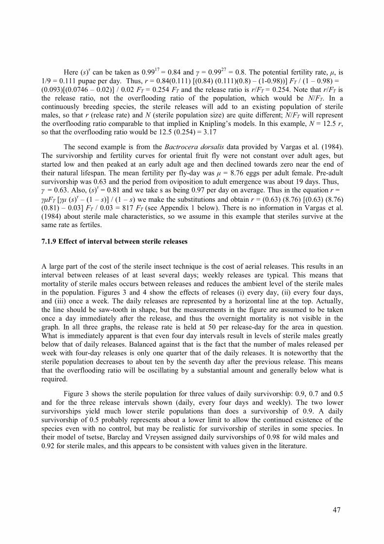
47

Here (s)τ can be taken as 0.9917 = 0.84 and γ = 0.9927 = 0.8. The potential fertility rate, µ, is 1/9 = 0.111 pupae per day. Thus, r = 0.84(0.111) [(0.84) (0.111)(0.8) – (1-0.98))] FT / (1 – 0.98) = (0.093)[(0.0746 – 0.02)] / 0.02 FT = 0.254 FT and the release ratio is r/FT = 0.254. Note that r/FT is the release ratio, not the overflooding ratio of the population, which would be N/FT. In a continuously breeding species, the sterile releases will add to an existing population of sterile males, so that r (release rate) and N (sterile population size) are quite different; N/FT will represent the overflooding ratio comparable to that implied in Knipling’s models. In this example, N = 12.5 r, so that the overflooding ratio would be 12.5 (0.254) = 3.17

The second example is from the Bactrocera dorsalis data provided by Vargas et al. (1984). The survivorship and fertility curves for oriental fruit fly were not constant over adult ages, but started low and then peaked at an early adult age and then declined towards zero near the end of their natural lifespan. The mean fertility per fly-day was µ = 8.76 eggs per adult female. Pre-adult survivorship was 0.63 and the period from oviposition to adult emergence was about 19 days. Thus, γ = 0.63. Also, (s)τ = 0.81 and we take s as being 0.97 per day on average. Thus in the equation r = γµFT [γµ (s)τ – (1 – s)] / (1 – s) we make the substitutions and obtain r = (0.63) (8.76) [(0.63) (8.76) (0.81) – 0.03] FT / 0.03 = 817 FT (see Appendix 1 below). There is no information in Vargas et al. (1984) about sterile male characteristics, so we assume in this example that steriles survive at the same rate as fertiles.

7.1.9 Effect of interval between sterile releases

A large part of the cost of the sterile insect technique is the cost of aerial releases. This results in an interval between releases of at least several days; weekly releases are typical. This means that mortality of sterile males occurs between releases and reduces the ambient level of the sterile males in the population. Figures 3 and 4 show the effects of releases (i) every day, (ii) every four days, and (iii) once a week. The daily releases are represented by a horizontal line at the top. Actually, the line should be saw-tooth in shape, but the measurements in the figure are assumed to be taken once a day immediately after the release, and thus the overnight mortality is not visible in the graph. In all three graphs, the release rate is held at 50 per release-day for the area in question. What is immediately apparent is that even four day intervals result in levels of sterile males greatly below that of daily releases. Balanced against that is the fact that the number of males released per week with four-day releases is only one quarter that of the daily releases. It is noteworthy that the sterile population decreases to about ten by the seventh day after the previous release. This means that the overflooding ratio will be oscillating by a substantial amount and generally below what is required.

Figure 3 shows the sterile population for three values of daily survivorship: 0.9, 0.7 and 0.5 and for the three release intervals shown (daily, every four days and weekly). The two lower survivorships yield much lower sterile populations than does a survivorship of 0.9. A daily survivorship of 0.5 probably represents about a lower limit to allow the continued existence of the species even with no control, but may be realistic for survivorship of steriles in some species. In their model of tsetse, Barclay and Vreysen assigned daily survivorships of 0.98 for wild males and 0.92 for sterile males, and this appears to be consistent with values given in the literature.

48

350

250

200

150

100

50

0

0 5 10 15 20 25

TIME (DAYS)

Figure 3. The effects of interval between sterile releases on the level of the sterile population. Daily releases yield the highest and most consistently high population. Releases at intervals of both four days and seven days yield much lower ambient levels of sterile male populations as a result of mortality, and levels fall close to zero for weekly releases when daily survivorship is relatively low. In all cases, the release rate was 50 males per release-day.

DAILY

FOUR DAYS

WEEKLY

SURVIVORSHIP = 0.7

ST

ER

ILE

A

ML

E

PO

PU

LA

TIO

N

49

FOUR DAYS

1200

1000

800

600

400

200

0

300

2 4 6 8

250

200

150

100

50

0

300

2 4 6 8

250

200

150

100

50

0

1 2 3 4 5 6 7

TIME (DAYS)

Figure 4. The combined effect of daily mortality and release interval on the levels of sterile males, shown for release intervals of one, four and seven days at a rate of 50 males per release-day; eight days are shown for daily releases, eight days for intervals of four days, and seven days for seven day intervals.

WEEKLY

ST

ER

ILE

P

OP

UL

AT

ION

DAILY

0.9

0.7

0.5

50

7.1.10 The fertility factor The fertility factor, F / (F+S), that occurs in the equations of SIT models is graphed in

Figure 5 for release intervals of one to seven days. The graphs are of the mean values of the fertility factors over the intervals between releases. It is apparent that the daily releases have low fertility factors, as the sterile population remains high, while the mean fertility factor increases as the interval between releases increases. Figure 5a, shows the results of a release rate of 50 per release, while Figure 5b shows the results of 50 times the number of days in the release interval; i.e., 50 for daily releases, 100 for releases every two days, up to 350 for weekly releases. It is seen that the fertility factors still increase with interval between releases (Fig. 5b). Thus, in planning sterile releases, account must be taken of the loss in efficiency as a result of long periods between releases.

0.8

0.6

0.4

0.2

0.0

0.8

0.6

0.4

0.2

0.0

1 2 3 4 5 6 7

INTERVAL BETWEEN RELEASES (DAYS)

Figure 5. The mean fertility factor (i.e., F / (F+S), over the interval between releases increases throughout the interval. In panel A, the level of sterile release is held constant at 50 per release for all release intervals; in panel B, the release rate is 50 per day for all release intervals. It is seen that even when release rates per day are constant, daily releases are superior and suppress the fertility factor more effectively than do longer release intervals.

0.9

0.8

0.7

0.6

0.5

A

FE

RT

ILIT

Y

FA

CT

OR

0.9

0.8

0.7

0.6

0.5

B

51

7.2 Shortcomings of SIT models

Knipling’s original model The virtues of Knipling’s original model are that it is easy to understand and that it forms

the basis of all of the more complicated models of SIT. It has been of great value in propagating the idea of area-wide application of SIT and in demonstrating its superiority to the alone insecticide treatments under some circumstances. However, the critical values of sterile release rates obtained from Knipling’s model are usually not completely realistic because of the existence of biological and operational complications that render these estimates insufficient, at least for most species of fruit flies. Furthermore, tropical fruit flies have a protracted breeding season and generations overlap, necessitating a more comprehensive approach to determining suitable release rates.

Density-Dependence

All the models of SIT with density-dependent population regulation show that critical sterile releases can be lower with density-dependence than without, but the various formulations of density-dependence make it clear that quantifying that reduction of required control effort depends on how the density-dependence works, and that is seldom known in detail, and thus the concept remains heuristic and not of much value in the calculation of critical sterile release rates.

Discrete vs continuous

Neither the discrete nor the continuous models completely capture the various biological aspects of any insect species. Continuous models generally ignore the seasonality of reproduction, and almost all SIT models ignore one or other of spatial variation and age distributions. The main problem is that mathematical models quickly become intractable as the number of realistic features increase, especially SIT models, with their inherent nonlinearity as a result of the ratio of ‘fertile females to total males’. All such models display a separation of behaviour in which a population above a certain critical threshold will increase under continuing sterile releases, while a population below that threshold will decrease.

Competitive ability

Competitive ability is really a collection of features, all of which can cause the mating frequency of sterile males with fertile females to be different from that of fertile males with fertile females. In the models, these are all lumped into one parameter, and this parameter is assumed to be constant, independent of population density, ratio of sterile males to fertile males, season, spatial distribution of steriles with respect to fertiles, etc. These is unlikely to be true, making the predictions suspect.

Lekking behavior

Lekking behaviour is complex compared to the usual assumption in most population models that mating is random. It yields unusual results compared with the usual simpler models (Horng & Plant 1992, Vreysen et al. 2006) and lekking should be considered in SIT models when it is present.

Dispersal and diffusion

Dispersal is often assumed to be random, but it may well be affected as well by the propensity of insects to preferentially move either towards a given area of highly suitable habitat, or away from areas that already have high densities of insects. These tendencies will distort the

52

predictions of any model that assumes dispersal is strictly random. This is difficult to determine, but does affect the results (Barclay & Vreysen 2013).

Immigration

The existence of immigration of wild insects into the control area generally disallows eradication (Prout 1978; Barclay 2001). In area-wide integrated pest management programmes, the control area is usually assumed to be large enough that it includes all of a local population and hence immigration is zero. However, this may not be the case, and if that is true, the extent of immigration should be estimated to assess its effects.

Equilibrium models

Most of the models of SIT have been equilibrium models, with little attention being given to what happens away from equilibrium. Equilibrium models can a give good idea of the effects of the parameters on the system and its behavior. However, in many situations, it is necessary to know what happens away from equilibrium, as in the situation involving the determination of an appropriate overflooding ratio after spraying examined above. For many operational questions the control programme manager will need to know what happens in these transient situations, and these should be investigated using species-specific computer models.

A list of SIT models is given in Appendix 2 at the end. Also, a glossary of terminology used in this book is provided as Appendix 4.

8. Estimation of SIT parameters Knowledge of some basic parameters is crucial to the success of any SIT programme (see

chapter 2). With reference to the models outlined above, the basic parameters that will always be of interest are: F, the population size; λ, the potential rate of population increase each generation if generations do not overlap, or a, the daily fertility, if generations do overlap; qm, the proportions of the released males that remain fertile; c, the competitive ability of sterile males relative to the wild fertile male population; and the rate of movement of insects, both within the control area and into the control area from outside. Some of the estimations can be done using standard population biology methods.

8.1 Population size The population size can be estimated from mark-recapture analysis or from relative indices,

if the relationships between relative indicies and population size is known (see chapter 4). Hargrove (1981) used mark-recapture techniques to estimate the size of tsetse fly populations. Population size is very important to estimate, as it will indicate whether a knockdown using aerial sprays or other suppression should be done before the release of sterile males. Population size is the basic parameter to decide on the required sterile release density to achieve suppression or eradication.

8.2 Population growth rate The rate of increase, λ, would normally be determined using oviposition rates together with

survivorships of the various life stages. Alternatively, µ (mean daily fertility) can be calculated for a population with overlapping life stages.

53

8.3 Daily sterile survivorship Survivorship of both fertile and sterile males is important in assessing the required

overflooding ratio for eradication. The standard method in the laboratory is to establish a cohort (i.e. a group of individuals all of the same age) and to follow their numbers until there are none left. Counts are usually done daily, noting decreases as days progress. The counts are reduced to proportions by dividing by the initial colony size. Examples of survivorship curves are given by Carey (1982) for medfly (Ceratitis capiata) and by Vargas (1984) for the medfly and the oriental fruit fly (Bactrocera dorsalis). From these curves the life expectancy at hatching can be calculated, and they are also useful in computing life tables.

8.4 Density-dependence The determination of density-dependence is problematic, because there are many models

and none of them is particularly mechanistic. Most of these models can loosely be interpreted as being related to competition, but the common ones (e.g., the logistic equation – dN/dt = rN(K-N)/K

(Pielou 1969), and the model of Varley et al. (1973) – N t+1 = (λ / α) N t (1-b)

) describe the numerical consequences of competition, but not the mechanisms of competition itself. Thus, rates of oviposition and subsequent survivorship would have to be monitored at various densities to derive a function to describe the depressing effects at various levels. In many wild populations, even just detecting the existence of density-dependence may be difficult, even more so the quantification of depressing effects. However, in view of the potential assistance to the SIT, an estimation of the effects of density-dependence is worthwhile. The subject of parameter estimation is partly addressed by Rogers and Randolph (1984) and developed further by Itô and Yamamura (2005). If estimation of density-dependence is impractical, it can be ignored and the resulting estimates of overflooding ratios will be overestimates, as density-dependence assists the action of sterile releases.

8.5 Sterile dispersal ability The dispersal ability of sterile males is very important and can be assessed by releasing

marked steriles and then recapturing them at several times after the release and noting the distance they have gone in the various time intervals (Shaw et al. 1967). This depends on their survivorship being high enough that there is a good chance of recapturing them at later times. It would be very useful to determine whether or not the sterile males disperse towards clumps of fertile males and females, or if dispersal is closer to random. This would perhaps be more meaningful if the steriles were released either uniformly or randomly and then observing subsequent redistribution by means of recaptures.

Plant and Cunningham (1991) gave procedures for estimating the dispersal of the medfly, and estimates of immigration could be obtained from considerations of dispersal. Vreysen et al. (2011) have demonstrated that tsetse in their study showed similar patterns of dispersal for steriles and wild males. Enkerlin (1987), by releasing marked sterile Mexican fruit fly (Anastrepha ludens,

Loew) from a single point, demonstrated that under the conditions of a non-suitable habitat, sterile flies disperse in an eccentric fashion following the direction of dominant winds, whereas, in a suitable homogeneous habitat the dispersion pattern was random. In the same study, using a simple method proposed by Hamada (1980), the mean dispersal distance of sterile flies released in the non- suitable habitat was of 1.3 fold compared with the flies released in a suitable habitat. These findings are useful in assessing fruit fly dispersal ability under different environmental conditions and thus for planning sterile fly releases.

54

8.6 Estimation of percent residual fertility The effect of some individuals remaining fertile following irradiation is to provide fertile

males to the pest population. This does not matter too much when the population is high, but becomes important as the wild population declines, and when it may prevent complete eradication (Barclay 2001). The measurement of residual fertility can be done by paired encounters between irradiated males and wild females in the lab. The number of such encounters must be large if the proportion of males remaining fertile is very small (e.g. less than 1%). For example, the required sample size to reject the hypothesis that the residual fertility is greater than 1% at the 95% confidence level is almost 400, assuming that there are no cases of fertility discovered in those paired encounters.

8.7 Estimation of sterile competitive ability Sterile competitive ability is a difficult factor to evaluate in the field. In the laboratory one

can put a number of females in an arena together with a number of sterile and fertile males and observe who mates with whom and then calculate the relative effectiveness of the sterile males by comparing the relative frequency of ‘sterile male with fertile female matings’ with the relative frequency of ‘sterile males to fertile males’ in the arena (Cayol et al. 1999). For example, if there are ten females together with five sterile males and five fertile males, and if it is observed that eight of the females mate with fertile males and only two with sterile males, then the relative success of the sterile males is only one quarter that of the fertile males. In the equation for mating success with inferior sterile male competitive ability, the parameter c measures this relative success, so c = 0.25 and the fertility factor is M / (M + 0.25S). If M = S, then the fertility factor is M / 1.25M = 0.8, as originally observed in the mating arena. One must again be careful in assigning values to c here because of sampling error. In order to be confident that we are close to the real value of c (relative competitive ability), one should perform the arena experiment many times to get a fairly large sample size and minimize the effects of sampling error.

Conditions in the field may be quite different from the arena situation and sterile males may perform differently in the field than in the arena. Thus, we may want to sample males with traps using marked sterile males and unmarked wild males and then also sample eggs (if possible), and then incubate the eggs and observe the relative frequency of sterile versus fertile eggs and compare that with the relative frequency of sterile males versus fertile males in the field and see if the two ratios match or are different. Here, allowance would have to be made for the usual fraction of eggs that would not hatch even from fertile-fertile matings. If the ratios are different, then a method outlined below can be used to derive the competition coefficient, c, for sterile male competitive ability in the field. If the number of sterile males in the traps is S and the number of wild males is M, and if the observed number of eggs that hatch is ef and the observed number that don’t hatch is es, and if we know that the hatchability of eggs is h, then we must subtract from es both the eggs that failed to hatch as a result of fertile matings (hef) and also those that would have failed to hatch from sterile matings even if they had resulted from fertile matings (hes), so that the two ratios then can be equated: cS/M = (es – h(ef + es) / ef, and so the estimate of c is:

c = M [es – h (ef + es)] / ef (76)

Part of the inability of sterile males to find fertile females to mate with in the field may be due to the inability of sterile males to disperse in the same pattern as the wild males, or otherwise integrate themselves into the wild population. This is not a direct sort of competitive disadvantage, but

55

operates as such since it results in lack of mating with fertile females. Note also that if the wild males and the sterile males are not equally trappable, then the above estimate will not be valid.

We have seen that competitive ability of sterile males, c, could then be determined where immigration could be assumed to be negligible, using equation 76, for competitive ability, and then solving for c. The information on growth rates and residual fertilites must be determined first, or the equation becomes confounded. Alternatively, Meats (1998) used release and recapture techniques to estimate the quality of released sterile insects. Immigration into the control area could then be determined using either mark-recapture or the equation involving immigration. For fruit flies, standard tests have been developed (FAO/IAEA/USDA 2003).

Fried (1971) provided a method of estimating mating competitive ability of sterile males relative to wild males by calculating egg hatchability with known numbers of fertile and sterile males. Thus, if there were 100 wild males in the population of a given area and releases had been made that maintained 200 sterile males in the same area, and the eggs were collected after oviposition and 40% of them hatched, then the expectation is that 33% would hatch and 67% would not hatch, so that the efficiency of the sterile males in fertilizing female eggs would be 60/67 = 0.89 (see also FAO/IAEA 2007).

8.8 Over-flooding ratios used to suppress insect populations with SIT Two contrasting situations exist that require different treatment to find the over-flooding ratio. One is that the pest species reproduces once per year in a short period during the growing season and then the adults die at the end of the season. This is what Knipling had in mind when he formulated his famous equation (eq. (1)) and for that reproductive pattern, his result works well. The other situation is that of a population that grows more or less continuously during the growing season, such as is the case with many fruit flies. In this case, the over-flooding ratio, calculated as the number of sterile males in the field divided by the number of wild males in the field, is not simply the release rate divided by the wild male population, because the sterile males in the field consist of those from several releases. This section explores the latter situation in which growth is more or less continuous during the growing season.

Many applications of SIT and other control agents will be applied when the population is at low levels and on the increase. Thus we will investigate below the relationship between the critical daily release rate, r*, and the required overflooding ratio for the use of SIT, as well as the relationship between the mean net daily fertility, µ, and the pre-adult survivorship, γ, with the critical daily release rate, r*.

The overflooding ratios required for eradicating the residual population left after an initial knockdown by bait sprays will depend on the induced sterility of the wild population by the released steriles and the reproductive rate of the pest. The size of the wild population after spraying will depend on the frequency and interval of spraying and this will necessitate the determination of the size of the wild population in order to apply the correct overflooding ratio. However, the size of this population may change immediately following the final spray. We offer three scenarios with differing requirements for overflooding ratios.

8.8.1 SIT without initial knockdown: Equilibrium population.

In the case of SIT against a stable population, the age structure of the population will be in its equilibrium configuration, with adults forming a substantial part of the total population. Figure

56

6a shows a typical configuration of the numbers in each of four stages (eggs, larvae, pupae and adults) for a population that is increasing; typically the adults form only a small proportion of the total population and are by far the least numerous stage. Figure 6b shows schematically the type of population structure to be expected from a population at equilibrium; the stages decrease in number from egg to adult, but the adults form a larger proportion of the total population. The population is at a stationary age distribution and the adult population will continue near its equilibrium level until the reduced recruitment of juveniles causes the younger adult age classes to also be reduced. The reduction of the population should proceed in an orderly manner from equilibrium down to eventual eradication.

The critical daily release rate (see Appendix 1) for a stable population has been given in eq (73) and it is: r* = γµFT [γµ (s)

τ – (1 – s)] / (1 – s), (Barclay et al. 2014) in which γ is the total pre-adult

survivorship, µ is the mean net daily fertility, s is the daily adult survivorship and τ is the time in days before adult females become receptive for mating following emergence from the pupae. For simplicity, s is taken as the geometric mean of the daily survivorships, si, and thus assumes an exponential survivorship curve in which the probability of survival over time is assumed to be a constant proportion of the remaining population. For the B. dorsalis data from Vargas et al. (1984), the parameter values are: µ = 12.18, γ = 0.63, τ = 6 and s = 0.961. This gives the critical value of r as r* = 817 FT.

8.8.2 SIT without initial knockdown: Increasing population as a resource becomes

available An increasing population will be proceeding towards a stable age distribution. In such a

population, the adult stage will form only a small proportion of the total number of individuals, and the early juvenile stages will be the major component of the population (Fig. 6a). This is characteristic of species that have a seasonal resource that they prefer. One example is medflies, which are polyphagous, but may have the most successful population increase in coffee (Coffea

arabiga) (Gutiérrez Samperio 1976, Midgarden and Lira 2006). During times when the coffee fruit is not available, the medflies can exist on other hosts, but the population increases dramatically as the coffee fruit ripens. This same behavior is observed with the West Indian Fruit Fly (Anastrepha

obliqua) that uses the hog plum (Spondias spp) and then the mango (Mangifera indica) just after Spondias spp, or the Mexican fruit fly (A. ludens) whose population increases as the grapefruit (Citrus paradisi) ripens (Aluja 1984, Enkerlin 1989). In this type of increasing population, each component of the population will increase each time period and so a constant overflooding ratio established at any time will immediately be out of date by the next time period. A stationary population is shown in Fig 6b. In a decreasing population, the juvenile stages are reduced and the adults are often numerically dominant (Fig. 6c).

57

200

150

100

50

0

200

100

0

200

150

100

50

0

Figure 6. The relative numbers of the four stages (eggs, larvae, pupae and adults) for (a) an increasing population, (b) a stable (stationary) population at carrying capacity, and (c) a decreasing population. In the increasing population, the juvenile stages greatly predominate, while in a decreasing population, the adults are relatively greater in numbers.

8.8.3 Initial knockdown followed by SIT

If the knockdown only kills adults (often the case with many fruit flies) then after the first spray the adults are at low levels, but there is still a large number of pupae. Immediately after the first spray as the pupae emerge, the adult population will increase dramatically. This makes obsolete an overflooding ratio calculated from the adults remaining after the spray, and the situation is somewhat similar to that of a growing population. If there are several sequential bait sprays, then the pre-adult stages (egg, larvae and pupae) will emerge and be killed off as young adults with each succeeding spray until the store of pre-adults is exhausted or greatly reduced; after this, if sprays cease, the overflooding ratio calculated on the basis adults remaining after the last spray will remain relatively stable for some time until enough pre-adults have been recruited to start causing the adult population to increase. If the overflooding ratio applied is above that which is theoretically required, then this population increase should be prevented from occurring.

a INCREASING

E

L

P

A

b STATIONARY

E

L

P A

c DECREASING

E L

AP

NU

MB

ER

S

IN

ST

AG

E

58

If the mature larvae are removed by collecting and destroying the fallen fruits at the same time as the bait sprays are done, then two waves of adults may emerge as the pupae and then the eggs in the fruits that remained in the tree complete development and become adults. This is again prevented from becoming an erupting rapidly growing population by means of using several sprays properly spaced and a liberal overflooding ratio.

8.8.4 Stopping a growing population

The previous computations of critical release rates are all from equilibrium populations. Most populations are in some stage of growth when a control program begins, unless the insect species reproduces only once per year and then dies, in which case Knipling’s formulation will work. In a growing population, one must allow for the fact that the population is increasing, so the required sterile release rate to reduce the population will necessarily be larger than the values of r* derived at equilibrium, because it takes some time for the effects of sterile releases to result in reduced recruitment and also because it requires several releases to bring the sterile population in the field up to equilibrium. Fig 7 shows that when the population is growing freely, the actual release rate needs to be much greater than that if the system were at equilibrium. A numerical treatment of the models shows that the release rate required to stop a growing population depends on the fertility rate, a, and the daily survivorship, s, and that the required release rate increases with both a and s. Figure 7 shows the discrepancy for sterile releases as a multiple of the control effort to hold a population at equilibrium for sterile releases. This multiple is virtually identical to the ratio of ‘the population size after stopping’ and ‘the population size at the onset of sterile releases’. This information is perhaps best obtained by a computer simulation of the species to be controlled and trials at various values of trapping effort.

9

8

7

6

5

4

3

2

1 2 3 4 5 6 7 8

DAILY FERTILITY (A)

Figure 7. The multiple of the critical release rate, r*, that is needed to stop a population that is freely growing when sterile males are first released. This multiple is almost exactly the same as the ratio of ‘the size of the population when sterile males are first released’ divided by ‘the size when it stops growing as a result of sterile releases’. This is shown for several values of fertility, a, and two values of adult daily survivorship, s.

S = 0.8

S = 0.9

STOPPING A GROWING POPULATION

MU

LT

IPL

E

OF

C

RIT

ICA

L

RE

LE

AS

E

RA

TE

(R

*)

59

9. Suppressing fruit fly populations with bait sprays If bait sprays are 100% effective in killing adults, then a series of sprays may be able to

eradicate the pest population without further control methods being required. However, this is seldom the case. Usually there are adults that are not affected by the sprays because they are under leaves, in holes, are resistant, or otherwise inaccessible to the action of the insecticide. Sometimes sprays are applied above a second layer of leaves, like in a coffee plantation or forest so the spray is less than the amount needed in areas where the adults are located. It is useful to know the approximate effectiveness of each spray in order to keep track of the probable size of the population after each spray.

9.1 Factors affecting bait spray effectiveness

9.1.1 Percent kill of each spray Percent kill may be known from previous spraying trials or may be estimated by using

mark-recapture techniques to estimate the size of the population both before and after each spray. It will be useful in planning the number of sprays as well as the intervals between sprays.

9.1.2 Intervals between sprays

Intervals will be affected by the stages that are killed by the sprays, the age to first oviposition by females, and the longevity of the stages not affected. Ideally, the interval should be short enough to prevent newly emerged adults from ovipositing, but long enough that the series of sprays will entirely cover the period from oviposition to emergence of adults. If the period from emergence to first oviposition is very short, then shorter intervals or extra sprays may be needed.

9.1.3 Number of sprays The number of sprays should be sufficient that the pest population is reduced enough to allow the SIT to operate effectively. The number of treatments has a wide range depending on the insect species, climate conditions, etc. The time from egg to ovipositing adult will be important in allowing the pre-adult stages to be reduced by natural progression into the adult stage if they are not directly affected by the sprays. This is the case in fruit flies, where the preadult stages occur inside the fruit or in the soil, so that they occupy a different habitat from the adults.

9.2 Optimizing spray interval

9.2.1 Age at first oviposition Age at first oviposition is a critical factor affecting spray intervals. Adult insects usually

take time to mature before mating and then ovipositing. If sprays are timed so that the interval between sprays is smaller than the interval from adult emergence to first oviposition, then subsequently emerging adults will be killed before being allowed to oviposit. The number of sprays will depend on the time it takes from oviposition to adult emergence and number of generations per year or number of generations during the critical period required for population suppression. An example will illustrate this. In tsetse, the period between larviposition, pupation, and emergence of adults from the pupae is about 27 days at 27oC, while the age to first larviposition is about 17 days

60

following emergence of the adults. If the mean temperature is 27oC, and the inter-spray interval is 15 days, and sprays kill 90% of the adult population, then the first spray will eliminate most of the adults, the second spray 15 days later will eliminate most of those adults that have emerged from the developing pupae, but before they start ovipositing, and a third spray will kill most of the adults that have emerged from the remaining pupae that were alive at the time of the first spray, again before they start ovipositing (Fig. 8). The population is then in a suitable state to be controlled by the sterile releases, as there will be little increase in the adult population for some time, long enough that SIT should decrease the recruitment of juveniles and prevent this increase.

The output from a model of tsetse developed by Barclay and Vreysen (2011) illustrates this. Fig. 9 shows the course of the adult population following two, three and four applications of aerial insecticide sprays, each of which kills 98% of the adult population. For each of these three scenarios, a sterile release ratio (daily releases divided by the existing wild male population) of 0.2 was used, calculated immediately after the last spray. The tsetse example is presented because it is particularly clear. However, tsetse is almost unique among insects in giving live birth to larvae. A more typical species is medfly, so an example is given for medfly below.

120

100

80

60

40

20

0

120

100

80

60

40

20

0

120

100

80

60

40

20

0

0 5 10 15 20 25 30 35 40 45 50

0 5 10 15 20 25 30 35 40 45 50

DAYS SINCE LARVIPOSITION

Figure 8. The results of three sprays that each kill about 90% of a population of adult tsetse flies. The six panels show the numbers of pupae (on the left within a panel) and adults (on the right within a panel) both immediately before a spray (left panels) and immediately after a spray (right panels) for each of the three sprays (top: first spray; middle: second spray; bottom: third spray). The pupae have all been reduced by the end of the third spray.

PUPAE ADULTS AFTER FIRST SPRAY

ADULTS

AFTER SECOND SPRAY

BEFORE THIRD SPRAY AFTER THIRD SPRAY

NU

MB

ER

S

IN

AG

E

CL

AS

S

61

350

300

250

200

150

100

50

0

0 2 4 6 8 10

DAYS AFTER LAST SPRAY

Figure 9. Determination of the number of sprays required to reduce all stages of the insect population to a low level. The example is for tsetse and shows that after two sprays, each kill 98% of the adult population, the adults still increase linearly in the days following the second spray. After the third spray, the adults increase for a few days and then level off. After the fourth spray, the adults stay at a low level for several days.

Medflies have a pre-adult period of about 19 days and a period from adult emergence to oviposition of about three days (Vargas 1984), at least for colony material under laboratory conditions; the pre-ovipositional period is closer to two weeks for wild Medfly (Vargas et al 2000), but we will use the lower value here. In this situation, the inter-spray interval would ideally have to be about three days (if the action of the spray did not persist longer) and the number of sprays would have to be sufficient to cover the 19 day developmental period. To ensure that significant reproduction would not occur after the first spray, seven sprays would have to be done following the first spray. In many cases, the insecticide remains active in the field for a week or more. For these insecticides, the number of sprays could be reduced, spraying only often enough that sufficient active insecticide is always present during the critical adult pre-oviposition period.

As noted above, Vargas' 1984 data were obtained from a laboratory colony under ideal insectary conditions, including excellent nutrition. If nutrition is less than ideal, as it often is in the field, then the delay between emergence of the adults and first oviposition may be considerably greater, so that the number of sprays required may be considerably fewer.

Besides nutritional differences between colony and field flies, it appears also that there is adaptation of the insects in the insectary for many generations leading to accelerated sexual maturation. Vargas et al 2000 estimate the length of the pre-ovipositional period of wild Bactrocera

dorsalis to be 37 days at 24oC, compared with just 7.3 days at the same temperature for colony material (Vargas et al 1997).

If the period until first oviposition were six days in the field (as is often said to be the case for medfly), then the required number of sprays would be reduced to five; the first would kill most of the adults and then the next four would cover the period required for the emergence of all the pre-adults remaining after the first spray. However, for fruit flies, one generation is often not enough, and sprays should continue until the population is down to the required level. For medfly

2

3

4

ADULTS AFTER SPRAYING

AD

UL

T

WIL

D

MA

LE

P

OP

UL

AT

ION

62

under tropical and subtropical conditions, it takes at least two generations (7 to 8 sprays with a seven to ten day interval using a spinosad based insecticide bait) to suppress populations to the required threshold for sterile release (FTD = 0.1). Since all biological processes display variability and things simply go wrong sometimes, it would seem prudent to add a few sprays to the minimum number calculated by the reasoning in the above examples, especially if there is much likelihood that one or more of the sprays would miss a significant proportion of the adults or there has been much variation in daily temperature. Also, if many individuals escape being killed (e.g. due to heavy rain after a spray), it would be necessary to add enough sprays to cover one more generation.

Species with very short times to oviposition might better be reduced by a combination of sprays and bait stations or mass trapping to avoid the very large number of sprays required for the reduction.

9.2.2 Temperature

The effects of temperature on development have been outlined in chapter 5 above. If the temperature is different from that used in the calculations above for tsetse, for example, then the calculations would have to be redone. This will have the effect of changing the inter-spray interval and may even have the effect of changing the number of sprays. The situation is illustrated for tsetse for a mean temperatures ranging from 15oC to 45oC, and these are shown in Fig. 10 (data from J. Hargrove). The pupal developmental period is less than double the period until first larviposition from about 23o up to 45o and thus the minimum number of sprays would be three for eradication if the sprays killed 100% of the insects. Below 22o the pupal period is greater than double the period until first larviposition, and at least one additional spray would be needed (more for very low temperatures). Thus the periods of development to the adult stage and age at first oviposition do not follow similar patterns at lower temperatures. Admittedly, the range of temperatures used has extremes outside the normal range for tsetse, but the graph illustrates the point that a determination for a single mean temperature will not necessarily be useful at all temperatures encountered by the species.

120

100

80

60

40

20

0

10 15 20 25 30 35 40 45 50

TEMPERATURE (DEGREES C)

TIME TO FIRST LARVIPOSITION

EMERGENCE FROM PUPAE

DU

RA

TIO

N (D

AY

S)

63

Figure 10. The effects of temperature on the determination of the number of sprays required to reduce a tsetse population to the point that all the pupae have been reduced. In this case, three sprays are sufficient for the temperatures above 24o. Below 23o, the pupal developmental period is so long that extra sprays are required to reduce the pupae if the inter-spray interval is to be short enough to disallow emerged adults from larvipositing for the first time (data for the graph from J. Hargrove).

10. Suppressing fruit flies with sterile insect releases The Sterile Insect Technique (SIT) is usually preceded or accompanied by a reduction in the

wild population through a combination of control methods including insecticidal bait-sprays, bait stations, mass trapping, fruit stripping, biological control and others. This initial reduction will be accomplished by the methods and considerations described in the previous chapter. As described above, a single spray may effectively reduce the adult population to very low levels, but it will usually increase quickly in the days following the spray with the emergence of new adults from larvae and pupae if they were not affected by the insecticide. Thus, often several sprays, or an extended period of bait stations or mass trapping, will be required to reduce the reservoir of recruits from the juvenile stages, before the application of SIT can be most efficacious.

A problem associated with SIT is estimation of the remaining adult population in order to estimate the release rates and overflooding ratios required for SIT to be effective. In addition, the actual overflooding ratio that exists after the release of steriles has begun will require monitoring, with adjustments in release rate if necessary. These topics are the main focus of this chapter.

For the calculation of required numbers of sterile releases, absolute estimates are preferable, although they may be obviated by monitoring the results of trapping both wild and steriles flies (see the section on determining sterile:fertile ratios from trapping, below) which can be used directly as an estimate of the existing overflooding ratio (for detailed information on the SIT principles and strategies see Sterile Insect Technique: Principles and Practice in Area-Wide Integrated Pest Management, Dyck et al. 2005).

10.1 Sampling sterile fly populations A major difference between sampling wild and sterile fly populations is that in the wild it

may be necessary to guess the fly’s whereabouts, but for the sterile flies managers should know where they were released, so sampling should correspondingly be easier, at least before they disperse.

10.1.1 Sterile fly distribution and abundance after releases or dispersal of sterile flies

Since SIT is more cost-effective at low densities and the release rate at higher pest densities must be higher, release events should be planned so that the clumps of wild flies get higher numbers of steriles than the areas sparsely occupied by the wild flies.

If it is not possible to selectively apply the steriles, as is the case with the chilled sterile adult aerial releases, then it is best to release sufficient steriles to cover the area at a density high enough that the clumps get reduced as well as the sparse areas. If only enough steriles are released such that the overflooding rate is sufficient to reduce the average density, then small clumps of residual insects where the density of steriles was insufficient to eliminate them will be left. For example, the Moscamed Program uses a gradient of sterile to fertile densities based on the pest

64

densities in the different control areas and also based on the control objective (suppression or eradication). If necessary, the densities are adjusted (increased or decreased) weekly, based on the sterile: fertile ratios obtained from monitoring traps (see Section 10.1.3 below on sterile: fertile ratios). The range of sterile to fertile fly densities is from 500 to 6000 per hectare (Programa Moscamed 2011). For detailed information on sterile fly packing, shipping and release see: Trapping Guidelines for Area-Wide Fruit Fly Programmes (IAEA, 2003).

The alternative plan would be to release enough steriles to reduce the average density of wild insects and hope that the steriles will redistribute themselves in the same spatial arrangement as the wild insects. This may or may not be realistic, depending on the reasons for clumping of the wild insects and the mobility of the sterile insects. If the clumping of the wild insects is caused by variation in attractiveness of habitat, then the steriles may redistribute themselves in the same pattern as the wild insects (Gavriel et al 2012). If the distribution of the wild insects is caused by local reproduction in spot infestations and lack of subsequent movement, then the steriles may not redistribute themselves in the same pattern, and the efficiency will be reduced. In some cases it appears that redistribution does occur (Vreysen et al. 2011).

One way of evaluating the sterile fly spatial distribution is by the number (percentage) of traps that capture sterile flies. The trapping network should cover the area where hosts are present and a minimum of 85% of the traps capturing at least one sterile fly is considered to be an acceptable sterile fly spatial distribution (Programa Moscamed 2011). This gives a fly per trap per day (FTD) index for sterile flies. With this figure it is possible to compare the efficacy of different methods of releasing sterile flies as: ground releases, released by helicopter, by airplane, releases in paper bags, as chilled adults, etc. The capture of fertile flies will give an FTD index for fertile flies; this is used to compute the sterile: fertile ratio by dividing the sterile FTD by the fertile FTD (FAO/IAEA, 2007). The ratio can be adjusted based on the progress of the programme as explained above. Unfortunately, unless an independent method is available for estimating the sterile population, separating the effects of population size from sterile trappability is intractable if steriles and wild insects are not equally attracted to the traps.

10.1.2 Sex ratio

The sex ratio in many species of fruit flies is one-to-one at adult emergence. This can be important in assessing the overflooding ratio when using SIT. The sex ratio can be estimated from single captures using traps. However, this assumes that both males and females are equally attracted to the traps and that both are available for capture at the same time and at the same location. This is not always the case and this possibility must be considered when making this assessment.

From a single capture of sufficient size to be useful, the female-to-male ratio is simply the number of females divided by the number of males captured. If multiple captures are used, then the ratio can be obtained by summing the numbers of females and the numbers of males and basing the ratio on the sums, rather than on individual captures. Thus, if the total number of females in the set of captures was 46 and the total number of males was 30, then the female-to-male ratio would be 46:30, which reduces to approximately 1.5:1.

This ratio is biased, as there is a variable in the denominator, and that always produces a bias. In addition, the bias will be larger if the numbers of females and males in each trap are

65

converted to a sex ratio and then the trap sex ratios averaged than if the numbers of females and males are summed before converting to a sex ratio. However, the bias will be small if the numbers of females and males in the sample is relatively large (i.e., more than 30). If the numbers are small, then the ratio can not be trusted; this is true for two reasons: (i) the bias is large, and (ii) sampling error is also large. Sampling error is the error that would occur if one was selecting a sample of items of two or more categories from a large population. For example, children in single families are such a case; considering families with four children, the numbers of boys may be none, one, two, three or four, even though the average sex ratio over all families of four children in a large area is approximately one-to-one. With very large families it would be unusual to have all the children of the same sex; with smaller families, it is not so unusual. This is the effect of sampling error and it is also the case with trap catches.

The sex ratio can be used to assess the progress of eradication of the pest population if the sterile males are unmarked and not distinguishable from wild males and sterile females are not being released. If one samples the pest population and finds that the sex ratio is 1:5, and if the sample is large, then one can estimate that the sterile male to fertile male ratio is about 4:1; assuming the sex ratio in the wild population is one-to-one. If this ratio increases over time with sterile releases remaining constant, then one can infer that the wild population is decreasing. This technique can be illustrated by an example. If F = wild females, M = wild males and S = sterile males, then with a sex ratio of 1:5 (females to males), and if we can assume that the wild sex ratio was 1:1 at adult emergence, then we can say that F = M, so that F / (M+S) = F / (F+S) = 1/5 = 0.2, so that 5F = F+S, so S = 4F, and the ratio of steriles to fertiles = S/F = S/M = 4:1.

10.1.3 Sterile : Fertile Ratio

This technique can be used to estimate the ratio of sterile: fertile males if the sterile males are marked. Using traps that attract males, the steriles can be marked before release and then counted on a subsequent recapture along with the wild males. If captures are sufficient, then meaningful results can be obtained and the effective overflooding ratio can be assessed. However, this assumes that sterile males and wild males are equally trappable. The estimation is straight forward. If such trapping yields S marked steriles and M unmarked wild males, then the overflooding ratio is S/M. This method gives a more precise estimate of the sterile-to-fertile ratio than if the steriles were not marked. However, if sterile and wild males have different survivorships, then the overflooding ratio will change following a sterile release (see chapter 11).

10.1.4 Aggregation

The distribution of Medflies in nature is thought to be patchy (Papadopoulos et al., 2003). Barclay (1992) used the Negative Binomial Distribution to determine the effects of clumping on the required release rate of sterile males for eradication and found that for k = 0.25 the required release rate was four times that for a uniformly distributed population (k is a parameter of the negative binomial distribution; see section 3.2.2 above). The curve of k versus required sterile release rate given by Barclay (1992) is approximately exponential, with the required sterile releases increasing greatly as aggregation increases and k becomes very small. In the other direction, as k increases towards infinity, the distribution approaches random, and the required release rate is not much more than that from the Knipling model. When the spatial distribution is uniform, the required release rate is exactly the value from the Knipling model.

66

10.1.5 Dispersal and immigration Movement of individuals is characteristic of all insect species. For most species, dispersal is

necessary to ensure mating and to locate food and shelter. If individuals move, they tend to intermix, and this allows sterile individuals to encounter mates in the wild population, which facilitates control by SIT. However, if wild insects move into the control area from outside of the control area, then this reduces the effectiveness of SIT and may make eradication more difficult or impossible. Also, if wild individuals move towards clumps (which may represent resource clumps, such as water, food or oviposition sites), then the degree of aggregation may increase, again increasing the difficulty of control by SIT; on the other hand, if they move away from the clumps (perhaps as a result of avoiding crowding effects), then aggregation becomes less extreme and control by SIT becomes easier.

If sterile insects move in patterns similar to the wild insects, then they too will move toward (or away from) clumps and control becomes easier; however, if they do not disperse in patterns similar to the wild insects, then control will be more difficult, as they will not encounter wild females as often as the wild males will.

When sterile flies are released by airplane, during the first moments after being released the population may maintain a relatively uniform or random distribution. Once these flies reach the ground and start moving according to ecological and environmental factors present in the release site, they may tend to clump. However, in homogeneous areas, (i.e. forest, jungle, coffee plantations, large areas covered with a single host orchards, etc.), the sterile population may maintain a more uniform or random distribution. These patterns of movement of sterile and wild insects should be determined in order to assess their consequences. This has been done with some species (e.g., tsetse by Vreysen et al. 2011) but movement may vary from one location to another, so it would be useful to do these estimations for each SIT programme (Enkerlin, 1987).

11. An intervention model: Fixed-area model. Hendrichs et al. (2005) describe the basic spatial elements of an Area-Wide Integrated Pest

Management (AW-IPM) programme. The first element is the core area, in which the aim is to reduce (in case of a suppression strategy) or eliminate (in case of an eradication strategy) the pest species. The second element is a buffer area that borders the core area on four sides and within which control methods attempt to kill the target insects within that zone, including those that enter the area from outside. The buffer area is the region of an AW-IPM program on the outer edge of the control area and is large enough to prevent the pest insects moving from outside the buffer to the core area; any individuals that enter the buffer area should be destroyed by the control methods operating within that zone. The width of the buffer area is central to determining the minimum area of an AW-IPM program, since it defines the smallest possible programme that is economically feasible.

The fixed area model considers a rectangular core area, surrounded by a rectangular buffer area (Fig. 11). This model reflects a situation where the farmer wishes to maintain an area (the core area) pest free or at low pest prevalence without enlarging or moving the area that contains the resource of value. The first aim of the model was to determine the minimum width of the buffer

67

area given the biological characteristics of the pest and the resources of the AW-IPM program. The second aim was to estimate the minimum core area that would result in a viable AW-IPM program.

Numerous simplifying assumptions are made: (i) there is a single target pest insect; (ii) the model does not include the initial process of pest density reduction in the core area because of the difficulties of assessing that aspect, i.e. the model assumes that the core area is already a pest free area (or an area of low pest prevalence); (iii) the host density in all areas (the core area, the buffer zone and outside the buffer zone) was assumed to be at equilibrium; (iv) there is a constant influx of pest insects from the region outside the buffer zone; and (v) no artificial movement of the target pest insects by wind, storms, other disturbances or accidental introduction by humans into the core area occurs.

Insect

Density

000

Distance

Figure 11. Schematic representation of the area-wide approach to pest management in which there is a central core area (A) to be protected and a buffer (B) surrounding the core area within which control occurs. The buffer must be wide enough to allow the pest population to be reduced to zero on its inner edge, so that the core area remains pest-free. Area on the right is outside the buffer and control area and is assumed to be a source of insects (the arrow) for the control area.

A model with a minimal number of parameters (inputs) is usually required if the model is to have a wide applicability. The required parameters will have to be determined for each species before the model can be used since parameter values will vary for different species and environments. The parameters are discussed below.

The fixed area model consists of two main components, i.e. a biological component (i.e. dispersal) and an economic component (break-even analysis). The dispersal part describes the movement of the insects across the buffer area and will determine the width of the buffer area. The economic component of the model will, given a certain width of the buffer area determined by the dispersal part, allow a calculation of costs and revenues of the control program and will determine the break-even size of the core area at which control costs equal revenues.

11.1 The biological component: Width of the buffer area The pest population will have a certain ambient density outside of the buffer area and will

disperse from outside into the buffer area. Because control measures are imposed within the buffer area, the density of the pest will decrease from the outer edge of the buffer to the inner edge. The width of any buffer area around a core area should be large enough to bring the density of the pest

Pest Free Area Buffer Zone

Infested Area

68

to zero (in case of a pest free area) or close to zero (in the case of an area of low pest prevalence) in the core area (A) (Fig. 11). The buffer zone should therefore be wide enough to prevent a gravid female insect and any of its offspring crossing the buffer zone.

If the population is growing and dying, as well as diffusing, then an appropriate model would be:

∂F (x, t ) ∂t

= D ∇ 2

F (x, t) + g(F (x, t))

(77)

where g is the growth function. If g is linear and births and deaths can be separated, then:

∂F (x, t ) ∂t

= D ∇ 2

F (x, t) + βF (x, t) − δF (x, t))

(78)

where βF(x,t) and δF(x,t) are the instantaneous birth and death rates (Barclay et al. 2011). This model in the differential equation (77), without the term using g, was originally formulated in the 18th century to describe the diffusion of heat along a metal rod, but has been widely used since then for various diffusive processes such as Brownian motion and animal movement. It assumes that all particles that are diffusing are identical and that movement is random. The model can be formulated in one, two or three dimensions.

The boundary conditions should be such that at the outside of the buffer area, F(0,t) = F0,

where F0 is the density of insects at the outer edge of the buffer as a result of the influx of insects, and at the inside edge of the buffer, F(w,t) = a small proportion of F0 (e.g. 10-6), so that almost all the insects have been killed before reaching the other side of the buffer (of width w).

If we are manipulating the death rate within the buffer by traps that are evenly spread out to cover the whole of the buffer region, then (βF - δF) will be negative, because now δ consists of the sum of natural and imposed mortality from traps or any other control source. To simplify the treatment here, we assume that we are dealing with a steady state situation in which the insects have been diffusing and the buffer has been under control for a long time. In this case, the time derivative is zero, since nothing is changing over time; only the space derivative is still non- zero. This yields the steady state equation:

D ∇ 2 F = (δ − β )F ) (79)

and this has solutions proportional to e-γx, where γ2 = (δ - β) / D. Assuming F(x) = c e

-γx, the boundary conditions dictate that c = F0 and that F0 e

-γw = 10-6 F0. Taking logarithms, -γw = ln(10-6)

= -13.8. This leads to the minimum buffer width:

w = 13.8 / γ = 13.8 / [(δ - β) / D]1/2 . (80)

The diffusion coefficient, D, is determined in the same way as it was for random walks (see chapter 5). If a decrease down to 10-6 of the original density outside the buffer (F0) is not satisfactory, then some other small fraction can be chosen and the constant 13.8 will be something else. The units of w in eq. (80) are in the units of D, and the units of β and δ must be the same as those of D. Thus if

69

the units of β and δ are in terms of numbers per week, then D should also be in terms of distance2

per week.

If sterile insects are used as the control method, then it is simplest to solve for the case in which the release of sterile insects is proportional to the ambient population; so, β is to be manipulated, rather than δ, and the development is similar. This case has the decrease in fertility being constant because the sterile release rate is proportional to the wild population, and thus the fertility (or sterility) ratio is constant. If this ratio can be determined to be some constant, β’, then it will have to be small enough that δ > β’ and then the determination of minimum buffer width proceeds in the same way as above, with β’ replacing β, and with δ only consisting of natural mortality in eq. (78) above. The rest of the calculations are identical to those in equations (77) to (78).

If sterile releases are to be maintained at a constant level throughout the buffer region, then we could use the first value computed for the model above and simply continue to use that throughout.

A minimum set of parameters for inclusion in the diffusion model are: the diffusion coefficient, daily birth and death rates, ambient density of the fertile population, competitive ability of the released sterile insects, and sterile release rate as a multiple of the ambient density of fertile insects.

11.2 An Approximate method

It may be that the method outlined above is not feasible, perhaps due to lack of parameter values. If that is the case, then we could use an approximate method for determining the minimum buffer width as follows. If one has estimates of the maximum lifetime of males and females and the maximum lifetime dispersal of fertile males and females as well as the time required to reduce the wild population to zero, then one can estimate the length of time it would require to reduce the wild population to approximately zero by the control methods used in the buffer, and then the minimum width would simply be the maximum distance that the insects could disperse in the time taken to reduce the buffer population to zero. If dmax is the maximum lifetime dispersal, Lmax is the maximum lifetime for the insect to live and tmin is the time required to reduce the wild population to zero under the control method and strength used in the buffer, then the minimum width, wmin would be:

wmin = dmax (tmin / Lmax) (81)

Thus, if the maximum lifetime dispersal distance is 4 km, the time required to reduce the buffer population to zero is six months and the maximum lifetime of an insect is three months, then the minimum buffer width would be 4 (6/3) = 8 km.

12. Assessing eradication status and reinfestation The ability to determine that eradication has occurred in an eradication programme is

paramount, as only a demonstration that the area is pest-free will allow the discontinuation of the control measures in that area. This, of course, presents a problem, as it is impossible to say absolutely for sure that there are no pest insects in a control area (Clift and Meats, 2004). The

70

answer to “Does a zero catch mean no flies in the area?” has been demonstrated to be “no” in many cases. The best one can do is to put a probability estimate on the statement. Thus, what follows uses probability models to estimate eradication status and reinfestation.

12.1 Probability models The following probability models are based on trapping (or sampling in any other way) with

zero results while assuming that there are insects present. The models then give the probability of a zero catch given that there are insects present, and then if the probability is sufficiently low, one can conclude that insects are not present. Two models are presented, one for local sampling involving one trap, and it is most suitable for spot infestations; the other model is for area-wide sampling, and is more suitable for an established pest that has existed over a considerable area. Both models involve attempting to sample a population that is close to extinction. Results from the two approaches should be fairly similar, because when residual population sizes are very low, the models converge (Barclay & Hargrove 2005; Barclay et al. 2005).

For an insect to be caught on a given day the following conditions must be met: (i) There must be a trap operative in its vicinity, (ii) The insect must be active, (iii) The insect must succeed in finding the trap and being captured by it.

12.1.1 Local Sampling with one or a few traps

We deal with the probability of a zero catch in each of a number of traps (Barclay and Humble 2009). Single or a few traps may also be used to detect the presence of exotic pests (de Waard et al. 2009). Consider a single trap and the “circle” (area) of attraction around it, within which the probability of catching a given insect with a given trap during one activity period is σ, called the detectability; the probability of not catching a given insect is 1 – σ. In calculating detectability, one day constitutes one sampling period, since it represents one complete cycle of activity. Then if there are k insects in the “circle”, the mean number caught per activity period is kσ. Also, if there are k insects present and if catches are independent, then the conditional probability of catching no insects during an activity period (or sampling period) is:

p(0|k) = (1 – σ)k (82)

Since the largest probability of a zero catch is for k = 1 (i.e., for one insect), we assume that k = 1 and the result will be a conservative test. Also, the probability of a zero catch given that there is one insect present is p(0) = 1 – σ, so the probability of a succession of n zero catches on n independent sampling occasions is

P(0) = (1 – σ)n (83)

and this is true for each trap. If the traps are of different types, then the detectability, σ, is specific to the trap type. The conservative approach is to calculate one probability for each trap and require that all of them satisfy the criterion for eradication to be declared before such a declaration should be made. This means that for each trap the number of trapping sessions needs to be large enough that (1 – σ)n is lower than the acceptable limit. For example, if the hypothesis that there are pests present is to be rejected at the α = 0.01 level and if σ was 0.1, then the number of trapping days, n, needs to be such that (1 – 0.1)n < 0.01. This can be found using the equation: n = log(0.01) / log(0.9) = -2.0 / -0.0458 = 43.7 ≈ 44 days. More generally, the equation is:

71

n = log (α) / log(1- σ) (84)

where α is the chosen rejection level. The base of the logarithms is immaterial, so long as both logarithms are of the same base. Once the rejection level has been chosen and the value of detectability, σ, is known, the required value of n can be easily computed.

12.1.2 Sampling fraction of the population

Each trap has an area of attraction such that within that small area, the probability of catching a given insect approximates the average detectability. If the number of traps is not sufficient to cover the whole area, so that the sum of the areas of attraction is less than the area to be evaluated for ‘pest-free’ status (called the ‘assessment region’), then one of two scenarios may occur. If the pests are sufficiently mobile to move around so that they move in and out of areas of attraction in their normal daily or weekly movements, then the detectability is simply reduced compared with the situation in which they are in the area of attraction all the time. Alternatively, the traps could be moved around from day to day or week to week so as to cover the assessment region, then the detectability would similarly be reduced. Assuming that every insect spends roughly the same amount of time in areas of attraction to traps, then the detectability will be reduced by the sampling fraction. If the sum of the areas of attraction to traps is a fraction f of the assessment region, then the average detectability will be σf. In that case, the criterion becomes:

P(0) = (1 – σf)n < α (85)

and solving for n: n = log (α) / log(1 – σ f) (86)

Thus, if detectability was 0.1, the sampling fraction was 0.5, and we used a 1% confidence level (α), then n = log(0.01) / log(1 – 0.1(0.5)) = -2.0 / -0.0223 = 90 days.

12.1.3 Area of attraction

The size of the area of attraction will be crucial to the calculation of the sampling fraction, and this area may depend on weather, since odour plumes will vary in size with wind speed; they may also vary with topography and surrounding vegetation. The area of attraction will depend on many things and may have to be intuitively estimated in the absence of experimental data. It may vary from a few metres line of sight up to one or two kilometres, in the case of some moths. If the pest species is highly mobile, then dispersal may allow insects from far outside of the area of attraction to encounter traps.

12.1.4 Trapping effectiveness

Detectability refers to the probability of a trap catching an insect that happens to be within its area of attraction. This is difficult to measure, as one has to know how many insects are in the area of attraction (or are susceptible by virtue of dispersal) in order to calculate it. It can be done experimentally and has been done for tsetse using various kinds of traps (Barclay & Hargrove, 2005; Table 3). However, detectability is either unknown or only known very approximately for many pest species and trap types. If it is not known, then some estimate must be made in order to supply the models with the required information.

72

12.1.5 Area-wide sampling of an established population Another approach is to consider area-wide sampling. The problem is to decide what

intensity and duration of sampling is required to interpret a series of zero catches as an indication of eradication at some specified level of probability.

We define:

A Area sampled (km2), assumed closed to immigration and emigration of the species concerned.

N Total insects surviving the eradication attempt, assumed randomly distributed in A.

σ Trap efficiency; i. e. the conditional probability that an insect is caught by a given trap, given that there is only one trap present in the 1-km2 square containing the insect.

S Number of traps present in all of A.

t Number of days for which each trap is operated.

With these definitions Hargrove (2003) showed that the approximation to the probability that we capture at least one fly is:

C(N , S,σ , t) = 1− exp(− StNσ

) ≈ StNσ

A A

(87)

the approximation holds when the exponent is small, as will be the case in a population that is close to extinction. The result of interest is the function relating the probability (p(0|k>0)) of observing a sequence of zero results if in fact there are insects in the control area:

p(0|k>0) = exp (-Stσλ) (88) where λ = N/A is the population density and other symbols are defined above. We would like to know when a series of zero catches is sufficiently long that we can reject the null hypothesis of the existence of insects at the assumed level. For example, if it is felt that the probability of a sequence of zero catches in the presence of insects is below a rejection level α = 0.01, then we require that:

exp (-Stσλ) < 0.01 (89)

from which, -Stσλ < ln (0.01) (90)

where ln denotes the natural logarithm. One can solve for one of the variables in terms of the others that are known. For example, if t is determined and σ is known (see below) and λ can be guessed at, then:

S > 4.605 / tσλ (91) and when this condition is met, then the required probability has been achieved.

Note that the value of σ used here includes the detectability, the area of attraction and the sampling fraction that were used in the first method (equation (91)) and these do not need to be made explicit in this model. This allows fractional values of the numbers of insects present per unit area. If inequality (90) results in an impracticably high number of traps, then a different criterion may be considered (see below). The value of S obtained from the inequality above assumes a risk

73

level of 0.01; that is, the probability of finding no insects when there are actually insects present must be less than 0.01 to justify concluding that there are no insects present.

It must be emphasized that the number of traps (S) that is calculated is independent of the area of the region to be controlled (unless the area is very small). However, with a very large area, there is a greater probability that pockets exist that evaded control and these pockets must be identified and then treated accordingly.

12.1.6 Incipient non-detectable populations

If control has proceeded to the point that a very few insects are present, but at levels that cannot be detected by trapping, and if control is then terminated, then one would expect the population to increase due to natural reproduction. The question is, “how long would it take to allow this small population to increase to detectable levels?” Here it is assumed that surveillance trapping will continue until a decision of “pest-free status” has been taken.

If population growth is in discrete time periods, as in seasonally reproducing insects, it can be modelled by a simple equation:

Nt+1 = a Nt (92)

where a is the rate of increase each generation and Nt is the population size at generation t. Starting with an initial (very small) population of size N0 following termination of the eradication effort, the size of the population t generations later would be Nt = N0 a

t. If population growth is continuous, as it may be in tropical regions with minimal seasonality, then it can be modelled as:

dN / dt = rN (93)

and at any time t the population will be of a size N(t) = N0 exp(rt). The relationship between the parameters for equations (92) and (93) to yield comparable growth is that r = ln(a). Both of these models are deterministic and will yield only single values for a given time, t.

When t is large enough that the population should have become easily detectable, and if continued trapping then still yields no pest insects, a declaration of “pest-free status” can be made. In calculating this critical value of t, allowance must be made for dormant or non-growing periods when equation (93) above does not apply. In addition, allowance of a comfortable buffer must be made, so that sufficient time must elapse for the population to be expected to be perhaps ten times the minimal detectable level before such a declaration should be made. Equations (92 and 93) are deterministic; events in nature, by contrast, involve random elements. This randomness can be due to variations in the environment or to demographic stochasticity by virtue of genetic or developmental variability. Reasonable lower limits of the growing population should therefore be used, rather than mean values, as are often used in calculations of ordinary population growth. Equations (92) and (93) will give mean values, but the variances and confidence limits are not readily available. Barclay and Hargrove (2005) give an example of this method for tsetse flies.

74

References Ailam, G., and R. Galun. 1967. Optimal sex ratio for the control of insects by the sterility method. Annals of the Entomological Society of America 60: 41–43.

Allen, J.C. 1976. A modified sine wave method for calculating degree days. Environmental Entomology 5: 388-396.

Baber, I., Keita, M., Sogoba, N., Konate, M., Diallo, M., Doumbia, S., Traore, S.F., Ribeiro, J.M.C. and Manoukis, N.C. 2010. Population size and migration of Anopheles gambiae in the Bancoumana region of Mali and their significance for efficient vector control. PLoS ONE, 5(4):e10270.

Barclay, H. J. 1992. Modelling the effects of aggregation on the efficiency of insect pest control. Researches on Population Ecology. 34: 131-141.

Barclay, H. J. 2001. Modeling incomplete sterility in a sterile release program: interactions with other factors. Population Ecology 43: 197-206.

Barclay, H. J. 2005. Mathematical models for the use of sterile insects. pp. 147-174 In V. A. Dyck, J. Hendrichs and A. S. Robinson (eds.), Sterile Insect Technique: Principles and Practice in Area-Wide Integrated Pest Management. Springer, Dordrecht, Netherlands.

Barclay, H. J., and J. W. Hargrove. 2005. Probability models to facilitate a declaration of pest- free status, with special reference to tsetse fly (Diptera: Glossinidae). Bulletin of Entomological Research 95: 1-11.

Barclay, H. J. and L. M. Humble. 2009. Probability models to facilitate a declaration that an exotic insect species has not yet invaded an area. Biological Invasions 11: 1267-1280.

Barclay, H.J., and M.J.B. Vreysen. 2011. A dynamic population model for tsetse (Diptera: Glossinidae) area-wide integrated peset management. Popul. Ecol. 53: 89-110.

Barclay, H.J. and M.J.B. Vreysen 2013. The interaction of dispersal and control methods for the riverine tsetse fly Glossina palpalis gambiensis (Diptera : Glossinidae): a modelling study. Population Ecology 55: 53-68.

Barclay, H.J. and J. Hendrichs. 2014. Models for Assessing the Male Annihilation of Bactrocera spp. with Methyl-Eugenol Baits. Annals of the Entomological Society of America, 107: 81-96.

Barclay, H.J., J.W. Hargrove, A. Clift and A. Meats. 2005. Procedures for declaring pest free status. pp. 363-386. In Dyck, V. A., J. Hendrichs, and A. S. Robinson (eds.), Sterile insect technique. Principles and practice in area-wide integrated pest management. Springer, Dordrecht, The Netherlands, 2005.

Barclay H. J., R. Matlock, S. Gilchrist, D. M. Suckling, J. Reyes, M. J. B. Vreysen, W.

Enkerlin. 2011. A Conceptual Model for Assessing the Minimum Size Area for an Area-Wide

75

Integrated Pest Management Program. International Journal of Agronomy doi:10.1155/2011/409328.

Barclay, H.J., D. McInnis and J. Hendrichs. 2014. Modeling the Area-wide Integration of Male Annihilation and the Simultaneous Release of Methyl-Eugenol-exposed Bactrocera spp. Sterile Males. Annals of the Entomological Society of America. 107: 97 – 112.

Baskerville, G. L., and P. Emin. 1969. Rapid estimation of heat accumulation from maximum and minimum temperatures. Ecology 50: 514-517.

Berg, H.C. 1983. Random Walks in Biology, Princeton University Press, Princeton, N.J., U.S.A. Bliss, C.I. and R.A. Fisher. 1953. Fitting the Negative Binomial Distribution to Biological Data. Biometrics 9: 176-200.

Bouyer, J., A. Sibert, M. Desquesnes, D. Cuisance and S. De la Rocque. 2007. A diffusion model for Glossina palpalis gambiensis in Burkina Faso. Bovet, P. and Benhamou, S. 1988. Spatial Analysis of Animals’ Movement Using a Correlated Random Walk Model. Journal of Theoretical Biology 131: 419-433.

Byers, J. A. 1991. Simulation of the mate-finding behaviour of pine shoot beetles, Tomicus

piniperda. Animal Behaviour, 41: 649-660. Byers, J.A. 2001. Correlated random walk equations of animal dispersal resolved by simulation. Ecology 82: 1680-1690.

Campbell G.S. and Norman J.M. 1997. An Introduction to Environmental Biophysics, 2nd edition.Springer, New York USA.

Carey, J. R. 1982. Demography and population analysis of the Mediteranean fruit fly Ceratitis

capitata. Ecological Modeling 16: 125-150. Cayol, J.P., J. Vilardi, E. Rial and M.T. Vera. 1999. New indices and method to measure the sexual compatibility and mating performance of medfly (Diptera: Tephritidae) laboratory reared strains under field cage conditions. J. Econ. Entomol. 92(1): 140-145.

Cesaraccio, C., Spano, D., Duce, P., and Snyder, R. L. 2001. An improved model for determining degree-day values from daily temperature data. International Journal of Biometeorology, 45:161-169.

Chiang, H. C. and A. C. Hodson. 1950. An analytical study of population growth in Drosophila

melanogaster. Ecological Monographs 20: 174-206. Chiles, J.P., and Delfiner, P. 1999. Geostatistics: Modelling spatial uncertainty. New York: Wiley.

Clift, A., and A. Meats. 2004. When does zero catch in a male lure trap mean no tephritid flies in the area? pp. 183-188. In Proceedings of the 6th International Fruit Fly Symposium. 6-10 May 2002. Stellenbosch, South Africa.

76

Cochran, W. G. 1977. Sampling Techniques. 3rd ed. Wiley, New York. deWaard, J.R., J-F. Landry, B.C. Schmidt, J. Derhousoff, J.A. McLean and L.M. Humble.

2009. In the dark in a large ubran park: DNA barcodes illuminate cryptic and introduced moth species. Biodiversity Conservation DOI 10.1007/s10531-009-9682-7.

Duyck P and Quilici S. 2002. Survival and development of different life stages of three Ceratitis

spp. (Diptera: tephritidae) reared at five constant temperatures. Bulletin of Entomological Research 92: 461–469.

Dyck V.A, J. Hendrichs and A.S. Robinson. 2005. Sterile Insect Technique: Principles and Practices in Area-Wide Integrated Pest Management. Springer Dordrecht, The Netherlands. Pp 878. L. Edelstein-Keshet, 1988. Mathematical Models in Biology, Random House, New York, NY, USA.

Enkerlin, W., E. Cotoc, A. Villaseñor, A. Arenas, A. Valle, and R. Castañeda. 2012. Efficient management of trapping networks in area-wide fruit fly control programs. 8avo Congreso Hemisférico Occidental de Moscas de la Fruta. Ciudad de Panamá, Panamá. 30 de julio a 3 de agosto de 2012.

Enkerlin, W. 1987. Orientación y dispersion de poblaciones de la mosca mexicana de la fruta (Anastrepha ludens, Loew) estériles y silvestres, en el municipio de Allende, N.L. en el periodo de septiembre de 1985 a agosto de 1986. Tesis presentada para obtener el grado de Mestro en Ciencias, Instituto Tecnológico y de Estudios Superiores de Monterrey (ITESM). Monterrey, México.

Enkerlin, D., L. Garcia, and F. López. 1989. Mexico, Central and South America. In: World crop pests fruit flies their biology, natural enemies and control. Edit. A,S. Robinson and G. Hooper. Elsevier, Amsterdam-Oxford-New York-Tokyo. Pp 83 – 90.

FAO/IAEA/USDA. 2003. Manual for product quality control and shipping procedures for sterile mass-reared tephritid fruit flies, Version 5.0. International Atomic Energy Agency. Vienna, Austria. 85 pp.

FAO. Food and Agriculture Organization of the United Nations. 2006. Fruit fly pest free areas. ISPM 26. Rome, Italy.

FAO/IAEA. 2007. Guidance for packing, shipping, holding and release of sterile flies in area-wide fruit fly control programmes. Edited by: Walther Enkerlin. FAO Plant Production and Protection Paper. Food and Agriculture Organization of the United Nations, Rome, 2007.

Fried, M. 1971. Determination of sterile insect competitiveness. Journal of Economic Entomology 71(4) 869-872.

Gavriel, S., Gazit, Y., Leach, A., Mumford, J., and Yuval, B. 2012. Spatial patterns of sterile Mediterranean fruit fly dispersal. Entomologia Experimentalis et Applicata 142:17-26.

77

Gleason H.A. 1920. Some applications of the quadrat method. Bulletin of the Torrey Botanical Club 47(1):21-33.

Green, R.H. 1979. Sampling design and statistical methods for environmental biologists. Wiley, New York USA.

Guillen, J.C. 1984. Manual for differentiation of wild (fertile) Mediterranean fruit flies Ceratitis

capitata (Wied.), from irradiated (sterile) ones, p. 102. Programa Mosca del Mediterráneo, Dirección General de Sanidad Vegetal. S.A.R.H. Talleres Gráficos de la Nación. Editorial Trillas, México D.F.

Gutiérrez Samperio, J. 1976. La mosca del mediterraneo (Ceratitis capitata, Wied.) y los factores ecológicos que favorecen su establecimiento y propagación en México. Secretaria de Agricultura y Ganadería, Dirección General de Sanidad Vegetal. México, pp 233.

Hagler, J. R., & Jackson, C. G. 2001. Methods for marking insects: current techniques and future prospects. Annual Review of Entomology, 46(1), 511-543.

Hamada, R. 1980. Studies on the doispersal behavior of melon flies, Dacus cucurbitae, Coquillett (Diptera: Tephritidae) and influence of gamma irradiation on dispersal. Appl. Ent. Zool. 15(4):363- 371.

Hargrove, J.W. 1981. Discrepancies between estimates of tsetse fly populations using mark- recapture and removal trapping techniques. - Journal of Applied Ecology, 18, 737-748.

Hargrove, J.W. 2001. Mark-recapture and Moran curve estimates of the survival probabilities of an island population of tsetse flies Glossina morsitans morsitans (Diptera: Glossinidae). Bulletin of Entomological Research 91: 25-35.

Hargrove, J.W. (2003) Tsetse eradication: sufficiency, necessity and desirability. 133+ix pp. DFID Animal Health Programme, Edinburgh, UK.

Hassell, M. P. 1978. The dynamics of arthropod predator-prey systems. Princeton University Press, Princeton, New Jersey, USA.

Hendrichs, J., M. J. B. Vreysen, W. R. Enkerlin, and J. P. Cayol. 2005. “Strategic options in using sterile insects for area-wide integrated pest management,” pp. 563-600. In Dyck, V. A., J. Hendrichs, and A. S. Robinson (eds.), Sterile insect technique. Principles and practice in area-wide

integrated pest management. Springer, Dordrecht, The Netherlands, 2005. Horng, S. B. and R. E. Plant. 1992. Impact of lek mating on the sterile insect technique: a modeling study. Researches on Population Ecology 34: 57–76.

IAEA. 1973. Computer Models and Application of the Sterile-Male Technique. AIEA, Vienna, Austria.

IAEA. 2003. Trapping Guidelines for Area-Wide Fruit Fly Programmes. IAEA, Vienna, Austria.

78

Ito, Y., and K. Yamamura. 2005. Role of population and behavioural ecology in the sterile insect technique. pp. 177-208 In V. A. Dyck, J. Hendrichs and A. S. Robinson (eds.), Sterile Insect Technique: Principles and Practice in Area-Wide Integrated Pest Management. Springer, Dordrecht, Netherlands.

Judd, G. and Gardiner, M. 1997. Forecasting phenology of Orthosia hibisci Guenee (Lepidoptera: Noctudiae) in British Columbia using sex-attractant traps and degree-day models. The Canadian Entomologist 129: 815-825.

Jolly, G. M. 1965. Explicit estimates from capture-recapture data with both death and immigration- stochastic model. Biometrika, 52(1/2), 225-247.

Kitching, R. 1971. A simple simulation model of dispersal of animals among units of discrete habitats. Oecologia, 7: 95-116.

Klassen, W., and J. F. Creech. 1971. Suppression of pest population with sterile male insects.

Miscellaneous Publication, Number 1182. USDA/ARS, Washington, D.C., USA. Knipling, E. F. 1955. Possibilities of insect control or eradication through the use of sexually sterile males. Journal of Economic Entomology 48: 459–462.

Knipling, E. F. 1979. The basic principles of insect population suppression and management. Agriculture Handbook Number 512. USDA/SEA, Washington, D.C., USA.

Krebs, C. J. 1999. Ecological methodology. Benjamin Cummings, Menlo Park California USA.

Lawson, F. R. 1967. Theory of control of insect populations by sexually sterile males. Annals of the Entomological Society of America 60: 713–722.

Le Cren, E.D. 1965. A Note on the History of Mark-Recapture Population Estimates. Journal of Animal Ecology 34: 453-454.

Lindsey A.A. and Newman J.E. 1956. Use of official weather data in spring time-temperature analysis of an Indiana phonological record. Ecology 37:812–823.

Magarey, R.D., Borchert, D.M., Fowler, G.L, Sutton, T.G., Colunga-Garcia, M., and

Simpson, J.A. 2007. NAPPFAST, an Internet System for the Weather-based Mapping of Plant Pathogens. Plant Disease 91:336-445.

Manoukis, N.C. and Hoffmann, K. 2013. An Agent-Based Simulation of Extirpation of Ceratitis

capitata Applied to Invasions in California. Journal of Pest Science, 87(1):39-51. Midgarden. .and E. Lira. 2006. Ecological relationship of Medfly and coffee in g uatemala and Mexico. Fruit Flies of Economic Importance: From Basic to Applied Knowledge. Proceedings of the 7th International Symposium on Fruit Flies of Economic Importance. 10-15 September 2006, Salvador, Brazil. pp. 241-247.

79

Meats, A. 1998 Predicting or interpreting trap catches resulting from natural propagules or releases of sterile fruit flies. An actuarial and dispersal model tested with data on Bactrocera

tryoni. Gen. Appl. Entomol. 28: 29 – 38. Nietshcke, B., Magarey, R.D., Borchert, D.M., Calvin, D.D. and Jones, E.M. 2007. A developmental database to support insect phenology models. Crop Protection 26:1444-1448. Papadopoulos, N. T., Katsoyannos, B. I., and Nestle, D. 2003. Spatial autocorrelation analysis of a Ceratitis capitata (Diptera: Tephritidae) adult population in a mixed deciduous fruit orchard in northern Greece. Environmental entomology, 32:319-326.

Pielou, E.C. 1969. An Introduction to Mathematical Ecology. Wiley Interscience. New York.

Plant, R. E., and R. T. Cunningham. 1991. Analyses of the dispersal of sterile Mediterranean fruit flies (Diptera: Tephritidae) released from a point source. Environmental Entomology 20: 1493–1503.

Programa Moscamed. 2011. Memoria Annual de Labores. Reporte interno del Programa Moscamed Guatemala-Mexico-Estados Unidos. Guatemala Centro America.

Prout, T. 1978. The joint effects of the release of sterile males and immigration of fertilized females on a density regulated population. Theoretical Population Biology 13: 40–71.

Rendon, P., D. McInnis, D. Lance, and J. Stewart. 2004. Medfly (Diptera: Tephritidae) genetic sexing: Large scale field comparison of male-only and bisexual fly releases in Guatemala. Journal of Economic Entomology 97: 1544-1553.

Rogers D.J. and S.E. Randolph. (1984) A review of density-dependent processes in tsetse populations. Insect Science and Applications 5:397–402.

Roltsch, W. J., Zalom, F. G., Strawn, A. J., Strand, J. F., and Pitcairn, M. J. 1999. Evaluation of several degree-day estimation methods in California climates. International Journal of Biometeorology, 42: 169-176.

Seber, G. A. F. 1965. A note on the multiple-recapture census. Biometrika, 52(1/2), 249-259.

Seber, G. A. F. 1982. The estimation of Animal Abundance and Related Parameters. 2nd ed. Charles Griffin, London.

Service, M. 1993. Mosquito Ecology: Field Sampling Methods. 2nd edition. Applied Science Publishers Ltd., London, United Kingdom.

Shaw J.G., M. Sánchez-Riviello, L. M. Spishakoff, P. Trujillo G., and F. López D. 1967. Dispersal and Migration of Tepa-Sterilized Mexican Fruit Flies. Journal of Economic Entomology Vol. 60, No. 4, pp. 992-994.

80

Shiga, M. 1986. Analysis of spatial distribution in fruit fly eradication, pp. 387–398. In M. Mangel, J. R. Carey and R. E. Plant (eds.), Proceedings: Pest Control: Operations and Systems Analysis in Fruit Fly Management. NATO Advanced Workshop, 5–9 August 1985, Bad Windsheim, Germany. Springer-Verlag, Berlin, Germany.

Shoukry, A., and M. Hafez. 1979. Studies on the biology of the Mediterranean fruit fly Ceratitis

capitata. Entomologia Experimentalis et Applicata 26: 33-39. Skellam, J. G. 1951. Random dispersal in theoretical populations. Biometrika 38:196-218. Snyder, R. L. 1985. Hand calculating degree days. Agricultural and Forest Meteorology, 35:353- 358.

Sokal, R. R. and F. J. Rohlf. 2012. Biometry: the principles and practice of statistics in biological research. 4th edition. W. H. Freeman and Co.: New York. 887 pp.

Southwood, T.R.E. 1978. Ecological methods. Chapman & Hall, London, United Kingdom.

Vargas, R. I., D. Miyashita, and T. Nishida. 1984. Life history and demographic parameters of three laboratory-reared tephritids (Diptera: Tephritidae). Annals of the Entomological Society of America 77: 651-656.

Vargas, R. I., Walsh, W. A., Kanehisa, D., Stark, J. D., and Nishida, T. 2000. Comparative demography of three Hawaiian fruit flies (Diptera: Tephritidae) at alternating temperatures. Annals

of the Entomological Society of America, 93:75-81. Varley G.C., G.R. Gradwell, and M.P. Hassell. 1973. Insect Population Ecology. Blackwell, Oxford.

Vreysen, M.J.B., H.J. Barclay and J. Hendrichs. 2006. Modeling of preferential mating in areawide control programs that integrate the release of strains of sterile males only or both sexes. Annals of the Entomological Society of America 99: 607-616.

Vreysen MJB, K. Saleh, R.J. Lancelot, Bouyer. 2011 Factory tsetse flies must behave like wild flies: a prerequisite for the sterile insect technique. PLOS Neglected Tropical Diseases 5(2):e907. DOI: 10.1371/journal.pntd.0000907.

Wackernagel, H. 2003. Multivariate geostatistics: An introduction with applications. Berlin: Springer.

81

Tables Table 1. Data on numbers of larvae found in each of 80 fruits, ten each from eight trees.

Tree(i) Fruit(j)

1 2 3 4 5 Number of Larvae

6 7 8

Total 824

= 10.3

1 21 5 14 9 31 16 17 4

2 14 3 10 5 23 4 21 0

3 0 0 9 11 14 11 13 0

4 15 1 17 3 9 3 24 8

5 18 6 5 15 27 19 19 7

6 12 9 16 16 11 7 7 2

7 2 5 7 4 27 6 16 1

8 8 0 4 2 19 8 11 5

9 19 1 8 0 13 13 13 6

10 10 3 11 7 23 9 19 13

Σ yij 119 33 101 72 197 96 160 46

yi 11.9 3.3 10.1 7.2 19.7 9.6 16.0 4.6 ygm Σ y 2 1859

ij 187 1197 786 4405 1162 2792 364 12752 (Σ yij)2 14161 1089 10201 5184 33809 9216 25600 2116 678976 Si

2 49.21 8.68 19.66 29.73 58.23 26.71 25.78 16.93

Table 2. Hypothetical frequencies of counts of numbers of insects occurring in traps or fruit.

Insects per trap 0

Number of traps 26

1 7 2 2 3 13 4 25 5 6 6 1

Total traps = 80

Table 3. Jolly-Seber estimates for the Blackkneed capsid (from Jolly 1965)

Table 3a. Tabulations of the number caught in the ith sample last captured in the hth sample (mh,i).

i 1 2 3 4 5

ni 54 146 169 209 220 h Ri 54 143 164 202 214 Totals (rh)

1 10 3 5 2 20 2 34 18 8 60 3 33 13 46 4 30 30

Total mi 0 10 37 56 53

82

Table 3b. Tabulations of the number caught in the ith sample last captured in or before the hth

sample (ch,i). h i 1 2 3 4 5 Totals (zi+1)

1 10 3 5 2 10 z2

2 37 23 10 33 z3

3 56 23 23 z4

4 53

Table 3c. Population estimates from the data in tables 3a and 3b.

i Mi Ni φ Bi Var(N)

2 33.83 493.87 0.9270 251.45

3 154.65 706.49 0.7487 261.91

4 210.87 787.12 - -

Table 4. Computations to calculate regression coefficients for the data on egg mass density (E) and adult population density (T). Here x is the difference between the values of E(X) and its mean and y is the corresponding difference between T(Y) and its mean.

E (X) T (Y) x y x2 xy

105 1015 18.0 147.5 324 2655 179 1853 92.0 985.5 8464 90666 121 1237 34.0 369.5 1156 12563 84 752 -3.0 -115.5 9 346.5 19 234 -68.0 -633.5 4624 43078 3 48 -84.0 -819.5 7056 68838 49 467 -38.0 -400.5 1444 15219 136 1334 49.0 466.5 2401 22858.5

Means 87.0 867.5 0.0 0.0 25478 256224 b = Σxy / Σx2 = 256224 / 25478 = 10.057.

a = Y – bX = 867.5 – 10.057 (87.0) = -7.459.

Then the estimation equation becomes

Adult density = a + b (egg mass density) = -7.459 + 10.057 (egg mass density), which is slightly biased because both variables are measured with some error, but still useful for our purposes.

In this particular case, as a rule of thumb, one can simply multiply the egg mass density by ten to get a rough estimate of total adult density, as a is small.

83

Table 5. Hourly temperatures, degree-day contributions and heat accumulations above a threshold of 8 oC towards the calculation of a degree-day total for that day.

Hour 1 2 3 4 5 6 7 8 9 10 11 12 13 14 15 16 17 18 19 20 21 22 23 24 Temperature 6 6 6 5 5 6 7 7 8 9 9 10 11 12 12 11 10 10 10 9 9 8 7 6 Deg-day contribution 0 0 0 0 0 0 0 0 0 1 1 2 3 4 4 3 2 2 2 1 1 0 0 0 Heat accumulation 0 0 0 0 0 0 0 0 0 1 2 4 7 11 15 18 20 22 24 25 26 26 26 26

The sum of the accumulated heat values is 26. The degree-day accumulation is then 26/24 = 1.08, i.e., and average of 1.08 degree-hours every hour.

Table 6. Comparison of fruit-bud development in Red Delicious apples with phenology of female emergence, oviposition and egg hatch of Orthosia hibisci in relation to degree-days at Summerland, British Columbia, Canada, in 1992.

Julian

Degree

Percentage of fruit buds at each stage of development

Tight Pink Bloom Petal fall

Cumulative percentage of various events.

Emerge Ovipos egg hatch Date days cluster

99 143 60 40 97 85 10 106 184 2 98 100 98 43 116 252 40 60 100 100 90 121 300 100 100 100 98 126 353 95 5 100 100 100

Table 7. Frequency distribution of the distances dispersed in nine days by a hypothetical insect.

Distance Frequency Σ d2

0 13 0(13) = 0 1 16 1(16) = 16 2 14 4(14) = 56 3 7 9(7) = 63 4 4 16(4) = 64 5 8 25(8) = 200 6 3 36(3) = 108 7 2 49(2) = 98 8 0 64(0) = 0 9 1 81(1) = 81 10 0 100(0) = 0

N = 68 Σ d2 = 686

84

Table 8. Knipling´s basic Sterile Insect Technique (SIT) model1.

G

WILD WILD STERILE

RATIO

No.

G

PROGENY

MALE MALE MALE RELEASE

NO WITH

CONTROL CONTROL RATE REPRODUCTIVE INSECTS

INCREASE

STERILE WILD

(M) (M1) (S*) (λ)

P 1,000,000 1,000,000 9,000,000 9 1 100,000 5 500,000

F1 5,000,000 500,000 9,000,000 18 1 26,316 5 131,579

F2 25,000,000 131,579 9,000,000 68.4 1 1,896 5 9,480

F3 125,000,000 9,480 9,000,000 949.4 1 10 5 50

F4 125,000,000 50 9,000,000 180458.9 1 0 5 0

1Assumes sterile insects equally compete for mates, even distribution between wild and sterile insects, no immigration occurs, the only mortality factor is induction of sterility to wild population.

Table A1. Chi Square (χ2) values for degrees of freedom (ν) of 1 to 100 and α = 0.05.

For a test of the coefficient of dispersion (CD = s2 / x), the degrees of freedom for the associated

chi square (χ2 = (ν s2 / x), are ν, where ν = n-1, and n is the number of samples (e.g., quadrats) that

were used in calculating the CD.

ν χ2

α, ν ν χ2

α, ν ν χ2

α, ν ν χ2

α, ν ν χ2

α, ν

1 3.84 21 32.67 41 56.94 61 80.23 81 103.01 2 5.99 22 33.92 42 58.12 62 81.38 82 104.14 3 7.82 23 35.17 43 59.30 63 82.53 83 105.27 4 9.49 24 36.42 44 60.48 64 83.67 84 106.39 5 11.07 25 37.65 45 61.66 65 84.82 85 107.52 6 12.59 26 38.89 46 62.83 66 85.97 86 108.65 7 14.07 27 40.11 47 64.00 67 87.11 87 109.77 8 15.51 28 41.34 48 65.17 68 88.25 88 110.90 9 16.92 29 42.56 49 66.34 69 89.39 89 112.02 10 18.31 30 43.77 50 67.51 70 90.53 90 113.15 11 19.68 31 44.98 51 68.67 71 91.67 91 114.27 12 21.03 32 46.19 52 69.83 72 92.81 92 115.39 13 22.36 33 47.40 53 71.00 73 93.94 93 116.51 14 23.69 34 48.60 54 72.15 74 95.08 94 117.63 15 25.00 35 49.80 55 73.31 75 96.22 95 118.75 16 26.30 36 51.00 56 74.47 76 97.35 96 119.87 17 27.59 37 52.19 57 75.62 77 98.48 97 120.99 18 28.87 38 53.38 58 76.79 78 99.62 98 122.11 19 30.14 39 54.57 59 77.93 79 100.75 99 123.23 20 31.41 40 55.76 60 79.08 80 101.88 100 124.34

85

Table A2. Proportions of area under a standard sine curve that are above the threshold value for development. The first number of each pair (f) is the proportion that the threshdold is of the maximum temperature minus the minimum temperature, and the second number is the proportion (p) of the area under the sine curve.

f p f p f p f p f p

0.00

1.000

0.20

0.678

0.40

0.425

0.60

0.225

0.80

0.078 0.01 0.981 0.21 0.664 0.41 0.414 0.61 0.216 0.81 0.072 0.02 0.962 0.22 0.650 0.42 0.403 0.62 0.208 0.82 0.066 0.03 0.944 0.23 0.636 0.43 0.392 0.63 0.199 0.83 0.061 0.04 0.927 0.24 0.622 0.44 0.381 0.64 0.191 0.84 0.055 0.05 0.910 0.25 0.609 0.45 0.370 0.65 0.183 0.85 0.050 0.06 0.893 0.26 0.596 0.46 0.359 0.66 0.175 0.86 0.045 0.07 0.876 0.27 0.583 0.47 0.349 0.67 0.167 0.87 0.040 0.08 0.859 0.28 0.570 0.48 0.339 0.68 0.159 0.88 0.036 0.09 0.843 0.29 0.557 0.49 0.329 0.69 0.152 0.89 0.031 0.10 0.827 0.30 0.544 0.50 0.318 0.70 0.144 0.90 0.027 0.11 0.811 0.31 0.532 0.51 0.309 0.71 0.137 0.91 0.023 0.12 0.796 0.32 0.519 0.52 0.299 0.72 0.130 0.92 0.019 0.13 0.780 0.33 0.507 0.53 0.289 0.73 0.123 0.93 0.016 0.14 0.765 0.34 0.495 0.54 0.279 0.74 0.116 0.94 0.013 0.15 0.750 0.35 0.483 0.55 0.270 0.75 0.109 0.95 0.010 0.16 0.735 0.36 0.471 0.56 0.261 0.76 0.102 0.96 0.007 0.17 0.721 0.37 0.459 0.57 0.252 0.77 0.096 0.97 0.004 0.18 0.706 0.38 0.448 0.58 0.243 0.78 0.090 0.98 0.002 0.19 0.692 0.39 0.436 0.59 0.234 0.79 0.084 0.99 0.001

86

Appendix 1. Overflooding Ratio for Age-Structured Populations with

SIT

We consider a population of a monogamous species with distinct egg, larval, pupal and adult

stages; there is no density-dependent regulation and the time step is daily. This age structured population has equations for eggs (E), larvae (L), pupae (P) and the three wild adult components, virgin females (V), fertile-mated females (F) and males (M) and two sterile adult components, females mated to sterile males (G) and sterile males (N). In this model only males are released. The release of sterile females would complicate the model somewhat, but should not significantly alter the results. The relative competitive ability of sterile males is c, which must be estimated experimentally, or taken as 1.0 if this estimation has not been done. The virgin females are assumed to become receptive to male mating advances at age kv days, and all of age kv mate on that day. Fertile-mated females, Fkv+1,t+1 are the same individuals as those in Vkv,t. Here Ei,t is the number of eggs in age class i at time t; the sum for egg age-classes is taken from 1 to ke (the number of days until egg hatch); mx is the fecundity of adult age class x and hx is the proportion of eggs laid by females of age x that hatch. Also, Li,t, Pi,t, Vi,t, Fi,t and Mi,t are the numbers of larvae, pupae, virgin female adults, fertile-mated female adults and male adults in age class i at time t, respectively. The parameters ke, kl, kp, kv, kf and km are the numbers of days occupied at a given temperature by eggs, larvae, pupae, virgin females, fertile-mated females and males, respectively. The parameter si, is the natural daily survivorship of adult males and females of age i days and the counter, t, measures time in days. The equations of the growth model with SIT are shown in Table A3 below.

In the equations in Table A3, the survivorships are all density-independent, and thus the total pre-adult survivorship can be compressed into one parameter, called γ, which is γ = (Π(kp)

ri) (Π(kl)

qi) and mean daily net fertility, taken over all adult age classes, called µ, can be calculated as the product of the age dependent fecundities and hatchabilities, so that µ = Σ mx hx lx/ Σ lx. The product of γ and µ is the quantity called mx in the equation for for E1 in the age structured equations in chapter 7.

87

Table A3. Equations of the age structured growth model with SIT

Pre-adult Stages Egg Stages: Larval Stages: Pupal Stages: E1,t+1

E2,t+1

E2,t+1

⋅

= = =

∑ kf Fi,t mx hx

E1,t

E2,t

⋅

⋅

L1,t+1

L2,t+1

L3,t+1

⋅

= = =

Eke,t

q1 L1,t

q2 L2,t

⋅

⋅

P1,t+1

P2,t+1

P3,t+1

= = =

qkl Lkl,t

w1 P1,t

w2 P2,t

⋅ ⋅ ⋅ ⋅ ⋅ ⋅

Eke,t+1 = Eke-1,t Lkl,t+1 = qkl-1 Lkl-1,t Pkp,t+1 = wkp-1 Pkp-1,t

Adult Stages

Virgin Females V1,t+1 = wkp Pkp,t

Fertile-Mated Females F1,t+1 = Πkv-1

si Vkv,t MT/(MT+NT)1

Wild Males M1,t+1 = wkp Pkp,t

V2,t+1 = s1 V1,t F2,t+1 = s1 F1,t M2,t+1 = s1 M1,t

V3,t+1 = s2 V2,t F3,t+1 = s2 F2,t M3,t+1 = s2 M2,t

⋅ ⋅ ⋅ ⋅ ⋅ ⋅

⋅ ⋅ ⋅ ⋅ ⋅ ⋅

Vkv,t+1 = skv-1 Vkv-1,t Fkf,t+1 = skf-1 Fkf-1,t Mkm,t+1 = skm-1 Mkm-1,t

1 MT / (MT + NT) is the fertility factor with SIT, in which MT is the total number of fértiles males

and NT is the total number of steriles males at a given time.

88

Equilibrium:

The equilibrium values of eggs are found by dropping the time subscript, t:

ET = E1 + E2 + E3 +… + Eke = ke E1, = ke ∑(kf) Fi mi hi = ke ∑(kf) µi Fi (A1)

Here ke is the number of days required for egg hatch at the ambient temperature; variations in temperature will complicate this and are not considered here. The subscript T denotes the total for the life stage and ∑(kf) denotes the sum from i = 1 to kf of the expression to the right of the summation sign i.e., Fi mi hi, while µi is the product mi hi. The sum is taken over the kf mated female age classes. There is no mortality here since the only eggs we consider are those that will hatch.

The equilibrium for the larvae is:

LT = L1 + q1 L1 + q1 q2 L1 + … + (∏(kl-1)qi) L1

= (1 + q1 + q1 q2 + … + (∏(kl-1)qi) L1

= (1 + q1 + q1 q2 + … + ∏(kl-1)qi) Eke (A2)

in which ∏(kl-1)qi is the product from i = 1 to kl-1 of the expression to the right of the

product sign i.e., qi; kl is the number of larval age classes and the qi values are the age- specific larval survivorships, and they can be summed as shown when they are known; also from Table 1, L1 = Eke.

The equilibrium for pupae is similarly

PT = P1 + w1 P1 + w1 w2 P1 + … + (∏(kp-1) wi) P1

= (1 + w1 + w1 w2 + … + ∏(kp-1) wi) P1

= (1 + w1 + w1 w2 + … + ∏(kp-1) wi) qkl Lkl

= (1 + w1 + w1 w2 + … + ∏(kp-1) wi) (∏

(kl) qi) Eke. (A3)

since P1 = qkl Lkl and also Lkl = L1 ∏(kl-1)

qi. The products, ∏(kp-1) wi, and ∏(kl)

qi are taken over kp-1 pupal age classes and the kl larval age classes. The equilibria for virgin females, (V), fertile-mated females (F) and males (M) are similarly: VT = V1 + V2 + V3 + … + Vkv = (1 + s1 + s1s2 + s1s2s3 + … + Π(kv-1)

si) V1

= (1 + s1 + s1s2 + s1s2s3 + … + Π(kv-1) si) wkp Pkp

= (1 + s1 + s1s2 + s1s2s3 + … + Π(kv-1) si) (Π(kp)

wi) P1

= (1 + s1 + s1s2 + s1s2s3 + … + Π(kv-1) si) (Π(kp)

wi) (Π(kl)

qi) Eke (A4)

FT = F1 + F2 + F3 + … + Fkf = (1 + s1 + s1s2 + s1s2 s3 + … + Π(kf-1)

si) F1 = (1 + s1 + s1s2 + s1s2 s3 + … + Π(kf-1)

si) skv Vkv =

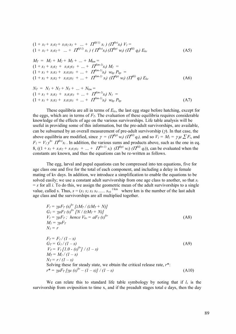
89

(1 + s1 + s1s2 + s1s2 s3 + … + Π(kf-1) si ) (Π

(kv)si) V1 =

(1 + s1 + s1s2 + … + Π(kf-1) si ) ( Π

(kv)si) (Π

(kp) wi) (Π

(kl) qi) Eke (A5)

MT = M1 + M2 + M3 + … + Mkm = (1 + s1 + s1s2 + s1s2s3 + … + Π(km-1)

si) M1 = (1 + s1 + s1s2 + s1s2s3 + … + Π(km-1)

si) wkp Pkp = (1 + s1 + s1s2 + s1s2s3 + … + Π(km-1)

si) (Π(kp)

wi) (Π(kl)

qi) Eke (A6)

NT = N1 + N2 + N3 + … + Nkm = (1 + s1 + s1s2 + s1s2s3 + … + Π(km-1)

si) N1 = (1 + s1 + s1s2 + s1s2s3 + … + Π(km-1)

si) wkp Pkp (A7)

These equilibria are all in terms of Eke, the last egg stage before hatching, except for the eggs, which are in terms of FT. The evaluation of these equilibria requires considerable knowledge of the effects of age on the various survivorships. Life table analysis will be useful in providing some of this information, but the pre-adult survivorships, are available, can be subsumed by an overall measurement of pre-adult survivorship (γ). In that case, the above equilibria are modified, since γ = (Π(kp)

wi) (Π(kl)

qi), and so V1 = M1 = γ µ ∑ Fi, and F1 = V1 y

kv Π(kv)si . In addition, the various sums and products above, such as the one in eq.

8, ((1 + s1 + s1s2 + s1s2s3 + … + Π(kv-1) si) (Π(kp)

wi) (Π(kl) qi)), can be evaluated when the

constants are known, and thus the equations can be re-written as follows.

The egg, larval and pupal equations can be compressed into ten equations, five for age class one and five for the total of each component, and including a delay in female mating of kv days. In addition, we introduce a simplification to enable the equations to be solved easily; we use a constant adult survivorship from one age class to another, so that si

= s for all i. To do this, we assign the geometric mean of the adult survivorships to a single value, called s. Thus, s = (s1 s2 s3 s4 ...... sw)

1/km where km is the number of the last adult age class and the survivorships are all multiplied together.

F1 = γµFT (s)

kv [zMT / (zMT + N)]

G1 = γµFT (s)kv

[N / (zMT + N)] V1 = γµFT ; hence Vkv = aFT (s)

kv (A8) M1 = γµFT

N1 = r

FT = F1 / (1 – s) GT = G1 / (1 – s) (A9) VT = V1 [1.0 - (s)

kv] / (1 – s)

MT = M1 / (1 – s) NT = r / (1 – s) Solving these for steady state, we obtain the critical release rate, r*: r* = γµFT [γµ (s)

kv – (1 – s)] / (1 – s) (A10)

We can relate this to standard life table symbology by noting that if lx is the

survivorship from oviposition to time x, and if the preadult stages total e days, then the day

90

of emergence of adults is e, and the survivorship of a cohort from oviposition until adult emergence is le, the same as γ; also, the survivorships of the adult stages are le+1, le+2, le+3, … etc., which in the notation of the model in equations A5 are V1, V1*s1, V1*s1*s2, etc. In the symbology used above, survivorships of the adult stages are si for the survivorship from the ith adult age to the i+1st adult age. Thus le+1 = γ s1 = s1 le, le+2 = γ s1 s2, = s2 le+1, le+3 = γ s1 s2 s3 = s3 le+2 … etc. , so that

γ Σ (kf-1) Π (j) si = γ [s1 + s1 s2 + s1 s2 s3 + … + s1 s2 ⋅⋅⋅⋅ skf-1 ] = le+1 +le+2 +le+3 + … +

le+1+kf-1 so that the equation for F1 in eq. (A8) can be written as:

F1 = V1 ( Π (kv) si) MT/(MT+NT) (A11)

= ( Π (kv) si) MT/(MT+NT) Π(kv-1)

si) wkp Pkp

= (Π (kv) si) MT/(MT+NT) (Π(kv-1)

si) ( Π (kp) wi) ) ( Π (kl)

qi) (Σ (kv-1) Π (kv-1)

si) Eke

= γ (MT/(MT+NT)) (Π (kv) si) (Π

(kv-1) si) (Σ

(kv-1) Π (kv-1) si) (∑ kf

F1 (Π (kv) si) mx hx)

= γ (MT/(MT+NT)) (Π (kv) si) (Π

(kv-1) si) (Σ

(kv-1) Π (kv-1) si) F1 (∑ kf

(Π (i) si) mx hx)

An example is shown for the data for Bactrocera dorsalis presented by Vargas (1984). For the survivorships shown (graphically) and the age specific fecunditites and egg hatchabilities, the total pre-adult survivorship was γ = 0.63 and the mean daily fertility per fly-day was µ = 8.76 (Barclay & Hendrichs 2014). Also, the delay in female mating was six days; the adult daily survivorship is taken as the 6th root of s1 s2 s3 s4 s5 s6 =, and kv = 6, so the critical value of sterile releases, r* is r* = γµFT [γµ (s)

kv – (1 – s)] / (1 – s) = (0.63)(8.76) FT [(0.63)(8.76) (0.81) – 0.03] / 0.03 = 817 FT.

We need to know the equilibrium wild male population in order to derive the release

ratio and the over-flooding ratio. From eqs. (A8) and (A9), we have MT = M1 / (1 – s) = γµFT / (1-s), and s has the value of 0.961. Thus the total number of wild males is:

MT = γµFT / (1-s) = (0.63) (8.76) FT / (1-0.961) = 141.5 FT

Thus, the release ratio, ρ, is r* / MT (A12)

= 817 FT / 141.5 FT = 5.77

and the daily release rate needs to be greater than 5.77 times the existing wild male population at equilibrium.

The over-flooding ratio is the sterile male population, NT / MT = φ, and so

φ = [r* / (1-s)] / [γµFT / (1-s)] = r* / γµFT (A13) and in the present example, φ = 817 FT / 5.52 FT = 148.0

This value is quite large, but the data are from a laboratory culture of insects under ideal

conditions, and as such are probably the maximum possible for the species. Data from the field would give much more realistic estimates of the critical daily release rates. Also, if the survivorship of sterile males were less than that of wild males, then these calculations would have to take that into account, and both ratios would be larger.

91

Appendix 2. Equations of SIT Models Fertility factor with sterile releases: M / (S+M)

Sterility factor: S / (S+M)

Knipling’s original model: Ft+1 = λFt Mt / (S+Mt)

Critical sterile release rate: S* = M (λ-1) Overflooding ratio: S* / M > λ-1

Unequal sterile male competitive ability: Ft+1 = λFt Mt / (cS+Mt)

Critical release rate: : S* = M (λ-1) / c Overflooding ratio: S* / M > (λ-1) / c

Residual fertility of irradiated males: Ft+1 = λFt (Mt +qS) / (S+Mt) (Modified by the residual fertility factor)

Density-dependent SIT model: Ft+1 = λFt exp [-b(F+M+S)] Mt / (S+Mt) (Normal growth modified by the density-dependent factor: exp [-b(F+M+S)])

Immigration of females from outside the control area

Virgin females: Ft+1 = λ(Ft+ I) (Ft+I) / (Ft+I+S)) where I is the number of immigrants per unit time (Prout 1978). This model has two positive roots, and zero is not a root.

Mated females: Ft+1 = λFt2 / (Ft+S) + λI

This model also has two positive roots, and zero is not a root.

Appendix 3. Software

Some computer software that might be useful to program managers and others involved in mathematical aspects of an SIT program is listed in this Appendix. We note that computer software changes and becomes out of date quite quickly, and that better tools are likely to become available. We have mostly focused on specialized software relating to the topic at hand. In any case this list should be considered a starting point and not a comprehensive resource on software relating to topics in this book.

Name

Program MARK

Curacao

MED-FOES

Populus

92

Summary Author/Maintai- ner

Platform Version/Date Sec- tion

URL

MRR data analysis

G. White MS Windows

4.3/02-2006 4.1 http://warnercnr.colostate.edu/~gwhite/ma rk/mark.htm

SIT simulation B. Ticknor MS Windows

2.2/1990 7, 10 http://ipmworld.umn.edu/chapters/SirSim ul.htm

Agent-Based Simulation of Invasive Pest Insects

N.C. Manoukis MS Windows, Mac OS X, Linux

0.42/04-2013 6.3, 12

http://medfoes.sourceforge.net/

Simulation models of biology and evolutionary ecology

D.N. Alstad MS Windows, Mac OS X, Linux

5.5/2007 6, 8 http://www.cbs.umn.edu/populus

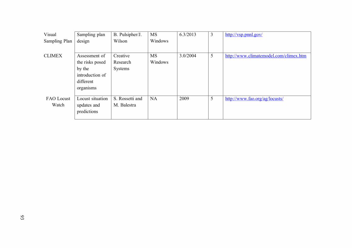
Visual Sampling Plan

CLIMEX

FAO Locust Watch

93

Sampling plan design

B. Pulsipher/J.Wilson

MS Windows

6.3/2013 3 http://vsp.pnnl.gov/

Assessment of the risks posed by the introduction of different organisms

Creative Research Systems

MS Windows

3.0/2004 5 http://www.climatemodel.com/climex.htm

Locust situation updates and predictions

S. Rossetti andM. Balestra

NA 2009 5 http://www.fao.org/ag/locusts/

94

Appendix 4. Glossary

Algorithm – a mathematical or numerical method of working out some problem or result.

Calculus – a branch of mathematics invented by Newton and Leibnitz that deals with continuous rates of change of variables with infinitely small time steps.

Differential equation – an equation involving calculus

Difference equation – an equation of rates of change involving finite time steps.

Competition coefficient – a number that represents the mating ability of sterile males as compared with wild males. Zero means no mating ability; 1.0 means the same ability as wild males.

Density dependent – the operation of some mortality or fertility factor that changes its effect (per insect) with population density.

Density independent – the operation of some mortality or fertility factor that does not change its effect per insect with population density.

Dispersal – the net movement of individual animals other than just minor local daily movements that return to the same place.

Diffusion equation – a differential equation that describes the net movement of individuals over time.

Emigration – net movement of individuals out of a population.

Immigration – net movement of individuals into a population.

Dispersion – spatial arrangement of individuals in a population.

Regular dispersion – arrangement in which individuals are evenly spaced.

Random dispersion – arrangement in which the spacing of individuals is independent of all other individuals in the population

Clumped (aggregated) dispersion – arrangement in which individuals occur in groups, or clumps.

Probability distribution – a numerical or graphic representation of the frequency of occurrences of individuals in a population.

Discrete distribution – a distribution in which frequencies of individuals are tabulated by frequencies of 0, 1, 2, … etc. occurrences.

Continuous distribution – a distribution in which relative frequencies of individuals are shown according to some continuous variable, such as height, weight, etc.

Sample distribution – the distribution obtained from a number of samples, such as the numbers of insects occurring on sampled branches

Sampling distribution – a probability distribution that approximately describes the results of sampling; these are mathematical distributions such as Poisson, Negative Binomial, Normal, etc.

Equilibrium – a configuration of population numbers that remains the same over time. The term equilibrium often implies that the configuration is stable and will return to its equilibrium value if the population is disturbed.

Steady state – another name for an equilibrium, but without any implication regarding stability.

Lek – a social gathering of animals for the purpose of mating, migration, etc.

Lekking behavior – the grouping of animals into leks.

Model – a theoretical representation of reality by ideas, mathematics, graphs, etc.

Mathematical model – the representation of reality (of population sizes, etc.) by means of mathematical equations or computer programs.

Percentage – represents the part of a group of items scaled to be out of 100. Thus, 10% is one tenth of the total.

Proportion – represents the part of a group of items scaled to be out of 1.0. Thus a proportion of 0.5 represents half of the total.

Probability – a numerical representation of the likelihood of occurrence of a particular event. Thus, a probability of 0.3 means that the event is expected to occur in about 30% of possible times. For example, in tossing a fair coin, heads is expected to occur in about half of the tosses, so that the probability is assigned to be 0.5.

Population – the total number of individuals of a given species that are within an area of interest. This is generally taken to be the total number of individuals that are capable of mating with each other. Thus, individuals from different populations are normally prevented from mating with each other by geographic separation.

Sample – a group of individuals that are captured for the purpose of obtaining information from them. This group in some way represents the population.

Residual fertility – fertility that persists following sterilization of a group of insects. If two percent of the insects remain fertile following irradiation, then the residual fertility is shown as 0.02 (a proportion), or 2% (a percentage).

95


The guideline is intended to be a reference book, to be consulted when necessary. As such, any particular AW-IPM programme using the SIT will probably only need certain sections, and much of the book can be ignored if that is the case.

SIT have produced over many years a vast amount of every-day data from the field operations and from the mass rearing facility and packing and sterile insect releasing centres. With the help of this guideline, that information can be used to develop predictive models for their particular conditions to better plan control measures.

I5573E/1/04.16

ISBN 978-92-5-109190-6

9 7 8 9 2 5 1 0 9 1 9 0 6

Guidelines for the use of mathematics in operational area-wide integrated pest management programmes using the sterile insect technique with a special focus on Tephritid fruit flies

16-08331

Guidelines for the use of mathematics in operational area ...

Documents

Transcript of Guidelines for the use of mathematics in operational area ...