Guidelines for Analytical Vulnerability Assessment - Low/Mid ...

GEMGLOBAL EARTHQUAKE MODEL

Vulnerability and loss modelling

GEM TECHNICAL REPORT 2014-12 V1.0.0

D’Ayala D., A. Meslem, D. Vamvatsikos, K. Porter, T. Rossetto and V. Silva

Guidelines for Analytical Vulnerability Assessment - Low/Mid-Rise

Copyright©2015 [D.D’Ayala,A.Meslem,D.Vamvatsikos,K.Porter,T.Rossetto,V.Silva] Exceptwhereotherwisenoted thiswork ismadeavailableunder the termsofCreativeCommonsAttribution-ShareAlike4.0(CCBY-SA4.0).

The views and interpretations in this document are those of the individual author(s) and should not beattributedtotheGEMFoundation.Withthemalsoliestheresponsibilityforthescientificandtechnicaldatapresented.Theauthorsdonotguaranteethattheinformationinthisreportiscompletelyaccurate.

Citation: D’Ayala, D., Meslem, A., Vamvatsikos, D., Porter, K., Rossetto, T., Silva, V. (2015) Guidelines forAnalyticalVulnerabilityAssessmentofLow/Mid-RiseBuildings,VulnerabilityGlobalComponentProject.DOI10.13117/GEM.VULN-MOD.TR2014.12

www.globalquakemodel.org

GuidelinesforAnalyticalVulnerabilityAssessmentofLow/Mid-RiseBuildings

Version:1.0

Author(s):D.D’Ayala,A.Meslem,D.Vamvatsikos,K.Porter,T.RossettoandV.Silva

Date:August01,2015

ii

ABSTRACT

Guidelines (GEM-ASV) for developing analytical seismic vulnerability functions are offered for use within the

framework of the Global Earthquake Model (GEM). Emphasis is on low/mid-rise buildings and cases where

the analyst has the skills and time to perform non-linear analyses. The target is for a structural engineer with

a Master’s level training and the ability to create simplified non-linear structural models to be able to

determine the vulnerability functions pertaining to structural response, damage, or loss for any single

structure, or for a class of buildings defined by the GEM Taxonomy level 1 attributes. At the same time,

sufficient flexibility is incorporated to allow full exploitation of cutting-edge methods by knowledgeable

users. The basis for this effort consists of the key components of the state-of-art PEER/ATC-58 methodology

for loss assessment, incorporating simplifications for reduced effort and extensions to accommodate a class

of buildings rather than a single structure, and multiple damage states rather than collapse only

considerations.

To inject sufficient flexibility into the guidelines and accommodate a range of different user needs and

capabilities, a distinct hierarchy of complexity (and accuracy) levels has been introduced for (a) defining index

buildings, (b) modelling, and (c) analysing. Sampling-wise, asset classes may be represented by random or

Latin hypercube sampling in a Monte Carlo setting. For reduced-effort representations of inhomogeneous

populations, simple stratified sampling is advised, where the population is partitioned into a number of

appropriate subclasses, each represented by one “index” building. Homogeneous populations may be

approximated using a central index building plus 2k additional high/low observations in each of k dimensions

(properties) of interest. Structural representation of index buildings may be achieved via typical 2D/3D

element-by-element models, simpler 2D storey-by-storey (stick) models or an equivalent SDOF system with a

user-defined capacity curve. Finally, structural analysis can be based on variants of Incremental Dynamic

Analysis (IDA) or Non-linear Static Procedure (NSP) methods.

A similar structure of different level of complexity and associated accuracy is carried forward from the

analysis stage into the construction of fragility curves, damage to loss function definition and vulnerability

function derivation.

In all cases, the goal is obtaining useful approximations of the local storey drift and absolute acceleration

response to estimate structural, non-structural, and content losses. Important sources of uncertainty are

identified and propagated incorporating the epistemic uncertainty associated with simplifications adopted by

the user. The end result is a set of guidelines that seamlessly fits within the GEM framework to allow the

generation of vulnerability functions for any class of low/mid-rise buildings with a reasonable amount of

effort by an informed engineer. Two illustrative examples are presented for the assessment of reinforced-

concrete moment-resisting frames with masonry infills and unreinforced masonry structures, while a third

example treating ductile steel moment-resisting frames appears in a companion document.

Keywords: vulnerability; fragility; low/mid-rise buildings.

iii

TABLE OF CONTENTS

Page

ABSTRACT ............................................................................................................................................................. ii

TABLE OF CONTENTS ........................................................................................................................................... iii

LIST OF FIGURES .................................................................................................................................................. vii

LIST OF TABLES ..................................................................................................................................................... ix

GLOSSARY ............................................................................................................................................................. 1

1 Introduction ..................................................................................................................................................... 3

1.1 Scope of the Guidelines ........................................................................................................................... 3

1.2 Purpose of the Guidelines ....................................................................................................................... 3

1.3 Structure of the Guidelines ..................................................................................................................... 4

1.4 Relationship to other GEM Guidelines .................................................................................................... 5

2 Methodology and Process of Analytical Vulnerability Assessment ................................................................. 6

2.1 Steps in the Methodology for Analytical Vulnerability Assessment ....................................................... 6

STEP A: Defining Index Buildings ............................................................................................................. 8

STEP B: Define Components for Response Analysis and Loss Estimation ............................................... 8

STEP C: Select Model Type ...................................................................................................................... 9

STEP D: Define Damage States at Element and Global Level .................................................................. 9

STEP E: Analysis Type and Calculation of EDPs Damage State Thresholds............................................ 10

STEP F: Construction of Vulnerability Curves ........................................................................................ 11

2.2 Mixing and Matching of Mathematical Model/Analysis Type (Calculation Effort - Uncertainty) ......... 12

2.3 Efficiency and Sufficiency for IM Selection............................................................................................ 12

3 STEP A: Defining Index Buildings ................................................................................................................... 14

3.1 One Index Building ................................................................................................................................ 16

3.2 Three Index Buildings ............................................................................................................................ 16

3.3 Multiple Index Buildings ........................................................................................................................ 17

3.3.1 Moment-Matching ...................................................................................................................... 17

3.3.2 Class Partitioning......................................................................................................................... 18

3.3.3 Monte Carlo Simulation .............................................................................................................. 19

4 STEP B: Define Components for Response Analysis and Loss Estimation ..................................................... 20

4.1 Structural Components ......................................................................................................................... 21

4.2 Dominant Non-Structural Categories .................................................................................................... 23

5 STEP C: Select Model Type ............................................................................................................................. 24

iv

5.1 MDoF Model: 3D/2D Element-by-Element ........................................................................................... 24

Frame / shear wall element modelling procedure ................................................................................ 25

Masonry infill panel modelling procedure ............................................................................................ 27

Unreinforced Masonry modelling procedure ........................................................................................ 28

5.2 Reduced MDoF Model: 2D Lumped ...................................................................................................... 30

5.3 SDoF Model: 1D Simplified Equivalent Model ....................................................................................... 33

6 STEP D: Define Damage States ...................................................................................................................... 34

6.1 Custom Defined for Each Sampled Building .......................................................................................... 35

6.2 Pre-Defined Values ................................................................................................................................ 39

7 STEP E: Analysis Type and Calculation of EDPs Damage State Thresholds .................................................... 41

7.1 Ground Motion Selection and Scaling ................................................................................................... 45

7.1.1 Ground Motions Selection .......................................................................................................... 45

7.1.2 Number of Ground Motion Records ........................................................................................... 46

7.2 Non-Linear Dynamic Analysis (NLD) ...................................................................................................... 47

7.2.1 Procedure 1.1: Incremental Dynamic Analysis (IDA) .................................................................. 47

7.3 Non-Linear Static Analysis (NLS) ............................................................................................................ 53

7.3.1 Case of Multilinear Elasto-Plastic (with Residual Strength) Form of Capacity Curve ................. 53

7.3.1.1 Procedure 2.1: N2 Method for Multilinear Elasto-Plastic Form of Capacity Curve .............. 54

Determination of the performance point ............................................................................................ 54

Determination of inelastic response spectrum .................................................................................... 55

Determination of EDPs damage state thresholds ................................................................................ 58

Use of Smoothed Elastic Response Spectrum ...................................................................................... 64

7.3.2 Case of Bilinear Elasto-Plastic Form of Capacity Curve ............................................................... 66

7.3.2.1 Procedure 3.1: N2 Method for Bilinear Elasto-Plastic Form of Capacity Curve ................... 66



Use of smoothed elastic response spectrum ....................................................................................... 71

7.3.2.2 Procedure 3.2: FRAgility through Capacity ASsessment (FRACAS) ....................................... 73



7.3.2.3 Procedure 3.3: Alternative Method for Considering Record-to-Record Variability ............. 77



7.4 Non-Linear Static Analysis Based on Simplified Mechanism Models (SMM-NLS) ................................. 80

7.4.1 Procedure 4.1: Failure Mechanism Identification and Vulnerability Evaluation (FaMIVE) ......... 81

Derivation of capacity curve and determination of the performance point ........................................ 82


v

8 STEP F: Vulnerability Curves Derivation ........................................................................................................ 87

8.1 STEP F-1: Building-Based Vulnerability Assessment Approach ............................................................. 87

8.1.1 Building-Based Fragility Curves ................................................................................................... 89

8.1.2 Building-Based Repair Cost Given Damage State ....................................................................... 92

8.1.3 Building-Based Vulnerability Curve ............................................................................................. 94

8.1.3.1 One Index Building Based Vulnerability Curve ..................................................................... 94

8.1.3.2 Three Index Buildings Based Vulnerability Curve ................................................................. 95

8.1.3.3 Multiple Index Buildings Based Vulnerability Curve ............................................................. 97

8.2 STEP F-2: Component-Based Vulnerability Assessment Approach ....................................................... 98

8.2.1 Component-Based Fragility Curve .............................................................................................. 98

8.2.2 Component-Based Repair Cost Given Damage State ............................................................... 100

8.2.3 Component-Based Vulnerability Curve ..................................................................................... 101

8.2.3.1 One Index Building Based Vulnerability Curve ................................................................... 101

8.2.3.2 Three Index Buildings Based Vulnerability Curve ............................................................... 106

8.2.3.3 Multiple Index Buildings Based Vulnerability Curve ........................................................... 108

REFERENCES ...................................................................................................................................................... 109

APPENDIX A Derivation of Capacity Curves ....................................................................................................... I

A.1 Perform Pushover Analysis ....................................................................................................................... I

A.2 Derivation of Equivalent SDoF-Based Capacity Curves ........................................................................... II

A.3 Fitting the Capacity into Idealised Representation ................................................................................ III

A.3.1 Multilinear Elasto-Perfectly Plastic Form ...................................................................................... V

A.3.2 Bilinear Elasto-Perfectly Plastic Form .......................................................................................... VI

A.4 Acceleration-Displacement Response Spectra (ADRS) Format .............................................................. VI

APPENDIX B Average Values of Dispersions for Response Analysis, FEMA P-58 ........................................... VII

APPENDIX C Compendium of Existing Building-Level Damage Factor (DF) Values ....................................... VIII

C.1 Damage Factors Function of Building Typology (GEM Damage-to-Loss Report – Rossetto, 2011) ..... VIII

C.1.1 General Damage Factor Values .................................................................................................. VIII

C.1.2 Damage Factor Values for Reinforced Concrete Frames with Masonry Infills ............................ XI

C.1.3 Damage Factor Values for Unreinforced Masonry Buildings ..................................................... XIV

C.2 Damage Factor Values Function of Building Occupancy Class (HAZUS-MH MR3) ............................... XVI

C.2.1 Structural Damage Factor Values Function of Building Occupancy Class (HAZUS-MH MR3, Table

15.2) XVI

C.2.2 Acceleration-Sensitive Non-Structural Damage Factor Values Function of Building Occupancy

Class (HAZUS-MH MR3, Table 15.3) .................................................................................................... XVII

C.2.3 Drift-Sensitive Non-Structural Damage Factor Values Function of Building Occupancy Class

(HAZUS-MH MR3, Table 15.4) ............................................................................................................ XVIII

APPENDIX D Illustrative Examples ................................................................................................................. XIX

D.1 Mid-Rise RC Building Designed According to Earlier Seismic Codes .................................................... XIX

vi

D.1.1 Define Building Index ................................................................................................................. XIX

D.1.2 Derivation of Structural Capacity Curves ................................................................................... XXI

D.1.3 Calculation of Performance Points for a Suite of Ground Motion Records ............................. XXIV

D.1.4 Determination of EDPs Damage State Thresholds .................................................................... XXV

D.1.5 Building-based repair cost for a specific level of intensity measurement ............................... XXVI

D.2 Low to Mid-Rise Unreinforced Masonry Buildings in Historic Town Centre .................................... XXVIII

D.2.1 Define Building Index ............................................................................................................... XXIX

D.2.2 Derivation of Structural Capacity Curves .................................................................................. XXX

D.2.3 Determination of EDPs Damage State Thresholds and Fragility Curves .................................. XXXI

D.2.4 Calculation of Performance Points ......................................................................................... XXXII

vii

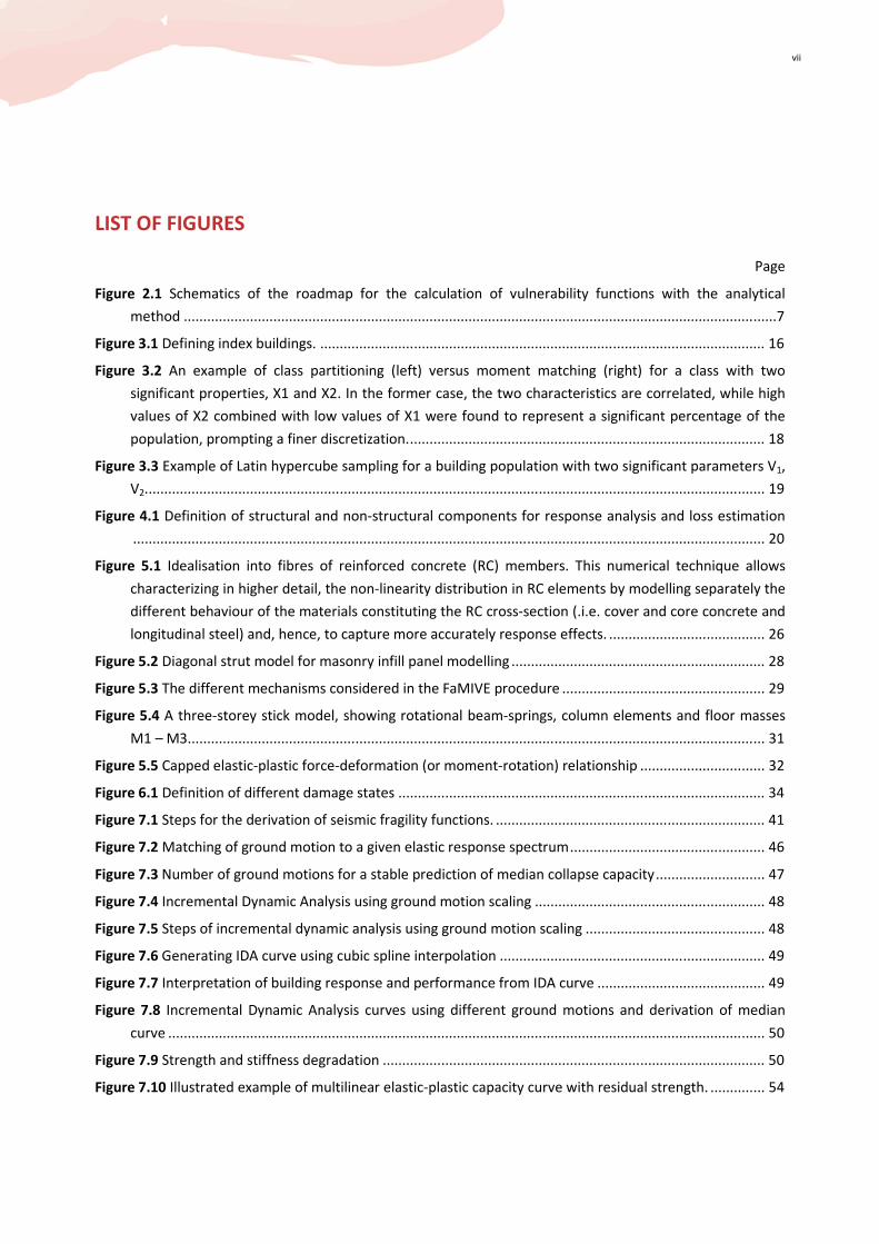
LIST OF FIGURES

Page

Figure 2.1 Schematics of the roadmap for the calculation of vulnerability functions with the analytical

method ........................................................................................................................................................7

Figure 3.1 Defining index buildings. .................................................................................................................. 16

Figure 3.2 An example of class partitioning (left) versus moment matching (right) for a class with two

significant properties, X1 and X2. In the former case, the two characteristics are correlated, while high

values of X2 combined with low values of X1 were found to represent a significant percentage of the

population, prompting a finer discretization. ........................................................................................... 18

Figure 3.3 Example of Latin hypercube sampling for a building population with two significant parameters V1,

V2. .............................................................................................................................................................. 19

Figure 4.1 Definition of structural and non-structural components for response analysis and loss estimation

.................................................................................................................................................................. 20

Figure 5.1 Idealisation into fibres of reinforced concrete (RC) members. This numerical technique allows

characterizing in higher detail, the non-linearity distribution in RC elements by modelling separately the

different behaviour of the materials constituting the RC cross-section (.i.e. cover and core concrete and

longitudinal steel) and, hence, to capture more accurately response effects. ........................................ 26

Figure 5.2 Diagonal strut model for masonry infill panel modelling ................................................................. 28

Figure 5.3 The different mechanisms considered in the FaMIVE procedure .................................................... 29

Figure 5.4 A three-storey stick model, showing rotational beam-springs, column elements and floor masses

M1 – Μ3 .................................................................................................................................................... 31

Figure 5.5 Capped elastic-plastic force-deformation (or moment-rotation) relationship ................................ 32

Figure 6.1 Definition of different damage states .............................................................................................. 34

Figure 7.1 Steps for the derivation of seismic fragility functions. ..................................................................... 41

Figure 7.2 Matching of ground motion to a given elastic response spectrum .................................................. 46

Figure 7.3 Number of ground motions for a stable prediction of median collapse capacity ............................ 47

Figure 7.4 Incremental Dynamic Analysis using ground motion scaling ........................................................... 48

Figure 7.5 Steps of incremental dynamic analysis using ground motion scaling .............................................. 48

Figure 7.6 Generating IDA curve using cubic spline interpolation .................................................................... 49

Figure 7.7 Interpretation of building response and performance from IDA curve ........................................... 49

Figure 7.8 Incremental Dynamic Analysis curves using different ground motions and derivation of median

curve ......................................................................................................................................................... 50

Figure 7.9 Strength and stiffness degradation .................................................................................................. 50

Figure 7.10 Illustrated example of multilinear elastic-plastic capacity curve with residual strength. .............. 54

viii

Figure 7.11 Illustrated example on the steps of the Procedure 2.1 for the evaluation of the performance point

given an earthquake record. ..................................................................................................................... 55

Figure 7.12 Repeat the process of Procedure 2.1 for multiple earthquake records. ........................................ 59

Figure 7.13 Clouds of structural-response results. ............................................................................................ 59

Figure 7.14 Derivation of fragility curves using GLM regression technique. ..................................................... 62

Figure 7.15 Derivation of fragility functions (median demand and dispersion) using Least Squares regression

technique. ................................................................................................................................................. 63

Figure 7.16 Calculation example of Median demand and dispersion for Complete Damage (CD) using Least

Squares regression .................................................................................................................................... 64

Figure 7.17 Illustrated example on the Procedure 2.1 for the calculation of performance point using

smoothed elastic response spectrum. ...................................................................................................... 65

Figure 7.18 Illustrated example on the steps of Procedure 3.1 for the evaluation of performance point for a

given earthquake record........................................................................................................................... 67

Figure 7.19 Repeat the process of the Procedure 2.1 for multiple earthquake records. .................................. 71

Figure 7.20 Illustrated example on the Procedure 3.1 for the calculation of performance point using

smoothed elastic response spectrum. ...................................................................................................... 72

Figure 7.21 Summary of the main steps carried out by FRACAS for a bilinear capacity curve ......................... 74

Figure 7.22 Repeat the process of the Procedure 3.2 for multiple earthquake records. .................................. 77

Figure 7.23 Workflow of the FaMIVE method for derivation of fragility functions .......................................... 81

Figure 7.24 Example of calculation of performance points for median capacity curves for types of

mechanisms triggered (COMB= combined mechanism, IP= in-plane mechanism, OOP= Out-of-plane

mechanism; see also Figure 5.3). ............................................................................................................. 85

Figure 8.1 Calculation of damage probabilities from the fragility curves for a specific level of intensity

measurement, im. ..................................................................................................................................... 88

Figure 8.2 Example of illustration of transformation of the fragility curves into vulnerability, with confidence

boundaries ................................................................................................................................................ 89

Figure 8.3 Example of derived one index-based building-level vulnerability curve for collapse damage state:

case of mid-rise storey RC shear wall office building, in region of 0.17 ≤SMS <0.5g for USA. ................. 106

Figure 8.4 Example of derived three index-based seismic vulnerability curve for collapse damage state: case

of mid-rise storey RC shear wall office building, in region of 0.17 ≤SMS <0.5g for USA. ......................... 107

Figure A.1. Plot of pushover curve and evaluation of different damage thresholds ............................................I

Figure A.2. Example of transformation of MDoF-based pushover curve to an equivalent SDoF........................III

Figure A.3. Idealization of capacity curves. (a) Multilinear elasto- plastic form; (b) Bilinear elasto-perfectly

plastic form. ............................................................................................................................................... IV

Figure A.4. Idealization of capacity curve using multilinear elasto-plastic form. ................................................ V

Figure A.5. Idealization of capacity curve using bilinear elasto-perfectly plastic form. ..................................... VI

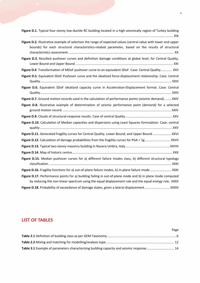
ix

Figure D.1. Typical four-storey low-ductile RC building located in a high-seismically region of Turkey building

................................................................................................................................................................. XIX

Figure D.2. Illustrative example of selection the range of expected values (central value with lower and upper

bounds) for each structural characteristics-related parameter, based on the results of structural

characteristics assessment ....................................................................................................................... XX

Figure D.3. Resulted pushover curves and definition damage conditions at global level, for Central Quality,

Lower Bound and Upper Bound. ............................................................................................................. XXI

Figure D.4. Transformation of MDoF pushover curve to an equivalent SDoF. Case: Central Quality. ............ XXII

Figure D.5. Equivalent SDoF Pushover curve and the idealized force-displacement relationship. Case: Central

Quality.................................................................................................................................................... XXIII

Figure D.6. Equivalent SDoF idealized capacity curve in Acceleration-Displacement format. Case: Central

Quality.................................................................................................................................................... XXIII

Figure D.7. Ground motion records used in the calculation of performance points (seismic demand). ....... XXIV

Figure D.8. Illustrative example of determination of seismic performance point (demand) for a selected

ground motion record. .......................................................................................................................... XXIV

Figure D.9. Clouds of structural-response results. Case of central Quality ..................................................... XXV

Figure D.10. Calculation of Median capacities and dispersions using Least Squares formulation. Case: central

quality ..................................................................................................................................................... XXV

Figure D.11. Generated fragility curves for Central Quality, Lower Bound, and Upper Bound ..................... XXVI

Figure D.12. Calculation of damage probabilities from the fragility curves for PGA = 1g. ............................ XXVII

Figure D.13. Typical two-storey masonry building in Nocera Umbra, Italy .................................................. XXVIII

Figure D.14. Map of historic centre ................................................................................................................. XXX

Figure D.15. Median pushover curves for a) different failure modes class, b) different structural typology

classification. ......................................................................................................................................... XXXI

Figure D.16. Fragility functions for a) out-of-plane failure modes, b) in-plane failure mode ........................ XXXI

Figure D.17. Performance points for a) building failing in out-of-plane mode and b) in plane mode computed

by reducing the non-linear spectrum using the equal displacement rule and the equal energy rule. XXXII

Figure D.18. Probability of exceedance of damage states, given a lateral displacement ............................ XXXIII

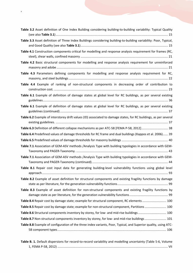
LIST OF TABLES

Page

Table 2.1 Definition of building class as per GEM-Taxonomy ..............................................................................6

Table 2.2 Mixing and matching for modelling/analysis type. ............................................................................ 12

Table 3.1 Example of parameters characterizing building capacity and seismic response ............................... 14

x

Table 3.2 Asset definition of One Index Building considering building-to-building variability: Typical Quality

(see also Table 3.1) ................................................................................................................................... 15

Table 3.3 Asset definition of Three Index Buildings considering building-to-building variability: Poor, Typical,

and Good Quality (see also Table 3.1) ...................................................................................................... 15

Table 4.1 Construction components critical for modelling and response analysis requirement for frames (RC,

steel), shear walls, confined masonry ...................................................................................................... 21

Table 4.2 Basic structural components for modelling and response analysis requirement for unreinforced

masonry and adobe .................................................................................................................................. 21

Table 4.3 Parameters defining components for modelling and response analysis requirement for RC,

masonry, and steel buildings .................................................................................................................... 22

Table 4.4 Example of ranking of non-structural components in decreasing order of contribution to

construction cost. ..................................................................................................................................... 23

Table 6.1 Example of definition of damage states at global level for RC buildings, as per several existing

guidelines .................................................................................................................................................. 36

Table 6.1 Example of definition of damage states at global level for RC buildings, as per several existing

guidelines (continued) .............................................................................................................................. 37

Table 6.2 Example of interstorey drift values (ID) associated to damage states, for RC buildings, as per several

existing guidelines. ................................................................................................................................... 37

Table 6.3 Definition of different collapse mechanisms as per ATC-58 [FEMA P-58, 2012] ............................... 38

Table 6.4 Predefined values of damage thresholds for RC frame and dual buildings (Kappos et al. 2006) ...... 39

Table 6.5 Predefined values of damage thresholds for masonry buildings ...................................................... 40

Table 7.1 Association of GEM-ASV methods /Analysis Type with building typologies in accordance with GEM-

Taxonomy and PAGER-Taxonomy. ........................................................................................................... 43

Table 7.1 Association of GEM-ASV methods /Analysis Type with building typologies in accordance with GEM-

Taxonomy and PAGER-Taxonomy (continued). ........................................................................................ 44

Table 8.1 Repair cost input data for generating building-level vulnerability functions using global level

approach ................................................................................................................................................... 93

Table 8.2 Example of asset definition for structural components and existing fragility functions by damage

state as per literature, for the generation vulnerability functions ........................................................... 99

Table 8.3 Example of asset definition for non-structural components and existing fragility functions by

damage state as per literature, for the generation vulnerability functions ............................................. 99

Table 8.4 Repair cost by damage state; example for structural component, RC elements ............................ 100

Table 8.5 Repair cost by damage state; example for non-structural component, Partitions ......................... 100

Table 8.6 Structural components inventory by storey, for low- and mid-rise buildings ................................. 100

Table 8.7 Non-structural components inventory by storey, for low- and mid-rise buildings ......................... 101

Table 8.8 Example of configuration of the three index variants, Poor, Typical, and Superior quality, using ATC-

58 component types ............................................................................................................................... 106

Table B. 1. Default dispersions for record-to-record variability and modelling uncertainty (Table 5-6, Volume

1, FEMA P-58, 2012) ................................................................................................................................. VII

xi

Table D.1. Classification of 4-storey RC building according to the GEM Basic Building Taxonomy .................. XX

Table D.2. Range of expected values for the structural characteristics-related parameters associated to the

building class represented by the index building ranges ......................................................................... XXI

Table D.3. Suite of ground motion records used in the calculation of performance points (seismic demand)

............................................................................................................................................................... XXIV

Table D.4. Resulting median capacities and their corresponding dispersions associated to the record-to-

record variability .................................................................................................................................... XXVI

Table D.5. Damage Factors values for reinforced concrete frames with masonry infills .............................. XXVII

Table D.6. Classification of URM building stock in Nocera Umbra, Italy, according to the GEM Basic Building

Taxonomy .............................................................................................................................................. XXIX

Table D.7. Median displacement thresholds and their corresponding dispersions due to capacity curves

variability in the sample ......................................................................................................................... XXXI

1

GLOSSARY

Building or Storey Fragility Curve/Function: A probability-valued function of the intensity measure that

represents the probability of violating (exceeding) a given limit-state or damage state of the building or the

storey given the value of the seismic intensity measure (IM) that it has been subjected to. Essentially, it is the

cumulative distribution function (CDF) of the IM-capacity value for the limit-state and it is thus often

characterized by either a normal or (more often) a lognormal distribution, together with the associated

central value and dispersion of IM-capacity.

Central Value of a Variable: The median value used to characterize the “central tendency” of the variable.

This is not necessarily the most frequent value that it can take, which is called its mode. The three quantities,

mean, median and mode, coincide for a normal distribution, but not necessarily for other types, e.g., a

lognormal.

Component Fragility Curve/Function: A probability-valued function of an engineering demand parameter

(EDP), that represents the probability of violating (exceeding) a given limit-state or damage-state of the

component, given the value of EDP that it has been subjected to. Essentially, it is the cumulative distribution

function (CDF) of the EDP-capacity value for the limit-state and it is thus often characterized by either a

normal or (more often) a lognormal distribution, together with the associated central value and dispersion of

EDP-capacity.

Cost Replacement (New): The cost of replacing a component/group of components/an entire building. Since

this is often compared to losses, demolition/removal costs may be added to it to fully represent the actual

cost of constructing a new structure in place of the (damaged or collapsed) existing one.

Dispersion of a Variable: A measure of the scatter in the random variable, as measured around its central

value. A typical quantity used is the standard deviation of the variable X, especially for a normal distribution,

represented by σX. For a lognormal distribution, one often uses the standard deviation of the logarithm of

the variable instead. The latter is often symbolized as βX or σlnX.

Distribution of a Variable: The probabilistic characterization of a random/uncertain variable.

Comprehensively, this is represented by the probability density function (PDF), or its integral, the cumulative

distribution function (CDF). For example, the PDF of a normally distributed variable is the well-known

Gaussian bell function, while its CDF (and actually most CDFs regardless of distribution) resembles a sigmoid

function, exactly like any fragility function.

Engineering Demand Parameter (EDP): A measure of structural response that can be recorded or estimated

from the results of a structural analysis. Typical choices are the peak floor acceleration (PFA) and the

interstorey drift ratio (IDR).

Intensity Measure (IM): Particularly for use within this document, IM will refer to a scalar quantity that

characterizes a ground motion accelerogram and linearly scales with any scale factor applied to the record.

2

While non-linear IMs and vector IMs have been proposed in the literature and often come with important

advantages, they will be excluded from the present guidelines due to the difficulties in computing the

associated hazard.

Joint Distribution of a Set of Variables: This refers to the probabilistic characterization of a group of

random/uncertain variables that may or may not depend on each other. If they are independent, then their

joint distribution is fully characterized by the product of their individual probability density functions (PDFs),

or marginal PDFs as they are often called. If there are dependencies, though, at a minimum one needs to

consider additionally the correlation among them, i.e., whether one increases/decreases as another

decreases, and how strongly.

Loss: The quantifiable consequences of seismic damage. These can be (a) the actual monetary cost of

repairing a component, a group of components, or an entire building, or (b) the casualties, i.e., number of

fatalities or injured occupants.

Loss ratio: For monetary losses, this is the ratio of loss to the cost replacement new for a component/group

of components/building. For casualties, it is the ratio of fatalities or injured over the total number of

occupants

Population (of Buildings): The ensemble of all buildings that actually constitute the class examined. For

example, the set of all the existing US West Coast steel moment-resisting frames.

Sample of Index Buildings: A sample of representative buildings, each called an index building, that may be

either real or fictitious, yet they have been chosen to represent the overall population by capturing the joint

probabilistic distribution of its most important characteristics.

Vulnerability Curve/Function: A loss or loss ratio valued function of the intensity measure (IM), that

represents the distribution of seismic loss or loss ratio given the value of IM that a certain building or class of

buildings has been subjected to. Since at each value of IM we actually get an entire distribution of losses,

there is never a single vulnerability curve. It is therefore most appropriate to directly specify which

probabilistic quantity of the distribution each vulnerability curve represents, thus resulting, for example, to

the 16/50/84% curves, the mean vulnerability curve or the dispersion curve.

Uncertainty: A general term that is used within these guidelines to describe the variability in determining any

EDP, cost, or loss value. The typical sources considered are the ground motion variability, the damage state

capacity and associated cost variability, and the errors due to modelling assumptions or imperfect analysis

methods.

3

1 Introduction

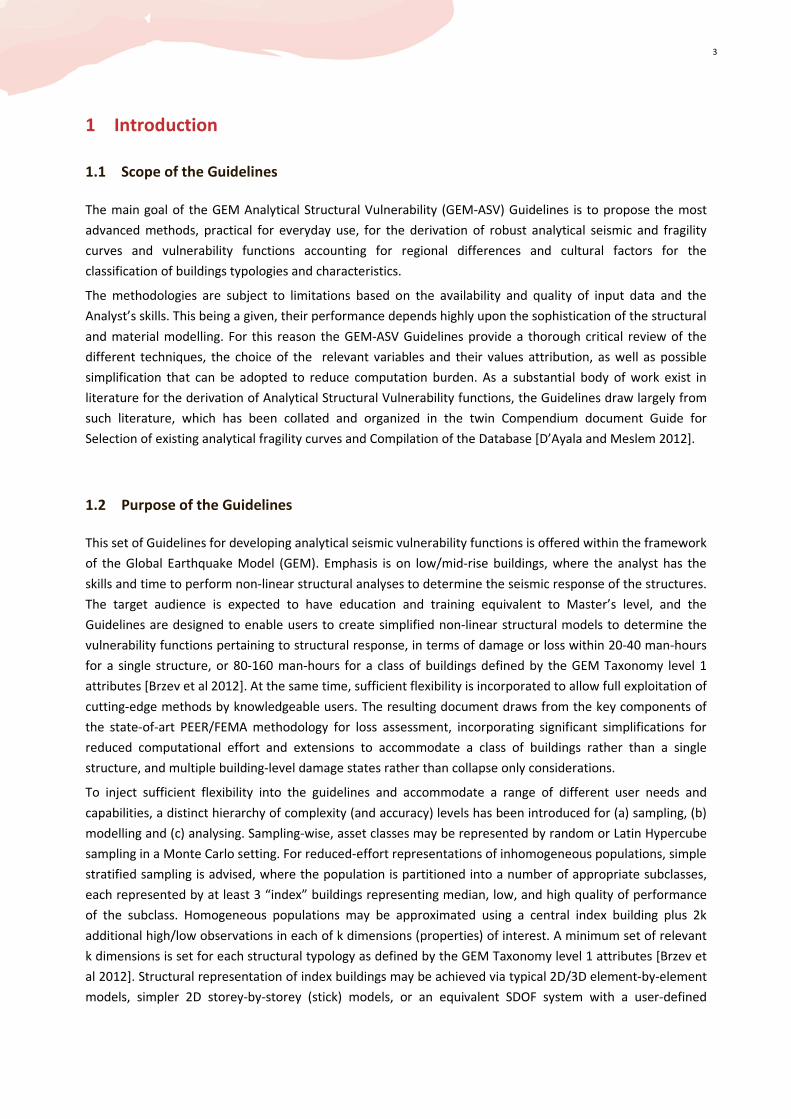
1.1 Scope of the Guidelines

The main goal of the GEM Analytical Structural Vulnerability (GEM-ASV) Guidelines is to propose the most

advanced methods, practical for everyday use, for the derivation of robust analytical seismic and fragility

curves and vulnerability functions accounting for regional differences and cultural factors for the

classification of buildings typologies and characteristics.

The methodologies are subject to limitations based on the availability and quality of input data and the

Analyst’s skills. This being a given, their performance depends highly upon the sophistication of the structural

and material modelling. For this reason the GEM-ASV Guidelines provide a thorough critical review of the

different techniques, the choice of the relevant variables and their values attribution, as well as possible

simplification that can be adopted to reduce computation burden. As a substantial body of work exist in

literature for the derivation of Analytical Structural Vulnerability functions, the Guidelines draw largely from

such literature, which has been collated and organized in the twin Compendium document Guide for

Selection of existing analytical fragility curves and Compilation of the Database [D’Ayala and Meslem 2012].

1.2 Purpose of the Guidelines

This set of Guidelines for developing analytical seismic vulnerability functions is offered within the framework

of the Global Earthquake Model (GEM). Emphasis is on low/mid-rise buildings, where the analyst has the

skills and time to perform non-linear structural analyses to determine the seismic response of the structures.

The target audience is expected to have education and training equivalent to Master’s level, and the

Guidelines are designed to enable users to create simplified non-linear structural models to determine the

vulnerability functions pertaining to structural response, in terms of damage or loss within 20-40 man-hours

for a single structure, or 80-160 man-hours for a class of buildings defined by the GEM Taxonomy level 1

attributes [Brzev et al 2012]. At the same time, sufficient flexibility is incorporated to allow full exploitation of

cutting-edge methods by knowledgeable users. The resulting document draws from the key components of

the state-of-art PEER/FEMA methodology for loss assessment, incorporating significant simplifications for

reduced computational effort and extensions to accommodate a class of buildings rather than a single

structure, and multiple building-level damage states rather than collapse only considerations.

To inject sufficient flexibility into the guidelines and accommodate a range of different user needs and

capabilities, a distinct hierarchy of complexity (and accuracy) levels has been introduced for (a) sampling, (b)

modelling and (c) analysing. Sampling-wise, asset classes may be represented by random or Latin Hypercube

sampling in a Monte Carlo setting. For reduced-effort representations of inhomogeneous populations, simple

stratified sampling is advised, where the population is partitioned into a number of appropriate subclasses,

each represented by at least 3 “index” buildings representing median, low, and high quality of performance

of the subclass. Homogeneous populations may be approximated using a central index building plus 2k

additional high/low observations in each of k dimensions (properties) of interest. A minimum set of relevant

k dimensions is set for each structural typology as defined by the GEM Taxonomy level 1 attributes [Brzev et

al 2012]. Structural representation of index buildings may be achieved via typical 2D/3D element-by-element

models, simpler 2D storey-by-storey (stick) models, or an equivalent SDOF system with a user-defined

4

capacity curve. Finally, structural analysis can be based on variants of Incremental Dynamic Analysis (IDA) or

Non-linear Static Procedure (NSP) methods.

A similar structure of different level of complexity and associated accuracy is carried forward from the

analysis stage into the construction of fragility curves, damage to loss function definition and vulnerability

function derivation, by indicating appropriate choices of engineering demand parameters, damage states,

and damage thresholds.

In all cases, the goal is obtaining meaningful approximations of the local storey drift and absolute

acceleration response to estimate structural, non-structural, and content losses. Important sources of

uncertainty are identified and propagated incorporating the epistemic uncertainty associated with

simplifications adopted by the analyst. The end result is a set of guidelines that seamlessly fits within the

GEM framework to allow the generation of vulnerability functions for any class of low/mid-rise buildings with

a reasonable amount of effort by an informed engineer. Two illustrative examples are presented for the

assessment of reinforced-concrete moment-resisting frames with masonry infills and unreinforced masonry

structures, while a third one concerning ductile steel moment-resisting frames appears in a companion

document [Vamvatsikos and Kazantzi 2015].

1.3 Structure of the Guidelines

The Guidelines document is structured to take the analyst through the process of producing vulnerability

functions by using analytical approaches to define the seismic performance of a variety of building

typologies. The Guidelines document is divided in seven Sections besides the present:

Section 2 summarises the main steps for the different options that are available to the analyst for the

calculation of vulnerability functions. These different options are presented in decreasing order of

complexity, time requirement, and accuracy.

Section 3 guides the analyst to the choice of the most appropriate sampling technique to represent a class of

buildings for analytical vulnerability estimation depending on the resources of the undertaking. The choice

between these different methods is guided by the trade-off of the reduced calculation effort and

corresponding increased uncertainty.

Section 4 discusses the basic criteria to distinguish components in structural and non-structural and reasons

for inclusion in or exclusion from the structural analysis and fragility curve construction. For each component,

the relevant attributes and parameters that affect the quality of the analysis and the estimation of fragility

and vulnerability are also included.

Section 5 provides details concerning the choice of modelling strategy that the analyst can use to evaluate

the seismic response of the structure: i.e. simulation of failure modes. Several options in terms of

simplifications and reduction of calculation effort are provided (the use of 3D/2D element-by-element, the

simplified MDoF model, simplified equivalent 1D model).

Section 6 discusses the different existing definitions of Engineering Demand Parameters (EDPs) damage

thresholds. The Analyst is offered two distinct choices/levels for the evaluation of these EDPs: Custom-

definition of capacities for each index building, and Pre-set definition of capacities for building typologies.

Section 7 presents a comprehensive overview of the variety of procedures available to compute EDPs

damage state thresholds, and how they relate to different types of structural analysis. This Section provides

the user with a robust set of criteria to inform the choice among such procedures, in relation to availability of

5

input data, analyst’s skills, acceptable level in terms of computational effort/cost, and declared level of

acceptable uncertainty.

Finally, Section 8 leads the analyst to generate different forms of vulnerability curves (estimation of repair

and reconstruction cost given a level of intensity measurement), depending on the study’s requirements and

objectives.

1.4 Relationship to other GEM Guidelines

At the quickly evolving state-of-the-art, the seismic vulnerability functions and fragility curves can be derived,

in decreasing order of credibility, by: EMPIRICAL, ANALYTICAL, and EXPERT OPINION approaches [Porter et al.

2012a]. Within GEM Vulnerability Estimation Methods, the purpose is developing guidelines for each of these

three categories. In terms of relationship, the three guidelines are complementary to each other. The

strategy foreseen by the GEM Global Vulnerability Methods (GEMGVM) consortium is that, when consistent

empirical vulnerability functions (see GEM Empirical Guidelines document by Rossetto et al. [2014] are

lacking, gaps are filled using the results from analytical methods, and then by using expert opinion (see

Jaiswal et al. [2013] if the gaps still remain. However the increasing volume of research on both

groundmotion prediction equations and performance based assessment of exisiting structures, together with

increasing availability of exposure data, is resuting in important improvements in the reliability of analytical

vulnerability and fragility curves. It is therefore important to highglights the best procedures to use to

maintain and enhance such reliability and robustness of the analytical approaches.

With this in mnd, the GEM Global Vulnerability Methods (GEMGVM) consortium has devised a framework for

the comparison and calibration of different vulnerability functions from the Empirical, Analytical and Expert

Opinion Guidelines, considering the framework of uncertainties treatment [Rossetto et al. 2014]. The process

of vulnerability assessment involves numerous assumptions and uses many approximations. As a result,

there are uncertainties at every step in the analysis that need to be identified and quantified. Different

sources of uncertainties might have significant effects for different steps in deriving analytical fragility curves

and vulnerability functions.

For what concerns the nomenclature of the typology and sub typology and the attributes at the various

levels, reference is made to the classification recommended by GEM-Taxonomy [Brzev et al. 2012]. For what

concerns the hazard and the seismic demand reference is made to the output of the Global Ground Motion

Prediction Equation component [Douglas et al. 2013] and the Uniform Hazard Model [Berryman et al. 2013],

while for data on typology distributions, exposure and inventory reference should be made to the Global

Exposure Database [Huyck et al. 2011].

6

2 Methodology and Process of Analytical Vulnerability Assessment

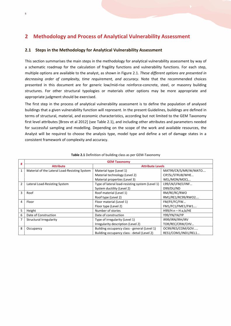
2.1 Steps in the Methodology for Analytical Vulnerability Assessment

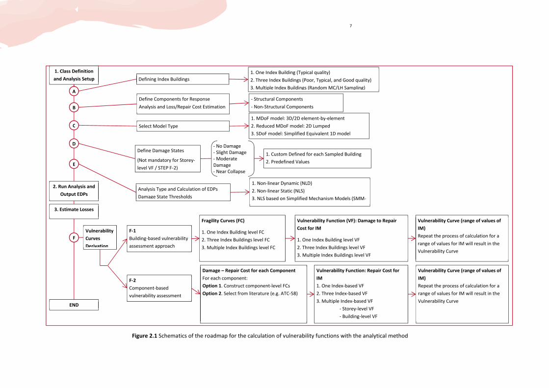
This section summarises the main steps in the methodology for analytical vulnerability assessment by way of

a schematic roadmap for the calculation of fragility functions and vulnerability functions. For each step,

multiple options are available to the analyst, as shown in Figure 2.1. These different options are presented in

decreasing order of complexity, time requirement, and accuracy. Note that the recommended choices

presented in this document are for generic low/mid-rise reinforce-concrete, steel, or masonry building

structures. For other structural typologies or materials other options may be more appropriate and

appropriate judgment should be exercised.

The first step in the process of analytical vulnerability assessment is to define the population of analysed

buildings that a given vulnerability function will represent. In the present Guidelines, buildings are defined in

terms of structural, material, and economic characteristics, according but not limited to the GEM Taxonomy

first level attributes [Brzev et al 2012] (see Table 2.1), and including other attributes and parameters needed

for successful sampling and modelling. Depending on the scope of the work and available resources, the

Analyst will be required to choose the analysis type, model type and define a set of damage states in a

consistent framework of complexity and accuracy.

Table 2.1 Definition of building class as per GEM-Taxonomy

# GEM Taxonomy

Attribute Attribute Levels

1 Material of the Lateral Load-Resisting System Material type (Level 1) MAT99/CR/S/MR/W/MATO….

Material technology (Level 2) CIP/SL/STRUB/WHE…

Material properties (Level 3) WEL/MON/MOCL…

2 Lateral Load-Resisting System Type of lateral load-resisting system (Level 1) L99/LN/LFM/LFINF…

System ductility (Level 2) D99/DU/ND

3 Roof Roof material (Level 1) RM/RE/RC/RWO

Roof type (Level 2) RM1/RE1/RC99/RWO2….

4 Floor Floor material (Level 1) FM/FE/FC/FW…

Floor type (Level 2) FM1/FC1/FME1/FW1….

5 Height Number of stories H99/H:n – H:a,b/HE

6 Date of Construction Date of construction Y99/YN/YA/YP

7 Structural Irregularity Type of irregularity (Level 1) IR99/IRN/IRH/IRV

Irregularity description (Level 2) TOR/REC/CRW/CHV…

8 Occupancy Building occupancy class - general (Level 1) OC99/RES/COM/GOV…..

Building occupancy class - detail (Level 2) RES1/COM1/IND1/REL1…

7

Figure 2.1 Schematics of the roadmap for the calculation of vulnerability functions with the analytical method

A

1. Class Definition

and Analysis Setup

2. Run Analysis and

Output EDPs

3. Estimate Losses

Defining Index Buildings

B

C

E

Analysis Type and Calculation of EDPs

Damage State Thresholds

Select Model Type

Define Damage States

(Not mandatory for Storey-

level VF / STEP F-2)

F-1

Building-based vulnerability

assessment approach

1. One Index Building (Typical quality)

2. Three Index Buildings (Poor, Typical, and Good quality)

3. Multiple Index Buildings (Random MC/LH Sampling)

1. Non-linear Dynamic (NLD)

2. Non-linear Static (NLS)

3. NLS based on Simplified Mechanism Models (SMM-

NLS)

1. MDoF model: 3D/2D element-by-element

2. Reduced MDoF model: 2D Lumped

3. SDoF model: Simplified Equivalent 1D model

- No Damage

- Slight Damage

- Moderate

Damage

- Near Collapse

1. Custom Defined for each Sampled Building

2. Predefined Values

D

Define Components for Response

Analysis and Loss/Repair Cost Estimation

F

- Structural Components

- Non-Structural Components

Vulnerability

Curves

Derivation

Fragility Curves (FC)

1. One Index Building level FC

2. Three Index Buildings level FC

3. Multiple Index Buildings level FC

Vulnerability Function (VF): Damage to Repair

Cost for IM

1. One Index Building level VF

2. Three Index Buildings level VF

3. Multiple Index Buildings level VF

F-2

Component-based

vulnerability assessment

Vulnerability Curve (range of values of

IM)

Repeat the process of calculation for a

range of values for IM will result in the

Vulnerability Curve

Damage – Repair Cost for each Component

For each component:

Option 1. Construct component-level FCs

Option 2. Select from literature (e.g. ATC-58)

Vulnerability Function: Repair Cost for

IM

1. One Index-based VF

2. Three Index-based VF

3. Multiple Index-based VF

- Storey-level VF

- Building-level VF

Vulnerability Curve (range of values of

IM)

Repeat the process of calculation for a

range of values for IM will result in the

Vulnerability Curve END

8

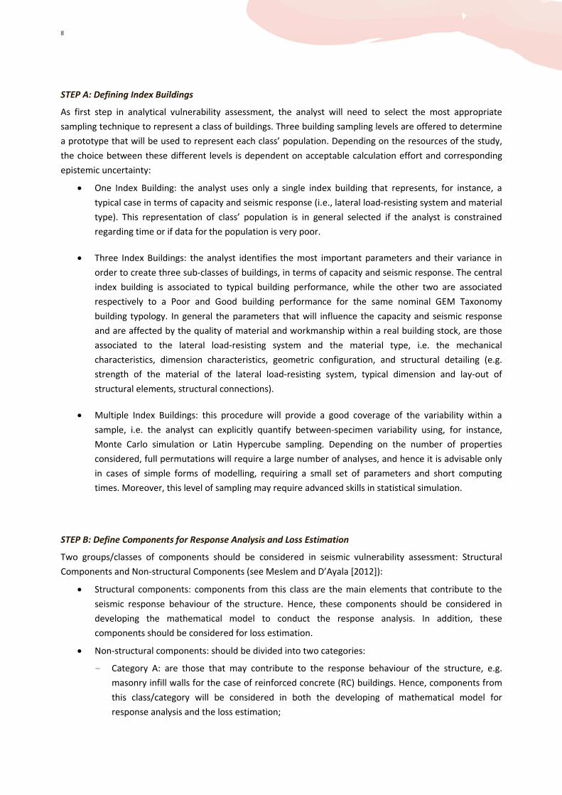
STEP A: Defining Index Buildings

As first step in analytical vulnerability assessment, the analyst will need to select the most appropriate

sampling technique to represent a class of buildings. Three building sampling levels are offered to determine

a prototype that will be used to represent each class’ population. Depending on the resources of the study,

the choice between these different levels is dependent on acceptable calculation effort and corresponding

epistemic uncertainty:

• One Index Building: the analyst uses only a single index building that represents, for instance, a

typical case in terms of capacity and seismic response (i.e., lateral load-resisting system and material

type). This representation of class’ population is in general selected if the analyst is constrained

regarding time or if data for the population is very poor.

• Three Index Buildings: the analyst identifies the most important parameters and their variance in

order to create three sub-classes of buildings, in terms of capacity and seismic response. The central

index building is associated to typical building performance, while the other two are associated

respectively to a Poor and Good building performance for the same nominal GEM Taxonomy

building typology. In general the parameters that will influence the capacity and seismic response

and are affected by the quality of material and workmanship within a real building stock, are those

associated to the lateral load-resisting system and the material type, i.e. the mechanical

characteristics, dimension characteristics, geometric configuration, and structural detailing (e.g.

strength of the material of the lateral load-resisting system, typical dimension and lay-out of

structural elements, structural connections).

• Multiple Index Buildings: this procedure will provide a good coverage of the variability within a

sample, i.e. the analyst can explicitly quantify between-specimen variability using, for instance,

Monte Carlo simulation or Latin Hypercube sampling. Depending on the number of properties

considered, full permutations will require a large number of analyses, and hence it is advisable only

in cases of simple forms of modelling, requiring a small set of parameters and short computing

times. Moreover, this level of sampling may require advanced skills in statistical simulation.

STEP B: Define Components for Response Analysis and Loss Estimation

Two groups/classes of components should be considered in seismic vulnerability assessment: Structural

Components and Non-structural Components (see Meslem and D’Ayala [2012]):

• Structural components: components from this class are the main elements that contribute to the

seismic response behaviour of the structure. Hence, these components should be considered in

developing the mathematical model to conduct the response analysis. In addition, these

components should be considered for loss estimation.

• Non-structural components: should be divided into two categories:

- Category A: are those that may contribute to the response behaviour of the structure, e.g.

masonry infill walls for the case of reinforced concrete (RC) buildings. Hence, components from

this class/category will be considered in both the developing of mathematical model for

response analysis and the loss estimation;

9

- Category B: they do not contribute to the response behaviour of the structure, but they are

considered to be dominant in terms of contribution to construction cost and hence should be

considered in loss estimation.

The remit of the present Guidelines is the fragility assessment and vulnerability function definition of

structural components and whole structure. Hence Structural Components and Category A of the Non-

Structural Components, form the object of the vulnerability assessment of these Guidelines. For the

vulnerability assessment of Category B Non-Structural Components the reader is referred to the relevant

Guidelines (see Porter et al. [2012b]). In addition, for adding the loss of Contents, appropriate guidelines can

be found in (see Porter et al. 2012c).

STEP C: Select Model Type

Three levels of model complexity are proposed (in decreasing order of complexity), offering three distinct

choices of structural detail:

• Multi Degree of Freedom (MDoF) model (3D/2D elements): a detailed 3D or 2D multi-degree-of-

freedom model of a structure, including elements for each identified lateral-load resisting

component in the building, e.g., columns, beams, infills walls, shear walls, URM walls, etc.

• Reduced MDoF model (2D lumped): a simplified 2D lumped stiffness-mass-damping representation

of a building, where each of the N floors (or diaphragms) is represented by one node having 3

degrees of freedom, two translational and one rotational to allow representation of both flexural

and shear types of behaviour. This representation is not suitable for plan-irregular buildings,

buildings where torsional effects are anticipated, or very slender structures.

• Single Degree of Freedom (SDoF) model: a simple SDoF representation by a one-dimensional non-

linear element, for which stiffness, mass damping, and ductility of the structure as a whole are

defined. This representation is in general very simplistic and assumes that higher vibration modes

are not relevant to the seismic response of the structure.

It should be noted that although modelling level 3 is not recommended as a choice of structural modelling,

the simplification to an equivalent degree of freedom system is called upon when computing the

performance point and damage state of a structure in a number of procedures illustrated in Chapter 7 for the

determination of fragility curves. The rationale for following this approach is further discussed in that

context.

All model levels incorporate the following interface variables: (a) seismic input via a scalar seismic intensity

measure (IM) to connect with probabilistic seismic hazard analysis results (e.g. hazard curves), (b) response

output via the Engineering Demand Parameters (EDPs) of individual storey drifts for allowing structural/non-

structural loss estimation.

STEP D: Define Damage States at Element and Global Level

Five levels structural damage states are suggested: No Damage, Slight, Moderate, Near Collapse and

Collapse. Thus four EDPs (i.e. Peak Storey Drift) thresholds are needed to differentiate among the five

damage states. These are inherently random quantities that are generally assumed to be log-normally

distributed and need a median and a dispersion value to be fully defined.

10

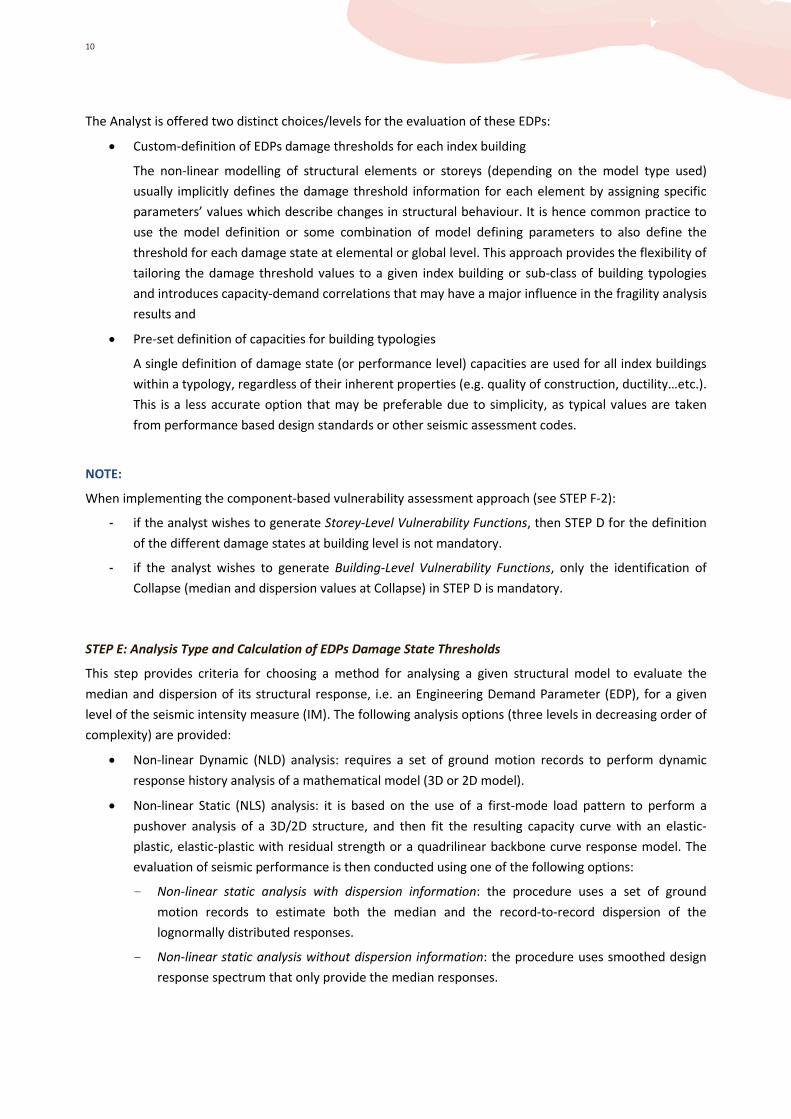
The Analyst is offered two distinct choices/levels for the evaluation of these EDPs:

• Custom-definition of EDPs damage thresholds for each index building

The non-linear modelling of structural elements or storeys (depending on the model type used)

usually implicitly defines the damage threshold information for each element by assigning specific

parameters’ values which describe changes in structural behaviour. It is hence common practice to

use the model definition or some combination of model defining parameters to also define the

threshold for each damage state at elemental or global level. This approach provides the flexibility of

tailoring the damage threshold values to a given index building or sub-class of building typologies

and introduces capacity-demand correlations that may have a major influence in the fragility analysis

results and

• Pre-set definition of capacities for building typologies

A single definition of damage state (or performance level) capacities are used for all index buildings

within a typology, regardless of their inherent properties (e.g. quality of construction, ductility…etc.).

This is a less accurate option that may be preferable due to simplicity, as typical values are taken

from performance based design standards or other seismic assessment codes.

NOTE:

When implementing the component-based vulnerability assessment approach (see STEP F-2):

- if the analyst wishes to generate Storey-Level Vulnerability Functions, then STEP D for the definition

of the different damage states at building level is not mandatory.

- if the analyst wishes to generate Building-Level Vulnerability Functions, only the identification of

Collapse (median and dispersion values at Collapse) in STEP D is mandatory.

STEP E: Analysis Type and Calculation of EDPs Damage State Thresholds

This step provides criteria for choosing a method for analysing a given structural model to evaluate the

median and dispersion of its structural response, i.e. an Engineering Demand Parameter (EDP), for a given

level of the seismic intensity measure (IM). The following analysis options (three levels in decreasing order of

complexity) are provided:

• Non-linear Dynamic (NLD) analysis: requires a set of ground motion records to perform dynamic

response history analysis of a mathematical model (3D or 2D model).

• Non-linear Static (NLS) analysis: it is based on the use of a first-mode load pattern to perform a

pushover analysis of a 3D/2D structure, and then fit the resulting capacity curve with an elastic-

plastic, elastic-plastic with residual strength or a quadrilinear backbone curve response model. The

evaluation of seismic performance is then conducted using one of the following options:

- Non-linear static analysis with dispersion information: the procedure uses a set of ground

motion records to estimate both the median and the record-to-record dispersion of the

lognormally distributed responses.

- Non-linear static analysis without dispersion information: the procedure uses smoothed design

response spectrum that only provide the median responses.

11

• Non-linear Static analysis based on Simplified Mechanical Models (SMM-NLS): non-numerically

based methods. The capacity curve is obtained through simplified analytical or numerical methods

(e.g. a limit-state analysis) which do not require finite elements modelling. Note that this approach

uses smoothed design response spectrum only, hence, the results are exploited without record-to-

record dispersion information.

STEP F: Construction of Vulnerability Curves

Depending on the needs of the study and the availability of data/information, alternatives are offered for the

generation of different types of vulnerability curves:

• vulnerability curve at the level of one index building,

• vulnerability curve at the level of three index buildings, and

• vulnerability curve at the level of multiple index buildings.

In order to generate these curves, two approaches can be used, depending on the level of available

information/data and a specific knowledge, as well as the analyst’s requirements:

• STEP F-1: Building-based vulnerability assessment approach:

The implementation of this approach is suited to studies of large population of buildings. As recommended in

HAZUS-MH [FEMA 2003], the approach consists of generating vulnerability curves by convolving of fragility

curves with the cumulative cost of given damage state ids (damage-to-loss functions). Hence, the analysts

will first need to derive the fragility curves at global building level, or, alternatively, select existing ones from

literature (if available) as long as they can be considered representative of the considered structural typology

performance.

The Guidelines document also provides details regarding the translation of these fragility curves to

loss/repair and replacement cost of new. The analyst might use existing average values of loss/cost, such as

those provided in HAZUS-MH [FEMA 2003], or other references.

• STEP F-2: Component-based vulnerability assessment approach:

In this approach, recommended in ATC-58 [FEMA P-58 2012], the vulnerability functions are obtained by

correlating the components level-based drifts directly to loss. In general, this approach is mostly suitable for

the vulnerability analysis of single buildings, and where the majority of the economic losses are associated to

non-structural components. The analyst will need to ensure that specific knowledge is available and time and

monetary resources are at hand to perform such detailed analysis.

Within this approach, the analyst will have two alternatives in order to estimate loss/cost associated to

damage for each component (i.e., component-level fragility curves and the translation to loss/cost):

- The first alternative requires the availability of necessary data/information to provide a

definition of the performance criteria (e.g. plastic rotation values...etc.) for each structural and

non-structural component and then run analyses to derived component-level fragility curves,

which can then be cumulated to determine overall vulnerability.

- The use of existing average component-level fragility curves, and their associated loss/cost, from

literature. As default source of data, ATC-58 PACT (FEMA P-58 2012), is suggested. The Analysts

12

may also adopt, if available, other sources for the selection of component-level fragility curves if

they are more suited to the real characteristics for the existing buildings in their regions.

In the component-based vulnerability assessment approach, the vulnerability function can be generated at

STOREY LEVEL, and at the ENTIRE BUILDING LEVEL. The generation of Storey-Level vulnerability functions

does not require the definition of different global damage states, i.e. STEP D/Section 6 is not mandatory. The

generation of Building-Level vulnerability functions requires the definition of median collapse capacity only

from STEP D/Section 6.

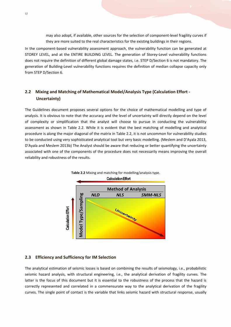
2.2 Mixing and Matching of Mathematical Model/Analysis Type (Calculation Effort -

Uncertainty)

The Guidelines document proposes several options for the choice of mathematical modelling and type of

analysis. It is obvious to note that the accuracy and the level of uncertainty will directly depend on the level

of complexity or simplification that the analyst will choose to pursue in conducting the vulnerability

assessment as shown in Table 2.2. While it is evident that the best matching of modelling and analytical

procedure is along the major diagonal of the matrix in Table 2.2, it is not uncommon for vulnerability studies

to be conducted using very sophisticated analytical tool but very basic modelling. (Meslem and D’Ayala 2013,

D’Ayala and Meslem 2013b) The Analyst should be aware that reducing or better quantifying the uncertainty

associated with one of the components of the procedure does not necessarily means improving the overall

reliability and robustness of the results.

Table 2.2 Mixing and matching for modelling/analysis type.

2.3 Efficiency and Sufficiency for IM Selection

The analytical estimation of seismic losses is based on combining the results of seismology, i.e., probabilistic

seismic hazard analysis, with structural engineering, i.e., the analytical derivation of fragility curves. The

latter is the focus of this document but it is essential to the robustness of the process that the hazard is

correctly represented and correlated in a commensurate way to the analytical derivation of the fragility

curves. The single point of contact is the variable that links seismic hazard with structural response, usually

13

referred to as intensity measure (IM). The IM can be chosen in different ways; however, for the analysis to be

robust, it needs to accurately represent the relevant seismological properties of ground motion to make any

assessment (a) practical (b) efficient and (c) sufficient with respect to the underlying issues related to site and

source [Luco and Cornell 2007]. Given the spatial distribution of the building stock and the relevance of its

exposure, it is practical and advisable to use IMs for which ground motion prediction equations (GMPEs, also

known as attenuation relationships) are available. At the current state of the art, these cover peak ground

acceleration, peak ground velocity, peak ground displacement, and (pseudo) spectral acceleration values.

Efficiency means that EDP response at any given level of the IM should show a reduced record-to-record

variability, thus enabling its evaluation with a small number of time-history analyses without incurring

considerable estimation errors. Finally, the sufficiency requirement stipulates that the IM can “cover” the

effect of any important seismological parameter, thus removing any bias from considering, e.g. ground

motions of different magnitude, distance, fault rupture mechanism, or epsilon. Epsilon represents the

number of standard deviation that a certain ground motion is away from the average for the site and source

parameters that characterize it. It is a measure of how extreme a response a record can cause at a period of

interest. An IM that still leaves the EDP response sensitive to any of these parameters can cause unwanted

bias to creep into vulnerability estimates wherever the ground motion characteristics do not match the

source and site requirements for the building and IM level that is being considered.

Since vulnerability curves are needed for low to high IM levels, a structure needs to be subjected to a wide

range of IM values that will force it to show its full range of response (and losses), from elasticity to global

collapse. Due to limitations in the catalogue of ground motion recordings at a given site or for a given source,

it is often desirable to be able to modify (i.e. scale) a record to display the desired IM level. A sufficient IM

theoretically allows unrestricted scaling of ground motions to match any IM levels. In reality, though, no

single IM is perfect. Therefore, exercising at least a minimum of care in selecting ground motions is advised.

Since vulnerability curves are usually developed to be applicable to wide geographic regions, it is often not

possible to do ground motion selection according to the most recent research findings, using the conditional

mean spectrum proposed by Baker and Cornell, (2008a), or incorporating near source directivity. In general,

is best to use an IM that will allow a wide range of scaling, plus a suite of relatively strong ground motion

records recorded on firm soil. For most applications, the far field suite recommended by FEMA P695 (FEMA,

2009) is a safe choice. Whenever sufficient information exists about the dominant seismic mechanism, range

of magnitudes or soil site in the region for which the vulnerability curve is developed (e.g. crustal

earthquakes in California, low magnitude events in central Europe or soft soil in Mexico City), it may help an

experienced analyst to choose records compatible with the source’s characteristics. More details can be

found in NIST GCR 11-917-15 (NIST, 2011)

The most commonly used IM is spectral acceleration Sa(T), i.e. the 5% damped spectral acceleration at the

period of interest (usually a structure’s first mode period). It is relatively efficient, yet it has often been

criticized for lack in sufficiency wherever large scale factors (higher than, say 3.0) are employed (Luco and

Cornell 2007, Luco and Bazzurro, 2007). This is mainly the case for modern structures that need considerably

intense ground motions to experience collapse. On the other hand, this is rarely the case for older and

deficient buildings. Better efficiency and sufficiency are obtained using the average spectral response

acceleration Sagm(Ti), i.e., the sum of the natural logarithm of spectral acceleration values computed over a

range of Ti values, when compared to Sa(T). It also remains practical as a GMPE for Sagm(Ti) although not

readily available, can be estimated from existing Sa(T) GMPEs. Since Sagm(Ti) offers considerable extension to

the applicability of scaling [Vamvatsikos and Cornell 2005, Bianchini et al. 2010], it is the recommended

14

approach when undertaking non-linear dynamic analysis (e.g., IDA). For non-linear static procedure methods,

the reduction of the structural response to an equivalent SDoF means that Sa(T1) is used by default.

3 STEP A: Defining Index Buildings

This section guides the analyst to the choice of the most appropriate sampling technique to represent a class

of buildings for analytical vulnerability estimation depending on the resources of the study. The choice

between these different methods is dependent on the calculation effort available and the level of acceptable

epistemic uncertainty.

Three levels/methods for building sampling are offered to identify and create a set of classes within a

building population: One Index Building, Three Index Buildings, and Multiple Index Buildings. For the

implementation of either of these different sampling methods, it is important to identify the most important

parameters, more specifically, those accounting for the lateral load-resisting system (structural elements)

and its material, as they highly influence building capacity and seismic response, and maybe subject to

considerable scatter due to the quality of workmanship and original materials.

In more details, the parameters that should be considered are those associated to the mechanical

characteristics, dimension characteristics, geometric configuration, and structural detailing as categorised in

Table 3.1.

It is important to ensure that each index building is defined in such a way to be comprehensively

representative of the building stock population; which can be achieved by defining a Central Value with

Lower Bound and Upper Bound values for each or many of the parameters in Table 3.1, as to reach a realistic

distribution of characteristics membership, even though this might not be normalised, as shown in Figure

3.1. This requires some statistical information for the structural characteristics-based parameters, i.e. such as

a mean or median value for each parameter and a most probable range of existence, if not a standard

deviation.

Table 3.1 Example of parameters characterizing building capacity and seismic response

Type of Parameter Examples

Mechanical Characteristics Strength of the material of the lateral load-resisting system

Dimension Characteristics Total height / Storey height

Number of storeys

Plan dimensions - Bay length

Structural Detailing Tie spacing at the column

Reinforcement ratio at the column

Hardening ratio of steel

Geometric Configuration Perimeter Frame Building - Space Frame Building (PFB/SFB)

Rigid Roof / Deformable Roof (RR/DR)

Column orientation (OR)

15

Table 3.2 Asset definition of One Index Building considering building-to-building variability: Typical Quality (see also Table 3.1)

Typical Quality

Lower Bound Central Value Upper Bound Standard Deviation

Mechanical Characteristics

Dimension Characteristics

Structural Detailing

Geometry Characteristics

Table 3.3 Asset definition of Three Index Buildings considering building-to-building variability: Poor, Typical, and Good Quality (see also Table 3.1)

Poor Quality Typical Quality Good Quality

Lower

Bound

Central

Value

Upper

Bound

Standard

Deviation

Lower

Bound

Central

Value

Upper

Bound

Standard

Deviation

Lower

Bound

Central

Value

Upper

Bound

Standard

Deviation

Mechanical

Characteristics

Dimension

Characteristics

Structural Detailing

Geometry

Characteristics

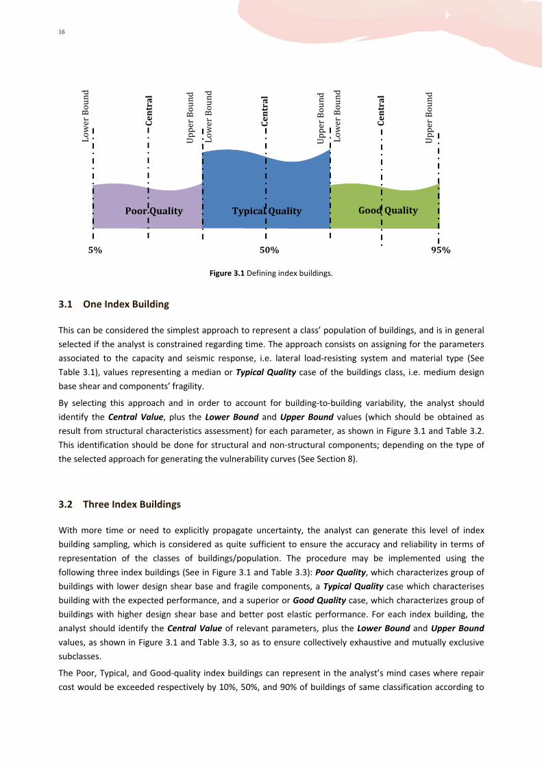
16

Figure 3.1 Defining index buildings.

3.1 One Index Building

This can be considered the simplest approach to represent a class’ population of buildings, and is in general

selected if the analyst is constrained regarding time. The approach consists on assigning for the parameters

associated to the capacity and seismic response, i.e. lateral load-resisting system and material type (See

Table 3.1), values representing a median or Typical Quality case of the buildings class, i.e. medium design

base shear and components’ fragility.

By selecting this approach and in order to account for building-to-building variability, the analyst should

identify the Central Value, plus the Lower Bound and Upper Bound values (which should be obtained as

result from structural characteristics assessment) for each parameter, as shown in Figure 3.1 and Table 3.2.

This identification should be done for structural and non-structural components; depending on the type of

the selected approach for generating the vulnerability curves (See Section 8).

3.2 Three Index Buildings

With more time or need to explicitly propagate uncertainty, the analyst can generate this level of index

building sampling, which is considered as quite sufficient to ensure the accuracy and reliability in terms of

representation of the classes of buildings/population. The procedure may be implemented using the

following three index buildings (See in Figure 3.1 and Table 3.3): Poor Quality, which characterizes group of

buildings with lower design shear base and fragile components, a Typical Quality case which characterises

building with the expected performance, and a superior or Good Quality case, which characterizes group of

buildings with higher design shear base and better post elastic performance. For each index building, the

analyst should identify the Central Value of relevant parameters, plus the Lower Bound and Upper Bound

values, as shown in Figure 3.1 and Table 3.3, so as to ensure collectively exhaustive and mutually exclusive

subclasses.

The Poor, Typical, and Good-quality index buildings can represent in the analyst’s mind cases where repair

cost would be exceeded respectively by 10%, 50%, and 90% of buildings of same classification according to

Typical Quality Poor Quality Good Quality

Ce

ntr

al

Lo

we

r B

ou

nd

Up

pe

r B

ou

nd

Ce

ntr

al

Lo

we

r B

ou

nd

Ce

ntr

al

Up

pe

r B

ou

nd

Lo

we

r B

ou

nd

Up

pe

r B

ou

nd

5% 50% 95%

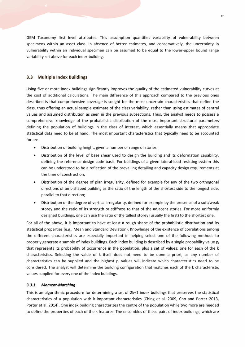
17

GEM Taxonomy first level attributes. This assumption quantifies variability of vulnerability between

specimens within an asset class. In absence of better estimates, and conservatively, the uncertainty in

vulnerability within an individual specimen can be assumed to be equal to the lower-upper bound range

variability set above for each index building.

3.3 Multiple Index Buildings

Using five or more index buildings significantly improves the quality of the estimated vulnerability curves at

the cost of additional calculations. The main difference of this approach compared to the previous ones

described is that comprehensive coverage is sought for the most uncertain characteristics that define the

class, thus offering an actual sample estimate of the class variability, rather than using estimates of central

values and assumed distribution as seen in the previous subsections. Thus, the analyst needs to possess a

comprehensive knowledge of the probabilistic distribution of the most important structural parameters

defining the population of buildings in the class of interest, which essentially means that appropriate

statistical data need to be at hand. The most important characteristics that typically need to be accounted

for are:

• Distribution of building height, given a number or range of stories;

• Distribution of the level of base shear used to design the building and its deformation capability,

defining the reference design code basis. For buildings of a given lateral-load resisting system this

can be understood to be a reflection of the prevailing detailing and capacity design requirements at

the time of construction;

• Distribution of the degree of plan irregularity, defined for example for any of the two orthogonal

directions of an L-shaped building as the ratio of the length of the shortest side to the longest side,

parallel to that direction;

• Distribution of the degree of vertical irregularity, defined for example by the presence of a soft/weak

storey and the ratio of its strength or stiffness to that of the adjacent stories. For more uniformly

designed buildings, one can use the ratio of the tallest storey (usually the first) to the shortest one.

For all of the above, it is important to have at least a rough shape of the probabilistic distribution and its

statistical properties (e.g., Mean and Standard Deviation). Knowledge of the existence of correlations among

the different characteristics are especially important in helping select one of the following methods to

properly generate a sample of index buildings. Each index building is described by a single probability value pi

that represents its probability of occurrence in the population, plus a set of values: one for each of the k

characteristics. Selecting the value of k itself does not need to be done a priori, as any number of

characteristics can be supplied and the highest pi values will indicate which characteristics need to be

considered. The analyst will determine the building configuration that matches each of the k characteristic

values supplied for every one of the index buildings.

3.3.1 Moment-Matching

This is an algorithmic procedure for determining a set of 2k+1 index buildings that preserves the statistical

characteristics of a population with k important characteristics [Ching et al. 2009, Cho and Porter 2013,

Porter et al. 2014]. One index building characterizes the centre of the population while two more are needed

to define the properties of each of the k features. The ensembles of these pairs of index buildings, which are

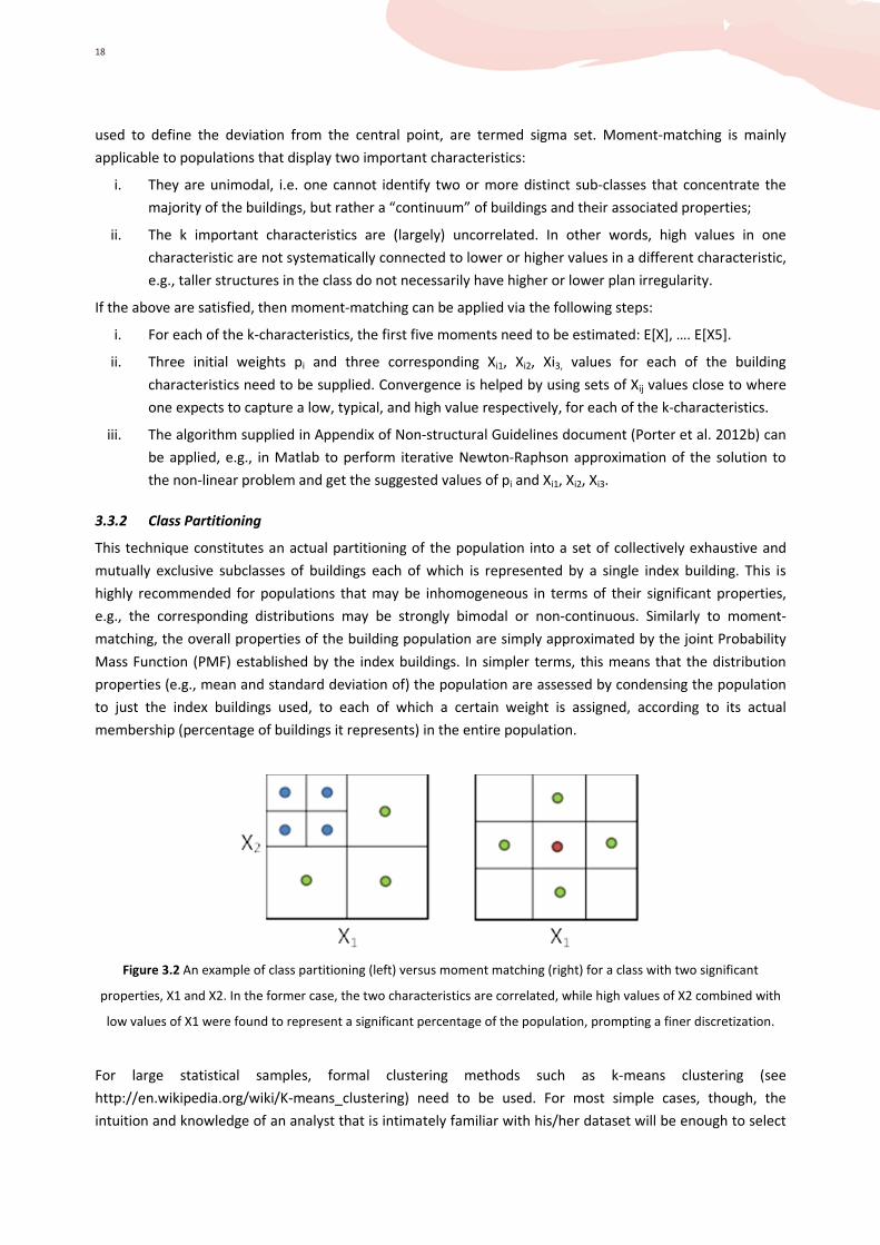
18

used to define the deviation from the central point, are termed sigma set. Moment-matching is mainly

applicable to populations that display two important characteristics:

i. They are unimodal, i.e. one cannot identify two or more distinct sub-classes that concentrate the

majority of the buildings, but rather a “continuum” of buildings and their associated properties;

ii. The k important characteristics are (largely) uncorrelated. In other words, high values in one

characteristic are not systematically connected to lower or higher values in a different characteristic,

e.g., taller structures in the class do not necessarily have higher or lower plan irregularity.

If the above are satisfied, then moment-matching can be applied via the following steps:

i. For each of the k-characteristics, the first five moments need to be estimated: E[X], …. E[X5].

ii. Three initial weights pi and three corresponding Xi1, Xi2, Xi3, values for each of the building

characteristics need to be supplied. Convergence is helped by using sets of Xij values close to where

one expects to capture a low, typical, and high value respectively, for each of the k-characteristics.

iii. The algorithm supplied in Appendix of Non-structural Guidelines document (Porter et al. 2012b) can

be applied, e.g., in Matlab to perform iterative Newton-Raphson approximation of the solution to

the non-linear problem and get the suggested values of pi and Xi1, Xi2, Xi3.

3.3.2 Class Partitioning

This technique constitutes an actual partitioning of the population into a set of collectively exhaustive and

mutually exclusive subclasses of buildings each of which is represented by a single index building. This is

highly recommended for populations that may be inhomogeneous in terms of their significant properties,

e.g., the corresponding distributions may be strongly bimodal or non-continuous. Similarly to moment-

matching, the overall properties of the building population are simply approximated by the joint Probability

Mass Function (PMF) established by the index buildings. In simpler terms, this means that the distribution

properties (e.g., mean and standard deviation of) the population are assessed by condensing the population

to just the index buildings used, to each of which a certain weight is assigned, according to its actual

membership (percentage of buildings it represents) in the entire population.

Figure 3.2 An example of class partitioning (left) versus moment matching (right) for a class with two significant

properties, X1 and X2. In the former case, the two characteristics are correlated, while high values of X2 combined with

low values of X1 were found to represent a significant percentage of the population, prompting a finer discretization.

For large statistical samples, formal clustering methods such as k-means clustering (see

http://en.wikipedia.org/wiki/K-means_clustering) need to be used. For most simple cases, though, the

intuition and knowledge of an analyst that is intimately familiar with his/her dataset will be enough to select

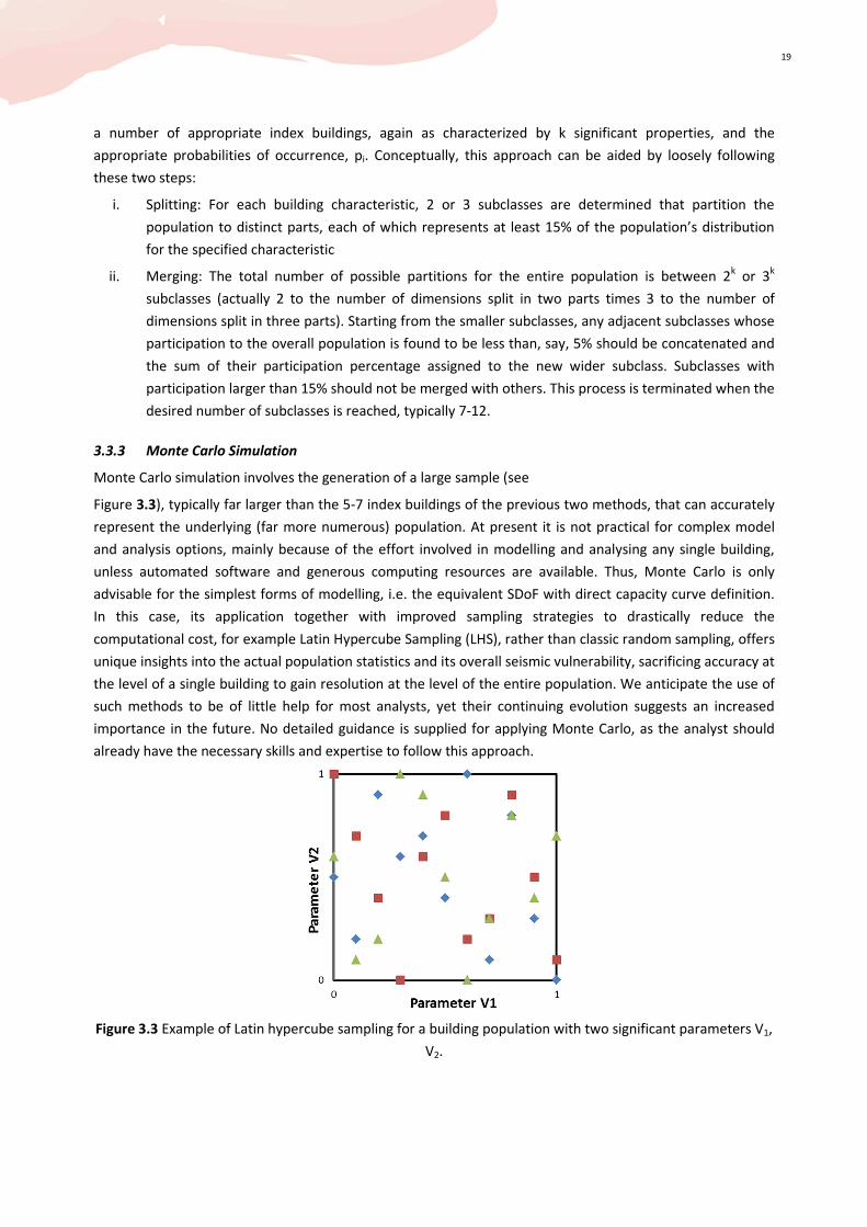
19

a number of appropriate index buildings, again as characterized by k significant properties, and the

appropriate probabilities of occurrence, pi. Conceptually, this approach can be aided by loosely following

these two steps:

i. Splitting: For each building characteristic, 2 or 3 subclasses are determined that partition the

population to distinct parts, each of which represents at least 15% of the population’s distribution

for the specified characteristic

ii. Merging: The total number of possible partitions for the entire population is between 2k or 3

k

subclasses (actually 2 to the number of dimensions split in two parts times 3 to the number of

dimensions split in three parts). Starting from the smaller subclasses, any adjacent subclasses whose

participation to the overall population is found to be less than, say, 5% should be concatenated and

the sum of their participation percentage assigned to the new wider subclass. Subclasses with

participation larger than 15% should not be merged with others. This process is terminated when the

desired number of subclasses is reached, typically 7-12.

3.3.3 Monte Carlo Simulation

Monte Carlo simulation involves the generation of a large sample (see

Figure 3.3), typically far larger than the 5-7 index buildings of the previous two methods, that can accurately

represent the underlying (far more numerous) population. At present it is not practical for complex model

and analysis options, mainly because of the effort involved in modelling and analysing any single building,

unless automated software and generous computing resources are available. Thus, Monte Carlo is only

advisable for the simplest forms of modelling, i.e. the equivalent SDoF with direct capacity curve definition.

In this case, its application together with improved sampling strategies to drastically reduce the

computational cost, for example Latin Hypercube Sampling (LHS), rather than classic random sampling, offers

unique insights into the actual population statistics and its overall seismic vulnerability, sacrificing accuracy at

the level of a single building to gain resolution at the level of the entire population. We anticipate the use of

such methods to be of little help for most analysts, yet their continuing evolution suggests an increased

importance in the future. No detailed guidance is supplied for applying Monte Carlo, as the analyst should

already have the necessary skills and expertise to follow this approach.

Figure 3.3 Example of Latin hypercube sampling for a building population with two significant parameters V1,

V2.

20

4 STEP B: Define Components for Response Analysis and Loss Estimation

A complete seismic vulnerability assessment of an asset or a building class or building stock, typically includes

the evaluation of the structural response to the expected hazards and computes the consequences of such

response, in terms of monetary losses accrued by damage to structural, non-structural component and

contents and, human losses, including casualties and fatalities. The remit of this Guidelines covers mainly the

loss associated to structural damage of structural components, while for a more detailed treatment of the

procedure used to establishes losses accruing from damage to non-structural components, content and

human casualties, the analyst is directed to the specific companion Guidelines in the GEM repository.

In the following we present the basic criteria to distinguish components in structural and non-structural and

reasons for inclusion in or exclusion from the structural analysis and fragility curve construction. For each

component the relevant attributes and parameters that affect the quality of the analysis and the estimation

of fragility and vulnerability are also included (see Meslem and D’Ayala 2012).

Within an asset construction two fundamental sets of component can be distinguished: Structural

Components, and Non-structural Components:

• Structural components: components from this class are the main elements that contribute to the

response behaviour of the structure. Hence, these components will be considered in developing the

mathematical model to conduct the response analysis. In addition, the components will be

considered for loss estimation.

• Non-structural components: they can be divided into two categories:

- Category A: are those that may contribute to the response behaviour of the structure, e.g.

masonry infill walls for the case of reinforced concrete (RC) buildings. Hence, components from

this class/category will be considered in both, the development of mathematical model for

response analysis and the loss estimation;

- Category B: they do not contribute to the response behaviour of the structure, but they are

considered to be dominant in terms of contribution to reconstruction cost.

Figure 4.1 Definition of structural and non-structural components for response analysis and loss estimation

Selected Index Building

Structural Components Non-structural Components

Numerical Modelling and Response Analysis

Loss Estimation

Category A

(e.g. masonry infills)

Category B

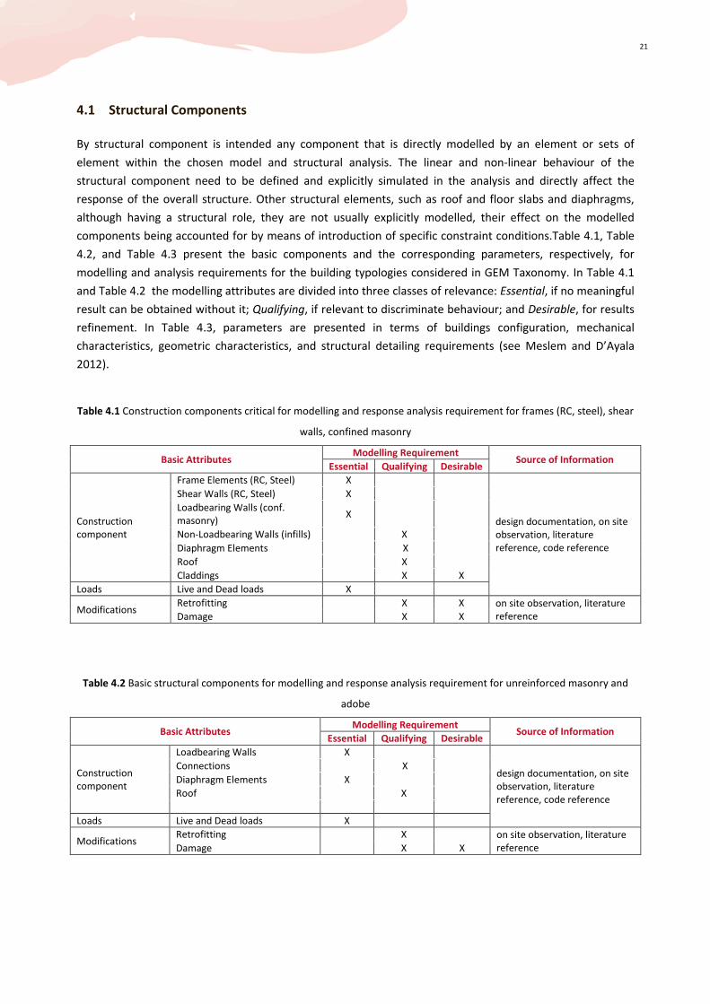
21

4.1 Structural Components

By structural component is intended any component that is directly modelled by an element or sets of

element within the chosen model and structural analysis. The linear and non-linear behaviour of the

structural component need to be defined and explicitly simulated in the analysis and directly affect the

response of the overall structure. Other structural elements, such as roof and floor slabs and diaphragms,

although having a structural role, they are not usually explicitly modelled, their effect on the modelled

components being accounted for by means of introduction of specific constraint conditions.Table 4.1, Table

4.2, and Table 4.3 present the basic components and the corresponding parameters, respectively, for

modelling and analysis requirements for the building typologies considered in GEM Taxonomy. In Table 4.1

and Table 4.2 the modelling attributes are divided into three classes of relevance: Essential, if no meaningful

result can be obtained without it; Qualifying, if relevant to discriminate behaviour; and Desirable, for results

refinement. In Table 4.3, parameters are presented in terms of buildings configuration, mechanical

characteristics, geometric characteristics, and structural detailing requirements (see Meslem and D’Ayala

2012).

Table 4.1 Construction components critical for modelling and response analysis requirement for frames (RC, steel), shear

walls, confined masonry

Basic Attributes Modelling Requirement

Source of Information Essential Qualifying Desirable

Construction

component

Frame Elements (RC, Steel) X

design documentation, on site

observation, literature

reference, code reference

Shear Walls (RC, Steel) X

Loadbearing Walls (conf.

masonry) X

Non-Loadbearing Walls (infills) X

Diaphragm Elements X

Roof X

Claddings X X

Loads Live and Dead loads X

Modifications Retrofitting X X on site observation, literature

reference Damage X X

Table 4.2 Basic structural components for modelling and response analysis requirement for unreinforced masonry and

adobe

Basic Attributes Modelling Requirement

Source of Information Essential Qualifying Desirable

Construction

component

Loadbearing Walls X

design documentation, on site

observation, literature

reference, code reference

Connections X

Diaphragm Elements X

Roof X

Loads Live and Dead loads X

Modifications Retrofitting X on site observation, literature

reference Damage X X

22

Table 4.3 Parameters defining components for modelling and response analysis requirement for RC, masonry, and steel

buildings

Basic Attributes Source of Information

Building Configuration and Dimension Number of stories Design

documentation,

Storey heights (floor-to-floor height for the ground floor,

and for other floors) on site observation,

Number of lines (number of bays) and spacing in x-

direction literature reference,

Number of lines (number of frames/walls) and spacing in

y-direction code reference

Mechanical

characteristics Concrete Compressive strength

Modulus of elasticity

Strain at peak stress

Specific weight

Reinforcing Bar Modulus of elasticity

Yield stress

Ultimate stress

Strain hardening parameter

Specific weight

Masonry-infill Compressive strength


Shear strength

Specific weight

Masonry-

loadbearing Compressive strength


Shear strength

Specific weight

Steel Modulus of elasticity

Shear strength

Yield stress

Ultimate stress

Specific weight

Geometry Characteristics Reinforced

concrete

Cross-section dimensions for columns and beams, or shear

walls

and Structural Detailing elements Transversal reinforcement: type and spacing

Longitudinal reinforcement: type and number

Thickness of slabs

Masonry infill

panel Dimensions and thickness of walls

Dimension of opening: windows and doors

Masonry

loadbearing Dimensions and thickness of walls

elements Dimension of opening: windows and doors

Connections with other walls

Steel Cross-section dimensions for columns and beams

Cross-section dimensions for bracing systems

Connection types

23

4.2 Dominant Non-Structural Categories

For the loss estimation purpose, and in addition to the structural components that have been identified in

Table 4.1 and Table 4.2, the analyst should also identify and consider the most dominant non-structural

components contributing to construction cost. An example for the selection and classification of the most

dominant non-structural components is shown in Table 4.4. As per Porter et al. [2013], the identified

dominant non-structural components/losses are as follows:

• Interior partitions

• Exterior closure

• Ceilings

• Heating, ventilation, and air conditioning equipment

• Electrical equipment

• Plumbing equipment

The analyst should be aware that the above list of dominant components might vary substantially among

building types (e.g. in terms of occupancy) and geographically according to living habits and standards. The

analyst should refer to the appropriate sources in each region which may provide additional guidance, e.g. RS

Means [2009] for US buildings.

Table 4.4 Example of ranking of non-structural components in decreasing order of contribution to construction cost.

Non-structural Components

Rank 1 2 3 4 5 6

Component Name Terminal &

package units

Plumbing

fixtures

Lighting

branch wiring Partitions Interior doors Exterior windows

Unit Ea N/A Ea 100 If = 30m Each Each (4’ by 8’ panel)

NISTIR 6389 class ID D3050 D2010 D5020 C1010 C1020 B2020

FEMA P-58 class ID D3052.011d C3034.001 C1011.001d C1020.001 B2022.035

Demand parameter PFA PFA PTD PTD PTD PTD

Ref (default PACT

1.0) PACT 1.0 N/A PACT 1.0 PACT 1.0

Porter

judgment PACT 1.0

Cost per m2 $196 $143 $126 $74 $47 $42

24

5 STEP C: Select Model Type

Structural models can only properly represent a number of failure modes, dependent on the modelling

capabilities of the structural analysis software chosen by the analyst. Thus, a careful distinction of simulated

and non-simulated modes of failure is needed. Non-simulated modes of failure can only be applied a

posteriori during post-processing and their effect may not be “cumulated”: The joint influence of more than

one such element failures that do not occur simultaneously cannot be judged reliably unless they are

included in the structural model itself. The analyst should consider that even advanced sophisticated

modelling may neglect some modes of failure.

Three levels of model complexity are proposed, offering three distinct choices of structural detail:

• MDoF model (3D/2D element-by-element): a detailed 3D or 2D multi-degree-of-freedom model of a

structure, including elements for each identified lateral-load resisting component in the building,

e.g., columns, beams, infills, walls, shear walls, etc.

• MDoF model (2D lumped): a simplified 2D lumped (2D stick) representation of a building, where

each of the N floors (or diaphragms) is represented by one node having 3 to 6 degrees of freedom,

allowing at best, representation of both flexural and shear types of behaviour.

• SDoF model (Simplified equivalent 1D model): a simple SDoF representation by a 1D non-linear

spring.

With regards to the choice of model type, it is clear that the performance of any selected path for

vulnerability assessment will depend upon the sophistication of numerical modelling (i.e. the adopted

materials behaviour, and the simplified assumptions that are made to reduce the calculation efforts…etc.).

Note that any adopted model type should be consistent with the type of analysis implemented. In the

following sections, some advice is provided in relation to the choices and limitation of modelling approaches

(D’Ayala and Meslem 2013a, 2013b, 2013c).

5.1 MDoF Model: 3D/2D Element-by-Element

For the implementation of 3D/2D element-by-element model, the analyst should identify the primary and

secondary elements or components of the building; define the non-structural elements; determine

foundation flexibility, determine level of diaphragm action; define permanent gravity actions (i.e. dead loads,

live loads). The level of detailed modelling of each structural component will depend on the choice of

analysis type selected. If non-linear dynamic analysis is performed, components should be modelled over

their full range of expected deformation response using hysteretic properties based upon test data. Similarly,

when performing non-linear pushover analysis, component strength and stiffness degradation should be

modelled explicitly for each structural component. For all types of analysis, the analyst should use median

values of structural characteristics-related parameters when defining the component behaviour. If median

values are not available, mean values should be used. The analyst should make sure to simulate all possible

modes of component damage and failure (e.g., axial, flexural, flexure-axial interaction, shear, and flexure-

shear interaction), P-Delta effects…etc. Further guidance on detailed component modelling for frame

structures is provided in ASCE/SEI 41-06 [ASCE 2007].The analyst may also refer to the NIST GCR 10-917-5

[NEHRP 2010] and ATC-58 [FEMA P-58 2012] where additional information is provided.

25

For unreinforced masonry structures further guidance maybe found in Eurocode-8 [CEN 2004], D’Ayala and

Speranza [2003].

Ideally, the building should be modelled as three-dimensional. In some cases the analyst may wish to use

two-dimensional (planar) in order to reduce the calculation effort. However, this later may be acceptable

only for buildings with regular geometries where the response in each orthogonal direction is independent

and torsional response is not significant.

It is worth to mention that only engineers well versed in non-linear structural modelling should follow this

approach for vulnerability analysis; it is bound to be quite time-consuming for the average analyst,

depending on the level of complexity of the analysed structure.

Frame / shear wall element modelling procedure

With regard to the choice of finite element for structural frames or flexure-critical shear walls, the analyst

will have the possibility to choose between two analytical modelling procedures for non-linear analysis, fibre-

based structural modelling procedure, and plastic hinge-based structural modelling procedure [D’Ayala and

Meslem 2013b].

Fibre-based structural modelling technique

This technique models a structural element by dividing it into a number of two-end frame elements, and by

linking each boundary to a discrete cross-section with a grid of fibres. The material stress-strain response in

Box 5.1: Development of MDoF model_3D/2D element-by-element

A proper 3D or 2D element-by-element model of the full-scale structure needs to be prepared by considering the

following steps:

Step 1: The choice of a 3D or 2D (planar) model depends on the plan asymmetry characteristics of the building,

3D being most appropriate wherever significant eccentricity exists, e.g. torsion effects;

Step 2: Identify primary and secondary elements or components; define non-structural elements, foundation

flexibility, etc.

Step 3: Each structural element (e.g. beam, column, loadbearing wall) and non-structural element (e.g. masonry

infill panel) should be represented by one or more finite elements;

Step 4: The level of detailed modelling of components will depend on the choice of analysis type that is selected.

If non-linear dynamic analysis is performed, components should be modelled over their full range of expected

deformation response using hysteretic properties based upon test data;

Step 5: For all type of analysis, median values of structural characteristics-related parameters should be used for

models. If median values are not available, mean values should be used;

Step 6: Make sure to simulate all possible modes of component deformation and failure (e.g., axial, flexure,

flexure-axial interaction, shear, and flexure-shear interaction), P-Delta effects…etc.;

Step 7: Define carefully all permanent gravity actions, i.e. dead loads, live loads.

26

each fibre is integrated to get stress-resultant forces and stiffness terms, and from these, forces and stiffness

over the length are obtained through finite element interpolation functions which must satisfy equilibrium

and compatibility conditions. Example of implementation of fibre modelling for the case of RC member is

shown in Figure 5.1.

Figure 5.1 Idealisation into fibres of reinforced concrete (RC) members. This numerical technique allows characterizing in

higher detail, the non-linearity distribution in RC elements by modelling separately the different behaviour of the

materials constituting the RC cross-section (.i.e. cover and core concrete and longitudinal steel) and, hence, to capture

more accurately response effects.

Plastic Hinge-based Structural Modelling.

This technique uses the assumption of the concentrated or distributed plasticity zones for the structural

elements, with corresponding plastic hinges formation. The lumped hinge model is applied for cases where

the yielding will most probably occur at the member ends, unlikely along a member. The distributed hinge

model is applied for cases where the yielding may occur along a member [CSI 2009].

It should be noted that in general both approaches outlined above, while they provide a reliable simulation

of flexural mode of failure (both) and combined axial and flexural mode of failure (mainly fibre models), they

do not simulate the through-depth shear and the mode of failure associated with it, neither the reduction in

flexural capacity due to combined shear and bending. For components which are expected to be subjected to

Box 5.2: Fibre-based numerical technique

Fibre-based numerical technique can be implemented by considering the following steps:

Step 1: Define number of section fibres used in equilibrium computations. It is important to ensure that the

selected number is sufficient to guarantee an adequate reproduction of the stress-strain distribution across the

element's cross-section. Actually, the required number of section fibres varies with the shape and material

characteristics of the cross-section, depending also on the degree of inelasticity to which the element will be

forced to;

Step 2: Define number of integration sections. The analyst may adopt a number between 4 and 7 integration

sections. Up to 7 integrations sections may be needed to accurately model hardening response, but, on the other

hand, 4 or 5 integration sections may be advisable when it is foreseen that the elements will reach their

softening response range.

The analyst may refer to the literature for further guidance.

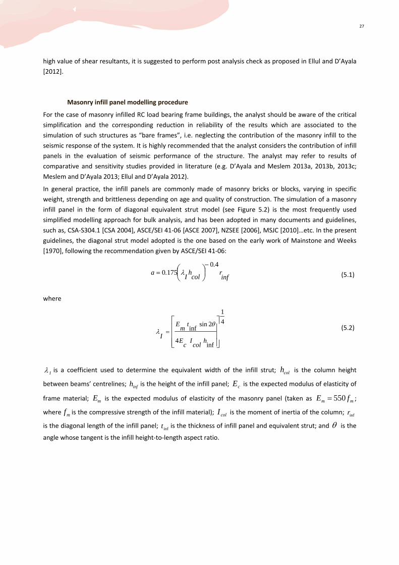
27

high value of shear resultants, it is suggested to perform post analysis check as proposed in Ellul and D’Ayala

[2012].

Masonry infill panel modelling procedure

For the case of masonry infilled RC load bearing frame buildings, the analyst should be aware of the critical

simplification and the corresponding reduction in reliability of the results which are associated to the

simulation of such structures as “bare frames”, i.e. neglecting the contribution of the masonry infill to the

seismic response of the system. It is highly recommended that the analyst considers the contribution of infill

panels in the evaluation of seismic performance of the structure. The analyst may refer to results of

comparative and sensitivity studies provided in literature (e.g. D’Ayala and Meslem 2013a, 2013b, 2013c;

Meslem and D’Ayala 2013; Ellul and D’Ayala 2012).

In general practice, the infill panels are commonly made of masonry bricks or blocks, varying in specific

weight, strength and brittleness depending on age and quality of construction. The simulation of a masonry

infill panel in the form of diagonal equivalent strut model (see Figure 5.2) is the most frequently used

simplified modelling approach for bulk analysis, and has been adopted in many documents and guidelines,

such as, CSA-S304.1 [CSA 2004], ASCE/SEI 41-06 [ASCE 2007], NZSEE [2006], MSJC [2010]…etc. In the present

guidelines, the diagonal strut model adopted is the one based on the early work of Mainstone and Weeks

[1970], following the recommendation given by ASCE/SEI 41-06:

infr

.

colh

I.a

401750

−=

λ (5.1)

where

4

1

inf 4

2sin inf

=

hcol

Ic

E

tm

E

I

θλ

(5.2)

Iλ is a coefficient used to determine the equivalent width of the infill strut; colh is the column height

between beams’ centrelines; infh is the height of the infill panel; cE is the expected modulus of elasticity of

frame material; mE is the expected modulus of elasticity of the masonry panel (taken as mm fE 550= ;

where mf is the compressive strength of the infill material); colI is the moment of inertia of the column; infr

is the diagonal length of the infill panel; inft is the thickness of infill panel and equivalent strut; and θ is the

angle whose tangent is the infill height-to-length aspect ratio.

28

Figure 5.2 Diagonal strut model for masonry infill panel modelling

It is worth to mention that in the literature many models of infill panel have been proposed in an attempt to

improve the simulation of the real behaviour of infilled frames. More details and a comparative analysis to

show variance associated to these models are provided in Meslem and D’Ayala [2012], D’Ayala and Meslem

[2013b] and in Asteris et al [2011].

Unreinforced Masonry modelling procedure

Modelling procedures for the structural analysis of unreinforced masonry structures can be classified

following two criteria: the first defines the scale of the analysis, whether the modelling focus is on material

behaviour or structural element behaviour (micro modelling or meso modelling); the second defines the type

of interaction among the component materials, leading to the simulation of a continuum or discrete model.

For the computation of capacity curves for masonry structures a number of procedures are available in

literature. These are based either on the equivalent frame approach or on the macro-elements’ kinematics

approach. Among the first, in the past decade a relatively significant number of procedures aimed at defining

reliable analytical vulnerability function for masonry structures in urban context have been published [Lang

and Bachmann 2004; Erberick 2008; Borzi et al. 2008; Erdik et al. 2003]. Although they share similar

conceptual hypotheses, they differ by modelling complexity, numerical complexity, and treatment of

uncertainties. Far fewer are the approaches based on limit state and mechanism behaviour, and among

those it is worth mentioning VULNUS [Bernardini et al. 2000] and FaMIVE [D’Ayala and Speranza 2003].

Incremental dynamic analysis can in theory be used for equivalent frame procedures, however usually, given

the geometric complexity of real structures, epistemic uncertainty on material constitutive laws and difficulty

in representing masonry hysteretic behaviour, it is advisable to use push-over analysis or limit state

kinematic approach, especially if the simulation entails the vulnerability assessment of a class of buildings,

rather than single buildings, as the computational effort associated with such approaches is rather high.

In the equivalent frame approach, each loadbearing wall contributing to the lateral capacity of the structure

is discretized into a set of masonry panels in which the non-linear behaviour is concentrated [Galasco et al.,

2004; Roca et al. 2005]. The masonry panels are modelled as bi-linear beam elements, the shear damage

being controlled by a Turnsek and Cacovic [1970] criterion, in which the ultimate shear is defined as follows:

0

00 5.1

15.1τ

στ +=

b

ltVt (5.3)

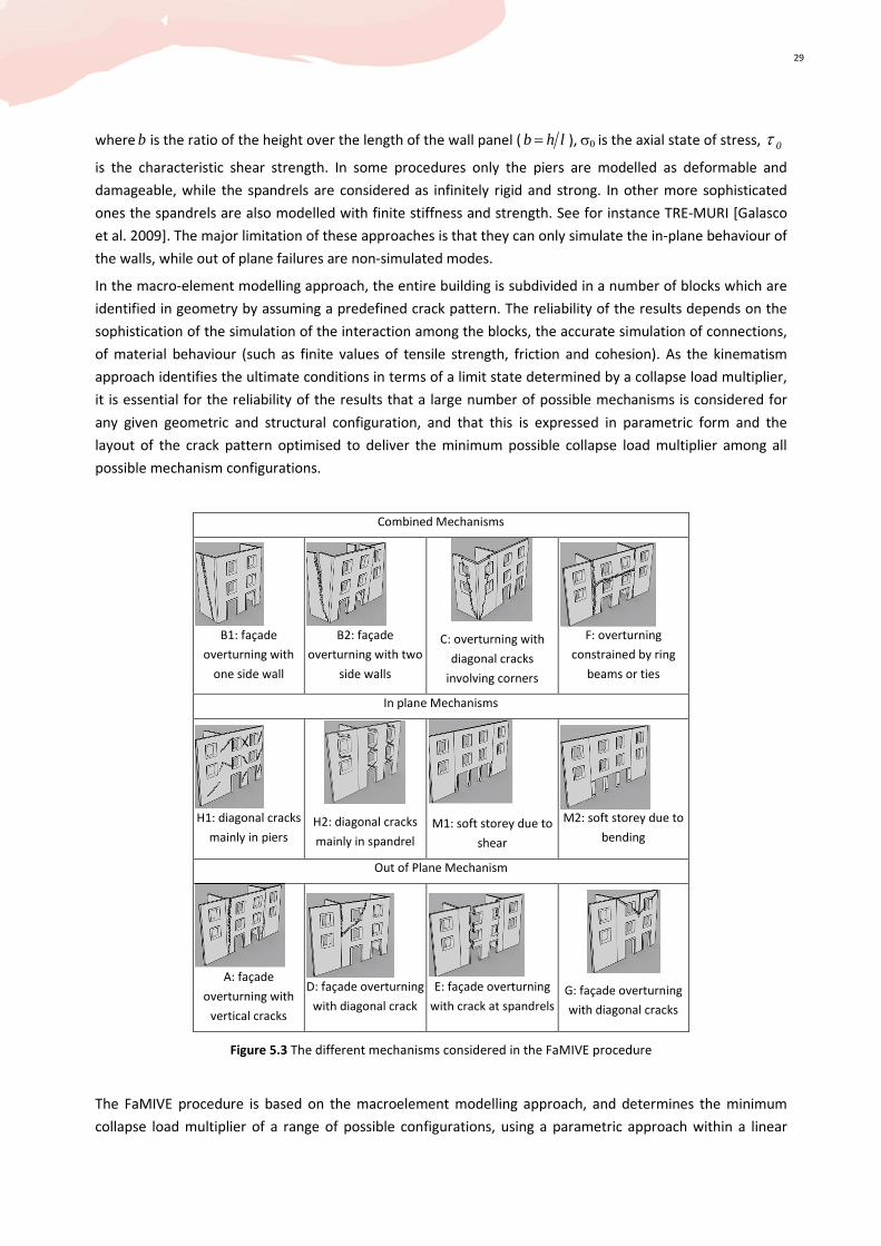
29

where b is the ratio of the height over the length of the wall panel ( lhb = ), σ0 is the axial state of stress, 0τ

is the characteristic shear strength. In some procedures only the piers are modelled as deformable and

damageable, while the spandrels are considered as infinitely rigid and strong. In other more sophisticated

ones the spandrels are also modelled with finite stiffness and strength. See for instance TRE-MURI [Galasco

et al. 2009]. The major limitation of these approaches is that they can only simulate the in-plane behaviour of

the walls, while out of plane failures are non-simulated modes.

In the macro-element modelling approach, the entire building is subdivided in a number of blocks which are

identified in geometry by assuming a predefined crack pattern. The reliability of the results depends on the

sophistication of the simulation of the interaction among the blocks, the accurate simulation of connections,

of material behaviour (such as finite values of tensile strength, friction and cohesion). As the kinematism

approach identifies the ultimate conditions in terms of a limit state determined by a collapse load multiplier,

it is essential for the reliability of the results that a large number of possible mechanisms is considered for

any given geometric and structural configuration, and that this is expressed in parametric form and the

layout of the crack pattern optimised to deliver the minimum possible collapse load multiplier among all

possible mechanism configurations.

Combined Mechanisms

B1: façade

overturning with

one side wall

B2: façade

overturning with two

side walls

C: overturning with

diagonal cracks

involving corners

F: overturning

constrained by ring

beams or ties

In plane Mechanisms

H1: diagonal cracks

mainly in piers

H2: diagonal cracks

mainly in spandrel

M1: soft storey due to

shear

M2: soft storey due to

bending

Out of Plane Mechanism

A: façade

overturning with

vertical cracks

D: façade overturning

with diagonal crack

E: façade overturning

with crack at spandrels

G: façade overturning

with diagonal cracks

Figure 5.3 The different mechanisms considered in the FaMIVE procedure

The FaMIVE procedure is based on the macroelement modelling approach, and determines the minimum

collapse load multiplier of a range of possible configurations, using a parametric approach within a linear

30

programming optimisation technique, implemented within an Excel VBA environment. The procedure

considers both in-plane and out of plane mechanisms as shown in Figure 5.3. The analyst is referred to

D’Ayala and Speranza [2003], Casapulla and D’Ayala, [2006] for details of the analytical formulation of each

mechanism.

The FaMIVE procedure allows to retain a high level of detail of the geometry and kinematics of the problem.

At the same time, because it computes only the ultimate condition, it does not require the computing and

time demands of a typical pushover analysis incremental approach. Once the ultimate conditions are

defined, an idealised capacity curve is obtained considering an equivalent single degree of freedom.

5.2 Reduced MDoF Model: 2D Lumped

As seen in the previous section, appropriate component level modelling requires advanced structural skills

and it is a critical aspect of the vulnerability estimation. When data is not very accurate and or resources are

modest, it might be worth to adopt a reduced MDOF model employing storey-level, rather than component-

level, characterization of mass, stiffness and strength. It should be noted that substantial approximations are

made in adopting these models, in the determination of storey level mass stiffness and strength, which

assume either an average or homogenous behaviour of single components. This may affect substantially the

global failure modes. The advantage is that such models can be analysed within a few seconds using either

non-linear dynamic or static methods. These simplified modelling techniques are only appropriate for

structures having (a) rigid diaphragms (b) no appreciable plan asymmetries in mass/stiffness/strength (c)

relatively uniform bay characteristics (length, stiffness, strength) within each floor, and (d) total building

height over width ratio that is less than 3. The analyst can choose between two approaches:

Stick Models

The basic idea stems from the use of fishbone models [Luco et al 2003, Nakashima et al 2002] to represent

moment-resisting frame buildings using only a single column-line with rotational restrictions for each floor

owing to the presence of beams. This idea is hereby simplified and standardized to cover different structural

moment resisting framed systems.

The concept is presented in Figure 5.4. It comprises N nodes for N stories, each with 3 degrees of freedom

(horizontal, vertical, rotational) in 2D space. The nodes are connected by N columns in series and further

restrained rotationally by N springs representing the strength and stiffness of beams at each floor. All

elements are non-linear, at the very minimum having a simple elastic-perfectly-plastic force-deformation (or

moment-rotation) behaviour with an ultimate (capping) ductility limit (or a dramatic loss of strength) that is

explicitly modelled. Element characteristics can be derived using the aggregate stiffness of the

columns/piers/walls/beams in each storey together with the corresponding yield and ultimate displacements

or rotations.

Columns may be modelled using lumped-plasticity or distributed-plasticity force-based beam-column

elements. Displacement-based elements are not recommended unless every single column is represented by

at least four such elements, with the ones closer to the ends being considerably smaller to allow for a reliable

localization of deformation. In all cases, for each storey-level column the user needs to define the moment-

rotation characteristics of the element section. Thus, assuming a capped elastic-plastic model (see Figure 5.5)

at the very minimum, together with a lumped plasticity column representation, each storey of a given height

is characterized at minimum by the following parameters:

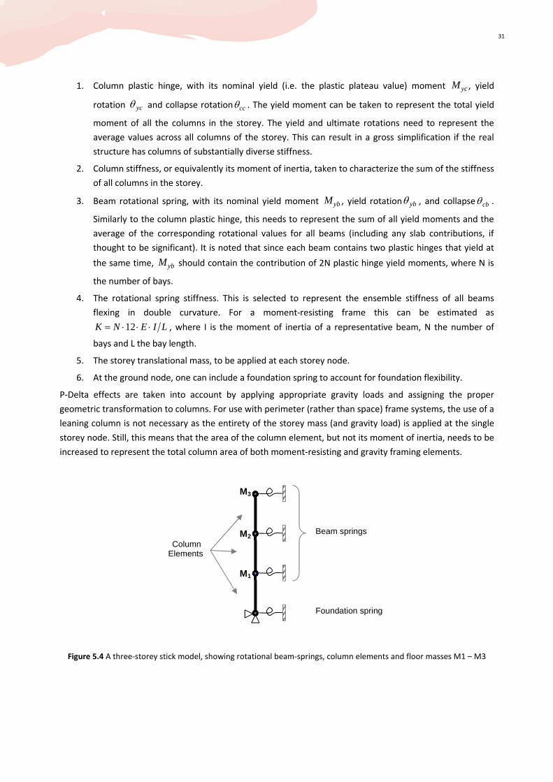
31

1. Column plastic hinge, with its nominal yield (i.e. the plastic plateau value) moment ycM , yield

rotation ycθ and collapse rotation ccθ . The yield moment can be taken to represent the total yield

moment of all the columns in the storey. The yield and ultimate rotations need to represent the

average values across all columns of the storey. This can result in a gross simplification if the real

structure has columns of substantially diverse stiffness.

2. Column stiffness, or equivalently its moment of inertia, taken to characterize the sum of the stiffness

of all columns in the storey.

3. Beam rotational spring, with its nominal yield moment ybM , yield rotation ybθ , and collapse cbθ .

Similarly to the column plastic hinge, this needs to represent the sum of all yield moments and the

average of the corresponding rotational values for all beams (including any slab contributions, if

thought to be significant). It is noted that since each beam contains two plastic hinges that yield at

the same time, ybM should contain the contribution of 2N plastic hinge yield moments, where N is

the number of bays.

4. The rotational spring stiffness. This is selected to represent the ensemble stiffness of all beams

flexing in double curvature. For a moment-resisting frame this can be estimated as

LIENK ⋅⋅⋅= 12 , where I is the moment of inertia of a representative beam, N the number of

bays and L the bay length.

5. The storey translational mass, to be applied at each storey node.

6. At the ground node, one can include a foundation spring to account for foundation flexibility.

P-Delta effects are taken into account by applying appropriate gravity loads and assigning the proper

geometric transformation to columns. For use with perimeter (rather than space) frame systems, the use of a

leaning column is not necessary as the entirety of the storey mass (and gravity load) is applied at the single

storey node. Still, this means that the area of the column element, but not its moment of inertia, needs to be

increased to represent the total column area of both moment-resisting and gravity framing elements.

Figure 5.4 A three-storey stick model, showing rotational beam-springs, column elements and floor masses M1 – Μ3

Beam springs

Foundation spring

Column Elements

M3

M2

M1

32

Figure 5.5 Capped elastic-plastic force-deformation (or moment-rotation) relationship

In general, stick models are not recommended for cases where the building height is larger than three times

its width, as the flexural component of deformation due to column elongation may become important. Still,

this is not considered an issue for most low/mid-rise buildings. When dual systems are to be modelled, e.g.

systems where both structural walls or braces and moment-frames significantly contribute to lateral stiffness

and strength, it is advised to employ two stick models side-by-side, connected by horizontal translation

constraints to represent the rigid diaphragm.

Single-bay frame:

Whenever it is desirable to further distinguish the behaviour of the column springs to their individual

constituents, a single-bay multi-storey frame may be employed instead of a simple stick. Each storey is now

represented by two columns and one connecting beam plus any additional element acting at the storey level,

such as, braces, infills etc. While a complex storey-level element would need to be defined for an equivalent

stick model, the larger number of elements employed by the single-bay model allows an easier way for

defining the behaviour of the storey. For example, braces and infills can be explicitly added by the inclusion

of the proper element(s), as for a proper 2D component-by-component model. Definition of beam and

column characteristics follows exactly the details laid out for the stick model. The only difference is that all

strength and stiffness terms need to be divided equally between the two columns. Similarly, each storey’s

beam has two distinct plastic hinges. Thus each of those should represent the contribution of N beam plastic

hinges, where N is the number of bays.

Such models should still be used with caution wherever the flexural component of deformation becomes

important as they may overestimate its magnitude if the columns are known to have appreciable axial

deformations. This is typically an issue only for high-rise buildings; therefore it is not considered to be

significant within the scope of this document.

The definition of appropriate stick or single-bay models should be assisted by using a small number of

detailed 2D-3D models as reference. This is particularly useful in cases where, for example, non-uniform bays

or several different lateral-load resisting systems are present in each (or any) storey. Using the results of

classical pushover analysis, appropriate beam and column spring properties can be calibrated to create stick

or single-bay models that can help capturing the behaviour of an entire class of structures similar to the

detailed model, with a reduced computational effort. However, attention should be paid to attribution of

realistic values to those springs when modifying the original configuration.

Fy, My

Force, Moment

Displacement, Rotation

δy, θy δc, θc

Significant Strength Loss

33

5.3 SDoF Model: 1D Simplified Equivalent Model

Although a very poor approximation of the real behaviour of the structure, an SDoF equivalent model might

be employed when there are very modest resources or the knowledge of the specific structural characteristic

is so poor that does not warrant the effort of detailed modelling. This becomes possible by adopting

experience-based mechanical models that are able to represent the dominant response characteristics of

specific structural types. Thus, each such model should use analytic expressions or simple calculations to

provide at least:

• the capacity curve of the structure;

• the first mode period and associated mass

• the equivalent stiffness of the system

Additionally, it is also desirable to have a normalized profile for interstorey drift ratios (IDRs) along the height

(i.e., at each story) of the building that can be scaled according to the roof drift corresponding to each point

of the capacity curve computed by the analysis. Having these components allows using the static pushover

based methodologies described earlier. Still, it is not recommended to employ the component-fragility

approach for vulnerability estimation, as the increased uncertainty associated with such simplified modelling

will nullify the advantages of having a more accurate assessment methodology.

There are several methods that use the equivalent SDOF model for low/mid-rise structures. One such

examples is DBELA (Procedure 4.2), described in Section 7.3.2, respectively.

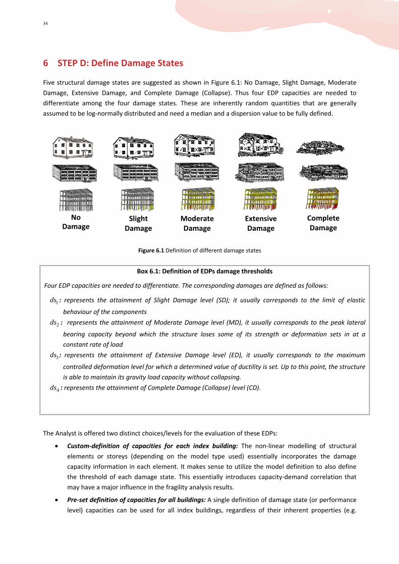
34

6 STEP D: Define Damage States

Five structural damage states are suggested as shown in Figure 6.1: No Damage, Slight Damage, Moderate

Damage, Extensive Damage, and Complete Damage (Collapse). Thus four EDP capacities are needed to

differentiate among the four damage states. These are inherently random quantities that are generally

assumed to be log-normally distributed and need a median and a dispersion value to be fully defined.

Figure 6.1 Definition of different damage states

The Analyst is offered two distinct choices/levels for the evaluation of these EDPs:

• Custom-definition of capacities for each index building: The non-linear modelling of structural

elements or storeys (depending on the model type used) essentially incorporates the damage

capacity information in each element. It makes sense to utilize the model definition to also define

the threshold of each damage state. This essentially introduces capacity-demand correlation that

may have a major influence in the fragility analysis results.

• Pre-set definition of capacities for all buildings: A single definition of damage state (or performance

level) capacities can be used for all index buildings, regardless of their inherent properties (e.g.

Box 6.1: Definition of EDPs damage thresholds

Four EDP capacities are needed to differentiate. The corresponding damages are defined as follows:

1ds : represents the attainment of Slight Damage level (SD); it usually corresponds to the limit of elastic

behaviour of the components

2ds : represents the attainment of Moderate Damage level (MD), it usually corresponds to the peak lateral

bearing capacity beyond which the structure loses some of its strength or deformation sets in at a

constant rate of load

3ds : represents the attainment of Extensive Damage level (ED), it usually corresponds to the maximum

controlled deformation level for which a determined value of ductility is set. Up to this point, the structure

is able to maintain its gravity load capacity without collapsing.

4ds : represents the attainment of Complete Damage (Collapse) level (CD).

Slight

Damage

Moderate

Damage

Extensive

Damage

Complete

Damage

No

Damage

35

quality of construction, ductility…etc.). This is a less accurate option that may be preferable due to

simplicity.

NOTE:

When implementing the component-based vulnerability assessment approach (see STEP F-2):

- if the analyst wishes to generate Storey-Level Vulnerability Functions, then STEP D for the definition

of the different damage states at building level is not mandatory.

- if the analyst wishes to generate Building-Level Vulnerability Functions, only the identification of

Collapse (median and dispersion values at Collapse) in STEP D is mandatory.

6.1 Custom Defined for Each Sampled Building

This option for assessment/ evaluation of different damage states is recommended for analysts with a high

degree of experience and knowledge of structural behaviour. The analyst is advised to refer to the definitions

implemented in ATC-58-2 [ATC, 2003] and Eurocode-8 [CEN 2004], which covers No Damage, Slight,

Moderate, and Extensive Damage. An example of existing definition of limit states for the case of RC building

is shown in Table 6.1. For global Complete Damage (or Collapse state), ATC-58 [FEMA P-58 2012] provides

different definition depending on different possibilities of mechanisms of Collapse (It is worth to mention

that these definitions of Collapse mechanisms were evaluated based on the analysis of RC bare frames only).

Table 6.3 shows examples, from literature, of interstorey drifts values associated to damage states for the

case of RC buildings. For instance:

For the first four damage states, the analyst might refer to the following definitions provided by Dolsek and

Fajfar [2008], to evaluate EDPs and the corresponding IM for the case of RC buildings: No Damage, Damage

Limitation (DL), Significant Damage (SD), and Near Collapse (NC).

• No Damage: No deformation is attained either for infill panels or members;

• Damage Limitation (which may be associated to Slight Damage): for the case of infilled frames: limit

state is attained at the deformation when the last infill in a storey starts to degrade. For the case of

bare frames: this limit state is attained at the yield displacement of the idealized pushover curve

• Significant Damage (which may be associated to Moderate Damage): the most critical column

controls the state of the structure: the limit state is attained when the rotation at one hinge of any

column exceeds 75% of the ultimate rotation;

• Near Collapse (which may be associated to Extensive Damage): the most critical column controls the

state of the structure: the limit state is attained when the rotation at one hinge of any column

exceeds 100% of the ultimate rotation.

For the Collapse level, the analyst might refer to any of the definitions provided by ATC-58 [FEMA P-58 2012]:

• instability occurs in the analysis;

• storey drift exceed non-simulated collapse limits;

• storey drift at which the analytical model is no longer believed to be reliable (examples of values

provided in Table 6.3 for the case of RC buildings).

Table 6.4 provides some definition of different Collapse mechanisms as per ATC-58 [FEMA P-58, 2012].

36

Table 6.1 Example of definition of damage states at global level for RC buildings, as per several existing guidelines Slight Damage Moderate Damage Extensive Damage Complete Damage

ASC

E/S

EI

41

-06

(A

SCE

20

07

); A

TC

-58

-2 (

AT

C 2

00

3),

FEM

A-3

56

(A

SCE

20

00

)

Performance Level Immediate Occupancy (IO) Life Safety (LS) Collapse Prevention (CP) C

on

cre

te F

ram

es Primary

Minor hairline cracking; limited

yielding possible at a few locations;

no crushing (strains below 0.003)

Extensive damage to beams; spalling

of cover and shear cracking (<1/8"

width) for ductile columns; minor

spalling in non-ductile columns; joint

cracks < 1/8" wide.

Extensive cracking and hinge formation in

ductile elements; limited cracking and/or

splice failure in some non-ductile columns;

severe damage in short columns.

Secondary

Minor spalling in a few places in

ductile columns and beams; flexural

cracking in beams and columns; shear

cracking in joints < 1/16" width.

Extensive cracking and hinge

formation in ductile elements; limited

cracking and/or splice failure in some

non-ductile columns; severe damage

in short columns.

Extensive spalling in columns (limited

shortening) and beams; severe joint damage;

some reinforcing buckled.

Un

rein

forc

ed

Ma

son

ry I

nfi

ll

Wa

lls Primary

Minor (<1/8" width) cracking of

masonry infills and veneers; minor

spalling in veneers at a few corner

openings.

Extensive cracking and some crushing

but wall remains in place; no falling

units. Extensive crushing and spalling

of veneers at corners of openings.

Extensive cracking and crushing; portions of

face course shed.

Secondary Same as primary. Same as primary. Extensive crushing and shattering; some walls

dislodge.

AT

C-5

8-2

(A

TC

20

03

), V

isio

n

20

00

(SE

AO

C 1

99

5)

Performance Level Operational Life Safe Near Collapse Collapse

Primary RC Elements

Minor hairline cracking (0.02”);

limited yielding possible at a few

locations; no crushing (strains below

0.003)

Extensive damage to beams; spalling

of cover and shear cracking (<1/8”)

for ductile columns; minor spalling in

non-ductile columns; joints cracked <

1/8” width.

Extensive cracking and hinge formation in

ductile elements; limited cracking and/or

splice failure in some non-ductile columns;

severe damage in short columns.

Partial or total

failure/cracking of

columns and beams

Secondary RC Elements

Same as primary

Extensive cracking and hinge

formation in ductile elements; limited

cracking and/or splice failure in some

non-ductile columns; severe damage

in short columns

Extensive spalling in columns (possible

shortening) and beams; severe joint damage;

some reinforcing buckled

Partial or total

failure/cracking of infill

panels and other

secondary elements

Eu

roco

de

-8 (

CE

N 2

00

4)

Performance level Damage Limitation (DL) Significant Damage (SD) Near Collapse (NC)

Observed damage

Building is considered as slightly

damaged. Sustain minimal or no

damage to their structural elements

and only minor damage to their non-

structural components.

Building is considered as significantly

damaged. Extensive damage to

structural and non-structural

components.

Building is considered as heavily damaged.

Experience a significant hazard to life safety

resulting from failure of non-structural

components.

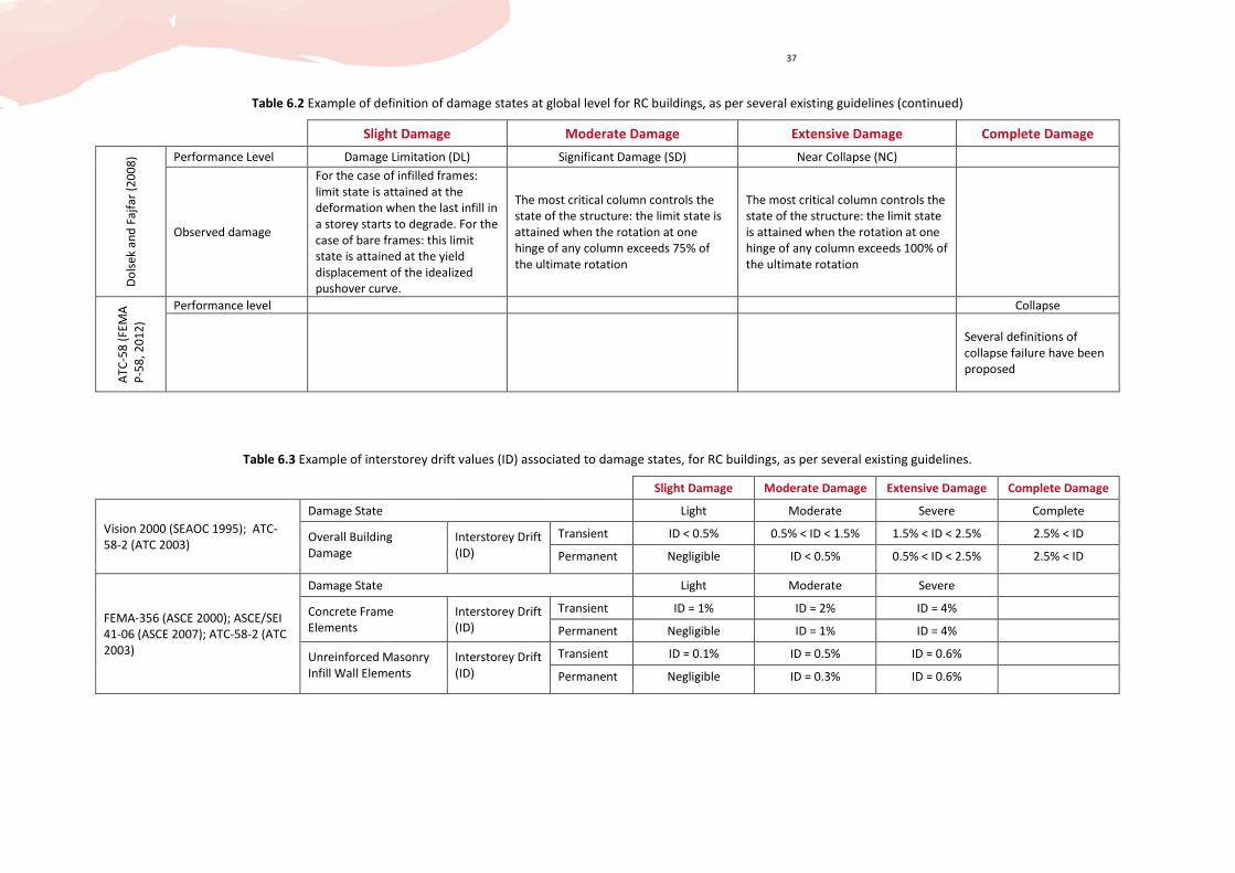
37

Table 6.2 Example of definition of damage states at global level for RC buildings, as per several existing guidelines (continued)

Slight Damage Moderate Damage Extensive Damage Complete Damage D

ols

ek

an

d F

ajf

ar

(20

08

) Performance Level Damage Limitation (DL) Significant Damage (SD) Near Collapse (NC)

Observed damage

For the case of infilled frames:

limit state is attained at the

deformation when the last infill in

a storey starts to degrade. For the

case of bare frames: this limit

state is attained at the yield

displacement of the idealized

pushover curve.

The most critical column controls the

state of the structure: the limit state is

attained when the rotation at one

hinge of any column exceeds 75% of

the ultimate rotation

The most critical column controls the

state of the structure: the limit state

is attained when the rotation at one

hinge of any column exceeds 100% of

the ultimate rotation

AT

C-5

8 (

FEM

A

P-5

8,

20

12

)

Performance level Collapse

Several definitions of

collapse failure have been

proposed

Table 6.3 Example of interstorey drift values (ID) associated to damage states, for RC buildings, as per several existing guidelines.

Slight Damage Moderate Damage Extensive Damage Complete Damage

Vision 2000 (SEAOC 1995); ATC-

58-2 (ATC 2003)

Damage State Light Moderate Severe Complete

Overall Building

Damage

Interstorey Drift

(ID)

Transient ID < 0.5% 0.5% < ID < 1.5% 1.5% < ID < 2.5% 2.5% < ID

Permanent Negligible ID < 0.5% 0.5% < ID < 2.5% 2.5% < ID

FEMA-356 (ASCE 2000); ASCE/SEI

41-06 (ASCE 2007); ATC-58-2 (ATC

2003)

Damage State Light Moderate Severe

Concrete Frame

Elements

Interstorey Drift

(ID)

Transient ID = 1% ID = 2% ID = 4%

Permanent Negligible ID = 1% ID = 4%

Unreinforced Masonry

Infill Wall Elements

Interstorey Drift

(ID)

Transient ID = 0.1% ID = 0.5% ID = 0.6%

Permanent Negligible ID = 0.3% ID = 0.6%

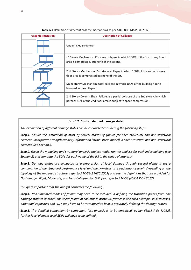
38

Table 6.4 Definition of different collapse mechanisms as per ATC-58 [FEMA P-58, 2012]

Graphic Illustation Description of Collapse

Undamaged structure

1st

Storey Mechanism: 1st

storey collapse, in which 100% of the first storey floor

area is compressed, but none of the second.

2nd Storey Mechanism: 2nd storey collapse in which 100% of the second storey

floor area is compressed but none of the 1st.

Multi-storey Mechanism: total collapse in which 100% of the building floor is

involved in the collapse

2nd Storey Column Shear Failure: is a partial collapse of the 2nd storey, in which

perhaps 40% of the 2nd floor area is subject to space compression.

Box 6.2: Custom defined damage state

The evaluation of different damage states can be conducted considering the following steps:

Step.1. Ensure the simulation of most of critical modes of failure for each structural and non-structural

element. Incorporate strength capacity information (strain-stress model) in each structural and non-structural

element. See Section 5;

Step.2. Given the modelling and structural analysis choices made, run the analysis for each index building (see

Section 3) and compute the EDPs for each value of the IM in the range of interest;

Step.3. Damage states are evaluated as a progression of local damage through several elements (by a

combination of the structural performance level and the non-structural performance level). Depending on the

typology of the analysed structure, refer to ATC-58-2 [ATC 2003] and use the definitions that are provided for

No Damage, Slight, Moderate, and Near Collapse. For Collapse, refer to ATC-58 [FEMA P-58 2012].

It is quite important that the analyst considers the following:

Step.4. Non-simulated modes of failure may need to be included in defining the transition points from one

damage state to another. The shear failure of columns in brittle RC frames is one such example. In such cases,

additional capacities and EDPs may have to be introduced to help in accurately defining the damage states;

Step.5. If a detailed component-by-component loss analysis is to be employed, as per FEMA P-58 [2012],

further local element-level EDPs will have to be defined.

39

6.2 Pre-Defined Values

Alternatively, the analyst might employ the proposed simplified formula and relations from literature, to

estimate directly global damage states and the corresponding median capacity values. Relations commonly

used are expressed as functions of yield and ultimate roof displacement. The global damage states are

estimated from a simplified bilinear capacity curve representative of an index building or class.

HAZUS 99 [FEMA 1999] provide the median values of spectral displacementsids,dS at the damage state ids

as:

Hiroof, dsdsd i

S 2, ˆ αδ= (6.1)

where,ids,roof

δ is the drift ratio at roof level at the damage state ids , 2α is the fraction of the building height

at the location of the pushover mode displacement and H is the typical roof level height of the building type

considered. HAZUS-MH [FEMA 2003] provides 2α and H values for different building types. The values of

ids,roofδ and 2α are provided as a function of the seismic design level and damage state for different building

types.

For the European building taxonomy, Kappos et al. (2006) define five damage thresholds for RC frame and

dual buildings, as shown in Table 6.5.

Table 6.5 Predefined values of damage thresholds for RC frame and dual buildings (Kappos et al. 2006)

Damage State

RC buildings

Infilled RC frames RC dual

Slight dyS7.0 ⋅ dyS7.0 ⋅

Moderate ( )dydudy SS05.0S −⋅+ ( )dydudy SS05.0S −⋅+

Substantial to Heavy ( ) ( ) ( ) ( )dydudydydudy SS21S~ SS31S −⋅+−⋅+ ( ) ( ) dudydudy S9.0~ SS32S ⋅−⋅+

Very Heavy ( ) ( )dydudy SS32S −⋅+ duS

Collapse duS duS3.1 ⋅

dyS and duS are the spectral displacments at yield and ultimate, respectively, at the equivalent SDOF system level.

Lagomarsino and Giovinazzi [2006] identify the following damage states on the global capacity curve (see

Equation 6.2); where ( )1,2,3,4i ˆ, =

idsdS identify the median value of spectral displacements at damage

states ids . Four damage states are associated with these median values: Slight, Moderate, Extensive, and

Complete (Collapse), respectively.

=

+⋅=

⋅=

=

du S

duS

dyS0.5

dyS1.5

dy S

4

3

2

1

ds,d

ds,d

ds,d

ds,d

S

S

S

S

(6.2)

40

dyS and duS are the spectral displacments at yield and ultimate, respectively, at the equivalent SDOF system

level.

For masonry buildings, D’Ayala et al. [2012], D’Ayala [2013] have suggested 4 damage thresholds, as shown

in Table 6.6, obtained by regression from available laboratory or in-situ experimental tests reported in

literature on whole houses or full size walls, distinguishing by mode of failure. The range given for each value

also reflects the scatter dependent on the type of masonry considered, which includes both stone and

brickwork, made with lime mortar. These values are used for reference in developing the fragility curves with

the procedure FaMIVE (see Section 7.3.1).

Table 6.6 Predefined values of damage thresholds for masonry buildings

Damage threshold Damage state Drift range (%)

In-plane failure Out-of-plane failure

1dsS Slight: cracking limit 0.18 -0.23 0.18-0.33

2dsS Structural damage: maximum capacity 0.65 -0.90 0.84-0.88

3dsS Near Collapse: loss of equilibrium 1.23 – 1.92 1.13-2.3

4dsS Collapse 2.0 – 4.0 2.32-4.

41

7 STEP E: Analysis Type and Calculation of EDPs Damage State Thresholds

A number of procedures based on different types of analysis can be followed to compute Engineering

Demand Parameters (EDPs) damage state thresholds and hence develop building fragility and vulnerability

functions. The choice between these procedures will depend on the availability of input data, the analyst’s

skills, and the acceptable level in terms of computational effort/cost. Note that the accuracy of these

procedures will be highly dependent on the choice of modelling type, and hence the choices in Step B and

Step C are highly correlated. Moreover the most appropriate choice is also a function of the lateral load

resisting system and material, as reliable structural modelling is not available for all material types and

structural forms at the same level of accuracy. The analyst is referred to the Sensitivity and Compendium

documents (D’Ayala and Meslem 2013a, 2013b; Meslem and D’Ayala 2013) for a critical discussion of

analytical and modelling approaches available in literature, their use in fragility and vulnerability curve

derivation, and their associated reliability.

Figure 7.1 Steps for the derivation of seismic fragility functions.

Procedures are subdivided in three categories according to the type of structural analysis chosen:

• Non-linear Dynamic Analysis (NLD): Incremental Dynamic Analysis (IDA) is the most accurate in

comparison to the two other procedures. IDA uses a large number of non-linear response history

simulations to determine a so-called backbone or envelop capacity curve. This allows an accurate

quantification of the uncertainties associated with record variability, but the accuracy of the

response is a function of the appropriate level of complexity of the model.

• Non-linear Static procedures (NLS): They are based on the use of capacity curve obtained from static

pushover analysis. Response history simulation is not required for the development of fragility and

vulnerability functions. Note that these procedures can provide reasonable and sufficient accuracy

for the estimation of fragility and vulnerability functions for many structures. Options for considering

record to record variability are proposed, alongside single spectrum evaluations

• Non-linear Static Analysis based on Simplified Mechanism Models (SMM-NLS): The reliability of

these procedures is highly dependent on the exhaustive identification of relevant realistic failure

mechanisms and the computation of their associated capacity curves.

In relation to the structural typology analysed it is recommended to use procedures NLD and NLS for

reinforced concrete (RC) and steel frames, RC shear walls, and confined or reinforced masonry, while

42

procedures SMM-NLS are most suitable for unreinforced masonry (URM), and adobe buildings. This does not

exclude the use of simplified procedures existing in literature for frame analysis such as DBELA [Silva et al.

2013], neither the use of advanced non-linear modelling for masonry structures such as TReMURI

[Lagomarsino et al. 2013]. The analyst is advised that in such cases attention should be paid to failure modes

that might be overlooked by the use of these procedures or to simplifying assumptions which might lead to

diverse levels of uncertainty.

Table 7.1 shows a list of existing building typologies in the world, as presented by GEM-Taxonomy [Brzev et

al. 2012] and PAGER-SRT Taxonomy [Jaiswal and Wald 2008] documents, and their associated analysis types

that have been recommended within the present GEM-ASV Guidelines. More details are discussed in the

next sub-sections.

43

Table 7.1 Association of GEM-ASV methods /Analysis Type with building typologies in accordance with GEM-Taxonomy and PAGER-Taxonomy.

Building Taxonomy Method for Seismic Performance

Assessment

GEM-Taxonomy PAGER-SRT Taxonomy

No

n-l

ine

ar

Dyn

am

ic

Pro

ced

ure

(N

LD)

No

n-l

ine

ar

Sta

tic

Pro

ced

ure

s (N

LS)

Sim

plif

ied

me

cha

nis

m

mo

de

ls (

SMM

-NLS

)

Main

Attribute

[ID]

Secondary Attributes [ID] Material ID Description

Pro

ced

ure

1.1

Pro

ced

ure

2.1

Pro

ced

ure

3.1

Pro

ced

ure

3.2

Pro

ced

ure

3.3

Pro

ced

ure

4.1

Material

[MA]

Material

Type

[MA**]

Timber [MATI] Wood/Timber W Wood frames, Timber frames / walls

Masonry

[MAMA]

Reinforced / Confined

Masonry RM Reinforced masonry bearing walls / Confined masonry

Reinforced

Concrete

[MACO]

Reinforced Concrete C Reinforced concrete with masonry infills Concrete moment-resisting frames/ shear walls

Precast Concrete PC Precast concrete frames / walls

Steel [MAST] Steel S Braced steel frames

Steel moment-resisting frames and others

Earthen [MAEA] Adobe/Mud Walls

M Mud walls

A Adobe blocks walls

RE Rammed earth walls

44

Table 7.2 Association of GEM-ASV methods /Analysis Type with building typologies in accordance with GEM-Taxonomy and PAGER-Taxonomy (continued).

Building Taxonomy Method for Seismic Performance

Assessment

GEM-Taxonomy PAGER-SRT Taxonomy

No

n-l

ine

ar

Dyn

am

ic

Pro

ced

ure

(N

LD)

No

n-l

ine

ar

Sta

tic

Pro

ced

ure

s (N

LS)

Sim

plif

ied

me

cha

nis

m

mo

de

ls (

SMM

-NLS

)

Main

Attribute

[ID]

Secondary Attributes [ID] Material ID Description

Pro

ced

ure

1.1

Pro

ced

ure

2.1

Pro

ced

ure

3.1

Pro

ced

ure

3.2

Pro

ced

ure

3.3

Pro

ced

ure

4.1

Material

[MA]

Material

Type

[MA**]

Masonry [MAMA] Stone/Block Masonry

RS Rubble stone (field stone) masonry walls

DS Rectangular cut-stone masonry block

MS Massive stone masonry in lime or cement mortar

UCB Unreinforced concrete block masonry with lime or cement

mortar

Brick Masonry UFB Unreinforced fired brick masonry

Other [MAOT] Other

MH Mobile homes

INF Informal constructions

UNK No specified

45

7.1 Ground Motion Selection and Scaling

7.1.1 Ground Motions Selection

In order to cover the full range of structural behaviour from elastic to inelastic and finally to global collapse

[Vamvatsikos and Cornell 2002], and account for record-to-record variability (variability related to the

mechanism of the seismic source, path attenuation effects, local site effects), suites of ground motion

records have to be selected and, if necessary, scaled to a certain level of seismic intensity.

As per EN 1998-1 [CEN 2005] the suite of records should be in accordance with the following rules:

• the duration of the records shall be consistent with the magnitude and the other relevant features of

the seismic event underlying the establishment of ag;

• in the range of periods between 0.2T1 and 2T1 (T1 being the fundamental period of the structure in

the direction of application of the record) the value of the mean 5% damping elastic spectrum,

calculated from all time histories, should not be less than 90% of the corresponding value of the 5%

damping elastic response spectrum;

• spectral matching of records to a design spectrum or site-specific spectrum may be used to

represent same hazard level.

The approaches adopted for record selection and spectrum matching, have a significant effect on the

resulting fragility curve, as shown by Gehl et al. [2014]. Figure 7.2 visualises the results of using different

criteria for the matching of the natural spectrum to a reference elastic response spectrum.

Since the properties of the seismic response depend on the intensity, or severity, of the seismic shaking, a

comprehensive assessment calls for numerous non-linear analyses at various levels of intensity to represent

different possible earthquake scenarios. Attention should be paid to the extent to which is reasonable to

scale a given record up or down to match a reference intensity. It is advisable to choose records that are

associated to the reference magnitude considered for the scenario of interest.

46

Figure 7.2 Matching of ground motion to a given elastic response spectrum

7.1.2 Number of Ground Motion Records

The calculated response can be very sensitive to the characteristics of the individual ground motion used as

seismic input; therefore, several analyses are required using different ground motion records to achieve a

reliable estimation of the probabilistic distribution of structural response. The minimum number of ground

motions that should be used to provide stable estimates of the medians capacity (Figure 7.3); analysts are

required to consider the following parameters that can strongly influence the stability in median capacity:

• Type of analysis: non-linear dynamic, non-linear static, simplified methods;

• Assumption used in selecting ground motion records;

• Type of structure and structural characteristics

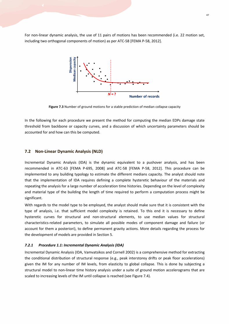
47

For non-linear dynamic analysis, the use of 11 pairs of motions has been recommended (i.e. 22 motion set,

including two orthogonal components of motion) as per ATC-58 [FEMA P-58, 2012].

Figure 7.3 Number of ground motions for a stable prediction of median collapse capacity

In the following for each procedure we present the method for computing the median EDPs damage state

threshold from backbone or capacity curves, and a discussion of which uncertainty parameters should be

accounted for and how can this be computed.

7.2 Non-Linear Dynamic Analysis (NLD)

Incremental Dynamic Analysis (IDA) is the dynamic equivalent to a pushover analysis, and has been

recommended in ATC-63 [FEMA P-695, 2008] and ATC-58 [FEMA P-58, 2012]. This procedure can be

implemented to any building typology to estimate the different medians capacity. The analyst should note

that the implementation of IDA requires defining a complete hysteretic behaviour of the materials and

repeating the analysis for a large number of acceleration time histories. Depending on the level of complexity

and material type of the building the length of time required to perform a computation process might be

significant.

With regards to the model type to be employed, the analyst should make sure that it is consistent with the

type of analysis, i.e. that sufficient model complexity is retained. To this end it is necessary to define

hysteretic curves for structural and non-structural elements, to use median values for structural

characteristics-related parameters, to simulate all possible modes of component damage and failure (or

account for them a posteriori), to define permanent gravity actions. More details regarding the process for

the development of models are provided in Section 5.

7.2.1 Procedure 1.1: Incremental Dynamic Analysis (IDA)

Incremental Dynamic Analysis (IDA, Vamvatsikos and Cornell 2002) is a comprehensive method for extracting

the conditional distribution of structural response (e.g., peak interstorey drifts or peak floor accelerations)

given the IM for any number of IM levels, from elasticity to global collapse. This is done by subjecting a

structural model to non-linear time history analysis under a suite of ground motion accelerograms that are

scaled to increasing levels of the IM until collapse is reached (see Figure 7.4).

48

Figure 7.4 Incremental Dynamic Analysis using ground motion scaling

Regarding the application of the procedure, the amplitude of each selected ground motion should be

incremented, and non-linear response history analysis performed until either global dynamic or numerical

instability occurs in the analysis, indicating that either collapse, or storey drift exceeding non-simulated

collapse limits, or large increase in storey drift associated with small increments in spectral acceleration is

affecting the structure (see Figure 7.5). As shown in Figure 7.5, the output of IDA is a set of discrete points,

(obtained by scaling each of the selected ground motions), of the IM versus the demand parameter of

interest, for instance the first mode spectral acceleration ( )1ds,a TS4

, and the maximum interstorey drift,

respectively.

Figure 7.5 Steps of incremental dynamic analysis using ground motion scaling

To obtain continuous curves, Cubic Spline interpolation technique is made use of, in order to save

computational time. This technique ensures continuity of first and second derivative at the merging points

(see Figure 7.6).

The location where each IDA curve becomes flat identifies the IM level beyond which it is assumed that

global collapse will occur.

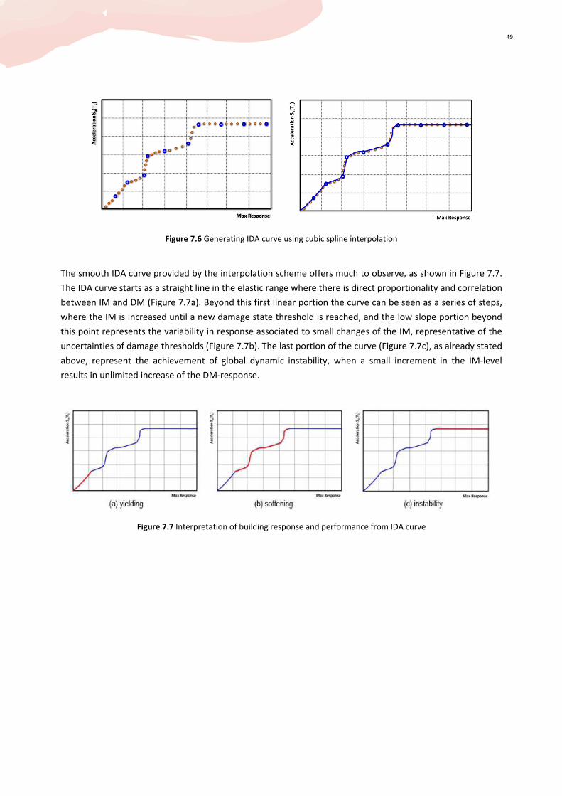
49

Figure 7.6 Generating IDA curve using cubic spline interpolation

The smooth IDA curve provided by the interpolation scheme offers much to observe, as shown in Figure 7.7.

The IDA curve starts as a straight line in the elastic range where there is direct proportionality and correlation

between IM and DM (Figure 7.7a). Beyond this first linear portion the curve can be seen as a series of steps,

where the IM is increased until a new damage state threshold is reached, and the low slope portion beyond

this point represents the variability in response associated to small changes of the IM, representative of the

uncertainties of damage thresholds (Figure 7.7b). The last portion of the curve (Figure 7.7c), as already stated

above, represent the achievement of global dynamic instability, when a small increment in the IM-level

results in unlimited increase of the DM-response.

Figure 7.7 Interpretation of building response and performance from IDA curve

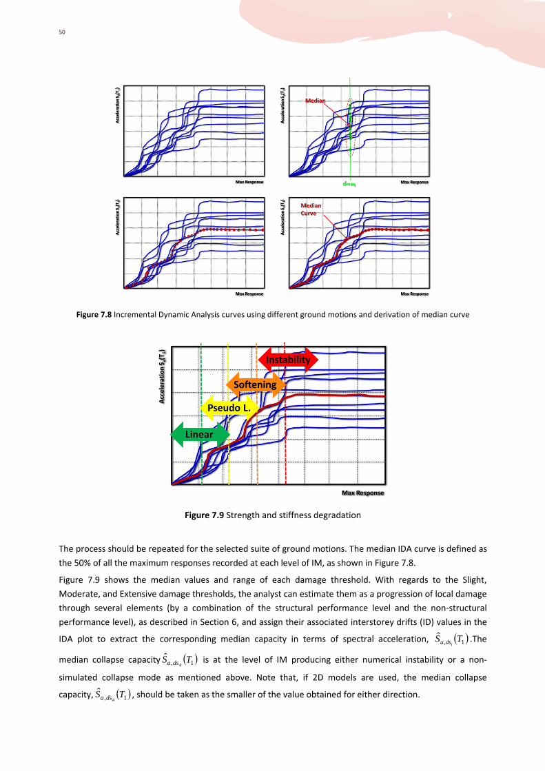
50

Figure 7.8 Incremental Dynamic Analysis curves using different ground motions and derivation of median curve

Figure 7.9 Strength and stiffness degradation

The process should be repeated for the selected suite of ground motions. The median IDA curve is defined as

the 50% of all the maximum responses recorded at each level of IM, as shown in Figure 7.8.

Figure 7.9 shows the median values and range of each damage threshold. With regards to the Slight,

Moderate, and Extensive damage thresholds, the analyst can estimate them as a progression of local damage

through several elements (by a combination of the structural performance level and the non-structural

performance level), as described in Section 6, and assign their associated interstorey drifts (ID) values in the

IDA plot to extract the corresponding median capacity in terms of spectral acceleration, ( )1,ˆ TS

idsa .The

median collapse capacity ( )1, 4

ˆ TS dsa is at the level of IM producing either numerical instability or a non-

simulated collapse mode as mentioned above. Note that, if 2D models are used, the median collapse

capacity, ( )1, 4

ˆ TS dsa , should be taken as the smaller of the value obtained for either direction.

51

The record-to-record dispersion can be estimated directly, as the lognormal standard deviation for the

selected records. For instance, the following formula can be used to calculate the record-to-record dispersion

associated to each damage threshold [Wen et al. 2004]:

( )Mean

STDEVCoV where1ln 2 =+= CoVβ (7.1)

As an alternative, the EDPs damage thresholds and their corresponding record-to-record variabilities can be

extracted using regression techniques as described in Section 7.3.1.1.

The non-linear dynamic analysis can be carried out using a number of alternatives.

Cloud or stripe analysis [Jalayer and Cornell 2009, Baker 2014] can be used to organize the execution of non-

linear dynamic analyses to estimate the distribution of demand given the IM. In stripe analysis, analyses at

performed at specified IM levels, creating characteristic stripes of points in an IM versus EDP response plot

(such as the one in Figure 7.9). If the same set of records is employed to match each IM level through scaling,

then this approach is practically identical to IDA. If different ground motion sets are employed at different IM

levels, typically the product of careful record selection by an informed analyst (see discussion in Section 2.3)

then this allows the use of relatively insufficient IMs without problems. Cloud analysis is a similar approach

that does not employ specific IM levels, but instead uses either scaled or typically unscaled sets of records for

analysis, resulting in a characteristic cloud of points in an IM-response plot. The main difference to the stripe

approach is that a statistical (e.g., regression) model needs to be assumed to obtain the distribution of

demand given the IM, or the distribution of collapse IM capacity. Striping, instead, allows a much simpler

estimation, as the response estimates are already arranged at given IM levels, thus offering direct estimates

of the statistics (mean/median/dispersion) of response given the IM.

52

Box 7.1: Calculation of the median capacity using Procedure 1.1

Step.1. Develop an appropriate mathematical model of the building for non-linear time histories analyses. The

model should be commensurate to the level of complexity of the analysis. The analyst should refer to Section 5

for details;

Step.2. Select pairs of ground motion records to perform dynamic response history analysis. The use of 11 pairs

of motions (i.e. 22 motions set) is recommended;

Step 3: For each ground motion pair, run IDA analysis: the amplitude should be incremented, and non-linear

response history analysis performed until the occurrence of either: Mode 1- Numerical instability or simulated

collapse; Mode 2- Predicted response that would result in non-simulated collapse; Mode 3- Large increment in

storey drift for small increase in ( )1TSa ; or Mode 4- Storey drifts at which the analytical model is no longer

believed to be reliable.

# If none of the above four modes occurs, the analysis should be repeated, with incremental amplitude

adjustment for the ground motion pair until one of these modes occurs.

# If needed, use scaling to increase the IM level of the ground motion records, until one of the model failure

modes is reached as defined above. Details on scaling procedures that the analyst may implement are beyond

the scope of these guidelines. Reference on this matter can be made to ATC-58 [FEMA P-58, 2012] or other

relevant literature. Excessive scaling (e.g., by factors larger than about 3.0) should be avoided, especially

whenever a relatively insufficient IM such as ( )1TSa is used. Alternatively, one may employ as a sufficient IM the

average spectral response acceleration Sagm(Ti), i.e., the sum of the natural logarithm of spectral acceleration

values computed over a range of Ti values appropriate for the building studied. An experienced analyst

undertaking a site-specific analysis of a given structure may want to employ cloud/stripe analysis with a more

rigorous selection of ground motions.

# At each IM level and for each ground motion record applied, if no collapse has been deemed to occur then all

response parameters of interest (e.g., peak storey drifts and peak floor accelerations at each storey) should be

recorded.

Step.4. Identify the different medians capacity associated to damage thresholds:

# The location where this curve becomes flat is defined as the point from which the collapse occurs; i.e.

( )1, 4TS dsa

# The minimum of the values of ( )1TSa at which any of the above Modes occurs is taken as the collapse capacity

( )1, 4TS dsa for the considered pair of ground motion.

# The median collapse capacity ( )1, 4

ˆ TS dsa is then defined as the value at which 50% of the ground motion pairs

produce either modes as mentioned above. Note that when 2D models are used, the median collapse capacity,

( )1, 4

ˆ TS dsa , should be taken as the smaller of the value obtained for either direction.

# At each IM level, the N values (where N is the number of ground motion records) recorded for each demand

parameter of interest (e.g., peak drift of any given storey or peak acceleration of any given floor) can be used to

define the distribution of demand for the specific IM value. Alternatively, one can also use these results to define

maximum interstorey drift (ID) values for Slight, Moderate, and Near Collapse damage thresholds that can be

estimated from the progression of local damage through several elements in Section 6. Assign these ID values in

IDA plot to estimate the corresponding median idsMI ,

ˆ and the associated dispersion.

53

7.3 Non-Linear Static Analysis (NLS)

The procedures presented in this subsection are based on the use of capacity curves resulting from Non-

linear Static Pushover analysis (see ANNEX A). The derivation of a capacity curve by use of pushover analysis,

does not directly account for the specific seismic motion, as the dynamic characteristics of demand and

response system are not taken into account in the analysis.

The resulting capacity curve from pushover analysis will then need to be fitted with a bilinear (an elastic-

plastic) or multilinear (elastic-plastic with residual strength) curve to idealise the behaviour. The procedure

for fitting capacity curves is provided in ANNEX A.

There are some cases where the analyst may prefer to use default capacity curves available in literature (e.g.

documents, guidelines), for instance:

• for simplification/reduction of calculation efforts

• lack of information for the assessed structures, especially, for the older ones, where design

documents are generally not available.

• when studies are conducted for large portions of the building stock and resources for direct survey

and data acquisition are modest.

However, special care should be given when assigning these default curves to represent the performance of

assessed structure. For instance, the existing HAZUS capacity curves [FEMA 1999] derived for buildings in the

US, have been widely used to generate fragility curves of buildings located in different regions of the world

and designed and built according to standards and construction practice very different from the ones

employed in the USA. Indeed differences in construction techniques and detailing between different

countries are significant, even when buildings are nominally designed to the same code clauses. Such

detailing can substantially affect fragility and vulnerability functions. It is hence recommended that capacity

curves be derived by the analyst based on directly acquired data on local building stock, using available non-

linear commercial analysis programmes.

In the following we recommend a number of procedures to determine median values of damage state

thresholds, depending on the shape of the capacity curve, multilinear or bilinear, and whether record-to-

record dispersion is taken into account or not in the analysis.

7.3.1 Case of Multilinear Elasto-Plastic (with Residual Strength) Form of Capacity Curve

The procedures offered herein are applicable to multilinear elasto-plastic (elastic-plastic with residual

strength) capacity curves (

Figure 7.10); it is ideal for frames structures with unreinforced masonry infills.

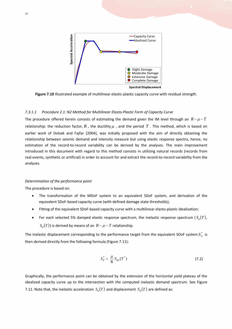
54

Figure 7.10 Illustrated example of multilinear elastic-plastic capacity curve with residual strength.

7.3.1.1 Procedure 2.1: N2 Method for Multilinear Elasto-Plastic Form of Capacity Curve

The procedure offered herein consists of estimating the demand given the IM level through an TR −− µ

relationship: the reduction factor, R , the ductility µ , and the period T . This method, which is based on

earlier work of Dolsek and Fajfar [2004], was initially proposed with the aim of directly obtaining the

relationship between seismic demand and intensity measure but using elastic response spectra, hence, no

estimation of the record-to-record variability can be derived by the analyses. The main improvement

introduced in this document with regard to this method consists in utilizing natural records (records from

real events, synthetic or artificial) in order to account for and extract the record-to-record variability from the

analyses.

Determination of the performance point

The procedure is based on:

• The transformation of the MDoF system to an equivalent SDoF system, and derivation of the

equivalent SDoF-based capacity curve (with defined damage state thresholds);

• Fitting of the equivalent SDoF-based capacity curve with a multilinear elasto-plastic idealization;

• For each selected 5% damped elastic response spectrum, the inelastic response spectrum ( ( )TSa ,

( )TSd ) is derived by means of an TR −− µ relationship.

The inelastic displacement corresponding to the performance target from the equivalent SDoF system *dS is

then derived directly from the following formula (Figure 7.11):

)(

R ** TSS ded

µ= (7.2)

Graphically, the performance point can be obtained by the extension of the horizontal yield plateau of the

idealized capacity curve up to the intersection with the computed inelastic demand spectrum. See Figure

7.11. Note that, the inelastic acceleration ( )TSa and displacement ( )TSd are defined as:

55

( ) ( )

R

TS ae

aS

T = (7.3)

( ) ( ) ( )TS

TTS

RS aeded 2

2

2

2

4

T

4R T

πµ

πµµ

===

(7.4)

Figure 7.11 Illustrated example on the steps of the Procedure 2.1 for the evaluation of the performance point given an

earthquake record.

Once the performance point (inelastic displacement) for a given earthquake (with a specific value of PGA) is

calculated, then the corresponding acceleration (elastic) can also be calculated using the following

expression:

( ) ( ) ( ) T

4 T *

2*

2*

1 deaea ST

STSπ

== (7.5)

Determination of inelastic response spectrum

According to the results of parametric study (using three different set of recorded and semi-artificial ground

motions, for a total of 20 recorded accelerograms and 24 semi-artificial accelerograms) for the case of

system with multilinear elasto-plastic capacity diagram, the ductility demand, µ , and reduction factor, R ,

are related through the following formula [Dolsek and Fajfar 2004]:

( ) 00 R- c1

µµ += R (7.6)

where the ductility demand is to be computed from the known reduction factor:

( )ay

ae

S

TR

*S = (7.7)

Elastic spectrum

Inelastic spectrum

56

( )*ae TS is the elastic spectral acceleration at the initial period of the SDoF system,

*T , ayS is the yield

acceleration of the given inelastic system defined as:

*

*

m

F y

ayS = (7.8)

The parameter c expresses the slope of the µ−R relation, and has been developed based on the

employment of three sets of ground motions in order to consider the effect of record-to-record variability.

This parameter is defined as:

=

C

*

T

T0.7 c ( ), RR sµ≤ CTT ≤*

(7.9)

T0.3 0.7 ∆+=c ( ), RR sµ≤ **DC TTT ≤<

u

1

C

*

uT

T0.7

rrc

= ( ), RR sµ> CTT ≤*

( ) T Δ - 10.7 u ∆+= Trc ( ), RR sµ> **

DC TTT ≤<

1 =c **DTT >

10 =µ ( )sRR µ≤

(7.10)

s µµ =0 ( )sRR µ>

10 =R ( )sRR µ≤

(7.11) ( )sRR µ=0 ( )sRR µ>

With:

( )sR µ is the reduction factor interval, defined as:

( ) ( ) 1 1 - T

T0.7

C

*

+

= ssR µµ CTT ≤*

(7.12) ( ) ( )( ) 1 1 - T0.3 0.7 +∆+= ssR µµ

**DC TTT ≤<

( ) ssR µµ = **DTT >

sµ is the ductility at the beginning of the strength degradation of the infills, defined as:

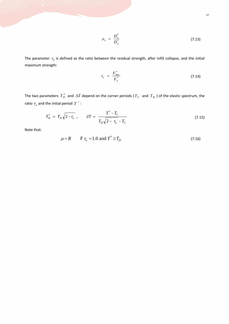
57

*y

*s

sD

D μ = (7.13)

The parameter ur is defined as the ratio between the residual strength, after infill collapse, and the initial

maximum strength:

*y

*

uF

F r min= (7.14)

The two parameters *DT and T∆ depend on the corner periods ( CT and DT ) of the elastic spectrum, the

ratio ur and the initial period *T :

CuD

C*

uD*D

- T rT

- TT ΔT , - r T T

−==

22 (7.15)

Note that:

TTrR D*

u ≥== and 1.0 ifµ (7.16)

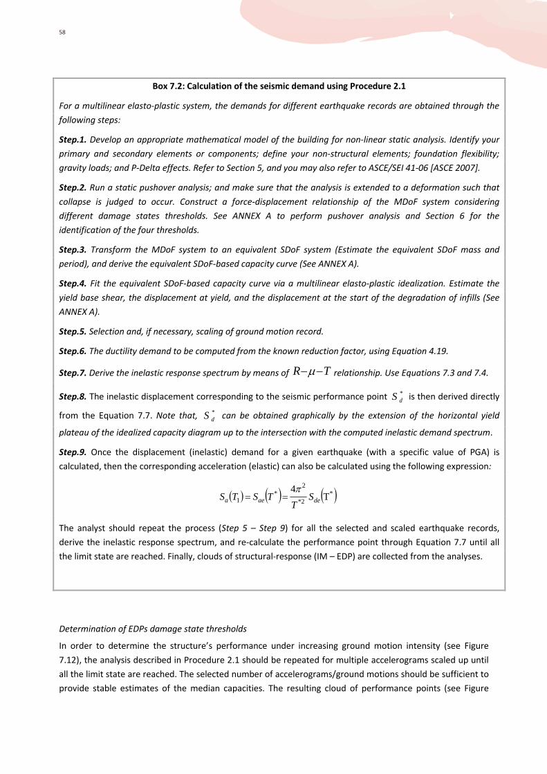
58

Determination of EDPs damage state thresholds

In order to determine the structure’s performance under increasing ground motion intensity (see Figure

7.12), the analysis described in Procedure 2.1 should be repeated for multiple accelerograms scaled up until

all the limit state are reached. The selected number of accelerograms/ground motions should be sufficient to

provide stable estimates of the median capacities. The resulting cloud of performance points (see Figure

Box 7.2: Calculation of the seismic demand using Procedure 2.1

For a multilinear elasto-plastic system, the demands for different earthquake records are obtained through the

following steps:

Step.1. Develop an appropriate mathematical model of the building for non-linear static analysis. Identify your

primary and secondary elements or components; define your non-structural elements; foundation flexibility;

gravity loads; and P-Delta effects. Refer to Section 5, and you may also refer to ASCE/SEI 41-06 [ASCE 2007].

Step.2. Run a static pushover analysis; and make sure that the analysis is extended to a deformation such that

collapse is judged to occur. Construct a force-displacement relationship of the MDoF system considering

different damage states thresholds. See ANNEX A to perform pushover analysis and Section 6 for the

identification of the four thresholds.

Step.3. Transform the MDoF system to an equivalent SDoF system (Estimate the equivalent SDoF mass and

period), and derive the equivalent SDoF-based capacity curve (See ANNEX A).

Step.4. Fit the equivalent SDoF-based capacity curve via a multilinear elasto-plastic idealization. Estimate the

yield base shear, the displacement at yield, and the displacement at the start of the degradation of infills (See

ANNEX A).

Step.5. Selection and, if necessary, scaling of ground motion record.

Step.6. The ductility demand to be computed from the known reduction factor, using Equation 4.19.

Step.7. Derive the inelastic response spectrum by means of TR −−µ relationship. Use Equations 7.3 and 7.4.

Step.8. The inelastic displacement corresponding to the seismic performance point *dS is then derived directly

from the Equation 7.7. Note that, *dS can be obtained graphically by the extension of the horizontal yield

plateau of the idealized capacity diagram up to the intersection with the computed inelastic demand spectrum.

Step.9. Once the displacement (inelastic) demand for a given earthquake (with a specific value of PGA) is

calculated, then the corresponding acceleration (elastic) can also be calculated using the following expression:

( ) ( ) ( ) T4

*2*

2*

1 deaea ST

TSTSπ

==

The analyst should repeat the process (Step 5 – Step 9) for all the selected and scaled earthquake records,

derive the inelastic response spectrum, and re-calculate the performance point through Equation 7.7 until all

the limit state are reached. Finally, clouds of structural-response (IM – EDP) are collected from the analyses.

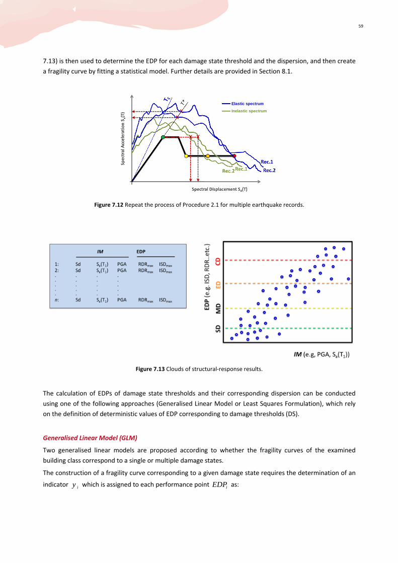
59

7.13) is then used to determine the EDP for each damage state threshold and the dispersion, and then create

a fragility curve by fitting a statistical model. Further details are provided in Section 8.1.

Figure 7.12 Repeat the process of Procedure 2.1 for multiple earthquake records.

Figure 7.13 Clouds of structural-response results.

The calculation of EDPs of damage state thresholds and their corresponding dispersion can be conducted

using one of the following approaches (Generalised Linear Model or Least Squares Formulation), which rely

on the definition of deterministic values of EDP corresponding to damage thresholds (DS).

Generalised Linear Model (GLM)

Two generalised linear models are proposed according to whether the fragility curves of the examined

building class correspond to a single or multiple damage states.

The construction of a fragility curve corresponding to a given damage state requires the determination of an

indicator iy which is assigned to each performance point iEDP as:

Elastic spectrum

Inelastic spectrum

60

1

0k

ik

EDPi EDPy

EDPi EDP

≥=

< (7.17)

The curves are then obtained by fitting a generalised linear model to these binary data and their

corresponding intensity measure levels (see Figure 7.14).

The indicator of a performance point for a given level of ground motion intensity ( iimIM = ), associated

with the demand spectrum, is considered to follow a Bernoulli distribution as:

[ ]11| ~ 1 ii

yy

i

Y imy

− −

µ µ (7.18)

where µ is the conditional mean response which represents here the fragility curve. The fragility curve is

obtained as:

( ) ( )( ) ( )1 0 | lng g P DS ds im im= ≥ = +µ θ θ (7.19)

where 1θ , 0θ is the unknown parameters of the statistical model; ( ).g is the link function obtained as:

( )

( )

( )

1 probit

log logit1

log log 1 complementary loglog

g

−Φ

= − −

µ

µµ

µ

µ

(7.20)

The construction of fragility curves corresponding to multiple damage states is estimated by fitting an

ordered generalised linear model to the data, which ensures that the fragility curves will not cross. In this

case, the iEDP are classified in N + 1 discrete ordered damage states, ds, as:

1

2 1

1

0

1

...

i

ij

k i k

i N

EDP EDP

EDP EDP EDPds

EDP EDP EDP

N EDP EDP+

>

≥ ≥=

≥ ≥ ≥

(7.21)

Where N is the most extreme damage state. The damage states for im in each damage state are assumed to

follow a discrete categorical distribution:

( )0

| ~ |j

N y

jj

DS im P DS ds im=

=∏ (7.22)

61

where iy is an indicator which is 1 if the building suffered damage j and 0 otherwise. Equation 8.22 shows

that the categorical distribution is fully defined by the determination of the conditional probability,

( )im|dsDSP j= . This probability can be transformed into the probability of reaching or exceeding jds

given im , ( )im|dsDSP j≥ , essentially expressing the required fragility curve, as:

( )( )

( ) ( )( )

1 | 1

| | 01

|

|j

P DS dsj im j j

P DS ds im P DS ds im j Nj j

P DS ds im j Nj

P DS ds im

− ≥ = −

≥ − ≥ < < +

≥ =

== (7.23)

The fragility curves are expressed in terms of one of the three link functions expressed in Equation 8.20, in

the form:

( ) ( )10 1| lnj ig P DS ds im im− ≥ = + θ θ (7.24)

where [ ]1i0 ,θθθ = is the vector of the ‘true’ but unknown parameters of the model; 1θ is the slope and

i0θ is the intercept for fragility curve corresponding to jds . Equation 8.24 assumes that the fragility curves

corresponding to different damage states have the same slope but different intercepts. This ensures that the

ordinal nature of the damage is taken into account leading to meaningful fragility curves, i.e. curves that do

not cross.

The unknown parameters of the generalised linear models are then estimated by maximising the likelihood

function as:

( )( )

( )

[ ]

st

1 0

nd

1

argmax log

!argmax log | 1 Stage

!

argmax log 1 2 Stage

ij

i ii

opt

M N ni

j ii j ij

Mm ni n

i ii i

L

mP DS ds im

n

m

n

= =

−

=

= =

= =

−

∏∏

∏

θ θ

µ µ

(7.25)

where M is the number of performance points.

The EDPs of damage state thresholds (fragility parameters) and their corresponding dispersions can be

computed as:

11

0 1 and -exp θ

βθθ

α =

= (7.26)

In addition to the mean fragility curves, their 5% - 95% confidence bounds can also be plotted, obtained by a

non-parametric bootstrap analysis [Efron and Tibshirani 1994] of the data points.

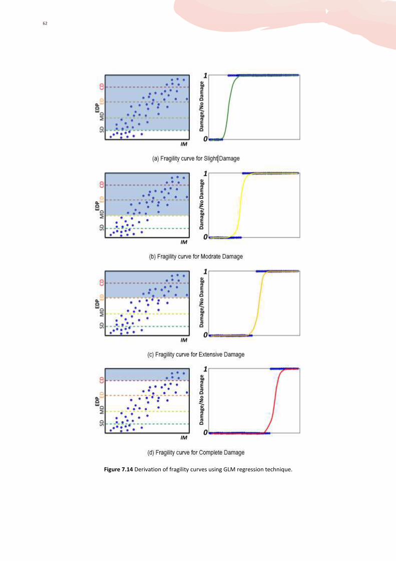
62

Figure 7.14 Derivation of fragility curves using GLM regression technique.

63

Least Squares Formulation

Least Squares regression is a widely used technique to estimate, for each damage threshold, the probabilistic

relation between EDPs and IMs (Figure 7.15) (e.g. Cornell et al. 2002; Ellingwood and Kinali 2009).

Assuming a lognormal distribution between EDP and DS [Shome and Cornell 1999], the predicted median

demand is represented by a normal cumulative distribution (Figure 7.16):

−Φ

βαlnln IM

(7.27)

where, Φ represents the stardard normal cumulative distribution function, β is the global standard-

deviation for the predicted median demand.

For an assumed probabilistic damage threshold, IMs are chosen in a way that roughly half the points are

below that damage threshold and half above, determining an interval of IMs values, which are assumed to be

lognormally distributed within each interval.

Performing piece-wise regression over these different IM intervals, the fragility parameters are computed

using the corresponding relation: ( ) ( ) ( )blnIMlnaEDPln += . The median demand idsα and its dispersion

idsβ for each assumed threshold, ids , can be written as:

( )a

ab

dsii ds

ids

ilnIMSTDEV and lnexp =

= βα (7.28)

For instance, the median demand of complete damage state threshold and the corresponding dispersion can

be computed as (Figure 7.16):

( )a

ab

CDCDCD

ilnIMSTDEV and lnexp =

= βα

Figure 7.15 Derivation of fragility functions (median demand and dispersion) using Least Squares regression technique.

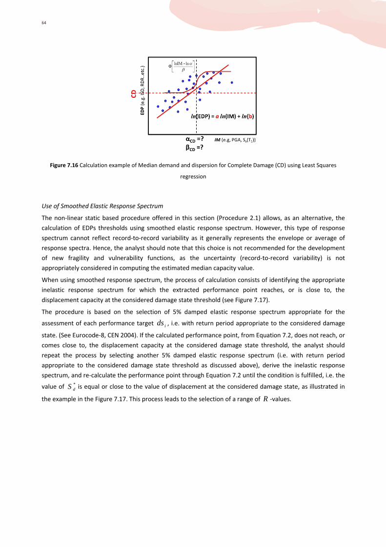
64

Figure 7.16 Calculation example of Median demand and dispersion for Complete Damage (CD) using Least Squares

regression

Use of Smoothed Elastic Response Spectrum

The non-linear static based procedure offered in this section (Procedure 2.1) allows, as an alternative, the

calculation of EDPs thresholds using smoothed elastic response spectrum. However, this type of response

spectrum cannot reflect record-to-record variability as it generally represents the envelope or average of

response spectra. Hence, the analyst should note that this choice is not recommended for the development

of new fragility and vulnerability functions, as the uncertainty (record-to-record variability) is not

appropriately considered in computing the estimated median capacity value.

When using smoothed response spectrum, the process of calculation consists of identifying the appropriate

inelastic response spectrum for which the extracted performance point reaches, or is close to, the

displacement capacity at the considered damage state threshold (see Figure 7.17).

The procedure is based on the selection of 5% damped elastic response spectrum appropriate for the

assessment of each performance target ids , i.e. with return period appropriate to the considered damage

state. (See Eurocode-8, CEN 2004). If the calculated performance point, from Equation 7.2, does not reach, or

comes close to, the displacement capacity at the considered damage state threshold, the analyst should

repeat the process by selecting another 5% damped elastic response spectrum (i.e. with return period

appropriate to the considered damage state threshold as discussed above), derive the inelastic response

spectrum, and re-calculate the performance point through Equation 7.2 until the condition is fulfilled, i.e. the

value of *dS is equal or close to the value of displacement at the considered damage state, as illustrated in

the example in the Figure 7.17. This process leads to the selection of a range of R -values.

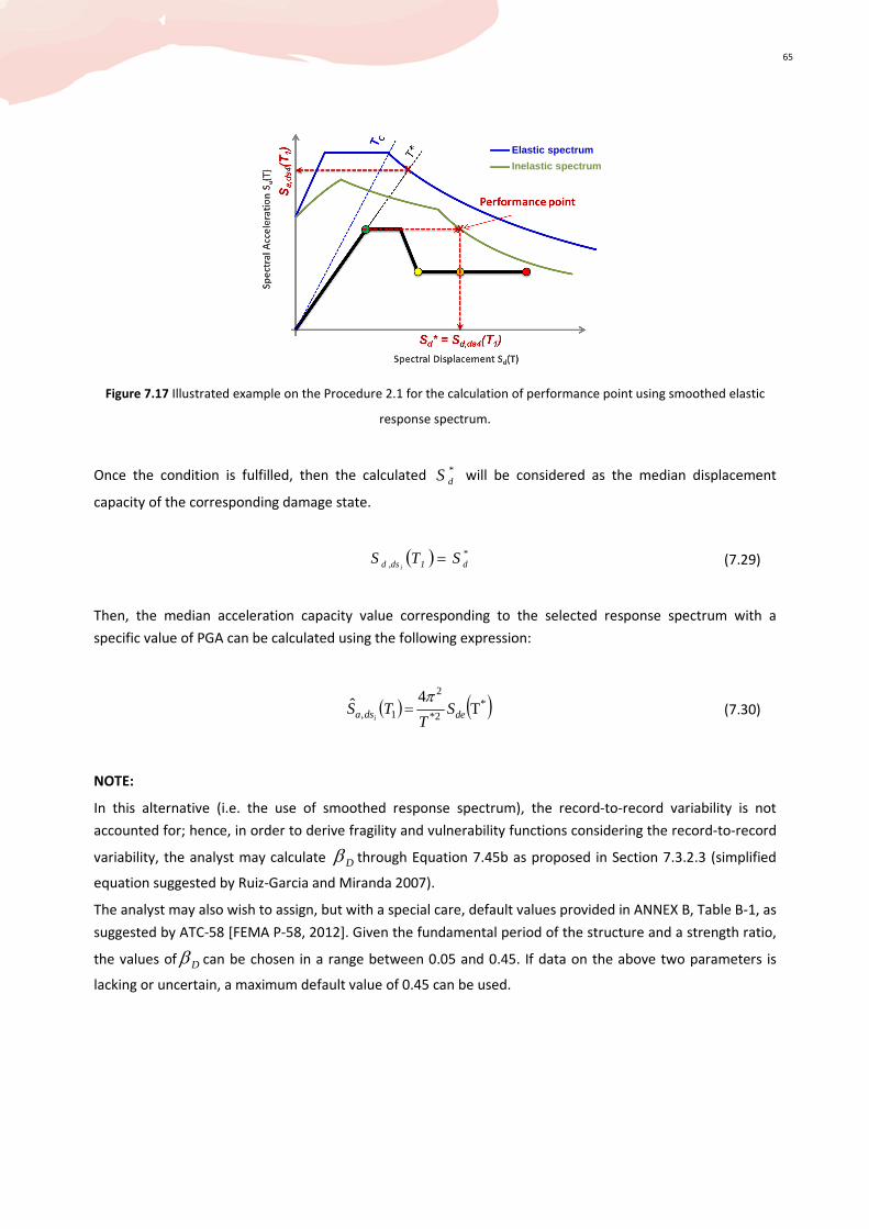
65

Figure 7.17 Illustrated example on the Procedure 2.1 for the calculation of performance point using smoothed elastic

response spectrum.

Once the condition is fulfilled, then the calculated *dS will be considered as the median displacement

capacity of the corresponding damage state.

( ) *d1ds,d STS

i= (7.29)

Then, the median acceleration capacity value corresponding to the selected response spectrum with a

specific value of PGA can be calculated using the following expression:

( ) ( ) T

4 ˆ *

2*

2

1, dedsa ST

TSi

π= (7.30)

NOTE:

In this alternative (i.e. the use of smoothed response spectrum), the record-to-record variability is not

accounted for; hence, in order to derive fragility and vulnerability functions considering the record-to-record

variability, the analyst may calculate Dβ through Equation 7.45b as proposed in Section 7.3.2.3 (simplified

equation suggested by Ruiz-Garcia and Miranda 2007).

The analyst may also wish to assign, but with a special care, default values provided in ANNEX B, Table B-1, as

suggested by ATC-58 [FEMA P-58, 2012]. Given the fundamental period of the structure and a strength ratio,

the values of Dβ can be chosen in a range between 0.05 and 0.45. If data on the above two parameters is

lacking or uncertain, a maximum default value of 0.45 can be used.

Elastic spectrum

Inelastic spectrum

66

7.3.2 Case of Bilinear Elasto-Plastic Form of Capacity Curve

The procedures presented herein are applicable to bilinear elasto-plastic capacity curve only; therefore, it is

ideal for Steel or Reinforced Concrete bare frame moment-resisting structures, masonry structures with

curtailed ductility, and wherever negative stiffness or reserve strength are not an issue.

7.3.2.1 Procedure 3.1: N2 Method for Bilinear Elasto-Plastic Form of Capacity Curve

This procedure is based on earlier work of Fajfar [2002], and has been recommended by Eurocode-8 [CEN

2004]. The procedure is specifically applicable only for structures that are characterised by bilinear Elasto-

Perfectly Plastic capacity curve. The process consists of obtaining the appropriate inelastic response, i.e.

performance point (defined as point of intersection of idealized SDoF system based capacity curve with the

inelastic demand spectrum) for a given earthquake record (see Figure 7.18).

Similarly to the previous procedure (i.e. Procedure 2.1), Procedure 3.1 was initially proposed with the aim of

obtaining directly the relationship between seismic demand and intensity measure but using a smoothed

response spectrum, hence, no estimation of the record-to-record variability can be derived by the analyses.

The main improvement introduced in this document with regard to this method consists in utilizing natural

records (records from real events; synthetic; or artificial) in order to account for and extract the record-to-

record variability from the analyses.


The procedure is based on:

• The transformation of the MDoF system to an equivalent SDoF system, and deriving the equivalent

SDoF-based capacity curve (with defined damage state thresholds);

• Fitting the equivalent SDoF-based capacity curve via a bilinear elasto-plastic idealization;

• For each selection of 5% damped elastic response spectrum ( ( )TSae , ( )TSde ), the inelastic response

spectrum ( ( )TSa , ( )TSd ) is derived by means of TR −−µ relationship (Equations 7.31 and 7.32).

( ) ( )

R

TS ae

aS

T = (7.31)

( ) ( ) ( ) ( )TSTS

TTS

RS aaeded 2

2

2

2

4

T

4R T

πµ

πµµ

=== (7.32)

Graphically, the seismic demand/performance point is defined by the intersection of the idealized capacity

curve and the inelastic demand spectrum for the relevant ductility value. See Figure 7.18.

67

(a) for medium and long period range: C* TT ≥

(b) for short period range: CTT <*, and ( )*

aeay TSS <

(c) for short period range: CTT <*, and ( )*

aeay TSS ≥

Figure 7.18 Illustrated example on the steps of Procedure 3.1 for the evaluation of performance point for a given

earthquake record.

Elastic spectrum

Inelastic spectrum

Elastic spectrum

Inelastic spectrum

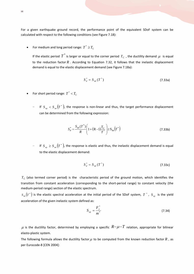
68

For a given earthquake ground record, the performance point of the equivalent SDoF system can be

calculated with respect to the following conditions (see Figure 7.18):

• For medium and long period range: C* TT ≥

If the elastic period *T is larger or equal to the corner period CT , the ductility demand µ is equal

to the reduction factor R . According to Equation 7.32, it follows that the inelastic displacement

demand is equal to the elastic displacement demand (see Figure 7.18a):

)( ** TS S ded = (7.33a)

• For short period range: C* TT <

- If ( )*aeay TSS < , the response is non-linear and thus, the target performance displacement

can be determined from the following expression:

( ) ( )*de*

** S 1 - R 1

)( T

T

T

R

TSS Cde

d ≥

+= (7.33b)

- If ( )*aeay TSS ≥ , the response is elastic and thus, the inelastic displacement demand is equal

to the elastic displacement demand:

)( ** TS S ded = (7.33c)

CT (also termed corner period) is the characteristic period of the ground motion, which identifies the

transition from constant acceleration (corresponding to the short-period range) to constant velocity (the

medium-period range) section of the elastic spectrum.

( )*TSae is the elastic spectral acceleration at the initial period of the SDoF system, *T , ayS is the yield

acceleration of the given inelastic system defined as:

*

*y

ay m

F S = (7.34)

µ is the ductility factor, determined by employing a specific TR −−µ relation, appropriate for bilinear

elasto-plastic system.

The following formula allows the ductility factor µ to be computed from the known reduction factor R , as

per Eurocode-8 [CEN 2004]:

69

( )

C*

C*

*

TT

TT 1 1 -

≥=

<+=

R

T

TR C

µ

µ (7.35)

Once the performance point (inelastic displacement) for a given earthquake (with a specific value of PGA) is

calculated, then the corresponding acceleration (elastic) can also be calculated using the following

expression:

( ) ( ) ( ) T

4 T *

2*

2*

1 deaea ST

STSπ

== (7.36)

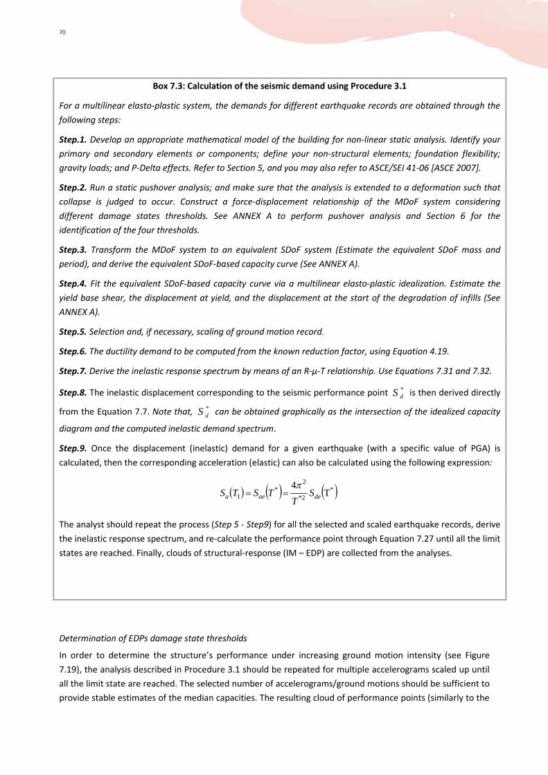
70


In order to determine the structure’s performance under increasing ground motion intensity (see Figure

7.19), the analysis described in Procedure 3.1 should be repeated for multiple accelerograms scaled up until

all the limit state are reached. The selected number of accelerograms/ground motions should be sufficient to

provide stable estimates of the median capacities. The resulting cloud of performance points (similarly to the

Box 7.3: Calculation of the seismic demand using Procedure 3.1

For a multilinear elasto-plastic system, the demands for different earthquake records are obtained through the

following steps:

Step.1. Develop an appropriate mathematical model of the building for non-linear static analysis. Identify your




collapse is judged to occur. Construct a force-displacement relationship of the MDoF system considering

different damage states thresholds. See ANNEX A to perform pushover analysis and Section 6 for the

identification of the four thresholds.

Step.3. Transform the MDoF system to an equivalent SDoF system (Estimate the equivalent SDoF mass and

period), and derive the equivalent SDoF-based capacity curve (See ANNEX A).

Step.4. Fit the equivalent SDoF-based capacity curve via a multilinear elasto-plastic idealization. Estimate the

yield base shear, the displacement at yield, and the displacement at the start of the degradation of infills (See

ANNEX A).

Step.5. Selection and, if necessary, scaling of ground motion record.

Step.6. The ductility demand to be computed from the known reduction factor, using Equation 4.19.

Step.7. Derive the inelastic response spectrum by means of an R-μ-T relationship. Use Equations 7.31 and 7.32.

Step.8. The inelastic displacement corresponding to the seismic performance point *dS is then derived directly

from the Equation 7.7. Note that, *dS can be obtained graphically as the intersection of the idealized capacity

diagram and the computed inelastic demand spectrum.

Step.9. Once the displacement (inelastic) demand for a given earthquake (with a specific value of PGA) is

calculated, then the corresponding acceleration (elastic) can also be calculated using the following expression:

( ) ( ) ( ) T4

*2*

2*

1 deaea ST

TSTSπ

==

The analyst should repeat the process (Step 5 - Step9) for all the selected and scaled earthquake records, derive

the inelastic response spectrum, and re-calculate the performance point through Equation 7.27 until all the limit

states are reached. Finally, clouds of structural-response (IM – EDP) are collected from the analyses.

71

Procedure 2.1, see Figure 7.13) is then used to determine the EDP for each damage state threshold and the

dispersion, and then create a fragility curve by fitting a statistical model. Further details are provided in

Section 8.1.

Figure 7.19 Repeat the process of the Procedure 2.1 for multiple earthquake records.




Generalized Linear Model (GLM)

Details are provided in Section 7.3.1.1



Use of smoothed elastic response spectrum

Similarly to the Procedure 2.1, the non-linear static based procedure offered in this section (Procedure 3.1)

allows, as an alternative, the calculation of EDPs thresholds using smoothed elastic response spectrum.

However, this type of response spectrum cannot reflect record-to-record variability as it generally represents

the envelope or average of response spectra. Hence, the analyst should note that this choice is not

recommended for the development of new fragility and vulnerability functions, as the uncertainty (record-to-

record variability) is not appropriately considered in computing the estimated median capacity value.

When using smoothed elastic response spectrum, the process of calculation consists of identifying the

appropriate inelastic response spectrum for which the extracted performance point reaches, or is close to,

the displacement capacity at the considered damage state threshold (see Figure 7.20).

Elastic spectrum

Inelastic spectrum

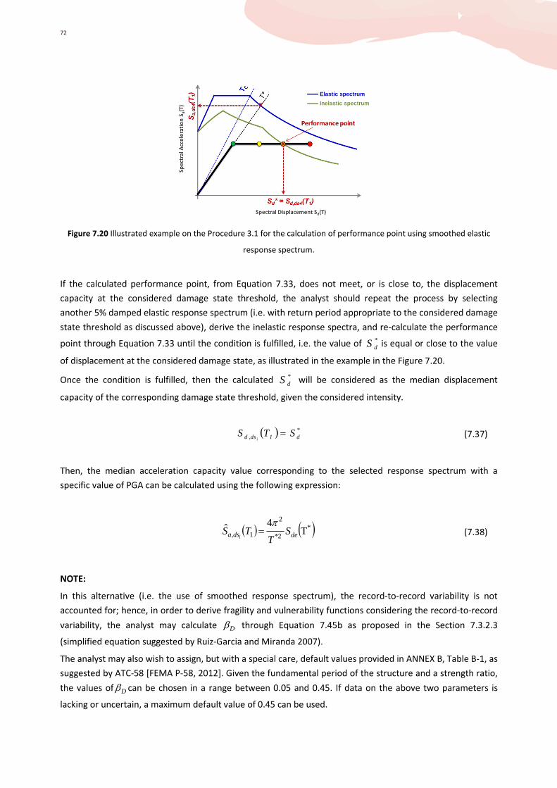
72

Figure 7.20 Illustrated example on the Procedure 3.1 for the calculation of performance point using smoothed elastic

response spectrum.

If the calculated performance point, from Equation 7.33, does not meet, or is close to, the displacement

capacity at the considered damage state threshold, the analyst should repeat the process by selecting

another 5% damped elastic response spectrum (i.e. with return period appropriate to the considered damage

state threshold as discussed above), derive the inelastic response spectra, and re-calculate the performance

point through Equation 7.33 until the condition is fulfilled, i.e. the value of *dS is equal or close to the value

of displacement at the considered damage state, as illustrated in the example in the Figure 7.20.

Once the condition is fulfilled, then the calculated *dS will be considered as the median displacement

capacity of the corresponding damage state threshold, given the considered intensity.

( ) *d1ds,d STS

i= (7.37)

Then, the median acceleration capacity value corresponding to the selected response spectrum with a

specific value of PGA can be calculated using the following expression:

( ) ( ) T4

ˆ *2*

2

1, dedsa ST

TSi

π= (7.38)

NOTE:

In this alternative (i.e. the use of smoothed response spectrum), the record-to-record variability is not

accounted for; hence, in order to derive fragility and vulnerability functions considering the record-to-record

variability, the analyst may calculate Dβ through Equation 7.45b as proposed in the Section 7.3.2.3

(simplified equation suggested by Ruiz-Garcia and Miranda 2007).





Elastic spectrum

Inelastic spectrum

73

7.3.2.2 Procedure 3.2: FRAgility through Capacity ASsessment (FRACAS)

FRACAS is a displacement-based procedure, originally developed by Rossetto and Elnashai (2005). The

procedure is applicable for structures that are characterised by Elastic-Perfectly Plastic (EPP), Linear Strain

Hardening (EST) or Tri-Linear Model (TLM); therefore, can cover different types of buildings with any number

of storeys. The proposed methodology for vulnerability curve derivation, prescribes the analysis of a

population of frames with different structural properties, subjected to a number of earthquake records with

distinct characteristics. In this way, the method is able to account for the effect of variability in seismic input

and structural characteristics on the damage statistics simulated for the building class, and evaluate the

associated uncertainty in the vulnerability prediction. The procedure has been implemented in a Matlab

programme through a collaborative effort between University College London (UCL) and Bureau de

Recherches Géologiques et Minières (BRGM), France. The FRACAS executable can be freely obtained by e-

mailing [email protected].


The determination of performance point using FRACAS procedure is based on the following steps (Figure

7.21):

• Transformation of the pushover curve (force-displacement format), resulting from non-linear static

analysis, to ADRS format.

• Idealisation of the capacity curve

• Discretisation of the idealised capacity curve and definition of a suite of SDoF for inelastic demand

analysis

• Inelastic demand calculation

• Determination of the performance point.

It is important to note that, in contrast to other capacity spectrum methods, FRACAS does not rely on

reduction factors or indices to estimate the inelastic spectrum from the elastic one. Instead, it carries out, for

each target ductility and period, a simplified dynamic analysis on the idealized non-linear SDOF model

corresponding to the capacity curve.

This process proves to be more time-consuming than the commonly used static approaches but it remains

faster and more robust than performing full time-history analyses on finite element models. This feature also

has the advantage of permitting the use of various natural accelerograms that generate unsmoothed spectra

as opposed to standardized design spectra. Therefore, the record-to-record variability can be directly

introduced and the resulting cloud of performance points leads to fragility curves that account for the natural

variability in the seismic demand.

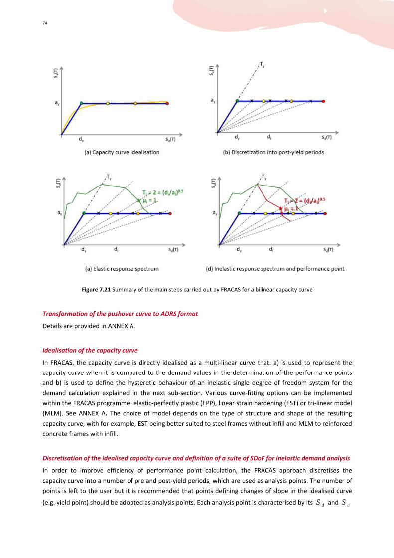
74

Figure 7.21 Summary of the main steps carried out by FRACAS for a bilinear capacity curve

Transformation of the pushover curve to ADRS format

Details are provided in ΑΝΝΕΧ Α.

Idealisation of the capacity curve

In FRACAS, the capacity curve is directly idealised as a multi-linear curve that: a) is used to represent the

capacity curve when it is compared to the demand values in the determination of the performance points

and b) is used to define the hysteretic behaviour of an inelastic single degree of freedom system for the

demand calculation explained in the next sub-section. Various curve-fitting options can be implemented

within the FRACAS programme: elastic-perfectly plastic (EPP), linear strain hardening (EST) or tri-linear model

(MLM). See ΑΝΝΕΧ Α. The choice of model depends on the type of structure and shape of the resulting

capacity curve, with for example, EST being better suited to steel frames without infill and MLM to reinforced

concrete frames with infill.

Discretisation of the idealised capacity curve and definition of a suite of SDoF for inelastic demand analysis

In order to improve efficiency of performance point calculation, the FRACAS approach discretises the

capacity curve into a number of pre and post-yield periods, which are used as analysis points. The number of

points is left to the user but it is recommended that points defining changes of slope in the idealised curve

(e.g. yield point) should be adopted as analysis points. Each analysis point is characterised by its dS and aS

75

coordinates, and a ductility value, defined by the dS coordinate of the analysis point divided by the dS

coordinate of global yield of the structure ( dyS ). Together with the elastic period of the idealised curve, this

ductility value is used to define a single degree of freedom system from which the inelastic demand is

calculated. The hysteretic behaviour of the SDoF is also defined by the shape of the idealised curve to the

analysis point.

Inelastic demand calculation

For a given earthquake record and scale factor, the inelastic seismic demand corresponding to each analysis

point is calculated through analysis of the SDOF associated with that analysis point (see above). The

earthquake record used in the analysis is discretised into time increments less than (1/50)th

of the smallest

vibration period of interest. The acceleration record is applied in these time steps to the SDoF and a Newton-

Raphson iterative scheme is used to solve the dynamic non-linear equilibrium equation for the evaluation of

the SDoF response. It is noted that only one inelastic dynamic analysis of the SDoF is required under the

applied accelerogram at each analysis point, increasing the rapidity of the assessment.


Each analysis point represents an effective period (defined by a line passing from the origin through the

analysis point) along which the inelastic demand and capacity curve can be directly compared, as they have

the same ductility. Hence, the performance point is determined directly from the intersection of the capacity

curve with the demand curve obtained by joining together the demand values of Sa and Sd calculated at each

analysis point (see Figure 7.21d).

In order to determine the EDPs corresponding to each performance point, the capacity curve coordinates at

the performance point are used to determine the corresponding load step of the non-linear static analysis

file, and relevant response parameters (e.g. maximum interstorey drift) are read from this file. Damage

thresholds of EDP should be determined from an appropriately selected damage scale for the structure being

analysed. See Section 6.

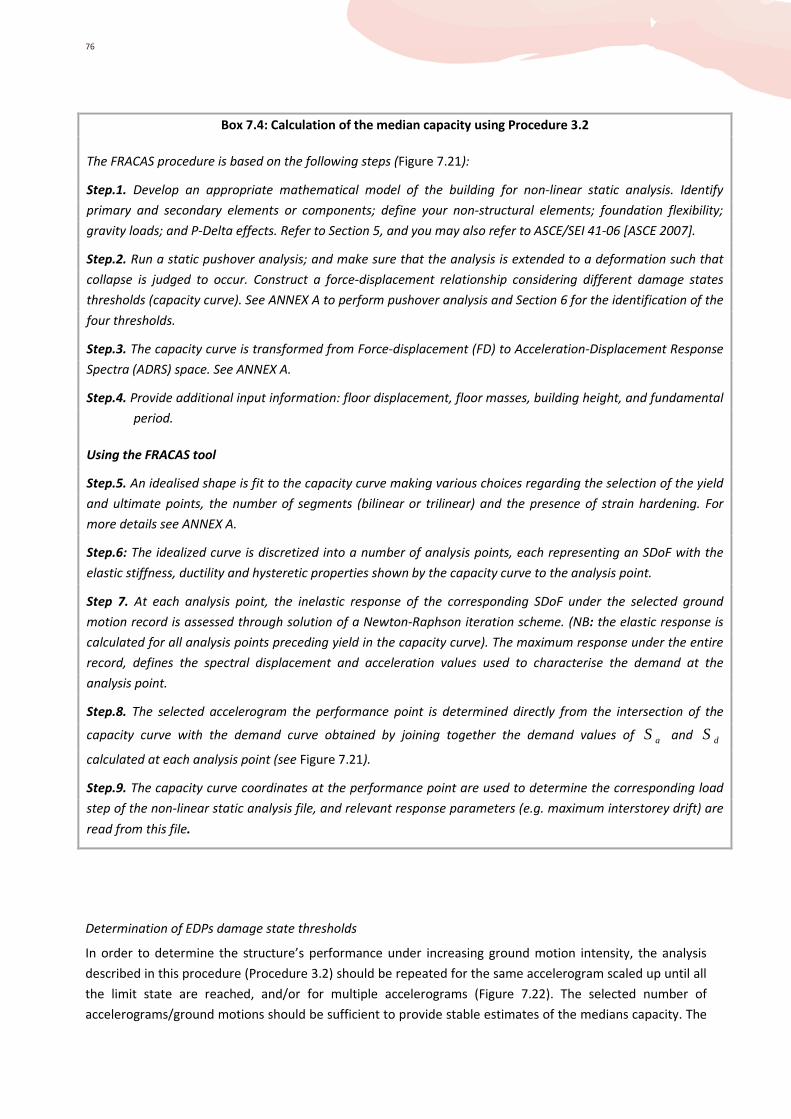
76


In order to determine the structure’s performance under increasing ground motion intensity, the analysis

described in this procedure (Procedure 3.2) should be repeated for the same accelerogram scaled up until all

the limit state are reached, and/or for multiple accelerograms (Figure 7.22). The selected number of

accelerograms/ground motions should be sufficient to provide stable estimates of the medians capacity. The


The FRACAS procedure is based on the following steps (Figure 7.21):

Step.1. Develop an appropriate mathematical model of the building for non-linear static analysis. Identify




collapse is judged to occur. Construct a force-displacement relationship considering different damage states

thresholds (capacity curve). See ΑΝΝΕΧ Α to perform pushover analysis and Section 6 for the identification of the

four thresholds.

Step.3. The capacity curve is transformed from Force-displacement (FD) to Acceleration-Displacement Response

Spectra (ADRS) space. See ΑΝΝΕΧ Α.

Step.4. Provide additional input information: floor displacement, floor masses, building height, and fundamental

period.

Using the FRACAS tool

Step.5. An idealised shape is fit to the capacity curve making various choices regarding the selection of the yield

and ultimate points, the number of segments (bilinear or trilinear) and the presence of strain hardening. For

more details see ΑΝΝΕΧ Α.

Step.6: The idealized curve is discretized into a number of analysis points, each representing an SDoF with the

elastic stiffness, ductility and hysteretic properties shown by the capacity curve to the analysis point.

Step 7. At each analysis point, the inelastic response of the corresponding SDoF under the selected ground

motion record is assessed through solution of a Newton-Raphson iteration scheme. (NB: the elastic response is

calculated for all analysis points preceding yield in the capacity curve). The maximum response under the entire

record, defines the spectral displacement and acceleration values used to characterise the demand at the

analysis point.

Step.8. The selected accelerogram the performance point is determined directly from the intersection of the

capacity curve with the demand curve obtained by joining together the demand values of aS and dS

calculated at each analysis point (see Figure 7.21).

Step.9. The capacity curve coordinates at the performance point are used to determine the corresponding load

step of the non-linear static analysis file, and relevant response parameters (e.g. maximum interstorey drift) are

read from this file.

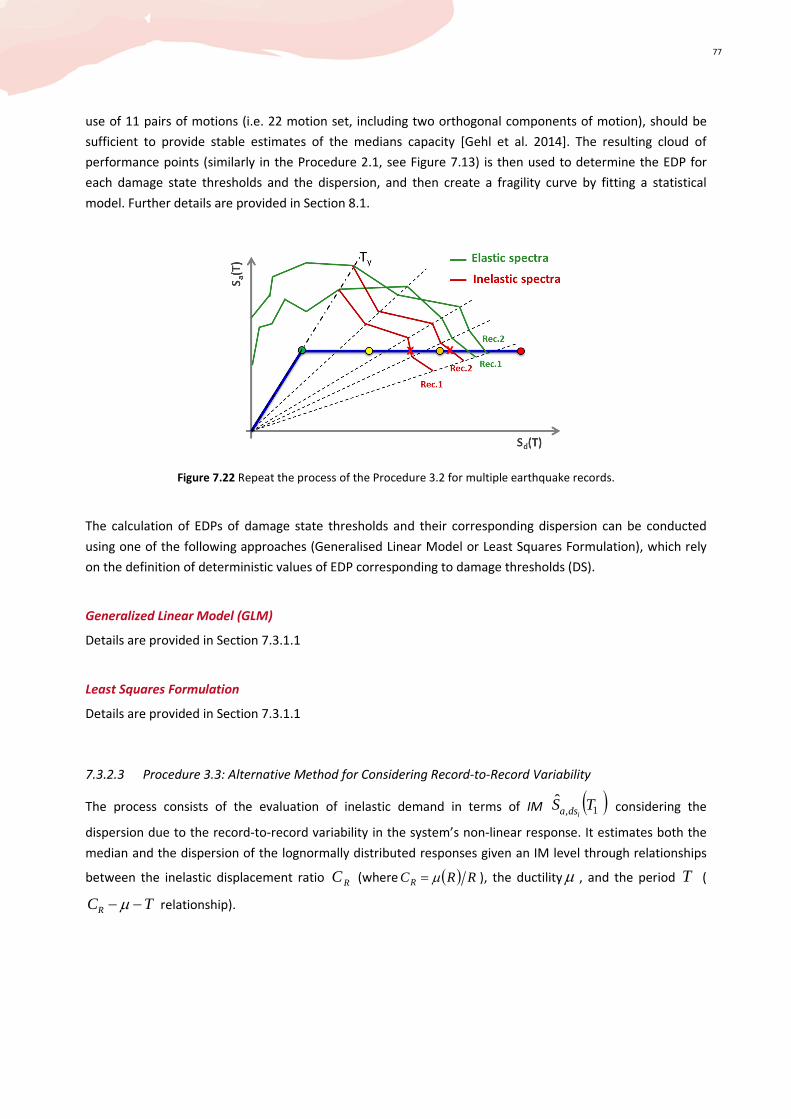
77

use of 11 pairs of motions (i.e. 22 motion set, including two orthogonal components of motion), should be

sufficient to provide stable estimates of the medians capacity [Gehl et al. 2014]. The resulting cloud of

performance points (similarly in the Procedure 2.1, see Figure 7.13) is then used to determine the EDP for

each damage state thresholds and the dispersion, and then create a fragility curve by fitting a statistical

model. Further details are provided in Section 8.1.

Figure 7.22 Repeat the process of the Procedure 3.2 for multiple earthquake records.




Generalized Linear Model (GLM)




7.3.2.3 Procedure 3.3: Alternative Method for Considering Record-to-Record Variability

The process consists of the evaluation of inelastic demand in terms of IM ( )1,ˆ TS

idsa considering the

dispersion due to the record-to-record variability in the system’s non-linear response. It estimates both the

median and the dispersion of the lognormally distributed responses given an IM level through relationships

between the inelastic displacement ratio RC (where ( ) RRCR µ= ), the ductility µ , and the period T (

TCR −− µ relationship).

78


The implementation of the procedure requires the transformation of the Multi Degree of Freedom (MDoF)

system, characterized by storey masses im and mode shapes iφ , to an equivalent Single Degree of

Freedom (SDoF) system, characterized by an equivalent mass *m (for more details see ΑΝΝΕΧ Α).

For MDoF system dominated by the first-mode shape, the roof lateral displacement response,ids,roofδ , is

related to the lateral displacement response of an equivalent elastic SDoF system, ( )1TSd , corresponding to

the building’s fundamental period of vibration, 1T , as follows [FEMA 440 2005]:

( ) 111dds,roof TSi

φΓδ ⋅= (7.39)

where 11 φΓ is the first mode participation factor, estimated for the first-mode shape normalized by the

roof displacement.


The central value of roof displacement corresponding to the median EDP capacity can be estimated using the

following expression as per ATC-55 [FEMA-440 2005]:

( ) 111,ˆˆ φδ Γ⋅⋅= TSC dRdsroof i

(7.40)

RC is the inelastic displacement ratio computed for non-linear SDoF systems having hysteretic behaviour

representative of the analysed structure, which is a function of the first-mode period of vibration and the

relative lateral strength of the system, R .

The roof displacement of a MDoF system corresponding to a damage state threshold ids , ( )iroof dsδ , can

easily be estimated from the result of pushover analysis. Considering the following relation between spectral

acceleration and displacement:

( ) ( )1a2

21

1d TS4

T TS

π= (7.41)

the median spectral acceleration of the equivalent SDoF can be estimated as follows:

( )

ii dsroofR

dsa TCTS ,

112

2

1,ˆ4ˆ δ

φ

π

Γ= (7.42)

Providing the relationship between the median IM and the corresponding median EDPs structural response.

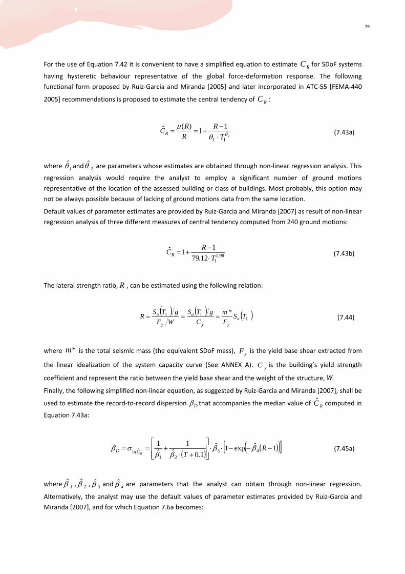
79

For the use of Equation 7.42 it is convenient to have a simplified equation to estimate RC for SDoF systems

having hysteretic behaviour representative of the global force-deformation response. The following

functional form proposed by Ruiz-Garcia and Miranda [2005] and later incorporated in ATC-55 [FEMA-440

2005] recommendations is proposed to estimate the central tendency of RC :

211

11

)( ˆ

θθµ

T

R

R

RCR

⋅

−+== (7.43a)

where 1θ and 2θ are parameters whose estimates are obtained through non-linear regression analysis. This

regression analysis would require the analyst to employ a significant number of ground motions

representative of the location of the assessed building or class of buildings. Most probably, this option may

not be always possible because of lacking of ground motions data from the same location.

Default values of parameter estimates are provided by Ruiz-Garcia and Miranda [2007] as result of non-linear

regression analysis of three different measures of central tendency computed from 240 ground motions:

98.1

112.79

11 ˆ

T

RCR

⋅

−+= (7.43b)

The lateral strength ratio, R , can be estimated using the following relation:

( ) ( ) ( )111 *

TSF

m

C

gTS

WF

gTSR a

yy

a

y

a === (7.44)

where *m is the total seismic mass (the equivalent SDoF mass), yF is the yield base shear extracted from

the linear idealization of the system capacity curve (See ΑΝΝΕΧ Α). yC is the building’s yield strength

coefficient and represent the ratio between the yield base shear and the weight of the structure, W.

Finally, the following simplified non-linear equation, as suggested by Ruiz-Garcia and Miranda [2007], shall be

used to estimate the record-to-record dispersion Dβ that accompanies the median value of RC computed in

Equation 7.43a:

( )( )( )[ ]1ˆexp1ˆ

1.0ˆ1

ˆ1

4321

ˆln−−−⋅⋅

+⋅+== R

TRCD ββββ

σβ (7.45a)

where 1β , 2β , 3β and 4β are parameters that the analyst can obtain through non-linear regression.

Alternatively, the analyst may use the default values of parameter estimates provided by Ruiz-Garcia and

Miranda [2007], and for which Equation 7.6a becomes:

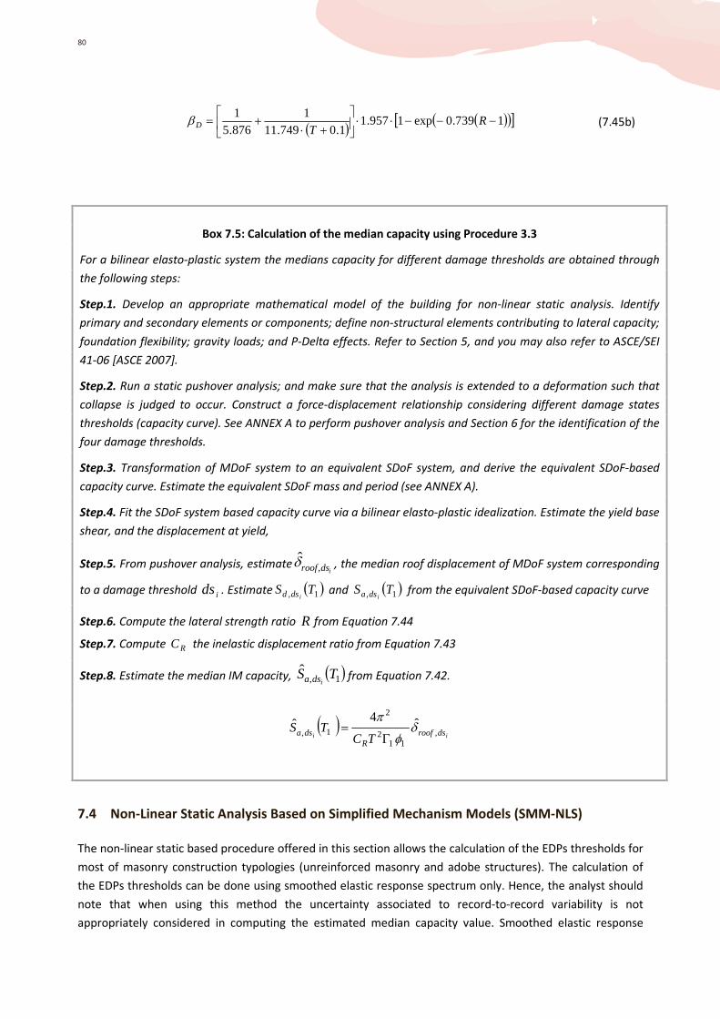
80

( )( )( )[ ]1739.0exp1957.1

1.0749.111

876.51

−−−⋅⋅

+⋅

+= RTDβ (7.45b)

7.4 Non-Linear Static Analysis Based on Simplified Mechanism Models (SMM-NLS)

The non-linear static based procedure offered in this section allows the calculation of the EDPs thresholds for

most of masonry construction typologies (unreinforced masonry and adobe structures). The calculation of

the EDPs thresholds can be done using smoothed elastic response spectrum only. Hence, the analyst should

note that when using this method the uncertainty associated to record-to-record variability is not

appropriately considered in computing the estimated median capacity value. Smoothed elastic response


For a bilinear elasto-plastic system the medians capacity for different damage thresholds are obtained through

the following steps:

Step.1. Develop an appropriate mathematical model of the building for non-linear static analysis. Identify

primary and secondary elements or components; define non-structural elements contributing to lateral capacity;

foundation flexibility; gravity loads; and P-Delta effects. Refer to Section 5, and you may also refer to ASCE/SEI

41-06 [ASCE 2007].


collapse is judged to occur. Construct a force-displacement relationship considering different damage states

thresholds (capacity curve). See ANNEX A to perform pushover analysis and Section 6 for the identification of the

four damage thresholds.

Step.3. Transformation of MDoF system to an equivalent SDoF system, and derive the equivalent SDoF-based

capacity curve. Estimate the equivalent SDoF mass and period (see ANNEX A).

Step.4. Fit the SDoF system based capacity curve via a bilinear elasto-plastic idealization. Estimate the yield base

shear, and the displacement at yield,

Step.5. From pushover analysis, estimateidsroof,δ , the median roof displacement of MDoF system corresponding

to a damage threshold ids . Estimate ( )1, TSidsd and ( )1, TS

idsa from the equivalent SDoF-based capacity curve

Step.6. Compute the lateral strength ratio R from Equation 7.44

Step.7. Compute RC the inelastic displacement ratio from Equation 7.43

Step.8. Estimate the median IM capacity, ( )1,ˆ TS

idsa from Equation 7.42.

( )ii dsroof

Rdsa

TCTS ,

112

2

1,ˆ4ˆ δ

φ

π

Γ=

81

spectrum cannot reflect record-to-record variability as it generally represents the envelope or average of

response spectra.

7.4.1 Procedure 4.1: Failure Mechanism Identification and Vulnerability Evaluation (FaMIVE)

The Failure Mechanism Identification and Vulnerability Evaluation (FaMIVE) procedure is based on

previous work presented in D’Ayala and Speranza [2003] and D’Ayala [2005]. The FaMIVE method uses a

non-linear pseudo-static structural analysis with a degrading pushover curve to estimate the performance

points, as it has been described in Procedure 2.1 and Procedure 3.1. It yields as output collapse multipliers

which identify the occurrence of possible different mechanisms for a given masonry construction typology,

given certain structural characteristics. The FaMIVE algorithm produces capacity curves, performance points

and outputs fragility curves for different seismic scenarios in terms of intermediate and ultimate

displacements or ultimate acceleration. Figure 7.23 shows the workflow of the FaMIVE method for the

seismic vulnerability assessment.

Figure 7.23 Workflow of the FaMIVE method for derivation of fragility functions

Data Collection

South East

Wes

tNorth

South East NorthWest

A .. M

South East NorthWest

A .. M A .. M A .. M

Min Min Min Min

Equivalent Shear Capacity Mechanism

Meff

Teff

Keff

DL SD NC

Mean STD

Logn. Distr

C

eff

Fb

Meffug(t)..

Non-LinearSDOF

Y

vU

v

vY

sd

DL

SD NC

U

Lateral displacement

Late

ral c

apac

ity

Cc

DL

for a selected SITE

Cap

acity

Cur

ve

Spe

ctra

l Res

pons

e A

ccel

erat

ion

SD NC

CSd (cm)

Sa

(a/g

)

Period T

Sa

(a/g

)

Per

form

ance

poi

nt

Mean STD

Logn. Distr

Mean STD

Logn. Distr

Mean STD

Logn. Distr

FaMIVE

82

Within the FaMIVE database capacity curves and fragility functions are available for various unreinforced

masonry typologies, from adobe to concrete blocks, for a number of reference typologies in a number of

regions of the world [D’Ayala and Kishali 2012, D’Ayala 2013]. The FaMIVE executable can be freely obtained

by e-mailing [email protected].

Derivation of capacity curve and determination of the performance point

The capacity curve for the structure is directly related to the collapse mechanism identified by the analysis as

the critical one. The construction of the capacity curve is obtained by first calculating the lateral effective

stiffness for each wall and its tributary mass. The effective stiffness for a wall is calculated on the basis of the

type of mechanism attained, the geometry of the wall and layout of opening, the constraints to other walls

and floors and the portion of other walls involved in the mechanism:

(7.46)

where effH is the height of the portion involved in the mechanism, tE is the estimated modulus of the

masonry as it can be obtained from experimental literature for different masonry typologies, effI and effA are

the second moment of area and the cross sectional area, calculated taking into account extent and position

of openings and variation of thickness over height, 1k and 2k are constants which assume different values

depending on edge constraints and whether shear and flexural stiffness are relevant for the specific

mechanism.

The tributary mass effΩ is calculated following the same approach and it includes the portion of the

elevation activated by the mechanisms plus the mass of the horizontal structures involved in the mechanism:

rfmeffeff V Ω+Ω+=Ω γ (7.47)

where effV is the solid volume of the portion of wall involved in the mechanism, mγ is the density of the

masonry, fΩ and rΩ are the masses of the horizontal structures involved in the mechanism. Effective mass

and effective stiffness are used to calculate a natural period effT , which characterises an equivalent SDoF

oscillator:

eff

effeff K

TΩ

= π2 (7.48)

The mass is applied at the height of the centre of gravity of the collapsing portion with respect to the ground

0h and a linear acceleration distribution over the wall height is assumed. The elastic limit acceleration ayS is

also computed depending on the failure mechanism identified; for failure mechanisms involving flexural

eff

efft

eff

effteff H

AEk

H

IEkK 231 +=

83

strain limit (assuming no tensile capacity in the material), for instance, ayS will be the value of lateral

acceleration that combined with gravitational load resultant, will cause a triangular distribution of

compression stresses at the base of the overturning portion, just before the onset of partialisation:

gh

tS b

ay0

2

6= with corresponding displacement eff

ayde T

SS

24π= (7.49)

where, bt is the effective thickness of the wall at the base of the overturning portion, 0h is the height to the

ground of the centre of mass of the overturning portion, and effT the natural period of the equivalent SDoF

oscillator. In the case of in-plane mechanism the geometric parameter used for the elastic limit is, rather

than the wall thickness, the width of the pier where the flexural strain limit is first attained.

The maximum lateral capacity auS is defined as:

1αλc

auS = (7.50)

where cλ is the load factor of the collapse mechanism chosen, calculated by FaMIVE, and 1α is the proportion

of total mass participating to the mechanism. This is calculated as the ratio of the mass of the façade and

sides or internal walls and floor involved in the mechanism effΩ , to the total mass of the involved macro-

elements (i.e. walls, floors, and roof). The displacement corresponding to first attainment of the peak lateral

force auS , identifying the damage threshold of structural damage, is dsS set as:

dydsdy SSS 63 ≤≤ (7.51)

as suggested by Tomazevic et al. [2007]. The range in Equation 7.51 is useful to characterize masonry fabric

of variable regularity and its integrity at ultimate conditions, with the lower bound better describing the

behaviour of adobe, rubble stone and brickwork in mud mortar, while the upper bound can be used for

massive stone, brickwork set in lime or cement mortar and concrete blockwork.

Finally the near collapse condition is determined by the displacement duS identified by the condition of loss

of vertical equilibrium which, for overturning mechanisms, can be computed as a lateral displacement at the

top or for in plane mechanism by the loss of overlap of two units in successive courses, i.e.:

2 or 3 /lS/tS udubdu ≥≥ (7.52)

where bt is the thickness at the base of the overturning portion and ul is the typical length of units forming

the wall.

Equations 7.49 to 7.52 identify the threshold points on the idealised capacity curve corresponding to the

damage limit states 1ds to 4ds defined in Table 6.6.

84

To calculate the coordinates of the performance point in the displacement-acceleration space, the

intersection of the capacity curve with the non-linear demand spectrum for an appropriate level of ductility

µ can be determined as shown in Equation 7.53, given the value of ultimate lateral capacity of the

equivalent SDoF oscillator, auS :

• For short period range: CTT <*

- If ( )*TSS aau ≥

( )( )( ) ( )*22

2**2*

4

1

)()(

TS

gTSTSTS

a

aaeCd π

µ

µµ ⋅

−

−= (7.53a)

- If ( ) ( )*TSSTS aauCa <<

( )( ) au

auaeC

S

gSTSTS

d 22

2*2*

4

1

)()(

πµ

µµ ⋅

−

−= (7.53b)

- If ( )Caau TSS ≤

( )au

aeC

S

TSgTS

d µπµ

2

2*2*

4

)()( = (7.53c)

• For medium and long period range: CTT ≥*

- If ( )*TSS aau ≥

( )( )*2

2*2*

4

)()(

TS

TSgTS

a

aeCd µπ

µ = (7.53d)

- If ( )*TSS aau <

( )au

aeC

S

TSgTS

d µπµ

2

2*2*

4

)()( = (7.53e)

where two different formulations are provided for values of ultimate lateral capacity auS greater or smaller

than the non-linear spectral acceleration ( )Ca TS associated with the corner period CT marking the transition

from constant acceleration to constant velocity section of the parent elastic spectrum.

Figure 7.24 shows an example of calculation of performance points for median capacity curves for some

different types of mechanisms (see Figure 5.3).

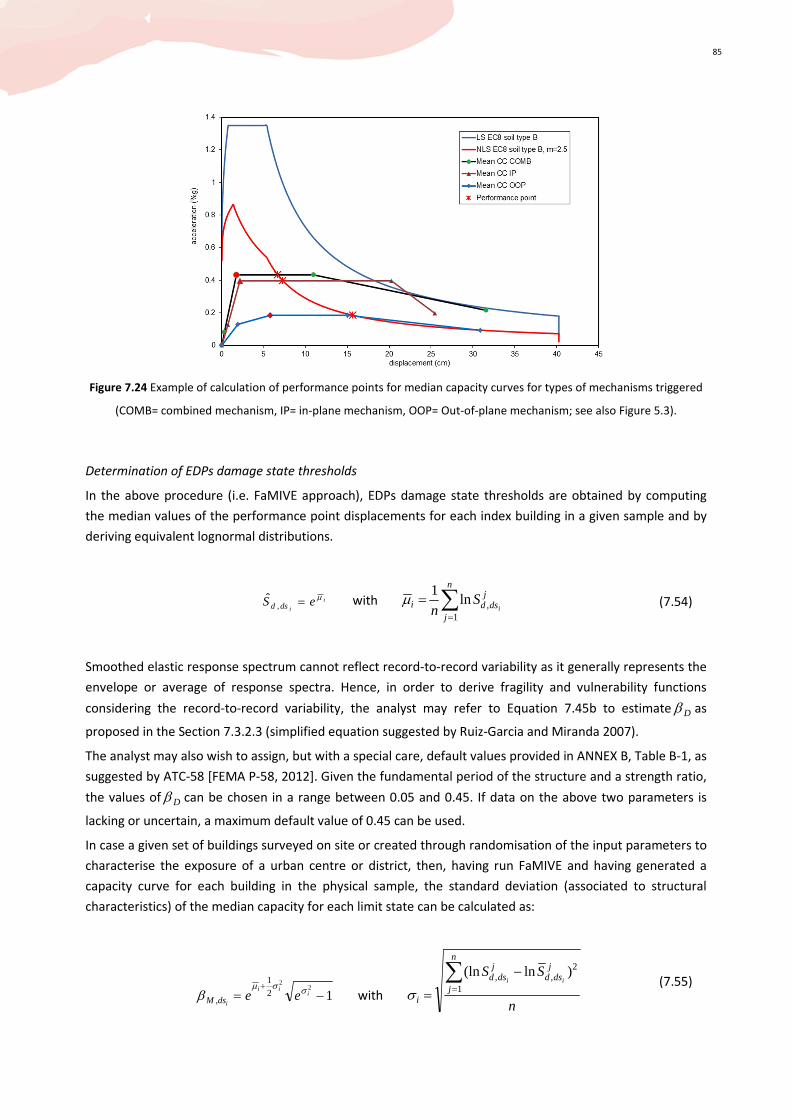
85

Figure 7.24 Example of calculation of performance points for median capacity curves for types of mechanisms triggered

(COMB= combined mechanism, IP= in-plane mechanism, OOP= Out-of-plane mechanism; see also Figure 5.3).


In the above procedure (i.e. FaMIVE approach), EDPs damage state thresholds are obtained by computing

the median values of the performance point displacements for each index building in a given sample and by

deriving equivalent lognormal distributions.

i

ieS dsd

µ=,ˆ with ∑

=

=n

j

jdsdi i

Sn 1

,ln1

µ (7.54)

Smoothed elastic response spectrum cannot reflect record-to-record variability as it generally represents the

envelope or average of response spectra. Hence, in order to derive fragility and vulnerability functions

considering the record-to-record variability, the analyst may refer to Equation 7.45b to estimate Dβ as

proposed in the Section 7.3.2.3 (simplified equation suggested by Ruiz-Garcia and Miranda 2007).





In case a given set of buildings surveyed on site or created through randomisation of the input parameters to

characterise the exposure of a urban centre or district, then, having run FaMIVE and having generated a

capacity curve for each building in the physical sample, the standard deviation (associated to structural

characteristics) of the median capacity for each limit state can be calculated as:

12

2

2

1

, −=+

iii

ieedsM

σσµβ with

n

SSn

j

jdsd

jdsd

i

ii∑=

−

= 1

2,, )ln(ln

σ (7.55)

86

To account for the reliability of the input parameters, three levels of reliability are considered, high, medium,

and low, respectively, to which three confidence ranges of the value given for a parameter can be considered

corresponding to 10% variation, 20% variation, and 30% variation. The parameter value is considered central

to the confidence range so that the interval of existence of each parameter is defined as %5±µ , %10±µ ,

%15±µ , depending on highest or lowest reliability. The reliability applied to the output parameters, in

particular, equivalent lateral acceleration and limit states’ displacement, is calculated as a weighted average

of the reliability of each section of the data form, with minimum 5% confidence range to maximum 15%

confidence range.

87

8 STEP F: Vulnerability Curves Derivation

Vulnerability curves translate the physical damage into monetary loss (estimation of repair and

reconstruction cost), given a level of intensity measure, im. Options are offered to the analyst to generate

different forms of vulnerability curves:

• vulnerability curve evaluated on the damage indicators of one index building,

• vulnerability curve evaluated on the damage indicators of three index buildings, and

• vulnerability curve evaluated on the damage indicators of multiple index buildings.

In order to generate these curves, two approaches can be used, depending on available data, project

requirement, and analyst’s skills:

Building-based vulnerability assessment approach:

In this approach, widely used in literature, the vulnerability functions are obtained by convolving

building level fragility curves with the cumulative cost of a given damage state ids (damage-to-loss

functions). In general, the implementation of this approach would be more reasonable, in terms of

calculation effort and the availability of detailed data, when performing studies of large population of

buildings.

Component-based vulnerability assessment approach:

In this approach, comprehensively presented in ATC-58 [FEMA P-58, 2012], the vulnerability functions

are obtained by correlating the components level-based drifts directly to loss. In general, this approach

is appropriate when performing loss analysis for single buildings, or when the majority of the economic

losses are related to content and non-structural components. The analyst will have to ascertain that the

relevant information on specific component loss is available and that time and monetary resources are

at hand to perform such detailed analysis.

Note: within this approach, the vulnerability curve can be generated at the storeys level, and at the

entire building-level.

8.1 STEP F-1: Building-Based Vulnerability Assessment Approach

The transformation of the fragility curves into vulnerability can be conducted through the following total

probability relation:

( ) ( ) ( )imdsPdscCEimcCE i

n

ii |||

0

⋅>=> ∑=

(8.1)

88

Where, n is the number of damage states considered, ( )imdsP i | is the probability of a building sustaining

damage state ids given intensity im; ( )idscCE |> is the complementary cumulative distribution of the cost

(loss) given ids ; ( )imcCE |> is the complementary cumulative distribution of cost (or loss) given a level of

intensity im.

The transformation expressed by Equation 8.1 requires the calculation of damage probabilities from the

fragility curves for specific level of intensity:

(a) Fragility curves corresponding to n =4 damage states (b) Column of a damage probability for intensity im

ds0 = No Damage; ds1 = Slight Damage; ds2 = Moderate Damage; ds3 = Near Collapse; ds4 = Collapse

Figure 8.1 Calculation of damage probabilities from the fragility curves for a specific level of intensity measurement, im.

Each element (or bar) in the damage probabilities is defined as the distance between two successive fragility

curves for a given intensity im, as shown in Figure 8.1. The mean, ( )imCE | , and the variance, ( )imC |var , of

the vulnerability can be then obtained by the following expressions (where n = is the number of damage

states considered):

( ) ( ) ( )imdsPdsCEimCE i

n

ii |||

0

⋅=∑=

(8.2)

( ) ( ) ( )[ ] ( ) ( )∑=

−⋅+=n

iiii imCEimdsPdsCEdsCimC

0

22 || ||var|var (8.3)

Repeating the process of calculation (using Equations 8.2 and 8.3) for a range of values for intensity measure

im ∈ 0.01, 0.02, ...3.0g, will result in the vulnerability curve, as shown in the example of

Figure 8.2, where the variance will provide the confidence boundary.

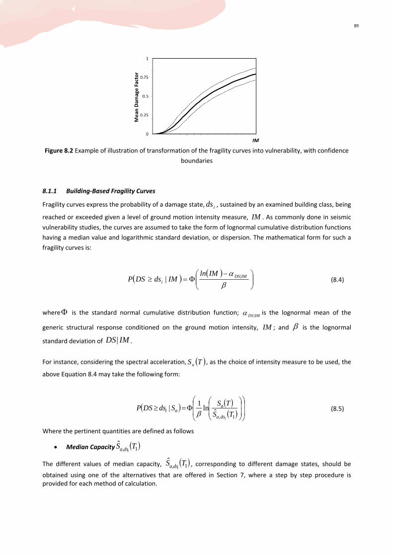
89

Figure 8.2 Example of illustration of transformation of the fragility curves into vulnerability, with confidence

boundaries

8.1.1 Building-Based Fragility Curves

Fragility curves express the probability of a damage state, ids , sustained by an examined building class, being

reached or exceeded given a level of ground motion intensity measure, IM . As commonly done in seismic

vulnerability studies, the curves are assumed to take the form of lognormal cumulative distribution functions

having a median value and logarithmic standard deviation, or dispersion. The mathematical form for such a

fragility curves is:

( ) ( )

−Φ=≥

β

α IM|DSi

IMlnIM|dsDSP (8.4)

where Φ is the standard normal cumulative distribution function; IM|DSα is the lognormal mean of the

generic structural response conditioned on the ground motion intensity, IM ; and β is the lognormal

standard deviation of IMDS| .

For instance, considering the spectral acceleration, ( )TSa , as the choice of intensity measure to be used, the

above Equation 8.4 may take the following form:

( ) ( )( )

Φ=≥

1,ˆ

ln1

|TS

TSSdsDSP

idsa

aai β

(8.5)

Where the pertinent quantities are defined as follows

• Median Capacity ( )1,ˆ TS

idsa

The different values of median capacity, ( )1,ˆ TS

idsa , corresponding to different damage states, should be

obtained using one of the alternatives that are offered in Section 7, where a step by step procedure is

provided for each method of calculation.

90

• Total Dispersion β

The total dispersion parameter β , defined as the lognormal standard deviation, should include: the

randomness in the demand imposed on the structure by the earthquake ground motion, the randomness in

the values of structural parameters, the uncertainty associated with the mathematical modeling; the

building-to-building variability when a class of buildings is considered, the uncertainty associated with the

definition of the damage thresholds [D’Ayala and Meslem 2013a].

A number of different formulae exist to represent the contributions of each of these uncertainties to the

total dispersion parameter β [FEMA P-58, 2012; FEMA, 2003]. Depending on the refinement of the

procedure used for the calculation of EDPs (Section 7), these uncertainties are accounted for implicitly or

explicitly. It should be kept in mind that the dispersions associated with record-to-record variability, Dβ ,

total modelling dispersion, Mβ , and damage threshold variability, dsβ , all are dependent on the damage

state considered, with increasing value of dispersion as the damage state increase.

According to ATC-58 [FEMA P-58, 2012], the following Equation could be used for the calculation of total

variability:

22MD βββ += (8.6a)

where, Dβ is the dispersion associated with uncertainty in the demand (record-to-record variability); Mβ is

the total modelling dispersion associated with uncertainty in the definition of structural characteristics of

building, quality and completeness of mathematical model (definition of different mechanisms, geometric

configuration…etc.), and building-to-building variability.

According to HAZUS-MH [FEMA 2003], the following Equation could be used for the calculation of total

variability:

[ ]( ) ( )22

,,, dsSdsdDC SCONV ββββ += (8.6b)

where, Cβ is the dispersion associated with variability in the capacity curve; Dβ is the uncertainty in the

demand (record-to-record variability); dsβ is the uncertainty in the estimate of the median value of the

threshold of structural damage state ds. The function “CONV” in Equation (8.6b) implies a complex process of

convolving probability distributions of the demand spectrum and the capacity curve, respectively.

Record-to-record dispersion, Dβ

The demand dispersion associated with ground motion uncertainty, Dβ , represents the variability in the

distribution of the recorded response at a given level of intensity IM due to different ground motion records.

It highly depends on the structure but also on the type of IM used. Shorter periods, higher levels of system

ductility, increased influence of higher modes but also the use of a less efficient IM (Section 2.3) will

generally result in increased values of Dβ :

91

- If natural records (records from real events; synthetic; or artificial) with different level of IM are

used, Dβ should be estimated directly from the computation as the lognormal standard

deviation for the selected records. Details are provided in Section 7.

- If smoothed elastic response spectrum (which generally represents the envelope or average of

response spectra) is used, the uncertainty in demand will not be appropriately considered, as

this type of response spectrum cannot reflect record-to-record variability. In this case, Dβ

should be calculated using the simplified relation offered in Equation 7.45b (Details are provided

in Section 7.3.2.3):

( )( )( )[ ]1739.0exp1957.1

1.0749.11

1

876.5

1 −−−⋅⋅

+⋅

+= RTDβ

Alternatively, but with special care, Dβ can be assumed through default values that are

provided in ANNEX B, Table B-1, as suggested by ATC-58 [FEMA P-58, 2012]. Given the

fundamental period of the structure and a strength ratio, the values of Dβ can be chosen in a

range between 0.05 and 0.45. If data on the above two parameters is lacking or uncertain, a

maximum default value of 0.45 can be used.

Total modelling dispersion, Mβ

Given the selected approach of modelling (from one index building to multiple index buildings) and analysis,

alternatives are offered to account for the total dispersion in modelling:

- In case a given set of buildings surveyed on site or created through randomisation of the input

parameters to characterise the exposure of an urban centre or district, then, having run selected

analysis type and having generated a capacity curve for each building in the physical sample, the

dispersion associated to the structural characteristics variability and building-to-building

variability, Mβ , should be estimated directly from the computation as standard deviation of the

median capacity for each limit state using one of the techniques (i.e. regression techniques)

offered in Section 7.

- Mβ is obtained by using First-Order Second-Moment (FOSM) procedure (Lee and Mosalam

2005; Baker and Cornell 2008b, Vamvatsikos and Fragiadakis 2010). Mβ is computed based on

the structural responses obtained from the assigned Central, Lower and Upper Bound values

(Figure 3.1) of the modelling parameters, the type of distribution for the structural

characteristics-based parameters, and model variability. Assuming that the logarithm of the

median capacity is a function of the random parameters, the standard deviation of the logs (i.e.,

the dispersion) is estimated using a first-order derivative:

92

2

2

1

minmax2

2

1

2 lnln

lnln

kk

Lowerk

Upperk

X

K

kLower

kUpper

k

aaX

K

kLower

kUpper

k

Xa

Xa

MXX

SS

XX

SSσσβ ⋅

−

−≈⋅

−

−≈ ∑∑

==

(8.7)

where, K is the total number of random modelling parameters considered in the analyses

(selected from Table 3.1); kX is the lower or upper value of the random modelling parameter

k ; kXσ is the standard deviation for each parameter considered, and should be obtained from

result of structural characteristics assessment. Further details are provided in D’Ayala and

Meslem 2013b, 2013c.

- When conducting a single analysis without extracting lower and upper bound values

corresponding to the parameter variability (one index building only central value), then a default

value of Mβ can be used, as summarised in ANNEX B, Table B-1. These values have been

suggested by ATC-58 (FEMA P-58, 2012), and are defined as the uncertainty due to ambiguity in

building definition and construction quality. These values range between 0.25 and 0.50

depending on the fundamental period of the structure and its strength ratio.

Damage threshold dispersion, dsβ

According to HAZUS-MH [FEMA 2003], the lognormal standard deviation parameter that describes the

uncertainty in the estimate of the median value of the threshold of structural damage state ds, dsβ , is

assumed to be independent of capacity and demand. The values of dispersion of this parameter available in

HAZUS-MH are computed in terms of spectral displacement.

8.1.2 Building-Based Repair Cost Given Damage State

For a reliable estimation of total repair cost it is quite important that the analyst accounts for the type of

occupancy of the assessed building. In addition to that, the analysts will need to provide their local estimates

of repair and reconstruction costs in order to reach a better level of accuracy for the derived vulnerability

curves.

If such data is available, the analyst can calculate the total repair cost, given damage threshold:

( ) ( ) ( )iii dsAreaMatCostEdsAreaLabCostEdsCE _|_|| += (8.8)

where

( )idsCE | = is the complementary cumulative distribution of the total repair cost given ids .

( )idsAreaLabCostE _| = is the local labour cost in the considered region (cost per percentage of damaged

area given ids ).

( )idsAreaMatCostE _| = is the local material cost in the considered region (cost per percentage of

damaged area given ids ).

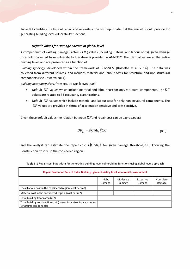
93

Table 8.1 identifies the type of repair and reconstruction cost input data that the analyst should provide for

generating building level vulnerability functions.

Default values for Damage Factors at global level

A compendium of existing Damage Factors ( DF) values (including material and labour costs), given damage

threshold, collected from vulnerability literature is provided in ANNEX C. The DF values are at the entire

building level, and are presented as a function of:

Building typology, developed within the framework of GEM-VEM [Rossetto et al. 2014]. The data was

collected from different sources, and includes material and labour costs for structural and non-structural

components (see Rossetto 2014).

Building occupancy class, from HAZUS-MH [FEMA 2003]:

• Default DF values which include material and labour cost for only structural components. The DF

values are related to 33 occupancy classifications.

• Default DF values which include material and labour cost for only non-structural components. The

DF values are provided in terms of acceleration sensitive and drift sensitive.

Given these default values the relation between DFand repair cost can be expressed as:

( ) CCDFids ids|CE = (8.9)

and the analyst can estimate the repair cost ( )idsCE / , for given damage threshold, ids , knowing the

Construction Cost CC in the considered region.

Table 8.1 Repair cost input data for generating building-level vulnerability functions using global level approach

Repair Cost Input Data of Index Building - global building level vulnerability assessment

Slight

Damage

Moderate

Damage

Extensive

Damage

Complete

Damage

Local Labour cost in the considered region (cost per m2)

Material cost in the considered region (cost per m2)

Total building floors area (m2)

Total building construction cost (covers total structural and non-

structural components)

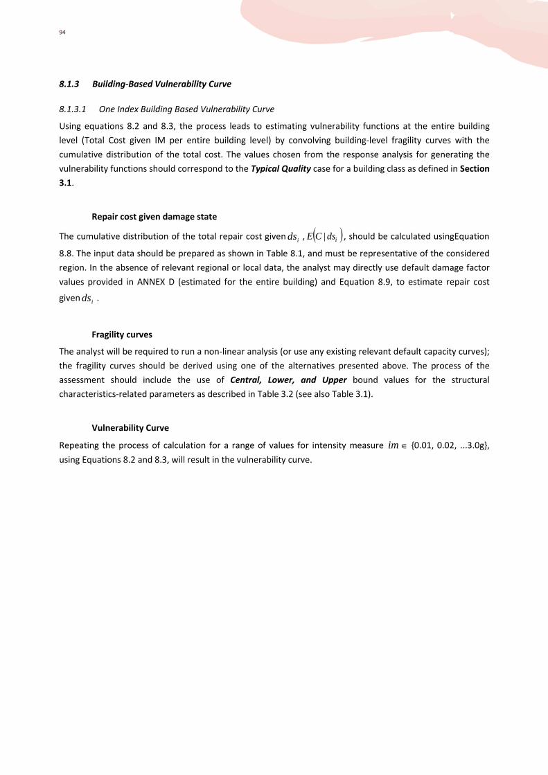
94

8.1.3 Building-Based Vulnerability Curve

8.1.3.1 One Index Building Based Vulnerability Curve

Using equations 8.2 and 8.3, the process leads to estimating vulnerability functions at the entire building

level (Total Cost given IM per entire building level) by convolving building-level fragility curves with the

cumulative distribution of the total cost. The values chosen from the response analysis for generating the

vulnerability functions should correspond to the Typical Quality case for a building class as defined in Section

3.1.

Repair cost given damage state

The cumulative distribution of the total repair cost given ids , ( )idsCE | , should be calculated usingEquation

8.8. The input data should be prepared as shown in Table 8.1, and must be representative of the considered

region. In the absence of relevant regional or local data, the analyst may directly use default damage factor

values provided in ANNEX D (estimated for the entire building) and Equation 8.9, to estimate repair cost

given ids .

Fragility curves

The analyst will be required to run a non-linear analysis (or use any existing relevant default capacity curves);

the fragility curves should be derived using one of the alternatives presented above. The process of the

assessment should include the use of Central, Lower, and Upper bound values for the structural

characteristics-related parameters as described in Table 3.2 (see also Table 3.1).

Vulnerability Curve

Repeating the process of calculation for a range of values for intensity measure im ∈ 0.01, 0.02, ...3.0g,

using Equations 8.2 and 8.3, will result in the vulnerability curve.

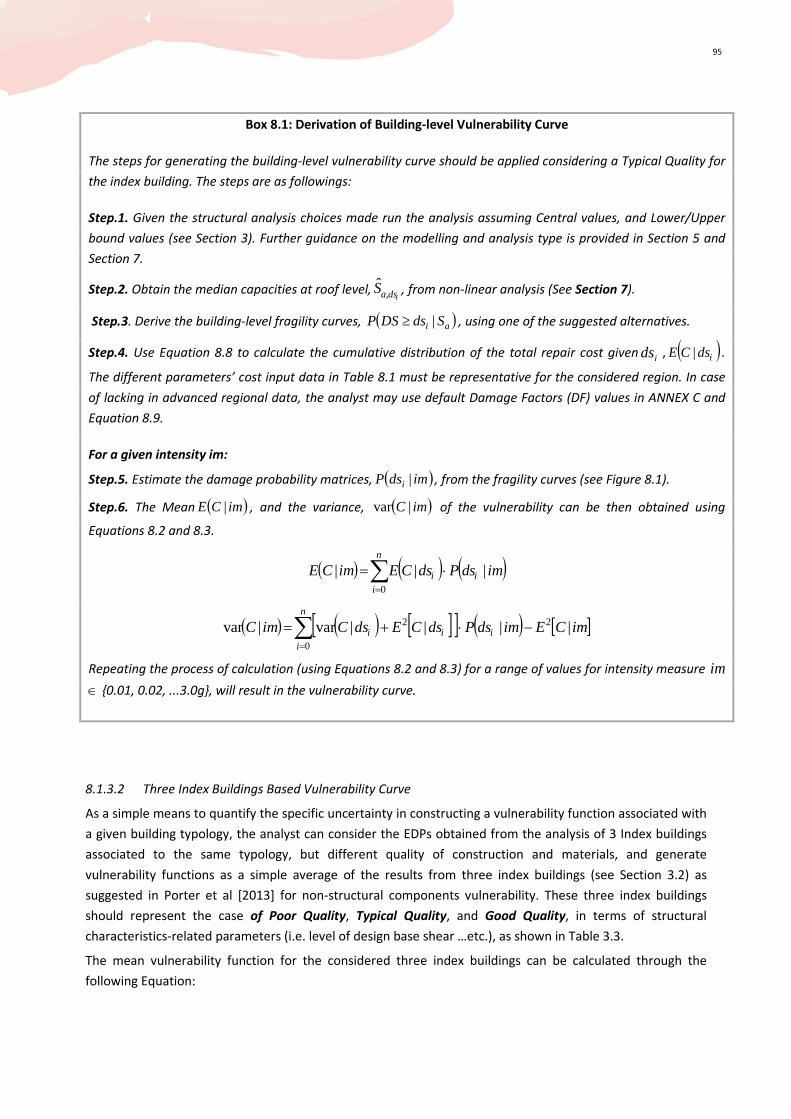
95

8.1.3.2 Three Index Buildings Based Vulnerability Curve

As a simple means to quantify the specific uncertainty in constructing a vulnerability function associated with

a given building typology, the analyst can consider the EDPs obtained from the analysis of 3 Index buildings

associated to the same typology, but different quality of construction and materials, and generate

vulnerability functions as a simple average of the results from three index buildings (see Section 3.2) as

suggested in Porter et al [2013] for non-structural components vulnerability. These three index buildings

should represent the case of Poor Quality, Typical Quality, and Good Quality, in terms of structural

characteristics-related parameters (i.e. level of design base shear …etc.), as shown in Table 3.3.

The mean vulnerability function for the considered three index buildings can be calculated through the

following Equation:

Box 8.1: Derivation of Building-level Vulnerability Curve

The steps for generating the building-level vulnerability curve should be applied considering a Typical Quality for

the index building. The steps are as followings:

Step.1. Given the structural analysis choices made run the analysis assuming Central values, and Lower/Upper

bound values (see Section 3). Further guidance on the modelling and analysis type is provided in Section 5 and

Section 7.

Step.2. Obtain the median capacities at roof level,idsaS ,

ˆ , from non-linear analysis (See Section 7).

Step.3. Derive the building-level fragility curves, ( )ai SdsDSP |≥ , using one of the suggested alternatives.

Step.4. Use Equation 8.8 to calculate the cumulative distribution of the total repair cost given ids , ( )idsCE | .

The different parameters’ cost input data in Table 8.1 must be representative for the considered region. In case

of lacking in advanced regional data, the analyst may use default Damage Factors (DF) values in ANNEX C and

Equation 8.9.

For a given intensity im:

Step.5. Estimate the damage probability matrices, ( )imdsP i | , from the fragility curves (see Figure 8.1).

Step.6. The Mean ( )imCE | , and the variance, ( )imC |var of the vulnerability can be then obtained using

Equations 8.2 and 8.3.

( ) ( ) ( )imdsPdsCEimCE i

n

ii |||

0

⋅=∑=

( ) ( ) [ ][ ] ( ) [ ]∑=

−⋅+=n

iiii imCEimdsPdsCEdsCimC

0

22 || ||var|var

Repeating the process of calculation (using Equations 8.2 and 8.3) for a range of values for intensity measure im

∈ 0.01, 0.02, ...3.0g, will result in the vulnerability curve.

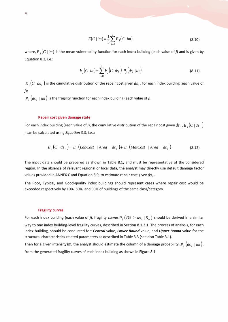
96

( ) ( )∑

=

=3

1

|3

1|

jj imCEimCE (8.10)

where, ( )im|CE j is the mean vulnerability function for each index building (each value of j) and is given by

Equation 8.2, i.e.:

( ) ( ) ( )imdsPdsCEimCE ij

n

iijj |||

0

⋅=∑=

(8.11)

( )ij ds|CE is the cumulative distribution of the repair cost given ids , for each index building (each value of

j);

( )im|dsP ij is the fragility function for each index building (each value of j).

Repair cost given damage state

For each index building (each value of j), the cumulative distribution of the repair cost given ids , ( )ij ds|CE

, can be calculated using Equation 8.8, i.e.,:

( ) ( ) ( )ijijij ds_Area|MatCostEds_Area|LabCostEds|CE += (8.12)

The input data should be prepared as shown in Table 8.1, and must be representative of the considered

region. In the absence of relevant regional or local data, the analyst may directly use default damage factor

values provided in ANNEX C and Equation 8.9, to estimate repair cost given ids .

The Poor, Typical, and Good-quality index buildings should represent cases where repair cost would be

exceeded respectively by 10%, 50%, and 90% of buildings of the same class/category.

Fragility curves

For each index building (each value of j), fragility curves ( )aij S|dsDSP ≥ should be derived in a similar

way to one index building-level fragility curves, described in Section 8.1.3.1. The process of analysis, for each

index building, should be conducted for: Central value, Lower Bound value, and Upper Bound value for the

structural characteristics-related parameters as described in Table 3.3 (see also Table 3.1).

Then for a given intensity im, the analyst should estimate the column of a damage probability, ( )im|dsP ij ,

from the generated fragility curves of each index building as shown in Figure 8.1.

97

8.1.3.3 Multiple Index Buildings Based Vulnerability Curve

The implementation of this approach would require a greater calculation effort, depending on the number of

properties considered (i.e. number of parameters that will be considered as significant). The process will

require the use of a large number of numerical simulations by implementing one of the following sampling

approaches: Moment-Matching, Class Partitioning, or Monte Carlo simulation. Further details are provided in

Section 3.3.

Box 8.2: Derivation of Three Index Buildings-based Vulnerability Curve

The steps for generating the three index buildings-based vulnerability curve should be applied considering the

case of: Poor, Typical, and Good quality. The steps are as followings:

For each index building j (j =1,2,3):

Step.1. Given the structural analysis choices made run the analysis assuming central values, lower values, and

upper values. Further guidance on the modelling and analysis type is provided in Section 5 and Section 7.

Step.2. Obtain the medians capacity at roof level,idsaS ,

ˆ , from non-linear analysis (See Section 7).

Step.3. Derive the building-level fragility curves, ( )aij S|dsDSP ≥ , using one of the suggested alternatives.

Step.4. Use Equation 8.12 to calculate the cumulative distribution of the total repair cost given ids , ( )ij ds|CE .

The different parameters’ cost input data in Table 8.1 must be representative for the considered region. In case

of lacking in advanced regional data, the analyst may use default damage factors values provided in ANNEX C,

and Equation 8.9.

For a given intensity im and from each index building:

Step.5. Estimate the column of different damage probability, ( )im|dsP ij , from the fragility curves (see Figure

8.1).

Step.6. The mean Ej(C|im) of the vulnerability for each building can be then obtained using Equation 8.11.

( ) ( ) ( )imdsPdsCEimCE ij

n

iijj |||

0

⋅=∑=

Repeating the process of calculation (using Equation 8.11) for a range of values for intensity measure 0.01,

0.02, ...3.0g, will result in the mean vulnerability curve for each index building.

Step.7. The three index buildings-based Mean Vulnerability curve can simply be calculated through the following

Equation 8.10:

( ) ( )∑=

=3

1

|3

1|

jj imCEimCE

98

8.2 STEP F-2: Component-Based Vulnerability Assessment Approach

The derivation of vulnerability functions using component level approach will require detailed information

for each structural and non-structural component, in terms of fragility functions and unit repair cost. The

selected non-structural components should be identified as the most dominant contributing to construction

cost.

Note that, the list of these dominant non-structural components might vary substantially between building

types (especially in terms of occupancy) and countries. An example of the selection and classification of the

most dominant non-structural components for the case of US building is shown in Table 4.4. More details are

provided in the Section 4.2.

8.2.1 Component-Based Fragility Curve

The component-level fragility curves can either be derived or estimated by adopting one the following

alternatives:

• Alternative 1: Provide a definition of the performance criteria (e.g. plastic rotation values...etc.) for

each structural and non-structural component and then run analyses to derive the component-level

fragility curves. This option would require the availability of necessary data/information and would

be considered cumbersome for general use. Further guidance on defining the performance criteria

of different components, depending on their material type, can be found in literature, such as, ATC-

58 (FEMA P-58, 2012) and Eurocode-8 (CEN 2004).

• Alternative 2: The use of existing component-level fragility curves from literature. As default source

of the data, ATC-58 PACT (FEMA P-58, 2012), NISTIR 6389 (NIST 1999) are suggested, where more

than 700 fragility curves for different type and category of components are provided. However, it is

quite important to keep in mind that these default component-level fragility curves are mostly

derived for US buildings.

Table 8.2 and Table 8.3 show an illustrative example of input data, in terms of component-level fragility

functions (medians capacity and log STD deviation), that the analyst should consider for asset definition of

structural and non-structural components.

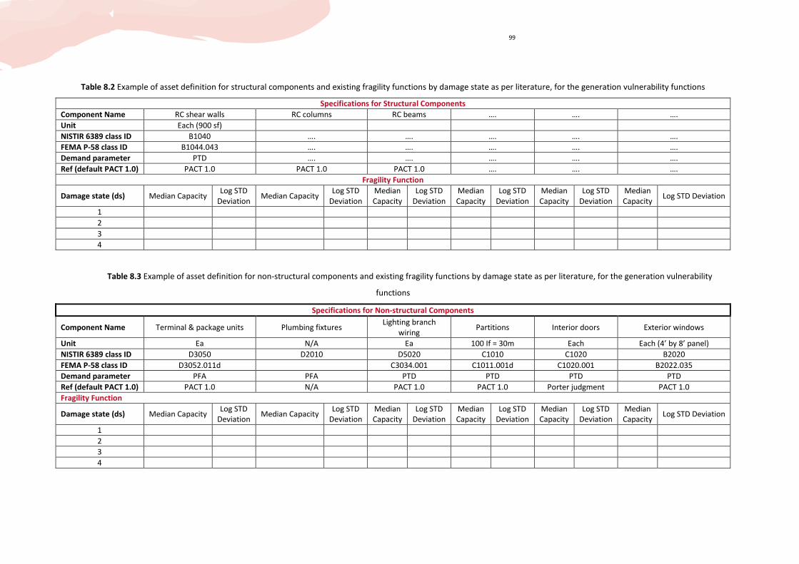
99

Table 8.2 Example of asset definition for structural components and existing fragility functions by damage state as per literature, for the generation vulnerability functions

Specifications for Structural Components

Component Name RC shear walls RC columns RC beams …. …. ….

Unit Each (900 sf)

NISTIR 6389 class ID B1040 …. …. …. …. ….

FEMA P-58 class ID B1044.043 …. …. …. …. ….

Demand parameter PTD …. …. …. …. ….

Ref (default PACT 1.0) PACT 1.0 PACT 1.0 PACT 1.0 …. …. ….

Fragility Function

Damage state (ds) Median Capacity Log STD

Deviation Median Capacity

Log STD

Deviation

Median

Capacity

Log STD

Deviation

Median

Capacity

Log STD

Deviation

Median

Capacity

Log STD

Deviation

Median

Capacity Log STD Deviation

1

2

3

4

Table 8.3 Example of asset definition for non-structural components and existing fragility functions by damage state as per literature, for the generation vulnerability

functions

Specifications for Non-structural Components

Component Name Terminal & package units Plumbing fixtures Lighting branch

wiring Partitions Interior doors Exterior windows

Unit Ea N/A Ea 100 If = 30m Each Each (4’ by 8’ panel)

NISTIR 6389 class ID D3050 D2010 D5020 C1010 C1020 B2020

FEMA P-58 class ID D3052.011d C3034.001 C1011.001d C1020.001 B2022.035

Demand parameter PFA PFA PTD PTD PTD PTD

Ref (default PACT 1.0) PACT 1.0 N/A PACT 1.0 PACT 1.0 Porter judgment PACT 1.0

Fragility Function

Damage state (ds) Median Capacity Log STD

Deviation Median Capacity

Log STD

Deviation

Median

Capacity

Log STD

Deviation

Median

Capacity

Log STD

Deviation

Median

Capacity

Log STD

Deviation

Median

Capacity Log STD Deviation

1

2

3

4

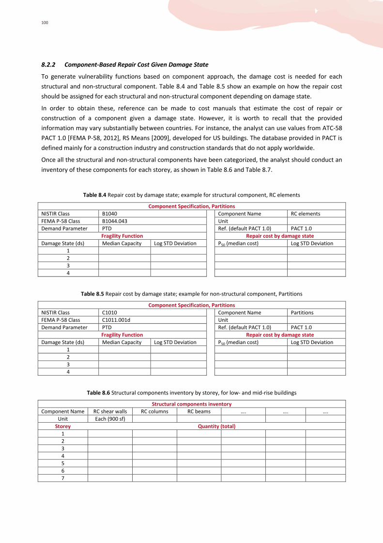
100

8.2.2 Component-Based Repair Cost Given Damage State

To generate vulnerability functions based on component approach, the damage cost is needed for each

structural and non-structural component. Table 8.4 and Table 8.5 show an example on how the repair cost

should be assigned for each structural and non-structural component depending on damage state.

In order to obtain these, reference can be made to cost manuals that estimate the cost of repair or

construction of a component given a damage state. However, it is worth to recall that the provided

information may vary substantially between countries. For instance, the analyst can use values from ATC-58

PACT 1.0 [FEMA P-58, 2012], RS Means [2009], developed for US buildings. The database provided in PACT is

defined mainly for a construction industry and construction standards that do not apply worldwide.

Once all the structural and non-structural components have been categorized, the analyst should conduct an

inventory of these components for each storey, as shown in Table 8.6 and Table 8.7.

Table 8.4 Repair cost by damage state; example for structural component, RC elements

Component Specification, Partitions

NISTIR Class B1040

Component Name RC elements

FEMA P-58 Class B1044.043

Unit

Demand Parameter PTD

Ref. (default PACT 1.0) PACT 1.0

Fragility Function

Repair cost by damage state

Damage State (ds) Median Capacity Log STD Deviation

P50 (median cost) Log STD Deviation

1

2

3

4

Table 8.5 Repair cost by damage state; example for non-structural component, Partitions

Component Specification, Partitions

NISTIR Class C1010

Component Name Partitions

FEMA P-58 Class C1011.001d

Unit

Demand Parameter PTD

Ref. (default PACT 1.0) PACT 1.0

Fragility Function

Repair cost by damage state

Damage State (ds) Median Capacity Log STD Deviation

P50 (median cost) Log STD Deviation

1

2

3

4

Table 8.6 Structural components inventory by storey, for low- and mid-rise buildings

Structural components inventory

Component Name RC shear walls RC columns RC beams …. …. ….

Unit Each (900 sf)

Storey Quantity (total)

1

2

3

4

5

6

7

101

Table 8.7 Non-structural components inventory by storey, for low- and mid-rise buildings

Non-structural components inventory

Component

Name

Terminal & package

units

Plumbing

fixtures

Lighting branch

wiring Partitions

Interior

doors

Exterior

windows

Unit Ea N/A Ea 100 If =

30m Each

Each (4’ by 8’

panel)

Storey Quantity (total)

1

2

3

4

5

6

7

8.2.3 Component-Based Vulnerability Curve

8.2.3.1 One Index Building Based Vulnerability Curve

Two levels for the construction of vulnerability functions can be derived: Storey-level vulnerability functions

and Building-level vulnerability functions.

8.2.3.1.1 Storey-Level Vulnerability Functions

The procedure offered here allows the calculation of storey-level vulnerability functions for all acceleration-

sensitive components on each individual storey, and all drift-sensitive components on each individual storey

(sum of different components repair costs on each storey). Any of the non-linear dynamic approaches

described in Section 7.1 can be used to obtain the needed distribution of peak storey drift and peak floor

acceleration at each storey/floor. The non-linear static pushover methods of Section 7.2.1 can also be

employed to obtain peak storey drift distributions, while simplified methods described in Porter et al. (2014)

should be used for extracting peak floor acceleration estimates. The use of pushover methods that do not

account for record-to-record dispersion (Section 7.2.2) is also possible.

When implementing the component-based vulnerability assessment approach, the generation of storey-level

vulnerability functions does not require the definition of different global damage states (i.e. STEP D/Section 6

is not mandatory).

The storey-level vulnerability function is derived for a discrete number of levels of floor acceleration or drift,

as follows:

• The storey-level mean vulnerability for acceleration-sensitive components should be estimated from

the following relation:

[ ] [ ]∑

=

===aN

iaahiaaha SSCESSCE

1,, || (8.13)

102

• The storey-level mean vulnerability for drift-sensitive components should be estimated from the

following relation:

[ ] [ ]∑

=

===dN

iddhiddhd SSCESSCE

1,, || (8.14)

where aC = repair cost of acceleration-sensitive components on the given storey

dC = repair cost of drift-sensitive components on the given storey

a,hS = storey-level acceleration at floor h .

aS = a particular value of a,hS ; i.e. peak floor acceleration at floor h , to be evaluated at 0, 0.01, 0.02,

...3.00g

d,hS = storey-level drift ratio at storey h .

dS = a particular value of d,hS ; i.e. peak transient drift at storey h , to be evaluated at ∈ 0, 0.005, 0.010,

...0.20. Note: the drifts reach 0.20 because wood frame buildings can tolerate drifts in excess of 10%

without collapse.

i = an index to the component categories present on the storey.

aN = number of acceleration-sensitive components categories present on the storey

dN = number of drift-sensitive components categories present on the storey

The mean vulnerability function per component of category i (in terms of either acceleration or drift) is given

by:

[ ] ( )∑

=

⋅⋅==dsN

dsdsidsihiiihi msPNSSCE

1,,,,| (8.15)

where,

dsN = number of the possible component damage state, ds(see Table 8.4 - Table 8.5).

h,iN = quantity of components of category i on storey h , from Table 8.6 (for structural components) or

Table 8.7 (for non-structural components).

ds,im denotes the mean repair cost per unit of component category i , component damage state ds. It can be

calculated from the median unit repair cost ds,i,50P and logarithmic standard deviation of unit repair cost b ,

as follows:

( )2ds,i,50ds,i b5.0expPm ⋅= (8.16)

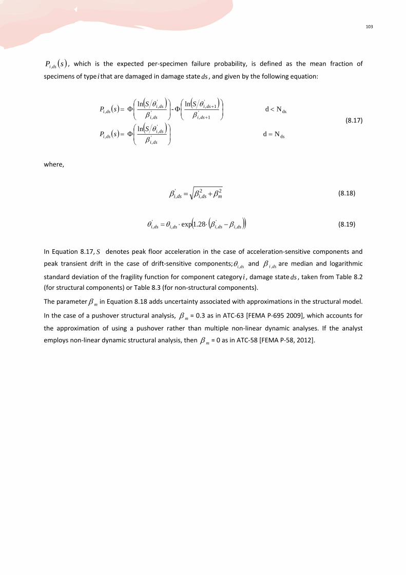
103

( )sP ds,i , which is the expected per-specimen failure probability, is defined as the mean fraction of

specimens of type i that are damaged in damage state ds, and given by the following equation:

( ) ( ) ( )

( ) ( )ds'

,

',

,

ds'1,

'1,

',

',

,

Nd ln

Nd ln

- ln

=

Φ=

<

Φ

Φ=

+

+

dsi

dsidsi

dsi

dsi

dsi

dsidsi

SsP

SSsP

β

θ

β

θ

β

θ

(8.17)

where,

22,

', mdsidsi βββ += (8.18)

( )( )dsidsidsidsi ,',,

', 28.1exp ββθθ −⋅⋅= (8.19)

In Equation 8.17, S denotes peak floor acceleration in the case of acceleration-sensitive components and

peak transient drift in the case of drift-sensitive components; dsi,θ and ds,iβ are median and logarithmic

standard deviation of the fragility function for component category i , damage state ds, taken from Table 8.2

(for structural components) or Table 8.3 (for non-structural components).

The parameter mβ in Equation 8.18 adds uncertainty associated with approximations in the structural model.

In the case of a pushover structural analysis, mβ = 0.3 as in ATC-63 [FEMA P-695 2009], which accounts for

the approximation of using a pushover rather than multiple non-linear dynamic analyses. If the analyst

employs non-linear dynamic structural analysis, then mβ = 0 as in ATC-58 [FEMA P-58, 2012].

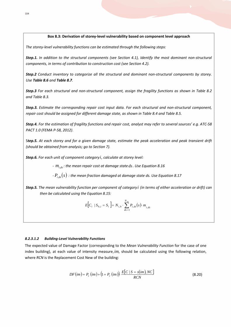
104

8.2.3.1.2 Building-Level Vulnerability Functions

The expected value of Damage Factor (corresponding to the Mean Vulnerability Function for the case of one

index building), at each value of intensity measure, im, should be calculated using the following relation,

where RCN is the Replacement Cost New of the building:

( ) ( ) ( )( ) ( )[ ]RCN

NCimsSCEimPimPimDF cc

,|1

=⋅++= (8.20)

Box 8.3: Derivation of storey-level vulnerability based on component level approach

The storey-level vulnerability functions can be estimated through the following steps:

Step.1. In addition to the structural components (see Section 4.1), Identify the most dominant non-structural

components, in terms of contribution to construction cost (see Section 4.2).

Step.2 Conduct inventory to categorize all the structural and dominant non-structural components by storey.

Use Table 8.6 and Table 8.7.

Step.3 For each structural and non-structural component, assign the fragility functions as shown in Table 8.2

and Table 8.3.

Step.3. Estimate the corresponding repair cost input data. For each structural and non-structural component,

repair cost should be assigned for different damage state, as shown in Table 8.4 and Table 8.5.

Step.4. For the estimation of fragility functions and repair cost, analyst may refer to several sources’ e.g. ATC-58

PACT 1.0 (FEMA P-58, 2012).

Step.5. At each storey and for a given damage state, estimate the peak acceleration and peak transient drift

(should be obtained from analysis; go to Section 7).

Step.6. For each unit of component category i , calculate at storey level:

- ds,im : the mean repair cost at damage state ds. Use Equation 8.16

- ( )sP ds,i : the mean fraction damaged at damage state ds. Use Equation 8.17

Step.5. The mean vulnerability function per component of category i (in terms of either acceleration or drift) can

then be calculated using the Equation 8.15:

[ ] ( )∑=

⋅⋅==dsN

dsdsidsihiiihi msPNSSCE

1,,,,|

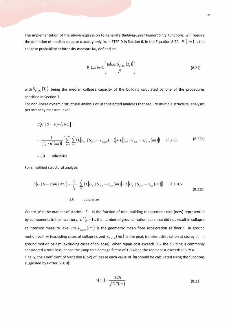
105

The implementation of the above expression to generate Building-Level Vulnerability Functions, will require

the definition of median collapse capacity only from STEP D in Section 6. In the Equation 8.20, ( )imPc is the

collapse probability at intensity measure im, defined as:

( )( )( )

Φ=

β1, 4

ˆln TSimimP dsa

c (8.21)

with ( )1, 4

ˆ TS dsa being the median collapse capacity of the building calculated by one of the procedures

specified in Section 7.

For non-linear dynamic structural analysis or user-selected analyses that require multiple structural analyses

per intensity measure level:

( )[ ]

( )( ) ( )[ ] ( )[ ]( )( )

otherwise 1.0

0.6 if ||1

,|

*

1 1,,,,,,*

1

=

≤=+=⋅⋅

=

==

∑ ∑= =

imn

m

N

hmdhdhdmahaha imsSCEimsSCE

imnf

NCimsSCE

(8.22a)

For simplified structural analysis

( )[ ] ( )[ ] ( )[ ]( )

otherwise 1.0

0.6 if ||1

,|1

,,,,

1

=

≤=+=⋅== ∑=

N

hdhdhdahaha imsSCEimsSCE

fNCimsSCE

(8.22b)

Where, N is the number of stories, 1f is the fraction of total building replacement cost (new) represented

by components in the inventory, ( )imn*is the number of ground motion pairs that did not result in collapse

at intensity measure level im, ( )ims mah ,, is the geometric mean floor acceleration at floor h in ground

motion pair m (excluding cases of collapse), and ( )ims mah ,, is the peak transient drift ration at storey h in

ground motion pair m (excluding cases of collapse). When repair cost exceeds 0.6, the building is commonly

considered a total loss, hence the jump to a damage factor of 1.0 when the repair cost exceeds 0.6·RCN.

Finally, the Coefficient of Variation (CoV) of loss at each value of im should be calculated using the functions

suggested by Porter [2010]:

( )( )imDF

imv25.0

= (8.23)

106

Repeating the process of calculation (using Equations 8.20 and 8.23) for a range of values for intensity

measure im ∈ 0.01, 0.02, ...3.0g, will result in the vulnerability curve as shown in the example of Figure 8.3

[Porter et al 2014].

Figure 8.3 Example of derived one index-based building-level vulnerability curve for collapse damage state: case of mid-

rise storey RC shear wall office building, in region of 0.17 ≤SMS <0.5g for USA.

8.2.3.2 Three Index Buildings Based Vulnerability Curve

The approach offered here will require from the analyst to identify three variants which should be associated

to the quality of the buildings as discussed in Section 3.2. For component level assessment, the different

quality classes can be defined as followings (see Table 8.8):

• Poor quality, with relatively low design base shear and fragile components;

• Typical quality that should be characterized as a median quality in terms of design base shear and

fragile components; and

• Superior quality, with relatively rugged or seismically restrained components and relatively design

high base shear.

Table 8.8 Example of configuration of the three index variants, Poor, Typical, and Superior quality, using ATC-58

component types

Three Index Buildings

Component Description Poor Typical Superior

Exterior Windows B2022.032 B2022.035 B2022.071

Partitions C1011.001a C1011.001c C1011.001b

Interior Doors C1021.001 C1021.001 C1021.001

Plumbing Fixtures

Terminal & Package Units D3052.011b D3052.011d D3052.013k

Lighting & Branch Wiring C3034.001 C3034.001 C3034.002

RC shear walls B1044.073 B1044.013 B1044.041

Other attributes

Sa, g 0.2 0.3 0.4

107

The analyst should identify other variables, considered as the most dominant in terms of response capacity,

to differentiate between these three indexes, which can be different from country to country, and from

typology to typology. For instance: number of stories, presence of vertical irregularity, and presence of plan

irregularity. The three variant Poor, Typical, and Superior-quality index buildings should represent cases

where repair cost would be exceeded respectively by 10%, 50%, and 90% of buildings of similar occupancy.

In this approach, the mean vulnerability function for the considered building class is given by the average of

the three variants, as shown in Equation 8.24:

( ) ( )∑

=

⋅=3

13

1

jj imDFimDF (8.24)

where, ( )imDF j for each index building (each value of j) is given by Equation 8.24.

The Coefficient of Variation (CoV) of loss at each value of im should be calculated using the following

relation:

( )( ) ( )( )

( )imDF

imDFimDF

imvj

j∑=

−⋅

⋅=

3

1

2

2

1

4.1 (8.25)

The conditional distribution of loss can be taken as lognormal with mean and coefficient of variation as

described above, or as beta with bounds 0 and 1 and the same mean and coefficient of variation. Figure 8.4

shows the resulting three index based vulnerability functions [Porter et al. 2014].

Figure 8.4 Example of derived three index-based seismic vulnerability curve for collapse damage state: case of mid-rise

storey RC shear wall office building, in region of 0.17 ≤SMS <0.5g for USA.

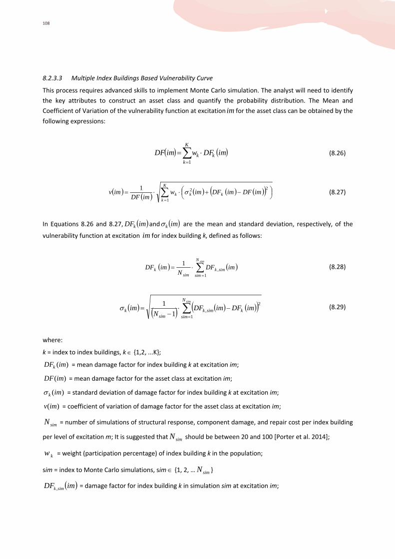
108

8.2.3.3 Multiple Index Buildings Based Vulnerability Curve

This process requires advanced skills to implement Monte Carlo simulation. The analyst will need to identify

the key attributes to construct an asset class and quantify the probability distribution. The Mean and

Coefficient of Variation of the vulnerability function at excitation im for the asset class can be obtained by the

following expressions:

( ) ( )∑=

⋅=K

kkk imDFwimDF

1

(8.26)

( )

( )( ) ( ) ( )( )∑

=

−+⋅⋅=

K

kkkk imDFimDFimw

imDFimv

1

221σ (8.27)

In Equations 8.26 and 8.27, ( )imDFk and ( )imkσ are the mean and standard deviation, respectively, of the

vulnerability function at excitation im for index building k, defined as follows:

( ) ( )∑

=

⋅=simN

simsimk

simk imDF

NimDF

1,

1 (8.28)

( ) ( ) ( ) ( )( )∑=

−⋅−

=simN

simksimk

simk imDFimDF

Nim

1

2

,1

1σ (8.29)

where:

k = index to index buildings, k ∈ 1,2, ...K;

)(imDFk = mean damage factor for index building k at excitation im;

)(imDF = mean damage factor for the asset class at excitation im;

)(imkσ = standard deviation of damage factor for index building k at excitation im;

)(imv = coefficient of variation of damage factor for the asset class at excitation im;

simN = number of simulations of structural response, component damage, and repair cost per index building

per level of excitation m; It is suggested that simN should be between 20 and 100 [Porter et al. 2014];

kw = weight (participation percentage) of index building k in the population;

sim = index to Monte Carlo simulations, sim ∈ 1, 2, … simN

( )imDF simk, = damage factor for index building k in simulation sim at excitation im;

109

REFERENCES

Abo El Ezz, A. (2008), Deformation and strength based assessment of seismic failure mechanisms for existing RC

frame buildings, MSc Thesis, ROSE School, Pavia, Italy.

American Society of Civil Engineers (ASCE) (2007), Seismic Rehabilitation of Existing Buildings, ASCE/SEI 41-06,

American Society of Civil Engineers, Reston, Virginia.

Applied Technology Council (ATC) (2003), Preliminary Evaluation of Methods for Defining Performance, ATC-58-2,

Redwood City, CA.

Asteris, P., Antoniou, S., Sophianopoulos, D., and Chrysostomou, C. (2011). Mathematical Macromodeling of

Infilled Frames: State of the Art, J. Struct. Eng, 137(12), 1508–1517.

Bal, I.E., Crowley, H. and Pinho, R., (2008), Detail assessment of structural characteristics of Turkish RC buildings

stock for loss assessment models, Soil Dynamic and Earthquake Engineering, 28, 914-932.

Bal, I.E., Crowley, H., and Pinho, R., (2010), Displacement-based earthquake loss assessment: Method

development and application to Turkish building stock, ROSE Research Report 2010/02, IUSS Press, Pavia, Italy.

Baker, J.W., (2007), Probabilistic structural response assessment using vector-valued intensity measures,

Earthquake Engineering and Structural Dynamics, 36, 1861-1883.

Baker, J.W, and Cornell C.A., (2008a), Spectral shape, epsilon and record selection, Earthquake Engineering and

Structural Dynamics, 35,1077–1095.

Baker, J.W., and Cornell, C.A. (2008b), Uncertainty propagation in probabilistic seismic loss estimation, Structural

Safety 30, 236-252.

Baker, J.W. (2014), Efficient analytical fragility function fitting using dynamic structural analysis, Earthquake

Spectra, in press, doi: 10.1193/021113EQS025M

Bernardini, A., D’Ayala, D., Modena, C., Speranza, E., and Valluzzi, M.R., (2008), Vulnerability assessment of the

historical masonry building typologies of Vittorio Veneto, Special issue of Bollettino di Geofisica Teorica e

Applicata Vol.49, n.3-4, 463-484.

Berryman, K., Wallace, L., Hayes, G., Bird, P., Wang, K., Basili, R., Lay, T., Stein, R., Sagiya, T., Rubin, C., Barreintos,

S., Kreemer, C., Litchfield, N., Pagani, M., Gledhill, K., Haller, K., and Costa C., (2013), The GEM Faulted Earth

Subduction Characterisation Project, Version 1.0, GEM Faulted Earth Project.

Bianchini, M., Diotallevi, P., and Baker, J.W., (2009), Prediction of Inelastic Structural Response Using an Average of

Spectral Accelerations, Proceedings of 10th International Conference on Structural Safety and Reliability

(ICOSSAR09), Osaka, Japan.

Borzi, B., Crowley, H., and Pinho, R. (2008), Simplified pushover-based earthquake loss assessment (SP-BELA)

method for masonry buildings, International Journal of Architectural Heritage; Conservation, Analysis, and

Restoration, 2(4), 353-376

Brzev, S, Scawthorn, C., Charleson, A.W., and Jaiswal, K. (2012), GEM basic building taxonomy. Report produced in

the context of the GEM Ontology and Taxonomy Global Component project, 45 pp.

Calvi, G.M. (1999), A displacement-based approach for the vulnerability evaluation of classes of buildings. Journal

of Earthquake Engineering, 26, 1091–1112.

Canadian Standards Association (CSA) (2004), Design of masonry structures (CSA-S304.1), Ontario, Canada.

Casapulla, C. and D'Ayala, D. F. (2006), In plane collapse behaviour of masonry walls with frictional resistance and

openings. In: Structural Analysis of Historical Construction V, 2006-11-01, Delhi.

Ching, J., Porter, K.A., and Beck, J.L. (2009), Propagating uncertainties for loss estimation in performance-based

earthquake engineering using moment matching, Structure and Infrastructure Engineering, 5(3), 245-262.

110

Cho, I.H., and Porter, K.A. (2013), Three techniques for modelling building classes using moment matching,

Structural Engineering and Structural Mechanics Program, SESM 13-01, University of Colorado, UCB 428.

Computers & Structures Inc (CSI) (2009), SAP2000, Integrated Software for Structural Analysis & Design, Berkeley,

CA.

Cornell C.A, Jalayer F., Hamburger R.O., and Foutch D.A., (2002), Probabilistic Basis for 2000 SAC Federal

Emergency Management Agency Steel Moment Frame Guidelines. Journal of Structural Engineering, 128(4),

526–533.

Crowley, H., Pinho, R., and Bommer, J., (2004), A probabilistic displacement-based vulnerability assessment

procedure for earthquake loss estimation, Bulletin of Earthquake Engineering, 2, 173–219.

Crowley, H., and Pinho, R. (2004), Period-height relationship for existing European reinforced concrete buildings.

Journal of Earthquake Engineering, 893-119.

Crowley, H., and Pinho, R. (2006), Simplified equations for estimating the period of vibration of existing buildings,

Proceedings of the 1st European Conference on Earthquake Engineering and Seismology, Geneva, Switzerland,

Paper No. 1122.

Crowley, H., Borzi, B., Pinho, R., Colombi, M., and Onida, M. (2008), Comparison of two mechanics-based methods

for simplified structural analysis in vulnerability assessment, Advances in Civil Engineering,

doi:10.1155/2008/438379.

D’Ayala, D. (2005), Force and Displacement Based Vulnerability Assessment for Traditional Buildings; Bulletin of

Earthquake Engineering, Vol.3, Springer, pp. 235-265.

D'Ayala, D. (2013), Assessing the seismic vulnerability of masonry buildings, In: Handbook of Seismic Risk

analysis and management of civil infrastructure systems , Woodhead publishing, 334-365.

D’Ayala, D., and Kishali, E. (2012), Analytically derived fragility curves for unreinforced masonry buildings in urban

contexts, 15th World Conference of Earthquake Engineering, Lisbon, Portugal.

D’Ayala, D., and Meslem, A. (2013a), Guide for selection of existing fragility curves and compilation of the

database”, GEM Technical Report 2013-X, GEM Foundation.

D’Ayala, D., and Meslem, A. (2013b), Sensitivity of analytical fragility functions to capacity-related parameters”,

GEM Technical Report 2013-X, GEM Foundation.

D’Ayala, D., and Meslem, A. (2013c), Derivation of analytical vulnerability functions considering modeling

uncertainties, Proceedings of the 11th International Conference on Structural Safety & Reliability, New York.

D'Ayala, D., and Speranza E. (2003), Definition of collapse mechanisms and seismic vulnerability of historic

masonry buildings, Earthquake Spectra, 19, 479-509

D Ayala, D., Kappos, A., Crowley, H., Antoniadis, P., Colombi, M., and Kishali, E. (2012), Providing building

vulnerability data and analytical fragility functions for PAGER, Technical Report, Earthquake Engineering

Research Institute..

Dolsek, M., and Fajfar, P. (2004), Inelastic spectra for infilled reinforced concrete frames, Earthquake Engineering

and Structural Dynamics, 33, 1395-1416.

Dolsek, M., and Fajfar, P. (2008), The effect of masonry infills on the seismic response of a four-storey reinforced

concrete frame – a deterministic assessment, Engineering Structures, 30, 1991-2001.

Douglas, J., Cotton, F., Abrahamson, N.A., Akkar, S., Boore, D.M., and Di Alessandro, C. (2013), Pre-selection of

ground motion prediction equations, Report produced in context of GEM GMPE project.

Efron, B., and Tibshirani, R.J. (1994), An Introduction to the Bootstrap, Chapman and Hall/CRC, 456 pages.

Ellingwood, B.R., and Kinali, K. (2009), Quantifying and communicating uncertainty in seismic risk assessment.

Structural Safety 31, 179–187, doi:10.1016/j.strusafe.2008.06.001.

111

Ellul, F.L., and D’Ayala, D. (2012), Realistic FE models to enable push-over nonlinear analysis of masonry infilled

frames, The Open Construction and Building Technology Journal, 6, 213-235.

Erberik, M.A. (2008), Generation of fragility curves for Turkish masonry buildings considering in-plane failure

modes, Earthquake Engineering and Structural Dynamics, 37, 387-405

Erdik, M., Aydinoglu, N., Fahjan, Y., Sesetyan, K., Demircioglu, M., Siyahi, B., Durukal, E., Ozbey, C., Biro, Y., Akman,

H., and Yuzugullu, O. (2003), Earthquake Risk Assessment for Istanbul Metropolitan Area, Earthquake

Engineering and Engineering Vibration, 2(,1), 1-25.

European Committee for Standardization (CEN) (2004), Design of structures for earthquake resistance, Part 1:

General rules, seismic actions and rules for buildings, Eurocode-8, ENV 1998-1-1, Brussels, Belgium.

European Committee for Standardization (CEN) (2005), Design of structures for earthquake resistance, Part 3:

Strengthening and repair of buildings, Eurocode 8, EN 1998-3, Brussels, Belgium.

Fajfar, P. (2002), Structural analysis in earthquake engineering- a breakthrough of simplified nonlinear methods,

Proceedings of the 12th

European Conference on Earthquake Engineering, London, paper 843.

Federal Emergency Management Agency (FEMA P-58) (2012), Seismic Performance Assessment of Buildings, ATC-

58, Applied Technology Council, Washington, D.C.

Federal Emergency Management Agency (FEMA P-695) (2009), Quantification of Building Seismic Performance

Factors, ATC-63, Applied Technology Council, Redwood City, CA.

Federal Emergency Management Agency (FEMA-440) (2005), Improvement of Nonlinear Static Seismic Analysis

Procedures, ATC-55, Applied Technology Council, Washington, D.C.

Federal Emergency Management Agency (FEMA-445) (2006), Next-Generation Performance-Based Seismic Design

Guidelines: Program Plan for New and Existing Buildings. Applied Technology Council, Washington, D.C.

Federal Emergency Management Agency – National Institute of Building Sciences (FEMA-NIBS) (2003), Multi-

hazard loss estimation methodology – earthquake model: HAZUS-MH Advanced engineering building module -

Technical and user’s manual, Washington, DC.

Federal Emergency Management Agency (FEMA) (1999), HAZUS 99 - Technical and user’s manual, Washington, DC.

Federal Emergency Management Agency (FEMA) (2003), HAZUS-MH - Multi-hazard loss estimation methodology,

Technical and user’s manual, Washington, DC.

Galasco, A., Lagomarsino, S., Penna, A., and Resemini, S. (2004), Non-Linear Seismic Analysis of Masonry

Structures, Proceedings of the 13th World Conference on Earthquake Engineering, Vancouver, Canada.

Galasco, A., Lagomarsino, S., Penna, A. and Cattari, S. (2009), TREMURI program: Seismic Analyses of 3D Masonry

Buildings, University of Genoa.

Gehl, P., Douglas, J., Rossetto, T., Macabuag, J., Nassirpour, A., Minas, S., and Duffour, P. (2014). Investigating the

use of record-to-record variability in static capacity approaches. Proceedings of the Second International

Conference on Vulnerability and Risk Analysis and Management (ICVRAM2014) & Sixth International

Symposium on Uncertainty Modelling and Analysis (ISUMA2014), Liverpool, UK.

Glaister, S., and Pinho, R. (2003), Development of a simplified deformation based method for seismic vulnerability

assessment, Journal of Earthquake Engineering, 7, 107–140.

Huyck, C., Esquivias, G., Gamba, P., Hussain, M., Odhiambo, O., Jaiswal, K., Chen, B., Becker, M., and Yetman, G.

(2011), Survey of available input databases for Global Exposure Database, GED4GEM, Global Earthquake

Model.

Jaiswal, K., and Wald, D.J. (2008), Creating a Global Building Inventory for Earthquake Loss Assessment and Risk

Management, USGS Open File Report, OF 2008-1160 , 103 pp., http://pubs.usgs.gov/of/2008/1160/.

112

Jaiswal, K.S., Wald, D.J., Perkins, D., Aspinall, W.P., and Kiremidjian, A.S. (2013), Estimating structural collapse

fragility of generic building typologies using expert judgement, Proceedings of 11th International Conference on

Structural Safety & Reliability, New York, USA.

Jalayer, F. and Cornell, C.A. (2009), Alternative non-linear demand estimation methods for probability-based

seismic assessments, Earthquake Engineering and Structural Dynamics, 38, 951–972.

Lagomarsino, S., and Giovinazzi, S. (2006), Macroseismic and Mechanical Models for the Vulnerability and Damage

Assessment of Current Buildings, Bulletin of Earthquake Engineering, 4(4).

Lagomarsino, S., Penna, A., Galasco, A., and Cattari, S. (2013), TREMURI program: An equivalent frame model for

the nonlinear seismic analysis of masonry buildings, Engineering Structures, 56, 1787-1799.

Lang, K., and Bachmann, H. (2004), On the seismic vulnerability of existing buildings: a case study of the city of

Basel, Earthquake Spectra, 20(1), 43–66.

Lee, T.H., and Mosalam, K.M. (2005), Seismic demand sensitivity of reinforced concrete shear-wall building using

FOSM method, Earthquake Engineering and Structural Dynamics, 34, 1719-1736.

Luco, N., and Cornell, C.A. (2007), Structure-Specific Scalar Intensity Measures for Near-Source and Ordinary

Earthquake Ground Motions, Earthquake Spectra, 23( 2), 357–392.

Luco N., and Bazzurro, P. (2007), Does amplitude scaling of ground motion records result in biased nonlinear

structural drift responses? Earthquake Engineering and Structural Dynamics, 36, 1813–1835.

Luco, N., Mori, Y., Funahashi, Y., Cornell, C.A., and Nakashima, M. (2003), Evaluation of predictors of non‐linear

seismic demands using ‘fishbone’models of SMRF buildings, Earthquake Engineering and Structural Dynamics,

32(14), 2267–2288.

Mainstone, R. J., and Weeks, G. A. (1970), The influence of bounding frame on the racking stiffness and strength of

brick walls, Proceedings of the 2nd

International Brick Masonry Conference, Stoke-on-Trent, UK.

Masonry Standards Joint Committee (MSJC) (2010), Building Code Requirements for Masonry Structures,

Commentary Working Draft, Building Code Requirements for Masonry Structures.

Meslem, A., and D’Ayala, D. (2012), Toward Worldwide Guidelines for the Development of Analytical Vulnerability

Functions and Fragility Curves at Regional Level", Proceedings of the 15th World Conference on Earthquake

Engineering, Lisbon, Portugal.

Meslem, A., and D’Ayala, D. (2013), Investigation into analytical vulnerability curves derivation aspects considering

modelling uncertainty for infilled buildings, Proceedings of the 4th International Conference on Computational

Methods in Structural Dynamics and Earthquake Engineering (COMPDYN’13), Kos Island, Greece.

Nakashima, M., Ogawa, K., and Inoue, K. (2002), Generic frame model for simulation of earthquake responses of

steel moment frames, Earthquake Engineering and Structural Dynamics, 31(3), 671– 692.

National Institute of Standards and Technology (NIST) (1999), UNIFORMAT II Elemental Classification for Building

Specifications, Cost Estimating, and Cost Analysis, NISTIR 6389, Washington, D.C.

National Institute of Standards and Technology (NIST) (2011), Selecting and Scaling Earthquake Ground Motions

for Performing Response-History Analyses, Prepared for the US National Institute of Standards and Technology

by the NEHRP Consultants Joint Venture, Gaithersburg, Maryland.

National Earthquake Hazards Reduction Program (NEHRP) (2010), Nonlinear structural Analysis for seismic design:

A guide for practicing engineers (NIST GCR 10-917-5), NEHRP Seismic Design Technical Brief No. 4, National

Institute of Standards and Technology.

New Zealand Society for Earthquake Engineering (NZSEE) (2006), Assessment and Improvement of the Structural

Performance of Buildings in Earthquakes. New Zealand.

113

Newmark, N.M. (1959), A method of computation for structural dynamics. Journal of the Engineering Mechanics

Division, ASCE, 85, EM3, 67-94.

Paulay, T., and Priestley, M.J.N. (1992), Seismic Design of Reinforced Concrete and Masonry Buildings, John Wiley

and Sons, Inc., New York.

Pinho, R., Bommer, J.J., and Glaister, S. (2002), A simplified approach to displacement-based earthquake loss

estimation analysis. Proceedings of the 12th European Conference on Earthquake Engineering, London, UK,

Paper N. 738.

Priestley, M.J.N., Calvi, G.M., and Kowalsky, M.J. (2007). Displacement-based Seismic Design of Structures, IUSS

Press, Pavia, Italy.

Porter, K.A., Farokhnia, K., Cho, I.H., Rossetto, T., Ioannou, I., Grant, D., Jaiswal, K., Wald, D., D’Ayala, D., Meslem,

A., So, E., Kiremidjian, A.S. and Noh, H. (2012a), Global Vulnerability Estimation Methods for the Global

Earthquake Model, Proceedings of the 15th World Conference on Earthquake Engineering, Lisbon.

Porter, K.A., Farokhnia, K., and Cho, I. (2012b), Nonstructural seismic vulnerability estimation guidelines, Global

Vulnerability Consortium.

Porter, K.A., Farokhnia, K., and Cho, I. (2012c), Contents seismic vulnerability estimation guidelines, Global

Vulnerability Consortium.

Porter, K.A., G. Johnson, R. Sheppard, and R. Bachman (2010), Fragility of mechanical, electrical, and plumbing

equipment. Earthquake Spectra, 26(2), 451-472.

Porter, K., Farokhnia, K., Vamvatsikos, D., and Cho, I., (2014), Analytical Derivation of Seismic Vulnerability

Functions for Highrise Buildings, Global Vulnerability Consortium, GEM Foundation.

Porter, K.A., R.P. Kennedy, and R.E Bachman (2007), Creating fragility functions for performance-based earthquake

engineering, Earthquake Spectra, 23(2), 471-489,

Porter, K.A. (2010), Cracking an open safe: uncertainty in HAZUS-based seismic vulnerability functions, Earthquake

Spectra, 26(3), 893-900.

Porter, K., Hu, Z., Huyck, C., and Bevington, J. (2014), User guide: Field sampling strategies for estimating building

inventories, GEM Technical Report 2014-02 V1.0.0, 42 pp., GEM Foundation, Pavia, Italy.

Rezaeian, S., Bozorgnia, Y., Idriss, I. M., Campbell, K., Abrahamson, N., and Silva, W. (2012), Spectral Damping

Scaling Factors for Shallow Crustal Earthquakes in Active Tectonic Regions, PEER Report No 2012/01, Pacific

Earthquake Engineering Research Center, California, USA.

Roca P., Molins C., and Marí A.R. (2005) Strength capacity of masonry wall structures by the equivalent frame

method, Journal of Structural Engineering, 131(10), 1601-1610

Rossetto, T. (2004), Vulnerability Curves for the Seismic Assessment of Reinforced Concrete Structure Populations,

PhD Thesis, Imperial College London. April 2004. pp.330.

Rossetto, T. (2014), The Conversion of Damage to Loss in GEM VEM Indirect Vulnerability Curve Derivation, GEM

Technical Report 2013-X, GEM Foundation.

Rossetto, T., and Elnashai, A. (2005), A new analytical procedure for the derivation of displacement-based

vulnerability curves for populations of RC structures, Engineering Structures, 27, 397-409.

Rossetto, T., Ioannou, I., Grant, D. N., and Maqsood, T. (2014). Guidelines for Empirical Vulnerability Assessment,

Global Vulnerability Consortium.

R S Means Engineering (2009), RSMeans Building Construction Cost Data, R. S. Means Company, Incorporated, pp.

869.

SYNER-G (2011), Fragility functions for common RC building types in Europe, Deliverable 3.1,. Available from URL:

http://www.vce.at/SYNER-G/.

114

Ruiz-Garcia, J., and Miranda, E. (2005), Performance-based assessment of existing structures accounting for

residual displacements, The John A. Blume earthquake Engineering Center, Report No. 153, Stanford

University.

Ruiz-Garcia, J., and Miranda, E. (2007), Probabilistic estimation of maximum inelastic displacement demands for

performance-based design, Earthquake Engineering and Structural Dynamics, 36, 1235-1254.

Shome, N., and Cornell, C.A. (1999), Probabilistic seismic demand analysis of nonlinear structures, Tech. Rep. RMS–

35, RMS Program, Stanford University, CA.

Silva, V., Crowley, H., Pinho, R., and Varum, H. (2013), Extending displacement-based earthquake loss assessment

(DBELA) for the computation of fragility curves, Engineering Structures, 56, 343-356.

Tomazevic, M. (2007), Damage as a measure for earthquake-resistant design of masonry structures: Slovenian

experience, Canadian Journal of Civil Engineering, 34(11), 1403-1412.

Turnsek, V., and Cacovic, F. (1970), Some experimental results on the strength of brick masonry walls, Proceedings

of the 2nd international brick masonry conference, Stoke on Trent, United Kingdom, 149-156.

Vamvatsikos D., and Cornell C.A. (2005), Developing efficient scalar and vector intensity measures for IDA capacity

estimation by incorporating elastic spectral shape information, Earthquake Engineering and Structural

Dynamics, 34(13), 1573–1600.

Vamvatsikos, D., and Cornell, C.A. (2006), Direct estimation of the seismic demand and capacity of oscillators with

multi-linear static pushovers through IDA, Earthquake Engineering and Structural Dynamics, 35(9), 1097-1117.

Vamvatsikos, D., and Fragiadakis, M. (2010), Incremental dynamic analysis for estimating seismic performance

sensitivity and uncertainty, Earthquake Engineering and Structural Dynamics, 39, 141-163.

Vamvatsikos, D., and Kazantzi, A.K (2015), Developing analytical vulnerability curves for Western US low-rise steel

frame buildings, Technical Report, Global Vulnerability Consortium, GEM Foundation.

Wasserman L. (2004), All of statistics: a concise course on statistical inference. New York, USA: Springer.

Wen Y.K, Ellingwood B.R, and Bracci J. (2004), Vulnerability Function Framework for Consequence-based

Engineering, MAE Center Project DS-4 Report.

I

APPENDIX A Derivation of Capacity Curves

A.1 Perform Pushover Analysis

The pushover analysis of a structure is a static nonlinear analysis under permanent vertical loads and

gradually increasing lateral loads (incremental loads) up to failure. The equivalent static lateral loads

approximately represent earthquake-induced forces. A plot of the total base shear versus top displacement

in a structure is obtained by this analysis allowing the determination of collapse load and ductility capacity

(see Figure A.1).

To implement a pushover analysis, the analyst will need to develop an appropriate mathematical model and

define the following parameters:

• Define structural model: 3D or a simplified 2D model; identify your primary and secondary elements

or components; define your non-structural elements; foundation flexibility; and P-Delta effects.

Procedures for performing a structural model are provided in Section 5.

• Define loads:

- Gravity: This is permanent gravity actions, i.e. dead load, live load;

- Lateral load pattern (vertical distribution): incremental loads consist of horizontal forces at each

storey level.

• Select increment control: different strategies may be employed: load control (force control),

response control.

For further details regarding the procedure to perform non-linear static analysis, analyst may refer to

ASCE/SEI 41-06 (ASCE 2007).

Figure A.1. Plot of pushover curve and evaluation of different damage thresholds

II

A.2 Derivation of Equivalent SDoF-Based Capacity Curves

For some non-linear static-based procedures suggested in the guidelines, the analyst should, firstly, derive

the equivalent SDoF-based capacity curves of the MdoF-based curve obtained from pushover analysis (see

Figure A.2), in order to conduct vulnerability assessment. The transformation of the Force-Displacement

(Base shear-Top Drift) curve to ADRS space is done using the modal participation factors and effective modal

weight ratios, determined from the fundamental mode of the structure.

The different steps for the derivation of equivalent SDoF-based capacity curve are provided in Box A.2.

Box A.1: Perform pushover analysis

The pushover analysis can be performed as follows:

Step 1: Develop an appropriate mathematical model of the building for non-linear static analysis. Refer to

Section 5, and you may also refer to ASCE/SEI 41-06.

Step 2: Select and determine the horizontal force pattern to be applied for each storey mass;

Step 3: Selection of control node: Roof node shall be selected as the control node;

Step 4: Selection of deformation level (target displacement): as ATC-40 (ATC 1996) requires, the capacity curve

shall be determined up to 4% of total height of the building; as Eurocode-8 (CEN 2005), the capacity curve shall

be determined up to Up to 150% of the control node displacement that corresponds to the limit-state of interest;

Step 5: Gravity loading is applied (with no lateral loads).

Step 6: At constant vertical load, gradually increase one-parameter lateral loads up to the attainment of the

target displacement.

Step 7: Make sure that the analysis is extended to a deformation such that collapse is judged to occur.

The output of this analysis is the capacity curve (force-displacement relationship) of MDoF system with the

estimated damage states.

Box A.2: Equivalent SDoF-based capacity curve

The equivalent SDoF-based capacity curve is obtained through the following steps:

Step 1: Run Eigenvalue analysis and extract the fundamental mode shapes,φ , of MDoF system.

Step 2: Obtain the Base Shear – Displacement relationship (capacity curve) as result of non-linear static

(pushover) analysis of MDoF system. See Section A.1.

Step 3: Derive the equivalent SDoF-based capacity curve (Figure A.2) by dividing the base shear and

displacement of the MDoF-based capacity curve with a Transformation Factor.

III

The mass of an equivalent SDoF system m* is determined as:

nimm ii K,2,1where,* =⋅= ∑ φ denotes roof level (A.1)

The transformation to an equivalent SDOF model is made by dividing the base shear, bF , and top

displacement, nd , of the MDOF model with a transformation factor Γ :

Γ=

Γ= n*b* d

d F

F (A.2)

where F* and d* are, respectively, the base shear force and the displacement of the SDoF system. The

transformation factor is given by:

∑ ⋅=

⋅⋅

⋅⋅=Γ

2ii

*m

M

1M

φφφ

φ

mT

T

(A.3)

Note that:

• For the calculation of an equivalent mass m* and the constant Γ, the assumed displacement shapeφ

is normalized – the value at the top is equal to 1. Usually a triangular shape for the first mode is

assumed, however any reasonable shape can also be used forφ .

• For the transformation from MDoF to SDoF system, both force and displacement must be divided by

the same constant Γ, so that the initial stiffness of the equivalent SDoF system remains the same as

that defined by the base shear – displacement diagram of the MDoF system.

Figure A.2. Example of transformation of MDoF-based pushover curve to an equivalent SDoF.

A.3 Fitting the Capacity into Idealised Representation

The implementation of some non-linear static-based procedures requires the determination of an

approximate idealized form for the derived capacity curve of the equivalent SDoF system.

IV

To derive the idealized capacity diagram of the SDoF system the equal energy principle is used, by which the

idealised curved is determined by imposing that the areas under the actual curve of SDoF and the idealized

curve are equal. Two forms of idealization are provided (see Figure A.3):

• Multilinear elasto-plastic form, which may be used, for instance, in the case of capacity curve

derived from infilled frames structures. The use of multilinear elasto-plastic form requires providing

the following segments (Figure A.3a):

- from the ordinate to point 1: defined as the elastic segment, where point 1 is defined as the

yield point;

- from point 1 to point 2: termed the hardening segment, where point 2 is defined as the point of

peak strength or initial degradation point;

- from point 2 to point 3: termed the softening segment, where point 3 represents the onset of

residual strength response (e.g. complete failure of the infill for infilled frames);

- from point 3 to point 4: represents the residual strength plateau, where point 4 represents the

ultimate deformation at collapse.

• Simple bilinear elasto-perfectly plastic form, which may be used, for instance, in the case of capacity

curve derived from bare frames structures, masonry buildings. The use of bilinear elasto-plastic form

requires providing the following segments (Figure A.3b):

- from the ordinate to point 1: defined as the elastic segment, where point 1 is defined as the

yield point;

- from point 1 to point2: the hardening and softening plateau up to the residual strength, where

point 2 represents the ultimate deformation at collapse.

Figure A.3. Idealization of capacity curves. (a) Multilinear elasto- plastic form; (b) Bilinear elasto-perfectly plastic form.

The subsections below present some examples for the calculation of these different segments and points

characterizing an idealized capacity curve. Note that these examples are one possibility, and the analyst may

perform any other procedure through which the different segments and points are accurately defined.

Indeed, at the level of yielding point, the choice of the yield displacement (yD ) and yield force (

yF ) might

have a significant influence. The period of the idealized equivalent SDoF system, T *, is determined by:

y

y*

* 2 F

DmT

⋅⋅= π (A.4)

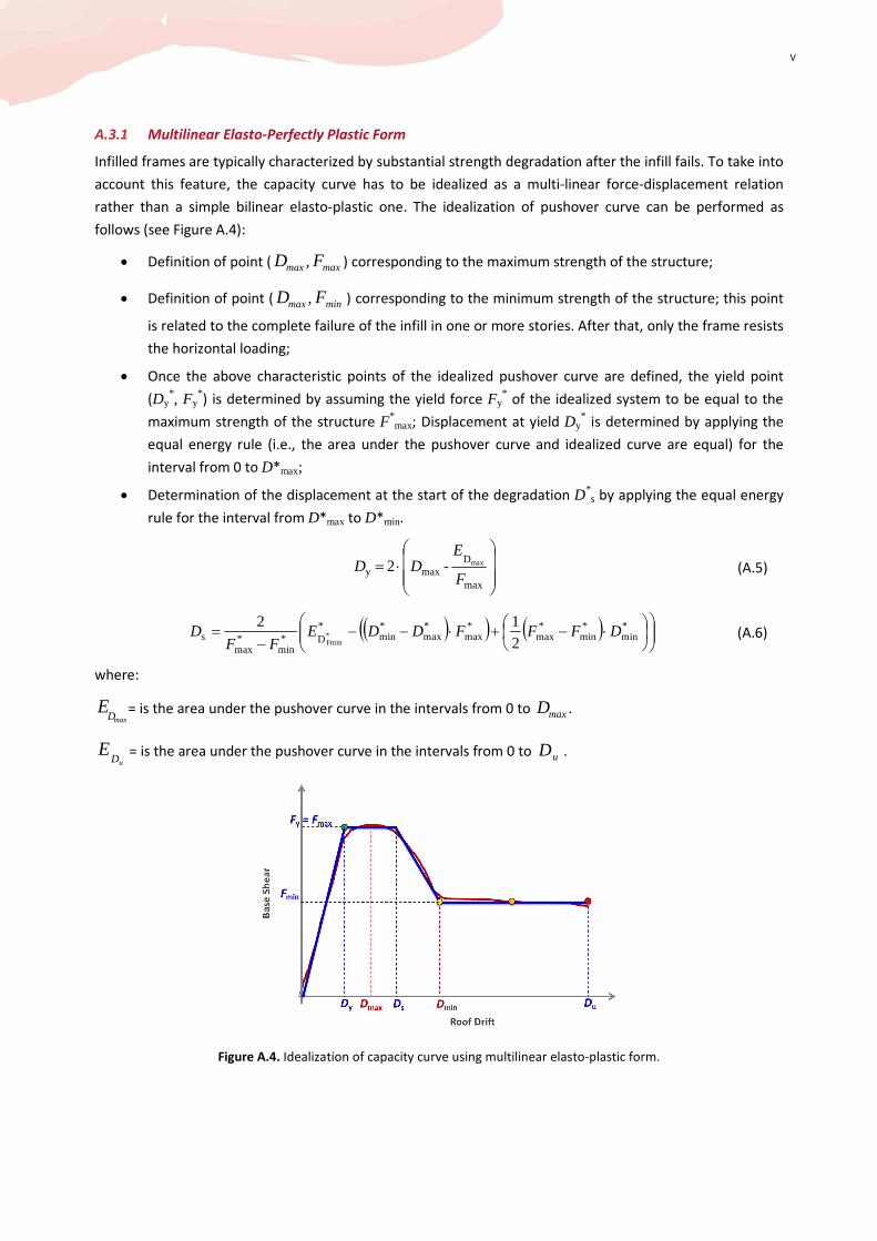
V

A.3.1 Multilinear Elasto-Perfectly Plastic Form

Infilled frames are typically characterized by substantial strength degradation after the infill fails. To take into

account this feature, the capacity curve has to be idealized as a multi-linear force-displacement relation

rather than a simple bilinear elasto-plastic one. The idealization of pushover curve can be performed as

follows (see Figure A.4):

• Definition of point ( maxD , maxF ) corresponding to the maximum strength of the structure;

• Definition of point ( maxD , minF ) corresponding to the minimum strength of the structure; this point

is related to the complete failure of the infill in one or more stories. After that, only the frame resists

the horizontal loading;

• Once the above characteristic points of the idealized pushover curve are defined, the yield point

(Dy*, Fy

*) is determined by assuming the yield force Fy

* of the idealized system to be equal to the

maximum strength of the structure F*max; Displacement at yield Dy

* is determined by applying the

equal energy rule (i.e., the area under the pushover curve and idealized curve are equal) for the

interval from 0 to D*max;

• Determination of the displacement at the start of the degradation D*s by applying the equal energy

rule for the interval from D*max to D*min.

⋅=

max

Dmaxy

max - 2 F

EDD (A.5)

( )( ) ( )

⋅−+⋅−−−

= *min

*min

*max

*max

*max

*min

*D*

min*max

s 21

2

*Fmin

DFFFDDEFF

D (A.6)

where:

maxDE = is the area under the pushover curve in the intervals from 0 to maxD .

uDE = is the area under the pushover curve in the intervals from 0 to uD .

Figure A.4. Idealization of capacity curve using multilinear elasto-plastic form.

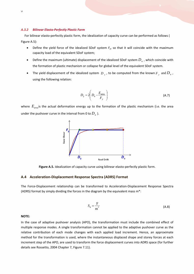
VI

A.3.2 Bilinear Elasto-Perfectly Plastic Form

For bilinear elasto-perfectly plastic form, the idealization of capacity curve can be performed as follows (

Figure A.5):

• Define the yield force of the idealized SDoF system Fy, so that it will coincide with the maximum

capacity load of the equivalent SDoF system;

• Define the maximum (ultimate) displacement of the idealized SDoF system uD , which coincide with

the formation of plastic mechanism or collapse for global level of the equivalent SDoF system.

• The yield displacement of the idealized system yD , to be computed from the known

yF and uD ,

using the following relation:

=

yu

F

EDD area

y - 2 (A.7)

where areaE is the actual deformation energy up to the formation of the plastic mechanism (i.e. the area

under the pushover curve in the interval from 0 to uD ).

Figure A.5. Idealization of capacity curve using bilinear elasto-perfectly plastic form.

A.4 Acceleration-Displacement Response Spectra (ADRS) Format

The Force-Displacement relationship can be transformed to Acceleration-Displacement Response Spectra

(ADRS) format by simply dividing the forces in the diagram by the equivalent mass m*:

*m

F =aS (A.8)

NOTE:

In the case of adaptive pushover analysis (APO), the transformation must include the combined effect of

multiple response modes. A single transformation cannot be applied to the adaptive pushover curve as the

relative contribution of each mode changes with each applied load increment. Hence, an approximate

method for the transformation is used, where the instantaneous displaced shape and storey forces at each

increment step of the APO, are used to transform the force displacement curves into ADRS space (for further

details see Rossetto, 2004 Chapter 7, Figure 7.11).

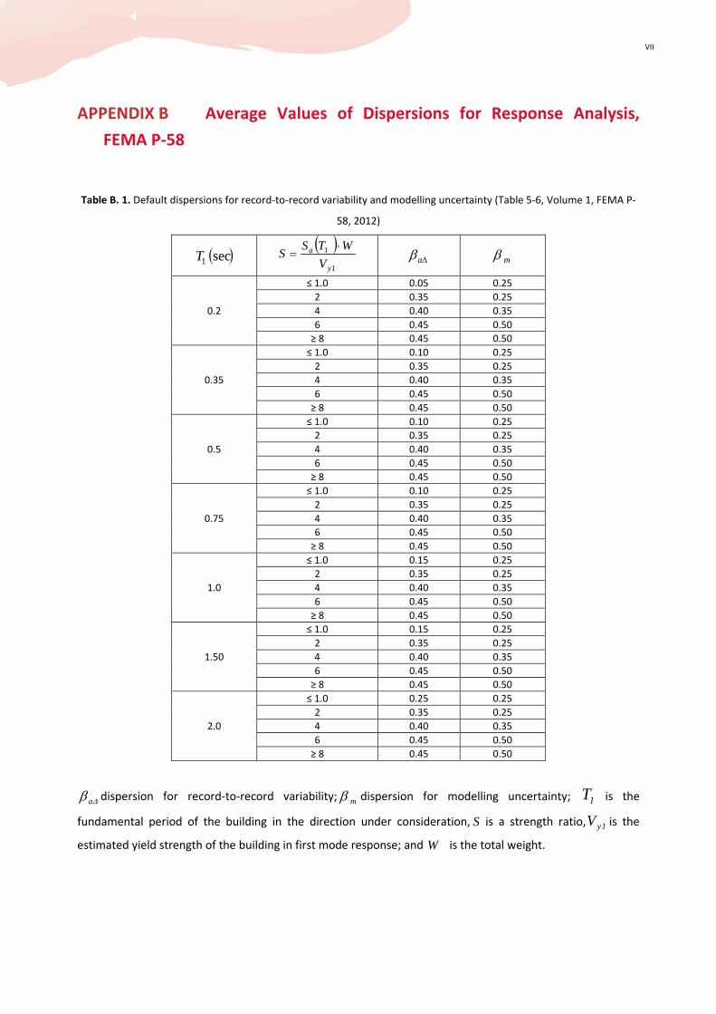
VII

APPENDIX B Average Values of Dispersions for Response Analysis,

FEMA P-58

Table B. 1. Default dispersions for record-to-record variability and modelling uncertainty (Table 5-6, Volume 1, FEMA P-

58, 2012)

( )sec1T ( )

1

1

y

a

V

WTSS

⋅=

∆aβ mβ

0.2

≤ 1.0 0.05 0.25

2 0.35 0.25

4 0.40 0.35

6 0.45 0.50

≥ 8 0.45 0.50

0.35

≤ 1.0 0.10 0.25

2 0.35 0.25

4 0.40 0.35

6 0.45 0.50

≥ 8 0.45 0.50

0.5

≤ 1.0 0.10 0.25

2 0.35 0.25

4 0.40 0.35

6 0.45 0.50

≥ 8 0.45 0.50

0.75

≤ 1.0 0.10 0.25

2 0.35 0.25

4 0.40 0.35

6 0.45 0.50

≥ 8 0.45 0.50

1.0

≤ 1.0 0.15 0.25

2 0.35 0.25

4 0.40 0.35

6 0.45 0.50

≥ 8 0.45 0.50

1.50

≤ 1.0 0.15 0.25

2 0.35 0.25

4 0.40 0.35

6 0.45 0.50

≥ 8 0.45 0.50

2.0

≤ 1.0 0.25 0.25

2 0.35 0.25

4 0.40 0.35

6 0.45 0.50

≥ 8 0.45 0.50

∆βa dispersion for record-to-record variability; mβ dispersion for modelling uncertainty; 1T is the

fundamental period of the building in the direction under consideration, S is a strength ratio, 1yV is the

estimated yield strength of the building in first mode response; and W is the total weight.

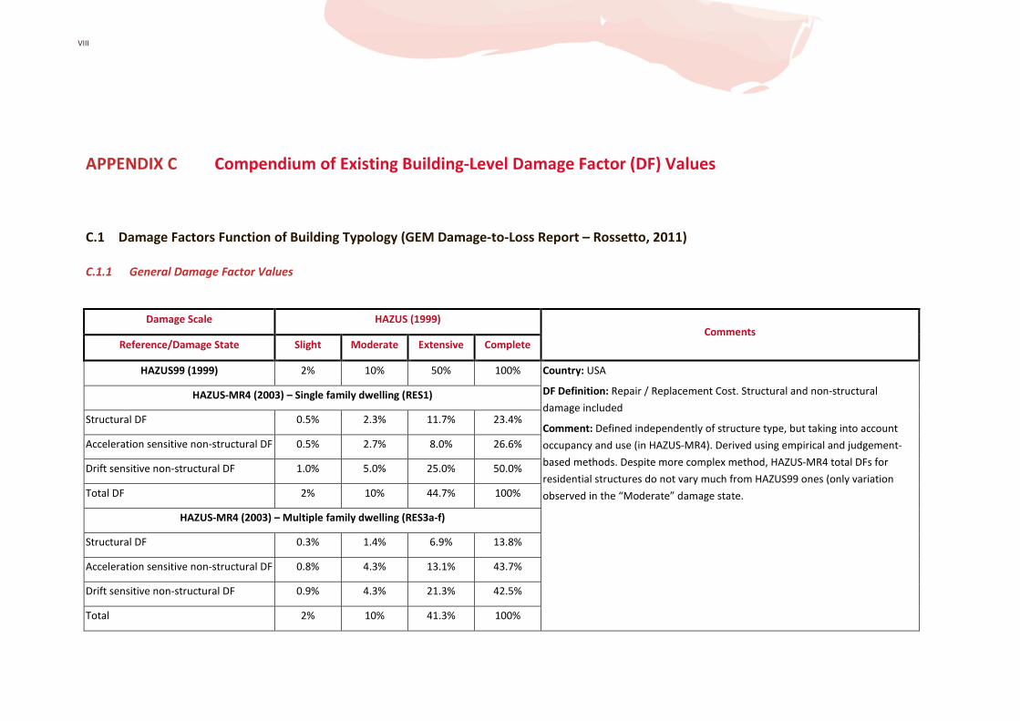
VIII

APPENDIX C Compendium of Existing Building-Level Damage Factor (DF) Values

C.1 Damage Factors Function of Building Typology (GEM Damage-to-Loss Report – Rossetto, 2011)

C.1.1 General Damage Factor Values

Damage Scale HAZUS (1999) Comments

Reference/Damage State Slight Moderate Extensive Complete

HAZUS99 (1999) 2% 10% 50% 100% Country: USA

DF Definition: Repair / Replacement Cost. Structural and non-structural

damage included

Comment: Defined independently of structure type, but taking into account

occupancy and use (in HAZUS-MR4). Derived using empirical and judgement-

based methods. Despite more complex method, HAZUS-MR4 total DFs for

residential structures do not vary much from HAZUS99 ones (only variation

observed in the “Moderate” damage state.

HAZUS-MR4 (2003) – Single family dwelling (RES1)

Structural DF 0.5% 2.3% 11.7% 23.4%

Acceleration sensitive non-structural DF 0.5% 2.7% 8.0% 26.6%

Drift sensitive non-structural DF 1.0% 5.0% 25.0% 50.0%

Total DF 2% 10% 44.7% 100%

HAZUS-MR4 (2003) – Multiple family dwelling (RES3a-f)

Structural DF 0.3% 1.4% 6.9% 13.8%

Acceleration sensitive non-structural DF 0.8% 4.3% 13.1% 43.7%

Drift sensitive non-structural DF 0.9% 4.3% 21.3% 42.5%

Total 2% 10% 41.3% 100%

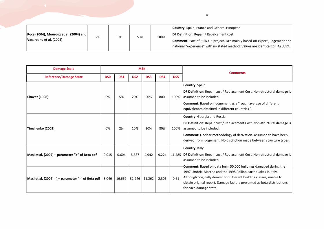
IX

Roca (2004), Mouroux et al. (2004) and

Vacareanu et al. (2004) 2% 10% 50% 100%

Country: Spain, France and General European

DF Definition: Repair / Repalcement cost

Comment: Part of RISK-UE project. DFs mainly based on expert judgement and

national “experience” with no stated method. Values are identical to HAZUS99.

Damage Scale MSK Comments

Reference/Damage State DS0 DS1 DS2 DS3 DS4 DS5

Chavez (1998) 0% 5% 20% 50% 80% 100%

Country: Spain

DF Definition: Repair cost / Replacement Cost. Non-structural damage is

assumed to be included.

Comment: Based on judgement as a “rough average of different

equivalences obtained in different countries “.

Timchenko (2002) 0% 2% 10% 30% 80% 100%

Country: Georgia and Russia



Comment: Unclear methodology of derivation. Assumed to have been

derived from judgement. No distinction made between structure types.

Masi et al. (2002) – parameter “q” of Beta pdf 0.015 0.604 5.587 4.942 9.224 11.585

Country: Italy



Comment: Based on data form 50,000 buildings damaged during the

1997 Umbria-Marche and the 1998 Pollino earthquakes in Italy.

Although originally derived for different building classes, unable to

obtain original report. Damage factors presented as beta-distributions

for each damage state.

Masi et al. (2002) - ) – parameter “r” of Beta pdf 3.046 16.662 32.946 11.262 2.306 0.61

X

Damage Scale EMS 98 Comments

Reference/Damage State DS0 DS1 DS2 DS3 DS4 DS5

Fah et al. (2001) Central DFs 0% <5% 20% 55% 90% 100%

Country: Switzerland



Comment: Values from ATC-13 applied to the EMS 98 damage scale

through interpretation by the authors, though no method in particular is

mentioned. No consideration of different structure types or occupancy

classes in DF estimates.

Milutinovic and Trendafiloski

(2003) 0% 1% 10% 35% 75% 100%

Country: Italy

DF Definition: Repair / Replacement cost

Comment: Part of RISK-UE project. Study carried out by Universita’ degli

Studi di Genova and reported in Milutinovic and Trendafiloski (2003). DFs

mainly based on expert judgement and national “experience” with no

stated method.

Kostov et al. (2004) 0% 1% 10% 40% 80% 100%

Country: Bulgaria

DF Definition: Repair / Replacement cost

Comment: Part of RISK-UE project. Study carried out by the Bulgarian

Academy of Sciences. DFs mainly based on expert judgement and national

“experience” with no stated method.

Di Pasquale et al. (2005) 0% 1% 10% 35% 75% 100%

Country: Italy



Comment: Values from judgment based on ATC-13 and the National

Seismic Survey (Di Pasquale and Goretti, 2001) applied to the EMS 98

damage. Exact method of derivation is not mentioned. No consideration

of different structure types or occupancy classes in DF estimates.

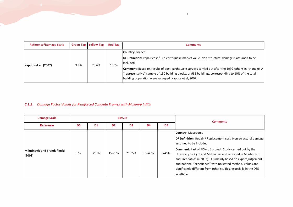
XI

Reference/Damage State Green-Tag Yellow-Tag Red-Tag Comments

Kappos et al. (2007) 9.8% 25.6% 100%

Country: Greece

DF Definition: Repair cost / Pre-earthquake market value. Non-structural damage is assumed to be

included.

Comment: Based on results of post-earthquake surveys carried out after the 1999 Athens earthquake. A

“representative” sample of 150 building blocks, or 983 buildings, corresponding to 10% of the total

building population were surveyed (Kappos et al, 2007).

C.1.2 Damage Factor Values for Reinforced Concrete Frames with Masonry Infills

Damage Scale EMS98 Comments

Reference D0 D1 D2 D3 D4 D5


(2003) 0% <15% 15-25% 25-35% 35-45% >45%

Country: Macedonia

DF Definition: Repair / Replacement cost. Non-structural damage


Comment: Part of RISK-UE project. Study carried out by the

University Ss. Cyril and Methodius and reported in Milutinovic

and Trendafiloski (2003). DFs mainly based on expert judgement

and national “experience” with no stated method. Values are

significantly different from other studies, especially in the DS5

category.

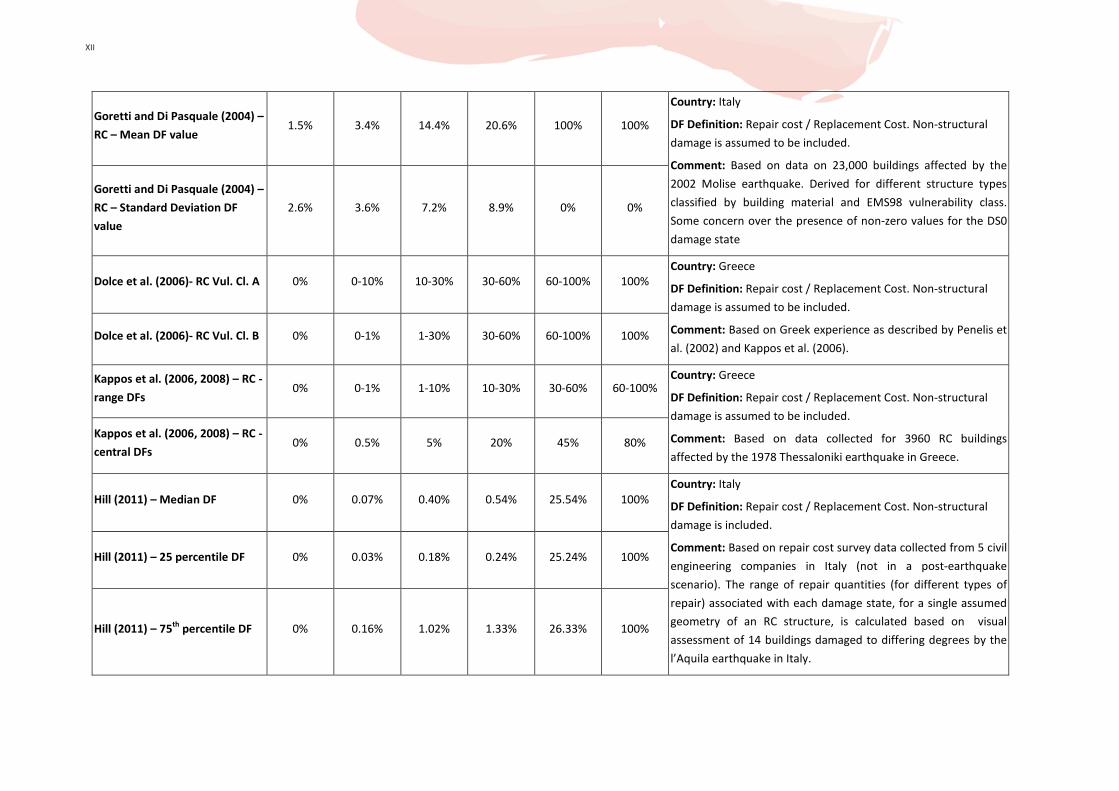
XII

Goretti and Di Pasquale (2004) –

RC – Mean DF value 1.5% 3.4% 14.4% 20.6% 100% 100%

Country: Italy

DF Definition: Repair cost / Replacement Cost. Non-structural

damage is assumed to be included.

Comment: Based on data on 23,000 buildings affected by the

2002 Molise earthquake. Derived for different structure types

classified by building material and EMS98 vulnerability class.

Some concern over the presence of non-zero values for the DS0

damage state

Goretti and Di Pasquale (2004) –

RC – Standard Deviation DF

value

2.6% 3.6% 7.2% 8.9% 0% 0%

Dolce et al. (2006)- RC Vul. Cl. A 0% 0-10% 10-30% 30-60% 60-100% 100%

Country: Greece



Comment: Based on Greek experience as described by Penelis et

al. (2002) and Kappos et al. (2006). Dolce et al. (2006)- RC Vul. Cl. B 0% 0-1% 1-30% 30-60% 60-100% 100%

Kappos et al. (2006, 2008) – RC -

range DFs 0% 0-1% 1-10% 10-30% 30-60% 60-100%

Country: Greece



Comment: Based on data collected for 3960 RC buildings

affected by the 1978 Thessaloniki earthquake in Greece.

Kappos et al. (2006, 2008) – RC -

central DFs 0% 0.5% 5% 20% 45% 80%

Hill (2011) – Median DF 0% 0.07% 0.40% 0.54% 25.54% 100%

Country: Italy


damage is included.

Comment: Based on repair cost survey data collected from 5 civil

engineering companies in Italy (not in a post-earthquake

scenario). The range of repair quantities (for different types of

repair) associated with each damage state, for a single assumed

geometry of an RC structure, is calculated based on visual

assessment of 14 buildings damaged to differing degrees by the

l’Aquila earthquake in Italy.

Hill (2011) – 25 percentile DF 0% 0.03% 0.18% 0.24% 25.24% 100%

Hill (2011) – 75th

percentile DF 0% 0.16% 1.02% 1.33% 26.33% 100%

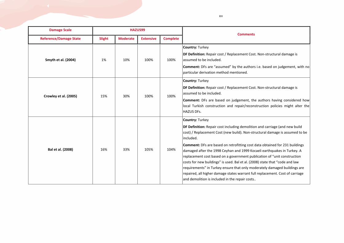
XIII

Damage Scale HAZUS99 Comments

Reference/Damage State Slight Moderate Extensive Complete

Smyth et al. (2004) 1% 10% 100% 100%

Country: Turkey



Comment: DFs are “assumed” by the authors i.e. based on judgement, with no

particular derivation method mentioned.

Crowley et al. (2005) 15% 30% 100% 100%

Country: Turkey



Comment: DFs are based on judgement, the authors having considered how

local Turkish construction and repair/reconstruction policies might alter the

HAZUS DFs.

Bal et al. (2008) 16% 33% 105% 104%

Country: Turkey

DF Definition: Repair cost including demolition and carriage (and new build

cost) / Replacement Cost (new build). Non-structural damage is assumed to be

included.

Comment: DFs are based on retrofitting cost data obtained for 231 buildings

damaged after the 1998 Ceyhan and 1999 Kocaeli earthquakes in Turkey. A

replacement cost based on a government publication of “unit construction

costs for new buildings” is used. Bal et al. (2008) state that “code and law

requirements” in Turkey ensure that only moderately damaged buildings are

repaired, all higher damage states warrant full replacement. Cost of carriage

and demolition is included in the repair costs..

XIV

C.1.3 Damage Factor Values for Unreinforced Masonry Buildings

Damage Scale EMS98 Comments

Reference D0 D1 D2 D3 D4 D5

Goretti and Di Pasquale (2004)

Country: Italy



Comment: Based on data on 23,000 buildings affected by the

2002 Molise earthquake. Derived for different structure types

classified by building material and EMS98 vulnerability class.

Some concern over the presence of non-zero values for the DS0

damage state

URM EMS98 vulny class A -

Mean 2.9% 10.8% 22.2% 30.6% 87.6% 100%

Standard Deviation 5.2% 5.0% 5.7% 6.7% 23.4% 0%

URM EMS98 vulny class B - Mean 0.9% 7.9% 20.3% 29.3% 97.5% 100%

Standard Deviation 2.6% 4% 4.8% 7.7% 11.2% 0%

URM EMS98 vulny class C - Mean 0.7% 5.8% 18.7% 26.7% 96.1% 100%

Standard Deviation 2% 4.2% 4.4% 5.2% 15.5% 0%

D’Ayala et al. (1997) 0% 5% 20% 50% 80% 100%

Country: Portugal



Comment: Values from judgment. Applied to predominantly 2-6

storey buildings in Alfama district of Lisbon. Building material is

typically poor quality rubble stone or brick masonry. Damage

scale used is EMS92 which approximately corresponds to EMS98.


(2003) 0% <20% 20-30% 30-40% 40-50% >50%

Country: Macedonia

DF Definition: Repair / Replacement cost. Non-structural damage


Comment: Part of RISK-UE project. Study carried out by the

University Ss. Cyril and Methodius and reported in Milutinovic

and Trendafiloski (2003). DFs mainly based on expert judgement

and national “experience” with no stated method. Values are

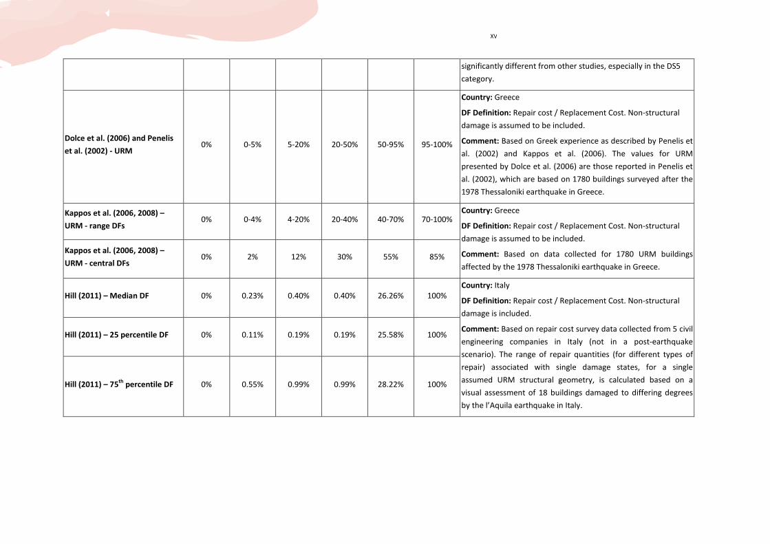
XV

significantly different from other studies, especially in the DS5

category.

Dolce et al. (2006) and Penelis

et al. (2002) - URM 0% 0-5% 5-20% 20-50% 50-95% 95-100%

Country: Greece



Comment: Based on Greek experience as described by Penelis et

al. (2002) and Kappos et al. (2006). The values for URM

presented by Dolce et al. (2006) are those reported in Penelis et

al. (2002), which are based on 1780 buildings surveyed after the

1978 Thessaloniki earthquake in Greece.

Kappos et al. (2006, 2008) –

URM - range DFs 0% 0-4% 4-20% 20-40% 40-70% 70-100%

Country: Greece



Comment: Based on data collected for 1780 URM buildings

affected by the 1978 Thessaloniki earthquake in Greece.

Kappos et al. (2006, 2008) –

URM - central DFs 0% 2% 12% 30% 55% 85%

Hill (2011) – Median DF 0% 0.23% 0.40% 0.40% 26.26% 100%

Country: Italy


damage is included.

Comment: Based on repair cost survey data collected from 5 civil

engineering companies in Italy (not in a post-earthquake

scenario). The range of repair quantities (for different types of

repair) associated with single damage states, for a single

assumed URM structural geometry, is calculated based on a

visual assessment of 18 buildings damaged to differing degrees

by the l’Aquila earthquake in Italy.

Hill (2011) – 25 percentile DF 0% 0.11% 0.19% 0.19% 25.58% 100%

Hill (2011) – 75th

percentile DF 0% 0.55% 0.99% 0.99% 28.22% 100%

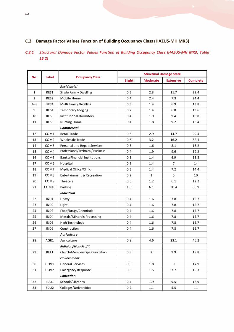
XVI

C.2 Damage Factor Values Function of Building Occupancy Class (HAZUS-MH MR3)

C.2.1 Structural Damage Factor Values Function of Building Occupancy Class (HAZUS-MH MR3, Table

15.2)

No. Label Occupancy Class Structural Damage State

Slight Moderate Extensive Complete

Residential

1 RES1 Single Family Dwelling 0.5 2.3 11.7 23.4

2 RES2 Mobile Home 0.4 2.4 7.3 24.4

3--8 RES3 Multi Family Dwelling 0.3 1.4 6.9 13.8

9 RES4 Temporary Lodging 0.2 1.4 6.8 13.6

10 RES5 Institutional Dormitory 0.4 1.9 9.4 18.8

11 RES6 Nursing Home 0.4 1.8 9.2 18.4

Commercial

12 COM1 Retail Trade 0.6 2.9 14.7 29.4

13 COM2 Wholesale Trade 0.6 3.2 16.2 32.4

14 COM3 Personal and Repair Services 0.3 1.6 8.1 16.2

15 COM4 Professional/Technical/ Business

Services 0.4 1.9 9.6 19.2

16 COM5 Banks/Financial Institutions 0.3 1.4 6.9 13.8

17 COM6 Hospital 0.2 1.4 7 14

18 COM7 Medical Office/Clinic 0.3 1.4 7.2 14.4

19 COM8 Entertainment & Recreation 0.2 1 5 10

20 COM9 Theaters 0.3 1.2 6.1 12.2

21 COM10 Parking 1.3 6.1 30.4 60.9

Industrial

22 IND1 Heavy 0.4 1.6 7.8 15.7

23 IND2 Light 0.4 1.6 7.8 15.7

24 IND3 Food/Drugs/Chemicals 0.4 1.6 7.8 15.7

25 IND4 Metals/Minerals Processing 0.4 1.6 7.8 15.7

26 IND5 High Technology 0.4 1.6 7.8 15.7

27 IND6 Construction 0.4 1.6 7.8 15.7

Agriculture

28 AGR1 Agriculture 0.8 4.6 23.1 46.2

Religion/Non-Profit

29 REL1 Church/Membership Organization 0.3 2 9.9 19.8

Government

30 GOV1 General Services 0.3 1.8 9 17.9

31 GOV2 Emergency Response 0.3 1.5 7.7 15.3

Education

32 EDU1 Schools/Libraries 0.4 1.9 9.5 18.9

33 EDU2 Colleges/Universities 0.2 1.1 5.5 11

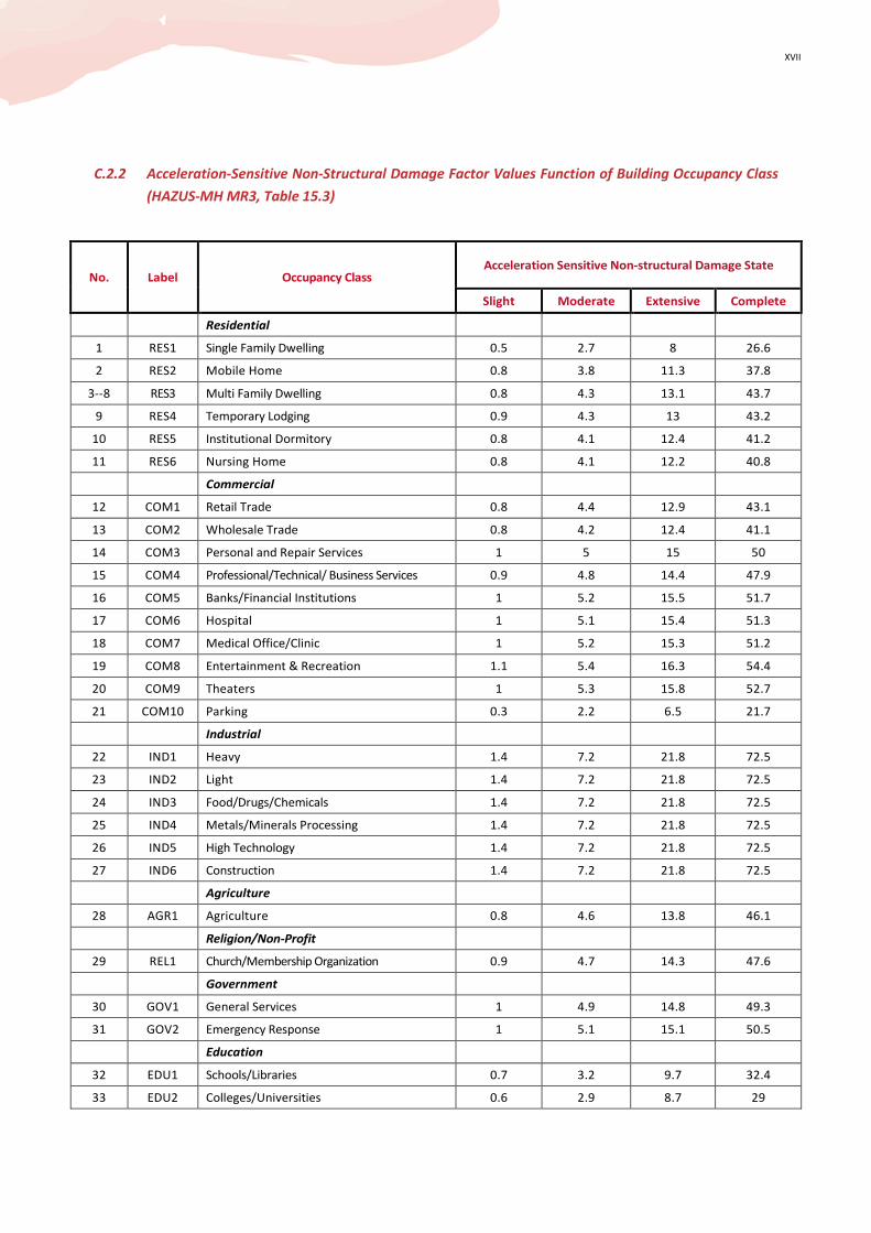
XVII

C.2.2 Acceleration-Sensitive Non-Structural Damage Factor Values Function of Building Occupancy Class

(HAZUS-MH MR3, Table 15.3)

No. Label Occupancy Class Acceleration Sensitive Non-structural Damage State


Residential

1 RES1 Single Family Dwelling 0.5 2.7 8 26.6

2 RES2 Mobile Home 0.8 3.8 11.3 37.8


9 RES4 Temporary Lodging 0.9 4.3 13 43.2

10 RES5 Institutional Dormitory 0.8 4.1 12.4 41.2

11 RES6 Nursing Home 0.8 4.1 12.2 40.8

Commercial

12 COM1 Retail Trade 0.8 4.4 12.9 43.1


14 COM3 Personal and Repair Services 1 5 15 50

15 COM4 Professional/Technical/ Business Services 0.9 4.8 14.4 47.9

16 COM5 Banks/Financial Institutions 1 5.2 15.5 51.7

17 COM6 Hospital 1 5.1 15.4 51.3

18 COM7 Medical Office/Clinic 1 5.2 15.3 51.2

19 COM8 Entertainment & Recreation 1.1 5.4 16.3 54.4

20 COM9 Theaters 1 5.3 15.8 52.7

21 COM10 Parking 0.3 2.2 6.5 21.7

Industrial

22 IND1 Heavy 1.4 7.2 21.8 72.5

23 IND2 Light 1.4 7.2 21.8 72.5





Agriculture

28 AGR1 Agriculture 0.8 4.6 13.8 46.1

Religion/Non-Profit

29 REL1 Church/Membership Organization 0.9 4.7 14.3 47.6

Government

30 GOV1 General Services 1 4.9 14.8 49.3

31 GOV2 Emergency Response 1 5.1 15.1 50.5

Education


33 EDU2 Colleges/Universities 0.6 2.9 8.7 29

XVIII

C.2.3 Drift-Sensitive Non-Structural Damage Factor Values Function of Building Occupancy Class (HAZUS-

MH MR3, Table 15.4)

No. Label Occupancy Class Drift Sensitive Non-structural Damage State


Residential

1 RES1 Single Family Dwelling 1 5 25 50

2 RES2 Mobile Home 0.8 3.8 18.9 37.8


9 RES4 Temporary Lodging 0.9 4.3 21.6 43.2

10 RES5 Institutional Dormitory 0.8 4 20 40

11 RES6 Nursing Home 0.8 4.1 20.4 40.8

Commercial

12 COM1 Retail Trade 0.6 2.7 13.8 27.5


14 COM3 Personal and Repair Services 0.7 3.4 16.9 33.8

15 COM4 Professional/Technical/ Business

Services 0.7 3.3 16.4 32.9

16 COM5 Banks/Financial Institutions 0.7 3.4 17.2 34.5

17 COM6 Hospital 0.8 3.5 17.4 34.7

18 COM7 Medical Office/Clinic 0.7 3.4 17.2 34.4

19 COM8 Entertainment & Recreation 0.7 3.6 17.8 35.6

20 COM9 Theaters 0.7 3.5 17.6 35.1

21 COM10 Parking 0.4 1.7 8.7 17.4

Industrial

22 IND1 Heavy 0.2 1.2 5.9 11.8

23 IND2 Light 0.2 1.2 5.9 11.8





Agriculture

28 AGR1 Agriculture 0 0.8 3.8 7.7

Religion/Non-Profit

29 REL1 Church/Membership Organization 0.8 3.3 16.3 32.6

Government

30 GOV1 General Services 0.7 3.3 16.4 32.8

31 GOV2 Emergency Response 0.7 3.4 17.1 34.2

Education


33 EDU2 Colleges/Universities 1.2 6 30 60

XIX

APPENDIX D Illustrative Examples

Authors: A. Meslem, D. D’Ayala, V. Novelli

D.1 Mid-Rise RC Building Designed According to Earlier Seismic Codes

The method selected for this illustrative example is one of the Non-linear Static-based approaches

recommended in this Guidelines document: i.e. Procedure 3.1. The building class selected as example of

application constitutes one of the largest portions of existing residential building stock in earthquake-prone

countries. For the seismic vulnerability analysis, the considered structure is a typical four-storey RC building,

built according to the first generation of seismic codes, and located in a high-seismicity region of Turkey (see

Figure D.1 and Table D.1).

The building class was defined based on structural characteristics-related parameters that are associated to

mechanical properties, geometric configuration, and structural details, and which are in general affected by

the quality of workmanship; i.e. compressive strength of concrete, yield strength of reinforcement, strength

and stiffness of infill walls (in terms of thickness of walls), storey height, and transverse reinforcement

spacing.

3D view of the building Plan view of the building

Reinforcement of columns in

storey-1 and 2 Reinforcement of

columns in storey-3 and 4

Figure D.1. Typical four-storey low-ductile RC building located in a high-seismically region of Turkey building

D.1.1 Define Building Index

In evaluating the central quality with lower and upper bounds, the choice of range of expected values for

each parameter has been based on the results of structural characteristics assessment (see Figure D.2)

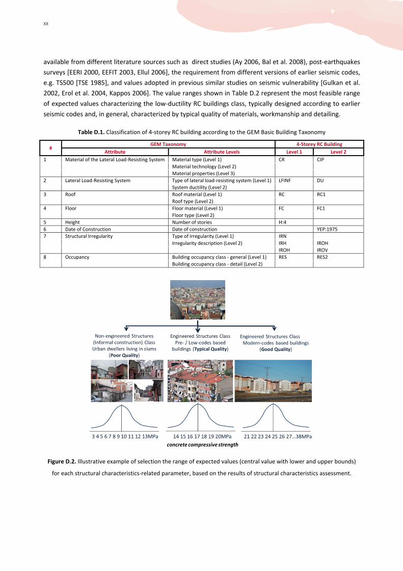
XX

available from different literature sources such as direct studies (Ay 2006, Bal et al. 2008), post-earthquakes

surveys [EERI 2000, EEFIT 2003, Ellul 2006], the requirement from different versions of earlier seismic codes,

e.g. TS500 [TSE 1985], and values adopted in previous similar studies on seismic vulnerability [Gulkan et al.

2002, Erol et al. 2004, Kappos 2006]. The value ranges shown in Table D.2 represent the most feasible range

of expected values characterizing the low-ductility RC buildings class, typically designed according to earlier

seismic codes and, in general, characterized by typical quality of materials, workmanship and detailing.

Table D.1. Classification of 4-storey RC building according to the GEM Basic Building Taxonomy

# GEM Taxonomy 4-Storey RC Building

Attribute Attribute Levels Level 1 Level 2

1 Material of the Lateral Load-Resisting System Material type (Level 1) CR CIP

Material technology (Level 2)

Material properties (Level 3)

2 Lateral Load-Resisting System Type of lateral load-resisting system (Level 1) LFINF DU

System ductility (Level 2)

3 Roof Roof material (Level 1) RC RC1

Roof type (Level 2)

4 Floor Floor material (Level 1) FC FC1

Floor type (Level 2)

5 Height Number of stories H:4

6 Date of Construction Date of construction YEP:1975

7 Structural Irregularity Type of irregularity (Level 1) IRN

Irregularity description (Level 2) IRH IROH

IROH IROV

8 Occupancy Building occupancy class - general (Level 1) RES RES2

Building occupancy class - detail (Level 2)

Figure D.2. Illustrative example of selection the range of expected values (central value with lower and upper bounds)

for each structural characteristics-related parameter, based on the results of structural characteristics assessment.

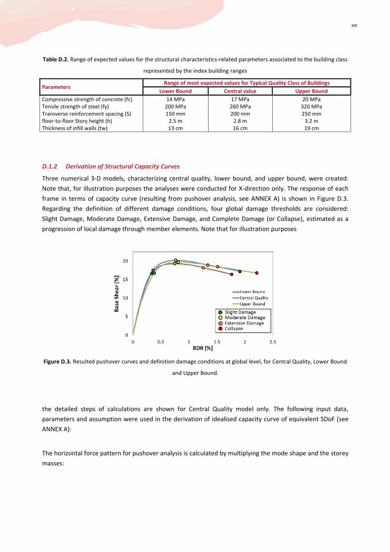
XXI

Table D.2. Range of expected values for the structural characteristics-related parameters associated to the building class

represented by the index building ranges

Parameters Range of most expected values for Typical Quality Class of Buildings

Lower Bound Central value Upper Bound

Compressive strength of concrete (fc) 14 MPa 17 MPa 20 MPa

Tensile strength of steel (fy) 200 MPa 260 MPa 320 MPa

Transverse reinforcement spacing (S) 150 mm 200 mm 250 mm

floor-to-floor Story height (h) 2.5 m 2.8 m 3.2 m

Thickness of infill walls (tw) 13 cm 16 cm 19 cm

D.1.2 Derivation of Structural Capacity Curves

Three numerical 3-D models, characterizing central quality, lower bound, and upper bound, were created:

Note that, for illustration purposes the analyses were conducted for X-direction only. The response of each

frame in terms of capacity curve (resulting from pushover analysis, see ANNEX A) is shown in Figure D.3.

Regarding the definition of different damage conditions, four global damage thresholds are considered:

Slight Damage, Moderate Damage, Extensive Damage, and Complete Damage (or Collapse), estimated as a

progression of local damage through member elements. Note that for illustration purposes

Figure D.3. Resulted pushover curves and definition damage conditions at global level, for Central Quality, Lower Bound

and Upper Bound.

the detailed steps of calculations are shown for Central Quality model only. The following input data,

parameters and assumption were used in the derivation of idealised capacity curve of equivalent SDoF (see

ANNEX A):

The horizontal force pattern for pushover analysis is calculated by multiplying the mode shape and the storey

masses:

XXII

==Φ=

65.177

97.179

42.137

84.45

000.1

800.0

600.0

200.0

177.656

224.96

229.03

229.18

M F

The mass of the equivalent SDOF system is (see Equation A.1):

∑ =⋅+⋅+⋅+⋅=Φ= tonne540.87 1.000177.65 0.800224.96 0.600229.03 200.018.229* 2imm

The transformation to an equivalent SDoF model is made by dividing the base shear and top displacement of

the MDoF with a transformation factor Γ (see Equation A.3). The result is presented in Figure D.4:

3088.1

000.1

800.0

600.0

200.0

65.177

96.224

03.229

18.229

000.1

800.0

600.0

200.0

1

1

1

1

65.177

96.224

03.229

18.229

000.1

800.0

600.0

200.0

1=

=Φ⋅⋅Φ⋅⋅Φ

=ΓT

T

T

T

M

M

Figure D.4. Transformation of MDoF pushover curve to an equivalent SDoF. Case: Central Quality.

The displacement at yield is determined by applying the equal energy rule for the interval from 0 to uD ,

which coincides with the maximum capacity load (see Equation A.7):

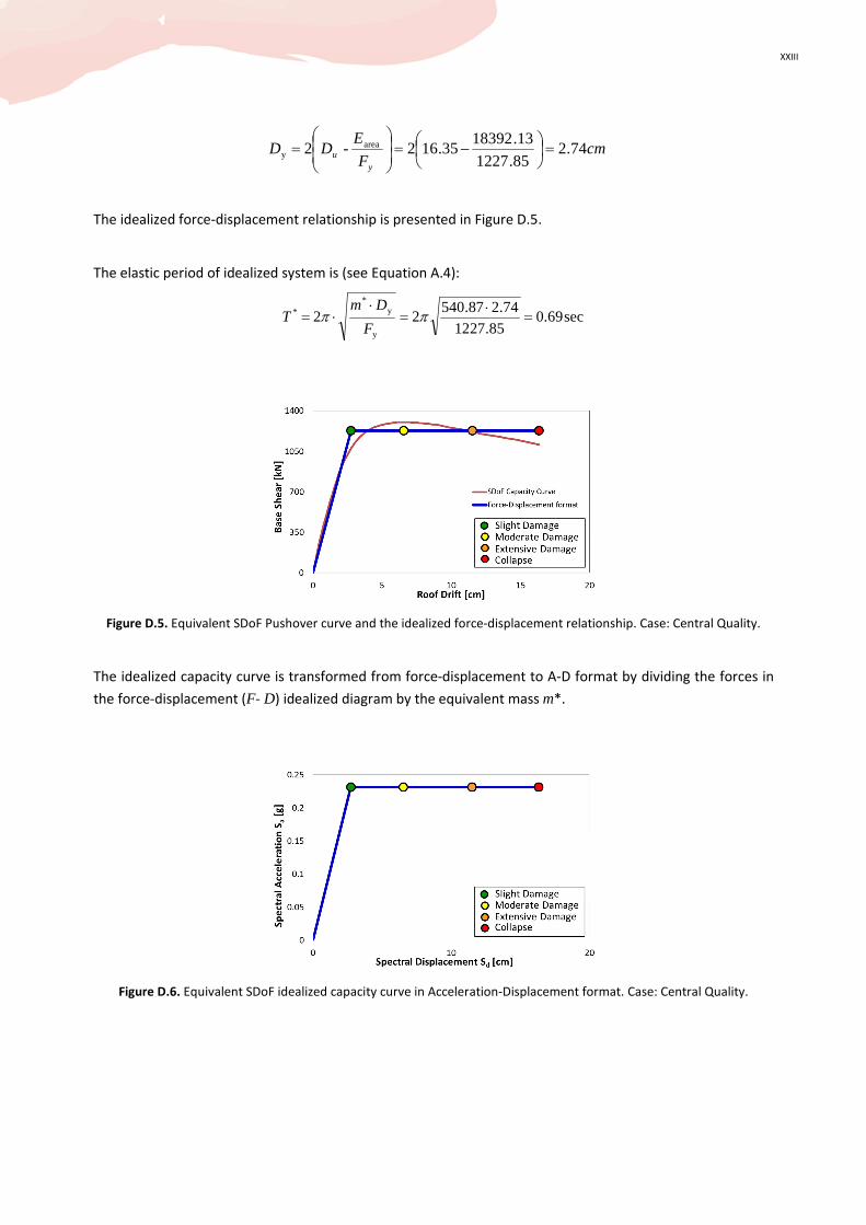
XXIII

cmF

EDD

yu 74.2

85.1227

13.1839235.162 - 2 area

y =

−=

=

The idealized force-displacement relationship is presented in Figure D.5.

The elastic period of idealized system is (see Equation A.4):

sec69.085.1227

74.287.54022

y

y*

* =⋅

=⋅

⋅= ππF

DmT

Figure D.5. Equivalent SDoF Pushover curve and the idealized force-displacement relationship. Case: Central Quality.

The idealized capacity curve is transformed from force-displacement to A-D format by dividing the forces in

the force-displacement (F- D) idealized diagram by the equivalent mass m*.

Figure D.6. Equivalent SDoF idealized capacity curve in Acceleration-Displacement format. Case: Central Quality.

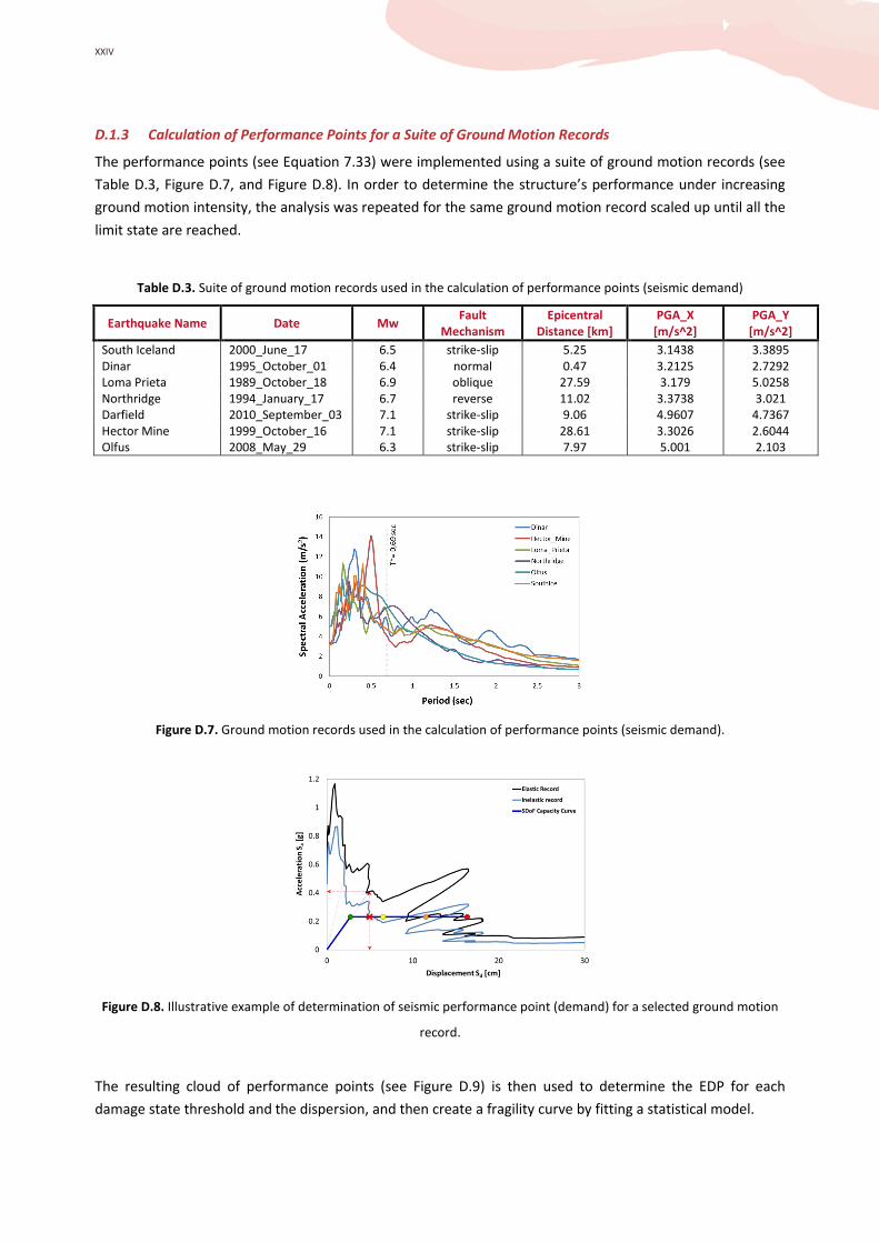
XXIV

D.1.3 Calculation of Performance Points for a Suite of Ground Motion Records

The performance points (see Equation 7.33) were implemented using a suite of ground motion records (see

Table D.3, Figure D.7, and Figure D.8). In order to determine the structure’s performance under increasing

ground motion intensity, the analysis was repeated for the same ground motion record scaled up until all the

limit state are reached.

Table D.3. Suite of ground motion records used in the calculation of performance points (seismic demand)

Earthquake Name Date Mw Fault

Mechanism

Epicentral

Distance [km]

PGA_X

[m/s^2]

PGA_Y

[m/s^2]

South Iceland 2000_June_17 6.5 strike-slip 5.25 3.1438 3.3895

Dinar 1995_October_01 6.4 normal 0.47 3.2125 2.7292

Loma Prieta 1989_October_18 6.9 oblique 27.59 3.179 5.0258

Northridge 1994_January_17 6.7 reverse 11.02 3.3738 3.021

Darfield 2010_September_03 7.1 strike-slip 9.06 4.9607 4.7367

Hector Mine 1999_October_16 7.1 strike-slip 28.61 3.3026 2.6044

Olfus 2008_May_29 6.3 strike-slip 7.97 5.001 2.103

Figure D.7. Ground motion records used in the calculation of performance points (seismic demand).

Figure D.8. Illustrative example of determination of seismic performance point (demand) for a selected ground motion

record.

The resulting cloud of performance points (see Figure D.9) is then used to determine the EDP for each

damage state threshold and the dispersion, and then create a fragility curve by fitting a statistical model.

XXV

Figure D.9. Clouds of structural-response results. Case of central Quality

D.1.4 Determination of EDPs Damage State Thresholds

The calculation of EDPs of damage state thresholds and their corresponding dispersions is conducted using

Least Squares formulation (Figure D.10), described in Section 7.3.1.1. The results are presented below.

Figure D.10. Calculation of Median capacities and dispersions using Least Squares formulation. Case: central quality

The resulting median capacities and their corresponding record-to-record dispersions are shown in Table D.4,

and Figure D.11 shows the fitted fragility curves for Central Quality, Lower Bound, and Upper Bound.

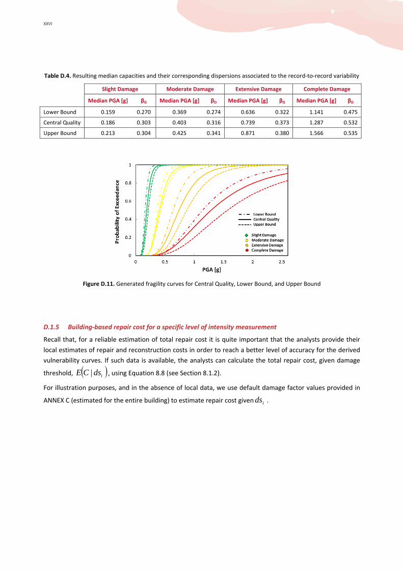
XXVI

Table D.4. Resulting median capacities and their corresponding dispersions associated to the record-to-record variability


Median PGA [g] βD Median PGA [g] βD Median PGA [g] βD Median PGA [g] βD

Lower Bound 0.159 0.270 0.369 0.274 0.636 0.322 1.141 0.475

Central Quality 0.186 0.303 0.403 0.316 0.739 0.373 1.287 0.532

Upper Bound 0.213 0.304 0.425 0.341 0.871 0.380 1.566 0.535

Figure D.11. Generated fragility curves for Central Quality, Lower Bound, and Upper Bound

D.1.5 Building-based repair cost for a specific level of intensity measurement

Recall that, for a reliable estimation of total repair cost it is quite important that the analysts provide their

local estimates of repair and reconstruction costs in order to reach a better level of accuracy for the derived

vulnerability curves. If such data is available, the analysts can calculate the total repair cost, given damage

threshold, ( )ids|CE , using Equation 8.8 (see Section 8.1.2).

For illustration purposes, and in the absence of local data, we use default damage factor values provided in

ANNEX C (estimated for the entire building) to estimate repair cost given ids .

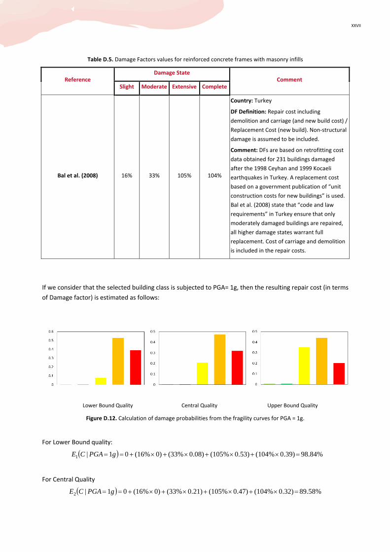
XXVII

Table D.5. Damage Factors values for reinforced concrete frames with masonry infills

Reference Damage State

Comment Slight Moderate Extensive Complete

Bal et al. (2008) 16% 33% 105% 104%

Country: Turkey

DF Definition: Repair cost including

demolition and carriage (and new build cost) /

Replacement Cost (new build). Non-structural


Comment: DFs are based on retrofitting cost

data obtained for 231 buildings damaged

after the 1998 Ceyhan and 1999 Kocaeli

earthquakes in Turkey. A replacement cost

based on a government publication of “unit

construction costs for new buildings” is used.

Bal et al. (2008) state that “code and law

requirements” in Turkey ensure that only

moderately damaged buildings are repaired,

all higher damage states warrant full

replacement. Cost of carriage and demolition

is included in the repair costs.

If we consider that the selected building class is subjected to PGA= 1g, then the resulting repair cost (in terms

of Damage factor) is estimated as follows:

Lower Bound Quality Central Quality Upper Bound Quality

Figure D.12. Calculation of damage probabilities from the fragility curves for PGA = 1g.

For Lower Bound quality:

( ) 98.84% 0.39) (104% 0.53) (105% 0.08) (33% 0) (16% 0 1|1 =×+×+×+×+== gPGACE

For Central Quality

( ) 89.58% 0.32) (104% 0.47) (105% 0.21) (33% 0) (16% 0 1|2 =×+×+×+×+== gPGACE

XXVIII

For Upper Bound Quality

( ) 78.84% 0.20) (104% 0.44) (105% 0.35) (33% 0) (16% 0 1|3 =×+×+×+×+== gPGACE

The mean vulnerability function (in terms of Damage Factor) for the considered three index buildings can be

calculated through the following Equation:

( ) ( ) % 89.10 1|3

11|

3

1

==== ∑=j

j gPGACEgPGACE

D.2 Low to Mid-Rise Unreinforced Masonry Buildings in Historic Town Centre

The method selected for this illustrative example is Non-Linear Static analysis based on Simplified Mechanism

Models (SMM-NLS) which allows the calculation of the EDPs thresholds for masonry construction typologies

(unreinforced masonry and adobe structures). The calculation of the EDPs thresholds can be done using

smoothed elastic response spectrum only. This example is developed using Procedure 4.1: Failure

Mechanism Identification and Vulnerability Evaluation (FaMIVE) (Section 7.4.1). The building sample used in

this application constitutes several UM building subclasses which typically form the building stock of historic

town centres in the Mediterranean countries. For the seismic vulnerability analysis, a centre in the Umbria

region of Italy is chosen, located in the highest seismicity zoning for Italy (see Figure D.13 and Table D.6).

The building class was defined based on structural characteristics-related parameters that are associated to

mechanical properties, geometric configuration, and structural details, and which are in general affected by

the quality of workmanship.

Figure D.13. Typical two-storey masonry building in Nocera Umbra, Italy

XXIX

D.2.1 Define Building Index

The building index is not defined in terms of its mechanical and geometric characteristics a priori, but the

analysis is run for a large number of buildings representative of the building stock of the site under study

and, a posteriori, according to their performance and failure mechanisms they are combined in subclasses

and median capacity curves are extracted. Table D.6 presents the Level 1 and Level 2 GEM Taxonomy classes

applicable to the whole building stock of Nocera Umbra.

Table D.6. Classification of URM building stock in Nocera Umbra, Italy, according to the GEM Basic Building Taxonomy

# GEM Taxonomy 4-Storey RC Building

Attribute Attribute Levels Level 1 Level 2

1 Material of the Lateral Load-Resisting System Material type (Level 1) MUR STRUB,STDRE, CLBRS

Material technology (Level 2)

Material properties (Level 3)

2 Lateral Load-Resisting System Type of lateral load-resisting system (Level 1) LWAL D99

System ductility (Level 2)

3 Roof Roof material (Level 1) RC, RWO, RM RC2, RWO2,

Roof type (Level 2)

4 Floor Floor material (Level 1) FC,FW,FM FC2,FW2, FM1,FM2

Floor type (Level 2)

5 Height Number of stories H:1,5

6 Date of Construction Date of construction YN:1500,1900

7 Structural Irregularity Type of irregularity (Level 1) IRH,IRV REC,IRHO,CRW,POP,CHV

Irregularity description (Level 2)

8 Occupancy Building occupancy class - general (Level 1) RES,COM RES1,RES2,COM1,COM3

Building occupancy class - detail (Level 2)

The distribution of the selected buildings used to compute the capacity curves, derive the fragility functions

for the historic centre of Nocera and compute the performance point for each building and its probability of

damage, are shown in Figure D.14.

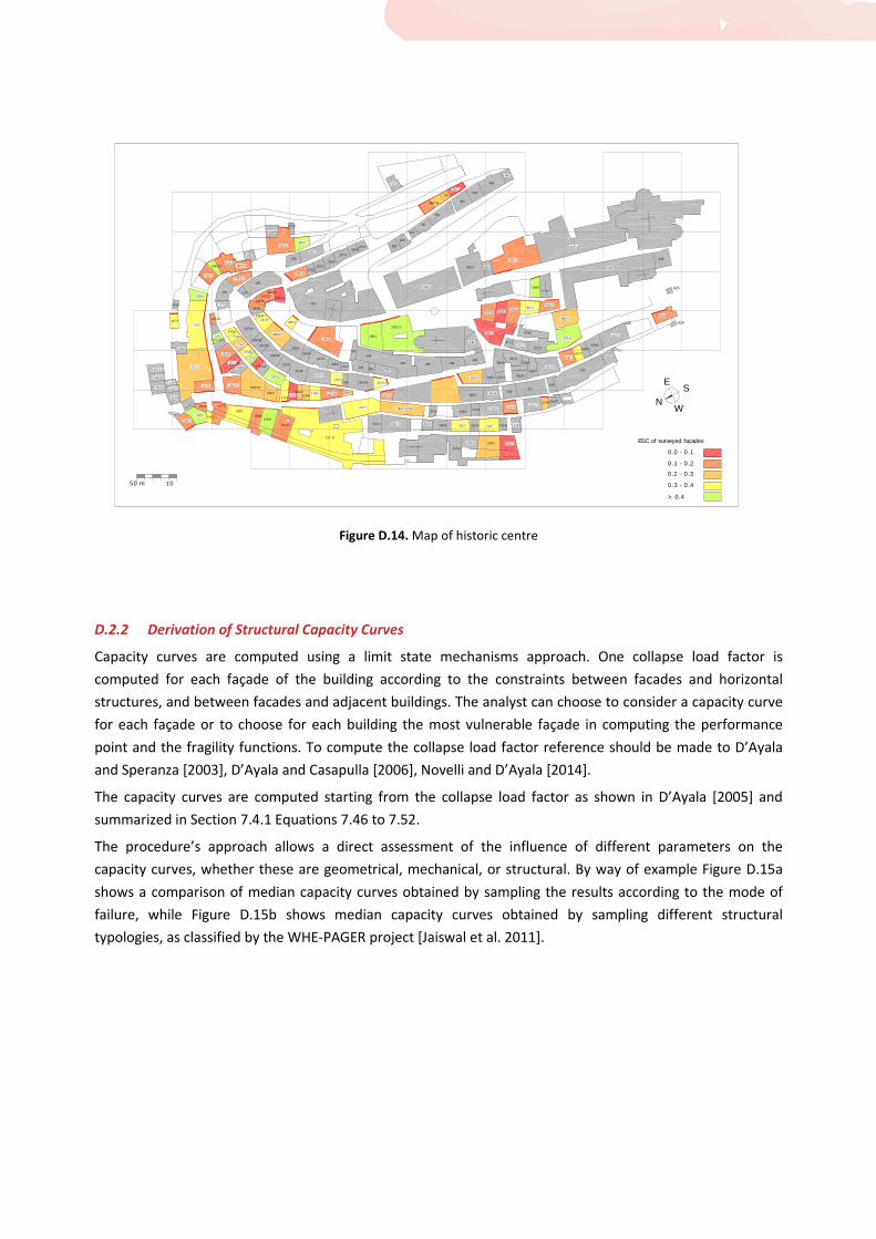
XXX

347

> 0.4

0.3 - 0 .4

0 .2 - 0 .3

0 .1 - 0 .2

0 .0 - 0 .1

ESC of surveyed facades

1050 m

298/1

107/11

106/10

105/9

113/6

112/7

111/8

115/2

114/1

116/5

117/1

118/1

119/3

120/4

110/2

109/1

154/3

155/4

156/5

157/6

158/7

159/8160/8

161/10

264/4

265/2

622/3

267/1

260

261

253/1254/2

255/3256/4

257/5

258/6259/7

315

308

309

310

311

405

406

404

300A

385/1 386/2

387/3

429/4

428

427

384/1

381/5370/4369/3367/2

366/1

371/1372/2

375/3

374/5

380/6

379/4

456

426

424

423/5

419/4418/3

417/2416/1 420

415

358357

356

421

341/6340/5290/4289/3287/1

342/1 343/2 359/3

360/4361/5

362/6364/7

365/9363/8

354/7353/6352/5

339/4338/3337/2

336/1285/5

231/1 281/2 283/3 326/4 332/5 333/6 334/7 335/8 350/1

330/1329/2328/3

327/4

232/1

218/7217/6216/5215/4

214/3213/2

212/1169/5

168/3/4162/1/2

164/6

163/7/8

165/9

10/11/12

167/13

177

178

179/1/2

229

230

247/13

246/12245/11

244/10

243/9

241/8

240/6/7

239/5

250/1

249/1

238/4

237/3

236/2235/1 291

248

294

292 293

295 297 344345

299/2/3

346

233/1/2234/3/4219/5220/6

221/7222/8

223/9

224/10

225/11

226/12

227/13176/8

175/8

174/7

171/3/4

170/1/2

251

394/3/4

393

395/2

396/1

403

144/2/3145/4

180/5/6

183

143/1

382/6

NS

W

E

166

173/6

172/5

211/11

242/8

284/1/2/3/4

Figure D.14. Map of historic centre

D.2.2 Derivation of Structural Capacity Curves

Capacity curves are computed using a limit state mechanisms approach. One collapse load factor is

computed for each façade of the building according to the constraints between facades and horizontal

structures, and between facades and adjacent buildings. The analyst can choose to consider a capacity curve

for each façade or to choose for each building the most vulnerable façade in computing the performance

point and the fragility functions. To compute the collapse load factor reference should be made to D’Ayala

and Speranza [2003], D’Ayala and Casapulla [2006], Novelli and D’Ayala [2014].

The capacity curves are computed starting from the collapse load factor as shown in D’Ayala [2005] and

summarized in Section 7.4.1 Equations 7.46 to 7.52.

The procedure’s approach allows a direct assessment of the influence of different parameters on the

capacity curves, whether these are geometrical, mechanical, or structural. By way of example Figure D.15a

shows a comparison of median capacity curves obtained by sampling the results according to the mode of

failure, while Figure D.15b shows median capacity curves obtained by sampling different structural

typologies, as classified by the WHE-PAGER project [Jaiswal et al. 2011].

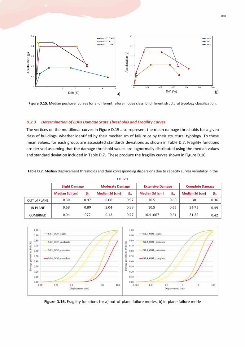
XXXI

a) b)

Figure D.15. Median pushover curves for a) different failure modes class, b) different structural typology classification.

D.2.3 Determination of EDPs Damage State Thresholds and Fragility Curves

The vertices on the multilinear curves in Figure D.15 also represent the mean damage thresholds for a given

class of buildings, whether identified by their mechanism of failure or by their structural typology. To these

mean values, for each group, are associated standards deviations as shown in Table D.7. Fragility functions

are derived assuming that the damage threshold values are lognormally distributed using the median values

and standard deviation included in Table D.7. These produce the fragility curves shown in Figure D.16.

Table D.7. Median displacement thresholds and their corresponding dispersions due to capacity curves variability in the

sample


Median Sd [cm] βD Median Sd [cm] βD Median Sd [cm] βD Median Sd [cm] βD

OUT of PLANE 0.30 0.97 0.88 0.97 10.5 0.60 30 0.36

IN PLANE 0.68 0.89 2.04 0.89 10.5 0.65 34.75 0.49

COMBINED 0.04 077 0.12 0.77 10.41667 0.51 31.25 0.42

Figure D.16. Fragility functions for a) out-of-plane failure modes, b) in-plane failure mode

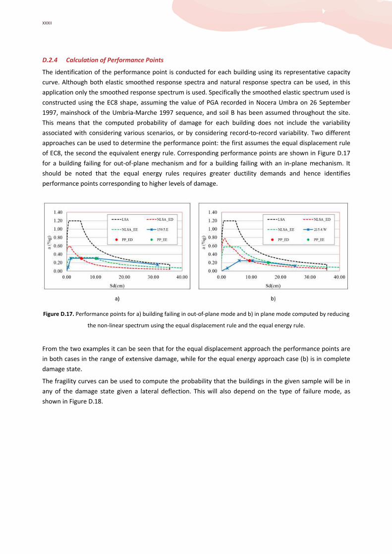
XXXII

D.2.4 Calculation of Performance Points

The identification of the performance point is conducted for each building using its representative capacity

curve. Although both elastic smoothed response spectra and natural response spectra can be used, in this

application only the smoothed response spectrum is used. Specifically the smoothed elastic spectrum used is

constructed using the EC8 shape, assuming the value of PGA recorded in Nocera Umbra on 26 September

1997, mainshock of the Umbria-Marche 1997 sequence, and soil B has been assumed throughout the site.

This means that the computed probability of damage for each building does not include the variability

associated with considering various scenarios, or by considering record-to-record variability. Two different

approaches can be used to determine the performance point: the first assumes the equal displacement rule

of EC8, the second the equivalent energy rule. Corresponding performance points are shown in Figure D.17

for a building failing for out-of-plane mechanism and for a building failing with an in-plane mechanism. It

should be noted that the equal energy rules requires greater ductility demands and hence identifies

performance points corresponding to higher levels of damage.

Figure D.17. Performance points for a) building failing in out-of-plane mode and b) in plane mode computed by reducing

the non-linear spectrum using the equal displacement rule and the equal energy rule.

From the two examples it can be seen that for the equal displacement approach the performance points are

in both cases in the range of extensive damage, while for the equal energy approach case (b) is in complete

damage state.

The fragility curves can be used to compute the probability that the buildings in the given sample will be in

any of the damage state given a lateral deflection. This will also depend on the type of failure mode, as

shown in Figure D.18.

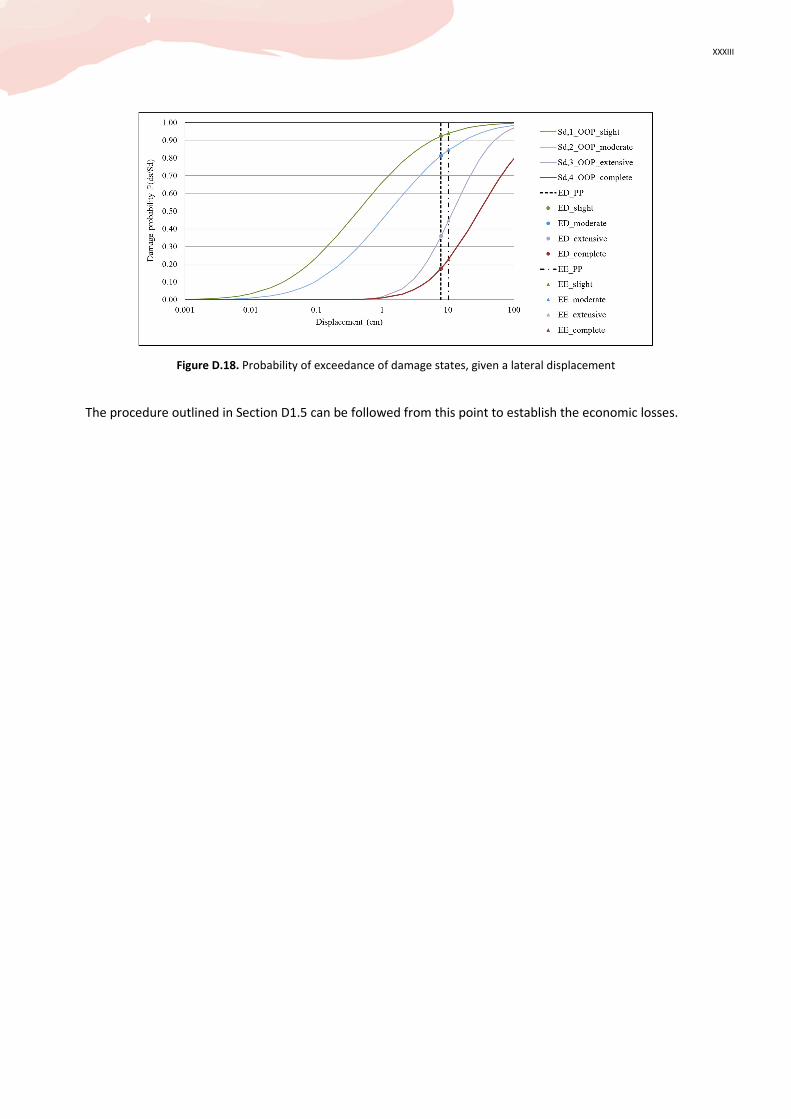
XXXIII

Figure D.18. Probability of exceedance of damage states, given a lateral displacement

The procedure outlined in Section D1.5 can be followed from this point to establish the economic losses.

the global earthquake model

The mission of the Global Earthquake Model (GEM) collaborative effort is to increase earthquake resilience worldwide.

To deliver on its mission and increase public understanding and awareness of seismic risk, the GEM Foundation, a non-profit public-private partnership, drives the GEM effort by involving and engaging with a very diverse community to:

- Share data, models, and knowledge through the OpenQuake platform

- Apply GEM tools and software to inform decision-making for risk mitigation and management

- Expand the science and understanding of earthquakes.

August 2015

GEM FoundationVia Ferrata 127100 Pavia, Italy Phone: +39 0382 5169865Fax: +39 0382 [email protected]

Copyright © 201 GEM Foundation, D’Ayala D., A. Meslem, D. Vamvatsikos, K. Porter and T. Rossetto.

This work is made available under the terms of the Creative Commons license CC BY 3.0 Unported

Guidelines for Analytical Vulnerability Assessment - Low/Mid ...

Documents

Transcript of Guidelines for Analytical Vulnerability Assessment - Low/Mid ...