Guided Local Search for the Three-Dimensional Bin-Packing Problem
28
-
Upload
independent -
Category
Documents
-
view
3 -
download
0
Transcript of Guided Local Search for the Three-Dimensional Bin-Packing Problem
Guided local search for thethree-dimensional bin packing problem�Oluf Faroe, David Pisinger, Martin ZachariasenyDecember 1999AbstractThe three-dimensional bin packing problem is the problem of orthogonally packing aset of boxes into a minimum number of three-dimensional bins. In this paper we present aheuristic algorithm based on Guided Local Search (GLS). Starting with an upper boundon the number of bins obtained by a greedy heuristic, the presented algorithm iterativelydecreases the number of bins, each time searching for a feasible packing of the boxesusing GLS. The process terminates when a given time limit has been reached or theupper bound matches a precomputed lower bound. The algorithm can also be appliedto two-dimensional bin packing problems by having a constant depth for all boxes andbins. Computational experiments are reported for two- and three-dimensional instanceswith up to 200 boxes, and the results are compared with those obtained by heuristics andexact methods from the literature.1 IntroductionThe three-dimensional bin packing problem asks for an orthogonal packing of a set of boxes intoa minimum number of three-dimensional bins. The only restriction imposed on the solutionis that the boxes have �xed orientation. The problem has several industrial applications incutting and loading contexts, and since rotation of the boxes is not allowed, the model canbe used for solving several scheduling problems.In this paper we present a new local search heuristic based on the Guided Local Search(GLS) method [20, 23] which has its origin in constraint satisfaction applications, but alsohas proven to be a very powerful metaheuristic for solving hard combinatorial problems. GLSuses memory to guide the search to promising regions of the solution space; this is done byaugmenting the cost function with a penalty term that penalizes \bad" features of previouslyvisited solutions.Starting with an upper bound on the number of bins obtained by a greedy heuristic, theGLS algorithm iteratively tightens the upper bound by removing one bin from a feasiblesolution. That is, for a given number of bins, GLS constructs a feasible packing of theboxes. When such a packing has been found, the number of bins is decreased by one, and theprocedure iterates until a given time limit has been reached or the upper bound matches thelower bound | in our case the L2 bound from Martello, Pisinger and Vigo [16].�Tech. Rep. 99/13, DIKU, University of Copenhagen, DenmarkyDept. of Computer Science, University of Copenhagen, Universitetsparken 1, DK-2100 Copenhagen �,Denmark. E-mail: foluf,pisinger,[email protected]

The GLS algorithm assigns coordinates (including bin numbers) to the boxes. Translationof boxes along coordinate axes within one bin or moving boxes from one bin to another de�nesthe neighbourhood of the local search algorithm. The objective value of a given solution isthe total volume of the pairwise overlap between boxes. Searching for a feasible solutionis therefore equivalent to minimizing the objective function since an objective value of zeroindicates a feasible packing.To speed up the local search an implementation of Fast Local Search (FLS) has beenused [20, 23]. Since the neighbourhood is fairly large in the current setting, FLS drasticallyspeeds up the search for a local minimum. This is done by shadowing less promising parts ofthe neighbourhood, that is, temporarily �xing box positions.The GLS algorithm has been evaluated on instances with up to 200 boxes of varying typesshowing very promising results compared to previous approaches: Within a �xed time limit,it generally �nds better solutions than the exact algorithm by Martello, Pisinger and Vigo[16], and this also applies when comparing to other heuristic algorithms as Lodi, Martelloand Vigo [14, 15]. Furthermore, it is easily generalized to problems in which rotations areallowed and/or when the items to be packed have irregular shape.The present paper is organized as follows: In Section 2 we de�ne the considered problemmore formally, and describe some lower bounds. Section 3 gives an overview of previousheuristics based on local search. The concept of Guided Local Search and our new algorithmis presented in Section 4. The paper is concluded with extensive empirical results in Section 5.2 The three-dimensional bin-packing problemCutting and packing problems have numerous applications, spanning from the direct use ofthe models (loading cargo into ships, vehicles, containers) to a more abstract use of the models(scheduling problems, budgeting, generation of valid inequalities). Due to the large number ofapplications, di�erent variants of the problems have been developed based on the additionalconstraints present in the concrete application. Nearly all the problems considered in theliterature are NP-hard, and thus di�cult to solve to optimality. This makes it attractiveto consider heuristic approaches, as heuristics often are able to return a \su�ciently" goodsolution in reasonable time, and generally are exible to handle additional side constraints.In the present paper we consider the three-dimensional bin-packing problem (3D-BPP) inwhich we have a set J of n rectangular-shaped boxes, each having a width wj, height hj anddepth dj (all integers), and an unlimited number of identical three-dimensional bins of widthW , height H and depth D. The objective is to pack all the boxes into the minimum number ofbins, such that the original orientation is respected. The two-dimensional bin-packing problem(2D-BPP) is the obvious restriction of 3D-BPP to two dimensions (width and height).Other variants of packing and loading include the knapsack container loading problemwhere the boxes have an associated pro�t, and the objective is to pack a subset of the boxesinto a single bin of �xed dimensions such that the pro�t of the included boxes is as largeas possible. Other applications consider the minimum depth container loading problem (alsoknown as the strip packing problem) where the objective is to pack all the boxes into asingle container with �xed width W and height H but variable depth D, which has to beminimized. There may be additional constraints to these models with respect to rotation ofthe boxes, and to the packing pattern. In a guillotine packing the boxes should be organizedsuch that one can separate them through a number of guillotine cuts (i.e. cuts through the2
whole subject). For recent surveys on cutting and packing problems see Dyckho� [11] andDyckho�, Scheithauer and Terno [12]. Using the typology of Dyckho� [11], our problem maybe classi�ed as 3/V/I/M with the additional information that the boxes have �xed orientationand there is no restriction on the packing pattern.Martello, Pisinger and Vigo [16] proposed the �rst exact algorithm for solving the orientedthree-dimensional bin packing problem. The algorithm is based on branch-and-bound andthus relies on tight lower bounds on the objective value. An obvious lower bound for 3D-BPPcomes from continuous relaxation, where it is assumed that any fraction of a box may bepacked into the bin. Thus the continuous lower bound L0 is given byL0 = &Pnj=1wjhjdjWHD ' (1)The bound L0 can be computed in O(n) time, and its worst-case performance ratio is 18 [16].In practice, L0 is not a very tight bound.Another lower bound can be derived by reduction to the one-dimensional case. Thus weconsider those boxes which do not �t besides or above each otherA = fj 2 J : wj > W=2 and hj > H=2g (2)For a given integer p with 0 < p � D=2 we de�ne the following three sets to contain thoseboxes which have a speci�c depth dj :Jd(p) = fj 2 A : dj > D=2gJ`(p) = fj 2 A : D � p � dj > D=2gJs(p) = fj 2 A : D=2 � dj � pg (3)LetL01(p) = max(&Pj2Js(p) dj � jJ`(p)jD +Pj2J`(p) djD ' ; & jJs(p)j �Pj2J`(p)b(D � dj)=pcbD=pc ')then a lower bound on 3D-BPP is given byL01 = jJd(p)j+ max1�p�D=2L01(p) (4)Let L001 be the bound (4) obtained by �rst rotating all boxes and bins 90� around the horizontalaxis and let L0001 be the same bound obtained by �rst rotating all boxes and bins 90� aroundthe vertical axis. In this way, we get the tighter lower bound [16]L1 = max �L01; L001 ; L0001 (5)which can be computed in O(n2) time [17, 9].A bound which explicitly takes all three dimensions into account is de�ned as follows. Forany pair of integers (p; q), with 0 < p � W=2 and 0 < q � H=2 we split the boxes into twoclasses K`(p; q) = fj 2 J : wj > W � p and hj > H � qgKs(p; q) = fj 2 J nK`(p; q) : wj � p and hj � qg (6)3

where the very small boxes with wj < p and hj < q are left out of the problem. LetL02(p; q) = L01 +max(0;&Pj2Ks(p;q)wjhjdj �WHDL01 +WHPj2K`(p;q) djWHD ')which leads to the valid lower bound:L02 = max1�p�W=2; 1�q�H=2L02(p; q) (7)If we again let L002 be the bound (7) obtained by �rst rotating all boxes and bins 90� aroundthe horizontal axis, and L0002 be the same bound obtained by �rst rotating all boxes and bins90� around the vertical axis, we get the tighter lower bound [16]L2 = max �L02; L002 ; L0002 (8)which can be computed in O(n2) time. In [16] it is shown that the bounds L0 and L1 do notdominate each other, but L2 dominates both L0 and L1. We will thus use L2 as lower boundin all our experiments.3 Local search heuristicsHeuristics for 3D-BPP may be divided into construction and local search heuristics. Simpleconstruction heuristics add one box at a time to an existing partial packing until all boxesare packed. The boxes are often pre-sorted by one of their dimensions and added using aparticular strategy, e.g., variants of �rst �t or best �t strategies.Local search heuristics iteratively try to �nd a better packing of the boxes. New solutionsare generated by de�ning a neighbourhood function N over the set of solutions X . In thecurrent context, the set of solutions is all possible packings of the boxes into bins; thesepackings need not be feasible, as will be shown later. The neighbourhood function assignsto every solution x 2 X a set N (x) � X of solutions that are in the \vicinity" of x, e.g.,solutions that can be obtained by moving a box to another location within its bin or to a newbin.Given an initial solution x0, local search visits a sequence of solutions x0;x1; : : : ;xk suchthat xi 2 N (xi�1) for every i = 1; 2; : : : ; k. Solutions are compared using the objectivefunction f , which assigns a value f(x) to every solution x 2 X . We assume that we wouldlike to minimize f , since our goal is to minimize the number of bins needed to pack the boxes.However, it should be pointed out that f need not be directly related to the number of binsused; other quality measures may be incorporated.When the series of solutions x0;x1; : : : ;xk ful�ls f(x0) > f(x1) > : : : > f(xk) the lo-cal search algorithm is denoted local optimization (also called iterative improvement or hill-climbing). Local optimization stops when the current solution xk a local minimum, that is,when N (xk) contains no solution better than xk. Applying local optimization to a solutionusing the objective function f will be denoted by the operator LocalOptf . In the abovecase we have xk = LocalOptf (x0).All the classical metaheuristics simulated annealing, tabu search and genetic algorithmshave been applied to 2D- and 3D-BPP (see [1] for a general description of these methods).In the following we describe some of the most successful local search algorithms from the4
literature. It should be noted that we have also included results on the related strip packingproblem. Furthermore, some of the algorithms only allow guillotine packings and/or do allow90� rotations of the boxes.The �rst method that may be characterized as a local search is the 2D-BPP heuristicgiven by Bengtson [4]. A construction heuristic for the strip packing problem which uses(partial) backtracking forms the basis for the overall algorithm. Starting with a packing ofa subset of the pieces (�boxes in 3D), the remaining pieces are iteratively packed into thebin having maximum unused space. The method uses an approach in which bins are either\active" or \inactive"; the latter are bins that appear to be di�cult to pack any further.When all bins become inactive, the search stops. Experiments showed that the algorithm wasfast and produced packings with a high utilization.Dowsland [10] presented a simulated annealing algorithm for the strip packing problemin 2D. The algorithm tries to pack the pieces into one containing rectangle. When a feasiblepacking has been found, the height of the containing rectangle is reduced and a new feasiblepacking is sought for. The problem of �nding a feasible solution for a given height is solvedby minimizing the overlap between the pieces (the objective function is the pairwise sum ofthe overlap). Neighbouring solutions are generated by moving any single piece to any otherposition. Only few experiments on small instances (10-14 pieces) were made.A tabu search algorithm for 2D-BPP was given by Lodi, Martello and Vigo [14]. Thisalgorithm uses two simple construction heuristics for doing the actual packing of pieces intobins. The tabu search algorithm only controls the movement of pieces between bins. Moreprecisely, two neighbourhood functions were considered. Both try to relocate a piece fromthe weakest bin to another bin (the weakest bin is essentially the bin that appears to beeasiest to empty). The �rst neighbourhood function simply tries to pack the piece directlyinto another bin, while the second tries to recombine two bins such that one of them can holdthe piece being moved. Since the heuristics used for packing the pieces produce guillotinepackings, so does the overall algorithm. In [15] this tabu search approach was generalized toother variants of 2D-BPP, including the one considered in this paper, that is, without theguillotine constraint. The experimental results obtained by these tabu search algorithms willbe discussed in Section 5.An implicit solution representation was also used by Corcoran and Wainwright [8] whopresented a genetic algorithm for strip packing in 3D. Solutions were represented by a per-mutation of boxes. Given such a permutation, a packing was constructed using a �rst or next�t packing heuristic which processed the boxes in the order given by the permutation. Thegenetic algorithm maintained a population of permutations on which standard crossover andmutation operators were applied. Fairly large instances were considered, but the algorithmwas not compared to other algorithms from the literature.Another genetic algorithm, also based on an implicit representation, was presented byKr�oger [13]. He considered the strip packing problem in 2D, constrained to guillotine packingsbut allowing 90� rotations of boxes. The approach used the fact that any guillotine packing canencoded using a slicing tree structure from which a packing can be constructed in linear time.Fairly complex crossover and mutation operators were devised for the slicing tree structure.Also, all solutions were locally optimized using a variant of the mutation neighbourhood(corresponds to using the LocalOptf operator on each generated o�spring). Experimentson medium sized problems showed that the genetic algorithm produced better solutions thansimpler alternatives such as simulated annealing.5
4 A new heuristic for 3D-BPPBased on the metaheuristic Guided Local Search (GLS) we present a new algorithm for pro-ducing good solutions to 3D-BPP. The section is organized as follows: First we give a shortdescription of GLS, and then an overview of the general approach taken to solve the problem.Finally there is a detailed description of the application of GLS.4.1 GLSGLS is a new metaheuristic that has proven to be e�ective on a wide range of hard combina-torial optimization problems. The heuristic was developed by Voudouris and Tsang [20, 23]| originally for solving constraint satisfaction problems. The heuristic may be classi�ed asa tabu search heuristic; it uses memory to control the search in a manner similar to tabusearch. However, the de�nition is simpler and more compact.GLS is based on the concept of features, i.e., a set of attributes which characterizes asolution to the problem in a natural way. We assume that any solution can be describedusing a set of M features: A solution x 2 X either has or does not have a particular featurei 2 f1; : : : ;Mg; the indicator function Ii(x) is 1 if x has feature i and 0 otherwise.The features should be de�ned such that the presence of a feature in a solution has a moreor less direct contribution to the value of the solution. This (direct or indirect) contributionis the cost ci of the feature. A feature with a high cost is not attractive and may be penalized.The number of times a feature has been penalized is denoted by pi (initially zero).Penalties are incorporated into the search by constructing an augmented objective functionh(x) = f(x) + � � MXi=1 pi � Ii(x)and performing local search on this function instead of the original objective function. The pa-rameter � should balance the original objective function to the contribution from the penaltyterm. This is the only parameter in GLS that must be determined experimentally.The main GLS algorithm performs a number of local optimization steps, each transforminga solution x into a local minimum x� = LocalOpth(x); note that since all penalties initiallyare zero, the �rst local optimization actually �nds a local optimum with respect to f . Everytime a local minimum has been reached, one or more features are penalized by incrementingtheir pi value by one. Those features that have maximum utility�i(x�) = ci1 + pi � Ii(x�)are penalized. Loosely speaking, these are the features with maximum cost in x� that havenot been penalized too often in the past. After having penalized these features, the localoptimization continues from x� (now with respect to the modi�ed h function).4.2 General approachOne of the key obstacles in applying metaheuristics like GLS to 3D-BPP is the representationof a solution space and a corresponding neighbourhood function which permits a naturaltraversal between all feasible solutions. The reason is that even the construction of feasiblesolutions which are better that the solutions obtained by polynomial heuristics is a di�cult6
task. We note that the crucial constraint that makes it hard to construct good feasiblesolutions is that there must be no overlap between boxes in the same bin. Therefore, we havechosen to relax this constraint such that we get a solution space for which the only constraintimposed is that the boxes must be placed within the walls of a bin.Empirical results from [16] show that the typical span we can expect between upperbounds (ub) obtained by heuristics and lower bounds (lb) like the L2-bound is likely to besmall compared to the optimal solution. Since the 3D-BPP asks for a packing of the boxesinto a minimum number of bins, the function we want to minimize will only map to a fewdiscrete values within the set flb; : : : ; ubg.We therefore apply an algorithm that can roughly be split into two separate phases. Theinitial phase starts by computing an upper bound and a lower bound while the second phasetightens the upper bound solution using a GLS-based heuristic. If it in the �rst phase turnsout that the lower bound equals the upper bound we have found an optimal solution andare done. Otherwise, we move to the second phase and use a heuristic to improve the upperbound by iteratively removing one bin from a feasible solution. The improving upper boundthen re ects the improving current solution for the 3D-BPP. A similar approach | but basedon simulated annealing | was used by Dowsland [10] in the context of two-dimensional strippacking of rectangles into a larger containing rectangle; the initial height of the containingrectangle was set to an upper bound value and reduced each time a feasible packing had beenfound.4.3 Application of GLSThe problem handed to the GLS heuristic is therefore to construct a feasible packing of theboxes into a �xed number of bins. When such a packing has been found the number of bins isdecreased by one and GLS is restarted with the remaining bins. This process continues untila given time limit is exceeded or the upper bound matches the lower bound.Since the core of GLS is a local search algorithm, we will �rst develop a local searchframework for the 3D-BPP. Based on this description a GLS heuristic will be implementedby adding solution features and penalties. The presentation is concluded with a descriptionof the Fast Local Search technique which drastically speeds up the local search.Local search for 3D-BPPLet J = f1; : : : ; ng denote the set of boxes, m the number of bins, and let xj ; yj; zj denote thecoordinates of the left-bottom-back corner of box j 2 J with respect to the left-bottom-backcorner of bin sj. A solution space X can now be de�ned as the set of all possible positions ofboxes j 2 J such that xj 2 f0; : : : ;W � wjgyj 2 f0; : : : ;H � hjgzj 2 f0; : : : ;D � djgsj 2 f1; : : : ;mg (9)Given a solution x 2 X we de�ne the neighbourhood N (x) as all solutions that can beobtained by translating any single box along one of the coordinate axes or to the same positionin another bin. The set N (x) is therefore constructed by assigning a new value to one of thevariables xj, yj, zj or sj for any single box j 2 J . It is clear that this de�nition of a solution7

space includes all feasible packings and that there is a path of moves between every pair ofsolutions in X .The initial solution with m bins is generated by moving the boxes in bin m+1 to randompositions in the bins 1 to m. If it is the �rst call to GLS for a given problem instance,i.e. m = ub � 1, the solution with m + 1 bins has been constructed by the upper boundheuristic, otherwise the previous call to GLS found a feasible packing with m + 1 bins. Bynot generating the initial solution purely on a random basis some of the information fromprevious solutions is preserved. Of course, a drawback to this approach is that the structureof a previous solution can con�ne GLS to an area of the solution space that can be di�cultto escape.The objective value of a given solution is the total volume of the pairwise overlap betweenboxes. Searching for a feasible solution is therefore equivalent to minimizing the objectivefunction since an objective value of zero indicates a feasible packing. For a given solutionx 2 X let overlapij(x) be the volume of overlap between boxes i and j, where i; j 2 J . Ifsi 6= sj we set the overlap equal to zero. The objective function can now be formulated asf(x) = Xi;j2J i<j overlapij(x) (10)A similar solution space and objective function was used by Dowsland [10], but with a def-inition of a larger set of neighbouring solutions obtained by moving any piece to any otherposition. Dowsland notes that the size of this neighbourhood gives a too slow convergencetowards a local minimum. Our set of neighbouring solutions is still fairly large but, as will bedescribe later, with the application of Fast Local Search it is possible to achieve a signi�cantspeedup of local search.Features and augmented objective functionA feature is de�ned for each pair of boxes i; j 2 J where i < j and we let a particular solutionx 2 X exhibit the feature if there is an overlap between box i and j. For boxes i; j 2 J thepresence of the feature is given by the indicator functionIij(x) = ( 1 if overlapij(x) > 00 otherwise (11)A similar de�nition of features is used by Voudouris and Tsang [21] where GLS is usedto solve Partial Constraint Satisfaction Problems (PCSP). In [21] each of the constraints ina PCSP is relaxed and incorporated into the formulation as a feature with the feature costgiven by the violation cost of a constraint. With a weight assigned to each constraint (highfor hard constraints) the objective is given as the weighted sum of violated constraints. Eachtime the local search settles in a local minimum the penalties for one or more of the mostexpensive violated constraints is increased.In the context of 3D-BPP �nding a feasible packing can be viewed as a constraint satisfac-tion problem with a constraint de�ned for each pair of boxes stating that the boxes may notoverlap. With the weight of a constraint dynamically set to the amount of overlap, it gives anobjective de�ned as the sum of pairwise overlap. The features capture the properties of thesolution which account to the value of the objective function. For each feature pij denotes the8

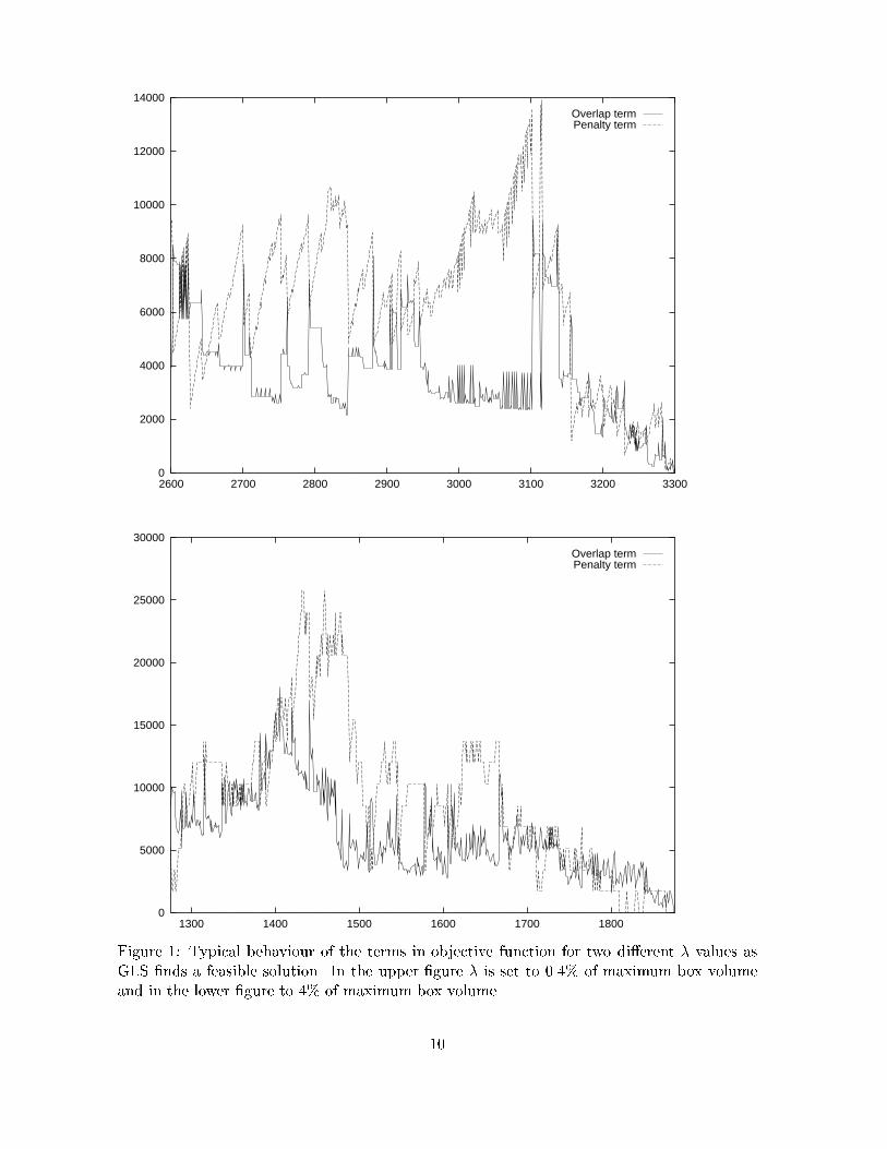
corresponding penalty parameter which initially is zero. The augmented objective functioncan now be de�ned as h(x) = f(x) + � � Xi;j2J i<j pij � Iij(x) (12)Feature costsThe purpose of the features is to introduce or strengthen constraints on the solution spaceon the basis of information collected during the search. The source of information thatdetermines which features are penalized in a local minimum x� is the feature cost and theamount of previous penalties assigned to the features in x�. To escape the local minimum wewant to penalize features in x� with maximum utility�ij(x�) = cij1 + pij � Iij(x�)Note that a feasible packing is equal to a solution with no exhibited features, so in the longrun all features must be eliminated. We have chosen to identify bad overlaps on the generalprinciple that an overlap between large boxes is worse than an overlap between small boxes.The feature cost cij on the one hand depends on the overlap between the boxes i and j andon the other hand on the volume of the boxes. The results presented later are based on thefollowing feature cost:cij(x) = ( overlapij(x) + volume(i) + volume(j) if overlapij(x) > 00 otherwise (13)where volume(i) denotes the volume of box i 2 J . Good results were also obtained with othercost functions, e.g. the product between overlap and volume which very aggressively avoidsoverlap between relatively large boxes. A cost function which only incorporated the overlapalso showed good results.The � parameterThe value of � determines to what degree an increased penalty will modify the augmentedobjective value and push the local search out of a local minimum. A large value will make thesearch more aggressive to avoid solutions with penalized features and provoke the search tomake large jumps in the solution space without paying much attention to the overlap term inthe augmented objective function. A small � on the other hand may require more penaltiesto escape a local minimum, but will result in a more cautious exploration of the solutionlandscape which is more sensitive to the gradient of f(x). However, a disadvantage with atoo small � value might be a too restricted exploration of the solution space.In Figure 1 two plots are shown that illustrate how the behaviour of the terms in theobjective function typically are a�ected by the choice of �. The plots show the overlap f(x)drawn with a solid line and the penalty term � �Pi;j2J i<j pij drawn with a dashed line asthe heuristic �nds a feasible packing for the problem.On the upper �gure a small �-value of 0.4% of the maximum box volume is used. Notethe plateaus of f(x) and how the penalty is increased until GLS escapes the local minimum.On the lower �gure a �-value of 4% is used. Most of the plateaus have disappeared and the9
0
2000
4000
6000
8000
10000
12000
14000
2600 2700 2800 2900 3000 3100 3200 3300
Overlap termPenalty term
0
5000
10000
15000
20000
25000
30000
1300 1400 1500 1600 1700 1800
Overlap termPenalty term
Figure 1: Typical behaviour of the terms in objective function for two di�erent � values asGLS �nds a feasible solution. In the upper �gure � is set to 0.4% of maximum box volumeand in the lower �gure to 4% of maximum box volume.10
overlap function shows a much larger variation, that is, GLS visits a more diverse part of thesolution space. Note however that the penalty term reaches much higher values than in theprevious �gure.With reference to the present formulation of 3D-BPP the � expresses the amount of volumethat is added to an overlap between the boxes that are associated with the penalized feature.Through empirical tests a value of a few percent of the maximum pairwise overlap showedgood results. During these experiments it also seemed as if � should be chosen dependenton the expected average volume of overlap between the boxes in a solution. As illustrated inFigure 1 a �-value of 0:4% of the maximum box volume lead to a too slow convergence since ittakes very long time before the penalty term grows large enough to escape a local minima. Onthe other hand a �-value of 4% implied a too scattered search, since the penalty term growsso quickly that a local minima is not investigated thoroughly. Thus in the computationalexperiments in Section 5 a �-value of 1% of the maximum box volume was used, since thisvalue lead to good results for most of the test instances.We also performed some experiments where the value of � was dynamically adapted tothe speci�c instance. This was done by looking at the number of plateaus (in the originalobjective function) during the local search and adjusting � so that they had an \appropriate"structure. However, we were not able to obtain better results by the self-adjusting frameworkthan those obtained by using a �xed �-value of 1% of the maximum box volume.Fast Local SearchAlready during the preliminary experiments it was clear that due to the very large neigh-bourhood adopted, conventional local search methods were to slow to converge to a localminimum. To speed up the local search an implementation of Fast Local Search (FLS) [20]has been used. Although FLS alone does not provide very good solutions it has proved to bea powerful tool when combined with GLS (see [19, 20, 21, 22, 23]).In FLS the neighbourhood is divided into a number of smaller sub-neighbourhoods thatcan be either active or inactive. Initially all sub-neighbourhoods are active. FLS now continu-ously visits the active sub-neighbourhoods in some order. If a sub-neighbourhood is examinedand does not contain any improving move it becomes inactive. Otherwise it remains activeand the improving move is performed; a reactivation of a number of other sub-neighbourhoodsmay be performed if we expect these to contain improving moves as a result of the move justperformed.The order in which the sub-neighbourhoods are visited may be either static or dynamic.As the solution value improves, more and more sub-neighbourhoods become inactive, andwhen all sub-neighbourhoods have become inactive the best solution found is returned byFLS as a local minimum.The key to decide how to split the neighbourhood into sub-neighbourhoods is to make anassociation between features and sub-neighbourhoods. The association should enable us toknow exactly which sub-neighbourhoods have a direct e�ect upon the state of a certain feature.This association is used each time GLS settles in a local minimum. As penalties are assignedto one or more features, the sub-neighbourhoods associated with the penalized features areactivated and FLS is restarted. Due to the limited reactivation each local optimization usingFLS will be aimed at removing the penalized features from the solution instead of exploringall possible moves.To apply FLS in the present 3D-BPP heuristic we let each box j 2 J correspond to a11
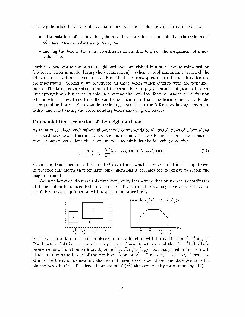
sub-neighbourhood. As a result each sub-neighbourhood holds moves that correspond to� all translations of the box along the coordinate axes in the same bin, i.e., the assignmentof a new value to either xj , yj or zj , or� moving the box to the same coordinates in another bin, i.e., the assignment of a newvalue to sj.During a local optimization sub-neighbourhoods are visited in a static round-robin fashion(no reactivation is made during the optimization). When a local minimum is reached thefollowing reactivation scheme is used. First the boxes corresponding to the penalized featureare reactivated. Secondly, we reactivate all those boxes which overlap with the penalizedboxes. The latter reactivation is added to permit FLS to pay attention not just to the twooverlapping boxes but to the whole area around the penalized feature. Another reactivationscheme which showed good results was to penalize more than one feature and activate thecorresponding boxes. For example, assigning penalties to the 5 features having maximumutility and reactivating the corresponding boxes showed good results.Polynomial-time evaluation of the neighbourhoodAs mentioned above each sub-neighbourhood corresponds to all translations of a box alongthe coordinate axes in the same bin, or the movement of the box to another bin. If we considertranslations of box i along the x-axis we wish to minimize the following objective:minxi=0;:::;W�wi Xj2J(overlapij(x) + � � pijIij(x)) (14)Evaluating this function will demand O(nW ) time, which is exponential in the input size.In practice this means that for large bin-dimensions it becomes too expensive to search theneighbourhood.We may, however, decrease this time complexity by showing that only certain coordinatesof the neighbourhood need to be investigated. Translating box i along the x-axis will lead tothe following overlap function with respect to another box j:i j-xi x1j x2j x3j x4j -
6overlapij(x) + � � pijIij(x)xipppppppp ppppppppx1j x2j x3j x4j��� @@@As seen, the overlap function is a piecewise linear function with breakpoints in x1j ; x2j ; x3j ; x4j .The function (14) is the sum of such piecewise linear functions, and thus it will also be apiecewise linear function with breakpoints fx1j ; x2j ; x3j ; x4jgj2J . Obviously such a function willattain its minimum in one of the breakpoints or for xi = 0 resp. xi = W � wi. There areat most 4n breakpoints meaning that we only need to consider these candidate positions forplacing box i in (14). This leads to an overall O(n2) time complexity for minimizing (14).12
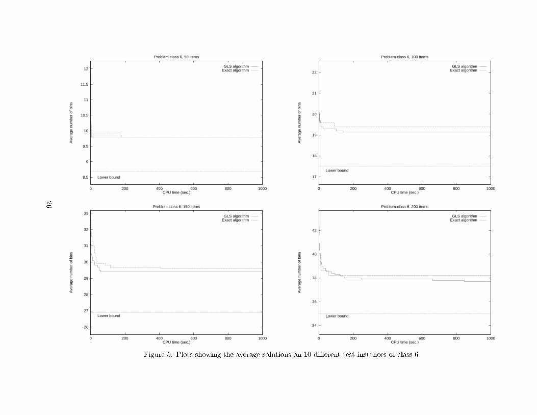
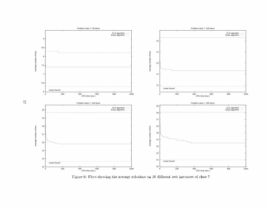
5 Computational experimentsIn this section we will present the results from the computational experiments. The presentedalgorithm was coded in C++ and compiled using the gnu C++ compiler. Experiments wereperformed on problem instances in both two and three dimensions. For the instances in threedimensions the algorithm was compared with the exact algorithm for 3D-BPP by Martello,Pisinger and Vigo [16] and for the two-dimensional case with the tabu search heuristic for2D-BPP by Lodi, Martello and Vigo [14, 15].To construct the initial upper bound the GLS algorithm uses the following simple heuris-tic: The boxes are sorted according to non-increasing depths, and a subset of boxes with totalvolume larger than the bin volume are selected. The selected boxes are packed in two dimen-sions using the shelf-approach [7, 5]. This process is repeated until a number of \bin-slices"have been generated. These \bin-slices" are then combined to whole bins by using a �rst-�tdecreasing algorithm on the depths of the \bin-slices". The heuristic runs in O(n2) time.In the following section we will �rst present the results obtained on the three-dimensionalproblem, and then the results for the two-dimensional problem.5.1 3D instancesIn order to evaluate the GLS algorithm we compared it with the exact algorithm (MPV)for 3D-BPP by Martello, Pisinger and Vigo [16]. The following instances from [16] wereconsidered for problems with 50 to 200 boxes:� Class 1: The majority of the boxes are very high and deep.� Class 4: The majority of the boxes have large dimensions.� Class 5: The majority of the boxes have small dimensions.� Class 6: Berkey-Wang [5] instances with dimensions randomly generated in a smallinterval.� Class 7: Berkey-Wang instances with dimensions randomly generated in a mediuminterval.� Class 8: Berkey-Wang instances with dimensions randomly generated in a large inter-val.For each class (i.e. 1, 4, 5, 6, 7 and 8) and number of boxes (i.e. 50, 100, 150 and 200) therewere generated 10 di�erent problem instances based on di�erent random seeds. We did notconsider classes 2 and 3 from [16], since these have similar properties as class 1. Also class 9was not considered, since these problems merely have the character of puzzles than of packingproblems. Both algorithms were run on a Digital 500au workstation with a 500 MHz 21164CPU (SPECint95 value of 15.7) with a time limit of 1000 seconds for each instance.While GLS uses a simple O(n2) heuristic to construct the �rst initial solution, the exactalgorithm uses two advanced heuristics [16]. The �rst is based on \bin-slices" which arecombined to whole bins by using an exact one-dimensional bin-packing algorithm, and thesecond based on a branch-and-bound algorithm with limited width of the search tree.Table 1 compares the average solutions from the GLS algorithm and the MPV algorithmover 10 di�erent problem instances for each class and box count. The �rst three columns13

Table 1: Results for the three-dimensional instances. Time limit is 1000 seconds. The so-lutions are compared with results obtained with the exact algorithm (MPV) for 3D-BPPby Martello, Pisinger and Vigo [16]. Columns indicate GLS solutions after 60 (z60sec), 150(z150sec) and 1000 (z1000sec) seconds, zMPV shows the best solution of the MPV algorithm,and L2 the corresponding lower bound. Column optGLS indicates the number of instancessolved to known optimality and \z1000sec � zMPV " the instances where GLS obtained equal orbetter solutions than the exact algorithm. GLS solutions are in italics when they are greaterthan zMPV .Class Bins n GLS MPV L2 optGLS z1000sec � zMPVz60sec z150sec z1000sec zMPV1 100 � 100 50 13.4 13.4 13.4 13.6 12.5 3 �100 26.9 26.7 26.7 27.3 25.1 0 �150 37.5 37.2 37.0 38.2 34.7 0 �200 52.8 52.1 51.2 52.3 48.4 0 �4 100 � 100 50 29.4 29.4 29.4 29.4 28.7 4 �100 59.0 59.0 59.0 59.1 57.6 1 �150 87.1 86.9 86.8 87.2 85.2 1 �200 119.9 119.7 119.0 119.5 116.3 1 �5 100 � 100 50 8.3 8.3 8.3 9.2 7.3 2 �100 15.1 15.1 15.1 17.5 12.9 0 �150 20.7 20.3 20.2 24.0 17.4 0 �200 27.8 27.5 27.2 31.8 24.4 0 �6 10 � 10 50 9.8 9.8 9.8 9.8 8.7 1 �100 19.3 19.1 19.1 19.4 17.5 0 �150 29.5 29.4 29.4 29.6 26.9 0 �200 38.5 38.0 37.7 38.2 35.0 0 �7 40 � 40 50 7.4 7.4 7.4 8.2 6.3 0 �100 12.5 12.3 12.3 15.3 10.9 1 �150 16.1 15.8 15.8 19.7 13.7 0 �200 24.4 24.1 23.5 28.1 21.0 0 �8 100 � 100 50 9.2 9.2 9.2 10.1 8.0 0 �100 18.9 18.9 18.9 20.2 17.5 1 �150 24.5 24.1 23.9 27.3 21.3 1 �200 30.6 30.1 29.9 34.9 26.7 0 �Total 738.6 733.8 730.2 769.9 684.0 16 24Average 30.78 30.58 30.43 32.08 28.50 0.6714

show the current GLS solution values after 60, 150 and 1000 seconds, respectively. The nextcolumn gives the solution value found by the MPV algorithm after 1000 seconds. The columnL2 is the common lower bound used by both the GLS heuristic and the MPV algorithm. Thecolumn optGLS gives the number of times the algorithm �nds a solution equivalent to thelower bound. The last column indicates when the GLS algorithm �nds an equal or bettersolution value compared to the MPV algorithm (within 1000 seconds).The GLS algorithm �nds similar or better solutions in all the cases, and even after 60seconds the solutions are on average considerably better than those obtained by the MPValgorithm. Note especially the class 4 instances where the MPV algorithm performs very wellsince it does not use much time on the exact �lling of a single bin | as only one or twoboxes �t into each bin. Anyhow, the GLS algorithm is capable of �nding equal or even bettersolutions for these instances.On average, the GLS algorithm used 30:43 bins while the MPV algorithm used 32:08 bins.Since the lower bound is 28:50 the relative gap is 6:8% and 12:6%, respectively, meaning thatthe GLS algorithm decreased the gap to the lower bound to about half its value.In the appendix �gures that plot the development of the GLS algorithm and the exactalgorithm as a function of the solution time are shown.5.2 2D instancesThe presented GLS algorithm is also used to solve 2D bin-packing problems by setting thedepth of all boxes and bins to a constant value of one. For the two-dimensional instanceswe compare the GLS algorithms with the tabu search (TS) algorithm by Lodi, Martello andVigo [14, 15]. This algorithm is based on construction algorithms for packing a single bin,where the tabu search algorithm is used to control the movement of pieces between the bins.It should be emphasized that the GLS algorithm does not take advantage of the fact that theinstances are two-dimensional, and thus obviously is somewhat slower than the TS algorithm.The GLS algorithm was run on a Digital 500au workstation with a 500 MHz 21164 CPU(SPECint95 value of 15.7), while the results for the tabu search algorithm were taken directlyfrom [14] and [15] (these experiments were run on a Silicon Graphics INDY R4000sc with a100 MHz CPU and Silicon Graphics INDY 10000sc with a 195 MHZ CPU, respectively). TheGLS algorithms was assigned a time limit of 100 seconds for each instance, approximatelymatching the computing e�ort of the tabu search algorithms.In the following tables we report the GLS solution values after 5, 30 and 100 seconds inthe columns z5sec, z30sec and z100sec, and the solution value found by TS is shown in columnzTS ; the TS solution is taken from [14], since no results were reported for these instancesin [15]. The column L2 is the lower bound used by GLS while LLMV shows the lower boundreported in [14].In Table 2 results on problem instances from the literature are reported. The consideredinstances are cgcut1-cgcut3 [6] and gcut1-gcut13/ngcut1-ngcut12 [2, 3] (all these in-stances are obtained from the OR-Library, see http://www.ms.ic.ac.uk/info.html). Theseinstances are two-dimensional cutting problems which were transformed to 2D-BPP in thefollowing way: First the value of the pieces is ignored and secondly for the cgcut and ngcutinstances the maximum number of pieces is generated for each type.The GLS algorithm always �nds a solution which is at least as good as the TS solution. Onaverage, GLS used 5:82 bins while TS used 6:11 bins. With a lower bound of 5:50 the relativegap has been decreased from 11:1% to 5:8%. It should be emphasized that since we use a very15
Table 2: Results for two-dimensional instances from the literature. Time limit is 100 CPUseconds. The columns z5sec, z30sec and z100sec indicate the solutions obtained by GLS after 5,30 and 100 seconds. The solutions are compared with results (zTS) obtained with the tabusearch algorithm by Lodi, Martello and Vigo [14]. In the following columns L2 is the lowerbound, and LLMV the lower bound from [14]. The column \z100sec � zTS" indicates theinstances where GLS obtained equal or better solutions than TS, \z100sec < ub" the instanceswhere GLS was able to improve the initial upper bound and optGLS the instances solved toknown optimality. GLS solutions written in italics indicate the GLS solutions that are greaterthan zTS .Instance GLS TS L2 LLMV z100sec � zTS z100sec < ub optGLSz5sec z30sec z100sec zTScgcut1 2 2 2 2 � �cgcut2 2 2 2 2 � �cgcut3 23 23 23 23 � �gcut1 5 5 5 5 4 4 � �gcut2 6 6 6 6 5 6 � � �gcut3 8 8 8 8 8 � � �gcut4 14 14 14 14 13 13 � �gcut5 3 4 3 3 � � �gcut6 7 7 7 7 6 6 � �gcut7 11 11 11 12 10 10 � �gcut8 14 13 13 14 12 12 �gcut9 3 3 3 3 � � �gcut10 7 7 7 8 6 7 � �gcut11 9 9 9 9 8 8 � � �gcut12 16 16 16 16 � �gcut13 2 2 2 2 � � �ngcut1 3 3 3 3 2 2 � �ngcut2 4 4 4 4 3 3 � �ngcut3 3 4 3 3 � �ngcut4 2 2 2 2 � �ngcut5 3 3 3 3 � � �ngcut6 3 3 3 3 2 2 � � �ngcut7 1 1 1 1 � � �ngcut8 2 2 2 2 � � �ngcut9 3 4 3 3 � � �ngcut10 3 3 3 3 � �ngcut11 2 3 2 2 � � �ngcut12 3 4 3 3 � � �Total 164 163 163 171 152 154 28 14 26Average 5.86 5.82 5.82 6.11 5.43 5.5016
Table 3: Problem classes proposed by Berkey-Wang [5]Class Items Bins1 [1; 10] � [1; 10] 10� 102 [1; 10] � [1; 10] 30� 303 [1; 35] � [1; 35] 40� 404 [1; 35] � [1; 35] 100� 1005 [1; 100] � [1; 100] 100� 1006 [1; 100] � [1; 100] 300� 300simple heuristic for the initial solution, it is in most cases the GLS algorithm which actually�nds the improved solutions. Moreover the GLS algorithm �nds the returned solutions alreadyafter 30 seconds, which is comparable to the solution times of the TS algorithm. Only twoinstances are not solved to known optimality.Table 4 compares the GLS and TS heuristics for the Berkey-Wang instances [5] (withTS results taken from [15]). The classes are described in Table 3 and were considered forproblems with 20, 40, 60, 80 and 100 items with 10 di�erent instances for each class itemnumber (we used the same generated problem instances as in [14]; these instances can beobtained from http://www.or.deis.unibo.it/ORinstances/).In all the instances the GLS algorithm �nds an equally good or better solutions than theTS algorithm. Actually, after 5 seconds, it �nds better solutions on average than the TSalgorithm. After 100 seconds, the GLS algorithm �nds the optimal solution for more than60% of the instances. Looking at the average values, the GLS algorithm �nds solutions using9:90 bins, while the TS algorithm �nds solutions using 10:11 bins. The average lower boundis 9:48 bins, and thus the relative deviation is 4:4% and 6:6%, respectively.Table 5 considers the problem instances proposed by Martello and Vigo [18]. All binshave dimensions 100 � 100 while the items have the following properties:� Class 7: The majority of the items are wide.� Class 8: The majority of the items are high.� Class 9: The majority of the items are large in both dimensions.� Class 10: The majority of the items are small in both dimensions.The GLS algorithm �nds equivalent or better solutions than the TS algorithm (from [15])for almost all of the problems. The GLS algorithm �nds the optimal solution for more than50% of these instances. The average solution values are 21:58 for GLS, and 21:65 for TS. Theaverage lower bound is 21:10, and thus the relative deviation is 2:3% and 2:6%, respectively.6 ConclusionOur experiments have shown that Guided Local Search can be applied to bin packing problemsin two- and three-dimensions with success. Since the concept of GLS is still relatively new,it is important to determine the classes of problems for which it is suitable.17
Table 4: Results for the two-dimensional Berkey-Wang instances [5]. Column optGLS indi-cates the number of instances solved to known optimality. The solutions are compared withresults (zTS) obtained with the tabu search algorithm by Lodi, Martello and Vigo [15]. Fora description of the other columns we refer to Table 2.Class Bins n GLS TS L2 LLMV optGLS z100sec � zTSz5sec z30sec z100sec zTS1 10 � 10 20 7.1 7.1 7.1 7.1 6.6 6.7 6 �40 13.4 13.4 13.4 13.6 12.8 12.8 5 �60 20.2 20.1 20.1 20.1 19.0 19.3 2 �80 27.7 27.5 27.5 28.2 26.2 26.9 5 �100 32.4 32.1 32.1 32.7 30.8 31.4 3 �2 30 � 30 20 1.0 1.0 1.0 1.0 1.0 1.0 10 �40 1.9 1.9 1.9 2.1 1.9 1.9 10 �60 2.5 2.5 2.5 2.8 2.5 2.5 10 �80 3.2 3.2 3.1 3.3 3.1 3.1 10 �100 4.0 3.9 3.9 4.0 3.9 3.9 10 �3 40 � 40 20 5.1 5.1 5.1 5.5 4.6 4.6 5 �40 9.6 9.5 9.4 9.8 8.9 8.8 5 �60 14.0 14.0 14.0 14.0 13.2 13.3 3 �80 19.6 19.3 19.1 19.9 17.9 18.4 6 �100 23.1 22.9 22.6 23.7 21.4 21.7 1 �4 100 � 100 20 1.0 1.0 1.0 1.0 1.0 1.0 10 �40 1.9 1.9 1.9 1.9 1.9 1.9 10 �60 2.5 2.5 2.5 2.6 2.3 2.3 8 �80 3.3 3.3 3.3 3.3 3.0 3.0 7 �100 3.9 3.9 3.8 3.8 3.7 3.7 9 �5 100 � 100 20 6.5 6.5 6.5 6.7 6.0 6.0 5 �40 11.9 11.9 11.9 11.9 11.3 11.4 6 �60 18.2 18.1 18.1 18.2 17.0 17.2 2 �80 25.0 25.0 24.9 25.0 23.4 23.6 1 �100 29.3 28.8 28.8 29.5 27.2 27.3 1 �6 300 � 300 20 1.0 1.0 1.0 1.0 1.0 1.0 10 �40 1.9 1.8 1.8 2.1 1.5 1.5 7 �60 2.2 2.2 2.2 2.2 2.1 2.1 9 �80 3.0 3.0 3.0 3.0 3.0 3.0 10 �100 3.5 3.4 3.4 3.4 3.2 3.2 8 �Total 299.9 297.8 296.9 303.4 281.4 284.5 194 30Average 10.00 9.93 9.90 10.11 9.38 9.48 6.4718

Table 5: Results for the two-dimensional Martello-Vigo instances [18]. Column optGLS indi-cates the number of instances solved to known optimality. The solutions are compared withresults (zTS) obtained with the tabu search algorithm by Lodi, Martello and Vigo [15]. Fora description of the other columns we refer to Table 2.Class Bins n GLS TS L2 LLMV optGLS z100sec � zTSz5sec z30sec z100sec zTS7 100 � 100 20 5.5 5.5 5.5 5.5 5.2 5.3 8 �40 11.3 11.3 11.3 11.4 10.4 10.8 5 �60 16.1 16.1 15.9 16.3 14.9 15.5 6 �80 23.5 23.3 23.2 23.2 21.7 22.3 1 �100 27.8 27.6 27.5 27.6 25.7 26.8 3 �8 100 � 100 20 5.8 5.8 5.8 5.8 5.3 5.5 7 �40 11.5 11.4 11.4 11.4 10.4 11.1 7 �60 16.5 16.3 16.3 16.2 15.3 15.9 680 22.8 22.8 22.5 22.6 21.4 22.2 7 �100 28.3 28.2 28.1 28.4 26.5 27.3 2 �9 100 � 100 20 14.3 14.3 14.3 14.3 14.3 14.3 10 �40 27.8 27.8 27.8 27.7 27.5 27.4 760 43.7 43.7 43.7 43.7 43.5 43.3 8 �80 57.7 57.7 57.7 57.5 57.3 56.9 6100 69.5 69.5 69.5 69.6 69.2 68.9 7 �10 100 � 100 20 4.2 4.2 4.2 4.4 3.9 4.0 8 �40 7.4 7.4 7.4 7.5 7.0 7.1 7 �60 10.3 10.2 10.2 10.4 9.5 9.7 5 �80 13.2 13.0 13.0 13.0 12.2 12.3 3 �100 16.3 16.3 16.2 16.5 15.3 15.3 1 �Total 433.5 432.4 431.5 433.0 416.5 421.9 114 17Average 21.68 21.62 21.58 21.65 20.83 21.10 5.70
19
However, a more important achievement is that the presented algorithm applies localsearch directly on the packing problems. Most other successful local search heuristics forcutting and packing somehow make use of a construction algorithm inside the search. Thusthe local search is restricted to a higher level of the search, like assigning items to bins, ordetermining an appropriate packing order. But the construction algorithm may become abottleneck for the search, since one will never �nd better solutions than the constructionalgorithm is able to produce. Another bene�t of working directly on the packing problem is,that we are able to handle items and bins of a general form as long as the overlap betweenitems can be determined e�ciently.Dowsland [10] used a similar objective function without signi�cant success. Using simu-lated annealing the investigated neighbourhood became too large, and thus the convergencetowards good solutions was slow. It is thus interesting how GLS and FLS are able to focusthe search on interesting parts of the solution space.AcknowledgementThe authors wish to thank Kenneth J�onsson for having taken part in the development of the�rst version of this algorithm.References[1] E. H. L. Aarts and J. K. Lenstra, editors. Local Search in Combinatorial Optimization. JohnWiley & Sons, 1997.[2] J.E. Beasley. Algorithms for unconstrained two-dimensional guillotine cutting. Journal of theOperational Research Society, 36:297{306, 1985.[3] J.E. Beasley. An exact two-dimensional non-guillotine cutting tree search procedure. OperationsResearch, 33:49{64, 1985.[4] B.E. Bengtsson. Packing rectangular pieces { a heuristic approach. The Computer Journal,25:353{357, 1982.[5] J.O. Berkey and P.Y. Wang. Two dimensional �nite bin packing algorithms. Journal of theOperational Research Society, 38:423{429, 1987.[6] N. Christo�des and C. Whitlock. An algorithm for two-dimensional cutting problems. OperationsResearch, 25:30{44, 1977.[7] F.K.R. Chung, M.R. Garey, and D.S. Johnson. On packing two-dimensional bins. SIAM Journalof Algebraic and Discrete Methods, 3(1):66{76, 1982.[8] A.L Corcoran III and R.L. Wainwright. A genetic algorithm for packing in three dimensions.In Proceedings of the 1992 ACM/SIGAPP Symposium on Applied Computing, pages 1021{1030,1992.[9] M. Dell'Amico and S.Martello. Optimal scheduling of tasks on identical parallel processors. ORSAJournal on Computing, 7(2):191{200, 1995.[10] K. Dowsland. Some experiments with simulated annealing techniques for packing problems.European Journal of Operational Research, 68:389{399, 1993.[11] H. Dyckho�. A typology of cutting and packing problems. European Journal of OperationalResearch, 44:145{159, 1990. 20

[12] H. Dyckho�, G. Scheithauer, and J. Terno. Cutting and Packing (C&P). In M. Dell'Amico,F. Ma�oli, and S. Martello, editors, Annotated Bibliographies in Combinatorial Optimization.John Wiley & Sons, Chichester, 1997.[13] B. Kr�oger. Guillotinable bin packing: A genetic approach. European Journal of OperationalResearch, 84:645{661, 1995.[14] A. Lodi, S. Martello, and D. Vigo. Approximation algorithms for the oriented two-dimensionalbin packing problem. European Journal of Operational Research, 112:158{166, 1999.[15] A. Lodi, S. Martello, and D. Vigo. Heuristic and metaheuristic approaches for a class of two-dimensional bin packing problems. INFORMS Journal on Computing, to appear.[16] S. Martello, D. Pisinger, and D. Vigo. The three-dimensional bin packing problem. OperationsResearch, march{april, 2000.[17] S. Martello and P. Toth. Lower bounds and reduction procedures for the bin packing problem.Discrete Applied Mathematics, 28:59{70, 1990.[18] S. Martello and D. Vigo. Exact solution of the two-dimensional �nite bin packing problem.Management Science, 44:388{399, 1998.[19] C. Voudouris and E. Tsang. Function optimization using guided local search. Technical ReportCSM-249, Dept. of Computer Science, University of Essex, England, 1995.[20] C. Voudouris and E. Tsang. Guided local search. Technical Report CSM-247, Dept. of ComputerScience, University of Essex, England, 1995.[21] C. Voudouris and E. Tsang. Partial constraint satisfaction problems and guided local search. InProceedings of Practical Application of Constraint Technology (PACT'96), pages 337{356, 1996.[22] C. Voudouris and E. Tsang. Fast local search and guided local search and their application tobritish telecom's workforce scheduling problem. Operations Research Letters, 20(3):119{127, 1997.[23] C. Voudouris and E. Tsang. Guided local search and its application to the traveling salesmanproblem. European Journal of Operational Research, 113:469{499, 1999.
21

AppendixOn the following pages �gures are shown for each problem class in three dimensions. The�gures show plots of the development of the GLS algorithm and the exact algorithm as afunction of the solution time.
22
12
12.5
13
13.5
14
14.5
15
15.5
0 200 400 600 800 1000
Ave
rage
num
ber
of b
ins
CPU time (sec.)
Problem class 1, 50 items
Lower bound
GLS algorithmExact algorithm
24
25
26
27
28
29
30
0 200 400 600 800 1000
Ave
rage
num
ber
of b
ins
CPU time (sec.)
Problem class 1, 100 items
Lower bound
GLS algorithmExact algorithm
33
34
35
36
37
38
39
40
41
0 200 400 600 800 1000
Ave
rage
num
ber
of b
ins
CPU time (sec.)
Problem class 1, 150 items
Lower bound
GLS algorithmExact algorithm
46
48
50
52
54
56
0 200 400 600 800 1000
Ave
rage
num
ber
of b
ins
CPU time (sec.)
Problem class 1, 200 items
Lower bound
GLS algorithmExact algorithm
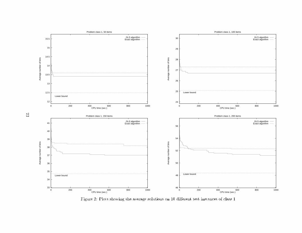
Figure 2: Plots showing the average solutions on 10 di�erent test instances of class 1.
23
27.5
28
28.5
29
29.5
30
30.5
31
0 200 400 600 800 1000
Ave
rage
num
ber
of b
ins
CPU time (sec.)
Problem class 4, 50 items
Lower bound
GLS algorithmExact algorithm
55
56
57
58
59
60
61
0 200 400 600 800 1000
Ave
rage
num
ber
of b
ins
CPU time (sec.)
Problem class 4, 100 items
Lower bound
GLS algorithmExact algorithm
81
82
83
84
85
86
87
88
89
90
0 200 400 600 800 1000
Ave
rage
num
ber
of b
ins
CPU time (sec.)
Problem class 4, 150 items
Lower bound
GLS algorithmExact algorithm
112
114
116
118
120
122
0 200 400 600 800 1000
Ave
rage
num
ber
of b
ins
CPU time (sec.)
Problem class 4, 200 items
Lower bound
GLS algorithmExact algorithm
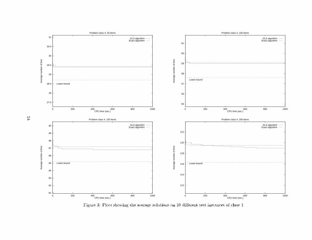
Figure 3: Plots showing the average solutions on 10 di�erent test instances of class 4.
24
7
7.5
8
8.5
9
9.5
10
10.5
0 200 400 600 800 1000
Ave
rage
num
ber
of b
ins
CPU time (sec.)
Problem class 5, 50 items
Lower bound
GLS algorithmExact algorithm
13
14
15
16
17
18
0 200 400 600 800 1000
Ave
rage
num
ber
of b
ins
CPU time (sec.)
Problem class 5, 100 items
Lower bound
GLS algorithmExact algorithm
17
18
19
20
21
22
23
24
0 200 400 600 800 1000
Ave
rage
num
ber
of b
ins
CPU time (sec.)
Problem class 5, 150 items
Lower bound
GLS algorithmExact algorithm
24
25
26
27
28
29
30
31
32
0 200 400 600 800 1000
Ave
rage
num
ber
of b
ins
CPU time (sec.)
Problem class 5, 200 items
Lower bound
GLS algorithmExact algorithm
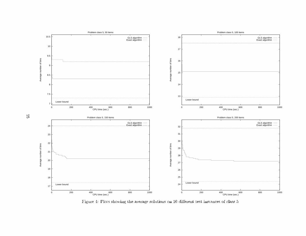
Figure 4: Plots showing the average solutions on 10 di�erent test instances of class 5.
25
8.5
9
9.5
10
10.5
11
11.5
12
0 200 400 600 800 1000
Ave
rage
num
ber
of b
ins
CPU time (sec.)
Problem class 6, 50 items
Lower bound
GLS algorithmExact algorithm
17
18
19
20
21
22
0 200 400 600 800 1000
Ave
rage
num
ber
of b
ins
CPU time (sec.)
Problem class 6, 100 items
Lower bound
GLS algorithmExact algorithm
26
27
28
29
30
31
32
33
0 200 400 600 800 1000
Ave
rage
num
ber
of b
ins
CPU time (sec.)
Problem class 6, 150 items
Lower bound
GLS algorithmExact algorithm
34
36
38
40
42
0 200 400 600 800 1000
Ave
rage
num
ber
of b
ins
CPU time (sec.)
Problem class 6, 200 items
Lower bound
GLS algorithmExact algorithm
Figure 5: Plots showing the average solutions on 10 di�erent test instances of class 6.
26
6
6.5
7
7.5
8
8.5
9
0 200 400 600 800 1000
Ave
rage
num
ber
of b
ins
CPU time (sec.)
Problem class 7, 50 items
Lower bound
GLS algorithmExact algorithm
11
12
13
14
15
0 200 400 600 800 1000
Ave
rage
num
ber
of b
ins
CPU time (sec.)
Problem class 7, 100 items
Lower bound
GLS algorithmExact algorithm
13
14
15
16
17
18
19
20
0 200 400 600 800 1000
Ave
rage
num
ber
of b
ins
CPU time (sec.)
Problem class 7, 150 items
Lower bound
GLS algorithmExact algorithm
20
21
22
23
24
25
26
27
28
29
0 200 400 600 800 1000
Ave
rage
num
ber
of b
ins
CPU time (sec.)
Problem class 7, 200 items
Lower bound
GLS algorithmExact algorithm
Figure 6: Plots showing the average solutions on 10 di�erent test instances of class 7.
27

8
8.5
9
9.5
10
10.5
11
11.5
0 200 400 600 800 1000
Ave
rage
num
ber
of b
ins
CPU time (sec.)
Problem class 8, 50 items
Lower bound
GLS algorithmExact algorithm
17
18
19
20
21
22
0 200 400 600 800 1000
Ave
rage
num
ber
of b
ins
CPU time (sec.)
Problem class 8, 100 items
Lower bound
GLS algorithmExact algorithm
21
22
23
24
25
26
27
28
29
0 200 400 600 800 1000
Ave
rage
num
ber
of b
ins
CPU time (sec.)
Problem class 8, 150 items
Lower bound
GLS algorithmExact algorithm
26
28
30
32
34
36
0 200 400 600 800 1000
Ave
rage
num
ber
of b
ins
CPU time (sec.)
Problem class 8, 200 items
Lower bound
GLS algorithmExact algorithm
Figure 7: Plots showing the average solutions on 10 di�erent test instances of class 8.
28