The Network Packing Problem in TerrestrialBroadcasting

C. Mannino ¤ F. Rossi, S. Smriglio y

AbstractThe introduction of digital terrestrial broadcasting all over Europe requires a com-plete and challenging re-planning of in-place analog systems. But an abrupt mi-gration of resources (transmitters and frequencies) from analog to digital networkscannot be accomplished, since the analog services must be preserved temporar-ily. Hence, a multi-network, multi-objective, problem arises, referred to as theNetwork Packing Problem, in which several networks, both analog and digital,sharing a common set of resources, have to be designed. In Italy this problem isparticularly challenging, because of a large number of transmitters, orographicalfeatures and strict requirements imposed by Italian law. In this paper we reportour experience developing solution methods at the major Italian broadcaster Ra-diotelevisione Italiana (RAI S.p.A.). We propose a two-stage heuristic. In the¯rst stage emission powers are assigned to each network separately. In the secondstage frequencies are assigned to all networks so as to minimize the loss from mu-tual interference. A software tool incorporating our methodology is currently inuse at RAI to help discover and select high-quality alternatives for the deploymentof digital equipment.

Subject classi¯cations: Communications: Frequency and Power Assignment. Program-ming, integer, heuristic: neighbourhood search.

¤Dipartimento di Informatica e Sistemistica, Universitµa di Roma \La Sapienza", e-mail:mannino@dis.uniroma1.ityDipartimento di Informatica, Universitµa di L'Aquila, e-mail: rossi[smriglio]@di.univaq.it

1

1 IntroductionIn the context of terrestrial video broadcasting, digital technology most likely will re-place analog technology. This transition has been recently claimed (Paris, September2003) by the French and German premiers as one of the main challenges of the Eu-ropean Union development programs [4]. The Terrestrial Digital Video Broadcastingstandard (DVB-T) has been introduced by European Telecommunication Standard In-stitute (ETSI) in 1997. Details on the development of DVB-T can be found in theweb sites of the major public bodies involved, namely, ETSI [12] and the InternationalTelecommunication Union (ITU) [18], as well as in the industry-led consortium DigitalVideo Broadcasting [9]. DVB-T has several advantages. First, it utilizes the availablebandwidth more e±ciently than analog systems: in fact, it allows to broadcast a multi-plex of programs (from two to ¯ve, depending on the required quality of service) over a 8Mhz width portion of the frequency spectrum (referred to as channel) instead of a singleanalog program. Second, DVB-T embeds a Multimedia Home Platform representing a¯rst step towards the integration of video broadcasting with both Internet and GlobalSystem for Mobile Communications (GSM) [21], making additional (interactive) ser-vices, such as e-commerce and home-banking, accessible through television [3]. Finally,receiving DVB-T programs only requires the installation of a decoder with actual roofantenna, a modest overload for users. DVB-T implementation is under investigation inseveral European countries, such as Great Britain, Spain, Germany, Norway, Finlandand Denmark [3]: the current status for each country can be found in [11]. Worldwidelaunch dates for DVB-T and analog switch-o® dates are reported in [9].In this paper we address new planning issues arising in the Italian broadcasting sys-

tem because of the analog to digital transition. Due to the large number of broadcastersand to the scarce penetration of cable and satellite networks, the Italian context appearsto be one of the most complex in Europe (details are reported in [17]). For instance,23,506 transmitters operate versus 12,455 in France and 10,099 in Germany (EuropeanRadiocommunications O±ce, May 2002 [11]). A recent study on the introduction ofdigital broadcasting has been carried out by the Italian Communications Authority(AGCOM). The results, reported in the White Book [3], provide the ground for theDigital National Plan for Frequency Assignment (D-PNAF) [3], devised by AGCOMin the year 2003. The purpose of D-PNAF is to rationalize the resource utilization so

2

as to guarantee the open competition in the video market. In particular, D-PNAF de-¯nes a target con¯guration for the future Italian broadcasting system, consisting of 18equivalent reference networks. Each network utilizes three channels and 300 transmit-ters (geographical sites) in order to broadcast a multiplex of ¯ve programs to at least90% of the Italian population. The implementation of D-PNAF looks quite complexand will take place through several steps. At the time of this study, the Italian law66/2001 ¯xed two important milestones: (i) D-PNAF has to be implemented withinthe end of year 2006, when all analog networks will be switched-o®; (ii) the public Ital-ian broadcaster Radiotelevisione Italiana (RAI), has to activate two digital networksreaching at least 50% of the population by January, 1, 2004, keeping safe the actualcoverage of analog networks. RAI, a state-owned Company with an executive boarddesignated by the Parliament, is also the major Italian broadcaster. The present studywas promoted by RAI Way S.p.A, the RAI network provider, to understand whetherrequirement (ii) could be accomplished with the available (and currently used entirelyby analog networks) resources.Even when not required by law, other broadcasters also must face the same problem.

In fact, the available system capacity (which depends on available transmitters andchannels) is not su±cient to grow one or more digital networks without reducing thecoverage of analog networks. On the other hand, the resources from analog networkscannot be released sharply since the actual service must be provided until the newnetworks guarantee a su±cient coverage. Under this respect, the high level reachedby analog networks (i.e., around 95% of population) represents a severe barrier forthe set-up of digital networks which appear, at the beginning, not competitive from acommercial point of view. Managing this transition is actually the key challenge formajor broadcasters.In conclusion, either the implementation of D-PNAF or, simply, the introduction

of new digital networks requires an expensive re-planning activity in which a set ofresources is shared among di®erent (analog or digital) networks. Since each networkhas its own technical features and commercial goals, the problem consists in allocatingresources to networks so as to optimize a multi-objective performance indicator (e.g.,the population coverage for each network). We designate this problem as NetworkPacking Problem (NPack, x3). In Section 5 we illustrate a two-phase heuristic for thesolution of NPack. This is based on two major ingredients: (i) an algorithm for the

3

optimal assignment of power and frequency to transmitters of a single network (SingleNetwork Planning problem, NPlan, x4) and (ii) an algorithm for the solution of avariant of the classical Frequency Assignment Problem (FAP, x5.2).This paper introduces three major novelties in the models addressed so far by the

OR community involved in frequency assignment. First, the coverage assessment isbased on the de¯nition of testpoints and is carried out by a statistical procedure rec-ommended for implementation purposes [3, 8]. Second, unlike problems investigatedin the literature, NPlan includes both emission powers and frequencies as decisionvariables and simultaneously optimizes over these variables. Third, several networksare optimized on a common set of resources.The resulting software tool has been tested together with RAI Way engineers and

is designed to cope with their assessed planning procedures. In particular, the tool notonly returns good solutions for very large scale instances, but also allows engineers toevaluate several high-quality alternatives.Computational results from several key experiments proposed by RAI Way engi-

neers are reported in x7 and their in°uence on strategic decisions is discussed. RAIinvestments in DVB-T implementation concern technological infrastructures and pur-chase of frequencies. As for the former, RAI management approved a 79 million Eurobudget in August 2003 (from the major Italian ¯nancial newspaper: Il Sole 24 Ore,August, 7, 2003).

2 System elementsA broadcasting system consists of a set R = f1; : : : ; jRjg of (either analog or digital)networks. Network k distributes its own program from a set T k of transmitters. T =SjRjr=1 T r denotes the whole transmitter set, where T k \ T h = ;, for all networks h6= k.Each transmitter is located in a geographical site (typically a site accommodates sev-

eral transmitters of di®erent networks) and its con¯guration depends on: transmissionfrequency, emission power, antenna height, polarization (horizontal/vertical), antennadiagram (directivity) and time o®set. In this paper we deal with deciding frequenciesand emission powers of transmitters, while all other quantities are ¯xed and will bereferred to as transmitter parameters (see x7).The frequency spectrum is subdivided into a set F = f1; : : : ; jFjg of equally sized

4

intervals called channels (or frequencies). The set of feasible frequencies for transmitteri 2 T is denoted by Fi µ F . It may happen that Fi ½ F because of technical orcommercial constraints (international agreements at boundaries, licensing, etc.).The transmission frequency assigned to transmitter i 2 T is denoted by fi, whilst

Pi denotes its emission power, ranging in the interval [0; PUi ]. For convenience, wealso introduce the power fading pi 2 [0; 1], that measures power attenuation w.r.t. themaximum power PUi (i.e., Pi = pi ¢ PUi ).Network k is designed to distribute video programs within a given territory por-

tion called target area. This is decomposed into a set Zk of \small", approximativelysquared, areas (about 2 £ 2 Km) called testpoints (TPs). Z = [r=1;:::;RZr denotes thewhole testpoint set.Each testpoint, identi¯ed by its coordinates, represents the behavior of all receivers

(i.e., roof antennae with TV sets) within it. In practice, distinct testpoints belongingto di®erent networks target areas often coincide on the map. All antennae in a TP havethe same, ¯xed, directivity (see [8] for details). A revenue uj 2 Z+ is de¯ned for eachTP j. Here, uj equals the number of inhabitants of TP j (for S µ Z, u(S) = P

j2S uj).The signal emitted by a transmitter propagates according to transmitter directivity

and orography. The power density Pij (watt=m2) received in TP j from transmitter iis proportional to the emission power. In particular, Pij = Aij ¢ Pi, where Aij 2 [0; 1]is de¯ned through a propagation model (detailed in [3]) and is given for each pairi 2 T; j 2 Z. A general treatment of propagation models can be found in [26]. We referto the matrix [A] = [Aij]i2T;j2Z as fading matrix. Finally, given a TP j, T (j) = fi 2T : Aij 6= 0g µ T denotes the set of signals received in j.Whenever a network k is received "clearly" in a TP j, this is said to be covered by

k. The coverage area of network k is the subset Ck µ Zk of testpoints covered underthe current assignment of emission powers (vector pk) and frequencies (vector fk) totransmitters. Coverage depends on system type (i.e., analog or digital) and receiverbehavior, as described in the next section.

2.1 Coverage evaluationWe resume the receiver behavior (more details can be found in [6]) and coverage eval-uation models adopted for practical implementation purposes [8, 10]. For the sake of

5

presentation, we start with a single network in which all transmitters have the samefrequency (i.e., jFj = 1).It is well known that the quality of service increases with the received power level

of wanted signals and degrades with interfering signals. In analog systems, di®erentsignals arriving on a receiver with the same frequency always interfere (co-channel in-terference). On the contrary, the Orthogonal Frequency Division Multiplexing (OFDM)scheme, adopted in the DVB-T standard, permits receivers to combine co-channel sig-nals so as to obtain a stronger wanted signal. To explain this, recall that, in DVB-Tsystems, transmitters (in the same network) broadcast simultaneously the same datasymbol; symbols arrive in a receiver (in TP j) according to the travel times over the cor-responding transmitter-TP distances. The receiver in TP j locates a pass band ¯lter attime ¿j (detection window), represented in Figure 1. A signal (symbol) from transmitteri arriving in TP j at time ¿ij fully contributes to the wanted signal if ¿j · ¿ij · ¿j +Tgwhile it is fully interfering if ¿ij > ¿j + 2Tg. In the technical literature, Tg is known asGuard Interval and a typical value for commercial receivers is Tg = 224 ¹sec. Formally,the power contribution from the i¡th transmitter to the wanted signals is wijPij andthe contribution to the interfering signal is (1 ¡ wij)Pij , where wij is the weightingfunction [10]:

wij =8><>:1 if ¿j · ¿ij · ¿j + Tg(1:5¡ ¿ij¡¿j

2Tg )2 if ¿j + Tg · ¿ij · ¿j + 2Tg0 otherwise

(1)

lh

k mtj tj+Tg tj+2Tg

h

kl

mj

Figure 1: TP j synchronized with signal h: h and l are fully wanted, m fully interfering,k is both wanted and interferingAlthough the number of window positions is in¯nite, it su±ces to consider only

values of ¿j corresponding to signal arriving times, i.e., ¿j = ¿hj, h 2 T (j) (see [27]).6

For this reason, a window position in TP j is denoted by the corresponding signalh 2 T (j). Once a position h is chosen, the sets W (j; h) = fh : whjPhj > 0g ofwanted contributions and I(j; h) = fh : (1¡ whj)Phj > 0g of interfering contributionsare identi¯ed. After such a classi¯cation, the coverage quality of TP j is assessed bystatistical methods. According to [3], we use the k-LNM method [5] [10]. Given aposition h of the detection window, k-LNM combines signals W (j; h) and I(j; h) so asto obtain two Log-normal distributions with mean value PWtot(h) and variance ¾2W;tot(h)for the wanted contributions (P Itot(h) and ¾2I;tot(h) for the interfering contributions). Ifwe let

¢P (h) = PWtot(h)¡ P Itot(h)q¾2W;tot(h) + ¾2I;tot(h)

(2)

then TP j is regarded as being covered under window h if

Erf(¢P (h)) ¸ 0:95 (3)

where Erf(¢) is the Gaussian error function.Summarizing, deciding whether TP j is covered (under the current setting) or not

consists in ¯nding a detection window h satisfying (3) or proving that none exists.Therefore, coverage evaluation in TP j is carried out by enumerating all jT (j)j val-ues Erf(¢P (h)). If j is covered, the receiver chooses signal h = s(j) maximizingErf(¢P (h)), called reference signal.In analog networks, the procedure is simpler: only the strongest signal is wanted;

all other co-channel signals are interfering and combined by Power Sum method [10].In case of multiple frequencies (jFj > 1), TP j is regarded as being covered if it is

covered for at least one frequency in F . Hence, TP coverage evaluation is repeated foreach set of co-channel signals. In practice, this corresponds to tuning the receiver oneach frequency of the network.When multiple networks are concerned, one must regard as interfering all co-channel

signals received in TP j 2 Zk from any network h6= k.In conclusion, the coverage Ck of network k is computed by evaluating the coverage

of each testpoint in Zk: it depends on emission powers and frequencies assigned to all

7

F = f1; : : : ; jFjg (Fi) set of available frequencies (of transmitter i)R = f1; : : : ; jRjg set of networksT (T k) set of transmitters (of network k)Z (Zk) set of testpoints (target area of network k)T (j), j 2 Z set of transmitters received in jfi transmission frequency of transmitter iPi (PUi ) emission power (upper bound for emission power) of transmitter ipi power fading at transmitter i (w.r.t. PUi )Aij fading out from propagation between transmitter i and TP jPij power density [W=m2] measured in TP j from transmitter is(j) reference signal for TP j(pk; fk; sk) network con¯guration for network k.W (j; h), h 2 T (j) set of (co-channel) wanted contributions in TP j under window hI(j; h), h 2 T (j) set of (co-channel) interfering contributions in TP j under window huj revenue (typically, number of inhabitants) of testpoint jCk(pk; fk; sk) coverage of network k

Table 1: Summary of notation

transmitters in T (not only to those in T k) and on chosen reference signals. These arerepresented by a (characteristic) vector sk 2 f0; 1gjZkj£jTkj, where

skjh =( 1 if h 2 T k is reference signal of j 2 Zk0 otherwise

(4)

The vector triple (pk; fk; sk) is called con¯guration of network k. Observe that, oncepk and fk have been ¯xed for all networks, the coverage evaluation procedure returnsthe vector of reference signals sk as well as the resulting coverage area Ck(pk; fk; sk),for all k 2 R.3 Problem de¯nitionProblem 3.1 (NPack) Given a set R = f(T 1; Z1); : : : ; (TR, ZR)g of networks, thefading matrix [A]i2T;j2Z, the power upper bound vector PU 2 IRjT j and the feasible fre-quency domain Fi 2 F for all i 2 T , the Network Packing Problem is the one of ¯nd-ing network con¯gurations f(p1; f1; s1); (p2; f2; s2); : : : ; (pR; fR; sR)g such that the vectorfunction fu(C1(p1; f1; s1)); u(C2(p2; f2; s2)); : : : ; u(CR(pR; fR; sR))g is maximized.

8

AGCOM the Italian Authority for CommunicationsAS Antenna Siting problemDVB-T Terrestrial Digital Video BroadcastingFAP Frequency Assignment problemMFAP Multi-network Frequency Assignment problemNPack Network Packing problemNPlan Network Planning problem: optimization of coverage revenue of a a single networkOFDM Orthogonal Frequency Division MultiplexingRAI Radiotelevisione Italiana, the Italian State owned broadcasting CompanyTP Testpoint

Table 2: Acronyms

The presence of several networks yields a multi-objective optimization problem. InAppendix A, NPack is shown to be NP-hard. A hierarchy of problems is derived fromNPack for algorithmic purposes. In particular, relevant subproblems are obtainedcombining three restrictions: (i) single network (R = 1); (ii) ¯xed frequencies; (iii)¯xed emission powers.

R = 1) NPlan. When the system consists of a single network (i.e., R = 1), NPackreduces to a single objective problem. For the sake of presentation, we refer to thisproblem as the Network Planning problem (NPlan). It has been introduced in theWhite Book of AGCOM [3].

Fixed powers ) MFAP. The emission power of all transmitters (of all networks)is ¯xed and frequencies have to be assigned. We refer to it as Multi-network FrequencyAssignment problem (MFAP).

R = 1, ¯xed powers. NPack reduces to the Frequency Assignment problem, widelystudied in the literature [1].

R = 1, ¯xed frequencies. The frequency of all transmitters is ¯xed and NPackreduces to a problem often referred to as Antenna Siting problem (AS) [20, 27].The problems hierarchy is summarized in Figure 2. So far, only the most constrainedproblems (white boxes) have been addressed in the literature. In x5 we illustrate a

9

heuristic for NPack incorporating algorithms for NPlan and MFAP as subroutines.

Network Packing(NPACK)

Network Planning(NPLAN)

FrequencyAssignment(FAP)

Multi-network (multi-objective) problems

Single network (single objective) problems

R=1

FixedPowers

FixedPowers

R=1

Multi-networkFrequency

Assigment (MFAP)

Antenna Siting(AS)Fixed

Frequencies

Figure 2: Problems hierarchy

4 Formulation, Bound and Heuristic for NPlan4.1 Mixed Integer Linear Programming FormulationA Mixed Integer Linear Programming (MILP) formulation for NPlan is here intro-duced. We start with a digital single frequency network (T;Z) and then discuss themulti-frequency case. The analog model turns out to be a special case of the digitalone. The key step concerns the coverage condition (3). We show that, under a suitableassumption, it becomes a linear inequality of the power fading vector p.Let us consider a TP j 2 Z and a detection window h 2 T (j). From (3), we get:

PWtot(h)¡ P Itot(h) ¸ Erf¡1(0:95)q¾2W;tot(h) + ¾2I;tot(h) = SIR (5)

where Erf¡1(¢) is the inverse of the Gaussian error function and SIR [dBW=m2] is therequired Signal to Interference Ratio. The ¯gures ¾2W;tot(h) and ¾2I;tot(h) are evaluatedby the k-LNM method as functions of emission powers [5, 10]. Nevertheless, we let

10

¾2W;tot(h) and ¾2I;tot(h) be equal to the values returned by the k-LNM method when allemission powers are ¯xed to their upper bounds (i.e., Pi = PUi , for all i 2 T ). Prelimi-nary computations showed that this assumption introduces a negligible approximationin coverage evaluation, while making SIR independent from emission powers. Then,recalling from [10] that Ptot = log(kP Pi Pij)¡ ¾2tot

2 , we obtain:

logPi2W (j;h) PijP

i2I(j;h) Pij + PC=N ¸¾2W;tot ¡ ¾2I;tot

2 + SIR = £ (6)

where PC=N , representing the system noise, is treated as an interfering signal (inde-pendent from p) with zero variance and mean value PC=N (values of PC=N for di®erentchannel types are reported in [8]). After some algebra one has:

Xi2W (j;h)

Pij ¸ 10£( Xi2I(j;h)Pij + PC=N) (7)

Expressing the power received in j (from i) as Pij = pi ¢Aij ¢PUi and letting aij = AijPUi ,for i 2 W (j; h); bij = 10£AijPUi for i 2 I(j; h)); dj = 10£ ¢ PC=N , the following linearinequality is obtained:

Xi2W (j;h)

aijpi ¡ Xi2I(j;h) bijpi ¸ dj (8)

If inequality (8) is satis¯ed, then TP j is covered and h is a potential reference signalfor j. On the other hand, j is covered if there exists at least one potential referencesignal h 2 T (j). This requirement can be expressed by the following set of constraints:µ X

i2W (j;h)aijpi ¡ X

i2I(j;h) bijpi ¡ dj¶wjh ¸ 0 8h 2 T (j) (9)

zj · Xh2T (j)whj (10)

where zj 2 f0; 1g is equal to 1 if TP j is covered (0 otherwise) and wjh 2 f0; 1g is equalto 1 if signal h is a potential reference signal for j. Constraint (9) can be linearized,as shown below. The objective function for Nplan amounts to maximizing coveragerevenue. Thus, an MILP model for NPlan (single frequency digital network) reads:

maxXj2Z ujzj

subject to

11

Xi2W (j;h)

aijpi ¡ Xi2I(j;h) bijpi ¡Mwjh ¸ dj ¡M 8j 2 Z; 8h 2 T (j) (11)

zj · Xh2T (j)whj 8j 2 Z

0 · pi · 1 8i 2 Tzj 2 f0; 1g 8j 2 Zwjh 2 f0; 1g 8j 2 Z; 8h 2 T (j)

where M is a constant larger than Pi2I(j;h) bij + dj .The model also applies to analog networks where only one positive contribution

(reference signal) appears in constraint (11).Observe that an optimal solution (p¤;w¤; z¤) may not identify a unique (single

frequency) network con¯guration (p¤; s¤). In fact, for each TP j, one can have morethan one variable w¤jh equal to one. Hence, reference signals s¤ are chosen as in x2.1.Practical applicability The above formulation can be easily extended to multi-frequency network. To this purpose, new binary variables xif , for i 2 T and f 2 F , areintroduced, with the following meaning: xif is equal to 1 if frequency f is assigned totransmitter i (0 otherwise). Furthermore, each variable wjh is replaced with a variablewjhf which is equal to 1 if signal h at frequency f is the reference signal of TP j (0otherwise). Finally, each constraint (11) is substituted by jFj constraints, one for eachf 2 F , of the following form:

Xi2W (j;h)

aijxifpi ¡ Xi2I(j;h) bijxifpi ¡Mwjhf ¸ dj ¡M (12)

Even this constraint can be easily linearized (details are omitted).The MILP model may be of practical usage only for small sized instances of NPlan

with jFj · 2. On the contrary, for large instances the MILP model cannot be solved tooptimality. For instance, a small test problem (jT j = 10; jZj = 1; 000) with jFj = 3 leadsto a MILP with 30,000 variables w and 1,000 coverage constraints. Real-life instancesare typically 50 times larger in size. The MILP size grows even more when the model isextended to NPack, requiring an additional dimension representing networks. Hence,in order to tackle such large scale problems, we devise the heuristic approach of x5.

12

Minimizing total emitted power Consider a network con¯guration (p; f ; s) andassume both f and s are ¯xed. Then, all binary variables xif and wjhf in (12) are ¯xed,leading to a set of linear constraints Ap ¸ d. Letting P = fp 2 IRjT j : Ap ¸ d;p ·11;p ¸ 0g, the linear program minp2P 110p minimizes the total emitted power (undercurrent reference signals). This will be of some practical usage (see x5.3).4.2 Upper boundAn upper bound on the optimal value u(C¤) = u(C(p¤; f¤; s¤)) of NPlan is obtainedby the following relaxation. Let us consider a network (T; Z) and a partition of Z intok clusters Z1, : : :, Zk. For i = 1; : : : ; k, compute the optimal values u(C¤i ) of (small)NPlan-s induced by (T; Zi). An upper bound on u(C¤) is given by Pk

i=1 u(C¤i ).Property 4.1 Consider the coe±cient matrix of constraints (12) in which rows in thesame cluster are consecutive. If the submatrix restricted to variables p is block diagonal,then Pk

i=1 u(C¤i ) equals the optimal value of NPlan.In fact, when no cross interference among clusters occurs, the problem naturally

decomposes. The rationale of the approach relies on the existence of a matrix decom-position which is close to ful¯lling the above property. There is a trade-o® betweenthe quality of the bound and the size of the clusters: small clusters produce poorbounds, while large clusters may result in instances of Nplan which cannot be solvedto optimality.In order to ¯nd a decomposition, de¯ne the complete bipartite graph G = (T[Z;E),

with edge weights cij = AijPUi , for ij 2 E. Consider a partition of vertices of G intok ¸ 2 non-empty subsets V1; : : : ; Vk: a k-cut of G with shores V1; : : : ; Vk is the set ofedges with endpoints in di®erent shores (crossing edges). The weight of a k-cut is thesum of its edge weights. A k-cut with value B in G corresponds to a partition of (T; Z)into k disjoint sub-networks T1 [ Z1; : : : ; Tk [ Zk with overall cross-interference equalto B.

Remark 4.2 A k-cut of value 0 identi¯es k blocks of the coe±cient matrix (12) andProperty 4.1 holds.

13

In practice, a k-cut of value 0 does not exist. However, a suitable decomposition isconstructed by computing the minimum weight cut in G. Such a min k-cut problem issolved using the METIS solver by Karypis and Kumar [25] which returns the (heuristic)partition T1 [Z1; : : : ; Tk [ Zk. The required testpoint clusters are precisely Z1; : : : ; Zk.The tightest bound has been obtained for k = 20 and the results are reported inx7. In addition, we observed (see Figure 3) that the corresponding clustering closely

reproduces the Italian administrative decomposition, i.e., clusters approximate regionaldistricts (some of the clusters are too small to perceive.)

Figure 3: Partition of Italy vs. regional districts

This is coherent with the fact that the actual networks have been designed and imple-mented by controlling cross interference among di®erent districts. In several cases thisoccurs because the boundary between two regions is located along mountains (mainly inthe center of Italy); in other cases this is obtained by properly shaping the transmitterdirectivity along the regional boundaries. The existence of such a decomposition withlow cross interference yields tight bounds on the coverage by the proposed relaxation.

4.3 A GRASP algorithm for NPlanIn this section we illustrate a Greedy Randomized Adaptive Search Procedure (GRASP)for NPlan. GRASP is a metaheuristic for combinatorial optimization problems whichhas been successfully applied in several application contexts. The general GRASPscheme consists of repeated applications of a randomized greedy algorithm. The latterdi®ers from a standard greedy algorithm since the (exact) greedy choice is replaced bya random choice in a set of candidate solutions. The candidate set contains, besides

14

the greedy solution, those whose value is not "too far" from it. At the end of theconstruction phase a local search is performed in order to provide a local optimum. Foran exhaustive treatment of GRASP methods we refer the reader to [15].Two tasks a®ect the algorithm performance: (i) optimizing over the greedy neigh-

borhood and (ii) evaluating the ¯tness function. Point (ii) requires the execution of thecoverage evaluation procedure (see x2.1): therefore, we developed an e±cient algorithmto carry out this task (see Appendix B).As for point (i), the greedy neighborhood adopted for NPlan contains all con-

¯gurations obtained by the activation of one switched-o® transmitter. Most of theneighborhoods proposed in related literature have polynomial size (e.g. [20, 29]). Onthe contrary, we de¯ne an exponential neighborhood searchable in polynomial time (ex-ponential neighborhood search [2]). For the sake of simplicity, let us consider a network(T;Z) where all TP-s have unit revenue (i.e., u(C) = jCj). In this section (¹p;¹f ;¹s)denotes the initial con¯guration.

Neighborhood structure Let ¹T = ft 2 T : ¹pt > 0g (set of active transmitters). Forany i 2 T n ¹T , let Ni(¹p;¹f ;¹s) be the set of con¯gurations (~p;~f ;~s) such that ~pt = ¹pt and~ft = ¹ft, for all t 2 T , t6= i. Then, the neighborhood of (¹p;¹f ;¹s) is de¯ned as N(¹p;¹f ;¹s) =Si2Tn ¹T Ni(¹p;¹f ;¹s). Observe that the number of di®erent feasible vectors s 2 Ni growsexponential in jZj and jT j, being in correspondence with the feasible assignments of TP-s to reference signals. In fact, after the activation of a new transmitter i, the referencesignal of every TP must be re-computed.

Neighborhood search Exploring the neighborhood N consists in searching eachNi, 8i 2 T n ¹T , and then choosing the best con¯guration obtained. Searching Ni isequivalent to ¯nding the con¯guration (p¤; f¤; s¤)i 2 Ni(¹p;¹f ;¹s) so that jC((p¤; f¤; s¤)i)jis maximized. Given TP j, signal i 2 T (j) and window h 2 T (j), the total power¢P (h) (expression (2)) is a monotone increasing function of pi if i 2 W (j; h), while itis a monotone decreasing function of pi if i 2 I(j; h). Now, assume j is covered underwindow h when pi = ~p. Since Erf(¢P ) is increasing with ¢P , two cases are possible:(1) i 2 W (j; h). Then, for any pi 2 [~p; 1], j remains covered; (2) i 2 I(j; h). Then, forany pi 2 [0; ~p], j remains covered. Therefore, the following property holdsProperty 4.3 The power fading values for i 2 T n ¹T such that j is covered correspond

15

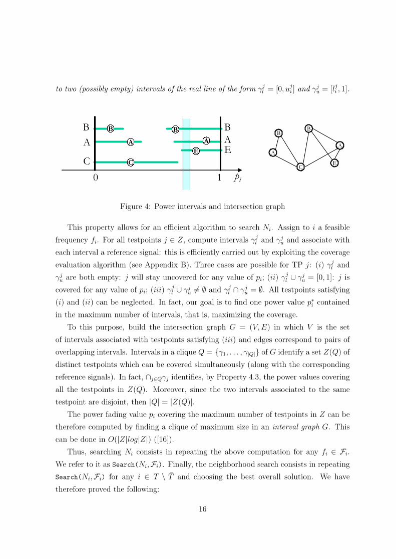
to two (possibly empty) intervals of the real line of the form °jl = [0; uji ] and °ju = [lji ; 1].

B

A

E

10 pi

AB

CEBA

C

AB B

AE

C

A

B

Figure 4: Power intervals and intersection graph

This property allows for an e±cient algorithm to search Ni. Assign to i a feasiblefrequency fi. For all testpoints j 2 Z, compute intervals °jl and °ju and associate witheach interval a reference signal: this is e±ciently carried out by exploiting the coverageevaluation algorithm (see Appendix B). Three cases are possible for TP j: (i) °jl and°ju are both empty: j will stay uncovered for any value of pi; (ii) °jl [ °ju = [0; 1]: j iscovered for any value of pi; (iii) °jl [ °ju 6= ; and °jl \ °ju = ;. All testpoints satisfying(i) and (ii) can be neglected. In fact, our goal is to ¯nd one power value p¤i containedin the maximum number of intervals, that is, maximizing the coverage.To this purpose, build the intersection graph G = (V;E) in which V is the set

of intervals associated with testpoints satisfying (iii) and edges correspond to pairs ofoverlapping intervals. Intervals in a clique Q = f°1; : : : ; °jQjg of G identify a set Z(Q) ofdistinct testpoints which can be covered simultaneously (along with the correspondingreference signals). In fact, \j2Q°j identi¯es, by Property 4.3, the power values coveringall the testpoints in Z(Q). Moreover, since the two intervals associated to the sametestpoint are disjoint, then jQj = jZ(Q)j.The power fading value pi covering the maximum number of testpoints in Z can be

therefore computed by ¯nding a clique of maximum size in an interval graph G. Thiscan be done in O(jZjlogjZj) ([16]).Thus, searching Ni consists in repeating the above computation for any fi 2 Fi.

We refer to it as Search(Ni;Fi). Finally, the neighborhood search consists in repeatingSearch(Ni;Fi) for any i 2 T n ¹T and choosing the best overall solution. We havetherefore proved the following:

16

Theorem 4.4 The neighborhood search can be done in O(jT j ¢ jFj ¢ (jZjlogjZj)).This low complexity is crucial for increasing the number of iterations of GRASP in

very large scale problems.

The GRASP algorithm The algorithm is referred to as Solve NPlan and sum-marized in Table 3. At each iteration of the activation loop, the neighborhood of thecurrent solution is explored, and one solution in the candidate set is chosen at random.The candidate set contains all solutions whose value is at least ®cmax, where ® 2 (0; 1)and cmax is the optimal value. Parameter ®, initialized at 0.9, is decreased at each iter-ation. Remark that (initial) larger values of ® enhance the probability of selecting (oneof) the most covering transmitters; smaller values increase diversi¯cation. The loopends when no improving solutions are found. Then, a local search is performed: follow-ing the activation order, one transmitter at time is switched o® and the neighborhoodis explored. The algorithm is repeated num iter times.

5 Heuristic for NPackIn a preliminary study, we investigated di®erent extensions of the above GRASP ap-proach to solve NPack, obtaining poor results. Indeed, it is common experience thatlarge scale problems with multiple sets of decision variables are e®ectively tackled bysome type of decomposition. Within this framework, two-phase heuristics decomposethe original problem into two more tractable subproblems (recent examples in [19, 30]),typically corresponding to di®erent sets of decision variables.We propose a two-phase heuristic for NPack: in the ¯rst phase emission powers are

determined for each stand-alone network (all other networks switched o®); in the secondphase frequencies are simultaneously assigned to all networks. The heuristic is basedon the goal programming approach to multi-objective optimization: the decision makerspeci¯es (optimistic) aspiration levels for the objective functions and the (weighted)sum of the deviations from these aspiration levels is minimized (weighted approach forgoal programming [24]). The goal programming version of NPack is obtained by (i)de¯ning suitable threshold values ¹uk for the coverage revenue of each network k 2 R,and (ii) minimizing the weighted sum of the deviations ¹uk ¡ u(Ck). This function has

17

||{||||||||||||||||||||||||||||||||||||||Solve NPlan

Input: network (T;Z), power upper bound vector PU 2 IRjT j,fading matrix [A]i2T;j2Z , revenue vector u 2 IRjZj,frequency spectrums Fi, for all i 2 T .

Output: A network con¯guration (p; f ; s)repeat num iter timesp = 0jT j; ® = 0:9; queue = ;;activation loop:for all i 2 T n ¹T

apply Search(Ni;Fi) to compute optimal con¯guration (p¤; f¤; s¤)i;cmax = maxi2Tn ¹Tfu(C((p¤; f¤; s¤)i))g;if cmax ¸ u(C((p; f ; s))) thenchoose randomly t 2 T n ¹T , satisfying ®cmax · u(C((p¤; f¤; s¤)t)) · cmax;(p; f ; s) = (p¤; f¤; s¤)t;push t in queue;® = maxf0:1;®¡ 0:01g;goto activation loop;

local search:while queue is not emptypop t from queue;(¹p;¹f ;¹s) = (p; f ; s) ;¹pt = 0 ;

for all i 2 T n ¹Tapply Search(Ni;Fi) to compute optimal con¯guration (p¤; f¤; s¤)i;

cmax = maxi2Tn ¹Tfu(C((p¤; f¤; s¤)i))g = u(C((p¤; f¤; s¤)q));if cmax ¸ u(C(p; f ; s)) then (p; f ; s) = (p¤; f¤; s¤)q;

endrepeat;||||||||||||||||||||||||||||||||||||||||{

Table 3: GRASP Algorithm for NPlan

18

been discussed with RAI Way engineers and validated in the testing phase (see x7).From now on we denote the complete two-phase heuristic by Solve NPack.

5.1 Phase 1: (stand-alone) Network PlanningThe input of this phase is an instance of NPack and one aspiration revenue ¹uk for eachnetwork k 2 R. The output is a con¯guration (pk; fk; sk) such that u(Ck) ¸ ¹uk, fork 2 R.Phase 1 treats each network k as a stand-alone network, by an iterative procedure:

starting from the initial value jFj = 1, a slight modi¯ed version of Solve NPlan (x4.3)is executed in which the algorithm stops (precisely, exits the activation loop) as soon asone solution with u(Ck) ¸ ¹uk is found. If no such solution is found, then the spectrumsize is increased by one and a new search is performed.This algorithm intends to minimize the number of frequencies used to meet the

threshold. These are temporary frequencies, since they are re-assigned in Phase 2, anddo not correspond to the actual available frequencies. Thus, the temporary spectrumsize is a parameter, whose e®ect on overall networks coverage is investigated in x7.Finally, observe that it is not required that all pairs of (intra-net) interfering trans-

mitters receive distinct temporary frequencies. Indeed, interfering transmitters oftenreceive the same temporary frequency in the ¯nal solution returned by Solve NPlan.

5.2 Phase 2: Multi-Network Frequency AssignmentThe input of Phase 2 consists of a stand-alone con¯guration (pk; fk; sk) and a threshold¹uk for each network k 2 R. The output is a (new) con¯guration (pk; fk; sk) for eachk 2 R.The purpose of this phase is to assign an available frequency to every transmitter, so

as to approximate the revenue levels obtained in Phase 1 (satisfactory for the planner)when the networks are simultaneously active. This is an instance of the Multi-networkFrequency Assignment Problem (MFAP), which is a generalization of well known FAP(see x3). The latter is usually solved by a graph model referred to as the MinimumInterference Frequency Assignment Problem (MI-FAP) ([1]).An instance of the MI-FAP is described by an undirected graph G = (V;E) (inter-

ference graph) with non-negative weights cuv for each (u; v) 2 E, where V is the set

19

of transmitters, E is the set of pairwise interfering transmitters and cuv represents therevenue loss when u and v receive the same frequency (computed as in [1]). Then theMI-FAP is the problem of assigning frequencies from F to the vertices of V so that thesum of the revenue losses is minimized. When only co-channel interference is consid-ered, the MI-FAP reduces to the well known max k-cut problem (where k = jFj) onweighted graphs, namely:

Problem 5.1 (max k-cut) Find a partition of V into k classes so that the sum of theweights of crossing edges (i.e. edges with endpoints in di®erent classes) is maximized.

The same graph model applies to MFAP, where edges connect transmitters eitherfrom the same network or from di®erent networks and the revenue losses are computedaccording to power levels established in Phase 1. We denote such a graph byG = (T;E).Using this de¯nition of multi-network graph we often experienced large gaps between

value of the max k-cut solutions and corresponding coverage value based on testpoints(x2.1). Precisely, we observed large deviations ¹uk ¡ u(Ck) for the single networks cov-erage because of increased intra-net interference. This turns out to be a consequenceof the modelling approximation introduced by the graph model.On the contrary, we experienced that this bad e®ect is remarkably reduced by the

following amendment to the standard model. Let ¹Ek be the (possibly empty) set oftransmitter pairs of network k in which the two transmitters are interfering but receivedthe same (temporary) frequency in Phase 1, yielding a coverage loss. The new multi-network interference graph is ¹G = (T; ¹E), where ¹E = E n [k2R ¹Ek. In practice, thishas two major e®ects: (i) forces the max k-cut solution to approximate the stand-alonefrequency assignment of Phase 1, ¯tting with the optimized power values; (ii) drivesthe frequency assignment toward coverage losses accepted by the aspiration thresholds.Several solution algorithms have been proposed for MI-FAP. For large real-life in-

stances (like those considered in this paper) exact methods fail and one resorts to heuris-tics. Among these, the most promising appear to be Monte Carlo methods, such asSimulated Annealing (SA) and Threshold Acceptance [1]. In our tool MI-FAP is solvedusing the variant of SA devised in [13], which outperforms other known approaches onseveral real-life large scale instances [14, 23].

20

5.3 Post-optimizationAt the end of Phase 2 a post-processing step concludes the heuristic for NPack. Itconsists in minimizing the overall emitted power with vectors f and s ¯xed by Phase2. This is carried out as explained in 4.1. We experienced that a few uncovered TP-smay gain a reference signal because of reduced interference from other signals, yieldinga slight coverage increase.

5.4 Advances to current practiceThe actual approach, referred to as segregation, adopted by the AGCOM in the elabora-tion of the national frequency plans ([3]) and also in implementation of multi-operatorsGSM systems works as follows. In order to con¯gure jRj distinct networks, the avail-able bandwidth is subdivided into jRj mutually non-interfering sets of frequencies, eachone being the set of feasible frequencies for exactly one network. In other words, eachnetwork operates in a segregated frequency domain and no-interference can occur be-tween transmitters belonging to distinct networks (inter-net interference). Then, everysingle network can be separately designed. This is typically carried out by a furtherdecomposition, namely, emission powers are established independently from frequencyallocation. The latter decomposition represents a ¯rst drawback of the current practice:we experienced that this yields solutions to NPlan of poor quality. On the contrary,Phase 1 of Solve NPack optimizes both emission powers and frequencies, providingbetter solutions.Two other major drawbacks can be identi¯ed in the segregation approach. The

¯rst drawback concerns the °exibility of the approach. In practice, splitting frequenciesamong non-identical networks (i.e., deciding the segregation scheme) is a hard task,requiring a trial-and-error process. Even more di±cult can be applying the segregationapproach under user-de¯ned coverage aspiration thresholds. In this case, infeasibil-ity problems may occur, whenever all feasible segregation schemes do not satisfy thethresholds. The methodology introduced in this paper ¯lls in this lack of °exibility.The second drawback is illustrated in Figure 5. In this example we consider two

identical networks N1; N2 (identical networks occur when the same network broadcastsdi®erent programs, a common event), with T 1 = fa; b; c; d; eg and T 2 = fA;B;C;D;Eg.The interference graph associated with each single network is depicted in Figure 5.a (we

21

fe=3

fa=1

(a) segregated solution

fd=2

a

e b

d c

fb=2

fc=1

A

B

CD

E

a

e b

d c

fb=3fa=1

fA=2

fB=4

fc=1

fC=5

fd=2

fD=3

fE=5fe=4

(b ) multi-inteference graph

Figure 5: (a) segregation approach vs: (b) multi-interference graph

can suppose that, for every edge, the co-channel revenue loss is equal to a large constantM). The corresponding multi-network interference graph is represented in Figure 5.b.Observe that the minimum number of frequencies required by a single network (sayN1) to avoid losses is 3. A 0-loss frequency assignment for a single network is shown inFigure 5.a, namely fa = fc = 1, fb = fd = 2 and fe = 3. Thus, in the segregation mode,6 distinct frequencies are required for two networks. On the other hand, one can obtaina 0-loss frequency assignment for the multi-network graph of Figure 5.b by assigningfa = fc = 1, fd = fA = 2, fb = fD = 3, fe = fB = 4 and fC = fE = 5. Therefore, if welet both networks draw frequencies from a common set, we can reduce the bandwidthrequirement to 5 frequencies. Observe that network N1 receives frequencies from theset f1; 2; 3; 4g, while network N2 from the set f2; 3; 4; 5g and the two sets have largeoverlap. Phase 2 of Solve NPack is designed to overcome the drawback highlighted inthe example through an improved spectrum usage.

6 Implementation issuesThe methodology described in this paper has been coded in a software tool which iscurrently in use at RAI Way [28]. In particular, the tool was developed under constantcoordination with company engineers during years 2000 and 2001. This process focusedon some key points illustrated below.

22

Simulation vs Optimization Tools available at RAI Way at the beginning of thisstudy perform ¯eld prediction and coverage evaluation, i.e., simulation of network con-¯gurations. In practice, such tools allow the engineers to compute coverage of hand-made network con¯gurations. Therefore, the planning activity was carried out by atrial-and-error process: (i) identi¯cation of promising modi¯cations of actual networks,(ii) validation of new candidate con¯gurations through simulation and (iii) accep-tance/rejection of new con¯gurations. New regulations from AGCOM and the DVBlaunch called for a signi¯cant re-planning of the broadcasting system and the previousplanning process became quickly ine®ective. On the contrary, our methodology hasbeen designed to cope with the new needs. In particular, the possibility of optimizingnetwork con¯gurations and the automatic handling of the design process is of great helpfor the company engineers. In fact, when system resources become scarce, the quality ofhand-made con¯gurations is simply unacceptable. As far as we know, RAI Way is the¯rst European broadcaster using automatic optimization, whereas most of the researche®ort at private broadcasters is focused on propagation and coverage assessment.

Tool °exibility In order to be compliant with the planning activity, the tool hasbeen designed to satisfy several requirements of RAI Way engineers:

(i) when planning a multi-network system, one wishes to de¯ne a coverage require-ment for every network, according to commercial strategies. The choice of goalprogramming in Solve NPack permits obtaining di®erent optimized con¯gura-tions for di®erent choices of thresholds ¹uk. This also helps evaluating the trade-o®between coverage and resource usage.

(ii) some transmitter may have pre-assigned emission power and/or frequency. Inthis experience, two situations occur: one of two networks is completely ¯xed andcannot be re-optimized (see x7); the frequency of transmitters near Italy's borderis ¯xed by international agreements. The tool easily manages this requirement byvariable ¯xing.

(iii) some TPs are regarded as critical for some networks. Such TPs typically coincidewith important town centers. In this case, the revenue uj of the TPs can beincreased according to the importance awarded to them.

23

Parameters All transmitter parameters (see x2) can be easily modi¯ed through input¯les. Furthermore, several system parameters are available in order to build speci¯cscenarios. Among them, the following emerge as the important ones:

² the antenna gain and directivity can represent several receiving conditions: roofantenna, omnidirectional indoor antenna, etc. [8];

² the tool can adopt any propagation model [3] and work with all frequency bands,from VHF to L-band.

² the guard interval Tg (see x2.1) and system noise PC=N (see x4.1) can be easilymodi¯ed. This allows the user to evaluate di®erent modulation schemes anddi®erent channel models [8].

7 Experimental ¯ndings and practical achievementsThe computational experience has three main purposes: (i) evaluating the qualityof solutions obtained by Solve NPlan (x7.1); (ii) evaluating the quality of solutionsobtained by Solve NPack (x7.2); (iii) illustrating practical achievements concerningthe RAI analog-to-digital (A to D) transition (x7.3). As for (iii), we discuss resultsobtained in reference scenarios based on the Italian law, which have been the technicalsupport for initial A to D transition strategies. Some details had to be omitted for notbeing authorized by the Company for publication (e.g., details about the networks usedin the experiments).All experiments regard subsets of 480 di®erent geographical transmitter sites. These

have been identi¯ed by the Italian Communications Authority (law 66/2001) as thoseaccommodating the transmitters of the future television networks. The digital terraindatabase provided to us by RAI is based on a grid with 2.5Km step, amounting to55,012 testpoints (15,442 inhabited, u(Z) = 56; 804; 187). Three types of instances areconsidered, according to their geographical extension: (a) national networks: the targetarea Z consists of all Italian inhabited TP-s; (b) regional networks: Z consists of allinhabited TP-s of one Italian regional district; (c) multi-regional networks: Z consistsof all inhabited TP-s of several regional districts. The instances of type (a) representthe focus of this study and are of very large scale (compare, for instance, with the 800

24

testpoints instances in [20]). Instances of other types can be of practical interest too,but are considered here only to assess performance of algorithms.A complete description of all system parameters, including transmission bands, an-

tenna diagrams and reception characteristics can be found in [8] and [3]. The algorithmsSolve NPlan and Solve NPack have been coded in C++ and run on a Pentium IV1.4 Ghz machine, with 512 MB of RAM.Throughout the computational section, the objective function value is often dis-

played as the (percentage) ratio u(C)=u(Z) (i.e. covered over total population). Allother percentage values derive consequently.

7.1 Evaluating Solve NPlanThe ¯rst experiment concerns regional networks and two spectrum sizes jFj 2 f1; 2g.These instances can be solved to optimality by MILP formulations (x4.1), allowing theevaluation of Solve NPlan solutions. The optimal solutions of MILP-s are computedby the commercial solver ILOG Cplex 8.0. After some testing, we established that thebest setting for Cplex is the default with one major modi¯cation: nodesel = 3 (strongbranching). In some instances a decisive improvement is obtained by MIPemphasis = 3and/or probing strategy = 3. For instances with jZj · 800 some advantage can beobtained with flowcovers generation level aggressive and heuristicfreq · 10.Results are collected in Table 4. The ¯rst four columns display instance features:

district identi¯er, number of inhabited testpoints jZj, target population u(Z) and num-ber of candidate transmitters jT j. The remaining columns report, for each value ofthe spectrum size, the following data: solution by Solve Nplan (percentage value%u(C) = u(C)=u(Z) ¤ 100), optimal solution by MILP (%u(C¤)), number of trans-mitters activated by the two algorithms (#T and #T ¤), CPU time (in seconds) andrelative percentage gap between the two solutions.One can observe that for all instances a very small gap is measured (less than 0.8%

in the case jFj = 2), decreasing on average as the spectrum size increases. Furthermore,the CPU time required by Solve NPlan is limited and does not increase signi¯cantlyas the spectrum size augments (the parameter num iter is set to 50 for all instances).On the contrary, a large amount of CPU time is typically required by Cplex. Finally,instances marked with an (¤) in the CPU time column (with jFj = 2), required a

25

speci¯c (instance dependent) ¯xing of variables in order to certify optimality. Observethat optimal solutions accommodate a number of transmitters larger than the one fromheuristic solutions.When national networks are concerned, MILP formulations (x4.1) cannot be solved

to optimality. Therefore, Solve NPlan solutions are evaluated resorting to the upperbound (UB) of x4.2. Table 5 reports on national networks with two possible sets ofcandidate sites. The ¯rst set contains all of the 480 sites while the second correspondsto a subset of 367 sites selected by the Company. For the second set, also an analognetwork is considered. In all the experiments the Solve NPlan parameter num iter isset to 100.When jFj ¸ 2, a fairly small percentage gap (from 1.06% to 2.17%) is measured,

proving the successful behavior of the heuristic as well as the e®ectiveness of the boundfrom decomposition. On the contrary, networks with jFj = 1 show a larger gap (from3.58% to 6.75%). However, this is due to a weaker bound rather than a poor heuristicsolution, because of large cross-interference among clusters.On the practical side, large Single Frequency Networks are of great interest in digital

systems, while they do not play any role in analog ones. Before the present study,coverage of Single Frequency Networks was estimated applying the digital coverageevaluation procedure to the actual (analog) transmitter con¯guration (or to some hand-made manipulation of it). Solve NPlan solutions largely outperform such estimates,revealing new insights to RAI Way engineers.

7.2 Evaluating Solve NPackTwo experiments are proposed to compare Solve NPack to the segregation approach(x5.4). In particular, the e®ect of Phase 2 is evaluated when applied over a ¯xedfrequency allocation (segregation scheme). The comparison is performed in four steps:(1) choose a segregation scheme; (2) compute by Solve NPlan a con¯guration for eachnetwork k 2 R with revenue u( ¹Ck); (3) set aspiration thresholds ¹uk = u(( ¹Ck)); (4) runSolve NPack.Under this choice of aspiration thresholds, the segregation approach coincides with

Phase 1 of Solve NPack: for each network, the minimum temporary spectrum sizerequired by Solve NPlan to meet the threshold equals, by construction, the segregated

26

|F|=

1|F|=

2

Net

wor

kA

ttri

bute

sSol

veN

Plan

MIL

PSol

veN

Plan

MIL

P

Dis

tric

t|Z|

u(Z

)|T|

%u(C

)#

TC

PU

%u(C

∗ )#

T∗

CP

UG

ap%

u(C

)#

TC

PU

%u(C

∗ )#

T∗

CP

UG

ap

150

71,

343,

650

1998

.25

1532

98.7

616

285

0.51

98.6

416

4098

.94

176,

042

0.30

253

75,9

7718

95.8

68

495

.86

810

095

.86

85

95.8

68

240

360

23,

451,

121

1682

.24

710

082

.59

956

,782

0.43

97.6

415

140

97.9

117

72,8

90∗

0.27

41,

258

3,85

4,43

945

89.6

98

104

90.1

59

63,0

270.

5198

.29

2024

898

.46

2191

,432

∗0.

17

547

579

9,70

332

92.2

440

2092

.51

4018

00.

3092

.35

4028

92.5

140

1,92

80.

18

656

61,

630,

641

1894

.44

1728

94.4

417

161

095

.69

1832

95.6

918

5,03

90

718

932

8,84

817

89.9

08

2090

.25

878

0.39

90.1

18

2890

.25

986

60.

15

879

32,

093,

580

3493

.55

2768

94.1

128

59,0

990.

6096

.69

3076

97.0

331

75,4

90∗

0.35

91,

092

3,51

5,46

831

94.9

820

124

95.9

422

38,9

071.

0196

.74

2318

897

.51

2567

,834

∗0.

79

1038

51,

979,

830

2993

.28

1128

94.0

412

115

0.82

97.4

118

4497

.71

201,

507

0.31

112,

227

9,36

8,78

056

93.7

022

232

94.5

623

79,0

870.

9197

.10

2642

097

.79

2896

,453

∗0.

71

1294

75,

614,

973

3298

.48

2410

898

.68

2452

,027

0.20

98.8

925

136

99.0

726

79,9

26∗

0.18

1391

85,

237,

954

3194

.10

2156

94.2

922

23,4

560.

2096

.16

2864

96.2

128

59,7

350.

05

1461

71,

140,

811

3793

.45

2372

93.5

423

15,8

020.

1097

.16

2584

97.2

025

75,8

450.

04

1533

370

3,38

717

99.5

513

4099

.613

277

0.05

99.5

512

5299

.60

123,

352

0.05

1622

364

1,38

826

96.5

717

6897

.55

1926

,891

1.01

97.2

417

8897

.55

1875

,238

0.32

1790

55,

139,

317

2296

.25

1976

97.1

220

54,2

280.

9096

.64

1910

497

.12

2184

,820

∗0.

50

181,

421

4,55

5,37

736

90.5

311

132

91.2

613

60,3

540.

8196

.72

2224

897

.20

2391

,502

∗0.

49

1958

81,

289,

670

2998

.34

2036

99.0

621

302

0.73

98.6

419

6099

.16

215,

194

0.52

201,

561

4,02

5,78

135

95.5

612

108

96.5

515

64,6

781.

0497

.41

1718

898

.17

1992

,415

∗0.

77

Tab

le4:

Sol

veN

Plan

vs.

MIL

Pon

Ital

ian

dis

tric

ts,|F|∈

{1,2}

27

jFj Technology jT j u(C) %u(C) #T CPU UB %UB Gap1 Digital 480 51,520,319 90.70 274 25,596 53,554,988 94.28 3.582 Digital 480 54,168,472 95.36 279 43,992 55,401,124 97.53 2.171 Digital 367 44,006,204 77.47 302 24,516 47,840,486 84.22 6.752 Digital 367 51,498,676 90.66 346 36,828 52,731,327 92.83 2.173 Digital 367 53,128,956 93.53 367 48,276 53,731,080 94.59 1.063 Analog 367 47,584,867 83.77 367 12,883 48,556,219 85.48 1.714 Analog 367 49,896,798 87.84 367 17,208 51,055,603 89.88 2.04Table 5: Solve NPlan solutions vs. upper bounds for national networks

spectrum size. In this setting, the experiment aims to demonstrate that Phase 2 ise®ective to counterbalance the increase of inter-net interference by reducing intra-netinterference.Both experiments concern two networks N1 and N2 and represent two di®erent

situations, i.e., complete and partial overlapping target areas. The results are or-ganized in tables with the following format. Each row corresponds to a segregationscheme (jF1j; jF2j) and displays: best percentage coverage %u( ¹C1) (%u( ¹C2)) of N1 (ofN2) found by Solve NPlan (segregated solution), best percentage coverage %u((C1)¤)(%u((C2)¤)) of N1 (of N2) found by Solve NPack, percentage sum of deviations%¢N1 +%¢N2. The deviation is de¯ned as ¢Nk = ¹uk ¡ u((Ck)¤), k = 1; 2 (x5).Scenario 1. One analog national network N1 = A and one digital national networkN2 = D (A and D have completely overlapping target areas). The candidate site isthe one with 367 sites used in x7.1: therefore, best stand-alone heuristic con¯gurationsand relative upper bounds can be found in Table 5.Results are reported in Table 6, in which three spectrum sizes jFj 2 f4; 5; 6g and ¯ve

di®erent segregation schemes are considered. In this scenario (Phase 2 of) Solve NPackimproves the segregation approach. In particular, for jFj 2 f4; 5g a small (i.e., within0.5%) loss for network A is pro¯tably counterbalanced by a relevant (i.e., up to 6.6%)gain for network D. This leads to a negative sum of deviations. For jFj = 6, the solu-tions from Solve NPack dominate those from the segregation approach. The practicalrelevance of this gain can be appreciated recalling that, in this scenario, an improvementof 1% corresponds to about 500,000 inhabitants.

28

Scheme Segregation approach Solve NPack Sum of deviationsjFj jFAj jFDj %u( ¹CA) %u( ¹CD) %u((CA)¤) %u((CD)¤) %¢A+%¢D4 3 1 83.77 77.47 83.32 79.34 -1.425 4 1 87.84 77.47 87.37 84.05 -6.115 3 2 83.77 90.66 85.94 89.95 -1.466 3 3 83.77 93.53 85.33 93.99 -2.026 4 2 87.84 90.66 87.85 91.73 -1.08

Table 6: Segregation vs. Solve NPack: Scenario 1

Scenario 2. Two multi-regional networks N1 and N2 with partially overlapping tar-get areas. Namely, Z1 (Z2) is the union of regional districts Abruzzo and Marche(Lazio and Abruzzo). Then, jZ1j = 3; 882, u(Z1) = 2; 503; 813, and jZ2j = 4; 572,u(Z2) = 5; 924; 318. Two spectrum sizes are considered (jFj 2 f3; 5g) and four segre-gation schemes. Results are reported in Table 7, including also the number of activetransmitters (#TX) .

Scheme Segregation Approach Solve NPack Sum of deviationsjFj jF1j jF2j %u( ¹C1) #T 1 %u( ¹C2) #T 2 %u((C1)¤) %u((C2)¤) %N1 +%N2

3 1 2 80.77 45 92.34 56 90.86 93.18 -10.933 2 1 90.89 49 87.49 52 91.01 90.24 -2.875 2 3 90.89 49 94.75 57 92.55 94.71 -1.625 3 2 92.73 49 92.34 56 92.81 93.52 -1.26

Table 7: Segregation vs. Solve NPack: Scenario 2

When jFj = 5, the solutions from Solve NPack "almost" dominate the segregatedones. In fact, the segregation schemes (2,3) and (3,2) slightly improve (i.e. less than0.1%) the coverage of the protected network (i.e., the one with 3 frequencies), butpenalizes the coverage of the other network by about 2%.When jFj = 3, Solve NPack largely outperforms the segregation approach. In fact,solutions from both segregation schemes (1,2) and (2,1) are dominated by those fromSolve NPack. Notice that the gain for single frequency networks ranges from 3% to10%. A similar enhancement was observed in tests involving a larger number of net-works. Partially overlapping target areas yield remarkable advantages for Solve NPack.In summary, in all cases of both scenarios a negative sum of deviation is measured.

29

7.3 A to D transitionThe key issue of digital start-up is growing digital networks sharing resources withoperating analog networks. The experiments of this section include one RAI nationalanalog network A, consisting of 367 active transmitters.The two experiments motivating the present study are here illustrated. In the ¯rst

experiment one digital network is grown over network A under its current (¯xed) setting.In the second experiment two digital networks are grown over A (which can now be re-planned) according to the new requirements ¯xed by Italian law. In both experimentsthe available spectrum is jFj = 7.Experiment 1: growing a national digital network D over A (¯xed). Thisscenario represents a classical start-up for a new service: managers wish to keep safe theold service until the new one guarantees at least the same revenue. Emission powers andfrequencies of A are ¯xed. Under this setting, the population coverage of A is 91:21%,used as reference threshold ¹uA. Forbidding power and frequency re-con¯guration for Aprevents users from re-tuning channels or turning antennas. Therefore this is consideredan interesting transition scenario.Two major questions were formulated by RAI Way engineers:

(i) set-up of D: is it possible to activate network D with at least 40% populationcoverage without a®ecting network A (namely, keeping A over 90% populationcoverage)?

(ii) development of D: what is the impairment on network A as the coverage of Dincreases?

Neither the simulation tools nor the segregation approach can be of any help foranswering the above questions. On the contrary, these have been addressed by runningSolve NPack for increasing values of the threshold ¹uD. The initial percentage thresholdis 40%, considered by broadcasters a suitable start-up value.Table 8 displays, for each value of ¹uD, the following data: (temporary) spectrum size

in Phase 1 (jFTDj), number of active digital transmitters (#TD), Phase 1 (stand-alone)digital population coverage (%u1(CD)), digital population coverage (%u((CD)¤)) foundby Solve NPack, digital percentage deviation (%¢D = %(u1(CD)¡u((CD)¤))), analog

30

percentage deviation found by Solve NPack (%¢A = %(¹uA ¡ u((CA)¤))) and sum ofpercentage deviations (%¢D + %¢A). The coverage requirement ¹uD is consideredful¯lled with a 0.2% tolerance.Notice that several spectrum sizes (jFTDj) are reported for each threshold ¹uD: the

¯rst of such values is the one computed by Phase 1, whilst the others have been reportedfor sensitivity analysis. Values f¹uD = 77%; 90%; 93%g represent maximum revenuesobtained for (jFTDj) = f1; 2; 3g, respectively.

¹uD jFTDj #TD %u1(CD) %u((CD)¤) %¢D %u((CA)¤) %¢A (%¢D +%¢A)40 1 9 39.88 35.11 4.77 90.41 0.80 5.57

2 9 41.99 35.11 6.88 90.01 1.20 8.083 7 41.50 33.47 8.03 89.99 1.22 9.25

50 1 14 50.41 43.99 6.42 90.15 1.06 7.482 13 50.52 43.98 6.54 90.02 1.19 7.733 13 51.17 43.98 7.19 89.95 1.26 8.45

60 1 21 58.79 55.75 3.04 90.07 1.14 4.182 22 59.46 52.02 7.44 89.95 1.26 8.703 23 60.93 52.49 8.44 89.69 1.52 9.96

65 1 40 65.08 64.18 0.90 89.96 1.25 2.152 31 65.52 60.48 5.04 89.67 1.54 6.583 25 64.67 56.98 7.69 89.64 1.57 9.26

70 1 76 70.38 72.33 -1.95 89.78 1.43 -0.522 45 69.94 65.91 4.03 89.53 1.68 5.713 38 69.41 62.50 6.91 89.52 1.69 8.60

75 2 63 74.86 70.28 4.58 89.15 2.06 6.643 62 75.02 68.54 6.48 89.14 2.07 8.55

77 1 302 77.47 81.63 -4.16 89.44 1.77 -2.3980 2 86 79.63 75.49 4.14 88.91 2.30 6.44

3 82 80.20 73.55 6.65 88.89 2.32 8.9785 2 134 84.31 80.58 3.73 88.24 2.97 6.70

3 117 84.53 78.62 5.91 88.17 3.04 8.9590 2 346 90.66 87.56 3.10 87.91 3.30 6.40

3 191 89.50 83.46 6.04 87.59 3.62 9.6693 3 367 93.53 87.93 5.60 87.12 4.09 9.69

Table 8: Solve Npack results: one digital network over a ¯xed analog network

31

-2024681012

40 50 60 65 70 75 80 85 90

totaldeviation

1F2F3F

threshold-20246810

40 50 60 65 70 75 80 85 90 95

Digitaldeviation

00.511.522.533.544.5

40 50 60 65 70 75 80 85 90 100thresholdAn

alogdeviation

threshold

Figure 6: Digital, analog and total deviations vs. design threshold and number offrequencies

The con¯gurations obtained by jFTDj = 1 (covering from 43 to 72 %) providepositive answers to question (i). Before the present study, RAI management could onlyguess the feasibility of digital start-up based on network engineers estimates.As for question (ii), results of Table 8 represent attractive con¯gurations, covering a

wide variety of possible extensions of networkD between two extreme con¯gurations: onthe one hand, a concentrated network reaching 40% by covering only major towns withfew transmitters (7 or 9); on the other hand, an extended network reaching 88% usingmost of the available transmitters. In addition, the above results also allowed engineersto perform cost bene¯t analysis of networks, investigating the trade-o® between coverageand required number of transmitters.

Sensitivity analysis As a byproduct, results in Table 8 allows for a sensitivity analy-sis: the stopping criterion in Phase 1 of Solve NPack is removed and Phase 2 has beenexecuted for all values of jFTDj satisfying thresholds (not only for the smallest one).The results highlight that, for all values of ¹uD, the greater the spectrum size jFTDj thelarger the sum of deviations. This e®ect is clear from Figure 6, in which digital, analogand total deviations are plotted as functions of design thresholds and spectrum size.

32

These results validate the stopping criterion of Phase 1, which terminates as soon asthe threshold is met.Finally, notice that jFTDj = 1 yields a negative digital deviation and the solution

(jFTDj = 1; ¹uD = 77%) dominates the solutions (jFTDj = 2; ¹uD = 80%) and (jFTDj =3; ¹uD = 80%) (see Table 8). The negative deviations arise since the increase of inter-net interference caused by network packing is overcome by the reduction of intra-netinterference obtained exploiting the shared spectrum.

Experiment 2 Planning one analog network A with 2 digital networks D1; D2.This experiment consists of investigating system con¯gurations implementing the newregulation. This imposed on RAI Way two requirements: (i) implement by January 1,2004, two digital networks covering at least 50% of the population (ii) implement byJanuary 1, 2005, two digital networks covering at least 70% of the population. Purposeof RAI Way is to exploit the available spectrum jFj = 7 to ful¯ll such requirementswhile minimizing the deviation of analog network A from actual value ¹uA = 91:21.The following experiments aim to show the achievements obtained by Solve NPack

versus those from the segregation approach (precisely, an improved segregation ap-proach in which stand-alone networks are optimized by Solve NPlan).Problems (i) and (ii) admit the same optimal segregation scheme, namely jFAj =

5; jFD1j = 1; jFD2j = 1. Corresponding percentage revenues computed by Solve NPlanare: u(CA) = 82:83%, u(CD1) = u(CD2) = 70:38%. This solution represents a goodcon¯guration for scenario (ii). On the contrary, requirements of scenario (i) are largelysatis¯ed, yielding an unforced penalty on CA. The result deviation ¢A = 8:38 is indeedconsidered unacceptable for digital start-up.This drawback can be e®ectively managed by Solve Npack. In fact, choosing

¹uD1 = ¹uD2 = 55%, Solve Npack returns u(CA) = 89:02%, u(CD1) = 51:40; u(CD2) =49:82%. In this case ¢A = 2:19%, which is considered satisfactory. As for scenario(ii) Solve NPack returns u(CA) = 82:91%, u(CD1) = 70:51; u(CD2) = 70:01%, ob-tained with thresholds ¹uD1 = ¹uD2 = 68%, representing a small gain over the segregatedsolution.RAI managers considered such deviation for network A satisfactory for digital start-

up. This new achievement has been regarded as a conclusive argument to start theimplementation design.

33

8 ConclusionsWe presented a method for optimizing emission powers and frequencies in multi-networkbroadcasting systems in which di®erent networks share transmitter sites and frequen-cies, and each network has its own goal (Network Packing Problem).The contribution of this paper is threefold: on models, algorithms and practice.

On models, we introduced a hierarchy of new and relevant problems generalizing themodels studied in the literature so far. Concerning solution algorithms, a new localsearch is introduced for simultaneously optimizing emission powers and frequencies ona single network. The algorithm is able to ¯nd near optimal solutions for large scaleinstances. Also, an e®ective relaxation for computing upper bounds is described andexploited to measure the quality of heuristic solutions; ¯nally a two-phase heuristic isdevised able to approximate the Pareto optimal boundary of the multi-network (i.e.,multi-objective) problem.On the practical side, the problem investigated here represents a key problem in the

current transition from analog to digital television. This is the subject of hot politicalcontroversy in Italy and has been receiving quotidian attention from the popular pressin the last three to four years. We reported on the development of solution methods forthe Network Packing Problem at RAI Way, the network provider of the major Italianbroadcaster. The proposed approach guarantees high °exibility, allowing managers toobtain several high quality con¯guration alternatives for the Italian system under di®er-ent exploitation patterns of the system resources. The results illustrated in this papercontributed to start the RAI digital service according to the schedule and requirements¯xed by Italian law.Acknowledgements. This work was partially supported by RAI Way s.p.a.. We

are grateful to Arturo Baglioni, Giuseppe Carere and Roberto Sera¯ni from RAIWay forpromoting this study. We wish to thank Antonio Sassano for his invaluable suggestionsand Andreas EisenblÄatter for his detailed observations. Finally, we are indebted to theanonymous referees, whose comments led to a signi¯cant improvement of the paper.

References[1] K. I. Aardal, S.P.M. van Hoesel, A.M.C.A. Koster, C. Mannino and A. Sassano,

34

Models and solution techniques for the frequency assignment problem,4OR, 1, 4,2003, 261-317

[2] Ahuja, K.R., Ergun, ÄE., Orlin, J.B., Punnen, A.P., A survey of very large-scaleneighborhood search techniques, Discrete Applied Mathematics, 123, 1-3, 2002,75{102.

[3] Autoritµa Nazionale per le Garanzie nelle Comunicazioni, http://www.agcom.it.

[4] BBC news, UK edition, Thursday, 18 September, 2003,http://news.bbc.co.uk/1/hi/business/3121084.stm.

[5] Beutler, R., Frequency Assignment and Network Planning for Digital TerrestrialBroadcasting Systems, Kluwer Academic Publishers, ISBN 1-4020-7872-2, 2004.

[6] R. Brugger and D. Hemingway, OFDM Receivers, EBU Technical Review.

[7] CEPT/EBU, Planning and Introduction of Terrestrial Digital Television (DVB-T) in Europe, Doc. FM(97) 160, 1997.

[8] The Chester 1997 Multilateral Coordination Agreement, Technical Criteria, Co-ordination Principles and Procedures for the introduction of Terrestrial DigitalVideo Broadcasting, 25 July 1997.

[9] The Digital Video Broadcasting project, http://www.dvb.org

[10] European Broadcasting Union, Terrestrial Digital Television Planning and Imple-mentation Considerations, BPN 005, second issue, July 1997.

[11] European Radiocommunications O±ce, http://www.ero.dk/

[12] European Telecommunication Standard Institute, http://www.etsi.org

[13] Successful Applications to GSM Networks, http://www.dis.uniroma1.it/ man-nino/fap.htm

[14] A. EisenblÄatter and A. Koster, FAP web - A website about Frequency AssignmentProblems, http://fap.zib.de/

35

[15] P. Festa and M.G.C. Resende, GRASP: an annotated bibliography, in C.C.Ribeiro and P. Hansen, Essays and Surveys on Metaheuristics, Kluwer AcademicPublishers, 325{367, 2001.

[16] U.I. Gupta, D.T. Lee and J.Y.T Leung, E±cient Algorithms for Interval Graphsand Circular-Arc Graphs, Networks, 12, 1982, 459-467.

[17] Italian site of broadcasting, http://www.broadcasting.it

[18] International Telecommunication Union, http://www.itu.int/home/

[19] Kim, S. and S.L. Kim, A Two-Phase Algorithm for Frequency Assignment inCellular Mobile Systems, IEEE Transactions on Vehicular Technology, 43, 1994,542{548.

[20] Ligeti, A. and J. Zander, Minimal Cost Coverage Planning for Single FrequencyNetworks, IEEE Transactions on Broadcasting, 45, 1, 1999, 78{87.

[21] Ligeti, A. and S.L. Kim, Optimization of DAB/DVB Networks for Wireless Per-sonal Services with Limited Frequency Band, 10th IEEE International Symposiumon Personal, Indoor, and Mobile Radio Communications, Osaka, Japan, 1999.

[22] L. Lov¶asz and M.D. Plummer. Matching Theory. North-Holland, 1986.

[23] C. Mannino, G. Oriolo and F.Ricci, Solving Stability Problems on a Superclass ofInterval Graphs, Tech. Rep. N. 26-02, DIS-Universitµa di Roma "La Sapienza".

[24] K. Miettinen, Nonlinear Multiobjective Optimization, International Series in Op-erations Research and Management Science, Kluwer, 1999

[25] K. Karipys and V. Kumar, Family of multilevel partitioning algorithms,http://www-users.cs.umn.edu/ karypis/metis/

[26] Rappaport, T.S., Wireless Communications, Prentice Hall, 2002.

[27] Rossi, F., Sassano, A. and S. Smriglio, Models and Algorithms for TerrestrialDigital Video Broadcasting, Annals of Operations Research, 107, 2001, 267 {283.

36

[28] RAI Way o±cial web site, http://www.raiway.rai.it/

[29] Vasquez, M. and J.K. Hao, A heuristic approach for Antenna positioning in cel-lular networks, Journal of Heuristics, 7(5), 2001, 443{472.

[30] Rajaram, K. and R. Ahmadi, Flow management to optimize retail pro¯ts at themeparks, Operations Research 51, 2, 2003, 175{184.

Appendix A ComplexityWe show that NPack is NP-hard, even when restricted to planning a single network(i.e. jRj = 1). In particular, we show that Nplan for one analog network is NP-hard in strong sense. Recall that Pij = AijPi is the power density in testpoint j fromtransmitter i 2 T , and I(j; i) is the set of co-channel (with i) transmitters r 2 T n figwith Prj > 0. Testpoint j is regarded as covered by i i®

Pij ¸ K1 (13)

and, whenever I(j; i)6= ;PijP

k2I(j;i) Pkj ¸ K2 (14)

where K1 is the system noise and K2 > 1 is an adimensional quantity (protection ratio)[3].Theorem A.1 NPlan is NP-hard in the strong sense.Proof. By reduction from graph coloring: Given a biconnected undirected graphG(V;E), does there exist a coloring of V with at most k colors?Associate with G an instance I of NPlan de¯ned by a network (T; Z), a power

upper bound vector PU 2 IRjT j, a fading matrix [A]i2T;j2Z , a revenue vector u 2 IRjZjand a frequency spectrum F . Speci¯cally, let T = V = fv1; : : : ; vng, Z = E andPUi = K1, for all i 2 T . Since G is biconnected, E can be partitioned into n non-empty subsets E1; : : : ; En such that, for j = 1 : : : ; n, vertex vj is endpoint of everyedge in Ej (i.e. Ej µ ±(vj)). Such partition can easily be obtained by exploiting anear decomposition of G, which certainly exists since G is biconnected [22]. For each

37

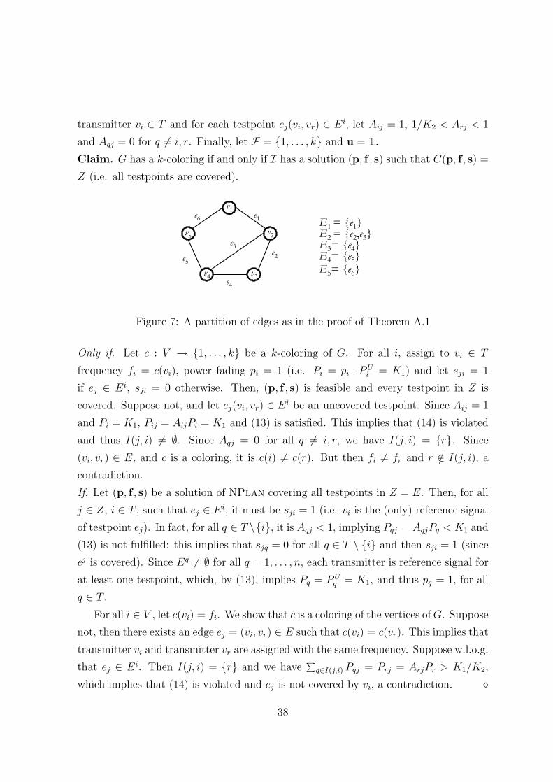
transmitter vi 2 T and for each testpoint ej(vi; vr) 2 Ei, let Aij = 1, 1=K2 < Arj < 1and Aqj = 0 for q6= i; r. Finally, let F = f1; : : : ; kg and u = 11.Claim. G has a k-coloring if and only if I has a solution (p; f ; s) such that C(p; f ; s) =Z (i.e. all testpoints are covered).

v1

v2

v3v4

v5e1

e2e3

e4

e5

e6 E1= {e1}E2= {e2,e3}E3= {e4}E4= {e5}E5= {e6}

Figure 7: A partition of edges as in the proof of Theorem A.1

Only if. Let c : V ! f1; : : : ; kg be a k-coloring of G. For all i, assign to vi 2 Tfrequency fi = c(vi), power fading pi = 1 (i.e. Pi = pi ¢ PUi = K1) and let sji = 1if ej 2 Ei, sji = 0 otherwise. Then, (p; f ; s) is feasible and every testpoint in Z iscovered. Suppose not, and let ej(vi; vr) 2 Ei be an uncovered testpoint. Since Aij = 1and Pi = K1, Pij = AijPi = K1 and (13) is satis¯ed. This implies that (14) is violatedand thus I(j; i) 6= ;. Since Aqj = 0 for all q 6= i; r, we have I(j; i) = frg. Since(vi; vr) 2 E, and c is a coloring, it is c(i)6= c(r). But then fi 6= fr and r =2 I(j; i), acontradiction.If. Let (p; f ; s) be a solution of NPlan covering all testpoints in Z = E. Then, for allj 2 Z, i 2 T , such that ej 2 Ei, it must be sji = 1 (i.e. vi is the (only) reference signalof testpoint ej). In fact, for all q 2 T nfig, it is Aqj < 1, implying Pqj = AqjPq < K1 and(13) is not ful¯lled: this implies that sjq = 0 for all q 2 T n fig and then sji = 1 (sinceej is covered). Since Eq 6= ; for all q = 1; : : : ; n, each transmitter is reference signal forat least one testpoint, which, by (13), implies Pq = PUq = K1, and thus pq = 1, for allq 2 T .For all i 2 V , let c(vi) = fi. We show that c is a coloring of the vertices ofG. Suppose

not, then there exists an edge ej = (vi; vr) 2 E such that c(vi) = c(vr). This implies thattransmitter vi and transmitter vr are assigned with the same frequency. Suppose w.l.o.g.that ej 2 Ei. Then I(j; i) = frg and we have Pq2I(j;i) Pqj = Prj = ArjPr > K1=K2,which implies that (14) is violated and ej is not covered by vi, a contradiction. ¦

38

Extension of the above proof to digital network planning is straightforward.

Appendix B A computing digital coverage in linearamortized time

We describe a linear time implementation of the coverage evaluation procedure for atestpoint, introduced in x2.1. The coverage probability is calculated by the error func-tion (3), which depends upon mean wanted (interfering) signal PWtot (P Itot) and variances¾2W;tot and ¾2I;tot. Recall that all of these values depend on the position of the detec-tion window. We show how to e±ciently select the position of the detection windowwhich maximises the coverage probability, by this simulating the behaviour of actualcommercial devices. Observe that if n signals arrive in a testpoint, then we have ndi®erent candidate windows, each containing at most n signals. So, a naive imple-mentation of this computation would require O(n2) operations. We show here how tocompute total wanted power PWtot in linear time; the extension to P Itot, ¾2W;tot and ¾2I;totis straightforward.A generic signal h 2 T arriving in a testpoint at time ¿h may contribute to the wanted

signal PWtot , to the interfering signal P Itot or to both. For sake of clarity, since copingwith a single testpoint, we remove all subscripts referring to testpoints, e.g. Phj = Ph.The contribution of signal h to PWtot is Ph ¢w(¿h), where w(¿h) is the weighting function(1) which can be rewritten as:

w(¿h) =8><>:1 if 0 · ¿h ¡ ¿ · Tg1t2u (tu + Tg + ¿ ¡ ¿h)2 if Tg < ¿h ¡ ¿ · 2Tg0 otherwise

(15)

where ¿ denotes the starting time of the detection window and tu is a constant (usefulsymbol period). Let T = f1; : : : ; ng be the n distinct signals in the testpoint. W.l.o.g.we can assume ¿1 · ¿2 · : : : · ¿n. We have seen that ¿ 2 f¿1; : : : ; ¿ng, i.e., thedetection window starting time coincides with the arrival time of one of the incomingsignals.When the receiver is synchronized with the i-th signal (i.e. ¿ = ¿i), let us denote byPW (i) the value of the total wanted signal, by U(i) = fh 2 T : ¿ = ¿i; w(¿h) = 1g the

39

set of fully contributing signals, and by M(i) = fh 2 T : ¿ = ¿i; 0 < w(¿h) < 1g the setof partially contributing signals, for i = 1; : : : ; n.Since ¿1 · ¿2 · : : : · ¿n, then U(i) and M(i) are sets of consecutive integers and

we can write U(i) = fi; i+ 1; : : : ; qig and M(i) = fsi; : : : ; tig, for i1; : : : ; n (see Fig. 8).Trivially, i · qi < si · ti.

qii si tiUi Mi

qi+1i+1 si+1 ti+1

Figure 8: Shifting the detection window from ¿i to ¿i+1

Denote by PU(i) = Pqij=i Pj the overall contribution to PW (i) of the signals in U(i),and by PM(i) = Ptij=si Pj ¢w(¿j) the overall contribution to PW (i) of the signals inM(i)(PW (i) = PU(i) + PM(i) for all i). We show ¯rst how to e±ciently evaluate PU(i+ 1)once PU(i) = Pi + : : :+ Pqi is known. When the detection window shifts from position¿i to the next position ¿i+1 we have that signal i is no more a wanted signal whilstsignals qi + 1; : : : ; qi+1 are now fully wanted signals (see Fig. 8), i.e.

PU(i+ 1) = PU(i)¡ Pi + Xj=qi+1;:::;qi+1

Pj :

Therefore, PU(i+ 1) can be obtained from PU(i) by performing qi+1 ¡ qi + 1 sim-ple arithmetic operations. Let us indicate as ri the number of elementary operationsrequired to compute PU(i), i = 1; : : : ; n. The following recursive expression holds:

ri+1 = ri + qi+1 ¡ qi + 1:Assuming r0 = q0 = 0, the total number of elementary operations required to computePU(n) is simply rn = rn¡1 + qn ¡ qn¡1 + 1 = : : : = qn + n = 2n. This shows that thecontribution of the fully wanted signals can be computed in optimum time O(n).

40

We evaluate now the complexity of calculating the contribution to PW (i+ 1) of thepartially contributing signals PM(i+ 1) when PM(i) is known. By (15) we have (lettingAj = tu + Tg ¡ ¿j):

PM(i) = 1t2u

tiXj=si

Pj(Aj + ¿i)2 = 1t2u [

tiXj=si

PjA2j + ¿ 2itiXj=si

Pj + 2¿itiXj=si

PjAj ] (16)

Observe ¯rst that computing the quantities Ak, PkAk, PkA2k, ¿2k and 2¿k, for k =1; : : : ; n, requires O(n) elementary operations. As before, let us shift the window to thenext position ¿i+1 and show how the three summations in the right hand side of (16)can be e±ciently re-computed. Consider ¯rst the term Pti+1

j=si+1 PjA2j . If si+1 · ti, thenti+1Xj=si+1

PjA2j =tiXj=si

PjA2j ¡ si+1Xj=si

PjA2j +ti+1Xj=ti

PjA2j :

So the termPti+1j=si+1 PjA2j can be obtained from

Ptij=si PjA2j by performing (si+1¡si)+(ti+1 ¡ ti) + 1 additions and subtractions. When si+1 > ti then the direct computationofPti+1

j=si+1 PjA2j involves ti+1¡st+1 < ti+1¡ti additions. So, in any case we can computethe new term in at most si+1 ¡ si + ti+1 ¡ ti elementary operations.Similarly one can show that both the second summation ¿ 2i+1Pti+1

j=si+1 Pj and the thirdsummation 2¿i+1Pti+1

j=si+1 PjAj can be computed by at most (si+1 ¡ si) + (ti+1 ¡ ti) + 1elementary operations.Finally, we can conclude that PM(i+ 1) can be calculated from PM(i) by performing

at most 3(si+1¡ si+ ti+1¡ ti)+ 2 elementary operations. By solving the correspondingrecursive equation, one can show that PM(1); : : : ; PM(n) can be computed in at most8n elementary operations (plus O(n) required to compute Ak, PkAk, PkA2k, ¿2k and 2¿k,for k = 1; : : : ; n).So, the overall wanted signal for each possible detection window can be computed

in linear (amortized) time. Similar arguments apply to the computation of the overallinterfering mean value, and the total wanted and interfering variances. This implies thatthe optimum detection window - and thus the coverage probability - can be calculatedin O(n).

41