www.elsevier.com/locate/rse

Remote Sensing of Environm

Ground measurements for the validation of land surface temperatures

derived from AATSR and MODIS data

Cesar Coll T, Vicente Caselles, Joan M. Galve, Enric Valor, Raquel Niclos,

Juan M. Sanchez, Raul Rivas

Department of Thermodynamics, Faculty of Physics, University of Valencia, C/ Dr. Moliner 50, 46100 Burjassot, Spain

Received 30 November 2004; received in revised form 3 May 2005; accepted 8 May 2005

Abstract

An experimental site was set up in a large, flat and homogeneous area of rice crops for the validation of satellite derived land surface

temperature (LST). Experimental campaigns were held in the summers of 2002–2004, when rice crops show full vegetation cover. LSTs

were measured radiometrically along transects covering an area of 1 km2. A total number of four thermal radiometers were used, which were

calibrated and inter-compared through the campaigns. Radiometric temperatures were corrected for emissivity effects using field emissivity

and downwelling sky radiance measurements. A database of ground-based LSTs corresponding to morning, cloud-free overpasses of Envisat/

Advanced Along-Track Scanning Radiometer (AATSR) and Terra/Moderate Resolution Imaging Spectroradiometer (MODIS) is presented.

Ground LSTs ranged from 25 to 32 -C, with uncertainties between T0.5 and T0.9 -C. The largest part of these uncertainties was due to the

spatial variability of surface temperature. The database was used for the validation of LSTs derived from the operational AATSR and MODIS

split-window algorithms, which are currently used to generate the LST product in the L2 level data. A quadratic, emissivity dependent split-

window equation applicable to both AATSR and MODIS data was checked as well. Although the number of cases analyzed is limited (five

concurrences for AATSR and eleven for MODIS), it can be concluded that the split-window algorithms work well, provided that the

characteristics of the area are adequately prescribed, either through the classification of the land cover type and the vegetation cover, or with

the surface emissivity. In this case, the AATSR LSTs yielded an average error or bias of �0.9 -C (ground minus algorithm), with a standard

deviation of 0.9 -C. The MODIS LST product agreed well with the ground LSTs, with differences comparable or smaller than the

uncertainties of the ground measurements for most of the days (bias of +0.1 -C and standard deviation of 0.6 -C, for cloud-free cases and

viewing angles smaller than 60-). The quadratic split-window algorithm resulted in small average errors (+’0.3 -C for AATSR and 0.0 -C for

MODIS), with differences not exceeding T1.0 -C for most of the days (standard deviation of 0.9 -C for AATSR and 0.5 -C for MODIS).

D 2005 Elsevier Inc. All rights reserved.

Keywords: Land surface temperature; Split-window; Ground measurement; AATSR; MODIS

1. Introduction

Land surface temperature (LST) is a very important

parameter controlling the energy and water balance between

the atmosphere and the land surface. Thermal infrared (TIR)

remote sensing is the only possibility to retrieve LST over

large portions of the Earth surface at different spatial

resolutions and periodicities. However, the retrieval of

0034-4257/$ - see front matter D 2005 Elsevier Inc. All rights reserved.

doi:10.1016/j.rse.2005.05.007

* Corresponding author. Tel.: +34 963 543247; fax: +34 963 543385.

E-mail address: cesar.coll@uv.es (C. Coll).

LST from satellite data requires the correction for the

effects introduced by the atmosphere, mainly the absorption

and emission of atmospheric water vapor, and the surface

emissivity, which can be significantly lower than unity and

varies spatially with surface cover and type. Several

approaches have been developed for the retrieval of LST

from TIR data in the last 20 years (see Dash et al., 2002, for

a revision). All these techniques need to be validated with

ground measurements, what is rarely done because the

difficulty of making ground measurements of LST com-

parable with satellite data. As recognized in Slater et al.

(1996) and Wan et al. (2002), validation sites must be in

ent 97 (2005) 288 – 300

C. Coll et al. / Remote Sensing of Environment 97 (2005) 288–300 289

areas larger than the pixel size with homogeneous cover

both in terms of surface temperature and emissivity. It is

required that the spatial variability of temperature and

emissivity is very small within one satellite pixel, so that

ground, point measurements could be compared with

satellite, area-averaged measurements. In order to minimize

the variability of surface temperature and emissivity, water

bodies (such as lakes and reservoirs) are often used for the

vicarious calibration of satellite TIR radiometers. However,

we consider that operational LST algorithms should be

validated in real land surfaces. For this end, fully vegetated

surfaces and bare surfaces or deserts are the most suitable.

Few databases exist with ground measurements of LST

for the validation of satellite products. An exception is the

field measurements described in Prata (1994) for different

sites in Australia, which were used for validating LSTs

derived from the National Oceanic and Atmospheric

Administration/Advanced Very High Resolution Radio-

meter (NOAA/AVHRR). Data collection has continued

along the years, and currently the ground data are being

used for the validation of the LST product (Prata, 2003) of

the Advanced Along-Track Scanning Radiometer (AATSR)

Fig. 1. ASTER color composite of the Valencia experimental site and environs, A

components are bands 3 (0.81 Am), 2 (0.66 Am) and 1 (0.56 Am), respectively.

onboard the Envisat satellite (Llewellyn-Jones et al., 2001).

Other smaller databases were used in Wan et al. (2002,

2004) for the validation of Terra/Moderate Resolution

Imaging Spectroradiometer (MODIS) derived LSTs. The

present work is a contribution to the existing number of

databases of ground-based LSTs suitable for the validation

of satellite-derived LSTs. To this end, an experimental site

was established in a large (¨100 km2) agricultural area of

rice crops close to Valencia, Spain. Ground measurements

were taken concurrently to morning overpasses of the

Envisat and Terra satellites during the summers of 2002–

04. Although the variability of ground temperatures is

smaller at night, satellite-derived LST products should be

validated also at day-time since LST data are mostly

required at day, e.g., for monitoring surface fluxes. The

Valencia test site has been already used for the validation

of the AATSR LST product (Coll et al., in press; Prata,

2003).

In the present study, we used the ground measurements

for the validation of LSTs derived from AATSR and

MODIS data using split-window algorithms. Concurrent

Terra/Advanced Spaceborne Thermal Emission and Reflec-

ugust 3, 2004. The two test sites (1 km2 squares) are indicated. The RGB

C. Coll et al. / Remote Sensing of Environment 97 (2005) 288–300290

tion Radiometer (ASTER) data were employed for analyz-

ing the thermal homogeneity of the test site at a spatial scale

resolution (90 m) smaller than AATSR and MODIS (1 km).

Probably, split-window methods are the simplest approach

for the derivation of LST and can be applied at global scale

in an operational way. They are based on the atmospheric

differential absorption in two adjacent channels in the 10–

12.5 Am window. Although the split-window technique was

initially used for the retrieval of the sea surface temperature

(SST), it can be extended for land surfaces provided that

emissivity effects are taken into account (Becker & Li,

1990, 1995; Coll & Caselles, 1997; Price, 1984). The

heterogeneity of land surfaces, both in temperature and

emissivity, makes that LSTs are more difficult to estimate

from satellite data than SSTs, and more difficult to validate

with ground measurements.

This paper is organized as follows. The Valencia

experimental site is described in Section 2. Section 3 shows

the methodology used for the ground measurements in the

field campaigns. Then, the ground LST database is

presented together with the list of concurrent satellite

acquisitions that can be validated with the ground data.

Section 4 gives a brief description of several split-window

algorithms for LST applicable to AATSR and MODIS data.

These algorithms were validated with the ground LSTs in

731500 732500732000 73300

731500 732500732000 73300

4349000

4348500

4348000

4347500

4347000

4346500

N

EW

S

TES

TEST SEverest

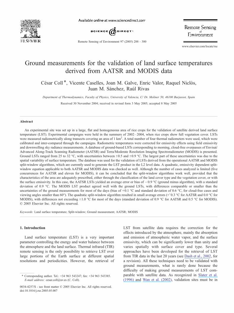
Fig. 2. Map of the area with the two 1 km2 test sites (UTM-Zone 30 coordinates,

AGA) is shown (*: 2003 campaign only). The center of test site 1 is at 733266E, 4

4348412N (0-17V43WW, 39-15V01WN).

Section 5, where the results of the validation are shown and

discussed. Finally, the conclusions are given in Section 6.

2. The Valencia experimental site

An experimental site suitable for the validation of

satellite-derived LSTs was set up in a large, flat and

homogeneous area in the Mediterranean coast of Spain,

close to the city of Valencia. The site is in a marshy plain

surrounding the Albufera Lake and separated from the sea

by a narrow strip of land. The area is shown in the color

composite image of Fig. 1, which is a part of an ASTER

scene taken on August 3, 2004. The region has been

traditionally dedicated to the intensive cultivation of rice.

From the end of June to the beginning of September, rice

crops are well developed and attain nearly full cover.

Crops are irrigated during the summer months, until

harvest in mid September. In these circumstances, the site

shows a high thermal homogeneity and is large enough for

making ground measurements of LST comparable to

satellite estimates. Only narrow tracks and irrigation

channels cross the site, which facilitates the accessibility

to the rice fields without breaking too much the

homogeneity of the area. In addition, the emissivity of

7335000 734500734000

7335000 734500734000

4349000

4348500

4348000

4347500

4347000

4346500

T SITE 2

ITE 1

CE 2

CE 1

Everest

Ce 1

Ce 2*

AG

A

in meters). The position of the TIR radiometers (CE 1, CE 2, Everest and

347050N (0-17V50WW, 39-14V27WN). The center of test site 2 is at 733397E,

C. Coll et al. / Remote Sensing of Environment 97 (2005) 288–300 291

green vegetation with full cover is well known (high

emissivity with small or null spectral variation between 8

and 13 Am; Rubio et al., 2003; Salisbury & D’Aria, 1992)

thus facilitating the measurement of surface temperatures

by means of TIR radiometers.

The ground LST measurements were performed in

squares of 1 km2 located in the southern part of the rice

field area, where it has a maximum extension (see Fig. 1). In

the campaigns of 2002 and 2003, the 1 km2 test site was

centered at 0-17V50W W, 39-14V27W N. For the 2004

campaign, the test site was moved 1 km North (center at

0-17V43W W, 39-15V01W N) because the new location was

apparently more homogeneous in terms of rice plant

development and growth this year. Fig. 2 shows a map

with the location of the 1 km2 test sites. Cloud free

atmospheric conditions are frequent in the area during the

months of July and August. According to the atmospheric

profile product of MODIS (MOD07), the total column

content of atmospheric water vapor (or precipitable water)

ranged between 1.5 cm and 3 cm for the days of the field

campaigns.

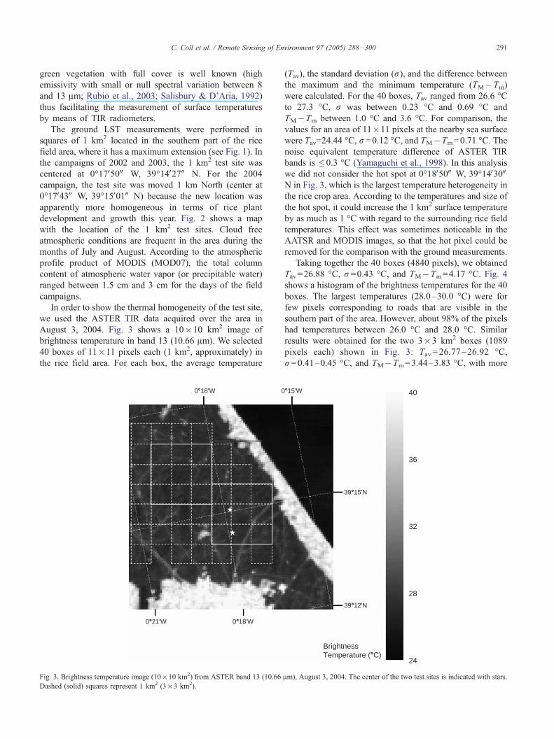
In order to show the thermal homogeneity of the test site,

we used the ASTER TIR data acquired over the area in

August 3, 2004. Fig. 3 shows a 10�10 km2 image of

brightness temperature in band 13 (10.66 Am). We selected

40 boxes of 11�11 pixels each (1 km2, approximately) in

the rice field area. For each box, the average temperature

0°18'W 0

0°21'W 0°18'W

Fig. 3. Brightness temperature image (10�10 km2) from ASTER band 13 (10.66

Dashed (solid) squares represent 1 km2 (3�3 km2).

(Tav), the standard deviation (r), and the difference between

the maximum and the minimum temperature (TM�Tm)

were calculated. For the 40 boxes, Tav ranged from 26.6 -Cto 27.3 -C, r was between 0.23 -C and 0.69 -C and

TM�Tm between 1.0 -C and 3.6 -C. For comparison, the

values for an area of 11�11 pixels at the nearby sea surface

were Tav=24.44 -C, r =0.12 -C, and TM�Tm=0.71 -C. Thenoise equivalent temperature difference of ASTER TIR

bands is �0.3 -C (Yamaguchi et al., 1998). In this analysis

we did not consider the hot spot at 0-18V50W W, 39-14V30WN in Fig. 3, which is the largest temperature heterogeneity in

the rice crop area. According to the temperatures and size of

the hot spot, it could increase the 1 km2 surface temperature

by as much as 1 -C with regard to the surrounding rice field

temperatures. This effect was sometimes noticeable in the

AATSR and MODIS images, so that the hot pixel could be

removed for the comparison with the ground measurements.

Taking together the 40 boxes (4840 pixels), we obtained

Tav=26.88 -C, r =0.43 -C, and TM�Tm=4.17 -C. Fig. 4shows a histogram of the brightness temperatures for the 40

boxes. The largest temperatures (28.0–30.0 -C) were for

few pixels corresponding to roads that are visible in the

southern part of the area. However, about 98% of the pixels

had temperatures between 26.0 -C and 28.0 -C. Similar

results were obtained for the two 3�3 km2 boxes (1089

pixels each) shown in Fig. 3: Tav =26.77–26.92 -C,r =0.41–0.45 -C, and TM�Tm=3.44–3.83 -C, with more

°15'W

39°15'N

39°12'N

40

36

32

28

24

BrightnessTemperature (°C)

Am), August 3, 2004. The center of the two test sites is indicated with stars.

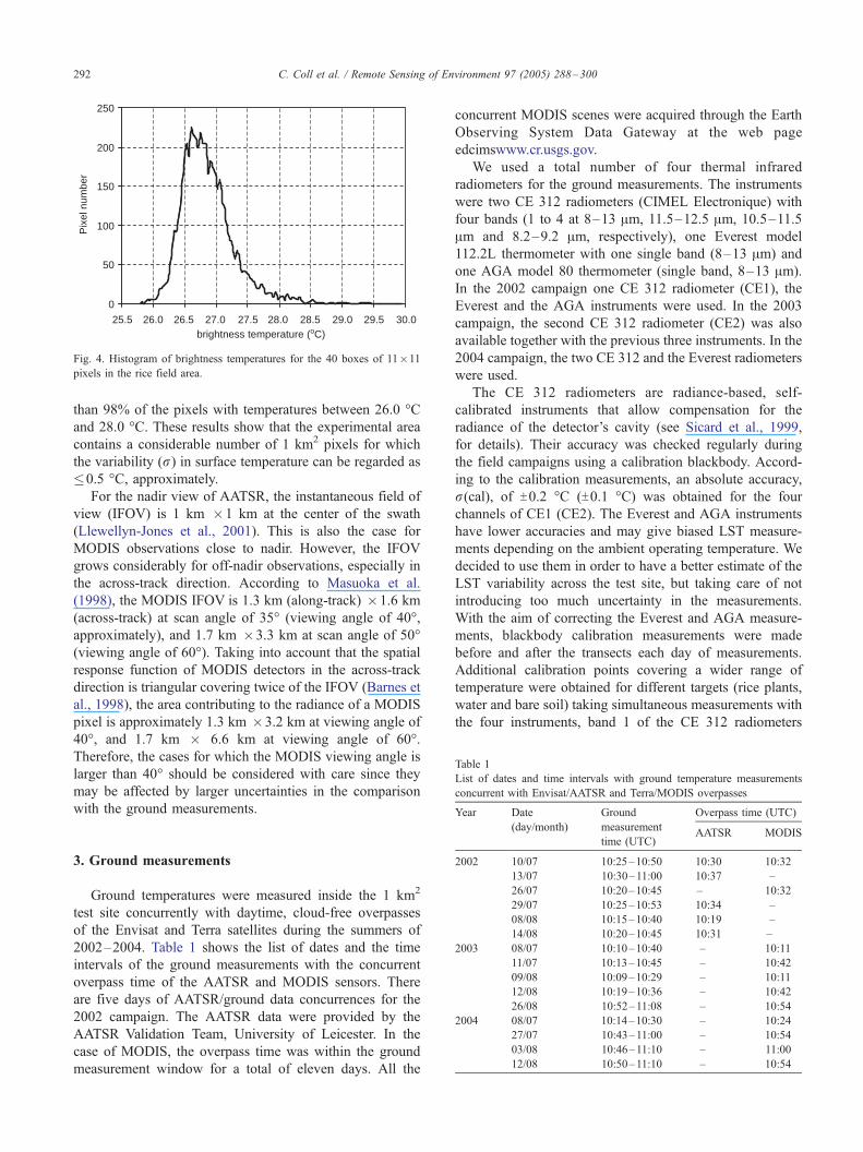
Table 1

List of dates and time intervals with ground temperature measurements

concurrent with Envisat/AATSR and Terra/MODIS overpasses

Year Date Ground Overpass time (UTC)

0

50

100

150

200

250

25.5 26.0 26.5 27.0 27.5 28.0 28.5 29.0 29.5 30.0

Pix

el n

umbe

r

brightness temperature (oC)

Fig. 4. Histogram of brightness temperatures for the 40 boxes of 11�11

pixels in the rice field area.

C. Coll et al. / Remote Sensing of Environment 97 (2005) 288–300292

than 98% of the pixels with temperatures between 26.0 -Cand 28.0 -C. These results show that the experimental area

contains a considerable number of 1 km2 pixels for which

the variability (r) in surface temperature can be regarded as

�0.5 -C, approximately.

For the nadir view of AATSR, the instantaneous field of

view (IFOV) is 1 km �1 km at the center of the swath

(Llewellyn-Jones et al., 2001). This is also the case for

MODIS observations close to nadir. However, the IFOV

grows considerably for off-nadir observations, especially in

the across-track direction. According to Masuoka et al.

(1998), the MODIS IFOV is 1.3 km (along-track) �1.6 km

(across-track) at scan angle of 35- (viewing angle of 40-,approximately), and 1.7 km �3.3 km at scan angle of 50-(viewing angle of 60-). Taking into account that the spatial

response function of MODIS detectors in the across-track

direction is triangular covering twice of the IFOV (Barnes et

al., 1998), the area contributing to the radiance of a MODIS

pixel is approximately 1.3 km �3.2 km at viewing angle of

40-, and 1.7 km � 6.6 km at viewing angle of 60-.Therefore, the cases for which the MODIS viewing angle is

larger than 40- should be considered with care since they

may be affected by larger uncertainties in the comparison

with the ground measurements.

(day/month) measurement

time (UTC)AATSR MODIS

2002 10/07 10:25–10:50 10:30 10:32

13/07 10:30–11:00 10:37 –

26/07 10:20–10:45 – 10:32

29/07 10:25–10:53 10:34 –

08/08 10:15–10:40 10:19 –

14/08 10:20–10:45 10:31 –

2003 08/07 10:10–10:40 – 10:11

11/07 10:13–10:45 – 10:42

09/08 10:09–10:29 – 10:11

12/08 10:19–10:36 – 10:42

26/08 10:52–11:08 – 10:54

2004 08/07 10:14–10:30 – 10:24

27/07 10:43–11:00 – 10:54

03/08 10:46–11:10 – 11:00

12/08 10:50–11:10 – 10:54

3. Ground measurements

Ground temperatures were measured inside the 1 km2

test site concurrently with daytime, cloud-free overpasses

of the Envisat and Terra satellites during the summers of

2002–2004. Table 1 shows the list of dates and the time

intervals of the ground measurements with the concurrent

overpass time of the AATSR and MODIS sensors. There

are five days of AATSR/ground data concurrences for the

2002 campaign. The AATSR data were provided by the

AATSR Validation Team, University of Leicester. In the

case of MODIS, the overpass time was within the ground

measurement window for a total of eleven days. All the

concurrent MODIS scenes were acquired through the Earth

Observing System Data Gateway at the web page

edcimswww.cr.usgs.gov.

We used a total number of four thermal infrared

radiometers for the ground measurements. The instruments

were two CE 312 radiometers (CIMEL Electronique) with

four bands (1 to 4 at 8–13 Am, 11.5–12.5 Am, 10.5–11.5

Am and 8.2–9.2 Am, respectively), one Everest model

112.2L thermometer with one single band (8–13 Am) and

one AGA model 80 thermometer (single band, 8–13 Am).

In the 2002 campaign one CE 312 radiometer (CE1), the

Everest and the AGA instruments were used. In the 2003

campaign, the second CE 312 radiometer (CE2) was also

available together with the previous three instruments. In the

2004 campaign, the two CE 312 and the Everest radiometers

were used.

The CE 312 radiometers are radiance-based, self-

calibrated instruments that allow compensation for the

radiance of the detector’s cavity (see Sicard et al., 1999,

for details). Their accuracy was checked regularly during

the field campaigns using a calibration blackbody. Accord-

ing to the calibration measurements, an absolute accuracy,

r(cal), of T0.2 -C (T0.1 -C) was obtained for the four

channels of CE1 (CE2). The Everest and AGA instruments

have lower accuracies and may give biased LST measure-

ments depending on the ambient operating temperature. We

decided to use them in order to have a better estimate of the

LST variability across the test site, but taking care of not

introducing too much uncertainty in the measurements.

With the aim of correcting the Everest and AGA measure-

ments, blackbody calibration measurements were made

before and after the transects each day of measurements.

Additional calibration points covering a wider range of

temperature were obtained for different targets (rice plants,

water and bare soil) taking simultaneous measurements with

the four instruments, band 1 of the CE 312 radiometers

C. Coll et al. / Remote Sensing of Environment 97 (2005) 288–300 293

being the reference temperature. The calibration database

was used to derive linear calibration equations that were

updated with new data each day (see Coll et al., in press, for

more details). Such calibration equations were used to

correct the bias in the Everest and AGA temperature

readings. However, the calibrated temperatures still had

relatively large dispersions, which were taken as the

calibration accuracy, r(cal) (typically, between T0.5 and

T0.7-C for the Everest, and between T0.7 and T0.9 -C for

the AGA).

In order to capture the spatial variability of the surface

temperature within the test site, each radiometer was

assigned to one part of the 1 km2 square (see Fig. 2).

Radiometers were carried back and forth along transects of

about 100 m length, looking at the surface at angles close to

nadir. The field of view of the radiometers was 30 cm on the

crop surface. Measurements were made at a rate of more

than 5 measurements per minute, covering a distance of 30–

50 m per minute. Data were collected during periods of 20–

30 min centered at the satellite overpass time, although

radiometers were in place and working 30 min before, in

order to assure a good stability of their response. For each

transect, we recorded the time of the individual measure-

ment and the corresponding radiometric temperature. With

these data we have obtained the ground LSTs to be

compared with the satellite derived LSTs, as well as the

spatial and temporal variability of LST at scales of 100 m

for different parts (transects) of the 1 km2 test site. The

processing of the ground temperatures is described below.

3.1. Emissivity correction

Radiometric temperatures must be corrected for emissiv-

ity effects, including the reflection of the downward sky

emission. If Tr is the radiometric temperature measured by a

thermal infrared radiometer, the true land surface temper-

ature T is given by

B Tð Þ ¼ B Trð Þ � 1� eð ÞLsky� �

=e ð1Þ

where B is the Planck function weighted for the filter of the

radiometer, e is the surface emissivity and Lsky is the

downward sky irradiance (Fsky) divided by p. The surface

emissivity was measured in the field using the box method

(Rubio et al., 2003). These measurements showed a high

emissivity (e =0.985) with negligible spectral variation (Collet al., in press), which is typical for green vegetation with

full cover (Rubio et al., 2003; Salisbury & D’Aria, 1992).

The downward sky radiance was measured at an angle of

53- from nadir, which is equivalent to Fsky/p according to

the diffusive approximation for clear skies (Kondratyev,

1969). These measurements were performed with each

radiometer at the start and the end of the temperature

transects. Then, the true LSTs can be calculated from the

radiometric temperatures according to Eq. (1) and inverting

the weighted Planck function. For e=0.985 the difference

T�Tr (i.e., the emissivity correction for the radiometric

temperatures) ranged between 0.3 -C and 0.6 -C, dependingon the magnitude of Lsky. The uncertainty associated to this

process is mainly due to the error in the emissivity value

used. For an error of T0.010 in emissivity, the resulting error

in temperature, r(em), ranged from T0.2 -C to T0.4 -C,depending on Lsky. The impact of the person carrying the

radiometer on the radiation reflected at the surface (which

affects Lsky in Eq. (2)) was evaluated to be 0.1 -C or less for

our conditions of measurement.

3.2. Averaging of ground temperatures for each transect

We considered only the temperatures measured within 3

min around the satellite overpass time (more than 20

temperature measurements covering a distance of about

100 m, for each transect) for comparison with the satellite

derived LSTs. These data were averaged for each transect/

radiometer and the standard deviation was calculated. It

gives us an estimation of the LST spatial and temporal

variability in a part of the test site, r(var). For the data

analyzed here, r(var) was between T0.3 -C and T0.5 -C for

both CE 312 radiometers, with similar values for the Everest

and AGA.

Moreover, we also considered the variability of LST for

the whole measurement period in order to check the

consistency of the ground data. For all the dates, we have

found no apparent temporal trend in temperature during the

¨20 min periods. The average LST for the whole period

differed from the 3-min average LST by only 0.0–0.3 -C for

most of the days. For the whole period, r(var) ranged

between T0.4 -C and T0.7 -C, comparable to the values for

the 3 min period mentioned above. As seen in Table 1, the

measurement interval for 12/08/2003 ended a few minutes

before the satellite overpass. Therefore, we could not take

the average LST for the 3 min period around the overpass

time. Instead, we considered the whole measurement period

for the average LST and r(var) on this date (no long-term

variability was observed in the ground temperatures).

The total uncertainty in the temperature measurement for

each radiometer, r(T), is given by the combination of the

three sources of error (calibration, emissivity correction and

spatial/temporal variability) according to

r Tð Þ ¼ r calð Þ2 þ r emð Þ2 þ r varð Þ2ih 1=2

: ð2Þ

For each day of measurement, we have 2–4 values of

ground LST (one for each radiometer/transect), with their

corresponding uncertainties. Tables 2 and 3 give the data

corresponding to the AATSR and MODIS overpasses of

Table 1, respectively. The accuracy of the ground LSTs

measured by the CE1 and CE2 radiometers was in the

range between T0.3 -C and T0.6 -C for most of the dates.

The largest part of this error was due to the natural variability

of surface temperatures, r(var). For the dates when the two

CE 312 instruments were available, the maximum difference

between their measured LSTs was 1.1 -C. In the case of the

Table 2

Ground LSTs (calibrated and emissivity corrected) and uncertainties

measured concurrently with the AATSR overpass during the 2002

campaign

Date (day/ AATSR Ground LST Tr(T) (-C)month/year) overpass

(UTC)CE 1 Everest AGA Average

10/07/02 10:30 28.4T0.6 29.1T1.0 – 28.6T0.6

13/07/02 10:37 27.2T0.8 28.2T0.8 27.9T1.0 27.6T0.9

29/07/02 10:34 28.1T0.5 27.2T0.8 28.1T1.0 27.9T0.7

08/08/02 10:19 26.4T0.6 – 26.7T1.0 26.5T0.714/08/02 10:31 28.4T0.5 28.6T0.8 – 28.5T0.5

C. Coll et al. / Remote Sensing of Environment 97 (2005) 288–300294

Everest and AGA instruments, the calibration error, r(cal),was usually the largest source of error (r(var) being similar

to that of CE1 and CE2). In order to avoid excessive

uncertainty due to the calibration problems of the Everest

and AGA instruments, we kept only their LST data with

r(T)�1.0 -C. In addition, we removed all LSTs measured

by these instruments that differed by more than 1.0 -C from

any of the CE 312 LSTs on the same day. As shown in Table

3, Everest and AGA were seldom used in the 2004

campaign.

3.3. Average ground LST

The ground LSTs to be compared with AATSR and

MODIS derived LSTs at 1 km2 resolution were calculated

by averaging all the individual ground temperatures within

the 3 min periods for the available radiometers each

measurement day. In this average, less weight was given

to the Everest and AGA readings since they are typically

less in number (owing to a smaller sampling frequency

compared with CE1 and CE2). The error associated with the

average LST was calculated with Eq. (2), including r(var)for all the individual temperatures averaged, the emissivity

correction error, and the calibration error for each instru-

ment. The average LSTs and uncertainties concurrent to the

AATSR and MODIS overpasses are given in the last column

of Tables 2 and 3, respectively. The range of the ground

LSTs was from 25 -C to 32 -C, with uncertainties between

Table 3

Ground LSTs (calibrated and emissivity corrected) and uncertainties measured co

Year Date (day/month) AATSR Ground LST Tr

CE 1

2002 10/07 10:32 28.6T0.5

26/07 10:32 28.0T0.6

2003 08/07 10:11 28.6T0.4

11/07 10:42 28.3T0.409/08 10:11 30.1T0.6

12/08 10:42 31.5T0.5

26/08 10:54 31.5T0.42004 08/07 10:24 25.3T0.5

27/07 10:54 27.9T0.6

03/08 11:00 29.5T0.6

12/08 10:54 28.6T0.5

T0.5 -C and T0.9 -C. This accuracy interval may not be

valid enough for the vicarious calibration of TIR satellite

radiometers, but we consider that it could be useful for the

validation of operational LST products derived from

satellite data in real conditions.

4. Split-window algorithms for LST

In this section, we briefly describe the different split-

window formulations for LST retrieval to be validated with

ground data in Section 5. They are (1) the algorithm used for

the derivation of the AATSR LST data product, (2) the

MODIS generalized split-window algorithm used to gen-

erate the MOD11_L2 LST product, and (3) a quadratic,

emissivity dependent split-window algorithm applicable to

both AATSR and MODIS data.

4.1. AATSR LST algorithm

Although the AATSR was primarily designed to obtain

accurate sea surface temperatures (Llewellyn-Jones et al.,

2001), it can be also applied for the retrieval of LSTs. The

AATSR LST algorithm (Prata, 2000) uses the brightness

temperatures at 11 Am and 12 Am, T11 and T12, for the nadir

view of AATSR. Basically the algorithm expresses the LST

as a linear combination of the brightness temperatures T11

and T12 with the coefficients being determined by regression

using simulated data-sets and depending on the land cover

type (i), the fractional vegetation cover ( f), the precipitable

water (pw) and the satellite zenith viewing angle (h). Itshould be noted that the algorithm has no explicit depend-

ence on surface emissivity. The effects of surface emissivity

are implicitly taken into account through the land cover type

and fractional cover dependent coefficients. The algorithm

can be written as

LST ¼ af ;i;pw þ bf ;i T11 � T12ð Þn þ bf ;i þ cf ;i� �

T12 ð3Þ

where n =cos(h/5) is approximately equal to 1 since

h <23.5- for the nadir view. (In fact, using n =1 in Eq. (3)

ncurrently with the MODIS overpass during the 2002–2004 campaigns

(T) (-C)

CE 2 Everest AGA average

– 29.6T0.9 – 28.8T0.7

– 27.8T0.8 28.4T1.0 28.1T0.7

28.6T0.4 29.1T0.9 – 28.7T0.5

29.3T0.5 29.3T0.7 – 28.9T0.829.1T0.7 – 29.7T0.7 29.7T0.8

30.8T0.5 31.3T0.8 31.5T0.9 31.2T0.6

32.2T0.5 – – 31.9T0.6– 25.5T0.8 – 25.3T0.6

27.8T0.5 – – 27.9T0.6

30.6T0.6 – – 30.0T0.7

28.8T0.3 – – 28.7T0.5

C. Coll et al. / Remote Sensing of Environment 97 (2005) 288–300 295

instead of the exact value of n implies a very small

difference in LST: for h =23.5-, we have n =0.9966, which

yields a LST difference lower than 0.04 -C for T11�T12=3

-C.) The coefficients of Eq. (3) are given by:

af ;i;pw ¼ 0:4 sec hð Þ � 1½ pwþ f av;i þ 1� fð Þ as;ibf ;i ¼ f bv;i þ 1� fð Þbs;icf ;i ¼ f cv;i þ 1� fð Þcs;i:

These coefficients have been calculated for the 13

different biomes or land cover classes (i =1 to 13) defined

by Dorman and Sellers (1989). For a given land cover class,

two separate sets of coefficients are given for the fully

vegetated surface (subscript v) and for the bare surface

(subscript s), which are weighted by the fractional vegeta-

tion cover f. The precipitable water (pw, in cm or g/cm2) is

obtained from climatologic data. It is only required for the

term 0.4[sec(h)�1]pw in coefficient af,i,pw and has a small

impact on LST: since h <23.5- for the AATSR nadir view,

flLST/flpw=0.4[sec(h)�1] is always smaller than 0.04 -C/cm. The AATSR LST algorithm is operationally imple-

mented at the Rutherford Appleton Laboratory (RAL) in the

so-called RAL processor. It uses the last version of the split-

window coefficients (Prata, 2002). The values of i, f and pw

required for the application of the algorithm are obtained

from global classification, fractional vegetation cover maps

and global climatology at a spatial resolution of 0.5-�0.5-longitude/latitude. Monthly variability is allowed for f and

pw. LST images produced with this algorithm are currently

provided with AATSR_L2 data.

Since the 0.5- grid cell is too coarse in order to properly

assign split-window coefficients to specific, relatively small

areas such as our test site, we implemented the LST

algorithm to the AATSR brightness temperatures T11 and

T12 from AATSR L1b data for our test area only. Thus, we

selected land cover class i =6 (broadleaf trees with ground-

cover, which is the class assigned to our site by the RAL

processor) with f =1 (full vegetation cover) which is

appropriate for the fully developed rice crops in summer

(the RAL processor assigned f =0.40–0.47 in July and

August). Using the last available version of the coefficients,

the AATSR LST equation locally tuned to our study areas is

LST ¼ 0:4 sec hð Þ � 1½ pwþ 0:9089

þ 3:3511 T11 � T12ð Þn þ 0:9621T12 ð4Þ

with LST, T11 and T12 in -C. The precipitable water taken

was pw=2.5 cm for midlatitude summer conditions. The

impact of pw in LST is very small for the viewing angles of

the AATSR nadir view, as mentioned above.

4.2. MODIS generalized split-window algorithm

The generalized split-window algorithm applied to the

MODIS brightness temperatures in channels 31 (10.78–

11.28Am) and 32 (11.77–12.27Am), T31 and T32, can be

written as (Wan and Dozier, 1996)

LST ¼ C þ A1 þ A2

1� ee

þ A3

Dee2

��T31 þ T32

2

þ B1 þ B2

1� ee

þ B3

Dee2

��T31 � T32

2ð5Þ

where e =(e31+ e32)/2 and De = e31� e32 are, respectively,

the mean emissivity and the emissivity difference in MODIS

channels 31 and 32. Coefficients C, Ai and Bi were obtained

from linear regression of MODIS simulated data for wide

ranges of surface and atmospheric conditions, and they

depend on the view angle, the column water vapor content

and the atmospheric lower boundary temperature. The

required emissivities are obtained form classification-based

emissivities (Snyder et al., 1998), which have been modeled

for 14 different land cover types. For each MODIS pixel, the

land cover class is assigned according to the classification

given by the MODIS land-cover product. The LST

generated with the generalized split-window algorithm is

provided in the MODIS product MOD11_L2 (Wan et al.,

2002).

4.3. Quadratic, emissivity dependent split-window

algorithm

The LST split-window algorithm of Coll and Caselles

(1997) has an explicit dependence on surface emissivity. For

two generic channels at 11 Am and 12 Am, channels 1 and 2,

respectively, and using the mean emissivity, e =(e1+ e2)/2,and the channel emissivity difference, De= e1� e2, the

algorithm can be written as

LST ¼ T1 þ a0 þ a1 T1 � T2ð Þ þ a2 T1 � T2ð Þ2

þ a 1� eð Þ � bDe ð6Þ

where coefficients a0, a1, a2, a and b depend on the

particular split-window channels used, coefficient b depend-

ing also on the precipitable water. This algorithm was

applied and validated with NOAA/AVHRR data in Coll and

Caselles (1997) and with GMS-5 VISSR data in Prata and

Cechet (1999). It has a quadratic dependence on the

brightness temperature difference (T1�T2) in order to

account for the increase of the atmospheric correction for

large amounts of atmospheric water vapor.

For the full cover rice crops of the Valencia test site, we

can expect a high value of surface emissivity with no

spectral variation in the spectral band between 10.5 Am and

12.5 Am. Based on the emissivity measurements performed

in the site, we can take e =0.985 and De =0 (Coll et al., in

press). In the case of AATSR, we used the values for the

coefficients of Eq. (6) given by Soria et al. (2002). These

coefficients were calculated from a regression analysis over

a database of simulated top-of-the-atmosphere AATSR

radiances covering global surface and atmospheric con-

Table 5

Brightness temperatures (in -C) interpolated for the four pixels closest to

the center of the test site, MODIS channels 31 and 32

Date

(day/month/year)

h (-) T31 r31 T32 r32 pw

(cm)

10/07/02 43.7 23.89 0.15 23.01 0.16 2.42

26/07/02 43.7 21.68 0.06 20.25 0.06 2.88

08/07/03 60.3 22.22 0.02 20.84 0.04 2.22

11/07/03 27.7 26.68 0.18 26.23 0.17 1.60

09/08/03 60.5 23.30 0.32 21.93 0.21 2.21

12/08/03 28.1 28.23 0.10 27.73 0.08 1.47

26/08/03 6.7 24.73 0.05 23.17 0.04 2.99

08/07/04 50.3 22.46 0.62 21.94 0.65 1.90

27/07/04 5.6 25.45 0.06 24.90 0.06 1.68

03/08/04 6.1 26.92 0.13 26.03 0.15 2.68

12/08/04 5.7 25.81 0.03 25.24 0.04 2.03

The standard deviation of temperatures, r, and the satellite viewing angle,

h, are given. The last column gives the atmospheric precipitable water, pw,

obtained from the MODIS atmospheric profile product (MOD07).

C. Coll et al. / Remote Sensing of Environment 97 (2005) 288–300296

ditions. The AATSR algorithm can be written specifically

for the test site (e =0.985; De =0) as

LST ¼ T11 þ 0:57þ 1:03 T11 � T12ð Þ

þ 0:26 T11 � T12ð Þ2: ð7Þ

Similarly, the coefficients for Eq. (6) appropriate for

MODIS were taken from Sobrino et al. (2003), which were

also obtained from regression analysis over a simulated

database of MODIS radiances covering worldwide con-

ditions. With these coefficients and taking e =0.985 and

De=0, the MODIS algorithm is

LST ¼ T31 þ 1:52þ 1:79 T31 � T32ð Þ

þ 1:20 T31 � T32ð Þ2: ð8Þ

5. Results and discussion

For AATSR, we tested three split-window equations (1)

the AATSR LST algorithm (Eq. (3)) as applied operationally

at RAL (i.e., the RAL processor), and provided as a product

in the AATSR_L2 data; (2) the AATSR LST algorithm

specific for the test site, i.e. Eq. (4), which was applied to

brightness temperatures from AATSR_L1b data; and (3) the

quadratic, emissivity dependent algorithm given by Eq. (7),

also applied to AATSR_L1b data. For MODIS, we checked

two formulations: (1) the generalized split-window algo-

rithm (Eq. (5)) as given by the MOD11_L2 product; and (2)

the quadratic, emissivity dependent algorithm given by Eq.

(8) applied to MODIS L1b data.

For each day with concurrent satellite data and ground

LSTs, the satellite brightness temperatures for the split-

window channels (T11 and T12, nadir view, for AATSR; T31

and T32 for MODIS) corresponding to the test site were

interpolated from the four pixels closest to the center of the

test site, according to Wan et al. (2002). The interpolated

brightness temperatures and the standard deviation (r) of

the four temperatures used are given in Table 4 for AATSR

and Table 5 for MODIS, together with the satellite viewing

zenith angle (h). In Table 5, the atmospheric precipitable

Table 4

Brightness temperatures (in -C) interpolated for the four pixels closest to

the center of the test site, AATSR channels at 11 and 12 Am, nadir view

Date

(day/month/year)

h (-) T11 r11 T12 r12

10/07/02 3.7 25.07 0.03 23.03 0.02

13/07/02 13.8 22.25 0.05 19.22 0.04

29/07/02 8.8 22.90 0.05 21.03 0.05

08/08/02 16.2 20.29 0.07 17.31 0.07

14/08/02 3.9 23.77 0.06 21.58 0.03

The standard deviation of temperatures, r, and the satellite viewing angle,

h, are given.

water (pw) obtained from the MODIS atmospheric profile

product (MOD07) is also shown. According to Table 4, the

standard deviation of the AATSR brightness temperatures

was always smaller than 0.1 -C, and observation was close

to nadir (h�16-). MODIS covers a wider range of viewing

angles (up to 60- for our data). For low h, the standard

deviation of the MODIS brightness temperatures was

similar to that of AATSR. The largest values of r were

generally associated with the largest viewing angles;

however, r�0.3 -C for most of the cases. These results

show a good thermal homogeneity of the test area at the

AATSR and MODIS spatial scales. Nevertheless, special

care should be taken in the case of large observation

angles, for which the uncertainty in the comparison with

the ground LST could be larger than for nadir observation.

On the other hand, the brightness temperature difference

(T11�T12 or T31�T32), which plays an important role in

the split-window algorithms, was between 1.87 -C and

3.03 -C for AATSR, and between 0.45 -C and 1.56 -C for

MODIS.

The results of the comparison between the ground LSTs

and the split-window LSTs are shown in Table 6 for AATSR

and in Table 7 for MODIS. For each date, the average

ground LST (from Table 2 for AATSR and from Table 3 for

MODIS) is given together with the AATSR or MODIS

derived LSTs. For each of the algorithms, we give the LST

for the test site interpolated from the four neighboring

pixels, and the difference between the ground and the

algorithm LST.

Although the number of data available for the LST

comparison was rather limited, some conclusions can be

drawn from these results. Regarding AATSR, the LSTs

obtained from the RAL processor seem to overestimate the

ground LSTs by 3 -C in average. However, the LSTs

calculated with Eq. (4) show a better agreement with the

ground data, with a maximum difference of �2.0 -C, anaverage difference or bias of �0.9 -C, and a standard

deviation of 0.9 -C. As mentioned before, the RAL

Table 6

Comparison of ground and AATSR derived LSTs

Date

(d/m/y)

Ground

LST (-C)

AATSR LST (-C) Ground-AATSR LST (-C)

RAL proc. Eq. (4) Eq. (7) RAL proc. Eq. (4) Eq. (7)

10/07/02 28.6 32.2 29.9 28.8 �3.6 �1.3 �0.2

13/07/02 27.6 31.8 29.6 28.3 �4.2 �2.0 �0.7

29/07/02 27.9 29.7 27.4 26.3 �1.8 0.5 1.6

08/08/02 26.5 29.4 27.6 26.2 �2.9 �1.1 0.3

14/08/02 28.5 30.9 29.0 27.8 �2.4 �0.5 0.7

Bias (-C) �3.0 �0.9 0.3

Standard deviation (-C) 0.9 0.9 0.9

The LST derived from the three algorithms is given as well as the difference between the ground and the algorithm LSTs.

C. Coll et al. / Remote Sensing of Environment 97 (2005) 288–300 297

processor assigns the split-window coefficients based on

global classification and fractional vegetation cover maps at

a spatial resolution of 0.5-�0.5- longitude/latitude (for the

Valencia test site, i =6; broadleaf trees with ground cover,

and f =0.40�0.47 in July and August). The only difference

in Eq. (4) is that we used f=1, which is more appropriate for

our test area and yields better results for LST. In order to

check the sensitivity of the AATSR LST algorithm to the

split-window coefficients, various sets of coefficients for

different land cover types were used with f =1 and pw=2.5

cm. The best results were found for i =5 (needleleaf

deciduous trees), with a maximum difference with regard

to the ground LST of 1.3 -C, average bias of 0.0 -C and a

standard deviation of 0.9 -C. Also, for i=8 (broadleaf

shrubs with groundcover), the maximum difference was 1.6

-C, the bias was 0.3 -C and the standard deviation was 0.9

-C. These results are comparable to those of Eq. (4), which

points out the consistence of the AATSR LST algorithm. On

the other hand, the quadratic, emissivity dependent LST

algorithm of Eq. (7) yielded also a good agreement with the

Table 7

Comparison of ground and MODIS derived LSTs

Date

(d/m/y)

Ground

LST (-C)MODIS LST (-C) Ground-MODIS LST (-C)

MOD11 Eq. (8) MOD11 Eq. (8)

10/07/02* 28.8 27.4 27.9 1.4 0.9

26/07/02a,* 28.1 26.4 28.2 1.7 �0.1

08/07/03** 28.7 27.5 28.5 1.2 0.2

11/07/03 28.9 29.3 29.2 �0.4 �0.3

09/08/03** 29.7 28.6 29.5 1.1 0.2

12/08/03 31.2 31.0 30.9 0.2 0.3

26/08/03a 31.9 29.7 32.0 2.2 �0.1

08/07/04* 25.3 25.4 25.2 �0.1 0.1

27/07/04 27.9 28.2 28.3 �0.3 �0.4

03/08/04 30.0 30.3 31.0 �0.3 �1.0

12/08/04 28.7 28.7 28.7 0.0 0.0

Bias (-C) 0.6 0.0

Standard deviation (-C) 0.9 0.5

The LST derived from the two algorithms is given as well as the difference

between the ground and the algorithm LSTs.a Cirrus clouds.

T h >40-.TT h >60-.

ground data (maximum difference of 1.6 -C, average bias of0.3 -C and standard deviation of 0.9 -C). The results of thesimple algorithm of Eq. (7), as well as those of Eq. (4), give

confidence to the use of split-window methods for the

retrieval of LST from AATSR data.

With regard to MODIS, the MOD11 LST product

showed a good agreement with the ground LST, with

differences around or smaller than the ground measurement

errors for most of the dates. It should be noted that, as

mentioned in Section 4.2, the emissivities for the general-

ized split-window algorithm used by MODIS (Eq. (5)) are

assigned on a pixel by pixel basis, which allows a good

representation of the variability of surface types across a

scene. Taking the eleven data of Table 7, the MOD11 LST

yielded an average bias of 0.6 -C and standard deviation of

0.9 -C. The maximum differences with regard to the ground

LST were around 2 -C for days 26/07/02 and 26/08/03. The

reason for such big discrepancies was investigated by

looking at the correlation between the brightness temper-

ature difference, T31�T32, and the precipitable water along

the MODIS viewing direction, pw/cosh, which can be

obtained from the data of Table 5. For these two days,

T31�T32 was the highest (1.4�1.6 -C) while pw/cosh had

moderate values (3.0�3.9 cm, for a total range of 1.7�4.5

cm). The anomalous large values of T31�T32 for the two

cases could be due to invisible cirrus clouds (Wan, personal

communication). If these two days were not considered, the

average bias of MOD11 was 0.3 -C with a standard

deviation of 0.7 -C. Additionally, the viewing angle was

very large (h >60-) for days 08/07/03 and 09/08/03.

Removing these dates also, the average bias was 0.1 -Cand the standard deviation was 0.6 -C. The maximum

difference was 1.4 -C for 10/07/02; however, the uncer-

tainty in the ground measurements for this day was large

since, as shown in Table 3, only two instruments (CE1 and

Everest) were used and they differed by 1 -C. On the other

hand, the quadratic algorithm of Eq. (8) yielded excellent

results when compared with the ground LSTs: a maximum

difference of �1.0 -C, a bias of 0.0 -C and a standard

deviation of 0.5 -C.As shown in Table 5, the MODIS data encompass

viewing angles from close to nadir to 60-. Ground LST

measurements were performed close to nadir, so there may

MOD11_L2 (v.a.<40o)

MOD11_L2 (v.a.>40o)

Eq. (8)

2.5

2.0

1.0

-1.0

1.5

0.5

-0.5

0.0

0.2 0.4 0.6 0.8 1.0 1.2 1.4 1.6

T31-T32 (°C)

∆T (

°C)

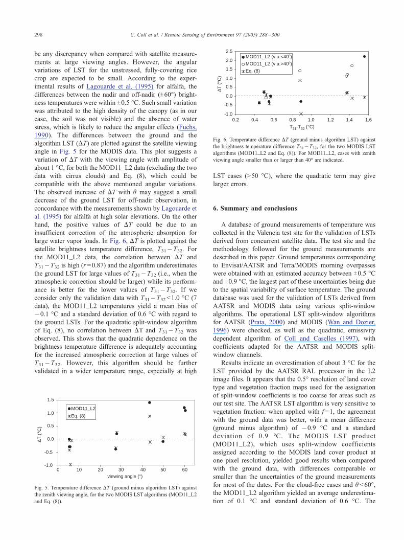
Fig. 6. Temperature difference DT (ground minus algorithm LST) against

the brightness temperature difference T31�T32, for the two MODIS LST

algorithms (MOD11_L2 and Eq. (8)). For MOD11_L2, cases with zenith

viewing angle smaller than or larger than 40- are indicated.

C. Coll et al. / Remote Sensing of Environment 97 (2005) 288–300298

be any discrepancy when compared with satellite measure-

ments at large viewing angles. However, the angular

variations of LST for the unstressed, fully-covering rice

crop are expected to be small. According to the exper-

imental results of Lagouarde et al. (1995) for alfalfa, the

differences between the nadir and off-nadir (T60-) bright-ness temperatures were within T0.5 -C. Such small variation

was attributed to the high density of the canopy (as in our

case, the soil was not visible) and the absence of water

stress, which is likely to reduce the angular effects (Fuchs,

1990). The differences between the ground and the

algorithm LST (DT) are plotted against the satellite viewing

angle in Fig. 5 for the MODIS data. This plot suggests a

variation of DT with the viewing angle with amplitude of

about 1 -C, for both the MOD11_L2 data (excluding the two

data with cirrus clouds) and Eq. (8), which could be

compatible with the above mentioned angular variations.

The observed increase of DT with h may suggest a small

decrease of the ground LST for off-nadir observation, in

concordance with the measurements shown by Lagouarde et

al. (1995) for alfalfa at high solar elevations. On the other

hand, the positive values of DT could be due to an

insufficient correction of the atmospheric absorption for

large water vapor loads. In Fig. 6, DT is plotted against the

satellite brightness temperature difference, T31�T32. For

the MOD11_L2 data, the correlation between DT and

T31�T32 is high (r =0.87) and the algorithm underestimates

the ground LST for large values of T31�T32 (i.e., when the

atmospheric correction should be larger) while its perform-

ance is better for the lower values of T31�T32. If we

consider only the validation data with T31�T32<1.0 -C (7

data), the MOD11_L2 temperatures yield a mean bias of

�0.1 -C and a standard deviation of 0.6 -C with regard to

the ground LSTs. For the quadratic split-window algorithm

of Eq. (8), no correlation between DT and T31�T32 was

observed. This shows that the quadratic dependence on the

brightness temperature difference is adequately accounting

for the increased atmospheric correction at large values of

T31�T32. However, this algorithm should be further

validated in a wider temperature range, especially at high

MOD11_L2

1.5

1.0

0.5

0.0

0 10viewing angle (°)

∆T (

°C)

20 30 40 50 60

-0.5

-1.0

Eq. (8)

Fig. 5. Temperature difference DT (ground minus algorithm LST) against

the zenith viewing angle, for the two MODIS LST algorithms (MOD11_L2

and Eq. (8)).

LST cases (>50 -C), where the quadratic term may give

larger errors.

6. Summary and conclusions

A database of ground measurements of temperature was

collected in the Valencia test site for the validation of LSTs

derived from concurrent satellite data. The test site and the

methodology followed for the ground measurements are

described in this paper. Ground temperatures corresponding

to Envisat/AATSR and Terra/MODIS morning overpasses

were obtained with an estimated accuracy between T0.5 -Cand T0.9 -C, the largest part of these uncertainties being due

to the spatial variability of surface temperature. The ground

database was used for the validation of LSTs derived from

AATSR and MODIS data using various split-window

algorithms. The operational LST split-window algorithms

for AATSR (Prata, 2000) and MODIS (Wan and Dozier,

1996) were checked, as well as the quadratic, emissivity

dependent algorithm of Coll and Caselles (1997), with

coefficients adapted for the AATSR and MODIS split-

window channels.

Results indicate an overestimation of about 3 -C for the

LST provided by the AATSR RAL processor in the L2

image files. It appears that the 0.5- resolution of land cover

type and vegetation fraction maps used for the assignation

of split-window coefficients is too coarse for areas such as

our test site. The AATSR LST algorithm is very sensitive to

vegetation fraction: when applied with f =1, the agreement

with the ground data was better, with a mean difference

(ground minus algorithm) of �0.9 -C and a standard

deviation of 0.9 -C. The MODIS LST product

(MOD11_L2), which uses split-window coefficients

assigned according to the MODIS land cover product at

one pixel resolution, yielded good results when compared

with the ground data, with differences comparable or

smaller than the uncertainties of the ground measurements

for most of the dates. For the cloud-free cases and h <60-,the MOD11_L2 algorithm yielded an average underestima-

tion of 0.1 -C and standard deviation of 0.6 -C. The

C. Coll et al. / Remote Sensing of Environment 97 (2005) 288–300 299

quadratic algorithm showed a good performance for both

AATSR and MODIS data, giving differences with the

ground LSTs within T1.0 -C for most of the days and the

smallest average biases (+0.3 -C for AATSR and 0.0 -C for

MODIS). Although the number of validation data is rather

small and limited to the case of a fully vegetated surface

with ground LSTs ranging from 25 to 32 -C and in

conditions of moderate loads of atmospheric water vapor

(1.5–3 cm), these results give confidence to the LSTs

derived by means of split-window methods. We expect to

augment the number of validation data in the Valencia test

site in future campaigns, for both day and night. More TIR

radiometers will be used in order to better characterize the

spatial variability of LST at the site.

Acknowledgements

This work has been financed by the Ministerio de

Ciencia y Tecnologıa(Accion Especial REN2002-11605-E/

CLI; Project REN2001-3116/CLI, and Ramon y Cajal

Research Contract of Dr. E. Valor), the Ministerio de

Educacion y Ciencia(Project CGL2004-06099-C03-01,

Accion Complementaria CGL2004-0166-E and Research

Grant of Dr. R. Niclos), the AlBan programme of the

European Union (Research Grant of Dr. R. Rivas) and the

University of Valencia (V Segles Research Grant of Mr. J.

M. Sanchez). NASA (Project EOS/03-0043-0379) is also

acknowledged. We wish to thank the AATSR Validation

Team and the EOS Data Gateway for providing the satellite

data. Fruitful discussions and suggestions from Dr. Zhengm-

ing Wan (UCSB) are greatly appreciated.

References

Barnes, W. L., Pagano, T. S., & Salomonson, V. V. (1998). Prelaunch

characteristics of the Moderate Resolution Imaging Spectroradiometer

(MODIS) on EOS-AM1. IEEE Transactions on Geoscience and Remote

Sensing, 36, 1088–1100.

Becker, F., & Li, Z.-L. (1990). Towards a local split-window method over

land surfaces. International Journal of Remote Sensing, 11, 369–394.

Becker, F., & Li, Z.-L. (1995). Surface temperature and emissivity at

various scales: Definition, measurement and related problems. Remote

Sensing Reviews, 12, 225–253.

Coll, C., & Caselles, V. (1997). A global split-window algorithm for

land surface temperature from AVHRR data: Validation and

algorithm comparison. Journal of Geophysical Research, 102D,

16697–16713.

Coll, C., Valor, E., Caselles, V., Niclos, R., Rivas, R., Sanchez, J.M., Galve,

J.M. (in press). Evaluation of the Envisat-AATSR land surface temper-

ature algorithm with ground measurements in the Valencia test site.

Proceedings of the Envisat Symposium, 6–10 September 2004,

Salzburg, Austria.

Dash, P., Gottsche, F. M., Olesen, F. S., & Fischer, H. (2002). Land surface

temperature and emissivity estimation from passive sensor data: Theory

and practice—current trends. International Journal of Remote Sensing,

23(13), 2563–2594.

Dorman, J. L., & Sellers, P. J. (1989). A global climatology for albedo,

roughness length and stomatal resistance for atmospheric general

circulation models as represented by the simple biosphere model

(SiB). Journal of Applied Meteorology, 28, 833–855.

Fuchs, M. (1990). Infrared measurements of canopy temperature and

detection of plant water stress. Theoretical and Applied Climatology,

42, 253–261.

Kondratyev, K. Ya. (1969). Radiation in the Atmosphere. New York’

Academic Press.

Lagouarde, J. P., Kerr, Y. H., & Brunet, Y. (1995). An experimental

study of angular effects on surface temperature for various plant

canopies and bare soils. Agricultural and Forest Meteorology, 77,

167–190.

Llewellyn-Jones, D., Edwards, M. C., Mutlow, C. T., Birks, A. R., Barton,

I. J., & Tait, H. (2001, February). AATSR: Global-change and surface-

temperature measurements from ENVISAT. ESA Bulletin, 11–21.

Masuoka, E., Fleig, A., Wolfe, R. E., & Patt, F. (1998). Key characteristics

of MODIS data products. IEEE Transactions on Geoscience and

Remote Sensing, 36(4), 1313–1323.

Prata, A. J. (1994). Land surface temperatures derived from the advanced

very high resolution radiometer and the along track scanning radio-

meter. II. Experimental results and validation of AVHRR algorithms.

Journal of Geophysical Research, 99D, 13025–13058.

Prata, A. J. (2000). Land surface temperature measurement from space:

AATSR Algorithm theoretical basis document. Technical report.

CSIRO 27 pp.

Prata, A. J. (2002). Land surface temperature measurement from space:

Global surface temperature simulations for the AATSR. Technical

report. CSIRO 15 pp.

Prata, A. J. (2003). Land surface temperature measurement from space:

Validation of the AATSR land surface temperature product. Technical

report. CSIRO 40 pp.

Prata, A. J., & Cechet, R. P. (1999). An assessment of the accuracy of land

surface temperature determination from the GMS-5 VISSR. Remote

Sensing of Environment, 67, 1–14.

Price, J. C. (1984). Land surface temperature measurements from the split-

window channels of the NOAA 7 AVHRR. Journal of Geophysical

Research, 89(D5), 7231–7237.

Rubio, E., Caselles, V., Coll, C., Valor, E., & Sospedra, F. (2003). Thermal-

infrared emissivities of natural surfaces: Improvements on the exper-

imental set-up and new measurements. International Journal of Remote

Sensing, 24(24), 5379–5390.

Salisbury, J. W., & D’Aria, D. M. (1992). Emissivity of terrestrial materials

in the 8–14 Am atmospheric window. Remote Sensing of Environment,

42, 83–106.

Sicard, M., Spyak, P. R., Brogniez, G., Legrand, M., Abuhassan, N.

K., Pietras, C., & Buis, J. P. (1999). Thermal infrared field ra-

diometer for vicarious cross-calibration: Characterization and com-

parisons with other field instruments. Optical Engineering, 38(2),

345–356.

Slater, P., Bigger, S. F., Thome, K., Gellman, D. I., & Spyak, P. R. (1996).

Vicarious radiometric calibration of EOS sensors. Journal of Atmos-

pheric and Oceanic Technology, 13, 349–359.

Snyder, W. C., Wan, Z., Zhang, Y., & Feng, Y.-Z. (1998). Classification-

based emissivity for land surface temperature from space. International

Journal of Remote Sensing, 19, 2753–2774.

Sobrino, J. A., El Kharraz, J., & Li, Z.-L. (2003). Surface temperature and

water vapour retrieval from MODIS data. International Journal of

Remote Sensing, 24(24), 5161–5182.

Soria, G., Sobrino, J. A., Cuenca, J., Prata, A. J., Jimenez-Munoz, J. C.,

Gomez, M., & El-Kharraz, J. (2002). Surface temperature retrieval from

AATSR data: Multichannel and multiangle algorithms. Proceedings of

recent advances in quantitative remote sensing (pp. 952–955).

University of Valencia.

Wan, Z., & Dozier, J. (1996). A generalized split-window algorithm for

retrieving land surface temperature from space. IEEE Transactions on

Geoscience and Remote Sensing, 34(4), 892–905.

Wan, Z., Zhang, Y., Zhang, Q., & Li, Z.-L. (2002). Validation of the land-

surface temperature products retrieved from terra moderate resolution

C. Coll et al. / Remote Sensing of Environment 97 (2005) 288–300300

imaging spectroradiometer data. Remote Sensing of Environment, 83,

163–180.

Wan, Z., Zhang, Y., Zhang, Q., & Li, Z. L. (2004). Quality assessment and

validation of the MODIS global land surface temperature. International

Journal of Remote Sensing, 25(1), 261–274.

Yamaguchi, Y., Kahle, A. B., Tsu, H., Kawakami, T., & Pniel, M. (1998).

Overview of Advanced Spaceborne Thermal Emission and Reflection

Radiometer (ASTER). IEEE Transactions on Geoscience and Remote

Sensing, 36, 1062–1071.