GREENHOUSE PUZZLES

KEELING'S WORLD MARTIN'S WORLD WALKER'S WORLD

Wallace S. Broecker LAMONT-DOHERTY EARTH OBSERVATORY

of Columbia University Palisades, NY 10964

Tsung-Hung Peng

ATLANTIC OCEANOGRAPHIC AND METEOROLOGICAL LABORATORY

of National Oceanic and Atmospheric Administration

Miami, FL 33149

Second Edition 1998

ELDIGIO PRESS

Preface

Our field suffers from a dearth of textbooks. Further, those that do exist are often

prohibitively expensive and often somewhat out-of-date. Because of this, our students

are forced to do much of their reading in specialized journal articles written for

professionals.

This problem is related to the highly competitive and rapidly changing character

of global change science. Researchers qualified to write textbooks are far too busy with

proposals, reports, journal articles, workshops... to take out the immense amount of time

it takes to put together a textbook. Books are often written over a period of years. The

publisher then takes a year or two more to review, tune, proofread and print the book. By

this time, the field has often advanced to the point where a revision is needed a few years

after publication.

Recognizing these problems, we have tried to dream up some innovations to the

process. Tracers in the Sea was self-published allowing the price to be held down by

threefold. The Glacial World According to Wally and this book go a step further. They

are designed to permit ease of continuing revision. No formal printing will be made.

Rather, spiral-bound xerox copies are sold to interested users. The user is encouraged to

xerox as many copies as he or she wishes.

The other advantage is that we, the authors, can produce these books with far less

effort than were they to be formally printed. As new information appears, we can make

revisions and put out updated versions.

Of course, this approach is not without its disadvantages. As the quality of

reproduction of photographs is poor, we avoid using them. The rigor in proofreading is

not up to publishing-house standards. But for a profession that does much of its reading

in preprints, this is not a serious drawback. The authors September 1998

Part I

KEELING'S WORLD

IS CO2 GREENING THE EARTH?

CONTENTS

Keeling's World: Is CO2 Greening the Earth-------------------------------------------- K-1 The Knowns --------------------------------------------------------------------------------- K-10 The Mirror Image Approach--------------------------------------------------------------- K-10 Ocean Uptake-------------------------------------------------------------------------------- K-16 Chemical Versus Isotope Adjustment Time --------------------------------------------- K-33 Isotopic Cross Checks ---------------------------------------------------------------------- K-35 Air to Sea CO2 Flux ------------------------------------------------------------------------ K-41 Interhemispheric CO2 Gradient ----------------------------------------------------------- K-46 Ocean Uptake Revisited -------------------------------------------------------------------- K-55 Global Greening----------------------------------------------------------------------------- K-58 Projections to the Future ------------------------------------------------------------------- K-67 CO2 Management --------------------------------------------------------------------------- K-69 Summary ------------------------------------------------------------------------------------- K-69 Commentary on Keeling's World Plates-------------------------------------------------- K-71 Keeling's World Problems ----------------------------------------------------------------- K-82 Super Problem------------------------------------------------------------------------------- K-89 Annotated Bibliography-------------------------------------------------------------------- K-94 CO2 Production Fossil Fuel Burning--------------------------------------------- K-94 Atmospheric CO2 Content and O2/N2 Ratio ------------------------------------ K-94 Terrestrial Carbon Inventory Changes ------------------------------------------- K-95 Ocean Uptake of Fossil Fuel CO2------------------------------------------------ K-98 Air-Sea Gas Exchange Rates------------------------------------------------------ K-102 13C to 12C Ratios in Atmospheric and Oceanic CO2 -------------------------- K-104 14C to C Ratios in Atmospheric and Oceanic CO2----------------------------- K-106 Radiocarbon and Carbon in Soils------------------------------------------------- K-110

K-1

KEELING'S WORLD:

IS CO2 GREENING THE EARTH?

This section's hero is Charles David Keeling. In the late 1950's, he had the

wisdom to establish two stations for the continuous precise measurement of atmospheric

carbon dioxide, one high on Hawaii’s extinct volcano Mauna Loa and the other at the

South Pole. The records from these stations provide the foundation upon which all

studies of man's perturbation of the Earth's carbon cycle rest. Not only did Keeling have

the foresight to establish these stations but also the tenacity to make sure that year in and

year out they produced accurate results. Keeling took on this task as part of a career-

long effort to understand the flux of CO2 gas through the atmosphere, into the ocean and

into and out of the terrestrial biosphere. He was the first to realize the wealth of

information contained in the spatial and seasonal texture of the atmosphere's CO2

content. In addition to his direct scientific contribution, he fostered a secondary one.

Son, Ralph, is doing for atmospheric O2 all the kinds of things papa did for atmospheric

CO2.

We know from the CO2 content of air trapped in glacial ice that during the

centuries prior to the Industrial Revolution, the CO2 content of the Earth's atmosphere

remained nearly constant. In other words, the world's carbon cycle remained close to

steady state; removal of CO2 through photosynthesis balanced its addition through

respiration. But starting in the last century, activities of the expanding human

population tipped the balance in favor of respiration. In response to the ever increasing

demand for agricultural products, forests were cut and lands were tilled. These activities

accelerated the oxidation of carbon stored in trees and in soil. In response to the

expanding need for energy, engines fueled by coal, oil and natural gas proliferated.

Organic matter which had survived for many tens of millions of years was recovered and

burned. As a result of these activities, the CO2 content of the atmosphere began a rise

which steepened with each passing year. When this book was last revised, the CO2

concentration was 30% higher than that for pre-industrial times

K-2

K-3

(in the year 1800, the CO2 content was 280 parts per million ppm; as of 1997, it was 360

ppm).

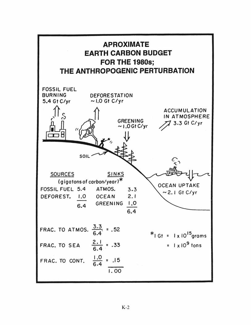
This section's mystery is not that the atmosphere's CO2 burden is rising, but

rather that it is rising much more slowly than expected. The amount of excess CO2

appearing in the atmosphere each year is just over one half that produced by fossil fuel

burning. Nearly fifty percent has disappeared! The mismatch between CO2 production

and CO2 buildup becomes even larger when the amount of CO2 released as the result of

forestry is taken into account. Although the magnitude of this activity remains poorly

documented, during the last decade or so, an amount of CO2 averaging about 25% that

from coal, oil, and natural gas was released as the result of forest cutting. When this

biosphere-derived CO2 is included as a source term, the fraction of the CO2 which

remains airborne drops to only about 40% of the input. Where has the rest gone?

The most obvious hiding place is the ocean. Excess CO2 in the atmosphere

passes across the air-water interface and reacts with CO=3 ions dissolved in the sea to

produce HCO−3 ions. Were the atmosphere to be at chemical equilibrium with the entire

ocean, about five sixths of the excess CO2 would take up residence in the sea. Only one

sixth would remain airborne. But it's not so simple; the sea mixes so slowly that only a

small fraction of its capacity for CO2 uptake is being utilized. Vast parts of the deep sea

are accessible only on the time scale of hundreds of years. When this dynamic limitation

is taken into account, it turns out that while the sea is an important hiding place, its

uptake can account for only about one half the missing CO2. Our mystery has to do with

the fate of the remainder. Where has it gone?

The search for the so called "missing carbon sink" has been pursued for more than

two decades. The conclusion is always the same. Only one reservoir, the organic matter

which makes up the terrestrial biosphere, is big enough for the task. Somehow human

activity must have increased the rate of photosynthesis. As a consequence, more carbon

is being stored in tree trunks and soil humus. One might say, while the terrestrial

K-4

K-5

biosphere reservoirs is being trimmed around the edges, it is becoming more lush in the

interior. Through our activities, we have been "greening", not just agricultural land but

the entire planet. Actually, agricultural land is part of the problem, and not of the

solution. First, as plants grown on agricultural land are harvested each year, no above

ground storage of carbon occurs. More important, agricultural practice has been shown

to drive down the humus content of soil. So, if the missing carbon is being packed away

in wood and humus, this storage is occurring on lands we classify as uncultivated.

Two mechanisms have been identified which might propel a global greening. The

first involves CO2 itself. As carbon is the primary building block for plant matter, the

increased abundance of CO2 in the atmosphere might be expected to accelerate

photosynthesis. More CO2 flows into the factory allowing more organic matter to be

manufactured. Indeed, experiments carried out in growth chambers suggest that, at least

on the short term, a 30% increase in the CO2 content of the air leads to growth

enhancements averaging 10%. If CO2 is driving an enhancement of this magnitude in the

wild, then, each year more wood is being generated (leading to fatter forests) and more

organics are being pumped into soils (leading to richer humus). The second mechanism

involves nitrogen. Growth in most plant communities is often limited by the availability

of this important nutrient. Farmers counter this deficiency by fertilizing their fields with

ammonia or by allowing them to remain fallow so that plants with nitrogen-fixing root

symbionts can generate natural fertilizer. The internal combustion engine extends

nitrogen fertilization to the wilds. Atmospheric N2 molecules are split at the high

temperatures achieved in automobile engines producing nitrogen oxide gases. These

gases become widely dispersed through the atmosphere before they are transformed to

nitric acid molecules which dissolve in raindrops. This automobile-generated fertilizer

allows more wood and soil humus to be generated. While a strong case can be made that

extra carbon dioxide and fixed nitrogen are greening the planet, as we shall see, this

greening process must be operating at maximum efficiency if it is to account for the

K-6

K-7

K-8

K-9

K-10

storage of the missing carbon. Before exploring this question, let us review the evidence

upon which carbon budgets are based.

The Knowns

Only two of the terms in the carbon budget are directly measured to a reasonably

high degree of accuracy. One is the amount of CO2 generated during each of the last 100

or so years through the burning of fossil fuels and the manufacture of cement. The

number of tons of coal mined, the number of barrels of oil pumped, the number of cubic

meters of natural gas recovered, and the number of tons of limestone thermally

decomposed have been laboriously compiled from records kept by individual nations.

The other is the CO2 content of the atmosphere. In 1957, Charles David Keeling

commenced continuous highly accurate measurement of the CO2 content of air atop the

extinct volcano Mauna Loa on the island of Hawaii. Keeling's measurement series has

continued unbroken and is now supplemented by measurements at many other locations

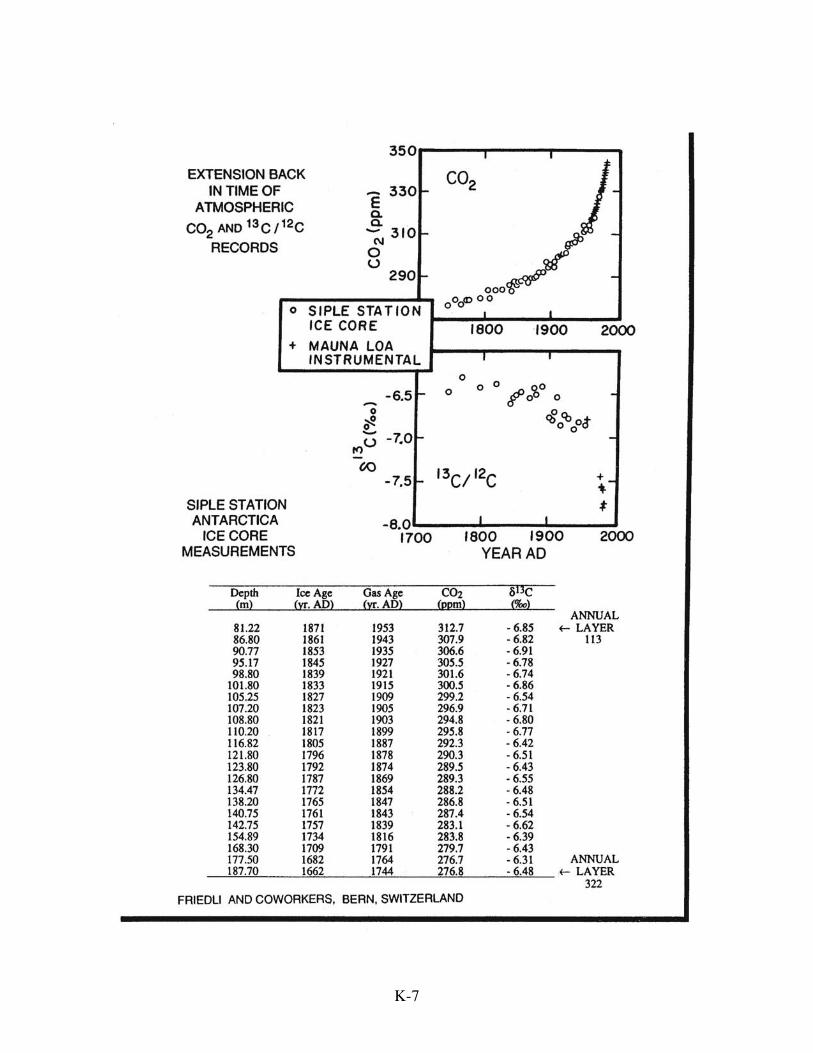
on our planet. Scientists at Bern, Switzerland and Grenoble, France discovered a means

of extending this record back in time. Their trick was to extract gas stored in the bubbles

contained in ice recovered from borings atop the Greenland and Antarctic ice caps. They

demonstrated that this mode of cold storage nicely preserves the CO2 content of the

trapped air.

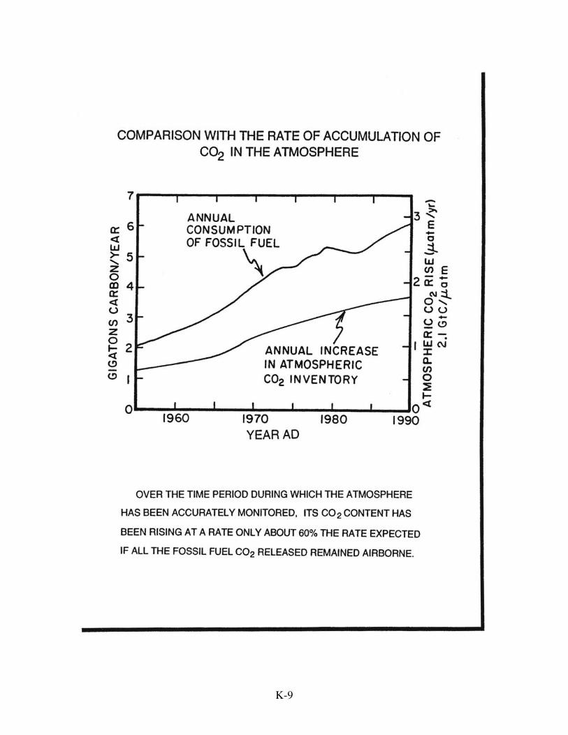
These two sets of data constitute our givens. Taken together, they tell us with

clarity that, over the time spanned by the instrumental record, CO2 has built up in the

atmosphere at a bit more than one half the rate it was being generated by fossil fuel

burning. The remaining three budgetary terms (described in the sections which follow:

ocean uptake, deforestation, and greening) must be estimated by less direct means.

The Mirror Image Approach

The CO2 produced by the burning of fossil fuels must be matched by an

equivalent consumption of atmospheric oxygen. For coal, about thirteen molecules of O2

disappears for each ten atoms of carbon combusted.

K-11

C10H6 + 13O2 → 10CO2 + 3H2O

For petroleum, the ratio is close to 3 O2 molecules for each 2 carbon atoms.

2CH2 + 3O2 → 2CO2 + 2H2O

For natural gas, the ratio is 2 to 1.

CH4 + 2O2 → CO2 + 2H2O

The current global mix of these three fuels requires the consumption of 15 molecules of

O2 for each 10 molecules of CO2 produced. The mirror image strategy is a simple one.

The measured rate of O2 decline is compared with that expected from the amount of

fossil fuels consumed. One might ask what advantage this information would have over

that obtained from comparing the observed rate of rise in atmospheric CO2 content with

the expected rate. There is a very important difference. While the ocean is capable of

absorbing five sixths of all the CO2 we have produced (and thereby constitutes a very

important term in the carbon budget), no comparable term exists in the O2 budget. The

reason is that 95 percent of the earth's O2 resides in the atmosphere and only 5 percent in

the ocean. The tiny amount of O2 which will flow from the ocean back to the atmosphere

to compensate for the loss through fossil fuel burning is unimportant in the O2 budget.

Thus O2 budgeting is far simpler than CO2 budgeting. Dead simple in fact. The

difference between the observed rate of O2 disappearance and that expected from fossil

fuel burning provides a measure of the rate of change in the overall global biomass. For

each molecule of CO2 released to the atmosphere through deforestation, about one

molecule of O2 disappears. For each unit atom of carbon stored in wood or humus as the

result of global greening, about one molecule of O2 will be released to the atmosphere.

Thus if more O2 is disappearing than required for fossil fuel combustion, then the

biosphere as a whole must be shrinking. Or if less O2 is disappearing than required for

fossil fuel burning, then the biosphere must be expanding.

But two difficulties remain. As already discussed, the biospheric carbon

inventory is being influenced in opposing ways by man. Farmers and foresters are

K-12

K-13

reducing its size. Greening by excess CO2 and fixed nitrogen is increasing its size. So,

for example, were measurements to reveal that O2 is declining exactly in accord with

expectation from fossil fuel burning, it would mean that losses driven by forestry and

agriculture were, by chance, just balanced by gains driven by greening. In order to reach

our goal of establishing how much greening is occurring, it is necessary to quantify

reduction in wood and humus stocks.

The second obstacle is one of measurement. In 1997, the atmosphere contained

364 ppm CO2. Two years from now, it will contain 367 ppm. This increase can be

documented precisely with modern instrumentation. By contrast, the atmosphere

contains about 209,000 ppm of O2. The expected drop during the same two-year period

from fossil fuel burning alone is about 5 ppm. This represents a change of only 0.0025%;

a daunting challenge to even the most clever experimentalist.

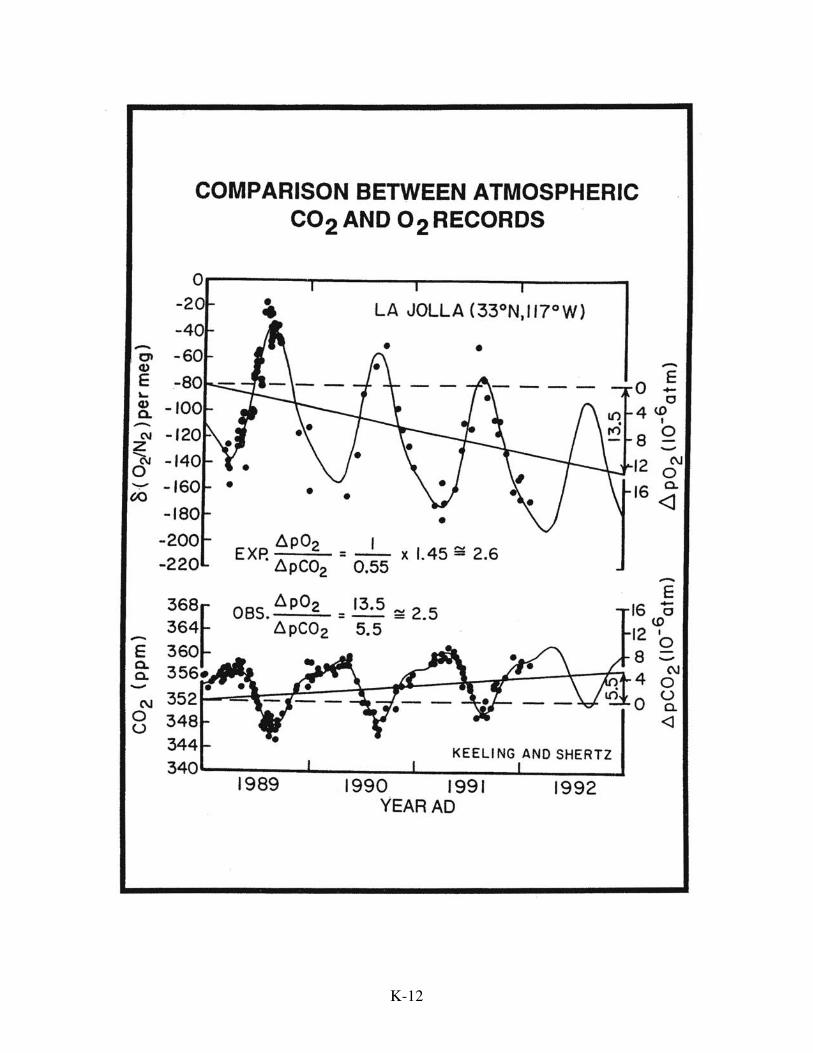
The second challenge was not met until 1989 when Ralph Keeling succeeded in

developing a method capable of determining changes in the O2 content in air to an

accuracy of 0.8 ppm. Then, working together with his colleague Shertz, he succeeded in

demonstrating that over the three-year period from 1989 to 1992, the O2 content of air in

La Jolla, California dropped at a rate consistent with that expected from global fossil fuel

burning. However, at that point the uncertainty in this result was big enough to permit

the possibility that the biosphere was either shrinking or expanding at a rate up to 2

gigatons a year. As this range covers virtually all possible scenarios, this early

measurement series didn't help much. But as the years clicked by, Keeling’s O2

measurements began to pay off. In fact, he has been able to document an amazing

occurrence. Between 1989 when his measurement series began and 1995, the O2 content

of the atmosphere dropped considerably less than would be expected. Taken together

with the rise in CO2 over this period, this shortfall in the magnitude of the O2 decline

indicates that during this period the split of fossil fuel CO2 flow was 35% to atmosphere,

35% to the ocean, and 30% to the biosphere. This came as a big surprise indicating that

K-14

K-15

the biosphere was taking up an average of about two gigatons of carbon per year during

this time interval. If, for example, forest cutting was releasing one gigaton of carbon per

year, this would require a greening of roughly three gigatons a year! We will return to

this finding later in this section, but before going on, it must be stated that this rate of

greening need not be entirely or even largely anthropogenic. Rather, it might reflect

unusually favorable growth conditions across the globe. Even though averaged over

many years, respiration must match growth; a pulse in global photosynthesis over a

several year period could temporarily outstrip respiration. It is likely that such a pulse

occurred in the early 1990s. If so, then respiration will soon gain the upper hand and

eliminate this short term excess storage. This finding emphasizes the need for a record of

sufficient duration so that the influence of changes in global photosynthesis induced by

short term climate changes can be averaged out.

Shortly after Keeling developed his index of refraction technique for precise

O2/N2 ratio measurement, Sowers and Bender came up with a nearly as precise a means

to accomplish this task using conventional mass spectrometry. Impatient with the

prospect of the long wait for a definitive result, they developed a hindcasting method. It

involves getting air samples from deep in the 70 or so meter thick layer of firn which

caps the Antarctic and Greenland ice caps. Firn is partially lithified snow which has open

pores which provide access to the overlying atmosphere. But diffusion of gases through

this matrix is so slow that the gas deep in the firn is replaced only once per decade or so.

The first measurements by Sowers and Bender showed that indeed air from deep in the

firn had a higher O2/N2 ratio than that in the atmosphere. It also had lower methane and

carbon dioxide contents. As the evolution of the methane and carbon dioxide contents of

the atmosphere over the last decade or so are well documented, these measurements

served to fix the average age for any given sample of firn air. Based on this age and the

O2/N2 ratio, Sowers and Bender hoped to obtain a rate of O2 decline for decades past.

But again the uncertainty in these preliminary measurements is too great to provide a

K-16

definitive answer. The reason is that despite the 5 times greater length of the Sowers-

Bender record, the measurement uncertainty is considerably larger. While firn provides a

superb storage environment in that it is very cold, very dry, free of bacteria, and immune

to contamination from underlying earth gas, it is not perfect. The long residence time of

gas in the firn allows preferential settling of heavy molecules relative to light ones. As

O2 (mass 32) is heavier than N2 (mass 28), this settling alters the ratio of interest.

Sowers and Bender were, however, armed with a means to correct for this gravitational

settling effect. They measured the ratio of 15N14N (mass 29) to 14N14N (mass 28) in the

same samples and used the enrichment of the heavy nitrogen molecule as a basis to

correct for the gravitational enrichment of O2 relative to N2.

As the record in firn extends back only 10 to 20 years, in order to be successful

the Sowers and Bender approach will have to be extended beyond the base of the firn into

the underlying ice. In attempting this extension, they have encountered a serious

problem. As the bubbles of trapped gas closed off, air diffuses in and out of the tiny

residual orifices creating a small separation between O2 and N2. In an attempt to develop

a means to correct for this separation, Jeff Severinghaus and Michael Bender are

currently measuring the Ar to N2 ratios as well as the O2 to N2 ratios in firn and ice. So

the question is whether the hares (Bender and coworkers) springing rapidly back time can

put aside potential biases created by ice storage and beat out the tortoises (Keeling and

coworkers) who are forced to plod along one year at a time. Clearly, however, both

results are of extreme importance. One will give information about the state of the

biosphere during the coming decades, and the other about its state during past decades.

Ocean Uptake

Another way to approach carbon budgeting is to estimate without the use of O2

data the uptake of CO2 by the ocean. Once this term has been defined, then change in the

Earth's biomass can be calculated by subtracting the CO2 increases in the ocean and

atmosphere reservoirs from the total amount of CO2 produced by man's activities. The

K-17

first point to be made in this regard is that ocean uptake cannot, at present, be estimated

from the results of repeated ∑CO2 inventories. Unlike the atmosphere for which a

combination of measurements on air bubbles stored in ice (prior to 1958) and direct

sampling (after 1958) provide a complete record of the inventory's evolution, we have no

equivalent for the ocean. The first detailed and accurate global survey of the dissolved

inorganic carbon content of ocean water (∑CO2) was made during the 1970s as part of

the GEOSECS (Geochemical Ocean Sections Study) expeditions. But even these

measurements were not of sufficient accuracy to provide an adequate base for future

surveys. The problem is that even for waters which have taken up their full component

of excess CO2, the increase in ∑CO2 since the 1970s has only been about one percent.

The accuracy of the GEOSECS measurements is no better than 0.5%. Of course, the

situation is even less favorable for sub-surface waters which have achieved only a

fraction of their uptake capacity. Because of this, the direct inventory approach is at

present hopeless.

During the 1990’s, a far more detailed and accurate (to ±0.1%) survey was made

under the banner of the global WOCE (World Ocean Circulation Experiment) program.

If a similar survey is conducted 15 to 25 years hence, it will then be possible for the first

time to directly measure the integrated CO2 uptake by the ocean. But of course this result

will apply only to the time between the two surveys.

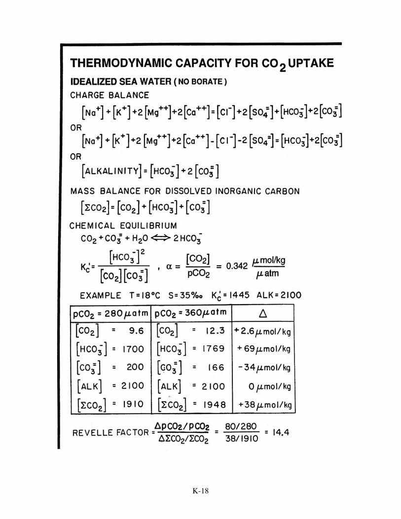
In the interim, the amount of excess CO2 which has entered the ocean must be

obtained by less direct means. One approach involves ocean models designed to take

into account not only the thermodynamic capacity of sea water for the uptake of excess

CO2 but also the two kinetic barriers to its uptake, namely, the resistance posed by

transport across the air-sea interface and the resistance posed by vertical mixing within

the sea. These models are initialized so as to be at steady state with the pre-industrial

atmosphere (pCO2 =280 µatm). Then the model's atmospheric CO2 content is time

stepped to follow the observations. After each step, CO2 is exchanged between the

K-18

K-19

K-20

K-21

K-22

K-23

K-24

atmosphere and surface ocean and mixing occurs within the ocean. The output of the

model is the evolution of the storage of excess CO2 in the ocean.

The models used for this purpose are of two types, tracer-calibrated reservoir

models and atmosphere-driven dynamic models. As the reservoir models are far simpler

in design, it makes best sense to discuss them first. In these models, no attempt is made

to duplicate the physics associated with either air-sea gas exchange or mixing within the

sea. Rather, these transports are represented by transfer coefficients. The magnitudes of

these coefficients are chosen to provide the best possible match to the distribution of

transient tracers whose distributions within the sea have been measured. The secret of

success in this endeavor is to keep the architecture of the model as simple as possible. In

this way, the number of variable parameters can be kept to a minimum. In the absence of

any dynamics, such models are merely vehicles to permit the measured distributions of

transients (i.e., those of bomb produced 14C and 3H and of industrially produced CFCs)

to be used as analogues for transients whose distributions we can't document (i.e., those

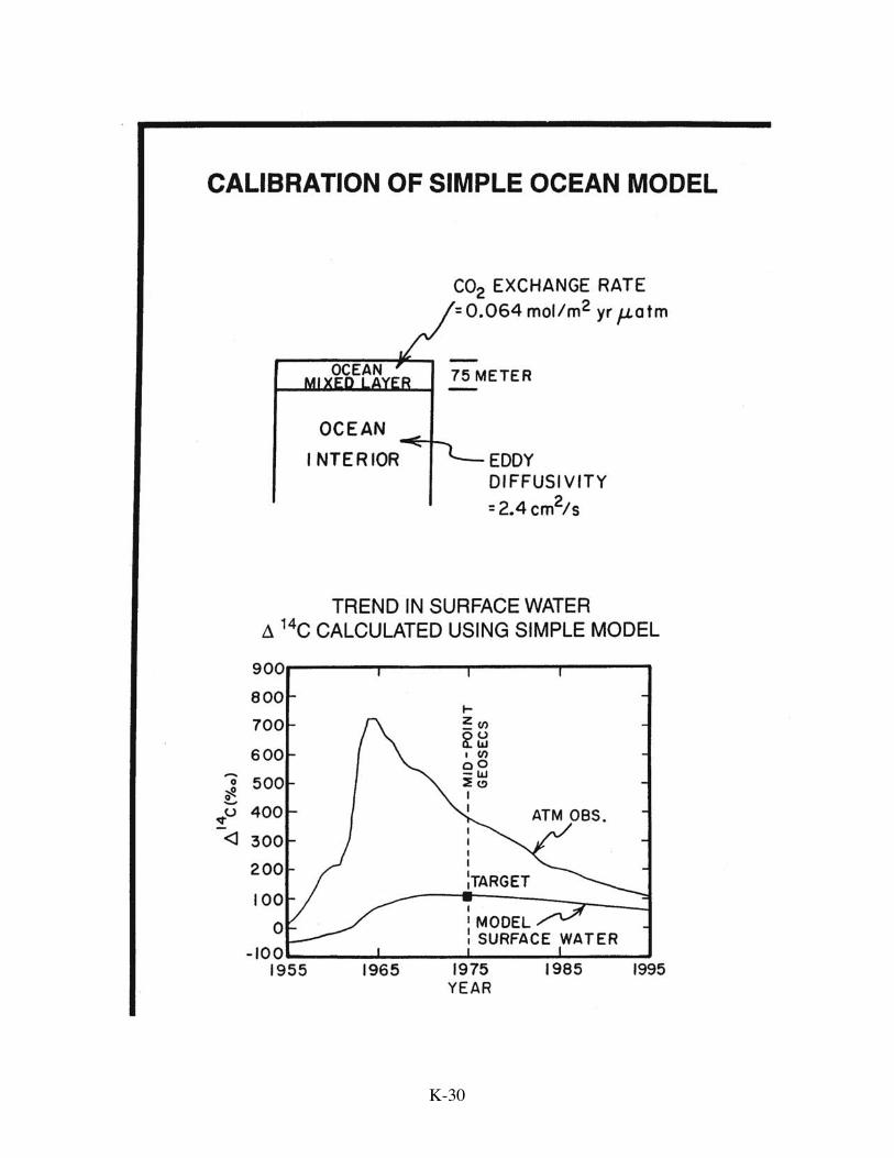
of anthropogenic CO2 and greenhouse heat). In our estimation, the most successful of

these models is that proposed by the Swiss scientists, Hans Oeschger and the late Uli

Siegenthaler. Their model is one dimensional consisting of a well-mixed atmosphere and

a two box ocean. The upper ocean box represents the wind-stirred upper ocean layer.

The lower box represents the remainder of the ocean as a semi-infinite half space (it does

not have to have a base because neither the calibration tracers nor the anthropogenic CO2

reach the 3800 meter-mean depth of the real ocean). Transport through the semi-infinite

half space is accomplished by a mixing process mathematically analogous to molecular

diffusion. Oceanographers refer to it as "eddy diffusion". In such a model, only three

parameters need to be defined: the thickness of the upper-ocean wind-mixed layer, the

exchange rate of CO2 gas between the ocean and atmosphere, and the coefficient of eddy

diffusion within the main body of the ocean. The first of these is usually set at value,

consistent with observation of the measured mean thickness of wind-stirred layer which

K-25

everywhere caps the ocean. As discussed below, the assignment of the air-sea CO2

exchange rate is obtained in three independent ways: i.e., radon deficiencies measured in

the oceanic-mixed layer and on the distributions of natural and bomb-produced

radiocarbon. These three estimates are broadly consistent. The eddy diffusivity is based

on measurements of the measured penetration depth of bomb testing tritium and

radiocarbon. Again, the two estimates are consistent with one another. This diffusional

representation of penetration of water entering into the body of the ocean carries with it

the assumption that the extent of vertical mixing varies as the square root of time. This

means, for example, that mixing to 700 meters beneath the base of the mixed layer takes

four times as long as mixing to 350 meters below this base. As we shall see, this

assumption is consistent with the two available calibration targets. The distribution of

natural radiocarbon in the ocean tells us that the entire body of the ocean (mean depth

3800 meters) is mixed on a time scale of about one millennium. The distribution of

bomb radiocarbon and tritium at the time of the GEOSECS survey tells us that on the

time scale of one decade, the mean penetration depth is about 380 meters (about one tenth

of the ocean volume). The ratio of these two mixing depths (i.e., ~10) matches the square

root of the ratio of the mixing times i.e.,

3800m

380m!

1000years

10years

Bomb radiocarbon provides the best tracer for setting both the model's gas

exchange rate and its coefficient of vertical eddy diffusion. This tracer was generated as

the result of atmospheric H-bomb tests conducted during the 1950s and early 1960s.

Neutrons released during these thermonuclear explosions eventually find their way, as do

cosmic ray neutrons, into the nuclei of atmospheric nitrogen atoms transforming them to

radiocarbon. Most of the products of these blasts were carried into the stratosphere by

explosion-generated updrafts. Here the radiocarbon atoms chemically combined with

K-26

K-27

K-28

oxygen atoms to form 14CO2. On the time scale of a few years these tracer molecules

mixed downward into the troposphere. Measurements of the 14C to C ratio in CO2

extracted from ground level air, at a number of places on the planet, thoroughly document

the evolution of the resulting tropospheric transient. The 14C/C ratio began to climb in

1954. It reached a sharp maximum in mid 1963 shortly after the treaty banning nuclear

tests in the atmosphere was implemented. With the cessation of bomb testing, the 14C/C

ratio in atmospheric CO2 began a decline which is still in progress. In the northern

hemisphere where the tests were conducted, at its maximum, the 14C/C ratio in

tropospheric CO2 reached almost twice its pre-nuclear value. In the southern

hemisphere, the maximum was somewhat smaller and occurred a bit later, reflecting the

roughly one-year time constant for interhemispheric mixing. After four or five years,

when the distribution had become nearly uniform, all parts of the atmosphere followed

the same decline. Now 35 years after the peak, the 14C/C ratio has fallen to 11% above

the pre-industrial value. The important point is that the bomb 14C atoms which have left

the atmosphere now reside in the ocean and in the biosphere and serve as valuable

tracers.

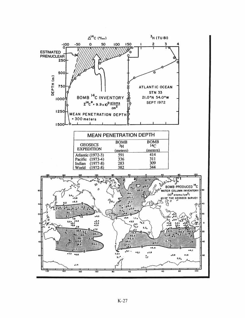
A survey of radiocarbon, encompassing the entire ocean, was conducted during

the period 1972-1978 as part of the GEOSECS program. When analyzed together with

results of a companion tritium survey, and with radiocarbon measurements on pre-nuclear

surface water, it is possible to separate the bomb radiocarbon and the natural radiocarbon

components at each station. The distribution of the bomb component is then used to fix

the two parameters in the Oeschger and Siegenthaler model. This is accomplished by

averaging two important properties of this distribution measured at each station: the

bomb 14C to C ratio in surface water and the mean penetration depth of bomb-produced

radiocarbon. These two quantities are calculated for each GEOSECS station. They are

then globally averaged. The result of this exercise yields an average 14C/C ratio for

surface water 16% higher at the time of the GEOSECS survey than just prior to nuclear

K-29

testing and an average penetration depth of 382 meters. These two values become the

targets for the calibration of the simple reservoir model. To do this, the model's

atmosphere is time stepped to follow both the rise in the atmosphere's CO2 content and

the time history of its 14C to C ratio. The model is run from 1954 (when the bomb 14C

rise commenced) to 1975, the mid time for the GEOSECS surveys. Runs are made for a

range of choices of both the CO2 invasion rate and the eddy diffusivity. One set of

values best fits both targets. The results obtained in this way are 0.064 moles

CO2/m2.yr.µatm for the CO2 invasion rate and 2.4 cm2/sec for the coefficient for eddy

diffusion.

Having calibrated the model's free parameters, the next step is to calculate the

ocean uptake of fossil fuel CO2. As for bomb 14C, this is done by time stepping the

model's atmosphere to follow the time history of atmospheric CO2 contents obtained

from measurements on ice cores and air samples. Of course, the CO2 invasion and

evasion rates and the eddy diffusivity employed are those obtained from the bomb 14C

calibration runs.

The model yields an ocean uptake of close to 2 gigatons of C per year for the

1980s. When this is combined with the observed atmospheric inventory increase, the

fossil fuel input is pretty much accounted for suggesting that the inventory of terrestrial

carbon remained more or less constant. In other words, gains resulting from greening

more or less matched losses resulting from deforestation and agriculture.

One might ask whether this approach to ocean uptake accounts for CO2 carried

into the deep sea as part of the ocean's thermohaline circulation. The answer is that it

does so only to the extent that the bomb radiocarbon carried to the deep sea has been

properly accounted for. This accounting is likely quite poor because the bomb 14C

component in deep waters is for the most part so small that it cannot be properly

identified. But a small signal distributed over a very large volume of deep-sea water

could be quite important. Thus the simple box model may underestimate the amount of

K-30

K-31

K-32

CO2 taken up by the sea. To get some idea how large the deep-sea component might be,

we can make a separate estimate. The flux of water into the deep sea is thought to be

about 30 Sverdrups (i.e., 30x106 m3/second). As an upper limit, we will assume this

water carries with it a full component of excess ∑CO2 (i.e., it is formed from old deep

water free of anthropogenic CO2 and it fully equilibrates with the atmosphere before

descending). If so, then during the mid 1980s when the atmosphere's CO2 content was

about 345 ppm, newly formed deep water carried with it about 40 µmoles/liter of excess

∑CO2. This yields an upper limit on the input of anthropogenic CO2 into the deep sea of

0.5 gigatons of carbon per year. But this must be an upper limit because newly formed

deep water cannot become fully charged with excess CO2 during the brief period of

winter-time deep convection.

An adequate assessment of the uncertainty in the ocean uptake estimates made

using tracer-calibrated one-dimensional (1-D) models is not possible. The main

uncertainty comes from the basic assumption that the depth of mixing increases as the

square root of time. For fossil fuel CO2 molecules, the time available for ocean

penetration is about 30 years, while for bomb radiocarbon-tagged CO2, it is about 10

years. Hence the model drives fossil fuel CO2 about 3 or 1.73 times deeper into the sea

than bomb 14C-tagged CO2. As we have no means to directly determine the extent of

ventilation of the real ocean on the time scale of 30 years, the appropriate multiplier

could perhaps be as low as 1.4 or as high as 2.0. Were these limits to be adopted as a

measure of the uncertainty in the ocean uptake, the answer comes out to be ±20% (0.4

gigatons of C per year during the 1980s).

There is a tracer which might be used to overcome the penetration time mismatch

between bomb 14C and fossil fuel CO2. It is the reduction in atmospheric 13C/12C ratio

due to the introduction of CO2 produced by fossil fuel burning. This CO2 has a 2% lower

13C to 12C ratio than that in the atmosphere. Repeated surveys of 13C/12C profiles for

ocean ∑CO2 could provide an estimate of the depth of penetration of this signal. As the

K-33

anthropogenic 13C anomaly is coupled directly to the production of CO2, no time

difference exists. Quay and his colleagues attempted to quantify the redistribution of the

anomaly created by the release of 13C deficient fossil fuel CO2 to the atmosphere by

documenting the magnitude of the decline in the 13C/12C ratio both for atmospheric CO2

and for upper ocean ∑CO2 for the period 1970 to 1990. While the uptake they obtained

is consistent with that based on the tracer-calibrated 1-D ocean model, due to the large

uncertainties in the measured trends, this approach did not narrow the range of

uncertainty in the amount of fossil fuel CO2 taken up by the ocean during this period.

Chemical Versus Isotope Adjustment Time

One aspect of the 1-D model results is, at least at first glance, puzzling. While, as

of 1975, the increase in the CO2 partial pressure in the model's surface mixed layer had

reached 85 to 90 percent of the atmospheric increase, the 14C/C ratio in surface water had

reached only about 50% of the atmospheric increase. Why such a big difference? The

obvious answer is that fossil fuel CO2 molecules had at that time a greater mean age than

bomb 14C-tagged CO2 molecules (30 years versus 12 years). Hence they had a longer

time to get into the ocean. However, this is not the major reason. Rather, the slowness of

the 14C response has to do with a fundamental difference between the time required for

equilibration of carbon isotope anomalies and the time required for the equilibration of

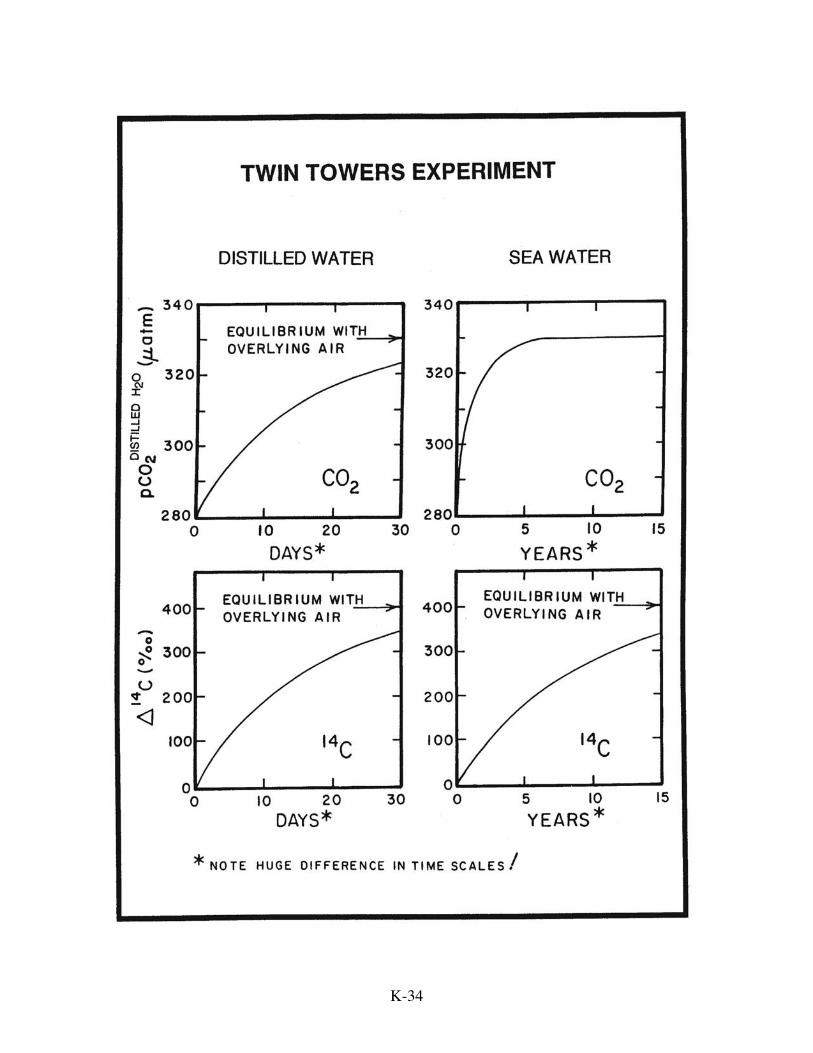
chemical anomalies. This difference is most easily understood by considering two

hypothetical 75-meter high towers. One is filled with normal sea water and the other

with distilled water. The waters in both towers have the same temperature and CO2

partial pressure (280 µatm). Also the dissolved carbon in both initially has the pre-

nuclear 14C/C ratio. The major difference is that the distilled water contains no HCO−3 or

CO=3 . The lids are removed from the tower tops and fans are activated so as to generate

CO2 exchange rates of 0.064 moles/m2.yr.µatm. The question is, "how rapidly will the

CO2 partial pressures and the 14C/C ratios in the tower waters approach those for the

overlying 1975 air (pCO2 = 330 µatm and ∆14C = 400‰)?" For the distilled water

K-34

K-35

tower, both the partial pressure and isotope ratio will approach the atmospheric value

with an e-folding time of 15 days. For the sea water tower, the isotope equilibration will

take 200 times longer, a staggering 8.2 year e-folding time! The reason for this huge

difference is that for the sea water tower, not only the isotopic composition of the 10

µmole/liter of dissolved CO2 gas has to be exchanged but also that of the 2000

µmole/liter of HCO−3 and CO

=3 ions.

More tricky to understand is the time constant for the CO2 partial pressure

adjustment in the sea water tower. The e-folding time turns out to be close to one year,

lying roughly geometrically between that for the distilled water (.04 yrs.) and that for the

isotopes in the sea water ∑CO2 (8.2 yrs.). The reason is that rise in the CO2 partial

pressure in the sea water involves mainly the adjustment of its CO=3 concentration. For

surface sea water, the CO=3 concentration is about 10 times lower than the ∑CO2

concentration and 20 times larger than the CO2 concentration. With this tower analogy in

mind, it is easy to answer our question regarding the difference between the extent of

isotope (14C) and chemical (CO2) equilibration yielded by the 1-D model for the time of

the GEOSECS survey. Isotopic equilibration takes ten times longer than chemical

equilibration, thus the 14C/C ratio rises toward the atmospheric value far more slowly

than the CO2 partial pressure. This factor of ten reflects the ratio of the ∑CO2 (isotopic

reservoir) to CO=3 (chemical reservoir) in surface sea water.

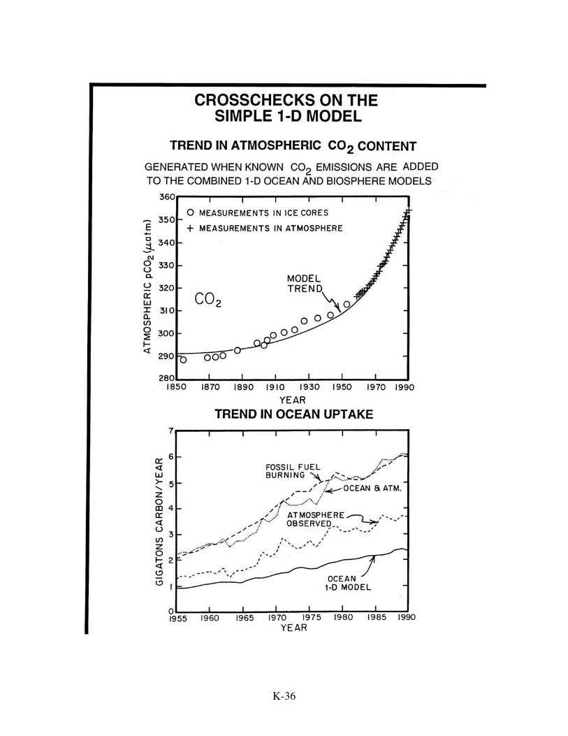
Isotopic Cross Checks

Three cross checks based on carbon isotope measurements can be used to evaluate

the performance of the simple model adopted here. The first has to do with the

magnitude of the change in the 14C/C ratio for atmospheric CO2 during the hundred-year

period from 1850 to 1950 as recorded in tree rings. Because of the advent of bomb

testing in the early 1950s, the 14C/C lowering approach is viable only for the period

before 1950. As the CO2 generated by fossil fuel burning is free of radiocarbon, the

14C/C ratio in atmospheric CO2 should have decreased during this period. Indeed it did.

K-36

K-37

K-38

K-39

K-40

The magnitude of the decrease depends not only on the amount of fossil fuel CO2

released, but also on the extent to which this carbon was diluted by exchange of

atmospheric carbon with carbon in the sea and in the terrestrial biosphere. As the amount

of fossil fuel CO2 generated is known, the magnitude of the 14C to C ratio decrease tells

us the extent of this dilution. Were no exchange with oceanic and biospheric carbon to

have occurred, the decrease in atmospheric 14C/C between 1850 and 1950 would have

been about 12%. The observed decrease was only about 2%. The second cross check is

based on the decrease in the 13C/12C ratio for atmospheric CO2 from 1850 to present.

Fossil fuel carbon has a 13C/12C ratio averaging 2% lower than that for atmospheric CO2.

Thus the release of CO2 from fuel burning is lowering the 13C/12C ratio for atmospheric

CO2. Again the magnitude of this lowering depends not only on the amount of CO2

released by fossil fuel burning, but also by the extent of dilution resulting from the

trading of atmospheric carbon atoms with terrestrial biosphere and ocean. This approach

is complicated by the fact that CO2 released as the result of deforestation and taken up as

the result of greening also has a 2% lower 13C/12C ratio than atmospheric CO2. The third

cross check involves the decrease in the atmospheric 14C/C ratio for the time period from

1970 to present. This decline is primarily the result of mixing of the bomb 14C into the

oceanic and biospheric carbon reservoirs.

The strategies for harnessing each of these pieces of isotopic information are

similar. The simple one-dimensional model described above is used to estimate the

extent of dilution through exchange with ocean carbon. In addition, an even simpler

reservoir model is used for exchange with carbon in the terrestrial biosphere. This model

divides the terrestrial biosphere into three compartments and treats each as a well-mixed

reservoir

Reservoir size Turnover time gigatons C years

Short-lived vegetation and litter 150 2

K-41

Active soil humus 500 25

Long-lived vegetation 500 60

As the biospheric contribution to the dilution is several times smaller than the oceanic

contribution, the larger uncertainties associated with the terrestrial model do not seriously

hamper the approach.

The cross checks are conducted as follows. The model is initiated at steady state

with the atmospheric CO2 content at 292 ppm and the 13C/12C and 14C/C ratios at their

observed pre-industrial values. Fossil fuel CO2 is then added to the model's atmosphere

in accord with the known production history. This CO2 has a 13C/12C ratio of -25‰ and

carries no radiocarbon. Uptake of excess CO2 by the model ocean occurs during each

time step as does isotopic exchange with the biosphere and ocean. Then the decline in

14C and in 13C obtained from the model can be compared with the observed atmospheric

trends.

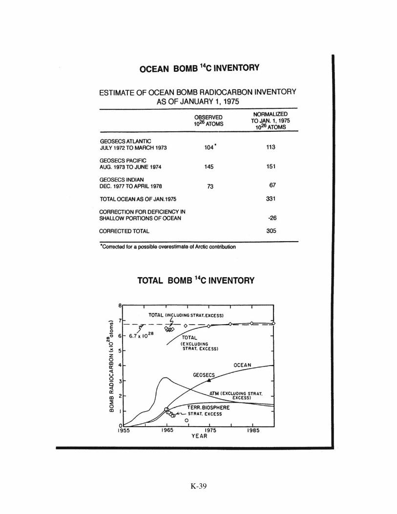
The bomb radiocarbon calculation is done in a different way. The 14C to C ratio

for atmospheric CO2 is constrained to follow the observed values. After each time step

the inventory of bomb 14C atoms in the atmosphere, ocean and biosphere reservoirs is

computed (for each it is equal to the total number of radiocarbon atoms minus the steady

state number of natural radiocarbon atoms). The post 1964 increase in the global

inventory of bomb radiocarbon is the result of the downward mixing of the excess bomb

14C stored in the stratosphere (based on surveys of the 14C/C in stratospheric CO2).

The simple tracer-calibrated model satisfactorily passes all three of these tests. It

correctly reproduces the evolution of the atmosphere's 13C to 12C ratio and of its pre-

nuclear 14C to C ratio. It also is consistent with the requirement that after the test ban the

total inventory of 14C remained constant.

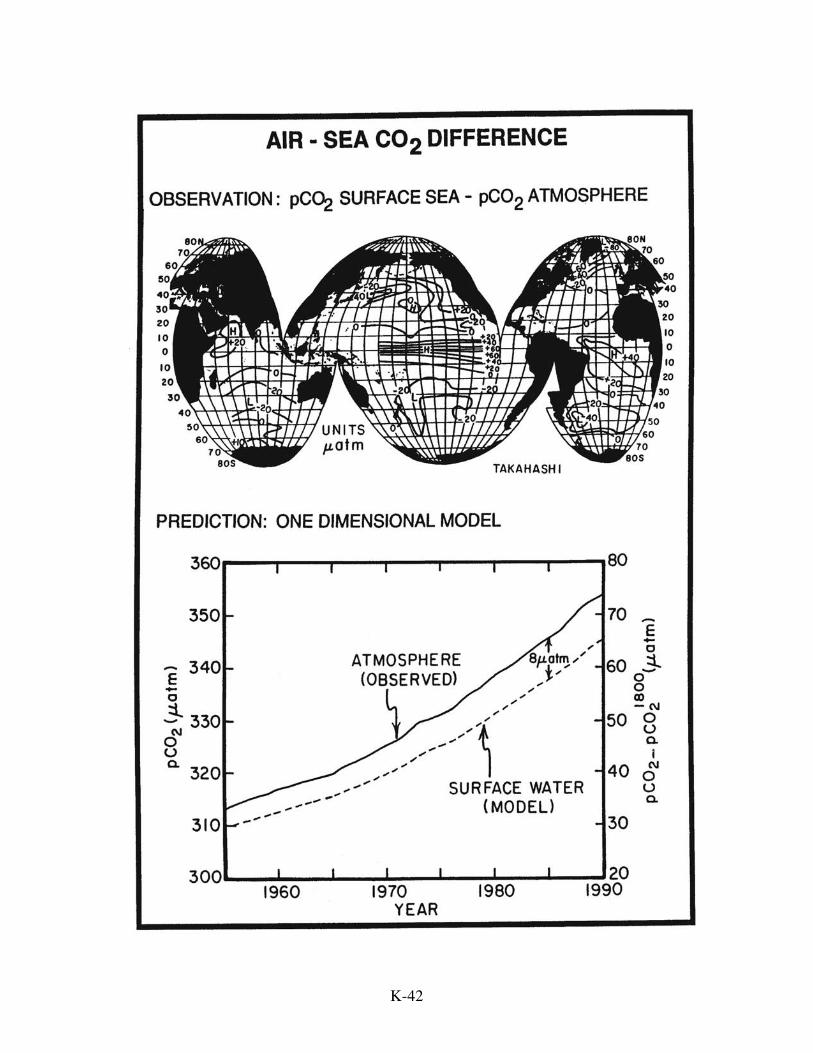
Air to Sea CO2 Flux

Before returning to the discussion of ocean uptake models, one other means of

K-42

K-43

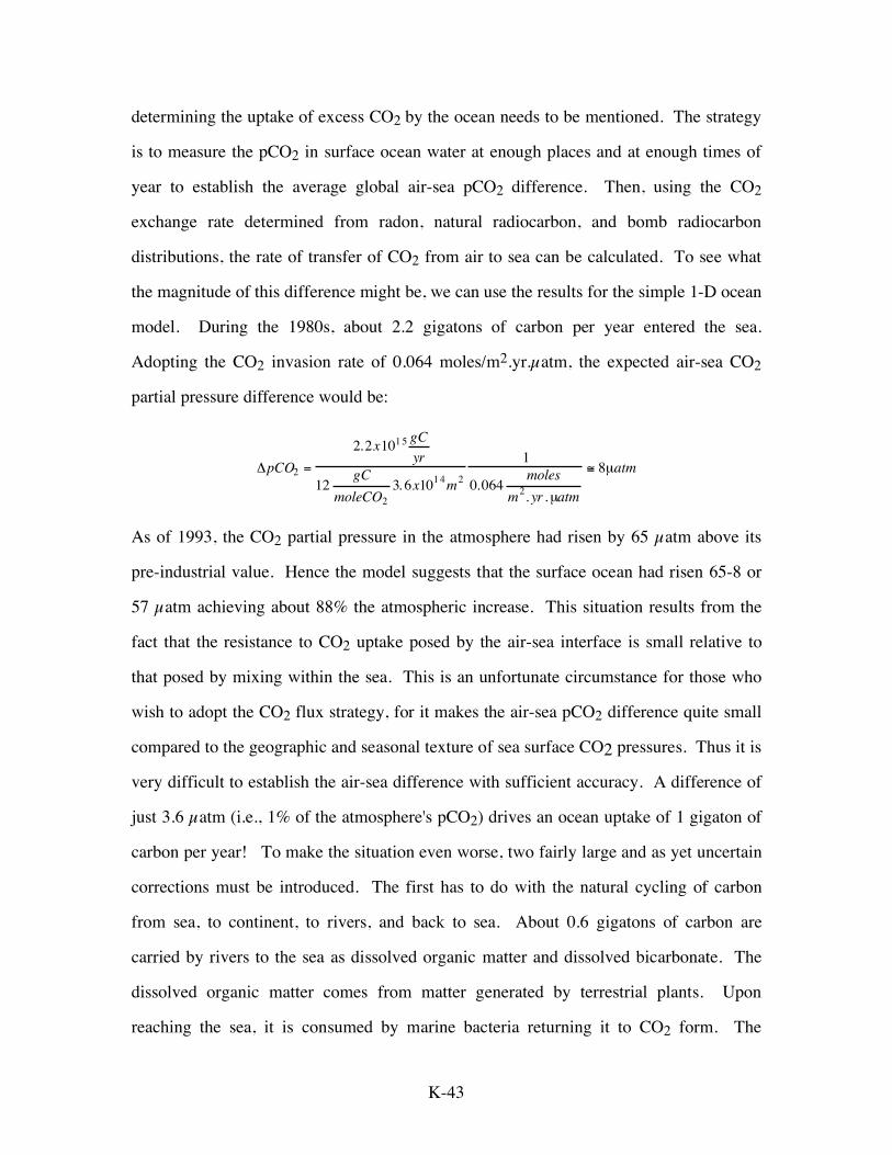
determining the uptake of excess CO2 by the ocean needs to be mentioned. The strategy

is to measure the pCO2 in surface ocean water at enough places and at enough times of

year to establish the average global air-sea pCO2 difference. Then, using the CO2

exchange rate determined from radon, natural radiocarbon, and bomb radiocarbon

distributions, the rate of transfer of CO2 from air to sea can be calculated. To see what

the magnitude of this difference might be, we can use the results for the simple 1-D ocean

model. During the 1980s, about 2.2 gigatons of carbon per year entered the sea.

Adopting the CO2 invasion rate of 0.064 moles/m2.yr.µatm, the expected air-sea CO2

partial pressure difference would be:

!pCO2 =

2.2x1015gC

yr

12gC

moleCO23. 6x10

14m2

1

0.064moles

m2. yr .µatm

" 8µatm

As of 1993, the CO2 partial pressure in the atmosphere had risen by 65 µatm above its

pre-industrial value. Hence the model suggests that the surface ocean had risen 65-8 or

57 µatm achieving about 88% the atmospheric increase. This situation results from the

fact that the resistance to CO2 uptake posed by the air-sea interface is small relative to

that posed by mixing within the sea. This is an unfortunate circumstance for those who

wish to adopt the CO2 flux strategy, for it makes the air-sea pCO2 difference quite small

compared to the geographic and seasonal texture of sea surface CO2 pressures. Thus it is

very difficult to establish the air-sea difference with sufficient accuracy. A difference of

just 3.6 µatm (i.e., 1% of the atmosphere's pCO2) drives an ocean uptake of 1 gigaton of

carbon per year! To make the situation even worse, two fairly large and as yet uncertain

corrections must be introduced. The first has to do with the natural cycling of carbon

from sea, to continent, to rivers, and back to sea. About 0.6 gigatons of carbon are

carried by rivers to the sea as dissolved organic matter and dissolved bicarbonate. The

dissolved organic matter comes from matter generated by terrestrial plants. Upon

reaching the sea, it is consumed by marine bacteria returning it to CO2 form. The

K-44

bicarbonate dissolved in rivers is also generated from soil CO2 to balance the positive

charge on cations released from soils as the result of weathering. As does the dissolved

organic carbon, this bicarbonate eventually reaches rivers and is carried back to the sea.

Both the carbon in the dissolved organic matter and bicarbonate ions carried to the sea by

rivers originated from CO2 in the atmosphere. In order to cycle 0.6 gigatons of carbon

cycled in this way requires that prior to the Industrial Revolution, the partial pressure of

CO2 in the surface sea averaged about 2 uatm higher than that in the atmosphere.

The second correction involves a temperature difference between the few tens of a

micron-thick sea water 'skin' and the ambient temperature for the bulk of mixed layer

water. This skin cooling is caused by heat loss during evaporation. The temperature

difference created in this way is thought to average about 0.2°C. As for each 0.1°C the

skin is cooled, its CO2 partial pressure drops by a bit over one µatm. In order to balance

a 0.2°C skin cooling requires that the pCO2 of bulk mixed layer water be about 2 µatm

higher than that in the overlying atmosphere.

Taken together, these two corrections suggest that, during pre-industrial time, the

pCO2 in the oceanic mixed layer water was about 4 µatm higher than that in the

atmosphere. If so, then an uptake of 2 gigatons of anthropogenic carbon by the sea would

require that the atmosphere average only 4 rather than 8 µatm higher in partial pressure

than the ocean mixed layer. Extensive measurements are now available from most

regions of the ocean. Taro Takahashi has summarized these results and concludes that on

the average the surface ocean mixed layer water has a CO2 partial pressure 4±4 µatm

lower than that for the atmosphere. While consistent with expectation from the simple

tracer-calibrated reservoir model, the error in this estimate remains far too large to be of

use in constraining the carbon budget. For this approach to be definitive, CO2 partial

pressure measurement coverage (both geographically and seasonally) will have to be

greatly expanded, river recycling and skin temperature biases will have to be accurately

established, and the wind velocity dependence of in CO2 invasion rates will have to be

K-45

K-46

taken into account. Our assessment is that this approach will never become competitive

with the others available to us.

Interhemispheric CO2 Gradient

One piece of evidence appears to be at odds with the conclusion that the amount

of carbon stored in the terrestrial biosphere has remained nearly constant over the last

several decades. It is based on the interhemispheric difference in the CO2 content of the

atmosphere. As expected, measurements show that northern hemisphere air has a higher

mean annual CO2 content than southern hemisphere air. We say "as expected", because

95 percent of the fossil fuel CO2 emissions occur in the north temperate latitude belt.

The problem is that atmospheric models designed to simulate meridional mixing predict a

gradient nearly twice as great as is observed. Fossil fuel CO2 is introduced into these

models in accord with the actual geographic pattern of emissions. The models are

programmed to dispense 2 gigatons of C per year to the oceans (uniformly across its

surface). The imbalance between fossil fuel production and atmosphere-ocean inventory

increase is assumed to enter the terrestrial biosphere (uniformly across the continents).

As continents lie mainly in the tropical and northern temperate zones, this uptake, like

fossil fuel CO2 production, is skewed strongly to the northern hemisphere. Models

programmed in this way generate an annually averaged 5 µatm difference in CO2 partial

pressure between north temperate and south temperate latitudes for the 1980s. The

observed difference is only about 3 µatm. With a 5 ppm interhemispheric gradient,

enough CO2 flows to the southern hemisphere to match both the 1.6 GtC/yr rise in its

atmospheric inventory and the 1.2 GtC/yr entering that 60% of the ocean surface lying in

the southern hemisphere. With an interhemispheric gradient of only 3 ppm, the models

would move only 3/5ths of this amount or 1.7 gigatons of carbon from the northern to the

southern hemisphere. As this amount is only slightly greater than that accumulating in

the southern hemisphere atmosphere, almost none is left over for uptake by the southern

hemisphere ocean. Based on this information in 1989, Tans, Fung and Takahashi stunned

K-47

K-48

the world’s carbon budgeters by bluntly stating that the yearly ocean uptake of CO2 had

been greatly overestimated. Rather than being on the order of 2 gigatons carbon per year,

it was more likely no more than one quarter this amount. If so, then greening must be

even larger than we had thought, outpacing forest cutting at a 2 to 1 clip! Further, if the

Tans et al. scenario is correct, the ocean is relegated to a minor role in fossil fuel CO2

budgeting. The terrestrial biosphere becomes dominant.

In addition to the arguments presented above, two rebuttals have been put forth to

counter the Tans et al. argument. One has to do with the reliability of the atmospheric

transport estimates. The other has to do with the implicit assumption underlying the Tans

et al. argument, namely, prior to the Industrial Revolution, no interhemispheric

atmospheric CO2 gradient existed. Let us first examine the transport rebuttal. Perhaps

the atmospheric models are not capable of estimating the interhemispheric transport to

better than a factor of two. If so, the Tans et al. argument crumbles. But atmospheric

modelers have an ace up their sleeves in this regard. Like oceanographers, they have

tracer distributions to lean on for verification. Two such tracers, 85Kr and CFCs, are

available. Like fossil fuel CO2, both tracers are generated primarily in the northern

hemisphere; 85Kr by nuclear reactors and CFCs by industry, and hence should be found

at higher concentrations in the northern hemisphere air. 85Kr is radioactive with a half

life of 11 years. Thus even though its concentration in the atmosphere was not rapidly

changing during the 1980s, the decay of 85Kr in the southern hemisphere had to be

balanced by transport across the equator. For CFCs, the atmospheric burden is steadily

rising. The rise in the southern hemisphere atmosphere must be supplied by cross-

equatorial transport. Models are checked to see whether they reproduce the observed

meridional gradients of 85Kr and/or CFCs. If the match is not satisfactory, the

formulation of the mixing dynamics is tweaked until the mismatch has been eliminated.

It turns out that models adjusted to meet the 85Kr constraint meet the CFC constraint as

well (or vice versa). Because the models which have been used to calculate the transport

K-49

of CO2 from one hemisphere to the other have passed the 85Kr-CFC test, modelers are

confident that the CO2 transports they generate is sufficiently accurate that the Tans et al.

argument must be taken seriously.

Even so, an escape hatch is still available. The latitudinal gradients for 85Kr and

for CFCs undergo only minor changes with season. By contrast, that for CO2 undergoes

large changes. During the October through April period, when respiration greatly

exceeds photosynthesis in the northern hemisphere, the CO2 content of the north

temperate atmosphere rises, creating a much enhanced north to south gradient. During

the May through September period when photosynthesis dominates, the CO2 content of

the air at these northern latitudes is drawn down well below that for the southern

hemisphere. So the difference between the CO2 content of air of north and south

temperate zones actually changes sign during the course of a year! While the 85Kr-CFC

test proves that over the course of an entire year the magnitude of cross equatorial air

exchange obtained in the models is correct, it does not verify that the seasonality of this

exchange is correct. If, for example, the model exchanges too little air during the Fall

period, when the CO2 gradient is lower than its mean annual value, and too much air

during the Spring period, when the CO2 gradient is higher than average, the result would

be an underestimation of the amount of CO2 transported from the northern to the

southern hemisphere. However, those who do this modeling are adamant that the

seasonality of transport is not flawed. But as we are not conversant with their arguments,

we cannot defend them. Sorry!

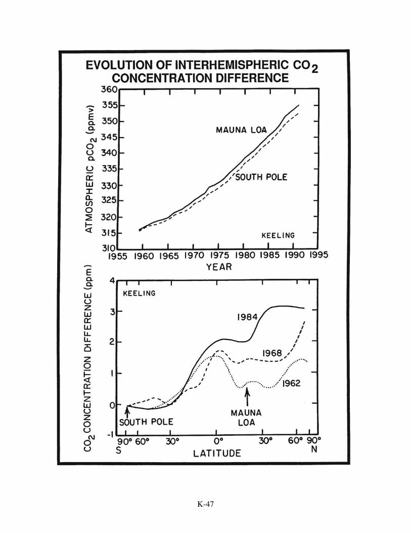
The other rebuttal shows more promise. It is based on an observation made by C.

D. Keeling and M. Heimann. They examined the evolution of the difference between the

annually averaged CO2 content measured at Mauna Loa, Hawaii and that measured at the

South Pole. As expected, this difference has increased with increasing fossil fuel CO2

production. At the beginning of the records (1958), the difference was very small. As

time progressed, it became larger and larger. What occurred to Keeling and Heimann

K-50

was that if the trends for these two stations were extrapolated back in time, they would

have intersected about 1950. Prior to 1950, the air over Antarctica would have had a

higher CO2 content than that over Hawaii! If so, then prior to the Industrial Revolution,

southern hemisphere air must have had a higher CO2 content than northern hemisphere

air. In other words, at that time CO2 must have been moving through the atmosphere

from south to north. Then, as fossil fuel CO2 generation in the northern hemisphere

grew, this natural northward flow of CO2 was compensated to an ever increasing extent

by a southward flow of fossil fuel CO2 until, about 1950, the two flows became equal,

eliminating the gradient.

Of course, Keeling and Heimann realized that if, during pre-industrial time, CO2

was moving from south to north through the atmosphere, then an equal amount must have

somehow moved in the opposite direction. Otherwise, the CO2 content of the northern

hemisphere atmosphere would have been going up and that in the southern hemisphere

going down. In fact, the ice core record tells us that neither was changing. The only

possible routes for such a return flow lie in the ocean.

The most likely ocean route is via the lower limb of what is referred to as the

Great Ocean Conveyor. This current system transports 20 million cubic meters per

second of water northward in the upper Atlantic. In the vicinity of southern Greenland

and Iceland, this water is cooled and sinks to the abyss forming a southward flowing deep

water mass, referred to by oceanographers as North Atlantic Deep Water (NADW).

Could it be that before sinking, this water picks up CO2 from the northern Atlantic

atmosphere? This CO2 would then be carried the length of the Atlantic to the Antarctic,

returned to the surface and dumped back into the atmosphere. In order to carry 1 gigaton

of carbon per year from the northern to the southern hemisphere, NADW would have to

contain 130 µmoles/liter (6%) excess ∑CO2.

A means exists to assess the magnitude of this excess. It involves a comparison

of the amount of ∑CO2 actually present in various waters in the ocean with the amount

K-51

K-52

they would contain were no transport of CO2 through the atmosphere from one region of

the ocean surface to another to occur. These hypothetical ∑CO2 amounts are based on

three measured properties of the water: salinity, phosphate content, and alkalinity

(corrected for the nitrate contribution). Salinity is important because the removal of fresh

water by evaporation enriches all the ions in sea water (and hence also ∑CO2) and, of

course, the addition of fresh water by precipitation dilutes them. The phosphate content

is important because it provides a measure of the changes in ∑CO2 related to biological

cycles. Each mole of phosphorus removed from sea water by photosynthesis is

accompanied by about 125 moles of ∑CO2. Or putting it the other way around, waters

rich in dissolved phosphate will have a correspondingly high respiration CO2 content.

The alkalinity is important because it provides a measure of the amount of ∑CO2 lost to

the formation of CaCO3 shells or gained from their dissolution. On the time scale of

ocean mixing, only two chemical mechanisms exist to change the alkalinity of sea water,

namely, gains or losses of Ca++ to CaCO3 and of NO−3 to organic tissue. The change in

the sum of the alkalinity and nitrate contents of the water provides a measure of the

change due to calcium alone. Were no transport of CO2 from one oceanic region to

another through the atmosphere to have occurred, then ∑CO2 contents calculated from

the measured salt, phosphate, alkalinity, and nitrate contents of the water would be

identical to the observed values (of course, a necessary part of the calculation is to

reference all the calculated salinities, ∑CO2s, and alkalinities to one of the measured

values).

What is found when this is done is that the differences (∑CO2 measured - ∑CO2

calculated) for surface waters are not all zero. Rather, they cover range of about 130

µmole/liter. The highest values are found in the northern Atlantic and the lowest in the

tropical ocean. The fact that they are not all equal to zero requires that CO2 be given up

to the atmosphere from some parts of the surface ocean and extracted from the

atmosphere in others. Of importance here, is that values for the northern Atlantic surface

K-53

waters are considerably higher than those for the Antarctic surface waters. This is

consistent with the hypothesis that the conveyor's lower limb is charged with excess

∑CO2 drawn in from the atmosphere over the northern Atlantic. Part of this excess is

dumped back into the atmosphere over the Antarctic Ocean. The difference in excess

CO2 content for surface waters in the northern Atlantic and those in the Antarctic is about

80 µmole/liter or enough to transport about 0.6 gigatons via the lower limb of the

Atlantic's conveyor belt from the northern to the southern hemisphere. This is about

60% of the amount needed to void the Tans et al. argument. Of course this assumes that

all 20 Sverdrups of NADW make it to the Southern Hemisphere and that all this water

upwells in the Southern Hemisphere.

But what is responsible for the great excess of ∑CO2 in surface waters in northern

Atlantic waters relative to those in the Antarctic? The answer has to do with the fact that

the northern water has a much lower phosphorus content than the southern water. Winter

surface waters in the northern Atlantic have about 0.8 µmoles/liter PO4 while those in the

Antarctic average about 1.6 µmoles/liter. The difference of 0.8 µmoles/liter corresponds

to about 100 µmoles/liter of respiration CO2. This difference endows Antarctic surface

waters with a higher CO2 partial pressure than those in northern Atlantic, creating a

tendency for CO2 to escape from Antarctic waters and invade northern Atlantic waters.

If buckets containing these waters were placed side by side in a sealed air space, then the

excess respiration CO2 would escape from the Antarctic bucket and invade the northern

Atlantic bucket. This transfer would continue until the difference in CO2 partial pressure

was eliminated. At this point the water in the Antarctic bucket would have lost 50

µmoles/liter of CO2 and that in the northern Atlantic bucket would have gained 50

µmoles/liter of CO2. This would create a 100 µmole/liter difference in the ∆∑CO2

values for these waters. Of course, in the real world, the transfer does not go to

completion. Surface waters do not remain in contact with the atmosphere long enough to

either give up or absorb their full component of CO2. It is for this reason that an 80

K-54

K-55

µmole/liter difference in ∆∑CO2 is observed rather than the full 100 µmole/liter

difference. The residual excess of respiration CO2 in Antarctic surface waters provides

the driving force for the expulsion of CO2 to the atmosphere and the residual deficiency

in respiration CO2 in the northern Atlantic the driving force for the uptake of CO2.

Thus the answer to the apparent mismatch between the magnitude of the net

cross-equatorial transport of CO2 and the accumulation of anthropogenic in the southern

hemisphere atmosphere and ocean lies in some combination of inadequacies in the

atmospheric models and ocean transport of CO2 via the conveyor. The reason is that we

see no way that fossil fuel CO2 uptake by the ocean can have been any less than about 1.5

GtC/yr. during the 1980s. Our confidence stems from the depth to which bomb testing

14C and 3H had been mixed into the sea as of the time of the GEOSECS program (i.e.,

circa 1975). These results show that on a decade time scale nearly 10% of the ocean is

exposed to the atmosphere. As fossil fuel CO2 molecules have had three decades to

penetrate the sea, regardless of the mixing model adopted, they must have equilibrated

with substantially more than 10% of the ocean volume. The distribution coefficient of

CO2 between the atmosphere and one tenth the ocean reservoir would be about 2 to 1.

During the 1980s the amount of CO2 accumulating in the atmosphere averaged about 3

gigatons. Hence at least 1.5 gigatons per year must have entered the sea. This is the

absolute minimum!

Ocean Uptake Revisited

Despite its tracer underpinnings and the cross checks provided by the atmospheric

O2 decline and reductions in the atmospheric 13C/12C and 14C/C ratios, the simple

reservoir model approach can yield answers no better than ±15% (i.e., ±0.3 gigatons of

uptake for the 1980s). The very simplicity of these models denies the possibility of

greater accuracy. To do better will require the development of models which simulate

the physics of the ocean's mixing. Models for this purpose are now in use in several

laboratories around the world. Particularly advanced are those at the NOAA Geophysical

K-56

Fluid Dynamics Laboratory in Princeton and at the Max Planck Institute for Meteorology

in Hamburg. While it is beyond the scope of this book to describe, in detail, the

architecture of these models, a brief accounting is necessary in order to provide an

appreciation for their strengths and limitations. The model ocean is divided into egg

crate-like boxes with edges several degrees on a side. Ten to twenty such boxes are

stacked above each grid square. The thicknesses of these boxes increases logarithmically

with depth in the model ocean. The model crudely replicates both the geography and

bathymetry of the real ocean. Water flow between adjacent boxes is driven by wind

stresses applied to the sea surface and by density differences prescribed across the

model's surface. In models designed to estimate the uptake of CO2 by the ocean over the

last century, the winds, temperatures and salinities are held at the observed climatic

means. In their more advanced form, these models include seasonality in these forcing

factors. Natural radiocarbon is carried as a passive tracer in these runs. The model ocean

is then run for several thousand model years to insure that its circulation has reached

steady state. The temperatures, salinities, circulation patterns and radiocarbon

distributions for the model ocean's interior are then compared with those for the real

ocean. Attempts are then made to remove anomalies between model output and

observation by modifying the model's wind field, its surface density field, its passage

geographies, and its horizontal and vertical eddy diffusivities. As the impacts of such

adjustments are globally complex, they are not equivalent to the tuning carried out for the

simple reservoir models where the adjustment of each variable parameter has a

predictable impact. Rather, changes are made and the new steady state fields are

observed. Often improvements in one aspect are accompanied by deteriorations in

others.

While the achievement of a match with the observed density and radiocarbon

fields provides evidence that the model's large scale thermohaline circulation is more or

less correct, this agreement does not guarantee that the ventilation rate of its thermocline

K-57

and polar water column is correct. As these are the regions where anthropogenic CO2 is

currently being stored, it is important to verify the correctness of this smaller scale

ventilation. Clearly, the distribution of the transient tracers produced by bomb testing

(3H and 14C), by reactors (85Kr) and by industry (CFCs) are ideal for this purpose.

Unlike the distribution of natural radiocarbon which is sensitive mainly to mixing

processes on the century time scale, the distributions of transient tracers are dictated by

mixing processes which occur on the time scale of decades. The challenge faced by

modelers during the next decade will be to adjust the architecture of their models so as to

achieve a satisfactory match to the observed distributions of these tracers.

For the near term, the most powerful constraints are offered by the joint use of

bomb 14C and 3H data. We say joint use because taken alone each tracer has a major

drawback. For radiocarbon, the drawback is that a separation must be made between the

natural component and the bomb component. This drawback does not apply to tritium,

for the bomb component overwhelms the natural component. The drawback for tritium

stems from the rather large uncertainties related to the geographic pattern and timing of

its input to the sea. Unlike radiocarbon which was spread fairly uniformly through the

troposphere and entered the sea as the result of CO2 exchange, tritium was quickly

carried to the planetary surface in precipitation and water vapor. Consequently, its input

was subject to large and not well understood geographic gradients. Fortunately, by

combining information from the limited number of pre-nuclear radiocarbon data points

for surface ocean water and the limit of penetration as established from tritium, it has

been possible to make a reasonably reliable separation between the contributions of

natural and bomb-testing radiocarbon for most parts of the ocean of interest. This

endeavor has been greatly improved by the realization that in the ocean’s thermocline a

very strong correlation exists between the distributions of dissolved silica and natural

radiocarbon.

K-58

Down the road a few years, powerful constraints will come from man-made

CFCs. No natural background exists. They are quite well mixed through the atmosphere.

Their solubilities are well known and their concentration in surface water should be very

close to equilibrium with the overlying atmosphere. We say "down the road" because

CFCs are late comers on the tracer scene. The GEOSECS program was conducted prior

to the advent of the technology used for CFC measurements in sea water. Measurements

were begun in about 1980. As a result of this late start until the recent WOCE surveys,

we lack a global survey. So the full power of the freon constraint awaits the assimilation

of the data gathered by this program.

It is interesting to note that ocean circulation models (OCMs) yield CO2 uptake

estimates very similar to those obtained employing the simple tracer-calibrated reservoir

models. While both approaches adopt the same thermodynamic capacities and CO2

exchange rates, the all important rates of physical mixing are handled in totally different

ways. The parameters in the simple reservoir models are constrained by transient tracer

data. To date, the OCMs have been tuned only to fit the large scale distribution of natural

radiocarbon. Hence the match between estimates of ocean uptake of anthropogenic CO2

obtained by these two quite different classes of models adds confidence to claims that we

have a firm handle on this aspect of the carbon budget. It also demonstrates that the

reservoir modelers lucked out in their assumption that penetration to greater depths

proceeds in accord with the square root of time. By chance, the real ocean came close to

following this simple relationship.

Global Greening

Every approach to establishing a carbon budget leads to the conclusion that as the

result of human activity the Earth is being greened. On the average over the past 40 years

greening must have more or less matched biomass losses attributable to forest cutting.

An exception is that during the early 1990s, R. Keeling’s O2 measurements make it clear

K-59

that greening has exceeded these losses; the terrestrial biosphere appears to have been

packing away carbon.

If during the 1980s greening balanced forest cutting, then presumably we could

estimate its magnitude from forest statistics. The oft-quoted satellite-based figure of

about 1.6 gigatons of carbon per year for the current losses resulting from forest cutting is

subject to a large uncertainty. For example, two components of the forest cutting

estimates have recently been revised downward. An analysis of satellite observations

suggests a reduction in estimates of the acreage cut in the tropics by as much as 30%.

New surveys of the mean standing biomass in the tropical forest being cut are also

significantly lower than those previously adopted value. Another correction which must

be made is that in many northern area forests previously cut are now regrowing.

Together, these corrections may bring the net annual decrease in forest stocks resulting

from the combination of deforestation and reforestation down to a gigaton or less.

Assuming that during the 1980s the humus content of agricultural lands had stabilized,

the required rate of greening would then be 0.9 ± 0.3 gigatons of carbon per year.

Is it feasible that carbon is being packed away in the terrestrial biosphere at this

pace as the result of increases in the availability of CO2 and fixed nitrogen? Let us first

examine the amount of growth enhancement to be expected from the availability to all

plants of excess atmospheric CO2. As of 1997, the CO2 content of the atmosphere (365

ppm) was 1.3 times higher than prior to the Industrial Revolution (280 ppm). This extra

CO2 must foster more rapid photosynthesis and hence more rapid production of wood

and humus. In turn, an increase carbon storage should result. But by how much?

As is the case for the ocean, estimates based on repeated inventories are not

feasible. It is difficult enough to get adequate data to quantify the highly visible impacts

of forest cutting across the globe, let alone the data required to document forest fattening

and soil humus enrichment. Rather, as for the ocean, we must attempt to model these

changes. These models require on three pieces of information. The first is the

K-60

acceleration of growth rates observed in chamber experiments in which plants are grown

under conditions differing only in CO2 partial pressure. In particular comparisons are

made between growth at normal CO2 and growth at doubled CO2. The second concerns

the size of the reservoirs being greened. Other things being equal, the bigger the

reservoir, the more carbon it will pack away. The third is the response time for carbon

storage in these reservoirs. By response time, we mean the ratio of the amount of carbon

stored in the particular reservoir to that added to the reservoir each year as the result of

new growth. These times range from a year or two for leaves and twigs, litter on the

ground, and fine rootlets in soils to millennia for the most resistant components of soil

humus.

Let us go back over these one at a time. Nearly 1000 growth chamber

experiments have been conducted. Most often, the growth rate at ambient CO2 is

compared with that at twice ambient CO2 . While a great variety of species have been

used, these tests are by necessity confined to plants or parts of plants small enough to be

conveniently housed in chambers. Also the plants are generally well lighted, generously

fertilized and adequately watered. Further, for trees the duration of the experiments is

only a small fraction of their lifetime. Because of this, a general criticism is leveled at

the results of these experiments. As growth conditions are optimal, the response in

chambers is likely to exceed that expected for wild environments where not only CO2 is

in limited supply. But as the chamber results are all we have to go by, they are, by

necessity, the basis for the greening calculations. One can only add the caveat that the

response of plants in the wild may well be smaller than that in the chambers. Hence

estimates made in this way are generally considered upper limits. The median growth

enhancement observed for plants grown in chambers with CO2 contents 100% above

ambient is 33%. The assumption is then made that this ratio also applies to the smaller

CO2 enhancements experienced by plants in the wild. For example, plants grown in a

chamber whose CO2 content is 365 ppm would be expected to grow at a rate about 10%

K-61

faster than plants in an identical chamber with a CO2 content of 280 ppm (i.e., the CO2

content is 30% higher, so growth rate is 10% higher).

Now the extent of biomass increase in a given reservoir as of 1997 will depend

not only on the degree to which the rate of photosynthesis has increased, but also on the

turnover time for carbon in the reservoir of interest. The carbon inventory of soil litter

reservoir would be expected to pretty much keep pace with the increasing rate of

photosynthesis. For today's CO2 content of 365 ppm, the litter production should be 10%

higher than that in the year 1800. Hence the amount of litter should also be about 10%

larger. By contrast, no increase in the amount of the millennial time-scale component of

soil humics would be expected. For reservoirs with turnover times in the range of a

decade to several centuries, the inventory increase will lag the photosynthesis increase.

Hence the increase will be smaller than 10%.

To understand this, let us consider a simple model. Think of a hypothetical

reservoir of organic matter analogous to a soil. Each year new material is added to the

reservoir, tending to increase its size. Each year organic matter within the reservoir is

consumed by bacteria, tending to decrease its size. We will assume that prior to the 19th

century, the reservoir was at steady state (i.e., input was matched by loss). We also

assume that the mean time of survival for each unit of organic matter added to the

reservoir is 25 years. If so, then the inventory of organic carbon in the reservoir at that

time would have been 25 times the annual input rate. The importance of this turnover

time to the inventory response is easily understood if one considers what would happen if

the production rate of organics in a reservoir previously at steady state were suddenly to

increase by 10% and thereafter remain at this level. Initially, the input rate of new litter

would be 10% higher than the rate of bacterial consumption of the material in the

reservoir, so the organic content of our hypothetical soil would begin to rise. The rise

would continue until the amount of organic matter in the reservoir had become 10%

greater than that initially present. Since the bacterial population would grow in

K-62

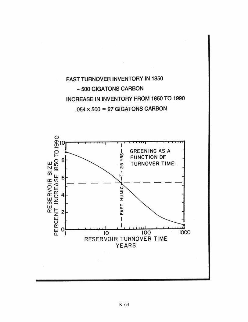
K-63

K-64

proportion to the food supply, at this point, bacterial destruction would once again

balance the input of new litter. The buildup of the inventory toward this new steady state

value would proceed as follows. After 25 ln2 or 17.3 years, it would be 5% greater; after

2x25 ln2 or 34.6 years, it would be 7.5% greater, after 3x25 ln2 or 51.9 years, it would be

8.75% greater, and so forth.

Assigning residence times to components of the soil humus reservoir proves

particularly difficult, for its complex of chemical compounds must have a very wide

range of survival times. Unlike trees which build annual rings, soils have no equivalent

built in clock. Our best source of information comes from radiocarbon measurements

made on bulk humus (i.e., on soil samples from which rootlets and litter have been

removed). Measurements based on soils sampled prior to the onset of nuclear testing

(i.e., prior to the rise in atmospheric radiocarbon) yield an average radiocarbon age of

roughly a millennium. By contrast, soils collected subsequent to the bomb-testing-

induced peak in atmospheric radiocarbon yield 14C to C ratios 10 to 20 percent higher

than those for the pre-nuclear atmosphere. These results confirm the expectation that a

wide spectrum of turnover times exists for the organic compounds in soils. While not

permitting this spectrum to be defined, the radiocarbon measurements allow the organics

in soils to be divided into two categories, those with lifetimes so long that little change in

amount (or in 14C/C) would be expected during the period of CO2 greening, and those

with lifetimes short enough to respond to greening (and to the bomb 14C transient). An

estimate of the turnover time for the long residence time component is obtained from

radiocarbon measurements on humus from the subsoil. It is assumed that these organics

are dominated by the long-lived component. The age obtained on such samples averages

3500 years. Knowing this age and also the bulk age for top soil, it is possible to divide

the soil organics into two types and to say what fraction of the carbon falls in each. The

result is that with regard to greening about 25% of the carbon is inert and about 75%

K-65

‘active’. The turnover time of the active reservoir carbon is obtained through modeling

of its response to the bomb radiocarbon transient. What is found is that the best fit to the

data for native soils is obtained using a turnover time of 25 years for the ‘active’

reservoir.

This exercise is much akin to that for the one dimensional ocean model. A

globally averaged top soil is divided into a part which is greened and a part which

responds too slowly to be greened. This corresponds to a division of the ocean into a part

which is accessible to fossil fuel CO2 and one which is isolated from contact with the

atmosphere. Measurements of bomb radiocarbon permit the transient response of the

active reservoir to be constrained. It must be emphasized, however, that the reliability of

soil model does not match that of the ocean model. It is based on far shakier assumptions

and is documented by a far, far smaller data set.

Nevertheless, the soil model provides at least a rough estimate of the extent to

which natural soils are being greened. Assuming that 500 gigatons of carbon reside in

the active reservoir of soils, 3.3% faster growth for each 10% higher atmospheric CO2

content, and a 25-year turnover time for carbon in this pool, the rate of accumulation of

extra carbon in the Earth's soils would be about 0.6 gigaton of carbon per year. Because

of the major uncertainties involved in this calculation, this result can be taken only as an

indication that the CO2 induced greening of the soil reservoir could make a significant

contribution to explaining the whereabouts of the missing carbon.

Greening of the wood reservoir can be treated in a similar fashion. This carbon

reservoir has a similar size as the active soil reservoir (i.e., 500 gigatons of C), but

because of its longer turnover time, the rate at which forests are packing away excess

carbon should be somewhat smaller, more like 0.3 gigatons of carbon per year for the

1980s.

The response time of the short lived leaf, litter, rootlet reservoir is so short that its

size should closely follow the atmospheric CO2 rise. During the 1980s, the CO2 content

K-66

of the atmosphere was rising at the rate of 1.5 ppm per year. Using the 0.33 greening

factor, this means that the rate of production of such material was rising at the rate of

0.14%/year. As the size of this reservoir is about 150 gigatons of carbon, the rate of

increase is estimated to be 0.2 gigatons per year.

Taken together, the greening of these three reservoirs adds up to about one

gigaton per year. This is about the amount required to balance the carbon budget. One

might conclude from this that the results obtained in chamber experiments are providing

reasonable estimates of what goes on in the real world.

But the situation is very likely much more complicated for there is another

potential greening agent. Most ecosystems, whether they be terrestrial or aquatic,

respond to additions of fixed nitrogen. Repeated forest surveys in six European countries

show that a substantial increase (~25%) in standing stock of wood occurred between

1970 and 1990. Prior to industrialization, growth in all European forests was nitrogen

limited. Currently, because of the fallout of anthropogenic NO3 and NH3, the fixed

nitrogen is super abundant. Hence the most likely explanation for the fattening of these

forests is driven by fixed nitrogen fertilization rather than by excess atmospheric CO2.

While not well established, the amount of fixed nitrogen fallout attributable to

anthropogenic sources is about 0.05 gigatons of nitrogen/yr. As the C/N ratio in soils is

about 12 and that in aquatic plants about 7, it is tempting to assume that for every mole of

fixed nitrogen reaching the planet's surface, about 10 moles of carbon are sequestered. If

so, then about 0.5 gigatons of carbon are being stored each year as the result of the fallout

of ammonia and nitric acid.

There may however be a flaw in the assumption that fixed nitrogen is used only

once and then stored until respiration or decay makes it available for recycling. Rather, it

may become part of the photosynthetic factory instead of the product. If so, the number

of carbon atoms stored per fixed nitrogen released to the environment may exceed the 10

to 1 ratio assumed above.

K-67

Support for the conclusion that nitrogen is an important player in greening comes

from the measurements of the interhemispheric gradient in 13C to 12C ratios in

atmospheric CO2. In order to make a self consistent picture for 13C, CO2 and O2, it is

necessary to call on the temperate forests of the northern hemisphere as a major site for

greening. As most agricultural-, industrial- and automotive-derived fixed N is released in

the north temperate zone and since its lifetime in the atmosphere is too short to permit

long distance transport, nitrogen fertilization occurs mainly in this zone

Projections to the Future

If international agreements in limiting CO2 emissions such as that concluded in

1997 in Kyoto are to be implemented, then it will be necessary to have models which

permit us to predict the evolution of the CO2 content of the atmosphere for any given fuel

use scenario. Essential to this enterprise are dynamic ocean models. Not only must these

models be able to correctly reproduce the temperature and salinity distributions in the sea

and the evolution of the transient tracer distributions, but these models will have to

undertake the more difficult task of predicting the response of the ocean’s operation to

the expected warming and freshening of high latitude surface ocean waters. The

consequent slowdown in ventilation of the thermocline and deep sea will tend to reduce

the rate of uptake by the ocean of fossil fuel CO2. But countering this to some extent will

be the more efficient utilization of the NO3 and PO4 in high latitude surface waters.

Putting aside the possible slowdown in ocean circulation, two factors will alter the

split of excess CO2 between the ocean and the atmosphere. First, the CO=3 and HBO

-3

ion contents of surface waters will gradually become depleted. Already the CO=3 content

is about 25 percent lower than during pre-industrial times. This diminishment will be

reflected by a reduction in the proportion of the CO2 taken up by the sea. Second, as the

growth rate of atmospheric CO2 content slows the mean age of fossil fuel CO2 molecules

will increase. This lengthening will be reflected by an increase in the proportion of the

CO2 taken up by the sea. Will these factors more or less cancel one another? On the

K-68

short term the answer is likely ‘yes’. The reduction in capacity will be just about

balanced by the increase in ‘swimming’ time. To see why this is the case, let’s say that

by the year 2025 the CO2 content has risen to 415 ppm (i.e., by 100 x [415-360]/360 or

15 percent). If during the same time period, the mean lifetime of fossil fuel CO2

molecules rises from let’s say 30 to 40 years. Then, the fraction of the ocean available

for CO2 uptake will rise by a factor of 40 / 30 or 1.15. Hence, in this case, the two

changes would indeed cancel one another.

Another possibility would be to increase the uptake of CO2 by the ocean through

the addition of fertilizer. The sinking to the ocean interior of the excess organic debris

created in this way would lower the CO2 content of surface water. This deficiency would

be compensated by the invasion of CO2 from the atmosphere. As plant productivity in

the temperate regions of the ocean is limited by the availability of fixed nitrogen, one

possibility would be to purposefully add ammonia or nitrate. But such an approach

would in a sense be self defeating for more CO2 could be emitted to the atmosphere by

the facilities in which the nitrogen was fixed than would be removed from the atmosphere

as a result of its application to temperate ocean surface waters.

More promising is the addition of iron to those areas of the surface ocean in

which sizable quantities of unused NO3 and PO4 are present (mainly the Southern

Ocean). The late John Martin pioneered this concept by clearly demonstrating that the

sparsity of iron limited plant productivity in these regions. His critics were silenced

when an open ocean experiment conducted in the eastern equatorial Pacific produced a

dramatic drawdown of nitrate and of CO2 partial pressure. Further, the required amounts

of iron are relatively small - only one mole of iron for each 1000 moles of PO4 and

16,000 moles of NO3 utilized by plants. Hence for each mole of iron, the CO2 removed

could range as high as 125,000 moles. Expressed in terms of Redfield ratios:

Fe:P:N:C

1:1000:16,000:125,000

K-69

But iron fertilization is not the panacea for the rise of atmospheric CO2 content.

Model calculations reveal that even if all those regions of the ocean containing unutilized

NO3 and PO4 were continually dosed with iron for the next 150 years and if this

fertilization allowed full utilization of the upwelled NO3 and PO4, the rise in the CO2

content of the atmosphere would only be reduced by 10 percent. If, for example, in the

absence of fertilization the CO2 content of the atmosphere were to reach 750 ppm in the

year 2150, then fully successful iron fertilization between now and then would hold this

rise to 680 ppm. But keep in mind that if at that time the iron fertilization program were

to be abandoned, then the CO2 removed in this way would be returned to the atmosphere.

CO2 Management

As the CO2 content of the atmosphere rises and the planet warms, more and more

attention is likely to be focused on stemming this rise. The option of purposeful removal

of CO2 from the air can be ruled out. To do so by scrubbing air would require far, far

more energy per CO2 molecule removed than was gained by producing the CO2 molecule

in the first place! While plants could surely do the job, the cost of harvesting and

conversion to a form which could be permanently stored (i.e., carbon block) would be

prohibitive.

A more reasonable approach would be to capture the CO2 created by fossil fuel

burning at the source. This CO2 could be liquefied under pressure and buried either on

the ocean floor or in deep wells on the continental interiors. Of course, the capture,

liquefaction and storage of CO2 would require energy. Estimates are that were this to be

done, energy derived from fossil fuels would double in cost. Summary

This section's puzzle regarding the fate of fossil fuel CO2 boils down to an

assessment of the carbon storage in the terrestrial biosphere. What is the balance

between the positive terms in its budget (greening by CO2 and fixed nitrogen and

regrowth of previously cut forests) and the negative terms (forest cutting and

K-70

agriculturally-induced losses of soil humus)? As we have seen averaged over the last

several decades, the estimates obtained using tracer-calibrated box models and using

ocean general circulation models yield answers which suggest that the sum of excess CO2

stored in the atmosphere and in the ocean comes close to matching the amount of CO2

generated by the burning of fossil fuels. This result suggests that during the 1980s global

greening was responsible for an increase in the standing biomass of forest and soil carbon

of about one gigaton per year. This requires that the excess CO2 in the atmosphere and

excess fixed nitrogen in soils has caused plants to grow about 10% faster. Thus, by

chance, cutting around the "edges" of the terrestrial biosphere was matched by a fattening

in its "middle". But there is no guarantee that this balance will hold in the future. It is

easy to imagine scenarios where greening will wane to the extent that the terrestrial

biosphere becomes a net source, thereby aggravating the buildup of CO2 in the

atmosphere.

K-71

Commentary on Keeling's World Plates

pg. 2

The consensus view of the annual perturbations experienced by various Earth

surface carbon reservoirs during the 1980s. The fossil-fuel source is estimated from

records of coal, oil and natural gas production kept by each nation. The deforestation

contribution is estimated using satellite photography and ground-based standing biomass

measurements. The magnitude of ocean uptake is based on modeling. Greening (i.e., the

increase in terrestrial biomass resulting from CO2 and fixed N-induced growth

enhancement) is determined by difference.

pg. 4

In the upper panel is shown the atmospheric CO2 record for Marina Loa Hawaii

from 1958 to 1993. In addition to the temporal trend driven by fossil fuel burning, there

are internal changes resulting from small mismatches between respiration and

photosynthesis (see for example, the dramatic flattening in the early 1990s). The

seasonal cycle is driven by the strong late spring and early summer drawdown of CO2 by

plant growth in the extensive northern hemisphere temperate regions. In the lower panel

is shown the atmospheric methane record.

pgs. 6-7

Sufficiently accurate direct measurements of the CO2 content of the atmosphere

are available only for the period 1958 to present. Fortunately, this record can be

extended back in time using air trapped in polar ice. One problem in this regard is

establishing the exact age of the trapped air. Measurements on material from a shallow

core from Antarctica show that the close off of pores in the firn begins at a depth of 60

meters and is complete by about 80 meters. The age of the siple ice at the depth of the

midpoint of this close off interval is 95 years (as determined by counting annual layers).

Based on CFC measurements, the replacement of the air at the base of the firn via

diffusion down through the web of pores is estimated to be about 13 years. Hence the air

K-72

in bubbles is 82 years less than that of the ice in which the bubbles are encased. Of

course, as the bubble close off is not instantaneous but is spread over a period of time and

as the diffusive ventilation of the firn mixes air of different ages, the air trapped at any

given depth is a mixture spanning a decade or so.

As can be seen on page 7, the ice-core-derived reconstruction of atmospheric CO2

content and of an 13C12C tie in nicely with atmospheric measurements. pgs. 8-9

Breakdown of the magnitude of individual CO2 sources as a function of time.

While the dramatic use of petroleum use leveled off in the early 1970’s, coal and natural

gas took up the slack. Since 1957 when CO2 monitoring began, the rate of increase of

the atmosphere’s CO2 content has averaged about 60 percent the rate of CO2 emissions

from fossil fuel burning.

p. 12

Comparison of the La Jolla, California record for O2 decline with that for the CO2

rise. When the seasonal cycle is removed, O2 shows a 13.5 µatm decline over this period

and CO2 a 5.5 µatm rise. Two reasons exist for this difference. First, 145 moles of O2

are required to produce 100 moles of CO2 (the extra oxygens are required to convert the

H in the fuel to H2O). Second, part of the CO2 goes into the ocean.

pg. 14

In the upper panel is shown the relationship between atmospheric O2 trend for a

four-year period. In the lower panel is a comparison between the predicted and observed

cumulative trends for O2 and CO2. The predicted trend is that expected if the atmosphere

were a closed system. In order to account for the difference between the observed and

predicted trends, it is necessary to invoke not only CO2 uptake by the ocean but also a

significant increase in the amount of carbon stored in the terrestrial biosphere.

K-73

pgs. 18-19

Sea water takes up significant amounts of fossil fuel CO2 mainly because it is a

basic solution. CO2 from the atmosphere mates with carbonate ion in the sea to form two

bicarbonate ions. As shown on the left, were sea water free of borate, the reaction

carbonate ion would enhance the uptake by more than a factor of 13 (i.e., 34/2.6) over

that resulting from the solution of CO2 gas alone. When the reaction with borate is

included, the enhancement of uptake reaches almost a factor of 19 (i.e., 49.1/2.6). Also

note that by adding fossil fuel CO2 to the sea, we are gradually eroding its capacity for

further uptake. Both the CO=3 and H4BO

-4 are being consumed. The Revelle factor is

the percentage increase in the partial pressure of CO2 in the atmosphere required to raise

the ∑CO2 content of surface sea water by one percent.

pgs. 20-21

Radon measurements in the ocean-mixed layer provide an estimate of the rate at

which gases pass back and forth across the air-sea interface. By measuring the ratio of

radon concentration in the water to that which would be present were no radon to escape

to the atmosphere (i.e., that amount of 222Rn were its decay rate to just match its

production by the decay of its parent 226Ra). Measurements at a large number of stations

from throughout the world ocean reveal that on the average about three quarters of the

equilibrium amount of radon atoms are present in surface water. The remaining one

quarter escape to the atmosphere. This means that the probability of escape is about one

third the probability of radio decay. As the mean life of a radon atom with regard to

radio-decay is about 5.6 days, the mean lifetime with regard to escape must be about 17

days. The mean thickness of the wind stirred upper ocean at these stations averaged 54

meters. The gases in one seventeenth of this (a layer three meters thick) are replaced

each day. However, one correction must be made when this radon-based result is to be

applied to other gases such as CO2. The rate escape of a gas is related to its molecular

diffusivity in water: the higher its diffusity, the greater its escape probability.

K-74

pgs. 22-23

The distribution of natural radiocarbon permits an estimate of the rate at which

CO2 moves back and forth across the air-sea interface to be made. Assuming that prior to

nuclear testing the distribution of 14C was close to steady state, the net number of 14C

atoms passing from the atmosphere into the sea must have balanced the number of 14C

atoms undergoing radio-decay within the sea. The net number of 14C atoms entering the

sea is proportional to the gas exchange rate and to the difference between the 14C/C ratio

in atmospheric CO2 and that in surface mixed ∑CO2. The number of 14C atoms

undergoing radio-decay within the sea is proportional to the amount of ∑CO2 in the sea

and its mean 14C/C ratio. The CO2 exchange rate obtained in this way is consistent with

that based on radon measurements.

pgs. 26-27

Measurements on CO2 extracted from the atmosphere at different times and

places document the evolution of the nuclear-testing induced transient in the atmospheric

14C/C ratio. Because the 14C produced during tests was injected largely into the

stratosphere of the northern hemisphere during and just after the period of large scale

nuclear testing, CO2 in the atmosphere of the northern hemisphere had a higher 14C/C

ratio than that in the southern hemisphere. However, soon after the ban on atmospheric

testing had been implemented, the 14C/C ratio in the two hemispheres even out.

Through gas exchange, this excess 14C entered the surface ocean. At the time of

the global ocean survey carried out during the 1970s, the 14C/C ratio in surface water

∑CO2 had risen by about 160‰ over its pre-nuclear value. The vertical distribution of

this excess 14C (and also of tritium released as the result of bomb tests) provides a

measure of the depth to which pollutants added to the ocean surface are mixed into its

interior on a timescale of about one decade. The so called mean penetration depth is

calculated by creating a rectangle on the concentration depth plot whose horizontal side

K-75

equals the surface excess of 14C (or 3H) and whose vertical side is such that the area in

the rectangle is equal in area to that of the observed excess (crosshatched in diagram).

At the mid-point of the GEOSECS survey (1975), these isotopes had penetrated to

a mean depth of 360 ± 30 meters (i.e., into nearly 10% of the ocean's volume). Based on

these measurements, the number of radiocarbon atoms beneath each square centimeter of

sea surface can be computed (using ∑CO2 measurements as well as 14C/C

measurements). The geographic pattern of these inventories is strongly influenced by the

sea’s major circulation systems. The inventories are lower than average in zones of

upwelling (i.e., the tropical ocean, the circum Antarctic Ocean and the northern-most

Pacific Ocean). In these regions, it is as if the 14C were being added to a fountain in

which the waters rise to the surface and then move laterally. The northern Atlantic

breaks the global symmetry of this pattern for it is the birthplace of much of the world's

deep water (in other words, a zone of downwelling instead of a zone of upwelling).

pgs. 30-31

A simple one-dimensional model yields a remarkably good simulation of the

uptake of fossil fuel CO2 by the sea. It consists of a well-mixed surface layer taken to be

75 meters thick in accord with temperature profiles measured throughout the world

ocean. This wind-stirred layer is underlain by the density-stratified main body of the

ocean. Vertical mixing in the sea’s interior is assumed to proceed in accord with the

square root of time (i.e., by eddy diffusion). The CO2 exchange rate between air and sea

and the vertical mixing rate in the stratified part of the ocean are selected so as to give the

best possible fit to the horizontally-averaged distribution of excess nuclear-testing 14C as

surveyed during the GEOSECS program. Vertical mixing is modeled in this way because

the time required to mix the entire ocean (i.e., 1000 years as determined from the

distribution of natural radiocarbon) is 100 times longer than the time required for tracers

to spread through the upper 10% of the sea. The CO2 exchange rate and vertical mixing

rate are constrained to match the GEOSECS observations (i.e., the increase in 14C/C ratio

K-76

in average surface water and the mean penetration depth of bomb-testing 14C and 3H).

Of course, if the model yields a match to the surface excess and to the mean penetration

depth, it will also yield the observed total ocean inventory of bomb-testing radiocarbon.

pg. 34

While the time required to exchange the gases in the oceanic mixed layer with

overlying air is measured in weeks, the time required for the oceanic mixed layer to reach

equilibrium with either a change in the CO2 content or 14C/C ratio in the overlying

atmosphere is far longer. This difference can be best understood by comparing the

response of two 75 meter high columns of water to a stepwise change in the CO2 content

and 14C/C ratio in the overlying air. One column contains distilled water (which is free

of HCO-3 and CO

=3 ). The other is sea water. As the distilled water contains only CO2

gas, its response to the stepwise change is rapid with no difference in timing between the

CO2 content and the isotopic ratio. By contrast, because of dissolved HCO-3 and CO

=3 ,

the sea water responds much more slowly. As its ∑CO2 content exceeds its CO2 content

by a factor of 200 (∑CO2 ≅ 2000 µmol/kg and CO2 ≅ 10 µmol/kg) its response time for

isotopic change is 200 times longer than that for the distilled water. The response time

for the ∑CO2 content of the sea water lies roughly geometrically between the response

time for the distilled water column and the isotopic response time for the sea water. In

simplest terms, the reason is that uptake of CO2 is dictated by the CO=3 content of the

surface sea water (~200 µmol/kg) which lies roughly geometrically between that for

∑CO2 (~2000 µmol/kg) and that for CO2 (~10 µmol/kg).

pgs. 36-37

The simple 1-D ocean model can be put to three additional tests. First, if CO2 is

fed into the atmosphere in accord with the fossil fuel emissions, does the model generate

a rise in atmospheric CO2 in accord with observation (assuming that the terrestrial

biosphere has remained nearly null). In order to pass this test, the model must be initiated

with an atmospheric CO2 content of 292 µatm rather than the value of 280 µatm obtained

K-77

from ice core measurements. The second test is to match the decline in 13C/12C ratio

resulting from the addition to the model's atmospheres of 13C deficient fossil fuel CO2.

As can be seen, the model passes this test handily. The third test is to match the decline

of 14C/C ratios resulting from the addition to the model's atmosphere of 14C-free CO2

from fossil fuel burning. Again, the match between model and observation is quite good.

It must be noted however, that the observed trend in atmospheric 14C/C ratio contains a

small natural component (due to fluctuations in the strength of the solar wind and its

associated magnetic field). As this contribution cannot be accurately assessed, it is

possible that by chance this natural contribution masks a deficiency in the model. It

should also be noted that were there no mixing between the carbon atoms in the

atmosphere and those dissolved in the sea, both the 13C and 14C changes would be five or

so times larger than the observed changes. Hence, these are quite stringent tests of the

ocean model.

pgs. 38-39

The model can be put to a fourth test. Does it produce a match to the observed

post-test-ban decline in the 14C/C ratio of the atmosphere. This crosscheck is performed

in a less direct manner. The atmosphere's 14C/C and CO2 contents are programmed to

follow their observed time trends. The model's ocean and terrestrial biosphere exchange

carbon isotopes with this atmosphere. The excess radiocarbon inventories are calculated

for each reservoir and then totaled. What is found is that after 1967 (i.e., the time when

the entire atmosphere (including the stratosphere) had become well mixed with respect to

bomb 14C, the total inventory of radiocarbon remained nearly constant. This constancy is

not found for the period prior to 1967 because up until this point the stratosphere retained

a significant excess 14C/C over that for the troposphere.

pg. 42

A map for the 1980s showing the difference between the CO2 partial pressure in

atmosphere and that in surface ocean constructed using measurements from along dozens

K-78

of ship tracks. Although this distribution has a fair amount of texture (for example, a

pronounced excess in the eastern equatorial Pacific and a pronounced deficiency in the

northern Atlantic), when averaged over the entire ocean, the difference is very small (~4

µatm). But the uncertainty on this measured average (±4 µatm) and in the corrections

required to compensate for the skin temperature bias (~2µatm) and for the

preanthropogenic excess balancing the river flux of carbon to the sea by rivers (~2µatm),

render untenable the use of this approach to make a meaningful independent estimate of

the flux of fossil fuel CO2 into the sea. All that can be said is that once corrected the

observed difference is consistent with that of 8 µatm predicted by models for the same

time period.

pg. 45

If, as we believe, an average 2 gigatons of fossil fuel carbon was entering the

ocean during the 1980s, then based on the global mean gas exchange rate obtained from

the distributions of mature 14C and radon (and confirmed by the GEOSECS survey of the

distribution of bomb-produced 14C), an average air-sea CO2 partial pressure difference of

8 micro-atmospheres would be required. However, as prior to the Industrial Revolution

the sea surface must have had a pCO2 of about 2 micro-atmospheres higher than the

atmosphere to balance the net transport to the sea by rivers of bicarbonate and dissolved

organic matter, the actual difference is reduced to 6 micro-atmospheres. Further, as

evaporation lowers the skin temperature of the ocean, a further correction is required

lowering the expected difference to only 4 micro-atmospheres.

pg. 47

Comparison of the annually averaged atmospheric CO2 record from atop the

extinct volcano, Mauna Loa, on the island of Hawaii with that from atop the Antarctic ice

cap. As can be seen, when in 1958 these records began, the two stations recorded nearly

the same mean annual CO2 content and since then, the difference has steadily grown. In

one sense, this is consistent with the rising production of CO2 from fossil fuel burning

K-79

(~2.3 GtC in 1958 to ~5.5 GtC in 1985). But one would expect the difference in 1958 to

have been 2.3/5.5 that in 1985. The records suggest that in 1958 the difference was close

to zero. This led to the speculation that prior to 1955, the difference might have been

reversed (in other words, the southern hemisphere had a higher partial pressure of CO2

than did the northern hemisphere). If so, then one would have to postulate that a natural

interhemispheric cycle exists which carries CO2 from the northern to the southern

hemisphere through the ocean and then back through the atmosphere.

pg. 51

The most obvious route for the interhemispheric ocean transport of CO2 is the

Atlantic's conveyor-like thermohaline circulation. Cold water manufactured in the

northern Atlantic sinks and flows southward around the tip of Africa into the circum

Antarctic deep water current. Much of this water upwells in the southern hemisphere.

This water carries excess CO2. This excess is related to the low nutrient (i.e., NO3 +

PO4) constituent content and hence respiration CO2 content of water sinking in the

northern Atlantic. In the Antarctic, the excess respiration CO2 associated with the much

higher nutrient constituent content of surface waters (compared to that for the low

latitude) more or less balances the reduction of CO2 partial pressure caused by the lower

temperature. Hence little tendency exists for CO2 to be transported to the Antarctic

through the atmosphere from other parts of the surface ocean. However, in the northern

Atlantic, the compensation by respiration CO2 is not adequate and hence the cooling

creates a surface water deficit in ∑CO2 of about 100 µmol CO2/kg. About 80 µmol/kg of

this deficit is compensated by the uptake of atmospheric CO2. Because of this, the

conveyor exports about 0.6 Gt of carbon to other parts of the ocean. While not enough to

create a south to north preanthropogenic atmospheric CO2 gradient big enough needed to

explain the seemingly too low current interhemispheric difference in atmospheric CO2

content, transport by the conveyor might explain up to half of it. A more complete

K-80

explanation of this phenomenon is provided by the authors in a paper published in Nature

(1992, v. 356, p. 587-589).

pg. 54

An estimate of the minimum amount of fossil fuel CO2 taken up by the sea during

the 1980s can be obtained by assuming that the mean penetration depth of fossil fuel CO2

into the sea was no greater than that of bomb produced 14C (or 3H) at the time of the

GEOSECS survey. This estimate is a lower limit because during their mean lifetime of

30 years, fossil fuel CO2 molecules must have penetrated deeper into the sea than the

bomb isotopes which, at the time of the GEOSECS survey, had had only a bit more than

a decade to "swim". As the mean penetration depth of the bomb-produced tracers was as

of 1975 about 360 meters (i.e., approximately, one tenth the mean depth of the sea), this

means that at least one tenth of the ocean's capacity for CO2 uptake was accomplished.

This capacity is set by the ∑CO2 content of the ocean water divided by the Revelle factor

(or so called buffer factor) described on pg. 15. For the surface ocean, the average value

of this factor is 9 (i.e., for each 9% increase in atmospheric CO2 pressure the equilibrium

increase in ocean ∑CO2 will be 1%). This yields an ocean capacity one half that of the

atmospheric capacity which means that for each three moles of fossil fuel CO2 added to

the atmosphere, one will enter the sea and two will remain airborne. For the 1980s, the

measured increase in atmospheric CO2 was on the order of 3.0 GtC/year. Thus at least

1.5 GtC/year must have entered the ocean during this time period.

pgs. 62-63

Radiocarbon measurements are available for only a few dozen topsoil samples

collected at various places during the course of the rapid bomb radiocarbon transient.

These measurements suggest that prior to nuclear testing, the 14C/C ratio in humus from

top soils averaged about 0.9 times the 14C/C ratio for preanthropogenic terrestrial

vegetation (i.e., an apparent radiocarbon age of about 900 years) and that this ratio rose

(as the result of introduction bomb-testing 14C) to a broad maximum in the 1970s and

K-81

1980s, about 1.1 times the preanthropogenic ratio. In order to account for both of these

observations, it is necessary to call on at least two classes of soil humus, one with a

turnover time measured in millennia and one with a turnover time measured in decades.

The former pool is necessary to account for the low 14C/C ratio prior to bomb testing and

the latter for the uptake of appreciable amounts of bomb 14C. A fit to the data can be

achieved by assuming that the top-soil humus consists of 75% material with a 25-year

turnover time (hence a pre-nuclear 14C/C ratio close to 1.0) and 25% material with a

4000-year turnover time (hence a pre-nuclear 14C/C ratio of about 0.6). While in reality

the situation must be much more complicated (i.e., a wide spectrum of turnover times

must exist) based on available constraints, no way exists to improve upon the very simple

two reservoir model shown here.

The two reservoir model allows an estimate of the extent of CO2-induced

"greening" of soils to be made. In this calculation, the chamber-experiment-based factor

of 3.5% growth enhancement per 10% increase in air CO2 content is applied to the entire

terrestrial biosphere (i.e., during the 1980s when the atmosphere’s CO2 content was about

27% higher than prior to the Industrial Revolution, the growth rate of plants and hence

the production rate of new humus was, presumably, about 9% higher than prior to the

Industrial Revolution.) The extent to which any reservoir increased its size as a result of

this greening would depend on its turnover time. Only reservoirs such as leaves, grass,

rootlets... with very short turnover times would show the full 9% increase. By contrast,

the millennium response-time fraction of soil humus would show almost no greening.

The fast response-time soil reservoir would be expected to show a bit more than half the

maximum response. Assuming that the global reservoir of fast responding humus contain

500 Gt of carbon, its inventory should have risen by about 27 GtC since the beginning of

the Industrial Revolution (an amount equal to about 9 years accumulation of CO2 in the

atmosphere at the 1980s rate).

K-82

Keeling's World Problems

1. If your car gets 30 miles to a gallon of gasoline, how many pounds of CO2 gas does

it release to the atmosphere per mile driven? (assume that gasoline has a density of

0.8 gm/cc, and a chemical formula with twice as many hydrogen atoms as carbon

atoms). If you were to drive your car 20,000 miles each year, how many tons of

CO2 would you produce annually? If all 5.5 billion people on the planet were to

drive cars 10,000 miles in each year, how many gigatons of carbon would be

produced? How does this compare to today's fossil fuel CO2 production rate of ~6

gigatons per year? (1 gallon = 3.785 liters, one ton = 106 gm, one pound = 453

gm).

2. For the year 1993, the CO2 content of the atmosphere averaged globally was about

358 ppm by volume. What would the CO2 content be 100 years from now (i.e., in

the year 2093) if:

a. CO2 production remained constant at 6.0 GtC/yr.

b. CO2 production rose at the rate of 1% per year.

Assume that 55% of the CO2 produced remains in the atmosphere.

3. What would the radon based estimate for the invasion rate of CO2 into the sea be if

the ratio of the mean measured concentration of radon in the surface mixed layer to

that if no radon were lost to the atmosphere were 0.60 (instead of 0.77) and the

mean thickness of ocean mixed layer were 70 meters (instead of 54 meters). Give

your answer in units of moles/m2yr µatm. What would be the invasion rate of CO2

at 280 µatm? If this were the true CO2 invasion rate, then what would be the pre-

nuclear ratio of the 14C/C in mean surface water ∑CO2 to 14C/C in the atmosphere

have been?

4. Assume that as of 1990 the total amount of fossil fuels burned since the beginning

of the Industrial Revolution was 230 gigatons. Assuming that all this CO2

remained in the atmosphere (i.e., no transfer into the ocean or into the terrestrial

K-83

biosphere), calculate the expected atmospheric CO2 content in 1990. Assuming

that fossil fuel carbon has an average δ13C -27‰ and that no isotopic exchange of

atmospheric carbon with either oceanic or biospheric carbon occurred, by how

many ‰ ratio have dropped? Assume that as of 1950, a total of 70 gigatons of

carbon had been added to the atmosphere as a result of fossil fuel burning since the

beginning of the Industrial Revolution. Assuming that the fossil fuels are free of

radiocarbon and again no isotopic exchange of atmospheric carbon with either

oceanic or biospheric carbon occurred, by how many ‰ should the atmospheres

14C/C ratio have dropped by the year 1950? Calculate the following ratios:

a. Actual CO2 rise 1850 to 1990

Expected rise if all fossil fuel CO2 remained airborne = _____

b. Actual 13C/12C drop 1850 to 1990

Expected drop if no isotopic exchange with carbon in other reservoirs = ______

c. Actual 14C/12C drop 1850 to 1950

Expected drop if no isotopic exchange with carbon in other reservoirs = _____

The definitions of δ13C and ∆14C are as follows:

δ13C = 1000 x (13C/12Catm - 13C/12C)mean ocean

(13C/12C)mean ocean

∆14C = 1000 x (14C/Catm - 14C/C)

1850atm

14C/C 1850atm

Both are akin to percentage differences from the ratio measured in a reference

material. But they are given in parts per thousand instead of parts per hundred.

Assume that in 1850 the atmosphere contained 550 gigatons of carbon and that this

CO2 had a δ13C value of -6.5‰.

5. Calculate the composition of sea water at equilibrium with an atmosphere with a

CO2 partial pressure of 560 µatm. Assume sea water to be borate free and to have

K-84

an alkalinity equal to 2100 µmol/kg and a Kc value of 1445. You can get the

answer either by trial and error or as by solving a quadratic equation. For the

former, guess at a CO =3 concentration. Then use the charge balance equation to

calculate the corresponding HCO−3 concentration. Then substitute both in the

equilibrium constant equation (along with CO2 = 20 µmol/kg).

Example:

guess CO=3 = 100 µmol/kg

then HCO−3 = 2100 - 2 x 100 = 1900

and Kc = 1900 x 190020 x 100 = 1805 Too high!

so choose a larger CO=3 ion concentration

and repeat until Kc = 1445.

6. Explain why it is that burning of fossil fuels causes the atmospheric O2 content to

drop 13.5 µatm for every 5.5 µatm CO2 rises, when for plant growth or plant

respiration this ratio is very close to 1.

7. Explain the difference between the atmospheric radiocarbon records for the

northern and southern hemispheres. Why the annual wiggles in these curves?

8. If the surface water bomb radiocarbon excess at the time of the GEOSECS survey

had averaged 80‰ (instead of 160 ‰) greater than the prenuclear Δ14C value (and

if the mean penetration depth were the same as shown on page 29), which of the

parameters in the simple model shown at the top of page 28 would have to be

changed? What would its new value be? How would the ocean inventory of bomb

radiocarbon atoms have differed?

9. Plants living in the surface sea produce O2 gas. These new molecules eventually

escape to the atmosphere. If the piston velocity for O2 is 3 meters/day and the

mean thickness of the mixed layer is 54 meters, how many days does the average

O2 molecule remain in the sea before escaping to the atmosphere?

K-85

10. The simple model shown on p. 28 predicts that during the 1980s the global mean

air-sea CO2 difference should have averaged 8µatm (see pg. 40). Let's say that

marine chemists had succeeded in measuring this difference at enough places and

seasons to convince the world that the true difference was only 4±1 µatm. How

might this difference be explained?

11. Had the measurements made during the GEOSECS survey have indicated that the

mean penetration depth of bomb radiocarbon tritium were ~720 meters instead of

~360 meters, then what would be the minimum amount of fossil fuel CO2 taken up

by the ocean at a time when the atmosphere was rising 3.0 GtC/year?

12. Planet X is identical to the Earth in most respects (same ocean and continent areas,

same ocean and atmosphere chemistry as that for the preindustrial earth, same size

atmosphere). One important difference exists; the mean depth of its ocean is only

475 meters (compared to 3800 for the Earth). Three hundred gigatons of carbon are

released as CO2 through the burning of fossil fuels. No nuclear bombs are

exploded nor nuclear reactors operated. Several hundred years later, this extra CO2

has become thoroughly equilibrated with Planet X's ocean and terrestrial biosphere.

Calculate the following quantities:

a. The atmospheric 14C/C reduction (assume that fossil fuels are radiocarbon

free)

b. The atmospheric δ13C change (assume that it started at -6.5‰ and that the

carbon isotope composition of fossil fuel carbon is -26.5‰)

c. The atmospheric CO2 content (assume that it started at 280µatm)

Give your answers as follows:

a. 14C/CAfter

14C/CBefore = ______________________

b. δ13CBefore - δ13CAfter = ___________________________‰

K-86

c. atm

pCO2After = _________________________µatm

The total mass of the biosphere (wood, soils...) is 1000 gigatons. Assume for

simplicity that prior to Planet X's industrial revolution, its ocean and biosphere had

uniform 14C/C ratios equal to that in the atmosphere. Assume that the ocean has a

uniform ΣCO2 concentration of 1.91 moles/meter3. The area of Planet X is 5.1 x

1014m2, that of the ocean is 3.6 x 1014m2. Assume for simplicity that the ocean has

the same δ13C as fossil fuels. Assume no change in biosphere size. Assume a

borate free ocean with preindustrial [CO2] = 10µmol/liter, [HCO−3 ] =

1700µmol/liter and [CO=3 ] = 200µmol/liter. The equilibrium constant, Kc, is 1445.

Do a and b first. They are relatively easy. By contrast, c is quite difficult. If you

can't get c, just write down the equations.

13. If in the year 1800 A.D., forests covered one third of the Earth's land area, and if

their total tree biomass was 600 GtC, how many grams of carbon were there per

square centimeter forest? How many tons of biomass per hectare (a square hectare

measures 100 meters on a side)? Trees can be thought of as umbrellas which when

folded up become cylinders extending 20 meters above ground and 10 meters below

ground with a uniform diameter equal to that of the trunk (assume it to be 50 cm).

If so, on the average, how many trees would there be per hectare? Assume the

density of wood to be 0.9 gm/cm3.

14. The UN mandates that enough trees be grown such that 30 years from now the

added biomass will be 60 GtC. If these trees achieve the mass given in problem

#13, how many will there be? If they are spaced as in problem #13, how many

hectares will be required? What fraction of the Earth's land area will this require?

Three people can be supported by the food grown on a single hectare. If existing

farm land were used to grow these trees, what fraction of today's farm land would

this require? (Assume the population to be 5.6 billion)

K-87

15. Assume that Biosphere 2 has an area of 2 hectares and a mean height of 10 meters.

Further, assume that its soils contain 2.8 gmC/cm2 but that the vegetation can

support at steady state only 0.8 gmc/cm2. The soils cover 80% of the area of

Biosphere 2. Further, assume that all the organic matter is of the 'active' variety and

has a survival (i.e. replacement) time of 20 years. Still further, assume that the

standing biomass of vegetation is at steady state (i.e. it is neither increasing or

decreasing) and that the concrete has been sealed so that it no longer takes up CO2.

On January 1, 1994, the pO2 was 210,000 µatm and the pCO2 was 2000 µatm. The

ratio of CO2 creation to O2 consumption is one mole per mole. If no remedial

action were taken, how would these values change over the course of one year (i.e.,

what would they be as of January 1, 1995?) If instead, the Biospherians had an

apparatus which allowed them to remove CO2 by reacting it with CaO stored in

anticipation of this problem, how much CaCO3 would they form in the course of

the year in order to maintain the initial CO2 content of their air? If they had a

second piece of apparatus which electrolized water to form H2 and O2, how much

water would they have to electrolize during the course of the year in order to

maintain the O2 content of the air at its initial value? A gigantic problem associated

with this solution would be what to do with the H2 gas. Assuming that it could be

kept separate from the O2 generated and transferred into a balloon mounted above

the roof of Biosphere 2, what would be the ratio balloon volume to the Biosphere 2

volume at the end of one year? (Assume that both the balloon and Biosphere 2 are

at one atmosphere pressure).

16. Assume that over the course of the year the average daytime photosynthetic

production of organic C is three times the consumption rate of excess soil carbon by

bacteria. If the biomass of Biosphere 2 is to be at steady state, this creation of new

biomass must be exactly balanced by oxidation of old biomass. One difference: assume

that respiration occurs at a uniform rate round the clock (i.e., no diurnal cycle) but

K-88

photosynthesis occurs only during an 8-hour period from 8 am to 4 pm (i.e., it is shut

down during the other 16 hours). If on a typical morning at 8 am the CO2 partial pressure

in Biosphere 2 air is 2500 µatm, what will it be at 4 pm when photosynthesis stops? The

volume occupied by one mole of air at one atmosphere pressure and 25°C is 24.6 liters.

K-89

Super Problem

In the year 2401, David Ralph Keeling, a distant descendant of the clan made

famous in the 20th century by their measurements of CO2 and O2 in the Earth's

atmosphere, is sent to assess what terrible fate befell a colony established by biospherians

sent forth from Earth in the year 2081 to Kri, a planet of the neighboring star Ciolki.

After three centuries of what seemed to be an extraordinarily successful venture, radio

communication abruptly ceased. Twenty years have passed since this last report was

transmitted. As he steps forth from his speed-of-light space ship, young Keeling is struck

by a horrible stench. Hulks of dead animals and plants strew the landscape. A quick

survey by rotocoptor confirms that some catastrophe must have struck down all life on

the planet. Only the most primitive of bacteria appear to have survived; they slowly

devour the rotted remains.

Dee-Ar, as he is known to his friends, has been assigned by the expedition leader

to assess whether this disaster could be related to the heavy exploitation of Kri's vast

graphite reserves. While the colony was established by 8 biospherians, its population

soared to a staggering 4 billion just before the catastrophe struck.

Question #1: Assuming that the catastrophe happened exactly 300 years after the

first group of 8 babies were born, if every woman on planet Kri gave birth to one set of

quadruplets (2 boys and 2 girls) and if everyone lived to the age of 80, then what was the

designated child-bearing age?

Dee-Ar's task is complicated by the fact that the Krians were very secretive about

their affairs. Communications with Earth were restricted to the bare minimum of

information agreed upon before the original biospherians were forced to leave Earth.

And try as he may, Dee-Ar can locate no records what-so-ever concerning Kri's carbon

cycle. The only information comes from measurements made by the expedition team.

Kri was selected for colonization because it so closely resembled Earth in size and

surface character. Its ocean covers almost half the planet and its atmosphere exerts a

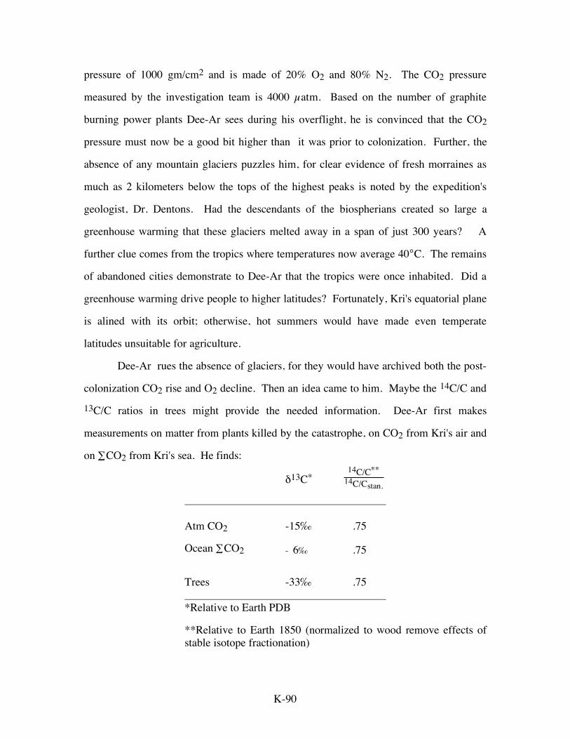
K-90

pressure of 1000 gm/cm2 and is made of 20% O2 and 80% N2. The CO2 pressure

measured by the investigation team is 4000 µatm. Based on the number of graphite

burning power plants Dee-Ar sees during his overflight, he is convinced that the CO2

pressure must now be a good bit higher than it was prior to colonization. Further, the

absence of any mountain glaciers puzzles him, for clear evidence of fresh morraines as

much as 2 kilometers below the tops of the highest peaks is noted by the expedition's

geologist, Dr. Dentons. Had the descendants of the biospherians created so large a

greenhouse warming that these glaciers melted away in a span of just 300 years? A

further clue comes from the tropics where temperatures now average 40°C. The remains

of abandoned cities demonstrate to Dee-Ar that the tropics were once inhabited. Did a

greenhouse warming drive people to higher latitudes? Fortunately, Kri's equatorial plane

is alined with its orbit; otherwise, hot summers would have made even temperate

latitudes unsuitable for agriculture.

Dee-Ar rues the absence of glaciers, for they would have archived both the post-

colonization CO2 rise and O2 decline. Then an idea came to him. Maybe the 14C/C and

13C/C ratios in trees might provide the needed information. Dee-Ar first makes

measurements on matter from plants killed by the catastrophe, on CO2 from Kri's air and

on ∑CO2 from Kri's sea. He finds:

δ13C* 14C/C**

14C/Cstan.

Atm CO2 -15‰ .75

Ocean ∑CO2 - 6‰ .75

Trees -33‰ .75 *Relative to Earth PDB

**Relative to Earth 1850 (normalized to wood remove effects of stable isotope fractionation)

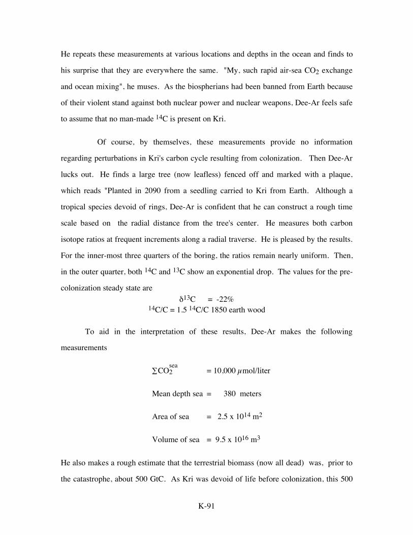
K-91

He repeats these measurements at various locations and depths in the ocean and finds to

his surprise that they are everywhere the same. "My, such rapid air-sea CO2 exchange

and ocean mixing", he muses. As the biospherians had been banned from Earth because

of their violent stand against both nuclear power and nuclear weapons, Dee-Ar feels safe

to assume that no man-made 14C is present on Kri.

Of course, by themselves, these measurements provide no information

regarding perturbations in Kri's carbon cycle resulting from colonization. Then Dee-Ar

lucks out. He finds a large tree (now leafless) fenced off and marked with a plaque,

which reads "Planted in 2090 from a seedling carried to Kri from Earth. Although a

tropical species devoid of rings, Dee-Ar is confident that he can construct a rough time

scale based on the radial distance from the tree's center. He measures both carbon

isotope ratios at frequent increments along a radial traverse. He is pleased by the results.

For the inner-most three quarters of the boring, the ratios remain nearly uniform. Then,

in the outer quarter, both 14C and 13C show an exponential drop. The values for the pre-

colonization steady state are δ13C = -22%

14C/C = 1.5 14C/C 1850 earth wood

To aid in the interpretation of these results, Dee-Ar makes the following

measurements

∑COsea2 = 10,000 µmol/liter

Mean depth sea = 380 meters

Area of sea = 2.5 x 1014 m2

Volume of sea = 9.5 x 1016 m3

He also makes a rough estimate that the terrestrial biomass (now all dead) was, prior to

the catastrophe, about 500 GtC. As Kri was devoid of life before colonization, this 500

K-92

GtC must have been produced during the last 300 years. Dee-Ar further assumes that its

half replacement time was 25 years.

Q-2. From this information, Dee-Ar calculates how much coal was burned. What

answer does he obtain?

Dee-Ar's next step is to calculate the expected 13C/12C ratio change assuming that

the only perturbation is from coal burning. He makes carbon isotope measurements on

Kri's graphite and finds that it has a quite uniform ratio of -25‰. At first Dee-Ar is

puzzled to see that the 13C decline measured in the tree is smaller than that predicted

from his coal consumption estimate. Then he realizes that the difference is the result of

biosphere growth and that he can use it to check his rough estimate of Kri's standing

biomass.

Q-3. What result does he obtain?

Having established the amount of excess CO2 added to Kri's atmosphere-ocean

system, Dee-Ar's next task is to attempt to reconstruct the pre-colonial CO2 partial

pressure. He equilibrates Kri's sea water with air containing 3600 and 4400 ppm CO2

and measures the ∑CO2 in these two sea water samples

pCO2 ∑CO2

µatm µmol/liter

3600 9950

4000* 10,000**

4400 10,050

*Kri's atmospheric CO2 content

**Kri's ocean ∑CO2

K-93

He also demonstrates that the pCO2 and ∑CO2 of Kri's ocean is everywhere the same.

Q-4. What does Dee-Ar conclude about the pre-colonial atmospheric CO2

content?

K-94

ANNOTATED BIBLIOGRAPHY CO2 PRODUCTION BY FOSSIL FUEL BURNING Keeling, C. D., 1973, Industrial production of carbon dioxide from fossil fuels and

limestone, Tellus, 25, 174-198. Rotty, R. M., 1977, Global carbon dioxide production from fossil fuels and cement, A.D.

1950-A.D. 2000, in: The Fate of Fossil Fuel CO2 in the Oceans, R. N. Anderson and A. Malahoff (eds.), pp. 167-181, Plenum Press, New York.

Review of data sources and summary of energy use trends up to 1975. Rotty, R. M., 1980, Past and future emission of CO2, Experientia, 36, 781-783. Marland, G., and R. M. Rotty, 1984, Carbon dioxide emissions from fossil fuels: A

procedure for estimation and results for 1950-1982, Tellus, Ser. B36, 232-261. Marland, G., R. M. Rotty, and N. L. Treat, 1985, CO2 from fossil fuel burning: global

distribution of emissions, Tellus, Ser. B37, 243-258. Marland, G., T. A. Boden, R. C. Griffin, S. F. Huang, P. Kanciruk, and T. R. Nelson,

1989, Estimates of CO2 emissions from fossil fuel burning and cement manufacturing, based on the United Nations energy statistics and the US Bureau of Mines cement manufacturing data, Publ. 3176, Rep. ORNL/CDIAC-25, NDP-030, Oak Ridge Nat. Lab., Environ. Sci. Div., Oak Ridge, Tenn.

Marland, G., and T. A. Boden, 1991, CO2 emissions - modern record, in: Trends '91: A

Compendium of Data on Global Change, pp. 386-507, ORNL/CDIAC-46, Carbon Dioxide Information Analysis Center, Oak Ridge National Laboratory, Oak Ridge, Tennessee.

Marland, G., and T. Boden, 1993, The magnitude and distribution of fossil-fuel-related

carbon releases, in: The Global Carbon Cycle, M. Heimann (ed.), pp. 117-138, NATO ASI Series, Vol. I 15, Springer-Verlag, Berlin.

Graedel, T. E., T. S. Bates, A. F. Bouwman, D. Cunnold, J. Dignon, I. Fung, D. J. Jacob,

B. K. Lamb, J. A. Logan, G. Marland, P. Middleton, J. M. Pacyna, M. Placet, and C. Veldt, 1993, A compilation of inventories of emissions to the atmosphere, Global Biogeochemical Cycles, 7, 1-26.

ATMOSPHERIC CO2 CONTENT AND O2/N2 RATIO Bolin, B., and W. Bischof, 1970, Variations of the carbon dioxide content of the

atmosphere in the northern hemisphere, Tellus, 22, 431-442. Keeling, C. D., R. B. Bacastow, A. E. Bainbridge, C. A. Ekdahl, P. R. Guenther, L. S.

Waterman, and J. F. S. Chin, 1978a, Atmospheric carbon dioxide variations at Mauna Loa Observatory, Hawaii, Tellus, 28, 538-551.

Keeling, C. D., J. A. Adams, Jr., C. A. Ekdahl, and P. R. Guenther, 1978b, Atmospheric

carbon dioxide variations at the South Pole, Tellus, , 28, 552-564.

K-95

Keeling, C., 1984, Atmospheric CO2 concentration Mauna Loa Observatory, Hawaii 1958-1983, Report NDP-001, U.S. Department of Energy, Carbon Dioxide Information Center, Oak Ridge, TN.

Keeling, C., T. Wharf, C. Wong, and R. Bellagag, 1985, The concentration of

atmospheric carbon dioxide at Ocean Weather Station P from 1969 to 1981, J. Geophys. Res., 90, 10511-10528.

Neftel, A., E. Moor, H. Oeschger, and B. Stauffer, 1985, Evidence from polar ice cores

for the increase in atmospheric CO2 in the past two centuries, Nature, 315, 45-47. Keeling, R. F., 1988, Measuring correlations in atmospheric O2 and CO2 mole fractions:

A preliminary study in urban air, J. Atmos. Chem, 7, 153-176. Oeschger, H., and U. Siegenthaler, 1988, How has the atmospheric concentration of CO2

changed? in: Rowland and Isaksen. Keeling, R. F., and S. R. Shertz, 1992, Seasonal and interannual variations in atmospheric

oxygen and implications for the global carbon cycle, Nature, 358. 723-727. First publication of measurements confirming downward trend in the atmospheric

O2 content. Keeling, R. F., R. P. Najjar, M. L. Bender, and P. P. Tans, 1993, What atmospheric

oxygen measurements can tell us about the global carbon cycle, Global Biogeochemical Cycles, 7, 37-67.

Bender, M. L., P. P. Tans, J. T. Ellis, J. Orchardo, and K. Habfast, 1994, A high precision

isotope ratio mass spectrometry method for measuring the O2/N2 ratio of air, Geochim. et Cosmochim. Acta, 58, 4751-4758.

Keeling, C. D., T. P. Whorf, M. Wahlen, and J. van der Plicht, 1995, Interannual

extremes in the rate of rise of atmospheric carbon dioxide since 1980, Nature, 375, 666-670.

Keeling, R. F., 1995, The atmospheric oxygen cycle: The oxygen isotopes of

atmospheric CO2 and O2 and the O2/N2 ratio, Reviews of Geophysics, Supplement, 1253-1262.

Keeling, R. F., and T.-H. Peng, 1995, Transport of heat, CO2 and O2 by the Atlantic’s

thermohaline circulation, Phil. Trans. R. Soc. Lond. B, 348, 133-142. Keeling, R. F., S. C. Piper, and M. Heimann, 1996, Global and hemispheric CO2 sinks

deduced from changes in atmospheric O2 concentration, Nature, 381, 218-221. TERRESTRIAL CARBON INVENTORY CHANGES Bolin, B., 1977, Changes of land biota and their importance for the carbon cycle, Science,

196, 613-615. First well-thought-out estimate of CO2 release as the result of deforestation. Meyers, N., 1980, Conversion of Tropical Moist Forests, Naitonal Academy of Sciences

Press, Washington, D.C. Tropical deforestation.

K-96

Houghton, R. A., J. E. Hobbie, J. M. Melillo, B. Moore, B. J. Peterson, G. R. Shaver, and G. M. Woodwell, 1983, Changes in the carbon content of terrestrial biota and soils between 1860 and 1980: A net release of CO2 to the atmosphere, Ecological Monographs, 53, 235-262

An upper limit on the magnitude of CO2 release resulting from deforestation. Woodwell, G. M., 1983, Biotic effects on the concentration of atmospheric carbon

dioxide: A review and projection, in: Changing Climate, pp. 216-241, National Academy Press, Washington, D.C.

Review article discussing the role of the biosphere in the global carbon budget. Brown, S., and A. E. Lugo, 1984, Biomass of tropical forests: A new estimate based on

volumes, Science, 223, 1290-1293. A new biomass estimate for tropical forests. Houghton, R. A., R. D. Boone, J. M. Melillo, C. A. Palm, G. M. Woodwell, N. Meyers,

B. Moore III, and D. L. Skole, 1985, Net flux of carbon dioxide from tropical forests in 1980, Nature, 316, 617-620.

Estimate of net carbon release in 1980 from deforestation in the tropics. Melillo, J. M., C. A. Palm, R. A. Houghton, G. M. Woodwell, and N. Myers, 1985, A

comparison of two recent estimates of disturbance in tropical forests, Enviornmental Conservation, 12, 37-40.

Presenting the logic and the evidence that two different approaches give the similar results for annual rate of disturbance in tropical forests in late 1970s.

Brown, S., A. E. Lugo, and J. Chapman, 1986, Biomass of tropical tree plantations and its

implications for the global carbon budget, Canadian J. Forest Res., 16, 390-394. Palm, D. A., R. A. Houghton, J. M. Melillo, D. Skole, and G. M. Woodwell, 1986, The

effect of tropical deforestation on atmospheric CO2, in: Land Clearing and Development in the Tropics, R. Lal, P. A. Sanchez, and R. W. Cummings, Jr., (eds.), pp. 181-194, A. A. Balkema, Rotterdam.

Describing how the net flux of carbon between terestrial ecosystems and the atmosphere is determined by use of a model initially developed by B. Moore.

Houghton, R. A., R. D. Boone, J. R. Fruci, J. E. Hobbie, J. M. Melillo, C. A. Palm, B. J.

Peterson, G. R. Shaver, G. M. Woodwell, B. Moore, D. L. Skole, and N. Myers, 1987, The flux of carbon from terrestrial ecosystems to the atmopshere in 1980 due to changes in land use: geographic distribution of the global flux, Tellus, 39B, 122-139.

Determining the geographic distribution of the biotic flux of carbon in 1980 produced as a result of deforestation, reforestation, logging and changes in agricultural area.

Woodwell, G. M., R. A. Houghton, T. A. Stone, R. F. Nelson, and W. Kovalick, 1987,

Deforestation in the tropics: New measurements in the Amazon Basin using Landsat and NOAA advanced very high resolution radiometer imagery, J. Geophys. Res., 92, 2157-2163.

Development and use of techniques for use of satellite imagery for measurements of rates of deforestation in tropics.

K-97

Detwiler, R. P., and C. A. S. Hall, 1988, Tropical forests and the global carbon cycle, Science, 239, 42-47.

Description of how the uncertainty in estimating the release of CO2 caused by land use change in the tropics might be reduced.

Melillo, J. M., J. R. Fruci, R. A. Houghton, B. Moore III, and D. L. Skole, 1988, Land-

use change in the Soviet Union between 1850 and 1980: causes of a net release of CO2 to the atmosphere, Tellus, 40B, 116-128.

A detailed analysis of the history of land use change in the Soviet Union. They found negligible net carbon release from USSR. They also concluded that the net flux of carbon from land due to land use change throughout the entire northern hemisphere's temperate and boreal systems was also small in 1980.

Fearnside, P. M., A. T. Tardin, and L. G. M. Filho, 1990, Deforestation Rate in Brazilian

Amazonia, National Secretariat of Science and Technology, 8 pp., Brasilia, Brazil.

Houghton, R. A. and D. L. Skole, 1990, Carbon, in: The Earth as Transformed by Human

Action, B. L. Turner II, et al., (eds.), pp. 393-408, Cambridge University Press with Clark Univ., Cambridge/New York.

A review of global carbon cycle. Post, W. M., and L. K. Mann, 1990, in: Soils and the Greenhouse Effect, A. F. Bowman,

(ed.), pp. 401-407, Wiley, New York. Summary of comparisons between carbon and nitrogen contents of agricultural

soils with their natural equivalents. Houghton, R. A., 1991, Tropical deforestation and atmospheric carbon dioxide, Climatic

Change, 19, 99-118. Re-estimate the rate of release of carbon to the atmosphere from tropical

deforestation using almost doubled rate of deforestation in 1980s, which is resulted from new tropic-wide estimate.

Houghton, R. A., D. S. Lefkowitz, and D. L. Skole, 1991, Changes in the landscape of

Latin America between 1850 and 1985, I. Progressive loss of forests, Forest Ecology and Management, 38, 143-172.

Using changes in the use of land, such as permanent croplands, pastures, shifting cultivation, logging, and degradation, to estimate reduction in the area of forest in Latin America.

Houghton, R. A., D. L. Skole, and D. S. Lefkowitz, 1991, Changes in the landscape of

Latin America between 1850 and 1985, II. Net release of CO2 to the atmosphere, Forest Ecology and Management, 38, 173-199.

Estimating the net annual flux of carbon based on the stocks of carbon in vegetation and soils of major ecosystems, and changes in these stocks as a result of disturbance which is given as reduction in the area of forest in Latin America.

Schlesinger, W. H., 1991, Biogeochemistry: An Analysis of Global Change, Academic,

San Diego, Calif. Kauppi, P. E., K. Mielifainen, and K. Kuusela, 1992, Biomass and carbon budget of

European forests, 1971-1990, Science, 256, 70-74. Forest surveys in six European countries suggest a 20% increase in woodstock

between 1970 and 1990.

K-98

Skole, D., and C. Tucker, 1993, Tropical deforestation and habitat fragmentation in the

Amazon: Satellite data from 1978 to 1988, Science, 260, 1905-1910. A satellite image-based estimate of tropical deforestation showing that the extents

are smaller than previously estimated. OCEAN UPTAKE OF FOSSIL FUEL CO2 Revelle, R., and H. E. Suess, 1957, Carbon dioxide exchange between atmosphere and

ocean and the question of an increase of atmospheric CO2 during past decades, Tellus, 9, 18-27.

First paper dealing with the uptake of fossil fuel CO2 by the sea. A one-box ocean model is employed.

Bolin, B., and E. Eriksson, 1959, changes in the carbon dioxide content of the atmosphere

and sea due to fossil fuel combustion, in: The Atmoshere and the Sea in Motion, Rossby Memorial Volume, B. Bolin, (ed.), pp. 130-142, Rockefeller Inst., New York.

Use of the two-box ocean model to estimate the amount of fossil fuel CO2 taken up by the sea.

Eriksson, E., 1963, Possible fluctuations in atmospheric CO2 due to changes in the

properties of the sea, J. Geophys. Res., 68, 3871-3876. Discussion of the possible effect of variations in sea water properties on the

atmospheric CO2 concentration.. Broecker, W. S., Y.-H. Li , and T.-H. Peng, 1971, Carbon dioxide - man's unseen artifact,

in: Impingement of Man in the Oceans, D. W. Hood (ed.), pp. 287-324, Wiley - Interscience, New York.

A consideration of the reliability of two-box models in estimating the amount of CO2 taken up by the ocean.

Machta, L., 1972, the role of the oceans and the biosphere in the CO2 cycle, in: The

Changing Chemistry of the Oceans, Nobel Symposium 20, D. Dryssen and D. Jagner, Almquist and Wiksell (eds.), pp. 121-145, Stockholm.

The possible causes of seasonal variations in atmospheric CO2 concentration is discussed. The conclusion is that they are mainly caused by the seasonal variation of biospheric uptake and release of CO2 to the atmosphere. The role of ocean is considered to be less important in this regard.

Bacastow, R. B., and C. D. Keeling, 1973, Atmospheric carbon dioxide radiocarbon in

the natural carbon cycle: II. Changes from A.D. 1700 to 2070 as deduced from a geochemical model, in: Carbon and the Biosphere, G. M. Woodwell and L. V. Pecon (eds.), pp. 86-135, U.S. Atomic Energy Comm., Washington, D.C. Prediction of future changes in atmospheric CO2 concentration using a nonlinear geochemical model of the interaction of atmospheric CO2 with the oceans and land biota.

Ekdahl, C. A., and C. D. Keeling, 1973, Atmospheric carbon dioxide and radiocarbon in

the natural carbon cycle: I. Quantitative deduction from records at Mauna Loa Observatory and at the South Pole, in: Carbon and the Biosphere, G. M. Woodwell and L. V. Pecon. (eds.), pp. 51-85, U.S. Atomic Energy Comm., Washington, D.C.

K-99

Discussion of airborne fraction of anthropogenic carbon dioxide. Geochemical models are used to interpret this atmospheric CO2 data.

Keeling, C. D., 1973, The carbon dioxide cycle: reservoir mdoels to depict the exchange

of atmospheric carbon dioxice with the oceans and land plants, in: Chemistry of the Lower Atmosphere, S. I. Rasool,(ed.), pp. 251-329.

A general discussion of revervoir models for the CO2 cycle. Machta, L., 1973, Prediction of CO2 in the atmosphere, in: Carbon and the Biosphere,

G. M. Woodwell and L. V. Pecon (eds.), pp. 51-85, U.S. Atomic Energy Comm., Washington, D.C.

Model predictions of future and past carbon dioxide concentration in the atmosphere.

Oeschger, H., U. Siegenthaler, U. Schotterer, and A. Gugelman, 1975, A box diffusion

model to study the carbon dioxide exchange in nature, Tellus, 27, 168-192. The first paper on the one-dimensional diffusional model. As this model

constitutes a considerable improvement over the two-box ocean model for problems involving transients it has been widely adopted for estimations of the uptake of fossil fuel CO2 by the sea.

Bacastow, R. B., 1976, Modulation of atmospheric carbon dioxide by the southern

oscillation, Nautre, 261, 116-118. Demonstration that the secular increase in the CO2 content of the atmosphere is

modulated by some phenomena associated with the two-year periodicity southern oscillation.

Bacastow, R. B., 1977, Influence of the southern oscillation on atmospheric carbon

dioxide, in: The Fate of Fossil Fuel CO2 in the Oceans, N. R. Andersen and A. Malahoff (eds.), pp. 33-43, Plenum Press, New York.

More on the correlation between anomalies in the shape of the secular increase in atmospheric CO2 content and the southern oscillation.

Bolin, B., 1977, Modeling the oceans and ocean sediments and their response to fossil

fuel carbon dioxide emissions, in: The Fate of Fossil Fuel CO2 in the Oceans, N. R. Andersen and A. Malahoff (eds.), pp. 81-95, Plenum Press, New York. Toward a more detailed ocean model for the uptake of fossil fuel CO2.

Keeling, C. D., and R. B. Bacastow, 1977, Impact of industrial gases on climate, in:

Energy and Climate, pp. 72-95, National Academy of Sciences, Washington, D.C.

A review of predictions of future atmospheric CO2 content rises associated with the burning of fossil fuels.

Newell, R. E., and B. C. Weare, 1977, A relation between atmospheric carbon dioxide

and Pacific sea surface temperature, Geophys. Res. Lett., 4, 1-2. Demonstration that the secular increase in atmospheric CO2 content is

modulated by some process associated with changes in the Pacific Ocean sea surface temperature.

Zimen, K. E., P. Offermann, and G. Hartmann, 1977, Source functions of CO2 and future

CO2 burden in the atmosphere, Z. Naturforsch., 32a, 1544-1554. Discussion of various source functions for CO2 and prediction of future CO2

concentration.

K-100

Bacastow, R. B., and C. D. Keeling, 1978, Models to predict future atmospheric CO2

concentrations, in: Workshop on the Global Carbon Dioxide from Fossil Fuels, W. P. Elliott and L. Machta (eds.), pp. 72-90, U.S. Dept. of Energy, CONF-770385, Washington, D.C.

Prediction of future CO2 concentrations. Siegenthaler, U., and H. Oeschger, 1978, Predicting future atmospheric carbon dioxide

levels, Science, 199, 388-395. Use of the one-dimensional diffusion model to predict future atmospheric CO2

contents for various energy scenarios. Also the problem is inverted to show what energy scenario would be required to yield a given atmospheric CO2 content trend.

Bacastow, R. B., 1979, Dip in the atmospheric CO2 level during the mid-1960's, J.

Geophys. Res., 84, 3108-3114. Demonstration that the dip in the rise of atmospheric CO2 during the mid-1960's

can be explained by a cooling of the ocean surface during this period. The one-dimensional diffusion model is used to quantify this explanation.

Broecker, W. S., T. Takahashi, H. J. Simpson, and T.-H. Peng, 1979, Fate of Fossil fuel

carbon dioxide and the global carbon budget, Science, 206, 409-418. A review of our knowledge of ocean uptake of fossil fuel CO2. The conclusion is

that no more than 50% of the CO2 produced to date can have taken up residence in the ocean and therefore that the forests and soil reservoirs have not been changing significantly over the last 20 years.

Broecker, W. S., T.-H. Peng, and R. Engh, 1980, Modeling the carbon system,

Radiocarbon, 22, 565-598. Use of a regional one-dimensional advection-diffusion model calibrated using the

distributions of bomb radiocarbon and tritium to estimate the uptake of fossil fuel CO2 by the oceans.

Bolin, B., 1981, Carbon Cycle Modeling, J. Wiley, New York (SCOPE 16). A summary of contributions of the SCOPE workshop on global carbon cycle

modelling. For model calibration, a list of various carbon and carbon isotope data is given.

Killough, G. G., and W. R. Emanuel, 1981, A comparison of several ocean models of

carbon turnover in the ocean with respect to their distributions of transit time and age, and responses to atmospheric CO2 and 14C, Tellus, 33, 274-290.

Five ocean models are comapred with respect to carbon transit-time distribution, age distribution, and integrated responses to histories of fossil CO2 and bomb 14C injection.

Siegenthaler, U., 1983, Uptake of excess CO2 by an outcrop-diffusion model of the

ocean, J. Geophys. Res., 88, 3599-3608. An elaboration of the original box-diffusion model. Moore, B., The oceanic sink for excess atmospheric carbon dioxide, 1985, in: Wastes in

the Ocean, Volume 4: Energy Wastes in the Ocean, I.W. Duedall, D. R. Kester, and P.K. Park, (eds.), pp. 95-125, John Wiley & Sons, Inc., New York.

K-101

Siegenthaler, U., 1986, Carbon dioxide, its natural cycle and anthropogenic perturbation, in: The Role of Air-Sea Exchange in Geochemical Cycling, P. Buat-Ménard (ed.), pp. 209-248, D. Reidel, Hingham, Mass.

Maier-Reimer, E., and K. Hasselmann, 1987, Transport and storage of CO2 in the ocean

-- an inorganic ocean-circulation carbon cycle model , Climate Dynamics, 2, 63-90.

Application of Hamburg's three-dimensional ocean general circulation model to the ocean carbon cycle without considering effects of marine biology.

Monfray, P., M. Heimann, and E. Maier-Reimer, 1989, Uptake of anthropogenic CO2 by

ocean models calibrated or tested by bomb radiocarbon sensitivity to uncertainties in gas exchange formulation and 14C data, in: Extended Abstracts of Papers Presented at the Third International Conference on Analysis and Evaluation of Atmospheric CO2 Data Present and Past, Environmental Pollution Monitoring and Research Programme, Res. 59, World Meteorological Organization, Geneva.

Description of the effects of uncertainties of sea-air CO2 gas exchange rate and of mixing rates based on 14C tracer on oceanic CO2 uptake.

Bacastow, R., and E. Maier-Reimer, 1990, Ocean-circulation model of the carbon cycle,

Climate Dynamics, 4, 95-125. Description of the geochemistry employed in the Hamburg dynamic ocean model. Tans, P. P., I. Y. Fung, and T. Takahashi, 1990, Observational constraints on the global

atmospheric CO2 budget, Science, 247, 1431-1438. The interhemispheric gradient as a constraint on ocean uptake of CO2. Orr, J. C., and J. L. Sarmiento, 1992, Potential of marine macroalgae as a sink for CO2:

Constraints from a 3 D general circulation model of the global ocean, Water, Air & Soil Pollution, 64, 405-421.

Sarmiento, J. L., J. C. Orr, and U. Siegenthaler, 1992, A perturbation simulation of CO2

uptake in an ocean general circulation model, J. Geopys. Res., 97, 3621-3645. CO2 uptake estimate based on the Princeton's GFDL dynamic ocean model. Broecker, W. S., and T.-H. Peng,1993, Evaluation of the 13C constraint on the uptake of

fossil fuel CO2 by the ocean, Global Biogeochemical cycles, 7, 619-626. Analysis of why oceanic 13C distribution does not offer useful constraint on

oceanic uptake of fossil fuel CO2. Sarmiento, J. L., 1993, Atmospheric CO2 stalled, Nature, 365, 697-698. Sarmiento, J. L., 1993, Ocean carbon cycle, Chemical and Engineering News, 71, 30-43. Review of carbon cycle in the ocean. Sarmiento, J. L., R. D. Slater, M. J. R. Fasham, H. W. Ducklow, J. R. Toggweiler, and G.

T. Evans, 1993, A seasonal three-dimensional ecosystem model of nitrogen cycling in the North Atlantic euphotic zone, Global Biogeochemical Cycles, 7, 417-450.

Siegenthaler, U., and J. L. Sarmiento, 1993, Atmospheric carbon dioxide and the ocean,

Nature, 365, 119-125. Sundquist, E. T., 1993, The global carbon dioxide budget, Science, 259, 934-941.

K-102

A review paper on the carbon budget. Broecker, W. S., and T.-H. Peng, 1994, The stratospheric contribution to the global bomb

radiocarbon inventory, Global Biogeochemical Cycles, 8, 377-384. Sarmiento, J. L., 1994, The carbon cycle and the role of the ocean in climate, in:

Ecological and Social Dimensions of Global Change, edited by D. D. Caron, F. S. Chapin III, J. Donoghue, M. Firestone, J. Harte, L. E. Wells, and R. Stewardson, Institute of International Studies, University of California, Berkeley, California, pp. 5-41.

Joos, F., and J. L. Sarmiento, 1995, Der Anstieg des atmosphärischen Kohlendioxids,

Phys. Bl., 51, 405-411. Sarmiento, J. L., R. Murnane, and C. Le Quéré, 1995, Air-sea CO2 transfer and the

carbon budget of the North Atlantic, Phil. Trans. R. Soc., 348, 211-219. Joos, F., M. Bruno, R. Fink, U. Siegenthaler, T. F. Stocker, C. Le Quéré, and J. L.

Sarmiento, 1996, An efficient and accurate representation of complex oceanic and biospheric models of anthropogenic carbon uptake, Tellus, 48B, 397-417.

Gruber, N., J. L. Sarmiento, and T. F. Stocker, 1996, An improved method for detecting

anthropogenic CO2 in the oceans, Global Biogeochemical Cycles, 10, 809-837. Sarmiento, J. L., and C. Le Quéré, 1996, Oceanic CO2 uptake in a model of century-scale

global warming, Science, 274, 1346-1350. AIR-SEA GAS EXCHANGE RATES Craig, H., 1957, The natural distribution of radiocarbon and the exchange time of carbon

dioxide between the atmosphere and the sea, Tellus, 9, 1-17. Box model calibrated with natural radiocarbon. Broecker, W. S., 1965, An application of natural radon to problems in ocean circulation,

in: Symposium on Diffusion in Oceans and Fresh Waters, pp. 116-145, Lamont-Doherty Geological Observatory, Palisades, NY

First application. Munnich, K. O., and W. Roether, 1967, Transfer of bomb 14C and tritium from the

atmosphere to the ocean: Internal mixing of the ocean on the basis of tritium and 14C profiles, Symposium on Radioactive Dating and Methods of Low Level Counting, Rep. UN DOC SM-87/22, pp. 93-103, Int. At. Energy Agency, Vienna. Based on bomb 14C in northern Atlantic..

Broecker, W.S., and T.-H. Peng., 1971, The vertical distribution of radon in the BOMEX

area, Earth Planet. Sci. Lett., 11, 99-108. Based on measurements in tropical Atlantic. Liss, P. S., 1973, Processes of gas exchange across an air-water interface, Deep Sea Res.

20, 221-238. Based on wind tunnel experiments - wind velocity dependence. Peng, T.-H., T. Takahashi, and W. S. Broecker, 1974, Surface radon measurements in the

North Pacific Ocean station Papa, J. Geophys. Res., 79, 1772-1780.

K-103

Based on winter measurements in the northern Pacific. Oeschger, H., U. Siegenthaler, U. Schotterer, and A. Gugelmann, 1975, A box diffusion

model to study the carbon dioxide exchange in nature, Tellus, 27, 168-192. Box-diffusion model calibrated by natural 14C distribution. Bainbridge, A.E., W. S. Broecker, R. M. Horowitz, Y.-H. Li, G. Mathieu, and J.

Sarmiento, 1977, GEOSECS Atlantic and Pacific surface hydrography and radon atlas, GOG Publication #120, Scripps Institution of Oceanography, La Jolla, Calif. Atlas of Atlantic and Pacific GEOSECS radon data.

Broecker, H.-C., J. Petermann, and W. Siems, 1978, The influence of wind on CO2-

exchange in a wind/wave tunnel, including the effects of monolayers, J. Mar. Res., 36, 595-610.

Based on wind tunnel experiments - wind velocity dependence. Peng, T.-H., W. S. Broecker, G. G. Mathieu, and Y.-H. Li, 1979, Radon evasion rates in

the Atlantic and Pacific Oceans as determined during the GEOSECS program. J. Geophys. Res., 84, 2471-2486.

Based on Atlantic and Pacific GEOSECS data. Broecker, W. S., T.-H. Peng, and R. Engh, 1980, Modeling the carbon system,

Radiocarbon, 22, 565-598. Inventories of bomb 14C as measured by the GEOSECS program. Kromer, B., and W. Roether, 1980, Wind dependence of gas exchange determined in

field experiments with the radon method, Symposium on Capillary wavers and gas exchange , Trier, 1979, pp. 87-90, published by SFB94 Meeresforschung, Hamburg.

Wind velocity dependence. Peng, T.-H., and W. S. Broecker, 1980, Gas exchange rates for three closed-basin lakes,

Limnol. and Oceanog., ,25, , 789-796. Based on bomb 14C evolution in three closed -basin lakes. Broecker, W. S., and T.-H. Peng, 1982, Chapter 3, The Atmospheric Imprint in: Tracers

in the Sea, pp. 110-161, Eldigio Press, Palisades, NY. A textbook in marine chemistry illustrated with data from the GEOSECS

program. Merlivat, L., and L. Memery, 1983, Gas exchange across an air-water interface:

experimental results and modeling of bubble contribution to transfer, J. Geophys. Res., 88, 707-724.

Based on wind tunnel experiments - wind velocity dependence. Broecker, W. S., T.-H. Peng, G. Ostlund, and M. Stuiver, 1985, The distribution of bomb

radiocarbon in the ocean, J. Geophys. Res., 90, 6953-6970,. Based on bomb 14C in ocean as measured during GEOSECS. Hartman, B., and D. E. Hammond, 1985, Gas exchange in San Francisco Bay,

Hydrobiologia, 129, 59-68. Based on measurements in San Francisco Bay.

K-104

Smethie, W. M., T. Takahashi, and D. W. Chipman, 1985, Gas exchange and CO2 flux in the tropical Atlantic Ocean determined from 222Rn and pCO2 measurements, J. Geophys. Res, 90, 7005-7022.

Based on measurements in the tropical Atlantic. Wanninkhof, R., J. R. Ledwell, and W. S. Broecker, 1985, Gas exchange-wind speed

relation measured with sulfur hexafluoride on a lake, Science, 227, 1224-1226. Based on lake SF6 experiment - wind velocity dependence.

Broecker, W. S., J. R. Ledwell, T. Takahashi, R. Weiss, L. Merlivat, L. Memery, T.-H.

Peng, B. Jahne, and K. O. Munnich, 1986, Isotopic versus micrometeorologic ocean CO2 fluxes: A serious conflict, J. Geophys. Res., 91, 10,517-10,527. Review article.

Wanninkhof, R., J. R. Ledwell, W. S. Broecker, and M. Hamilton, 1987, Gas exchange

on Mono Lake and Crowley Lake, California, J. Geophys. Res., 92, 14,567-14,580.

Based on SF6 injection in lakes - wind velocity dependence. Cember, R., 1989, bomb radiocarbon in the Red Sea: a medium-scale gas exchange

experiment, J. Geophys. Res., 94, 2111-2123. Based on bomb 14 C evolution in Red Sea. Watson, A., R. Upstill-Goddard, and P. S. Liss, 1991, Air-sea exchange in rough and

stormy seas, measured by a dual tracer technique, Nature, 349, 145-147. Wanninkhof, R., 1992, Relationship between wind speed and gas exchange over the

ocean, J. Geophys. Res., 97, 7373-7382. Wallace, D. W. R., and C. D. Wirick, 1992, Large air-sea gas fluxes associated with

breaking waves, Nature, 356, 694-698. Wanninkhof, R., W. Asher, R. Weppernig, H. Chen, P. Schlosser, C. Langdon, and R.

Sambrotto, 1993, Gas transfer experiment on Georges Bank using two volatile deliberate tracers, J. Geophys. Res., 98, 20,237-20,248.

Soloviev, A. V., and P. Schlüssel, 1994, Parameterization of the cool skin of the ocean

and of the air-ocean gas transfer on the basis of modeling surface renewal, J. Phys. Ocean., 24 1339-1346.

Clark, J. F., P. Schlosser, R. Wanninkhof, H. J. Simpson, W. S. F. Schuster, and D. T.

Ho, 1995, Gas transfer velocities for SF6 and 3He in a small pond at low wind speeds, Geophys. Res. Lett., 22, 93-96.

13C TO 12C RATIOS IN ATMOSPHERIC AND OCEANIC CO2 Craig, H., 1953, The geochemistry of the stable carbon isotopes, Geochem. Cosmochim.

Acta., 3, 53-92. Survey of the variation of the 13C to 12C ratio in nature and discussion of the

causes for these variations. Keeling, C. D., 1961, The concentration and isotopic abundances of carbon dioxide in

rural and marine air, Geochim. Cosmochim. Acta., 24, 277-298.

K-105

Craig, H., and C. D. Keeling, 1963, The effects of atmospheric N2O on the measured

isotopic composition of atmospheric CO2, Geochim. Cosmochim. Acta, 27, 529-551.

Correction for interference of at mass 44. Siegenthaler, U., M. Heimann, and H. Oeschger, 1978, Model responses of the

atmospheric CO2 level and 13C/12C ratio to biogenic CO2 input in carbon dioxide, in Climate and Society, J. Williams (ed.), pp. 79-84, Pergamon, New York.

Using box-diffusion model to calculate the effects of fossil fuel and biomass carbon release on the atmospheric CO2 and 13C levels.

Keeling, C. D., W. G. Mook, and P. P. Tans, 1979, Recent trends in the 13C/12C ratio of

atmospheric carbon dioxide, Nature, 277, 121-123. Comparison of the atmospheric 13C/12C ratio measured 22 years earlier with that

made in 1977-78 shows a decrease of 0.6 permil. Discussion of how this ratio made in tree rings is representative of atmospheric 13CO2 variations.

Freyer, H. D., 1979a, On the 13C record in tree rings, 1, 13C variations in northern

hemispheric trees during the last 150 years, Tellus, 31, 124-137. Freyer, H. D., 1979b, On the 13C record in tree rings, 2, Registration of

microenvironmental CO2 and anomalous pollution effect, Tellus, 31, 308-312. Keeling, C. D., R. B. Bacastow, and P. P. Tans, 1980, Predicted shift in the 13C/12C ratio

of atmospheric carbon dioxide, Geophys. Res. Lett, 7, 505-508. Assuming no significant 13C fractionation during CO2 uptake by the ocean, the

very accurate measurement of atmospheric 13C over a decade or longer is predicted to offer possible estimate of the net global loss or gain of biospheric carbon.

Francey, R. J., 1981, Tasmanian tree rings belie suggested anthropogenic 13C/12C trends,

Nature, 290, 232-235. Tans, P., 1981, 13C/12C of industrial CO2, in Carbon Cycle Modelling, B. Bolin (ed.),

pp. 127-129, John Wiley, New York. Francey, R. J., and G. D. Farquhar, 1982, An explanation of the 13C/12C variations in tree

rings, Nature, 297, 28-31. Problems in the use of tree rings as an atmospheric proxy. Freyer, H. D., and N. Belacy, 1983, 13C/12C records in northern hemispheric trees during

the past 500 years - Anthropogenic impact and climatic superpositions, J. Geophys. Res., 88, 6844-6852.

An attempt to use tree rings as an atmospheric proxy. Keeling, C. D., A. F. Carter, and W. G. Mook, 1983, Seasonal, latitudinal, and secular

variations in the abunance and isotopic ratios of atmospheric carbon dioxide, 2, Results from oceanographic cruises in the tropical Pacific Ocean, J. Geophys. Res.

Secular and latitudinal dependence of atmospheric 13C/12C.

K-106

Mook, W. G., and M. Koopmans, 1983, Seasonal, latitudinal, and secular variations in the abundance and isotopic ratios of atmospheric carbon dioxide, 1. Results from Land Stations, J. Geophys. Res., 88, 10,915-10,933.

Peng, T.-H., W. S. Broecker, H. D. Freyer, and S. Trumbore, 1983, A deconvolution of

the tree ring based δ13C record, J. Geophys. Res., 88, 3609-3620. Friedli, H., H. Lötscher, H. Oeschger, U. Siegenthaler, and B. Stauffer, 1986, Ice core

record of the 13C/12C ratio of atmospheric CO2 in the past two centruies, Nature, 324, 237-238.

Measurements of stable carbon isotope ratios in CO2 extracted from bubbles in ice cores covering the period 1800 to 1960.

Quay, P. D., B. Tilbrook, and C. S. Wong, 1992, Oceanic uptake of fossil fuel CO2:

carbon-13 evidence, Science, 256, 74-79. Tans, P. P., J. A. Berry, and R. F. Keeling, Oceanic 13C/12C observations: A new

window on ocean CO2 uptake, 1993, Global Biogeochem. Cycles, 7, 353-368. Ciais, P., P. P. Tans, M. Trolier, J. W. C. White, and R. J. Francey, 1995a, A large

northern hemisphere terrestrial CO2 sink indicated by 13C/12C of atmospheric CO2, Science, 269, 1098-1100.

Ciais, P., P. P. Tans., J. W. C. White, M. Trolier, R. J. Francey, J. A. Berry, D. R.

Randall, P. J. Sellers, J. G. Collatz, and D. S. Schimel, 1995b, Partitioning of ocean and land uptake of CO2 as inferred by δ13C measurements from the NOAA/CMDL global air sampling network, J. Geophys. Res., 100, 5050-5070.

Enting, I. G., C. M. Trudinger, and R. J. Francey, 1995, A synthesis inversion of the

concentration and δ13C of atmospheric CO2, Tellus, Ser. B., 47, 35-52. Francey, R. J., P. P. Tans, C. E. Allison, I. G. Enting, J. W. C. White, and M. Trolier,

1995, Changes in oceanic and terrestrial carbon uptake since 1982, Nature, 373, 326-330.

Keeling, C. D., T. P. Whorf, M. Whalen, and J. van der Plicht, 1995, Interannual

extremes in the rate of rise of atmospheric carbon dioxide since 1980, Nature, 375, 666-670.

Heimann, M., and E. Maier-Reimer, 1996, On the relations between the oceanic uptake

of CO2 and its carbon isotopes, Global Biogeochem. Cycles, 10, 89-110. 14C TO C RATIOS IN ATMOSPHERIC AND OCEANIC CO2 Suess, H. E., 1955, Radiocarbon concentration in modern wood, Science, 122, 415. Rafter, T. A., and G. J. Fergusson, 1957, Atom bomb effect--Recent increase of carbon-

14 content of the atmosphere and biosphere, Science, 126, 566-578. Vries, H. de, 1958, Variations in concentration of radiocarbon with time and location on

the earth, Koninkl Nederlandse Akad Wetensch, Proc. Sec. B, 61, 1-9. The first demonstration that the atmosphere has undergone short-term variations

in 14C/C ratio due to natural causes.

K-107

Fergusson, G. J., 1958, Reduction of atmospheric radiocarbon concentration by fossil fuel carbon dioxide and the mean life of carbon dioxide in the atmosphere, Proc. R. Soc. London, Ser. A 243, 561.

Broecker, W. S., and A. Walton, 1959, Radiocarbon from Nuclear tests, Science, 130,

309-314. Broecker, W. S., R. Gerard, M. Ewing, and B. C. Heezen, 1960, Natural radiocarbon in

the Atlantic Ocean, J. Geophys. Res., 65, 2903-2931. Radiocarbon measurements on samples from throughout the Atlantic ocean

collected before significant amounts of bomb testing 14C had reached the oceans. Bien, G. S., N. W. Rakestraw, and H. E. Suess, 1960, Radiocarbon concentration in

Pacific Ocean water, Tellus, 12, 436-443. Radiocarbon measurements on samples from the Pacific Ocean collected before

significant amounts of bomb testing 14C had reached the ocean. Broecker, W. S., 1963, 14C/12C ratios in surface ocean water, Nat. Acad. Sci., Nat. Res.

Counc. Publ. 1075, 138-149. A summary of radiocarbon measurements made on surface ocean water and shell

samples collected prior to the onset of the contamination of the ocean with nuclear radiocarbon.

Nydal, R., 1963, Increase in radiocarbon from the most recent series of thermonuclear

tests, Nature, 200, 212-214. Nydal, R., and K. Lövseth, 1965, Distribution of radiocarbon from nuclear tests, Nature,

206, 1029-1031. Rafter, T. A., 1965, Increase in the C-14 activity in the atmosphere of the southern

hemisphere from the testing of nuclear weapons, N. Z. J. Sci., 8, 472. Nydal, R., 1966, Variation in C-14 concentration in the atmosphere during the last

several years, Tellus, 18, 271-279. Houtermans, J., H. E. Suess, and W. Munk, 1967, Effect of industrial fuel combustion on

the carbon-14 level of atmospheric CO2, in: Radioactive Dating and Methods of Low-level Counting, At. Energy Agency, STI/PUB/152, 57.

Munnich, K. O., and W. Roether, 1967, Transfer of bomb 14C and tritium from the

atmosphere to the ocean: Internal mixing of the ocean on the basis of tritium and 14C profiles, in: Symposium on Radioactive Dating and Methods of Low Level Counting, At. Energy Agency, UN DOC SM-87/22, 93-103.

Measurements of bomb radiocarbon in atmospheric CO2 over the period 1959 to 1966 and in the North Atlantic Ocean samples collected in 1966.

Rafter, T. A., 1968, Carbon-14 measurements in the South Pacific and Antarctic Oceans,

New Zealand J. Sci., 7, 551-589. Measurements of the bomb 14C in surface waters in the South Pacific over the

time interval 1954 to 1968. Nydal, R., and K. Lövseth, 1970, Prospective decrease in atmospheric radiocarbon, J.

Geophys. Res., 75, 2271-2278.

K-108

Nydal, R., K. Lövseth, and O. Syrstad, 1971, Bomb 14C in the human population, Nature, 232, 418-421.

Linick, T. W., 1978, La Jolla measurements of radiocarbon in the oceans, Radiocarbon,

20, 333-359. Radiocarbon measurements on samples from the Pacific and Indian Oceans

collected after the onset of the build-up of bomb radiocarbon in the oceans. Druffel, E. M., and T. W. Linick, 1978, Radiocarbon in annual coral rings of Florida,

Geophys. Res. Lett., 5, 913-916. A reconstruction of the 14C/C ratio in surface ocean water in the Florida Straits

from 1800 to 1974 based on measurements in growth ring dated corals. Tans,, P. P., A. F. M. de Jong, and W. G. Mook, 1979, Natural atmospheric 14C variation

and the Suess effect, Nature, 280, 826. Broecker, W. S., T.-H. Peng, and R. Engh, 1980, Modeling the carbon system,

Radiocarbon, 22, 565-598. Druffel, E. M., 1980, Radiocarbon in annual coral rings of Belize and Florida,

Radiocarbon, 22, 363-371. Reconstruction of the 14C/C ratio in surface ocean water of the eastern

Caribbean Sea from 1890 to 1977 based on measurements in growth ring dated corals.

Levin, I., K. O. Münnich, and W. Weiss, 1980, The effect of anthropogenic CO2 and 14C

sources on the distribution of 14C in the atmosphere, Radiocarbon, 22, 379-391. Oslund, H. G., and M. Stuiver, 1980, GEOSECS Pacific Radiocarbon, Radiocarbon, 22,

25-53. Radiocarbon measurements on samples collected as part of the GEOSECS survey

of the Pacific Ocean during the period September 1973 to June 1974. Roether, W., K. O. Munnich, B. Ribbot, and J. L. Sarmiento, 1980, A transatlantic 14C-

section near 40°N. "Meteor" Forsh.-Ergelenisse Reihe A, 22, 57-69. Radiocarbon measurements on a track from Lisbon to Nova Scotia run by the

West German research vessel "Meteor" in 1971. These measurements nicely complement those of the GEOSECS survey in the Atlantic Ocean.

Stuiver, M., 1980, 14C distribution in the Atlantic Ocean, J. Geophys. Res., 85, 2711-

2718. Description of the distribution of bomb-produced radiocarbon in the thermocline

of the Atlantic Ocean. Stuiver, M., and H. G. Ostlund, 1980, GEOSECS Atlantic Radiocarbon, Radiocarbon, 22,

1-24. Radiocarbon measurements on samples collected as part of the GEOSECS survey

of the Atlantic Ocean during the period July 1972 to April 1973. Stuiver, M., and P. D. Quay, 1980, Changes in atmospheric carbon-14 attributed to a

variable sun, Science, 207, 11-19. Ultra-high accuracy measurements on tree ring samples of the 14C/C record for

the period 1000 to 1900 AD. The authors show that the variations are correlated with the sun spot, auroral and magnetic index records. Changes in the sun's

K-109

magnetic field have modulated the flux of cosmic rays to the earth's atmosphere and hence the rate of 14C production.

Stuiver, M., and P. D. Quay, 1981, Atmospheric 14C changes resulting from fossil fuel

CO2 release and cosmic ray flux variability, Earth Planet. Sci. Lett., 53, 349-362. Stuiver, M., H. G. Ostlund, and T. A. McConnauqhey, 1981, GEOSECS Atlantic and

Pacific 14C distribution, in: Carbon Cycle Modeling, edited by B. Bolin, pp. 201-209.

Nydal, R., and K. Lövseth, 1983, Tracing bomb 14C in the atmosphere 1962-1980, J.

Geophys. Res., 88, 3621-3642. Quay, P. D., M. Stuiver, and W. S. Broecker, 1983, Upwelling rates for the equatorial

Pacific Ocean derived from bomb 14C distribution, J. Mar. Res., 41, 769-792. Stuiver, M., and H. G. Ostlund, GEOSECS Indian Ocean and Mediterranean radiocarbon,

Radiocarbon, 25, 1-29, 1983. Broecker, W. S., T.-H. Peng, G. Ostlund, and M. Stuiver, 1985, The distribution of bomb

radiocarbon in the ocean, J. Geophys. Res., 90, 6953-6970. Levin, I., B. Kromer, D. Wagenbach, and K. O. Münnich, 1987, Carbon isotope

measurements of atmospheric CO2 at a coastal station in Antarctica, Tellus, 39B, 89-95.

Druffel, E. R. M., 1987, Bomb radiocarbon in the Pacific: Annual and seasonal timescale

variations, J. Marine Res., 45, 667-698. Druffel, E. R. M., and S. Griffin, 1993, Large variations of surface ocean radiocarbon:

Evidence of circulation changes in the southwestern Pacific, J. Geophys. Res., 98, 20,249-20,259.

Broecker, W. S., and T.-H. Peng, 1994, Stratospheric contribution to the global bomb

radiocarbon inventory: Model versus observation, Global Biogeochemical Cycles, 8, 377-384.

Broecker, W. S., T.-H. Peng, S. Sutherland, G. Ostlund, and W. Smethie, 1995, Oceanic

radiocarbon: Separation of the natural and bomb components, Global Biogeochemical Cycles, 9, 263-288.

Duffy, P. B., D. E. Eliason, A. J. Bourgeois, and C. C. Covey, 1995, Simulation of bomb

radiocarbon in two global ocean general circulation models, J. Geophys. Res., 100, 22,545-22,563.

Duffy, P. B., P. Eltgroth, A. J. Bourgeois, and K. Caldeira, 1995, Effect of improved

subgrid scale transport of travers on uptake of bomb radiocarbon in the GFDL ocean general circulation model, Geophys. Res. Letts., 22, 1065-1068.

Jain, A. K., H. S. Kheshgi, M. I. Hoffert, and D. J. Wuebbles, 1995, Distribution of

radiocarbon as a test of global carbon cycle models, Global Biogeochemical Cycles, 9, 153-166.

K-110

Schlosser, P., G. Bönisch, B. Kromer, H. H. Loosli, R. Bühler, R. Bayer, G. Bonani, and K. P. Koltermann, 1995, Mid-1980s distribution of tritium, 3He, 14C and 39Ar in the Greenland/Norwegian Seas and the Nansen Basin of the Arctic Ocean, Progress in Oceanography, 35, 1-28.

Moore, M. D., D. P. Schrag, and M. Kashgarian, 1997, Coral radiocarbon constraints on

the source of the Indonesian throughflow, J. Geophys. Res., 102, 12,359-12,365. Rodgers, K. B., M. A. Cane, and D. P. Schrag, 1997, Seasonal variability of sea surface

∆14C in the equatorial Pacific in an ocean circulation model, J. Geophys. Res., 102, 18,627-18,639.

RADIOCARBON AND CARBON IN SOILS Jenny, H., 1950, Cuases of high nitrogen and organic matter content in temperate and

tropical soils, Soil Science, 69, 63-69. Paul, E. A., C. A. Campbell, D. A. Rennie, and K. J. McCallum, 1964, Investigations of

the dynamics of soil humus utilizing carbon dating techniques, in: Transactions of the 8th International Soil Science Society (Bucharest, Romania), 3, pp. 201-208, International Soil Science Society, Vienna.

Scharpenseel, H. W., C. Ronzani, and F. Pietig, 1968a, Comparative age determinations

on different humic-matter fractions, in: Proceedings of a symposium on the use of isotopes and radiation in soil organic matter studies, July, 1968, pp. 67-74, International Atomic Energy Commission, Vienna.

Scharpenseel, H. W., M. A. Tamers,. and F. Pietig, 1968b, Altersbestimmung von Boden

durch die Radiokohlenstoffdatierungsmethode, Z. Pflanz. Bodenk., 119, 34-52. Goh, K. M., T. A. Rafter, J. D. Stout, and T. W. Walker, 1976, The accumulation of soil

organic matter and its carbon isotope content in a chronosequence of soils developed on aeolian sand in New Zealand, N. Z. J. Soil Sci., 27, 89-100.

Goh, K. M., J. D. Stout, and T. A. Rafter, 1977, Radiocarbon enrichment of soil organic

matter fractions in New Zealand soils, Soil Sci., 123, 385-391. Jenkinson, D. J., and J. H. Raynor, 1977, The turnover of soil organic matter in some of

the Rothamsted classical experiments, Soil Sci., 123, 298-305. Schlesinger, W. H., 1977, Carbon balance in terrestrial detritus, Annu. Rev. Ecol. Syst.,

8, 51-81. O'Brien, B. J., and J. D. Stout, 1978, Movement and turnover of soil organic matter as

indicated by carbon isotopic measurements, Soil Biol. Biochem., 10, 309-317. Stout, J. D., K. M. Goh, and T. A. Rafter, 1981, Chemistry and turnover of naturally

occurring resistant organic compounds in soil, E. A. Paul and J. N. Ladd (eds.), Soil Biochem., 5, 1-73.

Post, W. M., W. P. Emanuel, P. J. Zinke, and A. G. Stangenberger, 1982, Soil carbon

pools and world life zones, Nature, 298, 156-159.

K-111

Goh, K. M., J. D. Stout, and B. J. O'Brien, 1984, The significance of fractionation dating in dating the age and turnover of soil organic matter, N. Z. J. Soil Sci., 35, 69-72.

O'Brien, B. J., 1984, Soil organic carbon fluxes and turnover rates estimated from

radiocarbon enrichment, Soil Biol. Biochem, 16, 155-220. Scharpenseel, H. W., H. Schiffmann, and B. Hintze, 1984, Hamburg University

radiocarbon dates III, Radiocarbon, 26, 196-205. Zinke, P. J., A. G. Stangenberger, W. M. Post, W. R. Emanual, and J. S. Olson, 1984,

Worldwide organic soil carbon and nitrogen data, Environ. Sci. Div. Publ. 2212, Oak Ridge Nat. Lab, Oak Ridge, Tenn., 141 pp.

Harkness, D. D., A. F. Harrison, and P. J. Bacon, 1986, The temporal distribution of

'bomb' 14C in a forest soil, Radiocarbon, 28, 328-337. O'Brien, B. J., 1986, The use of natural anthropogenic 14C to investigate the dynamics of

soil organic carbon, Radiocarbon, 28, 358-362. Balesdent, J., 1987, The turnover of soil organic fractions estimated by radiocarbon

dating, Sci. Total Environ., 62, 405-408. Parton, W. J., D. S. Schimel, C. V. Cole, and D. S. Ojima, 1987, Analysis of factors

controlling soil organic matter levels in Great Plains grasslands, Soil Sci. Soc. Am. J., 51, 1173-1179.

Becker-Heidmann, P., Liu Liang-wu, H. W. Scharpenseel, 1988, Radiocarbon dating of

organic matter fractions of a Chinese mollisol. Z. Pflanzenernahr. Bodenk., 151, 37-39.

Parton, W. J., J. W. Stewart, and C. V. Cole, 1988, Dynamics of C, N, P and S in

grassland soils: a model, Biogeochemistry, 5, 109-131. Becker-Heidmann, P., and H. W. Scharpenseel, 1989, Carbon isotope dynamics in some

tropical soils, Radiocarbon, 31, 672-679. Scharpenseel, H. W., P. Becker-Heidmann, H. U. Neue, and K. Tsutsuki, 1989, Bomb-

carbon, 14C dating and 13C measurements as tracers of organic matter dynamics as well as of morphogenic and turbation processes, Sci. Total Environ., 81-82, 99-110.

Trumbore, S. E., J. S. Vogel, and J. R. Southon, 1989, AMS 14C measurements of

fractionated soil organic matter: an approach to deciphering the soil carbon cycle, Radiocarbon, 31, 644-654.

Jenkinson, D. S., 1990, The turnover of organic carbon and nitrogen in soil. Phil. Trans.

R. Soc. Lond., B, 329, 361-368. Schlesinger, W. H., 1990, Evidence from chronosequence studies for a low carbon-

storage potential of soils, Nature, 348, 232-234. Trumbore, S. E., G. Bonani, and W. Wölfli, 1990, The rates of carbon cycling in several

soils from AMS 14C measurements of fractionated soil organic matter, in: Soils

K-112

and the Greenhouse Effect, A. F. Bouwman (ed.), pp. 405-414, John Wiley, New York.

Schlesinger, W. H., 1991, Biogeochemistry: An analysis of Global Change, Academic

Press, New York. Hsieh, Y-P., 1992, Pool size and mean age of stable soil organic carbon in cropland, Soil

Sci. Soc. Am. J., 56, 460-464. Trumbore, S. E., 1993, Comparison of carbon dynamics in tropical and temperate soils

using radiocarbon measurements, Global Biogeochemical Cycles, 7, 275-290. Harrison, K., and W. Broecker, 1993, A strategy for estimating the impact of CO2

fertilization on soil carbon storage, Global Biogeochem. Cycles, 7, 69-80. Harrison, K. G., W. S. Broecker, and G. Bonani, 1993, The effect of changing land use

on soil radiocarbon, Science, 262, 725-726. Amundson, R., Y. Wang, O. Chadwick, S. Trumbore, L. McFadden, E. McDonald, S.

Wells, and M. DeNiro, 1994, Factors and processes governing the 14C content of carbonate in desert soils, Earth Planet. Sci. Lett., 125, 385-405.

Wang, Y., R. Amundson, and S. Trumbore, 1994, A model for soil 14CO2 and its

implications for using 14C to date pedogenic carbonate, Geochim. et Cosmochim. Acta, 58, 393-399.

Townsend, A. R., P. M. Vitousek, and S. E. Trumbore, 1995, Soil organic matter

dynamics along gradients of temperature and land-use on the island of Hawaii, Ecology, 76, 721-733.

Rutberg, R. L., D. S. Schimel, I. Hajdas, and W. S. Broecker, 1996, The effect of tillage on soil organic matter using 14C: A case study, Radiocarbon, 38, 209-217.

Part II

MARTIN'S WORLD

CO2'S GLACIAL HIDEOUT?

CONTENTS Martin's World: CO2's Glacial Hideout? ------------------------------------------------ M-1 Introduction---------------------------------------------------------------------------------- M-1 Ice Core Measurements -------------------------------------------------------------------- M-2 Whole Ocean ∑CO2 Inventory ------------------------------------------------------------ M-6 Physical Properties of Surface Water ----------------------------------------------------- M-10 Biologic Pumping--------------------------------------------------------------------------- M-17 Carbonate Ion Concentration -------------------------------------------------------------- M-25 Iron Fertilization to the Rescue------------------------------------------------------------ M-39 Summary ------------------------------------------------------------------------------------- M-46 Commentary on Plates in Martin's World ------------------------------------------------ M-48 Annotated Bibliography-------------------------------------------------------------------- M-60

CO2 Measurements on Ice Core Air --------------------------------------------- M-60

The Dominance of High Latitude Surface Waters------------------------------ M-62

Oceanic Nutrient Cycles----------------------------------------------------------- M-63

Carbon Isotopes in Foraminifera from Deep Sea Sediments ------------------ M-64

Nitrogen Isotopes in Marine Organic Matter------------------------------------ M-66

Cadmium and Barium in Foraminifera from Deep Sea Sediments ----------- M-67

Oceanic CaCO3 Cycles ------------------------------------------------------------ M-69

Sedimentary Record of Calcite Preservation Transition Zone ---------------- M-70

Boron-Isotope-Paleo pH Method------------------------------------------------- M-72

M-1

MARTIN’S WORLD:

CO2'S GLACIAL HIDEOUT?

The selection of the hero of this section has proven difficult. Under

consideration were those who first measured the low CO2 contents of air trapped in

glacial age ice, those who used carbon isotope ratios and cadmium contents in

foraminifera to set constraints on scenarios designed to explain this drop, and those who

demonstrated that the high latitude outcrops of the deep sea dictated the CO2 content of

the entire surface ocean and in turn that of the atmosphere. But in the end, we selected a

dark horse, David Archer, who at the time this book was being written, put his finger on

what appeared to be the mechanism responsible for the atmosphere's glacial to

interglacial CO2 cycle. He obtained microelectrode O2 and pH data from the upper few

centimeters of deep sea sediments which clearly demonstrated the importance of

bacterial respiration as a driver of calcite dissolution. Encouraged by preliminary

boron-isotope-based paleo pH measurements which suggested larger deep sea CO=3

concentrations during glacial time, Archer showed that an increase in the rain rate of

organic matter could generate the required CO=3 ion change with little or no change in

lysocline depth. But alas, now five years later, Archer’s hypothesis has like its

predecessors fallen on hard times. Danny Sigman, while a graduate student at Woods

Hole, demonstrated that the requisite large separation between the saturation horizon

and the lysocline required by this hypothesis could not be sustained. So in this second

edition, we replace David Archer with the late John Martin who pioneered the concept

that the availability of iron limits plant productivity in many parts of the oceans. He also

pointed out that the large excess of iron carried to the sea during glacial time by the

several-fold higher dust rain may have been responsible for the CO2 drawdown.

Introduction

This section's puzzle concerns the cause of the glacial to interglacial difference in

the atmosphere's CO2 content. Twenty-five years ago, groups in Bern, Switzerland and

M-2

in Grenoble, France independently made measurements on air trapped in polar ice which

stunned the world of paleoclimatology by revealing that the atmosphere's CO2 content

was substantially lower during the last glacial period. Measurements made subsequent to

this discovery confirmed these preliminary findings. During times of peak glaciation, the

CO2 content of the atmosphere averaged about 200 parts per million. By contrast, prior

to the Industrial Revolution, it was 280 parts per million. Any doubts regarding the

validity of these observations were put aside when the French group published their

marvelous set of CO2 measurement on air trapped in the Vostok Antarctica ice core.

This record, revealed that the 80 parts per million rise in CO2 content which occurred at

the close of the last glaciation (i.e., Termination I) also characterized the close of the

proceeding glaciations (i.e., Terminations II, III and IV).

Pinpointing the cause of these changes has proven to be a far more difficult task

than anyone imagined. One thing is clear, because the ocean contains 60 times more

carbon than the atmosphere, the search for an explanation must be focused on the factors

controlling the ∑CO2 content and alkalinity of surface ocean water. Over the last decade

a number of clever scenarios have been put forward. But each in turn has bitten the dust,

defeated by its failure to conform to observational constraints recorded in marine

sediments.

Ice Core Measurements

Although a strong case can be made for the validity of the 80 parts per million rise

in atmospheric CO2 content between peak glacial and peak interglacial time, one

unsettling aspect of the record exists. It has to do with a series of CO2 content

fluctuations associated with the millennia duration Dansgaard-Oeschger (D-O) oxygen

isotope cycles which punctuate last glacial interval in the Greenland ice core record.

During the cold portion of each of these cycles, the CO2 content of the air trapped in the

ice is close to the ambient glacial value of 200 parts per million. But during the warm

portion of each of these cycles, CO2 contents midway between the glacial and interglacial

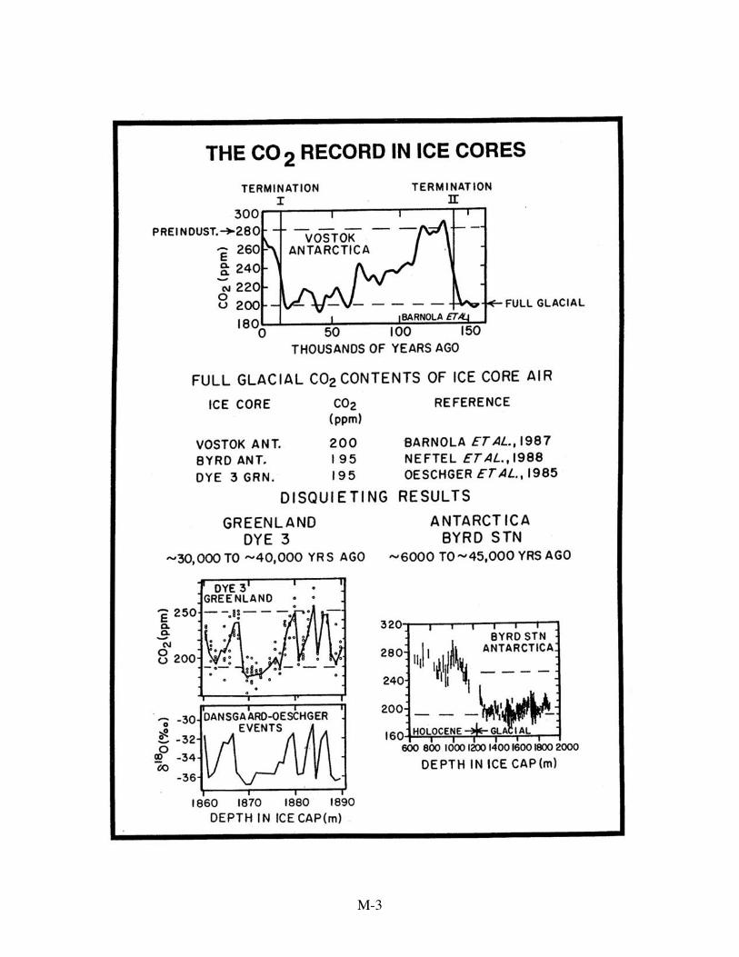
M-3

M-4

values (i.e., at about 240 parts per million) are found. Three lines of argument strongly

suggest that these high values must be spurious. First, a detailed series of measurements

on the Byrd Station Antarctica ice core, covering the same time period, fail to show any

values deviating significantly from the glacial ambient (i.e., 200 ppm). As the

atmosphere mixes pole to pole on a time scale of about one year, no mechanism exists to

support Greenland to Antarctic differences of more than about one part per million.

Hence, one or the other of these records must be misleading. The second argument has to

do with the high rates of change of CO2 content at the transitions between the cold and

warm phases of the D-O cycles. The 40 ppm rises occur on a time scale of decades. As

these rise rates rival those experienced during the last several decades of intense fossil

fuel burning, it is difficult to conceive a mechanism by which they might have been

driven. Finally, the expected offset between the gas record and the ice record discussed

in Keeling’s World is not found. Rather, the CO2 and 18O shifts occur at the same depth.

This suggests that the extra CO2 was generated in the ice after lithification was complete.

Despite this blemish in the ice core CO2 record, a strong case can be made in

defense of the 80 ppm CO2 content difference between glacial and interglacial time. The

most powerful argument is based on the agreement of the results from ice formed under

the ultra cold, low dustiness and low accumulation rate conditions which prevailed during

glacial time at Vostok, Antarctica and those from ice formed under the less cold, high

dustiness and high accumulation rate conditions which prevailed during glacial time in

Greenland.

If the 240 parts per million values found for the warm portions of the Greenland

D-O events are indeed spurious, then what mechanisms might be responsible?

Melting: The air-filled pore space in polar ice contains only about 2.5

micromoles of CO2 per liter of ice. Distilled water close to its freezing point in contact

with air contains about 25 micromoles of dissolved CO2 per liter. Hence, were melting

followed by refreezing to occur in the firn, significant amounts of excess CO2 would be

M-5

built into the ice. This excess CO2 would initially be dissolved in the ice, but it might

subsequently migrate to the air-bearing voids. While a possible explanation for the high

CO2 contents observed of the warm parts of Dansgaard-Oeschger cycles, this explanation

suffers from a serious drawback. The refrozen melt water would not be expected to be

homogeneously distributed. Rather, were this the correct explanation, one would expect

a large sample to sample scatter in CO2 content. Yet, the scatter for samples from the

warm glacial intervals is no greater than that for those from the cold glacial intervals.

Further, as Holocene ice contains no melt-induced excess CO2, why should that from

colder glacial times?

Clathrates: As ice is buried ever more deeply in the polar caps, the bubbles are

squeezed to ever smaller size. At one kilometers depth, the pressure is nearly 100 times

atmospheric. Below this depth, the air crystallizes into solids known as clathrates. When

clathrate-containing ice from these depths is brought to the surface, the bubbles slowly

reform. The annealing process responsible for their recreation takes a year or more. The

question then arises as to whether the composition of the reformed gas phase has been

altered. First of all, extractions accomplished by melting give results similar to those

accomplished by the standard crushing method. A strong argument against the

importance of this bias is that no offset in CO2 content is seen as between ice from above

and below the depth of clathrate formation. Were such an offset to occur, it would

produce differences in the CO2 verses time records obtained from ice cores differing in

accumulation rate, for the ice at the depth of clathrate formation would be older for low

than for high accumulation rate sites. Additional evidence against clathrate-induced

biases comes from the Vostok record where an 80 ppm rise in CO2 is found across both

Termination I (above the depth of clathrate formation) and Termination II (below the

depth of clathrate formation).

CaCO3: The dust in polar ice consists, in part, of CaCO3. The aerosols in polar

ice contain H2SO4 and HNO3. Interaction between the calcite and the strong acids

M-6

constitutes a potential source of excess CO2. As the dust and aerosols are located on grain

boundaries, any CO2 produced in this way would likely find its way into the air-filled

voids. During glacial intervals, the concentration of calcium in the Greenland ice reaches

several micromoles per liter. Most of this calcium was initially contained in CaCO3.

Hence, if this CaCO3 were subsequently to be dissolved by interaction with aerosol acids,

then several micromoles of CO2 per liter of ice would be released to the grain boundaries.

Then why doesn’t this interaction bias all the CO2 results from Greenland ice cores? The

answer must be that during interglacial intervals there is too little CaCO3 to contribute

significant amounts of CO2 and during peak glacial colds the CaCO3 completely

neutralizes the acid in the firn allowing the excess CO2 to escape to the atmosphere

before the air bubbles close. This is the preferred explanation.

In summary, clearly the last word has yet to be written with regard to the validity

of paleoatmospheric CO2 content estimates that are based on measurements made on air

trapped in polar ice. But it is unlikely that future work will reveal a sizable bias in the 80

ppm CO2 content difference between times of full glacial and full interglacial conditions.

This difference is almost certainly real; therefore, some mechanism must exist which

explains it.

Whole Ocean ∑CO2 Inventory

The discussion of mechanisms which might be responsible for the glacial to

interglacial change in the atmosphere's CO2 content focuses on the ocean. The reason is

that on the time scale of more than one oceanic mixing time (i.e., ~1000 years) the

atmosphere's CO2 content is dictated by the state of the ocean's chemistry. Even when

the buffering capacity of the ocean is taken into account, its effective carbon reservoir is

about six times greater than the atmosphere's. Hence, on the time scale of glacial cycles,

it is the ocean which tells the atmosphere what CO2 content it must have. While surface

waters call the atmosphere’s tune, their chemistry, in turn, is held in the grip of that of the

much larger underlying deep sea reservoir. So we will start by considering those

M-7

processes which influence the ∑CO2 and alkalinity of the deep ocean. Then we will

consider those processes which control the offset in ∑CO2 and alkalinity between surface

waters and those in the deep sea. Finally, we will be concerned with the temperature and

salinity of surface water which for any given chemical composition sets their CO2 partial

pressure and therefore that of the atmosphere.

The CO2 partial pressure of any given sample of sea water depends on its excess

of alkalinity over ∑CO2: the greater this excess, the higher the CO=3 ion content and the

lower the CO2 partial pressure. On the time scale of glacial to interglacial cycles (i.e.,

~104 years), the alkalinity of sea water changes primarily as the result of deposition or

dissolution of CaCO3. For each mole of CO=3 fixed into or released from CaCO3 the

alkalinity is changed by two equivalents (one unit of carbon per two units of charge

carried by the Ca++ ion.). This extra unit of charge is what counts for it changes in the

excess of alkalinity over ∑CO2. The excess of alkalinity over ∑CO2 is balanced by the

conversion of HCO-3 to CO

=3 . As we shall see, CaCO3 storage in and retrieval from

deep sea sediments has very likely played a role in the glacial to interglacial CO2 change.

But it is not clear whether this role is a major or minor one.

In addition to the formation and dissolution of CaCO3, the concentration of ∑CO2

is changed by the creation and destruction of terrestrial organic matter. Storage of carbon

in trees and humus removes CO2 from the ocean-atmosphere reservoir. Oxidation of

previously stored organic matter returns the CO2 to the ocean-atmosphere reservoir.

Taken together, tree wood and soil humus contain several times more carbon than does

the atmosphere. Fortunately, a means exists to estimate how the sizes of these reservoirs

changed between glacial and interglacial time. As the carbon isotope composition of

terrestrial organic material (δ13C ~ − 25‰) is quite different than that for average ocean-

atmosphere carbon (δ13C ~ 0‰), inter-reservoir transfers lead to shifts in the carbon

isotope composition of average ocean-atmosphere carbon. Measurements on benthic

foraminifera from deep sea sediments suggest that the average 13C content of carbon in

M-8

M-9

M-10

the ocean-atmosphere reservoir was about 0.35‰ lower during glacial than during

interglacial time. This requires a transfer of an amount of carbon equal to 1.4 percent of

that in today’s ocean-atmosphere reservoir. When equilibrated with the carbon dissolved

in the sea, this extra CO2 creates a 56 ppm higher glacial atmospheric CO2 content. But

after compensation through the interaction with CaCO3 in marine sediments (see below),

the increase is reduced to only 16 ppm. So we have an embarrassment on our hands; our

task has grown rather than diminished. We now have to find a way to change the

atmosphere's CO2 content by 96 parts per million rather than 80 ppm!

Physical Properties Of Surface Water

The partial pressure of CO2 in surface water depends not only on its chemical

composition but also on its temperature and salinity. Before considering the more

difficult question of what determines the chemical offset between surface and deep

waters, let us consider the possible contribution to the glacial to interglacial change in the

atmosphere's CO2 content of temperature and salinity.

The first point to be made in this connection is that despite their relatively small

combined area (~ 20% of the total) the cold portions of the surface ocean have an

influence on the atmosphere’s CO2 partial pressure exceeding that for their more

extensive warm counterparts. This important concept was simultaneously articulated by

three groups: McElroy and Knox at Harvard, Toggweiller and Sarmiento at Princeton

and Siegenthaler and Wenk at Bern. What the Harvardton Bears showed was that

because the deep sea is ventilated from polar regions, the chemistry of cold surface

waters is closely tied to that of the chemically dominant deep sea reservoir. Further,

because CO2 can be transported through the atmosphere from one part of the surface

ocean to another, a tendency exists for the CO2 partial pressure of warm surface waters to

be drawn toward that for cold surface waters. If, for example, the CO2 pressure in the

warm surface ocean tended toward higher values than that for cold surface ocean, then

CO2 would escape to the atmosphere from the warm regions and be reabsorbed in the

M-11

cold regions. The extent to which this CO2 equalization is achieved depends on the ratio

of the rate of interchange of CO2 gas between air and sea to the rate of interchange of

water between the ocean's warm and cold realms. The higher this ratio, the stronger the

influence of the cold surface ocean on the CO2 partial pressure for warm surface waters

and therefore for the atmosphere as well.

A relatively simple test can be applied to any ocean model to determine its

equalization index. This test can be carried out by arbitrarily changing the coefficient

relating CO2 partial pressure to CO2 gas content of the model's warm surface waters (i.e.,

those lying between 40˚ N and 40˚ S). The model is then run until a new CO2 steady

state is achieved. The object of the test is to see by how much the transfer of CO2 from

warm to the cold surface ocean reduces the arbitrarily imposed excess or deficiency of

CO2 pressure in the warm ocean. If, for example, an initial CO2 partial pressure excess

of 30% for warm surface water drops to a steady state excess of 6%, then the equalization

index would be 0.2. The lower the model's equalization index the less sensitive it is to

conditions in the warm surface water sphere.

The simple three-box models used by the Harvardton Bears to illustrate this point,

were constrained to yield the observed distribution of natural radiocarbon both between

the atmosphere and surface ocean and between the warm surface and deep ocean. In

order to match this 14C distribution, for these very simple models the CO2 exchange had

to be rapid with respect to thermohaline circulation. As a consequence, the equilibration

index was quite small. Hence these simple models suggest that glacial to interglacial

changes in temperate and tropical surface water have relatively little impact on the

atmosphere's CO2 content.

Rather, the Harvardton Bears would contend that were the glacial cooling to have

played a significant role in lowering the atmosphere's CO2 content, it must have operated

in the polar regions where deep waters form. In today's ocean, deep waters form in two

places, in the Southern Ocean and in the northern Atlantic. No significant deep water

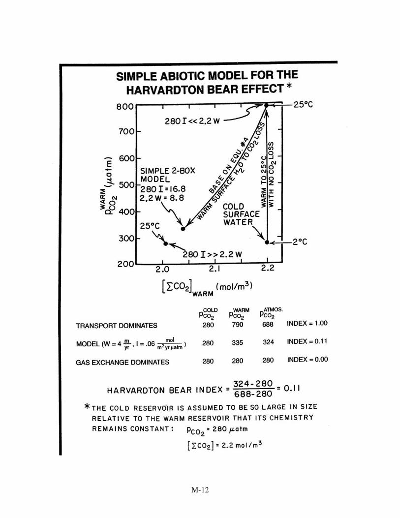
M-12

M-13

M-14

formation occurs in the northern Pacific. A number of lines of evidence lead us to

believe that the deep waters which formed during glacial time were on the average

somewhat colder than those which form today. Hence, so also must have been the

surface waters in the polar regions where deep waters form. However, it is difficult to

believe that this cooling was greater than 2˚ C. The reason is that the temperature of deep

water formed around Antarctica is currently very near the freezing point so it is as cold as

it can get. Thus if a change occurred, it must have been in the northern Atlantic. As the

waters currently sinking in this region of the ocean have temperatures averaging about

2°C, glacial age deep waters formed in the Atlantic could have been as much as 4°C

colder than today's average. However, as in today's ocean only about half of the deep

water currently forms in the northern Atlantic, it is difficult to accept that the overall deep

ocean cooling was more than about 2°C. A 2°C cooling would lower the CO2 partial

pressure by only 20 micro-atmospheres. Again, small potatoes!

With the advent of ocean general circulation models, it was possible to check

whether the equilibration index for the real ocean is indeed as low as predicted by the

three box models. It turns out that these models yield similar indices.

What about salinity? We know that sea level stood about 115 meters lower than

today during peak glacial time. Hence, the ocean's volume was about 3 percent smaller

than today's. As the salt inventory remained the same, the ocean's salinity must have

been 3% higher. Other things being equal, this would raise the atmosphere’s CO2 partial

pressure by about 10 µatm. Taken together with the temperature-induced change in CO2

content of about 20 µatm the net change would be only 10 µatm. Hence, it can be

concluded that the changes in the physical properties of surface water did not play a

significant role in the glacial to interglacial CO2 change. Together they failed to more

than compensate for the 16 ppm increase driven by a reduction in the size of the

terrestrial biosphere. So, after all this, we are left with close to the original 80 µatm to

explain!

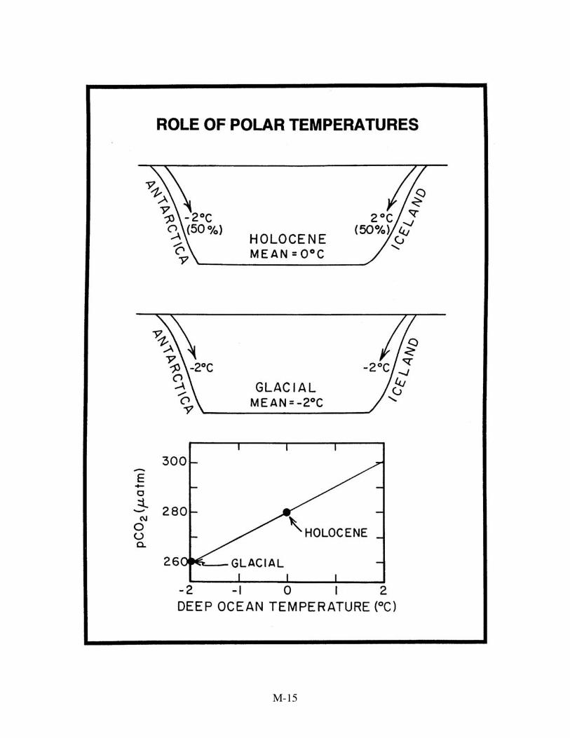
M-15

M-16

M-17

Biologic Pumping

From the very beginning of this quest, attempts to explain the low CO2 content of

the glacial atmosphere have focused on the CO2 pumping action by marine organisms.

Plants living in surface water convert CO2 into organic matter. Some of this organic

matter falls to the sea's interior where it is oxidized releasing the CO2. Hence the action

of this biologic cycle holds the CO2 partial pressure in surface waters below that for

waters of the sea's interior. In much of the ocean, this pumping action is limited by the

availability of the nutrients, phosphate and nitrate. On the average microorganisms

utilize about 16 nitrogen atoms and about one phosphorus atom per 125 carbon atoms.

As the molar ratio of nitrate to phosphate in the sea is close to 16, currently these two

nutrients appear to colimit plant productivity. However, in regions of strong upwelling

such as the Southern Ocean, the eastern tropical Pacific and the northern Pacific, much of

the NO3 and PO4 reaching the surface goes unused. To some extent, this inefficiency in

usage is due to a scarcity of iron. If for some reason, the nutrients available in these

regions of the ocean were to be utilized with 100% efficiency, then the atmosphere's CO2

content would fall below its glacial level. Deep waters formed along the margins of the

Antarctic continent leave the surface carrying about 1.6 micromoles per liter of PO4 (i.e.

about three quarters the average deep sea concentration). Those forming in the northern

Atlantic carry about 0.8 micromoles per liter. It is this situation the Harvardton Bears

had in mind when they proposed the dominance of high latitude surface waters in setting

the atmosphere's CO2 content. It is then tempting to postulate that the extent of nutrient

utilization in these regions was greater during glacial time and consequently the

atmosphere's CO2 content was lower.

A large boost was given to the Harvardton Bears scenario by John Martin’s

discovery that in those regions of the surface ocean where the efficiency of nutrient

utilization is low, the scarcity of iron may be the villain. The conclusions he drew from

his early experiments carried out on the decks of ships were proven to be right on the

M-18

M-19

money by a large scale in situ fertilization experiments conducted in the eastern tropical

Pacific. Much of the nitrate and phosphate present in the iron-fertilized patch were

utilized, the chlorophyll content increased and, of course, the CO2 content of the surface

water was drawn down. Martin pointed out in a paper published shortly before his death

that the iron made available by the very large excess dust fall of glacial time likely

permitted a higher degree of utilization of nutrients in the Southern Ocean. However,

because the expected 13C signal in the glacial-age shells of Southern Ocean planktonic

organisms was not found, his paper was not received enthusiastically by most marine

geochemists. As outlined below, a new twist on Martin’s idea may change this.

Unfortunately, a key prediction made by this hypothesis appears not to have been

fulfilled. It has to do with the carbon isotope record for Southern Ocean surface water

kept by the shells of planktonic foraminifera. During photosynthesis in cold water, the

heavy isotope of carbon, 13C, is discriminated against by about 25‰. Because of this,

the 13C/12C ratio in surface ocean ∑CO2 water is greater than that in deep water ∑CO2.

Hence, were the biologic pumping action at high latitudes stronger during glacial time,

then the 13C/12C ratio for planktonic foraminifera shells formed in surface waters in these

regions should have been more positive than now. But this is not the case. In the

Southern Ocean, the 13C/12C ratio in both planktonic and benthic foraminifera was about

0.9‰ lower during peak glacial time than during peak interglacial time. These results

suggest that the 13C/12C difference between surface and deep water was about the same

for glacials as for interglacials. Hence the carbon isotope record appears to be telling us

that the efficiency of nutrient utilization in the Southern Ocean was similar to today’s.

Finally, further support for the absence of any large increase in the efficiency of

nutrient utilization throughout the Southern Ocean appeared to come from nitrogen

isotope measurements made on organic material from circum Antarctic sediments.

During the conversion of NO3 dissolved in the sea into NH3 incorporated into the amino

acids in plant matter, there is an 8‰ depletion of the heavy nitrogen isotope (15N).

M-20

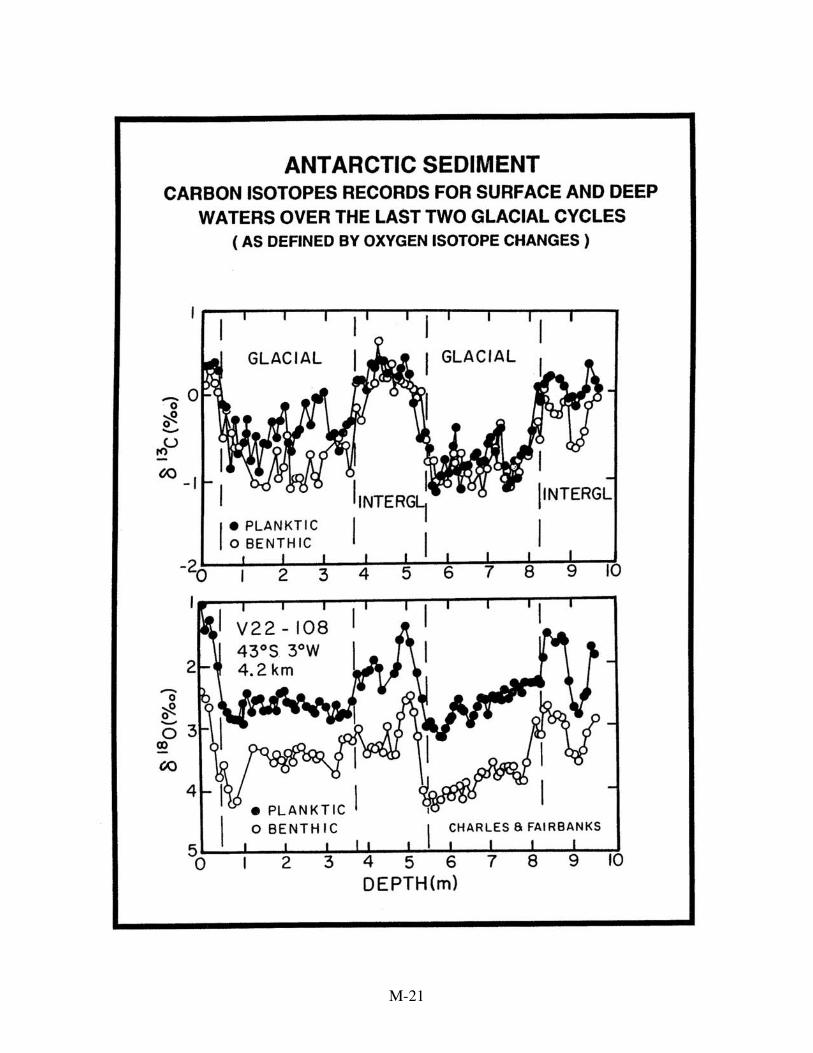
M-21

M-22

However, the actual difference in isotopic composition between the inorganic nitrogen

upwelling to the surface and the organic nitrogen raining to the sea floor depends on the

efficiency of nutrient utilization. Only if a very small fraction of the available NO-3 is

utilized will the full fractionation be seen. By contrast, if all the upwelled NO-3 were

utilized, there could be no difference between the isotope composition of the upwelled

inorganic nitrogen and that of the sinking organic nitrogen.

Meridianal traverses of nitrogen isotopes in Holocene sediments from the

Antarctic region nicely reflect the degree of utilization of nutrients in the overlying water.

The ratio of 15N to 14N in the sediment organics is about 8‰ lower for the high latitude

portion than for the low latitude portion of the traverse. Furthermore, the shape of this

latitude trend is the mirror image of the concentrations of NO-3 in the overlying surface

water. This relationship is exactly as expected; close to Antarctica where the utilization

efficiency is low, the full fractionation is observed, and well away from Antarctica where

the nutrients are fully utilized, diatoms have a δ15N value close to that for NO3 in the

deep sea. Early studies suggested that the trend of the nitrogen isotope ratios for glacial

sediments from the same traverse of cores was nearly the same as for Holocene

sediments. These results tell a story consistent with that told by the carbon isotope in

planktic foraminifera shells. During glacial time, the nutrients in surface waters at high

latitude in the Antarctic Ocean were utilized with similar efficiency as at present.

This is how things stood at the time the first edition of this book was completed.

Since then a host of new results have appeared which have forced a rethinking of

conditions in the glacial Southern Ocean. While 13C measurements on both benthic and

planktonic foraminifera confirm earlier results, new cadmium measurements suggest that

Southern Ocean waters of glacial age were depleted rather than enriched in nutrients.

Measurements of uranium concentrations and of 231Pa to 230Th ratios suggest that

productivity was lower to the south of the present day position of the polar front and

higher to the north. With the development of a more rigorous cleaning procedure for

M-23

M-24

M-25

diatoms, Roger Francois and his coworkers from Woods Hole were able to show that

while north of the polar front (~50°S) in the Atlantic and Indian sectors of the Antarctic,

the δ15N in diatom bound organic remained nearly the same, south of 50°S the values

were 2‰ more negative during glacial than during interglacial time. This suggests a

higher nutrient utilization efficiency then than now. These new results also suggest a

major difference between the magnitude of the changes in the Pacific sector on the one

hand and the Atlantic and Indian sectors on the other. All in all as of June 1998, things

were in such a state of flux. Clearly what went on during glacial time in the Southern

Ocean will occupy the attention of marine geochemists for the next decade. The

implications of these findings to the cause of the lower than present CO2 content of the

glacial atmosphere will of course be of utmost importance!

Carbonate Ion Concentration

As we have already discussed, the CO2 partial pressure exerted by a given parcel

of sea water depends on its excess of alkalinity over ∑CO2 concentration. Changes in

this excess are reflected in the CO=3 ion concentration. To the simplest approximation

[CO=3 ] ≅ [ALK] - [∑CO2] = ALK Excess

Furthermore, the CO2 gas concentration of sea water is to the simplest approximation

inversely proportional to its CO=3 concentration. Hence

[CO2] ≅ 1

[ALK] - [∑CO2] =

The major cause for differences in the alkalinity excess from one place to another in the

sea is the production or dissolution of CaCO3. This cycle is akin to that for organic

material in that CaCO3 is produced in the surface ocean and is destroyed at depth in the

sea. However, two important differences exist. First, the generation of CaCO3 raises

rather than lowers the CO2 content of sea water. The reason for this is that the alkalinity

change associated with CaCO3 formation is twice as great as the ∑CO2 change. Hence,

the alkalinity excess is decreased when CaCO3 is manufactured by marine organisms.

Second, rather than being almost completely destroyed as is organic matter, roughly one

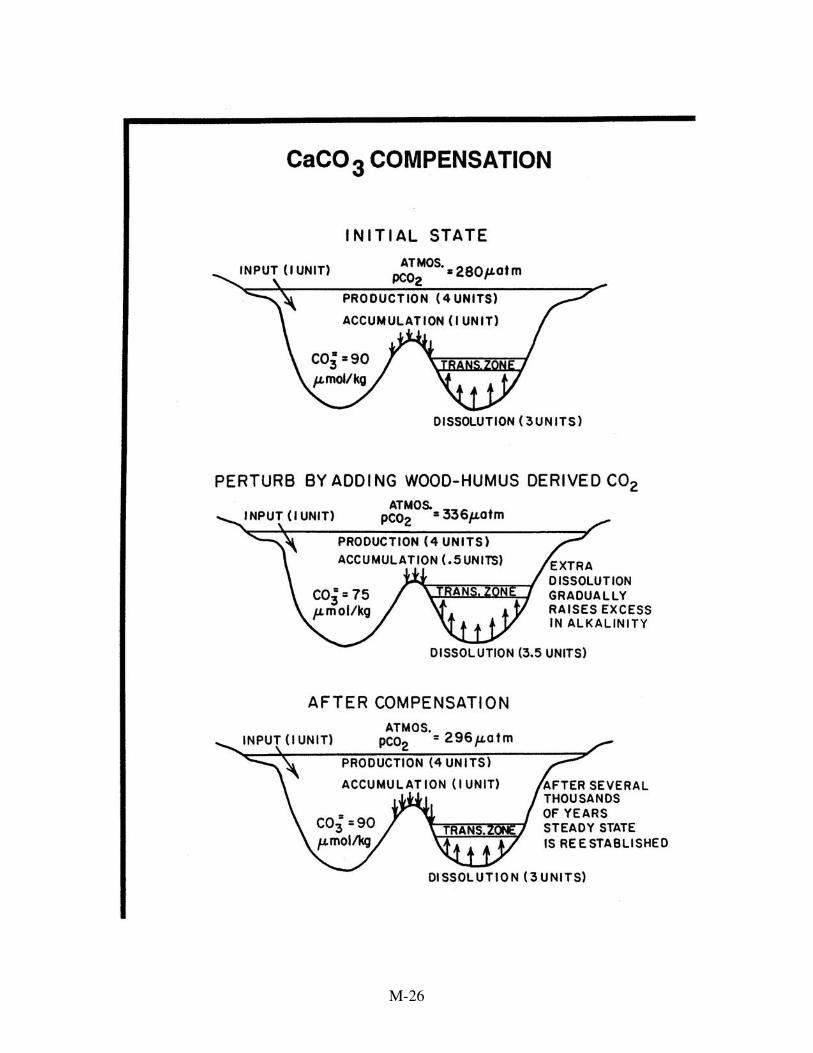
M-26

M-27

M-28

quarter of the CaCO3 produced by marine organisms survives dissolution and

accumulates on the sea floor.

The first point to be made is that the cycle of CaCO3 sets the CO=3 ion content in

the deep sea and in so doing influences the CO2 content of the atmosphere. The basis of

the control is economic: namely, unless the rate at which CaCO3 accumulates in deep sea

sediments just matches the rate at which the ingredients for CaCO3 (i.e., CaO and CO2)

are supplied to the ocean, the ocean’s chemistry will gradually change. In today's ocean,

marine organisms manufacture CaCO3 at a rate about four times faster than that at which

the ingredients are being supplied. In order to compensate for this overproduction, the

chemical composition of sea water has adjusted so that three quarters of the CaCO3

produced redissolves. This compensation is accomplished by adjustments in the ratio of

the area of the sea's floor bathed in waters supersaturated with respect to the mineral

calcite to the area bathed in waters undersaturated with respect to the mineral calcite. As

the Ca++ ion content of sea water is 100 times larger than that of CO=3 ion, it remains

nearly uniform throughout the sea and constant over the course of a glacial cycle. Thus

the tendency toward CaCO3 dissolution is dictated by the CO=3 ion concentration. In

particular, it is related to the ratio of the in situ CO=3 ion concentration to the saturation

CO=3 ion concentration. When this ratio is less than unity, calcite tends to dissolve. Due

to the pressure dependence of the solubility of calcite, the saturation concentration

increases by about 18 µmol/kg per kilometer water depth. By contrast, in most parts of

the deep sea, the in situ CO=3 concentration changes very little with water depth.

Because of this, at shallower depths the in situ CO=3 concentration exceeds the saturation

concentration and, at great depth, the reverse is true. At that depth where the saturation

CO=3 concentration curve crosses the in situ concentration, the water is exactly saturated

with respect to the mineral calcite.

This situation is clearly imprinted in marine sediments. Sediments well above the

crossover are rich in calcite reflecting the fact that in most parts of the ocean the rain rate

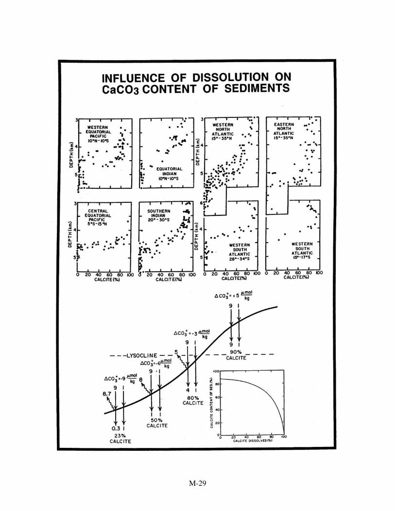
M-29

M-30

of calcite exceeds that of mineral detritus by roughly an order of magnitude. Sediments

well below the crossover lose all their calcite to dissolution. If for some reason the match

between ingredient supply and calcite accumulation is disrupted, then the CO=3 ion

concentration in the deep sea is driven toward a new value at which accumulation once

again matches ingredient supply. As the readjustment time is only several thousand

years, glacial to interglacial changes in either the rate of delivery of the ingredients for

CaCO3 or in the production rate of CaCO3 would have caused changes in the CO=3 ion

content of the deep sea and hence also the CO2 content of the atmosphere. So we have

the makings of another scenario. Changes in either the rate of supply of ingredients or in

the production rate of CaCO3 by marine organisms offer a way to push the atmosphere's

CO2 content up and down.

Firm evidence exists for glacial to interglacial changes in the depth of the

transition zone separating the realms of CaCO3-rich and CaCO3-poor sediments. Cores

from the tropical Pacific and Indian Ocean taken within and adjacent to this transition

zone reveal that during glacial time the transition zone was shifted to greater depth. In

other words, dissolution during glacial time was less intense at any given water depth.

For the Atlantic, the change was in the opposite direction. Dissolution was more intense

during glacial time. However, as the Pacific and Indian Oceans cover a much larger area

than the Atlantic, globally the average CO=3 concentration of average deep water appears

to have been somewhat higher during glacial time. If so, then the CO2 content of the

atmosphere must have been correspondingly lower. The problem is that the magnitude of

the CO=3 ion shift calculated from the change in the depth of the transition zone is far too

small to account for the required 80 ppm lowering of atmospheric CO2 content. In order

to create a lowering of this magnitude, the CO=3 ion content of glacial deep water would

have to have been about twice as high as today's. Such an increase would have deepened

the transition zone separating calcite preservation and dissolution by several kilometers.

As today's transition zone is centered at about 4 kilometers, this would have led to calcite

M-31

M-32

accumulation on the ocean's abyssal planes. But glacial age sediments from abyssal

planes are devoid of calcite. The observed transition depth shift for the Pacific and

Indian Ocean was no more than 0.8 km. When the Atlantic's opposing change is taken

into account, the global shift becomes more like 0.5 km. Foiled again! Just as the carbon

isotope record for Antarctic foraminifera appeared to rule out enhanced biological

pumping at high southern latitudes as the cause for lower atmospheric CO2 contents, the

calcite record from the sea floor appeared to rule out a large increase in the CO=3 ion

content of deep ocean water as the cause.

Our original hero, David Archer, found a way around this lysocline constraint by

suggesting that under certain circumstances the tie between transition zone depth and

saturation horizon could be broken. But before exploring this new idea, we must

consider a couple of loose ends. The first of these has to do with the statement that the

CO=3 ion concentration in the deep sea would adjust to any imbalance between CaCO3

accumulation rate and ingredient supply rate on the time scale of several thousands of

years. At first thought, this appears to be at odds with residence times of both ∑CO2 and

alkalinity in the sea. Based on estimates of the amount of limestone dissolved from the

continents and the amount of CO2 outgassed from the Earth's interior, the time required

to replace the inorganic carbon stored in the ocean is about 105 years. Based on the

alkalinity flux to the sea from the world's rivers, the alkalinity replacement time is also

about 105 years. If so, how can the carbonate ion content of the sea adjust on a time scale

of a few times 103 years? The reason is related to that depicted in the Twin Towers

experiment outlined in Keeling's World. Carbonate ion content of deep sea water (~95

µmoles/kg) constitutes only about 4% of the ∑CO2 (~2200 µmoles/kg) in deep sea water.

Hence the CO=3 content responds to imbalances in the CaCO3 budget 25 times faster than

the ∑CO2 content.

The other issue left unmentioned is what might induce imbalances in the CaCO3

budget. One such scenario has to do with the storage of CaCO3 in coral reefs. During

M-33

periods of glaciation, sea level dropped to the point where the vast continental shelves

were

left high and dry. This greatly reduced the habitat for corals. Then during interglacials

when the sea rose and flooded across the shelves, coral reef communities were able to

store away CaCO3 at a rate rivaling that occurring on the sea floor. According to this

hypothesis the imbalance created in this way caused a draw down of the carbonate ion

concentration in the sea thereby raising the CO2 content of the atmosphere. During low

sea stands, not only was this rate of storage greatly decreased but CaCO3 deposited on

the shelves during the preceding interglaciation was subject to chemical erosion.

Another scenario holds that the rate of production of calcite by marine organisms

may have been lower during glacial time. Perhaps conditions during glacial time were

more favorable to organisms living in silica houses allowing these organisms to partially

displace their calcite-housed brothers. Yet another scenario proposes that the supply of

alkalinity from rivers was higher during glacial time. Perhaps increased freeze-thaw

activity on the colder planet created fresh mineral surfaces accelerating chemical

weathering. If so, then in order to compensate, the rate of alkalinity removal via CaCO3

burial on the sea floor would have to have risen correspondingly. But as we have seen, to

explain the entire atmospheric CO2 content change, these scenarios would require that

during glacial time the CaCO3 transition zone deepened by several kilometers. It didn't.

But now David Archer to the rescue! Following the lead of his mentor, Steve

Emerson, Archer pursued as his Ph.D. research the role of the CO2 released by bacterial

respiration within the upper few centimeters of deep sea sediments in promoting calcite

dissolution. Two observations made this avenue an appealing one. First, analyses of the

material caught in deeply moored sediment traps reveals that the ratio of organic matter

carbon to CaCO3 carbon falling to the deep sea floor is close to unity. Hence, if the CO2

released when the organic matter is eaten were neutralized by reaction with calcite, a near

neutral addition of calcium bicarbonate would be generated;

M-34

H2O + CO2 + CaCO3 ⇒ Ca++ + 2HCO-3

What this tells us is that respiration CO2 has the potential to do the job. The second

observation is that the geographical trend in the chemistry of deep waters in the Pacific

and Indian Oceans suggests that such a titration is indeed occurring. The increases in

∑CO2 along the pathway of deep water flow is matched by an increase in alkalinity such

that the CO=3 concentration remains very nearly constant. These two observations led to

the suspicion that CO2 released by bacteria living within the upper few centimeters of

deep sea sediment might be responsible for much of the CaCO3 dissolution taking place

on the sea floor.

In order to determine whether this was indeed the case, Archer employed micro

pH and O2 electrodes which could be inserted into the sediment from a bottom lander.

What he found was that the O2 concentration dropped sharply in the upper few

millimeters of sediment in response to bacterial consumption of organic matter. As

expected, he found that the respiration CO2 drew down the pore water pH creating a

minimum of ten or so centimeters below the sediment water interface. Above this

minimum, the pH increased so that at the interface it matched that for bottom water.

Below this minimum, it also increased eventually reaching the value corresponding to

saturation with calcite. The important point is that the magnitude of the pH minimum

was not as large as that predicted from the rate at which respiration CO2 was being

created (as indexed by the O2 results). The reason is that roughly one half of the

respiration CO2 had reacted with calcite. Only about one half of the CO2 managed to

escape the pores into the overlying bottom waters. What this demonstrated was that

indeed much of the sea-floor dissolution of calcite was being driven by respiration CO2

released into the sediment pore water. It also provided a possible way around the

requirement that the depth of the calcite saturation horizon closely match the depth of the

top of the transition zone. Rather, dissolution commences well above the saturation

horizon.

M-35

M-36

It is because of this upward displacement of the transition zone by respiration

CO2 that Archer saw a way to decouple the tie between transition zone depth and deep

sea carbonate ion concentration. He reasoned that if, for example, the rain rate of organic

carbon to the sea floor relative to that for calcite were higher during glacial time, then the

amount of respiration CO2 released by bacterial activity within the sediment column

would increase and the transition zone would temporarily shift to shallower depths. This

would throw the ocean's CaCO3 budget out of kilter for the rate of accumulation of

CaCO3 would fall below the rate of ingredient supply. Hence, the ocean's CO=3 ion

content would begin to climb. This climb would continue until the additional bottom

water CO=3 just balanced the impact of the excess respiration CO2. The transition zone

would have moved back to its original position restoring the balance between calcite

accumulation and ingredient supply. So here we have a situation where an increase in

CO=3 ion content in the deep sea produces no corresponding change in the steady state

depth of the transition zone!

Fortunately, a means was discovered by which Archer's scenario might be

verified. It involved a paleo pH method based on measurements of the isotopic

composition of the boron contained in foraminifera shells. A thermodynamic isotope

separation occurs between the two species of borate present in sea water. The singly

charged form, B(OH)−4 , has a 20‰ lower 11B to 10B ratio than the neutral form, B(OH)3.

In today's surface water (pH =8.2), about 80% of the boron is in the neutral state and 20%

is in the charged state. Were sea water to be acidified, the proportions would be shifted

in favor of the neutral state. By contrast, were it to be made more basic, the proportions

would be shifted in favor of the charged state. Such changes in the pH would bring about

shifts in the isotopic composition of both B(OH)3 and the B(OH)-4 . In low pH sea water,

the neutral species would have the same isotopic composition as bulk borate while the

tiny fraction of remaining charged borate form would be depleted in 11B by 20‰. In high

pH sea water, the opposite would be found; the charged borate ions would have the same

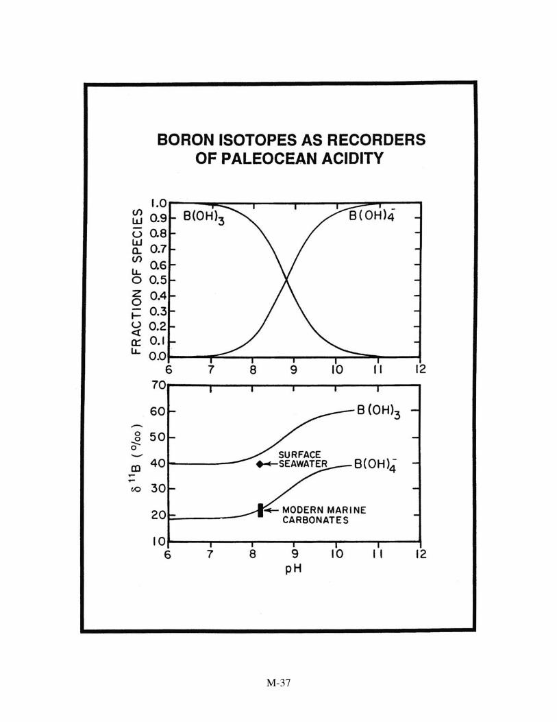
M-37

M-38

isotopic composition as bulk borate and the tiny fraction of remaining neutral species

would be enriched in 11B by 20‰. At that pH, where the B(OH)3 to B(OH)-4 ratio was

unity, the 11B to 10B ratio for the charged form would be 10‰ lower than that for bulk

borate and the ratio for the uncharged form, 10‰ higher.

The paleo pH method assumes that the boron contained in the shells of

foraminifera is built into the calcite lattice as charged borate and carries with it the

isotopic composition of this species in sea water. As residence time of borate in sea

water is about 20 million years, it is quite safe to conclude that on the time scale of a

glacial cycle the isotopic composition of sea water borate remains constant. The hope is

that the sole control on the isotopic composition of borate in the shells of foraminifera is

the pH of the sea water in which they grow and, of course, that no change in isotopic

composition occurs after burial in the sediment.

In the fall of 1993 when the first edition of this book was being completed,

Abhijit Sanyal, a graduate student at Lamont, in cooperation with Gary Hemming, a

research scientist at SUNY, Stony Brook had just completed preliminary measurements

of boron isotopes in planktic and benthic foraminifera from Holocene and last glacial

sediments. These measurements suggested that the glacial deep ocean had a pH 0.3 of a

unit more basic than the Holocene ocean. This translates to CO=3 ion contents for deep

water twice as great as today’s. Because the CO=3 ion content of surface water in the sea

averages about twice that of deep water, the dissolution of enough CaCO3 to raise the pH

of deep water by 0.3 units would raise the pH of surface waters by only one half this

amount. Boron isotope measurements on planktonic foraminifera yielded as required a

smaller pH shift. The exciting result is that the boron-based pH changes predict a

lowering of the atmospheric CO2 content consistent with that observed in ice cores.

Confidence increased when Sanyal went on to culture the planktonic species Orbulina

universa at the Santa Catalina Wrigley laboratory at a range of pHs. The results

confirmed the predicted pH dependence of the isotope ratios for the boron incorporated

into these shells.

M-39

However, there remained some disquieting aspects of Archer’s respiration

hypothesis. First no compelling explanation appeared as to why the rain of organic

matter to the sea floor was higher during glacial time. Explaining this increase proved

especially difficult since its magnitude would have to have been nearly the same across

the entire ocean. Were this not the case, then the topography of the glacial lysocline

would have developed some very large bumps. No such bumps have been found.

Second, the absence of CaCO3 in the upper portion of sediments on the ocean's abyssal

plains is very difficult to explain. According to Archer’s scenario if during glacial time

the carbonate ion content of deep sea water was twice as high as at present, then the

saturation horizon would have been driven down well below the depth of the abyssal

plains. The problem is that when at the close of glacial time the excess flux of organic

matter to the sea floor was shut down, CaCO3 would have begun to accumulate across

the entire ocean floor. Only when a substantial portion of the excess CO=3 ion had been

consumed as a result of this deposition would the saturation horizon have risen above the

abyssal plains. At this point, a 3 cm-thick layer of CaCO3-rich sediment would have

accumulated acorss the entire abyssal ocean floor and would have been bioturbated into

the underlying clay. It seems extremely unlikely that this CaCO3 could have been

completely dissolved away during the remainder of the Holocene. Yet measurements on

cores from abyssal plains consistently yield CaCO3 contents less than 0.2 percent.

The coup de grâce came when, using model calculations, Danny Sigman

demonstrated that it was quite impossible to separate the lysocline from the saturation

horizon by anywhere near the several kilometers required by the Sanyal-Hemming paleo

pH reconstructions. Archer repeated these calculations and had to admit that Sigman had

a point. So this beautiful scenario appears to have bitten the dust.

Iron Fertilization to the Rescue

But it seems that no sooner has one idea regarding the cause of the low CO2

content of the glacial atmosphere paled that another arises to seek its place. Indeed,

M-40

M-41

within a year after Sigman put aside the Archer hypothesis a new idea emerged. It came

into being in a rather round about way. In reexamining the Vostok Antarctica ice core

record for the end of the penultimate glaciation (i.e., Termination II), Broecker and

Henderson puzzled over the observation that the transition from glacial to interglacial

conditions came in three distinct steps. The first was the demise of the heavy glacial dust

fall onto the Antarctic ice cap. This was followed by a 7000-year period during which

the air temperature over the Antarctic ice cap warmed and the CO2 and CH4 contents of

the atmosphere increased. Only after this second step was complete did the 18O content

of the O2 trapped in the Antarctic ice begin to decrease. The reason for this fall is that

the 18O content of sea water decreased as the 18O-deficient ice cap water reentered the

sea. Confirmation of the validity of the 18O in O2 proxy for ice volume came from the

observation that the rain of silicate debris onto the Southern Ocean sea floor and the rise

in surface water temperatures in the southern Indian Ocean led the 18O shifts in benthic

foraminifera (also due to the return of 18O-deficient ice-cap melt water to the sea). If as

seems reasonable, the 18O decline in atmospheric O2 paralleled the meltdown of the

northern hemisphere ice caps, then the entire rise of CO2 was completed before the ice

caps began to melt. This eliminates any hypotheses for the CO2 change requiring the

flooding of the shelves. Also since the rejuvenation of the Atlantic’s conveyor

circulation occurred during the ice-melt interval, it also eliminates any hypothesis tied to

the reorganization of ocean circulation.

These observations led Broecker and Henderson to ponder the role of dust.

Instead of thinking in terms of iron fertilization of high latitude waters, they proposed

that the higher global dust fall during glacial time allowed nitrogen fixing cyanobacteria

to proliferate in their subtropical habitats. These organisms are known to have a tenfold

higher iron demand than other planktonic organisms. So the idea was that during glacial

time the increased iron availability created by the excess dust fall led to a 40 percent

increase in the oceanic inventory of NO3. If, and its a big if, this extra NO3 could be

M-42

utilized with more or less the same efficiency as that presently in the ocean, then the

biologic pump would have been correspondingly strengthened.

The residence time of fixed nitrogen in the sea (i.e., N2→NO3→N2) is estimated

to be about 3000 years. Hence, no matter where it was manufactured, the extra NO3

produced by the cyanobacteria would become mixed throughout the entire sea. Further,

when the dust fall ceased, the NO3 decline would take several thousand years helping to

explain the 7000-year-duration atmospheric CO2 climb at the end of the penultimate

glaciation.

One possible drawback to this new idea is that were it to explain the entire

drawdown of the atmosphere's CO2 content, it would create a 1‰ increase in the δ13C

for glacial age planktonic shells. No such increase is seen anywhere in the world ocean.

But easing this situation are two new findings. First, laboratory growth experiments by a

group led by Howie Spiro show that there is a pH dependence on the carbon isotope

fractionation for planktonic foraminifera. As the lowered glacial atmospheric CO2

content requires that the pH of the surface ocean averaged 0.2 units higher than today’s,

the Spiro et al. measurements suggest that this would have lowered the δ13C in

planktonic foraminifera by about 0.5‰.

The other factor is that the fractionation of carbon isotopes during photosynthesis

depends on CO2 content of sea water, the lower the concentration, the lower the

fractionation (as explained in the ‘Walker’s World’ section, this dependence involves the

interplay between the resistance posed by diffusion through the cell wall and that posed

by the reaction with the photosynthetic enzyme). Such a reduction would decrease the

contrast in 13C/12C difference between surface and deep water for any given strength of

the biological pump. This would further reduce the expected δ13C planktonic shells by

about 0.3‰. When combined with the -0.35‰ change in the δ13C for glacial ocean

∑CO2, instead of a 1.0‰ increase in the δ13C for planktonic foraminifera, an 0.15‰

M-43

M-44

M-45

decrease would be expected. Although not well defined, the glacial to interglacial ∆δ13C

for planktonic foraminifera lies in the range 0.0 to -0.3‰.

A second drawback has to do with the phosphorus requirement of marine

microplankton. Along with most geochemists, we had always assumed that the strong

correlation between NO3 and PO4 in the sea reflected a tight-knit biochemical demand

for these nutrients by marine plankton. Somehow shifts in ecology allowed nitrogen

fixation to maintain the required 16 to 1 ratio. But the discovery that nitrogen-fixing

bacteria are strongly limited by the availability of iron requires that this line of thinking

be reexamined. Perhaps instead the close correlation between NO3 and PO4 reflects

luxury storage of phosphorus. Certainly observations made in lakes and experiments

carried out in chemostats show that these micro-organisms can function with a wide

range of N to P ratios.

A third drawback is that an increase in the strength of the biological pump would

increase the O2 demand in the ocean interior. Models suggest that an 80 µatm drawdown

in the atmosphere's CO2 partial pressure would require a 40% increase in the oceanic

NO3 inventory (based on the assumption that the utilization efficiency for nutrients

remained the same as today's). Other things being equal (i.e., circulation patterns, the

depth profile of respiration...), this would produce a 40% increase in O2 demand. As

only roughly a third of this would be compensated by the higher O2 capacity of colder

surface waters, those parts of the deep ocean currently low in O2 would have gone

anoxic. Yet, as documented by the ubiquitous presence of benthic foraminifera, this did

not occur.

Finally, this scenario is at odds with the Harvardton Bear concept which would

suggest that any drawdown of the CO2 content of warm ocean waters associated with an

increased strength of the biological pump would be compensated by an inflow (via the

atmosphere) of CO2 supplied by the cold surface ocean. If so, then only the increased

pumping action in the cold surface waters would contribute significantly to the CO2

M-46

drawdown. As these waters already have large inventories of unused nutrients, it is not

clear why they should benefit from a nitrate content increase.

Putting aside the problems raised in connection with the Archer hypothesis, one

could argue that the increased global production of organic matter created by the excess

nitrate could be responsible for the excess rain of organic matter required by this

hypothesis. Of course, if, as one might expect, the production of CaCO3 increased

correspondingly, then this increase would be nullified.

At this point, one might ask why direct iron fertilization of the Southern Ocean is

not the invoked. After all, this is the scenario suggested by this chapter's hero. The

problem lies in the observation that at the time of the penultimate deglaciation, the fall of

dust onto Antarctica bottomed out early in the 7000-year duration period of CO2 rise.

Were direct fertilization the answer, then as iron has a very short residence time in the

sea, the CO2 content of the atmosphere should follow directly on the heels of the decline

in iron supply. It did not.

Recent studies demonstrating that the small amount of iron found in the deep sea

is stabilized by an organic ligand suggest yet another scenario. The fact that the same

amount of iron is found in deep Atlantic waters as in deep Pacific waters suggests that

these ligands have lifetimes of several ocean mixing times (i.e., several times 103 yrs). If

so, it is possible that the higher glacial dust rain somehow led to an increased ligand

inventory. Gaia in action! This in turn would permit higher plant productivity in ocean

regions currently deficient in iron. It would also prevent a rapid response to the sudden

dust demise because several thousands of years would be required for the ligand

inventory to drop from its glacial to its interglacial level. Summary

This section's puzzle had to do with the mechanism responsible for the 30%

reduction of the atmosphere's CO2 content during glacial time. While a number of

M-47

fascinating scenarios have been proposed, all have stumbled because they appear to

violate the record kept in ocean sediments or constraints placed by models. Those

scenarios involving a strengthening of the biologic pump were initially put aside because

the carbon isotope record in foraminifera shells was not consistent with such a

strengthening. Those scenarios involving changes in the ocean's alkalinity resulting from

calcium carbonate accumulation in the shallow ocean were blocked by the observation

that the depth of the transition zone separating calcite-rich from calcite-poor sediments

did not deepen nearly enough during glacial time. The exciting scenario proposed by

David Archer at first received strong support from the boron isotope record, but then was

put into question by its requirement that a several kilometer separation existed between

the depth of the saturation and lysocline horizons. But then two new findings reopened

the possibility that a strengthening of the biological pump was after all responsible for the

CO2 lowering during glacial time. The first was John Martin’s discovery that in many

parts of the ocean the availability of iron limits marine productivity. Coupled with the

finding that planetary dust fall was several times higher during glacial time, this provided

a mechanism to strengthen the biological pump. Second, a large pH dependence was

demonstrated for the 13C fractionation between ∑CO2 and marine calcite. This latter

finding removes the impasse created by the failure of the carbon isotope ratios in the

shells of glacial age planktonic foraminifera to show a shift toward heavier values. So

perhaps we are at last closing in on the answer to our mystery. In one way or another, the

high glacial dust fall supplied the iron required to strengthen the ocean's biological

pump.

M-48

Commentary on Plates in Martin's World

pg. 3

Analyses of air trapped in polar ice offers a means of reconstructing trace gas

concentrations in the glacial atmosphere. Records from Antarctica representing areas of

low snow accumulation and colder temperature (Vostok) and high snow accumulation

rate and warmer temperature (Byrd) yield nearly the same CO2 content for ambient

glacial time. While similar results are obtained at the Dye 3 site in southern Greenland,

the details differ from those for the two Antarctic sites. Specifically, during the millennia

duration interstadials which punctuate the glacial portion of the Greenland record, the

CO2 content rises halfway back to the interglacial value. Matching excursions are absent

in the very detailed Byrd Station, Antarctica, record. As the mean-annual CO2 contents

at the two poles can not have differed significantly, these disagreements indicate

problems with the ice archive. The suspicion is that the villain is CaCO3 accompanying

the dust contained in the ice. The Greenland ice has at all times an order of magnitude

more dust than Antarctic ice. Thus if CaCO3 were the cause of the biases, then they

would be expected to be far more serious in the Greenland. The electrical conductivity

record reveals that during the interstadial warms the electrical conductivity jumps up

from near zero value during times of extreme cold, demonstrating that unneutralized acid

is present. Perhaps this acid is responsible for the dissolution of CaCO3 releasing excess

CO2 gas within the ice.

pg. 8-9

Carbon isotope ratio measurements carried out on benthic foraminifera shells

from deep sea sediments suggest that the 13C to 12C ratio in deep ocean ∑CO2 was on the

average about 0.35‰ lower during the peak of the last glaciation than it was during the

Holocene. The most likely way such an isotope shift could be accomplished on this

short a time scale (i.e., ~5000 years) would be via changes in the size of the biospheric

carbon pool. To create an 0.35‰ rise in δ13C at the end of the last glaciation would

M-49

require that the biospheric pool increase in size by about 500 GtC. This carbon was

stored not only in the trees and soils of the northern areas previously covered by the ice

caps and tundra of glacial time but also in expanded tropical forests.

The cycling of this carbon back and forth between the ocean and the terrestrial

biosphere would of course have changed the atmospheric CO2 content. In the absence of

any impact of this CO2 on the sea-floor CaCO3, the CO2 content of the atmosphere

would have been raised by 56 µatm during glacial intervals relative to interglacial

intervals. This change is in the opposite sense to that observed in ice cores. But on the

time scale of several thousand years, the ocean would partially compensate for this CO2

change by reducing the amount of CaCO3 stored on the sea floor. The CO2 released to

the ocean at the onset of a glacial period would react with CaCO3 otherwise destined to

accumulate in sediments.

H2O + CO2 +CaCO3 ⇒ 2HCO−3 + Ca++

This reaction would consume CO2 reducing the magnitude of the rise. When

compensation had returned the CO=3 ion content of deep water to a new steady state

value, the excess CO2 pressure would have been reduced from 56 to 16 µatm.

Nevertheless, the change in terrestrial biomass makes the problem more difficult for it

shifts the atmospheric CO2 content 16 µatm in the wrong direction.

One caveat must be given. If, as described later in this section, the boron-isotope-

based 0.3 unit increase in the pH of the glacial deep ocean proves to be correct, then a

corresponding correction will have to be made for a change in the carbon isotope

fractionation during shell growth. This correction would more than compensate for the

observed -0.35‰ shift in the δ13C for glacial age benthics suggesting that the terrestrial

biomass was greater rather than smaller during glacial time.

pgs. 12-13

A simple two-box abiotic ocean model consisting of a warm reservoir which

occupies 80% of the surface and a cold reservoir which underlies the warm but has a

M-50

polar outcrop occupying the remaining 20% of the ocean surface is employed to

demonstrate the potential importance of the high latitude ocean in controlling the

atmosphere's CO2 content. As the volume of cold reservoir is assumed to be so much

larger than that of the warm reservoir, its CO2 partial pressure is immutable. Hence,

regardless of what happens to the atmosphere and warm ocean, the CO2 partial pressure

for the cold sea remains pegged at 280 µatm. Water is circulated between the two

reservoirs as shown. Were no transport of CO2 through the atmosphere from the warm to

the cold reservoir to occur, the CO2 partial pressure in the warm reservoir would be

raised to 790 µatm (simply because it is warmer). In this limiting case, the atmosphere

would have the following CO2 partial pressure:

pCO2atm = 0.2 pCO2cold + 0.8 pCO2warm

= 0.2 x 280 + 0.8 x 790

= 688 µatm

The other extreme would be the situation where CO2 could readily move through the

atmosphere from the warm to the cold reservoir. CO2 would escape from the warm

reservoir, pass through the atmosphere and be absorbed into the cold reservoir. In this

way, the pCO2 difference would be eliminated and both reservoirs would have a CO2

partial pressure of 280 µatm. So also would the atmosphere.

Where between these extremes our simple model ocean comes to balance depends on

the ratio of the rate of water circulation to the rate of CO2 transport across the air-sea

interface. The higher this ratio, the greater the CO2 partial pressures for the warm

reservoir and atmosphere. The CO2 exchange rate is set at the ocean average given in

section one of the book (i.e., 0.06 moles/µatm m2yr) and the upwelling rate is set to yield

a residence time in the deep sea consistent with that obtained based on radiocarbon

measurements (i.e., an upwelling rate of 4 m/yr). In this case, for a pCO2 partial pressure

of 280 µatm, 16.8 moles of CO2 will pass across the air-sea interface each year and for a

∑CO2 content of the cold reservoir of 2.2 moles per m3, 8.8 moles/m2 of ∑CO2 will pass

M-51

upward into the warm reservoir each year. In this case, the CO2 partial pressure for the

warm reservoir will stabilize at 335 µatm and that for the atmosphere at 324 µatm. The

resulting 44 µatm increase in the atmosphere's CO2 pressure turns out to be only 11% of

that which would have existed were no CO2 transferred through the atmosphere from the

warm to the cold reservoir. This is an example of the Harvardton Bear effect.

On the right hand page are shown the equations used to make this calculation.

Equation 1 gives the flux of carbon, T, carried by the water upwelling into the warm

reservoir (i.e., water flux per unit area x area x ∑CO2 concentration). Equation 2 gives

the net flux of carbon, ∆T, from the atmosphere into the cold reservoir. Equation 3 gives

the ratio of these fluxes and matches it to the deficit in ∑CO2 transport from the warm

to the cold reservoir.

In the diagram on the left, the solution is shown graphically. The long curved line

coming down from the upper right corner is the path followed the warm surface water as

it loses ever more CO2 to the atmosphere (and from there to the cold ocean). The arrows

end shows the balance point.

pg. 15

In today's ocean, deep waters of nearly the same density are created in two regions:

along the perimeter of the Antarctic continent and in the northern Atlantic. In the

Antarctic, newly formed deep waters have a temperature close to the freezing point of sea

water (i.e. -1.8°C). Because the Atlantic waters are saltier, this density is achieved at a

temperature of about 4°C greater than the freezing point of sea water. During glacial

time, when the northern Atlantic was surrounded by ice, the deep water formed there

likely had a temperature much closer to the freezing point. If so, then the mean

temperature of deep ocean water was perhaps 2°C colder than now. Were the Harvardton

Bears principle to hold, this would suggest that glacial cooling caused a 20 µatm drop in

the atmosphere's CO2 content. The reason for this drop is that the equilibrium constants

M-52

relating pCO2 to ∑CO2 and alkalinity change such that cooling reduces the water's CO2

concentration and hence its CO2 partial pressure.

pg. 16

A number of lines of evidence including direct estimates based on the depth of

radiometrically-dated surface-dwelling corals retrieved from borings off-shore from the

island of Barbados suggest that sea level stood about 115 meters lower during the peak of

the last glaciation. The missing water was in the ice caps of glacial time. As the salt

associated with this missing water remained behind, the ocean's salinity must have been

about 3% (i.e., 100 x 115/3800) higher than today's. Such a rise would cause an increase

of about 10 µatm in the ocean's CO2 partial pressure. This change is caused by the effect

of salinity on the equilibrium constants relating CO2 concentration to ∑CO2 and

alkalinity.

pg. 18

All plants require the elements N and P. In sea water, the ratio of N (as NO−3 ) to P

(as H3PO−4 ) dissolved in the sea is close to 16. Over much of the surface ocean both

dissolved nitrate and phosphate have been drawn down to near zero values. In these

places, plant growth is limited by the rate at which these nutrient constituents are stirred

up from below. Exceptions are found in high latitude waters and in regions of tropical

upwelling. Here far more dissolved N and P are supplied to the surface than can be

utilized by plants. This unused fertilizer caught the eyes of the Harvardton Bears who

postulated that if for some reason during glacial time the nutrients upwelling at high

latitude were more efficiently utilized, this could explain the reduction of the

atmosphere's CO2 content as revealed by measurements on ice cores. Our hero, John

Martin, supplied a possible cause for such a glacial drawdown, namely, the increased

availability of the element iron carried to the sea with the large glacial dust fall.

M-53

Shown here are maps of the distribution of phosphate in surface waters and in the

deep sea (at a depth of 3 kilometers). Equivalent maps for nitrate would look much the

same except the concentrations would be everywhere about 16 times higher.

pg. 20

In the polar regions, the CO2 partial pressure of surface waters depends strongly on

the efficiency with which nutrients are utilized. The reason is that for each mole of PO4

utilized, roughly 125 moles of CO2 are fixed into organic matter. As shown in this

example in today's Southern Ocean, the partial pressure of CO2 could range from 514

µatm were none of the nutrients to be utilized to 103 µatm were they to be completely

utilized. For the present day Antarctic, roughly one third of the nutrients upwelled are

utilized, giving rise to a CO2 partial pressure near the middle of this range.

Important for paleoceanographic reconstructions is the fact that the 13C/12C ratio in

surface water ∑CO2 depends on the efficiency of utilization changing by 3.8‰ for the

full range from 0% to 100% utilization, the greater the extent of utilization, the higher

the 13C to 12C ratio. The reason for this dependence is that 12C-bearing CO2 molecules

are fixed during photosynthesis in slight preference to the heavier 13C-bearing CO2

molecules. The organic material formed in cold water has a 30‰ lower 13C to 12C ratio

than the ∑CO2 in the water. Thus utilization of nutrients causes an enrichment of 13C in

the ∑CO2 remaining behind in the water. As the shells of foraminifera bear a record of

the 13C to 12C ratio in the water in which they grow, changes in the efficiency of nutrient

are potentially imprinted in the planktonic shells preserved in Southern Ocean sediments.

pg. 21

Carbon isotope records from Antarctic sediments fail to show the increase in

13C/12C ratio in glacial planktonics predicted by the Harvardton Bears. Rather, glacial

age sediments show a depletion in 13C. However, as a comparable depletion is seen for

bottom dwelling forams, one might conclude that the efficiency of utilization was nearly

the same.

M-54

pg. 23

The nitrogen isotope composition for a traverse of Holocene-age sediment across the

Southern Ocean is the mirror image of the NO−3 content of overlying surface water. At

high latitudes where the NO−3 content of surface waters is high, the 15N content of the

nitrogen bound into the sedimentary organic matter is low. At lower latitudes where the

NO−3 is largely depleted, the 15N/14N ratio in the organic matter is several per mil

higher. This difference is attributed to preferential incorporation of the light nitrogen

isotope (14N) by organisms. Where only a small fraction of the available NO−3 is

utilized, the full fractionation is seen. However, where nearly all the NO−3 is consumed,

there can be no difference in between the isotope composition of the sediment nitrogen

and that of the nitrate upwelled to the surface.

pg. 24

Traverse with latitude obtained by Roger Francois and his colleagues of the

difference in the isotopic composition of the nigrogen bound in diatoms from glacial and

from Holocene sediments in the Atlantic and Indian Ocean sectors of the Southern

Ocean. While north of 50°S the differences are small, south of this latitude the glacial

age forams have δ15N values closer to that for today's oceanic NO3 suggesting that

nutrient utilization was more efficient during glacial time.

pg. 26-27

The production of calcite by marine organism exceeds by several fold the supply of

the ingredients required for the manufacture of this mineral. In order to compensate, the

carbonate ion concentration in deep ocean water adjusts itself (through a chemical

feedback loop) to that value where dissolution forces accumulation on the sea floor into

balance with ingredient supply. If this balance between ingredient supply and calcite

burial is disrupted by the introduction to the ocean of CO2 from the destruction of

biomass, the CO=3 ion concentration would be driven to lower values causing excess

dissolution which in turn would cause both the alkalinity and ∑CO2 concentrations in sea

M-55

water to rise. However, the alkalinity would rise twice as fast as the ∑CO2 and hence

the CO=3 ion content of sea water would increase. The rise would continue until the

CO=3 ion content of deep water had returned to that value where accumulation of calcite

on the sea floor once again matched the supply of the ingredients for calcite.

The tendency toward calcite dissolution always increases with depth in the sea. The

reason is that the solubility of calcite increases with pressure (because the volume

occupied by the Ca++ and CO=3 ions is smaller when they are in solution than when they

are in a mineral lattice). In the deep sea, the saturation CO=3 ion content increases by

about 18 µmol/kg per kilometer. As the CO=3 ion content in the deep sea is nearly

uniform with depth, this leads to a crossover of the in situ concentration profile and the

solubility profile. The depth of this crossover is related (but not identical) to the top of

the transition zone which separates the realm of calcite ooze from that of red clay. If the

CO=3 ion concentration in sea water is decreased, the depth at which this crossover occurs

will become shallower and area of sea floor on which dissolution occurs will be

correspondingly increased.

Important to understanding temporal trend of the glacial to interglacial change in

atmospheric CO2 content is the time required for compensation to occur. It turns out that

the half-response time is on the order of only several thousand years. This is fast enough

to permit a role for the CaCO3 cycle in the rapid glacial to interglacial transitions in

atmospheric CO2 content.

pg. 29

All ocean sediments on ridge crests and plateaus are rich in CaCO3. By contrast,

those on the abyssal planes are devoid of CaCO3. This difference reflects the saturation

state of the deep waters. At a depth of 2.5 kilometers, the ocean is everywhere

supersaturated with respect to CaCO3. At a depth of 5.0 kilometers, it is everywhere

undersaturated. The depth and shape of the transition zone separating the realm of

M-56

CaCO3 preservation from that of complete dissolution depends on the depth profile of

CO=3 concentration and on the rain rate of CaCO3 to the sea floor.

While the CaCO3 content of sediments is a handy index of the extent of dissolution,

as illustrated in the lower part of this plate, the relationship between extent of dissolution

and CaCO3 content is highly non linear.

pg. 31

Variations with time of the water depth at which sediments in the eastern equatorial

Pacific achieve a given CaCO3 content. As can be seen, the horizons of equal CaCO3

content are deeper during times of glaciation (i.e., odd numbered 18O stages) than during

times of interglaciation (i.e., even numbered 18O stages). These depth excursions are

largest for the high CaCO3 content contours than for the low CaCO3 content contours. In

no case, do they exceed about 600 meters.

Based on studies similar to this in other parts of the ocean, it is possible to

reconstruct the glacial lysocline in the three major oceans. If the offset between the

saturation horizon and the lysocline were roughly the same during glacial time as it is

today, then these depth changes can be used to reconstruct the CO=3 ion concentrations in

the deep glacial ocean (see lower portion of plate). Keep in mind however, that if Archer

and Maier-Reimer hypothesis is correct, then the offset between the lysocline and

saturation horizon was far greater during glacial time.

pg. 35

Much of the dissolution of calcite on the sea floor occurs within the upper several

centimeters of the sediment column. It is driven by CO2 respired by bacteria as they

devour organic matter. This CO2 can either diffuse out of the sediment into the overlying

water or it can react with calcite in the sediment to form bicarbonate:

CO2 + H2O + CaCO3 ⇒ Ca++ + 2HCO−3

Bacterial respiration produces a CO2 maximum and hence a CO=3 minimum several

centimeters below the sediment-water interface. Above this depth, the CO2 content drops

M-57

because it diffuses out to the overlying sea. Below this depth, the availability of organic

matter decreases rapidly reducing the rate of bacterial production of CO2. Also the

respiration CO2 is neutralized by the result of reaction with the surrounding calcite.

Deeper in the sediment, the CO=3 content stabilizes at the saturation value.

If during glacial time the rain rate of organic carbon to the sea floor were greater

than today's, the magnitude of the respiratory bulge would have been greater. So also

would be the extent of calcite dissolution within the upper sediment. This would shift the

transition zone to greater depths creating too rapid a rate of dissolution (in other words,

the rate of accumulation of calcite would dip below the rate of supply of the ingredients).

This would cause the CO=3 ion content in deep water to increase. As the CO

=3

concentration increased, the negative bulge in CO=3 concentration would shrink.

Eventually its size would return to that at which dissolution once again matched the over-

production of calcite. The interesting aspect of this scenario is that, while it leads to a

large increase in the CO=3 ion content of deep sea water, it does not produce a large

deepening of the transition zone. Thus it offers a way around the constraint placed by the

observation that the deepening in the transition zone during glacial time was too small to

be consistent with any CaCO3-based hypotheses purporting to explain the low glacial

CO2 content. Unfortunately, as shown by Danny Sigman, the required large separation

between the saturation horizon and the transition zone cannot be maintained.

pg. 37

Like that of ∑CO2, the speciation of borate dissolved in sea water changes with pH.

At high pHs, the charged borate species dominates and at low pHs, the neutral species

dominates. The two species are equal in abundance at a pH of 8.8. The isotopes of boron

are not distributed uniformly between these two chemical forms. Rather, the heavy

isotope, 11B, is enriched by about 20‰ in the neutral species relative to the charged

species. As it is the charged borate which becomes incorporated into marine calcite, its

isotopic composition is preserved in the sedimentary record. The isotopic composition of

M-58

this species depends on pH. The higher the pH, the closer this value will be to the

isotopic composition of bulk borate in sea water. It is for this reason that the boron

isotopic record in foraminifera offers a means to test the idea that it was a higher rain rate

of organic matter to the sea floor during glacial time which caused the atmosphere's CO2

content to drop. The higher CO =3 ion content of deep sea water required by this scenario

would be accompanied by a higher pH and hence a higher 11B to 10B ratio in the shells of

benthic foraminifera.

pg.40

Records of dust content of the ice, D/H ratio in the ice, of the CO2 and CH4 contents

of the air trapped in the ice, and of the 18O/16O ratio in the O2 trapped in the ice for the

Vostok Antarctica ice core. Note that the depth scale for the gases has been shifted

upward by 40 meters with respect to that for the properties measured in the ice itself.

Although the initial offset is about 80 meters (i.e., the firn depth), at a depth of 2000

meters, models for the Antarctic ice cap suggest that each layer has thinned (through

lateral spreading) by about a factor of two.

Note the sequence of the changes associated with the end of the penultimate glacial

period (i.e., marine isotope stage 6). The heavy glacial dust fall comes to an end. Then,

the D/H ratio, CO2 content and CH4 content begin rises which take about 7000 years to

be completed. Only then does the δ18O in the O2 begin its decline. If, as we believe, this

decline closely follows the return to the sea of the isotopically 'light' water stored in the

stage 6 ice, then the melting of these ice sheets did not begin until the Antarctica had

warmed, the ocean's biological pump had weakened and the area of methane producing

swamps had been expanded (and perhaps warmed).

pg. 43

Expected ∆δ13C between glacial and interglacial planktonic foraminifera if the NO3

content of the glacial ocean were 1.5 times higher than now and if its utilization

M-59

efficiency remained the same as today's. Putting aside the three corrections, if half

again as much CO2 were extracted from surface waters by plants, then the surface to deep

∆δ13C should have increased from 2‰ to 3‰. From this must be subtracted -0.35‰

decrease in the δ13C of ocean ∑CO2 (based on the measured glacial to interglacial δ13C

difference for benthic foraminifera). Also, a correction must be made for the reduction in

the fractionation between plant tissue and surface ocean ∑CO2 caused by the drop in the

CO2 content of surface waters. As this reduction in CO2 content brings about a 10

percent fractionation reduction, the surface to deep water ∆13C drops by 0.3‰ (i.e., from

3.0 to 2.7‰). Finally, the pH dependence of the carbon isotope fractionation between

∑CO2 and the shells of planktonic foraminifera must be taken into account. The

atmospheric pCO2 drop of from 280 to 200 µatm must have been accompanied by an

increase in the CO=3 ion concentration in warm surface waters from 200 to 280 µmol/kg.

As recently documented by Spero and his colleagues through laboratory calcification

experiments, this would have led to a drop of 0.5‰ in the shell δ13C. After these three

corrections have been applied, the expected glacial to interglacial ∆13C becomes -0.15‰

and hence is consistent with the observation (i.e., 0.0 to -0.3‰).

pg. 44

Map showing sites at which the glacial to interglacial difference in the 13C to 12C

ratio in the shells of planktonic foraminifera has been determined.

M-60

ANNOTATED BIBLIOGRAPHY CO2 MEASUREMENTS ON ICE CORE AIR

Berner, W., B. Stauffer, and H. Oeschger, 1979, Past atmospheric composition and climate, gas parameters measured on ice cores, Nature, 275, 53-55. Reconstruction of atmospheric CO2 content from the CO2 to air ratio in air bubbles trapped in glacial ice. Results from Greenland and Antarctica suggest that the CO2 pressure was about 30% lower during glacial time than during Holocene time.

Delmas, R. J., J.-M. Ascencio, and M. Legrand, 1980, Polar ice evidence that

atmospheric CO2 29,000 yr BP was 50% of the present, Nature, 284, 155-157. A separate study of the CO2 to air ratio in glacial ice leading to the same

conclusion. The CO2 content of the atmosphere was lower during glacial time. Berner, W., H. Oeschger, and B. Stauffer, 1980, Information on the CO2 cycle from ice

core studies, Radiocarbon, 22, 227-235. Measurements of CO2 content in ice cores from Camp Century (Greeenland) and

Byrd Station (Antarctica). Neftel, A., H. Oeschger, J. Swander, B. Stauffer, and R. Zumbrunn, 1982, Ice core

sample measurements give atmospheric CO2 content during the past 40,000 years, Nature, 295, 220-223.

Measurements of CO2 to air ratio made by crushing one cubic centimeter ice samples in a vacuum. The CO2 released is detected by a very sensitive laser technique. Records for both Antarctica and Greenland are given. Again 30% lower glacial values are found.

Zumbrunn R., A. Neftel, and H. Oeschger, 1982, CO2 measurements on 1-cm3 ice

samples with an IR laser-spectrometer (IRLS) combined with a new dry extraction device, Earth and Planetary Science Letters, 60, 318-324.

Description of gas extraction system used to release gas from small dry ice samples.

Neftel, A., H. Oeschger, J. Schwander, and B. Staugger, 1983, Carbon dioxide

concentration in bubbles of natural cold ice, Journal of Physical Chemistry, 87, 4116-4120.

Schwander, J., and B. Stauffer, 1984, Age difference between polar ice and the air

trapped in its bubbles, Nature, 311, 45-47. Measurements across the firn-ice transition in the Siple Antarctica ice core

demonstrating the duration of the interval of bubble closure and the mid-point age of the ice in which bubbles close.

Stauffer, B., H. Hofer, H. Oeschger, J. Schwander, and U. Siegenthaler, 1984,

Atmospheric CO2 concentration during the last glaciation, Annals of Glaciology, 5, 160-164.

Depiction of CO2 variations associated with the Dansgaard-Oeschger18O cycles in the Dye 3 Greenland ice core.

M-61

Neftel, A., E. Moor, H. Oeschger, and B. Stauffer, 1985, Evidence from polar ice cores

for the increase in atmospheric CO2 in the past two centuries, Nature, 315, 45-47. Measurements on the high accumulation rate, Siple Station, West Antarctica ice

core showing that the CO2 content of pre-industrial air was about 280 ppm by volume.

Oeschger, H., B. Stauffer, R. Finkel, and C. C. Langway, 1985, Variations of the CO2

concentration of occluded air and of anions and dust in polar ice cores, in: The Carbon Cycle and Atmospheric CO2: Natural Variations Archean to Pesent, Geophysical Monograph 32, E. Sundquist and W. S. Broecker (eds.), pp. 132-142, , American Geophysical Union, Washington, D. C.

Review paper on ice core CO2 and other chemical measurements Raynaud, D., and J. M. Barnola, 1985, An Antarctic ice core reveals atmospheric CO2

variations over the past few centuries, Nature, 315, 309-311. CO2 record from East Antarctica ice core D57 covering the period back to 1300

A.D. Barnola, J. M., D. Raynaud, Y. S. Korotkevich, and C. Lorius, 1987, Vostok ice core

provides 160,000-year record of atmospheric CO2, Nature, 329, 408-414. Measurements on the Vostok Antarctica ice core showing that the CO2 change

across the penultimate termination was very nearly the same as that across the last terminaton.

Neftel, A., H. Oeschger, T. Staffelbach, and B. Stauffer, 1988, CO2 record in the Byrd ice

core 50000-5000 years BP, Nature, 331, 609-611. Detailed CO2 measurements in an Antarctic ice core covering the last glacial

show no evidence for the large CO2 fluctuations seen in the Greenland ice covering the same time period.

Barnola, J. M., P. Pimienta, D. Raynaud, and Y. S. Korotkevich, 1991, CO2-climate

relationship as deduced from the Vostok ice core: A re-examination based on new measurements and on a re-evaluation of the air dating, Tellus, 43, 83-90.

Staffelback, T., B. Stauffer, A. Sigg, and H. Oeschger, 1991, CO2 measurements from

polar ice cores: more data from different sites, Tellus, 43B, 91-96. Uptake on CO2 measurements on pre-industrial and Dansgaard-Oeschger event

ice. Chappellaz, J., T. Blunier, D. Raynaud, J. M. Barnola, J. Schwander, and B. Stauffer,

1993, Synchronous changes in atmospheric CO2 and Greenland climate between 40 and 8 kyr BP, Nature, 366, 443-445.

Jouzel, J., N.I. Barkov, J.M. Barnola, M. Bender, J. Chappellaz, C. Genthon, V.M.

Kotlyakov, V. Lipenkov, C. Lorius, J.R. Petit, D. Raynaud, G. Raisbeck, C. Ritz, T. Sowers, M. Stievenard, F. Yiou, and P. Yiou, 1993, Extending the Vostok ice-core record of palaeoclimate to the penultimate glacial period, Nature, 364, 407-412.

Extension of Vostok CO2 record back to 200,000 years and comparison with δ18O in O2, CH4, and dust records.

Blunier, T., J. Schwander, B. Stauffer, T. Stocker, A. Dällenbach, A. Indermühle, J.

Tschumi, J. Chappellaz, D. Raynaud, and J.-M. Barnola, 1997, Timing of the

M-62

Antarctic cold reversal and the atmospheric CO2 increase with respect to the Younger Dryas event, Geophysical Research Letters, 24, 2683-2686.

Relationship between the rise in atmospheric CO2 content and the southern polar warming as recorded in Antarctic ice.

Indermühle, A., et al., 1998 (in press), High-resolution Holocene CO2-record from the

Taylor Dome ice core (Antarctica), Nature. Records of CO2 content and 13C to 12C ratio for the Holocene. THE DOMINANCE OF HIGH LATITUDE SURFACE WATERS Knox, F., and M. B. McElroy, 1984, Changes in atmospheric CO2: Influence of the

marine biota at high latitude, Journal of Geophysical Research, 89, 4629-4637. One of the three independently generated Harvardton Bear papers demonstrating

the dominance of high latitude waters in setting the CO2 content of the atmosphere and of the warm surface ocean.

Sarmiento, J. L., and J. R. Toggweiler, 1984, A new model for the role of the oceans in

determining atmospheric PCO2, Nature, 308, 621-624. One of the three independently generated Harvardton Bear papers demonstrating

the dominance of high latitude waters in setting the CO2 content of the atmosphere and of the warm surface ocean.

Siegenthaler, U., and Th. Wenk, 1984, Rapid atmospheric CO2 variations and ocean

circulation, Nature, 308, 624-626. One of the three independently generated Harvardton Bear papers demonstrating

the dominance of high latitude waters in setting the CO2 content of the atmosphere and of the warm surface ocean.

Ennever, F. K., and M. B. EcElroy, 1985, Changes in atmospheric CO2: Factors

regulating the glacial to interglacial transition, in: The Carbon cycle and Atmospheric CO2: Natural Variations Archean to Present, Geophysical Monograph 32, E. T. Sundquist and W. S. Broecker, (eds.), pp. 154-162, American Geophysical Union, Washington, D. C.

A further elaboration on the Harvardton Bear concept of high latitude ocean control.

Toggweiler, J. R., and J. L. Sarmiento, 1985, Glacial to interglacial changes in

atmospheric carbon dioxide: The critical role of ocean surface water in high latitudes, in: The Carbon Cycle and Atmospheric CO2: Natural Variations Archean to Present, Geophysical Monograph 32, E. T. Sundquist and W. S. Broecker, (eds.), pp. 163-184, American Geophysical Union, Washington, D.C.

A further elaboration on the Harvardton Bear concept of high latitude ocean control.

Volk, T., and M. I. Hoffert, 1985, Ocean carbon pumps: Analysis of relative strengths

and efficiencies in ocean-driven atmospheric CO2 changes, in: The Carbon Cycle and Atmospheric CO2: Natural Variations Archean to Present, Geophysical Monograph 32, E. T. Sundquist and W. S. Broecker, (eds.), pp. 99-110, American Geophysical Union, Washington, D.C.

Separation of the CO2 pumping effect related to biology from that related to temperature.

M-63

Wenk, T., and U. Siegenthaler, 1985, The high-latitude ocean as a control of atmospheric CO2, in: The Carbon Cycle and Atmospheric CO2: Natural Variations Archean to Present, Geophysical Monograph 32, E. T. Sundquist and W. S. Broecker (eds.), pp. 185-194, American Geophysical Union, Washington, D.C.

A further elaboration on the Harvardton Bear concept of high latitude ocean control.

Martin, J. H., 1990, Glacial-interglacial CO2 change: The iron hypothesis,

Paleoceanography, 5, 1-13. Proposal that the vastly larger dust fall of glacial time delivered enough iron to

the sea to permit a major strengthening of the biological pump. Keir, R. S., 1993, Cold surface ocean ventilation and its effect on atmospheric CO2,

Journal of Geohysical Research, 98, 849-856. Examination of the Harvardton Bear effect in a more complicated reservoir

model. OCEANIC NUTRIENT CYCLES Redfield, A. C., 1958, The biological control of chemical factors in the environment,

American Science, 46, 205-222. A summary of Redfield's pioneering work on the chemistry of biologically utilized

constituents in sea water. Broecker, W. S., 1982, Glacial to interglacial changes in ocean chemistry, Progress in

Oceanography, 11, 151-197. First discussion of possible links between the nutrient chemistry of the ocean and

the lowered atmospheric low CO2 content of glacial time. Broecker, W. S., and T.-H. Peng, 1982, Tracers in the Sea, 690 pp., Lamont-Doherty

Geological Observatory, Columbia University, Palisades, New York. Treatise covering the ocean's nutrient cycles and their impact on atmospheric

CO2 content. Froelich, P. N., M. L. Bender, N. A. Luedtke, G. R. Heath, and T. DeVries, 1982, The

marine phosphorus cycle, American Journal of Science, 282, 474-511. First major attempt to define the input of phosphorus to the sea and the

mechanisms by which this nutrient is removed to marine sediments. Keir, R. S., and W. H. Berger, 1983, Atmospheric CO2 content in the last 120,000 years:

The phosphate-extraction model, Journal of Geophysical Research, 88, 6027-6038.

Model depicting the dependence of atmospheric CO2 content on the oceanic phosphorus cycle.

McElroy, M. F., 1983, Marine biological controls on atmospheric CO2 climate, Nature,

302, 328-329. Discussion of the dependence of atmospheric CO2 content on the nitrate content

of sea water. Broecker, W. S., and T.-H. Peng, 1986, Carbon cycle: 1985 - Glacial to interglacial

changes in the operation of the global carbon cycle, Radiocarbon, 28, 309-327. Review paper on the factors contributing to the lowered glacial CO2 content.

M-64

Boyle, E. A., 1988, The role of chemical fractionation in controlling late Quaternary atmospheric carbon dioxide, J. Geophysical Research, 93, 15,701-15,714.

Demonstration that the observed glacial deepening of the nutrient maximum in the oceanic water column would lead to an increase in alkalinity and a corresponding decrease in CO2 partial pressure.

Keir, R. S., 1988, On the late Pleistocene ocean geochemistry and circulation,

Paleoceanography, 3, 413-445. Use of a multibox ocean model to explore the impact of ocean nutrient changes on

atmospheric CO2 content. Shaffer, G., 1989, A model of biogeochemical cyclng of phosphorus, nitrogen, oxygen,

and sulphur in the ocean: one step toward a global climate model, Journal of Geophysical Research, 94, 1979-2004.

Keir, R. S., 1990, Reconstructing the ocean carbon system variation during the last

150,000 yeas according to the Antarctic nutrient hypothesis, Paleoceanography, 5,, 253-276.

Heinze, C., and E. Maier-Reimer, 1991, Glacial pCO2 reduction by the world ocean:

experiments with the Hamburg carbon cycle model, Paleoceanography, 6, 395-430.

Use of the Hamburg ocean general circulation model to explore the impacts of nutrient changes on atmospheric CO2 content.

Keir, R. S., 1991, The effect of vertical nutrient redistribution on surface ocean δ13C,

Global Biogeochemical Cycles, 5, 351-358. Gruber, N., and J. L. Sarmiento, 1997, Global patterns of marine nitrogen fixation and

denitrification, Global Biogeochemical Cycles, 11, 235-266. Analysis of the NO3 to PO4 data for the world ocean demonstrating that nitrogen

fixation is occurring in the western temperate North Atlantic and North Pacific Oceans. Also a case is made that the residence time of fixed nitrogen in the sea is about 3000 years.

Broecker, W.S. and Henderson, G.M., 1998, The sequence of events surrounding

Termination II and their implications for the cause of glacial-interglacial CO2 changes, Paleoceanography, 13, 352-364.

A suggestion that the cause of the reduction of CO2 in the glacial atmosphere was the result of excess N fixation promoted by the iron carried to the sea along with glacial dust.

CARBON ISOTOPES IN FORAMINIFERA FROM DEEP SEA SEDIMENTS Shackleton, N.J., 1977, in: Fate of Fossil Fuel CO2 in the Oceans, N. R. Andersen and

A. Malahoff (eds.), pp. 401-42, Plenum, NY. First demonstration of a glacial to interglacial change in deep water 13C/12C and

proposal that it reflected a change in the amount of carbon stored in wood and humus.

Boyle, E.A. and Keigwin, L.D., 1982, Science, 218, 784-787. Deep circulation in the Atlantic over the last 200,000 years.

M-65

Shackleton, N.J., Imbrie, J., and Hall, M.A., 1983, Earth and Planetary Science Letters,

65, 233-244. First record clearly showing a change in the surface water - deep water 13C/12C

ratio difference through the last two glacial cycles. Shackleton, N.J., Hall, M.A., Line, J., and Shuxi, C., 1983, Nature, 306, 319-322. The relationship between the surface to deep ocean 13C/12C ratio difference and

atmospheric CO2 content. Duplessy, J.C., Shackleton, N.J., Matthews, R.K., Prell, W., Ruddiman, W.F., Caralp, M.,

and Hendy, C., 1984, Quaternary Research, 21, 225-243. Distribution of 13C/12C ratios in the deep sea during the last interglacial. McCorkle, D.C., Emerson, S.R., and Quay, P.D., 1985, Earth and Planetary Science

Letters, 74, 13-26. Carbon isotope ratios in pore water from marine sediments. Boyle, E. and Keigwin, L.D., 1987, Nature, 330, 35-40. Evidence for the impact of the Younger Dryas event on deep water circulation in

the Atlantic. Curry, W. B., and T. J. Crowley, 1987, The δ13C of equatorial Atlantic surface waters:

Implications for ice age pCO2 levels, Paleoceanography, 2, 489-517. Oppo., D.W. and Fairbanks, R.G., 1987, Earth and Planetary Science Letters, 86, 1-15.

Circulation in the deep Atlantic over the last 25,000 years. Curry, W. B., J. C. Duplessy, L. D. Labeyrie, and N. J. Shackleton, 1988, Changes in the

distribution of δ13C of deep water ∑CO2 between the last glaciation and the Holocene, Paleoceanography, 3, 317-342.

The magnitude of the glacial to interglacial 13C/12C change in the ocean. Sayles, F.L. and Curry, W.B., 1988, Geochimica et Cosmochimica Acta, 52, 2963-2978.

Carbon isotope ratios in pore waters from marine sediments. McCorkle, D.C. and Keigwin, L.D., 1990, Paleoceanography, 5, 161-185. The influence of sediment pore water ∑CO2 on the carbon isotope composition of

benthic foraminifera. Oppo, D. W., and R. G. Fairbanks, 1990. Atlantic Ocean thermohaline circulation of the

last 150,000 years: Relationship to climate and atmospheric CO2, Paleoceanography, 5, 277-288.

M-66

Raymo, M.E., Ruddiman, W.F., Shackleton, N.J., and Oppo, D.W., 1990, Earth and Planetary Science Letters, 97, 353-368.

Atlantic-Pacific carbon isotope differences over the last 2.5 million years. Spero, H. J., I. Lerche, and D. F. Williams, 1991, Opening the carbon isotope "vital

effect" black box, 2, quantitative model for interpreting foraminiferal carbon isotope data, Paleoceanography, 6, 639-655.

Broecker, W. S., 1993, An oceanographic explanation for the apparent carbon isotope-

cadmium discordancy in the glacial Antarctic? Paleoceanography, 8, 137-139. Keir, R. S., 1993, Cold surface ocean ventilation and its effect on atmospheric CO2,

Journal of Geophysical Research, 98, 849-856. Mackensen, A., H.-W. Hubberton, T. Bickert, G. Fischer, and D. K. Futterer, 1993, The

δ13C in benthic foraminiferal test of Fontbotia wuellerstorfi (Schwager) relative to the δ13C of dissolved inorganic carbon in Southern Ocean deep water: implications for glacial ocean circulation models, Paleoceanography, 6, 587-610.

Oppo, D. W., and S. J. Lehman, 1993, Mid-depth circulation of the subpolar North

Atlantic during the last glacial maximum, Science, 259, 1148-1152. Charles, C. D., J. Lynch-Stieglitz, U. S. Ninnemann, and R. G. Fairbanks, 1996, Climate

connections between the hemisphere revealed by deep sea sediment core/ice core correlations, Earth and Planetary Science Letters, 142, 19-27.

Spero, H. J., J. Bijma, D. W. Lea, and B. E. Bemis, 1997, Effect of seawater carbonate

concentration on foraminiferal carbon and oxygen isotopes, Nature, 390, 497-500. Demonstration of a strong dependence of the ∆δ13C between ∑CO2 and the shells

of planktonic foraminifera on the CO=3 concentration in the water in which they

grow. A major discovery! NITROGEN ISOTOPES IN MARINE ORGANIC MATTER Francois, R., Altabet, M. A., and Burkle, L. H., 1992, Glacial to interglacial changes in

surface nitrate utilization in the Indian sector of the Southern Ocean as recorded by sediment δ15N, Paleoceanography, 7, 589-606.

Francois, R., Bacon, M. P., Altabet, M. A., and Labeyrie, L. D., 1993, Glacial/interglacial

changes in sediment rain rate in the S.W. Indian sector of Cubantarctic waters as recorded by 230Th, 231Pa, U, and δ15N, Paleoceanography, 9, 611-630.

Altabet, M. A. and Francois, R., 1994a, Sedimentary nitrogen isotopic ratio as a recorder

for surface ocean nitrate utilization, Global Biogeochemical Cycles, 8, 103-116. Altabet, M. A., and Francois, R., 1994b, The use of nitrogen isotopic ratio for

reconstruction of past changes in surface ocean nutrient utilization, in: Carbon Cycling in the Glacial Ocean: Constraints on the Ocean's Role in Global Change, R. Zahn, M. Karminski, L. Labeyrie, and T. F. Pederson (eds), pp. 281-306, NATO ASI series, Springer Verlag, Berlin, Heidelberg, New York.

M-67

Altabet, M. A., Francois, R., Murray, D. W., and Prell. W. L., 1995, Climate-related variations in denitrification in the Arabian Sea from sediment 15N/14N ratios, Nature, 373, 506-509.

Francois, R. F., Altabet, M. A., Yu, E.-F., Sigman, D. M., Bacon, M. P., Frank, M.,

Bohrmann, G., Bareille, G., And Labeyrie, L. D., 1997, Water column stratification in the Southern Ocean contributed to the lowering of glacial atmospheric CO2, Nature, 389, 929-935.

CADMIUM AND BARIUM IN FORAMINIFERA FROM DEEP SEA SEDIMENTS Chow, T. J., and E. Goldberg, 1960, Geochimica et Cosmochimica Acta, 20, 192-198.

The marine geochemistry of barium. Boyle, E. A., F. Sclater, and J. M. Edmond, 1976, Nature, 263, 42-44. Measurements of cadmium in sea water. Chan, L. H., J. M.Edmond, R. F.Stallard, W. S. Broecker, Y. C. Chung, R. F. Weiss,

and T. L. Ku, 1976, Earth & Planetary Science Letters, 32, 258-267. Distribution of barium in the deep Pacific. Chan, L. H., D. Drummond, J. M. Edmond, and B. Grant, 1977, Deep Sea Research, 24,

613-649. Distribution of barium in the deep Atlantic. Bruland, K. W., G. A. Knauer, and J. H. Martin, 1978, Limnology Oceanography, 23,

618-625. Cadmium distribution in the northeast Pacific. Bruland, K. W., 1980, Earth & Planetary Science Letters, 47, 176-198. Distribution of cadmium in the ocean. Knauer, G. A., and J. H. Martin, 1981, Journal of Marine Research, 39, 65-76;

Phosphorus and cadmium cycling in the northeast Pacific. Boyle, E. A., 1981, Earth and Planetary Science Letters, 53, 11-35. Cadmium concentration in foraminiferal tests. Boyle, E. A., and L. D. Keigwin, 1982, Science, 218, 784-787. Glacial to interglacial change in the cadmium content of deep Atlantic water. Hester, K., and E. Boyle, , 1982, Nature, 298, 260-262. Distribution coefficient for barium between sea water and the CaCO3 in benthic

foraminifera.

M-68

Boyle, E. A., and L. D. Keigwin, 1985, Earth and Planetary Science Letters, 76, 135-150. Comparison of cadmium records in benthic foraminifera from Atlantic and Pacific cores.

Boyle, E.A., 1986, Geochimica et Cosmochimica Acta, 50, 265-276. Cadmium record for the east equatorial Pacific. Boyle, E. A., and L. D. Keigwin, 1987, Nature, 330, 35-40. Demonstration of a Younger Dryas increase in the cadmium content of the deep

western Atlantic. Bishop, J. K. B., 1988, Nature, 332, 341-343. Barite crystals in marine organic matter. Boyle, E. A., 1988, Paleoceanography, 3 (4), 471-489. A summary of cadmium comparisons between deep water and benthic

foraminifera. Keigwin, L. D. and E. A. Boyle, 1989, Palaeogeography, Palaeoclimatology,

Palaeoecology, 73, 85-106. Cadmium concentrations and carbon isotope ratios in planktonic foraminifera

from high latitude surface waters. Lea, D., and E. Boyle, , 1989, Nature, 338, 751-753. Barium content of benthic foraminifera. Lea, D. W., and E. A. Boyle, 1990a, Nature, 347, 269-272. Glacial to interglacial change in the barium content of deep Atlantic waters. Lea, D.W., and E. A. Boyle, 1990b, Paleoceanography, 5, 719-742. Distribution of barium in the glacial deep ocean. Lea, D. W., and E. A. Boyle, 1991, Geochimica et Cosmochimica Acta, 55, 3321-3331.

Barium in planktonic foraminifera. McCorkle, D. C., and G. P. Klinkhammer, 1991, Geochimica et Cosmochimica Acta, 55,

161-168. Measurements of cadmium concentration and carbon isotope ratios in the pore

waters of deep sea sediments. Boyle, E. A., 1992, Annual Review of Earth and Planetary Sciences, 20, 245-287.

Distributions of cadmium and carbon isotope ratios in the glacial ocean. Lea, D. W., and H. J. Spero, 1992, Experimental determination of barium uptake in shells

of the planktonic foraminifera Orbulina universa at 22°C, Geochimica et Cosmochimica Acta, 56, 2673-2680.

M-69

Lea, D. W., 1993, Constraints on the alkalinity and circulation of glacial circumpolar

deep water from benthic foraminiferal barium, Global Biogeochemical Cycles, 7, 695-710.

van Geen, A., and D. M. Husby, 1996, Cadmium in the California current system: Tracer

of past and present upwelling, Journal of Geophysical Research, 101, 3489-3507. The strength of coastal upwelling is recorded by the cadmium content of mollusks

living in small lagoons. Rosenthal, Y., Boyle, E. A., and Labeyrie, L., 1997, Last glacial maximum

paleochemistry and deepwater circulation in the Southern Ocean: Evidence from foraminiferal cadmium, Paleoceanography, 12, 787-796.

Demonstration that Cd to Ca ratios in glacial age Antarctic benthic and planktonic foraminifera do not agree with 13C to 12C ratios. Rather, they suggest nutrient depletion rather than nutrient enrichment.

OCEANIC CACO3 CYCLES Broecker, W. S., 1971, Calcite accumulation rates and glacial to interglacial changes in

oceanic mixing, in: The late Cenozoic Glaical Ages, K. K. Turekian, (ed.), pp. 239-265, Yale University Press, New Haven, Conn.

First exposition of the control by chemical feedbacks of the depth of the transition zone between calcite-rich and calcite-poor ocean sediments.

Emerson, S., and M. Bender, 1981, Carbon fluxes at the sediment-water interface of the

deep-sea: calcium carbonate preservation, Journal of Marine Research, 39, 139-162.

A discussion of the role of bioturbated organic material to the dissolution of calcite.

Berger, W. H., 1982, Increase of carbon dioxide in the atmosphere during deglaciation:

The coral reef hypothesis, Naturwissenschaften, 69, 87-88. First discussion of the possible rate of CaCO3 storage in coral reefs as a driver

of glacial to interglacial cycles in atmospheric CO2 content. Berger, W. H., and R. S. Keir, 1984, Glacial-Holocene changes in atmospheric CO2 and

the deep-sea record, in: Climate processes and climate sensitivity, J. E. Hansen and T. S. Takahashi (eds.), v. 29, pp. 337-351, American Geophysical Union, Washington, D.C.

Further elaboration of the coral reef hypothesis. Keir, R. S., and W. H. Berger, 1985, Late Holocene carbonate dissolution in the

equatorial Pacific: Reef growth or neoglaciation? in: The carbon cycle and atmospheric CO2 Natural variations Archean to present, Geophysical Monograph 32, E. T. Sundquist, and W. S. Broecker (eds.), pp. 208-220, American Geophysical Union, , Washington, D.C.

Suggestion from 14C and CaCO3 measurements that an intensification of calcite dissolution occurred during late Holocene time in the deep tropical Pacific.

Broecker, W. S., and T.-H. Peng, 1987, The role of CaCO3 compensation in the glacial to

interglacial atmospheric CO2 change, Global Biogeochemical Cycles, 1, 15-29. Discussion of the role of CaCO3 compensation in the various hypotheses put forth

to explain the glacial to interglacial change in atomospheric CO2 content.

M-70

Broecker, W. S., and T.-H. Peng, 1990, The cause of the glacial to interglacial CO2

change, A polar alkalinity hypothesis, Global Biogeochemical Cycles, 3, 215-239. Suggestion that a change in the alkalinity of Antarctic surface waters was

responsible for the glacial to interglacial change in atmospheric CO2 content. Archer, D., S. Emerson, and C. Reimers, 1990, Dissolution of calcite in deep-sea

sediments: pH and O2 microelectrode results: Geochimica et Cosmochimica Acta, 54, 2169-2175.

Demonstration that respiration CO2 released to the upper centimeter of deep sea sediments plays an important role in sea floor calcite dissolution.

Archer, D. E., 1991, Equatorial Pacific calcity preservation cycles: Production or

dissolution? Paleoceanography, 6, 561-572. A discussion of the possible causes for the observed change between glacial and

interglacial times of the depth and width of the calcite transition zone in the tropical Pacific Ocean.

Emerson, S., and D. Archer, 1992, Glacial carbonate dissolution cycles and atmospheric

pCO2: A view from the ocean bottom, Paleoceanography, 7, 319-331. The incorporation of respiration CO2 impacts on glacial to interglacial changes

in atmospheric CO2 content. Opdyke, B. N., and J. C. G. Walker, 1992, Return of the coral reef hypothesis: Basin to

shelf partitioning of CaCO3 and its effect on atmospheric CO2, Geology, 20, 733-736.

A new look at the influence of cyclic growth and dissolution of coral reefs on atmospheric CO2 content.

Archer, D., M. Lyle, K. Rodgers, and P. Froelich, 1993, What controls opal preservation

in tropical deep-sea sediments? Paleoceanography, 8, 7-21. The interaction between the factors influencing opal and calcite preservation in deep sea sediments. Archer, D., and E. Maier-Reimer, 1994, Effect of deep-sea sedimentary calcite

preservation on atmospheric CO2 concentration, Nature, 367, 260-263. Demonstration that a change in the ratio of the rain rates of organic matter and

calcite to the sea floor would, at steady state, cause a change in deep sea CO

=3 (and CO2) without a corresponding change in lysocline depth.

Hales, B., S. Emerson, and D. Archer, 1994, Respiration and dissolution in the sediments

of the western North Atlantic: estimates from models in in situ microelectrode measurements of porewater oxygen and pH, Deep Sea Research, 41, 695-719.

A very clever hypothesis involving increased respiration in pore water during glacial time to explain the drawdown of atmospheric CO2.

Archer, D. E., 1996, An atlas of the distribution of calcium carbonate in sediments of the

deep sea, Global Biogeochemical Cycles, 1, 159-174. Relationship between the depth and width of the transition zone separating

sediments rich in CaCO3 and the distribution of CO=3 ion in the deep sea.

SEDIMENTARY RECORD OF CALCITE PRESERVATION TRANSITION ZONE

M-71

Arrhenius, G., 1952, Sediment cores from the East Pacific, Swedish Deep Sea Expedition (1947-1948) Reports, 5, 1-227.

Analysis of CaCO3 content, foram fragment to whole foram ratios and planktonic to benthic foram ratios with depth in a series of equatorial Pacific cores.

Broecker, W. S., 1971, Calcite accumulation rates and glacial to inter-glacial changes in

oceanic mixing, in: The Late Cenozoic Glacial Ages U, K. K. Turekian (ed.), pp. 239-265, Yale Univ. Press, New Haven, Conn.

A discussion of the factors influencing of the calcium carbonate budget in the ocean and an examination of the record of budgetary changes kept in deep sea cores.

Berger, W. H., 1975, Deep-sea carbonates: Dissolution profiles from foraminiferal

preservation, in: Dissolution of Deep Sea Carbonates, Special Publication #13., W. V. Sliter, A. W. H. Be, and W. H. Berger (eds.), pp. 82-86, Cushman Foundation for Foraminiferal Research.

Gardner, J. V., 1975, Late Pleistocene carbonate dissolution cycles in the eastern

equatorial Atlantic, in: Dissolution of Deep Sea Carbonates, Special Publication #13.,W. V. Sliter, A. W. H. Be, and W. H. Berger, (eds.), pp. 129-141, Cushman Foundation for Foraminiferal Research.

Evidence for glacial to interglacial changes in the extent of dissolution of the calcite accumulating in the eastern equatorial Atlantic.

Broecker, W. S., and T. Takahashi, 1978, The relationship between lysocline depth and in

situ carbonate ion concentration, Deep Sea Research, 25, 65-95. An attempt to determine the solubility of calcite and aragonite in the deep sea

using saturometer measurements and lysocline depth observations. Sayles, F. L., 1980, The solubility of CaCO3 in seawater at 2°C based upon in situ

samples pore water composition, Marine Chemistry, 9, 223-235. Estimates of the apparent solubility products of sedimentary calcite and aragonite

in seawater based upon measurements on water collected in situ from the pores of deep sea sediments. A particularly nice piece of research.

Berger, W. H., M.-C. Bonneau, and F. L. Parker, 1982, Foraminifera on the deep-sea

floor: lysocline and dissolution rate, Oceanologica Acta, 5, 249-258. Broecker, W. S., and T.-H. Peng, 1982, Tracers in the Sea, 690 pp., Lamont-Doherty

Geological Observatory, Columbia University, Palisades, NY. Treatise which includes a discussion of the factors influencing CaCO3

preservation on the sea floor. Crowley, T. J., 1983, Calcium-carbonate preservation patterns in the central north

Atlantic during the last 150,000 years, Marine Geology, 51, 1-14. Curry, W. B., and G. P. Lohmann, 1986, Late Quaternary carbonate sedimentation at the

Sierra Leone Rise (Eastern Equatorial Atlantic Ocean), Marine Geology, 70, 223-250.

A precise look at the depth dependence of CaCO3 dissolution and accumulation in the tropical Atlantic during glacial and Holocene time.

M-72

Farrell, J. W., and W. L. Press, 1989, Climate change and CaCO3 preservation: An 800,000 year bathymetric reconstruction from the central equatorial Pacific Ocean, Paleoceanography, 4, 447-466.

Demonstration that the calcite lysocline of the tropical Pacific both shoaled and greatly thickened during times of glaciation.

Broecker, W. S., M. Klas, E. Clark, G. Bonani, S. Ivy, and W. Wolfli, 1991, The

influence of CaCO3 dissolution on core top radiocarbon ages for deep-sea sediments, Paleoceanography, 6, 593-608.

Suggestion that chemical erosion has occurred in the tropical Pacific during Holocene time and that it can account for Farrell's observation of a thickened glacial transition zone.

Broecker, W. S., Y. Lao, M. Klas, E. Clark, G. Bonani, S. Ivy, and C. Chen, 1993, A

search for an early Holocene CaCO3 preservation event, Paleoceanography, 8, 333-339.

CO2 extraction from the ocean-reservoir caused by atmosphere forest regrowth during early Holocene time should have caused a temporary use of CO

=3 ion

throughout the sea. Oxburgh, R., and W. S. Broecker, 1993, Pacific carbonate dissolution revisited,

Palaeogeography, Palaeoclimatology, Palaeoecology, 103, 31-40. A demonstration that the depth dependence of the CaCO3 content of Holocene

sediments in the eastern equatorial Pacific cannot be the result of chemical erosion.

Sigman, D. M., McCorkle, D. C., and Martin, W. R., 1998 (in review), The calcite

lysocline as a constraint on glacial/interglacial low latitude production changes, Global Biogeochemical Cycles,.

BORON-ISOTOPE-PALEO pH METHOD Schwarcz, H. P., E. K. Agyei, and C. C. McMullen, 1969, Boron isotopic fractionation

during clay adsorption from seawater, Earth and Planetary Science Letters, 6, 1-5. Earliest demonstration of low temperature boron isotope fractionation in natural

systems. Kakihana, H., M. Kotaka, S. Satoh, M. Nomura, and M. Okamoto, 1977, Fundamental

studies on the ion exchange separation of boron isotopes, Bulletin of Chemical Society Japan, 50, 158-163.

Laboratory studies of boron isotope fractionation. Duchateau, N. L., and P. De Biévre, 1983, Boron isotopic measurements by thermal

ionization mass spectrometry using the negative BO−2 ion, International Journal

of Mass Spectrometry and Ion Processes, 54, 289-297. Demonstration that by switching from positive to negative ion mass spectrometry

a large increase in sensitivity could be achieved permitting much smaller amounts of boron to be analyzed.

Spivack, A. J., and J. M. Edmond, 1987, Boron isotope exchange between seawater and

the oceanic crust, Geochimica et Cosmochimica Acta, 51, 1033-1043. An attempt to quantify the marine goechemistry of boron.

M-73

Palmer, M. R., A. J. Spivack, and J. M. Edmond, 1987, Temperature and pH controls over isotopic fractionation during adsorption of boron on marine clay, Geochimica et Cosmochimica Acta, 51, 2319-2323.

Vengosh, A., A. R. Chivas, and M. T. McCulloch, 1989, Direct determination of boron

and chlorine isotopic compositions in geological materials by negative thermal-ionization mass spectrometry, Chemical Geology, 79, 333-343.

First study of boron isotope variations in marine carbonates. Hemming, N. G., and G. N. Hanson, 1992, Boron isotopic composition and concentration

in modern marine carbonates, Geochimica et Cosmochimica Acta, 56, 537-543. Dependence of the boron isotope composition of marine carbonates on sea water

pH. Spivack, A. J., C.-F. You, and H. J. Smith, 1993, Foraminiferal boron isotope ratios as a

proxy for surface ocean pH over the past 21 Myr, Nature, 363, 149-151. First attempt to apply the boron isotope pH indicator to the reconstruction of

long-term changes in ocean chemistry. Hemming, N. G., and G. N. Hanson, 1994, A procedure for the analysis of boron by

negative thermal ionization mass spectrometry, Chemical Geology, 114, 147-156. Title speaks for itself. Sanyal, A., N. G. Hemming, G. N. Hanson, and W. S. Broecker, 1995, Evidence for a

higher pH in the glacial ocean from boron isotopes in foraminifera, Nature, 373, 234-236.

Application of the boron isotope paleo pH method to benthic forams suggesting that the carbonate ion content of glacial age deep sea water was twice today’s.

Sanyal, A., N. G. Hemming, W. S. Broecker, D. W. Lea, H. J. Spero, and G. N. Hanson,

1996, Oceanic pH control on the boron isotopic composition of foraminifera: Evidence from culture experiments, Paleoceanography, 11, 513-517.

The pH dependence of the isotopic composition of boron incorporated into the shells of the planktonic foraminifera Orbulina universa grown in the laboratory.

Sanyal, A., N. G. Hemming, and W. S. Broecker, 1997, Changes in pH in the eastern

equatorial Pacific across stage 5-6 boundary based on boron isotopes in foraminifera, Global Biogeochemical Cycles, 11, 125-133.

Part III

WALKER'S WORLD

CO2, CHEMICAL TRAFFIC CONTROLLER?

CONTENTS

Walker's World: CO2 Chemical Traffic Controller? ............................................. W-1 Compensating for the Faint Young Sun................................................................. W-2 The Earth's Anti-Freeze......................................................................................... W-4 Directing Chemical Traffic.................................................................................... W-6 The BLAG Scenario.............................................................................................. W-9 But Might the Policeman Reside in the Ocean? ..................................................... W-12 The Rates of CO2 Degassing and Ca Supply From Silicates.................................. W-14 The Marine Strontium Isotope Record................................................................... W-21 The Influence of Mechanical Breakup on Chemical Weathering Rates .................. W-25 Possible Proxies for Atmospheric CO2 Contents of the Distant Past...................... W-30 Carbon isotope ratios in marine organic matter .......................................... W-30 Carbon isotope ratios in soil caliche........................................................... W-36 Ocean Chemistry................................................................................................... W-39 Paleolysocline Depth............................................................................................. W-41 Surface Ocean to Deep Ocean Carbon Isotope Difference ..................................... W-45 Paleocean Oxygen Content.................................................................................... W-49 Controls on the Phosphate Inventory of the Sea..................................................... W-56 Paleo pH Measurements ........................................................................................ W-59 Summary............................................................................................................... W-61 Commentary of Walker's World Plates.................................................................. W-64 Super Problem....................................................................................................... W-76 Annotated Bibliography ........................................................................................ W-78 The Tectonics-Climate Connection............................................................ W-78 Planetary Outgassing of CO2..................................................................... W-80 Chemical Weathering ................................................................................ W-82 The Global Phosphate Cycle...................................................................... W-85 The Evolution of Atmospheric Oxygen...................................................... W-86 The Marine Strontium Isotope Record: A Proxy for Continental Weathering Rate?................................................................................. W-87 Carbon Isotopes in Organic Matter: A Proxy for Past CO2 Concentrations in Surface Sea Water?.......................................................................... W-89 Carbon Isotopes in Soil Carbonates: A Proxy for Paleo Atmospheric CO2 Content? .............................................................................................. W-92 Redfield Ratios W-93

W-1

WALKER'S WORLD:

CO2, CHEMICAL TRAFFIC CONTROLLER?

This section's hero is James C.G. Walker, a space physicist at the University of

Michigan. In 1981, together with his colleagues P.B. Hays and J.F. Kasting, he

published a paper which lays out in beautiful simplicity the role of atmospheric CO2 as

the chemical policeman controlling the flow of continental weathering products to the

sea, and thereby maintaining a balance between the rate of outgassing of CO2 gas from

our planet's interior and the rate of CO2 removal to sea floor sediments as calcite. The

important consequence of this police action is its influence on Earth climate. Walker and

his colleagues pointed out that early in the Earth's history the tendency toward cooler

temperatures related to the faintness of the young Sun was most likely compensated by

higher atmospheric CO2 contents. In an attempt to explain the cooling of the Earth over

the last 100 million years, the role of Walker's mechanism was subsequently expanded by

Berner, Lasaga and Garrels who postulated that the cooling was driven by a decrease in

the planetary outgassing rate related to a progressive slowing of plate motions. This

suggestion was met with wide interest and became known as the BLAG hypothesis in

honor of its creators. In the enthusiasm to explore all the aspects of BLAG, the earlier

contribution of Walker tended to be forgotten. Hopefully, in naming this section, we

will help to return the credit for the CO2 policing concept to its originator, James C.G.

Walker.

Our third puzzle has to do with the proposal that a tie exists between tectonics and

climate. It is well documented that the temperature of the Earth has drifted back and

forth between conditions cold enough to support polar ice caps and warm enough to

allow forests to flourish in these regions. It is tempting to call on changing CO2 content

of the Earth's atmosphere as the driving force behind these changes. As we have already

learned, the CO2 molecules residing in the atmosphere-ocean reservoir are currently

W-2

being replaced on the time scale of about 105 years. Because this residence time is so

short, the amount of CO2 present in the atmosphere will be sensitive to both fluctuations

in the rate of addition of CO2 through outgassing from the Earth's interior and to the rate

of removal of CO2 to sediments (as CaCO3 and organic matter). Earth degassing is

influenced by the motions of the great crustal plates (i.e., tectonics) and CaCO3

accumulation in marine sediments by the rate at which the element calcium is made

available through chemical weathering (a process influenced by climate). This section's

hero, Jim Walker, proposed a self-regulating mechanism by which Earth surface

temperature (via the atmosphere's CO2 content) is tied to the rate of CO2 outgassing. He

suggested that the atmosphere's CO2 content serves as a policeman controlling the flow

of the elements carbon and calcium through the ocean-atmosphere reservoir. The validity

of this proposal has been debated for more than a decade. The jury is still out. However,

regardless of the verdict, the beauty of the logic behind Walker's idea makes it worth our

consideration. To see why, let us first consider the early history of out planet.

Compensating for the Faint Young Sun

The geologic record tells us that liquid water has existed on the planet

continuously for at least 3.8 billion years. We know this because representing all epochs

are sediments deposited beneath liquid water in river deltas and on seafloors. By

contrast, deposits left behind by glaciers appear only sporadically in the record and were

with two possible exceptions restricted to land masses residing at high latitudes. At first

thought this is not surprising, for to cool the tropics to the freezing point, would require

either a large reduction in the Sun's energy output or in the Earth's greenhouse shielding.

However, it is surprising when one takes into account calculations carried out by

astrophysicists which reveal that the Sun's energy output must have steadily increased

and is now about 30 percent greater than it was in the beginning (4.6 billion years ago).

Thus at the onset of the preserved geologic record, 3.8 billion years ago, about 25 percent

less sunshine reached us than now. The reason for this increase is that the Sun's

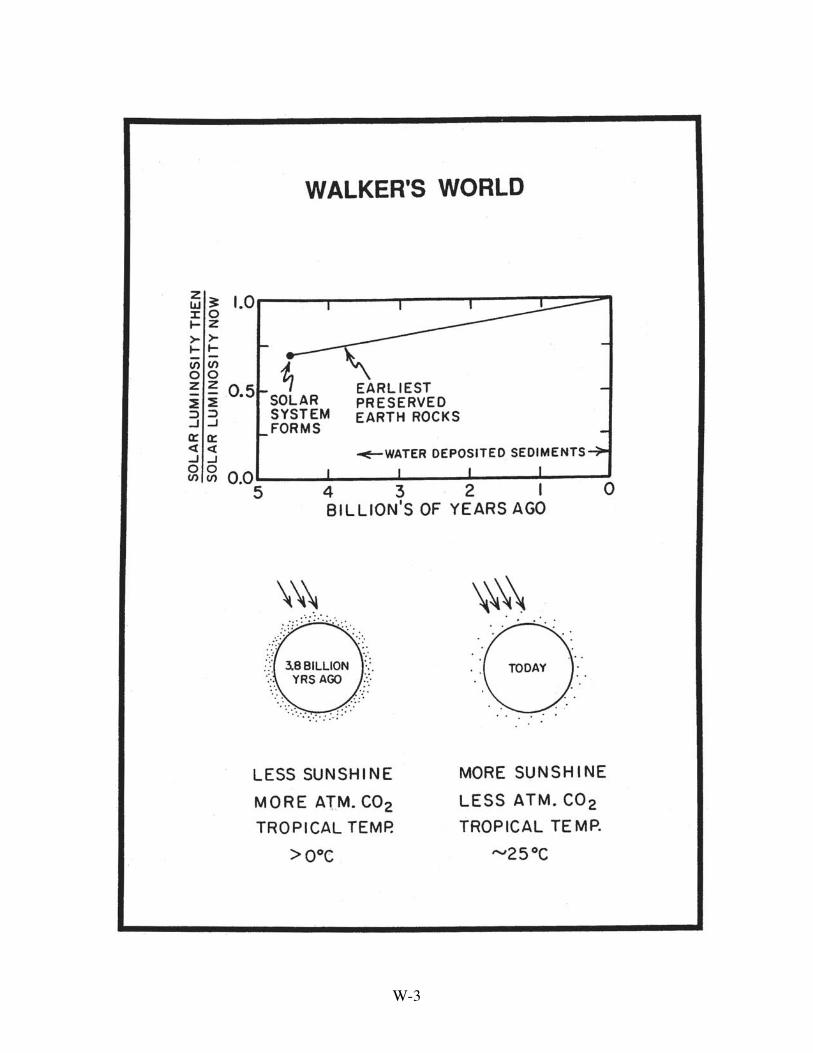
W-3

W-4

nuclear furnace has steadily fused hydrogen into helium, gradually reducing the number

of atomic nuclei flying about in its hot interior. This, in turn, has reduced the thermal

pressure holding back the forces of gravity. In order to maintain a balance between the

gravitational tendency to collapse and the thermal tendency to expand, the rate of energy

production in the Sun's nuclear furnace has steadily risen compensating for the decrease

in the number of nuclear entities. The current rate of energy release from the Sun tells us

how many hydrogen mergers occur each year. Based on this conversion rate,

astrophysicists can calculate how the Sun's helium to hydrogen ratio has evolved and

hence how its energy output must have increased in order to compensate for this change.

The bottom line is that, early on, the amount of energy reaching us from the Sun was not

large enough to maintain equatorial temperatures on our planet (at least with an

atmosphere like the present one) above the freezing point. Thus, in order to account for

the presence of liquid water on the planet at that time, something must have compensated

for the dearth of sunshine. That something was very likely extra greenhouse gases in the

atmosphere: CO2 being the top candidate.

The Earth's Anti-Freeze

The Earth has a built-in thermostat which prevents freezing. The active element

of this thermostat is CO2 gas. Roughly a tenth of a gigaton of carbon escapes from the

planet's interior each year in the form of CO2 gas. In a period of several thousand years,

this flux brings to the surface an amount of CO2 equal to that currently present in the

atmosphere. But the CO2 content of the atmosphere is not becoming larger. For this to

be the case, the carbon atoms contained in this CO2 must be removed to sediments (as

calcite and organic matter) at approximately the same rate as they are being gained from

the Earth's interior through outgassing.

Let us consider what would happen if Kurt Vonnegut's ice-nine catastrophe were

to strike the Earth. In the absence of liquid water, no further CaCO3 or organic residues

would be formed. However, the release of CO2 from the Earth's interior would chug

W-5

along virtually unchanged, for outgassing is driven by heat produced by the radiodecay of

the 40K, 235U, 238U and 232Th contained in the Earth's mantle. Considering that interior

temperatures are measured in thousands of degrees, a change in the temperature of a few

tens of degrees at the surface would go unnoticed by the Earth's mantle. So, were the

Earth's surface to freeze, the outgassing would continue and CO2 would accumulate in

the atmosphere. No pathway for removal would be available. After ten or so million

years, the atmosphere's CO2 partial pressure would approach one atmosphere! Of course

long before this level was achieved, the warming induced by the extra greenhouse

insolation would bring about a thaw. As at any one time only a tiny fraction of the

Earth's carbon resides in the atmosphere as CO2, no chance exists that the supply from

the interior would ever have been so measly that the Earth was at risk of becoming

permanently ice bound. Our planetary twin, Venus, with its 100-fold larger atmosphere

of nearly pure CO2 and greenhouse supported surface temperature of 450°C stands

witness to the potential power of this blanket.

A potential flaw has been found in this argument. Jim Kasting, a co-author on the

1981 Walker paper, and his Penn State colleague, Ken Caldeira, point out that were the

Earth ever to have become 'white', the supposed savior might instead have sealed its

doom. It is possible that before CO2 had built up to the point where the Earth's ice cover

could melt, this gas would condense to form globe straddling ice clouds. The reflection

of sunlight from these clouds would have so starved the planet of solar heat that it would

forever remain in its frozen state. Were this to have happened, Earth and Venus would

have stood as twin sentinels, one bearing witness to a CO2-driven runaway cooling and

the other to a CO2-driven runaway warming!

Evidence from carbon isotope ratios has led Harvard's Paul Hoffman and his

colleagues to suggest that at least twice the Earth did freeze over and that both times it

was bailed out by a build up of CO2. Following up on reconstructions by Kirshvink

which suggest that two major late Proterozoic glaciations (one at about 740 and the other

W-6

at about 550 million years ago) reached well into the tropics. Further, as these glaciers

extended to sea level, it is difficult to explain their existence unless the Earth had become

one large snowball. It has long been known that the tills laid down by these glaciers are

immediately overlain by limestones referred to as 'cap carbonates'. Hoffman et al.

provide a fascinating explanation for this sequence. Once frozen over, no mechanism

would exist to deposit the CO2 escaping from the Earth's interior either as CaCO3 or as

organic debris. Hence the CO2 content of the atmosphere would steadily increase.

Eventually, the greenhouse warming created by the CO2 buildup would overcome the

massive cooling created by the snowball's ability to reflect away the sun's rays. At this

point, the ice cover would begin to retreat progressively darkening the planet's surface. A

runaway warming would ensue eliminating all the planet's ice cover and thereby flooding

the low-lying portions of the continents. Weathering of the newly exposed land surface

would supply the calcium required to precipitate the great excess of CO2 in the

atmosphere and oceans. The result would be to produce the limestones which now cap

these glacial deposits. As the CO2 disappeared the Earth would cool.

Hoffman et al. point to the carbon isotope ratios in the cap carbonates as evidence

in support of their proposal. Instead of the near zero δ13C values which have

characterized most of geologic time, these limestones have quite negative values (δ13C -

5‰). The important point is that this value is equal to that for our estimate for average

Earth carbon. Thus, the isotopic composition of the limestone carbon is entirely

consistent with the idea that it is the product of an enormous buildup of mantle-derived

CO2.

Directing Chemical Traffic

Not only has CO2 stood guard against an Earth freeze-up but, as Walker

proposed, it may have exerted an active influence on the climate. This can be seen by

carrying the above logic one step further. To do so, let us consider the hypothetical

planet X made of only two minerals, CaO and CaCO3. The temperature in this planet's

W-7

interior is high enough to thermally decompose CaCO3 to CaO and CO2. The CO2

generated in this way migrates to the surface where it accumulates in the atmosphere

maintaining temperatures sufficiently high to allow water to exist in liquid form. Water

evaporates from the planet's ocean and falls on its continents as rain. CaO dissolves from

the planet's soils and is carried to the sea by rivers. The sea becomes supersaturated with

respect to CaCO3, allowing CO2 to mate with CaO. The calcite formed by this union falls

to the sea floor producing a sedimentary blanket. In this way, the CO2 escaping from the

planet's interior is returned to solid form.

Now, if for some reason the supply of CO2 from the interior were to temporarily

exceed the supply of CaO from rivers, then the mateless CO2 molecules would be forced

to accumulate in the atmosphere and the planet would warm. This warming would drive

up the chemical weathering rate to rise (more rain and faster chemical kinetics). The

warming would continue until the dissolution rate of CaO once again matched the rate at

which CO2 was being supplied from the planet's interior. Because of this, the planet's

chemical system would be self regulating. If CO2 were outgassed faster than CaO was

eroded, the atmosphere's CO2 content (and consequently also Earth's temperature) would

rise until balance was reestablished. Or, on the other hand, if CaO were dissolved from

the continents faster than CO2 escaped from the interior, the atmosphere's CO2 content

and (consequently Earth's temperature) would fall until the balance was reestablished.

Even on this simple planet, the temperature at which a balance between CO2

outgassing and CaO erosion was achieved need not have remained constant. For

example, as its radioactive isotopes decayed away, the planet's interior would cool and

the rate of outgassing of CO2 would ebb. Less matching CaO would be required and

hence surface temperatures would fall.

But the Earth is not a ball of CaO and CaCO3. Nor do its rates of continental

weathering and oceanic calcite precipitation follow the simple rules postulated for

planet

W-8

W-9

X. However, a feedback loop similar to that for planet X very likely operates. As CO2

resides in the ocean-atmosphere reservoir for only a hundred thousand or so years, a

control mechanism must exist which forces a balance between CO2 loss to sediments and

CO2 supply from the interior. The difference is that Earth chemical cycles are far more

complex than those for planet X. These complexities offer many more possibilities for

shifts in the temperature at which the balance between CO2 loss matches CO2 gain.

Changes in the rate of plate motion, in the height of mountain belts, in the freeboard of

continental blocks, in the physiology of terrestrial plants and in the habitat of CaCO3

precipitating marine organisms, all have the potential to change the temperature at which

CaO supply balances CO2 outgassing.

The BLAG Scenario

In a paper which attracted much interest to this subject, Berner, Lasaga and

Garrels (BLAG) treated the Earth much as if it were planet X. They assumed that the rate

of CO2 release from the Earth's interior is proportional to the rate of sea-floor spreading

and that the main factor perturbing the Earth's CO2 budget over the last 100 million years

was the gradual slowdown in this rate as first postulated by marine geologists Pitman and

Hays. If so, then following Pitman and Hays' suggestion that 100 million years ago sea

floor spreading rates were twice today's, the rate of CO2 outgassing must also have been

roughly twice today's. As the Earth-surface CO2 budget is balanced on the time scale

considerably less than one million years, the delivery rate of CaO to the sea as the result

of the chemical weathering of silicate rocks must also have been twice as great at that

time. The major factor controlling the chemical weathering rates is assumed by BLAG to

be soil temperature. As chemical reaction rates rise by about a factor of two for each

10°C warming, in order for the CaO supply to have been twice its present values, the

Earth would have to have been 10°C warmer 100 million years ago. BLAG assumes that

this extra warmth was maintained by a higher atmospheric CO2 content. Simulations

carried out in general circulation models suggest that for each doubling of the

W-10

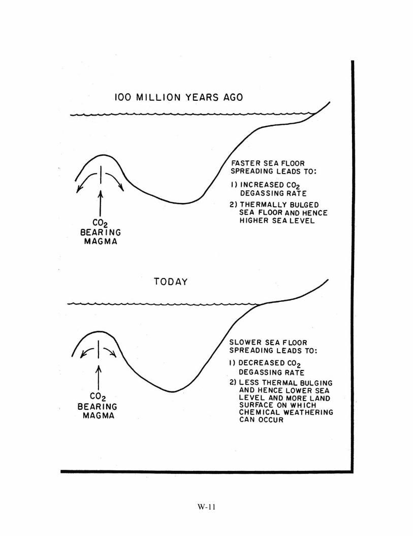
W-11

W-12

atmosphere's CO2 content the temperature rises about 3.3°C. Hence a 10°C warming

would require an eight fold increase in the atmosphere's CO2 content. We know from

measurements on air trapped in ice cores that, over the last 250,000 years, the CO2

content of the atmosphere has averaged about 250 ppm. If the BLAG reconstruction is

correct, then the CO2 content of the atmosphere must have been about 2000 ppm 100

million years ago. The fact that oxygen isotope evidence demonstrates that the earth's

polar regions were considerably warmer at this time has been taken as a confirmation of

BLAG scenario.

Since the publication of BLAG, much discussion has occurred concerning the

details of their argument. Did sea floor spreading rates really drop by as much as a factor

of two over the last 100 million years or, as other reconstructions suggest, has the extent

of slowdown been much smaller? Do the chemical weathering rates for silicate minerals

really depend primarily on temperature, or as some have suggested, do other factors such

as mechanical breakup or plant enzymes play important roles? Does Earth climate

change only as the result of fluctuations in the CO2 content of the atmosphere, or as some

have suggested, has it been more strongly influenced by the geography of continents and

oceans? While these and other uncertainties cast doubt on the specific conclusions of

BLAG, the concept has stood the test of time.

But Might the Policeman Reside in the Ocean?

While the most attractive candidate for chemical traffic director is the CO2

content of the atmosphere, other choices exist. The assumption that the sole fate for the

CaO released by the weathering of continental silicate rocks is deposition as CaCO3 on

the sea floor is open to challenge. Perhaps the supply of calcium is in excess of what's

needed to match the CO2 being degassed from the Earth's interior. In this case, the

excess calcium would have to be taken up in silicate minerals. One pathway would be

into minerals forming on the sea floor. Unfortunately, minerals formed by this so-called

"reverse weathering" process are not present in nearly the abundance expected if they

W-13

W-14

were to constitute a calcium sink comparable in magnitude to that of marine calcite which

makes up about half of presently forming open ocean sediment. If the silicate route is an

important one, the product must be hidden from view either in basins adjacent to

continental margins where the rate of deposition of detrital material is very rapid or in the

basalts which lie beneath the blanket of open-ocean sediment. While little support exists

that the former hiding place is important, the chemical signature of hydrothermal waters

issuing forth from the ridge crests clearly demonstrates that extensive alteration of the

underlying basalt is occurring. Hence if significant amounts of calcium are being

removed into silicate minerals, this is likely occurring in sea floor basalts. But, at least

close to the centers of sea floor spreading, calcium is being released rather than taken up.

The effluent from ridge-crest geothermal vents contains on the average about twice as

much calcium as does sea water. The major reaction appears to be a replacement of

calcium in the basalt by magnesium carried into the hot crust with the circulating sea

water. So, if calcium is being removed, it must be as a result of lower temperature

reactions occurring away from the spreading centers.

We shall refer to this alternate scenario as GALB. For BLAG the policeman

resides in the atmosphere; for GALB he resides in the sea. For BLAG calcium supplied

to the sea is removed almost entirely as CaCO3. For GALB silicate minerals, formed on

the sea floor, constitute a major additional sink for calcium. For BLAG the flow of CaO

through the system is closely tied to that of CO2. For GALB, the control is most likely

the pH of deep sea water. The higher the pH the more rapidly CaO is removed.

The Rates of CO2 Degassing and Ca Supply From Silicates

First let us put aside an obvious strategy for distinguishing between the BLAG

and GALB scenarios. It involves measurements of today's rates of input of CaO and CO2

to the ocean-atmosphere reservoir. If such studies were to reveal that the rate of delivery

of CaO derived from the chemical weathering of silicate minerals closely matched the

rate of outgassing of CO2 from the Earth's interior, then the case for BLAG would be

W-15

strengthened. On the other hand, if the delivery of silicate-derived CaO proved to be

significantly higher than that of CO2, the finger would point toward GALB. But this

strategy proves to be impractical. The reason is that to be successful these fluxes would

have to be measured with an accuracy of better than ±15%. We are hard pressed to

achieve even a factor of two.

These endeavors are bedeviled by a common problem; the erosion of limestone

dominates the supply of both CaO and CO2 to the sea. This greatly diminishes the value

of the two fluxes we can measure with a fair degree of accuracy, i.e., the accumulation

rate of calcite on the sea floor and the supply rate of calcium by the world's rivers. As

both fluxes are dominated by the recycling of limestone (dissolved from the continents

and redeposited on the sea floor), it is not possible to separate out the lesser contribution

made by the weathering of silicate minerals. One might conclude that such a separation

is not necessary, for if the rate of removal of calcium to the sea floor as calcite exactly

matched the rate at which calcium is supplied to the ocean from rivers and sea floor

hydrothermal activity, then we could be assured that no excess remained for the

formation of silicate minerals in the basaltic crust or sediment column. However, as the

recycling of limestone dominates the fluxes of calcium and carbon to the sea, the two

rates would have to be known to a very high degree of accuracy. It has been estimated

that only about one quarter of the calcium eroded from the continents is derived from

silicates. If so, then a 25% uncertainty in the estimate of river flux of calcium could

create a factor of two uncertainty in the amount of CaO available for matching the CO2

added by mantle outgassing. Unfortunately, it is not possible to determine either the river

flux or input of calcium to better than 20%. Hence, this approach does not offer a means

of distinguishing between BLAG and GALB.

One of the complications associated with any attempt to use today's river fluxes

has to do with the dependence of chemical weathering rate on climate. We live in the

W-16

W-17

warm phase of one of a long series of 100-thousand-year duration glacial cycles. As

these intervals of warmth constitute only about ten percent of each climate cycle, the

chemical weathering rates that we compute from today's river discharge may not typify

the entire cycle. The situation is further complicated by anthropogenic impacts on river

chemistry. Plowing, irrigation, acid rain... have all accelerated the release of

exchangeable ions bound in soils. Thus the chemical load of many of the world's rivers

is not even typical of interglacial climates. Frustration!

The failure of this obvious approach leaves us with the more difficult one of

separately determining the rates of CO2 degassing and silicate weathering. In the case of

CO2, we know that sea-floor spreading centers are major conduits for CO2 emanating

from the Earth's interior. The reason is that basalt glasses dredged from mid-ocean ridge

crests have CO2-bearing inclusions (which often burst when brought aboard

oceanographic vessels, giving rise to the term 'popping rocks'). The ratio of CO2 gas to

solid in these glasses offers a means of estimating the amount of CO2 carried to the

surface with basaltic magmas. We know reasonably well the rate of sea floor spreading

and hence the amount of basalt formed each year. Ultimately all the CO2 brought up with

the basalt magma escapes into the overlying ocean. CO2 is also released from zones

where plates are subducted and from zones of continental metamorphism. These

contributions currently defy quantification. Hence the likelihood that the aggregate CO2

flux from all three sources can be adequately quantified is remote.

An additional complication in the CO2 budget is that only part of the carbon

removed from the ocean-atmosphere reservoir becomes calcite. The rest becomes bound

into organic residues. Hence, in order to estimate the required supply rate of CO2

destined to become CaCO3, the amount of carbon going into organic residues must be

subtracted from the amount of CO2 being outgassed. Fortunately, we have a means to

assess the magnitude of this correction. It is based on carbon isotope ratios measured in

marine carbonates. From a knowledge of the approximate isotope composition of bulk

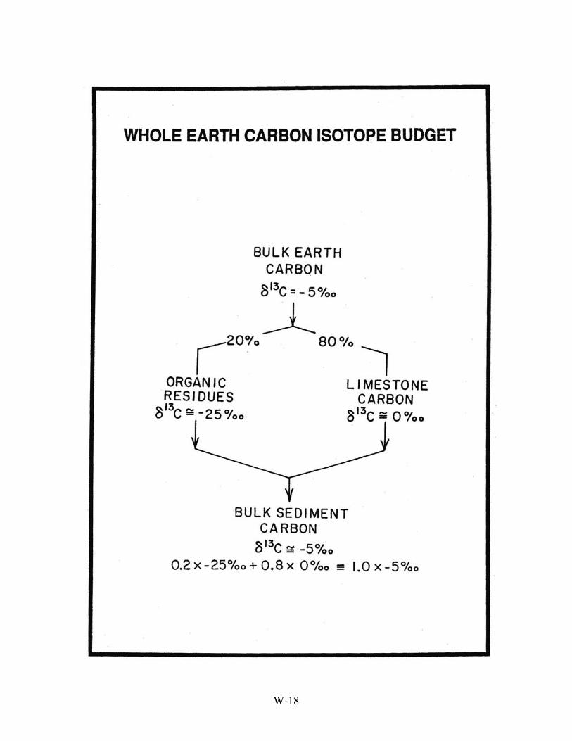
W-18

W-19

Earth carbon (δ13C=-5‰) and of the difference between the carbon isotope ratio in plant

carbon and in marine calcite carbon (∆δ13C= -25‰), we can use the isotopic composition

record for marine carbonate to tell us how the carbon output has been divided between

organic residues and calcite. For example, if the δ13C for marine CaCO3 of a given age

is close to 0‰, then mass balance requires that at that time 80% of the carbon went into

limestone and 20% into organic residues. The results of thousands of carbon isotope

measurements on marine CaCO3 of all ages suggest that the fraction of carbon going into

organic residues has remained small. For the last 100 million years, it has been in the

range 20±5% of the total. But organic matter cannot be written off as a minor player.

The reason is as follows. Since only about one quarter of the calcium delivered to the sea

is derived from the weathering of silicate minerals, organic matter accounts for the

removal of roughly half of the CO2 supplied by Earth outgassing (and oxidation of

recycled organics).

An alternate approach would be to estimate the contribution made by the chemical

weathering of silicate rocks to the dissolved Ca++ carried in rivers. One means by which

this might conceivably be done is through measurements of the carbon isotope ratios in

river water ∑CO2. The plus charges on cations derived from silicates are balanced by

minus charges on bicarbonate ions derived from soil CO2 (δ13C=-26‰). The plus

charges on cations derived from carbonate rocks are also matched by minus charges of

bicarbonate ions. But, in this case half the carbon atoms are from the carbonate rocks

(δ13C=0‰) and half from soil CO2 (δ13C=-26‰). Together they would yield a δ13C

value of -13‰. Were the situation simple, then the δ13C for bicarbonate would be

expected to lie somewhere between -13‰ for streams draining limestone terrane and -

26‰ streams draining silicate terrane. For example, were the δ13C for the HCO-3 of

average river water -20‰, then one could conclude that about half the cations were

derived from the weathering of limestone and about half from the weathering of silicate

rocks. Unfortunately, the situation is far more complex. First, the

W-20

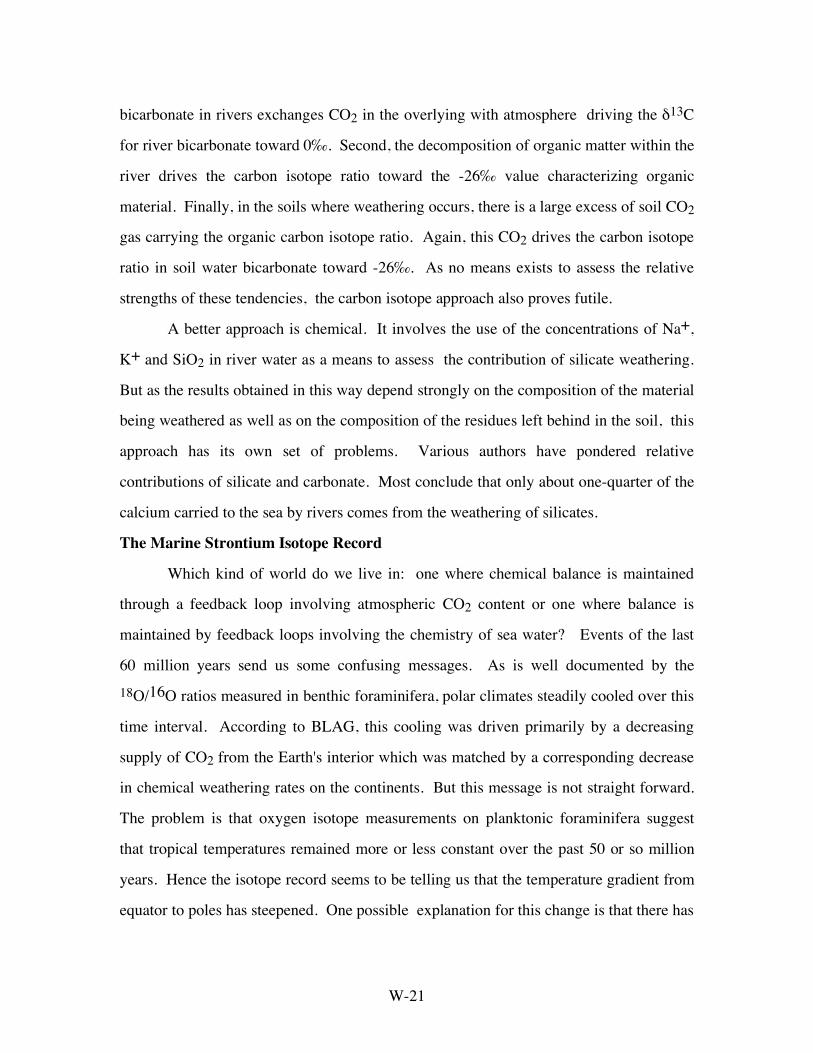
W-21

bicarbonate in rivers exchanges CO2 in the overlying with atmosphere driving the δ13C

for river bicarbonate toward 0‰. Second, the decomposition of organic matter within the

river drives the carbon isotope ratio toward the -26‰ value characterizing organic

material. Finally, in the soils where weathering occurs, there is a large excess of soil CO2

gas carrying the organic carbon isotope ratio. Again, this CO2 drives the carbon isotope

ratio in soil water bicarbonate toward -26‰. As no means exists to assess the relative

strengths of these tendencies, the carbon isotope approach also proves futile.

A better approach is chemical. It involves the use of the concentrations of Na+,

K+ and SiO2 in river water as a means to assess the contribution of silicate weathering.

But as the results obtained in this way depend strongly on the composition of the material

being weathered as well as on the composition of the residues left behind in the soil, this

approach has its own set of problems. Various authors have pondered relative

contributions of silicate and carbonate. Most conclude that only about one-quarter of the

calcium carried to the sea by rivers comes from the weathering of silicates.

The Marine Strontium Isotope Record

Which kind of world do we live in: one where chemical balance is maintained

through a feedback loop involving atmospheric CO2 content or one where balance is

maintained by feedback loops involving the chemistry of sea water? Events of the last

60 million years send us some confusing messages. As is well documented by the 18O/16O ratios measured in benthic foraminifera, polar climates steadily cooled over this

time interval. According to BLAG, this cooling was driven primarily by a decreasing

supply of CO2 from the Earth's interior which was matched by a corresponding decrease

in chemical weathering rates on the continents. But this message is not straight forward.

The problem is that oxygen isotope measurements on planktonic foraminifera suggest

that tropical temperatures remained more or less constant over the past 50 or so million

years. Hence the isotope record seems to be telling us that the temperature gradient from

equator to poles has steepened. One possible explanation for this change is that there has

W-22

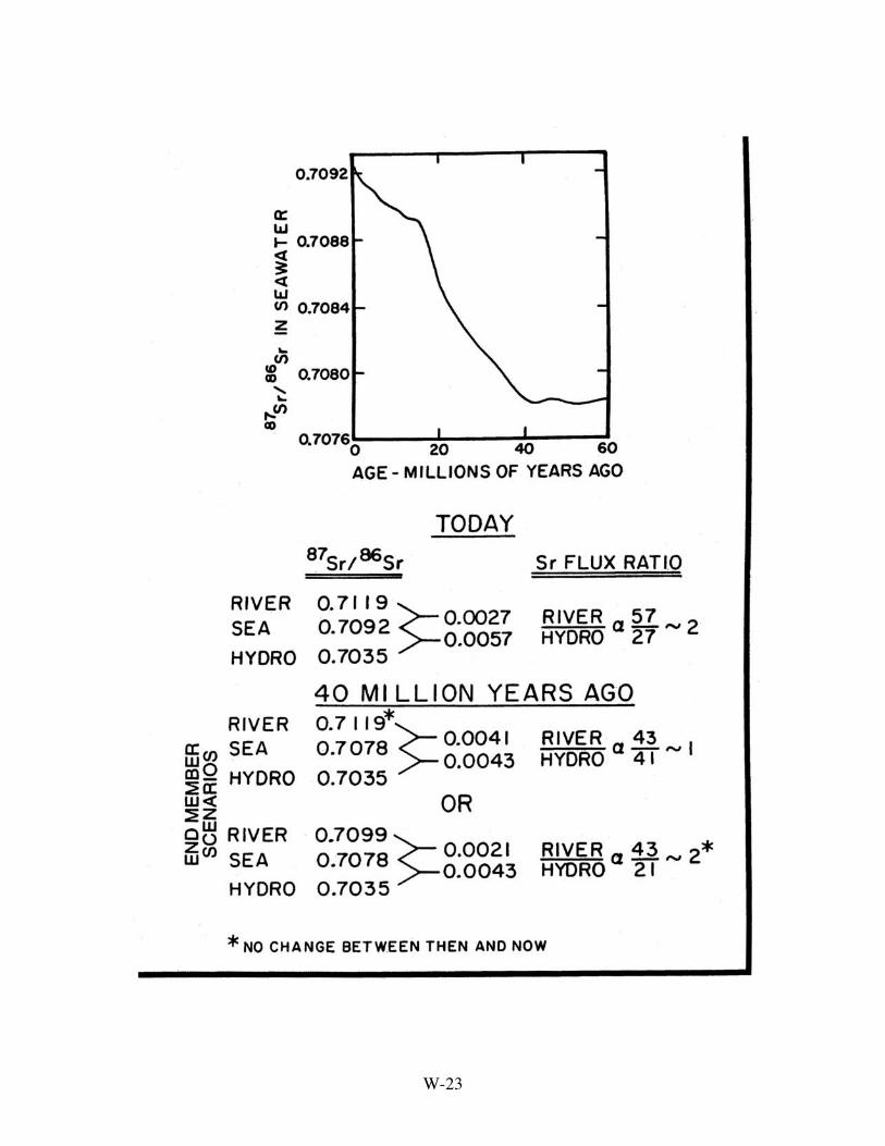
W-23

W-24

been a decrease in the efficiency of poleward heat transport (by air and sea). As the polar

area is small compared to that of the tropics, such redistributions of heat would lead to

larger changes in polar temperature. By contrast, the warming generated in atmospheric

models when CO2 is increased are not limited to high latitudes; it is global. However,

whatever its origin, this cooling should according to BLAG have been accompanied by a

decrease in chemical weathering rate.

But the record of the strontium isotopic composition of sea water kept by the

foraminifera preserved in deep sea sediments seems to be telling us that chemical

weathering rates have been increasing over the last 40 million years. The logic is as

follows. The strontium supplied to the sea through continental weathering is richer in

radiogenic 87Sr (derived from the decay of radioactive rubidium-87) than strontium

supplied through the hydrothermal alteration of sea floor basalts. The 87Sr/86Sr of

strontium dissolved in sea water lies between that for these two end members, giving the

appearance that it is a mixture of about two parts strontium from rivers and one part

strontium from ridge crest hydrothermal systems. As the average strontium atom resides

in the sea for several million years before being removed to sediments, the strontium

added to the sea from these two sources has become so well mixed that no measurable

difference in isotopic composition exist from one place in the sea to another. Thus the

strontium incorporated into the shells of foraminifera records the average isotopic

composition of the strontium delivered to the sea over the previous several million years.

Hundreds of Sr isotope analyses on foraminifera from many sea floor borings yield a

detailed record of the evolution of the strontium isotopic composition of sea water over

the last 100 million years. While nearly uniform during the first half of this time interval,

the record reveals that an increase in the amount of radiogenic 87Sr commenced 40

million years ago and has continued right up to the present. The most obvious

explanation for this increase is that the supply of strontium derived from the chemical

weathering of continental rocks has been on the increase. However, another explanation

W-25

exists, namely, that the content of radiogenic strontium in continental-derived strontium

has been increasing. Indeed, this alternative explanation has become the leading

contender. The advocates of this view look to the collision with Asia of the northward-

moving Indian subcontinent which took place just prior to 40 million years ago as the

villian which initiated the 87Sr increase. The thrusting of one continental block beneath

another led to the creation of the Himalayan mountain belt and the Tibetan Plateau.

Contained in this collision zone are igneous bodies, referred to by petrologists as

leucogranites, whose feldspars contain strontium particularly rich in 87Sr. So radiogenic

is the strontium in the rivers draining the Himalayas that it alone could be responsible for

the observed change in the oceanic strontium isotope ratio.

Were the BLAG reconstruction correct, then one might have expected the

opposite trend in the isotopic composition of oceanic strontium. As soils cooled, the

supply to the sea of continental weathering products would have decreased causing the

ocean's strontium to become less radiogenic. But this need not have been the case for the

rate of hydrothermal activity responsible for the release of strontium from ridge crest

basalts would also have dropped in proportion to the rate of sea floor spreading. These

two changes might well have compensated for one another and there would be no

tendency for the isotopic composition of strontium in sea water to change. Less

strontium would reach the sea but its isotopic composition would remain unchanged.

Thus BLAG supporters would have to maintain that the observed increase is primarily

the result of the input of highly radiogenic strontium from rivers draining the Himalayas.

Viewed from this perspective, one would have to conclude that the strontium isotope

record in sea water, while not lending support to BLAG, cannot be taken as evidence that

the BLAG concept is incorrect.

The Influence of Mechanical Breakup on Chemical Weathering Rates

Now as already mentioned, the defenders of BLAG point to the observation that

the Earth has cooled and therefore postulate that chemical weathering rates should have

W-26

W-27

decreased. Cooler temperatures mean slower chemical reaction rates in soils and less

precipitation to carry away dissolution products. But this way of looking at things is built

on the assumption that the rate-limiting step for silicate dissolution is chemical. As

pointed out by MIT's John Edmond, this need not be the case; the rate limiting step could

equally well be mechanical. Chemically reactive surfaces are created when rocks are

broken. Freeze-thaw cycles are powerful agents of mechanical breakup. Were the rate-

limiting step mechanical rather than chemical, the dependence on climate might be the

reverse. The progressive cooling during the last 60 million years has surely led to an

increase in the continental area experiencing freeze-thaw cycles. Perhaps the increased

rate of production of grist for the chemical mill has more than compensated for the drop

in soil temperature. As a consequence, the cooling may have speeded the rate of

chemical weathering! Indeed, Edmond has shown that Siberian rivers draining silicate

terrain carry to the sea as much calcium (per acre draine) as does the Amazon River. In

the Amazon, a thick mantle of cation-depleted material presently shields the underlying

fresh rock from chemical attack. No such mantle is present in Siberia. Not only do

freeze-thaw cycles break up the rock but the runoff during fierce spring melts allows the

chemically weathered material to be sluiced away.

As might be expected, Edmond's suggestion that the rate of chemical weathering

may decrease rather than increase with rising Earth temperature has met with

considerable resistance. Where are the Siberian clay minerals which must be a byproduct

of the weathering of primary igneous minerals? Instead, could the calcium in Siberian

rivers be derived from limestone units as yet undiscovered in this poorly mapped terrain?

These critics also point out that while the Amazon, because of its immensity, dominates

today's tropical weathering, this low-lying and very flat region cannot typify the tropics

of the distant past. Because of the drift of continents and the uplift of mountain ranges,

the tropics of earlier time very likely had higher relief and hence a less complete mantle

of chemically-depleted debris than does today's Amazon jungle.

W-28

W-29

Increased rock breakup as the result of freeze-thaw cycles is not the only

mechanism by which mechanical weathering might be increased. The topographic relief

generated by mountain uplift is also important. Steep slopes accelerate mechanical

erosion and also allow chemically spent material to be sluiced away exposing the fresh

underlying material. Just as the rate of CO2 emission from the Earth's interior is expected

to decrease with the rate of sea floor spreading, so also is the rate of mountain building.

So one might ask, wouldn't the Earth have been even more mountainous 100 million

years ago if, at that time, the plates were moving faster? Perhaps, but in the case of

mountain building, an important stochastic element exists; rare headon collisions between

major continental blocks can lead to exceptional high and extensive mountain belts.

About forty million years ago such an event took place. India collided with Asia

creating the Himalayan mountain chain. Pelted by monsoonal rains, this small highland

region is currently responsible for about 16% of the world's chemical weathering. MIT's

Maureen Raymo contends that increased chemical weathering from the Himalayas

negates the BLAG hypothesis. True, at a time when CO2 outgassing was apparently

decreasing, one would expect global weathering rates to have been on the decrease.

Raymo's argument rests on an interpretation of the strontium isotope record for the last

40 million years which calls on increasing continental weathering rates. But as we have

seen, it is not necessarily the case. The rise in 87Sr content of marine strontium may be

due entirely to the more radiogenic character of the strontium derived from the

Himalayas. Defenders of BLAG would claim instead that the increase in calcium supply

related to the Asian uplift was compensated by a small decrease in chemical weathering

rate in the rest of the world (brought about by an additional atmospheric CO2 drop and

the consequent cooling). Looked at this way, the rise in the Himalayas would according

to BLAG cool the planet!

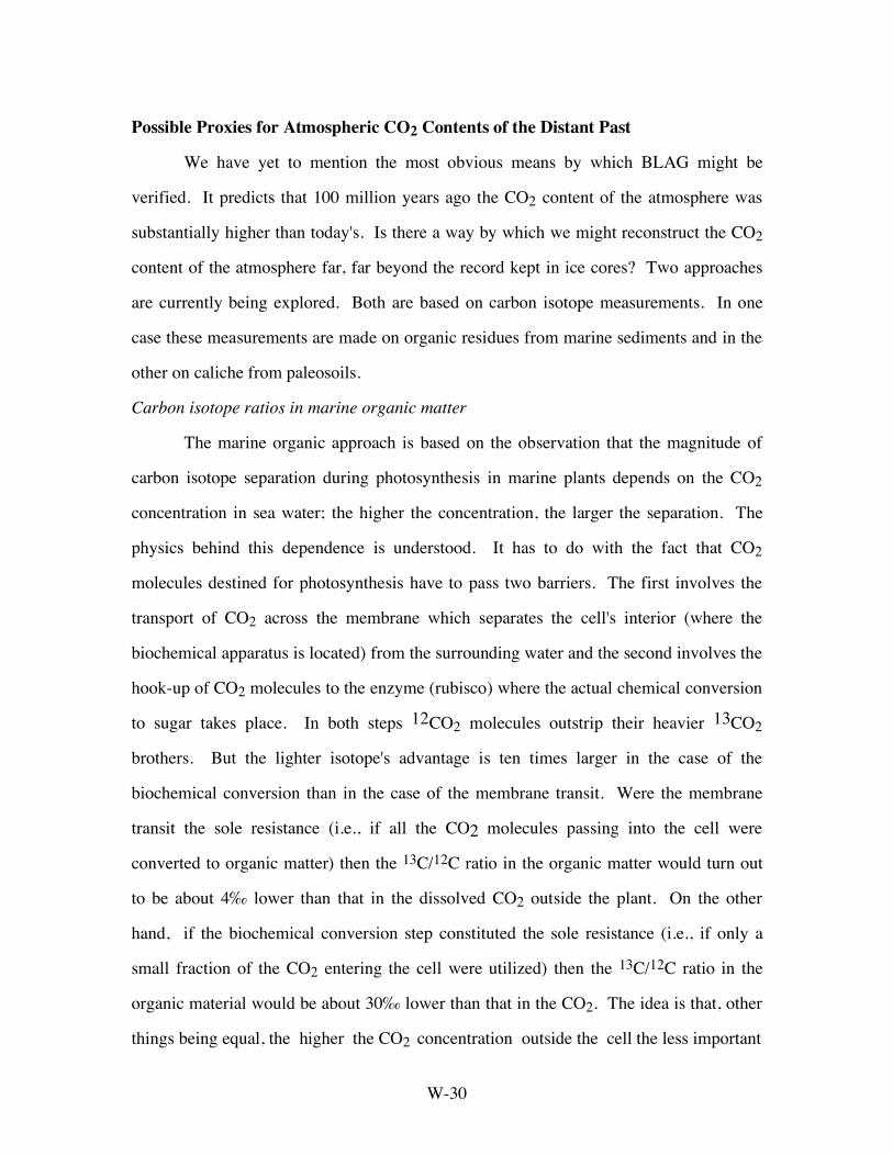
W-30

Possible Proxies for Atmospheric CO2 Contents of the Distant Past

We have yet to mention the most obvious means by which BLAG might be

verified. It predicts that 100 million years ago the CO2 content of the atmosphere was

substantially higher than today's. Is there a way by which we might reconstruct the CO2

content of the atmosphere far, far beyond the record kept in ice cores? Two approaches

are currently being explored. Both are based on carbon isotope measurements. In one

case these measurements are made on organic residues from marine sediments and in the

other on caliche from paleosoils.

Carbon isotope ratios in marine organic matter

The marine organic approach is based on the observation that the magnitude of

carbon isotope separation during photosynthesis in marine plants depends on the CO2

concentration in sea water; the higher the concentration, the larger the separation. The

physics behind this dependence is understood. It has to do with the fact that CO2

molecules destined for photosynthesis have to pass two barriers. The first involves the

transport of CO2 across the membrane which separates the cell's interior (where the

biochemical apparatus is located) from the surrounding water and the second involves the

hook-up of CO2 molecules to the enzyme (rubisco) where the actual chemical conversion

to sugar takes place. In both steps 12CO2 molecules outstrip their heavier 13CO2

brothers. But the lighter isotope's advantage is ten times larger in the case of the

biochemical conversion than in the case of the membrane transit. Were the membrane

transit the sole resistance (i.e., if all the CO2 molecules passing into the cell were

converted to organic matter) then the 13C/12C ratio in the organic matter would turn out

to be about 4‰ lower than that in the dissolved CO2 outside the plant. On the other

hand, if the biochemical conversion step constituted the sole resistance (i.e., if only a

small fraction of the CO2 entering the cell were utilized) then the 13C/12C ratio in the

organic material would be about 30‰ lower than that in the CO2. The idea is that, other

things being equal, the higher the CO2 concentration outside the cell the less important

W-31

W-32

the resistance posed by the cell membrane and hence the greater the 13C depletion in the

plant matter. Indeed algae cultured in the laboratory over a range of CO2 concentrations

show this trend. This proves to be the case for the ocean as well. Organic matter formed

in the cold and hence higher CO2 concentration waters found in the Southern Ocean are

more depleted in 13C than organic matter grown in the lower CO2 concentrations of

tropical surface waters. Thus both in the lab and in the sea, at low CO2 gas

concentrations, the extent of isotope separation is shifted toward the smaller value

associated with diffusion through the cell membrane.

Attempts to apply this method must take into account that the relationship

between the CO2 concentration in surface water and the CO2 partial pressure in the

atmosphere overlying the sea water is strongly dependent on temperature. At the same

partial pressure, the coldest polar waters contain about three times more CO2 than

warmest tropical waters. Thus even if the 13C to 12C ratio in organic residues were to

yield reliable paleo CO2 concentrations for the ocean water in which they grew, the

conversion to an atmospheric CO2 pressure would require that the temperature of the

water in which the plant grew be known.

The idea behind the paleo CO2 indicator is that a universally applicable tie exists

between CO2 content of sea water and the isotope separation between the dissolved

inorganic carbon content of sea water and that in the organic matter formed by marine

organisms. In other words, given the CO2 concentration in the water, the magnitude of

isotope separation is uniquely determined. But this is a bit much to hope for. While the

expected trend in isotope separation with CO2 content will always exist, the position

between the two limiting situations will almost certainly depend on factors other than

just the CO2 concentration. The reason is that the degree of isotope separation is

controlled by the competition between two opposing forces. Diffusion across the cell

wall tends to keep the CO2 concentration in the cell fluid equal to that in the surrounding

water. Photosynthesis tends to draw down the CO2 content of the cell fluid well below

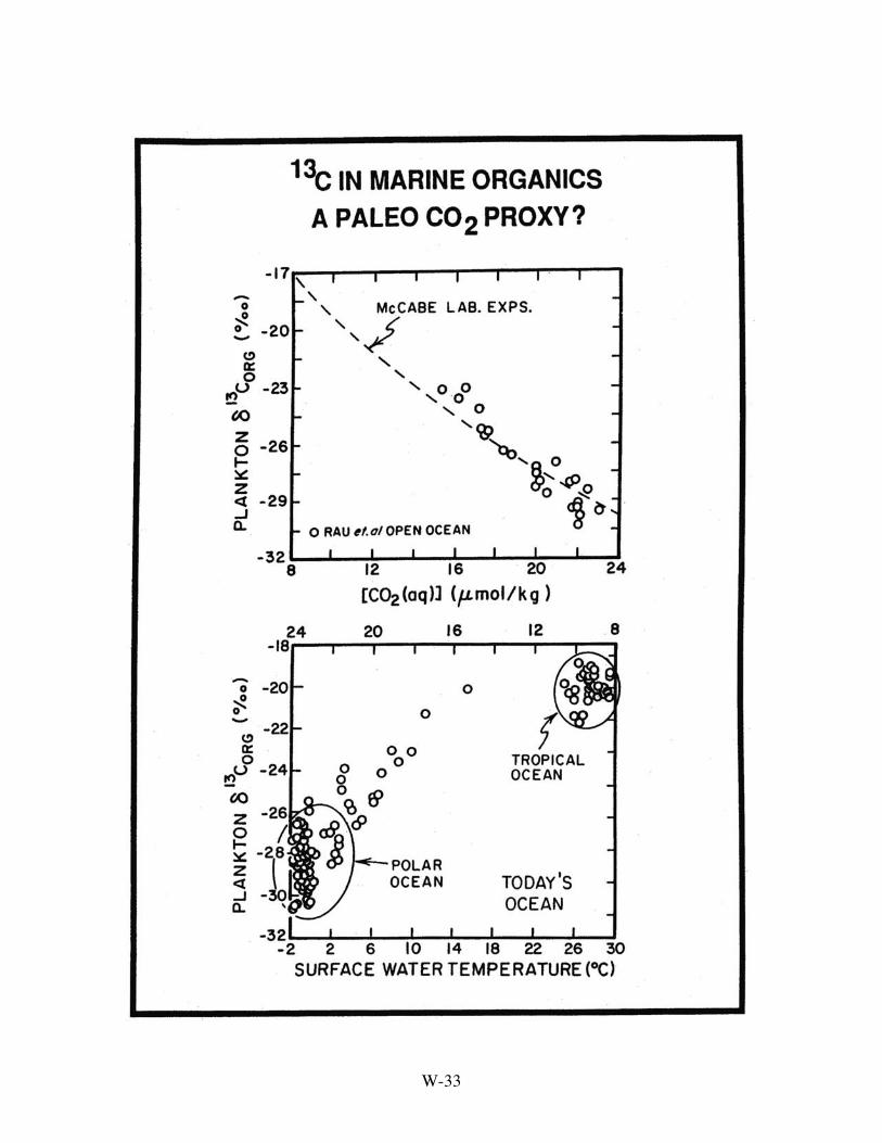
W-33

W-34

that in the surrounding sea water. The isotope separation reflects the balance between

these two opposing tendencies. If, for example, the CO2 content of the cell fluid were to

be drawn down to half the value characterizing the surrounding sea water, then the

isotope separation would lie half way between the limiting values. The point is that the

balance between these opposing forces must be influenced by factors other than the CO2

concentration. For example, it has been shown that the magnitude of the isotope

separation is also dependent on growth rate (as measured by the frequency of cell

division). The faster the growth the more important the resistance posed by the cell wall

and hence the smaller the isotope separation. This being the case, the magnitude of the

fractionation will depend on the availability of nutrients and of light. Finally, other

factors being equal (CO2, nutrients, light...), each species of plant has its own cell

structure and photosynthetic capability.

Indiana University's John Hays, who with his students and post docs has

pioneered this field, has come up with an innovative means of coping with two of these

potential problems. First, instead of analyzing bulk organic material, he separates out

specific compounds formed by only select groups of marine plants. Early work was done

with porphyrins because they are derivatives of chlorophyll and hence represent the

primary plant material. More recent efforts have concentrated on alkenones which are

produced by a specific plant group. This latter approach has enormous potential for not

only does it ease complications associated with the inclusion of carbon from the animals

and bacteria which feed on the primary plant matter, but also complications associated

with differences in physiology among plant groups. Second, it has been shown that the

ratio of alkenones of different carbon number produced by certain marine plant types

depends on growth temperature. If this proves to be a reliable paleotemperature method,

then the combination of the chemical ratio and carbon isotope ratio measured on the same

sample will give the partial pressure of CO2 in the water in which the plant grew!

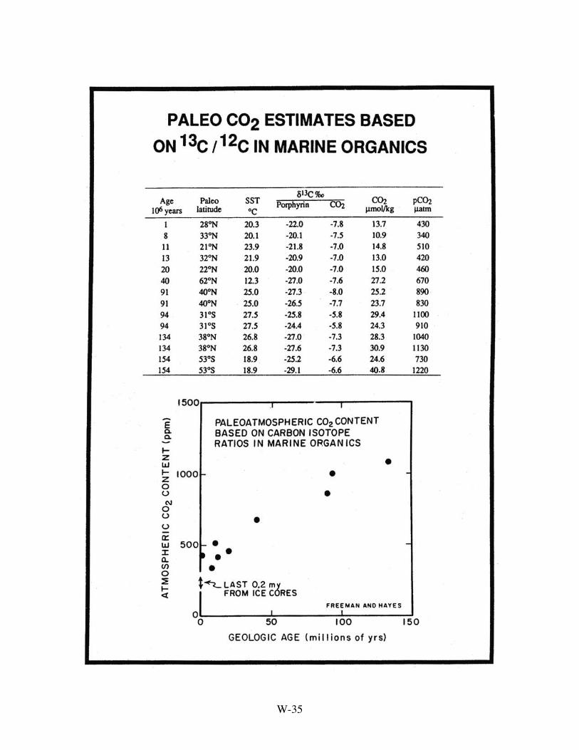
W-35

W-36

A first try at applying this method to organic material from sediments covering

the last 150 million years, does suggest that in accord with BLAG the CO2 content of the

atmosphere has been steadily decreasing. Measurements on porphyrins made in John

Hays' lab suggested that the atmospheric CO2 partial pressure 100 million years ago was

about 1000 µatm. However, until hundreds of such samples have been run it will not be

clear whether this trend is real or whether it reflects differences in growth conditions. A

convincing case will require the analysis of samples covering a wide geographical area

from a series of time slices. Only if for each time slice do these results point to similar

atmospheric CO2 values will the paleoclimate community take them seriously.

Carbon isotope ratios in soil caliche

The second carbon isotope-based paleo-CO2 method involves measurements of

the difference between the carbon isotope composition of coexisting CaCO3 and organic

matter in paleosoils. Cerling, its originator, has demonstrated that in today's soils the

isotopic composition of the CO2 is, as would be expected, closely related to that of

organic matter growing in the soil. But, as 12CO2 diffuses a bit faster than 13CO2, it

escapes more quickly from the soil. Hence, at steady state, soil CO2 is enriched in 13C

by 4.4‰ with respect to respiration CO2. The CaCO3 found in soils consists of CaO

leached from soil minerals and CO2 from soil gas. Because of the fractionation between

air phase CO2 and CaCO3 precipitated from soil waters, the isotopic composition of the

caliche is about 10‰ heavier than that in soil CO2. The important point is that in today's

situation, the contribution of atmospheric CO2 is too small to significantly influence the

isotopic composition of soil gas CO2. For example, were the excess CO2 pressure in the

soil 9700 µatm, the overlying air (with its CO2 pressure of only 300 µatm) would make

up only 3 percent of the soil's CO2. As atmospheric CO2 and respiration CO2 differ in

isotopic composition by about 15‰, the isotopic shift created by the presence of this

small amount of air CO2 would be only about 0.5‰. By contrast, if at some time in the

past, the CO2 content of the atmosphere were ten times higher than today's (i.e., 3000

W-37

W-38

µatm) and if the soil to atmosphere difference in CO2 partial pressure were the same as

today's (i.e., in our example ~9700 µatm) then the atmosphere-induced isotope shift

would be 15 x 3000/(3000 + 9700) or 3.5‰. Cerling hopes to use the magnitude of this

atmospheric CO2-induced shift in isotope composition of CaCO3 in paleosoils to

determine whether or not CO2 pressures were significantly higher in the past.

An ingenious method, but will it work? The shift upon which Cerling's method is

based is quite small (a few ‰); therefore, close attention must be given factors which

might bias the isotopic composition of soil CaCO3. Cerling points out several.

1. As the magnitude of the fractionation between soil CO2 and soil CaCO3

changes by 1‰ per 10°C, a temperature correction must be made.

2. The 13C to 12C ratio in atmospheric CO2 depends on both the temperature and

the 13C to 12C ratio for surface ocean water. Measurements by Shackleton on marine

CaCO3 suggest that the 13C to 12C ratio in surface ocean ∑CO2 was 1 to 2‰ higher 20

million years ago than today. Further, the warmer temperatures at that time would have

reduced the air-sea carbon isotope difference and thereby raised the atmosphere's 13C/12C

ratio by a bit more. It must be kept in mind, however, that the influence of the

atmosphere's isotope composition shift is diminished by the ratio pairCO2 /p

respiration excessCO2

. So even if, as in the above example, the p atmCO2 were ten times higher, a 2‰ difference

in the isotopic composition of atmospheric CO2 would cause only a 0.7‰ shift in the soil

CaCO3 isotope composition.

3. It must be demonstrated that the original 13C to 12C ratio in paleosoil CaCO3

has not been altered by subsequent diagenesis.

Another problem faced by Cerling is that his method is not a direct index of

atmospheric CO2 pressure. Rather, it is a measure of the ratio of atmospheric CO2

pressure to soil CO2 pressure. Modern soils show a wide range of CO2 pressures

reflecting both differences in plant productivity (and hence the rate of production of CO2

by respiration) and in porosity (and hence in residence time of CO2 in the soil before

W-39

escape to the overlying atmosphere). Cerling would like to believe that the range of

respiration CO2 contents of soils is relatively small and that its mean has not changed

over time. The only way he has to assess whether this is the case is to run samples from

many geographic localities for each time interval of interest. Cerling is currently seeking

to carry out this test. At the time of this revision, he and a PhD student were writing up

hundreds of such analysis.

Ocean Chemistry

For BLAG there is no need to define the mechanisms responsible for the control

of the ocean's chemistry. One only has to assume that the CaO and CO2 which arrive

there are mated to form CaCO3. We have already seen that in today's ocean this mating

goes smoothly; marine organisms produce CaCO3 several times faster than its ingredients

are supplied to the sea. In order to compensate for this overproduction, the horizon

separating supersaturated from undersaturated water rises and falls insuring that a balance

between input of the ingredients is matched by the accumulation of CaCO3 in the

sediment. As we shall see, paleolysocline reconstructions tell us that overproduction of

calcite by organisms has been the rule throughout the last 100 million years.

Nevertheless, it is of interest to consider how the chemistry of the ocean might have

evolved over this period.

One might ask whether we can restrict our inquiry to species directly involved in

the cycles of carbon and calcium, or must we deal with the salt matrix with which these

species interact. Four ions, Na+, Cl-, Mg++ and SO=4 , dominate the seas' salt. Only the

first two of these have such long replacement times that they can be viewed as

unchangeable on a 100 million year time scale. The other two, Mg++ and SO=4 , turn

over on the time scale of 10 to 15 million years. Hence their concentrations are subject to

change on the time scale of interest here. But as these changes are of only secondary

importance to the cycles of carbon and calcium of interest to us, we shall not ponder what

they might have been.

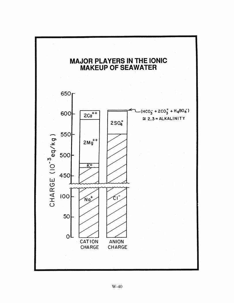
W-40

W-41

For our purposes, the concentrations of five ions must be fixed: H+, Ca++, CO2,

HCO −3 and CO

=3 . Three chemical equilibria relate the concentrations of these species:

1) CO2 + H2O ⇔ Η+ + HCO−3

K = [H+] [HCO

−3]

[CO2]

2) CO2 + CO =3 + H2O ⇒ 2HCO

−3

K = [HCO

−3]2

[CO2] [CO=3]

3) Ca++ + CO=3 ⇔ CaCO3 solid (at depth of lysocline)

K = [Ca++] [CO=3 ]

Hence if the concentrations of two of these five species are fixed, those of the other three

are uniquely determined. Once the concentrations of the five ions are set, so also are both

the ∑CO2 content and alkalinity (assuming the concentration of borate has remained

unchanged). For BLAG, the atmosphere's CO2 pressure is set to yield the proper flow of

CaO to the sea. Hence the CO2 content of sea water is also fixed, leaving only one other

concentration to be set. This remaining constraint could be set by an exchange reaction

between Ca++ and Mg++ or between H+ and Na+. One complication remains, i.e.,

establishing the difference between the compositions of surface waters and deep waters.

As we have seen, the ocean cannot be treated as a single well-mixed reservoir.

Paleolysocline Depth

As we saw in "Martin's World", the depth of the transition zone separating

sediments rich in calcite from those devoid of calcite potentially carries information

regarding the deep sea's carbonate ion concentration. Ideally, the top of this zone

(referred to by marine geologists as the lysocline) should correspond roughly to the depth

W-42

W-43

where sea water is just saturated with respect to the mineral calcite. The greater the depth

below the saturation horizon, the stronger the undersaturation and hence the stronger the

tendency for calcite to dissolve. The base of the transition from calcite-rich to calcite-

poor sediment lies at that depth where calcite dissolves just as fast as it rains to the sea

floor, leaving none to accumulate in the sediment. As the solubility of calcite increases

about twenty percent per kilometer, the depth of this transition zone is a very sensitive

indicator of the product of the Ca++ and CO=3 concentrations in the deep sea.

It turns out that a means exists to reconstruct the depth of the lysocline at times in

the past. This is done by studying the sediment from holes drilled through the sea floor

sediment column at water depths beneath the present-day calcite transition zone.

Although the material in the upper portion of these sediment columns contains no

CaCO3, at some depth in the hole, sediments rich in CaCO3 appear. This sedimentary

horizon marks that point in the history of the sinking sea floor when it dropped far

enough beneath the saturation horizon that the raining calcite completely dissolved. The

age of this event is recorded by the fossils contained in the uppermost calcite-bearing

sediment. Because the subsidence of the sea floor is ongoing, the depth below sea

surface at which this transition is found does not correspond to that of the paleolysocline.

But as the rules regarding the rates of subsidence have been firmly established (it is

driven by cooling of the lithosphere), a correction can be made allowing the water depth

at the time of deposition to be established.

By drilling many, many such holes, it has been possible to reconstruct how the

depth of the transition zone has varied over the last 100 million years. This record tells

us that the transition depth has not changed by very much. It has remained in the range

4000 ± 800 meters. As the solubility of calcite increases by only about 20 percent per

kilometer, this suggests that the product of Ca++ x CO =3 in the deep sea has not changed

very much during this time period. If this result could be interpreted as indicating a

constancy in carbonate ion concentration it would prove to be an extremely valuable

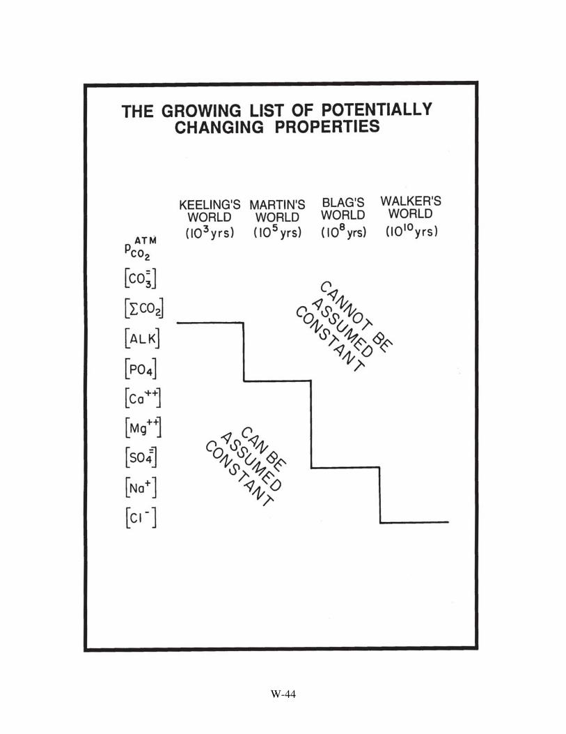
W-44

W-45

piece of information. But a problem exists. This conclusion requires that Ca++

concentration in the ocean has remained constant. As Ca++ has a residence time in the

sea of about one million years, on the time scale of glacial to interglacial changes it is

safe to assume that its concentration remained unchanged. However, as in this chapter

we are dealing with a time interval of 108 rather than 105 years, there is no guarantee that

the Ca++ content of sea water has remained unchanged. So the constancy of the

transition zone depth really tells us only that any changes in Ca++ concentration were

accompanied by reciprocal changes in CO=3 concentration. The reason for the near

constancy of the lysocline depth has to do with the fact that the overproduction of calcite

by marine organisms must be compensated by dissolution. The steeply inclined margins

of the sea floor dictate that the boundary between CaCO3 rich and poor sediments lie in

the depth range bounded by the ridge crests (~2.5 km depth) and the abyssal planes (~5.0

km depth). Therefore, as long as calcite production by marine organisms exceeds the

supply of calcite's ingredients, it is not surprising that the depth of calcite transition zone

has remained in the range 2.5 to 5.0 km.

Surface Ocean to Deep Ocean Carbon Isotope Difference

One other paleoclimate indicator holds promise in our attempt to reconstruct the

difference in ∑CO2 between surface and deep water. It is the difference between the

δ13C for nutrient depleted warm surface water and that for average deep water. This

difference depends on the carbon to phosphorus ratio in the organic matter falling from

the sea surface (i.e., C/P)org), the ratio of the PO4 to ∑CO2 in the ocean as a whole and

magnitude of the photosynthetic fractionation of carbon isotopes between surface ocean

∑CO2 and the organic matter produced by marine organisms (i.e., ∆photo). The

relationship is as follows:

∆δ13Cs-d = ∆photo . C/P)org . [PO4]/[∑CO2]

By reconstructing δ13C difference between foraminifera formed in surface and those

formed in deep water at times in the past, it should be possible to place limits on how the

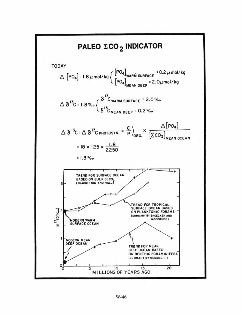
W-46

W-47

∑CO2 content of sea water has changed with time. However, to do this it is necessary to

get some handle on how the other three factors (i.e., ∆photo, C/P)org, [PO4]) may have

changed.

But first let us examine the reconstructions of the surface to deep δ13C difference.

Measurements covering the last 20 million years suggest that this difference has remained

more or less constant. A less complete record obtained for the Pacific Ocean extending

from 50 to 62 million years suggest that the difference was similar at that time as well.

Keeping in mind that were the atmospheric CO2 content higher, the photosynthetic

isotope fractionation factor must have been larger; this suggests that either the ocean's

∑CO2 content was somewhat higher or its nutrient content somewhat lower during the

early Cenozoic. If we could come up with an independent means of estimating how the

nutrient content of the ocean changed with time, then we would get a handle on how the

∑CO2 content has changed. Even a "fluffy" constraint on this quantity would be of great

help in our quest to understand the chemical history of the ocean. To see why this is the

case consider the following scenario. First, we will accept the Freeman and Hayes

estimate that the CO2 content of the atmosphere was about three times higher than now

55 million years ago. Second, as the planktonic-benthic δ13C results suggest, the PO4 to

∑CO2 ratio was about two thirds today's value. Are these two pieces of chemical

information self consistent? The answer is yes. Were the atmosphere's CO2 content

three times higher than today's, then under almost any scenario, the ocean's ∑CO2 would

also have been higher. For example, were the Ca++ content to have been the same as

today's, then the near constancy of the lysocline depth would require that the CO=3 ion

content would also have been the same. Chemical equilibria among CO2, CO =3 , and

HCO−3 would require that the HCO

−3 content would have increased by the square root of

the factor by which the CO2 content increased. This would give a bicarbonate ion

concentration of about 3 or 1.7 times today's. As HCO−3 is the dominant species, the

∑CO2 concentration would also have been about 1.7 times higher. Were PO4 to have

W-48

W-49

remained the same, then the 1.7 fold increase in ∑CO3 would have dropped the ∆δ13C

difference between planktonic and benthic foraminifera from its present day value of

1.8‰ to 1.1‰. However, the higher CO2 content of the surface ocean would have

increased the photosynthetic fractionation from 18 to 24‰ and hence the ∆δ13C from

1.1‰ to 1.4‰, a value consistent with Miller's measurements.

But what about the PO4 content of sea water? Might it have changed? PO4 is

replaced on a 105-year time scale. Thus its ocean content must also be subject to some

sort of feedback control. As outlined in the section which follows, the content of PO4 in

the sea is very likely tied to the amount of O2 in the atmosphere.

Paleocean Oxygen Content

While we have no proxy for the amount of oxygen in the Earth's atmosphere, we

do have a paleo indicator regarding the state of oxygenation of the deep sea. Benthic

foraminifera can survive only in oxygenated waters. As the shells of these organisms are

ubiquitous in the Cenozoic marine sediments, we can infer that the deep waters of the

major ocean basins have remained oxygenated over the past 65 million years. In one

sense, this is puzzling. Waters below 1500 meters in today's North Pacific have

dangerously low O2 contents (6-15% of the saturation value). Yet no where in the deep

sea does O2 disappear altogether. True, a few small anoxic pockets exist in the so called

'shadow zones' of the main thermocline. These zones which lie along the eastern oceanic

margins are equatorward of the temperate gyres and poleward of the equatorial current

systems. Therefore, they are ventilated only sluggishly putting their O2 supply in danger

of being depleted by the rain of organic debris. But these regions constitute only a very

small fraction of the ocean's volume. But as a sizable fraction of the deep sea currently

appears to be poised on the brink of anoxia, one might ask why there weren't periods in

the past when it slipped over the edge into anoxia causing benthic foraminifera to be

excluded from vast regions of the sea floor. But viewed through the glasses of

geochemical theory, the continued existence of finite amounts of O2 in deep sea water is

W-50

not surprising. Just as some feedback loop must control the flow of carbon through the

ocean-atmosphere reservoir, so also must there be one which controls the flow of

electrons. The number of electrons leaving the ocean-atmosphere reservoir must match

the number entering. Stated in chemical terminology, the aggregate oxidation state of the

sea's outputs must match that of its inputs. If this match is not met, then the O2 content

of the atmosphere will take up the slack and in so doing generate a feedback loop that

forces the flow of electrons back into balance.

An example will help to explain how this loop works. Consider a simplified

planet on which the only substances of importance are calcite, organic matter, water, and

oxygen gas (no outgassing of CO2 occurs). These materials are recycled on the planet's

surface. The inputs to this planet's ocean-atmosphere reservoir are CO2 derived from the

oxidation of previously buried organic matter and CaCO3 generated by chemical

weathering of the planet's continents. The output is plant residues and marine shells

which accumulate in marine sediment. For the system's electron flow to be in balance,

the amount of carbon leaving the system as new organic residues would just match the

amount of carbon entering as the result of oxidation of old residues. In this situation, the

amount of O2 created as a byproduct of the production of new residues would just

balance that consumed by the oxidation of old residues and the O2 content of the planet's

atmosphere would remain unchanged. However, if for some reason this balance were

temporarily disrupted by an anoxic condition and more new residues were buried than old

residues were being oxidized, then the planet's O2 content would rise. As it rose, the

planet's anoxic environments would gradually be reduced in size, thereby increasing the

likelihood that a given organic residue would be 'eaten'. The rise would continue until

the balance was restored.

In the real ocean, the element sulfur plays an important role. This element can

exist in two oxidation states: +6 in sulfate and -2 in sulfide. Eight electrons must be

traded if a sulfur atom is to go from one of these oxidation states to the other. Sulfide

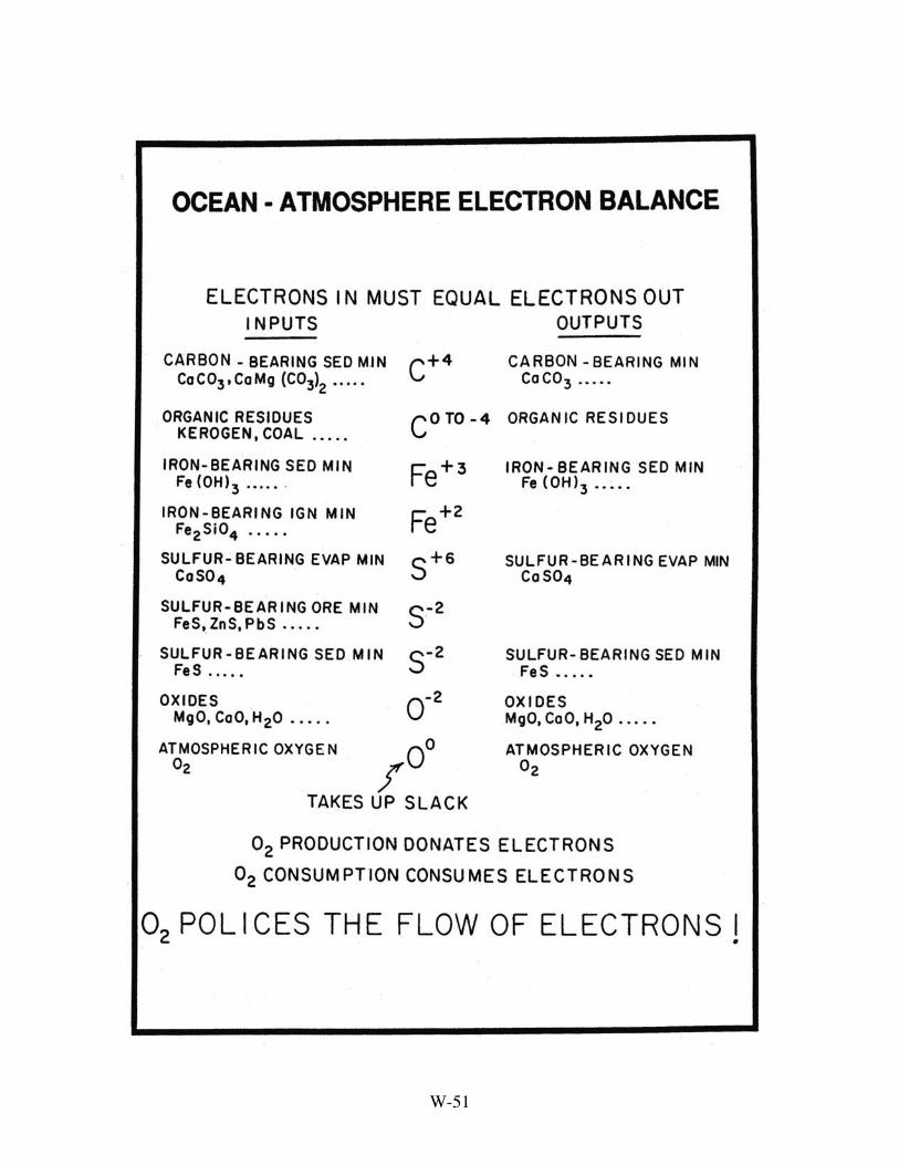
W-51

W-52

W-53

minerals are eroded from the continents and sulfide minerals form in the anaerobic pore

waters of sediments. Sulfate minerals are eroded from ancient evaporite deposits and

sulfate minerals form in isolated hypersaline arms of the sea (and perhaps in ridge crest

hydrothermal systems).

With this background in mind, we can understand why it is unlikely that the deep

ocean was anoxic at any time during the last 100 million years. The important point is

that the survival probability of organic matter is thought to be greater if it falls into an

anoxic environment. For each mole of carbon preserved in this way, one mole of O2 is

added to the atmospheric pool. The logic is as follows. The bacteria which make their

living in anaerobic environments by using NO−3 and SO

=4 as oxidants likely lack the

combined destruction efficiency of the much wider range of organisms which inhabit

oxygenated environments. Further, the fate of much of the SO =4 used by bacteria as an

oxidant is to be buried in the sediment as a metal sulfide. Thus, if a major portion of the

deep sea were to slip into anoxia, far too great a fraction of the carbon and sulfur passing

through the ocean-atmosphere reservoir would be buried in reduced form. If such a slip

to anoxia were to have taken place, then the O2 content of the atmosphere would have

experienced a climb which would have continued until newly formed deep waters were

charged with sufficient oxygen to burn virtually all the organic residues falling into the

deep sea. The episode of anoxia would be squelched.

Events which took place 250 million years ago at the beginning of the Triassic

provide an interesting example of the interplay between the cycles of carbon and sulfur.

The preceding Permian epoch was brought to an abrupt close by a major catastrophe

which led to the extinction of 85 percent of the existing species. The consequences of

this catastrophe are imprinted in both the isotopic records for marine calcium carbonate

and calcium sulfate. The carbon isotope ratio (13C/12C) undergoes a sudden 3‰ drop

and the sulfur isotope ratio (34S/32S) a more gradual 5‰ rise. If one assumes that both

the oxidation states and isotopic composition of the carbon and sulfur added to the ocean

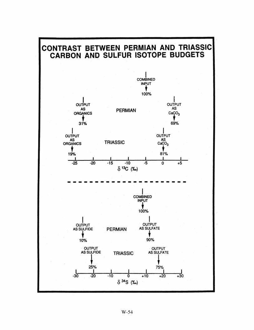
W-54

W-55

was the same during the early Triassic as during the late Permian, then these changes

must herald a major change in the mode of output of carbon and sulfur to sediments.

This should not be surprising as the terrestrial and marine ecosystems which had

developed during the previous 200 or so million years must have unraveled as the result

of the massive extinctions. The new food webs which replaced them likely operated

quite differently. In order to produce a 3‰ drop in the δ13C for marine CaCO3, there

must have been a 12 percent drop in the fraction of carbon removed in organic form. If,

as is generally assumed, the δ13C for the combined input of new carbon to the ocean-

atmosphere reservoir is -5‰, then the fraction being removed as organic material would

have to have dropped from 31 percent during the late Permian to 19 percent during the

early Triassic. The imbalance between the oxidation state of the input and output created

in this way would have had to be taken up by an increase in the fraction of the sulfur

removed in reduced form. During the several million years required to reach a new

steady state, part of the slack may have been taken up by a decrease in atmospheric O2.

But, as this gas governs the steady state, its content would have eventually stabilized at

that level required to maintain an equality between the oxidation state of the output and

that of the input. At steady state, a 15 percent increase in the fraction of the sulfur buried

in reduced form would have to have taken place. Assuming that the δ34S for incoming

sulfur was +8‰, this would have required a shift from 10 percent removed in reduced

form during the late Permian to 25 percent during the early Triassic.

What might account for such a huge change? One possible scenario is as follows.

Assume that during the Permian the burial of organic material in continental swamps was

so great that it dominated the reduced component of the removal budget. As continental

waters are low in SO =4 content even though the mud in swamps were anoxic, relatively

little sulfur reduction would have accompanied the burial of reduced carbon. Then came

the massive extinctions. Perhaps the terrestrial plants primarily responsible for the

production of inedible carbon disappeared and with them the burial of large amounts of

W-56

carbon on the continents. Simultaneously, an equally important change occurred in the

marine environment. The efficient food web of late Paleozoic time then, as now,

consumed most of the organic matter generated by marine plants before it reached the

sediments. This is important because once in the sediment, the likelihood of adequate O2

supply for their destruction drops substantially, for only by molecular diffusion can this

gas be supplied to the pore waters. So the idea is that the food web void created by the

great extinction event allowed a far greater fraction of the marine photosynthetic product

to reach the sea floor. And, as documented by the geologic record, consequently anoxic

conditions in sea floor sediments were widespread. It is well known that under such

conditions both reduced carbon (as organic residues) and reduced sulfur (as iron sulfide)

accumulate in the sediments. Together these two changes could account for the observed

isotope shifts. During the Permian, the reduced fraction of the output to sediments was

mainly terrestrial in origin and hence low in reduced sulfur. During the Triassic, the

reduced fraction of the output to sediments was mainly marine in origin and hence rich in

sulfides.

Controls on the Phosphate Inventory of the Sea

With this background in mind, it is easy to see that a tie must exist between the

atmosphere's O2 content and the ocean's PO4 content. The amount of PO4 dissolved in

the sea determines how much organic matter is produced per oceanic mixing cycle and

hence also the amount falling into the deep sea. The atmosphere's O2 content sets the

amount of O2 dissolved in newly formed deep waters and hence how much is supplied to

the deep sea. In order to maintain a balance between the oxidation state of materials

entering and leaving the ocean-atmosphere reservoir, it is necessary that the amount of

O2 supplied to the deep sea exceed the amount required to consume the organic residues

falling into the deep sea. For this to be the case, the concentration of O2 in the polar

surface waters must be comparable to the product of the PO4 concentration of average

ocean water times the ratio of O2 utilization to PO4 release during deep sea respiration

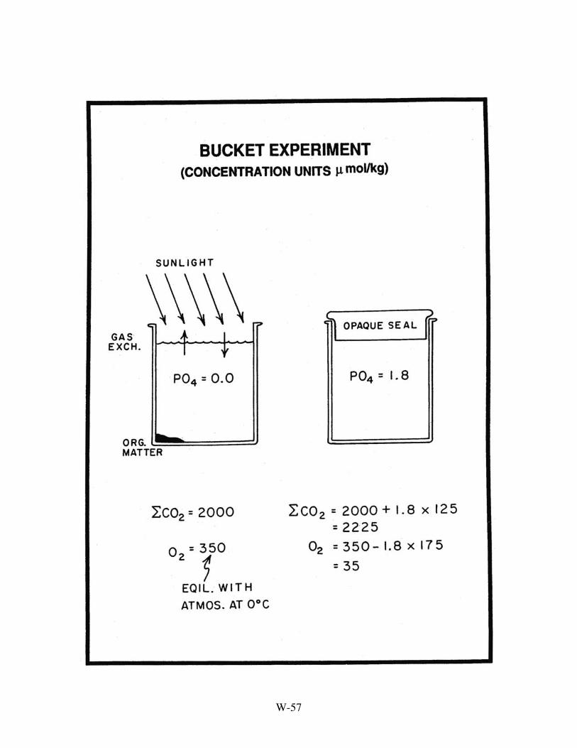
W-57

W-58

(175 moles per mole of phosphorus). In today's sea, the mean PO4 concentration is about

2.2 micromoles per liter and the saturation O2 concentration in polar surface water is

about 330 micromoles per liter. Hence, the O2 demand of 2.2 x 175 or 385 micromoles

per liter would seemingly slightly exceed the supply. This is not the case because of the

inefficient utilization of nutrients in polar surface waters from which deep waters form.

The effective phosphorus content of sea water is more like 1.2 micromole per liter and

hence the O2 demand is only 210 micromoles per liter leaving one third of the O2

entering the deep sea unused.

Another interesting aspect of the long term control of the atmosphere's O2 is the

so called O2 compensation partial pressure. The key C-3 plant enzyme, rubisco, reacts

with O2 as well as with CO2. As the O2 partial pressure rises, the ratio of CO2 uptake

(which leads to O2 production) to O2 uptake (which leads to O2 consumption) approaches

unity. The partial pressure of O2 at which this occurs is referred to as the compensation

point. The point at which C-3 plants go from O2 producers to O2 consumers depends on

atmospheric CO2 content. For tobacco plants, the compensation point atmospheric

composition is 23% O2 at 220 ppm CO2, 27% at 350 ppm CO2, and 35% at 700 ppm

CO2. Were the O2 content to approach this compensation limit, the ability of plants to

grow and hence to produce O2 would be seriously limited. Thus the O2 level in the

atmosphere appears to have an upper bound set by the level at which oxygen

consumption by plants matches its production. We have already seen that 60 million

years ago, the deep sea was about 10°C warmer. Hence, were the atmosphere's pO2 the

same as today's, the saturation O2 concentration for the water descending into the deep

sea would have been only 250 micromoles per liter. Under these conditions, too great a

portion of the sea floor would have been anoxic and the O2 content of the atmosphere

would have been driven up as the result of the excess storage of reduced material until

balance was restored.

W-59

However, it is possible that the excess burial of organic carbon was accompanied

by a reduction in the oceanic residence time of phosphate. The probability of loss during

any given mixing cycle would have risen causing the steady state inventory of PO4 in the

ocean to fall. As the residence time for phosphorus in the sea (104 to 105 yr) is much less

than the adjustment time for atmospheric O2 content (106 to 107 yr), the job would be

accomplished by a fall in the ocean's PO4 content rather than a rise in the atmosphere's

O2 content.

Paleo pH Measurements

A complete description of the paleochemistry of both the warm surface ocean and

the deep ocean requires that we have at least two additional pieces of information. The

only candidates now in the offing are boron isotope-based paleo pHs. As we have seen,

boron isotope ratios in foraminifera shells offer a potential pH recorder. While in theory

this might be possible, two problems must be addressed. First, it will have to be shown

that the boron contained in foraminifera shells remains firmly bound for periods of tens

of millions of years. Were exchange with the boron dissolved in the pore water and that

absorbed onto the clays surrounding the shell to occur, such measurements would prove

misleading. In order to check this out, shells of the same geologic age from a wide range

of burial environments will have to be analyzed to see if a self-consistent picture is

obtained. One check will be to see if planktic-benthic boron isotope differences are

consistent with carbon isotope differences. Second, it will have to be shown that the

boron isotope composition of sea water did not change with time. While on the time

scale of glacial cycles, no such change would be expected, on time scales approaching or

exceeding the residence time of boron in the sea (i.e., 10 to 20 million years), it is

possible that such changes did occur.

Art Spivack and his colleagues at Scripps took the first step toward evaluating the

constancy of the boron isotope composition of sea water. Their strategy was to measure

the boron content and boron isotope ratio in pore waters from a 700-meter-deep drill hole

W-60

W-61

on the sea floor in the equatorial Pacific. Although the constituents of these pore waters

are continuously exchanging with those in the overlying sea, the isolation time near the

base of the sediment column is likely 10 or so million years. It is encouraging that these

investigators found no evidence for either a shift in boron concentration or isotope ratio.

Spivack and his coworkers also measured the boron isotope ratios in boron extracted

from four foraminifera samples ranging in age back to 20 million years. They interpret

these results to suggest that the pH of the surface ocean 20 million years ago was 7.4, or

0.8 pH units lower than today's. If so, then the hydrogen ion was likely about 6 times

higher! If this were the case then, since the lysocline lay close to its present depth, the

bicarbonate ion (and also the ∑CO2) content of the sea must have been 6 times higher.

Were this the case, then the ∆δ13C between surface and deep waters should have been

much smaller than today's. It wasn't. Hence this boron-based result is difficult to accept.

Many, many more boron isotope results will have to be obtained before the utility of this

proxy will become apparent.

Summary

So where does this leave us as to the status of Walker's hypothesis that

atmospheric CO2 controls chemical traffic and hence that a tie must exist between Earth

climate and tectonics? It is our view that the evidence is broadly consistent with this

idea. Consider:

1) Although the rate of sea floor spreading has not slowed by the factor of two

originally proposed by Pitman and Hays, a consensus exists among geophysicists that the

rate was somewhat higher during Cretaceous time. Nor would many challenge that this

post Cretaceous slow down in spreading rate was accompanied by a reduction in the rate

of CO2 outgassing. But the exact magnitude of this change remains uncertain.

2) Based on oxygen isotope measurements on benthic foraminifera, it is clear that

at least the polar regions have cooled dramatically since Cretaceous time. The absence of

W-62

W-63

firm evidence for an equivalent tropical change, while complicating the situation, does

not necessarily prove that the cooling was not CO2 induced.

3) Based on carbon isotope measurements on marine organic residues, it appears

that the CO2 content of temperate surface waters has dropped since Cretaceous time.

Taken together with the oxygen isotope-based cooling of these regions, these

measurements suggest that the atmosphere's CO2 content has dropped by several fold

since that time.

4) The record of the planktonic-benthic carbon isotope difference is consistent

with the carbon isotope-based estimate of the atmospheric CO2 content decrease.

5) Unfortunately, no evidence in support of a drop in chemical weathering rates

has been found. The strontium isotope record is inconclusive in this regard. BLAG

would dictate that both the supply of strontium from ridge crests and the supply from

continents would change in unison. Hence in the absence of changes in the isotope

composition of the strontium end members, no change in the isotopic composition of

ocean strontium would be expected. It is likely that the observed increase in the 87Sr to

86Sr ratio is related to the exposure to weathering of Himalayan rocks unusually rich in

radiogenic strontium.

Critics of BLAG will scream "But the evidence is all circumstantial - it doesn't

prove a thing." True, but keeping in mind that as some mechanism must exist by which

chemical traffic is controlled, these critics are obligated to do more than throw stones.

Rather, they must come up with an alternative set of controls and a scenario for post-

Cretaceous time which is consistent with the above mentioned observations. It seems to

us that the only feasible alternative scenario is to transfer traffic control to the ocean.

This being the case, it is important to firm up our ability to define ocean chemistry at

times in the past. This is no easy chore. It will require that each of our paleoindicators

be pushed to its very limit.

W-64

Commentary of Walker's World Plates

pg. 3

Astrophysical models clearly indicate that the energy output from the Sun has

steadily increased. Four and one half billion years ago, when the Earth formed, the Sun's

output was about 30 percent lower than it is now. Were the Earth's reflectivity and

greenhouse shielding no different from today's, then its surface would have been ice

bound. But we know from the geological record that water-deposited sediments

representing all ages are present. An obvious solution exists for this seeming enigma.

Early in its history, the Earth's CO2 greenhouse blanket was much thicker than today's.

As explained in the text, a steady release of CO2 from the Earth's interior guarantees that

the Earth can never have become a permanently frosty ball.

pg. 8

Hypothetical Planet X has a very simple geochemical cycle. CaO dissolved from

its soils combines with CO2 outgassed from its interior forming CaCO3. This material

settles to the sea floor forming a blanket of sediment. As on Earth, the sea floor on Planet

X is subducted beneath its continental crust. Some of the mantling sediment is dragged

down into the hot interior where it is decomposed to CO2 and CaO completing the cycle.

While the Earth's geochemical cycle is more complex, the formation of calcite by

organisms living in the sea and the thermal decomposition of carbonate minerals within

the Earth's interior play dominant roles.

pgs. 10-11

Berner, Lasaga and Garrels (BLAG) reasoned that if, as geophysicists claim, over

the last 100 million years the rate of sea floor spreading has slowed, then as a result, the

Earth must have cooled. Their logic is as follows. A slowing of spreading would have

led to a corresponding decrease in CO2 outgassing. Further, as the rate of generation of

sea floor dropped, more time would be available for the oceanic crust to cool. The

shrinkage related to this extra cooling would lower the elevation of the sea bottom and

W-65

hence also sea level. As sea level dropped more, land would be exposed to the

atmosphere and hence be subject to chemical erosion. With less CO2 to match and more

land from which to derive CaO, the chemical weathering demand per unit of land area

would lessen. As outlined in the text, this situation would have led to a drop in the

atmosphere's CO2 content and hence the Earth's surface temperature. If, as Pitman and

Hays proposed, sea floor spreading rates were twice as high as today's 100 million years

ago, then in order to deliver the amount of CaO to match the then higher CO2 outgassing

rate, the planet must have been about 10°C warmer. Other climatic factors being equal,

this would have required an 8 fold higher atmospheric CO2 content.

pg. 13

As explained in the text, BLAG assumes that the supply of CaO goes entirely into

matching that of CO2. If so, the system must be regulated by the CO2 content of the

atmosphere. By negative feedback, it is driven to that level where soil temperatures

permit a chemical weathering rate just large enough to supply the needed calcium. By

contrast, in the case of GALB, the supply of CaO is always in excess of that needed to

balance the supply of CO2. In this case, an oceanic feedback loop must operate which

brings about a removal of the excess CaO into silicate minerals at just the rate this excess

is added to the sea.

pg. 16

By measuring the volume flow and the concentration of dissolved chemical

species in the world's major rivers, it is possible to estimate today's flux of cations to the

sea. It turns out that about two times more Ca++ than Mg++ and about six times more

Ca++ than K+ enters the sea. The dominance of calcium reflects both the recycling of

ancient limestone (CaCO3) and the ease with which calcium-bearing feldspars dissolve.

Although weakly constrained, it is thought that the supply of calcium from limestone is

about three times that from silicates. The circulation of sea water through the newly

formed ridge-crest basalts modifies the sea's chemistry. The magnesium carried into the

W-66

ridge crest is quantitatively removed as demonstrated by its absence in the high

temperature effluents. While the total flux of hydrothermal water remains uncertain, the

loss of Mg++ is thought to roughly match the input from rivers. In contrast, vent waters

have higher Ca++ and K+ contents than do sea water. Thus high-temperature

hydrothermal circulation enhances the supply of these cations to the sea. BLAG assumes

that the amount of calcium reaching the sea is just equal to the amount needed to match

the CO2 added by planetary outgassing and limestone dissolution (minus that going into

organic residues). In other words, all the calcium added to the sea leaves as CaCO3.

Thus if 14x1012 moles of calcium reach the sea each year, 14x1012 moles must also be

buried in marine sediments as calcite. If as suggested by the global carbon isotope

budget about 18% of the carbon reaching the sea is removed as organic residues, then a

total of 17x1012 moles of carbon must reach the ocean-atmosphere reservoir each year.

If only 9x1012 come from the weathering of limestone, the other 8x1012 must come from

a combination of outgassing and the oxidation of recycled sedimentary organic matter.

pg. 18

Based on the analyses of carbonatites, diamonds and CO2 contained in ridge crest

glasses (i.e., of materials which have their origin in the mantle), the mean δ13C for Earth

carbon is estimated to be about -5‰. Carbon isotope analyses of organic matter and

calcite from sediments covering the last 500 million years' record show that the former

has hovered around -25‰ and the latter around 0‰. This suggests that on the average

about 20% of the carbon entering the oceanic system is removed as organic matter and

about 80% as calcite.

pg. 20

While a first order consideration of the carbon isotope geochemistry suggests that

the δ13C for the ∑CO2 in rivers might provide a means of estimating the relative

contributions of limestone and silicate weathering, in practice this approach cannot work.

The reason is that excess organic-derived CO2 pushes the isotopic composition toward

W-67

the 13C deficient value characteristic of organic matter (i.e., -26‰) while exchange with

atmospheric CO2 drives the value toward the 13C-rich value of limestone (i.e., 0‰). As

it is not possible to quantify these opposing influences, the δ13C of ∑CO2 in rivers is not

a useful index of the source of the rivers cations.

pgs. 22-23

That over the past 40 million years the 87Sr content of oceanic strontium has

steadily risen is well documented by the analysis of strontium contained in marine

carbonates. The fact that the onset of this rise just postdates to the time of the collision

between the Indian and Asian continental blocks suggests that erosion of the great

Himalayan mountain chain was responsible for this rise. This rise could reflect either an

increase in the ratio of continental-derived strontium to ridge crest-derived strontium

delivered to the sea, or an increase in the radiogenic 87Sr content of continental

strontium. The evidence appears to favor the latter explanation, for rivers draining the

Himalayas carry unusually radiogenic strontium.

pg. 26

Oxygen isotope ratios in benthic foraminifera shells from marine sediments have

undergone a 3‰ increase since early Eocene time (i.e., about 55 million years ago).

While a small amount of this change is the result of the growth of the Antarctic and

Greenland ice sheets, the remainder must reflect a major cooling (~10°C) of the high

latitude oceans (and hence of the polar regions). The I and G on the left hand scale

represent the swings in the δ18O of benthic foraminifera associated with the glacial

cycles of the last 800,000 years. In this case, the ice volume contribution is the larger

(~1.2‰) and the polar temperature contribution the smaller (~0.6‰). The left end of the

heavy black curve represents the average value for benthic 18O during this period of

repeated glaciation. For each meter of sea level lowering (resulting from glacial growth)

the δ18O of the sea increases by about 0.010‰. For each degree of ocean cooling, the

δ18O in CaCO3 formed rises by about 0.23‰.

W-68

pg. 28

The igneous minerals formed when magmas cool are not chemically stable under

the Earth surface conditions. The oxides of silica, potassium, sodium, calcium and

magnesium tend to dissolve producing H4SiO04 , K+, Na+, Ca++ and Mg++ ions which

are carried by rivers to the sea. By contrast, the oxides of aluminum and iron are quite

insoluble and remain behind in solid residues. But the weathering process is more

complicated than a quick and complete separation of the five soluble oxides from the

two insoluble oxides. In many cases, only part of the soluble oxides are delivered to

solution. The rest remain behind bound into clay minerals. At some later time, these first

generation clays may undergo a second round of weathering and will give up to solution

some of their remaining silica and cations. The second generation residues are then

greatly eniched in the oxides iron and aluminum.

pg. 31

The carbon in marine plant material is always depleted in 13C relative to the CO2

gas in the surrounding air or water. However, the extent of this depletion depends on the

magnitude of the resistance posed by the cell membrane. The reason is that the 13C

depletion associated with molecular diffusion is on order of magnitude smaller than that

associated with the enzymatic reaction which converts CO2 to organic matter. Hence in

situations where the supply of CO2 is limited relative to the biochemical demand within

the cell, the fractionation will shift toward the smaller value associated with molecular

diffusion. By contrast, in situations where the CO2 supply is plentiful compared to the

biochemical demand, the magnitude of the fractionation will shift toward the larger value

associated with the enzymatic reaction. It is for this reason that the isotopic composition

of marine organic matter might serve as a paleo CO2 concentration proxy. The higher the

atmospheric CO2 partial pressure, the higher the surface ocean CO2 concentration and

hence the less important the resistance posed by the cell membrane. Thus the extent of

W-69

isotope fractionation should vary in direct proportion to the amount of CO2 dissolved in

surface sea water.

pg. 33

Measurements carried out by a New Zealand graduate student were the first to

clearly demonstrate the dependence of the extent of carbon isotope fractionation on the

concentration of aqueous CO2. For his Ph.D. thesis research, McCabe grew algae (at the

same temperature) but at different CO2 concentrations and found that the higher the CO2

pressure, the greater the depletion of 13C in the organic matter. A similar trend was

found by Rau and his coworkers for plankton samples from various regions of the ocean.

Although the CO2 partial pressure in the atmosphere is very nearly globally uniform, the

CO2 is much less soluble in warm waters than in cold water. Hence, organic matter

formed in cold water is more deficient in 13C than that formed in warm water. Thus in

order to obtain a paleoatmospheric CO2 partial pressure estimate from carbon isotope

measurements in marine organic matter, the temperature of the water in which the

organic matter formed must also be known.

pg. 35

The analysis by Freeman and Hayes of carbon isotope measurements on porphyrins from

marine organic material samples ranging in age back to 135 million years suggest that

the atmospheric CO2 content has steadily declined. It appears to have been about 1000

µatm 100 million years ago. In order to obtain these CO2 partial pressure, they had to

reconstruct the latitude at which the organic matter grew (based on plate motion

reconstructions). Then they had to use oxygen isotope-based reconstructions of the

surface water temperature to convert from CO2 concentration to CO2 partial pressure.

pg. 37

CO2 in soils is somewhat richer in 13C than that in the organic matter being

oxidized for two reasons. First, because 12CO2 diffuses more rapidly than 13CO2, the

13C to 12C ratio in soil air is about 4.4‰ higher than that in the CO2 produced by

W-70

respiration. Second, the soil contains atmospheric CO2 which has a higher 13C content

than organic matter. In today's soils the atmospheric contribution is quite small. The

reason is that the partial pressure exerted by respiration CO2 is between one and two

orders of magnitude higher than the partial pressure of CO2 in the atmosphere. However,

if at some time in the past, the atmospheric CO2 pressure was, as proposed by BLAG, an

order of magnitude higher than now, then its larger contribution would lead to a

significant shift in carbon isotope ratio in soil CO2. Thure Cerling proposed to use this

shift as a paleo CO2 indicator. His recorder, soil caliche (CaCO3), has a 13C/12C ratio

about 10‰ higher than that in soil CO2. His method requires 1) that the respiration

contribution to the soil CO2 partial pressure has remained nearly the same, 2) that

caliche forms sufficiently at a depth in the soil profile where the CO2 concentration

gradient has become small, 3) that the 13C/12C in the soil organic matter be known and

finally, 4) that the soil temperature be known (in order to correct for the temperature

dependence of the soil CO2 to soil CaCO3 carbon isotope fractionation).

pg. 40

The ionic charge in sea water is dominated by Na+ and Cl-. The remainder of the

cationic charge is contributed by Mg++, Ca++ and K+. The remaining anionic charge is

supplied mainly by SO=4 with only a small contribution from HCO

−3 , CO

=3 and

H4BO−4 (i.e., alkalinity) .

pg. 42

At ridge axes where molten basalt is being injected from the underlying mantle,

the Earth's lithosphere is puffed up forming a topographic high. As the crust moves away

form the ridge axis, it slowly cools causing it to shrink and hence the ocean floor to

deepen. Eventually, this deepening carries the sediment water interface below the

CaCO3 saturation horizon into corrosive water. This crossing is marked by a transition

from the deposition of carbonate ooze (calcite rich) to red clay (calcite poor). This

transition is encountered in holes drilled through sediment column. Its age is obtained

W-71

from the fossils contained in the uppermost carbonate ooze. The depth of the saturation

horizon at the time of the transition can be obtained by correcting for the sea floor sinking

which occurred between the time of the transition and the present. Such a correction is

possible because the cooling (and hence crustal shrinkage) proceeds as a simple function

of time. By drilling many such holes, it has been possible to reconstruct the transition

zone depth over the last 100 million years in all three oceans.

pg. 44

All the constituents in sea water are being gradually replaced. For any given

problem, only the concentrations of those constituents having a residence time far longer

than the time interval of interest can be considered to have remained unchanged. The rest

are subject to change. For example, calcium which has a residence time of about one

million years can be considered to remain constant during the course of the single glacial

cycles of interest to Archer, but not over the 100 million year period of interest to BLAG.

pgs. 46

Carbon isotope measurements on material formed in surface ocean water and in

the deep ocean water suggest that the approximately 1.8‰ difference between the 13C to

12C ratio for surface water and deep water carbon seen in today's ocean has persisted for

the last 20 million years. This isotope ratio difference depends on the ratio of PO4 to

∑CO2 in average ocean water, on the C to P ratio in marine organic matter and on the

isotope fractionation during photosynthesis. Assuming that the latter two of these factors

have remained more or less constant, this record suggests that the ratio of ∑CO2 to PO4

in the sea has also remained more or less the same.

pg. 48

Detailed data from a single core in the Pacific Ocean suggest that during

Paleocene and Eocene time the ∆δ13C was only slightly smaller than that for the last 20

million years. However, when account is taken of the larger photosynthetic fractionation

W-72

factor (resulting from the higher CO2 content of surface waters), this data set suggests

that the oceanic PO4/∑CO2 ratio might have been only two thirds today's value.

pg. 51

Four elements, carbon, iron, sulfur, and oxygen are the main participants in the

electron trades conducted on the Earth's surface. The number of electrons associated

with a carbon atom ranges from a deficiency of four in CO2 and in CaCO3 to an excess of

four in methane. Iron atoms can go from a deficiency of three electrons in ferric

compounds to a deficiency of two electrons in ferrous compounds. Sulfur can go from a

deficiency of six electrons in sulfates to an excess of two electrons in sulfides. Oxygen

can go from a deficiency of two electrons in oxides to null in oxygen gas. As electrons

must be conserved, if one or more of these elements undergoes a net oxidation (i.e., loss

of electrons) in passing through the ocean-atmosphere system, the others must undergo a

corresponding reduction (i.e., gain of electrons). For example, if together carbon, sulfur

and iron undergo a net reduction in passing through the ocean-atmosphere reservoir, then

this imbalance would be compensated by an increase in the atmosphere's O2 content. As

the extent to which reduced species become oxidized in passing through the ocean-

atmosphere system depends on the O2 content of the atmosphere, this gas serves as the

policeman for electron flow.

pg. 52

Three examples of possible oxidation reduction situations for the Earth system.

In the first, a net oxidation of sulfur is exactly balanced by a net reduction of carbon,

leaving the oxygen content of the atmosphere unchanged. In the second, the net

reduction of carbon is not adequate to balance the net oxidation of sulfur. This requires

that a net consumption of O2 occurs decreasing the atmospheric inventory of this gas. In

the third, a net reduction of sulfur is not matched by the net oxidation of carbon. This

means that a net production of O2 occurs increasing the atmospheric inventory of this

gas.

W-73

pg. 54

The carbon isotopic composition of Permian marine carbonates averaged about

3‰ heavier than that of Triassic marine carbonates. Assuming that the isotopic

composition of the combined carbon inputs remained unchanged, this requires a shift in

the ratio of carbonate to organic matter being buried from 69:31 during the Permian to

81:19 during the Triassic. If then, as now, the turnover time of ocean carbon was on the

order of 105 years, this new split must have been maintained for many, many ocean

residence times; i.e., it represented a steady state flow of carbon through the ocean-

atmosphere system.

The sulfur isotope composition of Permian marine sulfate deposits average about

5‰ lighter than that for their Triassic equivalents. Assuming that the isotopic

composition of the combined sulfur inputs remained unchanged, this requires a shift in

the ratio of sulfate to sulfide being removed from 90:10 during the Permian to 75:25

during the Triassic.

pg. 57

A simple experiment carried out in a bucket of sea water illustrates the tie

between the O2 content of the atmosphere and the PO4 content of deep sea water. Sea

water containing 1.8 µmol/kg of PO4 and 2225 µmol/kg of ∑CO2 and kept at 0°C is

exposed to sunlight. Plants grow until all the PO4 has been utilized. The excess O2 gas

produced in this way is lost to the overlying air. Then an opaque seal is inserted into the

top of the bucket, blocking out sunshine, eliminating the air space, and preventing gas

exchange. Bacteria consume the plant mattter (and then each other) returning the PO4 to

solution. In so doing, 90% of the O2 is consumed. If the PO4 content of the water had

been 2.2 instead of 1.8 µmol/kg, the O2 would have been entirely depleted before the

organic matter had been eaten. The water would have gone anoxic.

W-74

pg. 60

Through information stored in deep sea sediments, it is potentially possible to

define the carbon chemistry of the ocean atmosphere system for past times. The situation

for surface waters could be defined from boron isotope measurements on planktonic

shells (yielding H+) and carbon isotope measurements on organic compounds (yielding

CO2) coupled with a paleotemperature estimate based on oxygen isotope or alkenone

measurements. This information would allow the HCO−3 , CO

=3 , ∑CO2 and alkalinity to

be computed. From the temperature and CO2 content, the atmosphere's pCO2 could be

estimated. For the deep sea, the product of the Ca++ and CO=3 ion concentrations could

be obtained from the paleo-lysocline depth, the pH could be obtained from boron isotope

measurements on benthic foraminifera. Finally, the difference between the ∑CO2

concentration between warm surface and cold deep water could be obtained from the

∆δ13C between planktic and benthic forams:

∆CO2resp ≡ ∆δ13Cp-b∆photo x [∑CO2]S.W.

This leaves only the alkalinity difference between surface and deep water resulting from

CaCO3 dissolution unaccounted for. It could be obtained by iteration.

pg. 62

Measurements of the pore water profile of borate and its isotopes have been

carried out in only one place in the ocean. Pore water squeezed from sediments obtained

from a long boring in the equatorial Pacific show no depth trend in either the

concentration of borate or in its isotope ratio. As the time required for replacement of the

water deep in the sediment by molecular diffusion from the overlying sea is ten or so

million years, this provides evidence that changes in the isotope ratio for boron

contained in the shells of planktic forams are the result of changes in the pH of surface

water. Assuming this to be the case, Spivack and his co-workers used measurements on

ancient forams to obtain paleo pH estimates for the period 5 to 22 million years ago.

W-75

They suggest that the ocean was 6 times more acid 20 million years ago than it is today.

As explained in the text, this result is inconsistent with the Freeman and Hayes estimate

of the CO2 content difference at this time.

W-76

Super Problem In the year 2250, Abe Highjit Sanyal, a distant descendant of an early 21st century geochemist, is assigned to an expedition to explore our galaxy. The Earth's environment has deteriorated to the point where serious consideration is being given to transferring civilization to another planet. Several promising candidates, spotted from space probe telescopes, appear to match Earth in size, stellar illumination, and day length. But from the great distance at which the observations were made, it is not possible to determine the composition of each planet's atmosphere, its surface temperatures, or whether life is present. Jit, as he is known, has been assigned to determine the history of the planet's climate. As the task of moving will be monumental, the Masters of Earth, as the ruling class is known, want to be sure that the climate the expedition team experiences during their brief three-year visit will be the climate they get if they move there. Jit is well prepared. He has mastered all that is known about Earth's paleoclimate and has brought with him the equipment and technicians necessary to repeat these studies on the candidate planets. Jit is disappointed when the expedition's commander decides to abandon the first candidate planet because it turns out to be too warm (40°C at its equator). Jit returns to his state of suspended animation, for it will be 10 years until the next candidate planet is reached. When he is at last awakened, Jit is excited to see that they are orbiting a planet which much resembles Earth. He notes about half ocean and half land and about half cloudy sky and half clear sky. He is struck by the absence of polar ice caps and mountain-top glaciers. Numerous volcanoes, some active, spot the landscape. The commander briefs the the party saying that from orbit this planet looks extremely promising. Its radius is 15% smaller than Earth's. Its mean surface temperature is 20°C and ranges from 10°C at the poles to 30°C at the equator. The planet's spin axis is perpendicular to the plane of its circular orbit (so it has no seasons). The green of chlorophyll is apparent both on land and in the sea. The atmosphere's O2 partial pressure is 0.17 atm. The N2 pressure is 1.2 atm. Upon landing, the explorers are pleased to find an ecosystem not unlike Earth's. Rooted plants cover the continents. The sea abounds with fish. But there is no sign of civilization. Jit immediately gets to work. He measures the carbon isotope ratio in the following materials and relates them to the Urey's standard. marine plants (tropical ocean) -35‰ CO2 from air - 4‰ ∑CO2 from the sea + 3‰ He does some chemistry: pCOatm

2 900 µatm [CO2]tropical surf water 24 x 10-6moles

kg [∑CO2]tropical surf water 2200 x 10-6moles

kg [ALK]tropical surf water 2400 x 10-6equiv

kg

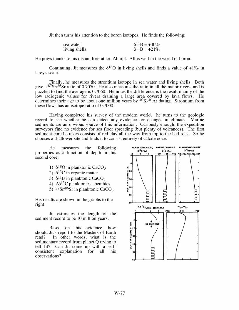
W-77

Jit then turns his attention to the boron isotopes. He finds the following: sea water δ11B = +40‰ living shells δ11B = +21‰ He prays thanks to his distant forefather, Abhijit. All is well in the world of boron. Continuing, Jit measures the δ18O in living shells and finds a value of +1‰ in Urey's scale. Finally, he measures the strontium isotope in sea water and living shells. Both give a 87Sr/86Sr ratio of 0.7070. He also measures the ratio in all the major rivers, and is puzzled to find the average is 0.7060. He notes the diffference is the result mainly of the low radiogenic values for rivers draining a large area covered by lava flows. He determines their age to be about one million years by 40K-40Ar dating. Strontium from these flows has an isotope ratio of 0.7000. Having completed his survey of the modern world, he turns to the geologic record to see whether he can detect any evidence for changes in climate. Marine sediments are an obvious source of this information. Curiously enough, the expedition surveyors find no evidence for sea floor spreading (but plenty of volcanoes). The first sediment core he takes consists of red clay all the way from top to the bed rock. So he chooses a shallower site and finds it to consist entirely of calcite ooze. He measures the following properties as a function of depth in this second core: 1) δ18O in planktonic CaCO3 2) δ13C in organic matter 3) δ11B in planktonic CaCO3 4) ∆δ13C planktonics - benthics 5) 87Sr/86Sr in planktonic CaCO3 His results are shown in the graphs to the right. Jit estimates the length of the sediment record to be 10 million years. Based on this evidence, how should Jit's report to the Masters of Earth read? In other words, what is the sedimentary record from planet Q trying to tell Jit? Can Jit come up with a self-consistent explanation for all his observations?

W-78

ANNOTATED BIBLIOGRAPHY THE TECTONICS-CLIMATE CONNECTION Chamberlin, T. C., 1898, The influence of great epochs of limestone formation upon the

constitution of the atmosphere, Jour. Geology, 6, 609-621. A paper 80 years before its time. What insight this man had! Budyko, M. I., and A. B. Ronov, 1979, Chemical evolution of the atmosphere in the

Phanerozoic, Geochemistry Internat., 1-9. A discussion of the role of CO2 emissions from volcanoes in climate change. Walker, J. C. G., P. B. Hays, and J. F. Kasting, 1981, A negative feedback mechanism for

the long-term stabilization of Earth's surface temperature, Jour. Geophys. Res., 86, 9776-9782.

The paper that laid the foundation for all further work on this subject. Berner, R. A., A. C. Lasaga, and R. M. Garrels, 1983, The carbonate-silicate geochemical

cycle and its effect on atmospheric carbon dioxide over the past 100 million years, Am. J. Sci., 283, 641-683.

The first attempt to use sea floor spreading rates and continental areas to reconstruct paleo-atmospheric CO2 contents and the consequent changes in Earth surface temperature, i.e., the birth of BLAG.

Berner, R. A., and E. J. Barron, 1984, Comments on the Blag Model: Factors affecting

atmospheric CO2 and temperature over the past 100 million years, Am. J. Sci., 284, 1183-1192.

The application of atmospheric global circulation models to BLAG reconstructions.

Kasting, J. R., and S. M. Richardson, 1985, Seafloor hydrothermal activity and spreading

rates: the Eocene carbon dioxide greenhouse revisited, Geochim. Cosmochim. Acta, 59, 2541-2544.

An elaboration on BLAG emphasizing the importance of the length of the ocean ridge system to the CO2 outgassing rate.

Knoll, M. A., and W. C. James, 1987, Effect of the advent and diversification of vascular

land plants on mineral weathering through geologic time, Geology, 15, 1099-1102.

An elaboration on BLAG emphasizing the importance of the root systems of vascular land plants in enhancing the rate of chemical weathering of soil minerals.

Volk, T., 1987, Feedbacks between weathering and atmospheric CO2 over the last 100

million years: Am. J. Sci., 287, 763-779. An elaboration on BLAG emphasizing the importance of the evolution of

angiosperm-deciduous ecosystems on the rate of chemical weathering. Marshall, H. G., J. C. G. Walker, and W. R. Kuhn, 1988, Long-term climate change and

the geochemical cycle of carbon, J. Geophys. Res., 93, 791-801. Inclusion of the carbon cycle in simple energy balance models. Raymo, M. E., W. F. Ruddiman, and P. N. Froelich, 1988, Influence of late Cenozoic

mountain building on ocean geochemical cycles, Geology, 16, 649-653.

W-79

The importance of the rise of the Tibetan Plateau in the evolution of global weathering rates.

Volk, T., 1989, Rise of angiosperms as a factor in long-term climatic cooling, Geology,

17, 107-110. More on the role of rooted plants in chemical weathering. Volk, T., 1989, Sensitivity of climate and atmospheric CO2 to deep-ocean and shallow-

ocean carbonate burial, Nature, 337, 637-640. The importance of the evolution of open ocean CaCO3 forming organisms to the

Earth's carbon cycle . Berner, R. A., 1990, Atmospheric carbon dioxide levels over Phanerozoic time, Science,

249, 1382-1386. An attempt to reconstruct the operation of the Earth's carbon cycle over the past

570 million years. Berner, R. A., 1991, A model for atmospheric CO2 over Phanerozoic time, Am. J. Sci.,

291, 339-376. A major revision of the original BLAG reconstruction. Caldeira, K., and M. R. Rampino, 1991, The Mid-Crataceous super plume, carbon

dioxide, and global warming, Geophys. Res. Lett., 18, 987-990. The potential importance of massive basalt forming events to the global carbon

cycle. Berner, R. A., 1992, Palaeo-CO2 and climate, Nature, 358, 114. A rebuttle to a claim by Kasting that Berner's reconstruction is inconsistent with

the well-established Ordovician glaciations. Berner, R. A., 1992, Weathering, plants, and the long-term carbon cycle, Geochim.

Cosmochim. Acta, 56, 3225-3231. An assessment of the role of CaO2 in chemical weathering. Caldeira, K., and J. F. Kasting, 1992, Susceptibility of the early Earth to irreversible

glaciation caused by carbon dioxide clouds, Nature, 359, 226-228. A possible flaw in the argument that the steady flux CO2 from the planetary

interior would prevent a surface freeze-up. Berner, R. A., 1993, Paleozoic Atmospheric CO2: Importance of solar radiation and

plant evolution, Science, 261, 68-70. Extension of the BLAG reconstruction back to the beginning of Paleozoic time

(i.e., 600 million years). Berner, R. A., 1994, Geocarb II: A revised model of atmospheric CO2 over Phanerozoic

time, Am. J. Sci., 294, 56-91. Resivion of early CO2 reconstructions. Lovelock, J. E., and L. R. Kump, 1994, Failure of climate regulation in a

geophysiological model, Nature, 369, 732-734. Michalopoulos, P., and R. C. Aller, 1995, Rapid clay mineral formation in Amazon delta

sediments: Reverse weathering and oceanic elemental cycles, Science, 270, 613-617.

W-80

Compton, J. S., and D. J. Mallinson, 1996, Geochemical consequences of increased late

Cenozoic weathering rates and the global CO2 balance since 100 Ma, Paleoceanography, 11, 431-446.

Goddéris and L. M. François, 1996, Balancing the Cenozoic carbon and alkalinity cycles:

Constraints from isotopic records, Geophys. Res. Lett., 23, 3743-3746. Kump, Lee R., 1996, The physiology of the planet, Nature, 381, 111-112. Berner, R. A., and K. Caldeira, 1997, The need for mass balance and feedback in the

geochemical carbon cycle, Geology, 955-956. Brady, P. V., and S. R. Gislason, 1997, Seafloor weathering controls on atmospheric CO2

and global climate, Geochim. Cosmochim. Acta, 61, 965-973. Raymo, M. E., 1997, Carbon cycle models: How strong are the constraints? in: Uplift

and Climate Change, edited by W. F. Ruddiman, pp. 367-381, Plenum Press, New York.

Ruddiman, W. F., M. E. Raymo, W. L. Prell, and J. E. Kutzbach, 1997, The uplift-

climate connection: A synthesis, in: Uplift and Climate Change, edited by W. F. Ruddiman, pp. 471-515, Plenum Press, New York.

PLANETARY OUTGASSING OF CO2 Pineau, F., M. Javoy, and Y. Bottinga, 1976, 13C/12C ratios of rocks and inclusions in

popping rocks of the mid-Atlantic ridge. Their bearing on the problem of isotopic composition of deep seated carbon, Earth Planet. Sci. Lett., 29, 413-421.

Javoy, M., F. Pineau, and C. J. Allegre, 1982, Carbon geodynamic cycle, Nature, 300,

171-173. Allard, P., 1983, The origin of hydrogen, carbon, sulphur, nitrogen and rare gases in

volcanic exhalations: Evidence from isotope geochemistry, in: Forecasting Volcanic Events, edited by H. Taxieff and J-C. Sabroux, pp. 337-397, Elsevier, Amsterdam.

Sakai, H., D. J. Des Marais, A. Ueda, and J. G. Moore, 1984, Concentrations and isotope

ratios of carbon, nitrogen and sulfur in ocean floor basalts, Geochim. Cosmochim. Acta, 48, 2433-2441.

DesMarais, D. J., and J. G. Moore, 1984, Carbon and its isotopes in mid-oceanic basaltic

glasses, Earth Planet. Sci. Lett., 69, 2433-2441. DesMarais, D. J., 1985, Carbon exchange between the mantle and the crust and its effect

upon the atmosphere: Today compared to Archean time, in: The Carbon Cycle and Atmospheric CO2: Natural Variations--Archean to the Present, edited by E. T. Sundquist and W. S. Broecker, Am. Geophys. Un. Geophys. Monogr., 32, 602-611.

Allard, P., 1986, Isotope composition, origin and emission rate of subaerial volcanic

carbon, Abstr. Vol. Norm. Watkins Symp., Univ. Rhode Island, Kingston, RI, USA, 3-8.

W-81

Javoy, M., F. Pineau, and H. Delorme, 1986, Carbon and nitrogen isotopes in the mantle,

Chem. Geol., 57, 41-62. Marty B., and A. Jambon, 1987, C/3He in volatile fluxes from the solid earth:

Implications for carbon geodynamics, Earth Planet. Sci. Lett., 83, 16-26. Dixon, J. E., E. M. Stolper, and J. R. Delaney, 1988, Infrared spectroscopic

measurements of CO2 and H2O in Juan de Fuca Ridge basaltic glasses, Earth Planet. Sci. Lett., 90, 87-104.

Stolper, E. M., and J. R. Holloway, 1988, Experimental determination of the solubility of

carbon dioxide in molten basalt at low pressure, Earth Planet. Sci. Lett., 87, 397-408.

Javoy, M., F. Pineau, and P. Agrinier, 1989, Volatiles and stable isotopes in recycling, in:

Crust/Mantle Recycling at Convergence Zones, edited by S. R. Hart and L. Gulen, pp. 121-138, Kluwer, Dordrecht.

Gerlach, T. M., 1989, Degassing of carbon dioxide from basaltic magma at spreading

centers: II. Mid-oceanic ridge basalts, J. Volcanol. Geotherm. Res., 39, 221-232. Nadeau, S., F. Pineau, M. Javoy, and D. Francis, 1990, Carbon concentrations and

isotopic ratios in fluid inclusion-bearing upper mantle xenoliths along the northwestern margin of North America, Chem. Geol., 81, 271-297.

Dixon, J. E., D. A. Clague, and E. M. Stolper, 1991, Degassing history of water, sulfur

and carbon in submarine lavas from Kilauea volcano, Hawaii, J. Geol., 99, 371-394.

Gerlach, T. M., 1991, Present-day CO2 emissions from volcanoes, EOS, Trans. Am.

Geoophys. Un., 72, 249-255. Caldeira, K. G., and M. R. Rampino, 1992, Mount Etna CO2 may effect climate, Nature,

365, 401-402. Varekamp, J. C., R. Kreulen, R. P. E. Poorter, and M. J. Van Bergen, 1992, Carbon

sources in arc volcanism, with implications for the carbon cycle, Global Change Spec. Issue, edited by F.-C. Wezel, Terra Nova, 4, 363-373.

Blank, J. G., J. R. Delaney, and D. J. DesMarais, 1993, The concentration and isotopic

composition of carbon in basaltic glasses from the Juan de Fuca Ridge, Pacific Ocean, Geochim. Coismochim. Acta, 57, 875-887.

Hauri, E. H., N. Shimizu, J. J. Dieu, and S. R. Hart, 1993, Evidence for hotspot-related

carbonatite metasomatism in the oceanic upper mantle, Nature, 365, 221-227. Pineau, F., and M. Javoy, 1994, Strong degassing at ridge crests: The bahaviour of

dissolved carbon and water in basalt glasses at 14°N, Mid-Atlantic Ridge, Earth Planet. Sci. Lett., 123, 179-198.

W-82

CHEMICAL WEATHERING Cawley, J. L., R. C. Burruss, and H. D. Holland, 1969, Chemical weathering in Central

Iceland: An analog of pre-silurian weathering, Science, 165, 391-392.

Boyle, J. R., and G. K. Voigt, 1973, Biological weathering of silicate minerales, Plant Soil, 38, 191-201.

Busemberg, E., and C. V. Clemency, 1976, The dissolution kinetics of feldspar at 25˚C and 1 atm CO2 partial pressure, Geochim. Cosmochim. Acta, 40, 41-49.

Johnson, D. W., D. W. Cole, S. P. Gessel, M. J. Singer, and R. V. Minden, 1977, Carbonic acid leaching in a tropical temperate, subalpine and northern forest soil, Arct. Alp. Res., 9, 329-343.

Paces, T., 1978, Reversible control of aqueous aluminum and silica during the irreversible evolution of natural waters, Geochim. Cosmochim. Acta, 42, 1487-1493.

Stumm, W., and J. J. Morgan, 1981, Aquatic Chemistry, 780 pp., John Wiley, New York.

The treatise on the physical chemistry of mineral dissolution.

Aagard, P., and H. G. Helgeson, 1982, Thermodynamic and kinetic constraints on reaction rates among minerals and aqueous solutions, I, Theoretical considerations, Am. J. Sci., 282, 237-285.

Fleer, V. N., 1982, The dissolution kinetics of anorthite(CaAl2Si2O8) and synthetic strontium feldspar (SrAl2Si2O8) in aqueous solution at temperatures below 100°C: With applications to the geological disposal of radioactive nuclear wastes, Ph. D. thesis, Pa. State Univ., University Park.

Paces, T., 1983. Rate constants of dissolution derived from the measurements of mass balance in hydrological catchments, Geochim. Cosmochim. Acta, 47, 1855-1863.

Stumm, W., G. Furrer, and B. Kunz, 1983, The role of surface coordination in precipitation and dissolution of mineral phases, Croat. Chem. Acta, 56, 593-611.

Helgeson, H. C., W. M. Murphy, and P. Aagaard, 1984, Thermodynamic and kinetic constraintson reaction rates among minerals and aqueous solutions, II, Rate constants, effective surface area, and the hydrolysis of feldspar, Geochim. Cosmochim. Acta, 48, 2405-2432.

Lasaga, A.C., 1984, Chemical kinetics of water-rock interaction, J. Geophys. Res., 89, 4009-4025.

Bohn, H. L., A. l. Mc Neal, and G. A. O'Connor, 1985, Soil Chemistry, John Wiley, New York.

Stumm, W., G. Furrer, E. Wieland, and B. Zinder, 1985, The effects of complex forming ligands on the dissolution of oxides and aluminosilicates, in The Chemistry of Weathering, edited by J. I. Drever, pp. 55-74, D. Reidel, Norwell, Mass..

W-83

Velbel, M. A., 1985, Geochemical mass balances and weathering rates in forested watersheds of the southern Blue Ridge, Am. J. Sci., 285, 904-930.

Wollast, R., and L. Chou, 1985, Kinetic study of the dissolution of albite with a continuous flow-through fluidized bed reactor, in The Chemistry of Weathering, edited by J. I. Drever, pp. 75-96, D. Reidel, Norwell, Mass.

Furrer, G., and W. Stumm, 1986, The coordination chemistry of weathering, I, Dissolution kinetics of d-Al2O3 and BeO, Geochim. Cosmochim. Acta, 50, 1847-1860.

Knauss, K. G., and T. J. Wolery, 1986, Dependence of albite dissolution kinetics on pH and time at 25°C and 70°C, Geochim. Cosmochim. Acta, 50, 2481-2497.

Manley, E. P., and L. J. Evans, 1986, Dissolution of feldspars by low-molecular-weight aliphatic and aromatic acids, Soil Sci., 141, 106-112.

Velbel, M. A., 1986, Influence of surface area, surface characteristics and solution composition on feldspar weathering rates, in Geochemical Processes at Mineral Surfaces, edited by J. A. Davis and K. F. Hayes, pp. 616-634, American Chemical Society, Washington D. C.

Knoll, M. A., and W. C. James, 1987, Effect of the advent and diversification of vascular land plants on mineral weathering through geological plants, Geology, 15, 1099-1102.

Mast, M. A., and J. I. Drever, 1987, The effect of oxalate on the dissolution rates of oligoclase and tremolite, Geochim. Cosmochim. Acta, 51, 2559-2568.

Amrhein, C., and D. L. Suarez, 1988, The use of surface complexation model to describe the kinetics of ligand-promoted dissolution of anorthite, Geochim. Cosmochim. Acta, 52, 2785-2793.

Blum, A., and A. Lasaga, 1988, Role of surface speciation in the low-temperature dissolution of minerals, Nature, 331, 431-433.

Sverdrup, H. and P. Warfinge, 1988, Weathering of primary silicate minerals in the natural soil environment in relation to a chemical weathering model, Water Air Soil Pollut., 38, 387-408.

Wieland, E., B. Wehrli , and W. Stumm, 1988, The coordination chemistry of weathering, III, A generalization on the dissolution rates of minerals, Geochim. Cosmochim. Acta, 52, 1969-1981.

Drever, J. I., and N. Swoboda-Colberg, 1989, Mineral weathering rates in acid-sensitive catchments: Extrapolation of laboratory experiments to the field, in Water-Rock Interaction, edited by D. L. Miles, pp. 211-214, Balkema, Rotterdam.

Furrer, G., and J. C. Westall, 1989, The study of soil chemistry through quasi-steady-state models, I, Mathematical definition of a model, Geochim. Cosmochim. Acta, 53, 595-601.

W-84

Schwartzman, D. W., and T. Volk, 1989, Biotic enhancement of weathering and the habitability of Earth, Nature, 340, 457-460.

Velbel, M. A., 1989, Effect of chemical affinity on feldspar hydrolisis rates in two natural weathering systems, Chem. Geol., 78, 245-253.

Furrer, G., P. Sollins, and J. C. Westall, 1990, The study of soil chemistry through quasi-steady-state models, II, Acidity of soil solution, Geochim. Cosmochim. Acta, 54, 2363-2374.

Lundström, U. and, L. O. Ohman, 1990, Dissolution of feldspars in the presence of natural, organic solutes, J. Soil Sci., 41, 359-369.

Schnoor, J. L., 1990, Kinetics of chemical weathering: A comparison of laboratory and field weathering rates, in Aquatic Chemical Kinetics, edited by W. Stumm, pp. 375-504, Wiley-Interscience, New York.

Stumm, W., and E. Wieland, 1990, Dissolution of oxide and silicate minerals: rates depend on surface speciation, in Aquatic Chemical Kinetics, edited by W. Stumm, pp. 367-400, Wiley-Interscience.

Velbel, M. A., 1990, Influence of temperature and mineral surface characteristics on feldspar weathering rates in natural and artificial systems: A first approximation, Water Resour. Res., 26, 3049-3053.

Berner, R. A., 1992, Weathering, plants and the long term carbon cycle, Geochim. Cosmochim. Acta, 56, 3225-3231.

Brantley, S. L., L. L. Stillings, and D. E. Voigt, 1992, Effect of oxalic acid on albite dissolution, paper presented at American Chemical Society 203rd National Meeting, Am. Chem. Soc., San Francisco.

Cochran, M. F., and R. A. Berner, 1992, The quantitative role of plants in weathering, in Water-Rock Interaction, edited by Y. K. Kharaka and A. S. Maest, pp. 473-476, Balkema, Rotterdam.

Drever, J. I., and J. Zobrist, 1992, Chemical weathering of silicate rocks as a function of elevation in the southern Swiss Alps, Geochim. Cosmochim. Acta, 56, 3209-3216.

Cochran, M. F., and R. A. Berner, 1993, Enhancement of silicate weathering rates by vascular land plants: Quantifying the effect, Chem. Geol., 107, 213-215.

Welch, S. A., and W. J. Ullman, 1993, The effect of organic acids on plagioclase dissolution rates and stoichiometry, Geochim. Cosmochim. Acta, 57, 2725-2736.

Oxburgh, R., J. I. Drever, and Y. T. Sun, 1994, Mechanism of plagioclase dissolution in acid solution at 25˚C, Geochim. Cosmochim. Acta, 58, 661-669.

Gwiazda, R., and W. S. Broecker, 1994, The separate and combined effects of temperature, soil pCO2, and organic acidity on silicate weathering in the soil

W-85

environment: Formulation of a model and results, Global Biogeochem. Cycles, 8, 141-155.

THE GLOBAL PHOSPHATE CYCLE Hutchinson, G. E., 1951, The biochemistry of phosphorus, in: The Biology of

Phosphorus, edited by L. J. Wolterink, pp. 1-35, East Lansing, Michigan State College Press.

Pytkowicz, R. M., and D. R. Kester, 1967, Relative calcium phosphate saturation in two

regions of the north Pacific Ocean, Limnol. Oceanog. 12, 714-718. Broecker, W. S., 1971, A kinetic model for the chemical composition of sea-water,

Quaternary Res., 1, 188-207. The role of supply and demand in Earth surface chemical economics. Berner, R. A., 1973, Phosphate removal from sea-water by absorption on volcanogenic

ferric oxides, Earth Planet. Sci. Lett., 18, 77-86. Does ridge crest iron dominate the removal of PO4 from the sea? Piper, D. Z., and L. A. Codispotti, 1975, Marine phosphorite deposits and the nitrogen

cycle, Science, 188, 15-18.

Atlas, E., and R. M. Pytkowicz, 1977, Solubility behavior of apatite in seawater, Limnol. Oceanog., 22, 290-300.

Froelich, P. N., M. L. Bender, and G. R. Heath, 1977, Phosphorus accumulation rates in

metalliferous sediments on the East Pacific Rise, Earth and Planet. Sci. lett., 34, 351-359.

Krom, M. D., and R. A. Berner, 1981, The diagenesis of phosphorus in nearshore marine

sediment, Geochim.Cosmochim. Acta, 45, 207-216. Froelich, P. N., M. L. Bender, N. A. Luedtke, G. R. Heath, and T. DeVries, 1982, The

marine phosphorus cycle, Am. J. Sci., 282, 474-511. Meybeck, M., 1982, Carbon, nitrogen and phosphorus transport by world rivers, Am. J.

Sci., 282, 401-450. Jahnke, R. A., S. R. Emerson, K. K. Roe, and W. C. Burnett, 1983, The present day

formation of apatite in Mexican continental margin sediments, Geochim Cosmochim. Acta,, 47, 259-266.

Froelich, P. N., 1988, Kinetic control of dissolved phosphate in mechanism, Limnol.

Oceanog., 33, 649-688. Ruttenberg, K. C., 1992, Diagenesis and burial of phosphorus in Amazon shelf

sediments: Comparison to the Mississippi Delta, EOS, Trans. Am. Geophys. Union, 269.

Berner, R. A., K. C. Ruttenberg, E. D. Ingall, and J.-L. Rao 1993, The nature of

phosphorus burial in modern marine sediments, in: Interactions of C, N, P, and S Biogeochemical Cycles and Global Change, NATO ASI Series 14, edited by R. Wollast, et al., pp. 365-378.

W-86

Ingall, E. D., R. M. Bustin, and P. Van Cappellen, 1993, Influence of water column

anoxia on the burial and preservation of carbon and phosphorus in marine shales, Geochim. Cosmochim. Acta, 57, 303-316.

Ruttenberg, K. C., and R. A. Berner, 1993, Authigenic apatite formation and burial in

sediments from non-upwelling continental margin environments, Geochim. Cosmochim. Acta, 57, 991-1007.

Berner, R. A., and J.-L. Rao, 1994, Phosphorus in sediments of the Amazon River and

estuary: Implications for the global flux of phosphorus to the sea, Geochim. Cosmochim Acta, 58, 2333-2339.

Filippelli, G. M., and M. L. Delaney, 1996, Phosphorus geochemistry of equatorial

Pacific sediments, Geochim. Cosmochim. Acta, 60, 1479-1495. THE EVOLUTION OF ATMOSPHERIC OXYGEN Berkner, L. V., and L. C. Marshall, 1964, The history of growth of oxygen in the earth's

atmosphere, in: The Origin and Evolution of Atmospheres and Oceans, edited by P. J. Brancazio and A. G. W. Cameron, pp. 102-126, John Wiley and Sons, New York.

Use of paleontologic data to imply that the atmospheric buildup of O2 occurred very late in Earth history.

Broecker, W. S., 1970, A boundary condition on the evolution of atmospheric oxygen, J.

Geophys. Res. 75, 3553-3557. Use of carbon isotope data to imply that the atmospheric buildup of O2 occurred

much earlier in Earth history. Holland, H. D., 1973, Ocean water, nutrients, and atmospheric oxygen, in:

Hydrogeochemistry and Biogeochemistry, Vol. I, The Clark, edited by E. Ingerson, pp. 68-81, Washington, D.C.

Walker, J. C. G., 1974, Stability of atmospheric oxygen, Am. J. Sci., 274, 193-214. Schidlowski, M., C. E. Junge, and H. Pietrek, 1977, Sulfur isotope variations in marine

sulfate evaporites and the Phanerozoic oxygen budget, J. Geophys. Res., 82, 2557-2565.

Walker, J. C. G., C. Klein, M. Schidlowski, J. W. Schopf, D. J. Stevenson, and M. R.

Walter, 1983, Environmental evolution of the Archean-Early Proterozoic Earth, in: Earth's Earliest Biosphere: Its Origin and Evolution, edited by J. W. Schopf, pp. 260-290, Princeton University Press, Princeton, NJ.

Holland, H. D., B. Lazar, and M. McCaffrey, 1986, Evolution of the atmosphere and

oceans, Nature, 320, 27-33. Kump, L. R., 1988, Terrestrial feedback in atmospheric oxygen regulation by fire and

phosphorus, Nature, 335, 152-154. Berner, R. A., and D. E. Canfield, 1989, A new model for atmospheric oxygen over

Phanerozoic time, Am. J. Sci., 289, 333-361.

W-87

Canfield, D. E., 1989, Sulfate reduction and oxic respiration in marine sediments: Implications for organic carbon preservation in euxinic environments, Deep Sea Res, 36, 121-138.

Robinson, J. M., 1989, Phanerozoic O2 variation, fire, and terrestrial ecology,

Palaeogeogr., Palaeoclimatol., Palaeoecol., 75, 223-240. Betts, J. N., and H. D. Holland, 1991, The oxygen content of ocean bottom waters, the

burial efficiency of organic carbon, and the regulation of atmospheric oxygen, Palaeogeogr., Palaeoclimatol., Palaeoecol., 97, 5-18.

Calvert, S. E., and T. F. Pederson, 1991, Organic carbon accumulation and preservation

in marine sediments: How important is anoxia? in: Production, Accumulation and Preservation of Organic Matter in Recent and Ancient Sediments, edited by J. Whalen and J. Farrington.

Tolbert, N. E., C. Benker, and E. Beck, 1995, The oxygen and carbon dioxide

compensation points of C3 plants: Possible role in regulating atmospheric oxygen, Proc. Natl. Acad. Aci., 92, 11230-11233.

THE MARINE STRONTIUM ISOTOPE RECORD: A PROXY FOR CONTINENTAL WEATHERING RATE? Peterman, Z. E., C. E. Hedge, and H A. Tourtelot, 1970, Isotopic composition of

strontium in seawater throughout Phanerozoic time, Geochim. Cosmochim. Acta, 34, 105-120.

Dasch, E. J., and P. E. Biscaye, 1971, Isotopic composition of strontium in Cretaceous-

to-Recent pelagic foraminifera, Earth Planet. Sci. Lett., 11, 201-204. Veizer, J., and W. Compston, 1974, 87Sr/86Sr composition of seawater during the

Phanerozoic: Geochim. Cosmochim Acta, 38, 1461-1484. Brass, G. W., 1976, The variation of marine 87Sr/86Sr ratio during Phanerozoic time:

Interpretation using a flux model, Geochim. Cosmochim. Acta, 40, 721-730. Faure, G., R. Assereto, and E. L. Tremba, 1978, Strontium isotope composition of

marine carbonates of Middle Triassic to Early Jurassic age, Lombardic Alps, Italy, Sedimentology, 25, 523-543.

Kovach, J., 1980, Variations in the strontium isotopic composition of seawater during

Paleozoic time determined by analysis of conodonts, Geol. Soc. America Abs. with Prog., 12,, 465.

Burke, W. H., R. E. Denison, E. A. Hetherington, R. B. Koepnick, H. F. Nelson, and J. B.

Otto, 1982, Variation of seawater 87Sr/86Sr throughout Phanerozoic time, Geology, 10, 516-519.

DePaolo, D. J., and B. L. Ingram, 1985, High-resolution stratigraphy with strontium

isotopes, Science, 227, 938-941. First ultraprecise strontium isotope record. Palmer, M. R., and H. Elderfield, 1985, Sr isotope composition of sea water over the past

75 Myr, Nature, 314, 526-528.

W-88

Hess, J., M. L. Bender, and J.-G. Schilling, 1986, Evolution of the ratio of strontium-87

to strontium-86 in seawater from Cretaceous to present, Science, 231, 979-984. Popp, B. N., F. A. Podosek, J. C. Brannon, T. F. Anderson, and J. Pier, 1986, 87Sr/86Sr

ratios in Permo-Carboniferous sea water from the analyses of well-preserved brachiopod shells, Geochim. Cosmochim. Acta, 50, 1321-1328.

Koepnick, R. B., R. E. Denison, and D. A. Dahl, 1988, The Cenozoic seawater 87Sr/86Sr

curve: Data review and implications for correlation of marine strata, Paleoceanography, 3, 743-756.

Richter, F. M., and D. J. DePaolo, 1988, Diagenesis and Sr isotopic evolution of seawater

using data from DSDP 590B and 575, Earth Planet. Sci. Lett., 90, 382-394. Hodell, D. A., P. A. Mueller, J. A. McKenzie, and G. A. Mead, 1989, Strontium isotope

stratigraphy and geochemistry of the late Neogene ocean, Earth Planet. Sci. Lett., 92, 165-178.

McCulloch, M. T., and P. De Deckker, 1989, Sr isotope constraints on the Mediterranean

environment at the end of the Messinian salinity crisis, Nature, 342, 62-65. Palmer, M. R., and J. M. Edmond, 1989, The strontium isotope budget of the modern

ocean, Earth Planet. Sci. Lett., 92, 11-26. Capo, R. C., and D. J. DePaolo, 1990, Seawater strontium isotopic variations from 2.5

million years ago to the present, Science, 249, 51-55. Palmer, M. R., and J. M. Edmond, 1992, Controls over the strontium isotope composition

of river water, Geochim. Cosmochim. Acta, 56, 2099-2111. Rea, D. K., 1992, Delivery of Himalayan sediment to the Northern Indian Ocean and its

relation to global climate, sea level, uplift, and seawater strontium, Geophys. Monograph 70, American Geophys. Union, 387-402.

Richter, F. M., D. B. Rowley, and D. J. DePaolo, 1992, Sr isotope evolution of seawater:

the role of tectonics, Earth Planet. Sci. Lett., 109, 11-23. Clemens, S. C., J. W. Farrell, and L. P. Gromet, 1993, Synchronous changes in seawater

strontium isotope composition and global climate, Nature, 363, 607-610. The results presented in this paper purporting to have established glacial to

interglacial changes have since been withdrawn. Paytan, A., M. Kastner, E. E. Martin, J. D. Macdougall, and T. Herbert, 1993, Marine

barite as a monitor of seawater strontium isotope composition, Nature, 366, 445-449.

Richter, F. M., and Y. Liang, 1993, The rate of consequences of Sr diagenesis in deep-sea

carbonates, Earth Planet. Sci. Lett., 117, 553-565. Henderson, G. M., D. J. Martel, R. K. O'Nions, and N. J. Shackleton, 1994, Evolution of

seawater 87Sr/86Sr over the last 400 ka: The absence of glacial/interglacial cycles, Earth Planet. Sci. Lett., 128, 643-651.

W-89

Ingram, B L., R. Coccioni, A. Montanari, and F. M. Richter, 1994, Strontium isotopic composition of mid-Cretaceous seawater, Science, 264, 546-550.

Ingram, B. L., 1995, High-resolution dating of deep-sea clays using Sr isotopes in fossil

fish teeth, Earth Planet. Sci. Lett., 134, 545-555. Derry, L. A., and C. France-Lanord, 1996, Neogene Himalayan weathering history and

river 87Sr/86Sr: Impact on the marine Sr record, Earth Planet. Sci. Lett., 142, 59-74.

Richter, F. M., 1996, Models for the coupled Sr-sulfate budget in deep-sea carbonates,

Earth Planet. Sci. Lett., 141, 199-211. McCauley, S. E., and D. J. DePaolo, 1997, the marine 87Sr/86Sr and δ18O records,

Himalayan alkalinity fluxes, and Cenozoic climate models, in: Uplift and Climate Change, edited by W. F. Ruddiman, pp. 427-467, Plenum Press, New York.

CARBON ISOTOPES IN ORGANIC MATTER: A PROXY FOR PAST CO2 CONCENTRATIONS IN SURFACE SEA WATER? Craig, H., 1953, The geochemistry of the stable carbon isotopes, Geochim. Cosmochim.

Acta, 37, 133-140. The first broad treatment of the information regarding the Earth's carbon cycle

carried by the stable isotopes of carbon. Degens, E. T., R. R. L. Guillard, W. M. Sackett, and J. A. Hellebust, 1968, Metabolic

fractionation of carbon isotopes in marine plankton, I., Temperature and respiration experiments, Deep Sea Res., 15, 1-9.

Deuser, W. G., E. T. Degens, and R. R. L. Guillard, 1968, Carbon isotope realtionships

between plankton and sea water, Geochim. Cosmochim. Acta, 32, 657-660. Calder, J. A., P. L. Parker, 1973, Geochemical implications of induced changes in 13C

fractionation by blue-green algae, Geochim. Cosmochim. Acta, 37, 133-140. Wong, W. W., and W. M. Sackett, 1978, Fractionation of stable carbon isotopes by

marine phytoplankton, Geochim. Cosmochim. Acta,, 42, 1809-1815. Rau, G., 1979, Carbon-13 depletion in a subalpine lake: Carbon flow implications,

Science, 201, 901-902. Farquhar, G. D., M. H. O'Leary, and J. A. Berry, 1982, On the relationship between

carbon isotope discrimination and the intercellular carbon dioxide concentration in leaves, Aust. J. Plant. Physiol., 9, 121-137.

Theory of isotope separation in leaves. Mizutani, H., and E. Wada, 1982, Effect of high atmospheric CO2 concentration on δ13C

of algae, Origins of Life, 12, 377-390. O'Leary, M. H., 1984, Measurement of isotope fractionation associated with diffusion of

carbon dioxide in aqueous solution, J. Phys. Chem., 88, 823-825. Arthur, M. A., W. E. Dean, and G. E. Claypool, 1985, Anomalous 13C enrichment in

modern marine organic carbon, Nature, 315, 216-218.

W-90

Descolas-Gros, C., and M. R. Fontugne, 1985, Carbon fixation in marine phytoplankton:

carboxylase activities and stable carbon-isotope ratios: physiological and paleoclimatological aspects, Mar. Biol., 87, 1-6.

McCabe, B., 1985, The dynamics of 13C in several New Zealand lakes, Ph.D.

dissertation, University of Waikato, New Zealand. Growth experiments carried out as part of this thesis dramatically demonstrate

the dependence of 13C to 12C ratio on the CO2 content of the water in which the algae live.

Sharkey, T. D., and J. A. Berry, 1985, Carbon isotope fractionation of algae as influenced

by an inducible CO2 concentrating mechanism, in: Inorganic Carbon Uptake by Aquatic Photosynthetic Organisms, edited by W. J. Lucas and J. A. Berry, pp. 389-401, Am. Soc. of Plant Physiologists, Rockville, MD.

Dean, W. E., M. A. Arthur, and G. E. Claypool, 1986, Depletion of 13C in Cretaceous

marine organic matter: Source, diagenetic or environmental signal? Mar. Geol., 70, 119-157.

Herczeg, A. L., and R. G. Fairbanks, 1987, Anomalous carbon isotope fractionation

between atmospheric CO2 and dissolved inorganic carbon induced by intense photosynthesis, Geochim. Cosmochim. Acta, 51, 895-899.

Berry, J. A., 1988, Studies of mechanisms affecting the fractionation of carbon isotopes

in photosynthesis, in: Stable Isotopes in Ecological Res., edited by P. W. Rundel, J. R. Ehleringer, and K. A. Nagy, pp. 82-94, Springer-Verlag, New York.

Popp, B. N., R. Takigiku, J. M. Hayes, J. W. Louda, and E. W. Baker, 1989, The post-

Paleozoic chronology and mechanism of 13C depletion in primary marine organic matter, Am. J. Sci., 289, 436-454.

Rau, G. H., T. Takahashi, and D. J. Des Maris, 1989, Latitudinal variations in plankton

δ13C: Implications for CO2 and productivity in past oceans, Nature, 341, 516-518.

Demonstration that CO2 content of ocean water directly influences the fractionation during photosynthesis.

Farquhar, G. D., J. R. Ehleringer, and K. T. Hubick, 1989, Carbon isotope discrimination

and photosynthesis, Annu Rev. Plant Mol. Biol., 40, 503-537. Descolas-Gros, C., and M. Fontugne, 1990, Stable carbon isotope fractionation by

marine phytoplankton during photosynthesis, Plant Cell Environ., 13, 207-218. Jasper, J. P., and J. M. Hayes, 1990, A carbon isotope record of CO2 levels during the

late Quaternary, Nature, 347, 462-464. Hollander, D. J., and J. A. McKenzie, 1991, CO2 control on carbon-isotope fractionation

during aqueous photosynthesis: A paleo-pCO2 barometer, Geology, 19, 929-932. Rau, G. H., P. N. Froelich, T. Takahashi, D. J. Des Marais, 1991, Does sedimentary

organic δ13C record variations in quaternary ocean [CO2(aq)]?, Paleoceanography, 6, 335-347.

W-91

Rau, G. H., C. W. Sullivan, and L. I. Gordon, 1991, δ13C and δ15N variations in Weddell Sea particulate organic matter, Mar. chem., 35, 355-369.

Rau, G. H., T. Takahashi, D. J. Des Marais, and C. W. Sullivan, 1991, Particulate

organic matter δ13C variations across the Drake Passage, J. Geophys. Res., 96, 15,131-15,135.

Rau, G. H., T. Takahashi D. J. Des Marais, D. J. Repeta, and J. H. Martin, 1992, The

relationship between δ13C of organic matter and [CO2(aq)] in ocean surface water: Data from a JGOFS site in the nrotheast Atlantic Ocean and a model, Geochim. Cosmochim. Acta, 56, 1412-1419.

Fontugne, M. R., and S. E. Calvert, 1992, Late Pleistocene variability of the carbon

isotopic composition of organic matter in the eastern Mediterranean: Monitor of changes in carbon sources and atmospheric CO2 concentrations, Paleoceanography, 7, 1-20.

Freeman, K. H., and J. M. Hayes, 1992, Fractionation of carbon isotopes by

phytoplankton and estimates of ancient CO2 levels, Global Biogeochem. Cycles, 6, 185-198.

An attempt to estimate the evolution of atmospheric CO2 content over the last 100 million years.

Thunell, R. C., M. Oingmin, S. E. Calvert, and T. F. Pedersen, 1992, Glacial-Holocene

biogenic sedimentation patterns in the South China Sea: Productivity variations and surface water pCO2, Paleoceanography, 7, 143-162.

Francois, R., M. A. Altabet, R. Georicke, D. C. McCorkle, C. Brunet, and A. Poisson,

1993, Changes in the δ13C of surface water particulate organic matter across the subtropical convergence in the SW Indian Ocean, Global Biogeochem. Cycles, 7, 627-644.

Shemesh, A., S. A. Macko, C. D. Charles, and G. H. Rau, 1993, Isotopic evidence for

reduced productivity in the glacial Southern Ocean, Science, 262, 407-410. Goericke, R., and B. Fry, 1994, Variations of marine plankton δ13C with latitude,

temperature, and dissolved CO2 in the world ocean, Global Biogeochem. Cycles, 8, 85-90.

Hinga, K. R., M. A. Arthur, M. E. Q. Pilson, and D. Whitaker, 1994, Carbon isotope

fractionation by marine phytoplankton in culture: The effects of CO2 concentration, pH, temperature, and species, Global Biogeochem. Cycles, 8, 91-102.

Jasper, J. P., J. M. Hayes, A. C. Mix, and F. G. Prahl, 1994, Photosynthetic fractionation

of 13C and concentrations of dissolved CO2 in the central equatorial Pacific during the last 255,000 years, Paleoceanography, 9, 781-798.

W-92

Laws, E. A., B. N. Popp, R. R. Bidigare, M. C. Kennicutt, and S. A. Macko, 1995, Dependence of phytoplankton carbon isotopic composition on growth rate and [CO2]aq: Theoretical considerations and experimental results, Geochim. Cosmochim. Acta, 59, 1131-1138.

Singer, A. J., and A. Shemesh, 1995, Climatically linked carbon isotope variation during

the past 430,000 years in Southern Ocean sediments, Paleoceanography, 10, 171-177.

Maslin, M. A., M. A. Hall, N. J. Shackleton, and E. Thomas, 1996, Calculating surface

water pCO2 from foraminiferal organic δ13C, Geochim. Cosmochim. Acta, 60, 5089-5100.

Raymo, M. E., and M. Horowitz, 1996, Organic carbon paleo-pCO2 and marine-ice core

correlations and chronology, Geophys. Res. Lett., 23, 367-370. Freeman, K. H., 1997, A new look at old carbon, Science, 277, 777-778. CARBON ISOTOPES IN SOIL CARBONATES: A PROXY FOR PALEO ATMOSPHERIC CO2 CONTENT? Cerling, T. E., 1984, The stable isotopic composition of modern soil carbonate and its

relationship to climate, Earth Planet. Sci. Lett., 71, 229-240. A suggestion as to how the 13C to 12C ratio in soil carbonates might record

atmospheric CO2 content. Kelly, E. F., R. G. Amundson, B. D. Marino, and M. J. Deniro, 1991, Stable isotope

ratios of carbon in Phytoliths as a quantitative method of monitoring vegetation and climate change, Quaternary Res., 35, 222-233.

Cerling, T. E., 1991, Carbon dioxide in the atmosphere: evidence from Cenozoic and

Mesozoic Paleosols, Am. J. Sci., 291, 377-400. Application of the soil carbonate method. Cerling, T. E., 1992, Use of carbon isotopes in paleosols as an indicator of the P(CO2) of

the paleoatmosphere, Global Biogeochem. Cycles, 6, 307-314. Further application of the soil carbonate method. Yapp, C. J., and H. Poths, 1993, The carbon isotope geochemistry of geothite (αFeOOH)

in ironstone of the Upper Ordovician Neda Formation, Wisconsin, USA: Implications for early Paleozoic continental environments., Geochim. Cosmochim. Acta, 57, 2599-2611.

The use of goethite to record soil CO2 and also atmospheric 13C to 12C ratio. Yapp, C. J., and H. Poths, 1994, Productivity of pre-vascular continental biota inferred

from the Fe(CO3) OH content of goethite, Nature, 368, 49-51. An extension of the goehite method. Davidson, G. R., 1995, The stable isotopic composition and measurement of carbon in

soil CO2, Geochim. Cosmochim. Acta, 59, 2485-2489.

W-93

Mora, C. I., S. G. Driese, L. A. Colarusso, 1996, Middle to late Paleozoic atmospheric CO2 levels from soil carbonate and organic matter, Science, 271, 1105-1107.

Yapp, C. J., and H. Poths, 1996, Carbon isotopes in continental weathering environments

and variations in ancient atmospheric CO2 pressure, Earth Planet. Sci. Lett. 137, 71-82.

REDFIELD RATIOS Redfield, A. C., B. H. Ketchum, and F. A. Richards, 1963, The influence of organisms on

the composition of sea-water, in: The Sea, 2, edited by M. N. Hill, pp. 26-77, Interscience, New York.

The classic paper summarizing early estimates of the chemical composition of marine microorganisms.

Menzel, D. W., and J. H. Ryther, 1964, The composition of particulate organic matter in

the western North Atlantic, Limnol. Oceanogr., 9, 179-186. Broecker, W. S., 1974, "NO" a conservative water-mass tracer, Earth Planet. Sci. Lett.,

23, 100-107. A suggestion that taken together NO3 and O2 might serve as conservative tracer. Knauer, G. A., and J. H. Martin, 1981, Primary production and carbon-nitrogen fluxes in

the upper 1,500 m of the northeast Pacific, Limnol. Oceanogr, 26, 181-186. Knauer, G. A., D. M. Karl, J. H. Martin, and C. N. Hunter, 1984, In situ effects of

selected preservatives on total carbon, nitrogen and metals collected in sediment traps, J. Mar. Res, 42, 445-462.

Takahashi, T., W. S. Broecker, and S. Langer, 1985, Redfield ratio based on chemical

data from isopycnal surfaces, J. Geophys. Res., 90, 6907-6924. Revision of the classical Redfield ratios. Broecker, W. S., T. Takahashi, and T. Takahashi, 1985, Sources and flow patterns of

deep-ocean waters as deduced from potential temperature, salinity, and initial phosphate concentration, J. Geophys. Res, 90, 6925-6939.

Application of the revised Redfield ratios. Minster, J.-F., and M. Boulahdid, 1987, Redfield ratios along isopycnal surfaces--A

complimentary study, Deep Sea Res, 34, 1981-2003. Criticism of the revised ratios. Peng, T.-H., and W. S. Broecker, 1987, C/P ratios in marine detritus, Global

Biogeochem. Cycles, 1, 155-161. Karl, D. M., G. A. Knauer, and J. H. Martin, 1988, Downward flux of particulate organic

matter in the ocean: A particle decomposition paradox, Nature, 332, 438-441. Smith, K. L., Jr., R. J. Baldwin, and P. M. Williams, 1992, Reconciling particulate

organic carbon flux and sediment community oxygen consumption in the deep North Pacific, Nature, 359, 313-316.

W-94

Anderson, L. A., and J. L. Sarmiento, 1994, Redfield ratios of remineralization determined by nutrient data analysis, Global Biogeochem. Cycles, 8, 65-80.

Confirmation of the revised Redfield ratios. Broecker, W. S., and G. M. Henderson, 1998, The sequence of events surrounding

Termination II and their implications for the cause of glacial-interglacial CO2 changes, Paleoceanography, in press.