Gray-box identification of dynamic models for the bleaching ...

www.elsevier.com/locate/jprocont

Journal of Process Control 15 (2005) 451–468

Gray-box identification of dynamic modelsfor the bleaching operation in a pulp mill

Harigopal Raghavan a, R. Bhushan Gopaluni a, Sirish Shah a,*, Johan Pakpahan b,Rohit Patwardhan b, Chris Robson c,1

a Department of Chemical and Materials Engineering, University of Alberta, Edmonton,

Alberta, Canada T6G 2G6b Matrikon Inc., Edmonton, Alberta, Canada T5J 3N4

c Millar Western Forest Products, Whitecourt, Alberta, Canada T7S 1N9

Received 30 December 2003; received in revised form 29 April 2004; accepted 7 June 2004

Abstract

The development and application of gray-box identification techniques for modelling the bleaching operation in a BleachedChemi-Thermo Mechanical Pulp (BCTMP) mill are explained. The process is characterized as a delay dominant recycle process withsignificant input nonlinearities. The identification was carried out using routine operating data in which the outputs were measuredirregularly. The effects of these characteristics and consequent modifications of the system identification techniques are discussed.The resulting models are being used for online prediction and model-based controller design at the mill with satisfactoryperformance.� 2004 Elsevier Ltd. All rights reserved.

Keywords: Gray-box identification; Recycle processes; Irregular sampling; Input nonlinearities; Routine operating data; Bleached chemi-thermo-mechanical pulp mill; Expectation maximization; Constrained identification

1. Introduction

Applications such as advanced control, process mon-itoring and dynamic simulation of chemical processesrequire the use of dynamic models. Phenomenologicalmodels developed using physical principles such as massand energy conservation are accurate in representingchemical processes. However, the development of suchmodels is a nontrivial exercise. Understanding theintricacies of a chemical process requires a significantinvestment of time and money. In the meantime simple,

0959-1524/$ - see front matter � 2004 Elsevier Ltd. All rights reserved.doi:10.1016/j.jprocont.2004.06.011

* Corresponding author. Tel.: +1 780 492 5162; fax: +1 780 4922881.

E-mail address: [email protected] (S. Shah).1 Currently with Alberta Newsprint, AB, Canada.

data-based empirical models are required to carry-outthe day-to-day operations.

Empirical models developed using system identifica-tion routines are used to capture the average behaviorof the process. Typically, these models treat units ofthe chemical process as time-invariant, lumped parame-ter systems subject to temporal variations in the mea-sured inputs and unmeasured disturbances. However,they can be more sophisticated if such complexity is nec-essary to capture the observed dynamics of the process.Such empirical models have been widely used to controlthe system at the desired operating point and achieveproduct quality targets in a large number of chemicalprocesses. Generally, these models are built usingbatches of measured data collected during routine oper-ation or by conducting specifically designed experi-ments. Among the traditional methods of dynamic

mailto:[email protected]

452 H. Raghavan et al. / Journal of Process Control 15 (2005) 451–468

system identification, Prediction Error Methods (PEM)[18], Instrumental Variable Methods [27] and SubspaceIdentification methods [22] are popular.

However it is difficult to apply these techniques di-rectly for the identification of models in an industrialsetting for a number of reasons. This is evident in theproblem under consideration, i.e., the problem of identi-fying a sensible model for the bleaching operation in aBCTMP mill from routine operating data. This processcan be characterized as a delay-dominant process withsignificant chemical recycle, irregularly sampled outputs,significant input nonlinearities. The task is difficult be-cause the complexity of the identification task requiresthe application of ideas used in the solution of a numberof challenging problems, some of which have not beenaddressed satisfactorily in traditional system identifica-tion literature.

Commonly used identification routines assume thatthe data is available at uniformly spaced sample in-stants. In many chemical processes, variables are mea-sured at differing sampling intervals. This may be inpart, due to physical and economic constraints in mea-suring certain quality variables, such as brightness ofpulp. The problem of identifying optimal models whensome of the variables are irregularly sampled has beenstudied in statistical literature using the ExpectationMaximization approach [3,24,21,7]. An overview ofthe use of various techniques for identifying ARXmodels subject to missing data can be found in Isaks-son [10]. In addition sub-optimal techniques usingapproaches like linear interpolation [1] have been pro-posed in chemical engineering literature. Some continu-ous-time model identification techniques [26], which usesimple numerical integration procedures like trapezoi-dal and Simpson�s rules to approximate the inter-sample behavior of the process can also be consideredas interpolation techniques. There has also been someinterest recently in using the lifting operator [2,6,11,12] to convert the multi-rate identification probleminto a slow, single-rate identification problem [16].However, performing unconstrained lifted system iden-tification using subspace identification techniques leadsto sub-optimal models in the sense of maximum likeli-hood estimation. In addition, extracting the fast-ratemodel and ensuring that these models are causal is dif-ficult. Constrained identification of lifted systems usinggray-box identification tools is also being pursued [29].However, the final model obtained using these tech-niques has a strong dependence on the initial guessand it is difficult to ensure that these models convergeto the global optimum because of the nonlinearity ofthe optimization problem. The identification problemdiscussed here was solved using a two-stage procedure.In the first stage, simple FIR-type models were identi-fied using constrained optimization techniques on ac-count of irregular sampling, fast dynamics, large time

delays and chemical recycle. Following this, the EMalgorithm was applied with the FIR model as the initialguess to obtain maximum likelihood estimates of themodel parameters.

Chemical processes operating with material and en-ergy recycle have attracted a lot of attention because ofthe complexity of their dynamics and the consequentchallenges they pose for controller design [19]. Re-search on the empirical model identification, dynamicsand control of recycle processes is of great practicalimportance because of the wide use of these systemsin the process industry. While most of the publishedwork on recycle processes concentrates on dynamicsand control, there have been relatively few publicationswhich address the corresponding identification prob-lems [14,15]. When identifying models for delay-domi-nant recycle processes the complexity of the dynamicsshould be taken into account. For instance, these sys-tems have staircase-shaped step responses. Hence theuse of black-box techniques may lead to the identifica-tion of inconsistent models which fail to capture thesecharacteristic staircase-shaped step-responses. Consid-ering these arguments, an approach which guaranteesconsistent model identification in delay-dominant re-cycle systems was used for the application underconsideration.

Chemical processes often exhibit nonlinear behavior.When the process operates around a small region of afixed operating point, it can be approximated accu-rately using a linear model. When this is not the case,it might be necessary to consider nonlinear effects. Theterm nonlinear is modest in that, it tells us what prop-erties the system lacks instead of revealing the proper-ties which the system possesses. Any system thatcannot be adequately represented using a linear modelcan be considered as a nonlinear system. Consequentlya large number of model structures have been pro-posed to characterize nonlinear systems. In additionto simple series expansion models, nonlinear black-box structures can be identified using approximatorssuch as neural networks. A number of articles havebeen published in engineering literature which give aprocess control oriented introduction to nonlinearmodel identification [23,18]. One of the problems withnonlinear identification is the selection of the appropri-ate model structure. There are a number of ways inwhich the regressor can be parameterized. However,it is recommended by experts in the field of modelidentification [18] that it is better to utilize physical in-sight into the character of possible nonlinearities forconstructing suitable model structures. Hence, it is bet-ter to use gray-box structures developed using processknowledge instead of using nonlinear black-box struc-tures because these give the user more confidence inthe model and a better insight into the process. Basedon process knowledge derived from operational experi-

H. Raghavan et al. / Journal of Process Control 15 (2005) 451–468 453

ence, a truncated second-order volterra series modelstructure is used in the initial model for the BCTMPbleaching operation.

The theory of identification of linear dynamic modelsfrom input-output data recommends the use of inputswhich are persistently exciting [18] up to the desiredmodel order. These specially designed inputs are appliedto the plant during dynamic plant tests, during whichthe productivity of the plant is greatly affected. In prac-tice however, the use of such input signals is avoided inthe chemical process industry and in many cases loworder dynamic models identified through simple steptests or bump tests are used to avoid degradation inthe process equipment and loss of productivity accom-panying these plant tests. The loss of productivity is aparticularly significant factor for plants which have slowdynamics. For example, it may be worthwhile notingthat settling times for the bleaching operation of theBCTMP process can be of the order of 24h. The useof traditional plant tests for identifying models for suchplants would require weeks of dynamic testing whichwould be prohibitively expensive. The costs of dynamictesting will have to be balanced by the savings which arebrought in by the implementation of the advanced con-trol scheme. Hence, dynamic plant testing will have tobe justified using long term economic benefit forecastingwhich is not straightforward. In view of these problems,the use of routine operating data which contains enoughexcitation through deliberate movement of the manipu-lated variables (during grade changes etc.) for identifyinglow order models becomes significant. While identifyingmodels from routine operating data, ensuring that thesemodels conform to what we know about the process interms of gain directions and values is very important.This is because, these models could easily reflect themoves made to the manipulated variables by the opera-tor in response to changes in the output caused byunmeasured disturbances. In the current application,constrained optimization and gray-box identificationroutines have been used to ensure that the models ob-tained have correct gain directions.

In the subsequent portions of the paper, the identi-fication of time-invariant dynamic models for thebleaching operation in a BCTMP mill is discussed.The procedures adopted to solve some of the prob-lems encountered during this identification exerciseand some of the issues which are relevant to the on-line application of the identified models as dynamicoutput predictors are described. The rest of the paperis organized as follows: The BCTMP bleaching opera-tion and the corresponding identification problem isdescribed in Section 2. Following this, the steps takento solve the problems peculiar to this application aredescribed in Sections 3–6. This is followed by asummary of the results in Section 7 and concludingremarks in Section 8.

2. Process description

In this application, gray-box identification of dy-namic models for the bleaching operation in a BCTMPprocess at Millar Western, in Whitecourt, AB, Canadawas performed.

Pulp is made from the cellulose fibres of wood chips.There are two basic ways to make pulp. The most com-mon process reduces wood chips to their individual fi-bres through strong chemical treatment to produce atype of pulp called kraft. On the other hand, a combina-tion of mild chemicals, heat and mechanical action isused to produce, Bleached Chemi-Thermo-MechanicalPulp (BCTMP). The pulp produced in this way is alsoreferred to as high-yield pulp, because the manufactur-ing process produces more pulp per tree than traditionalpulping methods. Millar Western�s pulp mill at White-court produces pulp of this variety. The unit operationsin this BCTMP process can be summarized as follows:

• Chipping. Softwood (Spruce, Pine and Fir) and Hard-wood (Aspen) logs are converted into chips for easeof processing.

• Pretreatment. The wood chips are screened andwashed to remove debris. Screw-type presses thensqueeze water and wood resins from the washedchips. Mild chemicals are added to soften the chips,which are then preheated to prepare them for therefining stage.

• Refining and screening. After treatment and preheat-ing, the chips pass through refiners where they areground between large steel disks to separate their cel-lulose fibres, creating pulp. The wet, refined pulp isscreened to sort the separated fibres from remainingfibre bundles.

• Cleaning and de-watering. The screened pulp passesthrough centrifugal cleaning cones. Heavier particleslike sand and bark spin to the outside and are dis-charged. The lighter, clean pulp exits through thetop of the cone, then passes through a disk filter toremove excess water before bleaching.

• Bleaching. The cleaned and filtered pulp is squeezedin presses and heated before entering bleach towers,where it is treated using hydrogen peroxide and caus-tic. The pulp is washed and pressed to extract bleachsolution, which is recycled to the first stage ofbleaching.

• Drying and baling. The bleached pulp is fluffed to aiddrying. In two stages, the fluffed pulp is flash-driedand blown through a series of cyclones before beingpressed, compacted, wrapped, tied and loaded intorailcars for delivery to customers.

The BCTMP mill at Whitecourt, consists of two par-allel units which are nearly identical in design. Theseparallel units are named Line 1 and Line 2 respectively.


They are subject to nearly the same stochastic environ-ment. However, the production and operating condi-tions are different. Line 1 produces pulp whichgenerally has lower brightness targets than Line 2 be-cause it uses more of softwood as the raw material incontrast with Line 2 where the raw material is predom-inantly of the hardwood variety. This is illustrated inFig. 1, where the plot has been re-scaled for confidenti-ality reasons. However, it is desired to have a singlemodel for both the lines for reasons of long-term use.The reason for using a single model across two differentunits is that there might be operational constraints in the

20 40 60 80 100 12017

18

19

20

21

22

23

24

25

26

27

28Brightness measurements

Days

Brig

htne

ss (

scal

ed)

Line 1 BrightnessLine 2 Brightness

Fig. 1. Line 1 and Line 2 brightness measurements.

Fig. 2. Flow sheet of BCT

future which may require the use of either line to pro-duce any of the currently produced grades and it isnot possible from an economic viewpoint to re-identifymodels whenever there is a change in the operationalstrategy.

Online brightness sensors have been developed formost pulp bleaching processes. They have also beentried on this particular market BCTMP process. How-ever, mill engineers found them to be difficult to use inpractice, because they required multiple calibrations tocover the range of grades produced and were expensiveto justify from an economic viewpoint. In addition,these units were found to have a weekly maintenancerequirement which from an operational perspective,can be expensive. On the other hand, the model-basedsoft-sensors developed in this project have been provid-ing consistently good predictions and are therefore beingpreferred for brightness and tensile control.

A flow-sheet of the bleaching unit is shown in Fig. 2.A simplified version of this schematic is presented in Fig.3. Each unit has four manipulated inputs, two measureddisturbance variables and two outputs. The manipulatedinputs are chemical add-rates (peroxide and caustic) tothe two towers. There are two additional measurements(Aspen and Freeness) which are classified as measureddisturbances. The outputs are the irregularly measuredquality variables viz., brightness and tensile strength ofpulp. The forward path dynamics of the process canbe captured by delay dominant low-order models. Thepresence of the recycle stream alters the dynamics ofthe process significantly. Hence it is necessary to takethis into account while building a model for the process.

MP bleaching unit.

0 2 4 6 8 10 12 14 16 18 200

50

100

150

200

Nu

mb

er o

f in

stan

ces Most common values

3.5 hours and 4.5 hours

Significant tail in the distribution

Distribution of sampling interval

Fig. 4. Distribution of the sampling intervals for the output variables.

P1 P2

H2O2 H2O2NaOH NaOH

WW

Recycle stream

Fig. 3. Simplified flow sheet of bleaching operation in a BCTMP mill.


Consequently, the average fraction of chemical beingrecycled must be captured in model. In addition thereare significant nonlinear effects in the system. For in-stance, caustic addition affects the brightening effect ofperoxide on the pulp though caustic is used predomi-nantly for controlling the tensile strength of the pulp.Hence, there is some insight into the structure of thenonlinearity. In addition, it is not desirable to have com-pletely black-box models (like those based on neural-networks) because of the difficulties in interpreting andexplaining these models to the plant personnel.

2.1. Model structure

Based on the above description the following modelstructure of the system was chosen:

yiðkÞ ¼X4

q¼1

aqiXmp¼1

ap�1r uqðk � pT dqÞ þ

X6

s¼1

X4

q¼1

bqsi

�Xmp¼1

ap�1r uqðk � pT dqÞusðk � T ds � ðp � 1ÞT dqÞ

þX6

s¼1

X4

q¼1

cqsiXmp¼1

ap�1r uqðk � pT dqÞ

� ðusðk � T ds � ðp � 1ÞT dqÞÞ2 þ a5iu5þ a6iu6 þ vðkÞ; i ¼ 1; 2; q 6¼ s; ar < 1

ð1Þ

In this representation, aqi refers to the gain from theinput terms, bqsi refers to the gain from the productsof pairs of inputs, cqsi refers to the gain from the prod-ucts of inputs and squared input terms and m refers tothe number of terms to which the FIR expansion canbe carried out without any significant loss of informa-tion and ar refers to the average fraction of chemicalrecycled. The formation of this model structure was pos-sible after a number of rounds of data analysis and dis-cussion with the process engineers.

The distribution of the sampling intervals, i.e., thetime interval between consecutive samples, is shownfor one of the output variables in Fig. 4. It is clear from

the histogram that the time interval between consecutivesamples is a highly varying quantity. The most commonvalues for this time interval are 3.5 or 4.5h. However,there are instances when this interval can take valuesas large as 20h. Given that the outputs are irregularlysampled, special interpolation strategies are requiredfor generating the inter-sample output information.Alternatively, other work-around strategies, like con-strained FIR-modelling or EM-algorithm based meth-ods may be used. Throughout this exercise, routineoperating data was used for model building. The mainreason for using routine operating data was the prohib-itive economic consequences of the loss of productivitycaused by plant tests. It was feasible to use operatingdata in this exercise because it was found to contain en-ough excitation and a high signal-to-noise ratio (see Fig.1). However it is important to note that routine operat-ing data contains a number of correlations, includingthose indicative of the plant relationships and additionalcorrelations introduced by control and operationalstrategies. The challenge is to identify useful modelsfrom process data. This is made easier if we haveapproximate knowledge of transport delays and gaindirections.

From the process description, it is clear that the chal-lenges in this identification problem include, using irreg-ularly sampled data, accounting for delay dominatedchemical recycle and nonlinear interactions. These arecommonly encountered problems in chemical processes.In the following sections methods are described whichcan be used to overcome these problems.

3. Identification of processes with irregularly sampledoutputs

This discussion is limited to the case where the inputis sampled at a faster rate compared to the output be-cause this is the commonly encountered situation inpractice. The term ‘‘missing-data’’ is used to refer tothe output value which is not available at a sampling in-stant when the input value is available.

10 20 30 40 50 60 700

0.1

0.2

0.3

0.4

0.6

0.7

0.5

0Input Signal

Output Signal

Consecutiveoutput

samples

Fig. 5. Various types of interpolation.


Assume that the true process is of the form

xt ¼ Axt�1 þ But�1 þ vt

yt ¼ Cxt þDut þ wtð2Þ

where A 2 Rn�n;B 2 Rn�l;C 2 Rm�n and D 2 Rm�l arethe system matrices and xt 2 Rn is the state vector. As-sume that the system is stable. Additionally, assume thatuðtÞ 2 Rl and yðtÞ 2 Rm are the input and output vectorsrespectively. vt 2 Rn and wt 2 Rm are uncorrelated whitenoise sequences i.e.,

E½wtwTt � ¼ Q; E½wt� ¼ 0; E½vtvTt � ¼ R;

E½vt� ¼ 0; E½wtvt� ¼ 0 8t ð3Þ

The time series data from t = 1–N for any variable isrepresented by (Æ)1:N. The following notation is used forthe expected values,

xst :¼ EðxtjY1:sÞ;

Pst :¼ Eðxt � xs

tÞðxt � xst Þ

T;

Pst;t�1 :¼ Eðxt � xs

t Þðxt�1 � xst�1Þ

T ð4Þ

In addition, the following assumptions are made:Assumptions:

A1. Inputs are sampled uniformly every T units of time.A2. Outputs are irregularly sampled and the maximum

sampling times are T1, . . . , Tn respectively.A3. The input sampling time, is assumed to be the

smallest sampling time i.e., T 6 Ti "i.A4. The initial state is zero. This assumption is just for

convenience. The results can easily be generalizedfor the case where the initial state is nonzero.

A5. The eigenvalues of A are strictly inside the unit cir-cle. The pair {A,C} is observable and {A,B} iscontrollable.

A6. The system input is an arbitrary, quasi-stationary[18] deterministic sequence.

3.1. What is wrong with arbitrary interpolation?

The most common method of dealing with datawhich is irregularly sampled, is to interpolate betweenthe known or observed data. This interpolation can bedone in a number of ways, zero-order-hold interpola-tion, linear interpolation, quadratic interpolation etc.Similarly interpolation is used implicitly in some contin-uous-time identification methods. If there are not toomany missing data points or, if the missing data pointsbetween any two observed data points are small innumber then interpolations of above nature may not sig-nificantly affect the quality of the identified model. How-ever, if the size of missing data points is significantlylarge compared to the number of observed data points,

arbitrary interpolation can have an adverse effect on theidentified model. In fact, there is no guarantee that theidentified model will be consistent with the real process.Moreover, interpolation-based identification methodsdo not lead to statistically optimal models.

In Fig. 5, a typical plot of input–output data isshown. The two diamonds on the output signal indicateconsecutive samples of the output. It is easy to noticethat during that period of time, the input varies in a par-ticular fashion. Now if this change in the input andthe input changes before this period are ignored andarbitrary interpolation is performed to fill the missingdata points, the filled missing data do not representthe real process. Hence, identification using arbitraryinterpolation is like using wrong data and expecting toobtain the right model. Clearly, the optimal method offilling the missing data points is to use the true processmodel in estimating the missing data. This sounds illog-ical because identification of this true model is theproblem under consideration. An intuitive alternativeis to estimate a crude model and use it to estimate themissing data. Once the missing data is estimated, acomplete data set can be created, which includes boththe missing and observed data. It is then possible touse standard identification techniques on the completedata set. The new model obtained can then be used tore-estimate the missing data. This is the philosophybehind some of the approaches proposed in statisticalliterature to handle the missing-data identificationproblem.

3.2. Methods for handling missing data

Some of the possible approaches proposed to handlemissing data while performing state and parameter esti-mation are discussed briefly. The most often used meth-ods are [17]:

1. List-wise Deletion. A large amount of data is deletedin order to create single rate data subset. However, bydeleting data we would lose valuable informationabout the process. Consequently the model qualityis poor and this method can lead to the identificationof biased models.


2. Mean Imputation. In this method a missing data valueis replaced by the sample mean of the output calcu-lated using a few samples around the missing sampleor using all the available samples of the output. How-ever, it is known to lead to biased estimates of samplequantities such as variances and covariances andhence may not be the appropriate solution.

3. Maximum Likelihood Estimation (MLE). In thisapproach, the likelihood function of the observeddata is maximized in order to estimate the modelparameters. This is a very general method and hencemaximum likelihood estimates can be developed for avariety of estimation problems. Once the likelihoodfunction is set up it is usually solved using numericaloptimization techniques like Newton–Raphsonmethod etc. The advantage of performing MLE isthat the estimates obtained have nice asymptoticproperties like unbiasedness (when adjusted fordegrees of freedom) and minimum variance. How-ever, there are a few disadvantages associated withthis approach. The computational effort involvedmay be too much and it is very easy to get stuck atlocal optima especially when there are too many miss-ing samples. In addition though maximum likelihoodestimates have good asymptotic properties, they canbe heavily biased for small data sets and the estimatesare sensitive to the initial guess. Hence methods suchas bootstrapping may be required to improve theestimates.

4. Expectation Maximization (EM). The EM algorithmprovides a simple and efficient approach to solve theMLE problem and is especially useful when there aremissing samples. This is an iterative approach whichinvolves an Expectation step (E-step) and a Maximi-zation step (M-step). In each iteration, the E-step isused to obtain the expected value of the complete-data likelihood function conditioned on the availabledata and the estimated model parameters from theprevious iteration. This is followed by the M-step inwhich a new set of model parameters which maximizethe likelihood function obtained from the E-step isobtained. The disadvantages include the computa-tional time and complexity. The E-step is imple-mented using Kalman filters, predictors andsmoothers and hence may be computationallyintensive.

5. Multiple Imputation. In Multiple Imputation (MI) anumber of possible replacements are generated foreach missing value, using Monte-Carlo simulations.Following this, parameter estimation is performedusing standard techniques like MLE on each simu-lated complete dataset and the results are combinedto produce estimates and confidence intervals thatincorporate missing-data uncertainty. MI is similarto the EM algorithm and other computational meth-ods for performing MLE based on the observed data

alone. These methods use the likelihood functionaveraged over a distribution which predicts for themissing values. MI performs this same type of averag-ing by Monte-Carlo rather than by analytical ornumerical methods. In general, as the sample sizeincreases, the inferences obtained by MI with suffi-ciently many imputations are nearly the same as thoseobtained by direct maximization of the likelihood.The reason for using Monte-Carlo simulations togenerate the imputations is closely related to theprobability model assumed for the complete dataset. More often than not, these probability distribu-tions tend to be complicated. Hence generatingmultiple imputations based on these models usinganalytical or numerical techniques (using methodslike the EM algorithm) is complicated and oftenintractable. An attractive alternative is offered bythe so-called Markov chain Monte-Carlo (MCMC)methods that have appeared in statistical literature[25].

The above discussion concludes that MI and EM areoptimal methods in the sense of Maximum LikelihoodEstimation, to use for model identification from multi-rate or irregularly sampled data. When dealing with a lin-ear-in-parameters model with a gaussian noise distribu-tion, it is unnecessary to use the MI approach, unlessone is interested in online recursive identification. Ifthe computational load of the EM approach isconsidered too high, a constrained FIR model identifica-tion can be performed using gray-box identification toolsto ensure that the model parameters obtained are reliable.

3.3. The EM algorithm

The EM algorithm is used to solve the problem ofobtaining maximum likelihood estimates of modelparameters. More often than not, the maximum likeli-hood function is a complicated nonlinear function ofthe unknown parameters and is especially difficult tosolve in the presence of irregularly sampled data. Oneof the earliest methods proposed to perform MLEwas to use Newton–Raphson method [9]. A simplermethod based on the EM algorithm was proposed in[24].

Consider the observed data set y1:N and the unob-served data set x1:N. Assume that the true data setconsists of both y1:N and x1:N. Then the idea is to findthe parameters bH which maximize the joint probabilitydensity function of the observed data, denoted byfy(y1:NjH), where H is the unknown parameter vector.This likelihood function can be rewritten by includingthe unobserved data as:

fyðy1:N jHÞ ¼ fyxðy1:N ; x1:N jHÞfxðx1:N jy1:N ;HÞ ð5Þ


Applying the natural logarithm on both sides,

log fyðy1:N jHÞ ¼ log fyxðy1:N ; x1:N jHÞ� log fxðx1:N jy1:N ;HÞ ð6Þ

Since the unobserved data, x1:N, is a random variableand its probability density function is, fx(x1:Njy1:N,H), itis not possible to evaluate the right hand side of Eq. (6).However, the expected value of the above equation canbe found with respect to the unobserved data given theobserved data and an estimate of the parameters, Hk�1

(obtained from a previous iteration). Noting that the ex-pected value of the term on the left hand side is the sameas the term itself, the expected value of Eq. (6) is:

log fyðy1:N jHÞ ¼ E½log fyxðy1:N ; x1:N jHÞjy1:N ;Hk�1�� E½log fxðx1:N jy1:N ;HÞjy1:N ;Hk�1� ð7Þ

The first term on the right hand side is often calledthe Q-function, i.e.,

Qðy1:N ;HÞ ¼ E log fyxðy1:N ; x1:N jHÞjy1:N ;Hk�1� �

ð8Þ

An important result on the convergence of the EMalgorithm is [3]:

E½log fxðx1:N jy1:N ;Hk�1Þjy1:N ;Hk�1�P E½log fxðx1:N jy1:N ;HÞjy1:N ;Hk�1� 8H ð9Þ

Suppose that a new estimate of H increases the valueof the Q-function. Then it is guaranteed to increasethe left hand side of Eq. (7). Hence the likelihood func-tion of the observed data increases. Using the aboveideas, the EM algorithm can be summarized into a fewsteps:

• Obtain an initial estimate of the parameter vector,H0.

• Carry out the following steps at each iteration, k,until convergence:

Expectation (E-step). Find the expected value of thecomplete data log likelihood function (Q-function) giventhe observed data set, y1:N and the previously estimatedparameter vector, Hk�1. This step is implemented usingKalman smoothers.Maximization (M-step). Maximize the Q-function withrespect to the parameter vector.

The above steps ensure that the log likelihood func-tion of the observed data increases at every iteration.Therefore, the EM algorithm is guaranteed to convergeto a local minimum of the likelihood function. This is animportant feature of the EM algorithm. However, thereare a few drawbacks associated with any iterative algo-rithm. EM algorithm can be sensitive to the initial guessand also the rate of convergence can sometimes be extre-mely slow. In order to avoid problems with bad initial

parameter guess, the identification of an initial unbiasedFIR model of the process is suggested.

Identification of the initial model. It is possible toidentify an initial model using a realization-basedsubspace identification approach [13]. The process de-scribed in Eq. (2) can be represented as a multivariateFIR model:

yk;p ¼Xl

q¼0

X2sr¼0

hpqruk�r;q þ mk;p 8p ¼ 1; . . . ;m ð10Þ

where, mk,p represents an arbitrary noise process. 2s is thenumber of terms involved in the FIR expansion andshould be much larger than n, the number of states ex-pected to be present in Eq. (2). The impulse response coef-ficients in Eq. (10) can be estimated using a simple linearregression. The variance of the parameters will be large.However, good initial estimates of the state-space matri-ces are obtained from a model reduction step which in-volves singular value decomposition. Following theestimation of the impulse response coefficients hpqr a setof matrices of the impulse response coefficients, bH r 2Rm�l corresponding to the lags r = 0, . . . , 2s � 1, can beformed. The matrix bD can be found from bH 0. Using theother matrices bH r a Hankel matrix bH is formed.

bH ¼

bH 1bH 2 � � � bH sbH 2bH 3 � � � bH sþ1

..

. ... . .

. ...

bH sbH sþ1 � � � bH 2s�1

2666664

3777775 2 Rms�sl ð11Þ

The matrix H is the product of the extended observ-ability and controllability matrices [28], i.e., H = CsXs,where Cs is the extended observability matrix and Xs isthe extended controllability matrix. Hence estimates ofthese matrices can be obtained by performing a singularvalue decomposition of bH.

bH ¼ bQbS bVT¼ bQs

bQn

� � bSs 0

0 0

" # bVT

sbVT

n

24 35bCs ¼ bQs

bS12

sbXs ¼ bS1

2

sbVT

s

In practice the singular values will all be positive andthe difficult decision of the number of zero singular val-ues will have to be made. It is better to use rules like theAkaike information criterion which lead to parsimoni-ous decisions. The bB and bC matrices can be read outfrom the first block column of bXs and the first blockrow of bCs respectively. bA can be estimated from the shiftinvariant structure of either bCs or bXs [22].

Remark. Using an FIR model structure for the initialmodel restricts the initial model to the output-error classof models. Hence the identification result yields only the

1 2 3 4 5 6 7 8

0.3

0.4

0.5

0.6

0.7

0.8

No.of Iterations

Para

met

ers

a

b

Fig. 6. Plot of H and H as a function of number of iterations.


deterministic sub-system (i.e., the plant dynamics only).Any additional stochastic states are ignored. To obtainthe noise model, it is necessary to fit a prewhitening filterto the residuals, lump the deterministic and stochasticstates and then perform a model reduction step. Anoptimal method to handle this stochastic realizationproblem is provided once again through the EMalgorithm because of the irregularly sampled residuals.Details of this stochastic realization problem can befound in standard textbooks on time series analysis [25].

An example illustrating the use of a simplified versionof the EM algorithm in estimating models from multi-rate data is presented below.

Example. Consider an ARX model,

yðkÞ ¼ 0:8yðk � 1Þ þ 0:3uðk � 1Þ þ eðkÞ ð12Þwhere e(k) is normally distributed white noise with var-iance q = 0.01. Assume that the input is sampled regu-larly, the output is available at every alternatesampling instant and that y(1) is known. Then the fol-lowing objective function based on squared predictionerrors can be used for identifying the model parameters:

V N ðhÞ :¼1

N

XNk¼1

eðk; hÞ2

¼ 1

N

XNk¼1

½yð2k � 1Þ � ayð2k � 2Þ � buð2k � 2Þ�2

ð13Þwhere N is the number of output samples, 2N � 1 thenumber of input samples and h = [a b]T. Since onlyalternate data points are available, the above objectivefunction can not be evaluated. Instead, it is possible toestimate the expected value of the above objective func-tion given the estimate of h from the previous iteration,

hðj�1Þ

i.e.,

E V N ðhÞjhðj�1Þ

; ZN

h i¼ E

1

N

X2N�1

k¼1

½yðkÞ � ayðk � 1Þ � buðk � 1Þ�2" #

ð14Þ

where ZN denotes all the available data. This expecta-tion is obtained using a Kalman smoother which in turndepends on a Kalman filter.

Expressing this ARX model in a state-space form weobtain,

xðkÞ ¼ h2xðk � 1Þ þ h1uðk � 1Þ þ eðkÞyðkÞ ¼ xðkÞ

ð15Þ

Now two cases can be considered:

Case I: y(k) is known:

xNk ¼ yðkÞ; PNk ¼ 0 ð16Þ

Case II: y(k) is unknown:

xNk ¼ 1

a2 þ 1

� �ayðk þ 1Þ þ ayðk � 1Þð

þ buðk � 1Þ � abuðkÞÞ;

PNk ¼ q

a2 þ 1ð17Þ

where, a, b, and q refer to the parameter estimates fromthe (j � 1)th iteration.

Using Eqs. (16) and (17) in Eq. (14) it is possible tofind the model parameters at the current (jth) iteration:

hðjÞ ¼ minh

E½V N ðhÞjhðj�1Þ

; ZN � ð18Þ

The iterations are performed until the parametersconverge. A plot showing the two parameters in thisexample and the number of iterations is shown in Fig.6. The corresponding decrease in the average predictionerror as a function of the iterations is shown in Fig. 7.

The estimated model parameters converge to the trueparameters in spite of the missing data. In general, theestimates using EM algorithm need not converge tothe true parameters when the number of samples is fi-nite. However, the estimated parameters converge tothe true parameters asymptotically. On the other hand,the parameters of the least squares model obtained byinterpolating the data are a ¼ 0:83 and b ¼ 0:24. Theseparameters are clearly biased. In general, the estimatedmodels are biased if arbitrary interpolation methodsare used to fill the missing data points.

The strength of EM algorithm lies in its ability to esti-mate asymptotically unbiased models even if a portionof the data is missing. It is possible to use the EM algo-rithm for identification of models from single rate datasets. However, the computational effort involved inusing the EM algorithm is too heavy to warrant theuse of this method for single-rate identification prob-lems. Moreover, traditional identification methods can

1 2

K1sTde

−

K2

+

u + yT−−

Fig. 8. Block diagram of gain–delay-recycle system.

0 5 10 15 200.016

0.018

0.02

0.022

0.024

0.026

0.028

0.03

0.032

0.034

No.of Iterations

Ave

rage

Pre

dict

ion

erro

r

Fig. 7. Plot of the average prediction error as a function of number ofiterations.


provide asymptotically unbiased estimates for single ratedata sets. On the other hand, in general, identificationmethods involving arbitrary interpolations to substitutefor missing data result in biased estimates. This necessi-tates the development of new methods for identificationof models from multi-rate data. It is interesting to notethat the EM algorithm treats the states as unknown/missing data. Hence, it is possible to extend the samealgorithm to include the case of missing data in the out-puts by making appropriate changes to the Kalman fil-ter and the Kalman Smoother used in the E-step. Fulldetails regarding these modifications can be derivedalong the lines of the arguments given in Shumwayand Stoffer [25]. The procedure can be summarized asfollows:

Step 1. Obtain an initial estimate of the model. Forinstance, it is easy to obtain an FIR model.

Step 2. Estimate the missing data points using the initialestimate of the model. This can be done usingthe Kalman Filter and the Kalman Smoother.

Step 3. Predict all the missing data points using the cur-rent model.

Step 4. Using the true and the estimated missing datapoints identify a new model by minimizing theQ-function.

Step 5. Repeat the above steps until convergence.

3.4. How irregular can the sampling be?

One question which arises when using irregularlysampled data or multi-rate data for identification iswhether there is enough information in the data set toidentify the parameters of the model structure of inter-est. While the EM algorithm and other optimal methods

provide a convenient way for handling missing data,they are still subject to sampling constraints. For identi-fying the parameters of a system, it is still necessary toensure that no information has been lost due to theirregular sampling. A few simple models, which can bereconstructed without any loss of information fromtheir discrete representations are considered with intui-tive arguments to verify the sampling requirements.

1. Steady-state model. For identifying the parameters ofa steady-state model, there are no restrictions on thesampling interval. The only restriction is in terms ofthe number of samples. As the number of samplesincreases, the properties of the estimates improve.Records containing missing data present two possibil-ities. One is to disregard these samples completelywhile identifying the parameters and then use theseincomplete records and the identified model to obtainestimates of the missing data. The other possibility isto use the incomplete records to identify the relation-ships which are orthogonal to the relationshipsinvolving the missing data. This is automaticallydone if one uses an optimal procedure like the EMalgorithm.

2. Gain-plus-delay model. There are two possibilitieswith this model structure. When the delay is knowna priori, this model can be reduced to the steady-statemodel structure by time-shifting the input records.The procedure is more complicated in the case ofmultiple outputs. When the delay has to be estimatedfrom the data, there could be estimation problemsespecially for multivariate systems and when one isdealing with closed-loop data. From a practical view-point, it is better to use transport delay estimatesbased on process knowledge rather than trying to findtime delay estimates from data especially when deal-ing with routine operating data. This is becauseroutine operating data contains a number of cor-relations, and one may be more interested in captur-ing the plant relationships rather than the othercorrelations.

3. Gain–delay-recycle model. Consider the system illus-trated in Fig. 8. A simplified continuous-time repre-sentation of this system is shown in Eq. (19).

GðsÞ ¼ K1e�T d s

1� K1K2e�T d s; K2 < 1 ð19Þ


Conjecture. The maximum sampling period for the system

shown in Eq. (19) to avoid any loss of information is given

by (Ts)max = Td.

Remark. The frequency function of the system depictedin Eq. (19) is given by:

GðjxÞ ¼ K1 cosðT dxÞ � K21K2 þ jK1 sinðT dxÞ

1þ K21K

22 � 2K1K2 cosðT dxÞ

ð20Þ

Hence,

jGðjxÞj ¼ K1ffiffiffiffiffiffiffiffiffiffiffiffiffiffiffiffiffiffiffiffiffiffiffiffiffiffiffiffiffiffiffiffiffiffiffiffiffiffiffiffiffiffiffiffiffiffiffiffiffiffiffiffiffiffiffiffiffiffi1þ K2

1K22 � 2K1K2 cosðT dxÞ

qargðGðjxÞÞ ¼ arctan

sinðT dxÞcosðT dxÞ � K1K2

� � ð21Þ

Eq. (21) illustrates that the magnitude and phase of fre-quency function are periodic. Hence the maximum sam-pling period for this system is given by (Ts)max = Td.Using a sampling period larger than Td, may lead to aloss of identifiability of the model parameters.

To intuitively verify these arguments, consider thetime domain representation of this system:

yðtÞ ¼ K1uðt � T dÞ þ K2yðt � T dÞ ð22ÞFor this purely deterministic system, the parameters

K1 and K2 can be estimated by considering two outputsamples, y(t1) and y(t2). Since the input is usually imple-mented using a known hold device, we can assume thatthe input value in Eq. (22) is available.

If the output sampling interval is Ts = Td, then theparameters K1 and K2 can be estimated, for example,using the choice, t2 = t1 + Td.

If the output is sampled at a fraction of Td, i.e.,Ts = Td/f, f being a positive integer, it is still possibleto solve for the parameters K1 and K2 uniquely.

Alternatively, let us assume that the output is sam-pled at a multiple of Td, i.e., Ts = f · Td, f being a posi-tive integer. For example, if the output is sampled atTs = 2Td, Eq. (22) can be written as:

yðtÞ ¼ K1uðt � T dÞ þ K1K2uðt � 2T dÞþ K2

2yðt � 2T dÞ ð23Þ¼ c1uðt � T dÞ þ c2uðt � 2T dÞ þ c3yðt � 2T dÞ ð24Þ

Unless a constraint is imposed on c2, it is possible tosolve for c1, c2 and c3 by choosing c2 = 0. Hence it is nec-essary to impose a constraint on the coefficients if thesampling interval is chosen to be a multiple of Td.

For the other cases, it is necessary to consider Eq.(22) as an infinite sum, i.e.,

yðtÞ ¼X1r¼0

K1Kr2uðt � ðr þ 1ÞT dÞ ð25Þ

In this case, there will always be a finite truncationerror when dealing with finite data lengths and henceit is not possible to estimate the parameters of thesystem perfectly even in the deterministic case unlessadditional restrictions are imposed on the inputsignals.

The above conjecture, that it is possible to recover theparameters of the system Eq. (1) when the sampling timeis equal to the delay, is important in the current applica-tion. If this conjecture is true, the estimates of theparameters of the system obtained through constrainedoptimization techniques can be expected to be reason-ably close to the true values given the fact that a major-ity of the sampling intervals in the system as shown inFig. 4 are smaller than the delay in the system.

4. Identification of delay-dominant recycle processes

Recycle systems consist of a forward path model and arecycle model with a positive feedback [4,20]. Hence,identification for recycle systems are similar to that ofclosed-loop systems. The dynamic behavior of recyclesystems can be totally different from the that of systemswith no recycle. Presence of recycle streams generallylead to a variety of interesting phenomena such as slowresponse, stair-case like step response and sensitivity todisturbances. Luyben [19] has shown that recycle streamscan sometimes lead to a snowball effect (a small change inthe disturbance variable causes a large change in themanipulated variable) especially for certain control con-figurations. The behavior of recycle systems has beenwell studied in the literature and it is also known thatdue to their atypical behavior special control algorithmsare needed to achieve good closed loop performance.Generally, chemical processes exhibit large time delays.When identifying models for delay-dominant recycleprocesses the complexity of the dynamics should betaken into account. The use of black-box techniquesmay lead to models which fail to capture the characteris-tic staircase-shaped step-responses. In traditional identi-fication methods, open-loop data is used for estimatingunbiased models. Alternatively, there are methods foridentifying models from closed-loop data [5]. The prob-lem in closed loop identification is to estimate both theprocess model and the controller using the set-pointand process input–output data. This can be done in anumber of ways viz. two-step closed loop identificationmethod, joint input–output identification and projectionmethods [5]. The problem of identification of recycle sys-tems reduces to that of closed loop systems. However,recycle systems pose certain challenges in identification.Many traditional closed loop identification methods uti-lize three signals namely—set point, process input andprocess output. On the other hand, for recycle systemsprocess input equivalent signal may not be available,

(q)Gf

(q)Gr

(q)H

u(t) y(t)

e(t)

+

+ +

++

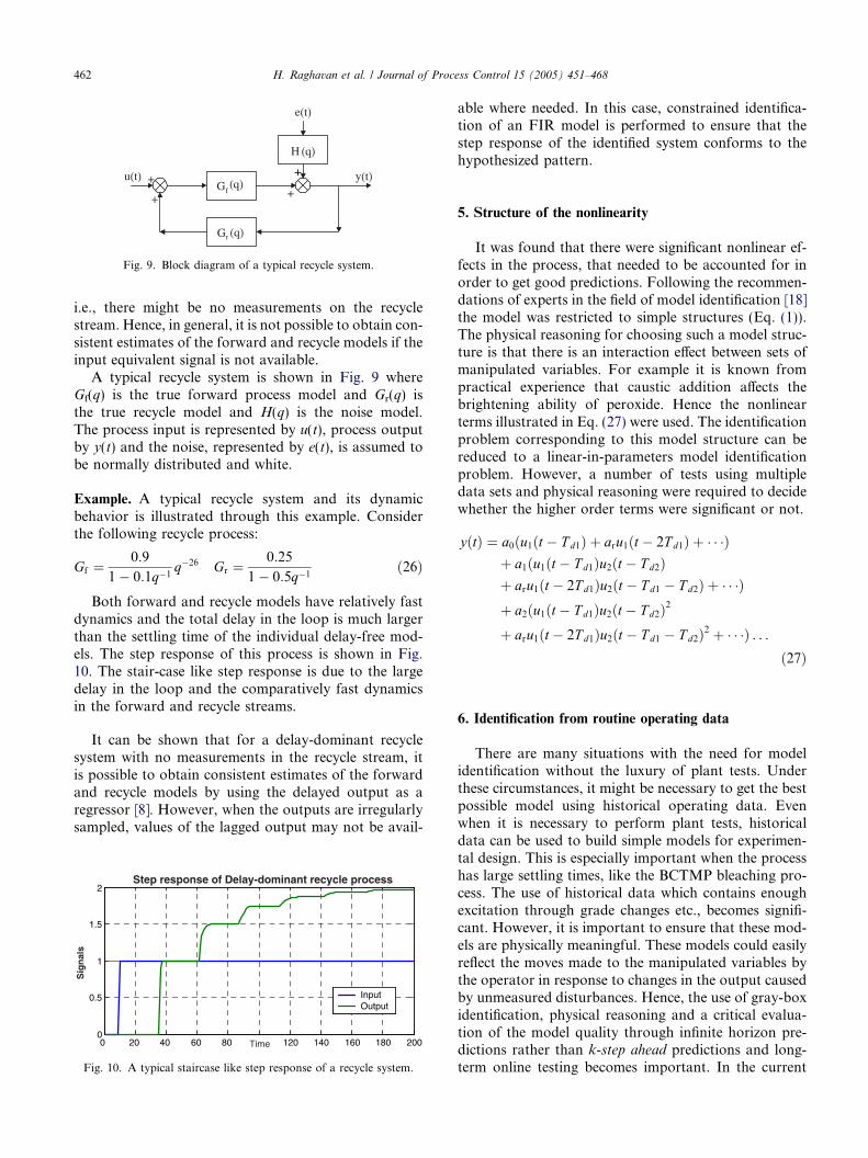
Fig. 9. Block diagram of a typical recycle system.


i.e., there might be no measurements on the recyclestream. Hence, in general, it is not possible to obtain con-sistent estimates of the forward and recycle models if theinput equivalent signal is not available.

A typical recycle system is shown in Fig. 9 whereGf(q) is the true forward process model and Gr(q) isthe true recycle model and H(q) is the noise model.The process input is represented by u(t), process outputby y(t) and the noise, represented by e(t), is assumed tobe normally distributed and white.

Example. A typical recycle system and its dynamicbehavior is illustrated through this example. Considerthe following recycle process:

Gf ¼0:9

1� 0:1q�1q�26 Gr ¼

0:25

1� 0:5q�1ð26Þ

Both forward and recycle models have relatively fastdynamics and the total delay in the loop is much largerthan the settling time of the individual delay-free mod-els. The step response of this process is shown in Fig.10. The stair-case like step response is due to the largedelay in the loop and the comparatively fast dynamicsin the forward and recycle streams.

It can be shown that for a delay-dominant recyclesystem with no measurements in the recycle stream, itis possible to obtain consistent estimates of the forwardand recycle models by using the delayed output as aregressor [8]. However, when the outputs are irregularlysampled, values of the lagged output may not be avail-

0 20 40 60 80 120 140 160 180 2000

0.5

1

1.5

2

Time

Step response of Delay-dominant recycle process

Sig

nal

s

InputOutput

Fig. 10. A typical staircase like step response of a recycle system.

able where needed. In this case, constrained identifica-tion of an FIR model is performed to ensure that thestep response of the identified system conforms to thehypothesized pattern.

5. Structure of the nonlinearity

It was found that there were significant nonlinear ef-fects in the process, that needed to be accounted for inorder to get good predictions. Following the recommen-dations of experts in the field of model identification [18]the model was restricted to simple structures (Eq. (1)).The physical reasoning for choosing such a model struc-ture is that there is an interaction effect between sets ofmanipulated variables. For example it is known frompractical experience that caustic addition affects thebrightening ability of peroxide. Hence the nonlinearterms illustrated in Eq. (27) were used. The identificationproblem corresponding to this model structure can bereduced to a linear-in-parameters model identificationproblem. However, a number of tests using multipledata sets and physical reasoning were required to decidewhether the higher order terms were significant or not.

yðtÞ ¼ a0ðu1ðt � T d1Þ þ aru1ðt � 2T d1Þ þ � � �Þþ a1ðu1ðt � T d1Þu2ðt � T d2Þþ aru1ðt � 2T d1Þu2ðt � T d1 � T d2Þ þ � � �Þþ a2ðu1ðt � T d1Þu2ðt � T d2Þ2

þ aru1ðt � 2T d1Þu2ðt � T d1 � T d2Þ2 þ � � �Þ . . .ð27Þ

6. Identification from routine operating data

There are many situations with the need for modelidentification without the luxury of plant tests. Underthese circumstances, it might be necessary to get the bestpossible model using historical operating data. Evenwhen it is necessary to perform plant tests, historicaldata can be used to build simple models for experimen-tal design. This is especially important when the processhas large settling times, like the BCTMP bleaching pro-cess. The use of historical data which contains enoughexcitation through grade changes etc., becomes signifi-cant. However, it is important to ensure that these mod-els are physically meaningful. These models could easilyreflect the moves made to the manipulated variables bythe operator in response to changes in the output causedby unmeasured disturbances. Hence, the use of gray-boxidentification, physical reasoning and a critical evalua-tion of the model quality through infinite horizon pre-dictions rather than k-step ahead predictions and long-term online testing becomes important. In the current

Validationdata

Training data

Comparison of measured output with black-box model simulations

Bri

ghtn

ess

(sca

led)

26.5

28

29.5

31PredictionsMeasurements


application infinite horizon predictions were used forvalidation because the lab information system couldnot communicate with the main DCS system. However,the continued good performance of the infinite horizonpredictions over more than two years enhances our con-fidence in the quality and reliability in the identifiedmodel.

Time (days)35 140 175

2510570

Fig. 11. Predictions from N4SID look good.

7. Results

In this section, online brightness and tensile predic-tions from models developed using different techniquesare presented. The performance of the identified modelsis evaluated using two indices, the cross-correlation(CC) and the root mean squared error (RMSE) whichare defined as follows:

CC ¼ covðy; yÞffiffiffiffiffiffiffiffiffiffiffiffiffiffiffiffiffiffiffiffiffiffiffiffiffiffivarðyÞvarðyÞ

p ;

RMSE ¼

ffiffiffiffiffiffiffiffiffiffiffiffiffiffiffiffiffiffiffiffiffiffiffiffiffiffiffiffiffiffiffiffiffiffiffiffiffiffiffi1

N

XNi¼1

ðyðiÞ � yðiÞÞ2vuut ð28Þ

7.1. Results using black-box identification

Initially black-box routines were used to developmodels, without explicitly taking the recycle effect intoaccount. These models did not separate the forwarddynamics from the recycle dynamics. In addition, be-cause black-box routines were used, an approximationof the overall dynamics of the process was obtained.For example, brightness predictions using a high ordermodel obtained using N4SID a black-box subspaceidentification routine are shown in Fig. 11. This plothas been re-scaled for confidentiality reasons. In thisplot, the first two-thirds of the samples were used foridentification and the final one-third was the validation

Step Res

1000 2000 30001000 2000 3000

From: u1 From: u2

Time (minutes) Time (minutes)

0

0.5

1

1.5

2

2.5

2

2.5

Fig. 12. N4SID step respons

data set. The predictions look very good and henceone might be easily misled into believing that the modelsare good. In fact the converse is true. Even though thepredictions are good, the model is not reliable becausethe step-responses, shown in Fig. 12, do not match withthe expected fast-dynamics and characteristic staircaseshape associated with the recycle effect.

7.2. Results using linear interpolation

Following this, it was decided to separate out the re-cycle effect by including a lagged output value as aregressor, as argued in Section 4. Hence y(t � Td) is usedlike an additional input. This leads to consistent models,provided that the impulse response of the delay-free for-ward model and the impulse response of the noise modeldie down in a time period less than the delay in the loop[8]. However, this method has the requirement that theoutput value y(t � Td) should be available. When theoutput is irregularly sampled, this requirement cannotbe met always. A seemingly simple way to overcome thisproblem is to perform some kind of interpolation likelinear interpolation to ensure the availability of the out-put value wherever it is required and not available. Inretrospect, this leads to poor models, because the inter-polation performed on the output is essentially univari-ate and does not take input variations into account.

ponses

1000 2000 30001000 2000 3000

From: u3 From: u4

Time (minutes) Time (minutes)

es are not satisfactory.

Training data Validation data

Bri

ghtn

ess

(sca

led)

25

26.5

28

29.5

31

Time (days)

35 140 17510570

PredictionsMeasurements

Fig. 13. Predictions using linear interpolation look good.

35 70 105 140 175

Time (Days)

Online validation of model based on interpolated data

Lab meas.PredictionsCC = 75.8%

MSE = 3.283

Fig. 15. Deterioration of predictions for model based on linearlyinterpolated data.


Brightness predictions using linear interpolation areshown in Fig. 13. This plot has been re-scaled for confi-dentiality reasons. Once again, the predictions look verygood. However the models are far from satisfactory as isevident from the step-responses shown in Fig. 14. Forexample, the settling time for the forward paths havebeen identified to be of the order of 33h while in realitythey are of the order of 20min. Validation on a new dataset (Fig. 15) shows a significant deterioration of predic-tions from the model based on linearly interpolateddata.

7.3. From black-box models to gray-box model model

structures

In order to arrive at the final model structure, multi-ple iterations of analysis and discussions with the millengineers were required. The observed dynamics wereused to characterize this process as a time delay domi-nant recycle process. The following observations justifythis hypothesis. The inputs are sampled every 10min.The process consists of two towers (P1 and P2 tower).The chemical add-rates are manipulated upstream ofeach tower. It is observed that on changing the P1add-rates, the output variables change 5h and 20minlater. On changing the P2 add-rates, the output variables

Step Response

0 1000 2000 3000

From: u1 From: u2 From: u3

Time (minutes)

0 1000 2000 3000 0 1000 2000

Time (minu

0

0.2

0.4

0.6

0.8

1

1.2

Fig. 14. Step responses using interpo

change 3h and 40min later. It is also observed that thedirect change in the brightness and tensile is almostinstantaneous, the change occurs with a couple of10min sampling intervals, after the delays mentionedin the previous point. This characterizes the fast dynam-ics of the process. In addition to the direct change in thebrightness and tensile there is a change because of thechemicals recycled to the front-end of the bleach plant.Given that the process can be characterized as a time-de-lay dominant recycle process, a strategy was needed toaccommodate chemical recycling and irregular sam-pling. As shown previously, initial black-box modelsdeveloped using Prediction Error Methods and Sub-space Identification using interpolation techniques were

From: u4

3000 0 1000 2000 3000 0 1000 2000 3000

Time (minutes)tes)

Recycle term

lated data are not satisfactory.


not acceptable to the mill engineers because the dynam-ics portrayed by these models were unconvincing. Hencethe model structure shown in Eq. (1) was chosen. Addi-tionally, following the observation that by manipulatingthe caustic add-rate, the brightening effect of peroxidecan be modified, nonlinearities were introduced intothe model structure. It also prompted the investigationof other similar nonlinear interactions, which were vali-dated on data sets over a long period of time.

7.4. Results using constrained FIR and EM algorithm

The final model structure chosen has the advantage ofproviding interpretable models as well as good predic-tions. This procedure involves the identification of con-strained Finite Impulse Response (FIR) models asinitial models. These models were later used as initialmodels in the EM algorithm following the procedureoutlined in Section 3.

7.4.1. Structure of FIR models

FIR models of the form given in Eq. (29) wereidentified.

yðtÞ ¼ a0 þ a1u1ðt � T d1Þ þ a1aRu1ðt � 2T d1Þ þ � � �þ a1ak�1

R u1ðt � kT d1Þ þ � � � þ a2u2ðt � T d2Þþ a2aRu2ðt � 2T d2Þ þ � � � þ a2ak�1

R u2ðt � kT d2Þþ � � � þ � � � þ a6u6ðt � T d6Þ þ mðtÞ

¼ GðqÞuðtÞ þ HðqÞeðtÞð29Þ

Here, a0 represents an intercept term, am refers to thecoefficient corresponding to the mth input, aR refers tothe average chemical recycle fraction and Tdi refersto the total delay in the forward and recycle paths fromthe ith input to the output. k can be chosen dependingon the number of past input values, which are hypothe-sized to affect the current value of the output.

7.4.2. Constrained identification of FIR models

The advantages of using an FIR structure for the ini-tial model include the ability to handle irregularly sam-pled outputs, chemical recycling and input nonlinearity.The structure of the optimization problem to be solvedis as follows:

hN ¼ argminh

1

N

XNt¼1

12e2ðt; hÞ s:t: f ðhÞ P 0 ð30Þ

Following Eq. (29) and assuming an output-errorstructure for the model, the optimal one-step ahead pre-diction of y is given by:

yðtjt � 1Þ ¼ H�1ðqÞGðqÞuðtÞ þ ½1� H�1ðqÞ�yðtÞ¼ GðqÞuðtÞ ð31Þ

This implies that the one-step ahead prediction is thesame as the infinite horizon prediction. Similarly, the k-step ahead prediction of y is also equal to the infinitehorizon prediction, yðtjt � kÞ ¼ GðqÞuðtÞ. Hence theoptimization problem simplifies to:

hN ¼ argminh

1

N

XNt¼1

ðyðtÞ � Gðq; hÞuðtÞÞ2 s:t: f ðhÞ P 0

ð32Þ

G(q) is defined according to Eq. (29) and f(h) P 0represents constraints applied on the identified para-meters in order to obtain physically meaningfulmodel parameters. For example, it is necessary toimpose the constraint a1 P 0 because it is known thatadding more peroxide, increases the brightness ofthe pulp. This constrained identification problem wassolved using gray-box identification tools in Matlab�.Several trials with different initial guesses for the para-meters were required to avoid convergence to localoptima.

7.4.3. Robust estimation of average recycle fraction

and selection of nonlinear effects

The term aR in Eq. (29) represents the average recyclefraction. In order to obtain robust model estimates theproblem of estimating aR is decoupled from the problemof identifying the other parameters. Since, aR is con-strained to take a value between 0 and 1, it was variedbetween 0 and 1 in steps of 0.01, models identified foreach of these values and the corresponding Root MeanSquared Error (RMSE) values were plotted. Followingthis, the model corresponding to the least RMSE waschosen. The estimated values of aR and other modelparameters depend on the set of chosen input factorsand the interaction terms. For example, a list of the pos-sible sets of direct factors and interaction terms for thebrightness models is given below:

1. {{u1, . . . , u6} or {u1, u2, (u3 + u4), u5, u6}}.2. {{u1, . . . , u6} or {u1, u2, (u3 + u4), u5, u6}} and

{u1 · u5 and u2 · u5}.3. {u1, . . . , u6, u1 · u3, u2 · u4} or {u1, u2, (u3 + u4), u5,

u6, (u3 + u4) · u1, (u3 + u4) · u2}.4. {u1, u2, (u3 + u4), u5, u6, (u3 + u4)

2}.

In addition, combinations of the above cases can alsobe considered. In view of the variety of possible cases,the following procedure is used to obtain the best possi-ble model:

• Choose a particular set of input factors.• Find the model which gives the least RMSE value.• Compare the RMSE values and find the best model

structure.

0.2 0.4 0.6 0.8 1

1.5

1.4

1.3

1.2

RM

SE

1111110 1ar

Plot of RMSE vs. Averge Recycle fraction for Brightnesswith P1 &P2 H2O2 & NaOH and Freeness as inputs

RMSEmin at ar = 0.4

Fig. 16. Choosing the best model using minimum RMSE.

200 220 240 260 280 300 320 340 360 380 4000

0.5

1

1.5

P1-

Per

oxi

de

220 240 260 280 300 320 340 360 380 40074.5

74.6

74.7

74.8

74.9

75

Bri

gh

tnes

s

Delay=32 samplesSettling time = 96 samplesTime constant =19.2 samplesGain =0.41

Fig. 17. Step response of brightness for unit change in P1 peroxide.


A sample plot of the RMSE as a function of the aver-age recycle fraction is shown in Fig. 16. In this case thechosen inputs were u1, u2, (u3 + u4) and u5.

The FIR models identified for predicting brightnessand tensile using this procedure are summarized below.For confidentiality reasons the values of the coefficientshave not been provided.

y1ðtÞ ¼ RðqÞfa1u1ðt � 32Þ þ a2u2ðt � 22Þ þ a3ðu3ðt � 32Þ

þ u4ðt � 22ÞÞ þ a13u1ðt � 32Þðu3ðt � 32Þ þ u4ðt � 22ÞÞ

þ a23u2ðt � 22Þ � ðu3ðt � 32Þ þ u4ðt � 22ÞÞg

þ a5u5ðtÞ þ a6u6ðtÞ þ a0

y2ðtÞ ¼ RðqÞfb1u1ðt � 32Þ þ b2u2ðt � 22Þ þ b3u3ðt � 32Þ

þ b4u4ðt � 22Þb16u1ðt � 32Þu6ðtÞ þ b26u2ðt � 22Þu6ðtÞ

þ b13u1ðt � 32Þu3ðt � 32Þ þ b24u2ðt � 22Þu4ðt � 22Þ

þ b132u1ðt � 32Þu3ðt � 32Þ2

þ b242u2ðt � 22Þu4ðt � 22Þ2g

þ b5u5ðtÞ þ b6u6ðtÞ þ b0 ð33Þ

Q1

Q2

Q3

Q4

Q5

Q6

PV

PV

PV

PV

PV

SP

OPC Read Blocks

Q1

2

3

4

5

6

1

2

3

4

5

6

OPC Read-L1 ADD712

OPC Read - L1 ADD802



OPC Read - L1 ASPEN

OPC Read - L1 FREENESS

L1_add712

L1_add802

L1_add713

L1_add813

L1_aspen

L1_freeness

L1_add802

L1_add713

L1_add813

L1_aspen

L1_freeness

L1_P2_Brightness

L1_add712

L1_P2_Tensile

Fig. 18. Block diagram showing im

where, RðqÞ ¼ ð1þ aRq�32 þ a2Rq�64 þ a3Rq

�96 þ a4Rq�128Þ

and aR = 0.17 is the average recycle fraction.Given such a model, the staircase shaped response of

an output can be simulated for a unit step change in aninput. Such a response is shown for a step change in theperoxide add-rate in Fig. 17. It is easy to see from Eq.(33) that, due the interaction effects, the gain is a func-tion of the absolute value of the inputs. For example,the brightening effect of peroxide depends on theamount of caustic present in the tower. Hence the rela-tion between u1 and y1 can be expressed as, G11 =R(q)(a1 + a13(u3(t � 32) + u4(t � 22))) u1(t � 32). Hencethe gain from u1 to y1 is K11 � (1.205) · (a1 +a13(u3(t � 32) + u4(t � 22))), which is a function of thecaustic present in the tower. The FIR models identifiedusing this gray-box procedure were used as initial mod-els in the EM algorithm. In order to avoid an artificial

In0

Line1 P2 Brightness

In0In1In2In3In4In5

Out0

Line1P2 Tensile

L1_P2_Brightness

L1_P2_Tensile

OPC Write - Dyn Predicted L1 Brightness

OPC Write - Dyn Predicted L1Tensile

Dynamic Predictors

OPC Write Blocks

Out0

In0Q

Q

In0In1In2In3In4In5

plementation of Predictors.


increase in the system order while performing the state-space model identification [1], the inputs were time-shifted by the known delays (32 and 22 samples as is evi-dent from Eq. (33).

7.4.4. ImplementationPredictors based on the models developed using the

FIR-EM procedure have been implemented on the mills�distributed control system (DCS) and have been runningsatisfactorily over an year. The implementation wasdone using Matrikon�s ProcessACT� software, whichprovides an environment for design, development, simu-lation, and implementation of process control applica-tions. A block diagram illustrating the implementationis shown in Fig. 18. Snapshots of the predictions usingthese models are also shown in Fig. 19. These modelsare also being used in the development of an advanced

Time (m

0 50 100 0 50 100 0 50

FromFrom: u2From: u1

Del

ay f

ree

Step

Res

pons

es

Fig. 21. Step responses of FIR-EM B

Fig. 19. Snapshot of predictions.

process control scheme for controlling brightness andtensile to their desired targets.

7.4.5. Online predictions

The results of prediction of Line 2 brightness andLine 1 tensile using the constrained FIR-EM strategiesare shown in Figs. 20 and 22 for a period of 12 months.The values on the y-axis have been masked for confiden-tiality reasons. The predictions for Line 1 brightness andLine 2 tensile are similar to the results shown and thesefigures are not shown in the interest of conserving space.The corresponding step responses are shown in Fig. 21.All these predictions are infinite horizon predictions. Itis clear from the high values of the correlation coefficientand the low RMSE values (shown in the respective fig-ures) that the predictions are quite satisfactory. In addi-tion because of the imposition of the desired structure,the model coefficients are interpretable and conform towhat is known from prior knowledge.

inutes)

Recycledynamics

100 0 50 100 0 50 100

From: u4: u3

rightness model are satisfactory.

Brightness Predictions

CC = 93.462%RMSE = 2.374

140 210 28070 350

Time (days)

PredictionsLab Meas.

Fig. 20. Line 2 brightness predictions.

PredictionsActualPredictionsLab Meas.

Tensile Predictions

PredictionsActualPredictionsLab Meas.CC = 93.957%

RMSE = 380.85

140 210 280 350

Time (days)

70

Fig. 22. Line 1 tensile predictions.


8. Conclusions

The application of gray-box techniques for modelidentification of the bleaching operation in a BCTMPprocess from routine operating data, has been presented.Novel techniques developed to deal with time-delaydominant recycle processes and irregularly sampled out-puts have been described. The dangers of using arbitraryinterpolation and black-box strategies have been dem-onstrated. Predictors based on the identified modelsare being used in the DCS for online prediction and con-troller design are performing satisfactorily.

Acknowledgments

This work was performed as a part of the IntelligentBleaching system (IBS) project supported by PrecarnInc. We thank Precarn Inc. for the financial support andour partners in the project, Millar Western ForestProducts Ltd., Alberta Pacific Forest Industries Inc.,Daishowa Marubeni International Ltd. and MatrikonInc. for their enthusiastic participation.

References

[1] R. Amirthalingam, S.W. Sung, J.H. Lee, A two step procedurefor data-based modeling for inferential predictive control systemdesign, AIChE J. 46 (2000) 1974–1988.

[2] T. Chen, B. Francis, Optimal Sampled-Data Control Systems,Springer-Verlag, Berlin, 1995.

[3] A.P. Dempster, N.M. Laird, D.B. Rubin, Maximum likelihoodfrom incomplete data via the EM algorithm, J. R. Statist. Soc.,Ser. B 39 (1977) 1–38.

[4] M.M. Denn, R. Lavie, Dynamics of plants with recycle, Chem.Eng. J. (London) 24 (1982) 54–59.

[5] U. Forssell, L. Ljung, Closed-loop identification revisited,Automatica 35 (1999) 1215–1241.

[6] B. Freidland, Sampled-data control systems containing periodi-cally varying members, in: Proceedings of the 1961 IFAC WorldCongress, vol. 37, 1961, pp. 361–367.

[7] S. Gibson, B. Ninness, On the relationship between state–space–subspace-based and maximum-likelihood system identificationmethods, in: Proceedings of the 2000 IEEE International Confer-ence on Decision and Control, Sydney, Australia, 2000.

[8] R.B. Gopaluni, H. Raghavan, R.S. Patwardhan, S.L. Shah, Onthe identification of consistent models for processes with materialand energy recycle, Presented at AIChE Annual Meeting,November 2003, San Francisco, USA, 2003.

[9] N.K. Gupta, R.K. Mehra, Computational aspects of maximumlikelihood estimation and reduction in sensitivity function calcu-lations, IEEE Trans. Auto. Contr. 19 (1974) 774–783.

[10] A.J. Isaksson, Identification of ARX-models subject to missingdata, IEEE Trans. Auto. Contr. 38 (1993) 813–819.

[11] P.P. Khargonekar, K. Poolla, A. Tannenbaum, Robust control oflinear time-invariant plants using periodic compensation, IEETrans. Auto. Contr. 30 (1985) 1088–1096.

[12] G.M. Kranc, Input–output analysis of multirate feedback sys-tems, IEE Trans. Auto. Contr. 3 (1957) 21–28.

[13] S.Y. Kung, A new identification and model reduction algorithmvia singular value decomposition, in: 12th Asilomar Conferenceon Circuits, Systems and Computers, Pacific Grove, CA, 1978,pp. 705–714.

[14] K.E. Kwok, M. ChongPing, G.A. Dumont, Seasonal model-based control of processes with recycle dynamics, Ind. Eng. Chem.Res. 40 (2001) 1633–1640.

[15] S. Lakshminarayanan, H. Takada, Empirical modelling andcontrol of processes with recycle: some insights via case studies,Chem. Eng. Sci. 56 (11) (2001) 3327–3340.

[16] D. Li, S.L. Shah, T. Chen, Identification of fast-rate models frommultirate data, Int. J. Control 74 (7) (2001) 680–689.

[17] R.J.A. Little, D.B. Rubin, Statistical Analysis with Missing Data,John Wiley and Sons, New York, 1987.

[18] L. Ljung, System Identification: Theory for the User, second ed.,Prentice-Hall, Inc., Englewood Cliffs, NJ, 1999.

[19] W.L. Luyben, Snowball effects in reactor–separator processeswith recycle, Ind. Eng. Chem. Res. 33 (2) (1994) 299–305.

[20] J.C. Morud, S. Skogestad, Effects of recycle on dynamics andcontrol of chemical processing plants, Comput. Chem. Engng. 18(1994) 529–534.

[21] B. Ninness, S. Gibson, Robust and simple algorithms formaximum likelihood estimation of multivariable systems, in:Proceedings of the 2002 IFAC World Congress, Barcelona, 2002.

[22] P.V. Overschee, B. DeMoor, Subspace Identification for LinearSystems—Theory, Implementation, Applications, Kluwer Aca-demic Publisher, Boston, MA, 1996.

[23] R.K. Pearson, B.A. Ogunnaike, Nonlinear model identification,in: M.A. Henson, D.E. Seborg (Eds.), Nonlinear Process Control,Prentice-Hall, Englewood Cliffs, NJ, 1996.

[24] R.H. Shumway, D.S. Stoffer, An approach to time seriessmoothing and forecasting using the EM algorithm, J. Time Ser.Anal. 3 (4) (1982) 253–264.

[25] R.H. Shumway, D.S. Stoffer, Time Series Analysis and itsApplications, Springer-Verlag, New York, 2000.

[26] N.K. Sinha, G.P. Rao, Identification of Continuous TimeSystems, Kluwer Academic Publishers, London, 1991.

[27] T. Soderstrom, P. Stoica, Instrumental variable methods forsystem identification, Lectures Notes in Control and InformationSciences, Springer-Verlag, Berlin, 1983.

[28] M. Viberg, Subspace-based methods for the identification oflinear time-invariant systems, Automatica 31 (12) (1995) 1835–1853.

[29] J. Wang, T. Chen, B. Huang, Multirate sampled-data systems:computing fast-rate models, J. Process Control 14 (1) (2004) 79–88.

Gray-box identification of dynamic models for the bleaching ...

Documents

Transcript of Gray-box identification of dynamic models for the bleaching ...