GraFIX: A semiautomatic approach for parsinglow- and high-quality eye-tracking data

Irati R. Saez de Urabain & Mark H. Johnson &

Tim J. Smith

# The Author(s) 2014. This article is published with open access at Springerlink.com

Abstract Fixation durations (FD) have been used widely as ameasurement of information processing and attention.However, issues like data quality can seriously influence theaccuracy of the fixation detection methods and, thus, affect thevalidity of our results (Holmqvist, Nyström,&Mulvey, 2012).This is crucial when studying special populations such asinfants, where common issues with testing (e.g., high degreeof movement, unreliable eye detection, low spatial precision)result in highly variable data quality and render existing FDdetection approaches highly time consuming (hand-coding) orimprecise (automatic detection). To address this problem, wepresent GraFIX, a novel semiautomatic method consisting of atwo-step process in which eye-tracking data is initially parsedby using velocity-based algorithms whose input parametersare adapted by the user and then manipulated using the graph-ical interface, allowing accurate and rapid adjustments of thealgorithms’ outcome. The present algorithms (1) smooth theraw data, (2) interpolate missing data points, and (3) apply anumber of criteria to automatically evaluate and remove arti-factual fixations. The input parameters (e.g., velocity thresh-old, interpolation latency) can be easily manually adapted tofit each participant. Furthermore, the present applicationincludes visualization tools that facilitate the manual codingof fixations. We assessed this method by performing anintercoder reliability analysis in two groups of infants present-ing low- and high-quality data and compared it with previousmethods. Results revealed that our two-step approach withadaptable FD detection criteria gives rise to more reliable andstable measures in low- and high-quality data.

Keywords Fixationduration .Eyetrackermethodology .Dataquality . Infant . Naturalistic . Attention

Introduction

Every day of our life, we use our eyes to sample and create aperceptual image of the world around us.Without noticing, wemanifest an array of eye movements that allow selecting andprocessing the parts of the visual field that are most relevant tous (Holmqvist et al., 2011). Fixations take place when theeyes remain relatively stable in a particular point, and it isonly during these periods that visual encoding and process-ing occurs. Saccades, on the other hand, are the ballisticeye movements that take place between fixations when theeyes are rapidly moving from one point to the next.During these moments, visual sensitivity is suppressed(Matin, 1974).

Measuring and reporting fixation durations is commonpractice in experimental psychology (e.g., Henderson &Smith, 2009; Martinez-Conde, 2005; Martinez-Conde,Macknik, & Hubel, 2004; Nuthmann, Smith, Engbert, &Henderson, 2010; Tatler, Gilchrist, & Land, 2005). There is,in fact, a growing body of research that associates fixationdurations with cognitive processes such as attention, informa-tion processing, memory, and anticipation (e.g., Castelhano &Henderson, 2008; Kowler, 2011; Malcolm & Henderson,2010; Rayner, Smith, Malcolm, & Henderson, 2009;Richardson, Dale, & Spivey, 2007). While fixations may notbe the only oculomotor event of interest to researchers mea-suring eye movements (e.g., researchers investigating atten-tional shifts may be interested in raw representations of sac-cadic or smooth pursuit trajectories), the majority of eyemovement research assumes that gaze location can be equatedto visual encoding of high-spatial-frequency foveal informa-tion, and for this to happen, the eyes need to be stable—that is,in a fixation (Rayner, 1998). The study of fixation durations isbecoming increasingly important when investigating popula-tions unable to follow the experimenter’s instructions, such asinfants (e.g., Colombo&Cheatham, 2006; Frick, Colombo, &Saxon, 1999; Hunnius & Geuze, 2004; Hunter & Richards,

I. R. Saez de Urabain (*) :M. H. Johnson : T. J. SmithCentre for Brain and Cognitive Development, Birkbeck College,University of London, Malet Street, WC1E 7HX London, UKe-mail: iurabain@gmail.com

Behav ResDOI 10.3758/s13428-014-0456-0

2011; Richards & Holley, 1999) or monkeys (e.g., Berg,Boehnke, Marino, Munoz, & Itti, 2009; Kano & Tomonaga,2011a, 2011b). For instance, in a recent study, Papageorgiouet al. (2014) showed how individual differences in fixationdurations in early infancy can predict individual differences intemperament and behavior in childhood, which can ultimatelylead to early intervention practices that aim to improve exec-utive attention and potentially identify infants at risk ofattentional disorders such as ADHD.

Traditionally, researchers have used many different metricsto measure infants’ attention, such as familiarization or habit-uation procedures, preferential looking, or average lookingtimes. These metrics, which should be applied to serve theexperimental demands, are not always appropriate for answer-ing certain questions, such as those concerned with the assess-ment of attention and information processing in spontaneousunconstrained settings (Aslin, 2007; Wass, Smith, & Johnson,2013). In these cases, the analysis of fixation durations canhelp to gain valuable insights into the mechanisms underlyingeye movement control.

Nevertheless, recent articles (Holmqvist, Nyström, &Mulvey, 2012; Wass et al., 2013) have highlighted thesubstantial impact that low-quality data can have on ex-perimental measures. Poor eye-tracking recording can af-fect the validity of results, and sadly, it is still not com-mon practice to report data quality measures or deeperdescriptions of the fixation detection methods used(Holmqvist et al., 2011; 2012). This can alter the viabilityof research results and, hence, lead to problems replicatingprevious studies.

The raw data recovered from any eyetracker includes atime stamp and the x- and y-coordinates for one eye (monoc-ular systems) or both eyes (binocular systems). Fixations canbe identified when these coordinates are relatively stable in apoint (and hence, the eyes’ velocity, defined as the rate ofchange in x- and y-coordinates from one gaze point to the next,is low), whereas saccades are flagged when the x- and y-coordinates are more variable in the scene and the eyes’velocity exceeds a given threshold (see Fig. 1). Additionally,other types of eye movements can be detected in the raw data,such as smooth pursuit (Larsson, Nyström, & Stridh, 2013) orblinks (e.g., Morris, Blenkhorn, & Zaidi, 2002). In caseswhere the data quality and the sampling frequency are veryhigh, it is even possible to identify very short fixational eyemovements, such as microsaccades, glissades, or tremor(Nyström & Holmqvist, 2010).

What is data quality and why it is so important

The quality of the raw data generated by the eyetracker mayvary depending on many different factors, such as theeyetracker model and manufacturer, the eye physiology, the

calibration procedure, the position of the participant relative tothe eyetracker, the degree of head motion (Holmqvist et al.,2011, 2012), or even ethnicity (Blignaut &Wium, 2013). Theterm data quality entails different aspects affecting eye-tracking data, but not all these aspects will necessarily affectfixation detection equally.

Low data quality can havemajor effects on both spatial andtemporal accuracy of gaze measurements. Spatial accuracy oroffset refers to the difference in space between the detectedgaze and the real gaze and can be an important issue whenanalyzing areas of interest (AOIs) (Holmqvist et al., 2012) .Apart from the vertical and horizontal accuracy that the eye-tracking systems report, aspects such as binocular disparityshould also be taken into account, especially when studyingspecial populations. For instance, we know that binoculardisparity in young infants may be markedly larger than inadults (Appel & Campos, 1977; Yonas, Arterberry, &Granrud, 1987). However, it is also common to find infantdata with very large disparities as a consequence of poorcalibrations or incorrect angles between the eyetracker andthe participant. Often, it is possible to minimize the effects ofpoor accuracy in AOIs analysis by simply enlarging the re-gions of interest or by quantifying and correcting the offset foreach participant (Holmqvist et al., 2011, 2012). Frank, Vul,and Saxe (2012) designed an offline procedure to correcterrors in calibration in order to increase the accuracy andinclude a measure that evaluates it. They presented theirparticipants (infants from 3 to 30 months) with calibrationpoints that appeared during the experiment and that weresubsequently used to correct the offset.

Nonetheless, a data set with a large offset can also presenthigh spatial precision and, thus, still be suitable for detectingfixations accurately. We refer to spatial precision as the con-sistency in detecting and calculating gaze points (see Fig. 1).Data sets with relatively low spatial precision will presenthigher gaze velocities as a result of noise in the data, and thiswill complicate the process of detecting fixations accurately.Precision can be affected by individual factors that vary on aparticipant basis (such as different eye physiologies or theposition of the participant relative to the eye cameras), envi-ronmental factors that change according to the experimentaldesign (such as the lighting conditions of the room where theparticipants are being tested), or the eye-tracking hardwareand software (Holmqvist et al., 2011, 2012). The defaultspatial precision for a particular eyetracker can be calculatedby using an artificial eye. Additionally, there are a number ofmethods for calculating spatial precision (Holmqvist et al.,2011, 2012), such as the root mean square (RMS) ofintersample distances (commonly used by manufacturers)or the standard deviation, which measures the dispersionof each sample from a mean value. To see the effect thatspatial precision has on the detection of fixations by avelocity-based algorithm, see Fig. 1.

Behav Res

Likewise, data loss (often a consequence of unreliabledetections of the pupil or the cornea reflection) is anotherissue that can considerably affect fixation detection(Holmqvist et al., 2011, 2012; Wass et al., 2013). This alsois highly dependent on individual and environmental factors,as well as on the eyetracker hardware and software. Theseindividual variations in the recordings from different partici-pants can lead to very different levels of data quality (accura-cy, precision, and data loss), even when participants haveperformed the same study under the same experimental con-ditions. This can, in fact, be a problematic issue when trying tostandardize the procedure to analyze the eye-tracking data: Dowe use exactly the same protocol and values to analyze thedata regardless of the noise that each participant presents? Orwould it be more appropriate to adapt it somehow?

Issues and recommendations when testing specialpopulations: Infants

All these data quality problems can be particularly concerningif testing with special populations, such as infants or partici-pants suffering from certain disorders. For instance, partici-pants on the Autism spectrum may present a high degree ofhead movements (Kelly, Walker, & Norbury, 2013), and this

can seriously affect the spatial precision and the accuracy ofthe data. Moreover, in some populations —such as inParkinson patients—the head motion can be constant andconsistent across all the participants for the study. Whereassome eye-tracking systems require the user to maintain thehead still by using a chinrest (e.g., EyeLink), others allow ahigh degree of free head movements (e.g., Tobii or SMIeyetrackers). However, these systems include some extra al-gorithms for the head position calculations that can interferewith the gaze estimation and, hence, affect spatial precision(Holmqvist et al., 2011; Kolakowski & Pelz, 2006).

Infants constitute a group that can be especially challengingto test in eye-tracking studies. As well as presenting a highdegree of head movement, especially from 7 to 8 months ofage, when their locomotor abilities are rapidly improving(Adolph & Berger, 2006), many of the quality problems arederived from poor calibration procedures. Traditionally, in-fants are calibrated using five-point calibrations where a col-orful puppet is presented in each corner and center of thescreen, while adults usually perform a nine-point calibrationfollowing a series of small dots.

The first obvious problem occurs when the infant does notlook at the calibration points when they are presented. As aconsequence, the offset calculation will be erroneous, and thespatial accuracy will be affected in one or more areas of the

Smoo

thed

dat

aV

eloc

ityFi

xatio

ns

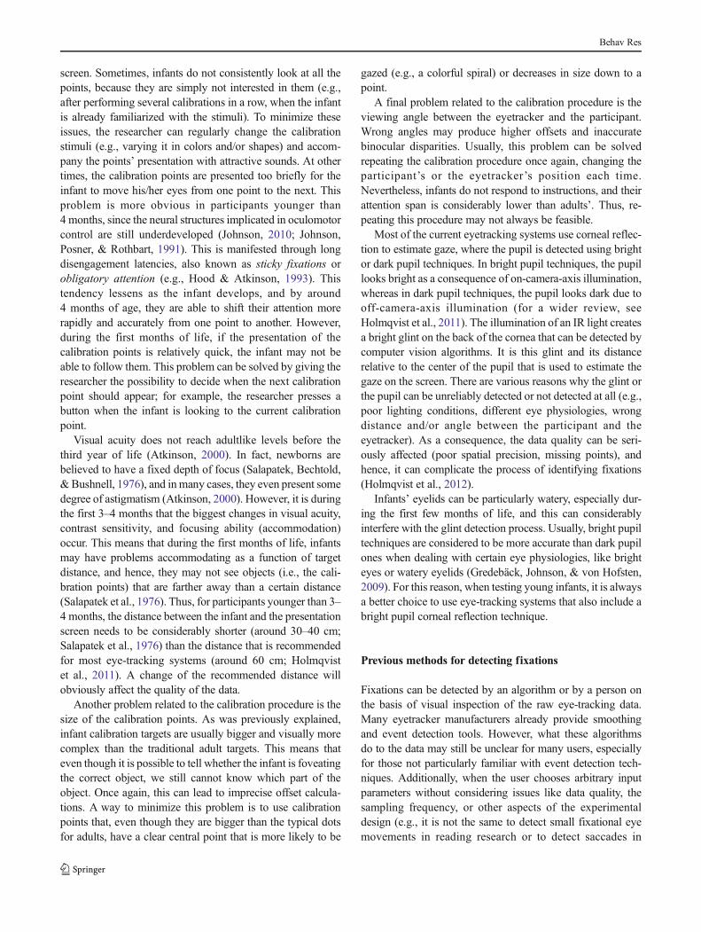
Subject 1: Low precision data Subject 2: High precision data Subject 3: Missing points

Raw

dat

a0 2 4 0 2 4 0 2 4

Seconds Seconds Seconds

0 °/sec

35 °/sec

Fig. 1 Data from 3 infant participants recorded with a Tobii TX300 at120 Hz. The first and the second row show the raw and the smootheddata, respectively. The third row displays the fixations detected by avelocity-based algorithm (velocity threshold = 35°/sec), and the fourththe velocity calculated from the smoothed data. Participant 1 shows low-precision data, which is very common in young infants. As a

consequence, the fixations-parsing algorithm detected a number of phys-iologically implausible artifactual fixations. Participant 2 displays high-precision data from infants. Although the algorithm was more accurate,due to the high velocity threshold, it merged together fixations that hadshort saccades in between (e.g., fixation 8). Participant 3 shows a partic-ipant that presents frequent missing data points

Behav Res

screen. Sometimes, infants do not consistently look at all thepoints, because they are simply not interested in them (e.g.,after performing several calibrations in a row, when the infantis already familiarized with the stimuli). To minimize theseissues, the researcher can regularly change the calibrationstimuli (e.g., varying it in colors and/or shapes) and accom-pany the points’ presentation with attractive sounds. At othertimes, the calibration points are presented too briefly for theinfant to move his/her eyes from one point to the next. Thisproblem is more obvious in participants younger than4 months, since the neural structures implicated in oculomotorcontrol are still underdeveloped (Johnson, 2010; Johnson,Posner, & Rothbart, 1991). This is manifested through longdisengagement latencies, also known as sticky fixations orobligatory attention (e.g., Hood & Atkinson, 1993). Thistendency lessens as the infant develops, and by around4 months of age, they are able to shift their attention morerapidly and accurately from one point to another. However,during the first months of life, if the presentation of thecalibration points is relatively quick, the infant may not beable to follow them. This problem can be solved by giving theresearcher the possibility to decide when the next calibrationpoint should appear; for example, the researcher presses abutton when the infant is looking to the current calibrationpoint.

Visual acuity does not reach adultlike levels before thethird year of life (Atkinson, 2000). In fact, newborns arebelieved to have a fixed depth of focus (Salapatek, Bechtold,& Bushnell, 1976), and inmany cases, they even present somedegree of astigmatism (Atkinson, 2000). However, it is duringthe first 3–4 months that the biggest changes in visual acuity,contrast sensitivity, and focusing ability (accommodation)occur. This means that during the first months of life, infantsmay have problems accommodating as a function of targetdistance, and hence, they may not see objects (i.e., the cali-bration points) that are farther away than a certain distance(Salapatek et al., 1976). Thus, for participants younger than 3–4 months, the distance between the infant and the presentationscreen needs to be considerably shorter (around 30–40 cm;Salapatek et al., 1976) than the distance that is recommendedfor most eye-tracking systems (around 60 cm; Holmqvistet al., 2011). A change of the recommended distance willobviously affect the quality of the data.

Another problem related to the calibration procedure is thesize of the calibration points. As was previously explained,infant calibration targets are usually bigger and visually morecomplex than the traditional adult targets. This means thateven though it is possible to tell whether the infant is foveatingthe correct object, we still cannot know which part of theobject. Once again, this can lead to imprecise offset calcula-tions. A way to minimize this problem is to use calibrationpoints that, even though they are bigger than the typical dotsfor adults, have a clear central point that is more likely to be

gazed (e.g., a colorful spiral) or decreases in size down to apoint.

A final problem related to the calibration procedure is theviewing angle between the eyetracker and the participant.Wrong angles may produce higher offsets and inaccuratebinocular disparities. Usually, this problem can be solvedrepeating the calibration procedure once again, changing theparticipant’s or the eyetracker’s position each time.Nevertheless, infants do not respond to instructions, and theirattention span is considerably lower than adults’. Thus, re-peating this procedure may not always be feasible.

Most of the current eyetracking systems use corneal reflec-tion to estimate gaze, where the pupil is detected using brightor dark pupil techniques. In bright pupil techniques, the pupillooks bright as a consequence of on-camera-axis illumination,whereas in dark pupil techniques, the pupil looks dark due tooff-camera-axis illumination (for a wider review, seeHolmqvist et al., 2011). The illumination of an IR light createsa bright glint on the back of the cornea that can be detected bycomputer vision algorithms. It is this glint and its distancerelative to the center of the pupil that is used to estimate thegaze on the screen. There are various reasons why the glint orthe pupil can be unreliably detected or not detected at all (e.g.,poor lighting conditions, different eye physiologies, wrongdistance and/or angle between the participant and theeyetracker). As a consequence, the data quality can be seri-ously affected (poor spatial precision, missing points), andhence, it can complicate the process of identifying fixations(Holmqvist et al., 2012).

Infants’ eyelids can be particularly watery, especially dur-ing the first few months of life, and this can considerablyinterfere with the glint detection process. Usually, bright pupiltechniques are considered to be more accurate than dark pupilones when dealing with certain eye physiologies, like brighteyes or watery eyelids (Gredebäck, Johnson, & von Hofsten,2009). For this reason, when testing young infants, it is alwaysa better choice to use eye-tracking systems that also include abright pupil corneal reflection technique.

Previous methods for detecting fixations

Fixations can be detected by an algorithm or by a person onthe basis of visual inspection of the raw eye-tracking data.Many eyetracker manufacturers already provide smoothingand event detection tools. However, what these algorithmsdo to the data may still be unclear for many users, especiallyfor those not particularly familiar with event detection tech-niques. Additionally, when the user chooses arbitrary inputparameters without considering issues like data quality, thesampling frequency, or other aspects of the experimentaldesign (e.g., it is not the same to detect small fixational eyemovements in reading research or to detect saccades in

Behav Res

infants), the detection results can be gravely affected, andhence, the validity of the experimental outcomes can bequestioned (Holmqvist et al., 2012).

Event detection algorithms can be classified into two maingroups: dispersion and duration algorithms and velocity andacceleration algorithms (for more detailed reviews, seeHolmqvist et al., 2011). Dispersal-based algorithms use aminimum fixation duration threshold (e.g., 50 ms) and thepositional information (dispersion) of the eye-tracking data inorder to decide whether consecutive points belong to the samefixation—in which case, they are grouped together. If not,they are assumed to be a saccade or a missing point.Dispersion can be measured according to different metrics(Blignaut, 2009), such as the distance between the points inthe fixation that are the farthest apart (Salvucci & Goldberg,2000), the distance between two random points in a fixation(e.g., Shic, Scassellati, & Chawarska, 2008), the distancebetween two points at the center of a fixation (e.g., Shicet al., 2008), the standard deviation of x- and y-coordinates(e.g., Anliker, 1976), or a minimum spanning tree of the pointsin a fixation (e.g., Salvucci & Goldberg, 2000). Currently, it ispossible to find a number of commercial (e.g., SMI BeGaze)and noncommercial implementations for these algorithms(e.g., Salvucci & Goldberg, 2000), which are mostly used toparse low-sampling-rate data (< 200 Hz). On the other hand,the algorithms from the second group calculate the velocityand/or acceleration for each point in order to detect events onthe data. Velocity-based algorithms, in particular, flag all thepoints whose velocity are over a threshold (e.g., 10–70 °/sec)as saccades and define the time between two saccades as afixation. Once again, there are a number of commercial (e.g.,Tobii, EyeLink) and noncommercial (Nyström & Holmqvist,2010; Smeets & Hooge, 2003; Stampe, 1993; Wass et al.,2013) variations for this type of event detection algorithms.These algorithms are commonly used in data collected at highsampling rates (e.g., >500). All these algorithms are verysensitive to noise, and unless the collected data have a veryhigh spatial precision, the results will include a number ofartifactual fixations.

The use of event detection algorithms implies decisionsabout which thresholds should be selected in order to obtainoptimal results. However, how these decisions are made,the range of parameters that can be manipulated, andwhether they are reported in published papers is not yetstandardized, making it difficult to compare or replicate resultsfrom different studies. Komogortsev, Gobert, Jayarathna,and Gowda (2010) compared the performance of differentvelocity- and dispersal-based algorithms and presented a stan-dardized scoring system for selecting a reasonable thresholdvalue (velocity or dispersion threshold) for different algo-rithms. Nevertheless, this article did not take into accountthe individual differences in data quality across participantsand/or trials.

Most researchers tend to use the same input parameters forall the participants, paying very little attention to these varia-tions in data quality and the effects that selecting differentthresholds may have on the data from different participants.Nyström and Holmqvist (2010) presented a new velocity-based algorithm for detecting fixations, saccades, and glis-sades, using an adaptive, data-driven peak saccade detectionthreshold that selects the smallest velocity threshold that thenoise level in data allows. The use of thresholds was motivat-ed by physiological limitations of eye movements. Thesealgorithms already highlighted the importance of adaptingthe input parameters to different levels of noise but still didnot solve the problem of accurately detecting fixations in datasets with relatively higher levels or noise, such as those frominfants.

Wass et al. (2013) analyzed standard dispersal-based fixa-tion detection algorithms and showed how results were highlyinfluenced by interindividual variations in data quality.Additionally, they went a step further to solve these problems,developing new detection algorithms that include a number ofpost hoc validation criteria to identify and eliminate fixationsthat may be artifactual. These algorithms already excludemany artifactual fixations that were included when othervelocity-based detection algorithms were used. However,any automatic approach for detecting fixations in data with acertain degree of noise are likely to produce artifactual fixa-tions that are erroneously calculated and/or fixations that arenot detected at all.

An alternative to using automatic algorithms is to hand-code eye movements on the basis of a visual inspection of thedata. For instance, developmental psychologists have tradi-tionally studied infants’ attention and eye movements byvideo-taping participants and hand-coding the direction ofthe gaze post hoc (e.g., Elsabbagh et al., 2009). Also, it is acommon practice, when analyzing the data from head-mounted eyetrackers, to replay the scene and eye videos frameby frame and make annotations of the onsets and offsets offixations on a separate file (e.g., Tatler et al., 2005). Obviouslythese techniques are highly time consuming and can limit thenumber of participants that a researcher is able to test and code.

With a view to avoiding these problems, some researchershave suggested excluding all participants whose spatial preci-sion is over a predefined threshold (Holmqvist et al., 2011,2012). This way the use of automatic algorithms should berelatively safe, although not perfect. However, excluding par-ticipants according to their data quality is a luxury that notevery study can afford. As was previously explained, the dataquality for many experiments studying high-cost populationssuch as infants or special populations to whom access islimited may be consistently low. Using data quality as aninclusion criterion might result in many participants (or evenall) being excluded. In cases of special populations, the datacan be too valuable to be discarded.

Behav Res

To address these issues, we developed GraFIX, a methodand software that implements a two-step approach: Fixationsare initially parsed by using an adaptive velocity algorithm,then hand-moderated using a graphical easy-to-use interface.This method aims to be as fast and accurate as possible, givingthe researcher the possibility of fixing and adapting the algo-rithm’s outcome in order to remove all the artifactual fixationsmanually and include those that were not accurately detected.The automatic detection algorithms include a number of posthoc validation criteria aiming to obtain the cleanest results thatthe algorithms alone permit, in order to facilitate and speed theprocess of hand-coding fixations.

Introducing GraFIX

GraFIX is a multiplatform application developed in C++ andQT frameworks that makes use of Armadillo C++ linearalgebra library. It works with any binocular or monoculareye-tracking system that can record raw X/Y gaze co-ordinates, including SMI, EyeLink or Tobii eyetrackers.

The present application implements a two-step approachwhere fixations are initially parsed by using an adaptivevelocity-based algorithm, before the algorithm’s outcome ishand-moderated using a graphical interface. Previous methodsfor detecting fixations have adopted either a purely automaticapproach or manual coding. Due to the high variability in dataquality across participants and even within a single participant(e.g., as a result of moving the head throughout the eye-tracking session), the automatic detection algorithms can beremarkably unreliable. On the other hand, current hand-coding methods (e.g., coding fixations looking at the videosframe by frame) can be extremely time consuming and, insome cases, imprecise if coding low-quality data sets.

The proposed method combines these two approachestogether in order to detect fixations in a rapid manner andobtain a fixation distribution with the lowest possible degreeof noise. The present fixation detection algorithm includes anumber of input parameters that can be easily adapted on aparticipant basis. Additionally, it implements three post hocvalidation criteria that fix or remove many of the artifactualfixations generated by the velocity-based algorithm. The ulti-mate aim of adapting the input parameters and applyingcertain post hoc validation criteria is to obtain the most accu-rate outcome by the algorithms alone and, thus, reduce thehand-coding time during the subsequent step. Once the fixa-tions have been automatically estimated, the researcher canevaluate them and fix those that were not accurately detectedusing the GraFIX graphical hand-coding tool.

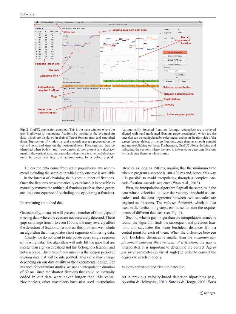
GraFIX displays the eye-tracking coordinates in the rawand the smoothed data boxes (see Fig. 2; for an extendedexplanation of the user interface, see Appendix 1). It presentsthe x- and y-coordinates on the vertical axis, and time on the

horizontal axis. Fixations can then be identified when both x-and y-coordinates do not present any displacement in thevertical axis, and saccades when there is a vertical displace-ment between two fixations accompanied by a velocity peak(see Fig. 2, velocity box). Occasionally, our eyes move tosmoothly pursue an object in the visual scene, and this type ofeye movement can be identified when there is a regularincreasing or decreasing displacement in the vertical axis withlow velocity and acceleration (not present in Fig. 2).

The following sections will present a detailed review forthe present two-step approach for fixation detection.

Automatic detection of fixations

The first action for the two-step approach to detecting fixa-tions is to parse the eye-tracking data using adaptive velocity-based algorithms. The present automatic detection algorithms(1) smooth the raw data, (2) interpolate missing data points,(3) calculate fixations using a velocity-based algorithm, and(4) apply a number of post hoc validation criteria to evaluateand remove artifactual fixations (to see the pseudo-code, go toAppendix 2). The input parameters (e.g., velocity threshold,interpolation latency) can easily be manually adapted to fit thedata from different participants that present different levels ofdata quality (see Fig. 3).

The objective of these algorithms is to obtain the mostaccurate fixation detection for each participant and, thus,reduce the amount of time spent manually correcting fixationsin the subsequent step.

Smoothing the data

GraFIX uses a bilateral filtering algorithm in order to decreasethe noise levels from the raw data. The present version of thealgorithm is based on previous implementations (Durand &Dorsey, 2002; Frank, Vul, & Johnson, 2009) that average thedata for both eyes and eliminate the jitter, while preservingsaccades.

If only one of the eyes is detected, GraFIX allows the userto decide whether the detected eye will still be smoothed or thesample should be excluded. Previous researchers have arguedthat when one eye is not detected, the data from the other eyemay be unreliable (Wass et al., 2013). However, when the eye-tracking data comes from special populations, such as infants,the fact that one of the eyes is not detected does not necessarilymean that the sample from the other eye is inaccurate. Forinstance, it can be the case that the infant is simply occludingone of his/her eyes with his/her hand, causing difficulties forthe accurate detection of both eyes. Occasionally, thesemissing points could lead to inaccurate results regardlessof the inclusion or exclusion of the data (e.g., if one eye wasoccluded during a fixation).

Behav Res

Unless the data come from adult populations, we recom-mend including the samples in which only one eye is available—in the interest of obtaining the highest number of fixations.Once the fixations are automatically calculated, it is possible tomanually remove the artifactual fixations (such as those gener-ated as a consequence of occluding one eye during a fixation).

Interpolating smoothed data

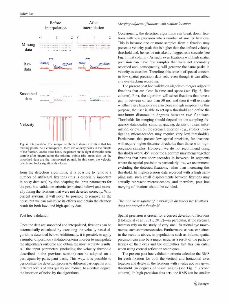
Occasionally, a data set will present a number of short gaps ofmissing data where the eyes are not accurately detected. Thesegaps can range from 1 to even 150 ms and may severely affectthe detection of fixations. To address this problem, we includean algorithm that interpolates short segments of missing data.

Clearly, we do not want to interpolate every single segmentof missing data: The algorithm will only fill the gaps that areshorter than a given threshold and that belong to a fixation, andnot a saccade. The interpolation latency is the longest period ofmissing data that will be interpolated. This value may changedepending on our data quality or the experimental design. Forinstance, for our infant studies, we use an interpolation durationof 60 ms, since the shortest fixations that could be manuallycoded in our data were never longer than this value.Nevertheless, other researchers have also used interpolation

latencies as long as 150 ms, arguing that the minimum timetaken to program a saccade is 100–130ms and, hence, this wayit is possible to avoid interpolating through a complete sac-cade–fixation–saccade sequence (Wass et al., 2013).

First, the interpolation algorithm flags all the samples in thedata whose velocities lie over the velocity threshold as sac-cades, and the data segments between two saccades aretargeted as fixations. The velocity threshold, which is alsoused in the forthcoming steps, can be set to meet the require-ments of different data sets (see Fig. 4).

Second, when a gap longer than the interpolation latency isfound, the algorithm finds the subsequent and previous fixa-tions and calculates the mean Euclidean distances from acentral point for each of them. When the difference betweenboth Euclidean distances is smaller than the maximum dis-placement between the two ends of a fixation, the gap isinterpolated. It is important to determine the correct degreeper pixel parameter (in visual angle) in order to convert thedegrees to pixels properly.

Velocity threshold and fixation detection

As in previous velocity-based detection algorithms (e.g.,Nyström & Holmqvist, 2010; Smeets & Hooge, 2003; Wass

Fig. 2 GraFIX application overview. This is the main window where theuser is allowed to manipulate fixations by looking at the eye-trackingdata, which are displayed in their different formats (raw and smootheddata). Top section of window: x- and y-coordinates are presented on thevertical axis, and time on the horizontal axis. Fixations can then beidentified when both x- and y-coordinates do not present any displace-ment in the vertical axis, and saccades when there is a vertical displace-ment between two fixations accompanied by a velocity peak.

Automatically detected fixations (orange rectangles) are displayedaligned with hand-moderated fixations (green rectangles), which are theones that can bemanipulated by selecting an action on the right side of thescreen (create, delete, or merge fixations; code them as smooth pursuit)and mouse-clicking on them. Furthermore, GraFIX allows defining andindicating the sections where the user is interested in detecting fixationsby displaying them on white or gray

Behav Res

et al., 2013), all the samples whose velocities lie over a certainthreshold are flagged as saccades and the data segmentsbetween two saccades are targeted as fixations. Choosing theright velocity threshold highly depends on the characteristicsof the data that are being analyzed or on how short thesaccades that need to be detected are (Holmqvist et al.,2011). For instance, low sampling rates will present somelimitations when detecting very fast eye movements, such asmicrosaccades. Previous research has shown that saccadessmaller than 10° cannot be detected with systems with asampling rate of 60 Hz and lower (Enright, 1998). This isbecause the peak velocity calculation may not be accurateenough if only a very few samples of a saccade were recorded.The lower the sampling frequency, the lower the calculatedvelocities for short saccades will be. In these cases, a fixationdetection algorithmwouldmerge the fixations before and afteran undetected saccade, and this would result in longer artifac-tual fixations. In order to reliably detect small saccades andreduce noise, it is recommended to use high sampling fre-quencies and lower velocity thresholds (see Fig. 4).

Nevertheless, data from special populations such as infantscan still represent a challenge, due to their low quality. Thus,when the noise levels are higher, the velocity threshold should

be increased accordingly in order to decrease the number of“false positive” saccades. This leads to the question of wheth-er different noise levels in a given data set could entail theinaccurate detection of fixations in low- or high-quality datamaking it difficult to compare and group participants together.As has been suggested in previous research (Wass et al.,2013), different levels of noise can seriously affect the out-come from fixation detection algorithms. There are two op-posing approaches that have been traditionally used to mini-mize this issue. Some researchers prefer to use exactly thesame input parameters for all the participants (such as thevelocity threshold), regardless of the level of noise each par-ticipant presents (Wass et al., 2013). Usually, these parametersare set to fit the requirements for participants with high levelsof noise. Consequently, the velocity threshold can be too highto detect relatively fast saccades, which could ultimately leadto the detection of long artifactual fixations. Moreover, thesesaccades would still remain undetected in very low-precisiondata sets even after lowering the velocity threshold. On theother hand, it is possible to adapt the input parameters accord-ing to the level of noise on a participant-by-participant basis(e.g., Nyström & Holmqvist, 2010). Although the use ofdifferent velocity thresholds can lead to different outcomes

Fig. 3 GraFIX Automatic detection of fixations. This screen displays theinput parameters for the automatic detection. It is possible to adapt theparameters by simply changing their values from the sliders. WhenEstimate fixations is pressed, GraFIX executes the detection algorithmsand displays the results on the orange rectangles. Flags indicating whichpost hoc validation criterion was executed are also displayed. This

process is relatively fast and, thus, allows multiple and easy adjustmentsof the parameters. Once the user is satisfied with the results, the detectioncan be accepted by pressing Accept estimation. This will copy theautomatically detected fixations (orange) on the hand-modulated fixa-tions area (green)

Behav Res

from the detection algorithms, it is possible to remove anumber of artifactual fixations (this is especially importantin noisy data sets) by also adapting the input parameters forthe post hoc validation criteria (explained below) and manu-ally fixing the fixations that were not detected correctly. Withcurrent systems, it will never be possible to remove all thenoise, but we can minimize its effects and obtain the cleanestresult for both low- and high-quality data.

Post hoc validation

Once the data are smoothed and interpolated, fixations can beautomatically calculated by executing the velocity-based al-gorithms described below. Additionally, it is possible to applya number of post hoc validation criteria in order to manipulatethe algorithm’s outcome and obtain the most accurate results.All the input parameters (including the velocity thresholddescribed in the previous section) can be adapted on aparticipant-by-participant basis. This way, it is possible topersonalize the detection process to different participants withdifferent levels of data quality and reduce, to a certain degree,the insertion of noise by the algorithms.

Merging adjacent fixations with similar location

Occasionally, the detection algorithms can break down fixa-tions with low precision into a number of smaller fixations.This is because one or more samples from a fixation maypresent a velocity peak that is higher than the defined velocitythreshold and, hence, be mistakenly flagged as a saccade (seeFig. 5, first column). As such, even fixations with high spatialprecision can have few samples that were not accuratelyrecorded and, consequently, will generate the same peaks invelocity as saccades. Therefore, this issue is of special concernin low-spatial-precision data sets, even though it can affectany eye-tracking recording.

The present post hoc validation algorithm merges adjacentfixations that are close in time and space (see Fig. 5, firstcolumn). First, the algorithm will select fixations that have agap in between of less than 50 ms, and then it will evaluatewhether these fixations are also close enough in space. For thispurpose, the user is able to set up a threshold and define themaximum distance in degrees between two fixations.Thresholds for merging should depend on the sampling fre-quency, data quality, stimulus spacing, density of visual infor-mation, or even on the research question (e.g., studies inves-tigating microsaccades may require very low thresholds).Participants that present low spatial precision, for instance,will require higher distance thresholds than those with high-precision samples. However, we do not recommend usingthresholds over 0.45°, since the algorithmmaymerge togetherfixations that have short saccades in between. In segmentswhere the spatial precision is particularly low, we recommendexcluding the detected fixations, rather than increasing thisthreshold. In high-precision data recorded with a high sam-pling rate, such small displacements between fixations mayactually represent microsaccades, and therefore, post hocmerging of fixations should be avoided.

The root mean square of intersample distances per fixationsdoes not exceed a threshold

Spatial precision is crucial for a correct detection of fixations(Holmqvist et al., 2011, 2012)—in particular, if the researchinterests rely on the study of very small fixational eye move-ments, such as microsaccades. Furthermore, as was explainedin the sections above, in populations such as infants, spatialprecision can also be a major issue, as a result of the particu-larities of their eyes and the difficulties that this can entailwhen using corneal reflection techniques.

The present post hoc validation criteria calculate the RMSfor each fixation for both the vertical and horizontal axestogether and delete all the fixations with a value above a giventhreshold (in degrees of visual angle) (see Fig. 5, secondcolumn). In high-precision data sets, the RMS can be smaller

0 1 2 0 1 2

Rawdata

Before interpolation

Afterinterpolation

Smootheddata

Velocity

Missingdata

Fig. 4 Interpolation. The sample on the left shows a fixation that hasmissing points. As a consequence, there are velocity peaks in the middleof the fixation. On the other hand, the picture on the right shows the samesample after interpolating the missing points (the green dots on thesmoothed data are the interpolated points). In this case, the velocitycalculation looks significantly cleaner

Behav Res

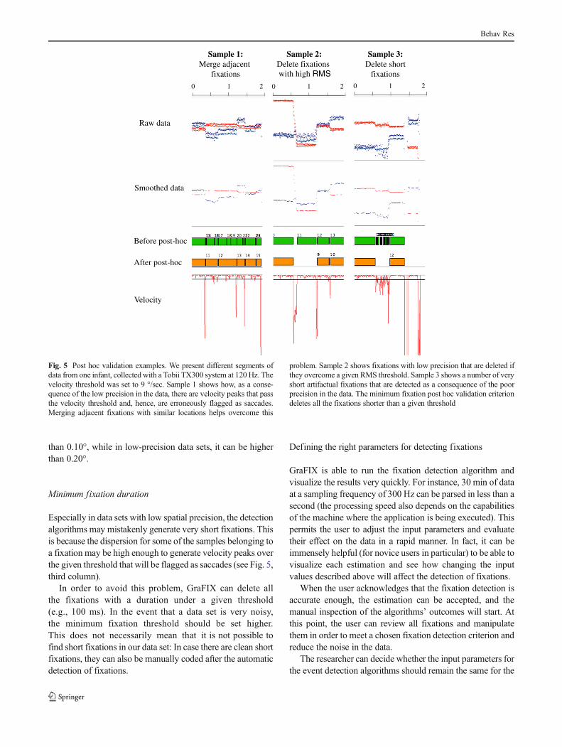
than 0.10°, while in low-precision data sets, it can be higherthan 0.20°.

Minimum fixation duration

Especially in data sets with low spatial precision, the detectionalgorithms may mistakenly generate very short fixations. Thisis because the dispersion for some of the samples belonging toa fixation may be high enough to generate velocity peaks overthe given threshold that will be flagged as saccades (see Fig. 5,third column).

In order to avoid this problem, GraFIX can delete allthe fixations with a duration under a given threshold(e.g., 100 ms). In the event that a data set is very noisy,the minimum fixation threshold should be set higher.This does not necessarily mean that it is not possible tofind short fixations in our data set: In case there are clean shortfixations, they can also be manually coded after the automaticdetection of fixations.

Defining the right parameters for detecting fixations

GraFIX is able to run the fixation detection algorithm andvisualize the results very quickly. For instance, 30 min of dataat a sampling frequency of 300 Hz can be parsed in less than asecond (the processing speed also depends on the capabilitiesof the machine where the application is being executed). Thispermits the user to adjust the input parameters and evaluatetheir effect on the data in a rapid manner. In fact, it can beimmensely helpful (for novice users in particular) to be able tovisualize each estimation and see how changing the inputvalues described above will affect the detection of fixations.

When the user acknowledges that the fixation detection isaccurate enough, the estimation can be accepted, and themanual inspection of the algorithms’ outcomes will start. Atthis point, the user can review all fixations and manipulatethem in order to meet a chosen fixation detection criterion andreduce the noise in the data.

The researcher can decide whether the input parameters forthe event detection algorithms should remain the same for the

Raw data

Smoothed data

Velocity

Before post-hoc

After post-hoc

Sample 1:Merge adjacent

fixations

Sample 2:Delete fixations with high RMS

Sample 3:Delete short

fixations

0 1 2 0 1 2 0 1 2

Fig. 5 Post hoc validation examples. We present different segments ofdata from one infant, collected with a Tobii TX300 system at 120 Hz. Thevelocity threshold was set to 9 °/sec. Sample 1 shows how, as a conse-quence of the low precision in the data, there are velocity peaks that passthe velocity threshold and, hence, are erroneously flagged as saccades.Merging adjacent fixations with similar locations helps overcome this

problem. Sample 2 shows fixations with low precision that are deleted ifthey overcome a given RMS threshold. Sample 3 shows a number of veryshort artifactual fixations that are detected as a consequence of the poorprecision in the data. The minimum fixation post hoc validation criteriondeletes all the fixations shorter than a given threshold

Behav Res

entire data set or whether they should change as a function ofdata quality. In case different parameters are used for differentparticipants at different levels of data quality, it can be arguedthat since the results for these participants were calculated byusing different criteria, they should not be grouped together.We know, however, that the selection of certain inputparameters will affect low- and high-quality data differently(see the Velocity Threshold and Fixation Detection section).Therefore, even when the parameters remain the same for theentire data set, they may affect the results from participantspresenting high and low data quality differently. For thisreason, it can also be argued that adapting the input parametersis a step in reducing the levels of noise for each participant’sresults. Nonetheless, the algorithms alone, even after adaptingthe input parameters on a participant basis, are always subjectto errors, particularly when processing low-quality data. Inorder to fix some of these errors and achieve the cleanestresults possible, we also propose the manual adjustment offixations.

Manual adjustments of fixations

Once the fixations have been automatically calculated, theuser can examine and manipulate them in order to fix thealgorithms’ outcome. Even the most accurate algorithms maygenerate a number of artifactual fixations that can corrupt thevalidity of the experimental results. This is because most ofthe time, the data are assumed to have high spatial precisionor, at least, to present similar levels of noise across the wholeduration of the experiment, and this is not always the case. Infact, when working with populations such as infants, it willrarely be the case.

Fixations can be created, deleted, or merged by simplyclicking and dragging the mouse on the main screen. Forinstance, in order to create a fixation, the user just needs toclick the point on the screen where the fixation starts and dragthe cursor until the point where the fixation ends. The tagsFrom and To, located at the upper right of the screen, indicatethe exact onset and offset of the current fixation (see Fig. 2).Once the fixation is created, it will appear on the fixations listat the upper left of the screen. If fixation A starts on the currentfragment and ends on the next, we need to (1) create a firstfixation whose onset fits with fixation A’s onset and drag thecursor a bit further than the end of the fixations box, (2) createa second fixation on the next fragment whose offset fits withfixation A’s offset, and (3) merge both fixations. Additionally,fixations can be coded as smooth pursuit once they arecreated.

In general, high-quality data sets will not need as muchmanual adjustment, whereas low-quality sets will require sig-nificantly more. We refer to the process of first parse fixationsapplying detection algorithms and then fix the outcome with

the hand-coding tool as the two-step approach. The onlydifference between this method and hand-coding is that forthe two-step approach, the detection algorithms are first exe-cuted and their output is used as a starting point for doing themanual coding. Thus, the results from the two-step approachand from a purely hand-coding approach should be approxi-mately the same, while the coding-time will be considerablyreduced with the proposed method (for more details, go to theSoftware validation, Comparing hand-coding with the two-step approach section). To demonstrate the time difference,we coded a randomly selected participant both manually(using GraFIX hand-coding tools) and by applying the two-step approach. The total length of the experiment was18.5 min. The coder invested considerably more time hand-coding the data (51 min), as compared with applying the two-step approach (35 min). Still, these values are both consider-ably lower than the time that was required by previous hand-coding approaches (e.g., coding the same videos frame byframe could easily take several hours).

Evidently, the amount of time that the researcher needs toexpend coding depends on his/her expertise and on the char-acteristics of the data (e.g., data quality). Furthermore, accu-rate detections will require less coding than inaccurate ones,and hence, the coding time in these cases will be shorter.

Visualizations

Most of the time, it is relatively easy to identify fixations bylooking at the 2-D representation of the x- and y-coordinates;however, when the coder is not entirely sure about coding aparticular fixation, it is very helpful to visualize the data inother formats.

GraFIX allows the 2-D visualization in real time of the rawand smoothed data together with the IDs of the fixations thatare being coded. Additionally, it is possible to include thestimuli in the background for all the different tasks of theexperiment. This permits a further evaluation of the fixationsand facilitates the coding process, especially for novicecoders.

Pupil dilation

GraFIX will also process the pupil dilation data, in case theyare provided. Once the pupil dilation data are included in theraw input file, they are automatically displayed on the mainwindow. Furthermore, the visualization dialogs include theoption to play the eye-tracking data together with pupil dila-tion. Each fixation that is created or modified by GraFIXincludes the pupil dilation means.

Behav Res

Software validation

GraFIX has been evaluated from four different perspectives.First, the agreement between two different raters was assessedusing the intraclass correlation coefficient (ICC) in two groupsof infants featuring low- and high-quality data. Second, hand-coding results were compared with those of the two-stepapproach (automatic detection + hand-coding), demonstratingthat both techniques were generating exactly the same results.Third, the outcome from GraFIX automatic algorithms wascompared with that of the two-step approach. Finally, wecompared hand-coding results with GraFIX automatic algo-rithms and previous automatic detection algorithms (thevelocity-based algorithms fromWass et al., 2013; the adaptivevelocity-based algorithms from Nyström & Holmqvist, 2010;and the I-VT filter velocity-based algorithm as implementedin Tobii-studio 3.0.0).

Additionally, GraFIX has been successfully used to codedata from various monocular and binocular eye-tracking sys-tems, such as Tobii, Eye Link, or SMI systems, at differentsampling rates. Even though using different eyetrackers doesnot affect the performance, high sampling rates may slowdown the execution of the algorithms.

Intercoder reliability

Manual coding always involves an evaluation of the degree ofagreement between different raters. Data from a group of threeinfants with low spatial precision (RMS > 0.30° per infant;20–25 min of data each) and another group of three infantswith high spatial precision data (RMS < 0.13° per infant; 20–25 min of data each) were recorded using a Tobii TX300eyetracker at a sampling rate of 120 Hz and MATLAB (withPsychophysics Toolbox1 Version 2 and T2T2). Note that eventhough the spatial precision for the second group was relative-ly high, it was still data coming from infants, and thus, therewas a high degree of head motion and frequent missing datapoints.

An external coder with no eye-tracking experience andnaive as to expected outcomes was trained to code fixationsfrom both groups. The second coder was one of the authors ofthis article. The coders had to (1) run the automatic detectionalgorithms, using the parameters from Table 1, and then (2)manipulate the resulting outcome in order to remove artifac-tual fixations or add those undetected by following thepredefined guidelines. The input values for automatic detec-tion were chosen after executing the algorithms with a widerange of values and evaluating the outcomes. The values fromTable 1 may not necessarily be optimal in data sets with othercharacteristics and may change for different participants,

experiments, and/or groups. We decided to have two sets ofparameters for the two different groups in order to facilitatethe process for the novice coder and to define some standardsfor the execution of the automatic detection algorithms.

In order to keep the same standards across participants andcoders, it is essential to define strict guidelines about how tocode the data. A fixation was coded when both the x- andy-coordinates were stable at one point, or in other words,when the 2-D representation of both x- and y-coordinates weredisplaying horizontal lines. If the detection of one eye wasimprecise, the data from the other eye were used. If the coderwas not entirely sure about coding a particular fixation, he orshe was advised to leave it out. Saccades that were too short tobe detected by the algorithms were also coded. Fixations thatwere cut by blinks and smooth pursuit eye movements (diag-onal movement of the X/Y trace) were deleted. These guide-lines may change depending on the experimental design. Forinstance, if the researcher is particularly interested in smoothpursuit eye movements, those would not be deleted.

The interrater reliability between the means and the numberof detected fixations was evaluated using the ICC. A strongagreement between the mean fixation durations was foundfor both the low-quality data group (with an ICC of.967, p = .016) and the high-quality data group (with an ICCof .887, p = .038). Additionally, we also found strong agree-ments in the number of fixations detected for low-quality(with an ICC of .938, p = .037) and high-quality (with anICC of .971, p = .009) data. Interestingly, the agreement in thelow-quality group is slightly higher than in the high-qualitygroup. This may be because fixations that were not clearenough were not coded, and this can appear to be slightlymore subjective in high-quality data sets, where the dataquality is a bit more variable across the time course of theexperiment (due to head motion and/or data loss). Possibly,one coder was a bit more strict than the other, removing ahigher number of automatically detected fixations in the parts

1 See Psychophysics Toolbox documentation: http://psychtoolbox.org/.2 See T2T documentation: http://psy.ck.sissa.it/t2t/.

Table 1 Input parameters for high- and low-spatial-precision data for theintercoder reliability data

High SpatialPrecision

Low SpatialPrecision

Interpolation latency (ms) 60 60

Velocity threshold (°/sec) 9 20

Maximum interpolationdisplacement (°)

0.25 0.25

Degree per pixel (°/pix) 0.0177 0.0177

Maximum distance for mergingadjacent fixations (°)

0.24 0.35

Maximum time for merging adjacentfixations (ms)

50 50

Maximum RMS per fixation (°) 0.24 0.21

Minimum fixation duration (ms) 99 120

Behav Res

where the data was not optimal. This demonstrates that themanual coding can be highly reliable, even in low-quality datasets.

Comparing hand-coding with the two-step approach

In this section, we demonstrate how the results generated byhand-coding are the same as those obtained applying the two-step approach, where the data are preprocessed using event-detection algorithms before it is hand-coded.

As was mentioned in previous sections, the main purposeof preprocessing the data before they are hand-coded is tospeed up the process of detecting fixations: The more fixationsthe algorithms are able to detect accurately, the less time thecoder will expend manually adjusting fixations afterward. Itcan be argued, however, that having the results from the eventdetection algorithms as a basis to hand-code fixations caninfluence the coder’s decisions for accepting or deleting fixa-tions. To demonstrate that this is not the case, we comparedresults from hand-coding (using GraFIX coding tool, butwithout preprocessing the data beforehand) with results fromthe two-step approach.

We used exactly the same data as in the previous sectionwhere two groups of infants featuring low- and high-qualitydata were analyzed. One of the coders recoded all the datausing a purely hand-coding approach in order to compare itwith results from the previous section coded with the two-stepapproach.

The interrater reliability between the means and the numberof detected fixations was evaluated using the ICC. All theinfants were included in the same analysis regardless oftheir data quality. A strong agreement between the meanfixation durations was found (with an ICC of .993, p < .001).Additionally, we also found a strong agreement in the numberof detected fixations (with an ICC of .994, p < .001).

This analysis demonstrates that the results from a purelyhand-coding approach and the two-step approach are thesame; thus, both can be considered as close to a “ground-truth” identification of fixations as is possible.

Comparing the automatic detection with the two-stepapproach

In this section, we compare GraFIX algorithms for the auto-matic detection of fixations with the two-step approach wherethe algorithm’s outcome was also hand-coded.

We used exactly the same data as in the previous sections.In particular, we took exactly the same fixations calculated byone of the raters, which were coded using the two-step ap-proach, and used them to compare with the outcome from thealgorithms alone. Since it was demonstrated in the previoussection, in terms of results, the only difference between hand-coding and the two-step approach is that the second one is

faster. In both cases, the data are manipulated to reach thesame criteria; thus, the two-step approach could be considereda method for hand-coding the data. The input values for theautomatic detection algorithms were the same as those spec-ified in Table 1.

For the high-quality data group, we found a strong agree-ment between the automatic and the hand-coding for bothmean fixation durations (with an ICC of .973, p = .019) andnumber of fixations (with an ICC of .966, p = .008). On theother hand, no significant agreements were found for the low-quality data group for the means (with an ICC of 14.969,p = .849), even though there was an agreement in the numberof detected fixations (with an ICC of .898, p = .073). This canalso be seen in the means and standard deviations fromTable 2: The values resulting from automatic algorithms andhand-coding in high-precision data look quite similar, whereasit is not the case for low-precision data.

Figure 6 shows how the algorithms are able to accuratelydetect fixations in high-spatial-precision data (Fig. 6, left),although even then, few manual adjustments are advisable.On the contrary, low-spatial-precision data (Fig. 6, right) needmajor adjustments, even though these algorithms alone canstill capture the trend in the fixation duration distribution.

Comparing GraFIX with previous approaches

In this section, we compare the detection results from GraFIX(both the automatic algorithms and the hand-coding) withthose from previous algorithms. In particular, we tested thefixation-parsing algorithms for low-quality data described inWass et al. (2013), the adaptive velocity-based algorithmsfrom Nyström and Holmqvist (2010), and the I-VT filter (asimplemented in Tobii Studio 3.0.0). The last two algorithmsare not designed to deal with particularly low-quality data,such as data recorded from infants. In fact, even thoughNyström and Holmqvist (2010) adapt the velocity thresholdaccording to the level of noise, they still maintain that thealgorithm is suitable only for data collected from viewers withrelatively stable heads while watching static stimuli.3 This isobviously not the case for most data coming from infants andother special populations, which is likely to be much noisierthan any of the recordings previously tested with these algo-rithms. However, given that these algorithms are considered awell-established method for event detection, we decided toinclude them in our comparison.

We selected three infants who presented high-precisiondata (RMS <0.13° per infant; 5–6 min of data each) andanother three infants that presented low-precision data(RMS > 0.25° per infant; 5–6 min of data each) from anexperiment that was recorded using a Tobii TX300 eyetrackerand Tobii Studio 3.0.0 at a sampling rate of 120 Hz. Once

3 See the README attached to the code the authors provide.

Behav Res

again, it is important to bear in mind that these are data frominfants and, thus, still present a high degree of movement,variability in the levels of noise across the experiment,and frequent missing data points, even in the high-precisiongroup.

When possible, we used the same input parameters for thefour algorithms (see Table 3). Nevertheless, we still kept twosets of parameters for GraFIX automatic algorithms (for high-precision and low-precision data), since adapting the inputvalues according to the data quality is still one of the mainadvantages of the present approach.

The parameters that we used for the Wass et al. (2013)algorithms and the I-VT filter were, if applicable, the same asfor GraFIX algorithms in low-quality data. This is because,when there are participants with various levels of noise, it is amore common practice to use thresholds that rather fit theparticipants with higher noise. The algorithms from Nyströmand Holmqvist (2010) include an adaptive velocity thresholdthat is recalculated every 10 s (we divided the data for eachparticipant in 10-s chunks). The input parameters that are notreported in Table 3, such as the blink acceleration threshold orthe post hoc validation inputs, were set to the values that were

recommended in the original articles by Nyström andHolmqvist (2010) and by Wass et al. (2013) respectively.

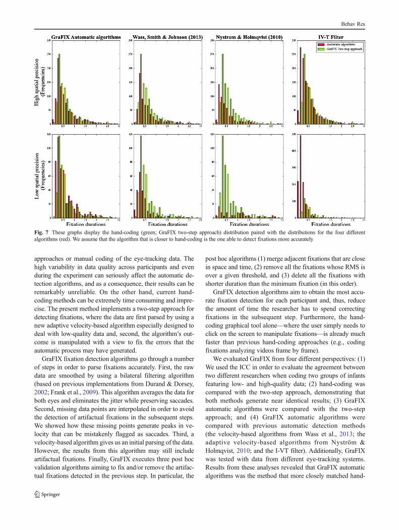
Table 4 shows the means and the standard deviationsobtained from the different algorithms and hand-coding, andFig. 7 displays the graphs with all the fixation duration distri-butions from the four algorithms paired with the hand-codingdistribution, which was coded by using the two-step approach.We assume that the algorithm that gets closer to the hand-coding distribution will be the one able to detect fixationsmore accurately. The differences between algorithms in bothhigh- and low-precision groups are striking. Results for thehigh-spatial-precision group revealed differences in the meansand also in the number of detected fixations. The I-VT filter, inparticular, presented an especially high number of de-tected fixations (N = 1199), as compared with hand-coding(N = 973), that can be the result of mistakenly flagging verysmall fixations in segments that were slightly noisier (seeFig. 7, first row, fourth column). For this reason, the meandurations (M = 554.0) are lower than the means for the otheralgorithms or for hand-coding. On the other hand, GraFIX andthe Wass et al. (2013) algorithms present means that are a bitabove the hand-coding mean (M = 674.5). An explanation forthis can be related to the selection of the velocity thresholdsand the sampling rate. As has previously been mentioned,saccades with very small amplitudes may go undetected byvelocity-based algorithms, especially when the data are re-corded at low sampling rates (<200). As a consequence, thefixations before and after these saccades will be mergedtogether in a longer fixation. Obviously, at higher velocitythresholds, it is more likely that fixations will be mergedtogether. Since the velocity threshold for Wass et al. (2013)

Table 2 Automatic versus hand-coding: Fixation duration (FD) meansand standard deviations in low- and high-spatial-precision data

High Spatial Precision Low Spatial Precision

Automaticalgorithms FDs

625.1 ± 847.8 (N = 2,410) 552.2 ± 536.3 (N = 863)

Two-stepapproach FDs

627.9 ± 866.2 (N = 2,268) 489.9 ± 445.9 (N = 858)

Fig. 6 GraFIX automatic algorithms versus two-step approach (automatic detection + hand-coding)

Behav Res

was higher (20 °/sec) than for GraFIX algorithms (9 °/sec), itis also not surprising that the mean for the first algorithms wasstill higher than for the present algorithms. The algorithms forNyström and Holmqvist (2010) avoided this problem byadapting the velocity threshold according to the level of noisein the data. Even though they still capture the trend in thedistribution, the data quality for the samples that were ana-lyzed (even for the high-precision group) is probably too lowto obtain more accurate results from these algorithms.Eyeballing the graphs from Fig. 7 (first row), it is possible tosee how the fixation duration distribution produced byGraFIX algorithms had the closest resemblance to the hand-coding distribution in high-precision data.

Results from the low-spatial-precision group revealed evenhigher differences between the four algorithms. As it can beseen in Table 4 and in Fig. 7 (second row, fourth column), theproblem that the I-VT filter presented in the high-precisiondata was even more obvious here. Likewise, the Nyström andHolmqvist (2010) algorithms did not manage to deal withsuch a high degree of noise (see Fig. 7, second row, thirdcolumn). Looking at the graphs and the means, it seems thatdue to the low precision in the data, the velocity threshold thatwas calculated may have been too high. It is also interesting tosee that even though the length of the recordings was approx-imately the same for the low- and high-quality groups, thenumber of detected fixations in the low-precision data wasalmost half the number of fixations detected in the high-precision data for the GraFIX algorithms, the Wass et al.

(2013) algorithms, and hand-coding. The Wass et al. (2013)algorithms exclude a high number of fixations with their posthoc validation criteria, and this is probably why their algo-rithms still detect many fewer fixations than do the algorithmsthat we propose. Once again, GraFIX algorithms seem toresemble the hand-coding fixation duration distribution moreaccurately, even though they would still need manual adjust-ments (the two-step approach) to be perfect.

Overall, even though all the algorithms are far from perfect,results from GraFIX algorithms were the ones that moreclosely matched the hand-coding results. We believe that thisis not only because of the particularities of our algorithms, butalso because we are adapting the input parameters to differentlevels of noise. We would not recommend, however, theexclusive use of automatic detection algorithms unless thedata quality is very high. Evidently, when the algorithms’outcome is accurate, the time that needs to be invested incorrecting artifactual fixations will be considerably lower.

In sum, GraFIX seems to be an effective alternative toprevious methods that will improve the quality of our resultsand the time invested coding eye-tracking data.

Discussion

In this article, we described a new method and software toparse fixations in low- and high-quality data. Previous fixationdetection methods are based on either purely automatic

Table 3 Input parameters for the automatic detection algorithms

GraFIX(High Quality)

GraFIX(Low Quality)

Wass, Smith, &Johnson (2013)

Nyström &Holmqvist (2010)

I-VTFilter

Interpolation latency (ms) 60 60 60 n.a. 60

Velocity threshold (°/sec) 9 20 20 Adaptive 20

Maximum interpolation displacement (°) 0.25 0.25 n.a. n.a. n.a.

Degree per pixel (°/pix) 0.0177 0.0177 0.0177 n.a. n.a.

Maximum distance for merging adjacent fixations (°) 0.24 0.35 n.a. n.a. 0.35

Maximum time for merging adjacent fixations (ms) 50 50 n.a. n.a. 50

Maximum RMS per fixation (°) 0.24 0.35 n.a. n.a. n.a.

Minimum fixation duration (ms) 99 120 100 100 100

Table 4 Comparing detection algorithms with hand-coding: Fixation durations means and standard deviations in low and high spatial precision data

High Spatial Precision Low Spatial Precision

Hand coding 674.5 ± 621.9 (N = 973) 657.3 ± 642.0 (N = 424)

GraFIX automatic algorithms 719.9 ± 696.4 (N = 954) 640.4 ± 589.3 (N = 505)

Wass, Smith, & Johnson (2013) 779.3 ± 826.5 (N = 676) 491.2 ± 490.2 (N = 229)

Nyström & Holmqvist (2010) 571.2 ± 588.7 (N = 540) 1,337.9 ± 1,435.1 (N =103)

I-VT Filter 554.0 ± 527.4 (N = 1,199) 240.7 ± 169.0 (N = 1,102)

Behav Res

approaches or manual coding of the eye-tracking data. Thehigh variability in data quality across participants and evenduring the experiment can seriously affect the automatic de-tection algorithms, and as a consequence, their results can beremarkably unreliable. On the other hand, current hand-coding methods can be extremely time consuming and impre-cise. The present method implements a two-step approach fordetecting fixations, where the data are first parsed by using anew adaptive velocity-based algorithm especially designed todeal with low-quality data and, second, the algorithm’s out-come is manipulated with a view to fix the errors that theautomatic process may have generated.

GraFIX fixation detection algorithms go through a numberof steps in order to parse fixations accurately. First, the rawdata are smoothed by using a bilateral filtering algorithm(based on previous implementations from Durand & Dorsey,2002; Frank et al., 2009). This algorithm averages the data forboth eyes and eliminates the jitter while preserving saccades.Second, missing data points are interpolated in order to avoidthe detection of artifactual fixations in the subsequent steps.We showed how these missing points generate peaks in ve-locity that can be mistakenly flagged as saccades. Third, avelocity-based algorithm gives us an initial parsing of the data.However, the results from this algorithm may still includeartifactual fixations. Finally, GraFIX executes three post hocvalidation algorithms aiming to fix and/or remove the artifac-tual fixations detected in the previous step. In particular, the

post hoc algorithms (1) merge adjacent fixations that are closein space and time, (2) remove all the fixations whose RMS isover a given threshold, and (3) delete all the fixations withshorter duration than the minimum fixation (in this order).

GraFIX detection algorithms aim to obtain the most accu-rate fixation detection for each participant and, thus, reducethe amount of time the researcher has to spend correctingfixations in the subsequent step. Furthermore, the hand-coding graphical tool alone—where the user simply needs toclick on the screen to manipulate fixations—is already muchfaster than previous hand-coding approaches (e.g., codingfixations analyzing videos frame by frame).

We evaluated GraFIX from four different perspectives: (1)We used the ICC in order to evaluate the agreement betweentwo different researchers when coding two groups of infantsfeaturing low- and high-quality data; (2) hand-coding wascompared with the two-step approach, demonstrating thatboth methods generate near identical results; (3) GraFIXautomatic algorithms were compared with the two-stepapproach; and (4) GraFIX automatic algorithms werecompared with previous automatic detection methods(the velocity-based algorithms from Wass et al., 2013; theadaptive velocity-based algorithms from Nyström &Holmqvist, 2010; and the I-VT filter). Additionally, GraFIXwas tested with data from different eye-tracking systems.Results from these analyses revealed that GraFIX automaticalgorithms was the method that more closely matched hand-

Fig. 7 These graphs display the hand-coding (green; GraFIX two-step approach) distribution paired with the distributions for the four differentalgorithms (red). We assume that the algorithm that is closer to hand-coding is the one able to detect fixations more accurately

Behav Res

coding results and that these algorithms alone can be a morereliable technique than other methods, overcoming some ofthe previous issues detecting fixation in low- and high-qualitydata. However, we strongly believe that given the nature ofour data, any automatic algorithm should be used in combi-nation with a later hand-coding approach.

Many of the current detection algorithms, especially thosecommercially available, obscure the quality of the data and thefixation detection process. Consequently, evaluating the reli-ability of results or checking how different parameters affectthe fixation detection may become an arduous task. GraFIXallows the adaptation of the input parameters for the automaticalgorithms (e.g., velocity threshold, interpolation latency) tofit the data from different participants that present differentlevels of data quality. As was previously explained, choosingthe right velocity threshold highly depends on the quality ofthe data and the experimental design. Ideally, the user willselect low thresholds in order to be able to detect smallfixational eye movements. However, the lower the data qual-ity is, the higher the velocity threshold needs to be. If all theparticipants are at very different levels of data quality, it can beworthwhile to adapt this value on a participant basis.Likewise, the rest of the parameters (such as the post hocvalidation parameters) should be adapted according to theparticipant’s data quality in the interest of obtaining themost accurate results. Additionally, the execution of thealgorithms is fast, and it displays all the informationthat we need to precisely evaluate what the algorithmscalculated (interpolation and post hoc validation flags foreach point, visualization of the results paired with the velocityand the raw and smoothed data.). This can enormously facil-itate the correct selection of the input parameters for thedetection algorithm.

Traditionally, all participants are grouped together, and asingle velocity threshold that is usually selected to fit low-quality sets is chosen to parse all the data. We have shownhow applying high velocity thresholds can be the reason whythe algorithms detect artifactual long fixations.We believe thatadapting the input parameters on a participant basis can avoidthe detection of artifactual fixations and will lead to moreaccurate and reliable experimental results. However, it is stillup to researchers to decide whether they prefer to use the sameparameters for all the participants, adapt the parameters on aparticipant basis, or rather have different input parameters fordifferent groups of participants featuring different levels ofdata quality (as we did in our validation section). It is also atopic of debate for the field of eye tracking as to how theparameters used to parse each participant’s data should bereported in publications, factored in to statistical analysis, orstandardized within populations and across labs.

But to which extent is it acceptable to group togetherparticipants with very different data quality? For instance, thiscan be an important issue in clinical group comparisons where

one group may present considerably lower quality data thanthe other (e.g., ADHD children vs. control groups), whenanalyzing different age groups (e.g., 3 month olds vs.14 month olds) or even when comparing “long fixators” with“short fixators.”We know that in low-quality data, there is lessprobability of finding clean long fixations that can be reliablydetected, also, when the data are hand-coded. This can lead tocorrelations between data quality and fixation durations wherelow-quality data sets are more likely to present shorter fixa-tions on average. To at least acknowledge these limitations inour studies, it would be advantageous to consistently reportdata quality measures and detailed descriptions of the detec-tion methods, together with a data quality correlationalanalysis. Nevertheless, this still does not solve the problem.

Another limitation is related to the way fixations are hand-coded. In the interest of improving the reproducibility of theexperimental outcomes, we believe it is very important toinclude precise guidelines to define how the fixations arebeing coded. In part, without these guidelines, the intercoderreliability loses its value.

In sum, the proposed method and software prove to bea more reliable and accurate technique for parsing fixa-tions in low- and high-quality data and overcomes manyof the issues that previous methods presented. More accu-rate outcomes and reporting data quality measures anddescriptions of the detection methods in scientific paperscan considerably improve the viability of research resultsand, hence, facilitate the replication of previous studies.This can have a big impact not only in research frompopulations that are particularly difficult to test and thattypically present higher degrees of noise (such as infants,people in the autism spectrum, or ADHD patients), butalso in participants that simply do not reach certain dataquality standards. In fact, nowadays we are experiencingan increase in the number of new low-cost eye-trackingsystems that inherently suffer from data quality issueseven with compliant participants. Additionally, GraFIXcould also be adapted to code data from head-mountedeye-tracking systems by including the head position and theeye and scene images.

Software download

Please download GraFIX from: http://sourceforge.net/projects/grafixfixationscoder/

Author note The authors wish to thank Kristen Swan Tummeltshammerfor her comments on the first draft of the manuscript. Thanks also toCasey Thornton for performing the hand-coding analysis. Thisresearch was supported by the EC Marie Curie Initial TrainingNetworks FP7-PEOPLE-2010-ITN PART B, and the UK MedicalResearch Council.

Behav Res

Appendix 1

Application overview

The main window consists of a number of boxes where theeye-tracking data and the application’s output is visualized, inaddition to all the necessary buttons used to manipulate fixa-tions (see Fig. 2). A brief explanation of these different com-ponents is included below.

1. Menu bar. The menu bar allows access to differentdialogs such as Project configuration, Visualizations, orAutomatic Detection of Fixations dialogs.

2. Raw data. The horizontal axis represents time, while thevertical axis displays the position of subsequent gazedata-points (Each data-point consists of the x- and y-coordinates for the right and/or the left eye.). For binoc-ular systems, the right- and left-eye coordinates aredisplayed (x-right = red; x-left = orange; y-right = darkblue; y-left = light blue). In case the system is monocular,the data from the second eye will simply not be displayed.

3. Smoothed data. As for the raw data, the horizontal axisrepresents time, while the vertical axis displays the po-sition of subsequent smoothed gaze data-points. Oncethe data is smoothed, the resulting x- and y-coordinatesare displayed.

4. Pupil dilation. In cases where the eye-tracking systemprovides pupil dilation data, it is displayed in this box.Further, the average pupil dilation is calculated for eachfixation.

5. Velocity. The horizontal axis represents time, while thevertical axis displays the velocity for subsequent gazedata-points.

6. Missing data from left and right eyes. If there is a data-point missing for either of the eyes, it is displayed in thisbox.

7. Automatically detected fixations. The orange boxes rep-resent the fixations that are automatically detected by theautomatic-detection algorithms.

8. Flags from the automatic-detection algorithm. Duringthe automatic detection, the data are interpolated, andthe post hoc validation criteria are applied. The flagsindicate which data-points were affected by differentalgorithms.

9. The cursor’s current location. A horizontal line isdisplayed at the cursor’s location, facilitating the accu-rate coding of fixations’ onsets and offsets. Additionally,the From label indicates the line in the raw file where thecursor is located.

10. Manually coded fixations. The green boxes represent thefixations that can be manipulated manually. Each fixa-tion has a fixation number that matches the numbersfrom the first column at the fixations list.

11. Fixations list. This is a list of the fixations that are beingmanually coded (green boxes). The first column showsthe fixation number, the second displays the line in theraw file where the fixation starts, the third displays theline in the raw file where the fixation ends, and finally,the fourth column reveals the fixation duration inseconds.

12. Select the action button. In order to perform an action,the corresponding option has to be selected. Once it isselected, one will need to click and drag the cursor inorder to create, delete, or merge fixations. Moreover, it ispossible to target smooth-pursuit fixations by selectingthis option and dragging the cursor on top of the fixa-tions that need to be coded. In order to add more preci-sion to the task, it is possible to enter in the textboxes thestart and the end of the fixation that needs to be manip-ulated and press Execute. This will execute the actioncurrently selected using the specified start and endpoints.

13. Nonactive segment. The portion of the screen in graycorresponds to the tasks in the experiment that do notneed to be coded.

14. Active segment. The portion of the screen in whitecorresponds to the tasks in the experiment that need tobe coded.

Input files

The raw input file is a csv file separated by commas with thefollowing columns: (1) time in microseconds; (2) zeros; (3)relative gaze-point x left eye; (4) relative gaze-point y left eye;(5) relative gaze-point x right eye; (6) relative gaze-point yright eye; (7) pupil diameter left eye (optional); and (8) pupildiameter right eye (optional).

If the eye-tracking system is monocular, all the columnscorresponding to the second eye should be substituted with−1 s.

The segments input file indicates which parts of theexperiment need to be coded. If the whole data file isthe subject of interest, this file does not need to beincluded.

The segments input file is a csv file separated by commaswith the following columns: (1) segment id, which is anunique number for each row; (2) row number in the raw filewhere the segment starts; (3) row number in the raw file wherethe segment ends.

Output files

File smooth_[subject number].csv This file is created whenthe data is smoothed. Each row corresponds to a data pointfrom the raw file; thus, both files have the same length. This

Behav Res

file is a csv file separated by commas with the followingcolumns: (1) time in microseconds; (2) zeros; (3) smoothedx-coordinate; (4) smoothed y-coordinate; (5) velocity; (6) Issaccade flag: 0/1; (7) Is interpolated flag: 0/1; (8) post hocmerge adjacent fixations flag: 0/1; (9) post hoc RMS flag: 0/1;(10) post hoc minimum fixation flag: 0/1.

File fix_auto_[subject number].csv This is created when fix-ations are automatically estimated. Each row contains theinformation for one fixation. This file is a csv file separatedby commas with the following columns: (1) row from the rawfile where the fixation starts; (2) row from the raw file wherethe fixation ends; (3) duration in seconds; (4) Average x-coordinate; (5) Average y-coordinate; (6) RMS; (7) Is smoothpursuit flag: 0/1; (8) Average pupil dilation.

File fix_all_[subject number].csv This file is generated whenthe first fixation is created, and it is updated every time afixation is manipulated. It is a csv file separated by commaswith the following columns: (1) row from the raw file wherethe fixation starts; (2) row from the raw file where the fixationends; (3) duration in seconds; (4) Average x-coordinate; (5)Average y-coordinate; (6) RMS; (7) Is smooth pursuit flag:0/1; (8) Average pupil dilation.

Appendix 2

Pseudo-code of the proposed interpolation algorithm

1. Calculate the velocities for each point2. Iteratively find velocity peaks and flag those over the

velocity threshold as saccades3. Find next gap

3.1. If the gap is longer than the interpolation latency:

3.1.1. Calculate the Euclidean distances from a centralpoint for the fixations preceding and followingthe gap.

3.1.2. If the difference between both Euclidean dis-tances is lower than the maximum displacementthreshold:

3.1.2.1. Interpolate.

Pseudo-code of the proposed velocity algorithm and thepost hoc validation

1. Calculate the velocities for each point2. Iteratively find velocity peaks and flag those over the

velocity threshold as saccades

3. The data points in between two saccades are grouped andflagged as fixations

4. Post hoc validation: Merge adjacent fixations with similarlocation

4.1. If this post hoc validation criterion is selected

4.1.1. Find next two adjacent fixations4.1.2. If the gap between the two fixations is shorter

then 50 ms

4.1.2.1. Calculate the distance in degrees betweenthe locations for the two fixations

4.1.2.2. If the distance is shorter than the maximumdisplacement threshold

4.1.2.2.1. Merge both fixations5. Post hoc validation: The RMS of intersample distances

per fixations does not exceed a threshold

5.1. If this post hoc validation criterion is selected

5.1.1. Find all fixations with an RMS over thethreshold

5.1.2. Delete them6. Post hoc validation: Minimum fixation duration

6.1. If this post hoc validation criterion is selected

6.1.1. Find all fixations with a duration over thethreshold

6.1.2. Delete them

Open Access This article is distributed under the terms of the CreativeCommons Attribution License which permits any use, distribution, andreproduction in any medium, provided the original author(s) and thesource are credited.

Referencces

Adolph, K. E., &Berger, S. E. (2006). Motor development. InW. Damon,R. Lerner, D. Kuhn, & R. S. Siegler (Eds.), Handbook of childpsychology: Vol 2: Cognition, perception and language (6th ed.,pp. 161–213). New York: Wiley.

Anliker, L. (1976). Eye movements: On-line measurement, analysis, andcontrol. In R. A. Monty & J. W. Senders (Eds.), Eye movements andpsychological processes (pp. 185–199). Hillsdale: Erlbaum.

Appel, M. A., & Campos, J. J. (1977). Binocular disparity as adiscriminable stimulus parameter for young infants. Journalof Experimental Child Psychology, 23(1), 47–56.

Aslin, R. N. (2007).What’s in a look?Developmental Science, 10(1), 48–53.Atkinson, J. (2000). The developing visual brain. Oxford University Press.Berg, D. J., Boehnke, S. E., Marino, R. A., Munoz, D. P., & Itti, L. (2009).

Free viewing of dynamic stimuli by humans and monkeys. Journalof Vision, 9(5).

Behav Res

Blignaut, P. (2009). Fixation identification: The optimum threshold for adispersion algorithm. Attention, Perception, & Psychophysics,71(4), 881–895.

Blignaut, P., & Wium, D. (2013). Eye-tracking data quality as affected byethnicity and experimental design. Behavior Research Methods, 1–14.

Castelhano, M. S., & Henderson, J. M. (2008). Stable individual differ-ences across images in human saccadic eye movements. CanadianJournal of Experimental Psychology/Revue Ccanadienne dePsychologie Expérimentale, 62(1), 1.

Colombo, J., & Cheatham, C. L. (2006). The emergence and basis ofendogenous attention in infancy and early childhood. Advances inChild Development and Behavior, 34, 283–322.

Durand, F., & Dorsey, J. (2002). Fast bilateral filtering for the display ofhigh-dynamic-range images.ACMTransactions onGraphics, 21(3),257–266.

Elsabbagh, M., Volein, A., Holmboe, K., Tucker, L., Csibra, G., Baron-Cohen, S., et al. (2009). Visual orienting in the early broader autismphenotype: disengagement and facilitation. Journal of ChildPsychology and Psychiatry, 50(5), 637–642.

Enright, J. T. (1998). Estimating peak velocity of rapid eye movementsfrom video recordings. Behavior Research Methods, Instruments, &Computers, 30(2), 349–353.

Frank, M. C., Vul, E., & Johnson, S. P. (2009). Development of infants’attention to faces during the first year. Cognition, 110(2), 160–170.

Frank, M. C., Vul, E., & Saxe, R. (2012). Measuring the development ofsocial attention using free-viewing. Infancy, 17(4), 355–375.

Frick, J. E., Colombo, J., & Saxon, T. F. (1999). Individual and develop-mental differences in disengagement of fixation in early infancy.Child Development, 70(3), 537–548.

Gredebäck, G., Johnson, S., & von Hofsten, C. (2009). Eye tracking ininfancy research. Developmental Neuropsychology, 35(1), 1–19.

Henderson, J. M., & Smith, T. J. (2009). How are eye fixation durationscontrolled during scene viewing? Further evidence from a sceneonset delay paradigm. Visual Cognition, 17(6–7), 1055–1082.

Holmqvist, K., Nyström, M., Andersson, R., Dewhurst, R., Jarodzka, H.,& van de Weijer, J. (2011). Eye Tracking. A comprehensive guide tomethods and measures. Oxford: Oxford University Press.

Holmqvist, K, Nyström, M., & Mulvey, F. (2012). Eye tracker data quality:what it is and how to measure it. In Proceedings of the Symposium onEye Tracking Research and Applications (pp. 45-52). ACM.

Hood, B. M., & Atkinson, J. (1993). Disengaging visual attention in theinfant and adult. Infant Behavior and Development, 16(4), 405–422.

Hunnius, S., & Geuze, R. H. (2004). Developmental changes in visualscanning of dynamic faces and abstract stimuli in infants: A longi-tudinal study. Infancy, 6(2), 231–255.

Hunter, S. K., & Richards, J. E. (2011). Characteristics of eye movements toSesame Street from 8 to 26 weeks of age. Manuscript submitted forpublication.

Johnson, M. H. (2010). Developmental cognitive Neuroscience (Thirdedit.). Oxford: Wiley-Blackwell.

Johnson, M. H., Posner, M. I., & Rothbart, M. K. (1991). Components ofvisual orienting in early infancy: Contingency learning, anticipatorylooking, and disengaging. Journal of Cognitive Neuroscience, 3(4),335–344.

Kano, F., & Tomonaga, M. (2011a). Perceptual mechanism underlyinggaze guidance in chimpanzees and humans. Animal Cognition,14(3), 377–386.

Kano, F., & Tomonaga, M. (2011b). Species difference in the timing ofgaze movement between chimpanzees and humans. AnimalCognition, 14(6), 879–892.

Kelly, D. J., Walker, R., & Norbury, C. F. (2013). Deficits in volitionaloculomotor control align with language status in autism spectrumdisorders. Developmental Science, 16(1), 56–66.

Kolakowski, S. M., & Pelz, J. B. (2006). Compensating for eye trackercamera movement. In Proceedings of the 2006 symposium on Eyetracking research & applications (pp. 79-85). ACM.

Komogortsev, O. V., Gobert, D. V., Jayarathna, S., & Gowda, S. M.(2010). Standardization of automated analyses of oculomotor fixa-tion and saccadic behaviors. Biomedical Engineering, IEEETransactions On, 57(11), 2635–2645.

Kowler, E. (2011). Eye movements: The past 25 years. Vision Research,51(13), 1457–1483.

Larsson, L., Nyström,M., & Stridh,M. (2013). Detection of saccades andpostsaccadic oscillations in the presence of smooth pursuit. IEEETransactions on Biomedical Engineering, 60(9).

Malcolm, G. L., & Henderson, J. M. (2010). Combining top-downprocesses to guide eye movements during real-world scene search.Journal of Vision, 10(2).

Martinez-Conde, S. (2005). The role of eye movements during visualfixation. Barrow Quarterly.

Martinez-Conde, S., Macknik, S. L., & Hubel, D. H. (2004). The role offixational eye movements in visual perception. Nature ReviewsNeuroscience, 5(3), 229–240.

Matin, E. (1974). Saccadic suppression: a review and an analysis.Psychological Bulletin, 81(12), 899.

Morris, T., Blenkhorn, P., & Zaidi, F. (2002). Blink detection for real-timeeye tracking. Journal of Network and Computer Applications, 25(2),129–143.

Nuthmann, A., Smith, T. J., Engbert, R., & Henderson, J. M. (2010).CRISP: A Computational model of fixation durations in sceneviewing. Psychological Review, 117(2), 382–405.

Nyström, M., & Holmqvist, K. (2010). An adaptive algorithm for fixa-tion, saccade, and glissade detection in eyetracking data. BehaviorResearch Methods, 42(1), 188–204.

Papageorgiou, K.A., Smith, T.J., Wu, R., Johnson, M.H., Kirkham, N.Z.,& Ronald, A. (2014) Individual Differences in Infant FixationDuration relate to Attention and Behavioral Control in Childhood.Manuscript under review.

Rayner, K. (1998). Eye movements in reading and information process-ing: 20 years of research. Psychological Bulletin, 124(3), 372.

Rayner, K., Smith, T. J., Malcolm, G. L., & Henderson, J. M. (2009). Eyemovements and visual encoding during scene perception.Psychological Science, 20(1), 6–10.

Richards, J. E., & Holley, F. B. (1999). Infant attention and the develop-ment of smooth pursuit tracking. Developmental Psychology, 35(3),856–867.

Richardson, D. C., Dale, R., & Spivey, M. J. (2007). Eye movements inlanguage and cognition : A brief introduction. Empirical Methods inCognitive Linguistics, 323–344.

Salapatek, P., Bechtold, A.G., &Bushnell, E.W. (1976). Infant visual acuityas a function of viewing distance. Child Development, 860–863.

Salvucci, D. D., & Goldberg, J. H. (2000). Identifying fixations andsaccades in eye-tracking protocols. In Proceedings of the 2000 sym-posium on Eye tracking research & applications (pp. 71-78). ACM.

Shic, F., Scassellati, B., & Chawarska, K. (2008, March). The incompletefixation measure. In Proceedings of the 2008 symposium on Eyetracking research & applications (pp. 111-114). ACM.

Smeets, J. B. J., & Hooge, I. T. C. (2003). Nature of variability insaccades. Journal of Neurophysiology, 90(1), 12–20.

Stampe, D.M. (1993). Heuristic filtering and reliable calibration methodsfor video-based pupil-tracking systems. Behavior ResearchMethods, Instruments, & Computers, 25(2), 137–142.

Tatler, B. W., Gilchrist, I. D., & Land, M. F. (2005). Visual memory forobjects in natural scenes: From fixations to object files. The QuarterlyJournal of Experimental Psychology Section A, 58(5), 931–960.

Wass, S. V., Smith, T. J., & Johnson, M. H. (2013). Parsing eye-trackingdata of variable quality to provide accurate fixation duration esti-mates in infants and adults. Behavior Research Methods, 45(1),229–250.

Yonas, A., Arterberry, M. E., & Granrud, C. E. (1987). Four-month-oldinfants’ sensitivity to binocular and kinetic information for three-dimensional-object shape. Child Development, 910–917.

Behav Res