GPS monitoring of the tropospheric water vapor distribution and variation during the 9 September...

GPS monitoring of the tropospheric water vapor distribution

and variation during the 9 September 2002 torrential

precipitation episode in the Cevennes (southern France)

C. Champollion,1 F. Masson,1 J. Van Baelen,2,3 A. Walpersdorf,4 J. Chery,1

and E. Doerflinger1

Received 13 April 2004; revised 10 September 2004; accepted 20 September 2004; published 17 December 2004.

[1] On 8–9 September 2002, torrential rainfall and flooding hit the Gard region insouthern France causing extensive damages and casualties. This is an exceptional exampleof a so-called Cevenol episode with 24 hour cumulative rainfall up to about 600 mmat some places and more than 200 mm over a large area (5500 km2). In this work we haveused GPS data to determine integrated water vapor (IWV) as well as horizontal wetgradients and residuals. Using the IWV, we have monitored the evolution of theconvective system associated with the rainfall from the water vapor accumulation stagethrough the stagnation of the convective cell and finally to the breakup of the system. Ourinterpretation of the GPS meteorological parameters is supported by synoptic maps,numerical weather analyses, and rain images from meteorological radars. We haveevidenced from GPS data that this heavy precipitation is associated with ongoingaccumulation of water vapor, even through the raining period, but that rain stopped assoon as the weather circulation pattern changed. The evolution of this event is typical inthe context of the Cevenol meteorology. Furthermore, we have shown that the horizontalwet gradients help describe the heterogeneity of the water vapor field and holdsinformation concerning the passage of the convective system. Finally, we have noticedthat the residuals, which in theory should be proportional to water vapor heterogeneity,were also highly perturbed by the precipitation itself. In our conclusions we discussthe interest of a regional GPS network for monitoring and for future studies on water vaportomography. INDEX TERMS: 3360 Meteorology and Atmospheric Dynamics: Remote sensing; 3394

Meteorology and Atmospheric Dynamics: Instruments and techniques; 6952 Radio Science: Radar

atmospheric physics; KEYWORDS: GPS, water vapor, wet gradients, intense rainfall, integrated water vapor,

residuals

Citation: Champollion, C., F. Masson, J. Van Baelen, A. Walpersdorf, J. Chery, and E. Doerflinger (2004), GPS monitoring of the

tropospheric water vapor distribution and variation during the 9 September 2002 torrential precipitation episode in the Cevennes

(southern France), J. Geophys. Res., 109, D24102, doi:10.1029/2004JD004897.

1. Introduction

[2] In autumn, southern France along the Mediterraneanarc is regularly the theater of extreme precipitation andflooding events producing societal damages including pub-lic and private goods destruction but also sometimes loss oflives. Such a strong event took place on 8–9 September2002 in the Gard region. It can be categorized as a

centennial catastrophe given the amount of precipitationand the extent of flooding. Indeed, the maximum value ofdaily accumulated precipitation recorded for 8 of Septemberis 543 mm at Saint-Christol-les-Ales in the Gard depart-ment, while the heavy precipitation occurred mainly in theafternoon of that day and the following night. Such a valueis close to the actual mean accumulated precipitation over ayear for that region. Furthermore, the geographical extent ofthe rainfall is extremely large as shown in Figure 1, wherean area of about 5000 km2 received an accumulated amountof precipitation of more that 300 mm for a 48 hour period.Finally, the 8–9 September 2002 event accounts for ahuman loss of life of 13 plus 6 missing, while propertydamages add up to several tens of million Euros.[3] This heavy precipitation event followed the classical

development scheme associated with the so-called ‘‘Cevenolepisodes’’ named after the Cevennes region which liesbetween the Massif Central mountainous region and theMediterranean plains. In this scheme [Barret et al., 1994], a

JOURNAL OF GEOPHYSICAL RESEARCH, VOL. 109, D24102, doi:10.1029/2004JD004897, 2004

1Laboratoire Dynamique de la Lithosphere, Universite MontpellierII-CNRS, Montpellier, France.

2Centre National de Recherches Meteorologiques CNRS-Meteo France,Toulouse, France.

3Now at Laboratoire de Meteorologie Physique, CNRS-UniversiteBlaise Pascal, Clermont-Ferrand, France.

4Laboratoire de Geophysique Interne et Tectonophysique, UniversiteJoseph Fourier-CNRS, Grenoble, France.

Copyright 2004 by the American Geophysical Union.0148-0227/04/2004JD004897

D24102 1 of 15

deep trough positioned between Ireland and Portugal gen-erates a stationary cut of low positioned over Spain associ-ated with cold stratospheric intrusion in altitude and a strongjet circulation which will produce lifting at its exit posi-tioned over the Cevennes region. Meanwhile, a surface lowdevelops over the Mediterranean Sea which induces asouthern low level flux of warm and humid air in the lowerlayers of the atmosphere. Thus the encounter of the coldaltitude air with the warm and humid surface flux plus theforcing due to the jet and the orography (the rise of theMassif Central and the funneling effect between thosemountains and the pre-Alps to the east) produces a veryunstable atmosphere prone to initiate deep convection andassociated strong precipitation. Autumn is such a criticalperiod because the artic cold air in altitude associated withthe trough formation often reaches these latitudes for thefirst time after the summer and come across a warmMediterranean sea and coastal regions. Hence more than70% of rain events with more that 200 mm daily accumu-lated precipitation take place between 25 August and15 November in that region [Barret et al., 1994].[4] The societal impact of such events could be strongly

mitigated if better forecasts of the expected amount ofprecipitation and its location were available. Usually, themain limitation for an accurate prediction of the precipita-tion and the modeling of the rain event dynamics is the poorknowledge of the water vapor field initial distribution andevolution [Emanuel et al., 1995; Ducrocq et al., 2002].Indeed, although the amount of water vapor cannot be

directly linked to precipitation amounts, water vapor canfuel the corresponding convective process.[5] Nowadays, to measure water vapor in the atmosphere,

meteorological services rely on standard synoptic radiosoundings. However, even though such devices providereasonably accurate measurements of water vapor profiles,they are far too sparsely distributed in space and time tosupport reliable forecasting of such rain events. Lately,Global Positioning Systems (GPS) has demonstrated itsability to monitor integrated water vapor (IWV) [Busingeret al., 1996; Duan et al., 1996; Tregoning et al., 1998] withan accuracy comparable to other means of measurements(radio soundings, microwave radiometers, . . .) [Niell et al.,2001; Revercomb et al., 2003; Van Baelen et al., 2004], butalso with good time resolution (better than hourly) andunder all meteorological conditions. As more and more GPSare being deployed and operated in a continuous mode forgeodetic purposes, they offer the potential for a dense andreliable water vapor measurement network. In this study, wehave used the data collected by continuously or semicon-tinuously operating geodetic and geodynamical networks insouthern France as well as some reference GPS stations inEurope.[6] In the following sections, we will first introduce the

GPS data used and their processing before focusing on thederivation of those parameters relevant to the meteorolog-ical documentation of the atmospheric water vapor content,distribution and variation. Then, we will present the mete-orological context of this event. We will study the IWVdistribution and evolution during the event while consider-ing the associated rainfall. From the wet gradients and theresiduals, we will describe the variability of the water vaporin the convective system. Furthermore, the effect of heavyrain on the GPS signals will be shown by a careful study ofthe residuals of the GPS processing. Finally, we will drawour conclusions and discuss the applications of GPS forweather monitoring and tomographic studies.

2. GPS Data and Processing

[7] The GPS data used in this study come from thecontinuously operating French networks RGP (Nationwidepermanent GPS network from the Institut GeographiqueNational: http://lareg.ensg.ign.fr/RGP/RGPhome.html) andREGAL (Alpine region GPS geodetic network: http://kreiz.unice.fr/regal), from the continuously operating GPSnetwork of Catalonia CATNET (http://draco.icc.es/geofons/catnet/en/home.php), and from 3 GPS stations of the semi-continuously operating French network VENICE [Massonet al., 2003]. The GPS station MAHO in the BalearicIslands is maintained by the Royal Observatory of Spain.The geographical spread and density of those GPS stationsis quite sparse but allows for the monitoring of the watervapor distribution and variations from the Balearic Islandsin the Mediterranean Sea to the Alps and over the area ofheavy precipitation and flooding.[8] The GPS data processing was performed with the

software GAMIT/GLOBK [King and Bock, 2000] in a quiteconventional way. We compute in a first run the precisecoordinates of the GPS stations in the ITRF 2000 frame[Altamimi et al., 2002] using 24 hour sessions, a cutoffangle of 10� and IGS final orbits. We use 10 GPS stations in

Figure 1. Map of the 48 hour (from 0600 UTC 8September to 0600 UTC 10 September 2002) cumulatedrainfall in millimeters in the south of France. The crossesindicate the rain gauges and the black circles the GPSpermanent stations. The topography is plotted every 1000 mwith black lines.

D24102 CHAMPOLLION ET AL.: GPS MONITORING OF THE WATER VAPOR

2 of 15

D24102

Europe for the frame referencing. The final station coor-dinates are obtained by constraining the fiducial GPSstations to their ITRF2000 coordinates using the Kalmanfilter GLOBK [Herring et al., 1990] in a global solution.We find a repeatability of about 2 mm on horizontal and5 mm on vertical baseline components. Then we perform asecond run with loose constraints of 1 meter on thecoordinates to evaluate hourly the tropospheric parameters[Bock et al., 2003], i.e., the zenith total delay (ZTD) and thetotal gradients. The lengths of the baselines are more than1500 km to decorrelate the tropospheric parameters estima-tion from vertical positioning. The zenith delay a prioriconstraints, the variation of the Gauss-Markov process andthe correlation time were set to 0.5 m, 0.01 m/

phour and

100 hours respectively and for the gradients 0.01 m, 0.01 m/phour and 100 hours. Once again we use the IGS final

orbits. We choose the ‘‘dry’’ and ‘‘wet’’ mapping functionsdescribed by Niell [1996]. We apply a sliding windowsession of 24 hours shifted by 12 hours to suppress theedge effect using the middle 12 hour of the session. Theatmospheric parameters calculated during the GPS treat-ment are the ZTD, the north-south and the east-west totalgradients at the elevation of 10�.

3. Wet Delay, Gradients, and One-Way Residuals

[9] The total atmospheric delay Latm between a GPSreceiver and each visible satellite is a function of both theelevation angle e and the azimuth angle a. Following Chenand Herring [1997], it can be decomposed into a sphericallysymmetric contribution of the atmosphere Lsym, an azimuth-dependent contribution of the atmosphere due to its anisot-ropy Laz, and residuals S:

Latm ¼ Lsym eð Þ þ Laz e;að Þ þ S; ð1Þ

with

Lsym eð Þ ¼ Lzhmh eð Þ þ Lz

wmw eð Þ; ð2aÞ

Laz e;að Þ ¼ Lnsh maz eð Þ cos að Þ þ Lew

h maz eð Þ sin að Þþ Lns

wmaz eð Þ cos að Þ þ Leww maz eð Þ sin að Þ: ð2bÞ

Lsym(e) is only elevation-dependent. Lhz and Lw

z are thezenith hydrostatic and wet delay, respectively, while mh(e)and mw(e) are the corresponding hydrostatic and wetmapping functions. In this study, we use the Niell mappingfunctions [Niell, 1996]. Laz(e, a) is azimuth and elevationdependent. Lh

ns, Lhew, Lw

ns and Lwew are respectively the north-

south and east-west components of the hydrostatic and wetgradients. maz is the gradient mapping function defined byChen and Herring [1997]. Residuals S are then defined asthe difference between the GAMIT final model results andthe observations (using the ionosphere free linear combina-tion LC). The ZTD obtained during the GPS treatment withthe GAMIT software is the sum of Lh

z and Lwz at the zenith or

Lsym(90�). The north-south and the east-west gradients

calculated by the GAMIT software are respectively Laz(10�,0�) and Laz(10�, 90�).[10] In order to study the water vapor contribution to the

GPS signals, we have to extract the wet delays and gradientsfrom the total atmospheric delay and gradients. To do so, wefirst derive the hydrostatic part of the zenith delay (Lh

z) fromsurface pressure measurements (Figure 2a) interpolated atthe station position following Davis et al. [1985]. Thesurface pressure measurements are the hourly synopticobservations of Meteo-France (French National WeatherService). The accuracy of the pressure measurement is0.1 hPa. The hydrostatic part of the total gradients(Figure 2b) is calculated from spatial variations of theground pressure. From the pressure field near the GPSstation, we calculate the spatial variations of the hydrostaticdelay per unit of distance (km) in the north-south and east-west directions: Zh

ns and Zhew. Thus the equations for the

Figure 2. (a) Surface pressure measurement at the sealevel the 8 September at 1800 UT. (b) Evolution of the total(circles, dark gray), hydrostatic (triangles, dark gray) andwet (triangles, light gray) gradients at CHRN between thedays 250 and 253.


3 of 15

D24102

hydrostatic gradients Lh and for the spatial variations of thehydrostatic delay Zh are:

Lh ¼Z1

0

z:g zð Þdz; ð3aÞ

and

Zh ¼Z1

0

g zð Þdz; ð3bÞ

where g is the horizontal gradient of the dry refractivity.Following Flores et al. [2000] or Elosegui et al. [1999], weconvert Zh to the hydrostatic gradients Lh assuming anexponential law in the hydrostatic refractivity such that:

Lnsh ¼ H:Zns

h and Lewh ¼ H:Zew

h ð4Þ

where H, the scale height of the gradients in the hydrostaticdelays is set to 13 km following Chen and Herring [1997],who propose a larger-scale height for the gradients thanthose normally associated with the atmosphere, althoughthey recognize that this assumption still needs to beconfirmed by atmospheric simulation tests with a nonhy-drostatic model.[11] The effect of the hydrostatic gradient correction

seems to be negligible in normal atmospheric conditions.On the contrary, during the passage of the convectivesystem over the area during the studied event, the hydro-static gradient amounts to about 20% of the total gradientwhich is not negligible (Figure 2b). Furthermore, thehydrostatic gradient is opposite to the total gradient, indi-cating that we need to take into account the hydrostaticgradient in order not to underestimate the wet gradient.[12] Removing the hydrostatic contributions from the

total delay leaves us with the zenith wet delay which canbe converted into integrated water vapor (IWV) using theformula obtained for the Mediterranean area by Emardsonand Derks [1999] from more than 37000 radio-soundingsand temperature surface measurements:

Lw

I¼ a0 þ a1:TD þ a2:T

2D; ð5Þ

where Lw is the ‘‘wet’’ delay, I the integrated water vapor(IWV), TD the surface temperature minus the mean surfacetemperature of the area (289.76�K for the Mediterraneanarea) and a0, a1, a2 coefficients derived by Emardson andDerks [1999] (respectively 6.324, �0.00177 and 0.000075).The accuracy of the equation (5) is estimated by the authorsto be approximately 1%.[13] The IWV represents the mean zenith integrated water

vapor as seen by one GPS station and depends on thespatial distribution of the satellites. Typical amplitudes ofthe IWV are between 5 and 40 kg/m2 with an accuracy ofabout 1 kg/m2 compared to VLBI, radio sounding andradiometer [Niell et al., 2001]. The wet gradients representthe integrated linear heterogeneity of the water vapor abovethe GPS station in the direction of those satellites. The

accuracy of the wet gradients is still poorly defined as thewet gradient is a parameter characteristic of GPS which isdifficult to reproduce with other instruments like the radi-ometer [Gradinarsky et al., 2000]. The postfit residuals arethe one-way (station-satellite) phase differences betweenthe model obtained from GAMIT by least squares inversionand the observations. During ‘‘normal’’ atmospheric con-ditions, they are mainly due to multipath, uncorrected phasecenter variations and receiver clock error and thus theycannot be interpreted in terms of water vapor content. Themagnitude of the residuals is about 1 mm of delay at thezenith. During particularly dynamic meteorological condi-tions, local atmospheric heterogeneities or hydrometeorscan greatly enhance these residuals (as shown later insection 7.).

4. Meteorological Context of the 8–9 September2002 Rain Event

[14] To study the meteorological background of thisevent, we will use 500 hPa geopotential analysis maps(Figure 3), surface wind and temperature analysis maps(Figure 4) and rain images (Figure 5) from the meteorolog-ical radar located near the town of Nımes, France. The beamof the radar is 1.8�. Each image is calculated from 3 scans at0.6�, 1.3� and 2.5� elevation above the horizon.[15] Figure 3 shows the 500 hPa geopotential analysis

maps for Sunday 8 September and Monday 9 September2002 at 1200 UTC. On the Sunday 8 September (Figure 3a),an upper cold pressure low is extended from Ireland toSpain by a deep trough. The low-level circulation associatedto this low pressure on the Iberian Peninsula is a warm andmoist south flow in the south France and in the RhoneValley. This surface circulation is clearly seen on the MeteoFrance operational model ARPEGE [Pailleux et al., 2000]analysis surface maps on Figure 4a. The convection startson the Mediterranean Sea (0400 UTC) as seen on therain radar images (Figure 5a) and in the land in themorning (Figure 5b). This deep convection organizes itselfin a V-shape, typical for high precipitation event in FrenchGard area (Figure 5c). The edge of the V is positioned at theplace of maximum convection where the clouds elevate thehighest and where the precipitation is maximum. The cloudsdevelop down-stream in a V shape fashion (Figure 5c)along the Massif Central contours and across the Rhonevalley [Barret et al., 1994]. The orientation of the V-shapeis given by the southwestern diffluent winds at the tropo-pause level (Figures 3a–3b). This deep convective systemwill give the main part of the precipitation. During theafternoon and the night of the 8 September, the region ofprecipitation moves slowly toward the east (Figure 5d).[16] On Monday 9 September in the morning, the arrival

of warm air from the Mediterranean Sea is still active(Figure 4b). Then, in the afternoon (Figure 3b), the axisof the trough changes from roughly north to south tonorthwest to southeast. The low-level flow begins to decay(Figure 4c) and the convection cells move toward the east(Figures 5e–5f ). The change in the synoptic circulation

Figure 3. The 500 hPa height analyses ofMeteo-France (FrenchNationalWeather Service) at 1200 UTC on (a) 8 Septemberand (b) 9 September. Geopotentials height (in mgp) and temperature (in �C) are represented respectively by solid and dashlines (H for high center of geopotential and B for low center).


4 of 15

D24102

Figure 3


5 of 15

D24102

corresponds to the end of the high precipitation in the southof France. More detailed description of the event and of theassociated precipitation can be found in the work of Delrieuet al. [2004]. This event associated with deep stationaryconvection above the Gard region caused the historicalprecipitation described in the introduction and representedon Figure 1.

5. IWV Variations and Associated Rainfall

5.1. Description of the IWV Time Series

[17] Figure 6 shows the temporal variation of the IWVfrom 7 to 9 September (days 250 to 252) 2002, at selectedstations used in our analysis. The initial amount of watervapor is high around the Balearic Islands (30 kg/m2 inMAHO, day 250 1200 UT), increases going to the north(35 kg/m2 in CREU, day 250 1800 UT) and is maximum inMTPL (40 kg/m2, day 251 1200 UT) close to the rainfall.Hence during the south to north travel, the air is continu-ously loaded with water vapor from evaporation due to theMediterranean Sea high surface temperatures at this periodof the year (Figure 4; Delrieu et al. [2004]). As the stationsMAHO, CREU and MTPL are situated on the flux trajec-tory, one can notice that the water vapor maximum is shiftedby about 6 hours between MAHO and CREU, whilebetween CREU and MTPL the shift takes about one dayindicating the stagnation of the mass of humid air whichcreates the favorable conditions for sustained convection.[18] Four groups of stations can be distinguished. First, the

southwestern stations (group 1: MALL, MAHO, EBRE,BELL and CREU), from the Balearic Islands to the easternPyrenees which document the inflow to the precipitationarea; second, the stations on the western border of the core ofthe precipitation area (group 2: MTPL, AIGL); third, thestations to the east of the precipitation area, at the foothills ofthe pre-Alps mountains (group 3: CHRN, MARS, VERC,SJDS, MICH, GINA); and finally, the stations in the exit partof the convective system, further to the east and the north(group 4: SJDV, JOUX, FCLZ, GRAS, SOPH, AJAC).[19] Considering the group 1 one can easily notice the

increase of IWV during the day 250 of about 10–15 kg/m2.One notices as well its south to north progression in timeand amplitude. Both are expected with the southern flowfrom the Mediterranean Sea (Figure 4). The IWV remainhigh during the end of the day 250 and the day 251. Thesestations within and around the Mediterranean Sea arelocated in the region of water vapor loading of the atmo-sphere: the area of convergence of water vapor of the southlow-level flux (Figure 4). Around the western border of therainfall zone, the group 2 shows an increasing IWV not onlyduring the day 250 but also during the day 251. Theincrease from 20 to 40 kg/m2 of the IWV is spectacularfor the MTPL station. This station location can be consid-ered as the southern limit of the catastrophic rainfall eventand demonstrates the high water vapor accumulation in thatregion prior to the start of the precipitation. Likewise, theAIGL station, which is in altitude on the first slopes of the

Figure 4. Wind vectors (unit vectors at the top right ofpanel corresponding to 25 ms�1) from the ARPEGEanalysis on at (a) 1200 UTC, 8 September, (b) 0000 UTC,9 September, and (c) 1200 UTC, 9 September.

Figure 5. Map of the rain rates observed by the Nımes weather radar at (a) 0400 UTC, (b) 1000 UTC, (c) 1800 UTC,8 September and at (d) 0200 UTC, (e) 1000 UTC, and (f) 1800 UTC, 9 September 2002. Black circles indicate the place ofGPS stations. In Figure 5c, black lines are represented the typical V-shape of rain system.


6 of 15

D24102

Figure 5


7 of 15

D24102

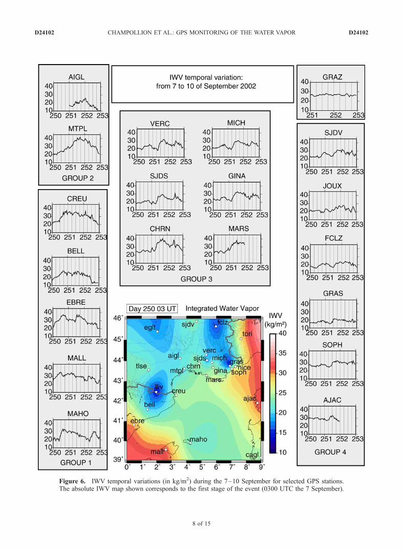
Figure 6. IWV temporal variations (in kg/m2) during the 7–10 September for selected GPS stations.The absolute IWV map shown corresponds to the first stage of the event (0300 UTC the 7 September).


8 of 15

D24102

Massif Central, exhibits relatively high values of IWVcorresponding to the ascent of water vapor loaded convec-tive clouds upon the orography (Figure 5c). The group 3located on the eastern border of the zone of the catastrophicrainfall does not show a clear evolution of the IWV on day250 up to the morning of day 251 and a very abrupt increaseof the IWV at about 0600 UTC on day 251. This indicatesthat there is no water vapor loading in that region: IWVincreases only when the convective system expands overthose stations. One will notice that the observed step of10 kg/m2 for the group 3 is generally preceded by a slightdecrease of the IWV. Most of the precipitation has beenobserved between the groups 2 and 3 where, unfortunately,no GPS permanent station was operating during this period.The contrasted IWV behavior between these two last groups(2 and 3) fits the common description of Cevenol episodeswith V shaped convective cloud formations. In our case, thegroup 2 are in the up-stream of the convective cell andmonitor the buildup of water vapor and fuelling of thesystem. The group 3 shows a decrease of water vaporprobably associated with low level convergence to the edgeof the system at the time of convective initiation, and a laterincrease of water vapor corresponding to the developmentof the convective clouds above their region. Therefore, asdemonstrated in Figure 2b, those stations of the group 3 willalso experience a strong east to west wet gradient withhigher values of IWV to the west, within the convectivecloud build up zone during the day 251 above the Gardregion. Finally, the stations of group 4 show signs of twoparts of the event. Its Mediterranean sites exhibit, to a lesserproportion, some water vapor increase associated with thesouthern flux of warm and humid air (Figure 4). Its northernsites show signs of fairly perturbed but high levels of watervapor associated with the exit phase of the convectiveregion during the night of 8 to 9 of September and thefollowing day. For comparison, the water vapor variation atthe GRAZ station in Austria is also shown to illustrateunperturbed meteorological conditions during those threedays of the study. In a processing point of view, thesimilarity and simultaneity of the transition for all thosestations located in a very small area is a good indication ofthe quality of the IWV estimates.

5.2. Spatial Evolution of the IWV

[20] To support the analysis above, we will now considerthe evolution of the water vapor field revealed by successiveIWV maps (Figure 7) over the area of interest. In order toplot the spatial variation of the IWV content corrected forthe effect of altitude (the altitude of the GPS stations variesfrom sea level to more than 1500 m high in the Cevennes orin the Pyrenees), we plot the IWV relative to a referencedistribution chosen at the beginning of the event: day 250 at0300 UTC. The IWV maps obtained are determined byHermit interpolation over the whole network. Hermit inter-polation uses the value and their derivatives in each point ofmeasure to constrain a polynomial interpolation. In thiscase, we use the east-west and north-south wet gradients as

the horizontal derivatives of the IWV values. Thus usingHermit interpolation the IWV variations are well definedeven in the areas without GPS stations but surrounded byseveral GPS stations. This is the case for the Gard depart-ment which corresponds to the region of maximum rainfall.Inversely, the borders of the map are noisier due to a lack ofneighboring data.[21] Although the GPS network is quite sparse, the large-

scale spatial and temporal variations can be studied fromthe IWV spatial distribution maps. They clearly point outthe water vapor displacement from the Mediterranean Sea(Figure 7a) to southern France and its accumulation overthe Gard region. The high water vapor zone is limited tothe west by the line CREU-MTPL, on the east by the lineMARS-MICH and on the north by the station SJDV. Thisindicates that the area of high water vapor content is largerthan the area of heavy precipitation as previously shown inFigure 1. The maximum IWV is located in the Gard regionduring about 24 hours between 0600 UTC day 251 and0600 UTC day 252 (Figures 7b–7d) and is well correlatedwith the area and period of maximum precipitation. At1200 UTC on day 252, the water vapor flux from the southbecomes weaker and its orientation changes, the watervapor and the convective cell move toward the east(Figures 7e–7f) indicating the end of the stagnation and thedilution of the convective system. All these characteristics arewell correlated with the rain images from Meteo-Franceradars, especially the eastward motion of the rain systemwhich marks the end of the catastrophic event (Figure 5).

5.3. Correlation Between IWV and Rain

[22] To investigate the correlation between IWV and rainat the ground level we will look at those GPS stationsclosest to the core of precipitation (AIGL, MTPL andCHRN) and which were almost collocated with rain gauges(less than 5 km). Rain gauges provide hourly accumulatedprecipitation data. The most intense rainfall has beenrecorded at the AIGL GPS station, with a maximum of50 mm/hour at midnight on day 251. IWV and rainfalltemporal variations do not show any clear correlation(Figure 8a). The increase of IWV is regular while the rainis abrupt. The maximum of IWV (30 kg/m2) occurs at theend of the rain time in early morning of day 252. It isinteresting to point out that the increase of IWV continuesduring the rain. In MTPL (Figure 8b), the rainfall is lessabrupt than in AIGL (25 mm/hour) but spreads over alonger period (about 12 hours). Once again there isa continual increase of water vapor during the rain and amaximum IWV at the end of the rain. This could indicatethat the decrease of water vapor due to the precipitation isovercompensated by the south flux of water vapor whichfuels the convective system and by evaporation. The mea-sured rain at CHRN is quite different (Figure 8c). We see ahigh increase of IWV on the beginning of the day 251followed by a small rain event (20 mm/hour) at noon. This iscomparable to the phenomena observed at MTPL but withless intensity. However, a stronger rain event (30 mm/hour)

Figure 7. (a–f) IWV maps of the southeast of France relative to day 250 at 1800 UT for each 8 hours from 8 September0200 UT. The topography is plotted every 1000 m with black lines. In Figure 7c, black lines represent the typical V-shapeof rain system taken from rain radar images (Figure 5).


9 of 15

D24102

Figure 7


10 of 15

D24102

Figure 8. Temporal variation of the amplitude of the rain (dark gray, in millimeters) and of the IWV(light gray, in kg/m2) for the Julian days 251–252 at the GPS locations (a–c) AIGL, MTPL, and CHRN.


11 of 15

D24102

is observed later at about 0600 UTC on day 252 and isdirectly correlated to a short term increase of water vapor.This is to be linked with intense but localized precipitationwhich can arise in the wake of the V-shape convectivesystem that has developed over the Gard region and hasfar less impacts than the large and continuous rain experi-enced at the core of the system. To summarize, the large rainevent occurred when the IWV reached high values of about30 to 40 kg/m2 (water vapor fuels the convective system) butthere is no direct relationship between IWV and the amountof precipitation.

6. Heterogeneity of Water Vapor Distribution:Study of Wet Gradients

[23] As the poor density of the GPS network availabledoes not allow for detailed studies of the water vaporheterogeneities based on the IWV only, we will now studythe meteorological information provided by the sum of thewet gradients and the residuals. It can be viewed as anaccurate description of the horizontal heterogeneities of theatmosphere within the GPS station field of view.

[24] The sky plots in Figure 9 show the sum of the wetgradients and the residuals for the CHRN station during theday 252 for a period of 4 hours, while the black arrowsrepresent the mean gradient and the ellipses its dispersion(RMS) during the corresponding periods. On these skyplots, one can easily observe the motion of the IWVassociated with the convective precipitation event studied.From 0000 to 0800 UTC, the gradients reveal a highconcentration of water vapor toward the west and the south.The sky plots show a clear east to west pattern, involving arelatively high gradient and a small RMS. This is consistentwith the stagnation of the convective system over the Gardregion (to the west) and its fuelling with water vaporcoming from the Mediterranean (to the south). From 0800to 1600 UTC, the gradients do not show any clear patternand their RMS over four hours becomes larger than thesignal. This can be related to the convective system extend-ing above the station considered and filling the GPS field ofview. After 1600 UTC, there is a clear (but small) west toeast pattern in the sky plots. The corresponding west to eastgradient associated with a small RMS is opposite to thegradient in the morning. This can be related to the fact that

Figure 9. Sky plot of the wet gradients and the residuals along the GPS satellites tracks for the9 September 2002. Each circle represents a period of 4 hours. The line in the north of the sky plotrepresents 19 mm of delay. Light gray (dark gray) indicates positive (negative) delay. The dark arrow inthe center of each circle represent the mean gradient during 4 hours and the ellipse the associated RMS.


12 of 15

D24102

the convective system has broken up and is being advectedfurther to the east. Observations from the other GPS stationsin the vicinity of the heavy rainfall area are all consistentwith the water vapor evolution scheme just described.Moreover, the water vapor evolution depicted here com-pares favorably with the meteorological radar observationsof the rain system (Figure 5). Finally, one will also noticethat the maximum amplitude of the wet gradients is notcorrelated with the rain itself. Actually, rain seems to occurwhen there are rapid changes in both the orientation and theamplitude of the wet gradients.[25] In summary, the information provided by the wet

gradients is a quasi-direct measure of the water vapor fieldhorizontal variability within a horizontal scale of about50 km. Thus a GPS station is capable not only to providean observation of the integrated water vapor content of thetroposphere above the receiver but can also provide anumerical measure of the azimuth variation of the watervapor distribution.

7. Investigation of the Residuals

[26] To get a more detailed look at the water vaporheterogeneity, we will now consider the residuals in an

isolated way. Compared to the wet gradients, the residualscould provide the finest-scale heterogeneity (less than50 km) of the water vapor field. They are not a mean modelof the heterogeneity over all the satellites like the gradientsbut the remaining signal between one GPS station and onesatellite. On the Figure 10, we have plotted the sky plots ofthe residuals along the GPS satellites tracks for the 8 Sep-tember at MTPL (Julian day 251 of 2002). During the mainrainfall from 0800 to 2000 UTC, the residuals are high andvariable. Compared to average values of the residuals at thisstation, the residuals observed during the rainfall are two tothree times larger. However, they do not allow identifyingany water vapor organized structure. These high residualsdo not result from multipath either as they are not elevationdependent. They could be due to an increase of electromag-netic (EM) effects of the fiberglass box of the GPS antennaduring the rain. Indeed, the water on the fiberglass boxcould change its EM characteristics. However, if that wasthe case, the rain should only enhance preexisting patternsof the residuals (see http://www-gpsg.mit.edu/�tah/web/japan_gps_met/GPSMetJapan.html) and that is not verifiedhere. Another explanation could be a large and very hightemporal variability of the water vapor during the rain withsome interaction between evaporation and condensation. To

Figure 10. Sky plot of the residuals along the GPS satellites tracks for the 9 September 2002. Lightgray (dark gray) indicates positive (negative) delay. Each circle represents a period of 4 hours. The line inthe north of the sky plot represents 9.5 mm of delay.


13 of 15

D24102

test this hypothesis, we compute gradients and ZTD every30 and 15 min to have a finer representation of the temporalvariation of water vapor field. If the temporal variability ofthe troposphere was the main reason for those residuals,they should decrease using shorter meteorological GPSparameter intervals. We find only a limited decrease ofthe residuals but not strong enough to retrieve the typicalamplitude of a normal day at these stations or of anotherGPS station (WTZR) in central Europe (Table 1). Theunmodeled spatial variability of water vapor within the fieldof view of the GPS antenna could also contribute to theresiduals. This kind of hypothesis could be tested with alocal tomography of water vapor [Champollion et al.,2004]. The tomography can however not be achieved forthis study because of the too large spacing between GPSstations. Finally, the most significant part of the residualscould be due to liquid water in the troposphere in the formof rain, ice and clouds. The enhancement of the residuals iswell correlated in time with the precipitation with a maxi-mum for MTPL and CHRN at about 1200 UTC the8 September. The levels of residuals found in our studyare in good agreement with the absorption model describedby Solheim et al. [1999] who find 5 mm/km of surface delayfor rainfall of 50 mm/hour with a scale height of 3 or 4 km.Further studies with high resolution numerical weathersimulations confirm this hypothesis (H. Brenot et al.,manuscript in preparation, 2004).

8. Conclusions

[27] IWV temporal variations (Figure 5), IWV spatialvariations (Figure 6) and wet gradients temporal variations(Figure 9) can improve the understanding of large rainfallevents. They allow an accurate and continuous descriptionof the water vapor field variations before, during and afterthe heavy precipitation.[28] In our case study, the IWV reveals that the water

vapor flux is initiated in the Mediterranean Sea south of theBalearic Islands and moves northward parallel to theSpanish shoreline. The water vapor content increases dur-ing the northward motion. The velocity of the fluxdecreases while reaching the French shoreline. Finally,the maximum water vapor content is observed in MTPL,just south of the maximum rainfall zone. Different temporalvariations of IWV are observed between the GPS stationswest and east of the rainfall area. The water vapor increasescontinuously and linearly for the stations southwest of theraining area. They are located in the ‘‘loading’’ zone. Eastof the raining area, the IWV variations are more complex,with successive increases and decreases, indicating thecomplexity of the phenomena close to the rainfall zone attime of precipitation but especially once the convective

system breaks up. These interpretations are confirmed bythe ARPEGE analyses and the rain images from radars(Figures 4 and 5).[29] This study also illustrates an important result about

the wet gradients: a single GPS station can provide partialinformation on the heterogeneity of the troposphere byextracting the wet gradients. During the passage of the rainsystem, the wet gradients are weak and highly variable.Before and after the rain, the wet gradients give clearinformation of the lateral heterogeneity of the atmosphere.They indicate the contrast of humidity between the differentparts of the meteorological system. For the monitoring of airmass heterogeneity, the wet gradients are a good indicatorwhich could be available in near real time like othermeteorological parameters. They could be used for estimat-ing the time of arrival of a front above a GPS station and,thus, for checking and updating the event chronology innumerical weather prediction forecasts.[30] Theoretically, the study of the residuals provides the

finest information about the water vapor heterogeneitywhich cannot be modeled by the IWV and the gradients.The residuals also include the noise due to the liquid water,the multipath, the errors of the mapping function, etc. TheMTPL data indicate that the residuals increase significantlyduring the large rainfall probably due to rain scattering. Ifthis observation is confirmed, GPS residuals could beinvestigated in relation with the characterization of the rain.Furthermore, the modeling of the residuals due to therain could be useful to correct the gradients for meteoro-logical applications like GPS water vapor tomography[Champollion et al., 2004]) or data assimilation in numer-ical models [Gutman et al., 2004].[31] This study has been conducted using the current

permanent GPS network of southern France and Spain.Further studies need a denser GPS network recording dataduring a long period to get a database covering severalcatastrophic rainfall events. A large database will allow tocharacterize the catastrophic rainfall situations and to dis-tinguish these events from standard autumnal precipitation.A field experiment could be conducted next autumn withmore temporary GPS stations from Marseille to Agde, i.e.,covering the zone of the maximum rainfall with a typicalspacing of 50 km. From these data, we will be able toresolve the small-scale variations in 3-D of the watervapor with the tomographic software we have developed[Champollion et al., 2004] and get an insight intomonitoring and the dynamics of strong rain events.GPS stations have been located close to the shorelineto study the potential of GPS to explore the troposphereabove the Mediterranean Sea, to provide a precursor ofthe catastrophic rainfall events. In ongoing work, gra-dients and residuals will be carefully studied.

Table 1. Mean RMS of the Residuals Between 0000 and 2400 UTC, Julian Day 251 for the GPS Stations MTPL, CHRN, and WTZRa

ZTD and GradientsEvaluated Every 2 Hours

ZTD and GradientsEvaluated Every Hour

ZTD and GradientsEvaluated Every 30 min

ZTD and GradientsEvaluated Every 15 min

CHRN 8.39.616.113.5 mean 11.9 mm 8.09.015.813.2 mean 11.5 mm 7.68.315.512.3 mean:10.9 mm 6.47.315.311.9 mean 10.2 mmMTPL 7.213.122.815.7 mean 14.7 mm 7.1 13.1 22.6 15.6 mean 14.6 mm 6.812.121.114.2 mean: 13.5 mm 6.011.120.112.4 mean 12.4 mmWTZR 6.55.97.86.9 mean 6.8 mm 6.25.87.36.5 mean 6.4 mm 6.25.87.3 6.5 mean 6.4 mm 6.15.67.36.0 mean 6.2 mm

aThe ZTD and gradients are evaluated every 2 hours, 1 hour, 30 min, and 15 min. The italic numbers indicate respectively the RMS of the residualsbetween 0000 and 0600, 0600 and 1200, 1200 and 1800, and 1800 and 2400 UTC. The mean RMS is for the whole 24 hours.


14 of 15

D24102

[32] Acknowledgments. This work was partially supported by theInstitut des Sciences de la Terre, de l’Environnement et de l’Espace deMontpellier (ISTEEM) and by the Observatoire HydrometeorologiqueMediterraneen Cevennes-Vivarais (OHMCV). We thank Philippe Collard,Laboratoire Dynamique de la Lithosphere (LDL), for his work in theinstallation and the maintenance of the VENICE semipermanent GPSnetwork, Sandrine Anquetin and Simon Yates, Laboratoire d’etude desTransferts en Hydrologie et Environnement (LTHE), for providing the raingauge data. We would like to thank the three anonymous reviewers for theirdetailed and relevant comments of this paper.

ReferencesAltamimi, Z., P. Sillard, and C. Boucher (2002), ITRF2000: A new releaseof the International Terrestrial Reference Frame for earth science applica-tions, J. Geophys. Res., 107(B10), 2214, doi:10.1029/2001JB000561.

Barret, I., V. Jacq, and J.-C. Rivrain (1994), Une situation a l’origine depluies diluviennes en region mediterraneenne, La Meteorol., 8(7), 38–60.

Bock, O., M.-N. Bouin, Y. Morille, and T. Lommatzsch (2003), Study ofthe sensitivity of ZTD estimates to GPS data analysis procedure, paperpresented at EGS-AGU-EUG Joint Assembly XXVII, Eur. Geophys.Soc., Nice.

Businger, S., S. R. Chiswell, M. Bevis, J. Duan, R. A. Anthes, C. Rocken,R. H. Ware, M. Exner, T. VanHove, and F. Solheim (1996), The promiseof GPS in atmospheric monitoring, Bull. Am. Meteorol. Soc., 77, 5–18.

Champollion, C., F. Masson, M.-N. Bouin, A. Walpersdorf, E. Doerflinger,O. Bock, and J. Van Baelen (2004), GPS water vapor tomography: Firstresults from the ESCOMPTE Field Experiment, Atmos. Res., in press.

Chen, G., and T. A. Herring (1997), Effects of atmospheric azimuthalasymmetry on the analysis of space geodetic data, J. Geophys. Res.,102(B9), 20,489–20,502.

Davis, J. L., T. H. Herring, I. I. Shapiro, A. E. E. Rogers, and G. Elgered(1985), Geodesy by radio interferometry: Effects of atmospheric model-ing errors on estimation of baseline length, Radio Sci., 20, 1593–1607.

Delrieu, G., et al. (2004), The catastrophic flash-flood event of 8–9September 2002 in the Gard region, France: A first case study forthe cevennes-Vivarais Mediterranean Hydrometeorological Observatory,J. Hydrometeorol., in press.

Duan, J. B., et al. (1996), GPS meteorology: Direct estimation of theabsolute value of precipitable water, J. Appl. Meteorol., 35(6), 830–838.

Ducrocq, V., D. Ricard, J.-P. Lafore, and F. Orain (2002), Storm-scalenumerical rainfall prediction for five precipitations events over France:On the importance of the initial humidity field, Weather Forecast., 17,1236–1256.

Elosegui, P., J. L. Davis, L. P. Gradinarsky, G. Elgered, J.M. Johansson,D. A.Tahmoush, and A. Rius (1999), Sensing atmospheric structure usingsmall-scale space geodetic networks, Geophys. Res. Lett., 26(16),2445–2448.

Emanuel, K. A., et al. (1995), Report of the first prospectus developmentteam of the U.S. Weather Research Program to NOAA and the NSF, Bull.Am. Meteorol. Soc., 76, 1194–1208.

Emardson, T. R., and H. J. P. Derks (1999), On the relation between the wetdelay and the integrated precipitable water vapour in the European atmo-sphere, Meteorol. Appl., 6, 1–12.

Flores, A., G. Ruffini, and A. Rius (2000), 4D tropospheric tomographyusing GPS slant wet delays, Annal. Geophys., 18, 223–234.

Gradinarsky, L. P., R. Haas, G. Elgered, and J. Jonhasson (2000), Wet pathdelay and delay gradients inferred from microwave radiometer, GPS andVLBI observations, Earth Planets Space, 52(10), 695–698.

Gutman, S., S. R. Sahm, S. G. Benjamin, B. E. Schwartz, K. L. Holub, J. Q.Stewart, and T. L. Smith (2004), Rapid retrieval and assimilation ofground based GPS precipitable water observations at the NOAA ForecastSystems Laboratory: Impact on weather forecasts, J. Meteorol. Soc. Jpn.,82(1B), 351–360.

Herring, T. A., J. L. Davis, and I. I. Shapiro (1990), Geodesy by radiointerferometry: The application of Kalman filtering to the analysis of verylong baseline interferometry data, J. Geophys. Res., 95(B8), 12,561–12,581.

King, R. W., and Y. Bock (2000), Documentation for the GAMIT GPSanalysis software, release 10.0, Dep. of Earth Atmos. and Planet. Sci.,Mass. Inst. of Technol., Cambridge, Mass.

Masson, F., P. Collard, J. Chery, J.-F. Ritz, E. Doerflinger, O. Bellier,D. Chardon, and M. Flouzat (2003), The VENICE project: A GPSnetwork to monitor the deformation in western Provence and easternLanguedoc (southern France), paper presented at EGS-AGU-EUGJoint Assembly, Eur. Geophys. Soc., XXVII, Nice.

Niell, A. E. (1996), Global mapping functions for the atmosphere delay atradio wavelengths, J. Geophys. Res., 101(B2), 3227–3246.

Niell, A. E., A. J. Coster, F. S. Solheim, V. B. Mendes, A. Toor, J. R. B.Langley, and C. A. Upham (2001), Comparison of measurements ofatmospheric wet delay by radiosonde, water vapour radiometer, GPS,and VLBI, J. Atmos. Oceanic Technol., 18, 830–850.

Pailleux, J., J.-F. Geleyn, and E. Legrand (2000), La prevision numeriquedu temps avec les modeles Arpege et Aladin, bilan et perspectives, LaMeteorol., 30, 32–60.

Revercomb, H. E., et al. (2003), The ARM program’s water vapour inten-sive observation periods: Overview, initial accomplishments, and futurechallenges, Bull. Am. Meteorol. Soc., 84, 217–236.

Solheim, F. S., J. Vivekanandan, R. Ware, and C. Rocken (1999), Propaga-tion delays induced in GPS signals by dry air, water vapour, hydrome-teors and other particulates, J. Geophys. Res., 104, 9663–9670.

Tregoning, P., R. Boers, D. O’Brien, and M. Hendy (1998), Accuracy ofabsolute precipitable water vapor estimates from GPS observations,J. Geophys. Res., 103, 28,701–28,710.

Van Baelen, J., J.-P. Aubagnac, and A. Dabas (2004), Comparison ofnear real-time estimates of integrated water vapour derived with GPS,radiosondes, and microwave radiometer, J. Atmos. Ocean. Technol., inpress.

��C. Champollion, J. Chery, E. Doerflinger, and F. Masson, Laboratoire

Dynamique de la Lithosphere, Universite Montpellier II-CNRS, MontpellierF-34095, France. ([email protected])J. Van Baelen, Laboratoire de Meteorologie Physique, CNRS-Universite

Blaise Pascal, Clermont-Ferrand, F-63006, France.A. Walpersdorf, Laboratoire de Geophysique Interne et Tectonophysique,

Universite Joseph Fourier-CNRS, Grenoble F-38041, France.


15 of 15

D24102

GPS monitoring of the tropospheric water vapor distribution and variation during the 9 September...

Documents

Transcript of GPS monitoring of the tropospheric water vapor distribution and variation during the 9 September...