GOCO06s – A satellite-only global gravity field model - ESSD

GOCO06s – A satellite-only global gravity field modelAndreas Kvas1, Jan Martin Brockmann2, Sandro Krauss1,5, Till Schubert2, Thomas Gruber3,Ulrich Meyer4, Torsten Mayer-Gürr1, Wolf-Dieter Schuh2, Adrian Jäggi4, and Roland Pail3

1Institute of Geodesy, Graz University of Technology, Steyrergasse 30/III, 8010 Graz, Austria2Institute of Geodesy and Geoinformation, University of Bonn, Nußallee 17, 53115 Bonn, Germany3Astronomical and Physical Geodesy, Technical University of Munich, Arcisstraße 21, 80333 Munich, Germany4Astronomical Institute, University of Bern, Sidlerstrasse 5, 3012 Bern, Switzerland5Austrian Academy of Sciences, Space Research Institute, Schmiedlstraße 6, 8042 Graz, Austria

Correspondence: Andreas Kvas ([email protected])

Abstract. GOCO06s is the latest satellite-only global gravity field model computed by the GOCO (“Gravity Observation

Combination“) project. It is based on over a billion observations acquired over 15 years from 19 satellites with different

complementary observation principles. This combination of different measurement techniques is key in providing consistent

high-accuracy and best possible spatial resolution of the Earth’s gravity field.

The motivation for the new release was in the availability of reprocessed observation data for GRACE and GOCE, updated5

background models, and substantial improvements in the processing chains of the individual contributions. Due to the long

observation period, the model consists not only of a static gravity field, but comprises additionally modeled temporal variations.

These are represented by time variable spherical harmonic coefficients, using a deterministic model for a regularized trend and

annual oscillation.

The main focus within the GOCO combination process is on the proper handling of the stochastic behavior of the input10

data. Appropriate noise modelling for the used observations result in realistic accuracy information for the derived gravity

field solution. This accuracy information, represented by the full variance-covariance matrix, is extremely useful for further

combination with, for example, terrestrial gravity data and is published together with the solution.

The primary model data (Kvas et al., 2019b) consisting of potential coefficients representing Earth’s static gravity field,

together with secular and annual variations are available on International Centre for Global Earth Models (http://icgem.gfz-15

potsdam.de/, last accessed 2020-06-11). This data set is identified with the DOI 10.5880/ICGEM.2019.002.

Supplementary material consisting of the full variance-covariance matrix of the static potential coefficients and estimated

co-seismic mass changes are available on ifg.tugraz.at/GOCO (last accessed 2020-06-11).

1 Introduction

Global models of Earth’s static gravity field are crucial for geophysical and geodetic applications. These include oceanography20

(e.g. Knudsen et al., 2011; Rio et al., 2014; Johannessen et al., 2014; Bingham et al., 2014), tectonics (e.g. Johannessen et al.,

2003; Ebbing et al., 2018), or establishing global reference and height systems (e.g. Rummel, 2013; Gerlach and Rummel,

2013). A special class of global gravity field models are the models derived solely from satellite observations. In contrast

1

https://doi.org/10.5194/essd-2020-192

Ope

n A

cces

s Earth System

Science

DataD

iscussio

ns

Preprint. Discussion started: 12 August 2020c© Author(s) 2020. CC BY 4.0 License.

to terrestrial observations – which are generally sparse and collected by various instruments in different quality levels and

samplings – satellite observations typically cover the entire Earth’s surface. As the measurements are captured with the same25

sensor platform, the global accuracy level of the observations is much more consistent compared to terrestrial observations.

This also alleviates adequate stochastic modelling at observation level (Ellmer, 2018; Schubert et al., 2019) to subsequently

provide uncertainty information for the derived gravity field.

The era of dedicated gravity field satellite missions (Rummel et al., 2002) provided a huge set of observations of the static as

well as time-variable gravity field. The satellite orbits are sensitive to the long wavelength of the gravity field (e.g. Montenbruck30

and Gill, 2000; Rummel et al., 2002). They are either determined from ground by Satellite Laser Ranging (SLR) or from

space via the tracking of a low-earth orbiter (LEO) with the satellites of the Global Position System (GPS) constellation. The

laser tracking of high-flying SLR satellites is sensitive only for the longest wavelengths, but allows to observe the temporal

variations as well (e.g. Maier et al., 2012; Sosnica et al., 2015; Bloßfeld et al., 2018). Starting with the dedicated CHAllenging

Minisatellite Payload satellite mission (CHAMP, Reigbar et al., 1999) different LEO satellites were tracked by GPS. This35

technique, called atellite-to-satellite tracking in high-low (SST-hl) configuration, has since been used to derive static, but also

temporal gravity field models of the Earth (e.g. Bezdek et al., 2016; Lück et al., 2018; Teixeira da Encarnação et al., 2016).

Although, SST-hl is sensitive to shorter wavelengths due to the generally lower satellite altitude compared to SLR, the spatial

resolution is still limited. With the Gravity Recovery And Climate Experiment (GRACE) twin satellite mission launched in

2002 (Tapley et al., 2004, 2019), inline satellite-to-satellite tracking (SST-low-low, SST-ll) was established. This then novel40

measurement principle relies on very precise measurements of inter-satellite distance variations between a leading and a trailing

satellite in the same orbit. While GRACE is dedicated to observe temporal changes in Earth’s gravitational field, typically in

the form of monthly snapshots (e.g. Rummel et al., 2002; Tapley et al., 2004; Mayer-Gürr, 2006; Chen et al., 2018a; Beutler

et al., 2010), accumulating observations over a longer time span allows to derive a mean (static) gravity field. After the end of

the mission in 2017, the GRACE Follow-On mission continues the observations since 2018 (Kornfeld et al., 2019; Landerer45

et al., 2020), following the same design principle.

To increase the spatial resolution, tailored to the requirements of geodetic, geophysical and oceanographic applications,

the Gravity field and steady-state Ocean Circulation Explorer (GOCE) mission (Battrick, 1999) was realized and launched in

2009. In addition to SST-hl, a gradiometer served for the first time as a core instrument to measure the second derivatives of

the Earth’s gravitational potential in gradiometer reference frame (Rummel and Colombo, 1985; Rummel et al., 2002, 2011b;50

Johannessen et al., 2003). Due to the design of the instrument (Stummer et al., 2012; Siemes et al., 2012, 2019), only four out

of the six derivatives of the Marussi tensor could be measured with high-precision (VXX , VXZ , VY Y and VZZ). Due to the

measurement of the second derivatives, the spatial resolution can be increased at the cost of more complex noise characteristics.

Since the determination of the long-wavelength signal is not accurate enough for time-variable gravity inversion, the focus of

GOCE is on the static gravity field. In the same fashion as for the other missions, multiple expert groups perform gravity field55

recovery with different processing strategies (e.g. Pail et al., 2011; Farahani et al., 2013; Migliaccio et al., 2011; Brockmann

et al., 2014; Bruinsma et al., 2014; Schall et al., 2014; Yi, 2012).

2


Ope

n A

cces

s Earth System

Science

DataD

iscussio

ns


Within typical processing workflows, mission (or technique) specific gravity field models are derived by technique-specific

experts and published as mission/technique-only gravity field models. These models are published in terms of a spherical

harmonic expansion and reflect the state-of-the-art analysis. Nowadays, these models are more often equipped with a full60

covariance matrix, which reflects the error structure specific to the analysis and observation technique (e.g. Brockmann et al.,

2014; Bruinsma et al., 2014; Mayer-Gürr et al., 2018a; Kvas et al., 2019a).

With a full covariance matrix in combination with a solution vector, the original system of normal equations can be recon-

structed. Together with additional meta-information, such as the number of observations and the weighted square sum of the

observation vector, multiple gravity field solutions can be used to derive combined gravity field models. As long as the used65

observations are statistically independent, the solution is the same as when starting from the raw observations. Combining

multiple observation principles and satellite missions (LEOs, GRACE, GOCE and SLR) has the advantage that possible weak-

nesses of the individual contributions can be compensated. However, for a proper relative weighting, it is essential that the used

individual models provide a realistic error description in form of the covariance matrix of the spherical harmonic coefficients.

In the case of satellite-only gravity field models, which are currently given to at most degree 300, SLR typically dominates the70

very long wavelengths (degree 2 to 5), the medium wavelengths are mainly determined by GRACE (up to degree 130), and

GOCE is the main contributor to the medium to short wavelengths (degree 130 to 300) (e.g. Pail et al., 2011; Maier et al., 2012;

Yi et al., 2013).

Primary focus of combined models is the static gravity field (e.g. Pail et al., 2010; Farahani et al., 2013; Yi et al., 2013),

nevertheless some of the more recent models also incorporate temporal variations, for example (piecewise) linear trends or75

annual oscillations (e.g. Rudenko et al., 2014). Since 2011, various models and approaches combining mainly GRACE and

GOCE were published. Whereas Farahani et al. (2013) did a joint least squares analysis of GRACE and GOCE observations

spending a lot of effort on the stochastic modelling of the observations, Yi et al. (2013) combined their self-computed GOCE

normal equations with the publicly available ITG-Grace2010 model.

A specific and updated series of combined satellite-only models is provided by the EIGEN-*S series which started as a pure80

CHAMP only model (Reigber et al., 2003) and turned to a GRACE, GOCE and SLR combination model in the latest EIGEN-

6S release (Förste et al., 2016). These models are closely related to the GOCE solutions determined with the direct approach,

which are already combination models (Bruinsma et al., 2014, 2013). Basically, GRACE normal equations processed by GFZ

(Dahle et al., 2019) are combined with GOCE normal equations assembled with the so called direct approach (Bruinsma et al.,

2014; Pail et al., 2011) and SLR normal equations. The combination is performed on normal equation level. To counteract85

the non-perfect stochastic modelling in the GRACE, GOCE and SLR analysis, the combination is performed only for certain

manually chosen degree ranges, which are selected according to the strengths of the individual techniques.

This paper continues the global satellite only models of the GOCO*s series, which are produced by the Gravity Observation

COmbination (GOCO) Consortium (GOCO, 2017). Since 2010, a series of satellite only models (Pail et al., 2010) were

computed by the group, which is composed by experts on SST-hl, GRACE, GOCE and SLR based gravity field determination.90

The GOCO models combine the GRACE models produced by Graz University of Technology (previously ITG Bonn, now

ITSG-series, Mayer-Gürr et al. (2018b); Kvas et al. (2019a)) with the time-wise GOCE normal equations (Brockmann et al.,

3


Ope

n A

cces

s Earth System

Science

DataD

iscussio

ns


2014), SST-hl normal equations of several LEOs (Zehentner and Mayer-Gürr, 2016) and since the second release GOCO02S

SLR normal equations (Maier et al., 2012). Within the assembly of all the used individual models, a lot of effort is spend on

the data-adaptive stochastic modelling of the observation error characteristics. Consequently, all input models come along with95

a realistic covariance matrix and are thus well suited as input for the applied combination procedure.

GOCO satellite-only models are widely used and accepted as state of the art by the community. The models published so

far (GOCO01s, GOCO02s, GOCO03s, and GOCO05s) were used in a wide range of applications, for example, for global and

local high resolution models (e.g. Huang and Véronneau, 2013; Pail et al., 2016, 2018; Klees et al., 2018; Slobbe et al., 2019),

geophysical studies (e.g. Rummel et al., 2011a; Abrehdary et al., 2017; Chen et al., 2018b), oceanographic studies (e.g. Farrell100

et al., 2012; Siegismund, 2013) or geodetic height unification (e.g. Vergos et al., 2018).

Within this contribution, the latest release – GOCO06S (Kvas et al., 2019b) – is presented. For that purpose, the data used to

estimate the global satellite-only model are discussed in Sect. 2. Sect. 3 covers the parametrization, which was used to describe

the gravity field as well as its temporal changes. Furthermore the applied methods are discussed. The properties of the final

estimate are discussed in Sect. 4 and validated with state of the art concepts. Sect. 5 summarizes the main characteristics of the105

model and presents some conclusions following from the analysis.

2 Data sources and background models

2.1 Gravity field and steady-state Ocean Explorer (GOCE)

The GOCO models make use of the normal equations of the time-wise gravity field models (e.g. Pail et al., 2011; Brockmann

et al., 2014). They are independent from any other gravity field information and only contain measurements collected by110

GOCE. Furthermore, due to the use of an advanced stochastic model for the gravity gradients during the assembly of the

SGG normal equations, the formal errors are a realistic description of the uncertainties which is beneficial for the combination

procedure.

Within GOCO06s, normal equations from the time-wise RL06 model (GO_CONS_EGM_TIM_RL06, Brockmann et al.,

2019) are used, which are based on satellite gravity gradient (SGG) observations of the latest reprocessing campaign in 2019.115

A single unconstrained normal equation assembled from the VXX , VXZ , VY Y and VZZ gravity gradient observations up to

spherical harmonic degree 300 enters the computation of GOCO06s (cf. Sect. 3).

Due to the sensitivity of the gravity gradients and their spectral noise characteristics, normal equations are assembled only

with respect to the static part of the Earth’s gravity field. To define a clear reference epoch and being consistent to the GRACE

processing, time-variable gravity signal was reduced from the along track gravity gradient observations in advance. For this120

purpose, the models as summarized in Tab. 1 were used to refer the observations (and thus the right hand side nSGG to the

reference epoch 2010-01-01. It enters the combination procedure (cf. Sect. 3) as a normal equation system of the form

NGOCExGOCE = nGOCE (1)

4


Ope

n A

cces

s Earth System

Science

DataD

iscussio

ns


Table 1. Used models to reduce the temporal gravity changes.

Force Model Reference

Earth’s gravity field (annual oscillation & trend) GOCO05s Mayer-Gürr et al. (2015)

Non-tidal atmosphere and ocean variationsAOD1B RL06 Dobslaw et al. (2017)

& atmospheric tides

Astronomical tides (Moon, Sun, planets) JPL DE421 Folkner et al. (2009)

Solid earth tides IERS2010 Petit and Luzum (2010)

Ocean tides FES2014b Carrere et al. (2015)

Pole tides IERS2010, linear mean pole Petit and Luzum (2010)

Ocean pole tides Desai (2002), linear mean pole Desai (2002)

where xGOCE is the vector of unknown static spherical harmonic coefficients, NGOCE and nGOCE are the normal equation

coefficient matrix and right-hand-side respectively. This system of normal equations is given in a predefined ordering for the125

GOCE contribution (spherical harmonic degrees 2 to 300). This single normal equation already contains the stochastic models

used in the time-wise processing (cf. Schubert et al., 2019), the relative weighting of the different gravity gradients and the

different time-periods of observations. It is the same normal equation as used in GO_CONS_EGM_TIM_RL06, which is in

the context of a GOCE-only model combined with SST-hl data and constrained.

2.2 Gravity Recovery and Climate Experiment (GRACE)130

The GRACE contribution to GOCO06s consists of a subset of the normal equations of ITSG-Grace2018s (Mayer-Gürr et al.,

2018; Kvas et al., 2019a). Similarly to the GOCE normal equations, ITSG-Grace2018s features a full stochastic model of the

used inter-satellite range-rates, hence provides realistic formal errors. The used normal equations incorporate GRACE data

in the time span of April 2002 to August 2016, because at the time of the computation, the reprocessed observation data

(, JPL) for the single-accelerometer months starting from 2016-09 to 2017-06 were not yet publicly available. The normal135

equations feature a static part parametrized up to degree/order 200 and secular and annual variations up to degree/order 120.

The background models used in the processing of the GRACE data are consistent with the GOCE contribution (see Kvas et al.,

2019a, for details). The normal equations

NGRACExGRACE = nGRACE (2)

are computed in monthly batches and then accumulated over the observation time span. Due to the high sensitivity of GRACE140

to the longer wavelengths of the spherical harmonic spectrum, it is the primary contributor to the temporal variations.

5


Ope

n A

cces

s Earth System

Science

DataD

iscussio

ns


2.3 Kinematic orbit of Low Earth orbit (LEO) satellites

For GOCO06s, we made use of kinematic orbit positions from 9 satellites including CHAMP, GRACE A/B, TerraSAR-X,

TanDEM-X, GOCE, and SWARM A+B+C. The kinematic orbit positions were computed using precise point positioning

following the approach of Zehentner and Mayer-Gürr (2016). The normal equations N(s)k , n(s)

k for gravity field determination145

were assembled using the short-arc approach (Mayer-Gürr, 2006; Teixeira da Encarnação et al., 2020), in monthly batches for

each satellite s and epoch k. For CHAMP, GRACE, TerraSAR-X, TanDEM-X and SWARM we set up the normal equations

up to degree and order 120 while for GOCE, due to the lower orbit altitude and the subsequent higher sensitivity, the normal

equations were assembled up to degree and order 150. For all LEO satellites, only the static gravity field was modeled. Since

we applied an appropriate stochastic model in the assembly of the systems of normal equations, the relative weighting between150

the satellites and epochs is already contained in the normal equations. Therefore, we only need to accumulate all satellites and

months, as

NLEO =∑

k

∑

s

N(s)k , nLEO =

∑

k

∑

s

n(s)k . (3)

The kinematic orbits provide gravity field information primarily to the lower (near-) sectorial coefficients of the spherical

harmonic spectrum, to which the GRACE inter-satellite range-rates are less sensitive.155

2.4 Satellite Laser Ranging (SLR)

To stabilize the long wavelength part of the spectrum, we added SLR observations to the combination. The used observations

match the GRACE time span from 2002-04 to 2016-08 and feature a total of 10 satellites, including LAGEOS 1/2, Ajisai, Stella,

Starlette, LARES, LARETS, Etalon 1/2 and BLITS. The SLR observations were processed in weekly batches consisting of

three 7-day arcs and one arc of variable length to complete the month, resulting in systems of normal equations N(s)k x(s)

k = n(s)k160

up to d/o 60 for each satellite s. To obtain the normal equations for static, trend, and annual oscillation from the weekly systems

of normal equations we first perform a parameter transformation. We express the weekly potential coefficients x(s)k in terms of

static, trend and annual oscillation as

x(s)k = x(s)

static + x(s)trend(tk − t0) + x(s)

cos cos(ω(tk − t0)) + x(s)sin sin(ω(tk − t0)), (4)

or equivalently in matrix notation165

x(s)k =

[I I · (tk − t0) I · cos(ω(tk − t0)) I · sin(ω(tk − t0))

]

︸︷︷︸:=F

x(s)static

x(s)trend

x(s)cos

x(s)sin

. (5)

Here, I is an identity matrix of appropriate dimension, t0 is the reference epoch of the combined gravity field and ω is the

angular frequency corresponding to an oscillation of 365.25 days. Using this parameter substitution we can transform the

6


Ope

n A

cces

s Earth System

Science

DataD

iscussio

ns


weekly systems of normal equations and accumulate over whole time span,

N(s)SLR =

∑

k

FTN(s)k F, n(s)

SLR =∑

k

FTn(s)k . (6)170

After the accumulation we determined the relative weight between the individual SLR satellites s by variance component

estimation (VCE). Since we processed all satellites consistently, it is reasonable to assume that the formal errors are underesti-

mated in the same fashion for all SLR targets, even though no proper stochastic model for the SLR observation was used in the

processing. To determine the relative weights w(s) of the satellites, we do not make use of the full system of normal equations,

but only use the static part up to degree and order 10. Additionally, we applied a Kaula constraint to stabilize the system of175

equations. The final normal equation matrix and right-hand-side used in the combination procedure is then computed as the

weighted sum of all satellites,

NSLR =∑

s

w(s)N(s), nSLR =∑

s

w(s)n(s). (7)

3 Combination process

We combined the individual contributions from GOCE, GRACE, kinematic LEO orbits, SLR, and constraints on the basis of180

normal equations using VCE. VCE is a widely used technique in geodesy for combining different observation groups (Koch

and Kusche, 2002; Lemoine et al., 2013; Meyer et al., 2019). The general idea is to determine the relative weights w∗ between

heterogeneous observation types within the same least squares adjustment where the unknown parameters, in our case the

gravity field, are estimated. Typically, this is an iterative procedure where initial weights are refined. The inverse of these

weights, called variance factors, are the quotient of a residual square sum and the redundancy of the observation group. In the185

most general form this quotient is given as

σ2k =

eTΣ−1VkΣ−1etrace (Σ−1−Σ−1AkN−1AT

kΣ−1)Vk, (8)

where e are post-fit residuals, Σ =∑k σ

2kVk is the compound covariance matrix and Ak is the design matrix of the k-th

observation group. The iterative nature of VCE can be seen in Eq. (8) where the compound covariance matrix computed from

the variance factors of the previous iteration is necessary to compute the new values. For observation groups which are given190

as normal equations, so all satellite contributions and also the Kaula constraint, this simplifies to

σ2k =

(lTPl)k − 2nT x + xTNkxn− trace N−1Nk ·σ−2

k

. (9)

The general form presented in Eq. (8) comes into play when we determine the weights of the regionally varying constraints for

the trend and annual signal (see Section 3.1). There we find that, for example, the variance factors for the trend constraint can

be computed from195

σ2k =

xTtrendΣ−1Ω VkΣ−1

Ω xtrend

trace [Σ−1Ω −Σ−1

Ω (Ntrend + Σ−1Ω )−1Σ−1

Ω ]Vk. (10)

7


Ope

n A

cces

s Earth System

Science

DataD

iscussio

ns


Here, xtrend are the estimated trend parameters and Ntrend is the accumulated system of normal equations of all satellites.

The determination of the relative weights w∗ = 1σ2∗

is a key criteria for the overall solution quality. The GOCE, GRACE and

kinematic orbit contributions feature a proper stochastic model of the used observables and therefore realistic formal errors.

This is a prerequisite for a proper determination of relative weights using VCE (Meyer et al., 2019). The SLR contribution used200

here lacks an adequate stochastic observation model which results in formal accuracies which are too optimistic. To counteract

the high weights arising from this mismodeling, the SLR system of normal equations was artificially downweighted by a factor

of 10 in each iteration step. The full, accumulated system of normal equations solved in each iteration step is given by

N = wGOCENGOCE +wGRACENGRACE +wLEONLEO +wSLRNSLR +wKaulaK + Σ−1trend(wtrend) + Σ−1

annual(wannual), (11)

n = wGOCEnGOCE +wGRACEnGRACE +wLEOnLEO +wSLRnSLR. (12)205

It features all satellite contributions as well as constraints for certain parameters. In order to reduce the power in the higher

spherical harmonic degrees and specifically the polar regions where the GOCE gradiometer observation provide little to no

information, the solution is zero-constrained using a Kaula-type signal model for degrees higher than 150. This Kaula regu-

larization is represented by the matrix K. Furthermore, the co-estimated trend and annual oscillation are also zero-constrained

with a regionally varying regularization matrix Σ−1trend and Σ−1

annual respectively. The vectors wtrend and wannual contain the210

weights for each modeled region (see Section 3.1).

The accumulation of the individual contributions in Eq. (11) assumes that the individual normal equations are of the same di-

mension. Since the maximum expansion degree differs between the techniques and not all contribute to the temporal variations,

the systems of normal equations have to be zero-padded. The structure of the combined normal equation coefficient matrix is

depicted in Figure 1. We estimate 211788 parameters in total with 90597 to describe the static gravity field and 121191 pa-215

rameters for the co-estimated temporal variations. Another 121191 parameters representing co-seismic mass change caused by

major earthquakes (see section 3.3) have been preeliminated. The upper triangle of the (symmetric) normal equation coefficient

matrix therefore requires 167 GB of memory. The published system of normal equations only features the unconstrained static

part with all temporal variations eliminated and requires only 31 GB.

3.1 Regularization of co-estimated temporal variations220

In order to properly decorrelate the co-estimated temporal variations from the long-term mean field, we constrained the corre-

sponding parameters. While the previous solution GOCO05s, featured a simple Kaula constraint, GOCO06s employs regionally

varying prior information to account for the greatly different signal levels in individual regions. Using a globally uniform signal

model, which a Kaula-type regularization provides, damps the secular signal in, for example, Greenland, while overestimating

the expected signal level in the ocean. To avoid this undesired behavior, but still introduce as little prior information as possible,225

we developed a tailored regularization strategy.

As a first step, the globe was subdivided into regions with similar temporal behavior such as the ocean, Greenland, Antarctica,

the Caspian Sea, and the remaining land masses. For each region Ωi, a signal covariance matrix was derived by applying a

window matrix WΩi to a Kaula-type signal covariance model K. We construct the window matrix in space domain by making

8


Ope

n A

cces

s Earth System

Science

DataD

iscussio

ns


Figure 1. Structure of the combined normal equation coefficient matrix, with all contributions overlaid. The different parameter groups for

trend, annual, and static potential coefficients are highlighted and plotted to scale.

use of spherical harmonic synthesis and analysis. The general idea is to create an operator which propagates a vector of potential230

coefficients to source masses on a grid (Wahr et al., 1998), applying a window function to this grid and then using quadrature

(Sneeuw, 1994) to transform the windowed source masses back to potential coefficients. All these operations are linear, so we

can express the window matrix as a matrix product,

WΩi = AMΩiS. (13)

The diagonal matrix MΩiis a binary window function convolved with a Gaussian kernel featuring a half-width of 220 km235

(Jekeli, 1981) to mitigate ringing effects on region boundaries.

Even though the observation contribution to the temporal variations is band-limited to degree and order 120, as outlined in

section 2.2, the higher expansion degree of the signal covariance matrix does provide additional information. Specifically, the

transition between regions can be modeled sharper thus enabling a better spatial separation. A similar form of this approach,

which combines band-limited observation information with high resolution prior information can be found in Save et al. (2016).240

The resulting global, compound covariance matrix

ΣΩ =∑

i

σ2iWΩi

KWTΩi

=∑

i

σ2iVi, (14)

9


Ope

n A

cces

s Earth System

Science

DataD

iscussio

ns


was then used to formulate a zero-constraint for trend parameters y, with

0 = Iy + v, v ∼N (0,ΣΩ), (15)

where I is a unit matrix of appropriate dimension. The formulation of the compound covariance matrix in Eq. (14) implies245

that the individual regions are treated as uncorrelated. This has the side-effect that ΣΩ will be dense, even though we use a

Kaula-type signal covariance model.

For each region the unknown signal level σi was determined through VCE during the adjustment process. This means that

apart from the isotropic signal model shape, only the geographic location of the region boundaries is introduced as prior

information. The same strategy was used to regularize the annual oscillation, however the globe was subdivided into only two250

regions, namely continents and the ocean. Furthermore, to conserve the phase of the oscillation, a combined variance factor was

estimated for both sine and cosine coefficients. The impact of this novel approach compared to the Kaula-type regularization of

the preceding GOCO satellite-only model on the estimated secular variations can be seen in figure 2. It is evident that the noise

over the ocean is greatly reduced in GOCO06s compared to its predecessor. In regions where we have a large gradient in the

signal level such as Greenland or the Antarctic Peninsula we observe a better confinement of the signal within the land masses.255

This means that with the new regularization strategy, less signal leaks from land into the ocean. But there are also limitations

to the employed approach. Looking at Greenland, a uniform signal level for the region is not sufficient given the dramatic mass

loss at the coasts. Still, there is a clear improvement visible in the new release GOCO06s.

3.2 Contribution of individual components

When dealing with combined satellite models, the contribution of each component is of particular interest. It clearly reveals260

the strengths and weaknesses of the different techniques in determining specific parts of the spherical harmonic spectrum.

We compute the contribution of each component i ∈ GOCE,GRACE,LEO,SLR and the regularization by first assembling

the contribution or redundancy matrix

Ri = N−1Ni. (16)

In Eq. (16), N is the combined normal equation coefficient matrix and Ni is the normal equation coefficient matrix of the i-th265

component.

The main diagonal of Ri then gives an indication of how much each estimated parameter is informed by the respective

component i. Since we only look at estimated potential coefficients, it is convenient to depict the contribution to each coefficient

per degree and order in the coefficient triangle. Figure 3 shows the contribution to the static gravity field of all contributing

sources. We can clearly see the complementary nature of GRACE and GOCE, where the former is the primary contributor to the270

long wavelength part of the spectrum up to degree 130. GRACE also constrains and compensates the polar gap of GOCE which

can be seen in the higher contribution to the near-zonal coefficients up to degree 200. The GOCE SGG observations dominate

degrees 130 to 280. Between degrees 280 to 300, where we approach a signal-to-noise ratio of 1, the effect of regularization

starts to play a role. LEO orbits primarily contribute to coefficients up to degree 10 and near-sectorial coefficients up to the

10


Ope

n A

cces

s Earth System

Science

DataD

iscussio

ns


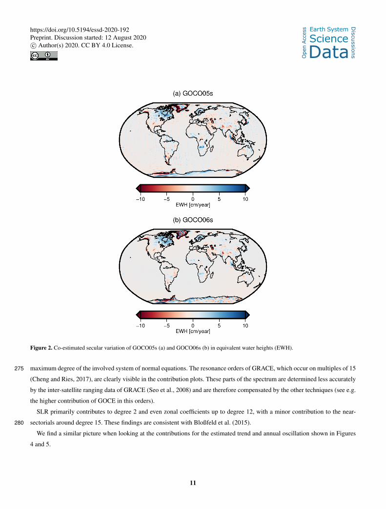
Figure 2. Co-estimated secular variation of GOCO05s (a) and GOCO06s (b) in equivalent water heights (EWH).

maximum degree of the involved system of normal equations. The resonance orders of GRACE, which occur on multiples of 15275

(Cheng and Ries, 2017), are clearly visible in the contribution plots. These parts of the spectrum are determined less accurately

by the inter-satellite ranging data of GRACE (Seo et al., 2008) and are therefore compensated by the other techniques (see e.g.

the higher contribution of GOCE in this orders).

SLR primarily contributes to degree 2 and even zonal coefficients up to degree 12, with a minor contribution to the near-

sectorials around degree 15. These findings are consistent with Bloßfeld et al. (2015).280

We find a similar picture when looking at the contributions for the estimated trend and annual oscillation shown in Figures

4 and 5.

11


Ope

n A

cces

s Earth System

Science

DataD

iscussio

ns


Figure 3. Individual contribution to the static part of the estimated potential coefficients for a) GRACE, b) GOCE SGG, c) Kaula regulariza-

tion, d) LEO orbits, and e) SLR. Note the different axis limits for panels d) and e).

12


Ope

n A

cces

s Earth System

Science

DataD

iscussio

ns


Figure 4. Contribution of a) GRACE and b) SLR to the estimated trend. Note the different axis limits.

Figure 5. Contribution of a) GRACE and b) SLR to the estimated annual oscillation. Note the different axis limits.

13


Ope

n A

cces

s Earth System

Science

DataD

iscussio

ns


3.3 Estimation of co-seismic gravity changes

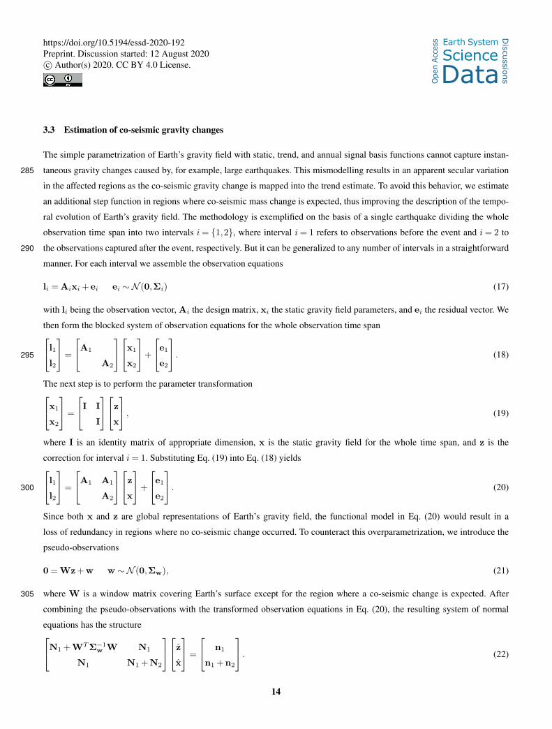
The simple parametrization of Earth’s gravity field with static, trend, and annual signal basis functions cannot capture instan-

taneous gravity changes caused by, for example, large earthquakes. This mismodelling results in an apparent secular variation285

in the affected regions as the co-seismic gravity change is mapped into the trend estimate. To avoid this behavior, we estimate

an additional step function in regions where co-seismic mass change is expected, thus improving the description of the tempo-

ral evolution of Earth’s gravity field. The methodology is exemplified on the basis of a single earthquake dividing the whole

observation time span into two intervals i= 1,2, where interval i= 1 refers to observations before the event and i= 2 to

the observations captured after the event, respectively. But it can be generalized to any number of intervals in a straightforward290

manner. For each interval we assemble the observation equations

li = Aixi + ei ei ∼N (0,Σi) (17)

with li being the observation vector, Ai the design matrix, xi the static gravity field parameters, and ei the residual vector. We

then form the blocked system of observation equations for the whole observation time spanl1

l2

=

A1

A2

x1

x2

+

e1

e2

. (18)295

The next step is to perform the parameter transformationx1

x2

=

I I

I

z

x

, (19)

where I is an identity matrix of appropriate dimension, x is the static gravity field for the whole time span, and z is the

correction for interval i= 1. Substituting Eq. (19) into Eq. (18) yieldsl1

l2

=

A1 A1

A2

z

x

+

e1

e2

. (20)300

Since both x and z are global representations of Earth’s gravity field, the functional model in Eq. (20) would result in a

loss of redundancy in regions where no co-seismic change occurred. To counteract this overparametrization, we introduce the

pseudo-observations

0 = Wz + w w ∼N (0,Σw), (21)

where W is a window matrix covering Earth’s surface except for the region where a co-seismic change is expected. After305

combining the pseudo-observations with the transformed observation equations in Eq. (20), the resulting system of normal

equations has the structureN1 + WTΣ−1

w W N1

N1 N1 + N2

z

x

=

n1

n1 + n2

. (22)

14


Ope

n A

cces

s Earth System

Science

DataD

iscussio

ns


Figure 6. Estimated co-seismic mass change for all modelled earthquakes (230 km Gaussian filter applied).

Increasing the weight of the constraint, that is setting Σw→ 0, which in practice is done by scaling with a number close to

numerically zero, then allows a signal in z only in regions within the predefined area. This retains the redundancy in points310

which are not affected by the earthquake, thus not influencing the estimate x there. We applied this approach to model three

major earthquakes during the GRACE lifespan, specifically, the 2004 Indian Ocean earthquake (Han et al., 2006), the 2010

Chile earthquake (Han et al., 2010), and the 2011 Tohoku-Oki earthquake (Panet et al., 2018). Since GRACE is the primary

contributor to the estimated temporal variations at these spatial scales, the parameter transformation was considered only to

the corresponding GRACE normal equations. The estimated co-seismic mass changes can be seen in Figure 6. We can clearly315

observe that the estimated signal is spatially confined, therefore, we retain the redundancy outside of the defined area. The

advantages and limitations regarding the estimation of the trend are best exemplified by comparison with GRACE monthly

solution and the previous GOCO05s release (not accounting for co-seismic changes). Figure 7 shows the estimated trends for

GOCO05s and GOCO06s (including the new co-estimated step) together with the time series of monthly solutions from ITSG-

Grace2018 (Kvas et al., 2019a), evaluated close to the epicenter of the 2004 Indian Ocean earthquake, where we observe a320

large co-seismic mass change. We can clearly observe that adding the co-estimation of co-seismic events greatly improves the

accuracy of the secular variations. However, the monthly solutions show different rates before and after the event, which can

obviously not be modelled by just a uniform trend over the whole observation time span. This is however a deliberate trade-off

to retain redundancy in the trend estimates and simple usability of the dataset.

15


Ope

n A

cces

s Earth System

Science

DataD

iscussio

ns


Figure 7. Comparison of estimated secular variation from GOCO05s, GOCO06s (including estimated co-seismic mass change) and filtered

GRACE monthly solutions in terms of equivalent water height (EWH).

4 Results and evaluation325

The complete published data set of GOCO06s consists of a static gravity field solution up to degree and order 300, an uncon-

strained system of normal equations of the static part for further combination, secular and annual gravity field variations up to

degree and order 200, and co-seismic mass changes for 3 major earthquakes. All components are published in widely used data

formats such as the ICGEM format for potential coefficients (Barthelmes and Förste, 2011) and the SINEX format for normal

equations (IERS, 2006).330

The data product of primary interest for the community certainly is the estimated static gravity field together with its un-

certainty information represented by the system of normal equations. Therefore, we focus our evaluations and discussions on

these components. Figure 8 depicts degree amplitudes of differences of state-of-the-art satellite only gravity field models and

XGM2016, a gravity field model which combines GOCO05s and terrestrial data (Pail et al., 2016). This is the explanation

for the small differences between XGM2016 and GOCO05s in the low degrees where the terrestrial data does not signifi-335

cantly contribute. The other large differences between the compared models in degrees below 60 are primarily explained by

the respective reference epochs (for example, 2010-01-01 for GOCO06s and 2010-09-01 for GOCE DIR6). This means, the

employed measurement techniques are sensitive to temporal variations in Earth’s gravity field, therefore we see signal rather

than noise in this frequency band. Concerning the GOCE gradiometer reprocessing we can see improvements from degree

150, where these data start to dominate the solutions. Here, we can clearly distinguish between models based on the new data340

(GOCO06s, TIM6, DIR6) and models based on the previous release (GOCO05s, EIGEN-GRGS RL04). Figure 9 shows the

degree amplitudes of component-wise differences with respect to the combined solution of each component of GOCO06s. We

excluded SLR here because the very ill-posed system of normal equations can only be solved up to degree 5-6 without addi-

tional information (Cheng et al., 2011). It nicely summarizes the major contributions to the final GOCO06s solution and shows

the consistency of formal and empirical errors. It further highlights the importance of stochastic modeling which enables this345

16


Ope

n A

cces

s Earth System

Science

DataD

iscussio

ns


Figure 8. Degree amplitudes of various state-of-the-art satellite-only models. (8 degree polar cap excluded).

Figure 9. Degree amplitudes and corresponding formal errors of the individual GOCO06s components (8 degree polar cap excluded). SLR

is not shown because no standalone solution can be computed due to the ill-posed adjustment problem.

17


Ope

n A

cces

s Earth System

Science

DataD

iscussio

ns


consistency. The deviation of the combined solution from the GOCE SGG contribution starting at degree 240 is explained by

the Kaula constraint applied to the combination.

4.1 Comparison with GNSS leveling

Over land geoid heights (height anomalies or geoid undulations) computed from global gravity models can be validated against

independent geoid observations as they are determined by on ground GNSS levelling. By subtracting physical heights deter-350

mined by spirit levelling (orthometric or normal heights) from ellipsoidal heights as they are observed with GNSS one can

compute such independent geoid heights. The challenge when comparing geoid heights derived from satellite-only gravity

field models to observed geoid heights mainly is to eliminate the so-called omission error. This error, which represents the

higher resolution geoid signal not observable by satellites due to the gravitational signal attenuation at satellite altitude, causes

the major part of the differences leading to unrealistic quality estimates for the satellite-only gravity model. Therefore, the355

omission error needs to be estimated from other sources and taken into account prior to computing the differences. For this

purpose, high resolution gravity field models as EGM2008 (Pavlis et al., 2012) or XGM2019e (Zingerle et al., 2019, 2020) and

an ultra-high resolution model of the gravity signal caused by the Earth’s topography as ERTM2160 (Hirt et al., 2014) are used.

The omission error computed from these models is subtracted from the observed geoid heights before they are compared to the

satellite-only model geoid heights. Apart from this, a second systematic error might be present in physical heights observed360

by spirit levelling. Depending on the spirit levelling technique and the carefulness of the observer errors accumulate along the

levelling lines leading to artificial tilts (or other systematics) of the physical heights with respect to the reference equipotential

surface, which is defined by the height system reference point in a country. Therefore, prior to analyze differences between

observed and global model derived geoid heights a correction surface for the geoid differences shall be estimated and applied.

This ensures that errors due to such tilts and due to offsets of regional height systems with respect to the global geoid are365

eliminated beforehand. The computational procedure to compute and analyze geoid height differences between observed geoid

heights and those determined from a global gravity field model is described in detail in (Gruber et al., 2011) and (Gruber and

Willberg, 2019).

For validating the GOCO06s model a number of global gravity field models and a number of GNSS levelling data sets is

applied. For gravity field models on one hand the previous satellite-only models of the GOCO series are used (GOCO01s,370

GOCO02s, GOCO03s and GOCO05s). These models are characterized by combining GRACE and GOCE satellite data with

increasing amount of observations and some additional satellite data (cf. Sect. 1). In addition, an independent GRACE/GOCE

satellite-only combination model namely GOCE-DIR6 is used for comparisons, which to a large extent is based on the same

amount of GRACE and GOCE data as GOCO06s (Förste et al., 2019). In order to identify the performance of pure GRACE

and pure GOCE models compared to the combined GOCO06s model the ITSG-Grace2018s (Kvas et al., 2019a) model and375

the GOCE-TIM6 (Brockmann et al., 2019) models are applied to the validation procedure. Finally, a model combining the

GOCO06s satellite data with surface, airborne and altimetric gravity data is used in order to identify the signal content higher

degrees of the GOCO06s model. This is the XGM2019e high resolution global gravity field model (Zingerle et al., 2019,

2020). GNSS levelling data are available from many sources for many areas in the world. Typically, these data sets show

18


Ope

n A

cces

s Earth System

Science

DataD

iscussio

ns


Figure 10. RMS of geoid height differences between global gravity models and independently observed geoid heights from GNSS levelling.

Global models are truncated with steps of 10 degrees starting from degree and order 10 to degree and order 300. Omission error is computed

from the degree of truncation to degree and order 2190 from EGM2008 and from the ERTM2160 topographic gravity field model for degrees

above 2160.

different quality levels, which strongly depends on the instruments, the measurement procedure and the observer carefulness.380

In general, the results for most of the comparisons show similar behavior, but at different levels of accuracy. We have selected

representative data sets from different continents and of different quality levels and validated the model derived geoid heights

against these data sets. Here we show the results for Brazil, Germany, Japan and the United States (see acknowledgement).

Figure 10 shows the results for the validation of the global models against the independently observed geoid heights at

GNSS levelling points for the four selected countries. Before drawing any conclusion from the results, the figure shall be385

explained shortly. Each tested model was truncated at steps of degree 10 of the spherical harmonic series starting from degree

19


Ope

n A

cces

s Earth System

Science

DataD

iscussio

ns


and order 10 until 300. For each area the model geoid heights were computed up to the degree and order given on the x-axis and

differences to the observed geoid heights were calculated. The omission error was computed separately from the EGM2008

and ERTM2160 models (see above) starting from the truncation degree to highest possible resolution and subtracted from the

geoid differences. Finally, a planar correction surface was calculated for each area for the geoid differences and subtracted.390

From the remaining differences the RMS values shown on the y-axis were computed. In general, the lowest level of the RMS

values is a good indicator about the quality of the GNSS levelling derived geoid heights as one can assume that the global

satellite-only models perform similar over the whole globe.

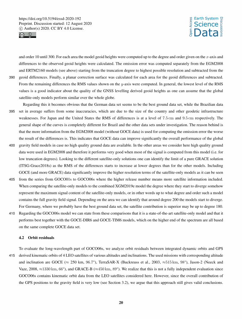
Regarding this it becomes obvious that the German data set seems to be the best ground data set, while the Brazilian data

set in average suffers from some inaccuracies, which are due to the size of the country and other geodetic infrastructure395

weaknesses. For Japan and the United States the RMS of differences is at a level of 7.5 cm and 9.5 cm respectively. The

general shape of the curves is completely different for Brazil and the other data sets under investigation. The reason behind is

that the more information from the EGM2008 model (without GOCE data) is used for computing the omission error the worse

the result of the differences is. This indicates that GOCE data can improve significantly the overall performance of the global

gravity field models in case no high quality ground data are available. In the other areas we consider here high quality ground400

data were used in EGM2008 and therefore it performs very good when most of the signal is computed from this model (i.e. for

low truncation degrees). Looking to the different satellite-only solutions one can identify the limit of a pure GRACE solution

(ITSG-Grace2018s) as the RMS of the differences starts to increase at lower degrees than for the other models. Including

GOCE (and more GRACE) data significantly improve the higher resolution terms of the satellite-only models as it can be seen

from the series from GOCO01s to GOCO06s where the higher release number means more satellite information included.405

When comparing the satellite-only models to the combined XGM2019e model the degree where they start to diverge somehow

represent the maximum signal content of the satellite-only models, or in other words up to what degree and order such a model

contains the full gravity field signal. Depending on the area we can identify that around degree 200 the models start to diverge.

For Germany, where we probably have the best ground data set, the satellite contribution is superior may be up to degree 180.

Regarding the GOCO06s model we can state from these comparisons that it is a state-of-the-art satellite-only model and that it410

performs best together with the GOCE-DIR6 and GOCE-TIM6 models, which on the higher end of the spectrum are all based

on the same complete GOCE data set.

4.2 Orbit residuals

To evaluate the long-wavelength part of GOCO06s, we analyze orbit residuals between integrated dynamic orbits and GPS

derived kinematic orbits of 4 LEO satellites of various altitudes and inclinations. The used missions with corresponding altitude415

and inclination are GOCE (≈ 250 km, 96.7°), TerraSAR-X (Buckreuss et al., 2003, ≈515 km, 98°), Jason-2 (Neeck and

Vaze, 2008, ≈1330 km, 66°), and GRACE-B (≈450 km, 89°). We realize that this is not a fully independent evaluation since

GOCO06s contains kinematic orbit data from the LEO satellites considered here. However, since the overall contribution of

the GPS positions to the gravity field is very low (see Section 3.2), we argue that this approach still gives valid conclusions.

20


Ope

n A

cces

s Earth System

Science

DataD

iscussio

ns


Furthermore, we used the kinematic GOCE and GRACE orbits of the Astronomical Institute at Bern University (Bock et al.,420

2014; Meyer et al., 2016) and not the in-house positions used in the gravity field recovery process.

First, a dynamic orbit for each satellite is integrated based on a fixed set of geophysical models, where only the static gravity

field is substituted. The models used can be found in Table 2. We included trend and annual gravity field variations from

Table 2. Background models used in the dynamic orbit integration.

Force Model Maximum degree

Earth’s gravity field estimated from GRACE solutions

(annual/secular variations) (CSR RL06, DDK4 filter applied) 96

Non-tidal ocean/atmosphere variation AOD1B RL06 180

Ocean Tides FES2014b 180

Astronomical tides IERS2010, JPL DE421 N/A

Solid earth tides IERS2010 4

Atmospheric tides AOD1B RL06 180

Pole tides IERS2010 (linear mean pole) c21,s21

Ocean pole tides Desai (2002, linear mean pole) 220

Relativistic corrections IERS2010 -

Nonconservative forces measured if available, else

JB2008 (drag), Knocke et al. (1988)/CERES (albedo),

Lemoine et al. (2013) (solar radiation pressure) -

GRACE to make sure all compared gravity fields relate to the same reference epoch.

Since satellites are not only affected by gravitational forces, but also non-conservative forces such as atmospheric drag, solar425

radiation pressure, and earth radiation pressure. Both GOCE and GRACE are equipped with accelerometers which measure

the impact of these forces. The other satellites (Jason-2, TerraSar-X), do not feature such an instrument, therefore we make

use of models to compute the effect. Specifically, we model the impact of atmospheric drag (Bowman et al., 2008), Earth’s

albedo (Knocke et al., 1988) and solar radiation pressure (Lemoine et al., 2013). Even though the quality of accelerometer

measurements is generally superior to the model output, sensor specific errors such as bias and scale need to be considered.430

Consequently we model and estimate both bias and scale as well as empirical parameters for both accelerometers and model

output to reduce the potential impact of mismodelling and sensor errors on our evaluation. The values of these calibration

parameters are estimated together with the initial state when the dynamic orbit is fitted to the kinematic satellite positions. One

constant bias for each axis and a single full scale matrix (Klinger and Mayer-Gürr, 2016) is estimated per each 1-day arc for

all satellites. For Jason-2 and TerraSAR-X we additionally estimate a once-per-revolution bias to further reduce the impact of435

non-conservative forces. The metric we are using for the evaluation is root-mean-square (RMS) of the orbit differences between

the integrated dynamic orbit and the purely GPS derived kinematic orbit positions. Epochs where the difference exceeds 15 cm

21


Ope

n A

cces

s Earth System

Science

DataD

iscussio

ns


Table 3. RMS of differences between integrated dynamic and GPS derived kinematic orbits in centimeters for four selected months during

the GOCE measurement time span for satellites of different altitude and inclination.

GOCO05s GOCO06s GOCE TIM6 GOCE DIR6

GOCE 2.39 2.36 3.54 2.39

TerraSAR-X 5.66 5.65 5.73 5.67

Jason-2 3.89 3.88 4.00 3.88

GRACE-B 2.41 2.24 5.08 2.25

Table 4. RMS of differences between integrated dynamic orbit and GPS derived kinematic positions for GRACE-C January 2020 in cen-

timeters.

EIGEN-GRGS RL04 GOCO06s GOCO05s ITSG-Grace op

GRACE-C 3.06 2.44 2.60 2.32

are treated as outliers and subsequently removed. We randomly selected four months over the GOCE measurement time span

(2009-11, 2010-03, 2011-10, and 2012-03).

We compare GOCO06s with its predecessor GOCO05s and other recent static gravity field models (see Fig. 8) models440

available on ICGEM (Ince et al., 2019). The results are summarized in Table 3. From the computed RMS values we can

conclude that the most recent combination models (GOCO06s and DIR6) perform nearly equally well, with GOCO06s having

a slight edge. Furthermore, we can see that there is a quality jump from the previous release GOCO05s. The GOCE-only

model TIM6 performs worst for all satellites which highlights the importance of GRACE for stabilizing the long to medium

wavelengths and the polar gap. The overall larger RMS values for TerraSAR-X and Jason-2 reflect the challenges in modelling445

non-conservative forces for these satellites. Combined with the higher altitude, the contrast between the individual static gravity

field solutions becomes very small. Still, we observe the same tendencies as for GOCE and GRACE.

Next to the validation of static gravity fields, orbit residuals are also very useful in evaluating the temporal constituents of

gravity field solutions. We gauge the quality of the co-estimated temporal constituents of GOCO06s by integrating a dynamic

orbit arcs for GRACE Follow-On 1 (GRACE-C). We compare GOCO06s to EIGEN-GRGS RL04, a recent gravity field model450

which also features a time-variable part, the previous solution GOCO05s, and a GRACE-FO monthly solution. Instead of the

trend and annual variation estimated from CSR RL06, we use the temporal constituents of the gravity fields to be compared.

Both GOCO06s and GOCO05s provide secular and annual variations while EIGEN-GRGS RL04 has secular, annual and

semi-annual variations estimated for shorter intervals. We perform the evaluation for January 2020, which is well beyond the

GRACE measurement time span. This choice is deliberate to assess the extrapolation capabilities of the compared gravity455

fields. The computed RMS values can be found in Table 4. We can see that GOCO06s outperforms both its predecessor and

EIGEN-GRGS RL04 while unsurprisingly, the GRACE-FO monthly solution performs best.

22


Ope

n A

cces

s Earth System

Science

DataD

iscussio

ns


5 Conclusions

The satellite-only gravity field model GOCO06s provides a consistent combination of spaceborne gravity observations from

a variety of satellite missions and measurement techniques. Each component of the solution was processed using state-of-the460

art methodology which results in a clear increase in the solution quality compared to the preceding GOCO solutions and the

individual input models. All contributing data sources were combined on the basis of full normal equations, with the individual

weights being determined by VCE. The long to medium spatial wavelengths covered by GOCO06s are mainly determined by

GRACE due to the high sensitivity of the intersatellite ranging observation to this frequency band. SLR primarily contributes to

degree 2, while the kinematic LEO orbits mainly contribute to the sectorial coefficients up to degree and order 150. Finally, the465

medium to short wavelengths of the solution, starting from degree 120, are dominated by the GOCE gradiometer observations.

To reduce the energy in the higher spherical harmonic degrees, a Kaula-type regularization was applied from degree 151 to

300. The complementary nature of the used data mitigates weaknesses of the individual observation types, thus providing the

highest accuracy throughout the spatial frequency band covered by the solution.

Since an appropriate stochastic observation model is used during processing, GOCO06s exhibits realistic formal errors,470

which alleviates further combination with additional, for example, terrestrial gravity field observations (Pail et al., 2016, 2018).

This extremely useful information is provided to the community in the form of the full system of unconstrained normal equa-

tions. All data products are published in well established file formats such as the ICGEM format for potential coefficients

(Barthelmes and Förste, 2011) and the SINEX format (IERS, 2006) for systems of normal equations.

6 Data availability475

The primary model data (Kvas et al., 2019b) consisting of potential coefficients representing Earth’s static gravity field, to-

gether with secular and annual variations are available on ICGEM (Ince et al., 2019). This data set is identified with the DOI

10.5880/ICGEM.2019.002.

Supplementary material consisting of the full variance-covariance matrix of the static potential coefficients and estimated

co-seismic mass changes are available on ifg.tugraz.at/GOCO.480

Author contributions. Andreas Kvas computed the GRACE and LEO normal equations, developed and implemented the regularization

strategies for the temporal constituents and earthquakes, performed the combination of all individual data contributions, performed the orbit

validation and partially wrote the manuscript. Jan Martin Brockmann computed the GOCE SGG system of normal equations and partially

wrote the manuscript. Till Schubert and Wolf-Dieter Schuh contributed to the GOCE processing. Sandro Krauss computed and provided the

systems of normal equations for all SLR satellites. Thomas Gruber performed the model validation with in-situ GNSS leveling data data.485

Ulrich Meyer provided the kinematic orbits of GRACE and GOCE used in the validation. Torsten Mayer-Gürr, Adrian Jäggi, Wolf-Dieter

Schuh, and Roland Pail acted as scientific advisors. All authors commented on the draft of the manuscript and on the discussion of the results.

23


Ope

n A

cces

s Earth System

Science

DataD

iscussio

ns


Competing interests. The author declare no competing interests.

Acknowledgements. Parts of this work was financially supported by ESA GOCE HPF (main contract No. 18308/04/NL/MM). JMB and WDS

gratefully acknowledge the Gauss Centre for Supercomputing e.V. (www.gauss-centre.eu) for funding this study by providing computing time490

through the John von Neumann Institute for Computing (NIC) on the GCS Supercomputer JUWELS at Jülich Supercomputing Centre (JSC).

Precise orbit determination of SLR satellites was accomplished with the software package GEODYN, kindly provided by the NASA

Goddard Space Flight Center.

GNSS levelling data sets applied in this study have been kindly provided by the Brazilian Institute of Geography and Statistics - IBGE,

2019 (Brazil), by the GeoBasis-DE / Geobasis NRW, 2018 (Germany), by the Japanese Geographical Survey Institute, 2003 (Japan) and by495

the National Geodetic Survey, 2012 (USA). The authors are grateful to the institutions who made available the GNSS-levelling data as they

provide a unique reference for validating global gravity field models.

The authors gratefully acknowledge the ISDC at the German Research Centre for Geosciences for providing Champ, TerraSAR-X and

TanDEM-X data, the European Space Agency for providing GOCE and SWARM data, and Aviso for providing Jason data and the Interna-

tional Laser Ranging Service for providing Satellite laser ranging measurements.500

24


Ope

n A

cces

s Earth System

Science

DataD

iscussio

ns


References

Abrehdary, M., Sjoberg, L. E., Bagherbandi, M., and Sampietro, D.: Towards the Moho Depth and Moho Density Contrast along with Their

Uncertainties from Seismic and Satellite Gravity Observations, Journal of Applied Geodesy, 11, 231–247, https://doi.org/10.1515/jag-

2017-0019, wOS:000411518900003, 2017.

Barthelmes, F. and Förste, C.: The ICGEM-format, Tech. rep., GFZ Potsdam, Department 1 Geodesy and Remote Sensing, 2011.505

Battrick, B., ed.: The Four Candidate Earth Explorer Core Missions – Gravity Field and Steady-State Ocean Circulation, vol. 1233 of ESA

SP, ESA Publications Division, Noordwijk, Netherlands, 1999.

Beutler, G., Jäggi, A., Mervart, L., and Meyer, U.: The Celestial Mechanics Approach: Theoretical Foundations, Journal of Geodesy, 84,

605–624, https://doi.org/10.1007/s00190-010-0401-7, 2010.

Bezdek, A., Sebera, J., Teixeira da Encarnação, J., and Klokocník, J.: Time-Variable Gravity Fields Derived from GPS Tracking of Swarm,510

Geophysical Journal International, 205, 1665–1669, https://doi.org/10.1093/gji/ggw094, 2016.

Bingham, R. J., Haines, K., and Lea, D. J.: How Well Can We Measure the Ocean’s Mean Dynamic Topography from Space?, Journal of

Geophysical Research: Oceans, 119, 3336–3356, https://doi.org/10.1002/2013JC009354, 2014.

Bloßfeld, M., Müller, H., Gerstl, M., Štefka, V., Bouman, J., Göttl, F., and Horwath, M.: Second-degree Stokes coefficients from multi-

satellite SLR, Journal of Geodesy, 89, 857–871, https://doi.org/10.1007/s00190-015-0819-z, https://doi.org/10.1007/s00190-015-0819-z,515

2015.

Bloßfeld, M., Rudenko, S., Kehm, A., Panafidina, N., Müller, H., Angermann, D., Hugentobler, U., and Seitz, M.: Consis-

tent Estimation of Geodetic Parameters from SLR Satellite Constellation Measurements, Journal of Geodesy, 92, 1003–1021,

https://doi.org/10.1007/s00190-018-1166-7, 2018.

Bock, H., Jäggi, A., Beutler, G., and Meyer, U.: GOCE: precise orbit determination for the entire mission, Journal of Geodesy, 88, 1047–1060,520

https://doi.org/10.1007/s00190-014-0742-8, https://doi.org/10.1007/s00190-014-0742-8, 2014.

Bowman, B. R., Tobiska, W. K., Marcos, F. A., Huang, C. Y., Lin, C. S., and Burke, W. J.: A new empirical thermospheric density model

JB2008 using new solar and geomagnetic indices, in: AIAA/AAS Astrodynamics Specialist Conference and Exhibit, American Institute

of Aeronautics and Astronautics, https://doi.org/10.2514/6.2008-6438, https://arc.aiaa.org/doi/abs/10.2514/6.2008-6438, 2008.

Brockmann, J. M., Zehentner, N., Höck, E., Pail, R., Loth, I., Mayer-Gürr, T., and Schuh, W.-D.: EGM_TIM_RL05: An Inde-525

pendent Geoid with Centimeter Accuracy Purely Based on the GOCE Mission, Geophysical Research Letters, 41, 8089–8099,

https://doi.org/10.1002/2014GL061904, 2014.

Brockmann, J. M., Schubert, T., Mayer-Gürr, T., and Schuh, W.-D.: The Earth’s Gravity Field as Seen by the GOCE Satellite - an Improved

Sixth Release Derived with the Time-Wise Approach (GO_CONS_GCF_2_TIM_R6), https://doi.org/10.5880/icgem.2019.003, http://

dataservices.gfz-potsdam.de/icgem/showshort.php?id=escidoc:4315891, 2019.530

Bruinsma, S. L., Förste, C., Abrikosov, O., Marty, J.-C., Rio, M.-H., Mulet, S., and Bonvalot, S.: The New ESA Satellite-Only Gravity Field

Model via the Direct Approach, Geophysical Research Letters, 40, 3607–3612, https://doi.org/10.1002/grl.50716, 2013.

Bruinsma, S. L., Förste, C., Abrikosov, O., Lemoine, J.-M., Marty, J.-C., Mulet, S., Rio, M.-H., and Bonvalot, S.: ESA’s Satellite-

Only Gravity Field Model via the Direct Approach Based on All GOCE Data, Geophysical Research Letters, 41, 2014GL062 045,

https://doi.org/10.1002/2014GL062045, 2014.535

Buckreuss, S., Balzer, W., Muhlbauer, P., Werninghaus, R., and Pitz, W.: The terraSAR-X satellite project, in: IGARSS 2003. 2003 IEEE

International Geoscience and Remote Sensing Symposium. Proceedings (IEEE Cat. No.03CH37477), vol. 5, pp. 3096–3098 vol.5, 2003.

25


Ope

n A

cces

s Earth System

Science

DataD

iscussio

ns


Carrere, L., Lyard, F., Cancet, M., and Guillot, A.: FES 2014, a New Tidal Model on the Global Ocean with Enhanced Accuracy in Shallow

Seas and in the Arctic Region, in: EGU General Assembly, vol. 17, p. 5481, Vienna, Austria, http://adsabs.harvard.edu/abs/2015EGUGA.

.17.5481C, 2015.540

Chen, Q., Shen, Y., Francis, O., Chen, W., Zhang, X., and Hsu, H.: Tongji-Grace02s and Tongji-Grace02k: High-Precision Static GRACE-

Only Global Earth’s Gravity Field Models Derived by Refined Data Processing Strategies, Journal of Geophysical Research: Solid Earth,

123, 6111–6137, https://doi.org/10.1029/2018JB015641, 2018a.

Chen, W., Braitenberg, C., and Serpelloni, E.: Interference of Tectonic Signals in Subsurface Hydrologic Monitoring through Gravity and

GPS Due to Mountain Building, Global and Planetary Change, 167, 148–159, https://doi.org/10.1016/j.gloplacha.2018.05.003, 2018b.545

Cheng, M. and Ries, J.: The unexpected signal in GRACE estimates of $$C_20$$C20, Journal of Geodesy, 91, 897–914,


Cheng, M., Ries, J. C., and Tapley, B. D.: Variations of the Earth’s figure axis from satellite laser ranging and GRACE, Journal of Geo-

physical Research: Solid Earth, 116, https://doi.org/10.1029/2010JB000850, https://agupubs.onlinelibrary.wiley.com/doi/abs/10.1029/

2010JB000850, 2011.550

Dahle, C., Murböck, M., Flechtner, F., Dobslaw, H., Michalak, G., Neumayer, K., Abrykosov, O., Reinhold, A., König, R., Sulzbach, R.,

and et al.: The GFZ GRACE RL06 Monthly Gravity Field Time Series: Processing Details and Quality Assessment, Remote Sensing, 11,

2116, https://doi.org/10.3390/rs11182116, http://dx.doi.org/10.3390/rs11182116, 2019.

Desai, S. D.: Observing the Pole Tide with Satellite Altimetry, Journal of Geophysical Research: Oceans, 107, 7–1–7–13,

https://doi.org/10.1029/2001JC001224, https://agupubs.onlinelibrary.wiley.com/doi/abs/10.1029/2001JC001224, 2002.555

Dobslaw, H., Bergmann-Wolf, I., Dill, R., Poropat, L., Thomas, M., Dahle, C., Esselborn, S., König, R., and Flechtner, F.: A New High-

Resolution Model of Non-Tidal Atmosphere and Ocean Mass Variability for de-Aliasing of Satellite Gravity Observations: AOD1B

RL06, Geophysical Journal International, 211, 263–269, https://doi.org/10.1093/gji/ggx302, https://academic.oup.com/gji/article/211/1/

263/3979461, 2017.

Ebbing, J., Haas, P., Ferraccioli, F., Pappa, F., Szwillus, W., and Bouman, J.: Earth Tectonics as Seen by GOCE - Enhanced Satellite Gravity560

Gradient Imaging, Scientific Reports, 8, 16 356, https://doi.org/10.1038/s41598-018-34733-9, 2018.

Ellmer, M.: Contributions to GRACE Gravity Field Recovery: Improvements in Dynamic Orbit Integration Stochastic Modelling of

the Antenna Offset Correction, and Co-Estimation of Satellite Orientations, Ph.D. thesis, Graz University of Technology (90000),

https://doi.org/10.3217/978-3-85125-646-8, 2018.

Farahani, H. H., Ditmar, P., Klees, R., Liu, X., Zhao, Q., and Guo, J.: The Static Gravity Field Model DGM-1S from GRACE565

and GOCE Data: Computation, Validation and an Analysis of GOCE Mission’s Added Value, Journal of Geodesy, 87, 843–867,

https://doi.org/10.1007/s00190-013-0650-3, 2013.

Farrell, S. L., McAdoo, D. C., Laxon, S. W., Zwally, H. J., Yi, D., Ridout, A., and Giles, K.: Mean Dynamic Topography of the Arctic Ocean,

Geophysical Research Letters, 39, L01 601, https://doi.org/10.1029/2011GL050052, wOS:000298930900003, 2012.

Folkner, W. M., Williams, J. G., and Boggs, D. H.: The Planetary and Lunar Ephemeris DE 421, Tech. Rep. 42-178, Jet Propulsion Laborator,570

Pasadena, California, http://adsabs.harvard.edu/abs/2009IPNPR.178C...1F, 2009.

Förste, C., Bruinsma, S., Abrikosov, O., Rudenko, S., Lemoine, J.-M., Marty, J.-C., Neumayer, K. H., and Biancale, R.: EIGEN-6S4 A

Time-Variable Satellite-Only Gravity Field Model to d/o 300 Based on LAGEOS, GRACE and GOCE Data from the Collaboration of

GFZ Potsdam and GRGS Toulouse, https://doi.org/10.5880/icgem.2016.008, 2016.

26


Ope

n A

cces

s Earth System

Science

DataD

iscussio

ns


Förste, C., Abrykosov, O., Bruinsma, S., Dahle, C., König, R., and Lemoine, J.-M.: ESA’s Release 6 GOCE Gravity Field Model by Means575

of the Direct Approach Based on Improved Filtering of the Reprocessed Gradients of the Entire Mission (GO_CONS_GCF_2_DIR_R6),

https://doi.org/10.5880/ICGEM.2019.004, http://dataservices.gfz-potsdam.de/icgem/showshort.php?id=escidoc:4232899, 2019.

Gerlach, C. and Rummel, R.: Global Height System Unification with GOCE: A Simulation Study on the Indirect Bias Term in the GBVP

Approach, Journal of Geodesy, 87, 57–67, https://doi.org/10.1007/s00190-012-0579-y, 2013.

GOCO: Combined Global Gravity Field Models, http://www.goco.eu/, 2017.580

Gruber, T. and Willberg, M.: Signal and Error Assessment of GOCE-Based High Resolution Gravity Field Models, Journal of Geode-

tic Science, 9, 71–86, https://doi.org/10.1515/jogs-2019-0008, http://www.degruyter.com/view/j/jogs.2019.9.issue-1/jogs-2019-0008/

jogs-2019-0008.xml, 2019.

Gruber, T., Visser, P. N. a. M., Ackermann, C., and Hosse, M.: Validation of GOCE Gravity Field Models by Means of Orbit Residuals

and Geoid Comparisons, Journal of Geodesy, 85, 845–860, https://doi.org/10.1007/s00190-011-0486-7, http://link.springer.com/article/585

10.1007/s00190-011-0486-7, 2011.

Han, S.-C., Shum, C. K., Bevis, M., Ji, C., and Kuo, C.-Y.: Crustal Dilatation Observed by GRACE After the 2004 Sumatra-Andaman Earth-

quake, Science, 313, 658–662, https://doi.org/10.1126/science.1128661, https://science.sciencemag.org/content/313/5787/658, 2006.

Han, S.-C., Sauber, J., and Luthcke, S.: Regional gravity decrease after the 2010 Maule (Chile) earthquake indicates large-scale mass redis-

tribution, Geophysical Research Letters, 37, https://doi.org/10.1029/2010GL045449, https://agupubs.onlinelibrary.wiley.com/doi/abs/10.590

1029/2010GL045449, 2010.

Hirt, C., Kuhn, M., Claessens, S., Pail, R., Seitz, K., and Gruber, T.: Study of the Earth’s Short-Scale Gravity Field Using the ERTM2160

Gravity Model, Computers & Geosciences, 73, 71–80, https://doi.org/10.1016/j.cageo.2014.09.001, https://linkinghub.elsevier.com/

retrieve/pii/S0098300414002039, 2014.

Huang, J. and Véronneau, M.: Canadian Gravimetric Geoid Model 2010, Journal of Geodesy, 87, 771–790, https://doi.org/10.1007/s00190-595

013-0645-0, 2013.

IERS, I. E. R. S.: SINEX - Solution (Software/technique) INdependent EXchange Format Version 2.02, Tech. rep., International Earth

Rotation Service (IERS), https://www.iers.org/IERS/EN/Organization/AnalysisCoordinator/SinexFormat/sinex.html, 2006.

Ince, E. S., Barthelmes, F., Reißland, S., Elger, K., Förste, C., Flechtner, F., and Schuh, H.: ICGEM – 15 years of successful collec-

tion and distribution of global gravitational models, associated services, and future plans, Earth System Science Data, 11, 647–674,600

https://doi.org/10.5194/essd-11-647-2019, https://www.earth-syst-sci-data.net/11/647/2019/, 2019.

Jekeli, C.: Alternative methods to smooth the Earth’s gravity field, Tech. Rep. 327, Department of Geodetic Science and Surveying, Ohio

State Univ., Columbus, OH., 1981.

Johannessen, J. A., Balmino, G., Provost, C. L., Rummel, R., Sabadini, R., Sünkel, H., Tscherning, C. C., Visser, P., Woodworth, P.,

Hughes, C., Legrand, P., Sneeuw, N., Perosanz, F., Aguirre-Martinez, M., Rebhan, H., and Drinkwater, M.: The European Gravity605

Field and Steady-State Ocean Circulation Explorer Satellite Mission Its Impact on Geophysics, Surveys in Geophysics, 24, 339–386,

https://doi.org/10.1023/B:GEOP.0000004264.04667.5e, 2003.

Johannessen, J. A., Raj, R. P., Nilsen, J. E. Ø., Pripp, T., Knudsen, P., Counillon, F., Stammer, D., Bertino, L., Andersen, O. B., Serra, N., and

Koldunov, N.: Toward Improved Estimation of the Dynamic Topography and Ocean Circulation in the High Latitude and Arctic Ocean:

The Importance of GOCE, Surveys in Geophysics, 35, 661–679, https://doi.org/10.1007/s10712-013-9270-y, 2014.610

(JPL), N. J. P. L.: GRACE LEVEL 1B JPL RELEASE 3.0, https://doi.org/10.5067/GRJPL-L1B03, https://podaac.jpl.nasa.gov/dataset/

GRACE_L1B_GRAV_JPL_RL03, 2018.

27


Ope

n A

cces

s Earth System

Science

DataD

iscussio

ns


Klees, R., Slobbe, D. C., and Farahani, H. H.: A Methodology for Least-Squares Local Quasi-Geoid Modelling Using a Noisy Satellite-Only

Gravity Field Model, Journal of Geodesy, 92, 431–442, https://doi.org/10.1007/s00190-017-1076-0, 2018.

Klinger, B. and Mayer-Gürr, T.: The role of accelerometer data calibration within GRACE gravity field recovery: Results from ITSG-615

Grace2016, Advances in Space Research, 58, 1597–1609, https://doi.org/10.1016/j.asr.2016.08.007, http://www.sciencedirect.com/

science/article/pii/S0273117716304409, 2016.

Knocke, P. C., Ries, J. C., and Tapley, B. D.: Earth radiation pressure effects on satellites, in: Astrodynamics Conference, 1988,

Guidance, Navigation, and Control and Co-located Conferences, pp. 577–587, American Institute of Aeronautics and Astronautics,

https://doi.org/10.2514/6.1988-4292, https://doi.org/10.2514/6.1988-4292, 1988.620

Knudsen, P., Bingham, R., Andersen, O., and Rio, M.-H.: A Global Mean Dynamic Topography and Ocean Circulation Estimation Using a

Preliminary GOCE Gravity Model, Journal of Geodesy, 85, 861–879, https://doi.org/10.1007/s00190-011-0485-8, 2011.

Koch, K. R. and Kusche, J.: Regularization of geopotential determination from satellite data by variance components, Journal of Geodesy,

76, 259–268, https://doi.org/10.1007/s00190-002-0245-x, https://doi.org/10.1007/s00190-002-0245-x, 2002.

Kornfeld, R. P., Arnold, B. W., Gross, M. A., Dahya, N. T., Klipstein, W. M., Gath, P. F., and Bettadpur, S.: GRACE-FO: The Gravity Re-625

covery and Climate Experiment Follow-On Mission, Journal of Spacecraft and Rockets, 56, 931–951, https://doi.org/10.2514/1.A34326,

2019.

Kvas, A., Behzadpour, S., Ellmer, M., Klinger, B., Strasser, S., Zehentner, N., and Mayer-Gürr, T.: ITSG-Grace2018: Overview and evaluation

of a new GRACE-only gravity field time series, Journal of Geophysical Research: Solid Earth, https://doi.org/10.1029/2019JB017415,

2019a.630

Kvas, A., Mayer-Gürr, T., Krauss, S., Brockmann, J. M., Schubert, T., Schuh, W.-D., Pail, R., Gruber, T., Jäggi, A., and Meyer, U.:

The satellite-only gravity field model GOCO06s, https://doi.org/10.5880/ICGEM.2019.002, http://dataservices.gfz-potsdam.de/icgem/

showshort.php?id=escidoc:4081892, 2019b.

Landerer, F. W., Flechtner, F. M., Save, H., Webb, F. H., Bandikova, T., Bertiger, W. I., Bettadpur, S. V., Byun, S. H., Dahle, C., Dobslaw,

H., Fahnestock, E., Harvey, N., Kang, Z., Kruizinga, G. L. H., Loomis, B. D., McCullough, C., Murböck, M., Nagel, P., Paik, M., Pie, N.,635

Poole, S., Strekalov, D., Tamisiea, M. E., Wang, F., Watkins, M. M., Wen, H.-Y., Wiese, D. N., and Yuan, D.-N.: Extending the Global Mass

Change Data Record: GRACE Follow-On Instrument and Science Data Performance, Geophysical Research Letters, 47, e2020GL088 306,

https://doi.org/10.1029/2020GL088306, https://agupubs.onlinelibrary.wiley.com/doi/abs/10.1029/2020GL088306, 2020.

Lemoine, F. G., Goossens, S., Sabaka, T. J., Nicholas, J. B., Mazarico, E., Rowlands, D. D., Loomis, B. D., Chinn, D. S., Caprette, D. S.,

Neumann, G. A., Smith, D. E., and Zuber, M. T.: High-degree gravity models from GRAIL primary mission data, Journal of Geophysical640

Research: Planets, 118, 1676–1698, https://doi.org/10.1002/jgre.20118, 2013.

Lück, C., Kusche, J., Rietbroek, R., and Löcher, A.: Time-Variable Gravity Fields and Ocean Mass Change from 37 Months of Kinematic

Swarm Orbits, Solid Earth, 9, 323–339, https://doi.org/https://doi.org/10.5194/se-9-323-2018, 2018.

Maier, A., Krauss, S., Hausleitner, W., and Baur, O.: Contribution of Satellite Laser Ranging to Combined Gravity Field Models, Advances

in Space Research, 49, 556–565, https://doi.org/10.1016/j.asr.2011.10.026, 2012.645

Mayer-Gürr, T.: Gravitationsfeldbestimmung Aus Der Analyse Kurzer Bahnbögen Am Beispiel Der Satellitenmissionen CHAMP Und

GRACE, Ph.D. thesis, University of Bonn, Bonn, Germany, http://nbn-resolving.de/urn:nbn:de:hbz:5N-09047, 2006.

Mayer-Gürr, T., Pail, R., Gruber, T., Fecher, T., Rexer, M., Schuh, W.-D., Kusche, J., Brockmann, J.-M., Rieser, D., Zehentner, N., Kvas, A.,

Klinger, B., Baur, O., Höck, E., Krauss, S., and Jäggi, A.: The Combined Satellite Gravity Field Model GOCO05S (Abstract), in: EGU

General Assembly Conference Abstracts, vol. 17, pp. EGU2015–12 364, Vienna, Austria, 2015.650

28


Ope

n A

cces

s Earth System

Science

DataD

iscussio

ns


Mayer-Gürr, T., Behzadpur, S., Ellmer, M., Kvas, A., Klinger, B., Strasser, S., and Zehentner, N.: ITSG-Grace2018 - Monthly and Daily

Gravity Field Solutions from GRACE, https://doi.org/10.5880/icgem.2018.003, 2018.

Mayer-Gürr, T., Behzadpur, S., Ellmer, M., Kvas, A., Klinger, B., Strasser, S., and Zehentner, N.: ITSG-Grace2018 - Monthly, Daily and

Static Gravity Field Solutions from GRACE, https://doi.org/10.5880/icgem.2018.003, 2018a.

Mayer-Gürr, T., Behzadpur, S., Ellmer, M., Kvas, A., Klinger, B., Strasser, S., and Zehentner, N.: ITSG-Grace2018 - Monthly, Daily and655

Static Gravity Field Solutions from GRACE, https://doi.org/10.5880/icgem.2018.003, 2018b.

Meyer, U., Jäggi, A., Jean, Y., and Beutler, G.: AIUB-RL02: An improved time-series of monthly gravity fields from GRACE data, Geo-

physical Journal International, 205, 1196–1207, https://doi.org/10.1093/gji/ggw081, http://dx.doi.org/10.1093/gji/ggw081, 2016.

Meyer, U., Jean, Y., Kvas, A., Dahle, C., Lemoine, J., and Jäggi, A.: Combination of GRACE monthly gravity fields on the normal equation

level, Journal of Geodesy, https://doi.org/10.1007/s00190-019-01274-6, 2019.660

Migliaccio, F., Reguzzoni, M., Gatti, A., Sansò, F., and Herceg, M.: A GOCE-Only Global Gravity Field Model by the Space-Wise Approach,

in: Proceedings of the 4th International GOCE User Workshop, ESA Publication SP-696, edited by Ouwehand, L., ESA/ESTEC, 2011.

Montenbruck, O. and Gill, E.: Satellite Orbits: Models, Methods, and Applications, Springer, Berlin : New York, 2000.

Neeck, S. P. and Vaze, P. V.: The Ocean Surface Topography Mission (OSTM), in: Proc.SPIE, vol. 7106, https://doi.org/10.1117/12.803677,

https://doi.org/10.1117/12.803677, 2008.665

Pail, R., Goiginger, H., Schuh, W.-D., Höck, E., Brockmann, J. M., Fecher, T., Gruber, T., Mayer-Gürr, T., Kusche, J., Jäggi, A., and Rieser,

D.: Combined Satellite Gravity Field Model GOCO01S Derived from GOCE and GRACE, Geophysical Research Letters, 37, L20 314,

https://doi.org/10.1029/2010GL044906, 2010.

Pail, R., Bruinsma, S., Migliaccio, F., Förste, C., Goiginger, H., Schuh, W.-D., Höck, E., Reguzzoni, M., Brockmann, J. M., Abrikosov, O.,

Veicherts, M., Fecher, T., Mayrhofer, R., Krasbutter, I., Sansò, F., and Tscherning, C. C.: First GOCE Gravity Field Models Derived by670

Three Different Approaches, Journal of Geodesy, 85, 819, https://doi.org/10.1007/s00190-011-0467-x, 2011.

Pail, R., Gruber, T., Fecher, T., and GOCO Project Team: The Combined Gravity Model GOCO05c, https://doi.org/10.5880/icgem.2016.003,

2016.

Pail, R., Fecher, T., Barnes, D., Factor, J. F., Holmes, S. A., Gruber, T., and Zingerle, P.: Short Note: The Experimental Geopotential Model

XGM2016, Journal of Geodesy, 92, 443–451, https://doi.org/10.1007/s00190-017-1070-6, 2018.675

Panet, I., Bonvalot, S., Narteau, C., Remy, D., and Lemoine, J.-M.: Migrating pattern of deformation prior to the Tohoku-Oki earth-

quake revealed by GRACE data, Nature Geoscience, 11, 367–373, https://doi.org/10.1038/s41561-018-0099-3, https://doi.org/10.1038/

s41561-018-0099-3, 2018.

Pavlis, N. K., Holmes, S. A., Kenyon, S. C., and Factor, J. K.: The Development and Evaluation of the Earth Gravitational Model 2008

(EGM2008), Journal of Geophysical Research: Solid Earth, 117, B04 406, https://doi.org/10.1029/2011JB008916, http://onlinelibrary.680

wiley.com/doi/10.1029/2011JB008916/abstract, 2012.

Petit, G. and Luzum, B.: IERS Conventions (2010), Technical Note 36, International Earth Rotation and Reference Systems Service, Frankfurt

am Main, 2010.

Reigbar, C., Schwintzer, P., and Lühr, H.: The CHAMP Geopotential Mission, Bolletino di Geofisica Teorica ed Applicata, 40, 285–289,

1999.685

Reigber, C., Balmino, G., Schwintzer, P., Biancale, R., Bode, A., Lemoine, J.-M., König, R., Loyer, S., Neumayer, H., Marty, J.-C.,

Barthelmes, F., Perosanz, F., and Zhu, S. Y.: Global Gravity Field Recovery Using Solely GPS Tracking and Accelerometer Data from

Champ, Space Science Reviews, 108, 55–66, https://doi.org/10.1023/A:1026217713133, 2003.

29


Ope

n A

cces

s Earth System

Science

DataD

iscussio

ns


Rio, M.-H., Mulet, S., and Picot, N.: Beyond GOCE for the Ocean Circulation Estimate: Synergetic Use of Altimetry, Gravimetry,

and in Situ Data Provides New Insight into Geostrophic and Ekman Currents, Geophysical Research Letters, 41, 2014GL061 773,690

https://doi.org/10.1002/2014GL061773, 2014.

Rudenko, S., Dettmering, D., Esselborn, S., Schöne, T., Förste, C., Lemoine, J.-M., Ablain, M., Alexandre, D., and Neumayer, K.-H.:

Influence of Time Variable Geopotential Models on Precise Orbits of Altimetry Satellites, Global and Regional Mean Sea Level Trends,

Advances in Space Research, 54, 92–118, https://doi.org/10.1016/j.asr.2014.03.010, 2014.

Rummel, R.: Height Unification Using GOCE, Journal of Geodetic Science, 2, 2013.695

Rummel, R. and Colombo, O. L.: Gravity Field Determination from Satellite Gradiometry, Bulletin géodésique, 59, 233–246,

https://doi.org/10.1007/BF02520329, 1985.

Rummel, R., Balmino, G., Johannessen, J., Visser, P., and Woodworth, P.: Dedicated Gravity Field Missions—Principles and Aims, Journal

of Geodynamics, 33, 3–20, https://doi.org/10.1016/S0264-3707(01)00050-3, 2002.

Rummel, R., Horwath, M., Yi, W., Albertella, A., Bosch, W., and Haagmans, R.: GOCE, Satellite Gravimetry and Antarctic Mass Transports,700

Surveys in Geophysics, 32, 643–657, https://doi.org/10.1007/s10712-011-9115-5, wOS:000295332800020, 2011a.

Rummel, R., Yi, W., and Stummer, C.: GOCE Gravitational Gradiometry, Journal of Geodesy, 85, 777, https://doi.org/10.1007/s00190-011-

0500-0, 2011b.

Save, H., Bettadpur, S., Tapley, B. D., Himanshu, S., Srinivas, B., and D., T. B.: High-resolution CSR GRACE RL05 mascons, Journal of

Geophysical Research: Solid Earth, 121, 7547–7569, https://doi.org/10.1002/2016JB013007, 2016.705

Schall, J., Eicker, A., and Kusche, J.: The ITG-Goce02 Gravity Field Model from GOCE Orbit and Gradiometer Data Based on the Short

Arc Approach, Journal of Geodesy, 88, 403–409, https://doi.org/10.1007/s00190-014-0691-2, 2014.

Schubert, T., Brockmann, J. M., and Schuh, W.-D.: Identification of Suspicious Data for Robust Estimation of Stochastic Processes, in: IX

Hotine-Marussi Symposium, International Association of Geodesy Symposia, pp. 1–9, Springer, https://doi.org/10.1007/1345_2019_80,

https://link.springer.com/chapter/10.1007/1345_2019_80, 2019.710

Seo, K. W., Wilson, C. R., Han, S. C., and Waliser, D. E.: Gravity Recovery and Climate Experiment (GRACE) alias error from ocean tides,

Journal of Geophysical Research: Solid Earth, 113, https://doi.org/10.1029/2006JB004747, https://agupubs.onlinelibrary.wiley.com/doi/

abs/10.1029/2006JB004747, 2008.

Siegismund, F.: Assessment of Optimally Filtered Recent Geodetic Mean Dynamic Topographies, Journal of Geophysical Research: Oceans,

118, 108–117, https://doi.org/10.1029/2012JC008149, 2013.715

Siemes, C., Haagmans, R., Kern, M., Plank, G., and Floberghagen, R.: Monitoring GOCE Gradiometer Calibration Parameters Using Ac-

celerometer and Star Sensor Data: Methodology and First Results, Journal of Geodesy, 86, 629–645, https://doi.org/10.1007/s00190-012-

0545-8, 2012.

Siemes, C., Rexer, M., Schlicht, A., and Haagmans, R.: GOCE Gradiometer Data Calibration, Journal of Geodesy,

https://doi.org/10.1007/s00190-019-01271-9, 2019.720

Slobbe, C., Klees, R., H. Farahani, H., Huisman, L., Alberts, B., Voet, P., and Doncker, F. D.: The Impact of Noise in a GRACE/GOCE

Global Gravity Model on a Local Quasi-Geoid, Journal of Geophysical Research: Solid Earth, 0, https://doi.org/10.1029/2018JB016470,

2019.

Sneeuw, N.: Global spherical harmonic analysis by least-squares and numerical quadrature methods in historical perspective, Geophysi-

cal Journal International, 118, 707–716, https://doi.org/10.1111/j.1365-246X.1994.tb03995.x, https://doi.org/10.1111/j.1365-246X.1994.725

tb03995.x, 1994.

30


Ope

n A

cces

s Earth System

Science

DataD

iscussio

ns


Sosnica, K., Jäggi, A., Meyer, U., Thaller, D., Beutler, G., Arnold, D., and Dach, R.: Time Variable Earth’s Gravity Field from SLR Satellites,

Journal of Geodesy, 89, 945–960, https://doi.org/10.1007/s00190-015-0825-1, 2015.

Stummer, C., Siemes, C., Pail, R., Frommknecht, B., and Floberghagen, R.: Upgrade of the GOCE Level 1b Gradiometer Processor, Advances

in Space Research, 49, 739–752, https://doi.org/10.1016/j.asr.2011.11.027, 2012.730

Tapley, B. D., Bettadpur, S., Ries, J. C., Thompson, P. F., and Watkins, M. M.: GRACE Measurements of Mass Variability in the Earth

System, Science, 305, 503–505, https://doi.org/10.1126/science.1099192, 2004.

Tapley, B. D., Watkins, M. M., Flechtner, F., Reigber, C., Bettadpur, S., Rodell, M., Sasgen, I., Famiglietti, J. S., Landerer, F. W., Cham-

bers, D. P., Reager, J. T., Gardner, A. S., Save, H., Ivins, E. R., Swenson, S. C., Boening, C., Dahle, C., Wiese, D. N., Dobslaw, H.,

Tamisiea, M. E., and Velicogna, I.: Contributions of GRACE to understanding climate change, Nature Climate Change, 9, 358–369,735


Teixeira da Encarnação, J., Arnold, D., Bezdek, A., Dahle, C., Doornbos, E., van den IJssel, J., Jäggi, A., Mayer-Gürr, T., Se-

bera, J., Visser, P., and Zehentner, N.: Gravity Field Models Derived from Swarm GPS Data, Earth, Planets and Space, 68, 127,

https://doi.org/10.1186/s40623-016-0499-9, 2016.

Teixeira da Encarnação, J., Visser, P., Arnold, D., Bezdek, A., Doornbos, E., Ellmer, M., Guo, J., van den IJssel, J., Iorfida, E.,740

Jäggi, A., Klokocník, J., Krauss, S., Mao, X., Mayer-Gürr, T., Meyer, U., Sebera, J., Shum, C. K., Zhang, C., Zhang, Y., and

Dahle, C.: Description of the multi-approach gravity field models from Swarm GPS data, Earth Syst. Sci. Data, 12, 1385–

1417, https://doi.org/10.5194/essd-12-1385-2020, https://essd.copernicus.org/articles/12/1385/2020/https://essd.copernicus.org/articles/

12/1385/2020/essd-12-1385-2020.pdf, 2020.

Vergos, G. S., Erol, B., Natsiopoulos, D. A., Grigoriadis, V. N., Isik, M. S., and Tziavos, I. N.: Preliminary Results of GOCE-Based745

Height System Unification between Greece and Turkey over Marine and Land Areas, Acta Geodaetica Et Geophysica, 53, 61–79,

https://doi.org/10.1007/s40328-017-0204-x, wOS:000429387700005, 2018.

Wahr, J., Molenaar, M., and Bryan, F.: Time variability of the Earth’s gravity field: Hydrological and oceanic effects and their possible

detection using GRACE, Journal of Geophysical Research: Solid Earth, 103, 30 205–30 229, https://doi.org/10.1029/98JB02844, http:

//doi.wiley.com/10.1029/98JB02844, 1998.750

Yi, W.: An Alternative Computation of a Gravity Field Model from GOCE, Advances in Space Research, 50, 371 – 384,

https://doi.org/10.1016/j.asr.2012.04.018, 2012.

Yi, W., Rummel, R., and Gruber, T.: Gravity Field Contribution Analysis of GOCE Gravitational Gradient Components, Studia Geophysica

et Geodaetica, 57, 174–202, https://doi.org/10.1007/s11200-011-1178-8, 2013.

Zehentner, N. and Mayer-Gürr, T.: Precise Orbit Determination Based on Raw GPS Measurements, Journal of Geodesy, 90, 275–286,755

https://doi.org/10.1007/s00190-015-0872-7, 2016.

Zehentner, N. and Mayer-Gürr, T.: Precise orbit determination based on raw GPS measurements, Journal of Geodesy, 90, 275–286,

https://doi.org/10.1007/s00190-015-0872-7, 2016.

Zingerle, P., Pail, R., Gruber, T., and Oikonomidou, X.: The Experimental Gravity Field Model XGM2019e,

https://doi.org/10.5880/ICGEM.2019.007, http://dataservices.gfz-potsdam.de/icgem/showshort.php?id=escidoc:4529896, 2019.760

Zingerle, P., Pail, R., Gruber, T., and Oikonomidou, X.: The Combined Global Gravity Field Model XGM2019e, Journal of Geodesy,

https://doi.org/10.1007/s00190-020-01398-0, 2020.

31


Ope

n A

cces

s Earth System

Science

DataD

iscussio

ns


GOCO06s – A satellite-only global gravity field model - ESSD

Documents

Transcript of GOCO06s – A satellite-only global gravity field model - ESSD