A&A 585, A101 (2016)DOI: 10.1051/0004-6361/201527292c© ESO 2015

Astronomy&

Astrophysics

Global survey of star clusters in the Milky Way

V. Integrated JHK S magnitudes and luminosity functions�

N. V. Kharchenko1,2, A. E. Piskunov1,3, E. Schilbach1,4, S. Röser1, and R.-D. Scholz5

1 Astronomisches Rechen-Institut, Zentrum für Astronomie der Universität Heidelberg, Mönchhofstraße 12−14, 69120 Heidelberg,Germany

2 Main Astronomical Observatory, 27 Academica Zabolotnogo Str., 03680 Kiev, Ukraine3 Institute of Astronomy of the Russian Acad. Sci., 48 Pyatnitskaya Str., 109017 Moscow, Russia4 Max-Planck-Institut für Astronomie, Königstuhl 17, 69117 Heidelberg, Germany5 Leibniz-Institut für Astrophysik Potsdam (AIP), An der Sternwarte 16, 14482 Potsdam, Germany

e-mail: rdscholz@aip.de

Received 1 September 2015 / Accepted 29 October 2015

ABSTRACT

Aims. In this study we determine absolute integrated magnitudes in the J,H,KS passbands for Galactic star clusters from theMilky Way Star Clusters survey. In the wide solar neighbourhood, we derive the open cluster luminosity function (CLF) for dif-ferent cluster ages.Methods. The integrated magnitudes are based on uniform cluster membership derived from the 2MAst catalogue (a merger of thePPMXL and 2MASS) and are computed by summing up the individual luminosities of the most reliable cluster members. We discusstwo different techniques of constructing the CLF, a magnitude-limited and a distance-limited approach.Results. Absolute J,H,KS integrated magnitudes are obtained for 3061 open clusters, and 147 globular clusters. The integrated mag-nitudes and colours are accurate to about 0.8 and 0.2 mag, respectively. Based on the sample of open clusters we construct the generalcluster luminosity function in the solar neighbourhood in the three passbands. In each passband the CLF shows a linear part coveringa range of 6 to 7 mag at the bright end. The CLFs reach their maxima at an absolute magnitude of −2 mag, then drop by one order ofmagnitude. During cluster evolution, the CLF changes its slope within tight, but well-defined limits. The CLF of the youngest clustershas a steep slope of about 0.4 at bright magnitudes and a quasi-flat portion for faint clusters. For the oldest population, we find aflatter function with a slope of about 0.2. The CLFs at Galactocentric radii smaller than that of the solar circle differ from those in thedirection of the Galactic anti-centre. The CLF in the inner area is flatter and the cluster surface density higher than the local one. Incontrast, the CLF is somewhat steeper than the local one in the outer disk, and the surface density is lower.

Key words. globular clusters: general – open clusters and associations: general – Galaxy: stellar content – galaxies: photometry –galaxies: fundamental parameters – galaxies: star clusters: general

1. Introduction

This paper continues the study of the Galactic star cluster pop-ulation based on the Milky Way Star Clusters (MWSC) survey.Within this project we aim at building a comprehensive sampleof star clusters of our Galaxy with well-determined parameters,which are spatially complete enough to enable an unbiased studyof the cluster population. To find cluster members and to deter-mine cluster parameters we used a combination of uniform kine-matic and near-infrared (NIR) photometric data gathered fromthe all-sky catalogue PPMXL1 (Röser et al. 2010). In the first pa-per (Kharchenko et al. 2012, hereafter Paper I), we gave an intro-duction to the survey and described the observational basis andthe data-processing pipeline. In a subsequent paper (Kharchenkoet al. 2013), we summarised the results of the full, all-sky surveycarried out for a compiled list of 3006 clusters. Moreover, werecently discovered 202 new clusters at high galactic latitudes

� The corresponding catalogue of integrated magnitudes is onlyavailable at the CDS via anonymous ftp to cdsarc.u-strasbg.fr(130.79.128.5) or viahttp://cdsarc.u-strasbg.fr/viz-bin/qcat?J/A+A/585/A1011 ftp://cdsarc.u-strasbg.fr/pub/cats/I/317

(Schmeja et al. 2014; Scholz et al. 2015). Therefore, our fullsample contains 3208 star clusters: 3061 open and 147 globularclusters.

For each cluster, we determined the combined spatial-kine-matic-photometric membership and a homogeneous set of basiccluster parameters (Kharchenko et al. 2013). In the present paperwe derive integrated absolute magnitudes in the three 2MASS2

(Skrutskie et al. 2006) photometric passbands J,H,KS for allthese clusters.

Within the framework of our previous project on open clus-ters (Kharchenko et al. 2005b,a), here referred to as COCD(Catalogue of Open Cluster Data), integrated parameters of650 open clusters in the B,V, J,H,KS passbands were deter-mined and used for constructing the cluster luminosity function,referred to hereafter as CLF (Piskunov et al. 2008; Kharchenkoet al. 2009). This earlier study was based on the ASCC-2.5catalogue3 (Kharchenko & Roeser 2009), which has a limit-ing magnitude of Vlim ≈ 12. Our present sample is larger bya factor of about 5, but because of the lack of homogeneous

2 ftp://cdsarc.u-strasbg.fr/pub/cats/II/2463 ftp://cdsarc.u-strasbg.fr/pub/cats/I/280B

Article published by EDP Sciences A101, page 1 of 10

A&A 585, A101 (2016)

all-sky optical photometry we can only determine integratedJ,H,KS magnitudes.

Luminosity functions of star clusters play an important rolein studies of extragalactic populations (see e.g. Larsen 2002;de Grijs et al. 2003; Gieles et al. 2006; Anders et al. 2007;Mora et al. 2009; Whitmore et al. 2014). However, studies ofthe CLF in the Milky Way are more informative, since localclusters have a number of advantages over those in extragalacticsystems. Among others there are a much fainter absolute magni-tude limit, and ages and distances are directly determined fromresolved colour-magnitude diagrams. Before the COCD surveywas completed and even in the close vicinity of the Sun, the onlyattempt to construct the luminosity function of open clusters(van den Bergh & Lafontaine 1984) was based on a sample of142 clusters that, according to the authors, is not complete, evenwithin 400 pc. The basic reason was the lack of a systematic sur-vey of integrated magnitudes of open clusters. With the COCDsurvey we were able to build the CLFs both for optical B,V andfor J,H,KS passbands (Piskunov et al. 2008; Kharchenko et al.2009). Nevertheless, the COCD survey is not large enough tostudy possible variations of the CLFs in the space or time do-mains. With MWSC we have a more abundant and deeper sam-ple, with a larger extent of the completeness area. This gives usthe possibility to tackle the topic of the cluster luminosity func-tion in more detail.

The paper has the following structure. Section 2 gives ashort overview on the input data and cluster parameters obtainedwithin the MWSC survey so far. In Sect. 3 we describe the algo-rithm for determining integrated magnitudes and their accuracy.In Sect. 4 we specify the approach used for constructing clusterluminosity functions and discuss the results in Sect. 5. Section 6summarises the results.

2. Data

A reliable estimate of integrated photometric parameters of starclusters requires proper information on cluster membership andhomogeneous photometric data for cluster members. Our studyis based on the all-sky catalogues PPMXL (Röser et al. 2010)and 2MASS (Skrutskie et al. 2006). We used an “improved”merger of these catalogues hereafter called 2MAst (see Paper Ifor a description of the 2MAst construction), to verify clustersfrom our input list and to determine cluster parameters in the as-trometric and photometric systems that are homogeneous overthe whole sky.

For each of the 3208 clusters identified in the 2MAst, themembership of stars in a cluster was determined in an iterativeprocess described in detail in Paper I. In summary, the ap-proach is based on a series of interactive checks of the vec-tor point diagram of proper motions (VPD), radial density pro-files, magnitude-proper motion relations, and the two-colour andcolour-magnitude diagrams (CMDs). The main purpose was toclean a cluster from possible fore- and background contamina-tion and to produce a list of the most probable members to useto determine the basic cluster parameters. For each star, we ex-pressed its cluster membership in terms of probabilities that werecalculated from the location of the star in the VPD and CMDsrelative to the mean proper motion of the cluster and to the clus-ter isochrone, respectively.

A star in the cluster area is considered to be a most probablecluster member if its kinematic and photometric membershipprobabilities turn out to be higher than 61%. For each clus-ter, we used the data on the most probable members to deter-mine the position of the cluster centre, its apparent size, proper

Table 1. Properties of the clusters shown in Fig. 1.

MWSC Name log t MbrKS

(J − KS)br ΔKmaxS

7 Blanco 1 7.75 0.257 −0.062 7.627274 Melotte 20 7.70 −1.048 −0.147 9.866875 ASCC 24 7.30 −3.871 −0.429 10.457

1393 NGC 2516 8.48 −7.199 1.079 14.0821527 NGC 2632 8.92 −2.181 0.722 10.8912403 NGC 6124 8.28 −5.012 0.656 10.924

motion, distance, colour excess, and age. Using this member-ship information, we estimated the integrated magnitudes in theJ,H,KS photometric passbands for all 3208 star clusters in theMWSC survey.

3. Determination of integrated magnitudesand colours of star clusters

The integrated magnitude of a star cluster is computed fromthe sum of the luminosities of individual members, beginningwith the brightest member and successively including fainter andfainter members. The integrated magnitude is assumed to be theasymptotic limit of this sum, and it can be estimated either byextrapolation (Gray 1965) or by adopting a stellar luminosityfunction in the cluster (Tarrab 1982).

We define the apparent I(P) and the absolute I(MP) inte-grated magnitudes of a cluster in a photometric passband P (withP corresponding to J, H, or KS) as

I(P) = −2.5 log

⎛⎜⎜⎜⎜⎜⎝N∑

i

10−0.4 Pi

⎞⎟⎟⎟⎟⎟⎠ + δI(P),

and

I(MP) = I(P) − (P − MP).

Here N is the number of the most probable cluster members in-cluded in the calculation, Pi the apparent magnitude of the ithmember, and (P − MP) the apparent distance modulus of thecluster in the passband P. The term δI(P) is a correction for“unseen” members, i.e. stars fainter than the limiting magnitudeof the 2MAst catalogue. We introduced this correction to relateI(P) and I(MP) to the same calibration interval of stellar mag-nitudes for all clusters of the MWSC survey. We describe thisprocedure in more detail below.

An intrinsic integrated colour, e.g. I(J − KS)0, is definedas the difference of absolute integrated magnitudes in the pass-bands J and KS

I(J − KS)0 = I(MJ) − I(MKS ).

Integrated magnitudes and colours were determined from thephotometric data of the most probable cluster members, i.e.stars with kinematic and photometric membership probabili-ties higher than 61%. The integrated parameters of star clus-ters are primarily defined by their brightest members whereasthe contribution of fainter members is rather moderate. To il-lustrate the change in the integrated magnitude by successivelyincluding fainter stars, we selected six clusters among thosethat contain members within a relatively wide magnitude rangeΔKmax

S = KfnS − Kbr

S (where KbrS and Kfn

S are the magnitudes ofthe brightest and faintest members, respectively). The selectedclusters are listed in Table 1, together with their ages log t and

A101, page 2 of 10

N. V. Kharchenko et al.: Global survey of star clusters in the Milky Way. V.

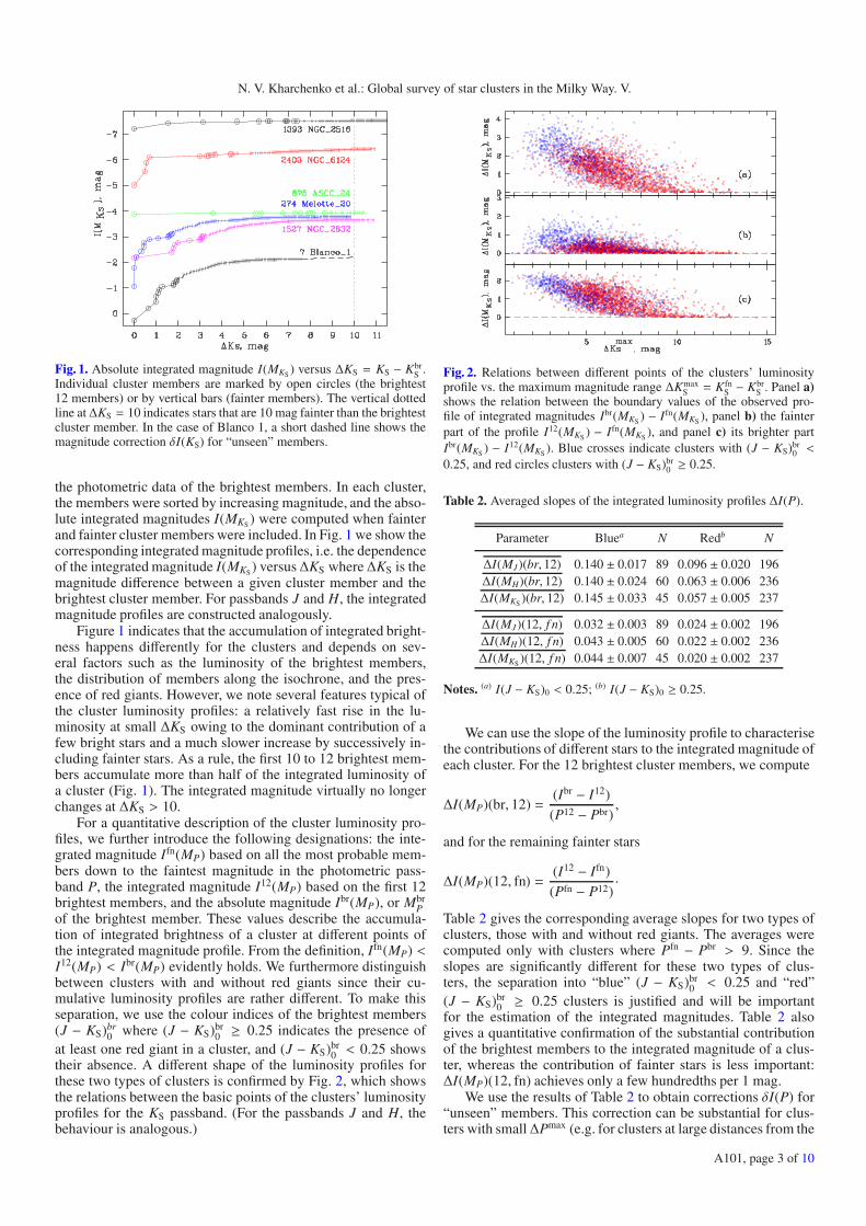
Fig. 1. Absolute integrated magnitude I(MKS ) versus ΔKS = KS − KbrS .

Individual cluster members are marked by open circles (the brightest12 members) or by vertical bars (fainter members). The vertical dottedline atΔKS = 10 indicates stars that are 10 mag fainter than the brightestcluster member. In the case of Blanco 1, a short dashed line shows themagnitude correction δI(KS) for “unseen” members.

the photometric data of the brightest members. In each cluster,the members were sorted by increasing magnitude, and the abso-lute integrated magnitudes I(MKS ) were computed when fainterand fainter cluster members were included. In Fig. 1 we show thecorresponding integrated magnitude profiles, i.e. the dependenceof the integrated magnitude I(MKS ) versusΔKS where ΔKS is themagnitude difference between a given cluster member and thebrightest cluster member. For passbands J and H, the integratedmagnitude profiles are constructed analogously.

Figure 1 indicates that the accumulation of integrated bright-ness happens differently for the clusters and depends on sev-eral factors such as the luminosity of the brightest members,the distribution of members along the isochrone, and the pres-ence of red giants. However, we note several features typical ofthe cluster luminosity profiles: a relatively fast rise in the lu-minosity at small ΔKS owing to the dominant contribution of afew bright stars and a much slower increase by successively in-cluding fainter stars. As a rule, the first 10 to 12 brightest mem-bers accumulate more than half of the integrated luminosity ofa cluster (Fig. 1). The integrated magnitude virtually no longerchanges at ΔKS > 10.

For a quantitative description of the cluster luminosity pro-files, we further introduce the following designations: the inte-grated magnitude Ifn(MP) based on all the most probable mem-bers down to the faintest magnitude in the photometric pass-band P, the integrated magnitude I12(MP) based on the first 12brightest members, and the absolute magnitude Ibr(MP), or Mbr

Pof the brightest member. These values describe the accumula-tion of integrated brightness of a cluster at different points ofthe integrated magnitude profile. From the definition, Ifn(MP) <I12(MP) < Ibr(MP) evidently holds. We furthermore distinguishbetween clusters with and without red giants since their cu-mulative luminosity profiles are rather different. To make thisseparation, we use the colour indices of the brightest members(J − KS)br

0 where (J − KS)br0 ≥ 0.25 indicates the presence of

at least one red giant in a cluster, and (J − KS)br0 < 0.25 shows

their absence. A different shape of the luminosity profiles forthese two types of clusters is confirmed by Fig. 2, which showsthe relations between the basic points of the clusters’ luminosityprofiles for the KS passband. (For the passbands J and H, thebehaviour is analogous.)

Fig. 2. Relations between different points of the clusters’ luminosityprofile vs. the maximum magnitude range ΔKmax

S = KfnS − Kbr

S . Panel a)shows the relation between the boundary values of the observed pro-file of integrated magnitudes Ibr(MKS ) − Ifn(MKS ), panel b) the fainterpart of the profile I12(MKS ) − Ifn(MKS ), and panel c) its brighter partIbr(MKS ) − I12(MKS ). Blue crosses indicate clusters with (J − KS)br

0 <

0.25, and red circles clusters with (J − KS)br0 ≥ 0.25.

Table 2. Averaged slopes of the integrated luminosity profiles ΔI(P).

Parameter Bluea N Redb N

ΔI(MJ)(br, 12) 0.140 ± 0.017 89 0.096 ± 0.020 196ΔI(MH)(br, 12) 0.140 ± 0.024 60 0.063 ± 0.006 236ΔI(MKS )(br, 12) 0.145 ± 0.033 45 0.057 ± 0.005 237

ΔI(MJ)(12, f n) 0.032 ± 0.003 89 0.024 ± 0.002 196ΔI(MH)(12, f n) 0.043 ± 0.005 60 0.022 ± 0.002 236ΔI(MKS )(12, f n) 0.044 ± 0.007 45 0.020 ± 0.002 237

Notes. (a) I(J − KS)0 < 0.25; (b) I(J − KS)0 ≥ 0.25.

We can use the slope of the luminosity profile to characterisethe contributions of different stars to the integrated magnitude ofeach cluster. For the 12 brightest cluster members, we compute

ΔI(MP)(br, 12) =(Ibr − I12)(P12 − Pbr)

,

and for the remaining fainter stars

ΔI(MP)(12, fn) =(I12 − Ifn)(Pfn − P12)

·

Table 2 gives the corresponding average slopes for two types ofclusters, those with and without red giants. The averages werecomputed only with clusters where Pfn − Pbr > 9. Since theslopes are significantly different for these two types of clus-ters, the separation into “blue” (J − KS)br

0 < 0.25 and “red”(J − KS)br

0 ≥ 0.25 clusters is justified and will be importantfor the estimation of the integrated magnitudes. Table 2 alsogives a quantitative confirmation of the substantial contributionof the brightest members to the integrated magnitude of a clus-ter, whereas the contribution of fainter stars is less important:ΔI(MP)(12, fn) achieves only a few hundredths per 1 mag.

We use the results of Table 2 to obtain corrections δI(P) for“unseen” members. This correction can be substantial for clus-ters with small ΔPmax (e.g. for clusters at large distances from the

A101, page 3 of 10

A&A 585, A101 (2016)

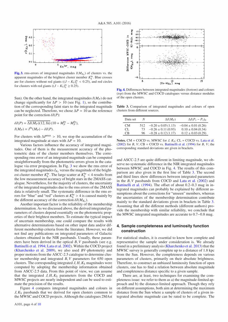
Fig. 3. rms-errors of integrated magnitudes I(MKS ) of clusters vs. theapparent magnitudes of the brightest cluster member Kbr

S . Blue crossesare for clusters without red giants ((J − KS)br

0 < 0.25), and red circlesfor clusters with red giants ((J − KS)br

0 ≥ 0.25).

Sun). On the other hand, the integrated magnitudes I(MP) do notchange significantly for ΔP > 10 (see Fig. 1), so the contribu-tion of the corresponding faint stars to the integrated magnitudecan be neglected. Therefore, we chose ΔP = 10 as the referencepoint for the correction δI(P):

δI(P) = ΔI(MP)(12, fn) (10 + MbrP − Mfn

P ),

I(MP) = Ifn(MP) − δI(P).

For clusters with ΔPmax > 10, we stop the accumulation of theintegrated magnitude at stars with ΔP = 10.

Various factors influence the accuracy of integrated magni-tudes. One of them is the measurement accuracy of the pho-tometric data of the cluster members themselves. The corre-sponding rms error of an integrated magnitude can be computedstraightforwardly from the photometric errors given in the cata-logue via error propagation. In Fig. 3 we show the rms error ofthe integrated magnitudes IKS versus the magnitude of the bright-est cluster member Kbr

S . The large scatter at KbrS < 4 results from

the low measurement accuracy of bright stars in the 2MASS cat-alogue. Nevertheless, for the majority of clusters, the uncertaintyof the integrated magnitudes due to the rms errors of the 2MASSdata is relatively small. The systematic difference in the rms er-rors for “blue” and “red” clusters at Kbr

S > 4 is caused mainly bythe different accuracy of the correction δI(MKS ).

Another important factor is the reliability of the membershipdetermination. As we discussed above, the derived integrated pa-rameters of clusters depend essentially on the photometric prop-erties of their brightest members. To estimate the typical impactof uncertain membership, one could compare the results withalternative determinations based on other input data and/or dif-ferent membership criteria from the literature. However, we didnot find any publications on integrated parameters of Galacticclusters obtained in the NIR passbands. Usually, these param-eters have been derived in the optical B,V passbands (see e.g.Battinelli et al. 1994; Lata et al. 2002). Within the COCD project(Kharchenko et al. 2009), we also used BV-photometry andproper motions from the ASCC-2.5 catalogue to determine clus-ter membership and integrated B,V parameters for 650 openclusters. The corresponding integrated J,H,KS magnitudes werecomputed by adopting the membership information obtainedfrom ASCC-2.5 data. From this point of view, we can assumethat the integrated J,H,KS parameters from the COCD andMWSC projects are nearly independent and can be used to esti-mate the precision of the results.

Figure 4 compares integrated magnitudes and colours inJ,KS passbands that we derived for open clusters common tothe MWSC and COCD projects. Although the catalogues 2MAst

Fig. 4. Differences between integrated magnitudes (bottom) and colours(top) from the MWSC and COCD catalogues versus distance modulusof the open clusters.

Table 3. Comparison of integrated magnitudes and colours of openclusters from different sources.

Data set N ΔI(MP) ΔI(P1 − P2)0

CM 512 −0.20 ± 0.05 (1.13) −0.04 ± 0.01 (0.26)CL 73 −0.26 ± 0.11 (0.93) 0.10 ± 0.04 (0.34)CB 96 −0.28 ± 0.12 (1.17) 0.12 ± 0.03 (0.29)

Notes. CM = COCD vs. MWSC for J, KS; CL = COCD vs. Lata et al.(2002) for B, V ; CB = COCD vs. Battinelli et al. (1994) for B, V ; thecorresponding standard deviations are given in brackets.

and ASCC-2.5 are quite different in limiting magnitude, we ob-serve no systematic difference in the NIR integrated magnitudesbetween MWSC and COCD in Fig. 4. The results of this com-parison are also given in the first line of Table 3. The secondand third lines show differences between integrated parametersin the B,V passbands from COCD and Lata et al. (2002) andBattinelli et al. (1994). The offset of about 0.2–0.3 mag in in-tegrated magnitudes can probably be explained by different as-sumptions about the corrections for “unseen” members, whereasthe uncertainties of the membership determination contributemainly to the standard deviations given in brackets in Table 3.Assuming that all the different methods (different authors) pro-vide the membership with similar reliability, we conclude thatthe MWSC integrated magnitudes are accurate to 0.7−0.8 mag.

4. Sample completeness and luminosity functionconstruction

For statistical studies, it is essential to know how complete andrepresentative the sample under consideration is. We alreadyfound in a preliminary analysis (Kharchenko et al. 2013) that theMWSC survey is generally complete up to a distance of 1.8 kpcfrom the Sun. However, the completeness depends on variousparameters of clusters, primarily on their absolute brightness.Therefore, to construct an unbiased luminosity function of openclusters, one has to find a relation between absolute magnitudeand completeness distance specific to a given sample.

There are, at least, two techniques for examining the com-pleteness issue: we refer to them as a) the magnitude-limited ap-proach and b) the distance-limited approach. Though they relyon different assumptions, both aim at determining the maximumdistance from the Sun where a sample of clusters of a given in-tegrated absolute magnitude can be rated to be complete. The

A101, page 4 of 10

N. V. Kharchenko et al.: Global survey of star clusters in the Milky Way. V.

first approach is based on the assumption that the sample con-tains all clusters brighter than a specific apparent magnitudeI(P). The second approach requires a uniform distribution ofclusters on the Galactic plane, and the sample is considered tobe complete up to a distance where the observed cluster densitystarts to deviate from some pre-specified law. The magnitude-limited approach is more economic, and it can be applied torelatively small samples, whereas the distance-limited method,being a more direct approach, requires larger samples to workeffectively.

In our previous study based on the COCD survey we con-structed the cluster luminosity functions using the magnitude-limited approach (Kharchenko et al. 2009). The size of theMWSC-survey enables us to apply the distance-limited ap-proach, hence to compare both techniques.

4.1. The magnitude-limited technique

Here we briefly outline the main idea of the CLF constructionbased on the magnitude-limited approach. The method is de-scribed in Kharchenko et al. (2009) in more detail. We assumethat our cluster sample is complete down to an integrated appar-ent magnitude I(P) in a photometric passband P, and we onlyconsider clusters that are brighter than I(P). For the jth clusterof such a subsample, we can determine a completeness distancedxy, j in the Galactic plane, which only depends on the complete-ness limit I(P), the cluster’s absolute magnitude I j(MP), and theinterstellar extinction AP, j on the line of sight to the cluster:

log dxy, j = 0.2 (I(P) − I j(MP) − AP, j + 5) + log cos b j, (1)

where b j is the galactic latitude of the cluster. We use herethe subscript j to emphasise the individual character of the de-rived limiting distance. With this parameter the cluster gives itsindividual contribution (a partial density) to the local surfacedensity, which can be computed as 1/(πd2

xy, j). Then, the clusterluminosity function φ is constructed as the sum of partial densi-ties of clusters with absolute integrated magnitudes in the rangeIi(MP), Ii(MP)+ΔI(MP) whereΔI(MP) is a bin of the distribution

φ[Ii(MP)] =1

ΔI(MP)

ni∑

j

1

π d 2xy, j

· (2)

Here ni is the number of clusters in the ith magnitude bin Ii(MP),and∑

ni is the number of clusters in the completeness subsam-ple. The CLF constructed in such a way represents a distributionof the surface density of open clusters over integrated magnitude.

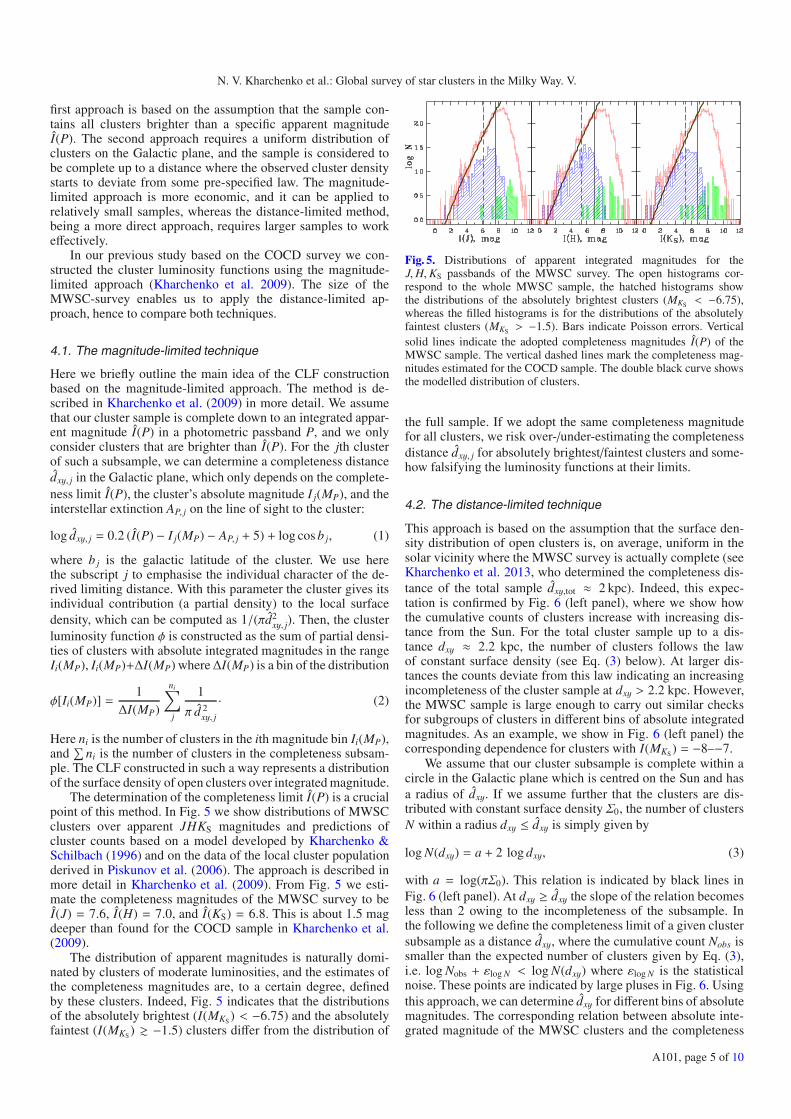
The determination of the completeness limit I(P) is a crucialpoint of this method. In Fig. 5 we show distributions of MWSCclusters over apparent JHKS magnitudes and predictions ofcluster counts based on a model developed by Kharchenko &Schilbach (1996) and on the data of the local cluster populationderived in Piskunov et al. (2006). The approach is described inmore detail in Kharchenko et al. (2009). From Fig. 5 we esti-mate the completeness magnitudes of the MWSC survey to beI(J) = 7.6, I(H) = 7.0, and I(KS) = 6.8. This is about 1.5 magdeeper than found for the COCD sample in Kharchenko et al.(2009).

The distribution of apparent magnitudes is naturally domi-nated by clusters of moderate luminosities, and the estimates ofthe completeness magnitudes are, to a certain degree, definedby these clusters. Indeed, Fig. 5 indicates that the distributionsof the absolutely brightest (I(MKS ) < −6.75) and the absolutelyfaintest (I(MKS ) � −1.5) clusters differ from the distribution of

Fig. 5. Distributions of apparent integrated magnitudes for theJ,H,KS passbands of the MWSC survey. The open histograms cor-respond to the whole MWSC sample, the hatched histograms showthe distributions of the absolutely brightest clusters (MKS < −6.75),whereas the filled histograms is for the distributions of the absolutelyfaintest clusters (MKS > −1.5). Bars indicate Poisson errors. Verticalsolid lines indicate the adopted completeness magnitudes I(P) of theMWSC sample. The vertical dashed lines mark the completeness mag-nitudes estimated for the COCD sample. The double black curve showsthe modelled distribution of clusters.

the full sample. If we adopt the same completeness magnitudefor all clusters, we risk over-/under-estimating the completenessdistance dxy, j for absolutely brightest/faintest clusters and some-how falsifying the luminosity functions at their limits.

4.2. The distance-limited technique

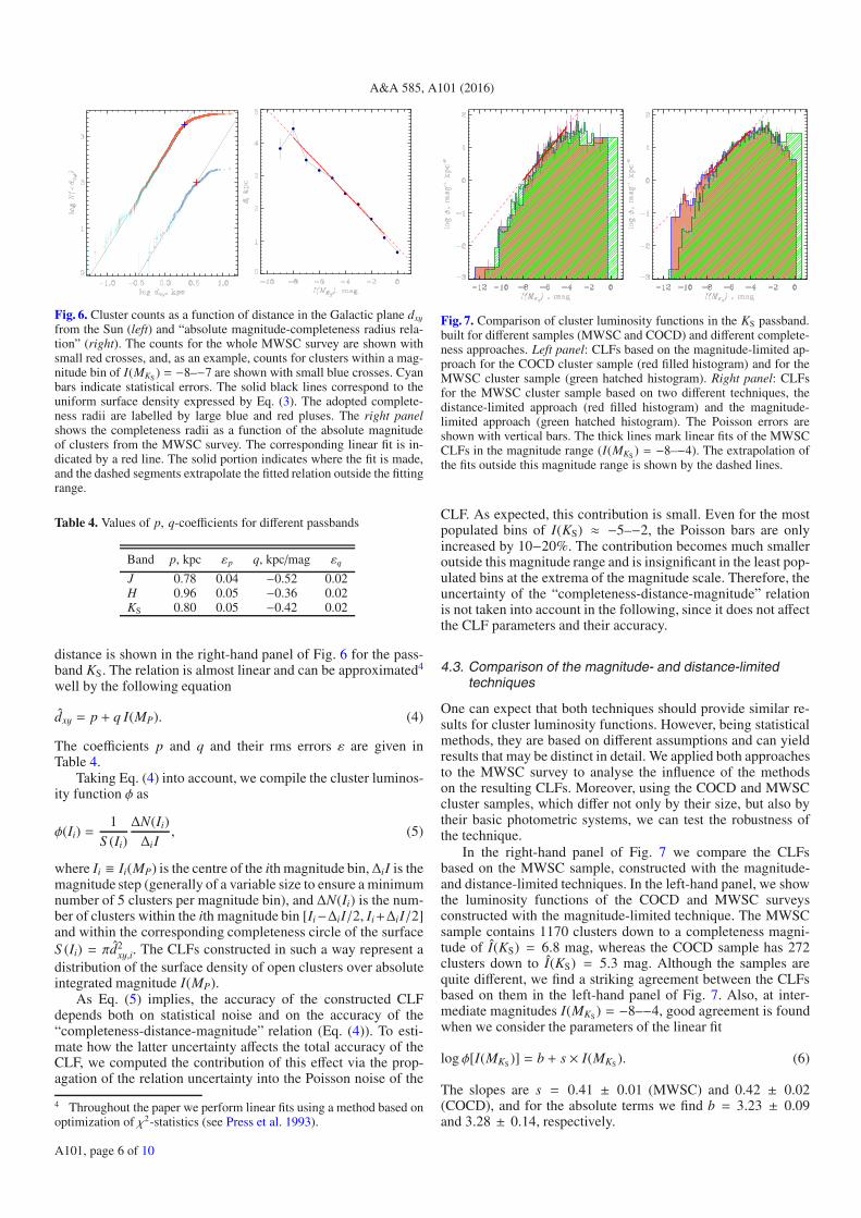
This approach is based on the assumption that the surface den-sity distribution of open clusters is, on average, uniform in thesolar vicinity where the MWSC survey is actually complete (seeKharchenko et al. 2013, who determined the completeness dis-tance of the total sample dxy,tot ≈ 2 kpc). Indeed, this expec-tation is confirmed by Fig. 6 (left panel), where we show howthe cumulative counts of clusters increase with increasing dis-tance from the Sun. For the total cluster sample up to a dis-tance dxy ≈ 2.2 kpc, the number of clusters follows the lawof constant surface density (see Eq. (3) below). At larger dis-tances the counts deviate from this law indicating an increasingincompleteness of the cluster sample at dxy > 2.2 kpc. However,the MWSC sample is large enough to carry out similar checksfor subgroups of clusters in different bins of absolute integratedmagnitudes. As an example, we show in Fig. 6 (left panel) thecorresponding dependence for clusters with I(MKS ) = −8–−7.

We assume that our cluster subsample is complete within acircle in the Galactic plane which is centred on the Sun and hasa radius of dxy. If we assume further that the clusters are dis-tributed with constant surface density Σ0, the number of clustersN within a radius dxy ≤ dxy is simply given by

log N(dxy) = a + 2 log dxy, (3)

with a = log(πΣ0). This relation is indicated by black lines inFig. 6 (left panel). At dxy ≥ dxy the slope of the relation becomesless than 2 owing to the incompleteness of the subsample. Inthe following we define the completeness limit of a given clustersubsample as a distance dxy, where the cumulative count Nobs issmaller than the expected number of clusters given by Eq. (3),i.e. log Nobs + εlog N < log N(dxy) where εlog N is the statisticalnoise. These points are indicated by large pluses in Fig. 6. Usingthis approach, we can determine dxy for different bins of absolutemagnitudes. The corresponding relation between absolute inte-grated magnitude of the MWSC clusters and the completeness

A101, page 5 of 10

A&A 585, A101 (2016)

Fig. 6. Cluster counts as a function of distance in the Galactic plane dxy

from the Sun (left) and “absolute magnitude-completeness radius rela-tion” (right). The counts for the whole MWSC survey are shown withsmall red crosses, and, as an example, counts for clusters within a mag-nitude bin of I(MKS ) = −8–−7 are shown with small blue crosses. Cyanbars indicate statistical errors. The solid black lines correspond to theuniform surface density expressed by Eq. (3). The adopted complete-ness radii are labelled by large blue and red pluses. The right panelshows the completeness radii as a function of the absolute magnitudeof clusters from the MWSC survey. The corresponding linear fit is in-dicated by a red line. The solid portion indicates where the fit is made,and the dashed segments extrapolate the fitted relation outside the fittingrange.

Table 4. Values of p, q-coefficients for different passbands

Band p, kpc εp q, kpc/mag εq

J 0.78 0.04 −0.52 0.02H 0.96 0.05 −0.36 0.02KS 0.80 0.05 −0.42 0.02

distance is shown in the right-hand panel of Fig. 6 for the pass-band KS. The relation is almost linear and can be approximated4

well by the following equation

dxy = p + q I(MP). (4)

The coefficients p and q and their rms errors ε are given inTable 4.

Taking Eq. (4) into account, we compile the cluster luminos-ity function φ as

φ(Ii) =1

S (Ii)ΔN(Ii)Δi I

, (5)

where Ii ≡ Ii(MP) is the centre of the ith magnitude bin,ΔiI is themagnitude step (generally of a variable size to ensure a minimumnumber of 5 clusters per magnitude bin), and ΔN(Ii) is the num-ber of clusters within the ith magnitude bin [Ii−ΔiI/2, Ii+Δi I/2]and within the corresponding completeness circle of the surfaceS (Ii) = πd2

xy,i. The CLFs constructed in such a way represent adistribution of the surface density of open clusters over absoluteintegrated magnitude I(MP).

As Eq. (5) implies, the accuracy of the constructed CLFdepends both on statistical noise and on the accuracy of the“completeness-distance-magnitude” relation (Eq. (4)). To esti-mate how the latter uncertainty affects the total accuracy of theCLF, we computed the contribution of this effect via the prop-agation of the relation uncertainty into the Poisson noise of the

4 Throughout the paper we perform linear fits using a method based onoptimization of χ2-statistics (see Press et al. 1993).

Fig. 7. Comparison of cluster luminosity functions in the KS passband.built for different samples (MWSC and COCD) and different complete-ness approaches. Left panel: CLFs based on the magnitude-limited ap-proach for the COCD cluster sample (red filled histogram) and for theMWSC cluster sample (green hatched histogram). Right panel: CLFsfor the MWSC cluster sample based on two different techniques, thedistance-limited approach (red filled histogram) and the magnitude-limited approach (green hatched histogram). The Poisson errors areshown with vertical bars. The thick lines mark linear fits of the MWSCCLFs in the magnitude range (I(MKS ) = −8–−4). The extrapolation ofthe fits outside this magnitude range is shown by the dashed lines.

CLF. As expected, this contribution is small. Even for the mostpopulated bins of I(KS) ≈ −5–−2, the Poisson bars are onlyincreased by 10−20%. The contribution becomes much smalleroutside this magnitude range and is insignificant in the least pop-ulated bins at the extrema of the magnitude scale. Therefore, theuncertainty of the “completeness-distance-magnitude” relationis not taken into account in the following, since it does not affectthe CLF parameters and their accuracy.

4.3. Comparison of the magnitude- and distance-limitedtechniques

One can expect that both techniques should provide similar re-sults for cluster luminosity functions. However, being statisticalmethods, they are based on different assumptions and can yieldresults that may be distinct in detail. We applied both approachesto the MWSC survey to analyse the influence of the methodson the resulting CLFs. Moreover, using the COCD and MWSCcluster samples, which differ not only by their size, but also bytheir basic photometric systems, we can test the robustness ofthe technique.

In the right-hand panel of Fig. 7 we compare the CLFsbased on the MWSC sample, constructed with the magnitude-and distance-limited techniques. In the left-hand panel, we showthe luminosity functions of the COCD and MWSC surveysconstructed with the magnitude-limited technique. The MWSCsample contains 1170 clusters down to a completeness magni-tude of I(KS) = 6.8 mag, whereas the COCD sample has 272clusters down to I(KS) = 5.3 mag. Although the samples arequite different, we find a striking agreement between the CLFsbased on them in the left-hand panel of Fig. 7. Also, at inter-mediate magnitudes I(MKS ) = −8–−4, good agreement is foundwhen we consider the parameters of the linear fit

logφ[I(MKS )] = b + s × I(MKS ). (6)

The slopes are s = 0.41 ± 0.01 (MWSC) and 0.42 ± 0.02(COCD), and for the absolute terms we find b = 3.23 ± 0.09and 3.28 ± 0.14, respectively.

A101, page 6 of 10

N. V. Kharchenko et al.: Global survey of star clusters in the Milky Way. V.

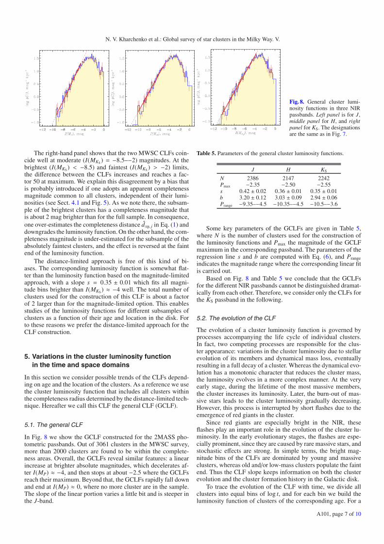
Fig. 8. General cluster lumi-nosity functions in three NIRpassbands. Left panel is for J,middle panel for H, and rightpanel for KS. The designationsare the same as in Fig. 7.

The right-hand panel shows that the two MWSC CLFs coin-cide well at moderate (I(MKS ) = −8.5–−2) magnitudes. At thebrightest (I(MKS ) < −8.5) and faintest (I(MKS ) > −2) limits,the difference between the CLFs increases and reaches a fac-tor 50 at maximum. We explain this disagreement by a bias thatis probably introduced if one adopts an apparent completenessmagnitude common to all clusters, independent of their lumi-nosities (see Sect. 4.1 and Fig. 5). As we note there, the subsam-ple of the brightest clusters has a completeness magnitude thatis about 2 mag brighter than for the full sample. In consequence,one over-estimates the completeness distance dxy, j in Eq. (1) anddowngrades the luminosity function. On the other hand, the com-pleteness magnitude is under-estimated for the subsample of theabsolutely faintest clusters, and the effect is reversed at the faintend of the luminosity function.

The distance-limited approach is free of this kind of bi-ases. The corresponding luminosity function is somewhat flat-ter than the luminosity function based on the magnitude-limitedapproach, with a slope s = 0.35 ± 0.01 which fits all magni-tude bins brighter than I(MKS ) ≈ −4 well. The total number ofclusters used for the construction of this CLF is about a factorof 2 larger than for the magnitude-limited option. This enablesstudies of the luminosity functions for different subsamples ofclusters as a function of their age and location in the disk. Forto these reasons we prefer the distance-limited approach for theCLF construction.

5. Variations in the cluster luminosity functionin the time and space domains

In this section we consider possible trends of the CLFs depend-ing on age and the location of the clusters. As a reference we usethe cluster luminosity function that includes all clusters withinthe completeness radius determined by the distance-limited tech-nique. Hereafter we call this CLF the general CLF (GCLF).

5.1. The general CLF

In Fig. 8 we show the GCLF constructed for the 2MASS pho-tometric passbands. Out of 3061 clusters in the MWSC survey,more than 2000 clusters are found to be within the complete-ness areas. Overall, the GCLFs reveal similar features: a linearincrease at brighter absolute magnitudes, which decelerates af-ter I(MP) ≈ −4, and then stops at about −2.5 where the GCLFsreach their maximum. Beyond that, the GCLFs rapidly fall downand end at I(MP) ≈ 0, where no more cluster are in the sample.The slope of the linear portion varies a little bit and is steeper inthe J-band.

Table 5. Parameters of the general cluster luminosity functions.

J H KS

N 2386 2147 2242Pmax −2.35 −2.50 −2.55s 0.42 ± 0.02 0.36 ± 0.01 0.35 ± 0.01b 3.20 ± 0.12 3.03 ± 0.09 2.94 ± 0.06Prange −9.35–−4.5 −10.35–−4.5 −10.5–−3.6

Some key parameters of the GCLFs are given in Table 5,where N is the number of clusters used for the construction ofthe luminosity functions and Pmax the magnitude of the GCLFmaximum in the corresponding passband. The parameters of theregression line s and b are computed with Eq. (6), and Prangeindicates the magnitude range where the corresponding linear fitis carried out.

Based on Fig. 8 and Table 5 we conclude that the GCLFsfor the different NIR passbands cannot be distinguished dramat-ically from each other. Therefore, we consider only the CLFs forthe KS passband in the following.

5.2. The evolution of the CLF

The evolution of a cluster luminosity function is governed byprocesses accompanying the life cycle of individual clusters.In fact, two competing processes are responsible for the clus-ter appearance: variations in the cluster luminosity due to stellarevolution of its members and dynamical mass loss, eventuallyresulting in a full decay of a cluster. Whereas the dynamical evo-lution has a monotonic character that reduces the cluster mass,the luminosity evolves in a more complex manner. At the veryearly stage, during the lifetime of the most massive members,the cluster increases its luminosity. Later, the burn-out of mas-sive stars leads to the cluster luminosity gradually decreasing.However, this process is interrupted by short flashes due to theemergence of red giants in the cluster.

Since red giants are especially bright in the NIR, theseflashes play an important role in the evolution of the cluster lu-minosity. In the early evolutionary stages, the flashes are espe-cially prominent, since they are caused by rare massive stars, andstochastic effects are strong. In simple terms, the bright mag-nitude bins of the CLFs are dominated by young and massiveclusters, whereas old and/or low-mass clusters populate the faintend. Thus the CLF slope keeps information on both the clusterevolution and the cluster formation history in the Galactic disk.

To trace the evolution of the CLF with time, we divide allclusters into equal bins of log t, and for each bin we build theluminosity function of clusters of the corresponding age. For a

A101, page 7 of 10

A&A 585, A101 (2016)

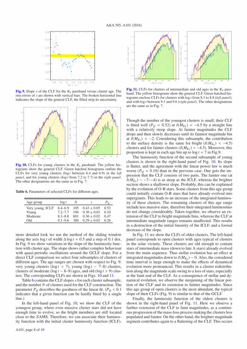
Fig. 9. Slope s of the CLF for the KS passband versus cluster age. Therms errors of s are shown with vertical bars. The broken horizontal lineindicates the slope of the general CLF, the filled strip its uncertainty.

Fig. 10. CLFs for young clusters in the KS passband. The yellow his-tograms show the general CLF. Green hatched histograms outline theCLFs for very young clusters (log t between 6.4 and 6.9) in the leftpanel, and for young clusters (log t from 7.2 to 7.7) in the right panel.The other designations are the same as in Fig. 7.

Table 6. Parameters of selected CLFs for different ages.

Age group log t N s PQ

Very young, ICLF 6.4–6.9 105 0.43 ± 0.05 0.52Young 7.2–7.7 194 0.30 ± 0.03 0.10Moderate 8.3–8.8 601 0.36 ± 0.02 0.47Old 9.1–9.6 380 0.29 ± 0.03 0.26

more detailed look we use the method of the sliding windowalong the axis log t of width Δ log t = 0.5 and a step of 0.1 dex.In Fig. 9 we show variations in the slope of the luminosity func-tion with cluster age. The slope shows rather complex behaviourwith quasi-periodic oscillations around the GCLF slope. For adirect CLF comparison we select four subsamples of clusters ofdifferent ages. The age ranges are chosen with respect to Fig. 9:very young clusters (log t < 7), young (log t ∼ 7–8) clusters,clusters of moderate (log t ∼ 8–9) ages, and old (log t > 9) clus-ters. The corresponding CLFs are shown in Figs. 10 and 11.

Table 6 contains the CLF slopes s for each cluster subsample,and the number N of clusters used for the CLF construction. Theparameter PQ describes the goodness of the linear fit. (PQ < 0.1indicates that a given function can be hardly fitted by a singleline.)

In the left-hand panel of Fig. 10, we show the CLF of theyoungest group, where even massive cluster stars did not haveenough time to evolve, so the bright members are still locatedclose to the ZAMS. Therefore, we can associate their luminos-ity function with the initial cluster luminosity function (ICLF).

Fig. 11. CLFs for clusters of intermediate and old ages in the KS pass-band. The yellow histograms show the general CLF. Green hatched his-tograms enclose CLFs for clusters with log t from 8.3 to 8.8 (left panel),and with log t between 9.1 and 9.6 (right panel). The other designationsare the same as in Fig. 7.

Though the number of the youngest clusters is small, their CLFis fitted well (PQ = 0.52) at I(MKS ) < −4.5 by a straight linewith a relatively steep slope. At fainter magnitudes the CLFdrops and then slowly decreases until its faintest magnitude binat I(MKS ) = −2. Considering this subsample, the contributionto the surface density is the same for bright (I(MKS ) < −4.5)clusters and for fainter clusters (I(MKS ) > −4.5). Moreover, thisproportion is kept in each age bin up to log t = 7 in Fig.9.

The luminosity function of the second subsample of youngclusters is shown in the right-hand panel of Fig. 10. Its slopeis flatter, and the agreement with the linear power law is muchworse (PQ = 0.10) than in the previous case. One gets the im-pression that the CLF consists of two parts. The fainter one (atI(MKS ) ∼ −7–−4) is as steep as the ICLF, whereas the brightersection shows a shallower slope. Probably, this can be explainedby the evolution of O-B stars. Some clusters from this age groupcould initially contain O-B stars that have already evolved intosupergiants. This leads to an increase of the integrated luminos-ity of these clusters. The remaining clusters of this age rangeinclude less massive stars, therefore their integrated luminositiesdo not change considerably. Taken together, we observe an ex-tension of the CLF to bright magnitude bins, whereas the CLF atintermediate magnitude ranges remains unaffected. This resultsin a destruction of the initial linearity of the ICLF, and a formaldecrease of the slope.

In Fig. 11 we show the CLFs of older clusters. The left-handpanel corresponds to open clusters with ages typical of clustersin the solar vicinity. These clusters are old enough to containstars of intermediate mass (down to late A stars) already evolvedfrom the main sequence. Thus stellar evolution has an effect atintegrated magnitudes down to I(MKS ) ∼ 0. Also, the consideredtime interval is large enough to make the effects of dynamicalevolution more pronounced. This results in a cluster redistribu-tion along the magnitude scale owing to a loss of stars, especiallyat the faint end of the CLF. As a consequence of stellar and dy-namical evolution, we observe the steepening of the linear por-tion of the CLF and its extension to fainter magnitudes. Sincethis age group of open clusters is the most abundant, the typicalslope of their CLFs (Fig. 9) is similar to that of the GCLF.

Finally, the luminosity function of the oldest clusters isshown in the right-hand panel of Fig. 11. Here we observe afurther extension of the CLF to faint magnitudes, as a continu-ous progression of the mass-loss process making the clusters lesspopulated and fainter. On the other hand, the brighter magnitudesegment contributes again to a flattening of the CLF. This occurs

A101, page 8 of 10

N. V. Kharchenko et al.: Global survey of star clusters in the Milky Way. V.

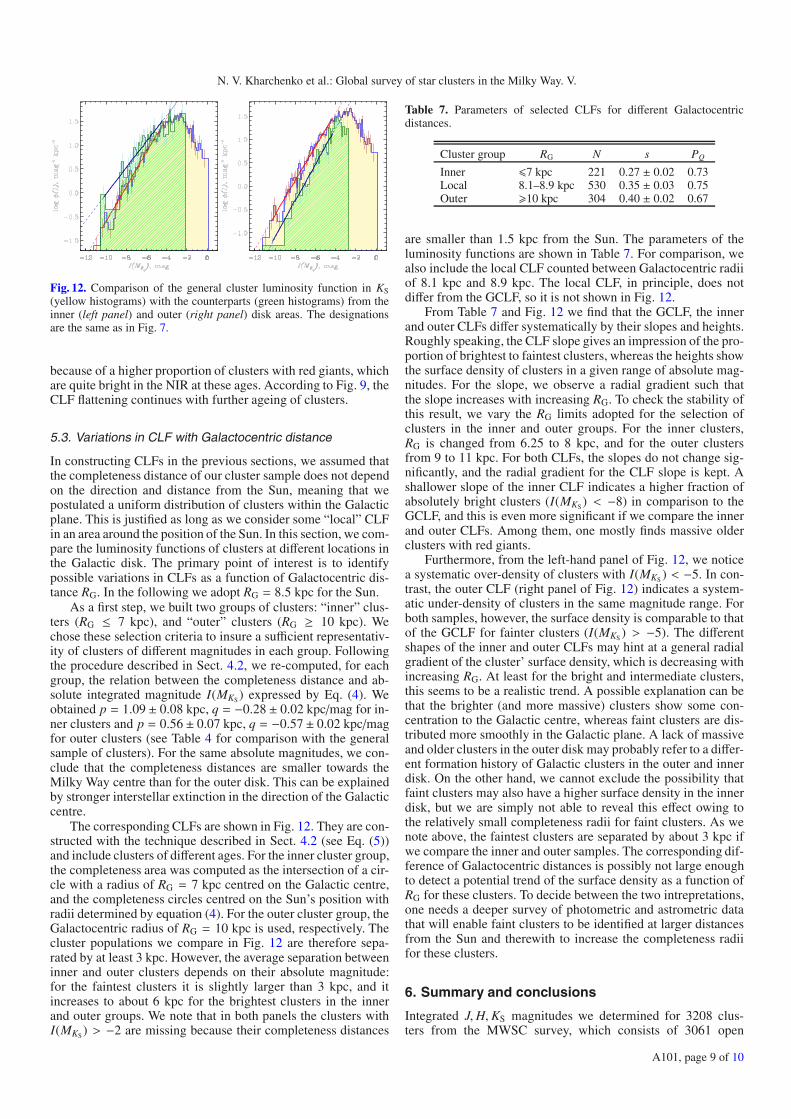
Fig. 12. Comparison of the general cluster luminosity function in KS

(yellow histograms) with the counterparts (green histograms) from theinner (left panel) and outer (right panel) disk areas. The designationsare the same as in Fig. 7.

because of a higher proportion of clusters with red giants, whichare quite bright in the NIR at these ages. According to Fig. 9, theCLF flattening continues with further ageing of clusters.

5.3. Variations in CLF with Galactocentric distance

In constructing CLFs in the previous sections, we assumed thatthe completeness distance of our cluster sample does not dependon the direction and distance from the Sun, meaning that wepostulated a uniform distribution of clusters within the Galacticplane. This is justified as long as we consider some “local” CLFin an area around the position of the Sun. In this section, we com-pare the luminosity functions of clusters at different locations inthe Galactic disk. The primary point of interest is to identifypossible variations in CLFs as a function of Galactocentric dis-tance RG. In the following we adopt RG = 8.5 kpc for the Sun.

As a first step, we built two groups of clusters: “inner” clus-ters (RG ≤ 7 kpc), and “outer” clusters (RG ≥ 10 kpc). Wechose these selection criteria to insure a sufficient representativ-ity of clusters of different magnitudes in each group. Followingthe procedure described in Sect. 4.2, we re-computed, for eachgroup, the relation between the completeness distance and ab-solute integrated magnitude I(MKS ) expressed by Eq. (4). Weobtained p = 1.09 ± 0.08 kpc, q = −0.28 ± 0.02 kpc/mag for in-ner clusters and p = 0.56 ± 0.07 kpc, q = −0.57± 0.02 kpc/magfor outer clusters (see Table 4 for comparison with the generalsample of clusters). For the same absolute magnitudes, we con-clude that the completeness distances are smaller towards theMilky Way centre than for the outer disk. This can be explainedby stronger interstellar extinction in the direction of the Galacticcentre.

The corresponding CLFs are shown in Fig. 12. They are con-structed with the technique described in Sect. 4.2 (see Eq. (5))and include clusters of different ages. For the inner cluster group,the completeness area was computed as the intersection of a cir-cle with a radius of RG = 7 kpc centred on the Galactic centre,and the completeness circles centred on the Sun’s position withradii determined by equation (4). For the outer cluster group, theGalactocentric radius of RG = 10 kpc is used, respectively. Thecluster populations we compare in Fig. 12 are therefore sepa-rated by at least 3 kpc. However, the average separation betweeninner and outer clusters depends on their absolute magnitude:for the faintest clusters it is slightly larger than 3 kpc, and itincreases to about 6 kpc for the brightest clusters in the innerand outer groups. We note that in both panels the clusters withI(MKS ) > −2 are missing because their completeness distances

Table 7. Parameters of selected CLFs for different Galactocentricdistances.

Cluster group RG N s PQ

Inner �7 kpc 221 0.27 ± 0.02 0.73Local 8.1–8.9 kpc 530 0.35 ± 0.03 0.75Outer �10 kpc 304 0.40 ± 0.02 0.67

are smaller than 1.5 kpc from the Sun. The parameters of theluminosity functions are shown in Table 7. For comparison, wealso include the local CLF counted between Galactocentric radiiof 8.1 kpc and 8.9 kpc. The local CLF, in principle, does notdiffer from the GCLF, so it is not shown in Fig. 12.

From Table 7 and Fig. 12 we find that the GCLF, the innerand outer CLFs differ systematically by their slopes and heights.Roughly speaking, the CLF slope gives an impression of the pro-portion of brightest to faintest clusters, whereas the heights showthe surface density of clusters in a given range of absolute mag-nitudes. For the slope, we observe a radial gradient such thatthe slope increases with increasing RG. To check the stability ofthis result, we vary the RG limits adopted for the selection ofclusters in the inner and outer groups. For the inner clusters,RG is changed from 6.25 to 8 kpc, and for the outer clustersfrom 9 to 11 kpc. For both CLFs, the slopes do not change sig-nificantly, and the radial gradient for the CLF slope is kept. Ashallower slope of the inner CLF indicates a higher fraction ofabsolutely bright clusters (I(MKS ) < −8) in comparison to theGCLF, and this is even more significant if we compare the innerand outer CLFs. Among them, one mostly finds massive olderclusters with red giants.

Furthermore, from the left-hand panel of Fig. 12, we noticea systematic over-density of clusters with I(MKS ) < −5. In con-trast, the outer CLF (right panel of Fig. 12) indicates a system-atic under-density of clusters in the same magnitude range. Forboth samples, however, the surface density is comparable to thatof the GCLF for fainter clusters (I(MKS ) > −5). The differentshapes of the inner and outer CLFs may hint at a general radialgradient of the cluster’ surface density, which is decreasing withincreasing RG. At least for the bright and intermediate clusters,this seems to be a realistic trend. A possible explanation can bethat the brighter (and more massive) clusters show some con-centration to the Galactic centre, whereas faint clusters are dis-tributed more smoothly in the Galactic plane. A lack of massiveand older clusters in the outer disk may probably refer to a differ-ent formation history of Galactic clusters in the outer and innerdisk. On the other hand, we cannot exclude the possibility thatfaint clusters may also have a higher surface density in the innerdisk, but we are simply not able to reveal this effect owing tothe relatively small completeness radii for faint clusters. As wenote above, the faintest clusters are separated by about 3 kpc ifwe compare the inner and outer samples. The corresponding dif-ference of Galactocentric distances is possibly not large enoughto detect a potential trend of the surface density as a function ofRG for these clusters. To decide between the two intrepretations,one needs a deeper survey of photometric and astrometric datathat will enable faint clusters to be identified at larger distancesfrom the Sun and therewith to increase the completeness radiifor these clusters.

6. Summary and conclusions

Integrated J,H,KS magnitudes we determined for 3208 clus-ters from the MWSC survey, which consists of 3061 open

A101, page 9 of 10

A&A 585, A101 (2016)

clusters and 147 globular clusters. The cluster sample coverswide ranges of absolute integrated magnitudes I(MKS ) = −11.7–0.6 (−12.4–−5.2), ages log t = 6.0–9.8 (9.8–10.1), and distancesfrom the Sun d = 0.1–14.7 (2.2–82.5) kpc. (The data for globu-lar clusters are given in brackets.)

Compared to the previous determination (Kharchenko et al.2009), the number of open clusters with integrated magnitudescould be increased by about a factor of five. This allows us toapply different statistical methods for constructing the clusterluminosity functions. Moreover, the variety in cluster age andlocation in the Galactic plane gives a chance to tackle possiblevariations of CLFs of different cluster groups.

For the CLF construction, we applied two different methodsto define cluster groups that can be considered as statisticallycomplete samples, i.e. distance-limited and magnitude-limitedapproaches. Comparing them, we found that both methods pro-vide similar CLFs within an intermediate rage of magnitudes(I(MKS ) = −7–−2), but they disagree at the limits of the mag-nitude scale. We conclude that the magnitude-limited approachunder-estimates the density of bright clusters and over-estimatesthe density of faint clusters.

Using the distance-limited method, we constructed the gen-eral cluster luminosity function in the solar neighbourhood forthe three 2MASS passbands. We found that the correspondingGCLFs depend only weakly on the passband. In each passbandthe GCLF shows a linear portion at bright magnitude bins. AtI(MP) ≈ −4.5 the increase slows down, and the CLF reachesthe maximum at about I(MP) ≈ −2 and then drops down atI(MP) ≈ 0. The luminosity function covers a magnitude rangeof about 9.5 mag for J and 11 mag for H and KS. The slopeof the linear portion of the GCLF is somewhat steeper for theJ magnitude than for the other two passbands.

Taking CLFs in the KS passband as an example, we tracedthe evolution of the CLF. We found that the slope of the CLFvaries with cluster ages in a complicated way reflecting the evo-lutionary state of the brightest cluster stars. Open clusters withages log t < 7 actually provide an initial cluster luminosityfunction (ICLF), which shows a relatively steep (with respectto the GCLF) slope of more than 0.4. The ICLF is clearly di-vided into two sections consisting of linear (bright) and quasiflat (faint) portions. The cluster luminosity function changes itsinitial shape at log t ∼ 7–8 and becomes flatter when the mostmassive stars leave the main sequence. They “extend” the brightend of the CLF, whereas the stars of intermediate masses keeptheir luminosities almost unchanged. Later, at ages log t ∼ 8–9,i.e. typical ages of “classical” open clusters, the most massivestars are burned out, whereas the evolution of the intermediate-mass stars defines the luminosity of the clusters. The slope ofthe CLF steepens again and the linear shape of the CLF holdsfor I(MKS ) < −4. Also, the CLF extends to fainter magnitudes,partly from dynamical mass loss. Finally, in the oldest clusters(log t > 9), the role of the brightest stars again increases due tomore numerous red giants, and the CLF flattens again.

The increase in the cluster sample to fainter apparent mag-nitudes meant that the completeness area of the MWSC surveywas extended compared to the COCD survey. This enabled thestudy of possible variations in CLFs at different Galactocentricdistances in two disk areas located at about RG = 6 kpc and RG =11 kpc. We found that the completeness radii are about 30%shorter towards the Galactic centre than in the anti-centre di-rection. Probably, this difference can be explained by a strongerextinction towards the Galactic centre. The CLF slope increasesfrom the inner to the outer disk. This may indicate that mas-sive clusters tend to be located in the inner disk. At least for thebright clusters, the surface density in the inner disk turns out tobe higher by a factor of two than the local density, whereas itis smaller in the outer disk. However, the MWSC survey is notdeep enough to investigate whether these trends are also validfor faint clusters.

Acknowledgements. This study was supported by SonderforschungsbereichSFB 881 “The Milky Way System” (subproject B5) of the German ResearchFoundation (DFG). We acknowledge the use of the Simbad database, the VizieRCatalogue Service, and other services operated at the CDS, France, and theWEBDA facility, operated at the Institute for Astronomy of the University ofVienna. We thank the anonymous referee for helpful questions and comments.

References

Anders, P., Bissantz, N., Boysen, L., de Grijs, R., & Fritze-v. Alvensleben, U.2007, MNRAS, 377, 91

Battinelli, P., Brandimarti, A., & Capuzzo-Dolcetta, R. 1994, A&AS, 104, 379de Grijs, R., Anders, P., Bastian, N., et al. 2003, MNRAS, 343, 1285Gieles, M., Larsen, S. S., Bastian, N., & Stein, I. T. 2006, A&A, 450, 129Gray, D. F. 1965, AJ, 70, 362Kharchenko, N. V., & Roeser, S. 2009, VizieR Online Data Catalog: I/280Kharchenko, N., & Schilbach, E. 1996, Balt. Astron., 5, 337Kharchenko, N. V., Piskunov, A. E., Röser, S., Schilbach, E., & Scholz, R.-D.

2005a, A&A, 440, 403Kharchenko, N. V., Piskunov, A. E., Röser, S., Schilbach, E., & Scholz, R.-D.

2005b, A&A, 438, 1163Kharchenko, N. V., Piskunov, A. E., Röser, S., et al. 2009, A&A, 504, 681Kharchenko, N. V., Piskunov, A. E., Schilbach, E., Röser, S., & Scholz, R.-D.

2012, A&A, 543, A156Kharchenko, N. V., Piskunov, A. E., Schilbach, E., Röser, S., & Scholz, R.-D.

2013, A&A, 558, A53Larsen, S. S. 2002, AJ, 124, 1393Lata, S., Pandey, A. K., Sagar, R., & Mohan, V. 2002, A&A, 388, 158Mora, M. D., Larsen, S. S., Kissler-Patig, M., Brodie, J. P., & Richtler, T. 2009,

A&A, 501, 949Piskunov, A. E., Kharchenko, N. V., Röser, S., Schilbach, E., & Scholz, R.-D.

2006, A&A, 445, 545Piskunov, A. E., Kharchenko, N. V., Schilbach, E., et al. 2008, A&A, 487, 557Press, W. H., Flannery, B. P., Teukolsky, S. S., & Vetterling, W. T. 1993,

Numerical Recipes (Cambridge: Cambridge Univ. Press)Röser, S., Demleitner, M., & Schilbach, E. 2010, AJ, 139, 2440Schmeja, S., Kharchenko, N. V., Piskunov, A. E., et al. 2014, A&A, 568, A51Scholz, R.-D., Kharchenko, N. V., Piskunov, A. E., Röser, S., & Schilbach, E.

2015, A&A, 581, A39Skrutskie, M. F., Cutri, R. M., Stiening, R., et al. 2006, AJ, 131, 1163Tarrab, I. 1982, A&A, 113, 57van den Bergh, S., & Lafontaine, A. 1984, AJ, 89, 1822Whitmore, B. C., Chandar, R., Bowers, A. S., et al. 2014, AJ, 147, 78

A101, page 10 of 10