Global manifold control in a driven laser: sustaining chaos and regular dynamics

Physica D 189 (2004) 70–80

Global manifold control in a driven laser: sustainingchaos and regular dynamics

R. Meuccia, D. Cinottia, E. Allariaa,∗, L. Billings b,I. Triandafc, D. Morganc, I.B. Schwartzc

a Istituto Nazionale di Ottica Applicata, Largo E. Fermi 6, 50125 Firenze, Italyb Department of Mathematical Sciences, Montclair State University, Upper Montclair, NJ 07043, USA

c Naval Research Laboratory, Plasma Physics Division, Code 6792, Washington, DC 20375-5000, USA

Received 27 June 2003; received in revised form 8 September 2003; accepted 26 September 2003Communicated by R. Roy

Abstract

We present experimental and numerical evidence of a multi-frequency phase control able to preserve periodic behaviorwithin a chaotic window as well as to re-excite chaotic behavior when it is destroyed by the presence of a mitigating unstableperiodic orbit created in the presence of the multi-frequency drive. The mitigating saddle controlling the global behavior isidentified and the controlling manifolds approximated.© 2003 Elsevier B.V. All rights reserved.

Keywords: Driven laser; Chaos dynamics; Regular dynamics

1. Introduction

Control of chaos represents one of the most inter-esting and stimulating ideas in the field of nonlineardynamics[1]. The original basic idea is to stabilize thedynamics over one of the different unstable periodicorbits visited during the chaotic motion by applyingsmall perturbations to the system[2]. Alternatively,one may wish to sustain chaos in certain situationswhere chaos is destroyed[3,4]. Both stabilizing un-stable orbits and sustaining chaos by exciting unsta-ble chaotic orbits may be considered as interventiontechniques to control the dynamical flow.

∗ Corresponding author. Tel.:+39-055-23081;fax: +39-055-2337755.E-mail addresses: [email protected] (R. Meucci),[email protected] (E. Allaria).

Different methods for controlling chaos have beenproposed based on determination of the stable and un-stable manifolds on the Poincaré section[2,5–7], ona self-controlling feedback procedure[8] and on theintroduction of open loop small perturbations[9–16].

On the other hand, chaos can be a desirable behav-ior in biological [4], mechanical[17], electrical[18]and optical systems[19]. In mechanics, small ampli-tude chaos, where the energy is spread over severalmodes, may be preferable to high amplitude resonantbehavior[20,21]. In such situations, the chaotic at-tracting window may be quite small, and sustainedchaos techniques are therefore required.

Once a chaotic regime appears, it typically anddramatically disappears as a result of a crisis, whichis an abrupt change from chaos to periodic behaviorat a critical parameter value of the system[22]. The

0167-2789/$ – see front matter © 2003 Elsevier B.V. All rights reserved.doi:10.1016/j.physd.2003.09.033

R. Meucci et al. / Physica D 189 (2004) 70–80 71

crisis typically occurs when the chaotic attractor col-lides with the stable manifold of an unstable periodicorbit, this stable manifold being, at the same time, thebasin boundary of the chaotic attractor[23,24]. Sucha saddle is called a basin saddle since it lies on thebasin boundary of the attractor and regions aroundsuch a saddle form escape regions for the chaotic tra-jectories resulting in non-chaotic behavior. Previoustechniques for sustaining chaos have been designedaround a feedback control mechanism in which a pa-rameter or state variable was used to maintain chaosby re-injecting the dynamics into a region containing achaotic saddle from a basin containing periodic attrac-tors [4,17,18,25–27]. In contrast, the global topologyof the basin boundary saddle manifold structure maybe used to design parameter control algorithms forsustaining chaos in parameter regimes where a crisisoccurs[3,28]. Chaos is sustained by adjusting a sys-tem parameter discretely based on measuring a timeseries obtained from the system, and using embed-ding methods to reconstruct the dynamics in a phasespace[3].

Closed loop control techniques have been demon-strated in fast electronic oscillators and in principleapplicable in optical systems with latency time be-low 1 ns[29]. However for controlling and sustainingchaos in systems such as those having fast time scalesopen loop methods are desirable for two primary rea-sons: (1) Open loop control methods have no feedbacktime scale with which to compete. (2) Many nonlinearoptical systems now are sufficiently modeled so thatthere exists excellent quantitative agreement betweentheory and experiment.

In the present paper we take an open loop approachto control and sustaining chaos. Let us first considerthe latter aspect. The approach still excites chaos, butit is an open-loop procedure that can be designed sothat stable chaotic regions may be achieved in placeswhere these were not stable previously. The procedurestarts with a periodically driven system at a primaryfrequency having a drive amplitude as an adjustableparameter. The drive amplitude is tuned so that thesystem operates in a crisis regime. Introduction ofadditional subharmonics may be expected to changelocal bifurcations, as well as global bifurcations. It is

well known that additive subharmonic perturbationsshift period doubling points in a cascade to chaos[30]. However, it may also change the nature of thebifurcation, where flip bifurcations become imper-fect bifurcations containing multiple stability andnew saddle-node points. Since the manifolds control-ling the global behavior are typically connected toregular saddles arising from such limit point bifur-cations, it is expected that global bifurcations suchas crises will be changed when introducing resonantsubharmonics.

The adopted strategy in our modulated laser is toconsider an amplitude modulation at half of the driv-ing frequency. We notice that the used perturbation isequivalent to applying an additive perturbation withcomponents atν/2 and 3ν/2. In addition, a phasedifference between the amplitude modulation and pri-mary frequency is considered as an extra parameter.The relevance of such a parameter in the frameworkof control of chaos has been demonstrated in exper-imental[13,16,31,32]and numerical works[14]. Theaddition of the amplitude modulation allows globalmanifold control at low energies in fast time scalesystems. Moreover, it is easily implemented in a largeclass of experiments that are forced by an externaldrive frequency.

The advantage of our method is that we can initiateregular (controlled) periodic behavior or sustainedchaos without any knowledge of a crisis in a chaoticattractor.

2. Experimental apparatus and measurements

The experimental apparatus is shown inFig. 1.It consists in a single mode CO2 laser with anintra-cavity acousto-optic modulator (AOM) allowingmodulation of the cavity losses. The optical cavity is1.30 m long and the total transmission coefficientT

is 0.10 for a single pass. The intensity decay ratek(t)

can be expressed as follows:

k(t) = k[1 + α sin2(B0(1 + f(t)))], (1)

wherek = cT/L, c is the speed of light in a vacuum,L the cavity length,α = (1 − 2T)/2T , B0 is a bias

72 R. Meucci et al. / Physica D 189 (2004) 70–80

Fig. 1. Experimental apparatus used to perform our measurements. AOM: acousto-optic modulator; BS: beam splitter; PM: power meter;PD: photodetector; TG: trigger generator; ADC: analog to digital converter; PC: personal computer.

andf(t) is the modulation signal,

fmod(t) = β sin(2πνt), (2)

whereν = 100 kHz andβ is the modulation ampli-tude. It is well known that by increasing the ampli-tude modulation, the system undergoes a sequenceof subharmonic bifurcation leading to chaos. A pro-grammable arbitrary function generator (FG) allowus to linearly scan the whole range ofβ by generatingthe function(2) whereβ is a saw tooth which goesfrom 0 to 1 V in 200 ms. In this configuration we donot consider hysteresis effects related to the scan inthe opposite direction.

In Fig. 2 the bifurcation diagram is shown, wherewe plot a stroboscopic record of the intensity versusthe amplitude modulation. The sampling period is 1/ν

Fig. 2. Experimental bifurcation diagram of the laser intensityas a function of the amplitude modulationβ. The first chaoticwindow is reached through a sequence of subharmonic bifurcationsoccurring atβ � 150 mV, the second one atβ � 320 mV. We notethe interior crisis atβ � 570 mV.

and the scanning time is 200 ms. From the bifurcationdiagram we observe the presence of a first chaoticregion (“chaos 1”) reached after a sequence of subhar-monic bifurcations. When the control parameterβ isincreased up toβ � 570 mV we observe the presenceof an interior crisis leading to a sudden expansionof the attractor. We denote such a region as “chaos2”. The “chaos 2” window is sudden destroyed by aboundary crisis at β � 900 mV.

Control and sustaining chaos are obtained by slightmodulation of the modulation amplitudeβ. Such aperturbation consists of a sinusoidal signal atν/2with amplitude δ and an adjustable phase offsetϕwith respect to the fundamental signalfmod(t); thenthe modulation signal becomes:

fmod(t) = β[1 + fpert(t)] sin (2πνt),

fpert(t) = δ sin(2πν

2t + ϕ

). (3)

The advantage of the subharmonic control approachis that it is easy to implement in many time forcedexperiments, regardless of time scales.

In Fig. 3, we report the perturbed bifurcation di-agram as a function ofβ for three different valuesof ϕ and for a fixed perturbation amplitudeδ of 5%.Around β = 500 mV, the perturbation stabilizes theperiod-2 orbit visited in the “chaos 1” regime. Wenote that this control effect is greater forϕ = π/2.We also note a sustaining chaos effect at the end ofthe bifurcation diagram, where region “chaos 2” wasdestroyed by a boundary crisis. The applied perturba-tion is able to re-excite this attractor, with the resultthat small parameter perturbations at 1/2 the drivefrequency have a global effect.


Fig. 3. Experimental perturbed bifurcation diagrams of the intensitylaser as a function of modulation amplitudeβ for different values ofthe phaseϕ. We can see the controlled periodic orbit forβ around500 mV and the sustained chaos at the end of the bifurcationdiagrams.

In Fig. 4, we report stroboscopic recordings of theintensity as a function of the phase at a fixed valueof amplitude modulationβ. These phase control dia-grams refer to three amplitude valuesβ correspondingto the first “chaos 1” window (β = 530 mV), to the“chaos 2” window (β = 730 mV) and to the sec-ond “chaos 1” window (β = 940 mV), respectively.We note that there are someϕ values for which wehave chaos control (β = 530 mV, ϕ ∈ [0,0.15π]and [0.4π,0.55π], β = 730 mV, ϕ ∈ [0,0.05] and[0.3π,0.35π], β = 940 mV,ϕ ∈ [0,0.05π]) and otherfor which we have sustaining chaos (β = 530 mV,ϕ ∈ [0.55π,0.95π], β = 940 mV, ϕ ∈ [0.1π, π]).Fig. 4a shows that, although the period-2 regime isthe most easier to stabilize, there are values for thephaseϕ where period-4 orbit is also stabilized.

Although not all orbits embedded in the chaoticattractor are stabilized, we can, in principle, stabilize

Fig. 4. Experimental phase control diagrams of the intensity laseras a function of the phaseϕ. Modulation amplitude is chosen: (a)in the first “chaos 1” window; (b) in “chaos 2” window; (c) in thesecond “chaos 2” window (compare withFig. 2). The relevance ofthe phase term to sustain or control chaos is evident. The originof the horizontal axis (phase) is arbitrary because the trigger isnot locked with the origin of the saw tooth.

other periods by adding other subharmonics. How-ever, for the purposes of control presented here, thegoal is to be able to sustain chaos or stabilize regularperiodic behavior.

Notice that as the modulation amplitude changes,so does the region over which chaos is excited. Sincethe phase changes the observed behavior betweenregular and chaotic behavior for each chosen ampli-tude, it plays a prominent role in determining controlor sustained chaos.

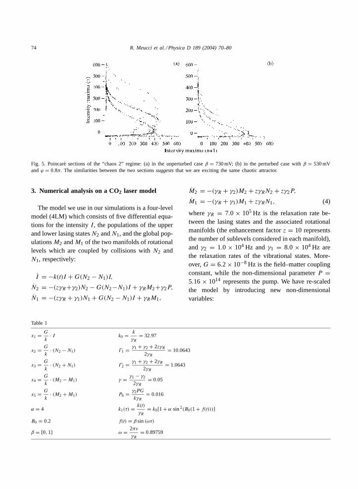
In Fig. 5, we compare the unperturbed “chaos 2”Poincaré section (Fig. 5a) with one perturbed (Fig. 5b).Similarity between the projected phase space portraitssuggests that our method re-excites the chaotic saddlecorresponding to the original pre-crisis saddle.


Fig. 5. Poincare sections of the “chaos 2” regime: (a) in the unperturbed caseβ = 730 mV; (b) in the perturbed case withβ = 530 mVandϕ = 0.8π. The similarities between the two sectionssuggests that we are exciting the same chaotic attractor.

3. Numerical analysis on a CO2 laser model

The model we use in our simulations is a four-levelmodel (4LM) which consists of five differential equa-tions for the intensityI, the populations of the upperand lower lasing statesN2 andN1, and the global pop-ulationsM2 andM1 of the two manifolds of rotationallevels which are coupled by collisions withN2 andN1, respectively:

I = −k(t)I +G(N2 −N1)I,

N2 = −(zγR+γ2)N2 −G(N2−N1)I + γRM2+γ2P,

N1 = −(zγR + γ1)N1 +G(N2 −N1)I + γRM1,

Table 1

x1 = G

k· I k0 = k

γR= 32.97

x2 = G

k· (N2 −N1) Γ1 = γ1 + γ2 + 2zγR

2γR= 10.0643

x3 = G

k· (N2 +N1) Γ2 = γ1 + γ2 + 2γR

2γR= 1.0643

x4 = G

k· (M2 −M1) γ = γ1 − γ2

2γR= 0.05

x5 = G

k· (M2 +M1) P6 = γ2PG

kγR= 0.016

α = 4 k1(τ) = k(t)

γR= k0[1 + α sin2(B0(1 + f(t)))]

B0 = 0.2 f(t) = β sin(ωτ)

β = [0,1] ω = 2πν

γR= 0.89759

M2 = −(γR + γ2)M2 + zγRN2 + zγ2P,

M1 = −(γR + γ1)M1 + zγRN1, (4)

whereγR = 7.0 × 105 Hz is the relaxation rate be-tween the lasing states and the associated rotationalmanifolds (the enhancement factorz = 10 representsthe number of sublevels considered in each manifold),and γ2 = 1.0 × 104 Hz andγ1 = 8.0 × 104 Hz arethe relaxation rates of the vibrational states. More-over,G = 6.2× 10−8 Hz is the field–matter couplingconstant, while the non-dimensional parameterP =5.16× 1014 represents the pump. We have re-scaledthe model by introducing new non-dimensionalvariables:


Fig. 6. Numerical bifurcation diagram of the intensity laser formEq. (3) as a function of the modulation amplitudeβ.

Fig. 7. Numerical perturbed bifurcation diagrams of the laserintensity as a function of amplitude modulationβ. (a)ϕ = 0.2; (b)ϕ = 0.7π; (c) ϕ = 1.2π. The correspondence with the experimentalresults shown inFig. 3 is clear. We note that there is a slightphase shift between experiment and numerical analysis.

x1 = −k1(τ)x1 + k0x1x2,

x2 = −Γ1x2 − 2k0x1x2 + γx3 + x4 + P6,

x3 = −Γ1x3 + γx2 + x5 + P6,

x4 = −Γ2x4 + zx2 + γx5 + zP6,

x5 = −Γ2x5 + zx3 + γx4 + zP6, (5)

whereτ = γR ·t is the re-scaled time and new variablesand constants are given inTable 1.

Using this re-scaled model we reproduce the exper-imental bifurcation measurements with a good degreeof accuracy. We have performed simulations modu-lating the losses with a signal according withEq. (3)assuming a bias valueB0 = 0.2. The agreement ofthe model with the experiment can be inferred fromFig. 6, showing the unperturbed bifurcation diagram,and from Fig. 7 where we report three perturbed

Fig. 8. Numerical perturbed bifurcation diagrams of the intensitylaser as a function of the phaseϕ. Modulation amplitude is chosen:(a) in the first “chaos 1” window; (b) in “chaos 2” window; (c)in the second “chaos 2” window as in the experiment (comparewith Fig. 6).


bifurcation diagrams. InFig. 8, we report other numer-ical results corresponding to the experimental mea-surements shown inFig. 1. The comparisons show thatthe agreement between theory and experiment is excel-lent. Moreover, since the bifurcation diagrams agreeon large parameter scales, the agreement is global.

4. Manifold control in the subharmonic laser

The reconstruction of the topology of the basinboundary saddle manifold structure is more eas-ily performed by using a suitable reduction of thefive-dimensional model ofEq. (5). We perform sucha reduction by approximating to the same value((γ1 + γ2)/2) the two relaxation ratesγ1 and γ2 inEq. (4). This implies inEq. (5) γ = 0 and the samevalues forΓ1 andΓ2.

The relevant variables arex1, the population leveldifference,x2, and the rotational level difference,x4.In this reduction procedure, a crucial role is played bythe pump parameterPinf which has been readjustedin order to provide the same steady state value of thelaser intensityx1. The main features of the full modelare retained by the following reduced 3D model:

y1 = k0(y2 − 1 − α sin2(fmod + B0)),

y2 = −Γ1y2 − 2k0 ey1y2 + y3 + Pinf ,

y3 = −Γ2y3 + zy2 + zPinf ,

fmod = Amod(1 + fpert) sin(ωt),

fpert = Apert sin(ωt

2+ φ

)(6)

with the parameterPinf = 0.0815. Notice the similar-ity of the bifurcation diagram inFig. 9to that ofFig. 2from the experiment andFig. 6 and the model.

By using the subharmonic amplitude modulation itis possible to control the chaotic behavior by acting onthe relative phaseφ [33]. As an example, we computethe maximal Lyapunov exponent forAmod = 0.1 asa function of subharmonic amplitudeApert and phaseφ to show the effect of the applied perturbation. Theresults are depicted inFig. 10.

ForApert = 0.05, Fig. 11shows the bifurcation di-agram as a function of the phaseφ in phase space.

Fig. 9. Bifurcation diagram of the intensity as a function of mod-ulation amplitude,Amod using Eq. (6). No subharmonic forcingwas applied.

Notice the four windows where large amplitude chaoschanges to a low-order stable periodic orbit.Fig. 10also predicts this change by an absence of a posi-tive Lyapunov exponent. The generic crisis bifurcationfrom chaos to periodic behavior is caused by the cre-ation of a saddle-node pair of periodic orbits of periodone when time is normalized to 4π/ω. (There also ex-ists a very small, four-piece chaotic attractor, which islong lived for these parameters that is not observed inthe experiment and does not seem to play a significantrole in the dynamics.) There are two transient timescales in the convergence to the periodic attractor. Thefirst is convergence from the immediate basin, which

Fig. 10. Maximal Lyapunov exponent of the 3D model as a functionof the subharmonic modulation amplitude,Apert and phase,φusingEq. (6)with Amod = 0.1. Asterisks denote parameters whichgenerate a positive exponent for some random initial condition.


Fig. 11. Control phase diagrams forAmod = 0.1 andApert = 0.05.

is bounded by the two-dimensional stable manifold ofthe associated period one saddle. The other is a slowerconvergence after a significant chaotic transient, alongthe chaotic saddle left by the chaotic attractor frombefore the bifurcation.

Notice that in the interval 1.6 < φ < 2.3, after thebifurcation from large amplitude chaos to a stable pe-riod one orbit, the stable periodic orbit goes througha period doubling cascade to small amplitude chaoticdynamics. At the end of the window, there is anotherbifurcation back to large amplitude chaos. This bifur-cation is caused by a crisis, when the small amplitudechaotic attractor intersects the stable manifold of theperiod one saddle from the original saddle node bifur-cation that created the window. The two-dimensionalversion of this bifurcation was reported in[33]. InFig. 12, we plot the relevant period one saddle at(y1, y2, y3) = (−5.5657,1.1588,11.8413) and itsstable manifolds forφ = 2.28, just prior to the onsetof the large amplitude chaotic attractor. It is the outershell of the union of the stable manifolds, representedby the small black points which lie on two-dimensionalfolded sheets. Overlaid in large black points is a sam-ple small amplitude chaotic trajectory. This set is em-bedded in one of the unstable manifolds of the saddle.As φ increases, the chaotic set intersects the stablemanifold of the period one saddle, similar to a homo-clinic bifurcation sincethe attractor is contained inthe unstable manifold, and a crisis to large amplitudechaos occurs. That is, since the attractor is a subsetof the unstable manifold, the attractor itself explodes

Fig. 12. Small amplitude chaotic attractor in large black dotsjust before the bifurcation to a large amplitude attractor. The starrepresents the period one saddle and the small black dots representits stable manifold. The parameters areAmod = 0.1, Apert = 0.05,andφ = 2.28.

in phase space upon intersection with the stable man-ifold sheet, creating the large amplitude attractor.

The stable and unstable manifolds in the phasespace can be approximated by the box-algorithmdescribed in[34]. Briefly, the algorithm works asfollows: Pick a region of interest interior to a box,B, containing the unstable saddle with part of its sta-ble and unstable manifolds. (If the box also containsperiodic points which are attractors, then we put asmall neighborhood about these points, and the boxis a punctured set.) Inside that box we randomly picka large number of initial conditions and record whichof these initial conditions will generate trajectoriesremaining in the box for a large number of iterations.In addition we monitor a small neighborhood of anyattracting orbits contained inB, and eliminate anypoints converging to this attractor, since these pointswill not represent the manifolds we approximate. Theinitial conditions remaining in the punctured box ap-proximate the union of the stable manifolds, whilethe last point which remains in the box approximatesthe unstable manifolds. This algorithm was used togenerate the stable manifolds inFig. 12.

In summary for the example ofAmod = 0.1 andApert = 0.05, when there exists a periodic attractor, itis connected to a minimal period one branch. Theseattracting branches are born through a saddle nodepair, typically embedded in a large amplitude chaoticattractor for someφ. It is the manifold of the saddle


branches which destroys and creates the regions oflarge amplitude chaos, and therefore, acts as the con-trolling mechanism for the sustaining of chaos in a re-gion in which the primary frequency has only periodicbehavior.

5. Conclusions

We have presented an open-loop control procedureto induce and control chaos in periodically drivensystems. The method is based on driving the systemwith a 1:2 resonance modulation and varying the am-plitude and the phase of the drive in this modulation.Open-loop control can either sustain chaos or stabi-lize regular periodic orbits, and is achieved throughglobal manifold control through the creation of asaddle-node bifurcation.

We have applied the procedure to a periodicallydriven CO2 laser and we have experimentally sus-tained or controlled chaos depending on the value ofthe relative phase between perturbation and modula-tion. Based on the choice of control parameters, theregions over which either regular periodic behavioror chaos may be sustained can be quite large, as seenin Fig. 10.

In order to verify our experimental measurements,we applied the method to a well tested 5-equation CO2

laser model; the numerical results match the experi-mental results with good agreement. We have reducedthis model to a lower dimensional model in order tovisualize the manifolds which are connected to anunstable periodic saddle created by the subharmonicterm.

We would like to acknowledge the fact that althoughthere exist a number of papers on multi-frequencydriving and bifurcation, most of them are driven pla-nar models, and those that have any global bifurcationresults are based on a Melnikov method, which is use-ful in mechanics. In our results, we have considered amodel which has been reduced to a three-dimensionalmulti-frequency system, and captures much of theexperimentally observed dynamics over a wide rangeof parameters. The primary controlling mechanism isthe interaction of a two-dimensional stable manifold

with a one-dimensional unstable manifold. The stablemanifold consists of two-dimensional sheets whichpossess a fractal-like structure. As the control param-eters are adjusted, the stable and unstable manifoldscross and uncross transversally, yielding the sustainedchaos or regular periodic behavior which is observedin both numerical and experimental dynamics. Oneof the interesting facets of the use of multi-frequencycontrol is that it may also be applied to discrete sys-tems as well as continuous flows. InAppendix A wehave shown that one may drive a map in much thesame way as we have done in the experiment. Specif-ically, we have applied our procedure to the logisticmap; we established chaos control in some range ofϕ value and sustaining chaos in some other one. Be-cause the sustaining chaos and control procedure iseffective also in this case, we can affirm its generalityto both continuous and discrete dynamical systems.

Acknowledgements

RM and EA are supported by the European Con-tract HPRN CT 2000 00158. IBS and IT are supportedby the Office of Naval Research. LB was supportedby ONR grant N00173-02-G909. DM is a NationalResearch Council Post Doctoral Fellow. We wouldlike to acknowledge Prof. Thomas Carr for usefuldiscussions, and for pointing out some of analyticlocal bifurcation results in the literature.

Appendix A. Sustaining chaos in the logistic map

The logistic map is described by the differenceequation:

xn+1 = Axn(1 − xn), (A.1)

wherexn ∈ [0,1] if A ∈ (0,4). The Lyapunov expo-nentλ of the map, can be evaluated as follows:

λ = limn→∞

1

n

n−1∑i=0

ln |A(1 − 2xi)|, (A.2)

where in our calculationn = 1500.


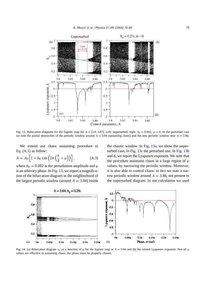
Fig. 13. Bifurcation diagrams for the logistic map forA ∈ [3.8,3.87]. Left: unperturbed; right:b0 = 0.002, ϕ = 0. In the perturbed casewe note the partial destruction of the periodic window aroundA = 3.84 (sustaining chaos) and the new periodic window nearA = 3.86.

We extend our chaos sustaining procedure toEq. (A.1)as follow:

A = A0

[1 + b0 cos

(2π

(n2

+ ϕ))]

, (A.3)

whereb0 = 0.002 is the perturbation amplitude andϕis an arbitrary phase. InFig. 13, we report a magnifica-tion of the bifurcation diagram in the neighborhood ofthe largest periodic window (aroundA = 3.84) inside

Fig. 14. (a) Bifurcation diagramxn as a function ofϕ for the logistic map atA = 3.84 and (b) the related Lyapunov exponent. Not allϕ

values are effective in sustaining chaos: the phase must be properly chosen.

the chaotic window. InFig. 13a, we show the unper-turbed case, inFig. 13c the perturbed one. InFig. 13band d, we report the Lyapunov exponent. We note thatthe procedure maintains chaos in a large region ofϕ

values, by narrowing the periodic window. Moreover,it is also able to control chaos: in fact we note a nar-row periodic window aroundA = 3.86, not present inthe unperturbed diagram. In our calculation we used


600 different values forA, with 1500 iterated for eachA, recording the last 200 to avoid transients.

We also build a bifurcation diagram by fixing themodulation amplitude atA0 = 3.84 and varying thephase. We have varied the phase from 0 toπ/4 (forA values greater thanπ/4 the diagram repeats itselfsymmetrically with respect toA = π/4); this bifurca-tion diagram can be seen inFig. 14. It is clear fromthis figure that there are someϕ values for which theperturbation is effective, but there are some other onefor which the behavior is again periodic. This resultconfirm the relevance of the relative phase termϕ inthe procedure. Because our method is effective alsoon the logistic map, the technique can be extended todiscrete dynamical systems.

References

[1] T. Shimbrot, E. Ott, C. Grebogi, J.A. Yorke, Nature 363(1993) 411;S. Boccaletti, C. Grebogi, Y.-C. Lai, H. Mancini, D. Maza,Phys. Rep. 103 (2000).

[2] E. Ott, C. Grebogi, J.A. Yorke, Phys. Rev. Lett. 64 (1990)1196;W.L. Ditto, S.N. Rauseo, M.L. Spano, Phys. Rev. Lett. 65(1990) 3211.

[3] I.B. Schwartz, I. Triandaf, Phys. Rev. Lett. 77 (1996) 4740.[4] W. Yang, M. Ding, A.J. Mandell, E. Ott, Phys. Rev. E 51

(1995) 102.[5] B. Peng, V. Petrov, K. Showalter, J. Phys. Chem. 95 (1991)

4957.[6] P. Parmananda, P. Sherard, R.W. Rollins, H.D. Dewald, Phys.

Rev. Lett. E 47 (1993) R3003.[7] E.R. Hunt, Phys. Rev. Lett. 67 (1991) 1953;

R. Roy, T.W. Murphy, T.D. Maier, Z. Gills, E.R. Hunt, Phys.Rev. Lett. 68 (1992) 1259;T.L. Carrol, I. Triandaf, I.B. Schwartz, L. Pecora, Phys. Rev.A 46 (1992) 6189;Z. Gills, C. Iwata, R. Roy, I.B. Schwartz, I. Triandaf, Phys.Rev. Lett. 69 (1992) 3169.

[8] K. Pyragas, Phys. Lett. A 170 (1992) 421;K. Pyragas, A. Tamaševicius, Phys. Lett. A 180 (1993) 99;

S. Bielawski, D. Derozier, P. Glorieux, Phys. Rev. E 50 (1994)245;S. Boccaletti, F.T. Arecchi, Europhys. Lett. 31 (1995) 127;R. Meucci, M. Ciofini, R. Abbate, Phys. Rev. E 53 (1996)R5537;S. Boccaletti, D. Maza, H. Mancini, R. Genesio, F.T. Arecchi,Phys. Rev. Lett. 79 (1997) 5246;D.W. Sukow, M.E. Bleich, D.J. Gauthier, J.E.S. Socolar,Chaos 7 (1997) 560.

[9] R. Lima, M. Pettini, Phys. Rev A 41 (1990) 726.[10] L. Fronzoni, M. Giocondo, M. Pettini, Phys. Rev. A 43 (1991)

6483.[11] Y. Braiman, I. Goldhirsch, Phys. Rev. Lett. 66 (1991) 2545.[12] A. Azevedo, S.M. Rezende, Phys. Rev. Lett. 66 (1991) 1342.[13] R. Corbalan, J. Cortit, A.N. Pisarchik, V.N. Chizhevsky, R.

Vilaseca, Phys. Rev. A 51 (1995) 663.[14] J. Yang, Z. Qu, G. Hu, Phys. Rev. E 53 (1996) 4402.[15] R. Chacón, J. Diaz Bejarano, Phys. Rev. Lett. 71 (1993) 3103;

R. Chacón, Phys. Rev. Lett. 86 (2001) 1737.[16] D. Dangoisse, J.-C. Celet, P. Glorieux, Phys. Rev. E 56 (1997)

1396.[17] V. In, et al., Chaos 7 (1997) 605.[18] M. Dhamala, Y.-C. Lai, Phys. Rev. E 59 (1999) 1646.[19] G.D. VanWiggeren, R. Roy, Science 279 (1998) 1198.[20] I.T. Georgiou, I.B. Schwartz, SIAM J. Appl. Math. 59 (1999)

1178.[21] I.B. Schwartz, I.T. Georgiou, Phys. Lett. A 242 (1998) 307.[22] C. Grebogi, E. Ott, J.A. Yorke, Physica D 7 (1983) 181.[23] K.T. Alligood, T.D. Sauer, J.A. Yorke, Chaos, Springer, New

York, 1997.[24] I.B. Schwartz, Phys. Rev. Lett. 60 (1988) 1359.[25] V. In, S.E. Mahan, W.L. Ditto, M.L. Spano, Phys. Rev. Lett.

74 (1995) 4420.[26] S. Codreanu, Chaos, Solitons Fractals 13 (2002) 839.[27] V. In, M. Spano, M. Ding, Phys. Rev. Lett. 80 (1998) 700.[28] I. Triandaf, I.B. Schwartz, Phys. Rev. E 62 (2000) 3529.[29] K. Myneni, T.A. Barr, N.J. Corron, S.D. Pethel, Phys. Rev.

Lett. 83 (1999) 2175.[30] T.C. Newell, A. Gavrielides, V. Kovanis, D. Sukow, T. Erneux,

S.A. Glasgow, Phys. Rev. E 56 (1997) 7223.[31] R. Meucci, W. Gadomski, M. Ciofini, F.T. Arecchi, Phys.

Rev. E 49 (1994) R2528.[32] V.N. Chizhevsky, R. Corbalán, A.N. Pisarchik, Phys. Rev. E

56 (1997) 1580.[33] I.B. Schwartz, I. Triandaf, R. Meucci, T.W. Carr, Phys. Rev.

E 66 (2002) 026213.[34] I. Triandaf, E. Bollt, I.B. Schwartz, Phys. Rev. E 67 (2003)

037201.

Global manifold control in a driven laser: sustaining chaos and regular dynamics

Documents

Transcript of Global manifold control in a driven laser: sustaining chaos and regular dynamics