GL 'BAL CHANGE - IGBP

GL 'BAL CHANGE

. REPORT NO. 18:2

Proceedings of the Asian Workshop New· Delhi, India

11-15 February, 1991

BAL CHANGE

REPORT NO. 18:2

Edited by

R.R. DANIEL B. BABUJI

Produced by The Committee on Science and Technology in Developing Countries

(COSTED)

and

The Indian National Committee for the IGBP for the

International Geosphere-Biosphere Programme A Study of Global Change (IGBP)

of the International Council of Scientific Unions (ICSU)

Madras - 1992

The Asian IGBP Workshop was jointly organized by : ICSU Committee on Science and Technology in Developing Countries (COSTED), the ICSU Scientific Committee for the IGBP, and the Indian National Committee for IGBP.

It was co-sponsored by : Unesco, New Delhi; ICSU, Paris; TWAS, Trieste; UNEP, Nairobi; Commonwealth Science Council, London; The Indian National Science Academy.

The Government of India, Departments of : Science and Technology; Environment and Forests; Ocean Development; Atomic Energy; Biotechnology; The National Physical Laboratory; The University Grants Commission; and The Council of Scientific and Industrial Research.

The proceeding was compiled by the editors from contributions by the invited speakers and participants of the Workshop.

The international planning and coordination of the IGBP is supportd by ICSU, IGBP National Committees, UNEP, Unesco, Shell Netherlands and the Dutch Electricity Generating Board.

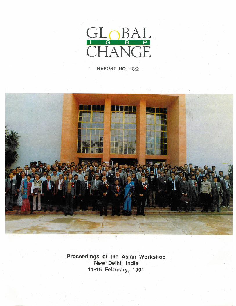
Cover Photograph : Participants who took part in the· Asian Workshop

ii

CONTENTS

FOREWORD - Prof. J. W.M. Ia Riviere

PREFACE - Prof. R.R. Daniel

INVITED TALKS

Page No.

v

vii

Global Change - Research Challenge and Policy Dilemma - Thomas Rosswa/1 . .. .. .. . .. .. . . . .. .. . 1

Ozone and Ozone Chemistry with Special Reference to Tropics • - A.P. M itra.. .............. ... . 8

Studies on the Past Global Changes (PAGES) with Special Reference to the Asian Region

Eiji Matsumoto ......... .... ... .... 23

The Role of Tibetan Plateau in Global Climate - Duzheng Ye .......... .......... 26

Recent Climate ' Changes and Trends over India - S.M. Kulshrestha. .. .. .. . .. .. . .. .. . . . 34

The Role of Ocean as a Regulator of Atmospheric C02 Concentration - Arthur Chen .................... 45

:Satellite Observations on _ ~lion Coyel· and Land •• ~ Patterns , , .... in Global Change Studies with Special Reference to Asia.

- B.L. Deekshatulu ... . . .. . .. .. . ... . .. . 53

Remote Sensing Data Availability in India for Geosphere - Biosphere Studies

- K. Kasturirangan. .. .. .. . .. .. . . . ..... 58

Biosphere - Atmosphere Trace Gas Exchange in the Tropics

NATIONAL REPORTS

Bangladesh

China

Indonesia

Nepal

Philippines

Sri Lanka

Taiwan

Thailand

iii

- J.R. Freney ... .......... .. ... .. 66

- S.D. Chaudhuri .. .................. 72

- Panqin Chen ... ................. 74

- A. G. 1/ahude .. ...... .... ... .. .. . 78

- J.S. Jha .: .... .............. 85

- Leoncio A. Amadore. .. . . .. . . . .. . ... . .. . 87

- Arudpragasam . .... .. . .. .. . . . .. .. . 89

- Ho Lin .: ..... ............. 91

Twesukdi Piyakarnchana .. . .. ... ..... .. ..... 95

.. ; I: • .

CONTRIBUTED PAPERS

Reconstruction of Rainy Season in Early Summer over East Asia during the Historical Period

Page No.

- Masatoshi Yoshino ...... ........... ... 97

Green House Gases, Environmental Stress and Ecological Analysis - J.S. Pandey, S. Moghe and P. Khanna. ............ ..... 1 03

Biogeochemical Cycle of Carbon for India - A Preliminary Estimate - V.K. Dadhwal and S.R. Nayak .. ....... ......... 109

Response of the Earth's Atmosphere to Increase in Green House Gases: Future projections of climate change

- M.Lat . .................. 114

Agrosphere - Atmosphere Interface Scope of Possible Contributions from Satellite Based Measurements

- Rajendra Kumar Gupta.. ...... ........ 118

Numerical Modelling of Tidal Circulation in an Estuary - P.C. Sinha .. ................ 122

Seasonal Variation of Atmospheric Particulates and Scattering of UV-B Radiation

- B.S.N. Prasad, N. Muralikrishnan, and H. B. Gayathri ...... .... ........ 126

Climate and Air-Quality Taiwan Station - Chung-Ming Liu. .. .. .. . .. . . . .. . . . 130

Rain and Lake Waters in Taiwan : Composition and Acidity . - C. T.A. Chen, J.J. Hung, J.S. Kuo, B.J. Wang and S.R. Yue ... ...... . .. ...... 135

Palaeoclimatic Studies in the Coastal Regions and Adjacent Seas of India using Trees, Corals and Marine Sediments

- R. Ramesh and B.L.K. Somayajulu .. .. .. . . . . . . .. 138

APPENDICES

Acronyms ... ..... ........... .. ............................... ... .......... ................ ..................... .............. .. 141

Participants List . .. .. ... .. . . . . . ... . . . . . . . .... . . . ... . . . . . . .. . . . . . . . . .. . . . . .. . . . . .. . . . .. . . . . . . . . . . .. .. . . . . . .. . . . .. . . . . . . . . .. . 142

IGBP Reports ...... ......... ............... .... .... .......................................................................... 151

iv

FOREWORD

The United Nations Conference on Environment and Development (UNCED, Rio de

Janeiro, 1992) is a response to the UN General Assembly Resolution of 1989 which called

for a conference that would deal with -

"Issues of major concern in maintaining the quality of the Earth environment

and especially in achieving environmentally sound and sustainable

development in all countries'.

It is obvious that the best available knowledge is requried in the design of strategies

for sustainable development that respect the limitations of the Earth system. Accordingly, it

became clear already during the preparations for UNCED that the interest of policy-makers

in ongoing Earth System Research programmes was growing and that an increased interaction

between science and the "body politic" during the post-UNCED period could be anticipated.

It furthermore became clear that there was widespread consenus that the international research

programmes now in place did not need to be supplemented by new institutional arrangements

and would deliver results in relation to the funding and the manpower committed to them.

A crucial condition for the success of the research efforts as well as of the action based

upon their results is the full participation of scientists from all parts of the world. Very rapidly

the fulfilment of this condition was recognised for what it was : a difficult and complicated

task that would require major special efforts if the emergence of a serious obstacle was to

be avoided.

This recognition is being shared by governments, UN bodies, donors, ICSU and the

leadership of the research programmes and has led to various interesting action processes.

One of these is IGBP's project START (Global Change System for Analysis, Research

and Training) aiming to develop regional networks for research, training and assessment,

especially in the developing world. Promising progress has been made in the past year,

particularly with respect to networks in the America's and Asia. The systems are going to

cooperate with IGBP, WCRP and HDGEC.

In parallel with this, IGBP is organizing regional meetings in the developing world to

stimulate full involvement of Third World scientists in the work of IGBP. The present meeting

is the third one in this series but it is the first one in which IGBP and COSTED joint forces

as organizers. Its success as demonstrated by these proceedings and, in particular, its positive

impact on the development of the START initiative in Asia, show that the cooperation of these

two ICSU bodies is productive and should be promoted to help keep up the momentum in

the UNCED followup.

v

In a process where meeting follows meeting it is important that the results of each of

them be well documented so as to enable each meeting to 'stand on the shoulders' of the

preceding ones. It is therefore highly commendable that after pre-publication of the

recommendations of the workshop now also the full proceedings are being published.

ICSU wishes to express its gratitude to the government and the scientific community

of the host country India, and in particular Professor R.R. Daniel, the Scientific Secretary of

COSTED, who along with Professor T. Rosswall, Executive Director of IGBP played a key

role in tl:le preparation of the meeting and of the publications resulting from it.

In addition. ICSU wishes to thank all participants collectively for the sense of realism

expressed in their general recommendations directed to various bodies including ICSU itself.

In response, I wish to confirm that their message has arrived and that ICSU as a whole is

working hard to respond to it.

Netherlands

March '92

vi

Prof. J.W.M. Ia Riviere

Secretary-General of ICSU

PREFACE

Recognizing the emerging importance of studying the Earth, its total environment and

the intimate interconnections between their different constituent parts as an interactive feedback

system, the International Council of Scientific Unions (ICSU) initiated detailed planning for the

IGBP in 1986 by appointing a Special Committee to guide the planning and implementation

of the programme. After a detailed and careful four-year study, and after 11 reports, the special

committee and its many working groups came up with the 12th Report embodying a well

formulated approach and long-term global programme which was accepted by ICSU in 1990.

ICSU has now constituted a regular Scientific Committee for IGBP (SC-IGBP). IGBP Report

12 now constitutes the primary source book for all future planning, management and strategies

of IGBP. However, the original objective of IGBP : "To describe and understand the interactive

physical, chemical and biological processes that regulate the total Earth system, the unique

environment it provides for life, the changes that are occurring in this system, and the manner

in which they are influenced by human action" remains unchanged. Furthermore, recognizing

the scientific complementarity between IGBP and the World Climate Research Programme

(WCRP) of the World Meteorological Organization (WMO) and ICSU, a close relationship has

been established.

IGBP Report 12 has stated that in order to carry out research in all regions of the world

in order to obtain necessary understanding of global processes, there is a clear need to stimulate

IGBP research in developing countries. It also became evident that special efforts, including

the organization of regional meetings, will be needed to establish adequate familiarity with the

scientific content and the interdisciplinary nature of IGBP in order to enable scientists from

developing countries to participate in IGBP. Such regional meetings can also be utilized with

great advantage to achieve a number of other desirable objectives such as : (i) to identify

region-specific problems of relevance to IGBP; (ii) to familarize scientists of the region with

the national efforts in IGBP-related activities; (iii) to organize regional co-operation including

observational and data networking; (iv) to arrange regional and international training

opportunities; (v) to evolve recommendations for national, regional and global participation of

developing countries and (vi) to involve and expose decision makers to the nature and relevance

of IGBP to developing countries . The workshop organised in Delhi in 11-15 February, 1991

had precisely these goals.

Of the total of about 200 participants, there were about 150 from developing countries

namely Bangladesh, China (CAST and China Academy in Taipei), India (about 100, including

25 young scientists), Indonesia, Malaysia, Nepal, Pakistan, Philippines; Sri Lanka and Thailand.

There were also participants from Japan, Poland, U.K., U.S.A., and U.S.S.R. Furthermore, we

were privileged to have for part of the time some of the ICSU officers who had attended a

meeting in Delhi just prior to the workshop. They included, apart from Prof. M.G.K. Menon,

the President; Prof.J.C.I. Dooge, the President Elect ; Prof . J.W.M. Ia Riviere, the Secretary

General,and Ms. Julia Marton-Lefevre, the Executive Secretary. Prof.Thomas Rosswall,

vii

Executive Director, IGBP, played a major role in organ1z1ng and conducting the scientific

programme of the workshop. Four Active participants from Japan also attended but no one

from Australia, New Zealand could attend because of unavoidable reasons . The largest

delegations, after India, were from China (CAST) and China (Academy in Taipei) with eight

from each.

The scientific programme comprised the following elements : two invited talks on the

general framework and scientific programme content of IGBP; nine invited talks on IGBP-related

problems and programmes unique or of special significance to the Asian activities for IGBP;

about 20 contributed poster paper presentations; four working group discussions; and formulation

of recommendations of the Workshop. On the evening of February 12, Prof. Thomas Rosswall

delivered a general lecture on "Global Change - Research Challenge and Policy Dilemma"

which was extremely well received by the audience. The Workshop was inaugurated by the

Prime Minister of India.

It was recognized right at the outset that the recommendations from the four working

group meetings and those from the workshop in general would constitute one of the most

important and useful outputs of the Workshop. The main topics of discussion at these working

group meetings were the 10 IGBP Core Projects and other major elements described in IGBP

Report 12. Each working group had a chairman, and a rapporteur to assist the chairperson

in preparing the report. Advance background papers based on IGBP report 12, emphasizing

elements of interest to the Asian region , were prepared and disributed to participants in advance.

Since the first three working group meetings were held in parallel, each participant chose

one working group of main interest for attendance. The fourth working group covered items

of common interest including Regional Research Centres. Each working group had about six

working hours With ample time for discussion. Participants who had given advance notice of

their intention and interest to raise major issues, emphasize issues of special interest to the

region, or to draw attention to existing gaps and lacunae were given 5-10 minutes to present

them. The summary and highlights of the working group deliberations were presented by the

respective chairperson and discussed thoroughly at the plenary on the final day. Based on

all these activities, the chairperson and convener of each working group prepared the final

report.

The reports of the working groups and the recommendations of the workshop have already

been published as IGBP Report No.18.1 and have also been distributed to all the participants.

It was agreed at the time of the conference to bring out the proceedings of the workshop.

Accordingly this publication has been brought out and is numbered as IGBP Report No.18.2.

This volume contains the keynote address, the invited talks and the national plans on IGBP.

The contents of this volume are expected to be useful to the scientific community in the

developing countries of Asia who have an interest on IGBP.

The workshop was co-sponsored by several national, regional and international

organisations. We gratefully acknowledge the support provided by them all.

MADRAS MAY'92

viii

R. R. Daniel Scientific Secretary COSTED

GLOBAL CHANGE :

RESEARCH CHALLENGE AND POLICY DILEMMA Professor Thomas Rosswall Executive Director, SC-IGBP

ABSTRACT

The Intergovernmental Panel on Climate Change (IPCC) has recently published a scientific assessment of our present knowledge of greenhouse warming and climate change. The IPCC report predicts that emissions of greenhouse gases will lead to a global temperature increase by 0.3°C per decade over the next century and the average rate of sea-level rise will be 6 em per decade during the same period. Such changes will have dramatic Impacts on our global resource base.

However, all predictions about future global change are uncertain at best. How well we anticipate and respond to our rapidly changing global environment depends on our commitment to document and understand the integrated Earth system processes Involved In such changes. The scientists must work together as quickly and as efficiently as possible to meet our future responsibility. The International Geosphere Biosphere Programme : A Study of Global Change (IGBP) and the World Climate Research Programme (WCRP) have been created to meet this challenge.

Discussions are presently under way within nations and in UN bodies to address the policy implications of the threat of global changes with far reaching consequences. There is a desire to develop an international convention for the protection of the global atmosphere to be followed by b inding protocols in a similar manner as was the case for the protection of the ozone layer. Many human activities lead to the emission of greenshouse gases that will affect the future c limate. But there are major d ifferences between industrialized and developing countries. A few industrialized countries are discussing the possibility of freezing emissions at present levels. This will be a difficult decision, but even so, it will be far from enough to stabilize the composition of the global atmosphere. In any case, a concerted scientific effort will be needed to narrow the present scientific uncertainties regarding global change phenomena.

Introduction

Man is presently affecting the composition of the global atmosphere in a major way. The best known example is the increased concentration of carbon dioxide . On a global scale, carbon dioxide concentrations have increased by nearly 25% since the industrial revolution. The main cause of this has undoubtedly been the burning of fossil fuels. The destruction of forests has also contributed to the rise in C0

2, because on land cleared for agriculture, the

new vegetation stores less carbon than the original forest. In addition, ploughing of virgin land leads to an increased flux of carbon to the atmosphere through decomposition processes. Our knowledge of the global carbon cycle is still too limited to allow accurate predictions of the fat e of present concentrations and future additions of carbon dioxide to the atmosphere.

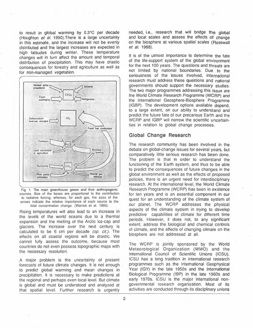
Carbon dioxide is one of the so-called "greenhouse gases". Several other gases are also important contributors to projected increases in temperature. It has been estimated that carbon dioxide will account for about half of the future temperature increases, while methane, nitrous oxide, ozone, . and chlorofluorocarbons will be responsible for the rest. Levels of all of these greenhouse gases are increasing in the atmosphere. Greenhouse gases are produced both by industrial and biological processes (Fig. 1 ), but while industrial emissions are fairly well documented, our knowledge of the production rates of greenhouse gases through biological processes and the factors regu lating emissions is still inadequate. We are at present unable to predict with any certainty the future emissions, and the effects of these on climate.

In the next 100 years, the increases in emrssrons of greenhouse gases to the atmosphere are estimated

to result in global warming by 0.3°C per decade (Houghton et at. 1990).There is a large uncertainty in this estimate. and the increase will not be evenly distributed and the largest increases are expected in high latitudes during winter. These temperature changes will in turn affect the amount and temporal distribution of precipitation. This may have drastic consequences for forestry and agriculture as well as for non-managed vegetation.

\

Doforestatioo/ ...---'\. ~ ~ Wlckse changes L--y' L:J ~

Fossil fuel combuSllon

·~~·~=/ ~b Land con\lefsiOn Biomass

10 agriculture ~ burning

Fig. 1. The main greenhouse gases and their anthropogenic sources. Size of the boxes are proportional to the contribution to radiative forcing , whereas, for each gas, the sizes of the

arrows indicate the relative importance of each source to the total concentration change. (Warrick et al. 1990).

Rising temperatures will also lead to an increase in the levels of the world oceans due to a thermal expansion and the melting of the Arctic ice-cap and glaciers. The increase over the next century is calculated to be 6 em per decade (op. cit.) . The effects on all coastal regions will be drastic. We cannot fully assess the outcome, because most countries do not even possess topographic maps with the necessary resolution.

A major problem is the uncertainty of present forecasts of future climate changes. It is not enough to predict global warming and mean changes in precipitation. It is necessary to make predictions at the regional and perhaps even local level. But climate is global and must be understood and analyzed at that spatial level. Further research is urgently

2

needed, i.e., research that will bridge the global and local scales and assess the effects of change on the biosphere at various spatial scales (Rosswall et at. 1988).

It is of the utmost importance to determine the fate of the life-support system of the global environment for the next 100 years . The questions and threats are not limited by national boundaries. Due to the seriousness of the issues involved, international research must address these questions and national governments should support the necessary studies. The two major programmes addressing this issue are the World Climate Research Programme (WCRP) and the International Geosphere-Biosphere Programme (IGBP). The development options available depend, to a large extent, on our ability to understand and predict the future fate of our precarious Earth and the WCRP and IGBP will narrow the scientific uncertainties in relation to global change processes.

Global Change Research

The research community has been involved in the debate on global-change issues for several years, but comparatively little serious research has been done. The problem is that in order to understand the functioning of the Earth system, and thus to be able to predict the consequences of future changes in the global environment as well as the effects of proposed policies, there is an urgent need for interdisciplinary research. At the international level, the World Climate Research Programme (WCRP) has been in existence for ten years and is an essential component in our quest for an understanding of the climate system of our planet. The WCRP addresses the physical aspects of the climate system in trying to develop predictive capabilities of climate for different time periods. However, it does not, to any significant extent, address the biological and chemical controls of climate, and the effects of changing climate on the biosphere are not addressed at all.

The WCRP is jointly sponsored by the World Meteorological Organization (WMO) and the International Council of Scientific Unions (ICSU). ICSU has a long tradition in international research programmes such as the International Geophysical Year (IGY) in the late 1950s and the International Biological Programme (IBP) in the late 1960s and early 1970s. ICSU is the major international nongovernmental research organization. Most of its activities are conducted through its disciplinary unions

and interdisciplinary committees. When ICSU perceives problems which call for new approaches in international research collaboration, it can take action and initiate programmes to address these problems.

In 1986, ICSU decided to launch the International Geosphere-Biosphere Programme : A Study of Global Change (IGBP). This is in its interdisciplinarity the most ambitious programme ever undertaken by ICSU and probably by any other organization.

The objective of the IGBP is (IGBP 1990):

* To describe and understand the interactive, physical, chemical, and biological processes that regulate the total Earth system, the unique environment that it provides for life, the changes that are occurring in this system, and the manner in which they are influenced by human activities.

The IGBP is an evolving programme that selects from the broad array of subjects that comprise the science of the Earth system, those questions that are deemed to be of greatest importance in contributing to our understanding of the changing nature of the global environment on time scales of decades to centuries, that most affect the biosphere, and that are most susceptible to human perturbations and that will most likely lead to practical, predictive capability.

The research questions and the projects that make up the programme are expected to evolve with new insights and understanding, but the initial operational phase of the programme focuses on seven key questions:

1. How is the chemistry of the global atmosphere regulated and what is the role of biological processes in producing and consuming trace gases?

* International Global Atmospheric Chemistry (IGAC) Project; An established IGBP Core Project.

* Stratosphere-Troposphere Interact ions and the Biosphere (STIB) ; A proposed IGBP Core Project.

3

2. How do ocean biogeochemical processes influence and respond to climate change ?

* Joint Global Ocean Flux Study (JGOFS); An established IGBP Core Project planned and implemented by the ICSU Scientific Committee on Ocean Research (SCOR).

* Global Ocean Euphotic Zone Study (GOEZS) ; A potential IGBP Core Project.

3. How are changes in land use affecting the resources of the coastal zone, and how will changes in sea level and climate alter coastal ecosystems ?

* Land-Ocean Interactions in the Coastal Zone (LOICZ); A proposed IGBP Core Project.

4. How does vegetation interact with physical processes of the hydrological cycle ?

* Biospheric Aspects of the Hydrological Cycle (BAHC); An established IGBP Core Project.

5. How ~ill global changes affect terrestrial ecosystems ?

* Global Change and Terrestrial Ecosystems (GCTE); An established IGBP Core Project.

* Global Change and Ecological Complexity (GCEC); A potential IGBP Core Project.

6. What significant climate and environmental changes have occurred in the past and what were their consequences ?

* Past Global Changes (PAGES); An established IGBP Core Project.

7. How can our knowledge of components of the Earth system be integrated and synthesized in a numerical framework that provides predictive capacity? ·

* Global Analysis, Interpretation and Modelling (GAIM); A proposed IGBP Core Project.

As indicated above, the IGBP Core Projects will not all be initiated at the sam~ time. Five of the projects (IGAC, JGOFS, BAHC, GCTE and PAGES) have been established and science plans published (IGBP 1990, Galbally 1989, Matson and Ojima 1990, JGOFS 1990, Eddy 1992). For the proposed projects (STIB,

LOICZ and .GAIM), detailed science plans have not yet been prepared, but it is expected that these will be ready within the next two years, at which time the Scientific Committee for the IGBP (SC-IGBP), which guides the planning and implementation of the IGBP, will decide if they will be established and implementation plans developed. The SC-IGBP will consider, at a later stage, if a science plan should be developed for the potential Core Projects (GOEZS and GCEC) followning full discussions and consideration by the international science community.

For the established projects, international Core Project Offices have been set up to prepare implementation plans and help develop a truly coordinated international research effort. The IGAC office is located in the US (Cambridge, MA), JGOFS and BAHC in the FRG (Kiel and Berlin, respectively) , GCTE in Australia (Canberra) and PAGES will be located in Switzeroland (Berne).

In addition, two framework projects relate to the needs of all research questions :

* The development of a global Data and Information System that will provide immediate and open access to al researchers, that will provide information needed for Earth system models, and that will define and sustain the longterm observations needed to detect significant global changes.

* The establishment of a set of Regional Research Networks and Centres, with special emphasis on the needs of developing countries, where strong synthesis and modelling projects of relevance to overall IGBP objectives and regional priorities will be undertaken . Training and exchange programmes will be one of the mechanisms to involve the scientists from the region in IGBP project activities. (Eddy et at. 1991 ).

National Involvement in the IGBP and Funding of Research

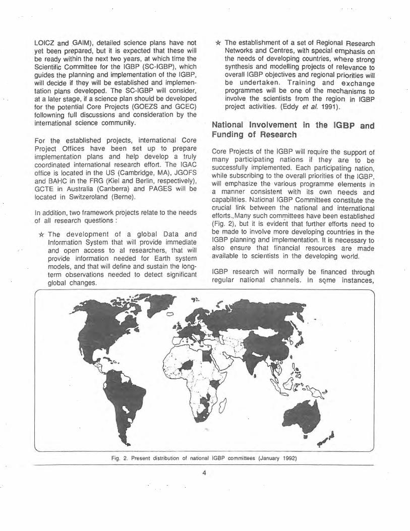
Core Projects of the IGBP will requ ire the support of many participating nations if they are to be successfully implemented. Each participating nation, while subscribing to the overall priorities of the IGBP, will emphasize the various programme elements in a manner consistel'lt with its own needs and capabilities. National IGBP Committees constitute the crucial link between the national and international efforts .. Many such committees have been established (Fig. 2). but it is evident that further efforts need to be made to involve more developing countries in the IGBP planning and implementation. It is necessary to also ensure that financial resources are made available to scientists in the developing world.

IGBP research will normally be financed through regular national channels. In sqme instances,

Fig. 2. Present distribution of national IGBP committees (January 1992)

4

countries have developed global change programmes for research with designated funding; in other instances, projects are evaluated solely on individual merit. In order to promote dialogue between national. funding agencies to create an informal mechanism of consultation, the International Group of Funding Agencies for Global Change Research (IGFA) has been established. Funding for international planning and coordination as well as funding for Regional Research Centres will have to be sec1:Jred from the nations participating in the programme. It is estimated that the core IGBP planning and coordination needs an annual budget of about 1-2 M US$; the total cost for the Core Project Offices is in the order of 3-5 M US$; funding for the RRCs once fully operational is needed in the order of 50-100 M US$; the cost for actual research needed may be some 1 ,000 M US$. In addition, satellite observations necessary, deployment of automatic submarines to collect ocean data, and a full Global Climate Observing System, as proposed during the Second World Climate Conference last year, might be in the order 10,000 M US$ annually.

A Policy Dilemma

World leaders in many countries have taken the threat of climate warming very seriously. It is necessary that the political dialogue is continued with the aim of achieving an international agreement on how to protect the atmosphere and thus the global climate system. It is a healthy sign that the world's political leaders now seem willing to discuss global environmental problems in a long-term perspective, although the scientific evidence is far from complete. The need for absolute certainty before a serious political discussion can take place has partly been countered.

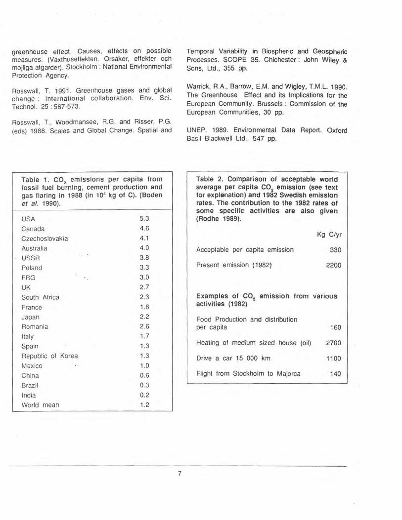
The Intergovernmental Panel on Climate Change (IPCC) has considered policy options at the international level. Any international agreement to reduce greenhouse-gas emissions, other than CFCs, is going to be very difficult to reach. Carbon dioxide is the single most important greenhouse gas. The emissions from fossil-fuel burning are very unevenly distributed between different countries (Table 1 ). There are large national differences in per capita emissions, reflecting difference between developing and developed countries and between those countries w1th relatively efficient energy production systems and those without . Countries will thus face different challenges in reducing emission rates . Some

5

governments have already set up energy policies with the aim of reducing regional and global pollution of the atmosphere. The problems are very serious and drastic changes are needed. A combination of legislative action, taxation, industrial development of environmentally acceptable techniques, and individual actions is needed to reduce the emissions of pollutants into the atmosphere. Decisions are now being made by some countries to maintain the present emission levels or reduce it by a few or ten per cent.

The developing countries will not, and should not, accept the condition that they freeze their emissions at the present level. Rodhe (1989) has presented an example of what measures are needed in order to both protect the atmosphere and to allow for an equitable level of emission for fossil-fuel carbon. If it is assumed that C02 levels in the atmosphere must not increase above 400 ppm (v) (present level 350 ppm (v)), the annual anthropogenic emissions must not be greater than 2.5 Pg carbon (Rodhe 1989: present emissions 5.5 Pg) from fossil-fuel burning and 1.7 Pg from deforestation (UNEP 1989). Rodhe (1989) assumed that one third of the "allowable" emissions would come from changes in land use and greenhouse gases other than C02, which leaves 1.7 Pg from fossil-fuel sources. If it is further assumed that each person would be allowed the same emission, the annual per capita emission rate must be limited to 330 kg of carbon as compared to the 1988 emissions of 5300 kg in the USA (Table 1). A crude estimate of the sources of anthropogenic C02 emissions in Sweden is given in Tabele 2. Sweden would need to reduce its emissions by 85%. The average private car consumes more than three times the allowable per capita emission. This clearly shows how dfficult any political action will be, if the aim is to stabilize the composition of the atmosphere at approximately the current level.

All discussions must be based on a development towards a sustainable and equitable future world. Policies must take scientific evidence into account, and scientists need to develop a much better understanding of the Earth system as a necessary guide for international governmental agreements on protection of the atmosphere.

Conclusions

Within the decade of the 1990s, the IGBP will launch a world-wide research effort, unprecedented in its comprehensive interdisciplinary scope, to address the

functioning of the Earth system and to understand how this system is changing. The body of information generated by the IGBP will form the scientific underpinning for predictions relating to future causes and effects of global changes. Through its obseiVational network and process studies, and the effective communication of the resulting data to scientists in all nations committed to this endeavour, the IGBP will help provide the world's decision makers with input necessary to wisely manage the global environment. Studies of the chemistry of the atmosphere and the effects of changed sources and sinks will be a crucial component of this research endeavour. It will also form an important link to the World Climate Research Programme (WCRP) of the World Meteorological Organisation (WMO) and ICSU. While the WCRP will address the physics of the climate system and the effect of radiative forcing on climate, the IGBP will address key aspects of the relationships between the biological and chemical processes that regulate the functioning of. the global system. These efforts will be paramount in narrowing the uncertainties in our understanding of the functioning of the global system.

The IGBP will design and implement research projects to produce global data sets on properties and processes central to global change. These will include obseNations and studies at the Earth's surface as well as from an array of Earth-sensing satellites. This research will make use of a network of Regional Research Centres in forging a new understanding of the interactions among biogeochemical cycles and physical processes of the Earth system.

In the course of this endeavour, the IGBP will promote an interdisciplinary approach to studies of the Earth system. It is essentia~ to educate the next generation of scientists in such a manner that they will more fully understand the complexities of this system. This knowledge will be they key to success in the wise use of the Earth's resources for generations to come. Even if prediqtions of global changes are uncertain, we are certain of one thing: The future is not what it has been!

Acknowledgements

This paper is based to a large extent on Rosswall (1991 ).

6

References

Boden, T.A., Kanciruk, P. and Farrell, M.P. 1990. Trends '90. A. Compendium of Data on Global Change. Oak Ridge, Tenn., USA: Oak Ridge National Laboratory, Carbon Dioxide Information Analysis Center, 257 pp.

Galbally, I.E. (ed.) 1989. The International Global Atmospheric Chemistry (IGAC) Programme. A Core Project of the International Geosphere-Biosphere Programme. Commission of Atmospheric Chemistry and Global Pollution of the ICSU International Association of Meteorology and Atmospheric Physics (IAMAP).

Houghton, J.T. Jenkins, G.J. and Ephraums, J .J. (eds) 1990. Climate Change . The IPCC Scientif ic Assessment. Cambridge: Cambridge University Press, 365 pp.

IGBP. 1990. The International Geosphere-Biosphere Programme: A Study of Global Change. The Initial Core Projects. IGBP Report No. 12. Stockholm : IGBP Secretariat.

Eddy, J.A. (ed). 1992. The PAGES Project: Proposed Implementation Plans for Research Activities. IGBP Report No. 19. Stockholm: IGBP Secretariat, 112 pp.

Eddy, J.A., Malone, T .F., McCarthy, J .J. and Rosswall, T. (eds) 1991. Global Change System for Analysis, Research and Training (START). Report of a Meeting at Bellagio December 3-7, 1990. IGBP Report No. 15. Boulder: OIES, 40 pp.

JGOFS. 1990. Joint Global Ocean Flux Study Science Plan. JGOFS Report No. 5. SCOR Secretariat, Halifax, N.S., Canada.

Matson, P.A. and Ojima, D.S. (eds) 1990. Terrestrial Biosphere Exchange with Global Atmospheric Chemistry.IGBP Report No. 13. Stockholm IGBP Secretariat.

Rodhe, H. 19e9. Reduce the emissions drastically! (Minska utslappen drastiskt) . Dagens Nyheter 18 January 1989. Also cited is: SNV. 1989. The

greenhouse effect. Causes, effects on possible measures. (Vaxthuseffekten. Orsaker, effekter och mojliga atgarder). Stockholm : National Environmental Protection Agency.

Rosswall, T. 1991 . Greenhouse ga$eS and global change : International collaboration. Env. Sci. Technol. 25 : 567-573.

Rosswall, T., Woodmansee, R.G. and Risser, P.G. (eds) 1988. Scales and Global Change. Spatial and

-

Table 1. C02

emissions per capita from fossil fuel burning, cement production and gas flaring in 1988 (in 103 kg of C). (Boden et at. 1990).

USA 5.3

Canada 4.6

Czechoslovakia 4.1

Australia 4.0

USSR 3.8

Poland 3.3

FAG 3.0

UK 2.7

South Africa 2.3

France 1.6

Japan 2.2

Romania 2.6

Italy 1.7

Spain 1.3

Republic of Korea 1.3

Mexico 1.0

China 0.6

Brazil 0.3

India 0.2

World mean 1.2

7

Temporal Variability in Biospheric and Geospheric Processes. SCOPE 35. Chichester : John Wiley & Sons, Ltd., 355 pp.

Warrick, A.A., Barrow, E.M. and Wigley, T.M.L. 1990. The Greenhouse Effect and its Implications for the European Community. Brussels: Commission of the European Communities, 30 pp.

UNEP. 1989. Environmental Data Report. Oxford Basil Blackwell Ltd., 547 pp.

Table 2. Comparison of acceptable world average per capita C02 emission (see text for expleoation) and 1982 Swedish emission rates. Tlie contribution to the 1982 rates of some specific activities are also given (Rodhe 1989).

Kg C/yr

Acceptable per capita emission 330

Present emission ( 1982) 2200

Examples of C02 emission from v·arious activities (1982)

Food Production anQ distribution per capita 160

Heating of medium sized house (oil) 2700

Drive a car 15 000 km 11 00

Flight from Stockholm to Majorca 140

OZONE AND OZONE CHEMISTRY WITH SPECIAL REFERENCE TO TROPICS

A.P. Mitra. INDIA

ABSTRACT

In this lecture the following ore described:

(0 measurement techniques and available network and gop in the tropics:

(ii) special characteristics of tropical regions:

(iii) chronological sequence of ozone chemistry going from the Initial pioneering work of Chapman (the so-called "dry chemistry·) to the present day chemical schemes involving catalytic cycles:

(iv) factors affecting ozone contents and distribution and the relative roles of natural and anthropogenic sources:

(v) chemistry behind the formation of ozone "holes· in the Antarctic and the Arctic regions.

1. Introduction

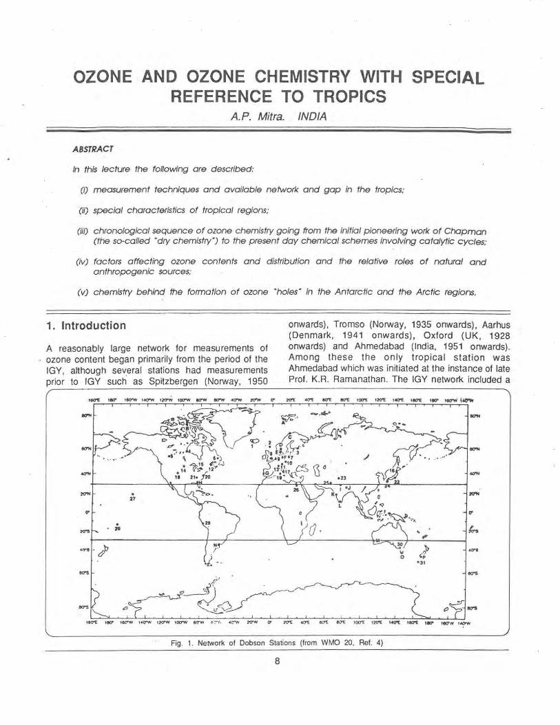
A reasonably large network for measurements of ozone content began primarily from the period of the IGY, although several stations had measurements prior to IGY such as Spitzbergen (Norway, 1950

onwards), Tromso (Norway, 1935 onwards), Aarhus (Denmark, 1941 onwards), Oxford (UK, 1928 onwards) and Ahmedabad (India, 1951 onwards). Among these the only tropical station was Ahmedabad which was initiated at the instance of late Prof. K.R. Ramanathan. The IGY network included a

Fig. 1. Network of Dobson Stations (from WMO 20, Ref. 4)

8

number of tropical stations such as Ouetta in Pakistan. New Delhi ard Ahmedabad in India and Brisbane in Australia.

Stations with long recor:ds are shown in Fig. 1 along with those lying within ± 30° latitudes.

Amongst the tropical countries India has taken a special interest in ozone measurements for several decades due primarily to the efforts of Prof. K.R. Ramanathan at the India Meteorological Department. The Chemistry of ozone as well as features of ozone distributions connected with weather phenomena were discussed at some length by Prof. S.K. Mitra in his well known book ''The Upper Atmosphere" as early as 1952.

Although ozone measurements have gone on for several decades the current interest arose from the recognition of possible destruction of ozone from artificial production of nitric oxide and chlorine through a varity of manmade efforts such as industrial chlorofluorocarbons. nitrogenous fertilizers, spacecraft effluents and nuclear explosions and the discovery in 1986 of the Antarctic Ozone Hole. Although the depletion observed in the Antarctic during the austral spring is pronounced and large scale depletion is also beginning to be observed in the Arct ic Region, the questions that has plagued the scientists is the extent to which ozone content (or profile) in latitudes other than the polar regions had changed over the last few decades during the period Jhe CFCs have. been increasing. ·This trend analysis for the last three decades has been hampered by the non-uniformity of the distribution of ozone stations· and the paucity of stations in several regions including the tropics. the sub-tropics and the southern hemisphere (apart from the Antarctica) . For trend analysis the only geographical region of 30° to 64°N.

Tropical regions have several characteristics that need to be kept in view in the study of the ozone chemistry and also in the assessment o( impact of the increasingly higher chlorine loading of the atmosphere. The special characteristics which are outlined at some length later are basically dependent on the low ozone content over the tropical regions allowing a larger flux of UV-B radiation coming in, the large variability at· the OH radical and the uncertain effects of lightning discharges which are far more frequent in the tropical regions.

9

2. Measurement Techniques and Available Network

Several techniques are in use for the measurement of the total ozone and for ozone profiles. These techniques can be broadly classified as those operated from the ground and those operated from space . The latter include primarily satellite measurements and also measurements of ozone distributions made with rockets and balloons.

An outline of the ozone measurement techniques is given below:

OZONE MEASURING TECHNIQUES

A. Groundbased

* DOBSON

* Filter Ozonemeters (M-83)

* Brewer Grating Spectrophotometer

71 Stations 9 within ± 20° Latitude

40 stations in USSR

Mainly in Germany

* UMKEHR Techniques Dozen Dobson Stations.

* UV-B Photometers Relatively new and data availability limited. Over Delhi measurements for nearly a decade.

B. Satellite Measurements of Ozone

* SBUV

*TOMS

Solar Backscatter Ultraviolet Experiment

Nimbus 7 : Late 1978 -1987

SBUV-2: Revised version 1985 onwards

Total Ozone Mapping Spectrometer on Nimbus 7

Continuous mapping of ozone on a latitudelongitude grid

* SAGE I & II Stratospheric Aerosol & Gas Experiment

* LIMS 6 - Channel IR Limb Scanning Radiometer on Nimbus 7

* SME UV & NIR Airglow Instruments

Satellite-borne multiwavelength Radiometers

SAGE I on AEM-8: Feb. 1979 - Nov. 1981

SAGE II on ERBS: Oct. 84

Launched Oct. 6, 81

The workhorse are the Dobson spectrophotometers and the satellite-borne techniques.

Ozone measurements used in the trend analysis are given in Fig. 2 (WMO Report No. 20)

There are only 18 stations within ± 30° latitudes and 9 within ± 20°. Stations within this regions along with the date of starting observation programme are given in Table 1.

OZONE MEASUREMENTS USED IN TREND ANALYSES

TOTAL OZONE

Dob!>On

M 83

TOMS

SBUv

SBUV 2

19:,:,

I I

1960

I I 1

196S

I I I

1970

I I I

1975

I I I

1980

I I I

1985

I I I

1990

I I

OZONE PROFILES

Figure 2

Dobson UmkE>hl

Balloon-Sondes

ROCOZ

SAGE

SBUV

SBUV 2

LIMS

..........•.......•........................•..

································----

T1me lines of measurements available for use in ozone trend analyses at the present time (from WMO 20)

Fig. 2. Types of ozone measurements used lor global trend analysis (from WWO 20, Ref. 4)

10

Northern Hemisphere

1. Ouetta, Pakistan

2. Cairo, Egypt

3. New Delhi, India

4. Naha, Japan

5. Varanasi, India

6. Kunming, China

7. Ahmedabad, India with Mt Abu

8. Mauna Loa, USA

9. Mexico City, Mexico

10. Poona, India

11. Bangkok, Thailand

12. Kodaikanal, India

13. Singapore, Singapore

Southern Hemisphere

14. Huancayo, Peru

15. Samoa, USA

16. Cairns, Australia

17. Cachoeira Pau, Brazil

18. Brisbane, Australia

For profile studies the role of rocket-borne and balloon-borne instruments should not be under estimated. Here intercomparison of observation is particularly important since instruments in the same rocket or in the same campaign can be different or can come from different institutions. Furthermore, we are looking for very small changes . Such intercomparison efforts have taken place on several occasions - the most important are the ones in Wallops Island and two sets of intercomparisons in India through joint efforts of Soviet and Indian scientists and using a wide variety of techniques (rockets, balloon, Dobson). The last two were conducted during March 23 - 31 , 1983 and December 30, 1987. The 1983 intercomparison campaign included 16 M-1 00 rockets, 7 balloon ozonesondes, several radiosondes, and a Dobson

30°1 1', 66°57'E 1957 onwards

30°05', 31°17'E 1974 onwards

28°38', 77°13',E 1957 onwards

26°12', 127°41'E 1974 onwards

25°18', 83°01',E 1963 onwards

25°01, 102°41'E 1980 onwards

23°01', 72°39'E 1951 onwards 24°36, 72°43'E 1969 onwards

19°32', 155°35'W 1964 onwards

19°20', 99°11'W 1973 onwards

18°32', 73°51'E 1973 onwards

13°44', 100°34'E 1978 onwards

10°14', 77°28'E 1957 onwards

1°20', 103°53'E 1979 onwards

12°03', 75°19'W 1964 onwards

14°15', 170°34,W 1964 onwards

16°53', 145°45',E

22°41', 45°00',W 1974 onwards

27°25', 153°05', 1957 onwards

spectrophotometer. Fig. 3 gives the results of the intercomparison for the 1983 campaign - the mm radiometry profile is for a different station (Bangalore and for a different period, but is included for comparison).

11

A special word about the UV-B photometer, the equipment is simple although absolute calibration is necessary. Its main interest lies in directly measuring the UV-B flux reaching the ground instead of indirect computation through measured ozone parameters.

Another technique which provides real time ozone profiles is laser heterodyning system. Such an equipment was introduced at New Delhi in India during the Indian Middle Atmosphere Programme

10

OZONE TRIVANORUM

h

0~----~ .. ~----~~--~--~~LA~~~--------------~, 10 '0 10 z ; 4 ~ , 1 a 1crz 1o'l

OZONE NUMBER DENSITY !cm3)

Fig. 3. Ozone profiles obtained by a variety of techniques over a tropical region (e.g. Trivandrum) : see text for details

:?7-01- 88 LASER HETERODYNE , N P L

o----<> 2 7 -01-88 BALLOON , IMO

0

OZONE MIXING RATIO !PPM )

\

Fig. 4. Profile obtained with Laser Heterodyning System compared with near simultaneous radisonde measurements (courtesy : S.L. Jain)

12

(IMAP) and has been in operation for several years . This particular facility uses a tunable C02 waveguide laser. Ozone profiling is possible over the height ranges 15 - 40 km. It is also capable of monitoring several other minor species; water vapour (0-20 km) and N0

2. The _effectiveness of the technique is shown

in Fig. 4. where 03

profile derived by this technique is compared with radiosonde measurements at nearly the same time by the India Meteorological Department.

3. Special Characteristics Of Tropical Regions

The two most significant characteristics of the tropical regions in the context of ozone study are:

(a) the low ozone content in the tropical zone (or, in other words, the protective umbrella is thinner at equator than at the poles and high latitudes)

4-00

::) C)

.36Q .....

TRV. JULY 265/.308 - /¥/.

JAN 2"5/335 - 26/.

(b) the high tropopause (N 15 - 16 km in contrast

with 8 km for mid-latitudes)

In regard to t~e first, the belt of ozone minimum (240

D.U) lies between 10°S and 15°N. This ozone trough

can be seen in the . representative diagram of Fig. 5.

Much of India, for example, lies even now In a "sort

of a hole" - 15% to 25% lower than the ~latitude

peak. The summer to wint~r changes in ozone content

is around 20 pu. larg~r llian a decadal change in

ozone conter,t outside the polar regions. The

correspondi~g .changes In UV-radiance is shown in

Fig. 6. The lo~ values in the tr?pical regions can also

be ~een !n Fig. 7 which gives the average total ozone

distribution for 1957-1975 der1ved from groundbased

measurements.

I

I

JAN I~

~ ~ < 320 0

I I

--- -=-==------=-~~1-_------t. -:.~.:17.1/.Y !6

u

"' "<! C) N <:>

280

:litO

1 55 .Ou

----- -+

r- IN.t>I A ~ I I

20~·~_.----~----~------L-----~~--~--~~~---L--------eo -60 · 20 0 20 40 (.O

LATITUDE

Fig. 5. Ozone trough over the tropical regions. Two representative diagrams for summer. and winter

13

uv RADIANCE 'q'

"' f. 0 ~ ~

i I)

~ o.a /{.JULY

"' 1.)

<! ~ 0 - 6 Q

~ ~ o.t. ::::,

~ 1.)

~ 0 - 2

~ /6 J.,N

V)

__ __j

-20 0 20 ~0

LATITUDE

Fig. 6. UV-B incidence on the surface calculated from distributions given in Fig. 5. (Courtesy : B.N. Srivastava)

Fig . 7. Distribution average of ozone content derived from groundbased measurements for 1957-1975 (from WMO Report No. 18, Ref. 6)

14

4. Chronological Sequence Of Ozone Chemistry

Ozone chemistry has gone through several important phases since the pioneering work of Sydney Chapman in 1932. The sequence has been as follows:

(a) the "dry" chemistry of Chapman

(b) the ''wet" chemistry of Nicolet and Bates

(c) introduction of nitric oxide by A.P. Mitra

(d) The concept of catalytic cycles by Johnston, Stolarski, Crutzen and others.

These four distinct phases are represented in Figs. 8 (a) - (d). A simplified picture of ozone connections is given in Fig. 8 (e) .

Fig. 8 (a) •Dry· Chemistry of ozone by Chapman

~ <242"m j hU

hV 0+02

0 2 + M

0 0 2 o2

0+ M H OH +02

OH HOz+O

Fig. 8 (b) ·wet• Chemistry of Ozone by Nicolet and Bates

15

Ill OXYGEN- HYDROGEN -NITROGEN

ATMOSPHERE A . P . MITRA, 1969

Fig. 8 (c) Introduction of Nitric Oxide in Ozone Chemistry by A.P. Mitra

Ptoduc:lion

(0) uv ( 1 0, UV+racombtnahon °' /

Calalylic: daplelion Source

~ + (0) - HO, + (0~ H,O+O('O) Sink

EJ-HO, + 0 - OH + 01/ - OH

fiO + (0 ) - NO + c·\ N10+0('0)

I'" ·t~( NO, • o, - •o• , o:) - NO

Q + (0') - CIO + (0,' CHCH, CF1CI, +UV

HCI CIO + O, - £! + O,/ - g

COUPLING BETWEEN OH, NO AND Cl

Fig. 8 (d) Current gas-phase ozone chemistry

SOLAR UV

8 UV HEATING 0

-..,..___. - T

T--DEPENOENT CHEMISTRY

j

FLARES FERTILIZERS AIRCRAFTS

CFCs

VOLCANOES

SPACE CRAFTS

FROM TROPOSPHERE

OZONE CONNECT! ()NS (MODIFIED FROM WMO 16)

Fig. 8 (e) Ozone Connections

16

WAVE . PROPAGATION

It is important to note that for both, production and destruction of ozone UV radiations are involved but in different wavelength ranges. The three sets of wavelength are those that: (a) produce ozone, (b) destroy ozone and (c) partially filter through are shown in Fig. 9. The key radicals involved in the catalytic cycles are OH, NO and CIO, and are produced from Hp, N20 and CFCs (Fig. 8d). At tropospheric heights, production of OH and NO are

I SOLAR UV J 1001- -"' z I ppm

0 N 0

~ ~ :1 - E E E c c c 8 8 0 • ,., ... N I 8 I 0 g .,

N .., so-

~~7:7/ T/7 7~~~ ----~ ON YE /d. IOppm ~ L'~/)..z')2 --------

Fig. 9. Simplified picture depicting the role ol UV radiations at different lengths in producing and destroying ozone and

also wavelengths that filter through

NO

~ EFFECT OF OZONE IN STRATOSPHERE

Ol

1 UV l,l."O • • I

0 11(0)

OH

I ATTACK ~ANY LOW-WATER SOLUBLE SPEOES IN TRoPOSPHERE .

2 STRONG EFFECT ON CHEMICAL BALANCES IN STRATOSPHERE

Fig. 10. Production of the critical species 0 (10) and its role in production of OH and NO.

17

possible only If an adequate concentration of 03

Is available. CIO, however, is produced in the stratosphere through association by ultraviolet radiation. The process of production of 0 (1 D) is given in Fig. 10. Consequently in order to properly evaluate the role of the increase in concentrations of CFCs, considered to be the most effective anthropogenic source and the cer:~tral theme for ozone protocol, one should have a comparative evaluation of all sources. The sources are tabulated in Table 2.

Ozone cannot be investigated in isolation as its chemistry is linked (as is clear from the preceding figures) with the chemistry of many other constituents in the troposphere and the stratosphere. These include (but are not limited to) NO, N02, N

20 and

HN03; Cl, CIO, HCI, CC14, CFCI3

and CF2CI

2; H, OH,

H02 and H20 and obviously 0 and 0 2. Since the effects depend upon the ambient stratospheric loadings the last few years have seen intense activity on: (a) experimental determination of many of the

Table 2: Sources for Radicals Involved in Catalytic Destruction of Ozone

A. Human Activities

CFCs

Aircrafts

Nuclear Explosions

Spacecraft Effluents

Nitrogenous Fertilizers

B. Natural

Solar Constant

UV Variation

Solar Proton Events

Volcanic Eruptions

Lightning Discharges

Variable : 0.2% over a solar cycle

Small Modulation in 0 3 content

120

w 3 60~----~--+-~----~~~~~~--~~--+-----1------+----~ ~ I ~ l 4 40~--~~----~~~~~---;~--~~ -~~~~~+----~~--~

c---~-..:--=-=--= I i ~=-'<""'-

zo:----j~---,-----r~~~~--~~--t-~~~~~~~~ L

10 3 10 9 1d0

CONCENTRATION (Cm3l

PROFILES OF IMPORTANT MINOR SPEClES

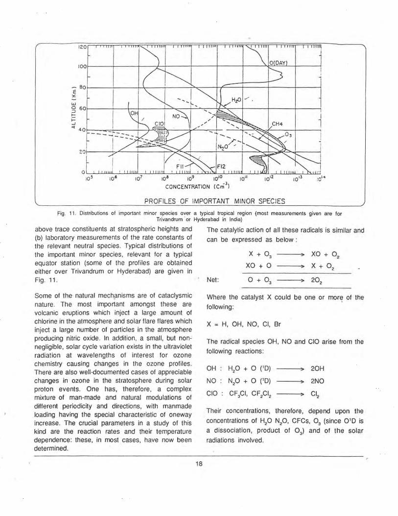
Fig. 11 . Distributions of important minor species over a typical tropical region (most measurements given are for Trivandrum ·or Hyderabad in India)

above trace constituents at stratospheric heights and (b) laboratory measurements of the rate constants of the relevant neutral species. Typical distributions of the important minor species, relevant for a typical equator station (some of the profiles are obtained either over Trivandrum or Hyderabad) are given in Fig. 11 .

Some of the natural mechanisms are of cataclysmic nature. The most important amongst these are volcanic eruptions which inject a large amount of chlorine in the atmosphere and solar flare flares which inject a large number of particles in the atmosphere producing nitric oxide. In addition, a small, but nonnegligible, solar cycle variation exists in the ultraviolet radiation at wavelengths of interest for ozone chemistry causing changes in the ozone profiles. There are also well-documented cases of appreciable changes in · ozone in the stratosphere during solar proton events. One has, therefore, a complex mixture of man-made and natural modulations of different periodicity and directions, with manmade loading having the special characteristic of oneway increase. The crucial parameters in a study of this kind are the reaction rates and their temperature dependence: these, in most cases, have now been determined.

18

The catalytic action of all these radicals is similar and can be expressed as below:

Net:

X + 0 3

xo + 0

Where the catalyst X could be one or mor~ of the following:

X = H, OH, NO, Cl, Br

The radical species OH, NO and CIO arise from the following reactions :

OH

NO

H20 + 0 CD)

Np + 0 CD)

20H

2NO

Their concentrations, therefore, depend upon the

concentrations of Hp N20, CFCs, 0 3 (since 0 1D is a dissociation, product of 0 3) and of the solar radiations involved.

In the present comprehensive scheme of reactions, the following specific aspects are to be noted:

Hydrogen System - The OH system (first brought up by the so-called 'wet' chemistry of ozone by Bates and Nicolet) destroys only 10% of 0 2 but is dominant above 40 km.

2 OH

Reactions particularly important above 40 km

Net :

OH can be formed from oxidation of methane

with ·subsequent reactions as above.

H, OH, H02

interconvert rapidly by reactions with 0, so that all three tend to be in steady state. The scavenging reaction is

resulting in formation of Hp which drifts down out of stratosphere. Since this reaction removes odd hydrogen out of the active system, its rate is one of the most important elements in stratospheric chemistry.

Nitrogen System -:- The possibility of NOx involvement in ozone chemistry was brought up by A.P. Mitra as early as 1969. Sixty per cent of ozone destruction occurs through this system. The sequence is as follows:

Np produced by bacterial action of micro-organisms in ocean and soil (denitrificat ion) diffuse upwards from troposphere to stratosphere, where

N20 + 0(10) 2NO

N02 + HV NO+ 0

and NO so formed catalyses ozone by :

NO+ 0 3 N02 + 0 2

N02 + HV NO+ 0 2

Net: , 03 + 0 202

19

The reaction of N02 with OH:

OH + N02 + M HN03 + M

produces HN03 which is eventually washed out of the troposphere and is the major sink.

Chlorine System - Natural chlorine contributes only very little (few per cent) to 0 3 destruction. CFMs (particularly CFCI3 and CF2CI2) are the main ozone destroyers. They are inert in the troposphere. but get dissociated in the stratosphere:

hV cFc~. c~c~ c~

180 - 220 nm

Then follow the following sequences:

Cl + 0 3 CIO + 0 2

CIO + 0 Cl + 0 2

Net:

CIO catalytic efficiency is reduced in the presence of NO because of the reaction:

CIO +NO

followed by:

N02 + H NO + OH

The sink is HCI, formed through

CH4 + Cl HCI + CH3 H02 + Cl HCI + 0 2

Chlorine can be recycled through:

HCI + OH Hp + Cl

Balance between Cl, CIO and HCI .is given by the above three reactions.

While chlorine catalysis of ozone is six times as efficient, catalysis of ozone conversion to 'inert' HCI is also more efficient than conversion of HN0

3, so

that the overall efficiency of the two are comparable.

Again we have a coupling reaction:

CIO + NO

CIO + N02

and

Reaction scenario - The three principal radical species OH, NO and Cl coming primarily from H

20,

N20 and CF xCiv respectively and interacting with ozone catalytically end up eventually as sink species HN03, CION02 and HCI. The summary scenario is shown in Fig. 8 (d).

.Q

E

I '

Ozone Vertical Profiles

Ozone Portiol Prenure nbl

TOMS Oct. 5,1987 Holley Boy

( s.o.Otloll

: , .. : ll

3~.---------------~--

~0 M~Murdo

'~.-.,,unul)

,. ---~~" ... G lt, t•ar

~ ................... ....a ............... .J

!>0 tOO t~O

Ozo"• Porc.ot Pre~~ure (nb)

tOO ·~ JOO 01eAt ,lft1QI ~tiUttf.

(A.,

Syowo

10

~~-L----~---L----J ~

tOO t!:>O ;:oo

Ozone Portiol PrHSur•

(nb)

iiO -"060 «>ICJD t»I+OI40

Olon• Porr iol Pru,~url ( ntJ)

.. l:

Fig. 12. Ozone hole over the Antarctic during October 1987. Observations include those made over the Indian Station Dakshin Gangotri

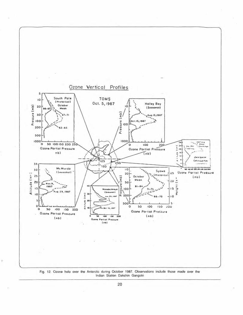
20

5. Antarctic Ozone Hole

The homogeneous chemistry described above is inadequate for the large depletion seen in the Antarctic and now in the Arctic. The depletion within the containment vassel defined by the polar vortex is large: an example the October of 1987 is shown in Fig. 12. Prior to the discovery of the Antarctic ozone hole, the conclusion emerging was of a relatively small change in ozone content and of recognizable changes only at upper stratospheric levels around 40 km. Theoretical calculations, both 1-D and 2-D, also predicted only a few per cent of change of the total ozone content, and not the near annihilation one sees over the Antarctica .

To understand the special chemistry obtaining in the Antarctic, one should first understand the very special conditions under which the "hole" appears. These are : (i) very low T : (- 80°C and below); (ii) presence of stratospheric clouds; (iii) CIO increase to values about 1 00 times larger than in mid-latitudes; (iv) decrease of odd nitrogen concentration ; and (v) dehydration and denitrification of the chemically depleted region.

A . PRE-WINTER: WITHOUT CLOUDS

CATALYTIC CHLORINE

RESERVOIR

HOCL

;/0~2 Cl CIO t ~HO, NONOz ~))

~ I CIO N02 I RESERVOIR

PARTITION lNG

Cl I CIO I HOCI

HCI , cro N02

DESTROYS 0 3

INHIBITS DESTRUCTION

ANTARCTIC OZONE CHEMISTRY

-CHEMISTRY BEFORE CLOUD FORMS

Fig. 13. Gas phase chemistry showing formation of reservoir species HCI and CJON0

2.

The most important thing is to understand how CIO can be increased by such a large magnitude between 12 and 20 km over such a short period. The existing gas phase chemistry (Fig. 13) would suggest that in this region chlorine exists primarily in a r-eservoir form as HCI and CION0

2• •

21

We have two alternatives. Either conditions occur which block the diversion of CIO into reservoir species or reactions occur that release CIO from the 'reservoir or both. An optimum condition would involve both increase in CIO and decrease in NOx.

The key factor, it is believed, is the occurrence of extremely low temperatures. Such low temperatures promote increased occurrences of polar stratospheric clouds (PSCs). There are two types of PSCs.

Type I PSC

Type II PSC

HN03, 3H20

Ice crystals.

Type I PSCs have particles of radii around 0.5 0.7Jlm and occur at temperatures about 5-7 K higher than the frost point. Type I temperature is consistant with thermodynamical stability of HN03 3Hp (NAT). Type II water-ice type clouds form at temperatures below the frost point, leading to large scale irreversible removal of H20 vapour in the Antarctic.

The key heterogeneous reactions are:

HCI(s) + CION02 (g) 0~ Cl

2(g) + HN0

2 (s) (1)

0.001 N20 5(g) + Hp(s) ----> 2HN03 (s) (2)

0 .009 CION02(g) + H20(s) ----> HOCI(g) + HN0

3(s) .. . (3)

0.003 N205(g) + HCI(s) ----> CION0

2(g) + HN0

3(s) .. . (4)

The sticking coefficients measured by several experimenters show that these coefficients are appreciable. These reactions provide pathways tor removal of N02, thus inhibiting CIO + NO ~ CIONO

2 2 pathway and also releasing Cl

2(g} as in (1) for PSC

Type I and HOCI as in (3) for ice-clouds for PSC Type II.

The sequence of events that are believed to occur as season progresses from prewinter conditions (period of reservoir formation) to winter (formation of PSCs and release of CJ2) to austral spring (when with the beginning of sunlight coming Cl

2 is dissociated

to Cl and from thereon to the destruction of ozone through an initial dimer formation) is shown in Fig. 14.

A new result of major implication is that surface reactions are not limited to ice-clouds, but can also occur on liquid sulphuric acid aerosols. These occur at higher temperatures. Laboratory measurements

STUDIES ON THE PAST GLOBAL C.HANGES (PAGES)

WITH SPECIAL REFERENCE TO THE ASIAN REGION Eiji Matsumoto, JAPAN

1. Introduction

The earth system is never in a state of absolute equilibrium. Therefore, the system is continually changing. Any current global warming may be superposed on natural changes. In foretelling global changes of the future we need to know the natural changes through a better knowledge of the past. It thus becomes a matter of some urgency to improve our knowledge of the past event.

Data concerning previous environmental conditions are available from instrumental and historical records, as well as from the information preserved in natural archives of many types, including ice cores; marine, lacustrine and terrestrial sediments; tree rings; and corals . Studies of the physical, chemical and biological parameters recorded in such archives have provided a wealth of information on the natural behaviour of the Earth system (Table 1). Quantitative information on global changes of the past can be used to document forcing function and to understand the responses to such forcing. The Earth system models should be tested through detailed comparisons of ·simulations with paleodata. The emergence of an integrated Earth system sciences calls for a much fuller knowledge of the past, in both space and time.

2. PAGES Project

The PAGES Core Project has been developed to respond to these needs through a set of coordinated activities that address key scientific questions through specific research tasks (Table 2) .

Focused research will be carried out in four general act ivities. The first three address fundamental Earth system processes for which paleodata are of particular value. The fourth is an all-pervasive effort in coordinated data collection that supports the other three. These activities are: (1) Solar and orbital forcing and response , (2) Fundamental Earth system processes, (3) Rapid and abrupt global changes, and (4) Multi-proxy mapping.

23

As described. in Table 2, specific research tasks within each activity are further divided into one of two streams of temporal emphasis: Stream I tasks will focus on the last 2,000 yr of Earth history; Stream II tasks will address the general period encompassing the glacial-interglacial cycles of the late Quaternary.

Three cross-project needs are also identified which are common to each of the research activities. These are: (1) Paleoclimatic and paleoenvironmental modeling, (2) Management of paleodata, and (3) Technological development. More information regarding the PAGES project maybe found in IGBP Report No. 12.

3. Past Monsoon Asia Mapping Project (PAMAMAP)

In the late Quaternary Monsoon Asia, it is well-known that some desert lakes disappeared, and vegetations were drastically altered. These changes can be explained as results of monsoon variations.

Global climate has long been postulated as a key factor influencing each of these regional changes, but until recently we were uncertain about both the causes of the global climate changes and the regional interconnections among key components of the global climate system. Asia monsoon is the major climate sub-system.

The PAMAMAP is a cooperative research project among countries in Asia to study paleoclimates and paleoenvironments of Monsoon Asia. The goal of PAMAMAP research is an improved understanding of the climate system, particularly the response of Asia monsoon to global changes. PAMAMAP uses paleodata and models to investigate the g1obal and regional dynamics of climate change. PAMAMAP researchers need to assemble data that provides paleo-records of spatial and temporal changes in climate from continents and oceans. These data should be systematically compared with the model simulations of past monsoon. Comparisons of reconstructed paleoclimates with model simulations provide a way to predict future changes in climate and environment.

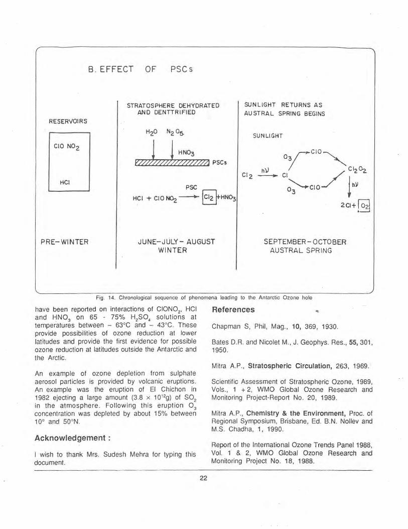
B. EFFECT OF PSCs

STRATOSPHERE DEHYDRATED AND DENTIRIFIEO

SUNLIGHT RETURNS AS AUSTRAL SPRING BEGINS

RESERVOIRS

H20 N2 05-SUNLIGHT

vJ//T~~A PSCs hV -HCI

PSC

HCI + CIO ~-+- @HN~

PRE-WINTER JUNE-JULY- AUGUST WINTER

SEPTEMBER-OCTOBER AUSTRAL SPRING

Fig. 14. Chronological sequence of phenomena leading to the Antarctic Ozone hole

have been reported on interactions of CION02 , HCI and HN0

3 on 65 - 75% H2S04 solutions at

temperatures between - 63°C and - 43°C. These provide possibilities of ozone reduction at lower latitudes and provide the first evidence for possible ozone reduction at latitudes outside the Antarctic and the Arctic.

An example of ozone depletion from sulphate aerosol particles is provided by volcanic eruptions. An example was the eruption of El Chichon in 1982 ejecting a large amount (3.8 x 1 012g) of S02 in the atmosphere. Following this eruption 0 3 concentration was depleted by about 15% between 1 0° and 50°N.

Acknowledgement :

1 wish to thank Mrs. Sudesh Mehra for typing this document.

22

References

Chapman S, Phil, Mag., 10, 369, 1930.

Bates O.R. and Nicolet M., J. Geophys. Res ., 55, 301, 1950.

Mitra A.P., Stratospheric Circulation, 263, 1969.

Scientific Assessment of Stratospheric Ozone, 1989, Vols., 1 + 2, WMO Global Ozone Research and Monitoring Project-Report No. 20, 1989.

Mitra A.P., Chemistry & the Environment, Proc. of Regional Symposium, Brisbane, Ed. B.N. Nollev and M.S. Chadha, 1, 1990.

Report of the International Ozone Trends Panel1988, Vol. 1 & 2, WMO Global Ozone Research and Monitoring Project No. 18, 1988.

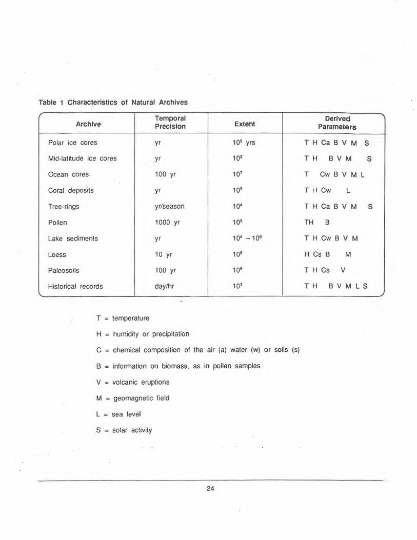
Table 1 Characteristics of Natural Archives

Archive Temporal

Extent Derived

Precision Parameters

Polar ice cores yr 105 yrs T H CaB V M s Mid-latitude ice cores yr 103 T H B V M s Ocean cores 100 yr 107 T Cw B V M L

Coral deposits yr 105 T H Cw L

Tree-rings yr/season 104 T H CaB V M s

Pollen 1000 yr 105 TH B

Lake sediments yr 104 -106 T H Cw B V M

Loess 10 yr 106 H Cs B M

Paleo soils 100 yr 105 T H Cs v

Historical records day/hr 103 T H BVM L S

T = temperature

H = humidity or precipitation

C = chemical composilion of the air (a) water (w) or soils (s)

B = information on biomass, as in pollen samples

V = volcanic eruptions

M = geomagnetic field

L = sea level

S = solar activity

24

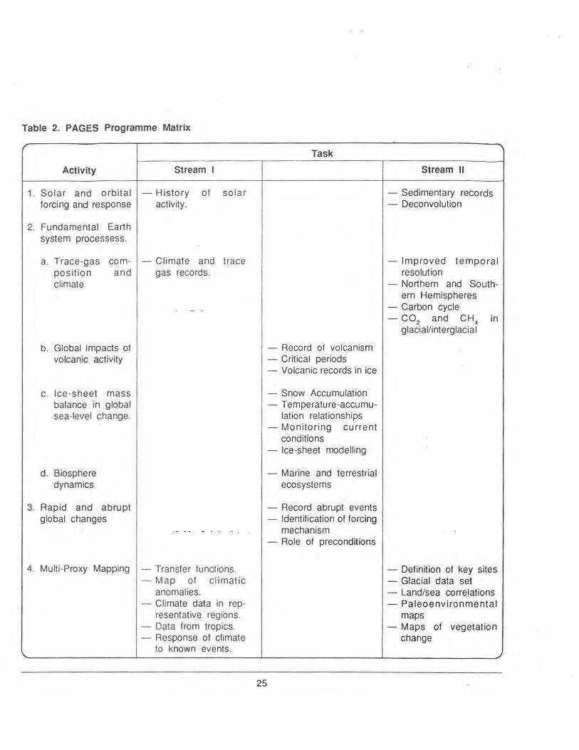
Table 2. PAGES Programme Matrix

Activity Stream I

1. Solar and orbital - History of solar forcing and response activity.

2. Fundamental Earth system processess.

a. Trace-gas com- - Climate and trace position and gas records. climate

b. Global impacts of volcanic activity

c. Ice-sheet mass balance in global sea-level change.

d. Biosphere dynamics

3. Rapid and abrupt global changes

4. Multi-Proxy Mapping - Transfer functions. - Map of climatic

anomalies. - Climate data in rep

resentative regions. - Data from tropics. - Response of climate

to known events.

25

Task

- Record of volcanism - Critical periods - Volcanic records in ice

- Snow Accumulation - Temperature-accumu-

lation relationships - Monitoring current

conditions - Ice-sheet modelling

- Marine and terrestrial ecosystems

- Record abrupt events - Identification of forcing

mechanism - Role of preconditions

Stream II

- Sedimentary records - Deconvolution

- Improved temporal resolution

- Northern and Southern Hemispheres

- Carbon cycle - C02 and CH 4 in

glacial/interglacial

- Definition of key sites - Glacial data set - Land/sea correlations - Paleoenvironmental

maps - Maps of vegetation

change

THE ROLE OF TIBETAN PLATEAU IN GLOBAL CLIMATE

Duzheng Ye, CHINA

I. Introduction

Tibetan Plateau plays an important role in local weather, general circulation as well as climate in northern hemisphere at least. Before 50's when people talked about these things, they usually only considered its dynamic effect due to its blocking the air currents. In first part of 50's Prof. Flohn and the author and his group independently found that Tibetan Plateau is a heat source in summer and the author also found that in winter it is a cold source. Since then the thermal influence of Tibetan Plateau on the general circulation and climate has been studied as well as its dynamic effect . Through some examples of our recent findings this extended abstract will illustrate the important role, dynamic as well as thermal, of Tibetan Plateau in the global climate.

II. The Dynamic Effects (of Tibetan Plateau and Rocky Mountain)

1. The correlation of the intensities of the two main winter troughs respectively off the Asiatic coast and east coast of North America

These two troughs are negatively correlated (Zou, Ye and Wu, 1987). When the monthly mean ·trough off the Asiatic coast is strong, the monthly mean trough off the east coast of North America is weak, and vice versa. North of 45N, the correlation coefficient is -0.40.

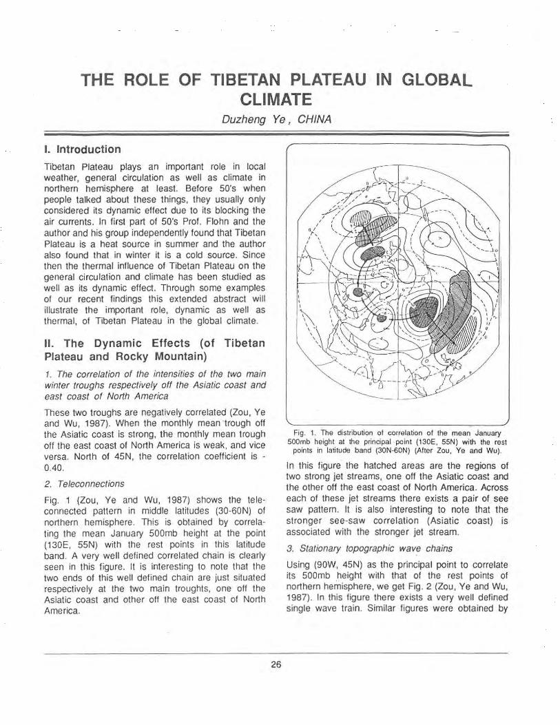
2. Teleconnections

Fig. 1 (Zou, Ye and Wu, 1987) shows the teleconnected pattern in middle latitudes (30-60N) of northern hemisphere. This is obtained by correlating the mean January 500mb height at the point (130E, 55N) with the rest points in this latitude band. A very well defined correlated chain is clearly seen in this figure. It is interesting to note that the two ends of this well defined chain are just situated respectively at the two main troughts, one off the Asiatic coast and other off the east coast of North America.

26

Fig. 1 .. The distribution of correlation of the mean January 500mb height at the principal point (130E, 55N) with the rest

points in latitude band (30N-60N) (After Zou, Ye and Wu).

In this figure the hatched areas are the regions of two strong jet · streams, one off the Asiatic coast and the other off the east coast of North America. Across each of these jet streams there exists a pair of see saw pattern. It is also interesting to note that the stronger see-saw correlation (Asiatic coast) is associated with the stronger jet stream.

3. Stationary topographic wave chains

Using (90W, 45N) as the principal point to correlate its 500mb height with that of the rest points of northern hemisphere, we get Fig. 2 (Zou, Ye and Wu, 1987). In this figure there ex ists a very well defined single wave train. Similar figures were obtained by

using (90W, 60N) or (70W, 45N) as the principal point. Using (90E, 60N) as the principal point we (Zou, Ye and Wu, 1987) get Fig 3. In Fig. 3 two wave trains are clearly shown. Similar figures were also obtained by using (90E, 45N) or (11 OE, 45N) as the principal point. The numerical model simulation shows that it is the difference in the characteristics of the horizontal structure of the zonal wind in the two regions makes the difference of the two wave trains. And the horizontal structure of the zonal wind is highly related to the topographical feature (Tibetan Plateau and Rocky Mountains) .

4. Horizontal propagation of waves

According to Hoskins and Karoly (1981) the amplitude of \jf of spherical waves satisfies the following equation.

I

/ , , , I

I I ro

__ I_! I

0 I I

:c. f I

' I I

Fig. 2 The distribution of correlation of the mean January 500mb height at the principal point (90W, 45N) with the rest

p0ints in northern hemisphere 11\fter Zou, Ye and Wu).

!Y_ = (k2 _ ~m ) \ji () y2 Um

where m indicates Mercator projection and k is the zonal wave number. The critical wave number k for c ~ropagating waves may be calculated by

27

kc = { ~ t2 = {l [2Q cos3 $ - cos2 $ ..£._ _1 _ _i_ ( u cos q, )]}¥2

u a aq, acos$ aq, For waves with K < Kc, they can propagate northward or southward. For k > kc, waves are damping or are trapped. Using the mean January 300 mb zonal wind (u) of 1983 for Asiatic and Pacific region (80E-140W) and American and Atlantic regions (120W-5W), k is calculated as a function of latitude ($) for these two region (Zou, Ye and Wu, 1987). The results show that for Asiatic region near the jet stream (cp, 30-35N) only waves of k < 3 can propagate through this latitude band and waves of k > 3 are trapped to the south of 35N and at some critical latitude «Pc ( < cjl1) they band southward. So the resultant atmospheric waves show splitting in Asiatic region.

Fo.r American region kc ~onotonically decreases with latitudes. Near 60N, kc IS already very small. Thus the disturbances of various scales created downstream of Rockies will band southward. So downstream of Rockies there is no splitting of wave trains.

Fig. 3. Same as Fig. 2, but with the principal point at (90E, SON) (After Zou, Ye and Wu).

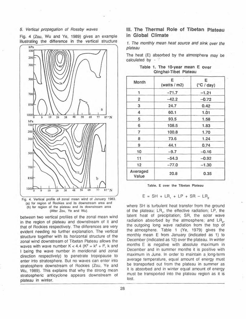
5. Vertical propagation of Rossby waves

Fig. 4 (Zou, Wu and Ye, 1989) gives an example illustrating the difference in the vertical structure

68 77 87 ·N

Fig. 4. Vertical profile o~ zonal mean wind of January 1983. (a) for region of Rockies and its downstream area and (b) lor region of the plateau and its downstream area

(After Zou, Ye and Wu).

between two vertical profiles of the zonal mean wind in the region of plateau and downstream of it and that of Rockies respectively. The differences are very evident needing no further explanation. The vertical structure together with its horizontal structure of the zonal wind downstream of Tibetan Plateau allows the waves with wave number K < 4.4 (K2 = k2 + 12, k and I being the wave number in meridional and zonal direction respectively) to penetrate tropopause to enter into stratosphere. But no waves can enter into stratosphere downstream of Rockies (Zou, Ye and Wu, 1989). This explains that why the strong mean stratospheric anticyclone appears downstream of plateau in winter.

28

Ill. The Thermal Role of Tibetan Plateau in Global Climate

1. The monthly mean heat source and sink over the plateau

The heat (E) absorbed by the atmosphere may be calculated by . ·. r

Table 1. The 10-year mean E over Qinghai-Tibet Plateau

Month E E (watts I m2) (°C I ~ay)

1 -71.7 -1.21

2 -42.2 -o.72

3 24.7 0.42

4 60.1 1.01

5 93.5 1.58

6 108.5 1.83

7 100.8 1.70

8 73.6 1.24

9 44.1 0.74

10 -9.7 -0.16

11 -54.3 -0.92

12 -77.0 -1.30

Averaged 20.8 0.35 Value

Table. E over the Tibetan Plateau

E = SH + LR 1 + LP + SR - LR2

where SH is turbulent heat transfer from the ground of the plateau; LR1' the effective radiation; LP, the latent heat of precipitation; SA, the solar wave radiation absorbed by the atmosphere; and LR2,

the outgoing long wave radiation from the top of the atmosphere. Table 1 (Ye, 1979) gives the monthly mean E from January (indicated as 1) to December (indicated as 12) over the plateau. In winter months E is negative with absolute maximum in December and in summer months it is positive with maximum in June. In order to maintain a long-term average temperature, equal amount of energy must be transported out from the plateau in summer as it is absorbed and in winter equal amount of energy must be transported into the plateau region as it is lost.

2. The influence of snowcover over the plateau in winter and spring on the summer climate in east Asia.

Fig. 5 (Chen, 1980) gives the correlation coefficient distribution between the winter-spring snow accumulation over central plateau and the June rainfall in South China.The hatched area indicates at least 95% significant level, with correlation coefficient in inner most part reaching + 0.65.

Fig. 5 The distribution of correlation coefficient between the winter-spring snow accumulation over central plateau and

the June rainfall in South China.

Fig. 6. (Chen, 1980) gives the June 850mb flow field anomaly charts for (a) snow-rich years and (b) snowpoor years. These charts show big differences.

Fig. 5 and Fig. 6 (a, b) indicate that the winter and spring snow accumulation over Tibetan Plateau has a profound influence on its surrounding climate in the following summer. The physical explanation may be as follows. Following the snow-rich winter and spring, the soil moisture in summer over the plateau is much higher than that following the snow-poor winter-spring. The evaporation from the ground surface is higher, then cooling the atmosphere is the boundary layer, in the former type of summer than that in the latter type of summer. The surface processes affect the climate.

3. The severe convective activities and the vertical velocity over summer plateau

Yuan (1979) has shown that the convective. activities over the plateau in summer are very active. Its activity in frequency at least can be compared with that over tropical oceans. The strong convective activites together with a mean convergence in the lower of the atmosphere (due to the mean heat source) result to a strong mean vertical velocity (upward) in the

Fig. 6. Average June 850mb flow field anomaly charts for snow-rich years (a) and snow-poor years (b) (After Chen).

atomosphere over the plateau. As an example Fig. 7 (Yang, Ye and Wu, 1987) gives the distribution the mean July w (dp/dt) of 1970*. There are two centres, one in east and one in west plateau. Surrounding the upward-motion region is a .belt of descending motion. This indicates that part of rising air descends in its immediate surrounding area. The vertical velocity undoubtedly influences the precipitation distribution.

4. Teleconnections.

Part of the ascending air over the plateau descends in its immediate surrounding area, where does the rest of the ascending air flow to? Fig. 8 (Yang, Ye and Wu, 1989) gives the mean July stream lines in a N-S vertical plane along 86.250E. It shows that the ascending air over the plateau can be carried far southward descending in southern hemisphere. But to the north of the plateau it can not be carried far

* 1979 was FGGE year. From May to September this year China launched a very large-scale meteorological experiment over QinghaiTibet Plateau. Many stations (upper-air and surface) were set up. So the data of this year were the best available.

29

Fig. 7. The distribution of mean July ro = (dp/dt) of 1979 (After Yang, Ye and Wu).

100~--~------~------~~--~------------------------~~

200

700

850

60 90

Fig. 8 The mean July stream line~ in meridional vertical plane along 86.250E (After Yang, Ye and Wu).

northward. It descends immediately to its north, convergence produces positive vorticity and the making very dry climate there. divergence produces negative vorticity in the lower

F. 9 (Y y d w 1989) · the me J 1 layer and upper layer respectively. To maintain the 1g. . ang, e an u, IS an u Y . d. f th · 1 · · · h ·

stream-line distribution in zonal vertical plan along quasl-stea 1~ess ~ e Clrcu a.t1.on. It IS t ~ conve~t1~e 35.625N. This figure shows that the ascending air systems whiCh bnng the pos1t1ve (negat1ve) vort1c1ty over the plateau can be carried by the westerlies very from the lower (upper) layer t? the upp~~ (lower) ~~~er far eastward, descending in eastern Pacific . Fig. 1 o to compensate ~he negative (positive) vort1c1ty (Yang, Ye and Wu. 1989) gives the mean July stream produced. by . dlvergen~~ (convergence). T_he line patt1rn in a zonal vertical plan along 28_125N, comp~nsatlon 1n the vort1c1ty budget b~ advect1on showing that the ascending air over the plateau can term IS proved to be small by observations.

be carried by the easterlies westward as far as Africa 6. The relationship between Tibet-tropical ocean and descending along the way. thermal contrast and Indian monsoon rainfafl

It should be pointed out that July 1979 was not an Fu and Flether (1985) defined SLO by odd month. In July averaged over 10 years (Ye et al. 1979) similar features were observed. These observat ions indicates that Tibetan Plateau is teleconnected with far remote regions.

5. The non-linear interaction between the small-scale convective activities and large-scale circulation

There is a strong mean convergence in the lower layer and a mean strong divergence in the upper layer of the atmosphere over the plateau in summer. The

30

where T 5 is the soil temperature of Tibetan Plateau (sumrrer); Tw, the SST in the region 5N-10S and 120W-160W (summer). Overbar indicates long-term average and N means the individual year. They then used IM = N

9-Nd to correlate with SLO, where Ne and

Nd are respectively the number of regions with excess of rainfall and the number of regions with deficit of rainfall in India. Totalnumber (N

9 + Nd) is 31. + 20%

or more than normal was defined as excess and -20% or less as deficit. They found y (IM, SLO) = 0.61 , y (lw T w) = 0.52 and y (IM, T5 ) = 0.30.

IV. Dynamical Studies and Simulations by Climate Models

Dynamical studies and various simulations (by simple as well as by sophisticated climate models) have been carried out. Here just an example of the simulations will be given. Long has been observed that there

• appears each year in east Asia an abrupt change of circulation from mainly winter type to mainly summer type in June and an abrupt change back to mainly winter type circulation from mainly summer type in

700

850

October (Ye, Tao and Li, 1956). This abrupt change phenomenon has been simulated by climate model of Institute of Atmospheric Physics (developed by Zeng and his group). Fig. 11. (Yuan, 1989) and Fig. 12 (a, b) (Yuan, 1989) give the illustration. Fig. 11 gives the simulated latitude-time variation of 5-day mean zonal wind speed along 120E on 400mb. Abrupt northward shift of the jet stream in middle June and abrupt increase of the wind speed in middle October may clearly be observed. Fig. 12a gives the 400mb mean wind vector of June 6-1 0 and Fig. 12b gives that of June 14-20. The big change of circulation in region 40E to 1 OOE is very clear. Hahns and Mana be (1976) had showed that without topography the abrupt change would not appear in model output.

60 90 I 20 I SO I 80 I SO I 20 90 30

Fig. 9. The mean July stream lines in zonal vertical plane along 35.625N (After Yang, Ye and Wu).

hPa

wo r-;::;~~~~~~~~::::::::-=:=:::=-~r::=::::::::::--;:::;:::--,

90 120 ISO 180 1SO 120 90 60 30. wo

Fig. 10. The mean July stream lines in zonal vertical plane along 28.125N (After Yang, Ya and Wu).

31

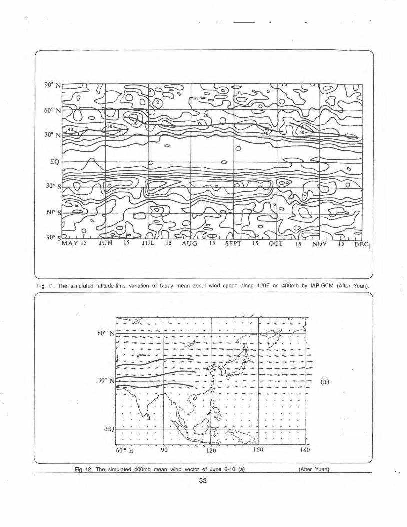
Fig. 11 . The simulated latitude-time variation of 5-day mean zonal wind speed along 120E on 400mb by IAP-GCM (After Yuan).

(a)

60° E 90 120 ISO 180

Fig. 12. The simulated 400mb mean wind vector of June 6-10 (a) (After Yuan).

32

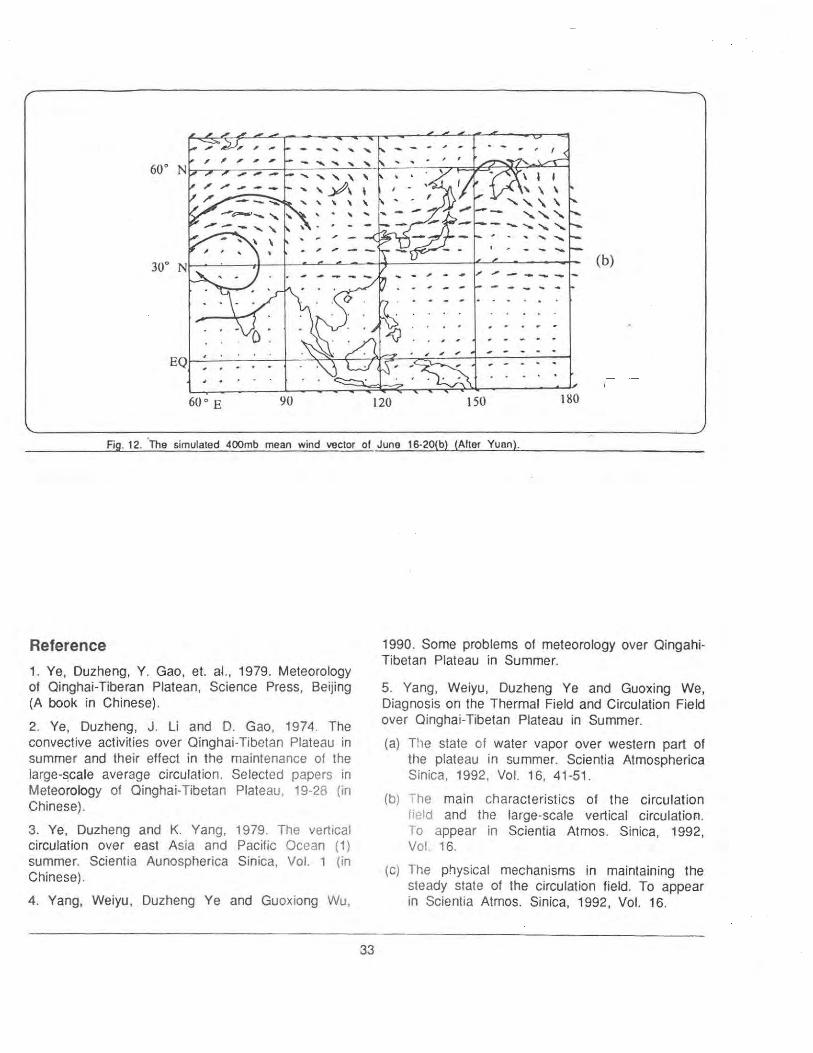
(b)

90 120 150

Fig. 12. ·The simulated 400mb mean wind vector of June 16-20(b) (After Yuan).

Reference

1. Ye, Duzheng, Y. Gao, et. al., 1979. Meteorology of Qinghai-Tiberan Platean, Science Press, Beijing (A book in Chinese).

2. Ye, Duzheng, J . Li and D. Gao, 1974. The convective activities over Qinghai-Tibetan Plateau in summer and their effect in the maintenance of the large-scale average circulation. Selected papers in Meteorology of Qinghai-Tibetan Plateau, 19-28 (in Chinese).

3. Ye, Duzheng and K. Yang, 1979. The vertical circulation over east Asia and Pacific Ocean ( 1) summer. Scientia Aunospherica Sinica, Vol. 1 (in Chinese).

4. Yang, Weiyu, Duzheng Ye and Guoxiong Wu,

33

1990. Some problems of meteorology over QingahiTibetan Plateau in Summer.

5. Yang, Weiyu, Duzheng Ye and Guoxing We, Diagnosis on the Thermal Field and Circulation Field over Qinghai-Tibetan Plateau in Summer.

(a) The state of water vapor over western part of the plateau in summer. Scientia Atmospherica Sinica, 1992, Vol. 16, 41-51 .

(b) ,.he main characteristics of the circulation field and the large-scale vertical circulation. To appear in Scientia Atmos. Sinica, 1992, Vol. 16.

(c) The physical mechanisms in maintaining the steady state of the circulation field. To appear in Scientia Atmos. Sinica, 1992, Vol. 16.

RECENT CLIMATE CHANGES AND

TRENDS OVER INDIA V. Thapliyal & S.M. Kulshrestha, INDIA

i. Introduction

In recent years, the adverse climatic events have frequently disrupted the human societies and have demonstrated the sensitivity of human welfare and international relations to climatic events. The climate has varied over past millenia and is likely to change in future also particularly, in view of the man-made causes. like rapidly increasing carbondioxide, deforestation, ozone depletion etc., which are contributing to the modification of the climate. All countries are vulnerable to long term climatic changes as the regional and global climates are interdependent. For this reason, and in view of ever increasing demand for resources by the fast growing world population that strives for improved living conditions, there is an urgent need for the development of a common regional as well as global strategy for greater understanding and a rational use of the climate.

In India, climatic data, based on instrumental observations are available only for the past 100 to 150 years. By using these data, the problem of recent climate changes and trends in India has been studied by several investigators and the reviews on the subject are available in the literature (Sarker and Thapliyal , 1988). In this article, an attempt has been made to summarise the evidence, if any, regarding climate change over India during recent one century for which the instrumental records over Indian stations are available. The problem has been discussed, in detail, with particular reference to the analysis made by using the Indian rainfall, temperature, pressure and ozone data collected during past several decades. In addition, the effects of man-made causes like increase in urbanisation, pollutants etc. have also been discussed in brief.

2. Trends in Rainfall of India

Among various climatic parameters, rainfall is of greatest concern to the population of the tropics, where the majority of nations including India lie fully or partially. The year to year variability of the annual

34

and the monsoon rainfall creates considerable impact on national activities like, agriculture, water ~anagement, power generation etc. Realising the Importance of the rainfall variability on Indian population, a number of scientists have studied in detail, the rainfall data of 100 to 150 years for which instrumental records are available. Findings of these studies have been summarised below.

2. 1. Trends in Annual Rainfall of India

Towards the end of the nineteenth century, the scientists from the India Meteorological Department from started analysing the available annual rainfall ?ata over ln~ia and noticed the year to year variability m the rainfall. Blanford (1886) was the first meteorologist who made extensive studies of Indian rainfall. The analysis of 19 years (1867 -1885) annual rainfall data for India as a whole did not reveal any systematic trend in the rainfall .

For studying the inter-annual and long term variability of the annual rainfall, Sarker and Thapliyal (1988) and Thapliyal (1990) have recently studied, in detail, the long period (1875 - 1989) annual rainfall of India obtained by using the data of large number of rain gauges (upto 2500), well distributed in the different parts of the country. The study of the 115 years data does not exhibit any increasing or decreasing trend since the beginning of the period. For the entire period, the rainfall anomalies as percentage of the yearly normal (based on 1901 -1950 data) are shown in Fig. 1. It is seen from the figure that the annual rainfall of India exhibits considerable year to year variation, but does not show any increasing or decreasing trend throu~hout the period. During past 115 years (1875 to 1989), the highest rainfall of 125% of the normal was recorded in 1917 while the lowest rainfall 77% of the normal was recorded in 1877. For 70 year period (1901 -1970) the average rainfall and its standard deviation (cr) are respectively equal to 1148 mm and 108 mm.

Five year running means, have been plotted at the end of the period in Fig. 1. Two dotted lines in the figure indicate the value of +1-<J (standard deviation

0 e +20 ~ 0 c .... +10 0

~ 0

~ 0 0 ., '- -10 ::J -- -6' -'-0 Q.

-20 ., ~

0 -30 -.E 0 ct:

-40 1875 80 90 1900 10 20 30 40 50 60 70 80 90

--YEAR__._

Fig. 1. Annual rainfall of India. Thick line - 5 year running mean

+8

0 +6 e '-0 c:: +4 .... 0

~ +2 0

Ill 0

0 ., ... :::1 ... ... -2 o · a. ., ~

-4 0 .... . : -6 0 ct:

-8 510 1880 90 1900 10 20 30 40

I I 1871 1901 1'941

--YEAR~

Fig. 2. Annual rainfall of India. - 10 year running mean

of the rainfall) . It is seen from the figure that during remaine.d within +1- one standard deviation. This 115 years (1875-1989), the 5 year running means perhaps suggests that the rainfall variability during the have fluctuated along the normal rainfall and have period has not exceeded the natural variability of the

climate.

35

For determining the decadal trend. 1 0 year running ~eans o! an~ual rainfall have been studied by dtfferent 1nvest1gators (Pramanik and Jagannathan, 1953, and Thapliyal, 1990). No significant decreasing or increasing trend has been found through out the entire period of 115 years (1875-1989) for which the ~nstrum_ental records are available. However, linearly mcreasmg trends are found during 3 epochs (1876 to 1894, 1904 to 1962 and 1973 onwards) while linearly decreasing trends are found during remaining two epochs (1895 to 1903 and 1963 to 1972). This suggests that the rainfall of India exhibits fluctuating epochal decreasing and increasing trends during recent 115 years.

It can therefore be concluded that the long period annual rainfall data exhibits year to year fluctuations and does not indicate any long term climate change and trend. During recent 115 years, the rainfall has shown fluctuating epochal trends. If rainfall shows increasing trend in one epoch, it shows decreasing trend in the subsequent epoch. Similar results have been noted (Aao, 1936; Agarwala, 1952; Pramanik · and Jagannathan, 1955; Rao and Raghavendra, 197 4 and 1980; Dhar et al., 1982; Sarker and Thapliyal, 1988 and Thapliyal, 1990) when the rainfall of different stations and regions of India have been analysed.

+30

0

E+2o 0 t:

2.2. Trends in Monsoon Rainfall of India

India is fortunate to have a unique season like Southwest monsoon (June to September) which contributes about 75% of the annual rainfall over the country. Instrumental measurements of monsoon rainfall over l~dia are available since the second half of the nmeteenth century. It is interesting to note that the scienti~ts from t~e India Meteorological Department recogmsed the 1mportance of studying the climate change and trend in the monsoon rainfall of India as early as in the first decade of this century. Walke; (1910) examined the summer monsoon rainfall over India from 1841 to 1908 and concluded that there was no perceptible climatic change. On detailed analysis he further indicated (Walker, 1910, 1914, 1922) that the abnormal changes in the atmosphere seem to be responsible for deficiency of monsoon rainfall over India . Subsequently several investigators (Aaghavendra, 1973; Banerjee and Raman, 1976; Sar~er and Thapliyal, 1988 and Thapliyal, 1990) have stud1ed monsoon rainfall of India and have indicated that (i) there is no persistence, cyclicity, trend or definite pattern in unfavorable monsoon occurrences (ii) the inter-annual variability is highest ove; northwest India and (iii) the interval between successive bad years varies widely between zero and 15 years while between good years it does not exceed

~ +10

'!~ 0~~~~~~~~~~~~~~~~~~~~~~~~~~ 0

G) ~

:I -10 t 0 Q. G)

~-20

~ ·= -30 0 a:;

- -0

-40 ~--~~~~~~~~~~~~L-~J-J•~~~1 -LI-J~~~

1875 eo 90 1900 10 20 30 40 50 so 10 80 so --YEAR--~

Fig. 3. Monsoon rainfall of India. (Thick line - 5 year running mean)

36

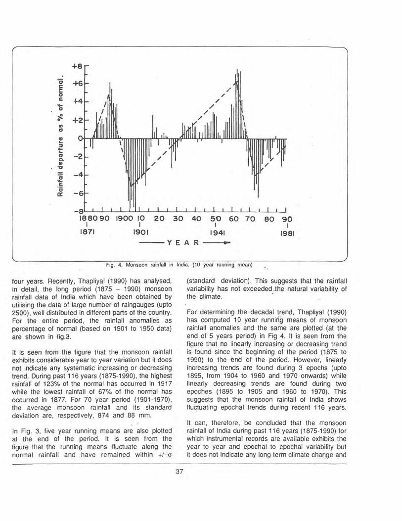
. -0 e / ~

0 c .... 0

~ • ., 0 ., ~

~ -~ 0 Q. • "0

! .5 CJ

a::

I I I I I I

18 80 90 1900 ro 20 30 40 50 60 70 I

80 90 I I I

1871 1901 1941 1981 ---YEAR .,..

Fig. 4. Monsoon rainfall in India. (10 year running mean)

four years. Recently, Thapliyal (1990) has analysed, in detail, the long period (1875 - 1990) monsoon rainfall data of India which have been obtained by utilising the data of large number of raingauges (upto 2500), well distributed in different parts of the country. For the entire period, the rainfall anomalies as percentage of normal (based on 1901 to 1950 data) are shown in fig.3.

It is seen from the figure that the monsoon rainfall exhibits considerable year to year variation but it does ·not indicate any systematic increasing or decreasing trend. During past 116 years (1875-1990), the highest rainfall of 123% of the normal has occurred in 1917 while the lowest rainfall of 67% of the normal has occurred in 1877. For 70 year period (1901 -1970), the average monsoon rainfall and its standard deviation are, respectively , 874 and 88 mm.

In Fig. 3, five year running means are also plotted at the end of the period. It is seen from the figure that the running means fluctuate along the normal rainfall and have remained within +1-<J

37

(standard deviation). This suggests that the rainfall variability has not exceeded .the natural variability of the climate. ·

For determining the decadal trend, Thapliyal (1990) has computed 1 0 year running means of monsoon rainfall anomalies and the same are plotted (at the end of 5 years period) in Fig 4. It is seen from the figure that no linearly increasing or decreasing trend is found since the beginning of the period (1875 to 1990) to the end of the period .. However, linearly increasing trends are found during 3 epochs (upto 1895, from 1904 to 1960 and 1970 onwards) while linearly decreasing trends are found during two epoches (1895 to 1905 and 1960 to 1970). This suggests that the monsoon rainfall of India shows fluctuating epochal trends during recent 116 years.

It can, therefore, be concluded that the monsoon rainfall of India during past 116 years (1875-1990) for which instrumental records are available exhibits the year to year and epochal to epochal variability but it does not indicate any long term climate change and

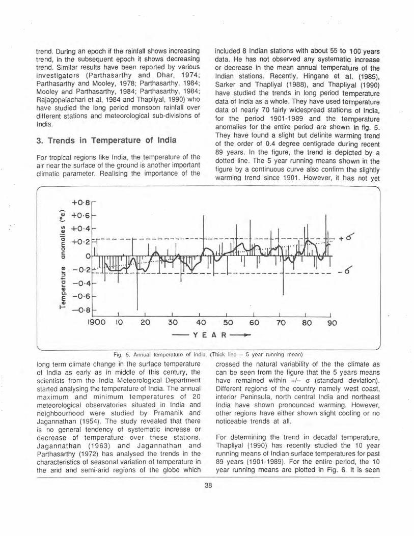
trend. During an epoch if the rainfall shows increasing trend, in the subsequent epoch it shows· decreasing trend. Similar results have been reported by various investigators (Parthasarthy and Dhar, 1974; Parthasarthy and Mooley, 1978; Parthasarthy, 1984; Mooley and Parthasarthy, 1984; Parthasarthy, 1984; Rajagopalachari et al, 1984 and Thapliyal, 1990) who have studied the long period monsoon rainfall over different stations and meteorological sub-divisions of India.

3. Trends in Temperature of India

For tropical regions like India, the temperature of the air near the surface of the ground is another important climatic parameter. Realising the importance of the

+0·8

u +0·6 0 --41)

-~ 0 +0·2 E 0 c:: 0

Q) ... :::J -0 ... Q) Q.

-0·6 E Q)

~

1900 10 20 30 40

included 8 Indian stations with about 55 to 100 years data. He has not observed any systematic increase or decrease in the mean annual temperature of the Indian stations. Recently, Hingane et al. (1985), Sarker and Thapliyal (1988), and Thapliyal (1990) have studied the trends in long period temperature data of India as a whole. They have used temperature data of nearly 70 fairly widespread stations of India, for the period 1901-1989 and the temperature anomalies for the entire period are shown in fig. 5. They have found a slight but definite warming trend of the order of 0.4 degree centigrade during recent 89 years. In the figure, the trend is depicted by a dotted line. The 5 year running means shown in the figure by a continuous curve also confirm the slightly warming trend since 1901 . However, it has not yet

-------- -------- -6

50 60 70 80 90

YEAR -

Fig. 5. Annual temperature of India. (Thick line - 5 year running mean)

long term climate change in the surface temperature of India as early as in middle of this century, the scientists from the India Meteorological Department started analysing the temperature of India. The annual maximum and minimum temperatures of 20 meteorological observatories situated in India and neighbourhood were studied by Pramanik and Jagannathan (1954). The study revealed that there is no general tendency of systematic increase or decrease of temperature over these stations. Jagannathan (1963) and Jagannathan and Parthasarthy (1972) has analysed the trends in the characteristics of seasonal variation of temperature in the arid and semi-arid regions of the globe which

38

crossed the natural variability of the the climate as can be seen from the figure that the 5 years means have remained within +1- cr (standard deviation). Different regions of the country namely west coast , interior Peninsula, north central India and northeast India have shown pronounced warming. However, other regions have either shown slight cooling or no noticeable trends at all.

For determining the trend in decadal temperature, Thapliyal ( 1990) has recently studied the 1 0 year running means of Indian surface temperatures for past 89 years (1901-1989). For the entire period, the 10 year running means are plotted in Fig. 6. It is seen

+0·20

+0·15

u !..+ 0·10 ~ ., 0 +005 E 0 c 0

r-

1-

1-

- /

J II

1', ,

·' / ' 1'.._

', " ,· ltll[~ll ., ...

:I

0

0 -0·05 JI~J! J~f

I

... ., Q.

E -0·10 ~

-0·15

-0·20

-

-

-

I

1910 I

1901

. //

I

20

, ...

I

30 I

1921

I

40 I

50 I

1941

I

60 I

70 I

1961

I

80 I

90 I

1981

-YEAR .-

Fig. 6. Annual rainfall in India. (10 year running mean)

from the figure that by and large the temperature 4. Trends in Atmospheric Pressure Over shows increasing trend, if the slight cooling around India 1930's and 1960's are neglected.

An interesting feature may be noted that the Indian mean annual temperature does not show the post 1940 cooling which has been observed for the Northern Hemisphere. On the contrary, the Indian temperatures have generally shown steadily increasing trends over past 8 decades (Hingane et al. , 1985; and Sarker and Thapliyal, 1988). It is difficult to interpret above result in terms of cause and effect. It may, however, be noted that during recent one century, considerable increase in the con·sumption of fossil-fuel, deforestation and land use have taken place in India.

During past eight decades, some regions of the country have generally indicated warming trend while some others have shown cooling trend (Hingane et al, 1985 and Sarker and Thapliyal, 1988). It is difficult to interpret the above result in terms of cause and effect particularly in view of the natural variability of the climate.

39

Detailed analysis of long period (80 to 100 years) pressure of India (Pramanik and Jagannathan, 1955, Sarker and Thapliyal, 1988) have not revealed any systematic increasing or decreasing trend of the surface pressure over the country-. However, considerable year to year fluctuat ions, have been noted during recent 100 years over India. Similar results are obtained when the available data for other important climatic parameters are analysed.

5. Trends in Total Ozone Over India

The threat to the atmospheric . ozone layer from chemicals released indiscriminately by man into the atmosphere has to be taken very seriously. The discovery of the Antarctic ozone hole from the satellites - and subsequent detection of the presence of ozone destroying chloroflorocarbons in the Antarctic atmosphere have reinforced the belief that the delicate balance of the atmospheric ozone is in

+40 42182 NEW DELHI 28·4N 7t·l E

+20 0~---------D~~~~~or~~~~~~~~~~~---

-20 -40

t- -eo 43540 SRINAGAR 34·1 N 74·S E i ;:)

z 0 Cl)

8 0

1-z :::::>

z 0 en ID 0 0

-20 -40 -60 +40 +20

43339 -KOOAIKANAL 10·1 N 77·3E

0~----------~~~~3-~nL~~~~~~~~~~~~~--

-20 -40 -60~~~~L-~~~~L-~~~-L~~~~~-L-L~~~~--

~8

450

400

350

300

250

200

150

Fig. 7. Ozone distribution over India

1981 .. ~~ .. :-:-19 8 2 ~~;QDij~== 1983 1984 1985 1986 1987 1988 1989 1990

09~o~·~s--~s~o~·~s~--~3~0~0-S----~ELa------3~0~.~N-----6~0~0~N----__J9ifN

LATITUDE

Fig. 8. Average october ozone amounts (1981 - 1990)

40

real danger of being progressively upset. The world community particularly the industrialised nations - has now woken up, to this threat to ozone layer by voluntarily imposing cuts and in some cases even banning the production of certain chloroflorocarbons. The developing nations are also being urged to follow suit in due course.

In India, ozone is being measured since 1928, when the first Dobson ozone spectrophotometer measurements were carried out at Kodaikanal. By using Indian data Ramanathan (1963) has studied the total ozone amounts observed at Mount Abu/ Ahmedabad (25° N - 22° N) and Kodaikanal (1 oo N) and have shown a biannual variation in ozone amount during the period 1954 to 1962. Ramanathan (1964) noted a drastic spring time reduction in ozone in 1957 and 1958 over both, Arctic and Antarctic zones. Recently, many investigators (e.g., Sreedharan and Sharma, 1986) have studied ozone observations taken by Indian scientists and have confirmed the occurrence of ozone hole over Antarctic. For past one decade, the average October ozone amounts are shown in Fig. 8. obtained from NIMBUS 7 SBUV DATA (Mani, 1988 and Hallgren, 1990). On analysing the trend values for ozone during these years, it appears that the steady fall was halted in 1990 as during last 3 consecutive years the ozone amounts over Antarctic have remained almost the same.

For studying the inter-annual and long term variability of ozone over India, a number of investigators (Tiwari 1973, Tiwari and Sreedharan 1973, Thapliyal 1990) have analysed ozone measurements over India. For past three decades the ozone distribution over 3 stations of India are shown in Fig. 7. It may be seen from the figure that ozone measurements exhibits year to year variability but do not show any systematic decreasing or increasing trend over India. However, as a precaution it is important to continue careful monitoring and analysis.

6. Trends in Air Pollution Related Parameters Over India

In India, like many other countries, the industrialisation and urbanization are increasing the air pollution. This has led many investigators (Mukherjee, 1964 and Krishna Nand, 1984) to study the danger of acid rain over different urban and rural stations of India. Acidity in a solution is synonymous with presence of

41

hydrogen ion (H•) and a common measure of acidity is pH. Due to impurities in rainwater, the precipitation at a pH below 5.6 (the equilibrium value for a pure distilled water) is considered as acidic. Analysis of pH data from 10 Back Ground Air Pollution Monitoring Network (BAPMoN) stations reveals the year to year variation in different parameters. During past 15 years (1975 to 1989) the temporal trends of pH at Indian BAPMoN stations are shown in Fig. 9. It is seen from the figure that over most of the stations the pH value exhibit a lowering trend. Similar results have been reported by Krishna Nand, 1984, Verma, 1988 and Khemani, et al. 1988. Different studies confirm the long term effects of pollutants on pH of rain water which are less in India as compared to those found in heavily industriaised countries. This is obvious as industrial growth is slow over India. Further, the soil in most parts of India being alkaline in nature provides aerosols which help in rendering the rainfall non-acidic.

Urbanisation also produces environmental problems such as air pollution, thermal stress on human body associated with urban heat islands etc. The surface energy over urban Indian areas is influenced by atmospheric pollutants as well by surface radiative and thermal properties. The spatial distribution of insolation in Delhi shows pollutants reducing values over the city (Padmanabhamurthy and Mandai, 1982). Extensive heat island studies using surface observations have been carried out in various Indian cities (Padmanabhamurthy, 1986, Mukherjee, 1986 and Jayanthi, 1991). The timing of daily peak heat islands differs among some cities of India. Although no significant changes have so far been found on long term basis but as a precaution it is necessary that adequate protective measures should be devised and effected at an early date.

7. Concluding Remarks

During the recent 100 to 150 years for which instrumental records are available, the important climatic parameters have exhibited considerable year to year random fluctuations. Except for temperature which has shown slight warming, although still within the limits of ± cr (standard deviation) over a century, all other climatic parameters like rainfall, pressure etc., have not indicated any systematic decreasing or increasing trend throughout the period. However, fluctuating epochal decreasing or increasing trends

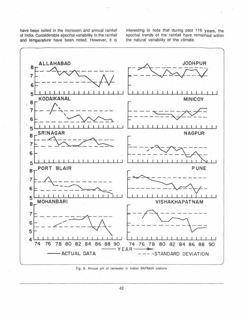
have been noted in the monsoon and annual rainfall of India. Considerable epochal variability in the rainfall and terJl>erature have been noted. However, it is

interesting to note that during past 116 years, the epochal trends of the rainfall have remained within the natural variability of the climate.

8

7

6

5

8

7

6

5 8

7

6

5 8

7

6

5 8

7

'6

5

ALLAHABAD JODHPUR

KODAIKANAL MINICOY

--t-~-------------'~

NAG PUR

PORT BLAIR PUNE

--'\::_----- -------~ ---- - ---- --

MOHANBARI VISHAKHAPATNAM

4~_.~~~~_.~~~~_.~._~

74 76' 78 80 82 84 86 88 90 74 76 78 ao 82 84 86 88 90 --YEAR -.,

--ACTUAL DATA ----STANDARD DEVIATION

Fig. 9. Annual pH of rainwater in Indian BAPMoN stations

42

References

Agarwala, K.S., 1952, Fluctuations of annual rainfall in central India, 1872-1947, Indian J. Met. Geophys., 3. p 229-230

Banerjee, A.K. and Raman, C.R.V. 1976, One hundred years of southwest monsoon rainfall over India, India Met. Dep., Sci. Report No. 76/6.

Blanford, H.F., 1886, Rainfall of India, Mem. India Met. Dep., 3, 658.

Chowdhury, A. and Abhyankar, V.P. 1979, Does precipitation pattern foretell Gujarat climate becoming arid? Mausam, 30. P 85-90.

Dhar, O.N.,Rakhecha, P.R. and Kulkarni, A.K., 1982, Trends and fluctuations of seasonal and annual rainfall of Tamil Nadu, Proc. of the Indian Acad. of Sci . (Earth and Planet Sci.) , 91. P 97-104.

Hallgren, R.E., 1990, 1989 Ozone hole matches 1987 record , News and Notes, Bull Am. Met. Soc. 71 . P 65.

Hingane, L.S., Rupakumar, K. and Ramanamurthy, Bh. V ., 1985, Longterm trends o'f surface air temperature in India, J. Climatol., 5. P 521-528.

Jagannathan, P. (1963), Trends in the characteristics of seasonal variation of temperature in the arid and semi-arid region, Indian J. Met. Geophys. 14. P 3.

Jagannathan, P. and Parthasarthy, B., 1972, Fluctuations in the seasonal oscillation of temperature in India, India J. met. Geophys., 23, P 15.

Jayanthi, N., 1991 , Heat island study over Madras city and neighbourhood, Mausam, 42. P 83-88.

Khemani, L.T., Mohin, G.A., Prakash Rao, P.S., Safai, P.O., Singh G., Chatterjee, R.N. and Prem Prakesh, 1966, Long term effects of pollutants on the pH of rain water in North India, Extended Abstracts, Proceeding of International Conference on Tropical micro-Meteorology and Air Pollution, 15-19 Feb. liT Delhi. P 246-248.

Krishna Nand, 1984, Prospects of acid rain over India, Mausam 35, 225-232.

Koteswaran, P. and Alvi, S.M.A., 1969, Secular trends and periodicities in rainfall at west coasts stations in India, Curr. Sci., 38. P 229-231.

43

Koteswaran, P. and Alvi, S.M.A., 1970 Secular Trends and variations in rainfall of Indian Regions, IDOJARAS, 74. P 76-183.

Mani, A., 1988, The ozone controversy, J. Sci & Industrial Res., 47, pp. 697-705.

Mooley D.A., and Parthasarthy, B., 1984, Fluctuations in All India summer monsoon rainfall during 1871-1978, Climatic change, 6, 287-301 .

Mukherjee, A.K., 1964, Acidity of monsoon rain water, Indian J. Met. Geophys .• 15, 267-270.

Mukherjee. A.K., 1986, Inferences about heat Island circulations, Mausam, 37. P 457-466.

Padmanabhamurthy, B. and Mandai, B.S., 1982, Urban - rural radiative differences, Mausam 33, 509.

Padmanabhamurthy, · B., 1986, Some Aspects of urban climate in India, WMO Report No. 652, 136-165.

Parthasarthy, B. 1984, Interannual and long term variability of Indian summer monsoon rainfall, Proc. Indian Acad. Sci. (Earth Planet Sci). 93. P 371-385.

Parthasarthy, B. and Dhar, O.N., 1974, Secular variation of regional rainfall over India, Quart. J. A. Met. Soc., 100, 245-257.

Parthasarthy, B. and Mooley, D.A., 1978, Some features of a long homogeneous series of Indian summer monsoon rainfall, Mon. Weath. Rev., 106. p 771-781.

Pramanik, S.K. and Jagannathan, P., 1953, Climatic changes in India (I) : Rainfall, Indian J. Met. Geophys .. 4. P 291-309.

Pramanik, S.K. and Jagannathan, P., 1954, Climatic changes in India (II) : Temperature, Indian J. Met. Geophys, 5. P 29-47.

Pramanik, S.K. and Jagannathan, P., 1955, Climatic changes in India (Ill) : Pressure, Indian. J. Met. Geophys., 6. P 137-148.

Raghavendra, V.K., 1973, A statistical study of the southwest monsoon rainfall in the Indian Peninsula and southwest monsoon rainfall and winter precipitation in Northwest India, Met. Monogr., 6. p 1-14.

Raghavendra. V.K. 1974, Trends and periodicities of rainfall in sub-divisions of Maharashtra State, Indian J.Met. Geophys., 25. P 197-210.

Raghavendra, V.K., 1976, Long period aspects of monsoon rainfall in southern State of Andhra Pradesh in India, Proc. Symp. Tropical Monsoon, I.I.T.M., Pune. P 445-457.

Raghavendra, V.K., 1980, Droughts in Kerala, Vayu Mandai, 10. P 28-31.

Rajgopalachari, P.J., Krishnan, V. and Sankaran, N., 1984, Indian rainfall variability during the -twentieth century, Symp. on climate and its variability, I.I.T., Delhi.

Rao, A., 1936, A note on statistical study of rainfall in Mysore State, India Met. Dep. Sci. Notes, No. 71, VI. p 21-34.

Rao, K.N. 1958, Some studies on rainfall of Rajasthan with particular reference to trends, Indian J. Met. Geophys., 9. P 97-116.

Rao, K.N. and Jagannathan, P., 1963, Climate changes in India, Symp. 'Changes of Climates·, held at Rome Arid Zone Research XX, Published by WMO, Geneva. P 49-66.

Ramanathan, K.R., 1963, Bi-annual variation of atmospheric ozone over the tropics, Quart. Jour., Roy. Met. Soc., 89, 540-542.

Ramanathan, K.R., 1964, Introductory note on atmospheric ozone observations in IGY and IGC, Annals of IGV 32, 101-120.

Sarker, R.P. and Thapliyal, V., 1988, Climatic change and variability, Mausam, 39. ·p 127-138.

Sreedharan, C.R., 1974, Ozone measurements in India, Proc. Inti. Conf. Structure, Comp. & Genl.

44

Circulation of the Lower and Upper Atmosphere and possible Anthropogenic perturbation, Melbourne 1. p 395-428.

Sreedharan, C.R. and Sharma, A.K., 1986, Vertical distribution of ozone over Dakshin Gangotri, Antarctica, Ind. J. of Radio & Space Physics. 15. p 159-162.

Thapliyal, V., 1990, Perspective of climate change in India, Report of the Expert Meeting on Climate Change Detection Project, Toronto (Niagara-on-theLake), 26-30 November 1990, World meterological Organisation, Geneva.

Tiwari, V.S., 1973 Ozone distribution over India, J. Pure & Appl. Geophys. P 1010-1017.

Tiwari, V.S. and Sreedharan, C.R., 1973, Short term ground ozone fluctuations· at Poona, J. Pure & Appl. Geophys. P 1197-1205.

Verma, G.S., 1988, Back Ground trends of pH of precipitation over India, Extended Abstracts, Proc. of International Conference on Tropical Micro Meteorology and Air Pollution, 15-19 Feb. liT Delhi. P 456-459.

Walker, G.T., 1910, On the Meteorological evidence for supposed changes of climate in India, Mem. India Met. Dep., 21 (Part 1) . P 1-21 .

Walker, G.T., 1914, A further study of relationship with Indian Monsoon rainfall, Mem. India Met. Dep.1 21, (Part VIII). P 1-12.

Walker, G.T. , 1922, Correlation in · seasonal variation of weather, VII, The local distribution of monsoon rainfall, Mem. India Met. Dep., 21, (Part VIII), 23-29.

THE ROLE OF THE OCEANS AS A REGULATOR OF ATMOSPHERIC CARBON DIOXIDE CONCENTRATIONS

Chen-Tung Arthur Chen, TAIWAN

ABSTRACT

The oceans contain on amount of dissolved carbon over 50 times that present in the atmosphere and hove acted as o major regulator of atmospheric carbon dioxide concentrations. The surface wind-mixed Ioyer (less than 200 m deep) of most of the oceans is more or less saturated with excess C0

2. The deep waters (from 200m to on overage depth of 3800m). on the other hand. hove not

been affected by the excess C02 except near their source regions. such as the northern North Atlantic Ocean. the Red Sea. and the Weddell Sea. This slow penetration of excess C0

2 into the deep waters

Is due to the slow exchange of waters across the thermocline that separates the surface and deep waters. More and more excess C0

2• however. will gradually penetrate into the deep oceans. 1

examine this process by discussing the excess C02

signal. and comparing the signal with signals of transient tracers. Data in the Red Sea. North Indian Ocean and the Pacific Ocean ore presented.

Introduction

The oceans cover around 60% of the surface in the Northern Hemisphere and over 80% in the Southern Hemisphere. Overall, the oceafls cover 70.8% of Earth's surface and are the giant of carbon dioxide control. There is 20 times more carbon dissolved in sea water than that occurs on land (in biota and soil) . The oceans' C0

2 reservoir is more than 50 times the

size of the atmospheric C02 reservoir and the release of just 2% of the carbon stored in the oceans would double the level of atmospheric C02. Furthermore, each year around 15 times more C02 is taken up and released by natural marine processes than the total produced by the burning of fossil fuels, deforestation and other human activities~.

The amounts of C02

entering and leaving the oceans over an annual cycle are usually close to global balance. However, air-sea exchanges are controlled by many different processes with large spatial and temporal variations. Circulation patterns and other physico-chemical conditions govern C02 solubility, gas transfer rates across the sea surface, and the bulk transport of carbon within the oceans. Superimposed on (and strongly influenced by) these effects are two basic biological processes : carbon fixation by photosynthesis, and C02 release by respiration 1• As a result, the surface ocean is rarely in equilibrium with the atmospheric C02 .

Photosynthesis is limited to the sunlit, upper ocean while respiration occurs throughout the water column.

45

Over geological periods of time, marine plankton have been responsible for a vast accumulation of carbon in the oceans and in sediments, altering atmospheric composition. Biological and physical C0

2 'pumps'

remove C02 from surface water and release it in the deep ocean (Fig 1) thereby providing the main driving forces for the ocean carbon cycle. At present, only the broad outline is known, with physical C02 uptake occurring mostly in sub-polar regions (particularly the North Atlantic) and C02 release mostly in equatorial regions (particularly the Pacific). Those features closely match the pattern of global ocean circulation, with surface water cooling and sinking in the former regions, and de~p water upwelling and warming in the latter. Lateral movements of waters complete the physical ocean 'conveyor belt' for the transport of carbon around the world1

•

Biological C02 pumps are more vertically-directed, promoting the transfer of carbon from surface to deep ocean. Several pathways are involved : the sinking of plant and animal debris, containing both organic carbon and calcium carbonate; active downward transport, brought about by the feeding and excretory behaviour of migratory zooplankton; and the downward advection and diffusion of dissolved organic carbon, produced mainly by decomposition processes in the upper ocean1.

The net effect of such biological activity is to reduce pC02 in surface waters, causing the drawdown of C0

2 from the atmosphere. Its rate of return is subsequently determined by the depth distribution of respiration and

NTC02 , .J.1 mole/kg

2000 2100 2200 2300 2400 0 - -- --

·' // _,.,....._SA

2 \ /

(

E 3 .X

J: .... 4 n.

L&J 0

5

6

7

Fig. 1. The distribution with depth of the total carbon dioxide concentration in seawater in various ocean basins. The concentrations are normalized to the mean world ocean salinity of 34.78%. NA, North Atlantic ; SA, South Atlantic ; AA, Antarctic

region south of 45•s; Sl, South Indian ; Nl , North Indian; SP, South Pacific ; and NP. North Pacific•.

decomposition processes, and by physical factors influencing carbon transport in the water column 1•

We cannot yet, however, measure the components of the global carbon cycle with sufficient accuracy to balance the carbon budget. While it is known that human activities add 5-6 giga tonnes (1 09} of carbon each year to the atmosphere, the annual increase in atmospheric C02 is equivalent to only 3 giga tonnes of carbon. We do not yet have an accurate account of where the remaining 2-3 giga tonnes of carbon goes. Quantifying and balancing carbon circulation processes in different oceans, and for the world as a whole, is a major aim of the JGOFS programme.

Oceanic Excess C02 Penetration

Recently it has been shown that the oceanic penetration of excess (anthropogenic) C02 can be calculated using carbonate data. Because the method

46

is subject to large uncertainties, the accuracy of the results is not known. However, the precision of the method is adequate to show the excess C0

2 signal.

The abundant carbonate data in the literature can thus be used to supplement the tracer data in showing oceanic mixing features for waters formed in the last 130 years 3-15 .

The method of computation and its limitations have been described in detail elsewhere &-18. The method involves a back-calculation of the C0

2 concentration

of a parcel of sea water to its initial concentration at the sea surface by correcting for changes due to the decomposition of organic material and dissolution of carbonate particulates. These back-calculated C0

2 concentrations of waters with various ages are then compared with each other and with the contemporary surface C02 concentrations to obtain the oceanic C0

2 increase.

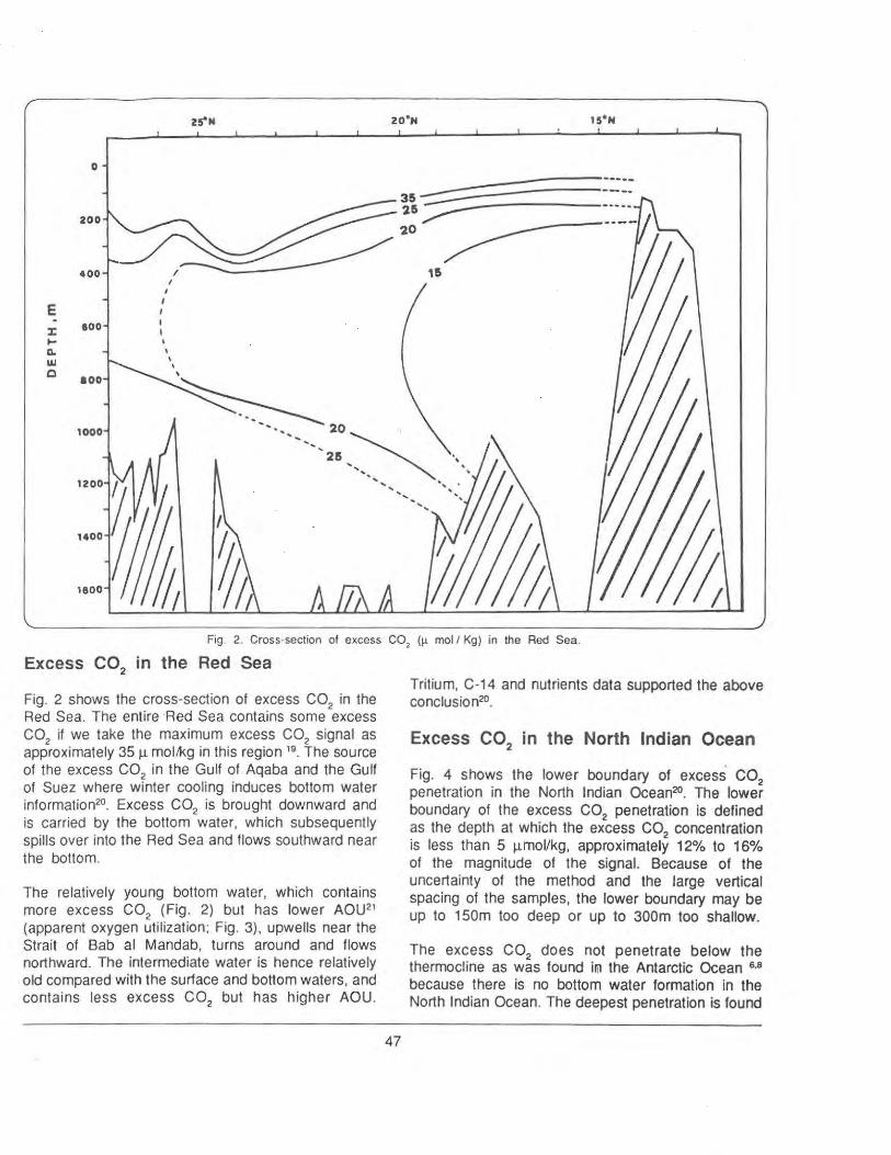
0 -:::::::=:====-----200

400

I

I E I

:r:: eoo 1- ' ~ ' w 0 aoo

1000

1800

Fig. 2. Cross-section of excess C02

(f! mol / Kg) in the Red Sea.

Excess C02

in the Red Sea

Fig. 2 shows the cross-section of excess C02 in the Red Sea. The entire Red Sea contains some excess CO if we take the maximum excess C0

2 signal as

app2roximately 35 Jl mol!l<g in this region 19

• The source of the excess C02 in the Gulf of Aqaba and the Gulf of Suez where winter cooling induces bottom water information20. Excess C02 is brought downward and is carried by the bottom water, which subsequently spills over into the Red Sea and flows southward near the bottom.

The relatively young bottom water, which contains more excess C02 (Fig. 2) but has lower AOU21

(apparent oxygen utilization; Fig. 3}, upwells near the Strait of Bab al Mandab, turns around and flows northward. The intermediate water is hence relatively old compared with the surface and bottom waters, and contains less excess C02 but has higher AOU.

47

Tritium, C-14 and nutrients data supported the above conclusion20.

Excess C02 in the North Indian Ocean

Fig. 4 shows the lower boundary of excess C02

penetration in the North Indian Ocean20. The lower boundary of the excess C02 penetration is defined as the depth at which the excess C0

2 concentration

is less than 5 J.!mol/kg, approximately 12% to 16% of the magnitude of the signal. Because of the uncertainty of the method and the large vertical spacing of the samples, the lower boundary may be up to 150m too deep or up to 300m too shallow.

The excess C02 does not penetrate below the thermocline as was found ilil the Antarctic Ocean 6·8

because there is no bottom water formation in the North Indian Ocean. The deepest penetration is found

E ~ IC.

"' 0

0

zo6

400

eoo

100

7

5 \ ~ zs•N

---

,

10

• ' 12

~ zo•N ~

0

' ' '

14

' 1s•N

' ' 10Q ,' --------------- ---.. _

-----120 1000

1200

1400

1800

Fig. 3. Cross-section of apparent oxygen utilization (J.1 mol / kg) in the Red Sea2 1•

outside of the Gulf of Aden, apparently due to the overflow of the Red Sea water, which sinks outside of the Gulf and carries the excess C02 along with it. This water, albeit very salty, is too warm for it to be dense enough to sink to the bottom. The volume of the water is also not large enough for it to affect much of the Arabian Sea.

48

The shallowest penetration is found in the equatorial region due to the world-wide equatorial upwelling , which brings up old, excess C02 - free deep water. Excess C02 penetrates deeper further sou th especially near 45°S14

• 15 (not shown on Fig.4) Little

data is available in the Bay of Bengal. Fig.4 looks similar to the tritium and C-1 4 distributions19

•

Excess CO in the Pacific Ocean 2

An isogram map of the lower boundary of the excess C0

2 penetration in the Pacific Ocean is shown in

Fig.5. Excess C02

also does not penetrate below the thermocline in the Pacific Ocean because there is no bottom water formation in the North Pacific. The shallowest penetration outside of the Southern Ocean occurs in the eastern equatorial region where the excess CO only penetrates to 400 m, or shallower.

2 • Because few data is available for the complex oceantc region in the western equatorial Pacific, results there are less reliable. The general trend, however, indicates a deeper penetration (BOOm) in the Western Pacific and in the South China Sea9

·22

. Overall, excess co penetrates to a shallower depth in the equatorial Pa~ific than· in the Atlantic6•8 and Indian Ocean, perhaps reflecting the higher equatorial upwelling rate in the Pacific and less influence of the newly formed water advected from the north9

•

Similar to what was found in the Weddeil Seas, intensive upwelling prevents excess C0

2 from

reaching more than 200m deep in the region around 65°S. The excess C02 penetrates deeper further south, and reaches more than 1000 m off Cape Adare at the northwest corner of the Ross Seas.

. I

I

I I I I I I

I I

I I I ,._ --- - - - ; - - - -. - - r - - - ... -· / I ~ ' I I

I I

I I

- .1. • .•

1000 I

I './ : oOOO \

1

; j I ' -· · · ··· ' I -~----~- ---.,,~ ~ ~60<)~1. >---l-~~~

' () ;-.......... : ~ ........ I t I -

2o·s ----L- - ---~ - -- -- --1 - - - - - ---j----40£ 60'E IOE 100E

Fig. 4. Lower boundary of excess C02 penetration (depth in meters) in the north lnd1an Ocean.

49

The deepest excess C02 penetration in the South Pacific occurs around 45°S near where the Subantarctic Mode Water is located, but the depth of penetration is slightly shallower than that found in the South Atlantic Ocean. Intensive vertical mixing in the Drake Passage also seems to result in deeper excess C02 penetration compared to the situation found elsewhere at the same latitude. The deepest penetration in the North Pacific occurs in the confluence of the Kuroshio and Oyashio currents. This is the region off Japan near the area of circulation of the North Pacific variety of the subtropical Mode Water. Here excess C02 has penetrated to a depth of more than 1400m (Fig. 5). In general, deeper penetration occurs on the western side of the Pacific.

Fig. 6, based on the GEOSECS data23 is an isogram map of the depth where tritium equals to 0.1·TU. The similarity in distribution with the excess C02 results is striking. Few tritium data exist, however, south of 6S"S. so we do not know whether tritium penetrates deeper near the Antarctic Continent. C-14 signals are similar to the tritium signals9 •

Conclusion

The lower boundary of anthropogenic C02

penetration based on carbonate data in the literature has been shown for the Red Sea, North Indian and Pacific Oceans. The results indicate that the distribution of excess, anthropogenic C0

2 ·follows the large-scale

movements of water masses. such as vertical mixing in the Red Sea, upwelling, and Mode Water formation .. The deepest penetration is found in the Red Sea where the entire water column has been contaminated by the excess C0

2• Other regions of

deep penetration are the areas where the Subtropical Mode Waters are found the northwest Pacific off Japan, and around 45°S in the Pacific. The shallowet penetration areas are around 65°S in the Pacific and in the eastern equatorial region in the Pacific and Indian Oceans.

Acknowledgement

1 thank NSC (80 - 029 - M 11 0 - 08) for 'its financial support.

-200M

Fig. 5. Lower boundary of excess C02

penetration (depth in meters) in the Pacific Ocean.

50

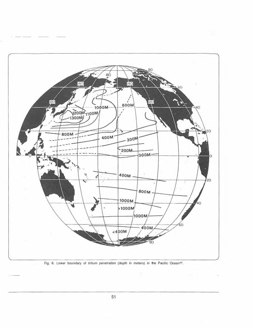
Fig. · 6. Lower boundary of tritium penetration (depth in meters) in the Pacific Ocean23•

51

References

1. Scientific Committee on Oceanic Research, 1990, An introduction to JGOFS, 12pp.

2. Takahashi, T. W.S. Broecker and A.E. Bainbridge 1981 in "Carbon Cycle Modelling" ed. B. Bolin, 271-86, J. Wiley, N.Y.

3. Brewer, P.G. 1978 Geophys. Res. Let., 5, 997-1000.

4. Chen. C.T. 1980 EOS, 61, 263.

5. Chen C.T. 1982, Geophys, Res. Let. 9, 117-119.

6. Chen, C.T. 1982, Deep-Sea Res., 29, 563-580

7. Chen, C.T. and F.J. Millero, 1978, EOS, 59, 1101

8. Chen C.T.A., 1987 Oceanologica Acta , No. sp. 97-102

9. Chen. C.T.A. 1989 Workshop on Long-term Air Quality Changes and Their Climatic Impact, Nov. 14-15, Taipei, Taiwan, 7pp.

10. Chen, C.T. and F.J. Millero 1979. Gradual increase of oceanic carbon dioxide. Nature 277, 205-206.

11. Chen, C.T. and A.M. Pytkowicz, 1979, Nature, 281, 362-365

12. Chen, C.T. F.J. Millero and R.M. Pytkowicz. 1982. J. Geophys, Res. 87, 2083-2085.

52

13. Chen, C.T.A., E.D. Jones and K.J . Lin. 1990. Deep Sea Res., 37, 1455-1473.

14. Chen, D.W. and C.T.A. Chen, 1989, Env. Prot., J. Chin. Env. Prot. Soc. 12(2), 45-64.

15. Chen, D.W. 1988. MS thesis, lnst. Mar. Geol. Sun Vat-Sen Univ. Kaohsiung, Taiwan, ROC, 173pp (in Chinese) .

16. Poisson, A. and C.T. Chen. 1987. Deep-Sea Res., 34, 7, 1255-1275.

17. Shiller, A.M. 1981. J. Geophys. Res., 86, 11. 083 - 088.

18. Broecker, W.S., T. Takahashi and T. H. Peng. 1985. DOE Tech. Rep., DOE/OR-857, 79pp.

19. Wu, C.T. 1990. MS thesis, lnst. Mar. Geol. Sun Vat-Sen Univ. Kaohsiung, Taiwan, ROC, 128pp (in Chinese).

20. Krumgalz, B.S., J. Erez and C.T.A. Chen. 1990. Oeano. Acta , 13, 283 - 290.

21 . Beauverger, C., C. Brunet and A. Poisson. 1984. Pub. Mission Rech. 824, TAAF, Paris, 181pp.

22. Wang, S.L. 1988. MS thesis, lnst. Mar. Geol. Sun Vat-Sen Univ, Kaohsiung, Taiwan. ROC, 122pp (in Chinese).

23. Ostlund, H.G., A. Brescher, ROleson and M.J. Ferguson. 1979, Tritium Lab. Data Rep. 8, Univ. of Miami, 384 pp.

SATELLITE OBSERVATIONS OF VEGETATION COVER AND LAND USE PATTERNS IN GLOBAL CHANGE STUDIES, WITH SPECIAL REFERENCE TO ASIA.

Prof B. L. Deekshatulu, INDIA

The changes in vegetation cover and land use patterns brought about by man's search for increasing food needs will bring about concommitant changes in the climate which in turn will affect vegetation cover and land use pattern.Given the complexity of the various interactive components of the global environment the basis for any credible analysis or predication of global change must be documentation of the changes that have occurred or are presently occurring. Global and regional observations of the earth by satellite sensors are required because ground measurement cannot be made at the required spatial and temporal resolutions. Many of the regional changes that are happening or expected to happen over ,Asia, as well over the entire globe, may be monitored with .remote sensing satellite systems. This monitoring can be direct, as in measuring surface temperature increase, or indirect through observations of parameters known to bring ·about changes in climate or to respond to changing climate. Example of the iatter are change in the distribution, composition and productivity of vegetation and changes in land use pattern. Vegetation may change as a result of stress imposed by moisture deficit or by change in the species tolerance range induced by climatic shifts. Such change in vegetation cover and land use pattern will have a feedback effect on climate, in terms of change in water vapour, C02 , N02, and Methane inputs to atmospheric as well as changes in albedo. In several parts of the globe satellite data have already revealed phenomenon that are expected to lead, or be symptomatic of global change. They include forest cover changes, desert shifts and land use patterns over India and other parts of Asia.

The value of satellite observations will increase exponentially with the length of the observational series. It is obvious that what is needed in long term is consistent objective data sets. The satellite observations need to be complemented by properly designed ground measurement programmes. The temporal satellite data, supported by ground data, can then be used to model various environmental changes for given country or region.

53

Current satellite sensors operate in the visible to thermal infrared portions of the electromagnetic spectrum, while sensors operating in the microwave region are expected to provide data from the early nineties. The value of satellite data archival will increase significantly towards the second half of this decade after the comprehensive EOS (Earth Observation Satellite) data are added to the time series.

Satellite observati0ns for global change studies can be obtained through direct down link to ground receiving stations, and can be provided either from sensors· launched by the country/region or from foreign satellites that are important in the regional context. Capability to design and operate remote sensing satellites has also been built up in Asia. The Indian Remote Sensing Satellite of India, MOS of Japan and Feng Yun 1 B of China are some examples. India has been acquiring satellite data through direct down link from 1979 onwards, consisting of Landsat , SPOT, NOAA and IRS satellite data. Bhaskara and Aryabhatta experimental satellites also have provided data. The followons to the IRS lA, which will be completing three years of successful sensing by march 1991 , will cover observations in the thermal and microwave regions of the EM spectrum and will have large swath and frequent visit capabilities. Direct reception from ERS-1 satellite is also planned.

Satellite observations of land use patterns involve the following global change issues

- Physical and chemical interactions between the Earth's surface and the atmosphere

- Climatic impact on vegetation processes and distribution

- Complex interactions between man, climate and vegetation

The goal of the programme could be to produce a consistent land use map of Asia perhaps at a

resolution of 1 km. or better . The mapping methodologies should be designed so that global change research issues, from local to global, can be supported using a hierarchy of spatial scales, sampling techniques and data sources. The satellite data set should provide ( 1) the nature and distribution of land cover, (2) seasonal dynamics of land cover and (3) long term trends in land cover change.

With the increasing availability of satellite data, broad changes in land use such as forests to agricultural or increasing urbanisation. decline in wetland and increasing soil hazards could be monitored. While such data may not replace the need for ground measurements it will however help analysts to improve short term monitoring capabilities.

A recent exercise in India has been using IRS lA satellite data to produce detailed and land use maps in 1 : 250000 Scale, for the entire country, using both visual and digital interpretation methodologies. This exercise, covering 504 IRS scenes, over 18 months, and involving 80 scientists and 120 cartographers, while providing details necessary for optimum agricultural development in 15 agroclimatic zones of the country, may not be called for regional level land use mapping studies. What is needed is a large swath, coarse resolution satellite sensor data, such as from NOAA or IRS 1-C, which is manageable for repetitive mapping purposes.

Satellite monitoring capabilities are also required in view of differing regional statistics available from different sources. For instance the area extent of wastelands in India has been variously estimated, ranging from 15 to 35 per cent and 60 to 65 per cent of the country's geographical area, while the satellite survey by DOS/NASA fixed it at 16 per cent. Similarly the exercise by DOS/NASA brought abou startling disclosure that the actual forest area with 30 to 40 per cent crown cover is about 11 per cent in contrast to reported forest land at about 23 per cent of the total geographical area. Again the extent of salt affected lands in India has been variously estimated from 7 m ha to 23.4 m ha. The national study by DOS/NASA which is in progress will provide definitive figures in regard to this aspect. Soil erosion, in terms of sheet and gully erosion have been studied using satellite data, ravinous lands have been mapped.

GCMs are particularly sensitive to albedo perturbations. Some research has been made to

54

obtain spectral albedo measurements from satellite data though translating these into climatological albedo remains to be more fully understood.1·2 One alternative would be to evaluate possible use of surface cover derived from satellite imageries calibrated against in situ data as a proxy indicator of climatological albedo.

The effect of Himalayan snow cover on the Indian monsoon is known. Annual snow cover mapping from satellite data has helped in forecasting snowmelt runoff in Himalyan rivers. However, in order to effectively model the global changes, both long term and short term records must be established and interpreted . Long-term information comes from reconstruction of past climates from sources such as ice cores from glaciers, while short term records may come from climatological data bases and remote sensing data sources.

Satellite observations of forest cover are especially important to understand the links between surface biophysical (albedo, roughness, canopy resistance) , biochemical (trace gas sink/source strength and origin) and ecological characteristics. Deforestation is the world's most pressing land use problem. However the extent of deforestation can not be accurately estimated because of varying estimates. Both areal extent of forest cover as also long term trends of changes are shrouded by uncertainty. A study by FAO/UNEP in 1982, which used satellite imageries where other data are absent or suspect, indicated that the rate of deforestation for closed tropical broad leaf forests is about 0.60 per cent for 1976-80 and 0.58 per cent per annum when open and coniferous forest types are included. The precise extent of deforestation thus remains uncertain.

An Indian study by Forest Survey of India (FSI) using satellite data revealed that India's total forest cover is only 19.52% of geographical area, much less than the national target of 33 per cent. The effective forest cover (closed forest) is only 10.88 per cent of the geographical area. The study has shown a decrease of 14 per cent of forest cover during 72-75 and 80-82 (updated to 1985).

The absence of dependable long term statistics on forest cover makes it imperative to organise a data collection campaign, using historic and future satellite data, to provide realistic estimation of long term changes in forest cover. However, data calibration and standardisation of data analysis and

interpretation procedures will be prerequisite to such an exercise.

Satellite data needs to be used to monitor the precise extent and composition of agricultural lands as well as to establish long term trends. Current estimates show wide variability even within the country. The extent of wastelands in India show variation from 15 to 35 percent to 60 to 65 percent of geographical area while a satellite survey by DOS/NASA estimated that at about 16 percent, these wastelands include highly saline soils caused by increase use of fertilisers along with nonoptimum irrigation practices, deforested areas, degraded land and areas of shifting cultivation. Another study using satellite imageries showed the eastward drift of desert sands in the northwestern part of India. A huge exercise is under way to map the agricultural lands of India in 1:250,000 scale using IRS lA data.This will show the location and content of single and double cropped lands among other categories. Another national study will use satellite data to map saline/alkaline soils of the country. Alkaline/saline lands are expected to contribute to neutralising the increased concentration of atmospheric carbondioxide. Many studies have demonstrated the use of satellite data to inventory irrigated crop lands in different parts of the country. Coastal wetlands have been mapped n 1 ;250000 scale. Similar country level exercise could provide realistic estimates of and status of agricultural lands in other pats of Asia. Satellite surveys have the potential to delineate rice growing areas as well as wetlands.

Many studies have shown the usefulness of vegetation indexes derived from satellite data for mapping vegetation cover and monitoring its interyear and interyear dynamics, which could help in a better understanding of the role of plant communities in climatic, hydrologic and geochemical cycles. Normalised difference vegetation index data sets have been used to establish general patterns of inter year biomass dynamics as well as to establish relationship between VI anomloies to specific environmental or anthropogenic events affecting the phytocenoses3.

Vegetation index data sets at decreasing resolution from 1 km to 15km grid size provide the capability to monitor vegetation dynamics at regional to continental to global scales. GAC resolution (4km) and GVI resolution (15 km) data sets are available with global

55

coverage from 1982 (Global vegetation Index users guide 1986), LAC resolution (1.1 km) data needs to directly down linked to ground receiving station and hence will be available where such stations exist. NDVI data sets at 1km resolution have been produced for NOAA AVHRR data received by the Indian earth station and has been used for drought monitoring studies.A global vegetation map, as well as vegetation maps of Africa and America have been produced4· s. e.. A study to prepare vegetation maps for India is under progress. The vegetation mapping effort utilises the annual vegetation index profile, characteristic of different vegetation types. Seasonally integrated index images and the temporal developmental curves are related to vegetation types and can thus be used for vegetation cover classification of Asia.

It has been demonstrated that the NDVI is strongly related to the intercepted photo synthetically active radiation, which is a major determinant of green matter production. Variations on NDVI may reflect the changing photosynthetic capacity of the plant canopy, related to the phenological development of the plant, canopy structure evaluation and usual plant conditions such as stress or vigour. It has also been shown that seasonally integrated vegetation index reflects to some extent the growing history of the crop and is therefore related to seasonal net primary productivity7

.

Malingreau has analysed 3 year GVI data sets over Asia for a wide range of vegetation formations3.

Despite the coarse resolution a large set of useful information on ecosystem dynamics and cropping practices could be derived. The compatibility between the scale of observation and the scale at which environmental processes influence the ecosystems has been established.

Long term data base on VI for the different vegetation types can help establish changes that are happening either as a result of human activities or due to natural climatic changes.

Terrestrial photosynthesis is inversly related to atmospheric C02 concentrations and is an important component of the global carbon cycle. The lack of temporal resolution and global data has prevented comparisons between estimated terrestrial photosynthesis and measurement of atmospheric C02 concentration at remote sensing stations8.

Fung et al demonstrated that satellite data of high

temporal and spatial resolution can be used to provide quantitative information about seasonal and longer term variations of photosynthetic activity on a global scale9

. Direct calibration of satellite data will require extensive ground truth and field measurements at ecosystem scales.

A study has shown that the difference of the vertically and horizontally polarised brightness temperatures observed on the 37 GHz channel of the scanning multichannel microwave radiometer on board NIMBUS - 7 satellite, hold substantial promise for monitoring vegetation over arid and semi arid areas while the AVHRR data would be suitable for more vegetated areas10• The two indexes, polarisation difference and NDVI, are well correlated.

While in the immediate past and near future NOAA AVHRR data at 1 km resolution will be the primary source, during the EOS era MODIS and multichannel SAR will be important data sources. The satellite data will be supplemented by ground observations collected at sample sites.

The various models required are, a model to estimate phytomass for different vegetation types ; vegetation growth and decay model and the vegetation succession model. The model should have maximum remote sensing inputs. Then development and verification will be the most important challenges of vegetation research.

Remote Sensing Programme for Global Change Studies

To pursue global change studies in the special context of Asia a variety of satellite data will be required. The data may be received and archived in the countries of Asia or by agencies outside Asia. In either case it is critical that such satellite data be available in a timely and aff,ordable manner.

Proper archival is essential to ensure preservation and retrieval for an essentially indefinite period. This implies permanency of the storage medium and upward compatibility of data storage and retrieval technology in the future . Since data archival involves large numbers, selective archival should be resorted to. Processed data should be archived in appropriate grid perhaps at 2.5 Deg x 2.5 Deg size. Updated information on satellite data availability is essential to determine where what data are available, and to

56

obtain the required data from the data bases. Access from remote terminal will facilitate information retrieval. The information system should have the capability to ascertain on-line those data characteristics which will determine whether data should be acquired, the capability to transfer or place an order for a subset of data base, capability to combine var.ious qata of different formats on a geographical framework and also the capability to manipulate elements of integrated data set into descriptive and predictive models.

An integral part of remote sensing survey is the verification of data analysis and interpretation procedures against ground data. The ground data collection should be focussed on representation surface water regime, snow/ice regime and urban environment. Ground observations for some variables must be made on a stratified sampling design to allow an assessment of the representation of spatial heterogenity. This will include data with pixel size ranging from 1 0 meters to that of NOAA scale of 1 km or more, with subsequent aggregation of these data to the scale of GCM of upto 2 Deg latitude by 2 Deg longitude.

Typically remote sensing methods will address annual cycle of processes and the interannual variability of these processes where possible field data collection should coincide with the imaging dates. In addition, ground observations of certain variables should be acquired continuously or for a longer time period around the image data to understand the temporal evolution of the prqcess. Continuously measured variables may include basic microclimate observations of wind, temperature, vapour density and C0

2 profiles

and radiation fluxes . An example of window measurements is vegetation leaf area index.

The studies will encompass a wide range of scales, from single parameter experiments on an area, comparable with the pixel size of satellite observations and are concerned with essentially one or a few parameters reflecting the interrelations between them. For example. this could be to determine the albedo and directional reflectance of a homogeneous area that could be resolved in satellite data. More complex experiments on pixel array scale may be conducted as for instance if evapotranspiration is to be inferred from temperature, vegetation index and microwave measurements. Then ground measurements must determ'ine not only these primary

quantities but also the fluxes to be inferred from them.

Such a complex boundary layer experiment will

require additional measurements of the heat and

moisture fluxes as wen as vegetation properties. In

order to survey the whole site and to interpolate

between surface measurements air craft survey may

be essential.

Grid scale experiments require validation over a

complete terrain. The equipment used for pixel scale

measurements has to be multiplied and distributed

over the large area of upto 200 km x 200 km.

Simple extrapolation from pixel size to sub grid to grid

scale may not be possible because in a complex

system such as the vegetation community, there

would be its own system of interactions. Thus

experiments at different spatial scales need to be

properly integrated.

Conclusions

Information on vegetation cover and land use patterns

is important in many aspects of global change studies,

both in regard to changes induced by natural climatic

shifts as well as due to anthropogenic activities. The

changes in surface cover also have a feedback impact

on climate. Remote sensing observations,

supplemented by and integrated with ground

observations, can provide the much needed

information for better descriptive and predictive

modeling of regional changes in Asian. as well as

provide inputs to. global change studies. The variety

of satellite data, at different temporal and spatial

resolutions, provide an opportunity to generate a long

term, objective data base for analysis. This in turn

calls for proper data acquisition, archival and retrieval

procedures. Adequate ground truth measurements

are necessary to understand and interpret satellite

data. Experiments at pixel, subgrid and grid scales

need to be integrated.

57

References

1. Saunders R.W. 1990, The determination of broad band surface albedo ·from AVHRR visible and nearinfrared radiances. Int. J. Remote Sensing, Vo1.11, No.1, 49-67

2. Gutman, G., Ohring, G., Tarpley, D., and Ambroziak, A., 1989, Albedo of the U.S. Great plains as Deter-mined from NOAA-9 AVHRR Data. J. Climate, Vol.2, 608-617

3. Malingreau J.P ., 1986, Global vegetation Dynamics : Satellite observations over Asia. Int. J. Remote Sensing, Vol.?, No.9, 1121-1146.

4. MuraL S., Honda, Y., Asakura, K., and Goto, S., 1990, An analysis of Global Environment by satellite Remote Sensing.

5. Tucker, C.J., Townshend, J.C.G., and Goff, T.E., 1985, African Land cover classification using Satellite Data, Science, Vol. 227 No. 4685 369-375.

6. Townshend J.C.G., Goff T.E., and Tucker C.J. 1985 Multitemporal Dimensionality of Images of Normalised Difference Vegetation Index at Continental Scales. IEEE Transactions on Geoscience and Remote sensing, Vol. GE-23, No.6, 888-895.

7. Monteith, J.C., 1977 Climate .and the Efficiency of Crop Production in Britain, Phil. Trans. R. Soc. B 271-277

8. Tucker C.J., Fung I.Y., Keeling C.D., & Gammon, A.H., 1986, Relationship between atmospheric C0

2 variations and a satellite-derived vegetation index. Nature Vol. 319, pp. 195-198.

9. Fung. I.Y., Tucker C.J., & Prentice, K.C., 1987, Application of Advancd very high resolution Radiometer vegetation Index to study AtmosphereBiosphere exchange of C02• J. Geophys. Res, Vol. 92, No.D3, pp 2999-3015.

1 o. Choudhury, B.J.,. and Tucker, C.J. 1987, monitoring global vegetation using Nimbus-7 37GHz Data : Some Empirical relations, Int. J. Remote Sensing Vol.8, No.1, 1-6.

t

REMOTE SENSING DATA AVAILABILITY IN INDIA FOR GEOSPHERE BIOSPHERE STUDIES K. Kasturirangan, B. Manikiam, S. K. Shivakumar, INDIA

1. Introduction

The remotely sensed data, especially from satellites, is of very high value in several applications of national importance in the areas related to agriculture, hydrology, geology, forestry, wasteland, land-use, drought monitoring, snow-cover, vegetation index etc. India has recognised the potentials of space-based remote sensing and has systematically adopted approaches to derive the benefits from the same. Aerial surveys of 1970 using Hasselblad camera to study the coconut wilt disease in the Kerala plantation mark the beginning of remote sensing programme in India. During the seventies, experimental remote sensing satellites, Bhaskara-1 and Bhaskara-11 , projects were launched which carried TV cameras, operating in visible and near infra red bands, and microwave radiometers . These projects gave the first feel of satellite data, operations, data products generation and applications. Parallely, studies were being conducted on possible Indian Remote Sensing Satellite which would provide remote sensing data on an operational basis. Joint Experiments Programme were also initiated at the same time to understand the users requirements and also to conduct the feas ibility studies. Aerial surverys were also undertaken. All these efforts culminated in the launching of Indian Remote Sensing Satellite project in 1981 with the primary objectives of building a threeaxes body stabilised satellite carrying state-of-the-art €ameras to provide imageries and to operate the same using a compatible ground segment to produce the data products on a routine basis. Thrust was also given to collect data from satellites launched by other agencies from an Indian ground station so as to supplement and complement the data obtainable from the Indian satellites. Thus, India has equipped herself with remote sensing data not only from India's own satellites but also from other satellites. All such data has been systematically archived for the country's scientific and development programmes.

In the context of the International Geosphere Biosphere Programme, space observations play a very important role. Data acquisition through earth observation satellites, its processing, analysis and

58

interpretation can enable observation of a number of parameters of GBP interest. These include vegetative cover. snow melting, desertification process, change of river courses, estuary dynamics etc. In this article we provide an account of the data acquistion programme from a variety of remote sensing satellites such as Landsat , SPOT and NOAA as well as Indian stellites like IRS. Some additional information is provided on the IRS mission in view of its significant role in the coming years to acquire data for a variety of geographic and geo-physical applications. Further, IRS programme is conceived to be one of a continuing type with plans to place at least one satellite after every two and a half ·years.

2. Data Acquisition Programme

Remote sensing data from space could be obtained through satellites operating in near-earth orbits or from geo-stationary orbits. The near-earth satellites provide data in different themes and higher resolutions whereas data from geo-stationary orbits are generally used for meteorological applications. Tables I through V provide information on the various satellites in-operation/planned in the global and Indian context.

Currently active satellites in the near earth orbits are, LANDSAT, SPOT, MOS. NOAA and IRS which provide data for resources applications. Recognising the importance of such data for ln~ian use the Department of Space commissioned earth stations, capable of receiving data from LANDSAT and NOAA satellites, at Shadnagar near Hyderabad. The stations have been operational since 1979 and have undergone requisite upgradation as and when new satellites have been launched in the respective programmes. Currently, Thematic mapper and Multispectral Scanner data from Landsat-5 and AVHRR data from NOAA-11 are being acquired from these terminals. Landsat earth station in its present form can support data acquisition activities of Landsat-6 scheduled for launch in 1991-92 time-frame. The data acquired is archived in its raw form at the data processing facility at HY.derabad. Data Acquisition Group of National Remotre Sensing Agency (NASA) is the focal point for these activities.

In 1986, the Landsat terminal was upgraded to receive the data from SPOT-1 satellite and the same activity was continued till end 1990. Data requested from users was acquired when the scheduled passed over Shadnagar.

For IRS, which is given higher priority over other missions, a dedicated terminal is operational. This terminal acquires data from all IRS passes visible to Shadnagar. It also supports acquisition of calibration data of each camera scheduled to operate once in a repetivity cycle. The station is also equipped to provide real time display of one selected band scene of selected camera. Another important activity supported by the IRS terminal is the generation of Ancillary Computer Compatible Tapes (ACCT) useful for data products generation .. The ACCT includes all information pertinent to orbit, altitude, cloud cover and camera housekeeping which are needed for further data processing. The station also produces the calibration data analysis results after each calibration pass. The total software system works under schedulers for operations ease and efficiency. The system has been operational since 1988. It is intended to use the same terminal for IRS-1 B, IRS-1 E and I RS-1 C missions with requisite upgradation. The Landsat/Spot terminal has been upgraded to receive data from the European Remote Sensing Satellite (ERS- 1 ). The station is ready now to receive the microwave remote sensors data.

3. Data Processing

Commensurate with the data acquisition programme, data products generation and dissemination steps were also undertaken parallely at NASA in order to demonstrate, popularise and then operationalise the use of remotely sensed data from space. Towards this, Landsat data processing system, NOAA data processing system and NASA Data Centre (NDC) were set-up in 1979 at Hyderabad. The data acquired at Shadnagar is subjected to mission-specific processing to generate different types of products. These products are disseminated to users through NDC. The products generated are archived for further use. There exists a clearly defined archival policy for the data collected from different missions. In 1986, Spot data processing system was established and added to the altready operational system of data processing and archival. The products generated from Spot system are commensurate with the standard products announced by SPOTIMAGE to users.

59

IRS data processing system is operational since March 1988 at Hyderabad. A totally indigeneous effort in terms of data processing software the system has been producing different types of data products to the mission specifications. Different types of data products of IRS, the type of processing for each product, turn-around time for each product etc., are provided in Table-VI. The system · is capable of producing products of IRS-1A and IRS-1B/1E missions.

It is planned to have a Master Flexible Data Processing System at NASA capable of producing data product of any mission. This will be in addition to the existing data processing system. Such a system can meet peak demands of any mission without much difficulty. The system is planned to support IRS, LANDSAT and SPOT data processing functions. The system is now geared up for processing the microwave sensors data from ERS-1 .

4. IRS-1 A Mission And Its Three Years InOrbit Performance

I RS-1 A is a three-axes body stabilised satellite orbiting in a polar sun-synchronous orbit at an altitude of 904 km at an inclination of 99.04 degrees. The satellite carries three push-broom scanners, based on charge-coupled devices, designated Linear Imaging Self Scanner (LISS)-1, IIA & liB. LISS- 1 provides imageries at a spatial resolution of 72 m and a swath of 148 km, while LISS-11 A & B provide a swath of 145 km com~inedly at a resolution of 36 m. The data from LISS-1 is transmitted at 5.2 Mbps (BPSK) on an S-Band carrier while LISS-11 A & II B data is transmitted at 10.4 Mbps each (QPSK) on an X-Band carrier. The cameras provide data in three visible and one near infra-red band. Refractive type of collecting optics with spectral selection by appropriate filter is used for each of the four spectral bands. The use of individual lens assembly for each spectral band allows performance optimisation in each band effective utilistaion of the full dynamic range of CCDs. Two LEOs per band are provided for in-flight calibration. Descending node is chosen for payload data collection over India.

IRS-1A launched on March 17, 1988 has completed 3 years of in-orbit operations on March 16, 1991 . 48 repetivity cycles have been completed and the country has been covered regularly and systematically during

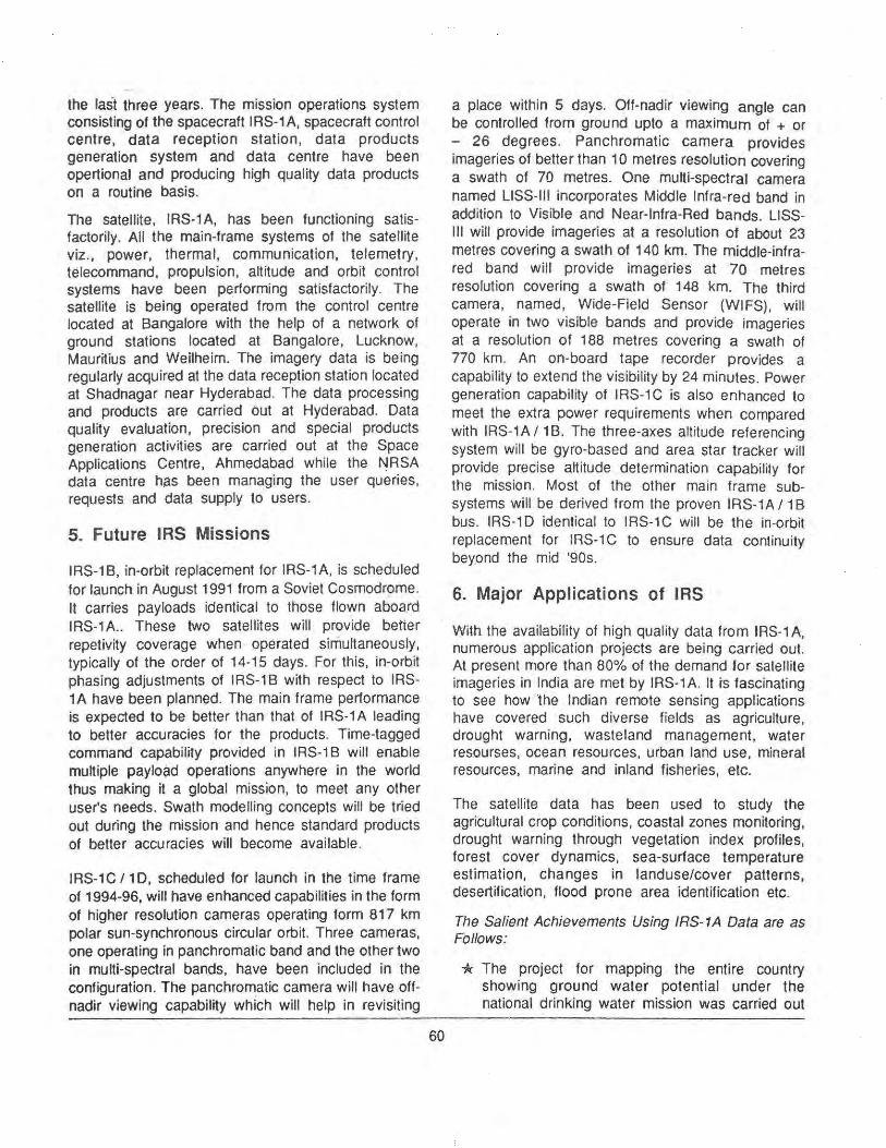
the last three years. The mission operations system consisting of the spacecraft IRS-1A, spacecraft control centre, data reception station, data products generation system and data centre have been opertional and producing high quality data products on a routine basis.

The satellite, IRS-1 A, has been functioning satisfactorily. All the main-frame systems of the satellite viz., power, thermal, communication, telemetry, telecommand, propulsion, altitude and orbit control systems have been performing satisfactorily. The satellite is being operated from the control centre located at Bangalore with the help of a network of ground stations located at Bangalore, Lucknow, Mauritius and Weilheim. The imagery data is being regularly acquired at the data reception station located at Shadnagar near Hyderabad. The data processing and products are carried out at Hyderabad. Data quality evaluation, precision and special products generation activities are carried out at the Space Applications Centre, Ahmedabad while the NASA data centre has been managing the user queries, requests and data supply to users.

5. Future IRS Missions

IRS-18, in-orbit replacement for IRS-1A, is scheduled for launch in August 1991 from a Soviet Cosmodrome. It carries payloads identical to those flown aboard IRS-1A .. These two satellites will provide better repetivity coverage when operated simultaneously, typically of the order of 14-15 days. For this, in-orbit phasing adjustments of IRS-1 B with respect to IRS-1A have been planned. The main frame performance is expected to be better than that of IRS-1A leading to better accuracies for the products. Time-tagged command capability provided in IRS-1 B will enable multiple paylo~d operations anywhere in the world thus making it a global mission, to meet any other user's needs. Swath modelling concepts will be tried out during the mission and hence standard products of better accuracies will become available.

IRS-1C /10, scheduled for launch in the time frame of 1994-96, will have enhanced capabilities in the form of higher resolution cameras operating form 817 km polar sun-synchronous circular orbit. Three cameras, one operating in panchromatic band and the other two in multi-spectral banos. have been included in the configuration. The panchromatic camera will have offnadir viewing capability which will help in revisiting

60

a place within 5 days. Off-nadir viewing angle can be controlled from ground upto a maximum of + or - 26 degrees. Panchromatic camera provides imageries of better than 10 metres resolution covering a swath of 70 metres. One multi-spectral camera named LISS-111 incorporates Middle Infra-red band in addition to Visible and Near-Infra-Red bands. LISS-111 will provide imageries at a resolution of about 23 metres covering a swath of 140 km. The middle-infrared band will provide imageries at 70 metres resolution covering a swath of 148 km. The third camera, named, Wide-Field Sensor (WIFS), will operate in two visible bands and provide imageries at a resolution of 188 metres covering a swath of 770 km. An on-board tape recorder provides a capability to extend the visibility by 24 minutes. Power generation capability of I RS-1 C is also enhanced to meet the extra power requirements when compared with IRS-1 A I 1 B. The three-axes altitude referencing system will be gyro-based and area star tracker will provide precise altitude determination capability for the mission. Most of the other main frame subsystems will be derived from the proven IRS-1A 1 1 B bus. IRS-1 D identical to IRS-1C will be the in-orbit replacement for lRS-1 C to ensure data continuity bey,ond the mid '90s.

6. Major Applications of IRS

With the availability of high quality data from I RS-1 A, numerous application projects are being carried out. At present more than 80% of the demand for salellite imageries in India are met by IRS-1A. It ts fascinating to see how lhe Indian remote sensing applications have covered such diverse fields as agriculture, drought warning, wasteland management, water resourses. ocean resources, urban land use, mineral resources, marine and inland fisheries, etc.

The satellite data has been used to study the agricultural crop conditions, coastal zones monitoring, drought warning through vegetation index profiles, forest cover dynamics, sea-surface temperature estimation, changes in landuse/cover patterns, desertification, flood prone area identification etc.

The Salient Achievements Using IRS-1A Data are as Follows:

* The project for mapping the entire country showing ground water potential under the national drinking water mission was carried out

using IRS data. These maps used in conjunction with conventional methods have led to a vastly increased success rate for drilling bore-wells from the earlier 45 per cent to 90 per cent.

* IRS-1A data has been used extensively in monitoring the extent of sedimentation and water spread in reservoirs in order to plan the irrigation scheduling and command area. development.

* Under geology, case studies have been conducted under the project Vasundhara, for prospecting base metal mineralisation zones in South India.

* Ocean 1 Coastal applications data include wetland mapping, off-shore sediment dispersion studies, mapping of mangroves, coastal zone geomorphological mapping etc. Studies on erosion and accretion processes in the coastal areas and identification of brackish water and water bodies suitable for inland fisheries have also been carried out.

* All major cities have been covered under a detailed study on urban sprawl using IRS data. Use of remote sensing was demonstrated recently for conducting a. survey to align the ring road for Bangalore Development Authority using satellite and ground based data.

* Satellite data is regularly used to have real time information on areas affected by floods and take up rehabilitation measures. All the major floods since 1988 have been mapped using IRS data. During the cyclone in May 1990 in the south eastern coast, IRS imageries provided an objective assessment of the severity of the damages and to assess crop damages.

61

* For the first time, a detailed inventory of wastelands at village level has been made. The data base so generated indicates that nearly half of this wasteland can be reclaimed. These maps are now used by various state level agencies to prioritise the wastelands for immediate reclamation for afforestation, agricultural production, etc. ·

* For the overall development of a district, it is necessary that the decision makers are provided with an integrated perspective of the resource potential and local constraints. It is in this context, the capacbility of satellite data to provide such a holistic view of the resources at taluk and mandai level has been successfully demonstrated using IRS-1 A. Such an information base will immensely help in the development of rural India.

From the above it may be seen that the satellite data with its synoptic coverage and repetivity has been found to be ideal for monitoring the dynamic aspects of the terrestrial and oceanic features. The availablity of microwave sensors data from satellites in the near future is expected to aid newer R & D applications relevant to terrestrial and oceanic interactions. Illustrations 1 through 4 provide some examples of applications using remote sensing data.

7. Conclusion

In conclusion, a brief account of the data acquisition programme relating to remote sensing, satellites in India has been presented. The 'data that is already available in the archival, those that are being acquired presently and the plans for acquisition in the coming years are suitably summarised. This information spread over more than a decade in the time scale could provide useful inputs for the 1GB Programme.

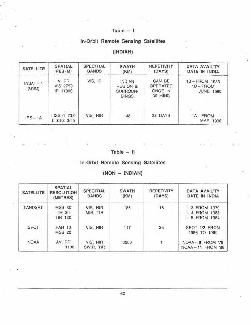
Table - I

In-Orbit Remote Sensing Satellites

(INDIAN)

SATELLITE SPATIAL SPECTRAL SWATH REPETIVITY DATA AVAIL'TY RES (M) BANDS (KM) (DAYS) DATE IN INDIA

INSAT -1 VHRR VIS, IR INDIAN CAN BE 18- FROM 1983

(GSO) VIS 2750 REGION & OPERATED 1D-FROM IR 11000 SURROUN- ONCE IN JUNE 1990

DINGS 30 MINS

IRS -1A LISS -1 73.0 VIS, NIR 148 22 DAYS 1A- FROM LISS-2 36.5 MAR 1990

Table - II


(NON - INDIAN)

SPATIAL SATELLITE RESOLUTION SPECTRAL SWATH REPETIVITY DATA AVAIL'TY

(METRES) BANDS (KM) (DAYS) DATE IN INDIA

LANDSAT MSS 80 VIS, NIR 185 16 L-3 FROM 1979 TM 30 MIR, TIR L-4 FROM 1983

TIR 120 L-5 FROM 1984

SPOT PAN 10 VIS, NIR 117 26 SPOT-1/2 FROM MSS 20 1986 TO 1990

NOAA AVHRR VIS, NIR 3000 1 NOAA - 6 FROM '79 1100 SWIR, TIR NOAA - 11 FROM '88

62

Table - Ill


(NON - INDIAN)

SPATIAL SPECTRAL REPETIVITY DATA AVAIL'TY SATELLITE RESOLUTION SWATH

(METRES) BANDS (KM) (DAYS) DATE IN INQIA

LANDSAT MSS 80 VIS, NIR 185 16 L-3 FROM 1979 TM 30 MIR, NIR L-4 FROM 1983

L-5 FROM 1984

SPOT TIR 120 VIS, NIR 117 26 SPOT-1/2 FROM PAN 10 1986 TO 1990 MSS 20

1 NOAA - 6 FROM '79 NOAA AVHRR SWIR, NIR 3000 NOAA - 11 FROM '88

1100

MOS MESS 50 VIS, NIR 100 17 -VTIR TIR 1500 VIS 900 ,.

TIR 2700

MIR MKF-6M 20 VIS, NIR 170 - -KATE-140 15 450

METEOR MSU-E 30 VIS, NIR 30 - -PRIRODA FRAGEMENT 85

80 2000 MSU-M 1000

KOSMOS SAR 1500 MICROWAVE 460 - -OCEANO- MSS 1500 VIS, NIR 2000 GRAPHIC 200 600

63

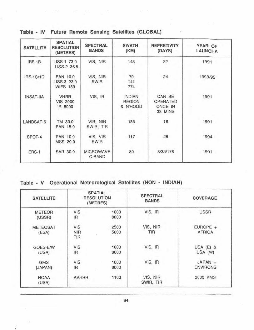
Table - IV Future Remote Sensing Satellites (GLOBAL)

SPATIAL SPECTRAL SWATH SATELLITE RESOLUTION REPRETIVITY YEAR OF

(METRES) BANDS (KM) (DAYS) LAUNCHA

IRS-18 LISS-1 73.0 VIS, NIR 148 22 1991 LISS-2 36.5

IRS-1C/1 D PAN 10.0 VIS, NIR 70 24 1993/95 LISS-3 23.0 SWIR 141 WIFS 189 774

INSAT-IIA VHRR VIS, IR INDIAN CAN BE 1991 VIS 2000 REGION OPERATED IR 8000 & N'HOOD ONCE IN

33 MINS

LANDSAT-6 TM 30.0 VIR, NIR 185 16 1991 PAN 15.0 SWIR, TIR

SPOT-4 PAN 10.0 VIS, VIR 117 26 1994 MSS 20.0 SWIR

ERS-1 SAR 30.0 MICROWAVE 80 3/35/176 1991 C-BAND

Table - V Operational Meteorological Satellites (NON - INDIAN)

SPATIAL SPECTRAL SATELLITE RESOLUTION COVERAGE

(METRES) BANDS

METEOR VIS 1000 VIS, IR USSR (USSR) IR 8000

METEOSAT VIS 2500 VIS, NIR EUROPE + (ESA) NIR 5000 TIR AFRICA

TIR

GOES-E/W VIS 1000 VIS, IR USA (E) & (USA) IR 8000 USA (W)

GMS VIS 1000 VIS, IR JAPAN + (JAPAN) IR 8000 ENVIRONS

NOAA AVHRR 1100 VIS, NIR 3000 KMS (USA) SWIR, TIR

64

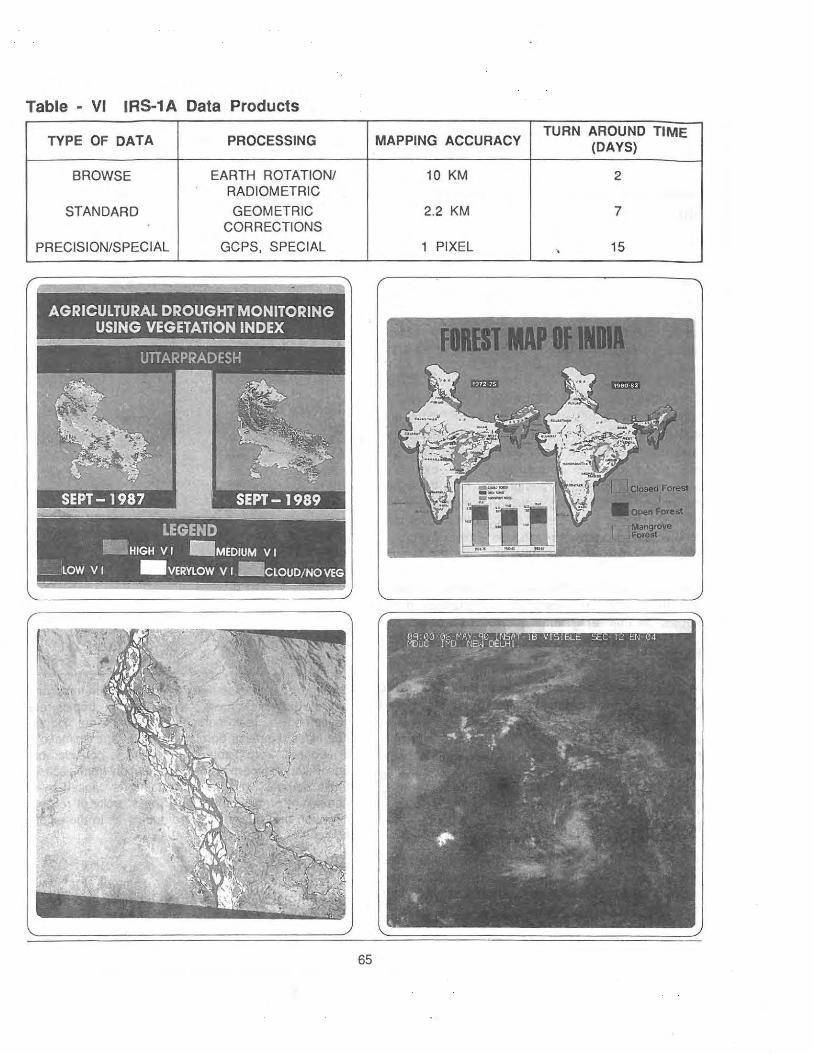
Table - VI IRS-1 A Data Products

TYPE OF DATA PROCESSING

BROWSE EARTH ROT A TION/ RADIOMETRIC

STANDARD GEOMETRIC CORRECTIONS

PRECISION/SPECIAL GCPS, SPECIAL

AGRICULTURAL DROUGHT MONITORING USING VEGETATION INDEX

LEGEND EliHIGH VI . MEDIUM VI

LOW VI -VERYLOW VI - CLOUD/ NOVEG

MAPPING ACCURACY TURN AROUND TIME

(DAYS)

10 KM 2

2.2 KM 7

1 PIXEL \ 15

65

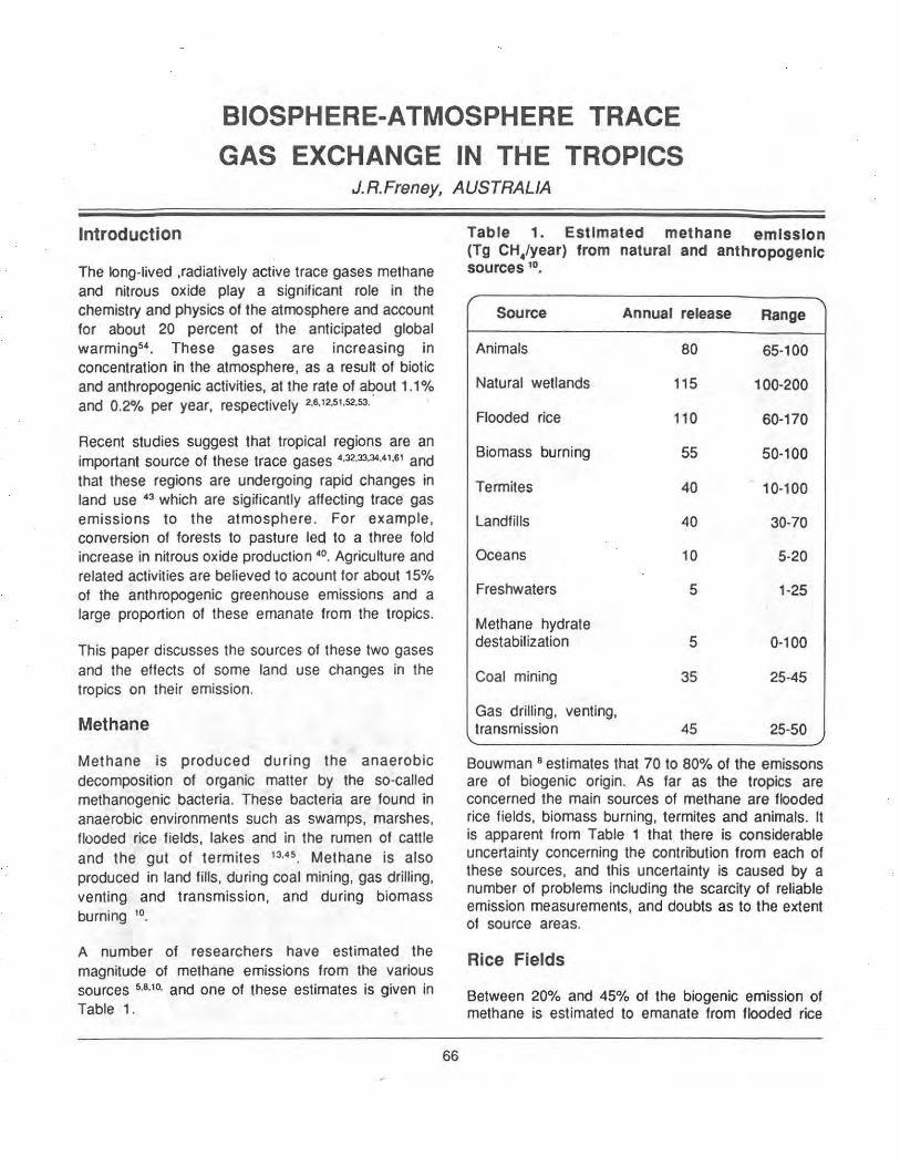
BIOSPHERE-ATMOSPHERE TRACE

GAS EXCHANGE IN THE TROPICS J.R.Freney, AUSTRALIA

Introduction

The long-lived ,radiatively active trace gases methane and nitrous oxide play a significant role in the chemistry and physics of the atmosphere and account for about 20 percent of the anticipated global warming54 . These gases are increasing in concentration in the atmosphere, as a result of biotic and anthropogenic activities, at the rate of at?out 1.1% and 0.2% per year, respectively 2.6.12,51.52.53.

Recent studies suggest that tropical regions are an important source of these trace gases 4

•32•33•34 .41

•61 and

that these regions are undergoing rapid changes in land use 43 which are sigificantly affecting trace gas emissions to the atmosphere. For example, conversion of forests to pasture led to a three fold increase in nitrous oxide production 40. Agriculture and related activities are believed to acount for about 15% of the anthropogenic greenhouse emissions and a large proportion of these emanate from the tropics.

This paper discusses the sources of these two gases and the effects of some land use changes in the tropics on their emission.

Methane

Methane is produced during the anaerobic decomposition of organic matter by the so-called methanogenic bacteria. These bacteria are found in anaerobic environments such as swamps, marshes. flooded rice fields, lakes and in the rumen of cattle and the gut of termites 13·45 • Methane is also produced in land fills, during coal mining, gas drilling, venting and transmission, and during biomass burning 10.

A number of researchers have estimated the magnitude of methane emissions from the various sources 5·8·10• and one of these estimates is given in Table 1.

66

Table 1. Estimated methane emission (Tg CH.fyear) from natural and anthropogenic sources 10

•

Source Annual release Range

Animals 80 65-100

Natural wetlands 115 100-200

Flooded rice 110 60-170

Biomass burning 55 50-100

Termites 40 10-100

Landfills 40 30-70

Oceans 10 5-20

Freshwaters 5 1-25

Methane hydrate destabilization 5 0-100

Coal mining 35 25-45

Gas drilling, venting, transmission 45 25-50

Bouwman 8 estimates that 70 to 80% of the emissons are of biogenic origin. As far as the tropics are concerned the main sources of methane are flooded rice fields, biomass burning, termites and animals. It is apparent from Table 1 that there is considerable uncertainty concerning the contribution from each of these sources. and this uncertainty is caused by a number of problems including the scarcity of reliable emission measurements, and doubts as to the extent of source areas.

Rice Fields

Between 20% and 45% of the biogenic emission of methane is estimated to emanate from flooded rice

fields 8 and most of the world's rice is grown in the tropics 44 . However, most of the informat ion on methane emission from flooded rice fields comes from a small number of investigations carried out in temperate regions (California, Spain, Italy, Japan and China) 11. 12. 21. s9. s2.

Since methane is produced by anaerobic microorganisms, any factor which controls the growth and metabolism of these organisms will influence methane production. Thus redox potential 11

· 70

, pH29,

temperature 35· 48· 55

· 73

· substrate availability 12·

17·

27·

71,

and toxic substances 65· 66· 69· 72• affect the production of methane in flooded rice fields . The redox potential of a flooded soil needs to be below - 200 mV for methane prodcution. Methanogenesis is favoured by a neutral to sligthly alkaline pH and a temperature around 30°C. The rate of methane emission from precultivated flooded rice soils was found to be related to the amount of readily decomposable organic matter present 44• and application of rice straw to flooded rice increased production of methane. However, addition of compost had little effect on methane emission 44

·

Addition of sulfate and nitrate depressed the production of methane 29

.

At this stage there is insufficient information to determine whether soil type has an effect on methane production. Sass et al. 58 found a three fold difference in methane emission between two different rice fields on different soil types, but Koyama 37 found no significant differenc in emissions between nine different rice soils. The main factors controlling methane emission from flooded rice are ebullition, diffusion, transport through the rice plant and oxidation near the floodwater-soil interface. Oxidation at the interface between the oxidized and reduced zones may greatly reduce methane emission 28.

The annual emission of methane from rice fields is estimated to be of the order of 40g methane/square metre 28• Using this emission rate and the known area of rice fields it is possible to estimate methane emission from tropical rice fields. However, as the bulk of the emission data has been obtained in temperate regions, and knowing the marked effect of temperature and agricultural practices on methane emission rates, it seems inappropriate to use the above emission rate for tropical regions. Minami 44

made adjustments for climate and soil water status, and estimated that between 22.1 and 73.1 Tg methane/year is emitted from rice fields globally.

67

When the calculated emissions of 0.5 to 1.8 TgJyear for the tempe·rate regions are deducted from the totals, the balance suggests that between 21 .6 and 71.3 Tg methane/year is emitted from tropical rice fields. Approximately 90% of the world's rice is produced in Asia, and 60% of the rice fields are located in India and China. Thus these two countries would be expected to contribute a large proportion of the methane emissions from rice 44

• Rice fields in tropical Australia would be expected to contribute little to this budget because of the small area cultivated (- 5000 ha) . The calculated emission using the emission rate given above is 0.002 Tg methane/year.

Biomass Burning

The burning of biomass, whether naturally in forest or grass fires or as a result of agricultural practices, results in the emission of methane because of incomplete combustiol'). Globally, the burning of biomass is estimated to contribute 50 to 100 Tg methane/year 10

•

Emission factors for methane (i.e., the fraction relative to emitted carbon dioxide) vary greatly (0 .1% - 2.5%) depending on whether the fire is hot, flaming combustion or a smouldering combustion. Galbally et al. 25 chose 0.6% for grass and stubble fires and 1% for other fire types, and estimated that 1.1 Tg methane/year was emitted from Australia as a result of biomass burning. It would appear from their calculations that burning tropical and subtropical grasslands would contribute more than half of this emission.

Animals

It is apparent from Table 1 that animals are an important source of methane; the methane arises from fermentation processes in the stomachs of ruminants. Using data provided by Galbally 24

·25 a rough estimate of 16 Tg/year can be made for methane emission from animals in tropical regions.

Termites

Methane is emitted from termites during the digestion of plant material in their gut by anaerobic protozoa and bacteria. Zimmerman et aF5 estimated that on a global scale termites would contribute 150 Tg/year, but other workers 19

• 35

• 62 suggest a much lower

contribution (12 Tg/year, with a range of 4-27 T/ year) .

Methane emission from tropical Australia as a result of termite digestion has been estimated to be in the range 0.1 - 1.6 Tg/year 25

. Using the emission rates quoted in 25 and the land areas for tropical regions given in 24 • the emission of methane from tropical areas is calculated to fall within the range of 1.4 to 13.6 Tg!year.

Methane Sinks

Aerobic soils have the capacity to consume considerable quantities of atmospheric methane because of the action of methane oxidising organisms. Current estimates put the value of this biological sink at about 32 Tg/Year 42

. Dry soils are greater sinks for methane than wet soils 42

, and this is believed to be a reflection of the importance of oxygen concentration in determining the balance between methane producing and oxidising bacteria 68

.

Dry tropical forest soils have been shown to consume significant methane 33. Keller et all. 33 estimated the net consumption by tropical and subtropical soils as -16 Tg methane/year or about 3% of the global emission.

Nitrous Oxide

Nitrous oxide is emitted into the atmosphere as a result of biomass burning, fossil fuel combustion, and nitrification and denitrification processes in soils, oceans and freshwater bodies. The current belief is that 90% of the emissions come from soils 8 , but there is considerable uncertainty in the global budget for nitrous oxide and the contribution of the various sources. This arises from the heterogeneity of the systems from which nitrous oxide is emitted and the scarcity of reliable measurements.

Biomass Burning

During combustion the nitrogen in fuel in end groups, open chains and heterocyclic rings can be converted into gaseous forms as decomposition or combustion products such as ammonia, nitric oxide, nitrous oxide, dinitrogen and hydrogen cyanide 24

. These compounds are liberated at all temperatures at which smouldering and combustion occur 24

• Crutzen et al. 15 estimated that 8 Tg nitrous oxide-N/year is emitted to the atmosphere as a result of biomass burning. However, recent work suggests that the emission factors used by them were too high, and that nitrous oxide is probably a minor product of biomass burning 25

·47

68

Bouwman and Sombroek 9 report that the contribution of biomass burning to nitrous oxide emission may be less than half of the 1.5 Tg/year assumed by Seiler and Conrad 6 1

•

Biomass burning is not only an instantaneous source of nitrous oxide, but it results in a longer term enhancement of the biogenic production of this gas. Measurements of nitrous oxide emissions from soils before and after a controlled burn showed that significantly more nitrous oxide was exhaled after the burn 1

· 39

• Emission from the pre-burned sites were less than 2 ng N/square metre/sec compared with emission of 9-22 ng N/square metre/sec from burned and wetted sites 39.

Soils

Nitrous ox ide is formed in soils during the microbiological processes nitrification (the oxidation of ammonium to nitrate under aerobic conditions) and denitrification (the reduction of nitrate under anaerobic conditions) 20

· 21

· 50

. Because nitrous oxide is a gas it can escape from soil during these transformations. Nitrous oxide is formed by microbial processes and therefore its production is controlled by factors which affect the growth of micro-organisms viz. temperature, pH, rainfall 56

. However, its production is also affected by fertilizer type, rate, time and mode of application, tillage practice, soil type, pH , and oxygen concentration, availability of carbon, vegetation, land use practices, use of chemicals, irrigation practices and water holding capacity of the soil ss.

Nitrous oxide can be consumed by waterlogged soils, but aerob'ic soils are unlikely to be sinks for atmospheric nitrous oxide.

Fertilizer induced emissions of nitrous oxide vary with the type of ferti lizer used, and range from 0.001% to 6.8% of the nitrogen applied. The largest emissions occurred when anhydrous ammonia was used and the smallest emissions were found when nitrogen solutions were applied 18·23. Median values given by Galbally 23 are 0.5% for anhydrous ammonia, 0.1% for ammonium fertilizers and 0.05% for nitrate. Median values are also given by Bouwman 8 who estimated that 0.4 to 1.4 Tg nitrous oxide-N was derived from fertilizer in 1987, and that 2.4-3.6 Tg is emitted annually from the 1500 x 106 ha of cultivated land in the world . It is very difficult to calculate a meaningful figure for fertilizer derived emissions for

the tropics; while statistics are available for many countries which fall wholly within the tropics it is not possible to obtain accurate figures for fertilizer use in tropical areas of countries like China which span tropical and temperate areas.

Galbally et al. 25 and Bouwman and Somebroek 9

discuss the role of legumes in the production and emission of nitrous oxide. It appears that legumes may contribute to nitrous oxide emission in a number of ways. Atmospheric nitrogen fixed by the legumes can be nitrified and denitrified in the same way as fertilizer nitrogen, thus providing a source of nitrous oxide. In addition symbiotically living Rhizobia in root nodules are able to denitrify and produce nitrous oxide 49

• Galbally et al. 25 suggest an emission rate of 4kg N/ha/year for improved pasture's and Duxbury et al. 17 suggest that legumes can increase nitrous oxide emissions from pastures by a factor of 2 to 3.

Tropical soils under rainforest and savanna are recognised as important sources of nitrous oxide 3·26•34 •

Soils in an Amazonian rainforest were shown to exhale nitrous oxide at rates which were 20 times greater than the global mean and 30 times greater than those occurring in a New England hardwood forest 34 • Later observations 33 indicated that tropical forest soils contribute about 40% of the global flux of nitrous oxide. The median value for emission from tropical forests is given as 1.7 kg N/ha/year 8

. Nitrous oxide emissions from tropical savannas range from 0.4 to 1.4 kg N/ha/year depending on the season 26

•57

•

Conversion of tropical forests to crop production and pasture has a significant effect on the emission of nitrous oxide. Keller et al. 33

. showed that emissions of nitrous oxide increased by about a factor of two when a forest in central Brazil was clear cut, and Luizao et al. 40 reported that pasture soils in the same area produced three times as much nitrous oxide as adjacent forest soils. Additional nitrous oxide may be transported from cleared areas in ground water and emitted elsewhere 7.

Flooded Rice Soils

Nitrous oxide emissions from temperature and tropical rice fields have been studied with chamber techniques and the results indicate that less than 0.1% of the applied nitrogen is emitted as nitrous oxide if the soils

69

are flooded for a number of days before fertilizer application 22

• 46

· 64

• However, if mineral nitrogen is present in the soil before flooding it will serve as a source of nitrous oxide during wetting and drying cycles before permanent flooding. Thus dry seeded rice can be a source of considerable nitrous oxide. If the trend from transplanted rice to direct seeded rice, which is occurring in Malaysia, spreads to other tropical rice growing countries, then flooded rice soils in the tropics could become an important source of nitrous oxide.

Termites

Khalil et al. 36 found that certain termite mounds emit nitrous oxide as well as methane, and that these gases are emitted in the ration of - 1 :20. If this ratio can be applied to all species of termites then the emission of nitrous oxide from termite mounds in the tropics might fall within the range 0.07 to 0.7 Tg/year.

Oceans

Water bodies depleted in Oxygen have been shown to produce nitrous oxide, and elevated nitrous oxide concentrations in the northwest Indian Ocean have been reported recently 38. These workers found that nitrous oxide was supersaturated in both oxygensaturated surface waters (up to 246% saturation) and oxygen-depleted sub-surface wat~rs (1 ,264% saturation). Law and Owens 38 calculated that this area (which represents 0.43% of the surface area of the world's oceans) contributes between 5% and 18% of the total marine flux , and thus represents a significant source of nitrous oxide.

Conclusions

It is apparent that there are large gaps in our knowledge of the sources and sinks for atmospheric methane and nitrous oxide, and there are large uncertainties in the derived fluxes. This applies for both the global scene and for the tropics. While some of the uncertainty arises from the heterogeneity of the sources and the extrapolation of measurements made for short periods on small areas to long periods and large areas, much of the uncertainty arises from the fact that few measurements of the fluxes have been made for the many types of ecosystems which exist. These gaps in our knowledge need to be addressed before we can devise suitable management practices to reduce emissions of these greenhouse gases.

References

1. Anderson, I.C. et al. (1988) J. Geophys. Res. 93, 3893-3898

2. Andrae, M.O & Schimel, D.S. (1989) Exchange of Trace Gases Between Terrestrial Ecosystems and the Atmosphere. (John Wiley & Sons: Chickester)

3. Arnold, P.W. (1954) J. Soil Sci. 5, 116-128

4. Bartlett, K.B. et al (1988) J. Geophys. Res. 93,1571-1582

5. Bingemar, H.G. & Crutzen, P.J. (1987) J. Geophys. Res. 92,2181-2187

6. Blake D.R. & Rowland, F.S. (1988) Science 239, 1129-1131

7. Bowden, W.B. & Bormann, F.H. (1986) Science 233, 867-869

8. Bouwman, A.F. (1990) Soils and the Greenhouse Effet. (John Wiley & Sons: Chichester)

9. Bouwman, A.F. & Sombroek, W.G. (1990) In H.W. Scharpenseel et al (eds) . Soils on a warmer Earth. pp. 15-30. (Elsevier: Amsterdam)

) 0. Cicerone, R.J. & Oremland, R.S. (1988) Global Biogeochem. Cycles 2, 299-327

11 . Cicerone, R.J. & Shetter, J.D. (1981) J. Geophys. Res. 86, 7203-7209

12. Cicerone, R.J. et al (1983) J. Geophys. Res. 88, 11022-11024

13. Conrad, R. (1989) In : M.O. Andral & D.S. Schimel (eds) . Exchange of Trace Gases Between Terrestrial Ecosystems and the Atmosphere pp. 39-58 (John Wiley & Sons : Chichester)

14. Crutzen, P.J. (1983) In : B.Bolin & R.B.Cook (eds). The Major Biogeochemical Cycles and their Interactions pp. 67-114. (John Wiley & Sons : Chickester)

15. Crutzen, P.J. et al (1979) Nature 282, 253-256

16. de Bont, J.A.M. et al (1978) Ecol. Bull. 26,91 -96

17. Duxbury, J.M. et al (1982) Nature 298, 462-464

70

18. Eichner, M.J. (1990) J. Environ. Qual. 19, 272-280

1~ . Fraser, P.J. et al (1986) J. Atmos. Chern. 4, 295-310

20. Freney, J.R. et al (1978) Nature 273, 530-532

21 . Freney, J.R. et al (1979) Soil Bioi. Biochem. 167-173

22. Freney, J.R. et al (1981) Aust J. Agric. Res. 32, 37-45

23. Galbaly, I.E. (1985) In: J.N. Galloway et al (eds). The Biogeochemica Cyclng of sulfur and Nitrogen in the Remote Atmosphere. pp. 27-53. (D. Reidel : Dordrecht)

24. Galbaly, I.E. & Gillett, R.W. (1988) In : H. Rodhe & R. Herrera (eds). Acidification in Tropical countries . pp. 73-116. (J.Wiley & Sons : Chichester)

25. Galqally I.E. et al (1991 ) Proceedings of IGBP workshop No.14, Canberra, Oct.3-5,1990

26. Hao, W.M. et al (1988) J. Atmos. Chern. 7, 93-105

27. Holzapfel - Pschorn, A. & Seiler, W. (1986) J. Geophys. Res. 91, 11803-11814

28. Holzapfel - Pschorn, A. et al ( 1986) Plant and Soil 92, 223-233

29. Jacobsen, P. et al (1981 ) Soil Sci. 132, 279-287

30. Johansson, C. & Sanhueza, E. (1988) J. Geophys. Res. 93, 14193-14198

31 . Johansson, C. et al (1988) J. Geophys. Res. 93, 7180 - 7192

32. Kaplan, W.A. et al (1988) J. Geopys. Res. 93, 1389-1395

33. Keller M. et al (1986) J. Geophys. Res. 91 , 11791-11802

34. Keller, M. et al (1983) Geophys. Res. Lett. 10,1156-1159

35. Khalil, A.K. et al (1989) Proc. Int. Conf. on Global & Regional Environmental Atmospheric Chemistry. Beijing, China. May 3-10, 1989

36. Khalil, A.K. et al (1990) J. Geophys. Res. 95, 3619-3634

37. Koyama, T. (1963) J. Geophys. Res. 68, 3971 - 3973

38. Law, C.S. & Owens, N.J.P. (1990) Nature 346, 826-828

39. Levine, J.S. et al (1988) Global Biogeochem. Cycles 2, 445-449

40. Luizao, F. et al (1989) Global Biogeochem. Cycles 3, 281-285

41. Matson, P.A. & Vitousek, P.M. (1987} Global Biogeochem. Cycles 1, 163-170

42. Melillo, J.M. et al (1989} In : M.O. Andrae & D.S. Schimel (eds). ·Exchange of Trace Gases Between Terrestrial Ecosystems and the Atmosphere. pp. 263-280. (John Wiley & Sons : Chichester}

43. Melilo, J.M. et al (1985} Environ. Conserv. 12, 37-40

44. Minami, K. (1991} Ecol. Bull. (in press}

45. Mooney, H.A. et al (1987} Science 238, 926-936

46. Mosier, A.A. et all (1989) Fert. Res. 19, 127-136

47. Muzio, L.J. & Kramlich, J.C. (1988} Geophys. Res. Lett. 15, 1369-1372

48. Neue, H.U. & Scharpenseel, H.W. (1984} In : Organic Matter and Rice. pp. 311-328. (IRRI : Los Banos}

49. O'Harra, G.W. & Daniel, A.M. (1985} Soil Bioi. Biochem. 17, 1-9

50. Payne, W.J. (1981} In : C.C. Delwiche (ed.} Denitrification, Nitrification and Atmospheric Nitrous Oxide. pp. 85-103. (Wiley : New York)

51 .Pearnman, G.l. et al (1986} Nature 320, 248-250

52. Ramanathan, V. et al (1985} J. Geophys. Res. 90, 5547-5566

53. Rasmussen, A.A. & Khalil, M.A.K. (1986) Science 232, 1632-1634

54. Rodhe, H. (1990) Science 248, 1217-1219

55. Ruttner, F. (1963) Fundamentals of Limnology. (University of Toronto Press : Toronto)

71

56. Sahrawat,- K. & Keeney, D.R. (1986} Adv. Soil Sci 4, 103-148

57. Sanhueza, E. et al (1990} J. Geophys. Res. 95, 22481-2488

58. Sass, R.L. et al (1990} Global Biogeochem. Cycles (n Press).

59. Schutz, H. et al (1989) Biogeochem. 7,33-53

60. Schutz, H. et al (1989) J. Geophys. Res. 94, 16405-16416)

61 . Seiler, W. & Conrad, R. (1987) In: R.E. Dickinson (ed.} Geophysiology of Amazonia. Vegetation and Climate Interactions. pp. 133-160. (John Wiley & Sons: Chichester)

62. Seiler, W. et al (1984} J. Atmos. Chern. 1, 171 - 186

63. Seiler, W. et al (1984} J. Atmos. Chern. 1, 241-268

64. Simpson, J.R. et al (1984) Aust. J. Agric. Res. 35, 189-200

65. Takai, Y. (1980} Fert. Sci. 3, 17-55

66. Takai, Y. ·et al (1 956} Soil and Plant Food 2, 63-66

67. Tsutsuki, K. & Ponnamperuma, F.N. (1987} Soil Sci. & Plant Nutr. 33, 13-33

68. Whalen, S.C. & Reeburg, W.S. (1990) Nature 346, 160-162

69. Winfrey, M.C. & Zeikus. J.G. (1977) Appl. Environ. Microbiol. 33, 275-281

70. Yagi, K. & Minami, K. (1989} Proc. Int. Cont. Soils and the Greenhouse Effect. ISRIC.

71. Yagi, K. & Minami, K. (1989) Soil Sci. Plant Nutr. (in press}

72. Yamane, I. (1957} Soil and Plant Food 3, 100-103

73. Yamane, I & Sato, K. (1961) Sci. Rep. Res. lnst. Tohoku Univ. Ser. D12, 31-46

74. Yamane, I & Sato, K. (1963) Soil Sci. Plant Nutr. 3, 29-31

75. Zimmerman, P.R. et al (1982} Science 218, 563-565

NATIONAL PROGRAMME ON IGBP S.D. Chaudhuri, BANGLADESH

Introduction

A National Committee of IGBP was established in late 1988 under the aegis of Bangladesh Academy of Science (BAS) with Dr.S.D. Chaudhuri fellow BAS, as Chairman. Currently the National Committee has 35 members representing government, universities, semi-government organisation and N.G.Os who are working on areas which are directly or indirectly related to some aspects of environment.

The National Committee had drawn up a few modest projects/studies that can contribute their inputs to IGBP core projects. These include :

* Assessment of chemical contaminants in Bangladesh soil and water and their impact on biogeochemical cycles of the region.

* Methodology for reduction of methane emanation from wet paddy fields.

* Study & monitor mean sea level changes, land subsidence, salinity changes biomass flux and mangrove degradation in the coastal belt (3 subprojects).

* Studies on the effects of climate and land use changes on soil process and greenhouse gases.

In addition, some priority areas of research/studies have been identified whicr. can lend themselves to national and regional studies. These include :

* Studies on land use pattern, cropping intensity and agricultural practices and their impact on trace gas emissions.

* Studies on South West Monsoon variability and its relation to floods and droughts in Bangladesh.

Study on Hydrological Cycle :

The most dominant influence on environment stems from the impact of floods as a result of over-flow of waters from the three mighty rivers, Ganges, Brahama

72

putra and Meghna (GBH) which together carry a sediment load estimated at 2.5 bill ion tons.

The frequency and intensity of floods have assumed catastrophic proportion in recent years because of various contributory factors, some of which are :

* Intensive rainfall in the up-country hill regions

* Snowmelt in the Himalayas and glacial displacement

* River silatation (Lateral river contraction)

* Deforestation and deundation in catchment areas.

There are many other factors not well studied and understood. In 1987 and 88 nearly three-fourth of the country came under the grip of floods which devastated crops, property & infrastructure worth millions of taka .

The problem of floods in the subcontinent was identified as a regional problem which involved following major areas of studies

* Himalayan snow melt

* Deforestation of the fluvial basin of the Ganges, Brahmaputra and Meghna

* Soil erosion , soil degradation and sedimentation in the watershed areas of the three major rivers

* Climate change.

Terrestrial Ecosystem

We have not taken any significant steps in this area except in establishing some gene banks. In the meantime many local cultivars are fast disappearing in our haste for getting high productivity at the expense of sustainability. An instance of unjudicious planning strategy can be cited in case of deep water paddy which has evolved over the years, cultivars, physiologically best adapted to varying depths of

water and has hundreds of races. Current attempts made by breeders with encouragement and support from donor agencies to produce a few standard varieties may be a very unwise step as many such varieties may not be able to cope with varying environmental situation brought about through global change.

Rice covers nearly 80 percent of the cultivated area and is grown almost round the year both under rainfed and irrigated condition. Exchange of methane and other trace gases in rice fields, therefore, form an important area of study. Bangladesh has initiated a small project in this connection particularly relating to methane emission and limitation measures. The interactive effect of land use and crop management and distribution intensity of some pests and disease vectors also need to be carefully studied in different biographical regions to establish predictive models; more comprehensive with India, China, Thailand & other regional countries in this connection which will help in pooling knowledge and experience in identifying management practices that will stabilise and or reduce emission of methane & other trace gases in our endeavour to achieve higher production.

73

Coastal Ecosystem :

The coastal area of Bangladesh extends along the Bay of Bengal over 760 km. and has an area of

36,000 sq.km. The coast comprises the complex delta of the Ganges-Brahmaputra-Meghna river system which is one of the largest river system in the world. The system has its origin in the Himalyas, the Megalayas and other hill regions and the system

carried an estimated annual sediment load of 2.4 billion tons. These sediments are subject to coastal

dynamics process generated mainly by river flow, tide and wind actions leading to accretion and erosion in the coastal area.

Regional studies on coastal areas in the subcontinent can provide important inputs to land ocean interaction

in the coastal zone core project. In view of rapid changes that is occurring in the coastal region of Bay

of Bengal the region will provide useful data within

a short period not normally available in other coastal regions.

ACTIVITIES ON THE STUDY OF GLOBAL CHANGE IN CHINA

Panqin Chen, CHINA

Recently the Chinese National Committee has organized a number of activities on the study of global change in order to actively participate in the IGBP. Today I would like, on behalf of the Chinese National committee to briefly introduce about this.

1. Pilot Study on assessment of current state of life supporting environment* in China.

(* life supporting environment is defined as composed of four basic components: atmosphere, water, vegetation and soil.)

Objectives :

* To see what changes that have already occurred in China in the past years.

* What roles does Chinese life environment play in global change or in significant global change events?

* To find some dominant factors and processes that regulate the changes due to land and water use, etc.,

* To locate where the present environment in China stands.

* Is it possible for us to distinguish human induced global change from nature induced change at present?

Scientific Components :

* Changes of atmospheric composition and climate (precipitation, temperature, trace gases, such as C0

2, CH4 , NOX, etc.).

* Changes of vegetatron cover (forests, grassland, crops) and their relationhips with human activities (e.g., over grazing, deforestation, etc.)

74

* Changes of soils (loess, salty soil, desertification, soil erosion, soil acidification, pollution and degradation) and their relationships with human activities.

* Changes of environment related to water (area of water body in China, run off of rivers, lake level, sw~mps, sea level, snow cover in winter, retrocession and advance of glacier, etc.), the causes of these occurrences (if can be found) and impacts on climate, as well as their relationships with human activities.

* Based on the above individual reviews, we ttien make a comprehensive and integrated review on the environmental changes in China by methods of system analysis and simple models. The purposes of this integrated review are (1) to analyze those affecting factors and physical, chemical and biological processes important to land-water-useinduced changes; and (2) to try to find out where the environmental change in China is now standing.

Some interesting results have been obtained and will be published later this year.

II. Contributions of China to be made to the project of IG B P

1. /GAG

Activity 1 China

Objectives

Atmospheric chemistry monitoring in

1. To find major chemical processes that govern atmospheric compositions and to understand the nature of concentration changes of atmospheric compositions.

2. To understand the interaction between ecosystems and atmospheric chemistry compositions and to quantify the contribution of different ecosystems in China to global atmosphere.

3. To understand the effects of human activities on both ecosystems and the atmospheric composition.

4. To predict the long-term trends of atmospheric composition.

Activity 2 : Participation in the Global Tropospheric Experiment/Pacific Exploratory Mission.

Objectives :

1. Investigate the atmospheric budgets and pt10tochemistry of trace gases and aerosols in China and over the pacific.

2. Development and application of global and regional models of atmospheric chemistry.

3. To investigate impacts of atmospheric composition change on climate and environment.

2. PAGES

Activity 1 : To study historical evolution of the life supporting environment in China.

Focus :

To reconstruct the eco-environmental series of timescale about 150000 years. with emphasis on past 1000 years. especially last two hundred years through analyses of loess, ice core and glacier, pollen, tree ring and historical literature, etc. in order to provide bases for appraising the vegetation-soil-water-climateatmospheric constitution relationships and estimating the human effect on the natural system.

Activity 2 : Impacts of paleoclimate change on underground water resources in the late pleitocene epoch (Especially the last 20,000 years .) and trends of climate change in the Arid and Semiarid areas.

3. GCTE

Activity 1 : Impacts of climate changes and atmospheric trace gases increase on ecosystems.

75

Focus 1 The possible impacts of increasing trace gases on climate and environment.

Focus 2 The possible impacts of trace gases on agriculture.

Focus 3 : Impacts on the sea level

Activity 2 : Interactions between the physical climate system and terrestrial eco-system.

Focus 1 : To establish some regional observational network to measure the fluxes of energy, water and the other matters and energy flow, material flow and water vapour exchange that cross the regional boundaries in order to obtain the general picture of regional cycle of these parameters.

Focus 2 To conduct special experiments to investigate the response of eco-system to the climate change, especially the extreme anomalies.

Activity 3 : Interaction between physical climate system and marine eco-system.

Focus 1 : To investigate the exchanges of the energy, water vapour, etc. between the air and sea in selected sea regions.

Focus 2 To investigate the human effect on the biogeochemistry in some selected river mouths and marine areas.

4. BAHC

Activity 1 : The Sino-Japanese cooperational programme on the Atmosphere-Land Surface Processes Experiment (HEIFE). This project has been supported jointly by the NSFC (National Science Foundation of China) and CAS in China and Japanese Ministry of Education, Science and Culture, and has been conducting at Heihe river basin, Western China.

Objectives :

a. To investigate the physical processes of the airland exchange of water, heat and momentum in area of different ecosystems in this basin; test and improve the parameterizing scheme of such fluxes in GCM.

b. To study the energy budget and water budget in different ecosystems in this basin.

c. To study boundary layer structure in different ecosystems and its relation to fluxes from the ground surfaces and to collect the necessary ground-based data for developing and validating the method to convert the satellite-observed radiance to the land surface nature the climatology variables.

d. To investigate the concentration and size distribution of atmospheric dust over desert, its dispersion and transport and its impacts on the radiative transfer.

e. To study the water requirement by crops, and technique of water-saving irrigation.

5. JGOFS

Activity 1 : To participate in the equatorial Pacific process study in the ·warm pool area of the western Pacific that will be collaborated with TOGA-COARE

Activity 2 : Marine flux study in the Yellow Sea and the East China Sea

* Exchange of nutrients in the river mouth and surrounding sea area

* Flux of carban and productivity.

6. GAIM • Activity 1 : Modelling of eco-environmental change

Focus :

Task 1

Task 2

Task 3

Task 4

To develop and improve the various subsystem models, especially the model of the atmospheric chemistry, and to integrate the different sub-models into a comprehensive eco-environmental climate model.

Development of AGCM and OGCM

Studies and modelling on the mathematical models of East lake system.

Development of alpine meadow ecosystem model.

Studies on theory of ecological boundary surface system and its application.

76

7. CERN (Chinese Ecological Research Network)

On the basis of existing 52 stations, the Chinese Academy of Sciences is going to build up a CERN in order to provide observational data, conduct process study and to make contribution to the IGBP.

During 1991-1995, 30 stations will be chosen to form networks including 1 0 stations at the first level of comprehensive-purpose stations, that will be used as the calibrating stations for the astronautical and aeronautical remote sensing, to closely link ground measurement with remove sensing, and thus through remove sensing observation realizing large-scale dynamic macroscopic monitoring of the ecosystem and environment. The entire network will include five sub-networks as follows:

* Network for long-term observation and monitoring of important elements of the ecoenvironment

* Network for research and experiment of elementary ecological processes

* Information system network

* Network for quality control of experiment and observation data

* Ecological system demonstration and construction network.

Process study

* Network wide observation and experiment of hydrological cycling and water balance in the soil-vegetation-atmosphere system.

* Network wide observation and experiment of nutritive material circulation and balance in the soil-vegetation-atmosphere system.

* Network wide observation and research on processes of generation, transport and transformation of trace gases in the soilvegetation-atmosphere system.

* Network wide observation and experiment on the decomposition, accumulation and

transport of organic chemical pollutants and heavy metal elements in the soil-vegetationatmosphere system.

* Network wide observation and experiment on the energy flow process.

8. RRNs :

Activity 1 : To develop a ground based observational network on the basis of CERN, about 3 pairs of stations in three different ecological zones are going to be selected for the comparative study of man made and natural vegetations and about four stations are going to be selected in the transit ional zone or sensitive area for the study of global change in China, which consists of a ground based observational network.

Activity 2 : Applications of Remote sensing data both . from satellites and airplanes.

Activity 3 : Research and training

Focus 1 : Reconstruction and analysis of paleoclimate and paleo-environment data.

77

Focus 2 Modelling of the life supporting environment in China in the past 2000 years.

9. DIS

Activity 1 : Observation and information system of the environmental change.

Focus 1 : To establish further a series of ground observational network for eco-environment research .

Focus 2 To analyze and apply the satellite data and exploit further the remote sensing techniques.

Focus 3 To set up practical information system and data bank on the environmental change which are designed as convenient as possible for international exchange.

REPORT ON GLOBAL CHANGE STUDIES IN INDONESIA

A.G. 1/ahude, INDONESIA

Introduction

The Equatorial Current systems of the Pacif ic Ocean bring warm trop1cal water masses from Central and South America westward to the Indones ian Archipelago and the Equatorial Current Systems of the Indian Ocean bring that water form Indonesia westward to the African Continent. This situation produces within the Indonesian waters two oceanographic conditions of global consequences.

Firstly, the accumulation of warm water mass within and around Indonesian Archipelago is the largest in the world's oceans. The warm surface water reduces the air pressure, makes the air lighter and buoyant, enhances vertical convective air currents and cloud formation, produces heavy rains and accumulations of sea surface fresh water in the region . The dry air that has released its mo1sture returns to the Central and Eastern Pacific in the upper layer, becomes cool and heavy and produces air subsidence in thee regions. At the sea surface the air pressure rises, and between the Eastern Pacific High Air Pressure and the Indonesian Low Air Pressure develop the Easterly Winds that drive the Pacific Equatoria l Current Systems. Thus air circulation called the Walker Air Circulation Cell develops between the Indonesian Archipelago and the Eastern Equatorial Pacific.

The interaction of the Walker Air Circulation and the ocean produces rains in Indonesia, dry period in the Central Pacific and upwelling along the coast of Peru , Ecuador and part of Chile. However, for the reason that still under world's investigation and studies. the Easterly Winds weaken, on the average every 4 years and replaced by the Westerly Anomaly Wind Bursts. The latter drive the Indonesian warm water pool easterly back to the Central and Eastern Pacific Ocean. The centres of the Low Air Pressure, the Convective Air Current, the cloud formation and the rain area also moves easterly, causing anomalous development of oceanographic and meteorological conditions in these regions. Among them are the arrival of warm water current, better known as EI-Nino, along the Ecuadorian and Peruvian coasts , the heavy rain in Central and

78

Eastern Pacific and the episodic long draught in Indonesia and adjacent regions. Since the Pacific Walker Air Circulation Cell is connected to the Equatorial Indian and Atlantic Cells and the Equatorical cells in return are connected to the subtropical and Polar Cells, the episodic anomalous oceanic and terrestrial weather conditions now called ENSO phenomenon are also felt everywhere in the world.

Secondly, the difference between the sea level height along the northern and eastern coasts of Irian Jaya, Halmahera and Sangir Talaud in the Pacific Ocean side and the sea level height along the southern coasts of Timor, Sumba, Sumbawa, Lombok, Bali, Jawa and Sumatra in the Indian Ocean Side. The difference varies seasonally but at times it can reach up to 30cm. The sea level difference drive oceans currents called ARLINDO form the Pacific to the Indian Ocean through the Indonesian strategic straits and channels. ARLINDO ("Arus Lintas Indonesia", Indonesian equivalent of : "Indonesian Through Flow") in turn determines three important oceanographic processes in Indonesia :

1. The rate of accumulation of warm water pool within and around Indonesia and therefore indirectly re lated to the ENSO phenomenon. There are also studies that indicate the indirect relation between the intensity of the flow of ARLINDO with the Eastern Australian Western boundary current and the Lewin current. ARLINDO is also part of the warm water circulation as proposed by Dr.Arnold Gordon.

2. The transportation of heat and fresh water from the Pacific to the Indian Ocean and therefore indirectly governs the exchange of heat, moisture and momentum, and the stability and variation of this exchange, between air and sea occurring each in the western Pacific Ocean and in the eastern Indian Ocean. One of the results of these processes or its anomaly may be the triggering factor of the ENSO phenomenon.

3. The process of small scale upwelling in various Indonesian waters that occur seasonally and the intensity of which is found to be closely related to the condition of the ARLINDO flow.

In general, oceanographical and meteorological studies for global change that are planned in Indonesia are directed to two major objectives, namely : the study of ARLINDO and the oceanographic process related to it and the monitoring of oceanographical and meteorological parameters that may help in predicting the ENSO phenomenon which in Indonesia is manifested as a period of severe draught with devastating economic consequences in agriculture, forestry, fisheries, tourism, and industrial and household electricity.

PRESENT STATUS

Oceanographic researches

On going research programmes that are being undertaken by Indonesia and can be related to global change studies at present include :

1. Project on Tides and Tidal Phenomena

This project is directed to the observation and collection of tidal data in seven locations in the western Indonesian Archipelago namely at Lhok Seumawe, Pasir Panjang, Tarempa, Pulau Pari (Jakarta), Pontianak, Tarakan and Banyuwangi (Fig. 1 and Table 1 ). These tidal stations have been operating since 1987 and will be continued upto the year 1994. The seven stations of Indonesia is part of about 25 tide stations presently operated by the ASEAN countries w1th the financial and technical ass1stance from the Australian Government. In Indonesia this project is carried out by P3.0-LIPI (Research and Development Centre !of Oceanology - Indonesian Institute of Sciences) in cooperation with DISHIDROS (Hydro Oceanographic service of the Indonesian navy). Apart from these 7 stations the BAKOSURTANAL (National Survey and Mapping Coordinating Agency) a non ministerial government body, operate other 16 tidal stations throughout Indonesian Archipelago (Table 1 ). The primary

79

objective of the tidal study they· made is for the determination of the mean sea level as the basis for geodesic application through out Indonesia. However, the tidal data collected can also be used for the purpose of global change studies specifically to monitor the strength and variability of the ARLINDO, the study of sea level rise due to global warming through green house effect and others. Tidal observation at some of these stations are carried out with the cooperation and assistance of the TOGA sea Level Centre in Hawaii.

2. JADE (Java-Australia Dynamic Experiment)

The project is a cooperation between Indonesia and France. The executing agencies in Indonesia are P3.0-LIPI, DISHIDROS and BPPT (the Agency for the Assessment and Application of Technology, a nonministerial government body) and in France is LODYC (Laboratoire d 'Oceanog raphie Dynamique et Climatologie} of the University of Paris VI.

Under this programme an· oceanographic cruise has been carried out in the Indian Ocean southwest of Sumatra and south of Java to Sumbawa in August and September 1989. The ship used was the R.V. "Marion Dufresne" of TAFF (Terres Australis et Antartique Francaises) in France. Sixty-seven Oceanographic stations have been occupied during the cruise. CTD castings have been made on all stations. Two moored current meter series were installed southwest and east of Roti Island (Figure 1).

The primary objective of the study is to assess the strength and variability of ARLINDO at its outgoing flow into the Indian Ocean and to learn the effect of mixing on the water masses characteristic during their passage from the Pacific to the Indian Ocean. The preliminary results of geostrophic calculation indicate that the major flow of ARLINDO occurs in the upper 600m with transport magnitude of about 16 million m3/s. Intensive mixing also occurs at about this level. The moored current meters were retrieved by the French and Indonesian marine scientists in September 1990 using the Indonesian R.V. "Baruna Jaya I" after one year of operation and the data are still being processed in France.

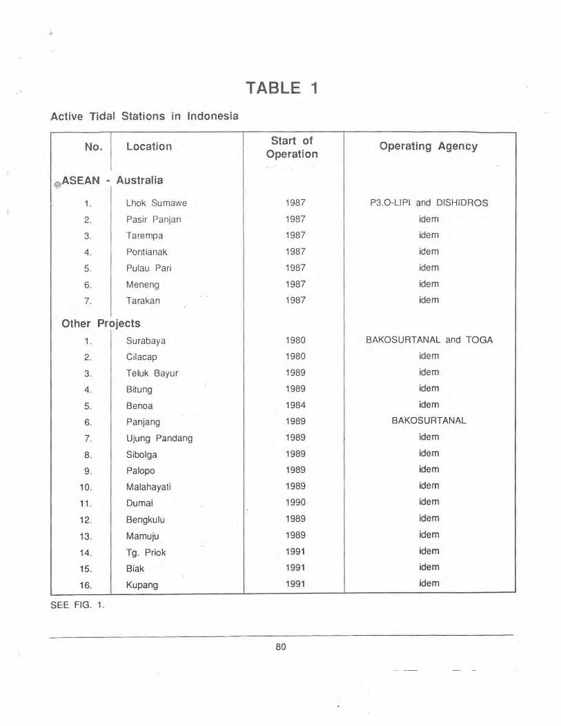
TABLE 1

Active Tidal Stations in Indonesia

No. Location Start of Operating Agency Operation

0 ASEAN - Australia

1. Lhok Sumawe 1987 P3.0-LIPI and DISHIDROS

2. Pasir Panjan 1987 idem

3. Tarempa 1987 idem

4. Pontianak 1987 idem

5. Pulau Pari 1987 idem

6. Meneng 1987 idem

7. Tarakan 1987 idem

Other Projects

1. Surabaya 1980 BAKOSURTANAL and TOGA

2. Cilacap 1980 idem

3. Teluk Bayur 1989 idem

4. Bitung 1989 idem

5. Be no a 1984 idem

6 . Panjang 1989 BAKOSURTANAL

7. Ujung Pandang 1989 idem

8. Sibolga 1989 idem

9. Palopo 1989 idem

10. Malahayati 1989 idem

11 . Dumai 1990 idem

12. Bengkulu 1989 idem

13. Mamuju 1989 idem

14. Tg. Priok 1991 idem

15. Biak 1991 idem

16. Kupang 1991 idem

SEE FIG. 1.

80

(X)

., tO

1<40 1120 13') I 1.<0 I -~~~110 I

"o '?0

I 0 w 11 ~ ~ ... ::~~-

150

10

L.i:GE">JD :

.a P~ . o-~oaPI t<d.: ~t~t i o"~ • BAKOWRTA~A~ S~ .. tio"~

II J"A DE· 'SO Ptloored c.me.Ler'

•

• [2 )) -~

pl ~ 0

lC

I 0

•

~ 0

!0

AUSTRALIA J · 1H'···:.-.~:=:: .. ,.,, . · ... fS . , , :::1 \ IL 150 10 C 110 1'20 130 140 150

Meteorological Studies

In the field of meteorology BMG (the Meteorological and Geophysical Agency) is the national level agency responsible of the management, evaluation and execution of meteorological studies. The BMG provides meteorological informations and services adapted to the requirements for aeronautics, maritime, agriculture and other sectors of the national development activities. In the international level BMG takes part in the WWW and other programmes instituted by WHO and the related international bodies.

Researches of atmosphere and ocean are executed by scientists from institutes such as BMG, LAPAN, BPPT, P3 .0 -LIPI, BAKOSURTANAL and some Universities.

Several meteorological observation stations were provided in connection with the contribution of Indonesia to World Weather Watch Programme and to meet the requirement of National Programme. At present the observation station network comprises of :

112 synoptic stations (60 basic, 52 nonbasic)

65 upper air stations ( 13 radiosonde, 6 rawin and 46 pilot balloon)

16 general climatological stations

89 special climatological stations

157 evaporation stations

4609 rainfall stations

The basic synoptic stations are now available for operating 24 hours a day; one or two times for 0000 GMT and 1200 GMT. Rason and/or rawin observations are carried out at the upper air stations.

Twenty to thirty sea weather data a day are received from ships sailing in the Indonesian waters and its surrounding. The data was analyzed as an aid for preparing the daily weather forecasting and seasonal forecasting. Data was complied in the disket format.

Three telecommunication systems are used in meteorology and they are the Aeronautical Fix Telecommunication Network (AFTN) used for aeronatutical purposes. It is controlled by the

82

Directorate General of Air Communications; the public telecommunications controlled by the Directorate General of Telecommunications and the special meteorological telecommunication network controlled by the Meteorological and Geophysical Agency (BMG).

The latter comprises of three subsystems, namely first the regional telecommunications subsystem for regional data collection and dissemination using Radio Single Side· Band (SSB). Data from stations in a region are collected at Subregional and at the Regional Centres. The second subsystem is inter regional telex subsystem used for data exchanges from/to sub-regional Centre, Sub-centre and National Centre, Jakarta using 50 bps channel capacity, and the third subsystem is the international telex subsystem for data exchanges with other meteorological centre in international scope as a link to Global Telecommunication System (GTS) (JakartaSingapore and Jaka·rta Melbourne). The capacity of this channel has been increased form 75 bps. to 9600bps. The other data di_ssemination system is the broadcast system operating on usual radio frequency.

Mainframe computer DPS-7000 is being installed as an upgrading of the old existing computer CII-HB 64/ 60. For computing the climatological data the CLICOM system will be installed and will be developed. Every month CLIMAT massages from local stations are sent to WMO in the form of hard copy. Starting from November 1990 the messages are also sent using the GTS link.

Data and meteorological informations are now widely used in many purposes in Indonesia. Daily weather forecast is provided for aviation and marine activities, and for public information. Long range and seasonal forecast is also required particularly for agriculture. For improving the extended range forecast, dynamical forecasting including the use of ENSO data and the numerical weather predicting modelling are currently being developed.

FUTURE PROGRAMMES Oceanography -

1. Tidal and Tidal Phenomena

The ASEAN - Australia project on tides will be continued up to the year 1994. Furthermore, this programme will be extended to the current metering

project. Four current meters moorings will be installed in the Malacca Strait, Singapore Strait, South China Sea and the Makassar Strait. ASEAN and Australian research ships will be used in the Current metering ADCP (Acoustic Doppler Current Profiler) will also be operated on board these ships to complement the current mooring. CTD casting will also be made on the cruises.

Tidal stations operation of BAKOSURT ANAL will be continued at least up to the end of this century.

DISHIDROS and the State Ministery for Population and Environment plan to install twelve additional tide gauges in the eastern Indonesian Seas in connection with the study of global sea level rise and the ARLIN DO.

2. JADE Programme.

The Franco-Indonesian cooperation in JADE (JavaAustralia Dynamic Experiment) will be continued in February 1992. The same number of oceanographic stations as in JADE 89-90 in the Indian Ocean between Java-Sumatra and Australia will be occupied. Both the RV "Marion Dufresne" and the "Baruna Jaya I" will be used. CTD and ADCP will be operated by both ships.

The cruises of the two ships will be complemented with moored current meter observation and tidal gauges operation. The location of current meter will be increased from two in JADE 90 to 4 locations in JADE 92, each of them will be installed in the Lombok Strait, Alas Strait, Sawu Sea, Roti Strait , all situated in the region of the outgoing flow of ARLINDO. The tide gauges will be installed in these channels, to monitor the relationship of the strength and variability of ARLINDO with the sea level height in these channels.

3. US-Indonesian Cooperation in Oceanic and Atmospheric Sciences

The US and Indonesian Governments at present are still discussing the possibility of cooperation in oceanic and atmospheric sciences to be carried out in Indonesian waters.

The research programme and the participating universities and agencies will be coordinated by BPPT in the Indonesian side and by NOAA in the us Side.

83

The field of study to be included in this co-operation are :

Topic 1 : Study on Sea Level changes in the Indonesian Waters.

Topic 2 Study on the Indonesian Ocean Circulation.

Topic 3 Study on the Climate Variability using Wind Profiling Radar.

Topic 4 Study on the Ocean-Atmosphere Interaction.

Topic 5 Climate computing

Topic 6 Monitoring Air Chemical composition

Topic 7 Environmental Pollution Control.

Under this arrangement P3.0-LIPI is at present seeking cooperation with the Lamont Doherty Geological Observatory, Columbia University to implement Topic 2, with the special objective of studying the ARLINDO and its effect on the water mass characteristics and vice versa.

4. XBT Casting by Ships of Opportunity

Plan is being set up to make XBT-Iines of crosssections within the Indonesian seas with the help of PELNI (National Indonesian Shipping Company) who now operate 8 new large passenger ships connecting about 30 Indonesian ports throughout the archipelago. At least five out of seven XBT are envisioned :

1. Jakarta - Medan

2. Jakarta - Padang

3. Jakarta - Ujaung Pandang - Bitung

4. Jakarta - Sorong

5. Jakarta - Kupang

6. Ambon - Kupang

7. Bitung - Biak

The objective is to monitor the SST (sea surface temperature) anomaly, SSP (sea surface (air) pressure] and the DOT (Jepth of thermocline). The data is useful to promote capability of predicting the occurrence of long draught in Indonesia in relation to the EI-Nino.

Meteorology

BMG will continue its present programmes and services. It is also expected that the data from the meteorological observing stations described earlier and from other stations will also contribute to WWW and TOGA programmes. For the purpose of TOGA data exchanges the GTS link Jakarta-Singapore and Jakarta-Melbourne will be of great help to provide means of communication.

In the atmospheric research activities, a joint research will be carried out by LAPAN (National Space and Aeronatutics Institute) and NOAA. Wind profiling radar will be installed at Biak in the late 1991 . Other cooperation being planned by LAPAN is that with the Kyoto University in Japan to study the Kelvin wave and the Rossby Gravity wave, among others through the use of radiosonde observation, wind finding radar and boundary layer radar. All of these equipments is expected to be completely installed in Surabaya and Bandung by 1992 or 1993.

BMG and LAPAN also plan to analyze the SST and cloud coverage data in their possession. These data is in the form of APT (automatic picture transmission) images received from NOAA's satellite at the Receiver Station at Pekayon, West Java. This analysis is excepted to help the monitoring and predicting works for long draught done by other means.

List of Acronyms

ADCP

ARLIN DO

BAKOSURTANAL

Acoustic Doppler Current Profi ler

Indonesian Through Flow

National Survey and Mapping Coordinating Agency (Government Non-Ministerial Agency/ GYMNA)

84

BPPT

CLICOM

CTD

DISHIDROS

DOT

ENSO

GTS

JADE

LAPAN

LODYC

PE. 0-LIPI

PELNI

SSP

SST

TAAF

TOGA

Agency for the Assessment and Application of Technology (GMNA).

Climate Computing

Conductivity Computing

Hydro-oceanographic Service, Indonesian Navy

Depth of Thermocline

EI-Nino Southern Oscillation

Global Telecommunication System

Java-Australia Experiment

Dynamic

National Space and Aeronautics Institute (GMNA)

Laboratoire d'Oceanographic Dynamique et Climatologie,University of Paris VI.

= Research and Development Centre for Oceanology, Indonesian Institute for Sciences (GMNA)

National Indonesian Shipping Company

Sea Surface (Air) Pressure

Sea Surface Temperature

Terres Australis et Antartique Francaises

= Tropical Oceans Global Atmosphere

ENVIRONMENT POLLUTION RESEARCH IN NEPAL J.S. Jha, NEPAL

Introduction

Nepal, the land of Mount Everest and the Gurkhas, is predominantly an agricultural country. Geographical setting of the country is so extreme that it ranges from a nearly sea-level to snow covered Himalayas. It has a great variety of topography hence diversity of weather and climate. The country experiences tropical, mesothermal, microthermal, taiga and tundra types of climate. Ecologically it is divided into 3 different regions : mountains, hills and terrains. About two-third of it is occupied by hills and mountains. About 18% of the total land area is cultivable. The total land covered by forest is 55,334 sq. km. which is 37.6% of the total area. Forest is one of the most important national resources and has been supplying fuel, timber and fodder for the animals. Wood is the traditional energy fuel and is still continuously dominating over the commercial fuel and its share is about 95% since last several years. Thus cutting of trees and depletion of its forest resources is causing a major ecological problem in Nepal resulting in landslides, soil erosion, floods, environmental pollution _and occasional outbreaks of epidemics. As it is in tt1e other part of the earth, Nepal too is experiencing a change in its ecological and environmental conditions. Pollution in air, water and land surfaces are reported to be increasing. River water gets contaminated at its very starting point in the high mountain glaciers by the solid wastes left by the increasing number of trekkers and mountaineers. Mountain air of Kathmandu valley can no longer be claimed to be fresh and pure due to continuous injection of smoke and other gases from various factories, brick kilns , old automobiles and putrefaction of solid wastes. But as it is rightly said, the greatest pollutant is the poverty of a country and Nepal, which is listed under the LDC category and whose per capita income is lowest along with Bhutan in the SAARC region , is not an exception to this maxim. It spends very little on public benefit and other developmental items. According to one study report only 0.13% of Nepal's total budget is spent on scientific research and development activities.

85

IGBP Related Activities

Coming to IGBP activities in Nepal, according to my knowledge, there is not any directly IGBP sponsored on going programme. So far a National Committee for IGBP has not been formed. However, there are certain institutions which have started some related scientific activities and they have been mentioned briefly here.

Tribhuvan University

Tribhuvan University department of Physics provides a special course in atmospheric physics and there is a separate ·department of Meteorology. Some research work about the study of troposphere and stratosphere over Nepal leading to Ph.D. degree in physics has been conducted in the department by a faculty member. Department of Geology has certain research programmes for the geological study of certain geographical regions particularly about the nature of rock formation on the upper crust. Department of Botany offers special course in ecology and has some small projects to study environmental pollution problems. But these activities are all due to a few individual initiatives and no systematic institutional approach has been there to study the Geosphere and Biosphere. There is n Research Centre for App lied Science and Technology (REC II ST) under the Tribhuvan University having modest physical facilities but it has not taken up any effective programme in the field of Geosphere and Biosphere except the measurement of solar radiation and wind power in a very limited area. The University does not have sufficient funds and infrastructural laboratory facilities and, therefore, scientific research work in its various departments has not gained much momentum.

Government Departments

His Majesty's Government of Nepal has certain departments which have been collecting scientific data useful for IGBP activities. HMG Department of Meteorology has established various stations

throughout the country to monitor and forecast weather conditions. It has a small laboratory to conduct routine analytical work. Department of Mines & Geology has a good laboratory for geological and chemical analysis but its work is centred around geological survey of the country for mines and minerals and no activity about the geospherical studies has come to light except regular seismological recordings at a few centres.

Ministry of Forest and Soil Conservation has certain activities related with the conservation of ecology and environment. It has initiated community Forest Development Programme in all the 75 districts of Nepal and has planted trees on more than 126 thousand hectares of land. It has established 7 national parks and 5 wildlife reserves on about one million hectares of land. Recently it has raised the status of its environment project to strengthen activities to check environmental degradation caused by deforestation, landslides, soil erosion etc. There is one Remote Sensing Centre equipped with basic instrumental facilities and has some dedicated technical experts.

Ministry of Education and Culture has a National Committee on Man and Biosphere which does not have sufficient funds to contribute effectively . However, it tries to create awareness in the country about the much talked problems of global warming, green house effect, ozone layer depletion and environmental pollution by occasionally conducting workshops and meetings in addition to celebrating the annual world environment day.

National Council for Science & Technology (NCST) is another important Governmental agency under the chairmanship of Vice-Chairman of National Planning Commission. There is one Environment cell in the Planning Commission but its main role is of listing various activities in th1s sector in the name of monitoring and it does not have much to do in the implementation of research activities.

86

Royal Nepal Academy for Science and Technology

RONAST is the most important organisation in Nepal which has mandated objectives for the advancement of S & T capabil ity as well as encouraging scientific research and its applications.

In the field of Environment it had initiated small projects to study river water pollution and air pollution in and outside of Kathmandu valley. After the Chernobyl incident RONAST initiated creating facility to monitor radiation level in food items as well as in the atmosphere of the valley and now it has a unit regularly monitoring radiation level in Kathmandu. In collaboration w ith Government Department of Meteorology it had a small project of studying wind and other climatic conditions at Jhomsom at the base of Dhaulagiri Himalaya. Recently a very important geospherical and biospherical research project in the higher Himalya has been launched by the National Research Council (CNR) of Italy with the local cooperation of RONAST. This ambitious activity is named K2-Ev CNR project after the K2 peak in Karakoram and Mount Everest in Nepal Himalayas. It has some support of EEC countries as well. Under this project a pyramid shaped three storied glass roofed permanent laboratory structure has been established at above 18000 ft. of height near Pumori Himalaya. This project would conduct multi discipl inary research work in various diverse fields like snow, clouds, glaciers, troposphere & stratosphere conditions, geological structure, physiological and psychological impacts of high altitude, chemical and microbiological examination of high altitude, natural resources etc. This project has good communication facility to quickly transmit scientific data to its headquarters in Italy for timely processing. It would be sending samples to CNR laboratories for complicated analytical work. It is hoped that from this project useful information about our biosphere and geosphere would be available for scientific use.

It is hoped that this brief presentation would be able to give some idea about the environmental and IGBP related activities being conducted in Nepal.

IGBP - RELATED ACTIVITIES IN THE PHILIPPINES Leoncio A. Amadore, PHILIPPINES

The Philippines is an archipelago bounded on the east by the vast Pacific ocean and on the west by the South China sea. The survival of communities along its 7,100 islands and islets with a total coastline of about 17,500 kilometres cou ld be seriously endangered by a worldwide rise in sea level brought about by global climate change. The country, being basically an agricultural one could likewise be adversely affected by any global change.

As a member of the international community, the Philippines is somehow involved in activities related to studies and monitoring of global change. At present, however, there is no national group or organisation yet re sponsible for an integrated approach towards IGBP-related studies. The country's participation in global climate change/IGBP activities consists, among others of the following :

* In cooperation with WMO's Global Atmospheric Watch, a background air pollution monitoring (BAPMON) and an ozone observing (GO OS) station had been established in the country. At the suggestion and initiative of the International Global Atmospheric Chemistry project (IGAC), through the Composition and Acidity of Asian Precipitation (CAAP) Experiment Planning Workshop held at the National University of Singapore from 20 - 24th August 1990, these stations are being upgraded to meet certain measurement standards required for a more meaningful analysis and interpretation of results.

* Marine pollution research studies are being conducted by various groups in the country. These are mainly about the assessment of the quality of the marine envi ronment , determination of pollutant behaviour in various media, and determination of effects of marine pollutants. These studies are necessary in view of the country's high dependence on its marine environment for food, raw materials, and other needs for sustenance and economic development.

87

* The Man Biosphere (MAB) Programme of the Philippines is undertaking projects based on the biosphere reserved concept , i.e. , conservation and management of natural and managed ecosystem. Such projects as Coastal Zone Management; Impact of Human Activities and Land-use Practices in the Environment ; Land Management Practices in Grassland Ecosystems, etc. are being pursued by MAB in coordination with other government agencies.

* Monthly climate impact assessment bulletins for agriculture are sent to concerned agencies as part of the monitoring activities on the effects of climate change on agriculture. Studies on the El Nino phenomenon and its implication to agriculture are also on-going activities in the country.

The Philippines is currently establishing linkages with other countries to participate in the Tropical Ocean and Global Atmosphere Program/Coupled OceanAtmosphere Response Experiment (TOGA/COARE) and the Global Oceanic Circulation Experiment (WOCE). Among the scientific goals of the experiments is to understand the principal processes for the coupling of the ocean and the atmosphere in the western Pacific warm pool system. The long-term goal is to develop a coupled ocean-atmosphere general circulation model. Initial activities consists of an intensive coastal-based, ship and mooring observations of relevant atmospheric and oceanographic parameters in the western Pacific ocean.

In response to WMO/UNEP call for the setting up of "a national coordinating group to handle national information requirements relevant to the negotiations, and to serve as a link to the secretariat of the negotiation" relative to the Convention on Climate change, the central instrument which will be considered for adoption at the UN conference for Environment and Development in Brazil in 1992, an Executive Order establishing an Inter-agency Committee on Climate Change has been submitted to the President of the Philippines for approvaL Among others, the Committee is tasked to :

* Formulate policies and response strategies related to climate change.

* Establish working groups to monitor and assess local climate change and its environmental and socio-economic impact in coordination with international agencies plans and programmes.

88

It is envisio-ned that national activities related to global climate change/global change will be under the coordination of this Committee. Aside form attuning and implementing existing plans and programmes, the Committee may also consider conducting comprehensive risk and vulnerability analysis to sea level rise at coastal areas and recommend measures to mitigate its potential adverse effect on coastal communities.

GLOBAL CHANGE ACTIVITIES IN SRILANKA K.D. Arudpragasam, SRILANKA

The Island of Sri Lanka has a total land area of about 64,000 sq. km. and the coast line is approximately 1,700 km in extent. About nine tenth of the Island is made up of Archaen crystalline rocks and the balance, of recent sediments. Part of the east coast, most of the south coast and the west cost upto the City of Colombo is made up of rocky headlands and bays. Most of the coast line is sandy. Beaches north of town of Negombo on the west coast are liable to erosion.

The climate of the Island is dominated by two monsoons; South West Monsoon-May to September; South-Westerly Wind speed average 19km/hr; NorthEast Monsoon - December to January; North Easterly winds speed 12 kmlhr.

Current systems in the vicinity of Sri Lanka undergo reversals in directions in relation to the prevailing wind systems.

The coastal habitat of the Island includes mangroves approximately 3,000ha. in extent with patchy distribution. Largest concentrations are on the east coast. There are coral reefs which are continuous on the north coast, with short stretches on the east and the south west coast. Other coastal habitat include sea-grass beds on the north-west coast where population of Dugong live.

About 70 per cent of the population of the island today live in the region backing the western and south western coast line between Negombo northwards and Malara on the South. The largest towns are also concentrated in this area. Five ci!ies or towns with populations in excess of 100,000 are located along this belt . The harbours of Colombo. Galle and Trincomalee are important centres of economic activity and development. A number of fishery harbours have also been developed in this area. A considerable percentage of the population along the coast line depends on coastal fishing .

In recent years, there ha::; been a rapid development of the tourist industry, which at present is concentrated along the south and south-west coasts. Certain amount of development also took place on the east coast. The potential for tourist development

89

in the Island is very high and if properly planned and managed could become one of the main development activities of the country, which will do little direct damage to the physical environment.

The question of Global Warming was first addressed in an organized manner in 1988 with the holding of a seminar "Global Warming-Global Warning". This was in response to an alert sent out by the United Nations System about impending changes in world temperature and its effects. Following this seminar, the Central Environmental Authority took steps to set up Task Forces on:

1. Climate and Climatic Change

2. Agriculture and Forestry

3. Sea Level and Coastal Erosion

It was intended that each group would be responsible for:

* Collecting all available information locally and maki ng contact wi th Regional and International groups which are active in the specific areas.

* Assessing potential risk areas and danger points and compiling a critical areas inventory.

* Working towards appropriate strategies and plans to ameliorate adverse effects. Taking into consideration also the strategies that are being proposed at International level and the impact of such strategies on the economic, social and cultural state of the country.

However, the progress achieved has been minimal.

The Meteorological Department of Sri Lanka has been maintaining records of weather parameters for a long period of time and has access to meteorological information of the region. Therefore ,even though specific studies in relation to global change are not taking place at the moment, information is being gathered from the regional system.

The Government has been concerned with the question of coastal erosion for a number of years, especially because many coastal areas which have high value for tourism development are highly erosionprone. A Department of Coast Conservation has been established in the Island. The coastal zone has been defined and the coast conservation department has specific authority in relation to the coastal zone. A coastal zone management plan has beer~ developed which is expected to define particular uses, resolve conflicts, preserve sensitive areas and monitor development. The Coast Conservation Department has studied erosion hazards along the coast line which has now been classified into six sectors in order of risk-

1 . South Coast

3. West Coast

5. South-East Coast

2. South West Coast

4. Northern Coast

6. North-East Coast

While Agriculturists, Forestry Officers and Ecologists are now aware of problems of Global warming and possible consequences, no special attention has been paid in Sir Lanka to making analysis of possible impacts in these fields.

From assessments made at present, the main impacts of Global Warming on Sri Lanka will have to do with sea level rise . If by 2030 there is a rise of 18cm. in sea level, certain effects will be felt on the coastal systems and populations along the coast line. Sea level rise is likely to be accompanied by changes in the patterns and intensity of monsoons, thus may result in the loss of parts of the coast line at risk as far as erosion is concerned.

Specific attention needs to be directed in this matter to the north-west and northern parts of the Island. These are built up of Miocene limestone deposits and are mostly flat terrain . Especially, the northern peninsula is the one that has no fresh water input

90

from rivers or streams and this depends on rainfall received from the North-East Monsoon for its water supply. Rising sea levels in these areas are likely to cause salt water intrusion on a large scale into the ground water systems.

In other areas of the Island nsmg sea levels may cause flooding of low-lying area adjacent to the coast, backup of river discharges, interference with sewage disposal systems in the cities. The extent to which these effects may be felt needs to be studied.

Fortunately, Sri Lanka's topography is such that the areas that will be directly lost to sea level rise will be fairly minimal in extent. Much of the Island is well above mean sea level.

For the present. the Ministry of Environment. Sri Lanka has set up a Committee to monitor climate change and impacts . This Committee has representations from the various sectors that are likely to be affected in the course of cl imate change and sea level rise . It is expected that the various experts will interact with regional and international groups to put together different information and to develop the necessary predictive capacity and evolve response strategies.

A small country like Sri Lanka cannot institut-e large scale high cost monitoring programmes. However, it is essential that where possible the country 's efforts should be integrated into the on-going regional programmes. It is also essential that the Scientists of the country should work together with regional and international experts, and participate at meetings such as the present meeting. Our sc ientists have participated for instance, in the IPCC deliberations at Geneva and at the Sea Level Rise Working Group in Perth. We hope to continue to work with the regional and the global scientific community in this manner in the future .

RESEARCH ACTIVITIES RELEVANT TO GLOBAL CHANGE IN TAIWAN

Ho Lin, TAIWAN

ABSTRACT

Taiwan is endowed with a variety of natural phenomena. It is metaphorical "interface·. caught between the largest continent and the largest ocean in the world. Our island dutifully watches annual monsoonal cycle. )yphoons. Mei-Yu front and cold surges are among the weather phenomena witnessed. The Eurasian plate also meets the Philippine Sea plate along our east coast. resulting in frequent earthquakes. In the ocean the Kuroshio is the dominant feature. The strong boundary current has been known by fishermen for centuries. The scientists studying h igh altitude atmosphere find that our location in a subtropical region leads to some rare obseNations. The wide array of interesting natural phenomena in Taiwan is enough to keep our scientists busy for many years to come.

That our human resources are sufficient. is a result of scholastic tradition and solid education system. As an indicator. about 400 scientists with Ph.D's on meteorology,geology. geophysics and oceanography are actively doing teaching and research in Taiwan. Yet there may be 10 times more Chinese scientists on earth Sciences working abroad. Some of them are top-notch researchers. For the past five years the scientific community has been growing rapidly, beyond anybody's expectation.

The government provides adequate funding for basic research. One of the primary goals is to better our knowledge of the environment. The current industrialization process tips the balance of this Island's delicate ecosystem. Acid raid. land subsidence and pollution are at the least a nuisance. if not life threatening. The worsening of air. water and soil quality may eventually erode our economical progress.

We have also detected clear signals of the global warming trend n Taiwan. Since last year. ·the National Science Councils (NSC) started to organize national global change programmes. We are already involved in WOCE. TOGA IGAC and JGOFS. It should be noted that as a member of ICSU. Academia Sinica has sent delegates to several IGBP meetings. Only in the past year. however. did we try to put together a global change programme which will emerge from our effort in the next year or two. We are also interested in the possibility of setting up a Regional Research Center under the IGBP umbrella. The time will come soon for ROC's global change programme to take off.

I. Introduction

It is evident that the effects of human activities have increased so much as to significantly affect climate and the environment on a global scale.

The people and government of the Republic of China on Taiwan, influenced by the scientific community, are keenly aware of the nature and consequences of this problem. As a result, the "Committee of GeosphereBiosphere Programme, Academia Sinica. Taipei, R.O.C. for the Scientific Committee for the

91

International Geosphere-Biosphere Programme, International Council of Scientific Unions" was formed in 1988.

Under the National Science Council and the Academia Sinica (AS). various national research initiatives concerning global change research have been developed (see "Structure of Organizations involved in Global Change Program of ROC"). These activities provide a framework for catalyzing and coordinating research among universities, research institutions, government and industrial establishments.

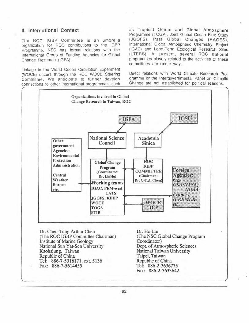
II. International Context

The ROC IGBP Committee is an umbrella organization for ROC contributions to the IGBP Programme. NSC has formal relations with the International Group of Funding Agencies for Global Change Research (IGFA).

Linkage to the World Ocean Circulation Experiment (WOCE) occurs through the ROC WOCE Steering Committee . We anticipate to further develop connections to other international programmes, such

as Tropical Ocean and Global Atmosphere Programme (TOGA) , Joint Global Ocean Flux Study (JGOFS), Past Global Changes (PAGES), International Global Atmospheric Chemistry Project (IGAC) and Long-Term Ecological Research Sites (L TEAS) . At present, several ROC national programmes closely related to the activities of these committees are under way.

Direct relations with World Climate Research Programme or the Intergovernmental Panel on Climatic Change are not established for political reasons.

Organizations involved in Global Change Research in Taiwan, ROC

Other government Agencies:

National Science Council

Environmental Protection Administration

G Change Program

(Coordinator: Dr. LinHo) Central

Weather Bureau teams

PEM-west CATS

JGOFS: KEEP WOCE TOGA STIB

Dr. Chen-Tung Arthur Chen (The ROC IGBP Committee Chairman) Institute of Marine Geology National Sun Yat-Sen University Kaohsiung, Taiwan Republic of China Tel: 886-7-5316171, ext. 5136 Fax: 886-7-5614455

92

Academia Sinica

IGBP COMMITTEE

(Chairman: Dr. C-T.A.

Dr. Ho Lin (The NSC Global Change Program Coordinator) Dept. of Atmospheric Sciences National Taiwan University Taipei, Taiwan Republic of China Tel: 886-2-3636775 Fax: 886-2-3633642

Goals, Structure and Operation of the ROC Global Change Programme.

The overall goal of the ROC global change programme is to ensure that ROC's approach to global change research is cohesive, comprehensive, and responsive to international initiatives. while remaining focussed upon regional problems and national needs.

Planning activity has been under way for the last two years under the aegis of the ROC IGBP Committee. Proposition and implementation of research plans were accelerated in the last 6 months due to increase in funding level from NSC, and the successful completion of the first Sino-Filipino WOCE cruise.

The national committee administrates through a committee of 16 scientists from Academia Sinica, National Taiwan University, National Sun Yat-Sen University and the Central Weather Bureau (CIJI{B) . A standing committee of 5 members. including the chairman, is responsible for routine operations.

Working committees of programmes related to global change are mostly organized by NSC. These working committees define the nature and scale of global change research activity in specific areas of concern. They also facilitate the development of projects by identifying needs and potential collaboration among

different groups. The direction and scope of the ROC national effort in global change are currently defined mostly py scientific projects.

Other government agencies, such as the Environmental Protection Administration and CWB also take part in, and fund some global change research programmes. Their roles are expected to increase in the future .

Bilateral Relations

Bilateral relations have been established through both formal and informal discussions, meetings and workshops between the ROC committees and the corresponding committees in the US, Japan, France and the Philippines.

Individual scientists have involved in planning and discussions for. the development of joint scientific projects with scientists from the above mentioned countries and Canada, Germany, Korea, Netherlands and USSR. Some contacts have been established by individual scientists with scholars of mainland China for data exchange .

Results of the Planning Activity

Many existing and planned projects have been identified. They are presented here as established and developing projects.

Established Projects

Study Budget Funding Related Title No. of Pis period (Million agencies International

US$) Projects

CATS 11 1990 3.8 NSC IGAC EPA CWB

KEEP 30 1989-94 6.0 NSC JGOFS

WOCE 6 1990-95 2.2 NSC WOCE

93

,

Title

PEM-west

PAGES

STIB

TOGA

Ecological Studies

Hydrological Studies

Note :

CATS

ECOLOGICAL STUDIES

KEEP

PEM-WEST

STIB

TOGA-COARE

Developing and Potential Projects

No. of Funding Related Pis Agencies International Status

Projects

3 NSC IGAC Planning

8 NSC PAGES Planning

15 NSC STIB Planning

8 NSC TOGA-COARE Planning

NSC, AS, NRC, EPA LTERS Unorganized

NSC GEWEX Unorganised

Climate and Air-quality Taiwan Station

(a) Ecological survey on waters adjacent to the nuclear power plants in Taiwan. (b) Mussel Watch-Chemical Changes in Coastal Zones (c) Ecological Effects of Fires (d) Dynamics of Water Bodies, Swamps and Marshes

Kuroshio Edge Exchange Processes

Pacific Exploratory Mission-West

Stratosphere-Troposphere Interactions and the Biosphere

Tropical Ocean and Global Atmosphere Programme - Coupled Ocean-Atmosphere Response Experiment

94

A BRIEF REPORT ON THE ACTIVITIES OF THE IGBP NATIONAL COMMITTEE OF THAILAND DURING 1990

Twesukdi Piyakarnchana, THAILAND

The IGBP National Committee of Thailand was officially established in July 1989 by the Ministry of Science, Technology and Energy.

The committee consists of 8 members from the universities and government agencies. Members have their specialities in the fields that are related to the IGBP established core projects. The Thailand National Research Council has provided the secretariat.

In 1990, there were a few activities that might be considered as highlight of the IGBP National Committee. There were two participations by the Chairman in the IGBP activities abroad. The first one was to participate in a National IGBP Coordination Meeting in Washington DC., 22-24 January 1990 and the second meeting of the Scientific. Advisory Council (SAC II). 3-7 September 1990 in Paris, France. The results from these meetings were summarised and distributed to the members of the National Research Council of Thailand. One of the real impacts to the Thai Scientific Community related to the IGBP, was the First National workshop on IGBP in Bangkok on September 16-17, 1990.

The first IGBP National Workshop had 4 objectives :

1. To inform Thai Scientific Committee on IGBP, the Global Change Programme.

2. To compile informations from the published and on going research projects by Thai researchers on the changing of the Terrestrial, Atmosphere, Hydrosphere and Marinesphere.

3. To exchange ideas and experiences on the future research projects development on the global change.

4. To set up the priority of the research projects which were proposed by the workshop.

95

The workshop recommended on the following :

The members of the workshop were divided into two groups based on their interests. The two groups were the Terrestrial and Hydrosphere group and the Marinesphere and Atmosphere group. Each group had formulated the recommendations. These recommendations were suggested to be used as a guidelines for the future research of IGBP and also the Environmental issues in Thailand.

1. Terrestrial and Hydropshere Group

* Research problems on the impact of industrial waste dumping to the agriculture land.

* Study on the changing climate to the flowering of the economically important plants and to the bio-diversity.

* Study on the relationship between the national forest destruction and global change.

* Study on the changing condition of soils on their distribution, preventive measures. soil improvement. (The study must aim at prediction of land slide, earthquake and coastal erosion).

* Study on the cause of decreasing fresh water supply.

* Study on the waste water treatments, solid wastes disposal. (These studies should aim at the increasing efficiency and economical feasibility to Thailand).

* Study on the impact of mineral excavation on environmental change.

* The group also recommended to apply remote sensing techniques for data gathering.

2. Marine Sphere and Atmosphere

* Continue monitoring on the change of temperature both in the sea and in the atmosphere.

* Study on the urban climatology.

* continue study on the past geological changes in Thailand and Southeast Asia.

* More detail study on the coastal and near shore circulation.

* Study on the coastal erosion, with the emphasise on the Gulf of Thailand.

* Study on the sediment at. on and in, through the rivers to, in the Gulf of Thailand and Andaman Sea.

* Strengthening the study on the Atmospheric Chemistry.

* Study the causative factors on the formation of typhoons in the Gulf of Thailand.

From the above recommendations one can see that if they were implemented, they could well contribute to the established core projects of the IGBP, as already outlined in the Report No.12, 1990.

Besides the above recommendations the workshop participants had learnt that some of the existing research projects of their colleagues might be used as a starting point in collaborating with the IGBP core projects. The examples are shown in the following.

In the discussion on the increasing use of the fresh water for various purposes such as in the agriculture, industries as well as for the water supply, one speaker pointed out that this situation might cause the future shortage of fresh water in Thailand. At present, for example, the increasing use of water for agriculture during the dry season in the central plain of Thailand might be one of the cause of the sea water intrusion inland.

In the area of Bangkok Metropolis, in dry season the salt water intruded up land for about 25 kilometres from the river mouth and caused severe damages to the orchards and vegetable growers.

96

The changing. of the coast lines along the Gulf of Thailand from 1969 to 1987 was also reported in this meeting. In certain places such as on the upper part of the Gulf of Thailand at the Chao Phraya River Mouth the erosions were stronger on the western part than on the eastern side. Few measures in order to prevent the coastal erosion were also proposed. However, with the more and intense strong winds together with high waves in the recent years, caused the coastal erosion to be expanded.

A speaker from the Department of Geology Chulalongkorn University told us about the ancient shorlines of the upper part of the Gulf of Thailand during the past 6,000 - 7,000 years . At that time the land of Bangkok, our present capital was under the sea water. He also told us about his prediction that in the year 2100, at least half of Bangkok Metropolis will be flooded by sea water again. However, this prediction was based on the condition that the sea level rise at low scenario and the present continuous subsidence of the land around Bangkok could not stop.

In the field of the Meteorology, the researchers from the Royal meteorology Department, Ministry of Communicat ion had informed us about their research on the annual frequency of the storms that hit Thailand. The possible impacts from the El Nino or La Nina phenomena in 1983 to. the amounts of rainfall at two stations Bangkok and Surathanee at before, during and after the El Nino periods were also reported. The results showed very small inf luence to the normal condition of the amount of the rain fall at these two selected stations.

Conclusion

Although the subject of the Global Change and its effects by the green house phenomena are frequently mentioned by many types of mass media in Thailand, the systematic resea rches in this field are not sufficiently supported by the funding agencies in this country. It needs some more time in order to bring those researchers who are interested in this field to come and work together as a team. The collaboration with the international scientific communities are also necessary. The leading roles of the IGBP of ICSU should be encouraged and fully supported by all means.

RECONSTRUCTION OF RAINY SEASON IN EARLY SUMMER OVER EAST ASIA

DURING THE HISTORICAL PERIOD Masatoshi Yoshino, JAPAN

Introduction:

The rainy season in East Asia is called Bai-u in Japan, Mae-ue in Korea, Mai Yu in China and provides water resources for paddy cultivation and energy for water power for long years. From the stand point of pure climatology, it has been studied for its regionality, inter annual variations, relation to the general circulation pattern, and meso-scale structures. In the recent years , reconst ruction of its characteristics has been made. Present paper reviews these studies and summarizes the problems to be solved in near future.

For the readers outside of East Asia, general situation of fronts, airmasses and air streams during the Baiu season is given in Fig.1 . Also, its interannual change, and its relation to the circulation at the 500 mb level are given elsewhere (Yoshino 1963,1977)

2. Reconstruction and Data Base:

a) Historical Data Base for Japan:

To reconstruct the climate in the historical period, a cooperation work of "Historical Weather Reconstruction Group" is established in Japan in cooperation with the Information and Computer Centre of Yamanashi University (Yoshimura and Yoshino,1988). The description of daily weat~er in the 20 old diaries and documents at the 18 sites in Japan during the time from about 1700 to 1880 is now available: (i) All weather information of a particular day, (ii) weather distribution in a region or in whole Japan under the particular weather, or (iii) a weather table for a particular month are obtained as a split map, distribution map, or sequence series of weather as an output. 18 kinds of maps can be provided. Using this database, we can study Bai-u conditions in the period before instrumental observations came into vogue.

b) Wet/dry Patterns in East Asia:

Mikami (1988) reconstructed the wet /dry patterns in

97

Japan and Korea for the 30 years period in the 18th century . His data base presents four kinds of daily weather at 19 stations from June to September, 1771-1800. Weather pattern calender expressed by the position of rainy areas from No.1 to 5, has been obtained for everyday.

This is further summarized for monthly average in each area so as to be compared for the 500 year wet/dry distributions in summer reconstructed in China (Central Weather Bureau, China, 1381).

c) Reconstruction of Bal-u Season:

Mizukoshi (1986,1987) reconstructed the climate for the recent 350 years for the Bai-u period, the beginning and ending dates since 1637, as well as the rainfall amount since 1692, of the Bai-u season by using various kinds of weather records. In particular, long-year fluctuation of Bai-u rainfall intensity has been studied in detail for the hundred years. 1771-1870.

d) Bal-u in the 15th Century:

Mizukoshi (1989) obtained another data set of the Baiu season by. reconstructing the beginning and ending dates in the central part of Kinki District, Central Japan. for the hundred years, 1413-1512. This is the earliest data set of the Bai-u season reconstructed by now.

e) Bai-u and Little Ice Age:

Maejima et al. (1983 a) reconstructed the climate of Hirosaki, Northeast Japan, from 1661 to 1868 by using the weather records in the diary of the feudal clan Tsugaru, which is one of the most valuable documents in Japan in the 17th century. Their database is expressed by the frequency (%) of precipitation for June, July and August. Hirosaki is located away from the main rainfall activity region along the Bai-u frontal zone, but still it provides sufficient information of the interannual fluctuation of rainfall during the Bai-u season.

f) Frequency of Weather Type, 600·1900 AD:

An attempt was made to reconstruct the climatic hazard records since the 7th Century. Cool summer weather and drought have caused famine, which are usually described in the historical documents.Maejima and Tagami (1986) plotted the hazards on charts by seasons for each year and classified the charts into four groups for summer: (i) hot summer, (ii) west -cool-north-hot-summer, (iii) north-cool-west-hot summer and (iv) cool summer. For example, i corresponds to droughts all over Japan, which means the Bai-u front is very weak. On the contrary, iv indicates that the Bai-u is very strong with continuous rain over Japan. ii means long rains by the Bai-u front only in southwest Japan, but iii means droughts in southwest Japan because the Bai-u front is located anomalously in north Japan. The century's summary is given in Table 1.

g) Rainy Days, 1855·1868:

Fukaishi ( 1985) reconstructed number of rainy days for every 10 days for every months in Shikoku, SW Japan.

3 Secular Variations:

The secular variations of the Bai-u front activities are shown on the right hand column of Table.1. It is estimated that the activity was generally weak from the 8th to 1Oth century, but was changeable, weak or strong from the 17th to 19th century. The former coincides with Neo-Atlantic warmer period(Bryson and Padoch, 1981) and the latter corresponds to the little Ice Age, which is generally observed all over the world, even though they are slightly different from region to region (Lamb, 1977).

As has been made clear by pollen analysis (Sakaguchi,1982,1983). the period 240-732 was cold, but it turned to warm until end of the 13th century. From the 14th century, the climate changed to cold. It is suggested that the Bai-u front activities coincided roughly with this deterioration of climate, which has been detected generally in Europe also (Lamb, 1977). The "Little Ice Age" in Japan has started clearly in the 17th century. In Table 2, the period division of the Little Ice Age for Japan if given (Maejima and Tagami, 1983). The rainy periods in summer in this table correspond to the active Bai-u periods.

98

Among them, extremely rainy and cool summer was experienced in 1783, called "Tenmei Famin". Mikami (1988), analysing natural seasons for the summer half years for 1781-1790, showed that the climates in 1781-1785 were estimated to have been markedly dry and hot, but there was very short summer in 1783, as shown in Fig.3. Yaji and Misawa (1981) examined the weather situation for 1833 and 1836, which are the famous famine years in Tohoku District in NE Japan, and made clear that the year 1836 was typical of a rainy, cool summer.

Long-term fluctuation of the Bai-u season was studied by Mizukoshi (1986). He reported that the end of the Bai-u season was delayed for more than half month in the 1780's, 1830's and from the 1890's to early 20th century. The amount of rainfall (ten-year averages) during the Bai-u has been fluctuating between 200 to 450 mm for the past 200 years.The reconstruction of rainfall amount from the weather records should be studied further in detail, because it is very much important.

The extended summer season from May to August consists of a long -term variat ion and a short-term variation. The former is represented by a periodicity of 40 days and determines the beginning and the end of the Bai-u season. The latter is represented by a periodicity of 15 days and forms seasonal steps inherent to the Bai-u season such as the pause of the Bai-u (Murata, 1989). It was also made clear that, for a peak of the Little Ice Age (1830-40) the longterm variation was indistinct and instead, the short variation was predominant. This means that in those days, weather changed periodically even after the end of the Bai-u season when fine weather continues by the arrival of the Pacific High for normal years. It was observed that the short-term variation prevails in such a year when cool summer damages or/and droughts occurred. This relationship was verified using instrumentally observed data.

4. Regionality of the Bai-u in the Historical Period:

Regionality of the Bai-u over East Asia is of interest not only for the recent period (Yoshino and Aoki, 1986), but also for the historical period (Yoshino, 1978). The regionality was examined statistically using methods of Cluster Analysis (Yoshino and Aoki, 1986) for rainfall in June, July and June+July and of

Principal Component Analysis for rainfall in July (Mikami, 1987). The results indicate that the rainfall zone extending from the Yangtze River region, nliddle China to SW Japan shows similar rainfall pattern. In north and south of this zone, an opposite tendency is found in the trend,

In conclusion, the regionality of the Bai-u in the historical period is different year to year, but it shows rough ly some resemblance in June ,July or June + July, which have been analysed for the recent instrumental period. Recently, this was confirmed statistically by another method (Yoshino and Murata, 1988). Murata (1989) further studied the regionality of Bai-u in the Little Ice Age and came to the following conclusion. In Central Japan, dry conditions were found in the years of 1750-1850, as far as monthly rainfall variations are concerned. Also , relatively large wetness was observed in the years of 1730-60 and 1830-50. The validity of this reconstructed result can be confirmed by the reconstructed rainfall variations in Beijing which were made independently of the present study.

References

Bryson, R.A. and Padoch, C. (1981) : On the climates of history, In : Climate and history, ed. ·by Rotberg, R.I. and Rabb, T.K. Studies in Interd isciplinary History, 3 - 17.

Central Wather Bureau, China (1981 ) : Atlas of the recent five hundred years' dry-wet distributions in China. Map Publ. Comp., Beijing, 332 Pages.

Fukaishi, K. {1985) : Reconstruction of climate made out of the weather records revealed in the diaries in the Shikoku Island at the end of the Edo Era. Hobungakubu-ronshu, Bungakuka-hen, Ehime Univ. 18, 71 -92. (in Japanese with Engl. abstr.)

Lamp, H.H. (1977) : Climate : Present, past and future. Vol. 2. Methuen, London, 835 P.

Maejima, I. Nogami, M. , Oka, S. and Tagami, Y. (1983 a) : Historical weather records at Hirososaki, Northern Japan, from 1661 to 1868. Geogr. Rep. Tokyo Metropolitan Univ., 18, 113-152.

Maejima, I. and Tagami, Y. (1983 b) : Ciimate of little Ice Age in Japan. Geogr. Rep. Tokyo Metropolitan Univ. , 18, 91-111.

99

Maejima, I. and Tagami, Y. (1986) : Climatic change during historical times in Japan - Reconstruction from climatic hazard records. Geogr. Rep. Tokyo metropolitan Univ., 21, 157-171.

Mikami, T. (1987) : Climate of Japan during 1781-1790 in comparison with that of China. In : The climate of China and global climate. Ed. by Ye, o., Fu, C., Chao, J. and Yoshino, M., China Ocean Press, Beijing, and Springer-Veri., Berlin 63-75.

Mikami, T. (1988) : Reconstruction of the wet/dry patterns in East Asia, 1771-1800, and some synoptic climatological discussions. Rep. Res. Project, Grantin-Aid for Sci. Res., 1985-1987, Tokyo Metropolitan Univ., Tokyo, 57 pages.

Mizukoshi, M. (1986) : Long-year variation trend of Bai-u in Kinki District. Ann. Rep. Disaster Prevention Institute, Kyoto University, 29b-2, 109-123.

Mizukoshi, M. (1989) : Reconstruction of climate in the historical time by old documents in Chubu and Kinki Districts. Rep. Res. Project, Grant-in-Aid for Sci. Res .. 1986-1988, Mie University, Tsu.

Murata, A. (1989) : Reconstruction of Bai-u in the "Little Ice Age" in Japan. Doctor of Science Thesis, Institute of Geoscience, University Tsukuba.

Sakaguchi , Y. (1982) : Climate variability during the Holocene Epoch in Japan and its causes. Bull. Dept. Geog. Univ. Tokyo, 14, 1-27.

Sakaguchi, Y. (1983) : Warm and cold stages in the past 1600 years in Japan and their global correlation - especially on climatic impacts to the global sea level changes and the ancient Japanese history -Bull. Dept. Geog. Uni':'. Tokyo, 15, 1-31.

Yaji, M. and Misawa, M. (1981) : Some notes on the Japanese climates before and after the Tempo Lean Years , 1828-1844. Sci. Rep. Yokohama National Univ. (Sec. II), 28, 91-108.

Yoshimura, M. and Yoshino, M. (1988) : Outline of historical weather data base for Japan. In : Recent Climatic Change, ed. by S. Gregory, Belhaver Press, London, 267-271.

Yoshino, M. (1963) : Rainfall , frontal zones and jet stream in early summer over East Asia. Bonner Met. Abhandlungen, 3, 1-126.

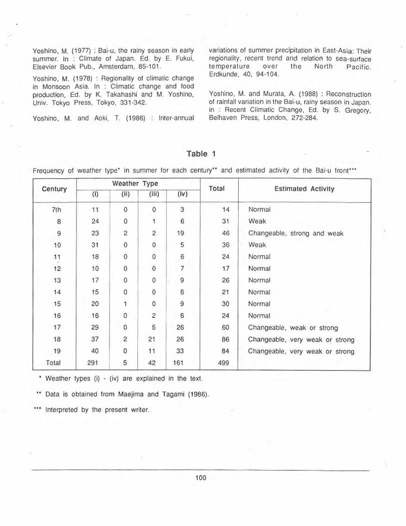
Yoshino, M. (1977) : Bai-u, the rainy season in early summer. In : Climate of Japan. Ed. by E. Fukui, Elsevier Book Pub., Amsterdam, 85-101 .

Yoshino, M. (1978) : Regionality of climatic change in Monsoon Asia. In : Climatic change and food production, Ed. by K. Takahashi and M. Yoshino, Univ. Tokyo Press, Tokyo, 331-342.

Yoshino, M. and Aoki, T. (1986) Inter-annual

variations of summer precipitation in East-Asia: Their regionality, recent trend and relation to sea-surface temperature over the North Pacific. Erdkunde, 40, 94-104.

Yoshino, M. and Murata, A. (1988) : Reconstruction of rainfall variation in the Bai-u, rainy season in Japan. in : Recent Climatic Change, Ed. by S. Gregory, Belhaven Press, London, 272-284.

Table 1

Frequency of weather type* in summer for each century** and estimated activity of the Bai-u front•••

Century Weather Type

Total Estimated Activity (i) (II) (iii) (iv)

7th 11 0 0 3 14 Normal

8 24 0 1 6 31 Weak

9 23 2 2 19 46 Changeable, strong and weak

10 31 0 0 5 36 Weak

11 18 0 0 6 24 Normal

12 10 0 0 7 17 Normal

13 17 0 0 9 26 Normal

14 15 0 0 6 21 Normal

15 20 1 0 9 30 Normal

16 16 0 2 6 24 Normal

17 29 0 5 26 60 Changeable, weak or strong

18 37 2 21 26 86 Changeable, very weak o~ strong

19 40 0 11 33 84 Changeable, very weak or strong

Total 291 5 42 161 499

• Weather types (i) - (iv) are explained in the text.

•• Data is obtained from Maejima and Tagami (1986).

*** Interpreted by the present writer.

100

Table 2

Pattern of thB Little Ice Age in Japan. (Maejima and Tagami , 1983 a)

Period Climate type Summers Winters

1611 -1650 Very cold Very cool, rainy? Very cold, heavy snow? Little Ice Age, Phase I

1651-1690 Mild Hot in the first half Mild, light snow Interglacial I

1691-1720 Very Cold Very cool, rainy Very cold, heavy snow Little Ice Age, Phase II

1721-1740 Cold Cool Cold Little Ice Age, Phase II

1741 -1780 Mild Hot in the second half Too mild, light snow Little Ice Age, Phase II

1781 -1820 Cold Very cool, rainy Cold Little Ice Age, Phase Ill

1821 -1950 Very cold Very cool rainy Very cold , heavy snow Little Ice Age, Phase Ill -

1851 -1880 Cold Warm Very cold, heavy show Little Ice Age, Phase Ill

Fig. 1 Schematic illustration of fronts, air masses & air streams in the Bai-u season

101

- - - .... . ... -~ .. C1,0)1JIUI

f-.--- _,- --~+-----.• ~ ... '"

~IJ ~'fiND

-,....\.t v'c..,

Fig. 2 Weather type of each year and chnage of its frequency from 601 to (1900 Maejima and Tagami. 1986.) Legend : Vertical line shows appearance of following types : ( 1) hot summer (2) west cool - north hot summer (3) north cool - west hot summer (4) cool summer (5) mild w1nter (6) cold winter. Curved line shows change of weather type frequency (weigthed running mean for 51 years). They are obtained by following coefficients ': type (1) and (2) are + 1, type (3) and (4) are -1 in summer while

type (5) is + 1, type (6) is - 1 in winter.

F1g. 3 Classification of natural seasons for the warmer half years for 1781-1790 (M1kami. 1988).

102

GREEN HOUSE GASES, ENVIRONMENTAL STRESS AND ECOLOGICAL ANALYSIS J.S. Pandey, S. Moghe and P. Khanna, INDIA

ABSTRACT

It has been obseNed that ozone formation in the troposphere is predominantly restricted to late spring and summer. Ozone alongwith additional air pollutants induces long-lasting physiological and biochemical disturbances. During last few decades there has been tremendous increse in forest damage and decline in forest area all over the globe. Well known damage symptoms and empirical data on the physiological responses of plants to pollutants including green house gases, have established the importance of role played by green house gases in regard to growth and development of a tree. The complex interactions and resulting environmental stress have been studied and analysed through application of sensitivity analysis. Sensitivity analysis has been carried out for leaf. stem and root (state variables representing a tree) in terms of changes in conversion efficiency parameter for the foliage, assimilate partitioning coefficients, and co-efficients dependent upon losses due to mortality. grazing and litter fall.

Introduction

Over the last three decades there has been a

dramatic increse in forest decline (Blank, 1985 and Mclaughin, 1985). Although it is well established that

air pollution is one of the most important factors behind forest decline, replication of many damage symptoms has not been possible. Suggestions

indicating synergistic interact ion between air pollutants and several other environmental stresses are widely gaining ground. It has been reported (Blank

et al. , 1988) that in Central Europ~ complex interactions between phytotoxic levels of ozone and

acid mist combined with shortage of nutrients and

excess of solar radiation have weakened trees at high

alt itude and made them more vunerable to a wide range of natural and anthropogenic environmental

perturbations.

There is evidence to suggest that ozone and acid mist increase the sensitivity of trees to drought, winter desiccation and freezing (Barnes et al. , 1988 and Barnes et al., 1990). Ozone formation in the

troposphere is predominantly restricted to late spring and summer (Eamus et al., 1990) and, in the presence of adverse environmental factors, it induces

long-lasting physiological and biochemical

disturbances.

103

Moreover, long-term ozone exposure at ambient or

modestly. above-ambient. concentrations leads to

reduction in photosynthetic activity in many tree

species (Chappelka et al. 1988). Respiration of

differet parts of the tree viz. leaf, stem and root may

also get severely affected (Barnes, 1972 and Yang

et al. 1983). Decreased quantum efficiency, lower

carboxilation efficiency and highly variable stomatal

responses have also been reported in literature (Reich

et al., 1985 and Jensen et al., 1989).

Well known damage symptoms and empirical d·ata on

the physiological responses of plants to pollutants

including green house gases, have established the

importance of the role played by green house gases

in regard to growth and development of a tree. The

complex interactions and resulting environmental

stress have been studied and analysed through

application of sensitivity analysis (Pandey et al. 1990).

Sensitivity analysis has been carried out for leaf, stem

and root (state variables representing a tree) in terms

of changes in conversion efficiency parameter for the

foliage , assimilate partitoning co-efficients and co

efficients dependent upon losses due to mortality,

grazing and litter fall .

Sensitivity Analysis

Expressions for sensitivity (Pandey et al., 1990) have been derived and denoted by expressions of the form (A-B), where A refers to the variable under consideration and B to the parameter w.r.t. which sensitivity is being studied. Some typical expressions for Root are shown below :

SRoo-AssPr

SRoo-Gimr

SRoo-Respr

SRoo-Assp1

SRoo-Gim1

SRoo-Resp1

SRoo-SLA

SRoo-k

SRoo-Photo

SRoo-Cep

Where,

F1

F2

F3

F4

F5

F6

F7

F8

F9

F10

F11

G1

G2

( F1) (G 1 )/(G2) (G3)

-(G8) (F1 )/ [(G2) 2 (G3)]

- (F1) (G8)/ [(G2)2 (G3)]

(G14) - [(F1) (G13)/(G3)]/[(G2)/(G3)]

(G16 + G 17)/[(G2) (G3) ]

F1 (G18 - G3)/[(G2) (G3)]

G8 (G5 + G19)/[(G2) (G3)]

~G11 ) (G8)/[(G2) (G3)n [1 + (G5) (G12)/(G3- G5)]

F1 (G7 + G5)/[(G2} (G3)]

F1 (G4 + G21 )/[(G2) (G3)]

1 -exp (-k (SLA) (Leaf) ]

(Cep) (Photo) [(Gim) , + (Resp), (Assp), (Cep)]

(Assp), + (Resp), (Photo) (Cep)

(Gim), + (Resp), (Assp), (Cep)

k (Cep) (SLA) (Photo) (Assp), (1 - F1)

(Assp), (Photo) [(Gim), + (Resp), (Assp) , (Cep)]

(Assp), 2 (Resp) , (Cep) (Photo)

(Assp), (Cep) (Photo) k (Leaf) (1 - F1)

k (Cep) (Assp), (Photo)exp (-k (SLA) (Leaf))

(Assp) , (Cep) (Photo)

(Assp),2 (Cep)2 (Photo)

(Cep) (Photo) (Gim),

(Gim), + (Resp), (Cep)

104

(1)

(2)

(3)

(4)

(5)

(6)

(7)

(8)

(9)

......... (1 0)

( 11 )

(12)

(13)

(14)

(15)

(16)

(17)

(18)

(19)

(20)

(21)

(22)

(23)

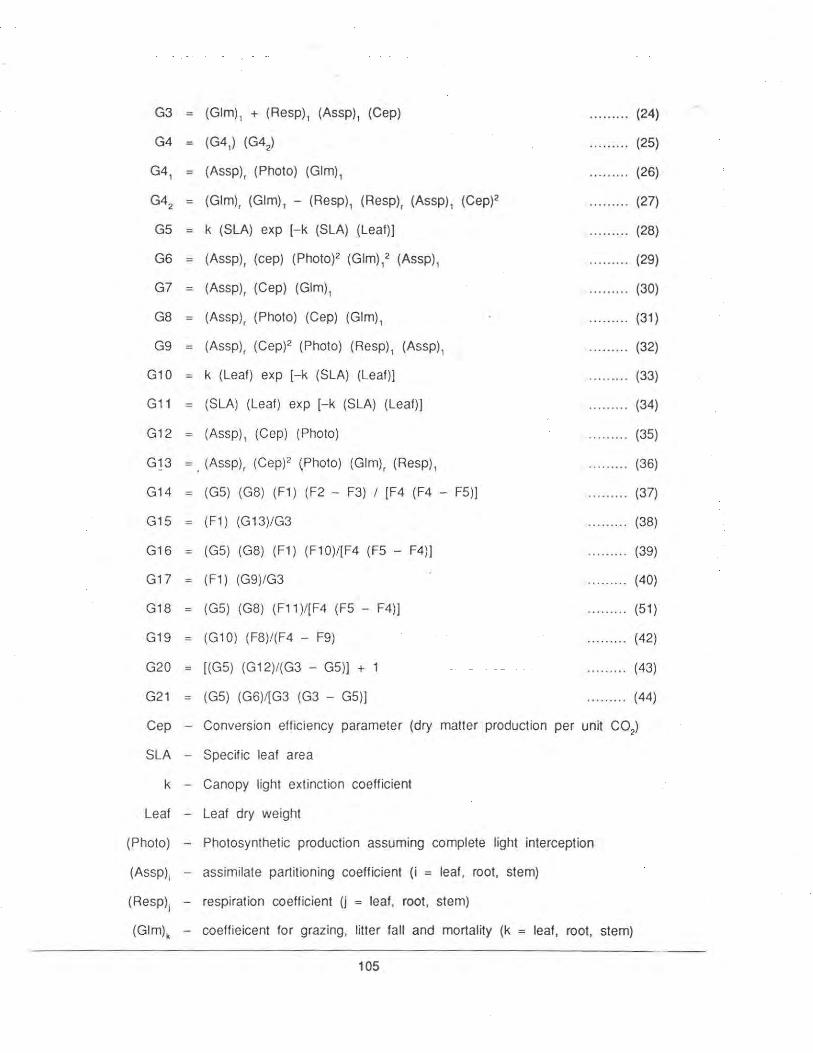
G3

G4

(Gim)1

+ (Resp)1

(Assp)1

(Cep)

(G4J (G42)

G41

(Assp), (Photo) (Gim)1

G42

(Gim), (Gim) 1 - (Resp)1

(Resp), (Assp)1

(Cep)2

G5 = k (SLA) exp [- k (SlA) (leaf))

G6 (Assp), (cep) (Photo)2 (Gim)12 (Assp)

1

G7 (Assp) , (Cep) (Gim)1

G8

G9

G10

G11

G12

(Assp), (Photo) (Cep) (Gim) 1

(Assp), (Cep)2 (Photo) (Resp)1

(Assp)1

k (leaf) exp [-k (SlA) (leaf)]

(SlA) (leaf) exp [-k (SlA) (leaf)]

(Assp)1

(Cep) (Photo)

G13 =. (Assp), (Cep)2 (Photo) (Gim), (Resp) 1

G14 (G5) (G8) (F1) (F2 - F3) I [F4 (F4 - F5))

G15 = (F1) (G13)/G3

G16 (G5) (G8) (F1) (F10)/[F4 (F5 - F4))

G17

G18

G19

G20

G21

(F1) (G9)/G3

(G5) (G8) (F11 )/[F4 (F5 - F4))

(G1 0) (F8)/(F4 - F9)

[(G5) (G12)/(G3 - G5)] + 1

(G5) (G6)/[G3 (G3 - G5)]

(24)

(25)

(26)

(27)

(28)

(29)

... . ..... (30)

(31)

(32)

. ........ (33)

.. . .. . .. . (34)

.. . .. ... . (35)

(36)

(37)

(38)

(39)

(40)

(51)

(42)

(43)

(44)

Cep - Conversion efficiency parameter (dry matter production per unit C02)

SlA - Specific leaf area

k - Canopy light extinction coefficient

Leaf - Leaf dry weight

(Photo) - Photosynthetic production assuming complete light interception

(Assp); - assimilate partitioning coefficient (i = leaf , root, stem)

(Resp); - respiration coefficient (j = leaf, root, stem)

(Gim)k - coeffieicent for grazing, litter fall and mortality (k = leaf, root, stem)

-----------------------------------------------------------------------105

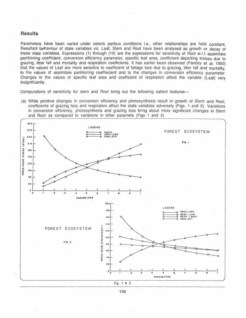
Results

Parameters have been varied under ceteris paribus conditions i.e., other relationships are held constant. Resultant behaviour of state variables viz. Leaf, Stem and Root have been analysed as growth or decay of these state variables. Expressions (1) through (10) are the expressions for sensitivity of Root w.r.t assimilate partitioning coefficient, conversion efficiency parameter, specific leaf area, coefficient depiciting losses due to grazing, litter fall and mortality and respiration coefficients. It has earlier been observed (Pandey et al. 1990) that the values of Leaf are more sensitive to coefficient of foliage loss due to grazing, litter fall and mortality, to the values of assimilate partitioning coeffiecient and to the changes in conversion efficiency parameter. Changes in the values of specific leaf area and coefficient of respiration affect the variable (Leaf) very insignificantly.

Computations of sensitivity for stem and Root bring out the following salient features-

(a) While positive changes in conversion efficiency and photosynthesis result in growth of Stem and Root, coefficients of grazing loss and respiration affect the state variables adversely (Figs. 1 and 2) . Variations in conversion efficiency, photosynthesis and grazing loss bring about more significant changes in Stem and Root as compared to variations in other paramets (Figs 1 and 2).

LEGEND

0.....__--a PHOTO FOREST ECOSYSTEM 0 0 GRAZ . LOSS - A .0. CONY. fFFI

2 .. .. FIG. I .. -.. ., .. .. .. .. .. .. :;) 0 2: z .. 10 .. .. ..

eo

30

0 0 ..

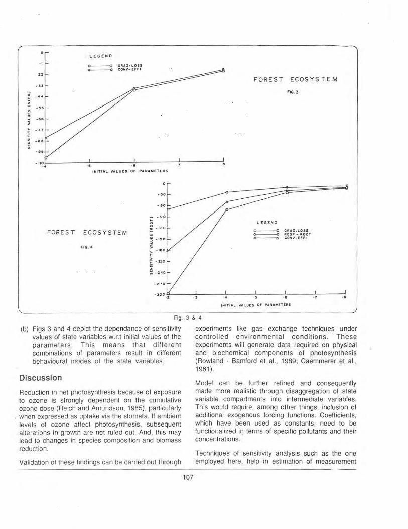
:1 .. .... ..

LEGEND

0 0 GRAZ•LOSS 0 0 COHV• EfFI

· ~ · 6

INITIAL VALUES Of PARAME T ERS

FOREST E CO SYSTEM

FIG . •

.. ~ .J:JO -' ~ > · 180 .... > ~ • 210 ;;; z :: .. 240

• 2 70

FOREST ECOSYSTEM

FIG.3

· 7 ·•

LEGEN D

~==~0 GRA Z .LOSS 0 0 RE SP- ROOT b 6 CONV, EFFI

·• INITIAL VAL UES OF PARAMETERS

Fig. 3 & 4

(b) Figs 3 and 4 depict the dependance of sensitivity values of state variables w. r.t initial values of the parameters. This means that different combinations of parameters result in different behavioural modes of the state variables.

Discussion

Reduction in net photosynthesis because of exposure to ozone is strongly dependent on the cumulative ozone dose (Reich and Amundson, 1985), particularly

. when expressed as uptake via the stomata. If ambient levels of ozone affect photosynthesis, subsequent alterations in growth are not ruled out. And, this may lead to changes in species composition and biomass reduction .

Validation of these findings can be carried out through

experiments like gas exchange techniques under contro lled environmental conditions. These experiments will generate data required on physical and biochemical components of photosynthesis (Rowland - Bamford et al., 1989; Caemmerer et al., 1981 ).

Model can be further ref ined and consequently made more realistic through disaggregation of state variable compartments into intermediate variables. This would require, among other things, inclusion of additional exogenous forcing functions. Coefficients, which have been used as constants, need to be functionalized if") terms of specific pollutants and their concentrations.

Techniques of sensitivity analysis such as the one employed here, help in estimation of measurement

----------------------------------------------------------------------· ----107

errors ahd in the study of effects of perturbation on · a dynamic system. It also helps in locating elements which suffer most due to data deficiences. Important processes which affect the system most, can thus be identified through sensitivity analysis. These processes can, then, be studied more closely in the laboratory and in the field. The method employed in the present research helps in setting priorties for model refinement and quantification for prediction purposes in environmental management.

References

Blank, L.W. (1985). A new type of forest decline in Germany. Nature, 341, 311-14.

Mclaughlin, S.B. (1985). Effects of air pollutants on forests. A Critical review. J. Air Pollut. Contr. Assoc., 35, 512-21 .

Blank, L.W., Roberts, T.M. and Skeffington, R.A. (1988). New perspectives on forest decline. Nature. 336, 27-30.

Barnes, J.D., Reiling, K., Davison. A.W. and Renner, C.J. ( 1988). Interactions between air pollutants and Winter stress. Environ. Pollut., 53, 235-54.

Barnes, J.D .. Eamus. D., Davison, A.W., Ro-Poulsen, H. and Mortensen, L. (1990). Persistent effects of ozone on needle water loss and wettability in Norway spruce. Environ. Pollut., 63(4), 345-63.

Chappelka, A.H., Chevone, B.l. and Seiler, J.R. (1988). Growth and physiological responses of yellowpoplar seedligns exposed to ozone and simulated acid rain. Environ. Pollut., 49, 1-18.

108

Barnes, R.L. (1972). Effects of chronic exposure to ozone on photosynthesis and respiration of pines. Environ. Pollut, 3, 133-8.

Yang, Y.S., Skelly, J.M., Chevone, B.l and Birch, J.B. (1983). Effect of long-term ozone exposure on photosynthesis and dark respiration of eastern white pine. Environ. Sci. Technol., 17, 371-3.

Reich. P.B. and Amundson R.G. (1985) . Ambient levels of ozone. reduce net phtosynthesis in tree and crop species. Science. 230, 566-70.

Jensen, K.F. and Dochinger, L.S. (1989). Response of eastern hardwood species to ozone, sulfur dioxide and acid precipitation. J. Air Pollut, Cont. Assoc .. 39, 852-5.

Pandey, J.S .. Shankar. A. , and Khanna, P. (1990). Investigations into behavioural modes of a forest growth model. J. Environ. Systems, 19(4), 349-354.

Rowland-bamford, A. J., Coghland,S. and Lea, P.J. (1989). Ozone induced changes in C~ assimilation, 0 2 evolution and chlorophyll fluorescence transients in bareley. Environ. Pollut,59, 129-40.

Caemmerer. V. and Farquhar, G.D. (1981 ). Some relationships between the biochemistry of photosynthesis and· the gas exchange of leaves. Planta. 153, 376-87.

Eamus, D. , Barnes. J.D., Mortensen. L., Ro-Poulson, H. and Davison, A.W. (1990). Persistent stimulation of C02 assimilation and stomatal conductance by summer ozone fumigation in Norway Spruce. Environ. Pollut. 63, 365-379.

BIOGEOCHEMICAL CYCLE OF CARBON FOR INDIA

A PRELIMINARY ESTIMATE V. K. Dadhwal and S. R. Nayak, INDIA

ABSTRACT

Sizes of major pools and fluxes of carbon for India (landmass and EEl) for mid-eighties were estimated by combining areas under different ecosystem types with their respective average values of carbon storage and transfer rates. Estimated pools sizes for rock. fossil fuels and terrestrial biospheric components (so il organic carbon. phytomass. litter) were 3371 x W'. 1262 x 10'4 and 323 - 390 x 10 14 g C. respectively. Forest phytomass had large uncertainty as volume/growing stock based estimates were 3.7 to 4.8 times lower than area based estimates. Terrestrial and oceanic net primary productivity and /itterfa/1 were 13.1- 15.5 x 10'4 • 3.47 x 10' 4 and 8.1- 9.7 x 10 14 g C a -1• Anthropogenic C0

2 released to atmosphere were 1.44 x 1014• 0.565 x (014 and 0.045 x 1014 g C a-1 for fossil fuel

use. fuelwood burning ond cement production. respectively.

Introduction

The concentration of C02 in the earth's atmosphere has increased from a pre-industrial level (ca. 1750) of 280 to 345 ppmv in 19841·2. The increase in C02

is due to alternation of biogeochemical cycle of carbon by various human activities, especially, fossil fuel burning, deforestation, landuse changes, etc., and may change earth's climate and influence human society in many profound ways3

. As international community moves towards reducing the release of C0

2 into atmosphere, national/regional estimates of

carbon cycle have assumed great significance. In this paper an attempt has been made to synthesize data from various sources to arrive at a preliminary estimate of major pools and fluxes of carbon cycle for India's landmass and its exclusive economic zone (EEZ) for mid-eighties.

A commonly adopted book-keeping approach, which uses areas under different ecosystem types and their average values of carbon storage and transfer rates to obtain biospheric components of carbon cycle has been followed. This has been supplemented with (a) production/consumption data to derive fluxes under anthropogenic control, such as fossil fuel and fuelwood burning, cement production and marine product harvest and (b) area, depth, and density of

109

rocktypes and estimates of carbon and hydrocarbon reservoirs to estimate pools of carbon in rocks and fossil fuels, respectively .

Ecosystem Areas

Information on area under seven major ecosystem

types (forest, agriculture, grazing lands, wastelands,

built-up-lands, wetlands and water bodies) and their

subclasses (Table 1 a) was obtained from various

sources. Area under agriculture (net area sown, other

tree crops, current and permanent fallows) and

permanent pqstures was based on land records4•

Area under16 forest-type categories of Champion and

Seth5 and alpine pastures was based on recent

remote sensing based inventory by Forest Survey of

India (FSI)6·7 . Areas of five subclasses comprising

wastelands was obtained from different sources, such

as, remote sensing inventories of culturable

wastelands and rocks, barren hills and ridges by

National Remote Sensing Agency (NRSA)8 ,

permanent snow cover by FSI7, hot and dry desert

by Gupta9 and coastal sands4•8 . Estimate of area

under 35 major rivers was based on their totallength10

(21.2 x 106 m) and a mean width of 50 m. Other

Table 1a. Estimates of ecosystem areas

Ecosystem Type Area (109m2)

FOREST 642.0

AGRICULTURE 1689.5 Net area sown 1417.7 Other tree crops 35.5 Current fallows 141 .3 Other fallows 95.0

GRAZING LAND 291 .2 Pastures & grazing lands 119.6 Alpine pastures 171.6

WASTELAND 345.2 Culturable wastelands 163.1 Non culturable wastelands

Permanent snow 50.1 Rocks & barren hills 27.5 Desert (hot and dry) 100.0 Coastal sands 4.5

BUILT· UP 180.0

WETLAND 5.0 Fresh water swamps 5.0

WATER BODIES 67.6 Streams & rivers 1.06 Lakes, reservoirs & Ponds 40.5 Estuaries 26.0

Statistics not available 67.3

TOTAL 3287.8

ecosystem areas considered were wetlands 11, built

up land12, water bodies13 and estuaries14

. The Indian EEZ has an areal extent of 2M sq. km. and includes 18 thousand sq. km. of coral reefs 15

• The rock type areas (7 categories, Table 1 b) for landmass was measured from a published map16

. EEZ was considered as made up of basalt and overlying sediments.

Major Pools

The rock carbon pools of the crustal compartment of landmass were estimated separately for carbonate and non-carbonate fractions from areas under 7 rock type (Table 1 b) and representative values for their depth17, porosity18 , density10•

17 and carbon fraction 17•19

.

Oceanic rock inorganic carbon pool was estimated similarly. These two pools (3771 x 1017 g C, Table 2) constitute the largest reservoir of carbon, which, however, has an insignificant contribution in context of current atmospheric build-up of C02 • The data on prognosticated fossil fuel reserves20 and their carbon fractions21 were used to estimate the carbon pools

110

1b. Rock-type areas

Rock Type Area (109 m2)

Unconsolidated Quaternary sediments 963.7

Semiconsolidated Cenozoic, lower

Mesozoic-upper Paleozoic sediments 448.2

Cenozoic, Mesozoic effusives 475.9

Cenozic-intrusives 54.8

Cenozoic, Mesozoic, Proteozoic-

metasediments 97.5

Cenozoic to Proterozoic, Azoic -

sediments and metasediments 311.4

Azoic-Basal crystalline 793.3

Statistics not available 143.0

TOTAL 3287.8

separately for coal, liginite and hydrocarbons (onshore and off-shore) . Fossil fuel pool of 1262 x 1014 g c (Table 2) has the potential of being transferred to atmosphere in a matter of decades at the current rate of their use.

In order to estimate biospheric pools from ecosystem areas, representative global values from Ajtay et al22

have been used. Ajtay et al used 14 main ecosystems types and a total of 33 categories . Because of differences in definitions adopted by Ajtay et al and the sources used here, in certain cases Indian data includes more than one category of Ajtay et al. In all such cases both high and lower values were used to obtain a probable range for this mixed class. The terrestrial biospheric pool carbon considered here (phytomass, litter and soil organic carbon) is of the order 323 - 390 x 1014 g C. In this the solid organic carbon (234 - 271 x 1014 g C) and standing phytomass (83 - 109 x 1 o 14 g C) are· the two dominant components. In case of phytomass, the major contribution (75 - 96 x 10 14 g C) is from forest.

Independent second estimates were made for the two largest terrestrial carbon pools, i.e., solid organic carbon and phytomass. Using the soil organic carbon estimates for 10 ecosystem types given by Schlesinger23 a pool size of 244 - 265 x 1014 g C was obtained. The two estimates, nearly match, as both are based on ecosystem areas. Estimate of forest phytomass carbon was also made using most recent forest volume/growing stock data24 and appropriate conversion factors25. This gave an estimate of only 19.94 x 1 014 g C in contrast to 75 - 96 x 1014 g C by area based procedure described earlier. The latter procedure may over estimate phytomass carbon since it did not consider the relative proportion of closed and open forests. Over estimation of forest phytomass carbon by point based destructive sampling over volume based inventory has also been noted by Bron and Lugo26

and Houghton et al25. The volume based estimates may be more representative as they are based on actual inventory of growing stock in 30.94 Mha out of total forest area of 64.2 Mha24. This also indicates the high pressure on forest biomass in India. If volume based estimates represent the correct situation, it would also call for making necessary adjustments in other pools and fluxes directly related to phytomass.

Major Fluxes

The flux between biospheric components for land (NPP : Net Primary productivity, litterfall) was also estimated from ecosystem areas (Table 1 a) and the carbon transfer rates of Ajtay et al22 (Table 3). The largest flux was NPP of land and was estimated

· between . 13.1 - 15 .5 x 1014 g c a-1 while litterfall was estimated to lie between 8.1-9.7 x 1014 g C a-1. Under the condition of steady state of litter pool, it should decompose to provide equal C02 release to atmosphere. However, the two main fluxes, namely, transfer of phytomass to herbivores and release of C02 to atmosphere due to decomposition of biomass. were not estimated for want of sufficient information. NPP of EEZ was estimated as 3.31 x 1014 g C a-1

and i~ based on 5 x 5 degree seasonal estimates27. NPP estimate for coral reefs was made separately using data from Wafar15 as 0.16 x 1014 g C a-1. The transfer of organic carbon by rivers to oceans was calculated from total sediment load of Indian rivers28·29

and annual discharge rate and discharge rate-organic

111

load regression30 as 0.17 and 0.14 x 1014 g c a-1, respectively.

The anthropogenic C02 release into atmosphere was derived from consumption of petroleum products, natural gas (including flared) and lignite20 and representative emission factors21 was 1.44 x 1014 g C a·1 while an additional release of 0.045 x 1 Q14 g C a-1 occurs due to cement production. The fuelwood burning estimate of 157 Mt24 would entail a further relase of 0.565 x 1014 g C a·1. As a significant proportion of fuelwood originates from litter pool, that component will represent a faster cycling only and not a net release into atmosphere.

Additional release of C02 from forests to atmosphere due to deforestation, shifting cultivation and forest fires are being quantified. Current deforestation rate of 47,000 ha a-1 (average between 1982 and 1986)6·7 is a significant drop from 147,000 ha a-1 between 1950-51 and 1975-7631. Shifting cultivation is practis~d mainly in north-eastern states and Orissa. In the former, the tofal area affected by shifting cultivation has decreased from 73 x 105 ha in 1975 to 63 x 105 ha in 1984. Annual area affected by shifting cultivation is of the order of 9.9 x 105 has. Houghton et aP2 attributed a net release of 0.33 x 1014 g C a-1 due to deforestation in India. Forest fires are another way of transfer of carbon from phytomass to air. An area of 5.7 x 105 ad was affected by forest fires during 1980-1985. Singh et aP3 estimated from a detailed analysis that central Himalayan forests ( 14.6 x 105 ha) are a net source of carbon to atmosphere (4.6 x 1012 g C a-1). Human harvest of organic carbon from the oceans as marine fish catch (1.5 Mt in 1985-86 4

) amounts to 0.017 x 10 14 g C a -1. This is lower bound as fishing boats of other countries also collect catch in Indian EEZ.

It may be pointed out again, that these estimates represent only a preliminary assessment of the sizes of pools and fluxes. This estimate can be improved and/or modified by incorporating the Indian data on vegetation (NPP and phytomass). using actual crop production estimates, estimating to transfer of C to consumers, and assessment of spatial and temporal variations in carbon cycle. The role of methane in the carbon cycle which contributes a small amount to total carbon but is an important greenhouse gas need also to be considered.

Table 2 Pools of Carbon (In 1014 g C)

LAND : Biospheric

Phytomass (Area based) 83.6 - 109.3

(Volume based) 28.5 - 33.2

Litter

Soil (organic C)

Other

Fossil fuels : Coal

Lignite

Hydrocarbon

Rock : Carbonate

Non-carbonate

OCEANS :

Fossil fuels : Hydrocarbons

Rocks : Carbonate

Non-carbonate

5.3 - 9.6

234.5 - 271.4

2119000

669000

696000

287000

1109.3

10.3

52.8

89.96

Table 3 Some Important annual fluxes of carbon (in 1014 g C a-1

)

NATURAL PROCESSES

NPP (over land)

Litterfall

River transport (Org.C)

NPP (Over oceans)

ANTHROPOGENIC (ca. 1985)

Fossil Fuel burning

Fuelwood burning

Cement production

Marine fish catch

Acknowledgements

13.1 - 15.5

8.1 - 9. 7

0.14 - 0.17

3.47

1.44

0.565

0.045

0.0017

VKD acknowledges receipt of financial support form Indian National Science Academy, New Delhi, under INSA Young Scientist Scheme. The authors acknowledge Dr.R .R. Navalgund, Head, Land Resources Division and Dr.Pranav Desai, Head, Meteorology and Oceanography Division for providing encourgement and taking keen interest in this study.

112

Reference

1. Keeling CD et al. (1976) Tellus 28 : 538 - 551

2. Neftel A, Moor E, Oeschger H and Stauffer B (1985) Nature 315 : 45-47

3. Bach W (1984) Our Threatened Climate, D. Reidel, Dordrecht, 368p.

4. Central Statistical organisation (1985) India 1985. Statistical Abstract. Govt of India (GOI), New Delhi, 690p.

5. Champion HG and Seth SK (1968) A revised survey of the forest types of India, GOI Publ , Delhi , 404p.

6. Forest Survey of India (1 987) The state of forest report 1987, GOI, Dehradun, 83p

7. Forest Survey of India (1989) The state of forest report, GOI, Dehradun, SOp

8. National Remote Sensing Agency (1985). Mapping of wastelands in India from satellite images, Project Report, GOI, Hyderabad.

9. Gupta R K (1986) In 'Ecosystems of the world. Vol. 12B : Hot Deserts and Arid Shrublands, B. M. Evenari, I. Noy-Meri, D.W. Goodwall, eds, Elsevier, Amsterdam, 55-1 00

10. Krishnan MS (1968) Geology of India and Burma, Higginbothams, Madras 536p.

11 . Fernando CH (1980) The fishery potential of manmade lakes in South-east Asia and some strategies for its optimisation, Biotrop Aniv. Puq.

12. National Land Use and Conservation Board (1988) National Land use Policy : Outline and action points, GOI,New Delhi 14p. ·

13. Ministry of Environment & Forests (1988) Directory of wetlands in India, GOI, New Delhi 58 p.

14. National Commission on Agriculture (1976) Report of the Nat. Comm. on Agric., GOI, New Delhi, Part VIII-Fisheries, 270p.

15. Wafar M v M (1986) Proc. of the Ind. Acad. Sci. Suppl. (Anim. Sci./Piant Sci.) , 19-43

16. Central Ground Water Board ( 1989). Hydrogeological map of India, GOI, New Delhi

17. Kempe S (1979) in 'Global Carbon Cycle', B Bolin, E T Degens, S. Kempe and P. Ketner, eds. J. Wiley & Sons, New York, 343-377.

18. Garrels RM, Mackenzie FT (1971) Evolution of Sedimentary Rocks, W W Norton, NY. 397p.

19. Garrels RM, Parry E A Jr (1974)1n 'The Sea, marine Chemistry', E Goldberg Ed. Vol. 5 : 303-336.

20. Tata Energy Researh Institute, (1987) , TERI Energy Data Directory and Yearbook, TEDDY, TERI, New Delhi.

21 . Rotty RM (1973) Tellus, 25 : 508-517

22 Ajtay GL, Ketner P and Duvigneaud P (1979) In 'The Global Carbon Cycle ' SCOPE-13, B. Bolin, E.T. Degens, S. Kempe and P. Ketner, Eds, J. Wiley & Sons, New York, 129-181.

23. Schlesinger WH (1983) In 'The role of terrestrial vegetation in the global carbon cycle : measurements by remote sensing·, J Wiley, New York, 111 -127.

113

24. Lal B (1989) India's Forests, Myth and Reality. Nataraj Publ. Dehradun, 304p.

25. Houghton R A et al. (1985) Nature 316 : 617-620

26. Brown S and Lugo AE (1984) Science 223 : 1290 -1293

27. Cushing D H (1973) In 'The Biology of the Indian Ocean', B. Zeitzschel, S.A. Gerlach eds, Chapman & Hall, London, 475-486.

28. Subramanian V. Sitasawad R. Abbas N and Jha P K (1987) J. Geol. Soc. India, 30 : 335 - 355.

29. Subramanian V, Biksham G and Ramesh R (1987) J Geol Soc. India, 30 : 393-401 .

30. Schelesinger W H and Melack JM (1981) Tellus, 33 : 172 - 187

31 . Central Forestry Commission (1980) India's Forests 1980, GOI, Delhi, 28p.

32. Houghton R A et al. (1987) Tellus, 39B: 122 -125

33. Singh J S, Tiwari A K and Saxena A K (1985) Environ. Conserv. 12 : 67 - 69.

RESPONSE OF THE EARTH'S ATMOSPHERE TO INCREASES IN GREENHOUSE GASES . FUTURE

PROJECTIONS OF CLIMATE CHANGE M. La/,

There has been much concern that increased anthropogenic release of trace gases such as C02 ,

CH4 , Np, and CFCs from industrial, agriculture and domestic activities will, in addition to enhancing the greenhouse effect, significantly modify the chemical composition of the atmosphere. This could lead to a substantial reduction in the density of stratospheric ozone with consequent climatic effects. Recent findings linking the rise in chlorine and oxides of nitrogen to the destruction of stratospheric ozone have stimulated renewed interest in the development of interactive chemistry-climate models. Such models may be used to diagnose the combined effect of physical and chemical processes, thus including both direct and indirect radiative effects, and to assess potential changes associated with future trace gas emissions to the atmosphere.

To obtain a new perspective on the effect of stratospheric chlorine and nitrogen on ozone photochemistry, and its implications for the thermal structure of the Earth-atmosphere system. a onedimensional chemical-radiative-transport model has been developed at the Indian Institute of Technology, Delhi. The model combines the radiative-convective (RC) model with a photochemical transport model. The model atmosphere is divided into 16 vertical layers extending from the surface upto 55 km and represents the annual mean thermal structure of the global atmosphere at equilibrium. Starting with a prescribed vertical distribution of temperature, cloud altitude and fraction and chemical composition of the atmosphere. the photochemical sources and sinks and the associated solar and thermal flux divergences are computed for each layer using a time-marching method to infer the surface and atmospheric temperatures. The radiative effects of optically active

trace gases, namely C02, 0 3, CH4 , Np and CFCs.

114

INDIA

are treated in addition to that of water vapour. The solar radiation absorbed by the model atmosphere is parameterized as a function of altitude such that the form of the solution and the coefficients involved are based on accurate multiple scattering computations. Long wave radiative flux calculations use an approximate method of accounting for the integration of the optical path length over all solid angles.

The phtochemical model coupled with the RC model includes a series of relevant chemical reactions responsible for altering the concentration of ozone and other trace constituents in the upper atmosphere. Four families of species, namely, Ox• NOx• Clx· and HOx are simulated. CFCs, CH4 , Np, and Hp are treated individually in the model. The formation of Ox resulting from the photo-decomposition of molecular oxygen as well as its destruction by the Chapman reactions and the catalytic effects of HOx• NOx• and Clx are explicitly included. The spectral distribution of the solar irradiance required to compute photodissociation rates associated with phtochemical reactions is taken from Brasseur and Simon (1981) and WMO (1985). The absorption cross-sections and the rate constants for the reactions are based on those recommended by the NASA Panel for Data Evaluation (DeMore et. al. , 1985, 1987, 1990). For further details on the model, the reader is referred to Lal and Holt (1991).

The 'business-as-usual' scenario (BAU) for past and future trace gas perturbations used in this study is based ~n WMO (1985) and Ramanathan et. al. (1987) and is in close proximity to that described in IPCC (1990). With rat ification of Amended Montreal Protocol in 1990, all the countries are expected to freeze any further prodcution of CFCs now and to reduce the production of CFCs by 50% of their 1986 level in the year 1995 followed by a complete phase-out in

the year 2000 (the developing countries are allowed a 1 0 year delay period in compliance with these controls). We have therefore also adopted a Amended Montreal Protocol scenario (MP) for the future trace gas concentrations in our numerical simulation. The direct radiative effects of the background atmospheric aerosols are included by appropriately prescribing the single scattering albedo, aerosol extinction and the asymmetry factor. With a view to understanding the nature and magnitude of the 'signature' of stratospheric aerosols of volcanic origin on the surfacetroposphere-stratosphere temperature, we have also used the optical properties and vertical structure of the aerosol clouds due to the 1982 El Chichon eruption. A series of numerical experiments have been performed with the coupled chemical - radiative -transport model to assess the sensitivity of interactive stratospheric chemistry to projected perturbations of trace gas concentration in the atmosphere.

Our model results indicate that the greenhouse warming at the surface for the period 1850-1986 due to increases in trace gases, resulting from the direct raditive effect alone, is 0.61 K. This global mean warming is enhanced to 0. 72K when we take into account the indirect thermal effects caused by the net ozone change due to the interactive photochemistry. In the stratosphere, the increased loss of energy to space caused by the radiative effect of increase in trace gases leads to local cooling. Further, the trace gas increase from the year 1850 to the year 1986 could have already contributed to a decline in the stratospheric ozone between 30 to 48 km, reaching a maximum of 10.7% at 42 km, although a net increase in the total column amount is observed. These changes in the vertical ozone distribution are notably reflected in the surface and atmospheric temperatures. The stratospheric cooling is substantially enhanced by the indirect effect of the local ozone decreases resulting from the radiativephotochemistry interaction.

Fig.1 depicts the model simulated changes in the global mean temperature at three selected levels in the atmosphefe as a function of time for the transient

115

response experiment (time-dependent model runs). The surface warming rises steadily except for a brief period when it is interrupted by a temporary cooling of O.BK due to the increase in dust load resulting from the El Chichon volcanic eruption. The recovery period from the sudden cooling is a little over 2 years. The modelled response to El Chichon is greater than the observed cooling, probably because of concurrent background warming associated with an El Nino event of 1982. The predicted global mean surface warming by the year 2050 for scenario BAU is 2.6K. This surface warming is likely to be marginally reduced to 2K with the restrictions on CFC production (scenario MP).

The volcanic eruption also caused marked warming of the lower stratosphere and the model predicted maximum warming ·of about 4.2K at 22 km. Interestingly, at this level, no significant warming/ cooling trends as a result of. trace gas increases are predicted. In the middle stratosphere (40 km), the temperature drops progressively except for a temporary warming of 0.8K in the year 1983 following the El Chichon eruption. For the scenarios BAU and MP, the stratospheric cooling at 40 km in the year 2050 is predicted to be about 16.4K and 12.6K respectively. Limited support for the model results comes from radiosonde/Satellite data for 1964-87, which indicate a cooling trend for the middle stratosphere (30 km) in the mid to high latitudes (25°N - 90°N) of the Northern Hemisphere. The stratospheric cooling projected for the middle of the next century as a consequence of greenhouse warming due to increases in atmospheric trace gases (Scenarios BAU and MP) could lead to substantial perturbations in the dynamics of the stratosphere.

For scenario BAU, a local maximum ozone depletion of 43% is predicted in our time-dependent model calculations at about 40km for the year 2050. The decreased solar absorption due to the ozone decline cools the stratosphere. This cooling is further enhanced by the reduction of IR absorption (by the 9.6 Jlm band of 0 3) in the stratosphere of surfacetroposphere emissions. For scenario MP, the local

~

~ ......___,

Q)

01 c 0

...c u Q) 1..... ::J -0 1..... Q)

0..

E Q)

1-

5

0

-5

-10

-15

0 co ())

Suriace __ ---- - .--- _____. ---------22 km

- - ---- - - ---=--==-==-==:--===-==-=-

BAU Scenario -

M P Scenario --

0 ()) ())

0 0 0 N

0

0 N

Year Fig. 1

116

0 N 0 N

0 f'l')

0 N

0 "'<t 0 N

0 l{)

0 N

maximum ozone depletion in the mid-stratosphere is restricted at only 17% in our model calculations. The total ozone column mixing ratio is predicted to decline by 12.7% by the year 2050 in our transient response model calculations for scenario BAU. With emission restrictions on CFCs as incorporated in scenario MP,

this decline in total column ozone for the year 2050 would be limited to only 2.9%. The expected decline

is found to be more rapid (double the rate prior to the year 2015 for scenario BAU) in the last three decades of the model calculation.

The findings based on calculations using our onedimensional interactive chemical-radiative-transport

model thus confirm that increasing concentrations of anthropogenic trace gases should considerably

modify the ozone and temperature distribution in the atmosphere. Photochemical processes seem to dominate in the middle and upper stratosphere. Large variations in the local concentration of ozone in the · middle stratosphere (near 40 km) are predicted for the year 2050 based on our projections of future emissions of trace gases. Recent control measures on emission of CFCs under the amended Montreal Protocol agreement will limit the CFC growth rate resulting in a smaller impact of CFCs on future greenhouse warming. The large local 0 3 decline and associated stratospheric cooling could however, still cause changes in the atmospheric circulation. The

surface warming projections presented here represent the global mean warming and therefore indicate general trends rather than specific geographical

variations. Regional warming tendencies can only be

fully considered using a three-dimensional dynamical model incorporating all the physical and chemical

interactions described in our simple model. As yet, such models do not exist. Efforts are currently underway at liT Delhi to develop an Integrated Clim.ate Model consisting of modules dealing with emission, concentration, Biota, Carbon cycle, Photochemistry, Radiation and Ocean. The modules aggregated within a dynamic system with discrete time steps should provide us regional climate changes in terms of greenhouse warming and associated sea

level rise for the future.

117

References

Brasseur, G. and Simon P.C. (1981) Stratospheric Chemical and thermal response to long-term variability in solar UV irradiance, J. Geophys. Res., 86, 7343 - 7362.

Demore, W.B., Margitan, J.J., Molina, M.J., Watson,

R.T., Golden, D.M., Hampson, R.F., Kurylo, M.J. Howard, C.J. and Ravishankara , A.R. (1985) Chemical kinetics and photochemical data for use in stratospheric modeling, Evaluation 7, JPL Publ. 85-37, pp 217.

Demore, W.B., Molina, M.J., Sander, S.P., Golden,

D.M., Hamson, R.F., Kurylo, M.J., Howard, C.J. and Ravishankara, A.R. {1987) Chemical kinetics and photochemical data for use in stratospheric modeling, JPL Publ. 87-41, pp. 317.

Demore, W.B., Sander, S.P., Golden, D.M., Molina, M.J., Hampson, R.F., Kurylo, M.J., Howard, C.J. and Ravishankara, A.R . { 1990) Chemical kinetics and photochemical data for use in stratospheric modeling JPL Publ. 90-1,pp. 217.

Intergovernmental Panel on Climate Change (1990) Scientific assessment of climate change, WMO/UNEP Rep; Sept. 1990, pp. 365.

Lal, M. and Ho.lt, T. (1991) Ozone depletion due to increasing anthropogenic trace gas emissions : The role of stratospheric chemistry and implications for future climate, CLIM.RES., (in Press).

Ramanathan, V., Callis, L., Cess, R., Hansen, J., Isaksen, 1., Kuhn, W., Lacis, A., Luther, F., Mahlman, J., Reck, R. and Schlesinger, M. (1987) Climatechemical interactions and effects of changing atmospheric trace gases, Rev. Geophys., 25(7), 1441-1482.

World Meteorological Organisation (1985) Atmos

pheric ozone : Assessment of our understanding of the processes controlling its present distribution and change, Rep. 16, Global Ozone Res. and Moni. Proj., Geneva, Chap. 3, 88-100.

AGROSPHERE - ATMOSPHERE INTERFACE : SCOPE OF POSSIBLE CONTRIBUTIONS FROM SATELLITE

BASED MEASUREMENTS Rajendra Kumar Gupta, INDIA

ABSTRACT

The study of agroecosystems needs the information at d istrict unit scale. The sensitivity of Normalized Difference Vegetation Index (NOV!) and Ratio Vegetation Index (RVI), for a d istrict having 94.9% agriculture area under wheat, as a function of crop growth cycle has been d iscussed. Towards interrelating atmospheric air temperature based crop growth indicators (Growing Degree Days for maximum and mean air temperatures) with crop based NOV/ and RVI, the study revealed that relationship was significant at 98 to 99% confidence level making NOV/ and RVI an indicator of agrosphere-atmosphere processes.

Introduction

The agrosphere aspects (Soil and its water status characteristics) could be assumed to be homogeneous at 10 km spatial scale. The atmospheric processes could be considered homogeneous over 100 km spatial scale. As the agrosphere and atmosphere intermodulates each other, the geometric mean of these two spatial scales (1 km} could be the spatial resolution over which the observ.ations have to be made for agrosphereatmosphere interaction studies. The 1 .1 km spatial resolution of Advanced Very High Resolution Radiometer (AVHRR} provides this capability . This paper discusses the relationship among AVHRR/ NDVI, AVHRR/RVI and the Growing Degree Days (GDDs) 1 expressed by,

GOD = ~ [T - (Tc) , ] ........... .... (1} I

Where 'T' is a particular air temperature (minimum or maximum or mean} and Tc is the corresponding critical temperature (below which plant growth becomes non-positive} for the 'i'th stage of crop growth cycle. The study refers to 1986-87 rabi season over Ludhiana district (30. 75° - 31 o N latitude and 75.5- 76.5°E longitude). The district had 84.98% area under agriculture, of which 94.9% area was under wheat cultivation.

Computation of GODs

Average sowing date for the district was taken as the date which witnessed prominent fall of the ratio of

118

maximum soil temperature at 0.05m depth to that of air from 1.0 over many days. With this criteria the average sowing date worked out to be 23 Nov. 1986 and table 1 gives the dates for the initiation of various phenological stages of wheat growth cycle. GODs have been computed using maximum, minimum and mean temperatures data obtained form the Ludhiana agromet observatory.

Table 1 : Average Dates for the Various Critical Growth stages of Wheat in Ludhiana District

Crop Stage Date

Emergence 30 Nov. 1986

Crown Root 14 Dec. 1986

Initiation

Late Tillering 07 Jan 1987

Jointing 27 Jan 1987

Heading 16 Feb 1987

Flowering 26 Feb 1987

Milking 08 Mar. 1987

Dough 23 Mar 1987

Maturity 07 Apr. 1987

Harvesting 15 Apr. 1987

Average day and night temperatures were computed using duration of sunshine hours as forcing parameter and by fitting two cosine curves to maximum and minimum temperatu res2 . Arithmetic average of these day and night temperatures was taken as Computed Mean Temperature. GODs were computed for

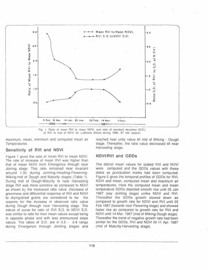
J ·O _...._.. Mean RVI to Mean NOVI. 3 .0

• .. • RVI S .O. toNOVI S.D.

> 2 ·~ 2·!> 0 > z c 0 0 z Q)

~ -2 · 2·0 0

0 - 0

> (J)

cr 0 -c: 1.~ 0 I·~ > Q)

~ cr -- 0 0

0 1.0 1·0 C!. 0 (J)

cr 0

0 cr

0·~ 0 ·~

4 Dec . 16 Dec. 14 Jan . 2~ Jan. 22 Feb. 14 ,_.or. 11 Apr.

----1986--~~----------------1987'------------------

Fig. 1. Ratio of mean AVI to mean NDVI, and ratio of standard deviation (S.D.) of AVI to that of NDVI for Ludhiana district during 1986 - 87 rabi season

maximum, mean, minimum and computed mean air Temperatures.

Sensitivity of RVI and NDVI

Figure 1 gives the ratio of mean RVI to mean NDVI. The rate of increase of mean RVI was higher than that of mean NDVI from Emergence through near Joining stage. This ratio remained near invariant around 1.32 during Jointing-Heading-Flowering Milking-mid of Dough and Maturity stages (Table 1 ). During mid of Dough-Maturity to near Harvesting stage RVI was more sensitive as compared to NDVI as shown by the increased ratio value. Decrease of greenness and differential response of RVI and NDVI to drying/dried grains are considered to be the reasons for the increase in observed ratio value during Dough through near Harvesting stage. The nature of curve for ratio of RVI S.D. to NDVI S.D. was similar to ratio for their mean values except being in opposite phase and with less pronounced slope values. The ratios of S.D. are in 0.5 0.9 range during Emergence through Jointing stages and

119

reached near unity value till mid of Milking - Dough stage. Thereafter, the ratio value decreased till near Harvesting stage.

NDVI/RVI and GODs

The district mean values for scaled RVI and NDVI were computed and the GODs values with these dates as punctuation marks had been computed. Figure-2 gives the temporal profiles of GODs for RVI, NDVI and mean, computed mean and maximum air temperatures. Here the computed mean and mean temperature GODs depicted smooth rise unit! 25 Jan 1987 (say Jointing stage) unlike NDVI and RVI. Thereafter the GODs growth slowed down as compared to growth rate for NDVI and RVI until 22 Feb 1987 (towards near Flowering stage) and showed faster rise as 9ompared to growth rate for RVI and NDVI until14 Mar. 1987 (mid of Milking-Dough stage). Thereafter the trend of negative growth rate had been similar for the GODs, RVI and NDVI till 11 Apr. 1987 (mid of Maturity-Harvesting stage).

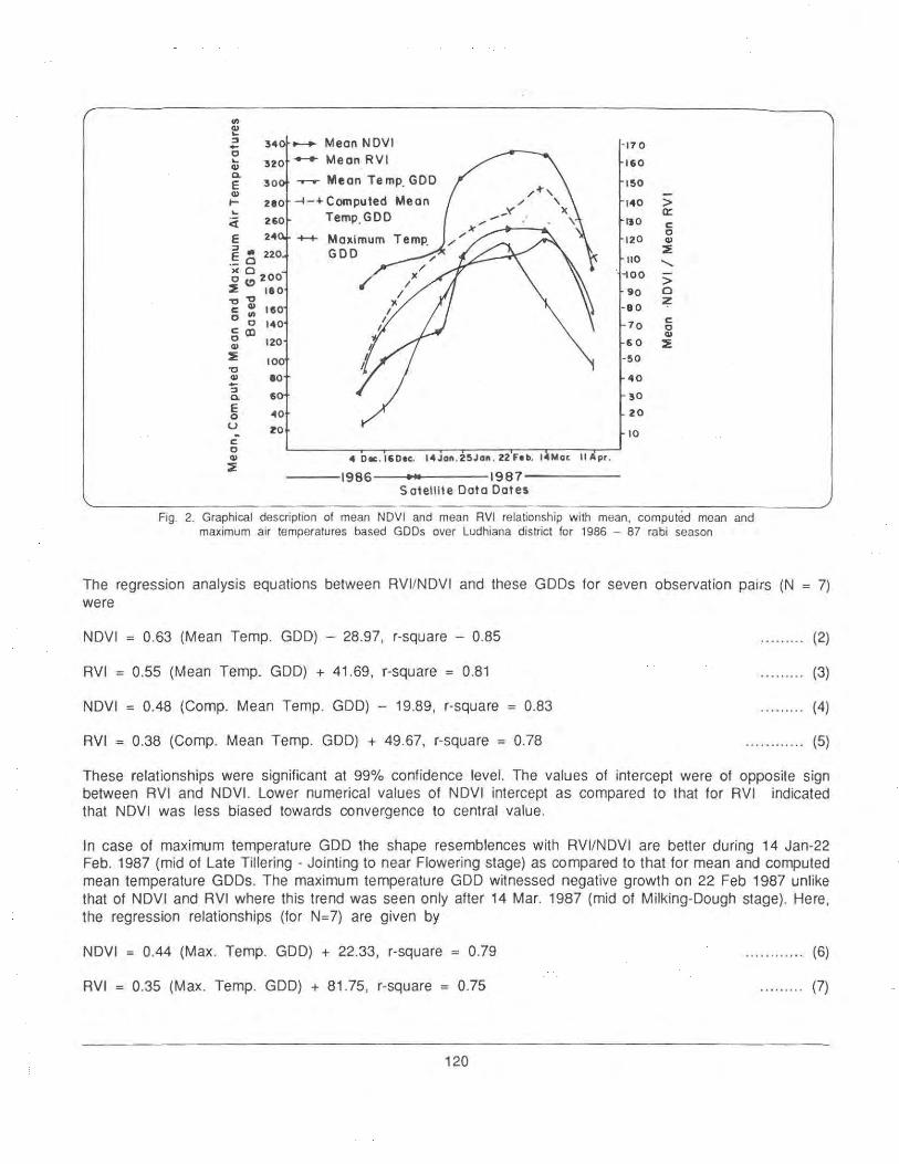
en ~ ::J 340 -Mean NOVI - 170 -0 -+-+Mean RVI .... 320 160 Q) Q.

~Mean Temp_ GOO E 30 150 Q)

-4-+ Computed Mean 1- 140 > .... Temp_ GOO a:: <i BO c E 24 +-+ Maximum 120

0 Q,)

g • 220 GOO ~

·- 0 110 ........ ><0 -roo 0 C) 200 > ~ 180 90 0 -o"O z c Q,) 180 -80 o en c 0 140 70 0 ~CD Q,)

Q,) 120 60 ~ ~ 10 -50 "0 Q,) 10 40 -::J

60 30 Q.

e 0 40 20 u 20 c 10

0 Q,) 4 oec . I6Dec. 14Jon. 25Jon . 22 Feb. 14M or. II Apr. ~

1986 1987 Satellite Octo Dotes

Fig. 2. Graphical description of mean NOVI and mean RVI relationship with mean, computed mean and maximum air temperatures based GODs over Ludhiana district for 1986 - 87 rabi season

The regression analysis equations between RVI/NDVI and these GODs for seven observation were

NDVI = 0.63 (Mean Temp. GOD) - 28.97, r-square - 0.85

RVI = 0.55 (Mean Temp. GOD) + 41 .69, r-square = 0.81

NDVI = 0.48 (Comp. Mean Temp. GOD) - 19.89, r-square = 0.83

RVI = 0.38 (Comp. Mean Temp. GOD) + 49.67, r-square = 0.78

pairs (N 7)

(2)

(3)

(4)

············ (5)

These relationships were significant at 99% confidence level. The values of intercept were of opposite sign between RVI and NDVI. Lower numerical values of NDVI intercept as compared to that for RVI indicated that NDVI was less biased towards convergence to central value.

In case of maximum temperature GOD the shape resemblences with RVI/NDVI are better during 14 Jan-22 Feb. 1987 (mid of Late Tillering - Jointing to near Flowering stage) as compared to that for mean and computed mean temperature GODs. The maximum temperature GOD witnessed negative growth on 22 Feb 1987 unlike that of NDVI and RVI where this trend was seen only after 14 Mar. 1987 {mid of Milking-Dough stage). Here, the regression relationships (for N= 7) are given by

NDVI = 0.44 (Max. Temp. GOD) + 22.33, r-square = 0.79

RVI = 0.35 (Max. Temp. GOD) + 81 .75, r-square = 0.75

120

....... ..... (6)

(7)

These relationships were significant at 99% and 98% confidence levels for NDVI and RVI respectively. In case of minimum temperature GOD, the shape proximity between GOD and NDVIIRVI curves was not seen during 14 Jan-14 Mar. 1987 and thereafter GOD and NDVIIRVI behaved in opposite phase. The regression analysis between GOD and RVI/NDVI became significant at 99% confidence level only when the analysis had been restricted to mid of Milking Dough stage (14 Mar. 1987). Minimum air temperature is not expected to play any significant role after this stage of crop growth cycle. The regression equations for analysis restricted to 14 Mar. 1987 (N = 6) were

NDVI = 0.44 (Min. Temp. GOD) - 4.30, r-square = 0.84

RVI = 0.35 (Min. Temp. GOD) + 61 .41 , r-square = 0.83

(8)

········· · ·· (9)

Conclusions

For a primarily wheat growing district the RVI was more sensitive as compared to NOVI during Emergence through near Jointing and Dough through near Harvesting stages. Further, RVI had less S.D. as compared to that of NDVI during these crop growth stages making it a better integrator of diversity in agriculture for district level studies. As RVI and NOV! are related by equation

NOV I = (RVI-1) I (RVI + 1) · · ····· ·· (10)

RVI could be used till near Jointing and after Dough stage and converted to NOV I using equation (1 0) to enable its joint use with NDVI during the Jointing through Milking stages as NOVI is considered to be better corrected for atmospheric effects as compared to RVI.

District level mean NDVI as well as RVI had been good indicator of crop agrometeorological growth (agrosphere · atmosphere) processes and where very

121

significantly related with mean and maximum temperature GODs for the whole of crop growth cycle. The relationship between NDVVRVI and minimum temperature based GOD remained significant only upto mid of Milking-Dough stage. The regression coefficients for NDVI were always better than that for RVI but RVI had better sensitivity than NDVI during Vegetative and Maturity phases. As the regression coefficients for RVI and NDVI were not very different, RVI together with NOVI could be used for district level crop productivity assessment.

References

1. Gupta, R.K., 1989, Satellite Vegetation Indices as District Level Agromet Growing Degree Days Indicator, Ph.D. thesis submitted to Jawaharlal Nehru Technological University, Hyderabad, 361 pp.

2. Food and Agriculture Organisation, 1980 : Report on the Agro-Ecotogical zones project : World Soil Resources Report No.48, Vol. IV : Methodology and Results for Southeast Asia, UN/FAO, Rome, 39 p.

NUMERICAL MODELLING OF TIDAL

CIRCULATION IN AN ESTUARY P.C. Sinha, INDIA

Introduction

Tidal forcing is one of the main energy sources for the estuarine ecosystem. The resulting motion and associated phenomena may have significant effects on productivity. The importance of circulation in estuarine systems and the fact that it is often omitted from ecological models speaks well of the difficulties in coupling hydrodynamic and ecological models. However, it is important to get a good estimate of how the complex circulation in an estuary affects the advective transport of ecological subsystems.

Keeping these objectives in mind a preliminary study has been undertaken to develop a depth averaged numerical hydrodynamic model of tidal flow in the Hooghly estuary. We consider the lower part of the Hooghly estuary between Diamond Habour and the Bay of Bengal at Saugor including Frasergunj channel creek to the right of Saugor Island (Fig. 1). The other numerical studies undertaken for the region include the investigations by McDowell and Prandtl (1972). Debnath and Chatterjee (1981) and Chatterjee (1983). The non-linear terms are included in the model formulation and the solution procedure of the model equations uses a conditionally stable semi-explicit finite difference scheme. Numerical experiments are performed with the help of this model to study the tidal elevation, tidal currents and residual currents. The computed water levels are found to be in agreement with the observed features in the estuary.

Formulation of the Model

Neglecting the sphericity of the earth's surface a system of rectangular Cartesian coordinates is used in which the origin is at the mean water level ; positive x-axis points eastward, positive y-axis points northward and positive z-axis is directed vertically upwards. The displaced position of the water surface is given by z = ~ {x , y, t) and the position of the estuary floor by z = - h (x, y) .

The pressure is taken as hydrostatic and the bottom friction is parameterized in terms of a conventional

122

quadratic law. Here, we neglect the surface stress term and the only forcing is provided by the astronomical tide of the adjacent Bay of Bengal.

The basic hydrodynamic equations of continuity and momentum in the vertically integrated form (Dube et al., 1985) are

a~; a a - + -(Hu) + -(Hv) = 0 .... .. (1) at ax ay

au+ u au + v av- fv = - g a~;- J.. ktu (u2+v2)¥2} at ax a y ax H ...... (2)

av + u ~+ v ~+ fv = - g a ~; - J..:{c(U (u2 + v2)¥2} at ax a y a Y H . . . . . . (3)

Where

u, v = x andy comps, of the depth averaged velocity

H = total depth, ~ + h

f = Coriolis parameter for latitude 22°N.

c, = bottom friction coefficient , 2.0 x 1 o-3

g = acceleration due to gravity.

Boundary and Initial Conditions

At the water-land interface the transport normal to the coastline is taken to be zero so that

u = 0, along y directed boundaries} for t ~ O (4)

v = 0, along x directed boundaries

The amplitude and phase of the M2 tide for seven stations of the analysis area is taken from a time series analysis in the form

2.40 cos (w t - 160°) at Dadanpara

2.43 cos (w t - 184°) at Saugor

2.20 cos (w t - 170°) at Frasergunj

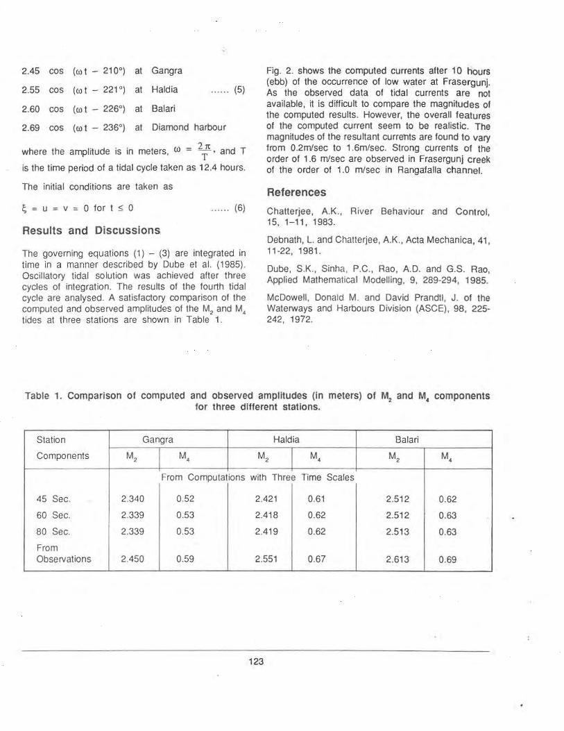
2.45 cos (wt - 210°) at Gangra

2.55 cos (w t - 221 °) at Haldia ...... (5)

2.60 cos (w t - 226°) at Balari

2.69 cos ( (J) t - 236°) at Diamond harbour

where the amplitude is in meters, w = 2Trt • and T

is the time period of a tidal cycle taken as 12.4 hours.

The initial conditions are taken as

~ = u = v = 0 for t ~ 0 .... .. (6)

Results and Discussions.

The governing equations (1) - (3) are integrated in time in a manner described by Dube et al. (1985). Oscillatory tidal solution was achieved after three cycles of integration. The results of the fourth tidal cycle are analysed. A satisfactory comparison of the computed and observed amplitudes of the M2 and M4 tides at three stations are shown in Table 1.

Fig. 2. shows the computed currents after 1 0 hours (ebb) of the occurrence of low water at Frasergunj. As the observed data of tidal currents are not available, it is difficult to compare the magnitudes of the computed results. However, the overall features of the computed current seem to be realistic. The magnitudes of the resultant currents are found to vary from 0.2m/sec to 1.6m/sec. Strong currents of the order of 1.6 m/sec are observed in Frasergunj creek of the order of 1.0 m/sec in Aangafalla channel.

References

Chatterjee, A.K., River Behaviour and Control, 15,1-11,1983.

Debnath, L. and Chatterjee, A.K., Acta Mechanica, 41, 11-22, 1981.

Dube, S.K., Sinha, P.C., Aao, A.D. and G.S. Aao, Applied Mathematical Modelling, 9, 289-294, 1985.

McDowell, Donald M. and David Prandtl, J. of the Waterways and Harbours Division (ASCE), 98, 225· 242, 1972.

Table 1. Comparison of computed and observed amplitudes (in meters) of M2

and M4

components for three different stations.

Station Gangra Haldia Balari

Components M2 M4 M2 M4 M2 M"

From Computations with Three Time Scales

45 Sec. 2.340 0.52 2.421 0.61 2.512 0.62

60 Sec. 2.339 0.53 2.418 0.62 2.512 0.63

80 Sec. 2.339 0.53 2.419 0.62 2.513 0.63

From Observations 2.450 0.59 2.551 0.67 2.613 0.69

123

87• Set aa• oo

•o·

HOOGHL Y ESTUARY

4000·t.· i:i ... ,;,. QCI2t:::=4i:3ro ....

0 9Q•

,,. sd

Fig. 1. Hooghly estuary

124

l - 0

I

I t ~t " I I I I ~ r~

11/lt~~ I I I ~ #

& I ~ f I I ~ I tl I I ' I I t I

11111111 ""'~ 11 "-IIIJ lttll ';~"IIIJJitll ll,lt#t#l'l~llll

.. ,r~;.;IJJIJII/1 '~t *"'' \~~J/1 "'~1t~~;ri1J '~,,,¥'

11 ~ 1

t + t ~It~\ \lj/1 '( " 1 • ; \ ~ # I t ...... ~ ., I """'~~\~~~~\I 1/rl

• ~_:-~~~j_J~_, r-~~~ Oadanpara

FIG -'l- Tidal stream current (ebb)

Fig. 2. Tidal stream current (ebb)

125

• Oiarno11d Hurbour

SEASONAL VARIATION OF ATMOSPHERIC PARTICULATES AND SCATTERING OF UV-B

RADIATION B.S.N. Prasad, N. Muralikrishnan and H.B. Gayathri, INDIA

Abstract

Increased scattering of the biologically effective solar ultraviolet radia tion (UV-8) due to enhanced atmospheric pollutants has been reported from field measurements' ·3• Similar results are obtained based on model calculations combined with experimental obseNation!f. We have examined the seasonal variation of the ground reaching global UV-8 flux at a /ow latitude. non-industria/location. The results show the role of seasonally varying atmospheric aerosols and particula tes in producing enhanced scatter of the solar UV-8 radiation in summer months. This finding complements the above mentioned results on the increased UV-8 scattering in the presence of atmospheric pollutants.

As part of Indian Middle Atmosphere Program (IMAP), global UV-B flux (sum QJ direct and diffuse radiations) is mesured at Mysore (12 .6° N, 76.6°E) which is a plateau station free from industrial pollution. The UV-B photometer radiometer setup deployed at Mysore (since April 1987) consists of a flux integrating sphere, four narrow band interference filters mounted on a rotating wheel, photomultiplier tube and the associated power supply. The central wavelengths of the filters as per the manufacturer's specification are 280, 290, 300 and 310 nm. The filters. however, have maximum transmission at 283, 295, 303 and 311 nm.The half power band width of the filters is less than 10 nm.

The instrument is to be calibrated periodically for converting the photometer output (mV) into absolute flux (W cm·2 nm -1) . The calibration was done in July, 1987 at the National Physical Laboratory, New Delhi using the UV-Spectroradiometer Model 742 of Optronics Laboratories. USA. The results of our study for the period January to December, 1988 are presented here. Regular UV-B data collection at Mysore is possible only during post -monsoon and pre-monsoon months, from October to May in any year. Monsoon period lasting from May/June to September/October is not conducive for recording the UV-B data.

Figure 1 shows the daily values of UV-B (mV) at the wavelength A. = 283 nm and for the solar zenith angles X = 40° , 50° and 60° for the pre-noon (AM) period. A marked diurnal asymmetry in the UV-B data for pre-noon and after-noon {PM) periods is noticed. but the PM data are not shown here. Also shown in

126

Fig.1 is the annual variation of ozone concentration (DU) at Kodaikanal (10.2° N, 77.5° E) from the Dobson spectrophotometer operated by the India Meteorological Department. The annual ozone variation shown here is based on the statistical analysis of sixteen years of data5 . The generally accepted picture of the anticorrelation between the ground reaching .UV-B flux and atmospheric ozone is evident from a comparison of the UV-B flux and ozone data in Fig.1 . However, we note a steeper decrease (January-May) or increase (October - December) in UV-B flux at the smaller zenith angle 40°. This is because of the direct and diffuse components in the global UV-B flux be ing not the same throughout the day. These components are nearly equal (50% each) for the solar zenith angle x = 0° and the diffuse component increases (while the direct component decreases) for larger zenith angles6 . It is noticed that the degree of variation of the measured global UV-B flux with ozone is less when the contribution of diffuse component is more than that due to direct component. This is also verified using the flux data of direct and d iffuse radiations from the model results of Dave and Halpern7 .

We have used the hourly ozone data for Kodaikanal to examine the seasonal variation of the dependence of the global UV-B flux on atmospheric ozone. Ozone data at Kodaikanal are recorded six times a day at x = 34°, 58.5° and 68° , both during the pre-noon and after-noon period. However, all the six observations may not be possible on all the days of the year due to adverse weather conditions. Also the times (1ST) of observations of the daily ozone data do not correspond to the exact times of the above mentioned

solar zenith positions but are very close. We have compared the UV-B flux data at Mysore with the ozone data at Kodaikanal for the same time (1ST) of the day. Because of this, a limited number of UV-B and ozone data are available for comparison although both UV-B and ozone data are recorded throughout the day.

Figure 2. shows the plots of UV-B flux (for I.. = 283 nm and 303 nm) versus the corresponding ozone at x = 34°, 58.5° and 68° for the pre-noon data. The after-noon data are rather sparse and these are not shown here. It is seen that the trend of UV-B flux variation with ozone is different for summer and winter months at x = 34°, but at larger zenith angles, 58.5° and 68°, the trend is nearly the same for both the seasons. Least square lines are fitted for all the data at x = 58.5° and 68° and only for the summer data at x = 34°. The winter data for x = 34° do not show the linear trend. However, the data for the last week of January show linear trend similar to summer months. The plots for the other wavelengths 295 nm and 311 nm (not shown here) are found to be similar.

As mentioned earlier, the diffuse component in the measured UV-B flux at larger zenith angles is more than that at smaller zenith angles, and the variation of global UV-B flux with ozone is less steep when the diffuse component is more than the direct component. From this point of view, the measured flux variation with ozone at x = 34° for the winter months (November, December, January) indicates the near total absence of diffuse component. In contrast to this, the flux variation at x = 34° for the summer months (February-May) is indicative of the presence of a large part of diffuse radiation. However, at large zenith angles, x = 58.5° and 68°, the diffuse component is generally more and hence the global UV-B flux variations are similar both for summer and winter months. The striking difference in the trend of UV-B flux variation at x = 34° for winter (post monsoon) and summer (pre-monsoon) months is illustrative of the seasonal variation of atmospheric aerosols and particulates which are responsible for scattering the UV-radiation .

The atmospheric turbidity in summer and winter months is indicative of the nature of variation of atmospheric aerosols and particulates. We have calculated the turbidity coefficient p by the nomogram method of Rangarajan and Mani8 , using the direct and

127

diffuse solar radiation data9 available for Mandya (125° N, 76.8° E) since the radiation data is not tabulated for Mysore. These p values also shown in Fig.1 refer to clear sky, noon conditions. The turbidity values show increase and decrease in the atmospheric aeroso l/particulate concentrations in summer and winter respect ively. Consequently the UV-B radiation suffers larger scatter in summer than in winter. This finding validates the assumption in the model studt that the UV-B scatter is more in summer for low latitudes.

Acknowledgement

The financial ass istance from the Indian Middle Atmosphere Programme for the installation, maintenance and operation of the UV-B radiometer system is gratefully acknowledged. We thank Indian Space Research Org·anisation for the award of RESPOND Junior ·Research Fellowship to one of the authors (NM).

References

Scotto, J., Cotton, G. Urbach, F. Berger, D. & Fears. T. Science 239, 762-764 (1988).

Grant W.B. Science 242, 1111 (1988)

Scotto, J .. Cotton, G. Urbach, F. Berger, D. & Fears, T. Science 242, 1111·1112 (1988).

Bruhl, C. & Crutzen, P.J. Geophys, Res. Lett. 16, 703-706 (1989).

Kundu, N. Reference Ozonosphere over India, Scientific Report, ISRO-IMAP-SR-09-82, Indian Space Research Organistion, Bangalore , INDIA.

Barton I.J. & Paltridge, G.W. Aust. J. Derm 20, 68-74 (1979)

Dave, J.V. & Halpern P. Atoms, Environ, 10, 547-555 (1976).

Rangarajan, S. & Mani, A. Tellus 368, 50-54 (1984) .

Mani, A. & Rangarajan, S., Hand Book of Solar Radiation over India (Allied Publishers Pvt. Ltd., New Delhi, 1982).

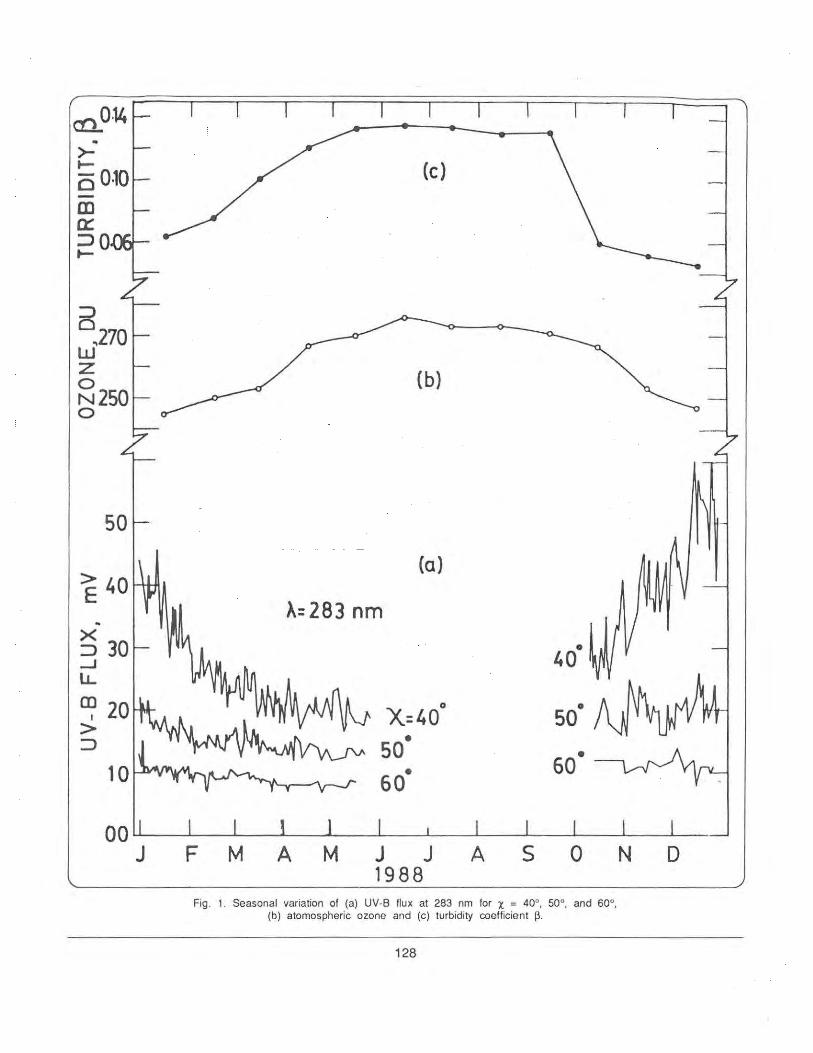
:::> 0

.. 270 w z 0 N25Q 0

-X ::J _J

LL CD

I

> ::J

(b)

(a)

).: 283 nm

• 40

X=40 0 • 50

so· Go· • 60

F M A M J J A s 0 1988

Fig. 1. Seasonal variation of (a) UV-8 llux at 283 nm for x = 40°, 50°, and 60°, (b) atomospheric ozone and (c) turbidity coefficient ~-

128

N D

Fig. 2. Variation of UV-8 flux (283 and 303 nm) with ozone at x = 34°, 58.5°, and 68°.

129

CLIMATE AND AIR-QUALITY TAIWAN STATION Chung-Ming Liu, TAIWAN

ABSTRACT

The programme to develop a Climate and Air-Quality Taiwan Station (CATS) is a five-year project with the research goal of developing highly-accurate instruments to measure both short and longlived chemical species at a clean background site. Meteorological and radiation measurements are inc luded. This station shall be run continuously after the first five-years development along with the set-up of a research team, so as to monitor the trend of trace gases and to analyze the process of long-range transport from upstream sources. Further, research on the effects of gases and aerosols on the atmospheric radiation field and even climate will be pursued.

During the first fiscal year (1990-97), a movable laboratory is developed, so as to facilitate the measurement of surface ozone, NO, NMHC, CO, etc. at a few selected clean sites. Data collected during the first a nd second years will be analyzed for the final decision on the permanent site.

1 Introduction

Since the beginning of the industrial revolution, atmospheric trace gases and aerosols from anthropogenic sources have increased significantly. One great potential consequence is the alteration of the earth's climate: trace gases and aerosols modify the radiation energy balance of the earth-atmosphere system. The climatic impact of the increase of trace gases such as CH

4, Np, chlorofluorocarbons (CFCs), troposp

heric ozone and stratospheric ozone suggest that these gases may have as much impact .as the projected increase of C02•

The trends and budget of many trace gases are still not well understood despite their importance to climate and to atmospheric chemistry. One major obstacle to understanding is the lack of a comprehensive database of these trace gases, spatial and temporal distribution. Only an international network of background observatories and cooperative research programmes can fill this data gap. Such programmes in Taiwan will fill a major gap in the database and contribute significantly to the international programme.

The proposal to establish a Climate Air Quality Taiwan Station (CATS) was materialized during the "Workshop on Long-term Air Quality Changes and Their Climatic Impact" on November 13-18, 1989, at Taipei, by the participating US and ROC scientists.

The following scientific objectives are identified:

1. To carry out reliable measurements of important gases, aerosols, and associated meteorological

130

variables for the assessment of air quality and climate change:

2. To contribute to international understanding of climate and environment changes both on the global and regional scales.

In Support of these objectives, two operational objectives are recommended :

1. To acquire and develop state-of-the-art instruments for measurement of trace gases and aerosols :

2. To establish research teams and to train scientific personnel to carry out research programmes in air pollution and climate .

2. The Unique Status of CATS

The CATS will be a bridge between continental and oceanic environments in Asia at a subtropical latitude, which therefore can provide data for understanding the chemical and physical transformation of species transported from Asia to Pacific or vice versa in comparison with those collected at midlatitudes and in tropics.

The CATS will establish the scientifically defensible background condition of Taiwan region. Such da1a will be very important in comparison with the local air quality monitored by the Environment Protection Administration (EPA} of the ROC for the assessment of air pollution control strategy. Also, the measurement techniques developed for CATS will be

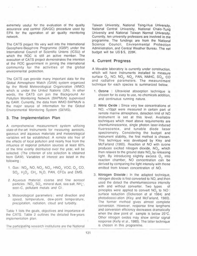
extremely useful for the evaluation of the quality assurance and control (OA/OC) procedure used by EPA for the operation of air quality monitoring network.

The CATS project fits very well into the International Geosphere-Biospt1ere Programme (IGBP) under the International Council of Scientific Unions (ICSU) of which the ROC is still an active member. The execution of CATS project demonstrates the intention of the ROC government in joining the international community for the activities of the global environmental protection.

The CATS can provide many important data for the Global Atmosphere Watch (GAW) system organized by the World Meteorological Organization (WMO} which is under the United Nat ions (UN}. In other words . the CATS can join the Background Air Pollution Monitoring Network (BAPMoN) supervised by GAW. Currently, the data from WMO BAPMoN is the major source of information for the Global Environmental Monitoring System (GEMS}.

3. The Implementation Plan

A comprehensive measurement system utilizing state-of-the-art instruments for measuring aerosols. gaseous and aqueous materials and meteorological variables will be established. A remote site free of the effects of local pollution and nearly free from the influence of regional pollution sources at least 60% of the time evenly distributed over the year. will be selected. (The criterion of site selection is obtained from GAW}. Variables of interest are listed in the following :

1. Gas: NOx, NO, N02

, NOv. HN03

, VOC, 03

, CO.

S02 , Hp2• CH4

, Np. PAN. CFCs and OMS.

2. Aqueous material . coarse and fine aerosol particles: N0

3, S04 , mineral dust, sea salt , NH4 ',

soot-C. pollutant metals and Cl-.

3. Meteorological parameters : wind direction and speed , temperature , dew-point temperature , precipitation , radiation , cloud and turbidity.

Table 1 lists the goals, objectives and importance of the CATS. Table 2 outlines the detailed five-years implementation plan.

The participating research institutions are the National

131

Taiwan University, National Tsing-Hua University, National Central University, National Chaio-Tung University and National Taiwan Normal University. Currently, ten university professors are involved in the programme. The fundings are from the National Science Council, Environmental Protection Administration. and Central Weather Bureau. The net budget will be US$ 5, 228K.

4. Current Progress

A Movable laboratory is currently under construction, which will have instruments installed to measure surface 0 3, NO, N02, NO. PAN, NMHC, SO. CO and radiative parametJrs. The measure

2ment

technique for each species is summarized below.

1. Ozone : Ultraviolet absorption technique is chosen for its easy to use, no chemicals addition, and continuous running nature.

2. Nitric Oxide : Since very low concentrations of NO, <1 Oppt were measured in certain part of remote marine atmosphere, detection limit of NO instrument is set at this level. Available techniques which meet above requirements are chemiluminescence, single photon laser-induced fluorescence, and tunable diode laser spectrometry. Considering the budget and instrument stability, the first method is chosen. This technique was developed by Kley and McFarland (1980) . Reaction of NO with ozone produces excited nitrogen dioxide, N0

2, which

then relaxes to the ground state N02

by re leasing light. By introducing slightly excess 0

3 into

reaction chamber, NO concentration can be derived by comparing the light intensity with those emitted from known concentration of NO.

3. Nitrogen Dioxide : In the adapted technique, nitrogen dioxide is fi rst converted to NO, and then used the detect the chemilumiescence intensity with and without converter. Two types of principles were applied to convert N0

2 to NO :

surface reduction (Dickerson et al 1984) and photodissoci-ation (K iey and McFarland, 1980). The form er method gives almost complete conversion. However, response time lengthens and conversion efficiency decreases dramatically when the dew point of sample is below 25°C. Other nitrogen oxides may show similar signal response (Kelly et al. . 1980}. The latter technique is chosen in this programme.

4. Sulphur-di-oxide : Ultraviolet absorption spectometry technique is adapted here. It has the advantage of strong absorption of so2 in the 240-330nm region (Calvert and Stockwell, 1984).

5. Non-Methane Hydrocarbons (NMHC) : Nonmethane hydrocarbons can be separated and detected using gas chromatography with either flame ionization detector or a mass spectrometer. When monitoring the background air, the most difficult task is to ensure the data reliability. It is very important for doing calibration and instrument intercomparison. Such studies are currently under negotiation with some laboratories in United States.

6. Carbon Monoxide : In the hope of monitoring more than one species at a time, a long-path Fourier Transform Infrared Spectrometry technique is chosen for measuring CO.

7. Peroxyacetyl Nitrate (PAN) : Measurements of PAN and other organic nitrates can be accomplished using gas chromatograph with electron capture detector, GC-ECD (Buhr et al., 1990).

8. Nitrogen oxides (NO ) : Similar technique as the one for monitoring N02 is adapted. Nov are converted to NO on a gold surface at 300°C (Fahey et al., 1986). Small amount of CO, 0.3%, will be added to the sample flow as a reducing agent, NO + CO --) NO + C02 + products. It is found that the conversion efficiencies of N02,

HN03

, Np5

and PAN are near 100%. Other nitrogen oxides are expected to t5e similar. (Fahey et. al. 1985)

Three potential sites . are chosen after the climatological data and the surrounding environment have been throughly studied. Plan is set up to transfer the movable laboratory to these

132

three sites to be operated for at least three months. Data collected (including meteorolgical and radiatio('l datasets) during these periods will be analysed for a final recommendation on the permanent CATS site.

Reference

Bhur, M.P. D.O. Parrish, R.B. Norton, F.C. Fehsenfeld, and R.E. Sievers, 1990: Contribution of organic nitrates to the total react ive nitrogen budget at a rural eastern U.S. site , J. Geophys. Res., 95, 9809-9816.

Calvert , J.G. , and W.R. Stockwell, 1984: Mechanism and rates of the gas-phase oxidations of sulfur dioxide and nitrogen oxides . in the atmosphere. Acid Precipitation Series, 3. J.l. Teasley, Series Ed. , Butterworth, Storeham, MA.

Fahey, D.W. C.S. Eubank, G. Huebler, and F.C. Fehsenfeld, 1985: Evaluation of a catalytic reduction technique for the measurement of total reactive oddnitrogen NOY in the atomosphere. J. Atmos. Chem. 3, 435-468.

G. Huebler, D.D. Parrish, E.J . Williams, R.B. Norton, B.A. Ridley , H.G. Singh, S.C. Liu , and F.C. Fehsenfeld, 1986: Reactive nitrogen species in the troposphere : Measurements of NO, N02 , HN03 ,

particulate nitrate, peroxyacetyl nitrate (PAN), 03

, and tota! reactive odd nitrogen (NOY) at Niwot Ridge, Colorado. J. Geophys. Res., 91 -9781-9793.

Kelly, T.J ., D.H. Steman, J.A. Ritter, and R.B. Harvey, 1980: Measurements of oxides of nitrogen and nitric acid in clean air. J. Geophys. Res., 85, 7417-7425.

Kley, D., and M. McFarland, 1980: Chemiluminescence detector for N0

4 and N02, Atmos. Techno!.,

12, 63-69.

TABLE 1 The goals, objectives and importance of the Climate and Air-quality Taiwan Station (CATS).

GOALS OBJECTIVES IMPORTANCE

Monitor long-term Climate 1. To anlyze the impact of global 1. Meteorological data To study long-term trend. atmospheric change on local 2. Atmospheric radiation data. climate and air-quality.

Monitor long-lived chemical 2. To monitor the long-term trend Species: of local climate .

1. Greenhouse gases : C02 • To study long-term trend. CH4 , CFCs. N

20. 3. To upgrade the academic

2. Total ozone and ozone profile. standard in the fields of atmospheric chemistry and air pollution measurement.

Monitor short-lived chemical 1. To Study long-term trend. 4. To assist the Environmental species : 2. To compare the air quality Protection Administration in

1. Surface 03

, NO, N02, NMHC, data at clean background site setting up the Standard Gas 80

2, CO. with those measured at Laboratory.

2. Particu late nitrate and sulfate, polluted sites. HN03, NOy, PAN. To analyze the effect of long- 5. To promote the internal ional

3. Precipitation chemistry. range tansport. cooperation on research.

TABLE 2 Five-year implementation plan of CATS

Years Items

First Year ( 1) Develop and deploy 03

, NO, N02, NOY, co and so2 instruments.

(2) Set-up a movable laboratory.

(3) Test and evaluate instrumental system.

(4) Identify potential sites.

Second Year ( 1) Acquire and deploy HN03, PAN, NMHC, particulate nitrate and sulfate instruments.

(2) Acquire and deploy radiation instruments.

(3) Test and deploy radiation instruments.

(4) Data analysis and interpertation.

(5) Design data management system.

(6) Participate in international project(s) .

Third Year ( 1) Acquire and deploy precipitation chemical analysis system.

(2) Data analysis, interpretation and publication.

(3) Select permanent site.

Fourth Year (1} Acquire and deploy boundary layer sounding sensors for ozone, wind and temperature profilers.

(2) Data analysis, interpretation and publication.

(3) Utilize the mobile unit for intercalibration with instruments at selected EPA monitoring sites.

Fifth Year Expand to full-scale operation with CH4 , NzO, CFCs instruments.

133

Fig. 1. Three selected potential CATS sites: A - Li-Shan (23'21'N, 120'48'E , 2406.1 M ; marked as 1) ; Hsin - Kang (23'06'N, 121'22'E, 32. 7M ;

marked as 2) ; Lan - Yu (22'02'N, 121'33'E, 323.3M ; marked as 3).

134

RAIN AND LAKE WATERS IN TAIWAN, COMPOSITION AND ACIDITY

Chen-Tung A Chen, Jia-Jang Hung, Jiing-Sheng Kuo,

Bing-Jy~ Wang and Show-Rong Yue, TAIWAN

Lately acid rain and lake acidification have attracted much attention and concern worldwide. In Taiwan, the adverse effects of acid rain, the offspring of rapid industrialization have also been felt and discussed. Unfortunately, because of the lack of historical data, we do not know clearly whether the lakes in Taiwan have changed, ·Or will soon change their acidity. We report here the acidity of rain and lake waters in Taiwan and the sensitivity ot these lakes to acid rain based on pH and alkalinity data. We also estimate possible future changes in lake. acidity based on studies of total dissolved salt, rock and soil types. This study has been integrated into ROC's contribution to the International Global Atmospheric Chemistry Project. ·

Ten automatic dry/wet samplers were used to collect dry deposits and rain water in southwestern Taiwan. Over six hundred lake water samples were collected from 115 lakes (Fig.1). Certified ERA (Environmental Resource Associate) potable water and NBS rain water samples (2694 I and 2694 II) were used ·as references to check the precision and accuracy of the analyses. Reliability of data was further checked by correlating the sum of cations with the sum of anions. A linear correlation was found (r = 0.98) with a slope of 1.04, which differs only slightly from the expected value of 1. Detailed sampling and analytical procedures were described elsewhere 1

·5 .

Dry deposits consists mostly of quartz, gypsum and aragonite probably coming from several cement plants in the sampling area. A one to fifty weight dilution of dry deposits with deionized/distilled water (pH = 5.66) results in solutions with pH values ranging from 7.34 to 1 0.232·3 .

The pH of rain waters collected covers a wide range because of large differences of local conditions. pH values are sometimes quite high in the dry season, perhaps because the samples contain a relatively large amount of air borne mineral particles. pH vlaue as high as 10.635 has been recorded, reflecting high gypsum and aragonite contents. In general, the higher the alkalinity or conductivity, the higher the pH vlaues

135

appear. The rain water becomes relatively more acidic during the wet seaons (May-Sept.). There is some indication that tne rain water is less acidic at the on set of a rain, suggesting that basic particles contribute to part of the rain water samples. Later during a precipitation event, the water becomes more acidic because basic particles have previously been removed from the atmosphere2•3 .

Rain brought in by three typhoons in 1986 are less acidic.The mean pH vlaues for normal rains in June through September in 1986 are slightly more acidic than the mean pH vlaues for all rains combined. The reverse is true, hoever, in1987 and 1988.

Of the areas studied, Hsiaogun (site 9) seems to be the most affected by the acid rain because it is adjacent to the h·eavy industrial area concentred in southern Kaohsiung. Rain waters there are frequently below pH 5. The amount of nitrate is inversely correlated with pH thus nitrate apparently is a heavy contributor of acid rain at Hsiaogun. The pH also correlates inversely with the excess sulfate, suggesting that excess sulflate also contributes to the formation of acid rain at this site. The effect of sulfate is potentially large becaus of its higher concentration than nitrate.

Rain water collected outside of the Kaohsiung area generally had a pH value grater than 5.0. The sulfate and nitrate concentrations are also lower in the less industralized region.These results reflect the relation between acid rain and air pollution.

We divide lakes in Taiwan into six categories based on alkalinity according to the classification Zimmerman and Harvey6 (Fig.1). As a first approximation, we also divide Taiwan into three major zones according to the rock and soil compositions (Fig.1). Zone I consists mainly of igneous rocks such as andesite, and andeistic pyroclastics. These rocks have low buffering capacity and the lakes in ths region should have low alkalinities and potentially low pH values. We have sampled 10 lakes in Zone I.Four are classified as A; one is B. The five small ponds

sampled on the Green Island off southeastern Taiwan. however, are classfied as E, perhaps because of local pollution and entrophication. Overall Na (57.6%), Mg (22%), Ca (12.8%), K (5.8%), and H (1.9%) are the major cations, and Cl (49%), HC0

3 (36.7%) • S0

4

(13.5%) and N03

(0.8%) are the major anions. The averge salt content is 1 .680 meq/1 and the average alkalinity is 0.354 meq/1. Further acidification of some of these lakes is possible becaue of the low buffering capacity of these lake waters and the surrounding rocks and sediments.

Zone II consists mainly of non-carbonaceous sedimentary and metamorphic rocks such as mudstone, sandstone, tuffaaceous sandstone, shale, coaly shale, sandly shale, gravel, conglomerate, agglomerate , argillite, slate, phyllite, and schists. These rocks have buffering capacities between igneous rocks (Zone I) and carbonaceous rocks (Zone Ill). The lakes in this region show a wide variety of alkalinity and pH values . The average salt content is 3. 751 meq/1 and the average alkalinity is 1.141 meq/1. The major cations are Ca (54.4 %), Mg (33.3%), Na (11.1 %}, K (1.0 %) and Sr (0.3%). The major anions are HC03 (61.3%), S04 (36.2%), Cl (1.4%), N0

3 (1.0%) and OH (0.1%). Many high

elevation lakes in Zone II (above 2000 m; hatched area in Fig.1) are either acid sensitive or might soon become acid sensitive (Fig. 1 ). Since little local pollut ion occurs near these lakes, acid rain and local geochemistry are possible causes of acidification.

Zone Ill consists mainly of gravel, sand, Clay, limestone and the alluvium zone. Most lakes have a alkalinity higher than 1.0 meq/1 and the waters are generally slightly basic (pH between 7.0 and 9.0) . A few lakes are heavily polluted. The average salt content and alkalinity are 5.223 meq/1 and 1.459 meq/1, respectively. The major cations are Ca (41.1%), Na (31.3%), Mg (24.1%), K (3 .4%) and Sr (0.1%} . The major anions are HC0

3 (55.1%}, Cl

(23%}, S04 (20. 1%) . N03

(1.7%), and OH (0.1%).

136

We do not believe that any of these lakes are in danger of acidification in the foreseeable future.

Overall, 34.2% of lakes in Taiwan are classified as class F, 23.9% E, 13.7% A, 13.7% C, 10.3% D, and 4.3% B. The average salt content is 4.720 meq/1 and the average alkalinity is 1.327 meq/I.The major cations are Ca (44%), Na (26.6%), Mg (26.3%) . K (2.8%), and Sr (0.1%). The major anions are HC0

3 (56.3%). S04 (24.2%). Cl (17.9%), N03 (1.5%) and OH (0.1 %). Calcium carbonate seems to contribute most to the alkalinity and calcium concentration correlates well with alkalinity (r =0.85)

We acknowledge assitance provided by H.L. Lin, and G.Y. Tsai for laboratory and field work : Dr. Y.H. Li of the University of Hawaii provided valuable comments. Financial support was provided by NSC (NSC80-0209-M110-04),EPA, and the Kenting National Park, R.O,C. ·

References

Chen C.T. and J.J. Hung, 1986, NSC Data Report, Unpublished, 17, NSC microfiche (NSC 74 -0407-M110-01). (in Chinese)

Hung, J.J. and C.T. Chen, 1986, EPA Data Report, Unpublished, 40pp. (in Chinese)

Chen, C.T.A. and J.J. Hung , 1987, Proc. NSIC (A), 11, 436-442.

Chen C.T.A., J.J. Hung and B.J. Wang, 1987, lnst. Mar. Geol. Tech. Rep. 2, 131 pp. (in Chinese)

Hung J.J. and C.T. Chen, 1989, J. Env. Prot. Soc., ROC, 12, 1, 1-11 .

Zimmerman. A.P. and H.H. Harvey, 1978-1979, Final report on sensitivity to acid ification of waters of Ontario and neighbouring states, Univ. of Ontario., 136pp.

A : o - <o,oe meq IL

B : o,os - <a.2 meq / L C: 0,2 - (0,!5 meq /L D: 0,8 - (,,0 meq /L E: ,,o - <2.0 meq /L F: it 2,0 meq/L

(Ill}

oO

F

(I)

{Ill)

A .B N;w\ Je., ln.._ (I)

~

Fig. 1. Locations of automatic rain water samplers (*). (numbered 1 through 10) in southwest Taiwan , and ol lakes sampled all over Taiwan (•). Letters A through F denote the alkalinities of lakes. Zones I through Ill are described in the text. Shaded area

has an elevation above 2000 m.

137

PALAEOCLIMATIC STUDIES IN THE COASTAL REGIONS AND ADJACENT SEAS OF INDIA USING

TREES, CORALS AND MARINE SEDIMENTS R. Ramesh and B. L. K. Somayajulu, INDIA

Abstract

This paper summarises the palaeoclimatic studies based on radioactive and stable Isotopes that hove been carried out in the Northern Indian ocean region using trees. corals and marine sediments. This work. relating to both streams 1 and 2 of the IGBP core project Past Global Changes (PAGES) reveals monsoonal and associated climatic changes on different time scales In the past.

1. Introduction

Under IGBP (PAGES) one seeks very high resolution (<1 yr.) proxy records of past climate for the past -2000 years and coarser resolution (a few hundered to a few thousand years) for the last -250 kyr. which are termed as Streams 1 and 2 respectively (IGBP, 1990). Some of the work carried out in the Geocosmophysics Area of the Physical Research Laboratory (PAL) ~during the past decade falls into these categories and is mainly related to the Northern Indian ocean (mostly the Arabian Sea) and adjoining coastal areas.

Sediments from the coastal and open ocean regions, trees and corals form the proxy records of past climate. It should be noted here that the main factor that controls climate in the northern Indian ocean is 'monsoon·. The southwest or summer monsoon (mid Ju.ne-mid October) is responsible for most of the rainfall in the country. During this period >90% of the annual quota of the water and sediment discharge from seven major rivers of the Indian sub-continent to the Bay of Bengal takes place. Whereas the Arabian sea is noted for high biological productivity primarily due to intense upwelling, the Bay of Bengal has high river discharges and fluvial activity and surface productivity (Qasim 1977: Sarin et al 1989), both these events take place during the southwest monsoon period.

2. Areas of Study and Sample Details

In Fig.1 are given the' sampling locations from Somali basin to the Bombay coast. The samples comprise of coastal and deep sea sediments, corals and trees from Bombay. The near-coastal sediments from the Gulf of Mannar (straits between India and Sri Lanka)

138

and the east coast of India have been studied from the goechronological point of view. Details of techniques and references can be found in Faure (1986) and Somayajulu (1990).

3. Results and Discussion

For clarity, results pertaining to streams 1 and 2 are discussed separately.

3.1 Stream-1

Trees, corals and near-coastal seiments belong to this stream.

3.1a Trees

Some trees lay d_own annual growth rings. The stable isotopic ratios of hydrogen (o D) oxygen (o 180) and carbon (o 13 cr in such trees can be a potential source of climatic variations in the past few hundred years with a high resolution. Teak trees from Thane (near Bombay - Fig.1) have been shown to record monsoon rainfall variations in the form of o D variations of their cellulose during the past -50 yrs. (Ramesh et al. 1989) with a high degree of correlation (r = 0. 71 ). Teak trees as old as a few hundred years are available from both the east and west coasts of India. These trees can. provide us the monsoon data for the past few centuries.

3.1b Corals

Like trees in the coast, corals that grow in the shallow regions of the Northern Indian ocean (water depths -20m) produce annual growth bands, that are visible under X-rays. In a preliminary study, corals from the Lakshadweep region (Fig. 1) have collected and the

,-\ ,--'--.., '- ... --""' '-'---..

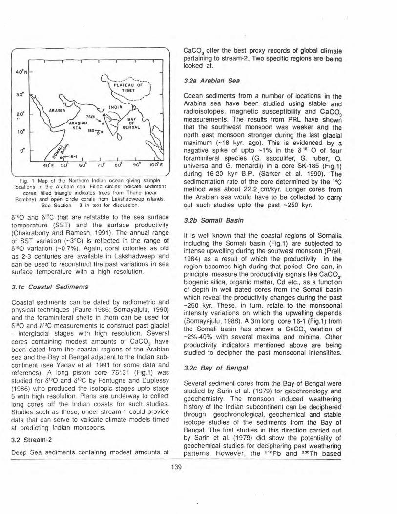
\ PLATEAU OF 'I TIBET ,, ,./

..... , ___ .,,

zo•

o•

Fig. 1 Map of the Northern Indian .ocean giving sample locations in the Arabain sea. Filled ctrcles andtcate sedtment

cores; filled triangle indicates trees from Thane (near Bombay) and open circle corals from Lakshadweep ISlands.

See Section 3 in text for dtscusston.

0ts() and o13C that are relatable to the sea surface temperature (SST) and the surface productivity (Chakraborty and Ramesh, 1991). The annual range of SST variation (-3°C) is reflected in the range of 0tso variation (- 0.7%). Again, coral colonies as old as 2-3 centuries are available in Lakshadweep and can be used to reconstruct the past variations in sea surface temperature with a high resolution.

3.1c Coastal Sediments

Coastal sediments can be dated by radiometric and physical techniques (Faure 1986; Somayajulu, 1990) and the foraminiferal shells in them can be used for 0tso and o13C measurements to construct past glacial . interglacial stages with high resolution. Several cores containing modest amounts of CaC03 have been dated from the coastal regions of the Arabian sea and the Bay of Bengal adjacent to the Indian subcontinent (see Yadav et al. 1991 for some data and referenes) . A long piston core 76131 (Fig.1) was studied for 8180 and o'3C by Fontugne and Duplessy (1986) who produced the isotopic stages upto stage 5 with high resolution. Plans are underway to collect long cores off the Indian coasts for such studies. Studies such as these, under stream-1 could provide data that can serve to validate climate models timed at predicting Indian monsoons.

3.2 Stream-2

Deep Sea sediments containng modest amounts of

139

CaC03 offer the best proxy records of global climate pertaining to stream·2. Two specific regions are being looked at.

3.2a Arabian Sea

Ocean sediments from a number of locations in the Arabina sea have been studied using stable and radioisotopes, magnetic susceptibility and CaC0

3 measurements. The results from PAL have shown that the southwest monsoon was weake·r and the north east monsoon stronger during the last glacial maximum (-18 kyr. ago). This is evidenced by a negative spike of upto -1% in the o 18 0 of four foraminiferal species (G. sacculifer, G. ruber, 0. universa and G. menardii) in a core SK-185 (Fig.1) during 16·20 kyr B.P. (Sarker et al. 1990). ·the sedimentation rate of the core determined by the 14C method was about 22.2. cmtkyr. Longer cores from the Arabian sea would have to be collected to carry out such studies upto the past -250 kyr.

3.2b Somali Basin

It is well known that the coastal regions of Somalia including the Somali basin (Fig.1) are subjected to intense upwelling during the soutwest monsoon (Prell, 1984) as a result of which the productivity in the region becomes high during that period. One can, in principle, measure the productivity signals like CaC03, biogenic silica, organic matter, Cd etc., as a function of depth in well dated cores from the Somali basin which reveal the productivity changes during the past -250 kyr. These, in turn, relate to the monsoonal intensity variations on which the upwelling depends (Somayajulu, 1988). A 3m long core 16-1 (Fig.1) from the Somali basin has shown a CaC0

3 vaiation of

- 2%-40% with several maxima and minima. Other productivity indicators mentioned above are being studied to decipher the past monsoonal intensitites.

3.2c Bay of Bengal

Several sediment cores from the Bay of Bengal were studied by Sarin et al. ( 1979) for geochronology and geochemistry. The monsoon induced weathering history of the Indian subcontinent can be deciphered through geochronological, geochemical and stable isotope studies of the sediments from the Bay of Bengal. The first studies in this direction carried out by Sarin et al. (1979) did show the potentiality of geochemical studies for deciphering past weathering patterns. Howev·er , the 210Pb and 230Th based

geochronological study revealed that northern Bay of Bengal may not be as ideal as the regions close to the equator. Stable isotope studies on good piston cores will help in ascertaining the sedimentation rates.

To sum up, both Arabian sea and the Bay of Bengal sediments, corals and trees from their coastal regions serve as short and long term proxy records for understanding the Indian monsoons.

References

Chakraborty, S. and Ramesh R. 1991. Stable isotope studies of corals from Lakshadweep islands, Proceedings of Inti. Symp. on Oceanography of the Indian Ocean, National Institute of Oceanography, Goa, January, (in Press) .

Faure, G., 1986. Principles of Isotope Geology, 2nd Edition, John Wiley, New York.

Fontugne, M.A. and Duplessy, J.C. 1986. variations of the monsoon regime during the Upper Quatern.ary : Evidence from the carbon isotopic record of organic matter in the NOrth Indian sediment core, Paleo -Paleo - Paleo - 56, 69-88.

IGBP, 1990. Report No.12 Stokholm, Sweden

Qasim, S.Z. 1977. Biological producvitiy of the Indian Ocean, Indian J. Mar. Sci. 6, 122-137.

' Prelt, W.L. ;004. Monsoonal climate In the Arabian sea during the late Quaternary : A response to changing solar radiation, In : Milankovich and -Climate (Eds. : A Berger, J . Imbrie, J. Hays, G. Kukula and B. Saltzman), D. Riedel, Hinghman.

~ .

. »

140

Ramesh, R., Bhattacharya, S.K. and Pant G.B. 1989. Climatic significance of D variations in a tropical tree species from India, Nature, 337, 149-150.

Sarin, M.M., Borole, D.V. and Krishnaswami, S. 1979. Geochemistry and geochronology of sediments from the bay of Bengal and the equatorial Indian Ocean, Proc. Ind. Acad. Sci., 88A, 131-154.

Sarin, M.M. Krishnaswami, S., Dilli, K., Somayajulu, B.L.K. and Moore, W.S. 1989. Major ion chemistry of the Ganga-Brahmaputra river system : weathering processes and fluxes to the Bay of Bengal, Geochim. Cosmochin Acta, 53, 997-1009.

Sarkar, A, Ramesh, R., Bhattacharya, S.K. and Rajagopalan G., 1990 (5180) evidence for a stronger Northeast monsoon current during the last glaciation, Nature 343, 549-551.

Somayajulu, B.L.K. 1988. Monsoonal activity during the quaternary based on the study of sediment cores from the Somali basin, Abstract, National Seminar on Recent Quaternary studies in India, Geology Dept. M.S. University, Baroda, Feb. 11 -13.

Somayajulu, B.L.K. 1990, Geochronological and geochemical approaches to the study of Quaternary climates, Man & Environ. Indian Society for Prehistory & Quaternary studies. (Deccan College, Pune) 15, 1-11 .

Yaclav, O.N., Sarin, M.M. and Somayajuki, . B.l.K. 1991. Weste.rn continental margins of India : Are they sink or source for trace elements in the Arabian sea? Proceedings of the Inti. Symp. on Oceanography of the Indian Ocean, NIO, Goa (in press).

4.1 ACRONYMS

BAHC

BAMA

BAPMoN

COSTED

DIS

GAIM

GCEC

GCTE

GOEZS

ICSU

IGAC

IGBP

liAS A

IOC

IRS

JGOFS

KEEP

LOICZ

NASA

NWIO

PAGES

ARCs

SC-IGBP

START

STt8 · ,

UN

UNCED

Unesco

WCRP

·~

WOCE

Biospheric Aspects of Hydrological Cycles

Background Atmospheric Monitoring in Asia

Background Air Pollution Monitoring

Committe on Science and Technology in Developing Countries

Data and Information Systems

Global Analysis , Interpretation and Modelling

Global Change and Ecological Complexities

Global Change and Terrestrial Ecosystems

Global Ocean Euphotic Zone Study

International Council of Scientific Unions

International Global Atmospheric Chemistry Project

The International Geosphere-Biosphere Programme : A Study. of Global Change

International Institute for Applied Systems Analysis

International Oceanographic Commission (Unesco)

Indian Remote Sensing Satellite

Joint Global Ocean Flux Study

Kuroshio Edge Exchange Processes

Land-Ocean Interactions in the Coastal Zone

National Remote Sensing Agency

North West Indian Ocean

Past Global Changes

Regional Research Centres

Scientific Committee for IGBP

Global Change System for Analysis, Research and Training

•stmpnere-Tro,ostthfre lnteractio(l and the ~

Un~ed Nation

UN Conference on Environment and Development

United National Educational, Scientific and Cultural Organization

Wood Climate Research Programme

.,._, ~ Organization

World Ocean Circulation Experiment

141

4.2 PARTICIPATION LIST OF THE ASIAN WORKSHOP New Delhi, India, 11·15 February, 1991

Dr. I.P. Abrol Indian Council of Agricultural Research Dr. Rajendra Prasad Road Krishi Bhawan, New Delhi 110 001 INDIA

Dr.Y.P. Abrol Division Plant Physiology Indian Agricultural Research Institute New Delhi 110 012 INDIA

Prof. D.P. Agrawal Continental Paleoclimate Studies Physical Research Laboratory Navrangpura, Ahmedabad 380 009 INDIA

Dr. Leoncio A. Amedore PAGASA 3rd Floor, Asia Trust Bank 1424 Quezon Avenue Quezon City PHILIPPINES

Dr.R.S. Arora National Physical Laboratory Sir K.S. Krishnan Road New Delhi 110 012 INDIA

Prof. K.D. Arudpragasam Central Environmental Authority P.O.Box 2205, Parisara Mawatha Mal igawatte New Town, Colombo 10 SRI LANKA

Dr.B.C. Arya National Physical Laboratory Sir K.S. Krishnan Road New Delhi 110012 INDIA

Dr.V. Asthana School of Environmental Science Jawaharlal Nehru University New Delhi 110 067 INDIA

Dr.R.N. Athavale National Geophysical Research Institute Council of Scientific & Industrial Research Uppal Road, Hyderabad 500 007 INDIA

142

Dr.B.R. Avasthi DOG India Meterological Department New Delhi 11 0 003 India

Dr.B. Babuji COST ED 24 Gandhi Mandap Road, Guindy Madras 600 025 INDIA

Dr.M. Bandyopadhyay ECD-1 Marine wing· Geological Survey of India 85 Prince Anwar Shah Road Calcutta 700 033 INDIA

Dr.S.K. Bhargawa Toxicology Research Centre M.G. Road Lucknow 226 001 INDIA

Mr.J.R. Bhatt Indian Institute of Petroleum Dehradun INDIA

Dr.K. Bhatacharya Visva-Bharathi University Shanthiniketan PO PIN : 713 235 Birbhum West Bengal INDIA

Dr. Indira Bhattarai Agricultural Botany Department IAAS Central Campus Rampur, Chitwan NEPAL

Dr.M.S. Chada Bhabha Atomic Research Centre Bio-chemical Group & Bio-organic Division Trombay, Bombay 400 085 INDIA

Prof. Sunirmal Chanda Division Palnology & Environmental Biology Bose Institute 93/1 Acharya Prafulla Chandra Road Calcutta 700 009 INDIA

Dr.A. Chakravorothy C.S.I.R. Headquarters Rafi Marg New Delhi 11 0 003 INDIA

Dr.Shri K. Chatterjee Mir.istry of Environment & Forests Paryavaran Bhavan, CGO Complex Lodi Road, New Delhi 110 003 INDIA

Dr.S.D. Chaudhuri Bangladesh Academy of Sciences 3/8 Asad Avenue Muhammadpur, Dhaka 1207 BANGLADESH

Mr.Chen-Tung Arthur Chen College of Marine Sciences National Sun Vat-Sen University Kaohsiung, Taiwan 80424 CHINA

Dr. Panqin Chen Bureau of Resources and Environmental Sciences Chinese Academy of Sciences 52, Sanhile Road, Beijing 100 864 CHINA

Dr. Renu Khanna Chopra RSD, National Physical Laboratory Sir K.S. Krishnan Road, New Delhi 110012 INDIA

Dr. Wen-Sen Chuang Institute of Oceanography National Taiwan University Taiwan CHINA

Dr. V.K. Dadhwal SE Land Resources Division, RSA Space Applications Centre SAC P.O., Ahmedabad 380 053 INDIA

Prof. R.R. Daniel COSTED, Asia Regional Office 24, Gandhi Mandap Road Guindy, Madrs 600 025 INDIA

Dr. Nachiketa Das Department of Science & Technology Technology Bhavan New Mehrauli Road, New Delhi 110 016 INDIA

143

Prof.P.K. Das Indian National Science Academy Bahadhur Shah Zafar Marg New Delhi 11 0 002 INDIA

Prof. B.L. Deekshatulu National Remote Sensing Agency Government of India Balanagar, Hyderabad 500 037 Andhra Pradesh INDIA

Prof. James C.l. Dooge Centre for Water Resources Research University College, Earlsfort Terrace Dublin 2 IRELAND

Dr.P.S. Dubey School of Studies in Botany Vikram University Ujjain 456 010 INDIA

Dr.H.N. Dutta National Physical Laboratory Sir K.S. Krishnan Road New Delhi 110 012 INDIA

Dr.S.N. Dwivedi Department of Ocean Development of Mahasagar Bhavan, Block 12 CGO Complex, Lodi Road New Delhi 110 003 INDIA

C.R.Eiangovan C.A.S. in Marine Biology Tamil Nadu, Parangipettai 608 502 INDIA

Prof. V.K. Gaur Department of Ocean Development Mahasagar Bhavan, CGO Complex Block 12, Lodhi Road, New Delhi 110 003 INDIA

Dr.A.B. Ghosh National Physical l-aboratory Dr.K.S. Krishnan Road, New Delhi 110 012 INDIA

Dr.B.A. Giriddhar Maharani Science College for Women Bangalore 560 001 INDIA

Dr. Malti Goel Ministry of Science & Technology, Government of India, Technology Bhavan New Mehrauli Road New Delhi 110 016 INDIA

Dr.R.P. Goel Publication & Information Directorate Hillside Road New Delhi 110012 INDIA

Dr.N.N. Goswami I.A. R.I. New Delhi 110 012 INDIA

Dr. Vasant Gowarikar Department of Science & Technology Technology Bhavan New Mehrauli Road New Delhi 110 016 INDIA

Dr. Harish K. Gupta Department of Science & Technology Technology Bhavan New Mehrauli Road, New Delhi 110 016 INDIA

Dr.Prabhat K. Gupta National Physical Laboratory Sir K.S. Krishnan Road, New Delhi 110 012 INDIA

Mr. Rajendra Kumar Gupta National Remote Sensing Agency Department of Space Balanagar, Hyderabad Andhra Pradesh 500 037 INDIA

Dr.S.K. Gupta Physical Research Laboratory Navrangpura, Ahmedabad 380 009 INDIA

Prof.S.Z. Haider Chemistry Department University of Dhaka, Dhaka 1 000 BANGLADESH

Dr.J. Robin E.Harger Unesco Jl. M.H. Thamrin 14 Tromol Pos 1273, Jakarta 10012 INDONESIA

144

Dr. Ho-Lin Department of Atmospheric Sciences National Taiwan University, Taiwan CHINA

Dr.Patrick Holligan NERC, Plymouth Marine Laboratory Prospect Place, West Hoe Plymouth PL1 3DH UK

Dr. Tsu-Chang Hung 42-6F, Yoyet Street Taipei, Taiwan CHINA

DrAG. llahude Indonesian Institute Science Centre R&D in Oceanology A LAMA T Jl. Pasir Putih 1 Ancol Timur Jakarta Utara 11001 INDONESIA

Dr.S.L. Jain Radio Science Division National Physical Laboratory New Delhi 110012 INDIA

Dr. Jai Shanker Jha Tribhuvan University Prithwi Narayan Campus Pokhara NEPAL

Mr.K.N. Johry International Scientific Collaboration Council of Scientific & Industrial Research Rafi Marg, New Delhi 110 003 INDIA

Dr.P.C. Joshi Industrial Toxicology Research Centre Phototoxicology Research Centre PO Box 80, Lucknow 226 001 INDIA

Dr.K. Kasturirangan Satellite Center Indian Space Research Organisation Vimanapuri Road, Bangalore 560 017 INDIA

Dr. R.N. Keshavamurthy Physical Research Laboratory Navrangpura Ahmedabad 380 009 INDIA

Dr. Shaukat Hayat Khan National Institute of Oceanography 37-K. Block 6 P.E.C.H.S., Karachi 29 PAKISTAN

Dr.L.T. Khemani Indian Institute of Tropical Meteorology Shivaji Nagar Pune 411 005 INDIA

Mr.F.C. Khullar National Physical Laboratory Sir K.S. Krishnan Road New Delhi 110 012 INDIA

Dr.I.L. Kothari Department of Biosciences Sardar Patel University Vall, Vidyanagar 388 120, Gujarat INDIA

Dr.S.M. Kulshrestha Indian Meteorological Department Mansam Bhavan, · Lodhi Road New Delhi 110 003 INDIA

Dr. Namita Kundu National Physical Laboratory Sir K.S. Krishnan Road, New Delhi 110 012 INDIA

Dr.M. Lal Indian Institute of Technology . Centre for Atmospheric Sciences Hauz Khas New Delhi 110 016 INDIA

Dr.J.W. Maurits Ia Riviere International Institute Hydraulic Engineering P.O. Box 3015, Oude Delft 95 NL-2601 DA Delft THE NETHERLANDS

Dr.P.J. Lavakare Department of Science & Technology Technology Bhavan, New Mehrauli Road New Delhi 110016 INDIA

Dr. Chung-Ming Liu Department of Atmosphere Science National Taiwan University, Taiwan CHINA

145

Dr.Kon-Kee Liu . Institute of Oceanography National Taiwan University, Taiwan CHINA

Dr. Zhenxia Liu First lnstitue of Oceanography State Oceanic Administration PO Box 98, Qingdao CHINA

Mrs.Julia Marton-Lefevre Executive Secretary, ICSU 51, Boulevard de Montmorency F-75016 Paris FRANCE

Prof. Eiji Matsumoto Nagoya University Water Research Institute Froucho Chikusa. Nagoya 464 JAPAN

Dr.B.S. Mathur Council of Scientific & Industrial Research Anusandhan Bhavan Rafi Marg, New Delhi 110 001 INDIA

Dr.K.K. Mahjan Radio Science Division National Physical Laboratory K.S. Krishnan Road. New Delhi 110 012 INDIA

Dr.K. Manoharan Ecology Unit, School of Biological Science Madurai Kamaraj University Madurai 625 020 INDIA

Dr.N.P. Melkania Faculty Ecosystem Management Indian Institute Forest Management Nehru Nagar, Post Box 357 Bhopal 462 003 INDIA

Dr. Uma Melkania College Basic Science & Humanities G.B. Pant University oJ Agriculture & Technology Pantnagar 263 145 (U.P.) INDIA

Prof. M.G.K. Menon ICSU 77 Lodi Estate. New Delhi 11 0 003 INDIA

Dr.U.C. Mishra Pollution Monitoring Division Bhabha Atomic Research Centre Trombay, Bombay 400 085 INDIA

Dr.A.P. Mitra Council of Scientific & Industrial Research Rafi Marg New Delhi 110 001 INDIA

Dr.P.K. Mohanty Marine Science Department Behrampur University Behrarnpur 7, Orissa INDIA

Dr.N.C. Monda! PID Hillside Road New Delhi 110 012 INDIA

Mr.B.V. Krishna Murthy Vikram Sarabhai Space Centre Government of India Trivandrum 695 022 INDIA

Mr.Shri P.S. Murthy · Indian Institute of Petroleum I.I.P. P.O. Mohkampur Dehradun 248 005 INDIA

Mr.Shri V.K. Nagar Survey of India Ministry of Science & Technology Technology Bhawan, New Delhi 110 016 INDIA

Dr.R. Nagaraga Land Use & Cartography Division National Remote Sensing Agency Balanager, Hyderabad 500.037 INDIA

Dr.V. Narayanan Nair Department of Geology University of Kerala Kariavattom, Trivandrum 695 581 INDIA

Dr.L.R.A. Narayan Institute of Remote Sensing Anna University, Madras 600 025 INDIA

146

Dr .A. R. Nautiyal IARI, Pusa New Delhi 110012 INDIA

Prof . Yasuyuki Oshima School of Human Sciences Waseda Univesity, Mikajima, 2-579-15 Tokorozawa, Saitama 359 JAPAN

Dr.J.S. Pandey National Environmental Engineering Research Institute Computer Applications Division Nehru Marg, Nagpur 440 020 INDIA

Dr.Aditi pant National Institute of Oceanography Dona Paula, GOA 403 004 INDIA

Dr.D.C. Parashar National Physical Laboratory Chemical Division, K.S. Krishnan Road New Delhi 110012 INDIA

Dr.M. Parbrahmam CP Division Ministry of Environment & Forest Paryavaran Bhavan, CGO Complex Lodi Road, New Delhi 11 0 003 INDIA

Dr.P.K. Pasricha National Physical Laboratory Sir. K.S. Krishnan Road New Delhi 110 012 INDIA

Mr. Janardanan Pillai Centre for Ecological Sciences Indian Institute of Sciences Bangalore 560 012 INDIA

Prof. T. Piyakanchana National Research Council of Thailand Bangkok 10900 THAILAND

Dr.B.S.N. Prasad University of Mysore Department of Post Graduate Studies Manasagangotri, Mysore 570 006 INDIA

Prof. A.N. Purohit G.B. Pant Institute Himalyan Environment & Development Kosi, Almora, Uttar Pradesh INDIA

Mr. Akhilesh S.Raghubanshi Ecosysems Analysis Laboratory Banaras Hindu University Varanasi 221 005 INDIA

Mr. Jitendra Rai National Physical Laboratory Sir. K.S. Krishnan Road New Delhi 110012 INDIA

Dr.M.K. Raina National Physical Laboratory Sir K.S. Krishnan Road New Delhi 110 012 INDIA

Dr.A. Rajanikanth Birbal Sahini Institute of Palaeobotany 53, University Road, GPO Box 106 Lucknow 226 001 INDIA

Prof. R. Rajaram Indian Institute of Geomagnetism Colaba, Bombay 400 005 INDIA

Prof. S.N. Rajguru P.G. & Research Institute Deccan College Pune 411 006 INDIA

Mr.Sri V. Ramachandran PID Sir Krishnan Marg New Delhi 10012 INDIA

Prof. P.S. Ramakrishnan School of Environmental Sciences Jawaharlal Nehru University New Mehrauli Road, New Delhi 110 067 INDIA

Dr.N. Raman Centre for Advanced Studies in Botany University of Madras Guindy Campus, Madras 600 025 INDIA

147

Prof. R. Ramesh Institute Ocean Management Anna University Center for Water Resources College of Engineering Madras 600 025 INDIA

Dr.R. Ramesh 265 PAL Physical Research Laboratory Navrangpura, Ahmedabad 380 009 INDIA

Dr.B.C.N. Rao National Physical Laboratory Sir K.S. Krishnan Road, New Delhi 110 012 INDIA

Dr.K.S. Jagannatha Rao Nutrition & Food Safety Discipline Central Food Technology Research Institute Mysore 570 013 INDIA

Dr.M. Venkateswara Rao C/64, V U M Hostel Ujjain 456 010 INDIA

Dr.M.N.M. Rao National Physical Laboratory Sir K.S. Krishnan Road, New Delhi 11 0 012 INDIA

Dr.P. Govinda Rao Department of Science & Technology Technology Bhavan New Mehrauli Road, New Delhi 110 016 INDIA

Dr. Yogeshwar Rao CSIR Headquarters Anushandhan Bhavan Rafi Marg New Delhi INDIA

Dr.S.I. Rasool Universite de paris VI Tour 26, 4eme Etage 4, place Jussieu 75230 Paris, Cedex 05 FRANCE

Dr.B.M. Reddy National Physical Laboratory Sri. K.S. Krishnan Road. New delhi 110 012 INDIA

Dr. Virupakshi Reddy Indian Institute of Geomagnetism Bomaby 400 005 INDIA

Prof. Thomas Rosswall IGBP Secretariat Royal Swedish Academy of Sciences Box 50005 1 04 05 Stockholm SWEDEN

Dr.Sen Roy India Meteorological Department Lodi Road New Delhi 11 0 003 INDIA

Dr.Kali Charan Sahu Department of Marine Sciences Berhampur University Berhampur 760 007 INDIA

Dr. Gupta Sarma National Geophysical Research Institute Uppal Road Hyderabad 500 007 INDIA

Mr.K. Madhav Sarma Ministry of Environment & Forests Paryavaran Bhavan, C.G.O. Complex Lodi Road, New Delhi 110 003 INDIA

Dr.S.S.S. Sarma School of Biological Science Madurai Kamaraj University Palkalai Nagar, Madurai 625 012 INDIA

Prof. G.H. Sastri Indian Institute of Astrophysics Bangalore 560 034 INDIA

Dr.R. Sengupta National Institute of Oceanography Dona Paula Goa 403 004 INDIA

Dr.V.K. Sengupta I.A.R.I., Pusa Sir K.S. Krishanan Road New Delhi 110 012 INDIA

148

Miss. Aruna Sharma IARI Sir K.S. Krishnan Road New Delhi 110 012 INDIA

Dr. Chhamendra Sharma Continental Palaeoclimate Studies Group Physical Research Centre Navrangpura, Ahmedabad 380 009 INDIA

Dr.Manju Sharma Department of Biotechnology Block 2, CGO Complex, Lodi Road New Delhi 11 o 003 INDIA

Dr.M.C. Sharma National Physical Laboratory New Delhi 110 012 INDIA

Dr. Der-Ouen Sheu lnsitute of Marine Geology National Sun-Yat Sen University Kaohsiung, Taiwan CHINA

Dr.A.K. Singh Indian Agricultural Research Institute Water Technology Centre New Delhi 110 012 INDIA

Dr.H.P. Singh Birbal Sahni Institute of Paleobotany 53, University Road, P.B. 106 G.P.O. Lucknow 226 001 INDIA

Dr.Ramesh P. Singh Deparment of Civil Engineering Indian Inst itute of Technology Kanpur 208 016 INDIA

Dr.Risal Singh RSD, National Physical Laboratory Sir K.S. Krishnan Road New Delhi 110 012 INDIA

Dr.R.B. Singh University of Delhi Department of Geography New Delhi 110 007 INDIA

Dr.R.N. Singh National Geophysical Research Institute Uppal Road Hyderabad, A.P. 500007 INDIA

Dr.Savithri Singh I.A.R.I., Pusa Sir K.S. Krishnan Road New Delhi 110 012 INDIA

Dr.P.C. Sinha Center for Atmospheric Science Indian Institute of Technology New Delhi 110 016 INDIA

Prof. Suresh K. Sinha Water Technology Center Agricultural Research Institute Sir K.S. Krishnan Road, New Delhi 110 012 INDIA

Prof. K. Sivaraman Indian Institute of Astrophysics Bangalore 560 034 INDIA

Prof. B.L.K. Somayajulu Physical Research Laboratory Navrangpura, Ahmedabad 380 009 INDIA

Dr.B.N. Srivastava National Physical Laboratory Radio Science Division Sir K.S. Krishn·an Road, New Delhi 110 012 INDIA

Prof. Leszek Starkel Department of Geomorphology & Hydrology Polish Academy of Sciences Ul.sw.Jana 22 PL-31 018 Krakw POLAND

Prof. Jong-Ching Su Department of Agricultural Chemistry National Taiwan University 1, Section 4, Rosevelt Road Taipei, Taiwan 10764 CHINA

Prof. B.H . Subbaraya Physical Research Laboratory Navrangpura, Ahmedabad 380 009 INDIA

149

Mr.A.K. Tagore Indian National Science Academy Bahadur Shah Zafar Marg New Delhi 11 0 002 INDIA

Dr.Shri R.S. Tamwar National Physical Laboratory Sir K.S. Krishnan Road, New Delhi 110 012 INDIA

Dr.C.J. Thampi National Bureau Soil Survey & Land Use Planning, Bidhan nagar Sector 11, DK Block, Salt Lake Calcutta 700 091 INDIA

Dr.V.C. Thakur Wadia Institute of Himilayan Geology 33 General Mahadeo Singh Road Dehra Dun 248 001 INDIA

Dr.G. Thiyagarajan C.L.R.I., Madras 600 020 INDIA

Dr.M.K. Tiwari ISRO · Head Quarters Antariksh Bhavan New Bel Road, Bangalore 560 054 INDIA

Prof. Kiyoshi Tsuchiya Chiba Univesity Remote Sensing & Image Research Centre Yayoicho 1-13, Chiba 260 JAPAN

Prof. B.S. Venkatachala Birbal Sahni Institute of Paleobotany 53 University Road, GPO Box 106 Lucknow 226 001 INDIA

Dr.K.G. Vernekar Indian Institute of Tropical Meteorology Shivaji Nagar, Pune 411 005 INDIA

Dr. Tashi Wangdi Ministry of Environment & Forest Government of India Regional Office (NEZ) Upland Road, Liatumkhrah Shillong 793 003 INDIA

Dr. Yuan Xiansheng Bureau of International Cooperation CAS, 52 Sanhile Road Beijing 100864 CHINA

Dr.K.S. Yajnik CSRI, Center Math. Modelling & Computer Simulation National Aeronautical Laboratory Belur Campus Bangalore 560 037 INDIA

Prof. Yashpal Univesity Grants Commission Bhadur Shah Zafar Marg New Delhi 110 002 INDIA

Prof. Deuzheng Ye Chinese Academy of Sciences 52 Sanlihe Road Beijing CHINA

Prof. Masatoshi Yoshino University Tsukuba, Institute Geoscience Tennoudai 1-1-1 Tsukuba, lbaraki 305 JAPAN

Prof. Zhi-fei Zh?ng National Science Foundation of China 43 Baojia Street Xicheng District, Beijing CHINA

Prof. An Zhisheng Xian Laboratory of Loess Quaternary Geology Academia Sinica PO Box 17, Xian, Shaanxi 710061 CHINA

150

4.3 IGBP REPORTS

1. The International Geosphere-Biosphere Programme : A study of Global Change. Final Report of the Ad

Hoc Planning Group, ICSU 21st General Assembly, Berne, Switzerland, 14-19 September, 1986 (1986) ·

2. A Document Prepared by the First Meeting of the Special Committee, ICSU Secretariat, Paris, 16-19

July, 1987 (1987)

3. A Report from the second Meeting of the Special Committee, Harvard University, Cambridge, MA, USA,

8-11 February, 1988 (1988) . •

4. The International Geosphere-Biosphere Programme. A Study of Global Change (IGBP). A Plan for Action.

A Report Prepared by the Special Committee for the IGBP for Discussion at the First Meeting of the

Scientific Advisory council for the IGBP, Stockholm, Sweden, 24-28 October, 1988 (1988).

5. Effects of Atmospheric and Climate Change on Terrestrial Ecosystems. Report of a Workshop Organized

by the IGBP Coordinating Panel on Effects of Climate Change on Terrestrial Ecosystems at CSIRO,

Division of Wildlife anq Ecology, Canberrra, Australia, 29 February - 2 March, 1988. Compiled by B.H.

Walker and A.D. Graetz (1989)

6. Giobal Changes of the Past. Report of a Meeting of the IGBP Working Group on Techniques for Extracting

Environmental Data of the Past held at the University of Berne, Switzerland, 6-8 July, 1988. Compiled

by H. Oeschger and J.A. Eddy (1989)

7. A Report from the First Meeting of the Scientific Advisory Council for the IGBP. Volumes I and II (1989)

8. Pilot Studies for Remote Sensing and Data Management. Report from Working Group workshop held

in Geneva, Switzerland, 11-13 January 1989. Edited by S.l. Rassol and D:S. Ojima (1989)

9. Southern Hemisphere Perspectives of Global Change. Scientific Issues, Research Needs and Proposed

Activites. Report from a Workshop held in Mbabane, Swaziland, 11 -16 December, 1988. Edited by B.H.

Walker and R.G. Dickson (1989)

0

10. The Land-Atmosphere Interface. Report on a Combined Modelling Workshop of IGBP Coordinating Panels

3,4 and 5. Brussels, Belgium, 8-11 June, 1989. Edited by S.J. Turner and B.H. Walker (1990).

11 . Proceedings of the Workshops of the Coordinating Panel on Effects of Global Change on Terrestrial

Ecosystems. I. A Framework for Modelling the Effects of Climate and Atmospheric Change on Terrestriat

Ecosystems, Woods Hole, USA, 15-17 April 1989. II. Non-Modelling Research Requirements for Under

standing, Predicting, and Monitoring Global Change, Canberra, 29-31 August 1989. Ill. The Impact of

Global Change on Agriculture and Forestry, Yaounde, 27 November-1 December 1989. Edited by B.H.

Walker, S.J. Turner, R.T. Prinsley, D.M. Stafford Smith and H.A. Nix (1990).

151

12. The International Geosphere-Biosphere Programme : A study of Global Change (IGBP). The Initial Core

Projects (1990).

13. Terrestrial Biosphere Exchange with Global Atmospheric Chemistry. Terrestrial Biosphere perspective of

the IGAC Project: Companion to the Dookie Report. Report on the Recommendations from the SCOPE/

IGBP workshop on Trace-Gas Exchange in a Global Perspective. Sigtuna, Sweden, 19-23 February,

1990. Editted by P.A. Matson and D.S. Ojima (1990).

14. Coastal Ocean Fluxes and Resources. Report of a CP2 Ad Hoc Workshop, Tokyo, Japan, 19-22

September 1989. Edited by P. Holligan (1990).

15. Global Change System for Analysis, Research and Training (START). Report of the Bellagio Meeting

(1991 ).

16. Report of the IGBP Regional Workshop for South America, Sao Jose dos Campos, SP Brazil , 5-9 March

1990. (1991).

17. Plant-Water Interactions in Large-Scale Hydrological Modelling. Report of a Workshop, Vadstena, Sweder

5-8 June 1990 (1991).

18.1 Recommendations of the Asia Workshop, New Delhi, 11-15 February 1991 . Edited by R.R. Daniel (1991)

18.2 Proceedings of the Asian workshop, New Delhi 11-15, February 1991. Edited by R. R. Dainel and B. Bab1

(1991 ).

19. The PAGES Project Proposed Implementation Plans for Research Activities Edited by John A. Eddy

(1992).

20. Improved Global Data for Land Applications ... A Proposal for a New High Resolution Data Set. Report

of the Land Cover Working Group of IGBP-DIS. Edited by J.R.G. Townshend. (1992).

21 . Global Change and Terrestrial Ecosystems : The Operational Plan. Edited by W.L. Steffen, B.H. Walker,

J.S. Ingram and G.W. Koch. (1992).

152

GL 'BAL CHANGE - IGBP

Documents

Transcript of GL 'BAL CHANGE - IGBP