GIBBON: General-purpose Information-Based Bayesian ...
49
Journal of Machine Learning Research 22 (2021) 1-49 Submitted 2/21;Revised 9/21; Published 9/21 GIBBON: General-purpose Information-Based Bayesian OptimisatioN Henry B. Moss * HENRY. MOSS@SECONDMIND. AI Secondmind.ai Cambridge, UK David S. Leslie D. LESLIE@LANCASTER. AC. UK Lancaster University Lancaster, UK Javier Gonz´ alez GONZALEZ.JAVIER@MICROSOFT. COM Microsoft Research Cambridge, UK Paul Rayson P. RAYSON@LANCASTER. AC. UK Lancaster University Lancaster, UK Editor: Marc Peter Deisenroth Abstract This paper describes a general-purpose extension of max-value entropy search, a popular approach for Bayesian Optimisation (BO). A novel approximation is proposed for the information gain — an information-theoretic quantity central to solving a range of BO problems, including noisy, multi-fidelity and batch optimisations across both continuous and highly-structured discrete spaces. Previously, these problems have been tackled separately within information-theoretic BO, each requiring a different sophisticated approximation scheme, except for batch BO, for which no computationally-lightweight information-theoretic approach has previously been proposed. GIB- BON (General-purpose Information-Based Bayesian OptimisatioN) provides a single principled framework suitable for all the above, out-performing existing approaches whilst incurring sub- stantially lower computational overheads. In addition, GIBBON does not require the problem’s search space to be Euclidean and so is the first high-performance yet computationally light-weight acquisition function that supports batch BO over general highly structured input spaces like molec- ular search and gene design. Moreover, our principled derivation of GIBBON yields a natural interpretation of a popular batch BO heuristic based on determinantal point processes. Finally, we analyse GIBBON across a suite of synthetic benchmark tasks, a molecular search loop, and as part of a challenging batch multi-fidelity framework for problems with controllable experimental noise. Keywords: Bayesian optimisation, entropy search, experimental design, multi-fidelity, batch * . Work completed while at the STOR-i Centre for Doctoral Training, Lancaster University, UK. ©2021 Henry B. Moss, David S. Leslie, Javier Gonz´ alez and Paul Rayson. License: CC-BY 4.0, see https://creativecommons.org/licenses/by/4.0/. Attribution requirements are provided at http://jmlr.org/papers/v22/21-0120.html.
-
Upload
khangminh22 -
Category
Documents
-
view
0 -
download
0
Transcript of GIBBON: General-purpose Information-Based Bayesian ...
Journal of Machine Learning Research 22 (2021) 1-49 Submitted 2/21;Revised 9/21; Published 9/21
GIBBON: General-purpose Information-Based BayesianOptimisatioN
Henry B. Moss ∗ [email protected], UK
David S. Leslie [email protected] UniversityLancaster, UK
Javier Gonzalez [email protected] ResearchCambridge, UK
Paul Rayson [email protected]
Lancaster UniversityLancaster, UK
Editor: Marc Peter Deisenroth
AbstractThis paper describes a general-purpose extension of max-value entropy search, a popular approachfor Bayesian Optimisation (BO). A novel approximation is proposed for the information gain— an information-theoretic quantity central to solving a range of BO problems, including noisy,multi-fidelity and batch optimisations across both continuous and highly-structured discrete spaces.Previously, these problems have been tackled separately within information-theoretic BO, eachrequiring a different sophisticated approximation scheme, except for batch BO, for which nocomputationally-lightweight information-theoretic approach has previously been proposed. GIB-BON (General-purpose Information-Based Bayesian OptimisatioN) provides a single principledframework suitable for all the above, out-performing existing approaches whilst incurring sub-stantially lower computational overheads. In addition, GIBBON does not require the problem’ssearch space to be Euclidean and so is the first high-performance yet computationally light-weightacquisition function that supports batch BO over general highly structured input spaces like molec-ular search and gene design. Moreover, our principled derivation of GIBBON yields a naturalinterpretation of a popular batch BO heuristic based on determinantal point processes. Finally, weanalyse GIBBON across a suite of synthetic benchmark tasks, a molecular search loop, and as partof a challenging batch multi-fidelity framework for problems with controllable experimental noise.Keywords: Bayesian optimisation, entropy search, experimental design, multi-fidelity, batch
*. Work completed while at the STOR-i Centre for Doctoral Training, Lancaster University, UK.
©2021 Henry B. Moss, David S. Leslie, Javier Gonzalez and Paul Rayson.
License: CC-BY 4.0, see https://creativecommons.org/licenses/by/4.0/. Attribution requirements are provided athttp://jmlr.org/papers/v22/21-0120.html.

MOSS, LESLIE, GONZALEZ AND RAYSON
1. Introduction
A popular solution for the optimisation of high-cost black-box functions is Bayesian optimisation(Mockus et al., 1978, BO). By sequentially deciding where to make each evaluation as the opti-misation progresses, BO can direct resources into evaluating promising areas of the search spaceto provide efficient optimisation. BO frameworks consist of two key components - a surrogatemodel and an acquisition function. By fitting a probabilistic surrogate model, typically a Gaussianprocess (Rasmussen, 2004, GP), to the previously collected objective function evaluations, we areable to quantify our current belief about which areas of the search space maximize our objectivefunction. An acquisition function then uses this belief to predict the utility of making a particularevaluation, producing large values at ‘reasonable’ locations. BO automatically evaluates the locationthat maximises this acquisition function and repeats until a sufficiently high-performing solutionis found. A popular application of BO is hyper-parameter tuning, with successful applicationsin computer vision (Bergstra et al., 2013), text-to-speech (Moss et al., 2020a) and reinforcementlearning (Chen et al., 2018). Of particular note are the recent extensions of BO beyond Euclideansearch spaces, for example when optimising synthetic genes (Gonzalez et al., 2014; Tanaka andIwata, 2018; Moss et al., 2020b) or performing molecular search (Gomez-Bombarelli et al., 2018;Griffiths and Hernandez-Lobato, 2020; Vakili et al., 2020).
Various heuristic strategies have been developed to form BO acquisition functions, includingExpected Improvement (Jones et al., 1998, EI), Knowledge Gradient (Frazier et al., 2008, KG)and Upper-Confidence Bound (Srinivas et al., 2010, UCB). More recently, a particularly intuitiveand empirically effective class of acquisition functions has arisen based on information theory.Information-theoretic BO seeks to reduce uncertainty in the location of high-performing areas of thesearch space, as measured in terms of differential entropy. Such entropy-reduction arguments havemotivated the three primary information-theoretic acquisition functions of Entropy Search (Hennigand Schuler, 2012, ES), Predictive Entropy Search (Hernandez-Lobato et al., 2014, PES) and Max-value Entropy Search (Wang and Jegelka, 2017, MES), differing in their chosen measure of globaluncertainty and employed approximation methods. Of particular popularity are acquisition functionsbased on MES, which reduce uncertainty in the maximum value attained by the objective function, aone-dimensional quantity. In contrast, both ES and PES seek to reduce uncertainty in the locationof the maximum, a quantity which, as well as being well-defined only for Euclidean search spaces,requires prohibitively expensive approximation schemes. Due to the large number of acquisitionfunction evaluations required to identify the next query point for each BO step, computationalcomplexity is an important practical consideration when designing acquisition functions, particularlyfor applications with structured search spaces containing combinatorial elements.
Although the advent of MES acquisition functions has enabled the application of information-theoretic BO beyond problems with low-dimensional Euclidean search spaces, MES can not yet beregarded as a general-purpose acquisition function for two reasons.
1. Firstly, the existing extensions of MES supporting common BO extensions like Multi-fidelityBO (Moss et al., 2020d) and batch BO (Takeno et al., 2020) require additional approximationsbeyond those of vanilla MES, typically through the numerical integration of low-dimensionalintegrals. Multi-fidelity BO (also known as multi-task BO) leverages cheap approximationsof the objective function to speed up optimisation, for example through exploiting coarseresolution simulations when calibrating large climate models (Prieß et al., 2011), whereas batchBO allows multiple objective function evaluations to be queried in parallel, a scenario arising
2

GIBBON
often in science applications, for example when training a collection of robots to cook (Jungeet al., 2020). Therefore, although still cheaper than their ES- and PES-based counterparts,extensions of MES for multi-fidelity and batch BO do not inherit the simplicity and low-costof vanilla MES.
2. Secondly, missing from the current extensions of MES is a computationally efficient methodfor general batch BO. Asynchronous batch BO supports scenarios where each ofB workers areallocated individually to evaluate different areas of the search space, returning queries and beingre-allocated one by one. In contrast, synchronous batch BO considers scenarios where whereB workers are to be allocated in parallel, as is the case for many real-world settings includingthose relying on wet-lab evaluations, physical experiments, or any framework where workers donot have sufficient autonomy to be controlled separately. Takeno et al. (2020) propose an low-cost MES formulation suitable for asynchronous batch BO, however, their proposed extensionof this method to synchronous batch BO (a distinction discussed in depth by Kandasamyet al. (2018a)) require prohibitively expensive approximations. Consequently, synchronousbatch applications of MES have so far relied on generic batch heuristics suitable for any BOacquisition function, including greedy allocation through local penalisation (Gonzalez et al.,2016a; Alvi et al., 2019) or using probabilistic repulsion models like determinantal pointprocesses (Kathuria et al., 2016; Dodge et al., 2017), both of which support only Euclideansearch spaces.
In this work we provide a single generalisation of MES suitable for BO problems arising from anycombination of noisy, batch, single-fidelity, and multi-fidelity optimisation tasks. Crucially, unlikeexisting extensions of MES, our general-purpose acquisition function retains the computational costof vanilla MES, with no requirement for numerical integration schemes. Therefore, we provide thefirst high-performing yet computationally light-weight framework for synchronous batch BO suitablefor search spaces consisting of discrete structures.
Our primary contributions are as follows:
1. We propose an approximation for a general-propose extension of MES named General-purposeInformation-Based Bayesian Optimisation (GIBBON). This approximation enables applicationof MES to a wide variety of problems, including those with combinations of synchronousbatch BO, multi-fidelity BO and non-Euclidean highly-structured input spaces.
2. Analysis of GIBBON leads to a novel connection between information-theoretic search,determinantal point processes (Kulesza et al., 2012, DPP) and local penalisation (Gonzalezet al., 2016a), providing currently missing theoretical justification for key attributes of thesetwo popular heuristics previously chosen arbitrarily by users.
3. We analyse the computational complexity of GIBBON in the wider context of information-theoretic acquisition functions, providing a comprehensive evaluation of the computationaloverheads of information-theoretic BO.
4. We demonstrate the performance of GIBBON across a suite of popular benchmark optimisationtasks, including the first application of information-theoretic acquisition functions to high-coststring optimisation tasks and a sophisticated batch multi-fidelity framework for BO undercontrollable observation noise.
3

MOSS, LESLIE, GONZALEZ AND RAYSON
The remainder of the paper is structured as follows. Section 2 reviews prior work on MES andintroduces the extended acquisition function that will be the focus of this work. In section 3, wepropose the GIBBON acquisition function, before examining GIBBON in the context of existingheuristics for batch BO (Section 4). In Section 5 we consider the computational complexity ofGIBBON in the wider context of information-theoretic BO. Finally, Section 6 provides a thoroughempirical evaluation.
2. Max-value Entropy Search for Black-Box Function Optimisation
We now introduce max-value entropy search (MES) for BO, providing an information-theoreticmotivation for the general-purpose framework that is the focus of this manuscript. We then introduceexisting work that has applied more restrictive formulations of MES to deal with specific BO tasks,before briefly summarising additional popular acquisition functions that are not based on MES.
BO routines seek the global maximum
x∗ = argmaxx⊂X
g(x)
of a ‘smooth’ but expensive to evaluate black-box function g : X → R. By sequentially choosingwhere and how to make each evaluation, BO directs resources into promising areas to efficientlyexplore the search space X ⊂ Rd and provide fast optimisation. In its simplest formulation(henceforth referred to as standard BO), BO controls the locations x ∈ X at which to collect(potentially noisy) queries of the objective function. A more general framework is that of multi-fidelity BO (Swersky et al., 2013) (also known as multi-task BO), where the ‘quality’ of each functionquery can also be controlled, for example by choosing the level of noise or bias across a (possiblycontinuous) space of fidelities s ∈ F . If these lower-fidelity estimates of g are cheaper to evaluate,then BO has access to cheap but approximate information sources that can be used to efficientlymaximise g. In practical terms, each step of multi-fidelity BO needs to choose a location-fidelitypair z = (x, s) ∈ Z = X × F upon which to make the next evaluation. A further extension arisesas batch BO, where we wish to exploit parallel resources by choosing a set of B ≥ 1 locations{z1, .., zB} ∈ ZB to be evaluated in parallel.
BO’s decisions are governed by two primary components - a surrogate model and an acquisitionfunction. The surrogate model makes probabilistic predictions of the objective function at not-yet-evaluated locations using the already collected location-evaluation tuples Dn = {(zi, yzi)}i=1,..,n.The most most popular choice of model is a Gaussian process (Rasmussen, 2004, GP). GPs providenon-parametric regression over all functions of a smoothness controlled by a kernel k : X ×X → R.Crucially, our GP conditioned on Dn produces a tractable Gaussian predictive distribution thatquantifies our current belief about the objective function across the whole search space. GP modelscan also be defined for multi-fidelity optimisation tasks (Kennedy and O’Hagan, 2000; Le Gratiet andGarnier, 2014; Klein et al., 2017a; Perdikaris et al., 2017; Cutajar et al., 2019) and when modellinghighly-structured input spaces likes strings (Beck and Cohn, 2017), trees (Beck et al., 2015) andmolecules (Moss and Griffiths, 2020).
Given such a probabilistic model over the search space, all that remains to perform an iteration ofBO is an acquisition function measuring the utility of making evaluations. The Max-value EntropySearch (MES) of Wang and Jegelka (2017), with similar formulations considered by Hoffman andGhahramani (2015) and Ru et al. (2018), seeks to query the objective function at locations that
4

GIBBON
reduce our current uncertainty in the maximum value of our objective function g∗ = maxx∈X g(x).In information theory (see Cover and Thomas, 2012, for a comprehensive introduction), uncertaintyin the unknown g∗ is measured by its differential entropy H(g∗|Dn) = −Eg∗ [log p(g∗)], where pis the predictive probability distribution function for g∗ (as induced by the surrogate model). Inparticular, the utility of making an evaluation is measured as the reduction in the uncertainty of g∗ itprovides, a quantity known as the mutual information (MI).
Although initially proposed for just standard BO problems, an MES-based search strategy can bereadily formulated for the general batch multi-fidelity framework (described above) by measuringthe utility of evaluating a batch of fidelity evaluations as their joint mutual information with themaximum value. We henceforth refer to this general formulation, formally expressed in Definition1, as General-purpose MES (GMES).
Definition 1 (The GMES acquisition function) The GMES acquisition function is defined as
αGMESn ({zi}Bi=1) :=MI(g∗; {yzi}Bi=1|Dn)
=H(g∗|Dn)− E{yzi}Bi=1
[H(g∗|Dn ∪ {yzi}Bi=1)
], (1)
where {zi}Bi=1 denotes the location-fidelity pairs of the batch elements and yz denote the yet-unobserved results of querying location-fidelity pair z = (x, s) ∈ X × F .
Note that standard BO, batch BO and multi-fidelity BO are trivial special cases of this general-purpose framework obtained by either or both of fixing the fidelity space F to a singleton containingjust the true objective function or setting B = 1.
To provide resource-efficient optimisation, we must balance how much we expect to learn aboutg∗ with the computational cost of the evaluations. Therefore, following the arguments of Swerskyet al. (2013), each BO step chooses to evaluate the set ofB locations that maximises the cost-weightedmutual information, i.e
{z|Dn|+1, .., z|Dn|+B} = argmax{zi}Bi=1∈ZB
αGMESn ({zi}Bi=1)
c({zi}Bi=1),
where c : ZB → R+ measures the costs of evaluating the batch. This cost function could be knowna priori or estimated from observed costs (Snoek et al., 2012). The optimisation of acquisitionfunctions is known as the inner-loop maximisation and, when considering continuous search spaces,is typically performed with a gradient-based optimiser. For discrete search spaces it is common touse local optimisation routines like DIRECT (Jones et al., 1993) or genetic algorithms (Moss et al.,2020b). For search spaces with discrete and continuous dimensions, hybrid optimisers can be used(Ru et al., 2020).
Unfortunately, calculating GMES in its full generality is challenging and providing a practicallyviable approximation strategy is the major contribution of this work. The primary difficulty in itscomputation arises from the lack of closed-form expression for the distribution of g∗, as required forall differential entropy calculations. We now end this section by discussing the three scenarios wherespecific sub-cases of GMES have already been used to provide highly effective BO — a noiselessvariant of standard BO, multi-fidelity BO, and a special case of batch BO.
5

MOSS, LESLIE, GONZALEZ AND RAYSON
2.1 Max-value Entropy Search for noiseless standard BO
Firstly, we consider the original MES formulation of Wang and Jegelka (2017), where they performstandard BO with noiseless observations. This acquisition function is formally expressed as
αMESn (x) := MI(yx; g∗|Dn) = H(yx|Dn)− Eg∗ [H(yx|g∗, Dn)|Dn] . (2)
Here, the symmetric property of mutual information has been used to swap yx and g∗ in its definition,yielding an equivalent (albeit less intuitive) expansion. Crucially, the first term of the expansion of(2) is now simply the entropy of a multivariate Gaussian distribution with a convenient closed-form.Moreover, Wang and Jegelka (2017) note that under the assumption of exact objective functionevaluations (where yx = g(x)), the distribution of yx conditional on its maximum possible value (i.eknowing that yx ≤ g∗) is simply that of a truncated Gaussian, also with a closed-form differentialentropy. All that remains to calculate MES is to approximate an expectation over g∗. Wang andJegelka (2017) build a Monte-Carlo estimate of the expectation with a set of samplesM from g∗,providing a closed-form approximation of MES as
αMESn (x) ≈ 1
|M|∑m∈M
[γx(m)φ (γx(m))
2Φ (γx(m))− log Φ (γx(m))
], (3)
where Φ and φ are the standard normal cumulative distribution and probability density functions(as arising from the expression for the differential entropy of a truncated Gaussian) and γx(m) =m−µn(x)σn(x) . Here, µn(x) and σ2
n(x) are the predictive mean and standard deviation for the objectivefunction value g at location x as easily extracted from our surrogate model. The set of samplemax-valuesM is built by modelling the empirical cumulative distribution function of g∗ with aGumbel distribution (see Wang and Jegelka (2017) for details) which can be sampled to yield Mcheap but approximate sampled max-values. This Gumbel approximation provides a fast samplingstrategy and has been successful across a wide range of BO applications (Wang and Jegelka, 2017;Moss et al., 2020d,c)
For the limited set of BO problems supported by this original MES acquisition function, MEShas had great empirical success, typically outperforming other information-theoretic BO methodswith an order of magnitude smaller computational overhead. However, once MES arguments areextended to support the more sophisticated BO frameworks (or even just to support noisy functionevaluations), we will see that the second term of (3) is no longer (the expectation of) the differentialentropy of a truncated Gaussian and additional approximations have to be made.
2.2 Max-value Entropy Search for multi-fidelity BO
MES-based search strategies have also been previously used for multi-fidelity BO through theMUlti-task Max-value Bayesian Optimisation (MUMBO) acquisition function of Moss et al. (2020d)(proposed in parallel by Takeno et al. (2020)) and, just like original MES, MUMBO has beenshown to perform highly efficient BO. However, unlike when collecting exact observations of g,fidelity evaluations yz|g∗ no longer follow a truncated Gaussian distribution and instead follow anextended skew Gaussian distribution (as shown by Moss et al. (2020d) and re-derived in Section3) which has no closed-form expression for its differential entropy (Azzalini, 1985). Therefore,the MUMBO acquisition function does not inherit all the computational savings of standard MES,requiring numerical integration. Note that by considering a single fidelity system, where low-fidelity
6

GIBBON
evaluations are just noisy observations of the true objective function, a multi-fidelity formulation ofMES also serves as an extended standard (single-fidelity) MES suitable for when evaluations arecontaminated with observation noise.
2.3 Max-value Entropy Search for Batch BO
Motivated by the empirical success of MES-based acquisition functions, it is natural to wonder ifthey can be used for batch BO. However, of the two popular batch scenarios of asynchronous andsynchronous batches commonly considered in the BO literature, only asynchronous batch BO iscurrently supported by a MES-based acquisition function (Takeno et al., 2020). The primary practicaldistinction is that, while synchronous batch acquisition functions must be able to measure the totalreduction in entropy provided by the joint evaluation of B locations, asynchronous batch BO has onlyto measure the relative reduction in entropy provided by making a single evaluation whilst takinginto account the B − 1 pending evaluations. Through clever algebraic manipulations, Takeno et al.(2020) require only single-dimensional numerical integrations when calculating the relative entropyreduction required for asynchronous batch BO. Unfortunately, as demonstrated in Section 3, complexinteractions between each of the B fidelity evaluations yzi once conditioned on g∗ (as present inthe second term of (1)) prevents the approximation strategies employed by Takeno et al. (2020) (orthose of Wang and Jegelka (2017) or Moss et al. (2020d)) being extended to the synchronous batchsetting. In particular, a naive extension of Takeno et al. (2020)’s approach requires the prohibitivelyexpensive numerical approximations of B-dimensional multivariate Gaussian cumulative densityfunctions. In this work, we propose a novel approximation strategy for (1) completely free fromnumerical integrations, thus providing the first computationally light-weight information-theoreticacquisition function for synchronous batch BO.
2.4 Alternatives to Max-value Entropy Search
As discussed in Section 1, MES is not the only information-theoretic BO acquisition function andis a descendent of ES and PES. However, the original ES and PES, as-well as their extensionsfor batch BO (Shah and Ghahramani, 2015; Hernandez-Lobato et al., 2017) and multi-fidelity BO(Swersky et al., 2013; Zhang et al., 2017), seek to reduce the differential entropy of the d-dimensionalmaximiser x∗ (rather than the single dimensional g∗ targeted by MES). The calculation of thisentropy is challenging, requiring sophisticated and expensive approximation strategies (see Section5). As well as being substantially more expensive than MES, the reliance of ES and PES on coarseapproximations means they provide less effective optimisation (Wang and Jegelka, 2017; Moss et al.,2020d; Takeno et al., 2020). Moreover, the approximation strategy employed by PES restricts its useto only Euclidean search spaces
Of course, attempts have been made to adapt other standard acquisition functions to multi-fidelityand batch BO, with examples including EI (Picheny et al., 2010; Chevalier and Ginsbourger, 2013;Marmin et al., 2015), UCB (Contal et al., 2013; Kandasamy et al., 2016, 2017) and KG (Wu andFrazier, 2016, 2017). However, extensions of EI and UCB, although computationally cheap andoften enjoying strong theoretical guarantees, are typically lacking in performance and even thoughKG-based methods can provide highly effective optimisation, their large computational cost restrictsthem to problems with function query costs large enough to overshadow very significant overheads(as demonstrated in Section 6). For batch BO, additional heuristic strategies have been developedthat are compatible with any acquisition function, with the most popular and empirically successful
7

MOSS, LESLIE, GONZALEZ AND RAYSON
being the Local Penalisation of Gonzalez et al. (2016a) and DPP-based approach of Kathuria et al.(2016) (see Section 4 for a thorough discussion). Alternative but less performant heuristics includeapproaches based on Stein methods (Gong et al., 2019) and Thompson sampling (Kandasamy et al.,2018a).
3. A Novel Approximation of General-purpose Max-value Entropy Search
In this section, we present the key theoretical contribution of this work: a novel approximation of theGMES acquisition function proposed in Section 2. In particular, we formulate GMES in terms of athe Information Gain (IG) — a measure of entropy reduction often used when pruning decision treeclassifiers (Raileanu and Stoffel, 2004) and when selecting features for statistical models of textualdata (Yang and Pedersen, 1997). The remainder of the section then details a novel approximationstrategy for the information gain based on simple well-known information-theoretic inequalities,before demonstrating explicitly how this IG approximation can be used to approximate the GMESacquisition function.
3.1 GMES as a Function of Information Gain
Recall our proposed GMES acquisition function (1), defined as the mutual information between a setof B fidelity evaluations and the objective function’s maximum value g∗. As in the derivation of theoriginal MES acquisition function (2), the symmetric property of mutual information can be used toyield the expansion
αGMESn ({zi}Bi=1) := H({yzi}Bi=1|Dn)− Eg∗
[H({yzi}Bi=1|Dn, g
∗)|Dn
]. (4)
For ease of notation, we now defineAi = yzi andCi = g(xi) for each of theB candidate location-fidelity tuples zi, as well as the multivariate random variables A = (A1, .., AB) and C = (C1, .., CB).The information gain is then defined as the reduction in the entropy of A provided by knowing themaximal value of C∗ = max C, i.e.
IGn (A,m|Dn) := H(A|Dn)−H(A|C∗ < m,Dn), (5)
Comparing (4) and (5), it follows that the GMES acquisition function can be expressed in terms ofIG as
αGMESn ({zi}Bi=1) = Em∼g∗ [IGn (A,m|Dn)] .
We can now see that efficiently calculating (5) in general scenarios will allow principled max-value entropy search across a wide range of BO settings. This goal is therefore the focus of theremainder of this section.
3.2 Required Predictive Quantities
Before presenting our proposed approximation for IG, it is convenient to discuss the distributionalforms induced by our surrogate GP model. All random variables are now assumed to be conditionedon the arbitrary information set Dn, which, alongside references to n, is henceforth dropped fromour notation.
8

GIBBON
Figure 1: The considered dependency structure between the two set of random variables {A1, .., AB}and {C1, .., CB}. Arrows denote the direction of dependence and latent variables are drawn insquares.
Courtesy of our GP surrogate model, we have that
A ∼ N(µA,ΣA), C ∼ N(µC ,ΣC) and Corr(Ai, Ci) = ρi,
for predictive means µC ,µA ∈ RB , predictive covariances ΣC ,ΣA ∈ RB×B and a vector ofpairwise predictive correlations ρ ∈ RB (Rasmussen, 2004; see Appendix A for details on how thesepredictive quantities are easily extracted from a GP).
In addition to these well-known distributional forms, we can exploit the specific conditionalstructure of our GP surrogate model (which we describe below and summarise in Figure 1) toderive the conditional distribution of the random variable A given that C∗ < m. In particular, ourplanned BO applications ensure that each Aj is conditionally independent of {Ci}i 6=j given Cj .This condition holds trivially for single-fidelity BO, where the difference between each Ai and Ciis just independent Gaussian noise. For multi-fidelity BO, this condition corresponds exactly tothe multi-fidelity Markov property that is a key assumption underlying multi-fidelity GP modelling(Kennedy and O’Hagan, 2000; Le Gratiet and Garnier, 2014; Perdikaris et al., 2017). This is not arestrictive assumption, with O’Hagan (1998) showing that the multivariate Markov property holdsfor any GP surrogate model with a kernel that can be factorised into a product of kernels, one definedacross the fidelity and one across the search space.
Under these dependence assumptions, Theorem 2 provides the distribution of A|C∗ < m inclosed-form, yielding a probability density function that, to the authors’ knowledge, has not beenpreviously considered in the statistics literature. Theorem 2 provides our first intuition for why theefficient calculation of the differential entropy H(A|C∗ < m) is challenging, i.e. the presence of themultivariate Gaussian cumulative density in its probability density function.
Theorem 2 (Distribution of A given C∗ < m) Consider two B-dimensional multivariate Gaus-sian random variables A and C where C ∼ N(µC ,ΣC) and each individual component of A isdistributed asAj ∼ N(µAj ,Σ
Aj,j). Suppose further that each each pair {Aj , Cj} are jointly Gaussian
with correlation ρj , and that each Aj is conditionally independent of {Ci}i 6=j given Cj . DefineC∗ = max C. Then the conditional density of A given that C∗ < m is given by
1
P(C∗ < m)φX1(a)ΦX2(m),
9

MOSS, LESLIE, GONZALEZ AND RAYSON
where m = (m, ..,m) ∈ RB and φX1 and ΦX2 are the probability density and cumulative densityfunctions for the multivariate Gaussian random variables
X1 ∼ N(µA, S +DΣCD
)and X2 ∼ N
(µC + Σ−1DS−1(a− µA),Σ−1
),
where ΣA = DΣCD + S for D and S, diagonal matrices with elements Dj,j = ρj
√ΣAj,jΣCj,j
and
Sj,j = (1− ρ2j )Σ
Aj,j , and Σ =
((ΣC)−1
+DS−1D)
.
Proof See Appendix B
Note that in the uni-variate case (i.e B = 1 and C∗ = C1), Theorem 2 collapses to the settingsalready considered when calculating MES and MUMBO in Section 2. Firstly, under the strongrestriction that C1 = A1 (arising from BO without observation noise), A1|C∗ < m follows thewell-known truncated Gaussian distribution, which can be seen directly from Theorem 2 by settingρj = 1, µCj,j = µAj and ΣC
j,j = ΣAj . This truncated Gaussian has a simple analytical expression for
its differential entropy which is exploited by standard MES. Secondly, if Cj and Aj are not perfectlycorrelated, we see that the density of Theorem 2 reduces to that of an Extended Skew Gaussian (ESG)distribution (Azzalini, 1985) as required for the MUMBO acquisition function (see Appendix A ofMoss et al. (2020d)). Although the differential entropy of an ESG has no closed-form expression(Arellano-Valle et al., 2013), we will later exploit the fact that its variance has an analytical form
Var(Aj |Cj < m) = ΣAj
(1− ρ2
j
φ(γj(m))
Φ(γj(m))
[γj(m) +
φ(γj(m))
Φ(γj(m))
]), (6)
where γj(m) = (m − µCj )/√
ΣCj,j . We stress that, due to the complex interactions between each
Aj |C∗ < m, the joint distribution of A|C∗ < m is not the multivariate ESG discussed by Azzaliniand Valle (1996)).
3.3 Approximating Information Gain
We now present a lower bound IGAPPROX for IG as Theorem 3. This bound is to be used as anapproximation IG ≈ IGApprox. We stress that replacing the maximisation of an intractable quantitywith the maximisation of a lower bound is a well established strategy in the ML literature, forexample in variational inference (Blei et al., 2017).
Theorem 3 (A lower bound for information gain) Under the assumptions of Theorem 2, it holdsthat IG(A,m) ≥ IGApprox(A,m), where
IGApprox (A,m) :=1
2log |RA| − 1
2
B∑i=1
log
(1− ρ2
i
φ(γi(m))
Φ(γi(m))
[γi(m) +
φ(γi(m))
Φ(γi(m))
]), (7)
where RA ∈ RB×B is the predictive correlation matrix of A with entries RAi,j = ΣAi,j/√
ΣAi,iΣ
Aj,j .
Proof
10
GIBBON
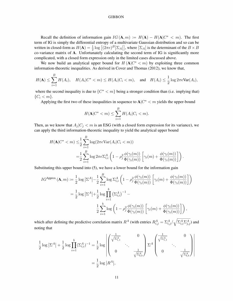
Recall the definition of information gain IG (A,m) := H(A) − H(A|C∗ < m). The firstterm of IG is simply the differential entropy of a multivariate Gaussian distribution and so can bewritten in closed-form as H(A) = 1
2 log[(2πe)B
∣∣ΣA
∣∣], where∣∣ΣA
∣∣ is the determinant of the B×Bco-variance matrix of A. Unfortunately calculating the second term of IG is significantly morecomplicated, with a closed form expression only in the limited cases discussed above.
We now build an analytical upper bound for H (A|C∗ < m) by exploiting three commoninformation-theoretic inequalities. As derived in Cover and Thomas (2012), we know that,
H(A) ≤B∑i=1
H(Ai), H(Ai|C∗ < m) ≤ H(Ai|Ci < m), and H(Ai) ≤1
2log 2πeVar(Ai),
where the second inequality is due to {C∗ < m} being a stronger condition than (i.e. implying that){Ci < m}.
Applying the first two of these inequalities in sequence to A|C∗ < m yields the upper-bound
H(A|C∗ < m) ≤B∑i=1
H(Ai|Ci < m).
Then, as we know that Aj |Cj < m is an ESG (with a closed form expression for its variance), wecan apply the third information-theoretic inequality to yield the analytical upper bound
H(A|C∗ < m) ≤1
2
B∑i=1
log(2πeVar(Ai|Ci < m))
=1
2
B∑i=1
log 2πeΣAi,i
(1− ρ2
j
φ(γi(m))
Φ(γi(m))
[γi(m) +
φ(γi(m))
Φ(γi(m))
]).
Substituting this upper bound into (5), we have a lower bound for the information gain
IGApprox (A,m) :=1
2log∣∣ΣA
∣∣−1
2
B∑i=1
log ΣAi,i
(1− ρ2
j
φ(γi(m))
Φ(γi(m))
[γi(m) +
φ(γi(m))
Φ(γi(m))
])
=1
2log∣∣ΣA
∣∣+1
2log
b∏i=1
(ΣAi,i
)−1−
1
2
b∑i=1
log
(1− ρ2
j
φ(γi(m))
Φ(γi(m))
[γi(m) +
φ(γi(m))
Φ(γi(m))
]),
which after defining the predictive correlation matrix RA (with entries RAi,j = ΣAi,j/√
ΣAi,iΣ
Aj,j) and
noting that
1
2log∣∣ΣA
∣∣+1
2log
b∏i=1
(ΣAi,i)−1 =
1
2log
∣∣∣∣∣∣∣∣∣
1√ΣA1,1
0
. . .0 1√
ΣAb,b
ΣA
1√ΣA1,1
0
. . .0 1√
ΣAb,b
∣∣∣∣∣∣∣∣∣
=1
2log∣∣RA∣∣,
11
MOSS, LESLIE, GONZALEZ AND RAYSON
provides the claimed expression.
3.4 GIBBON: General-purpose Information-Based Bayesian OptimisatioN
We end this section with explicitly demonstrating how IGApprox can be used to approximate theGMES acquisition function. Recall that GMES can be expressed in terms of IG as
αGMESn ({zi}Bi=1) = Em∼g∗ [IGn (A,m|Dn)] .
We have already provided an approximation for IG and so all that remains to approximate GMESis to deal with its outer expectation over g∗. Following the arguments of Wang and Jegelka (2017),we build a Monte-Carlo approximation of this expectation using a Gumbel-based sampler. Therefore,given a set of sampled max-values M = {m1, ..,mM} of g∗|Dn and access to the predictivedistributions
{yzi}Bi=1|Dn ∼ N(µy,Σy), {g(xi)}Bi=1|Dn ∼ N(µg,Σg) and Corr(yzi , g(xi)|Dn) = ρi,
we can approximate GMES with
αGIBBONn ({z}Bi=1) =
1
|M|∑m∈M
IGAPPROX({yz1 , .., yzb},m).
This construction is henceforth referred to as the General Information-Based Bayesian OptimisatioN(GIBBON) acquisition function and is defined as the closed-form expression in Definition 4 anddemonstrated within a BO loop as Algorithm 1.Definition 4 (The GIBBON acquisition function.) The GIBBON acquisition function is definedas
αGIBBONn ({z}Bi=1) =
1
2log∣∣R∣∣− 1
2|M|∑m∈M
B∑i=1
log
(1− ρ2
i
φ(γi(m))
Φ(γi(m))
[γi(m) +
φ(γi(m))
Φ(γi(m))
]),
where R is the correlation matrix with elements Ri,j = Σyi,j/√
Σyi,iΣ
yj,j and γi(m) =
m−µgi√Σgi,i
.
At first glance, GIBBON’s analytical form looks complex. However, as GIBBON contains onlysimple algebraic operations, it can be easily calculated in just a few lines of code, unlike existingES-based and PES-based acquisition functions and all existing extensions of MES (as discussed indepth in Section 5). An important practical consideration for GIBBON is that, for continuous searchspaces, it has accessible gradients that can easily be derived from its analytical expression, allowingefficient inner-loop optimisation.
We end this section with a visual analysis of the accuracy of the GIBBON approximation. Weconsider a standard BO task with exact objective function evaluations (i.e not multi-fidelity or batchoptimisation) as, in this setting, the MES acquisition function provides an exact calculation of theentropy reductions. In Figure 2 we see that the approximation provided by GIBBON is very close tothe ground truth provided by MES, with GIBBON and MES sharing modes and differing only inareas of the space that would never be selected by BO, i.e those locations with very low utility.
12

GIBBON
Algorithm 1: GIBBON for general-purpose BO tasks.Input: Resource budget R, Batch size B, Gumbel sample size N
1 Initialise n← 0 and spent resource counter r ← 02 Propose initial design I3 while r ≤ R do4 Begin new iteration n← n+ 15 Fit GP model to collected evaluations Dn
6 Simulate N samples from g∗|Dn
7 Compute αGIBBONn as given by Definition 4
8 Find B locations {zi}Bi=1 maximising αGIBBONn ({zi}Bi=1)
c({zi}Bi=1)
9 Evaluate new locations and collect evaluations Dn+1 ← Dn⋃{(zi, yzi)}Bi=1
10 Update spent budget r ← r + c({zi}Bi=1)
11 endOutput: Believed maximiser argmaxx∈Dn g(x)
(a) MES acquisition function surface (ground truth). (b) GIBBON acquisition function surface.
Figure 2: Comparison of the MES and GIBBON acquisition functions for a two-dimensional BOtask where MES can calculate entropy reductions exactly. The crosses denote the locations alreadyqueried by the BO routine. GIBBON provides a very close approximation of MES that reliablycaptures all its modes.
13

MOSS, LESLIE, GONZALEZ AND RAYSON
4. Relationship Between GIBBON and Heuristics for Batch Bayesian Optimisation
We now provide insights into the batch capabilities of our GIBBON acquisition function by drawingequivalences between GIBBON and two popular heuristics for batch BO — determinantal pointprocesses (Section 4.1) and local penalisation (Section 4.2).
Recall that performing an iteration of BO requires the identification of optimal candidate pointsacross the search space, i.e the maximisation of our acquisition function. For GIBBON, this inner-loop maximisation task corresponds to allocating a batch of B locations as
{z|Dn|+1, .., z|Dn|+B} = argmaxz∈Z
αGIBBONn ({zi}Bi=1).
Before introducing the two batch BO heuristics, it is convenient to provide an alternativeexpression for the GIBBON acquisition function. From Definition 4, we see that the GIBBONacquisition function for a candidate batch of B location-fidelity tuples can be decomposed intoa sum of B GIBBON acquisition function evaluated separately for each tuple with an additionaldeterminant term as
αGIBBONn ({z}Bi=1) =
1
2log∣∣R∣∣+
B∑i=1
αGIBBONn (zi), (8)
where R is the predictive correlation matrix of the batch. Note that the first term of this decompositionencourages diversity within the batch (achieving high values for points with low predictive correlation)whereas the second term ensures that evaluations are targeted in areas of the search space providinglarge amounts of information about g∗.
4.1 Relationship with Determinantal Point Processes
We can now interpret GIBBON in the context of a popular heuristic approach for batch design basedon probabilistic models of repulsion known as Determinantal Point Processes (DPPs) (Kulesza et al.,2012). This comparison provides previously missing theoretical justification for choices of key DPPattributes which previously had to be chosen arbitrarily by practitioners.
DPPs provide a probability distribution over sets of points, such that sets of high-quality points(as measured by a quality function q : X → R) with a diverse spread (as measured by a similaritykernel s : X × X → R+) occur with high probability. More precisely, a particular set of points{xi}Bi=1 occurs with probability.
P({xj}Bj=1) ∝ |L({xj}Bj=1)|, (9)
where L({xj}Bj=1) is a b× b matrix with elements Li,j = q(xi)q(xj)s(xi, xj).Generating diverse but high-quality collections of points is exactly what we seek when allocating
batches in BO problems. Unfortunately, a lack of understanding of how to choose appropriatequality functions and similarity kernels a-priori have previously limited the performance of DPPmethods in BO, with existing applications requiring users to plug in arbitrary choices. The primarycomplication is that the relative scales of q and s trade-off the quality and diversity of batches, andso, for high-performance BO, these measures must be carefully chosen to complement (rather thandominate) each other. Consequently, the most common approach for using DPPs for BO is as partof pure exploration strategies, where the quality function is ignored (q(x) = 1) and a DPP with a
14

GIBBON
radial basis function kernel as its similarity measure is sampled to allocate a whole batch (Dodgeet al., 2017), or to allocate the B − 1 elements remaining after choosing an initial point through astandard sequential BO routine (Kathuria et al., 2016). Related approaches have also been used forhigh-dimensional BO (Wang et al., 2017), where DPPs are used to sample a subset of the availablesearch space dimensions. Note that these existing applications of DPPs to batch BO are limited inscope, supporting only single-fidelity problems over Euclidean search spaces, i.e those over which astandard similarity kernel can easily be defined.
We now explicitly show that our GIBBON acquisition function is equivalent to a DPP withspecific choices of quality functions and similarity kernels. First define the exponential of ourGIBBON acquisition function (withB = 1) as a quality function qG(z) = exp
(αGIBBON(z)
)and the
predictive correlation (as specified by our GP surrogate model) as a similarity kernel sG(zi, zj) = Ri,j .Then, after defining LG({zj}Bj=1) as the matrix with elements LG
i,j = qG(zi)qG(zj)sG(zi, zj), simplealgebraic manipulations allow the batch GIBBON acquisition function (8) to be expressed as
αGIBBONn ({zj}Bj=1) =
1
2log|LG|,
i.e the maximisation of our acquisition function corresponds to allocating the batch with maximal|LG|, known as the maximum a posteriori (MAP) problem of DPPs. This is known to be NP -hard (Ko et al., 1995). However, the submodularity of DPPs ensures reasonable performance ofgreedy approximate solutions (as demonstrated by Gillenwater et al., 2012), explaining the observedeffectiveness of a greedy batch-filling strategy when optimising our GIBBON acquisition function(see Section 6).
Recasting GIBBON as a DPP provides the first theoretical motivation for using DPPs for batchBO, with the particular choices of quality and similarity function arising from our information-theoretical derivation leading to significant improvements over existing DPP heuristics (Section 6).Moreover, we have greatly increased the generality of DPP-based BO, providing a formulation thatsupports multi-fidelity and structured search spaces, or any other framework using a surrogate modelwhere posterior correlation is easily accessible.
4.2 Relationship with Local Penalisation
Another class of popular heuristics for batch BO are those based on local penalisation (LP) (Gonzalezet al., 2016a; Alvi et al., 2019). Rather than explicitly balancing the diversity and quality of batches astwo additive contributions, LP methods apply a multiplicative scaling to down-weight an acquisitionfunction around locations already present in the batch, thus ensuring the selection of a diverse set ofpoints. We now show that GIBBON can be interpreted as a penalisation strategy and consequently,we can make an explicit link between DPP- and LP-based BO routines. By recasting GIBBON asa local penalisation, we are able to derive a novel theoretically-justified penalisation function thatoutperforms existing LP methods.
For any choice of acquisition function αn : X → R taking positive values, an LP strategygreedily chooses the ith element of the n+ 1th batch as
xn+1,i = argmaxx∈X
αn (x)
i−1∏j=1
ψ(x; xn+1,j),
where ψ(x, x′) : X × X → [0, 1] is a penalisation function. By requiring that ψ(x, x′) is a non-increasing function of ||x− x′||, we ensure that penalisation is largest when considering x close to
15

MOSS, LESLIE, GONZALEZ AND RAYSON
elements already present in the batch. The most popular penalisation function is the soft penaliser ofGonzalez et al. (2016a)
ψsoft(x, x′) =1
2erfc(−z) for z =
1√σ2n(x′)
(L||x− x′|| − g∗ + µn(x′)
),
where erfc is the complementary error function and g∗ is the current believed optimum. An importantpractical consideration of LP routines is that their performance is sensitive to predicting a Lipschitzconstant L (i.e |g(x)−g(x′)| ≤ L||x−x′|| ∀x, x′ ∈ X ), for which point-estimates must be carefullyextracted from previous function evaluations. Note that this Lipschitz constant can only be definedfor Euclidean search spaces.
We now show that allocating batches by performing a greedy maximisation of GIBBON canbe interpreted as an LP routine for specific choices of acquisition and penalisation functions.
Define a re-scaled GIBBON acquisition function αscaledn (x) =(eα
gibbonn (x)
)2and a penaliser
ψcorr(x; {xj}i−1j=1) =
∣∣R({xj}i−1j=1 ∪ {x})
∣∣ as the determinant of the batch’s predictive correlation.After routine algebraic manipulations, we can see that allocating the ith element of the n+ 1th batchaccording to a greedy maximisation of our GIBBON acquisition function is equivalently expressed as
xn+1,i = argmaxx∈X
αGIBBONn
({x} ∪ {xn+1,j}i−1
j=1
)= argmax
x∈Xαscaledn (x)ψcorr(x; {xn+1,j}i−1
j=1),
i.e. the predictive correlation term in GIBBON can be interpreted as a form of local penalisation.However, unlike ψsoft and the hard penaliser of Alvi et al. (2019), ψcorr does not require theestimation of L, instead just using the easily accessible predictive correlation of our GP. In fact thesuperior performance of our proposed approach over existing LP methods suggests that complicatedpenalisation functions are not needed at all.
5. The Computational Complexity of Information-theoretic Bayesian Optimisation
In this final section before our experimental results, we analyse the computational overhead incurredby GIBBON and compare with all other existing information-theoretic acquisition functions, manyof which are included in our experimental results of Section 6. We discuss the complexity of theinformation-theoretic acquisition functions mentioned in Sections 1 and 2: Entropy Search (Hennigand Schuler, 2012, ES), Predictive Entropy Search (Hernandez-Lobato et al., 2014, PES) and itsextensions PPES (Hernandez-Lobato et al., 2017) and MF-PES (Zhang et al., 2017), Max-valueEntropy Search (Wang and Jegelka, 2017, MES) and its extensions MUMBO (Moss et al., 2020d)and MF-MES (Takeno et al., 2020), as well as the Fast Information-Theoretic BO of Ru et al. (2018,FITBO). Although MFMES was originally designed for asynchronous batch BO, Takeno et al. (2020)do discuss (in their Appendix D.4) an alteration that allows the support for synchronous batch BOproblems but with large computational cost. It is this variant of MFMES that we consider in thissection and for our experimental results (Section 6).
The computational complexity of BO routines is hard to measure exactly as we do not know a-priori how many evaluations are required to maximise the highly multi-modal acquisition function ineach inner loop. However, there are two main contributors to the computational cost of information-theoretic BO that can be analysed: a one-off initialisation calculation required to ‘prepare’ the
16
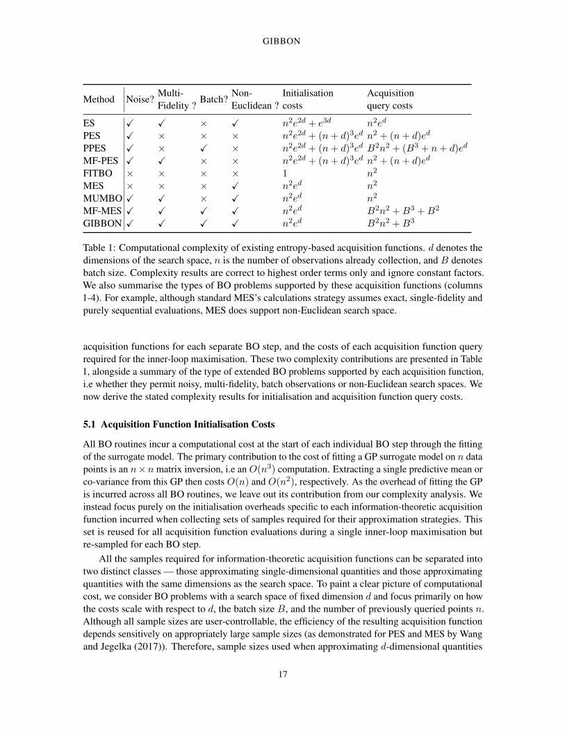
GIBBON
Method Noise?Multi-Fidelity ?
Batch?Non-Euclidean ?
Initialisationcosts
Acquisitionquery costs
ES X X × X n2e2d + e3d n2ed
PES X × × × n2e2d + (n+ d)3ed n2 + (n+ d)ed
PPES X × X × n2e2d + (n+ d)3ed B2n2 + (B3 + n+ d)ed
MF-PES X X × × n2e2d + (n+ d)3ed n2 + (n+ d)ed
FITBO × × × × 1 n2
MES × × × X n2ed n2
MUMBO X X × X n2ed n2
MF-MES X X X X n2ed B2n2 +B3 +B2
GIBBON X X X X n2ed B2n2 +B3
Table 1: Computational complexity of existing entropy-based acquisition functions. d denotes thedimensions of the search space, n is the number of observations already collection, and B denotesbatch size. Complexity results are correct to highest order terms only and ignore constant factors.We also summarise the types of BO problems supported by these acquisition functions (columns1-4). For example, although standard MES’s calculations strategy assumes exact, single-fidelity andpurely sequential evaluations, MES does support non-Euclidean search space.
acquisition functions for each separate BO step, and the costs of each acquisition function queryrequired for the inner-loop maximisation. These two complexity contributions are presented in Table1, alongside a summary of the type of extended BO problems supported by each acquisition function,i.e whether they permit noisy, multi-fidelity, batch observations or non-Euclidean search spaces. Wenow derive the stated complexity results for initialisation and acquisition function query costs.
5.1 Acquisition Function Initialisation Costs
All BO routines incur a computational cost at the start of each individual BO step through the fittingof the surrogate model. The primary contribution to the cost of fitting a GP surrogate model on n datapoints is an n×n matrix inversion, i.e an O(n3) computation. Extracting a single predictive mean orco-variance from this GP then costs O(n) and O(n2), respectively. As the overhead of fitting the GPis incurred across all BO routines, we leave out its contribution from our complexity analysis. Weinstead focus purely on the initialisation overheads specific to each information-theoretic acquisitionfunction incurred when collecting sets of samples required for their approximation strategies. Thisset is reused for all acquisition function evaluations during a single inner-loop maximisation butre-sampled for each BO step.
All the samples required for information-theoretic acquisition functions can be separated intotwo distinct classes — those approximating single-dimensional quantities and those approximatingquantities with the same dimensions as the search space. To paint a clear picture of computationalcost, we consider BO problems with a search space of fixed dimension d and focus primarily on howthe costs scale with respect to d, the batch size B, and the number of previously queried points n.Although all sample sizes are user-controllable, the efficiency of the resulting acquisition functiondepends sensitively on appropriately large sample sizes (as demonstrated for PES and MES by Wangand Jegelka (2017)). Therefore, sample sizes used when approximating d-dimensional quantities
17

MOSS, LESLIE, GONZALEZ AND RAYSON
must grow exponentially as O(ed) in order to preserve approximation accuracy. In contrast, thesample sizes required for effective approximations of single dimensional quantities can be chosenindependently of d and so are denoted as O(1) in our complexity analysis.
As discussed in Section 2, MES-based acquisition functions (including GIBBON), uses a Gumbelsampler to access samples of the maximum value g∗. This sampler evaluates our GP surrogate model’sposterior (at O(n2) cost) across O(ed) points to form a discretisation of the d-dimensional searchspace. Each of the required O(1) samples of g∗ (a single dimensional quantity) can then be extractedwith O(1) cost, yielding an overall complexity of O(n2ed). As shown in Table 1, GIBBON’sinitialisation costs are substantially lower than those of the acquisition functions based on PESand ES. Only FITBO has a lower initialisation cost, however it has not seen widespread use as itsupports only noiseless standard BO tasks and employs a complicated construction requiring linearapproximations of non-central χ2 process (operations not supported by GP libraries). For the ES andPES-based acquisition functions, which require samples from the d-dimensional objective functionmaximiser x∗, initialisation costs are substantial.
In ES, each sample of x∗ is the maximum of a sample function drawn from the GP acrossan O(ed) discretisation of the search space. Simulating these function draws requires a one-offO(e3d) computation for the Cholesky factor of the predictive co-variance matrix evaluated across thediscretisation, as accessed with an O(n2) cost for each of its O(e2d) elements. Consequently, theinitialisation of ES incurs a sizeable O(n2e2d + e3d) complexity scaling. PES also requires samplesof x∗ but instead maximises the sample draws from a finite feature approximation of the GP surrogatemodel (Rahimi and Recht, 2008), requiring just anO(n2) cost for each of the requiredO(ed) samples.However, unlike ES, PES incurs the additional cost of pre-computing an n+ d-dimensional matrixinversion for each sample. Therefore, PES has a total initialisation cost of O(n2ed + (n+ d)3ed)).Note that the finite feature approximation employed by PES and its variants is only rigorously definedfor GPs with stationary kernels and Euclidean search spaces.
5.2 Acquisition Function Query Costs
We now discuss the computational complexity of each individual acquisition function query. Ashighlighted in Table 1, not only does the GIBBON acquisition function match the lowest query costsattained by any information-theoretic acquisition functions, but it is suitable for standard, stochastic,multi-fidelity and batch optimisation.
To calculate GIBBON and the other MES-based acquisition functions, we require the joint predic-tive distribution across B proposed batch locations. Accessing these B2 predictive co-variance termsfrom a GP surrogate model and then taking its determinant cost O(B2n2) and O(B3), respectively.Finally, GIBBON calculates an analytical expression for each of the O(1) samples from g∗ andacross each of the batch elements, yielding an overall complexity of O(B2n2 +B3). MF-MES has asimilar construction to GIBBON, but requires the additional calculation of a B-dimensional integral,for which a naive numerical approximation would require an O(eB) cost. Following Takeno et al.(2020), this integral can also be evaluated using a sophisticated recursive strategy for calculatingmulti-variate Gaussian cumulative density functions withO(B2) cost, however, we found this routineto incur a large constant overhead that dominated our acquisition function calculations. Similarly, westress that although all MES-based acquisition functions have O(n2) cost (in the non-batch setting),FITBO, MUMBO and MF-MES all require additional numerical integrations (over GIBBON) thatincur a significant constant cost factor that does not show in our highest order complexity analy-
18
GIBBON
sis. Consequently, the experiments of Section 6 show that GIBBON is substantially cheaper thanMUMBO and MF-MES in practice.
The ES and PES-based acquisition functions incur a substantially larger query cost than GIBBON.Their primary computational bottleneck is the requirement of separate calculations for each of theirO(ed) samples of x∗. In ES, each evaluation requires an n2 prediction from the GP for each locationacross a small O(1)-sized collection of points for each sampled x∗. In contrast, PES requires onlya single prediction from the GP but additional O(n + d) manipulations for each of its O(ed) pre-computed kernel matrices. For batch BO, PPES requires B2 GP predictions and a B3 calculation toaccess the determinant of the batch’s posterior co-variance, as well as an additional B3 determinantcalculations for each pre-computed kernel matrix.
6. Experiments
We now finish this manuscript with a comprehensive empirical evaluation of our GIBBON acquisitionfunction. In particular, we consider batch (Section 6.1) and multi-fidelity (Section 6.3) syntheticbenchmarks, as-well as well as a molecular design loop over a non-Euclidean and highly-structuredsearch space (Section 6.5). Finally, we examine the performance of GIBBON when inserted intoa challenging real-world BO framework that requires both batch and multi-task decision making.Implementations of GIBBON are available in three popular Python libraries for BO: Emukit (Paleyeset al., 2019), BoTorch (Balandat et al., 2020) and Trieste (Berkeley et al., 2021) .
For clarity, all of our experiments follow a similar format. We run each of the considered BOmethods across 50 random seeds, plotting mean performance and a single standard error. For batchalgorithms, we count the evaluation of a batch as a single BO iteration. Suboptimality of the currentbelieved optimum x is measured by the regret g(x∗) − g(x), where x∗ is the true maximiser. Forsome experiments we also measure the time taken to choose the next query points (referred to as theoptimisation overhead). This computational cost of performing BO includes fitting the GP surrogatemodel as well as initialising and maximising the acquisition function. All experiments reportingoptimisation overheads were performed on a quad core Intel Xeon 2.30GHz processor.
Across all our experiments, we see the same general behaviour: GIBBON at least matches, andoften exceeds, the performance of existing high-performance acquisition functions whilst incurringan order of magnitudes lower computational overhead. Moreover, the breadth of our experimentsshowcases that GIBBON is truly a general-purpose acquisition function, forming a computationallylight-weight acquisition function suitable for standard BO extensions, batch high-cost string designproblems and sophisticated synchronous batch multi-task BO frameworks.
Overall, the purpose of our experiments is to demonstrate how GIBBON performs relativeto other BO acquisition functions, with a primary focus on existing MES-based approaches. Forcompleteness, we also compare against a range of additional methods, chosen to reflect theirpopularity, code availability and suitability for the particular experiment. To this end, we compareGIBBON with all the acquisition functions supported by BoTorch and Emukit, as-well as our ownimplementations of the batch heuristics discussed in Section 4. We will introduce these competitorsalongside the relevant empirical results. Unfortunately, the PES-based methods discussed in Section5 do not have implementations in BoTorch or Emukit. Moreover, we could not find any othercomparable maintained software implementations, likely due to demonstrably worse performance ofPES than MES (as shown by Wang and Jegelka, 2017) and PES’s difficult-to-implement subroutines(Section 5).
19

MOSS, LESLIE, GONZALEZ AND RAYSON
6.1 Standard and Batch Optimisation
For our first set of experiments, we consider a set of synthetic functions provided with the BoTorchpackage. In particular, we recreate two of the experiments of Balandat et al. (2020) by maximisingthe Hartmann (d = 6) and Ackley functions (d = 4), each with observations perturbed by centredGaussian noise with a variance of 0.25. In addition, we also consider the Shekel function (d = 4)under exact observations. For details of these synthetic functions, we refer readers to Appendix C.1.Following the setup of Balandat et al. (2020), we initialise all routines by evaluating 2d+ 2 randomlocations, refit our GP’s kernel parameters after each BO step, and choose the current believedoptimum x∗ by maximising the posterior mean of the GP surrogate model. For each experiment, weseparately consider purely sequential BO (B = 1) and batch BO (B = 5), recording the evaluationof the whole batch as a single optimisation step.
For all our experiments, we report the performance of GIBBON and Expected Improvement (EI),as well as standard MES (applied to noisy problems by assuming exact observations). In addition,we also ran the acquisition functions already supported in BoTorch, i.e Knowledge Gradient (KG),Noisy Expected Improvement (NEI) (Picheny et al., 2010), and MFMES (the multi-fidelity MESextension of Takeno et al. (2020), used here to support noisy observations). We stress that MFMESwas designed to provide computationally light-weight asynchronous batch BO and we will see that itsadaptation to synchronous problems (as implemented by BoTorch and discussed earlier in Sections 2and 5) incurs a substantial computational overhead. For our batch problems, we also implementedBoTorch versions of Local Penalisation (LPEI) and the DPP heuristic (DPPEI) of Kathuria et al.(2016), both using EI as their base acquisition function (as considered by Gonzalez et al. (2016a) andKathuria et al. (2016)). In addition, we also provide local penalisation with an MES base acquisitionfunction (LPMES), a combination not tested by Gonzalez et al. (2016a) but found to be particularlyeffective in our experimentation. All MES-based acquisition functions (including GIBBON) use 5max-values sampled from a Gumbel distribution fit to surrogate model predictions at 10, 000 ∗ drandom locations and are re-sampled for each BO step. All other implementation parameters followthe BoTorch defaults.
For acquisition function maximisation we use BoTorch’s gradient-based maximiser. However,as this inner-loop maximisation can be challenging since it corresponds to a highly multi-modalmaximisation across a B × d-dimensional space. Therefore most batch BO routines build batchesgreedily by breaking batch design into B separate d-dimensional maximisations. Consequently, forall approaches (including our GIBBON acquisition function) except KG , batches are constructed inthis greedy manner with a maximisation budget of 10 ∗ d random restarts for each element of thebatch. Although KG is able to jointly allocate batches, its large computational cost restricted us to 20restarts (the amount recommended by the BoTorch authors).
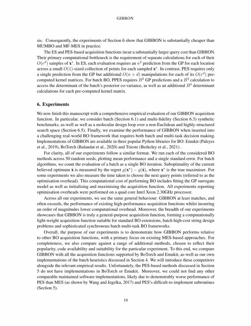
Across the three synthetic experiments (Figure 3) we see that GIBBON provides efficient high-precision optimisation, yielding small regret in competitively few iterations for both sequential andbatch BO. Note that in the noiseless and purely sequential case (Figure 3a), although MFMES can beshown to collapse exactly to the acquisition function of MES, the performance of these two methodsdiffer as BOTorch’s implementation of MFMES still relies on numerical approximations (albeitwith a a very small observation noise term). Moreover, MFMES’s reliance on rough numericalapproximations means that its acquisition function struggles to provide high-precision optimisationonce the acquisition function values are sufficiently small (i.e towards the end of the optimisation).Consequently, although sometimes achieving fast initial optimisation, MFMES fails to achieve as
20
GIBBON
(a) Noiseless Shekel (d = 4, B = 1) (b) Noiseless Shekel (d = 4, B = 5)
(c) Noisy Ackley (d = 4, B = 1) (d) Noisy Ackley (d = 4, B = 5)
(e) Noisy Hartmann (d = 6, B = 1) (f) Noisy Hartmann (d = 6, B = 5)
Figure 3: Optimisation of synthetic benchmark functions. GIBBON provides efficient and high-precision optimisation, matching or exceeding the performance of existing approaches.
21
MOSS, LESLIE, GONZALEZ AND RAYSON
(a) B=1 (b) B=5
Figure 4: The computational overheads incurred while optimising the Hartmann function. GIBBON’scosts remains low throughout the optimisation, whereas the other high-performing batch acquisitionfunctions costs increase dramatically as the optimisation progresses.
small final regret as GIBBON. Surprisingly, GIBBON is able to outperform even standard MESin the noiseless optimisation task of Figure 3a, the scenario for which standard MES is exact. AsGIBBON approximates MES, we expected it to perform strictly worse for this example. We delvedeeper into this phenomenon in Appendix E.
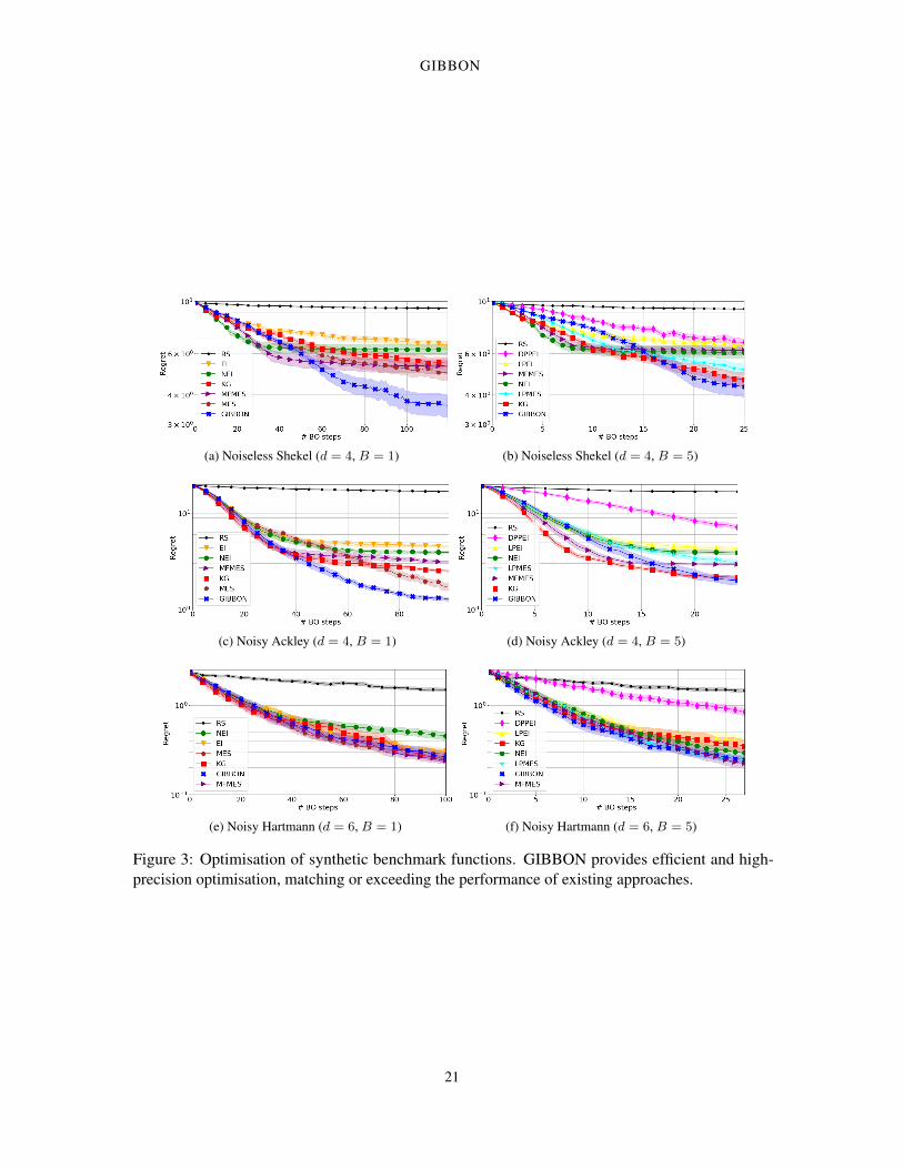
Of particular note is the order of magnitude smaller overhead incurred by GIBBON over theother high-performing acquisition functions (NEI, KG and MFMES) as summarised in Table 2a(for B = 1) and Table 2b (for B = 5). In particular, batch KG incurs at least a 10 times largeroverhead than GIBBON. Moreover, Figure 4 shows that, while the computational overhead of batchKG, MFMES and NEI increase substantially as the optimisation progresses, GIBBON’s overheadsettles to fixed cost. We hypothesise that the initial (small) rise in the computational overhead ofGIBBON is caused due to early acquisition functions having wider modes that require more localoptimisation steps, a property also likely shared by other acquisition functions but disguised by theirgrowing acquisition function cost. Although MFMES and GIBBON share the same order complexitywith respect to the number of BO steps (see Table 1), we see that the large cost of numericalintegration renders MFMES significantly more expensive than GIBBON in practice. Moreover, theBoTorch implementation of synchronous batch MFMES employs multiple model fits within eachbatch allocation to ensure approximation accuracy and so its cost scales poorly with the number ofoptimisation steps.
Figure 5 confirms our earlier claim that GIBBON is indeed a high-performance yet computation-ally light-weight acquisition function, showing that GIBBON performs better than all competingacquisition functions while incurring a computational overhead only slightly worse than the simplebut low-performance approaches.
6.2 Ablation Study
Before assessing GIBBON across a wider range of BO tasks, we now perform a brief ablation studyinto GIBBON’s user-controllable parameters and how they affect performance on the noisy Hartmannfunction introduced above. In particular, we focus on batch size (B) and sensitivity to the quality ofmax-value samples used to calculate GIBBON.
22

GIBBON
Computational Overhead (seconds 1 d.p.)Shekel (d=4) Ackley (d=4) Hartmann (d=6)
EI 0.2 (±0.0) 0.2 (±0.1) 0.8 (±0.1)MES 0.5 (±0.1) 0.5 (±0.0) 1.0 (±0.1)NEI 3.5 (±0.3) 3.0 (±0.2) 8.9 (±0.7)MFMES 3.0 (±0.4) 0.7 (±0.1) 4.5 (±0.2)KG 13.0 (±0.8) 22 (±1.0) 66.6 (±4.6)GIBBON 0.6 (±0.1) 0.8 (±0.1) 1.5 (±0.1)
(a) Computational overheads for sequential BO (B = 1).
Computational Overhead (seconds 1 d.p.)Shekel (d=4) Ackley (d=4) Hartmann (d=6)
DPPEI 0.8 (±0.1) 0.8 (±0.0) 1.2 (±0.0)LPEI 1.4 (±0.2) 2.3 (±0.1) 2.9 (±0.1)LPMES 2.9 (±0.1) 3.3 (± 0.1) 3.5 (± 0.1)NEI 21.3 (±1.8) 23.4 (±0.6) 43.0 (±2.6)MFMES 24.4 (±2.3) 26.7 (±0.6) 38.6 (±1.9)KG 58.1 (±4.4) 53.0 (±3.1) 103.4 (±6.2)GIBBON 5.0 (±0.5) 5.8 (±0.7) 13.3 (±1.3)
(b) Computational overheads for batch BO (B = 5)
Table 2: Computational overheads for the synthetic benchmarks of Figure 3 averaged over thewhole optimisation run. The two algorithms achieving lowest regret for each task are highlighted,demonstrating that GIBBON at least matches the overhead of other high-performing sequentialacquisition functions and incurs a significantly lower overhead than other batch high-performingacquisition functions.
(a) B=1 (b) B=5
Figure 5: Comparison of the final regret achieved by each BO method with their computationaloverheads. Scores are standardised to sit within [0, 1] and averaged across the three syntheticbenchmark tasks. Lower scores on the x and y axis represent a smaller computational overheads andmore effective optimisation, respectively.
23

MOSS, LESLIE, GONZALEZ AND RAYSON
(a) GIBBON (b) LPEI
Figure 6: Optimisation of the noisy Hartmann function over 20 iterations across a range of batchsizes. GIBBON is able to provide effective batch optimisation for small to moderate batch size(B < 25), however, fails to effectively control large batches. Although LPEI is able to leveragelarger parallel resources than GIBBON, it still fails to match the performance of GIBBON (B=10)even when controlling much larger batches (B=50).
6.2.1 GIBBON FOR LARGE BATCH OPTIMISATION
GIBBON is a promising candidate for optimising under a large degree of parallelism as its batchescan be constructed greedily without requiring B posterior updates. Unfortunately, GIBBON failsto realise this promise in practice. Figure 6 shows that GIBBON fails to effectively leverage largeparallel resources and even displays a significant drop in performance once considering batches ofsize 25. In contrast, LPEI is able to continually improve regret by considering larger and largerbatches. We stress that LPEI, even when controlling batches of 50 elements (i.e. 1, 000 totalevaluations), still achieves lower regret than GIBBON with batches of size 10 (i.e 200 evaluations).
As demonstrated in Appendix D, GIBBON can be easily modified to support optimisation underlarge batches by a simple down-weighting of its repulsion term. Therefore, we posit that poorperformance of GIBBON in this large batch setting is due to a degradation of the approximationaccuracy in our analytical lower bound as we increase batch size. To see this, consider GIBBON’sdiversity-quality decomposition first introduced in Section 4 (i.e. Equation (8)). Considering largebatches ensures that at least some candidate elements must be close together and so have highcorrelation. Consequently, GIBBON is dominated by its repulsion term (the determinant of thebatch’s predictive correlation matrix) and the maximisation of GIBBON leads to repeated querypoints around the edge of the search space, resulting in a substantial degradation in the stability ofour GP surrogate model and poor exploration in more important areas of the space. Therefore, in thislarge batch setting, GIBBON effectively collapses to an almost pure exploration DPP-based methodsimilar to the poorly performing DPPEI examined in our synthetic experiments.
6.2.2 GIBBON WITH THOMPSON-SAMPLED MAXIMUM VALUES
Our proposed calculation strategy for GIBBON requires access to M samples from the objectivefunction’s currently unknown maximum value g∗. We now investigate the sensitivity of GIBBONwith respect to the quality of these random samples. For all the other experiments in this work weused the low-cost but approximate Gumbel sampler, as proposed by Wang and Jegelka (2017). Byapproximating the empirical CDF of g∗ with an analytical Gumbel distribution, Gumbel samplingis able to return M approximate max-value samples over a grid of N candidate locations with
24

GIBBON
(a) Regret (B=1) (b) Computational Overhead (B=1)
(c) Regret (B=5) (d) Computational Overhead (B=5)
Figure 7: Regret performance (left) and computational overhead (right) of GIBBON when optimisingthe noisy Hartmann function using batches of size 1 (top row) or 5 (bottom row) across differentmax-value sampling strategies. Although exact sampling provides a small boost in GIBBON’sperformance for the batch experiment, Gumbel sampling seems adequate for sequential optimisation.Moreover, the resulting computational overhead of GIBBON with exact sampling is five and threetimes the cost of GIBBON with Gumbel sampling, when controlling batches of size B = 1 andB = 5, respectively.
cost O(M + N). Of course, we can access exact samples of g∗ by maximising sample functionsdrawn from our GP (i.e a Thompson-sampling style approach). However, extracting M such exactsamples incurs an O(MN + N3) cost and so, if used as part of GIBBON’s calculation strategy,would add significantly to GIBBON’s optimisation overhead. However, as using exact max-valuesamples removes the only source of approximation in GIBBON aside from our information-theoreticlower bound, this alternative Thompson sampling strategy may lead to improved optimisation — ahypothesis we now investigate.
In Figure 7, we present the performance of GIBBON when using 1, 5 and 10 approximate(Gumbel) or exact (Thompson) sampled maximum values. Due to the significant cost of the exactThompson sampler, we can sample over only 1, 000 ∗ d random candidate locations, as opposedto the 10, 000 ∗ d used for our Gumbel sampler. We see that, in exchange for a large increase incomputational overhead, the exact sampler can sometimes lead to a small increase in performanceover our standard Gumbel-based batch GIBBON implementation. We stress that changing samplerhad no effect on the performance of purely sequential (B = 1) BO. This small and inconsistentperformance improvement is not enough to justify the additional overhead of exact sampling andso, in order to remain loyal to our motivation of GIBBON as a computationally light acquisition
25

MOSS, LESLIE, GONZALEZ AND RAYSON
Overhead for Multi-fidelity Optimisation (Seconds 1 d.p.)Curin (d=4) Hartmann (d=3) Hartmann (d=6) Borehole (d=8)
ES 16.6 (±0.7) 59.7 (±4.2) 229.8 (±15.3) -MUMBO 13.7 (±0.6) 18.6 (±1.0) 79.9 (±6.2) 51.5 (±7.5)GIBBON 4.0 (±0.2) 9.9 (±0.7) 50.2 (±4.0) 46.1 (±7.5)
Table 3: Computational overheads of the multi-fidelity synthetic benchmarks of Figure 8. GIBBONenjoys the lowest overheads for all the tasks (as highlighted in bold), often less than half those ofMUMBO.
function, we continue using the Gumbel sampler for all our remaining experiments. Investigatingalternative sampling strategies to use within GIBBON is an important area of future work.
6.3 Multi-fidelity Optimisation
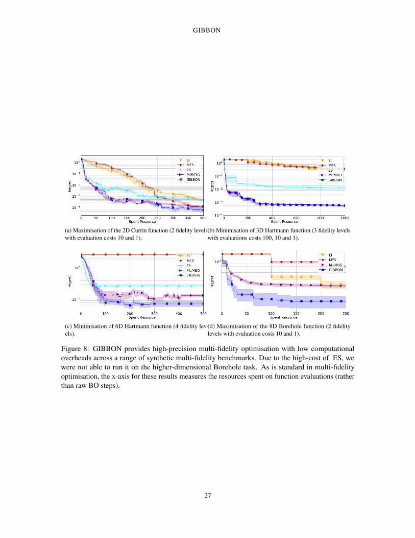
We now turn to multi-fidelity optimisation, where the current state-of-the-art acquisition functionsare the effectively equivalent MUMBO (Moss et al., 2020d) and MFMES (Takeno et al., 2020)acquisition functions. Moss et al. (2020d) demonstrates comprehensively that MUMBO outperformsa wide range of existing multi-fidelity acquisition functions, including the entropy search-basedapproach of Swersky et al. (2013), the upper-confidence bound variants of Kandasamy et al. (2016)and Kandasamy et al. (2017), as well as extensions of EI (Huang et al., 2006) and KG (Wu andFrazier, 2016). Therefore, to test GIBBON’s multi-fidelity optimisation capabilities, it is sufficientto compare with MUMBO. To this end, we provide an implementation of GIBBON for the EmukitPython library and recreate exactly the synthetic experiments from Figure 2 of Moss et al. (2020d).These experiments consider popular synthetic multi-fidelity benchmarks with discrete fidelity spacesconsisting of between 2 and 4 fidelity levels (each with differing query costs) and search spacedimensions ranging from 2 to 8 dimensions (see Appendix C.2 for the analytical forms of thesesynthetic benchmarks). In these experiments, we use the linear multi-fidelity GP model of Kennedyand O’Hagan (2000) as our surrogate model, initialise the GP with a random sample of 2 ∗ d pointsqueried across all fidelity levels, and fit the GP’s kernel parameters to maximise model marginallikelihood after each BO step.
Figure 8 shows that GIBBON provides at least as effective optimisation as MUMBO and Table 3shows that GIBBON has a significantly lighter computational overhead. To provide context for thehigh performance and low overhead of GIBBON we also present the performance of EI and MESwhen restricted to just querying the true objective function (i.e no access to low-fidelity observations)and the performance of the ES acquisition function, used to perform multi-fidelity optimisationby Swersky et al. (2013). Although the difference in overhead between MUMBO and GIBBONdecreases as we consider higher-dimensional search spaces (primarily due to the growing cost of theGumbel sampler used by both approaches), the difference in achieved regret increases in GIBBON’sfavour.
6.4 Batch Molecular Search
BO has recently been applied to high-cost string design problems by Moss et al. (2020b), whoconsider, among other problems, the task of optimising over molecules. Such tasks are well-suitedfor BO, due to the high cost of evaluating candidate molecules via wet-lab experiments. Moss
26
GIBBON
(a) Maximisation of the 2D Currin function (2 fidelity levelswith evaluation costs 10 and 1).
(b) Minimisation of 3D Hartmann function (3 fidelity levelswith evaluations costs 100, 10 and 1).
(c) Minimisation of 6D Hartmann function (4 fidelity lev-els).
(d) Maximisation of the 8D Borehole function (2 fidelitylevels with evaluation costs 10 and 1).
Figure 8: GIBBON provides high-precision multi-fidelity optimisation with low computationaloverheads across a range of synthetic multi-fidelity benchmarks. Due to the high-cost of ES, wewere not able to run it on the higher-dimensional Borehole task. As is standard in multi-fidelityoptimisation, the x-axis for these results measures the resources spent on function evaluations (ratherthan raw BO steps).
27

MOSS, LESLIE, GONZALEZ AND RAYSON
et al. (2020b) propose a BO framework that fits a GP surrogate model to a popular string-basedrepresentation of molecules known as SMILES strings (Anderson et al., 1987) through a string kernelGP (Beck et al., 2015). Standard EI arguments are then applied, yielding a highly effective strategyfor searching large candidate set of molecules. One practical limitation of this framework, however,is the large computational cost of string kernels, as incurred for each prediction from the surrogatemodel GP. Consequently, the framework of Moss et al. (2020b) is limited to acquisition functions thatrequire a small number sof surrogate model predictions. Aside from GIBBON, our other consideredhigh-performing batch acquisition functions (MFMES, NEI and KG) require many kernel evaluationsfor each acquisition function query and the low-cost approaches of DPPEI and LPEI are limited toonly Euclidean search spaces. In contrast, GIBBON requires only B surrogate model predictions tomeasure the utility of a candidate batch and makes no assumptions on the properties of the searchspace. Therefore, GIBBON can be used to extend the framework of Moss et al. (2020b) to batchdesigns, a property particularly attractive for molecular search applications where it is commonpractice to synthesis collections of candidate molecules in parallel.
We now recreate the Zinc example (also considered by Kusner et al. (2017) and Griffiths andHernandez-Lobato (2020)), where we seek to explore a large collection of 250,000 molecules. Thetask is then to quickly find molecules that score highly according to a chemically-inspired metric, i.e.forming a proxy molecular design loop with this metric forming our objective function. As stringkernel GPs, which are used to model our moelcules’ SMILE strings, have a very large evaluationcost, we cannot evaluate our acquisition function across all the candidate molecules. Therefore, werandomly sample 1, 000 molecules for each BO step from which we (greedily) choose to evaluatethe B molecules that maximise our GIBBON acquisition function.
We fit our Gumbel sampler on this same sample, re-sampling both the max-values required forGIBBON and the considered 1, 000 molecules at the start of each BO step. We evaluate 20 randomlychosen molecules to initialise our GP and then allow BO to choose 100 further molecules, eitherone by one or as 20 batches of 5 molecules or 10 batches of 10 molecules. Figure 9 shows thateven in the purely sequential case, GIBBON provides a modest boost in performance over EI (theacquisition function previously used by Moss et al. (2020b)). More importantly, Figure 9 also showsthat GIBBON is able to provide effective batch optimisation over batches of size 5 and 10, thereforeproviding an extension of Moss et al. (2020b)’s framework where parallel synthesising resources canbe used to speed up the molecular search.
6.5 Bayesian Optimisation by Sampling Hierarchically
For our final set of examples, we demonstrate the efficacy of GIBBON as part of a real-worldoptimisation framework. In particular, we turn to a challenging batch multi-fidelity BO probleminspired by the Knowledge Gradient for Common Random Numbers (KG-CRN) framework ofPearce et al. (2019). We now provide a brief very overview of the KG-CRN framework and we referthe reader to Pearce et al. (2019) for further details. Our implementation is built upon the EmukitPython package (Paleyes et al., 2019) and was first reported in a workshop paper (Moss et al., 2020c).
KG-CRN considers BO under highly stochastic evaluations, a scenario where it is commonplaceto disregard the original objective function entirely and instead optimise the average of a collectionof K specific function realisations, e.g. K-fold cross validation (CV) (Kohavi, 1995) or sampleaverage approximations (Kleywegt et al., 2002). However, as demonstrated for hyper-parametertuning (Moss et al., 2018), model selection (Moss et al., 2019) and simulation optimisation (Kim
28
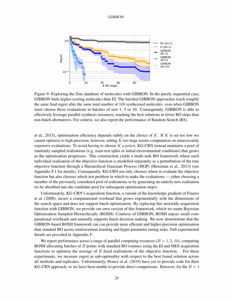
GIBBON
Figure 9: Exploring the Zinc database of molecules with GIBBON. In the purely sequential case,GIBBON finds higher-scoring molecules than EI. The batched GIBBON approaches reach roughlythe same final regret after the same total number of 100 synthesised molecules even when GIBBONmust choose these evaluations in batches of size 1, 5 or 10. Consequently, GIBBON is able toeffectively leverage parallel synthesis resources, reaching the best solutions in fewer BO steps thannon-batch alternatives. For context, we also report the performance of Random Search (RS).
et al., 2015), optimisation efficiency depends subtly on the choice of K. If K is set too low wecannot optimise to high precision, however, setting K too large wastes computation on unnecessarilyexpensive evaluations. To avoid having to choose K a-priori, KG-CRN instead maintains a pool ofrandomly sampled realisations (e.g. train-test splits or initial environmental conditions) that growsas the optimisation progresses. This construction yields a multi-task BO framework where eachindividual realisation of the objective function is modelled separately as a perturbation of the trueobjective function through a Hierarchical Gaussian Process (HGP) (Hensman et al., 2013) (seeAppendix F.1 for details). Consequently, KG-CRN not only chooses where to evaluate the objectivefunction but also chooses which test problem in which to make the evaluations — either choosing amember of the previously considered pool of realisations or by generating an entirely new realisation(to be absorbed into the candidate pool for subsequent optimisation steps).
Unfortunately, KG-CRN’s acquisition function, a variant of the knowledge gradient of Frazieret al. (2008), incurs a computational overhead that grows exponentially with the dimensions ofthe search space and does not support batch optimisation. By replacing this unwieldy acquisitionfunction with GIBBON, we provide our own version of this framework, which we name BayesianOptimisation Sampled Hierarchically (BOSH). Courtesy of GIBBON, BOSH enjoys small com-putational overheads and naturally supports batch decision making. We now demonstrate that theGIBBON-based BOSH framework can can provide more efficient and higher-precision optimisationthan standard BO across reinforcement learning and hyper-parameter tuning tasks. Full experimentaldetails are provided in Appendix F.
We report performance across a range of parallel computing resources (B = 1, 5, 10), comparingBOSH allocating batches of B points with standard BO routines using the EI and MES acquisitionfunctions to optimise the average of B fixed realisations of the objective function. For theseexperiments, we measure regret as sub-optimality with respect to the best found solution acrossall methods and replicates. Unfortunately, Pearce et al. (2019) have yet to provide code for theirKG-CRN approach, so we have been unable to provide direct comparisons. However, for the B = 1
29

MOSS, LESLIE, GONZALEZ AND RAYSON
(a) B=1
(b) B=5 (c) B=10
Figure 10: Optimising 7 parameters of a Lunar Lander controller. We present the regret achieved byeach algorithm (top panel) alongside a running count of the number of realisations considered byBOSH (bottom panel). Courtesy of our GIBBON acquisition function, BOSH is able to adaptiveconsider up to 15 random conditions to quickly find the optimal controller configuration.
case, we are able to consider FASTCV (Swersky et al., 2013), an EI-based framework that speeds upoptimisation by allowing the evaluation of the individual splits making up K-fold CV (for a specificchoice of K). Unlike our previous examples, we now include the evaluations spent on randominitialisation in our plots as the required size of this initialisation is different for each framework (seeAppendix F.2). BOSH, for example, is initialised with evaluations at d+ 5 random locations foreach of two initial seeds.
6.5.1 REINFORCEMENT LEARNING
For our first experiment, we consider a challenging seven-dimensional stochastic optimisation test-case. We wish to fine-tune a controller for a well-studied reinforcement learning problem, wherewe must guide a lunar lander across a randomly initialised space to its landing zone with minimalthruster usage (as provided in the OpenAI Gym). Our controller is parameterised by seven unknownconstants and a particular configuration can be tested by running a single (or B) randomly generatedscenarios. We seek to minimise the extra fuel required to land the lander over OpenAI’s hard-codedcontroller (as measured according to a ‘true’ performance measured over a set of 100 fixed initial
30
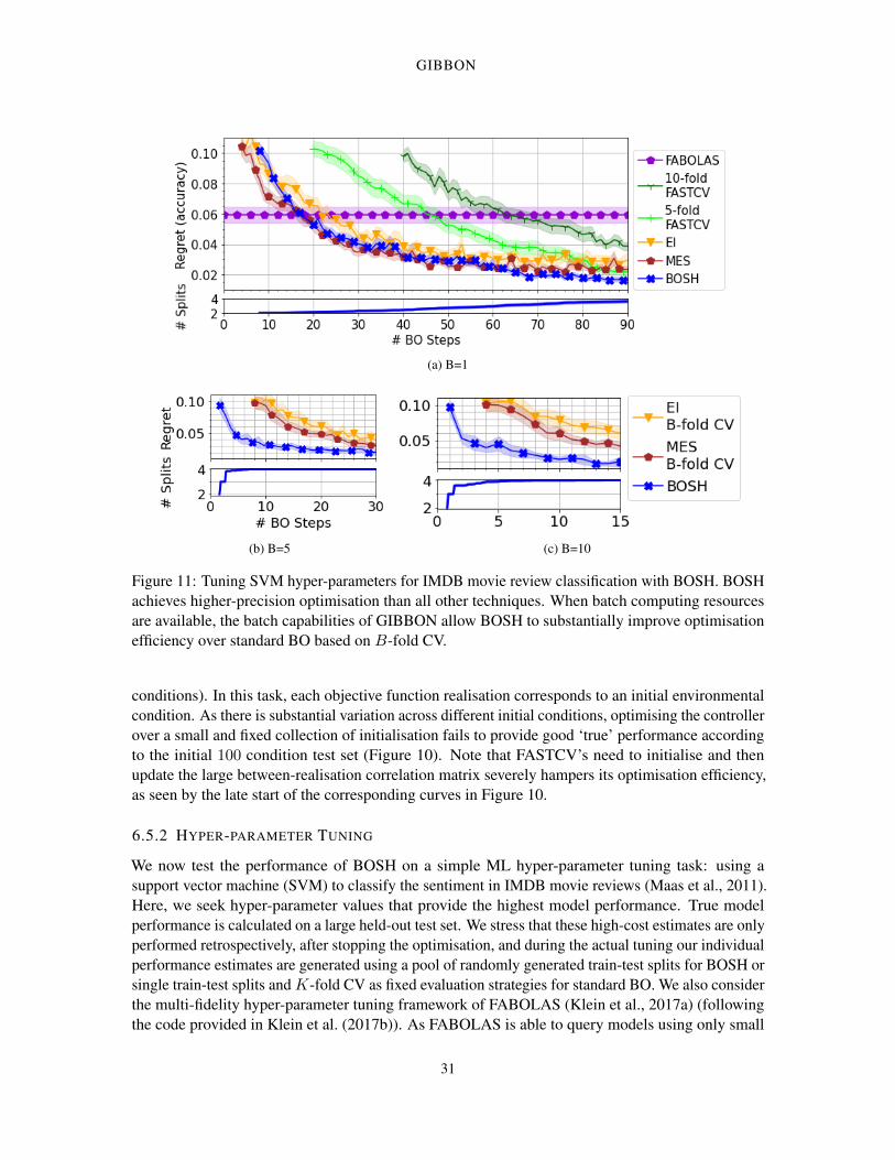
GIBBON
(a) B=1
(b) B=5 (c) B=10
Figure 11: Tuning SVM hyper-parameters for IMDB movie review classification with BOSH. BOSHachieves higher-precision optimisation than all other techniques. When batch computing resourcesare available, the batch capabilities of GIBBON allow BOSH to substantially improve optimisationefficiency over standard BO based on B-fold CV.
conditions). In this task, each objective function realisation corresponds to an initial environmentalcondition. As there is substantial variation across different initial conditions, optimising the controllerover a small and fixed collection of initialisation fails to provide good ‘true’ performance accordingto the initial 100 condition test set (Figure 10). Note that FASTCV’s need to initialise and thenupdate the large between-realisation correlation matrix severely hampers its optimisation efficiency,as seen by the late start of the corresponding curves in Figure 10.
6.5.2 HYPER-PARAMETER TUNING
We now test the performance of BOSH on a simple ML hyper-parameter tuning task: using asupport vector machine (SVM) to classify the sentiment in IMDB movie reviews (Maas et al., 2011).Here, we seek hyper-parameter values that provide the highest model performance. True modelperformance is calculated on a large held-out test set. We stress that these high-cost estimates are onlyperformed retrospectively, after stopping the optimisation, and during the actual tuning our individualperformance estimates are generated using a pool of randomly generated train-test splits for BOSH orsingle train-test splits and K-fold CV as fixed evaluation strategies for standard BO. We also considerthe multi-fidelity hyper-parameter tuning framework of FABOLAS (Klein et al., 2017a) (followingthe code provided in Klein et al. (2017b)). As FABOLAS is able to query models using only small
31

MOSS, LESLIE, GONZALEZ AND RAYSON
proportions of the available data, it is able to find reasonably well performing hyper-parameterconfigurations in a fraction of the computation used by standard BO and BOSH. However, even ifallowed a significantly longer run-time, FABOLAS fails to improve upon this chosen configuration(which we plot as a horizontal line). Figure 11a shows that BOSH adaptively considers a pool ofup to four train-test splits as the optimisation progresses, providing higher-precision tuning thanstandard BO based on single train-test splits and substantially faster tuning than standard BO under5-fold and 10-fold cross-validation (Figures 11b and 11c).
7. Discussion
We have presented GIBBON, a general-purpose acquisition function that extends max-value entropysearch to provide computationally light-weight yet high performing optimisation for a wide range ofBO problems. The efficiency of GIBBON relies on a novel information-theoretical approximation.Moreover, the derivation of this approximation allowed the exploration of the first explicit connectionbetween information-theoretic search, determinantal point process and local penalisation, tyingtogether large sections of the BO literature previously developed and analysed independently.
Not only does GIBBON provide competitive optimisation for common BO extensions like batchand multi-fidelity optimisation, but it forms high-performance batch acquisition function suitablefor applying BO across highly-structured search spaces, as we demonstrated within a moleculardesign loop. BO for structured optimisation tasks is a fast growing frontier of the BO literature,with recent work tackling BO for strings (Moss et al., 2020b; Swersky et al., 2020), combinatorialspaces (Deshwal et al., 2020) and spaces of neural network architectures (Kandasamy et al., 2018b).Therefore, we believe that GIBBON (and our flexible software implementation) will have substantialutility for the machine learning community.
7.1 Limitations and Future Work
GIBBON, in its current form, has the two primary practical limitations investigated in our ablationstudy of Section 6.2. Firstly, GIBBON performs poorly for large batch sizes. Improving the largebatch capabilities, perhaps though artificially manipulating GIBBON’s diversity-quality trade-off,is an important avenue of future work, particularly as the low-cost construction of GIBBON isespecially well-suited to large batch scenarios which are currently dominated by simple sampling-based approaches like Thompson sampling (Vakili et al., 2020). Secondly, the performance ofGIBBON is sensitive to the quality of the max-value samples used within its calculation strategy.Although using a Gumbel sampler to calculate GIBBON provides a truly light-weight acquisitionfunction, we have shown that the performance of the acquisition function can be improved byconsidering exact max-value samples. In future work, we will investigate alternative samplingstrategies that are more accurate than Gumbel samplers but cheaper than exact Thompson sampling.A promising approach is to follow Hernandez-Lobato et al. (2016) or Takeno et al. (2020) and employapproximate Thompson sampling methods though kernel decompositions.
Although shown to be empirically successful, GIBBON has no theoretical guarantees, primarilydue to the lack of analysis around our information-theoretical lower bound. Analysing the tightnessof this bound could help disentangle which aspects of GIBBON’s behaviour are caused by approxi-mation error and which are due to limitations of information-theoretic search strategies in general.In particular, a stronger understanding of approximation quality should explain why GIBBON’sperformance degrades when building large batches or show exactly when our lower bound is a
32
GIBBON
better approximation of the mutual information than the sampling-based approximations of existingMES extensions. A bound on the approximation error of this bound would also pave the way forconvergence guarantees for GIBBON through extensions of the regret bounds of Wang and Jegelka(2017). To the author’s knowledge, no such bound exists for noisy, batch or multi-fidelity MES-basedacquisition functions.
As a final comment, we would like to point out that, although we have already shown GIBBON tohave wide applicability, GIBBON can be readily applied to an even wider collection of BO problems.For example, GIBBON can be combined with MESMO (Belakaria et al., 2019), an extension ofMES for multi-objective optimisation, to provide computationally light-weight acquisition functionfor batch multi-objective BO. Similarly, GIBBON can also provide a computationally light-weightapproach for batch constrained optimisation by extending the MES-based approach of Belakaria et al.(2020). Finally, GIBBON can be used to improve the performance and reduce the computationalcost of any framework relying on batch BO heuristics, for example in non-myopic BO (Gonzalezet al., 2016b; Jiang et al., 2020).
33
MOSS, LESLIE, GONZALEZ AND RAYSON
Appendix A. Extracting The Required Predictive Quantities from a GaussianProcess Surrogate Model
We now demonstrate how the distributional quantities required to calculate GIBBON can easily beextracted from a GP surrogate model. For observationsDn, let yn be the already observed evaluationsy , and define the kernel matrix Kn = [k(zi, zj)]zi,zj∈Dn and kernel vectors kn(z) = [k(zi, z)]zi∈Dnfor any valid kernel defined over the combined search space Z = X ×F . Finally, denote the locationin the fidelity space corresponding to the true objective function as s0 (i.e fs0(x) = g(x)). Here, as isstandard in multi-fidelity optimisation, we have assumed the ability to query (at least noisily) thetrue objective function. Then, following Rasmussen (2004) our GP surrogate model provides thefollowing:
µCi =kn((xi, s0))T (Kn + diag(σn))−1ynµAi =kn(zi)T (Kn + diag(σn))−1yn
ΣCi,j =k((xi, s0), (xj , s0))− kn((xi, s0))T (Kn + diag(σn))−1kn((xj , s0))
ΣAi,j =k(zi, zj)− kn(zi)T (Kn + diag(σn))−1kn(zj)
ρi =k(zi, (xi, s0))− kn(zi)T (Kn + diag(σn))−1kn((xi, s0)))√
Σgi,iΣ
yi,i
,
where diag(σn) is the |Dn| × |Dn| diagonal matrix of observation noises in the evaluations Dn.
Appendix B. Proof of Theorem 2
Theorem 2 (Distribution of A given C∗ < m) Consider two B-dimensional multivariate Gaus-sian random variables A and C where C ∼ N(µC ,ΣC) and each individual component of A isdistributed asAj ∼ N(µAj ,Σ
Aj,j). Suppose further that each each pair {Aj , Cj} are jointly Gaussian
with correlation ρj , and that each Aj is conditionally independent of {Ci}i 6=j given Cj . DefineC∗ = max C. Then the conditional density of A given that C∗ < m is given by
1
P(C∗ < m)φX1(a)ΦX2(m),
where m = (m, ..,m) ∈ RB and φX1 and ΦX2 are the probability density and cumulative densityfunctions for the multivariate Gaussian random variables
X1 ∼ N(µA, S +DΣCD
)and X2 ∼ N
(µC + Σ−1DS−1(a− µA),Σ−1
),
where ΣA = DΣCD + S for D and S, diagonal matrices with elements Dj,j = ρj
√ΣAj,jΣCj,j
and
Sj,j = (1− ρ2j )Σ
Aj,j , and Σ =
((ΣC)−1
+DS−1D)
.
ProofAs detailed in the main body of this report, we have that
C ∼ N(µC ,ΣC) and Aj ∼ N1
(µAj ,Σ
Aj
),
34

GIBBON
for some known mean vectors µC ,µA ∈ RB , a variance vector ΣA ∈ RB and a co-variance matrixΣC ∈ RB×B , as well as a vector ρ ∈ RB of the correlation between each pair {Aj , Cj}. In thissection we use fX to denote the probability density function for the random variable X and fX,Y todenote the joint probability density function for the random variables X and Y.
Now, consider the probability distribution function of random variable of interest:
fA|C∗≤m(a) =1
P(C∗ ≤ m)
∫m
fA,C(a,b) db
=1
P(C∗ ≤ m)
∫m
fA|C=b(a)fC(b) db
=1
P(C∗ ≤ m)
∫m
B∏i=1
[fAi|Ci=bi(ai)
]fC(b) db, (10)
where b ∈ RB and m = (m, ..,m) ∈ RB . The factorisation of fA|C=b is due to the conditionalindependence of Aj |Cj from {Ci}i 6=j .
A well-known result for the conditional distribution from a bi-variate Gaussian gives us that foreach i ∈ {1, .., B}
Ai = ai|Ci = bi ∼ N1
(µAi + ρi
√ΣAi
ΣCi,i
(bi − µCi ), (1− ρ2i )Σ
Ai
),
i.e. we have that
A|C = b ∼ N(µA +D(b− µC), S
), (11)
for diagonal matrices D,S ∈ RB with elements Di,i = ρi
√ΣAiΣCi,i
and Si,i = (1− ρ2i )Σ
Ai .
Using (11), the integrand of (10) can now be regarded as the product of two b-dimensionalGaussian densities[
b∏i=1
fAi|Ci=bi(ai)
]fC(b) = N
(a;µA +D(b− µC), S
)∗N(b;µC ,ΣC)
= |D|N(b;µC +D−1(a− µA), D−1SD−1
)∗N(b;µC ,ΣC),
which, using the following standard formula for the product of Gaussians densities
N(x; m1,Σ1) ∗N(x; m2,Σ2) =N(m1; m2,Σ1 + Σ2)
∗N(x;(Σ−1
1 + Σ−12
)−1 (σ−1
1 m1 + Σ−12 m2
),(Σ−1
1 + Σ−12
)−1),
35

MOSS, LESLIE, GONZALEZ AND RAYSON
can be re-expressed as[b∏i=1
fAi|Ci=bi(ai)
]fC(b) = |D|N
(µC ;µC +D−1(a− µA), D−1SD−1 + ΣC
)∗N
(b;µC + Σ−1DS−1(a− µA),Σ−1
)= N
(a;µA, S +DΣCD
)∗N
(b;µC + Σ−1DS−1(a− µA),Σ−1
)where Σ =
((ΣC)−1
+DS−1D)
.Therefore, we have rewritten the integrand of (10) as a product of two Gaussian densities, where
only one depend on b. Consequently, the first Gaussian term can be taken outside the integral,yielding the claimed expression
fA|C∗<m(a) =1
P(C∗ < m)φX1(a)ΦX2(m), (12)
where φX1 and ΦX2 are the probability density and cumulative density functions for the multivariateGaussian variables
X1 ∼ Nb
(µA, S +DΣCD
)and X2 ∼ Nb
(µC + Σ−1DS−1(a− µA),Σ−1
).
Appendix C. Experimental Details for Synthetic Benchmarks.
We now provide detailed information about each of our synthetic benchmarks.
C.1 Standard BO benchmarks
Shekel function. A four-dimensional function with ten local and one global minima defined onX ∈ [0, 10]4:
f(x) = −10∑i=1
4∑j=1
(xj −Aj,i)2 + βi
−1
,
where
β =
1224463755
and A =
4 1 8 6 3 2 5 8 6 74 1 8 6 7 9 3 1 2 3.64 1 8 6 3 2 5 8 6 74 1 8 6 7 9 3 1 2 3.6
.
36

GIBBON
Ackley function. A four-dimensional function with many local minima and a nearly flat outerregion surrounding a single global minima defined on X ∈ [−32.768, 32.768]4:
f(x) = −20 exp
−0.2 ∗
√√√√1
4
d∑i=1
x2i
− exp
(1
4
4∑i=1
cos(2πxi)
)+ 20 + exp(1).
Hartmann 6 function. A six-dimensional function with six local minima and a single globalminima defined on X ∈ [0, 1]6:
f(x) = −4∑i=1
αi exp
− 6∑j=1
Ai,j(xj − Pi,j)2
,
where
A =
10 3 17 3.5 1.7 8
0.05 10 17 0.1 8 143 3.5 1.7 10 17 817 8 0.05 10 0.1 14
, α =
1
1.23
3.2
,
P = 10−4
1312 1696 5569 124 8283 58862329 4135 8307 3736 1004 99912348 1451 3522 2883 3047 66504047 8828 8732 5743 1091 381
.
C.2 Multi-fidelity benchmarks
Currin exponential function (discrete fidelity space). A two-dimensional function defined onX = [0, 1]2 with two fidelities queried with costs 10 and 1:
f(x1, x2, 0) =
(1− exp(− 1
2x2)
)2300x3
1 + 1900x21 + 2092x1 + 60
100x31 + 500x2
1 + 4x1 + 20
f(x1, x2, 1) =1
4f(x1 + 0.05, x2 + 0.05, 0)
+1
4f(x1 + 0.05,max(0, x2 − 0.05), 0)
+1
4f(x1 − 0.05, x2 + 0.05, 0)
+1
4f(x1 − 0.05,max(0, x2 − 0.05), 0).
Hartmann 3 function. A three-dimensional function with 4 local extrema defined onX = [0, 1]3
with three fidelities (m = 0, 1, 2) queried at costs 100, 10 and 1:
f(x1, x2,x3,m) = −4∑i=1
αi,m+1 exp
− 3∑j=1
Ai,j(xj − Pi,j)2
,
37

MOSS, LESLIE, GONZALEZ AND RAYSON
where
A =
3 10 30
0.1 10 353 10 30
0.1 10 35
, α =
1 1.01 1.02
1.2 1.19 1.183 2.9 2.8
3.2 3.3 3.4
, P =
3689 1170 26734699 4387 74701091 8732 5547381 5743 8828
.
Hartmann 6 function. A six-dimensional function defined on X = [0, 1]6 with four fidelities(m = 0, 1, 2, 3) queried at costs 1000, 100, 10 and 1:
f(x1, x2, x3, x4, x5, x6,m) = −4∑i=1
αi,m+1 exp
− 6∑j=1
Ai,j(xj − Pi,j)2
,
where
A =
10 3 17 3.5 1.7 8
0.05 10 17 0.1 8 143 3.5 1.7 10 17 817 8 0.05 10 0.1 14
, α =
1 1.01 1.02 1.03
1.2 1.19 1.18 1.173 2.9 2.8 2.7
3.2 3.3 3.4 3.5
,
P = 10−4
1312 1696 5569 124 8283 58862329 4135 8307 3736 1004 99912348 1451 3522 2883 3047 66504047 8828 8732 5743 1091 381
.
Borehole function. An eight-dimensional function defined on
X = [0.05, 0.15; 100, 50, 000; 63070, 115600; 990,
1110; 63.1, 116; 700, 820; 1120, 1680; 9855, 12055]
with two fidelities queried with costs 10 and 1:
f(x, 0) =2πx3(x4 − x6)
log(x2/x1)(
1 + 2x7x3log(x2/x1)x21x8
+ x3x5
) ,f(x, 1) =
5x3(x4 − x6)
log(x2/x1)(
1.5 + 2x7x3log(x2/x1)x21x8
+ x3x5
) .Appendix D. A modified GIBBON for BO with large batches
In Section 6.2, we demonstrated that GIBBON fails to effectively control large batches (B >> 10)and hypothesised that this was due to a dominance of GIBBON’s diversity term over its quality term(8) in these large batch regimes. To support this hypothesis and to propose a variant of GIBBONsuitable for large batches, we now investigate a simple modification to GIBBON. In particular, wedown-weight GIBBON’s diversity term by a factor of B2, with this scaling chosen to reflect the B2
38

GIBBON
(a) Standard GIBBON (b) Modified
Figure 12: Optimisation of the noisy Hartmann function over 20 iterations across a range of batchsizes. Modified GIBBON (left) is able to effectively allocate even the largest batches (B = 50),achieving faster convergence for each increase in batch size. In contrast, standard GIBBON (right)fails to control batches of size B > 10.
elements present in the the predictive co-variance of a candidate batch of size B. Therefore, we havethe modified GIBBON acquisition function
αn({z}Bi=1) =1
2B2log∣∣R∣∣+
B∑i=1
αGIBBONn (zi)
with performance demonstrated in Figure 12, which repeats the experiment of Section 6.2. We seethat this simple re scaling is all that is required to allow GIBBON to effectively control large parallelresources.
Appendix E. Comparing GIBBON with MES
In our synthetic experiments of Section 6, we were surprised to see that GIBBON was able tooutperform MES even in the noiseless standard BO case for which MES provides an exact calculationof entropy reductions. As GIBBON approximates MES, we actually expected GIBBON to performstrictly worse than MES in this particular setting. However, we stress that although GIBBON isdesigned to approximate MES, they are still distinct acquisition functions with differing analyticalexpressions (see Definition 4 and Equation 2). Consequently, MES and GIBBON induce (poten-tially slightly) different exploration-exploitation trade-offs, with the behaviour of GIBBON beingparticularly well-suited to the Shekel and Ackley, but not Hartmann functions (see Figure 3).
In the specific case (not used in practice) where where we base our MES and GIBBON calcula-tions on a single max-value sample, we can show that GIBBON and MES always choose the samequery points (see Section E.1 ). However this equivalence does not hold for practical implementationsof GIBBON and MES (where we typically use 5 or 10 samples of g∗)
E.1 Equivalence of the degenerate forms of MES and GIBBON
To gain further intuition about the relationship between MES and GIBBON, we analyse the so-calleddegenerate forms their acquisition functions. In the degenerate setting, the acquisition functions are
39
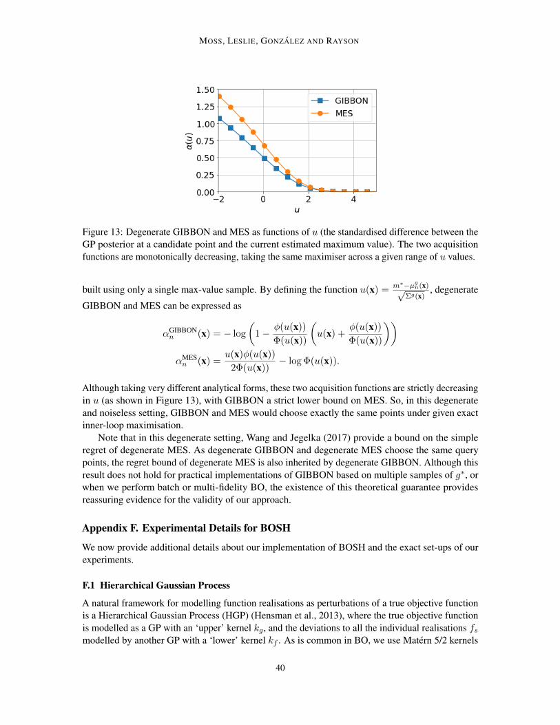
MOSS, LESLIE, GONZALEZ AND RAYSON
Figure 13: Degenerate GIBBON and MES as functions of u (the standardised difference between theGP posterior at a candidate point and the current estimated maximum value). The two acquisitionfunctions are monotonically decreasing, taking the same maximiser across a given range of u values.
built using only a single max-value sample. By defining the function u(x) = m∗−µgn(x)√Σg(x)
, degenerate
GIBBON and MES can be expressed as
αGIBBONn (x) = − log
(1− φ(u(x))
Φ(u(x))
(u(x) +
φ(u(x))
Φ(u(x))
))αMESn (x) =
u(x)φ(u(x))
2Φ(u(x))− log Φ(u(x)).
Although taking very different analytical forms, these two acquisition functions are strictly decreasingin u (as shown in Figure 13), with GIBBON a strict lower bound on MES. So, in this degenerateand noiseless setting, GIBBON and MES would choose exactly the same points under given exactinner-loop maximisation.
Note that in this degenerate setting, Wang and Jegelka (2017) provide a bound on the simpleregret of degenerate MES. As degenerate GIBBON and degenerate MES choose the same querypoints, the regret bound of degenerate MES is also inherited by degenerate GIBBON. Although thisresult does not hold for practical implementations of GIBBON based on multiple samples of g∗, orwhen we perform batch or multi-fidelity BO, the existence of this theoretical guarantee providesreassuring evidence for the validity of our approach.
Appendix F. Experimental Details for BOSH
We now provide additional details about our implementation of BOSH and the exact set-ups of ourexperiments.
F.1 Hierarchical Gaussian Process
A natural framework for modelling function realisations as perturbations of a true objective functionis a Hierarchical Gaussian Process (HGP) (Hensman et al., 2013), where the true objective functionis modelled as a GP with an ‘upper’ kernel kg, and the deviations to all the individual realisations fsmodelled by another GP with a ‘lower’ kernel kf . As is common in BO, we use Matern 5/2 kernels
40

GIBBON
(Matern, 1960). The HGP structure is equivalently understood as each fs being a conditionallyindependent GPs with shared mean function g, i.e.
yi = fsi(xi) + εi for fs ∼ GP(g, kf ) where g ∼ GP(0, kg),
for εii.i.d∼ N (0, σ2). This induces a prior covariance structure of
Cov(fs(x), fs′(x′))) = kg(x, x′) + Is=s′kf (x, x′) and Cov(fs(x), g(x′)) = kg(x, x′),
where I is an indicator function.
F.1.1 PREDICTIVE DISTRIBUTION OF AN HGP
Crucially, given observations Dn = {(xi, si, yi)}ni=1, the HGP provides a bi-variate Gaussian jointdistribution for (ys(x), g(x)) |Dn, the quantities required to evaluate GIBBON. We will now provideclosed form expressions for this joint predictive distributions of g(x) and ys(x) given a set of collectedevaluations Dn = {(xi, si, yi)}ni=1 (location-realisation-evaluations tuples), where yi = fsi(xi) + εunder Gaussian noise ε ∼ N (0, σ2).
Defining a compound kernel k (defined overX×S) as k((x, s), (x′, s′)) = kg(x, x′)+Is=s′kf (x, x′)and following Rasmussen (2004) and Hensman et al. (2013), our joint posterior distribution can bewritten as
(g(x)ys(x)
) ∣∣∣∣Dn ∼ N[(
µgn(x)µn(x, s)
),
(σg2n (x) Σn(x, s)
Σn(x, s) σ2n(x, s) + σ2
)],
where
µn(x, s) =kn((x, s))T(Kn + σ2In
)−1 ynµgn(x) =kgn((x, s))T
(Kn + σ2In
)−1 ynσ2n(x, s) =k ((x, s), (x, s))− kn((x, s))T
(Kn + σ2In
)−1 kn((x, s))
σg2n (x) =kg (x, x)− kgn(x)T(Kn + σ2In
)−1 kgn(x)
Σn(x, s) =kg ((x, s), (x, s))− kn((x, s))T(Kn + σ2In
)−1 kgn(x),
for Kn =[k((xi, si), (xj , sj))
]i,j=1,..,n
, kn((x, s)) =[k((xi, si), (x, s))
]i=1,..,n
,kgn(x) = [kg(xi, x)]i=1,..n
and y = [yi]i=1,..,n.Note that predicting from our HGP requires the inversion of the n× n matrix Kn + σ2In and so
has comparable cost to predictions from standard GPs.
F.1.2 BOSH’S KERNEL STRUCTURE
Our implementation of BOSH uses the following structure for the upper and lower kernels of theHGP:
kg(x, x′) = kαg ,β(x, x′)kf (x, x′) = kαf ,β(x, x′) + σ2
f ,
41
MOSS, LESLIE, GONZALEZ AND RAYSON
where kα,β denotes the Matern 5/2 (Matern, 1960) kernel with variance α ∈ R term and length scalesβ ∈ Rd hyper-parameters, i.e
kα,β(x, x′) = α(1 +√
5dβ(x, x′) +5
3dβ(x, x′)2)e−
√5dβ(x,x′),
for a weighted distance measure dβ(x, x′) = (x− x′)Tdiag(β)(x− x′).As the length-scales are shared between the lower and upper kernels, the total number of kernel
parameters for BOSH (including the scale of observation noise σ2in our Gaussian likelihood) isd+ 4, only two more than a standard GP with a Matern 5/2 kernel.
F.2 Initialisation Costs
Before beginning any BO routine, we must collect an initialisation of points to fit the surrogatemodel. To allow stable maximisation of the marginal likelihood, it is common to initialise with atleast as many evaluations as unknown kernel parameters (to guarantee identifiability). For standardBO, this corresponds to d+ 3 evaluations of the chosen evaluation strategy (i.e requiring B ∗ (d+ 3)individual function evaluations). For BOSH, rather than using separate lower and upper kernels forour HGP, we found that tying length-scales between each kernel greatly improved the stability ofthe HGP. Therefore, our HGP has d + 4 kernel parameters. we allowed BOSH d + 5 evaluationsfor each of the seeds in an initial seed pool with two elements. In contrast, reliable initialisationof FASTCV’s B × B correlation matrix (of which its performance was very sensitive) requiredat least d + 3 evaluations for each of its B considered seeds. We found that using fewer initialpoints severely limited the initial performance of all these methods. Therefore, as well as providingimproved efficiency and precision once optimisation begins, BOSH’s ability to model only as manyindividual seeds as required allows significantly lower initialisation costs.
F.3 Reinforcement Learning: Lunar Lander
The Lunar Lander problem is a well-known reinforcement learning task, where we must controlthree engines (left, main and right) to successfully land a rocket. The learning environment and ahard-coded PID controller is provided in the OpenAI gym 1. We seek to optimize the 7 thresholdspresent in the description of the controller to provide the largest average reward over 100 randominitial conditions. Our RL environment is exactly as provided by OpenAI, with the small modificationof randomly initializing the initial lander location (as-well as random initial velocities and terrain) tomake a more challenging stochastic optimization problem. We lose 0.3 points per second of fuel useand 100 if we crash. We gain 10 points each time a leg makes contact with the ground, 100 points forany successful landing, and 200 points for a successful landing in the specified landing zone· Eachindividual run of the environment allows the testing of a controller on a specific random seed.
F.4 Hyper-parameter Tuning: IMDB SVM
We tested the performance of BOSH on a real ML problem: tuning a sentiment classification modelon the collection of 25, 000 positive and 25, 000 negative IMDB movie reviews used by Maas et al.(2011), seeking the hyper-parameter values that provide the model with the highest accuracy. Wetune the flexibility of the decision boundary (C) and the RBF kernel coefficient (gamma) for an SVM
1. https://gym.openai.com/
42
GIBBON
(Cortes and Vapnik, 1995), a standard model for binary text classification. As is common in thenatural language processing literature, we train our classifier on a bag-of-words representation ofthe data (Jurafsky and Martin, 2014), using tf-idf weightings (Salton and Buckley, 1988). In orderto measure the true performance of tuned hyper-parameters, we must use the available data in anunconventional way. By restricting our model fitting and tuning to a randomly sub-sampled 1, 000review subset to act as our training set for all our experiments, we provide a large held-out collectionof 49, 000 movie reviews, upon which we can calculate the ‘true’ performance of the hyper-parameterconfigurations chosen by our tuning algorithms. We then randomly draw our train-test splits from thisfixed training set, with test sets of 10%. As already argued, the model scores based on a particularevaluation strategy do not necessarily correspond to the true performance and so, although weacknowledge that this contrived use of the data is not standard, this set-up is necessary to measurethe improved efficiency and reliability provided by BOSH.
References
Ahsan S Alvi, Binxin Ru, Jan Calliess, Stephen J Roberts, and Michael A Osborne. Asynchronousbatch Bayesian optimisation with improved local penalisation. International Conference onMachine Learning, 2019.
Eric Anderson, Gilman D Veith, and David Weininger. SMILES, a line notation and computerizedinterpreter for chemical structures. US Environmental Protection Agency, 1987.
Reinaldo B Arellano-Valle, Javier E Contrera-Reyes, and Marc G Genton. Shannon entropy andmutual information for multivariate skew-elliptical distributions. Scandinavian Journal of Statistics,2013.
Adelchi Azzalini. A class of distributions which includes the normal ones. Scandinavian Journal ofStatistics, 1985.
Adelchi Azzalini and A Dalla Valle. The multivariate skew-normal distribution. Biometrika, 1996.
Maximilian Balandat, Brian Karrer, Daniel R. Jiang, Samuel Daulton, Benjamin Letham, An-drew Gordon Wilson, and Eytan Bakshy. BoTorch: a framework for efficient Monte-CarloBayesian optimization. In Advances in Neural Information Processing Systems, 2020.
Daniel Beck and Trevor Cohn. Learning kernels over strings using Gaussian processes. In Interna-tional Joint Conference on Natural Language Processing, 2017.
Daniel Beck, Trevor Cohn, Christian Hardmeier, and Lucia Specia. Learning structural kernels fornatural language processing. Transactions of the Association for Computational Linguistics, 2015.
Syrine Belakaria, Aryan Deshwal, and Janardhan Rao Doppa. Max-value entropy search for multi-objective Bayesian optimization. In Advances in Neural Information Processing Systems, 2019.
Syrine Belakaria, Aryan Deshwal, and Janardhan Rao Doppa. Max-value entropy search for multi-objective Byesian optimization with constraints. arXiv preprint arXiv:2009.01721, 2020.
James Bergstra, Daniel Yamins, and David Daniel Cox. Making a science of model search: hyper-parameter optimization in hundreds of dimensions for vision architectures. Journal of MachineLearning Research, 2013.
43
MOSS, LESLIE, GONZALEZ AND RAYSON
Joel Berkeley, Henry B. Moss, Artem Artemev, Sergio Pascual-Diaz, Uri Granta, Hrvoje Stojic,Ivo Couckuyt, Jixiang Quing, Loka Satrio, and Victor Picheny. Trieste, 2021. URL https://github.com/secondmind-labs/trieste.
David M Blei, Alp Kucukelbir, and Jon D McAuliffe. Variational inference: a review for statisticians.Journal of the American Statistical Association, 2017.
Yutian Chen, Aja Huang, Ziyu Wang, Ioannis Antonoglou, Julian Schrittwieser, David Silver, andNando de Freitas. Bayesian optimization in alphago. arXiv preprint arXiv:1812.06855, 2018.
Clement Chevalier and David Ginsbourger. Fast computation of the multi-points expected improve-ment with applications in batch selection. In International Conference on Learning and IntelligentOptimization, 2013.
Emile Contal, David Buffoni, Alexandre Robicquet, and Nicolas Vayatis. Parallel Gaussian processoptimization with upper confidence bound and pure exploration. In Joint European Conference onMachine Learning and Knowledge Discovery in Databases, 2013.
Corinna Cortes and Vladimir Vapnik. Support-vector networks. Machine Learning, 1995.
Thomas M Cover and Joy A Thomas. Elements of information theory. John Wiley & Sons, 2012.
Kurt Cutajar, Mark Pullin, Andreas Damianou, Neil Lawrence, and Javier Gonzalez. Deep Gaussianprocesses for multi-fidelity modeling. arXiv preprint arXiv:1903.07320, 2019.
Aryan Deshwal, Syrine Belakaria, and Janardhan Rao Doppa. Mercer features for efficient combina-torial Bayesian optimization. arXiv preprint arXiv:2012.07762, 2020.
Jesse Dodge, Kevin Jamieson, and Noah A Smith. Open loop hyperparameter optimization anddeterminantal point processes. arXiv preprint arXiv:1706.01566, 2017.
Peter I Frazier, Warren B Powell, and Savas Dayanik. A knowledge-gradient policy for sequentialinformation collection. SIAM Journal on Control and Optimization, 2008.
Jennifer Gillenwater, Alex Kulesza, and Ben Taskar. Near-optimal map inference for determinantalpoint processes. In Advances in Neural Information Processing Systems, 2012.
Rafael Gomez-Bombarelli, Jennifer N Wei, David Duvenaud, Jose Miguel Hernandez-Lobato,Benjamın Sanchez-Lengeling, Dennis Sheberla, Jorge Aguilera-Iparraguirre, Timothy D Hirzel,Ryan P Adams, and Alan Aspuru-Guzik. Automatic chemical design using a data-driven continu-ous representation of molecules. ACS Central Science, 2018.
Chengyue Gong, Jian Peng, and Qiang Liu. Quantile stein variational gradient descent for batchBayesian optimization. In International Conference on Machine Learning, 2019.
Javier Gonzalez, Joseph Longworth, David C James, and Neil D Lawrence. Bayesian optimizationfor synthetic gene design. Advances in Neural Information Processing Systems: Workshop inBayesian Optimization, 2014.
Javier Gonzalez, Zhenwen Dai, Philipp Hennig, and Neil Lawrence. Batch Bayesian optimizationvia local penalization. In Artificial intelligence and statistics, 2016a.
44

GIBBON
Javier Gonzalez, Michael Osborne, and Neil Lawrence. Glasses: Relieving the myopia of Bayesianoptimisation. In Artificial Intelligence and Statistics, 2016b.
Ryan-Rhys Griffiths and Jose Miguel Hernandez-Lobato. Constrained Bayesian optimization forautomatic chemical design. Chemical Sciences, 2020.
Philipp Hennig and Christian J Schuler. Entropy search for information-efficient global optimization.Journal of Machine Learning Research, 2012.
James Hensman, Neil D Lawrence, and Magnus Rattray. Hierarchical Bayesian modelling of geneexpression time series across irregularly sampled replicates and clusters. BMC Bioinformatics,2013.
Daniel Hernandez-Lobato, Jose Hernandez-Lobato, Amar Shah, and Ryan Adams. Predictiveentropy search for multi-objective bayesian optimization. In International Conference on MachineLearning, pages 1492–1501, 2016.
Jose Miguel Hernandez-Lobato, Matthew W Hoffman, and Zoubin Ghahramani. Predictive entropysearch for efficient global optimization of black-box functions. In Neural Information ProcessingSystems, 2014.
Jose Miguel Hernandez-Lobato, James Requeima, Edward O Pyzer-Knapp, and Alan Aspuru-Guzik.Parallel and distributed Thompson sampling for large-scale accelerated exploration of chemicalspace. In International Conference on Machine Learning, 2017.
Matthew W Hoffman and Zoubin Ghahramani. Output-space predictive entropy search for flexibleglobal optimization. In Advances in Neural Information Processing Systems: Workshop onBayesian Optimization, 2015.
Deng Huang, Theodore T Allen, William I Notz, and Ning Zeng. Global optimization of stochasticblack-box systems via sequential kriging meta-models. Journal of Global Optimization, 2006.
Shali Jiang, Henry Chai, Javier Gonzalez, and Roman Garnett. Binoculars for efficient, nonmyopicsequential experimental design. In International Conference on Machine Learning, 2020.
Donald R Jones, Cary D Perttunen, and Bruce E Stuckman. Lipschitzian optimization without theLipschitz constant. Journal of optimization Theory and Applications, 1993.
Donald R Jones, Matthias Schonlau, and William J Welch. Efficient global optimization of expensiveblack-box functions. Journal of Global optimization, 1998.
Kai Junge, Josie Hughes, Thomas George Thuruthel, and Fumiya Iida. Improving robotic cookingusing batch Bayesian optimization. IEEE Robotics and Automation Letters, 2020.
Dan Jurafsky and James H Martin. Speech and Language Processing. 2014.
Kirthevasan Kandasamy, Gautam Dasarathy, Junier B Oliva, Jeff Schneider, and Barnabas Poczos.Gaussian process bandit optimisation with multi-fidelity evaluations. In Advances in NeuralInformation Processing Systems, 2016.
45
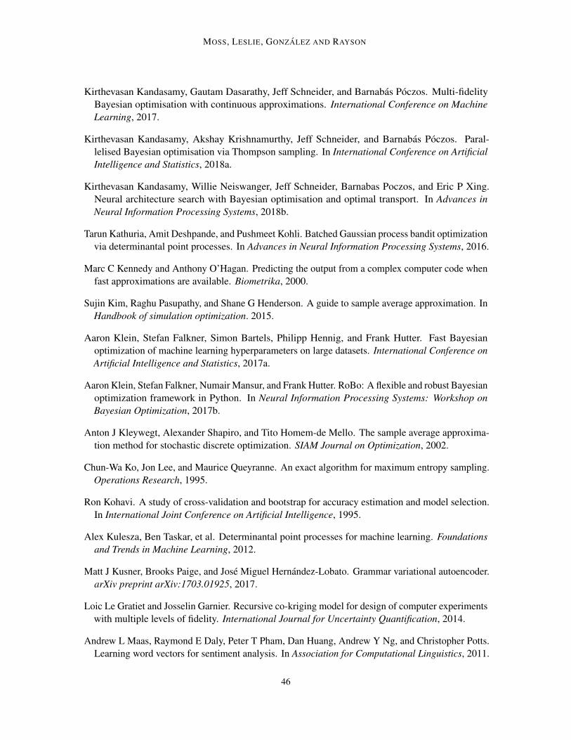
MOSS, LESLIE, GONZALEZ AND RAYSON
Kirthevasan Kandasamy, Gautam Dasarathy, Jeff Schneider, and Barnabas Poczos. Multi-fidelityBayesian optimisation with continuous approximations. International Conference on MachineLearning, 2017.
Kirthevasan Kandasamy, Akshay Krishnamurthy, Jeff Schneider, and Barnabas Poczos. Paral-lelised Bayesian optimisation via Thompson sampling. In International Conference on ArtificialIntelligence and Statistics, 2018a.
Kirthevasan Kandasamy, Willie Neiswanger, Jeff Schneider, Barnabas Poczos, and Eric P Xing.Neural architecture search with Bayesian optimisation and optimal transport. In Advances inNeural Information Processing Systems, 2018b.
Tarun Kathuria, Amit Deshpande, and Pushmeet Kohli. Batched Gaussian process bandit optimizationvia determinantal point processes. In Advances in Neural Information Processing Systems, 2016.
Marc C Kennedy and Anthony O’Hagan. Predicting the output from a complex computer code whenfast approximations are available. Biometrika, 2000.
Sujin Kim, Raghu Pasupathy, and Shane G Henderson. A guide to sample average approximation. InHandbook of simulation optimization. 2015.
Aaron Klein, Stefan Falkner, Simon Bartels, Philipp Hennig, and Frank Hutter. Fast Bayesianoptimization of machine learning hyperparameters on large datasets. International Conference onArtificial Intelligence and Statistics, 2017a.
Aaron Klein, Stefan Falkner, Numair Mansur, and Frank Hutter. RoBo: A flexible and robust Bayesianoptimization framework in Python. In Neural Information Processing Systems: Workshop onBayesian Optimization, 2017b.
Anton J Kleywegt, Alexander Shapiro, and Tito Homem-de Mello. The sample average approxima-tion method for stochastic discrete optimization. SIAM Journal on Optimization, 2002.
Chun-Wa Ko, Jon Lee, and Maurice Queyranne. An exact algorithm for maximum entropy sampling.Operations Research, 1995.
Ron Kohavi. A study of cross-validation and bootstrap for accuracy estimation and model selection.In International Joint Conference on Artificial Intelligence, 1995.
Alex Kulesza, Ben Taskar, et al. Determinantal point processes for machine learning. Foundationsand Trends in Machine Learning, 2012.
Matt J Kusner, Brooks Paige, and Jose Miguel Hernandez-Lobato. Grammar variational autoencoder.arXiv preprint arXiv:1703.01925, 2017.
Loic Le Gratiet and Josselin Garnier. Recursive co-kriging model for design of computer experimentswith multiple levels of fidelity. International Journal for Uncertainty Quantification, 2014.
Andrew L Maas, Raymond E Daly, Peter T Pham, Dan Huang, Andrew Y Ng, and Christopher Potts.Learning word vectors for sentiment analysis. In Association for Computational Linguistics, 2011.
46

GIBBON
Sebastien Marmin, Clement Chevalier, and David Ginsbourger. Differentiating the multipointexpected improvement for optimal batch design. In International Workshop on Machine Learning,Optimization and Big Data, 2015.
Bertil Matern. Spatial variation, volume 36 of. Lecture Notes in Statistics, 1960.
Jonas Mockus, Vytautas Tiesis, and Antanas Zilinskas. The application of Bayesian methods forseeking the extremum. Towards global optimization, 1978.
Henry Moss, David Leslie, and Paul Rayson. Using J-K-fold cross validation to reduce variancewhen tuning nlp models. In International Conference on Computational Linguistics, 2018.
Henry B Moss and Ryan-Rhys Griffiths. Gaussian process molecule property prediction withflowmo. Advances in Neural Information Processing Systems: Workshop on Machine Learningfor Molecules, 2020.
Henry B Moss, Andrew Moore, David S Leslie, and Paul Rayson. Fiesta: Fast identification of state-of-the-art models using adaptive bandit algorithms. Association for Computational Linguistics,2019.
Henry B Moss, Vatsal Aggarwal, Nishant Prateek, Javier Gonzalez, and Roberto Barra-Chicote.Boffin tts: few-shot speaker adaptation by Bayesian optimization. In International Conference onAcoustics, Speech and Signal Processing, 2020a.
Henry B. Moss, Daniel Beck, Javier Gonzalez, David L. Leslie, and Paul. Rayson. Boss: Bayesianoptimisation over string spaces. In Advances in neural information processing systems, 2020b.
Henry B Moss, David S Leslie, and Paul Rayson. Bosh: Bayesian optimization by samplinghierarchically. International Conference on Machine Learning: Workshop on Active Learning andExperimental Design, 2020c.
Henry B. Moss, David S. Leslie, and Paul Rayson. MUMBO: Multi-task max-value Bayesianoptimization. In Joint European Conference on Machine Learning and Knowledge Discovery inDatabases, 2020d.
Anthony O’Hagan. A Markov property for covariance structures. Statistics Research Report, 1998.
Andrei Paleyes, Mark Pullin, Maren Mahsereci, Neil Lawrence, and Javier Gonzalez. Emulation ofphysical processes with emukit. In Advances in Neural Infromation Processing Systems: Workshopon Machine Learning and the Physical Sciences, 2019.
Michael Pearce, Matthias Poloczek, and Juergen Branke. Bayesian optimization allowing forcommon random numbers. Winter Simulation Conference, 2019.
Paris Perdikaris, Maziar Raissi, Andreas Damianou, Neil D Lawrence, and George Em Karniadakis.Nonlinear information fusion algorithms for data-efficient multi-fidelity modelling. Royal SocietyA: Mathematical, Physical and Engineering Sciences, 2017.
Victor Picheny, David Ginsbourger, and Yann Richet. Noisy expected improvement and on-linecomputation time allocation for the optimization of simulators with tunable fidelity. InternationalConference on Engineering Optimisation, 2010.
47

MOSS, LESLIE, GONZALEZ AND RAYSON
Malte Prieß, Slawomir Koziel, and Thomas Slawig. Surrogate-based optimization of climate modelparameters using response correction. Journal of Computational Science, 2011.
Ali Rahimi and Benjamin Recht. Random features for large-scale kernel machines. In Advances inneural information processing systems, 2008.
Laura Elena Raileanu and Kilian Stoffel. Theoretical comparison between the gini index andinformation gain criteria. Annals of Mathematics and Artificial Intelligence, 2004.
Carl Edward Rasmussen. Gaussian processes in machine learning. In Advanced Lectures on MachineLearning. 2004.
Binxin Ru, Michael A Osborne, Mark McLeod, and Diego Granziol. Fast information-theoreticBayesian optimisation. In International Conference on Machine Learning, pages 4384–4392,2018.
Binxin Ru, Ahsan S Alvi, Vu Nguyen, Michael A Osborne, and Stephen J Roberts. Bayesianoptimisation over multiple continuous and categorical inputs. International Conference on MachineLearning, 2020.
Gerard Salton and Christopher Buckley. Term-weighting approaches in automatic text retrieval.Information Processing an Management, 1988.
Amar Shah and Zoubin Ghahramani. Parallel predictive entropy search for batch global optimizationof expensive objective functions. In Advances in Neural Information Processing Systems, pages3330–3338, 2015.
Jasper Snoek, Hugo Larochelle, and Ryan P Adams. Practical Bayesian optimization of machinelearning algorithms. In Neural Information Processing Systems, 2012.
Niranjan Srinivas, Andreas Krause, Sham M Kakade, and Matthias Seeger. Gaussian processoptimization in the bandit setting: No regret and experimental design. International Conferenceon Machine Learning, 2010.
Kevin Swersky, Jasper Snoek, and Ryan P Adams. Multi-task Bayesian optimization. In NeuralInformation Processing Systems, 2013.
Kevin Swersky, Yulia Rubanova, David Dohan, and Kevin Murphy. Amortized Bayesian optimizationover discrete spaces. In Conference on Uncertainty in Artificial Intelligence, 2020.
Shion Takeno, Hitoshi Fukuoka, Yuhki Tsukada, Toshiyuki Koyama, Motoki Shiga, Ichiro Takeuchi,and Masayuki Karasuyama. Multi-fidelity Bayesian optimization with max-value entropy search.International Conference on Machine Learning, 2020.
Ryokei Tanaka and Hiroyoshi Iwata. Bayesian optimization for genomic selection: a method fordiscovering the best genotype among a large number of candidates. Theoretical and AppliedGenetics, 2018.
Sattar Vakili, Victor Picheny, and Artem Artemev. Scalable Thompson sampling using sparseGaussian process models. arXiv preprint arXiv:2006.05356, 2020.
48

GIBBON
Zi Wang and Stefanie Jegelka. Max-value entropy search for efficient Bayesian optimization. InInternational Conference in Machine Learning, 2017.
Zi Wang, Chengtao Li, Stefanie Jegelka, and Pushmeet Kohli. Batched high-dimensional Bayesianoptimization via structural kernel learning. In International Conference on Machine Learning,2017.
Jian Wu and Peter Frazier. The parallel knowledge gradient method for batch Bayesian optimization.In Advances in Neural Information Processing Systems, 2016.
Jian Wu and Peter I Frazier. Continuous-fidelity Bayesian optimization with knowledge gradient.Advances in Neural Information Processing Systems: Workshop in Bayesian Optimization, 2017.
Yiming Yang and Jan O Pedersen. A comparative study on feature selection in text categorization.In International Conference on Machine Learning, 1997.
Yehong Zhang, Trong Nghia Hoang, Bryan Kian Hsiang Low, and Mohan Kankanhalli. Information-based multi-fidelity Bayesian optimization. In Advances in Neural Information Processing Systems:Workshop on Bayesian Optimization, 2017.
49