Geometric Correction for Very HighResolution Satellite Images

Dr. Ismail Elkhrachy

Assistant professor at Najran University, Faculty of Engineering,

Civil Engineering Department. K.S.A, king Abdul-Aziz Rd. Post Code

11001 P.O. Box 1988. E-mail: I.Elkhrachy@yahoo.com .. Currently on

leave from: Faculty of Engineering Civil Department, Al-Azhar

University, Cairo, Egypt.

Dr. Tarek A.E., El-Damaty

Assistant professor at Banha University, Faculty of Engineering, Civil

Engineering Department. Cairo, Egypt. E-mail: tdamaty@hotmail.com.

ي� ب�� ص ال�عر ال�ملخاع�ي� م����ر ال�ص����ن طة� ال�ق� واس����� ل ال�ص����ور ال�ممس����وحة� ب�� ة� ك�من����+ وح ال�عال�ي����� ة� ال�وض����� ات� درح����� ة� د اع�ي� م����ار ال�ص����ن ق�� ور الأ8 Worldض�����

view2 ع م�هم�ة� مي�� ي� ج�� ط ف طي�� خ راض ال�ملأح�ة� وال�ت� غ�� ي� ا8 دة� ف ن�� ط م�ف ط. ال�خ رائ��8 ي�Sث+ ال�خ رائ��8 ح�د ة� ت�� احY او ع�ملي�� ن�� Z[ة� ان ي� ع�ملي�� دا ف ج���. ة� وي���� دس��ي� ل�لص��ور ال�ج� ح ال�هن ص��حي� ة� ال�ي� حY ل�عملي��� ات]8 ن��� Zل ال�ن ض�� ول الي اف� و ال�وض��� حث+ ه��� ا ال�ب� د س��ي�� م�نY ه��� ي� لأد. ال�ه��دف ال�رئ�8 ال�ن�

ة� ) ي� م الأرض�� ي� ي� ق��� اط ال�ي� ق�� ط ل�ي وس��� عي� ال�مت� ي� �ط��ا8 ال�ت�رن� دم ح�سات� ال�خ ح ة� CPsاس�ت� اع�ي� طة� الأق��م��ار ال�ص�ن واس��� اس�ة� ب�� ي�GPS( ال�مق� فع���اد ة� الأب�� ي���� ن]8 ا ن ة� ن�� ي� اض���� ة� ل�لمح���ددات� ال�ري]� ل درح���� ض��� د اف� حدي���]� حث+ ت�� منY ال�ب� ض��� ي� . ن�� الأت� ال�دراس���ة� ل ج�ال���ة� م�نY ج���� م ك���� ي� ف� ة� ب�� ع�ملي����

ة� ) ي� حكم الأرض��� اط ال�ب� ق��� دد ب� ر ع��� ت� ي]+ ا8 حث+ ي���� منY ال�ب� ض�� ي� ح, ك�م��ا ن�� ص��حي� ة� ال�ي� ي� ع�ملي��� دمة� ف ح دس��ي�GCPsال�مس��ت� ح ال�هن ص��ي� ة� ال�ي� ( ع�لي دق���دد ة� و ع���� ي���� ن] ا ة� ال�ن+ عمال ال�مح���ددات� م�نY ال�درح���� ي� حث+ انY اس���� حY ال�ب� ات]8 ن���� Zحث� ن� . اوض���� ة� وي����� ة� )33ل�لص���ور ال�ج� ي� حكم ارض���� ط���ة� ت�� ق� ب�

GCPs ة مي� ي� وس�ط ق�� عي� م�ت� ي� �رن� طا ت�� عطي خ� ة� ال�دراسة� ب�� طق� ل م�ي ام داج� ط¯ ي� Zان� عة� ي�� ار )13 مت�ر ل�عدد 0.96( م�ور ن��� ي� طة� اج� ق� (CPs ب�

دمة� ح دمة� )ال�ص�ور ال�مس�ت� ح وح ل�لص�ور ال�مس�ت� ة� ال�وض� عف درح� ل م�نY ض� حY اق�� ي� Zن طا8 ال�مسن� . ال�خ ة� ال�دراسة� طق� ل م�ي عة� داج� م�وروح ة� وض���� ات� درح���� دام م�نY 50د ح ت� ي� ج�ال���ة� اس���� ة ف حث+ اي���� حY ال�ب� ات]8 ن���� Zن� Yا م�ن ض��� ي )33 الي 20 س���م(. ائ�� حكم ارض��� ط���ة� ت�� ق� ب�

GCPs. ة� م م�لجوظ�¯ ي� ف� ح ب�� صحي� ة� ال�ي� ة� ع�ملي� ر دق� ت� غ ي� ( لأ ن��

Abstract:Very high resolution satellite images, such as World

view2, are important for produce new maps or update

existing ones. Maps are useful for planning and navigation

purposes in any country. Main aim of this work is the

assessment of a methodology to achieve the best possible

geometric accuracy in rectified imagery products obtained

from World view2. The research includes, studying the

effect of the number of Ground Control Points (GCPs) with

various 2D polynomial rectification models on the accuracy

geometric correction step. The resulting RMSE on the check

points (CPs) will be evaluated. Results showed that using a

second order polynomial for world view 2 image

rectification with 33 well distributed GCPs resulted in a

total RMSE 0.96 m for a number of 13 CPs which is less than

the value of two pixel size of the used satellite image.

Also, by using from 20 GCPs till 33, the accuracy of

geometric correction for all polynomial orders has a small

variation.

Keywords: Satellite Image, Remote Sensing, Erdas Imagine,Georeferencing , Accuracy Assessment.

1 Introduction

1.1 Maps Production Techniques

Raw satellite images usually contain such significant

geometric distortions that they cannot be used directly

with map base products in any engineering purposes such as

geographic information system (GIS). Also multi-source data

integration (raster and vector), for applications in

Geomatics, needs geometric correction. Many new very high

resolution (VHR) satellites capable of capturing imagery

with Ground Sample Distance (GSD) of less than 0.5 m and

even lower, such as WorldView-1 and 2, have launched during

2006 and 2007. Besides maps production, satellite images

have been used for numerous applications in: building

detection [10] and [11], road extraction [21] and [12],

vegetation studies [17], greenhouses delineation [2] and

[1], location of damages caused by natural disasters [4],

shoreline mapping [14] and finally for urban regional

planning [15].

Map production technology is a rapidly developing field.

The new mapping technologies from satellite remote sensing,

laser-scanning technologies and advanced global navigation

satellite system offer both fast and accurate acquisition

of topographic data. However they also give new challenges

for research and development as well as innovations for

several application areas. A continuously developing range

of field and remote data collection techniques ensures that

map production flow lines must be able to handle spatial

data varying in source, format, scale, quality, reliability

and area of coverage. Field surveying is an accurate

production technique, however it is very costly and slow.

Digital photogrammetry is the most adopted worldwide

technique for city maps production at the time being with

scale of 1: 5000 or 1: 2500 or even 1: 1000 maps [5]. But,

in spite of its advantages, such as high accuracy, it

cannot map areas which is constrained by limiting flight

planning. During the past several years, high resolution

satellite imagery has been used in mapping production. It

has the advantage of less than one meter of resolution,

short revisit time, and capabilities of getting stereo

images. Moreover, this technique makes it possible and easy

to map an area without the special flight planning required

by photogrammetric method. Recently, the rapid advancement

in satellite sensor development enhances the capability in

image acquisition with improved spatial, spectral and

temporal resolutions [6]. This can be noticed in the

radiometric resolution of the recently launched satellite

sensor, for instance Worldview-2, where four more spectral

bands, including coastal (400-450 nm), yellow (585-625 nm),

red-edge (705-745 nm) and infrared red (IR), can be found

in addition to the existing red, green, blue and near IR

bands. The spatial resolution of Worldview-2 reaches 0.46 m

and 1.84 m (at nadir) in PAN mode and MS mode,

respectively. It becomes a suitable alternative tool for

digital city map production and updating in many countries,

in Egypt [7], in Lybia [19] in K.S.A. [3] and in India

[13], either in a planimetric mode using single (mono)

images (x, y) or in a topographic mode using stereo images

(x, y, z).

In this study, Najran city, located in the south western of

Saudi Arabia is chosen as a test area. The test study area

was covered with World view2 images 0.5 meter resolution,

GCPs and CPs. In our study, many experiments were done to

achieve the best possible geometric correction accuracy for

test area. The order of used polynomial the number of used

GCPs are investigated.

Fig. 1 Study area location map.

.

2 Study Site and Data Set

2.1 Study Area

The study area is called Najran city, located in the

south western of Saudi Arabia, near the border of Yemen.

Study area is bounded by coordinates of (219205.660E,

3633792.740N) and (223405.060E, 3637277.540N). The total

area (90 square kilometers) is considered to be flat

terrain area surrounded by high mountains (Figure 1). The

area includes various land use activities: urban, desert

and road network.

2.2 Data Set

For this study, Worldview-2 Satellite images with 50 cm

spatial resolution was used. Acquisition date for used

images is 01/10/2010. The data are projected to Universal

Transverse Mercator (UTM), zone 38N on the WGS84 ellipsoid.

Table 1 shows characteristics of WorldView-2 spacecraft and

imaging system. Najran Municipality has also main control

points, they are distributed inside Najran city to be used

for mapping purposes. The main control points are used to

measure used GCPs and CPs by GPS (see figure2). The data

sets used in this study were obtained from Najran

Municipality.

3 Satellite Image Processing

Recorded satellite image by sensors on satellites

contains errors in geometry and in the measured brightness

values of the image pixels. The latter are called to

radiometric errors. It can result from the used recording

instrumentation, solar radiation and from effect of the

atmosphere. Many factors can arise image geometry errors,

for example, relative motions of the platform, the

curvature of the earth and uncontrolled variations in the

position and attitude of the remote sensing platform. There

are many more sources of geometric errors of satellite

image than radiometric one and their effects are more

severe. Used image was provided corrected from radiometric

errors. Geometric errors are corrected by a computational

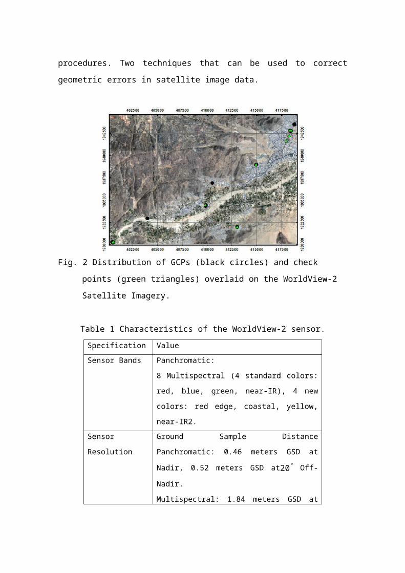
procedures. Two techniques that can be used to correct

geometric errors in satellite image data.

Fig. 2 Distribution of GCPs (black circles) and check

points (green triangles) overlaid on the WorldView-2

Satellite Imagery.

Table 1 Characteristics of the WorldView-2 sensor.Specification ValueSensor Bands Panchromatic:

8 Multispectral (4 standard colors:

red, blue, green, near-IR), 4 new

colors: red edge, coastal, yellow,

near-IR2.Sensor

Resolution

Ground Sample Distance

Panchromatic: 0.46 meters GSD at

Nadir, 0.52 meters GSD at20° Off-

Nadir.

Multispectral: 1.84 meters GSD at

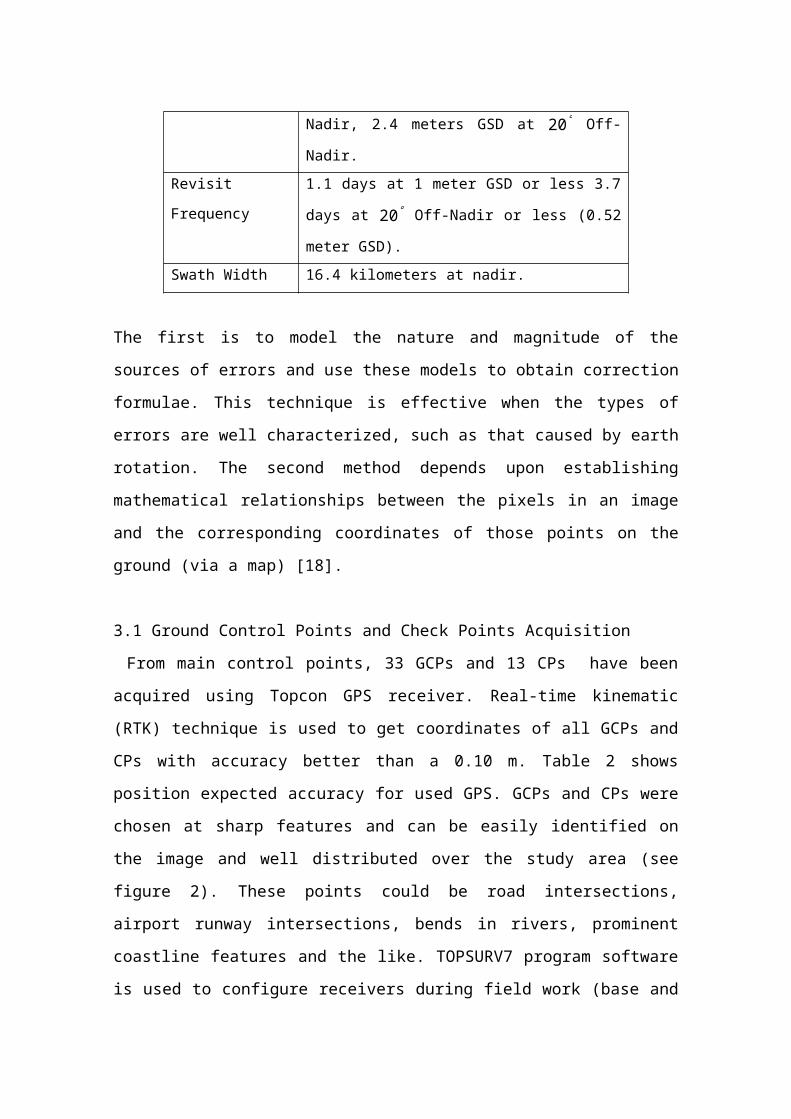
Nadir, 2.4 meters GSD at 20° Off-

Nadir.Revisit

Frequency

1.1 days at 1 meter GSD or less 3.7

days at 20° Off-Nadir or less (0.52meter GSD).

Swath Width 16.4 kilometers at nadir.

The first is to model the nature and magnitude of the

sources of errors and use these models to obtain correction

formulae. This technique is effective when the types of

errors are well characterized, such as that caused by earth

rotation. The second method depends upon establishing

mathematical relationships between the pixels in an image

and the corresponding coordinates of those points on the

ground (via a map) [18].

3.1 Ground Control Points and Check Points Acquisition

From main control points, 33 GCPs and 13 CPs have been

acquired using Topcon GPS receiver. Real-time kinematic

(RTK) technique is used to get coordinates of all GCPs and

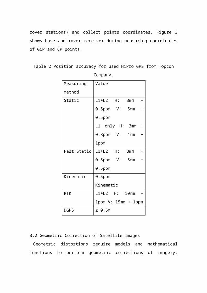
CPs with accuracy better than a 0.10 m. Table 2 shows

position expected accuracy for used GPS. GCPs and CPs were

chosen at sharp features and can be easily identified on

the image and well distributed over the study area (see

figure 2). These points could be road intersections,

airport runway intersections, bends in rivers, prominent

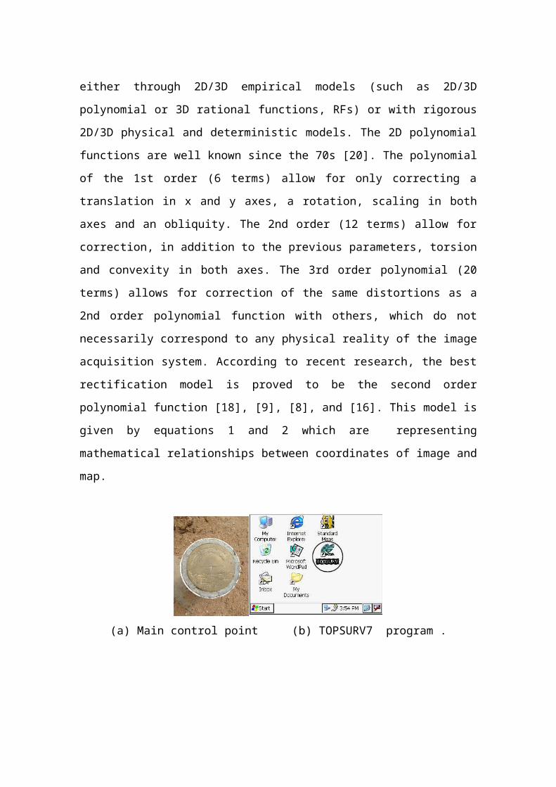
coastline features and the like. TOPSURV7 program software

is used to configure receivers during field work (base and

rover stations) and collect points coordinates. Figure 3

shows base and rover receiver during measuring coordinates

of GCP and CP points.

Table 2 Position accuracy for used HiPro GPS from Topcon

Company.

Measuring

method

Value

Static L1+L2 H: 3mm +

0.5ppm V: 5mm +

0.5ppm

L1 only H: 3mm +

0.8ppm V: 4mm +

1ppmFast Static L1+L2 H: 3mm +

0.5ppm V: 5mm +

0.5ppmKinematic 0.5ppm

KinematicRTK L1+L2 H: 10mm +

1ppm V: 15mm + 1ppmDGPS ≤ 0.5m

3.2 Geometric Correction of Satellite Images

Geometric distortions require models and mathematical

functions to perform geometric corrections of imagery:

either through 2D/3D empirical models (such as 2D/3D

polynomial or 3D rational functions, RFs) or with rigorous

2D/3D physical and deterministic models. The 2D polynomial

functions are well known since the 70s [20]. The polynomial

of the 1st order (6 terms) allow for only correcting a

translation in x and y axes, a rotation, scaling in both

axes and an obliquity. The 2nd order (12 terms) allow for

correction, in addition to the previous parameters, torsion

and convexity in both axes. The 3rd order polynomial (20

terms) allows for correction of the same distortions as a

2nd order polynomial function with others, which do not

necessarily correspond to any physical reality of the image

acquisition system. According to recent research, the best

rectification model is proved to be the second order

polynomial function [18], [9], [8], and [16]. This model is

given by equations 1 and 2 which are representing

mathematical relationships between coordinates of image and

map.

(a) Main control point (b) TOPSURV7 program .

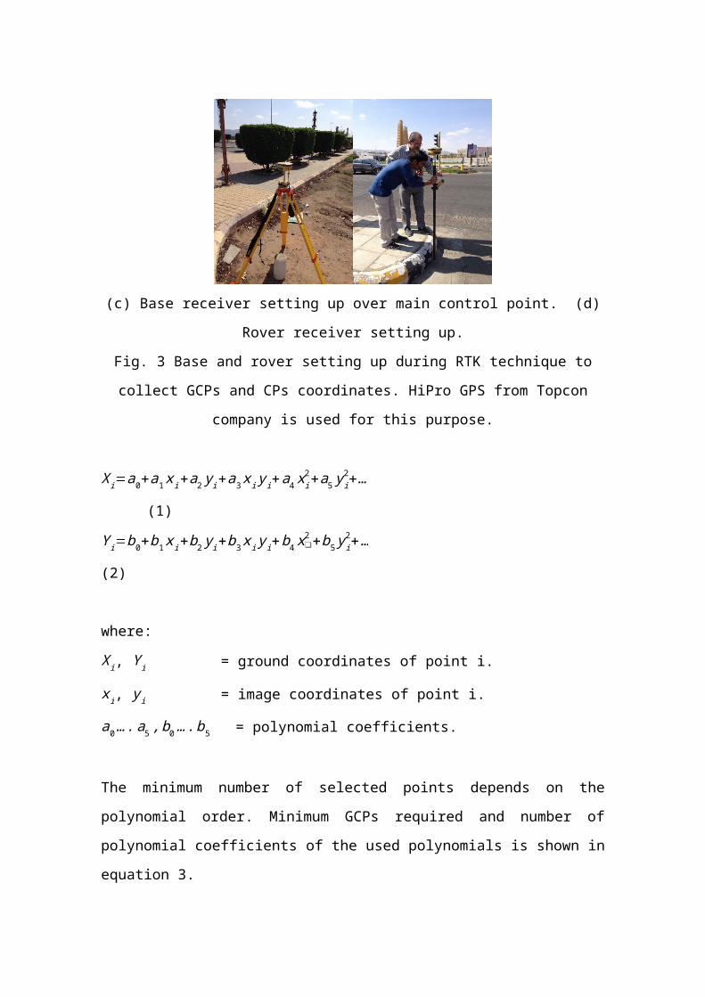
(c) Base receiver setting up over main control point. (d)

Rover receiver setting up.

Fig. 3 Base and rover setting up during RTK technique to

collect GCPs and CPs coordinates. HiPro GPS from Topcon

company is used for this purpose.

Xi=a0+a1xi+a2yi+a3xiyi+a4xi2+a5yi

2+…

(1)

Yi=b0+b1xi+b2yi+b3xiyi+b4x❑2 +b5yi

2+…

(2)

where:

Xi, Yi = ground coordinates of point i.

xi, yi = image coordinates of point i.

a0….a5,b0….b5 = polynomial coefficients.

The minimum number of selected points depends on the

polynomial order. Minimum GCPs required and number of

polynomial coefficients of the used polynomials is shown in

equation 3.

min=(t+1)(t+2)

2 , m=(t+1)(t+2)

(3)

where:

min = minimum number of GCPs.

t = polynomial order.

m=¿ number of polynomial coefficients.

According to equation 3, the minimum number of GCPs for

first order polynomials is 3, while minimum 6 GCPs for

second order are needed.

4 Accuracy Assessment

Horizontal accuracy can be done by calculation of the

discrepancies of E, N coordinates of CPs, which are located

on the used image covering the whole test area. The x, y

coordinate are compared with the corresponding ones derived

from GPS observations which are considered as a reference.

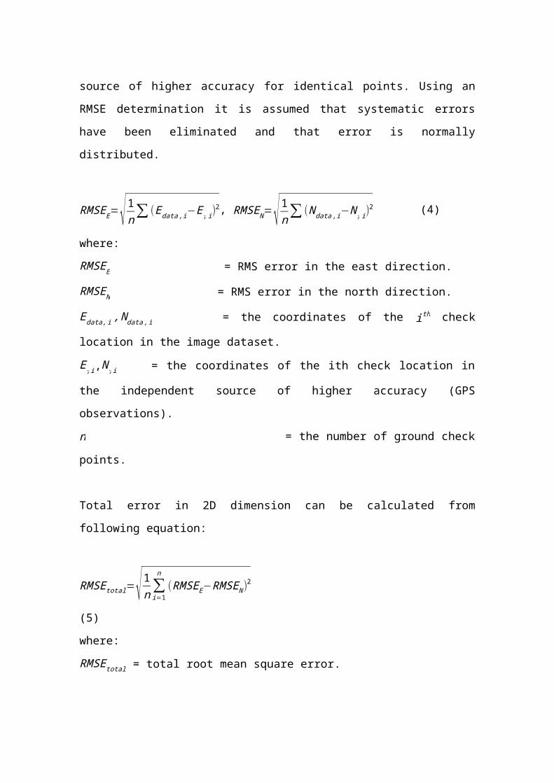
The root mean square error ( RMSE) in E and N directions

and the total root mean square error (TRMS) will be

calculated (as shown in equations 4 and 5). Allowable error

is 0.5 mm x map scale. RMSE is the square root of the

average of the set of squared differences between dataset

coordinate values and coordinate values from an independent

source of higher accuracy for identical points. Using an

RMSE determination it is assumed that systematic errors

have been eliminated and that error is normally

distributed.

RMSEE=√1n∑ (Edata,i−E,̌i)2, RMSEN=√1n∑ (Ndata,i−N,̌i)

2 (4)

where:

RMSEE = RMS error in the east direction.

RMSEN = RMS error in the north direction.

Edata,i,Ndata,i = the coordinates of the ith check

location in the image dataset.

E,̌i,N,̌i = the coordinates of the ith check location in

the independent source of higher accuracy (GPS

observations).

n = the number of ground check

points.

Total error in 2D dimension can be calculated from

following equation:

RMSEtotal=√1n∑i=1

n(RMSEE−RMSEN)2

(5)

where:

RMSEtotal = total root mean square error.

5 Results and Analysis

5.1 Effect of Polynomial Order

ERDAS IMAGINE commercial software package was used to

perform the rectification process for all the study cases.

To study the effect of the order of polynomial

transformation on the accuracy of the rectified image a 1st

, 2nd and 3rd order transformations were tested. To do

geometric correction for satellite image, there is an

iterative process that takes place. First, all of the

original GCPs (e.g., 40 GCPs) are used to compute an

initial set of transformation coefficients and constants.

The RMSE associated with each of these initial GCPs is

computed and summed. Then, the individual GCPs that

contributed the greatest amount of error are determined and

deleted. After the first iteration, a new set of

coefficients is then computed after deleting weak GCPs. The

process continues until the RMSE reaches a user-specified

threshold (e.g., less than 1 pixel error in the x and y

directions). The goal is to remove the GCPs that introduce

the most error into the multiple-regression coefficient

computation. When the acceptable threshold is reached, the

final coefficients and constants are used to rectify the

input image to an output image in a standard map

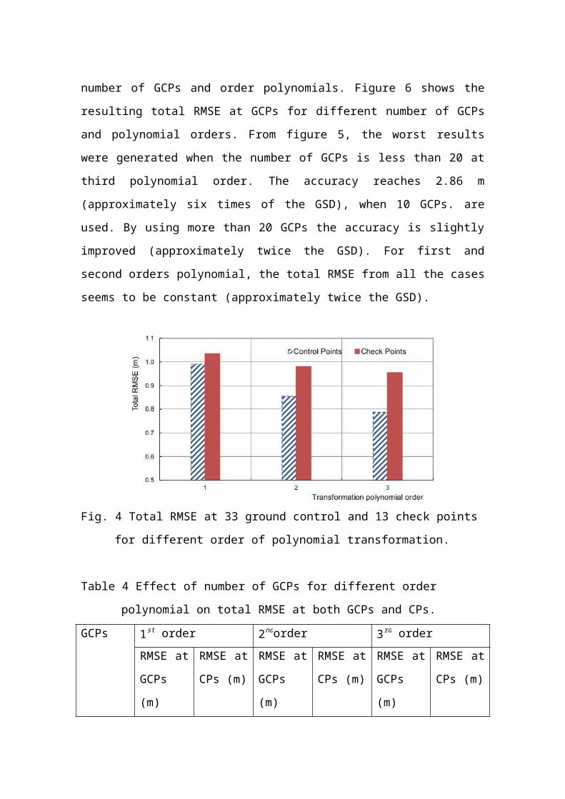
projection. Table 3 gives a summary of the results. Figure

4 shows relation between polynomial order and total RMSE

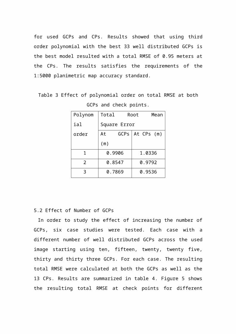
for used GCPs and CPs. Results showed that using third

order polynomial with the best 33 well distributed GCPs is

the best model resulted with a total RMSE of 0.95 meters at

the CPs. The results satisfies the requirements of the

1:5000 planimetric map accuracy standard.

Table 3 Effect of polynomial order on total RMSE at both

GCPs and check points.

Polynom

ial

order

Total Root Mean

Square ErrorAt GCPs

(m)

At CPs (m)

1 0.9906 1.03362 0.8547 0.97923 0.7869 0.9536

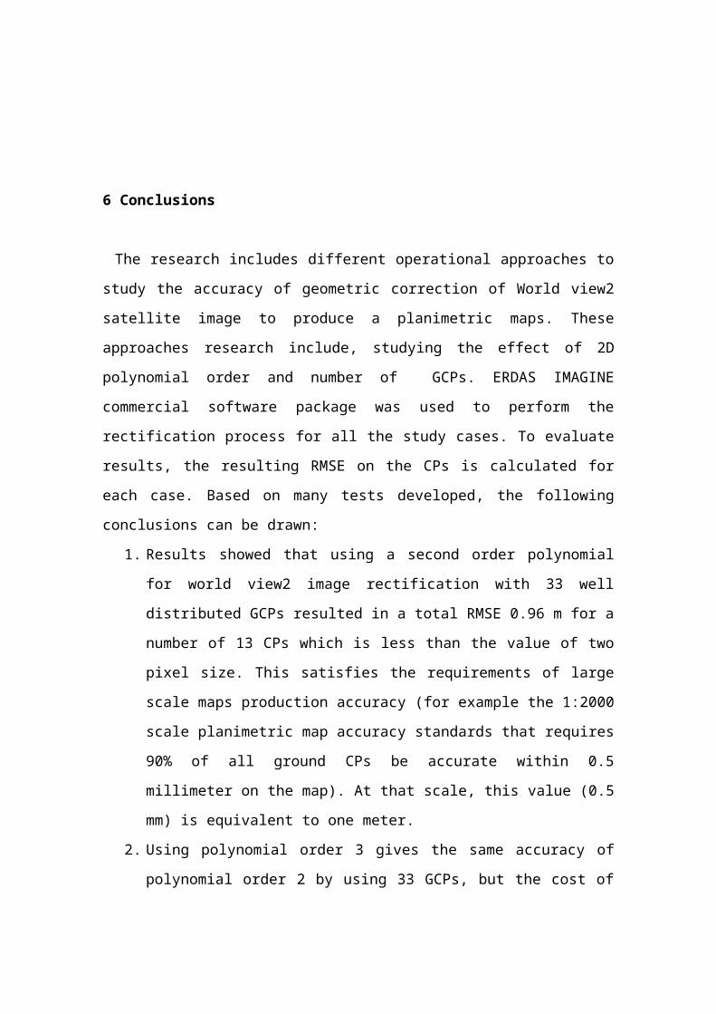
5.2 Effect of Number of GCPs

In order to study the effect of increasing the number of

GCPs, six case studies were tested. Each case with a

different number of well distributed GCPs across the used

image starting using ten, fifteen, twenty, twenty five,

thirty and thirty three GCPs. For each case. The resulting

total RMSE were calculated at both the GCPs as well as the

13 CPs. Results are summarized in table 4. Figure 5 shows

the resulting total RMSE at check points for different

number of GCPs and order polynomials. Figure 6 shows the

resulting total RMSE at GCPs for different number of GCPs

and polynomial orders. From figure 5, the worst results

were generated when the number of GCPs is less than 20 at

third polynomial order. The accuracy reaches 2.86 m

(approximately six times of the GSD), when 10 GCPs. are

used. By using more than 20 GCPs the accuracy is slightly

improved (approximately twice the GSD). For first and

second orders polynomial, the total RMSE from all the cases

seems to be constant (approximately twice the GSD).

Fig. 4 Total RMSE at 33 ground control and 13 check points

for different order of polynomial transformation.

Table 4 Effect of number of GCPs for different order

polynomial on total RMSE at both GCPs and CPs.

GCPs 1st order 2ndorder 3rd orderRMSE at

GCPs

(m)

RMSE at

CPs (m)

RMSE at

GCPs

(m)

RMSE at

CPs (m)

RMSE at

GCPs

(m)

RMSE at

CPs (m)

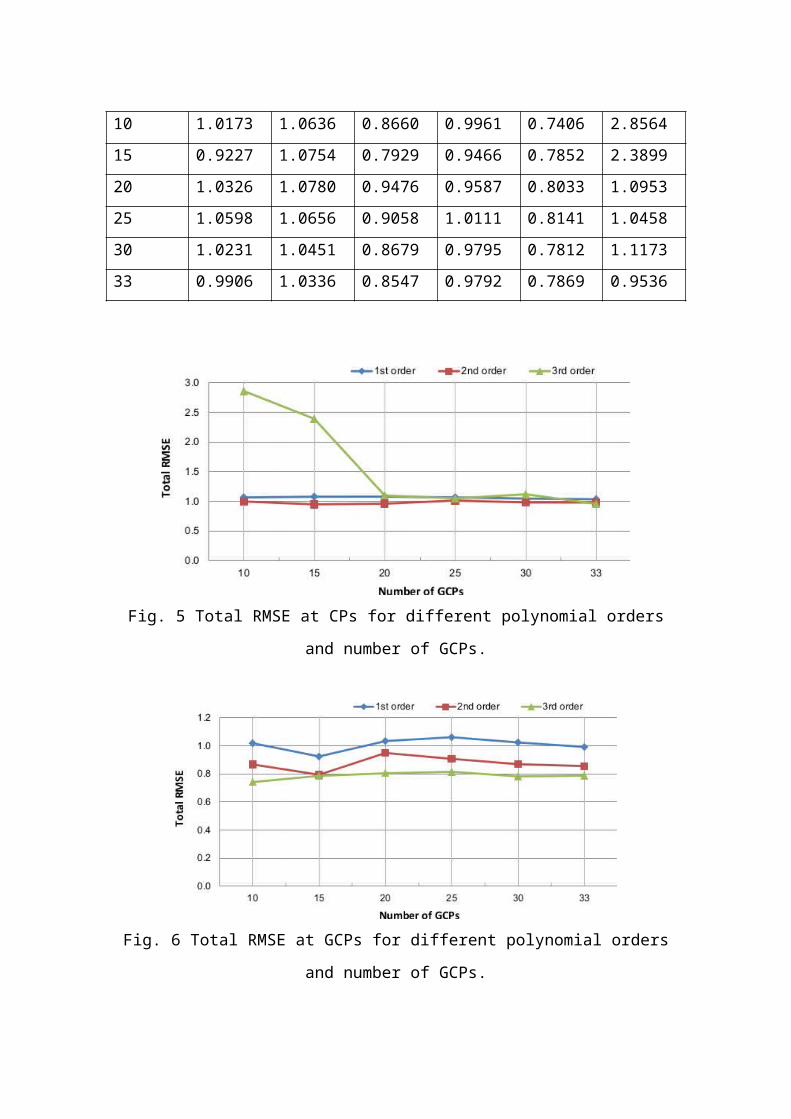
10 1.0173 1.0636 0.8660 0.9961 0.7406 2.856415 0.9227 1.0754 0.7929 0.9466 0.7852 2.389920 1.0326 1.0780 0.9476 0.9587 0.8033 1.095325 1.0598 1.0656 0.9058 1.0111 0.8141 1.045830 1.0231 1.0451 0.8679 0.9795 0.7812 1.117333 0.9906 1.0336 0.8547 0.9792 0.7869 0.9536

Fig. 5 Total RMSE at CPs for different polynomial orders

and number of GCPs.

Fig. 6 Total RMSE at GCPs for different polynomial orders

and number of GCPs.

6 Conclusions

The research includes different operational approaches to

study the accuracy of geometric correction of World view2

satellite image to produce a planimetric maps. These

approaches research include, studying the effect of 2D

polynomial order and number of GCPs. ERDAS IMAGINE

commercial software package was used to perform the

rectification process for all the study cases. To evaluate

results, the resulting RMSE on the CPs is calculated for

each case. Based on many tests developed, the following

conclusions can be drawn:

1. Results showed that using a second order polynomial

for world view2 image rectification with 33 well

distributed GCPs resulted in a total RMSE 0.96 m for a

number of 13 CPs which is less than the value of two

pixel size. This satisfies the requirements of large

scale maps production accuracy (for example the 1:2000

scale planimetric map accuracy standards that requires

90% of all ground CPs be accurate within 0.5

millimeter on the map). At that scale, this value (0.5

mm) is equivalent to one meter.

2. Using polynomial order 3 gives the same accuracy of

polynomial order 2 by using 33 GCPs, but the cost of

mapping production would be extremely high while

acquiring coordinates of more GCPs cost extra money

and time.

3. By increasing the number of GCPs the accuracy will be

improved. This is true as long as the accuracy of the

GCPs is homogeneous and is well distributed all over

the used satellite image. In our experiment using a

number of well distributed GCPs ranging from 10 to 33

covering the whole study area (90 km2) resulted in

acceptable results, the accuracy of geometric

correction for all polynomial order has a small

variation. This is equivalent to 1 GCPs each 9 to 3km2. The degrees of freedom of solution system will be

reduced when only 10 GCPs with polynomial order 3 is

used. That reduce the reliability of the obtained

results.

References

[1] F. Aguera, F. J. Aguilar, and M. A. Aguilar. Using

texture analysis to improve per-pixel classification of

very high resolution images. ISPRS Journal of

Photogrammetry and Remote Sensing, 63(6):635–646, 2008.

[2] F. Aguera, M. A. Aguilar, and F. J. Aguilar. Detecting

greenhouses changes from quickbird imagery on the

mediterranean coast. Internacional Journal of Remote

Sensing, 27(21):4751–4767, 2006.

[3] A. M. Al-Garni. Experiences with ikonos and quick bird

images in a mass production project. Dirasat,

Engineering Sciences, 34(1), 2007.

[4] D. H. A. Al-Khudhairy, I. Caravaggi, and S. Giada.

Structural damage assessments from ikonos data using

change detection, object-oriented segmentation, and

classification techniques. Photogrammetric Engineering

and Remote Sensing, 71(7):825–837,2005.

[5] J. M. Andersonand and E. M. Mikhail. Surveying: Theory

and Practice. the McGraw Hill Company, Inc., New York,

U.S.A., 2001.

[6] J. A. Benediktsson, J. Chanussot, and W. M. Moon. Very

high-resolution remote sensing: Challenges and

opportunities. Proceedings of the IEEE, 100(6):1907–

1910, 2012.

[7] Y. S. El-Manadili. Production of 1:5000 digital city

maps from high resolution satellite images: a case

study for marsa matrouh city. Civil Engineering

Research Magazine CERM, El-azher University, Nasr City

Cairo, Egypt, 29(1):57–72, 2007.

[8] N. Elashmawy. Implementation of High Resolution Stereo

Satellite Images and Decision Support System for Flood

Extent Prediction. Ph.d. thesis, Faculty of

Engineering, Cairo University, 2005.

[9] S. S. Elghazali. Assessment of indian remote sensing

satellite (irs) imaging for production and updating of

1: 25000 planimetric city maps. Master’s thesis,

Faculty of Engineering, Cairo University, 2005.

[10] C. S. Fraser, E. Baltsavias, and A. Gruen. Processing

of ikonos imagery for submetre 3d positioning and

building extraction. ISPRS Journal of Photogrammetry

and Remote Sensing, 56(3):177–194, 2002.

[11] P. Gamba, F. Dell Acqua, G. Lisini, and G. Trianni.

Improved vhr urban area mapping exploting object

boundaries. Geoscience and Remote Sensing, IEEE

Transactions on, 45(8):2676–2682, 2007.

[12] X. Jin and C. H. Davis. An integrated system for

automatic road mapping from high resolution

multispectral satellite imagery by information fusion.

Information Fusion, 6:257–273, 2005.

[13] J. Krishnamurthy, S. Natarajan, P. Krishnaiah, K.

Kalyanaraman, Mukund Rao, and V Jayaraman. Large scale

mapping using high resolution satellite data. Global

spatial data infrastructure,7 Conference, February 2-6

Bangalore, India, 2013.

[14] R. Li, S. Deshpande, X. Niu, Z. Feng, K. Di, and

B.Wu. Geometric integration of aerial and high-

resolution satellite imagery and application in

shoreline mapping. Marine Geodesy, 31(3):143–159, 2008.

[15] G. Meinel, R. Lippold, and M. Netzband. The potential

use of new high resolution satellite data for urban and

regional planning. IAPRS, Vol. 32 Part 4 GIS-Between

Visions and Applications, Stuttgart, 42(4), 1998.

[16] L. K. Mohamed. Geometric quality assessment of

various sensor modeling techniques. Master’s thesis,

Faculty of Engineering, Cairo University, 2006.

[17] J. Nichol and C. M. Lee. Urban vegetation monitoring

in Hong Kong using high resolution multispectral

images. International Journal of Remote Sensing,

26(5):903–918, 2005.

[18] J. A. Richardsand and X. Jia. Remote Sensing Digital

Image Analysis: An Introduction. Springer, 2006.

[19] A. E. Saida, H. M. O. Shandoulb, and Y. Z. Yekhlefc.

Up dating large scale maps using high resolution

satellite image. 4th International Conference on

Environmental Science and Development- ICESD, 5:435–

440, 2013.

[20] K.W.Wong. Geometric and cartographic accuracy of

erts-1 imagery. Photogrammetric Engineering and Remote

Sensing, (41):621–635, 1975.

[21] D. Yan and Z. Zhao. Road detection from quickbird

fused image using his transform and morphology.

Geoscience and Remote Sensing Symposium. IGARSS ’03.

Proceedings IEEE International, 2003.

Websites

http://www.digitalglobe.com accessed on

September 2013.

http://www.topconpositioning.com/products/gnss/rece

ivers/hiper-ii accessed on January 2014.

http://www.intergraph.com/assets/pressreleases/2012

/10-23-2012b.aspx accessed on January 2014.