W&M ScholarWorks W&M ScholarWorks

Dissertations, Theses, and Masters Projects Theses, Dissertations, & Master Projects

2018

Genetic Analyses of Striped Bass in the Chesapeake Bay: an Genetic Analyses of Striped Bass in the Chesapeake Bay: an

Investigation of Connectivity Among Virginia Subestuaries and an Investigation of Connectivity Among Virginia Subestuaries and an

Evaluation of Close-Kinship Mark Recapture Methodology to Evaluation of Close-Kinship Mark Recapture Methodology to

Estimate Spawning Abundance. Estimate Spawning Abundance.

Savannah Michaelsen College of William and Mary - Virginia Institute of Marine Science, smichaelsen@vims.edu

Follow this and additional works at: https://scholarworks.wm.edu/etd

Part of the Aquaculture and Fisheries Commons, and the Genetics Commons

Recommended Citation Recommended Citation Michaelsen, Savannah, "Genetic Analyses of Striped Bass in the Chesapeake Bay: an Investigation of Connectivity Among Virginia Subestuaries and an Evaluation of Close-Kinship Mark Recapture Methodology to Estimate Spawning Abundance." (2018). Dissertations, Theses, and Masters Projects. Paper 1550153637. http://dx.doi.org/10.25773/v5-pvgc-eb03

This Thesis is brought to you for free and open access by the Theses, Dissertations, & Master Projects at W&M ScholarWorks. It has been accepted for inclusion in Dissertations, Theses, and Masters Projects by an authorized administrator of W&M ScholarWorks. For more information, please contact scholarworks@wm.edu.

Genetic analyses of striped bass in the Chesapeake Bay: an investigation of connectivity among

Virginia subestuaries and an evaluation of close-kinship mark recapture methodology to estimate

spawning abundance.

A Thesis

Presented to

The Faculty of the School of Marine Science

The College of William and Mary in Virginia

In Partial Fulfillment

of the Requirements for the Degree of

Master of Science

by

Savannah Ann Michaelsen

August 2018

APPROVAL PAGE

This thesis is submitted in partial fulfillment of

the requirements for the degree of

Master of Science

Savannah Ann Michaelsen

Approved by the Committee, July 2018

John E Graves, Ph.D.

Committee Chair / Advisor

Jan R. McDowell, Ph.D.

John M. Hoenig, Ph.D.

Mark J. Brush, Ph.D.

TABLE OF CONTENTS

ACKNOWLEDGEMENTS ..................................................................................................................... iv

LIST OF TABLES ................................................................................................................................... v

LIST OF FIGURES .................................................................................................................................. vii

ABSTRACT ............................................................................................................................................. viii

CH I: GENERAL INTRODUCTION ...................................................................................................... 2

LITERATURE CITED ..................................................................................................................... 12

CH 2: ASSESSMENT OF STRIPED BASS GENETIC STRUCTURE AND

CONNECTIVITY OF THE LOWER CHESAPEAKE BAY .................................................................. 20

INTRODUCTION............................................................................................................................. 21

MATERIALS AND METHODS ...................................................................................................... 25

Sample Collection ........................................................................................................................ 25

Molecular Marker Selection ......................................................................................................... 26

Extraction and Amplification ....................................................................................................... 26

Descriptive Statistics .................................................................................................................... 27

Population Genetics ..................................................................................................................... 28

RESULTS ......................................................................................................................................... 29

Population Genetic Statistics ........................................................................................................ 29

Genetic Structure .......................................................................................................................... 32

DISCUSSION .................................................................................................................................................................. 35

Population Structure ................................................................................................................................................ 37

Evaluation of Connectivity.................................................................................................................................... 40

Conclusions and Management Implications.................................................................................................... 43

LITERATURE CITED ..................................................................................................................... 53

CH III: FEASIBILITY OF CLOSE-KNISHIP MARK-RECAPTURE METHODOLOGY TO ESTIMATE

STRIPED BASS ADULT ABUNDANCE .............................................................................................. 64

INTRODUCTION............................................................................................................................. 65

MATERIALS AND METHODS ...................................................................................................... 71

Sample Collection ........................................................................................................................ 71

Molecular Marker Selection, DNA Extraction, and Amplification .............................................. 71

Recovery of POPs ........................................................................................................................ 73

Estimation of Population Size ...................................................................................................... 73

RESULTS ......................................................................................................................................... 76

POP Assignment .......................................................................................................................... 77

Adult Abundance Estimates ......................................................................................................... 77

DISCUSSION .................................................................................................................................................................. 79

LITERATURE CITED ..................................................................................................................... 89

CH IV: CONCLUSIONS ......................................................................................................................... 98

APPENDIX I ............................................................................................................................................ 101

iv

ACKNOWLEDGEMENTS

I would first like to thank my advisor, Dr. John Graves, for taking a chance on me and

giving me the opportunity to pursue my research interests. You always encouraged me to

be more than I am, and the reach higher than I thought that I could. I wouldn’t have been

able to complete this work without your guidance, encouragement, and positive attitude.

I would also like to thank my committee: Dr. Jan McDowell for her wise words, moral

support, and help with genetic analyses; Dr. John Hoenig for his willingness to help me,

always with a cold Fresca; and Dr. Mark Brush for his willingness to be on my

committee and lament over the fact that we’d be skiing.

My thesis would not have been possible without the support of everyone in the VIMS

Fisheries Genetics Lab. I would like to thank Heidi Brightman for her support with lab

processing and techniques, and Hamish Small for his encouragement and positive

attitude. A special thanks to Michael Pugh, our visiting scientist, who helped me finish

my project with smile. To my labmate and close friend, Nadya Mamoozadeh, thank you

for always being there when I needed you. You always lifted my spirits, and I am grateful

to have shared the lab with you. To the additional members of the Fisheries Genetics Lab,

William Goldsmith and Jingwei Song, thank you for offering advice and supporting me.

This thesis would not have been possible without the support and comradery of the VIMS

community. I am eternally thankful to my office mate, Darbi Jones, who went above and

beyond the call of a friend. I would not have finished without you, and for that I am

forever grateful. To my roommate while I was at VIMS, Kelsey Fall, thank you for being

not only a friend, but a role model. You constantly inspired me to be better than I am, at

school and outside of it. You always had my back, no matter what. The VIMS

community as a whole, there are too many people to thank, but I am so thankful to have

been a part of such a wonderful group of people.

Finally, I would like to thank my family. They not only believed in me but supported me

from over 1,000 miles away with phone calls, visits, and care packages. I am especially

grateful to my husband, Shaun Lewis, who came along just when I needed him. His love

and support inspired me to achieve my dreams no matter what. Thank you for always

keeping me laughing, even when things seemed impossible.

v

LIST OF TABLES

Chapter II

Table 1: Sample sizes of striped bass collections from each river and year,

and the number of samples that were used in the analyses after

removal of problematic individual. .......................................................................... 45

Table 2: The number of alleles, private alleles, mean allelic richness

adjusted for sample size, and the inbreeding coefficient for each

collection of striped bass pooled over all loci .......................................................... 45

Table 3: Number of alleles, expected and observed heterozygosities, FST,

and the inbreeding coefficient for each locus pooled over all striped

bass collections ........................................................................................................ 46

Table 4: Number of alleles, private alleles, and mean allelic richness for

each for all samples, and by sex, for all striped bass collections. ............................ 47

Table 5: Population pairwise FST values for each striped bass collection ..................... 48

Table 6: Population pairwise FST values between striped bass collections

from each river pooled over years ........................................................................... 48

Table 7: Population pairwise FST values for male striped bass in each

collection ................................................................................................................ 49

Table 8: Population pairwise FST values for female striped bass in each

collection ................................................................................................................ 49

Table 9: Effective population size for each striped bass collection from the

adult population ....................................................................................................... 50

Table 10: Recapture locations of striped bass tagged on spawning grounds

of the James and Rappahannock rivers during the spawning season and

subsequently recaptured during the spawning season after being at

large for at least one year.. ....................................................................................... 50

Chapter III

Table 1: Sample sizes of adult and young-of-year (YOY) striped bass

collected in the Rappahannock River in 2016 used in this study from

each river and year used in the analyses after removal of problematic

individuals. Values shown for overall numbers, males, and females. ..................... 86

vi

Appendix I

Supplementary Table 1: Table of the multiplexes, microsatellite loci, and

protocols used for both Ch. II and Ch. III. ............................................................... 101

Supplementary Table 2: Table representing tagging recapture rates ............................. 102

vii

LIST OF FIGURES

Chapter II

Figure 1: Map showing the sampling locations on the Rappahannock,

Mattaponi, and James rivers over the two sampling years ...................................... 51

Figure 2: PCA of all populations showing principal components 1 and 2. ................... 52

Chapter III

Figure 1: Map of sample locations for adult and young-of-year striped

bass samples taken in the Rappahannock River in 2016 ......................................... 86

viii

ABSTRACT

The striped bass (Morone saxatilis) is an anadromous fish distributed along the

eastern coast of North America that currently supports one of the most lucrative and

important commercial and recreational fisheries in the region. Since the recovery of the

Atlantic stock after a collapse in the late 1970s, studies have focused on understanding

the connectivity of major spawning grounds and improving methods of abundance

estimation. Studies support strong site fidelity of striped bass to major estuaries along the

Atlantic coast, but there has been disagreement about connectivity within the largest

spawning ground, the Chesapeake Bay. Additionally, no estimates exist for striped bass

abundance within the Chesapeake Bay. The objectives of my thesis were to examine the

fine scale genetic population structure of striped bass within the lower Chesapeake Bay,

and to test the feasibility of a novel, fishery-independent molecular methodology, close-

kinship mark-recapture analysis (CKMR), to estimate spawning adult abundance within

the Rappahannock River. Sampling of 1,132 adult striped bass and 389 young-of-year

(YOY) striped bass was done during the 2016 and 2017 spawning seasons on major

spawning grounds of the James, Mattaponi, and Rappahannock rivers. Twenty

microsatellite loci were used to examine both the spatial genetic heterogeneity among the

river systems and the temporal heterogeneity between sampling years within a river.

Significant population pairwise FST values were recovered from 18 of the 21 pairwise

comparisons. However, mean FST values between temporal comparisons were higher than

those among spatial comparisons, suggesting a lack of biologically meaningful

population structure among rivers. Additional analyses and a 30-year tagging data set

also support a rate of connectivity among the major rivers high enough to maintain

similar allele frequencies. Combined, the data support one genetic stock of striped bass

within the lower Chesapeake Bay. The same suite of markers was then used to test the

feasibility of CKMR to estimate adult abundance of striped bass within the

Rappahannock River system. Using existing sampling programs, 371 spawning adults

and 389 YOY were collected on the spawning and nursey grounds of the Rappahannock

River in 2016. These samples yielded 2 parent-offspring pairs, resulting in an abundance

estimate of 145,081 adult spawning striped bass. Additional analyses indicated that a

relatively precise estimate (recovery of 50 POPs) would be made if sample sizes totaled

850 adults and 850 YOY. CKMR can be a feasible option of abundance estimation for

striped bass. Overall, my study has provided the first estimate of abundance for

Chesapeake Bay striped bass, and has provided strong support of a single, spawning

stock of striped bass within the Chesapeake Bay.

Genetic analyses of striped bass in the Chesapeake Bay: an investigation of connectivity

among Virginia subestuaries and an evaluation of close-kinship mark recapture

methodology to estimate spawning abundance

2

CHAPTER I

GENERAL INTRODUCTION

3

Introduction

Striped bass (Morone saxatilis) support one of the largest commercial and

recreational fisheries of the United States Atlantic coast (ASMFC, 2016). The Atlantic

stock of striped bass collapsed in the late 1970s due to overfishing and habitat

degradation (ASMFC, 2013). Today the striped bass stock has rebounded, but there are

many uncertainties associated with the assessment of the stock. This study examined two

of these uncertainties: genetic connectivity of striped bass among the major sub-estuaries

of Chesapeake Bay and the estimation of abundance of adult striped bass within a sub-

estuary. A suite of highly polymorphic molecular markers was used to investigate genetic

connectivity of striped bass among major Virginia sub-estuaries of the Chesapeake Bay.

In addition, the applicability of a novel fishery independent method, close-kinship mark-

recapture analysis (CKMR), was evaluated to provide an independent estimate of the size

of the striped bass spawning stock within a major spawning ground, the Rappahannock

River.

Striped bass are an anadromous species that undertake a seasonal migration from coastal

marine waters, through estuaries, and into fresh water for spawning (Paramore and

Rulifson, 2001). Anadromy is not displayed by all striped bass, and some individuals

exhibit resident ‘riverine’ life histories (Secor et al., 2000; Paramore and Rulifson, 2001).

Differences in life histories are influenced by fish size, sex, year class strength, and

latitude (Setzler et al., 1980; Dunning et al., 2006; Ng et al., 2007; Callihan et al., 2014).

4

Striped bass exhibit sexual dimorphism in population dynamics and life histories

including growth rates, movement patterns, and maturity schedules. Males mature much

faster than females, reaching 50% maturity by age 1 (ASMFC 2013), and are thought to

exhibit larger proportions exhibiting resident riverine life histories than females

(Mansueti 1961; Hassin et al., 2000; Secor and Piccoli, 2004). Historically, females have

been thought to reach 50% maturity between years 6 and 7 (ASMFC, 2016; Andrews et

al., 2017). Female striped bass are thought to live longer than males, with >90% of fish

caught over age 10 identified as female (ASMFC, 2016). The coastal migratory stock is

comprised of up to 70% females of 2+ years of age (Secor and Piccoli, 2004), and these

fish mix with the male dominated residential estuarine populations in the mid to upper

freshwater reaches of major river systems during spawning season, which occurs in

spring (late March to May) (Kohlenstein 1981; Chapman 1990).

The peak of striped bass spawning season is generally between April and May.

Females are batch spawners capable of producing millions of pelagic eggs during

spawning events (Secor and Houde, 1998). Survival of striped bass larvae is heavily

affected by environmental conditions, such as freshwater flow and temperature

(Ulanowicz and Polgar, 1980; Secor and Houde, 1995; Richards and Rago, 1999). The

freshwater flow affects the location of the salt front and estuarine turbidity maximum

(ETM), and this, in turn, influences the quantity and quality of food available for larval

striped bass (North and Houde, 2003). Survival of striped bass larvae is greatest between

15°C and 19°C and temperatures outside of this range lead to higher rates of mortality

(Secor and Houde, 1995; Secor, 2006). It is hypothesized that the striped bass life history

strategy to spawn multiple batches over a long season increases the chances that some

5

larvae will be exposed to optimal environmental conditions including temperatures and

freshwater flows (Secor and Houde, 1995). Within the Chesapeake Bay there are

numerous areas that serve as spawning grounds for striped bass, and if one area has

conditions not conducive to larval survival, another area may have conditions favoring

high recruitment, ensuring the continuance of the population (Secor 2006).

The Chesapeake Bay is considered one of the most important spawning grounds for

striped bass (Kernehan 1981; Kohlenstein 1981; Richards and Rago, 1999). While

contributions of the major spawning areas may vary annually depending on both the

number of individuals spawning in the area and the impact of environmental variables,

the Chesapeake Bay stock has been estimated to contribute as much as 84% of the total

Atlantic stock in some years (Berggren and Lieberman, 1978; Waldman et al., 2012). A

recent genetic study indicated that Chesapeake Bay striped bass have served as a large

source of recruits supporting other Atlantic coastal regions (Gautier et al., 2013).

Additional major spawning areas, in order of contribution to the Atlantic stock, include

the Hudson River, the Delaware River, and the Roanoke River (Wirgin et al., 1993).

Results of conventional tagging, acoustic tagging, and genetic studies demonstrate

spawning site fidelity to the major spawning estuaries (Nichols and Miller, 1967; Ng et

al., 2007; Gautier et al., 2013).

Striped bass have supported important commercial and recreational fisheries along

the eastern US Atlantic coast since the 1600s (Richards and Rago, 1999). Recreational

fisheries exist across the range of the Atlantic stock (Canada to South Carolina), while

commercial fisheries operate in Massachusetts, Rhode Island, New York, Delaware,

Maryland, Virginia, and North Carolina (ASMFC, 2013). In 2015, commercial fishery

6

landings of striped bass totaled 617,698 fish, primarily aged 3-10 years. Over 80% of the

landings were from Chesapeake Bay, consisting of fish aged 3-8 years (ASMFC, 2016).

The largest commercial fishery is currently in Maryland with landings of over 350,000

fish a year (Shepard et al., 2016). Recreational fisheries are larger, with 1.34 million fish

landed in 2015 from Virginia, Maryland, New Jersey, and Massachusetts targeting fish

aged 4-10 years (ASMFC 2016).

In the late 1970s and early 1980s, managers became alarmed by drastically

decreasing catches of striped bass from commercial and recreational fisheries, as well as

high rates of estimated fishing mortality for young striped bass (Richards and Deuel,

1987; Gibson, 1993). The fisheries did not experience an immediate collapse, but a slow

decline as the successful year classes of older fish sustained the fisheries until 1983

(Richards and Rago, 1999). At that time, the majority of fish were less than 6 years of age

(Gibson, 1993). The steady decline of the Atlantic stock biomass and changing

environmental conditions resulted in a series of years with poor recruitment classes, and

the spawning biomass was not able to replace itself (Goodyear 1985). As the number of

older fish declined, there was increased fishing pressure on younger fish.

Due to the migratory nature of striped bass, independent (non-coordinated) state

management measures were not effective in preventing overfishing. In several instances,

measures to preserve and rebuild the spawning stock biomass adopted by one state were

offset by less restrictive conservation measures in adjoining states (Richards and Rago,

1999). To ensure that all states participated equally in the management and conservation

of striped bass, Congress enacted the Emergency Striped Bass Research Study in 1979.

The measure allowed federal oversight of striped bass by the U.S. Fish and Wildlife

7

Service and the National Marine Fisheries Service (Richards and Deuel, 1987), and it

provided research funding to federal agencies, state agencies, and academic institutions to

determine the causes of the decline in the striped bass population with research published

in annual reports (Shepard et al., 2005). The congressional measure also directed the

Atlantic States Marine Fisheries Commission (ASMFC) to develop a striped bass

fisheries management plan (FMP) which was implemented in 1981. Shortly thereafter, in

1984, Congress approved the Striped Bass Conservation Act (Field 1997; Richards and

Rago, 1999). This legislation gave the ASMFC power to implement management policies

across multiple states by allowing the secretaries of Commerce and Interior to place a

moratorium on striped bass fishing for any state not complying with the FMP. The act

was amended into the 1990s to provide continued federal oversight and funding to the

recovery of striped bass stocks (Public Law 98-613).

The striped bass spawning stock decline during the late 1970s and 1980s in the

Chesapeake Bay led to a decrease of the Atlantic Stock overall (Richards and Deuel,

1987). The primary cause of the population decline was a lack of strong recruitment from

the Chesapeake Bay since 1970 that was combined with total mortality rates of 60-93%

for males and 45% for females (Richards and Deuel, 1987). In addition, immature striped

bass were experiencing high rates of fishing mortality from a lack of minimum size

regulations and overfishing. Comparisons of fishing mortalities between the Hudson

River, which did not experience a major stock collapse, and the Chesapeake Bay

indicated that the Hudson River striped bass experienced about half the fishing mortality

of those in the Chesapeake Bay (Richards and Rago, 1999). In addition to overfishing,

the striped bass population was affected by degraded water quality (Hall 1989; Finger et

8

al., 1998), habitat impairment (Richards and Rago, 1999), nutritional stress (Setzler-

Hamilton et al., 1981), and overall poor environmental conditions (Hall et al., 1993).

Prior to the stock crash, the only management measures for striped bass were

minimum size limits that ranged from 10-14 inches total length (TL) depending on the

state (ASMFC, 2013). The implementation of the Fisheries Management Plan for striped

bass by the ASMFC in 1981 resulted in a minimum size limit for all states of 14 inches

TL within bays and estuaries and 24 inches TL in coastal areas. Additionally, ASMFC

recommended a fishing closure on spawning grounds during spawning season. ASMFC

amended the FMP in 1984 and again in1985, to set fishing mortality targets on a state by

state basis (Richards and Rago, 1999). A third amendment adopted in 1985 included

measures to protect a strong 1982-year class in the Chesapeake Bay. A minimum size of

38 inches TL was implemented to ensure that 95% of the females of the 1982-year class

survived to have an opportunity to spawn. Rather than requiring the large minimum size,

most states, with the exception of Massachusetts, implemented a moratorium on the

striped bass fishery (Richards and Rago, 1999; ASMFC 2013). Mandatory monitoring

surveys in subsequent years indicated that populations were recovering, and an

amendment to the FMP reopened the fishery in 1990 with a target fishing mortality of

F=0.25. Dual minimum size limits of 18 inches TL in bays and estuaries and 28 inches

TL in coastal areas were implemented, as well as fishery restrictions including

recreational trip limits and commercial fishing seasons (ASMFC 2013).

As a result of management efforts that reduced fishing mortality on striped bass

and favorable environmental conditions that facilitated good recruitment, the striped bass

spawning biomass within the Chesapeake Bay was restored to management thresholds by

9

1995 (Field 1997). An amendment to the striped bass FMP in 1995 eased some of the

existing strict fishery regulations, but still allowed for the stock to continue to rebuild.

Coastal states were also provided greater freedom to adjust regulations to fit their needs

as long as ASMFC goals were being met (Richards and Rago, 1999). The population size

of striped bass peaked in 1997 at 249 million fish, and the stock remained close to this

size until 2005 when abundance began to decline (ASMFC 2013). Additional

amendments to the striped bass FMP have since been adopted, the largest of which

includes management triggers to protect female spawning biomass. Due to declines in the

female SSB, management action was triggered in 2014 that resulted in 2015 harvest

quotas being cut 25% for coastal states and 20.5% for Chesapeake Bay states (ASMFC

2015).

The 2016 striped bass assessment update indicated that the Atlantic stock of

striped bass is not overfished nor experiencing overfishing; however, the stock is not

considered fully rebuilt as the female spawning stock biomass (SSB) is estimated at

58,853 metric tons, just above the biomass threshold of 57,626 metric tons and well

below the biomass target of 72,032 metric tons (ASMFC 2016). A lack of strong

recruitment since 2012 has led to a further reduction in abundance of striped bass on the

Atlantic Coast. Projections of the 2016 Atlantic Striped Bass Stock Assessment Update

indicate that there is ~39% probability that female SSB will drop below the management

biomass threshold over the next three years. Some studies have attributed this recent

decline to an increase in the prevalence of Mycobacteriosis, a bacterial disease in striped

bass shown to have large impacts on reproductive output and natural mortality (Gautier et

al., 2008; Gervasi 2015; Hoenig et al., 2017), while others have attributed the decline to a

10

reduction in the availability of prey species (ASMFC 2013). Declines in the Atlantic

stock often result from declines in Chesapeake Bay (Richard and Deuel, 1987). In 2015,

estimates of the SSB within Virginia rivers for both males and females were both ~40%

below the average SSB for the years 1987 to 2015, with survival estimates the lowest

seen in recent years (Hoenig et al., 2016).

The recent declining trend in abundance of striped bass within the Chesapeake

Bay has highlighted the need for an understating of the contributions of each subestuary

to the Chesapeake Bay striped bass population. While connectivity and abundance of the

Atlantic coastal stock is relatively well known, there has been little focus within

Chesapeake Bay. The Chesapeake Bay is differentiated from other major striped bass

spawning grounds because it is a large, complex estuary composed of several major

subestuary river systems (Marshall and Alden, 1990; Boynton et al., 1995) while all other

areas largely consist of one large river system with much smaller supporting tributaries

(Chittenden 1971; Carmichael et al; 1998). Each of the subestuaries within Chesapeake

Bay has the potential to host separate spawning populations of striped bass. Knowledge

regarding the stock structure of striped bass within subestuaries of Chesapeake Bay, and

estimates of the number of breeding individuals on each spawning ground can help

fishery managers to address regionally the recent decline of striped bass spawning stock

biomass.

Researchers have studied striped bass population structure within Chesapeake

Bay since the early 20th century. Investigations of morphological characteristics (Lewis

1957; Lund 1957; Raney 1957; Murawski 1958) and tagging studies (Massmann and

Pacheco, 1961; Nichols and Miller, 1967) supported the hypothesis of distinct stocks of

11

striped bass within Chesapeake Bay subestuaries. Modern molecular studies that

examined genetic population structure using allozymes (Grove et al., 1976; Sidell et al.,

1980), mitochondrial DNA (Chapman 1987, 1990; Wirgin et al., 1989, 1993), and

nuclear DNA microsatellite loci (Laughlin and Turner, 1996; Diaz et al., 1997; Brown et

al., 2005; Gauthier et al., 2013) have reached conflicting conclusions concerning the

existence of separate striped bass stocks on the different subestuary spawning grounds

within Chesapeake Bay. Additionally, there is little information regarding the abundance

and spawning stock size of striped bass within subestuaries of Chesapeake Bay.

The research recommendations highlighted in the 2013 Striped Bass Benchmark

Assessment included an in-depth analysis of stock composition and the need for the

development of an independent estimate of abundance. The objective of this study was to

address these two recommendations. Using a suite of highly polymorphic molecular

markers, the second chapter of this thesis evaluated genetic connectivity of striped bass to

determine if genetically distinct spawning populations exist within the Chesapeake Bay

to provide an in-depth description of the stock composition. Using the same molecular

markers, the third chapter of this thesis assessed the applicability of a novel fishery

independent method, close-kinship mark-recapture analysis (CKMR), to estimate of the

size of the striped bass spawning stock for striped bass within a well-known spawning

river, the Rappahannock River.

References

Atlantic States Marine Fisheries Commission. 2013. Striped Bass Stock Assessment for

2013. Arlington, VA. Retrieved from

http://www.asmfc.org/uploads/file/529e5ca12013StripedBassBenchmarkStockAsses

sment_57SAWReport.pdf.

Atlantic States Marine Fisheries Commission. 2015. 2015 Atlantic Striped Bass Stock

Assessment Update. Arlington, VA. Retrieved

from http://www.asmfc.org/uploads/file/564106f32015AtlStripedBassAssessmentUp

date_Nov2015.pdf.

Atlantic States Marine Fisheries Commission. 2016. 2016 Atlantic Striped Bass Stock

Assessment Update. Arlington, VA. Retrieved

from http://www.asmfc.org/uploads/file/581ba8f5AtlStripedBassTC_Report2016Ass

mtUpdate_Oct2016.pdf.

Andrews SN, Linnansaari T, Curry RA, Dadswell MJ. 2017. The misunderstood striped

bass of the Saint John River, New Brunswick: Past, present, and future. North

American Journal of Fisheries Management 37(1):235-254.

Berggren TJ, Lieberman JT.1978. Relative contribution of Hudson, Chesapeake and

Roanoke striped bass, Morone saxatilis, stocks to the Atlantic coast fishery. U. S.

Fish. Bull. 76: 335-345.

Boynton WR, Garber JH, Summers R, Kemp WM. 1995. Inputs, transformations, and

transport of Nitrogen and phosphorus in Chesapeake Bay and selected tributaries.

Estuaries 18(1): 285-314.

13

Brown KM, Baltazar GA, Hamilton MB. 2005. Reconciling nuclear microsatellite and

mitochondrial marker estimates of population structure: breeding population

structure of Chesapeake Bay striped bass (Morone saxatilis). Heredity 94: 606-615.

Callihan, JL. Godwin CH, Buckel JA. 2014. Effect of demography on spatial distribution:

movement patterns of the Albemarle Sound-Roacnoke River stock of Striped Bass

(Morone saxatilis) in relation to their recovery. Fishery Bulletin 112: 131-143.

Carmichael JT. Haeseker SL, Hightower JE. 1998. Spawning migration of telemetered

striped bass in the Roanoke River, North Carolina. Transactions of the American

Fisheries Society 127(2): 286-297.

Chapman RW. 1987. Changes in the population structure of male striped bass, Morone

saxatilis, spawning in three areas of Chesapeake Bay from 1984 to 1986. Fishery

Bulletin 85: 167-171.

Chapman RW. 1990. Mitochondrial DNA analysis of striped bass populations in the

Chesapeake Bay. Copeia, 1990: 355-366.

Chittenden ME. 1971. Status of the striped bass, Morone saxatilis, in the Delaware River.

Chesapeake Science 12(3): 131-136.

Diaz M. Leclerc GM, Fishtec BE. 1997. Nuclear DNA markers reveal low levels of genetic

divergence among Atlantic and Gulf of Mexico populations of striped bass.

Transactions of the American Fisheries Society 126(1): 163-165.

14

Dunning DJ, Ross QE, Blumberg AF, Heimbuch DG. 2006. Transport of striped bass larvae

out of the lower Hudson River estuary. American Fisheries Society Symposium 51:

273.

Field J. 1997. Atlantic striped bass management: where did we go right? Fisheries 22(7):6–

8.

Finger SE, Livingstone AC, Olson SJ. 1998. Influence of contaminants on survival of

striped bass in Chesapeake Bay tributaries. In Second US–USSR symposium on

reproduction, rearing, and management of anadromous fishes Edited by: Weaver, J.

E. 77–86. Seattle: U.S. Geological Survey, Biological Resources Division.

Gautier DT, Latour RJ, Heisey DM, Bonzek CF, Gartland J, Burge EJ, Vogelbein WK.

2008. Mycobateriosis associated mortality in wild striped bass (Morone saxatilis)

from Chesapeake Bay, USA. Ecological Applications 18: 1718-1727.

Gauthier DT, Audemard CA, Carlsson JEL, Darden TL, Denson MR, Reece KS, Carlsson J.

2013. Genetic population structure of US Atlantic coastal striped bass

(Morone saxatilis). Journal of Heredity 104: 510-520.

Gervasi CL. 2015. The reproductive biology of striped bass (Morone saxatilis) in

Chesapeake Bay (MS Thesis). [Williamsburg, (VA)]: College of William & Mary.

Gibson MR. 1993. Historical estimates of fishing mortality on the Chesapeake Bay striped

bass stock using Separable Virtual Population Analysis applied to market class catch

data. Report of Rhode Island Division of Fish and Wildlife to the Atlantic States

Marine Fisheries Commission, West Kingston.

15

Goodyear CP, Cohen JE, Christensen SW. 1985. Maryland striped bass: recruitment

declining below replacement. Transactions of the American Fisheries Society, 114:

146–151.

Grove TL, Berggren TS, Powers DA. 1976. The use of innate genetic tags to segregate

spawning stocks of striped bass (Morone saxatilis). Estuarine Processes 1: 166-176.

Hall LW Jr., Ziegenfuss MC, Bushong SJ, Unger MA, Herman RL. 1989. Studies of

contaminant and water quality effects on striped bass prolarvae and yearlings in the

Potomac River and upper Chesapeake Bay in 1988. Transactions of the American

Fisheries Society. 118(6): 619-629.

Hall LW, Finger SE, Ziegenfuss MC. 1993. A review of in situ and on-site striped bass

contaminant and water-quality studies in Maryland waters of the Chesapeake Bay

watershed. In Water quality and the early life stages of fishes, Symposium 14 Edited

by: Fuiman, L. A. 3–15. Bethesda, Maryland: American Fisheries Society.

Hassin S, Claire M, Holland H, Zohar Y. 2000. Early maturity in the male striped bass,

Morone saxatilis: follicle-stimulating hormones and luteinizing hormone gene

expression and their regulation by gonadotropin-relaeasing hormone analogue and

testosterone. Biology of Reproduction 63(6): 1691-1697.

Hoenig JM, Sadler PW, Michaelsen S, Goins LM, Harris RE (2016) Evaluation of striped

bass stocks in Virginia: monitoring and tagging studies, 2015-2019,

Progress Report.VMRC.

Hoenig JM, Groner ML, Smith MW, Vogelbein WK, Taylor DM, Landers Jr DF,

Swenarton JT, Gauthier DT, Sadler P, Matsche MA, Haines AN. (2017) Impact of

16

disease on the survival of three commercially fished species. Ecological

Applications 27: 2116-2127.

Kernehan RJ, Headrick MR, Smith RE. 1981. Early life history of Striped Bass in the

Chesapeake and Delaware Canal and vicinity. Transactions of the American

Fisheries Society 110: 137-150.

Kohlenstein LC. 1981. On the proportion of the Chesapeake Bay stock of Striped Bass that

migrates into the coastal fishery. Transactions of the American Fisheries

Society 110: 168-179.

Laughlin TF, Turner BJ. 1996. Hypervariable DNA markers reveal high genetic variability

within striped bass populations of the lower Chesapeake Bay. Transactions of the

American Fisheries Society 125: 49-55.

Lewis RM. 1957. Comparative study of the populations of the striped bass. U.S. Fish and

Wildlife Service Species Science Report, 204.

Lund WA Jr. 1957. Morphometric study of the striped bass, Roccus saxatilis. U.S. Fish and

Wildlife Service Species Science Report, 216.

Mansueti RJ. 1961. Age, growth, and movements of the striped bass, Roccus saxatilis, taken

in size selective fishing gear in Maryland. Chesapeake Science 2: 9-36.

Marshall HG, Alden RW. 1990. A comparison of phytoplankton assemblages and

environmental relationships in three estuarine rivers of the lower Chesapeake Bay.

Estuaries 13(3): 287-300.

Massmann WH, Pacheco AL. 1961. Movements of striped bass tagged in Virginia waters of

the Chesapeake Bay. 2(1): 3-44.

17

Murawski WS. 1958. Comparative study of populations of striped bass, Roccus saxatilis,

based on lateral line scale counts. (MS Thesis), [Ithaca (NY)]: Cornell University.

Ng CL., Able KW, Grothues TM. 2007. Habitat use, site fidelity, and movement of adult

Striped Bass in a southern New Jersey estuary based on mobile acoustic

telemetry. Transactions of the American Fisheries Society 136:1344-1355.

Nichols PR, Miller RV. 1967. Seasonal movements of striped bass, Roccus saxatilis

(Walbaum), tagged and released in the Potomac River, Maryland, 1959–1961.

Chesapeake Science, 8: 102–124.

North EW, Houde ED. 2003. Linking ETM physics, zooplankton prey, and fish early-life

histories to striped bass, Morone saxatilis, and white perch, M. Americana,

recruitment. Marine Ecology Progress Series 260:219-236.

Paramore LM, Rulifson RA. 2001. Dorsal coloration as an indicator of different life history

patterns for Striped Bass within a single watershed of Atlantic Canada. Transactions

of the American Fisheries Society 130: 663-674.

Raney, EC. 1957. Subpopulations of the Striped Bass Roccus saxatilis (Walbaum) in

Tributaries of Chesapeake Bay. US Fish and Wildlife Service.

Richards RA, Deuel DG. 1987. Atlantic striped bass: stock status and the recreational

fishery. U.S. National Marine Fisheries Service Marine Fisheries Review, 49(2): 58–

66.

Richards RA, Rago PJ. 1999. A case history of effective fishery management: Chesapeake

Bay striped bass. North American Journal of Fisheries Management 19(2): 356-375.

Secor DH. 2006. The year-class phenomenon and the storage effect in marine fishes. Journal

of Sea Research 57: 91-103.

18

Secor DH, Houde ED. 1995. Temperature effects on the timing of Striped Bass egg

production, larval viability, and recruitment potential in the Patuxent River

(Chesapeake Bay). Estuaries, 18: 527-544.

Secor DH, Houde ED. 1998. Use of larval stocking in restoration of Chesapeake Bay striped

bass. ICES Journal of Marine Science 55(2): 228-239.

Secor DH, Piccoli PM. 2004. Oceanic migration rates of upper Chesapeake Bay striped bass

(Morone saxatilis) determined by otolith microchemical analysis. Fishery Bulletin

105: 62-73.

Secor DH, Gunderson TE, Karlsson K. 2000. Effect of temperature and salinity on growth

performance in anadromous (Chesapeake Bay) and nonanadromous (Santee-Cooper)

strains of Striped Bass Morone saxatilis. Copeia 2000: 291-296.

Setzler EM, Boynton WR, Wood KV, Zion HH, Lubbers L, Mountford NK, Frere P, Tucker

L, Mihursky JA. 1980. Synopsis of biological data on Striped Bass, Morone

saxatilis (Walbaum). NOOA technical report NMFS circular. FAW Fisheries

Synopses (FAO) no. 121.

Setzler-Hamilton EM, Boynton WR, Mihursky JA, Polgar TT, Wood KV. 1981. Spatial and

temporal distribution of striped bass eggs, larvae, and juveniles in the Potomac

estuary. Transactions of the American Fisheries Society, 110: 121–136.

Shepherd GR, Laney RW, Appelman M, Honabarger D, Wright CL. 2016. Biennial Report

to Congress on the Progress and Findings of Studies of Striped Bass Populations-

2015, 13 p. National Marine Fisheries Service, Silver Spring, MD.Shepherd GR,

Laney RW, Meyer T, Beal R. 2005. Atlantic Striped Bass Studies 2005 Biennial

Report to Congress, 39 p. National Marine Fisheries Service, Silver Spring, MD.

19

Sidell, BD, Otto RG, Powers DA, Kerweit M, Smith J. 1980. A reevaluation of the

occurrence of subpopulations of striped bass (Morone saxatilis, Walbaum) in the

Upper Chesapeake Bay. Transactions of the American Fisheries Society 109:99-107.

Striped Bass Conservation Act of 1984, Public Law No. 98-613, § 98 STAT 3187 (1984).

Ulanowicz, RE. Polgar TT. 1980. Influences of anadromous spawning behavior and optimal

environmental conditions upon striped bass (Morone saxatilis) year-class success.

Canadian Journal of Fisheries and Aquatic Sciences 37: 143-154.

Waldman J, Maceda L, Wirgin I. 2012. Mixed-stock analysis of wintertime aggregations of

Striped Bass along the Mid-Atlantic coast. Journal of Applied Ichthyology 28:2012.

Wirgin I, Procenca R, Grossfield J. 1989. Mitochondrial DNA diversity among populations

of striped bass in the Southeastern United Sates. Canadian Journal of Zoology 67:

891-907.

Wirgin I, Maceda L, Waldman JR, Crittenden RN. 1993. Use of mitochondrial DNA

polymorphisms to estimate the relative contributions of the Hudson River and the

Chesapeake Bay striped bass stocks to the mixed fishery on the Atlantic

Coast. Transactions of the American Fisheries Society 122: 669-684.

20

CHAPTER II

ASSESSMENT OF STRIPED BASS GENETIC STRUCTURE AND

CONNECTIVITY OF THE LOWER CHESAPEAKE BAY

21

Introduction

Striped bass are distributed along the Atlantic coast of North America from

Canada to northern Florida and support important recreational and commercial fisheries

throughout their range (Kirkley et al., 2000). The species exhibits multiple life history

strategies including riverine residential populations in the southern portion of the range

and coastal, more migratory populations in the northern portion of the range (Boreman

and Lewis, 1987; Greene et al., 2009; Wingate et al., 2011). Striped bass spawning occurs

in the freshwater reaches of major river and estuary systems (Paramore and Rulifson,

2001), and both tagging and genetic studies have indicated significant spatial population

structuring among the major spawning grounds of the Atlantic stock which include the

Hudson River, Delaware Bay, Chesapeake Bay, and the Roanoke River (Wirgin et al.,

1993; Gautier et al., 2013). Of these systems, the Chesapeake Bay is considered the

largest and most productive spawning ground (Kohlenstein 1981), contributing upwards

of 90% of the stock composition in some years (Waldman et al., 2012).

Striped bass are managed as a single stock but results from tagging and molecular

genetic studies suggest the presence of distinct spawning populations in major estuary

systems along the Atlantic Coast (Merriman, 1941; Kohlenstein 1981; Fabrizio, 1987;

Dorazio et al., 1994; Lindley et al., 2011). Conventional tagging studies (Mansueti,

22

1961; Nichols and Miller; 1967; McLaren et al., 1981) and acoustic tagging studies (Ng

et al., 2007; Gahagen et al., 2015; Callihan et al., 2015) have demonstrated that striped

bass exhibit a high rate of spawning site fidelity during the spawning season to major

spawning grounds. Genetic analyses of striped bass of both mitochondrial DNA

(mtDNA) and nuclear DNA markers have reported significant genetic heterogeneity

among striped bass from the major Atlantic coast spawning grounds (Wirgin et al., 1993;

Gautier et al., 2013).

While genetic and tagging studies of striped bass indicate that there is spawning

site fidelity to the major spawning grounds, spawning site fidelity to river systems, or

subestuaries, within the major spawning grounds may also exist. For the Chesapeake

Bay, the largest and most diverse estuary that striped bass inhabit (Marshall and Alden,

1990; Boynton et al., 1995), tagging studies have demonstrated high spawning site

fidelity to specific subestuaries within the Chesapeake Bay. Studies in which fish were

tagged on riverine spawning grounds during the spawning season and ultimately

recaptured on spawning grounds during the spawning season in subsequent years

reported a fidelity to the spawning ground on which they were tagged in excess of 70%

(Vladykov and Wallace, 1938; Massmann and Pacheco, 1961; Nichols and Miller, 1967).

Based on the results, these authors hypothesized that separate spawning populations of

striped bass exist in each river system, and their hypothesis receives support from

subsequent tagging studies (Wingate et al., 2011).

In contrast to conventional tagging, results of genetic studies of striped bass

population structure within Chesapeake Bay have been conflicting (Wirgin et al., 1987,

1990; Chapman 1990; Laughlin and Turner, 1996; Brown et al., 2005). Early allozyme

23

studies found little electrophoretic variation and no significant heterogeneity among

striped bass populations sampled during one year within the upper- and mid-Chesapeake

Bay (Grove et al., 1976; Sidell et al., 1980). Restriction fragment length polymorphism

analyses of striped bass mtDNA found significant heterogeneity among collection

locations within Chesapeake Bay (Chapman et al., 1987; Wirgin et al., 1993). The studies

sampled spawning adults, with Wirgin et al. (1993) sampling spawning males and

Chapman (1990) sampling spawning adults as well as immature fish collected in prior

years. Genetic studies analyzing nuclear DNA loci from Chesapeake Bay striped bass

have reported conflicting results. Laughlin and Turner (1996) reported no significant

genetic differentiation among samples of young-of-year (YOY) striped bass collected

during one year from the major subestuaries of the lower Chesapeake Bay. Similarly,

Brown et al. (2005) found no significant heterogeneity among pooled samples of YOY

striped bass collected from both Virginia and Maryland subestuaries of Chesapeake Bay

during two, non-consecutive years. In contrast to Laughlin and Tuner (1996) and Brown

et al. (2005), Gautier et al. (2013) reported weak, but statistically significant genetic

population structuring among collections of YOY striped bass taken from different

sampling periods throughout the entire Chesapeake Bay.

The inferences of genetic studies for striped bass population structure within

Chesapeake Bay have varied depending on the types of molecular markers analyzed and

the sampling framework employed. Resolution of genetic differences for Chesapeake

Bay striped bass may be facilitated by using a biologically informed sampling design that

includes individuals collected on the spawning grounds during spawning season (or early

life history stages that could not have moved far from the spawning grounds), temporal

24

replicates to assess interannual variation, and large sample sizes of both individuals and

molecular markers (Hedgecock, 1991; Ruzzante 1998; Kalinowski 2005). The objective

of this study was to closely examine the population genetic structure of striped bass

within the lower Chesapeake Bay using a biologically informed sample design that

incorporated large numbers of adult striped bass captured on spawning grounds during

two consecutive spawning seasons in the James River, the Rappahannock River, and the

York River, screened with a panel of 20 highly variable microsatellite loci. Specifically,

I was testing the null hypothesis that my collections were drawn from a single genetic

population, and that significant population structure would be signaled by higher levels of

variation between collections from different rivers in the same year than the variation

between collections taken from the same river in consecutive years.

25

Materials and Methods

Sample Collection

Caudal fin clips were taken from adult striped bass captured on the spawning

grounds of the James, Mattaponi, and Rappahannock rivers during the spawning season

(March to May) in 2016 and 2017 (Figure 1). Striped bass were sampled from three

commercial pound nets on the Rappahannock River (river miles 46, 47, 55), with samples

collected twice a week at all sampling sites from 4 April to 26 May 2016 and 10 April to

27 April 2017. Fish from the James River (river miles 43-62) and Mattaponi River (river

miles 30-42) were sampled using multiple-meshed anchored gill nets (3 in-10 in) and a

drift gill net (4.5”-8”). The gill nets were fished from 30 min to 60 min, with shorter

deployments at higher water temperatures. Only fish with a total length equal to or

greater than 458 mm were sampled to ensure that all fish were mature (Mansueti, 1961).

Fish were released alive after being tagged. For each individual, fork length and total

length were measured, and a sample of scales taken for aging. Sex was determined in the

field by expressing reproductive products. Fin clips were stored in 95% ethanol.

Young-of-year striped bass were sampled from the Rappahannock River (rivers

miles 28 to 75) from June to September 2016 using a 100 ft long, 4ft deep, 0.25 in mesh

beach seine net and had fork lengths of 22 mm to 73 mm, well below 118mm reported

mean size for YOY striped bass prior to their first winter (Hurst and Connover, 2003).

Genetic samples were taken as fin clips or white muscle tissue and stored in 95% ethanol.

26

Molecular Marker Selection

Candidate nuclear loci were selected from the more than 500 potential striped

bass microsatellite markers available in the literature (Couch et al., 2006; Rexroad et al.,

2006; Fountain et al., 2009; Gauthier et al., 2013). Microsatellite loci were selected based

on allelic diversity, chromosome location (linkage map from Liu et al., 2011), estimated

heterozygosity, and repeat length. Each candidate microsatellite locus was amplified over

a thermal gradient to verify optimum annealing temperatures and subsequently assembled

into multiplexes using Multiplex Manager (Holleley and Geerts, 2009). Each multiplex

was evaluated on a temperature gradient to determine an optimal annealing temperature

for the combination of loci. The final selection was of 20 microsatellite loci comprised of

four multiplex panels consisting of five loci each (Supplementary Table 1).

Extraction and Amplification

Total genomic DNA was extracted from each fin clip using Machary Nagel

NucleoSpin® DNA tissue kits. Extractions were performed in 96-well plates following

the manufacturer’s protocol on the Tecan Freedom EVO® 75 liquid handling system.

DNA quantity and quality was assessed using both a NanoDrop spectrophotometer and

Qubit fluorometric quantitation. Microsatellite multiplexes were amplified using the

polymerase chain reaction (PCR) with locus-specific fluorescent labels in 10 ul reactions.

Following amplification, 2 ul of product was combined with 8 ul of formamide and 0.2 ul

500 LIZ Gene Scan Size standard (Applied Biosystems), and denatured for 10 minutes at

95°C before sequencing on a 36 cm 3130xl Capillary Genetic Analyzer (Applied

Biosystems, Inc.). The chromatic peaks representing each microsatellite locus were

scored using GeneMarker v2.6.0 (SoftGenetics, LLC). After scoring, evidence of scoring

27

errors and the presence of null alleles were evaluated using MicroChecker 2.2.3 (Van

Oosterhout et al., 2004). Accuracy of allele calling was verified by scoring all

electropherograms from the initial year of data twice to ensure consistency in allele calls.

To ensure reliability in amplification and allele calling, 5% of all samples were re-

analyzed (PCR amplification through allele scoring).

Descriptive Statistics

Observed heterozygosity (Ho) and expected heterozygosity (He) were calculated

using GenePop v4.0 (10,000 iterations; Rousset 2008), and the conformation of genotypic

distributions to expectations of Hardy Weinberg Equilibrium was evaluated using

probability tests (10,000 iterations; Guo and Thompson, 1992) with significance values

adjusted using the sequential Bonferroni correction for multiple comparisons (Rice,

1990). PopGenReport (Gruber and Adamack, 2014) was used within the statistical

language R (R Core Team, 2017) to calculate allele frequencies, number of alleles per

locus, mean allelic richness (following El Mousadik and Petit, 1996), genetic distances,

private alleles (alleles observed in only one population; Kalinowski 2004), and FIT, FST,

and FIS values for each locus. Effective population size was estimated using NeEstimator

v2.01 (Do et al., 2014) using the linkage disequilibrium method by jackknifing over loci

with random mating and a Pcrit value of 0.02.

Previous studies have reported that male striped bass tend to be more resident

than females (Mansueti, 1961), and genetic results suggest an asymmetrical homing of

adults (Chapman et al., 1987; Wirgin et al., 1993; Laughlin and Turner, 1996; Brown et

al., 2005). To compare sex-specific connectivity in this study, all analyses were also

performed on datasets consisting of only adult males and of only adult females.

28

Population Structure

Arlequin v 3.5.1.2 (Excoffier and Lischer, 2010) was used to calculate population

pairwise FST values and significance was assessed based on 10,000 permutations of the

data and a critical value based on a modified false discovery rate (Narum 2006) was used

that corrected for multiple comparisons. A hierarchical analysis of molecular variance

(AMOVA) was performed in Arlequin to examine spatial differences (between rivers),

temporal differences (between years), and sex differences over 1,000 permutations of the

data. A Mantel Test (Smouse et al., 1986) was used to assess isolation by distance, by

using the coordinates of central sampling locality for each river. STRUCTURE v2.3.4

(Pritchard et al., 2000, Falush et al., 2003; Falush et al., 2007) was used to recover any

potential population subdivision and genotypic clusters using the R package

ParallelStructure run on CIPRES (Miller et al., 2010), a high-performance computing

cluster. The simulations utilized the loci prior option (Hubisz et al., 2009), consisted of

five iterations of K of 1-7 with a 1,000,000 MCMC after the burn-in of 100,000, and

utilized an admixture ancestry model. A principal component analysis was preformed to

examine the relationships between collections in multivariate space using custom R code.

29

Results

Population Genetic Statistics

A total of 2,197 adult and young of year (YOY) striped bass were sampled during

2016 and 2017 from the Rappahannock, James, and Mattaponi rivers. The samples

comprised seven collections: six adult striped bass collections consisting of individuals

caught on the spawning grounds during the spawning season of each of the three rivers in

2016 and 2017, and a single collection of YOY striped bass caught in the Rappahannock

River during 2016. All 2,197 individuals were genotyped for 20 microsatellite markers;

however, 676 individuals were removed from the dataset because 10% or more of the loci

could not be used due to problems with amplification or sizing of alleles (Table 1). The

greatest numbers of samples were removed from the Rappahannock 2016 collection

(50%) due to inconsistent amplifications and trouble getting correct allele size calls

across all loci. The fraction of individuals removed from the other collections ranged

from 12% (Mattaponi 2016) to 30% (YOY Rappahannock). In an attempt to include

samples with inconsistent amplifications and troubleshoot the amplification problem,

subsets of individuals from each river were re-isolated and amplified using different

protocols. No methodology yielded consistent amplifications for the problematic

samples. Additionally, the 5% of the samples that were redone to assess error included

individuals with inconsistent amplifications and consistent amplifications to confirm the

protocol. Of these, samples from individuals with the original inconsistent amplifications

remained inconsistent, and the samples from individuals with consistent amplifications

remained consistent. Prior to removing loci from the analysis, the samples with

inconsistent amplification were removed to ensure that no bias was introduced. The 1,521

samples used in these analyses included 1,132 adults collected in 2016 and 472 from

30

2017. Males (840, overall; 487 in 2016, 354 in 2017) were much more abundant in adult

collections than females (overall 202 overall; 173 in 2016, 119 in 2017). The YOY

collection consisted of 389 individuals.

Tests for conformation of genotypic distributions to Hardy-Weinberg equilibrium

expectations indicated three loci, 1322, 1437, and 1491, had significant deviations in two

or more collections after correction for multiple comparisons. Additionally, reanalysis of

5% of all samples (PCR amplification through scoring) indicated these three loci did not

have consistent amplification and had issues assessing allele sizes; they were removed

from further analyses. Reanalysis of the 17 remaining loci demonstrated an error rate of

less than 1% due to peak shifts of 1 to 3 repeat motifs. MicroChecker indicated that the

genotypic distributions of one locus, 1559, showed evidence of the presence of a null

allele in five of seven collections; however, due to the low impact of null alleles on FST

estimates (Carlsson 2008), and no other foreseen issues, the marker was included in

subsequent analyses. In total, 17 loci were used for the analyses.

Pairwise tests for linkage disequilibrium between the 17 loci revealed significant

disequilibrium between 65 of 952 pairwise comparisons after correction for multiple

comparisons, indicating a non-random association of the alleles at some loci (Bartley et

al., 1992). Of these, 43 were pairwise comparisons of loci of adult Rappahannock River

collections from 2016 and 2017. No pairwise comparisons between loci demonstrated

significant disequilibrium in more than one collection, indicating independent assortment

of loci indicating that loci were not physically linked. These results are consistent with a

linkage map produced by Li (2009) that indicated that loci are on different chromosomes.

No loci were excluded due to linkage disequilibrium.

31

Levels of genetic variation were comparable among collections, regardless of

collection year or river (Table 2). The total number of alleles for all loci for each

collection ranged from 248 (James 2017) to 278 (YOY Rappahannock). The number of

private alleles varied across collections, with the largest collection YOY Rappahannock

having 10 private alleles, and all other adult collections having 0-5 private alleles. No

private allele occurred in more than two individuals in a collection. Values of mean

allelic richness pooled across all loci for all collections were similar, ranging from 13.931

(Mattaponi 2016) to 14.605 (Mattaponi 2017). The average number of alleles per locus

for pooled collections was 18, and the total number of alleles per locus ranged from 6

(1271) to 30 (1556) (Table 3). The mean observed heterozygosity across all loci for the

pooled collections was 0.834 and ranged from 0.518 (S1271) to 0.926 (S1273). Observed

heterozygosities were similar among collections pooled across loci and ranged from

0.827 (James 2016) to 0.883 (Rappahannock 2017). For rivers pooled over years,

observed heterozygosities were 0.862 in the Rappahannock, 0.848 in the James, and

0.841 in the Mattaponi. For years pooled over rivers, the observed heterozygosities were

0.835 in 2016 and 0.865 in 2017. Inbreeding coefficients (FIS) for each collection ranged

from -0.064 to 0.031, with a mean of 0.002.

Levels of variation between male and female striped bass pooled across loci and

pooled across collections were comparable (Table 4). Male striped bass had a similar

number of alleles for pooled loci ranging from 237 (James 2017) to 257 (Rappahannock

2016). Female striped bass had slightly lower numbers of alleles relative to males across

collections for all loci combined from 200 (James 2016 & Mattaponi 2017) to 233

(Rappahannock 2016); the slightly lower values could be the result of the smaller number

32

of females sampled compared to male fish (850 compared to 292). Mean allelic richness

for males was similar among rivers, ranging from 13.835 (Mattaponi 2017) to 13.277

(Rappahannock 2017). Female mean allelic richness was slightly lower than males,

ranging from 11.046 (James 2017) to 10.539 (James 2016). The average number of

alleles per locus across all male collections was 17.29, with the total number of alleles

ranging from 26 (1591) to 6 (1271). The average number of alleles per locus across all

female populations was 16.11, with the total number of alleles ranging from 26 (1556) to

6 (1271). Mean inbreeding coefficients (FIS) for male collections was -0.010, while the

mean FIS for females was 0.01. Mean observed heterozygosity for males across all loci

was 0.853 and ranged from 0.518 (S1271) to 0.936 (S1556), and for females mean

observed heterozygosity across all loci was 0.840. For both male and female fish,

observed heterozygosities were similar when pooled across both years and among rivers.

Genetic Structure

The global FST among the seven collections was 0.003 (P<0.05) and single locus

FST values ranged from 0.001 (1598) to 0.014 (1602) (Table 3). Locus 1602 produced the

highest individual locus FST value (0.0135). Removal of this locus from subsequent

analyses did not result in changes of significance of the results. Pairwise multi-locus FST

values were calculated between all collections among rivers in each year. The two lowest

values were between the juvenile Rappahannock and the sampled parents in

Rappahannock 2016 (-0.0002) and between juvenile Rappahannock and Mattaponi 2016

(-0.0005). The highest FST value was 0.007 between James 2016 and James 2017. Out of

21 pairwise comparisons, 18 were significant (P<0.05) after corrections for multiple

comparisons. The three non-significant comparisons (P>0.05) were between collections

33

from different rivers in different years (Table 6). For all three rivers, the FST values

between years for the same river were comparable to values among rivers in the same

year. For the same river between years, all FST values were statistically significant

(P<0.05) and ranged from 0.00725 for the James, 0.00293 for the Mattaponi, and 0.00498

for the Rappahannock. When adults were pooled together across years from each of the

three rivers (Table 5), the Mattaponi River was not significantly different from the

Rappahannock River (FST=0.0003, P>0.05), but was significantly different from the

James River (FST=0.002, P<0.05). The Rappahannock had a significant pairwise

comparison between the James River (FST=0.003, P<0.05).

When males and females were analyzed separately, population pairwise FST

values among males and females were also low across river collections and temporal

replicates. Population pairwise FST comparisons among male collections had 14 out 15

pairwise comparisons significant after corrections for multiple comparisons (Table 7),

with values ranging from 0.002 between the Mattaponi and James rivers in 2016 to 0.006

between the James and Rappahannock rivers in 2017. Population pairwise FST

comparisons of female collections had with 3 out 15 comparisons being significant after

corrections for multiple comparisons (Table 8) with values ranging from 0.001 between

the James and Rappahannock rivers in 2016 to 0.006 between the Mattaponi and

Rappahannock rivers in 2017.

A variety of AMOVA analyses found no significant population genetic variation

between sample years pooled over river collections (2016 vs. 2017) or in sampling

location (between rivers pooled over years). AMOVA analysis indicated that temporal

differences between 2016 and 2017 pooled across rivers accounted for 0.27% of the

34

overall genetic variation for all river collections with a small, but significant FCT (0.003,

P<0.05). AMOVA analysis for spatial differences among rivers pooled over years was

non-significant (FCT=-0.001, P > 0.05), and genetic variation among rivers accounted for

0.04% of the total variation. For both AMOVA analyses, the largest partitioning of

genetic variance was found within samples (99.6%). Tests for isolation by distance

indicated no significant relationship between three geographic distance points (one for

each river) and pairwise FST values (P>0.05, R2= 0.035).

STRUCTURE analyses using proposed genetic clusters (K) of 1 to 7 revealed that

the most likely K was 1, even with the Evanno correction (Evanno et al., 2005). The

mean likelihood value was Ln(P)=-113946.46. The STRUCTURE output indicated that

only one genetic cluster of individuals exists over temporal replicates and river

collections. A principal component analysis (PCA) for all collections showed no patterns

of correlation between the geographical groups or temporal replicates (Figure 2). For all

sample groups combined, the first PC explained 2.51% of total variability in the data set,

and PC2 explained 2.40% of the data set. The PC1 for males explained 3.11% of

variability in the data set, and PC2 explained 2.95% variability. For females, PC1

explained 3.91% of variability in the data set, and PC2 explained 3.82% variability.

Contemporary effective population sizes were variable, ranging from 194.5 (2017

Rappahannock) to 1187 (Mattaponi 2017) (Table 9). Both Rappahannock year samples

had the lowest effective population sizes for each year, and the Mattaponi had the highest

effective population size for both yearly collections.

35

Discussion

The objective of this study was to investigate regional genetic connectivity of

striped bass within the lower Chesapeake Bay using a biologically informative sampling

protocol with large sample sizes, temporal replicates, and highly polymorphic

microsatellite markers. A total of 1,521 striped bass samples, comprising 1,132 adults and

389 YOY and, were collected from the spawning and nursery grounds of the James,

York, and Rappahannock rivers over two years (2016 and 2017). Samples were analyzed

at 20 polymorphic microsatellite loci selected based on their availability for striped bass

and, in some cases, documented utility for resolving population structure in this species

(Abdul-Muneer, 2014; Putman and Carbone, 2014; Gautier et al., 2013).

Difficulties were encountered with the analysis of some of the microsatellite loci

including problems with amplification of all loci in some samples that resulted in

unreliable sizing of alleles, as well as a few loci that failed to amplify consistently over

all samples. Several DNA isolations, most notably for individuals in the Rappahannock

River collections, either failed to amplify any loci or amplified inconsistently for most

loci. These included some samples that produced high molecular weight DNA

extractions. Various attempts were made to improve amplification success, including

adjusting primer binding conditions, re-extracting DNA, and concentrating DNA.

Microsatellite allele electropherograms exhibited stuttering artifacts for a large proportion

of loci for some individuals. These artifacts may have resulted from slipped-strand

mispairing (O’Reilly and Wright, 1995), annealing of truncated products (Hauge and Litt,

1993), an addition of a 3' nucleotide to the end of some strands (Weber 1989; O’Reilly et

al 1995), or the generation of extra electrophoresis products on the ABI during

36

sequencing reactions (Fernando et al., 2001). Microsatellite loci with tri- and tetra-

nucleotide repeats were selected to avoid problems with stuttering that can lead to

incorrect genotyping, but an unknown external factor or factors resulted in poor

amplification success across most loci for some samples. Those individuals with

amplification issues that resulted in unreliable scoring for more than 2 loci were removed

from further analysis. Due to the large sample sizes of most collections, removal of these

individuals did not significantly reduce the power of subsequent analyses.

Initial analyses of genotypic data indicated significant deviations from the

expectations of Hardy-Weinberg equilibrium for three loci in two or more collections. In

each case the deviations resulted from a lack of heterozygotes. Re-amplification and

analysis of these three markers revealed one to three repeat motif peak shifts, and many

samples failed to amplify again. Previous studies have shown that the mobility of some

microsatellite loci may be sensitive to temperature shifts during electrophoresis (Applied

Biosystems, 2002; Davison and Chiba, 2003), and temperature control has been an issue

in the Fisheries Genetics Laboratory space. Microsatellite locus panels were optimized

during summer months, with the majority of 2016 collection samples run in the

fall/winter months. The presence of null alleles (which arise from mutations in the primer

binding sites) and/or allelic dropouts may have also contributed to deviations from

Hardy-Weinberg equilibrium (Pompanon et al., 2005). Because all three loci had

significant deviations in multiple collections, they were removed to ensure that

subsequent analyses, such as calculations of FST, were not biased (Morin et al., 2009).

The 17 loci selected for analysis revealed considerable variation within all

collections, levels that were comparable to prior microsatellite-based studies of striped

37

bass population structure. The mean number of alleles per locus was 18, higher than

values reported by both Brown et al. (2005), with a mean of 10 alleles per locus, and

Gautier et al. (2013), with an average of 15 alleles per locus. The mean observed

heterozygosity across all sample collections was 0.851, with a value of 0.833 in 2016 and

0.869 in 2017. Brown et al. (2005) had a mean observed heterozygosity at ten

microsatellite loci of 0.505 (range of 0.255 to 0.893) and Gautier et al. (2013) had a mean

observed heterozygosity of 0.757 (range of 0.610 to 0.910).

Population Structure

Previous genetic studies of striped bass within Chesapeake Bay have reached

differing conclusions regarding the presence of population structure. Some investigations

have revealed statistically significant genetic heterogeneity, whereas others have not.

However, in all of the studies, the magnitude of genetic differences between samples was

very low, leaving the biological significance of the observed results in question. In an

effort to better understand population structure of striped bass in the lower Chesapeake

Bay, this study employed a sampling design that incorporated temporal replicates for

each of the three river systems sampled. The expectation was that variation among

temporal replicates from the same river system in different years would reflect the

baseline stochastic “noise” in the system, and that if there was significant population

structuring, levels of variation between collections from different rivers would be greater

than the differences between collections taken on the same river in different years.

A total of 21 pairwise comparisons were made between the collections, 5 of

which were comparisons of temporal replicates from the same river, and 16 were between

collections from different rivers. Overall, 18 of the 21 pairwise comparisons resulted in

38

statistically significant FST values, although the magnitude of the significant FST values

was quite low (0.00124 to 0.00725). Analysis indicated that the significant FST values

were not driven by a single locus or group of loci. Interestingly, and contrary to

expectations, the mean FST value for pairwise comparisons of temporal replicates was

larger (0.005) than the mean FST value for pairwise comparisons of samples from

different rivers (0.003 for 2016 collections and 0.002 for 2017 collections). Two of the

non-significant FST values were between collections from different rivers within the same

year, and the third was a comparison of YOY and adults from the same river in the same

year. Based on the difference in the magnitude of the FST values between comparisons of

temporal replicates and collections from different rivers, I conclude that the statistical

significance of the low magnitude FST values reflects sampling error or biological noise

rather than true population structuring.

The results of several other analyses support the null hypothesis of a single

genetic stock of striped bass within the lower Chesapeake Bay. The genetic clustering

analysis software STRUCTURE failed to recover multiple clusters on spatial or temporal

scales, supporting the existence of a single genetic population. Principal component

analysis also produced a single cluster and did not detect significant genetic heterogeneity

among collections. AMOVA analyses found no significant partitioning of genetic

variance among temporal collections. Finally, a Mantel test did not detect a significant

relationship between geographic distances of FST values, consistent with a lack of spatial

genetic structure. Together, these analyses provide no support to reject the null

hypothesis of a lack of a single genetic population of striped bass within the lower

Chesapeake Bay.

39

In a previous study using analysis of microsatellite loci to evaluate population

structuring of the striped bass population in the lower Chesapeake Bay, Brown et al.

(2005) found a nonsignificant global analog to the FST value of -0.007, and the recovery

of one genetic grouping of YOY striped bass in a STRUCTURE analysis. In contrast,

Gautier et al. (2013) found a significant global FST of 0.001 between YOY striped bass

pooled into upper and lower Chesapeake Bay groups over sample years, and the study

concluded that shallow population genetic structure existed within the Chesapeake Bay.

The magnitude of the indices of genetic differentiation reported in Brown et al. (2005),

Gautier et al. (2013), and the current study are very similar, ranging from 0.000 to

0.0072. The current study, by employing temporal replicates, was able to evaluate the

biological significance of spatial structure over time, a comparison that supports the

existence of a single homogenous population of striped bass in the lower Chesapeake

Bay.

Striped bass exhibit less genetic population structuring relative to other

anadromous species along the U.S. the Atlantic coast. A population genetic study of

alewife and Blueback herring, anadromous fishes with distributions along the U.S.

Atlantic coast and with spawning grounds in the Chesapeake Bay, showed strong support

for genetic structuring within the Bay (Ogburn et el., 2017). Population pairwise FST

values for blueback herring were more than an order of magnitude higher than values

recovered in this study (0.018 to 0.156) and STRUCTURE analyses indicated multiple

genetic clusters for both species. American shad populations showed genetic

differentiation among eastern and western Chesapeake Bay shores, with significant FST

values ranging from 0.081 to 0.468 (Hasselman et al., 2013). For striped bass, straying

40

during spawning runs may prevent the establishment of differentiated spawning areas on

an evolutionary time-scale, and the amount of straying can be evaluated using traditional

tagging studies (Secor, 2000a).

Evaluation of Connectivity

The lack of robust genetic spatial structuring among spawning striped bass from

the major rivers of the lower Chesapeake Bay suggests that there is either some level of

connectivity between the river systems, or the populations are sufficiently recent that

there has not been enough time for genetic differences to accrue. Since the Chesapeake

Bay is a geologically young estuary, having reached the current shoreline position only

7,000 to 6,000 years ago (Colman and Mixon, 1988), enough generational time may not

have elapsed for striped bass genetic divergence to occur in the major river systems of

Chesapeake Bay (Begg and Waldman, 1999). Based on generation time of 9 years

(Ginzburg et al. 1982), there have been fewer than 800 generations of striped bass since

the Chesapeake Bay arrived at its current configuration.

Conventional tagging studies of striped bass have supported the existence of

separate spawning aggregations in each of the larger Chesapeake Bay rivers,

documenting high rates of fidelity by adult fish to a particular river (Vladykov and

Wallace, 1938; Massmann and Pacheco, 1961; Nichols and Miller, 1967; Winegate et al.

2011). Many of these studies reported more than 90% of adult striped bass returning to

spawn in the same river in a subsequent year. The other tag returns during the spawning

season suggested the animals were spawning in other spawning grounds or not spawning

that year. As low levels of migration may be sufficient to prevent the accumulation of

41

significant genetic differences, I analyzed a 30-year conventional tagging dataset of

striped bass from the James and Rappahannock rivers to evaluate levels of connectivity.

From 1987 to present day, the VIMS Striped Bass Tagging Program has tagged

99,694 adult fish on spawning grounds of the Chesapeake Bay, and at the time of this

study there have been 23,495 tag returns reported. Filtering the tag return data to include

only those fish tagged on the Rappahannock and James rivers during the spawning season

(February to May), at large for at least one year, and subsequently recaptured during the

spawning season, resulted in a total of 1,118 recaptures between 1988 and 2016

(Supplementary Table 2). Of these, 90% occurred within Chesapeake Bay waters, and

10% were collected outside of the Bay (Table 10). For fish tagged in the James River

during the spawning season and recaptured during a subsequent spawning seasons, 76%

were recaptured in the James River, 6% on spawning grounds of other rivers within the

Chesapeake Bay, 5% in the main stem of the Bay, and 13% outside of the Chesapeake

Bay. For fish tagged initially in the Rappahannock River during the spawning season and

recaptured during a subsequent spawning season, 74% were recaptured in the

Rappahannock River during the spawning season, 8% were recaptured on spawning

grounds of other rivers within Chesapeake Bay, 7% in the main stem of the Bay, and 11%

outside of the Chesapeake Bay.

Although these tagging data demonstrate high fidelity of striped bass to specific

rivers within the lower Chesapeake Bay, but they also show movement of fish between

the major rivers during the spawning season (straying). At least 6% of striped bass

recovered during the spawning season were caught on the spawning grounds of a

different river from the one on which they were originally tagged. As only a handful of

42

migrants per generation (~10) are needed to negate the impacts of genetic drift between

local populations of striped bass to maintain similar allele frequencies (Lowe and

Allendorf, 2010), the conventional tagging data support the genetic results of this study.

For striped bass in the lower Chesapeake Bay, genetic and conventional tagging data

support the hypothesis that there is sufficient straying of adult fish to spawning grounds

in different rivers to homogenize a gene pool.

The collections of spawning adult and YOY striped bass from the Rappahannock

River in the same year provide an opportunity to evaluate differential reproductive

success for striped bass. For many highly fecund species that have a high census

population size low effective population sizes have been estimated when small but

statistically significant differences between spawning adults and their progeny are seen

with reduced genetic variation within progeny relative to adults and increased linkage

disequilibrium within progeny. These factors have been attributed to the “sweepstakes

effect” in which a few spawning individuals have extremely high reproductive success

relative to their conspecifics (Hedgecock 1994; Flowers et al 2002; Hedgecock 2011). It

has been suggested that older, larger striped bass may have disproportionately high

reproductive success (Rago and Goodyear, 1987; Secor 2000a, 2000b). A comparison of

the 2016 adult Rappahannock collection with the 2016 YOY Rappahannock collection,

did not reveal significant genetic heterogeneity between the collections, or reduced

variation in the YOY collection. In fact, the YOY had a higher number of alleles than the

adults and had the lowest linkage disequilibrium observed. Therefore, realizing that

sample sizes were not huge, no evidence was found to support the existence of a

sweepstakes effect in the Rappahannock River.

43

Conclusions and Management Implications

Ecological stocks and evolutionary stocks are both important concepts for the

management of striped bass, as each type considers the stock on a different time scale.

Ecological stocks are mainly concerned with the demographics of the stock and the co-

occurrence of individuals over time and space for ecological interactions (Waples and

Gaggiotti, 2006). In contrast, evolutionary stocks have a genetic basis, and are impacted

by forces such as genetic drift and natural selection (Carvalho and Hauser, 1994). For

striped bass, the Atlantic stock was primarily managed as one ecological and

evolutionary stock until Amendment 6 to the Atlantic Striped Bass Fisheries

Management Plan in 2003. This amendment delineated the Chesapeake Bay as a distinct

management area due to the demography of smaller, male fish relative to the Atlantic

stock. This allowed managers to set separate biological reference points for the

Chesapeake Bay to allow for a more ecologically managed species. The recognition of a

Chesapeake Bay stock is supported by genetic data (e.g. Gautier et al. 2013) and

conventional tagging data (e.g. Nichols and Miller 1967; Wingate et al. 2011).

While separate evolutionary and ecological stocks have been identified for striped

bass along the Atlantic coast, there is controversy regarding the stock structure within

Chesapeake Bay. For the lower Chesapeake Bay, this study observed small, but

statistically significant genetic heterogeneity among collections of striped bass on

different spawning grounds, but the heterogeneity between collections from the same

river in consecutive years was greater than that among river systems in the same year,

suggesting that differences between rivers were not biologically (evolutionarily)

meaningful. While the straying of adults may be sufficient to prevent the development of

44

evolutionary stocks, the observed fidelity to spawning areas of 75% or more clearly

suggests the existence of ecological stocks. Known areas of site fidelity may allow

fisheries managers to apply area-specific management measures to conserve well-

documented spawning stocks and grounds (Thorrold et al., 2001). Evidence indicates that

while faithful to the Chesapeake Bay and generally to a river system, striped bass may

choose different breeding grounds in different years. Straying may occur for a variety of

reasons including prey availability, water temperature, and river flow, and it has been

suggested that females may be more likely to stray among rivers compared to males

(Secor 2000a).

This study aimed to improve prior attempts to determine if significant temporally

stable heterogeneity existed among striped bass sampled from major spawning grounds in

the lower Chesapeake Bay. The results of this study support the presence of a single

genetic stock of striped bass in the lower Chesapeake Bay using an improved sampling

design and increased power with large sample sizes and many microsatellite markers.

Connectivity among striped bass spawning grounds within Chesapeake Bay is high

enough to overcome genetic forces that create evolutionary stocks. The examination of

tagging data indicates that a large majority of striped bass are faithful to their spawning

grounds potentially creating ecological stocks. Further investigation including the

analysis of additional spawning grounds within the Chesapeake Bay may provide some

evidence of genetic heterogeneity, but the tagging data show that straying of individuals

from two major rivers across the entire Chesapeake Bay during spawning season may be

large enough to prevent the detection of significant heterogeneity.

45

Table 1: Sample sizes of striped bass collections from each river and year, and the

number of samples that were used in the analyses after removal of problematic

individuals. The values shown include original samples, overall numbers, males, and

females.

Table 2: The number of alleles, private alleles, mean allelic richness adjusted for sample

size, and the inbreeding coefficient for each collection of striped bass pooled over all loci.

Alleles

Private

Alleles

Mean Allelic

Richness FIS

2016

James 248 1 13.951 0.004

Mattaponi 250 2 13.931 0.02

Rappahannock 261 5 13.995 0.031

Juvenile Rappahannock 278 9 14.334 0.013

2017

James 249 0 13.999 -0.024

Mattaponi 258 2 14.605 0.003

Rappahannock 257 1 13.997 -0.064

Original

Sample

Size

Analyzed

Sample Size Male Female

2016

James 164 139 105 34

Mattaponi 171 150 100 50

Rappahannock 755 371 282 89

Juvenile Rappahannock 555 389 - -

2017

James 172 143 80 63

Mattaponi 138 118 92 26

Rappahannock 243 211 181 30

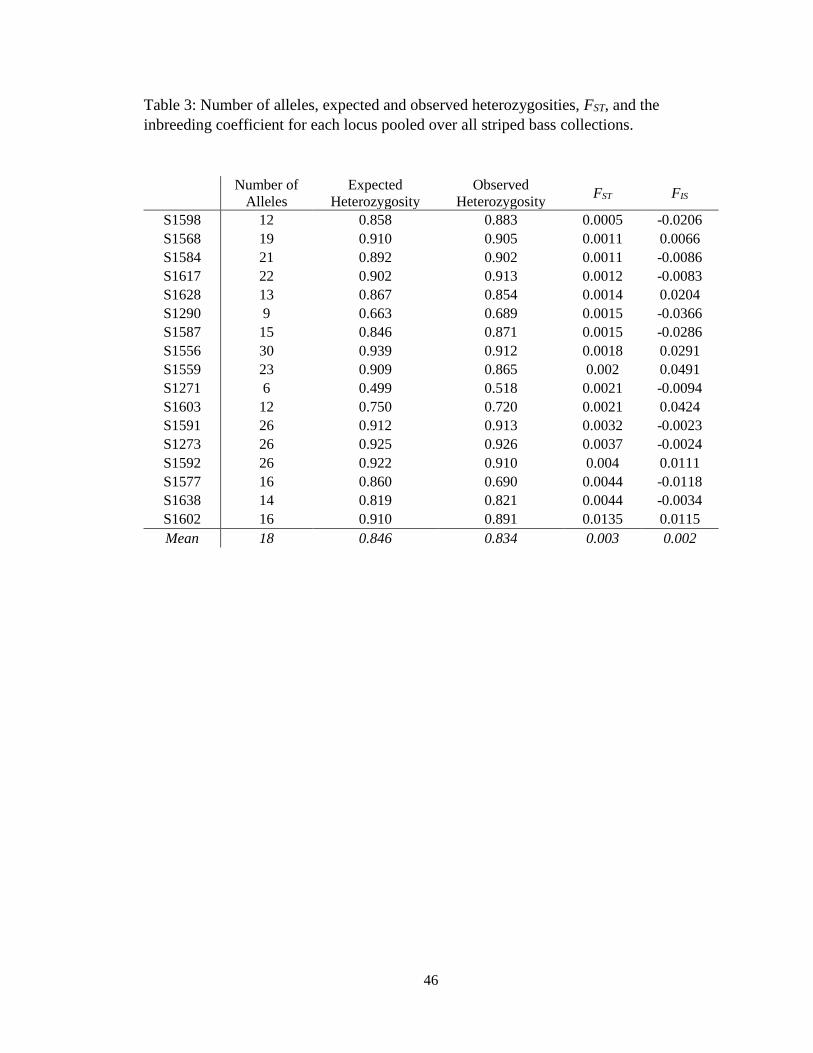
46

Table 3: Number of alleles, expected and observed heterozygosities, FST, and the

inbreeding coefficient for each locus pooled over all striped bass collections.

Number of

Alleles

Expected

Heterozygosity

Observed

Heterozygosity FST FIS

S1598 12 0.858 0.883 0.0005 -0.0206

S1568 19 0.910 0.905 0.0011 0.0066

S1584 21 0.892 0.902 0.0011 -0.0086

S1617 22 0.902 0.913 0.0012 -0.0083

S1628 13 0.867 0.854 0.0014 0.0204

S1290 9 0.663 0.689 0.0015 -0.0366

S1587 15 0.846 0.871 0.0015 -0.0286

S1556 30 0.939 0.912 0.0018 0.0291

S1559 23 0.909 0.865 0.002 0.0491

S1271 6 0.499 0.518 0.0021 -0.0094

S1603 12 0.750 0.720 0.0021 0.0424

S1591 26 0.912 0.913 0.0032 -0.0023

S1273 26 0.925 0.926 0.0037 -0.0024

S1592 26 0.922 0.910 0.004 0.0111

S1577 16 0.860 0.690 0.0044 -0.0118

S1638 14 0.819 0.821 0.0044 -0.0034

S1602 16 0.910 0.891 0.0135 0.0115

Mean 18 0.846 0.834 0.003 0.002

47

Table 4: Number of alleles, private alleles, and mean allelic richness for each for all

samples, and by sex, for all striped bass collections.

Males

Alleles

Private

Alleles

Mean Allelic

Richness

2016

James 240 6 13.458

Mattaponi 240 5 13.294

Rappahannock 257 8 13.38

2017

James 237 0 13.398

Mattaponi 249 3 13.835

Rappahannock 253 5 13.277

Females

Alleles

Private

Alleles

Mean Allelic

Richness

2016

James 200 5 10.539

Mattaponi 217 5 10.868

Rappahannock 233 5 10.907

2017

James 226 1 11.046

Mattaponi 200 2 10.861

Rappahannock 209 3 10.906

48

Table5: Population pairwise FST values for each striped bass collection on the lower diagonal with p-values on the upper diagonal.

Statistically significant pairs are shown in bold and with a *.

Rappahannock

2016

Juvenile

Rappahannock

Rappahannock

2017

James

2016

James

2017

Mattaponi

2016

Mattaponi

2017

Rappahannock 2016 - 0.8447 0.0000 0.0000 0.0000 0.0000 0.1318

Juvenile Rappahannock -0.0002 - 0.0000 0.0000 0.0000 0.0000 0.5371

Rappahannock 2017 0.00498* 0.00534* - 0.0000 0.0000 0.0000 0.0000

James 2016 0.00452* 0.00392* 0.00409* - 0.0000 0.0020 0.0000

James 2017 0.00235* 0.00186* 0.00263* 0.00725* - 0.0098 0.0000

Mattaponi 2016 0.00268* 0.0034* 0.00288* 0.00158* 0.00534* - 0.0000

Mattaponi 2017 0.00029 -0.0005 0.00412* 0.00386* 0.00124* 0.00293* -

Table 6: Population pairwise FST values between striped bass collections from each river pooled over years on the lower diagonal with

p-values on the upper diagonal. Statistically significant pairs are shown in bold and with a *.

Rappahannock Mattaponi James

Rappahannock - 0.0684 0.0000

Mattaponi 0.0002 - 0.0000

James 0.0030* 0.0020* -

49

Table 7: Population pairwise FST values for male striped bass in each collection on the lower diagonal with p-values on the upper

diagonal. Statistically significant pairs are shown in bold and with a *.

Rappahannock

2016

Rappahannock

2017

James

2016

James

2017

Mattaponi

2016

Mattaponi

2017

Rappahannock 2016 - 0.0000 0.0000 0.0000 0.1855 0.0000

Rappahannock 2017 0.00496* - 0.0000 0.0000 0.0000 0.0010

James 2016 0.00247* 0.0081* - 0.0010 0.0156 0.0000

James 2017 0.00562* 0.00577* 0.0029* - 0.0000 0.0039

Mattaponi 2016 0.004* 0.00538* 0.00155* 0.0046* - 0.0000

Mattaponi 2017 0.00307* 0.00184* 0.00543* 0.00284 0.00335* -

Table 8: Population pairwise FST values for female striped bass in each collection on the lower diagonal with p-values on the upper

diagonal. Statistically significant pairs are shown in bold and with a *.

Rappahannock

2016

Rappahannock

2017

James

2016

James

2017

Mattaponi

2016

Mattaponi

2017

Rappahannock 2016 - 0.1201 0.1221 0.0000 0.0195 0.0957

Rappahannock 2017 0.00185 - 0.2471 0.0664 0.0020 0.0283

James 2016 0.00123 0.00138 - 0.0020 0.0547 0.0713

James 2017 0.00529* 0.0023 0.00374* - 0.0147 0.0225

Mattaponi 2016 0.00348 0.00644* 0.00288 0.00384 - 0.1201

Mattaponi 2017 0.00223 0.00505 0.0029 0.00405 0.0022 -

50

Table 9: Effective population size for each striped bass collection from the adult

population is shown with 95% confidence intervals.

Ne 95% CI

2016

James 869.4 574.6-1716.4

Mattaponi 888.5 608.3-1598.3

Rappahannock 507.6 451.1-577.4

2017

James 882.5 593.7-1660.2

Mattaponi 1186.7 677.7-4301.3

Rappahannock 194.5 176.3-215.9

Table 10: Recapture locations of striped bass tagged on spawning grounds of the James

and Rappahannock rivers during the spawning season and subsequently recaptured during

the spawning season after being at large for at least one year.

River of Origin James River Rappahannock River

Area of Recapture

Out of Chesapeake Bay 33 82

In Chesapeake Bay 222 773

On Spawning Grounds

James River 194 13

Rappahannock River 7 645

Potomac River 3 22

Other Rivers 6 34

Non-Spawning Grounds 45 151

Total 255 865

51

Figure 1: Map showing the sampling locations on the Rappahannock, Mattaponi, and

James Rivers over the two sampling years. The black dots indicate sampling sites. Within

the smaller boxes, blue indicates 2016 sampling, red indicates 2017 sampling, and yellow

indicates both years. Triangles indicate juvenile samplings and pentagons indicate adult

samplings. Mile markers at each end of sampling are shown with black numbers.

52

Figure 2: PCA of all populations showing principal components 1 and 2. Rappahannock

2016 is blue, Rappahannock 2017 is brown, Juvenile Rappahannock is orange, James

2016 is purple, James 2017 is green, Mattaponi 2016 is pink, and Mattaponi 2017 is

yellow. Eigenvalues are presented in the lower right-hand corner.

53

References

Abdul-Muneer, PM. 2014. Application of microsatellite markers in conservation genetics

and fisheries management: recent advances in population structure analysis and

conservation strategies. Genetics Research International 2014: 691759.

Adamack, AT, Gruber, B. 2014. PopGenReport: simplifying basic population genetic

analyses in R. Methods in Ecology and Evolution, 5: 384-387.

Allendorf, FW, Phelps, SR. 1981. Use of allelic frequencies to describe population

structure. Canadian Journal of Fisheries and Aquatic Sciences 38: 1507-1514.

Atlantic States Marine Fisheries Commission (2013) Striped Bass Stock Assessment for

2013. Arlington, VA. Retrieved from

http://www.asmfc.org/uploads/file/529e5ca12013StripedBassBenchmarkStockAsses

sment_57SAWReport.pdf.

Balloux, F, Lugon‐Moulin, N. 2002. The estimation of population differentiation with

microsatellite markers. Molecular Ecology 11: 155-165.

Bartley, D, Bagley, M, Gall, G, Bentley, B. 1992. Use of linkage disequilibrium data to

estimate effective size of hatchery and natural fish populations. Conservation

Biology 6: 365-375.

Beacham, TD, Candy, JR, Supernault, KJ, Wetklo, M, Deagle, B, Labaree, K, Irvine, JR,

Miller, KM, Nelson, RJ, Withler, RE. 2003. Evaluation and application of

microsatellites for population identification of Fraser River Chinook salmon

(Oncorhynchus tshawytscha). Fishery Bulletin 101: 243-259.

Begg, GA, Waldman, JR. 1999. An holistic approach to fish stock identification. Fisheries

Research 43: 35-44.

54

Boreman, J, Lewis, RR. 1987. Atlantic coastal migration of striped bass. In American

Fisheries Society Symposium 1:331-339.

Boynton WR, Garber JH, Summers R, Kemp WM. 1995. Inputs, transformations, and

transport of Nitrogen and phosphorus in Chesapeake Bay and selected tributaries.

Estuaries 18: 285-314.

Brown KM, Baltazar GA, Hamilton MB. 2005. Reconciling nuclear microsatellite and

mitochondrial marker estimates of population structure: breeding population

structure of Chesapeake Bay striped bass (Morone saxatilis). Heredity 94: 606-615.

Callihan, JL. Godwin CH, Buckel JA. 2014. Effect of demography on spatial distribution:

movement patterns of the Albemarle Sound-Roacnoke River stock of Striped Bass

(Morone saxatilis) in relation to their recovery. Fishery Bulletin 112: 131-143.

Carvalho, GR, Hauser, L. 1994. Molecular genetics and the stock concept in

fisheries. Reviews in Fish Biology and Fisheries 4: 326-350.

Chambers, RC., Waiwood, KG. 1996. Maternal and seasonal differences in egg sizes and

spawning characteristics of captive Atlantic cod, Gadus morhua. Canadian Journal

of Fisheries and Aquatic Sciences 53: 1986-2003.

Chapman RW. 1990. Mitochondrial DNA analysis of striped bass populations in the

Chesapeake Bay. Copeia, 1990: 355-366.

Colman, SM, Mixon, RB. 1988. The record of major Quaternary sea-level changes in a

large coastal plain estuary, Chesapeake Bay, eastern United States:

Palaeogeography, Palaeoclimatology, and Palaeoecology 68: 99-116.

55

Couch, CR, Garber, AF, Rexroad, CE, Abrams, JM, Stannard, JA, Westerman, ME,

Sullivan, CV. 2006. Isolation and characterization of 149 novel microsatellite DNA

markers for striped bass, Morone saxatilis, and cross‐species amplification in white

bass, Morone chrysops, and their hybrid. Molecular Ecology Resources 6: 667-669.

Davison, A, Chiba, S. 2003. Laboratory temperature variation is a previously unrecognized

source of genotyping error during capillary electrophoresis. Molecular Ecology

Resources 3: 321-323.

Diaz M. Leclerc GM, Fishtec BE. 1997. Nuclear DNA markers reveal low levels of genetic

divergence among Atlantic and Gulf of Mexico populations of striped bass.

Transactions of the American Fisheries Society 126(1): 163-165.

Do, C, Waples, RS, Peel, D, Macbeth, GM, Tillett, BJ, Ovenden, JR. 2014. NeEstimator v2:

re‐implementation of software for the estimation of contemporary effective

population size (Ne) from genetic data. Molecular Ecology Resources, 14: 209-214.

Dorazio, RM, Hattala, KA, McCollough, CB, Skjeveland, JE. 1994. Tag recovery estimates

of migration of striped bass from spawning areas of the Chesapeake

Bay. Transactions of the American Fisheries Society 123: 950-963.

El Mousadik, A, Petit, RJ. 1996. High level of genetic differentiation for allelic richness

among populations of the argan tree [Argania spinosa (L.) Skeels] endemic to

Morocco. Theoretical and Applied Genetics 92: 832-839.

Excoffier L, Lischer HEL. 2010. Arlequin suite ver 3.5: A new series of programs to

perform population genetics analyses under Linux and Windows. Molecular

Ecology Resources 10: 564-567.

56

Fabrizio, MC. 1987. Growth-invariant discrimination and classification of striped bass

stocks by morphometric and electrophoretic methods. Transactions of the American

Fisheries Society 116: 728-736.

Falush D, Stephens M, Pritchard JK. 2003. Inference of population structure

using multilocus genotype data: linked loci and correlated allele

frequencies. Genetics 4:1567-1587.

Falush D, Stephens M, Pritchard JK. 2007. Inference of population structure

using multilocus genotype data: dominant markers and null alleles. Molecular

Ecology Notes 5:1322-1332.

Fernando, P, Evans, BJ, Morales, JC, Melnick, DJ. 2001. Electrophoresis artefacts—a

previously unrecognized cause of error in microsatellite analysis. Molecular Ecology

Resources 1: 325-328.

Flowers, JM, Schroeter, SC, Burton, RS. 2002. The recruitment sweepstakes has many

winners: genetic evidence from the sea urchin Strongylocentrotus

purpuratus. Evolution 56: 1445-1453.

Fountain J, Darden T, Jenkins W, Denson M. 2009. Three multiplexed microsatellite panels

for striped bass. Southeastern Naturalist 8: 671-676.

Gahagan, BI, Fox, DA, Secor, DH. 2015. Partial migration of striped bass: revisiting the

contingent hypothesis. Marine Ecology Progress Series 525: 185-197.

Gauthier DT, Audemard CA, Carlsson JEL, Darden TL, Denson MR, Reece KS, Carlsson J.

2013. Genetic population structure of US Atlantic coastal striped bass

(Morone saxatilis). Journal of Heredity 104: 510-520.

57

Ginzburg, LR, Slobodkin, LB, Johnson, K, Bindman, AG. 1982. Quasiextinction

probabilities as a measure of impact on population growth. Risk Analysis 2: 171-

181.

Goudet, J. 2001. FSTAT, a program to estimate and test gene diversity and fixation indices

(v 2.9.3). http://www2.unil.ch/popgen/softwares/fstat. htm.

Greene, KE, Zimmerman, JL, Laney, RW, Thomas-Blate, JC, 2009. Atlantic coast

diadromous fish habitat: a review of utilization, threats, recommendations for

conservation, and research needs. Atlantic States Marine Fisheries Commission

Habitat Management Series: 464.

Grove TL, Berggren TS, Powers DA. 1976. The use of innate genetic tags to segregate

spawning stocks of striped bass (Morone saxatilis). Estuarine Processes 1: 166-176.

Guo, SW, Thompson, EA. 1992. Performing the exact test of Hardy-Weinberg proportion

for multiple alleles. Biometrics, 361-372.

Hasselman, DJ, Ricard, D, Bentzen, P. 2013. Genetic diversity and differentiation in a wide

ranging anadromous fish, American shad (Alosa sapidissima), is correlated with

latitude. Molecular Ecology 22: 1558-1573.

Hauge, XY, Litt, M. 1993. A study of the origin of ‘shadow bands’ seen when typing

dinucleotide repeat polymorphisms by the PCR. Human Molecular Genetics 2: 411-

415.

Hedgecock, D. 1991. Contrasting population genetic structures of pelagic clupeoids in the

California current. Long term variability of pelagic fish populations and their

environment. Pergamon Press, Oxford, 199-207.

58

Hedgecock, D. 1994. Does variance in reproductive success limit effective population sizes

of marine organisms? In Genetics and Evolution of Aquatic Organisms, London:

Chapman & Hall: 122-134.

Hedgecock, D, Pudovkin, AI. 2011. Sweepstakes reproductive success in highly fecund

marine fish and shellfish: a review and commentary. Bulletin of Marine Science 87:

971-1002.

Holleley CE and Geerts PG. 2009. Multiplex Manager 1.0: a crossplatform computer

program that plans and optimizes multiplex PCR. BioTechniques 7: 511-517.

Hurst, TP, Conover, DO. 2003. Seasonal and interannual variation in the allometry of

energy allocation in juvenile striped bass. Ecology 84: 3360-3369.

Kalinowski ST, Taper ML, Marshall TC. 2007. Revising how the computer program

CERVUS accommodates genotyping error increases success in paternity

assignment. Molecular Ecology, 19, 1099-1106.

Kirkley JE, McConnell KE, Ryan W. 2000. Economic aspects of allocating striped bass

among competing user groups in Virginia. Virginia Marine Resources Report,

No. 2000-05, Newport News, Virginia, US

Kohlenstein LC. 1981. On the proportion of the Chesapeake Bay stock of Striped Bass that

migrates into the coastal fishery. Transactions of the American Fisheries

Society 110: 168-179.

Laughlin TF, Turner BJ. 1996. Hypervariable DNA markers reveal high genetic variability

within striped bass populations of the lower Chesapeake Bay. Transactions of the

American Fisheries Society 125: 49-55.

59

Lindley, ST, Erickson, DL, Moser, ML, Williams, G, Langness, OP, McCovey, BW,

Belchik, M., Vogel, D, Pinnix, W, Kelly, JT, Heublein, JC. 2011. Electronic tagging

of green sturgeon reveals population structure and movement among

estuaries. Transactions of the American Fisheries Society 140: 108-122.

Liu, JX, Ely, B. 2009. Sibship reconstruction demonstrates the extremely low effective

population size of striped bass Morone saxatilis in the Santee–Cooper system, South

Carolina, USA. Molecular Ecology 18: 4112-4120.

Liu S, Rexroad CE 3rd, Couch CR, Cordes JF, Reece KS, Sullivan CVA. 2011.

Microsatellite linkage map of striped bass (Morone saxatilis) reveals

conserved synteny with the three-spined stickleback

(Gasterosteus aculeatus). Marine Biotechnolgy 14:237–244.

Lowe, WH, Allendorf, FW. 2010. What can genetics tell us about population

connectivity? Molecular Ecology 19: 3038-3051.

Mamoozadeh, NR, McDowell, JR, Rooker, JR., Graves, JE. 2017. Genetic evaluation of

population structure in white marlin (Kajikia albida): the importance of statistical

power. ICES Journal of Marine Science: fsx047.

Mansueti, RJ. 1961 Age, growth, and movements of the striped bass, Roccus saxatilis, taken

in size selective fishing gear in Maryland. Chesapeake Science, 2, 9-36.

Marshall HG, Alden RW. 1990. A comparison of phytoplankton assemblages and

environmental relationships in three estuarine rivers of the lower Chesapeake Bay.

Estuaries 13: 287-300.

Massmann WH, Pacheco AL. 1961. Movements of striped bass tagged in Virginia waters of

the Chesapeake Bay. 2(1): 3-44.

60

McLaren, JB, Cooper, JC, Hoff, TB, Lander, V. 1981. Movements of Hudson River striped

bass. Transactions of the American Fisheries Society 110: 158-167.

Merriman, D. 1941. Studies on the striped bass (Roccus saxatilis) of the Atlantic coast. US

Government Printing Office.

Miller, MA, Pfeiffer, W, Schwartz, T. 2010. Creating the CIPRES Science Gateway for

inference of large phylogenetic trees. In Gateway Computing Environments

Workshop (GCE), 2010: 1-8.

Morin, PA, Leduc, RG, Archer, FI, Martien, KK, Huebinger, R, Bickham, JW, Taylor, BL.

2009. Significant deviations from Hardy–Weinberg equilibrium caused by low levels

of microsatellite genotyping errors. Molecular Ecology Resources 9: 498-504.

Narum, S. 2006. Beyond Bonferroni: less conservative analyses for conservation genetics.

Conservation Genetics, 7: 783–787.

Ng CL, Able KW, Grothues TM. 2007. Habitat use, site fidelity, and movement of adult

Striped Bass in a southern New Jersey estuary based on mobile acoustic

telemetry. Transactions of the American Fisheries Society 136:1344-1355.

Nichols, PR, Miller, RV. 1967. Seasonal movements of striped bass, Roccus saxatilis

(Walbaum), tagged and released in the Potomac River, Maryland, 1959–

61. Chesapeake Science 8: 102-124.

Ogburn, MB, Hasselman, DJ, Schultz, TF, Palkovacs, EP. 2017. Genetics and Juvenile

Abundance Dynamics Show Congruent Patterns of Population Structure for

Depleted River Herring Populations in the Upper Chesapeake Bay. North American

Journal of Fisheries Management 37: 1083-1092.

61

O'Reilly, P, Wright, JM. 1995. The evolving technology of DNA fingerprinting and its

application to fisheries and aquaculture. Journal of Fish Biology, 47: 29-55.

Paramore LM, Rulifson RA. 2001. Dorsal coloration as an indicator of different life history

patterns for Striped Bass within a single watershed of Atlantic Canada. Transactions

of the American Fisheries Society 130: 663-674.

Pompanon, F, Bonin, A, Bellemain, E, Taberlet, P. 2005. Genotyping errors: causes,

consequences and solutions. Nature Reviews Genetics 6: 847.

Pritchard JK, Stephens M, Donnelly P. 2000. Inference of population structure using

multilocus genotype data. Genetics, 155, 945-959.

Putman, AI, Carbone, I. 2014. Challenges in analysis and interpretation of microsatellite

data for population genetic studies. Ecology and Evolution 4: 4399-4428.

Rago PJ, Goodyear CP. 1987. Recruitment mechanisms of striped bass and Atlantic salmon:

comparative liabilities of alternative life histories. American Fisheries Society

Symposium 1: 402-416.

Rexroad C, Vallejo R, Coulibaly I, Couch C, Garber A, Westerman M, Sullivan C. 2006.

Identification and characterization of microsatellites for striped bass from repeat-

enriched libraries. Conservation Genetics 7:971-982.

Rice, WR. 1990. A consensus combined P-value test and the family-wide significance of

component tests. Biometrics 46: 303-308.

Rousset, F. 2008. Genepop’007: a complete reimplementation of the Genepop software for

Windows and Linux. Molecular Ecology Resources 8: 103-106.

62

Ruzzante, DE. 1998. A comparison of several measures of genetic distance and population

structure with microsatellite data: bias and sampling variance. Canadian Journal of

Fisheries and Aquatic Sciences 55: 1-14.

Secor, DH. 2000a. Longevity and resilience of Chesapeake Bay striped bass. ICES Journal

of Marine Science 57: 808-815.

Secor, DH. 2000b. Spawning in the nick of time? Effect of adult demographics on spawning

behaviour and recruitment in Chesapeake Bay striped bass. ICES Journal of Marine

Science 57: 403-411.

Sidell, BD, Otto RG, Powers DA, Kerweit M, Smith J. 1980. A re-evaluation of the

occurrence of subpopulations of striped bass (Morone saxatilis, Walbaum) in the

Upper Chesapeake Bay. Transactions of the American Fisheries Society 109:99-

107.

Smouse PE, Long JC, Sokal RR. (1986) Multiple regression and correlation extensions of

the Mantel test of matrix correspondence. Systematic Zoology, 35: 627-632.

Thorrold, S. R., Latkoczy, C., Swart, P. K., & Jones, C. M. (2001). Natal homing in a

marine fish metapopulation. Science, 291(5502), 297-299.

Van Oosterhout, C, Hutchinson, WF, Wills, DP, Shipley, P. 2004. MICRO‐CHECKER:

software for identifying and correcting genotyping errors in microsatellite

data. Molecular Ecology Resources 4: 535-538.

Vladykov, VD, Wallace, DH. 1938. Is the striped bass (Roccus lineatus) of Chesapeake Bay

a migratory fish? Transactions of the American Fisheries Society 67: 67-86.

Waldman J, Maceda L, Wirgin I (2012) Mixed-stock analysis of wintertime aggregations of

Striped Bass along the Mid-Atlantic coast. Journal of Applied Ichthyology 28:2012.

63

Waples, RS. 1998. Separating the wheat from the chaff: patterns of genetic differentiation in

high gene flow species. Journal of Heredity 89: 438-450.

Waples, RS., Teel, DJ. 1990. Conservation genetics of Pacific salmon I. Temporal changes

in allele frequency. Conservation Biology 4: 144-156.

Waples, RS, Gaggiotti, O. 2006. What is a population? An empirical evaluation of some

genetic methods for identifying the number of gene pools and their degree of

connectivity. Molecular Ecology 15: 1419-1439.

Weber, JL., May, PE. 1989. Abundant class of human DNA polymorphisms which can be

typed using the polymerase chain reaction. American Journal of Human Genetics 44:

388.

Wingate, RL, Secor, DH, Kraus, RT. 2011. Seasonal patterns of movement and residency by

Striped Bass within a subestuary of the Chesapeake Bay. Transactions of the

American Fisheries Society 140: 1441-1450.

Wirgin I, Procenca R, Grossfield J. 1987 Mitochondrial DNA diversity among populations

of striped bass in the Southeastern United Sates. Canadian Journal of Zoology 67:

891-907.

Wirgin, II, Grunwald, C, Garte, SJ, Mesing, C. 1991. Use of DNA fingerprinting in the

identification and management of a striped bass population in the southeastern

United States. Transactions of the American Fisheries Society 120: 273-282.

Wirgin, I, Maceda, L, Waldman, JR, Crittenden, RN. 1993. Use of mitochondrial DNA

polymorphisms to estimate the relative contributions of the Hudson River and

Chesapeake Bay striped bass stocks to the mixed fishery on the Atlantic

coast. Transactions of the American Fisheries Society 122: 669-684.

64

CHAPTER III

FEASIBILITY OF CLOSE-KNISHIP MARK-RECAPTURE METHODOLOGY TO

ESTIMATE STRIPED BASS ADULT ABUNDANCE

65

Introduction

Striped bass support important recreational and commercial fisheries along the

Atlantic Coast of North America from Canada to northern Florida (Boreman and Lewis,

1987; Kirkley et al., 2000; Greene et al., 2009; Wingate et al., 2011). Striped bass are

anadromous with spawning occurring each spring in the freshwater reaches of major river

and estuary systems (Paramore and Rulifson, 2001), including the Chesapeake Bay, the

Hudson River, Delaware Bay, and the Roanoke River. Of these systems, the Chesapeake

Bay is considered the largest and most productive spawning ground (Kohlenstein 1981),

contributing upwards of 90% of young-of-the-year (YOY) individuals in some years

(Waldman et al., 2012). The Chesapeake Bay differs from other major spawning grounds

because it is a large estuary composed of several major sub-estuary river systems

(Marshall and Alden, 1990; Boynton et al., 1995), and each of these systems is thought to

host separate spawning populations of striped bass (Nichols and Miller, 1967; Wirgin et

al., 1993, Ng et al., 2007).

Recent assessment of the status of the Atlantic striped bass stock indicates that it

is not overfished nor experiencing overfishing; however, the female spawning stock

biomass (SSB) is just above the Atlantic States Marine Fisheries Commission (ASMFC)

biomass threshold of 67,626 metric tons (ASMFC 2016). Since 2012, annual recruitment

levels of striped bass have been average to low, with no evidence of a strong year class

during that time. The Atlantic Striped Bass Stock Assessment Update

66

2016 model projections indicate that there is a 39% probability that female SSB will drop

below the management biomass threshold over the next three years. While several

hypotheses have been put forward to explain the recent decline of striped bass SSB, no

single factor or factors have been identified with certainty (ASMFC 2016). Some studies

indicate that Mycobacteriosis, a bacterial disease in striped bass shown to have large

impacts on reproductive output and natural mortality, may be a large contributor (Gautier

et al., 2008; Gervasi 2015; Hoenig et al., 2017). The ASMFC (2013) attributed the

decline in SSB to a reduction in the availability of prey species in combination with

Mycobacteriosis.

The indices of relative abundance and SSB for the Atlantic stock of striped bass

are derived from fishery independent and fishery dependent catch-per-unit-effort (CPUE)

data (ASMFC 2013). In addition to a coast wide tagging program, annual spawning stock

and juvenile index surveys are conducted in the major subestuaries of the Chesapeake

Bay by both the Maryland Department of Natural Resources and the Virginia Institute of

Marine Science (ASMFC, 2016). The Maryland Department of Natural Resources striped

bass spawning stock survey uses a CPUE-based method similar to the Virginia survey to

determine an index of adult spawning abundance, as well as an index of spawning

potential and an age-independent measure for female striped bass (Maryland Department

of Natural Resources, Personal Communication). The Virginia Pound Net Survey targets

spawning striped bass on the Rappahannock River. This survey calculates an annual

abundance index (number, sex, and age of fish captured) and a spawning stock biomass

index (SSBI), defined as the catch-per-unit-effort, or CPUE, (kg/net day) of mature male

and female fish sampled during the spawning season (Hoenig et al, 2016). Per

67

Amendment 6 of the Striped Bass Fisheries Management Plan (FMP), both states conduct

juvenile striped bass recruitment surveys to develop annual recruitment indices. Data

from these surveys are assumed to reflect relative abundance trends of the fishery, and

supply data to all striped bass assessments and assessment updates (ASMFC 2016).

Striped bass are assessed as a single Atlantic coastal stock (Maine to South

Carolina), and there is little information regarding spawning stock abundance for the

major spawning grounds that contribute to the stock. The exception to this is the

Chesapeake Bay, which for some analyses is considered a separate management unit

within the Atlantic stock (ASMFC 2003; Gautier et al., 2013); however, there are no

estimates of striped bass abundance for Chesapeake Bay as a whole or its subestuaries.

Annual recruitment or year class strength is known to vary among the subestuaries of

Chesapeake Bay (Davis et al., 2016), but lacking good estimates of the number of

individuals spawning in each subestuary annually, it is not possible to confidently

determine spawning stock/recruitment relationships within subestuaries.

The 2013 striped bass benchmark assessment highlighted the need for new,

fishery independent methodologies to estimate adult striped bass abundance. Recently,

novel molecular approaches have provided researchers with an alternative method to

estimate abundance of spawning adults (Bravington et al., 2014a). Close-kinship mark-

recapture analysis (CKMR) is one such genetic approach for abundance estimates that

has been applied to Minke whales (Skaug 2001), southern bluefin tuna (Bravington et al.,

2014a; Bravington et al., 2016a), and Antarctic blue whales (Bravington et al., 2014b),

and may be applicable to striped bass.

68

CKMR analyses are similar to traditional mark-recapture studies in which

individuals are marked with a physical tag (e.g. a spaghetti tag); however, in CKMR

studies, individuals are marked by a ‘genetic tag’. These genetic tags are identified using

molecular markers, which must be sufficiently numerous and variable to allow for

unambiguous individual identification. In essence, spawning adults are ‘marked’ by the

genotypes of the YOY. Each YOY receives an allele from each parent at each nuclear

locus, effectively ‘marking’ two adults. The genetic tags of the YOY can be ‘recaptured’

(essentially, before the YOY exist) in random samples of spawning adults as genetically

identified parent-offspring pairs (POPs). If the population of adults is large, then the

number of POPs will be low, whereas if many POPs are recovered, the population is

small. The probability that a captured adult is one of the parents for a selected YOY is

2/Na where Na represents the total number of adults alive when the YOY was spawned.

Comparing all sampled adults (ma) to a selected YOY, the expected number of POPs is

ma*2/Na. Comparing all sampled YOY (mj) to all sampled adults (ma), the expected

number of POPS (𝔼[h]) is mjma*2/Na (Bravington et al., 2014a). Rearranging the formula

to include the actual number of POPs, or hits (h):

𝑁�̂� =2𝑚𝑗𝑚𝑎

ℎ

This closely resembles the estimate of abundance using the Lincoln-Peterson

abundance estimator, a conventional tag-based estimator (Bravington et al., 2016a).

While the relationship is useful, a more explicit statistical mark-recapture model is

required to accommodate several life-history characters of striped bass, including age-

69

dependent sampling probability, and non-equilibrium conditions in the spawning

population (Bravington et al., 2014a).

A more explicit statistical model used for a CKMR analysis incorporates a length,

sex, and age-structured population dynamics model in which demographic parameters are

estimated from a maximum likelihood model that combines POP likelihood values from

pairwise comparisons of genotypes from all juveniles and adults, length and age

compositions of adults, and life history parameters, such as growth and size- or age-

specific fecundity (Bravington et al., 2016b). Assumptions of this model include: 1)

adults and offspring are independently sampled 2) the von Bertalanffy growth curve

closely models fish growth, 3) genetic markers are in Hardy-Weinberg and linkage

equilibria, 4) random mating of adults, and 5) individuals are sampled from a ‘closed

population’ wherein sampled YOYs are the result of the adults that spawned in the area

during the year of the YOY’s birth. A pairwise comparison of every sampled juvenile

genotype to every sampled adult genotype provides an estimate of the number of POPs.

To qualify as a POP, the putative parent must contain at least one of the YOY’s alleles at

each locus. Bravington et al. (2016a) recommend a minimum of 50 confidently assigned

parent-offspring pairs (POPs) to reduce the coefficient of variation and increase precision

of CKMR estimates.

The purpose of this study was to evaluate the utility of CKMR to estimate

abundance of striped bass in a model river system, the Rappahannock River. Specifically,

the main objective was to determine if a large enough number of POPs could be

recovered using ongoing sampling programs for spawning adults and YOY to develop

and implement CKMR to estimate the population size of spawning adults. Based on the

70

number of POPs recovered, a secondary objective was to estimate the sample sizes

required to obtain 50 POPs, the number recommended by Bravington et al. (2016a) to

provide precise estimates of abundance for CKMR analyses with a coefficient of

variation (CV) of 15%. Testing the feasibility of this novel methodology is an important

first step in the application of a new abundance model, and it has been noted that the

testing of new methodologies on a smaller scale is an important, but often overlooked

step (Teijlingen and Hundley, 2001).

71

Materials and Methods

Sample Collection

Adult striped bass were sampled on the spawning grounds of the Rappahannock

River during the spawning season (March to May) in 2016 (Figure 1). Striped bass were

captured using two commercial pound nets (river miles 46, 47) checked twice a week

from 4 April to 26 May 2016. Genetic samples were taken in the form of caudal fin clips

stored in 95% ethanol, and only fish with a total length of 458 mm were clipped to ensure

that all fish sampled were mature (Mansueti, 1961). Sex was determined by the

expression of reproductive products and scales were removed for aging. Following

sampling, fish were released alive.

From June to September 2016, young-of-year (YOY) striped bass were collected

from the Rappahannock River (river miles 75 to 37) using a 100 ft long, 4ft deep, 0.25

inch mesh beach seine net. YOY fish ranged in size from 22 mm to 73 mm, well below

118mm, the reported mean size of YOY striped bass prior to their first winter (Hurst and

Connover, 2003). Genetic samples were taken in the form of fin clips or muscle tissue

and stored in 95% ethanol.

Marker Selection, DNA Extraction, and Amplification

Candidate microsatellite loci were selected from more than 500 potential striped

bass microsatellite markers available in the literature (Couch et al., 2006; Rexroad et al.,

2006; Fountain et al., 2009; Gauthier et al., 2013), based on allelic diversity, chromosome

location (linkage map from Liu et al., 2011), and estimated heterozygosity. Candidate

microsatellite loci were evaluated to ensure proper amplification. Optimum annealing

72

temperatures were determined using thermal gradients, and loci were subsequently

assembled into multiplexes using Multiplex Manager (Holleley and Geerts, 2009). To

ensure each multiplex amplified consistently, each was run on a temperature gradient to

ensure an optimal annealing temperature. In total, the 20 microsatellite markers used

comprised four multiplex panels consisting of five markers each (Supplementary Table

1).

Total genomic DNA was extracted using Machary Nagel NucleoSpin® DNA

tissue kits on the Tecan Freedom EVO® 75 liquid handling system. Microsatellite

multiplexes were amplified for plates of 92-95 samples at a time, with negative controls

for each step to check for possible contamination. Polymerase chain reaction (PCR)

amplifications were performed in 10 ul reactions with locus-specific fluorescent probes.

In order to visualize the PCR product, 2 ul of product was combined with 8 ul of

formamide and 0.2 ul 500 LIZ Gene Scan Size standard (Applied Biosystems), denatured

for 10 minutes at 95°C, and sequenced on a 36 cm 3130xl Capillary Genetic Analyzer

(Applied Biosystems, Inc.). The output consisted of electropherograms with different

chromatic peaks representing the alleles at each microsatellite locus. The

electropherograms were scored using GeneMarker v2.6.0 (SoftGenetics, LLC). To check

for evidence of scoring errors and null allele presence, scores were evaluated using

MicroChecker 2.2.3 (Van Oosterhout et al., 2004). To ensure consistency in amplification

and allele calling, 5% of samples were re-analyzed from PCR reaction to allele scoring.

To ensure accuracy of allele calling, the entire data set was scored twice.

73

Recovery of POPs

The conformation of genotypic distributions to expectations of HWE was

evaluated using probability tests (Guo and Thompson, 1992) within GenePop v4.0

(Rousset 2008), with significance values corrected using the sequential Bonferroni

correction for multiple comparisons (Rice, 1990).

The presence of POPs among all sampled adults and juveniles was investigated

using the parentage analysis program COLONY (Jones and Wang, 2010). The software

allows for the assignment of parents to offspring based on genotypes while accounting

for allelic dropout and mistyping. The settings for the analyses in COLONY used the full

likelihood run, a medium run length, a high likelihood precision, and with a 5% error

rate. The relatively high error rate was allowed to ensure that no false negatives would be

missed in the analyses. Additionally, inbreeding and polygamy were allowed. All

potential POPs that COLONY identified were screened by eye within GeneMarker to

confirm that the pair had at least one allele in common at every locus.

COLONY was also used to infer sib-ship relations between sampled YOY.

Effective population size (Ne) was estimated using the full likelihood method within

COLONY, and the analysis was run with the assumption of random mating (Wang 2009).

Estimation of Population Size

To provide a rough estimate of population size, a modified version of the Lincoln-

Petersen model was used combining Bravington et al. (2014a) and the Chapman

modification (Chapman, 1951) to account for a small sample size as follows:

74

𝑁�̂� =2(𝑚𝑗+1)(𝑚𝑎+1)

(ℎ+1) = 2𝑁�̂�

Here 𝑁𝑎 ̂ is the estimated number of adults, mj is the number of juveniles (or originally

marked individuals), ma is the number of adults (or size of second sample), and h is the

number of POPs (or number of marked individuals in the second sample) (Chapman

1951; Pollock et al., 1990, Bravington et al 2014a).

Confidence intervals (95% CI) for the estimates of adult abundance were

calculated by first determining the unbiased estimate of variance wherein 𝑣𝑎𝑟(2𝑁�̂�) =

4𝑣𝑎𝑟(𝑁�̂�), given by equation 2, and then equation 3 was used to estimate 95% CI where

z is the standard normal variable (Seber 1970, 1982; Pollock et al., 1990)

𝑣𝑎𝑟 = 4(𝑚𝑗+1)(𝑚𝑎+1)(𝑚𝑗−ℎ)(𝑚𝑎−ℎ)

(ℎ+1)2(2+2)

𝐶𝐼 = 𝑁𝑎 ± 𝑧 ∗ √𝑣𝑎𝑟

The coefficient of variation was calculated using the estimated adult abundance,

𝑁�̂�, in equation 4 taken from Bravington et al. (2014a).

𝐶𝑉 =√𝑣𝑎𝑟

𝑁�̂�

If more than 1 but less than 50 POPs are recovered in this study, the number of

samples expected to result in 50 POPs will be estimated using the CKMR population size

estimate. Bravington et al (2014a) and Bravington et al (2016b) provide methodology

that allows for a crude estimation of the number of samples needed for relatively precise

estimates using the metric of 50 POPs (htarget) and/or a CV of 15%. Formula 5 and

Formula 6 were both used to estimate the sample sizes needed where 𝑁�̂�the estimated

(2)

(1)

(3)

(4)

75

adult abundance size is, and c is a variable representing the fraction of the overall sample

comprised of YOY. For these purposes, it was assumed that the sample size was half

YOY and half adults. Formula 6 is an analog to formula 5, and the two were compared to

determine the appropriate sample size.

𝑛𝑡𝑎𝑟𝑔𝑒𝑡 ≈ √𝑁�̂�ℎ𝑡𝑎𝑟𝑔𝑒𝑡𝑐⁄ (5)

10√�̂�𝑎 (6)

76

Results

Adult and young-of-year (YOY) samples were collected and analyzed from 2016

from the Rappahannock. All samples were genotyped for 20 microsatellite markers.

Individuals that were unable to be accurately scored or failed to amplify for 3 or more

loci were removed from the dataset. A total of 755 adults and 555 YOY were collected

from spawning and nursery grounds on the Rappahannock River. However, 384 adult and

166 juvenile samples were removed from the dataset due to problems with amplification.

The remaining760 samples, comprising 371 adults and 389 YOY, were used for CKMR

analysis (Table 1). The adult samples consisted of 282 males and 89 females.

Loci were removed that exhibited consistent amplification issues and deviations

from Hardy Weinberg Equilibrium. Tests for HWE indicated that the genotypic

distributions among individuals for three loci, 1322, 1437, and 1491, were significantly

out of equilibrium in two or more sample groups after Bonferroni correction for multiple

comparisons. Visual inspection of the multiple electropherograms showed large peak

shifts at these three loci and they were not included in further analyses. The remaining

loci showed a less than 1% error rate in amplification due to peak shifts of 1 to 3 repeat

motifs. MicroChecker indicated that one locus, 1559, showed evidence of a null allele

presence in sampled groups. To reduce the effect of possible null alleles, a slight increase

in the error rate was allowed to be 5% in COLONY. Matches identified by COLONY as

parent-offspring pairs were then checked by eye to confirm a 100% POP match and no

null allele impacts at 1559. The use of likelihood scores aided in determining if

mismatches at this marker were due to null alleles, and this would be detected by

comparing alleles by eye to see if one allele was a homozygote where there should be a

77

heterozygote (Bravington, personal communication). No issues were detected with the

use of this locus either by eye or by likelihood scores. In total, 17 loci were used for the

analyses.

POP Assignment

COLONY identified 18 potential POPs from the dataset. After checking the

genotypes of each POP by eye in GeneMarker, it was found that the dataset contained 2

true POPs with 100% matches of at least one allele at each locus. One potential POP had

a mismatch at one locus, but with the likelihood values indicated 70% support and both

alleles mismatching, it was considered a false positive. For the two recovered POPs, one

parent was a female 4 years of age with a total length of 498 mm. The other POP parent

was a male 5 years of age with a total length 512 mm.

Analysis of the offspring dataset revealed 14 pairs of potential full siblings, and

of these, 9 pairs had probability values of >90%. There were 405 pairs of potential half

siblings recovered in the offspring dataset, of which 121 pairs had a probability >90%.

COLONY estimated the effective population size of adults at 823, with 95% confidence

intervals of 718-946.

Adult Abundance Estimates

Using the modified Lincoln-Petersen estimator, the estimated adult abundance of

spawning adult striped bass in the Rappahannock River in 2016 was 145,081 individuals.

The 95% confidence intervals around this estimate were 51,042 on the lower boundary

and 239,119 on the upper boundary, with a CV of 0.33. Based on the recovery of 2 POPs

with a sample of 371 adults and 389 juveniles, a total (adults and juveniles) of 1,703

78

individuals would be required to recover 50 POPs, resulting in an abundance estimate

with a 15% CV.

79

Discussion

The primary objective of this work was to test the feasibility of a novel molecular

abundance model, close-kinship mark-recapture (CKMR), to estimate striped bass

spawning stock abundance for a major sub-estuary in the Chesapeake Bay, the

Rappahannock River. Specifically, this study first sought to determine if a relatively

precise estimate of adult abundance could be made using the number of adult and

juvenile samples typically available from ongoing surveys. If a sufficiently precise

estimate could not be made, I wished to determine how many additional samples would

be needed to achieve a desired level of precision. Genetic screening of 371 spawning

adults and 389 YOY collected from the Rappahannock River in 2016 resulted in the

identification of two parent-offspring pairs (POPs) and an estimated adult population size

of 145,081 individuals. The recovery of 2 POPs was well below the target of 50 POPs

recommended by Bravington et al. (2014a) for adequate precision. Further calculations

showed that a minimum sample size of 1,703 individuals comprising equal numbers of

adults and YOY would be required to produce a sufficiently precise estimate of adult

abundance. These preliminary results suggest that CKMR analysis is a practical, fishery

independent method to estimate the population size of adult striped bass.

This study represents the first attempt to estimate abundance of spawning striped

bass within a subestuary of the Chesapeake Bay. Using CKMR, the estimated abundance

of adult striped bass in the Rappahannock River during the 2016 spawning season was

145,081 fish (51,042 – 239,119 individuals, 95% CI). The current striped bass assessment

is for the entire Atlantic stock, and there are no estimates of population sizes within

estuaries or subestuaries with which to compare the CKRM estimate. The 2016 Striped

80

Bass Stock Assessment Update estimated over 30 million age 4+ fish in the Atlantic

stock (ASMFC 2016), and Berggren and Lieberman (1978) suggested that 75% of the

Atlantic stock may be of Chesapeake Bay origin. For the Chesapeake Bay, 90% of all the

freshwater discharge comes from five major rivers, with the Susquehanna providing 50%

of the freshwater discharge (Environmental Protection Agency, 2003). The Potomac,

James, Rappahannock, and York rivers account for the remaining 40%, with the

Rappahannock River contributing2.2% of the freshwater discharge (Brush, personal

communication). If one assumes that the number of spawning striped bass within a river

is proportional to freshwater discharge, it is estimated that 501,332 age 4+ fish in the

Rappahannock River, or about three times more than that estimated by CKMR in this

study.

While the estimated number of adult striped bass in the Rappahannock River

based on a division of the ASMFC coastwide assessment is much larger than the number

estimated using CKMR, the numbers might not be as disparate as they seem. The

majority of female striped bass do not start spawning until age 7 or 8 (Cowan et al.,

1993), and the ASMFC assessment number includes several year classes that may not be

spawning, and these individuals would not be detected by CKMR. Alternately, one can

compare the CKMR estimate of 145,081 adults to the 2016 commercial catch from the

Rappahannock River of 9,554 adults and an exploitation rate of 7% (exploitation rate =

catch/abundance) (VMRC, data request, May 2018).

The estimate of striped bass abundance made in this study using CKMR was for

adults within the Rappahannock River during the 2016 spawning season. Future estimates

using the CKMR theory should be cautious in combining samples from multiple years.

81

CKMR theory assumes individuals are randomly sampled from a ‘closed population’, and

that YOYs are the result of the adults that spawned in the area during the year of the

YOY’s birth. Previous work (see Chapter II) suggests that some adult fish may stray to

spawn in other rivers in subsequent years. Pooling collections across years to obtain

larger sample sizes can bias CKMR estimates, as individuals may spawn in different

rivers in different years, and some spawners may be lost due to natural and fishing

mortality. These aspects can be addressed in a full implementation of the CKMR model,

and Bravington et al (2016b) provide recommendations for addressing various population

scenarios. CKMR provides a methodology to estimate adult spawning abundances on an

annual basis and over a time series if certain assumptions are considered and sample sizes

are appropriate.

For the single year estimate made in this study, 2 POPS were recovered from one

sampling season. Recovering less than 50 POPs resulted in a relatively imprecise

estimate, with a CV of 33% well above the target CV of 15%. To provide a relatively

precise estimate (50 POPs), a total sample size of at least 3,807 individuals comprising an

equal number of adults and YOY fish would be needed. The second estimate for total

sample size was 3,809 individuals. Both formulas give approximately the same estimated

sample size. Annual collections of 1900 adult and 1900 YOY fish may possibly be

achieved with the current sampling scheme, but additional sampling will be required in

some years. It is important to note that the target of 50 POPs and a CV of 15% was

proposed for southern bluefin tuna and may not be an appropriate target for striped bass.

However, more samples and research will be needed to determine an appropriate number

of POPs and CV for striped bass

82

The samples for this study were collected using existing VIMS surveys of adult

and juvenile striped bass. In the Rappahannock River, the adult tagging survey has

averaged 362 adult live releases per year over the last 8 years (Sadler et al., 2017), while

the juvenile seine survey has averaged 804 YOY per year over the last 7 years (Gallagher

et al., 2017). Both surveys have had annual sample sizes that have ranged from 100 fish

to over 1,000 fish. In 2016, the adult survey averaged about 13 fish per day from two

pound nets in the Rappahannock, and the juvenile striped bass survey averaged 10 YOY

fish per seine haul from a total of 50 hauls. The peak sampling time for adults was mid to

late April, and YOY peak sampling time was June to early July. Additional sampling

during these time periods could increase samples for both adults and YOY. For adult

striped bass, the sampling of four pound nets instead of the two or three pound nets

historically sampled would provide additional samples needed in the Rappahannock. Gill

nets are used to sample adult striped bass on other rivers, and this gear type could be used

to augment pound net samples in the Rappahannock. To sample additional YOY striped

bass, more sample sites can be added near documented peak sampling areas between

river mile 44 and river mile 55 (Gallagher et al., 2017). Additionally, more frequent visits

to peak areas as well as extra tows during June and early July would bolster sample sizes;

repeating one or two tows per visit to the three highest catch areas during the first or

second round of sampling would provide the study the samples it needs. A few

modifications to the sampling schemes in place would provide sufficiently large sample

sizes of striped bass for future applications of CKMR.

In addition to increasing sampling efforts, improvements in molecular

methodologies could result in greater efficiencies to match parents and offspring.

83

Original sample sizes collected for this project approached a fraction of the estimated

sample sizes with 755 adult samples and 555 YOY samples collected. However,

problems with the DNA isolations and amplifications occurred and resulted in the loss of

adult and YOY samples. No specific cause for the isolation and amplification issues was

determined, despite several attempts to salvage the samples. The use of a robotic

methodology for DNA isolations may have contributed to the high failure rate, either

with protocol errors or with contamination. While controls were used to test for

contamination, there was no way to exclude the possibility of contamination in all DNA

isolations. The robot was in a shared space with other research, and while every effort

was made to eliminate cross contamination, the high rate of failure may indicate more

stringent protocols are needed. For future studies, increased care in sample collection and

improvements to DNA isolation could result in a higher success rate for collected

samples.

Microsatellite loci were used to determine parentage in this analysis, and they

were also surveyed in the original applications of CKRM analysis to other species.

Microsatellite markers were selected for this study based on their availability and proven

utility in previous genetic analyses of striped bass (Brown et al., 2005; Gautier et al.,

2013), and parentage analysis studies (O’Reilly et al., 2002; Castro et al., 2006;

Bravington et al., 2016a). Stringent quality control measures were implemented in this

study to ensure consistent and reliable sizing of microsatellite alleles. However, due to

problems with amplifications, it was necessary to re-amplify and resize several loci to

ensure accurate allele sizing. As correct allele calling is necessary to provide absolute

certainty that a pair were a parent and offspring match (Selkoe and Toonen, 2006;

84

Bravington et al, 2014a), and the use of microsatellite alleles has many challenges, the

application of a newer molecular marker, single nucleotide polymorphisms, may be of

interest to future studies.

Single nucleotide polymorphisms, SNPs, are becoming the preferred molecular

marker for genetic fisheries studies (Anderson and Garza, 2006; Hauser et al., 2011).

These are bi-allelic markers that are not only abundant in the genome but have been

shown to have low error rates and high replicability between labs (Anderson and Garza,

2006). Because SNPs only have two alleles, whereas the microsatellite loci used in this

study had as many as 30 alleles, a greater number of SNP loci will be needed to provide

unambiguous individual identification and identify POPs in CKMR analysis. However,

the reliability and consistency of SNPs outweighs the cost of development, which would

also be offset with decreasing high-throughput costs (Glover et. al, 2010; Hauser et al.,

2011; Bravington et al., 2016a; Feutry et al., 2017).

In future studies, the combined use of SNPs and the implementation of a full

CKMR model may allow for abundance estimates of not only the Rappahannock River,

but other major Chesapeake Bay tributaries. A full CKMR model is needed over the basic

Lincoln-Peterson estimation used here because of the non-equilibrium sampling that

occurs in spawning populations, likelihood estimation adjustments, and the variation in

sampling probability of different ages (Bravington et al., 2014). For this full operating

model, an integration of statistical-catch-at-age models is needed to address the unique

life history parameters for striped bass by way of covariates for age, growth rate,

residence, selectivity, fecundity, length, and sex identification. For striped bass, the

incorporation of the life history parameters, including growth curves and fecundity, must

85

be separated by sex because of compelling evidence that supports different growth rates,

movement patterns, and maturity schedules for male and female striped bass (Mansueti

1961, Setzler et al., 1980, Secor and Piccoli, 2004; Bravington et al., 2014; Bravington et

al., 2016a). Additionally, the post-release mortality of striped bass, which can introduce a

bias into the abundance estimation, can vary depending on gear type, age, and water

temperature (Dunning et al., 1989; Hopkins and Cech, 1992; Brick and Cech, 2002). The

full CKMR model has provided reliable estimates of abundance for other marine species,

including southern bluefin tuna, white sharks (Hillary et al., 2018), and Antarctic blue

whales (Bravington et al., 2016b).

The application of CKMR provides a potential fishery independent methodology

to recover relatively precise abundance estimates of spawning striped bass in the

Rappahannock River utilizing sample sizes of adults and YOY collected by ongoing

sampling programs. Though crude, this study was able to provide the first estimate of

adult abundance for a local, spawning population of striped bass in the Chesapeake Bay.

With the addition of increased sampling, improved molecular methodologies, and the use

of SNP markers, CKMR for striped bass may yield relatively precise estimates of adult

abundance that are specific to spawning grounds within the Chesapeake Bay. The

development of a full CKMR model is feasible with the incorporation of striped bass-

specific biological parameters. A relatively precise estimate of the number of spawning

adults present in a subestuary during specific years, combined with the annual juvenile

index, would allow for managers to determine how recruitment varies over time and

space, and to better identify those factors that may be directly influencing adult

abundance and recruitment.

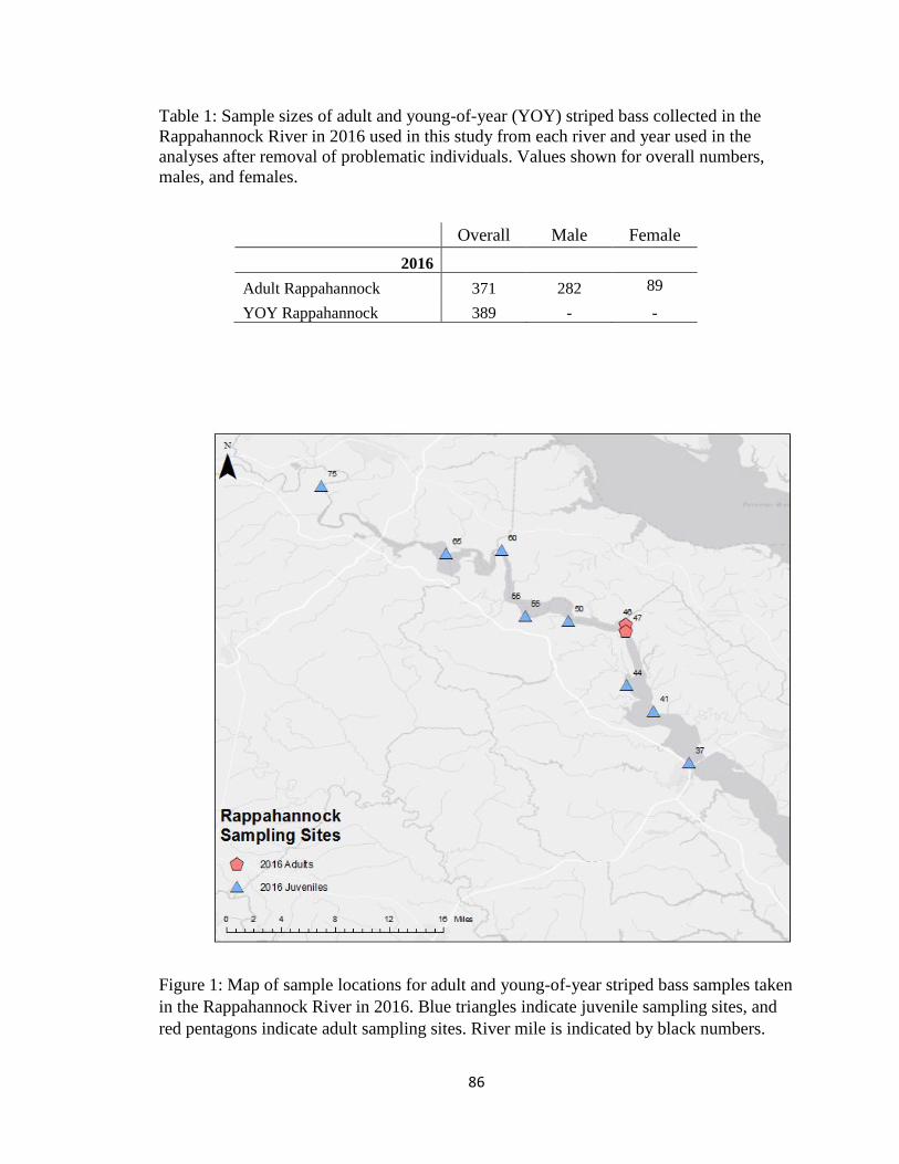
86

Table 1: Sample sizes of adult and young-of-year (YOY) striped bass collected in the

Rappahannock River in 2016 used in this study from each river and year used in the

analyses after removal of problematic individuals. Values shown for overall numbers,

males, and females.

Figure 1: Map of sample locations for adult and young-of-year striped bass samples taken

in the Rappahannock River in 2016. Blue triangles indicate juvenile sampling sites, and

red pentagons indicate adult sampling sites. River mile is indicated by black numbers.

Overall Male Female

2016

Adult Rappahannock 371 282 89

YOY Rappahannock 389 - -

87

References

Anderson EC, Garza JC. 2006. The power of single-nucleotide polymorphisms for large-

scale parentage inference. Genetics Society of America 172: 2567-2582.

Atlantic States Marine Fisheries Commission (2016) 2016 Atlantic Striped Bass Stock

Assessment Update. Arlington, VA. Retrieved

from http://www.asmfc.org/uploads/file/581ba8f5AtlStripedBassTC_Report2016

AssmtUpdate_Oct2016.pdf.

Atlantic States Marine Fisheries Commission. 2015. 2015 Atlantic Striped Bass Stock

Assessment Update. Arlington, VA. Retrieved

from http://www.asmfc.org/uploads/file/564106f32015AtlStripedBassAssessment

Update_Nov2015.pdf.

Berggren TJ, Lieberman JT.1978. Relative contribution of Hudson, Chesapeake and

Roanoke striped bass, Morone saxatilis, stocks to the Atlantic coast fishery. U. S.

Fish. Bull. 76: 335-345.

Boreman, J, Lewis, RR. 1987. Atlantic coastal migration of striped bass. American

Fisheries Society Symposium 1:331-339.

Boynton WR, Garber JH, Summers R, Kemp WM. 1995. Inputs, transformations, and

transport of Nitrogen and phosphorus in Chesapeake Bay and selected tributaries.

Estuaries 18: 285-314.

Bravington MV, Grewe PM, Davies CR. 2014a. Fishery-independent estimate of

spawning biomass of Southern Bluefin Tuna through identification of close-kin

using genetic markers. FRDC Report 2007/034. CSIRO, Australia.

88

Bravington MV, Jarman SN, Skaug HJ. 2014b. Antarctic blue whale surveys:

augmenting via genetics for close-kin and ordinal age. International Whaling

Commission Background Paper.

Bravington, MV, Grewe, PM., Davies, CR. 2016a. Absolute abundance of southern

bluefin tuna estimated by close-kin mark-recapture. Nature Communications 7:

13162.

Bravington, M. V., Skaug, H. J., & Anderson, E. C. (2016b). Close-kin mark-

recapture. Statistical Science 31: 259-274.

Brick, M. E., & Cech, J. J. (2002). Metabolic responses of juvenile striped bass to

exercise and handling stress with various recovery environments. Transactions of

the American Fisheries Society 131: 855-864.

Brown KM, Baltazar GA, Hamilton MB. 2005. Reconciling nuclear microsatellite and

mitochondrial marker estimates of population structure: breeding population

structure of Chesapeake Bay striped bass (Morone saxatilis). Heredity 94: 606-

615.

Castro, J., Pino, A., Hermida, M., Bouza, C., Riaza, A., Ferreiro, I., Sánchez, L. and

Martínez, P., 2006. A microsatellite marker tool for parentage analysis in Senegal

sole (Solea senegalensis): Genotyping errors, null alleles and conformance to

theoretical assumptions. Aquaculture, 261(4), pp.1194-1203.

Chapman, D. G. 1951. Some properties of the hypergeometric distribution, with

applications to zoological sample censuses. University of California Publications

in Statistics 1:131–160.

89

Couch, CR, Garber, AF, Rexroad, CE, Abrams, JM, Stannard, JA, Westerman, ME,

Sullivan, CV. 2006. Isolation and characterization of 149 novel microsatellite

DNA markers for striped bass, Morone saxatilis, and cross‐species amplification

in white bass, Morone chrysops, and their hybrid. Molecular Ecology

Resources 6: 667-669.

Cowan, J. H., Jr, Rose, K. A., Rutherford, E. S., and Houde, E. D. 1993. Individual-

based model of young-of-the-year striped bass population dynamics. II. Factors

affecting recruitment in the Potomac River, Maryland. Transactions of the

American Fisheries Society, 122: 439–458

Davis, CD, Fabrizio, MC, Tuckey, TD. 2016. Estimation of juvenile striped bass relative

abundance in the Virginia portion of Chesapeake Bay: annual progress report:

2015-2016. Virginia Institute of Marine Science, College of William and Mary.

https://scholarworks.wm.edu/reports/1157

Dunning DJ, Ross QE, Blumberg AF, Heimbuch DG. 2006. Transport of striped bass

larvae out of the lower Hudson River estuary. American Fisheries Society

Symposium 51: 273.

Feutry, P, Berry, O, Kyne, PM, Pillans, RD, Hillary, RM, Grewe, PM, Marthick, JR,

Johnson, G, Gunasekera, RM, Bax, NJ Bravington, M. 2017. Inferring

contemporary and historical genetic connectivity from juveniles. Molecular

Ecology, 26: 444-456.

Fountain J, Darden T, Jenkins W, Denson M. 2009. Three multiplexed microsatellite

panels for striped bass. Southeastern Naturalist 8: 671-676.

90

Gallagher, BK, Fabrizio, MC, Tuckey, TD. 2017 Estimation of Juvenile Striped Bass

Relative Abundance in the Virginia Portion of Chesapeake Bay: Annual Progress

Report 2016-2017. Virginia Institute of Marine Science, College of William and

Mary. https://doi.org/10.21220/V5NC83

Gautier DT, Latour RJ, Heisey DM, Bonzek CF, Gartland J, Burge EJ, Vogelbein WK.

2008. Mycobateriosis associated mortality in wild striped bass (Morone saxatilis)

from Chesapeake Bay, USA. Ecological Applications 18: 1718-1727.

Gauthier DT, Audemard CA, Carlsson JEL, Darden TL, Denson MR, Reece

KS, Carlsson J. 2013. Genetic population structure of US Atlantic coastal striped

bass (Morone saxatilis). Journal of Heredity 104: 510-520.

Gervasi CL. 2015. The reproductive biology of striped bass (Morone saxatilis) in

Chesapeake Bay (MS Thesis). [Williamsburg, (VA)]: College of William &

Mary.

Glover, KA, Hansen, MM, Lien, S, Als, TD, Høyheim, B, Skaala, Ø. 2010. A

comparison of SNP and STR loci for delineating population structure and

performing individual genetic assignment. BMC Genetics 11: 2.

Greene, KE, Zimmerman, JL, Laney, RW, Thomas-Blate, JC, 2009. Atlantic coast

diadromous fish habitat: a review of utilization, threats, recommendations for

conservation, and research needs. Atlantic States Marine Fisheries Commission

Habitat Management Series: 464.

Guo, SW, Thompson, EA. 1992. Performing the exact test of Hardy-Weinberg

proportion for multiple alleles. Biometrics: 361-372.

91

Hauser, L, Baird, M, Hilborn, RAY, Seeb, LW, Seeb, JE. 2011. An empirical

comparison of SNPs and microsatellites for parentage and kinship assignment in a

wild sockeye salmon (Oncorhynchus nerka) population. Molecular Ecology

Resources 11: 150-161.

Hillary RM, Bravington MV, Patterson TA, Greme P, Bradford R, Feutry P, Gunasekera

R, Peddemors V, Werry J, Francis MP, Duffy CAJ, Bruce BD. Genetic

relatedness reveals total population size of white sharks in eastern Australia and

New Zealand. Scientific Reports, 8: 2661.

Hoenig JM, Sadler PW, Michaelsen S, Goins LM, Harris RE. 2016. Evaluation of

striped bass stocks in Virginia: monitoring and tagging studies, 2015-2019,

Progress Report.VMRC.

Holleley CE and Geerts PG. 2009. Multiplex Manager 1.0: a cross platform computer

program that plans and optimizes multiplex PCR. BioTechniques 7: 511-517.

Hopkins, TE, & Cech Jr, JJ. 1992. Physiological effects of capturing striped bass in gill

nets and fyke traps. Transactions of the American Fisheries Society 121: 819-822.

Hurst, TP, Conover, DO. 2003. Seasonal and interannual variation in the allometry of

energy allocation in juvenile striped bass. Ecology 84: 3360-3369.

Jones, OR, Wang, J. 2010. COLONY: a program for parentage and sibship inference

from multilocus genotype data. Molecular Ecology Resources, 10: 551-555.

Kohlenstein LC. 1981. On the proportion of the Chesapeake Bay stock of Striped Bass

that migrates into the coastal fishery. Transactions of the American Fisheries

Society 110: 168-179.

92

Kirkley JE, McConnell KE, Ryan W. 2000. Economic aspects of allocating striped bass

among competing user groups in Virginia. Virginia Marine Resources Report,

No. 2000-05, Newport News, Virginia, US.

Liu S, Rexroad CE 3rd, Couch CR, Cordes JF, Reece KS, Sullivan CVA. 2011.

Microsatellite linkage map of striped bass (Morone saxatilis) reveals

conserved synteny with the three-spined stickleback

(Gasterosteus aculeatus). Marine Biotechnolgy 14:237–244.

Mansueti RJ. 1961. Age, growth, and movements of the striped bass, Roccus saxatilis,

taken in size selective fishing gear in Maryland. Chesapeake Science 2: 9-36.

Marshall HG, Alden RW. 1990. A comparison of phytoplankton assemblages and

environmental relationships in three estuarine rivers of the lower Chesapeake

Bay. Estuaries 13: 287-300.

Nichols PR, Miller RV. 1967. Seasonal movements of striped bass, Roccus saxatilis

(Walbaum), tagged and released in the Potomac River, Maryland, 1959–1961.

Chesapeake Science, 8: 102–124.

Ng CL, Able KW, Grothues TM. 2007. Habitat use, site fidelity, and movement of adult

Striped Bass in a southern New Jersey estuary based on mobile acoustic

telemetry. Transactions of the American Fisheries Society 136:1344-1355.

O'Reilly, P, Wright, JM. 1995. The evolving technology of DNA fingerprinting and its

application to fisheries and aquaculture. Journal of Fish Biology 47: 29-55.

Paramore LM, Rulifson RA. 2001. Dorsal coloration as an indicator of different life

history patterns for Striped Bass within a single watershed of Atlantic

Canada. Transactions of the American Fisheries Society 130: 663-674.

93

Pollock, KH, Nichols, JD, Brownie, C, Hines, JE. 1990. Statistical inference for capture-

recapture experiments. Wildlife Monographs, 3-97.

Rexroad C, Vallejo R, Coulibaly I, Couch C, Garber A, Westerman M, Sullivan C.

2006. Identification and characterization of microsatellites for striped bass from

repeat-enriched libraries. Conservation Genetics 7: 971-982.

Rice, WR. 1990. A consensus combined P-value test and the family-wide significance of

component tests. Biometrics 46: 303-308.

Rousset, F. 2008. Genepop’007: a complete reimplementation of the Genepop software

for Windows and Linux. Molecular Ecology Resources 8: 103-106.

Sadler, PW, Goins, LM, Hoenig, JM, Michaelsen, S, Groner, ML, Harris, RE. 2017.

Evaluation of Striped Bass Stocks in Virginia: Monitoring and Tagging Studies,

2015-2019 Progress Report. Virginia Institute of Marine Science, College of

William and Mary. https://doi.org/10.21220/V5SF00

Seber, GAF. 1970. The effects of trap response on tag recapture estimates. Biometrics:

13-22.

Seber, GAF. 1982. The estimation of animal abundance and related parameters.

Secor DH, Piccoli PM. 2004. Oceanic migration rates of upper Chesapeake Bay striped

bass (Morone saxatilis) determined by otolith microchemical analysis. Fishery

Bulletin 105: 62-73.

Selkoe, KA, Toonen, RJ. 2006. Microsatellites for ecologists: a practical guide to using

and evaluating microsatellite markers. Ecology Letters, 9: 615-629.

Setzler, EM., Boynton, WR., Wood, KV, Zion, HH, Lubbers, L, Mountford, NK, Frere,

P, Tucker, L, Mihursky, JA, 1980. Synopsis of biological data on striped bass,

94

Morone saxatilis (Walbaum). NOOA technical report NMFS circular 433. FAO

Fisheries Synopses (FAO). no. 121.

Skaug, H. 2001. Allele‐Sharing Methods for Estimation of Population

Size. Biometrics, 57: 750-756.

Teijlingen, ER, Hundley, V. 2001. The importance of pilot studies. Social research

Update, 35: 1-4.

United States Environmental Protection Agency. 2003. Technical Support Document for

Identification of Chesapeake Bay Designated Uses and Attainability. Region III

Chesapeake Bay Program Office. Retrieved

from https://www.chesapeakebay.net/content/publications/cbp_13218.pdfhttp://w

ww.asmfc.org/uploads/file/581ba8f5AtlStripedBassTC_Report2016AssmtUpdate

_Oct2016.pdf.

Van Oosterhout, C, Hutchinson, WF, Wills, DP, Shipley, P. 2004. MICRO‐CHECKER:

software for identifying and correcting genotyping errors in microsatellite

data. Molecular Ecology Resources 4: 535-538.

Waldman J, Maceda L, Wirgin I. 2012. Mixed-stock analysis of wintertime aggregations

of Striped Bass along the Mid-Atlantic coast. Journal of Applied Ichthyology

28:2012.

Wang, J. and Santure, A. W. (2009) Parentage and sibship inference from multilocus

genotype data under polygamy. Genetics 181: 1579–1594.

Wingate, RL, Secor, DH, Kraus, RT. 2011. Seasonal patterns of movement and

residency by Striped Bass within a subestuary of the Chesapeake

Bay. Transactions of the American Fisheries Society 140: 1441-1450.

95

Wirgin I, Maceda L, Waldman JR, Crittenden RN. 1993. Use of mitochondrial DNA

polymorphisms to estimate the relative contributions of the Hudson River and the

Chesapeake Bay striped bass stocks to the mixed fishery on the Atlantic

Coast. Transactions of the American Fisheries Society 122: 669-684.

CHAPTER IV

CONCLUSION

97

Conclusion

The objectives of this study were to 1) examine the genetic population

structure of striped bass within the subestuaries of lower Chesapeake Bay, and 2)

to determine the feasibility of a new methodology, close-kinship mark-recapture

(CKMR), to estimate the adult abundance within a subestuary. Knowledge of the

genetic population structure of striped bass and the development of fishery

independent estimates of adult abundance have been identified as critical

management needs for this important resource.

In Chapter II, I was unable to reject the null hypothesis of a single genetic

population of striped bass in the Virginia portion of the Chesapeake Bay. Prior

studies of striped bass population structure along the Atlantic coast concluded that

striped bass within the major estuaries of the Atlantic coast comprised genetically

distinct spawning populations, but within the Chesapeake Bay conflicting

conclusions have been drawn regarding the existence of intra-estuary genetic

structure. My study found low, but significant population pairwise FST values

between the James, Mattaponi, and Rappahannock rivers; however, the pairwise

FST values between years (2016 and 2017) for collections from the same river

were higher than those among rivers in the same year. Additional genetic analyses

showed no support for significant genetic structuring among subestuaries,

providing support for genetic connectivity among subestuaries within the lower

Chesapeake Bay. A long-term striped bass tagging data set was reviewed to

determine if there is straying of adults among major river systems between

different years. While the majority of adult striped bass return to the same

98

spawning grounds in subsequent years, the tagging date demonstrate sufficient

straying to prevent the accumulation of genetic differences between spawning

grounds. In effect, each subestuary represents an ecological stocks, but not an

evolutionary stock.

In Chapter III, the feasibility of a new methodology to estimate spawning

stock abundance using CKMR was tested within a model river system, the

Rappahannock River in 2016. This method has been successfully applied to

estimate adult abundance for a few pelagic species and provides a new fishery

independent methodology for stock assessment. Using samples of spawning

adults and young-of-year collected by on-going surveys, this study recovered 2

parent-offspring pairs (POPs), resulting in an estimate of 148,081 striped bass

adults in the Rappahannock River. There are no fishery-dependent abundance

estimates with which to compare this number with, however the total commercial

catches from the Rappahannock River number less than 10,000 individuals in

2016. Additional calculations show that with extra sampling, the 50 POPs

recommended for a relatively precise estimate can be obtained. This study

represents a preliminary use of the CKMR method and theory. For management

purposes, a larger number of POPs as well as a full, empirical model that accounts

for sampling biases, life history parameters, and sex differences among striped

bass should be employed.

Improvements on the work done in this study include the expansion of the

sampling range, the addition of more samples of a longer period of time, and the

use of a newer molecular marker. Both parts of this study focused on Virginia

99

river systems. The tagging data analyzed in Chapter II indicate that straying is

occurring among Maryland and Virginia river systems. Expansion of sampling to

include more rivers can provide a more complete picture of striped bass genetic

population structure throughout the Bay. Additionally, for both studies,

incorporating additional years of sampling would allow evaluation of temporal

stability of samples. For CKMR, a longer time series would allow for an

investigation into how abundance estimates change between spawning years. Both

studies complement each other in that understanding where striped bass spawn

impacts how inferences of adult spawning abundance can be made.

For both studies, future genetic analyses incorporating single-nucleotide

polymorphisms (SNPs) over microsatellite are recommended. Recent studies

show that the use of SNP markers not only match, but can greatly exceed, the

power of microsatellite markers to resolve genetic population structure, and the

cost of SNPs has come down to allow for the high-throughput needed for CKMR

estimations. The complications encountered in this study may have been avoided

with the development of SNP markers, which show greater consistency in scoring

within and among laboratories, but these markers have yet to be developed for

striped bass.

Overall, the results from my study will improve the understanding of

striped bass habitat use for spawning, spawning patterns, and spawning

abundance within Chesapeake Bay to better address key management concerns.

Currently, management is primarily focused on the Atlantic stock, with little local

focus on the stock characteristics within the Chesapeake Bay management area.

100

This is important because the Chesapeake Bay is the largest striped bass spawning

ground, and, in most years, provides the most recruits to the Atlantic stock. A

decline in recruitment in the Chesapeake Bay was one of the driving forces

behind the striped bass stock collapse in the late 1970s and early 1980s.

Understanding how striped bass recruitment is impacted on a more local, river-by-

river level can provide managers with the ability to allocate management

resources more efficiently to prevent negative impacts to the striped bass Atlantic

stock.

101

Appendix I

Supplementary Table 1: Table of the multiplexes, microsatellite loci, and protocols used for both Ch. II and Ch. III

Multiplex Protocol Locus Repeat

Motif Marker Dye Color Source

1

Denature: 95°C for 5 minutes

1584 Tetra FAM Blue Rexroad et al 2006

Annealing:

1556 Tetra VIC Green Rexroad et al 2006

28 Cycles at 63°C 1568 Tetra NED Black Rexroad et al 2006

1271 Tri VIC Green Rexroad et al 2006

Final Extension at 60°C for

30 minutes 1617 Tetra PET Red Rexroad et al 2006

2

Denature: 95°C for 5 minutes

1322 Tetra FAM Blue Rexroad et al 2006

Annealing:

1591 Tri FAM Blue Rexroad et al 2006

28 Cycles at 63°C 1437 Tri NED Black Rexroad et al 2006

1491 Tri PET Red Rexroad et al 2006

Final Extension at 60°C for

30 minutes 1559 Tetra VIC Green Rexroad et al 2006

3

Denature:

95°C for 5 minutes 1577 Tetra VIC Green Rexroad et al 2006

Annealing:

1587 Tetra FAM Blue Rexroad et al 2006

28 Cycles at 56°C 1592 Tetra FAM Blue Rexroad et al 2006

1628 Tetra PET Red Rexroad et al 2006

Final Extension at 60°C for 30 minutes

1273 Tetra PET Red Rexroad et al 2006

4

Denature:

95°C for 5 minutes 1602 Tetra NED Black Rexroad et al 2006

Annealing:

1603 Tetra PET Red Rexroad et al 2006

28 Cycles at 56°C 1290 Tetra NED Black Rexroad et al 2006

1598 Tetra MED Black Rexroad et al 2006

Final Extension at 60°C for 30 minutes

1638 Tetra VIC Green Rexroad et al 2006

102

Supplementary Table 2: Table representing tagging recapture rates. The columns

represent the river in which fish were originally tagged. The area of recapture on each

row shows the percentage of fish originally tagged in a river that were recaptured in a

specific area. The last two rows indicate what percentages of fish from a river were

recaptured within Chesapeake Bay and outside the Chesapeake Bay.

River of Origin

James River Rappahannock River

Area of Recapture

Atlantic VA 0 7

Choptank 2 2

DC 0 1

DE 0 4

Elk River 0 1

James 194 13

MA 17 20

Main Stem MD 8 38

Main Stem VA 4 24

ME 2 0

NC 2 11

NJ 6 27

NY 3 16

Patapsco 0 1

Patuxent 0 4

Piankatank 0 2

Potomac 3 21

Rappahannock 7 645

RI 3 4

Severn 1 6

Susquehanna 0 1

VA Wimico 0 2

York 3 15

In Chesapeake Bay 222 776

Out of Chesapeake Bay 33 89