«Generative Adversarial Networks » : théorie et pratique
202
«Generative Adversarial Networks » : théorie et pratique Generative Adversarial Networks: theory and practice Ugo Tanielian Laboratoire de Probabilités, Statistique et Modélisation - UMR 8001 Sorbonne Université Thèse pour l’obtention du grade de : Docteur de l’université Sorbonne Université Sous la direction de : Gérard Biau et Maxime Sangnier Rapportée par : Jérémie Bigot et Arnak Dalalyan Présentée devant le jury suivant :Chloé-Agathe Azencott, Mines ParisTech, Examinateur Gérard Biau, Sorbonne Université, Directeur Jérémie Bigot, Université de Bordeaux, Rapporteur Arnak Dalalyan, ENSAE, Rapporteur Patrick Gallinari, Sorbonne Université, Examinateur Jérémie Mary, Criteo AI Lab, Invité Eric Moulines, Ecole Polytechnique, Président Maxime Sangnier, Sorbonne Université, Directeur Flavian Vasile, Criteo AI Lab, Co-encadrant École Doctorale de Sciences Mathématiques de Paris-Centre Section Mathématiques appliquées 23/04/2021
-
Upload
khangminh22 -
Category
Documents
-
view
6 -
download
0
Transcript of «Generative Adversarial Networks » : théorie et pratique

«Generative Adversarial Networks » :théorie et pratique
Generative Adversarial Networks: theory and practice
Ugo Tanielian
Laboratoire de Probabilités, Statistique et Modélisation - UMR 8001Sorbonne Université
Thèse pour l’obtention du grade de :Docteur de l’université Sorbonne Université
Sous la direction de : Gérard Biau et Maxime Sangnier
Rapportée par : Jérémie Bigot et Arnak Dalalyan
Présentée devant le jury suivant :Chloé-Agathe Azencott, Mines ParisTech, ExaminateurGérard Biau, Sorbonne Université, DirecteurJérémie Bigot, Université de Bordeaux, RapporteurArnak Dalalyan, ENSAE, RapporteurPatrick Gallinari, Sorbonne Université, ExaminateurJérémie Mary, Criteo AI Lab, InvitéEric Moulines, Ecole Polytechnique, PrésidentMaxime Sangnier, Sorbonne Université, DirecteurFlavian Vasile, Criteo AI Lab, Co-encadrant
École Doctorale de Sciences Mathématiques deParis-CentreSection Mathématiques appliquées 23/04/2021


Remerciements
Mes premiers remerciements vont à mes directeurs de thèse Gérard, Maxime et Flavianqui m’ont toujours soutenu depuis le début de cette thèse. Je vous remercie pour votreinvestissement, votre bienveillance et vos connaissances sans lesquels cette thèse n’auraitjamais pu aboutir. Gérard, merci pour les milliers de Skype que l’on a fait, merci pourton honnêteté toujours alliée d’humour et merci pour ta patience, plus d’une fois mise àrude épreuve! Maxime, merci pour toutes tes remarques minutieuses et nos nombreusesconversations, toujours enrichissantes. Flavian, merci pour ta confiance, tes idées, ton béret ettes chemises hawaïennes. Merci tous les trois pour votre oreille attentive et vos conseils avisés,tant pour mon développement professionnel que personnel. J’ai eu l’immense chance de vousavoir en tant que directeurs et je garderai d’excellents souvenirs de ces dernières années.
De plus, je tiens à remercier Sorbonne Université et tout particulièrement le LPSM pourm’avoir accueilli pendant ces trois années de thèse. Un grand merci pour les bons momentspassés avec les membres du labo mais surtout ceux du Politbureau 206: Nicolas, Adeline,Sébastien, Clément et Taieb.
Je tiens également à remercier vivement Criteo pour m’avoir donné la possibilité de réalisercette thèse Cifre et pour offrir aux chercheurs un cadre de travail incroyable. Quelle chanced’avoir pu évoluer chaque jour avec cette équipe du Criteo AI Lab! Un grand merci toutparticulièrement à Anne-Marie Tousch (pour m’avoir recruté), Flavian, Mike, David, Liva,Alain, Eustache, Patrick, Vianney, Benjamin, Alex, Sergey, Martin, Amine, Thomas, Otmane,Lorenzo, Morgane et Matthieu. Au dynamique groupe des thésards. Une mention particulière auduo Clément et l’abeille pour leurs discussions sur la terasse. Egalement, un grand remerciementaux co-fondateurs de l’équipe GAN we do it: Jérémie et Thibaut. C’est vraiment un plaisir detravailler avec vous, j’espère que de nombreux ’best papers’ nous attendent! Enfin, un grandmerci à Loulou pour ces moments passés à bosser Machine Learning autour du baby-foot: onen aura fait du chemin depuis la 1ère S3.
Mon doctorat n’aurait pas été aussi agréable si je n’avais pas pu partager mes idées avec tousles chercheurs du CAIL et du LPSM. Vous m’avez tant apporté, merci. Tout particulierement,je tiens à remercier Jérémie Bigot et Arnak Dalalyan qui ont accepté de relire ma thèse. Mercipour vos commentaires enrichissants! J’adresse également mes remerciements à Chloé-Agathe

iv
Azencott, Patrick Gallinari, Eric Moulines et Jérémie d’avoir accepté de faire partie de monjury de soutenance.
Plus personnellement, je tiens également à remercier les taupally et les picheurs. Tels le yinet le yang, ce sont deux forces qui parfois se repoussent mais restent indissociables malgré tout.Je suis plus que chanceux de vous avoir à mes côtés! Ne changez surtout pas! Un remerciementtout particulier aux deux Nico (V & J) pour leurs relectures assidues! Sans oublier bien sur lePhil, le Jood, le Sach’, Samoens Escape et tous les autres!
Enfin, un grand merci à toute ma famille! Merci à mes parents pour leurs sacrifices etleur soutien. Cette thèse, c’est clairement grâce à vous. A mes soeurs, qui sont toujoursprésentes, inconditionnellement. A mon père et ma soeur pour leurs relectures rigoureuses quim’ont permis de peaufiner l’introduction. A ma grand-mère, dont l’oreille ne pourrait être plusattentive. A mon grand-père Dédé, qui fut le meilleur des profs de maths pendant près de 10ans. Il reste encore aujourd’hui un fervent critique des réseaux de neurones, sûrement à raison.Enfin, last but not least, une dédicace toute particulière à notre Andréa adorée qui anime nosvies depuis maintenant plus de deux ans.

Abstract
Generative Adversarial Networks (GANs) were proposed in 2014 as a new method efficientlyproducing realistic images. Since their original formulation, GANs have triggered a surge ofempirical studies, and have been successfully applied to different domains of machine learning:video, sound generation, and image editing. However, our theoretical understanding of GANsremains limited. This thesis aims to reduce the gap between theory and practice by studyingseveral statistical properties of GANs. After reviewing the main applications of GANs in theintroduction, we introduce a mathematical formalism necessary for a better understanding ofGANs. This framework is then applied to the analysis of GANs defined by Goodfellow et al.(2014) and Wasserstein GANs, a variant proposed by Arjovsky et al. (2017), well-known in thescientific community for its strong empirical results. The rest of the thesis attempts to solve twopractical problems often encountered by researchers: the approximation of Lipschitz functionswith constrained neural networks and the learning of non-connected manifolds with GANs.
Key-words: GANs, generative models, adversarial training, deep learning theory, Wasser-stein distance.
Résumé
Les Generative Adversarial Networks (GANs) ont été proposés en 2014 comme une nouvelleméthode pour produire efficacement des images réalistes. Les premiers travaux ont été suivispar de nombreuses études qui ont permis aux GANs de s’imposer dans des domaines variésde l’apprentissage automatique tels que la génération de vidéos, de sons, ou encore l’éditiond’images. Cependant, les résultats empiriques de la communauté scientifique devancentlargement leurs progrès théoriques. La présente thèse se propose de réduire cet écart en étudiantles propriétés statistiques des GANs. Après avoir rappelé succinctement l’état de l’art dansle chapitre introductif, le second chapitre présente un formalisme mathématique adapté à une

vi
meilleure compréhension des GANs. Ce support théorique est appliqué à l’analyse des GANsdéfinis par Goodfellow et al. (2014). Le troisième chapitre se concentre sur les WassersteinGANs, variante proposée par Arjovsky et al. (2017), qui s’est imposée dans la communautéscientifique grâce à de très bons résultats empiriques. La suite de la thèse est plus appliquéeet apporte des éléments de compréhension à deux problèmes souvent associés aux GANs :d’une part, l’approximation des fonctions Lipschitz avec des réseaux de neurones contraints et,d’autre part, l’apprentissage de variétés non connexes avec les GANs.
Mots-clés: GANs, modèles génératifs, entraînement antagoniste, théorie de l’apprentis-sage profond, distance de Wasserstein.

Contents
1 Introduction 11.1 Contexte général . . . . . . . . . . . . . . . . . . . . . . . . . . . . . . . . 11.2 Introduction du problème . . . . . . . . . . . . . . . . . . . . . . . . . . . . 21.3 Tour d’horizon des GANs . . . . . . . . . . . . . . . . . . . . . . . . . . . . 91.4 Deux problèmes existants dans les GANs . . . . . . . . . . . . . . . . . . . 131.5 Organisation du manuscrit et présentation des contributions . . . . . . . . . . 18
2 Some theoretical properties of GANs 252.1 Introduction . . . . . . . . . . . . . . . . . . . . . . . . . . . . . . . . . . . 262.2 Optimality properties . . . . . . . . . . . . . . . . . . . . . . . . . . . . . . 292.3 Approximation properties . . . . . . . . . . . . . . . . . . . . . . . . . . . . 342.4 Statistical analysis . . . . . . . . . . . . . . . . . . . . . . . . . . . . . . . . 352.5 Conclusion and perspectives . . . . . . . . . . . . . . . . . . . . . . . . . . 53Appendix 2.A Technical results . . . . . . . . . . . . . . . . . . . . . . . . . . . 55
3 Some theoretical properties of Wasserstein GANs 613.1 Introduction . . . . . . . . . . . . . . . . . . . . . . . . . . . . . . . . . . . 623.2 Wasserstein GANs . . . . . . . . . . . . . . . . . . . . . . . . . . . . . . . 643.3 Optimization properties . . . . . . . . . . . . . . . . . . . . . . . . . . . . . 713.4 Asymptotic properties . . . . . . . . . . . . . . . . . . . . . . . . . . . . . . 803.5 Understanding the performance of WGANs . . . . . . . . . . . . . . . . . . 85Appendix 3.A Technical results . . . . . . . . . . . . . . . . . . . . . . . . . . . 91
4 Approximating Lipschitz continuous functions with GroupSort neural networks 1114.1 Introduction . . . . . . . . . . . . . . . . . . . . . . . . . . . . . . . . . . . 1124.2 Mathematical context . . . . . . . . . . . . . . . . . . . . . . . . . . . . . . 1134.3 Learning functions with a grouping size 2 . . . . . . . . . . . . . . . . . . . 1154.4 Impact of the grouping size . . . . . . . . . . . . . . . . . . . . . . . . . . . 120

viii Contents
4.5 Experiments . . . . . . . . . . . . . . . . . . . . . . . . . . . . . . . . . . . 1224.6 Conclusion . . . . . . . . . . . . . . . . . . . . . . . . . . . . . . . . . . . 127Appendix 4.A Technical results . . . . . . . . . . . . . . . . . . . . . . . . . . . 127Appendix 4.B Complementary experiments . . . . . . . . . . . . . . . . . . . . 134
5 Learning disconnected manifolds: a no GAN’s land 1395.1 Introduction . . . . . . . . . . . . . . . . . . . . . . . . . . . . . . . . . . . 1405.2 Related work . . . . . . . . . . . . . . . . . . . . . . . . . . . . . . . . . . 1425.3 Our approach . . . . . . . . . . . . . . . . . . . . . . . . . . . . . . . . . . 1435.4 Experiments . . . . . . . . . . . . . . . . . . . . . . . . . . . . . . . . . . . 1505.5 Conclusion and future work . . . . . . . . . . . . . . . . . . . . . . . . . . . 155Appendix 5.A Technical results . . . . . . . . . . . . . . . . . . . . . . . . . . . 158Appendix 5.B Complementary experiments . . . . . . . . . . . . . . . . . . . . 169Appendix 5.C Supplementary details . . . . . . . . . . . . . . . . . . . . . . . . 177
Conclusion 1815.4 Conclusion on the present thesis . . . . . . . . . . . . . . . . . . . . . . . . 1815.5 Broader perspectives on GANs . . . . . . . . . . . . . . . . . . . . . . . . . 183
References 185

Chapter 1
Introduction
Contents1.1 Contexte général . . . . . . . . . . . . . . . . . . . . . . . . . . . . . . . 1
1.2 Introduction du problème . . . . . . . . . . . . . . . . . . . . . . . . . . 2
1.3 Tour d’horizon des GANs . . . . . . . . . . . . . . . . . . . . . . . . . . 9
1.4 Deux problèmes existants dans les GANs . . . . . . . . . . . . . . . . . 13
1.5 Organisation du manuscrit et présentation des contributions . . . . . . 18
1.1 Contexte général
De janvier 2018 à décembre 2020, notre travail de recherche a été mené grâce à la collaborationdu Criteo AI Lab (CAIL) et du laboratoire LPSM de Sorbonne Université. Criteo est unleader de la French Tech française qui s’est imposé dans l’industrie du digital. Spécialiséedans le ciblage publicitaire sur Internet, l’entreprise a pour cœur de métier l’analyse de trèsgrandes bases de données. Chaque heure, Criteo suggère des dizaines de millions d’annoncespublicitaires pour des dizaines de millions d’utilisateurs différents. Il s’agit d’être rapide,précis et efficace. Soucieuse d’améliorer la qualité de ses modèles de recommandation, Criteodéveloppe une activité de recherche au sein de son AI Lab. Nous y étudions la recommandation,mais aussi les bandits manchots et l’efficacité des différents systèmes d’enchères. De son côté,le LPSM est un laboratoire réputé pour ses nombreux travaux dans le domaine des statistiquesparamétriques, celui de l’apprentissage statistique et des valeurs extrêmes. Travailler pendanttrois années au sein de ces deux institutions a été, pour moi, une expérience passionnante.
La présente thèse porte sur l’analyse théorique des Generative Adversarial Networks(GANs), un algorithme récent mais très prometteur. Depuis sa publication en 2014, le modèle
2 Introduction
proposé par Goodfellow et al. (2014) a été largement étudié, modifié et amélioré, commeen témoignent les 25 000 citations sur Google scholar. Ian Goodfellow, son inventeur, estdésormais devenu un pilier du Machine Learning. Pour la seule année 2018, plus de 11 000publications ont traité du sujet des GANs, soit une trentaine quotidiennement. Le rapide succèsdes GANs s’est opéré dans des domaines divers et variés. Ce prompt déploiement s’expliquepar leur définition simple, leur utilisation ludique et leurs résultats saisissants.
En revanche, comme c’est souvent le cas dans le domaine de l’intelligence artificielle,les résultats empiriques de la communauté scientifique devancent largement leurs progrèsthéoriques. En effet, de nombreuses interrogations subsistent sur la compréhension théoriqueet bien des sujets restent encore inexplorés. Etant donné les importantes applications desGANs dans des domaines très visuels, la communauté scientifique a priorisé la performanceempirique au détriment de la connaissance théorique. Six ans après la première publicationsur le sujet, il existe de nombreuses architectures différentes pour entraîner un GAN maisaucune méthode d’évaluation fiable pour les comparer. Partant de cette observation, l’objectifde la thèse est donc de progresser vers une meilleure compréhension de cet algorithme et desenjeux qu’il représente. Pour mener ce projet à bien, les recherches se sont portées sur deuxdomaines distincts. Au LPSM, nous nous sommes concentrés sur une étude probabiliste etstatistique tournée vers l’objectif d’élargir le formalisme mathématique des GANs. Au CAIL,la conception plus appliquée de la recherche nous a mené à examiner des problèmes concretspropres à l’entraînement des GANs. Cette double facette théorique et pratique a été à la foisenrichissante et prolifique - le formalisme permettant de mieux appréhender les problèmes.
1.2 Introduction du problème
1.2.1 Du Deep Learning aux Generative Adversarial Networks
Le début des années 2010 a marqué un véritable tournant pour le développement de l’apprentis-sage automatique (Machine Learning). D’un côté, les systèmes d’information des entreprises sesont améliorés, augmentant considérablement le nombre de données à disposition. D’un autrecôté, la capacité de stockage et la puissance de calcul des ordinateurs a énormément progressé,facilitant le traitement de ces données. Cette conjonction entre l’augmentation de la quantité dedonnées disponible et l’amélioration de traitement de ces mêmes données s’est traduite par uneprogression considérable des algorithmes de Machine Learning. Tombé en désuétude pendantplusieurs années, l’apprentissage profond (Deep Learning) a refait son entrée sur le devant dela scène. Dopés par ce surplus de données, les réseaux de neurones profonds se sont révélésparticulièrement efficaces pour la résolution de problèmes complexes, dépassant tous les autres

1.2 Introduction du problème 3
algorithmes concurrents (modèles linéaires généralisés, forêts aléatoires, arbre de décision,machines à vecteurs de supports, etc.).
Le Deep Learning s’est montré extrêmement bénéfique dans le domaine de la classificationmulti-classe qui s’attache à distinguer des objets appartenant à différentes catégories. Denombreuses études empiriques ont montré l’efficacité de ces réseaux de neurones notammentsur des jeux de données complexes où la dimension des objets est grande. Dans le domainede l’analyse d’images par exemple, (par example le jeu de données MNIST (LeCun et al.,1998) ou ImageNet (Krizhevsky et al., 2012)), les meilleurs modèles sont exclusivement desréseaux à convolution. La force de ces algorithmes est qu’il n’est maintenant plus nécessairede traiter préalablement les données et de sélectionner les variables (feature engineering)puisque les modèles profonds façonnent automatiquement leurs propres variables. De manièreplus informelle, l’abandon de la sélection manuelle des variables au profit de l’utilisation desmodèles plus profonds est analysée avec humour par Frederick Jelinek : "Every time I fire alinguist, my performance goes up".
En revanche, le développement de modèles génératifs a connu un progrès plus tardif. Celaest principalement dû au fait que les méthodes d’entraînement existantes telles que l’estimationde densité n’étaient pas réalisables sur des données de grande dimension comme des images. Ila fallu attendre l’année 2014 et le développement de l’entraînement antagoniste proposé parles Generative Adversarial Networks (GANs) (Goodfellow et al., 2014) pour voir émerger desréseaux de neurones capables de générer des images de haute qualité et extrêmement réalistes.
1.2.2 Présentation succincte des GANs
Les GANs (Goodfellow et al., 2014) font partie de la famille des modèles génératifs. A partird’un ensemble de données, il s’agit d’être capable de générer des objets similaires sans pourautant qu’ils soient identiques à ceux déjà existants. Dans le contexte de visages humains,l’objectif des GANs est donc de générer des photos à la fois réalistes, uniques et diverses. Deuxexemples des résultats obtenus par Karras et al. (2019) sont exhibés dans la Figure 1.1. Nousconstatons que les résutats visuels sont impressionnants.
Les GANs se composent de deux fonctions paramétriques : le générateur et le discriminateur.En pratique, les modèles utilisés sont des réseaux de neurones - qu’ils soient à propagation avant(feed-forward), convolutionnels ou récurrents selon les applications. L’objectif du générateurest de créer les meilleures images possibles : prenant un bruit en entrée (Gaussien ou uniforme)il le transforme dans l’espace des images. Pour être correctement défini, le générateur nécessitedonc un espace latent sur lequel une distribution est définie : c’est la distribution latente. Lediscriminateur, quant à lui, apprend à distinguer les fausses images produites par le générateurdes vraies données disponibles dans le jeu d’entraînement. Même si le discriminateur joue

4 Introduction
Fig. 1.1 Exemples de visages humains générés à partir de la structure proposée par Karras et al.(2019). Source :thispersondoesexist.com.
un rôle de support, il n’en demeure pas moins essentiel car il transmet au générateur lesinformations nécessaires et suffisantes pour qu’il s’améliore.
Du point de vue de l’optimisation, le générateur essaie de tromper le discriminateur tandisque le discriminateur est entraîné de manière supervisée : il prend en entrée des images vraieset fausses et essaie de les classifier correctement. L’ensemble de cette structure est illustréedans la Figure 1.2.
Du point de vue probabiliste, le générateur transfère la distribution latente sur l’espaced’arrivée et définit donc une mesure image. Le but des GANs est alors d’approcher la dis-tribution cible à l’aide de cette mesure image. Quant au discriminateur, nous verrons plustard qu’en discriminant entre les images vraies et fausses, il définit également une distance(ou divergence) entre les deux distributions de probabilité que sont la distribution cible et ladistribution générée.
En pratique, à la fois le générateur et le discriminateur sont paramétrés par des réseauxde neurones. En fonction des domaines d’application et des tâches à réaliser, de nombreusesparamétrisations différentes ont été proposées pour l’entraînement. En ce qui concerne lagénération d’images, c’est l’architecture DCGAN (Radford et al., 2015) qui a été largementrépandue dans la communauté scientifique : cette dernière correspond en une simple sériede convolutions pour le générateur. Gulrajani et al. (2017) propose l’utilisation de réseauxrésiduels (He et al., 2016) pour améliorer la qualité des images générées. D’un point devue purement qualitatif, c’est la structure proposée par Karras et al. (2019) qui a permis unevéritable amélioration. Au lieu d’apprendre directement la transformation, Karras et al. (2019)proposent de rajouter un réseau de neurones à propagation avant (feedforward neural network)

1.2 Introduction du problème 5
Fig. 1.2 Exemple d’architecture classique d’un GAN entraîné sur le jeu de données de digitsMNIST. Source : Trending in AI capabilities.
afin d’intégrer une distribution latente plus complexe et mieux adaptée à la génération devisages humains.
Du fait de l’opposition entre le générateur et le discriminateur, l’entraînement des GANs estcomplexe et peut aboutir à des solutions non optimales. Goodfellow et al. (2014) ont confirméque les gradients du discriminateur s’amenuisent lorsque celui-ci s’approche de l’optimalité.La procédure par gradients alternés utilisée pour entraîner les GANs complique la détection deconvergence. Mertikopoulos et al. (2018) relèvent en effet que des cycles peuvent se répéterindéfiniment. Goodfellow et al. (2014) et Salimans et al. (2016) se sont rendus compte dèsles premières études empiriques que le générateur pouvait finir par concentrer toute sa massesur une portion minime de la distribution cible : c’est le phénomène de perte de modes (modecollapse). Dans le cas où la distribution cible est multimodale, cela signifie que le générateurignore certains de ces modes. Il finit donc par générer un petit ensemble d’images très réalistesmais peu diversifiées. Comme nous le verrons par la suite, une grande partie des chercheurstentent de comprendre et de minimiser ce phénomène.
1.2.3 Les divers domaines d’application des GANs
L’efficacité des GANs s’est d’abord révélée dans la génération d’images. Karras et al. (2018,2019) ont perfectionné la génération de visages humains allant jusqu’à générer des images1024x1024 pixels. Brock et al. (2019) ont étendu cette réussite au jeu de données complexeImageNet contenant plus de 1000 classes distinctes. Néanmoins, il est important de soulignerque les GANs se sont révélés également efficaces pour toutes sortes de tâches qui dépassentlargement le domaine de la génération d’images. Afin de mieux saisir l’engouement scientifique

6 Introduction
créé par les GANs, la sous-section qui suit présente, succinctement et simplement, leursdifférents domaines d’application.
L’analyse d’images. La littérature portant sur l’analyse d’images à partir des GANs estextrêmement variée. Shen et al. (2020) ont souligné comment les GANs pouvaient faciliterl’édition d’images. En se déplaçant selon certaines directions de l’espace latent, la Figure 1.3illustre comment, partant d’un visage initial, il est possible de le vieillir, lui rajouter des lunettesou changer son genre. Yi et al. (2017) sont parvenus à modifier une image en lui donnant lestyle d’un tableau ou d’une photo. Reed et al. (2016) ont appliqué les GANs à la générationd’images à partir d’un texte descriptif. Enfin, Ledig et al. (2017) ont décrit comment restaurerdes images floutées en haute résolution avec une efficacité surpenante.
Fig. 1.3 Exemple d’éditions d’images en se déplaçant simplement dans certaines directions del’espace latent. Source : Shen et al. (2020).
La génération de vidéos. Au delà de l’analyse d’images, les GANs ont été utilisés avecsuccès dans différents domaines de recherche. S’appuyant sur les récents progrès réalisés enanalyse vidéo et en particulier la convolution 3D (Ji et al., 2013), les GANs se sont révélésparticulièrement efficaces dans la génération de vidéos (Vondrick et al., 2016; Saito et al., 2017;Tulyakov et al., 2018) comme l’illustre la Figure 1.4.
Améliorer la robustesse des algorithmes de Deep Learning. En 2014, la communautéscientifique s’est rendue compte que les modèles profonds pouvaient facilement être dupés.S’ils sont performants dans le domaine de la classification supervisée, leurs prédictions peuventêtre faussées par une perturbation aussi minime soit-elle (Goodfellow et al., 2015) : ce sontdes "attaques adverses". Un exemple frappant est celui proposé par Su et al. (2019) qui ontréussi à tromper des réseaux de neurones en ne modifiant qu’un seul pixel. Une branche de

1.2 Introduction du problème 7
Fig. 1.4 Exemples de générations de vidéos à l’aide des GANs. Source : Clark et al. (2019).
la recherche s’est alors concentrée à améliorer la robustesse des réseaux profonds face à cesattaques adverses. Pour réaliser cette tache, les GANs se sont révélés très utiles.
Tout d’abord, après avoir entraîné un GAN sur un jeu de données d’entraînement, le généra-teur peut maintenant étendre ce jeu d’entraînement, fournir un ensemble infini d’exemples sup-plémentaires labélisés permettant d’améliorer la généralisation du modèle. Ensuite, les GANspeuvent être spécifiquement utilisés pour permettre à des classifieurs extérieurs d’observer desexemples complexes sur lequel le classifieur est indécis. Xiao et al. (2018) ont utilisé les GANspour générer directement les attaques adverses et faciliter l’amélioration du classifieur. Prenantun angle d’attaque différent, Samangouei et al. (2018) ont adopté les GANs comme moyen dedéfense : avant de faire une prévision avec le classifieur, chaque point de donnée corrompuest projeté sur la variété apprise par le GAN. Quelques exemples pour les jeux de donnéesMNIST et Fashion-MNIST sont montrés dans la Figure 1.6a. Dans ce cas précis, le GAN peutêtre utilisé sur n’importe quel type de classifieurs et ce dernier n’a même pas besoin d’êtreré-entraîné. Enfin, dans le domaine de la classification multi-classe, les GANs permettent ausside générer des points dans les zones complexes où la donnée est plus rare. La Figure 1.6billustre la faculté du GAN à produire des points au niveau de la frontière entre deux classes.
Comme nous pouvons le constater la faculté générative des GANs est tour à tour une finalité,quand il s’agit de produire des images ou des vidéos, ou bien un moyen, quand il s’agit derendre plus robustes certains algorithmes.
Le langage. Le langage (ou NLP, Natural Language Processing) est l’un des domaines oùl’utilisation des GANs n’est pas directe. En effet, dans leur formulation initale, l’entraînementdes GANs nécessite de pouvoir calculer les gradients de la sortie du générateur. Dans ledomaine discret, dont fait partie le traitement naturel du langage, cette dernière opérationn’est pas possible. En revanche, en apportant quelques modifications, il devient possible

8 Introduction
(a) Source : Su et al. (2019).
Fig. 1.5 Exemple d’attaque adverse perturbant considérablement la réponse du réseau deneurones alors que seulement un pixel de l’image d’entrée a été modifié.
(a) Source : Samangouei et al. (2018). (b) Source : Sun et al.(2019).
Fig. 1.6 Exemple d’utilisation des GANs dans le domaine de la robustesse des réseaux profonds.A gauche, les images corrompues sont projetées sur la variété apprise par le GAN. A droite, leGAN vient sampler au niveau de la frontière entre les deux classes pour diminuer l’indécisiondu classifieur.
1.3 Tour d’horizon des GANs 9
de contourner ce problème. Kusner and Hernández-Lobato (2016) ont proposé d’utiliser unalgorithme d’échantillonage basé sur une distribution de Gumbel. Yu et al. (2017) et Cheet al. (2017) ont proposé une fonction de coût inspirée de l’apprentissage par renforcement(Reinforcement Learning). Ils suggèrent d’utiliser le discriminateur comme un agent externe etentraîne le générateur via policy gradient (Sutton et al., 2000).
1.3 Tour d’horizon des GANs
1.3.1 Contexte mathématique
Précisons tout d’abord le contexte mathématique dans lequel se place les Generative AdversarialNetworks. Comme nous l’avons précisé précedemment, l’objectif des GANs est de pouvoirapprocher avec un modèle paramétrique, une distribution cible, inconnue. Pour le reste del’étude, cette dernière sera notée µ⋆. Elle est définie sur un espace métrique RD, dont ladimension peut-être très grande : c’est notamment le cas de la génération d’images en hauterésolution. L’espace de départ (espace latent) est également un espace métrique Rd dont ladimension est en pratique nettement plus petite que cele de l’espace d’arrivée. Cet espacelatent est muni d’une variable aléatoire latente Z de mesure γ . Il s’agit le plus souvent d’unegaussienne multivariée ou de la mesure uniforme sur [−1,1]d .
Formellement, le générateur est paramétré par une classe de fonctions mesurables del’espace latent Rd dans l’espace d’arrivée RD, on note
G = Gθ : θ ∈Θ, où Θ ⊆RP,
l’ensemble des paramètres décrivant le modèle. Chaque function Gθ prend en entrée un vecteurdans Rd échantilloné par Z et renvoie une fausse observation Gθ (Z) dont la loi est notée µθ .Par conséquent, la collection de mesures images P = µθ : θ ∈Θ est la classe naturelle desdistributions associée avec le générateur. Quant au discriminateur, il est décrit par une classede fonctions mesurables de RD dans R, notée
D = Dα : α ∈ Λ, où Λ ⊆RQ
correspond à l’ensemble des paramètres du discriminateur. L’objectif des GANs est de trouverau sein de cette famille de distributions celle qui est la plus proche de la distribution cible µ⋆
selon le critère donné par le discriminateur.
10 Introduction
1.3.2 Les fonctions de coût
GANs originels. Dans leur définition initiale, Goodfellow et al. (2014) proposent les GANscomme une manière originale d’entraîner deux réseaux de manière antagoniste: le générateurcherche à tromper le discriminateur qui, quant à lui, cherche à classifier le vrai du faux.Considérons une variable aléatoire Y à valeurs dans 0,1 et notons X |Y = 1 la variablealéatoire de distribution µ⋆ et X |Y = 0 la variable aléatoire de distribution µθ . Alors l’objectifdu discriminateur est le suivant :
Dα(X) = P(Y = 1|X).
En choisissant le discriminateur comme une classe de fonctions mesurables, paramétriques àvaleurs dans [0,1], les auteurs définissent l’objectif plus général des GANs comme suit:
infθ∈Θ
supα∈Λ
E log(Dα(X |Y = 1))+E log(1−Dα(X |Y = 0)), (1.3.1)
où le symbole E fait référence à l’espérance. Pour mieux comprendre cette fonction de coût,plaçons nous dans le contexte spécifique où :
1. les distributions µ⋆ et µθ sont absolument continues par rapport à la mesure de Lebesgueµ . Notons respectivement p⋆ et pθ leur densités par rapport à µ .
2. l’ensemble des fonctions discriminatives correspond à la classe non paramétrique D∞
des fonctions mesurables de RD dans [0,1].
Dans ce cas précis, nous pouvons montrer que le problème des GANs revient à résoudre
infθ∈Θ
DJS(µ⋆,µθ ), (1.3.2)
où DJS correspond à la divergence de Jensen-Shannon définit comme suit :
DJS(µ⋆,µθ ) =∫
p⋆ ln( 2p⋆
p⋆+ pθ
)dµ +
∫ p⋆+pθ
2ln(p⋆+pθ
2p⋆
)dµ.
Etant donné les propriétés d’approximation universelle des réseaux de neurones, nous com-prenons bien le rôle joué par le discriminateur : c’est une approximation paramétrique de ladivergence de Jensen-Shannon.
En modifiant la fonction de discrimination utilisée dans (1.3.1), Nowozin et al. (2016) etMao et al. (2017) montrent que le problème des GANs peut s’étendre à l’objectif suivant :
infθ∈Θ
D f (µ⋆,µθ ), (1.3.3)

1.3 Tour d’horizon des GANs 11
où D f (µ⋆,µθ ) =∫
p⋆(x) f( p⋆(x)
pθ (x)
)dµ(x) correspond à la f -divergence entre µ⋆ et µθ .
Le défaut général des formulations impliquant des f -divergences est qu’elles nécessitentde fortes hypothèses. En effet, la f -divergence D f (µ⋆,µθ ) n’est définie que si l’on supposela distribution µθ absolument continue par rapport à la distribution µ⋆. En pratique, Arjovskyand Bottou (2017, Theorem 2.2) a montré qu’il est fort probable qu’en grande dimension,µ⋆ et µθ ne soit pas absolument continue par rapport à la même mesure de base. Roth et al.(2017) appellent ce phénomène une erreur de dimensionnalité (dimensionality mispecification):la variété cible et la variété générée n’ont dans ce cas pas la même dimension. Dans ce casprécis, Arjovsky and Bottou (2017) ont montré que lorsque le discriminateur se rapprochede l’optimalité, les gradients renvoyés au générateur sont soit nuls, soit instables; empêchantl’apprentissage de la distribution cible et facilitant l’apparition du phénomène de perte demodes.
IPM GANs. Pour s’attaquer aux problèmes présentés ci-dessus, il est possible d’utiliser unedifférente famille de distances entre distributions de probabilité qui nécessite des hyptohèsesplus faibles : ce sont les Integral Probability Metric (IPM) (Müller, 1997). Etant donnéune classe de fonctions mesurables F définie de RD dans R, on définit l’IPM entre deuxdistributions de probabilité µ et ν de RD, comme suit :
dF (µ,ν) = supf∈F
Eµ f −Eν f . (1.3.4)
Pour être définie, la distance dF (µ,ν) ne nécessite que des hypothèses de finitude des mo-ments sur les distributions de probabilité µ et ν . Les IPMs vérifient la propriété de symétriedF (µ,ν) = dF (ν ,µ) ainsi que l’inégalité triangulaire dF (µ,ν)⩽ dF (µ,η)+dF (η ,ν) (pourtoute distribution de probabilité η). Elles sont fréquemment rencontrées en machine learning,notamment la distance de 1-Wasserstein W qui, en utilisant sa forme duale, s’écrit comme uneIPM (Villani, 2008) :
W (µ,ν) = supf∈Lip1
Eµ f −Eν f = dLip1(µ,ν), (1.3.5)
où Lip1 correspond à l’ensemble des fonctions 1-Lipschitz.Pour corriger les défauts des f-GANs, Arjovsky et al. (2017) définissent les Wasserstein
GANs comme une manière de minimiser la distance de Wasserstein entre la distribution cibleµ⋆ et la distribution modélisée µθ . Le nouveau problème des GANs devient :
infθ∈Θ
dLip1(µ⋆,µθ ), (1.3.6)

12 Introduction
En revanche, étant donné que la classe des fonctions 1-Lipschitz n’est pas paramétrable, lesauteurs approximent cette dernière par un critique (ou discriminateur) paramétré par un réseaude neurones. Le véritable objectif des WGANs se formule comme suit :
infθ∈Θ
supα∈Λ
Eµ⋆Dα −EµθDα = inf
θ∈ΘdD(µ⋆,µθ ), (1.3.7)
où dD(µ⋆,µθ ) = supα∈Λ
Eµ⋆Dα −EµθDα correspond à l’IPM générée par D . Comme l’illustre
la Figure 1.7, Arjovsky et al. (2017) montrent l’intérêt de cette formulation en justifiantqu’elle stabilise l’entraînement des GANs : les gradients du discriminateur ne s’annulentpas. Au contraire, Gulrajani et al. (2017, Theorem 1) montrent que la norme du gradient dudiscriminateur optimal est égale à 1 presque partout sur chaque ligne du transport optimal.
Fig. 1.7 Comparaison entre un discriminateur GAN optimal de classification et un discrimina-teur (critique) optimal WGAN (en bleu). On observe, en effet, que les gradients du discrimina-teur en rouge sont nuls presque partout contrairement au critique WGAN. Source : Arjovskyet al. (2017).
Il est important de noter qu’en jouant sur différentes classes paramétriques de fonctions,divers objectifs peuvent être proposés. Dans Li et al. (2015, 2017), le discriminateur D
approxime la boule unité dans un espace de Hilbert à noyau reproduisant (RKHS, ReproducingKernel Hilbert Space). Mroueh and Sercu (Fisher GANs, 2017) imposent des contraintes surle moment d’ordre 2 du discriminateur et proposent un objectif qui approxime la distance duKhi-deux χ2 (Mroueh and Sercu, 2017, Theorem 2).
Les formulations proposées en (1.3.1) et (1.3.6) repose donc sur une minimisation dedistance (ou pseudo-distaces) paramétriques. Arora et al. (2017) parlent de distances neuronales

1.4 Deux problèmes existants dans les GANs 13
(neural net distances). Liu et al. (2017) font référence à des divergences adverses. Cettecaractérisation des GANs comme minimisation de distances neuronales est à la base de notreréflexion.
Régularisation d’un GAN. Dans le cadre des WGANs, pour contraindre le discriminateur aune classe de fonctions 1-Lipschitz, Arjovsky et al. (2017) proposent de restreindre les poidsdu discriminateur (weigth clipping). Néanmoins, il existe d’autres manières plus efficaces pourimplémenter cette contrainte sur le gradient du discriminateur. Gulrajani et al. (2017) ajoutentà la fonction de pertes, une pénalisation sur le gradient du discriminateur :
infθ∈Θ
supα∈Λ
Eµ⋆Dα −EµθDα +λEµ(∥∇αDα −1∥)2, (1.3.8)
où µ est la distribution associée à la variable aléatoire X = εX +(1− ε)Gθ (Z) (X ∼ µ⋆ andZ ∼ γ). Miyato et al. (2018), quant à eux, normalisent la norme spectrale des matrices apprisestandis que Anil et al. (2019) proposent de projeter chaque matrice de poids sur une bouleunité en utilisant l’orthonormalisation de Björck (Bjorck and Bowie, 1971). Empiriquement,la régularisation du discriminateur a permis une amélioration significative de l’entraînementdes GANs. Roth et al. (2017) ont montré que régulariser le gradient du discriminateur pouvaitégalement améliorer les f -GANs. Kodali et al. (2017) ont, quant à eux, souligné le fait quel’utilisation de cette régularisation permettait de diminuer le nombre des minimums locauxassociés à la perte de modes. La régularisation des GANs est maintenant largement utilisée.
1.4 Deux problèmes existants dans les GANs
1.4.1 L’apprentissage de variétés non connexes
Comme vu précédemment, dans leur formulation standard, les GANs sont définis comme lamesure image d’une distribution le plus souvent unimodale par un générateur continu. Il estalors facile de montrer que, dans ce cas précis, la loi apprise µθ aura un support connexe dansl’espace d’arrivée RD. Par conséquent, quand la distribution cible est complexe et à supportsur une variété non connexe, Khayatkhoei et al. (2018) ont montré que, dans ce cas, les GANspêchent par le problème suivant :
• soit le générateur concentre sa masse sur l’un des modes de la distribution cible et produitdes points hautement réalistes mais très peu diversifiés : c’est le cas de la perte de modes.
14 Introduction
• soit le générateur essaie de couvrir le plus de modes possibles et met, de ce fait, de lamasse là où la distribution cible n’en met pas (entre deux modes). Le générateur est, dansce cas précis, nécessairement amené à produire certains points de très faible qualité.
Pour résoudre ce problème, certaines recherches se sont concentrées sur le développementd’architectures qui améliorent l’apprentissage de lois au support non connexe. Cela sous-tendla question suivante : comment faire en sorte que la distribution apprise puisse avoir un supportnon connexe ?
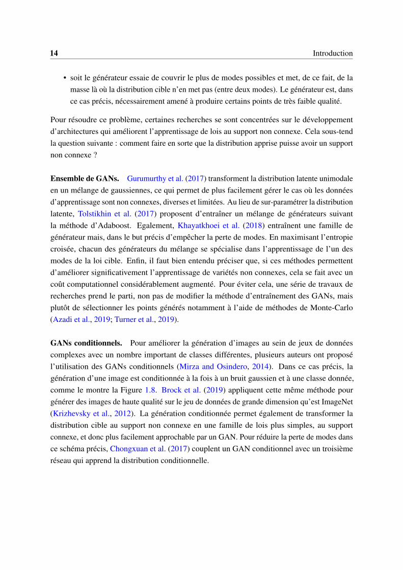
Ensemble de GANs. Gurumurthy et al. (2017) transforment la distribution latente unimodaleen un mélange de gaussiennes, ce qui permet de plus facilement gérer le cas où les donnéesd’apprentissage sont non connexes, diverses et limitées. Au lieu de sur-paramétrer la distributionlatente, Tolstikhin et al. (2017) proposent d’entraîner un mélange de générateurs suivantla méthode d’Adaboost. Egalement, Khayatkhoei et al. (2018) entraînent une famille degénérateur mais, dans le but précis d’empêcher la perte de modes. En maximisant l’entropiecroisée, chacun des générateurs du mélange se spécialise dans l’apprentissage de l’un desmodes de la loi cible. Enfin, il faut bien entendu préciser que, si ces méthodes permettentd’améliorer significativement l’apprentissage de variétés non connexes, cela se fait avec uncoût computationnel considérablement augmenté. Pour éviter cela, une série de travaux derecherches prend le parti, non pas de modifier la méthode d’entraînement des GANs, maisplutôt de sélectionner les points générés notamment à l’aide de méthodes de Monte-Carlo(Azadi et al., 2019; Turner et al., 2019).
GANs conditionnels. Pour améliorer la génération d’images au sein de jeux de donnéescomplexes avec un nombre important de classes différentes, plusieurs auteurs ont proposél’utilisation des GANs conditionnels (Mirza and Osindero, 2014). Dans ce cas précis, lagénération d’une image est conditionnée à la fois à un bruit gaussien et à une classe donnée,comme le montre la Figure 1.8. Brock et al. (2019) appliquent cette même méthode pourgénérer des images de haute qualité sur le jeu de données de grande dimension qu’est ImageNet(Krizhevsky et al., 2012). La génération conditionnée permet également de transformer ladistribution cible au support non connexe en une famille de lois plus simples, au supportconnexe, et donc plus facilement approchable par un GAN. Pour réduire la perte de modes dansce schéma précis, Chongxuan et al. (2017) couplent un GAN conditionnel avec un troisièmeréseau qui apprend la distribution conditionnelle.

1.4 Deux problèmes existants dans les GANs 15
Fig. 1.8 Architecture d’un GAN conditionnel Source : Mirza and Osindero (2014).
1.4.2 L’évaluation des GANs : une question ouverte.
L’évaluation des GANs est toujours une question ouverte et complexe. La principale raison estdue au fait, qu’à ce jour, le but final des GANs n’a pas encore été clairement défini. Selon lestâches, les méthodes d’évaluation peuvent donc varier. Le lecteur intéressé pourra se référer àl’étude menée par Borji (2019) qui présente une liste de 25 différentes méthodes d’évaluationsdes GANs. L’auteur de l’étude souligne lui-même qu’il n’y a à ce jour "pas de consensusquant à la mesure qui capturerait le mieux les forces et les limites d’un GAN et qui devrait êtreutilisée pour une comparaison équitable des différents modèles".
Il est clair qu’en fonction des différents objectifs choisis et/ou des différentes paramétri-sations du discriminateur, les optimums globaux vérifiant l’équation (1.3.7), ne seront pascertainement pas identiques. La question de la comparaison des différents modèles génératifsµθ obtenus se pose. Par souci d’équité, ces différents modèles ne peuvent être comparés parexemple ni sur la divergence de Jensen-Shanon ou la distance de Wassertein, ce qui favoriseraitrespectivement les GANs standards (Goodfellow et al., 2014) ou les WGANs (Arjovsky et al.,2017). Lucic et al. (2018) ont mené une étude empirique importante comparant une grandevariété de GANs différents. Ils concluent que la comparaison des différents modèles obtenusdoit se faire sur un terrain neutre tel que l’Inception Score ou la distance de Fréchet (étudiés plusbas). Ils montrent que la plupart des modèles peuvent obtenir des scores similaires après avoir

16 Introduction
joué sur les hyper-paramètres. De manière similaire, l’étude empirique menée par Meschederet al. (2018) montre qu’aucun objectif n’est stabilisé sensiblement plus l’entraînement desGANs.
La mesure d’évaluation ne doit pas reposer sur des densités de probabilité. L’un desprincipaux problèmes des mesures d’évaluation des GANs réside dans le fait qu’elles nepeuvent pas reposer sur les densités de probabilité. Tout d’abord, la mesure cible est inconnue.Ensuite, il est fort possible que les mesures µ⋆ et µθ ne soient pas absolument continue parrapport à la mesure de Lebesgue. Pour résoudre ce problème, certaines études proposentl’utilisation d’un 3ème réseau qui agit comme un juge. Par exemple, Salimans et al. (2016);Heusel et al. (2017) proposent d’utiliser InceptionNet (Szegedy et al., 2015) pour quantifier laqualité des GANs. D’autres métriques reposent plus spécifiquement, sur des approximations enéchantillon fini qui permettent l’utilisation de méthodes non paramétriques telles que les plusproches voisins (Devroye and Wise, 1980).
La mesure d’évaluation doit évaluer à la fois la qualité et diversité. Le second enjeu estdirectement lié avec la finalité des GANs : doivent-ils être capables de générer des imagesde qualité ou bien avoir la plus grande diversité possible ? Salimans et al. (2016) utilisentl’Inception Score (IS) et un réseau préalablement entraîné pour mesurer la qualité des imagesgénérées. Si l’IS évalue à la fois le réalisme et la diversité des points générés, il n’évalueen revanche, pas correctement la diversité au sein d’une même classe. Sajjadi et al. (2018)argumentent que pour quantifier proprement la qualité et la diversité des images générées,une seule mesure ne suffit pas. Par conséquent, ils définissent la métrique Précision/Rappel.Pour améliorer la robustesse de cette métrique, en particulier quand le générateur s’effondre,Kynkäänniemi et al. (2019) ont proposé la métrique Precision/Rappel améliorée (Improved PR)basée sur une estimation non paramétrique du support. La précision évalue la proportion de laloi µθ qui appartient au support de la distribution cible. Réciproquement, le rappel s’intéresseà la mesure de la distribution cible qui peut être reconstruite par le générateur. La figure 1.9illustre synthétiquement ces deux notions.
La mesure d’évaluation doit-elle être une distance entre lois de probabilité ou entre var-iétés topologiques ? Il est clair que le choix d’une mesure d’évaluation est intimement liéà l’objectif des GANs. De ce point de vue là, l’objectif des GANs est-il d’approcher la dis-tribution cible ou seulement son support ? Succinctement, on distingue les distances entrelois de probabilités (mesures probabilistes) de celles entre variétés topologiques (mesurestopologiques):

1.4 Deux problèmes existants dans les GANs 17
µθ
µ⋆
Précision Rappel
Fig. 1.9 A gauche, la distribution cible µ⋆ et le modèle µθ . Au milieu, la mesure des pointssurlignés en rouge correspond à la précision du modèle. A droite, la mesure des points surlignésen bleu correspond à son rappel. Source : Kynkäänniemi et al. (2019).
• mesure probabiliste : Heusel et al. (2017) utilisent la distance de Fréchet. Ils esti-ment deux gaussiennes multivariées à partir des données d’entraînement et des donnéesgénérées et comparent les moyennes et variances obtenues. Plus récemment, la distancede Wasserstein et son approximation, la Earth Mover’s distance, basée sur des collectionsde points échantillonés par µ⋆ et µθ a également été proposée.
• mesure topologique : la métrique Précision/Rappel améliorée proposée par Kynkään-niemi et al. (2019) est, quant à elle, basée sur une estimation non paramétrique du support.De même, la distance de Hausdhorff (Xiang and Li, 2017) mesure l’éloignement entredeux sous-ensembles d’un espace métrique. De manière similaire, Roth et al. (2017)mesurent pour chaque point présent dans le jeu de données, la distance à la variété créepar le générateur, c’est-à-dire que,
∀x ∈ supp(µ⋆), infy∈supp(µθ )
∥x− y∥,
où ∥.∥ correspond à la norme euclidienne et supp(µ) correspond au support d’une loi µ
donnée. Enfin, Khrulkov and Oseledets (2018) définissent le score géométrique (geometryscore), et comparent les similitudes entre deux variétés topologiques en utilisant desnotions de topologie algébrique.
Evaluation de la généralisation d’un GAN. L’objectif des GANs est-il de générer desexemples qui représentent fidèlement le jeu de données ou, au contraire, doivent-ils êtrecapables de générer des images qui n’ont jamais été observées pendant l’entraînement. Il esten effet extrêmement intéressant de se demander si les GANs apprennent la distribution cibleou mémorisent simplement le jeu d’entraînement observé. Arora and Zhang (2017) proposentd’utiliser le paradoxe des anniversaires pour évaluer le nombre d’images distinctes générer par
18 Introduction
les GANs et répondre à la question. De manière plus générale, il n’existe encore à ce jour quetrès peu de travaux sur l’évaluation empirique des capacités de généralisation des GANs ? Eneffet, la communauté ne fait pas nécessairement la différence entre les données d’entraînementdes données de test, signifiant que comprendre la généralisation des GANs n’est pas l’unedes priorités de la communauté. Enfin, il faut noter que cette question a tout de même suscitéquelques recherches théoriques (Zhang et al., 2018; Qi, 2019).
1.5 Organisation du manuscrit et présentation des contri-butions
Ce travail de thèse est structuré en cinq chapitres. Le Chapitre 2 vise à formaliser l’entraînementdes GANs et s’intéresse principalement aux propriétés statistiques des GANs définis parGoodfellow et al. (2014). Ces travaux menés en collaboration avec Gérard Biau (LPSM),Benoit Cadre (IRMAR, Université Rennes 2) et Maxime Sangnier (LPSM) ont été publiésau journal Annals of Statistics. Le Chapitre 3 étend cette recherche aux Wasserstein GANs(Arjovsky et al., 2017), réputés plus stables. Mené conjointement avec Gérard Biau et MaximeSangnier, ce travail a fait l’objet d’un article soumis pour publication. Le Chapitre 4 découlede l’utilisation de réseaux de neurones paramétrés avec la fonction d’activation GroupSort(Anil et al., 2019). Il se propose d’étudier l’expressivité de ces réseaux et sera proposé à uneconférence. La suite de la thèse est axée autour d’un problème plus appliqué. Le Chapitre 5traite en effet de la difficulté d’apprendre une variété non connexe avec les GANs. C’est le sujetde deux travaux de recherche menés conjointement avec Thibaut Issenhuth (Criteo) et JérémieMary (Criteo), dont l’un a été publié à ICML 2020 et le second est en cours de révision.
1.5.1 Chapitre 2 : Etude statistique des GANs
Ce chapitre propose une formalisation théorique des GANs et analyse certaines de leurs pro-priétés mathématiques et statistiques. Nous commençons par rappeler que pour un générateurGθ et un discriminateur D ∈ D , les GANs optimisent le critère probabiliste suivant :
L(θ ,D) =∫
ln(D)p⋆dµ +∫
ln(1−D)pθ dµ.
En particulier, les GANs cherchent à résoudre
infθ∈Θ
supD∈D
L(θ ,D).

1.5 Organisation du manuscrit et présentation des contributions 19
Nous commençons par étudier le cas où le discriminateur n’est pas restreint à un modèleparamétrique et où D = D∞ correspond à l’ensemble des fonctions mesurables de RD dans[0,1]. Dans ce contexte non paramétrique, nous établissons le lien entre l’entraînement adversedes GANs et la divergence de Jensen-Shannon. Le Théorème 2.2.2 montre l’existence etl’unicité de l’optimum des GANs, c’est-à-dire que, sous certaines hypothèses,
θ⋆= argmin
θ∈Θ
supD∈D∞
L(θ ,D) = argminθ∈Θ
DJS(p⋆, pθ ),
existe et est un singleton. Ici DJS correspond à la divergence de Jensen-Shannon. Nous nousramenons, par la suite, à un cas plus réaliste où la classe de fonctions discriminatives estparamétrée par un réseau de neurones. En utilisant la notation L(θ ,D) = L(θ ,α) dans le casparamétrique, l’objectif des GANs consiste alors à trouver le modèle génératif suivant :
Θ = argminθ∈Θ
supα∈Λ
L(θ ,α) = argminθ∈Θ
supα∈Λ
∫log(Dα)p⋆dµ +
∫log(1−Dα)pθ dµ.
En particulier, le Théorème 2.3.1 montre, en supposant que le discriminateur optimal estapproché à ε près, que pour chaque θ ∈ Θ , il existe une constante c > 0 (indépendante de ε)telle que :
0 ≤ DJS(p⋆, pθ)−DJS(p⋆, pθ⋆)≤ cε
2.
En revanche, il est clair qu’en pratique nous n’avons uniquement accès qu’à un jeu de donnéesde n échantillons X1, . . . ,Xn indépendants et identiquement distribués selon p⋆. Le critèreempirique des GANs devient,
L(θ ,D) =1n
n
∑i=1
lnD(Xi)+1n
n
∑i=1
ln(1−DGθ (Zi)),
où ln est le logarithme naturel et Z1, . . . ,Zn sont des variables indépendantes et identiquementdistribuées de loi Z. Par conséquent, l’ensemble des paramètres optimaux associés se définitcomme suit :
Θ = argminθ∈Θ
supα∈Λ
L(θ ,α).
L’un des principaux résultats du chapitre (Théorème 2.4.1) montre que, sous des hypothèsessimilaires à celles du Théorème 2.3.1, nous avons, pour tout θ ∈ Θ :
EDJS(p⋆, pθ)−DJS(p⋆, pθ⋆) = O
(ε
2 +1√n
).

20 Introduction
1.5.2 Chapitre 3 : Extension et développement pour le cas des WGANs
Plusieurs études empiriques (Gulrajani et al., 2017; Roth et al., 2017) ont validé les bénéficesde l’approche cousine appelée Wasserstein GANs (WGANs) proposée par Arjovsky et al.(2017). Cette dernière apporte une stabilisation dans le processus d’entraînement. Il est doncimportant d’approfondir notre compréhension de cette architecture. De manière similaire, auchapitre précédent, pour bien comprendre le fonctionnement de ces WGANs, il est nécessairede distinguer deux problèmes.
Tout d’abord, dans le cas où la classe de fonctions discriminatives D correspond à la classenon paramétrique des fonctions 1-Lipschitz, l’objectif des WGANs revient à minimiser ladistance de Wasserstein entre la distribution cible µ⋆ et le modèle P . Plus formellement,l’objectif théorique des WGANs est le suivant :
infθ∈Θ
W (µ⋆,µθ ) = infθ∈Θ
supf∈Lip1
|Eµ⋆ f −Eµθf |, (1.5.1)
où W correspond à la distance de 1-Wasserstein et Lip1 =
f : E →R : | f (x)− f (y)|⩽ ∥x− y∥,(x,y) ∈ (RD)2.
Ensuite, le second problème, plus réaliste, vise à considérer une classe de fonctions discrim-inatives paramétrique plus restreinte, D = Dα : α ∈ Λ. Dans cette approche, le véritableproblème des WGANs s’écrit :
infθ∈Θ
supα∈Λ
|Eµ⋆Dα −EµθDα |. (1.5.2)
En ré-écrivant les deux objectifs des WGANs théoriques (T-WGANs) et des WGANs sousforme d’Integral Probability Metric (Müller, 1997), nous obtenons :
T-WGANs: infθ∈Θ
dLip1(µ⋆,µθ ) et WGANs: inf
θ∈ΘdD(µ⋆,µθ ),
où pour une classe de fonctions F donnée, l’IPM entre deux distributions µ et ν s’écritdF (µ,ν) = sup
f∈G|Eµ f −Eν f |.
Comme pour le chapitre précédent, nous nous intéressons à l’influence de l’échantillonet considérons le cas où nous n’avons accès qu’à un ensemble fini de points, représentés parla mesure empirique µn. Finalement, cela nous permet d’identifier les trois ensembles deparamètres correspondants :
Θ⋆ = argmin
θ∈Θ
dLip1(µ⋆,µθ ) & Θ = argmin
θ∈Θ
dD(µ⋆,µθ ) & Θn = argminθ∈Θ
dD(µn,µθ ).

1.5 Organisation du manuscrit et présentation des contributions 21
L’objectif du présent chapitre est de parvenir à étudier ces trois ensembles et de pouvoircomparer la performance des différents modèles génératifs obenus à partir de Θ ⋆, Θ et Θn.Pour avoir une meilleure compréhension de la performance finale des WGANs dLip1
(µ⋆,µθn)
où θn ∈ Θn, nous proposons la décomposition suivante :
dLip1(µ⋆,µ
θn)⩽ εestim + εoptim + εapprox, (1.5.3)
où
• εapprox = infθ∈Θ
dLip1(µ⋆,µθ ) est liée à la capacité d’approximation du modèle génératif et
la performance des paramètres θ ⋆ ∈Θ ⋆;
• εoptim = supθ∈Θ
dLip1(µ⋆,µθ
)− infθ∈Θ
dLip1(µ⋆,µθ ) correspond à l’écart de performance entre
un paramètre θ ∈ Θ et θ ⋆ ∈Θ ⋆. L’analyse de cette erreur est menée dans la Section 3.3et, en particulier, le Théorème 3.3.1 montre que, sous certaines hypothèses, elle peut êtrearbitrairement petite;
• εestim mesure l’écart de performance lié à l’obtention d’un paramètre θn ∈ Θn plutôt queθ ∈ Θ . Notons que le Théorème 3.4.1 prouve que, sous certaines hypothèses, la sommeεoptim + εestim peut être arbitrairement petite avec grande probabilité.
Des expériences sur données réelles et simulées viennent compléter les résultats théoriques.
1.5.3 Chapitre 4 : Etude des réseaux de neurones dits GroupSort etapplication aux GANs
Les récentes publications sur les attaques adverses liées aux réseaux profonds (Goodfellowet al., 2015) et le développement des WGANs ont préconisé l’utilisation de réseaux de neuronesavec des constantes de Lipschitz restreintes. Motivés par ces observations, Anil et al. (2019) ontproposé l’utilisation de réseaux de neurones dits GroupSort avec des contraintes sur les poids.Les auteurs de cette publications ont notamment prouver que les réseaux GroupSort pouvaientapprocher n’importe quelle fonction Lipschitz tout en garantissant le caractère Lipschitz del’estimateur. Dans ce chapitre, nous visons à mieux comprendre l’intérêt des réseaux GroupSort,utilisés dont le chapitre précédent, et faisons un pas théorique vers une meilleure compréhensionde leur expressivité.
Les réseaux GroupSort se caractérisent par leur fonction d’activation GroupSort qui sépareles entrées en groupes et les trie par ordre croissant. La fonction d’activation GroupSort avecune taille de regroupement (grouping size) k ⩾ 2 est appliquée sur un vecteur x1, . . . ,xkn. Tout

22 Introduction
d’abord, elle sépare le vecteur en n groupes G1 = x1, . . . ,xk, . . .Gn = xnk−k−1, . . . ,xnk. Puis,elle trie chaque groupe comme suit:
σk(x1, . . . ,xk, . . . ,xnk−(k−1), . . . ,xnk) =(xG1(k), . . . ,x
G1(1)), . . . ,
(xGn(k), . . . ,x
Gn(1)),
où xG(i), la notation des statistiques d’ordre, correspond au ième plus petit élément du groupe
G. Tout comme les réseaux ReLU, les réseaux GroupSort paramètrent des fonctions linéairespar morceaux. L’étude d’expressivité de ces réseaux commencent par analyser leur faculté àreprésenter l’ensemble des fonctions linéaires continues par morceaux. Nous montrons, en par-ticulier avec le Corollaire 4.3.1, que pour toute fonction Lipschitz f linéaires par morceaux surm f sous-domaines convexes Ω1, . . . ,Ωm f (m f = kn avec n ⩾ 1), il existe un réseau GroupSort
avec une taille de regroupement k, une profondeur 2⌈logk(m f )⌉+1 et une taille au plusm2
f−1k−1
qui reproduit la fonction f .La faculté de ces réseaux à reproduire les fonctions linéaires par morceaux nous permet
de passer au cas plus général de l’approximation des fonctions Lipschitz. Nous prouvonsque pour tout ε > 0, et toute fonction f Lipschitz définie sur [0,1]d , il existe un réseau deneurones GroupSort D avec une taille de groupement ⌈2
√d
ε⌉ tel que ∥ f −D∥∞ ⩽ ε . De plus, la
profondeur de D est O(d2). Pour conclure, nous illustrons l’efficacité des réseaux GroupSortpar rapport à celles des réseaux ReLU sur un ensemble d’expériences synthétiques.
1.5.4 Chapitre 5 : L’apprentissage de variétés non connexes avec lesGANs
Dans la formulation standard des GANs, une distribution latente unimodale (unifome ougaussienne) est transformée par un générateur continu dans l’espace des images. Par conséquent,dans le cas où la distribution cible a un support non connexe, aucune des distributions modéliséesµθ ne pourra parfaitement approcher µ⋆. Dans ce chapitre, nous formalisons ce cadre précis etétablissons des résultats qui mesurent la quantité de données simulées se trouvant en dehors dela variété cible.
Notre étude part du constat suivant établi dans un contexte simple : pour apprendre unmélange de deux gaussiennes, les GANs divisent l’espace latent en deux zones, comme lemontre la ligne de séparation en rouge sur la figure 1.10a. Plus important encore, chaquebruit gaussien à l’intérieur de cette zone rouge sur la figure 1.10a est ensuite envoyé dansl’espace de sortie entre les deux modes (voir Figure 1.10b) de la loi cible. En utilisant desrésultats connus de l’inégalité gaussienne isopérimétrique, nous quantifions la quantité dedonnées en dehors de la variété cible. La métrique choisie pour définir si un échantillon

1.5 Organisation du manuscrit et présentation des contributions 23
(a) Heatmap de la norme du ja-cobien du générateur. Les cer-cles blancs correspondent auxquantiles de la distribution la-tente N (0, I).
(b) En vert : la distribution cible. Lespoints colorés correspondent aux échantil-lons générés par le générateur. Ils sont col-orés en fonctions de la norme du jacobiende Gθ . La même heatmap que dans la fig-ure (a) est utilisée.
Fig. 1.10 L’apprentissage d’une variété non connexe avec un GAN standard amène àl’apparition d’une zone à forts gradients dans l’espace de départ où chaque échantillon estenvoyé en dehors de la variété.
donné appartient à la variété cible est donc primordiale. Pour la présente étude, nous avonschoisi la métrique Précision/Rappel (PR) proposée par Sajjadi et al. (2018) et, en particulier, laversion améliorée (Improved PR) (Kynkäänniemi et al., 2019) construite sur une estimationnon paramétrique des supports. Comme précisé plus haut, la précision quantifie la part de lafausse distribution qui peut être générée par la distribution cbile µ⋆, tandis que le rappel mesurela part de la vraie distribution qui peut être reconstruite par la distribution µθ du modèle. Plusformellement, soient (X1, . . . ,Xn)∼ µn
θ(ensemble de données générées par le générateur) et
(Y1, . . . ,Yn)∼ µnθ
(ensemble de données échantillonées par la distribution cible). Pour chaqueX (ou respectivement chaque Y ), on considère (X(1), . . . ,X(n−1)), l’arrangement des élémentsdans (X1, . . .Xn) \X selon leur distance croissante à X (X(1) = argmin
Xi∈(X1,...Xn)\X∥Xi −X∥). Pour
chaque k ∈N et chaque X , la précision αnk (X) du point X est définie par
Précision: αnk (X) = 1 ⇐⇒ ∃Y ∈ (Y1, . . . ,Yn),∥X −Y∥⩽ ∥Y(k)−Y∥.
De manière similaire, le rappel β nk (Y ) d’un point Y ∈ (Y1, . . . ,Yn) est défini par
Rappel: βnk (Y ) = 1 ⇐⇒ ∃X ∈ (X1, . . . ,Xn),∥Y −X∥⩽ ∥X(k)−X∥.
Après cette analyse théorique, nous poursuivons notre étude en définissant une méthoded’échantillonnage de rejet basée sur la norme du Jacobien du générateur. Nous montrons sacapacité à enlever les points de données de mauvaise qualité et ceux, à la fois sur des jeux

24 Introduction
de données synthétiques (approximation de mélanges de gaussiennes), mais aussi sur de lagénération d’images en grande dimension.

Chapter 2
Some theoretical properties of GANs
AbstractGenerative Adversarial Networks (GANs) are a class of generative algorithms that have been shown toproduce state-of-the-art samples, especially in the domain of image creation. The fundamental principleof GANs is to approximate the unknown distribution of a given data set by optimizing an objectivefunction through an adversarial game between a family of generators and a family of discriminators. Inthis paper, we offer a better theoretical understanding of GANs by analyzing some of their mathematicaland statistical properties. We study the deep connection between the adversarial principle underlyingGANs and the Jensen-Shannon divergence, together with some optimality characteristics of the problem.An analysis of the role of the discriminator family via approximation arguments is also provided.In addition, taking a statistical point of view, we study the large sample properties of the estimateddistribution and prove in particular a central limit theorem. Some of our results are illustrated withsimulated examples.
Contents2.1 Introduction . . . . . . . . . . . . . . . . . . . . . . . . . . . . . . . . . 26
2.2 Optimality properties . . . . . . . . . . . . . . . . . . . . . . . . . . . . 29
2.3 Approximation properties . . . . . . . . . . . . . . . . . . . . . . . . . . 34
2.4 Statistical analysis . . . . . . . . . . . . . . . . . . . . . . . . . . . . . . 35
2.5 Conclusion and perspectives . . . . . . . . . . . . . . . . . . . . . . . . 53
Appendix 2.A Technical results . . . . . . . . . . . . . . . . . . . . . . . . . 55
26 Some theoretical properties of GANs
2.1 Introduction
The fields of machine learning and artificial intelligence have seen spectacular advances inrecent years, one of the most promising being perhaps the success of Generative AdversarialNetworks (GANs), introduced by Goodfellow et al. (2014). GANs are a class of generativealgorithms implemented by a system of two neural networks contesting with each other in azero-sum game framework. This technique is now recognized as being capable of generatingphotographs that look authentic to human observers (e.g., Salimans et al., 2016), and itsspectrum of applications is growing at a fast pace, with impressive results in the domains ofinpainting, speech, and 3D modeling, to name but a few. A survey of the most recent advancesis given by Goodfellow (2016).
The objective of GANs is to generate fake observations of a target distribution p⋆ fromwhich only a true sample (e.g., real-life images represented using raw pixels) is available. Itshould be pointed out at the outset that the data involved in the domain are usually so complexthat no exhaustive description of p⋆ by a classical parametric model is appropriate, nor itsestimation by a traditional maximum likelihood approach. Similarly, the dimension of thesamples is often very large, and this effectively excludes a strategy based on nonparametricdensity estimation techniques such as kernel or nearest neighbor smoothing, for example. Inorder to generate according to p⋆, GANs proceed by an adversarial scheme involving twocomponents: a family of generators and a family of discriminators, which are both implementedby neural networks. The generators admit low-dimensional random observations with a knowndistribution (typically Gaussian or uniform) as input, and attempt to transform them into fakedata that can match the distribution p⋆; on the other hand, the discriminators aim to accuratelydiscriminate between the true observations from p⋆ and those produced by the generators. Thegenerators and the discriminators are calibrated by optimizing an objective function in such away that the distribution of the generated sample is as indistinguishable as possible from thatof the original data. In pictorial terms, this process is often compared to a game of cops androbbers, in which a team of counterfeiters illegally produces banknotes and tries to make themundetectable in the eyes of a team of police officers, whose objective is of course the opposite.The competition pushes both teams to improve their methods until counterfeit money becomesindistinguishable (or not) from genuine currency.
From a mathematical point of view, here is how the generative process of GANs can berepresented. All the densities that we consider in the article are supposed to be dominated by afixed, known, measure µ on E, where E is a Borel subset of Rd . Depending on the practical

2.1 Introduction 27
context, this dominating measure may be the Lebesgue measure, the counting measure, or moregenerally the Hausdorff measure on some submanifold of Rd . We assume to have at hand ani.i.d. sample X1, . . . ,Xn, drawn according to some unknown density p⋆ on E. These randomvariables model the available data, such as images or video sequences; they typically take theirvalues in a high-dimensional space, so that the ambient dimension d must be thought of aslarge. The generators as a whole have the form of a parametric family of functions from Rd′
toE (usually, d′ ≪ d), say G = Gθθ∈Θ , Θ ⊂Rp. Each function Gθ is intended to be appliedto a d′-dimensional random variable Z (sometimes called the noise—in most cases Gaussianor uniform), so that there is a natural family of densities associated with the generators, sayP = pθθ∈Θ , where, by definition, Gθ (Z)
L= pθ dµ . In this model, each density pθ is a
potential candidate to represent p⋆. On the other hand, the discriminators are described by afamily of Borel functions from E to [0,1], say D , where each D ∈ D must be thought of asthe probability that an observation comes from p⋆ (the higher D(x), the higher the probabilitythat x is drawn from p⋆). At some point, but not always, we will assume that D is in fact aparametric class, of the form Dαα∈Λ , Λ ⊂Rq, as is always the case in practice. In GANsalgorithms, both parametric models Gθθ∈Θ and Dαα∈Λ take the form of neural networks,but this does not play a fundamental role in this paper. We will simply remember that thedimensions p and q are potentially very large, which takes us away from a classical parametricsetting. We also insist on the fact that it is not assumed that p⋆ belongs to P .
Let Z1, . . . ,Zn be an i.i.d. sample of random variables, all distributed as the noise Z. Theobjective is to solve in θ the problem
infθ∈Θ
supD∈D
[ n
∏i=1
D(Xi)×n
∏i=1
(1−DGθ (Zi))], (2.1.1)
or, equivalently, to find θ ∈Θ such that
supD∈D
L(θ ,D)≤ supD∈D
L(θ ,D), ∀θ ∈Θ , (2.1.2)
where
L(θ ,D)def=
1n
n
∑i=1
lnD(Xi)+1n
n
∑i=1
ln(1−DGθ (Zi))
(ln is the natural logarithm). The zero-sum game (2.1.1) is the statistical translation of makingthe distribution of Gθ (Zi) (i.e., pθ ) as indistinguishable as possible from that of Xi (i.e., p⋆).Here, distinguishability is understood as the capability to determine from which distributionan observation x comes from. Mathematically, this is captured by the discrimination valueD(x), which represents the probability that x comes from p⋆ rather than from pθ . Therefore,

28 Some theoretical properties of GANs
for a given θ , the discriminator D is determined so as to be maximal on the Xi and minimal onthe Gθ (Zi). In the most favorable situation (that is, when the two samples are scattered by D ,supD∈D L(θ ,D) is zero, and the larger this quantity, the more distinguishable the two samplesare. Hence, in order to make the distribution pθ as indistinguishable as possible from p⋆, Gθ
has to be driven so as to minimize supD∈D L(θ ,D).This adversarial problem is often illustrated by the struggle between a police team (the
discriminators), trying to distinguish true banknotes from false ones (respectively, the Xi andthe Gθ (Zi)), and a counterfeiters team, slaving to produce banknotes as credible as possibleand to mislead the police. Obviously, their objectives (represented by the quantity L(θ ,D))are exactly opposite. All in all, we see that the criterion seeks to find the right balancebetween the conflicting interests of the generators and the discriminators. The hope is thatthe θ achieving equilibrium will make it possible to generate observations G
θ(Z1), . . . ,Gθ
(Zn)
indistinguishable from reality, i.e., observations with a distribution close to the unknown p⋆.The criterion L(θ ,D) involved in (2.1.2) is the criterion originally proposed in the adversar-
ial framework of Goodfellow et al. (2014). Since then, the success of GANs in applications hasled to a large volume of literature on variants, which all have many desirable properties but arebased on different optimization criteria—examples are MMD-GANs (Li et al., 2017), f-GANs(Nowozin et al., 2016), Wasserstein-GANs (Arjovsky et al., 2017), and an approach based onscattering transforms (Angles and Mallat, 2018). All these variations and their innumerablealgorithmic versions constitute the galaxy of GANs. That being said, despite increasinglyspectacular applications, little is known about the mathematical and statistical forces behindthese algorithms (e.g., Arjovsky et al., 2017; Liu et al., 2017; Zhang et al., 2018), and, in fact,nearly nothing about the primary adversarial problem (2.1.2). As acknowledged by Liu et al.(2017), basic questions on how well GANs can approximate the target distribution p⋆ remainlargely unanswered. In particular, the role and impact of the discriminators on the quality of theapproximation are still a mystery, and simple but fundamental questions regarding statisticalconsistency and rates of convergence remain open.
In the present article, we propose to take a small step towards a better theoretical under-standing of GANs by analyzing some of the mathematical and statistical properties of theoriginal adversarial problem (2.1.2). In Section 2.2, we study the deep connection between thepopulation version of (2.1.2) and the Jensen-Shannon divergence, together with some optimalitycharacteristics of the problem, often referred to in the literature but in fact poorly understood.Section 2.3 is devoted to a better comprehension of the role of the discriminator family viaapproximation arguments. Finally, taking a statistical point of view, we study in Section 2.4 thelarge sample properties of the distribution p
θand of θ , and prove in particular a central limit
theorem for this parameter. Section 2.5 summarizes the main results and discusses research

2.2 Optimality properties 29
directions for future work. For clarity, most technical proofs are gathered in Section 2.A. Someof our results are illustrated with simulated examples.
2.2 Optimality properties
We start by studying some important properties of the adversarial principle, emphasizing therole played by the Jensen-Shannon divergence. We recall that if P and Q are probabilitymeasures on E, and P is absolutely continuous with respect to Q, then the Kullback-Leiblerdivergence from Q to P is defined as DKL(P ∥ Q) =
∫ln dP
dQdP, where dPdQ is the Radon-Nikodym
derivative of P with respect to Q. The Kullback-Leibler divergence is always nonnegative, withDKL(P ∥ Q) zero if and only if P = Q. If p = dP
dµand q = dQ
dµexist (meaning that P and Q are
absolutely continuous with respect to µ , with densities p and q), then the Kullback-Leiblerdivergence is given as
DKL(P ∥ Q) =∫
p lnpq
dµ,
and alternatively denoted by DKL(p ∥ q). We also recall that the Jensen-Shannon divergenceis a symmetrized version of the Kullback-Leibler divergence. It is defined for any probabilitymeasures P and Q on E by
DJS(P,Q) =12
DKL
(P∥∥∥ P+Q
2
)+
12
DKL
(Q∥∥∥ P+Q
2
),
and satisfies 0 ≤ DJS(P,Q)≤ ln2. The square root of the Jensen-Shannon divergence is a metricoften referred to as Jensen-Shannon distance (Endres and Schindelin, 2003). When P and Qhave densities p and q with respect to µ , we use the notation DJS(p,q) in place of DJS(P,Q).
For a generator Gθ and an arbitrary discriminator D ∈ D , the criterion L(θ ,D) to beoptimized in (2.1.2) is but the empirical version of the probabilistic criterion
L(θ ,D)def=
∫ln(D)p⋆dµ +
∫ln(1−D)pθ dµ.
We assume for the moment that the discriminator class D is not restricted and equals D∞, theset of all Borel functions from E to [0,1]. We note however that, for all θ ∈Θ ,
0 ≥ supD∈D∞
L(θ ,D)≥− ln2(∫
p⋆dµ +∫
pθ dµ
)=− ln4,

30 Some theoretical properties of GANs
so that infθ∈Θ supD∈D∞L(θ ,D) ∈ [− ln4,0]. Thus,
infθ∈Θ
supD∈D∞
L(θ ,D) = infθ∈Θ
supD∈D∞:L(θ ,D)>−∞
L(θ ,D).
This identity points out the importance of discriminators such that L(θ ,D)>−∞, which wecall θ -admissible. In the sequel, in order to avoid unnecessary problems of integrability, weonly consider such discriminators, keeping in mind that the others have no interest.
Of course, working with D∞ is somehow an idealized vision, since in practice the discrimi-nators are always parameterized by some parameter α ∈ Λ , Λ ⊂Rq. Nevertheless, this pointof view is informative and, in fact, is at the core of the connection between our generativeproblem and the Jensen-Shannon divergence. Indeed, taking the supremum of L(θ ,D) overD∞, we have
supD∈D∞
L(θ ,D) = supD∈D∞
∫ [ln(D)p⋆+ ln(1−D)pθ
]dµ
≤∫
supD∈D∞
[ln(D)p⋆+ ln(1−D)pθ
]dµ
= L(θ ,D⋆θ ),
whereD⋆
θ
def=
p⋆p⋆+ pθ
. (2.2.1)
(We use throughout the convention 0/0 = 0 and ∞× 0 = 0.) By observing that L(θ ,D⋆θ) =
2DJS(p⋆, pθ )− ln4, we conclude that, for all θ ∈Θ ,
supD∈D∞
L(θ ,D) = L(θ ,D⋆θ ) = 2DJS(p⋆, pθ )− ln4.
In particular, D⋆θ
is θ -admissible. The fact that D⋆θ
realizes the supremum of L(θ ,D) overD∞ and that this supremum is connected to the Jensen-Shannon divergence between p⋆ andpθ appears in the original article by Goodfellow et al. (2014). This remark has given rise tomany developments that interpret the adversarial problem (2.1.2) as the empirical version ofthe minimization problem infθ DJS(p⋆, pθ ) over Θ . Accordingly, many GANs algorithms tryto learn the optimal function D⋆
θ, using for example stochastic gradient descent techniques
and mini-batch approaches. However, it remains to prove that D⋆θ
is unique as a maximizerof L(θ ,D) over all D. The following theorem, which completes a result of (Goodfellow et al.,2014), shows that this is the case in some situations.

2.2 Optimality properties 31
Theorem 2.2.1. Let θ ∈ Θ and D ∈ D∞ be such that L(θ ,D) = L(θ ,D⋆θ). Then D = D⋆
θon
the complementary of the set p⋆ = pθ = 0. In particular, if µ(p⋆ = pθ = 0) = 0, thenthe function D⋆
θis the unique discriminator that achieves the supremum of the functional
D 7→ L(θ ,D) over D∞, i.e.,D⋆
θ=argmaxD∈D∞
L(θ ,D).
Before proving the theorem, it is important to note that if we dot not assume that µ(p⋆ =pθ = 0) = 0, then we cannot conclude that D = D⋆
θµ-almost everywhere. To see this, suppose
that pθ = p⋆. Then, whatever D ∈ D∞ is, the discriminator D⋆θ
1pθ>0+ D1pθ=0 satisfies
L(θ ,D⋆θ 1pθ>0+ D1pθ=0) = L(θ ,D⋆
θ ).
This simple counterexample shows that uniqueness of the optimal discriminator does not holdin general.
Proof. Let D ∈ D∞ be a discriminator such that L(θ ,D) = L(θ ,D⋆θ). In particular, L(θ ,D)>
−∞ and D is θ -admissible. Thus, letting A def= p⋆ = pθ = 0 and fα
def= p⋆ ln(α)+ pθ ln(1−α)
for α ∈ [0,1], we see that ∫Ac( fD − fD⋆
θ)dµ = 0.
Since, on Ac,fD ≤ sup
α∈[0,1]fα = fD⋆
θ,
we have fD = fD⋆θ
µ-almost everywhere on Ac. By uniqueness of the maximizer of α 7→ fα onAc, we conclude that D = D⋆
θµ-almost everywhere on Ac.
By definition of the optimal discriminator D⋆θ
, we have
L(θ ,D⋆θ ) = sup
D∈D∞
L(θ ,D) = 2DJS(p⋆, pθ )− ln4, ∀θ ∈Θ .
Therefore, it makes sense to let the parameter θ ⋆ ∈Θ be defined as
L(θ ⋆,D⋆θ⋆)≤ L(θ ,D⋆
θ ), ∀θ ∈Θ ,
or, equivalently,DJS(p⋆, pθ⋆)≤ DJS(p⋆, pθ ), ∀θ ∈Θ . (2.2.2)
The parameter θ ⋆ may be interpreted as the best parameter in Θ for approaching the unknowndensity p⋆ in terms of Jensen-Shannon divergence, in a context where all possible discriminators

32 Some theoretical properties of GANs
are available. In other words, the generator Gθ⋆ is the ideal generator, and the density pθ⋆ isthe one we would ideally like to use to generate fake samples. Of course, whenever p⋆ ∈ P
(i.e., the target density is in the model), then p⋆ = pθ⋆ , DJS(p⋆, pθ⋆) = 0, and D⋆θ⋆ = 1/2. This
is, however, a very special case, which is of no interest, since in the applications covered byGANs, the data are usually so complex that the hypothesis p⋆ ∈ P does not hold.
In the general case, our next theorem provides sufficient conditions for the existence anduniqueness of θ ⋆. For P and Q probability measures on E, we let δ (P,Q) =
√DJS(P,Q), and
recall that δ is a distance on the set of probability measures on E (Endres and Schindelin, 2003).We let dp⋆ = p⋆dµ and, for all θ ∈Θ , dPθ = pθ dµ .
Theorem 2.2.2. Assume that the model P = Pθθ∈Θ is convex and compact for the metric δ .If p⋆ > 0 µ-almost everywhere, then there exists a unique p ∈ P such that
p=argminp∈P
DJS(p⋆, p).
In particular, if the model P is identifiable, then
θ⋆=argmin
θ∈Θ
L(θ ,D⋆θ )
or, equivalently,θ
⋆=argminθ∈Θ
DJS(p⋆, pθ ).
We note that the identifiability assumption in the second statement of the theorem is hardlysatisfied in the high-dimensional context of (deep) neural networks. In this case, it is likelythat several parameters θ yield the same function (generator), so that the parametric setting ispotentially misspecified. However, if we think in terms of distributions instead of parameters,then the first part of Theorem 2.2.2 ensures existence and uniqueness of the optimum.
Proof. Assuming the first part of the theorem, the second one is obvious since L(θ ,D⋆θ) =
supD∈D∞L(θ ,D) = 2DJS(p⋆, pθ )− ln4. Therefore, it is enough to prove that there exists a
unique density p of P such that
p=argminp∈P
DJS(p⋆, p).
Existence. Since P is compact for δ , it is enough to show that the function
P → R+
P 7→ DJS(p⋆,P)

2.2 Optimality properties 33
is continuous. But this is clear since, for all P1,P2 ∈ P , |δ (p⋆,P1)−δ (p⋆,P2)| ≤ δ (P1,P2) bythe triangle inequality. Therefore, argminp∈PDJS(p⋆, p) = /0.
Uniqueness. For a ≥ 0, we consider the function Fa defined by
Fa(x) = a ln( 2a
a+ x
)+ x ln
( 2xa+ x
), x ≥ 0,
with the convention 0ln0 = 0. Clearly, F ′′a (x) =
ax(a+x) , which shows that Fa is strictly convex
whenever a > 0. We now proceed to prove that L1(µ)⊃P ∋ p 7→ DJS(p⋆, p) is strictly convexas well. Let λ ∈ (0,1) and p1, p2 ∈ P with p1 = p2, i.e., µ(p1 = p2)> 0. Then
DJS(p⋆,λ p1 +(1−λ )p2) =∫
Fp⋆(λ p1 +(1−λ )p2)dµ
=∫p1=p2
Fp⋆(p1)dµ +∫p1 =p2
Fp⋆(λ p1 +(1−λ )p2)dµ.
By the strict convexity of Fp⋆ over p⋆ > 0, we obtain
DJS(p⋆,λ p1 +(1−λ )p2)
<∫p1=p2
Fp⋆(p1)dµ +λ
∫p1 =p2
Fp⋆(p1)dµ +(1−λ )∫p1 =p2
Fp⋆(p2)dµ,
which implies
DJS(p⋆,λ p1 +(1−λ )p2)< λDJS(p⋆, p1)+(1−λ )DJS(p⋆, p2).
Consequently, the function L1(µ) ⊃ P ∋ p 7→ DJS(p⋆, p) is strictly convex, and its argminover the convex set P is either the empty set or a singleton.
Remark 2.2.1. There are simple conditions for the model P = Pθθ∈Θ to be compact forthe metric δ . It is for example enough to suppose that Θ is compact, P is convex, and
(i) For all x ∈ E, the function θ 7→ pθ (x) is continuous on Θ ;
(ii) One has sup(θ ,θ ′)∈Θ 2 |pθ ln pθ ′| ∈ L1(µ).
Let us quickly check that under these conditions, P is compact for the metric δ . Since Θ
is compact, by the sequential characterization of compact sets, it is enough to prove that ifΘ ⊃ (θn)n converges to θ ∈Θ , then DJS(pθ , pθn)→ 0. But,
DJS(pθ , pθn) =∫ [
pθ ln( 2pθ
pθ + pθn
)+ pθn ln
( 2pθn
pθ + pθn
)]dµ.

34 Some theoretical properties of GANs
By the convexity of P , using (i) and (ii), the Lebesgue dominated convergence theorem showsthat DJS(pθ , pθn)→ 0, whence the result.
Interpreting the adversarial problem in connection with the optimization programinfθ∈Θ DJS(p⋆, pθ ) is a bit misleading, because this is based on the assumption that all possiblediscriminators are available (and in particular the optimal discriminator D⋆
θ). In the end this
means assuming that we know the distribution p⋆, which is eventually not acceptable froma statistical perspective. In practice, the class of discriminators is always restricted to be aparametric family D = Dαα∈Λ , Λ ⊂Rq, and it is with this class that we have to work. Fromour point of view, problem (2.1.2) is a likelihood-type problem involving two parametric fami-lies G and D , which must be analyzed as such, just as we would do for a classical maximumlikelihood approach. In fact, it takes no more than a moment’s thought to realize that the keylies in the approximation capabilities of the discriminator class D with respect to the functionsD⋆
θ, θ ∈Θ . This is the issue that we discuss in the next section.
2.3 Approximation properties
In the remainder of the article, we assume that θ ⋆ exists, keeping in mind that Theorem 2.2.2provides us with precise conditions guaranteeing its existence and its uniqueness. As pointedout earlier, in practice only a parametric class D = Dαα∈Λ , Λ ⊂Rq, is available, and it istherefore logical to consider the parameter θ ∈Θ defined by
supD∈D
L(θ ,D)≤ supD∈D
L(θ ,D), ∀θ ∈Θ .
(We assume for now that θ exists—sufficient conditions for this existence, relating to com-pactness of Θ and regularity of the model P , will be given in the next section.) The densityp
θis thus the best candidate to imitate pθ⋆ , given the parametric families of generators G and
discriminators D . The natural question is then: is it possible to quantify the proximity betweenp
θand the ideal pθ⋆ via the approximation properties of the class D? In other words, if D is
growing, is it true that pθ
approaches pθ⋆ , and in the affirmative, in which sense and at whichspeed? Theorem 2.3.1 below provides a first answer to this important question, in terms ofexcess of Jensen-Shannon error DJS(p⋆, p
θ)−DJS(p⋆, pθ⋆). To state the result, we will need
an assumption.Let ∥ · ∥2 be the L2(µ) norm. Our condition guarantees that the parametric class D is rich
enough to approach the discriminator D⋆θ
in the L2 sense. In the remainder of the section, it isassumed that D⋆
θ∈ L2(µ).

2.4 Statistical analysis 35
Assumption (Hε) There exist ε > 0, m ∈ (0,1/2), and D ∈ D ∩L2(µ) such that m ≤ D ≤1−m and ∥D−D⋆
θ∥2 ≤ ε .
We observe in passing that such a discriminator D is θ -admissible. We are now equippedto state our approximation theorem. For ease of reading, its proof is postponed to Section 2.A.
Theorem 2.3.1. Assume that, for some M > 0, p⋆ ≤ M and pθ≤ M. Then, under Assumption
(Hε) with ε < 1/(2M), there exists a positive constant c (depending only upon m and M) suchthat
0 ≤ DJS(p⋆, pθ)−DJS(p⋆, pθ⋆)≤ cε
2. (2.3.1)
This theorem points out that if the class D is rich enough to approximate the discriminatorD⋆
θin such a way that ∥D−D⋆
θ∥2 ≤ ε for some small ε , then working with a restricted class
of discriminators D instead of the set of all discriminators D∞ has an impact that is not largerthan a O(ε2) factor with respect to the excess of Jensen-Shannon error. It shows in particularthat the Jensen-Shannon divergence is a suitable criterion for the problem we are examining.
2.4 Statistical analysis
The data-dependent parameter θ , achieves the infimum of the adversarial problem (2.1.2).Practically speaking, it is this parameter that will be used in the end for producing fake data,via the associated generator G
θ. We first study in Subsection 2.4.1 the large sample properties
of the distribution pθ
via the excess of Jensen-Shannon error DJS(p⋆, pθ)−DJS(p⋆, pθ⋆), and
then state in Subsection 2.4.2 the almost sure convergence and asymptotic normality of theparameter θ as the sample size n tends to infinity. Throughout, the parameter sets Θ and Λ areassumed to be compact subsets of Rp and Rq, respectively. To simplify the analysis, we alsoassume that µ(E)< ∞. In this case, every discriminator is in Lp(µ) for all p ≥ 1.
2.4.1 Asymptotic properties of GANs
As for now, we assume that we have at hand a parametric family of generators G = Gθθ∈Θ ,Θ ⊂Rp, and a parametric family of discriminators D = Dαα∈Λ , Λ ⊂Rq. We recall that thecollection of probability densities associated with G is P = pθθ∈Θ , where Gθ (Z)
L= pθ dµ
and Z is some low-dimensional noise random variable. In order to avoid any confusion, fora given discriminator D = Dα we use the notation L(θ ,α) (respectively, L(θ ,α)) instead ofL(θ ,D) (respectively, L(θ ,D)) when useful. So,
L(θ ,α) =1n
n
∑i=1
lnDα(Xi)+1n
n
∑i=1
ln(1−Dα Gθ (Zi)),

36 Some theoretical properties of GANs
andL(θ ,α) =
∫ln(Dα)p⋆dµ +
∫ln(1−Dα)pθ dµ.
We will need the following regularity assumptions:Assumptions (Hreg)
(HD) There exists κ ∈ (0,1/2) such that, for all α ∈ Λ , κ ≤ Dα ≤ 1−κ . In addition, thefunction (x,α) 7→ Dα(x) is of class C1, with a uniformly bounded differential.
(HG) For all z ∈ Rd′, the function θ 7→ Gθ (z) is of class C1, uniformly bounded, with a
uniformly bounded differential.
(Hp) For all x ∈ E, the function θ 7→ pθ (x) is of class C1, uniformly bounded, with a uniformlybounded differential.
Note that under (HD), all discriminators in Dαα∈Λ are θ -admissible, whatever θ . All ofthese requirements are classic regularity conditions for statistical models, which imply inparticular that the functions L(θ ,α) and L(θ ,α) are continuous. Therefore, the compactness ofΘ guarantees that θ and θ exist. Conditions for the existence of θ ⋆ are given in Theorem 2.2.2.
We have known since Theorem 2.3.1 that if the available class of discriminators D ap-proaches the optimal discriminator D⋆
θby a distance not more than ε , then DJS(p⋆, p
θ)−
DJS(p⋆, pθ⋆) = O(ε2). It is therefore reasonable to expect that, asymptotically, the differenceDJS(p⋆, p
θ)−DJS(p⋆, pθ⋆) will not be larger than a term proportional to ε2, in some proba-
bilistic sense. This is precisely the result of Theorem 2.4.1 below. In fact, most articles to datehave focused on the development and analysis of optimization procedures (typically, stochastic-gradient-type algorithms) to compute θ , without really questioning its convergence propertiesas the data set grows. Although our statistical results are theoretical in nature, we believe thatthey are complementary to the optimization literature, insofar as they offer guarantees on thevalidity of the algorithms.
In addition to the regularity hypotheses, we will need the following requirement, which is astronger version of (Hε):
Assumption (H ′ε) There exist ε > 0 and m ∈ (0,1/2) such that: for all θ ∈Θ , there exists
D ∈ D such that m ≤ D ≤ 1−m and ∥D−D⋆θ∥2 ≤ ε .
We are ready to state our first statistical theorem.
Theorem 2.4.1. Assume that, for some M > 0, p⋆ ≤ M and pθ ≤ M for all θ ∈Θ . Then, underAssumptions (Hreg) and (H ′
ε) with ε < 1/(2M), one has
EDJS(p⋆, pθ)−DJS(p⋆, pθ⋆) = O
(ε
2 +1√n
).

2.4 Statistical analysis 37
Remark 2.4.1. The constant hidden in the O term scales as p+q. Knowing that (deep) neuralnetworks, and thus GANs, are often used in the so-called overparameterized regime (i.e., whenthe number of parameters exceeds the number of examples), this limits the impact of the resultin the neural network context, at least when p+q is large with respect to
√n. For instance,
successful applications of GANs on common datasets such as LSUN (√
n ≈ 1740) and FACES(√
n ≈ 590) make use of more than 1500000 parameters (Radford et al., 2015).
Proof. Fix ε ∈ (0,1/(2M)) as in Assumption (H ′ε), and choose D∈D such that m≤ D≤ 1−m
and ∥D−D⋆θ∥2 ≤ ε . By repeating the arguments of the proof of Theorem 2.3.1 (with θ instead
of θ ), we conclude that there exists a constant c1 > 0 such that
2DJS(p⋆, pθ)≤ c1ε
2 +L(θ , D)+ ln4 ≤ c1ε2 + sup
α∈Λ
L(θ ,α)+ ln4.
Therefore,
2DJS(p⋆, pθ)≤ c1ε
2 + supθ∈Θ ,α∈Λ
|L(θ ,α)−L(θ ,α)|+ supα∈Λ
L(θ ,α)+ ln4
= c1ε2 + sup
θ∈Θ ,α∈Λ
|L(θ ,α)−L(θ ,α)|+ infθ∈Θ
supα∈Λ
L(θ ,α)+ ln4
(by definition of θ )
≤ c1ε2 +2 sup
θ∈Θ ,α∈Λ
|L(θ ,α)−L(θ ,α)|+ infθ∈Θ
supα∈Λ
L(θ ,α)+ ln4.
So,
2DJS(p⋆, pθ)≤ c1ε
2 +2 supθ∈Θ ,α∈Λ
|L(θ ,α)−L(θ ,α)|+ infθ∈Θ
supD∈D∞
L(θ ,D)+ ln4
= c1ε2 +2 sup
θ∈Θ ,α∈Λ
|L(θ ,α)−L(θ ,α)|+L(θ ⋆,D⋆θ⋆)+ ln4
(by definition of θ ⋆)
= c1ε2 +2DJS(p⋆, pθ⋆)+2 sup
θ∈Θ ,α∈Λ
|L(θ ,α)−L(θ ,α)|.
Thus, letting c2 = c1/2, we have
DJS(p⋆, pθ)−DJS(p⋆, pθ⋆)≤ c2ε
2 + supθ∈Θ ,α∈Λ
|L(θ ,α)−L(θ ,α)|. (2.4.1)
Clearly, under Assumptions (HD), (HG), and (Hp), (L(θ ,α)−L(θ ,α))θ∈Θ ,α∈Λ is a separablesubgaussian process (e.g., van Handel, 2016, Chapter 5) for the distance d = S∥ · ∥/
√n, where
∥ ·∥ is the standard Euclidean norm on Rp ×Rq and S > 0 depends only on the bounds in (HD)

38 Some theoretical properties of GANs
and (HG). Let N(Θ ×Λ ,∥ · ∥,u) denote the u-covering number of Θ ×Λ for the distance ∥ · ∥.Then, by Dudley’s inequality (van Handel, 2016, Corollary 5.25),
E supθ∈Θ ,α∈Λ
|L(θ ,α)−L(θ ,α)| ≤ 12S√n
∫∞
0
√ln(N(Θ ×Λ ,∥ · ∥,u))du. (2.4.2)
Since Θ and Λ are bounded, there exists r > 0 such that N(Θ ×Λ ,∥ · ∥,u) = 1 for u ≥ r and
N(Θ ×Λ ,∥ · ∥,u) = O((√p+q
u
)p+q)for u < r.
Combining this inequality with (2.4.1) and (2.4.2), we obtain
EDJS(p⋆, pθ)−DJS(p⋆, pθ⋆)≤ c3
(ε
2 +1√n
),
for some positive constant c3 that scales as p+q. The conclusion follows by observing that, by(2.2.2),
DJS(p⋆, pθ⋆)≤ DJS(p⋆, pθ).
Theorem 2.4.1 is illustrated in Figure 2.1, which shows the approximate values ofEDJS(p⋆, p
θ). We took p⋆(x) = e−x/s
s(1+e−x/s)2 (centered logistic density with scale parameters = 0.33), and let G and D be two fully connected neural networks parameterized by weightsand offsets. The noise random variable Z follows a uniform distribution on [0,1], and theparameters of G and D are chosen in a sufficiently large compact set. In order to illustrate theimpact of ε in Theorem 2.4.1, we fixed the sample size to a large n = 100000 and varied thenumber of layers of the discriminators from 2 to 5, keeping in mind that a larger number oflayers results in a smaller ε . To diversify the setting, we also varied the number of layers ofthe generators from 2 to 3. The expectation EDJS(p⋆, p
θ) was estimated by averaging over 30
repetitions (the number of runs has been reduced for time complexity limitations). Note that wedo not pay attention to the exact value of the constant term DJS(p⋆, pθ⋆), which is intractablein our setting.
Figure 2.1 highlights that EDJS(p⋆, pθ) approaches the constant value DJS(p⋆, pθ⋆) as
ε ↓ 0, i.e., as the discriminator depth increases, given that the contribution of 1/√
n is certainlynegligible for n = 100000. Figure 2.2 shows the target density p⋆ vs. the histograms and kernelestimates of 100000 data sampled from G
θ(Z), in the two cases: (discriminator depth = 2,
generator depth = 3) and (discriminator depth = 5, generator depth = 3). In accordance with the

2.4 Statistical analysis 39
Fig. 2.1 Bar plots of the Jensen-Shannon divergence DJS(p⋆, pθ) with respect to the number of
layers (depth) of both the discriminators and generators. The height of each rectangle estimatesEDJS(p⋆, p
θ).
decrease of EDJS(p⋆, pθ), the estimation of the true distribution p⋆ improves when ε becomes
small.
(a) Discriminator depth = 2, generator depth = 3.(b) Discriminator depth = 5, generator depth = 3.
Fig. 2.2 True density p⋆, histograms, and kernel estimates (continuous line) of 100000 datasampled from G
θ(Z). Also shown is the final discriminator Dα .
Some comments on the optimization scheme. Numerical optimization is quite a toughpoint for GANs, partly due to nonconvex-concavity of the saddle point problem describedin equation (2.1.2) and the nondifferentiability of the objective function. This motivates avery active line of research (e.g., Goodfellow et al., 2014; Nowozin et al., 2016; Arjovskyet al., 2017), which aims at transforming the objective into a more convenient function and

40 Some theoretical properties of GANs
devising efficient algorithms. In the present paper, since we are interested in original GANs,the algorithmic approach described by Goodfellow et al. (2014) is adopted, and numericaloptimization is performed thanks to the machine learning framework TensorFlow, workingwith gradient descent based on automatic differentiation. As proposed by Goodfellow et al.(2014), the objective function θ 7→ supα∈Λ L(θ ,α) is not directly minimized. We used insteadan alternated procedure, which consists in iterating (a few hundred times in our examples) thefollowing two steps:
(i) For a fixed value of θ and from a given value of α , perform 10 ascent steps on L(θ , ·);
(ii) For a fixed value of α and from a given value of θ , perform 1 descent step on θ 7→−∑
ni=1 ln(Dα Gθ (Zi)) (instead of θ 7→ ∑
ni=1 ln(1−Dα Gθ (Zi))).
This alternated procedure is motivated by two reasons. First, for a given θ , approximatingsupα∈Λ L(θ ,α) is computationally prohibitive and may result in overfitting the finite trainingsample (Goodfellow et al., 2014). This can be explained by the shape of the function θ 7→supα∈Λ L(θ ,α), which may be almost piecewise constant, resulting in a zero gradient almosteverywhere (or at best very low; see Arjovsky et al., 2017). Next, empirically, − ln(Dα Gθ (Zi))
provides bigger gradients than ln(1−Dα Gθ (Zi)), resulting in a more powerful algorithmthan the original version, while leading to the same minimizers.
In all our experiments, the learning rates needed in gradient steps were fixed and tunedby hand, in order to prevent divergence. In addition, since our main objective is to focuson illustrating the statistical properties of GANs rather than delving into optimization issues,we decided to perform mini-batch gradient updates instead of stochastic ones (that is, newobservations of X and Z are not sampled at each step of the procedure). This is different ofwhat is done in the original algorithm of Goodfellow et al. (2014).
All in all, we realize that our numerical approach—although widely adopted by the machinelearning community—may fail to locate the desired estimator θ (i.e., the exact minimizer in θ
of supα∈Λ L(θ ,α)) in more complex contexts than those presented in the present paper. It isnevertheless sufficient for our objective, which is limited to illustrating the theoretical resultswith a few simple examples.
2.4.2 Asymptotic properties of θ
Theorem 2.4.1 states a result relative to the excess of Jensen-Shannon error DJS(p⋆, pθ)−
DJS(p⋆, pθ⋆). We now examine the convergence properties of the parameter θ itself as thesample size n grows. We would typically like to find reasonable conditions ensuring that θ → θ
almost surely as n → ∞. To reach this goal, we first need to strengthen a bit the Assumptions(Hreg), as follows:

2.4 Statistical analysis 41
Assumptions (H ′reg)
(H ′D) There exists κ ∈ (0,1/2) such that, for all α ∈ Λ , κ ≤ Dα ≤ 1−κ . In addition, the
function (x,α) 7→ Dα(x) is of class C2, with differentials of order 1 and 2 uniformlybounded.
(H ′G) For all z ∈Rd′
, the function θ 7→ Gθ (z) is of class C2, uniformly bounded, with differen-tials of order 1 and 2 uniformly bounded.
(H ′p) For all x∈E, the function θ 7→ pθ (x) is of class C2, uniformly bounded, with differentials
of order 1 and 2 uniformly bounded.
It is easy to verify that under these assumptions the partial functions θ 7→ L(θ ,α) (respectively,θ 7→ L(θ ,α)) and α 7→ L(θ ,α) (respectively, α 7→ L(θ ,α)) are of class C2. Throughout, we letθ = (θ1, . . . ,θp), α = (α1, . . . ,αq), and denote by ∂
∂θiand ∂
∂α jthe partial derivative operations
with respect to θi and α j. The next lemma will be of constant utility. In order not to burden thetext, its proof is given in Section 2.A.
Lemma 2.4.1. Under Assumptions (H ′reg), ∀(a,b,c,d) ∈ 0,1,24 such that a+ b ≤ 2 and
c+d ≤ 2, one has
supθ∈Θ ,α∈Λ
∣∣∣∣ ∂ a+b+c+d
∂θ ai ∂θ b
j ∂αcℓ∂αd
mL(θ ,α)− ∂ a+b+c+d
∂θ ai ∂θ b
j ∂αcℓ∂αd
mL(θ ,α)
∣∣∣∣→ 0 almost surely,
for all (i, j) ∈ 1, . . . , p2 and (ℓ,m) ∈ 1, . . . ,q2.
We recall that θ ∈Θ is such that
supα∈Λ
L(θ ,α)≤ supα∈Λ
L(θ ,α), ∀θ ∈Θ ,
and insist that θ exists under (H ′reg) by continuity of the function θ 7→ supα∈Λ L(θ ,α). Simi-
larly, there exists α ∈ Λ such that
L(θ , α)≥ L(θ ,α), ∀α ∈ Λ .
The following assumption ensures that θ and α are uniquely defined, which is of course a keyhypothesis for our estimation objective. Throughout, the notation S (respectively, ∂S) standsfor the interior (respectively, the boundary) of the set S.
Assumption (H1) The pair (θ , α) is unique and belongs to Θ ×Λ .

42 Some theoretical properties of GANs
Finally, in addition to θ , we let α ∈ Λ be such that
L(θ , α)≥ L(θ ,α), ∀α ∈ Λ .
Theorem 2.4.2. Under Assumptions (H ′reg) and (H1), one has
θ → θ almost surely and α → α almost surely.
Proof. We write
| supα∈Λ
L(θ ,α)− supα∈Λ
L(θ ,α)|
≤ | supα∈Λ
L(θ ,α)− supα∈Λ
L(θ ,α)|+ | infθ∈Θ
supα∈Λ
L(θ ,α)− infθ∈Θ
supα∈Λ
L(θ ,α)|
≤ 2 supθ∈Θ ,α∈Λ
|L(θ ,α)−L(θ ,α)|.
Thus, by Lemma 2.4.1, supα∈Λ L(θ ,α) → supα∈Λ L(θ ,α) almost surely. In the lines thatfollow, we make more transparent the dependence of θ in the sample size n and set θn
def= θ .
Since θn ∈Θ and Θ is compact, we can extract from any subsequence of (θn)n a subsequence(θnk)k such that θnk → z ∈Θ (with nk = nk(ω), i.e., it is almost surely defined). By continuityof the function θ 7→ supα∈Λ L(θ ,α), we deduce that supα∈Λ L(θnk ,α)→ supα∈Λ L(z,α), andso supα∈Λ L(z,α) = supα∈Λ L(θ ,α). Since θ is unique by (H1), we have z = θ . In conclusion,we can extract from each subsequence of (θn)n a subsequence that converges towards θ : thisshows that θn → θ almost surely.
Finally, we have
|L(θ , α)−L(θ , α)|≤ |L(θ , α)−L(θ , α)|+ |L(θ , α)− L(θ , α)|+ |L(θ , α)−L(θ , α)|= |L(θ , α)−L(θ , α)|+ |L(θ , α)− L(θ , α)|+ | inf
θ∈Θsupα∈Λ
L(θ ,α)− infθ∈Θ
supα∈Λ
L(θ ,α)|
≤ supα∈Λ
|L(θ ,α)−L(θ ,α)|+2 supθ∈Θ ,α∈Λ
|L(θ ,α)−L(θ ,α)|.
Using Assumptions (H ′D) and (H ′
p), and the fact that θ → θ almost surely, we see that thefirst term above tends to zero. The second one vanishes asymptotically by Lemma 2.4.1, andwe conclude that L(θ , α)→ L(θ , α) almost surely. Since α ∈ Λ and Λ is compact, we mayargue as in the first part of the proof and deduce from the uniqueness of α that α → α almostsurely.
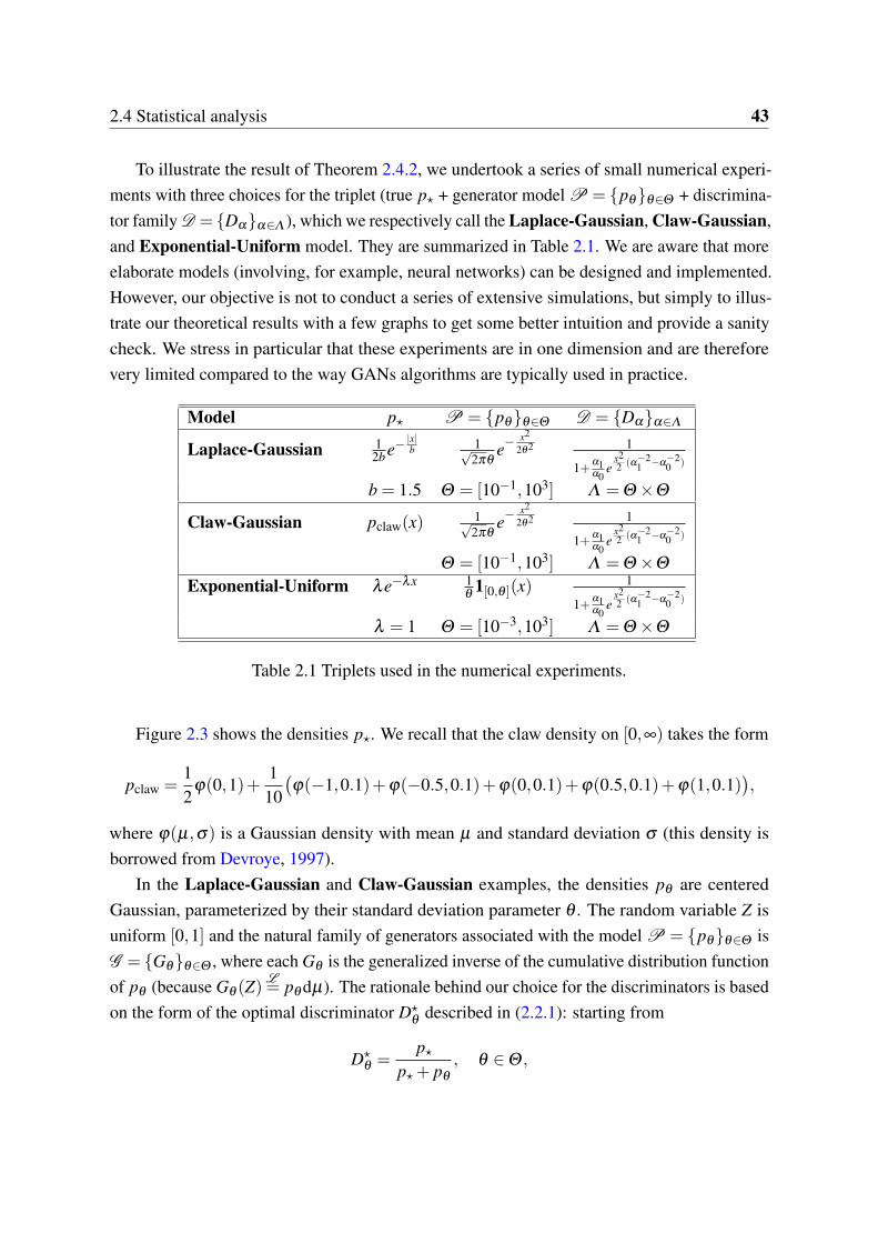
2.4 Statistical analysis 43
To illustrate the result of Theorem 2.4.2, we undertook a series of small numerical experi-ments with three choices for the triplet (true p⋆ + generator model P = pθθ∈Θ + discrimina-tor family D = Dαα∈Λ ), which we respectively call the Laplace-Gaussian, Claw-Gaussian,and Exponential-Uniform model. They are summarized in Table 2.1. We are aware that moreelaborate models (involving, for example, neural networks) can be designed and implemented.However, our objective is not to conduct a series of extensive simulations, but simply to illus-trate our theoretical results with a few graphs to get some better intuition and provide a sanitycheck. We stress in particular that these experiments are in one dimension and are thereforevery limited compared to the way GANs algorithms are typically used in practice.
Model p⋆ P = pθθ∈Θ D = Dαα∈Λ
Laplace-Gaussian 12be−
|x|b 1√
2πθe−
x2
2θ2 1
1+α1α0
ex22 (α−2
1 −α−20 )
b = 1.5 Θ = [10−1,103] Λ =Θ ×Θ
Claw-Gaussian pclaw(x) 1√2πθ
e−x2
2θ2 1
1+α1α0
ex22 (α−2
1 −α−20 )
Θ = [10−1,103] Λ =Θ ×Θ
Exponential-Uniform λe−λx 1θ
1[0,θ ](x) 1
1+α1α0
ex22 (α−2
1 −α−20 )
λ = 1 Θ = [10−3,103] Λ =Θ ×Θ
Table 2.1 Triplets used in the numerical experiments.
Figure 2.3 shows the densities p⋆. We recall that the claw density on [0,∞) takes the form
pclaw =12
ϕ(0,1)+1
10(ϕ(−1,0.1)+ϕ(−0.5,0.1)+ϕ(0,0.1)+ϕ(0.5,0.1)+ϕ(1,0.1)
),
where ϕ(µ,σ) is a Gaussian density with mean µ and standard deviation σ (this density isborrowed from Devroye, 1997).
In the Laplace-Gaussian and Claw-Gaussian examples, the densities pθ are centeredGaussian, parameterized by their standard deviation parameter θ . The random variable Z isuniform [0,1] and the natural family of generators associated with the model P = pθθ∈Θ isG = Gθθ∈Θ , where each Gθ is the generalized inverse of the cumulative distribution functionof pθ (because Gθ (Z)
L= pθ dµ). The rationale behind our choice for the discriminators is based
on the form of the optimal discriminator D⋆θ
described in (2.2.1): starting from
D⋆θ =
p⋆p⋆+ pθ
, θ ∈Θ ,

44 Some theoretical properties of GANs
Fig. 2.3 Probability density functions p⋆ used in the numerical experiments.
we logically consider the following ratio
Dα =pα1
pα1 + pα0
, α = (α0,α1) ∈ Λ =Θ ×Θ .
Figure 2.4 (Laplace-Gaussian), Figure 2.5 (Claw-Gaussian), and Figure 2.6 (Exponential-Uniform) show the boxplots of the differences θ − θ over 200 repetitions, for a sample sizen varying from 10 to 10000. In these experiments, the parameter θ is obtained by averagingthe θ for the largest sample size n. In accordance with Theorem 2.4.2, the size of the boxplotsshrinks around 0 when n increases, thus showing that the estimated parameter θ is gettingcloser and closer to θ . Before analyzing at which rate this convergence occurs, we may have alook at Figure 2.7, which plots the estimated density p
θ(for n = 10000) vs. the true density
p⋆. It also shows the discriminator Dα , together with the initial density pθ init and the initialdiscriminator Dα init fed into the optimization algorithm. We note that in the three models, Dα
is almost identically 1/2, meaning that it is impossible to discriminate between the originalobservations and those generated by p
θ.
In line with the above, our next step is to state a central limit theorem for θ . Although simpleto understand, this result requires additional assumptions and some technical prerequisites. Onefirst needs to ensure that the function (θ ,α) 7→ L(θ ,α) is regular enough in a neighborhoodof (θ , α). This is captured by the following set of assumptions, which require in particularthe uniqueness of the maximizer of the function α 7→ L(θ ,α) for a θ around θ . For afunction F : Θ → R (respectively, G : Θ ×Λ → R), we let HF(θ) (respectively, H1G(θ ,α)

2.4 Statistical analysis 45
Fig. 2.4 Boxplots of θ − θ for different sample sizes (Laplace-Gaussian model, 200 repeti-tions).
Fig. 2.5 Boxplots of θ − θ for different sample sizes (Claw-Gaussian model, 200 repetitions).
Fig. 2.6 Boxplots of θ − θ for different sample sizes (Exponential-Uniform model, 200repetitions).

46 Some theoretical properties of GANs
Fig. 2.7 True density p⋆, estimated density pθ
, and discriminator Dα for n = 10000 (fromleft to right: Laplace-Gaussian, Claw-Gaussian, and Exponential-Uniform model). Alsoshown are the initial density pθ init and the initial discriminator Dα init fed into the optimizationalgorithm.

2.4 Statistical analysis 47
and H2G(θ ,α)) be the Hessian matrix of the function θ 7→ F(θ) (respectively, θ 7→ G(θ ,α)
and α 7→ G(θ ,α)) computed at θ (respectively, at θ and α).Assumptions (Hloc)
(HU) There exists a neighborhood U of θ and a function α : U → Λ such that
argmaxα∈Λ
L(θ ,α) = α(θ), ∀θ ∈U.
(HV ) The Hessian matrix HV (θ) is invertible, where V (θ)def= L(θ ,α(θ)).
(HH) The Hessian matrix H2L(θ , α) is invertible.
We stress that under Assumption (HU), there is for each θ ∈U a unique α(θ) ∈ Λ suchthat L(θ ,α(θ)) = supα∈Λ L(θ ,α). We also note that α(θ) = α under (H1). We still needsome notation before we state the central limit theorem. For a function f (θ ,α), ∇1 f (θ ,α)
(respectively, ∇2 f (θ ,α)) means the gradient of the function θ 7→ f (θ ,α) (respectively, thefunction α 7→ f (θ ,α)) computed at θ (respectively, at α). For a function g(t), J(g)t is theJacobian matrix of g computed at t. Observe that by the envelope theorem,
HV (θ) = H1L(θ , α)+ J(∇1L(θ , ·))αJ(α)θ,
where, by the chain rule,
J(α)θ=−H2L(θ , α)−1J(∇2L(·, α))
θ.
Therefore, in Assumption(HV ), the Hessian matrix HV (θ) can be computed with the soleknowledge of L. Finally, we let
ℓ1(θ ,α) = lnDα(X1)+ ln(1−Dα Gθ (Z1)),
and denote by L→ the convergence in distribution.
Theorem 2.4.3. Under Assumptions (H ′reg), (H1), and (Hloc), one has
√n(θ − θ)
L→ Z,
where Z is a Gaussian random variable with mean 0 and covariance matrix
V = Var[−HV (θ)−1
∇1ℓ1(θ , α)+HV (θ)−1J(∇1L(θ , ·))αH2L(θ , α)−1∇2ℓ1(θ , α)
].

48 Some theoretical properties of GANs
The expression of the covariance is relatively complex and, unfortunately, cannot besimplified, even for a dimension of the parameter equal to 1. We note however that if Y is arandom vector of Rp whose components are bounded in absolute value by some δ > 0, thenthe Euclidean norm of the covariance matrix of Y is bounded by 4pδ 2. But each component ofthe random vector of Rp involved in the covariance matrix V is bounded in absolute value byCpq2, for some positive constant C resulting from Assumption (H ′
reg). We conclude that theEuclidean norm of V is bounded by 4C2 p3q4. Thus, our statistical approach reveals that in theoverparameterized regime (i.e, when p and q are very large compared to n), the estimator θ hasa large dispersion around θ , which may affects the performance of the algorithm.
Nevertheless, the take-home message of Theorem 2.4.3 is that the estimator θ is asymp-totically normal, with a convergence rate of
√n. This is illustrated in Figures 2.8, 2.9, and
2.10, which respectively show the histograms and kernel estimates of the distribution of√
n(θ − θ) for the Laplace-Gaussian, the Claw-Gaussian, and the Exponential-Uniformmodel in function of the sample size n (200 repetitions).
Proof. By technical Lemma 2.A.1, we can find under Assumptions (H ′reg) and (H1) an open
set V ⊂ U ⊂ Θ containing θ such that, for all θ ∈ V , α(θ) ∈ Λ . In the sequel, to lightenthe notation, we assume without loss of generality that V = U . Thus, for all θ ∈ U , wehave α(θ) ∈ Λ and L(θ ,α(θ)) = supα∈Λ L(θ ,α) (with α(θ) = α by (H1)). Accordingly,∇2L(θ ,α(θ)) = 0, ∀θ ∈U . Also, since H2L(θ , α) is invertible by (HH) and since the function(θ ,α) 7→ H2L(θ ,α) is continuous, there exists an open set U ′ ⊂ U such that H2L(θ ,α) isinvertible as soon as (θ ,α) ∈ (U ′,α(U ′)). Without loss of generality, we assume that U ′ =U .Thus, by the chain rule, the function α is of class C2 in a neighborhood U ′ ⊂ U of θ , sayU ′ =U , with Jacobian matrix given by
J(α)θ =−H2L(θ ,α(θ))−1J(∇2L(·,α(θ))
)θ, ∀θ ∈U.
We note that H2L(θ ,α(θ))−1 is of format q×q and J(∇2L(·,α(θ)))θ of format q× p.Now, for each θ ∈U , we let α(θ) be such that L(θ , α(θ)) = supα∈Λ L(θ ,α). Clearly,
|L(θ , α(θ))−L(θ ,α(θ))| ≤ |L(θ , α(θ))− L(θ , α(θ))|+ |L(θ , α(θ))−L(θ ,α(θ))|≤ sup
α∈Λ
|L(θ ,α)− L(θ ,α)|+ | supα∈Λ
L(θ ,α)− supα∈Λ
L(θ ,α)|
≤ 2 supα∈Λ
|L(θ ,α)−L(θ ,α)|.
Therefore, by Lemma 2.4.1, supθ∈U |L(θ , α(θ))−L(θ ,α(θ))| → 0 almost surely. The eventon which this convergence holds does not depend upon θ ∈U , and, arguing as in the proof of

2.4 Statistical analysis 49
Fig. 2.8 Histograms and kernel estimates (continuous line) of the distribution of√
n(θ − θ) fordifferent sample sizes n (Laplace-Gaussian model, 200 repetitions).
Theorem 2.4.2, we deduce that under (H1), P(α(θ)→ α(θ)∀θ ∈U) = 1. Since α(θ) ∈ Λ
for all θ ∈U , we also have P(α(θ) ∈ Λ ∀θ ∈U)→ 1 as n → ∞. Thus, in the sequel, it willbe assumed without loss of generality that, for all θ ∈U , α(θ) ∈ Λ .
Still by Lemma 2.4.1, supθ∈Θ ,α∈Λ ∥H2L(θ ,α)−H2L(θ ,α)∥ → 0 almost surely. SinceH2L(θ ,α) is invertible on U ×α(U), we have
P(H2L(θ ,α) invertible ∀(θ ,α) ∈U ×α(U)
)→ 1.
Thus, we may and will assume that H2L(θ ,α) is invertible for all (θ ,α) ∈U ×α(U).Next, since α(θ) ∈ Λ for all θ ∈U , one has ∇2L(θ , α(θ)) = 0. Therefore, by the chain
rule, α is of class C2 on U , with Jacobian matrix
J(α)θ =−H2L(θ , α(θ))−1J(∇2L(·, α(θ))
)θ, ∀θ ∈U.

50 Some theoretical properties of GANs
Fig. 2.9 Histograms and kernel estimates (continuous line) of the distribution of√
n(θ − θ) fordifferent sample sizes n (Claw-Gaussian model, 200 repetitions).
Let V (θ)def= L(θ , α(θ)) = supα∈Λ L(θ ,α). By the envelope theorem, V is of class C2,
∇V (θ) = ∇1L(θ , α(θ)), and HV (θ) = H1L(θ , α(θ))+ J(∇1L(θ , ·))α(θ)J(α)θ . Recall thatθ → θ almost surely by Theorem 2.4.2, so that we may assume that θ ∈Θ by (H1). Moreover,we can also assume that θ + t(θ − θ) ∈U , ∀t ∈ [0,1]. Thus, by a Taylor series expansion withintegral remainder, we have
0 = ∇V (θ) = ∇V (θ)+∫ 1
0HV (θ + t(θ − θ))dt(θ − θ). (2.4.3)

2.4 Statistical analysis 51
Fig. 2.10 Histograms and kernel estimates (continuous line) of the distribution of√
n(θ − θ)for different sample sizes n (Exponential-Uniform model, 200 repetitions).
Since α(θ) ∈ Λ and L(θ , α(θ)) = supα∈Λ L(θ ,α), one has ∇2L(θ , α(θ)) = 0. Thus,
0 = ∇2L(θ , α(θ))
= ∇2L(θ ,α(θ))+∫ 1
0H2L
(θ ,α(θ)+ t(α(θ)−α(θ))
)dt(α(θ)−α(θ)).
By Lemma 2.4.1, since α(θ)→ α(θ) almost surely, we have
I1def=
∫ 1
0H2L
(θ ,α(θ)+ t(α(θ)−α(θ))
)dt → H2L(θ , α) almost surely.
52 Some theoretical properties of GANs
Because H2L(θ , α) is invertible, P(I1 invertible)→ 1 as n → ∞. Therefore, we may assume,without loss of generality, that I1 is invertible. Hence,
α(θ)−α(θ) =−I−11 ∇2L(θ ,α(θ)). (2.4.4)
Furthermore,
∇V (θ) = ∇1L(θ , α(θ)) = ∇1L(θ ,α(θ))+ I2(α(θ)−α(θ)),
where
I2def=
∫ 1
0J(∇1L(θ , ·))
α(θ)+t(α(θ)−α(θ))dt.
By Lemma 2.4.1, I2 → J(∇1L(θ , ·))α(θ) almost surely. Combining (2.4.3) and (2.4.4), we
obtain0 = ∇1L(θ ,α(θ))− I2I−1
1 ∇2L(θ ,α(θ))+ I3(θ − θ),
where
I3def=
∫ 1
0HV (θ + t(θ − θ))dt.
By technical Lemma 2.A.2, we have I3 → HV (θ) almost surely. So, by (HV ), it can be assumedthat I3 is invertible. Consequently,
θ − θ =−I−13 ∇1L(θ ,α(θ))+ I−1
3 I2I−11 ∇2L(θ ,α(θ)),
or, equivalently, since α(θ) = α ,
θ − θ =−I−13 ∇1L(θ , α)+ I−1
3 I2I−11 ∇2L(θ , α).
Using Lemma 2.4.1, we conclude that√
n(θ − θ) has the same limit distribution as
Sndef=−
√nHV (θ)−1
∇1L(θ , α)+√
nHV (θ)−1J(∇1L(θ , ·))αH2L(θ , α)−1∇2L(θ , α).
Letℓi(θ ,α) = lnDα(Xi)+ ln(1−Dα Gθ (Zi)), 1 ≤ i ≤ n.
With this notation, we have
Sn =1√n
n
∑i=1
(−HV (θ)−1
∇1ℓi(θ , α)+HV (θ)−1J(∇1L(θ , ·))αH2L(θ , α)−1∇2ℓi(θ , α)
).

2.5 Conclusion and perspectives 53
One has ∇V (θ) = 0, since V (θ) = infθ∈Θ V (θ) and θ ∈ Θ . Therefore, under(H ′
reg), E∇1ℓi(θ , α) = ∇1Eℓi(θ , α) = ∇1L(θ , α) = ∇V (θ) = 0. Similarly, E∇2ℓi(θ , α) =
∇2Eℓi(θ , α) = ∇2L(θ , α) = 0, since L(θ , α) = supα∈Λ L(θ ,α) and α ∈Λ . Using the centrallimit theorem, we conclude that
√n(θ − θ)
L→ Z,
where Z is a Gaussian random variable with mean 0 and covariance matrix
V = Var[−HV (θ)−1
∇1ℓ1(θ , α)+HV (θ)−1J(∇1L(θ , ·))αH2L(θ , α)−1∇2ℓ1(θ , α)
].
2.5 Conclusion and perspectives
In this paper, we have presented a theoretical study of the original Generative AdversarialNetworks (GAN) algorithm, which consists in building a generative model of an unknowndistribution from samples from that distribution. The key idea of the procedure is to simul-taneously train the generative model (the generators) and an adversary (the discriminators)that tries to distinguish between real and generated samples. We made a small step towards abetter understanding of this generative process by analyzing some optimality properties of theproblem in terms of Jensen-Shannon divergence in Section 2.2, and explored the role of thediscriminator family via approximation arguments in Section 2.3. Finally, taking a statisticalview, we studied in Section 2.4 some large sample properties (convergence and asymptoticnormality) of the parameter describing the empirically selected generator. Some numericalexperiments were conducted to illustrate the results.
The point of view embraced in the article is statistical, in that it takes into account thevariability of the data and its impact on the quality of the estimators. This point of view isdifferent from the classical approach encountered in the literature on GANs, which mainlyfocuses on the effective computation of the parameters using optimization procedures. In thissense, our results must be thought of as a complementary insight. We realize however thatthe simplified context in which we have placed ourselves, as well as some of the assumptionswe have made, are quite far from the typical situations in which GANs algorithms are used.Thus, our work should be seen as a first step towards a more realistic understanding of GANs,and certainly not as a definitive explanation for their excellent practical performance. We givebelow three avenues of theoretical research that we believe should be explored as a priority.
1. One of the basic assumptions is that the family of densities pθθ∈Θ (associated with thegenerators Gθθ∈Θ ) and the unknown density p⋆ are dominated by the same measure
54 Some theoretical properties of GANs
µ on the same subset E of Rd . In a way, this means that we already have some kind ofinformation on the support of p⋆, which will typically be a manifold in Rd of dimensionsmaller than d′ (the dimension of Z). Therefore, the random variable Z, the dimension d′
of the so-called latent space Rd′, and the parametric model Gθθ∈Θ should be carefully
tuned in order to match this constraint. From a practical perspective, the original article ofGoodfellow et al. (2014) suggests using for Z a uniform or Gaussian distribution of smalldimension, without further investigation. Mirza and Osindero (2014) and Radford et al.(2015), who have surprisingly good practical results with a deep convolutional generator,both use a 100-dimensional uniform distribution to represent respectively 28×28 and64×64 pixel images. Many papers have been focusing on either decomposing the latentspace Rd′
to force specified portions of this space to correspond to different variations(as, e.g., in Donahue et al., 2018) or inverting the generators (e.g., Lipton and Tripathi,2017; Srivastava et al., 2017; Bojanowski et al., 2018). However, to the best of ourknowledge, there is to date no theoretical result tackling the impact of d′ and Z on theperformance of GANs, and it is our belief that a thorough mathematical investigationof this issue is needed for a better understanding of the generating process. Similarly,whenever the Gθθ∈Θ are neural networks, the link between the networks (number oflayers, dimensionality of Θ , etc.) and the target p⋆ (support, dominating measure, etc.)is also a fundamental question, which should be addressed at a theoretical level.
2. Assumptions (Hε) and (H ′ε) highlight the essential role played by the discriminators
to approximate the optimal functions D⋆θ
. We believe that this point is critical for thetheoretical analysis of GANs, and that it should be further developed in the context ofneural networks, with a potentially large number of hidden layers.
3. Theorem 2.4.2 (convergence of the estimated parameter) and Theorem 2.4.3 (asymptoticnormality) hold under the assumption that the model is identifiable (uniqueness of θ andα). This identifiability assumption is hardly satisfied in the high-dimensional context of(deep) neural networks, where the function to be optimized displays a very wild landscape,without immediate convexity or concavity. Thus, to take one more step towards a morerealistic model, it would be interesting to shift the parametric point of view and movetowards results concerning the convergence of distributions not parameters.
2.A Technical results 55
Appendix 2.A Technical results
2.A.1 Proof of Theorem 2.3.1
Let ε ∈ (0,1/(2M)), m ∈ (0,1/2), and D ∈D be such that m ≤ D ≤ 1−m and ∥D−D⋆θ∥2 ≤ ε .
Observe that
L(θ ,D) =∫
ln(D)p⋆dµ +∫
ln(1−D)pθ
dµ
=∫
ln( D
D⋆θ
)p⋆dµ +
∫ln( 1−D
1−D⋆θ
)p
θdµ +2DJS(p⋆, p
θ)− ln4. (2.A.1)
We first derive a lower bound on the quantity
I def=
∫ln( D
D⋆θ
)p⋆dµ +
∫ln( 1−D
1−D⋆θ
)p
θdµ
=∫
ln(D(p⋆+ p
θ)
p⋆
)p⋆dµ +
∫ln((1−D)(p⋆+ p
θ)
pθ
)p
θdµ.
Let dp⋆ = p⋆dµ , dPθ= p
θdµ ,
dκ =D(p⋆+ p
θ)∫
D(p⋆+ pθ)dµ
dµ, and dκ′ =
(1−D)(p⋆+ pθ)∫
(1−D)(p⋆+ pθ)dµ
dµ.
Observe, since m ≤ D ≤ 1−m, that p⋆ ≪ κ and Pθ≪ κ ′. With this notation, we have
I =−DKL(p⋆ ∥ κ)−DKL(Pθ∥ κ
′)+ ln[∫
D(p⋆+ pθ)dµ
(2−
∫D(p⋆+ p
θ)dµ
)]. (2.A.2)
Since ∫D(p⋆+ p
θ)dµ =
∫(D−D⋆
θ)(p⋆+ p
θ)dµ +1,
the Cauchy-Schwartz inequality leads to∣∣∣∫ D(p⋆+ pθ)dµ −1
∣∣∣≤ ∥D−D⋆θ∥2∥p⋆+ p
θ∥2
≤ 2Mε, (2.A.3)

56 Some theoretical properties of GANs
because both p⋆ and pθ
are bounded by M. Thus,
ln[∫
D(p⋆+ pθ)dµ
(2−
∫D(p⋆+ p
θ)dµ
)]≥ ln(1−4M2
ε2)
≥− 4M2ε2
1−4M2ε2 , (2.A.4)
using the inequality ln(1−x)≥−x/(1−x) for x ∈ [0,1). Moreover, recalling that the Kullback-Leibler divergence is smaller than the chi-square divergence, and letting F = F/(
∫Fdµ) for
F ∈ L1(µ), we have
DKL(p⋆ ∥ κ)≤∫ ( p⋆
D(p⋆+ pθ)−1
)2D(p⋆+ p
θ)dµ.
Hence, letting J def=
∫D(p⋆+ p
θ)dµ , we see that
DKL(p⋆ ∥ κ)
≤ 1J
∫ (p⋆
∫D(p⋆+ p
θ)dµ −D(p⋆+ p
θ))2 1
D(p⋆+ pθ)dµ
=1J
∫ (p⋆
∫(D−D⋆
θ)(p⋆+ p
θ)dµ +(D⋆
θ−D)(p⋆+ p
θ))2 1
D(p⋆+ pθ)dµ.
Since ε < 1/(2M), inequality (2.A.3) gives 1/J ≤ c1 for some constant c1 > 0. By Cauchy-Schwarz and (a+b)2 ≤ 2(a2 +b2), we obtain
DKL(p⋆ ∥ κ)
≤ 2c1
(∫ (∫(D−D⋆
θ)(p⋆+ p
θ)dµ
)2 (p⋆)2
D(p⋆+ pθ)dµ +
∫(D⋆
θ−D)2 p⋆+ p
θ
Ddµ
)≤ 2c1
(∥D−D⋆
θ∥2
2∥p⋆+ pθ∥2
2
∫(p⋆)2
D(p⋆+ pθ)dµ +
∫(D⋆
θ−D)2 p⋆+ p
θ
Ddµ
).
Therefore, since p⋆ ≤ M, pθ≤ M, and D ≥ m,
DKL(p⋆ ∥ κ)≤ 2c1
(4M2
m+
2Mm
)ε
2.
One proves with similar arguments that
DKL(Pθ∥ κ
′)≤ 2c1
(4M2
m+
2Mm
)ε
2.

2.A Technical results 57
Combining these two inequalities with (2.A.2) and (2.A.4), we see that I ≥ −c2ε2 for someconstant c2 > 0 that depends only upon M and m. Getting back to identity (2.A.1), we concludethat
2DJS(p⋆, pθ)≤ c2ε
2 +L(θ ,D)+ ln4.
But
L(θ ,D)≤ supD∈D
L(θ ,D)≤ supD∈D
L(θ ⋆,D)
(by definition of θ )
≤ supD∈D∞
L(θ ⋆,D)
= L(θ ⋆,D⋆θ⋆) = 2DJS(p⋆, pθ⋆)− ln4.
Thus,2DJS(p⋆, p
θ)≤ c2ε
2 +2DJS(p⋆, pθ⋆).
This shows the right-hand side of inequality (2.3.1). To prove the left-hand side, just note thatby inequality (2.2.2),
DJS(p⋆, pθ⋆)≤ DJS(p⋆, pθ).
2.A.2 Proof of Lemma 2.4.1
To simplify the notation, we set
∆ =∂ a+b+c+d
∂θ ai ∂θ b
j ∂αcℓ∂αd
m.
Using McDiarmid’s inequality (McDiarmid, 1989), we see that there exists a constant c > 0such that, for all ε > 0,
P(∣∣∣ sup
θ∈Θ ,α∈Λ
|∆ L(θ ,α)−∆L(θ ,α)|−E supθ∈Θ ,α∈Λ
|∆ L(θ ,α)−∆L(θ ,α)|∣∣∣≥ ε
)≤ 2e−cnε2
.
Therefore, by the Borel-Cantelli lemma,
supθ∈Θ ,α∈Λ
|∆ L(θ ,α)−∆L(θ ,α)|−E supθ∈Θ ,α∈Λ
|∆ L(θ ,α)−∆L(θ ,α)| → 0 almost surely.
(2.A.5)It is also easy to verify that under Assumptions (H ′
reg), the process (∆ L(θ ,α) −∆L(θ ,α))θ∈Θ ,α∈Λ is subgaussian. Thus, as in the proof of Theorem 2.4.1, we obtain via

58 Some theoretical properties of GANs
Dudley’s inequality that
E supθ∈Θ ,α∈Λ
|∆ L(θ ,α)−∆L(θ ,α)|= O( 1√
n
), (2.A.6)
since E∆ L(θ ,α) = ∆L(θ ,α). The result follows by combining (2.A.5) and (2.A.6).
2.A.3 Some technical lemmas
Lemma 2.A.1. Under Assumptions (H ′reg) and (H1), there exists an open set V ⊂Θ containing
θ such that, for all θ ∈V , argmaxα∈Λ L(θ ,α)∩Λ = /0.
Proof. Assume that the statement is not true. Then there exists a sequence (θk)k ⊂Θ such thatθk → θ and, for all k, αk ∈ ∂Λ , where αk ∈ argmaxα∈Λ L(θk,α). Thus, since Λ is compact,even if this means extracting a subsequence, one has αk → z ∈ ∂Λ as k → ∞. By the continuityof L, L(θ ,αk)→ L(θ ,z). But
|L(θ ,αk)−L(θ , α)| ≤ |L(θ ,αk)−L(θk,αk)|+ |L(θk,αk)−L(θ , α)|≤ sup
α∈Λ
|L(θ ,α)−L(θk,α)|+ | supα∈Λ
L(θk,α)− supα∈Λ
L(θ ,α)|
≤ 2 supα∈Λ
|L(θ ,α)−L(θk,α)|,
which tends to zero as k → ∞ by (H ′D) and (H ′
p). Therefore, L(θ ,z) = L(θ , α) and, in turn,z = α by (H1). Since z ∈ ∂∆ and α ∈ ∆ , this is a contradiction.
Lemma 2.A.2. Under Assumptions (H ′reg), (H1), and (Hloc), one has I3 → HV (θ) almost
surely.
Proof. We have
I3 =∫ 1
0HV (θ + t(θ − θ))dt =
∫ 1
0
(H1L(θt , α(θt))+ J(∇1L(θt , ·))α(θt)
J(α)θt
)dt,
where we set θt = θ + t(θ − θ). Note that θt ∈U for all t ∈ [0,1]. By Lemma 2.4.1,
supt∈[0,1]
∥H1L(θt , α(θt))−H1L(θt , α(θt))∥
≤ supθ∈Θ ,α∈Λ
∥H1L(θ ,α)−H1L(θ ,α)∥→ 0 almost surely.

2.A Technical results 59
Also, by Theorem 2.4.2, for all t ∈ [0,1], θt → θ almost surely. Besides,
|L(θ , α(θt))−L(θ ,α(θ))| ≤ |L(θ , α(θt))−L(θt , α(θt))|+ |L(θt , α(θt))−L(θ ,α(θ))|≤ sup
α∈Λ
|L(θ ,α)−L(θt ,α)|+2 supθ∈Θ ,α∈Λ
|L(θ ,α)−L(θ ,α)|.
Thus, via (H ′reg), (H1), and Lemma 2.4.1, we conclude that almost surely, for all t ∈ [0,1],
α(θt)→ α(θ) = α . Accordingly, almost surely, for all t ∈ [0,1], H1L(θt , α(θt))→ H1L(θ , α).Since H1L(θ ,α) is bounded under (H ′
D) and (H ′p), the Lebesgue dominated convergence
theorem leads to ∫ 1
0H1L(θt , α(θt))dt → H1L(θ , α) almost surely. (2.A.7)
Furthermore,
J(α)θ =−H2L(θ , α(θ))−1J(∇2L(·, α(θ))
)θ, ∀(θ ,α) ∈U ×α(U),
where U is the open set defined in the proof of Theorem 2.4.3. By the cofactor method,H2L(θ ,α)−1 takes the form
H2L(θ ,α)−1 =c(θ ,α)
det(H2L(θ ,α)),
where c(θ ,α) is the matrix of cofactors associated with H2L(θ ,α). Thus, each componentof −H2L(θ ,α)−1J(∇2L(·,α))θ is a quotient of a multilinear form of the partial derivativesof L evaluated at (θ ,α) divided by det(H2L(θ ,α)), which is itself a multilinear form in the
∂ 2L∂αi∂α j
(θ ,α). Hence, by Lemma 2.4.1, we have
supθ∈U,α∈α(U)
∥H2L(θ ,α)−1J(∇2L(·,α))θ −H2L(θ ,α)−1J(∇2L(·,α))θ∥→ 0 almost surely.
So, for all n large enough,
supt∈[0,1]
∥J(α)θt+H2L(θt , α(θt))
−1J(∇2L(·, α(θt))
)θt∥
≤ supθ∈U,α∈α(U)
∥H2L(θ ,α)−1J(∇2L(·,α))θ −H2L(θ ,α)−1J(∇2L(·,α))θ∥
→ 0 almost surely.

60 Some theoretical properties of GANs
We know that almost surely, for all t ∈ [0,1], α(θt)→ α . Thus, since the function U ×α(U) ∋(θ ,α) 7→ H2L(θ ,α)−1J(∇2L(·,α))θ is continuous, we have almost surely, for all t ∈ [0,1],
H2L(θt , α(θt))−1J
(∇2L(·, α(θt))
)θt→ H2L(θ , α)−1J(∇2L(·, α))
θ.
Therefore, almost surely, for all t ∈ [0,1], J(α)θt→ J(α)
θ. Similarly, almost surely, for all
t ∈ [0,1], J(∇1L(θt , ·))α(θt)→ J(∇1L(θ , ·))α . All involved quantities are uniformly bounded
in t, and so, by the Lebesgue dominated convergence theorem, we conclude that
∫ 1
0J(∇1L(θt , ·))α(θt)
J(α)θt
dt → J(∇1L(θ , ·))αJ(α)θ
almost surely. (2.A.8)
Consequently, by combining (2.A.7) and (2.A.8),
I3 → H1L(θ , α)+ J(∇1L(θ , ·))αJ(α)θ= HV (θ) almost surely,
as desired.
Acknowledgments
We thank Flavian Vasile (Criteo) and Antoine Picard-Weibel (ENS Ulm) for stimulatingdiscussions and insightful suggestions. We also thank the Associate Editor and two anonymousreferees for their careful reading of the paper and constructive comments, which led to asubstantial improvement of the document.

Chapter 3
Some theoretical properties ofWasserstein GANs
AbstractGenerative Adversarial Networks (GANs) have been successful in producing outstanding results inareas as diverse as image, video, and text generation. Building on these successes, a large number ofempirical studies have validated the benefits of the cousin approach called Wasserstein GANs (WGANs),which brings stabilization in the training process. In the present paper, we add a new stone to the edificeby proposing some theoretical advances in the properties of WGANs. First, we properly define thearchitecture of WGANs in the context of integral probability metrics parameterized by neural networksand highlight some of their basic mathematical features. We stress in particular interesting optimizationproperties arising from the use of a parametric 1-Lipschitz discriminator. Then, in a statistically-drivenapproach, we study the convergence of empirical WGANs as the sample size tends to infinity, and clarifythe adversarial effects of the generator and the discriminator by underlining some trade-off properties.These features are finally illustrated with experiments using both synthetic and real-world datasets.
Contents3.1 Introduction . . . . . . . . . . . . . . . . . . . . . . . . . . . . . . . . . 62
3.2 Wasserstein GANs . . . . . . . . . . . . . . . . . . . . . . . . . . . . . . 64
3.3 Optimization properties . . . . . . . . . . . . . . . . . . . . . . . . . . . 71
3.4 Asymptotic properties . . . . . . . . . . . . . . . . . . . . . . . . . . . . 80
3.5 Understanding the performance of WGANs . . . . . . . . . . . . . . . . 85
Appendix 3.A Technical results . . . . . . . . . . . . . . . . . . . . . . . . . 91

62 Some theoretical properties of Wasserstein GANs
3.1 Introduction
Generative Adversarial Networks (GANs) is a generative framework proposed by Goodfellowet al. (2014), in which two models (a generator and a discriminator) act as adversaries in azero-sum game. Leveraging the recent advances in deep learning, and specifically convolutionalneural networks (LeCun et al., 1998), a large number of empirical studies have shown theimpressive possibilities of GANs in the field of image generation (Radford et al., 2015; Lediget al., 2017; Karras et al., 2018; Brock et al., 2019). Lately, Karras et al. (2019) proposed anarchitecture able to generate hyper-realistic fake human faces that cannot be differentiated fromreal ones (see the website thispersondoesnotexist.com). The recent surge of interest in thedomain also led to breakthroughs in video (Acharya et al., 2018), music (Mogren, 2016), andtext generation (Yu et al., 2017; Fedus et al., 2018), among many other potential applications.
The aim of GANs is to generate data that look “similar” to samples collected from someunknown probability measure µ⋆, defined on a Borel subset E ofRD. In the targeted applicationsof GANs, E is typically a submanifold (possibly hard to describe) of a high-dimensional RD,which therefore prohibits the use of classical density estimation techniques. GANs approachthe problem by making two models compete: the generator, which tries to imitate µ⋆ using thecollected data, vs. the discriminator, which learns to distinguish the outputs of the generatorfrom the samples, thereby forcing the generator to improve its strategy.
Formally, the generator has the form of a parameterized class of Borel functions from Rd
to E, say G = Gθ : θ ∈ Θ, where Θ ⊆ RP is the set of parameters describing the model.Each function Gθ takes as input a d-dimensional random variable Z—it is typically uniform orGaussian, with d usually small—and outputs the “fake” observation Gθ (Z) with distributionµθ . Thus, the collection of probability measures P = µθ : θ ∈ Θ is the natural class ofdistributions associated with the generator, and the objective of GANs is to find inside this classthe distribution that generates the most realistic samples, closest to the ones collected from theunknown µ⋆. On the other hand, the discriminator is described by a family of Borel functionsfrom E to [0,1], say D = Dα : α ∈ Λ, Λ ⊆RQ, where each Dα must be thought of as theprobability that an observation comes from µ⋆ (the higher D(x), the higher the probability thatx is drawn from µ⋆).
In the original formulation of Goodfellow et al. (2014), GANs make G and D fight eachother through the following objective:
infθ∈Θ
supα∈Λ
[E log(Dα(X))+E log(1−Dα(Gθ (Z)))
], (3.1.1)

3.1 Introduction 63
where X is a random variable with distribution µ⋆ and the symbol E denotes expectation. Sinceone does not have access to the true distribution, µ⋆ is replaced in practice with the empiri-cal measure µn based on independent and identically distributed (i.i.d.) samples X1, . . . ,Xn
distributed as X , and the practical objective becomes
infθ∈Θ
supα∈Λ
[1n
n
∑i=1
log(Dα(Xi))+E log(1−Dα(Gθ (Z)))]. (3.1.2)
In the literature on GANs, both G and D take the form of neural networks (either feed-forwardor convolutional, when dealing with image-related applications). This is also the case inthe present paper, in which the generator and the discriminator will be parameterized byfeed-forward neural networks with, respectively, rectifier (Glorot et al., 2011) and GroupSort(Chernodub and Nowicki, 2016) activation functions. We also note that from an optimizationstandpoint, the minimax optimum in (3.1.2) is found by using stochastic gradient descentalternatively on the generator’s and the discriminator’s parameters.
In the initial version (3.1.1), GANs were shown to reduce, under appropriate conditions,the Jensen-Shanon divergence between the true distribution and the class of parameterizeddistributions (Goodfellow et al., 2014). This characteristic was further explored by Biau et al.(2020), who stressed some theoretical guarantees regarding the approximation and statisticalproperties of problems (3.1.1) and (3.1.2). However, many empirical studies (e.g., Metz et al.,2016; Salimans et al., 2016) have described cases where the optimal generative distributioncomputed by solving (3.1.2) collapses to a few modes of the distribution µ⋆. This phenomenonis known under the term of mode collapse and has been theoretically explained by Arjovskyet al. (2017). As a striking result, in cases where both µ⋆ and µθ lie on disjoint supports, theseauthors proved the existence of a perfect discriminator with null gradient on both supports,which consequently does not convey meaningful information to the generator.
To cancel this drawback and stabilize training, Arjovsky et al. (2017) proposed a modifica-tion of criterion (3.1.1), with a framework called Wasserstein GANs (WGANs). In a nutshell,the objective of WGANs is to find, inside the class of parameterized distributions P , the onethat is the closest to the true µ⋆ with respect to the Wasserstein distance (Villani, 2008). In itsdual form, the Wasserstein distance can be considered as an integral probability metric (IPM,Müller, 1997) defined on the set of 1-Lipschitz functions. Therefore, the proposal of Arjovskyet al. (2017) is to replace the 1-Lipschitz functions with a discriminator parameterized by neuralnetworks. To practically enforce this discriminator to be a subset of 1-Lipschitz functions, theauthors use a weight clipping technique on the set of parameters. A decisive step has been takenby Gulrajani et al. (2017), who stressed the empirical advantage of the WGANs architecture byreplacing the weight clipping with a gradient penalty. Since then, WGANs have been largely

64 Some theoretical properties of Wasserstein GANs
recognized and studied by the Machine Learning community (e.g., Roth et al., 2017; Petzkaet al., 2018; Wei et al., 2018; Karras et al., 2019).
A natural question regards the theoretical ability of WGANs to learn µ⋆, considering thatone only has access to the parametric models of generative distributions and discriminativefunctions. Previous works in this direction are those of Liang (2018) and Zhang et al. (2018),who explore generalization properties of WGANs. In the present paper, we make one stepfurther in the analysis of mathematical forces driving WGANs and contribute to the literaturein the following ways:
(i) We properly define the architecture of WGANs parameterized by neural networks. Then,we highlight some properties of the IPM induced by the discriminator, and finally stresssome basic mathematical features of the WGANs framework (Section 3.2).
(ii) We emphasize the impact of operating with a parametric discriminator contained inthe set of 1-Lipschitz functions. We introduce in particular the notion of monotonousequivalence and discuss its meaning in the mechanism of WGANs. We also highlight theessential role played by piecewise linear functions (Section 3.3).
(iii) In a statistically-driven approach, we derive convergence rates for the IPM induced bythe discriminator, between the target distribution µ⋆ and the distribution output by theWGANs based on i.i.d. samples (Section 3.4).
(iv) Building upon the above, we clarify the adversarial effects of the generator and thediscriminator by underlining some trade-off properties. These features are illustrated withexperiments using both synthetic and real-world datasets (Section 3.5).
For the sake of clarity, proofs of the most technical results are gathered in the Appendix.
3.2 Wasserstein GANs
The present section is devoted to the presentation of the WGANs framework. After havinggiven a first set of definitions and results, we stress the essential role played by IPMs and studysome optimality properties of WGANs.
3.2.1 Notation and definitions
Throughout the paper, E is a Borel subset of RD, equipped with the Euclidean norm ∥ · ∥, onwhich µ⋆ (the target probability measure) and the µθ ’s (the candidate probability measures)

3.2 Wasserstein GANs 65
are defined. Depending on the practical context, E can be equal to RD, but it can also be asubmanifold of it. We emphasize that there is no compactness assumption on E.
For K ⊆ E, we let C(K) (respectively, Cb(K)) be the set of continuous (respectively,continuous bounded) functions from K to R. We denote by Lip1 the set of 1-Lipschitz real-valued functions on E, i.e.,
Lip1 =
f : E →R : | f (x)− f (y)|⩽ ∥x− y∥, (x,y) ∈ E2.The notation P(E) stands for the collection of Borel probability measures on E, and P1(E) forthe subset of probability measures with finite first moment, i.e.,
P1(E) =
µ ∈ P(E) :∫
E∥x0 − x∥µ(dx)< ∞
,
where x0 ∈ E is arbitrary (this set does not depend on the choice of the point x0). Until the end,it is assumed that µ⋆ ∈ P1(E). It is also assumed throughout that the random variable Z ∈Rd isa sub-Gaussian random vector (Jin et al., 2019), i.e., Z is integrable and there exists γ > 0 suchthat
∀v ∈Rd, Eev·(Z−EZ) ⩽ eγ2∥v∥2
2 ,
where · denotes the dot product in Rd and ∥ · ∥ the Euclidean norm. The sub-Gaussian propertyis a constraint on the tail of the probability distribution. As an example, Gaussian randomvariables on the real line are sub-Gaussian and so are bounded random vectors. We note thatZ has finite moments of all nonnegative orders (Jin et al., 2019, Lemma 2). Assuming that Zis sub-Gaussian is a mild requirement since, in practice, its distribution is most of the timeuniform or Gaussian.
As highlighted earlier, both the generator and the discriminator are assumed to be parame-terized by feed-forward neural networks, that is,
G = Gθ : θ ∈Θ and D = Dα : α ∈ Λ
with Θ ⊆RP, Λ ⊆RQ, and, for all z ∈Rd ,
Gθ (z) = UpD×up−1
σ(
Up−1up−1×up−2
· · ·σ( U2u2×u1
σ( U1u1×d
z+ b1u1×1
)+ b2u2×1
) · · ·+ bp−1up−1×1
)+ bp
D×1, (3.2.1)
for all x ∈ E,
Dα(x) = Vq1×vq−1
σ( Vq−1vq−1×vq−2
· · · σ( V2v2×v1
σ( V1v1×D
x+ c1v1×1
)+ c2v2×1
)+ · · ·+ cq−1vq−1×1
)+ cq1×1
, (3.2.2)

66 Some theoretical properties of Wasserstein GANs
where p,q⩾ 2 and the characters below the matrices indicate their dimensions (lines×columns).Some comments on the notation are in order. Networks in G and D have, respectively, (p−1)and (q− 1) hidden layers. Hidden layers from depth 1 to (p− 1) (for the generator) andfrom depth 1 to (q−1) (for the discriminator) are assumed to be of respective even widths ui,i = 1, . . . , p−1, and vi, i = 1, . . . ,q−1. The matrices Ui (respectively, Vi) are the matrices ofweights between layer i and layer (i+1) of the generator (respectively, the discriminator), andthe bi’s (respectively, the ci’s) are the corresponding offset vectors (in column format). We letσ(x) = max(x,0) be the rectifier activation function (applied componentwise) and
σ(x1,x2, . . . ,x2n−1,x2n) = (max(x1,x2),min(x1,x2), . . . ,max(x2n−1,x2n),min(x2n−1,x2n))
be the GroupSort activation function with a grouping size equal to 2 (applied on pairs ofcomponents, which makes sense in (3.2.2) since the widths of the hidden layers are assumed tobe even). GroupSort has been introduced in Chernodub and Nowicki (2016) as a 1-Lipschitzactivation function that preserves the gradient norm of the input. This activation can recover therectifier, in the sense that σ(x,0) = (σ(x),−σ(−x)), but the converse is not true. The presenceof GroupSort is critical to guarantee approximation properties of Lipschitz neural networks(Anil et al., 2019), as we will see later.
Therefore, denoting by M( j,k) the space of matrices with j rows and k columns, wehave U1 ∈ M(u1,d), V1 ∈ M(v1,D), b1 ∈ M(u1,1), c1 ∈ M(v1,1), Up ∈ M(D,up−1), Vq ∈ M(1,vq−1),bp ∈ M(D,1), cq ∈ M(1,1). All the other matrices Ui, i = 2, . . . , p−1, and Vi, i = 2, . . . ,q−1,belong to M(ui,ui−1) and M(vi,vi−1), and vectors bi, i= 2, . . . , p−1, and ci, i= 2, . . . ,q−1, belongto M(ui,1) and M(vi,1). So, altogether, the vectors θ = (U1, . . . ,Up,b1, . . . ,bp) (respectively,the vectors α = (V1, . . . ,Vq,c1, . . . ,cq)) represent the parameter space Θ of the generator G
(respectively, the parameter space Λ of the discriminator D). We stress the fact that the outputsof networks in D are not restricted to [0,1] anymore, as is the case for the original GANs ofGoodfellow et al. (2014). We also recall the notation P = µθ : θ ∈Θ, where, for each θ ,µθ is the probability distribution of Gθ (Z). Since Z has finite first moment and each Gθ ispiecewise linear, it is easy to see that P ⊂ P1(E).
Throughout the manuscript, the notation ∥ · ∥ (respectively, ∥ · ∥∞) means the Euclidean(respectively, the supremum) norm on Rk, with no reference to k as the context is clear. ForW = (wi, j) a matrix in M(k1,k2), we let ∥W∥2 = sup∥x∥=1 ∥Wx∥ be the 2-norm of W . Similarly,the ∞-norm of W is ∥W∥∞ = sup∥x∥∞=1 ∥Wx∥∞ = maxi=1,...,k1 ∑
k2j=1 |wi, j|. We will also use the
(2,∞)-norm of W , i.e., ∥W∥2,∞ = sup∥x∥=1 ∥Wx∥∞. We shall constantly need the followingassumption:
3.2 Wasserstein GANs 67
Assumption 1. For all θ = (U1, . . . ,Up,b1, . . . ,bp) ∈Θ ,
max(∥Ui∥2,∥bi∥2 : i = 1, . . . , p)⩽ K1,
where K1 > 0 is a constant. Besides, for all α = (V1, . . . ,Vq,c1, . . . ,cq) ∈ Λ ,
∥V1∥2,∞ ⩽ 1, max(∥V2∥∞, . . . ,∥Vq∥∞)⩽ 1, and max(∥ci∥∞ : i = 1, . . . ,q)⩽ K2,
where K2 ⩾ 0 is a constant.
This compactness requirement is classical when parameterizing WGANs (e.g., Arjovskyet al., 2017; Zhang et al., 2018; Anil et al., 2019). In practice, one can satisfy Assumption 1 byclipping the parameters of neural networks as proposed by Arjovsky et al. (2017). An alternativeapproach to enforce D ⊆ Lip1 consists in penalizing the gradient of the discriminative functions,as proposed by Gulrajani et al. (2017), Kodali et al. (2017), Wei et al. (2018), and Zhou et al.(2019). This solution was empirically found to be more stable. The usefulness of Assumption 1is captured by the following lem.
Lemma 3.2.1. Assume that Assumption 1 is satisfied. Then, for each θ ∈Θ , the function Gθ isK p
1 -Lipschitz on Rd . In addition, D ⊆ Lip1.
Recall (e.g., Dudley, 2004) that a sequence of probability measures (µk) on E is said toconverge weakly to a probability measure µ on E if, for all ϕ ∈Cb(E),∫
Eϕ dµk →
k→∞
∫E
ϕ dµ.
In addition, the sequence of probability measures (µk) in P1(E) is said to converge weaklyin P1(E) to a probability measure µ in P1(E) if (i) (µk) converges weakly to µ and if (ii)∫
E ∥x0 − x∥µk(dx) →∫
E ∥x0 − x∥µ(dx), where x0 ∈ E is arbitrary (Villani, 2008, Definition6.7). The next proposition offers a characterization of our collection of generative distributionsP in terms of compactness with respect to the weak topology in P1(E). This result is interestingas it gives some insight into the class of probability measures generated by neural networks.
Proposition 3.2.1. Assume that Assumption 1 is satisfied. Then the function Θ ∋ θ 7→ µθ iscontinuous with respect to the weak topology in P1(E), and the set of generative distributionsP is compact with respect to the weak topology in P1(E).

68 Some theoretical properties of Wasserstein GANs
3.2.2 The WGANs and T-WGANs problems
We are now in a position to formally define the WGANs problem. The Wasserstein distance (oforder 1) between two probability measures µ and ν in P1(E) is defined by
W1(µ,ν) = infπ∈Π(µ,ν)
∫E×E
∥x− y∥π(dx,dy),
where Π(µ,ν) denotes the collection of all joint probability measures on E ×E with marginalsµ and ν (e.g., Villani, 2008). It is a finite quantity. In the present article, we will use thedual representation of W1(µ,ν), which comes from the duality theorem of Kantorovich andRubinstein (1958):
W1(µ,ν) = supf∈Lip1
|Eµ f −Eν f |,
where, for a probability measure π , Eπ f =∫
E f dπ (note that for f ∈ Lip1 and π ∈ P1(E), thefunction f is Lebesgue integrable with respect to π).
In this context, it is natural to define the theoretical-WGANs (T-WGANs) problem asminimizing over Θ the Wasserstein distance between µ⋆ and the µθ ’s, i.e.,
infθ∈Θ
W1(µ⋆,µθ ) = infθ∈Θ
supf∈Lip1
|Eµ⋆ f −Eµθf |. (3.2.3)
In practice, however, one does not have access to the class of 1-Lipschitz functions, whichcannot be parameterized. Therefore, following Arjovsky et al. (2017), the class Lip1 is restrictedto the smaller but parametric set of discriminators D = Dα : α ∈ Λ (it is a subset of Lip1, byLemma 3.2.1), and this defines the actual WGANs problem:
infθ∈Θ
supα∈Λ
|Eµ⋆Dα −EµθDα |. (3.2.4)
Problem (3.2.4) is the Wasserstein counterpart of problem (3.1.1). Provided Assumption 1 issatisfied, D ⊆ Lip1, and the IPM (Müller, 1997) dD is defined for (µ,ν) ∈ P1(E)2 by
dD(µ,ν) = supf∈D
|Eµ f −Eν f |. (3.2.5)
With this notation, dLip1=W1 and problems (3.2.3) and (3.2.4) can be rewritten as the mini-
mization over Θ of, respectively, dLip1(µ⋆,µθ ) and dD(µ⋆,µθ ). So,
T-WGANs: infθ∈Θ
dLip1(µ⋆,µθ ) and WGANs: inf
θ∈ΘdD(µ⋆,µθ ).

3.2 Wasserstein GANs 69
Similar objectives have been proposed in the literature, in particular neural net distances (Aroraet al., 2017) and adversarial divergences (Liu et al., 2017). These two general approachesinclude f-GANs (Goodfellow et al., 2014; Nowozin et al., 2016), but also WGANs (Arjovskyet al., 2017), MMD-GANs (Li et al., 2017), and energy-based GANs (Zhao et al., 2016). Usingthe terminology of Arora et al. (2017), dD is called a neural IPM. If the theoretical propertiesof the Wasserstein distance dLip1
have been largely studied (e.g., Villani, 2008), the story isdifferent for neural IPMs. This is why our next subsection is devoted to the properties of dD .
3.2.3 Some properties of the neural IPM
The study of the neural IPM dD is essential to assess the driving forces of WGANs architectures.Let us first recall that a mapping ℓ : P1(E)×P1(E)→ [0,∞) is a metric if it satisfies the followingthree requirements:
(i) ℓ(µ,ν) = 0 ⇐⇒ µ = ν (discriminative property)
(ii) ℓ(µ,ν) = ℓ(ν ,µ) (symmetry)
(iii) ℓ(µ,ν)⩽ ℓ(µ,π)+ ℓ(π,ν) (triangle inequality).
If (i) is replaced by the weaker requirement ℓ(µ,µ) = 0 for all µ ∈ P1(E), then one speaks ofa pseudometric. Furthermore, the (pseudo)metric ℓ is said to metrize weak convergencein P1(E) (Villani, 2008) if, for all sequences (µk) in P1(E) and all µ in P1(E), one hasℓ(µ,µk)→ 0 ⇐⇒ µk converges weakly to µ in P1(E) as k → ∞. According to Villani (2008,Theorem 6.8), dLip1
is a metric that metrizes weak convergence in P1(E).As far as dD is concerned, it is clearly a pseudometric on P1(E) as soon as Assumption
1 is satisfied. Moreover, an elementary application of Dudley (2004, Lemma 9.3.2) showsthat if span(D) (with span(D) = γ0 +∑
ni=1 γiDi : γi ∈R,Di ∈ D ,n ∈N) is dense in Cb(E),
then dD is a metric on P1(E), which, in addition, metrizes weak convergence. As in Zhanget al. (2018), Dudley’s result can be exploited in the case where the space E is compact toprove that, whenever D is of the form (3.2.2), dD is a metric metrizing weak convergence.However, establishing the discriminative property of the pseudometric dD turns out to be morechallenging without an assumption of compactness on E, as is the case in the present study.Our result is encapsulated in the following proposition.
Proposition 3.2.2. Assume that Assumption 1 is satisfied. Then there exists a discriminator ofthe form (3.2.2) (i.e., a depth q and widths v1, . . . ,vq−1) such that dD is a metric on P ∪µ⋆.In addition, dD metrizes weak convergence in P ∪µ⋆.

70 Some theoretical properties of Wasserstein GANs
Standard universal approximation theorems (Cybenko, 1989; Hornik et al., 1989; Hornik,1991) state the density of neural networks in the family of continuous functions defined oncompact sets but do not guarantee that the approximator respects a Lipschitz constraint. Theproof of Proposition 3.2.2 uses the fact that, under Assumption 1, neural networks of the form(3.2.2) are dense in the space of Lipschitz continuous functions on compact sets, as revealed byAnil et al. (2019).
We deduce from Proposition 3.2.2 that, under Assumption 1, provided enough capacity, thepseudometric dD can be topologically equivalent to dLip1
on P ∪µ⋆, i.e., the convergentsequences in (P ∪µ⋆,dD) are the same as the convergent sequences in (P ∪µ⋆,dLip1
)
with the same limit—see O’Searcoid (2006, Corollary 13.1.3). We are now ready to discusssome optimality properties of the T-WGANs and WGANs problems, i.e., conditions underwhich the infimum in θ ∈Θ and the supremum in α ∈ Λ are reached.
3.2.4 Optimality properties
Recall that for T-WGANs, we minimize over Θ the distance
dLip1(µ⋆,µθ ) = sup
f∈Lip1
|Eµ⋆ f −Eµθf |,
whereas for WGANs, we use
dD(µ⋆,µθ ) = supα∈Λ
|Eµ⋆Dα −EµθDα |.
A first natural question is to know whether for a fixed generator parameter θ ∈Θ , there existsa 1-Lipschitz function (respectively, a discriminative function) that achieves the supremumin dLip1
(µ⋆,µθ ) (respectively, in dD(µ⋆,µθ )) over all f ∈ Lip1 (respectively, all α ∈ Λ ). ForT-WGANs, Villani (2008, Theorem 5.9) guarantees that the maximum exists, i.e.,
f ∈ Lip1 : |Eµ⋆ f −Eµθf |= dLip1
(µ⋆,µθ ) =∅. (3.2.6)
For WGANs, we have the following:
Lemma 3.2.2. Assume that Assumption 1 is satisfied. Then, for all θ ∈Θ ,
α ∈ Λ : |Eµ⋆Dα −EµθDα |= dD(µ⋆,µθ ) =∅.
Thus, provided Assumption 1 is verified, the supremum in α in the neural IPM dD is alwaysreached. A similar result is proved by Biau et al. (2020) in the case of standard GANs.

3.3 Optimization properties 71
We now turn to analyzing the existence of the infimum in θ in the minimization over Θ ofdLip1
(µ⋆,µθ ) and dD(µ⋆,µθ ). Since the optimization scheme is performed over the parameterset Θ , it is worth considering the following two functions:
ξLip1: Θ →R and ξD : Θ →R
θ 7→ dLip1(µ⋆,µθ ) θ 7→ dD(µ⋆,µθ ).
Theorem 3.2.1. Assume that Assumption 1 is satisfied. Then ξLip1and ξD are Lipschitz
continuous on Θ , and the Lipschitz constant of ξD is independent of D .
Theorem 3.2.1 extends Arjovsky et al. (2017, Theorem 1), which states that dD is locallyLipschitz continuous under the additional assumption that E is compact. In contrast, thereis no compactness hypothesis in Theorem 3.2.1 and the Lipschitz property is global. Thelipschitzness of the function ξD is an interesting property of WGANS, in line with many recentempirical works that have shown that gradient-based regularization techniques are efficient forstabilizing the training of GANs and preventing mode collapse (Kodali et al., 2017; Roth et al.,2017; Miyato et al., 2018; Petzka et al., 2018).
In the sequel, we let Θ ⋆ and Θ be the sets of optimal parameters, defined by
Θ⋆ = argmin
θ∈Θ
dLip1(µ⋆,µθ ) and Θ = argmin
θ∈Θ
dD(µ⋆,µθ ).
An immediate but useful corollary of Theorem 3.2.1 is as follows:
Corollary 3.2.1. Assume that Assumption 1 is satisfied. Then Θ ⋆ and Θ are non empty.
Thus, any θ ⋆ ∈Θ ⋆ (respectively, any θ ∈ Θ ) is an optimal parameter for the T-WGANs(respectively, the WGANs) problem. Note however that, without further restrictive assumptionson the models, we cannot ensure that Θ ⋆ or Θ are reduced to singletons.
3.3 Optimization properties
We are interested in this section in the error made when minimizing over Θ the pseudo-metric dD(µ⋆,µθ ) (WGANs problem) instead of dLip1
(µ⋆,µθ ) (T-WGANs problem). Thisoptimization error is represented by the difference
εoptim = supθ∈Θ
dLip1(µ⋆,µθ
)− infθ∈Θ
dLip1(µ⋆,µθ ).
72 Some theoretical properties of Wasserstein GANs
It is worth pointing out that we take the supremum over all θ ∈ Θ since there is no guarantee thattwo distinct elements θ1 and θ2 of Θ lead to the same distances dLip1
(µ⋆,µθ1) and dLip1
(µ⋆,µθ2).
The quantity εoptim captures the largest discrepancy between the scores achieved by distributionssolving the WGANs problem and the scores of distributions solving the T-WGANs problem.We emphasize that the scores are quantified by the Wasserstein distance dLip1
, which is thenatural metric associated with the problem. We note in particular that εoptim ⩾ 0. A naturalquestion is whether we can upper bound the difference and obtain some control of εoptim.
3.3.1 Approximating dLip1with dD
As a warm-up, we observe that in the simple but unrealistic case where µ⋆ ∈ P , providedAssumption 1 is satisfied and the neural IPM dD is a metric on P (see Proposition 3.2.2), thenΘ ⋆ = Θ and εoptim = 0. However, in the high-dimensional context of WGANs, the parametricclass of distributions P is likely to be “far” from the true distribution µ⋆. This phenomenonis thoroughly discussed in Arjovsky and Bottou (2017, Lemma 2 and Lemma 3) and is oftenreferred to as dimensional misspecification (Roth et al., 2017).
From now on, we place ourselves in the general setting where we have no information onwhether the true distribution belongs to P , and start with the following simple observation.Assume that Assumption 1 is satisfied. Then, clearly, since D ⊆ Lip1,
infθ∈Θ
dD(µ⋆,µθ )⩽ infθ∈Θ
dLip1(µ⋆,µθ ). (3.3.1)
Inequality (3.3.1) is useful to upper bound εoptim. Indeed,
0 ⩽ εoptim = supθ∈Θ
dLip1(µ⋆,µθ
)− infθ∈Θ
dLip1(µ⋆,µθ )
⩽ supθ∈Θ
dLip1(µ⋆,µθ
)− infθ∈Θ
dD(µ⋆,µθ )
= supθ∈Θ
[dLip1
(µ⋆,µθ)−dD(µ⋆,µθ
)]
(since infθ∈Θ
dD(µ⋆,µθ ) = dD(µ⋆,µθ) for all θ ∈ Θ )
⩽ TP(Lip1,D), (3.3.2)
where, by definition,
TP(Lip1,D) = supθ∈Θ
[dLip1
(µ⋆,µθ )−dD(µ⋆,µθ )]
(3.3.3)

3.3 Optimization properties 73
is the maximum difference in distances on the set of candidate probability distributions inP . Note, since Θ is compact (by Assumption 1) and ξLip1
and ξD are Lipschitz continuous(by Theorem 3.2.1), that TP(Lip1,D) < ∞. Thus, the loss in performance when comparingT-WGANs and WGANs can be upper-bounded by the maximum difference over P betweenthe Wasserstein distance and dD .
Observe that when the class of discriminative functions is increased (say D ⊂ D ′) whilekeeping the generator fixed, then the bound (3.3.3) gets reduced since dD(µ⋆, ·)⩽ dD ′(µ⋆, ·).Similarly, when increasing the class of generative distributions (say P ⊂ P ′) with a fixeddiscriminator, then the bound gets bigger, i.e., TP(Lip1,D)⩽ TP ′(Lip1,D). It is important tonote that the conditions D ⊂ D ′ and/or P ⊂ P ′ are easily satisfied for classes of functionsparameterized with neural networks using either rectifier or GroupSort activation functions,just by increasing the width and/or the depth of the networks.
Our next theorem states that, as long as the distributions of P are generated by neuralnetworks with bounded parameters (Assumption 1), then one can control TP(Lip1,D).
Theorem 3.3.1. Assume that Assumption 1 is satisfied. Then, for all ε > 0, there exists adiscriminator D of the form (3.2.2) such that
0 ⩽ εoptim ⩽ TP(Lip1,D)⩽ cε,
where c > 0 is a constant independent from ε .
Theorem 3.3.1 is important because it shows that for any collection of generative distribu-tions P and any approximation threshold ε , one can find a discriminator such that the loss inperformance εoptim is (at most) of the order of ε . In other words, there exists D of the form(3.2.2) such that TP(Lip1,D) is arbitrarily small. We note however that Theorem 3.3.1 isan existence theorem that does not give any particular information on the depth and/or thewidth of the neural networks in D . The key argument to prove Theorem 3.3.1 is Anil et al.(2019, Theorem 3), which states that the set of Lipschitz neural networks are dense in the set ofLipschitz continuous functions on a compact space.
3.3.2 Equivalence properties
The quantity TP(Lip1,D) is of limited practical interest, as it involves a supremum over allθ ∈Θ . Moreover, another caveat is that the definition of εoptim assumes that one has accessto Θ . Therefor, our next goal is to enrich Theorem 3.3.1 by taking into account the fact thatnumerical procedures do not reach θ ∈ Θ but rather an ε-approximation of it.

74 Some theoretical properties of Wasserstein GANs
One way to approach the problem is to look for another form of equivalence between dLip1
and dD . As one is optimizing dD instead of dLip1, we would ideally like that the two IPMs
behave “similarly”, in the sense that minimizing dD leads to a solution that is still close tothe true distribution with respect to dLip1
. Assuming that Assumption 1 is satisfied, we let, forany µ ∈ P1(E) and ε > 0, Mℓ(µ,ε) be the set of ε-solutions to the optimization problem ofinterest, that is the subset of Θ defined by
Mℓ(µ,ε) =
θ ∈Θ : ℓ(µ,µθ )− infθ∈Θ
ℓ(µ,µθ )⩽ ε,
with ℓ= dLip1or ℓ= dD .
Definition 3.3.1. Let ε > 0. We say that dLip1can be ε-substituted by dD if there exists δ > 0
such thatMdD
(µ⋆,δ )⊆ MdLip1(µ⋆,ε).
In addition, if dLip1can be ε-substituted by dD for all ε > 0, we say that dLip1
can be fullysubstituted by dD .
The rationale behind this definition is that by minimizing the neural IPM dD close tooptimality, one can be guaranteed to be also close to optimality with respect to the Wassersteindistance dLip1
. In the sequel, given a metric d, the notation d(x,F) denotes the distance of x tothe set F , that is, d(x,F) = inf f∈F d(x, f ).
Proposition 3.3.1. Assume that Assumption 1 is satisfied. Then, for all ε > 0, there existsδ > 0 such that, for all θ ∈ MdD
(µ⋆,δ ), one has d(θ ,Θ)⩽ ε .
Corollary 3.3.1. Assume that Assumption 1 is satisfied and that Θ ⋆ = Θ . Then dLip1can be
fully substituted by dD .
Proof. Let ε > 0. By Theorem 3.2.1, we know that the function Θ ∋ θ 7→ dLip1(µ⋆,µθ )
is Lipschitz continuous. Thus, there exists η > 0 such that, for all (θ ,θ ′) ∈ Θ 2 satisfying∥θ −θ ′∥⩽ η , one has |dLip1
(µ⋆,µθ )−dLip1(µ⋆,µθ ′)|⩽ ε . Besides, using Proposition 3.3.1,
there exists δ > 0 such that, for all θ ∈ MdD(µ⋆,δ ), one has d(θ ,Θ)⩽ η .
Now, let θ ∈ MdD(µ⋆,δ ). Since d(θ ,Θ)⩽ η and Θ =Θ ⋆, we have d(θ ,Θ ⋆)⩽ η . Conse-
quently, |dLip1(µ⋆,µθ )− infθ∈Θ dLip1
(µ⋆,µθ )|⩽ ε , and so, θ ∈ MdLip1(µ⋆,ε).
Corollary 3.3.1 is interesting insofar as when both dD and dLip1have the same minimizers
over Θ , then minimizing one close to optimality is the same as minimizing the other. Therequirement Θ ⋆ = Θ can be relaxed by leveraging what has been studied in the previoussubsection about TP(Lip1,D).

3.3 Optimization properties 75
Lemma 3.3.1. Assume that Assumption 1 is satisfied, and let ε > 0. If TP(Lip1,D)⩽ ε , thendLip1
can be (ε +δ )-substituted by dD for all δ > 0.
Proof. Let ε > 0, δ > 0, and θ ∈ MdD(µ⋆,δ ), i.e., dD(µ⋆,µθ )− inf
θ∈ΘdD(µ⋆,µθ ) ⩽ δ . We
have
dLip1(µ⋆,µθ )− inf
θ∈ΘdLip1
(µ⋆,µθ )⩽ dLip1(µ⋆,µθ )− inf
θ∈ΘdD(µ⋆,µθ )
(by inequality (3.3.1))
⩽ dLip1(µ⋆,µθ )−dD(µ⋆,µθ )+δ
⩽ TP(Lip1,D)+δ ⩽ ε +δ .
Lemma 3.3.1 stresses the importance of TP(Lip1,D) in the performance of WGANs.Indeed, the smaller TP(Lip1,D), the closer we will be to optimality after training. Movingon, to derive sufficient conditions under which dLip1
can be substituted by dD we introduce thefollowing definition:
Definition 3.3.2. We say that dLip1is monotonously equivalent to dD on P if there exists a
continuously differentiable, strictly increasing function f :R+ →R+ and (a,b) ∈ (R⋆+)
2 suchthat
∀µ ∈ P, a f (dD(µ⋆,µ))⩽ dLip1(µ⋆,µ)⩽ b f (dD(µ⋆,µ)).
Here, it is assumed implicitly that D ⊆ Lip1. At the end of the subsection, we stress, empir-ically, that Definition 3.3.2 is easy to check for simple classes of generators. A consequence ofthis definition is encapsulated in the following lem.
Lemma 3.3.2. Assume that Assumption 1 is satisfied, and that dLip1and dD are monotonously
equivalent on P with a = b (that is, dLip1= f dD ). Then Θ ⋆ = Θ and dLip1
can be fullysubstituted by dD .
To complete Lemma 3.3.2, we now tackle the case a < b.
Proposition 3.3.2. Assume that Assumption 1 is satisfied, and that dLip1and dD are mono-
tonously equivalent on P . Then, for any δ ∈ (0,1), dLip1can be ε-substituted by dD with
ε = (b−a) f ( infθ∈Θ
dD(µ⋆,µθ ))+O(δ ).
Proposition 3.3.2 states that we can reach ε-minimizers of dLip1by solving the WGANs
problem up to a precision sufficiently small, for all ε larger than a bias induced by the modelP and by the discrepancy between dLip1
and dD .

76 Some theoretical properties of Wasserstein GANs
In order to validate Definition 3.3.2, we slightly depart from the WGANs setting and run aseries of small experiments in the simplified setting where both µ⋆ and µ ∈ P are bivariatemixtures of independent Gaussian distributions with K components (K = 1, 2, 3, 25). Weconsider two classes of discriminators Dq : q = 2,6 of the form (3.2.2), with growing depthq (the width of the hidden layers is kept constant equal to 20). Our goal is to exemplify therelationship between the distances dLip1
and dDq by looking whether dLip1is monotonously
equivalent to dDq .First, for each K, we randomly draw 40 different pairs of distributions (µ⋆,µ) among the set
of mixtures of bivariate Gaussian densities with K components. Then, for each of these pairs,we compute an approximation of dLip1
by averaging the Wasserstein distance between finitesamples of size 4096 over 20 runs. This operation is performed using the Python package byFlamary and Courty (2017). For each pair of distributions, we also calculate the correspondingIPMs dDq(µ⋆,µ). We finally compare dLip1
and dDq by approximating their relationship with aparabolic fit. Results are presented in Figure 3.1, which depicts in particular the best parabolicfit, and shows the corresponding Least Relative Error (LRE) together with the width (b−a)from Definition 3.3.2. In order to enforce the discriminator to verify Assumption 1, we use theorthonormalization of Bjorck and Bowie (1971), as done for example in Anil et al. (2019).
Interestingly, we see that when the class of discriminative functions gets larger (i.e., whenq increases), then both metrics start to behave similarly (i.e., the range (b−a) gets thinner),independently of K (Figure 3.1a to Figure 3.1f). This tends to confirm that dLip1
can beconsidered as monotonously equivalent to dDq for q large enough. On the other hand, for afixed depth q, when allowing for more complex distributions, the width (b−a) increases. Thisis particularly clear in Figure 3.1g and Figure 3.1h, which show the fits obtained when mergingall pairs for K = 1,4,9,25 (for both µ⋆ and P).
These figures illustrate the fact that, for a fixed discriminator, the monotonous equivalencebetween dLip1
and dD seems to be a more demanding assumption when the class of generativedistributions becomes too large.
3.3.3 Motivating the use of deep GroupSort neural networks
The objective of this subsection is to provide some justification for the use of deep GroupSortneural networks in the field of WGANs. This short discussion is motivated by the observationof Anil et al. (2019, Theorem 1), who stress that norm-constrained ReLU neural networks arenot well-suited for learning non-linear 1-Lipschitz functions.
The next lemma shows that networks of the form (3.2.2), which use GroupSort activations,can recover any 1-Lipschitz function belonging to the class AFF of real-valued affine functionson E.

3.3 Optimization properties 77
5.0 7.5 10.0 12.5 15.0 17.5d
5.0
7.5
10.0
12.5
15.0
17.5
d Lip
1
LRE=0.01b-a=0.02
(a) dDq vs. dLip1, q = 2, K = 1.
5.0 7.5 10.0 12.5 15.0 17.5d
5.0
7.5
10.0
12.5
15.0
17.5
d Lip
1
LRE=0.01b-a=0.02
(b) dDq vs. dLip1, q = 5, K = 1.
4 5 6 7 8 9 10d
4
6
8
10
d Lip
1
LRE=1.54b-a=0.17
(c) dDq vs. dLip1, q = 2, K = 4.
4 5 6 7 8 9 10d
4
6
8
10
d Lip
1
LRE=1.01b-a=0.13
(d) dDq vs. dLip1, q = 5, K = 4.
2 4 6 8d
4
6
8
10
d Lip
1
LRE=1.21b-a=0.15
(e) dDq vs. dLip1, q = 2, K = 9.
2 4 6 8d
4
6
8
10
d Lip
1
LRE=1.21b-a=0.15
(f) dDq vs. dLip1, q = 5, K = 9.
5 10 15d
5
10
15
20
d Lip
1
LRE=5.61b-a=0.26
(g) dDq vs. dLip1, q= 2, K = 1,4,9,25.
5 10 15d
5
10
15
20
d Lip
1
LRE=4.69b-a=0.2
(h) dDq vs. dLip1, q= 5, K = 1,4,9,25.
Fig. 3.1 Scatter plots of 40 pairs of distances simultaneously measured with dLip1and dDq , for
q = 2,5 and K = 1,4,9,25. The red curve is the optimal parabolic fitting and LRE refers to theLeast Relative Error. The red zone is the envelope obtained by stretching the optimal curvefrom b to a.
78 Some theoretical properties of Wasserstein GANs
Lemma 3.3.3. Let f : E →R be in AFF∩Lip1. Then there exists a neural network of the form(3.2.2) verifying Assumption 1, with q = 2 and v1 = 2, that can represent f .
Motivated by Lemma 3.3.3, we show that, in some specific cases, the Wasserstein distancedLip1
can be approached by only considering affine functions, thus motivating the use of neuralnetworks of the form (3.2.2). Recall that the support Sµ of a probability measure µ is thesmallest subset of µ-measure 1.
Lemma 3.3.4. Let µ and ν be two probability measures in P1(E). Assume that Sµ andSν are one-dimensional disjoint intervals included in the same line. Then dLip1
(µ,ν) =
dAFF∩Lip1(µ,ν).
Lemma 3.3.4 is interesting insofar as it describes a specific case where the discriminator canbe restricted to affine functions while keeping the identity dLip1
= dD . We consider in the nextlemma a slightly more involved setting, where the two distributions µ and ν are multivariateGaussian with the same covariance matrix.
Lemma 3.3.5. Let (m1,m2) ∈ (RD)2, and let Σ ∈ M(D,D) be a positive semi-definite matrix.Assume that µ is Gaussian N (m1,Σ) and that ν is Gaussian N (m2,Σ). Then dLip1
(µ,ν) =
dAFF∩Lip1(µ,ν).
Yet, assuming multivariate Gaussian distributions might be too restrictive. Therefore, wenow assume that both distributions lay on disjoint compact supports sufficiently distant fromone another. Recall that for a set S ⊆ E, the diameter of S is diam(S) = sup(x,y)∈S2 ∥x−y∥, andthat the distance between two sets S and T is defined by d(S,T ) = inf(x,y)∈S×T ∥x− y∥.
Proposition 3.3.3. Let ε > 0, and let µ and ν be two probability measures in P1(E) withcompact convex supports Sµ and Sν . Assume that max(diam(Sµ),diam(Sν)) ⩽ εd(Sµ ,Sν).Then
dAFF∩Lip1(µ,ν)⩽ dLip1
(µ,ν)⩽ (1+2ε)dAFF∩Lip1(µ,ν).
Observe that in the case where neither µ nor ν are Dirac measures, then the assumptionof the lemma imposes that Sµ ∩ Sν = /0. In the context of WGANs, it is highly likely thatthe generator badly approximates the true distribution µ⋆ at the beginning of training. Thesetting of Proposition 3.3.3 is thus interesting insofar as µ⋆ and the generative distributionwill most certainly verify the assumption on the diameters at this point in the learning process.However, in the common case where the true distribution lays on disconnected manifolds, theassumptions of the proposition are not valid anymore, and it would therefore be interesting toshow a similar result using the broader set of piecewise linear functions on E.
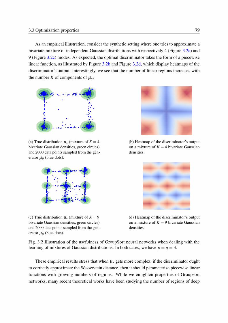
3.3 Optimization properties 79
As an empirical illustration, consider the synthetic setting where one tries to approximate abivariate mixture of independent Gaussian distributions with respectively 4 (Figure 3.2a) and9 (Figure 3.2c) modes. As expected, the optimal discriminator takes the form of a piecewiselinear function, as illustrated by Figure 3.2b and Figure 3.2d, which display heatmaps of thediscriminator’s output. Interestingly, we see that the number of linear regions increases withthe number K of components of µ⋆.
(a) True distribution µ⋆ (mixture of K = 4bivariate Gaussian densities, green circles)and 2000 data points sampled from the gen-erator µθ (blue dots).
(b) Heatmap of the discriminator’s outputon a mixture of K = 4 bivariate Gaussiandensities.
(c) True distribution µ⋆ (mixture of K = 9bivariate Gaussian densities, green circles)and 2000 data points sampled from the gen-erator µθ (blue dots).
(d) Heatmap of the discriminator’s outputon a mixture of K = 9 bivariate Gaussiandensities.
Fig. 3.2 Illustration of the usefulness of GroupSort neural networks when dealing with thelearning of mixtures of Gaussian distributions. In both cases, we have p = q = 3.
These empirical results stress that when µ⋆ gets more complex, if the discriminator oughtto correctly approximate the Wasserstein distance, then it should parameterize piecewise linearfunctions with growing numbers of regions. While we enlighten properties of Groupsortnetworks, many recent theoretical works have been studying the number of regions of deep

80 Some theoretical properties of Wasserstein GANs
ReLU neural networks (Pascanu et al., 2013; Montúfar et al., 2014; Arora et al., 2018; Serraet al., 2018). In particular, Montúfar et al. (2014, Theorem 5) states that the number of linearregions of deep models grows exponentially with the depth and polynomially with the width.This, along with our observations, is an interesting avenue to choose the architecture of thediscriminator.
3.4 Asymptotic properties
In practice, one never has access to the distribution µ⋆ but rather to a finite collection ofi.i.d. observations X1, . . . ,Xn distributed according to µ⋆. Thus, for the remainder of the article,we let µn be the empirical measure based on X1, . . . ,Xn, that is, for any Borel subset A of E,µn(A) = 1
n ∑ni=11Xi∈A. With this notation, the empirical counterpart of the WGANs problem
is naturally defined as minimizing over Θ the quantity dD(µn,µθ ). Equivalently, we seek tosolve the following optimization problem:
infθ∈Θ
dD(µn,µθ ) = infθ∈Θ
supα∈Λ
[1n
n
∑i=1
Dα(Xi)−EDα(Gθ (Z))]. (3.4.1)
Assuming that Assumption 1 is satisfied, we have, as in Corollary 3.2.1, that the infimum in(3.4.1) is reached. We therefore consider the set of empirical optimal parameters
Θn = argminθ∈Θ
dD(µn,µθ ),
and let θn be a specific element of Θn (note that the choice of θn has no impact on the value ofthe minimum). We note that Θn (respectively, θn) is the empirical counterpart of Θ (respectively,θ ). Section 3.3 was mainly devoted to the analysis of the difference εoptim. In this section, weare willing to take into account the effect of having finite samples. Thus, in line with the above,we are now interested in the generalization properties of WGANs and look for upper-boundson the quantity
0 ⩽ dLip1(µ⋆,µθn
)− infθ∈Θ
dLip1(µ⋆,µθ ). (3.4.2)
Arora et al. (2017, Theorem 3.1) states an asymptotic result showing that when providedenough samples, the neural IPM dD generalizes well, in the sense that for any pair (µ,ν) ∈P1(E)2, the difference |dD(µ,ν)−dD(µn,νn)| can be arbitrarily small with high probability.However, this result does not give any information on the quantity of interest dLip1
(µ⋆,µθn)−
infθ∈Θ dLip1(µ⋆,µθ ). Closer to our current work, Zhang et al. (2018) provide bounds for

3.4 Asymptotic properties 81
dD(µ⋆,µθn)− infθ∈Θ dD(µ⋆,µθ ), starting from the observation that
0 ⩽ dD(µ⋆,µθn)− inf
θ∈ΘdD(µ⋆,µθ )⩽ 2dD(µ⋆,µn). (3.4.3)
In the present article, we develop a complementary point of view and measure the generalizationproperties of WGANs on the basis of the Wasserstein distance dLip1
, as in equation (3.4.2).Our approach is motivated by the fact that the neural IPM dD is only used for easing theoptimization process and, accordingly, that the performance should be assessed on the basis ofthe distance dLip1
, not dD .Note that θn, which minimizes dD(µn,µθ ) over Θ , may not be unique. Besides, there is no
guarantee that two distinct elements θn,1 and θn,2 of Θn lead to the same distance dLip1(µ⋆,µθn,1)
and dLip1(µ⋆,µθn,2) (again, θn is computed with dD , not with dLip1
). Therefore, in order toupper-bound the error in (3.4.2), we let, for each θn ∈ Θn,
θn ∈ argminθ∈Θ
∥θn − θ∥.
The rationale behind the definition of θn is that we expect it to behave “similarly” to θn.Following our objective, the error can be decomposed as follows:
0 ⩽ dLip1(µ⋆,µθn
)− infθ∈Θ
dLip1(µ⋆,µθ )
⩽ supθn∈Θn
dLip1(µ⋆,µθn)− inf
θ∈ΘdLip1
(µ⋆,µθ )
= supθn∈Θn
[dLip1
(µ⋆,µθn)−dLip1(µ⋆,µθn
)+dLip1(µ⋆,µθn
)]− inf
θ∈ΘdLip1
(µ⋆,µθ )
⩽ supθn∈Θn
[dLip1
(µ⋆,µθn)−dLip1(µ⋆,µθn
)]+ sup
θ∈Θ
dLip1(µ⋆,µθ
)− infθ∈Θ
dLip1(µ⋆,µθ )
= εestim + εoptim, (3.4.4)
where we set εestim = supθn∈Θn
[dLip1(µ⋆,µθn)−dLip1
(µ⋆,µθn)]. Notice that this supremum can
be positive or negative. However, it can be shown to converge to 0 almost surely when n → ∞.
Lemma 3.4.1. Assume that Assumption 1 is satisfied. Then limn→∞
εestim = 0 almost surely.

82 Some theoretical properties of Wasserstein GANs
Going further with the analysis of (3.4.2), the sum εestim + εoptim is bounded as follows:
εestim + εoptim ⩽ supθn∈Θn
[dLip1
(µ⋆,µθn)−dLip1(µ⋆,µθn
)]+TP(Lip1,D)
(by inequality (3.3.2))
⩽ supθn∈Θn
[dLip1
(µ⋆,µθn)− infθ∈Θ
dD(µ⋆,µθ )]+TP(Lip1,D).
Hence,
εestim + εoptim
⩽ supθn∈Θn
[dLip1
(µ⋆,µθn)−dD(µ⋆,µθn)+dD(µ⋆,µθn)− infθ∈Θ
dD(µ⋆,µθ )]+TP(Lip1,D)
⩽ supθn∈Θn
[dLip1
(µ⋆,µθn)−dD(µ⋆,µθn)]+2dD(µ⋆,µn)+TP(Lip1,D)
(upon noting that inequality (3.4.3) is also valid for any θn ∈ Θn)
⩽ 2TP(Lip1,D)+2dD(µ⋆,µn). (3.4.5)
The above bound is a function of both the generator and the discriminator. The termTP(Lip1,D) is increasing when the capacity of the generator is increasing. The discrimi-nator, however, plays a more ambivalent role, as already pointed out by Zhang et al. (2018).On the one hand, if the discriminator’s capacity decreases, the gap between dD and dLip1
getsbigger and TP(Lip1,D) increases. On the other hand, discriminators with bigger capacitiesought to increase the contribution dD(µ⋆,µn). In order to bound dD(µ⋆,µn), Proposition 3.4.1below extends Zhang et al. (2018, Theorem 3.1), in the sense that it does not require the set ofdiscriminative functions nor the space E to be bounded. Recall that, for γ > 0, µ⋆ is said to beγ sub-Gaussian (Jin et al., 2019) if
∀v ∈Rd, Eev·(T−ET ) ⩽ eγ2∥v∥2
2 ,
where T is a random vector with probability distribution µ⋆ and · denotes the dot product inRD.
Proposition 3.4.1. Assume that Assumption 1 is satisfied, let η ∈ (0,1), and let D be adiscriminator of the form (3.2.2).

3.4 Asymptotic properties 83
(i) If µ⋆ has compact support with diameter B, then there exists a constant c1 > 0 such that,with probability at least 1−η ,
dD(µ⋆,µn)⩽c1√
n+B
√log(1/η)
2n.
(ii) More generally, if µ⋆ is γ sub-Gaussian, then there exists a constant c2 > 0 such that,with probability at least 1−η ,
dD(µ⋆,µn)⩽c2√
n+8γ
√eD
√log(1/η)
n.
The result of Proposition 3.4.1 has to be compared with convergence rates of the Wassersteindistance. According to Fournier and Guillin (2015, Theorem 1), when the dimension D of E issuch that D > 2, if µ⋆ has a second-order moment, then there exists a constant c such that
0 ⩽ EdLip1(µ⋆,µn)⩽
cn1/D
.
Thus, when the space E is of high dimension (e.g., in image generation tasks), under theconditions of Proposition 3.4.1, the pseudometric dD provides much faster rates of convergencefor the empirical measure. However, one has to keep in mind that both constants c1 and c2
grow in O(qQ3/2(D1/2 +q)).Our Theorem 3.3.1 states the existence of a discriminator such that εoptim can be arbitrarily
small. It is therefore reasonable, in view of inequality (3.4.5), to expect that the sum εestim +
εoptim can also be arbitrarily small, at least in an asymptotic sense. This is encapsulated inTheorem 3.4.1 below.
Theorem 3.4.1. Assume that Assumption 1 is satisfied, and let η ∈ (0,1).
(i) If µ⋆ has compact support with diameter B, then, for all ε > 0, there exists a discriminatorD of the form (3.2.2) and a constant c1 > 0 (function of ε) such that, with probability atleast 1−η ,
0 ⩽ εestim + εoptim ⩽ 2ε +2c1√
n+2B
√log(1/η)
2n.
(ii) More generally, if µ⋆ is γ sub-Gaussian, then, for all ε > 0, there exists a discriminatorD of the form (3.2.2) and a constant c2 > 0 (function of ε) such that, with probability atleast 1−η ,
0 ⩽ εestim + εoptim ⩽ 2ε +2c2√
n+16γ
√eD
√log(1/η)
n.

84 Some theoretical properties of Wasserstein GANs
Theorem 3.4.1 states that, asymptotically, the optimal parameters in Θn behave properly. Acaveat is that the definition of εestim uses Θn. However, in practice, one never has access to θn,but rather to an approximation of this quantity obtained by gradient descent algorithms. Thus,in line with Definition 3.3.1, we introduce the concept of empirical substitution:
Definition 3.4.1. Let ε > 0 and η ∈ (0,1). We say that dLip1can be empirically ε-substituted
by dD if there exists δ > 0 such that, for all n large enough, with probability at least 1−η ,
MdD(µn,δ )⊆ MdLip1
(µ⋆,ε). (3.4.6)
The rationale behind this definition is that if (3.4.6) is satisfied, then by minimizing theIPM dD close to optimality in (3.4.1), one can be guaranteed to be also close to optimality in(3.2.3) with high probability. We stress that Definition 3.4.1 is the empirical counterpart ofDefinition 3.3.1.
Proposition 3.4.2. Assume that Assumption 1 is satisfied and that µ⋆ is sub-Gaussian. Letε > 0. If TP(Lip1,D) ⩽ ε , then dLip1
can be empirically (ε + δ )-substituted by dD for allδ > 0.
This proposition is the empirical counterpart of Lemma 3.3.1. It underlines the fact that byminimizing the pseudometric dD between the empirical measure µn and the set of generativedistributions P close to optimality, one can control the loss in performance under the metricdLip1
.Let us finally mention that it is also possible to provide asymptotic results on the sequences
of parameters (θn), keeping in mind that Θn and Θ are not necessarily reduced to singletons.
Lemma 3.4.2. Assume that Assumption 1 is satisfied. Let (θn) be a sequence of optimalparameters that converges almost surely to z ∈Θ . Then z ∈ Θ almost surely.
Proof. Let the sequence (θn) converge almost surely to some z ∈Θ . By Theorem 3.2.1, thefunction Θ ∋ θ 7→ dD(µ⋆,µθ ) is continuous, and therefore, almost surely, lim
n→∞dD(µ⋆,µθn
) =
dD(µ⋆,µz). Using inequality (3.4.3), we see that, almost surely,
0 ⩽ dD(µ⋆,µz)− infθ∈Θ
dD(µ⋆,µθ ) = limn→∞
dD(µ⋆,µθn)− inf
θ∈ΘdD(µ⋆,µθ )
⩽ liminfn→∞
2dD(µ⋆,µn).
Using Dudley (2004, Theorem 11.4.1) and the strong law of large numbers, we have that thesequence of empirical measures (µn) almost surely converges weakly to µ⋆ in P1(E). Besides,since dD metrizes weak convergence in P1(E) (by Proposition 3.2.2), we conclude that z ∈ Θ
almost surely.

3.5 Understanding the performance of WGANs 85
3.5 Understanding the performance of WGANs
In order to better understand the overall performance of the WGANs architecture, it is instructiveto decompose the final loss dLip1
(µ⋆,µθn) as in (3.4.4):
dLip1(µ⋆,µθn
)⩽ εestim + εoptim + infθ∈Θ
dLip1(µ⋆,µθ )
= εestim + εoptim + εapprox, (3.5.1)
where
(i) εestim matches up with the use of a data-dependent optimal parameter θn, based on thetraining set X1, . . . ,Xn drawn from µ⋆;
(ii) εoptim corresponds to the loss in performance when using dD as training loss instead ofdLip1
(this term has been thoroughly studied in Section 3.3);
(iii) and εapprox stresses the capacity of the parametric family of generative distributions P toapproach the unknown distribution µ⋆.
Close to our work are the articles by Liang (2018), Singh et al. (2018), and Uppal et al.(2019), who study statistical properties of GANs. Liang (2018) and Singh et al. (2018) exhibitrates of convergence under an IPM-based loss for estimating densities that live in Sobolevspaces, while Uppal et al. (2019) explore the case of Besov spaces. Remarkably, Liang(2018) discusses bounds for the Kullback-Leibler divergence, the Hellinger divergence, and theWasserstein distance between µ⋆ and µ
θn. These bounds are based on a different decomposition
of the loss and offer a complementary point of view. We emphasize that, in the present article,no density assumption is made neither on the class of generative distributions P nor on thetarget distribution µ⋆.
3.5.1 Synthetic experiments
Our goal in this subsection is to illustrate (3.5.1) by running a set of experiments on syntheticdatasets. The true probability measure µ⋆ is assumed to be a mixture of bivariate Gaussiandistributions with either 1, 4, or 9 components. This simple setting allows us to controlthe complexity of µ⋆, and, in turn, to better assess the impact of both the generator’s anddiscriminator’s capacities. We use growing classes of generators of the form (3.2.1), namelyGp : p = 2,3,5,7, and growing classes of discriminators of the form (3.2.2), namely Dq :q = 2,3,5,7. For both the generator and the discriminator, the width of the hidden layers iskept constant equal to 20.

86 Some theoretical properties of Wasserstein GANs
Two metrics are computed to evaluate the behavior of the different generative models. First,we use the Wasserstein distance between the true distribution (either µ⋆ or its empirical versionµn) and the generative distribution (either µ
θor µ
θn). This distance is calculated by using the
Python package by Flamary and Courty (2017), via finite samples of size 4096 (average over 20runs). Second, we use the recall metric (the higher, the better), proposed by Kynkäänniemi et al.(2019). Roughly, this metric measures “how much” of the true distribution (either µ⋆ or µn) canbe reconstructed by the generative distribution (either µ
θor µ
θn). At the implementation level,
this score is based on k-nearest neighbor nonparametric density estimation. It is computed viafinite samples of size 4096 (average over 20 runs).
Our experiments were run in two different settings:
Asymptotic setting: in this first experiment, we assume that µ⋆ is known from the experi-menter (so, there is no dataset). At the end of the optimization scheme, we end up with oneθ ∈ Θ . Thus, in this context, the performance of WGANs is captured by
supθ∈Θ
dLip1(µ⋆,µθ
) = εoptim + εapprox.
For a fixed discriminator, when increasing the generator’s depth p, we expect εapprox to decrease.Conversely, as discussed in Subsection 3.3.1, we anticipate an augmentation of εoptim, since thediscriminator must now differentiate between larger classes of generative distributions. In thiscase, it is thus difficult to predict how sup
θ∈ΘdLip1
(µ⋆,µθ) behaves when p increases. On the
contrary, in accordance with the results of Section 3.3, for a fixed p we expect the performanceto increase with a growing q since, with larger discriminators, the pseudometric dD is morelikely to behave similarly to the Wasserstein distance dLip1
.These intuitions are validated by Figure 3.3 and Figure 3.4 (the bluer, the better). The first
one shows an approximation of supθ∈Θ
dLip1(µ⋆,µθ
) computed over 5 different seeds as afunction of p and q. The second one depicts the average recall of the estimator µ
θwith respect
to µ⋆, as a function of p and q, again computed over 5 different seeds. In both figures, weobserve that for a fixed p, incrementing q leads to better results. On the opposite, for a fixeddiscriminator’s depth q, increasing the depth p of the generator seems to deteriorate both scores(Wasserstein distance and recall). This consequently suggests that the term εoptim dominatesεapprox.

3.5 Understanding the performance of WGANs 87
q=2 q=3 q=5 q=7
p=7
p=5
p=3
p=2
0.262 0.218 0.098 0.131
0.196 0.166 0.07 0.085
0.173 0.061 0.087 0.069
0.064 0.064 0.084 0.063
(a) supθ∈Θ dLip1(µ⋆,µθ ), K = 1.
q=2 q=3 q=5 q=7
p=7
p=5
p=3
p=2
2.963 3.366 1.466 1.752
3.071 1.165 0.992 0.771
0.982 0.825 1.108 0.503
1.407 0.819 0.426 0.728
(b) supθ∈Θ dLip1(µ⋆,µθ ), K = 9.
q=2 q=3 q=5 q=7
p=7
p=5
p=3
p=2
5.966 3.007 3.932 1.557
1.873 4.104 1.858 1.437
1.444 1.433 1.664 1.361
1.325 1.484 1.359 1.364
(c) supθ∈Θ dLip1(µ⋆,µθ ), K = 25.
Fig. 3.3 Influence of the generator’s depth p and the discriminator’s depth q on the maximalWasserstein distance sup
θ∈ΘdLip1
(µ⋆,µθ).
q=2 q=3 q=5 q=7
p=7
p=5
p=3
p=2
0.788 0.9 0.943 0.827
0.822 0.888 0.927 0.952
0.968 0.936 0.96 0.92
0.965 0.985 0.981 0.989
(a) Av. recall of µθ w.r.t. µ⋆, K =1.
q=2 q=3 q=5 q=7
p=7
p=5
p=3
p=2
0.968 0.082 0.349 0.718
0.655 0.972 0.894 0.82
0.988 0.991 0.983 0.989
0.993 0.993 0.994 0.995
(b) Av. recall of µθ w.r.t. µ⋆, K =9.
q=2 q=3 q=5 q=7
p=7
p=5
p=3
p=2
0.197 0.881 0.701 0.907
0.909 0.679 0.97 0.99
0.99 0.998 0.997 0.996
0.997 0.995 0.992 0.995
(c) Av. recall of µθ w.r.t. µ⋆, K =25.
Fig. 3.4 Influence of the generator’s depth p and the discriminator’s depth q on the averagerecall of the estimators µ
θw.r.t. µ⋆.
Finite-sample setting: in this second experiment, we consider the more realistic situationwhere we have at hand finite samples X1, . . . ,Xn drawn from µ⋆ (n = 5000).
Recalling that supθn∈Θn
dLip1(µ⋆,µθn)⩽ εestim + εoptim + εapprox, we plot in Figure 3.5 the
maximal Wasserstein distance supθn∈Θn
dLip1(µ⋆,µθn), and in Figure 3.6 the average recall of
the estimators µθn with respect to µ⋆, as a function of p and q. Anticipating the behavior ofsup
θn∈ΘndLip1
(µ⋆,µθn) when increasing the depth q is now more involved. Indeed, accordingto inequality (3.4.5), which bounds εestim + εoptim, a larger D will make TP(Lip1,D) smallerbut will, on the opposite, increase dD(µ⋆,µn). Figure 3.5 clearly shows that, for a fixed p, themaximal Wasserstein distance seems to be improved when q increases. This suggests that theterm TP(Lip1,D) dominates dD(µ⋆,µn). Similarly to the asymptotic setting, we also make the

88 Some theoretical properties of Wasserstein GANs
observation that bigger p require a higher depth q since larger class of generative distributionsare more complex to discriminate.
q=2 q=3 q=5 q=7
p=7
p=5
p=3
p=2
0.119 0.14 0.115 0.1
0.081 0.11 0.104 0.089
0.108 0.068 0.074 0.042
0.102 0.073 0.064 0.044
(a) supθn∈Θn
dLip1(µ⋆,µθn), K = 1.
q=2 q=3 q=5 q=7
p=7
p=5
p=3
p=2
4.499 2.55 1.421 0.867
1.285 0.661 0.661 0.761
0.78 0.718 0.743 0.491
0.552 0.785 0.711 0.444
(b) supθn∈Θn
dLip1(µ⋆,µθn), K =
4.
q=2 q=3 q=5 q=7
p=7
p=5
p=3
p=2
6.364 5.274 3.576 1.364
1.396 3.864 1.412 1.403
1.523 1.461 1.32 1.348
1.425 1.397 1.295 1.287
(c) supθn∈Θn
dLip1(µ⋆,µθn), K = 9.
Fig. 3.5 Influence of the generator’s depth p and the discriminator’s depth q on the maximalWasserstein distance sup
θn∈ΘndLip1
(µ⋆,µθn), with n = 5000.
q=2 q=3 q=5 q=7
p=7
p=5
p=3
p=2
0.938 0.721 0.847 0.968
0.828 0.89 0.953 0.942
0.986 0.988 0.989 0.987
0.979 0.973 0.94 0.989
(a) Av. recall of µθn
w.r.t. µ⋆, K =1.
q=2 q=3 q=5 q=7
p=7
p=5
p=3
p=2
0.202 0.64 0.748 0.97
0.959 0.904 0.969 0.903
0.99 0.983 0.994 0.992
0.992 0.991 0.942 0.993
(b) Av. recall of µθn
w.r.t. µ⋆, K =9.
q=2 q=3 q=5 q=7
p=7
p=5
p=3
p=2
0.392 0.359 0.788 0.968
0.98 0.652 0.976 0.917
0.993 0.998 0.997 0.995
0.994 0.995 0.988 0.997
(c) Av. recall of µθn
w.r.t. µ⋆, K =25.
Fig. 3.6 Influence of the generator’s depth p and the discriminator’s depth q on the averagerecall of the estimators µθn w.r.t. µ⋆, with n = 5000.
We end this subsection by pointing out a recurring observation across different experiments.In Figure 3.4 and Figure 3.6, we notice, as already stressed, that the average recall of theestimators is prone to decrease when the generator’s depth p increases. On the opposite,the average recall increases when the discriminator’s depth q increases. This is interestingbecause the recall metric is a good proxy for a stabilized training, insofar as a high recallmeans the absence of mode collapse. This is also confirmed in Figure 3.7, which compares twodensities: in Figure 3.7a, the discriminator has a small capacity (q = 3) and the generator a largecapacity (p = 7), whereas in Figure 3.7b, the discriminator has a large capacity (q = 7) and

3.5 Understanding the performance of WGANs 89
the generator a small capacity (p = 3). We observe that the first WGAN architecture behavespoorly compared to the second one. We therefore conclude that larger discriminators seemto bring some stability in the training of WGANS both in the asymptotic and finite sampleregimes.
(a) p = 7 and q = 3. (b) p = 3 and q = 7.
Fig. 3.7 True distribution µ⋆ (mixture of K = 9 bivariate Gaussian densities, green circles) and2000 data points sampled from the generator µ
θ(blue dots).
3.5.2 Real-world experiments
In this subsection, we further illustrate the impact of the generator’s and the discriminator’scapacities on two high-dimensional datasets, namely MNIST (LeCun et al., 1998) and Fashion-MNIST (Xiao et al., 2017). MNIST contains images in R28×28 with 10 classes representing thedigits. Fashion-MNIST is a 10-class dataset of images in R28×28, with slightly more complexshapes than MNIST. Both datasets have a training set of 60,000 examples.
To measure the performance of WGANs when dealing with high-dimensional applicationssuch as image generation, Brock et al. (2019) have advocated that embedding images into afeature space with a pre-trained convolutional classifier provides more meaningful information.Therefore, in order to assess the quality of the generator µ
θn, we sample images both from the
empirical measure µn and from the distribution µθn
. Then, instead of computing the Wasserstein(or recall) distance directly between these two samples, we use as a substitute their embeddingsoutput by an external classifier and compute the Wasserstein (or recall) between the two newcollections. Such a transformation is also done, for example, in Kynkäänniemi et al. (2019).Practically speaking, for any pair of images (a,b), this operation amounts to using the Euclideandistance ∥φ(a)−φ(b)∥ in the Wasserstein and recall criteria, where φ is a pre-softmax layer ofa supervised classifier, trained specifically on the datasets MNIST and Fashion-MNIST.
For these two datasets, as usual, we use generators of the form (3.2.1) and discriminatorsof the form (3.2.2), and plot the performance of µ
θnas a function of both p and q. The results

90 Some theoretical properties of Wasserstein GANs
of Figure 3.8 confirm the fact that the worst results are achieved for generators with a largedepth p combined with discriminators with a small depth q. They also corroborate the previousobservations that larger discriminators are preferred.
q=2 q=3 q=5 q=7
p=7
p=5
p=3
p=2
81.195 84.449 82.25 85.056
77.84 82.021 72.328 78.599
74.067 75.713 72.037 76.617
83.448 76.08 73.659 69.944
(a) supθn∈Θn
dLip1(µn,µθn), MNIST
dataset.
q=2 q=3 q=5 q=7
p=7
p=5
p=3
p=2
139.762 139.86 137.325 123.097
137.39 138.441 128.459 132.77
135.037 137.331 132.245 132.514
137.099 139.123 139.534 129.002
(b) supθn∈Θn
dLip1(µn,µθn), FMNIST
dataset.
Fig. 3.8 Influence of the generator’s depth p and the discriminator’s depth q on the maximalWasserstein distance sup
θn∈ΘndLip1
(µn,µθn) for the MNIST and F-MNIST datasets.

3.A Technical results 91
Appendix 3.A Technical results
3.A.1 Proof of Lemma 3.2.1
Recall that the notation ∥ · ∥ (respectively, ∥ · ∥∞) means the Euclidean (respectively, thesupremum) norm, with no specific mention of the underlying space on which it acts. For(z,z′) ∈ (Rd)2, we have
∥ f1(z)− f1(z′)∥⩽ ∥U1z+b1 −U1z′−b1∥(since σ is 1-Lipschitz)
= ∥U1(z− z′)∥⩽ ∥U1∥2 ∥z− z′∥⩽ K1∥z− z′∥
(by Assumption 1).
Repeating this for i = 2, . . . , p, we thus have, for all (z,z′) ∈ (Rd)2, ∥Gθ (z)− Gθ (z′)∥ ⩽
K p1 ∥z− z′∥. We conclude that, for each θ ∈Θ , the function Gθ is K p
1 -Lipschitz on Rd .Let us now prove that D ⊆ Lip1. Fix Dα ∈ D , α ∈ Λ . According to (3.2.2), we have, for
x ∈ E, Dα(x) = fq · · · f1(x), where fi(t) = σ(Vit + ci) for i = 1, . . . ,q−1 (σ is applied onpairs of components), and fq(t) =Vqt + cq.
Consequently, for (x,y) ∈ E2,
∥ f1(x)− f1(y)∥∞ ⩽ ∥V1x−V1y∥∞
(since σ is 1-Lipschitz)
= ∥V1(x− y)∥∞
⩽ ∥V1∥2,∞ ∥x− y∥⩽ ∥x− y∥
(by Assumption 1).

92 Some theoretical properties of Wasserstein GANs
Thus,
∥ f2 f1(x)− f2 f1(y)∥∞ ⩽ ∥V2 f1(x)−V2 f1(y)∥∞
(since σ is 1-Lipschitz)
⩽ ∥V2∥∞ ∥ f1(x)− f1(y)∥∞
⩽ ∥ f1(x)− f1(y)∥∞
(by Assumption 1)
⩽ ∥x− y∥.
Repeating this, we conclude that, for each α ∈Λ and all (x,y)∈E2, |Dα(x)−Dα(y)|⩽ ∥x−y∥,which is the desired result.
3.A.2 Proof of Proposition 3.2.1
We first prove that the function Θ ∋ θ 7→ µθ is continuous with respect to the weak topologyin P1(E). Let Gθ and Gθ ′ be two elements of G , with (θ ,θ ′) ∈Θ 2. Using (3.2.1), we writeGθ (z) = fp · · · f1(z) (respectively, Gθ ′(z) = f ′p · · · f ′1(z)), where fi(x) = max(Uix+bi,0)(respectively, f ′i (x) = max(U ′
i x+b′i,0)) for i = 1, . . . , p−1, and fp(x) =Upx+bp (respectively,f ′p(x) =U ′
px+b′p).Clearly, for z ∈Rd ,
∥ f1(z)− f ′1(z)∥⩽ ∥U1z+b1 −U ′1z−b′1∥
⩽ ∥(U1 −U ′1)z∥+∥b1 −b′1∥
⩽ ∥U1 −U ′1∥2 ∥z∥+∥b1 −b′1∥
⩽ (∥z∥+1)∥θ −θ′∥.
Similarly, for any i ∈ 2, . . . , p and any x ∈Rui ,
∥ fi(x)− f ′i (x)∥⩽ (∥x∥+1)∥θ −θ′∥.
Observe that
∥Gθ (z)−Gθ ′(z)∥= ∥ fp · · · f1(z)− f ′p · · · f ′1(z)∥⩽ ∥ fp · · · f1(z)− fp · · · f2 f ′1(z)∥+ · · ·+∥ fp f ′p−1 · · · f ′1(z)− f ′p · · · f ′1(z)∥.
3.A Technical results 93
As in the proof of Lemma 3.2.1, one shows that for any i ∈ 1, . . . , p, the function fp · · · fi
is K p−i+11 -Lipschitz with respect to the Euclidean norm. Therefore,
∥Gθ (z)−Gθ ′(z)∥⩽ K p−1
1 ∥ f1(z)− f ′1(z)∥+ · · ·+K01∥ fp f ′p−1 · · · f ′1(z)− f ′p · · · f ′1(z)∥
⩽ K p−11 (∥z∥+1)∥θ −θ
′∥+ · · ·+(∥ f ′p−1 · · · f ′1(z)∥+1)∥θ −θ′∥
⩽ K p−11 (∥z∥+1)∥θ −θ
′∥+ · · ·+(K p−11 ∥z∥+∥ f ′p−1 · · · f ′1(0)∥+1)∥θ −θ
′∥.
Using the architecture of neural networks in (3.2.1), a quick check shows that, for eachi ∈ 1, . . . , p,
∥ f ′i · · · f ′1(0)∥⩽i
∑k=1
Kk1 .
We are led to∥Gθ (z)−Gθ ′(z)∥= (ℓ1∥z∥+ ℓ2)∥θ −θ
′∥, (3.A.1)
where
ℓ1 = pK p−11 and ℓ2 =
p−1
∑i=1
K p−(i+1)1
i
∑k=1
Kk1 +
p−1
∑i=0
Ki1.
Denoting by ν the probability distribution of the sub-Gaussian random variable Z, we note that∫Rd(ℓ1∥z∥+ ℓ2)ν(dz)< ∞. Now, let (θk) be a sequence in Θ converging to θ ∈Θ with respect
to the Euclidean norm. Clearly, for a given z ∈Rd , by continuity of the function θ 7→ Gθ (z),we have lim
k→∞Gθk(z) = Gθ (z) and, for any ϕ ∈Cb(E), lim
k→∞ϕ(Gθk(z)) = ϕ(Gθ (z)). Thus, by the
dominated convergence theorem,
limk→∞
∫E
ϕ(x)µθk(dx) = limk→∞
∫Rd
ϕ(Gθk(z))ν(dz) =∫Rd
ϕ(Gθ (z))ν(dz) =
∫E
ϕ(x)µθ (dx).
(3.A.2)

94 Some theoretical properties of Wasserstein GANs
This shows that the sequence (µθk) converges weakly to µθ . Besides, for an arbitrary x0 in E,we have
limsupk→∞
∫E∥x0 − x∥µθk(dx)
= limsupk→∞
∫Rd
∥x0 −Gθk(z)∥ν(dz)
⩽ limsupk→∞
∫Rd
(∥Gθk(z)−Gθ (z)∥+∥Gθ (z)− x0∥
)ν(dz)
⩽ limsupk→∞
∫Rd
(ℓ1∥z∥+ ℓ2)∥θk −θ∥ν(dz)+∫Rd
∥Gθ (z)− x0∥ν(dz)
(by inequality (3.A.1)).
Consequently,
limsupk→∞
∫E∥x0 − x∥µθk(dx)⩽
∫Rd
∥Gθ (z)− x0∥ν(dz) =∫
E∥x0 − x∥µθ (dx).
One proves with similar arguments that
liminfk→∞
∫E∥x0 − x∥µθk(dx)⩾
∫E∥x0 − x∥µθ (dx).
Therefore, putting all the pieces together, we conclude that
limk→∞
∫E∥x0 − x∥µθk(dx) =
∫E∥x0 − x∥µθ (dx).
This, together with (3.A.2), shows that the sequence (µθk) converges weakly to µθ in P1(E),and, in turn, that the function Θ ∋ θ 7→ µθ is continuous with respect to the weak topology inP1(E), as desired.
The second assertion of the proposition follows upon noting that P is the image of thecompact set Θ by a continuous function.
3.A.3 Proof of Proposition 3.2.2
To show the first statement, we are to exhibit a specific discriminator, say Dmax, such that, forall (µ,ν) ∈ (P ∪µ⋆)2, the identity dDmax(µ,ν) = 0 implies µ = ν .
Let ε > 0. According to Proposition 3.2.1, under Assumption 1, P is a compact subsetof P1(E) with respect to the weak topology in P1(E). Let x0 ∈ E be arbitrary. For any µ ∈ P
there exists a compact Kµ ⊆ E such that∫
K∁µ
∥x0 − x∥µ(dx)⩽ ε/4. Also, for any such Kµ , the

3.A Technical results 95
function P1(E) ∋ ρ 7→∫
K∁µ
∥x0 − x∥ρ(dx) is continuous. Therefore, there exists an open setUµ ⊆ P1(E) containing µ such that, for any ρ ∈Uµ ,
∫K∁
µ
∥x0 − x∥ρ(dx)⩽ ε/2.The collection of open sets Uµ : µ ∈ P forms an open cover of P , from which we can
extract, by compactness, a finite subcover Uµ1, . . . ,Uµn . Letting K1 = ∪ni=1Kµi , we deduce that,
for all µ ∈ P ,∫
K∁1∥x0 − x∥µ(dx)⩽ ε/2. We conclude that there exists a compact K ⊆ E and
x0 ∈ K such that, for any µ ∈ P ∪µ⋆,∫K∁
||x0 − x||µ(dx)⩽ ε/2.
By Arzelà-Ascoli theorem, it is easy to see that Lip1(K), the set of 1-Lipschitz real-valuedfunctions on K, is compact with respect to the uniform norm ∥ · ∥∞ on K. Let f1, . . . , fNε
denote an ε-covering of Lip1(K). According to Anil et al. (2019, Theorem 3), for eachk = 1, . . . ,Nε there exists under Assumption 1 a discriminator Dk of the form (3.2.2) such that
infg∈Dk
∥ fk −g1K∥∞ ⩽ ε.
Since the discriminative classes of functions use GroupSort activations, one can find a neural net-work of the form (3.2.2) satisfying Assumption 1, say Dmax, such that, for all k ∈ 1, . . . ,Nε,Dk ⊆ Dmax. Consequently, for any f ∈ Lip1(K), letting k0 ∈ argmin
k∈1,...,Nε∥ f − fk∥∞, we have
infg∈Dmax
∥ f −g1K∥∞ ⩽ ∥ f − fk0∥∞ + infg∈Dmax
∥ fk0 −g1K∥∞ ⩽ 2ε.
Now, let (µ,ν) ∈ (P⋃µ⋆)2 be such that dDmax(µ,ν) = 0, i.e., sup f∈Dmax
|Eµ f −Eν f |= 0.Let f ⋆ be a function in Lip1 such that Eµ f ⋆−Eν f ⋆ = dLip1
(µ,ν) (such a function existsaccording to (3.2.6)) and, without loss of generality, such that f ⋆(x0) = 0. Clearly,
dLip1(µ,ν) = Eµ f ⋆−Eν f ⋆
⩽∣∣∣∫
Kf ⋆dµ −
∫K
f ⋆dν
∣∣∣+ ∣∣∣∫K∁
f ⋆dµ −∫
K∁f ⋆dν
∣∣∣⩽
∣∣∣∫K
f ⋆dµ −∫
Kf ⋆dν
∣∣∣+ ε.
Letting g f ⋆ ∈ Dmax be such that
∥( f ⋆−g f ⋆)1K∥∞ ⩽ infg∈Dmax
∥( f ⋆−g)1K∥∞ + ε ⩽ 3ε,

96 Some theoretical properties of Wasserstein GANs
we are thus led to
dLip1(µ,ν)⩽
∣∣∣∫K( f ⋆−g f ⋆)dµ −
∫K( f ⋆−g f ⋆)dν +
∫K
g f ⋆dµ −∫
Kg f ⋆dν
∣∣∣+ ε.
Observe, since x0 ∈ K, that |g f ⋆(x0)| ⩽ 3ε and that, for any x ∈ E, |g f ⋆(x)| ⩽ ∥x0 − x∥+ 3ε .Exploiting Eµg f ⋆ −Eνg f ⋆ = 0, we obtain
dLip1(µ,ν)⩽ 7ε +
∣∣∣∫K∁
g f ⋆dµ −∫
K∁g f ⋆dν
∣∣∣⩽ 7ε +
∫K∁
∥x0 − x∥µ(dx)+∫
K∁∥x0 − x∥ν(dx)+6ε
⩽ 14ε.
Since ε is arbitrary and dLip1is a metric on P1(E), we conclude that µ = ν , as desired.
To complete the proof, it remains to show that dDmax metrizes weak convergence in P ∪µ⋆. To this aim, we let (µk) be a sequence in P ∪µ⋆ and µ be a probability measure inP ∪µ⋆.
If (µk) converges weakly to µ in P1(E), then dLip1(µ,µk) → 0 (Villani, 2008, Theorem
6.8), and, accordingly, dDmax(µ,µk)→ 0.Suppose, on the other hand, that dDmax(µ,µk)→ 0, and fix ε > 0. There exists M > 0 such
that, for all k ⩾ M, dDmax(µ,µk)⩽ ε . Using a similar reasoning as in the first part of the proof,it is easy to see that for any k ⩾ M, we have dLip1
(µ,µk)⩽ 15ε . Since the Wasserstein distancemetrizes weak convergence in P1(E) and ε is arbitrary, we conclude that (µk) converges weaklyto µ in P1(E).
3.A.4 Proof of Lemma 3.2.2
Using a similar reasoning as in the proof of Proposition 3.2.1, one easily checks that for all(α,α ′) ∈ Λ 2 and all x ∈ E,
|Dα(x)−Dα ′(x)|⩽ Q1/2(q∥x∥+K2
q−1
∑i=1
i+q)∥α −α
′∥
⩽ Q1/2(q∥x∥+ q(q−1)K2
2+q
)∥α −α
′∥,

3.A Technical results 97
where q refers to the depth of the discriminator. Thus, since D ⊂ Lip1 (by Lemma 3.2.1), wehave, for all α ∈ Λ , all x ∈ E, and any arbitrary x0 ∈ E,
|Dα(x)|⩽ |Dα(x)−Dα(x0)|+ |Dα(x0)|
⩽ ∥x0 − x∥+Q1/2(q∥x0∥+q(q−1)K2
2+q
)∥α∥
(upon noting that D0(x0) = 0)
⩽ ∥x0 − x∥+Q1/2(q∥x0∥+q(q−1)K2
2+q
)Q1/2 max(K2,1),
where Q is the dimension of Λ . Thus, since µ⋆ and the µθ ’s belong to P1(E) (by Lemma 3.2.1),we deduce that all Dα ∈ D are dominated by a function independent of α and integrable withrespect to µ⋆ and µθ . In addition, for all x ∈ E, the function α 7→ Dα(x) is continuous on Λ .Therefore, by the dominated convergence theorem, the function Λ ∋ α 7→ |Eµ⋆Dα −Eµθ
Dα |is continuous. The conclusion follows from the compactness of the set Λ (Assumption 1).
3.A.5 Proof of Theorem 3.2.1
Let (θ ,θ ′) ∈Θ 2, and let γZ be the joint distribution of the pair (Gθ (Z),Gθ ′(Z)). We have
|ξLip1(θ)−ξLip1
(θ ′)|= |dLip1(µ⋆,µθ )−dLip1
(µ⋆,µθ ′)|⩽ dLip1
(µθ ,µθ ′)
= infγ∈Π(µθ ,µθ ′)
∫E2∥x− y∥γ(dx,dy),
where Π(µθ ,µθ ′) denotes the collection of all joint probability measures on E × E withmarginals µθ and µθ ′ . Thus,
|ξLip1(θ)−ξLip1
(θ ′)|⩽∫
E2∥x− y∥γZ(dx,dy)
=∫Rd
∥Gθ (z)−Gθ ′(z)∥ν(dz)
(where ν is the distribution of Z)
⩽ ∥θ −θ′∥∫Rd
(ℓ1∥z∥+ ℓ2)ν(dz)
(by inequality (3.A.1)).

98 Some theoretical properties of Wasserstein GANs
This shows that the function θ ∋Θ 7→ ξLip1(θ) is L-Lipschitz, with L =
∫Rd(ℓ1∥z∥+ ℓ2)ν(dz).
For the second statement of the theorem, just note that
|ξD(θ)−ξD(θ ′)|= |dD(µ⋆,µθ )−dD(µ⋆,µθ ′)|⩽ dD(µθ ,µθ ′)
⩽ dLip1(µθ ,µθ ′)
(since D ⊆ Lip1)
⩽ L∥θ −θ′∥.
3.A.6 Proof of Theorem 3.3.1
The proof is divided into two parts. First, we show that under Assumption 1, for all ε > 0 andθ ∈Θ , there exists a discriminator D (function of ε and θ ) of the form (3.2.2) such that
dLip1(µ⋆,µθ )−dD(µ⋆,µθ )⩽ 10ε.
Let f ⋆ be a function in Lip1 such that Eµ⋆ f ⋆−Eµθf ⋆ = dLip1
(µ⋆,µθ ) (such a function existsaccording to (3.2.6)). We may write
dLip1(µ⋆,µθ )−dD(µ⋆,µθ ) = Eµ⋆ f ⋆−Eµθ
f ⋆− supf∈D
|Eµ⋆ f −Eµθf |
= Eµ⋆ f ⋆−Eµθf ⋆− sup
f∈D(Eµ⋆ f −Eµθ
f )
= inff∈D
(Eµ⋆ f ⋆−Eµθf ⋆−Eµ⋆ f +Eµθ
f )
= inff∈D
(Eµ⋆( f ⋆− f )− Eµθ( f ⋆− f ))
⩽ inff∈D
(Eµ⋆| f ⋆− f |+Eµθ| f ⋆− f |). (3.A.3)
Next, for any f ∈ D and any compact K ⊆ E,
Eµ⋆| f ⋆− f |= Eµ⋆| f ⋆− f |1K +Eµ⋆| f ⋆− f |1K∁
⩽ ∥( f ⋆− f )1K∥∞ +Eµ⋆| f ⋆|1K∁ +Eµ⋆| f |1K∁.
For the rest of the proof, we will assume, without loss of generality, that f ⋆(0) = 0 and thus| f ⋆(x)|⩽ |x|. Therefore, there exists a compact set K such that 0 ∈ K and
max(Eµ⋆| f ⋆|1K∁, Eµθ
| f ⋆|1K∁
)⩽ ε.
3.A Technical results 99
Besides, according to Anil et al. (2019, Theorem 3), under Assumption 1, for any compactK, we can find a discriminator of the form (3.2.2) such that inf f∈D ∥( f ⋆− f )1K∥∞ ⩽ ε . So,choose f ∈ D such that ∥( f ⋆− f )1K∥∞ ⩽ 2ε . For such a choice of f , we have, for any x ∈ E,| f (x)|⩽ | f (x)− f (0)|+ | f (0)|⩽ |x|+2ε , and thus, recalling that f ⋆(0) = 0,
max(Eµ⋆| f |1K∁, Eµθ
| f |1K∁
)⩽ 3ε.
Consequently,Eµ⋆| f ⋆− f |⩽ ∥( f ⋆− f )1K∥∞ +4ε.
Similarly,Eµθ
| f ⋆− f |⩽ ∥( f ⋆− f )1K∥∞ +4ε.
Plugging the two inequalities above in (3.A.3), we obtain
dLip1(µ⋆,µθ )−dD(µ⋆,µθ )⩽ 2 inf
f∈D∥( f ⋆− f )1K∥∞ +8ε.
We conclude that, for this choice of D (function of ε and θ ),
dLip1(µ⋆,µθ )−dD(µ⋆,µθ )⩽ 10ε, (3.A.4)
as desired.For the second part of the proof, we fix ε > 0 and let, for each θ ∈Θ and each discriminator
of the form (3.2.2),
ξD(θ) = dLip1(µ⋆,µθ )−dD(µ⋆,µθ ).
Arguing as in the proof of Theorem 3.2.1, we see that ξD(θ) is 2L-Lipschitz in θ , whereL =
∫Rd(ℓ1∥z∥+ ℓ2)ν(dz) and ν is the probability distribution of Z.
Now, let θ1, . . . ,θNε be an ε-covering of the compact set Θ , i.e., for each θ ∈Θ , there
exists k ∈ 1, . . . ,Nε such that ∥θ −θk∥ ⩽ ε . According to (3.A.4), for each such k, thereexists a discriminator Dk such that ξDk(θk)⩽ 6ε . Since the discriminative classes of functionsuse GroupSort activation functions, one can find a neural network of the form (3.2.2) satisfyingAssumption 1, say Dmax, such that, for all k ∈ 1, . . . ,Nε, Dk ⊆ Dmax. Clearly, ξDmax(θ) is2L-Lipschitz, and, for all k ∈ 1, . . . ,Nε, ξDmax(θk)⩽ 6ε . Hence, for all θ ∈Θ , letting
k ∈ argmink∈1,...,Nε
∥θ −θk∥,

100 Some theoretical properties of Wasserstein GANs
we haveξDmax(θ)⩽
∣∣ξDmax(θ)− ξDmax(θk)∣∣+ ξDmax(θk)⩽ (2L+6)ε.
Therefore,
TP(Lip1,Dmax) = supθ∈Θ
[dLip1
(µ⋆,µθ )−dDmax(µ⋆,µθ )]= sup
θ∈Θ
ξDmax(θ)⩽ (2L+6)ε.
We have just proved that, for all ε > 0, there exists a discriminator Dmax of the form (3.2.2)and a positive constant c (independent of ε) such that
TP(Lip1,Dmax)⩽ cε.
This is the desired result.
3.A.7 Proof of Proposition 3.3.1
Let us assume that the statement is not true. If so, there exists ε > 0 such that, for all δ > 0,there exists θ ∈MdD
(µ⋆,δ ) satisfying d(θ ,Θ)> ε . Consider δn = 1/n, and choose a sequenceof parameters (θn) such that
θn ∈ MdD
(µ⋆,
1n
)and d(θn,Θ)> ε.
Since Θ is compact by Assumption 1, we can find a subsequence (θϕn) that converges to someθacc ∈Θ . Thus, for all n ⩾ 1, we have
dD(µ⋆,µθϕn)⩽ inf
θ∈ΘdD(µ⋆,µθ )+
1n,
and, by continuity of the function Θ ∋ θ 7→ dD(µ⋆,µθ ) (Theorem 3.2.1),
dD(µ⋆,θacc)⩽ infθ∈Θ
dD(µ⋆,µθ ).
We conclude that θacc belongs to Θ . This contradicts the fact that d(θacc,Θ)⩾ ε .

3.A Technical results 101
3.A.8 Proof of Lemma 3.3.2
Since a = b, according to Definition 3.3.2, there exists a continuously differentiable, strictlyincreasing function f :R+ →R+ such that, for all µ ∈ P ,
dLip1(µ⋆,µ) = f (dD(µ⋆,µ)).
For (θ ,θ ′) ∈Θ 2 we have, as f is strictly increasing,
dD(µ⋆,µθ )⩽ dD(µ⋆,µθ ′) ⇐⇒ f (dD(µ⋆,µθ ))⩽ f (dD(µ⋆,µθ ′)).
Therefore,
dD(µ⋆,µθ )⩽ dD(µ⋆,µθ ′) ⇐⇒ dLip1(µ⋆,µθ )⩽ dLip1
(µ⋆,µθ ′).
This proves the first statement of the lemma.Let us now show that dLip1
can be fully substituted by dD . Let ε > 0. Then, for δ > 0(function of ε , to be chosen later) and θ ∈ MdD
(µ⋆,δ ), we have
dLip1(µ⋆,µθ )− inf
θ∈ΘdLip1
(µ⋆,µθ ) = f (dD(µ⋆,µθ ))− infθ∈Θ
f (dD(µ⋆,µθ ))
= f (dD(µ⋆,µθ ))− f ( infθ∈Θ
dD(µ⋆,µθ ))
⩽ supθ∈MdD
(µ⋆,δ )
∣∣ f (dD(µ⋆,µθ ))− f ( infθ∈Θ
dD(µ⋆,µθ ))∣∣.
According to Theorem 3.2.1, there exists a nonnegative constant c such that for any θ ∈Θ , dD(µ⋆,µθ ) ⩽ c. Therefore, using the definition of MdD
(µ⋆,δ ) and the fact that f iscontinuously differentiable, we are led to
dLip1(µ⋆,µθ )− inf
θ∈ΘdLip1
(µ⋆,µθ )⩽ δ supx∈[0,c]
∣∣∣∂ f (x)∂x
∣∣∣.The conclusion follows by choosing δ such that δ sup
x∈[0,c]|∂ f (x)
∂x |⩽ ε .
3.A.9 Proof of Proposition 3.3.2
Let δ ∈ (0,1) and θ ∈ MdD(µ⋆,δ ), i.e., dD(µ⋆,µθ )− infθ∈Θ dD(µ⋆,µθ ) ⩽ δ . As dLip1
ismonotonously equivalent to dD , there exists a continuously differentiable, strictly increasing
102 Some theoretical properties of Wasserstein GANs
function f :R+ →R+ and (a,b) ∈ (R⋆+)
2 such that
∀µ ∈ P, a f (dD(µ⋆,µ))⩽ dLip1(µ⋆,µ)⩽ b f (dD(µ⋆,µ)).
So,
dLip1(µ⋆,µθ )⩽ b f ( inf
θ∈ΘdD(µ⋆,µθ )+δ )
⩽ b f ( infθ∈Θ
dD(µ⋆,µθ ))+O(δ ).
Also,inf
θ∈ΘdLip1
(µ⋆,µθ )⩾ a f ( infθ∈Θ
dD(µ⋆,µθ )).
Therefore,
dLip1(µ⋆,µθ )− inf
θ∈ΘdLip1
(µ⋆,µθ )⩽ (b−a) f ( infθ∈Θ
dD(µ⋆,µθ ))+O(δ ).
3.A.10 Proof of Lemma 3.3.3
Let f : RD → R be in AFF∩Lip1. It is of the form f (x) = x · u+ b, where u = (u1, . . . ,uD),b ∈ R, and ∥u∥ ⩽ 1. Our objective is to prove that there exists a discriminator of the form(3.2.2) with q = 2 and v1 = 2 that contains the function f . To see this, define V1 ∈ M(2,D) andthe offset vector c1 ∈ M(2,1) as
V1 =
[u1 · · · uD
u1 · · · uD
]and c1 =
0...0
.
Letting V2 ∈ M(1,2), c2 ∈ M(1,1) be
V2 =[1 0
], c2 =
[b],
we readily obtain V2σ(V1x+ c1)+ c2 = f (x). Besides, it is easy to verify that ∥V1∥2,∞ ⩽ 1.
3.A.11 Proof of Lemma 3.3.4
Let µ and ν be two probability measures in P1(E) with supports Sµ and Sν satisfying theconditions of the lemma. Let π be an optimal coupling between µ and ν , and let (X ,Y ) be a

3.A Technical results 103
random pair with distribution π such that
dLip1(µ,ν) = E∥X −Y∥.
Clearly, any function f0 ∈ Lip1 satisfying f0(X)− f0(Y ) = ∥X −Y∥ almost surely will be suchthat
dLip1(µ,ν) = |Eµ f0 −Eν f0|.
The proof will be achieved if we show that such a function f0 exists and that it may bechosen linear. Since Sµ and Sν are disjoint and convex, we can find a unit vector u of RD
included in the line containing both Sµ and Sν such that (x0 − y0) · u > 0, where (x0,y0) isan arbitrary pair of Sµ × Sν . Letting f0(x) = x · u (x ∈ E), we have, for all (x,y) ∈ Sµ × Sν ,f0(x)− f0(y) = (x− y) ·u = ∥x− y∥. Since f0 is a linear and 1-Lipschitz function on E, thisconcludes the proof.
3.A.12 Proof of Lemma 3.3.5
For any pair of probability measures (µ,ν) on E with finite moment of order 2, we let W2(µ,ν)
be the Wasserstein distance of order 2 between µ and ν . Recall (Villani, 2008, Definition 6.1)that
W2(µ,ν) =(
infπ∈Π(µ,ν)
∫E×E
∥x− y∥2π(dx,dy)
)1/2,
where Π(µ,ν) denotes the collection of all joint probability measures on E ×E with marginalsµ and ν . By Jensen’s inequality,
dLip1(µ,ν) =W1(µ,ν)⩽W2(µ,ν).
Let Σ ∈ M(D,D) be a positive semi-definite matrix, and let µ be Gaussian N (m1,Σ) and ν beGaussian N (m2,Σ). Denoting by (X ,Y ) a random pair with marginal distributions µ and ν
such thatE∥X −Y∥=W1(µ,ν),
we have
∥m1 −m2∥= ∥E(X −Y )∥⩽ E∥X −Y∥=W1(µ,ν)⩽W2(µ,ν) = ∥m1 −m2∥,
104 Some theoretical properties of Wasserstein GANs
where the last equality follows from Givens and Shortt (1984, Proposition 7). Thus,dLip1
(µ,ν) = ∥m1 −m2∥. The proof will be finished if we show that
dAFF∩Lip1(µ,ν)⩾ ∥m1 −m2∥.
To see this, consider the linear and 1-Lipschitz function f : E ∋ x 7→ x · (m1−m2)∥m1−m2∥ (with the
convention 0×∞ = 0), and note that
dAFF∩Lip1(µ,ν)⩾
∣∣∣∫E
x · (m1 −m2)
∥m1 −m2∥µ(dx)−
∫E
y · (m1 −m2)
∥m1 −m2∥ν(dy)
∣∣∣=∣∣∣∫
Ex · (m1 −m2)
∥m1 −m2∥µ(dx)−
∫E(x−m1 +m2) ·
(m1 −m2)
∥m1 −m2∥µ(dx)
∣∣∣= ∥m1 −m2∥.
3.A.13 Proof of Proposition 3.3.3
Let ε > 0, and let µ and ν be two probability measures in P1(E) with compact supports Sµ andSν such that max(diam(Sµ),diam(Sν))⩽ εd(Sµ ,Sν). Throughout the proof, it is assumed thatd(Sµ ,Sν)> 0, otherwise the result is immediate. Let π be an optimal coupling between µ andν , and let (X ,Y ) be a random pair with distribution π such that
dLip1(µ,ν) = E∥X −Y∥.
Any function f0 ∈ Lip1 satisfying ∥X −Y∥ ⩽ (1+2ε)( f0(X)− f0(Y )) almost surely will besuch that
dLip1(µ,ν)⩽ (1+2ε)|Eµ f0 −Eν f0|.
Thus, the proof will be completed if we show that such a function f0 exists and that it may bechosen affine.
Since Sµ and Sν are compact, there exists (x⋆,y⋆)∈ Sµ ×Sν such that ∥x⋆−y⋆∥= d(Sµ ,Sν).By the hyperplane separation theorem, there exists a hyperplane H orthogonal to the unitvector u = x⋆−y⋆
∥x⋆−y⋆∥ such that d(x⋆,H ) = d(y⋆,H ) = ∥x⋆−y⋆∥2 . For any x ∈ E, we denote by
pH (x) the projection of x onto H . We thus have d(x,H ) = ∥x− pH (x)∥, and x⋆+y⋆2 =
pH (x⋆+y⋆2 ) = pH (x⋆) = pH (y⋆). In addition, by convexity of Sµ and Sν , for any x ∈ Sµ ,
∥x− pH (x)∥⩾ ∥x⋆− pH (x⋆)∥. Similarly, for any y ∈ Sν , ∥y− pH (y)∥⩾ ∥y⋆− pH (y⋆)∥.Let the affine function f0 be defined for any x ∈ E by
f0(x) = (x− pH (x)) ·u.

3.A Technical results 105
Observe that f0(x) = f0(x+x⋆+y⋆
2 ). Clearly, for any (x,y) ∈ E2, one has
| f0(x)− f0(y)|=∣∣ f0
(x− y+
x⋆+ y⋆
2)∣∣
=∣∣((x− y+
x⋆+ y⋆
2)− pH
(x− y+
x⋆+ y⋆
2)).u∣∣
⩽∥∥(x− y+
x⋆+ y⋆
2)− pH
(x− y+
x⋆+ y⋆
2)∥∥
⩽∥∥x− y+
x⋆+ y⋆
2− x⋆+ y⋆
2
∥∥(since
x⋆+ y⋆
2∈ H )
= ∥x− y∥.
Thus, f0 belongs to Lip1. Besides, for any (x,y) ∈ Sµ ×Sν , we have
∥x− y∥⩽ ∥x− pH (x)∥+∥pH (x)− pH (y)∥+∥pH (y)− y∥
⩽ (x− pH (x)) ·u− (y− pH (y)) ·u+∥∥pH (x)− x⋆+ y⋆
2
∥∥+∥∥pH (y)− x⋆+ y⋆
2
∥∥= (x− pH (x)) ·u− (y− pH (y)) ·u+∥pH (x)− pH (x⋆)∥+∥pH (y)− pH (y⋆)∥.
Thus,
∥x− y∥⩽ (x− pH (x)) ·u− (y− pH (y)) ·u+2max(diam(Sµ),diam(Sν))
⩽ f0(x)− f0(y)+2εd(Sµ ,Sν)
= f0(x)− f0(y)+2ε( f0(x⋆)− f0(y⋆))
= f0(x)− f0(y)+2ε( f0(x⋆)− f0(x)+ f0(x)− f0(y)+ f0(y)− f0(y⋆))
⩽ (1+2ε)( f0(x)− f0(y))
(using the fact that f0(x⋆)− f0(x)⩽ 0 and f0(y⋆)− f0(y)⩾ 0).
Since f0 ∈ Lip1, we conclude that, for any (x,y) ∈ Sµ ×Sν ,
| f0(x)− f0(y)|⩽ ∥x− y∥⩽ (1+2ε)( f0(x)− f0(y)).
3.A.14 Proof of Lemma 3.4.1
Using Dudley (2004, Theorem 11.4.1) and the strong law of large numbers, the sequenceof empirical measures (µn) almost surely converges weakly in P1(E) to µ⋆. Thus, we havelimn→∞
dLip1(µ⋆,µn) = 0 almost surely, and so lim
n→∞dD(µ⋆,µn) = 0 almost surely. Hence, recalling

106 Some theoretical properties of Wasserstein GANs
inequality (3.4.3), we conclude that
supθn∈Θn
dD(µ⋆,µθn)− infθ∈Θ
dD(µ⋆,µθ )→ 0 almost surely. (3.A.5)
Now, fix ε > 0 and recall that, by our Theorem 3.2.1, the function Θ ∋ θ 7→ dLip1(µ⋆,µθ ) is
L-Lipschitz, for some L > 0. According to (3.A.5) and Proposition 3.3.1, almost surely, thereexists an integer N > 0 such that, for all n ⩾ N, for all θn ∈ Θn, the companion θn ∈ Θ issuch that ∥θn − θn∥⩽ ε
L . We conclude by observing that |εestim|⩽ supθn∈Θn
|dLip1(µ⋆,µθn)−
dLip1(µ⋆,µθn
)|⩽ L× ε
L .
3.A.15 Proof of Proposition 3.4.1
Let µn be the empirical measure based on n i.i.d. samples X1, . . . ,Xn distributed according toµ⋆. Recall (equation (3.2.5)) that
dD(µ⋆,µn) = supα∈Λ
|Eµ⋆Dα −EµnDα |= supα∈Λ
∣∣∣Eµ⋆Dα − 1n
n
∑i=1
Dα(Xi)∣∣∣.
Let g be the real-valued function defined on En by
g(x1, . . . ,xn) = supα∈Λ
∣∣∣Eµ⋆Dα − 1n
n
∑i=1
Dα(xi)∣∣∣.
Observe that, for (x1, . . . ,xn) ∈ En and (x′1, . . . ,x′n) ∈ En,
|g(x1, . . . ,xn)−g(x′1, . . . ,x′n)|⩽ sup
α∈Λ
∣∣∣1n
n
∑i=1
Dα(xi)−1n
n
∑i=1
Dα(x′i)∣∣∣
⩽1n
supα∈Λ
n
∑i=1
|Dα(xi)−Dα(x′i)|
⩽1n
n
∑i=1
∥xi − x′i∥. (3.A.6)
We start by examining statement (i), where µ⋆ has compact support with diameter B. In thiscase, letting X ′
i be an independent copy of Xi, we have, almost surely,
|g(X1, . . . ,Xn)−g(X1, . . . ,X ′i , . . . ,Xn)|⩽
Bn.

3.A Technical results 107
An application of McDiarmid’s inequality (McDiarmid, 1989) shows that for any η ∈ (0,1),with probability at least 1−η ,
dD(µ⋆,µn)⩽ EdD(µ⋆,µn)+B
√log(1/η)
2n. (3.A.7)
Next, for each α ∈ Λ , let Yα denote the random variable defined by
Yα = Eµ⋆Dα − 1n
n
∑i=1
Dα(Xi).
Using a similar reasoning as in the proof of Proposition 3.2.1, one shows that for any (α,α ′) ∈Λ 2 and any x ∈ E,
|Dα(x)−Dα ′(x)|⩽ Q1/2(q∥x∥+ q(q−1)K2
2+q
)∥α −α
′∥,
where we recall that q is the depth of the discriminator. Since µ⋆ has compact support,
ℓ=∫
EQ1/2(q∥x∥+ q(q−1)K2
2+q
)µ⋆(dx)< ∞.
Observe that|Yα −Yα ′|⩽ 1
n∥α −α
′∥ |ξ (n)|,
where
ξn =n
∑i=1
Q1/2(ℓ+q∥Xi∥+q(q−1)K2
2+q
).
Thus, using Vershynin (2018, Proposition 2.5.2), there exists a positive constant c =
O(qQ1/2(D1/2 +q)) such that, for all λ ∈R,
Eeλ (Yα−Yα ′) ⩽ Eeλ
1n∥α−α ′∥ |ξn| ⩽ ec2 1
n∥α−α ′∥2λ 2.
We conclude that the process (Yα) is sub-Gaussian (van Handel, 2016, Definition 5.20) for thedistance d(α,α ′) = c∥α−α ′∥√
n . Therefore, using van Handel (2016, Corollary 5.25), we have
EdD(µ⋆,µn) = Esupα∈Λ
∣∣∣Eµ⋆Dα − 1n
n
∑i=1
Dα(Xi)∣∣∣⩽ 12c√
n
∫∞
0
√logN (Λ ,∥ · ∥,u)du,

108 Some theoretical properties of Wasserstein GANs
where N (Λ ,∥ · ∥,u) is the u-covering number of Λ for the norm ∥ · ∥. Since Λ is bounded,there exists r > 0 such that N (Λ ,∥ · ∥,u) = 1 for u ⩾ rQ1/2 and
N (Λ ,∥ · ∥,u)≤(
rQ1/2
u
)Q
for u < rQ1/2.
Thus,EdD(µ⋆,µn)⩽
c1√n
for some positive constant c1 = O(qQ3/2(D1/2 +q)). Combining this inequality with (3.A.7)shows the first statement of the lemma.
We now turn to the more general situation (statement (ii)) where µ⋆ is γ sub-Gaussian.According to inequality (3.A.6), the function g is 1
n -Lipschitz with respect to the 1-norm on En.Therefore, by combining Kontorovich (2014, Theorem 1) and Vershynin (2018, Proposition2.5.2), we have that for any η ∈ (0,1), with probability at least 1−η ,
dD(µ⋆,µn)⩽ EdD(µ⋆,µn)+8γ√
eD
√log(1/η)
n. (3.A.8)
As in the first part of the proof, we let
Yα = Eµ⋆Dα − 1n
n
∑i=1
Dα(Xi),
and recall that for any (α,α ′) ∈ Λ 2 and any x ∈ E,
|Dα(x)−Dα ′(x)|⩽ Q1/2(q∥x∥+ q(q−1)K2
2+q
)∥α −α
′∥.
Since µ⋆ is sub-Gaussian, we have (see, e.g., Jin et al., 2019, Lemma 1),
ℓ=∫
EQ1/2(q∥x∥+ q(q−1)K2
2+q
)µ⋆(dx)< ∞.
Thus,
|Yα −Yα ′|⩽ 1n∥α −α
′∥ |ξ (n)|,
where
ξn =n
∑i=1
Q1/2(ℓ+q∥Xi∥+q(q−1)K2
2+q
).

3.A Technical results 109
According to Jin et al. (2019, Lemma 1), the real-valued random variable ξn is sub-Gaussian.We obtain that, for some positive constant c2 = O(qQ3/2(D1/2 +q)),
EdD(µ⋆,µn)⩽c2√
n,
and the conclusion follows by combining this inequality with (3.A.8).
3.A.16 Proof of Theorem 3.4.1
Let ε > 0 and η ∈ (0,1). According to Theorem 3.3.1, there exists a discriminator D of theform (3.2.2) (i.e., a collection of neural networks) such that
TP(Lip1,D)⩽ ε.
We only prove statement (i) since both proofs are similar. In this case, according to Proposition3.4.1, there exists a constant c1 > 0 such that, with probability at least 1−η ,
dD(µ⋆,µn)⩽c1√
n+B
√log(1/η)
2n.
Therefore, using inequality (3.4.5), we have, with probability at least 1−η ,
0 ⩽ εestim + εoptim ⩽ 2ε +2c1√
n+2B
√log(1/η)
2n.
3.A.17 Proof of Proposition 3.4.2
Observe that, for θ ∈Θ ,
0 ⩽ dD(µ⋆,µθ )− infθ∈Θ
dD(µ⋆,µθ )
= dD(µ⋆,µθ )−dD(µn,µθ )+dD(µn,µθ )− infθ∈Θ
dD(µn,µθ )
+ infθ∈Θ
dD(µn,µθ )− infθ∈Θ
dD(µ⋆,µθ )
⩽ dD(µ⋆,µn)+dD(µn,µθ )− infθ∈Θ
dD(µn,µθ )+dD(µ⋆,µn)
= 2dD(µ⋆,µn)+dD(µn,µθ )− infθ∈Θ
dD(µn,µθ ),
110 Some theoretical properties of Wasserstein GANs
where we used respectively the triangle inequality and
| infθ∈Θ
dD(µn,µθ )− infθ∈Θ
dD(µ⋆,µθ )|⩽ supθ∈Θ
|dD(µ⋆,µθ )−dD(µn,µθ )|⩽ dD(µ⋆,µn).
Thus, assuming that TP(Lip1,D)⩽ ε , we have
0 ⩽ dLip1(µ⋆,µθ )− inf
θ∈ΘdLip1
(µ⋆,µθ )
⩽ dLip1(µ⋆,µθ )−dD(µ⋆,µθ )+dD(µ⋆,µθ )− inf
θ∈ΘdD(µ⋆,µθ )
⩽ TP(Lip1,D)+dD(µ⋆,µθ )− infθ∈Θ
dD(µ⋆,µθ )
⩽ ε +2dD(µ⋆,µn)+dD(µn,µθ )− infθ∈Θ
dD(µn,µθ ). (3.A.9)
Let δ > 0 and θ ∈ MdD(µn,δ/2), that is,
dD(µn,µθ )− infθ∈Θ
dD(µn,µθ )⩽ δ/2.
For η ∈ (0,1), we know from the second statement of Proposition 3.4.1 that there exists N ∈N⋆
such that, for all n ⩾ N, 2dD(µ⋆,µn) ⩽ δ/2 with probability at least 1−η . Therefore, weconclude from (3.A.9) that for n ⩾ N, with probability at least 1−η ,
dLip1(µ⋆,µθ )− inf
θ∈ΘdLip1
(µ⋆,µθ )⩽ ε +δ .

Chapter 4
Approximating Lipschitz continuousfunctions with GroupSort neuralnetworks
AbstractRecent advances in adversarial attacks and Wasserstein GANs have advocated for use of neural networkswith restricted Lipschitz constants. Motivated by these observations, we study the recently introducedGroupSort neural networks, with constraints on the weights, and make a theoretical step towards abetter understanding of their expressive power. We show in particular how these networks can representany Lipschitz continuous piecewise linear functions. We also prove that they are well-suited forapproximating Lipschitz continuous functions and exhibit upper bounds on both the depth and size.To conclude, the efficiency of GroupSort networks compared with more standard ReLU networks isillustrated in a set of synthetic experiments.
Contents4.1 Introduction . . . . . . . . . . . . . . . . . . . . . . . . . . . . . . . . . 112
4.2 Mathematical context . . . . . . . . . . . . . . . . . . . . . . . . . . . . 113
4.3 Learning functions with a grouping size 2 . . . . . . . . . . . . . . . . . 115
4.4 Impact of the grouping size . . . . . . . . . . . . . . . . . . . . . . . . . 120
4.5 Experiments . . . . . . . . . . . . . . . . . . . . . . . . . . . . . . . . . 122
4.6 Conclusion . . . . . . . . . . . . . . . . . . . . . . . . . . . . . . . . . . 127
Appendix 4.A Technical results . . . . . . . . . . . . . . . . . . . . . . . . . 127
Appendix 4.B Complementary experiments . . . . . . . . . . . . . . . . . . 134

112 Approximating Lipschitz continuous functions with GroupSort neural networks
4.1 Introduction
In the past few years, developments in deep learning have highlighted the benefits of operatingneural networks with restricted Lipschitz constants. An important illustration is provided byrobust machine learning, where networks with large Lipschitz constants are prone to be moresensitive to adversarial attacks, in the sense that small perturbations of the inputs can lead tosignificant misclassification errors (e.g., Goodfellow et al., 2015). In order to circumvent theselimitations, Gao et al. (2017), Esfahani and Kuhn (2018), and Blanchet et al. (2019) studieda new regularization scheme based on penalizing the gradients of the networks. Constrainedneural networks also play a key role in the different but not less important domain of WassersteinGANs (Arjovsky et al., 2017), which take advantage of the dual form of the 1-Wassersteindistance expressed as a supremum over the set of 1-Lipschitz functions (Villani, 2008). Thisformulation has been shown to bring training stability and is empirically efficient (Gulrajaniet al., 2017). In this context, many different ways have been explored to restrict the Lipschitzconstants of the discriminator. One possibility is to clip their weights, as advocated by Arjovskyet al. (2017). Other solutions involve enforcing a gradient penalty (Gulrajani et al., 2017) orpenalizing norms of the matrices of the weights (Miyato et al., 2018).
However, all of these operations are delicate and may significantly affect the expressivepower of the neural networks. For example, Huster et al. (2018) show that ReLU neuralnetworks with constraints on the weights cannot represent even the simplest functions, such asthe absolute value. In fact, little is known regarding the expressive power of such restrictednetworks, since most studies interested in the expressiveness of neural networks (e.g., Horniket al., 1989; Cybenko, 1989; Raghu et al., 2017) do not take into account eventual constraintson their architectures. As far as we know, the most recent attempt to tackle this issue is byAnil et al. (2019). These authors exhibit a family of neural networks, with constraints on theweights, which is dense in the set of Lipschitz continuous functions on a compact set. To showthis result, Anil et al. (2019) make critical use of GroupSort activations.
Motivated by the above, our objective in the present article is to make a step towards abetter mathematical understanding of the approximation properties of Lipschitz feedforwardneural networks using GroupSort activations. Our contributions are threefold:
(i) We show that GroupSort neural networks, with constraints on the weights, can representany Lipschitz continuous piecewise linear function and exhibit upper bounds on boththeir depth and size. We make a connection with the literature on the depth and size ofReLU networks (in particular Arora et al., 2018; He et al., 2018).
(ii) Building on the work of Anil et al. (2019), we offer upper bounds on the depth andsize of GroupSort neural networks that approximate 1-Lipschitz continuous functions on
4.2 Mathematical context 113
compact sets. We also show that increasing the grouping size may significantly improvethe expressivity of GroupSort networks.
(iii) We empirically compare the performances of GroupSort and ReLU networks in thecontext of function regression estimation and Wasserstein distance approximation.
The mathematical framework together with the necessary notation is provided in Section4.2. Section 4.3 is devoted to the problem of representing Lipschitz continuous functionswith GroupSort networks of grouping size 2. The extension to any arbitrary grouping size isdiscussed in Section 4.4 and numerical illustrations are given in Section 4.5. For the sake ofclarity, all proofs are gathered in the Appendix.
4.2 Mathematical context
We introduce in this section the mathematical context of the article and describe more specifi-cally the GroupSort neural networks, which, as we will see, play a key role in representing andapproximating Lipschitz continuous functions.
Throughout the paper, the ambient space Rd is assumed to be equipped with the Euclideannorm ∥ · ∥. For E a subset of Rd , we denote by Lip1(E) the set of 1-Lipschitz real-valuedfunctions on E, i.e.,
Lip1(E) =
f : E →R : | f (x)− f (y)|⩽ ∥x− y∥, (x,y) ∈ E2Let k ⩾ 2 be an integer. We let Dk = Dk,α : α ∈ Λ be the class of functions from Rd to Rparameterized by feedforward neural networks of the form
Dk,α(x) = Vq1×vq−1
σk( Vq−1vq−1×vq−2
· · ·σk( V2v2×v1
σk( V1v1×D
x+ c1v1×1
)
+ c2v2×1
)+ cq−1vq−1×1
)+ cq1×1
, (4.2.1)
where q ⩾ 2 and the characters below the matrices indicate their dimensions (lines× columns).For q = 1, we simply let Dk,α(x) =V1x+ c1 be a simple linear regression in R without hiddenlayers. Thus, a network in Dk has (q− 1) hidden layers, and hidden layers from depth 1 to(q−1) are assumed to be of respective widths vi, i = 1, . . . ,q−1, divisible by k. Such a networkis said to be of depth q and of size ν1 + · · ·+νq−1. The matrices Vi are the matrices of weightsbetween layer i and layer (i+1) and the ci’s are the corresponding offset vectors (in columnformat). So, altogether, the vectors α = (V1, . . . ,Vq,c1, . . . ,cq) represent the parameter space Λ
of the functions in Dk.
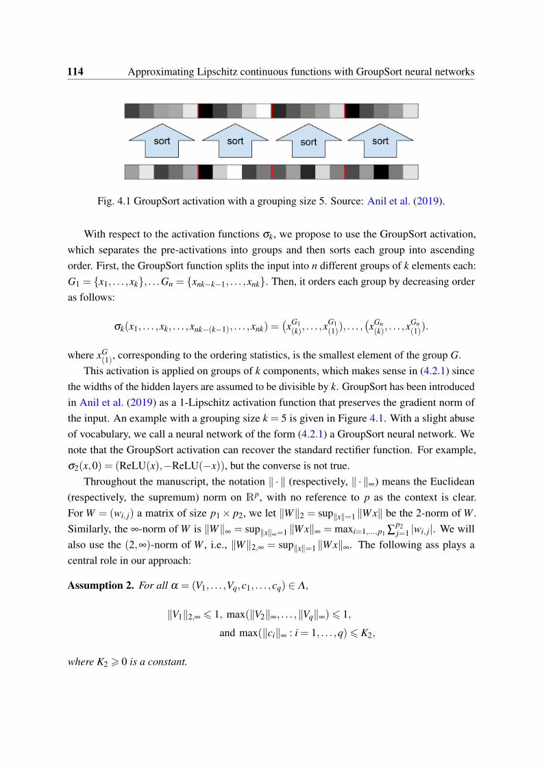
114 Approximating Lipschitz continuous functions with GroupSort neural networks
Fig. 4.1 GroupSort activation with a grouping size 5. Source: Anil et al. (2019).
With respect to the activation functions σk, we propose to use the GroupSort activation,which separates the pre-activations into groups and then sorts each group into ascendingorder. First, the GroupSort function splits the input into n different groups of k elements each:G1 = x1, . . . ,xk, . . .Gn = xnk−k−1, . . . ,xnk. Then, it orders each group by decreasing orderas follows:
σk(x1, . . . ,xk, . . . ,xnk−(k−1), . . . ,xnk) =(xG1(k), . . . ,x
G1(1)), . . . ,
(xGn(k), . . . ,x
Gn(1)).
where xG(1), corresponding to the ordering statistics, is the smallest element of the group G.
This activation is applied on groups of k components, which makes sense in (4.2.1) sincethe widths of the hidden layers are assumed to be divisible by k. GroupSort has been introducedin Anil et al. (2019) as a 1-Lipschitz activation function that preserves the gradient norm ofthe input. An example with a grouping size k = 5 is given in Figure 4.1. With a slight abuseof vocabulary, we call a neural network of the form (4.2.1) a GroupSort neural network. Wenote that the GroupSort activation can recover the standard rectifier function. For example,σ2(x,0) = (ReLU(x),−ReLU(−x)), but the converse is not true.
Throughout the manuscript, the notation ∥ · ∥ (respectively, ∥ · ∥∞) means the Euclidean(respectively, the supremum) norm on Rp, with no reference to p as the context is clear.For W = (wi, j) a matrix of size p1 × p2, we let ∥W∥2 = sup∥x∥=1 ∥Wx∥ be the 2-norm of W .Similarly, the ∞-norm of W is ∥W∥∞ = sup∥x∥∞=1 ∥Wx∥∞ = maxi=1,...,p1 ∑
p2j=1 |wi, j|. We will
also use the (2,∞)-norm of W , i.e., ∥W∥2,∞ = sup∥x∥=1 ∥Wx∥∞. The following ass plays acentral role in our approach:
Assumption 2. For all α = (V1, . . . ,Vq,c1, . . . ,cq) ∈ Λ ,
∥V1∥2,∞ ⩽ 1, max(∥V2∥∞, . . . ,∥Vq∥∞)⩽ 1,
and max(∥ci∥∞ : i = 1, . . . ,q)⩽ K2,
where K2 ⩾ 0 is a constant.

4.3 Learning functions with a grouping size 2 115
This type of compactness requirement has already been suggested in the statistical andmachine learning community (e.g., Arjovsky et al., 2017; Anil et al., 2019; Biau et al., 2020).In the setting of this article, its usefulness is captured in the following simple but essentiallemma:
Lemma 4.2.1. Assume that Assumption 2 is satisfied. Then, for any k ⩾ 2, Dk ⊆ Lip1(Rd).
Combining Lemma 4.2.1 with Arzelà-Ascoli theorem, it is easy to see that, under Assump-tion 2, the class Dk restricted to any compact K ⊆ Rd is compact in the set of continuousfunctions on K with respect to the uniform norm. From this point of view, Assumption 2 istherefore somewhat restrictive. On the other hand, it is essential in order to guarantee that allneural networks in Dk are indeed 1-Lipschitz. Practically speaking, various approaches havebeen explored in the literature to enforce this 1-Lipschitz constraint. Gulrajani et al. (2017),Kodali et al. (2017), Wei et al. (2018), and Zhou et al. (2019) proposed a gradient penalty term,Miyato et al. (2018) applied spectral normalization, while Anil et al. (2019) have shown theempirical efficiency of the orthonormalization of Bjorck and Bowie (1971).
Importantly, Anil et al. (2019, Theorem 3) states that, under Assumption 2, GroupSortneural networks are universal Lipschitz approximators on compact sets. More precisely, forany Lipschitz continuous function f defined on a compact, one can find a neural network ofthe form (4.2.1) verifying Assumption 2 and arbitrarily close to f with respect to the uniformnorm. Our objective in the present article is to explore the properties of these networks. Westart in the next section by examining the case of piecewise linear functions.
4.3 Learning functions with a grouping size 2
For this section, we only consider GroupSort neural networks with a grouping size 2 and aim atstudying their expressivity. The capacity of GroupSort networks to approximate continuousfunctions is studied via the representation of piecewise linear functions. For feedforward ReLUnetworks, their ability to represent such functions has been largely studied. In particular, Aroraet al. (2018, Theorem 2.1) reveals that any piecewise linear function from Rd → R can berepresented by a ReLU network of depth at most ⌈log2(d +1)⌉ (the symbol ⌈·⌉ stands for theceiling function), whereas He et al. (2018) specify an upper bound on their size. In the presentsection, we extend these results and first tackle the problem of representing piecewise linearfunctions with constrained GroupSort networks. Then we move to the non-linear case.
4.3.1 Representation of piecewise linear functions
Let us start gently by fixing the vocabulary.
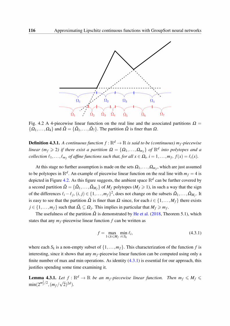
116 Approximating Lipschitz continuous functions with GroupSort neural networks
Ω1 Ω2 Ω3 Ω4
Ω1 Ω2 Ω3 Ω4 Ω5 Ω6 Ω7
Fig. 4.2 A 4-piecewise linear function on the real line and the associated partitions Ω =Ω1, . . . ,Ω4 and Ω = Ω1, . . . ,Ω7. The partition Ω is finer than Ω .
Definition 4.3.1. A continuous function f :Rd →R is said to be (continuous) m f -piecewiselinear (m f ⩾ 2) if there exist a partition Ω = Ω1, . . . ,Ωm f of Rd into polytopes and acollection ℓ1, . . . , ℓm f of affine functions such that, for all x ∈ Ωi, i = 1, . . . ,m f , f (x) = ℓi(x).
At this stage no further assumption is made on the sets Ω1, . . . ,Ωm f , which are just assumedto be polytopes in Rd . An example of piecewise linear function on the real line with m f = 4 isdepicted in Figure 4.2. As this figure suggests, the ambient space Rd can be further covered bya second partition Ω = Ω1, . . . ,ΩM f of M f polytopes (M f ⩾ 1), in such a way that the signof the differences ℓi − ℓ j, (i, j) ∈ 1, . . . ,m f 2, does not change on the subsets Ω1, . . . ,ΩM f . Itis easy to see that the partition Ω is finer than Ω since, for each i ∈ 1, . . . ,M f there existsj ∈ 1, . . . ,m f such that Ωi ⊆ Ω j. This implies in particular that M f ⩾ m f .
The usefulness of the partition Ω is demonstrated by He et al. (2018, Theorem 5.1), whichstates that any m f -piecewise linear function f can be written as
f = max1⩽k⩽M f
mini∈Sk
ℓi, (4.3.1)
where each Sk is a non-empty subset of 1, . . . ,m f . This characterization of the function f isinteresting, since it shows that any m f -piecewise linear function can be computed using only afinite number of max and min operations. As identity (4.3.1) is essential for our approach, thisjustifies spending some time examining it.
Lemma 4.3.1. Let f : Rd → R be an m f -piecewise linear function. Then m f ⩽ M f ⩽
min(2m2f /2,(m f /
√2)2d).

4.3 Learning functions with a grouping size 2 117
Lemma 4.3.1 is an improvement of He et al. (2018, Lemma 5.1), which shows that M f ⩽m f !.Our proof method exploits the inequality M f ⩽Cm f (m f−1)/2,d , where Cn,d denotes the numberof arrangements of n hyperplanes in a space of dimension d (Devroye et al., 1996, Chapter 5).Another application of (4.3.1) is encapsulated in Proposition 4.3.1 below, which will be usefulfor later analysis, in combining maxima and minima in neural networks of the form (4.2.1).
Proposition 4.3.1. Let f1, . . . , fm : Rd → R be a collection of functions (m ⩾ 2), each repre-sented by a neural network of the form (4.2.1), with common depth q and sizes si, i = 1, . . . ,m.
In the specific case where m = 2n for some n ⩾ 1, there exist neural networks of the form(4.2.1) (with grouping size 2) with depth q+ log2(m) and size at most s1+ · · ·+ sm+m−1 thatrepresent the functions f = max( f1, . . . , fm) and g = min( f1, . . . , fm).
If m is arbitrary, then there exist neural networks of the form (4.2.1) with depth q +
⌈log2(m)⌉ and size at most s1 + · · ·+ sm +2m−1 that represent the functions f and g.
Interestingly, Arora et al. (2018, Lemma D.3), which is the analog of Proposition 4.3.1asserts that the size with ReLU activations is at most s1 + · · ·+ sm +8m−4. For the specificcomputation of maxima/minima of functions, it should be stressed that GroupSort activationsslightly reduces the size of the networks. By combining Lemma 4.3.1, Proposition 4.3.1, andidentity (4.3.1), we are led to the following theorem, which reveals the ability of GroupSortnetworks for representing 1-Lipschitz piecewise linear functions.
Theorem 4.3.1. Let f ∈ Lip1(Rd) that is also m f -piecewise linear. Then there exists a neural
network of the form (4.2.1) verifying Assumption 2 that represents f . Besides, its depth is⌈log2(M f )⌉+ ⌈log2(m f )⌉+1 and its size is at most 3m f M f +M f −1.
This result should be compared with state-of-the-art results known for ReLU neural net-works. In particular, Arora et al. (2018, Theorem 2.1) reveals that any m f -piecewise linearfunction f can be represented by a ReLU network with depth at most ⌈log2(d+1)⌉. The upperbound of Theorem 4.3.1 can be larger since it involves both M f and m f . On the other hand, theupper bound O(m f M f ) on the size significantly improves on He et al. (2018, Theorem 5.2),which is at least O(d2m f M f ). This improvement in terms of size can be roughly explained by thedepth/size trade-off results known in deep learning theory. As a matter of fact, many theoreticalresearch papers have underlined the benefits of depth relatively to width for parameterizingcomplex functions (as, for example, in Telgarsky, 2015, 2016). For a fixed number of neurons,when comparing two neural networks, the deepest is the most expressive one (Lu et al., 2017).
It turns out that Theorem 4.3.1 can be significantly refined when the partition Ω satis-fies some geometrical properties. Our next proposition examines the case where the setsΩ1, . . . ,Ωm f are convex.

118 Approximating Lipschitz continuous functions with GroupSort neural networks
Corollary 4.3.1. Let f ∈ Lip1(Rd) that is also m f -piecewise linear with convex subdomains
Ω1, . . . ,Ωm f . Then there exists a neural network of the form (4.2.1) verifying Assumption 2that represents f . Besides, its depth is 2⌈log2(m f )⌉+1 and its size is at most 3m2
f +m f −1.
Corollary 4.3.1 offers a significant improvement over Theorem 4.3.1, since in generalM f ≫ m f . We note in passing that the result of this proposition is dimension-free.
4.3.2 GroupSort neural networks on the real line
Piecewise linear functions defined on R deserve a special treatment, since in this case, anyconnected subset is convex.
Proposition 4.3.2. Let f ∈ Lip1(R) that is also m f -piecewise linear. Then there exists a neuralnetwork of the form (4.2.1) verifying Assumption 2 that represents f . Besides, its depth is2⌈log2(m f )⌉+1 and its size is at most 3m2
f +m f −1.In the specific case where f is convex (or concave), then there exists a neural network of
the form (4.2.1) verifying Assumption 2 that represents f . Its depth is ⌈log2(m f )⌉+1 and itssize is at most 3m f −1.
When f is convex (or concave) and m f = 2n for some n ⩾ 1, then there exists a neuralnetwork of the form (4.2.1) verifying Assumption 2 that represents f . Its depth is log2(m f )+1and its size is at most 2m f −1.
This proposition is the counterpart of Arora et al. (2018, Theorem 2.2), which states thatany m f -piecewise linear function from R→R can be represented by a 2-layer ReLU neuralnetwork with a size at least m f −1 . He et al. (2018, Theorem 5.2) shows that the upper-boundon the size of ReLU networks is O(2m2+2(m−1)). Thus, for the representation of piecewiselinear functions on the real line, GroupSort networks require larger depths but smaller sizes.Besides, bear in mind that the obtained ReLU neural networks do not necessarily verify arequirement similar to the one of Assumption 2.
Regarding the number of linear regions of GroupSort networks on the real line, we have thefollowing result:
Lemma 4.3.2. Any neural network of the form (4.2.1) on the real line, with depth q and widthsν1, . . . ,νq−1, parameterizes a piecewise linear function with at most 2q−2 × (ν1/2+1)×ν2 ×·· ·×νq−1 linear subdomains.
We deduce from this lemma that for a neural network of the form (4.2.1) with depth q ⩾ 2and constant width ν , the maximum number of linear regions is O(2q−3νq−1). Similarly toReLU networks (Montúfar et al., 2014; Arora et al., 2018), the maximum number of linear

4.3 Learning functions with a grouping size 2 119
regions for GroupSort networks with grouping size 2 is also likely to grow polynomially in ν
and exponentially in q.Our next corollary now illustrates the trade-off between depth and width for GroupSort
neural networks.
Corollary 4.3.2. Let f ∈ Lip1(R) be an m f -piecewise linear function. Then, any neuralnetwork of the form (4.2.1) verifying Assumption 2 and representing f with a depth q, has asize s at least 1
2(q−1)m1/(q−1)f .
The lower bound highlighted in Corollary 4.3.2 is dependent on the depth q of the neuralnetwork. By looking at the minimum of the function, we get that any neural network repre-senting f has a size s ⩾ e ln(m f )
2 . Thus, merging this result with Proposition 4.3.2, we have thatfor any m f -piecewise linear function from R→R, there exists a GroupSort network verifyingAssumption 2 with a size s satisfying
e ln(m f )
2⩽ s ⩽ 3m2
f −m f −3.
We realize that this inequality is large but, up to our knowledge, this is first of this type forGroupSort neural networks.
4.3.3 Approximating Lipschitz continuous functions on compact sets
Following our plan, we tackle in this subsection the task of approximating Lipschitz continuousfunctions on compact sets using GroupSort neural networks. The space of continuous functionson [0,1]d is equipped with the uniform norm
∥ f −g∥∞ = maxx∈[0,1]d
| f (x)−g(x)|.
The main result of the section, and actually of the article, is that GroupSort neural networks arewell suited for approximating functions in Lip1([0,1]
d).
Theorem 4.3.2. Let ε > 0 and d ⩾ 2, f ∈ Lip1([0,1]d). Then there exists a neural network
D of the form (4.2.1) verifying Assumption 2 such that ∥ f −D∥∞ ⩽ ε . The depth of D isO(d2 log2(
2√
dε
)) and its size is O((2√
dε
)d2).
To the best of our knowledge, Theorem 4.3.2 is the first one that provides an upper boundon the depth and size of neural networks, with constraints on the weights, that approximateLipschitz continuous functions.

120 Approximating Lipschitz continuous functions with GroupSort neural networks
As for the representation of piecewise linear functions, one can, for the sake of completeness,compare this bound with those previously found in the literature of ReLU neural networks.Yarotsky (2017) establishes the density of ReLU networks in Sobolev spaces, using a differenttechnique of proof. In particular, Theorem 1 of this paper states that for any f ∈ Lip1([0,1]
d)
continuously differentiable, there exists a ReLU neural network approximating f with precisionε , with depth at most c(ln(1/ε)+ 1) and size at most cε−d(ln(1/ε)+ 1) (with a constantc function of d). Comparing this result with our Theorem 4.3.2, we see that, with respectto ε , both depths are similar but ReLU networks are smaller in size. However, one has tokeep in mind that both lines of proof largely differ. Besides, our formulation ensures that theapproximator is also a 1-Lipschitz function, a feature that cannot be guaranteed under theformulation of Yarotsky (2017).
It turns out however that our framework provides smaller neural networks as soon as d = 1.
Proposition 4.3.3. Let ε > 0 and f ∈ Lip1([0,1]). Then there exists a neural network D of theform (4.2.1) verifying Assumption 2 such that ∥ f −D∥∞ ⩽ ε . The depth of D is 2⌈log2(1/ε)⌉+1and its size is O((1
ε)2).
Besides, if f is assumed to be convex or concave, then the depth of D is ⌈log2(1/ε)⌉+1and its size is O(1
ε).
4.4 Impact of the grouping size
The previous section paved the way for a better understanding of GroupSort neural networksand their ability to approximate Lipschitz continuous functions. As mentioned in Section 4.2,one can play with the grouping size k of the neural network when defining its architecture.However, it is not clear how changing this parameter might influence the expressivity of thenetwork. The present section aims at bringing some understanding. Following a similarreasoning as in Section 4.3, we start by analyzing how GroupSort networks with an arbitrarygrouping size k ⩾ 2 can represent any piecewise linear functions:
Proposition 4.4.1 (Extension of Proposition 4.3.1). Let f1, . . . , fm : Rd → R be a collectionof functions (m ⩾ 2), each represented by a neural network of the form (4.2.1), with commondepth q and sizes si, i = 1, . . . ,m.
In the specific case where m = kn for some n ⩾ 1, there exist neural networks of the form(4.2.1) (with grouping size k) with depth q+ logk(m) and size at most s1 + · · ·+ sm + m−1
k−1 −1that represent the functions f = max( f1, . . . , fm) and g = min( f1, . . . , fm).
Similarly to Section 4.3, this leads to the following corollary:

4.4 Impact of the grouping size 121
Methods Up Depth Up Size Down Size ReferenceRepresenting m = kn-PWL functions in Rd with a constant width ν
ReLU ⌈log2(d +1)⌉+1 O(d2m2) O(m) He et al. (2018)
GroupSort GS = k ⌈2logk(m)⌉+1 m2−1k−1
ν logk(m)2logk(ν)
present article
Approximating 1-Lipschitz continuous functions in [0,1]d
ReLU O(ln(1ε)) O( ln(1/ε)
εd ) \ Yarotsky (2017)
GroupSort GS = ⌈2√
dε
⌉ O(d2) O((2√
dε
)d2−1) \ present articleApproximating 1-Lipschitz continuous functions in [0,1]ReLU (PWL representation) 2 O(21/ε2+2/ε) \ He et al. (2018)
ReLU (different approach) O(ln(1ε)) O( ln(1/ε)
ε) \ Yarotsky (2017)
Adaptative ReLU 6 O( 1ε ln(1/ε)) \ Yarotsky (2017)
GroupSort GS = ⌈1ε⌉ 3 O(1
ε) \ present article
Table 4.1 Summary of the results shown in the present paper together with results previouslyfound for ReLU networks. “Up Depth” refers to upper bounds on the depths, “Up Size” toupper bounds on the sizes, and “Down Size” to lower bounds on the sizes. The symbol “\”means that no result is known (up to our knowledge).
Corollary 4.4.1 (Extension of Corollary 4.3.1). Let f ∈ Lip1(Rd) that is also m f -piecewise
linear with convex subdomains Ω1, . . . ,Ωm f such that m f = kn for some n ⩾ 1. Then thereexists a neural network of the form (4.2.1) verifying Assumption 2 that represents f . Besides,
its depth is 2⌈logk(m f )⌉+1 and its size is at mostm2
f−1k−1 .
Proposition 4.4.1 and Corollary 4.4.1 exhibit the nice properties of using larger groupingsizes. Indeed, for a given q ⩾ 1, there exists a neural network with depth 2q+1 and groupingsize k representing a function with kq pieces. Consequently, the use of larger grouping sizeshelps have more expressive neural networks. The efficiency of larger grouping sizes may alsobe explained by the following result for GroupSort networks on the real line:
Lemma 4.4.1 (Extension of Lemma 4.3.2). Any neural network of the form (4.2.1) on the realline, with depth q, widths ν1, . . . ,νq−1, and grouping size k, parameterizes a piecewise linearfunction with at most kq−2 × ( (k−1)ν1
2 +1)×ν2 ×·· ·×νq−1 linear subdomains.
Thus, the number of linear regions of a GroupSort network is likely to increase polynomiallywith the grouping size, which highlights the benefits of using larger groups. Similarly to Section4.3, when moving to the approximation of Lipschitz continuous functions on [0,1]d , we arelead to the following theorem:
Theorem 4.4.1 (Extension Theorem 4.3.2). Let ε > 0, d ⩾ 2, and f ∈ Lip1([0,1]d). Then there
exists a neural network D of the form (4.2.1) verifying Assumption 2 with grouping size ⌈2√
dε
⌉such that ∥ f −D∥∞ ⩽ ε . The depth of D is O(d2) and its size is O((2
√d
ε)d2−1).

122 Approximating Lipschitz continuous functions with GroupSort neural networks
Using a grouping size proportional to 1/ε , we thus have a bound on the depth that isindependent from the error rate. The uni-dimensional case leads to a different result:
Proposition 4.4.2 (Extension of Proposition 4.3.3). Let ε > 0 and f ∈ Lip1([0,1]). Then thereexists a neural network D of the form (4.2.1) verifying Assumption 2 (with grouping size k)such that ∥ f −D∥∞ ⩽ ε . The depth of D is 2⌈logk(
1ε)⌉+1 and its size is at most O( 1
kε2 ).In particular, if k is chosen to be equal to ⌈1
ε⌉, then the depth of D is 3 and its size is O(1
ε).
When approximating real-valued functions, the use of larger grouping sizes can significantlydecrease the required size since it goes from O(1/ε2) in Proposition 4.3.3 to O(1/ε) inProposition 4.4.2. When f is assumed to be convex or concave, the depth of the network D canfurther be reduced to 2.
Using a different approach for approximating Lipschitz continuous functions in [0,1],Yarotsky (2017, Theorem 1) shows that ReLU networks with a depth of O(ln(1/ε)) is neededtogether with a size O( ln(1/ε)
ε) to approximate with an error rate ε . To sum-up, when compared
with ReLU networks, GroupSort neural networks with well-chosen grouping size can besignificantly more expressive.
Table 4.1 summarizes the results shown in the present paper together with results previ-ously found for ReLU networks. Bear in mind that GroupSort neural networks also have thesupplementary condition that any parameterized function verifies the 1-Lipschitz continuity.
4.5 Experiments
Anil et al. (2019) have already compared the performances of GroupSort neural networks withtheir ReLU counterparts, both with constraints on the weights. In particular, they showedthat ReLU neural networks are more sensitive to adversarial attacks while stressing the factthat if their weights are limited, then these networks lose their expressive power. Building onthese observations, we further illustrate the good behavior of GroupSort neural networks inthe context of estimating a Lipschitz continuous regression function and in approximating theWasserstein distance (via its dual form) between pairs of distributions.
Impact of the depth. We start with the problem of learning a function f in the modelY = f (X), where X follows a uniform distribution on [−8,8] and f is 32-piecewise linear. Tothis aim, we use neural networks of the form (4.2.1) with respective depth q = 2, 8, 14, 20,and a constant width ν = 50. Since we are only interested in the approximation properties ofthe networks, we assume to have at hand an infinite number of pairs (Xi, f (Xi)) and train themodels by minimizing the mean squared error. We give in the Appendix, the full details of our

4.5 Experiments 123
5 0 50.0
0.1
0.2
0.3
0.4
0.5
Target y Predicted y
(a) q = 2 (b) q = 20
2 8 14 20Network depth
0.028
0.083
0.138
0.193
0.248
Unifo
rm n
orm
(c) Uniform norm
2 8 14 20Network depth
0.136
0.339
0.541
0.744
0.946
Lipsc
hitz
con
stan
t
(d) Lipschitz constants
Fig. 4.3 Reconstruction of a 32-piecewise linear function on [−8,8] with a GroupSort neuralnetwork of the form (4.2.1) with depth q = 2, 8, 14, 20, and a constant width ν = 50 (thethickness of the line represents a 95%-confidence interval).
experimental setting. The quality of the estimation is evaluated using the uniform norm betweenthe target function f and the output network. In order to enforce Assumption 2, GroupSortneural networks are constrained using the orthonormalization of Bjorck and Bowie (1971). Theresults are presented in Figure 4.3. Note that throughout this section, confidence intervals arecomputed over 20 runs. In line with Theorem 4.3.1, which states that f is representable by aneural network of the form (4.2.1) with size at most 3×322+32−1= 3104, we clearly observethat, as the depth of the networks increases, the uniform norm decreases and the Lipschitzconstant of the network converges to 1. The reconstruction of this piecewise linear function iseven almost perfect for the depth q = 20, i.e., with a network of size only 20×60 = 1200, avalue significantly smaller than the upper bound of the theorem.
We also illustrate the behavior of GroupSort neural networks in the context of WGANs(Arjovsky et al., 2017). We run a series of small experiments in the simplified setting where we
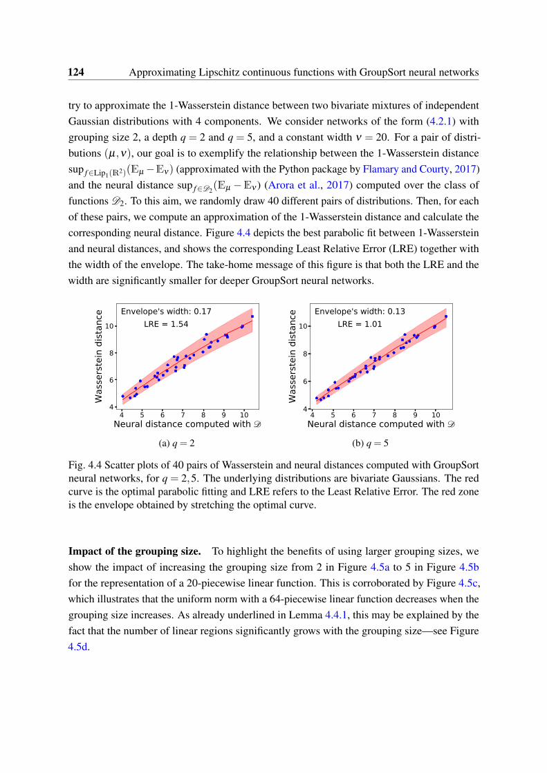
124 Approximating Lipschitz continuous functions with GroupSort neural networks
try to approximate the 1-Wasserstein distance between two bivariate mixtures of independentGaussian distributions with 4 components. We consider networks of the form (4.2.1) withgrouping size 2, a depth q = 2 and q = 5, and a constant width ν = 20. For a pair of distri-butions (µ,ν), our goal is to exemplify the relationship between the 1-Wasserstein distancesup f∈Lip1(R
2)(Eµ −Eν) (approximated with the Python package by Flamary and Courty, 2017)and the neural distance sup f∈D2
(Eµ −Eν ) (Arora et al., 2017) computed over the class offunctions D2. To this aim, we randomly draw 40 different pairs of distributions. Then, for eachof these pairs, we compute an approximation of the 1-Wasserstein distance and calculate thecorresponding neural distance. Figure 4.4 depicts the best parabolic fit between 1-Wassersteinand neural distances, and shows the corresponding Least Relative Error (LRE) together withthe width of the envelope. The take-home message of this figure is that both the LRE and thewidth are significantly smaller for deeper GroupSort neural networks.
4 5 6 7 8 9 10Neural distance computed with
4
6
8
10
Was
sers
tein
dist
ance
LRE = 1.54Envelope's width: 0.17
(a) q = 2
4 5 6 7 8 9 10Neural distance computed with
4
6
8
10
Was
sers
tein
dist
ance
LRE = 1.01Envelope's width: 0.13
(b) q = 5
Fig. 4.4 Scatter plots of 40 pairs of Wasserstein and neural distances computed with GroupSortneural networks, for q = 2,5. The underlying distributions are bivariate Gaussians. The redcurve is the optimal parabolic fitting and LRE refers to the Least Relative Error. The red zoneis the envelope obtained by stretching the optimal curve.
Impact of the grouping size. To highlight the benefits of using larger grouping sizes, weshow the impact of increasing the grouping size from 2 in Figure 4.5a to 5 in Figure 4.5bfor the representation of a 20-piecewise linear function. This is corroborated by Figure 4.5c,which illustrates that the uniform norm with a 64-piecewise linear function decreases when thegrouping size increases. As already underlined in Lemma 4.4.1, this may be explained by thefact that the number of linear regions significantly grows with the grouping size—see Figure4.5d.

4.5 Experiments 125
(a) Grouping size = 2 (b) Grouping size = 6
(c) Uniform norm (d) Linear regions
Fig. 4.5 Reconstruction of a 20-piecewise linear function on [−5,5] (top line) and a 64-piecewise linear function (bottom line) with GroupSort neural networks of the form (4.2.1)with depth q = 4 and varying grouping sizes k = 2,4,6,8,10.
Comparison with ReLU neural networks. Next, in a second series of experiments, wecompare the performances of GroupSort networks against two baselines: ReLU neural networkswithout constraints on the weights (dense in the set of continuous functions on a compactset; see Yarotsky, 2017), and ReLU neural networks with orthonormalization of Bjorck andBowie (1971). The architecture of the ReLU neural networks in terms of depth and width is thesame as for GroupSort networks: q = 2, 4, 6 ,8, and w = 20. The task is now to approximatethe 1-Lipschitz continuous function f (x) = (1/15)sin(15x) on [0,1] in the models Y = f (X)
(noiseless case) and Y = f (X)+ ε (noisy case), where X is uniformly distributed on [0,1] andε follows a Gaussian distribution with standard deviation 0.05. In both cases, we assume tohave at hand a finite sample of size n = 100 and fit the models by minimizing the mean squarederror.

126 Approximating Lipschitz continuous functions with GroupSort neural networks
2 4 6 8Network depth
0.007
0.020
0.033
0.046
0.059
Unifo
rm n
orm
ReLU bjorckReLU bjorckGroupSort
(a) Prediction quality
2 4 6 8Network depth
0.340
0.595
0.850
1.105
1.360
Lipsc
hitz
con
stan
t
ReLU bjorckReLU bjorckGroupSort
(b) Lipschitz constants
2 4 6 8Network depth
5.0
48.7
92.4
136.1
179.8
Num
line
ar re
gion
s
ReLU bjorckReLU bjorckGroupSort
(c) Number of linear regions
2 4 6 8Network depth
0.032
0.042
0.052
0.063
0.073
Unifo
rm n
orm
ReLU bjorckReLU bjorckGroupSort
(d) Prediction quality
2 4 6 8Network depth
0.342
1.080
1.818
2.555
3.293
Lipsc
hitz
con
stan
t
ReLU bjorckReLU bjorckGroupSort
(e) Lipschitz constant
2 4 6 8Network depth
4.0
30.2
56.5
82.8
109.0Nu
m li
near
regi
ons
ReLU bjorckReLU bjorckGroupSort
(f) Number of linear regions
Fig. 4.6 (Top line) Estimating the function f (x) = (1/15)sin(15x) on [0,1] in the modelY = f (X), with a dataset of size n = 100. (Bottom line) Estimating the function f (x) =(1/15)sin(15x) on [0,1] in the model Y = f (X) + ε , with a dataset of size n = 100 (thethickness of the line represents a 95%-confidence interval).

4.6 Conclusion 127
Both results (noiseless case and noisy case) are presented in Figure 4.6. We observe that inthe noiseless setting Figure 4.6a, 4.6b, and 4.6c, ReLU neural networks without normalizationhave a slightly better performance with respect to the uniform norm with, however, a Lipschitzconstant larger than 1. On the other hand, in the noisy case, ReLU neural networks withoutconstraints have a tendency to overfitting (a high Lipschitz constant close to 2.7), leadingto a deteriorated performance, contrary to GroupSort neural networks. Furthermore, in bothcases (noiseless and noisy), ReLU with constraints are found to perform worse (due to aLipschitz constant much smaller than 1) than their GroupSort counterparts in terms of prediction.Interestingly, we see in the two examples shown in Figure 4.6e and Figure 4.6f, that the numberof linear regions for GroupSort neural networks is smaller than for ReLU networks.
Finally, we quickly show in Appendix a comparison between GroupSort and ReLU networkswhen approximating Wasserstein distances. The take home message is that, on this specifictask, GroupSort networks perform better.
4.6 Conclusion
The results presented in this article show the advantage of using GroupSort neural networks overstandard ReLU networks. On the one hand, ReLU neural networks without any constraints aresensitive to adversarial attacks (as they may have a large Lipschitz constant) and, on the otherhand, lose expressive power when enforcing limits on their weights. On the opposite, GroupSortneural networks with constrained weights are proved to be both robust and expressive, and aretherefore an interesting alternative. Moreover, by allowing larger grouping sizes for GroupSortnetworks, one can further increase their expressivity. These properties open new perspectivesfor broader use of GroupSort networks.
Appendix 4.A Technical results
4.A.1 Proof of Lemma 4.2.1
We prove the result for D2. The result for Dk holds following a similar argument.Fix D2,α ∈D2, α ∈Λ . According to (4.2.1), we have, for x ∈Rd , D2,α(x) = fq · · · f1(x),
where fi(t) = σ2(Vit + ci) for i = 1, . . . ,q− 1 (σ2 is applied on pairs of components), and

128 Approximating Lipschitz continuous functions with GroupSort neural networks
fq(t) =Vqt + cq. Therefore, for (x,y) ∈ (Rd)2,
∥ f1(x)− f1(y)∥∞ ⩽ ∥V1x−V1y∥∞
(since σ2 is 1-Lipschitz)
= ∥V1(x− y)∥∞
⩽ ∥V1∥2,∞ ∥x− y∥⩽ ∥x− y∥
(by Assumption 2).
Thus,
∥ f2 f1(x)− f2 f1(y)∥∞ ⩽ ∥V2 f1(x)−V2 f1(y)∥∞
(since σ2 is 1-Lipschitz)
⩽ ∥V2∥∞ ∥ f1(x)− f1(y)∥∞
⩽ ∥ f1(x)− f1(y)∥∞
(by Assumption 2)
⩽ ∥x− y∥.
Repeating this, we conclude that, for each α ∈ Λ and all (x,y) ∈ (Rd)2, |D2,α(x)−D2,α(y)|⩽∥x− y∥, which is the desired result.
4.A.2 Proof of Lemma 4.3.1
Recall that m f ⩾ 2. Throughout the proof, we let · refer to the dot product in Rd . Let(i, j) ∈ 1, . . . ,m f 2, i = j. There exist (ai,bi) ∈ Rd ×R and (a j,b j) ∈ Rd ×R such thatℓi = ai · x+bi and ℓ j = a j · x+b j. Therefore,
ℓi(x)− ℓ j(x)⩽ 0 ⇐⇒ x · (ai −a j)⩽ b j −bi.
So, there exist two subdomains Ω1 and Ω2, separated by an affine hyperplane, in which ℓi − ℓ j
does not change sign. By repeating this operation for the m f (m f −1)/2 different pairs (ℓi, ℓ j),we get that the number M f of subdomains on which any pair ℓi − ℓ j does not change sign issmaller than the maximal number of arrangements of m f (m f −1)/2 hyperplanes.
Denoting by Cn,d the maximal number of arrangements of n hyperplanes in Rd , we knowthat when d > n then Cn,d = 2n, whereas if n > d the upper bound Cn,d ⩽ (1+n)d becomes

4.A Technical results 129
preferable (Devroye et al., 1996, Chapter 30). Thus, we have
m f ⩽ M f ⩽ min(2m2
f /2,(m f /√
2)2d).4.A.3 Proof of Proposition 4.3.1
We prove the first part of the proposition by using an induction on n. The case where n = 1and thus m = 21 is clear since the function f = max( f1, f2) can be represented by a neuralnetwork of the form (4.2.1) with depth q+ 1 and size s1 + s2 + 1. Now, let m = 2n withn > 1. We have that m/2 = 2n−1. By the induction hypothesis, g1 = max( f1, . . . , fm/2) andg2 = max( fm/2+1, . . . , fm) can be represented by neural networks of the form (4.2.1) withdepths q+n−1, and sizes at most s1 + · · ·+ sm/2 +m/2−1 and sm/2+1 + · · ·+ sm +m/2−1,respectively. Consequently, the function G(x) = (g1(x),g2(x)) can be implemented by a neuralnetwork of the form (4.2.1) with depth q+ n− 1 and size s1 + · · ·+ sm +m− 2. Finally, byconcatenating a one neuron layer, we have that the function f = max(g1,g2) can be representedby a neural network of the form (4.2.1) with depth q+ n = q+ log2(m) and size at mosts1 + · · ·+ sm +m−1.
Now, let us prove the case where m is arbitrary. Let f1, . . . , fm : Rd → R be a collectionof functions (m ⩾ 2), each represented by a neural network of the form (4.2.1) with depthq and size si, i = 1, . . . ,m. We prove below by an induction on n that there exists a neuralnetwork of the form (4.2.1) with depth q+ ⌈log2(m)⌉, a final layer of width νq−1 = 2, and asize at most s1 + · · ·+ sm +2⌈log2(m)⌉−1 that represents the functions f = max( f1, . . . , fm) andg = min( f1, . . . , fm) (the symbol ⌈·⌉ stands for the ceiling function and the symbol ⌊·⌋ standsfor the integer function).
The base case m = 2 is clear using the GroupSort activation and ν1 = 2. For m > 2, letn ⩾ 2 be such that 2n−1 ⩽ m < 2n. Let g1 = max( f1, . . . , f2n−1) and g2 = max( f2n−1+1, . . . , fm).From the first part of the proof, we know that g1 can be represented by a neural network ofthe form (4.2.1) with depth q1 = q+ ⌊log2 m⌋= q+n−1 and size s1 + · · ·+ s2n−1 +2n−1 −1.Also, by the induction hypothesis, g2 can be represented by a neural network of the form (4.2.1)with depth q2 = q+ ⌈log2(m−2n−1)⌉ and size at most s2n−1+1 + · · ·+ sm +2⌈log2(m−2n−1)⌉−1.Therefore, by padding identity matrices with two neurons (recall that νq2−1 = 2) on layers from

130 Approximating Lipschitz continuous functions with GroupSort neural networks
q+ ⌈log2(m−2n−1)⌉ to q+n−1, we have:
2⌈log2(m−2n−1)⌉−1+2(n−2−⌈log2(m−2n−1)⌉) =k=⌈log2(m−2n−1)⌉−1
∑k=0
2k +k=n−2
∑k=⌈log2(m−2n−1)⌉
21
⩽k=n−2
∑k=0
2k = 2n−1 −1.
Thus, g2 can be represented by a neural network of the form (4.2.1) with depth q2 = q+⌊log2 m⌋and size at most s2n−1+1+ · · ·+sm+2n−1−1. Now, the bivariate function G(x) = (g1(x),g2(x))can be implemented by a neural network of the form (4.2.1) with depth q+ ⌊log2(m)⌋ and sizes such that
s ⩽ s1 + · · ·+ sm +2(2n−1 −1) = s1 + · · ·+ sm +2n −2.
By concatenating a one neuron layer, we have that the function f = max(g1,g2) can berepresented by a neural network of the form (4.2.1) with depth q+ ⌈log2(m)⌉ and size at mosts1+ · · ·+sm+2n−1 = s1+ · · ·+sm+2⌈log2 m⌉−1. The conclusion follows using the inequality2⌈log2 m⌉ ⩽ 2m.
4.A.4 Proof of Theorem 4.3.1
Let f ∈ Lip1(Rd) that is also m f -piecewise linear. We know that each linear function can
be represented by a 1-neuron neural network verifying Assumption 2 (no need for hiddenlayers). Combining (4.3.1) with Proposition 4.3.1, for each k ∈ 1, . . . ,M f there exists aneural network of the form (4.2.1), verifying Assumption 2 and representing the functionmini∈Sk ℓi, with depth equal to ⌈log2(m f )⌉+1 (since |Sk|⩽ m f ) and size at most 3m f −1.
Using again Proposition 4.3.1, we conclude that there exists a neural network of the form(4.2.1), verifying Assumption 2 and representing f , with depth⌈log2(M f )⌉+ ⌈log2(m f )⌉+1and size at most 3m f M f +M f −1.
4.A.5 Proof of Corollary 4.3.1
According to He et al. (2018, Theorem A.1), the function f can be written as
f = max1⩽k⩽m f
mini∈Sk
ℓi,

4.A Technical results 131
where |Sk|⩽ m f . Using the same technique of proof as for Theorem 4.3.1, we find that thereexists a neural network of the form (4.2.1), verifying Assumption 2 and representing f , withdepth equal to 2⌈log2(m f )⌉+1 and size at most 3m2
f +m f −1.
4.A.6 Proof of Proposition 4.3.2
Let f ∈ Lip1(R) that is also m f -piecewise linear. The proof of the first statement is animmediate consequence of Corollary 4.3.1 since connected subsets of R are also convex.
As for the second claim of the proposition, considering the case where f is convex, weknow from He et al. (2018, Theorem A.1) that f can be written as
f = max1⩽k⩽m f
ℓk.
Each function ℓk, k = 1, . . . ,m f , can be represented by a 1-neuron neural network verifyingAssumption 2. Hence, by Proposition 4.3.1, there exists a neural network of the form (4.2.1),verifying Assumption 2 and representing f , with depth ⌈log2(m f )⌉+1 and size at most 3m f −1.
The last claim of the proposition for m = 2n is clear using Proposition 4.3.1.
4.A.7 Proof of Lemma 4.3.2
The result is proved by induction on q. To begin with, in the case q = 2 we have a neuralnetwork with one hidden layer. When applying the GroupSort function with a grouping size2, every activation node is defined as the max or min between two different linear functions.The maximum number of breakpoints is equal to the maximum number of intersections, that isν1/2. Thus, there is at most ν1/2+1 pieces.
Now, let us assume that the property is true for a given q ⩾ 3. Consider a neural networkwith depth q and widths ν1, . . . ,νq−1. Observe that the input to any node in the last layer isthe output of a R→R GroupSort neural network with depth (q−1) and widths ν1, . . . ,νq−2.Using the induction hypothesis, the input to this node is a function from R→ R with atmost 2q−3 × (ν1/2+ 1)× ·· · × νq−2 pieces. Thus, after applying the GroupSort functionwith a grouping size 2, each node output is a function with at most 2× (2q−3 × (ν1/2+1)×ν2 ×·· ·×νq−2). With the final layer, we take an affine combination of νq−1 functions, eachwith at most 2q−2 × (ν1/2+ 1)× ν2 × ·· · × νq−2 pieces. In all, we therefore get at most2q−2 × (ν1/2+1)×ν2 ×·· ·×νq−1 pieces. The induction step is completed.

132 Approximating Lipschitz continuous functions with GroupSort neural networks
4.A.8 Proof of Corollary 4.3.2
Let f be an m f -piecewise linear function. For a neural network of depth q and widths ν1, . . . ,νq
representing f , we have, by Lemma 4.3.2,
2q−1 × (ν1/2+1)×·· ·×νq−1 ⩾ m f .
By the inequality of arithmetic and geometric means, minimizing the size s = ν1/2+ · · ·+νk
subject to this constraint, means setting ν1/2+ 1 = ν2 = · · · = νk. This implies that s ⩾12(q−1)m1/(q−1)
f .
4.A.9 Proof of Theorem 4.3.2
The proof follows the one from Cooper (1995, Theorem 3). Tesselate [0,1]d by cubes of sides = ε/(2
√d) and denote by n = (⌈1/s⌉)d the number of cubes in the tesselation. Choose
n data points, one in each different cube. Then any Delaunay sphere will have a radiusR < ε/2M f . Now, construct f by linearly interpolating between values of f over the Delaunaysimplices. According to Seidel (1995), the number m f of subdomains is O(nd/2) and each ofthem is convex. Besides, by Cooper (1995, Lemma 2), f guarantees an approximation error∥ f − f∥∞ ⩽ ε .
Using Corollary 4.3.1, we know that there exists a neural network of the form (4.2.1)verifying Assumption 2 and representing f . Besides, its depth is 2⌈log2(m f )⌉+ 1 and itssize is at most 3m2
f +m f −1. Consequently, we have that the depth of the neural network is
2⌈log2(m f )⌉+1 = O(d2 log2(2√
dε
)) and the size at most O(m2) = O((2√
dε
)d2).
4.A.10 Proof of Proposition 4.3.3
Let f ∈ Lip1([0,1]) and fm be the piecewise linear interpolation of f with the following 2m +1breakpoints: k/2m, k = 0, . . . ,2m. We know that the function fm approximates f with an errorεm ⩽ 2−m. In particular, for any m ⩾ log2(1/ε), we have εm ⩽ ε . Besides, for any m, fm is a1-Lipschitz function defined on [0,1], piecewise linear on 2m subdomains. Thus, according toProposition 4.3.2, there exists a neural network of the form (4.2.1), verifying Assumption 2 andrepresenting fm, with depth 2m+1 and size at most 3×22m+2m−1. Taking m = ⌈log2(1/ε)⌉shows the desired result.
Let ε > 0, let f be a convex (or concave) function in Lip1([0,1]), and let fm be thepiecewise linear interpolation of f with the following 2m +1 breakpoints: k/2m, k = 0, . . . ,2m.The function fm approximates f with an error εm = 2−m. In particular, for any m ⩾ log2(1/ε),we have εm ⩽ ε . Besides, for any m, fm is a 2m-piecewise linear convex function defined on

4.A Technical results 133
[0,1]. Hence, by Proposition 4.3.2, there exists a neural network of the form (4.2.1), verifyingAssumption 2 and representing fm, with depth m+ 1 and size at most 2× 2m − 1. Takingm = ⌈log2(1/ε)⌉ leads to the desired result.
4.A.11 Proof of Proposition 4.4.1
We prove the result by using an induction on n. The case where n = 1 and thus m = k1 istrue since the function f = max( f1, . . . , fk) can be represented by a neural network of theform (4.2.1) with grouping size k, depth q+ 1, and size s1 + · · ·+ sk + 1. Now, let m = kn
with n > 1. We have that ⌊m/k⌋ = ⌈m/k⌉ = m/k = kn−1. Let g1 = max( f1, . . . , fm/k),g2 =
max( fm/k+1, . . . , f2m/k), . . . ,gk = max( f((k−1)m/k)+1, . . . , fm). By the induction hypothesis,g1, . . . ,gk can all be represented by neural networks of the form (4.2.1) with grouping sizek, width depths equal to q+n−1 and sizes at most s1 + · · ·+ sm/k +
kn−1−1k−1 , . . . ,s(k−1)m/k+1 +
· · ·+ sm + kn−1−1k−1 , respectively.
Consequently, the function G(x) = (g1(x), . . . ,gk(x)) can be implemented by a neuralnetwork of the form (4.2.1) with grouping size k, depth q + n − 1, and size at most s1 +
· · ·+ sm +m− 2. Finally, by concatenating a one neuron layer, we see that the functionf = max(g1, . . . ,gk) can be represented by a neural network of the form (4.2.1) with depthq+n = q+ logk(m) and size at most
s1 + · · ·+ sm + k(kn−1 −1
k−1
)+1 = s1 + · · ·+ sm +
kn −1k−1
= s1 + · · ·+ sm +m−1k−1
.
4.A.12 Proof of Corollary 4.4.1
According to He et al. (2018, Theorem A.1), the function f can be written as
f = max1⩽k⩽m f
mini∈Sk
ℓi,
where |Sk| ⩽ m f and m f = kn for some n ⩾ 1. From Proposition 4.4.1, there exists a neuralnetwork verifying Assumption 2 with grouping size k representing min
i∈Skℓi with depth logk(m)+1
and size at most m f−1k−1 .
Using again Proposition 4.4.1, we find that there exists a neural network, verifying Assump-tion 2, with grouping size k, representing f with depth 2logk(m f )+1 and size at most
m f
(m f −1k−1
)+
m f −1k−1
=m2
f −1
k−1.
134 Approximating Lipschitz continuous functions with GroupSort neural networks
4.A.13 Proof of Lemma 4.4.1
The result is proved by induction on q. To begin with, in the case q = 2 we have a neuralnetwork with one hidden layer. When applying the GroupSort function with a grouping size k,the maximum number of breakpoints is equal to the maximum number of intersections of linearfunctions. In each group of k functions, there are at most k(k−1)
2 intersections. Thus, there areat most k(k−1)
2 × ν1k = (k−1)ν1
2 breakpoints, that is (k−1)ν12 +1 pieces.
Now, let us assume that the property is true for a given q ⩾ 3. Consider a neural networkwith depth q and widths ν1, . . . ,νq−1. Observe that the input to any node in the last layer isthe output of a R→R GroupSort neural network with depth (q−1) and widths ν1, . . . ,νq−2.Using the induction hypothesis, the input to this node is a function from R→R with at mostkq−3 × ( (k−1)ν1
2 + 1)× ·· ·× νq−2 pieces. Thus, after applying the GroupSort function witha grouping size k, each node output is a function with at most k× (kq−3 × ( (k−1)ν1
2 + 1)×ν2 ×·· ·×νq−2). With the final layer, we take an affine combination of νq−1 functions, eachwith at most kq−2 × ( (k−1)ν1
2 + 1)× ν2 × ·· ·× νq−2 pieces. In all, we therefore get at mostkq−2 × ( (k−1)ν1
2 +1)×ν2 ×·· ·×νq−1 pieces. The induction step is completed.
4.A.14 Proof of Theorem 4.4.1
The proof of Theorem 4.4.1 is straightforward and follows the one of Theorem 4.3.2 combinedwith the result obtained in Corollary 4.4.1.
4.A.15 Proof of Proposition 4.4.2
Let f ∈ Lip1([0,1]) and fm be the piecewise linear interpolation of f with the following kn +1breakpoints: i/kn, k = 0, . . . ,kn. We know that the function fm approximates f with an errorεm ⩽ k−n. In particular, for any n ⩾ logk(1/ε), we have εn ⩽ ε . Besides, for any n, fkn is a1-Lipschitz function defined on [0,1], piecewise linear on kn subdomains. Thus, accordingto Corollary 4.4.1, there exists a neural network of the form (4.2.1), verifying Assumption2 and representing fkn , with grouping size k, depth 2n+ 1, and size at most k2n−1
k−1 . Takingn = ⌈logk(1/ε)⌉ shows the desired result.
Appendix 4.B Complementary experiments
4.B.1 Extended comparison between GroupSort and ReLU networks
We provide in this section further results and details on the experiments ran in Section 4.5.

4.B Complementary experiments 135
4.B.1.1 Task 1: Approximating functions
Piecewise linear functions. We complete the experiments of Section 4.5 by estimating the6-piecewise linear function f in the model Y = f (X) (noiseless case, see Figure 4.7 and Figure4.8) and in the model Y = f (X)+ ε (noisy case, see Figure 4.9 and Figure 4.10). Recall that inboth cases, X follows a uniform distribution on [−1.5,1.5] and the sample size is n = 100.
2 4 6 8Network depth
0.012
0.075
0.138
0.200
0.263
Unifo
rm n
orm
ReLU bjorckReLU bjorckGroupSort
2 4 6 8Network depth
0.287
0.626
0.964
1.303
1.642
Lipsc
hitz
con
stan
t
ReLU bjorckReLU bjorckGroupSort
2 4 6 8Network depth
6.0
51.8
97.6
143.4
189.2
Num
line
ar re
gion
s
ReLU bjorckReLU bjorckGroupSort
Fig. 4.7 Estimating the 6-piecewise linear function in the model Y = f (X), with a dataset ofsize n = 100 (the thickness of the line represents a 95%-confidence interval).
1.5 1.0 0.5 0.0 0.5 1.0 1.50.0
0.1
0.2
0.3
0.4
0.5
Target y Predicted y
(a) ReLU
1.5 1.0 0.5 0.0 0.5 1.0 1.50.0
0.1
0.2
0.3
0.4
0.5
Target y Predicted y
(b) bjorckReLU
1.5 1.0 0.5 0.0 0.5 1.0 1.50.0
0.1
0.2
0.3
0.4
0.5
Target y Predicted y
(c) bjorckGroupSort
Fig. 4.8 Reconstructing the 6-piecewise linear function in the model Y = f (X), with a datasetof size n = 100.
2 4 6 8Network depth
0.058
0.108
0.157
0.207
0.256
Unifo
rm n
orm
ReLU bjorckReLU bjorckGroupSort
2 4 6Discriminator depth
0.312
1.256
2.200
3.144
4.089
||.||
ReLU bjorckReLU bjorckGroupSort
2 4 6 8Network depth
7.0
47.1
87.2
127.4
167.5
Num
line
ar re
gion
s
ReLU bjorckReLU bjorckGroupSort
Fig. 4.9 Estimating the 6-piecewise linear function in the model Y = f (X)+ ε , with a datasetof size n = 100 (the thickness of the line represents a 95%-confidence interval).

136 Approximating Lipschitz continuous functions with GroupSort neural networks
1.5 1.0 0.5 0.0 0.5 1.0 1.50.1
0.0
0.1
0.2
0.3
0.4
0.5
0.6
Target y Predicted y Training y
(a) ReLU
1.5 1.0 0.5 0.0 0.5 1.0 1.50.1
0.0
0.1
0.2
0.3
0.4
0.5
0.6
Target y Predicted y Training y
(b) bjorckReLU
1.5 1.0 0.5 0.0 0.5 1.0 1.50.1
0.0
0.1
0.2
0.3
0.4
0.5
0.6
Target y Predicted y Training y
(c) bjorckGroupSort
Fig. 4.10 Reconstructing the 6-piecewise linear function in the model Y = f (X)+ ε , with adataset of size n = 100.
The sinus function. We provide in this subsection additional details for the learning of thesinus function f (x) = (1/15)sin(15x) defined on [0,1] (see Section 4.5). Figure 4.11 is thecase without noise while Figure 4.12 is the case with noise.
0.4 0.2 0.0 0.2 0.4
0.06
0.04
0.02
0.00
0.02
0.04
0.06
Target y Predicted y
(a) ReLU
0.4 0.2 0.0 0.2 0.4
0.06
0.04
0.02
0.00
0.02
0.04
0.06
Target y Predicted y
(b) bjorckReLU
0.4 0.2 0.0 0.2 0.4
0.075
0.050
0.025
0.000
0.025
0.050
0.075
Target y Predicted y
(c) bjorckGroupSort
Fig. 4.11 Reconstructing the function f (x) = (1/15)sin(15x) in the model Y = f (X), with adataset of size n = 100.
0.4 0.2 0.0 0.2 0.40.2
0.1
0.0
0.1
Target y Predicted y Training y
(a) ReLU
0.4 0.2 0.0 0.2 0.40.2
0.1
0.0
0.1
Target y Predicted y Training y
(b) bjorckReLU
0.4 0.2 0.0 0.2 0.40.2
0.1
0.0
0.1
Target y Predicted y Training y
(c) bjorckGroupSort
Fig. 4.12 Reconstructing the function f (x) = (1/15)sin(15x) in the model Y = f (X)+ ε , witha dataset of size n = 100.

4.B Complementary experiments 137
4.B.1.2 Task 2: Calculating Wasserstein distances
20 40 60Neural distance computed with
4
6
8
10
12
14
16
Was
sers
tein
dist
ance
LRE = 4.33Envelope's width: 0.43
(a) D = ReLU network
4 6 8Neural distance computed with
4
6
8
10
12
14
16
Was
sers
tein
dist
ance
LRE = 2.49Envelope's width: 0.35
(b) D = bjorckReLU network
4 5 6 7 8 9 10Neural distance computed with
4
6
8
10
Was
sers
tein
dist
ance
LRE = 1.54Envelope's width: 0.17
(c) D = bjorckGroupSort network
Fig. 4.13 Scatter plots of 40 pairs of Wasserstein and neural distances, for q= 2. The underlyingdistributions are bivariate Gaussian distributions with 4 components. The red curve is theoptimal parabolic fitting and LRE refers to the Least Relative Error. The red zone is theenvelope obtained by stretching the optimal curve.
4.B.2 Impact of the grouping size
(a) Grouping size = 2 (b) Grouping size = 5 (c) Grouping size = 10
Fig. 4.14 Reconstruction of a 20-piecewise linear function with varying grouping sizes (k =2,5,10).
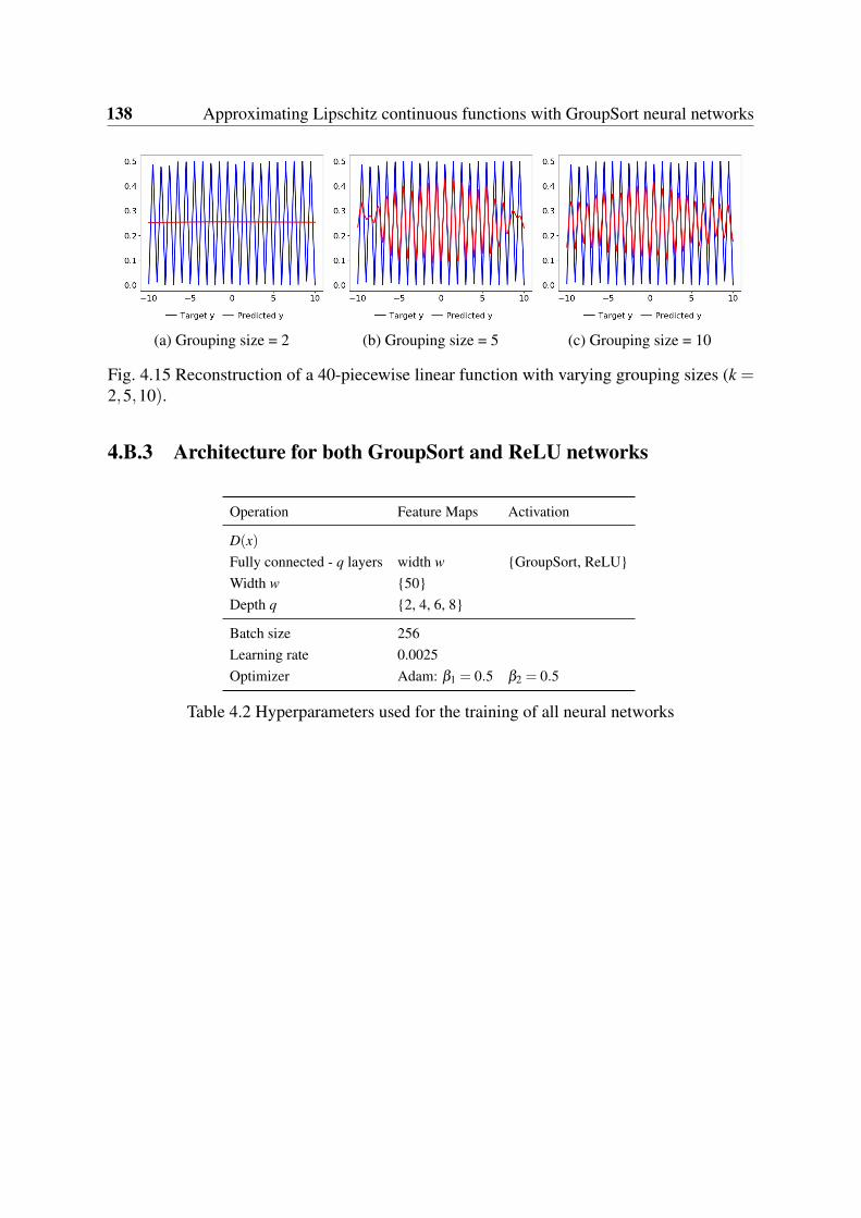
138 Approximating Lipschitz continuous functions with GroupSort neural networks
(a) Grouping size = 2 (b) Grouping size = 5 (c) Grouping size = 10
Fig. 4.15 Reconstruction of a 40-piecewise linear function with varying grouping sizes (k =2,5,10).
4.B.3 Architecture for both GroupSort and ReLU networks
Operation Feature Maps Activation
D(x)Fully connected - q layers width w GroupSort, ReLUWidth w 50Depth q 2, 4, 6, 8
Batch size 256Learning rate 0.0025Optimizer Adam: β1 = 0.5 β2 = 0.5
Table 4.2 Hyperparameters used for the training of all neural networks

Chapter 5
Learning disconnected manifolds: a noGAN’s land
AbstractTypical architectures of Generative Adversarial Networks make use of a unimodal latent/input dis-tribution transformed by a continuous generator. Consequently, the modeled distribution always hasconnected support which is cumbersome when learning a disconnected set of manifolds. We formalizethis problem by establishing a "no free lunch" theorem for the disconnected manifold learning stating anupper-bound on the precision of the targeted distribution. This is done by building on the necessary exis-tence of a low-quality region where the generator continuously samples data between two disconnectedmodes. Finally, we derive a rejection sampling method based on the norm of generator’s Jacobian andshow its efficiency on several generators including BigGAN.
Contents5.1 Introduction . . . . . . . . . . . . . . . . . . . . . . . . . . . . . . . . . 140
5.2 Related work . . . . . . . . . . . . . . . . . . . . . . . . . . . . . . . . . 142
5.3 Our approach . . . . . . . . . . . . . . . . . . . . . . . . . . . . . . . . 143
5.4 Experiments . . . . . . . . . . . . . . . . . . . . . . . . . . . . . . . . . 150
5.5 Conclusion and future work . . . . . . . . . . . . . . . . . . . . . . . . 155
Appendix 5.A Technical results . . . . . . . . . . . . . . . . . . . . . . . . . 158
Appendix 5.B Complementary experiments . . . . . . . . . . . . . . . . . . 169
Appendix 5.C Supplementary details . . . . . . . . . . . . . . . . . . . . . . 177
140 Learning disconnected manifolds: a no GAN’s land
5.1 Introduction
GANs Goodfellow et al. (2014) provide a very effective tool for the unsupervised learning ofcomplex probability distributions. For example, Karras et al. (2019) generate very realistichuman faces while Yu et al. (2017) match state-of-the-art text corpora generation. Despitesome early theoretical results on the stability of GANs Arjovsky and Bottou (2017) and on theirapproximation and asymptotic properties Biau et al. (2020), their training remains challenging.More specifically, GANs raise a mystery formalized by Khayatkhoei et al. (2018): how canthey fit disconnected manifolds when they are trained to continuously transform a unimodallatent distribution? While this question remains widely open, we will show that studying itcan lead to some improvements in the sampling quality of GANs. Indeed, training a GANwith the objective of continuously transforming samples from an unimodal distribution intoa disconnected requires balancing between two caveats. On one hand, the generator couldjust ignore all modes but one, producing a very limited variety of high quality samples: this isan extreme case of the well known mode collapse Arjovsky and Bottou (2017). On the otherhand, the generator could cover the different modes of the target distribution and necessarilygenerates samples out of the real data manifold as previously explained by Khayatkhoei et al.(2018).
As brought to the fore by Roth et al. (2017), there is a density mis-specification betweenthe true distribution and the model distribution. Indeed, one cannot find parameters such thatthe model density function is arbitrarily close to the true distribution. To solve this issue,many empirical works have proposed to over-parameterize the generative distributions, as forinstance, using a mixture of generators to better fit the different target modes. Tolstikhin et al.(2017) rely on boosting while Khayatkhoei et al. (2018) force each generator to target differentsub-manifolds thanks to a criterion based on mutual information. Another direction is to addcomplexity in the latent space using a mixture of Gaussian distributions Gurumurthy et al.(2017).
To better visualize this phenomenon, we consider a simple 2D motivational example wherethe real data lies on two disconnected manifolds. Empirically, when learning the distribution,GANs split the Gaussian latent space into two modes, as highlighted by the separation linein red in Figure 5.1a. More importantly, each sample drawn inside this red area in Figure5.1a is then mapped in the output space in between the two modes (see Figure 5.1b). Forthe quantitative evaluation of the presence of out-of-manifold samples, a natural metric is thePrecision-Recall (PR) proposed by Sajjadi et al. (2018) and its improved version (Improved

5.1 Introduction 141
(a) Heatmap of the generator’s Jaco-bian norm. White circles: quantiles ofthe latent distribution N (0, I).
(b) Green: target distribution. Coloured dots:generated samples colored w.r.t. the JacobianNorm using same heatmap than (a).
Fig. 5.1 Learning disconnected manifolds leads to the apparition of an area with high gradientsand data sampled in between modes.
PR) (Kynkäänniemi et al., 2019). A first contribution of this paper is to formally link them.Then, taking advantage of these metrics, we lower bound the measure of this out-of-manifoldregion and formalize the impossibility of learning disconnected manifolds with standard GANs.We also extend this observation to the multi-class generation case and show that the volume ofoff-manifold areas increases with the number of covered manifolds. In the limit, this increasedrives the precision to zero.
To solve this issue and increase the precision of GANs, we argue that it is possible to removeout-of-manifold samples using a truncation method. Building on the work of Arvanitidis et al.(2017) who define a Riemaniann metric that significantly improves clustering in the latentspace, our truncation method is based on information conveyed by the Jacobian’s norm of thegenerator. We empirically show that this rejection sampling scheme enables us to better fitdisconnected manifolds without over-parametrizing neither the generative class of functionsnor the latent distribution. Finally, in a very large high dimensional setting, we discuss theadvantages of our rejection method and compare it to the truncation trick introduced by Brocket al. (2019).
In a nutshell, our contributions are the following:
• We discuss evaluation of GANs and formally link the PR measure Sajjadi et al. (2018)and its Improved PR version Kynkäänniemi et al. (2019).
• We upper bound the precision of GANs with Gaussian latent distribution and formalizean impossibility result for disconnected manifolds learning.
• Using toy datasets, we illustrate the behavior of GANs when learning disconnectedmanifolds and derive a new truncation method based on the Jacobian’s Frobenius norm
142 Learning disconnected manifolds: a no GAN’s land
of the generator. We confirm its empirical performance on state-of-the-art models anddatasets.
5.2 Related work
Fighting mode collapse. Goodfellow et al. (2014) were the first to raise the problem of modecollapse in the learning of disconnected manifolds with GANs. They observed that whenthe generator is trained too long without updating the discriminator, the output distributioncollapses to a few modes reducing the diversity of the samples. To tackle this issue, Salimanset al. (2016); Lin et al. (2018) suggested feeding several samples to the discriminator. Srivastavaet al. (2017) proposed the use of a reconstructor network, mapping the data to the latent spaceto increase diversity.
In a different direction, Arjovsky and Bottou (2017) showed that training GANs usingthe original formulation Goodfellow et al. (2014) leads to instability or vanishing gradients.To solve this issue, they proposed a Wasserstein GAN architecture Arjovsky et al. (2017)where they restrict the class of discriminative functions to 1-Lipschitz functions using weightclipping. Pointing to issues with this clipping, Gulrajani et al. (2017); Miyato et al. (2018)proposed relaxed ways to enforce the Lipschitzness of the discriminator, either by using agradient penalty or a spectral normalization. Albeit not exactly approximating the Wasserstein’sdistance (Petzka et al., 2018), both implementations lead to good empirical results, significantlyreducing mode collapse. Building on all of these works, we will further assume that generatorsare now able to cover most of the modes of the target distribution, leaving us the problem ofout-of-manifold samples (a.k.a. low-quality pictures).
Generation of disconnected manifolds. When learning complex manifolds in high dimen-sional spaces using deep generative models, Fefferman et al. (2016) highlighted the importanceof understanding the underlying geometry. More precisely, the learning of disconnected man-ifold requires the introduction of disconnectedness in the model. Gurumurthy et al. (2017)used a multi-modal entry distribution, making the latent space disconnected, and showed bettercoverage when data is limited and diverse. Alternatively, Khayatkhoei et al. (2018) studied thelearning of a mixture of generators. Using a mutual information term, they encourage eachgenerator to focus on a different submanifold so that the mixture covers the whole support.This idea of using an ensemble of generators is also present in the work of Tolstikhin et al.(2017) and Zhong et al. (2019), though they were primarily interested in the reduction of modecollapse.
5.3 Our approach 143
In this paper, we propose a truncation method to separate the latent space into severaldisjoint areas. It is a way to learn disconnected manifolds without relying on the previouslyintroduced over-parameterization techniques. As our proposal can be applied without retrainingthe whole architecture, we can use it successfully on very larges nets. Close to this idea, Azadiet al. (2019) introduced a rejection strategy based on the output of the discriminator. However,this rejection sampling scheme requires the discriminator to be trained with a classification losswhile our proposition can be applied to any generative models.
Evaluating GANs. The evaluation of generative models is an active area of research. Someof the proposed metrics only measure the quality of the generated samples such as the Inceptionscore Salimans et al. (2016) while others define distances between probability distributions.This is the case of the Frechet Inception distance Heusel et al. (2017), the Wasserstein distanceArjovsky et al. (2017) or kernel-based metrics Gretton et al. (2012). The other main caveatfor evaluating GANs lies in the fact that one does not have access to the true density nor themodel density, prohibiting the use of any density based metrics. To solve this issue, the useof a third network that acts as an objective referee is common. For instance, the Inceptionscore uses outputs from InceptionNet while the Fréchet Inception Distance compares statisticsof InceptionNet activations. Since our work focuses on out-of-manifold samples, a naturalmeasure is the PR measure (Sajjadi et al., 2018) and its Improved PR version (Kynkäänniemiet al., 2019), extensively discussed in the next section.
In the following, alongside precise definitions, we exhibit an upper bound on the precisionof GANs with high recall (i.e. no mode collapse) and present a new truncation method.
5.3 Our approach
We start with a formal description of the framework of GANs and the relevant metrics. Welater show a "no free lunch" theorem proving the necessary existence of an area in the latentspace that generates out-of-manifold samples. We name this region the no GAN’s land sinceany data point sampled from this area will be in the frontier in between two different modes.We claim that dealing with it requires special care. Finally, we propose a rejection samplingprocedure to avoid points out of the true manifold.
5.3.1 Notations
In the original setting of Generative Adversarial Networks (GANs), one tries to generatedata that are “similar” to samples collected from some unknown probability measure µ⋆. To

144 Learning disconnected manifolds: a no GAN’s land
do so, we use a parametric family of generative distribution where each distribution is thepush-forward measure of a latent distribution Z and a continuous function modeled by a neuralnetwork.
Assumption 3 (Z Gaussian). The latent distribution Z is a standard multivariate Gaussian.
Note that for any distribution µ , Sµ refers to its support. Assumption 3 is common forGANs as in many practical applications, the random variable Z defined on a low dimensionalspace Rd is either a multivariate Gaussian. Practicioners also studied distribution or uniformdistribution defined on a compact.
The measure µ⋆ is defined on a subset E of RD (potentially a highly dimensional space),equipped with the norm ∥ · ∥. The generator has the form of a parameterized class of functionsfrom Rd (a space with a much lower dimension) to E, say G = Gθ : θ ∈Θ, where Θ ⊆Rp
is the set of parameters describing the model. Each function Gθ thus takes input from ad-dimensional random variable Z (Z is associated with probability distribution γ) and outputs“fake” observations with distribution µθ . Thus, the class of probability measures P = µθ :θ ∈Θ is the natural class of distributions associated with the generator, and the objective ofGANs is to find inside this class of candidates the one that generates the most realistic samples,closest to the ones collected from the unknown distribution µ⋆.
Assumption 4. Let L > 0. The generator Gθ takes the form of a neural network whose Lipchitzconstant is smaller than L, i.e. for all (z,z′), we have ∥Gθ (z′)−Gθ (z)∥⩽ L∥z− z′∥.
This is a reasonable assumption, since Virmaux and Scaman (2018) present an algorithmthat upper-bounds the Lipschitz constant of deep neural networks. Initially, 1-Lipschitznesswas enforced only for the discriminator by clipping the weigths Arjovsky et al. (2017), addinga gradient penalty Gulrajani et al. (2017); Roth et al. (2017); Petzka et al. (2018), or penalizingthe spectral norms Miyato et al. (2018). Nowadays, state-of-the-art architectures for large scalegenerators such as SAGAN Zhang et al. (2019) and BigGAN Brock et al. (2019) also make useof spectral normalization for the generator.
5.3.2 Evaluating GANs with Precision and Recall
When learning disconnected manifolds, Srivastava et al. (2017) proved the need of measuringsimultaneously the quality of the samples generated and the mode collapse. Sajjadi et al. (2018)proposed the use of a PR metric to measure the quality of GANs. The key intuition is thatprecision should quantify how much of the fake distribution can be generated by the truedistribution while recall measures how much of the true distribution can be re-constructed bythe model distribution. More formally, it is defined as follows:

5.3 Our approach 145
Definition 5.3.1. Sajjadi et al. (2018) Let X ,Y be two random variables. For α,β ∈ (0,1], X issaid to have an attainable precision α at recall β w.r.t. Y if there exists probability distributionsµ,νX ,νY such that
Y = β µ +(1−β )νY and X = αµ +(1−α)νX .
The component νY denotes the part of Y that is “missed” by X , whereas, νX denotes the"noise" part of X . We denote α (respectively β ) the maximum attainable precision (respectivelyrecall). Th. 1 of Sajjadi et al. (2018) states:
X(SY
)= α and Y
(SX
)= β .
Improved PR metric. Kynkäänniemi et al. (2019) highlighted an important drawback of thePR metric proposed by Sajjadi et al. (2018): it cannot correctly interpret situations when a largenumbers of samples are packed together. To better understand this situation, consider a casewhere the generator slightly collapses on a specific data point, i.e. there exists x ∈ E,µθ (x)> 0.We show in Appendix 5.A.1 that if µ⋆ is a non-atomic probability measure and µθ is highlyprecise (i.e. α = 1), then the recall β must be 0.
To solve these issues, Kynkäänniemi et al. (2019) proposed an Improved Precision-Recall(Improved PR) metric built on a nonparametric estimation of support of densities.
Definition 5.3.2. Kynkäänniemi et al. (2019) Let X ,Y be two random variables and DX ,DY
two finite sample datasets such that DX ∼ Xn and DY ∼ Y n. For any x ∈ DX (respectively forany y ∈ DY ), we consider (x(1), . . . ,x(n−1)), the re-ordening of elements in DX \ x given theireuclidean distance with x. For any k ∈N and x ∈ DX , the precision αn
k (x) of point x is definedas:
αnk (x) = 1 ⇐⇒ ∃y ∈ DY ,∥x− y∥⩽ ∥y(k)− y∥.
Similarly, the recall β nk (y) of any given y ∈ DY is:
βnk (y) = 1 ⇐⇒ ∃x ∈ DX ,∥y− x∥⩽ ∥x(k)− x∥.
Improved precision (respectively recall) are defined as the average over DX (respectively DY )as follows:
αnk =
1n ∑
xi∈DX
αnk (xi) β
nk =
1n ∑
yi∈DY
βnk (yi).
A first contribution is to formalize the link between PR and Improved PR with the followingtheorem:

146 Learning disconnected manifolds: a no GAN’s land
Theorem 5.3.1. Let X ,Y two random variables with probability distributions µ and ν . Assumethat both µ and ν are associated with uniformly continuous probability density functionsfµ and fν . Besides, there exists constants a1 > 0,a2 > 0 such that for all x ∈ E we havea1 < fµ⋆(x)⩽ a2 and a1 < fµθ
(x)⩽ a2 for some c > 0. Also, (k,n) are such that klog(n) →+∞
and kn → 0. Then,
αnk → α in probability and β
nk → β in probability.
This theorem, whose proof is delayed to Appendix 5.A.2, underlines the nature of theImproved PR metric: the metric compares the supports of the modeled probability distributionµθ and of the true distribution µ⋆. This means that Improved PR is a tuple made of bothmaximum attainable precision α and recall β (e.g. Theorem 1 of Sajjadi et al. (2018)). AsImproved PR is shown to have a better performance evaluating GANs sample quality, we usethis metric for both the following theoretical results and experiments.
5.3.3 Learning disconnected manifolds
In this section, we aim to stress the difficulties of learning disconnected manifolds with standardGANs architectures. To begin with, we recall the following lemma.
Lemma 5.3.1. Assume that Assumptions 3 and 4 are satisfied. Then, for any θ ∈Θ , the supportSµθ
is connected.
There is consequently a discrepancy between the connectedness of Sµθand the disconnect-
edness of Sµ⋆ . In the case where the manifold lays on two disconnected components, our nexttheorem exhibit a no free lunch theorem:
Theorem 5.3.2. ("No free lunch" theorem) Assume that Assumptions 3 and 4 are satisfied.Assume also that true distribution µ⋆ lays on two equally measured disconnected manifoldsdistant from a distance D > 0. Then, any estimator µθ that samples equally in both modes
must have a precision α such that α + D√2πL
e−Φ−1( α
2 )2
2 ⩽ 1, where Φ is the c.d.f. of a standardnormal distribution.
Besides, if α ⩾ 3/4, α ≲ 1−√
2π
W ( D2
4L2 ) where W is the Lambert W function.
The proof of this theorem is delayed to Appendix 5.A.3. It is mainly based on the Gaussianisoperimetric inequality Borell (1975); Sudakov and Tsirelson (1978) that states that among allsets of given Gaussian measure in any finite dimensional Euclidean space, half-spaces have theminimal Gaussian boundary measure. If in Fig. 5.1, the generator has thus learned the optimal

5.3 Our approach 147
separation, it is yet not known, to the limit of our knowledge, how to enforce such geometricalproperties in the latent space.
In real world applications, when the number of distinct sub-manifolds increases, we expectthe volume of these boundaries to increase with respect to the number of different classescovered by the modeled distribution µθ . Going in this direction, we better formalize thissituation, and show an extended "no free lunch theorem" by expliciting an upper-bound of theprecision α in this broader framework.
Assumption 5. The true distribution µ⋆ lays on M equally-measured disconnected componentsat least distant from some constant D > 0.
This is likely to be true for datasets made of symbol designed to be highly distinguishable(e.g. digits in the MNIST dataset). In very high dimension, this assumption also holds forcomplex classes of objects appearing in many different contexts (e.g. the bubble class inImageNet, see Appendix).
To better apprehend the next theorem, note Am the pre-image in the latent space of mode mand Ar
m its r-enlargement: Arm := z ∈Rd | dist(z,Am)≤ r, r > 0.
Theorem 5.3.3. (Generalized "no free lunch" theorem) Assume that Assumptions 3, 4, and 5are satisfied, and that the pre-image enlargements Aε
m, with ε = D2L , form a partition of the
latent space with equally measured elements.Then, any estimator µθ with recall β > 1
M must have a precision α at most 1+x2
x2 e−12 ε2
e−εx
where x = Φ−1(1− 1βM
) and Φ is the c.d.f. of a standard normal distribution.
Theorem 5.3.3, whose proof is delayed to Appendix 5.A.4, states a lower-bound themeasure of samples mapped out of the true manifold. We expect our bound to be loose since notheoretical results are known, to the best of our knowledge, on the geometry of the separationthat minimizes the boundary between different classes (when M ⩾ 3). Finding this optimal cutwould be an extension of the honeycomb theorem Hales (2001). In Appendix 5.A.4.2 we givea more technical statement of Theorem 5.3.3 without assuming equality of measure of the setsAε
m.The idea of the proof is to consider the border of an individual cell with the rest of the
partition. It is clear that at least half of the frontier will be inside this specific cell. Then, toget to the final result, we sum the measures of the frontiers contained inside all of the differentcells. Remark that our analysis is fine enough to keep a dependency in M which translatesinto a maximum precision that goes to zero when M goes to the infinity and all the modes arecovered. More precisely, in this scenario where all pre-images have equal measures in the latent

148 Learning disconnected manifolds: a no GAN’s land
(a) WGAN 4 classes: visualisation of∥JG(z)∥F .
(b) WGAN 9 classes: visualisation of∥JG(z)∥F .
(c) WGAN 25 classes: visualisation of∥JG(z)∥F .
(d) Precision w.r.t. D (mode distance) andM (classes).
Fig. 5.2 Illustration of Theorem 5.3.3. If the number of classes M → ∞ or the distance D → ∞,then the precision α → 0. We provide in appendix heatmaps for more values of M.

5.3 Our approach 149
space, one can derive the following bound, when the recall β is kept fixed and M increases:
αM→∞
⩽ e−12 ε2
e−ε
√2log(βM) where ε =
D2L
. (5.3.1)
For a fixed generator, this equation illustrates that the precision α decreases when either thedistance D (equivalently ε) or the number of classes M increases. For a given ε , α convergesto 0 with a speed O( 1
(βM)√
2ε). To better illustrate this asymptotic result, we provide results
from a 2D synthetic setting. In this toy dataset, we control both the number M of disconnectedmanifolds and the distance D. Figure 5.2 clearly corroborates (5.3.1) as we can easily get themaximum precision close to 0 (M = 25, D = 27).
5.3.4 Jacobian-based truncation (JBT) method
The analysis of the deformation of the latent space offers a grasp on the behavior of GANs. Forinstance, Arvanitidis et al. (2017) propose a distance accounting for the distortions made bythe generator. For any pair of points (z1,z2)∼ Z2, the distance is defined as the length of thegeodesic d(z1,z2) =
∫[0,1] ∥JGθ
(γt)dγtdt ∥dt where γ is the geodesic parameterized by t ∈ [0,1] and
JGθ(z) denotes the Jacobian matrix of the generator at point z. Authors have shown that the use
of this distance in the latent space improves clustering and interpretability. We make a similarobservation that the generator’s Jacobian Frobenius norm provides meaningful information.
Indeed, the frontiers highlighted in Figures 5.2a, 5.2b, and 5.2c correspond to areas of lowprecision mapped out of the true manifold: this is the no GAN’s land. We argue that whenlearning disconnected manifolds, the generator tries to minimize the number of samples that donot belong to the support of the true distribution and that this can only be done by making pathssteeper in the no GAN’s land. Consequently, data points Gθ (z) with high Jacobian Frobeniusnorm (JFN) are more likely to be outside the true manifold. To improve the precision ofgenerative models, we thus define a new truncation method by removing points with highestJFN.
However, note that computing the generators’s JFN is expensive to compute for neuralnetworks, since being defined as follows,
∥JGθ(z)∥2
F =m
∑i=1
n
∑j=1
(∂Gθ (z)i
∂ z j
)2
,
it requires a number of backward passes equal to the output dimension. To make our truncationmethod tractable, we use a stochastic approximation of the Jacobian Frobenius norm based on

150 Learning disconnected manifolds: a no GAN’s land
the following result from Rifai et al. (2011):
∥JGθ(z)∥2 = lim
N→∞σ→0
1N
N
∑εi
1σ2∥Gθ (z+ εi)−Gθ (z)∥2,
where εi ∼∼N (0,σ2I and I is the identity matrix of dimension d. The variance σ of the noiseand the number of samples are used as hyper-parameters. In practice, σ in [1e−4;1e−2] andN = 10 give consistent results.
Based on the preceding analysis, we propose a new Jacobian-based truncation (JBT)method that rejects a certain ratio of the generated points with highest JFN. This truncationratio is considered as an hyper-parameter for the model. We show in our experiments that ourJBT can be used to to detect samples outside the real data manifold and that it consequentlyimproves the precision of the generated distribution as measured by the Improved PR metric.
5.4 Experiments
In the following, we show that our truncation method, JBT, can significantly improve theperformances of generative models on several models, metrics and datasets. Furthermore,we compare JBT with over-parametrization techniques specifically designed for disconnectedmanifold learning. We show that our truncation method reaches or surpasses their performance,while it has the benefit of not modifying the training process of GANs nor using a mixtureof generators, which is computationally expensive. Finally, we confirm the efficiency of ourmethod by applying it on top of BigGAN Brock et al. (2019).
Except for BigGAN, for all our experiments, we use Wasserstein GAN with gradient penaltyGulrajani et al. (2017), called WGAN for conciseness. We give in Appendix 5.C the full detailsof our experimental setting. The use of WGAN is motivated by the fact that it was shownto stabilize the training and significantly reduce mode collapse Arjovsky and Bottou (2017).However, we want to emphasise that our method can be plugged on top of any generative modelfitting disconnected components.
5.4.1 Evaluation metrics
To measure performances of GANs when dealing with low dimensional applications - as withsynthetic datasets - we equip our space with the standard Euclidean distance. However, for highdimensional applications such as image generation, Brock et al. (2019); Kynkäänniemi et al.(2019) have shown that embedding images into a feature space with a pre-trained convolutionalclassifier provides more semantic information. In this setting, we consequently use the euclidean

5.4 Experiments 151
distance between the images’ embeddings from a classifier. For a pair of images (a,b), wedefine the distance d(a,b) as d(a,b) = ∥φ(a)−φ(b)∥2 where φ is a pre-softmax layer of asupervised classifier, trained specifically on each dataset. Doing so, they will more easilyseparate images sampled from the true distribution µ⋆ from the ones sampled by the distributionµθ .
We compare performances using Improved PR Kynkäänniemi et al. (2019). We also reportthe Marginal Precision which is the precision of newly added samples when increasing theratio of kept samples. Besides, for completeness, we report FID Heusel et al. (2017) and recallprecise definitions in Appendix 5.B.2. Note that FID was not computed with InceptionNet, buta classifier pre-trained on each dataset.
5.4.2 Synthetic dataset
We first consider the true distribution to be a 2D Gaussian mixture of 9 components. Both thegenerator and the discriminator are modeled with feed-forward neural networks.
Interestingly, the generator tries to minimize the sampling of off-manifolds data duringtraining until its JFN gets saturated (see Appendix 5.B.3). One way to reduce the number ofoff-manifold samples is to use JBT. Indeed, off-manifold data points progressively disappearwhen being more and more selective, as illustrated in Figure 5.3c. We quantitatively confirmthat our truncation method (JBT) improves the precision. On Fig. 5.3d, we observe that keepingthe 70% of lowest JFN samples leads to an almost perfect precision of the support of thegenerated distribution. Thus, off-manifold samples are in the 30% samples with highest JFN.
5.4.3 Image datasets
We further study JBT on three different datasets: MNIST LeCun et al. (1998), FashionMNISTXiao et al. (2017) and CIFAR10 Krizhevsky et al. (2009). Following Khayatkhoei et al. (2018)implementation, we use a standard CNN architecture for MNIST and FashionMNIST whiletraining a ResNet-based model for CIFAR10 (Gulrajani et al., 2017).
Figure 5.4 highlights that JBT also works on high dimensional datasets as the marginalprecision plummets for high truncation ratios. Furthermore, when looking at samples ranked byincreasing order of their JFN, we notice that samples with highest JFN are standing in-betweenmanifolds. For example, those are ambiguous digits resembling both a "0" and a "6" or shoeswith unrealistic shapes.
To further assess the efficiency of our truncation method, we also compare its performanceswith two state-of-the-art over-parameterization techniques that were designed for disconnectedmanifold learning. First, Gurumurthy et al. (2017) propose DeliGAN, a reparametrization trick

152 Learning disconnected manifolds: a no GAN’s land
(a) WGAN - 2500 samples (b) WGAN 90% JBT.
(c) WGAN 70% JBT. (d) 97% confidence intervals .
Fig. 5.3 Mixture of 9 Gaussians in green, generated points in blue. Our truncation method(JBT) removes least precise data points as marginal precision plummets.
to transform the unimodal Gaussian latent distribution into a mixture. The different mixturecomponents are later learnt by gradient descent. For fairness, the re-parametrization trick is usedon top of WGAN. Second, Khayatkhoei et al. (2018) define DMLGAN, a mixture of generatorsto better learn disconnected manifolds. In this architecture, each generator is encouraged totarget a different submanifold by enforcing high mutual information between generated samplesand generator’s ids. Keep in mind that for DeliGAN (respectively DMLGAN), the optimalnumber of components (respectively generators) is not known and is a hyper-parameter of themodel that has to be cross-validated.
The results of the comparison are presented in Table 5.1. In both datasets, JBT 80 %outperforms DeliGAN and DMLGAN in terms of precision while keeping a reasonnable recall.This confirms our claim that over-parameterization techniques are unnecessary. As noticedby Kynkäänniemi et al. (2019), we also observe that FID does not correlate properly with theImproved PR metric. Based on the Frechet distance, only a distance between multivariate

5.4 Experiments 153
(a) MNIST dataset. (b) F-MNIST dataset. (c) CIFAR10 datatset.Fig. 5.4 For high levels of kept samples, the marginal precision plummets of newly addedsamples, underlining the efficiency of our truncation method (JBT). Reported confidenceintervals are 97% confidence intervals. On the second row, generated samples ordered by theirJFN (left to right, top to bottom). In the last row, the data points generated are blurrier andoutside the true manifold.
MNIST Prec. Rec. FIDWGAN 91.2±0.3 93.7±0.5 24.3±0.3
WGAN JBT 90% 92.5±0.5 92.9±0.3 26.9±0.5
WGAN JBT 80% 93.3±0.3 91.8±0.4 33.1±0.3
W-Deligan 89.0±0.6 93.6±0.3 31.7±0.5
DMLGAN 93.4±0.2 92.3±0.2 16.8±0.4
F-MNISTWGAN 86.3±0.4 88.2±0.2 259.7±3.5
WGAN JBT 90% 88.6±0.6 86.6±0.5 257.4±3.0WGAN JBT 80% 89.8±0.4 84.9±0.5 396.2±6.4
W-Deligan 88.5±0.3 85.3±0.6 310.9±3.1
DMLGAN 87.4±0.3 88.1±0.4 253.0±2.8
Table 5.1 JBT x% means we keep the x% samples with lowest Jacobian norm. Our truncationmethod (JBT) matches over-parameterization techniques. ± is 97% confidence interval.

154 Learning disconnected manifolds: a no GAN’s land
(a) House finch. (b) Parachute. (c) Bubble.Fig. 5.5 On the first row, per-class precision-recall curves comparing Brock et al. (2019)’struncation trick and our truncation method (JBT), on three ImageNet classes generated byBigGAN. We show better results on complex and disconnected classes (e.g. bubble). Reportedconfidence intervals are 97% confidence intervals. On the second row, generated samplesordered by their JFN (left to right, top to bottom). We observe a concentration of off-manifoldsamples for images on the bottom row, confirming the soundness of JBT.
Gaussians, we argue that FID is not suited for disconnected manifold learning as it approximatesdistributions with unimodal ones and looses many information.
5.4.4 Spurious samples rejections on BigGAN
Thanks to the simplicity of JBT, we can also apply it on top of any trained generative model.In this subsection, we use JBT to improve the precision of a pre-trained BigGAN modelBrock et al. (2019), which generates class-conditionned ImageNet Krizhevsky et al. (2012)samples. The class-conditioning lowers the problem of off-manifold samples, since it reducesthe disconnectedness in the output distribution. However, we argue that the issue can still existon high-dimensional natural images, in particular complex classes can still be multi-modal(e.g. the bubble class). The bottom row in Figure 5.5 shows a random set of 128 images forthree different classes ranked by their JFN in ascending order (left to right, top to bottom). Weobserve a clear concentration of spurious samples on the bottom row images.
To better assess the Jacobian based truncation method, we compare it with the truncationtrick from Brock et al. (2019). This truncation trick aims to reduce the variance of the latentspace distribution using truncated Gaussians. While easy and effective, this truncation has

5.5 Conclusion and future work 155
some issues: it requires to complexify the loss to enforce orthogonality in weight matrices ofthe network. Moreover, as explained by Brock et al. (2019) "only 16% of models are amenableto truncation, compared to 60% when trained with Orthogonal Regularization". For fairnessof comparison, the pre-trained network we use is optimized for their truncation method. Onthe opposite, JBT is simpler to apply since 100% of the tested models were amenable to theproposed truncation.
Results of this comparison are shown in the upper row of Figure 5.5. Our method canoutperform their truncation trick on difficult classes with high intra-class variation, e.g. bubbleand house finch. This confirms our claim that JBT can detect outliers within a class. However,one can note that their trick is particularly well suited for simpler unimodal classes, e.g.parachute and reaches high precision levels.
5.5 Conclusion and future work
In this paper, we provide insights on the learning of disconnected manifolds with GANs. Ouranalysis shows the existence of an off-manifold area with low precision. We empirically showon several datasets and models that we can detect these areas and remove samples located inbetween two modes thanks to a newly proposed truncation method.
Similarly to what has been proposed in this chapter, we want to briefly stress anotherpossible solution that aims at improving the quality of trained generators. Note that this is alsopart of an ongoing work.
There is an already existing research that post-processes GANs’ samples heavily relying ona variety of Monte-Carlo algorithms: Azadi et al. (2019) use the Rejection Sampling algorithm,Turner et al. (2019) the Metropolis-Hastings method, and Grover et al. (2019) the Samplingimportance re-sampling method. These methods aim at sampling from a target distribution,while having only access to samples generated from a proposal distribution. This idea wassuccessfully applied to GANs, using the previously learned generative distribution µθ as aproposal distribution. However, one of the main drawback is that Monte-Carlo algorithmsonly guarantee to sample from the target distribution under strong assumptions. First, we needaccess to the density ratios between the proposal and target distributions or equivalently to aperfect discriminator (Azadi et al., 2019). Second, the support of the proposal distribution mustfully cover the one of the target distribution, which means no mode collapse. This is known tobe very demanding in high dimension since the intersection of supports between the proposaland target distribution is likely to be negligible (Arjovsky and Bottou, 2017, Lemma 3). Inthis setting, an optimal discriminator would give null acceptance probabilities for almost anygenerated points, leading to a lower performance.

156 Learning disconnected manifolds: a no GAN’s land
To tackle the aforementioned issue, we propose a novel method aiming at reducing theWasserstein distance between the previously trained generative model and the target distribution.This is done via the adversarial training of a third network that learns importance weights inthe latent space. The goal is to learn the redistribution of mass of the modeled distributionthat best fits the target distribution. More formally, we propose to over parameterize the classof generative distributions and define a parametric class Ω = wϕ ,ϕ ∈ Φ of importanceweighters. Each function wϕ learns importance weights in the latent space and is consequentlydefined from Rd to R+. For any given importance weighter wθ , we impose the constraintEµθ
wϕ = 1 and define µϕ
θthe new weighted probability distribution defined as follows:
for all x ∈RD, dµϕ
θ(x) = wϕ(x)dµθ (x).
Denoting by Lip1 the set of 1-Lipschitz real-valued functions on RD, i.e.,
Lip1 =
f :RD →R : | f (x)− f (y)|⩽ ∥x− y∥, (x,y) ∈ (RD)2,the objective is to find the optimal importance weighter wϕ such that:
argminϕ∈Φ
W (µ⋆,µϕ
θ) = argmin
wϕ∈Ω
supD∈Lip1
Eµ⋆D−Eµ
ϕ
θ
D
= argminwϕ∈Ω
supD∈Lip1
Eµ⋆D−EµθwϕD.
To better understand our approach, we first consider a simple 2D motivational example wherethe real data lies on four disconnected manifolds. To approximate this, the generator splitsthe latent space into four distinct areas and maps data points located in the frontiers, areas inorange in Figure 5.6b, out of the true manifold (see Figure 5.6a). Our method consequentlyaims at learning latent importance weights that can identify these frontiers and simply avoidthem. This is highlighted in Figure 5.6d where the importance weighter has identified thesefour frontiers. When sampling from the new latent distribution, we can now perfectly fit themixture of four gaussians (see Figure 5.6c).
Consequently, future would thorougly compare the proposed method with a large set ofprevious approaches such as Azadi et al. (2019), Grover et al. (2019) and Tanaka (2019). Theseexperiments should be ran on a variety of datasets and distributions.

5.5 Conclusion and future work 157
(a) WGAN: real samples in green andfake ones in blue.
(b) Latent space: heatmap of the distancebetween a generated sample and its near-est real sample.
(c) WGAN with latent rejection sampling:real samples in green and fake ones inblue.
(d) Latent space: heatmap of the learnedimportance weights. The blue frontiershave zero weights.
Fig. 5.6 Learning disconnected manifolds leads to the apparition of an area in the latent spacegenerating points outside the target manifold. With the use of the importance weighter, one canavoid this specific area and better fit the target distribution.
158 Learning disconnected manifolds: a no GAN’s land
Appendix 5.A Technical results
5.A.1 Highlighting drawbacks of the Precision/Recall metric
Lemma 5.A.1. Assume that the modeled distribution µθ slightly collapses on a specific datapoint, i.e. there exists x ∈ E,µθ (x) > 0. Assume also that µ⋆ is a continuous probabilitymeasure and that µθ has a recall β = 1. Then the precision must be such that α = 0.
Proof. Using Definition 5.3.1, we have that there exists µ such that
µ⋆ = αµ +(1−α)νµ⋆ and µθ = µ.
Thus, 0 = µ⋆(x)⩾ αµ(x) = αµθ (x). Which implies that α = 0.
5.A.2 Proof of Theorem 5.3.1
The proof of Theorem 5.3.1 relies on theoretical results from non-parametric estimation of thesupports of probability distribution studied by Devroye and Wise (1980).
For the following proofs, we will require the following notation: let ϕ be a strictlymonotonous function be such that lim
n→∞
ϕ(n)n = 0 and lim
n→∞
ϕ(n)log(n) = ∞. We note B(x,r)⊆ E, the
open ball centered in x and of radius r. For a given probability distribution µ , Sµ refers to itssupport. We recall that for any x in a dataset D, x(k) denotes its k nearest neighbor in D. Finally,for a given probability distribution µ and a dataset Dµ sampled from µn, we note Rmin andRmax the following:
Rmin = minx∈E
∥x− x(ϕ(n))∥, Rmax = maxx∈E
∥x− x(ϕ(n))∥. (5.A.1)
In the following lemma, we show asymptotic behaviours for both Rmin and Rmax.
Lemma 5.A.2. Let µ be a probability distribution associated with a uniformly continuousprobability density function fµ . Assume that there exists constants a1 > 0,a2 > 0 such that forall x ∈ E, we have a1 < fµ(x)⩽ a2. Then,
Rmin −→n→∞
0 a.s. and Rdmin −→n→∞
∞ a.s.
Rmax −→n→∞
0 a.s. and Rdmax −→n→∞
∞ a.s.
Proof. We will only prove that Rmax −→n→∞
0 a.s. and and Rdmin −→n→∞
∞ a.s. as the rest follows.The result is based on a nearest neighbor result from Biau and Devroye (2015). Considering
the ϕ(n) nearest neighbor density estimate f ϕ(n)n based on a finite sample dataset Dµ , Theorem

5.A Technical results 159
4.2 states that if fµ is uniformly continuous then:
supx∈E
∥ f ϕ(n)n (x)− fµ(x)∥→ 0.
where f ϕ(n)n (x) = ϕ(n)
nVd∥x−xϕ(n)∥d with Vd being the volume of the unit ball in Rd .
Let ε > 0 such that ε < a1/2. There exists N ∈N such that for all n ⩾ N, we have, almostsurely, for all x ∈ E:
a1 − ε ⩽ f ϕ(n)n (x)⩽ a2 + ε
a1 − ε ⩽ϕ(n)
nVd∥x− xϕ(n)∥d ⩽ a2 + ε
Consequently, for all n ⩾ N, for all x ∈ E almost surely:
∥x− xϕ(n)∥⩽(
ϕ(n)nVd(a1 − ε)
)1/d
Thus, supx∈E
∥x− xϕ(n)∥→ 0 a.s..
Also, almost surely
n∥x− xϕ(n)∥d ⩾ϕ(n)
Vd(a2 + ε)
Thus, infx∈E
∥x− xϕ(n)∥→ ∞ a.s..
Lemma 5.A.3. Let µ,ν be two probability distributions associated with uniformly continuousprobability density functions fµ and fν . Assume that there exists constants a1 > 0,a2 > 0 suchthat for all x ∈ E, we have a1 < fµ(x) ⩽ a2 and a1 < fν ⩽ a2. Also, let Dµ ,Dν be datasetssampled from νn,µn. If µ is an estimator for ν , then
(i) for all x ∈ Dµ , αnϕ(n)(x) →
n→∞1supp(ν)(x) in proba.
(ii) for all y ∈ Dν , βnϕ(n)(y) →
n→∞1supp(µ)(x) in proba.
Proof. We will only show the result for (i), since a similar proof holds for (ii).Thus, we want to show that
for all x ∈ Dµ , αnϕ(n)(x) →
n→∞1supp(ν)(x) a. s.
160 Learning disconnected manifolds: a no GAN’s land
First, let’s assume that x /∈ Sν . Biau and Devroye (2015, Lemma 2.2) have shown that
limn→∞
∥x(ϕ(n))− x∥= inf∥x− y∥ | y ∈ Sν a.s.
As Sν is a closed set - e.g. (Kallenberg, 2006) - we have
limn→∞
∥x− x(ϕ(n))∥> 0 a.s.
andfor all y ∈ Dν , lim
n→∞∥y− y(ϕ(n))∥= 0 a.s.
Thus, limn→∞
αnϕ(n)(x) = 0 a.s..
Now, let’s assume that x ∈ Sν . Using Definition 5.3.2, the precision of a given data point xcan be rewritten as follows:
αnϕ(n)(x) = 1 ⇐⇒ ∃y ∈ Dν ,x ∈ B(y,∥y− y(ϕ(n))∥)
Using notation from (5.A.1), we note
Rmin = miny∈
∥y− y(ϕ(n))∥, Rmax = maxy∈E
∥y− y(ϕ(n))∥.
It is clear that : ⋃y∈Dν
B(y,Rmin)⊆ Snν ⊆
⋃y∈Dν
B(y,Rmax), (5.A.2)
where Snν =
⋃y∈Dν
B(y,∥y− y(ϕ(n))∥)).Besides, combining Lemma 5.A.2 with Devroye and Wise (1980, Theorem 1), we have
that:
ν(Sν∆⋃
y∈Dν
B(y,Rmin))−→n→0
0 in proba.
ν(Sν∆⋃
y∈Dν
B(y,Rmax))−→n→0
0 in proba.
where ∆ here refers to the symmetric difference.Thus, using (5.A.2), it is now clear that, µ(Sν∆Sn
ν)→ 0 in probability. Finally, given x ∈ Sµ ,we have µ(x ∈ Sn
ν) = ν(αnϕ(n)(x) = 1)→ 1 in probability.

5.A Technical results 161
We can now finish the proof for Theorem 5.3.1. Recall that α = µ(Sν
)and similarly,
β = ν(Sµ
).
Proof. We have that
|αnϕ(n)− α|= |1
n ∑xi∈Dµ
αnϕ(n)(xi)−
∫E1x∈Sν
µ(dx)|
Then,
|αnϕ(n)− α|= |1
n ∑xi∈Dµ
(αnϕ(n)(xi)−1xi∈Sν
)
+(1
n ∑xi∈Dµ
1xi∈Sν−
∫E1x∈Sν
µ(dx))|
= |Exi∼µn(αnϕ(n)(xi)−1xi∈Sν
) (5.A.3)
+(Eµn1Sν
−Eµ1Sν
)| (5.A.4)
where µn is the empirical distribution of µ . As µn converges weakly to µ almost surely (e.g.Dudley (2004, Theorem 11.4.1)) and since 1x∈Sν
is bounded, we can bound (5.A.4) as follows:
limn→∞
Ex∼µn1x∈supp(µ)−Ex∼µ1x∈supp(µ) = 0 a. s.
Now, to bound (5.A.3), we use the fact that for any x ∈ Dµ , the random variable αnϕ(n)(x)
converges to 1x∈Sνin probability (Lemma 5.A.3) and that for all x ∈ Dµ , both αn
ϕ(n)(x)⩽ 1 and1x∈Sν
⩽ 1. Consequently, using results from the weak law for triangular arrays, we have that
limn→∞
1n ∑
xi∈Dµ
(αnϕ(n)(xi)−1xi∈Sν
) = 0 in proba.
Finally,|αn
ϕ(n)− α| →n→∞
0 in proba.,
which proves the result. The same proof works for limk→∞
β nk = β .
5.A.3 Proof of Theorem 5.3.2
This proof is based on the Gaussian isoperimetric inequality historically shown by Borell(1975); Sudakov and Tsirelson (1978).

162 Learning disconnected manifolds: a no GAN’s land
Proof. Let µ⋆ be a distribution defined on E laying on two disconnected manifolds M1 andM2 such that µ⋆(M1) = µ⋆(M2) =
12 and d(M1,M2) = D. Note that for any subsets A ⊆ E and
B ⊆ E, d(A,B) := inf(x,y)∈A×B
∥x− y∥.
Let G−1θ(M1) (respectively G−1
θ(M2) be the subset in Rd be the pre-images of M1 (respec-
tively M2).Consequently, we have for all k ∈ [1,n]
γ(G−1θ(M1)) = µθ (M1) = γ(G−1
θ(M2))⩾
α
2
We consider (G−1θ(M1))
ε (respectively (G−1θ(M2))
ε ) the ε enlargement of G−1θ(M1) (re-
spectively G−1θ(M2) where ε = D
2L . We know that (G−1θ(M1))
ε⋂(G−1
θ(M2))
ε = /0.Thus, we have that:
γ((G−1
θ(M1))
ε)+ γ
((G−1
θ(M2))
ε)⩽ 1
Besides, by denoting Φ the function defined for any t ∈R by Φ(t) =∫ t−∞
exp(−t2/2)√2π
ds, we have
γ((G−1
θ(M1))
ε)+ γ
((G−1
θ(M2))
ε)⩾ 2Φ
(Φ
−1(α
2)+ ε
)(using Theorem 1.3 from Ledoux (1996))
⩾ α +2ε√2π
e−Φ−1(α
2 )2/2
(since Φ−1(
α
2)+ ε < 0 and Φ convex on ]−∞,0])
Thus, we have that
α +2ε√2π
e−Φ−1(α
2 )2/2 ⩽ 1
Thus, by noting
α⋆ = supα ∈ [0,1] | α +
2ε√2π
e−Φ−1(α
2 )2
2 ⩽ 1,
we have our result.
5.A Technical results 163
For α ⩾ 3/4. By noting α = 1− x, we have
Φ−1(
α
2) =
√2πx2
+O(x3)
And, e−Φ−1(α
2 )2
2 = e−πx2
4 +O(e−x4)
Thus, 1− x+2ε√2π
e−πx2
4 +O(e−x4)⩽ 1
⇐⇒ x ⩾2ε√2π
e−πx2
4 +O(e−x4)
=⇒ x ⩾
√2π
W (ε2)
where W is the product log function. Thus, α ⩽ 1−√
2π
W (ε2).
As an example, in the case where ε = 1, we have that W (1) ≈ 0.5671, x > 0.4525 andα < 0.5475.
5.A.4 Proof of Theorem 5.3.3
5.A.4.1 Equitable setting
This result is a consequence of Theorem 5.A.1 that we will assume true in this section.We consider that the unknown true distribution µ⋆ lays on M disjoint manifolds of equal
measure. As specified in Section 5.3, the latent distribution γ is a multivariate Gaussian definedon Rd . For each k ∈ [1,M], we consider in the latent space, the pre-images Ak.
It is clear that A1, . . . ,AM are pairwise disjoint Borel subsets of Rd . We denote M, thenumber of classes covered by the estimator µθ , such that for all i ∈ [1,M], we have γ(Ai)> 0.We know that M ⩾ Mβ > 1.
For each i ∈ [1,M], we denote Aεi , the ε-enlargement of Ai. For any pair (i, j) it is clear that
Aεi⋂
Aεj = 0 where ε = D
2L (D being the minimum distance between two sub-manifolds and Lbeing the Lipschitz constant of the generator).
As assumed, we know that Aεi , i ∈ [1,M] partition the latent space in equal measure, conse-
quently, we assume that
n
∑i=1
γ(Aεi ) = 1 and γ(A1) = . . .= γ(AM) = 1/M (5.A.5)

164 Learning disconnected manifolds: a no GAN’s land
Thus, we have that
α =M
∑i=1
γ(Aεi ) = 1− γ(∆−ε(Aε
1, . . . ,Aε
M))
Using Theorem 5.A.1, we have
γ(∆−ε(Aε1, . . . ,A
εn))⩾ 1− 1+ x2
x2 e−12 ε2
e−εx
Thus, α ⩽1+ y2
y2 e−12 ε2
e−εy
where y = Φ−1(
1−maxk∈[M] γ(Aεk))= Φ−1( M−1
M ) and Φ(t) =∫ t−∞
exp(−t2/2)√2π
ds.
Knowing that M ⩾ βM we have that
Φ−1(1− 1
M)⩾ Φ
−1(1− 1βM
)
We conclude by saying that the function x 7→ 1+x2
x2 e−εx is decreasing for x > 0. Thus,
α ⩽1+ y2
y2 e−12 ε2
e−εy (5.A.6)
where y = Φ−1(1− 1βM
) and Φ(t) =∫ t−∞
exp(−t2/2)√2π
ds.
For further analysis, when M → ∞, refer to subsection 5.A.5 and note using the result in(5.A.14) that one obtains the desired upper-bound on α
αM→∞
⩽ e−12 ε2
e−ε
√2log(M)
5.A.4.2 More general setting
As done previously, we denote M, the number of classes covered by the estimator µθ , suchthat for all i ∈ [1,M], we have γ(Ai)> 0. We still assume that M > 1. However, we now relaxthe previous assumption made in (5.A.5) and assume the milder assumption that there existsw1, . . . ,wM ∈ [0,1]M such that for all m ∈ [1,M],γ(Aε
m) = wm, ∑m wm ⩽ 1 and maxi∈[1,M]
wm =
wmax < 1.

5.A Technical results 165
Consider, A∁ =(⋃M
i=1 Aεi
)∁and denote wc = γ(A∁)⩽ 1− α . Consequently, we have
n
∑i=1
γ(Aεi )+ γ(A∁) = 1
γ(∆−ε(Aε1, . . . ,A
εM,A∁))+
M
∑i=1
γ(Aεi ) = 1− γ(A∁)
α = 1−w∁− γ(∆−ε(Aε1, . . . ,A
εM,A∁))
In this setting, it is clear that A1, . . . ,AM,A∁ is a a partition of Rd under the measure γ .Using, result from Theorem 5.A.1, we have
γ(∆−ε(Aε1, . . . ,A
εM,A∁))⩾ 1− 1+ x2
x2 e−12 ε2
e−εx
where x = Φ−1(
1−max(w∁,wmax))
and Φ(t) =∫ t−∞
exp(−t2/2)√2π
ds.Finally, we have that
α ⩽1+ x2
x2 e−12 ε2
e−εx −w∁ (5.A.7)
In the case where γ(A∁) = 0, we find a result similar to (5.A.6).
5.A.5 Lower-bounding boundaries of partitions in a Gaussian space
Notations and preliminaries Given ε ≥ 0 and a subset A of euclidean space Rd = (Rd,∥·−·∥), let Aε := z ∈Rd | dist(z,A)≤ ε be its ε-enlargement, where dist(z,A) := infz′∈A ∥z′−z∥2is the distance of the point z ∈ Rd from A. Let γ be the standard Gaussian distribution in Rd
and let A1, . . . ,AK be K ≥ 2 pairwise disjoint Borel subsets of Rd whose union has unit (i.efull) Gaussian measure ∑
Kk=1 wk = 1, where wk := γ(Ak). Such a collection A1, . . . ,AK will
be called an (w1, . . . ,wK)-partition of standard d-dimensional Gaussian space (Rd,γ).For each k ∈ [[K]], define the compliment A−k := ∪k′ =kAk′ , and let ∂−εAk := z ∈ Ak |
dist(z,A−k)≤ ε be the inner ε-boundary of Ak, i.e the points of Ak which are within distanceε of some other Ak′ . For every (k,k′) ∈ [[K]]2 with k′ = k, it is an easy exercise to show that
∂−εAk ∩∂
−εAk′ = /0 (5.A.8)
∂−εAk ∩A−k = /0
Aε−k = ∂
−εAk ∪A−k
166 Learning disconnected manifolds: a no GAN’s land
Now, let ∆−ε(A1, . . . ,AK) := ∪Kk=1∂−εAk be the union of all the inner ε-boundaries. This is
∆−ε(A1, . . . ,AK) the set of points of ∪Kk=1Ak which are on the boundary between some two
distinct Ak and Ak′ . We want to find a lower bound in the measure γ(∆−ε(A1, . . . ,AK)).
Theorem 5.A.1. Given K ≥ 4 and w1, . . . ,wK ∈ (0,1/4] such that ∑Kk=1 wk = 1, we have the
bound:
infA1,...,AK
γ(∆−ε(A1, . . . ,AK))≥ 1− 1+ x2
x2 e−12 ε2
e−εx
where the infinimum is taken over all (w1, . . . ,wk)-partitions of standard Gaussian space(Rd,γ), and x := Φ−1 (1−maxk∈[[M]]wk
).
Proof. By (5.A.8), we have the formula
γ(∆−ε(A1, . . . ,AK)) =K
∑k=1
γ(∂−εAk) (5.A.9)
=K
∑k=1
γ(Aε−k)− γ(A−k). (5.A.10)
Let w−k := γ(A−k) = 1−wk, and assume w−k ≥ 3/4, i.e wk ≤ 1/4, for all k ∈ [[K]].For example, this condition holds in the equitable scenario where wk = 1/K for all k.Now, by standard Gaussian Isoperimetric Inequality (see Boucheron et al. (2013) for
example), one has
γ(Aε−k)≥ Φ(Φ−1(γ(A−k)+ ε)
= Φ(Φ−1(1−wk)+ ε). (5.A.11)
Using the bound x1+x2 ϕ(x)< 1−Φ(x)< 1
x ϕ(x) ∀x > 0 where ϕ is the density of the standardGaussian law. We can further find that
Φ(Φ−1(1−wk)+ ε)≥ 1−wk1+Φ−1(1−wk)
2
Φ−1(1−wk)2 ×
e−12 ε2
e−εΦ−1(1−wk)
≥ 1−wk1+ x2
x2 e−12 ε2
e−εx > 0 (5.A.12)
(since the function x 7→ 1+ x2
x2 e−εx is decreasing for x > 0)

5.A Technical results 167
where x := mink∈[[K]]Φ−1(1−wk) = Φ−1 (1−maxk∈[[K]]wk
)≥ Φ−1(3/4)> 0.67. Combining
(5.A.9), (5.A.11), and (5.A.12) yields the following
γ(∆−ε(A1, . . . ,AK))≥K
∑k=1
(1−wk
1+ x2
x2 e−12 ε2
e−εx
− (1−wk)))
=K
∑k=1
(1− 1+ x2
x2 e−12 ε2
e−εx)
wk
= 1− 1+ x2
x2 e−12 ε2
e−εx,
Asymptotic analysis In the limit, it is easy to check that in the case where maxk∈[[K]]wk −→ 0,
we have that x −→ ∞. In this setting, we thus have 1+x2
x2 −→ 1 and can now derive the followingbound:
infA1,...,AK
γ(∆−ε(A1, . . . ,AK))maxk∈[[K]] wk→0
−→ 1− e−12 ε2
e−εx.
Equitable scenario In the equitable scenario where wk = 1/K for all k, we have
infA1,...,AK
γ(∆−ε(A1, . . . ,AK))⩾ 1− 1+ x2
x2 e−12 ε2
e−εx
where x = Φ−1(1−1/K). When K ≥ 8 we have:
Φ−1(1−1/K)⩾
√2log
(K (q(K)2 −1)√
2πq(K)3
)(5.A.13)
where q(K) =√
2log(√
2πK).Consequently, we have when K → ∞, the following behavior:
γ(∆−ε(A1, . . . ,AK))K→∞
⩽ 1− e−12 ε2
e−ε√
2log(K) (5.A.14)
Proof of the inequality (5.A.13). Set p := 1/K. First, for any x > 0, we have the followingupper: ∫
∞
xe−y2/2dy =
∫∞
x
yy
e−y2/2dy ≤ 1x
∫∞
xye−y2/2dy =
e−x2/2
x.

168 Learning disconnected manifolds: a no GAN’s land
For a lower bound:
∫∞
xe−y2/2dy =
∫∞
x
yy
e−y2/2dy =e−x2/2
x−
∫∞
x
1y2 e−y2/2dy
and ∫∞
x
1y2 e−y2/2dy =
∫∞
x
yy3 e−y2/2dy ≤ e−x2/2
x3
and combining these gives
∫∞
xe−y2/2dy ≥
(1x− 1
x3
)e−x2/2.
Thus1√2π
(1x− 1
x3
)e−x2/2 ≤ 1−Φ(x)≤ 1√
2π
1x
e−x2/2,
from where
1√2π
(1
Φ−1(1− p)− 1
Φ−1(1− p)3
)e−Φ−1(1−p)2/2 (5.A.15)
≤ p ≤ 1√2π
1Φ−1(1− p)
e−Φ−1(1−p)2/2 (5.A.16)
Using (5.A.16), when Φ−1(1− p)≥ 1 (that is p ⩽ 0.15 or equivalently K ≥ 8), we have the
following upper bound Φ−1(1− p)⩽ q(p) where q(p) :=√
2log(√
2π/p). Then, injectingq(p) in (5.A.15):
1√2π
(1
q(p)− 1
q(p)3
)e−Φ−1(1−p)2/2 ≤ p.
Now when q(p)≥ 1 you have:
e−Φ−1(1−p)2/2 ≤√
2π pq(p)3
q(p)2 −1
and
Φ−1(1− p)≥
√2log
(q(p)2 −1√2π pq(p)3
).
There is one additional requirement on p which is simply that the argument of the log shouldbe ≥ 1 i.e. q(p)2 −1 ≥
√2π pq(p)3, which is true as soon as K ≥ 8.
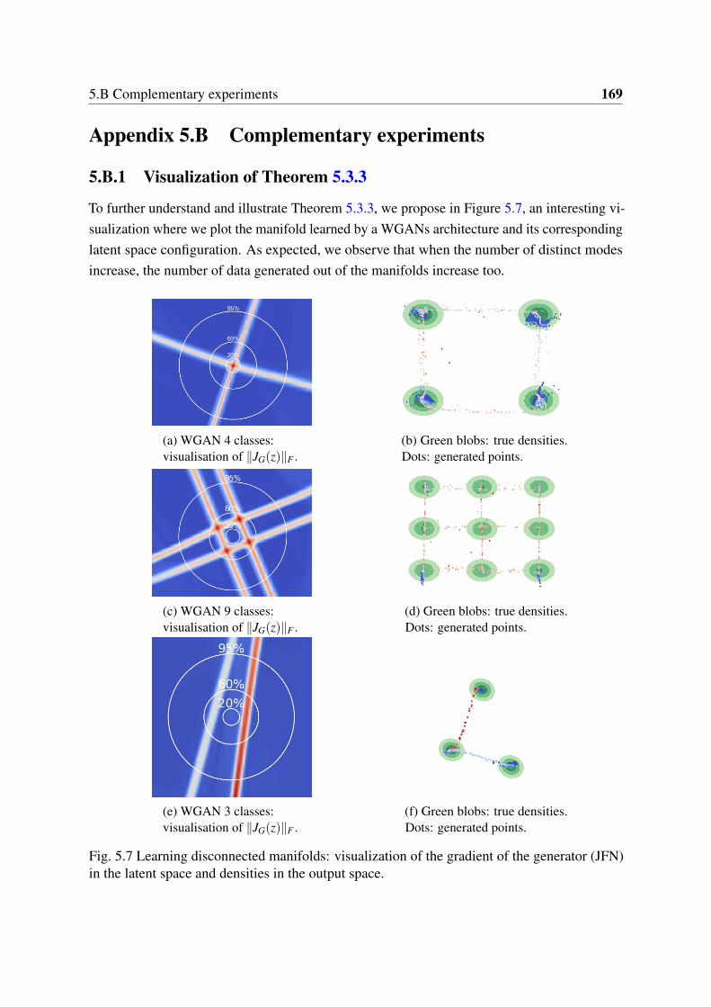
5.B Complementary experiments 169
Appendix 5.B Complementary experiments
5.B.1 Visualization of Theorem 5.3.3
To further understand and illustrate Theorem 5.3.3, we propose in Figure 5.7, an interesting vi-sualization where we plot the manifold learned by a WGANs architecture and its correspondinglatent space configuration. As expected, we observe that when the number of distinct modesincrease, the number of data generated out of the manifolds increase too.
(a) WGAN 4 classes:visualisation of ∥JG(z)∥F .
(b) Green blobs: true densities.Dots: generated points.
(c) WGAN 9 classes:visualisation of ∥JG(z)∥F .
(d) Green blobs: true densities.Dots: generated points.
(e) WGAN 3 classes:visualisation of ∥JG(z)∥F .
(f) Green blobs: true densities.Dots: generated points.
Fig. 5.7 Learning disconnected manifolds: visualization of the gradient of the generator (JFN)in the latent space and densities in the output space.

170 Learning disconnected manifolds: a no GAN’s land
5.B.2 Definition of the different metrics used
In the sequel, we present the different metrics used in Section 5.4 of the paper to assessperformances of GANs. We have:
• Improved Precision/Recall (PR) metric Kynkäänniemi et al. (2019): it has been presentedin Definition 5.3.2. Intuitively, Based on a k-NN estimation of the manifold of real (resp.generated) data, it assesses whether generated (resp. real) points belong in the real (resp.generated) data manifold or not. The proportion of generated (resp. real) points that arein the real (resp. generated) data manifold is the precision (resp. recall).
• the Hausdorff distance: it is defined by
Haus(A,B) = max
maxa∈A
minb∈B
∥a−b∥,maxb∈B
mina∈A
∥a−b∥
Such a distance is useful to evaluate the closeness of two different supports from a metricspace, but is sensitive to outliers because of the max operation. It has been recently usedfor theoretical purposes by Pandeva and Schubert (2019).
• the Frechet Inception distance: first proposed by Dowson and Landau (1982), the Frechetdistance was applied in the setting of GANs by Heusel et al. (2017). This distancebetween mutlivariate Gaussians compares statistic of generated samples to real samplesas follows
FID = ∥ν⋆−νθ∥2 +Tr(Σ⋆+Σθ +2(Σ⋆Σθ )
12)
where X⋆ = N (ν⋆,Σ⋆) and Xθ = N (νθ ,Σθ ) are the activations of a pre-softmax layer.However, when dealing with disconnected manifolds, we argue that this distance is notwell suited as it approximates the distributions with unimodal one, thus loosing manyinformation.
The choice of such metrics is motivated by the fact that metrics measuring the performances ofGANs should not rely on relative densities but should rather be point sets based metrics.
5.B.3 Saturation of a MLP neural network
In Section 5.4.2, we claim that the generator reduces the sampling of off-manifold data pointsup to a saturation point. Figure 5.8 below provides a visualization of this phenomenon. In thissynthetic case, we learn a 9-component mixture of Gaussians using simple GANs architecture(both the generator and the discriminator are MLP with two hidden layers). The minimal

5.B Complementary experiments 171
distance between two modes is set to 9. We clearly see in Figure 5.8d that the precisionsaturates around 80%.
(a) Data points sampled after 5,000 stepsof training.
(b) Data points sampled after 50,000steps of training.
(c) Data points sampled after 100,000steps of training.
(d) Evolution of the precision α dur-ing training.
Fig. 5.8 Learning 9 disconnected manifolds with a standard GANs architecture.
5.B.4 More results and visualizations on MNIST/F-MNIST/CIFAR10
Additionally to those in Section 5.4.3, we provide in Figure 5.9 and Table 5.2 supplementaryresults for MNIST, F-MNIST and CIFAR-10 datasets.
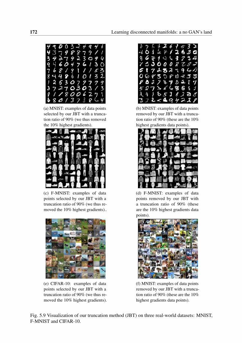
172 Learning disconnected manifolds: a no GAN’s land
(a) MNIST: examples of data pointsselected by our JBT with a trunca-tion ratio of 90% (we thus removedthe 10% highest gradients).
(b) MNIST: examples of data pointsremoved by our JBT with a trunca-tion ratio of 90% (these are the 10%highest gradients data points).
(c) F-MNIST: examples of datapoints selected by our JBT with atruncation ratio of 90% (we thus re-moved the 10% highest gradients)..
(d) F-MNIST: examples of datapoints removed by our JBT witha truncation ratio of 90% (theseare the 10% highest gradients datapoints).
(e) CIFAR-10: examples of datapoints selected by our JBT with atruncation ratio of 90% (we thus re-moved the 10% highest gradients).
(f) MNIST: examples of data pointsremoved by our JBT with a trunca-tion ratio of 90% (these are the 10%highest gradients data points).
Fig. 5.9 Visualization of our truncation method (JBT) on three real-world datasets: MNIST,F-MNIST and CIFAR-10.
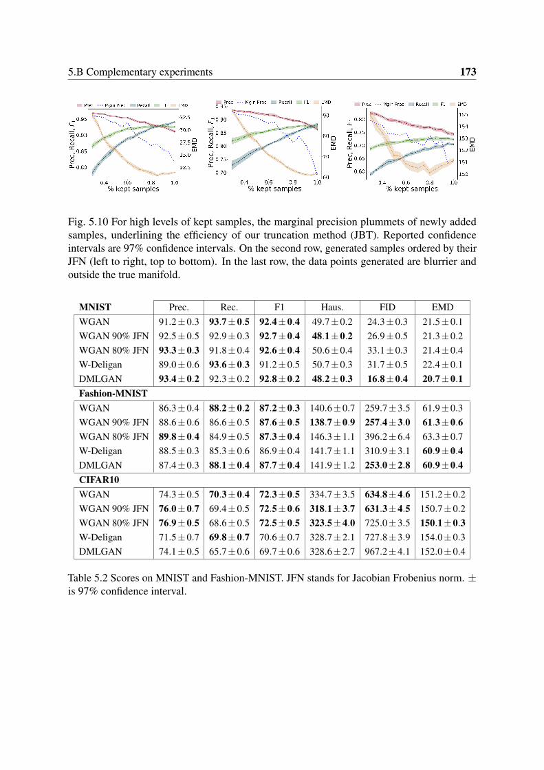
5.B Complementary experiments 173
Fig. 5.10 For high levels of kept samples, the marginal precision plummets of newly addedsamples, underlining the efficiency of our truncation method (JBT). Reported confidenceintervals are 97% confidence intervals. On the second row, generated samples ordered by theirJFN (left to right, top to bottom). In the last row, the data points generated are blurrier andoutside the true manifold.
MNIST Prec. Rec. F1 Haus. FID EMDWGAN 91.2±0.3 93.7±0.5 92.4±0.4 49.7±0.2 24.3±0.3 21.5±0.1WGAN 90% JFN 92.5±0.5 92.9±0.3 92.7±0.4 48.1±0.2 26.9±0.5 21.3±0.2WGAN 80% JFN 93.3±0.3 91.8±0.4 92.6±0.4 50.6±0.4 33.1±0.3 21.4±0.4W-Deligan 89.0±0.6 93.6±0.3 91.2±0.5 50.7±0.3 31.7±0.5 22.4±0.1DMLGAN 93.4±0.2 92.3±0.2 92.8±0.2 48.2±0.3 16.8±0.4 20.7±0.1Fashion-MNISTWGAN 86.3±0.4 88.2±0.2 87.2±0.3 140.6±0.7 259.7±3.5 61.9±0.3WGAN 90% JFN 88.6±0.6 86.6±0.5 87.6±0.5 138.7±0.9 257.4±3.0 61.3±0.6WGAN 80% JFN 89.8±0.4 84.9±0.5 87.3±0.4 146.3±1.1 396.2±6.4 63.3±0.7W-Deligan 88.5±0.3 85.3±0.6 86.9±0.4 141.7±1.1 310.9±3.1 60.9±0.4DMLGAN 87.4±0.3 88.1±0.4 87.7±0.4 141.9±1.2 253.0±2.8 60.9±0.4CIFAR10WGAN 74.3±0.5 70.3±0.4 72.3±0.5 334.7±3.5 634.8±4.6 151.2±0.2WGAN 90% JFN 76.0±0.7 69.4±0.5 72.5±0.6 318.1±3.7 631.3±4.5 150.7±0.2WGAN 80% JFN 76.9±0.5 68.6±0.5 72.5±0.5 323.5±4.0 725.0±3.5 150.1±0.3W-Deligan 71.5±0.7 69.8±0.7 70.6±0.7 328.7±2.1 727.8±3.9 154.0±0.3DMLGAN 74.1±0.5 65.7±0.6 69.7±0.6 328.6±2.7 967.2±4.1 152.0±0.4
Table 5.2 Scores on MNIST and Fashion-MNIST. JFN stands for Jacobian Frobenius norm. ±is 97% confidence interval.

174 Learning disconnected manifolds: a no GAN’s land
5.B.5 More results on BigGAN and ImageNet
In Figure 5.11, we show images from the Bubble class of ImageNet. It supports our claim ofmanifold disconectedness, even within a class, and outlines the importance of studying thelearning of disconnected manifolds in generative models. Then, in Figure 5.12 and Figure5.13, we give more exemples from BigGAN 128x128 class-conditionned generator. We plot inthe same format than in 5.4.4. Specifically, for different classes, we plot 128 images rankedby JFN. Here again, we see a concentration of off-manifold samples on the last row, provingthe efficiency of our method. Example of classes responding particularly well to our rankingare House Finch c, Monnarch Butterfly e or Wood rabbit c. For each class, we also show anhistogram of JFN based on 1024 samples. It shows that the JFN is a good indicator of thecomplexity of the class. For example, classes such as Cornet (see Figure 5.13e) or Footballhelmet (see Figure 5.13a) are very diverse and disconnected, resulting in high JFNs.
Fig. 5.11 Images from the Bubble class of ImageNet showing that the class is complex andslightly multimodal.
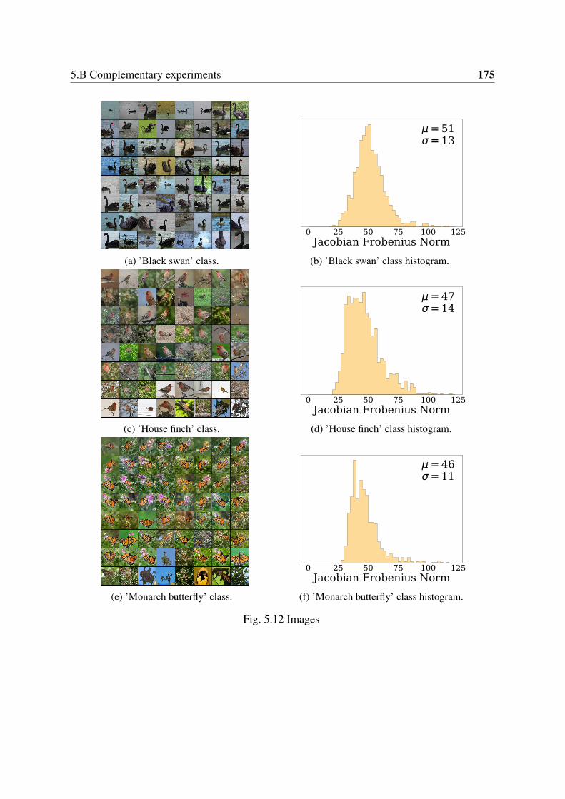
5.B Complementary experiments 175
(a) ’Black swan’ class.
0 25 50 75 100 125Jacobian Frobenius Norm
= 51= 13
(b) ’Black swan’ class histogram.
(c) ’House finch’ class.
0 25 50 75 100 125Jacobian Frobenius Norm
= 47= 14
(d) ’House finch’ class histogram.
(e) ’Monarch butterfly’ class.
0 25 50 75 100 125Jacobian Frobenius Norm
= 46= 11
(f) ’Monarch butterfly’ class histogram.
Fig. 5.12 Images

176 Learning disconnected manifolds: a no GAN’s land
(a) ’Football helmet’ class.
0 25 50 75 100 125Jacobian Frobenius Norm
= 73= 13
(b) ’Football helmet’ class histogram.
(c) ’Wood rabbit’ class.
0 25 50 75 100 125Jacobian Frobenius Norm
= 33= 10
(d) ’wood rabbit’ class histogram.
(e) ’Cornet’ class.
0 25 50 75 100 125Jacobian Frobenius Norm
= 68= 20
(f) ’Cornet’ class histogram.
Fig. 5.13 Images

5.C Supplementary details 177
Appendix 5.C Supplementary details
We now provide the different network’s architecture used and their corresponding hyperparam-eters.
Table 5.3 Models for Synthetic datasets
Operation Feature Maps Activation
G(z): z ∼ N (0,1) 2Fully Connected - layer1 20 ReLUFully Connected - layer2 20 ReLU
D(x)Fully Connected - layer1 20 ReLUFully Connected - layer2 20 ReLU
Batch size 32Leaky ReLU slope 0.2Gradient Penalty weight 10Learning Rate 0.0002Optimizer Adam: β1 = 0.5 β2 = 0.5
For DeliGan, we use the same architecture and simply add 50 Gaussians for thereparametrization trick. For DMLGAN, we re-use the architecture of the authors.

178 Learning disconnected manifolds: a no GAN’s land
Table 5.4 WGAN for MNIST/Fashion MNIST
Operation Kernel Strides Feature Maps Activation
G(z): z ∼ N(0, Id) 100Fully Connected 7×7×128Convolution 3×3 1×1 7×7×64 LReLUConvolution 3×3 1×1 7×7×64 LReLUNearest Up Sample 14×14×64Convolution 3×3 1×1 14×14×32 LReLUConvolution 3×3 1×1 14×14×32 LReLUNearest Up Sample 14×14×64Convolution 3×3 1×1 28×28×16 LReLUConvolution 5×5 1×1 28×28×1 Tanh
D(x) 28×28×1Convolution 4×4 2×2 14×14×32 LReLUConvolution 3×3 1×1 14×14×32 LReLUConvolution 4×4 2×2 7×7×64 LReLUConvolution 3×3 1×1 7×7×64 LReLUFully Connected 1 -
Batch size 256Leaky ReLU slope 0.2Gradient Penalty weight 10Learning Rate 0.0002Optimizer Adam β1 : 0.5 β2 : 0.5
Table 5.5 DMLGAN for MNIST/Fashion MNIST
Operation Kernel Strides Feature Maps BN Activation
G(z): z ∼ N(0, Id) 100Fully Connected 7×7×128 -Convolution 3×3 1×1 7×7×64 - Leaky ReLUConvolution 3×3 1×1 7×7×64 - Leaky ReLUNearest Up Sample 14×14×64 -Convolution 3×3 1×1 14×14×32 - Leaky ReLUConvolution 3×3 1×1 14×14×32 - Leaky ReLUNearest Up Sample 14×14×64 -Convolution 3×3 1×1 28×28×16 - Leaky ReLUConvolution 5×5 1×1 28×28×1 - Tanh
Encoder Q(x), Discriminator D(x) 28×28×1Convolution 4×4 2×2 14×14×32 - Leaky ReLUConvolution 3×3 1×1 14×14×32 - Leaky ReLUConvolution 4×4 2×2 7×7×64 - Leaky ReLUConvolution 3×3 1×1 7×7×64 - Leaky ReLUD Fully Connected 1 - -Q Convolution 3×3 7×7×64 Y Leaky ReLUQ Convolution 3×3 7×7×64 Y Leaky ReLUQ Fully Connected ng = 10 - Softmax
Batch size 256Leaky ReLU slope 0.2Gradient Penalty weight 10Learning Rate 0.0002Optimizer Adam β1 = 0.5 β2 = 0.5

5.C Supplementary details 179
Table 5.6 WGAN for CIFAR10, from Gulrajani et al. (2017)
Operation Kernel Strides Feature Maps BN Activation
G(z): z ∼ N(0, Id) 128Fully Connected 4×4×128 -ResBlock [3×3]×2 1×1 4×4×128 Y ReLUNearest Up Sample 8×8×128 -ResBlock [3×3]×2 1×1 8×8×128 Y ReLUNearest Up Sample 16×16×128 -ResBlock [3×3]×2 1×1 16×16×128 Y ReLUNearest Up Sample 32×32×128 -Convolution 3×3 1×1 32×32×3 - Tanh
Discriminator D(x) 32×32×3ResBlock [3×3]×2 1×1 32×32×128 - ReLUAvgPool 2×2 1×1 16×16×128 -ResBlock [3×3]×2 1×1 16×16×128 - ReLUAvgPool 2×2 1×1 8×8×128 -ResBlock [3×3]×2 1×1 8×8×128 - ReLUResBlock [3×3]×2 1×1 8×8×128 - ReLUMean pooling (spatial-wise) - - 128 -Fully Connected 1 - -
Batch size 64Gradient Penalty weight 10Learning Rate 0.0002Optimizer Adam β1 = 0. β2 = 0.9Discriminator steps 5
Table 5.7 DMLGAN for CIFAR10, from Gulrajani et al. (2017)
Operation Kernel Strides Feature Maps BN Activation
G(z): z ∼ N(0, Id) 128Fully Connected 4×4×128 -ResBlock [3×3]×2 1×1 4×4×128 Y ReLUNearest Up Sample 8×8×128 -ResBlock [3×3]×2 1×1 8×8×128 Y ReLUNearest Up Sample 16×16×128 -ResBlock [3×3]×2 1×1 16×16×128 Y ReLUNearest Up Sample 32×32×128 -Convolution 3×3 1×1 32×32×3 - Tanh
Encoder Q(x), Discriminator D(x) 32×32×3ResBlock [3×3]×2 1×1 32×32×128 - ReLUAvgPool 2×2 1×1 16×16×128 -ResBlock [3×3]×2 1×1 16×16×128 - ReLUAvgPool 2×2 1×1 8×8×128 -ResBlock [3×3]×2 1×1 8×8×128 - ReLUD ResBlock [3×3]×2 1×1 8×8×128 - ReLUD Mean pooling (spatial-wise) 2×2 1×1 128 -D Fully Connected 1 - -Q ResBlock [3×3]×2 1×1 8×8×128 - ReLUQ Mean pooling (spatial-wise) 2×2 1×1 128 -Q Fully Connected ng = 10 - Softmax
Batch size 64Gradient Penalty weight 10Learning Rate 0.0002Optimizer Adam β1 = 0. β2 = 0.9Discriminator steps 5


Conclusion
5.4 Conclusion on the present thesis
The present thesis is intended to develop methodological tools to study Generative AdversarialNetworks and provide some theoretical results on GANs. More informally, it is an attempt atnarrowing the gap between theory and practice.
5.4.1 Statistical study
Chapter 2 and Chapter 3 analyze properties of respectively GANs (Goodfellow et al., 2014)and Wasserstein GANs (Arjovsky et al., 2017).
To understand these two frameworks, one has to distinguish the theoretical non-parametricobjectives from the practical ones involving parametric classes of discriminative functions.More formally, when allowing discriminative functions to be any measurable functions fromRD → [0,1] (in GANs) or any 1-Lipschitz functions RD →R (WGANs) we have the followingset of optimal parameters:
In Chapter 2, Θ⋆ = θ ∈Θ ,DJS(µ⋆,µθ ) = inf
θ∈ΘDJS(µ⋆,µθ ).
In Chapter 3, Θ⋆ = θ ∈Θ ,W (µ⋆,µθ ) = inf
θ∈ΘW (µ⋆,µθ ).
where W is the Wasserstein distance and dJS is the Jensen-Shanon divergence. In Chapter 2,Theorem 2.2.2 shows the existence and the uniqueness of the solution. However, the practitionerhas to rely on a parametric discriminator D . The main consequence of optimizing using thisneural net distance is that one can only expect to find the following set of parameters:
In Chapter 2, Θ = θ ∈Θ ,DD(µ⋆,µθ ) = infθ∈Θ
DD(µ⋆,µθ ).
In Chapter 3, Θ = θ ∈Θ ,dD(µ⋆,µθ ) = infθ∈Θ
dD(µ⋆,µθ ).

182 Learning disconnected manifolds: a no GAN’s land
where DD = supα∈λ
Eµ⋆ log(Dα)+Eµθlog(1−Dα) and dD = sup
α∈λ
Eµ⋆Dα −EµθDα .
Both chapters study these approximation properties. Ideally, one would like Θ ⊂Θ ⋆ suchthat any parameter obtained by the practitioner is also an optimal parameter. However, thiscondition is highly demanding and depends on Θ , Λ , and the global shape of the chosen lossfunction. Alternatively, one would like to exhibit specific parameterization under which anyparameter θ ∈ Θ has a performance ε-away to the optimal performance of a parameter θ ⋆ ∈Θ ⋆
(ε being arbitrary). Respectively, Theorem 2.3.1 and Theorem 3.3.1 show that for any givengenerative parameterization Θ , there exists a discriminative parameterization Λ such that thiscondition is verified for respectively the GANs and WGANs framework.
Interestingly, apprehending the relationship between Θ and Θ ⋆ could be made possiblevia a better understanding of the behavior of the neural net distances DD and dD . Chapter 3attempted to study the question and proposed the monotonous equivalence as a way to link theWasserstein distance dLip1
with the neural net distance dD . It is clear that many trade-offs areat play when training GANs: the more generative capacity the model has, the more demandingthe monotonous equivalence is; conversely, the more discriminative capacity the model has, themore realistic the monotonous equivalence is.
As recalled in both Chapter 2 and Chapter 3, one only has access to the empirical measureµn of the target distribution µ⋆. Therefore, due to this estimation error, one ends up with thefollowing parameters:
In Chapter 2, Θ = θ ∈Θ ,DD(µn,µθ ) = infθ∈Θ
DD(µn,µθ ).
In Chapter 3, Θ = θ ∈Θ ,dD(µn,µθ ) = infθ∈Θ
dD(µn,µθ ).
Interestingly, Theorem 2.4.1 and Theorem 3.4.1 prove that both formulations are consistent.However, many questions remain unanswered:
• Finite-sample analysis of εestim: in Theorem 3.4.1, we were able to find convergencerates for εoptim + εestim. Lemma 3.4.1 has shown that limn→∞ εestim = 0, but it wouldbe interesting to find a finite sample upper-bound for εestim? This would also enable usto better understand the impact of the capacity of the discriminator Dα on this quantityεestim and thus correctly parameterize it.
• Bounding εapprox+εoptim+εestim: this specific analysis is missing in the present thesis.A first theoretical step was made by Uppal et al. (2019) who exhibited convergencerates. However, their study specifically studied the case where both µ⋆ and µθ areabsolutely continuous with respect to the Lebesgue measure and their density lie in thesame Besov ball. In high dimension, such study would not hold since it is highly likely

5.5 Broader perspectives on GANs 183
that none of these probability distributions would have densities (Fefferman et al., 2016).Similarly, Schreuder et al. (2020) also bring an interesting contribution in the case wherethe target distribution can be written as the push-forward between a multivariate uniformdistribution and a smooth generator.
5.4.2 Post-processing trained generative networks
Another line of research present in this thesis has to do with the learning of disconnectedmanifolds with standard Generative Adversarial Networks. Using results from the GaussianIsoperimetric inequality, Theorem 5.3.2 and Theorem 5.3.3 give lower bounds on the portionof generated samples that are mapped out of the target manifold. To solve this issue, previousworks recommended to over-parameterize the model using either latent mixtures of Gaussians(Gurumurthy et al., 2017) or an ensemble set of generators (Tolstikhin et al., 2017; Khayatkhoeiet al., 2018). In Chapter 5, we exhibited a simple heuristic, based on the generator’s Jacobiannorm, that efficiently remove off-manifold data points. Finally, another line of work relies onon the use of Monte-Carlo methods to post-process pre-trained generators (Azadi et al., 2019;Grover et al., 2019; Turner et al., 2019).
Interestingly, what we have observed so far is that these methods are very efficient whenit comes to removing items that are located in between two modes of the target manifold.However, to detect blurry items within a class (or respectively when there is only one distinctclass), all these methods seem to behave poorly. One of the possible hypothesis is that thesetwo tasks might have to be tackled separately. Indeed, a single discriminator network may notbe able to efficiently detect simultaneously fake items both within a given class and in-betweentwo different classes.
5.5 Broader perspectives on GANs
Recent studies have been efficient at opening a series of broad questions on GANs. To closethe present thesis, we propose a small discussion on three of the main challenges ahead for abetter understanding of GANs:
• Innovation in GANs: there might be in GANs a discrepancy between expectations ofthe generative model and the chosen objective function. Since the model is trained tominimize the Wasserstein distance to the empirical distribution, it is a legitimate questionto determine and understand how are generated samples linked to the training dataset.For example, could we identify what is new when generating the face of a person thatdoes not exist (see, thispersondoesnotexist.com)?

184 Learning disconnected manifolds: a no GAN’s land
• Generalization in GANs: theoretical research aim at understanding the ability ofGANs at approximating the target distribution from finite samples. In order to improveour understanding of GANs and efficiently compare different formulations, it would bebeneficial to have a clear evaluation protocol, measuring both the quality and diversityof the generated images. The Improved Precision/Recall metric (Kynkäänniemi et al.,2019) is a first step. However, the downside is that when evaluating empirically GANs, itis still not a common practice in the community to consistently have a train/test split.
• Trade-off properties in GANs: when it comes to training GANs, it is well-known thata tricky competition is at play between the generator and the discriminator. On the onehand, a close-to-optimality discriminator can lead to vanishing gradients (Arjovsky andBottou, 2017) and on the other, if the discriminator does not have enough capacity, itcould be easily "fooled" and one could have dD(µ⋆,µθ ) = 0 even though both probabilitydistributions are significantly different. Similarly, Section 3.5 highlighted that increasingthe capacity of the generator alone does not necessarily lead to an improved performance,mostly because it also makes the task harder for the discriminator. Interestingly, Liang(2018) also hypothesized diagrams on how the discriminator and the generator shouldbe simultaneously parameterized. To enable further improvements, future research willhave to thoroughly study the intricacies at play between both networks’ capacity.

References
Acharya, D., Huang, Z., Paudel, D., and Van Gool, L. (2018). Towards high resolution videogeneration with progressive growing of sliced Wasserstein GANs. arXiv.1810.02419.
Angles, T. and Mallat, S. (2018). Generative networks as inverse problems with scatteringtransforms. In International Conference on Learning Representations.
Anil, C., Lucas, J., and Grosse, R. (2019). Sorting out Lipschitz function approximation.In Chaudhuri, K. and Salakhutdinov, R., editors, Proceedings of the 36th InternationalConference on Machine Learning, volume 97, pages 291–301. PMLR.
Arjovsky, M. and Bottou, L. (2017). Towards principled methods for training generativeadversarial networks. In International Conference on Learning Representations.
Arjovsky, M., Chintala, S., and Bottou, L. (2017). Wasserstein generative adversarial networks.In Precup, D. and Teh, Y., editors, Proceedings of the 34th International Conference onMachine Learning, volume 70, pages 214–223. PMLR.
Arora, R., Basu, A., Mianjy, P., and Mukherjee, A. (2018). Understanding deep neural networkswith rectified linear units. In International Conference on Learning Representations.
Arora, S., Ge, R., Liang, Y., Ma, T., and Zhang, Y. (2017). Generalization and equilibrium ingenerative adversarial nets (gans). CoRR, abs/1703.00573.
Arora, S. and Zhang, Y. (2017). Do gans actually learn the distribution? an empirical study.arXiv:1706.08224.
Arvanitidis, G., Hansen, L. K., and Hauberg, S. (2017). Latent space oddity: on the curvatureof deep generative models. In ICLR.
Azadi, S., Olsson, C., Darrell, T., Goodfellow, I., and Odena, A. (2019). Discriminator rejectionsampling. In International Conference on Learning Representations.
Biau, G., Cadre, B., Sangnier, M., and Tanielian, U. (2020). Some theoretical properties ofGANs. The Annals of Statistics, in press.
Biau, G. and Devroye, L. (2015). Lectures on the nearest neighbor method. Springer.
Bjorck, A. and Bowie, C. (1971). An iterative algorithm for computing the best estimate of anorthogonal matrix. SIAM Journal on Numerical Analysis, 8:358–364.
Blanchet, J., Kang, Y., and Murthy, K. (2019). Robust Wasserstein profile inference andapplications to machine learning. Journal of Applied Probability, 56:830–857.

186 References
Bojanowski, P., Joulin, A., Lopez-Paz, D., and Szlam, A. (2018). Optimizing the latent space ofgenerative networks. In Dy, J. and Krause, A., editors, Proceedings of the 35th InternationalConference on Machine Learning, volume 80, pages 600–609. Proceedings of MachineLearning Research.
Borell, C. (1975). The brunn-minkowski inequality in gauss space. Inventiones mathematicae,30(2):207–216.
Borji, A. (2019). Pros and cons of gan evaluation measures. Computer Vision and ImageUnderstanding, 179:41–65.
Boucheron, S., Lugosi, G., and Massart, P. (2013). Concentration inequalities: A nonasymptotictheory of independence. Oxford university press, address="Oxford".
Brock, A., Donahue, J., and Simonyan, K. (2019). Large scale GAN training for high fidelitynatural image synthesis. In International Conference on Learning Representations.
Che, T., Li, Y., Zhang, R., Hjelm, R. D., Li, W., Song, Y., and Bengio, Y. (2017).Maximum-likelihood augmented discrete generative adversarial networks. arXiv preprintarXiv:1702.07983.
Chernodub, A. and Nowicki, D. (2016). Norm-preserving Orthogonal Permutation Linear Unitactivation functions (OPLU). arXiv.1604.02313.
Chongxuan, L., Xu, T., Zhu, J., and Zhang, B. (2017). Triple generative adversarial nets. InAdvances in neural information processing systems, pages 4088–4098.
Clark, A., Donahue, J., and Simonyan, K. (2019). Adversarial video generation on complexdatasets. arXiv, pages arXiv–1907.
Cooper, D. (1995). Learning Lipschitz functions. International Journal of Computer Mathe-matics, 59:15–26.
Cybenko, G. (1989). Approximation by superpositions of a sigmoidal function. Mathematicsof Control, Signals and Systems, 2:303–314.
Devroye, L. (1997). Universal smoothing factor selection in density estimation: Theory andpractice. TEST, 6:223–320.
Devroye, L., Györfi, L., and Lugosi, G. (1996). A Probabilistic Theory of Pattern Recognition.Springer, New York.
Devroye, L. and Wise, G. (1980). Detection of abnormal behavior via nonparametric estimationof the support. SIAM Journal on Applied Mathematics, 38:480–488.
Donahue, C., Lipton, Z., Balsubramani, A., and McAuley, J. (2018). Semantically decomposingthe latent spaces of generative adversarial networks. In International Conference on LearningRepresentations.
Dowson, D. and Landau, B. (1982). The fréchet distance between multivariate normal distribu-tions. Journal of multivariate analysis, pages 450–455.

References 187
Dudley, R. (2004). Real Analysis and Probability. Cambridge University Press, Cambridge, 2edition.
Endres, D. and Schindelin, J. (2003). A new metric for probability distributions. IEEETransactions on Information Theory, 49:1858–1860.
Esfahani, P. and Kuhn, D. (2018). Data-driven distributionally robust optimization using theWasserstein metric: Performance guarantees and tractable reformulations. MathematicalProgramming, 171:115–166.
Fedus, W., Goodfellow, I., and Dai, A. M. (2018). Maskgan: Better text generation via fillingin the _. arXiv:1801.07736.
Fefferman, C., Mitter, S., and Narayanan, H. (2016). Testing the manifold hypothesis. Journalof the American Mathematical Society, 29:983–1049.
Flamary, R. and Courty, N. (2017). POT: Python Optimal Transport library.
Fournier, N. and Guillin, A. (2015). On the rate of convergence in Wasserstein distance of theempirical measure. Probability Theory and Related Fields, 162:707–738.
Gao, R., Chen, X., and Kleywegt, A. (2017). Wasserstein distributional robustness andregularization in statistical learning. arXiv:1712.06050.
Givens, C. and Shortt, R. (1984). A class of Wasserstein metrics for probability distributions.Michigan Mathematical Journal, 31:231–240.
Glorot, X., Bordes, A., and Bengio, Y. (2011). Deep sparse rectifier neural networks. InGordon, G., Dunson, D., and Dudík, M., editors, Proceedings of the Fourteenth InternationalConference on Artificial Intelligence and Statistics, volume 15, pages 315–323. PMLR.
Goodfellow, I. (2016). NIPS 2016 Tutorial: Generative Adversarial Networks.arXiv:1701.00160.
Goodfellow, I., Pouget-Abadie, J., Mirza, M., Xu, B., Warde-Farley, D., Ozair, S., Courville, A.,and Bengio, J. (2014). Generative adversarial nets. In Ghahramani, Z., Welling, M., Cortes,C., Lawrence, N., and Weinberger, K., editors, Advances in Neural Information ProcessingSystems 27, pages 2672–2680. Curran Associates, Inc.
Goodfellow, I., Shlens, J., and Szegedy, C. (2015). Explaining and harnessing adversarialexamples. In International Conference on Learning Representations.
Gretton, A., Borgwardt, K. M., Rasch, M., Schölkopf, B., and Smola, A. (2012). A kerneltwo-sample test. Journal of Machine Learning Research, 13:723–773.
Grover, A., Song, J., Kapoor, A., Tran, K., Agarwal, A., Horvitz, E. J., and Ermon, S. (2019).Bias correction of learned generative models using likelihood-free importance weighting. InAdvances in Neural Information Processing Systems, pages 11056–11068.
Gulrajani, I., Ahmed, F., Arjovsky, M., Dumoulin, V., and Courville, A. (2017). Improvedtraining of Wasserstein GANs. In Guyon, I., von Luxburg, U., Bengio, S., Wallach, H.,Fergus, R., Vishwanathan, S., and Garnett, R., editors, Advances in Neural InformationProcessing Systems 30, pages 5767–5777. Curran Associates, Inc.

188 References
Gurumurthy, S., Kiran Sarvadevabhatla, R., and Venkatesh Babu, R. (2017). Deligan: Genera-tive adversarial networks for diverse and limited data. In Proceedings of the IEEE Conferenceon Computer Vision and Pattern Recognition.
Hales, T. C. (2001). The honeycomb conjecture. Discrete & Computational Geometry, pages1–22.
He, J., Li, L., Xu, J., and Zheng, C. (2018). Relu deep neural networks and linear finiteelements. arXiv preprint arXiv:1807.03973.
He, K., Zhang, X., Ren, S., and Sun, J. (2016). Deep residual learning for image recognition.In Proceedings of the IEEE Conference on Computer Vision and Pattern Recognition, pages770–778.
Heusel, M., Ramsauer, H., Unterthiner, T., Nessler, B., and Hochreiter, S. (2017). Gans trainedby a two time-scale update rule converge to a local nash equilibrium. In Advances in neuralinformation processing systems, pages 6626–6637.
Hornik, K. (1991). Approximation capabilities of multilayer feedforward networks. NeuralNetworks, 4:251–257.
Hornik, K., Stinchcombe, M., and White, H. (1989). Multilayer feedforward networks areuniversal approximators. Neural Networks, 2:359–366.
Huster, T., Chiang, C.-Y. J., and Chadha, R. (2018). Limitations of the Lipschitz constant as adefense against adversarial examples. In Joint European Conference on Machine Learningand Knowledge Discovery in Databases, pages 16–29. Springer.
Ji, S., Xu, W., Yang, M., and Yu, K. (2013). 3d convolutional neural networks for human actionrecognition. IEEE Transactions on Pattern Analysis and Machine Intelligence, 35(1):221–231.
Jin, C., Netrapalli, P., Ge, R., Kakade, S., and Jordan, M. (2019). A short note on concentrationinequalities for random vectors with subGaussian norm. arXiv.1902.03736.
Kallenberg, O. (2006). Foundations of modern probability. Springer Science & BusinessMedia.
Kantorovich, L. and Rubinstein, G. (1958). On a space of completely additive functions. VestnikLeningrad University Mathematics, 13:52–59.
Karras, T., Aila, T., Laine, S., and Lehtinen, J. (2018). Progressive growing of GANs forimproved quality, stability, and variation. In International Conference on Learning Repre-sentations.
Karras, T., Laine, S., and Aila, T. (2019). A style-based generator architecture for generativeadversarial networks. In Proceedings of the IEEE Conference on Computer Vision andPattern Recognition, pages 4401–4410.
Khayatkhoei, M., Singh, M. K., and Elgammal, A. (2018). Disconnected manifold learning forgenerative adversarial networks. In Advances in Neural Information Processing Systems,pages 7343–7353.

References 189
Khrulkov, V. and Oseledets, I. (2018). Geometry score: A method for comparing generativeadversarial networks. In International Conference on Machine Learning, pages 2621–2629.
Kodali, N., Abernethy, J., Hays, J., and Kira, Z. (2017). On convergence and stability of GANs.arXiv.1705.07215.
Kontorovich, A. (2014). Concentration in unbounded metric spaces and algorithmic stability.In Xing, E. and Jebara, T., editors, Proceedings of the 31st International Conference onMachine Learning, volume 32, pages 28–36. PMLR.
Krizhevsky, A., Hinton, G., et al. (2009). Learning multiple layers of features from tiny images.
Krizhevsky, A., Sutskever, I., and Hinton, G. (2012). Imagenet classification with deepconvolutional neural networks. In Pereira, F., Burges, C., Bottou, L., and Weinberger, K.,editors, Advances in Neural Information Processing Systems 25, pages 1097–1105. CurranAssociates, Inc.
Kusner, M. J. and Hernández-Lobato, J. M. (2016). Gans for sequences of discrete elementswith the gumbel-softmax distribution. arXiv preprint arXiv:1611.04051.
Kynkäänniemi, T., Karras, T., Laine, S., Lehtinen, J., and Aila, T. (2019). Improved precisionand recall metric for assessing generative models. In Wallach, H., Larochelle, H., Beygelz-imer, A., d’Alché Buc, F., Fox, E., and Garnett, R., editors, Advances in Neural InformationProcessing Systems 32, pages 3927–3936. Curran Associates, Inc.
LeCun, Y., Bottou, L., Bengio, Y., and Haffner, P. (1998). Gradient-based learning applied todocument recognition. In Proceedings of the IEEE, pages 2278–2324.
Ledig, C., Theis, L., Huszár, F., Caballero, J., Cunningham, A., Acosta, A., Aitken, A., Tejani,A., Totz, J., Wang, Z., and Shi, W. (2017). Photo-realistic single image super-resolutionusing a generative adversarial network. In Proceedings of the IEEE Conference on ComputerVision and Pattern Recognition, pages 4681–4690.
Ledoux, M. (1996). Isoperimetry and gaussian analysis. In Lectures on probability theory andstatistics, pages 165–294. Springer.
Li, C.-L., Chang, W.-C., Cheng, Y., Yang, Y., and Poczos, B. (2017). MMD GAN: Towardsdeeper understanding of moment matching network. In Guyon, I., von Luxburg, U., Bengio,S., Wallach, H., Fergus, R., Vishwanathan, S., and Garnett, R., editors, Advances in NeuralInformation Processing Systems 30, pages 2203–2213. Curran Associates, Inc.
Li, Y., Swersky, K., and Zemel, R. (2015). Generative moment matching networks. InInternational Conference on Machine Learning, pages 1718–1727.
Liang, T. (2018). On how well generative adversarial networks learn densities: Nonparametricand parametric results. arXiv.1811.03179.
Lin, Z., Khetan, A., Fanti, G., and Oh, S. (2018). Pacgan: The power of two samples ingenerative adversarial networks. In Advances in Neural Information Processing Systems,pages 1498–1507.

190 References
Lipton, Z. and Tripathi, S. (2017). Precise recovery of latent vectors from generative adversarialnetworks. arxiv:1702.04782.
Liu, S., Bousquet, O., and Chaudhuri, K. (2017). Approximation and convergence properties ofgenerative adversarial learning. In Guyon, I., Luxburg, U., Bengio, S., Wallach, H., Fergus,R., Vishwanathan, S., and Garnett, R., editors, Advances in Neural Information ProcessingSystems 30, pages 5551–5559. Curran Associates, Inc., Red Hook.
Lu, Z., Pu, H., Wang, F., Hu, Z., and Wang, L. (2017). The expressive power of neuralnetworks: A view from the width. In Advances in Neural Information Processing Systems,pages 6231–6239.
Lucic, M., Kurach, K., Michalski, M., Gelly, S., and Bousquet, O. (2018). Are gans createdequal? a large-scale study. In Advances in neural information processing systems, pages697–706.
Mao, X., Li, Q., Xie, H., Lau, R. Y. K., Wang, Z., and Smolley, S. P. (2017). Least squaresgenerative adversarial networks. In Computer Vision (ICCV), 2017 IEEE InternationalConference on, pages 2813–2821. IEEE.
McDiarmid, C. (1989). On the method of bounded differences. In Siemons, J., editor, Surveysin Combinatorics, London Mathematical Society Lecture Note Series 141, pages 148–188.Cambridge University Press, Cambridge.
Mertikopoulos, P., Papadimitriou, C., and Piliouras, G. (2018). Cycles in adversarial regularizedlearning. In Proceedings of the Twenty-Ninth Annual ACM-SIAM Symposium on DiscreteAlgorithms, pages 2703–2717. SIAM.
Mescheder, L., Geiger, A., and Nowozin, S. (2018). Which training methods for gans doactually converge? In International Conference on Machine learning, pages 3481–3490.PMLR.
Metz, L., Poole, B., Pfau, D., and Sohl-Dickstein, J. (2016). Unrolled generative adversarialnetworks. arXiv.1611.02163.
Mirza, M. and Osindero, S. (2014). Conditional generative adversarial nets. CoRR, 1411.1784.
Miyato, T., Kataoka, T., Koyama, M., and Yoshida, Y. (2018). Spectral normalization forgenerative adversarial networks. In International Conference on Learning Representations.
Mogren, O. (2016). C-RNN-GAN: Continuous recurrent neural networks with adversarialtraining. arXiv.1611.09904.
Montúfar, G., Pascanu, R., Cho, K., and Bengio, Y. (2014). On the number of linear regionsof deep neural networks. In Ghahramani, Z., Welling, M., Cortes, C., Lawrence, N., andWeinberger, K., editors, Advances in Neural Information Processing Systems 27, pages2924–2932. Curran Associates, Inc.
Mroueh, Y. and Sercu, T. (2017). Fisher gan. In Advances in Neural Information ProcessingSystems, pages 2513–2523.

References 191
Müller, A. (1997). Integral probability metrics and their generating classes of functions.Advances in Applied Probability, 29:429–443.
Nowozin, S., Cseke, B., and Tomioka, R. (2016). f-GAN: Training generative neural samplersusing variational divergence minimization. In Lee, D., Sugiyama, M., Luxburg, U., Guyon,I., and Garnett, R., editors, Advances in Neural Information Processing Systems 29, pages271–279. Curran Associates, Inc., Red Hook.
O’Searcoid, M. (2006). Metric Spaces. Springer, Dublin.
Pandeva, T. and Schubert, M. (2019). Mmgan: Generative adversarial networks for multi-modaldistributions. arXiv:1911.06663.
Pascanu, R., Montúfar, G., and Bengio, Y. (2013). On the number of response regions of deepfeed forward networks with piece-wise linear activations. In International Conference onLearning Representations.
Petzka, H., Fischer, A., and Lukovnikov, D. (2018). On the regularization of WassersteinGANs. In International Conference on Learning Representations.
Qi, G. (2019). Loss-sensitive generative adversarial networks on Lipschitz densities. Interna-tional Journal of Computer Vision, pages 1–23.
Radford, A., Metz, L., and Chintala, S. (2015). Unsupervised representation learning with deepconvolutional generative adversarial networks. arXiv:1511.06434.
Raghu, M., Poole, B., Kleinberg, J., Ganguli, S., and Dickstein, J. (2017). On the expressivepower of deep neural networks. In Precup, D. and Teh, Y., editors, Proceedings of the 34thInternational Conference on Machine Learning, volume 70, pages 2847–2854. PMLR.
Reed, S., Akata, Z., Yan, X., Logeswaran, L., Schiele, B., and Lee, H. (2016). Generativeadversarial text to image synthesis. In International Conference on Machine Learning, pages1060–1069.
Rifai, S., Mesnil, G., Vincent, P., Muller, X., Bengio, Y., Dauphin, Y., and Glorot, X. (2011).Higher order contractive auto-encoder. In Joint European Conference on Machine Learningand Knowledge Discovery in Databases, pages 645–660. Springer.
Roth, K., Lucchi, A., Nowozin, S., and Hofmann, T. (2017). Stabilizing training of generativeadversarial networks through regularization. In Guyon, I., von Luxburg, U., Bengio, S.,Wallach, H., Fergus, R., Vishwanathan, S., and Garnett, R., editors, Advances in NeuralInformation Processing Systems 30, pages 2018–2028. Curran Associates, Inc.
Saito, M., Matsumoto, E., and Saito, S. (2017). Temporal generative adversarial nets withsingular value clipping. In 2017 IEEE International Conference on Computer Vision (ICCV),pages 2849–2858.
Sajjadi, M., Bachem, O., Lucic, M., Bousquet, O., and Gelly, S. (2018). Assessing generativemodels via precision and recall. In Bengio, S., Wallach, H., Larochelle, H., Grauman, K.,Cesa-Bianchi, N., and Garnett, R., editors, Advances in Neural Information ProcessingSystems 31, pages 5228–5237. Curran Associates, Inc.
192 References
Salimans, T., Goodfellow, I., Zaremba, W., Cheung, V., Radford, A., and Chen, X. (2016).Improved techniques for training GANs. In Lee, D., Sugiyama, M., von Luxburg, U., Guyon,I., and Garnett, R., editors, Advances in Neural Information Processing Systems 29, pages2234–2242. Curran Associates, Inc.
Samangouei, P., Kabkab, M., and Chellappa, R. (2018). Defense-gan: Protecting classifiersagainst adversarial attacks using generative models. In International Conference on LearningRepresentations.
Schreuder, N., Brunel, V.-E., and Dalalyan, A. (2020). Statistical guarantees for generativemodels without domination. arXiv:2010.09237.
Seidel, R. (1995). The upper bound theorem for polytopes: An easy proof of its asymptoticversion. Computational Geometry, 5:115–116.
Serra, T., Tjandraatmadja, C., and Ramalingam, S. (2018). Bounding and counting linearregions of deep neural networks. In International Conference on Machine Learning, pages4565–4573.
Shen, Y., Gu, J., Tang, X., and Zhou, B. (2020). Interpreting the latent space of gans forsemantic face editing. In Proceedings of the IEEE/CVF Conference on Computer Vision andPattern Recognition, pages 9243–9252.
Singh, S., Uppal, A., Li, B., Li, C.-L., Zaheer, M., and Poczos, B. (2018). Nonparametricdensity estimation under adversarial losses. In Bengio, S., Wallach, H., Larochelle, H.,Grauman, K., Cesa-Bianchi, N., and Garnett, R., editors, Advances in Neural InformationProcessing Systems 31, pages 10225–10236. Curran Associates, Inc.
Srivastava, A., Valkov, L., Russell, C., Gutmann, M. U., and Sutton, C. (2017). Veegan:Reducing mode collapse in gans using implicit variational learning. In Advances in NeuralInformation Processing Systems, pages 3308–3318.
Su, J., Vargas, D. V., and Sakurai, K. (2019). One pixel attack for fooling deep neural networks.IEEE Transactions on Evolutionary Computation, 23(5):828–841.
Sudakov, V. N. and Tsirelson, B. S. (1978). Extremal properties of half-spaces for sphericallyinvariant measures. Journal of Mathematical Sciences, pages 9–18.
Sun, K., Zhu, Z., and Lin, Z. (2019). Enhancing the robustness of deep neural networks byboundary conditional gan. arXiv preprint arXiv:1902.11029.
Sutton, R. S., McAllester, D. A., Singh, S. P., and Mansour, Y. (2000). Policy gradient methodsfor reinforcement learning with function approximation. In Advances in neural informationprocessing systems, pages 1057–1063.
Szegedy, C., Liu, W., Jia, Y., Sermanet, P., Reed, S., Anguelov, D., Erhan, D., Vanhoucke, V.,and Rabinovich, A. (2015). Going deeper with convolutions. In Proceedings of the IEEEconference on computer vision and pattern recognition, pages 1–9.
Tanaka, A. (2019). Discriminator optimal transport. In Advances in Neural InformationProcessing Systems, pages 6813–6823.

References 193
Telgarsky, M. (2015). Representation benefits of deep feedforward networks. arXiv 1509.08101.
Telgarsky, M. (2016). Benefits of depth in neural networks. In Feldman, V., Rakhlin, A.,and Shamir, O., editors, 29th Annual Conference on Learning Theory, volume 49, pages1517–1539. PMLR.
Tolstikhin, I., Gelly, S., Bousquet, O., Simon-Gabriel, C.-J., and Schölkopf, B. (2017). Adagan:Boosting generative models. In Advances in Neural Information Processing Systems, pages5424–5433.
Tulyakov, S., Liu, M.-Y., Yang, X., and Kautz, J. (2018). Mocogan: Decomposing motion andcontent for video generation. In Proceedings of the IEEE conference on computer vision andpattern recognition, pages 1526–1535.
Turner, R., Hung, J., Frank, E., Saatchi, Y., and Yosinski, J. (2019). Metropolis-hastingsgenerative adversarial networks. In International Conference on Machine Learning, pages6345–6353.
Uppal, A., Singh, S., and Poczos, B. (2019). Nonparametric density estimation and convergencerates for GANs under Besov IPM losses. In Wallach, H., Larochelle, H., Beygelzimer, A.,d’Alché Buc, F., Fox, E., and Garnett, R., editors, Advances in Neural Information ProcessingSystems 32, pages 9089–9100. Curran Associates, Inc.
van Handel, R. (2016). Probability in High Dimension. APC 550 Lecture Notes, PrincetonUniversity.
Vershynin, R. (2018). High-Dimensional Probability: An Introduction with Applications inData Science. Cambridge University Press, Cambridge.
Villani, C. (2008). Optimal Transport: Old and New. Springer, Berlin.
Virmaux, A. and Scaman, K. (2018). Lipschitz regularity of deep neural networks: analysisand efficient estimation. In Advances in Neural Information Processing Systems, pages3835–3844.
Vondrick, C., Pirsiavash, H., and Torralba, A. (2016). Generating videos with scene dynamics.In Advances in neural information processing systems, pages 613–621.
Wei, X., Gong, B., Liu, Z., Lu, W., and Wang, L. (2018). Improving the improved training ofwasserstein gans: A consistency term and its dual effect. arXiv:1803.01541.
Xiang, S. and Li, H. (2017). On the effects of batch and weight normalization in generativeadversarial networks. arXiv:1704.03971.
Xiao, C., Li, B., Zhu, J.-Y., He, W., Liu, M., and Song, D. (2018). Generating adversarial ex-amples with adversarial networks. In Proceedings of the 27th International Joint Conferenceon Artificial Intelligence, pages 3905–3911.
Xiao, H., Rasul, K., and Vollgraf, R. (2017). Fashion-MNIST: A novel image dataset forbenchmarking machine learning algorithms. arXiv:1708.07747.
Yarotsky, D. (2017). Error bounds for approximations with deep ReLU networks. NeuralNetworks, 94:103–114.
194 References
Yi, Z., Zhang, H., Tan, P., and Gong, M. (2017). Dualgan: Unsupervised dual learningfor image-to-image translation. In Proceedings of the IEEE international conference oncomputer vision, pages 2849–2857.
Yu, L., Zhang, W., Wang, J., and Yu, Y. (2017). Seqgan: Sequence generative adversarial netswith policy gradient. In Thirty-first AAAI conference on artificial intelligence.
Zhang, H., Goodfellow, I., Metaxas, D., and Odena, A. (2019). Self-attention generativeadversarial networks. In Chaudhuri, K. and Salakhutdinov, R., editors, Proceedings of the36th International Conference on Machine Learning, volume 97 of Proceedings of MachineLearning Research, pages 7354–7363.
Zhang, P., Liu, Q., Zhou, D., Xu, T., and He, X. (2018). On the discriminative-generalizationtradeoff in GANs. In International Conference on Learning Representations.
Zhao, J., Mathieu, M., and LeCun, Y. (2016). Energy-based generative adversarial network.arXiv:1609.03126.
Zhong, P., Mo, Y., Xiao, C., Chen, P., and Zheng, C. (2019). Rethinking generative modecoverage: A pointwise guaranteed approach. In Advances in Neural Information ProcessingSystems, pages 2086–2097.
Zhou, Z., Liang, J., Song, Y., Yu, L., Wang, H., Zhang, W., Yu, Y., and Zhang, Z. (2019).Lipschitz generative adversarial nets. In Chaudhuri, K. and Salakhutdinov, R., editors,Proceedings of the 36th International Conference on Machine Learning, volume 97, pages7584–7593. PMLR.