6 ADVERSARIAL SEARCH

6 ADVERSARIAL SEARCH

In which we examine the problems that arise when we try to plan ahead in a worldwhere other agents are planning against us.

6.1 GAMES

Chapter 2 introduced multiagent environments, in which any given agent will need to con-sider the actions of other agents and how they affect its own welfare. The unpredictabilityof these other agents can introduce many possible contingencies into the agent’s problem-solving process, as discussed in Chapter 3. The distinction between cooperative and compet-itive multiagent environments was also introduced in Chapter 2. Competitive environments,in which the agents’ goals are in conflict, give rise to adversarial search problems—oftenknown as games.GAMES

Mathematical game theory, a branch of economics, views any multiagent environmentas a game provided that the impact of each agent on the others is “significant,” regardless ofwhether the agents are cooperative or competitive.1 In AI, “games” are usually of a ratherspecialized kind—what game theorists call deterministic, turn-taking, two-player, zero-sumgames of perfect information. In our terminology, this means deterministic, fully observableZERO-SUM GAMES

PERFECTINFORMATION environments in which there are two agents whose actions must alternate and in which the

utility values at the end of the game are always equal and opposite. For example, if oneplayer wins a game of chess (+1), the other player necessarily loses (–1). It is this oppositionbetween the agents’ utility functions that makes the situation adversarial. We will considermultiplayer games, non-zero-sum games, and stochastic games briefly in this chapter, but willdelay discussion of game theory proper until Chapter 17.

Games have engaged the intellectual faculties of humans—sometimes to an alarmingdegree—for as long as civilization has existed. For AI researchers, the abstract nature ofgames makes them an appealing subject for study. The state of a game is easy to represent,and agents are usually restricted to a small number of actions whose outcomes are defined by

1 Environments with very many agents are best viewed as economies rather than games.

161

162 Chapter 6. Adversarial Search

precise rules. Physical games, such as croquet and ice hockey, have much more complicateddescriptions, a much larger range of possible actions, and rather imprecise rules definingthe legality of actions. With the exception of robot soccer, these physical games have notattracted much interest in the AI community.

Game playing was one of the first tasks undertaken in AI. By 1950, almost as soon ascomputers became programmable, chess had been tackled by Konrad Zuse (the inventor of thefirst programmable computer and the first programming language), by Claude Shannon (theinventor of information theory), by Norbert Wiener (the creator of modern control theory),and by Alan Turing. Since then, there has been steady progress in the standard of play, to thepoint that machines have surpassed humans in checkers and Othello, have defeated humanchampions (although not every time) in chess and backgammon, and are competitive in manyother games. The main exception is Go, in which computers perform at the amateur level.

Games, unlike most of the toy problems studied in Chapter 3, are interesting becausethey are too hard to solve. For example, chess has an average branching factor of about 35,and games often go to 50 moves by each player, so the search tree has about 35 100 or 10 154

nodes (although the search graph has “only” about 10 40 distinct nodes). Games, like the realworld, therefore require the ability to make some decision even when calculating the optimaldecision is infeasible. Games also penalize inefficiency severely. Whereas an implementationof A∗ search that is half as efficient will simply cost twice as much to run to completion, achess program that is half as efficient in using its available time probably will be beaten intothe ground, other things being equal. Game-playing research has therefore spawned a numberof interesting ideas on how to make the best possible use of time.

We begin with a definition of the optimal move and an algorithm for finding it. Wethen look at techniques for choosing a good move when time is limited. Pruning allows usto ignore portions of the search tree that make no difference to the final choice, and heuristicevaluation functions allow us to approximate the true utility of a state without doing a com-plete search. Section 6.5 discusses games such as backgammon that include an element ofchance; we also discuss bridge, which includes elements of imperfect information becauseIMPERFECT

INFORMATION

not all cards are visible to each player. Finally, we look at how state-of-the-art game-playingprograms fare against human opposition and at directions for future developments.

6.2 OPTIMAL DECISIONS IN GAMES

We will consider games with two players, whom we will call MAX and MIN for reasons thatwill soon become obvious. MAX moves first, and then they take turns moving until the gameis over. At the end of the game, points are awarded to the winning player and penalties aregiven to the loser. A game can be formally defined as a kind of search problem with thefollowing components:

• The initial state, which includes the board position and identifies the player to move.

• A successor function, which returns a list of (move, state) pairs, each indicating a legalmove and the resulting state.

Section 6.2. Optimal Decisions in Games 163

• A terminal test, which determines when the game is over. States where the game hasTERMINAL TEST

ended are called terminal states.• A utility function (also called an objective function or payoff function), which gives

a numeric value for the terminal states. In chess, the outcome is a win, loss, or draw,with values +1, −1, or 0. Some games have a wider variety of possible outcomes; thepayoffs in backgammon range from +192 to −192. This chapter deals mainly withzero-sum games, although we will briefly mention non-zero-sum games.

The initial state and the legal moves for each side define the game tree for the game. Fig-GAME TREE

ure 6.1 shows part of the game tree for tic-tac-toe (noughts and crosses). From the initialstate, MAX has nine possible moves. Play alternates between MAX’s placing an X and MIN’splacing an O until we reach leaf nodes corresponding to terminal states such that one playerhas three in a row or all the squares are filled. The number on each leaf node indicates theutility value of the terminal state from the point of view of MAX; high values are assumed tobe good for MAX and bad for MIN (which is how the players get their names). It is MAX’s jobto use the search tree (particularly the utility of terminal states) to determine the best move.

Optimal strategies

In a normal search problem, the optimal solution would be a sequence of moves leading to agoal state—a terminal state that is a win. In a game, on the other hand, MIN has somethingto say about it. MAX therefore must find a contingent strategy, which specifies MAX’s moveSTRATEGY

in the initial state, then MAX’s moves in the states resulting from every possible response byMIN, then MAX’s moves in the states resulting from every possible response by MIN to thosemoves, and so on. Roughly speaking, an optimal strategy leads to outcomes at least as goodas any other strategy when one is playing an infallible opponent. We will begin by showinghow to find this optimal strategy, even though it should be infeasible for MAX to compute itfor games more complex than tic-tac-toe.

Even a simple game like tic-tac-toe is too complex for us to draw the entire game tree,so we will switch to the trivial game in Figure 6.2. The possible moves for MAX at the rootnode are labeled a1, a2, and a3. The possible replies to a1 for MIN are b1, b2, b3, and so on.This particular game ends after one move each by MAX and MIN. (In game parlance, we saythat this tree is one move deep, consisting of two half-moves, each of which is called a ply.)PLY

The utilities of the terminal states in this game range from 2 to 14.Given a game tree, the optimal strategy can be determined by examining the minimax

value of each node, which we write as MINIMAX-VALUE(n). The minimax value of a nodeMINIMAX VALUE

is the utility (for MAX) of being in the corresponding state, assuming that both players playoptimally from there to the end of the game. Obviously, the minimax value of a terminalstate is just its utility. Furthermore, given a choice, MAX will prefer to move to a state ofmaximum value, whereas MIN prefers a state of minimum value. So we have the following:

MINIMAX-VALUE(n) =

UTILITY(n) if n is a terminal statemaxs∈Successors(n) MINIMAX-VALUE(s) if n is a MAX nodemins∈Successors(n) MINIMAX-VALUE(s) if n is a MIN node.


XXXX

XX

X

XX

X XO

OX O

O

X OX O

X

. . . . . . . . . . . .

. . .

. . .

. . .

XX

� –1 0 +1

XXX XO

X XOX XOOO

XX XO

OOO O X X

MAX (X)

MIN (O)

MAX (X)

MIN (O)

TERMINAL

Utility

Figure 6.1 A (partial) search tree for the game of tic-tac-toe. The top node is the initialstate, and MAX moves first, placing an X in an empty square. We show part of the search tree,giving alternating moves by MIN (O) and MAX, until we eventually reach terminal states,which can be assigned utilities according to the rules of the game.

MAX A

B C D

3 12 8 2 4 6 14 5 2

3 2 2

3

a1a2

a3

b1b2

b3

c1c2

c3 d1d2

d3

MIN

Figure 6.2 A two-ply game tree. The 4 nodes are “MAX nodes,” in which it is MAX’sturn to move, and the 5 nodes are “MIN nodes.” The terminal nodes show the utility valuesfor MAX; the other nodes are labeled with their minimax values. MAX’s best move at the rootis a1, because it leads to the successor with the highest minimax value, and MIN’s best replyis b1, because it leads to the successor with the lowest minimax value.

Let us apply these definitions to the game tree in Figure 6.2. The terminal nodes on thebottom level are already labeled with their utility values. The first MIN node, labeled B, hasthree successors with values 3, 12, and 8, so its minimax value is 3. Similarly, the other twoMIN nodes have minimax value 2. The root node is a MAX node; its successors have minimax

Section 6.2. Optimal Decisions in Games 165

values 3, 2, and 2; so it has a minimax value of 3. We can also identify the minimax decisionMINIMAX DECISION

at the root: action a1 is the optimal choice for MAX because it leads to the successor with thehighest minimax value.

This definition of optimal play for MAX assumes that MIN also plays optimally—itmaximizes the worst-case outcome for MAX. What if MIN does not play optimally? Then itis easy to show (Exercise 6.2) that MAX will do even better. There may be other strategiesagainst suboptimal opponents that do better than the minimax strategy; but these strategiesnecessarily do worse against optimal opponents.

The minimax algorithm

The minimax algorithm (Figure 6.3) computes the minimax decision from the current state.MINIMAX ALGORITHM

It uses a simple recursive computation of the minimax values of each successor state, directlyimplementing the defining equations. The recursion proceeds all the way down to the leavesof the tree, and then the minimax values are backed up through the tree as the recursionBACKED UP

unwinds. For example, in Figure 6.2, the algorithm first recurses down to the three bottom-left nodes, and uses the UTILITY function on them to discover that their values are 3, 12, and8 respectively. Then it takes the minimum of these values, 3, and returns it as the backed-upvalue of node B. A similar process gives the backed up values of 2 for C and 2 for D. Finally,we take the maximum of 3, 2, and 2 to get the backed-up value of 3 for the root node.

The minimax algorithm performs a complete depth-first exploration of the game tree.If the maximum depth of the tree is m, and there are b legal moves at each point, then thetime complexity of the minimax algorithm is O(b m). The space complexity is O(bm) foran algorithm that generates all successors at once, or O(m) for an algorithm that generatessuccessors one at a time (see page 76). For real games, of course, the time cost is totallyimpractical, but this algorithm serves as the basis for the mathematical analysis of games andfor more practical algorithms.

Optimal decisions in multiplayer games

Many popular games allow more than two players. Let us examine how to obtain extend theminimax idea to multiplayer games. This is straightforward from the technical viewpoint, butraises some interesting new conceptual issues.

First, we need to replace the single value for each node with a vector of values. Forexample, in a three-player game with players A, B, and C, a vector 〈vA, vB, vC〉 is associatedwith each node. For terminal states, this vector gives the utility of the state from each player’sviewpoint. (In two-player, zero-sum games, the two-element vector can be reduced to a singlevalue because the values are always opposite.) The simplest way to implement this is to havethe UTILITY function return a vector of utilities.

Now we have to consider nonterminal states. Consider the node marked X in the gametree shown in Figure 6.4. In that state, player C chooses what to do. The two choices leadto terminal states with utility vectors 〈vA = 1, vB = 2, vC =6〉 and 〈vA =4, vB = 2, vC = 3〉.Since 6 is bigger than 3, C should choose the first move. This means that if state X is reached,subsequent play will lead to a terminal state with utilities 〈vA = 1, vB = 2, vC = 6〉. Hence,


function MINIMAX-DECISION(state) returns an action

inputs: state , current state in game

v←MAX-VALUE(state)return the action in SUCCESSORS(state) with value v

function MAX-VALUE(state) returns a utility value

if TERMINAL-TEST(state) then return UTILITY(state)v←−∞for a, s in SUCCESSORS(state) do

v←MAX(v, MIN-VALUE(s))return v

function MIN-VALUE(state) returns a utility value

if TERMINAL-TEST(state) then return UTILITY(state)v←∞for a, s in SUCCESSORS(state) do

v←MIN(v, MAX-VALUE(s))return v

Figure 6.3 An algorithm for calculating minimax decisions. It returns the action corre-sponding to the best possible move, that is, the move that leads to the outcome with thebest utility, under the assumption that the opponent plays to minimize utility. The functionsMAX-VALUE and MIN-VALUE go through the whole game tree, all the way to the leaves, todetermine the backed-up value of a state.

to moveA

B

C

A(1, 2, 6) (4, 2, 3) (6, 1, 2) (7, 4,� 1) (5,� 1,� 1) (1, 5, 2) (7, 7,� 1) (5, 4, 5)

(1, 2, 6) (6, 1, 2) (1, 5, 2) (5, 4, 5)

(1, 2, 6) (1, 5, 2)

(1, 2, 6)

X

Figure 6.4 The first three ply of a game tree with three players (A, B, C). Each node islabeled with values from the viewpoint of each player. The best move is marked at the root.

the backed-up value of X is this vector. In general, the backed-up value of a node n is theutility vector of whichever successor has the highest value for the player choosing at n.

Anyone who plays multiplayer games, such as DiplomacyTM, quickly becomes awarethat there is a lot more going on than in two-player games. multiplayer games usually involvealliances, whether formal or informal, among the players. Alliances are made and brokenALLIANCES

Section 6.3. Alpha–Beta Pruning 167

as the game proceeds. How are we to understand such behavior? Are alliances a naturalconsequence of optimal strategies for each player in a multiplayer game? It turns out thatthey can be. For example suppose A and B are in weak positions and C is in a strongerposition. Then it is often optimal for both A and B to attack C rather than each other, lestC destroy each of them individually. In this way, collaboration emerges from purely selfishbehavior. Of course, as soon as C weakens under the joint onslaught, the alliance loses itsvalue, and either A or B could violate the agreement. In some cases, explicit alliances merelymake concrete what would have happened anyway. In other cases there is a social stigma tobreaking an alliance, so players must balance the immediate advantage of breaking an allianceagainst the long-term disadvantage of being perceived as untrustworthy. See Section 17.6 formore on these complications.

If the game is not zero-sum, then collaboration can also occur with just two players.Suppose, for example, that there is a terminal state with utilities 〈vA = 1000, vB = 1000〉, andthat 1000 is the highest possible utility for each player. Then the optimal strategy is for bothplayers to do everything possible to reach this state—that is, the players will automaticallycooperate to achieve a mutually desirable goal.

6.3 ALPHA–BETA PRUNING

The problem with minimax search is that the number of game states it has to examine isexponential in the number of moves. Unfortunately we can’t eliminate the exponent, but wecan effectively cut it in half. The trick is that it is possible to compute the correct minimaxdecision without looking at every node in the game tree. That is, we can borrow the ideaof pruning from Chapter 4 in order to eliminate large parts of the tree from consideration.The particular technique we will examine is called alpha–beta pruning. When applied to aALPHA–BETA

PRUNING

standard minimax tree, it returns the same move as minimax would, but prunes away branchesthat cannot possibly influence the final decision.

Consider again the two-ply game tree from Figure 6.2. Let’s go through the calculationof the optimal decision once more, this time paying careful attention to what we know ateach point in the process. The steps are explained in Figure 6.5. The outcome is that we canidentify the minimax decision without ever evaluating two of the leaf nodes.

Another way to look at this is as a simplification of the formula for MINIMAX-VALUE.Let the two unevaluated successors of node C in Figure 6.5 have values x and y and let z bethe minimum of x and y. The value of the root node is given by

MINIMAX-VALUE(root) = max(min(3, 12, 8),min(2, x, y),min(14, 5, 2))

= max(3,min(2, x, y), 2)

= max(3, z, 2) where z ≤ 2

= 3.

In other words, the value of the root and hence the minimax decision are independent of thevalues of the pruned leaves x and y.


(a) (b)

(c) (d)

(e) (f)

3 3 12

3 12 8 3 12 8 2

3 12 8 2 14 3 12 8 2 14 5 2

A

B

A

B

A

B C D

A

B C D

A

B

A

B C

[−∞, +∞] [−∞, +∞]

[3, +∞][3, +∞]

[3, 3][3, 14]

[−∞, 2]

[−∞, 2] [2, 2]

[3, 3]

[3, 3][3, 3]

[3, 3]

[−∞, 3] [−∞, 3]

[−∞, 2] [−∞, 14]

Figure 6.5 Stages in the calculation of the optimal decision for the game tree in Figure 6.2.At each point, we show the range of possible values for each node. (a) The first leaf belowB has the value 3. Hence, B, which is a MIN node, has a value of at most 3. (b) The secondleaf below B has a value of 12; MIN would avoid this move, so the value of B is still at most3. (c) The third leaf below B has a value of 8; we have seen all B’s successors, so the valueof B is exactly 3. Now, we can infer that the value of the root is at least 3, because MAX hasa choice worth 3 at the root. (d) The first leaf below C has the value 2. Hence, C, which isa MIN node, has a value of at most 2. But we know that B is worth 3, so MAX would neverchoose C. Therefore, there is no point in looking at the other successors of C. This is anexample of alpha–beta pruning. (e) The first leaf below D has the value 14, so D is worth atmost 14. This is still higher than MAX’s best alternative (i.e., 3), so we need to keep exploringD’s successors. Notice also that we now have bounds on all of the successors of the root, sothe root’s value is also at most 14. (f) The second successor of D is worth 5, so again weneed to keep exploring. The third successor is worth 2, so now D is worth exactly 2. MAX’sdecision at the root is to move to B, giving a value of 3.

Alpha–beta pruning can be applied to trees of any depth, and it is often possible toprune entire subtrees rather than just leaves. The general principle is this: consider a node nsomewhere in the tree (see Figure 6.6), such that Player has a choice of moving to that node.If Player has a better choice m either at the parent node of n or at any choice point further up,then n will never be reached in actual play. So once we have found out enough about n (byexamining some of its descendants) to reach this conclusion, we can prune it.

Remember that minimax search is depth-first, so at any one time we just have to con-sider the nodes along a single path in the tree. Alpha–beta pruning gets its name from the

Section 6.3. Alpha–Beta Pruning 169

Player

Opponent

Player

Opponent

m

n

… … …

Figure 6.6 Alpha–beta pruning: the general case. If m is better than n for Player, we willnever get to n in play.

following two parameters that describe bounds on the backed-up values that appear anywherealong the path:

α = the value of the best (i.e., highest-value) choice we have found so far at any choice pointalong the path for MAX.

β = the value of the best (i.e., lowest-value) choice we have found so far at any choice pointalong the path for MIN.

Alpha–beta search updates the values of α and β as it goes along and prunes the remainingbranches at a node (i.e., terminates the recursive call) as soon as the value of the currentnode is known to be worse than the current α or β value for MAX or MIN, respectively. Thecomplete algorithm is given in Figure 6.7. We encourage the reader to trace its behavior whenapplied to the tree in Figure 6.5.

The effectiveness of alpha–beta pruning is highly dependent on the order in which thesuccessors are examined. For example, in Figure 6.5(e) and (f), we could not prune anysuccessors of D at all because the worst successors (from the point of view of MIN) weregenerated first. If the third successor had been generated first, we would have been able toprune the other two. This suggests that it might be worthwhile to try to examine first thesuccessors that are likely to be best.

If we assume that this can be done,2 then it turns out that alpha–beta needs to examineonly O(bd/2) nodes to pick the best move, instead of O(bd) for minimax. This means that theeffective branching factor becomes

√b instead of b—for chess, 6 instead of 35. Put another

way, alpha–beta can look ahead roughly twice as far as minimax in the same amount oftime. If successors are examined in random order rather than best-first, the total number ofnodes examined will be roughly O(b3d/4) for moderate b. For chess, a fairly simple orderingfunction (such as trying captures first, then threats, then forward moves, and then backwardmoves) gets you to within about a factor of 2 of the best-case O(bd/2) result. Adding dynamic

2 Obviously, it cannot be done perfectly; otherwise the ordering function could be used to play a perfect game!


function ALPHA-BETA-SEARCH(state) returns an actioninputs: state , current state in game

v←MAX-VALUE(state ,−∞, +∞)return the action in SUCCESSORS(state) with value v

function MAX-VALUE(state , α, β) returns a utility value

inputs: state , current state in gameα, the value of the best alternative for MAX along the path to state

β, the value of the best alternative for MIN along the path to state

if TERMINAL-TEST(state) then return UTILITY(state)v←−∞for a, s in SUCCESSORS(state) do

v←MAX(v, MIN-VALUE(s , α, β))if v ≥ β then return v

α←MAX(α, v)return v

function MIN-VALUE(state , α, β) returns a utility value

inputs: state , current state in gameα, the value of the best alternative for MAX along the path to state

β, the value of the best alternative for MIN along the path to state

if TERMINAL-TEST(state) then return UTILITY(state)v←+∞for a, s in SUCCESSORS(state) do

v←MIN(v, MAX-VALUE(s , α, β))if v ≤ α then return v

β←MIN(β, v)return v

Figure 6.7 The alpha–beta search algorithm. Notice that these routines are the same asthe MINIMAX routines in Figure 6.3, except for the two lines in each of MIN-VALUE andMAX-VALUE that maintain α and β (and the bookkeeping to pass these parameters along).

move-ordering schemes, such as trying first the moves that were found to be best last time,brings us quite close to the theoretical limit.

In Chapter 3, we noted that repeated states in the search tree can cause an exponentialincrease in search cost. In games, repeated states occur frequently because of transposi-tions—different permutations of the move sequence that end up in the same position. ForTRANSPOSITIONS

example, if White has one move a1 that can be answered by Black with b1 and an unre-lated move a2 on the other side of the board that can be answered by b2, then the sequences[a1, b1, a2, b2] and [a1, b2, a2, b1] both end up in the same position (as do the permutationsbeginning with a2). It is worthwhile to store the evaluation of this position in a hash table thefirst time it is encountered, so that we don’t have to recompute it on subsequent occurrences.

Section 6.4. Imperfect, Real-Time Decisions 171

The hash table of previously seen positions is traditionally called a transposition table; it isTRANSPOSITIONTABLE

essentially identical to the closed list in GRAPH-SEARCH (page 83). Using a transpositiontable can have a dramatic effect, sometimes as much as doubling the reachable search depthin chess. On the other hand, if we are evaluating a million nodes per second, it is not practicalto keep all of them in the transposition table. Various strategies have been used to choose themost valuable ones.

6.4 IMPERFECT, REAL-TIME DECISIONS

The minimax algorithm generates the entire game search space, whereas the alpha–beta algo-rithm allows us to prune large parts of it. However, alpha–beta still has to search all the wayto terminal states for at least a portion of the search space. This depth is usually not practical,because moves must be made in a reasonable amount of time—typically a few minutes atmost. Shannon’s 1950 paper, Programming a computer for playing chess, proposed insteadthat programs should cut off the search earlier and apply a heuristic evaluation functionto states in the search, effectively turning nonterminal nodes into terminal leaves. In otherwords, the suggestion is to alter minimax or alpha–beta in two ways: the utility function isreplaced by a heuristic evaluation function EVAL, which gives an estimate of the position’sutility, and the terminal test is replaced by a cutoff test that decides when to apply EVAL.CUTOFF TEST

Evaluation functions

An evaluation function returns an estimate of the expected utility of the game from a givenposition, just as the heuristic functions of Chapter 4 return an estimate of the distance tothe goal. The idea of an estimator was not new when Shannon proposed it. For centuries,chess players (and aficionados of other games) have developed ways of judging the value ofa position, because humans are even more limited in the amount of search they can do thanare computer programs. It should be clear that the performance of a game-playing programis dependent on the quality of its evaluation function. An inaccurate evaluation function willguide an agent toward positions that turn out to be lost. How exactly do we design goodevaluation functions?

First, the evaluation function should order the terminal states in the same way as thetrue utility function; otherwise, an agent using it might select suboptimal moves even if itcan see ahead all the way to the end of the game. Second, the computation must not take toolong! (The evaluation function could call MINIMAX-DECISION as a subroutine and calculatethe exact value of the position, but that would defeat the whole purpose: to save time.) Third,for nonterminal states, the evaluation function should be strongly correlated with the actualchances of winning.

One might well wonder about the phrase “chances of winning.” After all, chess is nota game of chance: we know the current state with certainty, and there are no dice involved.But if the search must be cut off at nonterminal states, then the algorithm will necessarilybe uncertain about the final outcomes of those states. This type of uncertainty is induced by


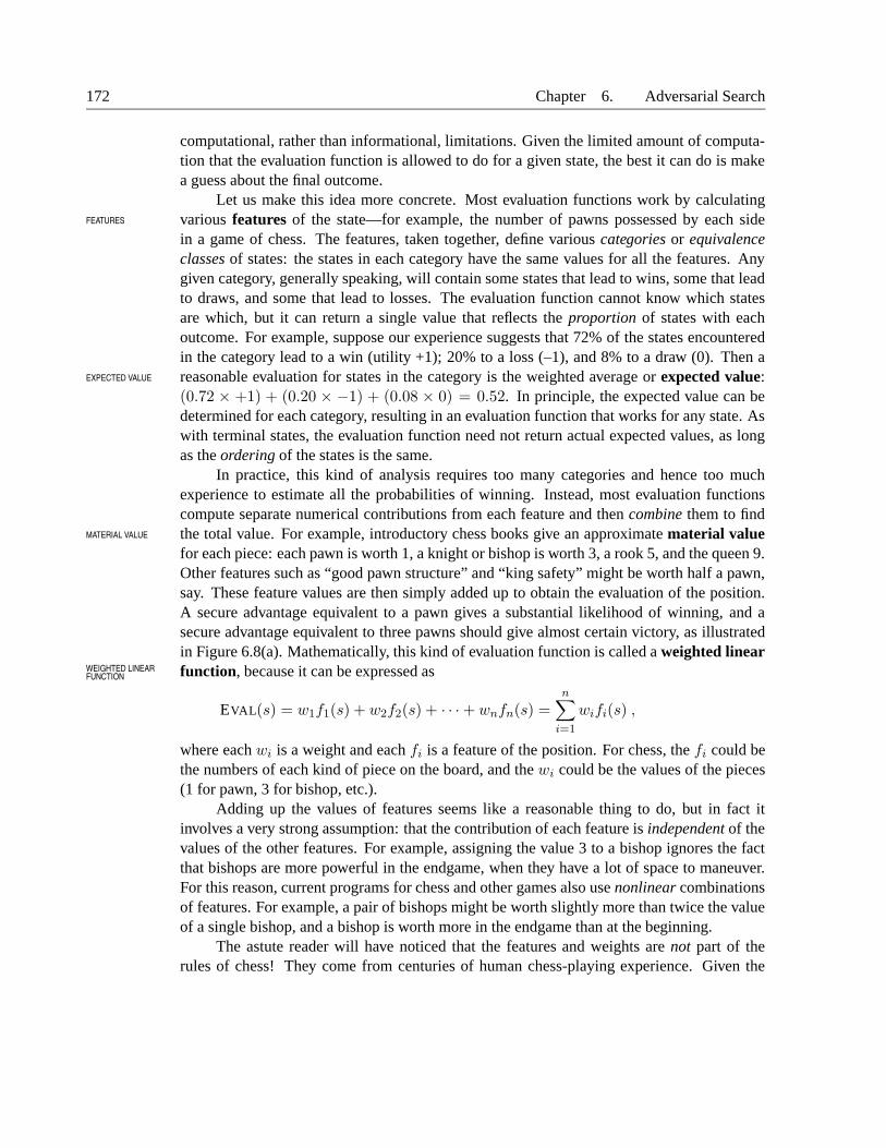
computational, rather than informational, limitations. Given the limited amount of computa-tion that the evaluation function is allowed to do for a given state, the best it can do is makea guess about the final outcome.

Let us make this idea more concrete. Most evaluation functions work by calculatingvarious features of the state—for example, the number of pawns possessed by each sideFEATURES

in a game of chess. The features, taken together, define various categories or equivalenceclasses of states: the states in each category have the same values for all the features. Anygiven category, generally speaking, will contain some states that lead to wins, some that leadto draws, and some that lead to losses. The evaluation function cannot know which statesare which, but it can return a single value that reflects the proportion of states with eachoutcome. For example, suppose our experience suggests that 72% of the states encounteredin the category lead to a win (utility +1); 20% to a loss (–1), and 8% to a draw (0). Then areasonable evaluation for states in the category is the weighted average or expected value:EXPECTED VALUE

(0.72 × +1) + (0.20 × −1) + (0.08 × 0) = 0.52. In principle, the expected value can bedetermined for each category, resulting in an evaluation function that works for any state. Aswith terminal states, the evaluation function need not return actual expected values, as longas the ordering of the states is the same.

In practice, this kind of analysis requires too many categories and hence too muchexperience to estimate all the probabilities of winning. Instead, most evaluation functionscompute separate numerical contributions from each feature and then combine them to findthe total value. For example, introductory chess books give an approximate material valueMATERIAL VALUE

for each piece: each pawn is worth 1, a knight or bishop is worth 3, a rook 5, and the queen 9.Other features such as “good pawn structure” and “king safety” might be worth half a pawn,say. These feature values are then simply added up to obtain the evaluation of the position.A secure advantage equivalent to a pawn gives a substantial likelihood of winning, and asecure advantage equivalent to three pawns should give almost certain victory, as illustratedin Figure 6.8(a). Mathematically, this kind of evaluation function is called a weighted linearfunction, because it can be expressed asWEIGHTED LINEAR

FUNCTION

EVAL(s) = w1f1(s) + w2f2(s) + · · ·+ wnfn(s) =n

∑

i=1

wifi(s) ,

where each wi is a weight and each fi is a feature of the position. For chess, the fi could bethe numbers of each kind of piece on the board, and the wi could be the values of the pieces(1 for pawn, 3 for bishop, etc.).

Adding up the values of features seems like a reasonable thing to do, but in fact itinvolves a very strong assumption: that the contribution of each feature is independent of thevalues of the other features. For example, assigning the value 3 to a bishop ignores the factthat bishops are more powerful in the endgame, when they have a lot of space to maneuver.For this reason, current programs for chess and other games also use nonlinear combinationsof features. For example, a pair of bishops might be worth slightly more than twice the valueof a single bishop, and a bishop is worth more in the endgame than at the beginning.

The astute reader will have noticed that the features and weights are not part of therules of chess! They come from centuries of human chess-playing experience. Given the

Section 6.4. Imperfect, Real-Time Decisions 173

(b) White to move(a) White to move

Figure 6.8 Two slightly different chess positions. In (a), black has an advantage of aknight and two pawns and will win the game. In (b), black will lose after white captures thequeen.

linear form of the evaluation, the features and weights result in the best approximation tothe true ordering of states by value. In particular, experience suggests that a secure materialadvantage of more than one point will probably win the game, all other things being equal;a three-point advantage is sufficient for near-certain victory. In games where this kind ofexperience is not available, the weights of the evaluation function can be estimated by themachine learning techniques of Chapter 18. Reassuringly, applying these techniques to chesshas confirmed that a bishop is indeed worth about three pawns.

Cutting off search

The next step is to modify ALPHA-BETA-SEARCH so that it will call the heuristic EVAL

function when it is appropriate to cut off the search. In terms of implementation, we replacethe two lines in Figure 6.7 that mention TERMINAL-TEST with the following line:

if CUTOFF-TEST(state , depth) then return EVAL(state)

We also must arrange for some bookkeeping so that the current depth is incremented on eachrecursive call. The most straightforward approach to controlling the amount of search is to seta fixed depth limit, so that CUTOFF-TEST(state, depth) returns true for all depth greater thansome fixed depth d. (It must also return true for all terminal states, just as TERMINAL-TEST

did.) The depth d is chosen so that the amount of time used will not exceed what the rules ofthe game allow.

A more robust approach is to apply iterative deepening, as defined in Chapter 3. Whentime runs out, the program returns the move selected by the deepest completed search. How-ever, these approaches can lead to errors due to the approximate nature of the evaluationfunction. Consider again the simple evaluation function for chess based on material advan-tage. Suppose the program searches to the depth limit, reaching the position in Figure 6.8(b),


where Black is ahead by a knight and two pawns. It would report this as the heuristic valueof the state, thereby declaring that the state will likely lead to a win by Black. But White’snext move captures Black’s queen with no compensation. Hence, the position is really wonfor White, but this can be seen only by looking ahead one more ply.

Obviously, a more sophisticated cutoff test is needed. The evaluation function should beapplied only to positions that are quiescent—that is, unlikely to exhibit wild swings in valueQUIESCENCE

in the near future. In chess, for example, positions in which favorable captures can be madeare not quiescent for an evaluation function that just counts material. Nonquiescent positionscan be expanded further until quiescent positions are reached. This extra search is called aquiescence search; sometimes it is restricted to consider only certain types of moves, suchQUIESCENCE

SEARCH

as capture moves, that will quickly resolve the uncertainties in the position.The horizon effect is more difficult to eliminate. It arises when the program is facingHORIZON EFFECT

a move by the opponent that causes serious damage and is ultimately unavoidable. Considerthe chess game in Figure 6.9. Black is ahead in material, but if White can advance its pawnfrom the seventh row to the eighth, the pawn will become a queen and create an easy winfor White. Black can forestall this outcome for 14 ply by checking White with the rook,but inevitably the pawn will become a queen. The problem with fixed-depth search is that itbelieves that these stalling moves have avoided the queening move—we say that the stallingmoves push the inevitable queening move “over the search horizon” to a place where it cannotbe detected.

As hardware improvements lead to deeper searches, one expects that the horizon effectwill occur less frequently—very long delaying sequences are quite rare. The use of singularextensions has also been quite effective in avoiding the horizon effect without adding tooSINGULAR

EXTENSIONS

much search cost. A singular extension is a move that is “clearly better” than all other movesin a given position. A singular-extension search can go beyond the normal depth limit withoutincurring much cost because its branching factor is 1. (Quiescence search can be thought ofas a variant of singular extensions.) In Figure 6.9, a singular extension search will find theeventual queening move, provided that black’s checking moves and white’s king moves canbe identified as “clearly better” than the alternatives.

So far we have talked about cutting off search at a certain level and about doing alpha–beta pruning that provably has no effect on the result. It is also possible to do forwardpruning, meaning that some moves at a given node are pruned immediately without furtherFORWARD PRUNING

consideration. Clearly, most humans playing chess only consider a few moves from eachposition (at least consciously). Unfortunately, the approach is rather dangerous because thereis no guarantee that the best move will not be pruned away. This can be disastrous if appliednear the root, because every so often the program will miss some “obvious” moves. Forwardpruning can be used safely in special situations—for example, when two moves are symmetricor otherwise equivalent, only one of them need be considered—or for nodes that are deep inthe search tree.

Combining all the techniques described here results in a program that can play cred-itable chess (or other games). Let us assume we have implemented an evaluation functionfor chess, a reasonable cutoff test with a quiescence search, and a large transposition table.Let us also assume that, after months of tedious bit-bashing, we can generate and evaluate

Section 6.5. Games That Include an Element of Chance 175

Black to move

Figure 6.9 The horizon effect. A series of checks by the black rook forces the inevitablequeening move by white “over the horizon” and makes this position look like a win for black,when it is really a win for white.

around a million nodes per second on the latest PC, allowing us to search roughly 200 millionnodes per move under standard time controls (three minutes per move). The branching factorfor chess is about 35, on average, and 355 is about 50 million, so if we used minimax searchwe could look ahead only about five plies. Though not incompetent, such a program can befooled easily by an average human chess player, who can occasionally plan six or eight pliesahead. With alpha–beta search we get to about 10 ply, which results in an expert level ofplay. Section 6.7 describes additional pruning techniques that can extend the effective searchdepth to roughly 14 plies. To reach grandmaster status we would need an extensively tunedevaluation function and a large database of optimal opening and endgame moves. It wouldn’thurt to have a supercomputer to run the program on.

6.5 GAMES THAT INCLUDE AN ELEMENT OF CHANCE

In real life, there are many unpredictable external events that put us into unforeseen situations.Many games mirror this unpredictability by including a random element, such as the throwingof dice. In this way, they take us a step nearer reality, and it is worthwhile to see how thisaffects the decision-making process.

Backgammon is a typical game that combines luck and skill. Dice are rolled at thebeginning of a player’s turn to determine the legal moves. In the backgammon position ofFigure 6.10, for example, white has rolled a 6–5, and has four possible moves.

Although White knows what his or her own legal moves are, White does not know whatBlack is going to roll and thus does not know what Black’s legal moves will be. That meansWhite cannot construct a standard game tree of the sort we saw in chess and tic-tac-toe. A


1 2 3 4 5 6 7 8 9 10 11 12

24 23 22 21 20 19 18 17 16 15 14 13

0

25

Figure 6.10 A typical backgammon position. The goal of the game is to move all one’spieces off the board. White moves clockwise toward 25, and black moves counterclockwisetoward 0. A piece can move to any position unless there are multiple opponent pieces there;if there is one opponent, it is captured and must start over. In the position shown, White hasrolled 6–5 and must choose among four legal moves: (5–10,5–11), (5–11,19–24), (5–10,10–16), and (5–11,11–16).

CHANCE

MIN

MAX

CHANCE

MAX

. . .

. . .

B

1

. . .

1,11/36

1,21/18

TERMINAL

1,21/18

......

.........

......

1,11/36

...

...... ......

...C

. . .

1/186,5 6,6

1/36

1/186,5 6,6

1/36

2 –11–1

Figure 6.11 Schematic game tree for a backgammon position.


game tree in backgammon must include chance nodes in addition to MAX and MIN nodes.CHANCE NODES

Chance nodes are shown as circles in Figure 6.11. The branches leading from each chancenode denote the possible dice rolls, and each is labeled with the roll and the chance that itwill occur. There are 36 ways to roll two dice, each equally likely; but because a 6–5 is thesame as a 5–6, there are only 21 distinct rolls. The six doubles (1–1 through 6–6) have a 1/36chance of coming up, the other 15 distinct rolls a 1/18 chance each.

The next step is to understand how to make correct decisions. Obviously, we still wantto pick the move that leads to the best position. However, the resulting positions do nothave definite minimax values. Instead, we can only calculate the expected value, where theexpectation is taken over all the possible dice rolls that could occur. This leads us to generalizethe minimax value for deterministic games to an expectiminimax value for games withEXPECTIMINIMAX

VALUE

chance nodes. Terminal nodes and MAX and MIN nodes (for which the dice roll is known)work exactly the same way as before; chance nodes are evaluated by taking the weightedaverage of the values resulting from all possible dice rolls, that is,

EXPECTIMINIMAX(n) =

UTILITY(n) if n is a terminal statemaxs∈Successors(n) EXPECTIMINIMAX(s) if n is a MAX nodemins∈Successors(n) EXPECTIMINIMAX(s) if n is a MIN node∑

s∈Successors(n) P (s) · EXPECTIMINIMAX(s) if n is a chance node

where the successor function for a chance node n simply augments the state of n with eachpossible dice roll to produce each successor s and P (s) is the probability that that dice rolloccurs. These equations can be backed up recursively all the way to the root of the tree, justas in minimax. We leave the details of the algorithm as an exercise.

Position evaluation in games with chance nodes

As with minimax, the obvious approximation to make with expectiminimax is to cut thesearch off at some point and apply an evaluation function to each leaf. One might think thatevaluation functions for games such as backgammon should be just like evaluation functionsfor chess—they just need to give higher scores to better positions. But in fact, the presence ofchance nodes means that one has to be more careful about what the evaluation values mean.Figure 6.12 shows what happens: with an evaluation function that assigns values [1, 2, 3,4] to the leaves, move A1 is best; with values [1, 20, 30, 400], move A2 is best. Hence,the program behaves totally differently if we make a change in the scale of some evaluationvalues! It turns out that, to avoid this sensitivity, the evaluation function must be a positivelinear transformation of the probability of winning from a position (or, more generally, of theexpected utility of the position). This is an important and general property of situations inwhich uncertainty is involved, and we discuss it further in Chapter 16.

Complexity of expectiminimax

If the program knew in advance all the dice rolls that would occur for the rest of the game,solving a game with dice would be just like solving a game without dice, which minimax


CHANCE

MIN

MAX

2 2 3 3 1 1 4 4

2 3 1 4

.9 .1 .9 .1

2.1 1.3

20 20 30 30 1 1 400 400

20 30 1 400

.9 .1 .9 .1

21 40.9

a1 a2 a1 a2

Figure 6.12 An order-preserving transformation on leaf values changes the best move.

does in O(bm) time. Because expectiminimax is also considering all the possible dice-rollsequences, it will take O(bmnm), where n is the number of distinct rolls.

Even if the search depth is limited to some small depth d, the extra cost compared withthat of minimax makes it unrealistic to consider looking ahead very far in most games ofchance. In backgammon n is 21 and b is usually around 20, but in some situations can be ashigh as 4000 for dice rolls that are doubles. Three plies is probably all we could manage.

Another way to think about the problem is this: the advantage of alpha–beta is thatit ignores future developments that just are not going to happen, given best play. Thus, itconcentrates on likely occurrences. In games with dice, there are no likely sequences ofmoves, because for those moves to take place, the dice would first have to come out the rightway to make them legal. This is a general problem whenever uncertainty enters the picture:the possibilities are multiplied enormously, and forming detailed plans of action becomespointless, because the world probably will not play along.

No doubt it will have occurred to the reader that perhaps something like alpha–betapruning could be applied to game trees with chance nodes. It turns out that it can. Theanalysis for MIN and MAX nodes is unchanged, but we can also prune chance nodes, usinga bit of ingenuity. Consider the chance node C in Figure 6.11 and what happens to its valueas we examine and evaluate its children. Is it possible to find an upper bound on the valueof C before we have looked at all its children? (Recall that this is what alpha–beta needs toprune a node and its subtree.) At first sight, it might seem impossible, because the value of Cis the average of its children’s values. Until we have looked at all the dice rolls, this averagecould be anything, because the unexamined children might have any value at all. But if weput bounds on the possible values of the utility function, then we can arrive at bounds for theaverage. For example, if we say that all utility values are between +3 and −3, then the valueof leaf nodes is bounded, and in turn we can place an upper bound on the value of a chancenode without looking at all its children.


Card games

Card games are interesting for many reasons besides their connection with gambling. Amongthe huge variety of games, we will focus on those in which cards are dealt randomly at thebeginning of the game, with each player receiving a hand of cards that is not visible to theother players. Such games include bridge, whist, hearts, and some forms of poker.

At first sight, it might seem that card games are just like dice games: the cards aredealt randomly and determine the moves available to each player, but all the dice are rolledat the beginning! We will pursue this observation further. It will turn out to be quite useful inpractice. It is also quite wrong, for interesting reasons.

Imagine two players, MAX and MIN, playing some practice hands of four-card twohanded bridge with all the cards showing. The hands are as follows, with MAX to play first:

MAX : ♥ 6 ♦ 6 ♣ 9 8 MIN : ♥ 4 ♠ 2 ♣ 10 5 .

Suppose that MAX leads the ♣ 9. MIN must now follow suit, playing either the ♣ 10 or the♣ 5. MIN plays the ♣ 10 and wins the trick. MIN goes next and leads the ♠ 2. MAX has nospades (and so cannot win the trick) and therefore must throw away some card. The obviouschoice is the ♦ 6 because the other two remaining cards are winners. Now, whichever cardMIN leads for the next trick, MAX will win both remaining tricks and the game will be tied attwo tricks each. It is easy to show, using a suitable variant of minimax (Exercise 6.12), thatMAX’s lead of the ♣ 9 is in fact an optimal choice.

Now let’s modify MIN’s hand, replacing the ♥ 4 with the ♦ 4:

MAX : ♥ 6 ♦ 6 ♣ 9 8 MIN : ♦ 4 ♠ 2 ♣ 10 5 .

The two cases are entirely symmetric: play will be identical, except that on the second trickMAX will throw away the ♥ 6. Again, the game will be tied at two tricks each and the lead ofthe ♣ 9 is an optimal choice.

So far, so good. Now let’s hide one of MIN’s cards: MAX knows that MIN has eitherthe first hand (with the ♥ 4) or the second hand (with the ♦ 4), but has no idea which. MAX

reasons as follows:

The ♣ 9 is an optimal choice against MIN’s first hand and against MIN’s second hand, soit must be optimal now because I know that MIN has one of the two hands.

More generally, MAX is using what we might call “averaging over clairvoyancy.” The ideais to evaluate a given course of action when there are unseen cards by first computing theminimax value of that action for each possible deal of the cards, and then computing theexpected value over all deals using the probability of each deal.

If you think this is reasonable (or if you have no idea because you don’t understandbridge), consider the following story:

Day 1: Road A leads to a heap of gold pieces; Road B leads to a fork. Take the left forkand you’ll find a mound of jewels, but take the right fork and you’ll be run over by a bus.Day 2: Road A leads to a heap of gold pieces; Road B leads to a fork. Take the right forkand you’ll find a mound of jewels, but take the left fork and you’ll be run over by a bus.Day 3: Road A leads to a heap of gold pieces; Road B leads to a fork. Guess correctly andyou’ll find a mound of jewels, but guess incorrectly and you’ll be run over by a bus.


Obviously, it’s not unreasonable to take Road B on the first two days. No sane person, though,would take Road B on Day 3. Yet this is exactly what averaging over clairvoyancy suggests:Road B is optimal in the situations of Day 1 and Day 2; therefore it is optimal on Day 3,because one of the two previous situations must hold. Let us return to the card game: afterMAX leads the ♣ 9, MIN wins with the ♣ 10. As before, MIN leads the ♠ 2, and now MAX isat the fork in the road without any instructions. If MAX throws away the♥ 6 and MIN still hasthe ♥ 4, the ♥ 4 becomes a winner and MAX loses the game. Similarly, If MAX throws awaythe ♦ 6 and MIN still has the ♦ 4, MAX also loses. Therefore, playing the ♣ 9 first leads to asituation where MAX has a 50% chance of losing. (It would be much better to play the ♥ 6and the ♦ 6 first, guaranteeing a tied game.)

The lesson to be drawn from all this is that when information is missing, one mustconsider what information one will have at each point in the game. The problem with MAX’salgorithm is that it assumes that in each possible deal, play will proceed as if all the cardsare visible. As our example shows, this leads MAX to act as if all future uncertainty will beresolved when the time comes. MAX’s algorithm will also never decide to gather information(or provide information to a partner), because within each deal there’s no need to do so; yetin games such as bridge, it is often a good idea to play a card that will help one discoverthings about one’s opponent’s cards or that will tell one’s partner about one’s own cards.These kinds of behaviors are generated automatically by an optimal algorithm for games ofimperfect information. Such an algorithm searches not in the space of world states (handsof cards), but in the space of belief states (beliefs about who has which cards, with whatprobabilities). We will be able to explain the algorithm properly in Chapter 17, once we havedeveloped the necessary probabilistic machinery. In that chapter, we will also expand onone final and very important point: in games of imperfect information, it’s best to give awayas little information to the opponent as possible, and often the best way to do this is to actunpredictably. This is why restaurant hygiene inspectors do random inspection visits.

6.6 STATE-OF-THE-ART GAME PROGRAMS

One might say that game playing is to AI as Grand Prix motor racing is to the car indus-try: state-of-the-art game programs are blindingly fast, incredibly well-tuned machines thatincorporate very advanced engineering techniques, but they aren’t much use for doing theshopping. Although some researchers believe that game playing is somewhat irrelevant tomainstream AI, it continues to generate both excitement and a steady stream of innovationsthat have been adopted by the wider community.

Chess: In 1957, Herbert Simon predicted that within 10 years computers would beat theCHESS

human world champion. Forty years later, the Deep Blue program defeated Garry Kasparovin a six-game exhibition match. Simon was wrong, but only by a factor of 4. Kasparov wrote:

The decisive game of the match was Game 2, which left a scar in my memory . . . we sawsomething that went well beyond our wildest expectations of how well a computer wouldbe able to foresee the long-term positional consequences of its decisions. The machine

Section 6.6. State-of-the-Art Game Programs 181

refused to move to a position that had a decisive short-term advantage—showing a veryhuman sense of danger. (Kasparov, 1997)

Deep Blue was developed by Murray Campbell, Feng-Hsiung Hsu, and Joseph Hoane atIBM (see Campbell et al., 2002), building on the Deep Thought design developed earlierby Campbell and Hsu at Carnegie Mellon. The winning machine was a parallel computerwith 30 IBM RS/6000 processors running the “software search” and 480 custom VLSI chessprocessors that performed move generation (including move ordering), the “hardware search”for the last few levels of the tree, and the evaluation of leaf nodes. Deep Blue searched 126million nodes per second on average, with a peak speed of 330 million nodes per second. Itgenerated up to 30 billion positions per move, reaching depth 14 routinely. The heart of themachine is a standard iterative-deepening alpha–beta search with a transposition table, but thekey to its success seems to have been its ability to generate extensions beyond the depth limitfor sufficiently interesting lines of forcing/forced moves. In some cases the search reached adepth of 40 plies. The evaluation function had over 8000 features, many of them describinghighly specific patterns of pieces. An “opening book” of about 4000 positions was used, aswell as a database of 700,000 grandmaster games from which consensus recommendationscould be extracted. The system also used a large endgame database of solved positions,containing all positions with five pieces and many with six pieces. This database has the effectof substantially extending the effective search depth, allowing Deep Blue to play perfectly insome cases even when it is many moves away from checkmate.

The success of Deep Blue reinforced the widely held belief that progress in computergame-playing has come primarily from ever-more-powerful hardware—a view encouragedby IBM. Deep Blue’s creators, on the other hand, state that the search extensions and eval-uation function were also critical (Campbell et al., 2002). Moreover, we know that severalrecent algorithmic improvements have allowed programs running on standard PCs to winevery World Computer-Chess Championship since 1992, often defeating massively parallelopponents that could search 1000 times more nodes. A variety of pruning heuristics are usedto reduce the effective branching factor to less than 3 (compared with the actual branchingfactor of about 35). The most important of these is the null move heuristic, which generatesNULL MOVE

a good lower bound on the value of a position, using a shallow search in which the oppo-nent gets to move twice at the beginning. This lower bound often allows alpha–beta pruningwithout the expense of a full-depth search. Also important is futility pruning, which helpsFUTILITY PRUNING

decide in advance which moves will cause a beta cutoff in the successor nodes.The Deep Blue team declined a chance for a rematch with Kasparov. Instead, the

most recent major competition in 2002 featured the program FRITZ against world cham-pion Vladimir Kramnik. The eight game match ended in a draw. The conditions of the matchwere much more favorable to the human, and the hardware was an ordinary PC, not a super-computer. Still, Kramnik commented that “It is now clear that the top program and the worldchampion are approximately equal.”

Checkers: Beginning in 1952, Arthur Samuel of IBM, working in his spare time, developedCHECKERS

a checkers program that learned its own evaluation function by playing itself thousands oftimes. We describe this idea in more detail in Chapter 21. Samuel’s program began as a


novice, but after only a few days’ self-play had improved itself beyond Samuel’s own level(although he was not a strong player). In 1962 it defeated Robert Nealy, a champion at “blindcheckers,” through an error on his part. Many people that felt this meant computers were su-perior to people at checkers, but this was not the case. Still, when one considers that Samuel’scomputing equipment (an IBM 704) had 10,000 words of main memory, magnetic tape forlong-term storage, and a .000001–GHz processor, the win remains a great accomplishment.

Few other people attempted to do better until Jonathan Schaeffer and colleagues de-veloped Chinook, which runs on regular PCs and uses alpha–beta search. Chinook uses aprecomputed database of all 444 billion positions with eight or fewer pieces on the board tomake its endgame play flawless. Chinook came in second in the 1990 U.S. Open and earnedthe right to challenge for the world championship. It then ran up against a problem, in theform of Marion Tinsley. Dr. Tinsley had been world champion for over 40 years, losing onlythree games in all that time. In the first match against Chinook, Tinsley suffered his fourth andfifth losses, but won the match 20.5–18.5. The world championship match in August 1994between Tinsley and Chinook ended prematurely when Tinsley had to withdraw for healthreasons. Chinook became the official world champion.

Schaeffer believes that, with enough computing power, the database of endgames couldbe enlarged to the point where a forward search from the initial position would always reachsolved positions, i.e., checkers would be completely solved. (Chinook has announced a winas early as move 5.) This kind of exhaustive analysis can be done by hand for 3×3 tic-tac-toeand has been done by computer for Qubic (4×4×4 tic-tac-toe), Go-Moku (five in a row), andNine-Men’s Morris (Gasser, 1998). Remarkable work by Ken Thompson and Lewis Stiller(1992) solved all five-piece and some six-piece chess endgames, making them available onthe Internet. Stiller discovered one case where a forced mate existed but required 262 moves;this caused some consternation because the rules of chess require some “progress” to occurwithin 50 moves.

Othello, also called Reversi, is probably more popular as a computer game than as a boardOTHELLO

game. It has a smaller search space than chess, usually 5 to 15 legal moves, but evaluationexpertise had to be developed from scratch. In 1997, the Logistello program (Buro, 2002)defeated the human world champion, Takeshi Murakami , by six games to none. It is generallyacknowledged that humans are no match for computers at Othello.

Backgammon: Section 6.5 explained why the inclusion of uncertainty from dice rolls makesBACKGAMMON

deep search an expensive luxury. Most work on backgammon has gone into improvingthe evaluation function. Gerry Tesauro (1992) combined Samuel’s reinforcement learningmethod with neural network techniques (Chapter 20) to develop a remarkably accurate eval-uator that is used with a search to depth 2 or 3. After playing more than a million traininggames against itself, Tesauro’s program, TD-GAMMON, is reliably ranked among the topthree players in the world. The program’s opinions on the opening moves of the game havein some cases radically altered the received wisdom.

Go is the most popular board game in Asia, requiring at least as much discipline from itsGO

professionals as chess. Because the board is 19 × 19, the branching factor starts at 361,which is too daunting for regular search methods. Up to 1997 there were no competent

Section 6.7. Discussion 183

programs at all, but now programs often play respectable moves. Most of the best programscombine pattern recognition techniques (when the following pattern of pieces appears, thismove should be considered) with limited search (decide whether these pieces can be captured,staying within the local area). The strongest programs at the time of writing are probablyChen Zhixing’s Goemate and Michael Reiss’ Go4++, each rated somewhere around 10 kyu(weak amateur). Go is an area that is likely to benefit from intensive investigation using moresophisticated reasoning methods. Success may come from finding ways to integrate severallines of local reasoning about each of the many, loosely connected “subgames” into whichGo can be decomposed. Such techniques would be of enormous value for intelligent systemsin general.

Bridge is a game of imperfect information: a player’s cards are hidden from the other players.BRIDGE

Bridge is also a multiplayer game with four players instead of two, although the players arepaired into two teams. As we saw in Section 6.5, optimal play in bridge can include elementsof information-gathering, communication, bluffing, and careful weighing of probabilities.Many of these techniques are used in the Bridge BaronTM program (Smith et al., 1998),which won the 1997 computer bridge championship. While it does not play optimally, BridgeBaron is one of the few successful game-playing systems to use complex, hierarchical plans(see Chapter 12) involving high-level ideas such as finessing and squeezing that are familiarto bridge players.

The GIB program (Ginsberg, 1999) won the 2000 championship quite decisively. GIBuses the “averaging over clairvoyancy” method, with two crucial modifications. First, ratherthan examining how well each choice works for every possible arrangement of the hiddencards—of which there can be up to 10 million—it examines a random sample of 100 arrange-ments. Second, GIB uses explanation-based generalization to compute and cache generalrules for optimal play in various standard classes of situations. This enables it to solve eachdeal exactly. GIB’s tactical accuracy makes up for its inability to reason about information.It finished 12th in a field of 35 in the par contest (involving just play of the hand) at the 1998human world championship, far exceeding the expectations of many human experts.

6.7 DISCUSSION

Because calculating optimal decisions in games is intractable in most cases, all algorithmsmust make some assumptions and approximations. The standard approach, based on mini-max, evaluation functions, and alpha–beta, is just one way to do this. Probably because itwas proposed so early on, the standard approach been developed intensively and dominatesother methods in tournament play. Some in the field believe that this has caused game playingto become divorced from the mainstream of AI research, because the standard approach nolonger provides much room for new insight into general questions of decision making. In thissection, we look at the alternatives.

First, let us consider minimax. Minimax selects an optimal move in a given searchtree provided that the leaf node evaluations are exactly correct. In reality, evaluations are


MAX

99 1000 1000 1000 100 101 102 100

10099MIN

Figure 6.13 A two-ply game tree for which minimax may be inappropriate.

usually crude estimates of the value of a position and can be considered to have large errorsassociated with them. Figure 6.13 shows a two-ply game tree for which minimax seemsinappropriate. Minimax suggests taking the right-hand branch, whereas it is quite likely thatthe true value of the left-hand branch is higher. The minimax choice relies on the assumptionthat all of the nodes labeled with values 100, 101, 102, and 100 are actually better than thenode labeled with value 99. However, the fact that the node labeled 99 has siblings labeled1000 suggests that in fact it might have a higher true value. One way to deal with this problemis to have an evaluation that returns a probability distribution over possible values. Thenone can calculate the probability distribution for the parent’s value using standard statisticaltechniques. Unfortunately, the values of sibling nodes are usually highly correlated, so thiscan be an expensive calculation, requiring hard to obtain information.

Next, we consider the search algorithm that generates the tree. The aim of an algorithmdesigner is to specify a computation that runs quickly and yields a good move. The mostobvious problem with the alpha–beta algorithm is that it is designed not just to select a goodmove, but also to calculate bounds on the values of all the legal moves. To see why thisextra information is unnecessary, consider a position in which there is only one legal move.Alpha–beta search still will generate and evaluate a large, and totally useless, search tree. Ofcourse, we can insert a test into the algorithm, but this merely hides the underlying problem:many of the calculations done by alpha–beta are largely irrelevant. Having only one legalmove is not much different from having several legal moves, one of which is fine and therest of which are obviously disastrous. In a “clear favorite” situation like this, it would bebetter to reach a quick decision after a small amount of search than to waste time that couldbe more productively used later on a more problematic position. This leads to the idea of theutility of a node expansion. A good search algorithm should select node expansions of highutility—that is, ones that are likely to lead to the discovery of a significantly better move. Ifthere are no node expansions whose utility is higher than their cost (in terms of time), thenthe algorithm should stop searching and make a move. Notice that this works not only forclear-favorite situations, but also for the case of symmetrical moves, for which no amount ofsearch will show that one move is better than another.

This kind of reasoning about what computations to do is called metareasoning (rea-METAREASONING

soning about reasoning). It applies not just to game playing, but to any kind of reasoning

Section 6.8. Summary 185

at all. All computations are done in the service of trying to reach better decisions, all havecosts, and all have some likelihood of resulting in a certain improvement in decision quality.Alpha–beta incorporates the simplest kind of metareasoning, namely, a theorem to the effectthat certain branches of the tree can be ignored without loss. It is possible to do much better.In Chapter 16, we will see how these ideas can be made precise and implementable.

Finally, let us reexamine the nature of search itself. Algorithms for heuristic search andfor game playing work by generating sequences of concrete states, starting from the initialstate and then applying an evaluation function. Clearly, this is not how humans play games. Inchess, one often has a particular goal in mind—for example, trapping the opponent’s queen—and can use this goal to selectively generate plausible plans for achieving it. This kind of goal-directed reasoning or planning sometimes eliminates combinatorial search altogether. (SeePart IV.) David Wilkins’ (1980) PARADISE is the only program to have used goal-directedreasoning successfully in chess: it was capable of solving some chess problems requiring an18-move combination. As yet there is no good understanding of how to combine the twokinds of algorithm into a robust and efficient system, although Bridge Baron might be a stepin the right direction. A fully integrated system would be a significant achievement not justfor game-playing research, but also for AI research in general, because it would be a goodbasis for a general intelligent agent.

6.8 SUMMARY

We have looked at a variety of games to understand what optimal play means and to under-stand how to play well in practice. The most important ideas are as follows:

• A game can be defined by the initial state (how the board is set up), the legal actions ineach state, a terminal test (which says when the game is over), and a utility functionthat applies to terminal states.

• In two-player zero-sum games with perfect information, the minimax algorithm canselect optimal moves using a depth-first enumeration of the game tree.

• The alpha–beta search algorithm computes the same optimal move as minimax, butachieves much greater efficiency by eliminating subtrees that are provably irrelevant.

• Usually, it is not feasible to consider the whole game tree (even with alpha–beta), so weneed to cut the search off at some point and apply an evaluation function that gives anestimate of the utility of a state.

• Games of chance can be handled by an extension to the minimax algorithm that evalu-ates a chance node by taking the average utility of all its children nodes, weighted bythe probability of each child.

• Optimal play in games of imperfect information, such as bridge, requires reasoningabout the current and future belief states of each player. A simple approximation canbe obtained by averaging the value of an action over each possible configuration ofmissing information.


• Programs can match or beat the best human players in checkers, Othello, and backgam-mon and are close behind in bridge. A program has beaten the world chess championin one exhibition match. Programs remain at the amateur level in Go.

BIBLIOGRAPHICAL AND HISTORICAL NOTES

The early history of mechanical game playing was marred by numerous frauds. The most no-torious of these was Baron Wolfgang von Kempelen’s (1734-1804) “The Turk,” a supposedchess-playing automaton that defeated Napoleon before being exposed as a magician’s trickcabinet housing a human chess expert (see Levitt, 2000). It played from 1769 to 1854. In1846, Charles Babbage (who had been fascinated by the Turk) appears to have contributedthe first serious discussion of the feasibility of computer chess and checkers (Morrison andMorrison, 1961). He also designed, but did not build, a special-purpose machine for playingtic-tac-toe. The first true game-playing machine was built around 1890 by the Spanish engi-neer Leonardo Torres y Quevedo. It specialized in the “KRK” (king and rook vs. king) chessendgame, guaranteeing a win with king and rook from any position.

The minimax algorithm is often traced to a paper published in 1912 by Ernst Zermelo,the developer of modern set theory. The paper unfortunately contained several errors anddid not describe minimax correctly. A solid foundation for game theory was developed inthe seminal work Theory of Games and Economic Behavior (von Neumann and Morgen-stern, 1944), which included an analysis showing that some games require strategies that arerandomized (or otherwise unpredictable). See Chapter 17 for more information.

Many influential figures of the early computer era were intrigued by the possibility ofcomputer chess. Konrad Zuse (1945), the first person to design a programmable computer,developed fairly detailed ideas about how it might be done. Norbert Wiener’s (1948) influen-tial book Cybernetics discussed one possible design for a chess program, including the ideasof minimax search, depth cutoffs, and evaluation functions. Claude Shannon (1950) laid outthe basic principles of modern game-playing programs in much more detail than Wiener. Heintroduced the idea of quiescence search and described some ideas for selective (nonexhaus-tive) game-tree search. Slater (1950) and the commentators on his article also explored thepossibilities for computer chess play. In particular, I. J. Good (1950) developed the notion ofquiescence independently of Shannon.

In 1951, Alan Turing wrote the first computer program capable of playing a full gameof chess (see Turing et al., 1953). But Turing’s program never actually ran on a computer; itwas tested by hand simulation against a very weak human player, who defeated it. MeanwhileD. G. Prinz (1952) had written, and actually run, a program that solved chess problems,although it did not play a full game. Alex Bernstein wrote the first program to play a fullgame of standard chess (Bernstein and Roberts, 1958; Bernstein et al., 1958).3

John McCarthy conceived the idea of alpha–beta search in 1956, although he did notpublish it. The NSS chess program (Newell et al., 1958) used a simplified version of alpha–

3 Newell et al. (1958) mention a Russian program, BESM, that may have predated Bernstein’s program.


beta; it was the first chess program to do so. According to Nilsson (1971), Arthur Samuel’scheckers program (Samuel, 1959, 1967) also used alpha–beta, although Samuel did not men-tion it in the published reports on the system. Papers describing alpha–beta were publishedin the early 1960s (Hart and Edwards, 1961; Brudno, 1963; Slagle, 1963b). An implementa-tion of full alpha–beta is described by Slagle and Dixon (1969) in a program for playing thegame of Kalah. Alpha–beta was also used by the “Kotok–McCarthy” chess program writtenby a student of John McCarthy (Kotok, 1962). Knuth and Moore (1975) provide a historyof alpha–beta, along with a proof of its correctness and a time complexity analysis. Theiranalysis of alpha–beta with random successor ordering showed an asymptotic complexity ofO((b/log b)d), which seemed rather dismal because the effective branching factor b/log b isnot much less than b itself. They then realized that the asymptotic formula is accurate only forb > 1000 or so, whereas the often-quoted O(b3d/4) applies to the range of branching factorsencountered in actual games. Pearl (1982b) shows alpha–beta to be asymptotically optimalamong all fixed-depth game-tree search algorithms.

The first computer chess match featured the Kotok-McCarthy program and the “ITEP”program written in the mid-1960s at Moscow’s Institute of Theoretical and ExperimentalPhysics (Adelson-Velsky et al., 1970). This intercontinental match was played by telegraph.It ended with a 3–1 victory for the ITEP program in 1967. The first chess program to competesuccessfully with humans was MacHack 6 (Greenblatt et al., 1967). Its rating of approxi-mately 1400 was well above the novice level of 1000, but it fell far short of the rating of 2800or more that would have been needed to fulfill Herb Simon’s 1957 prediction that a computerprogram would be world chess champion within 10 years (Simon and Newell, 1958).

Beginning with the first ACM North American Computer-Chess Championship in 1970,competition among chess programs became serious. Programs in the early 1970s became ex-tremely complicated, with various kinds of tricks for eliminating some branches of search,for generating plausible moves, and so on. In 1974, the first World Computer-Chess Champi-onship was held in Stockholm and won by Kaissa (Adelson-Velsky et al., 1975), another pro-gram from ITEP. Kaissa used the much more straightforward approach of exhaustive alpha–beta search combined with quiescence search. The dominance of this approach was confirmedby the convincing victory of CHESS 4.6 in the 1977 World Computer-Chess Championship.CHESS 4.6 examined up to 400,000 positions per move and had a rating of 1900.

A later version of Greenblatt’s MacHack 6 was the first chess program to run on cus-tom hardware designed specifically for chess (Moussouris et al., 1979), but the first pro-gram to achieve notable success through the use of custom hardware was Belle (Condonand Thompson, 1982). Belle’s move generation and position evaluation hardware enabledit to explore several million positions per move. Belle achieved a rating of 2250, becomingthe first master-level program. The HITECH system, also a special-purpose computer, was de-signed by former World Correspondence Chess Champion Hans Berliner and his student CarlEbeling at CMU to allow rapid calculation of evaluation functions (Ebeling, 1987; Berlinerand Ebeling, 1989). Generating about 10 million positions per move, HITECH became NorthAmerican computer champion in 1985 and was the first program to defeat a human grand-master, in 1987. Deep Thought, which was also developed at CMU, went further in thedirection of pure search speed (Hsu et al., 1990). It achieved a rating of 2551 and was the


forerunner of Deep Blue. The Fredkin Prize, established in 1980, offered $5000 to the firstprogram to achieve a master rating, $10,000 to the first program to achieve a USCF (UnitedStates Chess Federation) rating of 2500 (near the grandmaster level), and $100,000 for thefirst program to defeat the human world champion. The $5000 prize was claimed by Belle in1983, the $10,000 prize by Deep Thought in 1989, and the $100,000 prize by Deep Blue forits victory over Garry Kasparov in 1997. It is important to remember that Deep Blue’s suc-cess was due to algorithmic improvements as well as hardware (Hsu, 1999; Campbell et al.,2002). Techniques such as the null-move heuristic (Beal, 1990) have led to programs thatare quite selective in their searches. The last three World Computer-Chess Championships in1992, 1995, and 1999 were won by programs running on standard PCs. Probably the mostcomplete description of a modern chess program is provided by Ernst Heinz (2000), whoseDARKTHOUGHT program was the highest-ranked noncommercial PC program at the 1999world championships.

Several attempts have been made to overcome the problems with the “standard ap-proach” that were outlined in Section 6.7. The first selective search algorithm with sometheoretical grounding was probably B∗ (Berliner, 1979), which attempts to maintain intervalbounds on the possible value of a node in the game tree, rather than giving it a single point-valued estimate. Leaf nodes are selected for expansion in an attempt to refine the top-levelbounds until one move is “clearly best.” Palay (1985) extends the B∗ idea using probabilitydistributions on values in place of intervals. David McAllester’s (1988) conspiracy numbersearch expands leaf nodes that, by changing their values, could cause the program to prefer anew move at the root. MGSS∗ (Russell and Wefald, 1989) uses the decision-theoretic tech-niques of Chapter 16 to estimate the value of expanding each leaf in terms of the expectedimprovement in decision quality at the root. It outplayed an alpha–beta algorithm at Othellodespite searching an order of magnitude fewer nodes. The MGSS∗ approach is, in principle,applicable to the control of any form of deliberation.

Alpha–beta search is in many ways the two-player analog of depth-first branch-and-bound, which is dominated by A∗ in the single-agent case. The SSS∗ algorithm (Stockman,1979) can be viewed as a two-player A∗ and never expands more nodes than alpha–beta toreach the same decision. The memory requirements and computational overhead of the queuemake SSS∗ in its original form impractical, but a linear-space version has been developedfrom the RBFS algorithm (Korf and Chickering, 1996). Plaat et al. (1996) developed a newview of SSS∗ as a combination of alpha–beta and transposition tables, showing how to over-come the drawbacks of the original algorithm and developing a new variant called MTD(f)that has been adopted by a number of top programs.

D. F. Beal (1980) and Dana Nau (1980, 1983) studied the weaknesses of minimax ap-plied to approximate evaluations. They showed that under certain independence assumptionsabout the distribution of leaf values in the tree, minimaxing can yield values at the root thatare actually less reliable than the direct use of the evaluation function itself. Pearl’s bookHeuristics (1984) partially explains this apparent paradox and analyzes many game-playingalgorithms. Baum and Smith (1997) propose a probability-based replacement for minimax,showing that it results in better choices in certain games. There is still little theory of theeffects of cutting off search at different levels and applying evaluation functions.


The expectiminimax algorithm was proposed by Donald Michie (1966), although ofcourse it follows directly from the principles of game-tree evaluation due to von Neumannand Morgenstern. Bruce Ballard (1983) extended alpha–beta pruning to cover trees withchance nodes. The first successful backgammon program was BKG (Berliner, 1977, 1980b);it used a complex, manually constructed evaluation function and searched only to depth 1. Itwas the first program to defeat a human world champion at a major classic game (Berliner,1980a). Berliner readily acknowledged that this was a very short exhibition match (not aworld championship match) and that BKG was very lucky with the dice. Work by GerryTesauro, first on NEUROGAMMON (Tesauro, 1989) and later on TD-GAMMON (Tesauro,1995), showed that much better results could be obtained via reinforcement learning, whichwe will cover in Chapter 21.

Checkers, rather than chess, was the first of the classic games fully played by a com-puter. Christopher Strachey (1952) wrote the first working program for checkers. Schaeffer(1997) gives a highly readable, “warts and all” account of the development of his Chinookworld champion checkers program.

The first Go-playing programs were developed somewhat later than those for checkersand chess (Lefkovitz, 1960; Remus, 1962) and have progressed more slowly. Ryder (1971)used a pure search-based approach with a variety of selective pruning methods to overcomethe enormous branching factor. Zobrist (1970) used condition–action rules to suggest plau-sible moves when known patterns appeared. Reitman and Wilcox (1979) combined rulesand search to good effect, and most modern programs have followed this hybrid approach.Muller (2002) summarizes the state of the art of computerized Go and provides a wealth ofreferences. Anshelevich (2000) uses related techniques for the game of Hex. The ComputerGo Newsletter, published by the Computer Go Association, describes current developments.

Papers on computer game playing appear in a variety of venues. The rather misleadinglynamed conference proceedings Heuristic Programming in Artificial Intelligence report on theComputer Olympiads, which include a wide variety of games. There are also several editedcollections of important papers on game-playing research (Levy, 1988a, 1988b; Marslandand Schaeffer, 1990). The International Computer Chess Association (ICCA), founded in1977, publishes the quarterly ICGA Journal (formerly the ICCA Journal). Important papershave been published in the serial anthology Advances in Computer Chess, starting with Clarke(1977). Volume 134 of the journal Artificial Intelligence (2002) contains descriptions of state-of-the-art programs for chess, Othello, Hex, shogi, Go, backgammon, poker, Scrabble.TMandother games.

EXERCISES

6.1 This problem exercises the basic concepts of game playing, using tic-tac-toe (noughtsand crosses) as an example. We define Xn as the number of rows, columns, or diagonalswith exactly n X’s and no O’s. Similarly, On is the number of rows, columns, or diagonalswith just n O’s. The utility function assigns +1 to any position with X3 = 1 and −1 to any


position with O3 = 1. All other terminal positions have utility 0. For nonterminal positions,we use a linear evaluation function defined as Eval(s) = 3X2(s)+X1(s)−(3O2(s)+O1(s)).

a. Approximately how many possible games of tic-tac-toe are there?

b. Show the whole game tree starting from an empty board down to depth 2 (i.e., one Xand one O on the board), taking symmetry into account.

c. Mark on your tree the evaluations of all the positions at depth 2.

d. Using the minimax algorithm, mark on your tree the backed-up values for the positionsat depths 1 and 0, and use those values to choose the best starting move.

e. Circle the nodes at depth 2 that would not be evaluated if alpha–beta pruning wereapplied, assuming the nodes are generated in the optimal order for alpha–beta pruning.

6.2 Prove the following assertion: for every game tree, the utility obtained by MAX usingminimax decisions against a suboptimal MIN will be never be lower than the utility obtainedplaying against an optimal MIN. Can you come up with a game tree in which MAX can dostill better using a suboptimal strategy against a suboptimal MIN?

6.3 Consider the two-player game described in Figure 6.14.

a. Draw the complete game tree, using the following conventions:

• Write each state as (sA, sB) where sA and sB denote the token locations.• Put each terminal state in a square boxes and write its game value in a circle.• Put loop states (states that already appear on the path to the root) in double square

boxes. Since it is not clear how to assign values to loop states, annotate each witha “?” in a circle.

b. Now mark each node with its backed-up minimax value (also in a circle). Explain howyou handled the “?” values and why.

c. Explain why the standard minimax algorithm would fail on this game tree and brieflysketch how you might fix it, drawing on your answer to (b). Does your modified algo-rithm give optimal decisions for all games with loops?

d. This 4-square game can be generalized to n squares for any n > 2. Prove that A winsif n is even and loses if n is odd.

A B1 432

Figure 6.14 The starting position of a simple game. Player A moves first. The two playerstake turns moving, and each player must move his token to an open adjacent space in eitherdirection. If the opponent occupies an adjacent space, then a player may jump over theopponent to the next open space if any. (For example, if A is on 3 and B is on 2, then A maymove back to 1.) The game ends when one player reaches the opposite end of the board. Ifplayer A reaches space 4 first, then the value of the game to A is +1; if player B reachesspace 1 first, then the value of the game to A is −1.


6.4 Implement move generators and evaluation functions for one or more of the followinggames: Kalah, Othello, checkers, and chess. Construct a general alpha–beta game-playingagent that uses your implementation. Compare the effect of increasing search depth, improv-ing move ordering, and improving the evaluation function. How close does your effectivebranching factor come to the ideal case of perfect move ordering?

6.5 Develop a formal proof of correctness for alpha-beta pruning. To do this, consider thesituation shown in Figure 6.15. The question is whether to prune node nj , which is a max-node and a descendant of node n1. The basic idea is to prune it if and only if the minimaxvalue of n1 can be shown to be independent of the value of nj .

a. The value of n1 is given by

n1 = min(n2, n21, . . . , n2b2) .

Find a similar expression for n2 and hence an expression for n1 in terms of nj .

b. Let li be the minimum (or maximum) value of the nodes to the left of node ni at depth i,whose minimax value is already known. Similarly, let ri be the minimum (or maximum)value of the unexplored nodes the right of ni at depth i. Rewrite your expression for n1

in terms of the li and ri values.

c. Now reformulate the expression to show that in order to affect n1, nj must not exceeda certain bound derived from the li values.

d. Repeat the process for the case where nj is a min-node.

6.6 Implement the expectiminimax algorithm and the *-alpha–beta algorithm, which is de-scribed by Ballard (1983), for pruning game trees with chance nodes. Try them on a gamesuch as backgammon and measure the pruning effectiveness of *-alpha–beta.

n1

n2

nj

Figure 6.15 Situation when considering whether to prune node nj .


6.7 Prove that with a positive linear transformation of leaf values (i.e., transforming a valuex to ax + b where a > 0), the choice of move remains unchanged in a game tree, even whenthere are chance nodes.

6.8 Consider the following procedure for choosing moves in games with chance nodes:

• Generate some die-roll sequences (say, 50) down to a suitable depth (say, 8).

• With known die rolls, the game tree becomes deterministic. For each die-roll sequence,solve the resulting deterministic game tree using alpha–beta.

• Use the results to estimate the value of each move and to choose the best.

Will this procedure work well? Why (not)?

6.9 Describe and implement a real-time, multiplayer game-playing environment, wheretime is part of the environment state and players are given fixed time allocations.

6.10 Describe or implement state descriptions, move generators, terminal tests, utility func-tions, and evaluation functions for one or more of the following games: Monopoly, Scrabble,bridge (assuming a given contract), and poker (choose your favorite variety).

6.11 Consider carefully the interplay of chance events and partial information in each of thegames in Exercise 6.10.

a. For which is the standard expectiminimax model appropriate? Implement the algorithmand run it in your game-playing agent, with appropriate modifications to the game-playing environment.

b. For which would the scheme described in Exercise 6.8 be appropriate?

c. Discuss how you might deal with the fact that in some of the games, the players do nothave the same knowledge of the current state.

6.12 The minimax algorithm assumes that players take turns moving, but in card gamessuch as whist and bridge, the winner of the previous trick plays first on the next trick.

a. Modify the algorithm to work properly for these games. You may assume that a functionWINNER(trick) is available that reports which card wins a given trick.

b. Draw the game tree for the first pair of hands shown on page 179.

6.13 The Chinook checkers program makes extensive use of endgame databases, whichprovide exact values for every position with eight or fewer pieces. How might such databasesbe generated efficiently?

6.14 Discuss how well the standard approach to game playing would apply to games suchas tennis, pool, and croquet, which take place in a continuous physical state space.

6.15 Describe how the minimax and alpha–beta algorithms change for two-player, non-zero-sum games in which each player has his or her own utility function. You may assumethat each player knows the other’s utility function. If there are no constraints on the twoterminal utilities, is it possible for any node to be pruned by alpha–beta?


6.16 Suppose you have a chess program that can evaluate 1 million nodes per second. De-cide on a compact representation of a game state for storage in a transposition table. Abouthow many entries can you fit in a 500MB in-memory table? Will that be enough for the threeminutes of search allocated for one move? How many table lookups can you do in the time itwould take to do one evaluation? Now suppose the transposition table is larger than can fit inmemory. About how many evaluations could you do in the time it takes to do one disk seekwith standard disk hardware?

6 ADVERSARIAL SEARCH

Documents

Transcript of 6 ADVERSARIAL SEARCH