Generating Character Animation for the Apex Game Engine ...

Generating Character Animation for theApex Game Engine using Neural NetworksImplementing immersive character animation in an industry-proven game engine by applying machine learning techniques

Master’s thesis in Computer science and engineeringfor a degree at MPIDE - Interaction Design and Technologies, MSc.

JOHN SEGERSTEDT

Department of Computer Science and EngineeringCHALMERS UNIVERSITY OF TECHNOLOGYUNIVERSITY OF GOTHENBURGGothenburg, Sweden 2020

Master’s thesis 2021

Generating Character Animation for theApex Game Engine using Neural Networks

Implementing immersive character animation in an industry-provengame engine by applying machine learning techniques

JOHN SEGERSTEDT

Department of Computer Science and EngineeringChalmers University of Technology

University of GothenburgGothenburg, Sweden 2021

i

Generating Character Animation for the Apex Game Engine using Neural NetworksImplementing immersive character animation in an industry-proven game engine byapplying machine learning techniques

JOHN SEGERSTEDT

Department of Computer Science and EngineeringChalmers University of Technology and University of Gothenburg

© JOHN SEGERSTEDT, 2021.

mentor:Andreas Tillema, Avalanche Studios Group

initial supervisor:Marco Fratarcangeli, Department of Computer Science and Engineering

substitute supervisor:Palle Dahlstedt, Department of Computer Science and Engineering

examiner:Staffan Björk, Department of Computer Science and Engineering.

Master’s Thesis 2021Department of Computer Science and EngineeringChalmers University of Technology and University of GothenburgSE-412 96 GothenburgTelephone +46 31 772 1000

Typeset in LATEXGothenburg, Sweden 2021

ii


JOHN SEGERSTEDT


AbstractThe art of machine learning, here using neural networks to map pairs of inputs tooutputs, has been greatly expanded upon recently. It has been shown to be able toproduce generalizable solutions within multiple different fields of research and hasbeen deployed in real-world commercial products. One of these research areas inwhich regular scientific achievements are made is game development, and specifi-cally character animation. However, compared to other fields, even though therehas been much work on applying machine learning techniques to character anima-tion, few efforts have been made to applying them in real-world game engines. Thisthesis project aimed to research the applicability of one such piece of previous work,within the proprietary Apex game engine. The final results included an in-enginesolution, producing character animation purely from a predicative phase-functionedneural network. Additionally, several different network configurations were evalu-ated to compare the impact of using, for example, a deeper network or a networkthat had trained for a longer period of time, in an attempt to investigate potentialimprovements to the original model. These alterations were shown to have negligiblepositive impacts on the final results. Also, an additional network configuration wasused to investigate the applicability of this approach on an industry-used skeleton,producing promising but imperfect results.

Keywords: machine learning, phase-functioned neural network, locomotive characteranimation, Avalanche Studios Group, Apex, thesis

iii


JOHN SEGERSTEDT


AcknowledgementsFirst and foremost, the author wants to show their appreciation for Andreas "Andy"Tillema for being an incredibly supportive mentor who has, especially during thelater stages of this project, been a pillar of support. Without Andys guidance, thisproject would not have been possible.

Secondly, the two supervisors Marco Fratarcangeli and Palle Dahlstedt deservesthanks for their support and feedback; Marco for initial project scope and Palle foraiding in the process of turning a programming implementation into an actual thesis.

Thirdly, there have been multiple Avalanche employees that have offered their aid tothis project. Some of these that deserve praise include Robert "Robban" Petterson,for helping with the .bvh retargeting, and Preeth Punnatjanath, for helping with.bvh to 3D model skinning. The later of which, able to provide aid on a short notice,even when tackling other deadlines.

John Segerstedt, Gothenburg, June 2021

v

Contents

1 Introduction 11.1 Background . . . . . . . . . . . . . . . . . . . . . . . . . . . . . . . . 11.2 Research Problem . . . . . . . . . . . . . . . . . . . . . . . . . . . . . 21.3 Research Question . . . . . . . . . . . . . . . . . . . . . . . . . . . . 21.4 Scope . . . . . . . . . . . . . . . . . . . . . . . . . . . . . . . . . . . 3

2 Theory 52.1 Artificial Neural Networks . . . . . . . . . . . . . . . . . . . . . . . . 5

2.1.1 Network Layers . . . . . . . . . . . . . . . . . . . . . . . . . . 52.1.2 The Mculloch-Pits Neuron . . . . . . . . . . . . . . . . . . . . 62.1.3 Supervised Learning of a Neural Network . . . . . . . . . . . . 72.1.4 Underfitting and Overfitting . . . . . . . . . . . . . . . . . . . 82.1.5 Gradient Descent . . . . . . . . . . . . . . . . . . . . . . . . . 92.1.6 Adam Optimizer . . . . . . . . . . . . . . . . . . . . . . . . . 10

2.2 Related Work . . . . . . . . . . . . . . . . . . . . . . . . . . . . . . . 112.2.1 Phase-Functioned Neural Networks for Character Control (2017) 122.2.2 Mode-Adaptive Neural Networks for Quadruped Motion Con-

trol (2018) . . . . . . . . . . . . . . . . . . . . . . . . . . . . . 122.2.3 Neural State Machine for Character-Scene Interactions (2019) 132.2.4 Local Motion Phases for Learning Multi-Contact Character

Movements (2020) . . . . . . . . . . . . . . . . . . . . . . . . 132.2.5 Learned Motion Matching (2020) . . . . . . . . . . . . . . . . 14

2.3 File Types & Software Libraries . . . . . . . . . . . . . . . . . . . . 152.3.1 The .bvh filetype . . . . . . . . . . . . . . . . . . . . . . . . . 152.3.2 Theano . . . . . . . . . . . . . . . . . . . . . . . . . . . . . . 162.3.3 Eigen . . . . . . . . . . . . . . . . . . . . . . . . . . . . . . . . 16

3 Methodology 173.1 To Answer the Research Questions . . . . . . . . . . . . . . . . . . . 17

3.1.1 Researching Responsivity . . . . . . . . . . . . . . . . . . . . . 173.1.2 Researching Accuracy . . . . . . . . . . . . . . . . . . . . . . 183.1.3 Researching Architecture . . . . . . . . . . . . . . . . . . . . . 193.1.4 Simple Difference Significance Evaluation . . . . . . . . . . . . 21

3.2 The Phase-Functioned Neural Network . . . . . . . . . . . . . . . . . 22

vii

Contents

3.2.1 Network Structure . . . . . . . . . . . . . . . . . . . . . . . . 223.2.2 The Input Vector . . . . . . . . . . . . . . . . . . . . . . . . . 223.2.3 The Output Vector . . . . . . . . . . . . . . . . . . . . . . . . 233.2.4 The Phase Function . . . . . . . . . . . . . . . . . . . . . . . 24

3.3 The Full PFNN Pipeline . . . . . . . . . . . . . . . . . . . . . . . . . 253.3.1 Generate Patches . . . . . . . . . . . . . . . . . . . . . . . . . 253.3.2 Generate Database . . . . . . . . . . . . . . . . . . . . . . . . 253.3.3 Network Training . . . . . . . . . . . . . . . . . . . . . . . . . 253.3.4 Neural Network . . . . . . . . . . . . . . . . . . . . . . . . . . 26

4 Process 294.1 The Runtime Package . . . . . . . . . . . . . . . . . . . . . . . . . . 29

4.1.1 Using the Runtime Package . . . . . . . . . . . . . . . . . . . 294.1.2 ProceduralAnimations . . . . . . . . . . . . . . . . . . . . . . 304.1.3 PFNN . . . . . . . . . . . . . . . . . . . . . . . . . . . . . . . 314.1.4 Character . . . . . . . . . . . . . . . . . . . . . . . . . . . . . 314.1.5 Trajectory . . . . . . . . . . . . . . . . . . . . . . . . . . . . . 314.1.6 Settings . . . . . . . . . . . . . . . . . . . . . . . . . . . . . . 314.1.7 HelperFunctions . . . . . . . . . . . . . . . . . . . . . . . . . . 324.1.8 ErrorCalculator . . . . . . . . . . . . . . . . . . . . . . . . . . 324.1.9 Waypoint . . . . . . . . . . . . . . . . . . . . . . . . . . . . . 33

5 Result 355.1 Responsivity Results . . . . . . . . . . . . . . . . . . . . . . . . . . . 355.2 Responsivity Visualizations . . . . . . . . . . . . . . . . . . . . . . . 375.3 Accuracy Results . . . . . . . . . . . . . . . . . . . . . . . . . . . . . 395.4 Accuracy Visualizations . . . . . . . . . . . . . . . . . . . . . . . . . 435.5 Training Process . . . . . . . . . . . . . . . . . . . . . . . . . . . . . 445.6 Pipeline Overview . . . . . . . . . . . . . . . . . . . . . . . . . . . . . 455.7 Skinning Visualization . . . . . . . . . . . . . . . . . . . . . . . . . . 46

6 Discussion 496.1 Discussing the Research Questions . . . . . . . . . . . . . . . . . . . . 49

6.1.1 Discussing Responsivity . . . . . . . . . . . . . . . . . . . . . 496.1.2 Discussing Accuracy . . . . . . . . . . . . . . . . . . . . . . . 506.1.3 Discussing Architecture . . . . . . . . . . . . . . . . . . . . . . 52

6.2 Ethical Considerations . . . . . . . . . . . . . . . . . . . . . . . . . . 536.3 Takeaways . . . . . . . . . . . . . . . . . . . . . . . . . . . . . . . . . 54

6.3.1 Integration Contextualization . . . . . . . . . . . . . . . . . . 546.3.2 Integration Placement . . . . . . . . . . . . . . . . . . . . . . 556.3.3 Implementation Expertise . . . . . . . . . . . . . . . . . . . . 556.3.4 Equipment Suitability . . . . . . . . . . . . . . . . . . . . . . 566.3.5 Neural Network Rigidity . . . . . . . . . . . . . . . . . . . . . 56

6.4 Future Work . . . . . . . . . . . . . . . . . . . . . . . . . . . . . . . . 566.4.1 Runtime skeleton retargeting . . . . . . . . . . . . . . . . . . . 566.4.2 Consistent world-axis orientations . . . . . . . . . . . . . . . . 576.4.3 Full pipeline integration . . . . . . . . . . . . . . . . . . . . . 58

viii

Contents

7 Conclusions 597.1 Summary . . . . . . . . . . . . . . . . . . . . . . . . . . . . . . . . . 597.2 Final Words . . . . . . . . . . . . . . . . . . . . . . . . . . . . . . . . 60

Bibliography 61

List of Figures 67

List of Tables 69

A Apendix IA.1 .bvh Interpolator . . . . . . . . . . . . . . . . . . . . . . . . . . . . . IIIA.2 Filenames . . . . . . . . . . . . . . . . . . . . . . . . . . . . . . . . . VIIA.3 AVA skeleton joint names . . . . . . . . . . . . . . . . . . . . . . . . IXA.4 Responsivity Data . . . . . . . . . . . . . . . . . . . . . . . . . . . . XIIIA.5 Accuracy Data - Means . . . . . . . . . . . . . . . . . . . . . . . . . . XVA.6 Accuracy Data - Standard Deviations . . . . . . . . . . . . . . . . . . XVIIA.7 Training Mean-Squared Error . . . . . . . . . . . . . . . . . . . . . . XIX

ix

1Introduction

1.1 BackgroundThe domain of machine learning techniques applied within video game developmenthas been greatly expanded during the last few years with multiple AAA-level pub-lishers funding machine learning dedicated departments. Amongst others, theseinclude Ubisoft La Forge funded by Ubisoft Entertainment [1], and SEED fundedby Eletronic Arts Inc [2]. Additionally, there has been great achievements withinacademia on this topic, such as the research done at the University of Edinburgh bySebastian Starke, Daniel Holden, and others [3].

Within the specific sub-domain of generated character animation, considerable achieve-ments in research has been made by some of the aforementioned entities, much ofwhich published as recently as during the year 2020, see Section 2.2.

One of the reasons behind the new additions of machine learning within characteranimation is the need of automation for managing potentially hundreds of thousandsof animation clips; as the demand for variation and fidelity, and also more adaptiveand life-like animations, has increased, there has been an exponential demand inthe number of animations within newer game titles. This great escalation of theproblem space can be exemplified when there is an expectancy of animations thatadapt to external factors, such as uneven terrain. Otherwise, the lack of morecontext-specific animations may lead to the players’ sense of immersion being broken.By using scalable and context-free machine learning techniques to generate moreenvironmentally feasible animations, players may be kept more emerged into thegameplay experience without having to manually link seemingly endless number ofanimation clips and states.

As a result of the video game industry’s immense size, there is a myriad of stakehold-ers to potential revolutionary and commercially viable innovations using the newlyemerging techniques within machine learning; amongst others within research, de-velopment, publishing, and consumption, of video games.

Within the context of this thesis, the video game development studio AvalancheStudios Group [4] is a direct stakeholder to the outcome of this project as a resultof their direct collaboration with the project.

1

1. Introduction

1.2 Research ProblemThe aim of this master’s thesis is to investigate the possibility of generating real-istic character animations using a predicative neural network trained on previouslycaptured animation data. This is to be achieved utilizing phase-functioned neuralnetworks (PFNN), based off of previous research by Holden et al. [5].

Additionally, this master thesis aims to contribute to the research field by developingan implementation solution within the Apex Game Engine [6], contrary to previousresearch. This proprietary game engine will be provided by the Avalanche StudiosGroup [4] for use within this thesis.

1.3 Research QuestionMain research question:

• How can the applicability of a Phase-Functioned Neural Network approach forgenerating real-time locomotive character animation in modern game enginesbe further improved?

To answer the wicked problem that is the main research question, this thesis aimsto investigate the following subsidiary questions:

• Responsivity - How much computational time is required for procedural single-character locomotive animations, in a industry-proven game engine, on consumer-grade hardware?

• Accuracy - How accurate are the generated locomotive character animations,in an industry-proven game engine, to the original animation data?

• Architecture - How can the phase-functioned neural network architecture pre-sented in Holden et al. be improved?

Additionally, analysis and comparisons will be made between the quantitative resultsduring the responsivity and accuracy research of the following networks, see Section3.1.3:

• Holden - Default

• Holden - Extra Trained

• Holden - Extra Layer

• Avalanche

Also, a summary of some of the most important learnings produced by this thesisproject will be written, see Section 6.3.

2

1. Introduction

1.4 Scopenetwork typeAs of its simplicity, which is further discussed in Section 2.2, a phase-functionedneural network was selected as the chosen network architecture for this project.

network architectureTo answer the subsidiary research question regarding network architecture, and asa clear delimitation of the scope of this thesis project, comparisons will be madesolely between the list of network archetypes listed in Section 1.3.

previous researchSince the phase-functioned neural network architecture was developed by Holden etal. at the University of Edinburgh [5], the publicized network pipeline and accompa-nying motion data will be used as a basis for this project. This previous research isbased on a left-handed world-axis orientation, see Section 3.3.4. The motion capturedata is of the .bvh filetype, see Section 2.3.1.

gait stylesTo limit the space of character animations, only standard bipedal locomotive char-acter animations are to be considered. Therefore, only animations such as walking,jogging, crouching, and strafing, are to be considered. Similarly, interactions withadvanced terrain and environments, such as balancing on elevated narrow beamsand dynamic crouching beneath low ceilings will not considered. As such, thesemovement styles will be obsolete from the responsivity evaluation, see Section 1.3.However, motion capture files associated with these movements will still be part ofthe data set for the evaluation process, see Section 1.3.

game engineThis thesis will evaluate the feasibility of procedural animations only within theApex game engine, provided by Avalanche Studios Group. This engine uses a right-handed world-axis orientation, see Section 3.3.4.

confidentialityAs a result of the Apex game engine being proprietary software solely used in-house,a certain level of discretion is required by Avalanche Studios Group. This includes,but is not limited to, potential omission of engine-specific details from the finalreport.

phase function computationOut of the three methods of computing the phase variable, as presented in Holdenet al. [5], only ‘constant’ is to be considered during this thesis project. This, in aneffort to reduce the number of permutations of network settings.

terrain and inclinationThe original demonstration application produced by Holden et al. [5] uses a staticheightmap for terrain height sampling. As this is not the case for the Apex gameengine, the phase-functioned neural network implementation integration as part ofthis project will assume a fully flat terrain during runtime.

3

1. Introduction

hardwareThe entire evaluation process, and the network training, will be limited to be per-formed on a single set of hardware specifications:

• CPU - Intel i7-8700k @ 3.70GHz

• GPU - NVIDIA GTX 1060 6GB

• RAM - 16.0GB

4

2Theory

2.1 Artificial Neural NetworksThis section provides an introduction to artificial neural networks, the machine learn-ing model used for mapping input features to output targets by updating networkweights and biases.

The concept of an artificial neural network is based off the human brain; given asensory input, and as internal energy levels surpasses specific thresholds, synapsesare fired between neurons connected in a graph network.

A neural network can be trained to model arbitrary input-output relationships usingeither:

• Supervised learning - Comparing network outputs to a ground truth; for anexample, used for image and speech recognition.

• Unsupervised learning - Attempts to minimize a given error measure as nospecific ground truths are given; for an example, used for clustering and clas-sification.

• Reinforcement learning - Traverses the solution space by being provided in-termediary encouragement and punishment given specific state spaces; for anexample, used for self-driving vehicles.

For this thesis project, and for the rest of this theory segment, supervised learningis the considered context.

2.1.1 Network LayersA neural network can be modelled as a feed-forward directed acyclical graph withmultiple connected layers, see Figure 2.1.

When a neural network is given sensory input, this data is feed into the inputlayer. Then, through evaluating the outputs of each layer given its predecessor’s,see Section 2.1.2, the resulting evaluation of the network is produced in the outputlayer. A network can have any number of hidden layers between the input and theoutput layers, and any different number of nodes in each layer.

5

2. Theory

Figure 2.1: Simplified fully connected neural network model

Within the research field of machine learning, there are different network architec-tures consisting of other types of network layers than the fully connected layer typeshown in Figure 2.1. Some other network types and examples of their usage are:

• Recurrent Neural Networks - By allowing for cyclical node connections, infor-mation is able to be passed and remembered between iterations. Used in textrecognition and translation, amongst other fields.

• Convolutional Neural Networks - Through using feature convolving kernelsthat sequentially read subsets of the input, pattern recognition can be per-formed independent of the location of that pattern within the input data.Used in image recognition, amongst other fields.

2.1.2 The Mculloch-Pits NeuronNamed after its founders, the smallest component of a neural network is the singleMculloch-Putts neuron [7]. Such a neuron, see Figure 2.2, produces an output givenan internal threshold and the weighted inputs of other neurons.

Figure 2.2: Simplified Mculloch-Pitts neuron model

Consider Equation 2.1; to evaluate the output signal of a Mculloch-Pitts neuron,one firstly considers the local field b

(L+1)i and inputs it into an activation function

g. Popular activation functions include the ReLU (= max(0, bi)) and the Sigmoid

6

2. Theory

(= 11+e−bi

) functions [8].

S(L+1)i = g(b(L+1)

i ) = g(∑

j

w(L+1)ij S

(L)j − θi) (2.1)

where:

• g is the activation function of the neuron

• wij is the weight scalar from neuron j to neuron i

• S(L)j is the output of neuron j in the previous layer L

• θi is the bias/threshold of neuron i

2.1.3 Supervised Learning of a Neural NetworkBy adjusting the weights and biases, a network can map any given set of inputfeatures X to any specific output Y . These are often referred to as pairs of inputand output vectors.

To achieve this, a training process such as the following is performed:

Simplified training algorithm of a neural network

1. Split the data into two sets: training and validation

2. Initialize the network with random weights and biases

3. Use backpropagation to train the network using the training data accordingto the algorithm below (= an ‘epoch’)

4. Evaluate the accuracy of the network by performing complete prediction of alldata points in the validation set, see Section 2.1.5

5. If the validation accuracy is increasing, according to some heuristic, go to step3. Otherwise, terminate training (= ‘early stopping’), see Section 2.1.4

Backpropagation is the technique of using the chain rule [9] to compute the updatefor weights backwards through the network, using the computed error in the outputlayer.

This is done by performing the following algorithm:

Backpropagation algorithm for a neural network

1. Forward propagate the input through the network

2. Calculate the output error using the difference to the ground truth

3. Propagate the errors back through the network

4. Update the weights using the backpropagated errors

7

2. Theory

5. Update the biases using the backpropagated error

equivalent to:

1. S(L)i ← g(∑j w

(L)ij S

(L+1)j − θ(L)

i ), for all neurons i in layers L

2. δ(O)k ← g′(b(O)

k )(yk − S(O)k ), for all neurons k in output layer O

3. δ(L)i ← ∑

j δ(L+1)i w

(L+1)ij g′(bL)

j ), for all neurons i in non-output layers L

4. w(L)ij ← w

(L)ij + ηδ

(L)j S

(L−1)i , for all neurons i in layers L

5. θ(L)i ← θ

(L)i − ηδ(L)

i , for all neurons i in layers L

where η ∈ (0, 1) is the learning rate of the network and which may decay during thetraining process. The learning rate, and other parameters such as number of epochsor the batchsize, are collectively referred to as hyperparameters.

2.1.4 Underfitting and OverfittingWhen training a neural network, or when performing other types of regression modelfitting, the choice of model complexity may give rise to issues as a result of a com-plexity level too low or too high.

Consider Figure 2.3, here one can observe the same data points and three differentregression models. The optimal model for these types of problems is that which canmost accurately represent the data distribution, and therefore can most preciselypredict future data points belonging to the same data set. In the figure, the leftmodel suffers from underfitting, wheras the right model suffers from overfitting.

Figure 2.3: Simplified example of under/overfitting in 2D regressionLeft: Underfitting, model fails to accurately represent data.Middle: Optimal fit, model mimics the sampled distribution.Right: Overfitting, model fails to generalize observations

In the previous example shown in Figure 2.3, the polynomial degree of a regressionmodel was shown to be directly relating to any potential underfitting or overfitting.However, when it comes to neural network training, the complexity of the modelis already decided upon previous to the training session. As such, the analogousparameter for neural network training is instead the number of training iterations.

8

2. Theory

Figure 2.4: Simplified example of early stoppingAs the prediction error on the training data reduces during the training process,the prediction error on the validation data initially decreases. After some time theprediction error starts to increase as generalizability is lost.

Consider Figure 2.4; here a neural network is trained repeatedly using a trainingdata set of input and output vector pairs, see Section 2.1.3. A trivial expectancy ofsuch a training process is that the prediction error on the training data set steadilydeclines as the training, often counted in the number of epochs, proceeds. However,to prevent the potential loss of generalization of the network, a separate validationdata set is used. The network is at no point allowed to learn from, or updateits network weights and biases in response to, being shown the validation data set.Instead, this data set is solely used to estimate the prediction qualities of the networkgiven unseen data.

In other words, the calculated error of the network predictions on the validationdata set is considered to be proportional to the generalizability of the network. Assuch, the ideal performance of the network is when the validation error reaches aminimum, at which the training process should terminate. This is visualized inFigure 2.4, where halting training before the validation error starts to increase leadsto potential underfitting, and halting post this minima leads to overfitting.

2.1.5 Gradient DescentThe backpropagation algorithm presented in Section 2.1.3 attempts to minimizethe prediction error by updating each weight and bias with regards to the functionderivative of the error function with respect to each variable respectively.

Conceptually, one can visualize this process by using Figure 2.5, which shows how theprediction error of a neural network is directly dependent on the values of the weightsand biases. Then, as a training process includes initializing random weights andbiases, consider a marked spot at a random starting point on the line. From thereone, through gradient descent during the network training process, that marked spotwill move downhill as the network weights and biases are updated.

9

2. Theory

Figure 2.5: Simplified example of prediction error depending on weights/biasesThis model is heavily simplified. In actuality, a more realistic representation hasone dimension for each weight value and for each bias value.

However, through using true gradient descent on an unknown error landscape, onemight get stuck in local minimas. This can be visualized in Figure 2.5 if one wereto initialize a network configuration close to the noted local minima. To avoidthis serious issue, one introduces even more randomness to the network trainingprocedure. As such, if we allow the network solution to occasionally move in anopposite direction of the error function gradient, a weights and biases configurationmay escape a local minima.

This introduction of further randomness in the network training process can bedone by updating the weights and biases after only having seen a randomly chosensubset, called a batch, of the training data set. This is called batch training andthe technique of adding further randomness to the model training is referred to asstochastic gradient descent.

2.1.6 Adam OptimizerThe Adam optimization algorithm [10] [11] is an extension to stochastic gradientdescent, see Section 2.1.5, first presented in 2015, aiming to increase efficiency duringneural network training.

The most impactful difference between the Adam optimization algorithm and stan-dard stochastic gradient descent is where the latter uses a single learning rate forall trainable parameters, the former uses individualized learning rates for each pa-rameter that may decay individually. This decay is controlled through the hyper-parameters beta1 and beta2.

10

2. Theory

2.2 Related WorkRecently, advancements in machine learning using deep neural networks has beenmade in a number of various fields:

Since ImageNet [12] 2015, the annual image recognition algorithm competition, com-petitors have been able to produce machine learning solutions that outperform hu-mans in classifying photographs of objects [13].

In 2020, the AlphaFold agent developed by the Deepmind team, funded by Google,was able to make accurate predictions of protein shapes based off its sequence ofamino acids, potentially beeing able to "accelerate research in every field of biology"[14].

The tech giant Google is using machine learning techniques for a multitude of theironline services, such as: busyness metrics for public areas, individual passage index-ing on webpages, song/music identification, breaking news detection, and languagetranslation [15] [16].

Within gaming specifically, there has been multiple recent breakthroughs:

In 2016, the machine learning agent AlphaGo, produced by the Deepmind team,defeated Lee Sedol, winner of 18 world titles, in the board game of Go [17]. Theachievement lead to AphaGo officially being the first ever computer agent beingrewarded the highest ranking certification within the sport; 9 dan [17], a large stepforward from the narrow matches between IBM’s Deep Blue and Garry Kasparovin the much less complex game of Chess in 1997.

In a similar vein after AlphaGo’s triumph in Go, computer games has become anew focus for deep learning agents. One of these is AlphaStar, also developed byDeepmind, which in 2019 became the first AI to achieve the highest ranking withina widely popular esport title without any game restrictions in the computer gameof StarCraft II [18].

Another such agent is OpenAI Five, developed by the OpenAI team and fundedamongst others by Elon Musk, which also in 2019 achieved both expert-level per-formance and human-AI cooperation in the computer game of Dota 2 [19].

However, world class competition is not the only use for neural network agents. Mul-tiple games have officially launched with either fully, or partially, machine learnedagents, such as the A.I. that players can play against in the game Planetary Annihi-lation [20]. Another example, where machine learning is only partially used, is thethreat response, the fight-or-flight reaction, of the A.I. agent in the game SupremeCommander 2 [21]. Additionally, similar agents have been developed to the benefitof the game designers and developers, for reasons such as gameplay balancing andstrategy win predictions [22].

Other uses of machine learning techniques to increase productivity, generalizability,or efficiency of the game development process include the field of procedurally gen-erated game content. Applicable areas were machine learning techniques have been

11

2. Theory

applied such research include: level design, text and narration, music and soundeffects, model textures, and character animations [23].

Some other specific examples of applied machine learning applied during game de-velopment is much of the research done at the machine learning research divisionUbisoft La Forge [1] who have conducted research on, amongst others; 3D charac-ter navigation [24], motion in-betweening for character animations [25], data-drivenphysics simulations [26], automatic code bug detection [27], and motion capturedata denoising [28].

As this report is on the topic of neural network generated locomotive character an-imations, the rest of this section is dedicated to presenting different advancementswithin this field and to, where relevant, relate their respective strengths and weak-nesses in contrast to that of phase-functioned neural networks.

The following research is presented chronologically.

2.2.1 Phase-Functioned Neural Networks for Character Con-trol (2017)

In this paper, Holden et al., at the University of Edinburgh, introduces a single net-work architecture for generating locomotive character animation over rough terrainusing a phase function [5].

At each frame during runtime, this neural network takes as input the current poseof the character, any potential user input, and information of specific sample pointsalong the ground ahead and behind the character, to produce the next characterpose. This character pose consists of information regarding each joint within thecharacter model, such as their position and orientation.

To accurately model the cyclical nature of the human walk, a phase variable produc-ing function is introduced. This variable models the transitions between the contactof each of the two feet of the character with the ground. This ensures a perpetualforward animation of the character, stepping with each foot sequentially.

For a more in-depth presentation of the phase-functioned neural network used inthis report, see Section 3.2.

2.2.2 Mode-Adaptive Neural Networks for Quadruped Mo-tion Control (2018)

This paper, authored by researchers at the University of Edinburgh, introducesa dual neural network system for generating locomotive character animation forquadrupeds [29].

The first of these two networks is the motion prediction network, highly similar tothe neural network used in a phase-functioned neural network, see Section 3.2. Thesecond, a gating network that outputs blending coefficients that are used as inputsin the motion prediction network similar to the phase variable of a phase-functioned

12

2. Theory

neural network, see Section 3.2.

By controlling the motion weights of the motion network using another generativeneural network, one trades manually labeling the phase of the motion training datafor the requirement of training this separate gating network. This, however, isnecessary for quadrupeds as the cyclical leg movement of these is heavily dependenton gait styles and cannot be modelled with a single phase variable [29].

Result-wise, the mode-adaptive neural networks approach achieve more realisticquadruped motion for flat terrain than that of a phase-functioned neural network[30]. However, direct comparisons in memory footprint or computational complexity,for either flat or rough terrain, was omitted from the original paper.

2.2.3 Neural State Machine for Character-Scene Interac-tions (2019)

Compared to other research presented here, this paper, also from the Universityof Edinburgh, specifically focuses on the interaction between a character and sceneobjects, such as opening doors, sitting on chairs, and lifting and carrying boxes [31].

For the training data, specific motion capture clips of the supported object interac-tions were recorded and a set of control points were manually labeled, such as thearmrests of an interacted with chair. A data augmentation scheme was then usedto generate a 16GB training set from the initial data.

At runtime, the state machine can transition and blend between animation modessuch as walk, sit, open, carry, etc, triggered by user input. Additionally, this systemis fed not solely the pose of the character and specific control points along thetrajectory of the character, but also the geometry of the nearby surroundings throughvoxelization.

Contrary to the neural state machine which was built for this specific purpose, aphase-functioned neural network produces unsatisfactory and jittery results when at-tempting to produce character animation of scene object interactions [32]. However,for strictly locomotive tasks, a phase-functioned neural network produced compara-ble results in areas such as foot sliding and response time [31].

Additionally, the neural state machine presented in this research includes two differ-ent conjoined neural networks, similar to the system structure presented in Section2.2.2, and one of which includes a phase variable similar to that of the comparedto solution. Also, the comparatively massive training data adds considerably longertraining time than that of a phase-functioned neural network [31].

2.2.4 Local Motion Phases for Learning Multi-Contact Char-acter Movements (2020)

This paper, authored by researchers at Electronic Arts and the University of Edin-burgh, presents the concept of local motion phases and shows successful applications

13

2. Theory

of this concept both within new fields of animations and within the context of pre-vious research from the university [33].

The local motion phase is conceptually similar to the phase variable in a phase-functioned neural network, see Section [5]. However, rather than modelling thelocomotive movement of an entire character with a single phase variable, local motionphases are automatically calculated and maintained on a per-bone basis. This allowsfor more realistic animations during highly detailed movements than that which canbe generated by a phase-functioned neural network [34].

At its core, the system presented in this paper has a similar dual network structureto those mentioned in Section 2.2.2 and Section 2.2.3. However, in addition tothe inclusion of the local motion phases, this paper introduces an autoencoder forthe user input. This generative control model encodes and decodes user input atruntime, pretrained on the motion capture data.

This approach has been shown to produce high quality animations for tasks suchas lifting boxes similar to those presented in Section 2.2.3, playing basketball, andfor quadruped movement similar to those presented in Section 2.2.2. However, asthis approach builds upon multiple advanced concepts, its final network structure issubstantially more intricate than that of the phase-functioned neural network.

2.2.5 Learned Motion Matching (2020)Traditional motion matching [35] consists of a system that regularly fetches the mostappropriate pre-processed animation from an animation database, given a set ofpose features, for a specific character. Such a database consists of highly structuredand non-overlapping directional movement, as to minimize the number of recordedanimation sequences. This, as the memory footprint of a motion matching systemscales linearly with the size of the database as the latter must be kept fully inmemory during runtime.

Learned motion matching [36], however, is a technique presented by Ubisoft La Forge[1] that introduces a neural network approach to motion matching that removesdirect dependency on an animation database. Performance-wise, although a learnedmotion matching system is able to produce indistinguishable results to that of atraditional motion matching system with a substantially smaller memory footprint,it does so requiring considerably longer computational time [36].

Compared to using a phase-functioned neural network, a learned motion matchingnetwork uses slightly less memory and significantly less computational time at run-time while requiring an incredibly shorter training period [36] and while being ableto produce similar or better results [37].

Although, a learned motion matching system does not require phase-labeling, itinstead demands to be trained on a meticulously constructed database of encom-passing motion capture data. Additionally, compared to a phase-functioned neuralnetwork, a motion matching system requires three distinct networks, each with theirown features, targets, and error functions.

14

2. Theory

2.3 File Types & Software LibrariesThis section aims to present relevant file types and software libraries used withinthis project, and to provide a brief introduction on how to use them.

2.3.1 The .bvh filetypeThe .bvh, Biovision Hierarchy, filetype can be used to store motion capture data.These are human-readable text files, containing both a structural definition for themotion capture joint skeleton and the per frame joint data.

HIERARCHYROOT Hips{

OFFSET 0.000000 0.000000 0.000000CHANNELS 6 Xposition Yposition Zposition Zrotation Yrotation XrotationJOINT LeftLeg{

OFFSET 1.000000 -1.000000 1.000000CHANNELS 3 Zrotation Yrotation XrotationEnd Site{

OFFSET 0.000000 0.000000 0.000000}

}JOINT RightLeg{

OFFSET -1.000000 -1.000000 1.000000CHANNELS 3 Zrotation Yrotation XrotationEnd Site{

OFFSET 0.000000 0.000000 0.000000}

}}MOTIONFrames: 3Frame Time: 0.0083332.801100 17.851100 -0.421913 -0.943466 0.030603 6.685755 -1.889587 17.864721 4.969343-14.847416 -7.065584 -13.249440 1.0256402.800815 17.848850 -0.421355 -0.932144 0.000126 6.685797 -1.904051 17.868369 4.931144-14.870445 -7.095567 -13.284463 1.0823332.800560 17.846750 -0.420267 -0.919127 -0.037791 6.682931 -1.919381 17.879059 4.896097-14.894115 -7.119117 -13.317921 1.137596

Figure 2.6: Simplified .bvh file example

Consider the simple .bvh example in Figure 2.6.

Firstly, a ‘HIERARCHY’ of skeleton nodes are defined by name and parent offset.Additionally, each joint has a number of ‘CHANNELS’ associated with them. Inthis example, a skeleton of three joints is defined: a parent ‘Hips’ joint with the twochildren joints: ‘LeftLeg’ and ‘RightLeg’.

Lastly, a .bvh file features a ‘MOTION’ section where the per frame motion captureddata is listed. In order, each floating point value here corresponds to one of the‘CHANNELS’ specified in the previous section. Each new row of data corresponds toa new frame. Joint orientations are stored in degrees, within the interval (−180, 180].

Software, such as Blender, can import .bvh files and render the motion applied tothe skeleton, as defined within the .bvh.

15

2. Theory

2.3.2 TheanoTheano [38] is a Python library built on top of Numpy [39] for efficient multi-dimensional array computations on the GPU. Theano was initially released in 2007and further development on the project was shut down in 2017 [40].

Usage of Theano is done by creating ‘theano.function’:s that specify both input/outputparameters and the actual operation to perform. For a simple example of Theanocode, see Figure 2.7. However, Theano can be used for much more complex compu-tations, such as neural network training, by passing the error function and learningrate update to the ‘theano.function’ function.

import theanofrom theano import tensor

a = tensor.dscalar()b = tensor.dscalar()

c = a + bf = theano.function([a,b], c)

print(f(0.5, 1.5))

Figure 2.7: Simplified Theano code snippet for addition on the GPUThe code snippet is expected to print ‘2’ to the console after performing an addition

of the scalars 0.5 and 1.5 on the GPU.

2.3.3 EigenEigen [41] is a C++98 library used to perform high-speed matrix and array oper-ations. Eigen was first released in 2006 and has since been used in the creation ofother software libraries, such as TensorFlow [41] [42].

In Eigen, one can define both statically-sized and dynamically-sized matrices andarrays. However, arithmetic inter-data type operations between matrices and arraysare not allowed, requiring users to cast objects between the types at runtime.

For a simple example on how to use Eigen arrays to represent a single-layed neuralnetwork, see Figure 2.8.

Eigen::ArrayXf W0;Eigen::ArrayXf b0;Eigen::ArrayXf Y;

void PerformNetworkPrediction(Eigen::ArrayXf X){Y = (W0.matrix() * X.matrix()).array() + b0;

}

Figure 2.8: Single-layered network implementation using EigenNote: this example requires variable initialization before use of the ‘PerformNet-workPrediction()’ function.

16

3Methodology

3.1 To Answer the Research QuestionsAfter the neural network solution has been fully integrated into the Apex gameengine, its viability for generating locomotive character animations will be quanti-tatively evaluated in the following two ways.

3.1.1 Researching ResponsivityResponsivity will be measured in computational time required, per frame, duringruntime for the network related code.

This will be tested for locomotive character animations around a static obstaclelesstrack course, as to ensure deterministic user input. This obstacle course will bedefined using waypoints, see Section 4.1.9, that both acts as positional checkpointsalong the course and which dictates what movement style the character is expectedto produce while traversing the environment toward the waypoint.

The track course will be defined using the following waypoints, see Table 3.1:

Index Pos (m) Gait Speed StrafeDir.0 (-30, 40) Walk 2.5 -1 (-50, 0) Walk 2.5 (-0.5, -0.5)2 (-25, -25) Jog 10.5 -3 (25, -40) Jog 10.5 -4 (10, -10) Crouch 2 -5 (25, 50) Walk 2.5 (0, -1)

Table 3.1: Track course detailsPos = the position of the waypoint in meters in world spaceGait = gait type, see Holden et al. [5]Speed = goal root speedStrafeDir. = normalized character facing direction vector when strafing

The final responsivity result will include the statistic for mean and standard devia-tions of frametime on a per lap basis of 19 laps. The in-engine representation of the

17

3. Methodology

track course can be seen in Section 5.2.

The reason behind the choice of evaluating responsivity specifically, is how highresponsiveness is a requirement for both immersive and interactive non-passive ex-periences, such as computer games, and that it that can be evaluated quantifiably.Additionally, low responsiveness may influence both player enjoyment and perfor-mance when playing computer games, interrupting a possible state of flow [43].

3.1.2 Researching AccuracyThe accuracy of the integrated network solution will be measured by comparisonbetween the predicted output pose and the corresponding ground truth for theentirety of the training data.

To allow for this comparison, pairs of input and output vectors will be generatedsimilarly as those during the database generation process, see Section 3.3.2, and willbe evaluated as part of the final runtime package, see Section 4.1.8.

There are multiple different error definitions used within regression, such as mean-squared error (MSE), root mean-square error (RMSE), and mean-absolute error(MAE) [44].

The error definition to be used as part of the accuracy evaluation in this reportwill be mean-absolute error. This was chosen as firstly, mean-absolute error is moreforgiving for outliers which may be expected in this particular data set, and secondly,mean-squared error is already used as part of the training process. A different errorcalculation for the evaluation process than what is used during training may be usefulfor testing generalization and to allow for comparisons between the two errors.

The error will be presented in both mean and standard deviation on a per-file basis,evaluated through a per-frame calculation according to the following mean-absoluteerror formula:

1|j|∑

j

|tj − pj|tj

(3.1)

Where |j| is the total number of frames in this file, tj is the three-dimensionalposition of joint j as defined in the motion capture database, and where pj is thethree-dimensional network predicted output position of joint j. The values takenfrom the motion capture database, including tj, is referred to as the ground truth.

As this definition includes the tj denominating term, an error evaluated using theformula can be interpreted as the relative prediction error in percentage. In otherwords, an error of 0.01 equals an average joint position error of 1%.

Additionally, as a result of restrictive system memory, the maximum number offrames considered in each motion capture data file is that which equals at most500’000 discrete joint positions. In other words, for a skeleton with 191 joints, onlythe first 2’617 unique frames will be considered.

18

3. Methodology

3.1.3 Researching ArchitectureTo answer the subsidiary research question regarding architecture optimality, com-parisons will be made between the results of the different network configurations, aspresented in Section see Section 1.3.

This analysis is to be done by comparison of the evaluation results, as presented inSection 3.1.1 and Section 3.1.2, between the following neural network configurations:

• Holden - Default (HOLDEN) - The default network solution as presented inHolden et al. [5]: a phase-functioned neural network with a single hiddennetwork layer of 512 nodes, trained for 2’000 epochs 3.3.3.

• Holden - Extra Layer (HOLDEN-XL) - The default network solution as pre-sented in Holden et al. [5] but using two hidden network layers of 512 nodeseach.

• Holden - Extra Trained (HOLDEN-XT) - The default network solution aspresented in Holden et al. [5] but trained for 4’000 epochs.

• Avalanche (AVA) - The default network solution as presented in Holden et al.[5] but heavily altered to accompany an in-house skeleton.

The reasoning behind these specific choices in network configurations were thatfirstly, there must be a control case network that mimics the original implementa-tion. Then, having a longer network, or a network that is trained for a longer periodof time, could be used for conceptually straightforward comparisons. Additionally,evaluating a network with a longer trained process would also be interesting to inves-tigate whether the original implementation by Holden et al. suffers from overfitting,see Section 2.1.4, given that that implementation uses no validation data or earlystopping 2.1.4.

the holden configurationsThe hyperparameters that will be used for the network configurations are directlybased on the work by Holden et al. [5], see Section 3.2.

Additionally, the 31 joint .bvh, see Section 2.3.1, skeleton used for these configura-tions is that of the original .bvh files made public by Holden et al. [5], see Figure3.1.

The HOLDEN and HOLDEN-XT networks will both have an input layer width of342, a hidden layer width of 512, and an output layer width of 311. The extrahidden layer present in the HOLDEN-XL network configuration will also have 512nodes.

19

3. Methodology

Figure 3.1: Visualization of the .bvh skeleton used by the Holden configurationsThis is the same skeleton as presented by Holden et al. [5].

the avalanche configurationThe altered AVA network will general use the same network hyperparameters asthat of the Holden configurations.

However, it will use a different skeleton, one that is used in a live Avalanche product.This skeleton is visualized in Figure 3.2.

Figure 3.2: Visualization of the .bvh skeleton used by the AVA configurationThe ‘extra’ joints that appear outside the character body are used for tasks such asdeformation, object interactions, and player camera locations. Do notice the manyextra, compared to in Figure 3.1, joints in the character head and hands. For thecomplete list of joint names in this skeleton, see Appendix A.3.

To accommodate for the AVA skeleton having 191 joints, rather than the 31 of theHolden configurations, the Avalanche network will have a input layer width of 1’302,

20

3. Methodology

the same hidden layer width of 512, and an output layer width of 1’751.

Also, since this configuration aims to use an in-house Avalanche skeleton, the .bvhfiles made public by Holden et al. [5] will need to be re-generated. This retargetingstep will be done by professionals employed at Avalanche.

Additionally, since the network is trained for 60Hz predictions, whereas the retar-geted .bvh files was retargeted to the in-house standard of 30Hz, these .bvh files willneed to be interpolated, see Figure A.1 and Figure A.2 in Appendix A.1.

As a consequence of the greater number of joints, the network training databaseused for the AVA configuration will only include every fourth motion capture frame.This, as otherwise the training database does not physically fit in the runtime mem-ory of the system used as part of this thesis, see 1.4. To reemphasize: the AVAconfiguration will be trained on a fourth of the number of motion capture framesthan that of the Holden configurations. However, each frame in the Ava trainingdatabase will contain data of more than six times the joints than in the Holdentraining database. This issue, however, could have been resolved by rewriting thenetwork training logic such that the network could onload, and offload, parts of thetraining database. This would lead to the network being able to indirectly trainon the entire data set, including all movement frames, even though the databasewould be too large to fit in system memory at once. However, this procedure wouldrequire an extensive rewrite of the original implementation by Holden et al., and thiswould potentially drastically increase the time required during the training processas onloading and offloading such large chunks of memory is a slow process.

Also, a specific subset of the joints most equivalent to those of the Holden skeletonused in the Avalanche skeleton will be referred to as the Avalanche Masked skeleton:AVA-M. In other words, the AVA-M skeleton are the subset of Avalanche joints mostsimilar to those in the Holden skeleton, see Section 3.3.3.

3.1.4 Simple Difference Significance EvaluationTo evaluate the statistical significance in the difference between two data sets, a andb, the following version of heuristic will be used:

2|mean(a)−mean(b)|sd(a) + sd(b) (3.2)

This is equivalent to evaluating the difference between the means of the two datasets in measurements of the average of their respective standard deviation.

The absolute difference is used here for the same reasons that mean-absolute erroris used for the accuracy evaluation, see Section 3.1.2.

21

3. Methodology

3.2 The Phase-Functioned Neural NetworkA phase-functioned neural network, as presented by Holden et al. [5], is a neuralnetwork with weights generated by a cyclic phase variable produced by a phasefunction.

This section aims to describe the functional components of a phase-functioned neuralnetwork within the specific context of this project, as presented in Holden et al. [45].

3.2.1 Network StructureThe network architecture used in Holden et al. [5] is a neural network with thefollowing structure, where each network node uses a trainable bias:

• H0 - Input layer of 342 nodes, see Section 3.2.2.

• H1 - Fully-connected hidden layer of 512 nodes.

• H2 - Output layer of 311 nodes, ELU [8] activation function, see Section 3.2.3.

3.2.2 The Input VectorThe input vector xi, at frame i, is a concatenation of, amongst others; sample pointson the terrain along the traversed and expected path of the animated character, seeFigure 3.3, and the current joint positions and velocities of the character.

xi = {tpi , td

i , thi , t

gi , j

pi−1, jvi−1} ∈ Rn (3.3)

where:

• tpi ∈ R2t, the x, y positions of the sample points in character local space

• tdi ∈ R2t, the x, y trajectories of the sample points in character local space

• thi ∈ R3t, the heights of each sample point and additional sub-sample points

• tgi ∈ R5t, a vector containing the gait of the character along the sample points

• jpi−1 ∈ R3j, the position of all j character joints in the previous frame j − 1

• jvi−1 ∈ R3j, the velocities of all j character joints in the previous frame j − 1

where:

t is the number of sample points centered around, and including the at the feet of,the character. This value was set to 12 in Holden et al. [5], equaling five samplepoints ahead, and six sample points behind, the character.

j is the number of joints within the character model. This value is was set to 31 inHolden et al. [5].

22

3. Methodology

Figure 3.3: Subset of PFNN input vector visualizeda: sample point positions - tp

i ∈ R2t

b: sample point trajectories - tdi ∈ R2t

c: (sub-)sample point heights - thi ∈ R3t

source: Holden et al. [46].

3.2.3 The Output VectorSimilarly, the output vector yi, at frame i, is a concatenation of both predictedfuture states, the next pose of the character, and an update of certain metadata.

yi = {tpi+1, td

i+1, jpi , jvi , jai , rx

i , rzi , r

ai , pi, ci, } ∈ Rm (3.4)

where:

• tpi+1 ∈ R2t, the predicted x, y positions of the sample points in character localspace of the next frame i+ 1

• tdi+1 ∈ R2t, the predicted x, y trajectories of the sample points in characterlocal space of the next frame i+ 1

• jpi ∈ R3j, the generated position of all j character joints

• jvi ∈ R3j, the generated velocities of all j character joints

• jai ∈ R3j, the generated angles of all j character joints

• rxi ∈ R, local character velocity in the relative x direction

• rzi ∈ R, local character velocity in the relative z direction

• rai ∈ R, local character angular velocity around the world up vector

• pi ∈ R, phase variable update delta

• ci ∈ R4, binary contact labels of heel and toe joints with the ground

23

3. Methodology

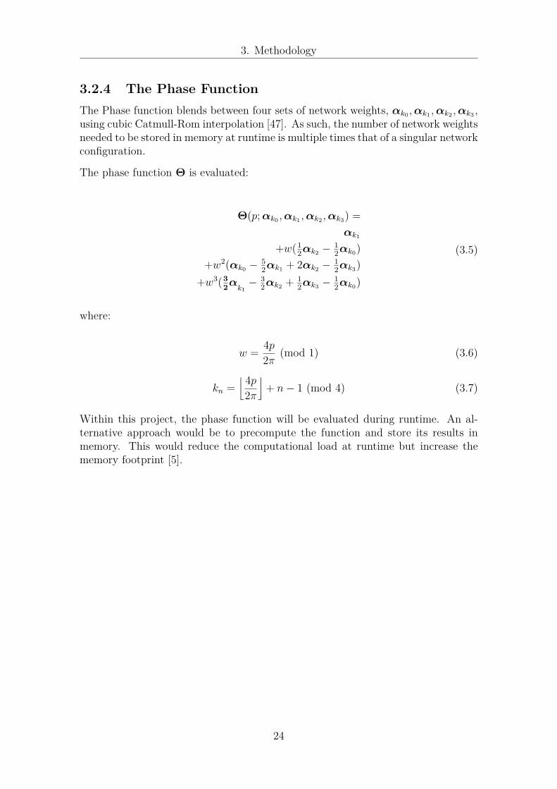
3.2.4 The Phase FunctionThe Phase function blends between four sets of network weights, αk0 ,αk1 ,αk2 ,αk3 ,using cubic Catmull-Rom interpolation [47]. As such, the number of network weightsneeded to be stored in memory at runtime is multiple times that of a singular networkconfiguration.

The phase function Θ is evaluated:

Θ(p; αk0 ,αk1 ,αk2 ,αk3) =αk1

+w(12αk2 − 1

2αk0)+w2(αk0 − 5

2αk1 + 2αk2 − 12αk3)

+w3(32α

k1− 3

2αk2 + 12αk3 − 1

2αk0)

(3.5)

where:

w = 4p2π (mod 1) (3.6)

kn =⌊ 4p

2π

⌋+ n− 1 (mod 4) (3.7)

Within this project, the phase function will be evaluated during runtime. An al-ternative approach would be to precompute the function and store its results inmemory. This would reduce the computational load at runtime but increase thememory footprint [5].

24

3. Methodology

3.3 The Full PFNN Pipeline

Figure 3.4: The full PFNN pipeline‘data’ = offline storage‘script’ = runnable files‘memory’ = temporary, runtime

This section aims to provide an overview of the full phase-functioned neural networkpipeline, as designed by Holden et al. [5] and as presented in Figure 3.4. The finalintegrated version of this model is presented in Section 4.1.

3.3.1 Generate PatchesTo allow for the generation of locomotive character animations that adhere to theroughness of the topography, the training data used later must include differenttypes of terrain. A solution to this is to fit heightmaps to the separately recordedmotion capture data, firstly producing intermediate patches of terrain.

3.3.2 Generate DatabaseDuring this step, each input and output vector pair, see Section 3.2.2 and Section3.2.3, is produced and stored. Each vector pair is created on a per-frame basis usingmotion captured data, see Section 2.3.1, and associated labels, such as the phaseand gait variables. Additionally, for each motion capture clip, the ten most suitableheightmaps are fitted to the foot-to-ground contacts of the character.

3.3.3 Network TrainingTraining will be performed using the Theano [38], a Python library for multi-dimensional array computations on the GPU - see Section 2.3.2, implementationby Holden et al. [5], and an Adam optimizer, see Section 2.1.6. The result of thisstep will be the finalized trained network weights. The default hyperparamters forthe training will be:

25

3. Methodology

• batchsize = 32

• learning rate = 0.0001

• beta1 = 0.9

• beta2 = 0.999

• epochs = 2000

• error function = mean-squared error

For the order of the motion capture data files, see Table A.1 in Appendix A.2.

During the training process, the translation and orientation of the joints not onthe following list, or equivalent to these in the case of the Avalanche configuration,within the input vector will be put to ≈ 0, as is done in Holden et al. [5]:

• Hips

• LeftUpLeg

• LeftLeg

• LeftFoot

• LeftToeBase

• RightUpLeg

• RightLeg

• RightFoot

• RightToeBase

• Spine

• Spine1

• Neck1

• Head

• LeftArm

• LeftForeArm

• LeftHand

• RightArm

• RightForeArm

• RightHand

Additionally, this training process will not make use of the early-stopping technique,see Figure 2.4.

3.3.4 Neural NetworkThis step includes the entire package necessary for runtime pose prediction. Dur-ing initialization, all necessary trained network weights will be read and loaded inmemory. Then, each frame, a prediction request is passed to the package, provid-ing a character pose in the current frame and expecting an updated character poseas return value. In addition to the character pose, other metadata is feed to thenetwork for prediction, such as sample points of the topography and user input, seeSection 3.2.2.

In this step is where the bulk of the integration work will be. However, the overallpackage structure will be based of the demonstration codebase made public byHolden et al. [5], with the neural network model defined in Eigen, see Section 2.3.3,arrays and matrices.

Additionally, as mentioned in Section 1.4, the motion capture data, and thereforethe trained neural network, uses left-handed world-axis, whereas the Apex engineuses a right-handed world-axis, see Figure 3.5.

26

3. Methodology

Figure 3.5: Visual representation of left/right-handed world-axis orientationsLeft: Left-handed world-axis (green)

Right: Right-handed world-axis (purple)

For this reason, the runtime neural network package must be altered such thatit can convert between the world-axis orientations. The character pose, living ina right-handed world-axis, is to be converted to the left-handed world-axis of theneural network. Then, the neural network outputted updated character pose mustbe converted back into right-handed world-axis before being applied to the characterskeleton.

27

3. Methodology

28

4Process

4.1 The Runtime PackageThis section aims to present the runtime package implemented for the phase-functionedneural network solution, originally based on the demonstration software made publicby Holden et al. [5]. An overview of this package is presented in Figure 4.1.

Figure 4.1: The Procedural Animations runtime packageThe neural network solution is accessible either from the ProceduralAnimationsclass, or indirectly through the ErrorCalculator class.

4.1.1 Using the Runtime PackageThe runtime package, see Section 4.1, is aimed to have a low level of coupling,such that other programmers need not to interact with, nor understand, the deepermachinations of the package.

As such, to use the runtime package, a programmer would only need to performtwo things: initialize the Procedural Animations class and to call ‘GetNextPose(...)’when wanting to use the network for predictions, see Section 4.1.2.

During initialization, the ProceduralAnimations constructor takes three optionalparameters, see Figure 4.2:

• new world transform - A 4D matrix for character scaling/rotation/translation.

• new setting - A Setting enum, see Section 4.1.6, for network configurations.

• new waypoint sptr - A pointer to a vector of Waypoint:s, see Section 4.1.9.

29

4. Process

CProceduralAnimations(AosMatrix4 new_world_transform = AosMatrix4(0.0f),CSettings::SETTING new_setting = CSettings::HOLDEN,std::vector<CProceduralAnimationsWaypoint*>* new_waypoints_ptr = nullptr);

Figure 4.2: Procedural Animations constructor

Then, during the constructor execution, the objects that the ProceduralAnimationclass owns are initialized.

During runtime prediction, only the ‘GenerateNextPose(...)’ function is required, seeFigure 4.3. This function takes two parameters: a pointer to the current characterpose, and a pointer to the translational character-in-world offset. Then, the ‘Gen-erateNextPose(...)’ updates the two input parameters in place, given the outputs ofthe neural network.

void GenerateNextPose(CPose* pose, AosVector3* translation_offset);

Figure 4.3: Procedural Animations per frame prediction

4.1.2 ProceduralAnimationsThis class owns the pointers to the PFNN, Character, Trajectory, and Settings rep-resentations. As the ErrorCalculator class is intended only for evaluation purposes,the ProceduralAnimations class is the default way to access the phase-functionedneural network solution.

Inside the ‘GenerateNextPose(...)’ function, see Figure 4.3, the flow of sub-functioncalls is organized as follows:

1. Prepare - Stores the input pose information in the Character object.

2. Input - Evaluates the Waypoint information and sets the Trajectory state.

3. Insert - Inserts the Character and Trajectory states into the input vector.

4. Predict - Runs the network prediction, setting the output vector.

5. Output - Stores the relevant output vector information in the return pose.

6. Update - Update Character and Trajectory states using output vector.

The time required to perform these six steps is recorded e ach frame for use inevaluating the systems responsivity, see Section 3.1.2.

Additionally, this class has debug rendering functionality for visually rendering net-work parameters, such as the joint skeleton, the sample points, character velocities,etc., in the engine.

30

4. Process

4.1.3 PFNNThis struct holds the memory representation of the neural network and is responsiblefor the network prediction.

When initialized, the PFNN struct loads the network weights and biases into Eigen,see Section 2.3.3, matrices in memory from stored .bin files. The .bin directory andnetwork configuration is fetched from the Settings object. Additionally, the PFNNstruct is the only part of the runtime package dependent on the Eigen library.

During the prediction step, the PFNN struct performs the matrix multiplicationsnecessary to propagate the input vector state, and then standardizes the resultbefore storing it in the output vector data structure.

4.1.4 CharacterThe Character struct stores the positions and translations, in model space, of allcharacter joints in the current frame. Additionally, the same information is storedfor the few previous frames to allow for output blending when setting the returnpose values.

4.1.5 TrajectorySimilar to the Character struct, the Trajectory struct holds all information regardingthe sample points along the ground, see Figure 3.3, such as positions and velocities.These values are also stored between multiple frames to allow for output blending.

4.1.6 SettingsThe Settings class is used to manage easy switching between the different networkconfigurations, see Section 3.1.3, which is represented as an enum passed to theconstructor.

To allow for a low level of coupling and extensibility, in the form of being ableto add additional network configurations requiring minimal changes in the codebase, the Setting class holds all data that may be affected by the choice of networkconfiguration. In other words, if one wants to add another network configuration,one would only need to add support for it in the Setting class.

For an example, all paths to the network .bins are defined in the Setting class. Thismeans that when a PFNN object initializes, it simply calls something similar to‘settings->GetWeightsPath()’, without needing any logic, e.g. switch cases, thatrequires the knowledge of a network configuration enum or how that configurationwould affect this class. This is shown in Figure 4.4

31

4. Process

class Settings{enum CONFIG {HOLDEN, AVA};

string path;

Settings(CONFIG new_config){switch(new_config){

case HOLDEN:path = "/holden_weights/"break;

case AVA:path = "/avalanche_weights/"break;

}}

string GetPath(){return path;

}}

Figure 4.4: Simplified example of Settings implementation(DISCLAIMER: PSEUDO CODE! NOT ACTUAL IMPLEMENTATION!)

4.1.7 HelperFunctionsThis is a simple, fully static class that holds functions such as debug outprints anddefinitions for specific matrix operations.

4.1.8 ErrorCalculatorWhen evaluating the network, rather than creating an instance of the Procedu-ralAnimations class, one initializes an ErrorCalculator instead. This object actsas a wrapper around a ProceduralAnimations instance and, rather than dependingon an input pose, uses stored input and output vector pairs, see Section 3.2.2 andSection 3.2.3.

This class is therefore responsible for calculating the evaluative results requiredin the answering of the research question regarding accuracy, see Section 1.3 andSection 3.1.2.

This evaluation process can either be run immediately on initialization, or on a perframe basis to allow for visualization of the network prediction, compared to theground truth. This is controlled with a ‘run-offline’ flag.

Since the ErrorCalculator constructs an internal ProceduralAnimations instance, italso requires the same input parameters; both in the constructor, see Figure 4.5,and on the per frame prediction, see Figure 4.6.

CProceduralAnimations(AosMatrix4 new_world_transform = AosMatrix4(0.0f),CSettings::SETTING new_setting = CSettings::HOLDEN,std::vector<CProceduralAnimationsWaypoint*>* new_waypoints_ptr = nullptr,bool run_offline = false);

Figure 4.5: Error Calculator constructor

32

4. Process

float CalculateError(CPose* pose);

Figure 4.6: Error Calculator per frame prediction

4.1.9 WaypointEach Waypoint instance is a simple datastructure, representing one checkpoint alongthe obstacle course that the characters will traverse as part of the responsivityresearch, see Table 3.1 in Section 3.1.1.

In addition to its inherent world translation, each Waypoint holds information rep-resenting the goal movement style that a character aims to perform when reachingit. This includes the gait styles; walking, jogging, crouching, etc, but also movementspeed and facing direction. This, in an aim to deterministically simulate user inputduring the evaluation process.

The ProceduralAnimations instance keeps track of the current Waypoint index, andincrements that number upon reaching the next checkpoint.

33

4. Process

34

5Result

5.1 Responsivity ResultsAll responsivity data, which is used to produce the figures and tables presented inthis section, is available in Appendix A.4. For more information regarding the trackcourse used, see Section 3.1.1.

The responsivity results presented in Figure 5.1 shows the average frame time com-putation in milliseconds per lap around the course. The same data is presented asa box plot in Figure 5.2, and summarized in Table 5.1.

Figure 5.1: Line chart of responsivity results

35

5. Result

Figure 5.2: Boxplot of responsivity results

HOLDEN HOLDEN-XL HOLDEN-XT AVAMean 0.376 0.499 0.382 1.55SD 0.0173 0.0161 0.0167 0.0430

Table 5.1: Mean and standard deviation results of responsivity evaluationValues are rounded to three significant digits.

By combining the visual results of the line chart in Figure 5.1 and the box plot inFigure 5.2, one can conclude that there is a considerably sized difference in compu-tational time required for that of the AVA network configuration. A potential rootcause of this is the great increase in number of joints for that network, see Section6.1.1 for further discussion on this topic.

For the Holden configurations, the results of HOLDEN and HOLDEN-XT have al-most perfect overlap in both Figure 5.1 and in Figure 5.2. As such, one can concludethat these two network configurations have practically equivalent responsivity. How-ever, this is not too surprising as, in theory, a network having trained longer, withotherwise the same hyperparameters, should only result in a different set of networkweights. Subsequently, two otherwise equivalent networks but with different weightsshould still be evaluated at runtime at the same speed.

Finally, for the HOLDEN-XL configuration, it is not as visually clear whether it atruntimes evaluates at a considerably different speed than that of the other Holdenconfigurations. For this, the similarity metric defined in Section 3.1.4 can be used.This metric evaluates the absolute difference between each mean result, standardizedby the average standard deviation of the two data series. In other words, the metricevaluates how many standard deviations two data points differ.

2|mean(a)−mean(b)|sd(a) + sd(b) (5.1)

36

5. Result

• HOLDEN to HOLDEN-XT: 2|0.382−0.376|0.0173+0.0167 ≈ 0.35

• HOLDEN-XL to HOLDEN-XT: 2|0.499−0.382|0.0161+0.0167 ≈ 7.1

• AVA to HOLDEN-XT: 2|1.55−0.499|0.0430+0.0161 ≈ 36

These calculations, together with the visualizations in both Figure 5.1 and in Fig-ure 5.2, can be combined to suggest the relative significance of the differences instandard deviations between the responsivity results. Even though the number ofstandard deviations between the results of the HOLDEN-XL configuration and thatof the HOLDEN-XT results are much smaller than that to the results of the AVAconfiguration, one can still make the argument that there is a noticeable dissimilarityin computational time required for the HOLDEN-XL configuration. This differencecould be explained through the fact that adding another layer in a neural networkstrictly increases the number of computations, and therefore the time, required forevaluation at runtime. For further discussion on this topic, see Section 6.1.1.

5.2 Responsivity VisualizationsVideo recordings of these visualizations are available here [48].

Figure 5.3: Some frames from the HOLDEN responsivity evaluationTop left: jogging, Top right: crouchingBottom left: strafing backwards, Bottom Right: walkingWhite globes are Waypoints, see Section 4.1.9.The golden Waypoint is the next positional target of the network.

37

5. Result

Figure 5.4: Some frames from the AVA responsivity evaluationTop left: jogging, Top right: crouchingBottom left: strafing backwards, Bottom Right: walkingWhite globes are Waypoints, see Section 4.1.9.The golden Waypoint is the next positional target of the network.

In Figure 5.3 and Figure 5.4, one can see examples of the skeleton joint positionoutputs the HOLDEN and AVA network configurations produced during their re-spective responsivity evaluations.

For the AVA configuration, certain errors occurred, potentially as a result of thenetwork not being trained on sufficient amount of data frames, see Section 6.1.3and 6.4.1 for further discussion. For an example, notice how poorly the producedjoint skeleton appears to be crouching in the bottom right photograph in Figure5.4. Additionally, the AVA configuration failed to adapt to tight turns, making theoutputted skeleton overshoot the target, see Figure 5.5.

Figure 5.5: Directional overshoot during the AVA responsivity evaluationThe goal of the network is to move the skeletal character towards the golden

Waypoint. However, the AVA configuration fails to sufficiently turn the charactertowards this goal before the character has passed it.

38

5. Result

5.3 Accuracy ResultsAll accuracy data, which is used to produce the figures and tables presented in thissection, is available in Appendix A.5 and Appendix A.6.

The accuracy results presented in Figure 5.6 shows the average error per motioncapture data file for each of the four network configurations. The error calculationis defined as presented in Section 3.1.2:

1|j|∑

j

|tj − pj|tj

(5.2)

Where |j| is the total number of frames in this file, tj is the three-dimensionalposition of joint j as defined in the motion capture database, and where pj is thethree-dimensional network predicted output position of joint j. The values takenfrom the motion capture database, including tj, is referred to as the ground truth.

Additionally, the fifth data series ‘AVA-M’ shown in this figure represents the resultsof the AVA network limited to the subset of network outputs equivalent to thosejoints present in the original motion capture data made public by Holden et al. [45],see Figure 3.1 and Section 3.1.3.

Similarly, Figure 5.7 presents the standard deviations, a measurement of spread inthe data distribution, of the per motion capture file network outputs for each of thenetwork configurations. A smaller standard deviation equates to little difference be-tween data points within a data series, whereas a higher standard deviation equatesto more fluctuating data points.

The same accuracy data is presented as a box plot in Figure 5.8, and summarizedin Table 5.2.

39

5. Result

Figure 5.6: Line chart of mean results of accuracy evaluationThe error is defined as mean absolute error compared to the training data.For full definition of error, see Section 3.1.2.For indexing of motion capture files, see Appendix A.2.

What can be seen in Figure 5.6 is that the results of the three Holden configura-tions are greatly overlapping throughout the training data set. The blue diamondHOLDEN data series is almost perfectly obscured by the green triangle HOLDEN-XT series.

Somewhat similarly, the two Ava results appear to follow a slightly similar curvature,however vertically translated to a lower error level than that of the Holden config-urations. Internally, however, the curvature of the two Ava data series is highlysimilar, though also vertically translated. In other words, if the AVA-M data serieswould be shifted downwards in the chart, there would be almost constant visualoverlap between it and the AVA data series. However, visually there is almost nosimilarity in the curvatures of the Holden and Ava configurations.

Throughout the entirety of Figure 5.6, the Ava data series produce a lower errorthan that of the Holden configurations. This is visualized through how the AVAand AVA-M data series are consistently below the other three.

The motion capture files that all network configurations performed the worst at,data files indexed at 72-75, were that of the files containing movement interactingwith more advanced terrain and environments, such as balancing on elevated narrowbeams and dynamic crouching beneath low ceilings.

40

5. Result

Figure 5.7: Line chart of standard deviation results of accuracy evaluationThe error is defined as mean absolute error compared to the training data.For full definition of error, see Section 3.1.2. For indexing of motion capture files,see Appendix A.2.

As a similar trend to the means presented in Figure 5.6, the standard deviationsshown in Figure 5.7 has almost perfect overlap for the three Holden configurations.Once again, the blue diamond HOLDEN data series is almost perfectly obscured bythe green triangle HOLDEN-XT series.

However, the curvature of the AVA-M data series appears to be a a midpoint tothat of the Holden configurations and that of the AVA data series. Visually, theAVA-M has local maxima and minima similar to both of aforementioned series.Additionally, the values of the AVA-M series are positionally closer to that of theHolden configurations than to that of the AVA data series. In other words, datapoints along the turqoise circle AVA-M line are further away from that of the purplecrossed AVA line than to those of the other three data series.

41

5. Result

Figure 5.8: Boxplot of accuracy resultsThe error is defined as mean absolute error compared to the training data.For full definition of error, see Section 3.1.2.

As a reminder: an error of 0.01 equates to an average prediction error of 1%, seeSection 3.1.2. As a concrete example; the predicted three-dimensional joint positionsthat the HOLDEN network configuration produced had, on average, a translationalerror of ≈ 4.4%.

HOLDEN HOLDEN-XL HOLDEN-XT AVA AVA-MMean 0.0439 0.0448 0.0446 0.0148 0.0258SD 0.00954 0.00980 0.00981 0.00283 0.00483

Table 5.2: Mean and standard deviation results of accuracy evaluationValues are rounded to three significant digits.

For all three Holden configurations, the results have almost perfect overlap in bothFigure 5.6 and in Figure 5.7. As such, one can conclude that these three networkconfigurations have practically equivalent accuracy. This is rather interesting asboth the HOLDEN-XL and HOLDEN-XT configurations each respectively have aspecific advantage, in the form of extra network depth and extra training time,compared to the default HOLDEN configuration. These results suggest that thereis no benefit to these specific network design alterations.

For the AVA configuration, by combining the visual results of the line chart in Figure5.6 and the box plot in Figure 5.8, one can conclude that there is a significantly lowererror in the AVA prediction than that of the Holden configurations.

Lastly, the AVA-M data series appear to share some similarity to both the Holdenand AVA data series. To measure this similarity, one may utilize the differencemetric used in Section 5.1 and originally presented in 3.1.1; calculating the numberof standard deviations between the means. This produces the following results:

42

5. Result

• HOLDEN to HOLDEN-XT: 2|0.0439−0.0446|0.00954+0.00981 ≈ 0.072

• HOLDEN to HOLDEN-XL: 2|0.0439−0.0448|0.00954+0.00980 ≈ 0.0093

• HOLDEN-XT to HOLDEN-XL: 2|0.0446−0.0448|0.0448+0.00980 ≈ 0.0073

• AVA-M to HOLDEN: 2|0.0258−0.0439|0.00483+0.00954 ≈ 2.5

• AVA to AVA-M: 2|0.0148−0.0258|0.00283+0.00483 ≈ 2.9

These differences can be summarized as the three Holden network configurationsproducing practically equivalent results, with an especially large overlap betweenHOLDEN and HOLDEN-XT, and the AVA-M results being slightly closer to thatof the Holden configurations than to that of the AVA configuration.

5.4 Accuracy VisualizationsVideo recordings of these visualizations are available here [48].

Figure 5.9: Some frames from the HOLDEN accuracy evaluationGray: Ground truth joint positions.Blue: HOLDEN joint positions.

Figure 5.10: Some frames from the AVA accuracy evaluationGray: Ground truth joint positions.Magenta: AVA joint positions.

In Figure 5.9 and Figure 5.10, one can see examples of the skeleton joint position

43

5. Result

outputs the HOLDEN and AVA network configurations produced during their re-spective accuracy evaluations.

5.5 Training ProcessDuring the training process, the prediction mean-squared error of the full outputvector was recorded after each epoch. Do note the difference in error definition, andthe fact that the entire output vector is used rather than just the predicted skeletonjoint positions, compared to the one used in Section 5.3. This data is available in infull in Appendix A.7, and presented as a line chart in Figure 5.11.

Figure 5.11: Mean-squared error of entire output vector during trainingHOLDEN-XT is hidden during the first half of its training process as its design, andtherefore results, is entirely equivalent to that of the HOLDEN configuration.

Figure 5.11 shows similarity through overlap between the HOLDEN and HOLDEN-XL configurations throughout their training period. Additionally, during the extratraining period of the HOLDEN data series, here equivalent to that of the HOLDEN-XT configuration, the mean-squared error remains relatively unchanged. This fur-ther reemphasizes the similarity in accuracy argued in Section 5.3.

As a reminder; the green triangle HOLDEN-XT was trained for twice the numberof epochs than the other network configurations, which results in a twice as longoutput error result.

For the AVA configuration, one can visibly determine a larger mean-squared errorduring the entirety of its training process compared to the Holden configurations.This is visualized through the fact that the purple crossed AVA data series liesrelatively significantly above the others in Figure 5.11. Additionally, the mean-squared error of the entire output vector appears visibly more irregular betweenepochs during the training process than that of the Holden configurations.

44

5. Result

5.6 Pipeline OverviewThis section aims to present the computation time, see Table 5.3, and the data size,see Table 5.4, for each step of the full phase-functioned neural network pipeline,presented in Section 3.3.

Step HOLDEN HOLDEN-XL HOLDEN-XT AVAGenerate Patches 28min - - -Generate Database 90min - - 55minNetwork Training 43h 47h 91h 31hNeural Network 0.38ms 0.50ms 0.38ms 1.5ms

Table 5.3: Computational time required throughout the pipelineEntries marked ‘-’ share the HOLDEN results.

In summary, for the HOLDEN-XL configuration, Table 5.3 shows that there is littledifference in training time when adding a new network layer to the Holden network.

The much longer training time of the HOLDEN-XT configuration was not unex-pected, as a result of it being trained for twice the number of epochs, see Section3.1.3.

Additionally, the table shows that the database generation, and to some extentthe network training, is considerably quicker for the AVA configuration. This meansthat even though the AVA configuration had six times the number of skeleton joints,see Section 3.1.3, the fact that it only had a fourth of the frames compared to theHolden configurations, see Section 3.1.3, resulted in it being trained considerablyfaster.

Data HOLDEN HOLDEN-XL HOLDEN-XT AVAHeight Fields 134MB - - -

Terrain Patches 606MB - - -Motion Capture Files 848MB* - - 7.62GB*

Phase Labels 7.04MB - - -Other Labels 56.9MB - - -

Training Database 7.12GB - - 10.4GBNetwork Weights 122MB 176MB 122MB 374MB

Table 5.4: Size of different data throughout the pipelineEntries marked ‘-’ share the HOLDEN results*: Motion Capture Files are in 120Hz.

In summary, Table 5.3 shows the considerable increase in memory size between thatof the Holden, to that of the AVA, network configurations. As mentioned in 3.1.3,do note that the AVA database only contains a number of frame data points equalto a quarter of that of the Holden configurations.

45

5. Result

Additionally, as discussed previously, given that the HOLDEN-XT configurationdiffers from the default HOLDEN configuration solely through training time, it isexpected that the network weights produced by the two have the same memory size.

In contrast, given that the HOLDEN-XL configuration has more network nodesthan that of the HOLDEN configuration, it is expected that there are more weights,requiring more memory, for the former.

5.7 Skinning VisualizationVideo recordings of these visualizations are available here [48].

These were the in-engine results of the network orientational outputs after switchingthe X- and Z-rotations, and inverting the Y- and switched X-rotations.

Figure 5.12: HOLDEN positional and orientational output skinnedLeft: The skinned HOLDEN character model in default stance.Middle: HOLDEN output skinned.Right: HOLDEN output skinned with visible skeleton.

Figure 5.13: AVA positional and orientational output skinnedLeft: The skinned AVA character model in default stance.Middle: AVA output skinned.Right: AVA output skinned with visible skeleton.

In Figure 5.12 and Figure 5.13, one can see examples of the skeleton joint translation

46

5. Result

and orientation outputs the HOLDEN and AVA network configurations producedduring their respective responsivity evaluations skinned to 3D character models.

The HOLDEN skinning, at a quick glance, appears correct in general. Occasionally,certain specific joints experience single-frame orientation errors. For an example,the head and torso sometimes rotate over 180 degrees around an axis in a singleframe. As of writing, this error is still being investigated.

Similarly, the skinned AVA results also produce certain erroneous orientations, how-ever much more frequently and for more than only two joints. In the middle panelof Figure 5.13, one can see the torso joint being rotated over 180 degrees. As ofwriting, this error is still being investigated. Additionally, the original skeleton file,on which the motion capture data was retargeted using, was lost and replaced witha new skeleton file for the runtime process. This new skeleton is perfectly equivalentto the old one, except for the facial structure. As such, the facial contortions shownin Figure 5.13 is to be expected.

However even though the character model occasionally appears incorrect, the un-derlying skeleton still moves correctly. This shows that the positional outputs of theneural networks are correct, however that is not always the case for the orientational.This is presumably a result of the fact that the network is trained in another setof world-axis orientations, see Section 3.3.4, compared to that of the Apex engine.The positional outputs of the neural networks are manually converted in runtimeto match that of the engine, hence the apparently correct skeletal output. Thisinconsistency in world-axis orientations, however, does not affect the results of theresponsivity or accuracy evaluations. This is further discussed in Section 6.4.2.

47

5. Result

48

6Discussion

6.1 Discussing the Research QuestionsThis section aims to, through discussion, answer the research questions as presentedin Section 1.3.

6.1.1 Discussing ResponsivityThe research question regarding responsivity asked how much computational time isrequired for procedural single-character locomotive animations, see Section 1.3. Thisis answered through testing an engine-integrated solution using the four differentnetwork configurations.

The responsivity results presented in Section 5.1 reveals a considerable computa-tional difference between the Avalanche and the Holden network configurations.

This significant distinction in frametime could be explained by the difference innumber of skeleton joints. As mentioned in Section 3.1.3, the two skeleton typeshave 31 and 191 joints, respectively. Since all skeleton joints are fed into the neuralnetwork during the runtime prediction process, the width of the networks, and inturn the number of computations each frame, depend on the number of joints.

Since the AVA network required a size of 1’302x512x1’751, whereas the two shallowerconfigurations required only a size of 342x512x311, the number of computationsrequired each frame to propagate the character pose through the network is thereforegreatly increased in the former configuration.

A naive, since it assumes sequential computing, way of counting computations in asimple feed-forward network like the one used in this project is to sum the numberof inter-layer network connections and the number of biases, like so:

∑l

nl(1 + nl+1) (6.1)

Where: ‘l’ is the index of all non-output network layers, ‘l + 1’ is the index of thesubsequent network layer following layer ‘l’, and ‘nl’ is the number of nodes (width)in layer ‘l’.

49

6. Discussion

The number of computations per network configuration using the above formula canbe seen in Table 6.1.

HOLDEN HOLDEN-XL HOLDEN-XT AVAcomputations 335’501 598’157 335’501 1’566’701

Table 6.1: The number of computations required per network configuration

These data points can then be inserted into a line chart to display the linear rela-tionship between the number of skeleton joints and the frametime, such as Figure6.1.

Figure 6.1: Linear regression of computational time over network calculationsBeware; this is a gross simplification simply to show a possible relation betweennetwork size and computational load at runtime.Regression line: y ≈ 9.6x · 10−7 + 0.018

6.1.2 Discussing AccuracyThe second subsidiary research question asked how accurate the generated locomo-tive character animations are to the original animation data, see Section 1.3. Thisis answered here through relative comparisons between the network configurations.

difference between the holdensThe three Holden network configurations maintain close resemblance with equivalentresults throughout the error evaluation process. This can be seen through consistentoverlap between the data shown in both Figure 5.6, Figure 5.7, and Figure 5.8, andwith a near zero divergence metric, as presented in Section 3.1.1. Additionally, themean-squared-error evaluation during the training process also shows no significantdifference between the Holden configurations, see Figure 5.11.

50

6. Discussion

Through these statistics, one can conclude that there was insignificant gain in eitherdoubling the number of hidden layers in the neural network, as was the case for theHOLDEN-XL configuration, or doubling the duration of the training process, as wasthe case for the HOLDEN-XT configuration.

Additionally, the lack of improvement in results between the default HOLDEN andthe long trained HOLDEN-XT configuration is evidence that the original imple-mentation by Holden et al. does not suffer from underfitting, see Section 2.1.4 andSection 3.1.3.

ava versus ava-mAdditionally, the AVA and AVA-M data series closely follow the same curvature inFigure 5.6, however translated vertically. This curvature is distinctively differentfrom that of the Holden configurations.

Given that the AVA data series has consistently less of an error than the AVA-Mseries, one can deduce that the masked joints, those not present in AVA-M, give riseto a constantly lower error in comparison.

The mean absolute error definition used in this project includes a normalizing de-nominator, see Equation 3.1, as to allow the error to be relative to the ground truthpositional values. For an example, an error of 0.01 equates to a predicted jointposition that is 1% off the ground truth, see Section 3.1.2. However, this meansthat further away joints, joints at positions with high positional values, would needa larger absolute error to produce the same effective evaluated error than that of ajoint closer to the axis origin.

As a concrete example, consider a joint a with a ground truth position at at = 100.For this joint to contribute with an error of 0.1, the predicted position would needto be at ap = 101. However, if we consider a different joint b with a ground truthposition at bt = 1, the predicted position would need only to be bp = 1.01 tocontribute with the same error.

Out of the the masked AVA joints, a considerable number of these are highly con-centration within the character head and face, see Section 3.1.3. As these joints arefurther away from the axis origin, the discrepancy in error between AVA and AVA-Mmay be a result of the inherent relativity design of the mean absolute error definitionused in this project. As such, AVA-M might be more suitable for comparisons withthe Holden configurations.

ava-m versus the holdensAlso, even though the mean-absolute prediction error at runtime of the AVA con-figuration was significantly lower than that of the Holden configurations, see FigureA.5, the mean-squared prediction error during the training process of the formerwas considerably higher than that of the latters, see Figure 5.11.

This difference could be a result of the fact that the runtime evaluation only con-sidered the three-dimensional skeleton joint positions, wheras the training processevaluation considered the entire output vector. This means that it is possible that

51

6. Discussion

the AVA network configuration is comparatively much better at joint position pre-diction than at predicting the other output features, such as: joint orientations andvelocities, and sample point positions and trajectories, see Section 3.2.3.

Additionally, another potential reason behind this difference is the fact that thetwo evaluation processes used different error definitions; mean-absolute error andmean-squared error. The fact that the absolute error was lower than the squarederror could be an indicator that the data, in this case the accuracy of the AVAnetwork, had many extreme outliers. This, as the mean-squared error definitionsquares the per data point error, meaning that errors smaller than one get reducedand errors larger than one get amplified, compared to that of the mean-absoluteerror definition.

However, a potential source of the difference in error between the AVA and Holdenconfigurations was the choice of evaluation frames per motion capture file, see Section3.1.2. As a result of insufficient system memory for keeping each joint position ineach frame in memory, a decision to only consider the first 500’000 three-dimensionaljoint positions in each datafile was made. This in combination with the fact that theAVA configuration only considered every fourth frame and that the AVA skeletonhad more than six times the skeleton joints, see Section 3.1.3, means that it isprobable that if the maximum joint position number is met, the two configurationswould consider different blocks of frames within the motion capture data.

In other words, if the Holden configurations reached the memory limit of 500’000joint positions, it will have considered the first 500′000

31 ≈ 16′000 frames. On the otherhand, if the AVA configuration reached the memory limit of 500’000 joint positions,it would have instead only considered the first 500′000·4

191 ≈ 10′000 frames. If thedifferent network configurations was evaluated on a different set of motion frames,then that could make for an unfair comparison.

6.1.3 Discussing ArchitectureThe final subsidiary research question asked about how the phase-functioned neuralnetwork architecture presented in Holden et al. could be improved, see Section 1.3.

An initial hypothesis may be that allowing a neural network to train for a longerperiod of time, or to have a deeper network, may increase the predictive accuracyof the network. However, when comparing the accuracy results between that of theHolden configurations, see Section 6.1.2, one can conclude that is not the case, atleast not for this particular model. This was shown through insignificant differencein accuracy between the three network configurations; default (HOLDEN), doublethe hidden layers (HOLDEN-XL), and double the training time (HOLDEN-XT),see Section 6.1.2.

On the other hand, not just that there was no strictly positive sides of any of the twoaltered Holden configurations, there was still strictly negative ones. For an example,given that the HOLDEN-XL configuration required an additional layer of networkweights and biases, it was shown to require both longer computational time, see

52

6. Discussion

Figure 5.1 and Table 5.3, and more memory, see Table 5.4, at runtime. For theHOLDEN-XT configuration, the only clear downside of it, compared to the defaultHOLDEN network, was the increase in training time, see Table 5.4. As such, thealtered Holden configurations have been shown to only perform equally, or worse,compared to that of the default HOLDEN configuration.

The fourth network configuration, AVA, that in one aspect may be used to evaluatethe generalizability of the phase-functioned neural network approach, had its ownfair share of issues. For the responsivity evaluation, the AVA network was shown tobe significantly much slower to evaluate at runtime, compared to all other networkconfigurations. This, however, may be quite unsuprising as it required many morecomputations for each prediction, see Figure 6.1, as a result of it being based ona character skeleton using more than six times the joints than that of the skeletonused for the other network configurations.

On the other hand, the accuracy evaluation implied an increase in prediction accu-racy for the AVA configuration. However, it is questionable whether this comparisonwas truly fair. Certain special considerations were taken to avoid memory overflowsas a result of, both directly and indirectly, the greatly increased number of skeletonjoint. These include introducing a maximum number of considered frames duringthe accuracy evaluation, see Section 3.1.2, and having the network train on only aquarter of the training data frames, see Section 3.1.3.

Additionally, as shown in Section 5.2, the actual orientational outputs of the AVAconfiguration is erroneous to the extent that they are practically useless within theengine. This is assumed to be a result a side-effect of the inconsistent world-axisorientations, see Section 3.3.4.

To produce a more fair comparison between the AVA and the Holden network config-urations, certain alterations in the AVA network configuration should be considered.These include only utilizing a subset of the skeleton joints, similar to the AVA-Msubset - see Section 3.1.3, in the AVA skeleton that are equivalent to the Holdenskeleton, see Section 6.4.1 , and implementing consistent world-axis orientationsthroughout the process, see section 6.4.2. This is further discussed in Section 6.4.

6.2 Ethical ConsiderationsGiven that this project encompassed work with proprietary software, the Apex gameengine, a certain level of consideration regarding confidentiality was taken, as pre-viously mentioned in Section 1.4. The disclosure or misuse of sensitive informationpertaining to the Avalanche Studios Group, including that of any of their systems orprojects, may indirectly damage both the company and its intellectual properties.To ensure the personal liability of the thesis author towards any such consequences,a non-disclosure clause regarding sensitive information was signed as part of thecollaborative contract. As such, no intricate details about the engine, in either textor photo, is included as part of this report.

As far as potential repercussions regarding the research content of this project, no

53

6. Discussion

further ethical considerations were taken into direct consideration. Theoretically,revolutionary development within this field of research may lead to to industry-wideadoption of new techniques, nullifying certain current artist and engineering employ-ment positions. Such a substantial alteration of the standard character animationpipeline might remove the need for the currently adapted animation state machines,and therefore eliminate certain common work tasks. However, a new animationpipeline, that uses neural networks, would still require plenty of similar talents, inaddition to the need of new machine learning programmers.

Much consideration must be taken during the planning and recording of the motioncapture data, or what other data is to be used during the training process. Assuch, there might be a shift in the work force towards the number of motion capturespecialists, in favor of the number of animators. Animation programmers will stillbe needed to attach the neural network solution to the project. Additionally, evenif a project were to shift to a neural network based animation engine, there mightstill be the need of standard animations. Certain specific animations, such as inobject interaction or those used in cutscenes and cinematics, may utilize hand-madeanimations to achieve the highest level of detail in the bodily expression.

6.3 TakeawaysThis section aims to summarize some of the most important learnings produced bythis project on the topic of neural network integration into a modern game engine,or integration work in general. As such, the goal of these takeaways is to be broaderlessons, based on the concrete scenario of this thesis project, valuable even withinother contexts.

6.3.1 Integration ContextualizationSome of the obstacles encountered during thesis work, as a result of mismatchingassumptions on the implementation, was handled in a way such as to avoid alteringthe to-be-integrated codebase and to rather adapt the solution at runtime. One suchexamplifying situation is where even though the original phase-functioned neuralnetwork pipeline by Holden et al., see Section 3.3, used a different set of world-axisorientations to that of the Apex engine, see Section 3.3.3 and Section 6.4.2, it waskept unaltered.

The original reasoning behind this was twofold. Firstly, as this thesis project aimedto only integrate this work within the specific context of the Apex game engine, itwas assumed that manually taking care of an issue such as the inconsistent world-axisorientations would be a more rapid way of handling the problem, rather than at-tempting to make editions throughout the original phase-functioned neural networkpipeline. Secondly, this decision was taken as to minimize the potential locations ofintegration bugs. If this thesis project included a fully altered pipeline, there wouldbe many more places in the code base in where issues and programming mistakescould arise, given that the original implementation by Holden et al. was assumedto be fully functional.

54

6. Discussion

However, even given these reasonings, there would be much to gain from fully con-textualizing the to-be-integrated solution before initiating an integration process.As such, similar future work could be recommended to have further preemptiveresearch on the integral differences between the two solutions of an integration pro-cedure, identifying in which aspects alterations to the to-be-integrated solution maybe necessary.

6.3.2 Integration PlacementSimilarly to how certain steps were taken to as most rapidly be able to integratethe work by Holden et al. into the Apex engine by the inelegant solution of solvingthe world-axis orientation mismatch at runtime, certain shortcuts were taken on theother side of the integration work. The location in the Apex game engine wherethe phase-functioned neural network solution developed as part of this thesis workresides, was one where the integration could occur most effortlessly.

As such, the integrated solution was located within the game engine editor where itcould be easily accessed and debugged by programmers. However, given the natureof its location, certain other parts of the engine became separated to the neuralnetwork solution. Therefore, the current implementation of the network integrationhas no access to neither the user input system nor the terrain sampling system,causing such features to be unavailable to the network solution.

A more rigorous integration process could potentially have unlocked the function-ality of these systems, allowing the network to be able to produce terrain-adaptiveanimation as a result of being able to be fed the raycasted height data of nearbyterrain, for an example, see Section 6.4.3.

6.3.3 Implementation ExpertiseSomething that may be overlooked in integration work is for there to be represen-tatives within the integration team that together are both read-up on the work tobe integrated and deeply experienced within the solution into which the integrationwill occur.

Within the context of this thesis project, both sides of the integration software coin,but especially the Apex engine, was brand new to the author. As such, much timewas spent tackling with obstacles inherent to the engine that was novel to the author.Additionally, some less optimal integrational design choices could be attributed tothis fact.

Even though the thesis mentor was able to provide guidance within this area, thereis only so much such a person can provide while still maintaining their expecteddaily tasks and obligations.

55

6. Discussion

6.3.4 Equipment SuitabilityCertain areas within computer science are more computationally dependent thanothers. One of these is working with neural networks. Even though networks canbe fluently used at runtime, the actual training process is extensive and may lockup a workstation for days. As such, it should be recommended to have designatedtraining stations where the networks can complete this process without disturbingother operations.

Additionally, one limitation that became evident as part of this thesis work was thedemand on system memory as a result of massive training databases. This issuecan of course be resolved in other ways, such as implementing a runtime skeletonretargeting system as to avoid bloating the network pipeline when using a skeletonwith a greatly increased number of joints, see Section 6.4.1. However, for this thesisproject, simply having a training station with larger system memory capacity wouldresolve any such issues without having to alter the training process itself.

6.3.5 Neural Network RigidityAnother inherent characteristic that became evident when working with the theneural network implementation of this project was their lack of flexibility.

A certain level of care must be taken, such as making sure that the framerate ofthe neural network during the training process matches with that in which it isexpected to operate at runtime. Similarly, the joint skeleton, both in numbers andposition, must be maintained when transitioning between the training and runtimeapplications, especially when considering skinning 3D models to the skeletons.

Therefore, other systems, such as inverse-kinematics or other pose-affecting features,cannot be allowed to operate on the character pose if that pose is part of a neuralnetwork feedback-loop.

The integration implementation produced during this project alleviated this issueby allowing the neural network to hold an internal copy of the character pose. Thismeans that the outputting pose is able to be kept unaltered, for being inputted inthe next frame, allowing other systems to operate on another copy, the one that thenetwork broadcasts.

6.4 Future WorkThis section presents three different avenues of potential improvements, or furtheradvancements, on the topic of this project: runtime skeleton retargeting, consistentworld axis orientations, and full pipeline integration.

6.4.1 Runtime skeleton retargetingMany issues with the AVA network configuration are likely inherent to the muchgreater number of joints in the AVA skeleton, compared to what was necessary in

56

6. Discussion

the Holden network configurations. These include the incredible computational timerequired during runtime, see Section 5.1, and the steps taken as a result of insufficientsystem memory, such as the max ceiling of evaluation frames, see Section 3.1.2 andthe quartering of training frames, see Section 3.1.3.

Many of the joints used in the AVA skeleton are, by design, not meant to be usedfor locomotive animations. Many joints that exist in the skeleton are there for otherpurposes, such as for deformation or inverse-kinematics. Additionally, a considerablylarge portion of the joints in the skeleton are used to represent the structure andmuscles of the face of the character.

A very clear avenue of improvement in the methodology of this report would be toonly consider a subset of the joints in the AVA skeleton, such as the joints used in theAVA-M data series, see Section 3.1.3. This would not only mean that the networkpotentially could more easily discern the locomotive motion of the character, butwould also mean that all frames of the motion capture data may be used in boththe training and for the evaluation.

This means that a runtime retargeting system would need to be written that sets allupdated joint values in the actual skeleton that is unaccounted for in the network.Otherwise, for an example, all the joints in the character face would stay perfectlystill while the character moves, as these are not updated by the engine. Such aretargeting system would need to store a resting character pose, such that it canupdate the child joints accordingly after the network updates the chosen parentjoints. In other words, when the neural network moves the singular head joint, theruntime retargeting system would need to correctly update the face joints to matchthat of the head.

Additionally, such a retargeting system would be highly useful in general if a neuralnetwork solution would be applied in a real-world project as the generated anima-tions must be able to be reproduced across multiple similar skeletons. It is unrealis-tic to have separate neural networks, and separately recorded motion capture data,trained for each character, given that there is expected to be variations within thedesign of the physique of different characters.

6.4.2 Consistent world-axis orientationsAs mentioned in Section 1.4 and explained in Section 3.3.4, the original work byHolden et al. assumes a left-handed world-axis orientation, different from the right-handed orientation used in the Apex game engine.

During this project, as the neural networks was trained using the motion capturedata provided by Holden et al., the clash in world-axis orientation required muchcare. As such, the final runtime package includes multiple conversions at runtimebetween the right-handed character pose and the left-handed neural network.

This handling of the axis inconsistencies was done at runtime, where both the in-putting, and outputting, data was flipped such that it was translated correctly be-tween the world-axis orientations, depending on where the data was to be used; in

57

6. Discussion

the neural network representation or in the engine. Additionally, these conversionswere made such that the Holden configurations produced accurate positional andorientational outputs, without taking further care for the AVA configuration. Thatthe AVA configuration may have been in need of special care to resolve the world-axis inconsistency issue could be reason why it produced such imperfect results, seeSection 5.7.

If a motion capture data set was used that featured right-handed world-axis orienta-tion, such that it is consistent for the game engine at runtime, the visual orientationalerrors in the skinnings could be potentially resolved, or at least more easily studied.

6.4.3 Full pipeline integrationThe runtime neural network solution produced as part of this project was integratedinto the Apex engine, as far as the solution executing as an internal part of the enginerunning.

However, this is still a far step away from a full integration into the runtime pipeline.The current network package is positioned where it would be most easy to be put;a part of the engine used by programmers during the development process. Ideally,the package would instead by integrated within the actual runtime engine pipeline.

Such a full integration would not just allow for more realistic evaluation of the in-game performance of the neural network solution, but would also open it up to becombined with multiple other engine sub-systems.

Currently, character input, in the form of where the character is moving towards,with what movement style, and at what speed, is deterministically determined bythe obstacleless track course, as defined in Section 3.1.1. With a full integration, theneural network solution could be able to poll the user input system, such that thecharacter could be controlled at runtime with a gamepad or mouse and keyboard.

Similarly, a full integration would allow the network package to utilize raycasts tosample the height of the terrain, such that the terrain adapting locomotive anima-tions may be unlocked without using hard-coded simulative values.

Finally, by moving the network package to the runtime system, one would be able tocombine animation techniques. In such a case, the neural network solution may beused to produce the underlying locomotive character animations, and then standardcharacter animations may be blended on top to provide more intricate characteranimations, such as interacting with, or holding, equipped items and scene objects.

58

7Conclusions

This section aims to provide closure to this thesis by firstly summarizing the answers,see Section 6.1, to the research questions, see Section 1.3. Additionally, this sectionfeatures some short closing words where the outcomes of this thesis is attempted tobe put into a broader context.

7.1 SummaryIn an attempt to evaluate the phase-functioned neural network architecture pre-sented in Holden et al. [5], and to investigate how it could be further improvedupon, this project evaluated different versions of the network, see Section 1.3. Thesenetwork configurations were to be integrated into the Apex game engine, providedby Avalanche Studios Group.

The first evaluated network was the default control configuration HOLDEN - thedefault network solution as presented in Holden et al. [5]: a network with a sin-gle hidden layer, see Section 3.3.3, trained for 2’000 epochs. For comparison, twootherwise direct replicas of this network was used: HOLDEN-XL, with two hiddenlayers, and HOLDEN-XT, which trained for 4’000 epochs.

The HOLDEN-XL network, as a result of it needing more network weights andcomputations for its additional hidden layer, required a larger computational andmemory footprint. The HOLDEN-XT configuration, however, required a twice aslong training process, but was at runtime not more cumbersome than the defaultHOLDEN network.

In summary, the two altered Holden networks did not yield any considerable im-provement to that of the original network; especially not considered their respectivedownsides.

Additionally, a fourth network configuration, AVA, was evaluated that used a differ-ent character skeleton. The original motion capture data used in Holden et al. [5]was retargeted to this skeleton for use during the training and evaluation process.

The AVA network, based on a skeleton with more than six times the joints than theone used in the Holden configurations, required a significantly larger computationaland memory footprint. To avoid system overflow, this great increase in memory wasattempted to be compensated through sub-sampling of the motion capture data. As

59

7. Conclusions

such, the AVA network was feed with only a quarter of the motion capture framesused in the Holden configurations. Additionally, the great increase in memory usagelead to a cap in how many frames were considered in each motion capture data fileduring the evaluation process.

The final results of the AVA configuration was a network that was much less respon-sive, had questionable accuracy, and unstable joint orientations. However, these is-sues are not considered testaments against the applicability of the phase-functionedneural network as they may be side-effects of unsuitable conversions during inte-gration, such as the overabundant number of skeleton joints or the mismatching ofworld-axis orientations, see Section 3.3.4.

7.2 Final WordsThis thesis project aimed to evaluate a specific machine learning approach, phase-functioned neural networks, to locomotive character animations. By continuing onprevious work made by Holden et al. [5], this thesis was able to evaluate the defaultphase-functioned neural networks, and similar configurations with minor alterations,rudimentarily integrated into a professional real-world game engine.

Additionally, this project also attempted to evaluate the generalizability of thephase-functioned neural network by attempting to utilize this prediction model witha new skeleton. Through this process, multiple affecting factors were identified thatare in need of addressing to fully be able to generalize this algorithm into a real-worldapplication, see Section 6.4.

Compared to the traditional approach to character animations, a machine learningperspective, like the phase-functioned neural network considered in this report, mayrequire a massive readjustment of the entire animations pipeline. Through applyingprevious research within this topic, and in combination with a professional gameengine, this thesis aimed to contribute to this research field - hopefully producingconclusions of value through both quantifiable results, summarized learnings, andsuggestions for future work, specifically to the Avalanche Studios Group.

It is likely that as further achievements are made within the field of machine learningfor character animations, or for machine learning in game development in general,various major actors may move to evaluate the possibility of integrating these stridesinto their products, in an effort to potentially reduce development costs and time.

60

Bibliography

[1] Ubisoft Entertainment, “Ubisoft La Forge,” 2020. [Online]. Available: https://montreal.ubisoft.com/en/our-engagements/research-and-development/ Ac-cessed on 12 December 2020.

[2] Electronic Arts Inc., “SEED // Search for Extraordinary ExperiencesDivision,” 2018. [Online]. Available: https://www.ea.com/seed Accessed on 12December 2020.

[3] S. Starke, “AI4Animation: Deep Learning, Character Animation, Control,”2020. [Online]. Available: https://github.com/sebastianstarke/AI4AnimationAccessed on 12 December 2020.

[4] Avalanche Studios Group, “Avalanche Studios Group,” 2020. [Online].Available: https://avalanchestudios.com/ Accessed on 12 December 2020.

[5] D. Holden, T. Komura, and J. Saito, “Phase-Functioned Neural Networksfor Character Control,” 2017. [Online]. Available: http://theorangeduck.com/media/uploads/other_stuff/phasefunction.pdf Accessed on 12 December 2020.

[6] Avalanche Studios Group, “OUR TECHNOLOGY,” 2020. [Online]. Available:https://avalanchestudios.com/technology Accessed on 12 December 2020.

[7] A. Chandra, “McCulloch-Pitts Neuron — Mankind’s First MathematicalModel Of A Biological Neuron,” 2018. [Online]. Available: https://towardsdatascience.com/mcculloch-pitts-model-5fdf65ac5dd1 Accessed on29 January 2021.

[8] C. Hanses, “Activation Functions Explained - GELU, SELU, ELU,ReLU and more,” 2019. [Online]. Available: https://mlfromscratch.com/activation-functions-explained/ Accessed on 28 January 2021.

[9] Q. Chen, “Deep learning and chain rule of calculus,” 2018.[Online]. Available: https://medium.com/machine-learning-and-math/deep-learning-and-chain-rule-of-calculus-80896a1e91f9 Accessed on 24 March2021.

[10] V. Bushaev, “Adam — latest trends in deep learning opti-mization.” 2018. [Online]. Available: https://towardsdatascience.com/adam-latest-trends-in-deep-learning-optimization-6be9a291375c Accessed on

61

https://montreal.ubisoft.com/en/our-engagements/research-and-development/

https://montreal.ubisoft.com/en/our-engagements/research-and-development/

https://www.ea.com/seed

https://github.com/sebastianstarke/AI4Animation

https://avalanchestudios.com/

http://theorangeduck.com/media/uploads/other_stuff/phasefunction.pdf

http://theorangeduck.com/media/uploads/other_stuff/phasefunction.pdf

https://avalanchestudios.com/technology

https://towardsdatascience.com/mcculloch-pitts-model-5fdf65ac5dd1

https://towardsdatascience.com/mcculloch-pitts-model-5fdf65ac5dd1

https://mlfromscratch.com/activation-functions-explained/


https://medium.com/machine-learning-and-math/deep-learning-and-chain-rule-of-calculus-80896a1e91f9

https://medium.com/machine-learning-and-math/deep-learning-and-chain-rule-of-calculus-80896a1e91f9

https://towardsdatascience.com/adam-latest-trends-in-deep-learning-optimization-6be9a291375c

https://towardsdatascience.com/adam-latest-trends-in-deep-learning-optimization-6be9a291375c

Bibliography

29 January 2021.

[11] J. Brownlee, “Gentle Introduction to the Adam Optimization Algorithm forDeep Learning,” 2021. [Online]. Available: https://machinelearningmastery.com/adam-optimization-algorithm-for-deep-learning/ Accessed on 14 April2021.

[12] Stanford Vision Lab, Stanford University, Princeton University, “ImageNet,”2021. [Online]. Available: https://image-net.org/index.php Accessed on 4 May2021.

[13] W. Zeng, “Toward human-centric deep video understanding,” 2020.[Online]. Available: https://www.researchgate.net/publication/338566118_Toward_human-centric_deep_video_understanding Accessed on 4 May 2021.

[14] The Deepmind Team, “AlphaFold,” 2020. [Online]. Available: https://deepmind.com/research/case-studies/alphafold Accessed on 4 May 2021.

[15] Kyle Wiggers, “Google details how it’s using AI and machine learning to im-prove search,” 2020. [Online]. Available: https://venturebeat.com/2020/10/15/google-details-how-its-using-ai-and-machine-learning-to-improve-search/ Ac-cessed on 4 May 2021.

[16] Barak Turovsky, “Found in translation: More ac-curate, fluent sentences in Google Translate,” 2016.[Online]. Available: https://blog.google/products/translate/found-translation-more-accurate-fluent-sentences-google-translate/ Accessedon 4 May 2021.

[17] The Deepmind Team, “AlphaGo,” 2017? [Online]. Available: https://deepmind.com/research/case-studies/alphago-the-story-so-far Accessed on4 May 2021.

[18] ——, “AlphaStar: Grandmaster level in StarCraft IIusing multi-agent reinforcement learning,” 2019, [On-line]. Available: https://deepmind.com/blog/article/AlphaStar-Grandmaster-level-in-StarCraft-II-using-multi-agent-reinforcement-learningAccessedon4May2021.

[19] The OpenAI Team, “OpenAI Five,” 2019? [Online]. Available: https://openai.com/projects/five/ Accessed on 4 May 2021.

[20] X. Matos, “Meet the computer that’s learning to kill and the man whoprogrammed the chaos,” 2014. [Online]. Available: https://www.engadget.com/2014-06-06-meet-the-computer-thats-learning-to-kill-and-the-man-who-progra.html Accessed on 7 May 2021.

[21] M. Robbins, “Using Neural Networks to Con-trol Agent Threat Response,” 2016. [Online]. Avail-able: http://www.gameaipro.com/GameAIPro/GameAIPro_Chapter30_Using_Neural_Networks_to_Control_Agent_Threat_Response.pdf Ac-

62

https://machinelearningmastery.com/adam-optimization-algorithm-for-deep-learning/

https://machinelearningmastery.com/adam-optimization-algorithm-for-deep-learning/

https://image-net.org/index.php

https://www.researchgate.net/publication/338566118_Toward_human-centric_deep_video_understanding

https://www.researchgate.net/publication/338566118_Toward_human-centric_deep_video_understanding

https://deepmind.com/research/case-studies/alphafold

https://deepmind.com/research/case-studies/alphafold

https://venturebeat.com/2020/10/15/google-details-how-its-using-ai-and-machine-learning-to-improve-search/

https://venturebeat.com/2020/10/15/google-details-how-its-using-ai-and-machine-learning-to-improve-search/

https://blog.google/products/translate/found-translation-more-accurate-fluent-sentences-google-translate/

https://blog.google/products/translate/found-translation-more-accurate-fluent-sentences-google-translate/

https://deepmind.com/research/case-studies/alphago-the-story-so-far

https://deepmind.com/research/case-studies/alphago-the-story-so-far

https://deepmind.com/blog/article/AlphaStar-Grandmaster-level-in-StarCraft-II-using-multi-agent-reinforcement-learning



https://openai.com/projects/five/

https://openai.com/projects/five/

https://www.engadget.com/2014-06-06-meet-the-computer-thats-learning-to-kill-and-the-man-who-progra.html



http://www.gameaipro.com/GameAIPro/GameAIPro_Chapter30_Using_Neural_Networks_to_Control_Agent_Threat_Response.pdf

http://www.gameaipro.com/GameAIPro/GameAIPro_Chapter30_Using_Neural_Networks_to_Control_Agent_Threat_Response.pdf

Bibliography

cessed on 7 May 2021.

[22] J. H. Kim and R. Wu, “Leveraging Machine Learning for GameDevelopment,” 2021. [Online]. Available: https://ai.googleblog.com/2021/03/leveraging-machine-learning-for-game.html Accessed on 7 May 2021.

[23] J. Liu et al., “Deep Learning for Procedural Content Generation,” 2020.[Online]. Available: https://arxiv.org/pdf/2010.04548.pdf Accessed on 7 May2021.

[24] E. Alonso et al., “Deep Reinforcement Learning for Navigation in AAAVideo Games,” 2020. [Online]. Available: https://montreal.ubisoft.com/en/deep-reinforcement-learning-for-navigation-in-aaa-video-games/ Accessed on 7May 2021.

[25] F. G. Harvey et al., “Robust Motion In-Betweening,”2020. [Online]. Available: https://montreal.ubisoft.com/en/automatic-in-betweening-for-faster-animation-authoring/ Accessed on 7 May2021.

[26] D. Holden, “A data-driven physics simulation based on MachineLearning,” 2019, [Online]. Available: https://montreal.ubisoft.com/en/ubisoft-la-forge-produces-a-data-driven-physics-simulation-based-on-machine-learning/Accessedon7May2021.

[27] J. Oliver, “US and China back AI bug-detecting projects ,” 2018. [Online]. Avail-able: https://www.ft.com/content/64fef986-89d0-11e8-affd-da9960227309 Ac-cessed on 7 May 2021.

[28] D. Holden, “Robust Solving of Optical Motion Capture Data by Denoising,”2018. [Online]. Available: https://montreal.ubisoft.com/wp-content/uploads/2018/05/neuraltracker.pdf Accessed on 7 May 2021.

[29] H. Zhang et al., “Mode-Adaptive Neural Networks for Quadruped MotionControl,” 2018. [Online]. Available: https://github.com/sebastianstarke/AI4Animation/raw/master/Media/SIGGRAPH_2018/Paper.pdf Accessed on12 December 2020.

[30] S. Starke, “[SIGGRAPH 2018] Mode-Adaptive Neural Networks for QuadrupedMotion Control,” 2018. [Online]. Available: https://youtu.be/uFJvRYtjQ4c?t=269 Accessed on 25 January 2021.

[31] H. Zhang et al., “Neural State Machine for Character-Scene Interactions,” 2019.[Online]. Available: https://github.com/sebastianstarke/AI4Animation/blob/master/Media/SIGGRAPH_Asia_2019/Paper.pdf Accessed on 12 December2020.

[32] S. Starke, “[SIGGRAPH Asia 2019] Neural State Machine for Character-SceneInteractions,” 2019. [Online]. Available: https://youtu.be/7c6oQP1u2eQ?t=393 Accessed on 25 January 2021.

63

https://ai.googleblog.com/2021/03/leveraging-machine-learning-for-game.html

https://ai.googleblog.com/2021/03/leveraging-machine-learning-for-game.html

https://arxiv.org/pdf/2010.04548.pdf

https://montreal.ubisoft.com/en/deep-reinforcement-learning-for-navigation-in-aaa-video-games/

https://montreal.ubisoft.com/en/deep-reinforcement-learning-for-navigation-in-aaa-video-games/

https://montreal.ubisoft.com/en/automatic-in-betweening-for-faster-animation-authoring/

https://montreal.ubisoft.com/en/automatic-in-betweening-for-faster-animation-authoring/

https://montreal.ubisoft.com/en/ubisoft-la-forge-produces-a-data-driven-physics-simulation-based-on-machine-learning/



https://www.ft.com/content/64fef986-89d0-11e8-affd-da9960227309

https://montreal.ubisoft.com/wp-content/uploads/2018/05/neuraltracker.pdf

https://montreal.ubisoft.com/wp-content/uploads/2018/05/neuraltracker.pdf

https://github.com/sebastianstarke/AI4Animation/raw/master/Media/SIGGRAPH_2018/Paper.pdf

https://github.com/sebastianstarke/AI4Animation/raw/master/Media/SIGGRAPH_2018/Paper.pdf

https://youtu.be/uFJvRYtjQ4c?t=269

https://youtu.be/uFJvRYtjQ4c?t=269

https://github.com/sebastianstarke/AI4Animation/blob/master/Media/SIGGRAPH_Asia_2019/Paper.pdf

https://github.com/sebastianstarke/AI4Animation/blob/master/Media/SIGGRAPH_Asia_2019/Paper.pdf

https://youtu.be/7c6oQP1u2eQ?t=393

https://youtu.be/7c6oQP1u2eQ?t=393

Bibliography

[33] S. Starke et al., “Local Motion Phases for Learning Multi-Contact CharacterMovements,” 2020. [Online]. Available: https://github.com/sebastianstarke/AI4Animation/blob/master/Media/SIGGRAPH_2020/Paper.pdf Accessed on12 December 2020.

[34] S. Starke, “[SIGGRAPH 2020] Local Motion Phases for Learning Multi-Contact Character Movements,” 2020. [Online]. Available: https://www.youtube.com/watch?v=Rzj3k3yerDk Accessed on 25 January 2021.

[35] S. Clavet, “Motion Matching and The Road to Next-Gen Anima-tion,” 2016. [Online]. Available: https://www.gdcvault.com/play/1023280/Motion-Matching-and-The-Road Accessed on 12 December 2020.

[36] D. Holden et al., “Learned Motion Matching,” 2020. [On-line]. Available: https://static-wordpress.akamaized.net/montreal.ubisoft.com/wp-content/uploads/2020/07/09154101/Learned_Motion_Matching.pdf Ac-cessed on 12 December 2020.

[37] Ubisoft La Forge, “Learned Motion Matching,” 2020. [Online]. Available:https://youtu.be/16CHDQK4W5k?t=92 Accessed on 25 January 2021.

[38] PyMC3, “Theano,” 2020. [Online]. Available: https://github.com/Theano/Theano Accessed on 29 January 2021.

[39] C. R. Harris et al., “Array programming with NumPy,” Nature, vol. 585, no.7825, pp. 357–362, Sep. 2020, accessed on 14 April 2021. [Online]. Available:https://doi.org/10.1038/s41586-020-2649-2

[40] OyMC Developers, “Theano, TensorFlow and the Future ofPyMC,” 2018. [Online]. Available: https://pymc-devs.medium.com/theano-tensorflow-and-the-future-of-pymc-6c9987bb19d5 Accessed on 14 April2021.

[41] Eigen, “Eigen’s Tuxfamily Main Page,” 2021. [Online]. Available: https://eigen.tuxfamily.org/index.php Accessed on 30 April 2021.

[42] Abadi et al., “TensorFlow: Large-scale machine learning on heterogeneoussystems,” 2015. [Online]. Available: https://www.tensorflow.org/ Accessed on30 April 2021.

[43] K. Claypool and M. Claypool, “On frame rate and player performance infirst person shooter games,” 2007. [Online]. Available: https://web.cs.wpi.edu/~claypool/papers/fr/fulltext.pdf Accessed on 4 May 2021.

[44] S. Wu, “3 Best metrics to evaluate Regression Model,”2020. [Online]. Available: https://towardsdatascience.com/what-are-the-best-metrics-to-evaluate-your-regression-model-418ca481755bAccessed on 4 May 2021.

[45] D. Holden, “Phase-Functioned Neural Networks for Character Con-trol,” 2017. [Online]. Available: http://theorangeduck.com/page/

64

https://github.com/sebastianstarke/AI4Animation/blob/master/Media/SIGGRAPH_2020/Paper.pdf

https://github.com/sebastianstarke/AI4Animation/blob/master/Media/SIGGRAPH_2020/Paper.pdf

https://www.youtube.com/watch?v=Rzj3k3yerDk

https://www.youtube.com/watch?v=Rzj3k3yerDk

https://www.gdcvault.com/play/1023280/Motion-Matching-and-The-Road

https://www.gdcvault.com/play/1023280/Motion-Matching-and-The-Road

https://static-wordpress.akamaized.net/montreal.ubisoft.com/wp-content/uploads/2020/07/09154101/Learned_Motion_Matching.pdf

https://static-wordpress.akamaized.net/montreal.ubisoft.com/wp-content/uploads/2020/07/09154101/Learned_Motion_Matching.pdf

https://youtu.be/16CHDQK4W5k?t=92

https://github.com/Theano/Theano

https://github.com/Theano/Theano

https://doi.org/10.1038/s41586-020-2649-2

https://pymc-devs.medium.com/theano-tensorflow-and-the-future-of-pymc-6c9987bb19d5

https://pymc-devs.medium.com/theano-tensorflow-and-the-future-of-pymc-6c9987bb19d5

https://eigen.tuxfamily.org/index.php

https://eigen.tuxfamily.org/index.php

https://www.tensorflow.org/

https://web.cs.wpi.edu/~claypool/papers/fr/fulltext.pdf

https://web.cs.wpi.edu/~claypool/papers/fr/fulltext.pdf

https://towardsdatascience.com/what-are-the-best-metrics-to-evaluate-your-regression-model-418ca481755b

https://towardsdatascience.com/what-are-the-best-metrics-to-evaluate-your-regression-model-418ca481755b

http://theorangeduck.com/page/phase-functioned-neural-networks-character-control



Bibliography

phase-functioned-neural-networks-character-control Accessed on 26 January2021.

[46] Yoshiboy2, “Phase-Functioned Neural Networks for Character Control,” 2017.[Online]. Available: https://youtu.be/Ul0Gilv5wvY Accessed on 27 January2021.

[47] J. Li and S. Chen, “The Cubic α-Catmull-Rom Spline,” 2016. [Online]. Avail-able: https://mlfromscratch.com/activation-functions-explained/ Accessed on28 January 2021.

[48] J. Segerstedt, “Videos of thesis results,” 2021.[Online]. Available: https://drive.google.com/drive/folders/1UDsGAKUhxKyQEd8yinwXLMOx1cRCvY-d?usp=sharing Accessed on 6June 2021.

65




https://youtu.be/Ul0Gilv5wvY


https://drive.google.com/drive/folders/1UDsGAKUhxKyQEd8yinwXLMOx1cRCvY-d?usp=sharing

https://drive.google.com/drive/folders/1UDsGAKUhxKyQEd8yinwXLMOx1cRCvY-d?usp=sharing

Bibliography

66

List of Figures

2.1 Simplified fully connected neural network model . . . . . . . . . . . . 62.2 Simplified Mculloch-Pitts neuron model . . . . . . . . . . . . . . . . . 62.3 Simplified example of under/overfitting in 2D regression . . . . . . . . 82.4 Simplified example of early stopping . . . . . . . . . . . . . . . . . . 92.5 Simplified example of prediction error depending on weights/biases . 102.6 Simplified .bvh file example . . . . . . . . . . . . . . . . . . . . . . . 152.7 Simplified Theano code snippet for addition on the GPU . . . . . . . 162.8 Single-layered network implementation using Eigen . . . . . . . . . . 16

3.1 Visualization of the .bvh skeleton used by the Holden configurations . 203.2 Visualization of the .bvh skeleton used by the AVA configuration . . . 203.3 Subset of PFNN input vector visualized . . . . . . . . . . . . . . . . . 233.4 The full PFNN pipeline . . . . . . . . . . . . . . . . . . . . . . . . . . 253.5 Visual representation of left/right-handed world-axis orientations . . . 27

4.1 The Procedural Animations runtime package . . . . . . . . . . . . . . 294.2 Procedural Animations constructor . . . . . . . . . . . . . . . . . . . 304.3 Procedural Animations per frame prediction . . . . . . . . . . . . . . 304.4 Simplified example of Settings implementation . . . . . . . . . . . . . 324.5 Error Calculator constructor . . . . . . . . . . . . . . . . . . . . . . . 324.6 Error Calculator per frame prediction . . . . . . . . . . . . . . . . . . 33

5.1 Line chart of responsivity results . . . . . . . . . . . . . . . . . . . . 355.2 Boxplot of responsivity results . . . . . . . . . . . . . . . . . . . . . . 365.3 Some frames from the HOLDEN responsivity evaluation . . . . . . . 375.4 Some frames from the AVA responsivity evaluation . . . . . . . . . . 385.5 Directional overshoot during the AVA responsivity evaluation . . . . . 385.6 Line chart of mean results of accuracy evaluation . . . . . . . . . . . 405.7 Line chart of standard deviation results of accuracy evaluation . . . . 415.8 Boxplot of accuracy results . . . . . . . . . . . . . . . . . . . . . . . . 425.9 Some frames from the HOLDEN accuracy evaluation . . . . . . . . . 435.10 Some frames from the AVA accuracy evaluation . . . . . . . . . . . . 435.11 Mean-squared error of entire output vector during training . . . . . . 445.12 HOLDEN positional and orientational output skinned . . . . . . . . . 465.13 AVA positional and orientational output skinned . . . . . . . . . . . . 46

6.1 Linear regression of computational time over network calculations . . 50

67

List of Figures

A.1 The .bvh Interpolator script . . . . . . . . . . . . . . . . . . . . . . . IVA.2 Side-by-side comparisons of the original and retargeted .bvh skeletons V

68

List of Tables

3.1 Track course details . . . . . . . . . . . . . . . . . . . . . . . . . . . . 17

5.1 Mean and standard deviation results of responsivity evaluation . . . . 365.2 Mean and standard deviation results of accuracy evaluation . . . . . . 425.3 Computational time required throughout the pipeline . . . . . . . . . 455.4 Size of different data throughout the pipeline . . . . . . . . . . . . . . 45

6.1 The number of computations required per network configuration . . . 50

A.1 Ordering of motion capture (.bvh) file names . . . . . . . . . . . . . . VIIA.2 Ordering and names of joints in the AVA skeleton . . . . . . . . . . . XIA.3 Full responsivity results - Average frametime per lap. . . . . . . . . . XIIIA.4 Full accuracy results - Mean errors . . . . . . . . . . . . . . . . . . . XVIA.5 Full accuracy results - Standard deviation errors . . . . . . . . . . . . XVIIIA.6 The mean-squared errors of the entire output vector - HOLDEN . . . XIXA.7 The mean-squared errors of the entire output vector - HOLDEN-XL . XXA.8 The mean-squared errors of the entire output vector - HOLDEN-XT . XXIA.9 The mean-squared errors of the entire output vector - AVA . . . . . . XXII

69

List of Tables

70

AApendix

I

A.1 .bvh InterpolatorTo allow for easy conversion between framerate, given that the project needed toat least be able to interpolate 30Hz .bvh files to 60Hz/120Hz .bvh files, see 3.1.3,a Python scrip able to convert .bvh files to any given target framerate value waswritten. When run, this script takes all files in a given source folder, interpolatesthem, and stores the results in another given target folder.

# ----- bvh_interpolator.bvh -----# This script takes all .bvh files in 'source_folder'...# ...converts the framerate to 'target_fps' and...# ...stores the resulting .bvh:s in 'target_folder'.

# Changable Parameterssource_folder = "source"target_folder = "target"target_fps = 60

############################################################################################################

# Importsimport os # .listdir()import re # .split()import math # .ceil()

# returns 'value', clamped between 'other_a' and 'other_b' ('other_a' < 'other_b')def clamp(value, other_a, other_b):

return max(other_a, min(other_b,value))

# returns 'value', clamped between 'other_a' and 'other_b'def clamp_bi(value, other_a, other_b):

return clamp(value, other_a, other_b) if other_a < other_b else clamp(value, other_b, other_a)

# returns linear interpolation between 'a' and 'b' with factor 'ratio'def interpolate(a, b, ratio):

return a * (1-ratio) + b * ratio

# returns linear interpolation between 'a' and 'b' with factor 'ratio', angles has to be [-180, 180)def interpolate_angles(a, b, ratio):

difference = abs(a-b)if difference > 170 and difference < 190:

a = (a+180) % 360

sensitivity = 90if a < -sensitivity and b > sensitivity:

a += 360if b < -sensitivity and a > sensitivity:

b += 360interpolated = (a * (1-ratio) + b * ratio)return_value = interpolated % 360 if (interpolated % 360) < 180 else (interpolated % 180) - 180return return_value

# returns list of interpolatd, clamped, and rounded stored frame data correctly formated into row datadef formatList(interpolation_ratio, source_frame_data, prev_source_frame, next_source_frame):

prev_data = source_frame_data[prev_source_frame]next_data = source_frame_data[next_source_frame]positions = [interpolate(prev_frame_data, next_frame_data, interpolation_ratio) \

for prev_frame_data, next_frame_data in zip(prev_data[:3], next_data[:3])]orientations = [interpolate_angles(prev_frame_data, next_frame_data, interpolation_ratio) \

for prev_frame_data, next_frame_data in zip(prev_data[3:], next_data[3:])]positions.extend(orientations)return positions

III

# Main Loop - For each file in source directory...for filename in os.listdir(source_folder):

# ------ VARIABLE INITIALIZIATION ------target_filename = "./"+target_folder+"/"+filenametarget_frametime = 1.0 / (float)(target_fps)target_num_frames = -1target_content = []

source_filename = "./"+source_folder+"/"+filenamesource_frametime = -1.0source_num_frames = -1source_frames_index = -1source_fps = -1source_file = open(source_filename, 'r')source_content = source_file.readlines()source_frame_data = []

conversion_ratio = -1

# ------ FIND START OF FRAME DATA ------is_at_frames = Falsecount = 0for line in source_content:

# ---- STORE SOURCE FRAME DATA INDEX AND METADATA ----if not is_at_frames:

if "Frames:" in line:source_num_frames = (int)((re.split(r'(\S[^:]+):\s*(.*\S)', line))[2])

if "Frame Time:" in line:source_frametime = (float)((re.split(r'(\S[^:]+):\s*(.*\S)', line))[2])source_fps = int(1.0 / source_frametime)target_num_frames = (int)(source_frametime * source_num_frames / target_frametime)conversion_ratio = target_frametime / source_frametimeis_at_frames = Truesource_frames_index = count+2

target_content.append(line[:-1])

# --- STORE FRAME DATA --if is_at_frames and count >= source_frames_index-1:

source_frame_data.append([float(i) for i in line.split()])

count += 1

# ----- INTERPOLATE FRAME DATA -----for target_frame in range(0, target_num_frames):

prev_source_frame = (int) (min(source_num_frames-2, max(0, target_frametime * target_frame \/ source_frametime)))next_source_frame = (int) (min(source_num_frames-1, 1 + prev_source_frame))prev_source_time = prev_source_frame * source_frametimenext_source_time = next_source_frame * source_frametimetarget_time = target_frame * target_frametimeinterpolation_ratio = clamp((target_time - prev_source_time) \/ (next_source_time - prev_source_time), 0, 1) if target_time - prev_source_time != 0 else 0target_content.append(formatList(interpolation_ratio, source_frame_data, \prev_source_frame, next_source_frame))

# ----- WRITE TARGET METADATA -----for line_index in range(0, len(target_content)):

if "Frames:" in target_content[line_index]:row = re.split(r'(\S[^:]+):\s*(.*\S)', target_content[line_index])target_content[line_index] = "Frames: " + str(target_num_frames)

if "Frame Time:" in target_content[line_index]:row = re.split(r'(\S[^:]+):\s*(.*\S)', target_content[line_index])target_content[line_index] = "Frame Time: " + str(target_frametime)

source_file.close()

# ----- WRITE TO TARGET FILE -----target_file = open(target_filename, 'w')target_file.writelines([re.sub('\,|\[|\]', '', "%s\n" % item) for item in target_content])target_file.close()

print("SUCCESS - Converted '"+filename+"' from "+str(source_num_frames)+"@"+str(source_fps)+"Hz to \"+str(target_num_frames)+"@"+str(target_fps)+"Hz")

print("TERMINATED SUCCESSFULLY")

Figure A.1: The .bvh Interpolator script

IV

Figure A.2: Side-by-side comparisons of the original and retargeted .bvh skeletonsLeft: Original .bvh skeleton as defined by Holden et al. [45].Right: Retargeted and interpolated .bvh AVA skeleton.

V

A.2 Filenames

Index Filename Index Filename0 LocomotionFlat01-000 40 NewCaptures04-0001 LocomotionFlat01-000-mirror 41 NewCaptures04-000-mirror2 LocomotionFlat02-000 42 NewCaptures05-0003 LocomotionFlat02-000-mirror 43 NewCaptures05-000-mirror4 LocomotionFlat02-001 44 NewCaptures07-0005 LocomotionFlat02-001-mirror 45 NewCaptures07-000-mirror6 LocomotionFlat03-000 46 NewCaptures08-0007 LocomotionFlat03-000-mirror 47 NewCaptures08-000-mirror8 LocomotionFlat04-000 48 NewCaptures09-0009 LocomotionFlat04-000-mirror 49 NewCaptures09-000-mirror10 LocomotionFlat05-000 50 NewCaptures10-00011 LocomotionFlat05-000-mirror 51 NewCaptures10-000-mirror12 LocomotionFlat06-000 52 NewCaptures11-00013 LocomotionFlat06-000-mirror 53 NewCaptures11-000-mirror14 LocomotionFlat06-001 54 WalkingUpSteps01-00015 LocomotionFlat06-001-mirror 55 WalkingUpSteps01-000-mirror16 LocomotionFlat07-000 56 WalkingUpSteps02-00017 LocomotionFlat07-000-mirror 57 WalkingUpSteps02-000-mirror18 LocomotionFlat08-000 58 WalkingUpSteps03-00019 LocomotionFlat08-000-mirror 59 WalkingUpSteps03-000-mirror20 LocomotionFlat08-001 60 WalkingUpSteps04-00021 LocomotionFlat08-001-mirror 61 WalkingUpSteps04-000-mirror22 LocomotionFlat09-000 62 WalkingUpSteps04-00123 LocomotionFlat09-000-mirror 63 WalkingUpSteps04-001-mirror24 LocomotionFlat10-000 64 WalkingUpSteps05-00025 LocomotionFlat10-000-mirror 65 WalkingUpSteps05-000-mirror26 LocomotionFlat11-000 66 WalkingUpSteps06-00027 LocomotionFlat11-000-mirror 67 WalkingUpSteps06-000-mirror28 LocomotionFlat12-000 68 WalkingUpSteps07-00029 LocomotionFlat12-000-mirror 69 WalkingUpSteps07-000-mirror30 NewCaptures01-000 70 WalkingUpSteps08-00031 NewCaptures01-000-mirror 71 WalkingUpSteps08-000-mirror32 NewCaptures02-000 72 WalkingUpSteps09-00033 NewCaptures02-000-mirror 73 WalkingUpSteps09-000-mirror34 NewCaptures03-000 74 WalkingUpSteps10-00035 NewCaptures03-000-mirror 75 WalkingUpSteps10-000-mirror36 NewCaptures03-001 76 WalkingUpSteps11-00037 NewCaptures03-001-mirror 77 WalkingUpSteps11-000-mirror38 NewCaptures03-002 78 WalkingUpSteps12-00039 NewCaptures03-002-mirror 79 WalkingUpSteps12-000-mirror

Table A.1: Ordering of motion capture (.bvh) file namesThe files are available at the online repository uploaded by Holden et al. [45].

VII

A.3 AVA skeleton joint names

Index Joint Name Index Joint Name0 Hips 40 fLeftBrowInnerADowner1 UpperHips 41 fLeftLwrCheek2 Spine 42 fLeftTemple3 Spine1 43 fLeftMouthCorner4 Spine2 44 fLeftEar5 Spine3 45 fLeftMidCheek6 Neck 46 fLeftNoseA7 Head 47 fLeftUprCheek8 offset-facialOrienter 48 fLeftNoseCheek9 fJaw 49 fLeftBrowOuterA10 fLeftChin 50 fLeftBrowMidA11 fLeftLwrLip2 51 fLeftBrowInnerA12 fLeftLwrLip 52 fRightUprLip13 fLeftLwrLipSticky 53 fRightUprLipSticky14 fRightChin 54 fRightEyeLidBulgeUp15 fRightLwrLip2 55 fRightEyeLidBulgeDown16 fMidLwrLip2 56 fRightBackCheek17 fToungeRoot1 57 fRightCheekCrease18 fToungeTip 58 fRightUprLid19 fChinDowner 59 fRightLwrLid20 fRightLwrLip 60 fRightEye21 fRightLwrLipSticky 61 fMidUprLip222 fMidLwrLip 62 fRightUprLip223 fChin 63 fRightJawFlesh24 fJaw-loose 64 fRightEyeCornerIn25 fLeftUprLip 65 fRightEyeCornerOut26 fLeftUprLipSticky 66 fRightBrowOuterADowner27 fLeftEyeLidBulgeUp 67 fRightBrowMidADowner28 fLeftEyeLidBulgeDown 68 fRightBrowInnerADowner29 fLeftBackCheek 69 fMidUprLip30 fLeftCheekCrease 70 fNoseback31 fLeftUprLid 71 fRightLwrCheek32 fLeftLwrLid 72 fRightTemple33 fLeftEye 73 fRightMouthCorner34 fLeftUprLip2 74 fRightEar35 fLeftJawFlesh 75 fRightMidCheek36 fLeftEyeCornerIn 76 fRightNoseA37 fLeftEyeCornerOut 77 fRightUprCheek38 fLeftBrowOuterADowner 78 fRightNoseCheek39 fLeftBrowMidADowner 79 fRightBrowOuterA

IX

Index Joint Name Index Joint Name80 fRightBrowMidA 120 FPAdjustorLeftShoulder81 fRightBrowInnerA 121 LeftShoulder82 fNoseFront 122 LeftArm83 fThroat 123 LeftForeArm84 fApple 124 LeftForeArmRoll85 FPAdjustorRightShoulder 125 LeftForeArmRoll-DF-186 RightShoulder 126 LeftForeArmRoll-DF-287 RightArm 127 LeftHand88 RightForeArm 128 LeftInHandPinky89 RightForeArmRoll 129 LeftHandPinky190 RightForeArmRoll-DF-1 130 LeftHandPinky291 RightForeArmRoll-DF-2 131 LeftHandPinky392 RightHand 132 LeftHandPinky493 RightInHandPinky 133 LeftInHandRing94 RightHandPinky1 134 LeftHandRing195 RightHandPinky2 135 LeftHandRing296 RightHandPinky3 136 LeftHandRing397 RightHandPinky4 137 LeftHandRing498 RightInHandRing 138 LeftHandIndex199 RightHandRing1 139 LeftHandIndex2100 RightHandRing2 140 LeftHandIndex3101 RightHandRing3 141 LeftHandIndex4102 RightHandRing4 142 LeftHandMiddle1103 RightHandIndex1 143 LeftHandMiddle2104 RightHandIndex2 144 LeftHandMiddle3105 RightHandIndex3 145 LeftHandMiddle4106 RightHandIndex4 146 LeftHandThumb1107 RightHandMiddle1 147 LeftHandThumb2108 RightHandMiddle2 148 LeftHandThumb3109 RightHandMiddle3 149 LeftHandThumb4110 RightHandMiddle4 150 LeftInHandAttach111 RightHandThumb1 151 LeftHandReverseIKOffset112 RightHandThumb2 152 LeftArmRoll113 RightHandThumb3 153 LeftArmRoll-DF-1114 RightHandThumb4 154 LeftArmRoll-DF-2115 RightHandReverseIKOffset 155 FPAdjustorWeaponAndCam116 RightInHandAttach 156 CharacterCam2117 RightArmRoll 157 CharacterCam2-PostAffector118 RightArmRoll-DF-1 158 Sternum-weaponRoot119 RightArmRoll-DF-2 159 Sternum-AimRef

X

Index Joint Name160 ChestToRightHandIK161 ChestToLeftHandIK162 Global-SternumRightHandAttach163 SternumRightHandAttach164 Global-SternumLeftHandAttach165 SternumLeftHandAttach166 LeftHandAttach167 CharacterCam1168 CharacterCam1-PostAffector169 LeftHandIKTarget170 RightHandIKTarget171 RightHandAttach172 HipsToLeftHandIK173 HipsToRightHandIK174 LowerHips175 LeftUpLeg176 LeftLeg177 LeftLegRoll178 LeftKnee179 LeftFoot180 LeftToeBase181 LeftUpLegRoll182 LeftAss-DF-1183 RightUpLeg184 RightLeg185 RightLegRoll186 RightKnee187 RightFoot188 RightToeBase189 RightUpLegRoll190 RightAss-DF-1

Table A.2: Ordering and names of joints in the AVA skeleton

XI

A.4 Responsivity Data

Lap HOLDEN HOLDEN-XL HOLDEN-XT AVA1 0.388623 0.496462 0.379074 1.4736212 0.393882 0.478219 0.372569 1.4874413 0.389684 0.527579 0.387475 1.4962024 0.362003 0.505760 0.415037 1.4567305 0.365993 0.489539 0.407157 1.4505696 0.388100 0.483170 0.350097 1.5541747 0.360687 0.483187 0.394324 1.4875008 0.353109 0.516471 0.362927 1.4837889 0.388259 0.474980 0.376687 1.48761310 0.357007 0.494261 0.370764 1.52147711 0.366729 0.509333 0.402152 1.48557912 0.385496 0.490648 0.389647 1.46231713 0.338432 0.504941 0.363286 1.47124914 0.398865 0.486274 0.383576 1.47103515 0.355426 0.513662 0.360077 1.45648616 0.387522 0.482759 0.382811 1.44975317 0.390639 0.517458 0.393618 1.51439918 0.379178 0.506789 0.374275 1.49024919 0.385632 0.524149 0.383185 1.397291

Table A.3: Full responsivity results - Average frametime per lap.Values are in milliseconds.

XIII

A.5 Accuracy Data - Means

Index HOLDEN HOLDEN-XL HOLDEN-XT AVA AVA-M0 0.0496 0.0477 0.0501 0.0403 0.05051 0.0503 0.0475 0.0517 0.0414 0.05362 0.0442 0.0370 0.0446 0.0298 0.03883 0.0456 0.0391 0.0480 0.0311 0.04154 0.0464 0.0396 0.0470 0.0316 0.04205 0.0444 0.0379 0.0451 0.0313 0.04276 0.0496 0.0457 0.0503 0.0340 0.04137 0.0497 0.0467 0.0508 0.0330 0.04308 0.0448 0.0431 0.0469 0.0332 0.04159 0.0474 0.0465 0.0483 0.0305 0.038310 0.0473 0.0449 0.0488 0.0305 0.042911 0.0488 0.0460 0.0501 0.0299 0.043312 0.0416 0.0354 0.0429 0.0235 0.030313 0.0406 0.0364 0.0434 0.0243 0.031814 0.0434 0.0373 0.0449 0.0245 0.032415 0.0437 0.0393 0.0457 0.0260 0.034416 0.0509 0.0492 0.0520 0.0356 0.044917 0.0532 0.0514 0.0549 0.0368 0.047618 0.0481 0.0448 0.0488 0.0288 0.040619 0.0462 0.0433 0.0470 0.0291 0.039820 0.0500 0.0474 0.0511 0.0297 0.040621 0.0509 0.0489 0.0525 0.0301 0.041222 0.0473 0.0457 0.0486 0.0317 0.044023 0.0447 0.0437 0.0468 0.0313 0.038924 0.0493 0.0450 0.0503 0.0353 0.045825 0.0484 0.0451 0.0503 0.0354 0.046026 0.0369 0.0395 0.0364 0.0301 0.038327 0.0419 0.0432 0.0409 0.0303 0.042628 0.0272 0.0304 0.0272 0.0274 0.038829 0.0271 0.0304 0.0273 0.0272 0.040030 0.0421 0.0441 0.0429 0.0285 0.037931 0.0438 0.0429 0.0449 0.0305 0.042932 0.0416 0.0468 0.0422 0.0303 0.039233 0.0419 0.0462 0.0430 0.0305 0.040434 0.0277 0.0296 0.0278 0.0280 0.039535 0.0283 0.0301 0.0284 0.0278 0.041636 0.0292 0.0316 0.0290 0.0280 0.040337 0.0282 0.0304 0.0285 0.0284 0.042238 0.0280 0.0296 0.0280 0.0255 0.036339 0.0291 0.0312 0.0294 0.0283 0.0434

XV


Table A.4: Full accuracy results - Mean errorsFor definition of error, see Section 3.1.2.

XVI

A.6 Accuracy Data - Standard Deviations


XVII


Table A.5: Full accuracy results - Standard deviation errorsFor definition of errorn, see Section 3.1.2.

XVIII

A.7 Training Mean-Squared Error

0 0.442 400 0.275 800 0.265 1200 0.260 1600 0.25610 0.354 410 0.275 810 0.265 1210 0.259 1610 0.25720 0.336 420 0.274 820 0.265 1220 0.260 1620 0.25630 0.326 430 0.276 830 0.266 1230 0.259 1630 0.25540 0.319 440 0.273 840 0.265 1240 0.260 1640 0.25550 0.315 450 0.274 850 0.264 1250 0.259 1650 0.25760 0.311 460 0.273 860 0.265 1260 0.260 1660 0.25670 0.307 470 0.273 870 0.264 1270 0.260 1670 0.25680 0.304 480 0.272 880 0.264 1280 0.259 1680 0.25590 0.303 490 0.273 890 0.263 1290 0.259 1690 0.256100 0.300 500 0.272 900 0.265 1300 0.259 1700 0.256110 0.298 510 0.271 910 0.264 1310 0.259 1710 0.256120 0.295 520 0.271 920 0.263 1320 0.259 1720 0.255130 0.295 530 0.271 930 0.264 1330 0.259 1730 0.256140 0.292 540 0.271 940 0.263 1340 0.258 1740 0.254150 0.292 550 0.271 950 0.263 1350 0.259 1750 0.255160 0.291 560 0.270 960 0.262 1360 0.258 1760 0.256170 0.290 570 0.270 970 0.263 1370 0.259 1770 0.255180 0.288 580 0.271 980 0.263 1380 0.258 1780 0.255190 0.287 590 0.270 990 0.263 1390 0.258 1790 0.254200 0.286 600 0.269 1000 0.262 1400 0.257 1800 0.255210 0.286 610 0.269 1010 0.263 1410 0.257 1810 0.255220 0.285 620 0.269 1020 0.262 1420 0.258 1820 0.255230 0.284 630 0.270 1030 0.262 1430 0.258 1830 0.255240 0.284 640 0.269 1040 0.262 1440 0.257 1840 0.254250 0.283 650 0.268 1050 0.262 1450 0.258 1850 0.253260 0.282 660 0.269 1060 0.261 1460 0.257 1860 0.255270 0.282 670 0.268 1070 0.262 1470 0.257 1870 0.255280 0.281 680 0.267 1080 0.261 1480 0.257 1880 0.254290 0.282 690 0.268 1090 0.261 1490 0.258 1890 0.254300 0.280 700 0.267 1100 0.260 1500 0.258 1900 0.253310 0.279 710 0.268 1110 0.261 1510 0.257 1910 0.254320 0.279 720 0.267 1120 0.261 1520 0.257 1920 0.254330 0.279 730 0.266 1130 0.260 1530 0.257 1930 0.254340 0.278 740 0.267 1140 0.262 1540 0.257 1940 0.253350 0.278 750 0.267 1150 0.261 1550 0.256 1950 0.254360 0.277 760 0.266 1160 0.261 1560 0.257 1960 0.254370 0.276 770 0.266 1170 0.261 1570 0.256 1970 0.253380 0.278 780 0.266 1180 0.260 1580 0.256 1980 0.253390 0.275 790 0.265 1190 0.260 1590 0.257 1990 0.254

Table A.6: The mean-squared errors of the entire output vector - HOLDEN

XIX

Ep. MSE Ep. MSE Ep. MSE Ep. MSE Ep. MSE0 0.474 400 0.273 800 0.261 1200 0.255 1600 0.25110 0.371 410 0.272 810 0.262 1210 0.255 1610 0.25020 0.350 420 0.272 820 0.261 1220 0.255 1620 0.25130 0.336 430 0.271 830 0.260 1230 0.254 1630 0.25140 0.326 440 0.271 840 0.261 1240 0.255 1640 0.25150 0.319 450 0.271 850 0.261 1250 0.255 1650 0.25060 0.314 460 0.271 860 0.260 1260 0.254 1660 0.25070 0.309 470 0.270 870 0.259 1270 0.254 1670 0.25080 0.306 480 0.270 880 0.260 1280 0.255 1680 0.25190 0.304 490 0.269 890 0.260 1290 0.254 1690 0.251100 0.301 500 0.269 900 0.259 1300 0.254 1700 0.251110 0.299 510 0.268 910 0.259 1310 0.253 1710 0.250120 0.297 520 0.268 920 0.259 1320 0.254 1720 0.250130 0.295 530 0.268 930 0.259 1330 0.253 1730 0.250140 0.293 540 0.268 940 0.258 1340 0.254 1740 0.250150 0.292 550 0.268 950 0.258 1350 0.253 1750 0.251160 0.290 560 0.267 960 0.259 1360 0.253 1760 0.249170 0.289 570 0.267 970 0.259 1370 0.253 1770 0.250180 0.288 580 0.266 980 0.258 1380 0.253 1780 0.249190 0.287 590 0.266 990 0.259 1390 0.254 1790 0.250200 0.285 600 0.265 1000 0.258 1400 0.253 1800 0.249210 0.285 610 0.266 1010 0.257 1410 0.253 1810 0.249220 0.283 620 0.266 1020 0.258 1420 0.254 1820 0.249230 0.282 630 0.266 1030 0.257 1430 0.252 1830 0.250240 0.283 640 0.265 1040 0.259 1440 0.252 1840 0.249250 0.281 650 0.265 1050 0.257 1450 0.252 1850 0.249260 0.280 660 0.264 1060 0.257 1460 0.253 1860 0.249270 0.280 670 0.264 1070 0.257 1470 0.252 1870 0.250280 0.280 680 0.264 1080 0.257 1480 0.252 1880 0.250290 0.280 690 0.264 1090 0.256 1490 0.252 1890 0.249300 0.278 700 0.264 1100 0.256 1500 0.253 1900 0.249310 0.277 710 0.263 1110 0.256 1510 0.252 1910 0.249320 0.277 720 0.263 1120 0.257 1520 0.253 1920 0.248330 0.276 730 0.264 1130 0.256 1530 0.251 1930 0.248340 0.276 740 0.263 1140 0.257 1540 0.251 1940 0.249350 0.275 750 0.262 1150 0.256 1550 0.252 1950 0.249360 0.275 760 0.262 1160 0.255 1560 0.251 1960 0.248370 0.274 770 0.261 1170 0.256 1570 0.251 1970 0.248380 0.274 780 0.261 1180 0.255 1580 0.252 1980 0.248390 0.273 790 0.261 1190 0.255 1590 0.251 1990 0.248

Table A.7: The mean-squared errors of the entire output vector - HOLDEN-XL

XX


Table A.8: The mean-squared errors of the entire output vector - HOLDEN-XT

XXI


Table A.9: The mean-squared errors of the entire output vector - AVA

XXII

Generating Character Animation for the Apex Game Engine ...

Documents

Transcript of Generating Character Animation for the Apex Game Engine ...