General RG Equationsfor Physical Neutrino Parameters

and their Phenomenological Implications

J.A. Casas1,2,3∗, J.R. Espinosa2,3,4†, A. Ibarra1‡and I. Navarro1§

1 I.E.M. (CSIC), Serrano 123, 28006 Madrid, Spain2 TH-Division, CERN, CH-1211 Geneva 23, Switzerland

3 I.F.T. C-XVI, U.A.M., 28049 Madrid, Spain4 I.M.A.F.F. (CSIC), Serrano 113 bis, 28006 Madrid, Spain.

Abstract

The neutral leptonic sector of the Standard Model presumably consists of threeneutrinos with non-zero Majorana masses with properties further determinedby three mixing angles and three CP-violating phases. We derive the generalrenormalization group equations for these physical parameters and apply themto study the impact of radiative effects on neutrino physics. In particular, weexamine the existing solutions to the solar and atmospheric neutrino problems,derive conclusions on their theoretical naturalness, and show how some of themeasured neutrino parameters could be determined by purely radiative effects.For example, the mass splitting and mixing angle suggested by solar neutrinodata could be entirely explained as a radiative effect if the small angle MSW so-lution is realized. On the other hand, the mass splitting required by atmosphericneutrino data is probably determined by unknown physics at a high energy scale.We also discuss the effect of non-zero CP-violating phases on radiative correc-tions.

CERN-TH/99-315October 1999

IEM-FT-196/99CERN-TH/99-315

IFT-UAM/CSIC-99-40hep-ph/9910420

∗E-mail: casas@mail.cern.ch†E-mail: espinosa@makoki.iem.csic.es‡E-mail: alejandro@makoki.iem.csic.es§E-mail: ignacio@makoki.iem.csic.es

1 Introduction

There is mounting experimental evidence [1–3] that flavour is not conserved in the flux

of atmospheric and solar neutrinos. The most plausible, simplest and best motivated

interpretation for this phenomenon is that interaction eigenstate neutrinos mix in a

non trivial way into neutrino mass-eigenstates with different non-zero masses, leading

to flavour oscillations [4]. The theoretical scenario that results most economical in

accounting for the observed neutrino anomalies1 assumes that the known neutrinos

of the Standard Model (νe, νµ, ντ ) acquire Majorana masses through a dimension-5

operator [6], generated at some high energy scale Λ (the model can also be made

supersymmetric).

The 3× 3 neutrino mass matrix Mν is diagonalized according to

UTMνU = diag(m1, m2, m3), (1)

and we can choose mi ≥ 0. The MNS [7] unitary matrix U relates flavour and mass

eigenstate neutrinos according to να = Uαiνi. The ’CKM’ matrix, V , is defined through

U = diag(eiαe , eiαµ , eiατ ) · V · diag(e−iφ/2, e−iφ′/2, 1), (2)

and we use the standard parametrization

V = R23(θ1) · diag(e−iδ/2, 1, eiδ/2) ·R31(θ2) · diag(eiδ/2, 1, e−iδ/2) · R12(θ3), (3)

where Rij(θk) is a rotation in the i-j plane by the mixing angle θk, that can be taken

0 ≤ θk ≤ π/2 without loss of generality. Explicitly,

V =

c2c3 c2s3 s2e−iδ

−c1s3 − s1s2c3eiδ c1c3 − s1s2s3e

iδ s1c2

s1s3 − c1s2c3eiδ −s1c3 − c1s2s3e

iδ c1c2

. (4)

where si ≡ sin θi, ci ≡ cos θi.

For later use, it is convenient to define the intermediate matrix W as

W = V · diag(e−iφ/2, e−iφ′/2, 1) . (5)

The phases αe, αµ, ατ , in eq. (2) are unphysical and may be rotated away by a redef-

inition of the flavour-eigenstate neutrinos νe, νµ, ντ , so that U coincides with W . It

1Leaving aside the, as yet unconfirmed, LSND anomaly [5].

1

is useful, however, to keep these phases for the discussions of the next sections. The

phases δ, φ and φ′ are physical and responsible for CP violation in the leptonic sector

(although only δ can have an effect in neutrino oscillation experiments). The physical

phases φ and φ′ (usually kept out of the diagonalization matrix) are extracted from

the equation

V TMνV = diag(m1, m2, m3), (6)

where m1 = m1eiφ, m2 = m2e

iφ′, m3 = m3.

Let us now summarize the experimental information on the neutrino sector as set-

ting the following bounds:

From SK + CHOOZ data [1,8] we learn that θ2 is small, with

sin2 θ2 < 0.1 (0.2), (7)

at 90% (99%) C.L., or sin2 2θ2 < 0.36 (0.64). The smallness of θ2 implies that the

oscillations of atmospheric and solar neutrinos are dominantly two-flavour oscillations,

described by a single mixing angle θi (precise analysis of the data must also include

the subdominant effects due to a non-zero θ2 [9]).

In this approximation, oscillations of atmospheric neutrinos are dominantly νµ → ντ

with [10]

5× 10−4 eV2 < ∆m2atm < 10−2 eV2 ,

sin2 2θ1 > 0.82 . (8)

Several parameter choices are possible to interpret the oscillations of solar neutrinos

[3]:

The large angle MSW solution (LAMSW), with

10−5 eV2 < ∆m2sol < 2× 10−4 eV2,

0.5 < sin2 2θ3 < 1. (9)

The small angle MSW solution (SAMSW), with

3× 10−6 eV2 < ∆m2sol < 10−5 eV2,

2× 10−3 < sin2 2θ3 < 2× 10−2. (10)

2

And the vacuum oscillation solution (VO), with

5× 10−11 eV2 < ∆m2sol < 1.1× 10−10 eV2,

sin2 2θ3 > 0.67 . (11)

Other relevant experimental information concerns the non-observation of neutrino-

less double β-decay, which requires the ee element of the Mν matrix to be bounded

as [11]

Mee ≡ |m1 c22c

23e

iφ + m2 c22s

23e

iφ′+ m3 s2

2 ei2δ| <∼ 0.2 eV. (12)

In addition, Tritium β-decay experiments indicate mi < 2.5 eV for any mass eigenstate

with a significant νe component [12]. Finally, no experimental information is available

yet on the CP-violating phases.

To write the previous bounds, we have followed the standard convention that or-

ders the three mass eigenvalues with m3 as the most split eigenvalue, i.e. |∆m221| <

|∆m232|, |∆m2

31| (where ∆m2ij ≡ m2

i − m2j ) and identifies |∆m2

21| = ∆m2sol, |∆m2

31| =

∆m2atm. Note that observations require |∆m2

21| � |∆m232| ∼ |∆m2

31| (see however [13]).

We do not adopt any particular ordering for m1, m2. Nevertheless, note that although

the interchange of m1, m2 leaves sin2 2θ1 and sin2 2θ2 unaffected, it flips the sign of

cos 2θ3, which is important for the MSW effect [14].

The relative wealth of experimental data has motivated efforts on the theoretical

side to understand the possible patterns of neutrino masses and to follow the hints

that such patterns offer on the fundamental symmetries underlying them. A more

modest approach, perhaps more powerful at this given time, is to study Standard Model

(SM) [or Minimal Supersymmetric Standard Model (MSSM)] radiative corrections (of

well known origin) to neutrino parameters. Although neutrinos are famous for having

extremely weak couplings to stable matter, this is not so for all the virtual particles

that may appear in loops. Moreover, as we have seen, some of the mass splittings

suggested by the data are very small and could be easily upset by radiative corrections

of modest size. It turns out that, in many cases of interest, radiative effects have a

very significant impact on neutrino physics.

Many papers have dealt recently with these issues [15–23]. The most often con-

sidered scenario is to assume that a (Majorana) effective mass operator for the three

light neutrinos is generated by some unspecified mechanism at a high energy scale, Λ.

3

If, apart from this mass operator, the effective theory below Λ is just the SM or the

MSSM, the lowest dimension operator of this kind is

δL = −1

4κij(H · Li)(H · Lj) + h.c., (13)

where H is the SM Higgs (or the MSSM Higgs with the appropriate hypercharge), Li

are the lepton doublets, and κij is a (symmetric) matricial coupling. The neutrino

mass matrix is then Mν = κv2/2, with v = 246 GeV (with this definition κ and Mν

obey the same RGE). Below the scale Λ, the most important radiative corrections to

Mν , which are proportional to log(Λ/MZ) (where the Z boson mass, MZ , sets the low-

energy scale of interest), can be most conveniently computed using renormalization

group (RG) techniques. In short, one has to run Mν from Λ down to MZ with the

appropriate RGE to obtain the radiatively corrected neutrino mass matrix. These

corrections have interesting implications for the neutrino masses, the mixing angles

and the CP-violating phases.

As we will see, and has been discussed extensively in the literature, even if one starts

with degenerate neutrino masses at the scale Λ, the relevant radiative corrections (with

a typical size controlled by the tau Yukawa coupling squared and a loop suppression

factor) tend to induce mass splittings that can be too large for some of the proposed

solutions to the observed neutrino problems. They are particularly dangerous for the

VO solution to the solar neutrino problem, and just about right for the SAMSW

solution, which is certainly suggestive. They tend to be too small to explain the

atmospheric mass splitting, which presumably requires to be generated by effects of

the physics beyond Λ. One interesting possibility that, beginning with degenerate

neutrinos, can produce radiatively a mass pattern in agreement with experiment is a

see-saw scenario, for which the RG analysis was performed in [15,16].

Degenerate (or nearly degenerate) neutrino mass eigenvalues, besides being a very

symmetrical initial condition (as befits the physics at a more fundamental scale) offer

two important bonuses: the mass splittings at low-energy would be entirely due to

radiative corrections and the mixing angles can evolve quickly to some particular values.

The reason for the latter is the following. In the presence of degenerate mass eigenvalues

there is an ambiguity in the choice of the eigenvectors which translates to the definition

of the mixing angles. When a perturbation is added that removes that degeneracy, the

ambiguity is resolved in a well defined way (which depends on the perturbation) and

4

a particular configuration of mixing angles is chosen. This is exactly what happens

when a (sufficiently precise) initial mass degeneracy of two neutrino masses is lifted

by radiative corrections. In RG language, the mixing angles can be driven quickly to

infrared quasi-fixed points. Thus, RG effects could in principle be capable of explaining

some of the measured values of the mixing angles.

In this paper we extend previous work of us [15–17] and others [18–23] along these

lines. Assuming three flavours of light Majorana neutrinos, we derive the general

renormalization group equations (RGEs) for their three masses, three mixing angles

and three CP-violating phases (information alternatively encoded in the RGE for the

mass eigenvalues and the complex mixing matrix U). This form of writing the RGEs

represents an advantageous alternative to using the RGE for Mν and, after obtaining

the radiatively corrected mass matrix, extracting from it the physical parameters in

whatever parametrization it is chosen. These two alternative methods can be described

in short as ’diagonalize and run’ versus ’run and diagonalize’. One advantage of the

method presented here is that it avoids the proliferation of unphysical parameters

(notice that Mν has 12 degrees of freedom, but only 9 are physical), which allows to

keep track of the physics in a more efficient way. Another one is that it permits to write

the RGEs in a quite general form, without any reference to a particular scenario, such

as the SM, the MSSM, see-saw, etc. This allows to appreciate interesting features, e.g.

the mentioned presence of stable (pseudo infrared fixed-point) directions for mixing

angles and CP phases, which are not consequence of a particular scenario. Finally,

this method allows to determine the physical conditions for the validity of certain

approximations, such as the two-flavour approximation, in a reliable way.

In section 2, these general RG formulas are extracted from the most general form

of the RGE for the neutrino mass matrix Mν . These can be particularized to any

model of interest. We give as particular examples the SM, the MSSM and a see-saw

scenario. Some conclusions that hold in general are also discussed. In section 3, using

the equations derived in the previous section, we study the implications of radiative

corrections for neutrino physics in the SM case (or the MSSM) neglecting the effect of

CP violating phases, so that the mixing matrix U is real. Section 4 extends this analysis

to the more general case of non-zero CP-violating phases. Section 5 is devoted to the

conclusions and the Appendix contains some technical details regarding the stability

conditions for the mixing matrix U in the general case, and how they are reached.

5

2 RGEs for physical parameters

The energy-scale evolution of the 3×3 neutrino mass matrixMν is generically described

by a RGE of the form (t = log µ):

dMν

dt= −(κUMν +MνP + P TMν), (14)

(in particular MTν = Mν is preserved). For interesting frameworks, such as the SM, the

MSSM or the see-saw mechanism (supersymmetric or not), κU and P are known explic-

itly [24,25,15]. In (14), the term κUMν gives a family-universal scaling of Mν which

does not affect its texture, while the non family-universal part (the most interesting

effect) corresponds to the terms that involve the matrix P .

The goal of this section is to extract the RGEs for the physical neutrino parameters:

the mass eigenvalues, the mixing angles and the CP phases. We find convenient to work

out the RGEs for the completely general case first (i.e. without specifying the form

of κU and P ), and later specialize them for particular cases of interest. This allows

to appreciate interesting features, e.g. the presence of stable (pseudo infrared fixed-

point) directions for angles and phases, which are not a consequence of the particular

framework chosen.

Using the parametrization and conventions of sect. 1, one gets from eqs. (1, 14),

after some amusing algebra, the RGEs for the mass eigenvalues and the MNS matrix

dmi

dt= −2miPii −miRe(κU), (15)

dU

dt= UT. (16)

We have defined

P ≡ 1

2U †(P + P †)U, (17)

while T is an anti-hermitian (so that the unitarity of U is preserved by the RG running)

3× 3 matrix with

Tii ≡ iQii,

Tij ≡ 1

(m2i −m2

j)

[(m2

i + m2j )Pij + 2mimjP

∗ij

]+ iQij

= ∇ijRe(Pij) + i[∇ij]−1Im(Pij) + iQij , i 6= j, (18)

6

where

Q ≡ − i

2U †(P − P †)U, (19)

and

∇ij ≡ mi + mj

mi −mj. (20)

With the above definitions we can write

U †PU = P + iQ, (21)

with P and Q hermitian. Note that the RGE for U does not depend on the universal

factor κU , as expected.

From eqs. (16–20), we can derive the general RGEs for the mixing angles, the

CP-violating phases and the unphysical phases. For this task, it is useful to define

T21 = T21ei(φ−φ′)/2, T31 = T31e

iφ/2, T32 = T32eiφ′/2, (22)

which allows to conveniently absorb2 the phases φ and φ′ everywhere. Then we find

the following expressions for the RGEs for the mixing angles:

dθ1

dt=

1

c2

Re[s3T31 − c3T32

], (23)

dθ2

dt= −Re

[(c3T31 + s3T32

)e−iδ

], (24)

dθ3

dt= − 1

c2

Re[c2T21 +

(s3T31 − c3T32

)s2e

−iδ]

; (25)

the RGEs for the CP-violating phases:

dδ

dt= Im

[1

s3c3T21 +

(V21

c1c2s2e−iδ − c3V

∗21

s1c2s3

)T32 −

(s3V

∗22

s1c2c3+

V22

c1c2s2e−iδ

)T31

], (26)

1

2

dφ

dt= Im

[c3

s3

T21 +(

V ∗32

c1c2

− c3V∗21

s1c2s3

)T32 +

(V ∗

31

c1c2

+V ∗

21

s1c2

)T31

]+ Q33 − Q11, (27)

1

2

dφ′

dt= Im

[s3

c3

T21 +(

V ∗32

c1c2

+V ∗

22

s1c2

)T32 +

(V ∗

31

c1c2

− s3V∗22

s1c2c3

)T31

]+ Q33 − Q22; (28)

2The formulas we have written do not depend on our convention mi ≥ 0, which is just a definitionfor φ and φ′, and we could change at will the sign of mi. The definition of the quantities Tij makesthem independent of such choices of sign conventions.

7

and the RGEs for the unphysical phases:

dαe

dt= Im

[1

c3s3T21 +

(V ∗

32

c1c2− c3V

∗21

s1c2s3

)T32 +

(V ∗

31

c1c2− s3V

∗22

s1c2c3

)T31

]+ Q33, (29)

dαµ

dt=

1

s1c2Im

[V ∗

21T31 + V ∗22T32

]+ Q33, (30)

dατ

dt=

1

c1c2Im

[V ∗

31T31 + V ∗32T32

]+ Q33 . (31)

Some comments are in order at this point: 1) the RGE (16) for U is only satisfied

if the unphysical phases are included [that is, in the general case W does not satisfy

eq. (16)]. The reason for this is that the phases αe, αµ, ατ , that translate between U

and the physical mixing matrix W , depend on the details in Mν . When these details

change through RG running the phases to be rotated away also change [thus eqs. (29–

31)]. However, the explicit RGEs for the physical parameters mi and δ, φ, φ′ do not

depend on αe, αµ, ατ as it should be the case; 2) from (26–28) we also see that, if

no phases are present in U originally, they are not generated by radiative corrections

(unless P contains phases. If it does, one could generate radiatively small non-zero

phases in U); 3) from the structure of Tij (or ∇ij) we see that large renormalization

effects can be expected in two cases: a) if some couplings in P are large (not the case

of the SM) or b) if there are (quasi)-degenerate mass eigenstates at tree level (causing

|∇ij | � 1).

An aspect of central importance in the discussion of the RG effects is that when the

neutrino spectrum has (quasi)-degenerate eigenvalues, one expects large (even infinite

for exact degeneracy) contributions to dU/dt. The reason is the following. When two

mass eigenvalues, say i and j, are equal, there is an ambiguity in the choice of the

associated eigenvectors, and thus in the definition of U . In particular, the columns

i, j could be rotated at will, i.e. the matrix URij , where R is an arbitrary rotation

in the i-j plane, will also diagonalize the initial Mν matrix. When the perturbation

due to RG running is added, the degeneracy mi = mj will be normally lifted and a

particular rotation of the columns i, j will be singled out: U ′ = URij , giving T ′ij ' 0

and removing the singularity in eq. (16). The form of R is thus determined by the

matrix P . In the Appendix we give the derivation of R for a general P . The matrix U ′

may be very different from the form of U originally chosen, thus the initial big jump

in the evolution of U . It is easy to see, however, that the subsequent evolution of the

matrix U will be smooth, even in the presence of a large |∇ij |. If the initial degeneracy

8

is not exact, but nearly so, then |∇ij| � 1 and the initial U , whatever it is, will be

rapidly driven by the RG-running close to the stable U ′ form. Thus, U ′ plays the role of

an infrared pseudo-fixed point. Therefore, if some initial neutrino masses are (exactly

or approximately) degenerate, we have the interesting possibility of predicting some

low-energy mixing angles or CP phases just from radiative corrections. This possibility

will be exploited in the next sections.

It is also useful to indicate that, in cases for which one particular Tij gives the dom-

inant contribution to the RGEs, the following quantities are approximately conserved

(here k can take any value):

|Uki|2 + |Ukj|2 , (32)

Im(U∗kiUkj) , (33)

[∇ij ]−1Re(Pij) , (34)

as can re readily proved by using (16) and keeping only terms ∼ Tij (for the last

conserved quantity we assume that dP/dt is never of the order of Tij , which is quite

reasonable to expect).

We turn now to particularly interesting scenarios. In the SM the expressions for

κU and P are given by [24,25]

κU =1

16π2[3g2

2 − 2λ− 6h2t − 2Tr(Y†

eYe)], (35)

where g2, λ, ht,Ye are the SU(2) gauge coupling, the quartic Higgs coupling, the top-

Yukawa coupling and the matrix of Yukawa couplings for the charged leptons, respec-

tively; and

P =1

32π2Y†

eYe ' h2τ

32π2diag(0, 0, 1), (36)

where hτ is the tau-Yukawa coupling. In the following, we will work in the approxima-

tion of neglecting the electron and muon Yukawa couplings.

In the MSSM one has instead [24,25]

κU =1

16π2

[6

5g2

1 + 6g22 − 6

h2t

sin2 β

], (37)

where g1 is the U(1) gauge coupling, tan β is the supersymmetric parameter given by

the ratio of the two Higgs vevs; and

P = − 1

16π2

Y†eYe

cos2 β' − 1

16π2

h2τ

cos2 βdiag(0, 0, 1). (38)

9

Note that we could have written these equations in terms of the supersymmetric cou-

plings ht = ht/sinβ, hτ = hτ/ cos β and Ye = Ye/ cos β.

In both cases, the previous formulas (15, 16) apply with [see (36–38)]

Pii = −κτ |U3i|2, (39)

Tii ≡ iQii = 0, (40)

Tij = κτ

[∇ijRe(U∗

3iU3j) + i∇−1ij Im(U∗

3iU3j)], (41)

where

κτ =h2

τ

32π2, (42)

for the SM case, and

κτ = − 1

16π2

h2τ

cos2 β, (43)

for the MSSM (note how κτ is enhanced for large tan β). For future use we also define

the related quantity

ετ ≡ κτ log(Λ/MZ). (44)

Hence, the RGEs for the neutrino masses given by eq. (15), as well as the RGEs for the

mixing angles, the CP-violating phases and the unphysical phases given by eqs. (23–31),

hold with the substitutions of eqs. (39, 41).

One can apply the general results to study other cases of interest beyond the SM

or the MSSM. One particularly relevant case is the see-saw scenario [26]. The model

includes three heavy right-handed neutrinos Ni with Majorana masses given by a 3×3

matrix M with overall scale M � MZ such that the see-saw mechanism is imple-

mented. Above M , the effective neutrino mass matrix is given by

Mν = mTDM−1mD, (45)

where mD is an ordinary Dirac mass matrix coming from the conventional Yukawa

couplings between the left-handed neutrinos, νe, νµ, ντ , and the right-handed ones. The

running of M and mD is of the general form

dMdt

= MPM + P TMM, (46)

anddmD

dt= mD(κ′UI3 + PD), (47)

10

where κ′U gives a family universal contribution. Combining (46) and (47) with (45) one

gets an RGE for Mν above the Majorana scale M of the form (14) with

P = m−1D PMmD − PD, (48)

where we have assumed that mD has an inverse. Applying the general formulas to this

particular case one can then easily reproduce previous results derived in the literature

for this kind of scenarios [15,16].

3 Implications (real case)

The case in which CP-violating phases are zero, and thus the ’CKM’ matrix V is real,

is the one most extensively studied in the literature, perhaps because there is not any

information yet about leptonic CP violation. This section is devoted to the study of

this particularly interesting scenario, assuming that below the high-energy scale, Λ, the

effective theory is just the SM or the MSSM, with an effective Majorana mass matrix

for the neutrinos. It is convenient in this real case to work with the mass eigenvalues

mi defined in eq. (6)

m1 = m1eiφ, m2 = m2e

iφ′, m3 = m3, (49)

where φ, φ′ = 0 or π. All mi’s are now real, but m1 and m2 can be negative. We also

define the quantities ∇ij as

∇ij ≡ mi + mj

mi − mj

. (50)

Then, neglecting all the charged-lepton Yukawa couplings except hτ , the RG equations

for the mass eigenvalues and the matrix V read

dmi

dt= −2κτmiV

23i − miκU , (51)

dV

dt= V T, (52)

where κU is given in eqs. (35, 37), κτ is given in eqs. (42,43) and

Tii = 0,

Tij = κτ ∇ijV3iV3j (i 6= j) . (53)

11

The RGEs for the mixing angles are

dθ1

dt= −κτ c1(−s3V31∇31 + c3V32∇32), (54)

dθ2

dt= −κτ c1c2(c3V31∇31 + s3V32∇32), (55)

dθ3

dt= −κτ (c1s2s3V31∇31 − c1s2c3V32∇32 + V31V32∇21) . (56)

From eqs. (52, 53), the first conclusion is that the radiative corrections to the matrix

V will be very small unless |κτ∇ij | >∼ 1 for some i, j. This generically requires mass de-

generacy (both in the absolute value and the sign), except for the supersymmetric case

with very large tan β, and thus large κτ . The interesting cases then are a completely

degenerate spectrum m21 ' m2

2 ' m23 or an intermediate one with m2

1 ' m22 6' m2

3.

The initial degree of degeneracy of two given neutrino masses, say i, j, plays a

crucial role for the subsequent RG evolution of V . In particular, it is important how

small the initial mass splitting ∆m(0)ij is compared with the typical one generated by

RG evolution |δRGE∆mij | ∼ |ετ |m0, where m0 is the average mass scale of the two

neutrinos. There are four possibilities: 1) If ∆m(0)ij = 0, there is exact degeneracy

and V jumps immediately to V ′ (note that we could have redefined the initial V to

coincide exactly with the stable matrix V ′ to start with, and then the evolution is

smooth). 2) If |∆m(0)ij | <∼ 2|κτ |m0 (i.e. |κτ∇ij | >∼ 1), V will quickly reach V ′ (we will

be more precise in the next subsection). 3) If 2|κτ |m0<∼ |∆m

(0)ij | <∼ 2|ετ |m0 (i.e. ,

[log(Λ/MZ)]−1 <∼ |κτ∇ij | <∼ 1), V will tend to approach V ′ but may not reach it if the

total amount of running is not long enough (other possible effects in this case will be

discussed later on). 4) Finally, if |∆m(0)ij | >∼ 2|ετ |m0, no dramatic effects are expected

from RG corrections to V (even if still the masses can be considered degenerate in the

sense |∆m(0)ij |/m0 � 1).

For the discussion of cases of physical relevance, we will assume that the solar

neutrino problem is solved by one of the standard solutions, so that |∆m221| � |∆m2

32| ∼|∆m2

31|. In some of the cases that we will analyze (in fact, in the most interesting cases)

the initial values for some of the mi’s are degenerate, so there exists an ambiguity in the

labelling, which generically is removed after RG running. If the initial mi’s are only

approximately degenerate (which we call quasi-degenerate), in principle there is no

such ambiguity, but the RG running may alter the relative size of the ∆m2ij splittings,

thus requiring a relabelling of the m3 eigenvalue at low energy. Let us study in turn

12

the impact (and physical implications) of the RG running on the neutrino masses and

the mixing angles.

3.1 Mixing angles

As we have discussed, in cases with some (sufficiently) degenerate neutrino masses,

large RG corrections to the matrix U have the effect of driving it close to a stable form

(an infrared pseudo-fixed point). This rises the interesting possibility of predicting (at

least partially) low-energy mixing angles just from radiative effects. In the event of

mi ' mj, the stable form of V , say V ′, is characterized by the condition T ′ij ' 0, which

removes potential singularities in eq. (52), and requires V ′3i = 0 or V ′

3j = 0. The sign

of the initial κτ ∇ij will determine which one is realized, as we will see shortly.

We can estimate more precisely how V evolves to V ′ in the following way. Suppose

there are two nearly degenerate neutrinos with |ετ∇ij | >∼ 1, so that this term dominates

the RGEs of V3i, V3j and ∇ij itself:

dV 23i

dt' −dV 2

3j

dt= −2κτV

23iV

23j∇ij , (57)

d∇−1ij

dt' κτ

(V 2

3j − V 23i

). (58)

Eq. (57) implies that, in the infrared, V3j → 0 (V3i → 0) for positive (negative) initial

κτ ∇ij. Without loss of generality, we can choose here the labels i, j so that κτ∇(0)ij > 0,

where the superscript (0) denotes the initial (high-energy) value. Hence, V3j → 0.

Eqs. (57, 58) imply

d

dt

[V3iV3j

∇ij

]' 0. (59)

The conserved quantity V3iV3j/∇ij is the SM real version of the general conserved

quantity given by eq. (34). Notice that [∇ij ]−1 = (m2

i −m2j)/(mi +mj)

2 is a measure of

the relative splitting of mi and mj . For quasi-degenerate masses, [∇ij ]−1 ' ∆m2

ij/4m2.

From (58) we find

[∇ij]−1 = [∇(0)

ij ]−1 − ετ 〈V 23j − V 2

3i〉, (60)

where by 〈V 23j − V 2

3i〉 we mean the average value in the interval of running. When

V → V ′ quickly, we can estimate that, with our choice of indexes

〈V 23j − V 2

3i〉 ∼ (V ′23j − V ′2

3i) ∼ −1

2, (61)

13

(note that V ′3j → 0 by the running, while V ′2

3i ∼ 1/2 is required to agree with experi-

mental indications).

Using (60) in the conservation equation (59) we end up with the useful relation

V3iV3j

V(0)3i V

(0)3j

=[1− ετ 〈V 2

3j − V 23i〉∇(0)

ij

]−1. (62)

This equation is interesting since it gives a measure of the change in V3iV3j , and thus

in V , as a function of the initial ∇ij and the amount of running. The stable form of

V is achieved for V3iV3j → 0. From eqs. (61,62) we can evaluate the initial ∇ij to get

V3iV3j = V(0)3i V

(0)3j /F , where F is an arbitrary factor

V3iV3j = V(0)3i V

(0)3j /F ⇒ κτ ∇(0)

ij ' 2(F − 1)

log ΛMZ

. (63)

If V finishes close to the stable form, that means F � 1. For example, for F > 10 and

Λ = 1010 GeV we need κτ∇(0)ij > 1.

Notice that the condition to get F � 1, from eq. (63), can be restated as [∆m2ij ]

(0) �2ετm

20 ∼ δRGE∆m2

ij . This means that the final value for ∆m2ij must be essentially given

by δRGE∆m2ij , that is

∆m2ij ' 2κτm

2 logΛ

MZ. (64)

This is interesting since it implies that if some |∇ij| is initially large enough to drive

the matrix V into a stable form, not only the final mixing angles, but also the final

∆m2ij splitting will be determined just by the radiative corrections. This result will be

useful for the analysis of cases of physical interest.

If V does not finish close to the stable form, |V3iV3j | may increase instead of going

to zero (thus the value of F could be less than 1). For this to happen, one must start

with κτV23i < κτV

23j . Then [∇ij ]

−1 decreases (as the mass eigenvalues get closer) and

by eq. (59), |V3iV3j| initially grows. If the running stops before the eventual decreasing

of |V3iV3j | below its initial value, then ετ 〈V 23j − V 2

3i〉 > 0 in eq. (62). Notice that a

large increasing in V3iV3j needs a cancellation in that equation, namely 12|κτ | log Λ

MZ'

(1−F )∣∣∣∇(0)

ij

∣∣∣−1, which implies a certain amount of fine-tuning (the initial mass splitting

must be of the order of the one generated by running, which implies a correlation

between two quantities of totally different physical origins).

14

In the rest of the section we will consider the physics of the different types of

spectrum which are relevant for the evolution of V (and thus of the mixing angles).

They are the following:

(i) ma ' mb ' mc ⇒ |∇ab|, |∇bc|, |∇ac| � 1,

(ii) −ma ' −mb ' mc ⇒ |∇ab| � 1,

(iii) ma ' mb 6' ±mc ⇒ |∇ab| � 1,

(iv) −ma ' mb 6' ±mc. (65)

We leave the indices unspecified as they will be determined only after RG evolution

(recall that m3 is defined as the most split eigenvalue). From the point of view of the

running of the matrix V , what matters are the sizable |∇ij|. So, case (iv) is trivial (the

matrix V changes little) and cases (ii)–(iii) can be analyzed simultaneously.

Before embarking in the discussion of these cases, note that experimental observa-

tions require

V3i ' (s3/√

2,−c3/√

2,±1/√

2), (66)

with different values for θ3 depending on the choice of solution to the solar neutrino

problem.

Case (i)

In case (i), if |κτ∇ij| > 1 for all i, j pairs, then V → V ′ with V ′3iV

′3j → 0, and this is

obviously incompatible with the desired form (66). Possible ways out would require

starting with nearly degenerate masses but not so close as to drive V to its infrared

fixed-point form. Such scenarios really belong in one of the next cases.

Cases (ii)– (iii)

Since m3 is by definition the most split eigenvalue, it is clear that in case (iii) the label

c corresponds to 3. This may not be so for case (ii), although we will see that a correct

phenomenology requires it too. For the moment we will maintain the a, b, c labels.

In these cases the RGEs for the matrix V are dominated by the Tab terms. Explicitly,

dV3a

dt' −κτV

23bV3a∇ab,

dV3b

dt' κτV

23aV3b∇ab,

dV3c

dt' 0. (67)

15

If initially κτ∇ab > 0 (κτ∇ab < 0), then V3b → 0 (V3a → 0) in the infrared. From (66)

we see that only V31 or V32 can be accepted to vanish [actually, this is guaranteed for

case (iii), since c = 3]. As we are free to interchange the labels 1,2, we choose V31 → 1.

On the other hand, the radiatively corrected masses are given by the expression (we

absorb the universal scaling factor in a multiplicative redefinition of mi)

mi → mi(1 + 2ετ 〈V 23i〉), (68)

where, as usual, 〈V 23i〉 is the average value of V 2

3i in the interval of running. If |κτ∇ij | > 1

then V → V ′ quickly and we can set 〈V 23i〉 ' V ′2

3i.

Eq. (66) and V31 → 0 imply that V ′232 ' V ′2

33 ' 1/2. We have then, from eq. (68),

m1 → m1,

m2 → m2(1 + ετ ),

m3 → m3(1 + ετ ). (69)

The conventional labelling requires |∆m232|, |∆m2

31| � |∆m221|, so m2

2 and m23 must have

an initial splitting large enough ∼ ∆m2atm from the beginning (it will not be generated

by the running)3. From eq. (65) we conclude that also in case (ii) c must be 3, in order

to guarantee a correct phenomenology. On the other hand, as was discussed before, if

initially |κτ∇21| > 1, so that V reaches the stable form V ′, then the low-energy mass

splitting is essentially the one generated by the running:

∆m221 ' 2|ετ |m2

0. (70)

Interestingly enough, this can be naturally of the right size for the SAMSW solution

(3 × 10−6 eV2 < ∆m2sol < 10−5 eV2). For example, in the intermediate cases (iii) this

is achieved with sizeable values of the cut-off (Λ >∼ 1012 GeV) and/or working in the

supersymmetric scenario.

The final (stable) form of V in this case is

V ′ ' V ′

11 V ′12 V

(0)13

V ′21 V ′

22 V(0)23

0 V ′32 V

(0)33

, (71)

3Conversely, if we do not start with such a splitting, eq. (69) indicates that m1 becomes the mostsplit eigenvalue, so it should be relabelled as m3, leading to V33 → 0, which is not acceptable.

16

where V(0)ij denote the initial Vij values. The values of the remaining V ′

ij can be straight-

forwardly written in terms of the former using the unitarity of the matrix V ′ and the

condition V ′31 = 0. Moreover, we know that at low energy s2 ' 0, s1 ' ±1/

√2, which

allows to fill the third column of eq. (71), and thus the complete final matrix V ′

V ′ ' 1 0 0

0 1/√

2 1/√

20 ∓1/

√2 ±1/

√2

, (72)

This implies sin2 2θ3 ' 0, which is also consistent with the SAMSW solution. It

is worth-stressing that the value of sin2 2θ3 is obtained just from the RG-running,

independently of its initial value4. This was noted in ref. [17] for the (intermediate)

case (iii) , but clearly it also works for the completely degenerate case (ii). Let us also

notice that the neutrinoless double β-decay constraint implies that case (ii) is only

consistent if m <∼ 0.2 eV, see eq. (12).

3.2 Neutrino masses

The first consequence from eq. (51) is that neutrino mass differences get small modifi-

cations, unless the scenario is supersymmetric and tanβ � 1, so that κτ>∼ O(1). This

means in particular that if the neutrino spectrum is hierarchical, i.e. m21 < m2

2 � m23,

satisfying ∆m2ij ∼ max{m2

i , m2j}, then radiative effects are not going to appreciably

change the spectrum and the mass splittings: |δRGE∆m2ij | � |∆m2

ij|.However, in a completely or partially degenerate neutrino scenario, i.e. m2

1 ' m22 '

m23 or m2

1 ' m22 6' m2

3 respectively, the shifts induced by the RGEs may be of the

order or larger than the initial ones. They could also be larger than those required

to explain solar neutrino oscillations. As for the mixing angles, the relevant cases in

the study of the RGEs for the masses involve some complete or partial degeneracy.

There is an important difference however. We learnt from the previous subsection

that the mixing angles can only appreciably change if some |κτ∇ij | >∼ 1. For the mass

splittings, there can be cases where, even for much smaller |κτ∇ij | the RG effects are

physically relevant. Actually, they can be very important too if the signs of the masses

are opposite, mi ' −mj , in clear contrast with the mixing angles (notice that in this

case |∇ij| � 1). In particular, starting from a high-energy scale, Λ, down to MZ the

4Note, however, that the value of V33 in this case is not affected by the RG running and thus hasto be fixed by physics beyond Λ.

17

“solar” splitting ∆m221 can get a RG correction

δRGE∆m221 ∼ 4m2κτ 〈V 2

32 − V 231〉 log

Λ

MZ

, (73)

where 〈V 232−V 2

31〉 is to be understood as an average value in the interval of running. In

degenerate scenarios this is typically much larger than the splitting required for the VO

solution, unless 〈V 232−V 2

31〉 ' 0, i.e. (s1s3−c1s2c3)2 ' (−s1c3−c1s2s3)2 or, equivalently

[17,20],

tan 2θ3 ' cos2 θ1 sin2 θ2 − sin2 θ1

sin θ2 sin 2θ1

. (74)

This can be most naturally achieved with s2 ' 0, sin2 2θ3 ' 1, which amounts to a

scenario close to bimaximal mixing, although it is not the only possibility. On the other

hand, this way-out for the VO solution requires that V 232 − V 2

31 must be stable along

the RG running. This implies in turn that both V32 and V31 must be stable. To see

this notice that if ∇21 is dominant, then V 232 + V 2

31 ' const., while if ∇32 is dominant,

then V 231 = 1 − V 2

32 − V 233 ' const. As discussed in the previous subsection, and it is

apparent from eq. (52), V will change little, unless some |κτ∇ij| >∼ 1, which corresponds

precisely to a (at least partially) degenerate case in which the mi and mj masses have

equal signs (|κτ∇ij| could also be sizeable if the scenario is supersymmetric with very

large tan β). Let us analyze all the possibilities.

If m1 ' m2, i.e. both have the same sign, then |∇21| is the largest |∇ij|. |∇21|should not be large enough to lead the matrix V to its stable form, as that would

imply either V31 → 0 or V32 → 0. But this means that ∆m221 cannot be too small

initially (or along the running). More precisely, it must be ∆m221

>∼ 2|ετ |m2. In the

case m21 ' m2

2 � m23 this is too large for the VO solution since m2 must be at least

∼ ∆m2atm. The opposite case, with m2

1 ' m22 � m2

3, can be viable but only if the

degenerate pair has very small masses, m2 <∼ 10−6 eV2.

With that caveat in mind, if m21 ∼ m2

2, the VO scenario requires m1 ' −m2, to

avoid a disastrously large |∇21|. In that case, |∇21| � 1 and ∇32 (or equivalently ∇31

if it is m1 the one with the same sign as m3) will be dominant. Still we need from

eq. (73) 〈V 232 − V 2

31〉 ' 0 with high accuracy, so one has to guarantee that the matrix

V does not change much, to avoid dangerous changes in V 232 − V 2

31. In particular, to

avoid running into the stable form of V we require again ∆m232

>∼ 2m2κτ log ΛMZ

. In the

present case, this condition is easily satisfied for realistic ∆m232, so it is natural to get a

18

quite stable matrix V , as required. But still, V 232 − V 2

31 will (slightly) change according

to

d(V 232 − V 2

31)

dt' 2κτV

233V

232∇32. (75)

Then, we can integrate eq. (75) in leading log approximation and substitute in eq. (73)

to obtain

δRGE∆m221 ∼ −4m2κ2

τV233V

232∇32 log2 Λ

MZ' −1

2m2κ2

τ∇32 log2 Λ

MZ, (76)

(we have used 〈V 233V

232〉 ' 1/16) which implies

∆m221 ≡ ∆m2

sol > 2m4

∆m2atm

κ2τ log2 Λ

MZ. (77)

This condition can be satisfied, but is barely compatible with a relevant cosmological

role for neutrino masses and the VO solution (for the MSSM this conclusion is stronger

as κτ is larger). On the other hand, condition (77) is easily fulfilled in a partially

degenerate scenario (the so-called pseudo-Dirac or intermediate case, m21 ∼ m2

2 � m23),

where m2 ∼ ∆m2atm. Let us also remark that the splitting induced by the RGEs

is potentially so large as compared to that required for the VO solution, that the

constraint (74) must be satisfied with enormous accuracy [if some symmetry is invoked

[20] to justify (74), it must be either exact or minutely broken].

The previous paragraphs summarize and extend to the general case the results from

refs.[15–17] concerning the mass splittings induced by radiative corrections, especially

in relation to the viability of the VO solution.

3.3 The two-flavour case

It has been claimed [18,19,25] that, working in the two flavour (νµ, ντ ) approximation,

the RG running could drive the atmospheric angle sin2 2θ1 from a nearly minimal value

at high energy to nearly maximal at low energy. This is an interesting possibility, since

sin2 2θ1 is known to be nearly maximal. This subsection is devoted to this particular

issue on the light of the previous discussions in this section.

The analysis of refs.[18,19,25] was based on the RG equation for sin2 2θ1 [25]

d

dtsin2 2θ1 = 2κτ sin2 2θ1 cos2 2θ1

M33 +M22

M33 −M22. (78)

19

The observation was that if the diagonal elements of the mass matrix are close enough,

sin2 2θ1 could undergo a large increment.

Now, starting from the general three flavour case, the two flavour approximation

concerning RG running (not to be confused with the two-flavour approximation for

oscillations) will be exact if s2 = s3 = 0, which is a stable condition. The matrix V is

then simply given by

V ' 1

c1 s1

−s1 c1

, (79)

There is a physically interesting instance, namely the SAMSW solution, which essen-

tially corresponds to this scenario. Then, from (54), the RGE for θ1 is

dθ1

dt= κτ sin θ1 cos θ1∇32 = κτ sin θ1 cos θ1

m3 + m2

m3 − m2. (80)

The corresponding RG equation for sin2 2θ1 is then given by

d

dtsin2 2θ1 = 2κτ sin2 2θ1 cos 2θ1

m3 + m2

m3 − m2. (81)

It is easy to check that eq. (81) is indeed equivalent to eq. (78), but it is more practical,

as it is written in terms of physical parameters. In any case, eq. (80) is the more useful

equation for the analysis5. Clearly, we can only expect a large modification in the

angle if |κτ∇32| >∼ 1. This requires m3 ∼ m2, unless the scenario is supersymmetric

with very large tan β (>∼ 100). So, we must be in case (ii) (note that case (iii) has c = 3

by definition). However, our conclusions were that case (ii) can only be acceptable if

labels a, b correspond to 1, 2, and thus c to 3, which is inconsistent with m3 ∼ m2. The

solution to this apparent contradiction is that the viability of this m3 ∼ m2 scenario

requires the running to stop before reaching the stability form of V , while in the analysis

of subsection 3.1 we assumed that the stable form was reached. Let us see this in closer

detail.

If we start for example with θ1 ' 0 (but not exactly θ1 = 0, which is a stable value)

and negative κτ∇32, the RGE (80) will drive θ1 → π/2. Schematically, 11 00 1

→ 1

1√2

1√2

− 1√2

1√2

→ 1

0 11 0

(82)

5Incidentally, sin2 2θ1 = 1, i.e. maximal, is not a stable RG point, as has been argued in theliterature [25]. From the general equations (54-56) we can see that this is also the generic case in the3-flavour scenario, although one can easily determine particular conditions for stability. E.g. if ∇32

is the dominant term and c3 = 0, then θ1 is stable for any value.

20

(changing the sign of κτ ∇32 would reverse the direction of the arrows). Notice that

this is in agreement with our conclusions for case (ii): if |κτ∇32| >∼ 1, V33 → 0, which

is inconsistent with experiment. However, there is an intermediate scale at which the

mixing must be maximal, sin2 2θ1 = 1 (of course this does not occur if we start already

near the stable θ1 = π/2 value). This critical scale may be at low energy, and this is

the possibility exploited in ref.[18,19,25]. This of course requires some tuning of the

initial parameters, and we will be more explicit about this shortly.

Comparison of eq. (80) with the general equation for θ1, eq. (54), shows that there

could be other ways in which the two-flavour approximation for the running is correct.

Namely, eq. (54) reduces to (80) if one of the following possibilities occur

(a) s3 = 0,

(b) ∇31 ' ∇32.

These cases were not apparent at all from eq. (78) used in previous analyses. Now,

scenario (a) is only acceptable if the s3 = 0 condition is stable along the running, while

s1 is substantially changing. It can be checked from (54–56) that this occurs only if

s2 = 0. Therefore, scenario (a) can only work in the case previously commented, i.e.

eq. (79). On the other hand, scenario (b) can work in many cases.

Let us now estimate the amount of fine-tuning that these two-flavour scenarios

require for the the atmospheric angle to be driven to maximal values at MZ thanks to

the RG running. In particular, for case (a), we notice that the product V32V33 ∝ sin 2θ1

must grow (V32V33 → V32V33/F ) in a factor 1/F , with F � 1. From the discussion in

subsection 3.1, we know that this requires a suitable cancellation in eq. (62) between

the initial mass splitting ∆m2 and that induced by the running 2ετm2. Assuming for

example a supersymmetric scenario (thus κτ < 0) with ∇ij > 0, we find∣∣∣∣∣∆m2 − 2ετm2

∆m2

∣∣∣∣∣ < F � 1, (83)

(we have made the estimate 〈V 233 − V 2

32〉 ∼ 1/2, which works well for small values of

the initial mixing, as we have checked numerically). This shows that the fine-tuning

between the two terms in the numerator of (83), which have completely different origins,

is of one part in 1/F . Therefore, the more important the increase in sin2 2θ1, the greater

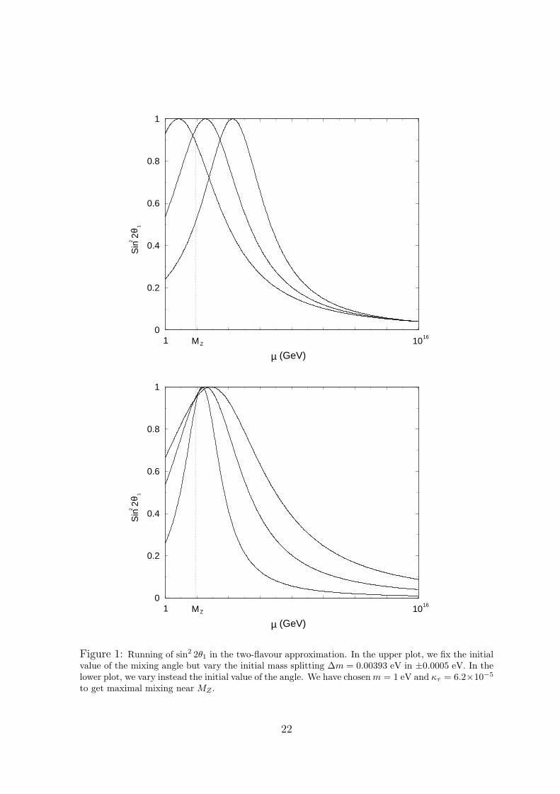
the fine-tuning. Figure 1 illustrates well the behaviour of the running sin2 2θ1 and the

21

0

0.2

0.4

0.6

0.8

1

1 M 10Z16

Sin

2θ

2

1

(GeV)µ

0

0.2

0.4

0.6

0.8

1

1 M 10Z16

Sin

2θ

2

1

(GeV)µ

Figure 1: Running of sin2 2θ1 in the two-flavour approximation. In the upper plot, we fix the initialvalue of the mixing angle but vary the initial mass splitting ∆m = 0.00393 eV in ±0.0005 eV. In thelower plot, we vary instead the initial value of the angle. We have chosen m = 1 eV and κτ = 6.2×10−5

to get maximal mixing near MZ .

22

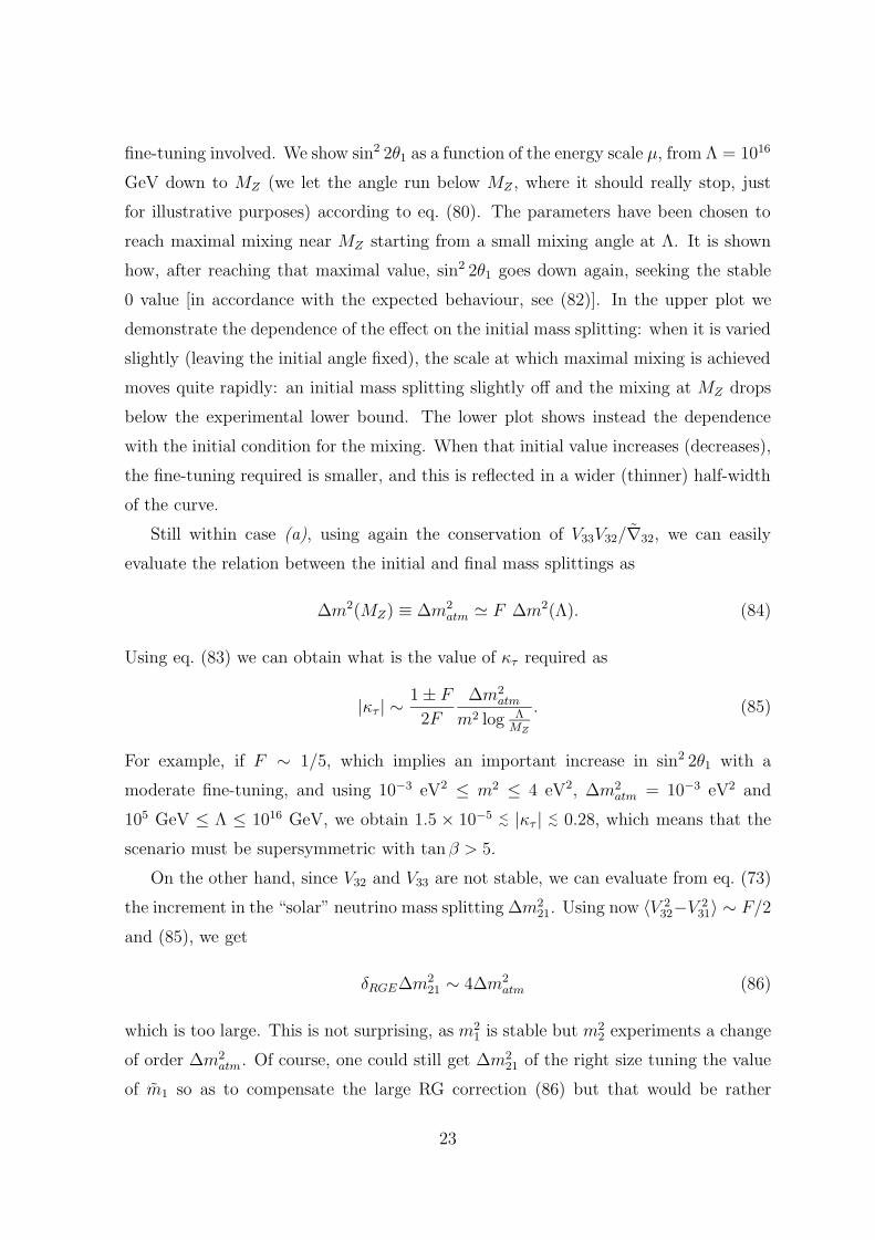
fine-tuning involved. We show sin2 2θ1 as a function of the energy scale µ, from Λ = 1016

GeV down to MZ (we let the angle run below MZ , where it should really stop, just

for illustrative purposes) according to eq. (80). The parameters have been chosen to

reach maximal mixing near MZ starting from a small mixing angle at Λ. It is shown

how, after reaching that maximal value, sin2 2θ1 goes down again, seeking the stable

0 value [in accordance with the expected behaviour, see (82)]. In the upper plot we

demonstrate the dependence of the effect on the initial mass splitting: when it is varied

slightly (leaving the initial angle fixed), the scale at which maximal mixing is achieved

moves quite rapidly: an initial mass splitting slightly off and the mixing at MZ drops

below the experimental lower bound. The lower plot shows instead the dependence

with the initial condition for the mixing. When that initial value increases (decreases),

the fine-tuning required is smaller, and this is reflected in a wider (thinner) half-width

of the curve.

Still within case (a), using again the conservation of V33V32/∇32, we can easily

evaluate the relation between the initial and final mass splittings as

∆m2(MZ) ≡ ∆m2atm ' F ∆m2(Λ). (84)

Using eq. (83) we can obtain what is the value of κτ required as

|κτ | ∼ 1± F

2F

∆m2atm

m2 log ΛMZ

. (85)

For example, if F ∼ 1/5, which implies an important increase in sin2 2θ1 with a

moderate fine-tuning, and using 10−3 eV2 ≤ m2 ≤ 4 eV2, ∆m2atm = 10−3 eV2 and

105 GeV ≤ Λ ≤ 1016 GeV, we obtain 1.5 × 10−5 <∼ |κτ | <∼ 0.28, which means that the

scenario must be supersymmetric with tan β > 5.

On the other hand, since V32 and V33 are not stable, we can evaluate from eq. (73)

the increment in the “solar” neutrino mass splitting ∆m221. Using now 〈V 2

32−V 231〉 ∼ F/2

and (85), we get

δRGE∆m221 ∼ 4∆m2

atm (86)

which is too large. This is not surprising, as m21 is stable but m2

2 experiments a change

of order ∆m2atm. Of course, one could still get ∆m2

21 of the right size tuning the value

of m1 so as to compensate the large RG correction (86) but that would be rather

23

unnatural. So, we conclude that the scenario (a), or equivalently eq. (79), cannot

implement a substantial increase of sin2 2θ1 in practice.

Let us consider now scenario (b). In principle, it can be acomplished in many cases.

Namely, whenever m21

<∼ m22 � m2

3 (hierarchical spectrum); m21 ' m2

2 � m23 (inter-

mediate or pseudo-Dirac spectrum); or m21 ' m2

2 ' m23 (degenerate spectrum) with

m1/m2 > 0 and ∆m221 � ∆m2

32. In the first two cases, ∇32 ' −1. Therefore, if one

demands a significant increase of sin2 2θ1 in eq. (80), then one needs |κτ | log ΛMZ

>∼ 1,

which signals the breakdown of perturbation theory. With regard to the degenerate

case, since m1 and m2 have equal signs, the neutrinoless double β-decay constraint im-

plies that m <∼ 0.2 eV, see eq. (12). This means that |∇32| cannot be very large. Taking

∆m2atm > 10−3 eV2, we get |∇32| = 4m2/∆m2

atm<∼ 160. Therefore, an appreciable vari-

ation of sin2 2θ1 requires |κτ | log ΛMZ

∼ ∆m2atm/m2 >∼ 1/40, which means tan β > 50,

quite a large value. Anyway, in this degenerate case, |∇21| � |∇32|. Consequently, if

|∇32| is large enough to modify the V3i entries (which is our assumption), ∇21 will lead

to V31 → 0 (or equivalently V32 → 0) rapidly, which requires an SAMSW scenario [see

discussion after eq. (71)]. But this is disastrous: from eq. (73), noting that 〈V 232 − V 2

31〉is necessarily sizeable, |δRGE∆m2

21| = O(∆m2atm), in disagreement with observations

(again barring an unnatural cancellation between the initial and the RG-induced mass

splitting).

To summarize, the two-flavour approximation for the running of the θ1 angle can

be a good one if the previous (a) or (b) conditions are fulfilled. Then the size of κτ∇32

will determine whether sin2 2θ1 can get a substantial increase or not. If it can, then

∆m221 will get too large along the running.

The possibility of obtaining an enhancement of sin2 2θ1 by the RG running seems

so attractive that one may wonder if it could be realized in a 3-flavour scenario. Unfor-

tunately, things do not seem to improve much. From the previous discussion, it is clear

that the only possibility to consider here is m21 ' m2

2 ' m23 (degenerate spectrum)

with m1/m2 < 0 and ∆m221 � ∆m2

32. Otherwise, the scenario is equivalent to the

two-flavour case, which we know does not work, or it has too small κτ∇ij to produce

appreciable modifications in the angles. In the scenario selected only κτ ∇32 can be

relevant. The effect of the running on the ∆m221 splitting is still given by eq. (73),

which means that we will get |δRGE∆m221| = O(∆m2

atm) (unacceptable in any scenario)

unless V 232−V 2

31 ∼ 0. This condition can be certainly arranged at low energy (i.e. at the

24

final point of the running) using s2 = 0, sin2 2θ3 = 1 (which implies a nearly bimaximal

scenario). However, if the running is going to modify appreciably the matrix V (which

is mandatory to get an important enhancement of sin2 2θ1) this condition will not be

stable. Notice that the dominance of κτ∇32 imply that V31 ' const., while V32, V33

should vary substantially. In consequence the final ∆m221 will be again too large.

Schematically, the modification of the matrix U (starting with low sin2 2θ1) will be1√2

− 1√6

1√3

−12

12√

32√6

12

√3

20

→

1√2

1√2

0

−12

12

1√2

12

−12

1√2

→

1√2

1√3

− 1√6

−12

2√6

12√

312

0√

32

. (87)

(This example has cos θ1 ∼ 0, but the conclusions are the same for examples with

sin θ1 ∼ 0). In the initial part of the running sin2 2θ1 experiments a large enhancement,

so the parameters (κτ∇32 and Λ) should be tuned to have the running finishing at the

intermediate point. But in any case, it is apparent that V 232−V 2

31 6= 0 along the running,

thus yielding too large ∆m221.

4 Implications (general complex case)

Non-zero CP-violating phases can have a non-trivial effect on the RG evolution of

neutrino mixing angles and masses. Such effects have been considered previously in a

2 generation case [21]. With the formalism presented in section 2 we can undertake

easily the more realistic analysis for 3 generations.

As in the previous section, we will assume that below the high-energy scale Λ, the

effective theory is just the SM or the MSSM, plus the effective Majorana mass matrix

for the neutrinos. As shown in sect. 2, the RGEs for the neutrino masses and the

matrix U are given by eqs. (15, 16), with the appropriate substitutions. Explicitly,

dmi

dt= −2mi|U3i|2 −miκU , (88)

dU

dt= UT, (89)

where κU gives a universal effect [see eqs. (35, 37)] and

Tii = 0

Tij = κτ

[∇ijRe(U∗

3iU3j) + i∇−1ij Im(U∗

3iU3j)], (i 6= j). (90)

25

The explicit RGEs for the mixing angles, the CP-violating phases and the unphysical

phases are given by eqs. (23–31), using everywhere the substitutions of eqs. (39, 41).

As in the real case, large effects in the radiative corrections are expected when

the neutrino spectrum has (quasi)-degenerate eigenvalues. When the degeneracy is

sufficiently good (see previous section), U changes rapidly from its unperturbed t = 0

form to a stable form that has non-singular dU/dt. To be more precise, if mi ' mj ,

then |∇ij| � 1, and U is rapidly driven to a form that ensures Tij ' 0. Since near

t = 0, one has Tij ∼ ∇ijRe(U∗3iU3j), the stable form, say U ′, must satisfy

Re(U ′∗3iU

′3j) = 0 (91)

for any pair i, j with mi ' mj . Since the unphysical phase ατ , cancels out in the

previous equation, we can also write

Re(W ′∗3iW

′3j) = 0, (92)

where the matrix W was defined in eq. (5).

If all masses are quite different, then no dramatic RG effects appear and the discus-

sion is similar to the corresponding one in the real case (see previous section). In the

following subsections we then consider the two interesting cases of two-fold or three-

fold degeneracy. The following general analysis contains as a particular case the real

scenario considered in detail in the previous section. Note that now, two real scenar-

ios with degenerate masses of either equal or opposite signs are treated together and

correspond to choices of φ (or φ′) equal to 0 or π, respectively. Note that, although

the case with opposite signs has now a very large |∇ij|, having φ − φ′ = π gives a Tij

under control, and the case is, of course, stable.

As in the real case, for the discussion of cases of physical relevance, we will as-

sume that the solar neutrino problem is solved by one of the standard solutions, with

|∆m221| � |∆m2

32| ∼ |∆m231|.

4.1 Three-fold degeneracy

In the case m1 ' m2 ' m3 ' m, with |κτ∇ij | � 1 for all i, j, the matrix U (or

equivalently W ) quickly reaches a stable value U ′ (W ′) with

Re(W ′∗31W

′32) = Re(W ′∗

32W′33) = Re(W ′∗

31W′33) = 0. (93)

26

Using the fact that W ′33 is real in the parametrization (4), the last two equalities in

(93) imply

W ′33 = 0 or Re(W ′

31) = Re(W ′32) = 0. (94)

If W ′33 6= 0, eq. (94) and the first equality in (93) imply

W ′31 = 0, or W ′

32 = 0. (95)

In other words, there must be some W ′3i = 0 (the ambiguity in the labelling of the

three original eigenvalues is reflected in the ambiguity in the i-label of W ′3i = 0). Then,

by unitarity, the values of |W ′3j |2 = |U ′

3j|2 are {0, x, 1− x}, with 0 ≤ x ≤ 1 (the value

of x is determined by the initial form of the matrix W ). So, from the expressions for

dmi/dt we obtain the following low-energy shifts in the mass eigenvalues:

∆mi ' mετ{0, x, 1− x}, (96)

where m is essentially the initial value of the three masses at the scale Λ.

Therefore, for a given value of x we know how the degeneracy in the mass spectrum

is lifted and then the labelling of the three eigenvalues is determined according to our

convention (thus U ′ is fixed). It is then easy to show that no value of x gives a stable

U ′ in agreement with the available experimental information on the neutrino mixing

angles. For x < 0.25 (or > 0.75) one has U ′31 → 0 and |U33|2 > 0.75, in conflict with the

limit c21c

22 < 0.71 which follows from the experimental bound (8). For 0.25 < x < 0.75,

U ′33 → 0 instead, and this is also incompatible with experimental limits: it implies

either c22 → 0 [in conflict with (7)], or c2

1 → 0 [in conflict with (8)].

In summary, the case of three-fold degeneracy of initial neutrino masses leads to a

stable U ′ which does not accomodate the values of θi and ∆m2ij suggested by exper-

iment. Note that this analysis contains and expands the subcases (i)–(ii) for real U

analyzed in the previous section. This negative result has two obvious way-outs. If the

spectrum is almost degenerate, but all |κτ∇ij | � 1, then the matrix U is very slightly

renormalized, so it never reaches the stable (disastrous) form. In this case the RG cor-

rections to mixing angles and phases are basically irrelevant. This extreme situation

is difficult to implement in the VO scenario, since |κτ∇21| is necessarily sizeable. The

second way-out is that |κτ∇32| � 1 (even though |∇32| � 1), while |κτ∇21| can be sig-

nificant. This will occur if the ∆m232 splitting is arranged to sensible (“atmospheric”)

27

values from the beginning. Then, the analysis for the mixing angles and CP phases is

identical to a case with two-fold degeneracy, which is analyzed in the next subsection.

4.2 Two-fold degeneracy

We assume here that the initial ∆m232, ∆m2

31 splittings are large enough to keep m3

as the most split eigenvalue after the RG effects, while m1 ' m2. In this case, only

|κτ∇21| >∼ 1. This drives the original matrix U to a stable form U ′ given by (see

Appendix)

U ′ = UR12(Γ), (97)

where R12(Γ) is a rotation in the 1-2 plane by an angle Γ, to be computed below. We

see that the third column of U is not changed appreciably, in accordance with the

fact that dUi3/dt does not depend on ∇21. The rotation angle Γ is determined by the

condition (91)

Re(U ′∗31U

′32) = 0, (98)

which gives

tan 2Γ =2Re(U∗

31U32)

|U32|2 − |U31|2 . (99)

This allows to determine U ′ completely and thus the physical parameters as a function

of the initial conditions. Let us examine this issue in closer detail.

With regard to the mixing angles, from the RGEs (23–25) one immediately sees

that θ1 and θ2 are not renormalized strongly (dθ1,2/dt do not depend on T12) while θ3

is driven to a stable value, θ(f)3 . More precisely,

θ(f)1 ' θ1

θ(f)2 ' θ2

sin2 2θ(f)3 = p2 + q2, (100)

where

p = sin 2Γ sin[(φ− φ′)/2], (101)

and

q = sin 2Γ cos 2θ3 cos[(φ− φ′)/2] + sin 2θ3 cos 2Γ. (102)

28

The CP-violating phases are also driven to particular values δ(f), φ(f), φ′(f) which are

complicated functions of the initial values of the parameters in U :

tan δ(f) =q tan δ − p

q + p tan δ, (103)

tan[(φ(f) − φ′(f))/2] =sin 2θ3 sin[(φ− φ′)/2]

cos 2Γ sin 2θ3 cos[(φ− φ′)/2] + sin 2Γ cos 2θ3

, (104)

and

φ(f) + φ′(f) − 2δ(f) = φ + φ′ − 2δ. (105)

The last equation follows from d(φ + φ′ − 2δ)/dt ' 0, which can be checked directly

from (26)-(28).

As explained in section 2, see (32-34), other quantities of interest which are con-

served in this case are Im(U∗k1Uk2). For k = 1, we obtain the conserved quantity

sin 2θ3 sin[(φ− φ′)/2], (106)

and, for k = 2, 3,

sin[(φ− φ′)/2] cos δ cos 2θ3 − sin δ cos[(φ− φ′)/2]. (107)

These expressions can be sometimes conveniently used instead of the explicit formulas

(100)-(104).

For physical applications it is interesting to use for θ1 and θ2 the values suggested by

experiment6, sin2 2θ1 ∼ 1 and θ2 ∼ 0, which permits to obtain more explicit expressions

for θ3 and the CP-violating phases at low energy. In doing this, it is important to keep

corrections due to a small (but non-zero) value of θ2, as they can become dominant for

some choices of the parameters. For the angle θ(f)3 , we obtain the remarkably simple

expression

sin2 2θ(f)3 = sin2 2θ3 sin2[(φ− φ′)/2] +O(s2

2), (108)

which gives the final θ(f)3 as a function of the initial θ3 and φ − φ′. We see that, for

the SAMSW solution of the solar neutrino problem, we must have either sin2 2θ3 ∼ 0

or sin2[(φ − φ′)/2] ∼ 0 at the scale Λ. On the other hand, if the solar mixing is also

6Due to the stability of θ1 and θ2, this initial condition at Λ is approximately maintained by RGevolution down to MZ . The origin of such initial condition could be some flavour symmetry or perhapsa fixed point in the RG running above Λ.

29

maximal, sin2 2θ(f)3 ∼ 1, then both sin2 2θ3 and sin2[(φ − φ′)/2] must be of order 1

originally.

A word of caution should be said about the higher order term in (108). The

neglected term, calculated exactly, is [we introduce the short-hand notation ϕ ≡ (φ−φ′)/2 and σ ≡ sin 2θ1 = ±1]:

4s22

N21

D21 + D2

2

, (109)

with

N1 = cϕcδ + sϕsδc2θ3 ,

D1 = −cϕc22s2θ3 + 2σs2(cϕcδc2θ3 + sϕsδ),

D2 = c22c2θ3 + 2σs2cδs2θ3 , (110)

where all the quantities are understood at the initial (high energy) scale. For generic

values of the parameters, the term (109) will be negligible as it is formally O(s22).

However, for some particular choices of the parameters the denominator in (109) can be

also O(s22) resulting in a non-suppressed correction in (108). This occurs, for example,

if c2θ3 ' 0 and cϕ ' 0 simultaneously.

Expressions (108) and (109) for sin2 2θ(f)3 , in conjunction with the conserved quan-

tities (105–107), are enough to determine exactly the rest of parameters at low-energy.

For example, we obtain

tan2[(φ(f) − φ′(f))/2] =sin2 2θ3 sin2 ϕ(D2

1 + D22)

4 sin2 θ2N21

, (111)

Note the 1/s22 dependence that would generically drive φ(f) − φ′(f) → ±π. However,

this is not necessarily the case because the smallness of s2 can be compensated by a

small numerator in (111), as commented above.

If φ = φ′ initially, it is easy to see that the only physical parameter that undergoes a

sizable change is θ3, with θ(f)3 = θ3+Γ. This follows directly from U ′ = UR12(Γ) because

now R12(Γ) commutes with diag(eiφ, eiφ, 1). Moreover, eq. (108) gives θ(f)3 → O(s2) ∼ 0

irrespective of the initial value of θ3. This is just right for the SAMSW solution of the

solar neutrino problem and reproduces the result discussed in the previous section for

the real case. We see however that this appealing possibility dissappears for generic

values of φ and φ′.

If φ− φ′ = ±π instead, one gets tan 2Γ ∼ s2 sin δ. For θ2 = 0 or δ = 0 this implies

a stable matrix U from the beginning, see eq. (97). This is in correspondence with

30

the real case φ = 0, φ′ = π discussed in the previous section. For non-zero values of δ

and/or θ2, however, the matrix U is no longer stable, although typically Γ, and thus

the corrections to U , will be small. We conclude that, the presence of a non-zero phase

δ = 0 tends to destabilize this scenario, but the effect is small for small θ2.

Another interesting result that we can extract from eq. (103) is the possiblility of

generating a non-zero phase δ(f) even if δ = 0 originally, provided the phases φ, φ′ are

non zero and satisfy sin[2(φ− φ′)] 6= 0. The resulting δ(f), when δ = 0, is given by

tan δ(f) = −p

q, (112)

or, explicitly,

tan δ(f) =−sϕcϕ(c2

2 sin 2θ3 − 2σs2 cos 2θ3)

c22s

2ϕ sin 2θ3 cos 2θ3 + 2σs2(1− s2

ϕ cos2 2θ3)(113)

This shows that one can generate radiatively even a maximal value for the CP-violating

phase.

4.3 Neutrino masses

In the complex case, the running of the neutrino mass eigenvalues is governed by

dmi

dt= −2κτmi|U3i|2 − κUmi, (114)

and many of the generic results obtained in the real case go over to the complex one.

Some of the significant differences are discussed in this subsection.

From (114) we see that the phases φ and φ′ do not affect directly the running of the

masses. However, they have an important influence in the stability of a given choice of

the matrix U , and this in turn will influence the evolution of the masses. For example,

in the degenerate case m1 ' m2 = m0, the initial choices φ − φ′ = 0 and φ − φ′ = π

(which correspond to m1 ' ±m2, already analyzed in the real case) give identical

dmi/dt at t = 0. However, in the first case U changes abruptly, while in the second

it evolves smoothly, and this has an evident effect on the subsequent running of m1,2.

The phase δ, on the other hand, enters U31 and U32, and thus has a direct effect on the

size of dmi/dt, although its importance is somewhat reduced by the smallness of θ2.

One important instance in which the stability of U is crucial for the viability of

the scenario is the VO solution to the solar neutrino problem. As discussed in the real

31

0.2 0.4 0.6 0.8 1

0.2

0.4

0.6

0.8

1

0.2 0.4 0.6 0.8 1

0.2

0.4

0.6

0.8

1

sin22θ2

sin22θ3

sin22θ1=1

0.2 0.4 0.6 0.8 1

0.2

0.4

0.6

0.8

1

0.2 0.4 0.6 0.8 1

0.2

0.4

0.6

0.8

1

sin22θ2

sin22θ3

sin22θ1=0.82

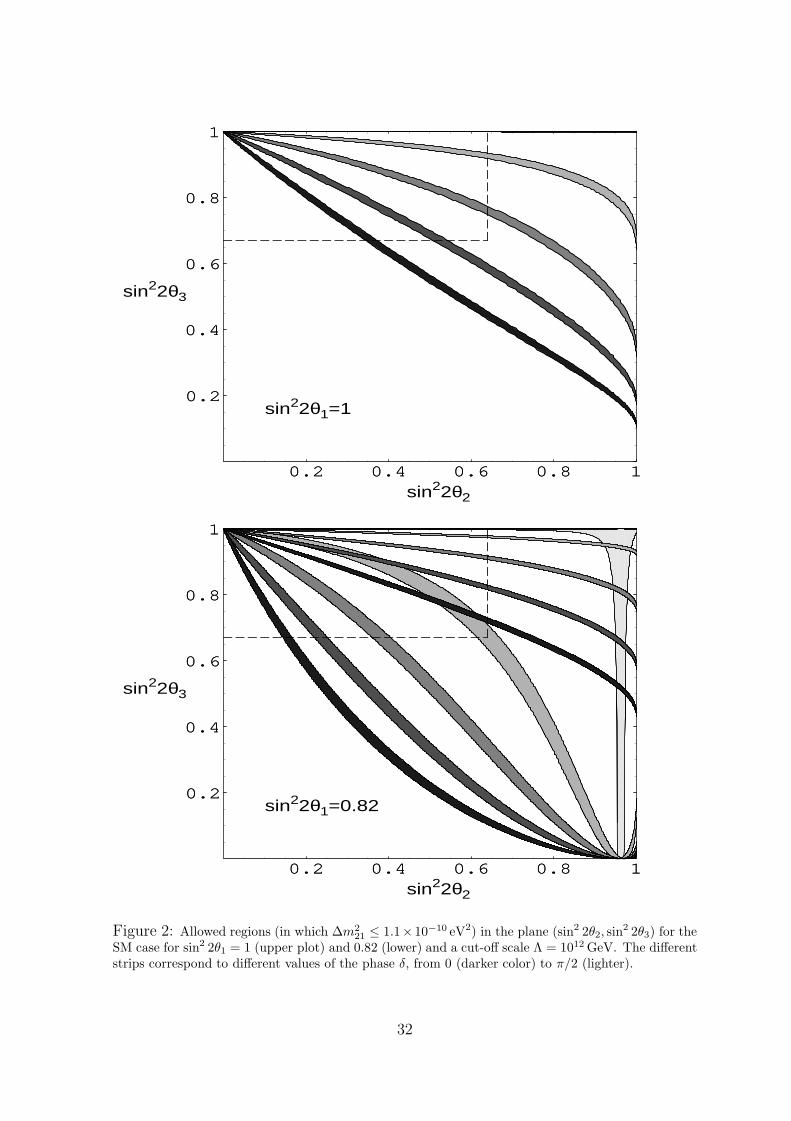
Figure 2: Allowed regions (in which ∆m221 ≤ 1.1×10−10 eV2) in the plane (sin2 2θ2, sin2 2θ3) for the

SM case for sin2 2θ1 = 1 (upper plot) and 0.82 (lower) and a cut-off scale Λ = 1012 GeV. The differentstrips correspond to different values of the phase δ, from 0 (darker color) to π/2 (lighter).

32

case, in a scenario with total or partial degeneracy of neutrino masses, the final ∆m221

has to be much smaller than the typical size of the RG shift in the masses squared

∼ 2m20ετ . Hence, starting with m1 ' m2 � m3 at the high energy scale Λ, to keep

∆m221 under control requires an exquisite cancellation in the running of m1 and m2.

From (114), this cancellation is

|(|U ′31|2 − |U ′

32|2)| <∼∆m2

sol

4m20ετ

. (115)

In this condition, we have written U ′ and not U , because if the degeneracy is good

enough U jumps to U ′ almost immediately away from Λ and remains close to it during

the rest of the running down to MZ . By definition, U ′ satisfies the stability condition

Re(U ′∗31U

′32) = 0. (116)

From (115) we find that, to keep the solar mass splitting under control, the mixing

angles (at low energy) must be correlated according to

tan 2θ3 ' cos2 θ1 sin2 θ2 − sin2 θ1

sin θ2 sin 2θ1 cos δ. (117)

This equation generalizes (74) to the complex case. Eqs. (116, 117) must be satisfied

simultaneously for the viability of the VO scenario in totally or partially degenerate

scenarios.

From eq. (117) we can see that a non-zero δ will influence the correlations that must

occur. The effect is discussed in figure 1, where, for two different values of sin2 2θ1 (the

maximal one, 1, and the experimental lower bound, 0.82) we plot the region of the

plane (sin2 2θ2, sin2 2θ3) where the cancellation (115) takes place. The different strips7

correspond to different values of cos δ, from 1 (darker color) to 0 (lighter), in 1/4

steps. We set the high energy scale Λ at the typical see-saw value 1012 GeV and require

∆m212 ≤ 1.1 × 10−10 eV2 with the initial neutrino mass m2

0 = ∆m2atm = 5 × 10−4 eV2.

For much smaller Λ the strips in figure 1 get thicker [it is easier to satisfy (115) because

the size of radiative corrections is smaller]. Note that δ = π/2 is special because, in

such case, eq. (117) has in principle two solutions: a) sin2 2θ3 = 1 and b) s22 = tan2 θ1.

The region satisfying (115) will consist of two strips centered around those two lines.

7For a fixed value of sin2 2θ2 and sin2 2θ1 there are in principle 4 values of sin2 2θ3 satisfying (117),corresponding to the fact that the interchange cos θ → sin θ leaves sin2 2θ invariant. We do not plotthe two solutions with s2 > c2, which would be in conflict with CHOOZ+SK data. Note that, forsin2 2θ1 = 1 the two remaining solutions merge in one.

33

In the case sin2 2θ1 = 1, the solution b) gives s22 = 1, which is beyond experimental

bounds and only solution a), sin2 2θ3 = 1, remains (the region around that line has

zero width and cannot be seen in the plot). For sin2 2θ3 < 1, solution b) can have

s2 < c2 and we include it in the figure. The corresponding region is T-shaped like the

one shown in figure 1, lower plot.

On the other hand, the condition (116) for stability can be satisfied for any choice

of mixing angles and δ by adjusting φ− φ′ to the apropriate value, which is given by

tan[(φ− φ′)/2] =sin 2θ3(sin2 θ1 − cos2 θ1 sin2 θ2)− sin 2θ1 cos 2θ3 sin θ2 cos δ

sin 2θ1 sin θ2 sin δ. (118)

This would be the complex version of the requirement of opposite signs for the two

degenerate eigenvalues in the real case. Using (117), the previous result simplifies

further to

tan[(φ− φ′)/2] = − 1

tan δ cos 2θ3. (119)

Unlike the real case, to impose condition (118) for generic values of the parameters,

seems hard to justify from some underlying symmetry.

5 Conclusions

Assuming three flavours of light Majorana neutrinos, with no reference to any particular

scenario, we have derived the general renormalization group equations (RGEs) for

the physical neutrino parameters: three masses, three mixing angles and three CP-

violating phases [information alternatively encoded in the RGE for the masses and

the complex mixing (MNS) matrix U ]. This form of writing the RGEs represents

an advantageous alternative to using the RGE for Mν . It avoids the proliferation of

unphysical parameters, which allows to keep track of the physics in a more efficient

way. It also permits to appreciate interesting features, e.g. presence of stable (pseudo

infrared fixed-point) directions for mixing angles and phases, which are not consequence

of a particular scenario.

We have then particularized the RGEs for relevant scenarios. Namely, when the

effective theory below Λ (the scale at which the neutrino mass operator is generated),

is given by the SM or MSSM; or when Mν is generated by a see-saw mechanism. In the

first two scenarios we have analyzed in detail the physical implications of the RGEs,

separating the case where U is real (i.e. no CP phases) and the general complex case.

34

For the real case, we have noticed that if one starts with two masses suficiently

degenerate (in absolute value and sign), say mi ' mj , the U matrix is driven to

a stable (infrared pseudo-fixed point) form, providing net predictions for the mixing

angles. Whenever this happens the corresponding mass splitting, ∆m2ij , is entirely

determined at low energy by the RG running. This amounts to a very predictive

scenario. Depending on what are the initial (quasi) degenerate neutrinos, the scenario

can be realistic or not. In particular, starting with m1 ' m2 and an initial ∆m232 ∼

∆m2atm, we finish at low energy with a small “solar” θ3 angle and a ∆m2

21 splitting

just of the right size for the SAMSW solution to the solar neutrino problem, which

is certainly remarkable. On the other hand, the radiative corrections to the mass

splittings are potentially dangerous for the VO scenario, which becomes unviable if

m21 ' m2

2 � m23, unless m1 ' −m2, the “solar” θ3 angle is close to maximal and the

common mass is below the range of cosmological relevance.

We have also shown that previous claims (realized in the two-flavour approximation)

in the sense that the RG running could provide a substantial enhancement of the

atmospheric mixing, sin2 2θ1 cannot work in practice, since the mechanism leads to an

unacceptably large “solar” splitting, ∆m221. We have shown that, unfortunately, this

is also the case in the more general 3-flavour scenario.

For the general complex case, most of the conclusions are similar, but there are

interesting new effects. In particular, the previously considered “radiative” SAMSW

scenario requires φ−φ′ ' 0 (unless the “solar” θ3 angle is set by hand at a small value

from the beginning). On the other hand, if φ−φ′ is different from zero and the neutrino

spectrum has a two-fold degeneracy, the RGEs will generically drive its value to ±π.

It is also worth-noticing that the CP phase δ can be driven to maximal values by RG

corrections. On the other hand, if cos δ 6= 0, the viability of the VO scenario when

m21 ' m2

2 requires, besides the previous conditions, a delicate cancellation involving

the three CP phases, which makes the scenario more unnatural.

Addendum

Shortly after the completion of this work, there appeared a paper by P.H. Chankowski,

W. Krolikowski and S. Pokorski [27] dealing with similar subjects. More precisely,

they work out the RGEs for mass eigenvalues and mixing angles below the high energy

35

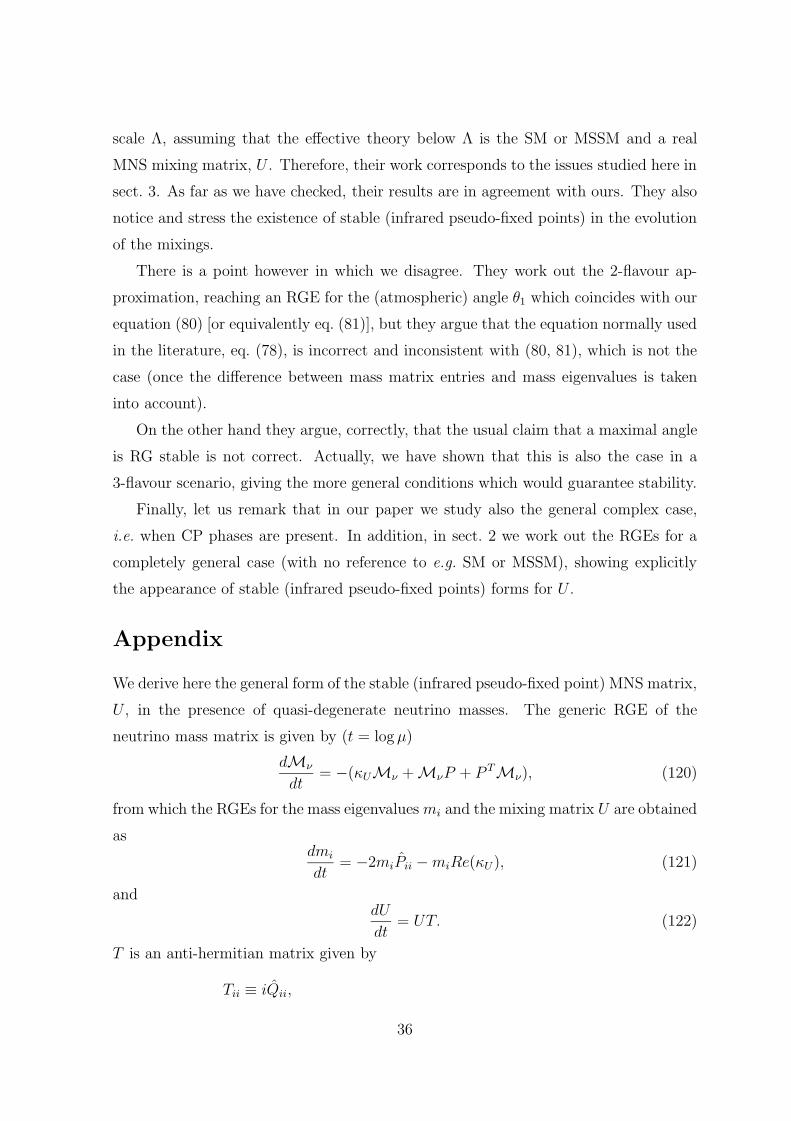
scale Λ, assuming that the effective theory below Λ is the SM or MSSM and a real

MNS mixing matrix, U . Therefore, their work corresponds to the issues studied here in

sect. 3. As far as we have checked, their results are in agreement with ours. They also

notice and stress the existence of stable (infrared pseudo-fixed points) in the evolution

of the mixings.

There is a point however in which we disagree. They work out the 2-flavour ap-

proximation, reaching an RGE for the (atmospheric) angle θ1 which coincides with our

equation (80) [or equivalently eq. (81)], but they argue that the equation normally used

in the literature, eq. (78), is incorrect and inconsistent with (80, 81), which is not the

case (once the difference between mass matrix entries and mass eigenvalues is taken

into account).

On the other hand they argue, correctly, that the usual claim that a maximal angle

is RG stable is not correct. Actually, we have shown that this is also the case in a

3-flavour scenario, giving the more general conditions which would guarantee stability.

Finally, let us remark that in our paper we study also the general complex case,

i.e. when CP phases are present. In addition, in sect. 2 we work out the RGEs for a

completely general case (with no reference to e.g. SM or MSSM), showing explicitly

the appearance of stable (infrared pseudo-fixed points) forms for U .

Appendix

We derive here the general form of the stable (infrared pseudo-fixed point) MNS matrix,

U , in the presence of quasi-degenerate neutrino masses. The generic RGE of the

neutrino mass matrix is given by (t = log µ)

dMν

dt= −(κUMν +MνP + P TMν), (120)

from which the RGEs for the mass eigenvalues mi and the mixing matrix U are obtained

asdmi

dt= −2miPii −miRe(κU), (121)

anddU

dt= UT. (122)

T is an anti-hermitian matrix given by

Tii ≡ iQii,

36

Tij ≡ ∇ijRe(Pij) + i[∇ij]−1Im(Pij) + iQij , i 6= j, (123)

with P ≡ 12U †(P + P †)U , Q ≡ − i

2U †(P − P †)U and ∇ij ≡ (mi + mj)/(mi −mj).

Let us suppose that two mass eigenvalues, say m1 and m2, are almost degenerate

at the initial high-energy scale Λ. Then, near the starting point of the running, t ∼ t0,

T is dominated by the (real) terms proportional to ∇12

T ∼ 0 −Re(T21) 0

Re(T21) 0 00 0 0

. (124)

Then, the formal solution to eq. (122) is given by

U ′ ≡ U(t) ∼ Uexp

0

∫ tt0

Re(T21)dt 0− ∫ t

t0Re(T21)dt 0 0

0 0 0

= UR12(Γ), (125)

where R12(Γ) is an ordinary rotation in the 1–2 plane by an angle Γ

R12(Γ) =

cΓ sΓ 0−sΓ cΓ 0

0 0 1

. (126)

The value of Γ will be such that dU/dt becomes non-singular, i.e. it renders Re(T12) '0. Thus the stable matrix U ′ satisfies

Re(P ′12) =

1

2Re(U ′†(P + P †)U ′)12 = 0 , (127)

which we can solve for Γ in terms of initial quantities obtaining

tan 2Γ =2Re(P12)

P22 − P11

. (128)

Therefore, using (125), we get unambiguously the stable U ′ matrix in terms of the

initial U .

One can further justify the condition (127) by showing that the RG evolution actu-

ally drives Re(P12) towards zero, as expected. The relevant RG when ∇12 dominates

isd

dtRe(P12) ' (P11 − P22)∇12Re(P12). (129)

For a sufficiently long running interval one has [using (121)]

∇12 ' 1

(P11 − P22) log(Λ/µ), (130)

37

and inserting this in (129) we get Re(P12) → 0 in the infrared.

Let us consider now the only remaining possibility, i.e. that all the mass eigenvalues

m1, m2, m3 are (almost) degenerate. Similarly to the previous case, for t ∼ t0, T is

dominated by the (real) terms

T ∼ 0 −Re(T21) −Re(T31)

Re(T21) 0 −Re(T32)Re(T31) Re(T32) 0

. (131)

So, the solution to eq. (122) is formally given by

U ′ ≡ U(t) ∼ Uexp

0

∫ tt0

Re(T21)dt∫ tt0

Re(T31)dt− ∫ t

t0Re(T21)dt 0

∫ tt0

Re(T32)dt− ∫ t

t0Re(T31)dt − ∫ t

t0Re(T32)dt 0

= UR,

(132)

where R is a general 3× 3 rotation, depending on three angles, say Γ1, Γ2, Γ3,

R =

c2c3 c2s3 s2

−c1s3 − s1s2c3 c1c3 − s1s2s3 s1c2

s1s3 − c1s2c3 −s1c3 − c1s2s3 c1c2

, (133)

with si = sin Γi, ci = cos Γi (the resemblance with the ’CKM’ matrix is only formal).

R is determined, as in the case of twofold degeneracy considered before, by the fact

that dU/dt becomes non-singular, i.e. Re(Tij) ' 0. Thus

Re(P ′12) =

1

2Re(U ′†(P + P †)U ′)12 = 0, (134)

Re(P ′31) =

1

2Re(U ′†(P + P †)U ′)31 = 0, (135)

Re(P ′32) =

1

2Re(U ′†(P + P †)U ′)32 = 0. (136)

Substituting U ′ = UR, these equations determine completely the rotation R, and

therefore U ′, in terms of U and the initial parameters. Another interesting remark is

that if one has information on the mixing angles in the stable matrix U ′, the phases

will be constrained, so as to satisfy the set of equations (134-136). And viceversa, if

the phases are known, the mixing angles cannot take arbitrary values.

Again, one can show that in this case RG evolution drives Re(Pij) → 0 for all i, j.

The relevant RGE that shows this is now

1

2

d

dt

{[Re(P12)]

2 + [Re(P23)]2 + [Re(P31)]2}

= (P11 − P22)∇12[Re(P12)]2

+(P22 − P33)∇23[Re(P23)]2 + (P33 − P11)∇31[Re(P31)]2. (137)

38

Using

∇ij ' 1

(Pii − Pjj) log(Λ/µ), (138)

in the equation above, we get Re(Pij) → 0 in the infrared for all i, j.

Acknowledgements

A. I. thanks the Comunidad de Madrid (Spain) for a pre-doctoral grant.

References

[1] Y. Fukuda et al., Super-Kamiokande Collaboration, Phys. Lett. B433 (1998)

9; Phys. Rev. Lett. 81 (1998) 1562; S. Hatakeyama et al., Kamiokande Collab-

oration, Phys. Rev. Lett. 81 (1998) 2016.

[2] W.W.M. Allison et al., SOUDAN2 Collaboration, Phys. Lett. B391 (1997)

491, Phys. Lett. B449 (1999) 137.

[3] B.T. Cleveland et al., Homestake Collaboration, Astrophys. J. 496 (1998) 505;

K.S. Hirata et al., Kamiokande Collaboration, Phys. Rev. Lett. 77 (1996)

1683; W. Hampel et al., GALLEX Collaboration, Phys. Lett. B388 (1996)

384; D.N. Abdurashitov et al., SAGE Collaboration, Phys. Rev. Lett. 77 (1996)

4708; Y. Fukuda et al., Super-Kamiokande Collaboration, Phys. Rev. Lett. 82

(1999) 1810, Phys. Rev. Lett. 82 (1999) 2430.

[4] B. Pontecorvo, Sov. Phys. JETP 26 (1968) 984.

[5] C. Athanassopoulos et al., LSND Collaboration, Phys. Rev. Lett. 77 (1996)

3082, [nucl-ex/9706006], [nucl-ex/9709006].

[6] S. Weinberg, Phys. Rev. Lett. 43 (1979) 1566.

[7] Z. Maki, M. Nakagawa and S. Sakata, Prog. Theor. Phys. 28 (1962) 870.

[8] A. Apollonio et al., CHOOZ Collaboration, Phys. Lett. B420 (1998) 397, [hep-

ex/9907037].

[9] A. De Rujula, M.B.Gavela and P. Hernandez, Nucl. Phys. B547 (1999) 21.

39

[10] R. Barbieri et al., JHEP 9812 (1998) 017; G.L. Fogli, E. Lisi, A. Marrone and

G. Scioscia, Phys. Rev. D59:033001 (1999), [hep-ph/9904465].

[11] L. Baudis et al., Heidelberg-Moscow exp., [hep-ex/9902014].

[12] V. Lobashev, Pontecorvo Prize lecture at the JINR, Dubna, January 1999; A.I. Be-

lesev et al., Phys. Lett. B350 (1995) 263.

[13] First ref. in [10]; A. Strumia, JHEP 9904 (1999) 026.

[14] L. Wolfenstein, Phys. Rev. D17 (1978) 2369; S.P. Mikheyev and A. Yu Smirnov,

Sov. J. Nucl. Phys. 42 (1986) 913.

[15] J.A. Casas, J.R. Espinosa, A. Ibarra and I. Navarro, Nucl. Phys. B556 (1999) 3.

[16] J.A. Casas, J.R. Espinosa, A. Ibarra and I. Navarro, [hep-ph/9905381], to appear

in Nucl. Phys. B.

[17] J.A. Casas, J.R. Espinosa, A. Ibarra and I. Navarro, JHEP 09 (1999) 015.

[18] J. Ellis and S. Lola, Phys. Lett. B458 (1999) 310.

[19] J. Ellis, G.K. Leontaris, S. Lola and D.V. Nanopoulos, Eur. Phys. J. C9 (1999)

389.

[20] R. Barbieri, G.G. Ross and A. Strumia, [hep-ph/9906470].

[21] N. Haba, Y. Matsui, N. Okamura and M. Sugiura, [hep-ph/9908429].

[22] N. Haba, Y. Matsui, N. Okamura and M. Sugiura, [hep-ph/9904292]; N. Haba and

N. Okamura, [hep-ph/9906481].

[23] E. Ma, J. Phys.G25 (1999) 97.

[24] P.H. Chankowski and Z. P luciennik, Phys. Lett. B316 (1993) 312.

[25] K. Babu, C. N. Leung and J. Pantaleone, Phys. Lett. B319 (1993) 191.

[26] M. Gell-Mann, P. Ramond and R. Slansky, proceedings of the Supergravity Stony

Brook Workshop, New York, 1979, eds. P. Van Nieuwenhuizen and D. Freedman

40

(North-Holland, Amsterdam); T. Yanagida, proceedings of the Workshop on Uni-

fied Theories and Baryon Number in the Universe, Tsukuba, Japan 1979 (edited

by A. Sawada and A. Sugamoto, KEK Report No. 79-18, Tsukuba); R. Mohapatra

and G. Senjanovic, Phys. Rev. Lett. 44 (1980) 912, Phys. Rev. D23 (1981) 165.

[27] P.H. Chankowski, W. Krolikowski and S. Pokorski, [hep-ph/9910231].

41