GC-MS for food safety analysis | Thermo Fisher Scientific
149
GC-MS for food safety analysis Applications compendium
-
Upload
khangminh22 -
Category
Documents
-
view
1 -
download
0
Transcript of GC-MS for food safety analysis | Thermo Fisher Scientific
GC-MS for food safety analysis Applications compendium

In order to protect consumers and the environment, monitoring the food supply to ensure levels of chemical residues and contaminants are compliant with statutory levels set by regulatory bodies is imperative. Because regulations differ in different parts of the world, analytical food testing laboratories and food manufacturers must first navigate the complexity of regulatory frameworks before considering the analysis. Detecting and quantifying many thousands of residues and contaminants from different chemical classes at potentially extremely low levels in diverse food commodities and products is very challenging. This challenge is further complicated when we consider that food products are traded in complex global supply chains, for which details of the history of products, such as cultivation, treatment, storage and processing, are often unknown. For example, the use of pesticides to protect crops from pests during cultivation, storage and transport will often leave detectable residues in food, while persistent organic pollutants (POPs) in the soil, water or in the air can contaminate crops. Additionally, chemicals in food packaging materials can leach into the food. Biocides used in food preparation facilities can also lead to contamination of food. These are just a few examples of many sources of contamination. It is easy to see why the comprehensive analysis of individual samples often requires multiple analyses assessments by a range of analytical techniques, such as liquid chromatography, ion chromatography and gas chromatography in combination with selective detectors and or mass spectrometers, as well as spectroscopic techniques. Thermo Fisher Scientific can offer the complete portfolio of instruments needed for comprehensive, targeted and non-targeted analysis. This compendium focuses on gas chromatographic solutions applicable to testing laboratories involved in food-related analyses.
This compendium incorporates selected application examples to highlight the use of Thermo Fisher Scientific GC-MS portfolio solutions for food analysis. One of the tasks for the analyst is to choose appropriate instrumentation based on the method requirements. The first application example is based on the use of the Thermo Scientific™ TRACE™ 1310 Gas Chromatograph equipped with a flame ionization detector (FID) for the analysis of fatty-acid methyl ester (FAMES) in the profiling of fatty foods. A unique feature of the
Thermo Scientific GC systems is modularity, which allows instant-connect injectors and detectors to be exchanged in minutes without tools, enabling a single GC system to provide a high level of flexibility. The use of head space sampling coupled with GC-FID/MS is demonstrated for the analysis of residual solvents in food packaging materials. Additional applications show the use of the Thermo Scientific™ ISQ™ 7000 single quadrupole GC-MS system for the analysis of phthalates, a ubiquitous contaminant class in plastics, and the quantitation of acrylamide, a process contaminant formed by the Maillard reaction between sugar and amino acid molecules when heated.
The Thermo Scientific™ TSQ™ 9000 triple quadrupole GC-MS/MS system which provides higher selectivity than the ISQ system, is highlighted in combination with automated online micro-SPE food extract cleanup for the analysis of pesticides. Automated micro-SPE is based on the Thermo Scientific™ TriPlus™ RSH robotic autosampler to automate the removal of matrix co-extractives online with GC injection, increasing method robustness and instrument uptime for an ultimate increase in productivity. Applications showing the TSQ 9000, equipped with an Advanced Electron Ionization (AEI) source for unparalleled ultra-high sensitivity, are included to demonstrate the ultra-trace targeted analysis of pesticides, dioxins and polychlorinated biphenyls (PCBs). An upgrade path from the single quadrupole system to any of the triple quadrupole systems, enables laboratories not only to adapt to analytical developments, but also to future proof their investment.
The final applications listed in this compendium focus on Thermo Scientific™ Q Exactive™ GC Orbitrap™ GC-MS/MS system which uses full-scan, high-resolution/accurate-mass non-targeted acquisition with unprecedented resolving power, sub-ppm accurate mass and ppt level sensitivity. The system can be used for targeted analysis of a pre-defined list of chemicals, or non-targeted analysis of unknown chemicals as demonstrated by the accurate and precise quantitation of pesticides, POPs and the profiling of food packaging materials.
More information on these technologies is available here.
Introduction
Back to contents2

GC-FID FAMES analysis 4
Rapid qualitative and quantitative analysis of residual solvents in food packaging by static headspace coupled to GC-FID/MS 15
Single quadrupole GC-MS Routine determination of phthalates in vegetable oil by single quadrupole GC-MS 24
Simple and cost-effective determination of acrylamide in food products and coffee using Gas Chromatography-Mass Spectrometry 33
Triple quadrupole GC-MS/MS Automated micro-SPE clean-up for GC-MS/MS analysis of pesticide residues in cereals 42
Ultra-low level quantification of pesticides in baby foods using an advanced triple quadrupole GC-MS/MS 64
Fast, ultra-sensitive analysis of PBDEs in food using advanced GC-MS/MS technology 86
Routine, regulatory analysis of dioxins and dioxin-like compounds in food and feed samples 101
GC high resolution accurate mass Characterizing unknowns in food packaging using GC Orbitrap mass spectrometry 116
Multi-residue pesticide screening in cereals using GC-Orbitrap mass spectrometry 125
The quantitative power of high-resolution GC-Orbitrap mass spectrometry for the analysis of pesticides and PCBs in food 134
Determination of short- and medium-chained chlorinated paraffins in salmon samples using GC Orbitrap-MS 143
Contents
3

No
. 21557
APPLICATION NOTE
Separation of 37 Fatty Acid Methyl Esters Utilizing a High-Efficiency 10 m Capillary GC Column with Optimization in Three Carrier Gases
Key Words TR-FAME, fatty acid methyl esters, FAMEs, GC, GC-MS, carrier gas
Goal To demonstrate the separation of 37 fatty acid methyl esters (FAMEs) on the highly efficient 10 m Thermo Scientific™ TRACE™ TR-FAME GC column, and to show increased sample throughput of up to 400% relative to a 100 m column by optimizing the separation for efficiency and speed using three commonly available carrier gases: nitrogen, hydrogen, and helium.
IntroductionFats are a major constituent of many foodstuffs including edible oils, meat, fish, grain, and dairy products. They consist of triacylglycerides, which are species that contain glycerol sub-units esterified with aliphatic fatty acid groups (Figure 1).
The aliphatic chain can vary in carbon length, degree of unsaturation, and isomerization around double bonds giving cis and trans forms of the fatty acids. Trans and hydrogenated fats are important food components that are regularly measured.
Aaron L. Lamb Thermo Fisher Scientific, Runcorn, UK
Figure 1. A general triacylglyceride.
4 Back to contents
2
Gas chromatography (GC) is a common method for determining identity and concentration of fatty acids. In order for the fatty acids to be analyzed by GC, the fats in any given matrix require a three-step preparation that includes: • Extraction from the matrix with a non-polar solvent for clean-up
• Saponification, rendering the free fatty acids
• Derivatization to FAMEs for more amenable analysis
Derivatization of the saponified fatty acids via methylation leads to the formation of the corresponding fatty acid methyl esters (FAMEs), which are the preferred derivatives due to their volatility and high thermal stability. However, separation of the 37 common FAMEs can be difficult to achieve as many differ only slightly in their physical and chemical properties.
Generally, high polarity cyanopropyl or biscyanopropyl chemistries are employed for GC separation to provide the necessary selectivity and resolve all components. In these instances, 100 m columns are often used to provide the required resolution; however, they are expensive, analysis times are extended, and sample throughput is low. This can result in a very high cost of analysis per sample.
TRACE TR-FAME columns have a high polarity phase optimized for FAME analysis. The 70% cyanopropyl polysilphenylene-siloxane phase utilized has a higher operating temperature compared to some other columns and gives extremely low bleed, making it amenable to detection by mass spectrometry.
Here, the advantages of utilizing shorter, high-efficiency FAME columns for this complex analysis are investigated. Higher throughput and potential cost savings for the customer can be realized if the shorter columns provide similar performance and reduced analysis time when compared to commonly used 100 m columns. Additionally, the effects of different carrier gases on the chromatography were investigated to tune the separation for speed or efficiency.
Carrier gas choice has a significant effect on the chromatography. Helium is the most common carrier gas for GC as it is widely available within laboratories,
inert, and amenable to MS detection. However, there are instances where hydrogen or nitrogen can be successfully employed to improve a separation.
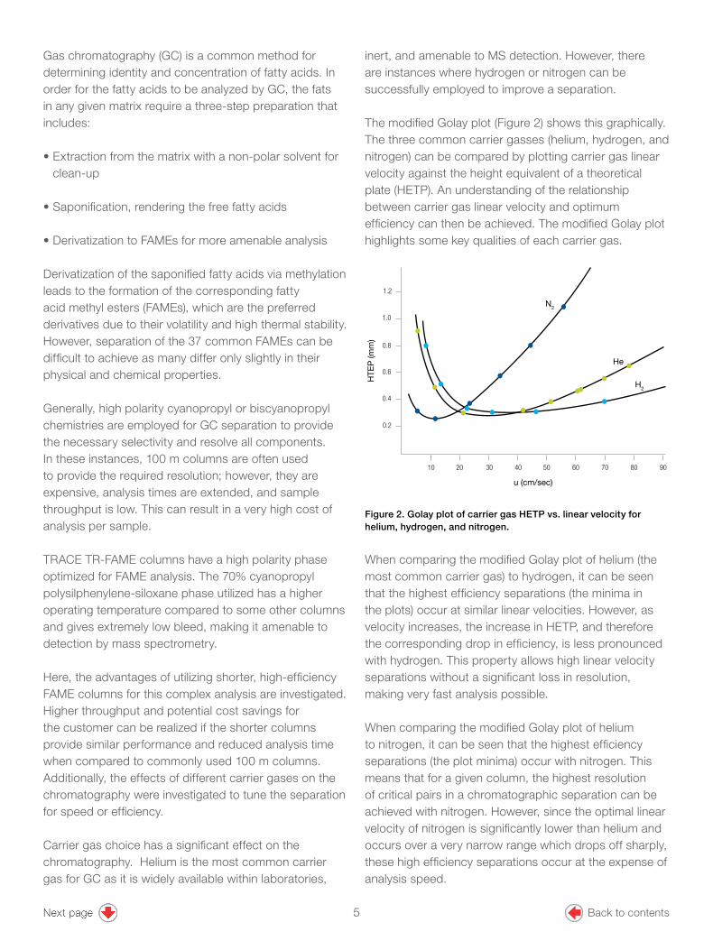
The modified Golay plot (Figure 2) shows this graphically. The three common carrier gasses (helium, hydrogen, and nitrogen) can be compared by plotting carrier gas linear velocity against the height equivalent of a theoretical plate (HETP). An understanding of the relationship between carrier gas linear velocity and optimum efficiency can then be achieved. The modified Golay plot highlights some key qualities of each carrier gas.
1.2
1.0
0.8
0.6
0.4
0.2
10 20 30 40 50 60 70 80 90
N2
He
H2
u (cm/sec)
HTE
P (m
m)
Figure 2. Golay plot of carrier gas HETP vs. linear velocity for helium, hydrogen, and nitrogen.
When comparing the modified Golay plot of helium (the most common carrier gas) to hydrogen, it can be seen that the highest efficiency separations (the minima in the plots) occur at similar linear velocities. However, as velocity increases, the increase in HETP, and therefore the corresponding drop in efficiency, is less pronounced with hydrogen. This property allows high linear velocity separations without a significant loss in resolution, making very fast analysis possible.
When comparing the modified Golay plot of helium to nitrogen, it can be seen that the highest efficiency separations (the plot minima) occur with nitrogen. This means that for a given column, the highest resolution of critical pairs in a chromatographic separation can be achieved with nitrogen. However, since the optimal linear velocity of nitrogen is significantly lower than helium and occurs over a very narrow range which drops off sharply, these high efficiency separations occur at the expense of analysis speed.
5 Back to contents

3
Instrument choice can also affect the analysis. The experiments performed here used the Thermo Scientific™ TRACE™ 1300 Series Gas Chromatograph, which is the latest technology to simplify workflow and increase analytical performance. The TRACE 1300 Series GC offers the most versatile GC platform in the market, with unique “Instant Connect” modularity for ground-breaking ease of use and performance, setting a new era in GC technology.
Detection was carried out on a Thermo Scientific™ Instant Connect Flame Ionization Detector (FID) and data capture and analysis using Thermo Scientific™ Chromeleon™ 7.2 SR3 Chromatography Data System.
ExperimentalConsumables Column• TRACE TR-FAME, 10 m × 0.1 mm × 0.2 µm
(P/N 260M096P)
Injection septum• Thermo Scientific™ BTO, 11 mm
(P/N 31303233-BP)
Injection liner• Thermo Scientific™ LinerGOLD™, Split/Splitless liner
with glass wool (P/N 453A2265-UI)
Column ferrules• 15% Graphite/85% Vespel® 0.1–0.25 mm
(P/N 290VA191)
Injection syringe• 10 µL fixed needle syringe for Thermo Scientific™
TriPlus™ RSH Autosampler (P/N 365D0291)
Vials and closures• Thermo Scientific™ National™ SureStop™ MS Certified
9 mm screw vials with Blue Silicone/PTFE AVCS closure (P/N MSCERT5000-34W)
Compounds A mixture containing the most common 37 FAMEs was used. Contents are detailed in Table 1.
Peak Name Component*Methyl butyrate 1Methyl hexanoate 2Methyl octanoate 3Methyl decanoate 4Methyl undecanoate 5Methyl laurate 6Methyl tridecanoate 7Methyl myristate 8Methyl myristoleate 9Methyl pentadecanoate 10Methyl cis-10-pentadecenoate 11Methyl palmitate 12Methyl palmitoleate 13Methyl heptadecanoate 14cis-10-Heptadecanoic acid methyl ester 15
Methyl stearate 16trans-9-Elaidic acid methyl ester 17cis-9-Oleic acid methyl ester 18Methyl linolelaidate 19Methyl linoleate 20Methyl arachidate 21Methyl γ-linolenate 22Methyl cis-11-eicosenoate 23Methyl linolenate 24Methyl heneicosanoate 25cis-11,14-Eicosadienoic acid methyl ester 26
Methyl behenate 27cis-8,11,14-Eicosatrienoic acid methyl ester 28
Methyl erucate 29cis-11,14,17-Eicosatrienoic acid methyl ester 30
cis-5,8,11,14-Eicosatetraenoic acid methyl ester 31
Methyl tricosanoate 32cis-13,16-Docosadienoic acid methyl ester 33
Methyl lignocerate 34cis-5,8,11,14,17-Eicosapentaenoic acid methyl ester 35
Methyl nervonate 36cis-4,7,10,13,16,19-Docosahexaenoic acid methyl ester 37
Table 1. Summary table of components present within the 37 FAME standard.
*Peaks were not identified by MS and were therefore only tentatively assigned.
6 Back to contents

4
Sample Pre-treatmentThe test mix was injected as supplied without any dilution.
Method Optimization Three carrier gases were investigated using the same instrumentation and column.
Instrumentation • TRACE 1310 GC (P/N 14800302)• TriPlus RSH Autosampler (P/N 1R77010-0100)• Instant Connect Electron Flame Ionization Detector (FID) (P/N 19070001FS)
Separation Conditions Experiment 1 (Helium)Carrier Gas HeliumSplit Flow 88.0 mL/minSplit Ratio 251:1Column Flow 0.35 mL/minOven Temperature 40 °C (1 min hold), 80 °C/min to 150 °C (0 min hold), 8 °C/min to 240 °C (1 min hold)Injector Type Split/SplitlessInjector Mode Split, constant flowInjector Temperature 220 °CDetector Type Flame ionization detector (FID)Detector Temperature 250 °CDetector Air Flow 350 mL/minDetector Hydrogen Flow 35 mL/minDetector Nitrogen Flow 40 mL/min Experiment 2 (Hydrogen)Carrier Gas HydrogenSplit Flow 75.0 mL/minSplit Ratio 250:1Column Flow 0.30 mL/minOven Temperature 40 °C (0.83 min hold), 96 °C/min to 150 °C (0 min hold), 9.6 °C/min to 240 °C (0.2 min hold)Injector Type Split/SplitlessInjector Mode Split, constant flowInjector Temperature 220 °CDetector Type Flame ionization detector (FID)Detector Temperature 250 °CDetector Air Flow 350 mL/minDetector Hydrogen Flow 35 mL/minDetector Nitrogen Flow 40 mL/min
Experiment 3 (Nitrogen)Carrier Gas NitrogenSplit Flow 28.0 ml/minSplit Ratio 255:1Column Flow 0.11 mL/minOven Temperature 40 °C (2.07 min hold), 38.57 °C/min to 150 °C (0 min hold), 3.86 °C/min to 240 °C (0.62 min hold)Injector Type Split/SplitlessInjector Mode Split, constant flowInjector Temperature 220 °CDetector Type Flame ionization detector (FID)Detector Temperature 250 °CDetector Air Flow 350 mL/minDetector Hydrogen Flow 35 mL/minDetector Nitrogen Flow 40 mL/min
Data ProcessingSoftware Chromeleon 7.2 SR3 Chromatography Data System.
Results and Discussion Typically, methods for FAME analysis have been carried out using a 100 m × 0.25 mm × 0.2 µm biscyanopropyl column with helium carrier gas. This required analysis times of around an hour to obtain the necessary resolution of the major components.
The equivalent separation on the 10 m length column with a narrower, 0.1 mm ID diameter is shown below (Figures 3a−c). By changing the column dimensions, the analysis time was reduced to approximately 12 minutes while maintaining resolution and efficiency.
In previously published methods, the components 25−32 were least resolved. Maintaining good separation of critical pairs in this region of the chromatogram was a key objective for this updated method. By using the 10 m column, the separation of critical pairs 25−26 and 28−29 was significantly improved compared to the 100 m column (Figures 3a−c). This is largely due to the increased efficiency of the narrower ID column.
7 Back to contents

5
1.5 2.0 3.0 4.0 5.0 6.0 7.0 8.0 9.0 10.0 11.0 11.7
2.9
10.0
20.0
30.031.0
min
pA
1-
2-
3-
4-
5-
6-
7-
8-
9- 10-
11-
12-
13-
14- 15
-
17-
18-
19-
20-
21-
22-
23-
24-
25-
26-
27-
28-
29-
30-
31-
32- 33-
34-
35-
36-
37-
min
16-
Figure 3a. Fast analysis on a TRACE TR-FAME GC column 10 m × 0.10 mm × 0.2 µm with helium carrier gas. (Experiment 1)
1.55 2.00 3.00 4.00 5.00 6.00 6.123.1
10.0
20.0
29.9
min
pA
15
-
1-
2-
3-
4-
5-
6-
7-
8-
9- 10-
11-
12-
13-
14-
Figure 3b (peaks 1−14). Fast analysis on a TRACE TR-FAME GC column 10 m × 0.10 mm × 0.2 µm with helium carrier gas. (Experiment 1)
14
-
min
pA
6.08 7.00 8.00 9.00 10.00 11.00 11.50
3.2
10.0
16.5
24-17-
18-
23-
37-36
-
35-
34-33
-
30-
28-
27-25
-26
-
31-22
-
29-
32-21
-
20-
19-
16-
15-
Figure 3c (peaks 15−37). Fast analysis on a TRACE TR-FAME GC column 10 m × 0.10 mm × 0.2 µm with helium carrier gas. (Experiment 1)
8 Back to contents
6
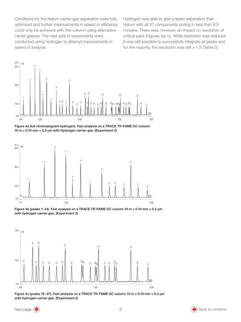
Conditions for the helium carrier gas separation were fully optimized and further improvements in speed or efficiency could only be achieved with this column using alternative carrier gasses. The next sets of experiments were conducted using hydrogen to attempt improvements in speed of analysis.
Hydrogen was able to give a faster separation than helium with all 37 components eluting in less than 9.3 minutes. There was, however, an impact on resolution of critical pairs (Figures 4a−c). While resolution was reduced, it was still possible to successfully integrate all peaks and for the majority, the resolution was still > 1.5 (Table 2).
1.24 2.50 5.00 7.50 9.57
3.5
10.0
20.0
30.0
32.2
1-
2-
3-
4-
5-
6-
7-
8-
9- 10-
11-
12-
13-
14- 15
-
16-
17-
18-
19-
20-
21-
22-
23-
24-
25-
26-
27-
28-
29-
30-
31-
32- 33
-34
-
35-
36-
37-
min
pA
Figure 4a (full chromatogram hydrogen). Fast analysis on a TRACE TR-FAME GC column 10 m × 0.10 mm × 0.2 µm with Hydrogen carrier gas. (Experiment 2)
3.2
pA
1.17 2.50 4.96
3.2
10.0
20.0
30.031.5
min
1-
2-
3-
4-
5-
6-
7-
8-
9- 10-
11-
12-
13-
14-
Figure 4b (peaks 1−14). Fast analysis on a TRACE TR-FAME GC column 10 m × 0.10 mm × 0.2 µm with hydrogen carrier gas. (Experiment 2)
1
4 -
min
pA
4.97 7.50 9.39
3.4
10.0
18.4
15-
16-
17-
18-
19-
20-
21-
22-
23-
24- 25
-26
-
27-
28-
29-
30-
31-
32- 33
-34
-
35-
36-
37-
Figure 4c (peaks 15−37). Fast analysis on a TRACE TR-FAME GC column 10 m × 0.10 mm × 0.2 µm with hydrogen carrier gas. (Experiment 2)
9 Back to contents
7
Peak Name Component* Helium Resolution
(EP)
Hydrogen Resolution
(EP)
NitrogenResolution
(EP)
Methyl butyrate 1 17.82 16.18 21.69
Methyl hexanoate 2 19.37 17.74 22.53
Methyl octanoate 3 21.46 19.83 24.28
Methyl decanoate 4 11.5 10.68 13.08
Methyl undecanoate 5 12.15 11.45 13.88
Methyl laurate 6 12.85 12.03 14.54
Methyl tridecanoate 7 13.49 12.57 15.27
Methyl myristate 8 7.75 7.28 8.92
Methyl myristoleate 9 5.94 5.41 6.59
Methyl pentadecanoate 10 8.62 7.73 9.47
Methyl cis-10-pentadecenoate 11 6.23 5.66 6.76
Methyl palmitate 12 6.52 6.07 7.31
Methyl palmitoleate 13 8.08 7.42 8.83
Methyl heptadecanoate 14 7.16 6.47 7.69
cis-10-Heptadecanoic acid methyl ester 15 8.04 7.54 8.82
Methyl stearate 16 3.18 3.08 3.67
trans-9-Elaidic acid methyl ester 17 2.33 2.2 2.62
cis-9-Oleic acid methyl ester 18 4.15 4.02 4.7
Methyl linolelaidate 19 5.52 5.13 6.15
Methyl linoleate 20 6.44 5.99 7.06
Methyl arachidate 21 5.41 4.99 5.78
Methyl γ-linolenate 22 2.33 2.29 2.48
Methyl cis-11-eicosenoate 23 5.61 5.26 6.15
Methyl linolenate 24 9.08 8.62 9.74
Methyl heneicosanoate 25 1.16 0.99 1.27
cis-11,14-Eicosadienoic acid methyl ester 26 6.38 5.87 7.07
Methyl behenate 27 4.19 3.94 4.71
cis-8,11,14-Eicosatrienoic acid methyl ester 28 0.92 0.85 1
Methyl erucate 29 1.63 1.66 1.81
cis-11,14,17-Eicosatrienoic acid methyl ester 30 5.52 5.43 6.09
cis-5,8,11,14-Eicosatetraenoic acid methyl ester 31 3.76 3.52 4.07
Methyl tricosanoate 32 4.49 4.48 4.86
cis-13,16-Docosadienoic acid methyl ester 33 1.66 1.54 1.79
Methyl lignocerate 34 11.87 11.88 13.1
cis-5,8,11,14,17-Eicosapentaenoic acid methyl ester
35 5.51 5.33 6.03
Methyl nervonate 36 9.32 8.76 10.05
cis-4,7,10,13,16,19-Docosahexaenoic acid methyl ester
37 “ “ “
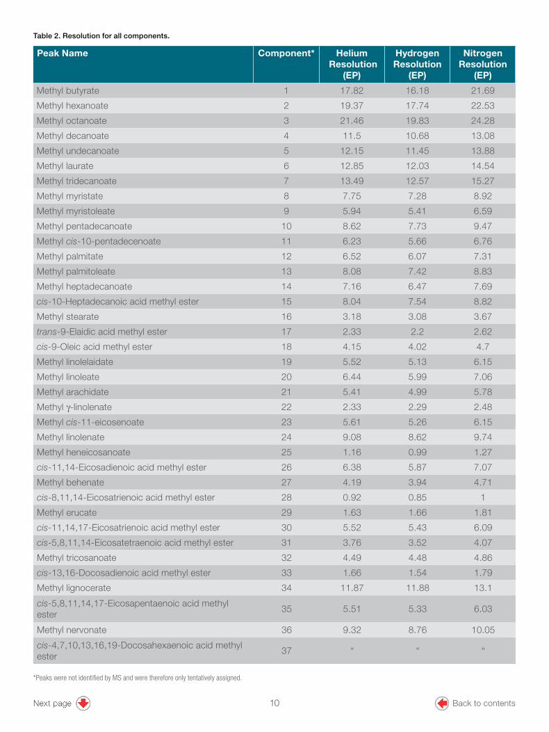
Table 2. Resolution for all components.
*Peaks were not identified by MS and were therefore only tentatively assigned.
10 Back to contents

8
The throughput of separations based on all three carrier gasses run times (Table 3) with 6-minute recycling time is given below (Figure 5). Published methods on 100 m columns using helium carrier gas could practically analyze up to 24 samples per day. Moving to a 10 m column increases throughput to a maximum of 80 samples per day. Even the use of a shorter column with nitrogen carrier gas increases throughput to 48 samples per day. If the carrier gas is then changed to hydrogen this further increases as high as 100 samples per day, a 400% increase.
Experiment Carrier gas Run time (min)
1 Helium 11.9
2 Hydrogen 9.5
3 Nitrogen 23.7
Table 3. Experiment run times. Figure 5. Sample throughput when comparing a 100 m column to a 10 m column using helium, hydrogen, and nitrogen as carrier gases.
Further experiments were then conducted using nitrogen in an attempt to increase separation efficiency and gain improvements in resolution. Figures 6a−c show the separation achieved.
pA
4.1
10.0
14.2
8.03.0 4.0 5.0 6.0 7.0 9.0 10.0 11.0 12.0 13.0 14.0 15.0 16.0 17.0 18.0 19.0 20.0 21.0 22.0 23.1
min
1-
2-
3-
4-
5-
6-
7-
8-
9- 10-
11-
12-
13-
14- 15
-
16-
17-
18-
19-
20-
21-
22-
23-
24- 25-
26-
27-
28-
29-
30-
31-
32- 33-
34-
35-
36-
37-
Figure 6a (full chromatogram nitrogen). Analysis on a TRACE TR-FAME GC column 10 m × 0.10 mm × 0.2 µm cyanopropyl phase using nitrogen carrier gas. (Experiment 3)
min
pA
3.04 4.00 5.00 6.00 7.00 8.00 9.00 10.00 11.00 12.16
3.7
10.0
16.6
1-
2-
3-
4-
5-
6-
7-
8-
9- 10-
11-
12-
13-
14-
Figure 6b (peaks 1−14). Analysis on a TRACE TR-FAME GC column 10 m × 0.10 mm × 0.2 µm cyanopropyl phase using nitrogen carrier gas. (Experiment 3)
80
60
40
20
0
Sam
ples
Ana
lyze
d
100
Sample thoughpit per day
10 m column N2
10 m column H2
10 m column He
10 m column He
11 Back to contents
9
Figure 5. Sample throughput when comparing a 100 m column to a 10 m column using helium, hydrogen, and nitrogen as carrier gases.
1
4 -
min
pA
12.0 13.0 14.0 15.0 16.0 17.0 18.0 19.0 20.0 21.0 22.0 23.0 23.7
3.57
10.00
12.98
15-
16-
17-
18-
19-
20-
21-
22-
23-
24-
25-
26-
27-
28-
29-
30-
31-
32- 33-
34-
35-
36-
37-
Figure 6c (peaks 15−37). Analysis on a TRACE TR-FAME GC column 10 m × 0.10 mm × 0.2 µm cyanopropyl phase using nitrogen carrier gas. (Experiment 3)
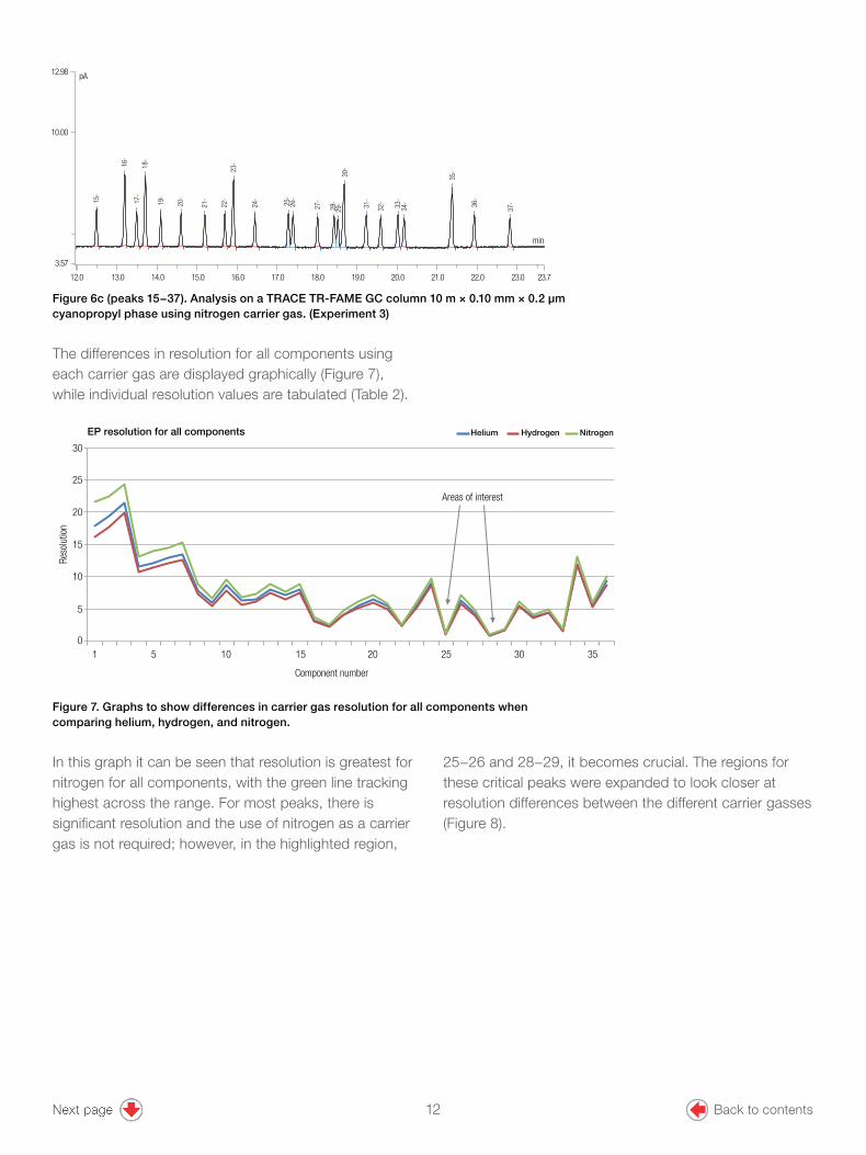
The differences in resolution for all components using each carrier gas are displayed graphically (Figure 7), while individual resolution values are tabulated (Table 2).
01
Reso
lutio
n
Helium Hydrogen Nitrogen
Component number
EP resolution for all components
5
10
15
20
25
30
5 10 15 20 25 30 35
Areas of interest
Figure 7. Graphs to show differences in carrier gas resolution for all components when comparing helium, hydrogen, and nitrogen.
In this graph it can be seen that resolution is greatest for nitrogen for all components, with the green line tracking highest across the range. For most peaks, there is significant resolution and the use of nitrogen as a carrier gas is not required; however, in the highlighted region,
25−26 and 28−29, it becomes crucial. The regions for these critical peaks were expanded to look closer at resolution differences between the different carrier gasses (Figure 8).
12 Back to contents
10
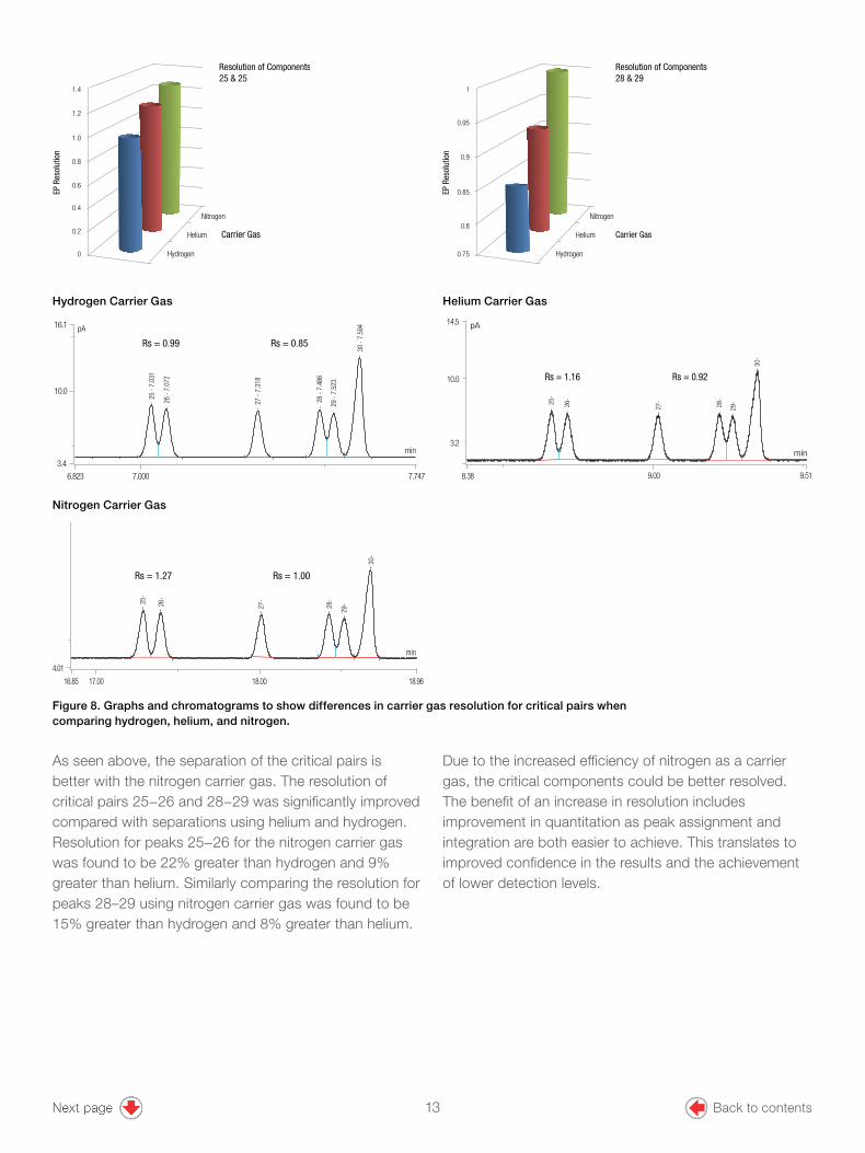
Figure 8. Graphs and chromatograms to show differences in carrier gas resolution for critical pairs when comparing hydrogen, helium, and nitrogen.
1.4
1.2
1.0
0.8
0.6
0.4
0.2
0
Nitrogen
Helium
Hydrogen
1
0.95
0.9
0.85
0.8
0.75
Nitrogen
Helium
Hydrogen
Carrier GasCarrier Gas
Resolution of Components25 & 25
Resolution of Components28 & 29
EP R
esol
utio
n
EP R
esol
utio
n
min
pA
3.4
10.0
16.1
6.823 7.000 7.747
25 -
7.03
1
26 -
7.07
2
27 -
7.31
8
28 -
7.48
6
29 -
7.52
3
30 -
7.59
4
Rs = 0.99 Rs = 0.85
min
pA
25-
26-
27-
28-
29-
30-
14.5
10.0
3.2
8.38 9.00 9.51
Rs = 1.16 Rs = 0.92
min
pA
4.01
9.63
16.85 17.00 18.00 18.96
25-
26-
27-
28-
29-
30-
Rs = 1.27 Rs = 1.00
As seen above, the separation of the critical pairs is better with the nitrogen carrier gas. The resolution of critical pairs 25−26 and 28−29 was significantly improved compared with separations using helium and hydrogen. Resolution for peaks 25−26 for the nitrogen carrier gas was found to be 22% greater than hydrogen and 9% greater than helium. Similarly comparing the resolution for peaks 28–29 using nitrogen carrier gas was found to be 15% greater than hydrogen and 8% greater than helium.
Due to the increased efficiency of nitrogen as a carrier gas, the critical components could be better resolved. The benefit of an increase in resolution includes improvement in quantitation as peak assignment and integration are both easier to achieve. This translates to improved confidence in the results and the achievement of lower detection levels.
Hydrogen Carrier Gas
Nitrogen Carrier Gas
Helium Carrier Gas
1.4
1.2
1.0
0.8
0.6
0.4
0.2
0
Nitrogen
Helium
Hydrogen
1
0.95
0.9
0.85
0.8
0.75
Nitrogen
Helium
Hydrogen
Carrier GasCarrier Gas
Resolution of Components25 & 25
Resolution of Components28 & 29
EP R
esol
utio
n
EP R
esol
utio
n
13 Back to contents
Find out more at thermofisher.com/columnsforgc
For Research Use Only. Not for use in diagnostic procedures. © 2016 Thermo Fisher Scientific Inc. All rights reserved. Vespel is a registered trademark of E. I. du Pont de Nemours and Company. All other trademarks are the property of Thermo Fisher Scientific and its subsidiaries unless otherwise specified. AN21557-EN 0916S
Conclusions• The separation of 37 fatty acid methyl esters (FAMEs) on the highly efficient 10 m TR-FAME GC column was significantly improved compared to the analysis on a 100 m FAMEs column, demonstrating greater resolution and increased sample throughput of up to 400%.
• By using different carrier gases, the separation of FAMEs can be optimized for reduced analysis time, resolution of critical pairs, and efficiency.
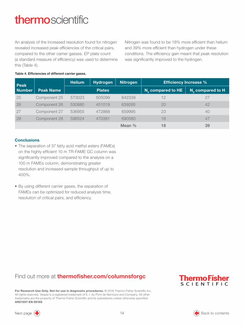
An analysis of the increased resolution found for nitrogen revealed increased peak efficiencies of the critical pairs, compared to the other carrier gasses. EP plate count (a standard measure of efficiency) was used to determine this (Table 4).
Peak Number Peak Name
Helium Hydrogen Nitrogen Efficiency Increase %
Plates N2 compared to HE N2 compared to H
25 Component 25 573023 505099 642339 12 27
26 Component 26 530880 451019 639285 20 42
27 Component 27 536955 472868 659995 23 40
28 Component 28 596524 470381 690580 16 47
Mean % 18 39
Table 4. Efficiencies of different carrier gases.
Nitrogen was found to be 18% more efficient than helium and 39% more efficient than hydrogen under these conditions. The efficiency gain meant that peak resolution was significantly improved to the hydrogen.
Find out more at thermofisher.com/columnsforgc
For Research Use Only. Not for use in diagnostic procedures. © 2016 Thermo Fisher Scientific Inc. All rights reserved. Vespel is a registered trademark of E. I. du Pont de Nemours and Company. All other trademarks are the property of Thermo Fisher Scientific and its subsidiaries unless otherwise specified. AN21557-EN 0916S
Conclusions• The separation of 37 fatty acid methyl esters (FAMEs) on the highly efficient 10 m TR-FAME GC column was significantly improved compared to the analysis on a 100 m FAMEs column, demonstrating greater resolution and increased sample throughput of up to 400%.
• By using different carrier gases, the separation of FAMEs can be optimized for reduced analysis time, resolution of critical pairs, and efficiency.
An analysis of the increased resolution found for nitrogen revealed increased peak efficiencies of the critical pairs, compared to the other carrier gasses. EP plate count (a standard measure of efficiency) was used to determine this (Table 4).
Peak Number Peak Name
Helium Hydrogen Nitrogen Efficiency Increase %
Plates N2 compared to HE N2 compared to H
25 Component 25 573023 505099 642339 12 27
26 Component 26 530880 451019 639285 20 42
27 Component 27 536955 472868 659995 23 40
28 Component 28 596524 470381 690580 16 47
Mean % 18 39
Table 4. Efficiencies of different carrier gases.
Nitrogen was found to be 18% more efficient than helium and 39% more efficient than hydrogen under these conditions. The efficiency gain meant that peak resolution was significantly improved to the hydrogen.
14 Back to contents

GoalThe aim of this application note is to demonstrate the qualitative and quantitative performance of the Thermo Scientific™ TriPlus™ 500 Gas Chromatography Headspace Autosampler coupled to a dual-detector GC-FID/MS for the determination of residual solvents in food packaging according to the European Standard EN 13628-1 method1 and to highlight a highly efficient workflow through extended automation from sampling to data reporting.
IntroductionPackaging materials are essential for maintaining food integrity and to ensure safe handling, transportation, and storage. Common food packaging materials are polymer-based thin films or paper-based coatings often layered or imprinted on the outside with inks, dyes, and paints intended to address the consumer appeal and convenience. The chemical components of such food packaging (especially from polymers, dyes, and inks) can migrate into the food products, modifying the organoleptic properties and the composition of the food and posing health risks to the consumer. As a consequence, regulatory measures are in place to make sure that food contact materials do not transfer any components to the packed foodstuff in quantities that could affect human health, change the composition, or modify the organoleptic
Authors Giulia Riccardino and Cristian Cojocariu
Thermo Fisher Scientific, Runcorn, UK
Keywords Residual solvents, flexible food packaging, food safety, valve and loop, headspace-gas chromatography, HS-GC, multiple headspace extraction, MHE, flame ionization detector, FID, mass spectrometer detector, MS, single quadrupole GC-MS, ISQ 7000, TriPlus 500 HS
Rapid qualitative and quantitative analysis of residual solvents in food packaging by static headspace coupled to GC-FID/MS
APPLICATION NOTE 10689
15 Back to contents

2
properties of the product.2 In the United States a migration limit of 50 ppm is applicable for residual solvents and non-volatile food additives.3 In addition, precise quantification of residual solvents in flexible packaging is also regulated through set methods such as EN 13628-1:2002.
Analysis of volatile impurities in solid polymers is challenging, especially with regard to sampling and extraction techniques. Liquid injections of such samples require dissolution of packaging polymers into a suitable solvent prior to gas chromatography (GC) injection. This can result in high viscosity solutions containing non-volatile, long chain polymers that can potentially contaminate the GC injector ports. This, in turn, will require frequent inlet liner replacement and system maintenance that will increase the cost of analysis.
An alternative to liquid injections is headspace sampling: a fast and simple technique that enables the extraction of volatile and semi-volatile compounds from food packaging samples without the need for time-consuming sample preparation. In particular, static headspace with multiple headspace extraction (MHE)4 can be used for absolute quantitative analysis of volatiles in solid matrices. This technique is particularly useful when matrix-matched calibration reference materials are not available.
In this study, the quantitative results for residual solvent analysis in food packaging materials, obtained with the TriPlus 500 Headspace (HS) autosampler, are reported. A dual detector FID/MS configuration allowed for the detection, identification (flame ionization detection), and confirmation (mass spectrometry detection) of unknown impurities. The experiments also focused on assessing method linearity1 according to EN 13628:1:2002 and precision, as well as the overall quantitative performance of the analytical setup for routine analysis of residual solvents in food packaging.
ExperimentalIn all experiments, a TriPlus 500 HS autosampler was coupled to a Thermo Scientific™ TRACE™ 1310 Gas Chromatograph equipped with a Thermo Scientific™ Instant Connect Split/Splitless SSL Injector. A Thermo Scientific™ Dual Detector Microfluidics device (P/N 19071030) was used to split 1:1 the carrier gas flow from the analytical column between a Thermo Scientific™ Instant Connect Flame Ionization Detector (FID) and a Thermo Scientific™ ISQ™ 7000 Single Quadrupole GC-MS system.
TRACE 1310 GC
Inlet Module and Mode: SSL, split
Split Ratio: 20:1
Septum Purge Mode, Flow (mL/min): Constant, 5
Carrier Gas, Carrier Mode, Pressure (kPa): He, constant pressure, 110
Oven Temperature Program
Temperature 1 (°C): 50
Hold Time (min): 1
Temperature 2 (°C): 110
Rate (°C/min): 30
Temperature 2 (°C): 250
Rate 2 (°C/min): 20
FID
Temperature (°C): 250
Air Flow (mL/min): 350
H2 Flow (mL/min): 35
N2 Flow (mL/min): 40
Acquisition Rate (Hz): 25
ISQ 7000 Single Quadrupole GC-MS system
Ion Source: ExtractaBrite
Transfer Line Temp. (°C): 250
Source Temperature (°C): 250
Ionization Mode: EI
Electron Energy (eV): 70
Acquisition Mode: Full-scan (m/z 25-350)
Table 1 (part 1). HS-GC-FID and ISQ 7000 mass spectrometer operating conditions for residual solvent determination
Chromatographic separation was achieved on a Thermo Scientific™ TraceGOLD™ TG-1MS GC capillary column, 30 m × 0.32 mm × 3.0 µm (P/N 26099-4840). Additional HS-GC-FID/MS conditions are given in Table 1. The GC oven temperature program was optimized to decrease the analysis time and improve sample throughput; all peaks of interest are eluting in <7 minutes with adequate peak chromatographic resolution (Rs > 1). An incubation time of 40 minutes per MHE step was optimized to cover the majority of food packaging material types. According to the EN 13628-1:2002 method, linearity was assessed on n = 4 headspace extraction cycles.
16 Back to contents

3
Data acquisition, processing and reportingThe data was acquired, processed, and reported using the Thermo Scientific™ Chromeleon™ Chromatography Data System (CDS) software, version 7.2. Integrated instrument control ensures full automation from instrument set-up to raw data processing, reporting, and storage. Simplified e-workflows deliver effective data management ensuring ease of use, sample integrity, and traceability. Chromeleon CDS also offers the option to scale up the data handling process in the laboratory from a single workstation to an enterprise environment to further improve productivity.5
Standard and sample preparationTwo standard mixtures, each containing different residual solvents that can be found in packaging materials (mixture 1 and mixture 2 at 7.14% v/v and 9.09% v/v, respectively), were purchased from Sigma Aldrich® (P/N 48994-U and 48995-U). A volume (1 μL) of each
TriPlus 500 HS Autosampler Parameters (MHE)
Incubation Temp. (°C): 120
Incubation Time (min): 40
Vial Shaking: Medium
Vial Pressurization Mode: Pressure
Vial Pressure (kPa) (Auxiliary Gas Nitrogen): 55
Vial Pressure Equilibration Time (min): 1
Loop Size (mL): 1
Loop/Sample Path Temp. (°C): 120
Loop Filling Pressure (kPa): 34
Loop Equilibration Time (min): 1
Extraction Cycles: 4
Needle Purge Flow Level: 4
Injection Mode: MHE
Injection Time (min): 1
Table 1 (part 2). HS-GC-FID and ISQ 7000 mass spectrometer operating conditions used for residual solvent determination
Table 1 (part 3). HS-GC-FID and ISQ 7000 mass spectrometer operating conditions for residual solvent determination
TriPlus 500 HS Autosampler Parameters (total vaporization)
Incubation Temp. (°C): 120
Incubation Time (min): 40
Vial Shaking: Medium
Vial Pressurization Mode: Pressure
Vial Pressure (kPa) (Auxiliary Gas Nitrogen): 55
Vial Pressure Equilibration Time (min): 1
Loop Size (mL): 1
Loop/Sample Path Temp. (°C): 120
Loop Filling Pressure (kPa): 34
Loop Equilibration Time (min): 1
Needle Purge Flow Level: 4
Injection Mode: Standard
Injection Time (min): 1
standard solution (corresponding to 71.4 μg and 90.9 μg of mixture 1 and 2, respectively) was spiked into the same 10 mL empty sealed headspace glass vial and used as retention time reference for compound identification as well as for MHE linearity assessment with total vaporization. A complete list of analyzed compounds is reported in Table 2.
Samples of packaged foods (pizza, cookies, bread, salad, and salami) were purchased locally and the packaging (cling film, wraps, and trays) was separated from the food and analyzed following the EN 13628-1:2002 method. A sample surface of 40 cm2 (2 × 20 cm) was cut, coiled, and sealed into a 10 mL crimp cap headspace vial (vials P/N 10CV, caps P/N 20-MCBC-ST3). As specified in the EN 13628-1:2002 method, the ratio between the sample area (in cm2) and the vial volume (in mL) was maintained between 3 and 5.
17 Back to contents

4
Results and discussionMHE linearity assessment according to EN 13628-1:2002 methodA reference solvent standard mix was prepared as described in the standard and sample preparation section and analyzed using the total vaporization technique4 applying the MHE conditions reported in Table 1. MHE allows the extrapolation of the total content of analytes in a liquid or solid matrix through multiple headspace cycles. The amount of analyte present in the sample is calculated by direct comparison of the peak area responses to external standards previously analyzed in a similar way but without matrix.
MHE linearity was assessed by plotting the natural logarithm of the peak areas in the standard solution versus the number of headspace cycles (n = 4). Chromeleon CDS interactive charts and reprocessing features allowed for fast MHE calibration plots and correlation coefficient calculations without the need of external calculation tools, as shown in Figure 1. For all the investigated compounds, the calculated correlation coefficients (R2) were 1.000 for FID data and ≥0.997 for EI full-scan MS traces (Table 2). In both cases calculated correlation coefficients met the method requirement (R2 ≥ 0.98) confirming an excellent linearity.
Quantification of residual solvent in food packaging materials using MHE The packaging materials were prepared as described and analyzed using the MHE conditions reported in Table 1. The microfluidic device allowed for splitting the gas flow 1:1 to the FID and the ISQ single quadrupole mass spectrometer, ensuring a minimal effect on the retention times (max RT shifts 0.04 min) by choosing either the FID or MS chromatogram as reference. The sample and the standard solution FID chromatograms were compared to verify the presence of known residual solvents. Several residual solvents such methanol (RT = 1.72 min) and ethylacetate (RT = 3.53 min) were detected in the sliced salami lid (D) and plastic tray (E), whereas ethanol (RT = 2.11 min) and acetone (RT = 2.37 min) were present in salad wrap (C) (Figure 3).
Table 2. Correlation coefficients (R2) calculated using the full-scan EI traces. For all compounds in the reference standard R2 ≥ 0.997. Correlation coefficients for FID data were 1.000 for all components, hence data are not shown.
MHE Linearity
Component NameRT
(min)Correlation
Coefficient (R2)Methanol 1.72 0.997
Ethanol 2.11 0.997
Acetone 2.37 0.998
2-Propanol 2.44 0.999
Methyl acetate 2.73 0.999
1-Propanol 2.98 0.998
2-Butanone 3.33 0.999
2-Butanol 3.42 1.000
Ethyl acetate 3.53 0.999
2-Methyl-1-propanol 3.68 0.999
2-Methoxyethanol 3.74 0.997
Tetrahydrofuran 3.80 0.999
Isopropyl acetate 4.04 0.998
1-Methoxy-2-propanol
4.20 0.997
Cyclohexane 4.34 0.998
Propylacetate 4.57 0.999
4-Methyl-2-pentanone
4.89 0.998
Isobutyl acetate 5.22 0.999
Toluene 5.38 0.997
Butyl acetate 5.63 0.999
2-Methoxyethyl acetate
5.74 0.997
2-Etoxyethyl acetate 6.47 0.998
Cyclohexanone 6.66 0.999
18 Back to contents

5
Figure 1. FID and TIC (full-scan, EI at 70 eV) traces for reference standard and corresponding MHE calibration curves for selected compounds (left to right: methanol, ethanol, acetone, ethyl acetate, toluene, and cyclohexanone) as examples. Calibration curves were obtained by plotting the natural logarithm of peak area responses (total vaporization MHE) versus the corresponding MHE extraction step.
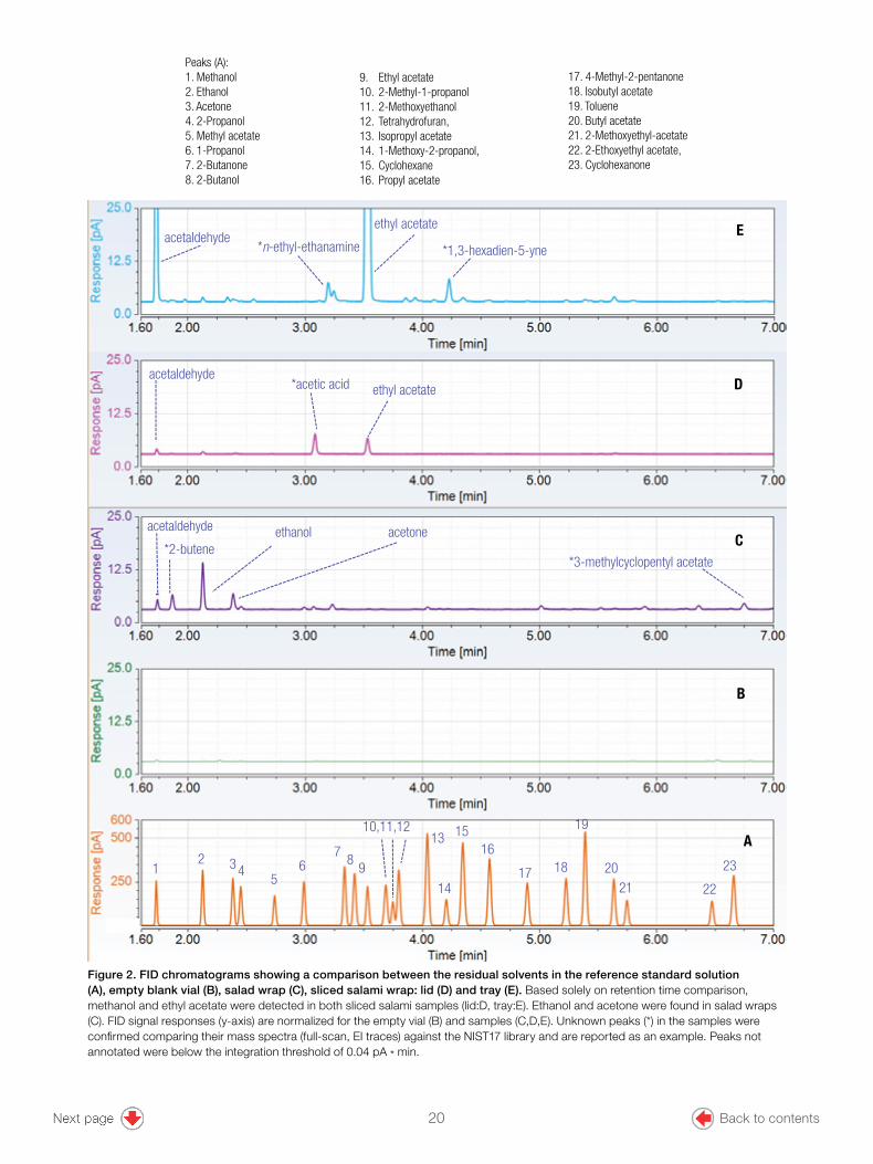
Full-scan data were used to putatively confirm the identity of detected solvent impurities, increasing the confidence in compound indentification. When searching the mass spectrum of the peak eluting at RT = 1.72 min against NIST17 library, the best library match was acetaldehyde (not included in the standard mixtures) with a SI score of 953 (sliced salami tray:E) and 729 (sliced salami lid:D) (Figure 3). Acetaldehyde is usually present in meat and meat products.6 Using the
same approach, ethanol and acetone in salad wrap (C) and ethyl acetate in sliced salami (lid:D and tray:E) were also putatively confirmed with a SI score of 929, 913, 874, and 950, respectively. These chemicals are actually released by the packaging since they are typically used in solvent-based inks imprinted on the external layer of flexible packages.7 Additional unknown compounds (*) detected in the samples were confirmed using spectral library comparison against NIST17 library (Figure 2).
12
34
5
6
78
9
10,11,12
13
14
15
16
17 18
19
20
21 22
23
FIDExtraction n=1 Extraction n=4
R2=1.00 R2=1.00R2=1.00R2=1.00R2=1.00R2=1.00
Extraction n=1 Extraction n=4
1
2
3 4 56
7 8 9
10,11,1213
14
15 16
17 1819 20
2122
23TIC
R2=0.997 R2=0.999R2=0.999R2=0.998R2=0.997 R2=0.997
1.60 4.00 6.003.00Minutes
7.005.002.00
1.60 4.00 6.003.00Minutes
7.005.002.00
Extraction n=2 Extraction n=3
Extraction n=2 Extraction n=3
19 Back to contents
6
Figure 2. FID chromatograms showing a comparison between the residual solvents in the reference standard solution (A), empty blank vial (B), salad wrap (C), sliced salami wrap: lid (D) and tray (E). Based solely on retention time comparison, methanol and ethyl acetate were detected in both sliced salami samples (lid:D, tray:E). Ethanol and acetone were found in salad wraps (C). FID signal responses (y-axis) are normalized for the empty vial (B) and samples (C,D,E). Unknown peaks (*) in the samples were confirmed comparing their mass spectra (full-scan, EI traces) against the NIST17 library and are reported as an example. Peaks not annotated were below the integration threshold of 0.04 pA * min.
12 34
56
78
9
10,11,1213
14
1516
17 18
19
2021 22
23
A
B
D
E
acetone
*acetic acid
ethanol
ethyl acetate
*2-butene
acetaldehyde
ethyl acetateacetaldehyde
acetaldehyde
*3-methylcyclopentyl acetate
*1,3-hexadien-5-yne*n-ethyl-ethanamine
C
17. 4-Methyl-2-pentanone18. Isobutyl acetate19. Toluene20. Butyl acetate21. 2-Methoxyethyl-acetate22. 2-Ethoxyethyl acetate,23. Cyclohexanone
Peaks (A):1. Methanol2. Ethanol3. Acetone4. 2-Propanol5. Methyl acetate6. 1-Propanol7. 2-Butanone8. 2-Butanol
9. Ethyl acetate10. 2-Methyl-1-propanol11. 2-Methoxyethanol12. Tetrahydrofuran,13. Isopropyl acetate14. 1-Methoxy-2-propanol,15. Cyclohexane16. Propyl acetate
20 Back to contents

7
Obtaining good (R2 ≥ 0.98) MHE linearity is fundamental to achieve accurate quantitation of residual solvents in solid food packaging materials. MHE linearity in the samples was assessed as previously described. The
correlation coefficients (R2) were 0.998 and 0.995 for ethyl acetate in sliced salami (lid and tray, respectively). R2 for ethanol and acetone in salad wrap were 0.996 and 0.998, respectively (Figure 4).
Figure 3. Identification of residual solvent peak eluting at RT=1.72 min in salami tray sample. Comparison of TIC chromatograms (full-scan, EI at 70 eV) showing retention time comparison of peak eluting at RT=1.72 min in solvent standard (blue) and salami tray (green) (A). Background subtracted EI mass spectra for this peak in solvent standard (B) and in the sliced salami tray (C) did not confirm methanol. NIST library result (D) putatively identified this compound as acetaldehyde with a SI score of 953 and a probability of 91%.
A
D
B
C
21 Back to contents

8
A
D
B
C
R2=0.998 R2=0.995
R2=0.996 R2=0.998
Figure 4. MHE linearity for ethyl acetate in sliced salami lid (A) and sliced salami tray (B), ethanol (C), and acetone (D) in salad wrap. The resulting correlation coefficients (R2) were 0.998 and 0.995 for sliced salami (lid and tray, respectively) and 0.996 and 0.998 for ethanol and acetone, respectively, in salad wrap.
The concentration (in mg/m2) of residual solvents detected in the samples was calculated using the FID data applying the formula reported in paragraph 9.2.10.1 of the EN method. No residual solvents were found in the majority of samples. Traces of ethyl acetate were found in the sliced salami wrap (lid: 0.76 mg/m2, tray: 29 mg/m2). Ethanol (0.97 mg/m2) and acetone (1.9 mg/m2) were also present in salad wrap. All levels were within the safety limits reported for residual solvent and non-volatile food additives.3
ConclusionsThe results obtained with the TriPlus 500 HS autosampler are compliant with the EN 13628-1:2002 standard method requirements.
• The MHE capability allows for absolute quantitative analysis of residual solvent impurities in solid samples, overcoming the matrix effect and eliminating the need of sample preparation. Using the MHE mode, excellent linearity with correlation coefficient R2 ≥ 0.995 was obtained for all analytes in both solvent standard and samples, meeting the minimum required value of R2 ≥ 0.98, thus confirming excellent instrument performance for MHE quantitative analysis.
• Traces of residual solvents were found in three of the six analyzed food packaging samples. Acetone and ethanol were detected at 1.9 and 0.97 mg/m2 in salad wrap samples, respectively, and ethyl acetate was found in sliced salami tray at 29 mg/m2 and lid at 0.76 mg/m2. No residual solvents were present in pizza cling film, cookies, and bread wraps.
• The dual detector configuration FID/MS increases the confidence in compound identification, allowing for the detection of possible analyte co-elution, otherwise difficult to assess in the absence of MS data. Moreover several unknown peaks in the samples have been putatively confirmed (using spectral library match score thresholds of >950 SI) through comparison with NIST17 spectral library.
• The low bleed and superior inertness of the TraceGOLD column allowed for highly reliable results. The high analytical column efficiency allowed for fast GC oven ramp with adequate chromatographic separation (Rs ≥ 1.0) for all the analyzed compounds, reducing analysis time. Moreover, up to 240 sample vials can be accommodated into the trays for unattended 24-hour operation.
22 Back to contents

©2019 Thermo Fisher Scientific Inc. All rights reserved. All trademarks are the property of Thermo Fisher Scientific and its subsidiaries unless otherwise specified. Sigma-Aldrich is a registered trademark of Sigma-Aldrich Co., LLC. This information is presented as an example of the capabilities of Thermo Fisher Scientific products. It is not intended to encourage use of these products in any manners that might infringe the intellectual property rights of others. Specifications, terms and pricing are subject to change. Not all products are available in all countries. Please consult your local sales representatives for details. AN10689-EN 0319S
Find out more at thermofisher.com/TriPlus500
• The automated cycle time optimization allows for continuous sample processing ensuring the overlapping between the MHE cycles of the same sample. The overlapping capability is maintained between the final injection of one sample and the incubation of the next one increasing the sample throughput.
• Chromeleon CDS software ensures data integrity, traceability, and effective data management from instrument control to the final report. The integrated charts and the advanced report capability allowed for easy and integrated MHE data reprocessing, thus eliminating the need for external calculation tools.
Overall the results obtained show that the TriPlus 500 HS autosampler coupled to the TRACE 1310 GC and the ISQ 7000 single quadrupole GC-MS system represents a robust analytical configuration for routine laboratories delivering outstanding reliability for MHE quantitative analysis of residual solvents in food packaging.
References1. EN 13628-1:2002 Packaging- Flexible Packaging Material – Determination of
residual solvents by static headspace gas chromatography – Part 1.; Absolute methods.
2. Food Contact Materials - Regulation (EC) No 1935/2004 – European Implementation Assessment Study, May 2016.
3. Title 21, Code of Federal Regulation, Direct Additive Part, 170.3, Indirect Additive, Part 174–179.
4. Kolb, B., Ettre, l., Static headspace-gas chromatography Theory and Practice, Second Edition Wiley, 2006.
5. Thermo Fisher Scientific, Chromeleon CDS Enterprise – Compliance, Connectivity, Confidence, BR72617-EN0718S.
6. Kosowska, M., Majcher, M.A., Fortuna, T., Volatile compounds in meat and meat products, Food Science and Technology, Campinas, vol. 37 issue 1, Jan-March 2017, 1–7.
7. Packaging Materials - Printing inks for food packaging composition and properties of printing inks, International Life Science Institute ILSI Europe, December 2011.
23 Back to contents

AuthorsAaron Lamb, Dominic Roberts, and Cristian Cojocariu Thermo Fisher Scientific, Runcorn, UK
Keywords Food safety, phthalates, trace analysis, gas chromatography, ISQ 7000, single quadrupole mass spectrometry, selected ion monitoring, vegetable oil, sensitivity, advanced electron ionization, AEI
APPLICATION NOTE 10589
GoalTo evaluate the suitability of the new Thermo Scientific™ ISQ™ 7000 GC-MS system, configured with the highly sensitive Advanced Electron Ionization (AEI) source, for the analysis of phthalates. Method selectivity, linearity, recoveries, and robustness were assessed using a challenging vegetable oil matrix.
IntroductionPhthalates (phthalate acid esters, PAEs) are a class of chemicals that are used mainly as plasticizers in various industries. Plasticizers are not chemically bound to their native polymer and therefore can leach into food from packaging materials in significant amounts.1 Due to their lipophilic nature, phthalates are highly likely to be found in fat containing foods including cooking oils. The most important congener is di-(2-ethylhexyl)-phthalate (DEHP), which accounts for about 50% of the world production of phthalates (Figure 1).1
Routine determination of phthalates in vegetable oil by single quadrupole GC-MS
Figure 1. Chemical structure of the most prevalent phthalate, di-(2-ethylhexyl)-phthalate).
CH3
CH3
CH3
CH3O
OO
O
24 Back to contents
2
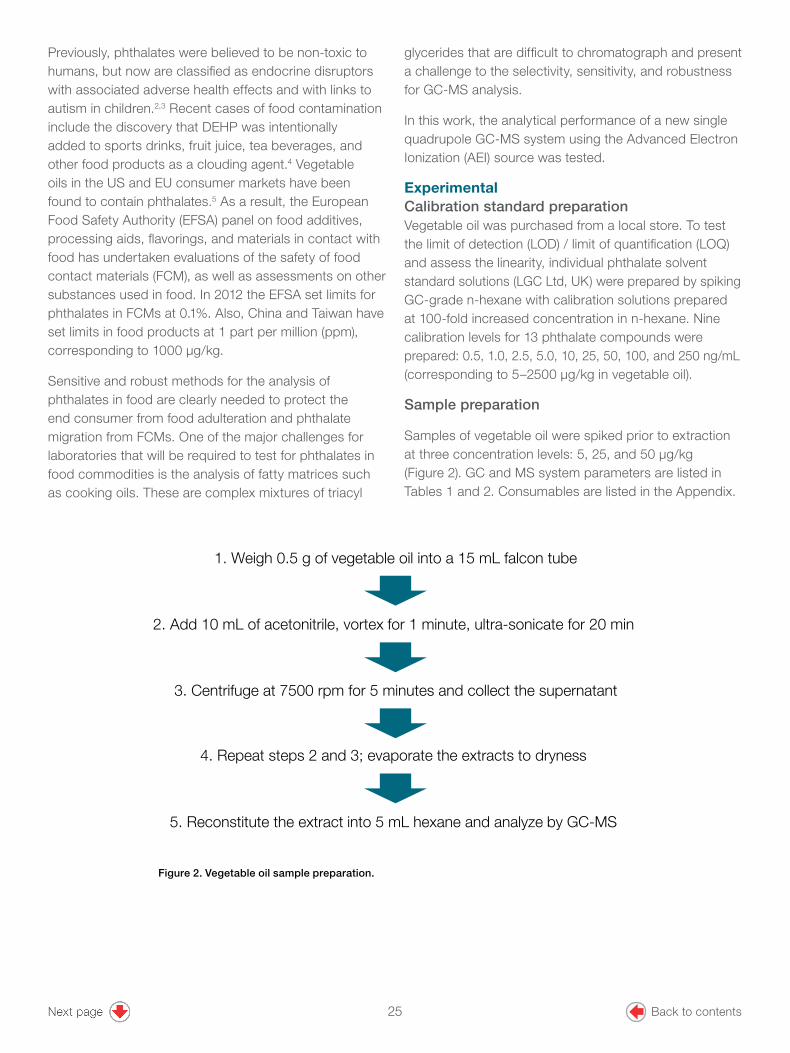
Previously, phthalates were believed to be non-toxic to humans, but now are classified as endocrine disruptors with associated adverse health effects and with links to autism in children.2,3 Recent cases of food contamination include the discovery that DEHP was intentionally added to sports drinks, fruit juice, tea beverages, and other food products as a clouding agent.4 Vegetable oils in the US and EU consumer markets have been found to contain phthalates.5 As a result, the European Food Safety Authority (EFSA) panel on food additives, processing aids, flavorings, and materials in contact with food has undertaken evaluations of the safety of food contact materials (FCM), as well as assessments on other substances used in food. In 2012 the EFSA set limits for phthalates in FCMs at 0.1%. Also, China and Taiwan have set limits in food products at 1 part per million (ppm), corresponding to 1000 µg/kg.
Sensitive and robust methods for the analysis of phthalates in food are clearly needed to protect the end consumer from food adulteration and phthalate migration from FCMs. One of the major challenges for laboratories that will be required to test for phthalates in food commodities is the analysis of fatty matrices such as cooking oils. These are complex mixtures of triacyl
glycerides that are difficult to chromatograph and present a challenge to the selectivity, sensitivity, and robustness for GC-MS analysis.
In this work, the analytical performance of a new single quadrupole GC-MS system using the Advanced Electron Ionization (AEI) source was tested.
ExperimentalCalibration standard preparationVegetable oil was purchased from a local store. To test the limit of detection (LOD) / limit of quantification (LOQ) and assess the linearity, individual phthalate solvent standard solutions (LGC Ltd, UK) were prepared by spiking GC-grade n-hexane with calibration solutions prepared at 100-fold increased concentration in n-hexane. Nine calibration levels for 13 phthalate compounds were prepared: 0.5, 1.0, 2.5, 5.0, 10, 25, 50, 100, and 250 ng/mL (corresponding to 5–2500 µg/kg in vegetable oil).
Sample preparation
Samples of vegetable oil were spiked prior to extraction at three concentration levels: 5, 25, and 50 µg/kg (Figure 2). GC and MS system parameters are listed in Tables 1 and 2. Consumables are listed in the Appendix.
Figure 2. Vegetable oil sample preparation.
1. Weigh 0.5 g of vegetable oil into a 15 mL falcon tube
2. Add 10 mL of acetonitrile, vortex for 1 minute, ultra-sonicate for 20 min
3. Centrifuge at 7500 rpm for 5 minutes and collect the supernatant
4. Repeat steps 2 and 3; evaporate the extracts to dryness
5. Reconstitute the extract into 5 mL hexane and analyze by GC-MS
25 Back to contents
3
Table 2. ISQ 7000 GC-MS system parameters.
Instrument conditions
Autosampler parameters
Fill strokes 10
Air volume 1.0 µL
Sample wash 2
GC inlet parameters
Injection volume 1 µL
Injection mode Splitless
Temperature 300 ºC
Split flow 80.0 mL/min
Splitless time 1.0 min
Purge flow 5.0 mL/min
Flow mode Constant flow (1.0 mL/min)
Carrier gas Helium
GC oven settings
Ramp rate (ºC) Target value (ºC) Hold time (min)
0 100 1.0
20 190 0.0
10 280 5.0
30 320 10.0
See Appendix for consumables used.
MS conditions
Transfer line temperature 300 ºC
Ion source temperature 350 ºC
Acquisition mode Timed (SIM)
Ionization mode EI (45 eV)
Emission current 10 µA
Minimum peak width 3 s
Minimum scans/peak 12
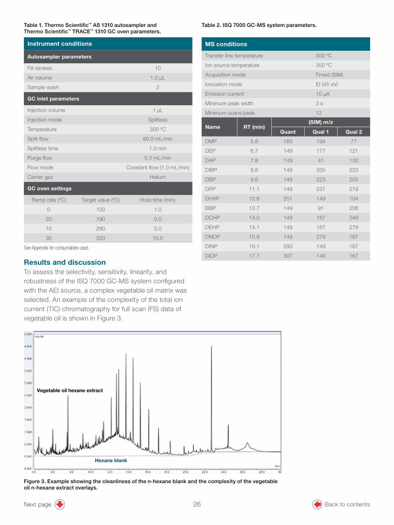
Table 1. Thermo Scientific™ AS 1310 autosampler and Thermo Scientific™ TRACE™ 1310 GC oven parameters.
Results and discussionTo assess the selectivity, sensitivity, linearity, and robustness of the ISQ 7000 GC-MS system configured with the AEI source, a complex vegetable oil matrix was selected. An example of the complexity of the total ion current (TIC) chromatography for full scan (FS) data of vegetable oil is shown in Figure 3.
Figure 3. Example showing the cleanliness of the n-hexane blank and the complexity of the vegetable oil n-hexane extract overlays.
Hexane blank
Vegetable oil hexane extract
Name RT (min)(SIM) m/z
Quant Qual 1 Qual 2
DMP 5.8 163 194 77
DEP 6.7 149 177 121
DAP 7.8 149 41 132
DIBP 8.8 149 205 223
DBP 9.6 149 223 205
DPP 11.1 149 237 219
DHXP 12.6 251 149 104
BBP 12.7 149 91 206
DCHP 14.0 149 167 249
DEHP 14.1 149 167 279
DNOP 15.6 149 279 167
DINP 16.1 293 149 167
DIDP 17.7 307 149 167
26 Back to contents

4
Figure 4. Example of selectivity and sensitivity obtained for DEHP when using SIM and FS for a vegetable oil hexane extract.
Full-scan = complex spectrum, less selective
DEHPs/n= 97
SIM = more selective and sensitive
Reduced background/interference ions
High background/interference ions
DEHPs/n= 337
Minutes
Con
f 2
counts
13.62 14.00 14.62
1.6e6
1.0e6
1.4e5
4.1e5
5.0e6
7.1e6
1.0e6
2.0e7
2.7e7
Con
f 1
counts
counts
Qua
n
0.0e0
5.0e8
1.0e9
Minutes
13.62 14.00 14.62
m/z=149
m/z=167
m/z=249
When using full scan acquisition, it is difficult to selectively detect phthalates such as DEHP from the background ions. In contrast, by using selective ion monitoring mode (SIM), a significant selectivity and sensitivity improvement is obtained (Figure 4).
Given the complexity of the chromatogram, analysis of phthalates in vegetable oil was carried out using timed-SIM. Timed-SIM mode is an excellent choice for quantitative GC-MS analysis because it allows the
detection of analytes with increased sensitivity. In SIM mode, data are gathered only for masses of interest rather than a full mass range, and the optimization of both scan rate and dwell time can be performed automatically using Thermo Scientific™ Chromeleon™ Chromatography Data System (CDS) software by inputting the desired number of points across the narrowest peak of interest and its peak width in seconds. This leads to greatly increased sensitivity and lower limits of quantification.
27 Back to contents
5
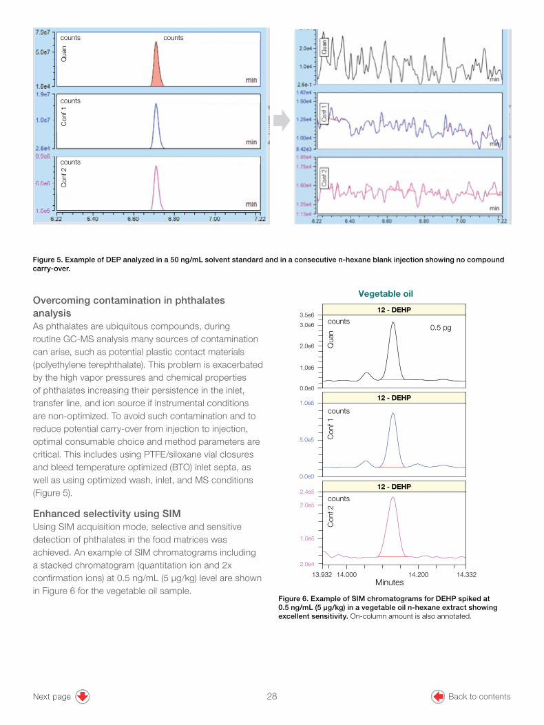
Overcoming contamination in phthalates analysisAs phthalates are ubiquitous compounds, during routine GC-MS analysis many sources of contamination can arise, such as potential plastic contact materials (polyethylene terephthalate). This problem is exacerbated by the high vapor pressures and chemical properties of phthalates increasing their persistence in the inlet, transfer line, and ion source if instrumental conditions are non-optimized. To avoid such contamination and to reduce potential carry-over from injection to injection, optimal consumable choice and method parameters are critical. This includes using PTFE/siloxane vial closures and bleed temperature optimized (BTO) inlet septa, as well as using optimized wash, inlet, and MS conditions (Figure 5).
Enhanced selectivity using SIMUsing SIM acquisition mode, selective and sensitive detection of phthalates in the food matrices was achieved. An example of SIM chromatograms including a stacked chromatogram (quantitation ion and 2x confirmation ions) at 0.5 ng/mL (5 µg/kg) level are shown in Figure 6 for the vegetable oil sample.
Figure 6. Example of SIM chromatograms for DEHP spiked at 0.5 ng/mL (5 µg/kg) in a vegetable oil n-hexane extract showing excellent sensitivity. On-column amount is also annotated.
Minutes
Con
f 2
counts
Vegetable oil
0.5 pgC
onf 1
counts
Qua
ncounts
12 - DEHP
12 - DEHP
12 - DEHP
13.932 14.000 14.200 14.332
2.0e4
1.0e5
2.0e5
2.4e5
0.0e0
5.0e5
1.0e6
0.0e0
1.0e6
2.0e6
3.0e6
3.5e6
Figure 5. Example of DEP analyzed in a 50 ng/mL solvent standard and in a consecutive n-hexane blank injection showing no compound carry-over.
counts counts
Qua
n
counts
Con
f 1
counts
Con
f 2
28 Back to contents

6
Determination of LOD and LOQPhthalate residues in food products currently have no regulatory limits in the EU. However in this application levels of 5–25 μg/kg were achieved.
To practically assess the method’s limit of detection, 18 replicate injections (of standards around the LOQ for each component) were performed. The instrumental detection limit (IDL) for each individual compound was then calculated by taking into account the injected amount, % RSD, and t-score of 2.567, corresponding to 17 degrees of freedom at 99% confidence (Table 3).
In addition to this, the LOQ was determined as the lowest concentration level of phthalates with a peak area repeatability of < 15% RSD and ion ratios within < ±15% of the expected values calculated as an average across a calibration curve ranging from 0.5 to 250 ng/mL (corresponding to 5–2500 µg/kg in vegetable oil). Based on these criteria, the estimated LOQs for compounds ranged from 5 to 25 µg/kg. An example of LOQ determination for the most difficult matrix is shown in Table 4.
Estimated IDL levels
ComponentLevel injected
(pg OC*)% RSD
IDL
(pg OC*)
DMP 0.1 4.1% 0.01
DEP 0.1 11% 0.03
DAP 0.1 7.8% 0.02
DIBP 0.1 2.7% 0.01
DBP 0.1 3.2% 0.01
DPP 0.1 5.7% 0.01
DXHP 1.0 9.2% 0.24
BBP 0.1 14% 0.04
DCHP 25 4.5% 3.0
DEHP 0.1 5.8% 0.01
DNOP 0.1 7.6% 0.02
DINP 25 2.4% 1.6
DIDP 25 3.0% 1.9
* OC = on column
Estimated LOQ levels
Compound name LOQ (µg/kg)
Peak area
% RSD
5 µg/kg
Ion ratio
% RSD
5 µg/kg
Peak area
% RSD
25 µg/kg
Ion ratio
% RSD
25 µg/kg
DMP 5.0 1.0 2.2 0.9 2.9
DEP 5.0 0.3 4.6 1.2 3.2
DAP 5.0 7.3 7.7 1.3 2.4
DIBP 5.0 0.9 6.8 1.0 2.5
DBP 5.0 3.1 4.1 1.2 0.9
DPP 5.0 11 7.7 1.5 11
DXHP 5.0 7.9 1.7 0.6 2.7
BBP 5.0 0.4 6.5 1.5 0.4
DCHP 25 NA NA 2.3 2.8
DEHP 5.0 6.9 1.6 1.1 1.9
DNOP 5.0 5.5 4.2 1.9 2.2
DINP 25 NA NA 2.5 5.4
DIDP 25 NA NA 2.8 4.7
Table 3. Estimated IDLs and absolute peak area repeatability (as % RSD) for phthalates determined from n=18 injections of a lowest concentrated standard where the peak area % RSD was lower than 15%.
Table 4. LOQ, absolute peak area, and ion ratio stability for targeted phthalates in vegetable oil (n=3 injections) at 5.0 µg/kg and at 25 µg/kg.
29 Back to contents

7
R2 = 0.9999% RSD = 1.7
R2 = 0.9999% RSD = 1.8
R2 = 0.9992% RSD = 4.9
R2 = 0.9986% RSD = 6.8
R2 = 0.9985% RSD = 6.8
R2 = 0.9983% RSD = 6.7
R2 = 0.9991% RSD = 5.2
R2 = 0.9984% RSD = 7.1
R2 = 0.9991% RSD = 5.2
R2 = 0.9998% RSD = 2.3
R2 = 0.9995% RSD = 4.0
R2 = 0.9990% RSD = 5.5
R2 = 0.9987% RSD = 6.4
With the innovative design of the new AEI source, less frequent source cleaning is required as the improved source geometry leads to increased ionization efficiency and a narrower ion beam. This means the source filament can be operated at a reduced emission current, which in turn means less ionization of complex matrices in the source. Additionally, the highly focused ion beam significantly reduces the risk of source contamination. These features make the AEI source extremely robust, extending the time before maintenance is required. The enhanced sensitivity of the new source also means that
Figure 7. Linearity of targeted compounds demonstrated using a solvent-based calibration curve ranging from 0.5 to 250 ng/mL (corresponding to 5–2500 µg/kg in vegetable oil). Calibration weighting was 1/x, with two replicate injections per level and no internal standard adjustment. Coefficient of determination (R2) and average response factors residual % RSD are displayed.
the sample matrix can be diluted more or the split ratio can be increased, further reducing the amount of potential contamination to the GC flow path.
LinearityLinearity was determined using n-hexane solvent phthalate standards at concentrations of 0.5–250 ng/mL (corresponding to 5–2500 µg/kg in vegetable oil extracts). All compounds showed excellent linear response with coefficient of determination R2 > 0.998, and average response factor values across this calibration range were all below 10% (Figure 7).
10.34 in
30 Back to contents

8
Conclusion• The new innovative Thermo Scientific AEI source
exhibits excellent sensitivity with unrivaled instrument detection limits of phthalate esters down to low ppt levels (0.01 ng/mL).
• Outstanding linearity for 13 phthalates analyzed was demonstrated over a range of 0.5 to 250 ng/mL (corresponding to 5–2500 µg/kg in vegetable oil). All compounds showed linear responses with coefficient of determinations R2 > 0.998 average response factor RSDs < 10%.
• Compound recoveries demonstrated across three separate spiking levels were between 80% and 102%, well within the required method performance limits.
The ISQ 7000 GC-MS system configured with the AEI source provides unrivaled levels of sensitivity and robustness due to improved source geometry resulting in enhanced ionization efficiency and a narrower ion beam. This allows the user the flexibility to dilute their sample more, inject less, or use split methods while still being
able to achieve the required limits of detection. Reduced matrix load on the GC-MS system means reduced frequency of costly preventive instrument maintenance, such as consumable replacement and source cleaning, increasing the profitability and laboratory productivity.
References1. Commission Regulation (EU) No 10/2011 of 14 January 2011 on plastic materials
and articles intended to come into contact with food, Official Journal of the European Union.
2. Kavlock, R.J.; Daston, G.P. DeRosa, C.; Fenner-Crisp, P.; Gray, L.E.; Kaattari, S., et al. Research needs for the risk assessment of health and environmental effects of endocrine disruptors: a report of the U.S.EPA-sponsoredworkshop. Environ. Health Perspect. 1996, Aug;104 Suppl 4, 715–40. doi: 10. 1289/ehp.96104s4715.
3. Clausen, P.A.; Hansen, V.; Gunnarsen, L.; Afshari, A.; Wolkoff, P. Emission of di-2-ethylhexyl phthalate from PVC flooring into air and uptake in dust: emission and sorption experiments in FLEC and CLIMPAQ. Environ. Sci. Technol. 2004, 38(9), 2531–7. doi: 10.1021/es0347944.
4. Yanga, J.; Hausera, R.; Goldman, R.H.; Taiwan food scandal: The illegal use of phthalates as a clouding agent and their contribution to maternal exposure, Food and Chemical Toxicology. 2013; 58, 362–368, doi.org/10.1016/j.fct.2013.05.010.
5. Serrano, S.E.; Braun, J.; Trasande, L.; Dills, R.; Sathyanarayana, S. Phthalates and diet: a review of the food monitoring and epidemiology data. Environ. Health. 2014, 13, 43.
Method performance The performance of the method was assessed by evaluating the recoveries in the pre- and post-spiked vegetable oil samples with a mixed phthalates standard at 5, 25, and
Table 5. Recoveries (%) calculated for mixed phthalates pre-spiked in vegetable oil at three different concentration levels (5, 25, and 50 µg/kg) from n=3 injections. Recovery % RSD (n=3) is also shown.
Compound name% Recovery
5.0 µg/kg spike level
% RSD (n=3)
% Recovery 25 µg/kg spike
level
% RSD (n=3)
% Recovery 50 µg/kg spike
level
% RSD (n=3)
DMP 101 1.7 98 1.9 104 5.2
DEP 102 1.8 98 4.8 100 3.7
DAP 97 1.7 95 0.8 99 3.0
DIBP 101 4.1 97 2.3 99 4.3
DBP 100 3.0 97 1.2 100 3.2
DPP 97 1.4 96 2.2 97 1.4
DXHP 97 5.9 91 0.5 95 0.6
BBP 92 3.4 93 0.3 91 2.0
DCHP* NA NA 91 1.3 84 4.8
DEHP 96 2.2 91 6.7 93 5.5
DNOP 93 3.9 93 2.6 97 0.5
DINP* NA NA 96 2.0 101 0.1
DIDP* NA NA 92 2.0 84 0.4
* The % recoveries were not calculated at the 5 µg/kg level as this was below the LOQ.
50 µg/kg. Three injections (technical replicates) per level were used and the results show average recovery values between 80% and 102% (Table 5).
31 Back to contents
Find out more at thermofisher.com/ISQ7000
©2018 Thermo Fisher Scientific Inc. All rights reserved. Corning and Falcon are trademarks of Corning Life Sciences. All other trademarks are the property of Thermo Fisher Scientific and its subsidiaries unless otherwise specified. This information is presented as an example of the capabilities of Thermo Fisher Scientific products. It is not intended to encourage use of these products in any manners that might infringe the intellectual property rights of others. Specifications, terms and pricing are subject to change. Not all products are available in all countries. Please consult your local sales representatives for details. AN10589-EN 0318S
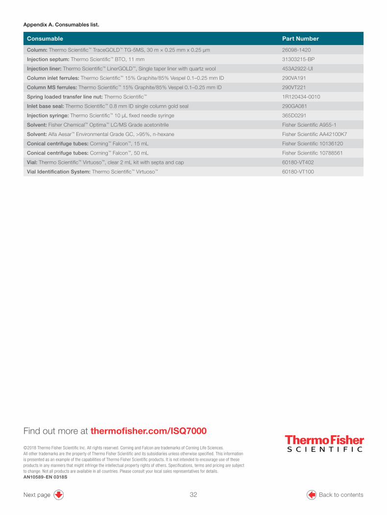
Appendix A. Consumables list.
Consumable Part Number
Column: Thermo Scientific™ TraceGOLD™ TG-5MS, 30 m × 0.25 mm x 0.25 µm 26098-1420
Injection septum: Thermo Scientific™ BTO, 11 mm 31303215-BP
Injection liner: Thermo Scientific™ LinerGOLD™, Single taper liner with quartz wool 453A2922-UI
Column inlet ferrules: Thermo Scientific™ 15% Graphite/85% Vespel 0.1–0.25 mm ID 290VA191
Column MS ferrules: Thermo Scientific™ 15% Graphite/85% Vespel 0.1–0.25 mm ID 290VT221
Spring loaded transfer line nut: Thermo Scientific™ 1R120434-0010
Inlet base seal: Thermo Scientific™ 0.8 mm ID single column gold seal 290GA081
Injection syringe: Thermo Scientific™ 10 µL fixed needle syringe 365D0291
Solvent: Fisher Chemical™ Optima™ LC/MS Grade acetonitrile Fisher Scientific A955-1
Solvent: Alfa Aesar™ Environmental Grade GC, >95%, n-hexane Fisher Scientific AA42100K7
Conical centrifuge tubes: Corning™ Falcon™, 15 mL Fisher Scientific 10136120
Conical centrifuge tubes: Corning™ Falcon™, 50 mL Fisher Scientific 10788561
Vial: Thermo Scientific™ Virtuoso™, clear 2 mL kit with septa and cap 60180-VT402
Vial Identification System: Thermo Scientific™ Virtuoso™ 60180-VT100
Find out more at thermofisher.com/ISQ7000
©2018 Thermo Fisher Scientific Inc. All rights reserved. Corning and Falcon are trademarks of Corning Life Sciences. All other trademarks are the property of Thermo Fisher Scientific and its subsidiaries unless otherwise specified. This information is presented as an example of the capabilities of Thermo Fisher Scientific products. It is not intended to encourage use of these products in any manners that might infringe the intellectual property rights of others. Specifications, terms and pricing are subject to change. Not all products are available in all countries. Please consult your local sales representatives for details. AN10589-EN 0318S
Appendix A. Consumables list.
Consumable Part Number
Column: Thermo Scientific™ TraceGOLD™ TG-5MS, 30 m × 0.25 mm x 0.25 µm 26098-1420
Injection septum: Thermo Scientific™ BTO, 11 mm 31303215-BP
Injection liner: Thermo Scientific™ LinerGOLD™, Single taper liner with quartz wool 453A2922-UI
Column inlet ferrules: Thermo Scientific™ 15% Graphite/85% Vespel 0.1–0.25 mm ID 290VA191
Column MS ferrules: Thermo Scientific™ 15% Graphite/85% Vespel 0.1–0.25 mm ID 290VT221
Spring loaded transfer line nut: Thermo Scientific™ 1R120434-0010
Inlet base seal: Thermo Scientific™ 0.8 mm ID single column gold seal 290GA081
Injection syringe: Thermo Scientific™ 10 µL fixed needle syringe 365D0291
Solvent: Fisher Chemical™ Optima™ LC/MS Grade acetonitrile Fisher Scientific A955-1
Solvent: Alfa Aesar™ Environmental Grade GC, >95%, n-hexane Fisher Scientific AA42100K7
Conical centrifuge tubes: Corning™ Falcon™, 15 mL Fisher Scientific 10136120
Conical centrifuge tubes: Corning™ Falcon™, 50 mL Fisher Scientific 10788561
Vial: Thermo Scientific™ Virtuoso™, clear 2 mL kit with septa and cap 60180-VT402
Vial Identification System: Thermo Scientific™ Virtuoso™ 60180-VT100
32 Back to contents

GoalTo demonstrate a simple, cost-effective analytical solution for the routine determination of low level acrylamide in food and coffee samples, from sample extraction to detection and quantification, using a Thermo Scientific™ ISQ™ 7000 GC-MS system coupled with a Thermo Scientific™ TRACE™ 1310 Gas Chromatograph and Thermo Scientific™ Chromeleon™ Chromatography Data System (CDS) software.
IntroductionAcrylamide (2-propeneamide) is a chemical that has been found in certain cooked foods, including fried and baked starchy foods, such as potato crisps (potato chips) and chips (French fries), roasted coffee, breads, peanuts, and cigarette smoke.1,2 In baked and fried foods, acrylamide is formed as a by-product of the Maillard reaction, occurring between asparagine and reducing sugars (fructose, glucose, etc.) or reactive carbonyls at temperatures above 120 °C.1,3,4,5
Acrylamide is highly toxic; can cause neurotoxicity, genotoxicity, and reproductive harm; and is a likely human carcinogen.6 The Food Standards Agency (FSA) regulation 2017/2158 provides legislation concerning acrylamide levels in food, guidance for food business operators, and benchmark levels of acrylamide in different food categories.7
Author Jane Cooper
Thermo Fisher Scientific, Runcorn, UK
Keywords Acrylamide, gas chromatography, mass spectrometry, GC-MS, single quadrupole mass spectrometry, ISQ 7000, vacuum probe interlock, VPI, ExtractaBrite, silylation, derivatization, MSTFA
Simple and cost-effective determination of acrylamide in food products and coffee using gas chromatography-mass spectrometry
APPLICATION NOTE 73241
33 Back to contents
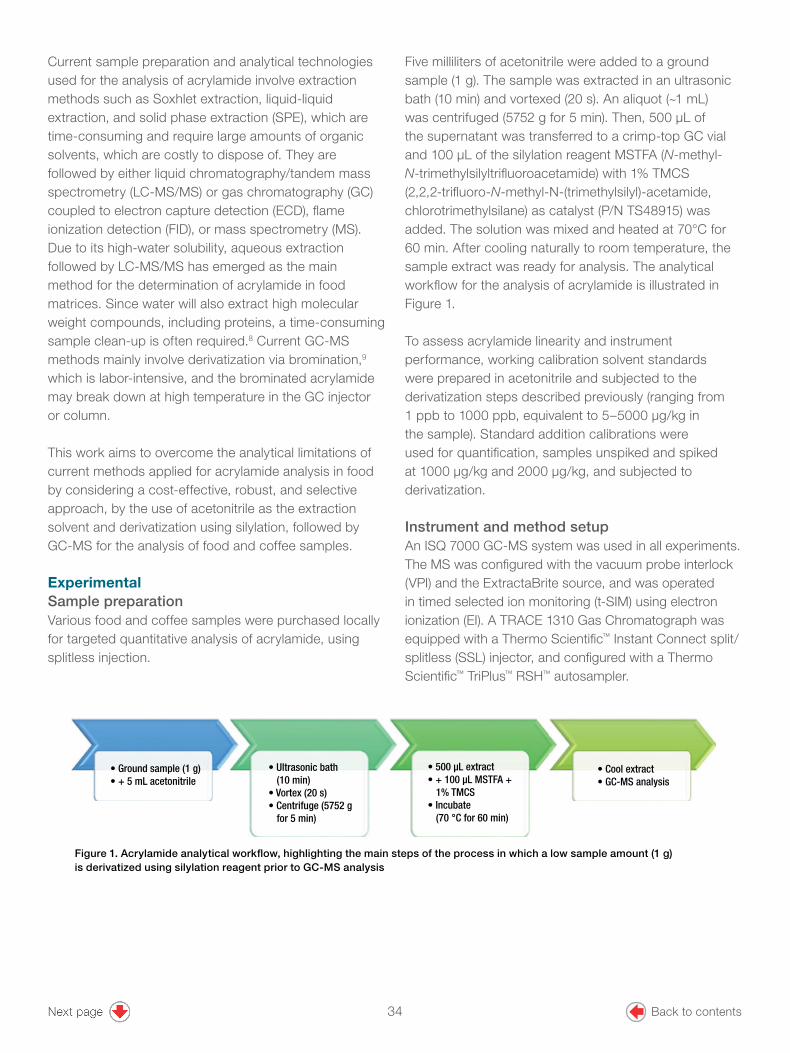
2
Current sample preparation and analytical technologies used for the analysis of acrylamide involve extraction methods such as Soxhlet extraction, liquid-liquid extraction, and solid phase extraction (SPE), which are time-consuming and require large amounts of organic solvents, which are costly to dispose of. They are followed by either liquid chromatography/tandem mass spectrometry (LC-MS/MS) or gas chromatography (GC) coupled to electron capture detection (ECD), flame ionization detection (FID), or mass spectrometry (MS). Due to its high-water solubility, aqueous extraction followed by LC-MS/MS has emerged as the main method for the determination of acrylamide in food matrices. Since water will also extract high molecular weight compounds, including proteins, a time-consuming sample clean-up is often required.8 Current GC-MS methods mainly involve derivatization via bromination,9 which is labor-intensive, and the brominated acrylamide may break down at high temperature in the GC injector or column.
This work aims to overcome the analytical limitations of current methods applied for acrylamide analysis in food by considering a cost-effective, robust, and selective approach, by the use of acetonitrile as the extraction solvent and derivatization using silylation, followed by GC-MS for the analysis of food and coffee samples.
Experimental Sample preparationVarious food and coffee samples were purchased locally for targeted quantitative analysis of acrylamide, using splitless injection.
Five milliliters of acetonitrile were added to a ground sample (1 g). The sample was extracted in an ultrasonic bath (10 min) and vortexed (20 s). An aliquot (~1 mL) was centrifuged (5752 g for 5 min). Then, 500 µL of the supernatant was transferred to a crimp-top GC vial and 100 µL of the silylation reagent MSTFA (N-methyl-N-trimethylsilyltrifluoroacetamide) with 1% TMCS (2,2,2-trifluoro-N-methyl-N-(trimethylsilyl)-acetamide, chlorotrimethylsilane) as catalyst (P/N TS48915) was added. The solution was mixed and heated at 70°C for 60 min. After cooling naturally to room temperature, the sample extract was ready for analysis. The analytical workflow for the analysis of acrylamide is illustrated in Figure 1.
To assess acrylamide linearity and instrument performance, working calibration solvent standards were prepared in acetonitrile and subjected to the derivatization steps described previously (ranging from 1 ppb to 1000 ppb, equivalent to 5–5000 µg/kg in the sample). Standard addition calibrations were used for quantification, samples unspiked and spiked at 1000 µg/kg and 2000 µg/kg, and subjected to derivatization.
Instrument and method setupAn ISQ 7000 GC-MS system was used in all experiments. The MS was configured with the vacuum probe interlock (VPI) and the ExtractaBrite source, and was operated in timed selected ion monitoring (t-SIM) using electron ionization (EI). A TRACE 1310 Gas Chromatograph was equipped with a Thermo Scientific™ Instant Connect split/splitless (SSL) injector, and configured with a Thermo Scientific™ TriPlus™ RSH™ autosampler.
• Ground sample (1 g)• + 5 mL acetonitrile
• Ultrasonic bath (10 min)• Vortex (20 s)• Centrifuge (5752 g for 5 min)
• 500 μL extract • + 100 μL MSTFA + 1% TMCS• Incubate (70 °C for 60 min)
• Cool extract• GC-MS analysis
Figure 1. Acrylamide analytical workflow, highlighting the main steps of the process in which a low sample amount (1 g) is derivatized using silylation reagent prior to GC-MS analysis
34 Back to contents

3
Data processingData were acquired, processed, and reported using Chromeleon CDS software, version 7.2. Chromeleon CDS software allows the analyst to set up acquisition, processing, and reporting methods with easy data reviewing and flexible data reporting.
Results and discussionThe object of this study was to evaluate the utility of a simplified approach that uses GC-MS to analyze acrylamide in food. For this, MSTFA was employed to derivatize acrylamide. In-depth investigation of the derivatization parameters, including derivatization volume, temperature, and time was performed. The analytical method was tested by considering various analytical parameters, including selected ion monitoring (SIM) conditions, chromatographic resolution, linearity, sensitivity, repeatability, and robustness in matrix, and selectivity.
ChromatographyUsing the GC conditions described in Table 1, the peak shapes obtained are shown in the extracted ion chromatograms (EIC, m/z 128) for acrylamide in solvent standards, samples containing incurred residues, and spiked samples (Figures 2A, 2B, and 2C, accordingly). Peak asymmetry values for acrylamide, with tailing factors (Tf) between 0.91 and 1.01 (indicating almost perfect Gaussian peak shapes), and narrow peak widths of ~4 s were observed, measured at 10% peak height (Figure 2).
Compound separation was achieved using a Thermo Scientific™ TraceGOLD™ TG-WaxMS 30 m × 0.25 mm i.d. × 0.25 µm film capillary column (P/N 26088-1420).
Additional details on instrument parameters are listed in Tables 1 and 2.
Table 1. GC and injector conditions
TRACE 1310 GC system parameters
Liner: Splitless liner, single taper, 4.0 mm × 6.5 mm × 78.5 mm
Inlet temperature (°C): 250
Carrier gas, mL/min, mode:
He, 1.2, constant flow
Inlet module and mode:
SSL, splitless
Split flow (mL/min): 100
Splitless time (min): 2
Septum purge flow (mL/min):
5
Column: TraceGOLD TG-WaxMS 30 m × 0.25 mm i.d. × 0.25 µm
Injection volume (µL): 1.0
Oven temperature program
RT Rate Target Hold
(min) (°C/min) Temp (°C) Time (min)Initial 0 - 50 2.0
Stage 1 2.0 3 100 0.0
Final 18.7 25 250 5.0
Run time 30 - - -
Table 2. Mass spectrometer conditions
Transfer line (°C): 250
Ionization mode: EI (ExtractaBrite)
Ion source (°C): 250
Electron energy (eV): 70
Acquisition mode: Timed selected ion monitoring (t-SIM)
SIM ions: m/z 128 (quantification ion) and m/z 85 (confirming ion)
35 Back to contents

4
Figure 2. Example of chromatographic separation of acrylamide in A: derivatized calibration solvent standards at 100, 250, and 1000 ppb, B: derivatized samples, instant coffee and crisps, and C: spiked samples, instant coffee and ground coffee. Annotated with tailing factor (Tf) and peak width, measured at 10% pk ht (green line). Samples and spiked sample results quoted using standard addition calibration.
Linearity of responseExternal standard calibrationSolvent standards were used to assess linearity and instrument performance. Linearity of external calibration was assessed using eight calibration levels (1 to 1000 ppb) prepared in solvent (equivalent to between 5 and 5000 µg/kg in the analyzed samples) using a 1/× weighting factor. Excellent linearity was demonstrated for acrylamide, with a coefficient of determination (R2) of 0.9993 and an average residual %RSD (AvCF %RSD) of 4.8. An example calibration curve for acrylamide is shown in Figure 3 where both the R2 value and the AvCF %RSD are annotated.
Standard addition calibrationStandard addition calibration was used for quantification, to compensate for matrix effects. Potato crisps, instant coffee, and ground coffee samples, unspiked and spiked at 1000 µg/kg and 2000 µg/kg (three replicates at each level), were quantified using a 1/× weighting factor. Excellent linearity was demonstrated for acrylamide, with an R2 value of ≥0.9987 and an AvCF %RSD of ≤4.0 achieved for crisps, instant coffee, and ground coffee standard addition calibration curves; see Figure 4 where both R2 value and the residual %RSD are annotated.
100 ppb (500 µg/kg) 1000 ppb (5000 µg/kg)[A]
[B]
[C]
Instant coffee, 143 µg/kg Crisp sample, 129 µg/kg
Instant coffee, spiked with 1000 µg/kg (1137 µg/kg)
Ground coffee, spiked with 1000 µg/kg (1198 µg/kg)
250 ppb (1250 µg/kg)
Ground coffee, 197 µg/kg
Crisp sample, spiked with 1000 µg/kg (1149 µg/kg)
36 Back to contents

5
R2 = 0.9989AvCF %RSD = 3.8
[A] - crisps [C] – ground coffee[B] - instant coffee
R2 = 0.9987AvCF %RSD = 4.0
R2 = 0.9987AvCF %RSD = 3.7
Figure 3. Example solvent calibration curve for acrylamide, illustrating the linearity obtained, over eight calibration levels ranging from 1 to 1000 ppb (equivalent to 5–5000 µg/kg in food samples). Annotated with coefficient of determination (R2) and the average calibration factor (AvCF) (as %RSD).
Acrylamide1 ppb to 1000 ppb
R2 = 0.9993AvCF %RSD = 4.8
Figure 4. Standard addition calibration curve used for quantification for A: crisps, B: instant coffee, and C: ground coffee, unspiked, and spiked at two levels (1000 µg/kg and 2000 µg/kg), three replicates at each level. Annotated with coefficient of determination (R2) and the average calibration factor (AvCF) (as %RSD).
SensitivityA limit of identification (LOI) of 1 ppb (equivalent to 5 µg/kg in the analyzed samples) was achieved using the detailed method (Figure 5). LOI is a measure of method sensitivity and was determined based on the criteria for identification of pesticide residue in food and feed (as outlined in the SANTE/11813/2017 guidelines)
considering the lowest concentration of acrylamide solvent standard passing the criteria: Ion ratios within ±30% of the expected values calculated as an average across the calibration range 1 to 1000 ppb (equivalent to between 5 and 5000 µg/kg in the analyzed samples) and ion co-elution within ±0.01 minutes.
37 Back to contents

6
Peak area repeatability and robustness in matrixRepeatability and robustness of acrylamide responses in matrix were assessed by carrying out repeated injections (n=16) of a QC ground coffee sample, spiked with 200 ppb acrylamide (equivalent to 1000 µg/kg) prior to extraction, as part of a 99-injection analytical sequence, containing derivatized blanks, calibration standards, crisp, instant coffee, and ground coffee samples. Three QC injections were mid sequence (lines 46–48), with the additional 13 injections analyzed near the end of the sequence (lines 79–92). Excellent repeatability is illustrated in Figure 6, with a peak area %RSD of 2.9 for the acrylamide absolute peak area for all 16 injections, and robustness highlighted with peak area %RSD of 1.3 comparing the spiked samples injection mid-sequence to those injected at the end of the analytical sequence. No inlet, column, MS maintenance, or MS tuning were performed over the injection sequence.
Standard level = 1 ppb (LOI)Expected ion ratio = 16.20 %Ion ratio range (+/- 30 %) = 11.34 to 21.06 %Observed ion ratio = 20.88 %Ion ratio pass/fail = pass
Figure 5. Extracted ion chromatograms for the quantification ion (m/z 128, upper) and the confirming ion (m/z 85, lower) at 1 ppb (LOI) for acrylamide. Ion ratio value achieved within ±30% of expected ion ratio (calculated as an average across the calibration range).
Figure 6. [A] Robustness data shown as consistent peak area counts for acrylamide determined in QC ground coffee samples spiked at 200 ppb (equivalent to 1000 µg/kg), analyzed mid (inj. no. 46–48), and end (inj. no. 79–92) of a 99-injection analytical sequence, containing derivatized blanks, calibration standards, crisp, instant coffee, and ground coffee samples. [B] overlaid EIC (m/z 128) of the QC ground coffee sample (n=16 injections) analyzed across the whole analytical sequence. For all QC ground coffee samples containing acrylamide at the 200 ppb level across the analytical sequence of 99 injections the calculated %RSD absolute peak area counts was 2.9.
0
250000
500000
750000
1000000
1250000
1500000
1750000
2000000
2250000
46 47 48 79 80 81 82 83 84 86 87 88 89 90 91 92
Peak
are
a (c
ount
s*m
in)
Sequence injection number
[A] Spiked ground coffee 1000 µg/kg
Injections46–48
Injections79–92
n = 15
%RSD = 2.9
[B]
38 Back to contents
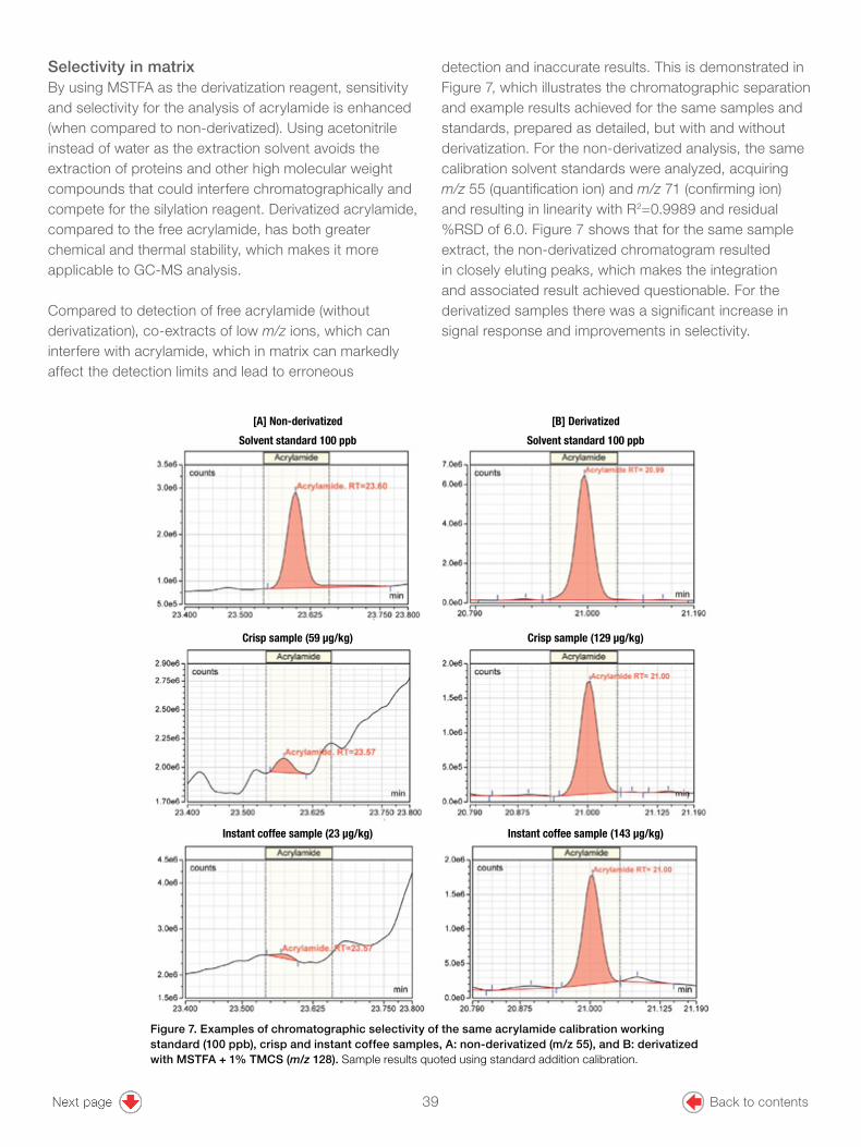
7
Selectivity in matrixBy using MSTFA as the derivatization reagent, sensitivity and selectivity for the analysis of acrylamide is enhanced (when compared to non-derivatized). Using acetonitrile instead of water as the extraction solvent avoids the extraction of proteins and other high molecular weight compounds that could interfere chromatographically and compete for the silylation reagent. Derivatized acrylamide, compared to the free acrylamide, has both greater chemical and thermal stability, which makes it more applicable to GC-MS analysis.
Compared to detection of free acrylamide (without derivatization), co-extracts of low m/z ions, which can interfere with acrylamide, which in matrix can markedly affect the detection limits and lead to erroneous
detection and inaccurate results. This is demonstrated in Figure 7, which illustrates the chromatographic separation and example results achieved for the same samples and standards, prepared as detailed, but with and without derivatization. For the non-derivatized analysis, the same calibration solvent standards were analyzed, acquiring m/z 55 (quantification ion) and m/z 71 (confirming ion) and resulting in linearity with R2=0.9989 and residual %RSD of 6.0. Figure 7 shows that for the same sample extract, the non-derivatized chromatogram resulted in closely eluting peaks, which makes the integration and associated result achieved questionable. For the derivatized samples there was a significant increase in signal response and improvements in selectivity.
Figure 7. Examples of chromatographic selectivity of the same acrylamide calibration working standard (100 ppb), crisp and instant coffee samples, A: non-derivatized (m/z 55), and B: derivatized with MSTFA + 1% TMCS (m/z 128). Sample results quoted using standard addition calibration.
[A] Non-derivatized
Solvent standard 100 ppb
Crisp sample (59 µg/kg) Crisp sample (129 µg/kg)
Instant coffee sample (23 µg/kg)
Solvent standard 100 ppb
[B] Derivatized
Instant coffee sample (143 µg/kg)
39 Back to contents

8
Quantification of acrylamide in food samplesSamples of potato crisps and coffee (instant and ground) were prepared and analyzed in triplicate using the derivatization protocol. Samples were analyzed before spiking, to determine the acrylamide content, and spiked at two levels (1000 and 2000 µg/kg) to assess recovery
and method precision. Acrylamide quantification was performed using a standard addition calibration for each matrix, which eliminated the need for an expensive 13C-labeled internal standard. A summary of results for potato crisps, instant and ground coffee samples is shown in Figure 8.
ConclusionThe results obtained clearly demonstrate that the ISQ 7000 GC-MS system with a TRACE 1310 Gas Chromatograph, in combination with the TriPlus RSH autosampler and the Chromeleon CDS software, offers a viable alternative to laboratories that analyze low level contaminants such as acrylamide in food commodities. This statement is based on the following findings:
• Good chromatographic resolution with excellent peak asymmetry values (tailing factors between 0.91 and 1.01), and peak width (+10%) ≤4 s was achieved.
• Compound linearity obtained for derivatized acrylamide over a calibration range of 1 to 1000 ppb resulted in an average coefficient of determination R2 of 0.9993 and average residual %RSD of 4.8.
• Excellent linearity was also demonstrated using standard addition calibration for acrylamide, to compensated for matrix effects, samples unspiked, and samples spiked at 1000 µg/kg and 2000 µg/kg, with R2 value of ≥0.9987 and average residual %RSD of ≤4.0 achieved for potato crisps, instant coffee, and ground coffee samples.
• The sensitivity of the method, defined as the limit of identification (LOI), of 1 ppb (equivalent to 5 µg/kg in the analyzed samples) was achieved using the detailed method.
• Excellent repeatability was achieved for the analysis of spiked ground coffee samples, 1000 µg/kg (n=16) achieving a %RSD of 2.9.
Figure 8. Average concentration of acrylamide (n=3) using standard addition calibration determined for unspiked and spiked (1000 and 2000 µg/kg) potato crisp, and instant and ground coffee samples, showing consistency at low and high levels. Standard deviation calculated from the three replicates is annotated, demonstrating the repeatability of the method.
40 Back to contents

©2019 Thermo Fisher Scientific Inc. All rights reserved. All trademarks are the property of Thermo Fisher Scientific and its subsidiaries. This information is presented as an example of the capabilities of Thermo Fisher Scientific products. It is not intended to encourage use of these products in any manners that might infringe the intellectual property rights of others. Specifications, terms and pricing are subject to change. Not all products are available in all locations. Please consult your local sales representatives for details. AN73241-EN 1219S
Find out more at thermofisher.com
• Robustness of acrylamide responses in matrix was assessed by analyzing spiked ground coffee samples, mid and late during the sequence (n=13) with %RSD of 1.3 when comparing average peak areas of mid to late sequence injected spiked samples. In addition, no inlet, column, MS maintenance, or MS tuning were performed over the injection sequence.
• Acylamide quantification using standard addition calibration eliminated the need for an expensive 13C-labeled internal standard. The results illustrated consistency at low to high levels.
• Silylation of food and coffee samples extracted with acetonitrile, quantified in t-SIM mode, maximizes sensitivity and selectivity for the analysis of acrylamide. The enhanced chemical and thermal stability of the silylated product compared to non-derivatized acrylamide analysis makes the analysis using silylation more applicable to GC-MS analysis.
• Chromeleon CDS software simplifies the workflow with user-friendly data acquisition and data processing suitable for high-throughput analysis, with intuitive data reviewing and flexible data reporting.
References1. Friedman, M.; Chemistry, Biochemistry, and Safety of Acrylamide. A Review.
J. Agric. Food Chem. 2003, 51, 4504.
2. Swedish National Food Administration: WHO to hold urgent expert consultation on acrylamide in food after findings of Swedish National Food Administration. April 2002. [Online] https://www.who.int/mediacentre/news/releases/release32/en/ (accessed 3rd July, 2019).
3. Mottram, D.S.; Wedzicha, B.L.; Dodson, A.T. Acrylamide is formed in the Maillard reaction. Nature 2002, 419, 448–449.
4. Stradler, R.H; Blank, I; Varga, N; Hau, J.; Guy, P.; Robert, M.C.; Riediker, S. Acrylamide from Maillard reaction products. Nature 2002, 419, 449–450.
5. Rydberg, P.; Eriksson, S.; Tareke, E. Karlsson, P.; Ehrenberg, L.; Tornqvist, M. Investigations of Factors That Influence the Acrylamide Content of Heated Foodstuffs. J. Agric. Food Chemistry 2003, 51, 7012.
6. Smith, E.A.; Oehme, F.W. Acrylamide and polyacrylamide: a review of production, use, environmental fate and neurotoxicity. Rev. Environmental Health 1991, 9, 215.
7. Acrylamide legislation: Information on the measures concerning acrylamide levels in food, guidance for food business operators and benchmark levels for monitoring acrylamide levels in different food categories. Food Standards Agency. [Online] https://www.food.gov.uk/business-guidance/acrylamide-legislation (accessed 3rd July, 2019).
8. Reiediker, S.; Stadler, R.H. Analysis of acrylamide in food by isotope-dilution liquid chromatography coupled with electrospray ionization tandem mass spectrometry. J. Chromatography 2003, 1020, 121–130.
9. Andrawes, F.; Greenhouse, S.; Draney, D. Chemistry of acrylamide bromination for trace analysis by gas chromatography and gas chromatography-mass spectrometry. J. Chromatography 1987, 399, 269–275.
41 Back to contents

APPLICATION NOTE 65906
Automated micro-SPE clean-up for GC-MS/MS analysis of pesticide residues in cereals
Authors: Sarvendra Pratap Singh, Subodh Kumar Budakoti, and Dasharath OulkarCustomer Solution Center, Thermo Fisher Scientific, Ghaziabad, India
Keywords: Pesticide residues, cereals, QuEChERS, micro-solid phase extraction (µSPE), GC-MS/MS, advanced electron ionization (AEI), targeted quantitation, TSQ 9000, Chromeleon Chromatography Data System
GoalTo assess the suitability of an automated micro-solid phase extraction (µSPE) clean-up of QuEChERS extracts for the determination of pesticide residues in cereal samples by gas chromatography coupled to triple quadrupole mass spectrometry.
Introduction Worldwide food demand is set to increase substantially in the next few decades1, and consequently, food safety concerns are also growing quickly2,3. To meet the demand for food, pesticides are used to control pests and ensure high crop yields, but there are some concerns that banned pesticides are still used illegally. If used incorrectly, pesticides can affect consumer’s health, hence the importance regulatory bodies place on screening food samples for the presence of pesticide residues.
Given the large number and types of food samples that need to be tested, any delays in the analysis could ultimately impact the timely import/export of food products, which is crucial for perishable products. The extraction of pesticides from food matrices is typically carried out using the QuEChERS (Quick, Easy, Cheap, Effective, Rugged, and Safe) acetonitrile method. Many versions of QuEChERS have been published but one of the most widely used versions is AOAC 2007.014. This method includes a manual dispersive solid-phase extraction clean-up step (dSPE) of the initial non-cleaned extract. This clean-up procedure can be time-consuming and can result in limited removal of matrix co-extractives. By replacing this manual clean-up step with an automated µSPE clean-up approach, laboratories can save time, achieve more effective removal of co-extractives, and thus improve the consistency of the results. A miniaturized SPE method, consisting of sorbents
Back to contents42

2
contained in a miniaturized cartridge, was first introduced by Morris and Schriner5 for LC-MSMS analysis. Lehotay et al6 and Goon et al7 have since published workflows based on the use of miniaturized SPE clean-up of QuEChERS extracts before GC-MS/MS analysis.
This work was aimed at assessing the suitability of an automated µSPE clean-up approach of QuEChERS extracts of rice and wheat samples for the multi-class determination of a large number of pesticides. The cleaned-up extracts were analyzed using a Thermo Scientific™ TSQ™ 9000 triple quadrupole GC-MS/MS system equipped with the advanced electron ionization source (AEI). The sample introduction and automated clean-up were performed using a Thermo Scientific™ TriPlus™ RSH robotic autosampler configured with a liquid injection tool as well as with the dedicated μSPE tool and cartridges tray for automated clean-up. Data acquisition and processing were carried out using the Thermo Scientific™ Chromeleon™ Chromatography Data System (CDS) software, version 7.2.
Experimental GC-MS/MS analysisA gas chromatograph (Thermo Scientific™ TRACE™ 1310 GC) was coupled to a TSQ 9000 triple quadrupole GC-MS/MS. The GC conditions are given in Table 1a, the MS parameters are detailed in Table 1b, and the autosampler parameters in Table 1c.
Glassware, reagents, and chemicals• Anhydrous MgSO4, Thermo Scientific™
(P/N 80020-415-500)
• Acetonitrile, Optima™ LC/MS Grade, Fisher Scientific™ (P/N A955-4)
• Acetic acid glacial (certified ACS), Fisher Scientific™ (P/N A38S-500)
• QuEChERS Salts (2007.01) mylar pouch 6 g magnesium sulfate (anhydrous),1.5 g sodium acetate, Thermo Scientific™ HyperSep™ (P/N 60105-341)
• µSPE GC cartridges 45 mg: 20 mg MgSO4, 12 mg PSA, 12 mg C18 and 1 mg CarbonX (P/N 60101-45GC)
• 2 mL screw vial kit, clear glass vials with caps, Thermo Scientific™ (P/N 60180-599)
• Screw caps with PTFE starburst slitted septum (LEAP PAL Parts + Consumables™, CAP-ND9-ST-SP10SB-100)
• Mixer grinder (Maharaja™ Whiteline, Delhi, India)
Table 1a. GC instrument conditions8
TRACE 1310 gas chromatograph parameters
Column
Thermo Scientific™ TraceGOLD™ TG-5SILMS with 5 m SafeGuard, 30 m × 0.25 mm ID × 0.25 µm (P/N 26096-1425 )
Injector Split/Splitless (SSL)
Liner SSL Splitless liner, single taper (P/N 453A1925UI)
Injector mode Splitless with surge
Splitless time 0.3 min
Surge pressure and time 250 kPa for 1 min
Injection volume 1.0 µL
Injector temperature 250 °C
Column flow 1.20 mL/min
Carrier gas and purity Helium (99.999%)
Purge flow 5.00 mL/min
Split flow 50.00 mL/min; Gas Saver Flow 10 mL/min after 10 min
Total run time 33.4 min
GC oven program
90 °C, 3 min 25 °C/min to 180 °C 5 °C/min to 280 °C 10 °C/min to 300 °C, 5 min
Table 1b. Mass spectrometer parameters
Table 1c. Autosampler parameters6
TSQ 9000 mass spectrometer parameters
Acquisition mode Timed selected reaction monitoring (t-SRM)
MS transfer line temp. 300 °C
Ion source temp. 320 °C
Ion source AEI (Advanced Electron Ionization)
Electron energy 70 eV
Ionization Electron Ionization (EI)
Collision gas and pressure Argon at 70 psi
Peak width 0.7 Da (both Q1 and Q3)
Tune AEI SmartTune
TriPlus RSH autosampler parameters
µSPE sample load volume 300 µL
µSPE sample fill speed 20 µL/s
µSPE sample load speed 2 µL/s
µSPE sample vial penetration depth 30 mm
Mixing cycles 5
Mixing speed 20 µL/s
Mixing volume 250 µL
Pre-wash solvent Acetonitrile
Pre-washing cycles 2
Post-wash solvent Acetonitrile:Methanol:Water (1:1:1)
Post-wash cycles 5
Injection mode Air plug
Back to contents43
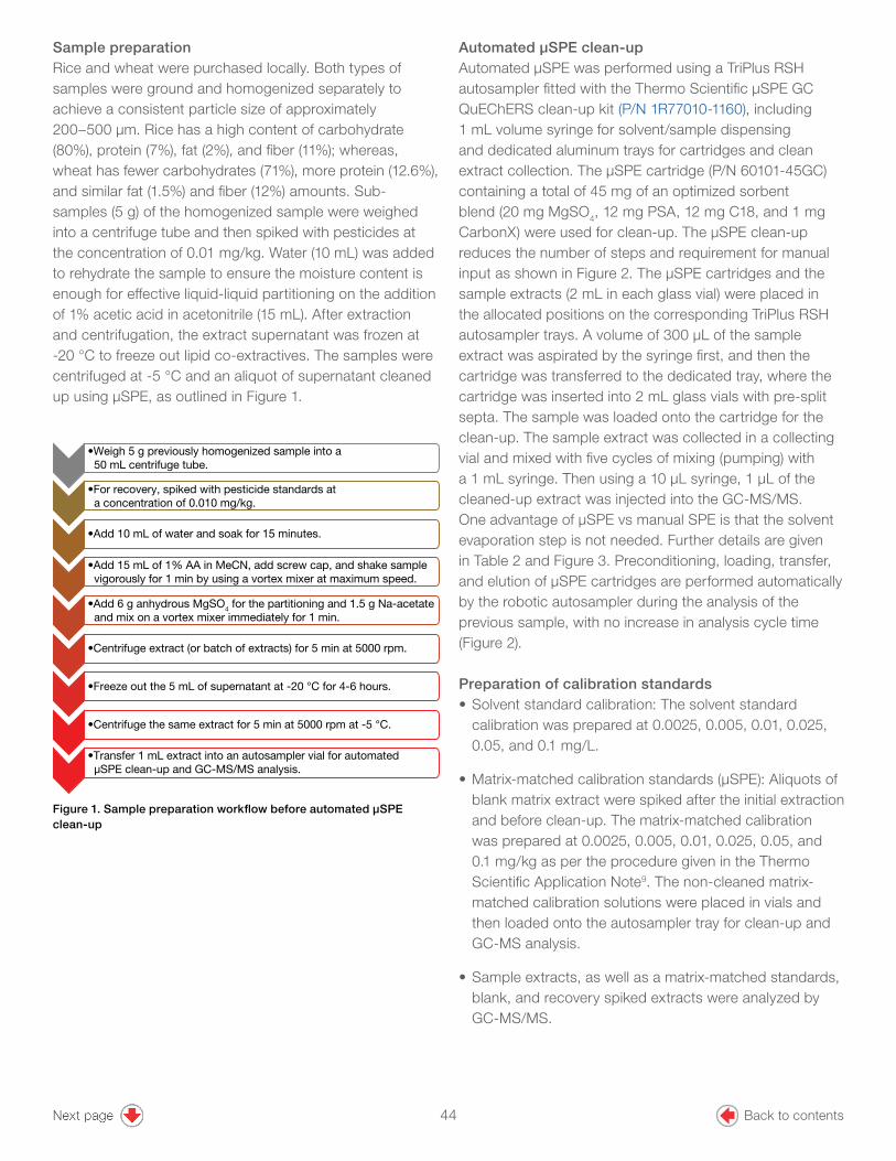
3
Figure 1. Sample preparation workflow before automated µSPE clean-up
Sample preparationRice and wheat were purchased locally. Both types of samples were ground and homogenized separately to achieve a consistent particle size of approximately 200–500 µm. Rice has a high content of carbohydrate (80%), protein (7%), fat (2%), and fiber (11%); whereas, wheat has fewer carbohydrates (71%), more protein (12.6%), and similar fat (1.5%) and fiber (12%) amounts. Sub-samples (5 g) of the homogenized sample were weighed into a centrifuge tube and then spiked with pesticides at the concentration of 0.01 mg/kg. Water (10 mL) was added to rehydrate the sample to ensure the moisture content is enough for effective liquid-liquid partitioning on the addition of 1% acetic acid in acetonitrile (15 mL). After extraction and centrifugation, the extract supernatant was frozen at -20 °C to freeze out lipid co-extractives. The samples were centrifuged at -5 °C and an aliquot of supernatant cleaned up using µSPE, as outlined in Figure 1.
Automated µSPE clean-upAutomated µSPE was performed using a TriPlus RSH autosampler fitted with the Thermo Scientific µSPE GC QuEChERS clean-up kit (P/N 1R77010-1160), including 1 mL volume syringe for solvent/sample dispensing and dedicated aluminum trays for cartridges and clean extract collection. The µSPE cartridge (P/N 60101-45GC) containing a total of 45 mg of an optimized sorbent blend (20 mg MgSO4, 12 mg PSA, 12 mg C18, and 1 mg CarbonX) were used for clean-up. The µSPE clean-up reduces the number of steps and requirement for manual input as shown in Figure 2. The µSPE cartridges and the sample extracts (2 mL in each glass vial) were placed in the allocated positions on the corresponding TriPlus RSH autosampler trays. A volume of 300 µL of the sample extract was aspirated by the syringe first, and then the cartridge was transferred to the dedicated tray, where the cartridge was inserted into 2 mL glass vials with pre-split septa. The sample was loaded onto the cartridge for the clean-up. The sample extract was collected in a collecting vial and mixed with five cycles of mixing (pumping) with a 1 mL syringe. Then using a 10 µL syringe, 1 µL of the cleaned-up extract was injected into the GC-MS/MS. One advantage of μSPE vs manual SPE is that the solvent evaporation step is not needed. Further details are given in Table 2 and Figure 3. Preconditioning, loading, transfer, and elution of µSPE cartridges are performed automatically by the robotic autosampler during the analysis of the previous sample, with no increase in analysis cycle time (Figure 2).
Preparation of calibration standards• Solvent standard calibration: The solvent standard
calibration was prepared at 0.0025, 0.005, 0.01, 0.025, 0.05, and 0.1 mg/L.
• Matrix-matched calibration standards (µSPE): Aliquots of blank matrix extract were spiked after the initial extraction and before clean-up. The matrix-matched calibration was prepared at 0.0025, 0.005, 0.01, 0.025, 0.05, and 0.1 mg/kg as per the procedure given in the Thermo Scientific Application Note9. The non-cleaned matrix-matched calibration solutions were placed in vials and then loaded onto the autosampler tray for clean-up and GC-MS analysis.
• Sample extracts, as well as a matrix-matched standards, blank, and recovery spiked extracts were analyzed by GC-MS/MS.
•Weigh 5 g previously homogenized sample into a 50 mL centrifuge tube.
•For recovery, spiked with pesticide standards at a concentration of 0.010 mg/kg.
•Add 10 mL of water and soak for 15 minutes.
•Add 15 mL of 1% AA in MeCN, add screw cap, and shake sample vigorously for 1 min by using a vortex mixer at maximum speed.
•Add 6 g anhydrous MgSO4 for the partitioning and 1.5 g Na-acetate and mix on a vortex mixer immediately for 1 min.
•Centrifuge extract (or batch of extracts) for 5 min at 5000 rpm.
•Freeze out the 5 mL of supernatant at -20 °C for 4-6 hours.
•Centrifuge the same extract for 5 min at 5000 rpm at -5 °C.
•Transfer 1 mL extract into an autosampler vial for automated µSPE clean-up and GC-MS/MS analysis.
Back to contents44

4
Figure 2. Sample extraction procedure as per the AOAC 2007.01; A) Manual clean-up with dSPE; B) Automated sample clean-up with µSPE; C) Script for the sample overlaid analysis and µSPE clean-up
Sample salt out
Sample centrifugation
QuEChERSsample extraction
Injection Shaking d-SPE clean-up
Sample salt out
Sample centrifugation
QuEChERS sample extraction
O�-line manual operations
On-line µSPE operations (B)
(A)
Injection µSPE clean-up
Freezing and centrifugation
Centrifugation
(C)
Table 2. TriPlus RSH autosampler cycle used for automated µSPE clean-up
No. Step description Time (s)
1 Parking of 10 µL syringe to the home position 40
2 Pick up of 1 mL syringe and move to the home position 20
3 Fast wash the 1 mL syringe with MeCN (2 pumps of 1 mL each) 60
4 Mixing the extract with 1 mL syringe (2 pumps of 0.25 mL each) 30
5 Load 300 μL extract from vial in Tray 1 into 1 mL syringe 40
6 Place mini-cartridge above collection vial (with glass insert) in Tray 2 10
7 Elute extract through mini-cartridge at 2 μL s−1 150
8 Discard mini-cartridge into a waste receptacle 10
9 Mix the eluate with 1 mL syringe (5 pumps of 250 µL each) 100
10 Wash the 1 mL syringe with 1/1/1 MeCN/MeOH/water (2 pumps of 0.5 mL each) 30
11 Wash the 1 mL syringe with MeCN (4 pumps of 0.5 mL each) 45
12 Switch to 10 μL syringe and wash with MeCN (2 pumps of 5 μL each) 80
13 Wash the 10 μL syringe with 1/1/1 MeCN/MeOH/water (5 pumps of 5 μL each) 40
14 Wash the 10 μL syringe with extract (3 pumps of 3 μL each) 30
15 Mixing the extract with 10 µL syringe (2 pumps of 3 µL each) 15
16 Injection of 1 μL of cleaned extract to GC-MS/MS 10
Data acquisition and processingThe data acquisition and processing were carried out using the Thermo Scientific™ Chromeleon™ Chromatography Data System (CDS) software, which allows instrument control, method development, quantitative analysis, and customizable reporting all within one package. The target list of analytes with their selected reaction monitoring
(SRM) parameters is given in Appendix 2. The data were acquired in t-SRM mode, which includes a minimum of two or more transitions per analyte. For data processing, the ion ratio (± 30%), retention time (± 0.1 min), linearity (R2 > 0.995 with residuals < ± 20%), recovery (70–120%) and precision (± 20%) were set as user-defined criteria as per the SANTE guidelines10.
Back to contents45
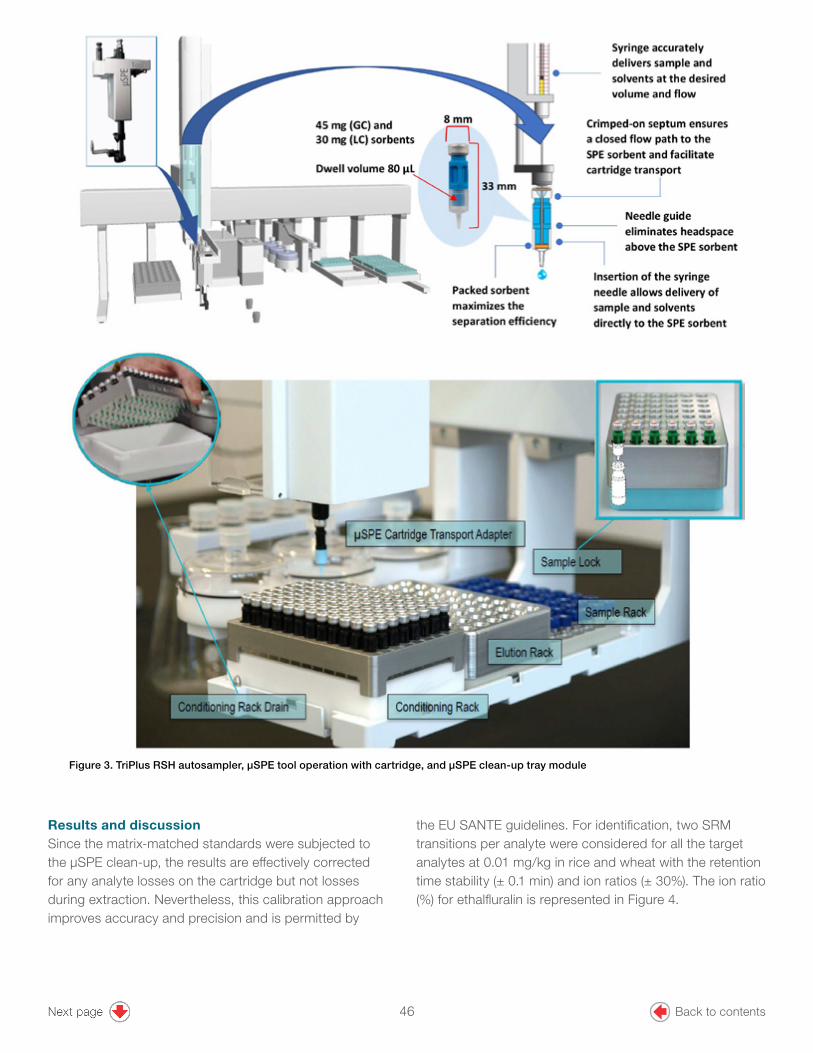
5
Results and discussionSince the matrix-matched standards were subjected to the μSPE clean-up, the results are effectively corrected for any analyte losses on the cartridge but not losses during extraction. Nevertheless, this calibration approach improves accuracy and precision and is permitted by
the EU SANTE guidelines. For identification, two SRM transitions per analyte were considered for all the target analytes at 0.01 mg/kg in rice and wheat with the retention time stability (± 0.1 min) and ion ratios (± 30%). The ion ratio (%) for ethalfluralin is represented in Figure 4.
Figure 3. TriPlus RSH autosampler, µSPE tool operation with cartridge, and µSPE clean-up tray module
Back to contents46

6
Figure 4. Ion ratio % for ethalfluralin in rice (top) and wheat (bottom) matrix-matched standards and recovery samples (n=6) pre-spiked at 0.01 mg/kg and subjected to µSPE clean-up. The EU SANTE ion ratio tolerance (%) is represented by red lines.
For confident quantification, maintaining peak symmetry with enough data points per peak is critical to achieving satisfactory repeatability. For example, the matrix-matched calibration standard of propachlor is shown in Figure 5 at 0.025 mg/kg. Also, propachlor provided excellent recovery and repeatability (RSD ≤ 4%, n=6) at 0.01 mg/kg (Appendix 1).
The matrix-matched calibration standards (rice and wheat) were linear over the concentration range of 0.0025 to 0.1 mg/kg. The coefficient of determination R2 were mostly >0.995 with residual values (as % average calibration factors) of <20% for all target analytes. An example of linearity is shown for propachlor in rice and wheat (Figure 6).
The recoveries at 0.01 mg/kg in rice were in the range of 78 to 119% (n=6) with less than 20% RSD for all target analytes (Figure 7), except chlorothalonil and tolylfluanid, which gave low responses. These pesticides are known to be susceptible to instability during analysis. At 0.01 mg/kg, the recoveries (n=6) of pesticides in wheat were between 75 and 104%, with associated %RSD < 13% for 203 of 209 pesticides as shown in Figure 8.
Wheat Rice
8.844 8.900 9.000 9.044Time [min]
-5.0e4
2.0e5
4.0e5
Inte
nsity
[cou
nts]
RT=8.94counts
Con
f 2
15 - Propachlor0.0e0
5.0e5
1.1e6
Inte
nsity
[cou
nts]
RT=8.94counts
Con
f 1
15 - Propachlor0.0e0
2.0e5
4.0e5
5.5e5
Inte
nsity
[cou
nts] RT=8.94counts
Qua
n
15 - Propachlor
Figure 5. Response observed for propachlor (quantitative and confirmatory ions) in rice (left) and wheat (right) matrix-matched standards prepared with the µSPE clean-up at a concentration of 0.025 mg/kg
Back to contents47

7
Figure 6. Calibration curve for propachlor analysis in rice and wheat matrix-matched standards with the µSPE clean-up over a concentration range of 0.0025 to 0.1 mg/kg
Rice Wheat
R2 = 0.9987RF %RSD = 4.1
R2 = 0.9988RF %RSD = 4.8
Figure 7. Recovery (%) and RSD (%) for rice matrix at 0.01 mg/kg followed by the µSPE clean-up
Figure 8. Recovery (%) and RSD (%) for wheat matrix pre-spiked at 0.01 mg/kg followed by the clean-up with µSPE
3
156
45
0
20
40
60
80
100
120
140
160
180
70-85% 85-110% 110-120%
No.
of a
naly
tes
%Recovery
Rice: %Recovery
51
128
196
0
20
40
60
80
100
120
140
<2%
No.
of
anal
ytes
%RSD
Rice: %RSD
2%–5% 5%–10% 10%–20%
14
185
10
50
100
150
200
Wheat: %Recovery
31
129
36
4
0
20
40
60
80
100
120
140
<2% 2%-5% 5%-10% 10%-20%
No.
of a
naly
tes
%RSD
Wheat: %RSD
79%–85% 85%–110% 110%–120%
No.
of a
naly
tes
%Recovery
Back to contents48

8
The vast majority of %RSDs at 0.01 mg/kg in rice and wheat were <5%. Information for individual pesticide-matrix combinations is given in Appendix 1. Overall, excellent recovery and precision values were obtained, which confirmed that the µSPE can be used as a replacement for the labor-intensive, more time-consuming dSPE manual clean-up method.
ConclusionThe experiments demonstrate that automated µSPE compared to dSPE with weighing the sorbents can significantly reduce the sample preparation time by 40 to 50% and increase sample throughput in routine laboratories by more than 1.5 times considering a batch of 10 samples. The miniaturized SPE cartridge features an optimized sorbent amount and composition, which acts with the optimum and controlled elution rate to provide high selectivity and high clean-up efficiency.
• Replacing the manual d-SPE procedures with µSPE delivers optimum recovery and precision while reducing the risk of human errors.
• The automated on-line clean-up workflow allows labor and time savings during sample preparation and increases unattended sample throughput in the laboratory.
• One cartridge type removes pigments, lipids, etc., so it is suitable for a large number of different sample types. Since it is not necessary to match the sample type to a specific blend of sorbents, the laboratory workflow is simplified.
• Excellent linearity was obtained using matrix-matched calibration standards over a concentration range of 0.0025 to 0.1 mg/kg with R2 values mostly >0.995 and %RSD of residuals <5%.
• The performance has been checked with six replicates of pre-spiked samples at 0.01 mg/kg. The results (%recovery and %RSD) were in the range of 70 to 120% and <20%, respectively, and thus in compliance with the EU SANTE guideline criteria.
References1. World Trade Organization, International trade statistics, 2014.
2. European Food Safety Authority, The 2013 European Union report on pesticide residues in food, EFSA Journal, 2015, 13, 1–169.
3. USDA Agricultural Marketing Service, Pesticide data program annual summary, calendar year 2014. https://www.ams.usda.gov/sites/default/files/media/2014%20PDP%20Annual%20Summary.pdf
4. AOAC Official Method 2007.01 Pesticide residues in foods by acetonitrile extraction and partitioning with magnesium sulfate. 2007 AOAC international.
5. Morris, B.D.; Schriner, R.B. Development of an automated column solid-phase extraction cleanup of QuEChERS extracts, using a zirconia-based sorbent, for pesticide residue analyses by LC-MS/MS. J. Agric. Food Chem. 2015, 63, 5107–5119.
6. Lehotay, S.J.; Han, L.; Sapozhnikova, Y. Automated mini-column solid-phase extraction cleanup for high-throughput analysis of chemical contaminants in foods by low-pressure gas chromatography—tandem mass spectrometry. Chromatographia, 2016, 79, 1113–1130.
7. Goon, et al.: Journal of AOAC International Vol. 103, No. x, 2019.
8. Budakoti, S.K.; Singh, S.P.; Oulkar, D. Thermo Scientific Application Note 65609: A sensitive and robust analytical solution for pesticide residues analysis in apple using GC-(AEI)-MS/MS, 2019. https://assets.thermofisher.com/TFS-Assets/CMD/Application-Notes/an-65609-gc-aei-ms-pesticides-apple-an65609-en.pdf
9. Singh, S.P.; Budakoti, S.K.; Oulkar, D. Thermo Scientific Application Note 73039: Large-scale screening and quantitation of pesticide residues in milk using GC-(EI)-MS/MS, 2019. https://assets.thermofisher.com/TFS-Assets/CMD/Application-Notes/an-73039-gc-ei-ms-pesticides-milk-an73039-en.pdf
10. Guidance document on analytical quality control and method validation procedures for pesticide residues and analysis in food and feed (2019) SANTE/12682/2019, 01/01/2019.
Back to contents49

9
Appendix 1. List of pesticides analyzed in rice and wheat results (retention time, linearity, recovery, and precision at 0.01 mg/kg) with the µSPE clean-up
RT
Rice (0.01 mg/kg) Wheat (0.01 mg/kg)
Sr. No. Compound Name R2 %Rec. %RSD R2 %Rec. %RSD
1 2,3,5,6-Tetrachloroaniline 9.19 0.9983 97 3.1 0.9980 92 2.9
2 2,4'-Methoxychlor 18.91 0.9960 108 1.3 0.9989 94 1.2
3 3,4-Dichloroaniline 7.55 0.9966 97 2.1 0.9988 79 2.9
4 4,4'-Methoxychlor olefin 18.32 0.9983 94 2.5 0.9987 94 1.4
5 Acetochlor 11.86 0.9940 111 6.7 0.9984 87 5.9
6 Acrinathrin 22.59 0.9977 105 1.9 0.9967 104 4.6
7 Alachlor 12.09 0.9955 111 2.7 0.9987 93 2.7
8 Aldrin 13.32 0.9993 87 2.2 0.9979 91 4.9
9 Allidochlor 6.47 0.9968 106 2.0 0.9990 96 2.3
10 Anthraquinone 13.32 0.9980 101 5.2 0.9941 89 3.2
11 Atrazine 10.31 0.9966 108 6.3 0.9990 91 4.6
12 Azinphos-ethyl 22.67 0.9988 113 2.8 0.9975 93 2.3
13 Azinphos-methyl 21.53 0.9956 115 2.3 0.9947 92 3.7
14 Benfluralin 9.21 0.9949 113 2.7 0.9963 91 2.8
15 BHC, Alpha 9.91 0.9973 101 1.0 0.9979 92 1.7
16 BHC, Beta 10.37 0.9971 99 2.6 0.9983 93 5.6
17 BHC, delta 11.16 0.9979 100 1.2 0.9981 93 3.2
18 BHC, gamma 10.60 0.9979 100 2.3 0.9963 90 3.4
19 Bifenthrin 20.36 0.9992 100 1.2 0.9984 96 2.2
20 Bromfenvinphos 15.58 0.9972 111 2.5 0.9988 99 4.6
21 Bromfenvinphos-methyl 14.38 0.9955 104 3.8 0.9987 100 5.5
22 Bromophos-ethyl 14.98 0.9978 107 3.0 0.9984 92 2.0
23 Bromophos-methyl (Bromophos) 13.76 0.9965 104 1.5 0.9985 93 4.0
24 Bromopropylate 20.38 0.9965 106 1.8 0.9985 93 1.7
25 Bupirimate 16.35 0.9971 103 2.1 NA NA NA
26 Carbophenothion 18.31 0.9928 108 2.2 0.9990 93 3.9
27 Carfentrazon-ethyl 18.23 0.9957 111 1.8 0.9989 91 2.7
28 Chlorbenside 15.02 0.9989 97 2.0 0.9981 83 3.0
29 Chlordane alpha-Cis 15.48 0.9973 110 5.6 0.9982 91 4.3
30 Chlordane Gamma-trans 15.07 0.9944 101 1.7 0.9978 94 2.8
31 Chlorfenapyr 16.64 0.9977 99 4.4 0.9983 88 10.3
32 Chlorfenson 15.75 0.9978 93 2.2 0.9981 94 2.8
33 Chlorfenvinphos 14.36 0.9928 109 2.6 0.9981 96 3.5
34 Chlorobenzilate 17.17 0.9980 101 3.8 0.9983 89 3.1
35 Chloroneb 8.07 0.9962 92 3.1 0.9977 95 2.4
36 Chlorpropham 9.35 0.9986 102 4.1 0.9986 84 4.1
37 Chlorpyrifos-ethyl 13.13 0.9972 104 2.0 0.9986 99 2.9
38 Chlorpyrifos-methyl 11.90 0.9920 108 3.0 0.9972 91 4.2
39 Chlorthal-dimethyl (Dacthal) 13.30 0.9972 95 2.7 0.9990 96 2.6
40 Chlorothalonil 10.95 NA NA NA 0.9952 100 6.0
41 Chlorthiophos 17.54 0.9985 100 1.0 0.9982 90 1.4
42 Chlozolinate 14.27 0.9954 99 3.6 0.9989 96 4.1
<LOQ= Below limit of quantification (0.01 mg/kg)
Back to contents50

10
Appendix 1 (continued). List of pesticides analyzed in rice and wheat results (retention time, linearity, recovery, and precision at 0.01 mg/kg) with the µSPE clean-up
RT
Rice (0.01 mg/kg) Wheat (0.01 mg/kg)
Sr. No. Compound Name R2 %Rec. %RSD R2 %Rec. %RSD
43 Clomazone 10.42 0.9980 104 2.0 0.9988 92 2.1
44 Coumaphos 23.84 0.9965 107 1.4 0.9982 94 3.1
45 Cycloate 9.22 0.9973 88 4.9 0.9940 103 6.2
46 Cyfluthrin peak 1 24.71 0.9984 109 3.1 0.9981 95 3.0
47 Cyfluthrin peak 2 24.91 0.9979 113 2.3 0.9982 98 2.5
48 Cyfluthrin peak 3 25.02 0.9988 108 2.9 0.9974 97 4.1
49 Cyfluthrin peak 4 25.11 0.9985 107 3.6 0.9978 94 2.0
50 Cyhalothrin I (lambda) 22.20 0.9969 108 2.4 0.9988 95 5.8
51 Cypermethrin peak 1 25.31 0.9984 104 4.4 0.9980 94 3.1
52 Cypermethrin peak 2 25.52 0.9978 109 3.9 0.9984 97 4.2
53 Cypermethrin peak 3 25.62 0.9985 109 2.9 0.9979 95 4.0
54 Cypermethrin peak 4 25.71 0.9978 111 4.2 0.9969 96 4.8
55 Cyprodinil 14.11 0.9988 102 2.3 0.9959 92 2.0
56 DDD p,p 17.45 0.9983 103 2.0 0.9991 96 3.0
57 DDD, o, p 16.34 0.9983 97 2.3 0.9988 95 2.5
58 DDE o,p 15.14 0.9982 93 1.9 0.9984 93 2.2
59 DDE p, p 16.13 0.9978 88 1.7 0.9983 92 2.6
60 DDT o,p 17.55 0.9972 97 2.4 0.9980 91 2.4
61 DDT p,p 18.70 0.9971 98 3.2 0.9982 90 2.7
62 Deltamethrin 28.25 0.9962 112 3.6 0.9968 99 4.8
63 Diallate-cis 9.95 0.9981 103 4.2 0.9989 93 4.6
64 Diallate-trans 9.74 0.9974 104 2.3 0.9984 93 4.0
65 Diazinon 10.71 0.9970 110 3.8 0.9981 94 3.9
66 Dichlobenil 6.90 0.9981 91 1.6 0.9989 94 1.4
67 Dichlorobenzophenone, 4, 4 13.56 0.9981 96 2.0 0.9983 92 0.9
68 Dicloran (Bortran) 10.15 0.9989 112 6.5 0.9958 94 1.8
69 Dieldrin 16.31 0.9965 94 4.8 0.9968 100 5.6
70 Dimethachlor 11.75 0.9956 116 1.5 0.9988 93 2.9
71 Diphenamid 13.75 0.9971 103 2.0 0.9992 90 2.9
72 Diphenylamine 9.13 0.9982 100 8.1 0.9982 78 5.6
73 Disulfoton 11.01 0.9942 111 1.5 0.9981 78 3.8
74 Edifenphos 18.38 0.9990 104 3.7 0.9961 104 3.9
75 Endosulfan ether 11.67 0.9978 97 2.0 0.9987 93 2.3
76 Endosulfan peak 1 15.48 0.9926 113 8.2 0.9977 93 8.5
77 Endosulfan peak 2 17.27 0.9966 93 5.0 0.9992 91 3.3
78 Endosulfan sulfate 18.51 0.9962 96 2.5 0.9985 104 4.3
79 Endrin 16.95 0.9971 106 2.4 0.9985 93 6.9
80 Endrin Aldehyde 17.75 NA NA NA 0.9935 100 6.7
81 Endrin-Ketone 20.05 0.9981 92 4.4 0.9979 92 6.4
82 EPN 20.31 0.9962 106 1.8 0.9972 96 2.6
83 Esfenvalerate 27.35 0.9992 104 5.5 0.9979 92 3.1
84 Ethalfluralin 9.23 0.9983 89 11.4 0.9986 92 7.5
85 Ethion 17.45 0.9943 107 1.9 0.9985 92 2.1
<LOQ= Below limit of quantification (0.01 mg/kg)
Back to contents51
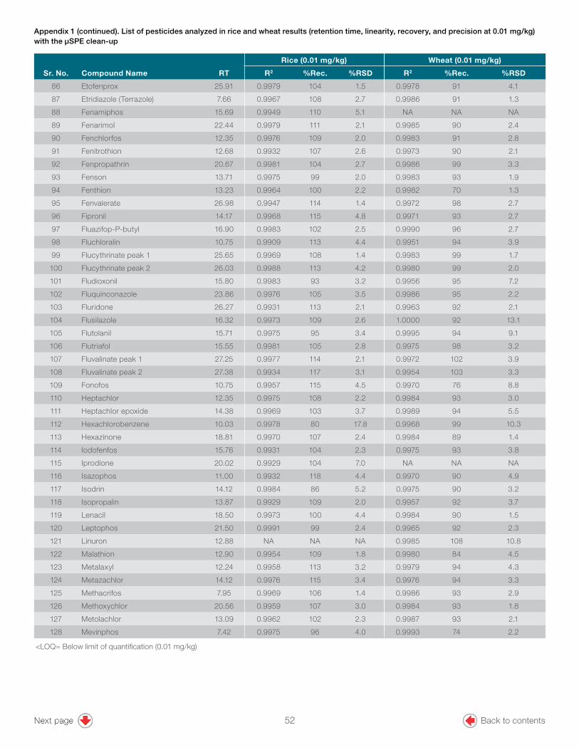
11
Appendix 1 (continued). List of pesticides analyzed in rice and wheat results (retention time, linearity, recovery, and precision at 0.01 mg/kg) with the µSPE clean-up
RT
Rice (0.01 mg/kg) Wheat (0.01 mg/kg)
Sr. No. Compound Name R2 %Rec. %RSD R2 %Rec. %RSD
86 Etofenprox 25.91 0.9979 104 1.5 0.9978 91 4.1
87 Etridiazole (Terrazole) 7.66 0.9967 108 2.7 0.9986 91 1.3
88 Fenamiphos 15.69 0.9949 110 5.1 NA NA NA
89 Fenarimol 22.44 0.9979 111 2.1 0.9985 90 2.4
90 Fenchlorfos 12.35 0.9976 109 2.0 0.9983 91 2.8
91 Fenitrothion 12.68 0.9932 107 2.6 0.9973 90 2.1
92 Fenpropathrin 20.67 0.9981 104 2.7 0.9986 99 3.3
93 Fenson 13.71 0.9975 99 2.0 0.9983 93 1.9
94 Fenthion 13.23 0.9964 100 2.2 0.9982 70 1.3
95 Fenvalerate 26.98 0.9947 114 1.4 0.9972 98 2.7
96 Fipronil 14.17 0.9968 115 4.8 0.9971 93 2.7
97 Fluazifop-P-butyl 16.90 0.9983 102 2.5 0.9990 96 2.7
98 Fluchloralin 10.75 0.9909 113 4.4 0.9951 94 3.9
99 Flucythrinate peak 1 25.65 0.9969 108 1.4 0.9983 99 1.7
100 Flucythrinate peak 2 26.03 0.9988 113 4.2 0.9980 99 2.0
101 Fludioxonil 15.80 0.9983 93 3.2 0.9956 95 7.2
102 Fluquinconazole 23.86 0.9976 105 3.5 0.9986 95 2.2
103 Fluridone 26.27 0.9931 113 2.1 0.9963 92 2.1
104 Flusilazole 16.32 0.9973 109 2.6 1.0000 92 13.1
105 Flutolanil 15.71 0.9975 95 3.4 0.9995 94 9.1
106 Flutriafol 15.55 0.9981 105 2.8 0.9975 98 3.2
107 Fluvalinate peak 1 27.25 0.9977 114 2.1 0.9972 102 3.9
108 Fluvalinate peak 2 27.38 0.9934 117 3.1 0.9954 103 3.3
109 Fonofos 10.75 0.9957 115 4.5 0.9970 76 8.8
110 Heptachlor 12.35 0.9975 108 2.2 0.9984 93 3.0
111 Heptachlor epoxide 14.38 0.9969 103 3.7 0.9989 94 5.5
112 Hexachlorobenzene 10.03 0.9978 80 17.8 0.9968 99 10.3
113 Hexazinone 18.81 0.9970 107 2.4 0.9984 89 1.4
114 Iodofenfos 15.76 0.9931 104 2.3 0.9975 93 3.8
115 Iprodione 20.02 0.9929 104 7.0 NA NA NA
116 Isazophos 11.00 0.9932 118 4.4 0.9970 90 4.9
117 Isodrin 14.12 0.9984 86 5.2 0.9975 90 3.2
118 Isopropalin 13.87 0.9929 109 2.0 0.9957 92 3.7
119 Lenacil 18.50 0.9973 100 4.4 0.9984 90 1.5
120 Leptophos 21.50 0.9991 99 2.4 0.9965 92 2.3
121 Linuron 12.88 NA NA NA 0.9985 108 10.8
122 Malathion 12.90 0.9954 109 1.8 0.9980 84 4.5
123 Metalaxyl 12.24 0.9958 113 3.2 0.9979 94 4.3
124 Metazachlor 14.12 0.9976 115 3.4 0.9976 94 3.3
125 Methacrifos 7.95 0.9969 106 1.4 0.9986 93 2.9
126 Methoxychlor 20.56 0.9959 107 3.0 0.9984 93 1.8
127 Metolachlor 13.09 0.9962 102 2.3 0.9987 93 2.1
128 Mevinphos 7.42 0.9975 96 4.0 0.9993 74 2.2
<LOQ= Below limit of quantification (0.01 mg/kg)
Back to contents52

12
Appendix 1 (continued). List of pesticides analyzed in rice and wheat results (retention time, linearity, recovery, and precision at 0.01 mg/kg) with the µSPE clean-up
<LOQ= Below limit of quantification (0.01 mg/kg)
RT
Rice (0.01 mg/kg) Wheat (0.01 mg/kg)
Sr. No. Compound Name R2 %Rec. %RSD R2 %Rec. %RSD
129 MGK-264 A 13.80 0.9983 96 3.8 0.9983 92 7.2
130 MGK-264 B 14.16 0.9975 99 3.9 0.9989 97 6.7
131 Mirex 22.20 0.9996 86 7.0 0.9957 81 5.7
132 Myclobutanil 16.23 0.9973 109 2.5 NA NA NA
133 N-(2,4-Dimethylphenyl)formamide 7.89 0.9963 112 7.1 0.9983 78 5.3
134 Nitralin 19.45 0.9944 107 4.0 0.9925 100 8.4
135 Nitrofen 16.87 0.9954 103 3.9 0.9978 92 1.9
136 Nonachlor-cis 17.47 0.9976 99 3.1 0.9980 92 2.5
137 Nonachlor-trans 15.58 0.9949 105 4.4 0.9963 89 4.6
138 Norflurazon 18.35 0.9971 107 1.5 0.9981 91 0.9
139 Ortho-phenylphenol 8.23 0.9994 96 1.6 0.9984 75 3.5
140 Oxadiazon 16.14 0.9972 93 2.6 0.9986 96 3.1
141 Oxyfluorfen 16.30 0.9929 110 4.3 0.9966 94 4.5
142 Paclobutrazol 15.21 0.9951 113 4.6 0.9979 89 3.5
143 Parathion (ethyl) 13.33 0.9959 108 3.4 0.9973 91 3.3
144 Parathion-methyl 12.04 0.9920 119 1.4 0.9982 90 3.5
145 Pebulate 7.71 0.9964 115 7.9 0.9989 103 2.5
146 Penconazole 14.25 0.9979 108 2.9 0.9986 92 1.3
147 Pendimethalin 14.08 0.9901 113 3.0 0.9951 91 5.8
148 Pentachloroaniline 11.64 0.9986 109 7.7 0.9974 101 4.6
149 Pentachloroanisole 10.12 0.9984 95 1.4 0.9987 90 3.6
150 Pentachlorobenzene 8.27 0.9977 88 11.0 0.9985 103 7.0
151 Pentachlorobenzonitrile 10.60 0.9958 104 3.1 0.9973 92 3.0
152 Pentachlorothioanisole 12.91 0.9951 87 4.2 0.9965 88 5.4
153 Permethrin peak 1 23.66 0.9983 78 7.4 0.9988 100 3.3
154 Permethrin peak 2 23.91 0.9980 110 5.0 0.9982 90 2.2
155 Perthane (Ethylan) 16.92 0.9975 103 2.1 0.9992 94 1.8
156 Phenothrin 21.38 0.9990 101 12.9 0.9985 105 11.3
157 Phorate 9.75 0.9975 117 2.9 0.9979 85 3.4
158 Phosalone 21.45 0.9905 108 1.2 0.9981 95 3.2
159 Phosmet 20.17 0.9958 101 2.3 0.9987 90 2.3
160 Phthalimide 7.80 0.9972 106 13.0 0.9989 87 5.6
161 Piperonyl butoxide 19.45 0.9945 107 2.8 0.9982 93 3.1
162 Pirimiphos-ethyl 13.71 0.9978 108 2.8 0.9984 94 1.9
163 Pirimiphos-methyl 12.60 0.9979 109 1.2 0.9991 93 5.6
164 Pretilachlor 15.93 0.9976 97 2.0 0.9982 93 4.2
165 Prochloraz 24.00 0.9936 112 4.2 0.9967 91 3.2
166 Procymidone 14.65 0.9968 104 3.6 0.9985 91 1.8
167 Prodiamine 12.64 0.9921 111 4.2 0.9972 92 1.7
168 Profenofos 15.99 0.9947 102 4.1 0.9973 103 6.1
169 Profluralin 10.49 0.9917 107 2.7 0.9987 89 4.4
Back to contents53

13
Appendix 1 (continued). List of pesticides analyzed in rice and wheat results (retention time, linearity, recovery, and precision at 0.01 mg/kg) with the µSPE clean-up
<LOQ= Below limit of quantification (0.01 mg/kg)
RT
Rice (0.01 mg/kg) Wheat (0.01 mg/kg)
Sr. No. Compound Name R2 %Rec. %RSD R2 %Rec. %RSD
170 Propachlor 8.94 0.9987 104 1.9 0.9990 96 3.2
171 Propanil 11.79 0.9945 114 7.4 0.9977 90 5.4
172 Propargite 19.26 0.9978 102 4.3 0.9991 92 9.2
173 Propisochlor 12.19 0.9958 112 2.5 0.9993 94 2.5
174 Propyzamide 10.70 0.9973 109 1.5 0.9987 91 2.6
175 Prothiofos 15.86 0.9982 93 3.4 0.9947 90 9.7
176 Pyraclofos 22.99 0.9946 97 4.1 0.9969 99 3.1
177 Pyrazophos 22.50 0.9931 117 2.0 0.9979 93 2.9
178 Pyridaben 23.91 0.9965 108 1.8 0.9979 96 2.2
179 Pyridaphenthion 19.97 0.9927 110 1.7 0.9987 93 2.9
180 Pyrimethanil 10.88 0.9985 110 4.0 0.9975 92 2.5
181 Pyriproxyfen 21.80 0.9981 105 1.7 0.9981 90 3.0
182 Quinalphos 14.54 0.9931 104 2.5 0.9969 91 7.5
183 Quintozene 10.52 0.9965 101 3.9 0.9983 89 3.1
184 Resmethrin peak 2 19.54 0.9982 98 3.2 0.9988 101 3.9
185 Sulfotep 9.48 0.9948 112 3.1 0.9974 93 1.4
186 Sulprofos 17.97 0.9982 101 2.5 0.9987 76 2.1
187 Tebuconazole 19.13 0.9933 109 3.1 0.9981 89 2.4
188 Tebufenpyrad 20.85 0.9992 101 1.2 0.9987 96 1.6
189 Tecnazene 8.85 0.9994 98 3.2 0.9990 89 4.5
190 Tefluthrin 11.01 0.9960 104 2.1 0.9985 92 3.2
191 Terbacil 11.00 0.9995 106 4.9 0.9974 87 5.0
192 Terbufos 10.62 0.9907 115 1.2 0.9975 88 1.7
193 Terbuthylazine 10.61 0.9984 103 2.9 0.9991 92 4.4
194 Tetrachlorvinphos 15.16 0.9910 101 3.3 0.9984 105 6.4
195 Tetradifon 21.24 0.9984 93 3.2 0.9985 93 1.2
196 Tetrahydrophthalimide (THPI) 7.97 0.9991 105 5.3 0.9986 97 2.9
197 Tetramethrin peak 1 20.13 0.9965 85 10.7 0.9966 115 9.1
198 Tetramethrin peak 2 20.42 0.9968 110 3.8 0.9986 96 2.6
199 Tolclofos-methyl 12.08 0.9968 110 2.9 0.9983 91 2.0
200 Tolyfluanid 14.34 NA NA NA 0.9991 69 3.9
201 Transfluthrin 12.10 0.9965 108 3.7 0.9979 96 3.5
202 Triadimefon 13.42 0.9967 107 4.0 0.9987 92 5.7
203 Triadimenol 14.65 0.9980 106 2.6 0.9978 98 6.8
204 Triallate 11.20 0.9966 108 2.3 0.9985 94 3.0
205 Triazophos 17.91 0.9915 117 1.7 0.9988 94 5.2
206 Triflumizole 14.71 0.9976 116 7.4 0.9988 91 9.4
207 Trifluralin 9.37 0.9987 116 1.5 0.9975 91 3.0
208 Vinclozolin 11.98 0.9952 103 2.8 0.9971 97 3.3
209 Tricyclazole 15.97 0.9964 116 8.5 NA NA NA
210 Triphenylphosphate (IS) 19.28 NA NA NA NA NA NA
Back to contents54

14
Compound NameRT
(min) Q1 Q3 CE
2,3,5,6-Tetrachloroaniline 9.19 230.8 157.9 18
2,3,5,6-Tetrachloroaniline 9.19 230.8 159.8 18
2,3,5,6-Tetrachloroaniline 9.19 230.8 194.8 10
2,4'-Methoxychlor 18.91 227.1 121.1 10
2,4'-Methoxychlor 18.91 228.1 122.1 16
2,4'-Methoxychlor 18.91 152.0 126.1 24
2,4'-Methoxychlor 18.91 152.0 151.1 16
3,4-Dichloroaniline 7.56 160.9 99.0 20
3,4-Dichloroaniline 7.56 160.9 90.0 18
3,4-Dichloroaniline 7.56 160.9 126.0 10
4,4'-Methoxychlor olefin 18.32 238.1 152.1 34
4,4'-Methoxychlor olefin 18.32 238.1 223.1 10
4,4'-Methoxychlor olefin 18.32 308.0 238.2 12
Acetochlor 11.86 146.1 130.0 24
Acetochlor 11.86 146.1 131.0 12
Acetochlor 11.86 174.1 146.1 10
Acetochlor 11.86 223.1 132.0 20
Acetochlor 11.86 131.8 117.0 14
Acetochlor 11.86 146.0 117.7 8
Acrinathrin 22.59 208.1 180.9 8
Acrinathrin 22.59 289.0 93.1 8
Acrinathrin 22.59 181.0 152.0 22
Alachlor 12.09 188.1 130.0 32
Alachlor 12.09 188.1 132.0 14
Alachlor 12.09 188.1 160.1 8
Alachlor 12.09 160.1 131.7 10
Aldrin 13.32 254.9 219.9 20
Aldrin 13.32 262.7 191.0 30
Aldrin 13.32 262.7 192.9 32
Aldrin 13.32 330.0 298.9 10
Allidochlor 6.48 132.0 56.1 8
Allidochlor 6.48 134.0 56.0 8
Allidochlor 6.48 132.0 49.0 26
Allidochlor 6.48 138.1 95.9 6
Anthraquinone 13.33 180.1 152.0 12
Anthraquinone 13.33 208.1 152.0 22
Anthraquinone 13.33 208.1 180.1 10
Atrazine 10.32 200.1 122.0 8
Atrazine 10.32 200.1 132.0 8
Atrazine 10.32 215.1 58.1 10
Azinphos-ethyl 22.67 132.0 77.0 12
Azinphos-ethyl 22.67 132.0 51.0 26
Azinphos-ethyl 22.67 160.0 77.0 16
Appendix 2. Target list of analytes with their SRM parameters
Compound NameRT
(min) Q1 Q3 CE
Azinphos-methyl 21.52 132.0 77.0 12
Azinphos-methyl 21.52 160.0 50.9 34
Azinphos-methyl 21.52 160.0 77.0 16
Benfluralin 9.42 292.0 264.0 8
Benfluralin 9.42 292.0 160.0 20
Benfluralin 9.42 292.0 206.0 12
BHC, Alpha 9.91 180.9 144.9 14
BHC, Alpha 9.91 216.9 181.0 8
BHC, Alpha 9.91 218.9 183.0 8
BHC, Alpha 9.91 182.8 146.7 12
BHC, Alpha 9.91 218.8 146.6 20
BHC, Beta 10.38 180.9 145.0 14
BHC, Beta 10.38 216.9 180.9 8
BHC, Beta 10.38 218.9 183.0 8
BHC, Beta 10.38 218.7 146.6 18
BHC, delta 11.16 180.9 144.9 14
BHC, delta 11.16 182.9 147.0 14
BHC, delta 11.16 218.9 182.9 8
BHC, delta 11.16 218.8 146.5 20
BHC, gamma 10.60 180.9 144.9 12
BHC, gamma 10.60 216.9 180.9 8
BHC, gamma 10.60 218.9 183.0 8
BHC, gamma 10.60 180.9 109.0 26
Bifenthrin 20.37 181.0 165.9 10
Bifenthrin 20.37 181.0 179.0 12
Bifenthrin 20.37 165.1 163.6 24
Bromfenvinphos 15.60 266.9 159.0 14
Bromfenvinphos 15.60 268.9 161.1 14
Bromfenvinphos 15.60 323.1 266.9 10
Bromfenvinphos 15.60 266.9 203.0 10
Bromfenvinphos-methyl 14.38 294.9 109.0 16
Bromfenvinphos-methyl 14.38 294.9 79.1 30
Bromfenvinphos-methyl 14.38 109.0 79.0 6
Bromophos-ethyl 14.99 358.8 302.8 14
Bromophos-ethyl 14.99 302.8 284.8 14
Bromophos-ethyl 14.99 302.8 210.9 30
Bromophos-ethyl 14.99 96.9 65.0 16
Bromophos-ethyl 14.99 96.9 78.9 12
Bromophos-methyl (Bromophos) 13.77 330.8 315.8 14
Bromophos-methyl (Bromophos) 13.77 328.9 313.8 14
Bromophos-methyl (Bromophos) 13.77 330.8 93.0 24
Bromophos-methyl (Bromophos) 13.77 125.0 79.0 6
Bromopropylate 20.39 340.8 185.0 14
Back to contents55

15
Compound NameRT
(min) Q1 Q3 CE
Bromopropylate 20.39 184.9 156.9 12
Bromopropylate 20.39 184.9 75.5 30
Bupirimate 16.36 273.1 193.2 8
Bupirimate 16.36 273.1 108.0 14
Bupirimate 16.36 316.2 208.1 10
Bupirimate 16.36 208.1 140.1 12
Bupirimate 16.36 208.1 165.0 12
Captafol 19.38 150.1 79.0 6
Captafol 19.38 151.1 79.1 18
Captafol 19.38 183.1 79.1 8
Captafol 19.38 150.1 77.2 24
Captan 14.58 149.0 70.0 20
Captan 14.58 117.0 82.0 30
Captan 14.58 151.0 79.0 14
Captan 14.58 151.0 80.0 6
Captan 14.58 149.0 78.8 14
Captan 14.58 149.0 105.0 6
Carbophenothion 18.31 342.0 157.0 10
Carbophenothion 18.31 157.0 45.0 12
Carbophenothion 18.31 199.0 142.9 10
Carfentrazon-ethyl 18.23 340.1 312.1 10
Carfentrazon-ethyl 18.23 290.0 99.9 36
Carfentrazon-ethyl 18.23 311.9 150.7 18
Chlorbenside 15.03 125.0 89.0 16
Chlorbenside 15.03 125.0 99.0 16
Chlorbenside 15.03 268.0 125.0 10
Chlorbenside 15.03 125.0 62.8 28
Chlordane alpha-Cis 15.49 372.8 265.9 14
Chlordane alpha-Cis 15.49 271.8 236.8 12
Chlordane alpha-Cis 15.49 271.8 236.8 14
Chlordane alpha-Cis 15.49 372.8 265.8 20
Chlordane alpha-Cis 15.49 374.7 265.8 20
Chlordane alpha-Cis 15.49 376.6 268.0 20
Chlordane Gamma-trans 15.08 372.8 265.9 20
Chlordane Gamma-trans 15.08 374.8 265.9 20
Chlordane Gamma-trans 15.08 271.9 236.9 14
Chlordane Gamma-trans 15.08 372.7 263.7 20
Chlorfenapyr 16.64 136.9 102.0 12
Chlorfenapyr 16.64 248.9 112.0 24
Chlorfenapyr 16.64 248.9 137.1 18
Chlorfenapyr 16.64 327.9 246.9 14
Chlorfenson 15.76 175.0 111.0 10
Chlorfenson 15.76 111.0 75.0 14
Appendix 2 (continued). Target list of analytes with their SRM parameters
Compound NameRT
(min) Q1 Q3 CE
Chlorfenson 15.76 175.0 75.0 28
Chlorfenvinphos 14.37 266.9 159.0 16
Chlorfenvinphos 14.37 268.9 161.0 14
Chlorfenvinphos 14.37 323.0 266.9 14
Chlorfenvinphos 14.37 266.9 203.0 10
Chlorobenzilate 17.18 139.0 111.0 12
Chlorobenzilate 17.18 251.0 111.0 34
Chlorobenzilate 17.18 251.0 139.0 14
Chlorobenzilate 17.18 111.0 75.1 14
Chlorobenzilate 17.18 139.0 74.9 26
Chlorobenzilate 17.18 139.0 111.0 12
Chloroneb 8.00 190.9 113.0 14
Chloroneb 8.00 193.0 53.1 32
Chloroneb 8.00 193.0 115.0 14
Chloroneb 8.00 190.9 141.0 10
Chloroneb 8.00 206.0 190.9 12
Chlorothalonil 10.95 263.9 132.9 40
Chlorothalonil 10.95 265.9 133.0 36
Chlorothalonil 10.95 265.9 170.0 24
Chlorothalonil 10.95 228.8 168.0 8
Chlorpropham 9.35 127.0 65.0 20
Chlorpropham 9.35 171.0 127.0 8
Chlorpropham 9.35 213.0 127.0 14
Chlorpropham 9.35 213.0 171.0 6
Chlorpyrifos-ethyl 13.14 198.9 171.0 14
Chlorpyrifos-ethyl 13.14 196.9 168.9 12
Chlorpyrifos-ethyl 13.14 313.9 257.9 12
Chlorpyrifos-ethyl 13.14 196.7 107.0 36
Chlorpyrifos-methyl 11.91 285.9 270.9 14
Chlorpyrifos-methyl 11.91 285.9 92.9 20
Chlorpyrifos-methyl 11.91 287.9 92.9 20
Chlorpyrifos-methyl 11.91 287.9 272.9 14
Chlorpyrifos-methyl 11.91 125.0 47.0 12
Chlorpyrifos-methyl 11.91 125.0 79.0 6
Chlorthal-dimethyl (Dacthal) 13.30 300.9 272.9 12
Chlorthal-dimethyl (Dacthal) 13.30 300.9 222.9 22
Chlorthal-dimethyl (Dacthal) 13.30 222.9 166.9 20
Chlorthiophos 17.55 324.9 268.9 12
Chlorthiophos 17.55 268.9 205.0 14
Chlorthiophos 17.55 296.9 268.9 8
Chlozolinate 14.28 186.0 145.0 14
Chlozolinate 14.28 188.0 147.0 14
Chlozolinate 14.28 259.0 187.9 12
Back to contents56

16
Compound NameRT
(min) Q1 Q3 CE
Chlozolinate 14.28 259.0 152.9 26
Chlozolinate 14.28 331.0 259.0 8
Clomazone 10.42 125.0 89.0 16
Clomazone 10.42 125.0 99.0 16
Clomazone 10.42 204.0 107.0 18
Clomazone 10.42 138.0 74.9 24
Clomazone 10.42 138.0 111.0 12
Coumaphos 23.85 226.0 163.0 18
Coumaphos 23.85 362.0 226.0 10
Coumaphos 23.85 209.9 119.0 22
Coumaphos 23.85 209.9 182.0 10
Cycloate 9.22 154.1 83.1 8
Cycloate 9.22 154.1 55.1 18
Cycloate 9.22 215.1 154.1 6
Cycloate 9.22 83.1 55.1 6
Cyfluthrin peak 1 24.70 163.0 127.1 6
Cyfluthrin peak 1 24.70 226.0 206.1 12
Cyfluthrin peak 1 24.70 163.0 91.1 12
Cyfluthrin peak 1 24.70 163.0 65.1 26
Cyfluthrin peak 2 24.91 163.0 127.0 6
Cyfluthrin peak 2 24.91 226.0 206.1 12
Cyfluthrin peak 2 24.91 163.0 91.1 12
Cyfluthrin peak 2 24.91 206.0 151.1 18
Cyfluthrin peak 3 25.02 163.0 127.0 6
Cyfluthrin peak 3 25.02 226.0 206.1 12
Cyfluthrin peak 3 25.02 163.0 91.1 12
Cyfluthrin peak 4 25.11 163.0 127.0 6
Cyfluthrin peak 4 25.11 226.0 206.1 10
Cyfluthrin peak 4 25.11 163.0 91.1 12
Cyhalothrin I (lambda) 22.21 180.9 152.0 22
Cyhalothrin I (lambda) 22.21 197.1 141.1 10
Cyhalothrin I (lambda) 22.21 207.9 180.9 8
Cypermethrin peak 1 25.32 163.0 127.1 6
Cypermethrin peak 1 25.32 165.0 127.1 5
Cypermethrin peak 1 25.32 163.0 91.1 12
Cypermethrin peak 1 25.32 180.9 152.1 20
Cypermethrin peak 2 25.53 163.0 127.0 6
Cypermethrin peak 2 25.53 165.0 127.1 5
Cypermethrin peak 2 25.53 163.0 91.1 12
Cypermethrin peak 2 25.53 180.9 151.9 18
Cypermethrin peak 3 25.61 163.0 127.0 6
Cypermethrin peak 3 25.61 165.0 127.1 5
Cypermethrin peak 3 25.61 163.0 91.0 12
Appendix 2 (continued). Target list of analytes with their SRM parameters
Compound NameRT
(min) Q1 Q3 CE
Cypermethrin peak 3 25.61 180.9 152.2 20
Cypermethrin peak 4 25.72 163.0 127.1 6
Cypermethrin peak 4 25.72 165.0 127.1 5
Cypermethrin peak 4 25.72 163.0 91.1 12
Cypermethrin peak 4 25.72 180.9 152.2 20
Cyprodinil 14.12 224.1 208.1 18
Cyprodinil 14.12 224.1 197.1 20
Cyprodinil 14.12 225.1 210.1 16
DDD p,p 17.46 235.0 165.0 20
DDD p,p 17.46 235.0 199.0 14
DDD p,p 17.46 237.0 165.0 20
DDD, o, p 16.34 235.0 165.0 20
DDD, o, p 16.34 235.0 199.0 14
DDD, o, p 16.34 237.0 165.0 20
DDE o,p 15.14 246.0 176.1 28
DDE o,p 15.14 248.0 176.1 30
DDE o,p 15.14 317.9 248.0 18
DDE o,p 15.14 317.8 246.0 20
DDE p, p 16.14 246.0 176.1 28
DDE p, p 16.14 315.9 246.0 14
DDE p, p 16.14 317.9 246.0 20
DDE p, p 16.14 317.9 248.0 18
DDT o,p 17.56 235.0 165.1 22
DDT o,p 17.56 235.0 199.1 10
DDT o,p 17.56 237.0 165.1 22
DDT p,p 18.70 235.0 165.1 22
DDT p,p 18.70 236.8 165.0 22
DDT p,p 18.70 235.0 199.5 10
Deltamethrin 28.25 252.8 92.9 16
Deltamethrin 28.25 181.0 152.1 22
Deltamethrin 28.25 252.8 172.0 8
Diallate-cis 9.94 234.1 150.0 18
Diallate-cis 9.94 235.8 152.0 18
Diallate-cis 9.94 235.8 194.0 12
Diallate-trans 9.75 234.1 150.0 18
Diallate-trans 9.75 234.1 192.0 12
Diallate-trans 9.75 235.8 152.0 18
Diallate-trans 9.75 235.8 194.0 12
Diazinon 10.72 137.1 84.1 12
Diazinon 10.72 137.1 54.1 20
Diazinon 10.72 199.0 92.9 14
Diazinon 10.72 179.1 121.5 26
Dichlobenil 6.90 170.9 99.9 24
Back to contents57

17
Compound NameRT
(min) Q1 Q3 CE
Dichlobenil 6.90 170.9 136.0 12
Dichlobenil 6.90 172.8 99.8 24
Dichlorobenzophenone, 4, 4 13.57 139.0 111.0 12
Dichlorobenzophenone, 4, 4 13.57 139.0 74.9 26
Dichlorobenzophenone, 4, 4 13.57 141.0 113.0 10
Dichlorobenzophenone, 4, 4 13.57 111.0 74.9 12
Dicloran (Bortran) 10.16 206.0 176.0 10
Dicloran (Bortran) 10.16 160.0 124.1 8
Dicloran (Bortran) 10.16 176.0 148.0 12
Dieldrin 16.31 262.9 192.9 30
Dieldrin 16.31 262.9 190.9 30
Dieldrin 16.31 262.9 227.8 16
Dieldrin 16.31 276.9 240.8 6
Dimethachlor 11.76 197.1 148.0 10
Dimethachlor 11.76 134.0 77.0 24
Dimethachlor 11.76 134.0 105.1 12
Diphenamid 13.75 167.1 152.1 16
Diphenamid 13.75 167.1 165.1 20
Diphenamid 13.75 239.1 167.1 8
Diphenamid 13.75 239.1 72.1 10
Diphenylamine 9.14 168.1 167.1 14
Diphenylamine 9.14 169.1 167.1 24
Diphenylamine 9.14 169.1 168.1 12
Diphenylamine 9.14 168.1 139.0 38
Disulfoton 11.01 88.0 59.8 6
Disulfoton 11.01 88.0 45.0 18
Disulfoton 11.01 142.0 81.0 10
Disulfoton 11.01 185.9 96.9 16
Edifenphos 18.39 172.9 109.0 8
Edifenphos 18.39 310.0 109.0 26
Edifenphos 18.39 172.9 65.1 30
Endosulfan ether 11.68 238.9 204.0 12
Endosulfan ether 11.68 240.9 206.0 14
Endosulfan peak 1 15.49 240.8 205.8 14
Endosulfan peak 1 15.49 262.8 192.9 30
Endosulfan peak 1 15.49 194.9 160.0 8
Endosulfan peak 1 15.49 194.7 125.0 22
Endosulfan peak 1 15.49 194.7 159.4 8
Endosulfan peak 2 17.28 158.9 123.0 12
Endosulfan peak 2 17.28 240.6 205.8 12
Endosulfan peak 2 17.28 194.9 159.0 8
Endosulfan peak 2 17.28 236.8 118.9 30
Endosulfan sulfate 18.52 271.7 236.8 12
Appendix 2 (continued). Target list of analytes with their SRM parameters
Compound NameRT
(min) Q1 Q3 CE
Endosulfan sulfate 18.52 238.7 203.9 12
Endosulfan sulfate 18.52 271.7 234.9 12
Endrin 16.97 262.8 192.9 30
Endrin 16.97 244.9 173.0 22
Endrin 16.97 280.8 244.9 8
Endrin Aldehyde 17.75 173.0 138.1 16
Endrin Aldehyde 17.75 249.8 214.9 24
Endrin Aldehyde 17.75 278.9 242.9 10
Endrin Aldehyde 17.75 344.9 281.0 8
Endrin-Ketone 20.06 316.8 281.0 10
Endrin-Ketone 20.06 316.8 208.9 28
Endrin-Ketone 20.06 209.2 138.4 30
EPN 20.31 169.0 77.0 22
EPN 20.31 157.0 77.0 22
EPN 20.31 169.0 141.0 8
Esfenvalerate 27.36 167.0 125.0 10
Esfenvalerate 27.36 125.0 89.0 18
Esfenvalerate 27.36 167.0 89.0 32
Esfenvalerate 27.36 225.1 119.1 18
Ethalfluralin 9.24 276.0 202.0 14
Ethalfluralin 9.24 276.0 248.1 8
Ethalfluralin 9.24 315.9 276.1 8
Ethalfluralin 9.24 292.0 264.0 8
Ethion 17.45 230.9 128.9 22
Ethion 17.45 230.9 174.9 12
Ethion 17.45 153.0 97.0 10
Ethion 17.45 120.9 65.0 10
Etofenprox 25.92 163.1 107.1 16
Etofenprox 25.92 163.1 135.1 10
Etofenprox 25.92 163.1 77.1 32
Etridiazole (Terrazole) 7.67 182.8 139.9 14
Etridiazole (Terrazole) 7.67 211.0 139.9 18
Etridiazole (Terrazole) 7.67 211.0 182.9 10
Fenamiphos 15.60 303.1 195.0 8
Fenamiphos 15.60 154.0 139.0 10
Fenamiphos 15.60 217.0 202.0 12
Fenarimol 22.45 139.0 111.0 14
Fenarimol 22.45 139.0 74.9 26
Fenarimol 22.45 219.0 107.0 10
Fenchlorfos 12.35 284.9 269.9 14
Fenchlorfos 12.35 284.9 93.0 24
Fenchlorfos 12.35 286.9 271.9 14
Fenchlorfos 12.35 124.9 47.0 12
Back to contents58
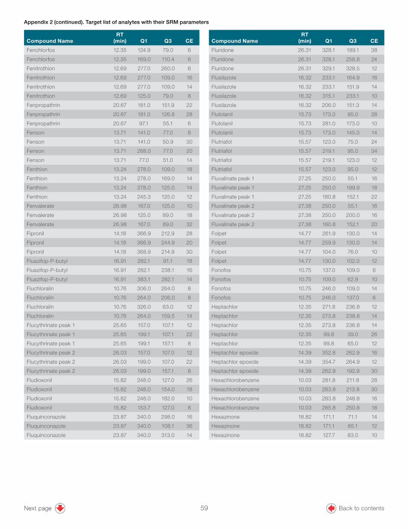
18
Compound NameRT
(min) Q1 Q3 CE
Fenchlorfos 12.35 124.9 79.0 6
Fenchlorfos 12.35 169.0 110.4 6
Fenitrothion 12.69 277.0 260.0 6
Fenitrothion 12.69 277.0 109.0 16
Fenitrothion 12.69 277.0 109.0 14
Fenitrothion 12.69 125.0 79.0 8
Fenpropathrin 20.67 181.0 151.9 22
Fenpropathrin 20.67 181.0 126.8 28
Fenpropathrin 20.67 97.1 55.1 6
Fenson 13.71 141.0 77.0 8
Fenson 13.71 141.0 50.9 30
Fenson 13.71 268.0 77.0 20
Fenson 13.71 77.0 51.0 14
Fenthion 13.24 278.0 109.0 18
Fenthion 13.24 278.0 169.0 14
Fenthion 13.24 278.0 125.0 14
Fenthion 13.24 245.3 125.0 12
Fenvalerate 26.98 167.0 125.0 10
Fenvalerate 26.98 125.0 89.0 18
Fenvalerate 26.98 167.0 89.0 32
Fipronil 14.18 366.9 212.9 28
Fipronil 14.18 366.9 244.9 20
Fipronil 14.18 368.9 214.9 30
Fluazifop-P-butyl 16.91 282.1 91.1 18
Fluazifop-P-butyl 16.91 282.1 238.1 16
Fluazifop-P-butyl 16.91 383.1 282.1 14
Fluchloralin 10.76 306.0 264.0 8
Fluchloralin 10.76 264.0 206.0 8
Fluchloralin 10.76 326.0 63.0 12
Fluchloralin 10.76 264.0 159.5 14
Flucythrinate peak 1 25.65 157.0 107.1 12
Flucythrinate peak 1 25.65 199.1 107.1 22
Flucythrinate peak 1 25.65 199.1 157.1 8
Flucythrinate peak 2 26.03 157.0 107.0 12
Flucythrinate peak 2 26.03 199.0 107.0 22
Flucythrinate peak 2 26.03 199.0 157.1 8
Fludioxonil 15.82 248.0 127.0 26
Fludioxonil 15.82 248.0 154.0 18
Fludioxonil 15.82 248.0 182.0 10
Fludioxonil 15.82 153.7 127.0 8
Fluquinconazole 23.87 340.0 298.0 16
Fluquinconazole 23.87 340.0 108.1 36
Fluquinconazole 23.87 340.0 313.0 14
Appendix 2 (continued). Target list of analytes with their SRM parameters
Compound NameRT
(min) Q1 Q3 CE
Fluridone 26.31 328.1 189.1 38
Fluridone 26.31 328.1 258.8 24
Fluridone 26.31 329.1 328.5 12
Flusilazole 16.32 233.1 164.9 16
Flusilazole 16.32 233.1 151.9 14
Flusilazole 16.32 315.1 233.1 10
Flusilazole 16.32 206.0 151.3 14
Flutolanil 15.73 173.0 95.0 28
Flutolanil 15.73 281.0 173.0 10
Flutolanil 15.73 173.0 145.0 14
Flutriafol 15.57 123.0 75.0 24
Flutriafol 15.57 219.1 95.0 34
Flutriafol 15.57 219.1 123.0 12
Flutriafol 15.57 123.0 95.0 12
Fluvalinate peak 1 27.25 250.0 55.1 16
Fluvalinate peak 1 27.25 250.0 199.9 18
Fluvalinate peak 1 27.25 180.8 152.1 22
Fluvalinate peak 2 27.38 250.0 55.1 16
Fluvalinate peak 2 27.38 250.0 200.0 16
Fluvalinate peak 2 27.38 180.8 152.1 20
Folpet 14.77 261.9 130.0 14
Folpet 14.77 259.9 130.0 14
Folpet 14.77 104.0 76.0 10
Folpet 14.77 130.0 102.0 12
Fonofos 10.75 137.0 109.0 6
Fonofos 10.75 109.0 62.9 10
Fonofos 10.75 246.0 109.0 14
Fonofos 10.75 246.0 137.0 6
Heptachlor 12.35 271.8 236.8 12
Heptachlor 12.35 273.8 238.8 14
Heptachlor 12.35 273.8 236.8 14
Heptachlor 12.35 99.8 39.0 26
Heptachlor 12.35 99.8 65.0 12
Heptachlor epoxide 14.39 352.8 262.9 16
Heptachlor epoxide 14.39 354.7 264.9 12
Heptachlor epoxide 14.39 262.9 192.9 30
Hexachlorobenzene 10.03 281.8 211.8 28
Hexachlorobenzene 10.03 283.8 213.8 30
Hexachlorobenzene 10.03 283.8 248.8 16
Hexachlorobenzene 10.03 285.8 250.8 18
Hexazinone 18.82 171.1 71.1 14
Hexazinone 18.82 171.1 85.1 12
Hexazinone 18.82 127.7 83.0 10
Back to contents59

19
Compound NameRT
(min) Q1 Q3 CE
Iodofenfos 15.76 376.8 361.8 16
Iodofenfos 15.76 378.8 363.8 14
Iodofenfos 15.76 125.0 47.0 12
Iodofenfos 15.76 125.0 79.0 6
Iodofenfos 15.76 376.8 361.8 16
Iprodione 20.03 314.0 245.0 10
Iprodione 20.03 315.7 247.0 10
Iprodione 20.03 315.7 273.0 8
Isazophos 11.00 160.9 119.0 8
Isazophos 11.00 118.9 76.0 18
Isazophos 11.00 256.9 161.9 4
Isazophos 11.00 161.0 146.0 6
Isodrin 14.13 192.9 157.0 20
Isodrin 14.13 146.9 111.1 10
Isodrin 14.13 192.9 123.0 28
Isopropalin 13.87 280.1 238.2 8
Isopropalin 13.87 280.1 180.2 10
Isopropalin 13.87 264.1 222.1 6
Isopropalin 13.87 280.1 117.8 26
Lenacil 18.52 153.0 135.6 12
Lenacil 18.52 153.0 82.1 16
Lenacil 18.52 153.0 110.0 14
Leptophos 21.51 171.0 77.1 18
Leptophos 21.51 171.0 51.0 38
Leptophos 21.51 171.0 124.3 10
Linuron 12.88 248.0 61.1 8
Linuron 12.88 159.8 133.0 12
Linuron 12.88 187.0 124.0 20
Malathion 12.90 158.0 125.0 6
Malathion 12.90 173.1 99.0 12
Malathion 12.90 127.0 99.0 6
Malathion 12.90 92.8 63.0 8
Malathion 12.90 125.0 79.0 8
Metalaxyl 12.25 234.1 146.1 20
Metalaxyl 12.25 249.1 190.1 6
Metalaxyl 12.25 234.1 174.1 10
Metazachlor 14.13 209.0 132.1 16
Metazachlor 14.13 133.1 132.1 12
Metazachlor 14.13 132.1 117.1 14
Metazachlor 14.13 133.1 117.3 22
Methacrifos 7.96 207.9 180.1 6
Methacrifos 7.96 124.9 47.1 12
Methacrifos 7.96 125.0 79.0 8
Appendix 2 (continued). Target list of analytes with their SRM parameters
Compound NameRT
(min) Q1 Q3 CE
Methacrifos 7.96 180.0 93.0 10
Methacrifos 7.96 240.0 180.0 10
Methoxychlor 20.56 227.1 141.1 32
Methoxychlor 20.56 227.1 169.1 22
Methoxychlor 20.56 227.1 212.1 12
Metolachlor 13.10 238.1 162.1 10
Metolachlor 13.10 238.1 133.1 26
Metolachlor 13.10 162.1 133.1 14
Mevinphos 7.43 127.0 109.0 10
Mevinphos 7.43 127.0 95.0 14
Mevinphos 7.43 192.0 127.0 10
MGK-264 A 13.80 164.1 98.1 10
MGK-264 A 13.80 164.1 80.1 24
MGK-264 A 13.80 164.1 93.1 10
MGK-264 B 14.17 164.1 98.1 12
MGK-264 B 14.17 164.1 67.1 6
MGK-264 B 14.17 164.1 80.1 22
Mirex 22.22 272.0 236.8 14
Mirex 22.22 273.8 238.8 14
Mirex 22.22 236.8 142.9 26
Myclobutanil 16.23 179.0 125.0 14
Myclobutanil 16.23 179.0 90.0 28
Myclobutanil 16.23 150.0 123.0 14
Myclobutanil 16.23 179.0 151.9 8
N-(2,4-Dimethylphenyl)formamide 7.90 149.1 106.1 16
N-(2,4-Dimethylphenyl)formamide 7.90 149.1 120.1 14
N-(2,4-Dimethylphenyl)formamide 7.90 149.1 121.1 6
Nitralin 19.46 316.2 274.0 8
Nitralin 19.46 274.0 216.0 8
Nitralin 19.46 274.0 169.0 12
Nitrofen 16.88 202.0 139.0 24
Nitrofen 16.88 283.0 162.0 20
Nitrofen 16.88 283.0 253.0 10
Nonachlor-cis 17.48 408.8 299.9 18
Nonachlor-cis 17.48 406.8 299.9 14
Nonachlor-cis 17.48 262.9 192.9 28
Nonachlor-cis 17.48 410.8 301.8 14
Nonachlor-cis 17.48 236.7 142.9 24
Nonachlor-trans 15.59 408.8 299.8 18
Nonachlor-trans 15.59 406.8 299.8 14
Nonachlor-trans 15.59 271.8 236.8 14
Nonachlor-trans 15.59 408.8 301.8 14
Nonachlor-trans 15.59 236.8 142.9 24
Back to contents60
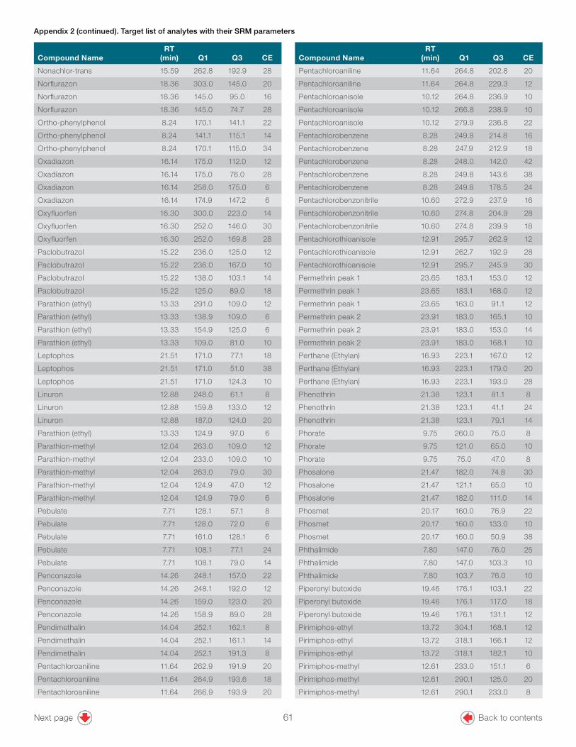
20
Compound NameRT
(min) Q1 Q3 CE
Nonachlor-trans 15.59 262.8 192.9 28
Norflurazon 18.36 303.0 145.0 20
Norflurazon 18.36 145.0 95.0 16
Norflurazon 18.36 145.0 74.7 28
Ortho-phenylphenol 8.24 170.1 141.1 22
Ortho-phenylphenol 8.24 141.1 115.1 14
Ortho-phenylphenol 8.24 170.1 115.0 34
Oxadiazon 16.14 175.0 112.0 12
Oxadiazon 16.14 175.0 76.0 28
Oxadiazon 16.14 258.0 175.0 6
Oxadiazon 16.14 174.9 147.2 6
Oxyfluorfen 16.30 300.0 223.0 14
Oxyfluorfen 16.30 252.0 146.0 30
Oxyfluorfen 16.30 252.0 169.8 28
Paclobutrazol 15.22 236.0 125.0 12
Paclobutrazol 15.22 236.0 167.0 10
Paclobutrazol 15.22 138.0 103.1 14
Paclobutrazol 15.22 125.0 89.0 18
Parathion (ethyl) 13.33 291.0 109.0 12
Parathion (ethyl) 13.33 138.9 109.0 6
Parathion (ethyl) 13.33 154.9 125.0 6
Parathion (ethyl) 13.33 109.0 81.0 10
Leptophos 21.51 171.0 77.1 18
Leptophos 21.51 171.0 51.0 38
Leptophos 21.51 171.0 124.3 10
Linuron 12.88 248.0 61.1 8
Linuron 12.88 159.8 133.0 12
Linuron 12.88 187.0 124.0 20
Parathion (ethyl) 13.33 124.9 97.0 6
Parathion-methyl 12.04 263.0 109.0 12
Parathion-methyl 12.04 233.0 109.0 10
Parathion-methyl 12.04 263.0 79.0 30
Parathion-methyl 12.04 124.9 47.0 12
Parathion-methyl 12.04 124.9 79.0 6
Pebulate 7.71 128.1 57.1 8
Pebulate 7.71 128.0 72.0 6
Pebulate 7.71 161.0 128.1 6
Pebulate 7.71 108.1 77.1 24
Pebulate 7.71 108.1 79.0 14
Penconazole 14.26 248.1 157.0 22
Penconazole 14.26 248.1 192.0 12
Penconazole 14.26 159.0 123.0 20
Penconazole 14.26 158.9 89.0 28
Pendimethalin 14.04 252.1 162.1 8
Pendimethalin 14.04 252.1 161.1 14
Pendimethalin 14.04 252.1 191.3 8
Pentachloroaniline 11.64 262.9 191.9 20
Pentachloroaniline 11.64 264.9 193.6 18
Pentachloroaniline 11.64 266.9 193.9 20
Appendix 2 (continued). Target list of analytes with their SRM parameters
Compound NameRT
(min) Q1 Q3 CE
Pentachloroaniline 11.64 264.8 202.8 20
Pentachloroaniline 11.64 264.8 229.3 12
Pentachloroanisole 10.12 264.8 236.9 10
Pentachloroanisole 10.12 266.8 238.9 10
Pentachloroanisole 10.12 279.9 236.8 22
Pentachlorobenzene 8.28 249.8 214.8 16
Pentachlorobenzene 8.28 247.9 212.9 18
Pentachlorobenzene 8.28 248.0 142.0 42
Pentachlorobenzene 8.28 249.8 143.6 38
Pentachlorobenzene 8.28 249.8 178.5 24
Pentachlorobenzonitrile 10.60 272.9 237.9 16
Pentachlorobenzonitrile 10.60 274.8 204.9 28
Pentachlorobenzonitrile 10.60 274.8 239.9 18
Pentachlorothioanisole 12.91 295.7 262.9 12
Pentachlorothioanisole 12.91 262.7 192.9 28
Pentachlorothioanisole 12.91 295.7 245.9 30
Permethrin peak 1 23.65 183.1 153.0 12
Permethrin peak 1 23.65 183.1 168.0 12
Permethrin peak 1 23.65 163.0 91.1 12
Permethrin peak 2 23.91 183.0 165.1 10
Permethrin peak 2 23.91 183.0 153.0 14
Permethrin peak 2 23.91 183.0 168.1 10
Perthane (Ethylan) 16.93 223.1 167.0 12
Perthane (Ethylan) 16.93 223.1 179.0 20
Perthane (Ethylan) 16.93 223.1 193.0 28
Phenothrin 21.38 123.1 81.1 8
Phenothrin 21.38 123.1 41.1 24
Phenothrin 21.38 123.1 79.1 14
Phorate 9.75 260.0 75.0 8
Phorate 9.75 121.0 65.0 10
Phorate 9.75 75.0 47.0 8
Phosalone 21.47 182.0 74.8 30
Phosalone 21.47 121.1 65.0 10
Phosalone 21.47 182.0 111.0 14
Phosmet 20.17 160.0 76.9 22
Phosmet 20.17 160.0 133.0 10
Phosmet 20.17 160.0 50.9 38
Phthalimide 7.80 147.0 76.0 25
Phthalimide 7.80 147.0 103.3 10
Phthalimide 7.80 103.7 76.0 10
Piperonyl butoxide 19.46 176.1 103.1 22
Piperonyl butoxide 19.46 176.1 117.0 18
Piperonyl butoxide 19.46 176.1 131.1 12
Pirimiphos-ethyl 13.72 304.1 168.1 12
Pirimiphos-ethyl 13.72 318.1 166.1 12
Pirimiphos-ethyl 13.72 318.1 182.1 10
Pirimiphos-methyl 12.61 233.0 151.1 6
Pirimiphos-methyl 12.61 290.1 125.0 20
Pirimiphos-methyl 12.61 290.1 233.0 8
Back to contents61

21
Compound NameRT
(min) Q1 Q3 CE
Pirimiphos-methyl 12.61 305.1 180.1 8
Pretilachlor 15.94 162.0 132.1 20
Pretilachlor 15.94 262.1 202.1 6
Pretilachlor 15.94 176.1 147.1 14
Pretilachlor 15.94 202.1 174.2 8
Pretilachlor 15.94 202.1 145.5 14
Pretilachlor 15.94 238.1 146.1 10
Prochloraz 24.01 308.0 70.0 12
Prochloraz 24.01 180.0 69.0 14
Prochloraz 24.01 180.1 138.1 12
Prochloraz 24.01 69.9 42.0 8
Prochloraz 24.01 308.0 147.1 12
Procymedone 14.66 283.0 96.1 8
Procymedone 14.66 283.0 68.1 24
Procymedone 14.66 285.0 96.1 10
Procymedone 14.66 95.9 53.0 16
Procymedone 14.66 95.9 67.1 8
Prodiamine 12.64 321.1 279.1 6
Prodiamine 12.64 275.1 255.1 8
Prodiamine 12.64 321.1 203.0 10
Prodiamine 12.64 279.0 203.1 6
Profenofos 16.00 338.9 268.9 14
Profenofos 16.00 336.9 266.9 12
Profenofos 16.00 296.9 268.9 10
Profenofos 16.00 336.9 308.9 8
Profluralin 10.49 318.1 199.1 12
Profluralin 10.49 318.1 55.0 12
Profluralin 10.49 347.1 330.1 6
Profluralin 10.49 318.1 284.1 10
Profluralin 10.49 330.2 69.1 20
Propachlor 8.94 120.0 50.9 32
Propachlor 8.94 120.0 77.0 16
Propachlor 8.94 176.1 57.1 8
Propanil 11.79 217.0 161.0 8
Propanil 11.79 161.0 90.0 24
Propanil 11.79 161.0 99.0 24
Propanil 11.79 160.9 125.7 16
Propargite 19.26 135.1 107.1 12
Propargite 19.26 135.1 77.1 26
Propargite 19.26 150.1 135.1 8
Propisochlor 12.20 162.1 144.1 8
Propisochlor 12.20 162.1 91.1 30
Propisochlor 12.20 162.1 120.1 12
Propisochlor 12.20 162.1 147.1 12
Propyzamide 10.70 172.9 109.0 24
Propyzamide 10.70 172.9 145.0 14
Propyzamide 10.70 174.9 147.0 14
Propyzamide 10.70 172.9 74.0 38
Prothiofos 15.87 266.9 220.9 18
Appendix 2 (continued). Target list of analytes with their SRM parameters
Compound NameRT
(min) Q1 Q3 CE
Prothiofos 15.87 266.9 238.9 8
Pentachlorothioanisole 12.91 295.7 262.9 12
Pentachlorothioanisole 12.91 262.7 192.9 28
Pentachlorothioanisole 12.91 295.7 245.9 30
Permethrin peak 1 23.65 183.1 153.0 12
Permethrin peak 1 23.65 183.1 168.0 12
Permethrin peak 1 23.65 163.0 91.1 12
Prothiofos 15.87 309.0 238.9 14
Pyraclofos 23.00 194.0 138.0 18
Pyraclofos 23.00 360.0 194.1 12
Pyraclofos 23.00 139.2 96.9 6
Pyrazophos 22.48 221.0 193.1 8
Pyrazophos 22.48 231.9 204.1 10
Pyrazophos 22.48 221.0 148.7 14
Pyridaben 23.90 147.1 117.1 20
Pyridaben 23.90 147.1 132.1 12
Pyridaben 23.90 147.1 119.1 8
Pyridaphenthion 19.97 340.0 199.1 8
Pyridaphenthion 19.97 199.0 77.1 24
Pyridaphenthion 19.97 199.0 92.1 14
Pyrimethanil 10.89 198.1 118.0 32
Pyrimethanil 10.89 198.1 158.1 18
Pyrimethanil 10.89 198.1 183.1 14
Pyriproxyfen 21.81 136.1 78.0 20
Pyriproxyfen 21.81 136.1 96.0 10
Pyriproxyfen 21.81 226.1 186.1 12
Quinalphos 14.55 146.0 118.1 10
Quinalphos 14.55 157.1 102.0 22
Quinalphos 14.55 157.1 129.0 14
Quintozene 10.53 294.8 236.9 14
Quintozene 10.53 213.8 178.9 14
Quintozene 10.53 213.8 141.9 28
Resmethrin peak 1 19.34 171.0 127.9 14
Resmethrin peak 1 19.34 143.0 128.1 10
Resmethrin peak 1 19.34 123.1 81.1 8
Resmethrin peak 2 19.54 171.0 127.9 14
Resmethrin peak 2 19.54 143.0 128.0 10
Resmethrin peak 2 19.54 123.1 81.1 8
Sulfotep 9.48 202.0 145.9 10
Sulfotep 9.48 237.9 145.9 12
Sulfotep 9.48 322.0 145.9 22
Sulfotep 9.48 265.9 145.9 15
Sulprofos 17.97 322.0 156.1 10
Sulprofos 17.97 156.0 108.0 30
Sulprofos 17.97 156.0 141.0 14
Tebuconazole 19.13 250.0 125.0 20
Tebuconazole 19.13 125.0 89.0 16
Tebuconazole 19.13 125.0 99.0 16
Tebufenpyrad 20.85 276.1 171.0 10
Back to contents62

© 2020 Thermo Fisher Scientific Inc. All rights reserved. LEAP PAL Parts + Consumables is a trademark of LEAP PAL Parts + Consumables, LLC. Maharaja is a trademark of Groupe SEB India. All other trademarks are the property of Thermo Fisher Scientific and its subsidiaries. This information is presented as an example of the capabilities of Thermo Fisher Scientific Inc. products. It is not intended to encourage use of these products in any manners that might infringe the intellectual property rights of others. Specifications, terms and pricing are subject to change. Not all products are available in all countries. Please consult your local sales representative for details. AN65906-EN 0920S
Find out more at thermofisher.com
Compound NameRT
(min) Q1 Q3 CE
Tebufenpyrad 20.85 318.1 131.1 14
Tebufenpyrad 20.85 318.1 145.1 14
Tecnazene 8.85 258.9 201.0 12
Tecnazene 8.85 202.9 142.9 18
Tecnazene 8.85 214.8 178.9 8
Tecnazene 8.85 214.8 143.6 20
Tecnazene 8.85 214.8 179.9 15
Tefluthrin 11.01 177.0 127.0 14
Tefluthrin 11.01 177.0 137.0 16
Tefluthrin 11.01 197.0 141.0 10
Terbacil 11.00 161.0 144.0 12
Terbacil 11.00 160.0 117.0 8
Terbacil 11.00 160.0 76.0 12
Terbufos 10.63 231.0 128.9 20
Terbufos 10.63 231.0 175.0 10
Terbufos 10.63 231.0 203.0 8
Terbuthylazine 10.62 214.1 104.1 16
Terbuthylazine 10.62 214.1 132.1 10
Terbuthylazine 10.62 229.1 173.1 10
Tetrachlorvinphos 15.17 328.9 109.0 18
Tetrachlorvinphos 15.17 330.9 109.0 18
Tetrachlorvinphos 15.17 332.9 109.0 14
Tetrachlorvinphos 15.17 109.0 79.0 6
Tetradifon 21.23 159.0 131.0 10
Tetrahydrophthalimide (THPI) 7.97 151.0 79.9 6
Tetrahydrophthalimide (THPI) 7.97 151.0 77.1 32
Tetrahydrophthalimide (THPI) 7.97 151.0 122.1 8
Tetramethrin peak 1 20.12 164.0 107.1 12
Tetramethrin peak 1 20.12 164.0 77.1 24
Tetramethrin peak 1 20.12 164.0 135.1 8
Tetramethrin peak 2 20.43 164.0 107.1 12
Tetramethrin peak 2 20.43 164.0 77.1 22
Tetramethrin peak 2 20.43 164.0 135.1 8
Tolclofos-methyl 12.09 265.0 250.0 12
Tolclofos-methyl 12.09 265.0 219.9 20
Appendix 2 (continued). Target list of analytes with their SRM parameters
Compound NameRT
(min) Q1 Q3 CE
Tolclofos-methyl 12.09 266.9 252.0 12
Tolylfluanid 14.34 238.0 137.0 10
Tolylfluanid 14.34 137.0 65.1 28
Tolylfluanid 14.34 137.0 91.1 18
Tolylfluanid 14.34 238.0 91.0 40
Tolylfluanid 14.34 240.0 137.0 14
Transfluthrin 12.10 163.0 143.0 14
Transfluthrin 12.10 127.0 91.1 8
Transfluthrin 12.10 163.0 91.1 12
Triadimefon 13.43 208.0 111.0 20
Triadimefon 13.43 208.0 126.7 12
Triadimefon 13.43 208.0 180.8 8
Triadimenol 14.66 168.1 70.0 10
Triadimenol 14.66 128.0 65.0 18
Triadimenol 14.66 112.0 58.0 8
Triadimenol 14.66 128.0 100.0 10
Triallate 11.21 268.0 183.9 18
Triallate 11.21 86.1 43.3 6
Triallate 11.21 268.0 226.0 12
Triazophos 17.92 161.1 134.1 8
Triazophos 17.92 257.0 162.1 6
Triazophos 17.92 161.1 106.1 12
Triazophos 17.92 162.1 119.1 12
Triflumizole 14.72 206.0 179.0 14
Triflumizole 14.72 179.0 144.0 14
Triflumizole 14.72 206.0 186.0 8
Trifluralin 9.37 306.1 264.1 8
Trifluralin 9.37 264.0 160.0 14
Trifluralin 9.37 306.1 206.0 10
Triphenylphosphate 19.28 215.0 168.1 16
Triphenylphosphate 19.28 326.1 325.1 10
Triphenylphosphate 19.28 326.1 169.1 28
Vinclozolin 11.98 186.8 124.0 18
Vinclozolin 11.98 197.9 145.0 14
Vinclozolin 11.98 212.0 172.0 14
Back to contents63

GoalThe aim of the study was to assess the quantitative performance of the Thermo Scientific™ TSQ™ 9000 triple quadrupole GC-MS/MS system fitted with the Advanced Electron Ionization (AEI) source for the analysis of pesticide residues at ultra low levels in baby food.
IntroductionThe detection and subsequent quantification of pesticides, contaminants, and other chemical residues are of paramount importance, especially when the food stuff is intended to be consumed by infants or young children. The maximum residue level (MRL) for the majority of pesticide-commodity combinations is set at the default level of 10 µg/kg.1–3 However, the European Union (EU) has established LOD MRLs between 3–8 μg/kg for specific pesticides prohibited in baby foods.4 These pesticides and their metabolites may cause infants and young children (under worst-case intake conditions) to exceed the acceptable daily intake (ADI) values. The high sensitivity and selectivity of GC-MS/MS enables the detection and identification of residues of prohibited compounds, in compliance with the residue definitions, even when dealing with the diverse composition of multi-ingredient baby foods.
Authors Richard Law, Aaron Lamb, Paul Silcock, and Cristian Cojocariu
Thermo Fisher Scientific, Runcorn, UK
Keywords TSQ 9000, advanced electron ionization, AEI, baby food, sensitivity, robustness, pesticide residue, QuEChERS, triple quadrupole mass spectrometry, GC-MS/MS, Programmable Temperature Vaporization, food safety
Ultra low level quantification of pesticides in baby foods using an advanced triple quadrupole GC-MS/MS system
APPLICATION NOTE 10586
64 Back to contents

2
Also, the increased levels of selectivity and sensitivity provided by triple quadrupole instruments compared to single quadrupole instruments enabled analysts to adopt faster, less specific sample extraction procedures such as QuEChERS (quick, easy, cheap effective, rugged and safe).
The QuEChERS procedure has become the standard approach for sample preparation in many laboratories because of improvement in productivity.5 The method usually involves extraction with acetonitrile in the presence of various salts followed by dispersive solid phase extraction (dSPE) clean-up with a combination of PSA, C18, and carbon sorbents. The efficiency of the dSPE clean-up is limited so high concentrations of matrix-coextractives can remain in the final extract and cause system contamination. Also, use of acetonitrile (which has a high coefficient of expansion) limits the injection volume and hence the sensitivity of the method.
Taking all of these considerations together, it is evident that an ultra-sensitive, selective, reliable, and robust GC-MS/MS system is needed to address the challenge of routine high-throughput determination of pesticide residues at trace concentrations in baby foods. In this study, the quantitative performance of the Thermo Scientific™ TSQ™ 9000 triple quadrupole GC-MS/MS system was assessed for the analysis of more than 200 pesticides in baby food at ultra low concentrations (as low as 0.025 µg/kg). A complete evaluation of method performance included sample preparation, overall method suitability measured from pesticides recoveries, selectivity, sensitivity, linearity, and long-term robustness.
ExperimentalSample preparationSamples of carrot/potato and apple/pear/banana baby food samples were extracted using the citrate-buffered QuEChERS protocol using Thermo Scientific™ HyperSep™ dispersive solid phase extraction (dSPE) products.
Homogenized sample (10 g) was extracted with acetonitrile (10 mL) followed by the addition of MgSO4 (4 g), NaCl (1.0 g), disodium hydrogen citrate sesquihydrate (0.5 g), and trisodium citrate dihydrate (1.0 g). Dispersive solid phase extraction (dSPE) [MgSO4 (150 mg), PSA (25 mg) and GCB (25 mg) per 1 mL of extract for carrot/potato and MgSO4 (150 mg) and PSA (25 mg) for apple/pear/banana] was used for sample clean-up.
Preparation of matrix-matched calibrationsImmediately after dSPE clean-up, the final extracts (1 g sample/mL of acetonitrile) were acidified with 5% formic acid in acetonitrile and were spiked with a mixture of 211 pesticides at 14 concentrations spanning a range of 0.025–250 µg/kg. Robustness was tested using repeat injections of samples (carrot/potato) spiked at the 10 µg/kg level.
For method evaluation, samples of carrot/potato and apple/pear/banana baby food samples were each spiked at 1.0, 2.5, and 10.0 µg/kg (n = 6 for each concentration) before extraction, clean-up, and acidification were carried out as described above.
GC-MS/MS analysisA TSQ 9000 triple quadrupole GC-MS/MS system equipped with a Thermo Scientific™ Advanced Electron Ionization (AEI) source and coupled with a Thermo Scientific™ TRACE™ 1310 GC system was used. The AEI source provides a highly efficient electron ionization of analytes and a more tightly focused ion beam that provides an unparalleled level of sensitivity.
Liquid injections of the sample extracts were performed using a Thermo Scientific™ TriPlus™ RSH™ autosampler, and chromatographic separation was achieved by a Thermo Scientific™ TraceGOLD™ TG-5SilMS 30 m × 0.25 mm I.D. × 0.25 μm film capillary column with 5 m integrated SafeGuard. Additional details of instrument parameters are displayed in Table 1.
65 Back to contents
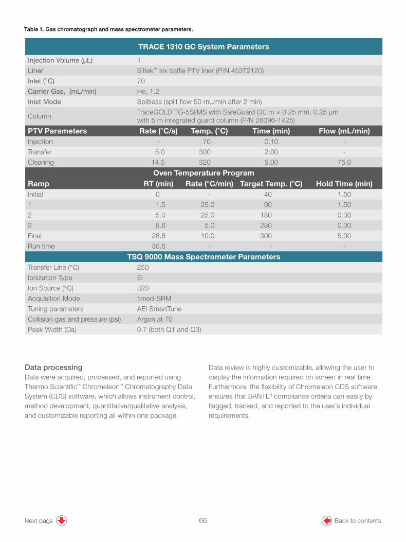
3
Data processingData were acquired, processed, and reported using Thermo Scientific™ Chromeleon™ Chromatography Data System (CDS) software, which allows instrument control, method development, quantitative/qualitative analysis, and customizable reporting all within one package.
Table 1. Gas chromatograph and mass spectrometer parameters.
Data review is highly customizable, allowing the user to display the information required on screen in real time. Furthermore, the flexibility of Chromeleon CDS software ensures that SANTE3 compliance criteria can easily by flagged, tracked, and reported to the user’s individual requirements.
TRACE 1310 GC System Parameters
Injection Volume (µL) 1
Liner Siltek™ six baffle PTV liner (P/N 453T2120)
Inlet (°C) 70
Carrier Gas, (mL/min) He, 1.2
Inlet Mode Splitless (split flow 50 mL/min after 2 min)
Column TraceGOLD TG-5SilMS with SafeGuard (30 m × 0.25 mm, 0.25 µm with 5 m integrated guard column (P/N 26096-1425)
PTV Parameters Rate (°C/s) Temp. (°C) Time (min) Flow (mL/min)Injection - 70 0.10 -
Transfer 5.0 300 2.00 -
Cleaning 14.5 320 5.00 75.0
Oven Temperature Program Ramp RT (min) Rate (°C/min) Target Temp. (°C) Hold Time (min)Initial 0 - 40 1.50
1 1.5 25.0 90 1.50
2 5.0 25.0 180 0.00
3 8.6 5.0 280 0.00
Final 28.6 10.0 300 5.00
Run time 35.6 - - -
TSQ 9000 Mass Spectrometer ParametersTransfer Line (°C) 250
Ionization Type EI
Ion Source (°C) 320
Acquisition Mode timed-SRM
Tuning parameters AEI SmartTune
Collision gas and pressure (psi) Argon at 70
Peak Width (Da) 0.7 (both Q1 and Q3)
66 Back to contents

4
Results and discussionCompliance with EU SANTE criteriaThe method performance was tested in accordance to the SANTE/11813/2017 guidance document, which requires that the following criteria are satisfied for identification of pesticide residues:
I. A minimum of two product ions are detected for each pesticide with peak S/N >3 (or, in case noise is absent, a signal should be present in at least five subsequent scans) and with the mass resolution for precursor-ion isolation equal to or better than unit mass resolution.
II. Retention time tolerance of ± 0.1 minutes compared with standards in the same sequence.
III. Ion ratio within ± 30% (relative) of the average of calibration standards from the same sequence.
Wherever SANTE compliance is referenced in this study, all three criteria have been met fully.
RecoveriesPesticide recoveries were obtained from the QuEChERS extractions performed on the samples spiked before extraction. All detected compounds, at the three spiking levels in both matrices satisfied all SANTE requirements. More than 97% of the target pesticide residues at 1 μg/kg had recoveries between 70% and 120%. An example of the recovery and precision data for the apple/pear/banana matrix spiked at the default MRL (10 µg/kg) is displayed in Figure 1. A full table of results can be found in Appendix B.
Chromatography and selectivityAnalysis of a large number of pesticides in a single injection requires careful optimization of parameters, especially when injecting acetonitrile. As acetonitrile is a low molecular weight low polarity solvent, it has a relatively high expansion volume and is insoluble in the low polarity phases normally used for routine pesticide analysis (this makes solvent focusing in a standard splitless type injection incredibly difficult). These issues can be addressed by using an optimized programmable temperature vaporisation (PTV) injection. Figure 2 shows an example of three pesticides eluting in the beginning (A–dichlobenil – 0.025 µg/kg), middle (B–dieldrin 0.5 µg/kg), and end (C–deltamethrin 0.05 µg/kg) of the chromatographic run in the lowest detectable standard in carrot and potato matrix, levels at which all compounds detected meet the SANTE requirements. Peak shapes were Gaussian and coefficient of determination (R2) was >0.990 for all three compounds indicating good chromatography and excellent linear response.
Identification of all 210 component peaks was made using an in-house, commercially available Thermo Scientific SRM pesticide compound database (cdb). In addition to this, retention time alignment of target compounds can be easily performed using the Thermo Scientific RTA tool,8 eliminating the need for manual correction of compound retention times whenever column maintenance is performed. The cdb database contains >1000 compounds with >3700 unique SRM transitions. Due to the fast scanning speed of the EvoCell technology and the intelligent scheduling of the timed-SRM,9 it is possible to acquire data with several transitions per compound with minimal loss in sensitivity. This makes it simple to select the most optimal transitions in differing matrices to perform quantitation and qualification on, removing the need to develop matrix-matched SRM compound databases (Figure 3).
67 Back to contents
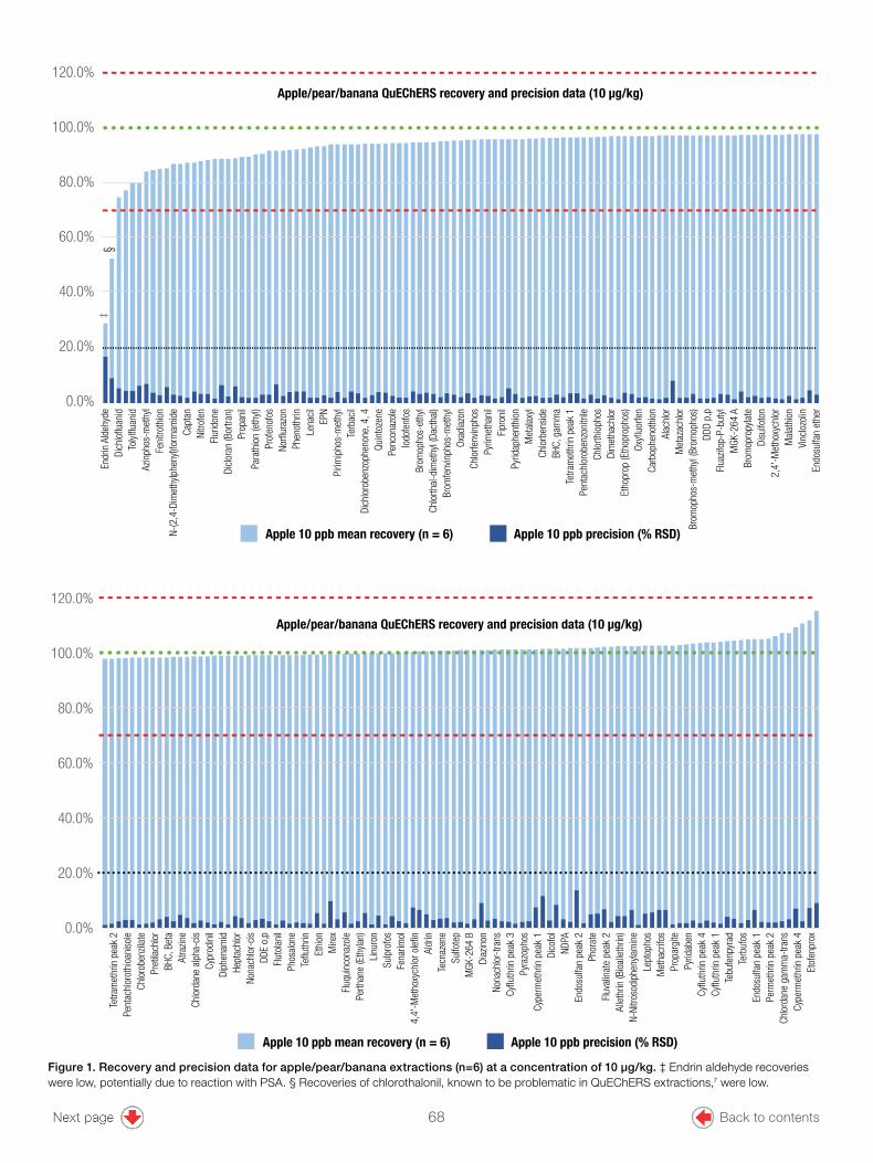
5
0.0%
20.0%
40.0%
60.0%
80.0%
100.0%
120.0%
Apple 10 ppb mean recovery (n = 6) Apple 10 ppb precision (% RSD)
Apple/pear/banana QuEChERS recovery and precision data (10 µg/kg)§
‡En
drin
Ald
ehyd
eDi
chlo
fluan
idTo
lylflu
anid
Azin
phos
-met
hyl
Feni
troth
ion
N-(2
,4-D
imet
hylp
heny
l)for
mam
ide
Capt
anNi
trofe
nFl
urid
one
Dicl
oran
(Bor
tran)
Prop
anil
Para
thio
n (e
thyl)
Prof
enof
osNo
rflur
azon
Phen
othr
inLe
naci
lEP
NPi
rimip
hos-
met
hyl
Terb
acil
Dich
loro
benz
ophe
none
, 4, 4
Quin
toze
nePe
ncon
azol
eIo
dofe
nfos
Brom
opho
s-et
hyl
Chlo
rthal
-dim
ethy
l (Da
ctha
l)Br
omfe
nvin
phos
-met
hyl
Oxad
iazo
nCh
lorfe
nvin
phos
Pyrim
etha
nil
Fipr
onil
Pyrid
aphe
nthi
onM
etal
axyl
Chlo
rben
side
BHC,
gam
ma
Tetra
met
hrin
pea
k 1
Pent
achl
orob
enzo
nitri
leCh
lorth
ioph
osDi
met
hach
lor
Etho
prop
(Eth
opro
phos
)Ox
yfluo
rfen
Carb
ophe
noth
ion
Alac
hlor
Met
azac
hlor
Brom
opho
s-m
ethy
l (Br
omop
hos)
DDD
p,p
Flua
zifop
-P-b
utyl
MGK
-264
ABr
omop
ropy
late
Disu
lfoto
n2,
4'-M
etho
xych
lor
Mal
athi
onVi
nclo
zolin
Endo
sulfa
n et
her
0.0%
20.0%
40.0%
60.0%
80.0%
100.0%
120.0%
Apple/pear/banana QuEChERS recovery and precision data (10 µg/kg)
Tetra
met
hrin
pea
k 2
Pent
achl
orot
hioa
niso
leCh
loro
benz
ilate
Pret
ilach
lor
BHC,
Bet
aAt
razin
eCh
lord
ane
alph
a-ci
sCy
prod
inil
Diph
enam
idHe
ptac
hlor
Nona
chlo
r-ci
sDD
E o,
pFl
utol
anil
Phos
alon
eTe
fluth
rinEt
hion
Mire
xFl
uqui
ncon
azol
ePe
rthan
e (E
thyla
n)Li
nuro
nSu
lpro
fos
Fena
rimol
4,4'
-Met
hoxy
chlo
r ole
finAl
drin
Tecn
azen
eSu
lfote
pM
GK-2
64 B
Diaz
inon
Nona
chlo
r-tra
nsCy
fluth
rin p
eak
3Py
razo
phos
Cype
rmet
hrin
pea
k 1
Dico
fol
NDPA
Endo
sulfa
n pe
ak 2
Phor
ate
Fluv
alin
ate
peak
2Al
leth
rin (B
ioal
leth
rin)
N-Ni
troso
diph
enyla
min
eLe
ptop
hos
Met
hacr
ifos
Prop
argi
tePy
ridab
enCy
fluth
rin p
eak
4Cy
fluth
rin p
eak
1Te
bufe
npyr
adTe
rbuf
osEn
dosu
lfan
peak
1Pe
rmet
hrin
pea
k 2
Chlo
rdan
e ga
mm
a-tra
nsCy
perm
ethr
in p
eak
4Et
ofen
prox
Apple 10 ppb mean recovery (n = 6) Apple 10 ppb precision (% RSD)
Figure 1. Recovery and precision data for apple/pear/banana extractions (n=6) at a concentration of 10 μg/kg. ‡ Endrin aldehyde recoveries were low, potentially due to reaction with PSA. § Recoveries of chlorothalonil, known to be problematic in QuEChERS extractions,7 were low.
68 Back to contents
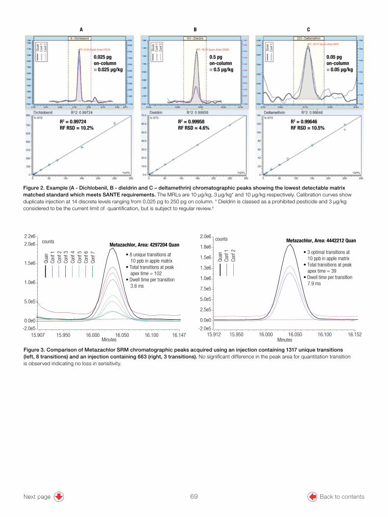
6
0.5 pg on-column≡ 0.5 µg/kg
0.025 pg on-column≡ 0.025 µg/kg
0.05 pg on-column≡ 0.05 µg/kg
R2 = 0.99646RF RSD = 10.5%
R2 = 0.99958RF RSD = 4.6%
R2 = 0.99724RF RSD = 10.2%
A CB
Figure 2. Example (A - Dichlobenil, B - dieldrin and C – deltamethrin) chromatographic peaks showing the lowest detectable matrix matched standard which meets SANTE requirements. The MRLs are 10 µg/kg, 3 µg/kg* and 10 µg/kg respectively. Calibration curves show duplicate injection at 14 discrete levels ranging from 0.025 pg to 250 pg on column. * Dieldrin is classed as a prohibited pesticide and 3 µg/kg considered to be the current limit of quantification, but is subject to regular review.4
Figure 3. Comparison of Metazachlor SRM chromatographic peaks acquired using an injection containing 1317 unique transitions (left, 8 transitions) and an injection containing 663 (right, 3 transitions). No significant difference in the peak area for quantitation transition is observed indicating no loss in sensitivity.
15.907 15.950 16.000 16.050 16.100 16.147-2.0e5
0.0e0
5.0e5
1.0e6
1.5e6
2.0e6
2.2e6
Metazachlor, Area: 4297204 Quan
Minutes
counts
Quan
Conf
1Co
nf 2
Conf
3Co
nf 4
Conf
5Co
nf 6
Conf
7
15.912 15.950 16.000 16.050 16.100 16.152-2.0e5
0.0e0
2.5e5
5.0e5
7.5e5
1.0e6
1.3e6
1.5e6
1.8e6
2.0e6Metazachlor, Area: 4442212 Quancounts
• 8 unique transitions at 10 ppb in apple matrix• Total transitions at peak apex time = 102• Dwell time per transition 3.8 ms
• 3 optimal transitions at 10 ppb in apple matrix• Total transitions at peak apex time = 39• Dwell time per transition 7.9 ms
Minutes
Quan
Conf
1Co
nf 2
69 Back to contents
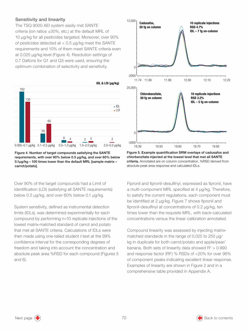
7
Figure 4. Number of target compounds satisfying the SANTE requirements, with over 90% below 0.5 µg/kg, and over 60% below 0.1µg/kg – 100 times lower than the default MRL [sample matrix – carrot/potato].
Sensitivity and linearityThe TSQ 9000 AEI system easily met SANTE criteria (ion ratios ±30%, etc.) at the default MRL of 10 µg/kg for all pesticides targeted. Moreover, over 90% of pesticides detected at < 0.5 µg/kg meet the SANTE requirements and 10% of them meet SANTE criteria even at 0.025 µg/kg level (Figure 4). Resolution settings of 0.7 Daltons for Q1 and Q3 were used, ensuring the optimum combination of selectivity and sensitivity.
Cadusafos,50 fg on column
Chlorobenzilate,50 fg on column
10 replicate injectionsRSD 4.7%IDL – 7 fg on-column
10 replicate injections RSD 3.2%IDL – 5 fg on-column
12,000
12.20
19.8019.7019.50 19.60
12.1012.0011.9011.80-2000
-5000
0
25,000
0
11.74
19.39
Figure 5. Example quantification SRM overlays of cadusafos and chlorbenzilate injected at the lowest level that met all SANTE criteria. Annotated are on column concentration, %RSD derived from absolute peak area response and calculated IDLs.
Fipronil and fipronil-desulfinyl, expressed as fipronil, have a multi-component MRL specified at 4 µg/kg. Therefore, to satisfy the current regulations, each component must be identified at 2 µg/kg. Figure 7 shows fipronil and fipronil-desulfinyl at concentrations of 0.2 µg/kg, ten times lower than the requisite MRL, with back-calculated concentrations versus the linear calibration annotated.
Compound linearity was assessed by injecting matrix-matched standards in the range of 0.025 to 250 µg/kg in duplicate for both carrot/potato and apple/pear/banana. Both sets of linearity data showed R2 > 0.990 and response factor (RF) % RSDs of <20% for over 96% of component peaks indicating excellent linear response. Examples of linearity are shown in Figure 2 and in a comprehensive table provided in Appendix A.
162
29
8 2
130
60
4 5 2
0.005–0.1 µg/kg
IDL & LOI (µg/kg)
IDLLOI
2.0–5.0 µg/kg1.0–2.0 µg/kg0.5–1.0 µg/kg0.1–0.5 µg/kg
Over 90% of the target compounds had a Limit of Identification (LOI) (satisfying all SANTE requirements) below 0.5 µg/kg, and over 60% below 0.1 µg/kg.
System sensitivity, defined as instrumental detection limits (IDLs), was determined experimentally for each compound by performing n=10 replicate injections of the lowest matrix-matched standard of carrot and potato that met all SANTE criteria. Calculations of IDLs were then made using one-tailed student t-test at the 99% confidence interval for the corresponding degrees of freedom and taking into account the concentration and absolute peak area %RSD for each compound (Figures 5 and 6).
70 Back to contents

8
Figure 6. Plot showing the calculated IDLs for all pesticides. IDLs ranged from ~5 fg (chlorobenzilate) to ~2.0 pg (bioallethrin) with >95% of compounds showing an IDL of less than 500 fg on column (equivalent to 0.5 µg/kg in sample extract). See Appendix A for tabulated data.
Figure 7. Fipronil and fiproni desulfinyl, at a concentration of 0.2 µg/kg equating to 0.4 µg/kg fipronil (sum), with SANTE compliance throughout.
71 Back to contents
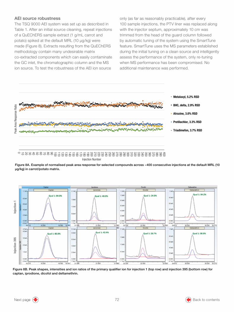
9
AEI source robustnessThe TSQ 9000 AEI system was set up as described in Table 1. After an initial source cleaning, repeat injections of a QuEChERS sample extract (1 g/mL carrot and potato) spiked at the default MRL (10 µg/kg) were made (Figure 8). Extracts resulting from the QuEChERS methodology contain many undesirable matrix co-extracted components which can easily contaminate the GC inlet, the chromatographic column and the MS ion source. To test the robustness of the AEI ion source
only (as far as reasonably practicable), after every 100 sample injections, the PTV liner was replaced along with the injector septum, approximately 10 cm was trimmed from the head of the guard column followed by automatic tuning of the system using the SmartTune feature. SmartTune uses the MS parameters established during the initial tuning on a clean source and intelligently assess the performance of the system, only re-tuning when MS performance has been compromised. No additional maintenance was performed.
Inje
ctio
n 1
Inje
ctio
n 39
5
Figure 8A. Example of normalised peak area response for selected compounds across ~400 consecutive injections at the default MRL (10 µg/kg) in carrot/potato matrix.
Figure 8B. Peak shapes, intensities and ion ratios of the primary qualifier ion for injection 1 (top row) and injection 395 (bottom row) for captan, iprodione, dicofol and deltamethrin.
0 10 20 30 40 50 60 70 80 90 100110120130140150160170180190200210220230240250260270280290300310320330340350360370380390400
Metalaxyl, 5.2% RSD
BHC, delta, 2.9% RSD
Atrazine, 3.0% RSD
Pretilachlor, 3.3% RSD
Triadimefon, 3.7% RSD
Injection Number
Peak
Are
a Re
spon
se R
atio
72 Back to contents
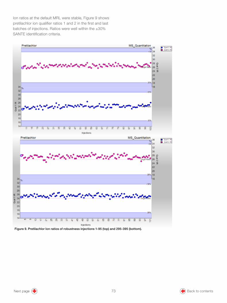
10
Ion ratios at the default MRL were stable, Figure 9 shows pretilachlor ion qualifier ratios 1 and 2 in the first and last batches of injections. Ratios were well within the ±30% SANTE identification criteria.
Figure 9. Pretilachlor Ion ratios of robustness injections 1-95 (top) and 295-395 (bottom).
73 Back to contents

11
ConclusionsIn this work it has been demonstrated that by using QuEChERS with Thermo Scientific HyperSep dSPE products and a direct injection of acetonitrile extracts, the TSQ 9000 AEI system delivers outstanding quantitative performance for low-level pesticide residue analysis in baby food.
• QuEChERS extraction and subsequent clean-up of over 200 pesticides from replicate analysis (n=6 each at three concentrations) of each of two sample matrices, demonstrating excellent accuracy (recovery) and precision.
• Accurate, quantitative analysis of over 200 pesticides over up to five orders of magnitude (0.025–250 µg/kg), showing outstanding LODs and linear response.
• Robustness displayed over approximately 400 consecutive injections of sample matrix (1 g/mL), with SANTE compliance at the default MRL throughout.
• High sensitivity providing the real possibility to dilute the sample extract, thus limiting matrix contamination and system maintenance, leading to an increase in laboratory productivity.
The results of this study establish the TSQ 9000 triple quadrupole GC-MS/MS system, in combination with Chromeleon CDS software and HyperSep dSPE products, as the ideal solution for the routine analysis of pesticides in baby food, providing unprecedented sensitivity, robustness, ease of use, cost effectiveness, and reliability.
References1. https://ec.europa.eu/food/plant/pesticides/max_residue_levels/guidelines_en
2. http://eur-lex.europa.eu/legal-content/EN/TXT/?uri=URISERV:l13002a
3. SANTE/11813/2017. Guidance document on analytical quality control and method validation procedures for pesticides residues analysis in food and feed. Supersedes SANTE/11945/2015. Implemented by 01/01/2018. https://ec.europa.eu/food/sites/food/files/plant/docs/pesticides_mrl_guidelines_wrkdoc_2017-11813.pdf
4. http://eur-lex.europa.eu/legal-content/EN/ALL/?uri=CELEX%3A32006L0125
5. http://quechers.cvua-stuttgart.de/
6. https://www.ncbi.nlm.nih.gov/pmc/articles/PMC4890451/
7. Belmonte Valles, N.; Retamal, M.; Martinez-Uroz, M.A.; Mezcua, M.; Fernandez-Al-ba, A.R.; de Kok, A. Determination of chlorothalonil in difficult-to-analyse vegetable matrices using various multiresidue methods. Analyst, 2012, 137(10), 2513–2520.
8. https://assets.thermofisher.com/TFS-Assets/CMD/Application-Notes/an-10580-gc-ms-ms-ptv-pesticides-water-an10580-en.pdf
9. http://tools.thermofisher.com/content/sfs/posters/PN-10394-Fast-SRM-Transition-PN10394-EN.pdf
74 Back to contents

12
Chart Number
Compound NameApple/Pear/Banana Linearity Carrot/Potato Linearity IDL99
R2 RF RSD(%)
Range (ppb)
R2 RF RSD(%)
Range (ppb)
pg on Column
IDL (fg)
1 2,3,5,6-Tetrachloroaniline 0.99931 6.80 0.1–250 0.99955 7.70 0.05–250 0.05 20
2 2,4'-Methoxychlor 0.99987 3.50 0.1–250 0.99950 7.30 0.025–250 0.05 8
3 4,4'-Methoxychlor olefin 0.99976 5.80 0.1–250 0.99932 4.20 0.05–250 0.05 31
4 Acetochlor 0.99972 3.60 0.2–250 0.99962 3.60 0.2–250 0.20 201
5 Acrinathrin 0.99963 2.70 0.2–250 0.99955 3.90 0.2–250 0.20 57
6 Alachlor 0.99965 5.50 0.1–250 0.99955 5.10 0.2–250 0.20 71
7 Aldrin 0.99959 8.00 0.1–250 0.99983 4.60 0.1–250 0.20 75
8 Allethrin (Bioallethrin) 0.99826 19.40 10–250 0.99888 7.50 5–250 5.00 2007
9 Allidochlor 0.99926 15.20 0.1–250 0.99631 6.30 0.2–250 0.20 145
10 Anthraquinone 0.99966 9.80 0.2–250 0.99988 17.60 0.025–250 0.05 27
11 Atrazine 0.99963 7.40 0.1–250 0.99990 6.70 0.05–250 0.05 19
12 Azinphos-ethyl 0.99465 9.40 0.2–250 0.99935 4.50 0.2–250 0.20 82
13 Azinphos-methyl 0.98165 16.90 1–250 0.99758 19.60 0.5–250 1.00 521
14 BHC, Alpha 0.99981 5.30 0.025–250 0.99949 6.60 0.025–250 0.05 15
15 BHC, Beta 0.99967 6.20 0.05–250 0.99985 8.80 0.025–250 0.05 15
16 BHC, delta 0.99971 4.10 0.05–250 0.99992 7.60 0.025–250 0.05 20
17 BHC, gamma 0.99970 7.30 0.05–250 0.99971 6.70 0.05–250 0.05 31
18 Bifenthrin 0.99989 4.20 0.5–250 0.99976 2.40 0.5–250 1.00 42
19 Biphenyl 0.99822 19.50 2–250 0.99573 14.50 5–250 5.00 865
20 Bromfenvinphos 0.99963 5.10 0.05–250 0.99960 7.60 0.025–250 0.05 31
21 Bromfenvinphos-methyl 0.99917 3.20 0.5–250 0.99971 3.60 0.1–250 0.20 33
22 Bromophos-ethyl 0.99946 3.30 0.1–250 0.99523 5.90 0.05–250 0.05 12
23Bromophos-methyl (Bromophos)
0.99957 5.60 0.05–250 0.99848 5.90 0.05–250 0.05 24
24 Bromopropylate 0.99960 4.80 0.1–250 0.99806 5.40 0.1–250 0.20 61
25 Bupirimate 0.99947 10.10 0.05–250 0.99961 5.50 0.05–250 0.05 33
26 Cadusafos 0.99982 3.80 0.1–250 0.99952 6.40 0.025–250 0.05 7
27 Captan 0.98233 23.80 1–250 0.98303 16.60 0.5–250 1.00 733
28 Carbophenothion 0.99968 3.50 0.2–250 0.99970 4.40 0.1–250 0.20 30
29 Carfentrazon-ethyl 0.99929 6.10 0.2–250 0.99575 7.50 0.1–250 0.20 41
30 Chlorbenside 0.99981 5.50 0.025–250 0.99984 3.20 0.025–250 0.05 11
31 Chlordane alpha-cis 0.99875 8.10 0.05–250 0.98923 8.10 0.1–250 0.20 61
32 Chlordane gamma-trans 0.99949 6.50 0.05–250 0.99956 7.30 0.025–250 0.05 38
33 Chlorfenapyr 0.99979 6.10 0.2–250 0.99983 3.30 0.2–250 0.20 90
34 Chlorfenson 0.99986 3.60 0.025–250 0.99979 2.30 0.025–250 0.05 10
35 Chlorfenvinphos 0.99966 8.60 0.05–250 0.99987 5.70 0.025–250 0.05 16
36 Chlorobenzilate 0.99990 3.10 0.025–250 0.99976 3.70 0.025–250 0.05 5
37 Chloroneb 0.99962 4.70 0.5–250 0.99907 10.90 0.1–250 0.20 28
38 Chlorothalonil 0.99752 7.40 0.1–250 0.99635 18.40 0.05–250 0.05 24
39 Chlorpropham 0.99985 13.90 0.5–250 0.99981 12.60 2–250 5.00 166
40 Chlorpyrifos-ethyl 0.99948 15.00 0.1–250 0.99916 5.50 0.05–250 0.05 22
Appendix A – Linearity data sets
Appendix A (Part 1). Linearity data sets.
75 Back to contents

13
Chart Number
Compound NameApple/Pear/Banana Linearity Carrot/Potato Linearity IDL99
R2 RF RSD(%)
Range (ppb)
R2 RF RSD(%)
Range (ppb)
pg on Column
IDL (fg)
41 Chlorpyrifos-methyl 0.99969 12.30 0.1–250 0.99960 15.70 0.025–250 0.05 24
42 Chlorthal-dimethyl 0.99917 6.20 0.1–250 0.99912 5.80 0.025–250 0.05 20
43 Chlorthiophos 0.99976 7.20 0.1–250 0.99971 3.00 0.2–250 0.20 153
44 Chlozolinate 0.99981 7.90 0.2–250 0.99988 4.30 0.2–250 0.20 67
45 Clomazone 0.99983 4.30 0.025–250 0.99993 6.40 0.025–250 0.05 12
46 Coumaphos 0.99817 4.80 0.5–250 0.99966 8.50 0.2–250 0.20 78
47 Cycloate 0.99815 13.10 2–250 0.99890 4.80 2–250 5.00 789
48 Cyhalothrin I (lambda) 0.99966 7.50 0.2–250 0.99959 2.90 0.2–250 0.20 28
49 Cyprodinil 0.99983 5.00 0.1–250 0.99993 3.90 0.1–250 0.20 86
50 DDD p,p 0.99985 4.30 0.05–250 0.99992 4.00 0.025–250 0.05 22
51 DDD, o, p 0.99988 3.00 0.05–250 0.99985 7.50 0.05–250 0.05 20
52 DDE o,p 0.99974 3.80 0.025–250 0.99976 4.30 0.025–250 0.05 8
53 DDE p, p 0.99957 2.60 0.05–250 0.99989 4.20 0.05–250 0.05 9
54 DDT o,p 0.99988 5.70 0.05–250 0.99960 9.20 0.05–250 0.05 25
55 DDT p,p 0.99962 8.40 0.2–250 0.99937 14.40 0.1–250 0.20 41
56 Deltamethrin 0.99983 6.70 0.05–250 0.99646 11.00 0.05–250 0.05 22
57 Diazinon 0.99949 5.20 0.1–250 0.99906 5.00 0.1–250 0.20 33
58 Dichlobenil 0.99866 5.10 0.025–250 0.99724 10.20 0.025–250 0.05 5
59 Dichlofluanid 0.99949 6.40 0.2–250 0.99966 4.40 0.1–250 0.20 28
60 Dichlorobenzophenone, 4, 4* 0.99979 2.80 0.05–250 0.99957 7.50 0.025–250 0.05 17
61 Dicloran (Bortran) 0.99908 7.10 0.2–250 0.99801 7.00 0.2–250 0.20 58
62 Dicofol* 0.99272 13.50 0.5–250 0.98598 14.70 0.5–250 1.00 973
63 Dieldrin 0.99909 7.20 0.5–250 0.99958 4.60 0.5–250 1.00 162
64 Dimethachlor 0.99964 5.10 0.025–250 0.99968 4.60 0.025–250 0.05 10
65 Dimethoate 0.99903 6.30 0.2–250 0.99973 10.40 0.1–250 0.20 30
66 Diphenamid 0.99974 7.30 0.2–250 0.99974 5.20 0.2–250 0.20 62
67 Diphenylamine 0.99981 9.50 0.2–250 0.99931 17.00 0.1–250 0.20 28
68 Disulfoton 0.99982 6.80 0.2–250 0.99943 4.30 0.2–250 0.20 19
69 Edifenphos 0.99908 4.00 0.05–250 0.99967 11.50 0.025–250 0.05 10
70 Endosulfan ether 0.99983 5.70 0.05–250 0.99982 12.20 0.025–250 0.05 21
71 Endosulfan peak 1 0.99963 4.50 0.2–250 0.99989 4.50 0.2–250 0.20 42
72 Endosulfan peak 2 0.99982 5.20 0.5–250 0.99988 4.00 0.5–250 1.00 190
73 Endosulfan sulfate 0.99981 3.10 0.1–250 0.99980 3.60 0.05–250 0.05 20
74 Endrin 0.99981 3.70 0.5–250 0.99975 4.80 0.2–250 0.20 59
75 Endrin Aldehyde 0.99893 7.30 0.5–250 0.99786 9.30 0.5–250 1.00 209
76 Endrin-Ketone 0.99920 6.00 0.5–250 0.99872 5.80 0.5–250 1.00 353
77 EPN 0.99591 7.10 1–250 0.99334 14.00 1–250 1.00 302
78 Ethion 0.99981 3.60 0.1–250 0.99987 3.90 0.05–250 0.05 29
79 Ethoprop (Ethoprophos) 0.99975 6.10 0.05–250 0.99923 6.40 0.1–250 0.20 39
80 Etofenprox 0.99978 7.40 0.2–250 0.99992 3.70 0.2–250 0.20 42
Appendix A (Part 2). Linearity data sets.
* - 4,4-dichlorobenzophenone is a breakdown product of dicofol and therefore may be overestimated.
76 Back to contents

14
Chart Number
Compound NameApple/Pear/Banana Linearity Carrot/Potato Linearity IDL99
R2 RF RSD(%)
Range (ppb)
R2 RF RSD(%)
Range (ppb)
pg on Column
IDL (fg)
81 Etridiazole (Terrazole) 0.99954 5.50 0.1–250 0.99599 16.30 0.025–250 0.05 18
82 Fenamiphos 0.99958 3.00 0.5–250 0.99848 3.70 0.5–250 1.00 147
83 Fenarimol 0.99984 3.20 0.2–250 0.99990 2.60 0.2–250 0.20 45
84 Fenchlorfos 0.99964 3.90 0.05–250 0.99956 4.80 0.05–250 0.05 17
85 Fenitrothion 0.99241 13.50 0.1–250 0.99559 13.30 0.1–250 0.20 52
86 Fenpropathrin 0.99969 3.70 0.5–250 0.99976 5.00 1–250 1.00 147
87 Fenson 0.99989 4.40 0.05–250 0.99995 5.60 0.025–250 0.05 11
88 Fenthion 0.99959 10.20 0.05–250 0.99970 10.60 0.05–250 0.05 18
89 Fenvalerate 0.99992 3.10 0.1–250 0.99974 5.80 0.1–250 0.20 36
90 Fipronil 0.99923 5.10 0.1–250 0.99405 8.90 0.05–250 0.05 20
91 Fipronil desulfinyl 0.99826 5.60 0.05–250 0.98489 10.00 0.05–250 0.05 27
92 Fluazifop-P-butyl 0.99971 7.40 0.1–250 0.99976 10.50 0.1–250 0.20 45
93 Fludioxonil 0.99980 9.90 0.05–250 0.99951 8.00 0.025–250 0.05 29
94 Fluquinconazole 0.99953 7.70 0.05–250 0.99609 7.40 0.025–250 0.05 15
95 Fluridone 0.99890 13.60 0.2–250 0.99593 7.10 0.025–250 0.05 22
96 Flusilazole 0.99969 11.20 0.1–250 0.99982 9.00 0.1–250 0.20 66
97 Flutolanil 0.99966 5.80 0.05–250 0.99982 9.30 0.025–250 0.05 51
98 Flutriafol 0.99960 7.20 0.1–250 0.99989 9.50 0.025–250 0.05 24
99 Folpet 0.97866 23.90 0.5–250 0.98874 14.20 0.2–250 0.20 757
100 Fonofos 0.99970 4.80 0.05–250 0.99986 4.20 0.05–250 0.05 14
101 Heptachlor 0.99963 4.20 0.025–250 0.99976 6.40 0.025–250 0.05 7
102 Hexachlorobenzene 0.99862 7.80 0.025–250 0.99939 5.60 0.025–250 0.05 11
103 Hexazinone 0.99971 7.20 0.1–250 0.99983 5.50 0.05–250 0.05 18
104 Iodofenfos 0.99859 6.10 0.05–250 0.99012 11.60 0.05–250 0.05 19
105 Iprodione 0.99976 7.70 0.2–250 0.99536 20.80 0.1–250 0.20 80
106 Isazophos 0.99934 6.60 0.1–250 0.99945 12.10 0.1–250 0.20 46
107 Isodrin 0.99983 5.90 0.1–250 0.99992 6.20 0.1–250 0.20 26
108 Lenacil 0.99928 7.90 0.2–250 0.99971 5.30 0.1–250 0.20 83
109 Leptophos 0.99947 3.30 0.2–250 0.99909 3.80 0.2–250 0.20 36
110 Linuron 0.99913 8.00 0.5–250 0.99831 8.70 0.2–250 0.20 92
111 Malathion 0.99989 5.70 0.05–250 0.99972 6.10 0.025–250 0.05 12
112 Metalaxyl 0.99947 4.70 0.2–250 0.99985 21.80 0.1–250 0.20 54
113 Metazachlor 0.99958 3.80 0.1–250 0.99978 8.10 0.025–250 0.05 32
114 Methacrifos 0.99977 4.50 0.2–250 0.99819 4.80 0.2–250 0.20 91
115 Methoxychlor 0.99918 4.50 0.1–250 0.99921 5.40 0.1–250 0.20 38
116 Metolachlor 0.99978 4.20 0.05–250 0.99992 4.20 0.025–250 0.05 49
117 Mevinphos 0.99985 3.80 0.05–250 0.99937 4.60 0.1–250 0.20 31
118 MGK-264 A 0.99986 5.00 0.2–250 0.99966 4.00 0.2–250 0.20 51
119 MGK-264 B 0.99984 4.50 0.2–250 0.99974 4.40 0.2–250 0.20 65
120 Mirex 0.99980 4.60 0.025–250 0.99981 3.00 0.025–250 0.05 8
Appendix A (Part 3). Linearity data sets.
77 Back to contents

15
Chart Number
Compound NameApple/Pear/Banana Linearity Carrot/Potato Linearity IDL99
R2 RF RSD(%)
Range (ppb)
R2 RF RSD(%)
Range (ppb)
pg on Column
IDL (fg)
121 Myclobutanil 0.99978 1.90 0.1–250 0.99986 3.50 0.1–250 0.20 40
122N-(2,4-Dimethylphenyl)formamide
0.99953 4.80 1–250 0.99982 8.30 1–250 1.00 106
123 NDBA 0.99866 18.00 0.5–250 0.99414 21.60 0.05–250 0.05 12
124 NDEA 0.99826 6.90 0.1–250 0.98989 9.80 0.2–250 0.20 74
125 NDPA 0.99865 8.70 0.5–250 0.99133 8.80 0.1–250 0.20 49
126 NEMA 0.99657 8.00 1–250 0.98500 12.80 0.2–250 0.20 87
127 Nitrofen 0.99590 13.50 0.05–250 0.99512 15.00 0.2–250 0.20 30
128 N-Nitrosodiphenylamine 0.99971 12.70 0.2–250 0.99931 17.00 0.1–250 0.20 28
129 N-Nitrosomorpholine 0.99759 18.50 0.5–250 0.99342 20.00 0.5–250 1.00 198
130 N-Nitrosopiperidine 0.99738 7.90 0.5–250 0.99368 14.20 0.5–250 1.00 217
131 N-Nitrosopyrrolidine 0.99830 14.70 1–250 0.99359 8.00 0.5–250 1.00 289
132 Nonachlor-cis 0.99591 7.20 0.2–250 0.97664 11.80 0.1–250 0.20 90
133 Nonachlor-trans 0.99924 4.70 0.1–250 0.99968 6.70 0.1–250 0.20 28
134 Norflurazon 0.99886 7.60 0.2–250 0.99937 5.10 0.05–250 0.05 23
135 Ortho-phenylphenol 0.99979 20.20 0.5–250 0.99957 14.70 0.5–250 1.00 102
136 Oxadiazon 0.99964 5.80 0.025–250 0.99970 14.10 0.1–250 0.20 22
137 Oxyfluorfen 0.99610 9.30 0.5–250 0.99445 18.80 0.5–250 1.00 73
138 Paclobutrazol 0.99977 5.40 0.05–250 0.99991 6.70 0.05–250 0.05 49
139 Parathion (ethyl) 0.99534 11.00 0.5–250 0.99395 19.40 0.5–250 1.00 158
140 Parathion-methyl 0.99478 12.00 0.05–250 0.99736 8.20 0.2–250 0.20 111
141 Pebulate 0.99885 14.30 0.5–250 0.99691 13.30 0.5–250 1.00 171
142 Penconazole 0.99985 6.30 0.05–250 0.99992 7.90 0.05–250 0.05 37
143 Pentachloroaniline 0.99973 6.10 0.1–250 0.99961 4.60 0.05–250 0.05 52
144 Pentachloroanisole 0.99939 5.30 0.05–250 0.99956 11.30 0.025–250 0.05 18
145 Pentachlorobenzene 0.99665 8.50 0.025–250 0.99765 11.40 0.025–250 0.05 12
146 Pentachlorobenzonitrile 0.99984 5.10 0.05–250 0.99973 8.40 0.025–250 0.05 23
147 Pentachlorothioanisole 0.99951 8.40 0.025–250 0.99973 6.00 0.05–250 0.05 22
148 Perthane (Ethylan) 0.99994 8.00 0.05–250 0.99982 4.50 0.1–250 0.20 30
149 Permethrin peak 1 0.99971 9.90 1–250 0.99979 12.90 0.2–250 0.20 219
150 Permethrin peak 2 0.99970 6.10 0.5–250 0.99979 5.80 0.5–250 1.00 48
151 Phenothrin 0.99950 17.90 1–250 0.99972 7.40 2–250 5.00 413
152 Phorate 0.99964 3.10 0.5–250 0.99910 13.50 0.025–250 0.05 18
153 Phosalone 0.99862 8.80 0.05–250 0.99982 8.90 0.05–250 0.05 18
154 Phosmet 0.99738 7.00 0.5–250 0.99916 24.50 0.2–250 0.20 54
155 Piperonyl butoxide 0.99977 6.50 0.1–250 0.99990 4.90 0.1–250 0.20 51
156 Pirimiphos-ethyl 0.99964 3.00 0.05–250 0.99967 5.30 0.025–250 0.05 21
157 Pirimiphos-methyl 0.99949 5.50 0.05–250 0.99949 4.80 0.025–250 0.05 18
158 Pretilachlor 0.99984 3.60 0.2–250 0.99989 2.40 0.2–250 0.20 44
159 Prochloraz (parent) 0.99749 14.30 1–250 0.99920 7.80 0.5–250 1.00 320
160 Procymidone 0.99991 4.00 0.1–250 0.99969 7.50 0.05–250 0.05 26
Appendix A (Part 4). Linearity data sets.
78 Back to contents
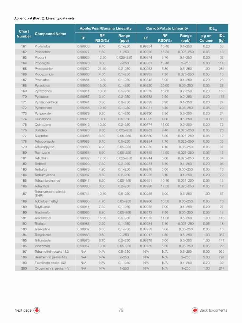
16
Chart Number
Compound NameApple/Pear/Banana Linearity Carrot/Potato Linearity IDL99
R2 RF RSD(%)
Range (ppb)
R2 RF RSD(%)
Range (ppb)
pg on Column
IDL (fg)
161 Profenofos 0.99938 9.40 0.1–250 0.99654 10.40 0.1–250 0.20 53
162 Propachlor 0.99977 1.60 1–250 0.99926 15.30 0.025–250 0.05 13
163 Propanil 0.99925 12.30 0.025–250 0.99974 3.70 0.1–250 0.20 32
164 Propargite 0.99970 3.30 2–250 0.99881 19.40 2–250 5.00 1143
165 Propisochlor 0.99972 21.10 0.2–250 0.99953 5.80 0.5–250 1.00 284
166 Propyzamide 0.99966 4.50 0.1–250 0.99985 4.20 0.025–250 0.05 15
167 Prothiofos 0.99881 10.50 0.1–250 0.99842 5.90 0.1–250 0.20 28
168 Pyraclofos 0.99656 15.00 0.1–250 0.99920 20.60 0.05–250 0.05 28
169 Pyrazophos 0.99911 13.30 0.5–250 0.99979 16.60 0.2–250 0.20 163
170 Pyridaben 0.99987 3.10 0.2–250 0.99988 2.50 0.2–250 0.20 186
171 Pyridaphenthion 0.99941 3.80 0.2–250 0.99699 8.90 0.1–250 0.20 24
172 Pyrimethanil 0.99985 19.10 0.1–250 0.99971 8.40 0.05–250 0.05 23
173 Pyriproxyfen 0.99979 9.20 0.1–250 0.99990 2.30 0.2–250 0.20 24
174 Quinalphos 0.99926 10.80 0.5–250 0.99925 4.60 0.5–250 1.00 88
175 Quintozene 0.99912 10.20 0.2–250 0.99774 15.00 0.2–250 0.20 72
176 Sulfotep 0.99970 9.80 0.025–250 0.99962 9.40 0.025–250 0.05 26
177 Sulprofos 0.99986 3.30 0.05–250 0.99850 5.20 0.025–250 0.05 12
178 Tebuconazole 0.99983 9.10 0.5–250 0.99994 4.70 0.025–250 0.05 30
179 Tebufenpyrad 0.99980 4.20 0.05–250 0.99976 4.10 0.05–250 0.05 37
180 Tecnazene 0.99958 8.90 0.05–250 0.99815 13.90 0.025–250 0.05 15
181 Tefluthrin 0.99982 12.50 0.025–250 0.99944 6.60 0.025–250 0.05 34
182 Terbacil 0.99929 7.30 0.2–250 0.99974 5.40 0.1–250 0.20 95
183 Terbufos 0.99973 4.90 0.1–250 0.99978 5.00 0.05–250 0.05 13
184 Terbuthylazine 0.99967 8.60 0.2–250 0.99982 6.10 0.1–250 0.20 72
185 Tetrachlorvinphos 0.99941 8.20 0.05–250 0.99651 10.10 0.025–250 0.05 13
186 Tetradifon 0.99988 3.80 0.2–250 0.99990 17.50 0.025–250 0.05 17
187Tetrahydrophthalimide (THPI)
0.99744 10.40 0.5–250 0.99985 6.00 0.5–250 1.00 67
188 Tolclofos-methyl 0.99985 4.70 0.05–250 0.99986 10.50 0.05–250 0.05 18
189 Tolylfluanid 0.99911 7.30 0.1–250 0.99952 7.90 0.1–250 0.20 27
190 Triadimefon 0.99965 8.80 0.05–250 0.99973 7.50 0.05–250 0.05 18
191 Triadimenol 0.99983 15.90 0.5–250 0.99973 11.20 0.5–250 1.00 116
192 Triallate 0.99983 2.20 0.1–250 0.99984 6.10 0.025–250 0.05 18
193 Triazophos 0.99937 6.30 0.1–250 0.99983 5.60 0.05–250 0.05 16
194 Tricyclazole 0.99883 9.50 2–250 0.99947 4.50 0.5–250 1.00 367
195 Triflumizole 0.99976 6.70 0.2–250 0.99978 6.00 0.5–250 1.00 147
196 Vinclozolin 0.99967 10.10 0.05–250 0.99969 5.50 0.05–250 0.05 22
197 Tetramethrin peaks 1&2 N/A N/A 0.5–250 N/A N/A 0.5–250 5.00 929
198 Resmethrin peaks 1&2 N/A N/A 2–250 N/A N/A 2–250 5.00 797
199 Fluvalinate peaks 1&2 N/A N/A 0.1–250 N/A N/A 0.1–250 0.20 32
200 Cypermethrin peaks I-IV N/A N/A 1–250 N/A N/A 1–250 1.00 214
Appendix A (Part 5). Linearity data sets.
79 Back to contents
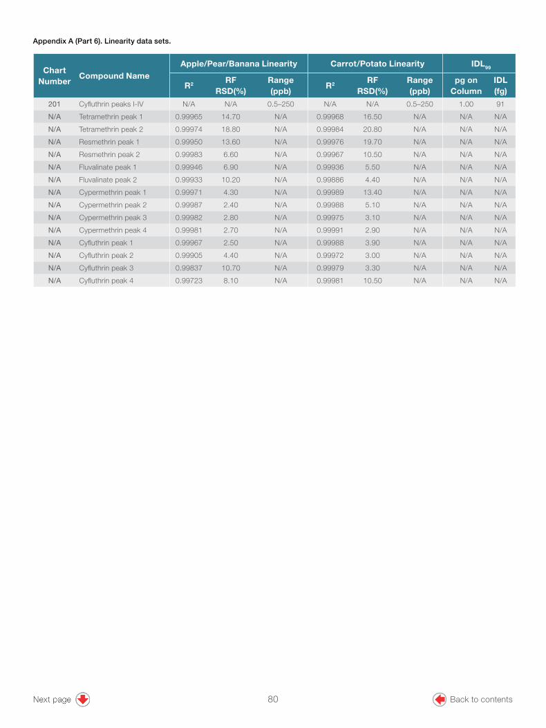
17
Chart Number
Compound NameApple/Pear/Banana Linearity Carrot/Potato Linearity IDL99
R2 RF RSD(%)
Range (ppb)
R2 RF RSD(%)
Range (ppb)
pg on Column
IDL (fg)
201 Cyfluthrin peaks I-IV N/A N/A 0.5–250 N/A N/A 0.5–250 1.00 91
N/A Tetramethrin peak 1 0.99965 14.70 N/A 0.99968 16.50 N/A N/A N/A
N/A Tetramethrin peak 2 0.99974 18.80 N/A 0.99984 20.80 N/A N/A N/A
N/A Resmethrin peak 1 0.99950 13.60 N/A 0.99976 19.70 N/A N/A N/A
N/A Resmethrin peak 2 0.99983 6.60 N/A 0.99967 10.50 N/A N/A N/A
N/A Fluvalinate peak 1 0.99946 6.90 N/A 0.99936 5.50 N/A N/A N/A
N/A Fluvalinate peak 2 0.99933 10.20 N/A 0.99886 4.40 N/A N/A N/A
N/A Cypermethrin peak 1 0.99971 4.30 N/A 0.99989 13.40 N/A N/A N/A
N/A Cypermethrin peak 2 0.99987 2.40 N/A 0.99988 5.10 N/A N/A N/A
N/A Cypermethrin peak 3 0.99982 2.80 N/A 0.99975 3.10 N/A N/A N/A
N/A Cypermethrin peak 4 0.99981 2.70 N/A 0.99991 2.90 N/A N/A N/A
N/A Cyfluthrin peak 1 0.99967 2.50 N/A 0.99988 3.90 N/A N/A N/A
N/A Cyfluthrin peak 2 0.99905 4.40 N/A 0.99972 3.00 N/A N/A N/A
N/A Cyfluthrin peak 3 0.99837 10.70 N/A 0.99979 3.30 N/A N/A N/A
N/A Cyfluthrin peak 4 0.99723 8.10 N/A 0.99981 10.50 N/A N/A N/A
Appendix A (Part 6). Linearity data sets.
80 Back to contents

18
Component Name
Carrot 1 µg/kg (n=6) Apple 1 µg/kg (n=6) Carrot 2.5 µg/kg (n=6) Apple 2.5 µg/kg (n=3) Carrot 10 µg/kg (n=6) Apple 10 µg/kg (n=6)
Mean Recovery
Precision RSD(%)
Mean Recovery
Precision RSD(%)
Mean Recovery
Precision RSD(%)
Mean Recovery
Precision RSD(%)
Mean Recovery
Precision RSD(%)
Mean Recovery
Precision RSD(%)
2,3,5,6-Tetrachloroaniline 100.9% 6.2% 97.8% 10.2% 94.7% 5.1% 99.2% 3.4% 87.6% 3.4% 99.4% 5.5%
2,4'-Methoxychlor 98.1% 0.9% 98.4% 1.2% 96.4% 1.0% 98.1% 1.2% 100.1% 1.2% 97.5% 1.1%
4,4'-Methoxychlor olefin 99.9% 2.8% 106.7% 3.5% 98.8% 2.6% 99.4% 1.6% 101.0% 1.1% 100.2% 1.6%
Acetochlor 89.9% 8.2% 90.9% 9.1% 79.1% 8.4% 110.5% 3.4% 97.0% 2.2% 98.2% 3.1%
Acrinathrin 96.5% 4.2% 92.3% 4.5% 112.3% 3.2% 96.4% 4.4% 109.2% 2.0% 97.4% 4.2%
Alachlor 107.8% 6.8% 97.5% 3.4% 96.9% 2.4% 102.0% 1.4% 100.9% 1.7% 97.2% 2.0%
Aldrin 109.8% 7.7% 105.3% 7.6% 93.5% 2.4% 107.7% 2.0% 98.7% 1.6% 100.4% 2.8%
Allethrin (Bioallethrin) <LOQ <LOQ <LOQ <LOQ <LOQ <LOQ <LOQ <LOQ 105.7% 1.2% 102.1% 2.2%
Allidochlor 113.1% 10.1% 93.4% 12.6% 104.7% 12.9% 99.6% 1.9% 88.9% 5.3% 100.4% 4.8%
Anthraquinone 36.3% 27.8% 102.4% 14.5% 39.6% 6.5% 94.6% 3.5% 34.1% 47.7% 95.8% 2.7%
Atrazine 111.1% 4.1% 94.4% 6.0% 90.9% 4.0% 98.7% 5.0% 98.7% 0.9% 98.4% 2.4%
Azinphos-ethyl 95.2% 6.4% 86.1% 2.8% 96.3% 3.3% 92.4% 2.0% 100.9% 3.3% 93.3% 1.9%
Azinphos-methyl 84.5% 4.3% 87.3% 11.4% 87.1% 7.1% 100.2% 0.5% 94.3% 6.3% 84.1% 6.9%
BHC, Alpha 102.0% 3.6% 95.0% 5.6% 94.3% 3.6% 104.2% 3.2% 94.1% 1.9% 99.8% 4.2%
BHC, Beta 98.3% 2.3% 96.3% 7.7% 94.8% 0.9% 96.7% 6.3% 97.7% 1.0% 98.2% 1.9%
BHC, delta 98.5% 1.8% 93.2% 3.2% 95.1% 2.8% 101.1% 0.8% 96.5% 1.5% 97.2% 1.8%
BHC, gamma 99.5% 4.2% 96.3% 5.2% 90.7% 2.9% 109.3% 3.1% 97.4% 2.0% 96.4% 3.2%
Bifenthrin 106.1% 2.2% 106.5% 2.5% 99.9% 1.5% 101.8% 0.9% 99.5% 0.3% 102.6% 1.3%
Biphenyl <LOQ <LOQ <LOQ <LOQ 86.4% 10.5% 118.1% 3.0% 79.5% 7.7% 111.6% 7.1%
Bromfenvinphos 111.2% 3.2% 97.0% 2.7% 91.8% 1.9% 103.6% 2.8% 97.3% 1.7% 94.6% 2.0%
Bromfenvinphos-methyl 110.5% 3.4% 87.8% 5.1% 92.3% 2.5% 106.4% 2.3% 98.4% 0.9% 95.2% 3.6%
Bromophos-ethyl 113.2% 2.4% 87.2% 6.8% 93.7% 7.1% 113.1% 3.6% 97.2% 3.0% 94.8% 3.4%
Bromophos-methyl (Bromophos)
104.0% 4.3% 90.0% 7.6% 93.2% 2.9% 114.8% 2.5% 95.9% 2.6% 97.3% 3.2%
Bromopropylate 101.2% 14.2% 97.2% 5.3% 96.1% 2.0% 111.1% 2.6% 97.1% 2.3% 97.4% 2.3%
Bupirimate 111.7% 11.6% 98.6% 5.9% 99.7% 2.4% 101.4% 0.7% 100.9% 2.0% 97.1% 2.1%
Cadusafos 101.9% 3.4% 101.4% 3.8% 96.4% 3.8% 101.9% 1.8% 97.6% 1.7% 101.4% 3.1%
Captan 85.0% 16.5% 80.4% 9.1% 96.7% 11.9% 78.8% 2.4% 97.6% 5.6% 87.5% 4.2%
Carbophenothion 103.2% 4.3% 99.3% 3.6% 95.6% 1.5% 96.6% 1.9% 99.2% 1.0% 97.1% 1.5%
Carfentrazon-ethyl 103.9% 11.0% 104.7% 7.6% 94.2% 4.3% 109.0% 3.8% 99.3% 2.7% 94.8% 3.3%
Chlorbenside 88.8% 4.8% 91.1% 4.0% 88.1% 0.8% 94.0% 2.5% 88.0% 6.6% 96.3% 1.8%
Chlordane alpha-cis 110.5% 4.8% 96.1% 2.9% 95.4% 3.0% 100.1% 4.1% 99.3% 3.1% 98.5% 1.7%
Chlordane gamma-trans 112.4% 4.5% 109.7% 5.3% 95.9% 1.9% 116.2% 2.9% 97.3% 1.9% 105.9% 1.8%
Chlorfenapyr 96.9% 6.2% 96.5% 6.0% 97.2% 3.2% 95.4% 4.0% 99.7% 2.3% 99.9% 2.4%
Chlorfenson 97.9% 2.5% 95.3% 3.5% 92.9% 1.8% 94.8% 0.4% 93.1% 2.2% 94.4% 3.7%
Chlorfenvinphos 105.9% 4.3% 92.1% 3.7% 99.5% 3.3% 104.5% 1.6% 100.6% 0.7% 95.7% 2.0%
Chlorobenzilate 102.5% 2.3% 95.7% 4.2% 95.5% 0.9% 95.0% 2.3% 97.4% 0.8% 98.1% 1.5%
Chloroneb 102.6% 4.3% 97.6% 5.5% 99.9% 6.3% 105.6% 4.8% 89.0% 4.6% 102.0% 6.6%
Chlorothalonil 34.1% 8.8% 30.7% 16.9% 35.8% 29.2% 36.4% 19.1% 38.7% 8.0% 52.5% 9.1%
Chlorpropham 92.2% 4.9% 99.7% 4.3% 92.3% 3.7% 92.0% 3.6% 93.1% 2.5% 94.3% 2.7%
Chlorpyrifos-ethyl 100.1% 5.6% 99.5% 6.2% 94.1% 2.1% 101.7% 1.2% 96.7% 1.2% 97.1% 1.2%
Chlorpyrifos-methyl 113.9% 2.8% 88.1% 5.5% 93.3% 5.8% 104.9% 2.5% 95.3% 1.9% 98.0% 2.7%
Chlorthal-dimethyl (Dacthal)
117.1% 4.7% 96.9% 4.0% 93.1% 1.5% 109.9% 5.4% 98.0% 1.4% 94.8% 3.8%
Chlorthiophos 110.4% 3.5% 102.1% 7.0% 96.4% 3.3% 103.8% 0.9% 100.4% 2.0% 96.7% 1.5%
Chlozolinate 117.5% 8.4% 99.7% 8.6% 94.6% 4.1% 98.4% 1.9% 100.6% 1.8% 97.3% 3.2%
Clomazone 99.1% 3.6% 98.3% 4.0% 95.0% 2.8% 96.8% 0.8% 97.8% 0.9% 99.0% 2.9%
Coumaphos 98.6% 6.7% 93.0% 3.5% 88.5% 5.6% 91.4% 2.3% 94.9% 3.7% 92.5% 4.2%
Cycloate <LOQ <LOQ <LOQ <LOQ <LOQ <LOQ <LOQ <LOQ 114.7% 6.3% 115.2% 9.0%
Appendix B (Part 1). QuEChERS Recovery data.
Appendix B – QuEChERS Recovery data
81 Back to contents
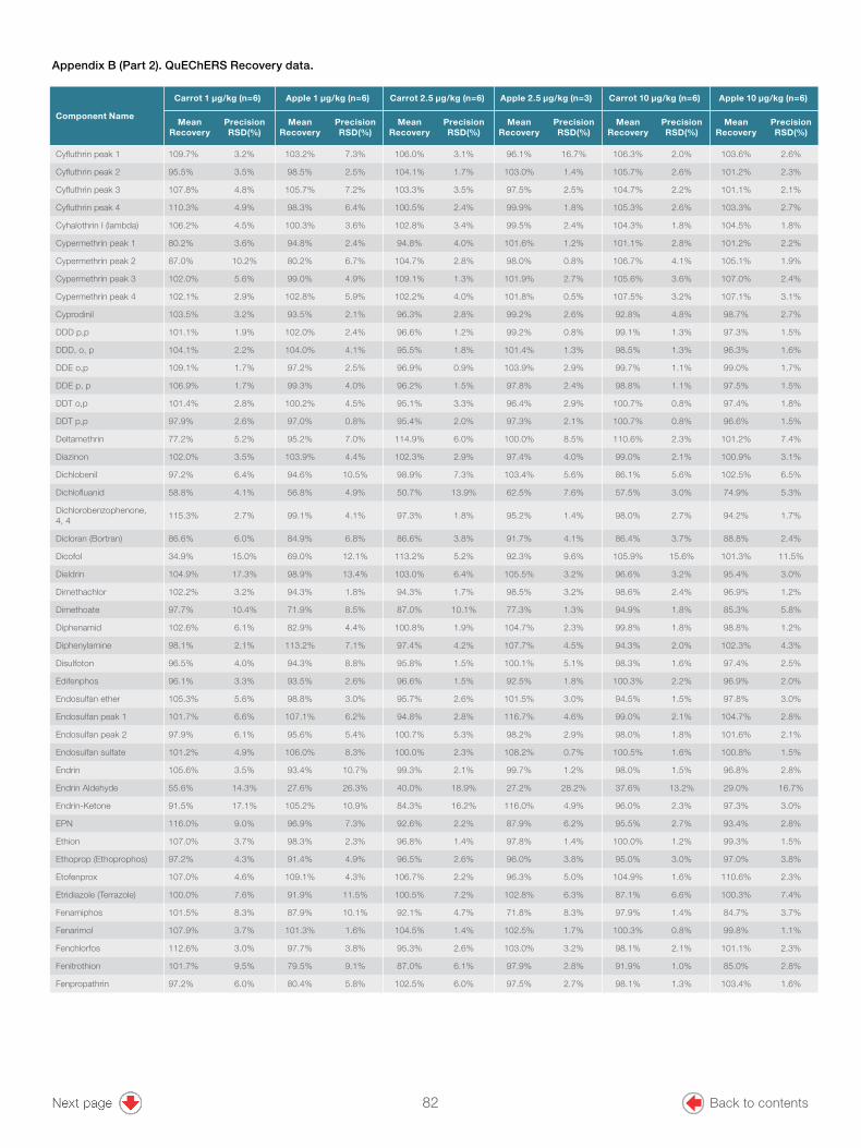
19
Component Name
Carrot 1 µg/kg (n=6) Apple 1 µg/kg (n=6) Carrot 2.5 µg/kg (n=6) Apple 2.5 µg/kg (n=3) Carrot 10 µg/kg (n=6) Apple 10 µg/kg (n=6)
Mean Recovery
Precision RSD(%)
Mean Recovery
Precision RSD(%)
Mean Recovery
Precision RSD(%)
Mean Recovery
Precision RSD(%)
Mean Recovery
Precision RSD(%)
Mean Recovery
Precision RSD(%)
Cyfluthrin peak 1 109.7% 3.2% 103.2% 7.3% 106.0% 3.1% 96.1% 16.7% 106.3% 2.0% 103.6% 2.6%
Cyfluthrin peak 2 95.5% 3.5% 98.5% 2.5% 104.1% 1.7% 103.0% 1.4% 105.7% 2.6% 101.2% 2.3%
Cyfluthrin peak 3 107.8% 4.8% 105.7% 7.2% 103.3% 3.5% 97.5% 2.5% 104.7% 2.2% 101.1% 2.1%
Cyfluthrin peak 4 110.3% 4.9% 98.3% 6.4% 100.5% 2.4% 99.9% 1.8% 105.3% 2.6% 103.3% 2.7%
Cyhalothrin I (lambda) 106.2% 4.5% 100.3% 3.6% 102.8% 3.4% 99.5% 2.4% 104.3% 1.8% 104.5% 1.8%
Cypermethrin peak 1 80.2% 3.6% 94.8% 2.4% 94.8% 4.0% 101.6% 1.2% 101.1% 2.8% 101.2% 2.2%
Cypermethrin peak 2 87.0% 10.2% 80.2% 6.7% 104.7% 2.8% 98.0% 0.8% 106.7% 4.1% 105.1% 1.9%
Cypermethrin peak 3 102.0% 5.6% 99.0% 4.9% 109.1% 1.3% 101.9% 2.7% 105.6% 3.6% 107.0% 2.4%
Cypermethrin peak 4 102.1% 2.9% 102.8% 5.9% 102.2% 4.0% 101.8% 0.5% 107.5% 3.2% 107.1% 3.1%
Cyprodinil 103.5% 3.2% 93.5% 2.1% 96.3% 2.8% 99.2% 2.6% 92.8% 4.8% 98.7% 2.7%
DDD p,p 101.1% 1.9% 102.0% 2.4% 96.6% 1.2% 99.2% 0.8% 99.1% 1.3% 97.3% 1.5%
DDD, o, p 104.1% 2.2% 104.0% 4.1% 95.5% 1.8% 101.4% 1.3% 98.5% 1.3% 96.3% 1.6%
DDE o,p 109.1% 1.7% 97.2% 2.5% 96.9% 0.9% 103.9% 2.9% 99.7% 1.1% 99.0% 1.7%
DDE p, p 106.9% 1.7% 99.3% 4.0% 96.2% 1.5% 97.8% 2.4% 98.8% 1.1% 97.5% 1.5%
DDT o,p 101.4% 2.8% 100.2% 4.5% 95.1% 3.3% 96.4% 2.9% 100.7% 0.8% 97.4% 1.8%
DDT p,p 97.9% 2.6% 97.0% 0.8% 95.4% 2.0% 97.3% 2.1% 100.7% 0.8% 96.6% 1.5%
Deltamethrin 77.2% 5.2% 95.2% 7.0% 114.9% 6.0% 100.0% 8.5% 110.6% 2.3% 101.2% 7.4%
Diazinon 102.0% 3.5% 103.9% 4.4% 102.3% 2.9% 97.4% 4.0% 99.0% 2.1% 100.9% 3.1%
Dichlobenil 97.2% 6.4% 94.6% 10.5% 98.9% 7.3% 103.4% 5.6% 86.1% 5.6% 102.5% 6.5%
Dichlofluanid 58.8% 4.1% 56.8% 4.9% 50.7% 13.9% 62.5% 7.6% 57.5% 3.0% 74.9% 5.3%
Dichlorobenzophenone, 4, 4
115.3% 2.7% 99.1% 4.1% 97.3% 1.8% 95.2% 1.4% 98.0% 2.7% 94.2% 1.7%
Dicloran (Bortran) 86.6% 6.0% 84.9% 6.8% 86.6% 3.8% 91.7% 4.1% 86.4% 3.7% 88.8% 2.4%
Dicofol 34.9% 15.0% 69.0% 12.1% 113.2% 5.2% 92.3% 9.6% 105.9% 15.6% 101.3% 11.5%
Dieldrin 104.9% 17.3% 98.9% 13.4% 103.0% 6.4% 105.5% 3.2% 96.6% 3.2% 95.4% 3.0%
Dimethachlor 102.2% 3.2% 94.3% 1.8% 94.3% 1.7% 98.5% 3.2% 98.6% 2.4% 96.9% 1.2%
Dimethoate 97.7% 10.4% 71.9% 8.5% 87.0% 10.1% 77.3% 1.3% 94.9% 1.8% 85.3% 5.8%
Diphenamid 102.6% 6.1% 82.9% 4.4% 100.8% 1.9% 104.7% 2.3% 99.8% 1.8% 98.8% 1.2%
Diphenylamine 98.1% 2.1% 113.2% 7.1% 97.4% 4.2% 107.7% 4.5% 94.3% 2.0% 102.3% 4.3%
Disulfoton 96.5% 4.0% 94.3% 8.8% 95.8% 1.5% 100.1% 5.1% 98.3% 1.6% 97.4% 2.5%
Edifenphos 96.1% 3.3% 93.5% 2.6% 96.6% 1.5% 92.5% 1.8% 100.3% 2.2% 96.9% 2.0%
Endosulfan ether 105.3% 5.6% 98.8% 3.0% 95.7% 2.6% 101.5% 3.0% 94.5% 1.5% 97.8% 3.0%
Endosulfan peak 1 101.7% 6.6% 107.1% 6.2% 94.8% 2.8% 116.7% 4.6% 99.0% 2.1% 104.7% 2.8%
Endosulfan peak 2 97.9% 6.1% 95.6% 5.4% 100.7% 5.3% 98.2% 2.9% 98.0% 1.8% 101.6% 2.1%
Endosulfan sulfate 101.2% 4.9% 106.0% 8.3% 100.0% 2.3% 108.2% 0.7% 100.5% 1.6% 100.8% 1.5%
Endrin 105.6% 3.5% 93.4% 10.7% 99.3% 2.1% 99.7% 1.2% 98.0% 1.5% 96.8% 2.8%
Endrin Aldehyde 55.6% 14.3% 27.6% 26.3% 40.0% 18.9% 27.2% 28.2% 37.6% 13.2% 29.0% 16.7%
Endrin-Ketone 91.5% 17.1% 105.2% 10.9% 84.3% 16.2% 116.0% 4.9% 96.0% 2.3% 97.3% 3.0%
EPN 116.0% 9.0% 96.9% 7.3% 92.6% 2.2% 87.9% 6.2% 95.5% 2.7% 93.4% 2.8%
Ethion 107.0% 3.7% 98.3% 2.3% 96.8% 1.4% 97.8% 1.4% 100.0% 1.2% 99.3% 1.5%
Ethoprop (Ethoprophos) 97.2% 4.3% 91.4% 4.9% 96.5% 2.6% 96.0% 3.8% 95.0% 3.0% 97.0% 3.8%
Etofenprox 107.0% 4.6% 109.1% 4.3% 106.7% 2.2% 96.3% 5.0% 104.9% 1.6% 110.6% 2.3%
Etridiazole (Terrazole) 100.0% 7.6% 91.9% 11.5% 100.5% 7.2% 102.8% 6.3% 87.1% 6.6% 100.3% 7.4%
Fenamiphos 101.5% 8.3% 87.9% 10.1% 92.1% 4.7% 71.8% 8.3% 97.9% 1.4% 84.7% 3.7%
Fenarimol 107.9% 3.7% 101.3% 1.6% 104.5% 1.4% 102.5% 1.7% 100.3% 0.8% 99.8% 1.1%
Fenchlorfos 112.6% 3.0% 97.7% 3.8% 95.3% 2.6% 103.0% 3.2% 98.1% 2.1% 101.1% 2.3%
Fenitrothion 101.7% 9.5% 79.5% 9.1% 87.0% 6.1% 97.9% 2.8% 91.9% 1.0% 85.0% 2.8%
Fenpropathrin 97.2% 6.0% 80.4% 5.8% 102.5% 6.0% 97.5% 2.7% 98.1% 1.3% 103.4% 1.6%
Appendix B (Part 2). QuEChERS Recovery data.
82 Back to contents

20
Component Name
Carrot 1 µg/kg (n=6) Apple 1 µg/kg (n=6) Carrot 2.5 µg/kg (n=6) Apple 2.5 µg/kg (n=3) Carrot 10 µg/kg (n=6) Apple 10 µg/kg (n=6)
Mean Recovery
Precision RSD(%)
Mean Recovery
Precision RSD(%)
Mean Recovery
Precision RSD(%)
Mean Recovery
Precision RSD(%)
Mean Recovery
Precision RSD(%)
Mean Recovery
Precision RSD(%)
Fenson 98.9% 2.5% 95.5% 3.8% 96.5% 2.2% 96.0% 2.0% 98.8% 1.1% 97.0% 2.0%
Fenthion 109.0% 4.5% 92.3% 2.3% 100.4% 2.7% 108.7% 1.9% 99.6% 2.2% 95.1% 2.2%
Fenvalerate 101.3% 2.9% 102.6% 4.2% 110.1% 2.6% 104.6% 2.6% 110.3% 1.8% 104.2% 4.0%
Fipronil 103.5% 7.8% 83.8% 8.6% 94.9% 3.7% 110.6% 4.4% 100.5% 2.8% 95.9% 3.3%
Fipronil desulfinyl 101.5% 8.4% 92.2% 8.3% 95.2% 5.4% 108.4% 2.1% 99.5% 1.8% 98.5% 3.6%
Fluazifop-P-butyl 111.0% 3.9% 96.2% 6.6% 95.8% 2.2% 100.8% 2.4% 99.7% 2.3% 97.3% 1.4%
Fludioxonil 105.1% 3.2% 93.7% 3.7% 89.3% 4.5% 93.9% 5.0% 92.3% 3.3% 89.6% 1.6%
Fluquinconazole 103.1% 16.6% 102.9% 7.0% 94.3% 3.0% 91.1% 3.9% 98.2% 2.3% 99.4% 3.0%
Fluridone 100.7% 17.2% 85.6% 11.3% 92.1% 4.2% 107.2% 0.4% 100.9% 2.3% 88.7% 1.5%
Flusilazole 95.2% 5.4% 98.4% 9.7% 96.9% 1.9% 92.0% 2.1% 95.6% 1.7% 98.8% 2.1%
Flutolanil 99.0% 2.7% 95.1% 1.9% 95.0% 0.9% 96.7% 0.6% 97.0% 0.8% 99.1% 1.6%
Flutriafol 96.9% 2.5% 99.4% 5.4% 93.3% 2.2% 99.8% 2.4% 95.6% 1.4% 97.8% 1.0%
Fluvalinate peak 1 100.3% 5.9% 115.1% 18.5% 118.9% 3.6% 98.5% 3.5% 120.0% 2.4% 100.6% 3.2%
Fluvalinate peak 2 93.7% 17.3% 108.4% 18.8% 117.6% 5.8% 104.1% 8.2% 113.6% 3.9% 101.9% 5.2%
Folpet 90.2% 11.4% 72.2% 4.1% 86.6% 10.8% 70.7% 7.1% 97.0% 4.2% 77.3% 4.4%
Fonofos 105.9% 3.9% 99.9% 4.6% 99.5% 2.1% 105.4% 4.8% 97.1% 2.7% 101.3% 2.5%
Heptachlor 108.7% 5.4% 97.1% 5.1% 95.9% 3.4% 105.2% 3.6% 94.8% 0.9% 98.9% 3.5%
Hexachlorobenzene 95.1% 7.1% 94.6% 8.3% 86.7% 2.9% 109.1% 4.6% 75.4% 9.7% 99.3% 5.4%
Hexazinone 89.1% 1.9% 87.7% 2.1% 93.5% 1.0% 91.6% 0.9% 95.0% 1.7% 93.9% 2.0%
Iodofenfos 97.6% 4.6% 96.9% 3.2% 83.3% 6.7% 96.7% 0.8% 93.5% 4.2% 94.6% 4.3%
Iprodione 95.2% 16.3% 99.6% 7.6% 97.3% 5.5% 108.6% 1.2% 107.3% 3.8% 90.5% 2.9%
Isazophos 111.1% 9.4% 72.2% 5.0% 105.2% 4.0% 101.5% 2.1% 98.7% 1.5% 99.1% 2.5%
Isodrin 103.3% 4.9% 98.0% 4.6% 96.0% 1.9% 100.4% 4.8% 97.2% 0.8% 98.7% 2.0%
Lenacil 90.0% 10.8% 92.5% 8.2% 93.8% 6.0% 88.3% 4.6% 94.0% 5.3% 92.8% 2.0%
Leptophos 98.9% 6.8% 101.1% 1.8% 97.9% 1.3% 95.0% 1.1% 97.8% 4.0% 102.4% 1.1%
Linuron 104.4% 9.9% 82.4% 3.2% 92.9% 4.7% 97.2% 7.8% 90.9% 3.6% 99.7% 4.5%
Malathion 103.0% 2.1% 82.6% 3.7% 91.5% 2.1% 91.4% 5.1% 94.3% 1.4% 97.6% 1.3%
Metalaxyl 106.0% 6.0% 99.8% 12.5% 96.2% 4.8% 111.5% 1.8% 98.5% 1.9% 96.0% 2.3%
Metazachlor 98.5% 5.0% 99.8% 4.9% 97.4% 1.3% 100.4% 0.2% 98.7% 0.9% 97.2% 1.6%
Methacrifos 95.6% 4.0% 95.7% 5.5% 101.9% 6.6% 103.1% 4.0% 92.6% 3.8% 102.5% 6.6%
Methoxychlor 95.5% 2.3% 97.0% 5.3% 98.2% 2.0% 102.6% 1.7% 102.0% 0.9% 98.9% 1.2%
Metolachlor 98.9% 2.9% 93.3% 2.4% 94.2% 1.1% 96.7% 3.1% 97.8% 1.5% 97.3% 1.2%
Mevinphos 94.2% 4.6% 89.4% 5.4% 99.3% 7.7% 94.4% 4.3% 104.1% 3.6% 95.9% 5.3%
MGK-264 A 109.5% 16.6% 96.3% 10.5% 102.3% 6.8% 94.6% 0.6% 100.0% 2.4% 97.3% 1.9%
MGK-264 B 105.9% 4.6% 100.4% 6.1% 96.7% 2.9% 105.4% 3.4% 97.1% 1.5% 100.8% 2.2%
Mirex 97.6% 4.0% 103.6% 2.2% 93.9% 1.8% 102.0% 1.0% 102.5% 1.7% 99.3% 1.4%
Myclobutanil 100.6% 4.5% 97.6% 5.4% 96.7% 2.7% 101.5% 2.8% 98.1% 2.0% 96.5% 2.1%
N-(2,4-Dimethylphenyl)formamide
86.6% 5.6% 85.0% 8.4% 90.0% 7.6% 77.6% 3.0% 89.8% 5.0% 86.8% 3.0%
NDBA 110.7% 7.6% 110.9% 10.8% 105.2% 9.0% 116.5% 7.8% 90.0% 7.3% 104.8% 6.4%
NDEA 94.9% 7.2% 91.1% 11.1% 97.3% 10.2% 105.3% 5.2% 97.0% 12.2% 101.6% 13.7%
NDPA 97.2% 8.1% 74.8% 13.5% 97.3% 7.7% 90.5% 11.7% 85.4% 9.4% 101.3% 8.4%
NEMA 87.5% 4.1% 85.2% 19.4% 91.7% 15.3% 104.7% 15.3% 83.1% 12.4% 97.2% 8.2%
Nitrofen 109.8% 9.3% 97.4% 2.2% 90.9% 3.3% 93.7% 1.7% 92.8% 1.5% 87.9% 3.2%
N-Nitrosodiphenylamine 98.1% 2.1% 113.2% 7.1% 97.4% 4.2% 107.7% 4.5% 94.3% 2.0% 102.3% 4.3%
N-Nitrosomorpholine 84.9% 8.2% 80.7% 10.3% 85.1% 8.4% 80.5% 3.5% 81.8% 6.9% 91.8% 6.8%
N-Nitrosopiperidine 95.5% 7.2% 81.0% 19.8% 105.0% 11.2% 98.9% 10.5% 86.5% 8.2% 102.3% 6.6%
N-Nitrosopyrrolidine 95.4% 11.0% 114.0% 13.8% 101.6% 6.4% 91.4% 14.2% 82.5% 6.1% 99.4% 9.7%
Appendix B (Part 3). QuEChERS Recovery data.
83 Back to contents
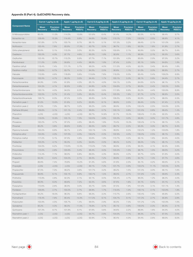
21
Component Name
Carrot 1 µg/kg (n=6) Apple 1 µg/kg (n=6) Carrot 2.5 µg/kg (n=6) Apple 2.5 µg/kg (n=3) Carrot 10 µg/kg (n=6) Apple 10 µg/kg (n=6)
Mean Recovery
Precision RSD(%)
Mean Recovery
Precision RSD(%)
Mean Recovery
Precision RSD(%)
Mean Recovery
Precision RSD(%)
Mean Recovery
Precision RSD(%)
Mean Recovery
Precision RSD(%)
N-Nitrosopyrrolidine 95.4% 11.0% 114.0% 13.8% 101.6% 6.4% 91.4% 14.2% 82.5% 6.1% 99.4% 9.7%
Nonachlor-cis 109.4% 15.3% 114.4% 8.8% 94.6% 10.4% 113.1% 7.2% 100.5% 2.5% 98.9% 4.1%
Nonachlor-trans 107.8% 3.7% 103.7% 8.7% 96.1% 5.1% 107.3% 2.2% 99.4% 2.1% 101.0% 2.6%
Norflurazon 100.4% 7.8% 83.9% 17.3% 93.7% 3.5% 96.7% 1.8% 95.5% 1.8% 91.8% 2.7%
Ortho-phenylphenol 90.6% 5.1% 115.5% 3.5% 82.3% 6.2% 102.6% 2.1% 90.9% 3.2% 99.7% 5.4%
Oxadiazon 100.3% 4.3% 97.7% 4.6% 95.2% 1.9% 92.9% 1.1% 96.9% 2.1% 95.5% 3.6%
Oxyfluorfen 102.4% 15.7% 113.2% 8.9% 97.7% 7.1% 101.6% 4.5% 95.6% 2.0% 97.0% 3.2%
Paclobutrazol 111.2% 2.9% 93.8% 4.4% 98.3% 1.9% 97.4% 2.0% 95.1% 3.9% 94.6% 1.9%
Parathion (ethyl) 118.4% 7.4% 111.1% 5.7% 96.0% 4.0% 111.5% 4.5% 92.0% 3.4% 90.4% 1.8%
Parathion-methyl 119.6% 6.7% 83.7% 4.1% 94.0% 2.5% 95.8% 1.1% 91.0% 3.3% 86.9% 2.7%
Pebulate 112.9% 4.6% 118.8% 5.6% 113.9% 7.6% 119.3% 0.3% 93.4% 5.4% 109.2% 6.9%
Penconazole 100.3% 4.7% 96.3% 3.5% 94.4% 1.7% 100.1% 5.3% 98.1% 0.9% 94.4% 2.7%
Pentachloroaniline 94.9% 2.8% 91.8% 4.3% 85.1% 4.0% 104.1% 0.3% 84.6% 8.2% 96.1% 2.7%
Pentachloroanisole 104.3% 4.1% 92.8% 4.9% 94.8% 4.3% 104.6% 3.7% 90.6% 2.4% 102.5% 5.6%
Pentachlorobenzene 100.1% 4.0% 94.5% 6.3% 95.8% 5.6% 117.9% 6.9% 83.2% 4.4% 100.9% 8.9%
Pentachlorobenzonitrile 102.5% 5.7% 91.4% 3.3% 95.2% 6.4% 103.3% 1.9% 87.7% 2.7% 96.6% 3.5%
Pentachlorothioanisole 106.7% 6.3% 97.4% 3.2% 86.8% 3.4% 106.5% 0.2% 82.8% 9.7% 98.0% 2.3%
Permethrin peak 1 91.6% 13.6% 81.8% 6.2% 82.8% 8.1% 98.9% 2.0% 89.4% 2.3% 97.4% 2.1%
Permethrin peak 2 97.6% 7.0% 98.7% 3.2% 96.2% 2.6% 98.9% 0.3% 100.4% 2.5% 104.8% 2.0%
Perthane (Ethylan) 109.8% 3.1% 101.1% 2.4% 96.6% 0.7% 103.1% 0.8% 101.0% 0.8% 99.4% 1.4%
Phenothrin <LOQ <LOQ <LOQ <LOQ 89.7% 14.9% 81.7% 13.3% 108.4% 11.3% 92.2% 4.2%
Phorate 116.6% 15.9% 103.1% 7.0% 102.5% 4.8% 103.3% 3.0% 98.9% 3.0% 101.7% 4.8%
Phosalone 100.2% 3.7% 97.2% 4.6% 98.4% 1.8% 70.4% 13.3% 100.4% 2.1% 99.1% 1.2%
Phosmet 85.2% 3.8% 89.6% 6.9% 89.3% 3.6% 89.7% 2.2% 95.3% 3.3% 88.7% 6.4%
Piperonyl butoxide 105.0% 6.8% 99.7% 2.4% 103.1% 1.3% 99.9% 0.5% 102.2% 1.2% 103.8% 1.8%
Pirimiphos-ethyl 104.9% 4.3% 107.5% 4.0% 100.2% 2.0% 102.9% 4.2% 100.0% 2.5% 98.1% 2.8%
Pirimiphos-methyl 117.2% 5.1% 97.0% 4.8% 93.6% 1.9% 110.7% 4.2% 99.1% 1.6% 94.0% 4.0%
Pretilachlor 103.3% 4.1% 95.3% 5.0% 94.6% 2.0% 98.4% 5.2% 99.4% 1.0% 98.1% 1.2%
Prochloraz 104.5% 6.2% 110.6% 12.3% 115.0% 7.9% 98.9% 2.3% 99.3% 4.1% 92.0% 3.9%
Procymidone 115.0% 2.8% 100.8% 5.4% 96.4% 3.0% 103.3% 1.5% 98.7% 1.5% 99.0% 3.2%
Profenofos 114.4% 7.1% 99.0% 6.8% 86.5% 4.3% 99.9% 4.2% 95.7% 3.5% 91.6% 3.0%
Propachlor 94.4% 8.4% 104.0% 2.1% 99.3% 7.2% 99.9% 2.8% 92.7% 1.3% 97.7% 4.6%
Propanil 89.6% 7.5% 78.8% 10.2% 91.3% 5.6% 91.6% 2.3% 95.1% 4.2% 89.5% 2.1%
Propargite <LOQ <LOQ <LOQ <LOQ 89.1% 7.3% 101.7% 4.9% 103.2% 11.1% 102.5% 5.2%
Propisochlor 97.5% 7.0% 99.2% 3.6% 101.7% 3.2% 99.2% 1.5% 101.3% 3.0% 99.1% 1.6%
Propyzamide 99.8% 6.1% 102.1% 8.9% 100.7% 1.5% 99.5% 2.7% 101.6% 1.3% 99.6% 2.4%
Prothiofos 115.8% 4.8% 92.3% 2.1% 92.1% 3.5% 105.4% 4.7% 96.0% 1.2% 98.2% 4.0%
Pyraclofos 96.9% 8.3% 89.6% 7.2% 92.3% 3.6% 87.6% 1.8% 94.1% 6.6% 94.1% 4.1%
Pyrazophos 110.6% 2.6% 96.0% 3.0% 93.7% 3.8% 97.5% 1.9% 101.9% 3.1% 101.1% 1.4%
Pyridaben 106.8% 2.7% 100.0% 2.7% 98.9% 1.7% 119.5% 1.0% 100.1% 2.1% 102.8% 1.8%
Pyridaphenthion 94.2% 18.0% 96.3% 8.6% 96.3% 3.3% 113.7% 2.6% 100.4% 1.9% 95.9% 2.2%
Pyrimethanil 118.4% 7.6% 80.4% 13.3% 117.0% 9.1% 104.7% 9.1% 101.3% 2.7% 95.8% 2.8%
Pyriproxyfen 103.9% 4.5% 105.7% 1.4% 99.5% 2.9% 80.0% 7.3% 101.2% 1.3% 102.9% 1.6%
Quinalphos 95.2% 4.3% 86.3% 11.5% 78.9% 3.7% 85.1% 4.9% 100.0% 2.3% 95.5% 2.1%
Quintozene 107.3% 8.7% 101.9% 6.1% 97.6% 5.6% 94.6% 2.2% 88.9% 1.6% 94.3% 4.0%
Resmethrin peak 1 <LOQ <LOQ <LOQ <LOQ 94.7% 2.9% 104.0% 7.1% 96.3% 3.7% 87.5% 2.0%
Resmethrin peak 2 <LOQ <LOQ <LOQ <LOQ 92.9% 7.7% 95.4% 4.3% 94.4% 2.6% 89.0% 6.0%
Appendix B (Part 4). QuEChERS Recovery data.
84 Back to contents

©2018 Thermo Fisher Scientific Inc. All rights reserved. All trademarks are the property of Thermo Fisher Scientific and its subsidiaries. This information is presented as an example of the capabilities of Thermo Fisher Scientific products. It is not intended to encourage use of these products in any manners that might infringe the intellectual property rights of others. Specifications, terms and pricing are subject to change. Not all products are available in all countries. Please consult your local sales representatives for details. AN10586-EN 0218S
Find out more at thermofisher.com/TSQ9000
Component Name
Carrot 1 µg/kg (n=6) Apple 1 µg/kg (n=6) Carrot 2.5 µg/kg (n=6) Apple 2.5 µg/kg (n=3) Carrot 10 µg/kg (n=6) Apple 10 µg/kg (n=6)
Mean Recovery
Precision RSD(%)
Mean Recovery
Precision RSD(%)
Mean Recovery
Precision RSD(%)
Mean Recovery
Precision RSD(%)
Mean Recovery
Precision RSD(%)
Mean Recovery
Precision RSD(%)
Sulfotep 103.2% 2.1% 101.1% 5.1% 96.7% 3.6% 101.8% 0.9% 96.7% 2.5% 100.6% 3.6%
Sulprofos 105.8% 2.6% 98.4% 4.3% 94.2% 1.4% 96.3% 3.0% 101.8% 1.3% 99.7% 1.1%
Tebuconazole 99.4% 3.2% 94.7% 4.5% 94.7% 1.2% 96.6% 1.8% 96.6% 0.6% 95.8% 1.5%
Tebufenpyrad 101.5% 4.7% 105.1% 2.2% 98.2% 1.5% 108.3% 0.7% 104.7% 2.0% 103.8% 1.4%
Tecnazene 100.9% 7.5% 94.3% 9.4% 94.2% 5.0% 104.3% 1.3% 86.9% 3.7% 100.4% 6.5%
Tefluthrin 103.2% 2.2% 101.7% 4.5% 99.0% 2.4% 104.5% 1.5% 100.1% 1.1% 99.1% 2.5%
Terbacil 98.7% 4.7% 89.0% 2.5% 94.6% 2.1% 89.2% 2.9% 95.1% 2.6% 94.1% 3.6%
Terbufos 109.8% 5.4% 97.9% 5.7% 98.0% 2.5% 107.3% 1.4% 98.8% 1.9% 104.3% 3.4%
Terbuthylazine 107.3% 6.2% 99.8% 4.3% 92.7% 4.0% 96.4% 4.9% 101.2% 3.9% 96.6% 3.0%
Tetrachlorvinphos 104.6% 4.4% 86.0% 5.3% 96.5% 3.5% 117.6% 1.7% 102.2% 4.7% 94.1% 1.6%
Tetradifon 92.1% 4.9% 105.0% 9.5% 94.4% 2.2% 99.1% 3.9% 97.5% 2.2% 100.8% 1.9%
Tetrahydrophthalimide (THPI)
88.8% 4.7% 87.6% 4.5% 98.6% 3.8% 89.3% 4.2% 93.8% 1.1% 88.3% 3.3%
Tetramethrin peak 1 <LOQ <LOQ <LOQ <LOQ 108.2% 15.9% 79.5% 12.3% 95.1% 2.7% 96.5% 3.4%
Tetramethrin peak 2 93.4% 6.4% 118.7% 11.5% 96.9% 2.7% 96.1% 3.0% 100.7% 0.8% 97.8% 1.5%
Tolclofos-methyl 111.6% 3.3% 103.2% 5.3% 97.3% 2.5% 106.7% 2.2% 98.1% 1.8% 99.1% 1.9%
Tolylfluanid 70.7% 3.5% 66.5% 5.9% 64.9% 8.7% 70.0% 3.6% 71.7% 2.7% 79.9% 4.4%
Triadimefon 108.2% 5.2% 94.9% 5.8% 97.3% 2.7% 99.0% 0.3% 96.7% 0.7% 97.6% 2.0%
Triadimenol 109.3% 5.6% 105.8% 4.3% 95.9% 2.4% 98.5% 1.8% 99.1% 1.1% 98.4% 4.6%
Triallate 110.7% 2.5% 98.8% 4.6% 97.6% 3.1% 103.0% 3.0% 96.6% 0.6% 101.0% 3.4%
Triazophos 99.1% 4.9% 92.7% 4.1% 97.4% 2.2% 91.5% 1.4% 98.1% 1.6% 95.9% 1.7%
Tricyclazole 88.2% 17.8% 71.2% 5.0% 81.3% 9.1% 78.4% 6.3% 78.1% 6.0% 80.0% 6.3%
Triflumizole 102.5% 8.0% 89.7% 6.8% 96.0% 4.6% 94.4% 4.7% 100.4% 3.1% 101.7% 1.8%
Vinclozolin 106.6% 7.2% 100.3% 6.7% 99.1% 2.3% 98.5% 6.4% 98.2% 1.6% 97.6% 2.5%
Appendix B (Part 5). QuEChERS Recovery data.
85 Back to contents
GoalThe aim of the study was to assess the quantitative performance of the Thermo Scientific™ TSQ™ 9000 triple quadrupole GC-MS/MS system equipped with the advanced electron ionization (AEI) source for the analysis of polybrominated diphenyl ethers (PBDEs) in food at low concentrations.
IntroductionPBDEs are a class of brominated hydrocarbons with a basic structure containing two phenyl rings linked by an oxygen atom. There are 209 possible PBDE congeners that differ in the number and location of bromine atoms in the phenyl rings.
PBDEs are used as additive flame retardants in different materials such as plastics, textiles, upholstery, and circuitry that can leach into the environment where they persist and bioaccumulate.1 As a consequence, the use of certain toxic PBDEs with links to cancer (including penta, tetra, and deca BDE) have been banned, and are currently listed in the Stockholm Convention inventory of persistent organic pollutants.2
Authors Aaron Lamb1, Cristian Cojocariu1, and Sean Panton2
1 Thermo Fisher Scientific, Runcorn, UK2 Fera Science, Ltd., York, UK
Keywords Food safety, polybrominated diphenyl ethers (PBDEs), trace analysis, gas chromatography, triple quadrupole mass spectrometry, selective reaction monitoring (SRM), sensitivity, routine, TSQ 9000, advanced electron ionization (AEI), Chromeleon, isotope dilution
Fast, ultra-sensitive analysis of PBDEs in food using advanced GC-MS/MS technology
APPLICATION NOTE 10674
86 Back to contents

2
The major challenges for PBDE analysis are sensitivity and selectivity in complex matrices, chromatographic resolution of critical pairs, degradation of higher brominated compounds, and the cost per sample. Gas chromatography-high resolution mass spectrometry (GC-HRMS) is the analytical technique of choice for PBDE determination in food, and triple quadrupole GC-MS/MS instrumentation in particular has recently become popular for this application due to its high selectivity and sensitivity provided through selective reaction monitoring (SRM) acquisition mode. High selectivity and sensitivity are required to (i) reduce interferences from matrix and background chemical ions that can result in false positive detection and erroneous quantification of PBDEs and (ii) detect ultra-trace levels of these toxic compounds in complex matrices.
The chromatographic resolution of the critical pair (BDE-49 and BDE-71) in PBDE analysis is essential because many of the congeners are isobaric and share common SRM transitions, meaning chromatographic separation is a necessity. For this reason reported methods have low sample throughput with analysis times of up to 45 minutes on costly capillary columns typically of 60 m in length.3 In this study a new high efficiency, high selectivity 15 m Thermo Scientific™ TraceGOLD™ TG-PBDE capillary column was evaluated for increased sample throughput and reduced cost per sample.
The aim of this project was to evaluate the analytical performance of the TSQ 9000 GC-MS/MS system using the AEI source for the ultra-trace analysis and separation of PBDEs in food matrices. This was attempted using a fast, sensitive, selective method on the high efficiency TraceGOLD TG-PBDE capillary column. The following analytical performance criteria were evaluated: sensitivity, repeatability, linearity, limit of quantification, and the accuracy of measurements in matrix.
The assessment of system robustness and suitability for routine PBDE GC-MS/MS analysis, which was outside the scope of this application note, can be found in a supporting 2018 technical note.
ExperimentalPreparation of solvent calibration curve, instrument detection limit (IDL), and limit of quantification (LOQ) standardsCalibration standards containing 27 native PBDE congeners at five concentration levels (Table 1, Appendix), and 16 (13C labeled) PBDEs internal standards (Table 2, Appendix), were acquired from Wellington Laboratories, Inc. (Ontario, Canada).
For the calculation of IDLs and LOQs for individual BDE congeners, the lowest concentration standard was serially diluted with n-nonane to 0.5, 0.25, 0.1, 0.075, and 0.05 pg/µL for BDE-209 ready for repeat injections.
Preparation of samplesSample preparation was performed according to that described in a scientific paper by A. Fernandes et al.3 The procedure involves sample homogenization/freeze drying, fortification of 10 g of homogenized/freeze-dried sample in 200 mL of n-hexane with isotopically labeled 13C PBDE internal standards followed by loading onto a multi-packed silica column containing acidified silica, basified silica, and activated charcoal. PBDEs were then eluted from the multi-packed silica/activated carbon column using 100 mL of n-hexane and 400 mL of n-hexane/dichloromethane (60:40, v:v) then evaporated to dryness and reconstituted to 0.5 mL in n-hexane. The extracts were cleaned further using a silica alumina column and 20 mL of DCM/n-hexane (30:70) followed by the addition of 13C-labeled PBDE syringe standards, evaporation, and reconstitution to 25 µL with n-nonane prior to analysis.
GC-MS/MS analysisA TSQ 9000 triple quadrupole GC-MS/MS instrument equipped with an AEI source and coupled with a Thermo Scientific™ TRACE™ 1310 gas chromatograph was used. The AEI source provides highly efficient electron ionization of analytes and a more tightly focused ion beam that leads to an unparalleled level of sensitivity.
87 Back to contents
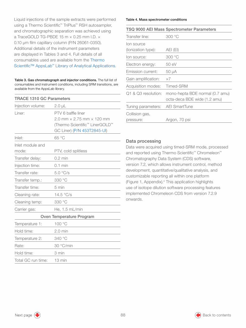
3
TRACE 1310 GC Parameters
Injection volume: 2.0 μL
Liner: PTV 6 baffle liner 2.0 mm × 2.75 mm × 120 mm (Thermo Scientific™ LinerGOLD™ GC Liner) (P/N 453T2845-UI)
Inlet: 65 °C
Inlet module and mode: PTV, cold splitless
Transfer delay: 0.2 min
Injection time: 0.1 min
Transfer rate: 5.0 °C/s
Transfer temp.: 330 °C
Transfer time: 5 min
Cleaning rate: 14.5 °C/s
Cleaning temp: 330 °C
Carrier gas: He, 1.5 mL/min
Oven Temperature Program
Temperature 1: 100 °C
Hold time: 2.0 min
Temperature 2: 340 °C
Rate: 30 °C/min
Hold time: 3 min
Total GC run time: 13 min
Table 3. Gas chromatograph and injector conditions. The full list of consumables and instrument conditions, including SRM transitions, are available from the AppsLab library.
Table 4. Mass spectrometer conditions
TSQ 9000 AEI Mass Spectrometer Parameters
Transfer line: 300 °C
Ion source (Ionization type): AEI (EI)
Ion source: 300 °C
Electron energy: 50 eV
Emission current: 50 µA
Gain amplification: ×7
Acquisition modes: Timed-SRM
Q1 & Q3 resolution: mono-hepta BDE normal (0.7 amu) octa-deca BDE wide (1.2 amu)
Tuning parameters: AEI SmartTune
Collision gas, pressure: Argon, 70 psi
Data processingData were acquired using timed-SRM mode, processed and reported using Thermo Scientific™ Chromeleon™ Chromatography Data System (CDS) software, version 7.2, which allows instrument control, method development, quantitative/qualitative analysis, and customizable reporting all within one platform (Figure 1, Appendix).4 This application highlights use of isotope dilution software processing features implemented Chromeleon CDS from version 7.2.9 onwards.
Liquid injections of the sample extracts were performed using a Thermo Scientific™ TriPlus™ RSH autosampler, and chromatographic separation was achieved using a TraceGOLD TG-PBDE 15 m × 0.25 mm I.D. × 0.10 μm film capillary column (P/N 26061-0350). Additional details of the instrument parameters are displayed in Tables 3 and 4. Full details of all consumables used are available from the Thermo Scientific™ AppsLab™ Library of Analytical Applications.
88 Back to contents

4
Results and discussionPBDE chromatography, selectivity, sensitivity in terms of IDLs, LOQs in sample, and linearity were evaluated using solvent-based standards. Extracted food samples were obtained from Fera Science, Ltd., York and were used in the experiments described below.
ChromatographyAll target congeners were separated in under 11 minutes including excellent separation of the critical pair BDE-49 and BDE-71 (Figure 2). Resolution of these compounds was 0.6% based on valley height relative to the height of the shortest peak, which is well within the EPA 1614 requirement of less than 40%.5 Compared with existing GC-HRMS methods (~45 min run times), this will allow for the analysis of up to 100 samples per day (compared to 30 in a published
paper) giving an increase in sample throughput of 3× and a significant reduction in cost per sample.3 Using the TG-PBDE capillary column, good chromatographic peak shape was obtained for all compounds (Figure 2), even for BDE-209, which is particularly challenging for this analysis due to susceptibility to breakdown and peak tailing.
SelectivityDue to the diversity of matrices with various degrees of complexity, selectivity can be challenging in routine GC-MS analysis. An example of sample complexity is shown in Figure 3 as an overlay of the TIC of fish containing incurred residues (top chromatogram) and of timed SRM (bottom chromatogram) showing target PBDEs.
Figure 2. Chromatogram showing the SRM transition (quant ion) for PBDEs in a 1–5 pg/µL solvent standard (CS-1) (equivalent to 2.5–12.5 ng/kg in sample) with excellent chromatographic peak shapes for all compounds. 13C-labeled internal and syringe standards were not displayed to show native peak shapes clearly.
PBDE
-49
4.50 5.00 5.50 6.00 6.50 7.00 7.50 8.00 8.50 9.00 9.50 10.00 10.50 11.00
PBDE
-3
PBDE
-85
PBDE
-119
PBDE
-100
PBDE
-66PB
DE-4
7
PBDE
-28
PBDE
-184
PBDE
-17
PBDE
-15
PBDE
-7
PBDE
-196
PBDE
-197
PBDE
-191
PBDE
-183
PBDE
-209
PBDE
-154
PBDE
-138
PBDE
-206
PBDE
-207
PBDE
-153
PBDE
-156
PBDE
-126
PBDE
-77 PB
DE-9
9
1.0e6
-1.0e5
Coun
ts
6.0 6.7
PBDE
-71
RT (min)
89 Back to contents

5
Carryover assessmentCarryover can be a problem for this application; however, it was found that using a mixed needle wash solvent of dichloromethane/toluene/n-nonane (50:25:25) eliminated this potential problem. In Figure 4 an example SRM transition of the highest concentration injected standard for BDE-209 (2000 pg/µL, 4 ng on column (oc)) (top chromatogram) and the consecutive n-nonane blank (bottom chromatogram) demonstrates that there is no carryover.
Sensitivity: determination of IDLsThe enhanced sensitivity of the new AEI source is demonstrated for the most challenging compound analyzed, BDE-209 (Figure 5). Here a 250 fg/µL (500 fg oc) solvent standard shows excellent signal precision with peak area repeatability <10% RSD at low ppt levels (equivalent to 0.6 ng/kg) in sample extracts). Excellent peak shape was also observed for this high molecular weight compound (MW = 959.2), which is due to the thin film and excellent surface deactivation of the TG-PBDE column coupled with the highly uniform heating profile of the newly designed TSQ 9000 GC-MS/MS system transfer line. These factors result in less peak tailing for low volatility, high boiling compounds such as higher brominated PBDEs and make accurate integration possible.
Figure 3. (A) Extracted fish matrix TIC acquired in full-scan containing late eluting acylglycerides (top chromatogram) and (B) corresponding timed-SRM for quant ion of targeted PBDEs (bottom chromatogram)
Aclyglycerides
A
B
4.08 4.50 5.00 5.50 6.00 6.50 7.00 7.50 8.00 8.50 9.00 9.50 10.00 10.50 11.00 11.36-2.0e5
0.0e0
2.0e5
4.0e5
6.0e5
8.0e5
1.0e6
1.2e6
1.4e6
1.6e6
1.8e6
RT (min)
Coun
ts
3.00
4.00
5.00
6.00
7.00
8.00
9.00
10.00
11.00
12.00
13.00 -2.0e9
0.0e0
2.0e9
4.0e9
6.0e9
8.0e9
1.0e10
1.2e10
1.4e10
1.6e10
RT (min)
Coun
ts
PBDE
-28
PBDE
-15
PBDE
-7
PBDE
-153
PBDE
-154
PBDE
-66
PBDE
-209
PBDE
-207
PBDE
-183
PBDE
-100
PBDE
-49
PBDE
-3
PBDE
-99
PBDE
-119
PBDE
-126
90 Back to contents

6
Figure 4. BDE 209 overlaid quantification ion and qualification ions for the highest standard in n-nonane/ toluene 2000 pg/µL corresponding to 4 ng on-column (OC) (top chromatogram) and a consecutive n-nonane blank (bottom chromatogram). Data is unsmoothed and was acquired in timed-SRM mode.
Figure 6. Graph showing individual IDLs in fg on column for 27 native PBDEs calculated from n=15 replicate injections of the lowest serially diluted standards
Figure 5. Overlaid quantification SRM transitions (797.3→637.3 m/z) from n=15 consecutive injections of a 250 fg/µL BDE-209 solvent standard (corresponding to 0.625 ng/kg in sample). No data smoothing was used and data was acquired in timed-SRM mode.
To practically assess the IDLs n=15 replicate injections of the lowest serially diluted solvent standard with a peak area % RSD of <15% was used. IDLs were then calculated by taking into account the injected amount, peak area % RSD, and t-score of 2.624, corresponding to n=14 degrees of freedom at 99% confidence level (Figure 6). The IDL values calculated ranged from 2 to 100 fg OC (corresponding to 0.003–0.125 ng/kg in sample).
BDE-209500 fg OCn=15 injections% RSD peak area = 7.7%Calculated IDL = 100 fg OC (0.625 ng/kg in sample)
Sensitivity: determination of limit of quantitation (LOQ)Method LOQs were calculated using serially diluted calibration standards described in the IDL section. Fifteen replicate injections of each of the diluted standards ranging between 0.02 pg/µL and 0.25 pg/µL were performed (equivalent to 0.05–0.63 ng/kg in sample (Table 6).
RT (min)
Coun
tsCo
unts
PBDE
-49
PBDE
-3
PBDE
-85
PBDE
-119
PBDE
-100
PBDE
-66
PBDE
-47
PBDE
-28
PBDE
-184
PBDE
-17
PBDE
-15
PBDE
-7
PBDE
-196
PBDE
-197
PBDE
-191
PBDE
-183
PBDE
-209
PBDE
-154
PBDE
-138
PBDE
-206
PBDE
-207
PBDE
-153
PBDE
-156
PBDE
-126
PBDE
-77
PBDE
-99
PBDE
-71
91 Back to contents

7
Table 6. Calculated equivalent LOQ concentration in sample from fifteen injections of solvent standards
BDE Number
Bromination No*
Quantification Transition
Amount Injected (pg OC)
Target Ion Ratio
%
Mean Measured Ion Ratio
(Average) %
Peak Area % RSD
LOQ (pg OC)
LOQ (ng/kg)
BDE-3 Mono 250→115 0.04 60 62 5.6% 0.04 0.05
BDE-7 Di 326→139 0.04 15 15 3.6% 0.04 0.05
BDE-15 Di 326→139 0.10 48 49 3.6% 0.10 0.13
BDE-17 Tri 406→139 0.04 95 93 5.9% 0.04 0.05
BDE-28 Tri 406→139 0.04 79 78 6.4% 0.04 0.05
BDE-49 Tetra 484→217 0.10 34 34 3.3% 0.10 0.13
BDE-71 Tetra 484→217 0.10 33 34 4.1% 0.10 0.13
BDE-47 Tetra 484→217 0.10 36 36 4.3% 0.10 0.13
BDE-66 Tetra 484→217 0.10 30 31 5.0% 0.10 0.13
BDE-77 Tetra 484→217 0.10 115 112 7.0% 0.10 0.13
BDE-100 Penta 564→404 0.10 85 74 4.1% 0.10 0.13
BDE-119 Penta 564→404 0.10 48 48 3.8% 0.10 0.13
BDE-99 Penta 564→404 0.10 62 57 3.0% 0.10 0.13
BDE-85 Penta 564→404 0.10 60 56 5.7% 0.10 0.13
BDE-126 Penta 564→404 0.20 122 131 7.1% 0.20 0.25
BDE-154 Hexa 642→482 0.20 66 64 8.1% 0.20 0.25
BDE-153 Hexa 642→482 0.20 65 57 7.3% 0.20 0.25
BDE-138 Hexa 642→482 0.20 68 63 8.0% 0.20 0.25
BDE-156 Hexa 642→482 0.20 70 74 8.7% 0.20 0.25
BDE-184 Hepta 721→564 0.20 46 46 6.3% 0.20 0.25
BDE-183 Hepta 721→564 0.20 47 49 4.3% 0.20 0.25
BDE-191 Hepta 721→564 0.20 48 47 5.0% 0.20 0.25
BDE-197 Octa 642→482 0.20 48 48 4.0% 0.20 0.25
BDE-196 Octa 642→482 0.20 61 64 5.8% 0.20 0.25
BDE-207 Nona 879→721 0.50 52 53 5.4% 0.50 0.63
BDE-206 Nona 879→721 0.50 60 49 6.3% 0.50 0.63
BDE-209 Deca 797→637 0.50 100 96 7.7% 0.50 0.63
92 Back to contents
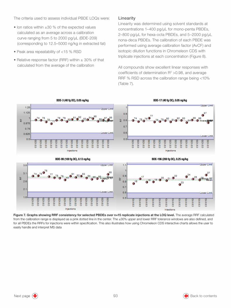
8
The criteria used to assess individual PBDE LOQs were:
• Ion ratios within ±30 % of the expected values calculated as an average across a calibration curve ranging from 5 to 2000 pg/µL (BDE-209) (corresponding to 12.5–5000 ng/kg in extracted fat)
• Peak area repeatability of <15 % RSD
• Relative response factor (RRF) within ± 30% of that calculated from the average of the calibration
Figure 7. Graphs showing RRF consistency for selected PBDEs over n=15 replicate injections at the LOQ level. The average RRF calculated from the calibration range is displayed as a pink dotted line in the center. The ±30% upper and lower RRF tolerance windows are also defined, and for all PBDEs the RRFs for injections were within specification. This also illustrates how using Chromeleon CDS interactive charts allows the user to easily handle and interpret MS data
LinearityLinearity was determined using solvent standards at concentrations 1–400 pg/µL for mono-penta PBDEs, 2–800 pg/µL for hexa-octa PBDEs, and 5–2000 pg/µL nona-deca PBDEs. The calibration of each PBDE was performed using average calibration factor (AvCF) and isotopic dilution functions in Chromeleon CDS with triplicate injections at each concentration (Figure 8).
All compounds show excellent linear responses with coefficients of determination R2 >0.98, and average RRF % RSD across the calibration range being <10% (Table 7).
BDE-3 (40 fg OC), 0.05 ng/kg BDE-17 (40 fg OC), 0.05 ng/kg
BDE-99 (100 fg OC), 0.13 ng/kg BDE-196 (200 fg OC), 0.25 ng/kg
93 Back to contents

9
Figure 8. (A) Linearity of PBDEs demonstrated using a solvent-based calibration curve ranging from 1.0 to 2000 pg/µL in the case of BDE-209 (corresponding to 2.5–5000 ng/kg in food). Average calibration factor (AvCF) function was used in Chromeleon CDS with three replicate injections at each concentration and internal standard adjustment was conducted. Coefficient of determination (R2) and average RRF % RSD are displayed. (B) Expanded region of calibration for BDE-209 from 5 to 100 pg/µL is shown (corresponding to 12.5–250 ng/kg in extracted fat) demonstrating excellent accuracy and precision for triplicate injections per point.
A
B
94 Back to contents

10
Table 7. Coefficient of determination (R2) and RRF % RSD
Compound R2 RRF % RSD Compound R2 RRF % RSD
BDE-3 0.9941 4.2 BDE-126 0.9980 2.8
BDE-7 0.9987 2.6 BDE-154 0.9923 5.1
BDE-15 0.9987 2.9 BDE-153 1.0000 1.8
BDE-17 0.9980 3.2 BDE-138 0.9976 2.7
BDE-28 0.9999 1.5 BDE-156 0.9795 9.9
BDE-49 0.9995 3.8 BDE-184 0.9927 5.9
BDE-71 0.9953 4.2 BDE-183 0.9992 1.8
BDE-47 0.9991 2.8 BDE-191 0.9879 7.6
BDE-66 0.9970 4.4 BDE-197 0.9976 2.5
BDE-77 0.9959 6.6 BDE-196 0.9823 9.3
BDE-100 0.9994 1.7 BDE-207 0.9982 2.8
BDE-119 0.9921 5.1 BDE-206 0.9988 2.6
BDE-99 0.9952 4.6 BDE-209 0.9991 2.6
BDE-85 0.9975 7.3
PBDE quantification in food samples and comparison to GC-HRMS dataSeveral food samples were tested for the PBDE content and examples of sensitivity, selectivity, and accuracy of measurements are highlighted below (Figures 9 and 10).
Figure 9. Examples of SRMs chromatograms (quantification in black, and confirmation ions in pink and blue) for BDE-28 in salmon (left chromatogram) and BDE-49 in tallow (right chromatogram); visit the AppsLab Library for full SRM transitions. Below each of the chromatograms the following is shown: (i) amount found in sample in ng/kg, (ii) HRMS (magnetic sector data) result provided from Fera Science, Ltd. in ng/kg, (iii) % deviation from Fera Science, Ltd. result, (iv) observed ion ratio between quantification and primary confirmation ion, (v) expected ion ratio calculated from the average of the calibration, and (vi) % deviation of observed ion ratio versus the expected ion ratio.
Ion ratio = PASS
BDE-28 (Tri) Salmon
BDE-49 (Tetra) Tallow
Ion ratio = PASS
1.1e6
-3.2e4
Coun
ts
5.819 6.2006.1006.0005.900RT (min)
6.255 6.475 6.7006.600RT (min)
6.774
1.4e4
-1.3e2
Coun
ts
Amount found 86 ng/kg
HRMS result 87 ng/kg
% deviation -1%
Observed ion ratio 79.8%
Expected ion ratio 78.6%
% deviation +1%
Amount found 3 ng/kg
HRMS result 4 ng/kg
% deviation 25%
Observed ion ratio 28.3%
Expected ion ratio 34.6%
% deviation -18%
95 Back to contents

11
Figure 10. The two chromatograms show the overlaid selective reaction monitoring transitions (quantification in black, and confirmation ions in pink and blue) for BDE-99 in fish oil (top left chromatogram), BDE-153 in cows liver (top right chromatogram), BDE-183 in reindeer (bottom left chromatogram), and BDE-209 in milk (bottom right chromatogram).
In summary, the results comparison for triple quadrupole technology versus GC-HRMS shows very close agreement. The low limits of quantification that are achievable using triple quadrupole technology are clearly demonstrated in the case of BDE-49 in tallow and BDE-183 in reindeer; in both cases low ppt (ng/kg in extracted fat) results were reported with ion confirmation within the ±30% tolerance of the averaged ion ratio across the
calibration. In the case of the complex fish oil matrix, the power of the mass spectrometer and TG-PBDE column combination become apparent in their ability to selectively resolve complex matrix interferences and congeners with the deviation in measured ion ratio versus the calibration of only 7%.
BDE-99 (Penta)Fish Oil
Ion ratio = PASS
Ion ratio = PASS
Ion ratio = PASS Ion ratio = PASS
3.8e5
-6.3e3
Coun
ts3.4e4
-1.5e3
Coun
ts
1.1e4
-3.0e2
Coun
ts
7.4e3
1.1e2
Coun
ts
7.243 7.5437.5007.4007.300RT (min) 7.751 8.1818.1258.0007.575
RT (min)
8.326 8.7268.8008.5008.400RT (min)
10.395 10.79510.62510.500RT (min)
BDE-153 (Hexa)Cows Liver
BDE-183 (Hepta)Reindeer
BDE-209 (Deca)Milk
121 ng/kg
108 ng/kg
+12%
54.7%
58.9%
-7%
Amount found
HRMS result
% deviation
Observed ion ratio
Expected ion ratio
% deviation
84 ng/kg
80 ng/kg
+5%
53.3%
52.6%
+1%
Amount found
HRMS result
% deviation
Observed ion ratio
Expected ion ratio
% deviation
Amount found
HRMS result
% deviation
Observed ion ratio
Expected ion ratio
% deviation
Amount found
HRMS result
% deviation
Observed ion ratio
Expected ion ratio
% deviation
86 ng/kg
<87 ng/kg
NA
86.1%
98.5%
-13%
3 ng/kg
<2 ng/kg
NA
39.2%
47.3%
-17%
96 Back to contents
12
ConclusionsThe purpose of these experiments was to assess the quantitative performance of the TSQ 9000 GC-MS/MS system for increased sample throughput. Additionally, the results obtained were compared with those from GC-HRMS to assess the measurement accuracy.
• All 27 native BDE congeners were chromatographically separated in <11 min, allowing an increase in sample throughput of 3X compared to existing GC-MS methods.3
• The levels of sensitivity obtained allowed IDLs ranging from 2 to 100 fg OC (corresponding to 0.003 to 0.125 ng/kg in extracted fat).
• LOQs (derived from solvent standards) were equivalent to 0.05 to 0.63 ng/kg in extracted fat calculated from n=15 repeat injections of the lowest serially diluted standard that satisfied the acceptance criteria defined below:
– Ion ratios within ±30% of the expected values calculated as an average across a calibration curve ranging from 5 to 2000 pg/µL (corresponding to 10–5000 ng/kg in extracted fat).
– Peak area repeatability of <15% RSD.
– RRFs were within ±30% of that calculated from the average of the calibration.
• Excellent linearity was achieved across a calibration of 1–2000 pg/µL (corresponding to 2.5–5000 ng/kg in extracted fat) with all RRF % RSDs <10% and R2 values >0.98.
• The overall quantitative performance of the TSQ 9000 GC-MS/MS system was demonstrated by the ability to easily detect and confirm (using ion ratio values) low levels of PBDEs even in most critical sample types such as fish oil.
• The results obtained from the TSQ 9000 GC-MS/MS system experiments were in close agreement with HRMS (magnetic sector) data provided from Fera Science, Ltd., York was achieved even at very low concentrations.
Taken together these results demonstrate that the TSQ 9000 GC-MS/MS system configured with the AEI source provides unparalleled levels of quantitative performance making it an ideal analytical tool for routine food safety testing laboratories.
References1. Hites, R.A. Polybrominated Diphenyl Ethers in the Environment and in People: A
Meta-Analysis of Concentrations. Environ. Sci. Technology 2004, 38, 945.
2. Guidance for the inventory of polybrominated diphenyl ethers (PBDEs) listed under the Stockholm Convention on POPs. [Online] http://chm.pops.int/Implementation/NationalImplementationPlans/Guidance/GuidancefortheinventoryofPBDEs/tabid/3171/Default.aspx (accessed May 8, 2018).
3. Fernandes, A.; White, S.; D’Silva, K.; Rose. M. Simultaneous determination of PCDDs, PCDFs, PCBs and PBDEs in food. Talanta 2004, 63, 1147–1155.
4. Thermo Fisher Scientific (2009) Timed SRM technical note: https://assets.thermofisher.com/TFS-Assets/CMD/Application-Notes/AN51797-TimedSRM-Multitarget-Compound-Analysis.pdf
5. United States Environmental Protection Agency, Method 1614A Brominated Diphenyl Ethers in Water, Soil, Sediment, and Tissue by HRGC/HRMS, May 2010. https://www.epa.gov/sites/production/files/2015-08/documents/method_1614a_2010.pdf
97 Back to contents

13
Table 1. Details of 27 native PBDE congeners analyzed, including BDE number, chemical formula, CAS number, and calibration range
BDE Number Native BDEs
Chemical Formula
CAS Number
Calibration Range (ng/mL)
3 4-Bromodiphenyl ether C12H9BrO 101-55-3 1.0 to 400
7 2,4-Dibromodiphenyl ether C12H8Br2O 171977-44-9 1.0 to 400
15 4,4'-Dibromodiphenyl ether C12H8Br2O 2050-47-7 1.0 to 400
17 2,2',4-Tribromodiphenyl ether C12H7Br3O 147217-75-2 0.96 to 384
28 2,4,4'-Tribromodiphenyl ether C12H7Br3O 41318-75-6 1.0 to 400
47 2,2',4,4'-Tetrabromodiphenyl ether C12H6Br4O 5436-43-1 1.0 to 400
49 2,2',4,5'-Tetrabromodiphenyl ether C12H6Br4O 243982-82-3 1.0 to 400
66 2,3',4,4'-Tetrabromodiphenyl ether C12H6Br4O 189084-61-5 1.0 to 400
71 2,3',4',6-Tetrabromodiphenyl ether C12H6Br4O 189084-62-6 1.0 to 400
77 3,3',4,4'-Tetrabromodiphenyl ether C12H6Br4O 93703-48-1 1.0 to 400
85 2,2',3,4,4'-Pentabromodiphenyl ether C12H6Br5O 182346-21-0 1.0 to 400
99 2,2',4,4',5-Pentabromodiphenyl ether C12H6Br5O 32534-81-9 1.0 to 400
100 2,2',4,4',6-Pentabromodiphenyl ether C12H6Br5O 189084-64-8 1.0 to 400
119 2,3',4,4',6-Pentabromodiphenyl ether C12H6Br5O 189084-66-0 1.0 to 400
126 3,3',4,4',5-Pentabromodiphenyl ether C12H6Br5O 366791-32-4 1.0 to 400
138 2,2',3,4,4',5-Hexabromodiphenyl ether C12H4Br6O 446254-95-1 2.0 to 800
153 2,2',4,4',5,5'-Hexabromodiphenyl ether C12H4Br6O 68631-49-2 2.0 to 800
154 2,2',4,4',5,6'-Hexabromodiphenyl ether C12H4Br6O 207122-15-4 2.0 to 800
156 2,3,3',4,4',5-Hexabromodiphenyl ether C12H4Br6O 405237-85-6 2.0 to 800
183 2,2',3,4,4',5',6-Heptabromodiphenyl ether C12H3Br7O 207122-16-5 2.0 to 800
184 2,2',3,4,4',6,6'-Heptabromodiphenyl ether C12H3Br7O 117948-63-7 2.0 to 800
191 2,3,3',4,4',5',6-Heptabromodiphenyl ether C12H3Br7O 446255-30-7 2.0 to 800
196 2,2',3,3',4,4',5,6'-Octabromodiphenyl ether C12H2Br8O 446255-39-6 2.0 to 800
197 2,2',3,3',4,4',6,6'-Octabromodiphenyl ether C12H2Br8O 117964-21-3 2.0 to 800
206 2,2',3,3',4,4',5,5',6-Nonabromodiphenyl ether C12HBr9O 63936-56-1 5.0 to 2000
207 2,2',3,3',4,4',5,6,6'-Nonabromodiphenyl ether C12HBr9O 437701-79-6 5.0 to 2000
209 Decabromodiphenyl ether C12Br10O 1163-19-5 5.0 to 2000
Appendix
98 Back to contents

14
Table 2. Details of 16 13C-labeled PBDEs internal standards, including BDE isomer number, chemical formula, CAS number, and concentration (suffix “L” indicates mass-labeled)
BDE isomer number
13C-labeled PBDEsChemical Formula
Concentration (ng/mL)
3L 4-Bromo[13C12]diphenyl ether 13C12H9BrO 100
15L 4,4'-Dibromo[13C12]diphenyl ether 13C12H8Br2O 100
28L 2,4,4'-Tribromo[13C12]diphenyl ether 13C12H7Br3O 100
47L 2,2',4,4'-Tetrabromo[13C12]diphenyl ether 13C12H6Br4O 100
79L 3,3',4,5'-Tetrabromo[13C12]diphenyl ether 13C12H6Br4O 100
99L 2,2',4,4',5-Pentabromo[13C12]diphenyl ether 13C12H5Br5O 100
100L 2,2',4,4',6-Pentabromo[13C12]diphenyl ether 13C12H5Br5O 100
126L 3,3',4,4',5-Pentabromo[13C12]diphenyl ether 13C12H5Br5O 100
138L 2,2',3,4,4',5-Hexabromo[13C12]diphenyl ether 13C12H4Br6O 200
153L 2,2',4,4',5,5'-Hexabromo[13C12]diphenyl ether 13C12H4Br6O 200
154L 2,2',4,4',5,6'-Hexabromo[13C12]diphenyl ether 13C12H4Br6O 200
183L 2,2',3,4,4',5',6-Heptabromo[13C12]diphenyl ether 13C12H3Br7O 200
197L 2,2',3,3',4,4',6,6'-Octabromo[13C12]diphenyl ether 13C12H2Br8O 200
206L 2,2',3,3',4,4',5,5',6-Nonabromo[13C12]diphenyl ether 13C12HBr9O 500
207L 2,2',3,3',4,4',5,6,6'-Nonabromo[13C12]diphenyl ether 13C12HBr9O 500
209L Decabromo[13C12]diphenyl ether 13C12Br10O 500
99 Back to contents

©2018 Thermo Fisher Scientific Inc. All rights reserved. All trademarks are the property of Thermo Fisher Scientific. This information is presented as an example of the capabilities of Thermo Fisher Scientific products. It is not intended to encourage use of these products in any manner that might infringe the intellectual property rights of others. Specifications, terms and pricing are subject to change. Not all products are available in all countries. Please consult your local sales representative for details. AN10674-EN 1018S
Find out more at thermofisher.com/TSQ9000
Figure 1. Example of the Chromeleon CDS interactive results browser used to assess and interrogate sample data in real time
100 Back to contents

GoalTo demonstrate the utility of the Thermo Scientific™ TSQ™ 9000 triple quadrupole GC-MS/MS system with Thermo Scientific™ Chromeleon™ Chromatography Data System (CDS) software for the routine and regulatory compliant analysis of polychlorinated dibenzo-p-dioxins and polychlorinated dibenzo-p-furans (PCDD/Fs), dioxin-like polychlorinated biphenyls (PCBs), and indicator PCBs in food and feed samples.
IntroductionDioxins and dioxin-like compounds are highly toxic substances classed as persistent organic pollutants (POPs). Due to their high fat-solubility, dioxins accumulate in the fatty tissues of animals. As a result, more than 90% of human exposure to dioxins is through food, especially meat, dairy, fish, etc. Therefore, accurate monitoring of food and feed is essential to control dioxin uptake from the food chain.1
In 2014 a change in European Commission regulations2,3 permitted gas chromatography-triple quadrupole mass spectrometry (GC-MS/MS) to be used as an alternative to gas chromatography-high resolution mass spectrometry (GC-HRMS) for confirmatory analysis and for the control of
Authors Richard Law1, Alexander Schaechtele2, Amit Gujar3, Jiangtao Xing4, and Cristian Cojocariu1
1Thermo Fisher Scientific, Runcorn, UK2European Union Reference Laboratory (EURL) for Halogenated POPs in Feed and Food, Freiburg, Germany3Thermo Fisher Scientific, Austin, Texas4Thermo Fisher Scientific, Beijing, China
Keywords Triple quadrupole GC-MS/MS, persistent organic pollutants, POPs, polychlorinated dibenzo-p-dioxins, polychlorinated dibenzo-p-furans, PCDD/Fs, dioxins, polychlorinated biphenyls, PCBs, confirmatory analysis, TSQ 9000, advanced electron ionization, AEI
Routine, regulatory analysis of dioxins and dioxin-like compounds in food and feed samples
APPLICATION NOTE 10703
101 Back to contents

2
maximum levels (MLs) and action levels (ALs) in certain food and feed samples. Even though the utility of GC-MS/MS for this application has been demonstrated in principle,4 there is a lack of robust data to validate the suitability of GC-MS/MS, especially for the long-term routine analysis of hundreds of samples. This is further confused by the absence of a clear protocol regarding the setting of appropriate limit of quantification (LOQ) values for GC-MS/MS analysis, with both signal-to-noise (S:N) and calibration-based approaches being used in some validations.
In addition to the deficiencies in validation data, there is a need for software packages to deal with the complexities of the calculations required to process and report data using isotopic dilution. As a consequence many laboratories adopt external software tools to manipulate the data. This practice is not only time-consuming, but can lead to errors in transcription and rounding, and also to an uncontrolled data trail. It is preferable to have the capability to acquire data, process data, and perform calculations and report the required results on a single, compliant software platform.
In this study, the performance of the TSQ 9000 triple quadrupole GC-MS/MS system equipped with an advanced electron ionization (AEI) source was evaluated. Data was acquired on two different TSQ 9000 AEI systems located in two different laboratories and operated by different chemists (UK and USA). Commercially available solvent standards, food/feedstuff, and proficiency test (PT) samples were used to evaluate the performance of each system for the analysis of polychlorinated dibenzo-p-dioxins (PCDDs), polychlorinated dibenzo-p-furans (PCDFs), dioxin-like polychlorinated biphenyls (PCBs), and non-dioxin-like (indicator) PCBs. Guidance from the European Union Reference Laboratories (EURL) on the use of a calibration approach was followed to set suitable LOQs:5 essentially, to demonstrate sufficient sensitivity to enable reporting at 1/5th of the maximum level (ML) upper bound sum toxic equivalences (TEQs).
To demonstrate the robustness required to operate in a routine environment an experiment involving continuous analysis of extracts over a period of two weeks was carried out.
ExperimentalInstrumental and method setupIn the experiments described here, a TSQ 9000 AEI triple quadrupole mass spectrometer was coupled to a Thermo Scientific™ TRACE™ 1310 Gas Chromatograph. Injection of liquid samples was performed automatically using a Thermo Scientific™ TriPlus™ RSH autosampler. See Appendix 2 for a list of the consumables used. Mass spectrometer operation was as per AN105904 unless otherwise specified. Importantly, acquisition, processing, and reporting of the data were all performed on a single platform using Chromeleon CDS software, version 7.2. Two separate GC-MS/MS methods were used: one for the analysis of non-ortho PCBs and PCDD/Fs (Table 1), and one to capture other dioxin and non dioxin-like compounds such as mono-ortho, di-ortho, and indicator PCBs fraction (Table 2). See Tables 1 and 2 in Appendix 1.
Samples, extraction, and clean-upFood and feedstuff samples (including PT samples) were provided by the EURL for Halogenated POPs in Feed and Food, Freiburg, Germany. A nominal sample intake weight of 2 grams (fat) was used for the samples unless indicated otherwise (Table 3). European method EN:1948 standard solutions; EN-1948CVS, WM48-CVS (calibration and quantitation), EN-1948ES, EN-1948IS, P48-W-ES, P48-M-ES, and P48-RS (extraction) were utilized for the extraction, calibration, and quantitation of PCDD/Fs, dioxin-like PCBs, and indicator PCBs. All standards were obtained from Wellington Laboratories Inc., Canada.
Extraction (where required) was performed by Twisselmann hot extraction (comparable with Soxhlet extraction) or pressurized liquid extraction. Automated clean-up of extracts was performed using a three column (multi-layered acidic silica, alumina, and carbon columns) setup on the DEXTech™ Plus system (LCTech GmbH). Two extract fractions were provided per sample, the first containing the non-ortho PCBs and PCDD/Fs (final volume 20 µL nonane) and the second containing the mono-ortho and di-ortho PCBs and indicator PCBs (final volume 100 µL nonane). Due to the absence of a non-ortho syringe standard in the calibration and extraction solutions, recoveries were not calculated for the four 13C-labeled non-ortho PCBs. As all the non-ortho PCBs were found in all samples at values greater than the LOQ this does not impact the validity of the results obtained.
102 Back to contents

3
2,3,4,7,8-pentachlorodibenzofuran (PeCDF) congener (a major contributor to the WHO-PCDD/F-TEQ) can sometimes co-elute with some of the other non-toxic PeCDF congeners,6 resulting in an overestimation of the concentration of this important congener. This could ultimately lead to a false TEQ being reported and, in a worst case scenario, false exceedance of MLs. All chromatographic criteria stated in regulation were met using the TG-Dioxin capillary GC column in this study.2-4
Table 3. Sample types and nominal intake weight
Sample type Matrix Nominal weight taken (g)
Number of replicates Basis
PT Pork sausage 2 2 Fat
PT Whole egg 2 2 Fat
PT Milk powder 2 2 Fat
PT Halibut fillet 13 2 Wet weight
PT Sugar beet pulp 20 2 Product
QK1 Mixed fat 2 6 Fat
Food Meat 2 5 (individual) Fat
Food Milk 2 4 (individual) Fat
Food Fish 25 and 34 2 (individual) Wet weight
Food Fish oil 2 2 (individual) Fat
Food Eggs 2 5 (individual) Fat
Feed Fish meal 12 1 Product
Feed Grass meal 20 1 Product
Feed Sepiolite 20 1 Product
Feed Palm fatty acid distillate (PFAD) 2 1 Product
Feed Feed fat 2 1 Product
Results and discussion ChromatographyThe proprietary phase of the Thermo Scientific™ TraceGOLD™ TG-Dioxin capillary GC column (P/N 26066-1540) provided excellent separation of all 17 toxic PCDD/F and 18 dioxin-like and non dioxin-like PCB congeners in under 45 minutes, particularly the tetra (Figure 1) and penta-substituted PCDD/Fs. By contrast, using a 5% phenyl type column, the
Figure 1. TCDD/F congener separation in solvent standard and palm fatty acid distillate (PFAD) PT sample. Associated 13C-labeled congeners are displayed. (A) 20 fg on-column 2,3,7,8-tetrachlorodibenzofuran (TCDF); solvent standard, (B) ~180 fg on column 2,3,7,8-TCDF; PFAD sample, (C) 20 fg on-column 2,3,7,8-tetrachlorodibenzodioxin (TCDD); solvent standard and, (D) ~55 fg on column 2,3,7,8-TCDD; PFAD sample. All quantification and confirmation ions are labeled.
103 Back to contents

4
Determination of limits of quantitation (LOQs)As previously described (AN10590), calculation of LOQs based on signal-to-noise ratios obtained using GC-MS/MS systems is unreliable; hence, it is more appropriate to use a calibration-based approach.4,5 Employing calibration standards at the LOQ, and subsequent check standards at this level, allows the user to demonstrate continual method performance throughout the analytical sequence (Figures 3 and 4). It also allows for a simple calculation to determine the LOQ, which will be achieved for PCDD/Fs using a fixed sample weight (Formula 1):
where Min Concn is the lowest calibration concentration point of congener n;
Sample volume is the final sample volume;
Sample weight is the sample intake weight;
Recovery l is the recovery of the associated 13C-labeled congener I.
Sample LOQ (pg⁄g) = ∑n = PCDD/F
17
Min Concn (pg⁄(µL) *Sample volume (µL)
Sample weight (g) * Recovery l (%)( )Formula 1. Calculation to determine the LOQ for PCDD/Fs
Figure 2. Typical Chromeleon processing browser showing (A) native quantification and confirmation peak with associated 13C-labeled quantification and confirmation peaks, (B) interactive sample results browser showing upper-, middle- and lower-bound, WHO-PCDD/F-TEQ values, flagged ion ratios (IRs) and 13C-labeled congener recovery, (C) IRs and LOQs visual display to easily check if the IR is outside the allowable range and if the peak amount is below the LOQ. Similar displays are available for PCBs. Sugar beet pulp PT sample shown; WHO-PCDD/F-TEQ 0.715 pg/g.
104 Back to contents

5
Assuming equal injection volume for standards and samples. This formula can also be applied to sum the total 29 PCDD/Fs and dioxin-like PCBs. Individual congener LOQs calculated in this way can be applied to upper-bound, middle-bound, and lower-bound TEQ results by simply replacing the result of any congeners that fall below the lowest calibration point with this value multiplied by the toxic equivalence factor (TEF) of the congener. Figure 2 shows an example of a real-time updated Chromeleon view including upper-, middle- and lower-bound sum values.
To assess the response factor (RF) deviation throughout the analytical sequences, regular standards at the specified LOQ were analyzed at the beginning, during (after every nine sample extracts injections), and end of the sequence. Chromeleon CDS interactive results panes with real-time updates including pass/fail for IR and RF deviation (calculated as deviation from the average calibration factor) are shown in Figure 3.
Using a nominal weight of 2 g and the lowest calibration level to establish the LOQ, a minimum upper-bound value of 0.152 pg/g WHO-PCDD/F-TEQ can be achieved (assuming 100% 13C-labeled standard recovery and all natives are less than the LOQ in sample). This level is sufficient to demonstrate 1/5th ML compliance for all food and feed stuffs with a nominal intake of 2 g with the exception of food for infants and young children and liver of terrestrial animals, both with legal limits on fresh weight basis.6,8 In which case, either a larger sample intake would be required or a magnetic sector instrument, such as the Thermo Scientific™ DFS™ Magnetic Sector GC-HRMS system, should be the technique of choice.
CalibrationCalibration standards (eight levels for PCDD/Fs and seven levels for PCBs) were analyzed for four analytical sequences (PCDD/Fs and non-ortho PCBs and di- and mono-ortho PCBs and indicator PCBs), over the two systems with duplicate injection per level. The results of
Figure 3. Chromeleon results browser showing (A) interactive results display with real-time updated Pass/Fail statements for each check standard, and (B) IR and RF deviation visual display to easily check if the IR is out of the allowable range (±15%) and if the congener has an RF within acceptable deviation (<30% from calibration average – indicated by the data label). Similar displays are available for PCBs.
105 Back to contents
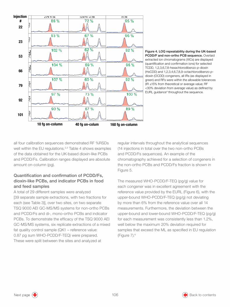
6
Figure 4. LOQ repeatability during the UK-based PCDD/F and non-ortho PCB sequence. Overlaid extracted ion chromatograms (XICs) are displayed (quantification and confirmation ions) for selected TCDD, 1,2,3,6,7,8-hexachlorodibenzo-p-dioxin (HxCDD) and 1,2,3,4,6,7,8,9-octachlorodibenzo-p-dioxin (OCDD) congeners, all IRs (as displayed in green) and RFs were within the allowable tolerances (IR ±15% from theoretical or average value; RF <30% deviation from average value) as defined by EURL guidance4 throughout the sequence.
all four calibration sequences demonstrated RF %RSDs well within the EU regulations.2,3 Table 4 shows examples of the data obtained for the UK-based dioxin-like PCBs and PCDD/Fs. Calibration ranges displayed are absolute amount on-column (pg).
Quantification and confirmation of PCDD/Fs, dioxin-like PCBs, and indicator PCBs in food and feed samplesA total of 29 different samples were analyzed [39 separate sample extractions, with two fractions for each (see Table 3)], over two sites, on two separate TSQ 9000 AEI GC-MS/MS systems for non-ortho PCBs and PCDD/Fs and di-, mono-ortho PCBs and indicator PCBs. To demonstrate the efficacy of the TSQ 9000 AEI GC-MS/MS systems, six replicate extractions of a mixed fat quality control sample (QK1 – reference value: 0.87 pg sum WHO-PCDD/F-TEQ) were prepared. These were split between the sites and analyzed at
regular intervals throughout the analytical sequences (14 injections in total over the two non-ortho PCBs and PCDD/Fs sequences). An example of the chromatography achieved for a selection of congeners in the non-ortho PCBs and PCDD/Fs fraction is shown in Figure 5.
The measured WHO-PCDD/F-TEQ (pg/g) value for each congener was in excellent agreement with the reference value provided by the EURL (Figure 6), with the upper-bound WHO-PCDD/F-TEQ (pg/g) not deviating by more than 6% from the reference value over all 14 measurements. Furthermore, the deviation between the upper-bound and lower-bound WHO-PCDD/F-TEQ (pg/g) for each measurement was consistently less than 1.2%, well below the maximum 20% deviation required for samples that exceed the ML as specified in EU regulation (Figure 7).6
22
23
53
66
79
92
101
Injection #
10 fg on-column 160 fg on-column40 fg on-colum
106 Back to contents

7
Table 4. Native dioxin-like PCBs and PCDD/Fs calibration data for the UK sequences (as average calibration response factors)
Peak NameRet.Time
(min)Number of Points
RF RSD (%)
Coeff. of Determination
(R2)
Average RF (Slope)
Range (pg)
PCB 81 16.38 14 1.49 0.9997 1.06 0.04 – 160
PCB 77 16.86 14 1.08 0.9997 1.00 0.04 – 160
PCB 123 17.40 14 2.66 0.9998 0.92 0.02 – 200
PCB 118 17.64 14 1.46 0.9999 0.96 0.1 – 1000
PCB 114 18.18 14 3.02 0.9989 1.04 0.02 – 200
PCB 105 18.96 14 5.95 0.9947 0.96 0.02 – 200
2378-TCDF 20.30 16 3.87 0.9995 0.96 0.01 – 64
2378-TCDD 20.86 16 4.72 0.9996 1.04 0.01 – 64
PCB 126 20.90 14 5.69 0.9985 0.95 0.04 – 160
PCB 167 21.52 14 1.74 0.9998 1.15 0.02 – 200
PCB 156 22.91 14 1.97 0.9998 1.14 0.02 – 200
PCB 157 23.12 14 2.41 0.9999 1.11 0.02 – 200
12378-PeCDF 24.34 16 1.66 0.9999 0.93 0.02 – 128
PCB 169 25.48 14 4.00 0.9999 1.08 0.04 – 160
23478-PeCDF 25.71 16 5.36 0.9977 1.03 0.02 – 128
12378-PeCDD 25.96 16 3.60 0.9999 1.05 0.02 – 128
PCB 189 27.28 14 1.96 0.9989 0.99 0.02 – 200
123478-HxCDF 29.06 16 2.98 0.9996 1.02 0.02 – 128
123678-HxCDF 29.17 16 1.95 0.9998 1.00 0.02 – 128
234678-HxCDF 29.86 16 2.83 0.9993 1.02 0.02 – 128
123478-HxCDD 29.94 16 2.49 0.9990 1.12 0.04 – 128
123678-HxCDD 30.04 16 2.01 0.9991 1.12 0.04 – 128
123789-HxCDD 30.35 16 3.82 0.9987 1.09 0.04 – 128
123789-HxCDF 30.71 16 3.52 0.9997 0.95 0.02 – 128
1234678-HpCDF 32.35 16 1.78 0.9999 1.03 0.04 – 256
1234678-HpCDD 33.78 16 5.99 0.9968 1.09 0.04 – 256
1234789-HpCDF 34.52 16 1.88 0.9998 1.04 0.04 – 256
OCDD 38.39 16 1.64 1.0000 1.12 0.16 – 256
OCDF 38.64 16 1.34 0.9997 0.94 0.16 - 256
Max 5.99 1.0000
Min 1.08 0.9947
107 Back to contents

8
The remainder of the samples were analyzed routinely, with eight sample injections bracketed by blanks, LOQ check standards, and quality control samples (QK1). Figures 8A, 8B, and 8C show the correlation of the results obtained on the TSQ 9000 AEI systems with the reference value obtained by the EURL for PCDD/Fs, dioxin-like PCBs, and indicator PCBs, respectively. Where the reference value was below the minimum reportable TSQ 9000 AEI upper-bound WHO-PCDD/F-
0.00
0.05
0.10
0.15
0.20
0.25
0.30
0.35
0.40
OCDF
1234
789-
HpCDF
1234
678-
HpCDF
OCDD
1237
89-H
xCDF
1237
8-Pe
CDF
2346
78-H
xCDF
1236
78-H
xCDF
1234
78-H
xCDF
2378
-TCDF
1234
78-H
xCDD
1237
89-H
xCDD
2378
-TCDD
1234
678-
HpCDD
2347
8-Pe
CDF
1236
78-H
xCDD
1237
8-Pe
CDD
WHO
-PC
DD/F
-TEQ
con
tribu
tion
(pg/
g)
QK 1 - Reference value QK1 Avg (n=14)
0.0000.0020.0040.0060.0080.0100.0120.0140.0160.018
OCDF
1234789-HpCDF
1234678-HpCDFOCDD
123789-HxCDF
12378-PeCDF
234678-HxCDF
123678-HxCDF
123478-HxCDF
TEQ (pg/g) value, the samples have been circled with a broken blue line (Figure 8A). These samples all had upper-bound WHO-PCDD/F-TEQ (pg/g) values of less than 0.3 pg/g, which is below 1/5th MLs for these sample types (meat ×2, eggs ×2, and milk).6 Pearson correlation coefficients were; 0.9902 for PCDD/Fs (Figure 8A), 0.9998 for dioxin-like PCBs (Figure 8B), and 0.9992 for indicator PCBs (Figure 8C), where a value of 1 is total positive linear correlation.
Figure 5. QK1 mixed fat quality control sample example chromatography where (A) 2,3,7,8-TCDD [0.03 pg on-column], (B) 1,2,3,7,8-PeCDD [0.14 pg on-column] and (C) OCDD [3.1 pg on-column]. The Chromeleon interactive results pane (left) displays IRs and internal standard recoveries, as well as real-time updated WHO-PCDD/F-TEQ (pg/g) values.
Figure 6. Congener contribution to the WHO-PCDD/F-TEQ (pg/g) for the mixed animal fat quality control sample. Congeners are ranked from left to right in order of contribution. Error bars show ±1σ standard deviation.
B CA
108 Back to contents

9
0.00
0.20
0.40
0.60
0.80
1.00
QK1
1
QK1
1
QK1
1
QK1
2
QK1
2
QK1
3
QK1
3
QK1
3
QK1
4
QK1
4
QK1
5
QK1
5
QK1
6
QK1
6
WHO
-PCD
D/F-
TEQ
(pg/
g)
Upper-bound
Lower-bound
Reference value
Figure 7. Upper-bound and lower-bound WHO-PCDD/F-TEQ (pg/g) results for all 14 measurements of the QK1 mixed animal fat quality control sample (six replicate extractions)
QK1 replicates
19 g19 g
13 g (Freshweight)
22 g
WMF -01
25 g (Freshweight)
33 g (Freshweight)
0.01
0.10
1.00
10.00
0.01 0.10 1.00 10.00
TSQ
9000
AEI
, WHO
-PCD
D/F-
TEQ
(pg/
g)
Reference value, WHO-PCDD/F-TEQ (pg/g)
PCDD/Fs GC-QqQ vs Reference valueQK1 - 1 Mixed fat QK1 - 2 Mixed fat
QK1 - 3 Mixed fat QK1 - 4 Mixed fat
QK1 - 5 Mixed fat QK1 - 6 Mixed fat
QK3 Eggs QK5 Fish meal
QK6 Fish oil QK7 Fish oil
QK8 Meat QK9 Grass meal
1201-PLA 1 Pork sausage 1201-PLA 2 Pork sausage
1202-HEA 1 Whole egg 1302-MIA 1 Milk powder
1302-MIA 2 Milk powder 1501-AFB 1 Sugar beet pulp
1501-AFB 2 Sugar beet pulp 1601-HFA 1 Fish
1601-HFA 2 Fish 1401-SEA Sepiolite
1701-PFA PFAD 1301-FF Feed fat
1302-MIB Milk fat WMF-01
9230 Meat 9253 Meat
9255 Meat 9449 Meat
9367 Milk 9373 Milk
9478 Milk 9182 Eggs
9370 Eggs 9371 Eggs
9487 Fish 9488 Fish
2g AEI LOQ (UB) 20g AEI LOQ (UB)
A
QK1 replicates
19 g
19 g
24 g
13 g (Freshweight)
22 g
0.058 pg/g contribution to TEQ from PCB 126
25 g (Freshweight)
33 g (Freshweight)
0.01
0.10
1.00
10.00
0.01 0.10 1.00 10.00
dl-PCBs - TSQ 9000 AEI vs Reference valueQK1 - 1 Mixed fat QK1 - 2 Mixed fat
QK1 - 3 Mixed fat QK1 - 4 Mixed fat
QK1 - 5 Mixed fat QK1 - 6 Mixed fat
QK3 Eggs QK5 Fish meal
QK7 Fish oil QK6 Fish oil
QK8 Meat QK9 Grass meal
1201-PLA 1 Pork sausage 1201-PLA 2 Pork sausage
1202-HEA 1 Whole egg 1302-MIA 1 Milk powder
1302-MIA 2 Milk powder 1501-AFB 1 Sugar beet pulp
1501-AFB 2 Sugar beet pulp 1601-HFA 1 Fish
1601-HFA 2 Fish 1401-SEA Sepiolite
1701-PFA PFAD 1301-FF Feed fat
1302-MIB Milk fat 9230 Meat
9449 Meat 9255 Meat
9367 Milk 9373 Milk
9182 Eggs 9370 Eggs
9371 Eggs 9487 Fish
9488 Fish 2g AEI LOQ (UB)
B
TSQ
9000
AEI
, WHO
-PCB
-TEQ
(pg/
g)
Reference value, WHO-PCDD/F-TEQ (pg/g)
Figure 8 (A). Comparison of data [(A) PCDD/Fs] obtained on the GC-MS/MS with the EURL reference values. The center red line represents 100% agreement with the value and the upper and lower greyed lines represent a ±30% deviation from this value. Unless specified, sample intake weight was 2 g, amount scales are logarithmic to aid comparison.
109 Back to contents

10
QK1 replicates
19 g19 g
13 g (Freshweight)
22 g
WMF -01
25 g (Freshweight)
33 g (Freshweight)
0.01
0.10
1.00
10.00
0.01 0.10 1.00 10.00
TSQ
9000
AEI
, WHO
-PCD
D/F-
TEQ
(pg/
g)
Reference value, WHO-PCDD/F-TEQ (pg/g)
PCDD/Fs GC-QqQ vs Reference valueQK1 - 1 Mixed fat QK1 - 2 Mixed fat
QK1 - 3 Mixed fat QK1 - 4 Mixed fat
QK1 - 5 Mixed fat QK1 - 6 Mixed fat
QK3 Eggs QK5 Fish meal
QK6 Fish oil QK7 Fish oil
QK8 Meat QK9 Grass meal
1201-PLA 1 Pork sausage 1201-PLA 2 Pork sausage
1202-HEA 1 Whole egg 1302-MIA 1 Milk powder
1302-MIA 2 Milk powder 1501-AFB 1 Sugar beet pulp
1501-AFB 2 Sugar beet pulp 1601-HFA 1 Fish
1601-HFA 2 Fish 1401-SEA Sepiolite
1701-PFA PFAD 1301-FF Feed fat
1302-MIB Milk fat WMF-01
9230 Meat 9253 Meat
9255 Meat 9449 Meat
9367 Milk 9373 Milk
9478 Milk 9182 Eggs
9370 Eggs 9371 Eggs
9487 Fish 9488 Fish
2g AEI LOQ (UB) 20g AEI LOQ (UB)
A
QK1 replicates
19 g
19 g
24 g
13 g (Freshweight)
22 g
0.058 pg/g contribution to TEQ from PCB 126
25 g (Freshweight)
33 g (Freshweight)
0.01
0.10
1.00
10.00
0.01 0.10 1.00 10.00
dl-PCBs - TSQ 9000 AEI vs Reference valueQK1 - 1 Mixed fat QK1 - 2 Mixed fat
QK1 - 3 Mixed fat QK1 - 4 Mixed fat
QK1 - 5 Mixed fat QK1 - 6 Mixed fat
QK3 Eggs QK5 Fish meal
QK7 Fish oil QK6 Fish oil
QK8 Meat QK9 Grass meal
1201-PLA 1 Pork sausage 1201-PLA 2 Pork sausage
1202-HEA 1 Whole egg 1302-MIA 1 Milk powder
1302-MIA 2 Milk powder 1501-AFB 1 Sugar beet pulp
1501-AFB 2 Sugar beet pulp 1601-HFA 1 Fish
1601-HFA 2 Fish 1401-SEA Sepiolite
1701-PFA PFAD 1301-FF Feed fat
1302-MIB Milk fat 9230 Meat
9449 Meat 9255 Meat
9367 Milk 9373 Milk
9182 Eggs 9370 Eggs
9371 Eggs 9487 Fish
9488 Fish 2g AEI LOQ (UB)
B
TSQ
9000
AEI
, WHO
-PCB
-TEQ
(pg/
g)
Reference value, WHO-PCDD/F-TEQ (pg/g)
QK1 replicates
19 g
19 g24 g
13 g (Freshweight)
22 g
25 g (Freshweight)
33 g (Freshweight)
0.10
1.00
10.00
100.00
0.10 1.00 10.00 100.00
Reference value (ng/g)
Indicator PCBs GC-QqQ vs Reference valuesQK1 - 1 Mixed fat QK1 - 2 Mixed fat
QK1 - 4 Mixed fat QK1 - 5 Mixed fat
QK1 - 6 Mixed fat QK3 Eggs
QK5 Fish meal QK6 Fish oil
QK7 Fish oil QK8 Meat
QK9 Grass meal 1201-PLA 1 Pork sausage
1201-PLA 2 Pork sausage 1202-HEA 1 Whole egg
1202-HEA 2 Whole egg 1302-MIA 2 Milk powder
1501-AFB 1 Sugar beet pulp 1501-AFB 2 Sugar beet pulp
1601-HFA 1 Fish 1601-HFA 2 Fish
1401-SEA Sepiolite 1701-PFA PFAD
1301-FF Feed fat 1302-MIB Milk fat
9230 Meat 9255 Meat
9253 Meat 9449 Meat
9367 Milk 9373 Milk
9182 Eggs 9370 Eggs
9371 Eggs 9487 Fish
9488 Fish
C
TSQ
9000
AEI
(ng/
g)
Figure 8 (B and C). Comparison of data [(B) dl-PCBs, and (C) indicator-PCBs] obtained on the GC-MS/MS with the EURL reference values. The center red line represents 100% agreement with the value and the upper and lower greyed lines represent a ±30% deviation from this value. Unless specified, sample intake weight was 2 g, amount scales are logarithmic to aid comparison.
110 Back to contents

11
To provide further validation data, an additional certified reference material (CRM) was extracted and analyzed on a PTV TSQ 9000 AEI system in Beijing, China. One gram of CRM WMF-01 (Wellington Laboratories Inc., Canada) was extracted and analyzed in triplicate (modified oven ramp, 5 µL PTV injection). The results
obtained were excellent agreement with the reference values published, with all congeners within the specified tolerance (Figure 9). The calculated SUM WHO-PCDD/F-TEQ (pg/g) for the measurements versus the calculated reference SUM WHO-PCDD/F-TEQ (pg/g) is also displayed in Figure 8A.
Figure 9. WMF-01 CRM reference value (pg/g) shown in dark blue, average (n = 3) TSQ 9000 AEI value for the WMF-01 CRM (pg/g) shown in light blue. Example XICs for quantification and confirmation ion are inlayed for 2,3,7,8-TCDD (15.13 pg/g), 1,2,3,4,6,7,8-heptachlorodibenzo-P-dioxin (HpCDD) (0.36 pg/g), and OCDD (2.01 pg/g). Error bars show the allowable deviation from the reference value and standard deviation of the TSQ 9000 AEI result.
0
5
10
15
20
Amou
nt (p
g/g)
PCDD/F congener
CRM WMF-01 Reference Value (pg/g)
TSQ 9000 AEI Average Value (n=3 pg/g)
RobustnessTo further assess the robustness of the analytical system, the remaining extracts from the non-ortho PCBs and PCDD/Fs samples were pooled together into mixed matrix extract. This pooled matrix sample was then analyzed alongside nonane blank and LOQ standard injections. The injection sequence was set up as follows: four injections (LOQ, blank, pooled matrix, blank) were followed by a four-hour hold at the initial
oven temperature and repeated, resulting in a total of 161 injection sequence containing n = 40 matrix injections and n = 40 LOQ standards, run over ~2 weeks period. The system maintained sensitivity throughout delivering excellent robustness, even considering the high matrix complexity and load on column (Figures 10A and B). No maintenance (such as source cleaning, liner replacement, tuning, or analytical column trimming) was performed during the sequence.
111 Back to contents
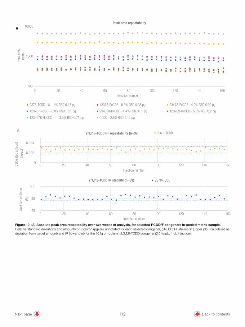
12
100
1000
10000
Peak
are
a(c
pm)
Injection number
Peak area repeatability
2378-TCDD - 6. 4% RSD 0.17 pg 12378-PeCDF - 6.3% RSD 0.36 pg 23478-PeCDF - 4.2% RSD 0.92 pg
12378-PeCDD - 6.0% RSD 0.21 pg 234678-HxCDF - 4.4% RSD 0.31 pg 123789-HxCDD - 5.3% RSD 0.2 pg
1234678-HpCDD - 3.5% RSD 0.71 pg OCDD - 2.8% RSD 6.12 pg
A
0
0.002
0.004
Calc
ulat
ed a
mou
nt
(pg/
µL)
Injection number
2,3,7,8-TCDD RF repeatability (n=39) 2378-TCDD
40
90
140
Qual
ifier
Ion
Ratio
(%)
Injection number
2,3,7,8-TCDD IR stability (n=39) 2378-TCDD
B
0 20 40 60 80 100 120 140 160
0 20 40 60 80 100 120 140 160
0 20 40 60 80 100 120 140 160
Figure 10. (A) Absolute peak area repeatability over two weeks of analysis, for selected PCDD/F congeners in pooled matrix sample. Relative standard deviations and amounts on-column (pg) are annotated for each selected congener, (B) LOQ RF deviation (upper plot, calculated as deviation from target amount) and IR (lower plot) for the 10 fg on-column 2,3,7,8-TCDD congener (2.5 fg/µL, 4 µL injection).
112 Back to contents

13
ConclusionsThe results of these comprehensive experiments demonstrate that the TSQ 9000 GC-MS/MS system, configured with the AEI source and controlled using Chromeleon CDS software, can deliver routine-grade performance for the quantification and confirmation of PCDD/Fs, dioxin-like PCBs, and indicator PCBs in food and feedstuffs.
• Successful validation of method performance criteria (LOQ, precision, accuracy, and calibration) was carried out on two separate TSQ 9000 AEI systems, in two geo-locations.
• The sensitivity achieved with the TSQ 9000 AEI system allowed for upper-bound WHO-PCDD/F-TEQ (pg/g) values as low as 0.15 (for a 2 g sample intake weight), meeting the 1/5th maximum level requirements for all but the most challenging matrices.
• The outstanding linear range and accurate quantitative performance generated excellent comparative data to the EURL reference data supplied, with calibration data showing RF %RSD of <6 over more than 4 orders of magnitude for many congeners.
• Minimizing user intervention has been demonstrated by running over two weeks with no maintenance (such as source cleaning, liner replacement, tuning, or analytical column trimming), allowing maximum uptime and sample throughput.
• Chromeleon CDS software, version 7.2, provides an integrated platform, with the ability to automatically setup, easily acquire, process and report compliant data in a fully regulated environment, eliminating the need for using external spreadsheet programs. Chromeleon eWorkflows, available from Thermo Scientific™ AppsLab Library of Analytical Applications, also provide error-free execution of each analysis to meet standard operating procedure (SOP) requirements, further simplifying the user experience.
Acknowledgement Thermo Fisher Scientific would like to acknowledge Wellington Laboratories Inc., Canada for the production and supply of the LOQ standards used in this validation.
References1. World Health Organization, Dioxins and their effects on human health. https://www.
who.int/news-room/fact-sheets/detail/dioxins-and-their-effects-on-human-health (assessed Jan 28, 2019).
2. European Commission, Commission Regulation (EU) 2017/644, Off. J. Eur. Union, L 92 9-34, 2017.
3. European Commission, Commission Regulation (EU) 2017/771, Off. J. Eur. Union, L 115 22-42, 2017.
4. Low level quantification of PCDD/Fs in animal feed using the TSQ 9000 triple quadrupole GC-MS/MS system with AEI source. https://www.thermofisher.com/uk/en/home/global/forms/industrial/low-level-quantification-pcdd-fs-animal-feed-tsq-9000-tq-gcms-ms.html (assessed Jan 28, 2019)
5. Guidance Document on the Estimation of LOD and LOQ for Measurements in the Field of Contaminants in Feed and Food. https://ec.europa.eu/jrc/en/publication/guidance-document-estimation-lod-and-loq-measurements-field-contaminants-feed-and-food (assessed Jan 28, 2019)
6. Directive 2002/32/EC of the European Parliament and of the Council of 7 May 2002 on undesirable substances in animal feed, Off. J. Eur. Communities, L 140 10-21, 2002, in current amendment http://data.europa.eu/eli/dir/2002/32/2015-02-27 (assessed Jan 28, 2019)
7. US EPA Method 1613: Tetra-through octa-chlorinated dioxins and furans by isotope dilution HRGC/HRMS (Revision B), 1994.
8. European Commission COMMISSION REGULATION (EC) No 1881/2006 of 19 December 2006 setting maximum levels for certain contaminants in foodstuffs, Off. J. Eur. Union, L 364 5-24, 2006, in current amendment
113 Back to contents
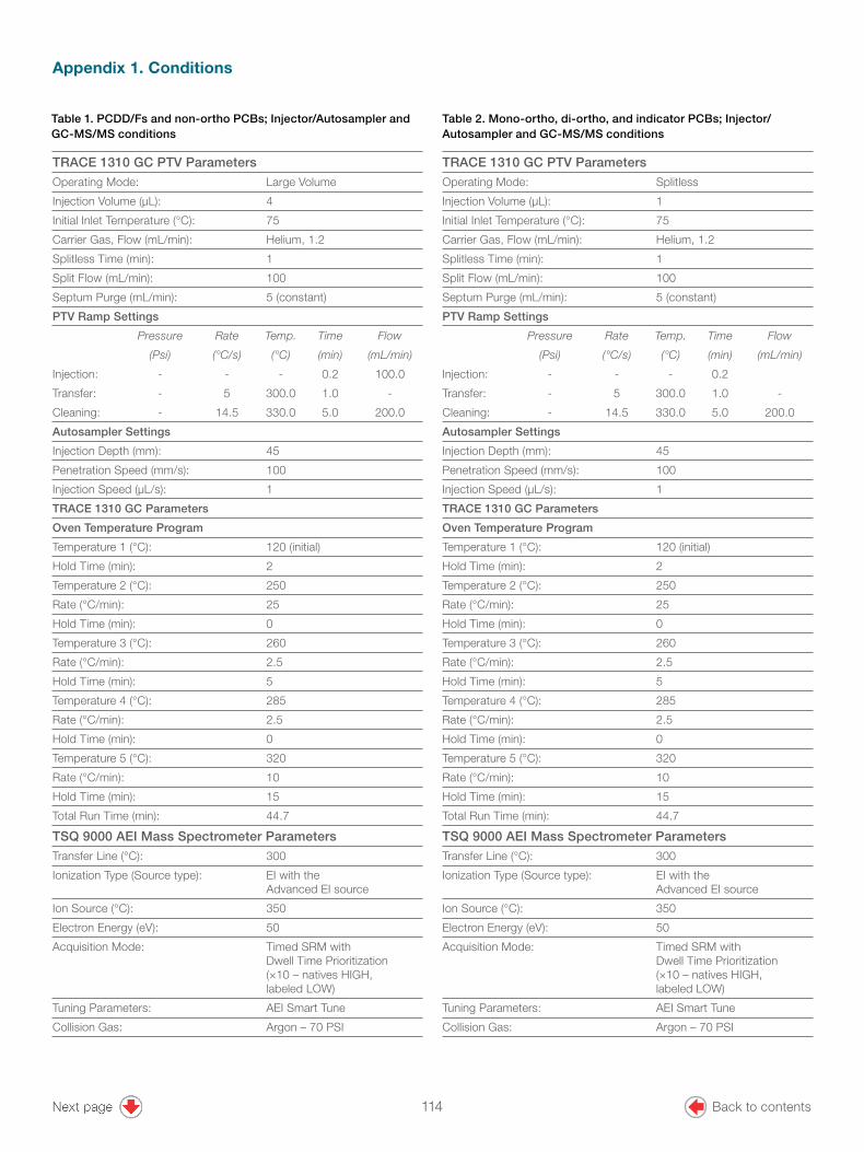
14
TRACE 1310 GC PTV Parameters
Operating Mode: Splitless
Injection Volume (µL): 1
Initial Inlet Temperature (°C): 75
Carrier Gas, Flow (mL/min): Helium, 1.2
Splitless Time (min): 1
Split Flow (mL/min): 100
Septum Purge (mL/min): 5 (constant)
PTV Ramp Settings
Pressure Rate Temp. Time Flow
(Psi) (°C/s) (°C) (min) (mL/min)
Injection: - - - 0.2
Transfer: - 5 300.0 1.0 -
Cleaning: - 14.5 330.0 5.0 200.0
Autosampler Settings
Injection Depth (mm): 45
Penetration Speed (mm/s): 100
Injection Speed (µL/s): 1
TRACE 1310 GC Parameters
Oven Temperature Program
Temperature 1 (°C): 120 (initial)
Hold Time (min): 2
Temperature 2 (°C): 250
Rate (°C/min): 25
Hold Time (min): 0
Temperature 3 (°C): 260
Rate (°C/min): 2.5
Hold Time (min): 5
Temperature 4 (°C): 285
Rate (°C/min): 2.5
Hold Time (min): 0
Temperature 5 (°C): 320
Rate (°C/min): 10
Hold Time (min): 15
Total Run Time (min): 44.7
TSQ 9000 AEI Mass Spectrometer Parameters
Transfer Line (°C): 300
Ionization Type (Source type): EI with the Advanced EI source
Ion Source (°C): 350
Electron Energy (eV): 50
Acquisition Mode: Timed SRM with Dwell Time Prioritization (×10 – natives HIGH, labeled LOW)
Tuning Parameters: AEI Smart Tune
Collision Gas: Argon – 70 PSI
Table 1. PCDD/Fs and non-ortho PCBs; Injector/Autosampler and GC-MS/MS conditions
Table 2. Mono-ortho, di-ortho, and indicator PCBs; Injector/Autosampler and GC-MS/MS conditions
TRACE 1310 GC PTV Parameters
Operating Mode: Large Volume
Injection Volume (µL): 4
Initial Inlet Temperature (°C): 75
Carrier Gas, Flow (mL/min): Helium, 1.2
Splitless Time (min): 1
Split Flow (mL/min): 100
Septum Purge (mL/min): 5 (constant)
PTV Ramp Settings
Pressure Rate Temp. Time Flow
(Psi) (°C/s) (°C) (min) (mL/min)
Injection: - - - 0.2 100.0
Transfer: - 5 300.0 1.0 -
Cleaning: - 14.5 330.0 5.0 200.0
Autosampler Settings
Injection Depth (mm): 45
Penetration Speed (mm/s): 100
Injection Speed (µL/s): 1
TRACE 1310 GC Parameters
Oven Temperature Program
Temperature 1 (°C): 120 (initial)
Hold Time (min): 2
Temperature 2 (°C): 250
Rate (°C/min): 25
Hold Time (min): 0
Temperature 3 (°C): 260
Rate (°C/min): 2.5
Hold Time (min): 5
Temperature 4 (°C): 285
Rate (°C/min): 2.5
Hold Time (min): 0
Temperature 5 (°C): 320
Rate (°C/min): 10
Hold Time (min): 15
Total Run Time (min): 44.7
TSQ 9000 AEI Mass Spectrometer Parameters
Transfer Line (°C): 300
Ionization Type (Source type): EI with the Advanced EI source
Ion Source (°C): 350
Electron Energy (eV): 50
Acquisition Mode: Timed SRM with Dwell Time Prioritization (×10 – natives HIGH, labeled LOW)
Tuning Parameters: AEI Smart Tune
Collision Gas: Argon – 70 PSI
Appendix 1. Conditions
114 Back to contents
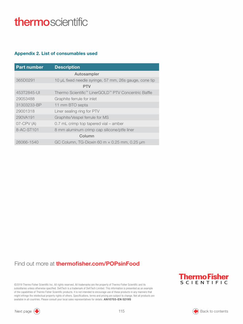
©2019 Thermo Fisher Scientific Inc. All rights reserved. All trademarks are the property of Thermo Fisher Scientific and its subsidiaries unless otherwise specified. DeXTech is a trademark of DeXTech Limited. This information is presented as an example of the capabilities of Thermo Fisher Scientific products. It is not intended to encourage use of these products in any manners that might infringe the intellectual property rights of others. Specifications, terms and pricing are subject to change. Not all products are available in all countries. Please consult your local sales representatives for details. AN10703-EN 0219S
Find out more at thermofisher.com/POPsinFood
Appendix 2. List of consumables used
Part number Description
Autosampler
365D0291 10 μL fixed needle syringe, 57 mm, 26s gauge, cone tip
PTV
453T2845-UI Thermo Scientific™ LinerGOLD™ PTV Concentric Baffle
29053488 Graphite ferrule for inlet
31303233-BP 11 mm BTO septa
29001318 Liner sealing ring for PTV
290VA191 Graphite/Vespel ferrule for MS
07-CPV (A) 0.7 mL crimp top tapered vial – amber
8-AC-ST101 8 mm aluminum crimp cap silicone/ptfe liner
Column
26066-1540 GC Column, TG-Dioxin 60 m × 0.25 mm, 0.25 μm
115 Back to contents
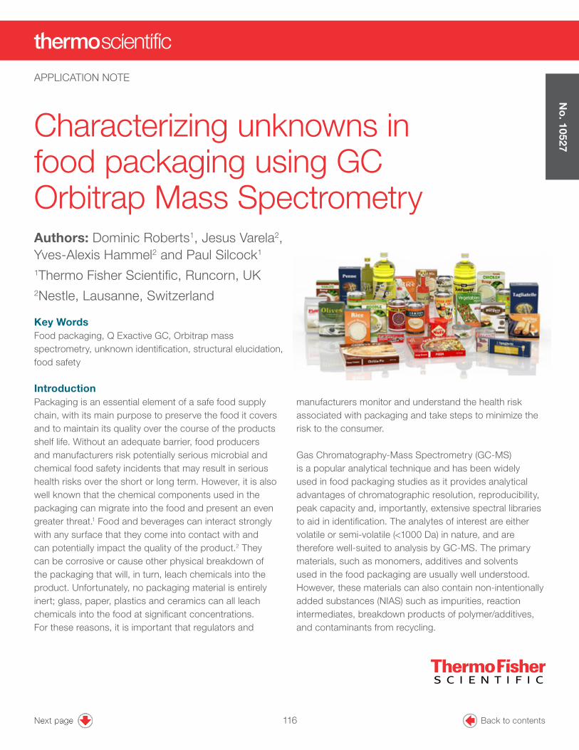
Characterizing unknowns in food packaging using GC Orbitrap Mass Spectrometry
manufacturers monitor and understand the health risk associated with packaging and take steps to minimize the risk to the consumer.
Gas Chromatography-Mass Spectrometry (GC-MS) is a popular analytical technique and has been widely used in food packaging studies as it provides analytical advantages of chromatographic resolution, reproducibility, peak capacity and, importantly, extensive spectral libraries to aid in identification. The analytes of interest are either volatile or semi-volatile (<1000 Da) in nature, and are therefore well-suited to analysis by GC-MS. The primary materials, such as monomers, additives and solvents used in the food packaging are usually well understood. However, these materials can also contain non-intentionally added substances (NIAS) such as impurities, reaction intermediates, breakdown products of polymer/additives, and contaminants from recycling.
Authors: Dominic Roberts1, Jesus Varela2, Yves-Alexis Hammel2 and Paul Silcock1
1Thermo Fisher Scientific, Runcorn, UK2Nestle, Lausanne, Switzerland
Key WordsFood packaging, Q Exactive GC, Orbitrap mass spectrometry, unknown identification, structural elucidation, food safety
IntroductionPackaging is an essential element of a safe food supply chain, with its main purpose to preserve the food it covers and to maintain its quality over the course of the products shelf life. Without an adequate barrier, food producers and manufacturers risk potentially serious microbial and chemical food safety incidents that may result in serious health risks over the short or long term. However, it is also well known that the chemical components used in the packaging can migrate into the food and present an even greater threat.1 Food and beverages can interact strongly with any surface that they come into contact with and can potentially impact the quality of the product.2 They can be corrosive or cause other physical breakdown of the packaging that will, in turn, leach chemicals into the product. Unfortunately, no packaging material is entirely inert; glass, paper, plastics and ceramics can all leach chemicals into the food at significant concentrations. For these reasons, it is important that regulators and
No
. 10527
APPLICATION NOTE
Back to contents116

When investigating NIAS in food packaging, the analysis is challenging because there is very little information of the potential chemicals involved. Therefore, the approach taken needs to be as non-selective as possible so that the maximum chemical information is captured. To achieve this, the sample extraction technique is generic and often involves simple liquid extraction and concentration. This is followed by analysis in full-scan to obtain wide coverage of a sample. When using nominal mass GC-MS instruments for unknown analysis the procedure can be complex, time consuming, and expensive as it takes longer to interpret the mass spectrum and the confidence in any proposed assignment is low. Furthermore, there is a need for improved sensitivity because currently there can be extensive sample preparation and pre-treatment to isolate and concentrate samples which adversely impacts on the time to result.
This study focused on the utilization of a new GC-MS system with high mass resolution performance and high mass accuracy for fast and confident identification of unknown compounds in food packaging. Prior to this work, some of the unknown compounds were initially detected using nominal mass instrumentation (single quadrupole GC-MS), but this proved limited in the ability to assign an elemental formula, structure, and confident compound identification. Full-scan and MS/MS high mass resolution experiments are important to achieve the selectivity and mass accuracy needed for confident elemental composition proposals, structural elucidation and discrimination of co-eluting compounds. These features, in combination with novel software algorithms for automated spectral deconvolution and compound ID, create a powerful solution for fast, confident and comprehensive chemical characterization of food packaging samples.
Experimental conditionsSample preparationThe sample investigated in this study was a tin can with an internal coating. The internal coating was extracted using a 300 mL solution of hexane: acetone (1:1) held at room temperature for 16 hours. The 300 mL was then evaporated to approximately 1 mL before being transferred to a crimp cap amber GC vial for analysis.
Instrument and method setupIn all experiments a Thermo Scientific™ Q Exactive™ GC Orbitrap™ GC-MS/MS hybrid quadrupole-Orbitrap mass spectrometer was used. Sample introduction was performed using a Thermo Scientific™ TriPlus™ RSH autosampler, and chromatographic separation was obtained with a Thermo Scientific™ TRACE™ 1310 GC system and a Thermo Scientific™ TraceGOLD TG-5SilMS 30 m × 0.25 mm I.D. × 0.25 µm film capillary column with a 10 m guard (P/N 26096-1421). Additional details of instrument parameters are displayed in Table 1 and Table 2.
TRACE 1310 GC System ParametersInjection Volume (µL) 1
Liner Single gooseneck P/N 453A0344-UI
Inlet (°C) SSL 280
Carrier Gas, (mL/min) He, 1.3
Oven Temperature ProgramTemperature 1 (°C) 40
Hold Time (min) 0.5
Temperature 2 (°C) 325
Rate (°C/min) 5.5
Hold Time (min) 12
Table 1. GC and injector conditions.
Table 2. Mass spectrometer conditions.
Q Exactive GC Mass Spectrometer Parameters Transfer line (°C) 280
Ionization type EI/PCI
Ion source (°C) 230 EI / 190 CI
Electron energy (eV) 70
Acquisition mode Full-scan
Mass range (Da) 50–700
Resolving power (FWHM at m/z 200)
120,000
Lockmass, column bleed (m/z)
207.03235
The Q Exactive GC system was operated in EI full-scan mode using 120,000 (FWHM at m/z 200) resolving power. Additional experiments were run using positive chemical ionization (PCI) with methane as reagent gas at a flow of 1.5 mL/min to obtain information on the molecular ions and to support the identification of unknown component peaks.
Back to contents117

Data processingData were acquired using the Thermo Scientific™ TraceFinder™ software. This single platform software package integrates instrument control, method development functionality, and qualitative and quantitation-focused workflows. TraceFinder also contains accurate mass spectral deconvolution and spectral matching functionality. Thermo Scientific™ MassFrontier™ spectral interpretation software was used for structural elucidation.
Results and discussionThe objective of this study was to analyze the packaging sample using a non-target full-scan data acquisition using electron ionization (EI) and positive chemical ionization (PCI), and to identify the most intense peaks. In addition, the aim was to provide structural information for the peaks detected using nominal mass GC-MS, where confirmation of the identity was not possible.
Figure 1. GC-MS electron ionization (EI) and positive chemical ionization (PCI) total ion chromatograms (TIC) of the packaging sample.
Extracting key featuresFull-scan chromatograms were obtained for the sample and the total ion chromatograms (TICs) are shown in Figure 1. The Q Exactive GC system acquires accurate mass data with a wide dynamic range. This is very powerful when the objective is to identify unknown peaks in a complex sample, such as a food packaging extract with a high degree of confidence. The first step in this analysis was to isolate the peaks of interest and although peaks can be seen visually in the TICs, it is essential that all features are extracted from the data.
This was achieved with TraceFinder which first performs a high resolution accurate mass deconvolution of the data with the aim of detecting all of the peaks above a signal to noise threshold of 100:1. The deconvolution ensures that only ions that maximize at the same retention time remain for library matching. Using these thresholds, 961 features (peak clusters) were detected in the packaging sample. An example peak for 2-Hydroxy-5-methyl-1,3-benzenedicarboxaldehyde is shown in Figure 2, along with the number of scans across the peak, the accurate mass and ppm difference.
EI TIC
PCI TIC
0 5 10 15 20 25 30 35 40 45 50 55Minutes
0
100
Rela
tive
Abun
danc
e
49.03 49.13
47.84
45.54
42.9853.1842.92
49.7430.6417.73
21.75 24.5826.19
22.07 33.0919.4111.38 33.4315.9814.77 26.42 39.82 51.009.44 36.597.305.15
48.99
47.8026.17 49.08
11.36 42.9643.0617.70
24.55 45.5230.67
15.9749.7014.75 53.1221.9421.73
26.7420.069.23 13.07 49.9933.44 33.70 42.0729.77 39.797.31
NL:1.65E10TIC MS Nestle_pk_001
NL:2.21E8TIC MS nestle_pk_017
RT: 0.00 - 55.01
90
80
70
60
50
40
30
20
10
0
100
Rela
tive
Abun
danc
e
90
80
70
60
50
40
30
20
10
Back to contents118
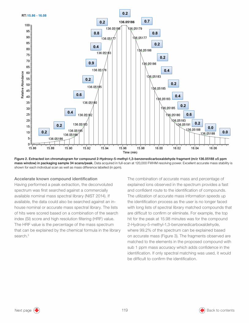
Figure 2. Extracted ion chromatogram for compound 2-Hydroxy-5-methyl-1,3-benzenedicarboxaldehyde fragment (m/z 136.05188 ±5 ppm mass window) in packaging sample 34 scans/peak. Data acquired in full-scan at 120,000 FWHM resolving power. Excellent accurate mass stability is shown for each individual scan as well as mass difference labelled (in ppm).
Accelerate known compound identificationHaving performed a peak extraction, the deconvoluted spectrum was first searched against a commercially available nominal mass spectral library (NIST 2014). If available, the data could also be searched against an in-house nominal or accurate mass spectral library. The lists of hits were scored based on a combination of the search index (SI) score and high resolution filtering (HRF) value. The HRF value is the percentage of the mass spectrum that can be explained by the chemical formula in the library search.3
The combination of accurate mass and percentage of explained ions observed in the spectrum provides a fast and confident route to the identification of compounds. The utilization of accurate mass information speeds up the identification process as the user is no longer faced with long lists of spectral library matched compounds that are difficult to confirm or eliminate. For example, the top hit for the peak at 15.98 minutes was for the compound 2-Hydroxy-5-methyl-1,3-benzenedicarboxaldehyde, where 99.2% of the spectrum can be explained based on accurate mass (Figure 3). The fragments observed are matched to the elements in the proposed compound with sub 1 ppm mass accuracy which adds confidence in the identification. If only spectral matching was used, it would be difficult to confirm the identification.
0.2
0.9
0.4
0.2
0.2
0.2
0.4
0.2
0.4
0.2
0.6
0.2 0.0
0.6
0.2
0.4
0.8
0.2
0.2 0.7
0.8
0.0
136.05186
RT:15.86 - 16.08
Back to contents119
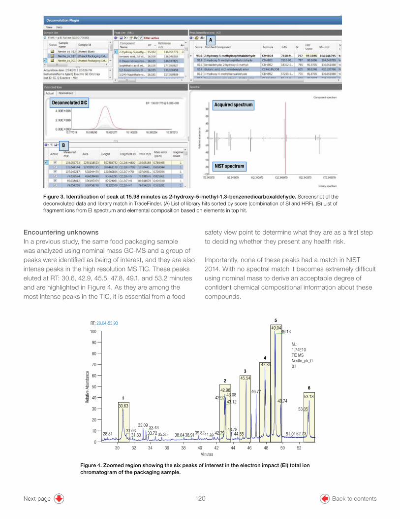
Figure 3. Identification of peak at 15.98 minutes as 2-hydroxy-5-methyl-1,3-benzenedicarboxaldehyde. Screenshot of the deconvoluted data and library match in TraceFinder. (A) List of library hits sorted by score (combination of SI and HRF). (B) List of fragment ions from EI spectrum and elemental composition based on elements in top hit.
Acquired spectrum
NIST spectrum
Deconvoluted XIC
A
B
Encountering unknownsIn a previous study, the same food packaging sample was analyzed using nominal mass GC-MS and a group of peaks were identified as being of interest, and they are also intense peaks in the high resolution MS TIC. These peaks eluted at RT: 30.6, 42.9, 45.5, 47.8, 49.1, and 53.2 minutes and are highlighted in Figure 4. As they are among the most intense peaks in the TIC, it is essential from a food
safety view point to determine what they are as a first step to deciding whether they present any health risk.
Importantly, none of these peaks had a match in NIST 2014. With no spectral match it becomes extremely difficult using nominal mass to derive an acceptable degree of confident chemical compositional information about these compounds.
Figure 4. Zoomed region showing the six peaks of interest in the electron impact (EI) total ion chromatogram of the packaging sample.
30 32 34 36 38 40 42 44 46 48 50 52Minutes
49.0449.13
47.84
45.54
42.98 46.7743.08
42.92 53.1849.7443.12
30.6353.05
33.09 33.43 43.7831.03 39.82 42.7933.72 44.55 51.0152.7341.5535.3528.81 31.83 38.9138.04
1
2
3
4
6
5
0
100
Rela
tive
Abun
danc
e
90
80
70
60
50
40
30
20
10
RT: 28.04-53.93
NL:1.74E10TIC MSNestle_pk_001
Back to contents120

When the spectral library match from the EI spectrum is inconclusive, then the PCI data can be used to establish the molecular ion, and to propose an elemental composition. When CI data is acquired using methane as the reagent gas, three adducts are typically observed: [M+H]+, [M+C2H5]
+ and [M+C3H5]+. Figure 5 shows the EI
and PCI spectra for the peak at 45.5 minutes. The PCI spectrum shows the adducts [M+H]+ (-0.8 ppm) for ion m/z 469.18532, [M+C2H5]
+ (-0.5 ppm) for ion m/z 497.21677. The presence of these adducts indicated that the m/z 468.17783 was the molecular ion. Without the PCI adducts it would not be possible to determine if the m/z 468.17783 was a fragment or the molecular ion. From this ion, an elemental composition of the parent molecule can be proposed.
Elemental composition assignment is a critical stage in the compound identification process and it is where excellent mass accuracy and isotopic pattern can be used to limit the number of possible chemical formulae. An elemental composition calculator was used to propose a formula for the [M+H]+ ion (Figure 6). The software assigns formulae by using an isotopic pattern matching algorithm that accounts for isotope accurate mass and intensity ratios. The algorithm uses a single mass to calculate all possible
elemental compositions that lie within a tolerance window and then calculates the theoretical isotopic pattern for each suggestion. It then gives a score between 0 and 100 percent, where 0 is completely different and 100 an exact isotopic match. For example, when a 5 ppm mass accuracy window is used 12 possible formulae are proposed for the [M+H]+ ion using the elements Carbon (1–30), Hydrogen (1–60), Nitrogen (1–5), Oxygen (1–10), Phosphorus (1) and Sulphur (1). This is compared to 1 ppm mass accuracy window that suggests three possible formulae. Only one of these suggestions has a 100 percent match with the theoretical isotopic pattern: C26H29O8. This level of mass accuracy significantly reduces the number of formulae that need to be investigated, which speeds up the analysis, and also increases the confidence in any proposed assignment.
One final stage to support the proposed formula and to derive structural information is to use the accurate mass fragments. To achieve this, either the fragments in the EI spectrum can be used or an additional MS/MS experiment can be performed to be confident that the fragments are indeed from the molecular ion. The [M+H]+ (PCI) m/z 469.18 was isolated in the quadrupole and fragmentation induced in the HCD cell using 15V energy.
Figure 5. EI and PCI spectra at 45.5 minutes in packaging sample proposing a chemical formula of C26H28O8. Peaks are annotated with chemical formula and mass difference in ppm. PCI data supports identification of parent ion with formula with sub 1 ppm mass accuracy.
[M+H]+
[M+C2H5 ]+
EI spectrum
PCI spectrum
M+
m/z
m/z
Back to contents121

Figure 7 shows the resulting MS/MS spectrum for m/z 469.18. The fragments measured contain the elements in the proposed parent and all with good mass accuracy. Based on this information, a proposed structure of the compound was made and is shown inset in Figure 7. MassFrontier was used to theoretically fragment the proposed chemical structure and match these to the measured fragments in the MS/MS spectrum. Therefore, even if at this stage a compound name cannot be confidently assigned, enough information can be obtained with respect to the chemical formula of the unknown compound.
Each of the six peaks were evaluated using the same workflow, and the results are summarized in Table 3. The mass accuracy obtained (<1 ppm) enabled confident elemental compositions to be assigned and these are supported by accurate mass fragments in the EI spectra. It was noted that all of the peaks contained a m/z 149.02332 ion and shared a common structure.
Figure 6. Elemental composition calculator screen in FreeStyle for the peak at 45.5 minutes in packaging sample proposing a chemical formula of C26H29O8 for the [M+H]+ ion based on accurate mass and isotope pattern. The three candidates are all within 1 ppm, but the top hit has a 100% isotopic match with the theoretical pattern.
Measured
Theoretical
Figure 7. MS/MS spectrum of PCI ion m/z 469.18 selected in the quadrupole and fragmented in the HCD cell. MassFrontier used to explain the fragments observed within 3 ppm mass accuracy window.
O O
OOOO
O OH
O O
OOO
O
O
O
O
O
O
O
O
O
OH
O
O OH
OO
O OH
O
O O
Parent
Back to contents122

Unlocking structural informationFurther investigation of the full-scan EI and PCI data showed that when the parent mass for C26H28O8 was extracted there were three peaks in the chromatogram (Figure 8). The capability to perform accurate mass MS/MS experiments provides valuable structural information that may be vital in determining what the compound is and if it is a safety concern. The MS/MS spectra for the three isomers (Figure 9) shows both similarities and differences between the isomers. Isomers 2 and 3 have a base peak at m/z 401.12309 (C21H21O8) and an additional ion m/z 132.02058 (C8H4O2).
Table 3. Summary of the peaks and the tentative identification of the elemental composition of the compounds. Excellent mass accuracy (<1 ppm) for all quasi-molecular ions adds confidence to the proposed identities.
Peak No.Retention Time (min)
Formula [M+H]+ m/zMass Error of [M+H]+ (ppm)
Mass Error of [M+C2H5]
+ (ppm)Mass Error of
[M+C3H5]+ (ppm)
1 30.6 C14H18O6 283.11762 0.0 0.5 0.1
2 42.98 C22H20O8 413.12303 -0.2 -0.3 0.0
3 45.5 C26H28O8 469.18532 0.7 -0.4 0.0
4 47.5 C24H24O8 441.15424 -0.4 -0.4 -0.3
5 49.1 C27H30O8 483.20112 -0.5 -0.1 0.3
6 52.0 C28H32O8 497.21684 -0.3 0.1 0.3
The base peak in isomer 1 is m/z 383.11253 (C21H19O7) and the m/z 132.02058 is absent. The capacity to confidently assign elemental compositions to these ions is highly beneficial and provides the analyst with a complete picture. The m/z 401.12309 corresponds to a loss of C5H7 from the parent and m/z 383.11253 a loss of C5H10O. MassFrontier was used to explain how these ions can be derived from the proposed chemical structure. From this information, the flexibility to perform MS/MS experiments with accurate mass information allows for detailed structural information to be determined.
Figure 8. XIC m/z 468.17783 from the full-scan EI data and m/z 469.18532 from the full-scan PCI data in packaging sample shows 3 isomers of the same parent mass. Inset proposed chemical structure of compound.
O O
OOO
O
O
O
1XIC m/z 468.17783
XIC m/z 469.18532
2
3
Back to contents123

Figure 9. MS/MS spectra of m/z 469.18 of the three isomers reveals different fragmentation patterns for isomers 2 and 3. Of particular note, the base peak is 401.12286 and the presence of m/z 132.02049 ion.
ConclusionsThe results of this study demonstrate that the Thermo Scientific Q Exactive GC hybrid quadrupole-Orbitrap mass spectrometer, in combination with easy-to-use software tools, is a powerful tool for the profiling of complex samples and for the identification of unknown chemicals. The Orbitrap mass spectrometer delivers excellent resolution and mass accuracy which leads to fast and confident characterization of samples regardless of the concentration. A food packaging sample was quickly screened for known compounds using spectral matching and rationalisation using accurate mass. EI and PCI information leads to confident chemical formulas to be proposed for molecular ions and fragments for compounds with no library match. Furthermore, the ability to perform
high resolution, accurate mass MS/MS experiments completes the unknown identification workflow and allows for an even higher level of confidence and provides important structural information.
References1. Migration from Food Contact Materials. L. L. Katan
(editor), Blackie Academic and Professional, Glasgow, UK, 1996.
2. Barnes, K.A., Sinclair, C.R. & Watson, D.H. (2006) Chemical Migration and Food Contact Materials. Woodhead publishing.
3. Thermo Fisher Scientific AN10492. Chemical profiling and differential analysis of whiskies using Orbitrap GC-MS. Runcorn, United Kingdom.
Find out more at www.thermofisher.com/QExactiveGC
©2016 Thermo Fisher Scientific Inc. All rights reserved. All trademarks are the property of Thermo Fisher Scientific and its subsidiaries. This information is presented as an example of the capabilities of Thermo Fisher Scientific products. It is not intended to encourage use of these products in any manners that might infringe the intellectual property rights of others. Specifications, terms and pricing are subject to change. Not all products are available in all countries. Please consult your local sales representatives for details. AN10527 1016
Back to contents124

GoalTo demonstrate the performance of the Thermo Scientific™ Exactive™ GC Orbitrap™ mass spectrometer for the routine analysis of GC-amenable pesticides in cereals (wheat, barley, oat, rye and rice).
IntroductionPesticides are used to improve cereal crop yields and to minimize degradation during storage and processing. However, the widespread use of pesticides and the potential for residues to remain on the final product is of concern to consumers and to governments whose responsibility it is to ensure a safe food supply. Consequently, legislation has been introduced to protect consumers from exposure to contaminated foods.1 Pesticide application to cereal crops is regulated by international organizations, and maximum residue levels (MRLs) are set for each pesticide/commodity combination. In the EU, if no substantive MRL has been set, a default MRL value of 0.01 mg/kg is usually applied.
AuthorsDominic Roberts,1 Mette Erecius Poulsen,2 and Paul Silcock1
1Thermo Fisher Scientific, Runcorn, United Kingdom 2European Union Reference Laboratory for Pesticide Residues in Cereals and Feedstuffs, Technical University of Denmark, Denmark
KeywordsPesticides, QuEChERS, Cereals, GC Orbitrap Mass Spectrometry, Screening, Quantitation, Accurate Mass, High Resolution, TraceFinder
APPLICATION NOTE 10541
Multi-residue pesticide screening in cereals using GC-Orbitrap mass spectrometry
125 Back to contents
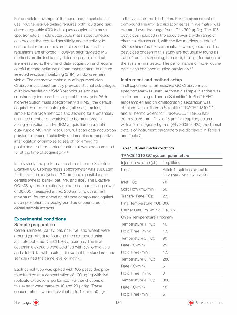
2
For complete coverage of the hundreds of pesticides in use, routine residue testing requires both liquid and gas chromatographic (GC) techniques coupled with mass spectrometers. Triple quadrupole mass spectrometers can provide the required sensitivity and selectivity to ensure that residue limits are not exceeded and the regulations are enforced. However, such targeted MS methods are limited to only detecting pesticides that are measured at the time of data acquisition and require careful method optimization and management to ensure selected reaction monitoring (SRM) windows remain viable. The alternative technique of high-resolution Orbitrap mass spectrometry provides distinct advantages over low-resolution MS/MS techniques and can substantially increase the scope of the analysis. With high-resolution mass spectrometry (HRMS), the default acquisition mode is untargeted (full-scan), making it simple to manage methods and allowing for a potentially unlimited number of pesticides to be monitored in a single injection. Unlike SRM acquisition on a triple quadrupole MS, high-resolution, full-scan data acquisition provides increased selectivity and enables retrospective interrogation of samples to search for emerging pesticides or other contaminants that were not screened for at the time of acquisition.2, 3
In this study, the performance of the Thermo Scientific Exactive GC Orbitrap mass spectrometer was evaluated for the routine analysis of GC-amenable pesticides in cereals (wheat, barley, oat, rye, and rice). The Exactive GC-MS system is routinely operated at a resolving power of 60,000 (measured at m/z 200 as full width at half maximum) for the detection of trace compounds against a complex chemical background as encountered in cereal sample extracts.
Experimental conditionsSample preparationCereal samples (barley, oat, rice, rye, and wheat) were ground (or milled) to flour and then extracted using a citrate buffered QuEChERS procedure. The final acetonitrile extracts were acidified with 5% formic acid and diluted 1:1 with acetonitrile so that the standards and samples had the same level of matrix.
Each cereal type was spiked with 105 pesticides prior to extraction at a concentration of 100 µg/kg with five replicate extractions performed. Further dilutions of this extract were made to 10 and 20 µg/kg. These concentrations were equivalent to 5, 10, and 50 µg/L
in the vial after the 1:1 dilution. For the assessment of compound linearity, a calibration series in rye matrix was prepared over the range from 10 to 300 µg/kg. The 105 pesticides included in the study cover a wide range of chemical classes and, with the five matrices, a total of 525 pesticide/matrix combinations were generated. The pesticides chosen in this study are not usually found as part of routine screening, therefore, their performance on the system was tested. The performance of more routine pesticides has been studied previously.2,3
Instrument and method setupIn all experiments, an Exactive GC Orbitrap mass spectrometer was used. Automatic sample injection was performed using a Thermo Scientific™ TriPlus™ RSH™ autosampler, and chromatographic separation was obtained with a Thermo Scientific™ TRACE™ 1310 GC and a Thermo Scientific™ TraceGOLD™ TG-5SilMS 30 m × 0.25 mm I.D. × 0.25 µm film capillary column with a 5 m integrated guard (P/N 26096-1425). Additional details of instrument parameters are displayed in Table 1 and Table 2.
TRACE 1310 GC system parameters
Injection Volume (µL): 1 splitless
Liner: Siltek 1, splitless six baffle PTV liner (P/N: 453T2120)
Inlet (°C): 70
Split Flow (mL/min): 50
Transfer Rate (°C): 2.5
Final Temperature (°C): 300
Carrier Gas, (mL/min): He, 1.2
Oven Temperature Program
Temperature 1 (°C): 40
Hold Time (min): 1.5
Temperature 2 (°C): 90
Rate (°C/min): 25
Hold Time (min): 1.5
Temperature 3 (°C): 280
Rate (°C/min): 5
Hold Time (min): 0
Temperature 4 (°C): 300
Rate (°C/min): 10
Hold Time (min): 5
Table 1. GC and injector conditions.
126 Back to contents

3
Data processingData were acquired using the Thermo Scientific™ TraceFinder™ software. This single platform software package integrates instrument control, method development functionality, and qualitative and quantitation-focused workflows. For targeted analysis, a customised compound database contained the 105 compound names, accurate masses for quantification and identification ions, retention times, and elemental compositions of fragment masses. For the generation of extracted ion chromatograms, an extraction mass window of ±5 ppm was used.
Results and discussionThe objective of this study was to screen for 105 pesticides in five replicate extractions of different cereal matrices with a high degree of confidence. The lowest concentration at which each pesticide could be detected was to be determined. Further assessments of mass accuracy, linearity in matrix, and repeatability are also reported.
The five sample types chosen provided both typical and difficult matrices that are encountered in routine cereals testing. The full-scan total ion chromatograms shown in Figure 1 illustrate the high complexity and diversity of the different cereal samples. This is one reason why high-resolution, accurate-mass mass spectrometry is required to selectively extract target analytes from background chemical noise. In comparison to most fruit and vegetable samples, cereals have a high fat content that results in heterogeneous extracts when generic extraction techniques are used. The low selectivity of the QuEChERS sample extraction approach needs to be compensated for by selective instrumental analysis. On the Exactive GC, this is achieved using high mass resolving power. This capability, in combination with a full-scan acquisition, increases the scope of the analysis without the need for optimization of acquisition parameters, as is the case with targeted analyses.
Exactive GC mass spectrometer parameters
Transfer Line (°C): 280
Ionization type: EI
Ion Source (°C): 250
Electron Energy (eV): 70
Acquisition Mode: Full-scan
Mass Range (Da): 50–600
Resolving Power (FWHM at m/z 200): 60,000
Lockmass, Column Bleed (m/z): 207.03235
Table 2. Mass spectrometer conditions.
Rye
Barley
Oat
Rice
Wheat
Figure 1. Full-scan total ion chromatogram (TIC) with zoomed Y axis of cereal extracts showing the complexity of the sample matrices used in this study.
127 Back to contents

4
The primary aim of the analysis was to determine how many of the fortified pesticides could be detected at each of the concentration levels (10, 20, and 100 µg/kg). For a positive detection, the following criteria based on SANTE guidelines4 had to be satisfied:
1. Two ions detected for each pesticide with mass accuracy < 5 ppm and peak S/N > 3.
2. Retention time tolerance of ± 0.1 minutes compared with standards in the same sequence.
3. Ion ratio within ±30% of the average of calibration standards from the same sequence.
Intelligent data processingTraceFinder software provides automated data acquisition and processing that quickly extracts and displays the identification information for all 105 spiked pesticides in approximately 20 seconds per sample file (0.75 GB). The software enables the analyst to rapidly review the data and to confidently confirm the presence of a pesticide. As Figure 2 shows, the analyst is presented with a traffic light system alongside raw data to show which identification criteria have been
satisfied. More importantly, it will also flag when a parameter is outside of expected tolerance and alert the analyst to carefully review all of the available information before making the final decision to confirm a positive identification. In the example in Figure 2, the ion ratio of one of the fragment ions of isocarbophos in oat sample A (46.7%) is just outside the allowable ratio window of 48–89% due to peak integration. This is flagged to the analyst by a red square in the ion ratio (IR) column. By hovering over this square, further details are displayed. In this case, isocarbophos can be confirmed despite this flag as the other criteria are met and alternative fragment ion ratios are within the 30% tolerance. The multiple identification points provided by full-scan analysis along with user friendly software enables a faster time to result, which is vital in routine pesticide analysis.
Following the criteria listed previously, the lowest concentration level at which each pesticide was detected and confirmed in each of the five matrices is summarized in Figure 3. Of the 525 pesticide/matrix combinations, 90% were confirmed at ≤ 10 µg/kg and 96% at ≤ 20 µg/kg. Having multiple identification points and
Figure 2. TraceFinder software browser enables fast data review and confirmation. The software quickly points the analyst to the data that supports a positive identification using a traffic light system along with real data values. More importantly, it will flag when a parameter is outside of tolerance, and by what value, and allow the analyst to make the final decision to confirm an identification. Hovering above the red square (below) brings up further details.
128 Back to contents

5
Figure 3. The lowest concentration confirmed (two ions within 5 ppm, ion ratios within ±30%) for each pesticide in each of the five sample matrices. The total number of pesticides is 105.
Rye
20
60
94100
Num
ber o
f Pes
ticid
es
100 µg/kg
20 µg/kg
10 µg/kg
Barley Oat Rice Wheat0
40
120
80
7
94
4
100
9
9490
15 6 56 46
limits of detection below the MRL increases the confidence in positive detections. This also minimizes the risk of false negative results and ensures that the limits of false positive detects are at a manageable level within a routine environment. All 105 pesticides were detected at concentrations lower than 10 µg/kg (5 μg/L in vial) if screened based on retention time and the main quantifier ion. The limiting factor for confirmed identification in the case of a few analytes was the sensitivity of additional ions that were much lower in intensity compared to the main ion. As the criteria applied here has shown, using
electron ionization (EI) in combination with full-scan acquisition provides the opportunity to use multiple diagnostic ions for the identification of pesticides. In addition to individual ions, compound spectra can be used to confirm identifications. The Exactive GC generates standard EI spectra that are highly reproducible and library searchable (using nominal- or high-resolution MS libraries commercially available or custom made). An example of spectral matching with NIST 2014 for the pesticide mexacarbate (SI 905) is shown in Figure 4.
Figure 4. TraceFinder software deconvoluted peaks (left). Acquired spectrum and library spectrum (right) for mexacarbate with search index score of 905.
129 Back to contents

6
True mass accuracy Acquiring reliable accurate mass measurements is critical when detecting pesticide residues at low concentrations in complex sample matrices. Low mass errors ensure that compound selectivity is high and that detection and indentification are robust. The low mass errors (ppm) observed with the Exactive GC are achieved through the high mass resolving power that can discriminate between matrix interferences and target analyte ions. Internal mass correction enables mass accuracies of ≤ 1 ppm to be consistently achieved regardless of analyte concentration or matrix complexity. As an example, the mass accuracy of all detected pesticides in wheat at 10 µg/kg is shown in Figure 5. All pesticides are detected with sub-1 ppm mass accuracy, well below the guideline limit of 5 ppm (< 1 mDa for m/z < 200), delivering the highest confidence in accurate and selective detection. The low mass accuracy also allows for tighter tolerances
to be applied for extracted ion chromatograms, which will result in fewer false positive detects thus increasing efficiency by reducing the need for manual review.
When the mass resolution is insufficient, it can result in target ions that have a mass accuracy outside of the required identification criteria. This is demonstrated in Figure 6 where the oat 20 µg/kg matrix sample was analyzed at resolving powers of 15K, 30K, and 60K. The zoomed mass spectra show the quantifier ion for tribufos. At 15K and 30K, the m/z 201.97042 ion demonstrates poor mass resolution resulting in mass accuracies of 6.4 and 3.7 ppm, respectively. However, the ion is well resolved at 60K resulting in the expected sub-1 ppm mass accuracy. At 15K this pesticide would have failed the identification criteria of < 5ppm and would have been reported as not detected.
Figure 5. Mass difference measurements at 10 µg/kg for each pesticide in wheat.
-2
0
2
Mas
s Ac
cura
cy (p
pm)
-3
-1
3
1
Pesticide Number
6020 800 40
130 Back to contents

7
Figure 6. Effect of resolving power on mass accuracy of diagnostic ion (m/z 201.97042) tribufos at 20 µg/kg in oat acquired at different resolutions of 15K, 30K, and 60K.
020406080
100
020406080
100
201.940 201.945 201.950 201.955 201.960 201.965 201.970 201.975 201.980 201.985 201.990 201.995 202.000 202.005 202.010m/z
020406080
100
201.96913C
4H
11OPS
3 = 201.97042
-6.37700 ppm
201.97116C
4H
11OPS
3 = 201.97042
3.71054 ppm
201.97039C
4H
11OPS
3 = 201.97042
-0.1118 ppm
Rela
tive
Abun
danc
eRe
lativ
e Ab
unda
nce
Rela
tive
Abun
danc
e
Mass Error = 6.4 ppm
Mass Error = 3.7 ppm
Mass Error = 0.1 ppm60,000
30,000
15,000
Robust quantitative performanceHaving reliably identified a pesticide in a sample, the final stage is to determine its concentration. The Exactive GC quantitative linearity was assessed using matrix matched standards in rye across a concentration of 10–300 µg/kg. In all cases, the coefficient of determination (R2) was > 0.99 for each pesticide from its LOD value to 300 µg/kg. An example of the TraceFinder software quantification results browser showing dichlorprop methyl ester is given in Figure 7.
A final assessment was made of the peak area repeatability at low analyte level by running n = 20 replicate injections at 10 µg/kg in wheat. All detected pesticides had RSD% of less than 13%, (Figure 8). This shows that the Exactive GC operated in full-scan at 60k resolution has the selectivity and sensitivity required for robust and reliable routine anlysis of pesticides residues at or below the MRLs in a range of different types of cereal samples.
131 Back to contents
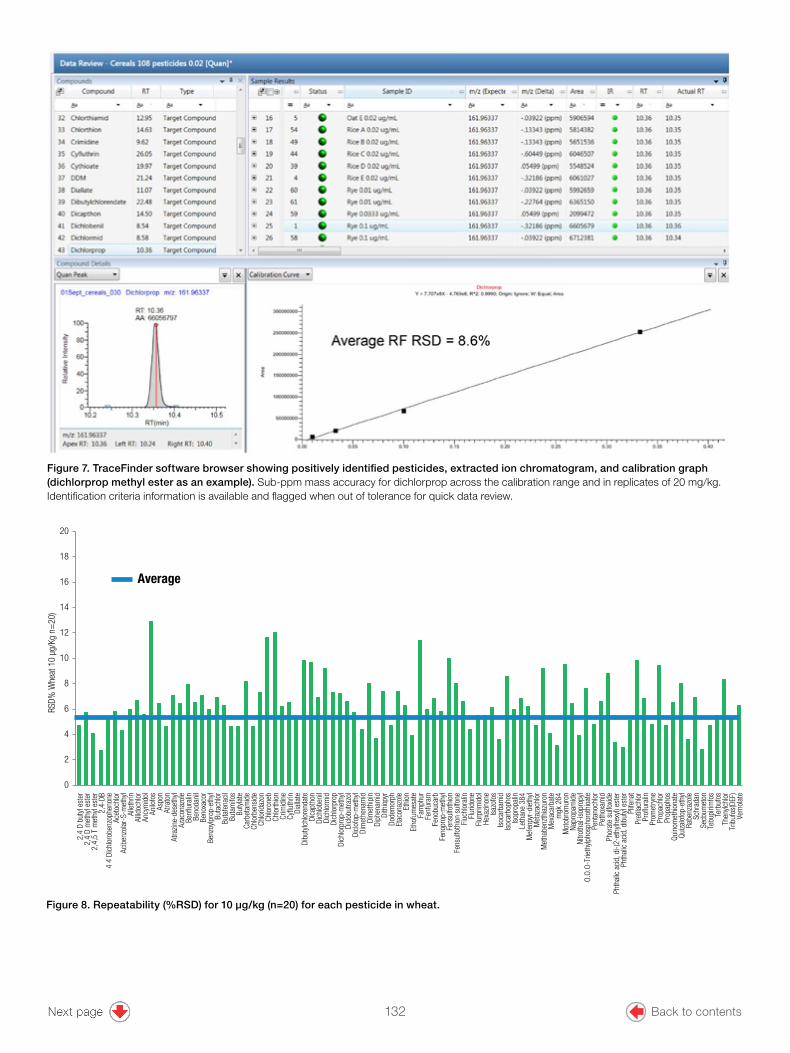
8
Figure 8. Repeatability (%RSD) for 10 µg/kg (n=20) for each pesticide in wheat.
Figure 7. TraceFinder software browser showing positively identified pesticides, extracted ion chromatogram, and calibration graph (dichlorprop methyl ester as an example). Sub-ppm mass accuracy for dichlorprop across the calibration range and in replicates of 20 mg/kg. Identification criteria information is available and flagged when out of tolerance for quick data review.
0
2
4
6
8
10
12
14
16
18
20
2,4
D bu
tyl e
ster
2,
4 D
met
hyl e
ster
2,
4,5
T m
ethy
l est
er
2,4-
DB
4 4
Dich
loro
benz
ophe
none
Ac
etoc
hlor
Ac
iben
zola
r-S-
met
hyl
Alle
thrin
Al
lidoc
hlor
An
cym
idol
An
ilofo
s As
pon
Atra
ton
Atra
zine-
dese
thyl
Azac
onaz
ole
Benfl
ural
in
Beno
dani
l Be
noxa
cor
Benz
oylp
rop-
ethy
l Bu
tach
lor
Buta
fena
cil
Buta
mifo
s Bu
tyla
te
Carb
etam
ide
Chlo
rben
side
Ch
lorid
azon
Ch
loro
neb
Chlo
rthio
n Cr
imid
ine
Cyflu
thrin
Di
alla
te
Dibu
tylc
hlor
enda
te
Dica
ptho
n Di
chlo
beni
l Di
chlo
rmid
Di
chlo
rpro
p Di
chlo
rpro
p-m
ethy
l Di
clob
utra
zol
Dicl
ofop
-met
hyl
Dim
ethe
nam
id
Dim
ethi
pin
Diph
enam
id
Dith
iopy
r Do
dem
orph
Et
acon
azol
e Et
hion
Et
hofu
mes
ate
Fam
phur
Fe
nfur
am
Feno
buca
rb
Feno
prop
-met
hyl
Fens
ulfo
thio
n Fe
nsul
foth
ion
sulfo
ne
Fluc
hlor
alin
Fl
urid
one
Flur
prim
idol
He
xazin
one
Isaz
ofos
Is
ocar
bam
id
Isoc
arbo
phos
Is
opro
palin
Le
than
e 38
4 M
efen
pyr-
diet
hyl
Met
azac
hlor
M
etha
benz
thia
zuro
n M
exac
arba
te
mgk
264
M
otob
rom
uron
Na
prop
amid
e Ni
troth
al-is
opro
pyl
O.O.
O-Tr
ieth
ylpho
spho
roth
ioat
e Pe
ntan
ochl
or
Peth
oxam
id
Phor
ate
sulfo
xide
Phth
alic
aci
d, d
i-(2-
ethy
lhex
yl) e
ster
Ph
thal
ic a
cid,
dib
utyl
este
r Pl
ifena
t Pr
etila
chlo
r Pr
oflur
alin
Pr
omet
ryne
Pr
opac
hlor
Pr
opap
hos
Quin
omet
hion
ate
Quiza
lofo
p-et
hyl
Rabe
nzaz
ole
Schr
adan
Se
cbum
eton
Te
bupi
rimfo
s Te
rbuf
os
Then
ylchl
or
Trib
ufos
(DEF
) Ve
rnol
ate
RSD%
Whe
at 1
0 µg
/Kg
n=20
)
Average
132 Back to contents

©2017 Thermo Fisher Scientific Inc. All rights reserved. All trademarks are the property of Thermo Fisher Scientific and its subsidiaries. This information is presented as an example of the capabilities of Thermo Fisher Scientific products. It is not intended to encourage use of these products in any manners that might infringe the intellectual property rights of others. Specifications, terms and pricing are subject to change. Not all products are available in all countries. Please consult your local sales representatives for details. AN10541-EN 0317S
Find out more at thermofisher.com/ExactiveGC
ConclusionsThe results of this study demonstrate that the Exactive GC Orbitrap high-resolution mass spectrometer, in combination with TraceFinder software, delivers robust and sensitive performance for routine pesticide analysis in cereals to regulatory standards.
• All 105 pesticides were detected at 10 μg/kg (5 μg/L in vial). 96% of the 525 pesticide/matrix combinations were confirmed at < 20 µg/kg (< 10 µg/L in vial) with excellent linearity, and in full compliance with the EU SANTE method performance criteria.
• The full scan acquisition permits efficient targeted data processing by use of a compound database and has the capability to easily add further analytes into the method scope.
• Intelligent software allows for results to be reviewed and detections confirmed in an efficient manner.
• Consistent sub-ppm mass accuracy was achieved for all compounds over a wide concentration range, ensuring that compounds are detected with high confidence at low and high concentration levels.
• Repeated injections of a wheat matrix at 10 µg/kg showed that the system is able to maintain a consistent level of performance over an extended period of time as is demanded by a routine testing laboratory.
References1. http://eur-lex.europa.eu/legal-content/EN/TXT/?uri=URISERV:l13002a
2. Mol, H.G.; Tienstra, M.; Zomer, P. Evaluation of gas chromatography - electron ion-ization - full scan high resolution Orbitrap mass spectrometry for pesticide residue analysis, Analytica Chimica Acta, 2016, doi: 10.1016/j.aca.2016.06.017.
3. Thermo Fisher Scientific Application Note: 10509. Routine quantitative method of analysis for pesticides using GC-Orbitrap mass spectrometry in accordance with SANTE/11945/2015 guidance.
4. SANTE/11945/2015. Guidance document on analytical quality control and method validation procedures for pesticides residues analysis in food and feed. Supersedes SANCO/12571/2013. Implemented by 01/01/2016.
133 Back to contents
GoalTo demonstrate the quantitative performance of the Thermo Scientific™ Exactive™ GC Orbitrap™ mass spectrometer for the analysis of GC-amenable pesticides and PCBs in grape and onion samples.
IntroductionThe accurate and reliable determination of pesticide residues and polychlorinated biphenyls (PCBs) in food is challenging because of the large number of compounds and diversity of sample types involved. The sensitivity requirements for these compounds are also demanding. In the European Union (EU), the default maximum residue level (MRL) for thousands of pesticide-commodity combinations is set at 10 µg/kg.1-3 Further to this, stringent confirmation and quantitative performance criteria are set so that residue results are equivalent across member states.
Authors Dominic Roberts,1 Jim Garvey,2 Richard Law,1 and Paul Silcock1
1Thermo Fisher Scientific, Runcorn, United Kingdom2Department of Agriculture, Food and the Marine, County Kildare, Ireland
Keywords Pesticides, fruits and vegetables, GC Orbitrap mass spectrometry, quantitation, accurate mass, TraceFinder software
The quantitative power of high-resolution GC-Orbitrap mass spectrometry for the analysis of pesticides and PCBs in food
APPLICATION NOTE 10584
134 Back to contents
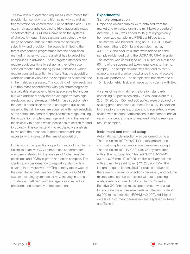
2
The low levels of detection require MS instruments that provide high sensitivity and high selectivity as well as fragmentation for confirmation. For pesticides and PCBs, gas chromatography coupled to triple quadruple mass spectrometers (GC-MS/MS) have been the systems of choice. Although these systems can detect a wide range of compounds with the required sensitivity, selectivity, and precision, the scope is limited to the target compounds programmed into the acquisition method. In other words, the analyst has to select the compounds in advance. These targeted methods also require additional time to set up, as they often use selected reaction monitoring (SRM) transitions, which require constant attention to ensure that the acquisition windows remain viable for the compounds of interest and in the matrices assessed. The coupling of high-resolution Orbitrap mass spectrometry with gas chromatography is a valuable alternative to triple quadrupole techniques but with additional analytical advantages.4–8 With high-resolution, accurate-mass (HRAM) mass spectrometry, the default acquisition mode is untargeted (full-scan) meaning that all the ions are acquired with high selectivity at the same time across a specified mass range, making the acquisition simple to manage and giving the analyst the flexibility to decide which pesticides to search for and to quantify. This can extend into retrospective analysis to evaluate the presence of other compounds not necessarily of interest at the time of acquisition.
In this study, the quantitative performance of the Thermo Scientific Exactive GC Orbitrap mass spectrometer was demonstrated for the analysis of GC-amenable pesticides and PCBs in grape and onion samples. The identification performance to regulatory standards is covered in previous work.4–8 The primary focus was on the quantitative performance of the Exactive GC-MS system including system sensitivity, linearity in terms of correlation coefficient and average response factors, precision, and accuracy of measurement.
Experimental Sample preparationGrape and onion samples were obtained from the market and extracted using the mini-Luke procedure9. Acetone (30 mL) was added to 15 g of cryogenically homogenized sample in a PTFE centrifuge tube. The sample was blended using an ULTRA-TURRAX®. Dichloromethane (30 mL) and petroleum ether, 40–60 °C, and sodium sulfate were added and the sample re-blended using the ULTRA-TURRAX blender. The sample was centrifuged at 3500 rpm for 5 min and 60 mL of the supernatant taken (equivalent to 1 g/mL sample). The sample volume was reduced by rotary evaporation and a solvent exchange into ethyl acetate (EA) was performed. The sample was transferred to a 10 mL volumetric flask and made up to volume with EA.
A series of matrix-matched calibration standards containing 88 pesticides and 7 PCBs, equivalent to 1, 2, 5, 10, 20, 50, 100, and 200 μg/kg, were prepared by spiking grape and onion extracts (Table 3A). In addition to the calibration series, grape and onion extracts were spiked with different combinations of the compounds at varying concentrations and analyzed blind to replicate real-life samples.
Instrument and method setupAutomatic sample injection was performed using a Thermo Scientific™ TriPlus™ RSH autosampler, and chromatographic separation was performed using a Thermo Scientific™ TRACE™ 1310 GC system fitted with a Thermo Scientific™ TraceGOLD™ TG-5SilMS 30 m × 0.25 mm I.D. x 0.25 µm film capillary column with a 5 m integrated guard (P/N 26096-1425). The integrated guard is beneficial for routine analysis as there are no column connections necessary and column maintenance can be performed without impacting analyte retention time. Finally, a Thermo Scientific Exactive GC Orbitrap mass spectrometer was used for accurate mass measurements in full-scan mode at 60,000 mass resolution (FWHM m/z 200). Additional details of instrument parameters are displayed in Table 1 and Table 2.
135 Back to contents
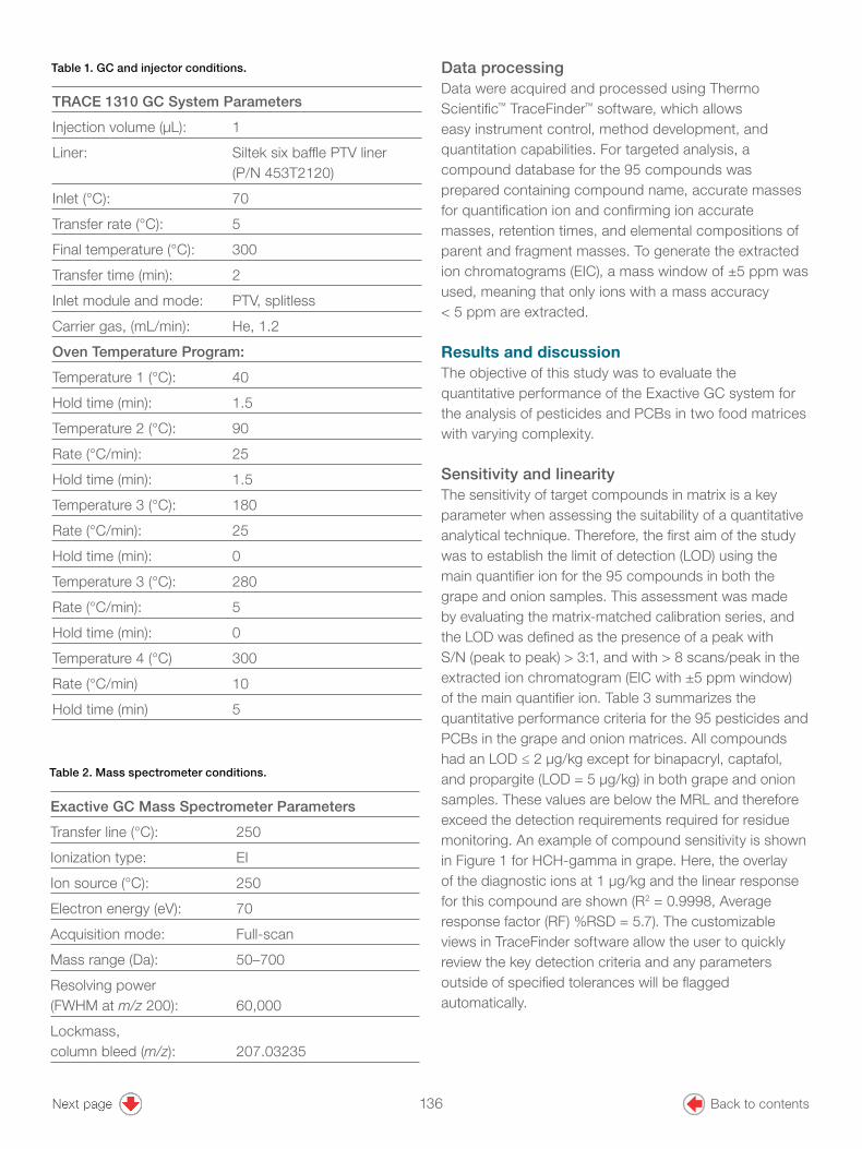
3
Table 1. GC and injector conditions.
TRACE 1310 GC System Parameters
Injection volume (µL): 1
Liner: Siltek six baffle PTV liner (P/N 453T2120)
Inlet (°C): 70
Transfer rate (°C): 5
Final temperature (°C): 300
Transfer time (min): 2
Inlet module and mode: PTV, splitless
Carrier gas, (mL/min): He, 1.2
Oven Temperature Program:
Temperature 1 (°C): 40
Hold time (min): 1.5
Temperature 2 (°C): 90
Rate (°C/min): 25
Hold time (min): 1.5
Temperature 3 (°C): 180
Rate (°C/min): 25
Hold time (min): 0
Temperature 3 (°C): 280
Rate (°C/min): 5
Hold time (min): 0
Temperature 4 (°C) 300
Rate (°C/min) 10
Hold time (min) 5
Table 2. Mass spectrometer conditions.
Exactive GC Mass Spectrometer Parameters
Transfer line (°C): 250
Ionization type: EI
Ion source (°C): 250
Electron energy (eV): 70
Acquisition mode: Full-scan
Mass range (Da): 50–700
Resolving power (FWHM at m/z 200): 60,000
Lockmass, column bleed (m/z): 207.03235
Data processingData were acquired and processed using Thermo Scientific™ TraceFinder™ software, which allows easy instrument control, method development, and quantitation capabilities. For targeted analysis, a compound database for the 95 compounds was prepared containing compound name, accurate masses for quantification ion and confirming ion accurate masses, retention times, and elemental compositions of parent and fragment masses. To generate the extracted ion chromatograms (EIC), a mass window of ±5 ppm was used, meaning that only ions with a mass accuracy < 5 ppm are extracted.
Results and discussionThe objective of this study was to evaluate the quantitative performance of the Exactive GC system for the analysis of pesticides and PCBs in two food matrices with varying complexity.
Sensitivity and linearityThe sensitivity of target compounds in matrix is a key parameter when assessing the suitability of a quantitative analytical technique. Therefore, the first aim of the study was to establish the limit of detection (LOD) using the main quantifier ion for the 95 compounds in both the grape and onion samples. This assessment was made by evaluating the matrix-matched calibration series, and the LOD was defined as the presence of a peak with S/N (peak to peak) > 3:1, and with > 8 scans/peak in the extracted ion chromatogram (EIC with ±5 ppm window) of the main quantifier ion. Table 3 summarizes the quantitative performance criteria for the 95 pesticides and PCBs in the grape and onion matrices. All compounds had an LOD ≤ 2 μg/kg except for binapacryl, captafol, and propargite (LOD = 5 μg/kg) in both grape and onion samples. These values are below the MRL and therefore exceed the detection requirements required for residue monitoring. An example of compound sensitivity is shown in Figure 1 for HCH-gamma in grape. Here, the overlay of the diagnostic ions at 1 µg/kg and the linear response for this compound are shown (R2 = 0.9998, Average response factor (RF) %RSD = 5.7). The customizable views in TraceFinder software allow the user to quickly review the key detection criteria and any parameters outside of specified tolerances will be flagged automatically.
136 Back to contents
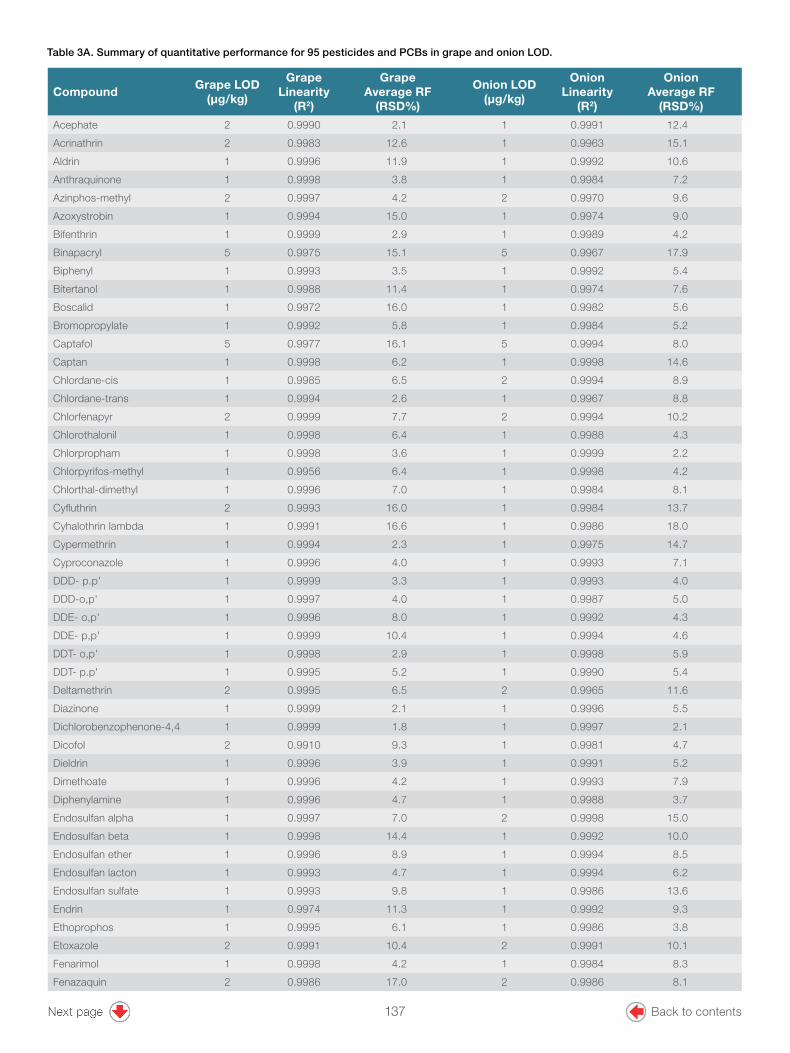
4
Table 3A. Summary of quantitative performance for 95 pesticides and PCBs in grape and onion LOD.
CompoundGrape LOD
(μg/kg)
Grape Linearity
(R2)
Grape Average RF
(RSD%)
Onion LOD (μg/kg)
Onion Linearity
(R2)
Onion Average RF
(RSD%)
Acephate 2 0.9990 2.1 1 0.9991 12.4
Acrinathrin 2 0.9983 12.6 1 0.9963 15.1
Aldrin 1 0.9996 11.9 1 0.9992 10.6
Anthraquinone 1 0.9998 3.8 1 0.9984 7.2
Azinphos-methyl 2 0.9997 4.2 2 0.9970 9.6
Azoxystrobin 1 0.9994 15.0 1 0.9974 9.0
Bifenthrin 1 0.9999 2.9 1 0.9989 4.2
Binapacryl 5 0.9975 15.1 5 0.9967 17.9
Biphenyl 1 0.9993 3.5 1 0.9992 5.4
Bitertanol 1 0.9988 11.4 1 0.9974 7.6
Boscalid 1 0.9972 16.0 1 0.9982 5.6
Bromopropylate 1 0.9992 5.8 1 0.9984 5.2
Captafol 5 0.9977 16.1 5 0.9994 8.0
Captan 1 0.9998 6.2 1 0.9998 14.6
Chlordane-cis 1 0.9985 6.5 2 0.9994 8.9
Chlordane-trans 1 0.9994 2.6 1 0.9967 8.8
Chlorfenapyr 2 0.9999 7.7 2 0.9994 10.2
Chlorothalonil 1 0.9998 6.4 1 0.9988 4.3
Chlorpropham 1 0.9998 3.6 1 0.9999 2.2
Chlorpyrifos-methyl 1 0.9956 6.4 1 0.9998 4.2
Chlorthal-dimethyl 1 0.9996 7.0 1 0.9984 8.1
Cyfluthrin 2 0.9993 16.0 1 0.9984 13.7
Cyhalothrin lambda 1 0.9991 16.6 1 0.9986 18.0
Cypermethrin 1 0.9994 2.3 1 0.9975 14.7
Cyproconazole 1 0.9996 4.0 1 0.9993 7.1
DDD- p.p' 1 0.9999 3.3 1 0.9993 4.0
DDD-o,p' 1 0.9997 4.0 1 0.9987 5.0
DDE- o,p' 1 0.9996 8.0 1 0.9992 4.3
DDE- p,p' 1 0.9999 10.4 1 0.9994 4.6
DDT- o,p' 1 0.9998 2.9 1 0.9998 5.9
DDT- p.p' 1 0.9995 5.2 1 0.9990 5.4
Deltamethrin 2 0.9995 6.5 2 0.9965 11.6
Diazinone 1 0.9999 2.1 1 0.9996 5.5
Dichlorobenzophenone-4,4 1 0.9999 1.8 1 0.9997 2.1
Dicofol 2 0.9910 9.3 1 0.9981 4.7
Dieldrin 1 0.9996 3.9 1 0.9991 5.2
Dimethoate 1 0.9996 4.2 1 0.9993 7.9
Diphenylamine 1 0.9996 4.7 1 0.9988 3.7
Endosulfan alpha 1 0.9997 7.0 2 0.9998 15.0
Endosulfan beta 1 0.9998 14.4 1 0.9992 10.0
Endosulfan ether 1 0.9996 8.9 1 0.9994 8.5
Endosulfan lacton 1 0.9993 4.7 1 0.9994 6.2
Endosulfan sulfate 1 0.9993 9.8 1 0.9986 13.6
Endrin 1 0.9974 11.3 1 0.9992 9.3
Ethoprophos 1 0.9995 6.1 1 0.9986 3.8
Etoxazole 2 0.9991 10.4 2 0.9991 10.1
Fenarimol 1 0.9998 4.2 1 0.9984 8.3
Fenazaquin 2 0.9986 17.0 2 0.9986 8.1
137 Back to contents

5
Table 3B. Summary of quantitative performance for 95 pesticides and PCBs in grape and onion LOD.
CompoundGrape LOD
(μg/kg)
Grape Linearity
(R2)
Grape Average RF
(RSD%)
Onion LOD (μg/kg)
Onion Linearity
(R2)
Onion Average RF
(RSD%)
Fenbuconazole 1 0.9999 9.3 1 0.9971 10.1
Fenitrothion 1 0.9989 9.8 1 0.9983 8.9
Fenpropathrin 1 0.9995 5.4 1 0.9987 4.6
Fenvalerate 2 0.9998 3.1 1 0.9975 18.0
Fludioxonil 1 0.9999 2.6 2 0.9983 11.9
Fluvalinate-tau 1 0.9996 17.3 1 0.9976 13.6
Folpet 1 0.9988 10.4 1 0.9984 8.2
HCH-alpha 1 0.9994 6.4 1 0.9999 4.1
HCH-beta 1 0.9999 4.0 1 0.9996 5.5
HCH-delta 1 0.9999 6.5 1 0.9996 3.1
HCH-gamma 1 0.9998 5.7 1 0.9999 5.2
Hexachlorobenzene 1 0.9995 5.9 1 0.9999 2.5
Hexaconazole 1 0.9998 8.7 1 0.9987 6.1
Iprodione 1 0.9998 7.2 1 0.9972 14.5
Iprovalicarb 1 0.9999 5.3 1 0.9994 2.7
Lenacil 1 0.9999 4.0 1 0.9989 4.3
MCPA Methyl ester 1 0.9985 7.9 1 0.9992 2.8
Methamidiphos 1 0.9995 11.4 2 0.9994 18.8
Molinate 2 0.9988 12.0 1 0.9994 5.3
o-Hydroxybiphenyl 1 0.9997 4.8 1 0.9991 2.8
Omethoate 1 0.9988 5.1 1 0.9995 7.6
Oxy-Chlordane 1 0.9999 11.6 1 0.9999 6.4
PCB 101 1 0.9990 6.3 1 0.9990 7.0
PCB 118 1 0.9994 2.3 1 0.9988 3.8
PCB 138 2 0.9997 13.8 1 0.9995 17.5
PCB 153 1 0.9996 8.9 1 0.9993 5.0
PCB 180 1 0.9998 18.8 2 0.9990 11.5
PCB 28 1 0.9985 4.0 1 0.9994 7.0
PCB 52 1 0.9974 11.8 1 0.9997 12.7
Pendimethalin 1 0.9952 16.6 1 0.9964 12.2
Permethrin 1 0.9999 1.8 1 0.9986 10.0
Phosmet 1 0.9999 2.5 1 0.9991 3.7
Prochloraz 2 0.9941 19.0 1 0.9914 19.0
Profenofos 1 0.9998 10.4 1 0.9995 16.0
Propargite 5 0.9956 18.0 5 0.9965 14.4
Propiconazole 1 0.9999 6.3 1 0.9988 9.5
Prothiofos 1 0.9999 7.7 1 0.9983 11.5
Pyridaben 2 0.9999 12.7 2 0.9983 12.5
Resmethrin 1 0.9997 2.0 1 0.9982 8.1
Spirodiclofen 1 0.9995 11.7 1 0.9985 16.4
Tefluthrin 1 0.9998 3.1 1 0.9999 2.7
Tetraconazole 1 0.9997 6.6 1 0.9989 7.6
Tetramethrin 1 0.9995 4.8 1 0.9983 4.7
Tolclofos-methyl 1 0.9996 4.9 1 0.9987 4.8
Triadimefon 1 0.9997 14.2 1 0.9984 13.0
Triadimenol 1 0.9999 7.4 1 0.9990 18.6
Trifluralin 2 0.9989 15.5 1 0.9985 8.1
138 Back to contents
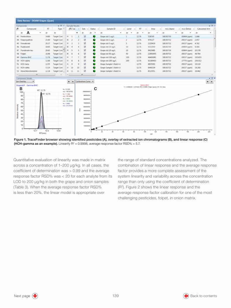
6
Quantitative evaluation of linearity was made in matrix across a concentration of 1–200 µg/kg. In all cases, the coefficient of determination was > 0.99 and the average response factor RSD% was < 20 for each analyte from its LOD to 200 µg/kg in both the grape and onion samples (Table 3). When the average response factor RSD% is less than 20%, the linear model is appropriate over
Figure 1. TraceFinder browser showing identified pesticides (A), overlay of extracted ion chromatograms (B), and linear response (C) (HCH-gamma as an example). Linearity R2 = 0.9998, average response factor RSD% = 5.7.
the range of standard concentrations analyzed. The combination of linear response and the average response factor provides a more complete assessment of the system linearity and variability across the concentration range than only using the coefficient of determination (R2). Figure 2 shows the linear response and the average response factor calibration for one of the most challenging pesticides, folpet, in onion matrix.
C
A
B
139 Back to contents

7
Figure 2. Calibration data for folpet in onion matrix.
Linear curve (1-200 µg/kg)
Average residuals RSD = 8.2%
Accurate quantitationTo assess the detectability and accuracy of quantitation, grape and onion samples were analyzed blind (the number and concentration of spiked compounds from a list of 97 were unknown to the analyst) after being post-
spiked with compounds at concentrations varying from 0.5 to 100 µg/kg. The concentrations were calculated from the matrix-matched calibration curves. Table 4 summarizes these results, which show good agreement between the spiked and calculated concentrations.
140 Back to contents

8
Table 4. Summary of spiked and calculated concentrations of pesticides and PCBs in grape and onion.
CompoundSpiked Grape Concentration
(µg/kg)
Calculated Grape Concentration
(µg/kg)
Spiked Onion Concentration
(µg/kg)
Calculated in Onion Concentration
(µg/kg)Azoxystrobin 17.0 14.0 50 50
Boscalid - - 34 32
Captan 5.0 4.9 - -
Chlordane-trans - - 53 56
Chlorothalonil 15.8 15.5 95 108
Chlorpropham 22.0 18.0 - -
Cyfluthrin 4.3 3.9 58 56
Cypermethrin 17.0 17.0 - -
Cyproconazole 44.0 37.0 - -
Deltamethrin - - 45 44
Diazinon 1.2 1.1 58 61
Dimethoate 29.0 30.0 58 56
Endosulfan beta 88.0 85.0
Fenbuconazole - - 47 50
Fludioxonil 24.0 32.0 63 54
Folpet 0.96 0.97 - -
HCB 1.1 1.1 58 49
Hexaconazole 5.9 5.1 - -
Iprodione 13.0 10.1 52 50
o,p-DDE 5.2 5.1 59 66
p,p-DDD 0.5 0.6 - -
Omethoate 45.0 39.1 75 71
PCB 180 1.0 1.2 34 32
PCB 153 17.0 20.0 - -
Permethrin 62.0 50.0 - -
Phosmet 45.0 36.0 - -
Propargite 6.3 5.7 95 97
Triadimenol 73.0 68.0
Furthermore, the grape sample was diluted by a factor of 5, and an example EIC for captan (1 µg/kg) is shown in Figure 3 along with a blank and the original grape sample
(4.9 µg/kg). This demonstrates the level of sensitivity that the Exactive GC Orbitrap mass spectrometer can deliver, even for complex matrices and for difficult pesticides.
141 Back to contents

©2017 Thermo Fisher Scientific Inc. All rights reserved. All trademarks are the property of Thermo Fisher Scientific and its subsidiaries unless otherwise specified. ULTRA-TURRAX is a registered trademark of IKA - Werke GMBH & Co. This information is presented as an example of the capabilities of Thermo Fisher Scientific products. It is not intended to encourage use of these products in any manners that might infringe the intellectual property rights of others. Specifications, terms and pricing are subject to change. Not all products are available in all countries. Please consult your local sales representatives for details. AN10584-EN 1117S
Find out more at thermofisher.com/OrbitrapGCMS
ConclusionsThe results of this study demonstrate that the Exactive GC Orbitrap HRAM mass spectrometer, in combination with TraceFinder software, offers an excellent solution that simplifies the analysis of pesticides in food commodities and delivers sensitive quantitative performance for pesticide analysis in fruits and vegetables.
• Sensitive and robust full-scan analysis allows for easy and flexible data acquisition and processing.
• All 95 compounds were detected at levels below the MRL, with calculated limits of detection of < 2 µg/kg for most compounds (92 of the 95 compounds).
• Excellent linearity was demonstrated with R2 > 0.99 and average response factors RSD% < 20 across the 8-point (1–200 µg/kg) matrix-matched calibration series, which ensures accurate quantitation. No internal standards were used to correct the response.
• Blind analysis of a grape and onion sample showed reliable detection and accurate quantitation of spiked compounds.
Figure 3. Extracted ion chromatogram and calculated concentration for captan in grape blank, 5× dilution and grape sample.
References1. http://ec.europa.eu/food/plant/docs/
plant_pesticides_mrl_guidelines_wrkdoc_11945_en.pdf
2. http://eur-lex.europa.eu/legal-content/EN/TXT/?uri=URISERV:l13002a
3. SANTE/11945/2015. Guidance document on analytical quality control and method validation procedures for pesticides residues analysis in food and feed. Supersedes SANCO/12571/2013. Implemented by 01/01/2016.
4. Mol, H.; Tienstra, M.; Zomer, P. Evaluation of gas chromatography electron ionization full scan high resolution Orbitrap mass spectrometry for pesticide residue analysis? Analytica Chimica Acta, 2016, 935, 161–172.
5. Ucles, S.; Lozano, A.; Martinez Bueno, M.J.; Fernandez-Alba, A.R. Shifting the paradigm in gas chromatography mass spectrometry pesticide analysis using high resolution accurate mass spectrometry. Journal of Chromatography A, 2017, 1501, 107–116.
6. Thermo Fisher Scientific, Application Note 10448. High efficiency, broad scope screening of pesticides using gas chromatography high resolution Orbitrap mass spectrometry, 2016. [online] https://assets.thermofisher.com/TFS-Assets/CMD/Application-Notes/AN-10448-GC-MS-Orbitrap-Pesticides-AN10448-EN.pdf
7. Thermo Fisher Scientific, Application Note 10509. Routine quantitative method of analysis for pesticides using GC-Orbitrap mass spectrometry in accordance with SANTE/11945/2015 guidelines, 2016. [online] https://tools.thermofisher.com/content/sfs/brochures/AN-10509-GC-MS-Pescitides-SANTE-11945-2015-AN10509-EN.pdf
8. Thermo Fisher Scientific, Application Note 10541. Multi-residue pesticide screening in cereals using GC-Orbitrap mass spectrometry, 2017. [online] https://tools.thermofisher.com/content/sfs/brochures/AN-10541-GC-MS-Pesticides-Cereal-AN10541-EN.pdf
9. Lozano, A.; Kiedrowsk, B.; Scholten, J.; de Kroon, M.; de Kok, A.; Fernández-Alba, A.R. Miniaturisation and optimisation of the Dutch mini-Luke extraction method for implementation in the routine multi-residue analysis of pesticides in fruits and vegetables. Food Chemistry. 2016, 192, 668–681.
Grape Matrix Blank
Grape ×5 Dilution1 ppb Captan
Grape4.9 ppb Captan
142 Back to contents

GoalTo demonstrate the quantitative performance of the Thermo Scientific™ Q Exactive™ GC Orbitrap™ mass spectrometer for the analysis of short- and medium-chained chlorinated paraffins in salmon samples.
IntroductionThe coupling of gas chromatography (GC) to high-resolution mass spectrometry (HRMS) using Orbitrap™ technology opens a broad spectrum of possible applications in environmental and food/feed analysis. Although known for several decades and widely used as plasticizers or flame retardants,1 short-chain chlorinated paraffins (SCCPs) have been only recently added to Annex A of the Stockholm Convention list of persistent organic pollutants (POPs).2
Authors Kerstin Krätschmer,1 Cristian Cojocariu,2 Alexander Schächtele,1 Paul Silcock,2 and Rainer Malisch1
1European Union Reference Laboratory (EURL) for Dioxins and PCBs in Feed and Food, Freiburg, Germany2Thermo Fisher Scientific, Runcorn, UK
Keywords Chlorinated paraffins, polychlorinated biphenyls, PCBs, Orbitrap, mass spectrometry, persistent organic pollutants, quantification, chemical ionization
Determination of short- and medium-chained chlorinated paraffins in salmon samples using GC Orbitrap-MS
APPLICATION NOTE 10585
143 Back to contents

2
Previous efforts to ban SCCPs caused the production of medium-chain CPs (MCCPs) to increase to replace SCCPs.3 As SCCPs alone consist of several thousand congeners with only four different carbon chain lengths to choose from, quantification of SCCPs and MCCPs in samples is a highly complex problem. In addition, other halogenated POPs like polychlorinated biphenyls (PCBs) are known to co-elute and add to the complexity of any analysis.
With this in mind, experiments focusing on linear dynamic range, sensitivity, and selectivity were performed using full-scan acquisition and negative chemical ionization (NCI) at 60,000 and 120,000 resolution (FWHM, m/z 200). In this study, mixtures of different CP and PCB standards were examined as well as food samples that were prepared with and without separation of co-eluting POPs during sample clean-up.
ExperimentalChemicals and standardsTwo standard solutions resembling technical mixtures of SCCP (100 mg/L in cyclohexane, C10–C13 55.5% Cl) and MCCP (100 mg/L in cyclohexane, C14–C17 42% Cl) were purchased from Dr. Ehrenstorfer GmbH (Augsburg, Germany). As internal standards, 1,5,5,6,6,10-13C-Hexachloro-decane (100 mg/L in nonane) was purchased from Cambridge Isotope Laboratories, Inc. (Andover, USA) and ε-HCH (100 mg/L in cyclohexane) was purchased from Dr. Ehrenstorfer GmbH.
For calibration, solutions of SCCP and MCCP with concentrations of 0.1 ppm, 0.5 ppm, 1 ppm, 5 ppm, 10 ppm, and 15 ppm and the addition of 0.1 ppm 1,5,5,6,6,10-13C-Hexachlorodecane and 0.05 ppm ε-HCH were prepared in cyclohexane.
For extraction and clean-up of the samples, silica gel 60 (230–400 mesh) and Florisil® PR (60–100 mesh) for pesticide analysis were purchased from Carl Roth GmbH & Co. KG (Karlsruhe, Germany). Acetone, n-hexane, and methanol in residue analysis grade (LCG Standards GmbH, Wesel, Germany) were used as solvents.
Samples acquisition and preparationThe samples were acquired from supermarkets and vendors in Baden-Württemberg as part of the food control. Part of the homogenized sample was extracted using accelerated solvent extraction (ASE) at 150 °C with acetone/n-hexane 1:3 (v/v), followed by elution through a sulfuric acid primed silica gel column. Further clean-up was done using a Florisil column and eluting the PCB fraction with n-hexane and the CP fraction with dichloromethane. Some of the samples were additionally prepared without the clean-up on a Florisil column.
GC-MS analysisExperiments were performed using a Q Exactive GC Orbitrap GC-MS/MS system coupled to a Thermo Scientific™ TRACE™ 1310 gas chromatograph equipped with a Thermo Scientific™ TraceGOLD™ TG5-SilMS 15 m × 0.25 mm × 0.25 µm column (P/N 26096-1300). Automatic tuning of the Q Exactive GC mass spectrometer was made using FC-43 as the tuning reagent and methane as the ionization gas. Full scans of the standards and samples were obtained using a mass range of m/z 50–650. Further details regarding the analytical system are given in Table 1.
Data processingData were acquired and processed using Thermo Scientific™ TraceFinder™ software.
144 Back to contents

3
Table 1. Parameters of the Q Exactive GC Orbitrap GC-MS/MS system used in this project.
TRACE 1310 GC System Parameters
Injection volume: 1.5 µL
Liner: Single gooseneck (P/N:4530924-UI)
Inlet: 280 °C
Inlet module and mode: Splitless/Surge (9 psi for 1 min)
Splitless time: 1.2 min
Split flow: 50 mL/min
Column flow: 1.4 mL/min
Oven Temperature Program:
Temperature 1: 60 °C
Hold time: 2 min
Temperature 2: 300 °C
Rate: 50 °C/min
Hold time: 5 min
Q Exactive GC Orbitrap GC-MS/MS System Parameters
Transfer line: 280 °C
Ionization type: NCI (methane)
Ion source: 180 °C
Electron energy: 70 eV
Acquisition mode: Full-scan
C-Trap energy: 2 V
Mass range: 50-650 m/z
Mass resolution (FWHM at m/z 200): 60k and 120k
Results and discussionLinearity and dynamic rangeThe linearity and dynamic range was assessed for both SCCP and MCCP technical mixtures (55.5% and 42% chlorine, respectively) using a dilution series in cyclohexane that resembles the usual analytical range of CP sample analysis in food. The coefficient of determination (R2) of over 0.99 indicates good linearity beyond this concentration range for almost all chosen congeners when assigned the concentration of the technical mixture. Taking their percentage of the technical mixtures in account, an LOQ of 1.5 ppb (MCCP) and 0.1 ppb (SCCP) could be achieved for some congeners, with the corresponding LOD being as low as 0.3 ppb (MCCP) and estimated below 0.05 ppb (SCCP).
SelectivityOne of the biggest challenges of CP analysis is the high complexity of the compound mixtures found in both samples and standards (Figure 1). In addition to a high degree of overlapping of the different CP homologues, other persistent organic pollutants such as PCBs are known to co-elute, thus further complicating the analysis. To investigate possible influences, a mixture of the SCCP and MCCP technical mixtures spiked with a high concentration of PCBs was analyzed. The mixture showed no significant influence on peak shapes in comparison with the separate technical mixtures (Figure 2), even with the PCB congeners clearly dominating the total ion chromatogram (TIC) and degrading the CP chromatographic hump to mere baseline disturbance. Therefore, the high resolution of the Q Exactive GC Orbitrap-MS system allows for the quantification of both SCCP and MCCP even in the presence of significant amounts of PCBs in samples without congener groups being overestimated due to mass overlaps. This was further verified by the sum concentrations of SCCP and MCCP, which were determined both in the standards and the standard mix. The twelve homologues chosen to serve as examples gave in ten cases relative standard deviations of < 10% from the sum concentration determined in the single standards. The slightly elevated concentrations of both groups of CPs shown in Table 2 most likely stem from the known impurities of both standards; a small amount of SCCPs could be found in the MCCP standard, and it has been commented on in literature that SCCP standards seem to contain MCCPs.4
145 Back to contents
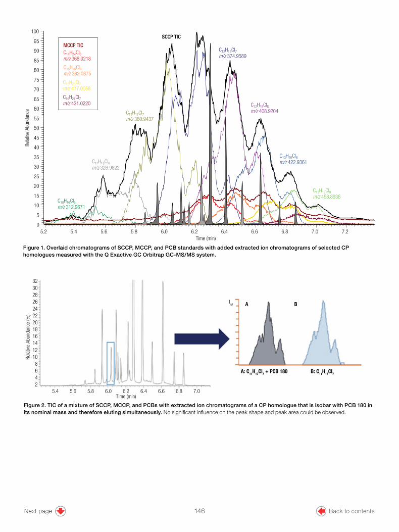
4
Figure 1. Overlaid chromatograms of SCCP, MCCP, and PCB standards with added extracted ion chromatograms of selected CP homologues measured with the Q Exactive GC Orbitrap GC-MS/MS system.
5.2 5.4 5.6 5.8 6.0 6.2 6.4 6.6 6.8 7.0 7.2Time (min)
0
5
10
15
20
25
30
35
40
45
50
55
60
65
70
75
80
85
90
95
100Re
lativ
e Ab
unda
nce
SCCP TIC
C10H16Cl6m/z 312.9671
C11H17Cl7m/z 360.9437
C12H19Cl7m/z 374.9589
C13H20Cl8m/z 422.9361
C12H18Cl8m/z 408.9204
C13H19Cl9m/z 458.8936
C11H18Cl6m/z 326.9822
MCCP TIC C14H24Cl6m/z 368.0218
C15H26Cl6m/z 382.0375
C15H25Cl7m/z 417.0058
C16H27Cl7m/z 431.0220
2468
101214161820
Rela
tive
Abun
danc
e (%
) 222426283032
5.4 5.6 5.8 6.0 6.2 6.4 6.6 6.8 7.0Time (min)
Irel
A: C11H17Cl7 + PCB 180 B: C11H17Cl7
A B
Figure 2. TIC of a mixture of SCCP, MCCP, and PCBs with extracted ion chromatograms of a CP homologue that is isobar with PCB 180 in its nominal mass and therefore eluting simultaneously. No significant influence on the peak shape and peak area could be observed.
146 Back to contents
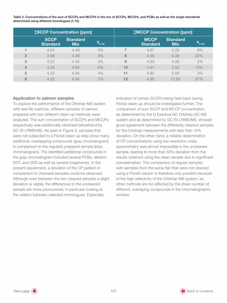
5
Table 2. Concentrations of the sum of SCCPs and MCCPs in the mix of SCCPs, MCCPs, and PCBs as well as the single standards determined using different homologues (1-12).
∑SCCP Concentration [ppm] ∑MCCP Concentration [ppm]
SCCP Standard
Standard Mix sx,rel
MCCP Standard
Standard Mix sx,rel
1 4.04 4.49 8% 7 4.87 5.28 6%
2 3.99 4.49 9% 8 4.86 6.38 22%
3 4.22 4.45 4% 9 4.83 4.95 2%
4 4.29 4.64 6% 10 4.81 5,50 10%
5 4.22 4.45 4% 11 4.82 5.03 3%
6 4.25 4.56 5% 12 4.85 10.82 87%
Application to salmon samplesTo explore the performance of the Orbitrap-MS system with real-life matrices, different samples of salmon prepared with two different clean-up methods were analyzed. The sum concentration of SCCPs and MCCPs respectively was additionally obtained beforehand by GC-EI-LRMS/MS. As seen in Figure 3, samples that were not subjected to a Florisil clean-up step show many additional, overlapping compounds (gray chromatogram) in comparison to the regularly prepared sample (blue chromatogram). The identified additional compounds in the gray chromatogram included several PCBs, dieldrin, DDT, and DDD as well as several toxaphenes. In the present experiment, a deviation of the CP pattern in comparison to cleansed samples could be observed. Although even between the two cleaned samples a slight deviation is visible, the differences to the uncleaned sample are more pronounced, in particular looking at the relation between selected homologues. Especially,
indication of certain SCCPs being held back during Florisil clean-up should be investigated further. The comparison of sum SCCP and MCCP concentration, as determined by the Q Exactive GC Orbitrap GC-MS system and as determined by GC-EI-LRMS/MS, showed good agreement between the differently cleaned samples for the Orbitrap measurements with less than 10% deviation. On the other hand, a reliable determination of CP concentrations using low-resolution mass spectrometry was almost impossible in the uncleaned sample, leading to more than 50% deviation from the results obtained using the clean sample due to significant overestimation. The comparison of regular samples with samples from the same fish that were not cleaned using a Florisil column is therefore only possible because of the high selectivity of the Orbitrap-MS system, as other methods are too affected by the sheer number of different, overlaying compounds in the chromatographic window.
147 Back to contents

©2017 Thermo Fisher Scientific Inc. All rights reserved. All trademarks are the property of Thermo Fisher Scientific and its subsidiaries unless otherwise specified. FLORISIL is a trademark of U.S. SILICA COMPANY. This information is presented as an example of the capabilities of Thermo Fisher Scientific products. It is not intended to encourage use of these products in any manners that might infringe the intellectual property rights of others. Specifications, terms and pricing are subject to change. Not all products are available in all countries. Please consult your local sales representatives for details. AN10585-EN 1117S
Find out more at thermofisher.com/OrbitrapGCMS
Conclusions• The results of this study demonstrate very good
linearity at concentrations of < 2 ppb. Determination of both CPs and PCBs in the same sample in one run is possible, suggesting the same for other halogenated compounds.
• TraceFinder software is an intuitive tool for processing data from full-scan analyses, allowing fast quantification and unprecedented insights into the pattern and content of CPs.
• A shortened sample preparation without separation of co-eluting compounds showed no influence on analysis results, while other instrumental setups struggled with the high number of compounds.
• Furthermore, the high selectivity of the Q Exactive GC Orbitrap GC-MS/MS system showed that possibly some CPs are held back during clean-up procedures, therefore influencing quantitative and qualitative results.
• Taken together, the Q Exactive GC mass spectrometer is a powerful analytical tool with simple setup and full-scan high-resolution experiments at a high selectivity, representing a potential for shorter sample preparation and quicker analyses of several types of POPs in one run, which is crucial considering the ever-growing list of compounds to be monitored in food and feed.
References1. Tomy, G.T. (2010) The Handbook of Environmental Chemistry, Vol. 10, Springer, London.
2. Stockholm Convention on Persistent Organic Pollutants, UNEP-POPS-COP.8/14, final report not yet published as of 24.July.2017.
3. Gluege, J.; Wang, Z. et al. Science of the Total Environment, 2016, 573, 1132–1146.
4. Reth, M. et al. Analytical and Bioanalytical Chemistry, 2004, 378, 1741–1747
5.0 5.2 5.4 5.6 5.8 6.0 6.2 6.4 6.6 6.8 7.0 7.2 7.4Time (min)
0
10
20
30
40
50
60
70
80
90
100
Rela
tive
Abun
danc
e (%
)
Figure 3. Q Exactive GC Orbitrap-MS full-scan TIC chromatograms of a regularly prepared salmon sample (blue) and of the same sample prepared without further clean-up (gray).
©2017 Thermo Fisher Scientific Inc. All rights reserved. All trademarks are the property of Thermo Fisher Scientific and its subsidiaries unless otherwise specified. FLORISIL is a trademark of U.S. SILICA COMPANY. This information is presented as an example of the capabilities of Thermo Fisher Scientific products. It is not intended to encourage use of these products in any manners that might infringe the intellectual property rights of others. Specifications, terms and pricing are subject to change. Not all products are available in all countries. Please consult your local sales representatives for details. AN10585-EN 1117S
Find out more at thermofisher.com/OrbitrapGCMS
Conclusions• The results of this study demonstrate very good
linearity at concentrations of < 2 ppb. Determination of both CPs and PCBs in the same sample in one run is possible, suggesting the same for other halogenated compounds.
• TraceFinder software is an intuitive tool for processing data from full-scan analyses, allowing fast quantification and unprecedented insights into the pattern and content of CPs.
• A shortened sample preparation without separation of co-eluting compounds showed no influence on analysis results, while other instrumental setups struggled with the high number of compounds.
• Furthermore, the high selectivity of the Q Exactive GC Orbitrap GC-MS/MS system showed that possibly some CPs are held back during clean-up procedures, therefore influencing quantitative and qualitative results.
• Taken together, the Q Exactive GC mass spectrometer is a powerful analytical tool with simple setup and full-scan high-resolution experiments at a high selectivity, representing a potential for shorter sample preparation and quicker analyses of several types of POPs in one run, which is crucial considering the ever-growing list of compounds to be monitored in food and feed.
References1. Tomy, G.T. (2010) The Handbook of Environmental Chemistry, Vol. 10, Springer, London.
2. Stockholm Convention on Persistent Organic Pollutants, UNEP-POPS-COP.8/14, final report not yet published as of 24.July.2017.
3. Gluege, J.; Wang, Z. et al. Science of the Total Environment, 2016, 573, 1132–1146.
4. Reth, M. et al. Analytical and Bioanalytical Chemistry, 2004, 378, 1741–1747
5.0 5.2 5.4 5.6 5.8 6.0 6.2 6.4 6.6 6.8 7.0 7.2 7.4Time (min)
0
10
20
30
40
50
60
70
80
90
100Re
lativ
e Ab
unda
nce
(%)
Figure 3. Q Exactive GC Orbitrap-MS full-scan TIC chromatograms of a regularly prepared salmon sample (blue) and of the same sample prepared without further clean-up (gray).
148 Back to contents

Thermo Scientific gas chromatography mass spectrometry systems provide complete solutions to the most challenging applications. Combined with productivity enhancing software, our advanced GC-MS instruments empower you to meet your application’s most stringent requirements for performance, reliability, and value.
Find out more at thermofisher.com/gcmsFor Research Use Only. Not for use in diagnostic procedures. © 2020 Thermo Fisher Scientific Inc. All rights reserved. All trademarks are the property of Thermo Fisher Scientific and its subsidiaries unless otherwise specified. AI73859-EN 1120M