Gamma-Radiation Induced Corrosion of Alloy 800 - CORE

Western University Western University

Scholarship@Western Scholarship@Western

Electronic Thesis and Dissertation Repository

11-9-2017 10:00 AM

Gamma-Radiation Induced Corrosion of Alloy 800 Gamma-Radiation Induced Corrosion of Alloy 800

Mojtaba Momeni The University of Western Ontario

Supervisor

Dr. Jungsook Clara Wren

The University of Western Ontario

Graduate Program in Chemistry

A thesis submitted in partial fulfillment of the requirements for the degree in Doctor of

Philosophy

© Mojtaba Momeni 2017

Follow this and additional works at: https://ir.lib.uwo.ca/etd

Part of the Materials Chemistry Commons, Metallurgy Commons, Nuclear Commons, Nuclear

Engineering Commons, Physical Chemistry Commons, and the Radiochemistry Commons

Recommended Citation Recommended Citation Momeni, Mojtaba, "Gamma-Radiation Induced Corrosion of Alloy 800" (2017). Electronic Thesis and Dissertation Repository. 5011. https://ir.lib.uwo.ca/etd/5011

This Dissertation/Thesis is brought to you for free and open access by Scholarship@Western. It has been accepted for inclusion in Electronic Thesis and Dissertation Repository by an authorized administrator of Scholarship@Western. For more information, please contact [email protected].

https://ir.lib.uwo.ca/

https://ir.lib.uwo.ca/etd

https://ir.lib.uwo.ca/etd?utm_source=ir.lib.uwo.ca%2Fetd%2F5011&utm_medium=PDF&utm_campaign=PDFCoverPages

http://network.bepress.com/hgg/discipline/135?utm_source=ir.lib.uwo.ca%2Fetd%2F5011&utm_medium=PDF&utm_campaign=PDFCoverPages







https://ir.lib.uwo.ca/etd/5011?utm_source=ir.lib.uwo.ca%2Fetd%2F5011&utm_medium=PDF&utm_campaign=PDFCoverPages

mailto:[email protected]

i

12 Abstract

This thesis presents a newly developed mechanism and predictive model for the

corrosion of Alloy 800. The Fe-Cr-Ni Alloy (Incoloy 800) is mainly used for steam generator

(SG) tubing in CANDU and PWR reactors and is a candidate material for the proposed

Canadian Supercritical Water Reactor (SCWR) in which it will be exposed to extreme

conditions of high radiation flux and large temperature gradients. The influence of gamma

radiation and water chemistry conditions on the corrosion behaviour of Alloy 800 are studied

in this work. Ionizing radiation creates reducing (•eaq–, •H, •O2

) and oxidizing radiolysis

(•OH, H2O2, O2) products that affect the redox chemistry, controlling corrosion. Water

chemistry conditions including pH, temperature and redox agents can significantly influence

the corrosion kinetics. A systematic study of Alloy 800 corrosion was carried out to

investigate the effect of these solution conditions. This analysis was used to develop a

mechanistic model that takes into account both metal dissolution and oxide formation during

the corrosion of Alloy 800. This model is designed to predict the effect of different variables

on the corrosion behaviour of Alloy 800 in extreme environments where direct corrosion

measurement is nearly impossible.

A series of electrochemical experiments and corrosion tests along with post-test

surface analyses were performed in order to gather information on the composition and

thickness of the oxide formed during corrosion and the metal cations dissolved in the

solution. This combination of electrochemical measurements and surface analyses provided

a highly-detailed understanding of Alloy 800 corrosion, allowing a mechanism to be

proposed. The proposed mechanism can explain the corrosion behaviour of Alloy 800 in a

variety of environments and temperatures, including aqueous and steam corrosion.

The principles behind the proposed mechanism were used to develop a model to

account for both oxide formation and metal cation dissolution. The model was used

successfully to model oxide thickness on pure iron, the Co-Cr alloy Stellite-6 and Alloy 800

in neutral and moderately alkaline aqueous solutions. The modeled results correlate well with

ii

experimental data. Using the model, it was possible to predict the time-dependent corrosion

potential in environments where direct measurements are not possible.

Keywords:

Alloy 800; Fe-Cr-Ni Alloy; Metal Oxides; Oxide Film Formation; Metal Dissolution;

Interfacial Reactions; Electrochemical Reactions; Water Radiolysis; -Radiation; Steady-

State Radiolysis;

iii

13 Dedication

To my wonderful and lovely family and wife

iv

14 Co-Authorship Statement

This thesis includes published data in chapters 7 and 8.

For all the chapters, I was the main author and Prof. J.C. Wren was co-author and Dr.

J. Joseph and G. Whitaker helped with writing and editing.

Chapter 4: The electrochemical data in the absence of radiation was done by T.V. Do

and J. Joseph helped with the experiments.

Chapter 5: The electrochemical experiments were done by T.V. Do and J. Joseph

helped with the experiments.

Chapter 6: The samples in the argon environment were prepared and analyzed by V.

Subramaniam and S. Hariharan. J. Joseph helped with all the experimental setup and

analysis.

Chapter 8: The experimental works were done by M. Behazin and I modeled them.

v

15 Acknowledgments

This works was not possible to complete without the help of my colleagues and

friends.

I would like to thank my supervisor, Dr. Clara Wren. She gave me the opportunity to

work on my dream project and helped me a lot to widen my horizons and think critically.

She was not only my research supervisor, but was a great help in every aspect of my life and

helped me whenever I asked for it. This work would not have been possible without her

mentorship.

I also would like to thank Dr. Jiju Joseph for being a great source of support over the

past four years and Dr. Jamie Noël for all of our scientific discussions. I also would like to

thank Dr. Dave Wren and G. Whitaker who helped me with the writing and gave me valuable

professional advice.

I would like to thank my wonderful friends and also all of my student peers, both past

and present, in the Wren lab and Shoesmith and Noël lab.

Most importantly, I would like to thank my family and my wife, Nasrin, from the

bottom of my heart for their unconditional support throughout my academic career.

vi

16 Symbols

°C Degree celcius

DR Dose rate

Transfer coefficient or symmetry factor, normally equal to 0.5

Asol Surface area exposed to solution (cm2)

oxide(t) Potential drop across the oxide layer at time t (V)

E(i=0) Potential at which net current is zero

EAPP Applied potential during polarization (V)

ECORR Corrosion potential (V)

Efinal Final potential

Einitial Initial potential

F Faraday’s constant (96485 C×mol-1)

fk-MO# Relative ratio of the oxide formation and dissolution constants

fl Relative monolayer length of Cr2O3 to chromite

𝑚𝑒𝑞 Fermi level at the metal oxide interface (V)

𝑠𝑜𝑙𝑒𝑞

Fermi level at the oxide solution interface (V)

LCr2O3 Thickness of air-formed chromium oxide (cm)

LMCr2O4 Thickness of growing chromite (cm)

Constant related to the potential drop in the oxide (cm-1)

LMO#(t) Thickness of the MO# oxide layer (cm)

m|ox Metal/oxide interface

mdiss# Dissolved amount of metal cations (mol)

N Number of electrons involving in the reaction.

ox|sol Oxide/solution interface

R Universal gas constant (8.314 J×mol-1×K-1)

T Absolute temperature (K)

Molar volume of oxide (cm3×mol-1)

V Driving force for corrosion (V)

VSCE Potential vs. SCE

𝐸𝑟𝑒𝑑#𝑒𝑞 Equilibrium potential of a redox pair # involved in corrosion (V)

𝐸𝑟𝑑𝑥#(𝑡) Electrochemical potential of the reacting system at time t (V)

𝐸𝑜𝑥#𝑒𝑞 Equilibrium potential for oxidation half-reaction (V)

𝐸𝑟𝑒𝑑#𝑒𝑞 Equilibrium reduction half reaction potential (V)

𝐸𝑒𝑞 Equilibrium half reaction potential (V)

𝐸𝑒𝑙𝑒𝑐(𝑡) Electrode potential at time t. It is ECORR in an open circuit and Eapp in

potentiostatic polarization (V)

vii

𝑟𝑑𝑥#

(𝑡) Overpotential at the reaction interface (V)

𝑜𝑥#

(𝑡) Anodic overpotential (V)

𝑟𝑒𝑑#

(𝑡) Cathodic overpotential (V)

𝑖𝑟𝑑𝑥#𝑒𝑞 Exchange current density (Acm-2)

𝑖𝑟𝑑𝑥#(𝑡) Current density at time t (Acm-2)

𝐽𝑀#𝑛+(𝑡)|𝑚|𝑜𝑥 Metal oxidation flux at the metal/oxide interface (mol×s-1×cm-2)

𝐽𝑟𝑒𝑑#(𝑡)|𝑜𝑥|𝑠𝑜𝑙 Solution reduction flux (mol×s-1×cm-2)

⟨𝐽𝑀𝑛+(𝑧, 𝑡)⟩𝑜𝑥𝑖𝑑𝑒 Average flux of metal cations across the oxide layer (mol×s-1×cm-2)

𝐽𝑀#𝑛+(𝑡)|𝑜𝑥|𝑠𝑜𝑙 Total flux of metal cations arriving at the ox|sol interface (mol×s-1×cm-2)

𝐽𝑀𝑂#(𝑡)|𝑜𝑥𝑖𝑑𝑒 Oxide growth flux (mol×s-1×cm-2)

𝐽𝑑𝑖𝑠𝑠#(𝑡)|𝑠𝑜𝑙 Dissolution flux (mol×s-1×cm-2)

−∆𝑟𝐺(𝑡) Free energy of reaction (J×mol-1)

𝑚𝑒𝑞 Fermi level of metal at equilibrium


Fermi level of solution at equilibrium

𝐸(𝑂𝑥)

Density of unoccupied electron energy states of oxidants

𝐸(𝑟𝑒𝑑)

Density of occupied electron energy states of reduction reaction products

𝐸(𝑀𝑛+)

Density of unoccupied electron energy states of metal cation

𝐸(𝑀)

Density of occupied electron energy states of metal atom

𝐶𝐵

Lowest energy of conduction band

𝑉𝐵

Highest energy of valence band

𝑀𝑂# Specific potential gradient of oxide (V×cm-1)

∆𝐸𝑎𝑀𝑂#(𝑡) Activation energy barrier for oxide growth at time t (J×mol-1)

∆𝐸𝑎𝑀𝑂#(0) Activation energy barrier for oxide growth at time t = 0 (no oxide on the

surface) (J×mol-1)

𝛥𝐸𝑎𝑜𝑥𝑖𝑑𝑒(𝑡) Activation energy barrier for oxide growth across the oxide present on the

surface at time t (J×mol-1)

𝑐𝑀𝑂# Specific activation energy gradient of oxide (J×mol-1×cm-1)

𝛥𝑉𝑜𝑥𝑖𝑑𝑒(𝑡) Potential drop across an oxide layer at time t (V)

𝛥𝑉𝑜𝑥𝑖𝑑𝑒(0) Potential drop across an oxide layer at time zero (V)

𝛥𝑉𝑀𝑂#(𝑡) Potential drop across the layer of MO# at time t (V)

𝐽𝑀𝑂" Constant component of metal cation flux

viii

17 Acronyms

AES Auger electron spectroscopy

Ag/Ag/Cl Silver/silver chloride reference electrode

BE Binding energy

BSE Backscattered electron

CANDU Canada deuterium uranium

DH Dissolved hydrogen

DO Dissolved oxygen

FCC Face-center cubic

HCP Hexagonal close packed

ICP-MS Inductively coupled plasma - mass spectroscopy

ICP-OES Inductively coupled plasma- optical emission spectroscopy

KE Kinetic energy

LET Linear energy transfer

PDM Point defect model

PHWR Pressurized heavy water reactor

PHTS Primary heat transport system

PLWR Pressurized light water reactor

PTFE Polytetrafluoroethylene

PWR Pressurized water reactor

SCE Saturated calomel electrode

SCW Supercritical water

SCWR Supercritical water reactor

SEM Scanning electron microscopy

SHE Standard hydrogen electrode

SG Steam generator

EDX Energy dispersive X-Ray spectroscopy

XPS X-Ray photoelectron spectroscopy

ix

18 Table of Contents

Abstract ............................................................................................................... i

Dedication ............................................................................................................. iii

Co-Authorship Statement .................................................................................................. iv

Acknowledgments .............................................................................................................. v

Symbols ............................................................................................................. vi

Acronyms ........................................................................................................... viii

Table of Contents ............................................................................................................. ix

List of Tables ........................................................................................................... xiii

List of Figures ........................................................................................................... xiv

Chapter 1 Introduction ....................................................................................................... 1

Motivation .............................................................................................................. 1

Research Objective and Approaches ........................................................................ 4

Thesis Outline .......................................................................................................... 5

References .............................................................................................................. 5

Chapter 2 Technical Background and Literature Review ............................................... 8

The Primary Coolant Water ............................................................... 13

2.3.2 Secondary System .............................................................................. 14

Corrosion of Alloy 800 .......................................................................................... 15

Iron, Nickel and Chromium Oxides ................................................... 16

Review of Corrosion of Fe-Ni-Cr Alloys .......................................... 22

Corrosion of Fe-Cr-Ni alloys ............................................................. 35

Cabrera-Mott model ........................................................................... 43

Point Defect Model (PDM) ................................................................ 46

Mixed conduction model (MCM) ...................................................... 47

Generalized Model for Oxide Film Growth ....................................... 48

Radiation Chemistry .......................................................................... 49

Radiation Induced Nanoparticle Formation ....................................... 59

x

Chapter 3 Experimental Techniques and Procedures .................................................... 73

Electrochemical cell setup ................................................................. 73

Linear Polarization Resistance (LPR) Measurements ....................... 74

Raman Spectroscopy .......................................................................... 75

Scanning Electron Microscopy .......................................................... 76

X-Ray Photoelectron Spectroscopy ................................................... 79

Auger Electron Spectroscopy ............................................................. 81

Inductively-Coupled Plasma Mass Spectrometry .............................. 82

Inductively-Coupled Plasma Optical Emission Spectrometry ........... 83

Material and Solution Preparation ..................................................... 84

Electrochemical Setup ........................................................................ 85

Radiation exposure tests ..................................................................... 88

Coupon exposure experiments at T ≥ 150 C .................................... 90

Post-test surface analysis ................................................................... 90

Solution Analysis ............................................................................... 91

Chapter 4 Effects of pH and -Radiation on Corrosion of Alloy 800 in Deaerated

Borate Buffer at Ambient Temperatures ........................................................................ 94

3-d Coupon Exposure Tests ............................................................... 96

Electrochemical Experiments .......................................................... 105

Effect of -Radiation on ECORR ......................................................... 116

Chapter 5 Combined Effects of Gamma-Radiation and pH on Corrosion of Alloy 800

at 150 oC .......................................................................................................... 123

Material and Solutions ..................................................................... 123

Electrochemical Tests ...................................................................... 124

Corrosion Experiments .................................................................... 125

Post-test Analysis ............................................................................. 125

xi

Corrosion at first 5 h ........................................................................ 138

Corrosion at longer times ................................................................. 140

Chapter 6 The Effect of Oxygen Content and Gas Phase Radiolysis on Corrosion of

Alloy 800H in High-Temperature Steam ....................................................................... 146

Materials ........................................................................................... 147

Experimental Conditions .................................................................. 147

Surface Characterization .................................................................. 148

Chapter 7 A Mechanistic Model for Oxide Growth and Dissolution during Corrosion

of Cr-Containing Alloys .................................................................................................. 169

Overview of the MCB Model .......................................................... 172

Elementary Electrochemical and Transport Processes .................... 174

Mass and Charge Balance ................................................................ 176

Formulation of the Metal Oxidation Flux, JM#n+(t)|m|ox ................ 179

Potential Distribution ....................................................................... 181

Formulation of the Oxide Growth and the Dissolution Fluxes ........ 188

Summary of the Mathematical Formulation of Model and Model

Parameters ......................................................................................................... 191

Oxide Thickness on Pure Iron .......................................................... 194

Corrosion of Cr-containing Alloys .................................................. 195

Chapter 8 Mass and Charge Balance (MCB) Model Simulations of Current, Oxide

Growth and Dissolution in Corrosion of Co-Cr Alloy Stellite-6 ................................. 202

Alloy composition ............................................................................ 208

Redox reactions and their equilibrium potentials ............................ 210

Potential drop across a growing oxide layer .................................... 214

Formulation of oxide growth and dissolution fluxes ....................... 216

Model output of experimental quantities ......................................... 218

Model calculations of potentiostatic polarization experiments ........ 221

Corrosion under open-circuit conditions .......................................... 224

xii

Oxide formation and dissolution ...................................................... 226

Chapter 9 Mass and Charge Balance (MCB) Model Simulations of Potential, Oxide

Growth and Dissolution During Corrosion of Alloy 800.............................................. 232

Corrosion under open-circuit conditions in the absence of radiation ....

.......................................................................................................... 234

Oxide formation and dissolution ...................................................... 235

Chapter 10 Summary and Future Works...................................................................... 241

APPENDIX A .......................................................................................................... 246

APPENDIX B .......................................................................................................... 251

APPENDIX C .......................................................................................................... 258

APPENDIX D .......................................................................................................... 261

xiii

19 List of Tables

Table 2-1: CANDU Primary Coolant Chemistry [3] .......................................................... 14

Table 2-2: Secondary System Water chemistry [3] ............................................................ 15

Table 2-3: thermodynamic data for iron species [29] ......................................................... 30

Table 2-4:The primary yields (μmolJ–1) from -radiolysis ................................................ 55

Table 4-1: Redox half-reactions involving metal and solution species ............................ 108

Table 5-1: Concentrations of metal cations dissolved ...................................................... 131

Table 7-1: Mathematical Formulation of the Model. ........................................................ 193

Table 7-2: Fitting parameters for Cr-alloy potentiostatic simulations. ............................. 198

Table 8-1: Mathematical Formulae of the Fluxes in the MCB Model. ............................. 208

Table 8-2: Elemental composition of Stellite-6 in both weight percentage ...................... 209

Table 8-3: The metal oxidation reactions considered in the simulation of Stellite-6 ....... 212

Table 8-4: The parameters derived for use in the MCB model ......................................... 221

Table 9-1: The parameters derived for use in the MCB model ......................................... 233

xiv

20 List of Figures

Figure 1-1: A simplified schematic of a CANDU reactor .................................................... 2

Figure 1-2: Schematics of corrosion product transport ......................................................... 3

Figure 2-1: Schematic illustrating the Butler-Volmer relationships ................................... 11

Figure 2-2: Diagram of atomic locations in a normal spinel ............................................. 17

Figure 2-3: A projection along c of the orthorhombic unit cell of lepidocrocite. ............... 18

Figure 2-4: Crystal structure of nickel oxide. ..................................................................... 19

Figure 2-5: The idealized crystal structure of α-Ni(OH)2⋅xH2O ......................................... 20

Figure 2-6: The crystal structure of β-Ni(OH)2 ................................................................. 21

Figure 2-7: Crystal structure of Cr2O3 [33]. ........................................................................ 22

Figure 2-8: Comparison between calculated and experimental solubility of NiO [24]. ..... 25

Figure 2-9: Ni Pourbaix diagram at different temperature from 25 °C to 300 °C [24] ...... 27

Figure 2-10: Influence of pH on the solubility of Cr2O3 and Cr(OH)3, at 25 °C [25]. ....... 28

Figure 2-11: Pourbaix diagram of the Cr-H2O system at 25 °C ......................................... 29

Figure 2-12: Solubility of Fe(II) and Fe(III) in aqueous environment at 25 °C [30].......... 30

Figure 2-13: E-pH diagram for pure iron at temperature 25 °C to 300 °C [29]. ................ 31

Figure 2-14: Pourbaix diagrams for iron species in the ternary system ............................. 33

Figure 2-15: Pourbaix diagrams for chromium species in the ternary system ................... 34

Figure 2-16: Pourbaix diagrams for nickel species in the ternary system .......................... 35

Figure 2-17: Scheme of the potential drop in the metal/oxide/solution system [92]. ......... 43

Figure 2-18: Scheme describing the reaction and transport processes .............................. 45

Figure 2-19: The radiation track of a fast electron ............................................................. 53

Figure 2-20: Schematic of water radiolysis ........................................................................ 54

Figure 2-21: Schematic of water radiolysis reaction mechanism ....................................... 56

Figure 2-22: Model simulation results ................................................................................ 57

Figure 2-23: Model simulation results ................................................................................ 57

Figure 3-1: Schematic of three-electrode electrochemical cell ........................................... 73

Figure 3-2: E-log(iapp) data for two hypothetical corroding surfaces ................................. 74

Figure 3-3: Illustration of Rayleigh (a), Stokes (b) and Anti-Stokes (c). ........................... 77

Figure 3-4: Schematic demonstrating the principles of XPS .............................................. 80

Figure 3-5: Schematic demonstrating the principles of AES .............................................. 82

Figure 3-6: Illustration of inductively coupled plasma mass spectrometry (ICP-MS). ...... 83

Figure 3-7: Illustration of ICP-OES .................................................................................... 84

Figure 3-8: Standard three-electrode electrochemical cell. ................................................ 86

Figure 3-9: Electrochemistry autoclave used for tests above 100 °C ................................. 87

Figure 3-10: Schematic representation of the reactions ..................................................... 89

Figure 4-1: Schematic of the experimental setup ............................................................... 95

Figure 4-2: (a) Dissolved concentrations (b) SEM micrographs ........................................ 98

Figure 4-3: XPS spectra taken from an Alloy 800 surface ............................................... 100

Figure 4-4: (a) Dissolved concentrations (b) enrichment ratios (c) compositions ............ 102

Figure 4-5: pH-dependent solubility ................................................................................. 103

Figure 4-6: ECORR as a function of time ............................................................................ 106

Figure 4-7: Equilibrium potentials of redox half-reactions .............................................. 110

Figure 4-8: Linear polarization resistant (LPR) measurment ........................................... 115

Figure 4-9: ECORR measurements in the presence and absence of radiation ..................... 117

xv

Figure 4-10: Proposed mechanism for Alloy 800 corrosion ............................................. 118

Figure 5-1: Experimental setup for corrosion tests and electrochemical experiments ..... 124

Figure 5-2: ECORR observed as a function of time ............................................................. 127

Figure 5-3: Proposed Alloy 800 corrosion pathways ....................................................... 129

Figure 5-4: Dissolved metal concentrations ..................................................................... 130

Figure 5-5: Solubilities of FeII, FeIII, NiII and CrIII ions .................................................... 132

Figure 5-6: AES depth analysis ........................................................................................ 135

Figure 5-7: Oxygen and carbon analysis of AES results .................................................. 137

Figure 6-1: SEM micrographs of the surfaces of Alloy 800H coupons ........................... 150

Figure 6-2: Raman spectra of the surfaces of Alloy 800H coupons ................................. 152

Figure 6-3: XPS spectra taken from an Alloy 800H surface ............................................ 154

Figure 6-4: Oxidation-state compositions ......................................................................... 155

Figure 6-5: AES depth profiles ......................................................................................... 159

Figure 6-6: Schematic of the four depth zones ................................................................. 160

Figure 6-7: Atomic percentage ratios ............................................................................... 162

Figure 6-8: Schematic of oxide formation ........................................................................ 163

Figure 7-1: Commonly accepted scheme for the distribution of the potential ................. 171

Figure 7-2: Schematic of the elementary processes considered in the MCB model ........ 176

Figure 7-3: Relative positions of the redox reaction potentials. ....................................... 182

Figure 7-4: Relative positions of the reaction potentials .................................................. 185

Figure 7-5: Relative positions of the reaction potentials .................................................. 186

Figure 7-6: Effect of linear oxide growth on the potential distribution ............................ 187

Figure 7-7: Effect of linear oxide growth on the potential distribution ............................ 188

Figure 7-8: Measured average oxide thickness ................................................................. 194

Figure 7-9: Current observed during polarization ............................................................ 196

Figure 8-1: Schematics illustrating ................................................................................... 205

Figure 8-2: SEM of a freshly polished surface of Stellite-6 ............................................. 209

Figure 8-3: Equilibrium potentials for the redox reactions ............................................... 212

Figure 8-4: Experimental (solid lines) and model calculations (broken lines) ................. 222

Figure 8-5: Comparison of the MCB model calculations ................................................. 223



Figure 8-8: Comparison of the MCB model calculations. ................................................ 227


Figure 9-1: The measured ECORR (black solid line) and calculated ECORR ........................ 235

Figure 9-2: Exprimentally measured and MCB model calculations ................................. 236

Figure 9-3: Measured oxide thickness by AES and calculated oxide thickness .............. 236

Figure 9-4: Predicted ECORR on Alloy 800 at three different ............................................ 237

1

1 Chapter 1

Introduction

Motivation

Nuclear energy is a clean, affordable and low greenhouse gas emitting energy source

with the power-generating capacity to meet industrial needs. Nuclear power contributes 10%

of worldwide energy production, 15% of Canada’s power generation and more than 60% of

Ontario’s energy supply.

The processes of electricity generation in a nuclear power plant are similar to those

in fossil fuel power plants, but the way heat is generated is different. A nuclear reactor uses

fissile material as fuel, typically in the form of uranium dioxide. When a neutron collides

with a fissile atom such as 235U the nucleus splits into two lighter nuclei and 2-3 neutrons, a

process known as fission. During fission, a large amount of heat is produced which is used

to generate steam which drives the turbines to produce electricity.

There are several types of nuclear reactor in operation around the world. The most

common design is the pressurized light water reactor (PLWR), which uses 3-4%, enriched

uranium (i.e., 3-4% 235U in mostly 238U) as fuel, and light water for both coolant and

moderator. All the nuclear reactors in Canada are the Canadian designed CANDU® (Canada

deuterium uranium) reactors which are pressurized heavy water reactors (PHWR) that use

natural uranium (containing only 0.7% 235U) as the fuel and heavy water as both coolant and

moderator. A schematic of a CANDU® reactor is shown in Figure 1-1.

The UO2 fuel is encased in Zr-alloy cladding to avoid contact of fuel with the coolant.

The structure that houses the circulating coolant is referred to as the heat transport system

(HTS). The materials and configuration of the HTS also depend on the reactor type. For

CANDU® the HTS system consists of Zr-pressure tubes inside the reactor core, connected

to carbon steel feeder pipes that feed the coolant to a header (a tank), which is then connected

to heat exchangers inside a steam generator. Heat exchanger tubes are usually constructed

2

from iron-chromium-nickel alloys such as Alloy 800. Nickel alloys are chosen because of

their good mechanical properties and resistance to corrosion.

Figure 1-1: A simplified schematic of a CANDU reactor

One of the major issues for nuclear power plants is the performance of materials in

irradiated environments. Under the highly ionizing radiation conditions in the reactor core,

the coolant water decomposes to form a range of chemically reactive species which include

highly oxidizing (•OH, H2O2, O2) and reducing (•eaq–, •H, •O2

) species as shown in reaction

1-1 [1].

H2O •OH, •eaq–, •H, HO2•, H2, H2O2, H

+ (1-1)

In environments where there is a constant flux of radiation such as those in nuclear

reactors, the radiolysis products stabilize to steady state concentrations. These concentrations

will determine the redox properties of the water which will affect the corrosion kinetics.

Corrosion is a complex process involving oxidation of metal, reduction of solution

species and interfacial transfer of electrons and ions. The transfer of metal cations to the

solution phase can induce changes in the physical and (electro-) chemical nature of the

3

interfacial region. Changes in the surface layer, in turn, can strongly affect the metal

oxidation rate and alter the corrosion pathway.

Corrosion of heat exchangers, while slow, poses two major concerns. Changing

defective tubes inside a steam generator is very costly, so ideally, they should last for the

lifetime of the reactor, or be repaired only at the time of planned reactor refurbishment.

Another concern involves transport of radioactive corrosion products inside the coolant

circuit. Corrosion of heat exchangers releases dissolved or dispersed metal cations into the

coolant. As the coolant circulates in and out of the reactor core, the metal cations are exposed

to neutron radiation and can become neutron-activated, producing radioactive products. For

example, neutron activation of Ni produces radioactive 58Co, which is a and emitter with

a half life of 70 d:

58Ni + neutron proton + 58Co (1-2)

If the neutron-activated product later deposits on the wall of the heat transport tubing

outside the reactor core, it can create radioactive hot spots outside the core (Figure 1-2). This

can pose a safety concern for reactor maintenance workers and make any maintenance

activities during planned reactor shutdown or decommissioning very expensive.

Figure 1-2: Schematics of corrosion product transport

Reactor Core

Radioactive sites

up

str

ea

m

58NiRadioactive

58Co

do

wn

str

ea

m

neutron activation

4

Although oxide film formation and corrosion of Fe-Cr-Ni alloys, including Alloy

800, have been investigated extensively [2-25], there is a complete lack of understanding of

corrosion behaviour of Alloy 800 under radiation. The effect of changing pH or temperature

has not been systematically investigated and the individual contributions of these parameters

to oxide film formation have not yet been established. Moreover, no comprehensive studies

of the effect of solution parameters on corrosion behaviour on Alloy 800 in the presence of

ionizing radiation have been carried out. This work is part of an extensive project on the

influence of environmental parameters on the corrosion of Alloy 800 under gamma radiation.

Research Objective and Approaches

The main aim of this research project is to develop a mechanistic understanding of

radiation induced corrosion of Alloy 800 and to develop a corrosion kinetic model that can

predict the corrosion rate of heat exchangers in the reactor coolant environments and the

probability of stress corrosion cracking over the reactor’s lifetime. To achieve these

objectives the corrosion kinetics of Alloy 800 are being studied using electrochemical

techniques and coupon-exposure tests. The electrochemical techniques include corrosion

potential (ECORR), linear polarization resistance, and potentiodynamic polarization

measurements. The corrosion tests are performed using Alloy 800 coupons immersed in

solutions in sealed quartz vials under different exposure conditions. These measurements are

supplemented by post-test surface analyses including scanning electron microscopy (SEM),

X-ray photoelectron spectroscopy (XPS) and Auger electron spectroscopy (AES), Raman

spectroscopy and dissolved metal analysis by inductively coupled plasma mass spectrometry

or optical emission spectroscopy (ICP-MS and ICP-OES). The solution parameters studied

are pH, presence of -radiation, oxygen content of the environment, temperature, and

corrosion environment in aqueous and steam conditions.

5

Thesis Outline

Chapter 1: Thesis motivation, objectives, approaches, and thesis outline.

Chapter 2: Materials background, literature reviews, and theoretical background for the

experimental results in chapters 4-7.

Chapter 3: Descriptions of the techniques used to obtain the data reported in Chapters 4-6.

Chapter 4: Comparative study of oxide formation on Alloy 800 to probe the roles of pH and

gamma-radiation. The oxides that formed were studied both electrochemically and by using

surface analytical methods.

Chapter 5: Results of experiments on the combined effects of pH and gamma-irradiation on

the kinetics of corrosion of Alloy 800. The electrochemical data and the coupon study was

only carried out at 150 °C.

Chapter 6: Results of experiments on the effect of -radiation and oxygen content on the

early stages of steam corrosion of Alloy 800H at 285 °C.

Chapter 7: Principles of the mass and charge balance model.

Chapter 8: Modeling and simulation results for the corrosion of Co-Cr-Stellite-6.

Chapter 9: Modeling and simulation results for the corrosion of Alloy 800.

Chapter 10: Thesis summary. Brief discussion of the scope for future work.

References

[1] J. Wren, Steady-state radiolysis: effects of dissolved additives, in: Nuclear Energy and

the Environment, ACS Publications, 2010, pp. 271-295.

[2] N.S. McIntyre, R.D. Davidson, T.L. Walzak, A.M. Brennenstuhl, F. Gonzalez, S.

Corazza, The corrosion of steam generator surfaces under typical secondary coolant

6

conditions: Effects of pH excursions on the alloy surface composition, Corrosion

Science, 37 (1995) 1059-1083.

[3] M. Sennour, L. Marchetti, F. Martin, S. Perrin, R. Molins, M. Pijolat, A detailed TEM

and SEM study of Ni-base alloys oxide scales formed in primary conditions of

pressurized water reactor, Journal of Nuclear Materials, 402 (2010) 147-156.

[4] L. Marchetti, S. Perrin, Y. Wouters, F. Martin, M. Pijolat, Photoelectrochemical study

of nickel base alloys oxide films formed at high temperature and high pressure water,

Electrochimica Acta, 55 (2010) 5384-5392.

[5] M. Dumerval, S. Perrin, L. Marchetti, M. Sennour, F. Jomard, S. Vaubaillon, Y.

Wouters, Effect of implantation defects on the corrosion of 316L stainless steels in

primary medium of pressurized water reactors, Corrosion Science, 107 (2016) 1-8.

[6] L. Marchetti, S. Perrin, F. Jambon, M. Pijolat, Corrosion of nickel-base alloys in

primary medium of pressurized water reactors: New insights on the oxide growth

mechanisms and kinetic modelling, Corrosion Science, 102 (2016) 24-35.

[7] S. Guillou, C. Cabet, C. Desgranges, L. Marchetti, Y. Wouters, Influence of Hydrogen

and Water Vapour on the Kinetics of Chromium Oxide Growth at High Temperature,

Oxidation of Metals, 76 (2011) 193-214.

[8] T. Dieudonné, L. Marchetti, M. Wery, F. Miserque, M. Tabarant, J. Chêne, C. Allely, P.

Cugy, C.P. Scott, Role of copper and aluminum on the corrosion behavior of austenitic

Fe–Mn–C TWIP steels in aqueous solutions and the related hydrogen absorption,

Corrosion Science, 83 (2014) 234-244.

[9] H. Lefaix-Jeuland, L. Marchetti, S. Perrin, M. Pijolat, M. Sennour, R. Molins,

Oxidation kinetics and mechanisms of Ni-base alloys in pressurised water reactor

primary conditions: Influence of subsurface defects, Corrosion Science, 53 (2011)

3914-3922.

[10] L. Marchetti, S. Perrin, O. Raquet, M. Pijolat, Corrosion mechanisms of Ni-base

alloys in pressurized water reactor primary conditions, in: Materials Science Forum,

Trans Tech Publ, (2008) 529-537.

[11] M. Sennour, L. Marchetti, S. Perrin, R. Molins, M. Pijolat, O. Raquet,

Characterization of the oxide films formed at the surface of Ni-base alloys in

pressurized water reactors primary coolant by transmission electron microscopy, in:

Materials Science Forum, Trans Tech Publ, (2008) 539-547.

[12] X. Li, J. Wang, E.-H. Han, W. Ke, Corrosion behavior for Alloy 690 and Alloy 800

tubes in simulated primary water, Corrosion Science, 67 (2013) 169-178.

7

[13] J. Crum, Stress corrosion cracking testing of Inconel alloys 600 and 690 under high-

temperature caustic conditions, CORROSION, 42 (1986) 368-372.

[14] J.Z. Wang, J.Q. Wang, E.H. Han, Influence of temperature on electrochemical

behavior and oxide film property of Alloy 800 in hydrogenated high temperature

water, Materials and Corrosion, 67 (2016) 796-803.

[15] P. Marcus, J. Grimal, The anodic dissolution and passivation of NiCrFe alloys studied

by ESCA, Corrosion Science, 33 (1992) 805-814.

[16] S. Leistikow, I. Wolf, H. Grabke, Effects of cold work on the oxidation behavior and

carburization resistance of Alloy 800, Materials and Corrosion, 38 (1987) 556-562.

[17] M. Faichuk, "Characterization of the Corrosion and Oxide Film Properties of Alloy

600 and Alloy 800" (2013). Electronic Thesis and Dissertation Repository. 1777.

[18] T. Nickchi, A. Alfantazi, Electrochemical corrosion behaviour of Incoloy 800 in

sulphate solutions containing hydrogen peroxide, Corrosion Science, 52 (2010) 4035-

4045.

[19] T. Nickchi, A. Alfantazi, Effect of Buffer Capacity on Electrochemical Corrosion

Behavior of Alloy 800 in Sulfate Solutions, Corrosion, The Journal of Science and

Engineering, 68 (2012) 015003-015001-015003-015011.

[20] D.-H. Xia, Y. Behnamian, H.-N. Feng, H.-Q. Fan, L.-X. Yang, C. Shen, J.-L. Luo, Y.-

C. Lu, S. Klimas, Semiconductivity conversion of Alloy 800 in sulphate, thiosulphate,

and chloride solutions, Corrosion Science, 87 (2014) 265-277.

[21] J. Hickling, N. Wieling, Electrochemical investigations of the resistance of Inconel

600, Incoloy 800, and Type 347 stainless steel to pitting corrosion in faulted PWR

secondary water at 150 to 250 °C, CORROSION, 37 (1981) 147-152.

[22] J. Huang, X. Wu, E.-H. Han, Influence of pH on electrochemical properties of passive

films formed on Alloy 690 in high temperature aqueous environments, Corrosion

Science, 51 (2009) 2976-2982.

[23] S. Persaud, A. Korinek, J. Huang, G. Botton, R. Newman, Internal oxidation of Alloy

600 exposed to hydrogenated steam and the beneficial effects of thermal treatment,


[24] S. Persaud, J. Smith, A. Korinek, G. Botton, R. Newman, High resolution analysis of

oxidation in Ni-Fe-Cr alloys after exposure to 315° C deaerated water with added

hydrogen, Corrosion Science, 106 (2016) 236-248.

[25] B. Langelier, S. Persaud, R. Newman, G. Botton, An atom probe tomography study of

internal oxidation processes in Alloy 600, Acta Materialia, 109 (2016) 55-68.

8

2 Chapter 2

Technical Background and Literature Review

Fe-Cr-Ni alloys in Nuclear Reactors

Iron-chromium-nickel (Fe-Cr-Ni) alloys, nickel-based alloys (Incoloy® Alloys) and

stainless steels are important materials used in nuclear power plants. Ni alloys are mainly

used for steam generator (SG) tubes (alloys 600, 800 and 690). Alloy 800 (also known as

Incoloy® 800) is considered a Ni-based alloy but is not technically a Ni-based alloy, as it

contains only 33 Wt.% Ni with 22 Wt.% Cr with 45 Wt.% Fe. These alloys are selected for

their good uniform and stress corrosion cracking resistance, and good mechanical properties

[1]. Stainless steels are used for components holding radioactive water or gas. The stainless

steels most commonly used in nuclear reactors are the 300 ASTM series (like 304 and 316),

which contain approximately 10 wt.% Ni and 20 wt.% Cr.

Fe-Cr-Ni alloys and in particular Alloy 800 are exposed to different solution

environments. These types of alloys are also candidate materials for fuel cladding in the

generation IV (Gen IV) supercritical water-cooled reactors (SCWR). In conventional nuclear

reactors, and in particular pressurized water reactors (PWR) and Canadian deuterium

uranium (CANDU®) reactors, they are used as thin-walled heat exchanger tubes in the steam

generators that are exposed to both primary and secondary coolant water systems. Firstly,

the principles of corrosion will be outlined, and then the solution environments in a range of

reactor environments will be summarized.

9

Principles of Corrosion

Corrosion is an electrochemical process typically involving the oxidation of a metal

(anodic reaction) coupled with the reduction of solution species (cathodic reaction). For

example, in the Ni case:

Anodic Reaction (oxidation): Ni0(m) Ni2+(aq) + 2e (2-1a)

Cathodic Reaction (reduction): H2O(aq) + e OH + ½ H2 (2-1b)

Overall Corrosion Reaction: Ni0(m) + 2 H2O(aq) Ni2+(aq) + 2OH + H2

(2-1c)

The oxidized metals (or metal cations) are then hydrated and diffuse to the solution

phase and/or precipitate with hydroxide or oxygen anions to form solid metal oxides.

When a metal with a specific chemical potential comes into contact with water which

has a different chemical potential, corrosion occurs because the metal-solution system is

trying to reach (electro-) chemical equilibrium by exchanging metal cations and electrons

between the two reacting phases. The thermodynamic driving force for each half-reaction is:

−𝑜𝑥𝐺 = 𝑛𝐹(𝐸𝐶𝑂𝑅𝑅 − 𝐸𝑒𝑞𝑜𝑥) (2-2a)

−𝑟𝑒𝑑𝐺 = −𝑛𝐹(𝐸𝐶𝑂𝑅𝑅 − 𝐸𝑒𝑞𝑟𝑒𝑑) (2-2b)

where 𝐸𝑒𝑞𝑜𝑥 and 𝐸𝑒𝑞

𝑟𝑒𝑑 are the equilibrium potentials for the metal oxidation half-reaction and

the solution reduction half-reaction, and 𝐸𝐶𝑂𝑅𝑅 is the electrochemical potential of the

corroding system at the time of reaction. By convention the reference potential is the standard

reduction potential for hydrogen. The equilibrium potential of each half reaction is quantified

by the Nernst equations:

𝐸𝑒𝑞𝑜𝑥 = 𝐸(𝑁𝑖2+/𝑁𝑖)

𝑜 +𝑅𝑇

𝑛𝐹ln (

𝑎𝑒𝑞𝑁𝑖2+

𝑎𝑒𝑞𝑁𝑖0 ) (2-2c)

10

𝐸𝑒𝑞𝑟𝑒𝑑 = 𝐸(𝐻2/𝐻2𝑂)

𝑜 +𝑅𝑇

𝑛𝐹ln (

𝑎𝑒𝑞𝐻2𝑂

𝑎𝑒𝑞𝑂𝐻−. 𝑎𝑒𝑞

𝐻21/2) (2-2d)

where R is the gas constant (8.314 J/mol), T is the temperature (in Kelvin), n is the number

of electrons transferred, F is Faraday’s constant (96485 C/mol), 𝐸(𝑁𝑖2+/𝑁𝑖)𝑜 and 𝐸(𝐻2/𝐻2𝑂)

𝑜 are

the standard reduction potentials for the corresponding half-reactions, and 𝑎𝑒𝑞𝑁𝑖2+

, 𝑎𝑒𝑞𝑁𝑖0

, 𝑎𝑒𝑞𝐻2𝑂,

𝑎𝑒𝑞𝐻2 and 𝑎𝑒𝑞

𝑂𝐻− represent the chemical activities of the corresponding species when the

corroding system reaches equilibrium. By definition, the activity of a solid metal species and

solvents is 1.0.

As a practically measurable quantity, the corrosion potential is the voltage difference

between a corrosion cell (a metal immersed in a solution) and a designated standard reference

electrode. The corrosion-cell potential is often referred to as the electrode potential.

As described above, at the corrosion potential, ECORR, the rates of the anodic reaction

and the cathodic reaction are equal. If the rate of each half reaction is controlled by the

interfacial transfer rate of electrons, the rate can be determined as a function of electrode

potential according to the Butler-Volmer equation.

𝑖(𝐸) = 𝑖0(exp (𝛼𝑛𝐹

𝑅𝑇(𝐸 − 𝐸𝑒𝑞)) − exp (

−(1−𝛼)𝑛𝐹

𝑅𝑇(𝐸 − 𝐸𝑒𝑞))) (2-3)

Where 𝑖(𝐸) is the current or the rate of charge transfer at electrode potential E, F is Faraday’s

constant, Eeq is the equilibrium potential, T is the absolute temperature, n is the number of

electrons, α is the charge transfer coefficient and 𝑖0 is the exchange current at equilibrium.

For a system to corrode, ECORR must lie sufficiently above the Eeq of the metal

oxidation half reaction (𝐸𝑒𝑞𝑜𝑥) and sufficiently below the Eeq of the solution reduction half

reaction (𝐸𝑒𝑞𝑟𝑒𝑑). That is, if interfacial electron transfer is rate determining, the rates of metal

oxidation (𝑖𝑜𝑥𝐸𝐶𝑂𝑅𝑅) and solution reduction (𝑖𝑟𝑒𝑑

𝐸𝐶𝑂𝑅𝑅) can be approximated as:

𝑖𝑜𝑥𝐸𝐶𝑂𝑅𝑅 ≈ 𝑖𝑜𝑥

𝐸𝑒𝑞𝑜𝑥

∙ exp (𝛼𝑜𝑥 ∙ (𝑛𝐹

𝑅𝑇) ∙ (𝐸𝐶𝑂𝑅𝑅 − 𝐸𝑒𝑞

𝑜𝑥)) (2-4)

11

𝑖𝑟𝑒𝑑𝐸𝐶𝑂𝑅𝑅 ≈ −𝑖𝑟𝑒𝑑


∙ exp (−(1 − 𝛼𝑟𝑒𝑑) ∙ (𝑛𝐹


𝑟𝑒𝑑)) (2-5)

The Butler-Volmer relationships for anodic and cathodic half reactions and the

corrosion potential are schematically presented in Figure 2-1. At ECORR the total oxidation

rate is the same as the total reduction rate, and the net current is zero:

𝑖𝑜𝑥𝐸𝐶𝑂𝑅𝑅 = −𝑖𝑟𝑒𝑑

𝐸𝐶𝑂𝑅𝑅 = 𝑖𝐶𝑂𝑅𝑅 (2-6a)

𝑖𝑛𝑒𝑡(𝑎𝑡 𝐸𝐶𝑂𝑅𝑅) = 𝑖𝑜𝑥𝐸𝐶𝑂𝑅𝑅 + (−𝑖𝑟𝑒𝑑

𝐸𝐶𝑂𝑅𝑅) = 0 (2-6b)

The corrosion current, 𝑖𝐶𝑂𝑅𝑅, corresponds to the rate of metal oxidation, whereas

𝑖𝑛𝑒𝑡(𝐸𝐶𝑂𝑅𝑅) is the current that we actually measure. The measured current on a naturally

corroding system is thus zero, and the corrosion rate, or corrosion current, cannot be obtained

by measuring the current of the corroding system directly.

Figure 2-1: Schematic illustrating the Butler-Volmer relationships for metal

oxidation and solution reduction reactions.

One way to determine the corrosion rate is to polarize the electrode away from ECORR,

and to measure the current as a function of polarization or applied potential (EAPP). The

measured relationship between current and EAPP can then be used to extract the corrosion

12

current at ECORR because from equations outlined above, we can derive the following current-

EAPP relationship:

𝑖𝑜𝑥𝐸𝐴𝑃𝑃 ≈ 𝑖𝑜𝑥


∙ exp ((𝛼𝑜𝑥𝑛𝐹

𝑅𝑇) ∙ (𝐸𝐴𝑃𝑃 − 𝐸𝐶𝑂𝑅𝑅 + 𝐸𝐶𝑂𝑅𝑅 − 𝐸𝑒𝑞

𝑜𝑥)) (2-7a)

𝑖𝑜𝑥𝐸𝐴𝑃𝑃 ≈ 𝑖𝑜𝑥


∙ exp ((𝛼𝑜𝑥𝑛𝐹


𝑜𝑥)) ∙ exp ((𝛼𝑜𝑥𝑛𝐹

𝑅𝑇) ∙ (𝐸𝐴𝑃𝑃 − 𝐸𝐶𝑂𝑅𝑅))

(2-7b)

𝑖𝑜𝑥𝐸𝐴𝑃𝑃 ≈ 𝑖𝐶𝑂𝑅𝑅 ∙ exp ((

𝛼𝑜𝑥𝑛𝐹

𝑅𝑇) ∙ (𝐸𝐴𝑃𝑃 − 𝐸𝐶𝑂𝑅𝑅)) (2-7c)

And similarly,

𝑖𝑟𝑒𝑑𝐸𝐴𝑃𝑃 ≈ −𝑖𝐶𝑂𝑅𝑅 ∙ exp (− (

(1−𝛼𝑟𝑒𝑑)𝑛𝐹

𝑅𝑇) ∙ (𝐸𝐴𝑃𝑃 − 𝐸𝐶𝑂𝑅𝑅)) (2-7d)

And the net current as a function of EAPP is:

𝑖𝑛𝑒𝑡 = 𝑖𝑜𝑥𝐸𝐴𝑃𝑃 + 𝑖𝑟𝑒𝑑

𝐸𝐴𝑃𝑃 (2-8a)

𝑖𝑛𝑒𝑡 ≈ 𝑖𝐶𝑂𝑅𝑅 ∙ (exp ((𝛼𝑜𝑥𝑛𝐹

𝑅𝑇) ∙ (𝐸𝐴𝑃𝑃 − 𝐸𝐶𝑂𝑅𝑅)) − exp (− (

(1−𝛼𝑟𝑒𝑑)𝑛𝐹

𝑅𝑇) ∙ (𝐸𝐴𝑃𝑃 −

𝐸𝐶𝑂𝑅𝑅))) (2-8b)

This current-potential relationship is known as the Wagner-Trude equation. If EAPP

is sufficiently greater than ECORR that the cathodic current has a negligible contribution to the

net current, it can be approximated to:

𝑖𝑛𝑒𝑡(𝑎𝑡 𝐸𝐴𝑃𝑃) ≈ 𝑖𝑜𝑥𝐸𝐴𝑃𝑃 ≈ 𝑖𝐶𝑂𝑅𝑅 ∙ exp ((

𝛼𝑜𝑥𝑛𝐹

𝑅𝑇) ∙ (𝐸𝐴𝑃𝑃 − 𝐸𝐶𝑂𝑅𝑅)) (2-9a)

log 𝑖𝑛𝑒𝑡 ≈ log 𝑖𝐶𝑂𝑅𝑅 + (𝛼𝑜𝑥𝑛𝐹

2.303𝑅𝑇) ∙ (𝐸𝐴𝑃𝑃 − 𝐸𝐶𝑂𝑅𝑅) (2-9b)

Similarly, for EAPP << ECORR, the net current is approximated to:

13

𝑖𝑛𝑒𝑡(𝑎𝑡 𝐸𝐴𝑃𝑃) ≈ 𝑖𝑟𝑒𝑑𝐸𝐴𝑃𝑃 ≈ −𝑖𝐶𝑂𝑅𝑅 ∙ exp (−𝛼𝑟𝑒𝑑 ∙ (

𝑛𝐹

𝑅𝑇) ∙ (𝐸𝐴𝑃𝑃 − 𝐸𝐶𝑂𝑅𝑅)) (2-9c)

log(−𝑖𝑛𝑒𝑡) ≈ log(𝑖𝐶𝑂𝑅𝑅) − ((1−𝛼𝑟𝑒𝑑)𝑛𝐹

2.303𝑅𝑇) ∙ (𝐸𝐴𝑃𝑃 − 𝐸𝐶𝑂𝑅𝑅) (2-9d)

Equations 2-9b and 2-9d are known as Tafel equations and the slope of EAPP versus

log (|𝑖𝑛𝑒𝑡|) is known as a Tafel slope.

The above equations show that the corrosion current can be theoretically obtained by

performing potentiodynamic polarization experiments, which measure the current as a

function of EAPP while scanning EAPP at a specific rate, and then by extrapolating to the

polarization curve to ECORR. However, the above current-potential relationships assume that

the overall metal oxidation rate is determined by the rate of interfacial electron transfer

between metal and solution phases, that only one type of metal oxidation reaction occurs and

that the interfacial electron transfer rate does not change over the potential range over which

the current-potential relationships are obtained.

Environment of Corrosion

The Primary Coolant Water

The role of primary coolant water is to transport the heat generated from the fission

reaction in the reactor core to the SG to produce steam. Due to the complexity of this system,

there are many types of materials used in this primary heat transport system (PHTS). The

design of PHTS varies in the different types of nuclear reactor that are currently in service

or under development. One of the primary objectives of water chemistry control in the PHTS

is to minimize the corrosion of alloys in the heat transport system. This goal causes different

coolant chemistry in the different type of reactors. The other objectives of chemistry control

in the PHTS are minimizing deposition of corrosion products on the fuel and controlling the

concentration of activated corrosion products and fission products in the system. These

objectives are accomplished through constant control of the pH, oxygen content and ion

concentrations in the coolant. As CANDU and PWR reactors comprise the vast majority of

14

in-service reactors worldwide, the main focus of this review will be on the published data for

these two types of reactors.

Normally, the water chemistry is different for each individual plant with each

maintaining its own chemistry practices and operational guidelines but general guidelines

for water chemistry in PHTS of CANDU are shown in Table 2-1. The water chemistry in the

PWRs is different from that of CANDU. It is reported as B: 1200 ppm (weight percentages)

as H3BO3, Li: 2.0 ppm as LiOH, and pressure ∼ 12.2 MPa at 310 °C. The pH of the solution

at 310 °C is 6.99. The normal PWR primary water chemistry or hydrogenated water

chemistry has a dissolved oxygen (DO) level <5 ppb and a dissolved hydrogen (DH) level

of 2.65 ppm [2].

Table 2-1: CANDU Primary Coolant Chemistry [3]

Parameter Typical Specification Range

pH 10.2 – 10.4

[Li+] 0.35 – 0.55 mg/kg (ppm)

[D2] 3 – 10 mL/kg

conductivity 0.86 – 1.4 mS/m (dependent upon LiOH concentration)

Dissolved O2 < 0.01 mg/kg

[Cl−], [SO42−], etc < 0.05 mg/kg

Isotopic > 98.65 % D2O

Fission products < 106 Bq/kg D2O; monitoring I-131 indicative of fuel failure

Temperature 260 – 325 °C

Secondary System

The Secondary Heat Transport System (also known as secondary system) is

responsible for producing steam to drive the turbines and generate electricity. Generally, the

secondary system environments are similar for both PWR and CANDU. However, the

secondary systems at each plant differ in terms of steam generator (SG) configuration and

the materials used for the various components. Normally, there are two classifications: all-

ferrous and copper-containing. These different configurations and materials produce

15

different solution chemistries in the SG. For iron-based systems the pH can be up to 10

because corrosion of iron is minimized at moderately alkaline pH. For copper-based systems,

the corrosion rate is at a minimum at pH close to 9, so the environmental pH is maintained

at 9.2-9.4. In addition, the use of ammonia is limited or totally avoided because of its

detrimental effect on copper corrosion. Hydrazine is added to produce a reducing

environment and help to reduce the risk of cracking in the tubing. Chemistry parameters that

are targets for the secondary system chemistry control (mainly in CANDU reactors) and are

shown in Table 2-2.

Table 2-2: Secondary System Water chemistry [3]

Parameter Typical Specification Range

pH 9.5 - 10 (for all-ferrous systems)

Hydrazine 0.020 – 0.030 mg/kg (ppm)

Na+ < 0.05 mg/kg

Dissolved O2 < 0.01 mg/kg

[Cl−], [SO42−], etc < 0.05 mg/kg

Temperature 220 – 288 °C

Corrosion of Alloy 800

Before examining the corrosion of Alloy 800, it is useful to review the oxides that

are known to form as it corrodes. While there are a few minor alloying elements in this alloy,

we will only examine the oxides of the major components of Alloy 800, Fe, Ni and Cr. The

oxides of these elements control the corrosion of Alloy 800. The oxy-hydroxides of these

elements are also considered as they are known to form as the hydrolyzed outermost layer of

the oxide that is in contact with water.

16

Iron, Nickel and Chromium Oxides

Magnetite (Fe3O4)

Magnetite is an oxide with a spinel structure (Figure 2-2). The formula Fe3O4 for

magnetite is sometimes written as FeO·Fe2O3, which is one part wüstite (FeO) and one part

hematite (Fe2O3). This indicates the two different oxidation states of iron in this compound.

Figure 2-2 is a schematic of the atomic locations in a spinel structure. The whole spinel unit

cell can be thought as cubic close-packed arrays of oxide ions with cations in the octahedral

and tetrahedral interstices. The distance between two adjacent O2−

is 0.298 nm [4]. The cubic

unit cell dimensions are a = b = c = 0.8396 nm [4]. The unit cell contains 32 oxide anions,

providing 16 octahedral sites and 8 tetrahedral sites for Fe cations. The tetrahedral sites are

located at the corners, face centres and quadrant centres in half of the quadrants. The

octahedral sites are in the other half of the quadrants, immediately above or below the oxide

anions. In magnetite (Fe3O4), the 8 tetrahedral sites and 8 of the octahedral sites are occupied

by FeIII ions, while the remaining 8 octahedral sites are occupied by FeII ions resulting a

formula 𝐹𝑒8𝐼𝐼𝐹𝑒16

𝐼𝐼𝐼𝑂32, or Fe3O4 [5]. Magnetite, with its small band gap of 0.07 eV [6] and a

dielectric permittivity of 16.9 is considered to be an almost conductive material [7]. Under

most of the experimental conditions of this study magnetite is reported to be insoluble [8].

17

Figure 2-2: Diagram of atomic locations in a normal spinel (or inverse spinel). Only

the bottom half of a single unit cell, i.e., four quadrants of the total eight

is shown. Oxide ions are represented by large dashed circles and each

quadrant contains four. The height of the oxide ions in the z-axis out of

the plane of the page is shown in units of the lattice parameter.

Tetrahedral sites are represented by oval circles, with their heights

shown in units of lattice parameter. Octahedral sites are represented by

the smallest open circles, with their height above the base plane in units

of lattice parameter. Two of the four quadrants contain a tetrahedral site

in their center, and these are categorized as -type quadrants in this

figure. The remaining two quadrants contain the octahedral sites and are

categorized as β-type quadrants [5].

Maghemite (-Fe2O3)

Maghemite is another spinel ferrite, which has the same structure as magnetite. The

distance between two adjacent O2-

is 0.295 nm [4]. The cubic unit cell dimensions for

maghemite are a = b = c = 0.8347 nm; however, the structure of maghemite is less well

definedas the 8 tetrahedral cation sites are fully occupied but the 16 octahedral cation sites

are fractionally occupied with, on average, 13.33 FeIII per unit cell. Specifically, 25% of the

octahedral sites have a 33% vacancy with a formula 32oct38

III

340tetra

III

8 O)Μ(Fe)(Fe where M

represents a vacancy, which gives the stoichiometry of Fe2O3 [5]. Maghemite can be

18

considered as an FeII deficient magnetite, or alternatively magnetite can be considered as

maghemite doped with FeII [9]. Maghemite is an insulator with a dielectric permittivity of

4.5 [4]. Under the mildly basic conditions used in this study, maghemite is insoluble [8]

Lepidocrocite (-FeOOH)

-FeOOH can be thought of as as FeO(OH). As with the above two iron oxides,

lepidocrocite has a cubic close-packed (ccp) oxygen (O2–

/OH) lattice structure with the

distance between two adjacent O2-

being 0.28 nm [10]. However, the cell unit is

orthorhombic rather than cubic. There are four FeO(OH) moieties in the orthorhombic unit

cell which has dimensions a = 1.252 nm, b = 0.3871 nm and c = 0.3071 nm [4]. There are 8

oxide anions forming 8 octahedral sites in each unit cell, which consists of arrays of ccp

anions (O2–

/OH−) stacked with FeIII ions occupying the octahedral interstices, i.e., 4 of the 8

octahedral sites are occupied by FeIII cations as illustrated in Figure 2-3. The cations form an

octahedral arrangement in corrugated layers and they are bonded by hydrogen bonding via

hydroxide layers. Thus, the conversion of either magnetite or maghemite to -FeOOH within

the oxide matrix will result in a change to the O-O bond distance, and producing stress that

can cause film breakdown. -FeOOH is an insulator [7, 11] with a dielectric permittivity of

9.6 [7].

Figure 2-3: A projection along c of the orthorhombic unit cell of lepidocrocite. The

small circles represent FeIII cations, the larger circles are the hydroxyl

anions and the dashed larger circles are oxide anions. Four of the 8

octahedral sites formed by O2−

/OH− anions are occupied by FeIII cations

[11].

19

Nickel oxide (NiO)

NiO has the same crystal structure as NaCl, with octahedral NiII and O2− sites (Figure

2-4). This theoretically simple structure is commonly known as the rock salt structure.

However, as is common for many of binary metal oxides, NiO is often non-stoichiometric

which means the Ni:O ratio deviates from 1:1. This non-stoichiometry in the NiO causes a

colour change. If the ratio is 1:1, NiO appears green and the non-stoichiometric NiO is black.

The reported optical band-gap of NiO is in the range of 3.4 eV [12] to 4.3 eV [13].

Figure 2-4: Crystal structure of nickel oxide. Oxygen sites are shown in white; nickel

sites are shown in grey [14].

Nickel hydroxide (Ni(OH)2)

Nickel hydroxide has two well-characterized polymorphs. The α structure (Figure

2-5) consists of Ni(OH)2 layers with intercalated anions or water [15, 16]. The β form (Figure

2-6) adopts a hexagonal close-packed structure of NiII and OH− ions [15, 16]. In the presence

of water, the α polymorph typically recrystallizes to the β form [16, 17]. In addition to the α

20

and β polymorphs, several γ nickel hydroxides have been described, distinguished by crystal

structures with much larger inter-sheet distances [16].

Figure 2-5: The idealized crystal structure of α-Ni(OH)2⋅xH2O represented by (a)

unit cell projection and (b) ball-and-stick unit cell for x = 0.67 (actual

value varies, 0.41 ≤ x ≤ 0.7). Small (grey) spheres, Ni2+; large (red)

spheres, OH−; medium size (blue) spheres, H2O [18, 19]

21

Figure 2-6: The crystal structure of β-Ni(OH)2 represented by (a) unit cell projection

and (b) ball-and-stick unit cell . Medium size (grey) spheres, Ni2+; large

(red) spheres, O2−; small (pink) spheres, H+ [18, 19]

Cr2O3 and FeCr2O4

Alloy 800 contains approximately 25% Cr. Even brief contact of chromium with

moist air is sufficient to create a thin oxide layer, Cr2O3, on the alloy surface, which protects

the alloy from further rapid oxidation [20]. This oxide has a corundum structure which

consists of a hexagonal close packed array of oxide anions with 2/3 of the octahedral sites

occupied by chromium atoms (Figure 2-7) [21]. Like corundum, Cr2O3 is a hard, brittle

material. The band gap of Cr2O3 is 3.3 eV [22]. Chromium oxide is a stable oxide but in

highly oxidizing conditions CrIII oxidizes to CrVI. This leads to the dissolution of Cr as a

chromate, CrO42– [20].

22

Figure 2-7: Crystal structure of Cr2O3 [33].

Chromium is known to form mixed oxides with many transition metal ions in a spinel

structure. In Alloy 800, Cr can combine with Fe to form FeCr2O4 [23]. This oxide is very

important in the corrosion of Alloy 800 under the conditions that we have studied. Like

Fe3O4, FeCr2O4 is spinel oxide in which FeII occupies the tetrahedral sites and CrIII lies at the

octahedral sites. It has been reported that the formation of FeCr2O4 is promoted at high

temperatures [23].

Review of Corrosion of Fe-Ni-Cr Alloys

The Behaviour of the Ni-H2O System at 25-300 °C

Predicting the corrosion behaviour of Ni Alloys requires a good understanding of the

behaviour of pure Ni metal in aqueous media, and in particular the solubility and stability of

applicable Ni species in water at 25-300 °C.

In aqueous solutions NiII ions are stable and the Ni2+ ion can exist in acidic and neutral

conditions. The known nickel hydroxyl monomers in solution are: NiOH+, Ni(OH)2 (aq),

Ni(OH)3–, and Ni(OH)4

2–. The NiIII and NiIV ions are unstable and they are reported to be

highly oxidizing [24].

23

The solubility of each species can be determined by a thermodynamic relationship,

𝑁𝑖2+ + 𝐻2𝑂 𝑁𝑖𝑂𝐻+ + 𝐻+ (2-10a)

logK =–∆Greaction

0

2.303 RT= log (

[Ni(OH)+][H+]

[Ni2+]) = −pHT + log[𝑁𝑖(OH)+] − log[Ni2+]

(2-10b)

where ΔG0 is the free energy of the reaction (kJ·mol–1), R is the ideal gas constant (8.314

J·mol–1·K–1), and T is the temperature at which the reaction takes place (K). The pHT is the

pH of the solution at the temperature T of the reaction. The total solubility for a given set of

conditions is equal to the sum of the concentrations from the individual reactions which

contribute to the dissolution of the solid.

To obtain the solubility of NiII at T > 25 °C, the free energy of each reaction must be

calculated to enable us to determine their equilibrium constants. According to chemical

thermodynamics the free energy of formation of a substance at temperature T2, can be

determined from the free energy of formation of that substance at T1, by evaluating equation

2-11,

∆𝐺T2= ∆𝐺T1

+ ∫ dGT2

T1 (2-11)

where ∆𝐺T1 and ∆𝐺T2

are the free energy of formation of the substance at temperature T1 and

T2, and ∫ dGT2

T1 is the change in the free energy between T1 and T2.

Equation 2-11 can be transformed to,


+ ∫ (– 𝑆dT + VdP)T2

T1 (2-12)

where S is the entropy of the substance and V is the standard molar volume and P is vapour

pressure.

24

The contribution of VdP to the free energy of solid and dissolved substances due to

the change in vapour pressure of water between 25 °C and 300 °C is small, and may be

neglected [22]. Thus equation 2-12 reduces to


− ∫ (SdT)T2

T1 (2-13)

which expands to,


− ∫ d(T2

T1S ∙ T) + ∫ TdS

T2

T1 (2-14)

and subsequently,


− [T2 ∙ 𝑆T2− T1 ∙ 𝑆T1

] + ∫ T (∂S

∂T) dT

T2

T1 (2-15)

The change in entropy with temperature can be expressed as,

𝑆T2= 𝑆T1

+ ∫ (Cp

0

T) dT

T2

T1 (2-16)

where Cp0 is the heat capacity of the substance of interest. Since,

(∂S

∂T)

p=

Cp0

T (2-17)

then substitution of equations (2-16) and (2-17) into equation (2-15) gives:


− [𝑆T1[T2 − T1] + T2 ∫ (

Cp0

T) dT] + ∫ Cp

0dTT2

T1

T2

T1 (2-18)

This is the basic equation for determining the free energies of substances at elevated

temperatures from known free energies at 25 °C and heat capacities. Figure 2-8 shows the

comparison between the theoretical and experimental solubility of NiO at 150 °C, 200 °C

and 300 °C.

25

Figure 2-8: Comparison between calculated and experimental solubility of NiO [24].

One of the most common ways to represent the thermodynamic stabilities of the

different metal species is with a Pourbaix, or E-pH diagram [25]. These diagrams show the

regions of potential and pH within which a particular species is the most thermodynamically

stable (stability region). Because Pourbaix diagrams do not include kinetic information, they

only provide an indication of the driving direction for a system [26]. The diagram can be

generated from the Nernst equations of the metal oxy-hydroxides [27]. The E-pH diagram

for the Ni-H2O system at 25 °C – 300 °C is presented in Figure 2-9. The areas between two

dashed lines represent the stability domain of water. The dashed vertical line indicates the

26

neutral pH at the particular pH and the solid lines demarcate the stability domains of solid

phases in the Ni-H2O system.

The E-pH diagrams at 25-300 °C indicate that the thermodynamically stable solid

compounds of nickel in equilibrium with aqueous solutions are NiH0.5 and β-Ni(OH)2/NiO.

They also indicate that nickel hydroxide is more stable than the nickel monoxide at

temperatures approximately below 200°C. As temperature increases, the region of stability

of the NiII oxide/hydroxide increases [24].

27

Figure 2-9: Ni Pourbaix diagram at different temperature from 25 °C to 300 °C [24]

The Behaviour of the Cr-H2O System at 25-300 °C

Figure 2-10 shows the solubility of chromic oxide Cr2O3 as Cr3+, CrO2– and CrO3

3–

ions as a function of pH. The minimum solubility of Cr2O3(s) is at pH 7.0.

28

Figure 2-10: Influence of pH on the solubility of Cr2O3 and Cr(OH)3, at 25 °C [25].

The E-pH diagram for the Cr-H2O system at 25 °C is shown in Figure 2-11. It can be

seen that in alkaline solutions Cr2O3 is stable and can dissolve as CrO42– only at high

potentials (E > 0.25 VSHE). For Cr-containing alloys such as Alloy 800, very brief contact

with moist air is sufficient to form Cr2O3 on the alloy surface. This naturally-formed air oxide

acts as a protective layer and suppresses further oxidation. The Cr/Cr2+ equilibrium is

unchanged in the temperature range of 25-150 °C, but the stability region for the Cr2+ and

Cr3+ decreases, and the stability region for CrO42– increases. The stability region of

Cr(OH)3/Cr2O3 increases at low pHs but decreases at high pHs.[28].

29

Figure 2-11: Pourbaix diagram of the Cr-H2O system at 25 °C with all ions at an

activity of 10–5 M. The potential scale is relative to the standard hydrogen

electrode (SHE) [25]. The lines labelled 0, –2, –4 and –6 correspond to

order of concentrations of Cr3+ [25]

The Behaviour of the Fe-H2O System at 25-300 °C

Iron has the electron configuration [Ar]3d64s2. The relatively low energy in the s- and

d levels makes it possible for iron to have the oxidation states 0-VI. For iron in water

solutions, the most common oxidation numbers are II and III. Fe (IV) and Fe (VI) might be

found in strongly alkaline solutions. The oxidation numbers −II, −I, 0 and I are usually not

stable in aqueous solutions [29]. In acidic solutions the Fe2+ ion is the predominant form of

iron(II), which hydrolyses to FeOH+ and Fe(OH)2(aq) in neutral solutions and may

precipitate as Fe(OH)2(s). In alkaline solutions, anionic species, such as Fe(OH)3− and

Fe(OH)42−, are formed. For iron(III) the aqueous species Fe3+ is formed in very acidic

solutions, and it hydrolyses as pH increases to FeOH2+, Fe(OH)2+, Fe(OH)3(aq) and several

polynuclear complexes like Fe2(OH)24+ Fe3(OH)4

5+. Iron (III) hydroxide (Fe(OH)3(s))

precipitates in neutral solutions, but the solubility increases again in very alkaline solutions

via formation of Fe(OH)4−.

30

The aqueous stable Fe species are listed in Table 2-3. Figure 2-12 shows the solubility

plot for Fe(II) and Fe(III) species.

2 4 6 8 10 12-14

-12

-10

-8

-6

-4

-2

0

2

FeIII

log [M

n+]

pH

FeII

Figure 2-12: Solubility of Fe(II) and Fe(III) in aqueous environment at 25 °C [30].

Table 2-3: Thermodynamic data for iron species [29]

Species 𝛥𝑓𝐺°

(kJmol−1)

S°

(J K−1

mol−1)

Cpo T/(j K−1 mol−1) = a+bT+cT−2

a B c

Fe(cr) 0 27.28 28.18 −7.32 −0.290

Fe3O4(cr) −1012.57 146.14 2659.108 −2521.53 20.7344

-Fe2O3(cr) −744.3 87.40 −838.61 −2343.4

Fe(OH)2(cr) −491.98 88 116.064 8.648 −2.874

-FeOOH(cr) −485.3 60.4 49.37 83.68

Fe(OH)3(cr) −705.29 106.7 127.612 41.639 −4.217

Fe2+ −91.88 −105.6 −2

FeOH+ −270.80 −120 450

Fe(OH)2(aq) −447.43 −80 435

Fe(OH)3− −612.65 −70 560

Fe(OH)42− −775.87 −170 600

Fe3+ −17.59 −276.94 −143

FeOH2+ −242.23 −118 50

Fe(OH)2+ −459.50 8 230

Fe(OH)3(aq) −660.51 30 365

Fe(OH)4− −842.85 45 300

Fe(OH)52− −322 37.7 −212

31

The Pourbaix diagrams for iron species at 25 °C – 300 °C are presented in Figure

2-13.

Figure 2-13: E-pH diagram for pure iron at temperature 25 °C to 300 °C [29].

The results show that the Fe(OH)2(cr) is stable at T < 85 °C, and therefore the

Schikorr reaction [29] is not thermodynamically possible above this temperature. In addition,

Fe(OH)3(cr) and goethite (-FeOOH) are not thermodynamically stable at any temperature

32

and the stable form of Fe(III) is hematite. In addition, the Fe3+ cation is only stable at

temperatures below 100 °C in acidic environments.

Pourbaix Diagram for the Ternary Fe-Cr-Ni System

Beverskog and Puigdomenech [31] calculated Pourbaix diagrams for the ternary

system of Fe-Cr-Ni at 25 °C to 300 °C. These calculations are needed because with this

alloying system and at elevated temperatures, mixed-cation spinel formation is possible.

Their results show that, depending on the metallic composition of the alloy, the passive film

may be built up by different oxides. One group of oxides, formed hydrothermally, has the

spinel structure. Spinels are very corrosion resistant and have very low solubilities. The

system Fe-Cr-Ni-O-H contains four spinel oxides: magnetite (Fe3O4), trevorite (NiFe2O4),

chromite (FeCr2O4), and nichromite (NiCr2O4). Figure 2-14, Figure 2-15 and Figure 2-16

show the Pourbaix diagram for Fe, Cr and Ni in the ternary system. The high stability of the

bimetallic spinel oxides (trevorite [NiFe2O4], chromite [FeCr2O4], and nichromite

[NiCr2O4]) is indicated by their large stability regions at the top of their single metal Pourbaix

diagrams. NiFe2O4 has the largest stability area of the spinels, covering the entire potential

range for the stability of water at intermediate pH. FeCr2O4 has a stability area located around

the hydrogen line. NiCr2O4 has the smallest stability area and is the least stable of the

bimetallic spinels.

33

Figure 2-14: Pourbaix diagrams for iron species in the ternary system of Fe-Cr-Ni at:

(a) 25°C, (b) 100°C, (c) 200°C, and (d) 300°C and [Fe(aq)]tot =

[Cr(aq)]tot = [Ni(aq)]tot = 10–6 molal [31].

34

Figure 2-15: Pourbaix diagrams for chromium species in the ternary system of Fe-Cr-

Ni at: (a) 25°C, (b) 100°C, (c) 200°C, and (d) 300°C and [Fe(aq)]tot =


35

Figure 2-16: Pourbaix diagrams for nickel species in the ternary system of Fe-Cr-Ni at:

(a) 25°C, (b) 100°C, (c) 200°C, and (d) 300°C and [Fe(aq)]tot =


Corrosion of Fe-Cr-Ni alloys

Oxide film formation and corrosion of Fe-Cr-Ni alloys in general and Alloy 800 in

particular have been investigated extensively. A few of these studies that focus on the

36

corrosion of Fe-Cr-Ni alloys in the nuclear industry and describe oxide film formation are

presented here.

Li et al. (2013) [32] studied corrosion of Alloy 800 and 690 in simulated primary

water by means of electrochemical experiments. Their results show that increases in pressure

and temperature shift the corrosion potential toward more negative values for both Alloy 690

and Alloy 800. They concluded that Alloy 690 shows a better corrosion resistance than Alloy

800 under their experimental conditions.

Le Canut et al. (2004) [33] used electrochemical techniques to compare the corrosion

resistance of Ni-based alloys in sulphate solution at 320 °C, at neutral and slightly alkaline

pHs. They found that the passive layers are more stable in neutral conditions. They attributed

this observation to the formation of more stable chromium oxide on the surface at near

neutral pH. According to their presented results, alloys 600TT and 690 showed the best

passivity. Their results also show that at alkaline pH, the passivation currents were higher

than those obtained at neutral pH and the alloys have a similar behaviour. Based on their

results, they claimed that the reduction of sulphates to sulphides is possible.

Crum and Scarberry (1982) [34] studied corrosion of Alloy 690 in a PWR steam

generator environment. Their tests in nitric acid and nitric hydrofluoric acid demonstrate that

Alloy 690, with its higher chromium content than Alloy 600, shows a very good resistance

to highly oxidizing environments. Their extensive laboratory testing indicates that the alloy

is very resistant to cracking in water over a wide range of high temperatures and oxygen

concentrations, in the presence of crevices and lead or chloride contamination. The analysis

by the authors confirms that Alloy 690 releases a negligible amount of material when

exposed to high velocity water at elevated temperatures. Their SCC experiments show that

in constant extension rate tests, Alloy 690 resists crack propagation in a deaerated sodium

hydroxide environment better than Alloy 600. Based on long time-duration experiments, they

also found a greater resistance of Alloy 690 to intergranular attack in deaerated corrosive

solutions than Alloy 600. Finally, they suggested that Alloy 690 offers the necessary

resistance to the highly oxidizing environments and high temperature oxidation conditions

for radioactive waste disposal involving nitric hydrofluoric acid dissolution and vitrification.

37

Crum (1986) [35] also studied the effects of heat treatment, carbon content, and

microstructure on the SCC of Alloy 690 and 600 and found the same results as presented in

1982.

Wang et al. (2016) [36] examined the effects of temperature on the electrochemical

behaviour and oxide film properties of Alloy 800 in hydrogenated high temperature water.

According to their results, the corrosion resistance of Alloy 800 passes through a local

minimum at 250 °C. They found that the kinetic controlling step of the growth of oxide films

changes from the diffusion of ions in the aqueous phase to the growth of a Cr-rich barrier

layer at 200–300 °C. Finally, they proposed a modified model to explain the effect of

temperature on the oxide film properties on Alloy 800 in hydrogenated high temperature

water.

Marcus and Grimal (1992) [37] investigated the surface compositions of two Ni-Cr-

Fe alloys (Ni-21Cr-8Fe (at%) single crystal and Ni-17Cr-10Fe) by angle-resolved electron

spectroscopy for chemical analysis (ESCA), after polarization in the passive state or in the

active state in 0.05 M H2SO4. They found that the passive layer formed on Ni-21Cr-8Fe

(100) has a bilayer structure. The inner layer is an oxide film and the outer part is made of a

hydroxide layer. In terms of film composition, their results indicate that the film is enriched

with chromium oxide and hydroxide. The composition of the inner oxide layer is determined

to be 96% Cr2O3 and 4% Fe2O3 and there was no detectable Ni2+. The outer layer is

composed completely of chromium hydroxide. They observed that the thickness increases

when the applied potential increases. They found the same result for the Ni-17Cr-10Fe alloy,

except that the film was slightly thicker. Their results reveal that the first metallic plane under

the passive film is enriched in Cr (~43%). When the applied potential is in the active region,

there is a monolayer on the surface that contains all three element cations. However, it is still

enriched in Cr3+. In this case they observed a higher chromium enrichment under the passive

film and attributed it to the selective dissolution of Fe and Ni that happens on this alloy.

Sik Hwang et al., (1997) [38] studied the effects of Pb on the passive film of Alloy

600 using polarization and immersion tests. Using the polarization technique, they observed

anodic dissolution behavior in water with up to 500 ppm of PbO at pH 4 and pH 10 at 90°C.

38

Their results indicate that as Pb concentration increased, the critical current densities of Alloy

600 increased at both pH 4 and pH 10. Their immersion tests at 250 °C with lead

concentrations of 0, 25, and 250 ppm suggest that at pH 10, the outermost surface films were

enriched in Cr and depleted in Ni with increased levels of Pb, but the inner layer showed the

opposite trend. The ICP solution analysis results indicated that higher concentrations of Ni

were found with increased levels of Pb, which suggests that Pb facilitates Ni dissolution.

The effects of cold work on the oxidation behaviour and carburization resistance of

Alloy 800 were investigated by Leistikow et al., (1987) [39]. Their results indicate the role

of the grain boundaries as easy diffusion paths for Cr and Mn to the alloy/oxide interface on

the structure of the oxide layer formed on Alloy 800 at 600 °C in superheated steam. In their

work the number of grain boundaries increased by applying 10-90% cold work and the

consequence was a higher fraction of Cr and Mn in the oxide that forms on the surface. They

observed a linear relationship between the oxide growth rate and the alloy grain size.

Faichuk (2013) [40] explored corrosion and the oxide film properties of Alloy 600

and Alloy 800. Her work indicates that Alloy 800 is more corrosion resistant than Alloy 600.

This observation was attributed to the easier formation of a Cr2O3 barrier layer due to the

higher Fe content. For Alloy 600, the more noble Ni is not so readily segregated to the outer

surface which results in the formation of a thinner, less protective barrier layer.

Nickchi and Alfantazi (2010 - 2013) [41-44], in a series of works, investigated the

effect of sulphate on corrosion of Alloy 800 in hydrogen peroxide-containing solutions at

temperatures between 25-200 °C. Their electrochemical investigations are an indication of

possibly active behaviour after 24 h corrosion in 25 mM sodium sulphate solution in the

absence of hydrogen peroxide. However, the alloy undergoes active–passive transition in

solutions containing 10−4 M hydrogen peroxide. The polarization resistance data

demonstrated that the passive film continues thickening after corrosion potential stabilization

in the presence of H2O2.

Xia et al. (2014) [45] studied the effect of pH on the sulphur-induced passivity

degradation of Alloy 800. Their experimental results reveal the significance of the solution

pH on the effect of impurities containing sulphur at the reduced or intermediate oxidation

39

level (Sx) on the passivity of Alloy 800. Impurities containing sulphur at the reduced or

intermediate oxidation level would cause Alloy 800 to lose its passivity and become active

in an acidic crevice chemistry. Experimental evidence also indicates that the solution pH

alters the semiconductor type of the surface film from n-type in neutral crevice solutions to

p-type in alkaline crevice solutions.

Hickling and Wieling (1981) [46] investigated the resistance of Alloy 800 to pitting

corrosion at elevated temperatures. They suggest that for the SG, the electrochemical data

indicate that a larger margin of resistance to pitting attack is achieved by using Alloy 800

rather than 600. Their experimental results indicate that to prevent pitting corrosion the SG

secondary water chemistry must be strictly controlled, and maintaining low oxygen levels in

the water must be considered at least as important as the control of chloride contamination.

An important conclusion from their work is that the danger of pitting attack in PWR SG may

be at a maximum at temperatures considerably below those in normal operating conditions.

Thus, particular attention should be paid to water chemistry during periods of intermediate

temperatures.

Edwards and McIntyre (2013) [47] studied oxides on the Alloy 800 surface in dilute

O2 gas at a temperature of 300 °C. They observed a multi-layered oxide film composed of

an exterior -Fe2O3 with a Cr2O3 layer at the oxide–metal interface. This oxide film also

contains significant concentrations of NiCr2O4. They could also detect minor concentrations

of another spinel oxide, NiFe2O4. According to their analysis, the kinetics of oxide growth

were found to follow a direct logarithmic relationship suggesting that the oxide would be

suitably protective.

Huang et al. (2009) [48] investigated the influence of pH on the electrochemical

properties of passive films formed on Alloy 690 in high temperature aqueous environments.

They observed that the chemical compositions and electronic structures of the passive films

are strongly pH-dependent. According to their results, the passive film is a mixture of

Cr2O3 and FeCr2O4 below the flat band potential of nickel oxide and NiFe2O4 above this

potential.

http://link.springer.com/search?facet-author=%22Michael+W.+Edwards%22

http://link.springer.com/search?facet-author=%22N.+Stewart+McIntyre%22

40

Persaud et al. [49-55], in a series of works, studied the effect of different anions and

the presence of hydrogen on the uniform, SCC and internal corrosion of Ni-based alloys,

using electrochemical experiments and surface analysis techniques. Their findings indicate

that in a mixture of chloride and sulfate anions, sulfate acts as an aggressive anion for

corrosion of Ni and Ni-based alloys. It was shown that Alloy 800 is susceptible to SCC while

Ni and Ni-rich alloys show faster general corrosion. They found that sulfate reduction at the

tip of a crack is possible and sulphur formation is more favourable than oxide formation in

the crack. Their studies exposing the alloys to high temperature environmenst in the presence

of hydrogen resulted in expulsion of Ni to the surface and internal oxidation of Cr at the grain

boundaries. The thickness of the oxide depends on the alloy chemical composition but it was

suggested that this chromium oxide formation at the grain boundaries is responsible for the

alloy embrittlement and intergranular progression of cracks in SCC.

McIntyre et al. [56] found that because of the pH change in the secondary system

water chemistry, different alloys show different behaviours. Monel 400, which does not have

enough chromium to form a chromium oxide layer on the surface, cannot restrict transport

of Ni to the solution and sulphide crystals grows on the surface of the Monel 400 alloy even

when subjected to a period of mildly acidic pH. However, for Alloy 600, 800 and 690, the

initial acid exposure resulted in the growth of a chromium-rich surface corrosion product

film on all alloys and the precipitation of nickel-rich sulphates. When pH increased to a

higher value, the alloy again had chromium-rich surface oxides but also exhibited sulphide

crystallites adhering to the base oxide, particularly for Inconel 600. They attributed the

tendency to retain these sulphides to the porosity of the protective oxide through which nickel

is transported to the solution.

Marchetti et al. [57-65], in a series of works, studied general corrosion and oxide

formation on Fe-Cr-Ni alloys in primary coolant water conditions and presented a kinetic

model based on their results, focusing on the link between the alloy subsurface defects

density and the shape of the oxidation kinetic curves.

There are also numerous studies on the corrosion of Fe-Cr-Ni alloys in the SCW

environment. Choudhary et al. [66] reported a reduction in the dissolved hydrogen level and

41

the apparent corrosion rate when the Ni content of an alloy increased. Data presented by

Steeves et al. [67] reveals that the oxidation mechanism changes with temperature, with

electrochemical oxidation occurring at subcritical temperatures and direct chemical

oxidation at supercritical temperatures. They also demonstrated that the corrosion rate goes

through a local maximum around the critical point but that the overall alloy corrosion rate

increases with increasing temperature, as would be expected.

Tan et al. [23, 68-70] reported that when Alloy 800 with different treatments (as-

received and grain boundary treated (GBE)) are exposed to SCW corrosion conditions, at

different temperatures and oxygen content for different times, oxidation was observed as the

primary corrosion behavior of the alloy with significantly mitigated oxide exfoliation on the

GBE-treated samples compared to that on the as-received samples. They also observed larger

weight gains on the treated samples with a near linear rate law at 500 °C and possibly a cubic

rate law at 600 °C for the growth of the oxide scales. They suggested an outer Fe-enriched

oxide on top of an inner Cr-enriched oxide layer with semi-continuous pure Ni at the

interface of metal and oxide. This is very consistent with what Sun et al., [71], Rodriguez

and Chidambaram [72] and Svishchev et al. [73] observed when stainless steel 316 (316 SS)

was exposed to the SCW environment under different conditions. The same oxide layer

structure has been reported for other alloying systems under SCW corrosion [74-87]

Choudhry et al. [88] presented an online monitoring study for oxide formation and

dissolution on Alloy 800 in SCW by measuring oxygen, hydrogen and metal release to the

solution. Their results suggest that oxide film formation on Alloy 800H can be divided into

five distinct stages. They noticed that the effect of flow rate on the metal release was small

relative to the effect of temperature for Fe, Ni and Mn, but significant for Cr and Al. Their

data show that the formation of a steady-state film requires several hundred hours, and the

time required increases with increasing temperature.

In general, for the use of Fe-Cr-Ni alloys in SCW conditions, it has been shown that

stainless steel 300-series alloys have a comparable corrosion rate with that of Ni-based alloys

up to 550 °C but their corrosion resistance increases rapidly as temperature increases [89]. It

was also shown that the corrosion behaviour of these alloys under SCW can be simulated by

42

doing experiments under 100% humidity steam environment, albeit with slower rates [90,

91].

Review of current oxide growth models

Several corrosion models have been developed for predicting oxide growth rates and

mechanisms on the surface of metals and alloys. To obtain the rate of corrosion under a given

driving force (V), many of these models focus on solving the transport rate equations for

individual charge carriers (interstitial cations and anions, cation and anion vacancies, and

electrons and holes) across the oxide film, as well as the rates of creation of these charge

species at the respective interfaces (i.e. electrochemical redox reaction rates). Since the rate

of charge transport (charge flux) depends on the electric field gradient (electric potential),

the electrochemical potentials of the metal and the oxide and the solution phases are

important parameters in determining the corrosion rate. These potentials may change with

time as corrosion progresses. In these models, it is considered that the driving force for oxide

formation in a metal/oxide/electrolyte system comprises three parts (Figure 2-17): (i) the

potential drop at the metal/oxide interface (m/f) that controls the internal interfacial

reactions, (ii) the potential drop at the oxide/electrolyte interface (f/s) that controls the

external interfacial reactions and (iii) the potential drop in the oxide layer (f) that controls

the transport mechanisms across the oxide film. Thus, the oxide layer is the result of complex

processes combining transport through the oxide and interfacial reactions. Four of these

models are reviewed here.

43

Figure 2-17: Scheme of the potential drop in the metal/oxide/solution system [92]. In

this figure V is the driving force for corrosion, m/f is the potential derop

at the metal / film interface, f/s is thepotential derop at the film and

solution interface and f is the potential dero inside the film.

Cabrera-Mott model

This is one of the first models developed for oxide film formation on metal alloys

[93-96]. There are three main assumptions in this model:

1. They consider that the oxide grows by the interstitial transport of cations

across the oxide film (transport (IM) in Figure 2-18) to the oxide/solution

interface, which then react with the electrolyte (reaction (g) in Figure 2-18).

2. The electric field set up in the oxide film controls the activation energy of

the rate-limiting step ( = f / x).

3. For thick oxide films that have a weak electric field a parabolic growth law

(x=√𝐸𝑡, where E is a constant) is used because of the assumption that the

limiting step is the transport of cations through the oxide (transport IM in

Figure 2-18). For thin oxide films (strong electric field) the oxide growth law

is logarithmic because of the slow rate of injection of cations at the

44

metal/oxide interface (reaction (c) in Figure 2-18). In this case, the rate of

oxide growth is calculated as: 𝑥−1 = 𝐴 − 𝐵 ln (𝑡). (A and B are constants)

Some of the limitations of this model are:

1. The model has initially been developed to describe oxides formed in air. Thus,

the potential drop at the oxide/solution interface that is responsible for the

dissolution of the oxide film according to reaction (i) in Figure 2-18, is not

considered. This means that in this model the pH of the solution does not

affect the oxide growth kinetics, although it is known to affect it.

2. The authors assume that oxide thickening reduces the activation energy for

the rate-limiting step but does not affect the potential drop at the metal/oxide

interface.

3. This model is only applicable for the pure metals and cannot be applied to

alloys.

45

Figure 2-18: Scheme describing the reaction and transport processes involved in the

system metal/oxide/electrolyte during the growth of the oxide layer [92].

The Fehlner-Mott model [96] is a modified Cabrera-Mott model with similar

assumptions. The modifications to the model are as follows: (a) The transport of interstitial

anions across the oxide film is assumed to be responsible for the oxide growth. (b) The

transport of the anions in the film is assumed to be the only rate-limiting step and it is assisted

by the electric field. (c) The electric field is assumed to be constant and to not vary with the

oxide thickness. However, the activation energy of the transport of anions across the film

(the rate-limiting step) is considered to increase linearly with the oxide thickness (WA = W°

+ μx, where W° and μ are constants for a given oxide structure) as was originally proposed

by Eley and Wilkinson in 1960 [97]. This assumption of activation energy increasing linearly

with the oxide thickness yields a logarithmic growth law:

x = A + Bln (t + t0) (2-19)

46

where A and B are parameters depending on μ and t0. The same limitations for the Cabrera-

Mott model apply for this model. One of the main drawbacks of this model is that it does not

allow for an accurate description of the behaviour of anodically-formed oxide films. In this

model, it is assumed that the electric field is not dependent on the oxide thickness ( =

constant). Also, no interfacial potential is considered; a more accurate approach for

anodically-formed oxide films is to define the electric field as =𝑉𝑎𝑝𝑝

𝑥 where Vapp is the

applied potential and x is the oxide thickness. In general, the assumptions of this model do

not reflect a correct physical description of the mechanisms involved.

Point Defect Model (PDM)

This model was initially developed in 1981 by Macdonald et al. to model the growth

of oxide films formed in electrochemical reactions. This model was the first to include

interfacial potential drops in the description of anodic oxide film growth on metals. It was

then improved to take into account different factors affecting oxide formation, oxide

dissolution and localized corrosion [98-121]. In its original version [119, 120] the main

assumptions of this model are:

a. The mechanism of oxide growth involves the transport of oxygen vacancies

from the metal / oxide interface to the oxide / solution interface (VO in Figure

2-18). This process to be considered as the rate limiting step for oxide

growth.

b. The oxide dissolution occurs via the diffusion of interstitial cations and / or

cation vacancies (f and d on Figure 2-18, respectively).

c. The electric field does not change across the oxide ( = constant).

In this case, the oxide growth law is formulated as:

𝑥 =1

2𝐾(ln(2𝐾 𝐴 (𝐵 − 1) + ln 𝑡) (2-20)

Where A, B and K are constants. In this model, the potential drops at the interfaces are

assumed to be functions of the pH and the applied potential Vapp. This model was later

47

extended for interfacial controlled oxide growth [121] by implementing another logarithmic

law, a function of pH and the applied potential (Vapp). The modified oxide growth law is

then:

𝑥 = 𝑥𝑡=0 + 1

𝑏𝑙𝑛(1 + 𝐴𝑏 exp[−𝑏𝑥𝑡=0] 𝑡) (2-21)

In this model oxide dissolution at the oxide/electrolyte interface, reaction (i) in Figure

2-18 is also considered. The oxide chemical dissolution rate is formulated as:

v = ks[H+]m (2-20)

where ks is the rate constant that depends on the oxide/electrolyte interface potential drop

and m the order of the reaction.

Mixed conduction model (MCM)

The PDM model was modified by Bojinov et al. to work for alloying systems in order

to develop the mixed conduction model (MCM). This model emphasizes the coupling

between ionic and electronic defects in quasi-steady-state passive films [122-139]. The

electronic properties of the oxide layer can be determined by this model as well as the main

kinetics and transport parameters. These parameters are then used to calculate the steady-

state current density, the oxide film impedance response and the time dependent oxide

thickness on many alloys. According to the MCM model, the passive film is considered as a

doped n-type–insulator-p-type semiconductor junction. They suggested that at a high

positive potential the concentration of ionic defects and electron holes reaches a critical value

for the film to act as a conductor. At this potential, oxidation of chromium oxide to CrVI and

/ or oxygen evolution happens on the film surface. The electronic conductivity is formulated

for both DC and AC experiments. For DC it is:

𝑒 𝜇𝑒𝐹𝑐𝑚𝑖𝑛 (2-21a)

𝑐𝑚𝑖𝑛 = 2[𝑘3𝑘1,𝑖

𝑘1𝑘3,𝑖]0.5 exp (−

𝐿

2𝑎) +

𝑘1,𝑖𝑎

𝐷𝑖′ +

𝑘3𝑎

𝐷𝑀′ (2-21b)

48

In these equations μe is the mobility of electronic charge carrier, k is the rate constant of the

reaction(s) involved in the process, L is the thickness of the film or of the space charge layer,

a is atomic jump distance and Di and DM are diffusion coefficient of interstitial cations and

cation vacancies respectively. The definitions of the parameters can be found in [139]. For

AC conditions, it is estimated as:

𝑒 = (𝐹2𝐷𝑒

𝑅𝑇) 𝑘3 [(𝑘1

−1 −𝑎

𝐷𝑀′ ) exp (−

𝐿−𝑥

𝑎) +

𝑎

𝐷𝑀′ ] (2-22)

Where x is distance within the film, and De is diffusion coefficient of electron. The rest of

the parameters are similar to the DC case (for the meaning of each parameter refer to [139]).

In the MCM model, like the PDM model, the system is assumed to be at quasi-steady-

state. As discussed previously for PDM, this model also considers that the interfacial

potential drop at the oxide/film interface and the electric field in the oxide remain constant

during oxide growth, which is valid for the stationary condition.

Generalized Model for Oxide Film Growth

Seyeux et al. present a “generalized model” [92, 140] for the kinetics of oxide growth.

In this model, they included the evolution of the interfacial potential drops as well as the

variation of the electric field in the growing oxide during the film growth. According to the

authors, this new model can describe the growth of oxide films on alloys under non-steady-

state conditions. In this model, two different conditions are considered, oxide growth

controlled by charge transport through the oxide, and controlled by injection of metal cations

at the metal oxide interface. In the case of the transport-controlled condition, the flux of

movement of each species is given by:

𝐽𝑖 = 𝑞𝑖𝐹𝜑𝑓(𝑥)

𝑅𝑇𝑥𝐷𝑖

∗𝐶𝑖|𝑚/𝑓 exp[𝑞𝑖

𝐹[𝜑𝑓0+∆𝑉(1−𝛼𝑓(𝑥)]

𝑅𝑇]−𝐶𝑖|𝑓/𝑠

exp[𝑞𝑖

𝐹[𝜑𝑓0+∆𝑉(1−𝛼𝑓(𝑥)]

𝑅𝑇]−1

(2-23)

49

Where 𝐶𝑖|𝑚/𝑓 and 𝐶𝑖|𝑓/𝑠 are concentrations of species i at the metal/oxide and oxide

/electrolyte interfaces, respectively. 𝜑𝑓(𝑥) is oxide potential drop, x is oxide thickness, 𝛼 is

a positive constant less than 1, ∆𝑉 is potential variation, 𝑞𝑖 and 𝐷𝑖∗ are charge and diffusion

coefficient of species i. When the oxide growth is controlled by cation injection, the rate of

growth is given by:

𝑑𝑥

𝑑𝑡=

𝑁𝑉𝜗𝐶𝑚

𝑀 exp (−𝑊𝐼

𝑀−𝑒𝑛𝜑𝑚/𝑓

𝑘𝑇) (2-24)

is molar volume of oxide per Cr cation, Nv is Avogadro’s number, 𝐶𝑚𝑀 is concentration of

M in the metal, 𝜗 is vibration frequency of M and 𝑊𝐼𝑀 is the activation energy of the reaction.

They also formulated the rate of cation dissolution as:

𝑣𝑑𝑖𝑠𝑠 = 𝑘0 exp ( −𝐸𝐴

𝑘𝑇+

𝑒(𝜑𝑓|𝑠𝑜 (𝑑𝑖)+𝛼𝑓(𝑥)∆𝑉

𝑘𝑇) [𝐻+]𝑚 (2-25)

The parameters are defined in [92].

None of the above-mentioned models express the potentials that control the charge

transport rates as a function of experimentally quantifiable potentials such as 𝐸𝑐𝑜𝑟𝑟 or 𝐸𝑟𝑑𝑥𝑒𝑞

.

The models assign different rates for the transport of different charge carriers across the solid

oxide phase (ions, ion vacancies, electrons and holes). The individual transport rate

parameters are difficult to verify, and this limits the predictive capabilities and the

application ranges of these models. Oddly, mass and charge balance for the overall corrosion

process, clear physical requirements, are not generally invoked in these models.

Radiation and Water Radiolysis

Radiation Chemistry

This thesis examines the effect of ionizing radiation on the corrosion of Alloy 800.

Hence, this section provides a brief overview of the chemistry induced in water by ionizing

radiation.

50

Radiation chemistry is the study of the chemical effects produced in a system when

exposed to high-energy ionizing radiation. Ionizing radiation includes high-energy charged

particles (e.g., and particles), fast electrons from accelerators, and electromagnetic

radiation (e.g., x-rays and -rays). The most common sources of ionizing radiation are

nuclear fission and radioactive isotope decay, but ionizing radiation can also be created by

high energy particle accelerators. The energy of a radiation particle or photon emitted from

a radionuclide is characteristic of the nuclide [141]. For example, the γ-rays emitted during

the β-decay of 60Co have energies of 1.332 MeV and 1.173 MeV. The energy of β particles

and photons from radionuclide decay typically range from 0.1 MeV to 5 MeV[141]. Particles

with this energy cannot induce nuclear reactions but the energy is much higher than that

required to ionize atoms and molecules (typically 10s of eV).

When radiation interacts with matter it leaves a track of ionized particles and hence

is known as ionizing radiation. The main energy transfer mechanism from a radiation particle

or photon to an interacting solvent medium is an inelastic collision whose probability

depends on the electron density of the solvent molecules. The rate of energy loss from the

radiation particle (or the rate of energy absorbed by the coolant) is nearly independent of the

initial energy of the radiation particle or photon. In determining the chemical effects of

ionizing radiation on a medium it is the energy transfer rate per unit mass of the medium that

counts. This is referred to as the linear energy transfer (LET) rate. The LET rate depends on

the type of radiation and the interacting medium. For a given medium, it is higher for α-

particles (due to their large size and charge), lower for β-particles, and lowest for γ-photons

[142].

The different LET rates result in different average penetration depths. The depth

depends on the mass density (and more importantly the electron density) of the medium. For

water at room temperature the penetration depths are: 20 – 25 μm for -particles, 0.5 – 1.0

cm for β-particles, and tens of cm for γ-photons. These depths are the distances into the

medium at which the incident energy flux is reduced by 50%. For -radiation, the incident

energy is deposited in a small volume very near the radiation source, while for and the

energy is deposited throughout the medium. Alpha particles are considered high LET

radiation while and are considered low LET radiation. Because -particles can be

51

‘stopped’ by thin layers of material and because they deposit their energy in very small

volumes, they play little role in the radiolysis of water systems. Alpha radiation is largely

confined to nuclear fuel and fuel cladding in a nuclear reactor. Hence in the following

discussion we only focus on the interaction of low LET radiation with water. The total

radiation energy depends on not only the energy of individual particles or photons but also

on the number of the particles/photons. The estimated radiation flux (or radiation dose rate)

of low LET radiation to the coolant in the core of a nuclear reactor ranges from 1000 to 4500

kGyh–1 (1 Gy = 1 Jkg–1) [143]. The LET rate is important in determining the density of ions

and electronically excited molecules that are formed along the radiation track. Since this

density can affect further collision/reactions of species in the track, it will have consequences

on the yields of radiolysis products that reach the bulk phase (after diffusing out of the

localized zone near the track) where they can undergo bulk chemical reactions.

Due to their high initial energy, each -particle or -photon undergoes many

collisions while it loses energy. Eventually the collisions will reduce the energy of the

residual electrons to the average kinetic energy of the medium being irradiated and the

electrons are “thermalized”. The high energy or interactions do not depend on the

chemical nature of the target matter; to a first order they only depend on the relative

abundance of electrons in the interacting matter. This is an important consideration when

irradiating dilute solutions. The total mass of the solutes in such solutions is very much less

than the mass of the surrounding water. Hence, the probability of an incident particle or

photon interacting with a solute molecule is very small compared to the probability of

interacting with a water molecule. For this reason, chemical processes induced by low LET

radiation of solutions are often referred to as solvent-oriented processes (as opposed to

solute-oriented processes).

Ionizing radiation transfers its energy to an interacting medium mainly by colliding

non-discriminately with the electrons bound to atoms and molecules in the medium. The

difference between and -radiation lies mainly in the different nature of the interactions.

For particles the energy is transferred directly via inelastic collisions between the incident

fast electron and the quasi-stationary bound electrons. Such collisions can result in the

ejection of a secondary electron from the target molecule leaving behind an ionized and

52

excited molecule (or atom). For -radiation the interaction is more complicated. It involves

a photo-electron process called Compton scattering which results in a lower energy photon

and an ejected electron [142, 144-146]. The Compton-scattered electron (a high energy

‘primary’ electron) behaves very much like a -particle in its subsequent collisions with

medium molecules and this is why the chemical effects induced by both and radiation in

water (for the same absorbed energy) are essentially the same. The probability of a Compton

scattering event is much lower than the probability of an electron scattering event (because

the latter is a direct charge-charge interaction). This allows gamma rays to penetrate a

medium much more deeply than a -particle with the same incident energy. However, once

a -photon produces a high energy secondary electron, the subsequent radiation deposition

is the same for and . Hence, we do not distinguish between them in their chemical impacts

on solutions and refer to both as a radiation particle hereafter.

The average energy transferred from a radiation particle to a water molecule, per

collision, typically ranges from 60 to 100 eV [142, 147]. This amount of energy is a very

small fraction of the initial energy of the radiation particle so that individual collisions do

not slow the particle much or change its path direction appreciably. The radiation particle

moves in a straight line that is described as a radiation track. The initial consequence of each

energy transfer collision is ionization and/or electronic excitation of a water molecule. The

result is creation of ion pairs (H2O•+ and e−hot) or electronically excited water molecules

(H2O*) along the radiation track. The electron of this ion pair is labelled as ‘hot’ because it

has a kinetic energy that is sufficient to excite or ionize one or more neighbouring water

molecules (the 60 - 100 eV transferred in a collision is well in excess of the ionization energy

of a water molecule (12.6 eV) [144]). Secondary (or even tertiary) ionization caused by this

‘hot’ electron will occur very near the location of the first ionization that created the ‘hot’

electron (because the ‘hot’ electron kinetic energy is low, it won’t move very far). This

results in clusters of 2-3 ion pairs (or excited water molecules) along the radiation track. This

cluster is referred to as a “spur” and is illustrated in Figure 2-19 [142, 147]. Any

electronically excited water molecules that arise because of a ‘hot’ electron impact have the

option of being stabilized (by radiative decay and de-excitation collisions with other water

53

molecules), dissociating into an ion pair (with a low kinetic energy), or separating into free

radical fragments (such as •OH and •H).

Figure 2-19: The radiation track of a fast electron showing spurs (spur size not to

scale) [21].

The density of spurs along a radiation track is an important parameter in determining

the chemical yields of radiolysis products. The spur density depends mainly on the collision

rate of the radiation particle with the bound electrons in the water molecules. If the spurs are

close enough together the ions and radicals in a spur can interact with those of an adjacent

spur before they diffuse into the bulk water phase. Also, if the spur density is sufficiently

high, these interactions can lead to a lower net decomposition rate of water (per absorbed

energy unit) and a higher ratio of molecular to radical primary radiolysis products.

Figure 2-20 illustrates in detail the process breakdown of water into radiolysis

products in the presence on ionizing radiation and subsequent reactions starting from the

instantaneous interaction of a radiation particle with a molecule to the formation of the

primary radiolysis products. Ionizing radiation initially produces a series of spurs of 2-3 ion

pairs (electrons and water cations) or excited water molecules along a radiation track. As

these species diffuse out, expanding the spurs, they can undergo dissociation, recombination

54

and ion-molecule reactions to form radical and molecular products as schematically

represented in Figure 2-20.

Figure 2-20: Schematic of water radiolysis as a function of time following absorption

of a single pulse of radiation energy. The figure on the right hand panel

shows the expansion of spurs with time.

The distribution of the radiolysis products in the solution is initially inhomogeneous

but it becomes homogeneous as the spurs expand. The homogeneous distribution is reached

in less than 10-6 s in water. This time is shorter than the time required for bulk aqueous phase

chemistry to take place. For this reason, the products formed at this stage are referred to as

the primary radiolysis products, even though they are not the very first species created by the

interaction of a radiation particle. The chemical yields per absorbed energy at this stage are

known as the primary radiolysis yields, commonly referred to as G-values (µmolJ-1). For

gamma-radiolysis of water the primary yields (G values in units of μmolJ–1 ) at different

temperatures are listed in Table 2-4 [142].

Time (s)

10-16

10-13

10-10

10-7

10-4

No

n-h

om

og

en

eo

us

kin

eti

cs

Ho

mo

gen

eo

us k

ineti

cs

Time (s)

10-16

10-13

10-10

10-7

10-4

No

n-h

om

og

en

eo

us

kin

eti

cs

Ho

mo

gen

eo

us k

ineti

cs

•• • •• • •••••• • •• • ••••

Tracks and Spurs

•eaq

H2O

H2O* H2O+ , e -

H• + •OH •OH + H3O+ •eaq

H2 •OH H2O2 H3O+ OH H•

H2 H2O2 O2 H2O

H2O

Stable products

•eaq

H2O

H2O* H2O+ , e -

H• + •OH •OH + H3O+ •eaq

H2 •OH H2O2 H3O+ OH H•

H2 H2O2 O2 H2O

H2O

Stable products

, ,

55

Table 2-4: The primary yields (μmolJ–1) from -radiolysis of liquid water at different

temperatures [21].

Temperature

(°C) G(eaq) G(H2) G(H) G(OH) G(H2O2)

25 0.275 0.044 0.06 0.281 0.071

50 0.285 0.045 0.064 0.307 0.067

100 0.310 0.047 0.071 0.357 0.059

150 0.331 0.049 0.08 0.407 0.051

200 0.346 0.051 0.094 0.457 0.043

250 0.351 0.056 0.118 0.512 0.035

300 0.343 0.064 0.156 0.574 0.043

350 0.319 0.076 0.211 0.645 0.019

After formation, the primary radiolysis products continue to react with each other,

solvent water ions (H+ and OH), water molecules and, if present, solute species. These

subsequent processes following the attainment of the homogeneous “out-of-spur”

distribution of the radiolysis products can be described very effectively by classical reaction

kinetic rate equations. Nevertheless, the chemical system is still very complex because of the

number of primary radiolysis products, the large number of reactions that can occur and the

coupling of these reactions, as schematically shown in Figure 2-21. About 50 elementary

reactions are required to describe the radiolysis kinetics of the pure water system.

In the case of continuous irradiation over a time period that is long compared to

chemical reaction rates (>ms), primary radiolysis products are produced continuously and

their concentrations reach a steady state on a time scale of seconds [142, 148, 149]. The

reactions of secondary radiolysis products, the reverse reactions of acid-base equilibria of

various radiolysis products and cyclic reactions contribute significantly to the net radiolysis

kinetics and the steady-state concentrations. In most practical environments where there is a

radiation source present, irradiation will be continuous and the pseudo-steady-state

concentrations of radiolysis products will dictate the effect of irradiation on the system (such

as the rate of corrosion or degradation of nuclear reactor structural materials in or near a

reactor core). Solid/liquid interfacial reactions such as corrosion generally occur over much

56

longer time scales (hours to years). Thus, the rates of the interfacial reactions are dictated by

the long-term steady-state concentrations of reactive species.

Figure 2-21: Schematic of water radiolysis reaction mechanism under long-term

(>ms) continuous irradiation.

To determine the effect of pH and temperature on the net radiolytic production of H2,

O2 and H2O2 and to establish the relationship between the measurable quantities

(concentrations of the molecular products) and non-measurable quantities (the

concentrations of radical species) a computational model has been developed [149].

Model calculations predict the effect of pH on the net radiolysis under deaerated

conditions at 25 °C and 150 °C with dose rate 4.5 kG·h–1 as shown in Figure 2-22 and Figure

2-23. These figures show the time evolution of the chemistry in water when exposed to a

continuous flux of radiation that is turned on at time 0. The model results show that the

radiolysis product behaviours at pH25°C 6.0 and 10.6 are the same at short times (< 10 µs) but

diverge considerably at longer times (> 1 s). This is because the short-term chemistry is

~ Steady State

•OH + H2O2 •HO2 + H2O

•OH + H2 •H + H2O

•OH + •O2 O2 + OH

•eaq + H+ •H

•eaq + H2O2 •OH + OH

•eaq + O2 •O2

H2O

H2O+, H2O

*, e

•eaq, •H, H+, H2, H2O2, •OH

~ 50 elementary rxns +

with dissolved speciese.g.,

Radiation Profile

Concentration Profile

[Radical]

[Molecule]

Steady State

On

>> ms scale

Off

57

mostly determined by the primary radiolysis rate while longer term chemistry involves more

chemical reactions.

Figure 2-22: Model simulation results that illustrate the effect of pH on radiolysis

chemistry in deaerated water at a dose rate of 4.5 kG·h–1 at 25 ºC [149].

Figure 2-23: Model simulation results that illustrate the effect of pH on radiolysis

chemistry in deaerated water at a dose rate of 4.5 kG·h–1 at 150 ºC [149].

The primary radiolysis rate is obtained from,

i =d[i]

dt= DR. Gi. ρ (2-26)

10-12

10-9

10-6

10-3

100

103

106

10-16

10-12

10-8

10-4

Co

nce

ntr

atio

n (

mo

ldm

-3)

Time (s)

•OH

•eaq

•H

H2O

2

H2

O2

HO2

•O2

pH = 10.6

5 min 5 h

H2

H2O2

•OH

•O2–

•HO2

1 s

•eaq–

O2

10 s[H+]

10-12

10-9

10-6

10-3

100

103

106

10-16

10-12

10-8

10-4

Co

nce

ntr

atio

n (

mo

ldm

-3)

Time (s)

•OH

•eaq

•H

H2O

2

H2

O2

HO2

•O2

pH = 6.0

H2O2

•O2–

5 min 5 h

[H+]

1 s

10 s

H2

•OH

•H•eaq

–

O2

pH= 6.0 pH= 10.6

10-12

10-9

10-6

10-3

100

103

106

10-16

10-12

10-8

10-4

Co

nce

ntr

atio

n (

mold

m-3)

Time (s)

H2

O2

•O2

H2O

2

•HO2

•OH

•eaq

•H

10-12

10-9

10-6

10-3

100

103

106

10-16

10-12

10-8

10-4

•O2

•HO2

H2O

2

O2

H2

•H•e

aq

Co

nce

ntr

atio

n (

mold

m-3)

Time (s)

•OH

pH= 6.0 pH= 10.6

58

where DR is the absorbed dose rate in units of Gys1 where 1 Gy (Gray) = 1 Jkg1,

Gi is the G-value of species i in units of mol·J–1, and is the density of water in units of

kg·dm–3. At a given temperature, the Gi··DR values are independent of pH. This explains

the similarities in the concentrations of the primary radiolysis products at the two different

pHs at early times.

The concentrations of the primary radiolysis products deviate from a linear

dependence on time after 1 ms. The model results show that the onset of the deviation occurs

earlier at pH 6.0 than at pH 10.6. This effect of pH on the long-term behaviour arises mainly

from a change in the rate of the reaction of •eaq with H+:

•eaq + H+ •H pKa of •H = 9.6 (2-27)

At pH < 9.6, the pKa of •H, this reaction is very fast and is the main loss path for •eaq

at long times. The main production path for •eaq is the primary radiolysis yield. Under these

conditions, [•eaq] reaches steady state relatively quickly and its pseudo-steady-state

concentration is relatively small.

At pH > 9.6, the net rate of reaction 2-27 is extremely small. Thus, •eaq accumulates

until the concentration of the secondary product O2 reaches a sufficient level to react with

•eaq at an appreciable rate:

O2 + •eaq •O2

k2-28 = 2.22 1010 mol–1dm3s–1 (2-28)

This reaction, however, produces •O2 which can react with another primary

radiolysis product, •OH, reforming O2:

•OH + •O2 O2 + OH k2-29 = 8.0 109 mol–1dm3s–1 (2-29)

Once the reaction cycle between reactions (2-28) and (2-29) is established, •OH and

•eaq are continually removed and their concentrations decrease steadily. Since the molecular

radiolysis products H2 and H2O2 are removed primarily via reactions with the radical species,

the decreases in [•OH] and [•eaq] result in an increase in [H2] and [H2O2].

59

With increase in temperature the rate of thermal decomposition of H2O2 increases.

The thermal decomposition can occur via two reaction pathways:

2 H2O2 O2 + H2O (2-30)

H2O2 2 •OH (2-31)

Due to faster decomposition, the pseudo-steady-state concentration of H2O2 is

reached at an earlier time and is lower at 150 °C than at 25 °C.

Radiation Induced Nanoparticle Formation

Gamma-radiation decomposes water to yield a range of redox active species and the

chemical yields per unit energy input of the radical species are very high, and cannot be

obtained by other thermal processes. Radiolysis is a promising new technique that can be

applied to the synthesis of metal oxide nanoparticles and thin films to provide superior

control of the size and morphology of the particles. Because -radiation penetrates deeply in

water, it generates a uniform homogeneous distribution of radiolysis products that, in turn,

leads to the simultaneous generation of homogeneously distributed nucleation sites. This

leads to the formation of nanoparticles with a narrow, uniform size distribution. Radiation-

induced nanoparticle formation is also considered a cleaner technique since the addition of

chemical additives or stabilizers is not required for particle formation or size control.

Important consequences of this are the generation of redox active species without altering

the metal-cation solubility in the solution and without unwanted waste products. This

eliminates the need for other chemical agents that can interfere with the particle growth

kinetics.

Wren et al. have reported the mechanism of -radiation-induced formation and

growth of metal-oxide nanoparticles from initially dissolved metal cations in aqueous

solutions (-FeOOH and Fe3O4 from Fe2+, Co3O4 from Co2+, and Cr2O3 from Cr6+) [150-

155]. In these studies, the strong oxidizing power of •OH and H2O2 or the strong reducing

power of •eaq–, and the difference in the solubility of the oxidation products are utilized for

metal oxide nanoparticle formation. Depending on the equilibrium potential of the redox

60

reactions involved, either the oxidizing or reducing water radiolysis products are utilized for

the generation of nucleation sites and particle growth. In the case of chromium oxide, the

reducing power of •eaq– is used whereas for the iron and cobalt systems the oxidizing powers

of •OH and H2O2 are employed.

References

[1] F. Cattant, D. Crusset, D. Féron, Corrosion issues in nuclear industry today, Materials

Today, 11 (2008) 32-37.

[2] J. Chen, Q. Xiao, Z. Lu, X. Ru, H. Peng, Q. Xiong, H. Li, Characterization of

interfacial reactions and oxide films on 316L stainless steel in various simulated PWR

primary water environments, Journal of Nuclear Materials, 489 (2017) 137-149.

[3] W. Garland, The Essential CANDU, University Network of Excellence in Nuclear

Engineering (UNENE), (2014).

[4] R.M. Cornell, U. Schwertmann, The Iron Oxides: Structure, Properties, Reactions,

Occurrences and Uses, Wiley, 2003.

[5] A.J. Davenport, L.J. Oblonsky, M.P. Ryan, M.F. Toney, The Structure of the Passive

Film That Forms on Iron in Aqueous Environments, Journal of The Electrochemical

Society, 147 (2000) 2162-2173.

[6] L. Wang, T. Maxisch, G. Ceder, Oxidation energies of transition metal oxides within

the GGA+U framework, Physical Review B, 73 (2006) 195107.

[7] D.A. Robinson, Calculation of the Dielectric Properties of Temperate and Tropical Soil

Minerals from Ion Polarizabilities using the Clausius–Mosotti Equation, Soil Science

Society of America Journal, 68 (2004) 1780-1785.

[8] T. Misawa, The thermodynamic consideration for Fe-H2O system at 25°C, Corrosion

Science, 13 (1973) 659-676.

[9] P. Schmuki, M. Büchler, S. Virtanen, H. Böhni, R. Müller, L.J. Gauckler, Bulk Metal

Oxides as a Model for the Electronic Properties of Passive Films, Journal of The

Electrochemical Society, 142 (1995) 3336-3342.

[10] J.P. Glusker, M. Lewis, M. Rossi, Crystal Structure Analysis for Chemists and

Biologists, Wiley, 1994.

61

[11] S.S. Kulkarni, C.D. Lokhande, Structural, optical, electrical and dielectrical properties

of electrosynthesized nanocrystalline iron oxide thin films, Materials Chemistry and

Physics, 82 (2003) 151-156.

[12] P. Patil, L. Kadam, Preparation and characterization of spray pyrolyzed nickel oxide

(NiO) thin films, Applied surface science, 199 (2002) 211-221.

[13] S. Pizzini, R. Morlotti, Thermodynamic and transport properties of stoichiometric and

nonstoichiometric nickel oxide, Journal of The Electrochemical Society, 114 (1967)

1179-1189.

[14] S. Dudarev, G. Botton, S. Savrasov, C. Humphreys, A. Sutton, Electron-energy-loss

spectra and the structural stability of nickel oxide: An LSDA+ U study, Physical

Review B, 57 (1998) 1505.

[15] P. Jeevanandam, Y. Koltypin, A. Gedanken, Synthesis of nanosized α-nickel

hydroxide by a sonochemical method, Nano Letters, 1 (2001) 263-266.

[16] P. Oliva, J. Leonardi, J. Laurent, C. Delmas, J. Braconnier, M. Figlarz, F. Fievet, A.

De Guibert, Review of the structure and the electrochemistry of nickel hydroxides and

oxy-hydroxides, Journal of Power Sources, 8 (1982) 229-255.

[17] P.V. Kamath, M. Dixit, L. Indira, A. Shukla, V.G. Kumar, N. Munichandraiah,

Stabilized α‐Ni(OH)2 as Electrode Material for Alkaline Secondary Cells, Journal of

the Electrochemical Society, 141 (1994) 2956-2959.

[18] C. Greaves, M. Thomas, Refinement of the structure of deuterated nickel hydroxide,

Ni(OD)2, by powder neutron diffraction and evidence for structural disorder in samples

with high surface area, Acta Crystallographica Section B: Structural Science, 42

(1986) 51-55.

[19] A. Szytula, A. Murasik, M. Balanda, Neutron diffraction study of Ni(OH)2, physica

status solidi (b), 43 (1971) 125-128.

[20] D. Marijan, M. Gojić, Electrochemical study of the chromium electrode behaviour in

borate buffer solution, Journal of Applied Electrochemistry, 32 (2002) 1341-1346.

[21] M. Behazin, “Radiation Induced Corrosion of Stellite-6” (2014). Electronic Thesis and

Dissertation Repository. 2434.

[22] R. Cheng, B. Xu, C. Borca, A. Sokolov, C.-S. Yang, L. Yuan, S.-H. Liou, B. Doudin,

P.A. Dowben, Characterization of the native Cr2O3 oxide surface of CrO2, Applied

Physics Letters, 79 (2001) 3122-3124.

[23] L. Tan, T.R. Allen, Y. Yang, Corrosion behavior of alloy 800H (Fe–21Cr–32Ni) in

supercritical water, Corrosion Science, 53 (2011) 703-711.

62

[24] B. Beverskog, I. Puigdomenech, Revised Pourbaix diagrams for nickel at 25–300 °C,


[25] M. Pourbaix, Atlas of Electrochemical Equilibria in Aqueous Solutions, National

Association of Corrosion Engineers, 1966.

[26] J. Chivot, L. Mendoza, C. Mansour, T. Pauporté, M. Cassir, New insight in the

behaviour of Co–H2O system at 25–150 °C, based on revised Pourbaix diagrams,


[27] F. Tack, O. Callewaert, M. Verloo, Metal solubility as a function of pH in a

contaminated, dredged sediment affected by oxidation, Environmental pollution, 91

(1996) 199-208.

[28] H.-X. You, H.-B. Xu, Y. Zhang, S.-L. Zheng, Y.-Y. Gao, Potential—pH diagrams of

Cr-H2O system at elevated temperatures, Transactions of Nonferrous Metals Society of

China, 20 (2010) s26-s31.

[29] B. Beverskog, I. Puigdomenech, Revised Pourbaix diagrams for iron at 25–300 °C,


[30] C.F. Baes, R.E. Mesmer, The Hydrolysis of Cations, Robert E. Krieger, 1986.

[31] B. Beverskog, I. Puigdomenech, Pourbaix diagrams for the ternary system of iron-

chromium-nickel, CORROSION, 55 (1999) 1077-1087.

[32] X. Li, J. Wang, E.-H. Han, W. Ke, Corrosion behavior for Alloy 690 and Alloy 800

tubes in simulated primary water, Corrosion Science, 67 (2013) 169-178.

[33] J.-M. Le Canut, S. Maximovitch, F. Dalard, Electrochemical characterisation of

nickel-based alloys in sulphate solutions at 320° C, Journal of Nuclear Materials, 334

(2004) 13-27.

[34] J.R. Crum, R.C. Scarberry, Corrosion Testing of INCONEL Alloy 690 for PWR steam

generators, Journal of Materials for Energy Systems, 4 (1982) 125-130.

[35] J. Crum, Stress corrosion cracking testing of Inconel alloys 600 and 690 under high-

temperature caustic conditions, CORROSION, 42 (1986) 368-372.

[36] J.Z. Wang, J.Q. Wang, E.H. Han, Influence of temperature on electrochemical

behavior and oxide film property of Alloy 800 in hydrogenated high temperature

water, Materials and Corrosion, 67 (2016) 796-803.

[37] P. Marcus, J. Grimal, The anodic dissolution and passivation of NiCrFe alloys studied

by ESCA, Corrosion Science, 33 (1992) 805-814.

63

[38] S.S. Hwang, U.C. Kim, Y.S. Park, The effects of Pb on the passive film of Ni-base

alloy in high temperature water, Journal of Nuclear Materials, 246 (1997) 77-83.

[39] S. Leistikow, I. Wolf, H. Grabke, Effects of cold work on the oxidation behavior and

carburization resistance of Alloy 800, Materials and Corrosion, 38 (1987) 556-562.

[40] M. Faichuk, "Characterization of the Corrosion and Oxide Film Properties of Alloy

600 and Alloy 800" (2013). Electronic Thesis and Dissertation Repository. 1777.

[41] T. Nickchi, A. Alfantazi, Effect of Buffer Capacity on Electrochemical Corrosion

Behavior of Alloy 800 in Sulfate Solutions, Corrosion, The Journal of Science and

Engineering, 68 (2012) 015003-015001-015003-015011.

[42] T. Nickchi, A. Alfantazi, Corrosion characteristics of alloy 800 in aqueous solutions

up to 200 C, Journal of The Electrochemical Society, 160 (2013) C64-C76.

[43] T. Nickchi, A. Alfantazi, Electrochemical corrosion behaviour of Incoloy 800 in

sulphate solutions containing hydrogen peroxide, Corrosion Science, 52 (2010) 4035-

4045.

[44] T. Nickchi, A. Alfantazi, Kinetics of passive film growth on Alloy 800 in the presence

of hydrogen peroxide, Electrochimica Acta, 58 (2011) 743-749.

[45] D.-H. Xia, Y. Behnamian, H.-N. Feng, H.-Q. Fan, L.-X. Yang, C. Shen, J.-L. Luo, Y.-

C. Lu, S. Klimas, Semiconductivity conversion of Alloy 800 in sulphate, thiosulphate,

and chloride solutions, Corrosion Science, 87 (2014) 265-277.

[46] J. Hickling, N. Wieling, Electrochemical investigations of the resistance of Inconel

600, Incoloy 800, and Type 347 stainless steel to pitting corrosion in faulted PWR

secondary water at 150 to 250 C, CORROSION, 37 (1981) 147-152.

[47] M.W. Edwards, N.S. McIntyre, Gas Phase Initial Oxidation of Incoloy 800 Surfaces,


[48] J. Huang, X. Wu, E.-H. Han, Influence of pH on electrochemical properties of passive

films formed on Alloy 690 in high temperature aqueous environments, Corrosion

Science, 51 (2009) 2976-2982.

[49] S. Persaud, A. Carcea, R. Newman, An electrochemical study assisting the

interpretation of acid sulfate stress corrosion cracking of NiCrFe alloys, Corrosion

Science, 90 (2015) 383-391.

[50] S. Persaud, A. Carcea, J. Huang, A. Korinek, G. Botton, R. Newman, Analytical

electron microscopy of a crack tip extracted from a stressed Alloy 800 sample exposed

to an acid sulfate environment, Micron, 61 (2014) 62-69.

64

[51] S. Persaud, S. Ramamurthy, R. Newman, Internal oxidation of alloy 690 in

hydrogenated steam, Corrosion Science, 90 (2015) 606-613.

[52] B. Langelier, S. Persaud, R. Newman, G. Botton, An atom probe tomography study of

internal oxidation processes in Alloy 600, Acta Materialia, 109 (2016) 55-68.

[53] S. Persaud, S. Ramamurthy, A. Korinek, G. Botton, R. Newman, The influence of the

high Fe and Cr contents of Alloy 800 on its inter-and intragranular oxidation tendency

in 480° C hydrogenated steam, Corrosion Science, 106 (2016) 117-126.

[54] S. Persaud, J. Smith, A. Korinek, G. Botton, R. Newman, High resolution analysis of

oxidation in Ni-Fe-Cr alloys after exposure to 315° C deaerated water with added

hydrogen, Corrosion Science, 106 (2016) 236-248.

[55] S. Persaud, A. Korinek, J. Huang, G. Botton, R. Newman, Internal oxidation of Alloy

600 exposed to hydrogenated steam and the beneficial effects of thermal treatment,


[56] N.S. McIntyre, R.D. Davidson, T.L. Walzak, A.M. Brennenstuhl, F. Gonzalez, S.

Corazza, The corrosion of steam generator surfaces under typical secondary coolant

conditions: Effects of pH excursions on the alloy surface composition, Corrosion

Science, 37 (1995) 1059-1083.

[57] T. Dieudonné, L. Marchetti, M. Wery, F. Miserque, M. Tabarant, J. Chêne, C. Allely,

P. Cugy, C.P. Scott, Role of copper and aluminum on the corrosion behavior of

austenitic Fe–Mn–C TWIP steels in aqueous solutions and the related hydrogen

absorption, Corrosion Science, 83 (2014) 234-244.

[58] M. Dumerval, S. Perrin, L. Marchetti, M. Sennour, F. Jomard, S. Vaubaillon, Y.

Wouters, Effect of implantation defects on the corrosion of 316L stainless steels in

primary medium of pressurized water reactors, Corrosion Science, 107 (2016) 1-8.

[59] S. Guillou, C. Cabet, C. Desgranges, L. Marchetti, Y. Wouters, Influence of Hydrogen

and Water Vapour on the Kinetics of Chromium Oxide Growth at High Temperature,


[60] H. Lefaix-Jeuland, L. Marchetti, S. Perrin, M. Pijolat, M. Sennour, R. Molins,

Oxidation kinetics and mechanisms of Ni-base alloys in pressurised water reactor

primary conditions: Influence of subsurface defects, Corrosion Science, 53 (2011)

3914-3922.




65

[62] L. Marchetti, S. Perrin, O. Raquet, M. Pijolat, Corrosion mechanisms of Ni-base

alloys in pressurized water reactor primary conditions, in: Materials Science Forum,

Trans Tech Publ, 2008, pp. 529-537.

[63] L. Marchetti, S. Perrin, Y. Wouters, F. Martin, M. Pijolat, Photoelectrochemical study

of nickel base alloys oxide films formed at high temperature and high pressure water,


[64] M. Sennour, L. Marchetti, F. Martin, S. Perrin, R. Molins, M. Pijolat, A detailed TEM

and SEM study of Ni-base alloys oxide scales formed in primary conditions of

pressurized water reactor, Journal of Nuclear Materials, 402 (2010) 147-156.

[65] M. Sennour, L. Marchetti, S. Perrin, R. Molins, M. Pijolat, O. Raquet,

Characterization of the oxide films formed at the surface of Ni-base alloys in

pressurized water reactors primary coolant by transmission electron microscopy, in:

Materials Science Forum, Trans Tech Publ, 2008, pp. 539-547.

[66] K.I. Choudhry, D.T. Kallikragas, I.M. Svishchev, Hydrogen Release Rate and

Corrosion Measurements on Alloy 800H and Stainless Steel 316 in Supercritical Water

Conditions, in: S. Penttilä (Ed.) The 7th International Symposium on Supercritical

Water-Cooled Reactors ISSCWR-7, VTT Technical Research Centre of Finland Ltd,

Helsinki, Finland, 2015, pp. 1-7.

[67] G. Steeves, W. Cook, Development of Kinetic Models for the Long-Term Corrosion

Behavior of Candidate Alloys for the Canadian SCWR, Journal of Nuclear

Engineering and Radiation Science, 3 (2017) 031001-031001-031007.

[68] L. Tan, X. Ren, K. Sridharan, T.R. Allen, Corrosion behavior of Ni-base alloys for

advanced high temperature water-cooled nuclear plants, Corrosion Science, 50 (2008)

3056-3062.

[69] L. Tan, K. Sridharan, T.R. Allen, The effect of grain boundary engineering on the

oxidation behavior of INCOLOY alloy 800H in supercritical water, Journal of Nuclear

Materials, 348 (2006) 263-271.

[70] L. Tan, K. Sridharan, T.R. Allen, R.K. Nanstad, D.A. McClintock, Microstructure

tailoring for property improvements by grain boundary engineering, Journal of Nuclear

Materials, 374 (2008) 270-280.

[71] M. Sun, X. Wu, Z. Zhang, E.-H. Han, Oxidation of 316 stainless steel in supercritical

water, Corrosion Science, 51 (2009) 1069-1072.

[72] D. Rodriguez, D. Chidambaram, Oxidation of stainless steel 316 and Nitronic 50 in

supercritical and ultrasupercritical water, Applied Surface Science, 347 (2015) 10-16.

66

[73] I.M. Svishchev, R.A. Carvajal-Ortiz, K.I. Choudhry, D.A. Guzonas, Corrosion

behavior of stainless steel 316 in sub- and supercritical aqueous environments: Effect

of LiOH additions, Corrosion Science, 72 (2013) 20-25.

[74] G.S. Was, P. Ampornrat, G. Gupta, S. Teysseyre, E.A. West, T.R. Allen, K. Sridharan,

L. Tan, Y. Chen, X. Ren, C. Pister, Corrosion and stress corrosion cracking in

supercritical water, Journal of Nuclear Materials, 371 (2007) 176-201.

[75] P. Kritzer, Corrosion in high-temperature and supercritical water and aqueous

solutions: a review, The Journal of Supercritical Fluids, 29 (2004) 1-29.

[76] Q. Zhang, R. Tang, K. Yin, X. Luo, L. Zhang, Corrosion behavior of Hastelloy C-276

in supercritical water, Corrosion Science, 51 (2009) 2092-2097.

[77] K.I. Choudhry, S. Mahboubi, G.A. Botton, J.R. Kish, I.M. Svishchev, Corrosion of

engineering materials in a supercritical water cooled reactor: Characterization of oxide

scales on Alloy 800H and stainless steel 316, Corrosion Science, 100 (2015) 222-230.

[78] M. Fulger, D. Ohai, M. Mihalache, M. Pantiru, V. Malinovschi, Oxidation behavior of

Incoloy 800 under simulated supercritical water conditions, Journal of Nuclear

Materials, 385 (2009) 288-293.

[79] G.S. Was, S. Teysseyre, Z. Jiao, Corrosion of Austenitic Alloys in Supercritical

Water, CORROSION, 62 (2006) 989-1005.

[80] S. Mahboubi, G.A. Botton, J.R. Kish, On the Oxidation Resistance of Alloy 800HT

Exposed in Supercritical Water (SCW), CORROSION, 71 (2015) 992-1002.

[81] X. Ru, R.W. Staehle, Historical Experience Providing Bases for Predicting Corrosion

and Stress Corrosion in Emerging Supercritical Water Nuclear Technology: Part 1—

Review, CORROSION, 69 (2013) 211-229.

[82] Q.J. Peng, S. Teysseyre, P.L. Andresen, G.S. Was, Stress Corrosion Crack Growth in

Type 316 Stainless Steel in Supercritical Water, CORROSION, 63 (2007) 1033-1041.

[83] S. Mahboubi, G.A. Botton, J.R. Kish, Technical Note: Corrosion Resistance of Alloy

33 (Fe-33Cr-32Ni) in Supercritical Water, CORROSION, 71 (2015) 1064-1070.

[84] Y. Yang, Q. Yan, R. Ma, F. Zhu, L. Zhang, C. Ge, Corrosion Behavior of Modified

UNS N08367 Austenitic Steel in Supercritical Water, CORROSION, 66 (2010)

096002-096002-096005.

[85] X. Ren, K. Sridharan, T.R. Allen, Corrosion Behavior of Alloys 625 and 718 in

Supercritical Water, CORROSION, 63 (2007) 603-612.

67

[86] S. Mahboubi, Y. Jiao, W. Cook, W. Zheng, D.A. Guzonas, G.A. Botton, J.R. Kish,

Stability of Chromia (Cr2O3)-Based Scales Formed During Corrosion of Austenitic

Fe-Cr-Ni Alloys in Flowing Oxygenated Supercritical Water, CORROSION, 72

(2016) 1170-1180.

[87] Y. Behnamian, A. Mostafaei, A. Kohandehghan, B. Zahiri, W. Zheng, D. Guzonas, M.

Chmielus, W. Chen, J.L. Luo, Corrosion behavior of alloy 316L stainless steel after

exposure to supercritical water at 500 °C for 20,000 h, The Journal of Supercritical

Fluids, 127 (2017) 191-199.

[88] K.I. Choudhry, D.A. Guzonas, D.T. Kallikragas, I.M. Svishchev, On-line monitoring

of oxide formation and dissolution on alloy 800H in supercritical water, Corrosion

Science, 111 (2016) 574-582.

[89] L. Zhang, Y. Bao, R. Tang, Selection and corrosion evaluation tests of candidate

SCWR fuel cladding materials, Nuclear Engineering and Design, 249 (2012) 180-187.

[90] S. Hariharan, M. Momeni, V. Subramanian, J.J. Noel, J. Joseph, J.C. Wren, The

Influence of Water Radiolysis on Corrosion By Supercritical Water, in: Meeting

Abstracts, The Electrochemical Society, 2015, pp. 682-682.

[91] H. Subramanian, V. Subramanian, M. Momeni, James J. Noël, J.M. Joseph, D.A.

Guzonas, J.C. Wren, The Effect of Water Radiolysis on Corrosion in High-temperature

Steam, in: 17th International Conference on Environmental Degradation of Materials

in Nuclear Power Systems - Water Reactors, Ottawa, ON, Canada, 2015.

[92] A. Seyeux, V. Maurice, P. Marcus, Oxide Film Growth Kinetics on Metals and

Alloys: I. Physical Model, Journal of The Electrochemical Society, 160 (2013) C189-

C196.

[93] N. Mott, The theory of the formation of protective oxide films on metals.—III,

Transactions of the Faraday Society, 43 (1947) 429-434.

[94] N. Mott, The theory of the formation of protective oxide films on metals, II,

Transactions of the faraday society, 35 (1940) 472-483.

[95] N. Mott, A theory of the formation of protective oxide films on metals, Transactions

of the faraday Society, 35 (1939) 1175-1177.

[96] N. Cabrera, N. Mott, Theory of the oxidation of metals, Reports on progress in

physics, 12 (1949) 163.

[97] D.D. Eley, P.R. Wilkinson, Adsorption and Oxide Formation on Aluminium Films,

Proceedings of the Royal Society of London. Series A. Mathematical and Physical

Sciences, 254 (1960) 327-342.

68

[98] D. Macdonald, Passivity: enabler of our metals based civilisation, Corrosion

Engineering, Science and Technology, 49 (2014) 143-155.

[99] D. Ellerbrock, D.D. Macdonald, Passivity of titanium, part 1: film growth model

diagnostics, Journal of Solid State Electrochemistry, 18 (2014) 1485-1493.

[100] F. Mao, C. Dong, S. Sharifi-Asl, P. Lu, D.D. Macdonald, Passivity breakdown on

copper: influence of chloride ion, Electrochimica Acta, 144 (2014) 391-399.

[101] P. Lu, G.R. Engelhardt, B. Kursten, D.D. Macdonald, The kinetics of nucleation of

metastable pits on metal surfaces: the Point Defect Model and its optimization on data

obtained on stainless steel, carbon steel, iron, aluminum and Alloy-22, Journal of The

Electrochemical Society, 163 (2016) C156-C163.

[102] D.D. Macdonald, X. Lei, Theoretical Interpretation of Anion Size Effects in Passivity

Breakdown, Journal of The Electrochemical Society, 163 (2016) C738-C744.

[103] F. Mao, P. Lu, D.D. Macdonald, Diagnosis of the Mechanism of Anodic Oxide Film

Growth on Platinum in KOH, Zeitschrift für Physikalische Chemie, 230 (2016) 79-95.

[104] X. Lei, Y. Feng, J. Zhang, A. Fu, C. Yin, D.D. Macdonald, Impact of Reversed

Austenite on the Pitting Corrosion Behavior of Super 13Cr Martensitic Stainless Steel,


[105] P. Lu, S. Sharifi-Asl, B. Kursten, D.D. Macdonald, The Modelling of Pitting

Corrosion of Carbon Steel in High Level Nuclear Waste Supercontainer, Meeting

Abstracts, MA2015-02 (2015) 716.

[106] P. Lu, G. Engelhardt, D.D. Macdonald, The Kinetics of the Metastable Pit Nucleation

on Metal Surfaces, Meeting Abstracts, MA2016-02 (2016) 1156.

[107] D.D. Macdonald, On the formation of voids in anodic oxide films on aluminum,

Journal of the Electrochemical Society, 140 (1993) L27-L30.

[108] L. Zhang, D.D. Macdonald, E. Sikora, J. Sikora, On the kinetics of growth of anodic

oxide films, Journal of the Electrochemical Society, 145 (1998) 898-905.

[109] D.D. Macdonald, On the existence of our metals-based civilization I. Phase-space

analysis, Journal of the Electrochemical Society, 153 (2006) B213-B224.

[110] D.D. Macdonald, K.M. Ismail, E. Sikora, Characterization of the passive state on

zinc, Journal of the Electrochemical Society, 145 (1998) 3141-3149.

[111] D.D. Macdonald, M. Urquidi‐Macdonald, Theory of Steady‐State Passive Films,

Journal of the Electrochemical Society, 137 (1990) 2395-2402.

69

[112] D.D. Macdonald, Passivity–the key to our metals-based civilization, Pure and

Applied Chemistry, 71 (1999) 951-978.

[113] D. Macdonald, G. Englehardt, The point defect model for bi-layer passive films, ECS

Transactions, 28 (2010) 123-144.

[114] O. Pensado‐Rodriguez, J.R. Flores, M. Urquidi‐Macdonald, D.D. Macdonald,

Electrochemical behavior of lithium in alkaline aqueous electrolytes. II. Point defect

model, Journal of the Electrochemical Society, 146 (1999) 1326-1335.

[115] R. Narayanan, S. Seshadri, Point defect model and corrosion of anodic oxide

coatings on Ti–6Al–4V, Corrosion Science, 50 (2008) 1521-1529.

[116] D.D. Macdonald, The history of the point defect model for the passive state: a brief

review of film growth aspects, Electrochimica Acta, 56 (2011) 1761-1772.

[117] D.D. Macdonald, The point defect model for the passive state, Journal of the


[118] C. Chao, L. Lin, D. Macdonald, A point defect model for anodic passive films III.

Impedance response, Journal of the electrochemical society, 129 (1982) 1874-1879.

[119] L. Lin, C. Chao, D. Macdonald, A point defect model for anodic passive films II.

Chemical breakdown and pit initiation, Journal of the Electrochemical Society, 128

(1981) 1194-1198.

[120] C. Chao, L. Lin, D. Macdonald, A point defect model for anodic passive films I. Film

growth kinetics, Journal of the Electrochemical Society, 128 (1981) 1187-1194.

[121] D.D. Macdonald, S.R. Biaggio, H. Song, Steady‐State Passive Films: Interfacial

Kinetic Effects and Diagnostic Criteria, Journal of The Electrochemical Society, 139

(1992) 170-177.

[122] I. Betova, M. Bojinov, P. Kinnunen, K. Mäkelä, T. Saario, Conduction mechanism in

oxide films on ferrous alloys studied by impedance spectroscopy in symmetrical and

asymmetrical configurations, Journal of Electroanalytical Chemistry, 572 (2004) 211-

223.

[123] M. Bojinov, I. Betova, R. Raicheff, A model for the transpassivity of molybdenum in

acidic sulphate solutions based on ac impedance measurements, Electrochimica acta,

41 (1996) 1173-1179.

[124] M. Bojinov, I. Betova, R. Raicheff, Kinetics of formation and properties of a barrier

oxide film on molybdenum, Journal of Electroanalytical Chemistry, 411 (1996) 37-42.

70

[125] I. Betova, M. Bojinov, T. Laitinen, K. Mäkelä, P. Pohjanne, T. Saario, The

transpassive dissolution mechanism of highly alloyed stainless steels: II. Effect of pH

and solution anion on the kinetics, Corrosion science, 44 (2002) 2699-2723.

[126] D. Pavlov, M. Bojinov, T. Laitinen, G. Sundholm, Electrochemical behaviour of the

antimony electrode in sulphuric acid solutions—II. Formation and properties of the

primary anodic layer, Electrochimica acta, 36 (1991) 2087-2092.

[127] M. Bojinov, G. Fabricius, T. Laitinen, K. Mäkelä, T. Saario, G. Sundholm,

Conduction Mechanism of the Anodic Film on Fe‐Cr Alloys in Sulfate Solutions,

Journal of the Electrochemical Society, 146 (1999) 3238-3247.

[128] M. Bojinov, P. Kinnunen, K. Lundgren, G. Wikmark, A mixed-conduction model for

the oxidation of stainless steel in a high-temperature electrolyte estimation of kinetic

parameters of oxide layer growth and restructuring, Journal of The Electrochemical

Society, 152 (2005) B250-B261.

[129] M. Bojinov, T. Laitinen, K. Mäkelä, T. Saario, Conduction mechanism of the passive

film on iron based on contact electric impedance and resistance measurements, Journal

of The Electrochemical Society, 148 (2001) B243-B250.

[130] M. Bojinov, A. Galtayries, P. Kinnunen, A. Machet, P. Marcus, Estimation of the

parameters of oxide film growth on nickel-based alloys in high-temperature water

electrolytes, Electrochimica acta, 52 (2007) 7475-7483.

[131] M. Bojinov, Modelling the formation and growth of anodic passive films on metals

in concentrated acid solutions, Journal of Solid State Electrochemistry, 1 (1997) 161-

171.

[132] B. Beverskog, M. Bojinov, A. Englund, P. Kinnunen, T. Laitinen, K. Mäkelä, T.

Saario, P. Sirkiä, A mixed-conduction model for oxide films on Fe, Cr and Fe–Cr

alloys in high-temperature aqueous electrolytes––I. Comparison of the electrochemical

behaviour at room temperature and at 200° C, Corrosion science, 44 (2002) 1901-

1921.

[133] M. Bojinov, G. Fabricius, P. Kinnunen, T. Laitinen, K. Mäkelä, T. Saario, G.

Sundholm, The mechanism of transpassive dissolution of Ni–Cr alloys in sulphate

solutions, Electrochimica Acta, 45 (2000) 2791-2802.

[134] B. Beverskog, M. Bojinov, P. Kinnunen, T. Laitinen, K. Mäkelä, T. Saario, A mixed-

conduction model for oxide films on Fe, Cr and Fe–Cr alloys in high-temperature

aqueous electrolytes—II. Adaptation and justification of the model, Corrosion Science,

44 (2002) 1923-1940.

71

[135] M. Bojinov, I. Betova, G. Fabricius, T. Laitinen, T. Saario, The stability of the

passive state of iron–chromium alloys in sulphuric acid solution, Corrosion Science,

41 (1999) 1557-1584.

[136] M. Bojinov, G. Fabricius, P. Kinnunen, T. Laitinen, K. Mäkelä, T. Saario, G.

Sundholm, Electrochemical study of the passive behaviour of Ni–Cr alloys in a borate

solution—a mixed-conduction model approach, Journal of Electroanalytical

Chemistry, 504 (2001) 29-44.

[137] I. Betova, M. Bojinov, T. Laitinen, K. Mäkelä, P. Pohjanne, T. Saario, The

transpassive dissolution mechanism of highly alloyed stainless steels: I. Experimental

results and modelling procedure, Corrosion Science, 44 (2002) 2675-2697.

[138] M. Bojinov, The ability of a surface charge approach to describe barrier film growth

on tungsten in acidic solutions, Electrochimica acta, 42 (1997) 3489-3498.

[139] M. Bojinov, G. Fabricius, T. Laitinen, K. Mäkelä, T. Saario, G. Sundholm, Coupling

between ionic defect structure and electronic conduction in passive films on iron,

chromium and iron–chromium alloys, Electrochimica Acta, 45 (2000) 2029-2048.

[140] K. Leistner, C. Toulemonde, B. Diawara, A. Seyeux, P. Marcus, Oxide film growth

kinetics on metals and alloys II. Numerical simulation of transient behavior, Journal of

The Electrochemical Society, 160 (2013) C197-C205.

[141] D.R. Lide, CRC Handbook of Chemistry and Physics, 85th Edition, Taylor &

Francis, 2004.

[142] J.W.T. Spinks, R.J. Woods, An introduction to radiation chemistry, Wiley, 1990.

[143] D. Janik, I. Janik, D.M. Bartels, Neutron and β/γ Radiolysis of Water up to

Supercritical Conditions. 1. β/γ Yields for H2, H• Atom, and Hydrated Electron, The

Journal of Physical Chemistry A, 111 (2007) 7777-7786.

[144] I. Draganic, The Radiation Chemistry of Water, Elsevier Science, 2012.

[145] J.H. O'Donnell, D.F. Sangster, Principles of Radiation Chemistry, Elsevier, 1970.

[146] M.A.J. Rodgers, Radiation chemistry: principles and applications, VCH Publishers,

1987.

[147] J. Wren, Steady-state radiolysis: effects of dissolved additives, in: Nuclear Energy

and the Environment, ACS Publications, 2010, pp. 271-295.

[148] P.A. Yakabuskie, J.M. Joseph, J.C. Wren, The effect of interfacial mass transfer on

steady-state water radiolysis, Radiation Physics and Chemistry, 79 (2010) 777-785.

72

[149] J.M. Joseph, B.S. Choi, P. Yakabuskie, J.C. Wren, A combined experimental and

model analysis on the effect of pH and O 2 (aq) on γ-radiolytically produced H 2 and

H 2 O 2, Radiation Physics and Chemistry, 77 (2008) 1009-1020.

[150] L. Alrehaily, J. Joseph, M. Biesinger, D. Guzonas, J. Wren, Gamma-radiolysis-

assisted cobalt oxide nanoparticle formation, Physical Chemistry Chemical Physics, 15

(2013) 1014-1024.

[151] L. Alrehaily, J. Joseph, A. Musa, D. Guzonas, J. Wren, Gamma-radiation induced

formation of chromium oxide nanoparticles from dissolved dichromate, Physical

Chemistry Chemical Physics, 15 (2013) 98-107.

[152] P. Yakabuskie, J. Joseph, P. Keech, G. Botton, D. Guzonas, J. Wren, Iron

oxyhydroxide colloid formation by gamma-radiolysis, Physical Chemistry Chemical

Physics, 13 (2011) 7198-7206.

[153] L. Alrehaily, J. Joseph, J. Wren, Radiation-Induced Formation of Chromium Oxide

Nanoparticles: Role of Radical Scavengers on the Redox Kinetics and Particle Size,

The Journal of Physical Chemistry C, 119 (2015) 16321-16330.

[154] L. Alrehaily, J. Joseph, J. Wren, Radiation-induced formation of Co 3 O 4

nanoparticles from Co 2+(aq): probing the kinetics using radical scavengers, Physical

Chemistry Chemical Physics, 17 (2015) 24138-24150.

[155] T. Sutherland, C. Sparks, J. Joseph, Z. Wang, G. Whitaker, T. Sham, J. Wren, Effect

of ferrous ion concentration on the kinetics of radiation-induced iron-oxide

nanoparticle formation and growth, Physical Chemistry Chemical Physics, 19 (2017)

695-708.

73

3 Chapter 3

Experimental Techniques and Procedures

This chapter describes the electrochemical methods, surface analysis techniques,

solution analysis techniques and general experimental procedures used in this research. Any

additional experimental details and information that are specific to each chapter are provided

in the appropriate experimental sections of those chapters.

Electrochemical Techniques

Electrochemical cell setup

A standard three-electrode electrochemical cell design consisting of a working

electrode (WE), a counter electrode (CE) and a reference electrode (RE) was used in this

study (Figure 3-1). A potentiostat is used to control and measure the potential and current.

Figure 3-1: Schematic of three-electrode electrochemical cell

In the electrochemical cell the current of the reaction under investigation passes

between the WE (the electrode of interest, in this case, Alloy 800) and the CE. The CE should

74

have high activity, negligible by-product production and a larger surface area compared to

the working electrode. For these reasons platinum mesh is a common choice for the CE and

was used in this work. The RE is a stable electrode of known potential against which the

potential of the WE can be controlled or measured. In the potentiostat, the WE and RE are

connected through a circuit with a high impedance voltmeter that ensures negligible current

flows through the external measurement circuit between the WE and RE [1]. Therefore, the

potential of the RE remains stable.

Linear Polarization Resistance (LPR) Measurements

The relationship between the applied potential and the corrosion current (ICORR) when

Wagner-Traude equation is applicable is known to be as following (Eq 2-8b).

𝐼 = 𝐼𝐶𝑂𝑅𝑅 [𝑒𝑥𝑝 (2.303 (𝐸−𝐸𝐶𝑂𝑅𝑅)

𝛽𝑎) − 𝑒𝑥𝑝 (

−2.303 (𝐸−𝐸𝐶𝑂𝑅𝑅)

𝛽𝑐)] (3-1)

where 𝛽𝑎 and 𝛽𝑐 are the anodic and cathodic Tafel slopes, respectively. Figure 3-2

shows the data for conditions that above equation is applicable [2].

Figure 3-2: E-log(iapp) data for two hypothetical corroding surfaces with two

different resistances [2]

75

If the applied potential is within the ±10 mV vs. ECORR, according to Stern-Geary [3]

the above Eq can be simplified to a linear relation expressing the kinetics of the charge

transfer process as:

𝑅𝑃 = [∆𝐸

∆𝐼𝐴𝑃𝑃]

𝐸−𝐸𝐶𝑂𝑅𝑅→0= (

𝛽𝑎 𝛽𝑐

2.303 𝐼𝐶𝑂𝑅𝑅 (𝛽𝑎 + 𝛽𝑐)) (3-2)

where 𝑅𝑃 is the linear polarization resistance and is inversely proportional to the

corrosion current (rate).

Surface Analysis Techniques

A combination of spectroscopic techniques (Raman spectroscopy, X-ray

Photoelectron spectroscopy, Auger electron spectroscopy) and scanning electron microscopy

were used in this study to characterize the composition and morphology of the oxides formed

on the metal substrate after electrochemical or radiation experiments. The principles behind

these techniques are described below.

Raman Spectroscopy

Raman spectroscopy is a surface analytical method used to probe the composition of

materials that are Raman active. The instrumentation of the Raman spectrometer consists of

a laser source, a sample-illumination system and a suitable detector. The laser produces a

beam of monochromatic light that passes through a sophisticated optical network in the

spectrometer, which is designed to align, collimate and attenuate the power of the beam. A

microscope is used to mount the sample on the stage and to locate and focus the laser beam

on the areas of interest on the sample. When the beam strikes the sample, it can polarize it

causing to emit photons that pass as a beam back into the optical network for detection and

analysis [4]. A charge coupled device (CCD) array detector is used to detect the optical

signals. The data from the CCD is read, stored, and processed by a computer.

The incident radiation is scattered by certain molecules and the scattered light is

detected. Scattering involves a distortion of electrons distributed around a bond in a

76

molecule, followed by reemission of the radiation as the bond returns to its normal state.

When this excitation occurs, the molecule can scatter the light elastically or inelastically.

Most of the interaction results in elastic, or Rayleigh scattering. In this process, the molecule

absorbs the incident photon, and is excited to a virtual energy state, but returns to the same

ground vibrational state by re-emitting a photon with the same amount of energy as shown

in Figure 3-3a. The molecule may also relax back to its original electronic state, but in a

different vibrational or rotational state. This results in the emission of a photon with different

energy than the incoming light. If the energy is lower than the incident photon energy, the

shift in the frequency of light is called a Stokes shift (Figure 3-3b). If it is higher than the

incident photon energy, it is called an Anti-Stokes shift [5, 6], Figure 3-3c.

Scanning Electron Microscopy

Scanning electron microscopy (SEM) is used for examination and analysis of

microstructure and morphology. A high-resolution beam of electrons is directed onto the

sample surface and the reflected electron intensity is measured and displayed on a cathode-

ray screen to produce an image. The resolution of an image taken by SEM is much higher

than that of an optical microscope, and images with a much greater depth of field are formed.

Samples are analyzed in a vacuum chamber in order to give both incident and resulting

scattered electrons free passage from the source to the sample and from the sample to the

detector. The incident electrons typically have an energy ranging from a few hundred eV to

40 keV. They are focused by one or two condenser lenses into a beam with a very fine focal

spot, typically sized from 0.4 to 5 nm in diameter. The beam passes through pairs of scanning

coils or pairs of deflector plates which deflect the beam either horizontally or vertically so

that a faster scan can be used to image a rectangular area of the sample [7, 8]. When the

incident electron beam hits the surface, scattering and absorption cause energy loss of the

incident beam within a certain volume of the sample, known as the interaction volume. This

volume is dependent on the beam energy, and the atomic number and density of the atoms

in the sample. Within this interaction volume, energy exchange between the beam and the

sample takes place. High energy electrons from elastic scattering and lower energy secondary

electrons formed by inelastic scattering can be detected. After suitable amplification, the

77

detected electrons can be used to modulate the intensity of the scanning image on display

video screen.

Figure 3-3: Illustration of Rayleigh Scattering (a), Stokes Scattering (b) and Anti-

Stokes Scattering (c).

78

When a sample surface is subjected to a focused beam of electrons, various processes

such as elastic and inelastic scattering can occur. Incident electrons can interact with the

atoms on the surface of the sample and eject secondary electrons and photons (characteristic

X-rays). These electrons are lower in energy than those in the incident beam (inelastic

scattering), and only arise from the top few nanometers of the sample surface. Measurements

of secondary electrons are used to study the sample topography and morphology. Due to

varying distances from the detector, secondary electrons from areas of higher points on the

sample surface are more likely to be detected than electrons from lower points. The varying

signal strengths of the secondary electrons results in a brightness contrast in the image that

gives the micrograph depth perspective.

Characteristic X-rays are used for elemental analysis. This technique is called energy

dispersive X-ray spectrometry (EDX). Qualitative analysis involves the identification of the

lines in the spectrum and is fairly straightforward owing to the simplicity of X-ray spectra

[9].

Electrons from the elastic scattering of the beam with the specimen are called

backscattered electrons. The escape depth of backscattered electrons can be greater than that

of secondary electrons and consequently resolution of surface topographical characteristics

can suffer. However, backscattered electrons have the advantage over secondary electrons

that they are sensitive to the atomic mass of the nuclei they scatter from [8]. As a result,

heavier elements which backscatter more efficiently appear brighter than lighter elements in

a backscattered electron image. The combined use of both secondary and backscattered

electron imaging modes provides valuable information not typically available through either

imaging method alone.

Secondary electrons and backscattered electrons are commonly used for imaging

samples: secondary electrons are most valuable for showing morphology and topography on

samples and backscattered electrons are most valuable for illustrating contrasts in

composition in multiphase samples.

79

X-Ray Photoelectron Spectroscopy

X-ray photoelectron spectroscopy (XPS) is a quantitative spectroscopic technique

that can measure the elemental composition, chemical state, and electronic state of the

elements within the first 1–30 monolayers of a surface. Because XPS only measures the

properties of a few nm of a surface, it can be used to determine elemental composition as a

function of depth by combining it with ion etching to progressively remove surface layers.

Spectra are obtained by irradiating a sample with X-rays of known energy, hν, and causing

photoelectrons, a core electron, to be emitted from the sample surface. The kinetic energies

(KE) of the photoelectrons are related to the ionization energy (or binding energy, BE) of a

particular element and the work function of the spectrometer, ϕsp, (typically 4-5 eV) by

equation 3-3 [10],

KE = hυ – BE – Φsp (3-3)

Since the binding energy is characteristic of the element from which it was ejected,

measurements of the photoelectron energy and can be used to identify all elements in the

periodic table with the exception of He and H. A typical XPS spectrum is a plot of the

measured photoelectron intensity as a function of the binding energy of the electrons

detected. Each element produces a set of XPS peaks or lines at characteristic binding energy

values. These peaks correspond to ejection of electrons from different orbitals of an atom

and the binding energies correspond to energies of those orbitals (Figure 3-4). The peak

locations and areas can be used (with appropriate sensitivity factors) to determine the

composition of the surface. The shape of each peak and the binding energy can be slightly

altered by the chemical environment of the emitting atom as well (e.g., oxidation state) [11].

The sizes of the peaks are directly related to the amount of a particular element within the

sample volume that is irradiated.

80

Figure 3-4: Schematic demonstrating the principles of XPS and the ejection of a

photoelectron.

XPS results analysis

For the relative enrichments, the atomic fractions of Cr, Fe and Ni in the surface layer,

[M]surf, obtained from the survey spectra were first normalized for their atomic abundances

in the alloy, [M]bulk to obtain the surface-to-bulk atomic ratios for individual elements. The

surface-to-bulk atomic ratios, [M]surf/[M]bulk, were then compared to that of Cr,

[Cr]surf/[Cr]bulk. The final ratio, ([M]surf/[M]bulk)/([Cr]surf/[Cr]bulk), represents the relative

enrichment in the surface layer of element M with respect to Cr:

𝐸𝑅 = ([𝑀]𝑠𝑢𝑟𝑓

[𝑀]𝑏𝑢𝑙𝑘) (

[𝐶𝑟]𝑠𝑢𝑟𝑓

[𝐶𝑟]𝑏𝑢𝑙𝑘)⁄ (3-4)

This ratio is referred to as an enrichment ratio (ER) hereafter. The ER for the reference

element, Cr is always 1.0, and a ratio less than 1.0 for Fe or Ni means that there is depletion

of Fe or Ni, or conversely enrichment of Cr, in the surface layer, relative to the bulk alloy

composition.

To obtain the composition of oxidation states, high resolution XPS spectra were

deconvoluted using reference spectra taken from well-characterized powder samples.

Detailed descriptions of binding energies and the spectral deconvolution method can be

found elsewhere [11]. For chromium, contributions of Cr0, Cr2O3, Cr(OH)3 and CrVI to the

Cr-2p spectra were considered. For iron those from Fe0, FeO, Fe3O4 (mixed FeII/FeIII oxide),

81

Fe2O3 and FeOOH to the Fe-2p spectra and for nickel those of Ni0, NiO and Ni(OH)2 to the

Ni-2p spectra were considered. The distinguishing of metal oxide from metal hydroxide was

further aided by deconvolution of the O-1s and C-1s spectra.

Auger Electron Spectroscopy

Auger electron spectroscopy (AES) is one of the most commonly used analytical

techniques to measure the chemical composition of the first few monolayers of a surface. It

can have a sensitivity on the order of 0.1 atomic % and a spatial resolution on the order of

10 nm [7]. Auger spectroscopy involves a three-electron process (Figure 3-5). This process

is initiated by ejection of a core electron of an atom by incident high-energy electrons

(typically with energy between 3 and 30 keV). The vacancy leaves the atom in an

electronically excited state. The excited atom can lose energy in one of two ways. Firstly, an

electron from a higher energy orbital drops down to fill the vacancy. This is accompanied by

either the ejection of a photon of the appropriate energy, or by the ejection of another

electron. Since the differences in energies of the orbitals involved are typically high, the

ejected photon has a high energy (in the X-ray region). The measurement of these X-rays is

known as X-ray fluorescence (XRF) spectroscopy. The kinetic energy of an ejected

secondary electron (a so-called Auger electron) is also characteristic of the source atom. The

Auger electron energy (EAuger) is related to the electronic orbital energies of an atom by,

EAuger = BEb – Eb (L1) – Eb (L23) (3-5)

where BEb is the binding energy of the 1s orbital (core electron), while Eb(L1) and

Eb(L2,3) are the binding energies of the first and second outer orbitals, respectively. Since the

atomic energy levels are characteristic of an atom, measurement of the energies of the X-

rays and the Auger electrons can determine the atoms that are present. Like XPS, the Auger

X-ray and electron energies can be influenced by the chemical environment of the atom and

give information on properties like the oxidation state.

Similar to XPS, Auger spectroscopy can be used to analyze elemental composition

as a function of depth by combining it with surface etching. For this technique bombardment

82

with a well-focused ion beam (Ar+) to remove successive surface layers is used. After

ablation each layer is analyzed for the individual components [10].

Figure 3-5: Schematic demonstrating the principles of AES and the ejection of an Auger

electron.

Solution Analysis Techniques

The concentration of metal ions dissolved into the test solution after each experiment

were determined using ICP-MS and ICP-OES techniques.

Inductively-Coupled Plasma Mass Spectrometry

Inductively-coupled plasma mass spectrometry (ICP-MS) combines a high

temperature ICP (inductively-coupled plasma) source with a mass spectrometer to determine

the levels of trace elements in a sample [12]. An ICP-MS system consist of four main

processes: (1) sample introduction and aerosol generation, (2) ionization by an argon plasma

source, (3) mass discrimination, and (4) ion detection [13], Figure 3-6. In the first phase,

digested solutions are introduced by a peristaltic pump and nebulized in a spray chamber.

The resultant aerosol particles are carried by a noble gas to a plasma region. In the plasma

X-ray

83

region, inductive coupling of energy from a microwave power supply coil heats the gas

stream to a temperature sufficiently high to vaporize and ionize the droplets creating plasma.

The ionization inside the plasma produces both simple and complex (polyatomic) ions. These

include dissociation products of water and the components of the solutes in a solution sample.

The ions produced are extracted from the plasma into a mass spectrometer (frequently a small

quadrupole unit). The ionic stream flows through the quadrupole mass spectrometer and is

separated based on atomic mass. The selected ions are collected by a detector which provides

an output signal. Based on the distribution of the mass fragments that are detected, the

composition of the sample can be determined. The magnitude of the signal can be related to

the quantity of the different compounds in the sample.

Figure 3-6: Illustration of inductively coupled plasma mass spectrometry (ICP-MS).

Inductively-Coupled Plasma Optical Emission Spectrometry

In ICP-OES, the light emitted by the excited atoms and ions in the plasma is measured

to obtain information about the sample, Figure 3-7. Because the excited species in the plasma

emit light at several different wavelengths, the emission from the plasma is polychromatic.

This polychromatic radiation must be separated into individual wavelengths so the emission

from each excited species can be identified and its intensity can be measured without

interference from emission at other wavelengths.

84

Figure 3-7: Illustration of inductively coupled plasma Optical Emission Spectrometry

(ICP-OES).

The separation of light according to wavelength is generally done using a

monochromator, which is used to measure light one wavelength at a time, or a

polychromator, which can be used to measure light of several different wavelengths at once.

The actual detection of the light, once it has been separated from other wavelengths, is done

using a photosensitive detector such as a photo-multiplier tube (PMT) or advanced detector

techniques such as a charge-injection device (CID) or a charge-coupled device (CCD) [14].

Experimental Procedures

Material and Solution Preparation

The working electrode in all experiments was Alloy 800 purchased from Goodfellow

Inc. and had a composition (in wt.%) of Cr: 22, Ni: 32.5 and Fe: 43. A 10 mm diameter Alloy

800 rod was cut into cylindrical pieces. For the aqueous corrosion studies, these coupons

85

were 3 mm thick and 10 mm in diameter, giving each coupon a total surface area of 2.12 cm2,

and for the electrochemical studies the electrode was set in an epoxy resin within a

polytetrafluoroetheylene (PTFE) cylinder so that only the flat front face (0.708 cm2) was

exposed to the electrolyte solution in the cell. Prior to each experiment, the working electrode

was polished manually with 180, 400, 800 and 1200 grit silicon carbide papers. This was

followed by polishing on a Texmet microcloth (Buehler) with a 1 m MetaDi Supreme

diamond paste suspension (Buehler) and lastly sonication in an acetone/methanol mixture

for 5 min to remove polishing residues. The electrode was then rinsed with Type 1 water and

dried with argon.

All solutions were prepared using water from a NANOpure Diamond UV ultrapure

water system (Barnstead International) which removes dissolved organic and inorganic

impurities. The resulting purified water had a consistent resistivity of 18.2 MΩcm. Borate

buffer solutions (0.01M) were prepared using Na2B4O7 (analytical grade, EMD Inc.). The

solution pH was adjusted to 10.6 by adding the required amount of 2 M sodium hydroxide

(NaOH) solution and pH 6.0 and 8.4 by adding boric acid (H3BO3, analytical grade, Caledon

Laboratories Ltd.). All solutions were purged with argon gas for an hour prior to the

electrochemical tests.

Electrochemical Setup

The Electrochemical tests at room temperature and 80 oC were carried out using a

standard 3-electrode electrochemical cell (Figure 3-8). The working electrode used was the

Alloy 800 sample under study; the counter electrode was a platinum mesh, and the reference

electrode was saturated calomel electrode (SCE) for room temperature and saturated

Ag/AgCl for 80 oC tests, respectively. The working electrode was cathodically cleaned for 5

minutes prior to the start of an experiment. This cleaning process helps to get rid of any

organic compounds on the sample’s surface. For all the experiments, the borate buffer

solution was purged with argon gas for an hour to remove the oxygen in the solution.

A Solartron potentiostat (either model 1480 or 1287) and a Solartron model 1252

frequency response analyzer were used in all electrochemical measurements. CorrwareTM

86

and ZplotTM software (Scribner and Associates) were used for experiment control and data

analysis.

Figure 3-8: Standard three-electrode electrochemical cell.

For the electrochemical experiments at temperature T ≥ 100 °C, an autoclave made

of stainless steel 316L equipped with a high temperature reference electrode, a titanium rod

for WE connection and a platinum mesh for CE were used (Figure 3-9). The design of the

cell is similar to that of the low temperature cell. An Ag/AgCl electrode was used for

unirradiated tests at 80 °C ≤ T ≤ 250 °C. For electrochemical tests performed under radiation

a Hg/HgO reference electrode (Radiometer Analytical) in a 1.0 M KOH solution was

employed. The Hg/HgO electrode has been found to be more resistant to radiation than either

the SCE or Ag/AgCl electrodes. It has a potential of 0.112 V vs. a standard hydrogen

electrode (SHE). All potentials measured in these tests are adjusted to the SCE scale (0.242

V vs. SHE).

87

Figure 3-9: Electrochemistry autoclave used for experiments above 100 °C

High-Temperature reference electrode

For high temperature electrochemistry, a high temperature/high pressure saturated

external Ag/AgCl reference electrode was used. The part of the reference electrode that

contains Ag wire (reference electrode) was continuously cooled by a fan during the

experiment to make sure the reference electrode remained at room temperature.

Bogaerts (2016) [15] proposed the following equation for potential conversion:

ESHET = Emeas + Ecorrection (3-6a)

Ecorrection = EAg/AgCl25 °C – [70 + 1.20 (ΔT – 75)] (mV) (3-6b)

At which ESHET is the potential vs. standard hydrogen electrode at temperature T,

Emeas is the potential measured by the instrument, Ecorrection is the correction potential (taking

into account all the thermal liquid junction phenomena), determined as a function of the

88

temperature difference (ΔT = T – 25 °C) across a cooled salt bridge and EAg/AgCl25 °C is the

potential of the Ag/AgCl electrode at 25 °C. The author showed the validity of this

conversion over a range of pH (7 - 10.5) and up to 4 M KCl.

Bratsch (1989) [16], You, et al., (2010) [17] showed that the standard potential for

hydrogen reduction reaction does not change with temperature. Thus:

ESHET = ESHE

25 °C (3-7)

and the difference between the saturated calomel electrode (SCE) and SHE is presented as:

ESHE25 °C = ESCE

25 °C – 242 (mV) (3-8)

The measured potential at temperature T using the high temperature-high pressure

saturated external Ag/AgCl reference electrode can be converted to the ESCE25 °C using

equations 3-6 to 3-8.

Radiation exposure tests

All radiation experiments were conducted in a MDS Nordion Gammacell 220 Excel

Cobalt-60 irradiator. The autoclave was positioned inside the gamma cell sample chamber,

and the chamber lowered into the irradiation zone, centred within a cylinder bounded by 11

tubular pencils containing 60Co.

The 60Co radiation source has a half-life of 5.3 years and emits two characteristic -

photons with energies of 1.332 MeV and 1.173 MeV [6].

60Co 60 Ni + 2 -photons + -particle (3-9)

A -particle is also emitted with energy of 0.318 MeV, but this particle is easily blocked

from entering the irradiation chamber by the metal shielding around the chamber. The

absorbed radiation dose rate in the irradiation chamber during the experiments was 3.1-

3.3 kGy·h−1, where 1 Gy = 1 J absorbed per kg of water, determined using Fricke Dosimetry.

89

Fricke Dosimetry

A Fricke dosimeter is a chemical dosimeter used to quantify the amount of energy

deposited by ionizing radiation in the irradiated system. The Fricke dosimeter consists of an

aerated solution of 1 mM FeSO4 under acidic conditions (0.4 M H2SO4). Under these

conditions, Fe2+ will be oxidized to Fe3+ by the oxidizing radiolysis products as shown in the

reaction scheme below (Figure 3-10).

Figure 3-10: Schematic representation of the reactions occurring during Fricke

dosimetry.

The rate of oxidation of Fe2+ to Fe3+ is determined by the rate of generation of the

oxidizing radiolysis products. A known volume of the Fricke solution is irradiated using the

gamma cell for a fixed amount of time (60 s). The amount of Fe3+ produced is determined

by measuring the absorbance at 304 nm and the dose is calculated from Eq 3-16.

𝐷𝑜𝑠𝑒(𝐺𝑦) =9.648∗106∗∆𝐴304

𝜀304𝑙𝜌𝐺(𝑝𝑟𝑜𝑑𝑢𝑐𝑡𝑠) (3-10)

where ∆𝐴304 is the difference in the absorbance of the irradiated sample and a sample

that was not irradiated, 𝜀304 is the molar extinction coefficient of Fe3+ at 304 nm, 𝑙 is the

length of the UV-Vis cuvette that the light passes through, 𝜌 is the density of the dosimeter

solution (1.024 g/cm3), 𝐺(𝑝𝑟𝑜𝑑𝑢𝑐𝑡𝑠) is the known dose required (15.5) to generate the

•eaq •H H2O2

•OHH2O

H2

Fe2+ + •OH Fe3+ + OH

Fe2+ + H2O2 Fe3+ + •OH + OH

(air)

•H + O2 HO2•

Fe2+ + HO2• Fe3+ + HO2

(acid)

H+ + •e aq •H

90

species necessary to produce the observed [Fe3+(aq)], 𝑡 is time, and 9.648106 is a

proportionality constant [18].

Coupon exposure experiments at T ≥ 150 C

For coupon exposure experiments the test samples were prepared inside an argon-

filled glove box. The freshly polished coupons were held on a specially designed sample

holder in quartz vials (for experiment performed at T ≥ 150 C) and the desired volume of

argon-purged buffer solution was added to the vials. The coupons were fully immersed in

the solution and the vials were capped under argon with PTFE septa. The sample vials were

placed in a 300 mL AISI 316 stainless steel autoclave purchased from Parr Instrument

Company. The autoclave was heated to the desired temperature before being lowered into

the irradiation zone.

The corrosion studies in saturated steam at 285 °C were carried out in a 300 mL AISI

316 stainless steel autoclave. The test specimens were arranged in a pre-oxidized zirconium

specimen holder. At the time of closure, the autoclave contained 20 mL (only 7% of the

autoclave volume) of liquid Type 1 water (Barnstead International NANOpure Diamond UV,

18.2 MΩ·cm) to ensure no exposure of the test specimen to the condensed phase during the

experiments. The gaseous headspace of the vessel was filled with either ultra-high purity Ar

(99.999%, Praxair), 35% O2 + 65% Ar or a 50% O2 + 65% Ar mixture (Praxair), which was

introduced by sparging within the partially closed vessel for 90 min before the autoclave was

sealed. The experiments were carried out either during exposure to gamma-radiation or

without radiation on the lab bench. The duration of each exposure was 5 h.

Post-test surface analysis

The surfaces of test coupons or working electrodes were analyzed by SEM, XPS, and

AES after each electrochemical experiment or coupon exposure test under irradiation. A

LEO (Zeiss) 1540XB focused ion beam (FIB)/SEM/EDX was used to examine the

morphology and carry out quantitative analysis of the surfaces. The chemical compositions

of the surface layers were determined from XPS spectra acquired using a KRATOS Axis

Nova spectrometer using monochromatic Al K() radiation and operating at 210 W, with a

91

base pressure of 10–8 Pa. The analysis depth of this instrument was approximately < 9 nm.

The analysis spot size was typically 400 µm × 700 µm and both low-resolution (or survey

spectra) and high-resolution spectra were obtained. The survey spectra were recorded with a

pass energy of 160 eV to verify spatial composition and cleanliness. High resolution spectra

were obtained using a pass energy of 20 eV and a step size of 0.05 eV over the, Ni 2p3/2

(852.6 ± 10.6 eV), Cr 2p3/2 (582.4 ± 12.6 eV), Fe 2p3/2 (720.0 ± 20.0 eV), O 1s (532.0 ± 8.0

eV), and C 1s (286.7 ± 8.5 eV) regions (calibration set point of 284.8 eV from adventitious

carbon) [10]. The high-resolution spectra were deconvoluted using standard peaks generated

from reference materials. All XPS spectral analyses were performed using CasaXPS

software (version 2.3.14).

Raman scattering measurements were performed using a Renishaw model 2000

Raman spectrometer (Renishaw PLC, UK), equipped with a MellesGriot 35 mW HeNe laser

with an excitation wavelength of 633 nm and a focused beam of ~2 μm diameter. The laser

power was reduced to 25% to avoid laser-heating effects, since small changes in temperature

can easily produce minor changes in the frequency and width of Raman lines.

AES combined with argon ion sputtering provided a depth profile of the chemical

composition of surface oxides. Auger spectra were obtained using a Phi 660 AES instrument

with excitation energy of 5 keV and sputtering was accomplished using an Ar+ ion beam.

The AES scans for Fe, Cr, Ni, C, and O were performed as a function of sputter time. The

AES intensities were calibrated using standard samples under the same sputtering conditions

to convert the measured intensities into mole fractions and the sputter time into sputter depth.

The sputter rate used for this study was 9 nmmin1 for thin oxides and 30 nmmin1 for

thicker oxides.

Solution Analysis

The test solutions from each coupon exposure test (8.5 ml) were collected after each

experiment for solution analysis. ICP-MS and ICP-OES were used to measure the amount of

dissolved Fe, Ni and Cr in solution after each corrosion test. The detection limits of the ICP

mass spectrometer for Fe, Ni and Cr were 10 μgL1, 2.5 μgL1 and 0.2 μgL1 respectively.

92

The detection limits of the ICP-OES for Fe, Ni and Cr were 2 μgL1, 5 μgL1 and 2 μgL1,

respectively. The pHs of the solutions were also measured after each experiment.

3.3. References

[1] K.J. Vetter, Electrochemical kinetics : theoretical and experimental aspects, Academic

Press, 1967.

[2] R.G. Kelly, J.R. Scully, D. Shoesmith, R.G. Buchheit, Electrochemical techniques in

corrosion science and engineering, CRC Press, 2002.

[3] M. Stern, A.L. Geary, Electrochemical polarization I. A theoretical analysis of the

shape of polarization curves, Journal of the electrochemical society, 104 (1957) 56-63.

[4] D.A. Skoog, F.J. Holler, S.R. Crouch, Principles of Instrumental Analysis, Thomson

Brooks/Cole, 2007.

[5] R.L. McCreery, Raman Spectroscopy for Chemical Analysis, Wiley, 2005.

[6] E. Smith, G. Dent, Modern Raman Spectroscopy: A Practical Approach, Wiley, 2013.

[7] J. O'Connor, B.A. Sexton, R.S.C. Smart, Surface Analysis Methods in Materials

Science, Springer, 2003.

[8] R.F. Egerton, Physical Principles of Electron Microscopy: An Introduction to TEM,

SEM, and AEM, Springer International Publishing, 2016.

[9] D. Bell, A. Garratt-Reed, Energy Dispersive X-ray Analysis in the Electron

Microscope, Taylor & Francis, 2003.

[10] J.T. Grant, Analysis of surfaces and thin films by using auger electron spectroscopy

and X-ray photoelectron spectroscopy, Journal of the Korean Physical Society, 51

(2007) 925-932.

[11] M.C. Biesinger, B.P. Payne, A.P. Grosvenor, L.W. Lau, A.R. Gerson, R.S.C. Smart,

Resolving surface chemical states in XPS analysis of first row transition metals, oxides

and hydroxides: Cr, Mn, Fe, Co and Ni, Applied Surface Science, 257 (2011) 2717-

2730.

[12] F. Vanhaecke, P. Degryse, Isotopic analysis: fundamentals and applications using

ICP-MS, John Wiley & Sons, 2012.

[13] A. Montaser, Inductively Coupled Plasma Mass Spectrometry, Wiley, 1998.

93

[14] C.B. Boss, K.J. Fredeen, Concepts, instrumentation and techniques in inductively

coupled plasma optical emission spectrometry, Perkin Elmer Norwalk, 1999.

[15] W.F. Bogaerts, Reference Electrodes for electrochemical measurements in high-

temperature high-pressure aqueous environments—Review of potential corrections for

‘external’reference systems, Electrochimica Acta, 212 (2016) 102-112.

[16] S.G. Bratsch, Standard electrode potentials and temperature coefficients in water at

298.15 K, Journal of Physical and Chemical Reference Data, 18 (1989) 1-21.

[17] H.-X. You, H.-B. Xu, Y. Zhang, S.-L. Zheng, Y.-Y. Gao, Potential—pH diagrams of

Cr-H2O system at elevated temperatures, Transactions of Nonferrous Metals Society of

China, 20 (2010) s26-s31.

[18] A. Mozumder, Fundamentals of Radiation Chemistry, Elsevier Science, 1999.

94

4 Chapter 4

Effects of pH and -Radiation on Corrosion of Alloy 800 in

Deaerated Borate Buffer at Ambient Temperatures

Introduction

Nickel-chromium-iron alloys such as Alloy 800 are used in nuclear power plant

components such as thin-walled heat exchange tubing and piping [1]. In nuclear reactors

these alloys are exposed to -radiation and a range of water chemistries [2]. Corrosion of

these alloys can release dissolved metal ions into the coolant. Corrosion products released

into the reactor coolant circulate through the reactor core and can be deposited on surfaces

in the reactor core where they can be neutron activated producing radioactive species. If these

radioactive species become re-suspended in the coolant, they can migrate out of the core and

deposit on piping and components located outside the biological shield of the reactor core

where they will pose a radiological hazard to plant workers.

When exposed to gamma radiation water decomposes to produce redox-active

species which can interact very effectively with metallic corrosion products, changing their

oxidation states. The solubility of hydrated metal species varies considerably depending on

their oxidation state and pH. This study investigates the effect of pH and gamma radiation

on the corrosion of Alloy 800 in deaerated water at ambient temperatures (room temperature

and 80 oC).

Experimental

Two sets of tests, coupon-exposure tests and electrochemical tests, were performed

to investigate the combined effects of pH and -radiation on Alloy 800 corrosion. The setup

and the analyses performed in these tests are schematically illustrated in Figure 4-1. The tests

were conducted primarily at 80 oC but some were conducted at room temperature (normally

95

21 oC). The solutions in all of the tests were 0.01 M sodium borate (Na2B4O7.10H2O) purged

with argon.

Figure 4-1: Schematic of the experimental setup for the study on the effects of pH

and -radiation on Alloy 800 corrosion at 21 oC and 80 oC.

The coupon exposure test cell was assembled in an Ar-purged glove box as described

in Chapter 3. A polished coupon with 2.5 cm2 total surface area was fully immersed in a 8.5

mL solution in a sealed quartz vial. The vial was then placed in an autoclave. The autoclave

assembly was heated to 80 oC, and the corrosion test began. For irradiation tests the autoclave

heated to 80 oC was placed in the Cobalt-60 -irradiator (MDS Nordion Gammacell 220

Excel). After 3-d coupon exposure test either with or without radiation present, post-test

analyses were performed for the solution and the coupon surface. The solutions were

analyzed for dissolved metal ions using inductively-coupled plasma mass spectrometry (ICP-

MS). The morphology of the coupon surface was examined by scanning electron microscope

(SEM), and the distribution and oxidation states of the three metal elements in the top ~ 8

96

nm surface layer was investigated by X-ray photoelectron spectroscopy (XPS). A detailed

description of these techniques is given in Chapter 3.

The electrochemical analyses performed in this study were open-circuit potential

(ECORR), linear polarization resistance (LPR) and potentiodynamic polarization (PD)

measurements. These analyses were carried out in a 3-electrode electrochemical cell. For the

electrochemical tests the Alloy 800 working electrode with surface area of 0.785 cm2 was

exposed to the deaerated solution containing 0.01 M sodium borate. The preparation of the

electrodes, electrolyte solutions, and the set-up of the electrochemical cell are described in

detail in Chapter 3.

Prior to each electrochemical measurement, the working electrode was cathodically

cleaned for 5 min to remove any air-formed oxides or any organic impurities from the alloy

surface. This was followed by either ECORR measurement for 72 h or by performing a

potentiodynamic scan. The PD scan was performed over the potential range from the

cleaning potential to a sufficiently high anodic potential (higher than the range of corrosion

potential) with a scan rate of 1 mV/s. The ECORR measurement was interrupted periodically

(every 2 h) to carry out an LPR measurement. The linear polarization was carried out in the

potential range of 10 mV vs. ECORR. After the ECORR /LPR measurements, a PD scan was

performed from (ECORR − 0.3 V) to a potential above ECORR with a scan rate of 1 mV/s.

Results

3-d Coupon Exposure Tests

Figure 4-2 compares the dissolved metal concentrations and the morphologies of the

corresponding surfaces. For corrosion without -radiation present, the dissolved

concentration of a given metal element depends on pH. Each metal element has a different

pH dependence; the dissolved concentration of Cr increases with an increase in pH, that of

Fe is nearly independent of pH, while that of Ni is at its minimum at pH 8.4.

97

Gamma-radiation increases the dissolved concentrations of all three metals at all

three pHs, except for the case of Fe at pH 6.0. With -radiation the pH dependence of

dissolved concentration also varies with metal. The dissolved concentration of Cr shows the

same pH dependence as that observed without radiation. However, those of Fe and Ni are

different; with radiation present the concentration of Fe increases with pH, while that of Ni

decreases.

The SEM micrographs of the corresponding surfaces show that the surface of the

coupon corroded for 3 d at pH 6.0 with radiation present is smoother, and the number density

of granular particles deposited on the surface is lower, than those corroded without -

radiation. The higher dissolved Ni concentration and the smoother surface indicates that the

3-d corrosion of Alloy 800 at pH 6.0 involves primarily metal dissolution with negligible

formation of oxide/hydroxide deposits, and that -radiation predominantly increases Ni

dissolution. The observation of the lower dissolved Fe concentration and the higher number

density of granular particles at pH 6.0 without than with radiation indicates that the granular

particles may be formed by precipitation of Fe ions dissolved at earlier times – see discussion

in 4.3.

The surface of the coupon corroded for 3 d at pH 10.6 without radiation present is

very smooth, smoother than the surfaces corroded at pH 6.0 and pH 8.4. However, the surface

of the coupon corroded at pH 10.6 with radiation present is covered extensively with oxide

particles. The smoother surface and the significantly lower dissolved Ni concentration at pH

10.6 than at the two lower pHs without than with radiation present indicate that the oxide on

the surface at pH 10.6 is uniform and compact. The earlier formation of a uniform and

compact oxide layer suppresses Ni dissolution early, lowering the overall Ni dissolution over

3 d. The higher dissolved Fe and Cr but the lower dissolved Ni concentrations, combined

with the higher density of granular particles, suggest that -radiation at pH 10.6 may promote

the formation of an underlying uniform and compact oxide layer. Alloy 800 corrosion at pH

8.4 with or without radiation present shows a behaviour somewhere between those observed

at pH 6.0 and pH 10.6.

98

Figure 4-2: (a) Dissolved concentrations of Cr, Fe and Ni species determined by ICP-

MS analysis and (b) SEM micrographs of the surfaces of the

corresponding coupons. These results were obtained after 3-d corrosion

of the coupons in Ar-purged solutions at three different pHs with or

without -radiation present (labeled as Rad and No Rad, respectively). Fe

dissolved concentration marked with * for pH 8.4 No Rad and pH 6.0

Rad were below the detection limit (10 μg/l).

99

The top 8 nm surface layers were investigated by XPS. Both the low-resolution

survey spectra over a wide binding energy range of 0 to 1200 eV and the high-resolution

spectra over the binding energy ranges of Cr-2p3/2, Fe-2p3/2, Ni-2p3/2, O-1s and C-1s were

taken. Examples of the raw XPS spectra are shown in Figure 4-3. The survey spectra were

used to determine the relative enrichments of metal elements in the surface layer. The high-

resolution spectra of different elements were used to determine the composition of individual

metals and their oxidation states in the top layer.

For the relative enrichments, the atomic fractions of Cr, Fe and Ni in the surface layer

obtained from the survey spectra ([M]surf where M = Cr, Fe or Ni) were first normalized for

their atomic abundances in the alloy phase ([M]bulk) in order to obtain the surface-to-bulk

atomic ratios for individual elements. The surface-to-bulk atomic ratios ([M]surf/[M]bulk) were

then compared to that of Cr ([Cr]surf/[Cr]bulk). The final ratio, ([M]surf/[M]bulk) to

([Cr]surf/[Cr]bulk), represents the relative enrichment of element M with respect to Cr:

𝐸𝑅𝑀/𝐶𝑟 = ([𝑀]𝑠𝑢𝑟𝑓

[𝑀]𝑏𝑢𝑙𝑘) (

[𝐶𝑟]𝑠𝑢𝑟𝑓

[𝐶𝑟]𝑏𝑢𝑙𝑘)⁄ where M = Cr, Fe, or Ni (4-1)

This ratio is referred to as simply enrichment ratio (𝐸𝑅𝑀/𝐶𝑟) hereafter. The 𝐸𝑅𝐶𝑟/𝐶𝑟 of the

reference element, Cr, is always 1.0. An enrichment ratio for Fe or Ni (𝐸𝑅𝐹𝑒/𝐶𝑟 or 𝐸𝑅𝑁𝑖/𝐶𝑟)

less than 1.0 means that there is depletion of Fe or Ni, or conversely enrichment of Cr in the

surface layer, relative to the bulk alloy composition. An 𝐸𝑅𝐹𝑒/𝐶𝑟 or 𝐸𝑅𝑁𝑖/𝐶𝑟 value higher

than 1.0 means enrichment of Fe or Ni, or conversely depletion of Cr, in the surface layer

relative to the bulk alloy composition.

100

Figure 4-3: XPS spectra taken from an Alloy 800 surface corroded for 3 d in

deaerated water at pH 6.0 at 80 °C under -irradiation: (a) the survey

spectrum in the binding energy range of 0 to 1200 eV, and the high-

resolution spectra of (b) the Ni 2p3/2 band, (c) the Fe 2p3/2 band and (d)

the Cr 2p3/2 band. The high-resolution spectra also show the deconvoluted

spectra of individual components, each consisting of multiple peaks.

The relative enrichment analysis results are compared with the corresponding

dissolved metal concentrations in Figure 4-4. Also shown in Figure 4-4 are the composition

of oxidation states of individual metal elements obtained by deconvoluting the high-

resolution XPS using the reference spectra of standard oxide powder samples. Detailed

descriptions of binding energies and the spectral deconvolution method can be found

elsewhere [3]. For chromium, contributions of Cr0, Cr2O3, Cr(OH)3 and CrVI to the Cr-2p3/2

spectra were considered. For iron, those of Fe0, FeO, Fe3O4 (mixed FeII/FeIII oxide), Fe2O3

and FeOOH to the Fe-2p3/2 spectra and for nickel those of Ni0, NiO and Ni(OH)2 to the Ni-

2p3/2 spectra were considered. The determination of the oxide and hydroxide fractions was

101

further aided by deconvolution of the O-1s and C-1s spectra (results not shown). Examples

of the deconvoluted spectra and their composite spectra are compared with the observed

spectra in Figure 4-3.

After 3-d corrosion at pH 6.0 without radiation present, the dissolved concentration

is largest to smallest in the order of Ni, Fe and Cr. The enrichment ratio in the top 8 nm layer

is smallest to largest in the order of Ni, Fe and Cr, while the metallic fraction (M0) in the top

layer is largest to smallest. These results indicate that the 3-d corrosion of Alloy 800 at pH

6.0 without radiation present has led to mostly dissolution of mostly Ni and some Fe. The

solubility of Ni2+ is lower than that of Fe2+ but higher than that of Fe3+ as shown in Figure

4-5. These results are consistent with the observation of the granular particles on the uniform

underlying surface seen by SEM (Figure 4-2) if the granular particles are mostly Fe3O4 and

the underlying layer is composed of Cr2O3 and FeCr2O4. A few monolayers of the surfaces

of oxides and metals submerged in water would be hydrated and hydrolyzed. Hence, the

observed hydroxide fractions of all three metal elements in the top 8 nm layer are not

negligible, particularly for Fe and Ni. The large Ni metallic (Ni0) fraction further supports

negligible formation of NiII oxide/hydroxide after 3-d corrosion at pH 6.0.

102

Figure 4-4: (a) Dissolved concentrations of Cr, Fe and Ni species determined by ICP-

MS analysis and (b) enrichment ratios (𝑬𝑹𝑴/𝑪𝒓) and (c) compositions of

metal oxidation states in the top ~8 nm surface layer.

103

Figure 4-5: pH-dependent solubility of FeII, FeIII, NiII and CrIII at 80 °C. The

solubilities are calculated from the thermodynamics data presented in [4-

7].

The pH has different effects on dissolved concentration, enrichment ratio and surface

composition of oxidation-states for different metal elements. For Cr, both the dissolved

concentration and the metallic fraction in the surface layer increase with pH. For Fe and Ni,

the dissolved concentration is lowest, and the enrichment ratio is highest, at pH 8.4.

However, the metallic fraction in the surface layer is nearly independent of pH for Fe while

it increases with pH for Ni. The hydroxide or oxyhydroxide fraction decreases with pH for

all three metals. The fraction of CrIII in the hydroxide form (Cr(OH)3) in the surface layer is

negligible, indicating negligible exposure of the surfaces of Cr0 or CrIII oxides to water. For

Fe, while the sum of oxide and hydroxide fractions is nearly independent of pH the fraction

of FeII/FeIII and FeIII oxides increases and the fraction of FeIII oxyhydroxide (FeOOH)

decreases with pH. For Ni, NiII is all in the form of hydroxide (Ni(OH)2) at all three pHs.

0 2 4 6 8 10 12-14

-12

-10

-8

-6

-4

-2

0

2

FeIII

CrIII

NiII

log

[M

n+]

pH80 °C

FeII

104

These results suggest that although the rates of dissolution for all three metals are

initially higher at a higher pH, a protective Fe-oxide layer is formed earlier which suppresses

the oxidation of Ni0 to Ni2+(aq) earlier. The solubility of Fe3+ is lowest at pH 8.4 (Figure 4-5).

The lower Fe and Ni dissolution at pH 8.4 than at the other two pHs can therefore be

attributed to the earlier formation of the mixed FeII/FeIII oxide (Fe3O4) and its conversion to

FeIII oxide/oxyhydroxide at pH 8.4. As the iron oxides cover the surface, further dissolution

of CrIII from chromium oxide/hydroxide, and oxidation of Ni0 to NiII which dissolves into

solution, are restricted.

For corrosion at pH 6.0 with radiation present, the relative values observed for

dissolved concentration, enrichment ratio and metallic fraction of the three metals followed

the same order observed for corrosion without radiation present. Of the three metals, Ni

shows the highest dissolved concentration, lowest enrichment ratio and highest metallic

fraction. Gamma-radiation at pH 6.0 increases the concentration of Ni ions dissolved over 3-

d and consequently lowers the enrichment ratio and the metallic fraction of Ni in the surface

layer. Gamma-radiation at pH 6.0 has smaller effects on those of Fe and Cr. These results

indicate that -radiolysis makes the solution environment more oxidizing and increases metal

oxidation rates, and hence the overall dissolution rates of metal cations, particularly that of

NiII.

The effect of pH on Alloy 800 corrosion with radiation present is different from that

observed without radiation present. With radiation present, the dissolved concentration

decreases while the enrichment ratio increases, steadily with pH for Ni. On the other hand,

the metallic fraction is lowest while the hydroxide fraction is highest at pH 8.4. For Fe, the

enrichment ratio increases while the metallic fraction and the oxyhydroxide fraction decrease

with pH. For Cr, the dissolved concentration increases, while the metallic fraction in the

surface layer remains nearly constant, with pH.

The metallic fractions of all three elements at a given pH are lower on the coupon

corroded with radiation than those on the coupon corroded without radiation, except for the

slight increase for Ni at pH 6.0. The decrease in metallic fraction or the increase in the

fraction of metal cations is mostly due to an increase in the fraction of the hydroxide and not

the oxides of the metal cations (except for NiO).

105

Electrochemical Experiments

The 3-d, 80 oC coupon exposure tests show that the dissolved concentrations of

individual metals, and the elemental and chemical compositions of oxides present on the

surface depend on the pH of the solution and whether -radiation is present or not. To

investigate how the corrosion might have progressed over the 3 d that produced the results,

electrochemical analyses, ECORR and LPR measurements and PD scans were performed as a

function of time. The electrochemical analyses of Alloy 800 corrosion over 72 h without

radiation present were performed at three different pHs (6.0, 8.4 and 10.6) and at 21 oC and

80 oC. With radiation present the analyses were performed for a shorter duration (15 h) and

only at room temperature due to concerns over the long-term stability of the reference

electrode.

The ECORR and the PD scan results obtained without radiation present are shown in

Figure 4-6. The linear polarization results will be presented in the following section where

the electrochemical analysis results are discussed.

106

Figure 4-6: ECORR as a function of time, and potentiodynamic polarization curves

taken immediately after cathodic cleaning (broken lines) and after 72-h

ECORR measurements (solid lines). The ECORR is plotted in two different

time scales. The black lines represent the data obtained at 80 °C and the

blue lines represent those obtained at 21 oC.

Evolution of ECORR over 72-h Corrosion

Corrosion is an interfacial charge transfer (or electrochemical) process, involving

metal oxidation coupled with solution reduction via interfacial transfer of ions and electrons.

Although ECORR does not provide direct information on the corrosion rate, it can provide

information on the types of metal oxidation reaction that can occur and hence the types of

oxide that can be formed. Without any externally applied potential, the rate of overall

electrochemical oxidation occurring at any given time must be the same as that of overall

electrochemical reduction due to charge and mass conservation. Mass and charge

conservation may not apply to microscopic space and time domains, but the electrochemical

0.0 0.5 1.0 1.5 2.0

-0.8

-0.4

0.0

E (

VS

CE)

time (h)

RT

80 °C

0.0 0.5 1.0 1.5 2.0

-0.8

-0.4

0.0

E (

VS

CE)

time (h)

0.0 0.5 1.0 1.5 2.0

-0.8

-0.4

0.0

E (

VS

CE)

time (h)

0 10 20 30 40 50 60 70

-0.8

-0.4

0.0

RT

80 °CE (

VS

CE)

time (h)

0 10 20 30 40 50 60 70

-0.8

-0.4

0.0

E (

VS

CE)

time (h)

0 10 20 30 40 50 60 70

-0.8

-0.4

0.0

E (

VS

CE)

time (h)

10-9

10-8

10-7

10-6

10-5

10-4

10-3

-0.8

-0.4

0.0

E (

VS

CE)

i (A/cm2)

10-9

10-8

10-7

10-6

10-5

10-4

10-3

-0.8

-0.4

0.0

E (

VS

CE)

i (A/cm2)

10-9

10-8

10-7

10-6

10-5

10-4

10-3

-0.8

-0.4

0.0

E (

VS

CE)

i (A/cm2)

pH

6.0

pH

8.4

pH

10.

6

0 to 72 h

Potentiodynamic PolarizationECORR

0 to 2 h

107

analyses performed here measure macroscopic properties of corrosion reactions. This

condition dictates the ECORR of a corroding system at any given time because there is only

one potential at which the overall oxidation (or anodic) current can be the same as the overall

reduction (or cathodic) current [8].

A layer of oxide may initially be present on the alloy surface. As corrosion

progresses, corrosion products (dissolved metal cations) may also deposit and grow metal

hydroxide/oxide on the surface. Oxide present on the corroding surface is a reaction potential

barrier for metal oxidation. As oxide grows and converts to different oxide, the magnitude

of the potential barrier (the activation energy) changes. If one can establish the magnitude of

the potential barrier for metal oxidation as a function of oxide thickness, the evolution of

oxide growth rate and its effect on the evolution of overall corrosion rate may be extracted

from the ECORR observed as a function of time [8, 9].

It is not the absolute value of ECORR, but the difference between ECORR and the

equilibrium potential (Eeq) of a specific redox reaction, that determines whether the redox

reaction can occur or not and the rate of the redox reaction. The difference between ECORR

and the Eeq of a redox reaction is commonly referred to as overpotential ( = ECORR – Eeq),

and is the driving force for the redox reaction. That is, net metal oxidation will proceed only

if the ECORR of the corroding system at the time is higher than the equilibrium potential (Eeq)

of the metal oxidation half-reaction and is lower than the Eeq of the solution reduction half-

reaction.

Alloy 800 contains multiple metal elements and each metal can also undergo many

different oxidation reactions coupled with solution reduction reactions. The metal oxidation

and solution reduction half-reactions that can occur during Alloy 800 corrosion within the

potential range of water stability and their Eeq values at 25 oC are listed in Table 4-1. The

equilibrium potentials at the three pHs studied were calculated using the Nernst equation and

the standard reduction potentials of these reactions [4, 5, 7].

108

Table 4-1: Redox half-reactions involving metal and solution species that can occur

during corrosion of Alloy 800 and their equilibrium potentials at

different pH.

Rxn# Metal Redox Half Reactions

Eeq (VSCE) at 25 oC*

pH25o

C

6.0 8.4 10.6

Ox0 2 Cr0 + 6 OH Cr2O3 + 3 H2O + 6 e −1.187 −1.329 −1.458

Ox1 Fe0 + Cr2O3 + 2 OH FeCr2O4 + 2 e −0.885 −1.027 −1.157

Ox2 Fe0 + 2 OH Fe(OH)2 + 2 e −0.701 −0.843 −0.973

Ox3 3 Fe(OH)2 + 2 OH Fe3O4 + 4 H2O + 2 e −0.621 −0.762 −0.893

Ox4 Fe(OH)2 + OH -FeOOH + H2O + e −0.349 −0.491 −0.622

Ox5 2 Fe3O4 + 2 OH 3 -Fe2O3 + H2O + 2 e −0.223 −0.364 −0.495

Ox6 Fe3O4 + OH + H2O 3 -FeOOH + e 0.193 0.050 −0.079

Ox7 Ni0 + 2 OH Ni(OH)2 + 2 e −0.517 −0.659 −0.789

Ox8 Ni0 + H2O NiO + 2 H+ + 2 e −0.482 −0.623 −0.754

Ox9 Cr0 + 3 H2O Cr(OH)3 + 3 H+ + 3 e −1.115 −1.297 −1.428

Ox10 Cr(OH)3 + H2O CrO42

+ 5 H+ + 3 e 0.339 0.253 0.175

Solution Redox Half-Reaction**

Red1 2 H2O + 2 e H2 + 2 OH −0.596 −0.612 −0.742

Red2 H2O2 + 2 e 2 OH 1.119 0.977 0.847

Red3 O2 + H2O + 2 e H2O2 + 2 OH 0.369 0.227 0.097

Red4 O2 + 2 H2O + 4 e 4 OH 0.515 0.373 0.242 * The equilibrium potentials were calculated using the Nernst equation and the standard reduction

potentials reported for these reactions [4, 5, 7, 10, 11]. ** The equilibrium potentials for solution reduction reactions are for H2 at 5.50 10−5 atm that more closely

represents the Ar-purged solution environment, and [H2O2] and [O2] at 10-4 M that more closely

represent the steady-state radiolysis environment [12, 13]

Not listed in the table are the redox half-reactions that involve dissolved metal cations

(Mn+(aq) such as Fe2+

(aq), Ni2+(aq) and Cr3+

(aq)) because their Eeq values depend on the dissolved

concentrations of these cations, which are continuously shifting as corrosion progresses. The

higher the dissolved concentration is, the higher the Eeq will be. If the dissolved concentration

of Mn+(aq) is at its saturation limit the Eeq for a redox reaction involving Mn+

(aq) will be the

same as the Eeq of the metal oxidation leading to its hydroxide (M(OH)n) because of the

hydrolysis equilibrium of the metal cation:

Mn+(aq) + n OH M(OH)x

(n-x)+(aq) + (n-x) OH M(OH)x(s) + (n-x) OH (4-2)

109

For example, at a given pH the Eeq of (Fe0 Fe2+(aq) + 2 e) when [Fe2+

(aq)] is at its saturation

limit is the same as Eeq of (Fe0 + 2 OH Fe(OH)2 + 2 e) because of the hydrolysis

equilibrium of ferrous ions (Fe2+(aq) + 2 OH Fe(OH)2). Note that the Eeq values of metal

and solution redox-half reactions all decrease by 59 mV per one pH unit increase (for one

proton transfer per one electron transfer).

Some of the metal oxidation half-reactions that can occur during Alloy 800 corrosion

and their Eeq values are also shown in Figure 4-7. Because the chemical activity of solid

species is 1.0, the Eeq values of the metal redox half-reactions that involve only solid species

(metals and oxides) all have the same pH dependence, all decreasing by 59 mV per pH unit

increase. Hence, different potential axes for different pHs are used in the potential diagram.

Plotted this way, the Eeq values at different pHs all appear on the same place on the pH-

dependent potential scales.

The oxidation reactions involving only chromium species are not shown in Figure

4-7. The Eeq of Cr0 oxidation to Cr2O3 is lower than that of Fe0 in the presence of Cr2O3 to

FeCr2O4, and the Eeq of the oxidation of CrIII (Cr2O3 and Cr(OH)3) to CrVI ions (e.g., Cr2O72-)

is higher than the Eeq of Fe3O4 oxidation to -FeOOH. Note that Cr2O3 is easily formed by

air oxidation and possibly during cathodic cleaning and hence, a thin layer of Cr2O3 is likely

to be present on the surface prior to corrosion. Due to its insulating nature, the Cr2O3 layer

is not expected to grow thicker during corrosion but as the CrIII is hydrated and dissolves into

solution, Cr0 can be oxidized to Cr2O3 to maintain the layer at a steady-state thickness with

minimal change.

Figure 4-6 shows that upon removal of the externally applied potential for cathodic

cleaning, ECORR rises nearly instantly (within a minute) to a certain value before it increases

at a much slower rate. The ECORR at which the slow increase begins are approximately 0.65,

0.77 and 0.90 VSCE at pH 6.0, 8.4 and 10.6 at 21 oC, and 0.68, 0.77 and 0.87 VSCE at

80 oC. These potentials will be referred to as the initial ECORR (ECORR (0 h)). The observed

ECORR ranges, from the initial (ECORR (0 h)) to the final ECORR (ECORR (72 h)), are indicated on

the pH-dependent potential scales in Figure 4-7.

110

Figure 4-7: Equilibrium potentials of redox half-reactions of iron, nickel and

chromium species, and the observed ECORR ranges (from ECORR (0 h) to

ECORR (72 h)) and potentiodynamic (PD) polarization curves. Different

potential scales are used depending on pH. In the Eeq diagram the Eeq

values are indicated by black bars, and the corresponding redox couples

are shown both sides of the bars. The PD polarization curves taken at 0

h and 72 h are shown with dotted and solid lines, respectively.

111

Some metal oxidation followed by dissolution may occur in the initial rapid transient

period prior to establishing the initial ECORR. However, the change in the double layer

structure (or the IR drop) in the interfacial region contributes significantly to the change in

ECORR in this short period. Hence, the initial transient ECORR behaviour will not be discussed.

The initial ECORR values all lie above the Eeq of the oxidation half-reaction of Fe0 in

the presence of Cr2O3 to FeCr2O4. The difference between ECORR(0 h) and the Eeq of Fe0

oxidation to FeCr2O4 (i.e., the overpotential for Fe0 oxidation to FeCr2O4) is larger at a higher

pH. This pH dependence is stronger at 80 oC than at 21 oC, and the ECORR (0 h) at pH 10.6 at

80 oC approaches the Eeq of Fe0 to Fe(OH)2.

Potentiodynamic Polarization at 0 h versus at 72 h

The voltammograms obtained during the PD scans presented in Figure 4-6 are also

replotted on the pH-dependent potential scales in Figure 4-7. The potential at which the

current switches from negative to positive during the PD scan will be referred to as the

potential of zero current (Ei=0). The Ei=0 during the PD scan obtained immediately after

cathodic cleaning will be referred to as Ei=0(0 h) and that obtained following 72-h corrosion

Ei=0(72 h).

At all studied pHs, the Ei=0(0 h) is close to the Eeq of Fe0 oxidation to Fe(OH)2

(Eeq(Fe0 Fe(OH)2)). Note that at pH 10.6 at 80 oC, there are two potentials at which the

current switches from negative to positive. The lower of the two is closer to the ECORR (0 h)

while the second Ei=0(0 h) lies above the Eeq of the oxidation of Ni to Ni(OH)2 (Eeq (Ni

Ni(OH)2)).

These observations indicate that irrespective of pH, temperature or radiation

environment the initial corrosion process is mainly the oxidation of Fe0 in the presence of

Cr2O3 to FeCr2O4, and the metal cations on the surfaces of the oxides are hydrated (Cr3+(aq)

and Fe2+(aq)) and diffuse into the bulk solution phase. The concentration of Fe2+

(aq) near the

surface at a given time will be determined by the combination of the rates of Fe0 oxidation

to FeCr2O4, and the surface hydration of FeII from the oxide followed by hydrolysis and

diffusion of the hydrated Fe2+(aq).

That ECORR (0 h) is lower than Eeq(Fe0 Fe(OH)2) indicates that it takes much longer

than a minute to saturate the solution near the surface with Fe2+(aq) and hence, it takes longer

for Fe2+(aq) to hydrolyze to Fe(OH)2. The observation that the ECORR(0 h) at pH 10.6 at 80 oC

112

is closer to Eeq(Fe0 Fe(OH)2) further suggests that the saturation concentration is reached

very fast at pH 10.6.

The surface hydration and hydrolysis of transition metal cations from their metal

oxides are known to increase with pH [14]. On the other hand, the solubility of Fe2+(aq)

decreases with pH within the studied pH range [14]. The net effect of pH is a faster approach

to the saturation limit and hence the earlier formation of Fe(OH)2. Increasing temperature

from 21 oC to 80 oC increases both the solubility of Fe2+(aq) and the rate of its hydrolysis to

Fe(OH)2. However, the latter rate is more sensitive to temperature and hence, the fastest

formation of Fe(OH)2 occurs at pH 10.6 and 80 oC.

Under all conditions ECORR continues to increase with time. The final ECORR values

reached after 72-h corrosion (ECORR(72 h)) are all below the Eeq of the oxidation of CrIII to

CrVI species (which is higher than that of Fe3O4 to -FeOOH and hence is not shown in Figure

4-7). However, the final ECORR values are all above the Eeq of the oxidation of Ni0 to NiII

species (NiFe2O4, Ni(OH)2 and NiO), indicating that the Ar-purged environment is oxidizing

enough to form NiII oxide/hydroxide on Alloy 800 surface from which Ni2+(aq) can dissolve

out.

The final ECORR values (ECORR(72 h)) are also above the Eeq values of the oxidation

of Fe0 to Fe(OH)2, Fe(OH)2 to Fe3O4 and Fe(OH)2 to -FeOOH, indicating that all three iron

oxides (Fe(OH)2, Fe3O4 and -FeOOH) can form during corrosion of Alloy 800 at all three

pHs in Ar-purged solutions. The ECORR(72 h) values at pH 8.4 and 10.6 at 80 oC as well as

pH 10.6 at 21 °C lie above the Eeq of Fe3O4 oxidation to -Fe2O3.

The final ECORR values are above the Eeq (Fe(OH)2 -FeOOH) but below the Eeq

(Fe3O4 -FeOOH). That is, the oxidation of Fe(OH)2 to -FeOOH (reaction 4-3) can

couple with the reduction of -FeOOH to Fe3O4 (reaction 4-4), and the redox coupling

(reaction 4-5) accelerates the growth of Fe3O4:

Fe(OH)2 + OH -FeOOH + H2O + e (4-3)

3 -FeOOH + e Fe3O4 + OH + H2O (4-4)

Overall: Fe(OH)2 + 2 -FeOOH Fe3O4 + 2 H2O (4-5)

113

Note that because Fe(OH)2 is in hydrolysis equilibrium with Fe2+(aq) and -FeOOH is in

equilibrium with Fe3+(aq) the conversion from one oxide to another is likely to occur through

dissolution and precipitation.

This catalytic redox coupling will be established earlier at a higher pH and at a higher

temperature due to faster saturation of the solution with Fe2+(aq) and Fe3+

(aq) and hence faster

formation of Fe(OH)2, -FeOOH and Fe3O4 on the alloy surface.

The catalytic redox coupling can then explain the high Ei=0(72 h) values observed at

pH 8.4 and pH 10.6 at 80 oC. These Ei=0(72 h) values are higher than the Eeq of water

reduction in Ar-purged solution, and hence water reduction cannot couple with metal

oxidation at these potentials. However, the observed Ei=0(72 h) values lie between

Eeq(Fe(OH)2 -FeOOH) and Eeq(-FeOOH Fe3O4) and the overall current during the

PD scan corresponds to the sum of the currents generated from these two redox reactions. In

addition, the increase in ECORR with time appears to continue after 72 h, which can be

attributed to the continuous growth of Fe3O4 as the coupled redox reactions continues. The

ECORR(72 h) values for some conditions also lie above Eeq(Fe3O4 -Fe2O3) as mentioned

before. The overpotential for this oxidation is small and hence, the conversion of Fe3O4 to -

Fe2O3 is slow. Nevertheless, -Fe2O3 is insulating and insoluble and its build-up can suppress

the subsequent metal oxidation reactions.

At pH 6.0 at 80 oC the ECORR(72 h) is below Eeq (Fe3O4 -Fe2O3), whereas the

Ei=0(72 h) is close to Eeq (Fe(OH)2 -FeOOH). The ECORR(72 h) and Ei=0(72 h) values

indicate that the net oxidation of Fe(OH)2 to -FeOOH is negligible and the catalytic redox

coupling of Fe(OH)2 oxidation to -FeOOH with -FeOOH to Fe3O4 cannot be established.

Hence, the formation of Fe3O4 is mainly via direct oxidation of Fe(OH)2 (in equilibrium with

Fe2+(aq) at a saturation level) and is much slower at pH 6.0 than at the other two pHs. Without

a thicker layer of Fe3O4 (which also oxidizes to -Fe2O3) the oxidation of Ni0 to NiII

oxide/hydroxide from which Ni2+(aq) can dissolve will not be suppressed. Thus, the ECORR(72

h) at 80 oC is mainly controlled by the oxidation of Ni0 to NiII species coupled with water

reduction.

114

Evolution of Linear Polarization Resistance over 72-h Corrosion

The linear polarization resistance (LPR) analysis was performed periodically during

the 72-h ECORR measurement to determine the evolution of the corrosion rate as corrosion

progresses. In this study the potential was scanned from ECORR (t) to (ECORR (t) 10 mV),

and to (ECORR (t) + 10 mV) and back to ECORR (t). A few examples of the LP curves (obtained

at 2, 10, 20, 40, 60 and 72 h) are presented in Figure 4-8. Each LP cycle shows a hysteresis

loop; the current during negative potential scan is not the same as the current observed during

positive scan. Nevertheless, the slope of current versus potential during the negative potential

scan is nearly the same as that observed during the positive scan. The inverse of LPR (1/RP)

presented in Figure 4-8 are the average value of the slopes obtained from the LP with

negative and positive scans.

It is generally considered that in a given corrosion environment the inverse of LPR

(1/RP) is proportional to corrosion rate. However, the current obtained during linear

polarization consists of a large contribution from charging and discharging current. The

magnitude of charging (or discharging) current can be obtained from (half of) the difference

in the current values at potentials at which the potential scan direction was switched. The

magnitude of the charging current is nearly proportional to the inverse of the polarization

resistance (1/RP).

115

Figure 4-8: Linear polarization resistant (LPR) measurment on Alloy 800 at 21 °C

and 80 °C at pH 6.0, 8.4 and 10.6. for each temperature and pH, the top

graph shows the LPR data after 2, 10, 20, 40, 60 and 72 h and the bottom

graph shows the 1/Rp as well as corrosion potential. Note that the

potential scale is corrected to account for the 59 mV/pH difference.

The average of the currents obtained during negative and positive potential scans

corresponds to the current due to interfacial charge transfer. That is, the line for the

polarization current due to only interfacial charge transfer (or electrochemical redox

reactions) lies in the middle of the two polarization lines during negative and positive scans.

The LP results presented in Figure 4-8 show that the current due to interfacial charge transfer

at ECORR (t) is not zero, but negative, in all cases except for that of pH 10.6 at 80 oC.

The interfacial charge transfer current (overall current – charging current or overall

current + discharging current) consists of two components, anodic and cathodic current. The

116

anodic current arises from the interfacial transfer of metal cations (produced by metal

oxidation) from the metal to the solution phase through the metal oxide phase, if present. The

cathodic current arises from the interfacial transfer of electrons (produced by solution

reduction) from the solution phase to the metal phase through the metal oxide phase. The

observations of the negative current at ECORR (t), while the slopes of current versus potential

during negative and positive potential scans are nearly the same, and the large contribution

of charging current to the overall current, indicate that the potential dependence of the

interfacial charge transfer current arises primarily from that of electron transfer. That is, the

electron transfer rate (or solution reduction current) increases exponentially (or linearly over

the small potential range of ±10 mV), while the metal cation transfer rate (or metal oxidation

rate) is nearly constant, with an increase in externally applied potential.

When the interfacial charge transfer current at ECORR(t) is negative, the 1/RP value is

a measure of the potential dependence of the overall electron transfer rate from the solution

to the metal phase through the metal oxide phase. Thus, the RP represents the resistance of

the oxide phase to electron transfer from the solution to the metal phase, and not necessarily

the resistance to metal oxidation (or corrosion). In particular, direct comparison of the 1/RP

values when different oxides are present does not provide any information about their relative

corrosion rates. This can explain the observations that higher 1/RP values are observed at pH

10.6 than at pH 6.0 (Figure 4-8), while the dissolved metal concentrations are lower at pH

10.6 than at pH 6.0 (Figure 4-2).

The oxides present on the alloy surface are in hydration and hydrolysis equilibrium

with the oxide constituent ions, metal cations and oxygen anions. The observation that the

magnitude of the charging current is proportional to 1/RP can then be attributed to the change

in the rate of migration of these ions in the double layer due to the changing electric potential

gradient in the layer as the potential is scanned.

Effect of -Radiation on ECORR

Exposed to -radiation, both the alloy and solution phases absorb the -photon

energy. In the alloy phase, the absorbed energy dissipates predominantly as heat (increasing

the alloy’s temperature slightly - by 2-3 oC). But in the solution phase it induces ionization

and decomposition of water molecules to produce a number of redox active species [15]:

117

H2O •OH, •eaq–, •H, HO2•, H2, H2O2, H

+ (4-6)

The reducing species are mostly radicals (e.g., •eaq and •H) and very reactive in the solution

phase where they are produced. The probability of the radicals reaching the surface and

engaging in electrochemical reactions is much lower than that of the longer-lived oxidizing

species (e.g., H2O2). Thus, the solution environment quickly becomes highly oxidizing under

continuous -irradiation [10, 16-21]. Of the radiolytically produced oxidants, H2O2 is most

effective for metal oxidation [10]. The Eeq of H2O2 reduction to OH− is higher than that of

O2 to OH and significantly higher than that of H2O to H2. The production of H2O2 increases

the driving force for interfacial electron transfer processes, and hence -radiolysis can

increase the rate of metal oxidation that is coupled with the reduction of solution species.

Unfortunately, we were not able to measure ECORR during corrosion at 80 oC with

radiation present due to concerns over the stability of the reference electrode. Thus, the ECORR

measurement with radiation present was performed only at 21 oC and for a shorter period.

The ECORR observed during corrosion at 21 oC with and without radiation present are

compared in Figure 4-9. The effect of -radiation on ECORR depends on the pH of the solution.

At all three pHs, the ECORR changes more slowly during corrosion with than without radiation

present. The duration of this initial stage depends on pH and is longer at a lower pH.

However, the ECORR at later times increases at a faster rate with radiation than without

radiation present, and the ECORR values reached after 15-h corrosion with radiation present

are the same as those reached after 72-h corrosion without radiation present (Figure 4-6).

Figure 4-9: ECORR measurements in the presence and absence of radiation and RT for

15 h at all three pH. The black line is RT No Rad and the red line is with

radiation results.

118

The faster approach to the final steady-state ECORR during corrosion with radiation

than without it is consistent with the expectation that -radiolysis produces stronger oxidants

and hence, increases metal oxidation rates causing metal oxidation to progress to the

formation of metal cations with higher oxidation states. However, the overall rate of

corrosion is determined by not only electron transfer but also metal cation transfer. The

interfacial metal cation transfer is affected by the rates of dissolution and oxide formation of

the metal cation.

Proposed Corrosion Mechanism

The experimental study indicates that the specific metal oxidation reactions that occur

during corrosion of Alloy 800, and their rates, change with time. Based on this analysis a

corrosion mechanism consisting of elementary metal oxidation steps is proposed and

schematically illustrated in Figure 4-10.

Figure 4-10: Proposed mechanism for Alloy 800 corrosion

The proposed mechanism considers that Alloy 800 corrosion mechanism involves a

series of metal oxidation reactions coupled with solution reduction reactions, and each metal

119

cation produced either dissolves into solution or precipitates as solid hydroxide/oxide. The

metal-solution redox reactions are interfacial charge transfer processes. Thus, the driving

force for a specific metal oxidation is the difference between the potential energy of the

corroding system (ECORR) and the Eeq of the metal oxidation half-reaction. However, because

corrosion (loss of metal from the metal phase) involves not only electron but also metal

cation transfer, the overall rate of metal oxidation is determined by not only interfacial

electron transfer but also other processes that affect the interfacial transfer of metal cation

from the alloy phase to the solution phase and, if present, the oxide phase.

Mass and charge conservation during corrosion dictates that the rate of each oxidation

reaction producing a metal cation must be equal to the sum of the rates of dissolution and

oxide formation of the metal cation. As metal oxidation to produce a specific metal cation

continues and the solution near the surface becomes saturated with the metal cation, the

dissolution of the metal cation becomes suppressed while the hydrolysis followed by

precipitation of the metal cation as solid hydroxide/oxide increases. The oxide present on the

metal surface is a potential energy barrier for metal oxidation leading to the formation of the

oxide. As long as metal oxidation continues the hydroxide/oxide of the metal cation

continues to grow. Once the solution is saturated with the metal cation the overall rate of the

metal oxidation is determined by the precipitation and growth of the oxide of the metal

cation. However, as the oxide grows it slows down the metal oxidation. Consequently, the

rates of metal oxidation, dissolution and oxide formation evolve as corrosion progresses,

before the system (consisting of the alloy and solution phases) reaches steady state.

The proposed mechanism shows that different corrosion pathways are available

because many metal oxidation reactions occur, some in sequence and some in parallel, and

each oxidation leads to dissolution and oxide formation of the metal cation produced.

Competition kinetics between different elementary processes determine the corrosion

pathway. The pH and -radiation affect the rates of individual elementary processes and

thereby influence not only the overall rate of corrosion but also the corrosion pathway.

The pH of the solution does not affect the driving force for an electrochemical redox

reaction (i.e., metal oxidation coupled with solution reduction), but it affects the hydration

and hydrolysis rates and the solubilities of metal cations. The rates of hydration (or solvation)

120

and hydrolysis of transition metal cation are known to increase with an increase in pH [14].

The solubility of a metal cation in water also depends strongly on pH, but it does not increase

continuously with pH but rather has a minimum at a mildly basic pH. Each metal cation has

a characteristic pH dependence and a specific pH of minimum solubility, as can be seen in

Figure 4-5.

On the other hand, -radiolysis produces highly redox active species and increases

the driving force for metal oxidation. However, it has a negligible effect of the solvation

properties of water such as the hydration rate and the solubility of metal cations.

Conclusions

This study has found that corrosion of Alloy 800 involves a series of metal oxidation

reactions coupled with solution reduction reactions, and each metal cation produced either

dissolves into solution or precipitates as solid hydroxide/oxide. The driving force for a

specific metal oxidation is the difference between the potential energy of the corroding

system (ECORR) and the Eeq of the oxidation half-reaction. However, the overall rate of

corrosion (sum of dissolution and oxide formation) is determined by not only the

electrochemical oxidation but also other chemical and transport processes. Mass and charge

conservation during corrosion dictate that the rate of each oxidation reaction producing a

metal cation must be equal to the sum of the rates of dissolution and oxide formation of the

metal cation. Consequently, the rates of metal oxidation, dissolution and oxide formation

evolve as corrosion progresses before the system (consisting of the alloy and solution phases)

reaches steady state.

Based on the experimental study, a corrosion mechanism has been proposed. The

mechanism shows that different corrosion pathways are available because many metal

oxidation reactions occur, some in sequence and some in parallel, and each oxidation leads

to dissolution and oxide formation. Competition kinetics between different elementary

processes determine the corrosion pathway. The pH and -radiation affect the rates of

individual elementary processes and thereby influence not only the overall rate of corrosion

but also the corrosion pathway. The pH of the solution does not affect the driving force for

121

metal oxidation, but it affects the hydration and hydrolysis rate and the solubility of metal

cation. Gamma-radiolysis produces highly redox active species and increases the driving

force for metal oxidation. However, it has a negligible effect of the solvation properties of

water such as hydration rate and solubility of metal cation.

The combined effect of pH and -radiation on 3-d corrosion of Alloy 800 in Ar-

purged solution at 80 oC is that -radiation increases the overall dissolution of Ni2+(aq) at pH

6.0 whereas it promotes the formation of a passive oxide layer at pH 10.6.

References


Today, 11 (2008) 32-37.






2730.

[4] B. Beverskog, I. Puigdomenech, Revised Pourbaix diagrams for iron at 25–300 C,


[5] B. Beverskog, I. Puigdomenech, Revised Pourbaix diagrams for nickel at 25–300 C,


[6] B. Beverskog, I. Puigdomenech, Revised Pourbaix diagrams for chromium at 25–300

C, Corrosion Science, 39 (1997) 43-57.


chromium-nickel, CORROSION, 55 (1999) 1077-1087.

[8] M. Momeni, J. Wren, A mechanistic model for oxide growth and dissolution during

corrosion of Cr-containing alloys, Faraday discussions, 180 (2015) 113-135.

[9] M. Momeni, M. Behazin, J. Wren, Mass and charge balance (MCB) model simulations

of current, oxide growth and dissolution during corrosion of Co-Cr alloy Stellite-6,

Journal of The Electrochemical Society, 163 (2016) C94-C105.

122

[10] R.P. Morco, A.Y. Musa, M. Momeni, J.C. Wren, Corrosion of carbon steel in the

[P14666][Br] ionic liquid: The effects of γ-radiation and cover gas, Corrosion Science,

102 (2016) 1-15.

[11] M. Pourbaix, Atlas of Electrochemical Equilibria in Aqueous Solutions, National

Association of Corrosion Engineers, 1966.



[13] J.M. Joseph, B.S. Choi, P. Yakabuskie, J.C. Wren, A combined experimental and

model analysis on the effect of pH and O2(aq) on γ-radiolytically produced H2 and

H2O2, Radiation Physics and Chemistry, 77 (2008) 1009-1020.

[14] C.F. Baes, R.E. Mesmer, The Hydrolysis of Cations, Robert E. Krieger, 1986.


[16] M. Behazin, "Radiation Induced Corrosion of Stellite-6" (2014). Electronic Thesis and

Dissertation Repository. 2434.

[17] M. Behazin, J.J. Noël, J.C. Wren, Combined Effects of pH and γ-Irradiation on the

Corrosion of Co-Cr Alloy Stellite-6, Electrochimica Acta, 134 (2014) 399-410.

[18] K. Daub, "A Study of Gamma Radiation Induced Carbon Steel Corrosion" (2013).

Electronic Thesis and Dissertation Repository. 1074.

[19] K. Daub, X. Zhang, J.J. Noël, J.C. Wren, Gamma-radiation-induced corrosion of

carbon steel in neutral and mildly basic water at 150 °C, Corrosion Science, 53 (2011)

11-16.

[20] Q.W. Knapp, J.C. Wren, Film formation on type-316L stainless steel as a function of

potential: Probing the role of gamma-radiation, Electrochimica Acta, 80 (2012) 90-99.

[21] A.Y. Musa, J.C. Wren, Combined effect of gamma-radiation and pH on corrosion of

Ni–Cr–Fe alloy inconel 600, Corrosion Science, 109 (2016) 1-12.

123

5 Chapter 5

Combined Effects of Gamma-Radiation and pH on

Corrosion of Alloy 800 at 150 oC

Introduction

Alloy 800, a member of the Fe-Cr-Ni alloy-family, is widely used in heat exchangers

in power generation plants, and especially nuclear power plants, due to its good mechanical

properties and acceptable corrosion behaviour [1-3]. It is typically used for applications that

involve long-term exposure to high temperature. Normally, in nuclear power plants, the

primary water coolant passes through tubes made of Alloy 800 where they exchange their

heat with the secondary system which has a different temperature and water chemistry [2,

4]. In pressurized light water reactors (PLWR) the primary coolant has a pHT ~ 7 and the

temperature ranges from ~ 270 to 325 °C [4] whereas in the pressurized heavy water reactors

(PHWR) also known as Canadian deuterium uranium (CANDU) it has a pH range of 10.2 –

10.4 and operates at temperature range of 265-325 °C [2, 4].

In this chapter, electrochemical experiments were performed to investigate the

general corrosion behaviour of Alloy 800 at a higher temperature in borate buffer solutions

at pH25 °C 6.0 and 10.6. The corrosion tests were performed at 150 °C for different time

periods to study the effect of pH and γ-radiation on the corrosion behaviour of Alloy 800.

Experimental

Material and Solutions

The electrochemical experiments and coupon exposure tests were performed as

shown in Figure 5-1. The details of the composition of Alloy 800 and sample preparation are

described in detail in Chapter 3. For the electrochemical measurement, only one side of the

124

samples with surface area 0.785 cm2 was exposed to the solution. All experiments were

conducted in argon-purged 0.01 M sodium borate (Na2B4O7.10H2O) solution at pH25 °C 6.0

and 10.6. The pH of the solutions was adjusted to 10.6 by adding the required amount of

sodium hydroxide (NaOH) and to 6.0 by adding boric acid (H3BO3). All solutions were

prepared with water purified using a Nano pure Diamond UV ultra-pure water system from

Barnstead International to give a resistivity of 18.2 MΩcm.

Figure 5-1: Experimental setup for coupon exposure tests and electrochemical

experiments

Electrochemical Tests

Open-circuit potential (ECORR) and potentiodynamic polarization (PD) experiments

were performed at 150 °C with borate buffer solution at pH25 °C 6.0 and 10.6. The tests were

carried out using an autoclave with a built-in 3-electrode electrochemical cell. The working

125

electrode was the Alloy 800 sample under study, the counter electrode used was a high

surface area platinum mesh, and the reference electrode used was a high-temperature high-

pressure external saturated Ag/AgCl electrode. All measured potentials are converted to SCE

values at room temperature using the procedure reported in Chapter 3. The borate solution

was purged with argon gas for an hour prior to start of experiment to remove dissolved

oxygen from the test solution. The working electrode was cathodically cleaned for 5 minutes

prior to the start of experiments to remove any organic impurities from the sample’s surface.

After cathodic cleaning, the corrosion potential was recorded for 10 h. At the end of this 10

h potential measurement, PD was performed from −0.3 V vs. ECORR to anodic potentials with

the same scan rate of 1 mV/s.

Corrosion Experiments

For coupon exposure experiments, both sides of the sample were exposed to the test

solution with a total surface area of 2.5 cm2 in a sealed quartz vial. The vials were then placed

in an autoclave and irradiated using a MDS Nordion Gammacell 220 Excel Cobalt-60

irradiator as described in detail in Chapter 3. The dose rate during the period of

experimentation was 2.7-2.9 kGy·h−1, as calibrated by Fricke dosimetry.

Post-test Analysis

After the coupon exposure test, the test solution was analysed for dissolved metal

concentration using inductively coupled plasma – optical emission spectroscopy (ICP-OES).

The lower limits of quantitation for Ni, Cr and Fe were 5 µg·L‒1, 2 µg·L‒1 and, 2 µg·L‒1,

respectively.

The corroded coupons were rinsed with water, dried with argon gas and stored under

vacuum prior to surface analysis. The morphology of the oxide formed on the coupon surface

was analyzed using a scanning electron microscope (SEM). The composition and thickness

of oxide formed was analyzed using Auger electron spectroscopy (AES).

126

Results

The ECORR measurement was performed only for the first 10 h of Alloy 800 corrosion

and only without radiation present and was followed by a potentiodynamic (PD) scan. The

ECORR and PD scan results are shown with the calculated equilibrium potentials of metal

redox half-reactions at 150 oC in Figure 5-2. The pH-dependent Eeq values were calculated

from thermodynamic data available in literature [5-10]. Only the Eeq values that are within

the observed ECORR ranges are shown in Figure 5-2.

The ECORR value increased rapidly upon removal of the externally applied potential

for cathodic cleaning. The increase was faster at pH25°C 10.6 (~ 30 min) than that at 6.0 (~ 2

h). This was followed by a slow change in ECORR before it reached a steady-state value. At

pH25°C 6.0 the ECORR stabilized at –0.2 VSCE for almost 90 min before it dropped to –0.25

VSCE for the rest of the measurement. The steady-state ECORR value at pH25°C 10.6 is about

100 mV higher than that observed at pH25°C 6.0. Not only the ECORR value, but also the

difference between ECORR and Eeq for any given reaction is larger at pH25°C 10.6 than that at

pH25°C 6.0.

The steady-state ECORR values all lie above the Eeq of the oxidation half-reactions of

Fe0 to FeCr2O4, Fe0 to Fe(OH)2, Fe(OH)2 to Fe3O4, Ni0 to NiII species (NiFe2O4 and

Ni(OH)2), Fe3O4 to -Fe2O3 and Fe(OH)2 to -FeOOH, but they are below the Eeq of the

redox half-reactions of CrIII to CrVI species (not shown in Figure 5-2) and at pH25°C 6.0 it is

below the equilibrium potential of Fe3O4 to -FeOOH. Note that the metal oxidation that can

lead to these oxides and hydroxides also results in the dissolution of the metal cations.

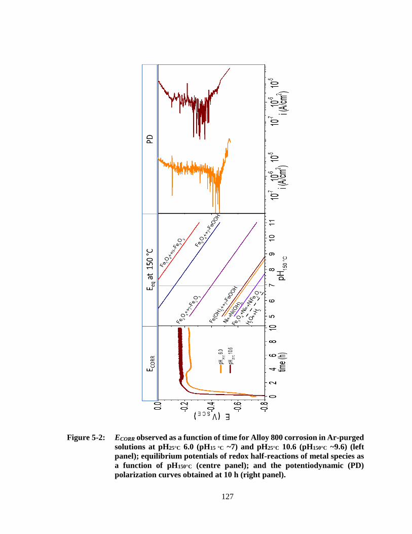
127

Figure 5-2: ECORR observed as a function of time for Alloy 800 corrosion in Ar-purged

solutions at pH25°C 6.0 (pH15 °C ~7) and pH25°C 10.6 (pH150°C ~9.6) (left

panel); equilibrium potentials of redox half-reactions of metal species as

a function of pH150°C (centre panel); and the potentiodynamic (PD)

polarization curves obtained at 10 h (right panel).

128

At pH25°C 10.6 the ECORR(10 h) value is above the Eeq (Fe3O4 -FeOOH) and close

to Eeq (Fe3O4 -Fe2O3). That is, the oxidation of Fe3O4 to -FeOOH and the dehydration

of -FeOOH to -Fe2O3 [11-13] can couple with the reduction of -Fe2O3 to Fe3O4. Note

that -Fe2O3 is a stable phase and if it has formed, its reduction would be slow. Therefore,

the ECORR(10 h) is close to Eeq (Fe3O4 -Fe2O3), due to the slow kinetics of the reaction.

At pH25°C 6.0 the ECORR(10 h) value is below the Eeq (Fe3O4 -FeOOH) and above the Eeq

(Fe(OH)2 -FeOOH). This is similar to the observed behaviour at lower temperature

presented in Chapter 4. Once Fe is oxidized to Fe2+, it hydrates forming Fe(OH)2 and it can

be further oxidized to -FeOOH. The electrode potential is below Eeq (Fe3O4 -FeOOH)

and causes reduction of -FeOOH to Fe3O4. In addition to Fe3O4 formation by this cycle,

reduction of -FeOOH can also oxidize Ni to NiII species (Ni(OH)2 and NiFe2O4 in the

presence of magnetite). Note that because Fe3O4 is in hydrolysis equilibrium with Fe2+(aq)

and Fe3+(aq) and -FeOOH is in equilibrium with Fe3+

(aq) the conversion from one oxide to

another is likely to occur through dissolution and precipitation. This catalytic redox coupling

will be established earlier at the pH with lowest solubility of a certain cation, due to the faster

saturation of the solution with Fe2+(aq) and Fe3+

(aq) and hence the faster formation of Fe(OH)2,

-FeOOH and Fe3O4 on the alloy surface.

The potential at which the current switches from negative to positive during PD scan

will be referred to as the potential of zero current (Ei=0). The potentials of zero current

(Ei=0(10 h)) are below the ECORR(10 h) values at both pHs. At pH25°C 6.0 (= pH150°C ~7) the

Ei=0(10 h) value is closer to the Eeq of the redox reaction between Fe3O4 and -Fe2O3, while

at pH25°C 10.6 (= pH150°C 9.6) the Ei=0(10 h) the value is closer to the Eeq of the redox reaction

between Fe3O4 and -FeOOH. These Ei=0(10 h) values are too high for the water reduction

half-reaction to effectively couple with the metal oxidation half-reactions (Figure 5-2).

Because at Ei=0 the overall oxidation rate is the same as the overall reduction reaction, the

PD scan results indicate that at pH25°C 6.0, the current as a function of potential near

Ei=0(10 h) is primarily determined by the oxidation and reduction cycle of Fe3O4 and -Fe2O3

and that of -FeOOH and Fe3O4 at pH25°C 10.6. The comparison of ECORR(10 h) with Eeq

indicates that adequate amounts of Fe3O4 and -Fe2O3 are present on the surface corroded

129

for 10 h at pH25oC 6.0 while sufficient amounts of -FeOOH and Fe3O4 are present on the

surface corroded for 10 h at pH25oC 10.6, to allow these redox cycles to occur.

The electrochemical analysis results are consistent with the results obtained in the

studies at room temperature and 80 oC presented in Chapter 4. The corrosion kinetic

pathways proposed from the low temperature studies are still applicable to the corrosion of

Alloy 800 in Ar-purged solution at 150 oC. The proposed corrosion pathways are presented

again here in Figure 5-3. The different observed behaviours at different temperatures can be

attributed to the fact that the rates of different elementary processes have different

temperature dependences.

Figure 5-3: Proposed Alloy 800 corrosion pathways

Alloy 800 corrosion kinetics at 150 oC over longer times (up to 5 d) were studied by

analyzing dissolved metal concentrations and the surfaces of coupons corroded for different

durations at pH25 °C 6.0 and pH25 °C 10.6 with or without -radiation present. The SEM images

of the surfaces and the dissolved concentrations of three different metal ions from the same

tests are presented in Figure 5-4.

130

Figure 5-4: Dissolved metal concentrations (Cr in blue, Fe in red and Ni in green)

and SEM micrographs of the surfaces of the coupons corroded for

different durations in Ar-purged solutions at pH25 °C 6.0 and 10.6 with -

radiation (Rad) or without -radiation present (No Rad). The

experimental uncertainties in the dissolved concentrations are indicated

with bars.

131

The dissolved metal concentrations are also listed in Table 5-1. Note that the

dissolved concentrations determined by ICP-OES include colloid particles dispersed in the

solutions as well as completely soluble species.

Table 5-1: Concentrations of metal cations dissolved over different durations of Alloy

800 corrosion in Ar-purged solutions at pH25o

C 6.0 and 10.6 at 150 oC with

radiation (Rad) and without radiation present (No Rad).

Duration

(h)

Concentration (M/cm2)

pH25 °C 6.0 pH25 °C 10.6

Cr Fe Ni Cr Fe Ni

No Rad

5 0.18 1.16 0.08 0.03 0.81 0.05

24 0.05 0.63 0.08 0.01 0.33 0.01

72 0.01 0.18 0.03 0.08 0.93 0.06

120 0.22 0.20 0.72 0.04 0.24 0.03

Rad

5 0.05 0.04 0.03 0.06 11.00 0.04

24 0.02 2.49 0.51 0.02 0.63 0.00

72 0.03 0.60 1.26 0.97 2.55 2.48

120 0.17 2.83 0.10 0.02 0.11 0.02

Although the ECORR reaches a steady state within 5 h (the first data collection time)

at a given pH without radiation present (Figure 5-2), the dissolved metal concentrations

fluctuate with time, showing wave patterns, under all conditions studied. The SEM images

of the surfaces also show changes in morphological characteristics with time. The dissolved

concentrations of metal cations are sometimes above their solubility limits except for the

solubility of ferrous ion. The solubilities for iron, chromium and nickel cations as a function

of pH at 150 °C were calculated from the Gibbs free energy of formation reported in literature

[5-8] and are presented in Figure 5-5.

132

Figure 5-5: Solubilities of FeII, FeIII, NiII and CrIII ions in water at 150 °C calculated

using the Gibbs free energies of formation reported in refs [5-8].

The decrease in the concentration of dissolved metal cations accumulated over the

duration of corrosion with time indicates that the fluctuation in dissolved metal concentration

is not due to fluctuation in the metal oxidation rate. While metal oxidation is occurring, the

overall amount of metal cation accumulated should increase, irrespective of the rate of

oxidation. Rather, the fluctuation in dissolved concentration indicates that the metal cations

dissolved at earlier times precipitate as solid oxide/hydroxide adhering to the surface at later

times. The period when dissolved metal concentration is observed to decrease is when the

rate of metal dissolution is lower than the precipitation of metal cation on solid metal

hydroxide and/or oxide.

The dissolved concentrations of individual metal ions as a function of time presented

in Figure 5-4 show wave patterns. For example, the dissolved Fe concentration is highest at

133

5 h (the first data collection time) under all conditions except for pH25 °C 6.0 with radiation.

This is followed by a decrease before the dissolved Fe concentration increases again. The

cycle of increase-decrease of dissolved concentration repeats within the studied duration.

Different metals have different rates of increase and decrease in dissolved concentration, and

the rates for individual metal cations depend on pH and whether radiation is present or not.

The cycling of dissolved metal concentration with time is a form of chemical wave,

a typical pattern produced by oscillating reactions. Chemical waves can be observed in the

time domain such as observed in the iodine clock reaction [14, 15], or in the space domain

such as observed in the Belousov–Zhabotinsky (B-Z) reaction [16-20]. Observation of a

chemical wave indicates that the reaction system is far from equilibrium and remains so for

a significant length of time. A feature of B-Z reactions is that they oscillate between two or

more metastable states. This does not contradict the laws of thermodynamics, as over longer

times these oscillations move towards equilibrium of the overall reaction system.

During corrosion, the concentration of dissolved metal cations in solution is initially

controlled by the rate of metal oxidation coupled with solution reduction. However, as

corrosion progresses and the solution becomes saturated with metal cations, the metal cations

precipitate and grow hydroxides/oxides. As the metal hydroxides/oxides grow they can

suppress further oxidation of metals. For Alloy 800 corrosion at 150 oC, the time to approach

the overall slow metal oxidation rate appears to be short (in 5 h). After 5 h the oxidation of

metallic species would have slowed down considerably.

The metal cations from oxide/hydroxide particles can be hydrated and hydrolyzed.

The dissolved metal cations that are in dynamic equilibrium with solid metal hydroxides can

diffuse into solution and then reprecipitate onto other oxide/hydroxide particles some

distance away. This coarsening (or Ostwald ripening) is considered mainly responsible for

the changes in the surface morphology and dissolved concentration at longer times. The wave

of dissolved metal concentration at times longer than 5 h may be attributed to the oscillation

between net dissolution (hydration and diffusion) of metal cations from oxide particles and

net precipitation of dissolved metal ions on oxide particles, while the overall amounts of

individual metal cations (as dissolved and oxide species) increase slowly as corrosion

134

progresses; see further discussion below. The metal oxides/hydroxides can further oxidize

and convert to different oxides.

The depth profiles of the atomic percentages (at.%) of the three main metal elements,

carbon and oxygen were determined by AES with Ar+ ion sputtering. The depth profiles for

the surface layers of the coupons corroded for 5 h and 120 h are shown in Figure 5-6.

The depth profiles presented in Figure 5-6 show that the C at.% near the surface is

significantly higher than its at.% in the bulk alloy and the front of the high C at.% moves to

a deeper depth with time. In addition, in the depth range over which the C at.% is high the

atomic percentages of Fe, Ni and Cr are very low while the O at.% is high. As discussed in

more detail later, these depth profiles suggest that the metal species have been dissolved from

this layer, enriching the fraction of carbon in the alloy bonded to titanium (which is very

low) in this layer. Note that a distinct solid phase of metal carbide is not likely to be present

in this alloy. However, carbon forms a strong covalent bond with titanium and chromium at

the alloying temperature in the interstitial sites of the FCC crystal structure of austenite and

is likely to be distributed uniformly in the alloy phase. These phases are hard to dissolve, and

as Fe and Ni (and to some extent Cr) dissolves into the solution, they remain on the surface.

Therefore, as the surface is sputtered by Ar+ in the AES analysis, because of depletion of Fe,

Cr and Ni, it shows a high C concentration. It should be noted that the first monolayers of C

on the surface might be because of contamination, but those deep into the metal are an

indication of carbon bonded to metals.

Dissolution of metal cations from the alloy phase results in high C at.% while very

low metal at.%. At later times, as the solution becomes saturated with the dissolved metal

cations, the metal cations can precipitate easily as metal hydroxide/oxide particles and films.

Accumulation of metal oxide/hydroxide increases the atomic percentages of metal elements

and O, and accordingly C at.% decreases. The depth profile of C at.% will depend on the

relative progression of dissolution and metal oxide growth.

135

Figure 5-6: AES depth analysis for coupons exposed to pH25°C 6.0 and 10.6 for 5 h

and 120 h in the presence and absence of radiation at 150 °C. The black

line represents oxygen, red Fe, blue Cr, green Ni and gray is C.

Due to the large contribution of C to the atomic percentages of other elements the

ratio of the atomic percentages of O to total metal (1.5Cr + Fe + Ni), not their absolute atomic

percentages, provides the type and thickness of the oxide/hydroxide deposited on the surface.

The depth profiles of O/(1.5Cr + Fe + Ni) obtained for the coupons corroded for 5 h and 120

h are compared in Figure 5-7. Also shown in the figure are the depth profiles of C at.% on

the same coupons. The depth at which the ratio of O/(1.5Cr + Fe + Ni) is one is the depth

where all of the metal species are present in oxide forms of metals in their lowest stable

oxidation states (e.g., FeCr2O4 and NiO). The depth at which the ratio is 0.5 thus represents

the average depth of the metal oxide/metal interface. The depth at which the ratio is 2.0 is

that at which the metal cations are in hydroxide forms, Cr(OH)3, FeOOH (or Fe(OH)2) and

Ni(OH)2. A ratio greater than 2.0 indicates the presence of highly hydrated metal cations

(e.g., Fe(OH)3‧3(H2O)) and adsorbed water molecules (or electrolyte ions). The ratio does

not stay constant with depth for all of the surfaces studied. The steep change in the ratio with

depth indicates that the oxides/hydroxides do not grow as pure or distinct oxide phases,

although with time they may slowly convert to stable distinct oxide phases. Note that the

lines representing different oxide compositions such as the line of O/(2Cr + 2Fe + 2Ni)

136

representing CrOOH, FeOOH and Ni(OH)2 can be constructed. However, the variation in

the ratio of O to metal is within a factor of 1.5.

Because of the continuous nature of the metal oxide/hydroxide transition, we define

the range between the depth at which the ratio is 0.5 and the depth at which the ratio is 3.0

(both arbitrary values based on the oxygen analysis) as the layer of metal oxide. The oxide

that grows on the surface can be considered as a spinel with a composition of NixFe1+xCr2-

2xO4 (0<x<1) where x=0 at the region close to the interface of metal and oxide and x=1 close

to the interface of solution and oxide. The range of depths shallower than this range is

depleted of metals and has not yet filled with metal oxides, consisting of mostly molecular

metal carbides and highly hydrated surfaces.

The average depth of the oxide/metal interface (i.e., the depth at which the ratio of

O/(1.5Cr + Fe + Ni) is 0.5) coincides with the depth at which the Ni at.% (Figure 5-6) is at

its maximum under all studied conditions. This is consistent with the general observation

that Ni is enriched at the interface of metal and oxide [21, 22]. This also indicates that Ni

dissolution is initially slower than Fe and Cr dissolution.

Under all studied conditions, the depth at which the interface lies increases steadily

with corrosion time. At 5 h the interface front is at a deeper depth at pH25 °C 10.6 than at

pH25 °C 6.0 without or with radiation present. However, the interface front moves more slowly

at pH25 °C 10.6 than at pH25 °C 6.0, and the difference in the interface depths at the two pH25 °C

values is much smaller at 120 h. These observations indicate that the rate of metal dissolution

is initially higher at higher pH, but metal dissolution continues longer at a lower pH. As

discussed in detail later, rates of surface hydration and hydrolysis of metal cations are higher

at a higher pH. This can explain the observation that the oxide/metal interface is at a greater

depth for the coupons corroded for 5 h at pH25 °C 10.6 than at pH25 °C 6.0. However, the faster

the dissolution of metal cation, the faster the solution near the surface becomes saturated by

the metal cation, and the hydroxide/oxide of the metal cation is formed earlier and grows

faster. The solubilities of metal cations are in general lower at pH25 °C 10.6 than at pH25 °C 6.0

(Figure 5-5). The combination of faster hydrolysis and lower solubility at pH25 °C 10.6 thus

promotes earlier and faster growth of metal oxide particles and films on the surface,

passivating the surface earlier.

137

Figure 5-7: Oxygen and carbon analysis of AES results on Alloy 800 after 5 h and

120 h immersion at pH25°C 6.0 and 10.6 at 150 °C in the presence and

absence of -radiation. The dashed vertical lines shows where the ratio is

0.5, 1.0 and 2.0. The ratio of 0.5 for the oxygen line is considered to be the

interface of metal and oxide, 1.0 is the oxide region and 2.0 is the

hydroxide layer.

The depleted region changes with pH and the presence of radiation. Without

radiation, the depth range increases with time at both pHs. With radiation, the change is not

significant for pH25 °C 6.0 while it increases with time at pH25 °C 10.6. The reason for the

different behaviour at pH25 °C 6.0 in the presence of radiation could be the homogeneous

oxidation of metal cations (mostly Fe) in the solution, as reported previously [23].

138

Corrosion at first 5 h

The rate of metal dissolution will be highest at the beginning of corrosion when the

solution is free of metal cations. The electrochemical results presented in Figure 5-2 indicate

that the ECORR already reaches a high steady-state value by 5 h, and the overall metal

oxidation rate should slow down considerably by the time the ECORR reaches the steady-state

value. Thus, most of metal dissolution occurs in the first 5 h, and perhaps even earlier.

The evolution of Alloy 800 corrosion at 150 oC in the first 5 h is difficult to observe

experimentally. However, the ECORR and the PD polarization results indicate that while the

ECORR approaches steady state faster, Alloy 800 corrosion at 150 oC involves the same metal

oxidation reactions and transport processes as those observed at lower temperatures, as

schematically shown in Figure 5-3.

The proposed mechanism suggests that corrosion of Alloy 800 proceeds first by

oxidizing Fe0 to FeII which quickly dissolves into solution as Fe2+(aq). Because its solubility

is high at all pHs the dissolution can continue for some time. The concentration near the

surface is determined by the rate of its production (i.e., Fe0 oxidation to FeII) and the rate of

FeII removal from the surface. The removal of metal cation from the surface of solid metal

or solid metal oxide requires hydration of the metal cation followed by diffusion from the

surface to the bulk solution phase. The surface hydration of metal cation increases with an

increase in pH (assisted by base catalyzed hydrolysis) and with temperature.

As the metal oxidation continues the concentration of Fe2+(aq) in the solution near the

surface increases. When the concentration of Fe2+(aq) in the solution near the surface

approaches its saturation limit, the diffusion of Fe2+(aq) from the surface into the solution

phase is significantly hindered. This slows down the net dissolution of the FeII species to the

solution phase and the concentration of FeII on the surface increases and the formation of

FeCr2O4 and hydrolysis of Fe2+(aq) to Fe(OH)2 increase accordingly. The FeII species on the

surfaces of metal or growing oxide/hydroxide particles are also more easily oxidized to the

less soluble FeII/FeIII oxide (Fe3O4) and/or -FeOOH, compared to homogeneous solution

oxidation. Thus, once the solution near the metal surface becomes saturated with Fe2+(aq) the

growth of iron hydroxides/oxides is accelerated.

139

As the layer of solid oxide/hydroxide particles grow, the oxidation of Fe0 to FeII slows

down because an oxide layer present on metal surface is an energy barrier for metal

oxidation. The conversion of the FeII species to the less soluble FeIII species will deplete the

surface of adsorbed ferrous ions, and Fe2+(aq) will continue to adsorb on the surface.

The ECORR values observed at 5 h are also above the Eeq of Ni0 oxidation to NiII and

hence dissolution of Ni2+ also occurs. Similarly, once the solution near the surface reaches

the NiII saturation limit, the formation and growth of Ni(OH)2 and/or NiFe2O4 starts to

accelerate. The rate of nickel oxidation is affected by the type of iron hydroxide/oxide as

well as the nickel hydroxide/oxide that forms and grows. The overall nickel oxidation slows

down while the growth of Ni(OH)2 and/or NiFe2O4 by precipitation of Ni2+(aq) continues,

decreasing the concentration of Ni2+(aq). The surface of Alloy 800 would be covered with air-

formed Cr2O3. Dissolution of Cr is limited by the hydration and hydrolysis of CrIII ions from

the chromium oxide which is replenished by oxidation of Cr0 to Cr2O3. As the FeCr2O4 starts

to form by precipitation of Fe2+(aq) and Cr3+

(aq) the dissolved Cr concentration can decrease.

The observed effects of pH on Alloy 800 corrosion in Ar-purged solutions at 150 oC

over 5 h can thus be explained as follows. The pH has a negligible effect on the driving force

(or overpotential) of metal oxidation coupled with water reduction (because of the same pH

dependences of the metal redox half-reaction and the water reduction half-reaction).

However, pH affects the rate of surface hydration and hydrolysis of metal cation and the

solubility of metal cation. The net dissolution rates of Fe2+(aq) and Ni2+

(aq) are initially higher

at pH25 °C 6.0 than at pH25 °C 10.6. Their solubility limits are higher at pH25 °C 6.0 than at

pH25 °C 10.6. Thus, the rate of metal dissolution is initially faster at pH25 °C 6.0 than at

pH25 °C 10.6 and the maximum dissolved concentration reached is higher at pH25 °C 6.0 than

at pH25 °C 10.6 because hydroxide/oxide formation is negligible until the concentration of

Fe2+(aq) in the solution near the surface reaches its saturation limit.

The faster metal dissolution at pH25 °C 6.0 than at pH25 °C 10.6 at early stages of

corrosion is consistent with the observed depth profiles of the atomic percentages of C and

the three metal elements determined by AES (Figure 5-6). On the coupon corroded for 5 h

without radiation present the depth at which the Ni at.% is maximum and the C at.% is

140

approximately that of the bulk alloy phase, and is deeper at pH25 °C 6.0 than at pH25 °C 10.6.

This layer is severely depleted of Fe, Ni and Cr. However, the dissolved concentrations of

all three metal elements observed at 5 h are lower at pH25 °C 10.6 than at pH25 °C 6.0,

indicating that the concentrations of these ions near the surface may have reached their

solubility limits and that hydroxide/oxide formation has occurred more significantly at

pH25 °C 10.6 than at pH25 °C 6.0. These observations are consistent with the observed effect of

pH over 5-h corrosion on the depth profile of O at.% (Figure 5-7) as well as the surface

morphology observed by SEM (Figure 5-4).

Corrosion under -radiation in the first 5-h seems to be faster than that with no

radiation. For pH25°C 10.6, dissolved Cr concentration is almost double of that of no radiation

and it is more than an order of magnitude higher for Fe while Ni dissolution is similar to the

No Rad condition. Also, for this sample, oxide is thicker than its no radiation counterpart.

These observations suggest that the rate of corrosion is higher in the presence of radiation

because radiolytic products act as oxidants and increase the overall rate of oxidation.

At pH 6.0, the results are different from that of no radiation. The dissolved metal

cation concentrations are lower than those with no radiation and the oxide is thicker. This

observed difference could be because of partial radiolytic oxidation of metal cations and

formation of nano-particles. In the other words, the highest dissolved metal concentation in

the presence of radiation might have been attained at a time shorter than 5 h. Therefore, it is

possible that similar behaviour to that of no radiation happens in the presence of radiation,

albeit in a shorter time scale than that studied here.

Corrosion at longer times

As exposure time increases the depleted region changes as well as the morphology

and the amount of dissolved metal cations in the solution. The ECORR measurement shows

that corrosion potential does not change significantly and no other oxidation / reduction

reactions except for those already seen in the shorter time are taking place. This suggests a

significant role for the solution pH at longer times. The solution pH dictates the solubility of

metal cations (Figure 5-5) and the difference between ECORR and Eeq (Figure 5-2) and

therefore, the corrosion pathway (Figure 5-3). The rate of solution reduction species is

141

significantly lower and most of metal and oxides oxidation is coupled with the reduction of

oxides with higher oxidation state. The adsorbed metal cations on the surface can precipitate

on the surface and form an oxide or diffuse into the solution. In the presence of radiation,

radiolytic precipitation of metal oxides is possible.

When time increases from 5 h to 24 h, the number of oxide particles on the surface

increases. This increase is greater for pH25 °C 10.6 than that for pH25 °C 6.0, which is consistent

with the more significant drop in the dissolved metal cations determined by ICP for pH25 °C

10.6. At both pHs, the surface is covered with more oxide for the sample exposed for 72 h

than that for 24 h. However, the morphology of oxide is different as it is more dispersed

small particles with size less than 100 nm for the pH25 °C 6.0 sample and filament-like film

for pH25 °C 10.6. It seems that the particles that form after 24 h (at pH25 °C 6.0) did not grow

and there are more particles that nucleated on the surface. The ICP-OES measurements

support this interpretation, as the concentration of the dissolved metal cations decreased from

24 h to 72 h at this pH. However, the sample immersed in a pH25 °C 10.6 solution has oxides

with a filament-like morphology. This type of morphology was previously reported for

transition metals at alkaline pH [3, 24-28]. The surface morphology after 72 h shows denser

and smaller filament-like oxides than those after 24 h at the same pH. However, the only

difference between 24 h and 5 h at pH25 °C 10.6 with no radiation is the increase in the number

of the filament-like oxides. The fact that the morphology of the sample after 72 h is different

from shorter times suggests that the type of oxide that forms on the surface is different in this

case. This new type of oxide is probably formed because of the change in the oxidation

pathway. The final morphology of the oxide on the surface after 120 h shows filament-like

oxide for both pHs. However, the filaments are larger at pH25 °C 6.0 than that at pH25 °C 10.6.

Generally, oxides are thicker at longer times; however, the change in the thickness is pH-

dependent.

The dissolved metal concentration of Cr at pH25 °C 6.0 under radiation is similar to

that with no radiation except for the continuous increase in the metal cation concentration in

the solution from 24 h to 120 h, after the initial drop from 5 h to 24 h. Cr dissolution at pH25

°C 10.6 and Ni dissolution at both pH under radiation show an initial increase in the dissolved

metal concentrations up to 72 h but then decrease as time increases to 120 h. Iron dissolution

142

at pH25 °C 10.6 under radiation mirrors that of no radiation except for the faster rate of

dissolution or redeposition. This shows that at pH25 °C 10.6, radiation affects mainly the rate

at which iron dissolves or forms an oxide.

The morphology of the oxides on the surface is similar to that in the no radiation

experiments except for the size of particles and the density and length of the filament-like

oxides. The only significant difference is observed for pH25 °C 6.0 after 120 h of experiments

which shows a surface where the particles that formed earlier are flattening on the surface

and forming an oxide layer instead of forming oxide filaments. In addition, at pH25 °C 6.0, the

particles formed under radiation are more spherical rather than the elongated oxides formed

in the absence of radiation. This may be due to the fast redeposition of the oxide on the

surface. As this rate is very high, the particles prefer to maintain the lowest possible surface

area to volume, which produces spheres.

The concentrations of metal cations dissolved during corrosion with radiation present

determined by ICP-OES are far above their solubility limits which also suggests that some

of these metal cations may be present as hydroxide/oxide colloid particles dispersed

uniformly in the solutions. Consequently, the ICP-OES analysis required considerable

digestion of the solution samples prior to the analysis.

Conclusions

The effects of pH and γ-radiation on oxide formation and metal dissolution on Alloy

800 surface in high temperature aqueous solution were investigated by coupon exposure

experiments and electrochemical tests. The results show that the rates of oxide formation and

metal dissolution vary with pH, but the main effect of γ-radiation is on the oxidation rate.

Normally, the oxide formed at pH25°C 10.6 is thicker than that at 6.0. Homogeneous radiolytic

oxidation of metal cations happens at pH25°C 6.0 but not at pH25°C 10.6. The oxide that grows

on the surface can be considered to be a spinel with the composition of NixFe1+xCr2-2xO4

(0<x<1) where x=0 at the region close to the interface of metal and oxide and x=1 close to

the interface of solution and oxide. The electrochemical experiments show that at higher pHs,

the difference in the equilibrium potential of oxidation (Eeq) and corrosion potential (ECORR)

143

is higher than that at low pH. This indicates that at higher pH, the oxide film provides a

greater potential barrier for the oxidation reaction.

References


today, 11 (2008) 32-37.



[3] A. Musa, J. Wren, Combined effect of gamma-radiation and pH on corrosion of Ni–Cr–

Fe alloy inconel 600, Corrosion Science, 109 (2016) 1-12.

[4] J. Killeen, F. Nordmann, J. Schunk, K. Vonkova, Optimisation of water chemistry to

ensure reliable water reactor fuel performance at high burnup and in ageing plant

(FUWAC): an International Atomic Energy Agency coordinated research project, (2010).

[5] B. Beverskog, I. Puigdomenech, Revised Pourbaix diagrams for iron at 25–300 C,


[6] B. Beverskog, I. Puigdomenech, Revised Pourbaix diagrams for nickel at 25–300 C,


[7] B. Beverskog, I. Puigdomenech, Revised Pourbaix diagrams for chromium at 25–300

C, Corrosion Science, 39 (1997) 43-57.


chromium-nickel, Corrosion, 55 (1999) 1077-1087.

[9] O. Kubaschewski, C.B. Alcock, P.J. Spencer, Materials thermochemistry, Pergamon

Press, 1993.

[10] J. Majzlan, E. Lang Brian, R. Stevens, A. Navrotsky, F. Woodfield Brian, J. Boerio-

Goates, Thermodynamics of Fe oxides: Part I. Entropy at standard temperature and

pressure and heat capacity of goethite (α-FeOOH), lepidocrocite (γ-FeOOH), and

maghemite (γ-Fe2O3), in: American Mineralogist, 2003, pp. 846.

[11] J.W. Geus, Preparation and properties of iron oxide and metallic iron catalysts,

Applied Catalysis, 25 (1986) 313-333.

[12] H. Franz, Process for the preparation of gamma-FeOOH, in, Google Patents, 1968.

[13] R. Jasinski, A. Iob, FTIR measurements of iron oxides on low alloy steel, Journal of

the Electrochemical Society, 135 (1988) 551-556.

144

[14] A.P. Oliveira, R.B. Faria, The chlorate− iodine clock reaction, Journal of the

American Chemical Society, 127 (2005) 18022-18023.

[15] R.S. Mitchell, Iodine clock reaction, J. Chem. Educ, 73 (1996) 783.

[16] Y. Pomeau, J. Roux, A. Rossi, S. Bachelart, C. Vidal, Intermittent behaviour in the

Belousov-Zhabotinsky reaction, Journal de Physique Lettres, 42 (1981) 271-273.

[17] V.K. Vanag, I.R. Epstein, Pattern formation in a tunable medium: The Belousov-

Zhabotinsky reaction in an aerosol OT microemulsion, Physical review letters, 87 (2001)

228301.

[18] V.K. Vanag, A.M. Zhabotinsky, I.R. Epstein, Oscillatory clusters in the periodically

illuminated, spatially extended Belousov-Zhabotinsky reaction, Physical review letters, 86

(2001) 552.

[19] V. Petrov, V. Gaspar, J. Masere, K. Showalter, Controlling chaos in the Belousov—

Zhabotinsky reaction, Nature, 361 (1993) 240-243.

[20] L. Györgyi, R.J. Field, A three-variable model of deterministic chaos in the Belousov–

Zhabotinsky reaction, Nature, 355 (1992) 808-810.

[21] C.-O. Olsson, D. Landolt, Passive films on stainless steels—chemistry, structure and

growth, Electrochimica acta, 48 (2003) 1093-1104.

[22] I. Olefjord, B.-O. Elfstrom, The composition of the surface during passivation of

stainless steels, Corrosion, 38 (1982) 46-52.

[23] T. Sutherland, C. Sparks, J. Joseph, Z. Wang, G. Whitaker, T. Sham, J. Wren, Effect

of ferrous ion concentration on the kinetics of radiation-induced iron-oxide nanoparticle

formation and growth, Physical Chemistry Chemical Physics, 19 (2017) 695-708.

[24] K. Daub, X. Zhang, L. Wang, Z. Qin, J.J. Noël, J.C. Wren, Oxide growth and

conversion on carbon steel as a function of temperature over 25 and 80°C under ambient

pressure, Electrochimica acta, 56 (2011) 6661-6672.


potential: Probing the role of gamma-radiation, Electrochimica acta, 80 (2012) 90-99.

[26] M. Behazin, M.C. Biesinger, J.J. Noël, J.C. Wren, Comparative study of film

formation on high-purity Co and Stellite-6: Probing the roles of a chromium oxide layer

and gamma-radiation, Corrosion Science, 63 (2012) 40-50.



145

[28] A.Y. Musa, M. Behazin, J.C. Wren, Potentiostatic Oxide Growth Kinetics on Ni-Cr

and Co-Cr Alloys: Potential and pH Dependences, Electrochimica Acta, 162 (2015) 185-

197.

146

6 Chapter 6

The Effect of Oxygen Content and Gas Phase Radiolysis on

Corrosion of Alloy 800H in High-Temperature Steam

Introduction

The importance of safe and optimal operation of nuclear power plants motivates

researchers to better understand the factors influencing the corrosion of metal alloys.

Uniform corrosion of system components in nuclear reactors introduces dissolved metal

impurities in the reactor coolant that can lead to the formation of insoluble metal oxide

particulates that deposit in the heat transport system. In addition, the circulation of these

dissolved metal species through the reactor core can cause neutron absorption by stable

isotopes to form radioactive products (e.g., 54Mn, 58Co, 59Fe, 60Co, or 58Ni) [1]. Deposition

of radioactive materials on coolant system components outside of the shielding of the reactor

core creates a potential source of radiation exposure for plant workers.

The emphasis in this study is on the effects of radiolysis products on the corrosion of

structural materials in high temperature steam. Strongly oxidizing radiolysis products such

as H2O2 and O2 can interact with the protective oxide on different materials and influence

their subsequent corrosion behaviour. Furthermore, it is important to understand the release

of corrosion products from these structural materials, as this influences the radioactivity

transport within the coolant circuit.

This study investigates the effect of O2 and -radiation on Alloy 800H corrosion in

steam at 285 oC. Alloy 800H is one of the candidate fuel cladding materials being

investigated for potential use in a Canadian design of a Generation IV supercritical water

reactor (SCWR). Because the solvent properties [2-10] and the radiolysis kinetics [10] of

SCW lie somewhere between those of liquid water and steam, this study on steam corrosion,

combined with existing studies [10-17], may provide an insight into SCW corrosion of Alloy

147

800H and, in particular, the effect of -radiolysis on the SCW corrosion. Due to difficulties

in performing SCW corrosion tests in the presence of high dose -radiation, it has been

suggested that SCW corrosion in the highly oxidizing environment induced by radiolysis

could be simulated by adding a high concentration of O2 into SCW. This study tries to

partially address this possibility by performing corrosion tests with different O2

concentrations in steam with or without radiation present.

Experimental

Materials

The Alloy 800H was purchased in rod form (American Special Metals Corp.). The

chemical composition of this alloy is given as (in wt.%) 45 Fe, 31 Ni and 23 Cr. The rod was

cut into discs. The total surface area of Alloy 800H exposed in each experiment was

9.12 cm². Prior to each experiment, the discs were ground manually in sequence with 180,

400, 800 and 1200 grit silicon carbide papers, followed by polishing on a Texmet micro cloth

(Buehler) with a 1 µm MetaDi Supreme diamond paste suspension (Buehler), and lastly,

sonication in a 1:1 acetone/methanol mixture for five minutes to remove polishing residues.

Experimental Conditions

Corrosion experiments were conducted in saturated steam at 285 °C. The corrosion

studies were carried out in a 300 mL AISI 316 stainless steel autoclave purchased from Parr

Instrument Company. The test specimens were arranged in a pre-oxidized zirconium

specimen holder to ensure no exposure of the test specimen to the condensed phase during

the experiments. At the time of closure, the autoclave contained 20 mL (only 7% of the

autoclave volume) of liquid Type-1 water (Barnstead International NANOpure Diamond

UV, 18.2 MΩ·cm). The gaseous headspace of the vessel was filled with either ultra-high

purity Ar (99.999%, Praxair), or a 35% O2 + 65% Ar or a 50% O2 + 50% Ar mixture

(Praxair), which was introduced by sparging the partially closed vessel for 90 min before the

autoclave was sealed. The experiments were carried out either during exposure to -radiation

or without radiation. The duration of each exposure was 5 h.

148

All experiments involving irradiation were conducted in a MDS Nordion

Gammacell 220 Excel Cobalt-60 irradiator. As described in Chapter 3, in irradiation

experiments, the autoclave was positioned inside the gammacell sample chamber, and the

chamber lowered into the gammacell irradiation zone, centred within a cylinder bounded by

11 tubular pencils containing 60Co. The dose rate during the period of experimentation was

3.1-3.3 kGy·h−1, as calibrated by Fricke dosimetry.

Surface Characterization

Scanning electron microscopy (SEM) images were obtained using a LEO (Zeiss)

1540XB focussed ion beam (FIB)/SEM/EDX. X-ray photoelectron spectroscopic (XPS)

analyses were performed using a Kratos Axis Ultra XPS with a monochromatic Al K(α)

source. Raman scattering measurements were performed using a Renishaw model 2000

instrument. Auger electron spectroscopy (AES) combined with argon-ion sputtering

provided a depth profile of the chemical composition of surface oxides. The AES analyses

were performed using a Physical Electronics Model PHI 660 instrument with an excitation

energy of 5 keV.

Results

The surfaces of Alloy 800H coupons corroded for 5 h in saturated steam containing

different concentrations of O2 with or without radiation present were examined using several

surface analysis techniques. The SEM micrographs are shown in Figure 6-1. On the sample

exposed to 285 °C saturated steam in an Ar atmosphere in the absence of radiation, scattered

crystallites of 100 nm dimensions were observed to be distributed over a surface that appears

to have experienced only minor amounts of corrosion, since the scratches from surface

preparation are still clearly visible. This picture shows that there is no preferential site for

nucleation of particles and they are randomly distributed on the surface. The sample exposed

to 285 °C saturated steam with added 35 % oxygen showed numerous particles, mostly in

the ~30 nm range, carpeting the Alloy 800H surface. Here also the superficial scratches from

the initial surface preparation remain visible, indicating that the total amount of corrosive

attack was minimal, but in this case the fine particulate corrosion products are found

149

everywhere on the surface including the ridges and valleys of surface scratches, however

they are too small to obscure the surface topography. The surface of the sample exposed to

the 50 % O2 shows an underlying oxide layer which is covered by secondary oxide particles.

These particles (generally less than few nm size) are agglomerated locally to form a network

of particles linked to each other. The effect of change in the oxygen content of environment

can be clearly seen in the number of particles nucleated on the surface and their size after

growth.

In the presence of gamma radiation, in the Ar environment, Alloy 800H appears

similar to the one in the absence of radiation except for the size and distribution of the

particles on the surface. In this case, number of density of particles is less and they are bigger

in the size than the one in the absence of radiation. In oxygen-bearing steam at 285 °C, with

the autoclave exposed to gamma radiation, only a few, widely dispersed filaments of

deposited material could be seen, along with the scratches from surface preparation.

However, in the presence of 50% O2, these particles seem to form on top of a thick oxide

layer underneath.

The oxide morphology analysis shows that the effect of change in the oxygen content

is not as significant as the presence of radiation. In the presence of radiation, increase in the

oxygen content significantly affect the surface morphology and oxide thickness. However,

in the absence of radiation, when oxygen content increases, change in the corrosion rate is

not as fast as in presence of radiation. In fact, it seems that presence of radiation completely

changes the corrosion pathway however, oxygen only changes the rate at which the reactions

happen under saturated steam corrosion.

150

Figure 6-1: SEM micrographs of the surfaces of Alloy 800H coupons exposed for 5 h

to saturated steam in Ar gas containing different O2 concentrations,

without (No Rad) or with (Rad) -radiation present.

The Raman spectra are compared with the spectra of standard powder samples of

various Cr, Fe and Ni oxides in Figure 6-2 [18]. Although more granular particles are present

on the coupons corroded without radiation, the intensities of the Raman spectra are much

Rad35

% O

2No Rad

0%

O2

2 μm

50%

O2

151

lower than those observed for the coupons corroded with radiation. For the coupons corroded

without radiation present, the spectrum of the coupon corroded in 0% O2 in Ar shows the

peaks that correspond to the two main peaks of FeCr2O4 and the main peak of Fe3O4 while

that spectrum of the coupon corroded in 50% O2 in Ar matches more closely that of magnetite

(Fe3O4). For the coupons corroded with radiation present, the spectrum of the coupon

corroded in 35% O2 in Ar consists of the main peak associated with Fe3O4 and minor peaks

that are associated with CrOOH and Ni(OH)2. The Raman spectrum of the coupon corroded

in 50% O2 in Ar is similar to that observed for the coupon corroded in a lower O2

concentration environment, but the intensities of the peaks associated with Fe3O4 and

Ni(OH)2 are higher while those of CrOOH are lower.

The Raman analysis suggests that the main oxide present on these surfaces is Fe3O4

(except for the coupon corroded in 0% O2 in Ar without radiation present). However, the

morphologies of the granular oxide particles are very different. These observations suggest

that the oxide particles may grow into different shapes and that the oxide morphology

evolution depends on the exposure environment. The oxide thickness and the depth variation

of the oxide composition can provide some information on oxide growth.

152

Figure 6-2: Raman spectra of the surfaces of Alloy 800H coupons exposed for 5 h to

saturated steam in Ar gas containing 0% or 50% O2, without -radiation

present and spectra for surfaces exposed in Ar gas containing 35% or

50% O2 with -radiation present. Shown below the coupon spectra are

the spectra of standard powder samples of various Cr, Fe and Ni oxides.

The Raman shifts of the main peaks of these oxides are also noted on the

top of the coupon spectra [18].

153

The XPS analysis was performed to determine the oxidation-state composition of the

metal elements in the top ~ 8 nm surface layer. A low-resolution survey spectrum over a

wide binding energy range of 0 to 1200 eV and high-resolution spectra over the binding

energy ranges of Cr-2p3/2, Fe-2p3/2 and Ni-2p3/2 along with those of O-1s and C-1s were

taken. Examples of the raw XPS spectra are shown in Figure 6-3. The high-resolution XPS

spectra were deconvoluted using reference spectra taken from well-characterized oxide

powder samples to obtain the composition of the oxidation states present of individual metal

elements. For chromium, contributions of Cr0, Cr2O3, Cr(OH)3 and CrVI to the Cr-2p3/2

spectra were considered. For iron, those from Fe0, FeO, Fe3O4 (mixed FeII/FeIII oxide), Fe2O3

and FeOOH to the Fe-2p3/2 spectra, and for nickel those of Ni0, NiO and Ni(OH)2 to the Ni-

2p3/2 spectra were considered. The separation of metal oxide from metal hydroxide was

further aided by deconvolution of the O-1s and C-1s spectra (results not shown). Detailed

descriptions of binding energies and the spectral deconvolution method can be found

elsewhere [19-22]. The results of the deconvolution of the high-resolution XPS data into

metallic and oxidized components for the three main metal elements are presented in Figure

6-4.

154

Figure 6-3: XPS spectra taken from an Alloy 800H surface corroded for 5 h in

saturated steam in 50% O2 in Ar at 285 oC without -radiation: (a) the

survey spectrum and the high-resolution spectra of (b) Ni 2p3/2, (c) Fe

2p3/2 and (d) Cr 2p3/2. Also shown are the deconvoluted spectra of

individual components, each consisting of multiple peaks, and the fitted

spectra from the deconvoluted spectra.

155

Figure 6-4: Oxidation-state compositions of chromium (blue), iron (red) and nickel

(green) determined by XPS analysis of Alloy 800H coupons exposed for 5

h to saturated steam in Ar gas containing different O2 concentrations

without (No Rad) or with (Rad) -radiation present. The atomic

percentages of metallic components are shown with white bars, those of

oxide components with solid bars, and those of hydroxides or

oxyhydroxides with patterned bars.

Except for the surface layer of the coupon corroded in 0% O2 in Ar with radiation

present, the metallic fractions are small but not negligible. For a given radiation condition,

the metallic fraction is generally lower at a higher O2 concentration in the exposure

environment. The lower the metallic fraction is, the thicker the oxide layer is. Interestingly,

156

for the coupons corroded in 0% O2 in Ar, the metallic fraction is higher on the coupon

corroded with radiation than on the one corroded without radiation present. However, the

metallic fraction decreases more extensively with increased O2 concentration in the exposure

environment with radiation present. Consequently, with radiation present the metal fraction

is extremely small or zero in the surface layer of the coupon corroded in 35% O2 or 50% O2.

Comparison of the oxidation-state compositions presented in Figure 6-4 with the

surface morphologies presented in Figure 6-1 provides interesting observations. The coupon

corroded in 50% O2 without radiation present shows more granular oxide than the one

corroded with radiation present, but the XPS analysis results indicate that the average

thickness of the oxide present on the coupon corroded without radiation present is thinner

(there is a higher metallic component) than that on the coupon corroded with radiation

present. Similarly, with radiation present the number density of oxide particles decreases

with increasing O2 concentration while the average thickness of the oxide increases.

The ratio of hydroxide to oxide fraction in the surface layer shows a different

dependence on O2 concentration depending on the metal element. For chromium, the

oxidized components in the surface layer are CrIII oxide and CrIII oxyhydroxide. Although

they are labeled as Cr2O3 and Cr(OH)3 they may not be present as pure Cr2O3 and Cr(OH)3

phases. For nickel, the oxidized components in the surface layer are NiII oxide and NiII

hydroxide. Although the NiII oxide is labeled as NiO in Figure 6-4 it may be present as

NiFe2O4 and NiCr2O4. For iron, the oxidized components in the surface layer are FeII/FeIII

oxide (labeled as Fe3O4), FeIII oxide (labeled as Fe2O3) and FeIII oxyhydroxide (FeOOH).

On the coupons corroded without radiation present, the oxyhydroxide fraction of iron

in the surface layer increases, while the metallic Fe0 fraction decreases, with increasing O2

concentration in Ar. For chromium, the hydroxide fraction is lowest while the metallic

fraction is highest on the coupon corroded in 35% O2 in Ar. For nickel, the NiII is all in the

form of hydroxide and the dependence of the NiII hydroxide fraction on the O2 concentration

follows that of Cr. These observations suggest that Ni(OH)2 and Cr(OH)3 are present in the

outer-most surface layer and underneath this hydrated and hydroxide layer is a layer of iron

oxides/hydroxides that grows thicker in a higher O2 environment.

On the coupons corroded with radiation present, the metallic fractions of all three

metal elements decrease with increasing O2 concentration. However, the Cr(OH)3 fraction

157

decreases with increasing O2 concentration, the opposite trend to that observed without

radiation present. In addition, the FeOOH and Ni(OH)2 fractions are highest when the O2

concentration is 35%. In 50% O2 in Ar, the average thickness of oxide is thicker than 8 nm

and within this surface layer, most of the chromium is present as CrIII oxide and most of the

iron is present as mixed FeII/FeIII oxide and FeIII oxide, while a significant fraction of the

oxidized nickel is in the form of NiII oxide as well as NiII hydroxide.

The XPS analysis results are consistent with the Raman analysis results. The

combined results indicate that during 5 h steam corrosion without radiation present the metal

oxidation progresses up to the oxidation of Fe0 to FeII forming FeCr2O4 (in the presence of

Cr2O3) but not to the oxidation to FeII/FeIII and FeIII oxides/hydroxides. The rate of formation

of Fe3O4 (and its conversion to -Fe2O3) increases with increasing O2 concentration. Without

radiation present the oxidation of Ni0 to NiII is limited to the formation of a few monolayers

of Ni(OH)2. The rates of the oxidation reactions are slow without radiation present even

under high O2 concentration conditions. The higher fractions of Cr(OH)3 and Ni(OH)2 with

an increase in O2 concentration are consistent with the claim that the formation of FeII/FeIII

and FeIII oxides is not fast enough to cover the metal surface quickly enough to suppress the

hydration and hydrolysis of CrIII ions from Cr2O3 and FeCr2O4, and the oxidation of Ni0 to

NiII, see further discussion later.

Gamma-radiolysis of water produce stronger oxidants than O2, such as OH and

H2O2 [23]. Hence, the rates of the oxidation of Fe0 to Fe3O4 (-Fe2O3) and Ni0 to NiII oxide

and hydroxide will all increase with radiation present. Of the radiolytically produced

oxidants, H2O2 is the more effective oxidant for surface reactions, and the steady-state

concentration of H2O2 produced by a continuous radiation flux increases with an increase in

O2 concentration in steam. This is consistent with the observed increases in the Raman peaks

associated with Fe3O4 (-Fe2O3) and Ni(OH)2 and the reduction in the peaks associated with

Cr(OH)3 with increasing O2 concentration with radiation present.

The SEM, Raman and XPS analysis results all indicate that different oxides are

formed at different rates and different stages of corrosion. The rates of individual oxide

formation and growth vary depending on O2 concentration and whether radiation is present

or not. To understand how the oxidation may have progressed over 5-h corrosion the depth

profiles of different metal elements and O atom were examined by AES with Ar+ sputtering.

158

The depth profiles of atomic percentages of three main metal elements (Cr, Fe and Ni) and

oxygen (O) are presented in Figure 6-5.

The depth profiles of elemental atomic percentages show four depth ranges with

different characteristic depth dependences. The four depth zones are most noticeable on the

coupon corroded in 50% O2 in Ar with radiation present, and the different zones on the depth

profiles of this coupon are illustrated in Figure 6-6. Also shown in the figure are the depth

profiles of atomic percentage ratios of O/(Fe + Ni + 1.5Cr) and O/(1.5Fe + 2Ni + 1.5Cr). On

this coupon, in the depth range of 0 - 8 nm (zone 1) the Cr at.% and Ni at.% remains nearly

constant with depth at ~ 5 at.%, while the Fe at.% increases very slowly with increasing

depth and the O at.% decreases at a similar rate. In zone 1, the ratio of O/(1.5Fe + 2Ni +

1.5Cr) is greater than 1.0. In depth range of 8 – 18 nm (zone 2), the Cr at.% and the Ni at.%

increase with increasing depth while the Fe at.% and the O at.% decrease with increasing

depth. In zone 2, the rate of decrease in the Fe at.% is faster than that of the O at.%. In this

zone, the ratio of O/(1.5Fe + 2Ni + 1.5Cr) is less than 1.0 while the ratio of O/(Fe + Ni +

1.5Cr) is greater than 1.0. At greater depths (> 18 nm) the O at.% decreases sharply while

the atomic percentages of all three metal elements increase. The Fe at.% and the Cr at.%

increase steadily until they reach constant values as the O at.% decreases to a background

level (~ 5 at.%), but the Ni at.% shows a maximum at ~ 25 nm before it decreases to a

constant value (Figure 6-5). The depth where the Ni at.% is maximum is typically the depth

where the ratio of O/(Fe + Ni + 1.5Cr) is 0.5. The ratio of 0.5 is the average depth of

oxide/metal interface. Thus, zone 3 is defined as the depth range over which the ratio of

O/(Fe + Ni + 1.5Cr) lies between 1.0 and 0.5. Zone 4 (22 – 30 nm) is the oxide-metal phase

transition range. The pure (unoxidized) alloy phase begins below zone 4.

159

Figure 6-5: AES depth profiles of the atomic percentages of metal elements (Fe, Cr

and Ni) and oxygen (O) obtained for Alloy 800H after 5-h exposure to

saturated steam containing different O2 concentrations without (No Rad)

or with (Rad) -radiation present.

RadNo Rad

0 10 20 30 40 50 600

20

40

60

At %

Depth (nm)

0 10 20 30 40 50 600

20

40

60

At %

Depth (nm)

0% O

2

0 10 20 30 40 50 600

20

40

60

At %

Depth (nm)

Fe

NiCr

O

0 10 20 30 40 50 600

20

40

60

At

%

Depth (nm)

50

% O

2

0 10 20 30 40 50 600

20

40

60

At %

Depth (nm)0 10 20 30 40 50 60

0

20

40

60

At

%

Depth (nm)

Fe

NiCr

O

35

% O

2

160

Figure 6-6: Schematic of the four depth zones of different characterisitic depth

profiles of the atomic percentateges of metal elements (Fe, Cr and Ni) and

O (black line) and the ratios of O/(Fe + Ni + 1.5Cr) and O/(1.5Fe + 2Ni +

1.5Cr) on a coupon corroded for 5 h in saturated steam and 50% O2 in

Ar with -radiation present.

In summary, there are four characteristic oxide zones and their depth ranges correlate

well with the atomic percentage ratios of O/(1.5Fe + 2Ni + 1.5Cr) and O/(Fe + Ni + 1.5Cr).

Zone 1 is the depth range where the ratio of O/(1.5Fe + 2Ni + 1.5Cr) is greater than 1.0, and

the high ratio indicates that this outermost layer is a hydrated or hydroxide layer. Zone 2 is

the range where the ratio of O/(1.5Fe + 2Ni + 1.5Cr) is less than 1.0 but the ratio of O/(Fe +

Ni + 1.5Cr) is greater than 1.0. This is the layer where all of the metals are in oxidized states.

161

In this oxide layer the chemical and phase composition may change with depth from that

consisting of FeIII and CrIII oxides and NiII hydroxide to that consisting of the oxides of FeII,

CrIII and NiII. Zone 3 is the range where the ratio of O/(Fe + Ni + 1.5Cr) is between 1.0 and

0.5. In this layer, not all metals are in oxidized states.

Because the different ratios of O/(1.5Fe + 2Ni + 1.5Cr) and O/(Fe + Ni + 1.5Cr) are

good indicators of the depths where the transitions from one zone to the next occur, the depth

profile data presented in Figure 6-5 are replotted as the depth profiles of the ratios in Figure

6-7. The depth range of each zone varies with O2 concentration and whether radiation is

present or not. Without radiation present, the range of zone 1 is very thin and it increases

with increasing O2 concentration. The ranges of zone 2 and zone 3 increase with increasing

O2 concentration. The increases in zone 2 and zone 3 are not significant when the O2

concentration is increased from 0% to 35%, but are more significant when the O2

concentration is increased from 35% to 50%. With radiation present, the depth ranges of all

three zones increase with increasing O2 concentration. The depth range of zone 3 is narrower

while the depth range of zone 2 is wider with radiation present compared to without radiation

present.

162

Figure 6-7: Atomic percentage ratios of O/(Fe + Ni + 1.5Cr) and O/(1.5Fe + 2Ni +

1.5Cr) calculated from the AES depth profiles taken for Alloy 800H after

5-h exposure to saturated steam containing different O2 concentrations

without (No Rad) or with (Rad) -radiation present. The vertical bars

indicate the depths where the ratios of O/(Fe + Ni + 1.5Cr) and O/(1.5Fe

+ 2Ni + 1.5Cr) are 1.0 and the ratio of O/(Fe + Ni + 1.5Cr) is 0.5 as shown

in Figure 6-6.

The AES depth profiles are consistent with the XPS results. The dependences of the

average oxide thickness (or the depth of the oxide/metal interface) on O2 concentration and

radiation determined by AES depth profile analysis are inversely related to the dependences

of the metallic fractions in the top ~ 8 nm layer determined by the XPS analysis. The

dependences of the thickness of zone 1 which contains a high fraction of hydrated and

hydrolyzed metal cations on O2 concentration and radiation correlate well with the

163

hydroxide/oxyhydroxide fractions in the top 8 nm layer, except for the coupon corroded in

50% O2 with radiation present which has an average oxide thickness far greater than the XPS

analysis depth.

Discussion

The depth profiles, the oxidation-state compositions determined by XPS, the

chemical and phase compositions of oxides characterized by Raman analysis and the surface

morphologies seen by SEM suggest that the oxide formation and growth over 5-h corrosion

in saturated steam may progress as schematically shown in Figure 6-8.

Figure 6-8: Schematic of oxide formation and growth pathways during corrosion of

Alloy 800H in saturated steam.

According to the proposed mechanism metal oxidation progresses to form metal

cations (Figure 6-8) having different oxidation states at different rates, depending on how

NiCr Fe

CrIII FeII NiII

Cr2O3(FeII,NiII)Cr2O4

Cr3+(aq)

Cr(OH)3

FeIICr2O4

Fe2+(aq),

FeIIxFeIII

y(OH)z

Fe3O4

FeIII

Fe3+(aq)

Fe(OH)2

FeIII

Fe3+(aq)

Fe(OH)3

Fe2+(aq)Ni2+(aq)

Ni(OH)2

NiIIFeIII2O4

Fe3O4

Ni(OH)2

Ni2+(aq)

More oxidizingLess oxidizing

164

oxidizing the exposure environment is. Steam with no added O2 (0% O2) without radiation

present provides the least oxidizing environment, and in this exposure environment the

dominant process is the oxidation of Fe0 to FeII which either dissolves into any condensed

steam droplets present as Fe2+(aq), grows as FeCr2O4, or further oxidizes to FeIII which

dissolves as Fe3+(aq) followed by precipitation as mixed FeII/FeIII hydroxides and their

conversion to Fe3O4. The rate of oxidation to form FeII is slow in 0% O2 without radiation

and hence the oxides that could be formed over 5 h are primarily FeCr2O4 and some Fe3O4.

The oxidation of Ni0 to NiII which either dissolves into condensed steam or precipitates as

Ni(OH)2 upon saturation of the condensed water with Ni2+(aq) may occur, but the 0% O2

environment is not oxidizing enough for the nickel oxidation to occur at any substantial rate.

Steam with 35% O2 in Ar without radiation present is more oxidizing and this increases the

rate of Fe0 oxidation to FeII and FeIII and the rate of formation and growth of Fe3O4. However,

the rates of metal oxidation and particle growth are still too slow to form an extensive layer

of Fe3O4 over 5 h. When the O2 concentration is increased to 50 % in Ar the formation and

growth of Fe3O4 over 5 h is more extensive. Without radiation present the oxidation of Ni0

to NiII is still too slow to compete with the formation of Fe3O4. The proposed mechanism is

consistent with the observed dependences of the thickness and composition of oxide on O2

concentration during 5-h corrosion of Alloy 800H in saturated steam without radiation

present.

As described earlier, -radiolysis of water produces stronger oxidants than O2. With

radiation present, the iron oxidation can progress beyond the formation of Fe3O4 as the

radiolytically produced oxidants can oxidize Fe3O4 to -Fe2O3. This oxidative conversion is

very fast because the two oxides share the same oxide phase structure [24]. The rates of

oxidation of Fe0 to Fe3O4 (-Fe2O3) and Ni0 to NiII oxide and hydroxide will also all increase

with radiation present. Of the radiolytically produced oxidants H2O2 is the more effective

oxidant for surface reactions, and the steady-state concentration of H2O2 increases with an

increase in O2 concentration in steam under a continuous radiation flux [25, 26]. Thus, the

thickness of Fe3O4 (-Fe2O3) and Ni(OH)2 increase with increasing O2 concentration with

radiation present, consistent with the surface analysis results presented above.

In 0% O2 a thinner oxide is formed with radiation present than with no radiation

despite the presence of oxidizing radiolysis products. This can be explained by the effect of

165

oxide growth on subsequent metal oxidation. As the layer of solid oxide/hydroxide particles

grows, metal oxidation slows down because an oxide layer present on metal surface is an

energy barrier for further metal oxidation. Thus, depending on how fast oxide can form and

grow, metal oxidation can be suppressed earlier in a more oxidizing environment.

Because -radiolysis produces more powerful oxidants, the relative rates of different

metal oxidation reactions occurring during corrosion with radiation present will be very

different from those occurring during corrosion without radiation present. It is often

suggested that the effect of radiolysis on steam or supercritical water corrosion can be

simulated by using a high O2 concentration. Comparison of the results observed for the

corrosion in 50% O2 without radiation with those observed for corrosion in 0% O2 with

radiation present indicates that using a high O2 concentration may not be able to simulate the

oxidizing environments induced by radiation.

The mechanism proposed for oxide formation and growth during steam corrosion of

Alloy 800H is the same as the mechanism proposed for aqueous corrosion based on studies

under wide ranges of temperature and pH with or without radiation present (Chapters 4 and

5). The aqueous corrosion mechanism consists of the same reaction steps involving metal

oxidation and dissolution, and oxide formation. The corrosion of Alloy 800 in saturated

steam at 285 oC occurs primarily through electrochemical oxidation of metals coupled with

reduction of oxidants dissolved in condensed steam or a thin water film. The main difference

between steam corrosion and aqueous corrosion would be the thickness or volume of the

water layer which affects the total amounts of metal cations that can dissolve. This, in turn,

can affect how early the metal cations can precipitate as solid hydroxide/oxide particles.

Conclusions

This study indicates that the corrosion of Alloy 800H in saturated steam at 285 °C

occurs primarily through electrochemical oxidation of metals coupled with reduction of

oxidants dissolved in condensed steam or a thin water film. The thin water film is quickly

saturated with the metal cations and the metal cations quickly precipitate as solid

hydroxide/oxide particles. Without -radiation present the oxides formed over 5-h corrosion

consist of mainly FeCr2O4 (without O2 present in steam) or Fe3O4 (with O2 present in steam).

166

An increase in O2 concentration in steam increases the amount of Fe3O4 formed and changes

the shape of the oxide particles. With radiation present, the oxides formed consist of Fe3O4/-

Fe2O3 and Ni(OH)2.

These short-term exposure studies showed that corrosion of Alloy 800H in steam

progresses differently with -radiation present and that the effect of -radiolysis on corrosion

in steam cannot be simulated by simply adding high concentrations of O2 to steam.

References



[2] D. Guzonas, F. Brosseau, P. Tremaine, J. Meesungnoen, J.-P. Jay-Gerin, Water

chemistry in a supercritical water-cooled pressure tube reactor, Nuclear Technology,

179 (2012) 205-219.

[3] J. Cline, K. Takahashi, T.W. Marin, C.D. Jonah, D.M. Bartels, Pulse radiolysis of

supercritical water. 1. Reactions between hydrophobic and anionic species, The


[4] D. Bartels, M. Anderson, P. Wilson, T. Allen, K. Sridharan, Supercritical water

radiolysis chemistry. Supercritical water corrosion, INL Generation IV Nuclear Energy

Systems, Technical Document,

http://nuclear.inel.gov/deliverables/docs/uwnd_scw_level_ii_sep_2006_v3. pdf,

(2006).

[5] D.M. Bartels, K. Takahashi, J.A. Cline, T.W. Marin, C.D. Jonah, Pulse radiolysis of

supercritical water. 3. Spectrum and thermodynamics of the hydrated electron, The


[6] G. Wu, Y. Katsumura, Y. Muroya, X. Li, Y. Terada, Hydrated electron in subcritical

and supercritical water: a pulse radiolysis study, Chemical Physics Letters, 325 (2000)

531-536.

[7] W.G. Cook, R.P. Olive, Pourbaix diagrams for the nickel-water system extended to

high-subcritical and low-supercritical conditions, Corrosion Science, 58 (2012) 284-

290.

[8] W.G. Cook, R.P. Olive, Pourbaix diagrams for the iron–water system extended to high-

subcritical and low-supercritical conditions, Corrosion Science, 55 (2012) 326-331.

167

[9] W.G. Cook, R.P. Olive, Pourbaix diagrams for chromium, aluminum and titanium

extended to high-subcritical and low-supercritical conditions, Corrosion Science, 58

(2012) 291-298.

[10] V. Subramanian, J.M. Joseph, H. Subramanian, J.J. Noël, D.A. Guzonas, J.C. Wren,

Steady-State Radiolysis of Supercritical Water: Model Predictions and Validation,

Journal of Nuclear Engineering and Radiation Science, 2 (2016) 021021-021021-

021026.




[12] S. Hariharan, M. Momeni, V. Subramanian, J.J. Noel, J. Joseph, J.C. Wren, The

Influence of Water Radiolysis on Corrosion By Supercritical Water, in: Meeting

Abstracts, The Electrochemical Society, 2015, pp. 682-682.

[13] Y. Behnamian, A. Mostafaei, A. Kohandehghan, B. Zahiri, W. Zheng, D. Guzonas, M.

Chmielus, W. Chen, J.L. Luo, Corrosion behavior of alloy 316L stainless steel after

exposure to supercritical water at 500° C for 20,000 h, The Journal of Supercritical

Fluids, 127 (2017) 191-199.

[14] K.I. Choudhry, D.A. Guzonas, D.T. Kallikragas, I.M. Svishchev, On-line monitoring

of oxide formation and dissolution on alloy 800H in supercritical water, Corrosion

Science, 111 (2016) 574-582.

[15] L. Tan, T.R. Allen, Y. Yang, Corrosion behavior of alloy 800H (Fe–21Cr–32Ni) in

supercritical water, Corrosion Science, 53 (2011) 703-711.

[16] D. Guzonas, R. Novotny, Supercritical water-cooled reactor materials–Summary of

research and open issues, Progress in Nuclear Energy, 77 (2014) 361-372.

[17] D. Guzonas, W. Cook, Cycle chemistry and its effect on materials in a supercritical

water-cooled reactor: a synthesis of current understanding, Corrosion Science, 65

(2012) 48-66.

[18] RRUFF, RRUFF Project website containing an integrated database of Raman spectra,

X-ray diffraction and chemistry data for minerals., in, The University of Arizona,

2017.

[19] M.C. Biesinger, B.P. Payne, L.W. Lau, A. Gerson, R.S.C. Smart, X‐ray photoelectron

spectroscopic chemical state quantification of mixed nickel metal, oxide and hydroxide

systems, Surface and Interface Analysis, 41 (2009) 324-332.

[20] A.P. Grosvenor, M.C. Biesinger, R.S.C. Smart, N.S. McIntyre, New interpretations of

XPS spectra of nickel metal and oxides, Surface Science, 600 (2006) 1771-1779.

168

[21] A. Grosvenor, B. Kobe, M. Biesinger, N. McIntyre, Investigation of multiplet splitting

of Fe 2p XPS spectra and bonding in iron compounds, Surface and Interface Analysis,

36 (2004) 1564-1574.




2730.


[24] A.J. Davenport, L.J. Oblonsky, M.P. Ryan, M.F. Toney, The structure of the passive

film that forms on iron in aqueous environments, Journal of The Electrochemical

Society, 147 (2000) 2162-2173.

[25] P.A. Yakabuskie, J.M. Joseph, J. Clara Wren, The effect of interfacial mass transfer on


[26] J.M. Joseph, B. Seon Choi, P. Yakabuskie, J. Clara Wren, A combined experimental

and model analysis on the effect of pH and O2(aq) on γ-radiolytically produced H2 and

H2O2, Radiation Physics and Chemistry, 77 (2008) 1009-1020.

169

7 Chapter 7

A Mechanistic Model for Oxide Growth and Dissolution

during Corrosion of Cr-Containing Alloys1

Abstract

We have developed a corrosion model that can predict metal oxide growth and

dissolution rates as a function of time for a range of solution conditions. Our model considers

electrochemical reactions at the metal/oxide and oxide/solution interfaces, and the metal

cation flux from the metal to the solution phase through a growing oxide layer, and

formulates the key processes using classical chemical reaction rate or flux equations. The

model imposes mass and charge balance and hence, has been named the “Mass Charge

Balance (MCB)” model. Mass and charge balance dictate that at any given time the oxidation

(or metal cation) flux must be equal to the sum of the oxide growth flux and the dissolution

flux. For each redox reaction leading to the formation of a specific oxide, the metal oxidation

flux is formulated using a modified Butler-Volmer equation with an oxide-thickness-

dependent effective overpotential. The oxide growth and dissolution fluxes have a first-order

dependence on the metal cation flux. The rate constant for oxide formation also follows an

Arrhenius dependence on the potential drop across the oxide layer and hence decreases

exponentially with oxide thickness. This model is able to predict the time-dependent

potentiostatic corrosion behaviour of both pure iron, and Co-Cr and Fe-Ni-Cr alloys.

1 A version of this chapter has been published as: “M. Momeni and J. C. Wren, A mechanistic model for

oxide growth and dissolution during corrosion of Cr-containing alloys, Faraday Discussion 180 (2015) 113-

135”.

170

Introduction

Several corrosion models have been developed for predicting the rate of metal

dissolution in the presence of an oxide film [1-13]. To obtain the rate of corrosion under a

given driving force (V), many of these models focus on solving the transport rate equations

for individual charge carriers (interstitial cations and anions, cation and anion vacancies, and

electrons and holes) across the oxide film, in addition to the rates of their creation at their

respective interfaces (i.e. electrochemical redox reaction rates). Since the rate of charge

transport (charge flux) depends on the electric field gradient (electric potential), the

electrochemical potentials of the metal, oxide and solution phases are important parameters

in determining the corrosion rate. These potentials may change with time as corrosion

progresses. However, these models do not specifically define the driving force for corrosion

as a function of quantifiable potentials such as the equilibrium potential of a redox pair

involved in corrosion (𝐸𝑟𝑑𝑥𝑒𝑞

), or the electrode potential (corrosion potential (ECORR)) on open

circuit, or the applied potential (Eapp) during polarization.

In these models, the distribution of the driving force for corrosion on a corroding

surface is often presented schematically as shown in Figure 7-1. The implicit assumptions in

this schematic are that the driving force for corrosion (V) is the potential difference between

the Fermi levels in the metal and the solution phases, that the driving force is distributed

between the metal/oxide (m|ox) and oxide/solution (ox|sol) interfaces and the oxide film

present, and that the potential may not be constant across the oxide film. The models differ

in their assumptions on how the driving force is distributed and on how the potential

distribution changes as the oxide film grows. For example, the potential drop across an oxide

film is assumed to be independent of oxide thickness in the Cabrera-Mott model [4], while

it increases with oxide thickness in other models [9-13]. Alternatively the potential difference

at the ox|sol interface may be assumed to be constant as the oxide grows (the Point Defect

Model (PDM)) [9] while the potential difference at the m|ox interface is assumed to be

constant in the Generalized Model for Oxide Film Growth [12, 13].

171

Figure 7-1: Commonly accepted scheme for the distribution of the potential

difference between the metal and solution phases, V, in a

metal/oxide/solution system.

In addition, these models do not explicitly express the potentials that control the

charge transport rates as a function of quantifiable potentials such as 𝐸𝑐𝑜𝑟𝑟 or 𝐸𝑟𝑑𝑥𝑒𝑞

. The

models assign different rates for the transport of different charge carriers across the solid

oxide phase (ions, ion vacancies, electrons and holes). The individual transport rate

parameters are difficult to verify, and this limits the predictive capabilities and the

application ranges of these models. Oddly, mass and charge balance for the overall corrosion

process, clear physical requirements, are not generally invoked in these models.

We have developed a corrosion kinetic model that can simulate both oxide film

growth and metal dissolution as a function of time for a range of potentials, pHs and

temperatures. Our model considers many of the elementary processes that are included in

other models: electrochemical redox reactions at the m|ox and ox|sol interfaces, the transport

of charged species across the oxide film, metal oxide formation and growth, and metal ion

dissolution. The rates of the individual elementary reactions/processes are formulated using

classical chemical reaction rate, and mass and charge flux equations. However, our model

imposes mass and charge balance requirements on these rates, and reaction thermodynamic

(e

lect

ron

en

ergy

)

metal solutionoxide

V

172

and kinetic constraints on electrochemical redox reactions. Hence, we have named our model

the “Mass Charge Balance (MCB)” model.

In this paper, we describe the fundamental physical and chemical processes that

underlie the MCB model and show how it can predict both oxide growth and dissolution

during corrosion of an alloy. The rationales for the MCB model assumptions and the rate or

charge flux equations used in the model are presented. In particular, we establish the driving

force for corrosion as a function of equilibrium potential and how the driving force is

distributed among the m|ox and ox|sol interfaces and across the oxide layer. The model

includes relationships between the potential drop across the oxide film and the film thickness,

and between the potential drop and the activation energy for oxide formation, and the rate of

oxide growth as a function of the oxide thickness. We present a few comparisons of model

simulations of the time-dependent corrosion current and oxide growth during potentiostatic

polarization with data obtained for pure iron (using data from Sato et al. [14]) and for Cr-

containing alloys: a Co-Cr alloy, Stellite 6 [15], and an Fe-Ni-Cr alloy, Alloy 800.

The MCB model

Overview of the MCB Model

The MCB model considers corrosion to consist of four elements: electrochemical

redox reactions at the m|ox and ox|sol interfaces, the transport of charged species across the

oxide film, metal oxide formation and growth, and metal ion dissolution. The rates of the

individual elementary reactions/processes in the model are formulated using classical

chemical reaction rate, and mass and charge flux equations. The MCB model imposes mass

and charge balance requirements on these rates, and reaction thermodynamic and kinetic

constraints on electrochemical redox reactions. The mass and charge balance requirements

invoked in the MCB model dictate that the rate of metal oxidation must equal the rate of its

coupled solution species reduction, and the rate of metal oxidation must equal the sum of the

rates of oxide formation and metal dissolution. This allows us to avoid the need for detailed

modeling of charge transport across the oxide film. Instead, the MCB model takes into

173

account the dependence of the potential drop across the oxide film on the type and thickness

of the oxide(s) that grow with time.

Metal alloys may contain more than one active element that may form an oxide or

hydroxide. This oxide may contain only a single metal element, or it can be a mixed oxide/

hydroxide with more than one metal element. In addition, transition metals have many stable

oxidation states and this, combined with the possibility of forming several different stable

oxides and hydroxides, leads to the possible formation of many different layers of

oxides/hydroxides on a metal surface. The MCB model recognizes that different metal oxides

can form and that the oxide composition and structure may change as corrosion progresses

[15, 16]. The result can be a complex and shifting set of oxides that form and grow as a

function of time, even at a fixed potential [15]. The different types of metal oxides can have

different oxide layer resistances and this will affect the potential drop across the oxide, and

evolution in the nature of the oxide layer with time will change the potential drop as a

function of time.

Irrespective of the type of oxide that forms and the rate of its formation, oxide

formation is an electrochemical reaction and constrained by reaction thermodynamics. The

thermodynamic constraints invoked in the MCB model dictate that metal oxidation (coupled

with solution reduction) leads to formation of a certain type of oxide with a driving force

given by the difference in the equilibrium potentials of the two coupled redox half-reactions

for that process. Energy pathway minimization prevents an oxide that requires a higher free

energy of reaction from forming in competition. The MCB model assumes that the

thermodynamic driving force is distributed between the m|ox and ox|sol interfaces and the

oxide layer, in a manner somewhat similar to that shown in Figure 7-1. Due to the potential

distribution, the effective driving force for metal oxidation decreases as the oxide grows. In

the MCB model the distribution of the driving force at the m|ox and ox|sol interfaces and

across the oxide layer is dictated by the mass and charge balance requirements. That is, the

potential is distributed such that the rate of metal oxidation that produces metal cations must

be the same as the rate of the metal cations moving across the oxide film, and these rates

must be the same as the sum of the rates of metal oxide formation and metal ion dissolution.

174

The MCB model assumes that for a given type of oxide there is a charge distribution

across the oxide layer (there is a higher metal cation concentration near the m|ox interface

and a higher oxygen anion concentration near the ox|sol interface). In this case the oxide film

on a corroding surface resembles a p-n junction in a solid-state diode device and is not a

uniform semiconductor. Consequently, the potential drop across an oxide layer (Voxide =

oxide) increases linearly with oxide thickness. An increase in Voxide decreases the

effective overpotentials for the redox half-reactions at the two interfaces. The result is that

the metal oxidation rate can be formulated using a modified Butler-Volmer equation with an

effective overpotential, provided that one can define the linear rate of oxide growth with

time.

The MCB model assumes that the rate of oxide growth has a first order dependence

on the flux of metal cations and that the oxide growth rate constant has an Arrhenius

dependence on the activation energy for the metal oxide formation. The activation energy

increases with an increase in Voxide, and hence, the rate constant for metal oxide formation

decreases exponentially with an increase in oxide thickness.

The last key component of the MCB model takes into account the competition

between oxide formation and dissolution for the metal cations produced by metal oxidation.

Due to the mass and charge balance requirements the rate of metal oxidation must be the

same as the sum of the rates of metal oxide formation and dissolution. In contrast to the

changing oxide growth rate with oxide thickness, the rate constant for metal dissolution at

the ox|sol interface is generally assumed to be independent of oxide thickness, but dependent

on the type of dissolving oxide and the metal cation dissolution properties of the contacting

solution (pH, temperature, etc.).

The principles behind the MCB model assumptions and the formulation of the rate

equations are described next.

Elementary Electrochemical and Transport Processes

The elementary physical processes considered in the MCB model are schematically

presented in Figure 7-2 [15]. Metal oxidation occurs at the m|ox interface (Process 1a) and

175

the reduction of aqueous species occurs on a counter electrode (Process 1b). On a naturally

corroding surface (an open circuit) both the metal oxidation and the aqueous species

reduction occur on the same (on a macroscopic scale) surface. When an alloy electrode is

polarized in an electrochemical cell the two redox reactions occur on separated surfaces. The

redox half-reactions are coupled via a flux of metal cations from the m|ox interface to the

ox|sol interface (Process 2). The metal cations at the ox|sol interface can be hydrated and

dissolve into the solution (Process 3), or combine with oxygen anions in the solution (O2 or

OH) to form a solid metal oxide that attaches to the ox|sol interface (Process 4). In this

schematic, the metal cations are depicted as moving from the m|ox interface to the ox|sol

interface. This does not mean that the individual metal cations physically move through the

oxide layer, but rather that there is relative movement of the interfaces with respect to each

other. Oxygen anions moving from the ox|sol to the m|ox interface results in the same

transport rate equation. The net result is the transfer of metal species from the metal phase to

the solution phase.

The oxyhydroxides of transition metals typically exhibit semiconducting properties

[17]. For a chemically inert semiconductor, charge transport through the semiconductor is

normally accomplished by movement of electrons (for an n-type) and holes (for a p-type).

On a corroding metal surface, transfer of more massive charged species (metal cations and/or

oxygen anions) also occurs. Movement of relatively massive ions through a solid oxide phase

is not easy. To account for the charge flux through a solid oxide lattice, many mechanisms,

such as transport of metal cations (or oxygen anions) via interstitials, or cation and anion

vacancies, and electron hopping (or ion exchanges), have been proposed [4, 5, 9, 11-13].

Irrespective of the ion transport mechanism, the charge flux through a corroding surface can

be modeled as the net flux of metal cations from the m|ox interface to the ox|sol interface.

For simplicity, only one active metal element, M, and its oxidation to one oxidation

state M2+ are shown in Figure 7-2. Similarly, only water is reduced. However, for an alloy

the set of elementary reactions will be much larger, taking into account all of the metal

components of the alloy and their possible stable oxidation states, and the solution redox

conditions. For example, in a highly oxidizing solution (e.g., containing H2O2) the oxide

growth process (Process 4) on a Ni-Fe-Cr alloy may consist of (1) oxidative conversion of

176

an pre-existing layer of defective Cr2O3 to FeCr2O4, followed by (2) formation and growth

of Fe3O4 and NiFe2O4 and then (3) formation and growth of NiO/Ni(OH)2 [16]. On a Co-Cr

alloy Process 4 may consist of (1) conversion of pre-existing Cr2O3 to CoCr2O4, followed by

(2) formation and growth of CoO/Co(OH)2 and then (3) formation and growth of CoOOH

and Co3O4 [15].

Figure 7-2: Schematic of the elementary processes considered in the MCB model

Mass and Charge Balance

In the MCB model, the rates of individual reactions/processes are formulated using

classical chemical reaction rate and mass and charge flux equations. The rates of the

individual processes shown in Figure 7-2 cannot vary independently. The mass and charge

balance requirements dictate that at any given time, the rate of metal oxidation must satisfy

Oxidation rate = rate (1a) = rate (1b) = rate (2) = rate (3) + rate (4) (7-1)

177

Mass balance dictates that the rates of the reactions that occur in series must be the same.

Also, the total rate of reactions in parallel is the sum of the individual reaction rates. Hence,

the slowest in a series of reactions dictates the oxidation rate while dissolution (3) and oxide

formation (4) in parallel compete for the metal cations.

For processes occurring at an interface the rates are better expressed in terms of fluxes

than in terms of the change in concentration of a species (although the flux may depend on

concentration gradient of a species at the interface). Furthermore, in electrochemical studies

of corrosion, the current (charge flux) is the measured quantity. The mass and charge balance

requirements in terms of charge flux are:

The flux of positive charges from the metal to the oxide phase at the m|ox interface

(Process 1a) must be equal to the flux of negative charges from the solution to oxide phase

at the ox|sol interface (Process 1b). Hereafter, these fluxes are referred to as the metal

oxidation flux, 𝐽𝑀#𝑛+(𝑡)|𝑚|𝑜𝑥 and the oxidant reduction flux, −𝐽𝑟𝑒𝑑#(𝑡)|𝑜𝑥|𝑠𝑜𝑙, respectively.

𝐽𝑀#𝑛+(𝑡)|𝑚|𝑜𝑥 = −𝐽𝑟𝑒𝑑#(𝑡)|𝑜𝑥|𝑠𝑜𝑙 (7-2)

where the fluxes are in units of mols-1cm-2.

The metal oxidation flux at the m|ox interface must be equal to the average flux of

the metal cations across the oxide phase, ⟨𝐽𝑀𝑛+(𝑧, 𝑡)⟩𝑜𝑥𝑖𝑑𝑒, (Process 2) and hence the total

flux of metal cations arriving at the ox|sol interface:

𝐽𝑀#𝑛+(𝑡)|𝑚|𝑜𝑥 = ⟨𝐽𝑀#𝑛+(𝑧, 𝑡)⟩𝑜𝑥𝑖𝑑𝑒 = 𝐽𝑀#𝑛+(𝑡)|𝑜𝑥|𝑠𝑜𝑙 (7-3)

The flux of the metal cations may vary along the oxide layer but the MCB model does not

formulate this in detail. The average flux is assumed to be inversely proportional to the

thickness of the oxide layer, Loxide(t), that may be initially present or growing

⟨𝐽𝑀#𝑛+(𝑧, 𝑡)⟩𝑜𝑥𝑖𝑑𝑒 =1

𝐿𝑀𝑂(𝑡)∙ (∫ J𝑀#𝑛+(𝑧, 𝑡) ∙ 𝑑𝑧

𝐿𝑀𝑂(𝑡)

0) (7-4)

Again, it should be emphasized that a flux of the metal cations from the m|ox to ox|sol

interface does not mean the physical movement of individual cations through the solid oxide

178

phase but rather the relative movement of the interfaces with respect to each other. A flux of

oxygen anions from the ox|sol to m|ox interface in the opposite direction yields the same flux

equation for positive charges.

The charge flux must be equal to the sum of the fluxes of metal cations that dissolve

into the solution phase (Process 3) and those that are used for growing an oxide film (Process

4)

𝐽𝑀#𝑛+(𝑡)|𝑜𝑥|𝑠𝑜𝑙 = 𝐽𝑑𝑖𝑠𝑠#(𝑡)|𝑠𝑜𝑙 + 𝐽𝑀𝑂#(𝑡)|𝑜𝑥𝑖𝑑𝑒 (7-5)

and these are referred to as the dissolution flux, 𝐽𝑑𝑖𝑠𝑠#(𝑡)|𝑠𝑜𝑙, and the oxide growth flux,

𝐽𝑀𝑂#(𝑡)|𝑜𝑥𝑖𝑑𝑒, respectively.

The condition of equal fluxes for metal oxidation and solution reduction dictates the

potential on a naturally corroding surface (ECORR) with the net current at ECORR being zero.

Under polarization, the rate of oxidation (or reduction) occurring on the working electrode

must equal the rate of reduction (or oxidation) occurring on the counter electrode, and this

rate depends on the polarization potential (Eapp).

In the MCB model we formulate the metal oxidation flux, 𝐽𝑀#𝑛+(𝑡)|𝑚|𝑜𝑥 and the

oxide growth flux, 𝐽𝑀𝑂#(𝑡)|𝑜𝑥𝑖𝑑𝑒 as functions of corrosion parameters (potentials, pH, T,

etc.) and the other fluxes are determined using the mass and charge balance equations

(equations 7-1 to 7-5).

In formulating 𝐽𝑀#𝑛+(𝑡)|𝑚|𝑜𝑥 and 𝐽𝑀𝑂#(𝑡)|𝑜𝑥𝑖𝑑𝑒, the MCB model takes the free

energy of reaction for the redox reaction forming a specific oxide MO as the driving force

(or reaction potential) for the reaction. The driving force is then distributed between the m|ox

and ox|sol interfaces and the oxide film present on the surface. How the potential is

distributed between the three components is discussed in Section 7.2.5.

Equal rates for metal oxidation and the sum of the metal oxide formation and metal

ion dissolution rates then dictate the rate of oxide growth and its dependence on pH and

temperature. Since metal oxidation results in both metal cation dissolution and oxide

179

formation, the competing kinetics of these two pathways affects the rate of oxide growth [15,

16]. These fluxes are discussed in Section 7.2.6.

Formulation of the Metal Oxidation Flux, 𝑱𝑴#𝒏+(𝒕)|𝒎|𝒐𝒙

The overall redox reaction of M during corrosion can be expressed as,

M + Ox Mn+ + Red (7-6)

where Ox represents the solution oxidant and Red represents its reduced species. Knowing

the nature of the metal and the solution redox species we can calculate the Gibbs free energy

of this reaction. The driving force for the overall reaction (the free energy of reaction,

−∆𝑟𝐺(𝑡)) is the difference in electrochemical potential of the reacting system at time t

(𝐸𝑟𝑑𝑥(𝑡)) and at equilibrium (𝐸𝑟𝑑𝑥𝑒𝑞

):

−∆𝑟𝐺(𝑡) = −𝑛 ∙ 𝐹 ∙ ∆𝑟𝐸(𝑡) (7-7a)

−∆𝑟𝐺(𝑡) = 𝑛 ∙ 𝐹 ∙ (𝐸𝑟𝑑𝑥(𝑡) − 𝐸𝑟𝑑𝑥𝑒𝑞 ) (7-7b)

By convention the electrochemical potential scale uses the reduction potential with respect

to the standard hydrogen electrode potential (SHE), but the scale zero point is not important.

A chemical reaction depends on the difference in potential and not the absolute values of the

potentials. The overall redox reaction is often expressed using two half-reactions:

Ox:M Mn+ + n e (7-8a)

Red:Ox + n e Red (7-8b)

This division is used for convenience in evaluating reaction thermodynamics. The

electrochemical equilibrium potential for the overall redox reaction (7-6) can then be

expressed using the equilibrium potentials of the two half-reactions,

∆𝐸𝑟𝑑𝑥𝑒𝑞

= 𝐸𝑟𝑒𝑑𝑒𝑞

− 𝐸𝑜𝑥𝑒𝑞

(7-9a)

On the potential scale with respect to VSHE this becomes

180

∆𝐸𝑟𝑑𝑥𝑒𝑞 = 𝐸𝑟𝑑𝑥

𝑒𝑞 (VSHE) (7-9b)

For an electrochemical reaction of a specific redox pair, rdx#, the net rate of the reaction (or

the net flux of charges) can be defined by the Butler-Volmer equation. In terms of current:

𝑖𝑟𝑑𝑥#(𝑡) = 𝑖𝑟𝑑𝑥#𝑒𝑞 ∙ (𝑒𝑥𝑝 (

𝑛∙𝐹

𝑅𝑇∙ 𝑟𝑑𝑥# ∙

𝑟𝑑𝑥#(𝑡)) − 𝑒𝑥𝑝 (−

𝑛∙𝐹

𝑅𝑇∙ (1 − 𝛼𝑟𝑑𝑥#) ∙

𝑟𝑑𝑥#

(𝑡))) (7-10a)

𝑟𝑑𝑥#

(𝑡) = 𝐸𝑒𝑙𝑒𝑐(𝑡) − 𝐸𝑟𝑑𝑥#𝑒𝑞

(7-10b)

where 𝑖𝑟𝑑𝑥#𝑒𝑞

is the exchange current, or the anodic or cathodic current at equilibrium, n is the

number of electrons involved in the reaction, 𝑟𝑑𝑥# is the transfer coefficient (typically with

a value of 0.5), F is Faraday’s constant, R is the universal gas constant (8.314 Jmol-1K-1), T

is absolute temperature (K), 𝑟𝑑𝑥#

(𝑡) is the overpotential at the reaction interface, and

𝐸𝑒𝑙𝑒𝑐(𝑡) is the electrode potential or the potential at the reaction interface at time t. The

electrode potential is the potential that we measure as the corrosion potential, ECORR, on an

open circuit or the applied potential, Eapp, on polarization. When 𝐸𝑒𝑙𝑒𝑐(𝑡) is sufficiently more

positive or more negative than the equilibrium potential 𝐸𝑟𝑑𝑥#𝑒𝑞

, the Butler-Volmer equation

can be approximated to:

𝑖𝑟𝑑𝑥#(𝑡) ≈ 𝑖𝑜𝑥#(𝑡) = 𝑖𝑜𝑥#𝑒𝑞

∙ (𝑒𝑥𝑝 ( 0.5∙ 𝑛∙𝐹

𝑅𝑇∙

𝑜𝑥#(𝑡))) for

𝑟𝑑𝑥#(𝑡) > 0

(7-11a)

𝑖𝑟𝑑𝑥#(𝑡) ≈ 𝑖𝑟𝑒𝑑#(𝑡) = 𝑖𝑟𝑒𝑑#𝑒𝑞 ∙ (−𝑒𝑥𝑝 (−

0.5∙ 𝑛∙𝐹

𝑅𝑇∙

𝑟𝑒𝑑#(𝑡))) for

𝑟𝑑𝑥#(𝑡) < 0

(7-11b)

where

𝑖𝑟𝑑𝑥#𝑒𝑞 = 𝑖𝑜𝑥#

𝑒𝑞 = −𝑖𝑟𝑒𝑑#𝑒𝑞

(7-11c)

181

𝑟𝑑𝑥#

(𝑡) = 𝑜𝑥#

(𝑡) = −𝑟𝑒𝑑#

(𝑡) (7-11d)

The transfer coefficient is often empirically determined for a particular corrosion

process [18]. In the MCB model the transfer coefficient for each elementary redox reaction,

rdx#, is fixed at 0.5 and is not an adjustable parameter.

On a bare metal surface, there is only one reaction interface, the metal/solution

interface, and the overpotential at the interface is defined as in Eq. 7-10b. In the presence of

an oxide film the corrosion process involves reactions between three phases and at two

different interfaces. The metal oxidation half-reaction (7-8a) occurs at the m|ox interface and

the aqueous reduction half-reaction (7-8b) occurs at the ox|sol interface and/or on a counter

electrode. The rate of each redox half-reaction can still be expressed using the Butler-Volmer

equation (Eq. 7-11). However, not all of the free energy of reaction is available due to the

potential barrier of the oxide film, ∆𝑉𝑜𝑥𝑖𝑑𝑒(𝑡):

𝑟𝑑𝑥#

(𝑡) = 𝑜𝑥#

(𝑡) = −𝑟𝑒𝑑#

(𝑡) = (𝐸𝑒𝑙𝑒𝑐(𝑡) − 𝐸𝑟𝑑𝑥#𝑒𝑞

) − ∆𝑉𝑜𝑥𝑖𝑑𝑒(𝑡) (7-12)

Thus, the rate of metal oxidation depends strongly on how the thermodynamic driving

force is distributed between the two interfaces and across the oxide film.

For each possible metal/metal cation oxidation reaction, rdx#, in a specific solution

environment the metal oxidation flux is formulated by a modified Butler-Volmer equation

with the overpotential for the metal oxidation as defined in equation (7-12):

𝐽𝑀#𝑛+(𝑡)|𝑚|𝑜𝑥 = 𝐽𝑟𝑑𝑥#𝑒𝑞 ∙ (𝑒𝑥𝑝 (

0.5∙𝑛∙𝐹

𝑅𝑇∙

𝑟𝑑𝑥#(𝑡))) (7-13)

Potential Distribution

The potential energy for an interfacial charge transfer process is often described using

the Fermi-levels (the total chemical potential of electrons ()) in the reacting phases. For a

given interfacial redox reaction, the change in the chemical potential of electrons and the

change in the chemical potential of the redox species must be the same. Although the electron

potential energy scale uses a different reference point and is opposite in sign to that of the

hydrogen reduction potential scale, the relative values are the same in both scales, = E.

182

At phase equilibrium, the Fermi-levels of the two reacting phases at the interface

must be the same. On a bare metal surface the Fermi-levels of the metal and solution phases

at the m|sol interface must be the same, 𝑓

𝑒𝑞 = 𝑚𝑒𝑞 =


. Thus,

𝑜𝑥#

(𝑡) = 𝜑𝑚 (𝑡) − 𝜑𝑚𝑒𝑞

(7-14a)

−𝑟𝑒𝑑#

(𝑡) = 𝜑𝑠𝑜𝑙𝑒𝑞 − 𝜑𝑠𝑜𝑙(𝑡) (7-14b)

𝑚

(𝑡) − 𝑠𝑜𝑙

(𝑡) = 𝐸𝑟𝑒𝑑𝑒𝑞 − 𝐸𝑜𝑥

𝑒𝑞 = ∆𝐸𝑟𝑑𝑥𝑒𝑞 = 𝐸𝑟𝑑𝑥

𝑒𝑞 (VSHE) (7-14c)

These relationships are schematically presented in Figure 7-3. The driving force for

corrosion on a bare metal surface is equivalent to the difference between the Fermi-levels of

the metal and solution phases at time t, and this is the same as the difference in the

equilibrium potentials of the two half-reactions. If there is no change in the electrochemical

potential of the solution as corrosion progresses, the corrosion rate on a bare metal surface

does not change.

Figure 7-3: Relative positions of the redox reaction potentials at time t during

corrosion on a bare metal surface. The potential drops across the double

layer and diffusion layer are not considered for simplicity.

183

The Fermi level in the solution at equilibrium is the electron energy level where the

density of unoccupied electron energy states (𝜑𝐸(𝑂𝑥)) and the density of occupied electron

energy states (𝜑𝐸(Red)) are the same. In the presence of an oxide, the Fermi-levels of the

solution and the oxide at the ox|sol interface must be the same. The Fermi level in the metal

phase at equilibrium is the electron energy level where the density of unoccupied electron

energy states (𝜑𝐸(𝑀𝑛+) ) and the density of occupied electron energy states (𝜑𝐸(𝑀)) are the

same. In the presence of an oxide film the Fermi-levels of the metal and the oxide at the m|ox

interface must be the same. The questions are then, “What is the Fermi gap across the oxide

layer?” and “Is this gap constant across the oxide layer during corrosion?”

Most of the transition metal oxides present on corroding surfaces exhibit

semiconducting properties [17]. The Fermi level of a pure n-type semiconductor lies closer

to the lowest energy of the conduction band, 𝜑𝐶𝐵, whereas the Fermi level of a pure p-type

semiconductor lies closer to the highest energy of the valence band, 𝜑𝑉𝐵. In order for

corrosion to progress at any appreciable rate, the Fermi-level of the metal at the interface

must lie above the 𝜑𝐶𝐵 of the semiconducting oxide while the Fermi-level of the solution

phase must lie below the 𝜑𝑉𝐵 of the oxide:

𝑚

(𝑡) > 𝜑𝐶𝐵 and 𝑠𝑜𝑙

(𝑡) < 𝜑𝑉𝐵 (7-15)

These conditions reduce the overpotential that is available for metal oxidation or solution

reduction:

𝑜𝑥

(𝑡) = 𝜑𝑚 (𝑡) − 𝜑𝑚𝑒𝑞 ∆𝜑𝑜𝑥𝑖𝑑𝑒(𝑡) for a p-type semiconductor (7-16a)

𝑟𝑒𝑑

(𝑡) = 𝜑𝑠𝑜𝑙(𝑡) − 𝜑𝑠𝑜𝑙𝑒𝑞 + ∆𝜑𝑜𝑥𝑖𝑑𝑒(𝑡) for an n-type semiconductor

(7-16b)

The mass and charge balance conditions further dictate that the effective overpotentials for

the metal oxidation and its coupled solution reduction are related as given in Eq. (7-13).

Thus, for both n-type and p-type semiconductors,

184

𝑟𝑑𝑥

(𝑡) = 𝑜𝑥

(𝑡) + (−𝑟𝑒𝑑

(𝑡)) = 𝜑𝑚 (𝑡) − 𝜑𝑠𝑜𝑙(𝑡) ∆𝜑𝑜𝑥𝑖𝑑𝑒(𝑡)

= 𝐸𝑟𝑑𝑥𝑒𝑞 ∆𝑉𝑜𝑥𝑖𝑑𝑒(𝑡) (7-17)

These relationships are schematically presented in Figure 7-4. (Here the potential

drops across the space charge layers such as Mott-Schottky and double layers are not

considered for simplicity. On a corroding surface, these barriers should be negligible

compared to the potential barrier of the oxide film.)

On a pure semiconductor, the potential drop, ∆𝜑𝑜𝑥𝑖𝑑𝑒(𝑡), is the band gap (Vbg). If the

oxide film is a pure phase, the band gap does not change with an increase in oxide thickness

and the growth of that oxide should not affect the interfacial charge transfer rate. This can

explain some of the observations where the potential drop across an oxide film is independent

of oxide thickness and justifies this assumption in the Cabrera-Mott model [4]. However,

typically the oxide film composition on a corroding surface will not be uniform. Instead,

there will be a charge distribution within the oxide lattice; the Mn+ concentration will be

higher nearer the m|ox interface and the O2- concentration will be higher nearer the ox|sol

interface. Therefore, the oxide near the m|ox interface will behave more like a p-type

semiconductor (due to doping of the positive charges) while near the ox|sol interface the

oxide will behave more like an n-type semiconductor (due to doping of the negative charges).

The oxide film present on a corroding surface will then behave like a p-n junction in a solid-

state diode device.

185

Figure 7-4: Relative positions of the reaction potentials at a time t during corrosion:

(middle panel) on the reduction potential scale (E(VSHE)), (left panel) for

an n-type film on the electron energy scale (φe), and (right panel) for a p-

type film on the electron

In the absence of any external potential the Fermi levels of two reacting phases at the

reaction interface must be the same. At equilibrium (no external force) the 𝜑𝐶𝐵 of the p-type

semiconductor is higher than the 𝜑𝐶𝐵 of the n-type semiconductor. This results in a potential

barrier to the flow of electrons (the majority of charge carriers). Similarly, holes cannot flow

forward (from p-type to n-type regions) unless a positive external potential (Vext) is applied

to overcome the potential barrier across the junction, and this potential barrier (Vj, the

junction potential) is not the band gap (Vbg). Only when Vext is larger than Vj and the Fermi-

level in the n-type semiconductor region is raised above the 𝜑𝐶𝐵 of the p-type semiconductor

region can electrons flow from the n-type to p-type regions.

We can envision the potential distribution across an oxide film on a corroding surface

as being similar to that in a p-n junction. In the presence of an oxide layer, the corrosion

redox reaction can occur only when the potential is sufficient to overcome the oxide potential

186

barrier, oxide (equivalent to Vj) so that electrons can migrate from the ox|sol interface to

the m|ox interface. If the potential at the m|ox interface is the same as the aqueous redox

potential, there will not be any current – i.e., no metal oxidation. The potential distribution

on such a corroding system is schematically shown in Figure 7-5.

Figure 7-5: Relative positions of the reaction potentials at a time t during corrosion

in the presence of a n-p type oxide film: (left panel) on the electron energy

scale (φe) and (right panel) on the reduction potential scale (E(VSHE)).

Figure 7-6 presents the potential energy distribution on a corroding surface at a

specific time under a specific solution redox condition. If the oxide grows as corrosion

progresses the potential barrier across the oxide film increases. For a system where a specific

metal oxidation coupled with a specific aqueous reduction reaction that leads to growth of a

specific oxide film, MO#, it is reasonable to assume that ∆𝑉𝑜𝑥𝑖𝑑𝑒(𝑡)(= −∆𝜑𝑜𝑥𝑖𝑑𝑒(𝑡)) is

proportional to the changing oxide thickness:

∆𝑉𝑜𝑥𝑖𝑑𝑒(𝑡) = ∆𝑉𝑜𝑥𝑖𝑑𝑒(0) + ∆𝑉𝑀𝑂#(𝑡) (7-18a)

∆𝑉𝑀𝑂#(𝑡) = 𝜀𝑀𝑂# ∙ 𝐿𝑀𝑂#(𝑡) (7-18b)

187

where ∆𝑉𝑜𝑥𝑖𝑑𝑒(0) is the potential drop over, if present, the pre-existing oxide layer,

𝜀𝑀𝑂# is the proportionality constant or the specific potential gradient (potential drop per unit

length) of oxide MO# and 𝐿𝑀𝑂#(𝑡) is the thickness of oxide MO# grown over time t.

Since the reaction potential energy is distributed such that it will satisfy the mass and

charge balance requirements, the effective overpotential for metal oxidation will change

according to Eq. (7-17). For a given solution redox condition where 𝐸𝑟𝑑𝑥#𝑒𝑞

is constant, the

potential gaps at the two interfaces and across the oxide film at two different times are

schematically shown in Figure 7-6. For simplicity ∆𝑉𝑜𝑥𝑖𝑑𝑒(0) is assumed to be zero. This

schematic also illustrates that even with a constant solution redox environment, as the oxide

layer thickens the corrosion potential, ECORR, which is the Fermi-level at pseudo equilibrium

(or steady state), increases. This occurs even though the effective overpotential and, hence,

the rate of the metal oxidation decreases. If the electrode potential, Eapp, instead of 𝐸𝑟𝑑𝑥𝑒𝑞

, is

maintained constant, as is the case for potentiostatic polarization, the effective overpotential

for metal oxidation decreases as the oxide grows, as schematically shown in Figure 7-7.

Figure 7-6: Effect of linear oxide growth on the potential distribution in a corroding

system: (left panel) on the electron energy scale (φe) and (right panel) on

the reduction potential scale (E(VSHE)).

188

Figure 7-7: Effect of linear oxide growth on the potential distribution during

potentiostatic polarization: (left panel) on the electron energy scale (e)

and (right panel) on the reduction potential scale (E(VSHE)).

The potential energy diagrams presented in Figure 7-5, Figure 7-6 and Figure 7-7

describe a system where there is only one redox reaction occurring. In a real system for an

alloy with multiple elements, there may be multiple redox reactions that occur in parallel or

in series. Nevertheless, the same principles apply to each individual redox reaction (rdx#)

with its own electrochemical equilibrium potential, 𝐸𝑟𝑑𝑥#𝑒𝑞

. The existence of multiple redox

reactions is also the reason that ECORR depends on the aqueous redox environment and the

type(s) of oxide that can be formed.

Formulation of the Oxide Growth and the Dissolution Fluxes

The electric potential barrier across the oxide film is an important rate controlling

parameter. As discussed above, for a specific redox reaction that leads to a specific oxide

film, it is reasonable to assume that ∆𝑉𝑀𝑂#(𝑡) is proportional to the oxide thickness, 𝐿𝑀𝑂#(𝑡)

(Eq. 7-18). The oxide growth flux and the time dependence of 𝐿𝑀𝑂#(𝑡) can be established as

follows. Oxide formation will compete with dissolution for the metal cations. Assuming that

both processes have a first order dependence on [M#n+] with rate constants, kMO# and kdiss#,

respectively, the mass balance requirement results in:

189

𝐽𝑀𝑂#(𝑡)|𝑜𝑥𝑖𝑑𝑒 = 𝑓𝑘−𝑀𝑂#(𝑡) ∙ 𝐽𝑀#𝑛+(𝑡)|𝑚|𝑜𝑥 (7-19)

𝐽𝑑𝑖𝑠𝑠#(𝑡)|𝑠𝑜𝑙 = (1 − 𝑓𝑘−𝑀𝑂#(𝑡)) ∙ 𝐽𝑀#𝑛+(𝑡)|𝑚|𝑜𝑥 (7-20)

𝑓𝑘−𝑀𝑂#(𝑡) = (𝑘𝑀𝑂#(𝑡)

𝑘𝑀𝑂#(𝑡)+ 𝑘𝑑𝑖𝑠𝑠#) (7-21)

The ratio of the rate constants, 𝑓𝑘−𝑀𝑂#(𝑡), depends strongly on pH and temperature. An

increase in temperature will increase both the oxide formation and dissolution rates whereas

a change in pH will primarily affect the dissolution rate.

Oxide formation is a chemical reaction and its rate constant can be assumed to have

a normal Arrhenius dependence on the activation energy for the reaction. The electric

potential energy gap across the oxide layer (∆𝑉𝑀𝑂#(𝑡)) contributes to the activation energy

for the formation of an oxide (MO#) (∆𝐸𝑎𝑀𝑂#(𝑡)):

∆𝐸𝑎𝑀𝑂#(𝑡) = ∆𝐸𝑎𝑀𝑂#(0) + 𝑐′ ∙ ∆𝑉𝑀𝑂#(𝑡) = ∆𝐸𝑎𝑀𝑂#(0) + 𝑐𝑀𝑂# ∙ 𝐿𝑀𝑂#(𝑡)

(7-22)

where c’ is the dependency of activation energy of oxide growth of the potential drop across

a layer of MO# and cMO# is the specific activation energy gradient of oxide. The activation

energy for the oxide formation increases as the oxide grows and the rate constant for the

oxide formation decreases accordingly:

𝑘𝑀𝑂#(𝑡) = 𝑘𝑀𝑂#(0) ∙ 𝑒𝑥𝑝 (−𝑐𝑀𝑂#∙𝐿𝑀𝑂#(𝑡)

𝑅𝑇) (7-23a)

where

𝑘𝑀𝑂#(0) = 𝑘0−𝑀𝑂# ∙ 𝑒𝑥𝑝 (−(∆𝐸𝑎𝑀𝑂#(0))

𝑅𝑇) (7-23b)

Note that the other contributors to the reaction activation energy are included in ∆𝐸𝑎𝑀𝑂#(0)

and the value of 𝑘0−𝑀𝑂# which is the pre-exponential factor for the oxide formation, and they

are assumed to be constant with time.

190

The fluxes calculated in the model are related to physical parameters that can be

measured. For example, the metal oxidation flux, 𝐽𝑀#𝑛+(𝑡)|𝑚|𝑜𝑥, can be measured as anodic

current if metal oxidation current can be effectively separated from the water reduction

current in an electrochemical cell:

𝑖𝑜𝑥#(𝑡) = 𝑛 ∙ 𝐹 ∙ 𝐽𝑀#𝑛+(𝑡)|𝑚|𝑜𝑥 (7-24)

The dissolution flux, 𝐽𝑑𝑖𝑠𝑠#(𝑡)|𝑠𝑜𝑙, is related to the amount of dissolved metal:

𝐴𝑠𝑜𝑙 ∙ (𝐽𝑑𝑖𝑠𝑠#(𝑡)|𝑠𝑜𝑙) ∙ 𝑑𝑡 = 𝑑𝑚𝑑𝑖𝑠𝑠#(𝑡) (7-25)

where 𝑑𝑚𝑑𝑖𝑠𝑠#(𝑡) represents the amount of dissolved metal over time dt (mol) and Asol is the

surface area exposed to solution (cm2). The oxide growth flux, 𝐽𝑀𝑂#(𝑡)|𝑜𝑥𝑖𝑑𝑒, is related to

the thickness of the oxide:

𝑀𝑂# ∙ (𝐽𝑀𝑂#(𝑡)|𝑜𝑥𝑖𝑑𝑒) ∙ 𝑑𝑡 = 𝑑𝐿𝑀𝑂#(𝑡) (7-26)

where MO# is the molar volume of MO# (cm3mol-1).

Equation (7-23) shows that the rate constant for oxide formation decreases

exponentially with increase in oxide thickness. If the metal oxidation flux does not depend

on oxide thickness, the oxide grows at a progressively slower rate (exponentially slower with

time). However, since the metal oxidation flux also decreases exponentially with oxide

thickness (Eqs. (7-11c), (7-13a) and (7-18)), the slower rate of oxide growth with time also

slows down the rate of decrease in metal oxidation flux with time (Eq. (7-22)). As derived

in more detail in Appendix A, the net effect is that the oxide thickness can be approximated

to increase logarithmically with time under a constant electrode potential (Eelec(t)) condition

(i.e., constant ECORR or Eapp):

𝐿𝑀𝑂#(𝑡) ≈1

𝑀𝑂#(𝑙𝑛(𝑀𝑂# ∙ 𝐽𝑀𝑂#") + ln 𝑡) (7-27a)

𝑀𝑂# =0.5∙𝑛∙𝐹

𝑅𝑇∙ 𝑀𝑂# (7-27b)

191

𝐽𝑀𝑂#" = 𝑀𝑂# ∙ 𝑓𝑘−𝑀𝑂#(0) ∙ 𝐽𝑟𝑑𝑥#𝑒𝑞 ∙ (𝑒𝑥𝑝 (

0.5∙𝑛∙𝐹

𝑅𝑇∙ (𝐸𝑒𝑙𝑒𝑐(𝑡) − 𝐸𝑜𝑥#

𝑒𝑞 −

∆𝑉𝑜𝑥𝑖𝑑𝑒(0)))) (7-27c)

𝑓𝑘−𝑀𝑂#(0) = (𝑘𝑀𝑂#(0)

𝑘𝑀𝑂#(0)+ 𝑘𝑑𝑖𝑠𝑠#) (7-27d)

where 𝑀𝑂# represents a constant related to the potential drop across a unit length of the

layer of oxide in inverse-length equivalent units, and 𝐽𝑀𝑂#" represents the constant

component of the metal cation flux.

The approximated analytical solution of the flux equations in the MCB model

(equation 7-27a) has the form that we recognize for logarithmic film growth as previously

reported by McDonald in his PDM model [6]. They expressed the rate law for film growth

(for 𝐿𝑀𝑂#(𝑡) > 5 ) as

𝐿𝑀𝑂(𝑡) ≈1

2𝐾(𝑙𝑛(2𝐾 ∙ 𝐴 ∙ (𝐵 − 1)) + ln 𝑡) (7-28)

where K, A and B are constants. That their derivation for the oxide growth rate is based on

very different physical and chemical descriptions, but results in the same rate expression,

suggests that the simpler approach used in the MCB model is sound.

Summary of the Mathematical Formulation of Model and Model Parameters

The MCB model is summarized in Table 7-1. It consists of three key flux equations:

metal oxidation flux, 𝐽𝑀#𝑛+(𝑡)|𝑚|𝑜𝑥, and metal oxide growth flux, 𝐽𝑀𝑂#(𝑡)|𝑜𝑥𝑖𝑑𝑒 and metal

cation dissolution flux, 𝐽𝑑𝑖𝑠𝑠#(𝑡)|𝑠𝑜𝑙. Due to mass and charge balance requirements the oxide

growth and dissolution fluxes cannot vary independently, and their sum must be the same as

the metal oxidation flux. Thus, the MCB model consists of really only two independent flux

equations. These flux equations are applied to each redox pair (designated with # in the flux

equation) of metal oxidation and solution reduction.

In the MCB model these flux equations are formulated based on well-established

classical rate equations. The metal oxidation flux is formulated using a modified Butler-

192

Volmer equation with an effective overpotential, where the effective overpotential takes into

account the decrease in the driving force due to the potential drop across the oxide layer that

is present or growing during corrosion. The oxide growth flux is formulated based on a first-

order dependence of the oxide formation on the metal cation flux, and on an Arrhenius

dependence of the rate constant on activation energy, which increases with an increase in the

potential drop across the oxide layer. The metal ion dissolution flux is simply the difference

between the metal oxidation flux and the metal oxide growth flux. The ratio of the oxide

growth flux to the dissolution flux is determined by their rate constants. The rate constant of

the oxide growth changes with time as the oxide grows while the rate constant for dissolution

from a given oxide surface is constant with time.

In the MCB model, the model parameters are: (1) the equilibrium potentials of the

two coupled half-redox reactions (𝐸𝑟𝑒𝑑#𝑒𝑞

and 𝐸𝑜𝑥#𝑒𝑞

), (2) the potential drop over the initially

present oxide layer (∆𝑉𝑜𝑥𝑖𝑑𝑒(0)) and the specific potential drop over the MO# oxide that is

growing (𝜀𝑀𝑂#), and (3) the rate constant for MO# oxide formation without an oxide barrier

(𝑘𝑀𝑂#(0)). The last term can be further divided into two more fundamental parameters, a

pre-exponential factor and an activation energy (𝑘0−𝑀𝑂# and ∆𝐸𝑎𝑀𝑂#(0)). These model

parameters for a given alloy depend on the corrosion environment (which includes the type

and concentration of aqueous redox species present, pH and temperature). The effects of the

environmental parameters on the overall corrosion kinetics are thus modeled through their

effects on the model parameters. The flux equations can be numerically solved using any

standard computer software differential equation solver. The results presented below were

obtained using MATLAB.

193

Table 7-1: Mathematical Formulation of the Model.

Flux Equations used in the Model Model Output

1 𝐽𝑀#𝑛+(𝑡)|𝑚|𝑜𝑥 = 𝐽𝑟𝑑𝑥#𝑒𝑞 ∙ (𝑒𝑥𝑝 (

0.5 ∙ 𝑛 ∙ 𝐹

𝑅𝑇∙

𝑜𝑥#(𝑡)))

Current (t)

𝑖𝑜𝑥#(𝑡) = 𝑛 ∙ 𝐹∙ 𝐽𝑀#𝑛+(𝑡)|𝑚|𝑜𝑥

2 𝐽𝑀𝑂#(𝑡)|𝑜𝑥𝑖𝑑𝑒 = (𝑘𝑀𝑂#(𝑡)

𝑘𝑀𝑂#(𝑡) + 𝑘𝑑𝑖𝑠𝑠#) ∙ 𝐽𝑀#𝑛+(𝑡)|𝑚|𝑜𝑥

Oxide thickness (t)

𝐿𝑀𝑂#(𝑡)= 𝑀𝑂#

∙ ∫(𝐽𝑀𝑂#(𝑡)|𝑜𝑥𝑖𝑑𝑒) ∙ 𝑑𝑡

𝑡

𝑡=0

3 𝐽𝑑𝑖𝑠𝑠#(𝑡)|𝑠𝑜𝑙 = 𝐽𝑀#𝑛+(𝑡)|𝑚|𝑜𝑥 − 𝐽𝑀𝑂#(𝑡)|𝑜𝑥𝑖𝑑𝑒

Dissolved amount (t)

𝑚𝑑𝑖𝑠𝑠#(𝑡)

= 𝐴𝑠𝑜𝑙 ∙ ∫(𝐽𝑑𝑖𝑠𝑠#(𝑡)|𝑠𝑜𝑙) ∙ 𝑑𝑡

𝑡

𝑡=0

Time Dependent Terms in the Flux Equations Model Parameters

1

𝑟𝑑𝑥#(𝑡) = 𝐸𝑟𝑒𝑑#

𝑒𝑞 − 𝐸𝑜𝑥#𝑒𝑞 − ∆𝑉𝑜𝑥𝑖𝑑𝑒(𝑡)

𝑜𝑥#

(𝑡) = 𝐸𝑒𝑙𝑒𝑐(𝑡) − 𝐸𝑜𝑥#𝑒𝑞 − ∆𝑉𝑜𝑥𝑖𝑑𝑒(𝑡)

𝐽𝑟𝑑𝑥#𝑒𝑞

, 𝐸𝑟𝑒𝑑#𝑒𝑞

, 𝐸𝑜𝑥#𝑒𝑞

2 ∆𝑉𝑜𝑥𝑖𝑑𝑒(𝑡) = ∆𝑉𝑜𝑥𝑖𝑑𝑒(0) + 𝑀𝑂# ∙ 𝐿𝑀𝑂#(𝑡)

∆𝑉𝑜𝑥𝑖𝑑𝑒(0), 𝑀𝑂#, 𝑀𝑂#

3 ∆𝐸𝑎𝑀𝑂#(𝑡) = ∆𝐸𝑎𝑀𝑂#(0) + 𝑐𝑀𝑂# ∙ 𝐿𝑀𝑂#(𝑡) ∆𝐸𝑎𝑀𝑂#(0), 𝑐𝑀𝑂#

4 𝑘𝑀𝑂#(𝑡) = 𝑘𝑀𝑂#(0) ∙ 𝑒𝑥𝑝 (−𝑐𝑀𝑂# ∙ 𝐿𝑀𝑂#(𝑡)

𝑅𝑇) 𝑘𝑀𝑂#(0), 𝑘𝑑𝑖𝑠𝑠#

Examples of model simulation results

The fluxes that the MCB model calculates correspond to measurable quantities, the

current, the oxide thickness and the amount of dissolved metal as a function of corrosion

time. These are all independently measurable quantities and so the model’s capability to

predict corrosion kinetics over a wide range of environmental conditions can be verified

experimentally. We have applied the MCB model to simulate the potentiostatic polarization

194

of a number of alloys including carbon steel, stainless steel, Co-Cr alloy Stellite 6, and Fe-

Ni-Cr alloys Inconel 600 and Alloy 800. The preliminary results are very promising in all

cases modelled to date and a few examples are presented here.

Oxide Thickness on Pure Iron

We have applied the MCB model to predict the thickness of iron oxide grown as a

function of Eapp and compared the results to experimental data obtained from potentiostatic

polarization of pure iron in mildly basic solutions by Sato et al.[14]. The model simulation

results and the experimental data are compared in Figure 7-8, showing an excellent

agreement. For this simulation, following parameters were used: 𝑖𝐹𝑒3𝑂4𝑒𝑞 = 610−6,

𝑓𝑘−𝑀𝑂#(0) = 0.9, 𝜀𝐹𝑒3𝑂4 = 3106 𝜐𝑀𝑂# = 30 and 𝐸𝑜𝑥#𝑒𝑞

was calculated based on the Eq. 5

of Sato’s work [19].

Figure 7-8: Measured average oxide thickness on pure iron after 1 h potentiostatic

polarization at 25 °C in a range of pHs from 7.45 to 10.45 in 0.15 N boric-

borate solution (symbols are data from Table 7-2 of Ref. [14]). The

straight line is the prediction of the MCB model at pH=10.45. (Note that

Sato’s work showed no dependence of oxide thickness on pH over the

range studied.)

-0.2 0.0 0.2 0.4 0.6 0.81.5

2.0

2.5

3.0

3.5

4.0

4.5

5.0

Th

ickn

ess (

nm

)

Potential (V)

Model

Experimental data

195

Corrosion of Cr-containing Alloys

Model simulations and the results of polarization tests (at 0.6 VSCE) of two alloys,

Co-Cr (Stellite 6) and Fe-Ni-Cr (Alloy 800), are shown in Figure 7-9. The tests were

performed at two different pHs, 10.6 and 8.4, in 0.01 M borate buffer solutions at 25 oC. The

polarization potentials modelled are near the corrosion potentials measured on these alloys

in deaerated solutions. The model predictions of the current behaviour are in very good

agreement with the data.

In these simulations, the surface was assumed to be initially covered with a 2 nm

thick layer of chromium oxide (Cr2O3) [20]. With this Cr2O3 layer present the only oxidation

pathway that is thermodynamically possible at 0.6 VSCE is the conversion of the chromium

oxide to chromite (CoCr2O4 or FeCr2O4) [15]. (When this conversion is complete Fe3O4 may

grow over the chromite layer for the Fe-Ni-Cr alloy. For simplicity, this process is not

considered in the following discussion as it did not occur under the test conditions.) Since

the solubility of chromium is much lower than that of cobalt (for the Co-Cr alloy) and iron

and nickel (for the Fe-Ni-Cr alloy) under the test conditions [21], we assumed that only cobalt

dissolution occurred (from the Co-Cr alloy), or that only iron dissolution occurred (from the

Fe-Ni-Cr alloy). The solubility of nickel is also lower than that of iron and hence nickel

dissolution from the Fe-Ni-Cr alloy at this low potential was not modeled. Nevertheless, the

oxidative conversion of Cr2O3 to chromite requires additional modeling considerations.

196

Figure 7-9: Current observed during polarization at −0.6 VSCE of (left panel) Co-Cr

alloy Stellite 6 and (right panel) Fe-Ni-Cr alloy 800 at (top row) pH 10.6

and (bottom row) pH 8.4. Experimental results are in black and

modelling results are in red.

Alloys which contain more than about 10% Cr typically display corrosion resistance

because of the presence of a thin protective layer of air-formed Cr2O3 on the surface. This is

the case for the Fe-Cr-Ni and Co-Cr alloys that we have studied. Mott [3] has shown that

there can be a 5 nm maximum thickness of chromium oxide formed after long time of

exposure to room temperature air. Even in deaerated solutions (ECORR ≈ 0.48 VSCE and 0.59

VSCE on Stellite 6 in deaerated solutions at pH 10.6 and 8.4, respectively [21]), this chromium

oxide is converted to a mixed element chromate layer (CoCr2O4 for cobalt alloys and

FeCr2O4 for Fe-Cr-Ni alloys):

197

M + Cr2O3 + 2 OH MCr2O4 + H2O + 2 e on WE (7-29a)

Ox + n e Red on CE (7-29b)

While this occurs, there are two types of oxide in the oxide film: a more chromite-like layer

and a more chromium oxide-like layer. During conversion of chromium oxide to chromite,

the thickness of the chromium oxide layer decreases while that of the chromite layer

increases correspondingly [20]:

𝐿𝐶𝑟2𝑂3(𝑡) = 𝐿0 − 𝑓𝑙 ∙ 𝐿𝑀𝐶𝑟2𝑂4(𝑡) (7-30)

where 𝐿𝐶𝑟2𝑂3(𝑡) and 𝐿𝑀𝐶𝑟2𝑂4(𝑡) are the thicknesses of the chromium oxide and chromite

layers, L0 is the initial air-formed chromium oxide thickness. The factor 𝑓𝑙 is used to adjust

for differences in the unit cell lengths of Cr2O3 and chromite oxide. In actuality, there may

not be a sharp division of the oxide into two distinct layers but a gradation between the two

oxide types. In the model, the oxide thicknesses in equation (32) are for pure-oxide-phase

equivalent thicknesses. The potential drop across the film can then be expressed as:

∆𝑉𝑜𝑥𝑖𝑑𝑒(𝑡) = 𝜀𝐶𝑟2𝑂3 ∙ 𝐿𝐶𝑟2𝑂3(𝑡) + 𝜀𝑀𝐶𝑟2𝑂4 ∙ 𝐿𝑀𝐶𝑟2𝑂4(𝑡) (7-31)

∆𝑉𝑜𝑥𝑖𝑑𝑒(𝑡) = 𝜀𝐶𝑟2𝑂3 ∙ 𝐿0 + (𝜀𝑀𝐶𝑟2𝑂4 − 𝑓𝑙 ∙ 𝜀𝐶𝑟2𝑂3) ∙ 𝐿𝑀𝐶𝑟2𝑂4(𝑡) (7-32)

where and 𝜀𝐶𝑟2𝑂3 and 𝜀𝑀𝐶𝑟2𝑂4 are the specific potential drops across the different oxide

layers, respectively. The specific potential drop, 𝜀𝑀𝑂#, is characteristic of the oxide [9] (with

a value in the range of 105 to 107 Vcm-1). The values for 𝜀𝐶𝑟2𝑂3 and 𝜀𝑀𝐶𝑟2𝑂4 are not known

and the values used in the simulations were those that yielded best fits of data on a given

alloy. The values used in the simulations shown in Figure 7-8 are listed in Table 7-2. Ideally,

at a given temperature these values are fixed, independent of pH and Eapp. The best-fit values

of these parameters in the MCB model are indeed nearly the same at two different pHs. The

values of the other model parameters are also listed in Table 7-2 and discussed below.

Under potentiostatic polarization, the aqueous reduction reaction that is not coupled

with metal oxidation, but coupled with aqueous oxidation on the counter electrode, can also

occur on the working electrode. This aqueous reduction reaction on the working electrode is

198

treated as a separate independent redox reaction with its own equilibrium potential (or the

difference of the equilibrium potentials of the two half-reactions of aqueous reduction and

aqueous oxidation). For example, reduction of H2O or dissolved O2 (at an impurity level)

can occur on the working electrode coupled with oxidation of H2 or H2O on the counter

electrode:

2 H2O + 2 e H2 + 2 OH on WE (7-33a)

H2 + 2 OH 2 H2O + 2 e on CE (7-33b)

and/or

O2 + 4 H+ + 4 e 2 H2O + 2 e on WE (7-34a)

2 H2O O2 + 4 H+ + 4 e on CE (7-34b)

The aqueous redox reactions do not contribute to the metal oxidation flux or oxide

growth flux, but only to the net current. Nevertheless, the aqueous reduction flux on the

working electrode is expressed in a manner similar to that used for the metal oxidation flux,

using an effective cathodic overpotential as a function of potential drop across the oxide

layer.

Table 7-2: Fitting parameters for Cr-alloy potentiostatic simulations.

Alloy

system pH

𝑖𝑀𝐶𝑟2𝑂4𝑒𝑞

(mAcm-2)

𝜀𝐶𝑟2𝑂3

(Vcm-1)

𝜀𝑀𝐶𝑟2𝑂4

(Vcm-1) 𝑐𝑀𝐶𝑟2𝑂4 𝑓𝑘−𝑀𝐶𝑟2𝑂4(0)

Co-Cr 10.6 1.0×10-7 1.7×106 5.5×106 1×107 0.91

8.4 5.0×10-7 1.2×106 5.5×106 1×107 0.15

Fe-Ni-

Cr

10.6 1.0×10-6 1.9×106 3.2×106 1×107 0.88

8.4 1.0×10-6 1.2×106 3.2×106 1×107 0.26

The values of the model parameters, the exchange current density (𝑖𝑀𝐶𝑟2𝑂4𝑒𝑞

) for the

metal oxidation (30) and the exchange current (𝑖𝑎𝑞−𝑟𝑑𝑥#𝑒𝑞 ) for the solution redox reaction (31,

32) and the initial rate constants ratio 𝑓𝑘−𝑀𝑂#(0) are also listed in Table 7-2. Although these

199

values were obtained from best fits to the data, these values are nearly the same for a given

alloy and all within acceptable ranges. The exchange current densities depend on the solution

conditions and factors related to the surface characteristics. The larger variation in the

exchange currents on Stellite 6 due to pH change can be attributed to the presence of two

alloy phases, Cr-rich and Co-rich phases, on Stellite 6.

The ratio 𝑓𝑘−𝑀𝑂#(0) depends on the solution environment, the type of growing oxide,

and other factors, but this ratio is always less than one, and the ratio should be higher at a pH

where the oxide solubility is lower. The solubilities of Fe2+ and Co2+species are lower at pH

10.6 than at pH 8.4, and the best-fit values for the ratio 𝑓𝑘−𝑀𝑂#(0) do indeed reflect this pH

dependence.

At a higher potential, more oxidation pathways are available. In the MCB model the

individual oxidation reactions are modelled separately and their contributions are added to

obtain the overall corrosion kinetics.

Summary

In this study, a new classical model for oxide growth and metal dissolution is

presented. This Mass Charge Balance (MCB) model is based on mass and charge balance

and consists of three key flux equations: metal oxidation, oxide growth, and dissolution flux.

The mass and charge balance requirements dictate that the oxide growth and dissolution

fluxes cannot vary independently, but their sum must be the same as the metal oxidation flux.

The metal oxidation flux is formulated using a modified Butler-Volmer equation with an

oxide-thickness-dependent effective overpotential. The oxide growth and dissolution fluxes

have a first-order dependence on the metal oxidation flux. Mass balance dictates that the ratio

of the oxide growth and the dissolution fluxes is determined by their respective first-order

rate constants. The rate constant for oxide growth is assumed to have a normal Arrhenius

dependence on the activation energy for the reaction where the potential drop across the

growing oxide layer contributes to the activation energy. Thus, the rate constant for oxide

growth decreases exponentially with oxide thickness while the rate constant for dissolution

200

remains constant. The analytical solution of this model results in a logarithmic dependence

of the thickness of oxide on time.

References

[1] N.F. Mott, A theory of the formation of protective oxide films on metals, Transactions

of the Faraday Society, 35 (1939) 1175-1177.

[2] N.F. Mott, The theory of the formation of protective oxide films on metals, II,


[3] N.F. Mott, The theory of the formation of protective oxide films on metals.-III,


[4] N. Cabrera, N.F. Mott, Theory of the oxidation of metals, Reports on Progress in

Physics, 12 (1949) 163.

[5] F.P. Fehlner, N.F. Mott, Low-temperature oxidation, Oxidation of Metals, 2 (1970) 59-

99.

[6] C.Y. Chao, L.F. Lin, D.D. Macdonald, A Point Defect Model for Anodic Passive Films:

I . Film Growth Kinetics, Journal of The Electrochemical Society, 128 (1981) 1187-

1194.

[7] L.F. Lin, C.Y. Chao, D.D. Macdonald, A Point Defect Model for Anodic Passive Films:

II . Chemical Breakdown and Pit Initiation, Journal of The Electrochemical Society,

128 (1981) 1194-1198.

[8] G.T. Burstein, A.J. Davenport, The Current‐Time Relationship during Anodic Oxide

Film Growth under High Electric Field, Journal of The Electrochemical Society, 136

(1989) 936-941.

[9] D.D. Macdonald, The Point Defect Model for the Passive State, Journal of The


[10] V. Battaglia, J. Newman, Modeling of a Growing Oxide Film: The Iron/Iron Oxide

System, Journal of The Electrochemical Society, 142 (1995) 1423-1430.




201

[12] K. Leistner, C. Toulemonde, B. Diawara, A. Seyeux, P. Marcus, Oxide Film Growth

Kinetics on Metals and Alloys: II. Numerical Simulation of Transient Behavior,




C196.

[14] N. Sato, K. Kudo, T. Noda, The anodic oxide film on iron in neutral solution,






[17] S. Fujimoto, Photoelectrochemical Response and Corrosion Property of Passive Films

on Fe-18Cr Alloy, in: P. Marcus, V. Maurice (Eds.) Passivation of Metals and

Semiconductors, and Properties of Thin Oxide Layers, Elsevier Science, Amsterdam,

2006, 285-290.

[18] W.A. Mueller, Theory of the polarization curve technique for studying corrosion and

electrochemical protection, Canadian Journal of Chemistry, 38 (1960) 576-587.

[19] N. Sato, T. Noda, K. Kudo, Thickness and structure of passive films on iron in acidic

and basic solution, Electrochimica Acta, 19 (1974) 471-475.

[20] K.J. Vetter, General kinetics of passive layers on metals, Electrochimica Acta, 16

(1971) 1923-1937.

[21] A.Y. Musa, M. Behazin, J.C. Wren, Potentiostatic Film Growth Kinetics on Ni-Cr and

Co-Cr Alloys: Potential and pH Dependences, Electrochimica Acta, 162 (2015) 185-

197.

202

8 Chapter 8

Mass and Charge Balance (MCB) Model Simulations of

Current, Oxide Growth and Dissolution in Corrosion of

Co-Cr Alloy Stellite-61

Abstract

A mass and charge balance (MCB) model that can simulate oxide growth and

dissolution kinetics simultaneously during corrosion of an alloy has been recently developed.

In this study, the MCB model was applied to the corrosion of the Co-Cr alloy Stellite-6. The

construction of the model and the assignment of values to the rate parameters for the model

are presented. The model simulation results are then compared with experimental corrosion

data collected as a function of pH, temperature and polarization potential. The data include

the current during potentiostatic polarization, the corrosion potential under open-circuit

conditions, and post-test analyses of the oxide formed and the amount of metal dissolved.

Excellent agreement between the model results and experimental data are found. This is

evidence that the MCB model is a useful tool for predicting time-dependent corrosion while

an oxide film is evolving.

Keywords: Modeling; Corrosion; Oxide Growth; Dissolution

1 A version of this chapter has been published as: “M. Momeni, M. Behazin and J. C. Wren, Mass and Charge

Balance (MCB) Model Simulations of Current, Oxide Growth and Dissolution in Corrosion of Co-Cr Alloy

Stellite-6, Journal of the Electrochemical Society 163 (2016) C94-C105”.

203

Introduction

Alloys owe their corrosion resistance to protective oxide films formed on their

surfaces [1-17]. Corrosion involves surface redox reactions (metal oxidation coupled with

solution reduction) and interfacial transfer of the charged species involved in the redox

reactions. The presence of an oxide film hinders the interfacial charge transfer, slowing the

rate of corrosion. Modeling oxide formation and growth as a function of solution

environments is an important component in predicting the corrosion behaviour of an alloy.

Several corrosion models have been developed for predicting the rate of oxide growth

[11, 18-31] and/or the rate of metal dissolution in the presence of an oxide film. To obtain

the overall rate of corrosion, many of these models focus on solving the transport rate

equations for individual charge carriers (interstitial cations and anions, cation and anion

vacancies, and electrons and holes) across the oxide film, in addition to the rates of their

creation at respective interfaces (i.e. electrochemical redox reaction rates). These models

assign rates to the transport of different charge carriers that are difficult to verify. Since the

rate of interfacial charge transfer depends on the electric field present at the interface, the

electrochemical potentials of the alloy, the oxide and the solution phases are important

parameters in determining the corrosion rate.

Many of the existing models acknowledge that the driving force for corrosion

depends on the potential of the corroding system (the corrosion potential (ECORR) in an open

circuit or the applied potential (Eapp) during polarization). However, these models do not

specifically quantify the driving force as a function of electrode potential and/or other

quantifiable potentials such as the equilibrium potential of a redox pair involved in corrosion

(𝐸𝑟𝑑𝑥𝑒𝑞

). The electrode potential and the redox pair may change with time as corrosion

progresses. The nature of oxide and the oxide layer structure can also change with time as

corrosion progresses even under potentiostatic polarization or constant solution conditions

[8-10, 12-17]. The type of oxide that can form and its rate of formation depend on solution

environmental parameters such as pH, temperature and the concentrations of redox active

species. Few existing models specifically incorporate the solution environment in their model

parameters and, even in those models that do so, the effects are formulated primarily based

204

on empirical relationships. No existing models consider changes in oxide composition and

layer structure as corrosion progresses. These shortcomings limit the predictive capabilities

and the application ranges of these models.

Recently, we have developed a corrosion kinetics model that can simulate the metal

oxidation rate (as a current), oxide film growth and metal dissolution as a function of

electrode potential, pH and temperature [11]. This Mass and Charge Balance (MCB) model

considers the elementary processes that are included in other models: electrochemical redox

reactions at the m|ox and ox|sol interfaces, the transport of charged species across the oxide

film, metal oxide formation and growth, and metal ion dissolution. The rates of the individual

elementary reactions/processes in the model are formulated using classical (electro-

)chemical reaction rate equations and mass and charge flux equations. However, the MCB

model imposes mass and charge balance requirements on these rates, and chemical reaction

thermodynamic and kinetic constraints on the electrochemical redox reactions involved in

corrosion. The mass and charge balance requirements invoked in the MCB model dictate that

the rate of metal oxidation must equal the rate of its coupled solution species reduction, and

the rate of metal oxidation must equal the sum of the rates of oxide formation and metal

dissolution. This allows us to avoid the need for detailed modeling of transport of different

charged species across the oxide film. Instead, the MCB model takes into account the

dependence of the potential drop across the oxide film on the type and thickness of the

oxide(s) that grow with time.

We have previously presented detailed descriptions of the fundamental physical and

chemical properties and processes that underlie the MCB model, and a few model calculation

results that show its capability of simulating corrosion. In this chapter, we expand on the

capabilities of the MCB model and its construction for an application to the corrosion of the

Co-Cr alloy, Stellite-6. Model simulation results are compared with experimental

measurements of current, potential, oxide composition and layer structure, and dissolved

metal concentrations at various pHs, temperatures and polarization potentials.

205

Overview of The MCB Model

Detail descriptions of the fundamental physical and chemical processes that underlie

the MCB model and the general formulation of the flux equations included in the model can

be found elsewhere [11]. Only brief description of the MCB model is provided here. The

MCB model takes into account the dependence of the potential drop across an oxide film on

the type and thickness of the oxide(s) that grow with time. Thus, the MCB model contains

only three flux equations, for metal oxidation (𝐽𝑀#𝑛+(𝑡)|𝑚|𝑜𝑥), oxide growth (𝐽𝑀𝑂#(𝑡)|𝑜𝑥𝑖𝑑𝑒)

and metal dissolution (𝐽𝑑𝑖𝑠𝑠#(𝑡)|𝑠𝑜𝑙), and of these only two fluxes are independent of each

other, see schematic in Figure 8-1. The mathematical formulae of these fluxes are given in

Table 8-1.

Figure 8-1: Schematics illustrating (a) the fluxes considered in the MCB model, and

(b) the distribution of the driving force for a corrosion reaction and the

relationship between the driving force and the effective overpotential.

The MCB model formulates the oxidation flux arising from each electrochemical

redox reaction using a modified Butler-Volmer equation with an effective overpotential,

𝑜𝑥#

(𝑡) (Formula 1 in Table 8-1). The oxidized metal either participates in oxide formation

or dissolves into solution. The MCB model formulates the fluxes of both oxide growth and

206

dissolution to have first-order dependences on the oxidation flux (Formula 2 and Formula 3,

respectively, in Table 8-1). However, due to mass balance the sum of the oxide growth and

dissolution fluxes must equal the oxidation flux, and their relative fluxes are determined by

competition kinetics, controlled by their first-order rate constants, 𝑘𝑀𝑂#(𝑡) 𝑎𝑛𝑑 𝑘𝑑𝑖𝑠𝑠#,

respectively.

The flux equations in the MCB model contain time-dependent terms, the effective

overpotential (𝑜𝑥#

(𝑡)) in the oxidation flux and the first-order rate constant for oxide MO#

formation (𝑘𝑀𝑂#(𝑡)) in the oxide growth flux. These kinetic parameters are further defined

as listed in Table 8-1. Irrespective of the type of oxide that forms and the rate of its formation,

oxide formation is an electrochemical reaction and is constrained by reaction

thermodynamics. The thermodynamic constraints invoked in the MCB model include a

requirement that the driving force for metal oxidation (coupled with solution reduction)

leading to formation of a specific oxide is the difference in the equilibrium potentials of the

two coupled redox half-reactions for that redox reaction (𝐸𝑟𝑒𝑑#𝑒𝑞

− 𝐸𝑜𝑥#𝑒𝑞

). The MCB model

distributes this thermodynamic driving force between the m|ox and ox|sol interfaces and the

oxide layer. The potential drop in the oxide (∆𝑉𝑜𝑥𝑖𝑑𝑒(𝑡)) is assumed to be linearly dependent

on the oxide thickness (𝐿𝑀𝑂#(𝑡)), see the schematic in Figure 8-1. This increase in

∆𝑉𝑜𝑥𝑖𝑑𝑒(𝑡) with 𝐿𝑀𝑂#(𝑡) decreases the effective overpotentials for the redox half-reactions

at the two interfaces. This allows the flux of metal oxidation to be formulated using a

modified Butler-Volmer equation with an effective overpotential. The effective overpotential

for a specific metal oxidation reaction can then be defined as a function of the thickness of

the oxide that is growing, as presented in Formula 4 and Formula 5 in Table 8-1, respectively.

Table 8-1 also provides formula for the model output of experimentally measured

parameters, current, oxide thickness and dissolved amount of metal ions.

The potential drop across a growing oxide layer depends on oxide thickness, and the

oxide thickness depends on the linear (1-D) rate for oxide growth with time. The MCB model

assumes that the rate of oxide growth has a first-order dependence on the oxidation flux, the

oxide growth rate constant (𝑘𝑀𝑂#(𝑡)) has an Arrhenius dependence on the activation energy,

and the oxide layer is an activation energy barrier. Because the activation energy increases

with an increase in ∆𝑉𝑜𝑥𝑖𝑑𝑒(𝑡) (Formula 6 in Table 8-1), the rate constant for oxide formation

207

decreases exponentially with an increase in oxide thickness (Formula 7 in Table 8-1). In

contrast to the changing oxide growth rate with oxide thickness, the rate constant for metal

dissolution at the ox|sol interface is generally assumed to be independent of oxide thickness.

It is recognized as being dependent on the type of dissolving oxide and the metal cation

dissolution properties of the contacting solution (pH, temperature, flow).

Alloys may contain more than one redox-active element that can form an oxide or

hydroxide of a single metal element. As well, an alloy can support the formation of a mixed

oxide/hydroxide that contains more than one metal element. In addition, transition metals

can exist in more than one oxidation state and this, combined with the possibility of forming

several different stable oxides and hydroxides, leads to the possible formation of many

different layers of oxides/hydroxides on a metal surface. The MCB model recognizes that

different metal oxides can form and that the oxide composition and structure may change as

corrosion progresses. The result can be a complex and shifting set of oxides that form and

grow as a function of time [10, 13-17]. The MCB model applies the three flux equations to

each metal oxidation reaction leading to the formation of a specific oxide and the dissolution

of the different metal ions. For each oxidation reaction, the MCB model imposes the mass

and charge balance requirements and the reaction thermodynamic and kinetic constraints on

each metal oxidation process. The MCB model formulates the specific (per unit thickness)

potential drop across an oxide layer to depend on the type of oxide and temperature but not

on the solution pH or electrode potential. The model allows the type and the thickness of the

oxide layer to evolve with time according to the flux equations. This in turn allows for

changes in the overall potential drop across the oxide layer as corrosion progresses.

208

Table 8-1: Mathematical Formulae of the Fluxes in the MCB Model.

Flux Equations used in the Model Model Output

𝐽𝑀#𝑛+(𝑡)|𝑚|𝑜𝑥 = 𝐽𝑟𝑑𝑥#𝑒𝑞 ∙ (𝑒𝑥𝑝 (

0.5∙𝑛∙𝐹

𝑅𝑇∙

𝑜𝑥#(𝑡)))

when 𝑜𝑥#

𝑒𝑓𝑓(𝑡) > 0

𝐽𝑀#𝑛+(𝑡)|𝑚|𝑜𝑥 = 0 when𝑜𝑥#

𝑒𝑓𝑓(𝑡) ≤ 0

Current (t)

𝑖𝑜𝑥#(𝑡) = 𝑛 ∙ 𝐹 ∙ 𝐽𝑀#𝑛+(𝑡)|𝑚|𝑜𝑥

1

𝐽𝑀𝑂#(𝑡)|𝑜𝑥𝑖𝑑𝑒 = (𝑘𝑀𝑂#(𝑡)

𝑘𝑀𝑂#(𝑡)+ 𝑘𝑑𝑖𝑠𝑠#) ∙ 𝐽𝑀#𝑛+(𝑡)|𝑚|𝑜𝑥

Oxide thickness (t)

𝐿𝑀𝑂#(𝑡) = 𝑀𝑂# ∙

∫ (𝐽𝑀𝑂#(𝑡)|𝑜𝑥𝑖𝑑𝑒) ∙ 𝑑𝑡𝑡

𝑡=0

2

𝐽𝑑𝑖𝑠𝑠#(𝑡)|𝑠𝑜𝑙 = 𝐽𝑀#𝑛+(𝑡)|𝑚|𝑜𝑥 − 𝐽𝑀𝑂#(𝑡)|𝑜𝑥𝑖𝑑𝑒

Dissolved amount (t)

𝑚𝑑𝑖𝑠𝑠#(𝑡) = 𝐴𝑠𝑜𝑙 ∙

∫ (𝐽𝑑𝑖𝑠𝑠#(𝑡)|𝑠𝑜𝑙) ∙ 𝑑𝑡𝑡

𝑡=0

3

Time Dependent Terms in the Flux Equations Model Parameters

𝑟𝑑𝑥#

(𝑡) = 𝐸𝑟𝑒𝑑#𝑒𝑞 − 𝐸𝑜𝑥#

𝑒𝑞 − ∆𝑉𝑜𝑥𝑖𝑑𝑒(𝑡)

𝑜𝑥#

(𝑡) = 𝐸𝑒𝑙𝑒𝑐(𝑡) − 𝐸𝑜𝑥#𝑒𝑞 − ∆𝑉𝑜𝑥𝑖𝑑𝑒(𝑡)

𝐽𝑟𝑑𝑥#𝑒𝑞

, 𝐸𝑟𝑒𝑑#𝑒𝑞

, 𝐸𝑜𝑥#𝑒𝑞

4

∆𝑉𝑜𝑥𝑖𝑑𝑒(𝑡) = ∆𝑉𝑜𝑥𝑖𝑑𝑒(0) + 𝑀𝑂# ∙ 𝐿𝑀𝑂#(𝑡) ∆𝑉𝑜𝑥𝑖𝑑𝑒(0), 𝑀𝑂#, 𝑀𝑂# 5

∆𝐸𝑎𝑀𝑂#(𝑡) = ∆𝐸𝑎𝑀𝑂#(0) + 𝑐𝑀𝑂# ∙ 𝐿𝑀𝑂#(𝑡) ∆𝐸𝑎𝑀𝑂#(0), 𝑐𝑀𝑂# 6


𝑅𝑇) 𝑘𝑀𝑂#(0), 𝑘𝑑𝑖𝑠𝑠# 7

The MCB Model for Stellite-6 Corrosion

In this section, we show how the MCB model (i.e., elementary corrosion reactions

and the corresponding flux equations) is constructed for Stellite-6 at different temperatures

(room temperature and 80 °C, pHs (8.4 and 10.6) and range of potential from ‒0.4 to 0.1

VSCE, and the rate parameters and boundary conditions that are formulated in the model. The

model simulations results are presented in Section 8.4.

Alloy composition

The alloy composition of Stellite-6 is provided in Table 8-2. The morphology of the

alloy surface shows two distinct phases, a Cr-carbide network (darker areas in the SEM

images) distributed in a Cr-Co solidus solution, Figure 8-2. For the model simulations

209

presented here, we assumed that the surface activity of Cr or Co is proportional to its atomic

fraction in the alloy. Hence, the oxidation flux of each metal element is the oxidation flux

determined by the modified Butler-Volmer equation multiplied by its atomic fraction. The

implicit assumption is that the surface electrochemical reactions of the individual elements

do not interact synergistically. Oxidation reactions of all other minor elements were ignored

for simplicity (not due to a model limitation). The model included all of the possible

oxidation reactions of the two main alloy elements that can occur within the reaction

thermodynamic constraints. Different rates of oxide growth on different alloy phases may be

possible, but the model simulation presented in this paper did not separate the rate equations

occurring over different phases. This again made the model simpler and it also reflects our

lack of verifiable experimental data for separate corrosion rates on the two phases.

Figure 8-2: SEM of a freshly polished surface of Stellite-6 showing two alloy phases.

The dark regions are the chromium-carbide phase and the grey regions

are the Co-Cr solidus solution phase.

Table 8-2: Elemental composition of Stellite-6 in both weight percentage (wt.%) and

atomic percentage (at.%).

Co Cr C W Ni Fe Si Mo

wt.% 57 27 1.4 4.1 2.6 2.9 1.1 0.4

at.% 54.7 29.4 6.6 1.3 2.5 2.9 2.2 0.2

210

Redox reactions and their equilibrium potentials

The oxidation flux (𝐽𝑀#𝑛+(𝑡)|𝑚|𝑜𝑥) for a specific metal oxidation reaction (ox#) is

determined by a modified Butler-Volmer equation with an effective overpotential (𝑜𝑥#

𝑒𝑓𝑓(𝑡)),

Formula 1 in Table 8-1:

𝐽𝑀#𝑛+(𝑡)|𝑚|𝑜𝑥 = 𝐽𝑟𝑑𝑥#𝑒𝑞

exp (0.5𝑛𝐹

𝑅𝑇∙

𝑜𝑥#

𝑒𝑓𝑓(𝑡)) when 𝑜𝑥#

𝑒𝑓𝑓(𝑡) > 0 (8-1a)

𝐽𝑀#𝑛+(𝑡)|𝑚|𝑜𝑥 = 0 when 𝑜𝑥#

𝑒𝑓𝑓(𝑡) ≤ 0 (8-1b)

where 𝐽𝑟𝑑𝑥#𝑒𝑞

is the forward and reverse rates of the redox reaction at equilibrium and

is equivalent to the exchange current, 𝑖𝑟𝑑𝑥#0 .

The oxidation flux equation contains two rate parameters, 𝑜𝑥#

𝑒𝑓𝑓(𝑡) and 𝐽𝑟𝑑𝑥#𝑒𝑞

. The

MCB model defines 𝑜𝑥#

𝑒𝑓𝑓(𝑡) as a function of the system potential (created by corrosion or

external polarization) (𝐸𝑒𝑙𝑒𝑐(𝑡)), the equilibrium potential (𝐸𝑜𝑥#𝑒𝑞

) for reaction ox# and the

potential drop across a growing oxide layer(s) (𝛥𝑉𝑜𝑥𝑖𝑑𝑒(𝑡)) (Formula 4 in Table 8-1):

𝑜𝑥#

𝑒𝑓𝑓(𝑡) = 𝐸𝑒𝑙𝑒𝑐(𝑡) − 𝐸𝑜𝑥#𝑒𝑞 − 𝛥𝑉𝑜𝑥𝑖𝑑𝑒(𝑡) (8-2)

where 𝐸𝑒𝑙𝑒𝑐(𝑡) and 𝛥𝑉𝑜𝑥𝑖𝑑𝑒(𝑡) may change with time. Even for constant 𝐸𝑒𝑙𝑒𝑐(𝑡),

the effective overpotential can change due to a change in 𝛥𝑉𝑜𝑥𝑖𝑑𝑒(𝑡) as corrosion progresses

and the oxide layer changes.

The exchange-current equivalent parameter, 𝐽𝑟𝑑𝑥#𝑒𝑞

, is the forward or reverse rate of a

redox reaction at equilibrium (e.g., Co0 CoII). The exchange current is a fundamental

parameter that is specific to a specific metal oxidation in a given corrosion environment. The

MCB model recognizes this. For example, the exchange current for the cobalt oxidation of

(Co0 CoII + 2 e) involving the alloy and a CoII oxide (e.g., CoCr2O4) phase will be

different from the chromium oxidation reaction of (Cr0 CrIII + 3 e) between the alloy and

that oxide. The values for these exchange currents are not generally available. To obtain a

consistent set of exchange current values we extracted them from our data for the total current

211

measured during potentiostatic polarization experiments. These experiments were performed

for sufficiently large number of different parameters to give us enough data for the fitting

process. We estimated an initial set of exchange current values and used them in the model

to calculate the total current (as a function of time) for a given experiment. We then modified

our initial estimates, repeated the calculation and compared the calculation result with the

data. This process was repeated until the difference between experiment and model

calculation was judged to be acceptably small. The final values of the exchange currents

obtained from this fitting process were then used in the model for the calculation of the results

of other experiments.

The MCB model consists of a set of oxidation flux equations (Eq. 8-1) for individual

redox reactions that can occur during corrosion of an alloy. The metal oxidation reactions

considered for the simulation of Stellite-6 corrosion are listed in Table 8-3. The equilibrium

potentials of these reactions are well established and their values at pH 10.6 and 25 oC are

presented also in Table 8-3 and Figure 8-3 [10, 16, 17]. Direct oxidation of metal to an

aqueous metal ion is not explicitly included in the oxidation flux calculations since metal

cation dissolution is formulated using the dissolution flux (𝐽𝑑𝑖𝑠𝑠#(𝑡)|𝑠𝑜𝑙). For metal oxidation

that can lead to formation of both oxide and hydroxide phases, the lower potential of the two

options was used in calculating the effective overpotential for that oxidation. For example,

reaction (1) of Table 8-3 occurs in the presence of Cr2O3 on a Stellite-6 surface and hence

the equilibrium potential for the oxidation of Cr to CrIII is that of Cr forming Cr2O3. The

Cr2O3 that is in contact with water can be hydrated and hydrolyzed (Cr2O3 + x H2O 2

Cr(OH)3-xx+ + 2x OH, x = 0,1,2,3) [32], leading to either formation of solid Cr(OH)3 or

dissolution of the hydrated CrIII ions into the solution. In contrast, the equilibrium potential

used for the oxidation of Co to CoII is the value that leads to the formation of CoCr2O4 with

Cr2O3 on the surface (reaction 2 of Table 8-3), or the formation of Co(OH)2 when Cr2O3 is

not available (reaction 3 of Table 8-3). Similarly, any CoCr2O4 or Co(OH)2 in contact with

water can then be hydrated and hydrolyzed, leading to either formation and growth of solid

Co(OH)2 or dissolution of the hydrated CoII ions into the solution. Any solid Co(OH)2 that

forms can build up and be slowly dehydrated to form solid CoO. The surface hydration and

212

hydrolysis of metal cations and the solid-state conversion of the oxide/hydroxide phases do

not generate a net current, but influences oxide growth and dissolution of metal.

Figure 8-3: Equilibrium potentials for the redox reactions that can occur on Stellite-

6. The potential regions of stability of different oxides are indicated on

top as bars with roman numerals. The arrows indicate dissolution

pathways of CoII.

Table 8-3: The metal oxidation reactions considered in the simulation of Stellite-6

corrosion and the corresponding equilibrium reactions and equilibrium

potentials.

𝑀#𝑛+ Metal Oxidation

Reaction

Corresponding

Equilibrium Reaction

Eeq at pH 10.6

(SCE)

1 Cr Cr2O3/Cr(OH)3 2 Cr + 3 H2O = Cr2O3 + 3 H2

(Cr2O3 + 3 H2O = 2 Cr(OH)3)* 1.4

2 Co + Cr2O3 CoCr2O4 Co + Cr2O3 + H2O = CoCr2O4 + H2 1.1

3 Co CoO/Co(OH)2 Co + 2 H2O = Co(OH)2 + H2

(Co(OH)2 = CoO + H2O)* 0.7

The oxide layer formed on an alloy may be passive for ion or ion vacancy transport

but not for electron and hole transport [33, 34]. Thus, while the presence of an oxide layer

II IV

CrO42-Cr(OH)3

I

Co + Cr2O3

CoCr2O4 Co2+(aq)

Co(OH)2 Co3O4

Co(OH)2 CoOOH

Co3O4 Co2O3

CoOCo

Co Co(OH)2 Co2+(aq)

Eeq III

0.0 VSCE-0.8 -0.4pH = 10.6

213

may supress further metal oxidation, under potentiostatic polarization the reduction reaction

of a solution species that is not coupled with metal oxidation but is coupled with the oxidation

of another solution species on the counter electrode, can continue to occur. For example,

reduction of H2O or dissolved O2 (at an impurity level) can occur on a ‘non-corroding’

working electrode coupled with oxidation of H2 or H2O on the counter electrode:

2 H2O + 2 e H2 + 2 OH onWE (8-3a)

H2 + 2 OH 2 H2O + 2 e on CE (8-3b)

and/or

O2 + 2 H2O + 4 e 4 OH on WE (8-4a)

4 OH O2 + 2 H2O + 4 e on CE (8-4b)

These solution redox reactions do not contribute to either a metal oxidation flux or

an oxide growth flux (on a passive alloy), but they do contribute to the net current that is

being monitored during polarization. To compare the results of model calculations with the

experimentally measured net current, the contribution of any such solution reactions on the

WE must be taken into account. To do this we considered a solution reduction reaction on

the working electrode as a separate independent redox reaction with its own equilibrium

potential (or the difference of the equilibrium potentials of the two half-reactions of aqueous

reduction and aqueous oxidation).

The solution reduction flux was modelled the same way as the metal oxidation flux,

i.e., using a modified Butler-Volmer equation with an effective overpotential:

𝐽𝑠𝑜𝑙−𝑟𝑒𝑑(𝑡)|𝑜𝑥|𝑠𝑜𝑙 = −𝐽𝑠𝑜𝑙−𝑟𝑑𝑥𝑒𝑞 ∙ exp (

0.5𝑛𝐹

𝑅𝑇(−

𝑠𝑜𝑙−𝑟𝑒𝑑

𝑒𝑓𝑓)) when

𝑜𝑥#

𝑒𝑓𝑓(𝑡) < 0

(8-5)

𝑜𝑥#

𝑒𝑓𝑓(𝑡) = 𝐸𝑠𝑜𝑙−𝑟𝑒𝑑𝑒𝑞 − 𝐸𝑒𝑙𝑒𝑐(𝑡) − 𝑓𝑠𝑜𝑙 ∙ 𝛥𝑉𝑜𝑥𝑖𝑑𝑒(𝑡) (8-6)

214

where 𝐸𝑠𝑜𝑙−𝑟𝑒𝑑𝑒𝑞

is the equilibrium potential for the solution redox reaction, and the factor 𝑓𝑠𝑜𝑙

is used to adjust for the difference in the potential barrier for electron transfer for solution

redox reactions and that for ion and ion vacancy transfer for metal/metal oxide redox

reactions. Since the resistance to ion and ion vacancy transport across a solid oxide layer is

several orders of magnitude higher than that of electrons and holes, 𝑓𝑠𝑜𝑙 was assumed to be

zero. Due to difficulties in accurately measuring the dissolved concentrations of H2, O2 and

other potential redox active impurities, 𝐸𝑠𝑜𝑙−𝑟𝑒𝑑𝑒𝑞

was obtained by measuring the open circuit

potential on a Pt working electrode in the same solution environment.

Potential drop across a growing oxide layer

Solving the oxidation flux equation requires formulation of 𝛥𝑉𝑜𝑥𝑖𝑑𝑒(𝑡) as corrosion

progresses and the oxide layer changes. In the MCB model the potential drop is formulated

as:

∆𝑉𝑜𝑥𝑖𝑑𝑒(𝑡) = ∑ 𝜀𝑀𝑂# ∙ 𝐿𝑀𝑂#(𝑡) (8-7)

where 𝐿𝑀𝑂#(𝑡) is the thickness of the layer of oxide, MO#, at time t, 𝜀𝑀𝑂# is the specific

potential drop per unit thickness, or field strength of the MO# layer, and the summation is

over all of the different types of oxides that comprise the oxide layer. The specific potential

drop is characteristic of the oxide and should be independent of solution pH and the

polarization potential but dependent upon temperature. The metal oxides that can form on

Stellite-6 within the studied potential range (‒0.4 VSCE to 0.1 VSCE) are Cr2O3, CoCr2O4 and

CoO/Co(OH)2. The values for the specific potential drops across these oxides are not

available. As for the exchange currents, we determined values for the specific potential drops

by comparing the results of model calculations with trail values against the oxide data

obtained as a function of potential at a given temperature. Recursion was used to obtain ‘best’

fit values. The values that were determined are within ranges of the values found for

transition metal oxides (105 to 107 Vcm-1) [11, 18-29].

In the simulations of Stellite-6 corrosion, the surface was assumed to be initially

covered with a 2-nm thick layer of chromium oxide (Cr2O3) [35]. It has been well established

that alloys containing more than 12% Cr display corrosion resistance and this resistance is

215

attributed to the presence of a thin protective layer of air-formed Cr2O3 on the surface. Mott

has shown that the thickness of the oxide on the surface of self-passivating metals like

chromium after long exposure to air at room temperature can be 5 nm thick at maximum

[27]. The oxide thickness used in the simulations is within this limit.

Our studies on oxide formation and growth on a range of Cr-containing alloys have

shown that the pre-formed chromium oxide can be converted to chromite under conditions

where oxide growth is favoured over dissolution, e.g., at a high pH [10, 16, 17]. On Stellite-6

the redox reaction for this conversion is:

Co0 + Cr2O3 + H2O = CoCr2O4 + H2 (8-8)

As corrosion progresses the oxide film changes from a chromium oxide layer to a

more chromite-like layer [16, 17]. While this occurs there is a slow change in the electric

field across the oxide layer. As the oxide changes two layers will become present, chromium

oxide and chromite. The boundary between the layers will not be sharp, but we can treat

them as distinct layers for mathematical formulation of the potential drop across the mixed

oxide film. The oxidation of chromium (albeit very slowly) will increase, while its

conversion into chromite will decrease the thickness of the chromium oxide layer with time:

𝐿𝐶𝑟2𝑂3(𝑡) = 𝐿0 − 𝑓𝑙 ∙ 𝐿𝐶𝑜𝐶𝑟2𝑂4(𝑡) +𝑑𝐿𝐶𝑟2𝑂3(𝑡)

𝑑𝑡𝛥𝑡 (8-9)

where 𝐿𝐶𝑟2𝑂3(𝑡) and 𝐿𝐶𝑜𝐶𝑟2𝑂4(𝑡) are the thicknesses of the chromium oxide and chromite

layers, and L0 is the initial air-formed chromium oxide thickness. The factor 𝑓𝑙 accounts for

the thickness change associated with the different sizes of the Cr2O3 and chromite oxide

crystal lattices. For the purpose of our initial simulations we have set fl = 1.

The oxidative conversion of Co0 to CoII to form CoCr2O4 is assumed to occur only in

the presence of Cr2O3. Thus, when all of the air-formed Cr2O3 has been converted to chromite

or dissolved into solution, the rate of formation of CoCr2O4 is limited by the rate of oxidation

of Cr0 to form Cr2O3. For an alloy in de-oxygenated water this rate is very slow. This is

because the activation energy for the Cr0 oxidation increases very rapidly with increasing

oxide thickness due to a very high lattice energy for Cr2O3 (15.186 kJ/mol) [27, 36].

216

In addition to the formation of CoCr2O4 the oxidation of Co0 to CoII can also lead to

formation of the CoO/Co(OH)2. In our simulations, we consider CoO to be a dehydrated

form of Co(OH)2 and treat them as a same oxide for the purpose of calculating oxidation

fluxes. The potential drop across the entire oxide layer on Stellite-6 at a given time can be

expressed as:

∆𝑉𝑜𝑥𝑖𝑑𝑒(𝑡) = 𝜀𝐶𝑟2𝑂3 ∙ 𝐿𝐶𝑟2𝑂3(𝑡) + 𝜀𝐶𝑜𝐶𝑟2𝑂4 ∙ 𝐿𝐶𝑜𝐶𝑟2𝑂4(𝑡) + 𝜀𝐶𝑜(𝑂𝐻)2 ∙ 𝐿𝐶𝑜(𝑂𝐻)2(𝑡)

(8-10)

where and 𝜀𝐶𝑟2𝑂3, 𝜀𝐶𝑜𝐶𝑟2𝑂4 and 𝜀𝐶𝑜(𝑂𝐻)2 are the specific potential drops across Cr2O3,

CoCr2O4 and Co(OH)2 layers, respectively.

Formulation of oxide growth and dissolution fluxes

Oxide formation will compete with dissolution for the metal cations produced by the

electrochemical oxidation reactions. Due to mass balance the oxide growth flux

(𝐽𝑀𝑂#(𝑡)|𝑜𝑥𝑖𝑑𝑒) and the dissolution flux (𝐽𝑑𝑖𝑠𝑠#(𝑡)|𝑠𝑜𝑙) are not independent and are related

to the oxidation flux as:

𝐽𝑀𝑂#(𝑡)|𝑜𝑥𝑖𝑑𝑒 = 𝑓𝑘−𝑀𝑂#(𝑡) ∙ 𝐽𝑀#𝑛+(𝑡)|𝑚|𝑜𝑥 (8-11)

𝐽𝑑𝑖𝑠𝑠#(𝑡)|𝑠𝑜𝑙 = (1 − 𝑓𝑘−𝑀𝑂#(𝑡)) ∙ 𝐽𝑀#𝑛+(𝑡)|𝑚|𝑜𝑥 (8-12)


𝑘𝑀𝑂#(𝑡)+ 𝑘𝑑𝑖𝑠𝑠#) (8-13)

where 𝑘𝑀𝑂#(𝑡) is the first-order rate constant for the formation of oxide, MO# at time t and

𝑘𝑑𝑖𝑠𝑠# is the first-order rate constant for the dissolution of 𝑀#𝑛+ from the oxide into solution.

The dissolution of the metal cations formed during corrosion occur via surface

hydration of the metal cation and the rate constant for this process will then depend only on

the surface hydration energy of the oxide. The MCB model recognizes this and the rate

constant for the dissolution of 𝑀#𝑛+ depends on the type of oxide and the solution

environment (pH, temperature, flow rate). Hence it does not change with time as corrosion

progresses and the oxide layer thickens. However, the rate of dissolution changes with time

217

because of the changes in 𝐽𝑀#𝑛+(𝑡)|𝑚|𝑜𝑥 and 𝑘𝑀𝑂#(𝑡) as corrosion progresses. The flow rate

included in the solution environmental parameters is intended to encompass all of the

processes affecting mass transfer to and from the alloy surface in the solution (diffusion,

turbulence, buoyancy flow, etc.). In our experiments, all of the parameters affecting mass

transfer rates were held constant (except for temperature) and the mass transfer process were

not included in the model.

The rate constant for oxide growth depends on the oxide layer thickness. Oxide

formation is a chemical reaction, and it is reasonable to assume that its rate constant has an

Arrhenius dependence on the activation energy for the reaction. The MO# layer constitutes

an activation energy barrier for the chemical bond formation between metal cation formed

on one side of the oxide and an oxygen anion present on the other side. One approximation

for this activation energy is the Coulombic potential energy gap across the oxide layer

(∆𝑉𝑀𝑂#(𝑡)), (∆𝐸𝑎𝑀𝑂#(𝑡)):

∆𝐸𝑎𝑀𝑂#(𝑡) = ∆𝐸𝑎𝑀𝑂#(0) + 𝑐′ ∙ ∆𝑉𝑀𝑂#(𝑡) = ∆𝐸𝑎𝑀𝑂#(0) + 𝑐𝑀𝑂# ∙ 𝐿𝑀𝑂#(𝑡)

(8-14)

where c’ is the proportionality constant of the activation energy for the formation of MO#

(in Jmol-1) to the potential drop across the MO# layer (in Vcm-1) and 𝑐𝑀𝑂# is the specific

activation energy gradient of the oxide MO# (Jmol-1cm-1). The activation energy for the

oxide formation increases as the oxide grows and the rate constant for the oxide formation

decreases accordingly:


𝑅𝑇) (8-15a)

where

𝑘𝑀𝑂#(0) = 𝑘0−𝑀𝑂# ∙ 𝑒𝑥𝑝 (−(∆𝐸𝑎𝑀𝑂#(0))

𝑅𝑇) (8-15b)

(Note that any other contributors to the reaction activation energy are included in ∆𝐸𝑎𝑀𝑂#(0)

and the value of 𝑘0−𝑀𝑂# which is the pre-exponential factor for the oxide formation; they are

assumed to be constant with time.)

218

The rate constants at time 0, 𝑘𝑀𝑂#(0) and 𝑘𝑑𝑖𝑠𝑠#, and the activation energy,

∆𝐸𝑎𝑀𝑂#(0), can be independently measured. However, these values as a function of solution

pH and temperature are not available for the cobalt and chromium oxides. In the model

simulations, the individual values of 𝑘𝑀𝑂#(0) and 𝑘𝑑𝑖𝑠𝑠# are not needed but only their

fractional contributions because mass balance requires the metal oxidation flux to be the

same as the sum of the oxide flux and dissolution flux. The initial oxide-flux fraction of the

metal oxidation flux at time 0, 𝑓𝑘−𝑀𝑂#(0), is defined as:

𝑓𝑘−𝑀𝑂#(0) = (𝑘𝑀𝑂#(0)

𝑘𝑀𝑂#(0)+ 𝑘𝑑𝑖𝑠𝑠#) (8-16)

The fractions are independent of the polarization potential and dependent upon pH

and temperature because of their impact on kdiss#. As for the exchange currents and specific

potential drops across oxides, we determined values for the initial oxide-flux fractions in the

same manner using the potentiostatic data obtained as a function of potential and pH at a

given temperature. Recursion was used to obtain ‘best’ fit values.

The oxide-flux fraction, 𝑓𝑘−𝑀𝑂#(𝑡), changes with time because 𝑘𝑀𝑂#(𝑡) changes with

oxide thickness according to Eq. 8-9. The value for the proportionality constant, 𝑐𝑀𝑂#, was

also the best fit of potentiostatic polarization data and was independent of potential, pH and

temperature but dependent only upon oxide type. The values used in the simulations are listed

in Section 8.4.

Model output of experimental quantities

In order to compare the model simulation results with experimental data, the different

fluxes calculated in the model were converted to the experimentally measured quantities

(e.g., oxide thickness, dissolved metal quantities).

Current: The current monitored as a function of time is the sum of the anodic current

arising from the oxidation fluxes, 𝐽𝑀#𝑛+(𝑡)|𝑚|𝑜𝑥, of all the cobalt and chromium reactions

listed in

219

Table 8-3, and the cathodic current arising from the reduction flux of solution species

at the working electrode (reactions 8-3a and 8-4a):

𝑖𝑛𝑒𝑡(𝑡) = 𝑖𝑎(𝑡) + 𝑖𝑐(𝑡) (8-17a)

𝑖𝑎(𝑡) = 𝑛 𝐹 ∙ ∑ 𝑓𝑀 ∙ 𝐽𝑀#𝑛+(𝑡)|𝑚|𝑜𝑥 (8-17b)

𝑖𝑐(𝑡) = −𝑛𝐹 ∙ 𝐽𝑠𝑜𝑙−𝑟𝑒𝑑(𝑡)|𝑜𝑥|𝑠𝑜𝑙 (8-17c)

Oxide composition and thickness: The oxide growth flux, 𝐽𝑀𝑂#(𝑡)|𝑜𝑥𝑖𝑑𝑒, is related to

the thickness of the oxide, MO#:

𝑀𝑂# ∙ (𝐽𝑀𝑂#(𝑡)|𝑜𝑥𝑖𝑑𝑒) ∙ 𝑑𝑡 = 𝑑𝐿𝑀𝑂#(𝑡) (8-18)

where 𝑀𝑂# is the molar volume of MO# (cm3mol-1). The molar volumes of Cr2O3, CoCr2O4

and CoO, Co(OH)2 reported in the literature are 24, 45 and 12 cm3mol-1, respectively, and

these values are used in the simulations.

Amount of dissolved metal: The dissolution flux, 𝐽𝑑𝑖𝑠𝑠#(𝑡)|𝑠𝑜𝑙, is the rate of

dissolution of metal cation 𝑀#𝑛+ per unit surface area exposed to solution:

𝐽𝑑𝑖𝑠𝑠#(𝑡)|𝑠𝑜𝑙 =𝑑𝑚𝑑𝑖𝑠𝑠#(𝑡)

𝑑𝑡 (8-19a)

𝑚𝑑𝑖𝑠𝑠#(𝑡) = 𝑀𝑊𝑀#𝐴𝑖𝑛𝑡

𝑉𝑠𝑜𝑙∙ ∫ (𝐽𝑑𝑖𝑠𝑠#(𝑡)|𝑠𝑜𝑙 ∙ 𝑑𝑡)

𝑡

0 (8-19b)

where 𝑚𝑑𝑖𝑠𝑠#(𝑡) represents the amount of dissolved 𝑀#𝑛+ over time t in units of gL-1,

𝑀𝑊𝑀# is the molar mass of metal M# (gmol-1), 𝐽𝑑𝑖𝑠𝑠#(𝑡)|𝑠𝑜𝑙 is in units of molcm-2s-1, Aint

is the interfacial surface area (cm2) and Vsol is the volume of solution (L). The molar masses

of Co and Cr are 59 and 52 gmol-1, respectively.

Model Simulation Results

We have performed a combination of electrochemical and coupon-exposure

experiments to investigate the corrosion kinetics of Stellite-6 as a function of potential, pH,

220

temperature and -radiation exposure [16, 17]. The electrochemical experiments include

potentiostatic polarization as a function of potential, Eelec(t). The electrochemical

experiments were augmented by post-test surface morphology and depth analyses using

scanning electron microscopy (SEM), X-ray photoelectron spectroscopy (XPS) and Auger

electron spectroscopy (AES) with Ar+ sputtering. The coupon exposure experiments were

performed in sealed quartz vials and the dissolved cobalt and chromium concentrations in

the solutions were determined using inductively coupled plasma – mass spectrometry (ICP-

MS). Some of these studies have been published and the details of the experiments can be

found elsewhere [16, 17]. The AES depth-profile data from those studies were reanalyzed to

enable comparison of the experimental results with model calculations. This AES data

reanalysis is summarized in Appendix B.

The MCB model calculations were performed for the experiments on Stellite-6 at two

different pHs (10.6 and 8.4) and two different temperatures (25 and 80 oC). The model

calculation results of potentiostatic polarization experiments as a function of potential are

presented in Section 8.4.1 and corrosion potential measurements and coupon exposure tests

in Section 8.4.2. The values of the rate parameters used in the model calculations are listed

in Table 8-4. It should be emphasized that at a given pH and temperature all of the model

parameters are independent of the electrode potential (corrosion potential or polarization

potential), and that at a given temperature, the only model parameter that depends on pH is

the initial oxide-flux fraction (𝑓𝑘−𝑀𝑂#(0)). The temperature affects 𝑓𝑘−𝑀𝑂#(0) and the

specific potential drop (𝜀𝑀𝑂#).

221

Table 8-4: The parameters derived for use in the MCB model for corrosion of

Stellite-6.

T (oC)

pH

Initial Oxide-Flux

Fraction

(𝑘𝑀𝑂#(0)

𝑘𝑀𝑂#(0)+ 𝑘𝑑𝑖𝑠𝑠#)

Specific

Potential

Drop

𝜀𝑀𝑂#

(106 Vcm-1)

Specific Ea

Gradient,

𝑐𝑀𝑂#

(106

Jmol-1cm-1)

Exchange

Current, 𝑖𝑟𝑑𝑥#0

(Acm-2)

Cr 2

O3

Co

Cr 2

O4

Co

(OH

) 2

Cr 2

O3

Co

Cr 2

O4

Co

(OH

) 2

Cr 2

O3

Co

Cr 2

O4

Co

(OH

) 2

Cr

CrII

I

Co

C

oII

(O2

OH)

(H2 O

H

2)

25 8.4 0.97 0.53 0.40

3.2 5.2 1.0 50

10

0.1

2

10

6

0.1

1

0-4

0

.1

10.6 0.99 0.70 0.28

80 10.6 0.96 0.53 0.42 3.0 4.4 0.1

Model calculations of potentiostatic polarization experiments

The model calculation results are compared with the data from potentiostatic

polarization experiments, the time-dependent behaviour of current in Figure 8-4, the layer

structure and thickness of the oxide formed at the end of each polarization test in Figure 8-5

and the composition of the oxide in the top 3 nm layer in Figure 8-6 (oxidized CoII & III and

metallic Co0). The oxide-layer structure presented in Figure 8-5 was determined by analyzing

the elemental depth profiles obtained by AES with Ar+ sputtering, as described in reference

[10] and summarized in the Appendix.

222

Figure 8-4: Experimental (solid lines) and model calculations (broken lines) of

current density as a function of time during potentiostatic polarization.

Data obtained at three different potentials, +0.1, − 0.1 and − 0.4 VSCE, at

pH 8.4 and 10.6, and at 25 °C and 80 °C.

In the Figure 8-5, at high potentials, model does not show any chromium oxide while

experimental results show that the oxide chemistry at the interface of metal and oxide is close

to Cr2O3. The reason for this behaviour, is not that the model cannot predict chromium oxide

formation but it is because of its slow formation and rapid conversion to the cobalt chromite.

In fact, based on the analytical method presented in the Appendix, we can consider interface

of oxide and metal at the deepest point that all chromium elements are bounded to oxygen

and form chromium oxide. Below this depth, there are chromium atoms that are not bonded

to oxygen due to the insufficient amount of oxygen and above that, part of this chromium

oxide is converted to cobalt chromite. This is well matched with our model results, however

it shows it as cobalt chromite layer on the surface.

0 1 2 3 4 5-9

-8

-7

-6

-5

-4

-3

log(t (s))

lo

g (

i (A

/cm

2))

0 1 2 3 4 5-8

-7

-6

-5

-4

-3

log(t (s))

lo

g (

i (A

/cm

2))

0 1 2 3 4 5-8

-7

-6

-5

-4

-3

-2

log(t (s))

lo

g (

i (A

/cm

2))

0 1 2 3 4 5-9

-8

-7

-6

-5

-4

-3

log(t (s))

lo

g (

i (A

/cm

2))

0 1 2 3 4 5-9

-8

-7

-6

-5

-4

-3

log(t (s)) lo

g (

i (A

/cm

2))

0 1 2 3 4 5-8

-7

-6

-5

-4

-3

log(t (s))

lo

g (

i (A

/cm

2))

0 1 2 3 4 5-9

-8

-7

-6

-5

-4

-3

log(t (s))

lo

g (

i (A

/cm

2))

0 1 2 3 4 5-9

-8

-7

-6

-5

-4

-3

log(t (s))

lo

g (

i (A

/cm

2))

0 1 2 3 4 5-9

-8

-7

-6

-5

-4

-3

log(t (s)) lo

g (

i (A

/cm

2))

pH 8.4, RT pH 10.6, RT pH 10.6, 80 °C

223

Figure 8-5: Comparison of the MCB model calculations with experimentally

determined oxide-layer structures on Stellite-6 electrodes polarized for 5

h at different potentials at pH 10.6 and 80 °C. The numbers on the top of

the graph indicate the polarization potentials

The experimental data for the fraction of oxidized cobalt were obtained from

deconvolution of high resolution XPS O-1s, Co-2p and Cr-2p bands [16, 17]. Note that the

analysis depth of the XPS instrument for a chromium oxide and cobalt oxide covered surface

is not well defined and hence the XPS results are compared with the calculated fraction of

oxidized cobalt in only the outer 3 nm of the oxide layer. The results obtained at only three

potentials are shown for brevity in Figure 8-4, Figure 8-5 and Figure 8-6. The model also

simulates the results obtained at other potentials (ranging from 0.8 VSCE to 0.1 VSCE) very

well.

224

0

20

40

60

80

100

0.10.2

CoII+Co

III Exp.

MCB

Fra

ction (

%)

Applied potential (VSCE

)

Co0

0.4

Figure 8-6: Comparison of the MCB model calculations with experimental

measurements of the fraction of oxidized cobalt in the top 3-nm layer on

electrodes polarized for 5 h at different potentials at pH 10.6 and 80 °C.

The solid columns show the metallic fraction (Co0) and the dashed

columns show the oxide fraction (CoII & CoIII)).

Corrosion under open-circuit conditions

Under potentiostatic polarization the potential on the working electrode is controlled

and any oxidation or reduction occurring on the working electrode is coupled with a redox

reaction on the counter electrode. Under naturally corroding or open-circuit conditions, both

half-reactions occur on the same (macroscopic) surface. In this case, the sum of all of the

oxidation fluxes (the anodic current) must be the same as the sum of all of the reduction

fluxes (the cathodic current) due to the charge and mass balance requirements, and these

requirements dictate the corrosion potential:

∑ 𝑖𝑎 = |∑ 𝑖𝑐| at corrosion potential (8-20)

This is a necessary condition for the time evolution of the corrosion potential.

225

The MCB model determination of ECORR on Stellite-6 in deaerated water was carried

out as follows. The flux equations and the values of the rate parameters used for the ECORR

simulations were those determined by fits to the potentiostatic polarization data. For the

solution reduction flux, Eqs. 8-5 and 8-6 were used. There is no data available for the

exchange current density on Co-Cr alloys, so we set the exchange current density for water

reduction (reaction 8-3a) on the surface of Stellite-6 at 107 A/cm2 (Table 8-4). This value is

in the range reported for the water reduction exchange current densities on the transitional

metals [37]. Hydrogen (H2) is produced by corrosion and quickly reaches a saturation level

at room temperature of 5 10-5 atm. This value is used to calculate the equilibrium potential

for water reduction, 𝐸𝐻2𝑂/𝐻2𝑒𝑞

= 0.74 VSCE at pH 10.6. Since the test solutions were Ar-

purged the partial pressure of oxygen is very low, on the order of 106 atm. This value was

used to calculate the equilibrium potential for the oxygen reduction reaction, 𝐸𝑂𝐻/𝑂2𝑒𝑞

= 0.2

VSCE at pH 10.6. The equilibrium potential for oxygen reduction is greater than the corrosion

potential measured on Stellite-6 under all conditions studied. Hence we assume that the rate

of oxygen reduction is limited by the rate of aqueous diffusion of O2 to the surface and not

by the rate of the reduction at the surface. It is possible to calculate a diffusion-controlled

current density for the O2 reduction if the value for the dissolved O2 concentration in the Ar-

purged solution is known. We could not measure this O2 concentration with our instruments.

For a dissolved O2 concentration of 10 ppb the diffusion-controlled current density is about

1010 A/cm2. This value was used as the limiting current density of oxygen reduction on the

Stellite-6 surface.

The model calculation starts at 1.1 VSCE (the potential used for cathodic cleaning

for 5-min prior to the ECORR measurement). At the end of cathodic cleaning the surface is

covered with a thin layer of chromium oxide formed by air oxidation that cannot be removed

by this cathodic cleaning. The anodic current density from the sum of cobalt and chromium

oxidation fluxes and the total cathodic current density from the sum of solution reduction

fluxes were calculated according to Eqs. 8-1 and 8-5. Current density calculations were

carried out at a potential over a potential range from 1.1 VSCE to the solution oxidation

potential of 0.2 VSCE. The upper limit was established by measuring open-circuit potential

using a platinum working electrode. The potential for the calculations was stepped by 0.1

226

mV and the potential at which the difference between the anodic and cathodic current

densities was less than 1% is taken as the corrosion potential.

Figure 8-7 compares the calculated and experimental corrosion potentials as a

function of time for a few selected conditions. The MCB model calculation results are in

excellent agreement with the data.


determined corrosion potentials as a function of time for pH 8.4 and 25

°C, pH 10.6 and 25 °C, and pH 10.6 and 80 °C. The solid black lines are

experimental data and the broken red lines are experimental data and

the broken red lines are model simulation results.

Oxide formation and dissolution

We have also performed MCB model simulations of the 3-d corrosion tests for

Stellite-6 coupons. The same set of kinetic parameters derived from the potentiostatic

polarization data were used for these calculations. The model results are compared with the

experimental data for oxide formation and metal ion dissolution in Figure 8-8 and Figure

8-9. The MCB model simulates the corrosion tests very well. The model predicts correctly

the effect of pH and temperature on not only the layer structure and thickness of the oxide

formed but also the amounts of Co and Cr dissolved. The rate parameters used in the

modeling of the corrosion tests were the same as those used for the other model calculations.

227


determined oxide-layer structures on Stellite-6 coupons corroded for 3 d

in deaerated solutions at pH 8.4 and pH 10.6 at 25 °C, and at pH 10.6 at

80 °C.

Figure 8-9: Comparison of the MCB model calculations with experimental

measurements of the amounts of dissolved Co and Cr ions at pH 10.6 and

80 °C.

Co Cr0

1

2

3

4

5

Am

ount

of

dis

solv

ed c

ations (g.L

-1)

Exp.

MCB

228

Conclusions

We have applied the mass and charge balance (MCB) model to simulate corrosion

tests and electrochemical experiments performed on the Co-Cr alloy, Stellite-6. We have

shown how the rate or flux equations for metal oxidation, oxide growth and dissolution are

constructed and the values of the rate parameters in the model can be derived. Most of the

model parameters are fundamental thermodynamic and reaction properties of the chemical

elements involved in the corrosion reactions. Of these parameters, the rate constants for metal

oxide growth and metal ion dissolution are the only ones that are sensitive to temperature

and solution pH.

The model simulation results are in excellent agreement with the data obtained from

different sets of experiments (electrochemical and corrosion tests) at two different pHs and

at two different temperatures. The data compared include the time-evolution of current

during polarization as a function of potential, the layer structure and thickness of oxide

formed, and the amounts of Co and Cr ions dissolved in the solutions.

This study demonstrates that the MCB model can simulate the oxide growth and

metal ion dissolution simultaneously during corrosion, even for an alloy with multiple

oxidizing elements, and predict the effects of different solution environmental conditions on

the overall corrosion rate.

References

[1] B.E. Wilde, The Role of Passivity in the Mechanism of Stress‐Corrosion Cracking and

Metal Dissolution of 18Cr ‐ 8Ni Stainless Steels in Boiling Magnesium and Lithium

Chlorides, Journal of The Electrochemical Society, 118 (1971) 1717-1725.

[2] S. Virtanen, H. Wojtas, P. Schmuki, H. Böhni, Passivity of High Corrosion Resistant

Cu‐Al‐Sn Alloys, Journal of The Electrochemical Society, 140 (1993) 2786-2790.

[3] H.H. Uhlig, P. Bond, H. Feller, Corrosion and Passivity of Molybdenum‐Nickel Alloys

in Hydrochloric Acid, Journal of The Electrochemical Society, 110 (1963) 650-653.

229

[4] N.D. Tomashov, R.M. Altovsky, G.P. Chernova, Passivity and Corrosion Resistance of

Titanium and Its Alloys, Journal of The Electrochemical Society, 108 (1961) 113-119.

[5] E. McCafferty, Graph Theory and the Passivity of Binary Alloys: More Examples,

Journal of The Electrochemical Society, 151 (2004) B82-B89.

[6] D.B. Hibbert, S.V. Murphy, Kinetic Model of Iron Corrosion and Passivity, Journal of

The Electrochemical Society, 138 (1991) L30-L32.

[7] A.P. Bond, H.H. Uhlig, Corrosion Behavior and Passivity of Nickel‐Chromium and

Cobalt‐Chromium Alloys, Journal of The Electrochemical Society, 107 (1960) 488-

493.

[8] L. Wang, K. Daub, Q. Knapp, Z. Qin, J.J. Noël, J.C. Wren, Effect of Ferrous Ions on

Oxide Film Formation and Conversion on Stainless Steel, Journal of The

Electrochemical Society, 159 (2012) C503-C512.



[10] A.Y. Musa, M. Behazin, J.C. Wren, Potentiostatic Oxide Growth Kinetics on Ni-Cr

and Co-Cr Alloys: Potential and pH Dependences, Electrochimica Acta, 162 (2015)

185-197.

[11] M. Momeni, J.C. Wren, A mechanistic model for oxide growth and dissolution during

corrosion of Cr-containing alloys, Faraday Discussions, 180 (2015) 113-135.

[12] L. Wang, K. Daub, Z. Qin, J.C. Wren, Effect of dissolved ferrous iron on oxide film

formation on carbon steel, Electrochimica Acta, 76 (2012) 208-217.


conversion on carbon steel as a function of temperature over 25 and 80 °C under

ambient pressure, Electrochimica Acta, 56 (2011) 6661-6672.

[14] K. Daub, X. Zhang, J.J. Noël, J.C. Wren, Gamma-radiation-induced corrosion of

carbon steel in neutral and mildly basic water at 150 °C, Corrosion Science, 53 (2011)

11-16.

[15] K. Daub, X. Zhang, J.J. Noël, J.C. Wren, Effects of γ-radiation versus H2O2 on

carbon steel corrosion, Electrochimica Acta, 55 (2010) 2767-2776.



230

[17] M. Behazin, M.C. Biesinger, J.J. Noël, J.C. Wren, Comparative study of film

formation on high-purity Co and Stellite-6: Probing the roles of a chromium oxide

layer and gamma-radiation, Corrosion Science, 63 (2012) 40-50.

[18] W.A. Mueller, Theory of the polarization curve technique for studying corrosion and

electrochemical protection, Canadian Journal of Chemistry, 38 (1960) 576-587.

[19] F.P. Fehlner, N.F. Mott, Low-temperature oxidation, Oxididation of Metals, 2 (1970)

59-99.

[20] G.T. Burstein, A.J. Davenport, The Current‐Time Relationship during Anodic Oxide

Film Growth under High Electric Field, Journal of The Electrochemical Society, 136

(1989) 936-941.

[21] V. Battaglia, J. Newman, Modeling of a Growing Oxide Film: The Iron/Iron Oxide

System, Journal of The Electrochemical Society, 142 (1995) 1423-1430.

[22] K. Leistner, C. Toulemonde, B. Diawara, A. Seyeux, P. Marcus, Oxide Film Growth

Kinetics on Metals and Alloys: II. Numerical Simulation of Transient Behavior,




C196.

[24] N. Cabrera, N.F. Mott, Theory of the oxidation of metals, Reports on Progress in

Physics, 12 (1949) 163-184.

[25] N.F. Mott, The theory of the formation of protective oxide films on metals.-III,


[26] N.F. Mott, The theory of the formation of protective oxide films on metals, II,


[27] N.F. Mott, A theory of the formation of protective oxide films on metals, Transactions

of the Faraday Society, 35 (1939) 1175-1177.




[29] D.D. Macdonald, The Point Defect Model for the Passive State, Journal of The


231

[30] L.F. Lin, C.Y. Chao, D.D. Macdonald, A Point Defect Model for Anodic Passive

Films: II . Chemical Breakdown and Pit Initiation, Journal of The Electrochemical

Society, 128 (1981) 1194-1198.

[31] C.Y. Chao, L.F. Lin, D.D. Macdonald, A Point Defect Model for Anodic Passive

Films: I . Film Growth Kinetics, Journal of The Electrochemical Society, 128 (1981)

1187-1194.

[32] C.F. Baes, R.E. Mesmer, The hydrolysis of cations, Wiley, 1976.

[33] N. Sato, Chapter 8 - Electrode reactions in electron transfer, in: N. Sato (Ed.)

Electrochemistry at Metal and Semiconductor Electrodes, Elsevier Science,

Amsterdam, 1998, pp. 235-288.

[34] N. Sato, Chapter 9 - Electrode reactions in ion transfer, in: N. Sato (Ed.)

Electrochemistry at Metal and Semiconductor Electrodes, Elsevier Science,

Amsterdam, 1998, pp. 289-323.

[35] K.J. Vetter, General kinetics of passive layers on metals, Electrochimica Acta, 16

(1971) 1923-1937.

[36] L.T. Mančić, Z.V. Marinković, P. Vulić, O.B. Milošević, The synthesis: Structure

relationship in the ZnO-Cr2O3 system, Science of Sintering, 36 (2004) 189-196.

[37] L.L. Shreir, R.A. Jarman, G.T. Burstein, Corrosion. - 2: Corrosion control,

Butterworth-Heinemann, 1994.

232

9 Chapter 9

Mass and Charge Balance (MCB) Model Simulations of

Potential, Oxide Growth and Dissolution During Corrosion

of Alloy 800

Introduction

In the previous chapters, it was shown how environmental factors affect the corrosion

behaviour of Alloy 800. A mechanism for corrosion of Alloy 800 is presented and a model

is developed based on the mechanism to account for both oxide formation and metal

dissolution during corrosion of Cr-containing alloys [1]. This model was applied to the Co-

Cr system [2] and it was shown that it can simulate the observed electrochemical results and

oxide thickness on the surface as well as the dissolved metal cations in the solution. The

preliminary results on the corrosion modeling in the Alloy 800 system have been presented

previously [1, 3]. Here, the results for the Alloy 800 modeling in the presence and absence

of radiation are presented.

The MCB Model for Alloy 800 Corrosion

The method used for alloy 800 corrosion modeling and simulation is similar to that

used for the Co-Cr alloy Stellite-6 [2] and is not repeated here. The MCB model is applied

for Alloy 800 at different pHs (6.0, 8.4 and 10.6) based on the experimental and

thermodynamic data presented in Chapter 4, and the rate parameters and boundary conditions

that are formulated in the model. The model simulation results are presented in Section 9-3.

233

Model Simulation Results

We have performed a combination of electrochemical and coupon-exposure

experiments to investigate the corrosion kinetics of Alloy 800 as a function of pH,

temperature and -radiation exposure. The electrochemical experiments include corrosion

potential measurements, ECORR. The coupon exposure experiments were performed in sealed

quartz vials and the dissolved iron, chromium and nickel concentrations in the solutions were

determined using inductively coupled plasma – mass spectrometry (ICP-MS). These data are

presented in Chapter 4. The AES depth-profile data from those studies were reanalyzed to

enable comparison of the experimental results with model calculations. This AES data

analysis is summarized in Appendix B.

The MCB model calculations were performed for the experiments on Alloy 800 at

three different pHs (6.0, 8.4 and 10.6) in the presence and absence of radiation. Note that

under radiation, it is not possible to measure the corrosion potential at 80 °C. Therefore, only

the coupon test results under radiation are modeled. The model calculation results of

corrosion potential measurements and coupon exposure tests are described in Section 9-3-2.

The values used to obtain these results are listed in Table 9-1.

Table 9-1: The parameters derived for use in the MCB model for corrosion of Alloy

800.

pH

Initial Oxide-Flux

Fraction

(𝒌𝑴𝑶#(𝟎)

𝒌𝑴𝑶#(𝟎) + 𝒌𝒅𝒊𝒔𝒔#)

Specific

Potential Drop

𝜺𝑴𝑶#

(106 Vcm-1)

Specific Ea

Gradient,

𝒄𝑴𝑶#

(106

Jmol-1cm-1)

Exchange Current, 𝒊𝒓𝒅𝒙#𝟎

(Acm-2)

Cr 2

O3

FeC

r 2O

4

Fe 3

O4

Cr 2

O3

FeC

r 2O

4

Fe 3

O4

Cr 2

O3

FeC

r 2O

4

Fe 3

O4

Cr

CrII

I

Fe

FeII

Ni

NiII

(O2

O

H)

(H2

O

H2)

10.6 0.99 0.498 0.498 3.2

±

0.3

4.0

±

1.0

1.0 50 1 1

10

5

15

3000

10

-4

1 8.4 0.99 0.498 0.498

6.0 0.99 0.07 0.154

234

Corrosion under open-circuit conditions in the absence of radiation

Under naturally corroding conditions or during corrosion potential measurements,

the anodic and cathodic reactions happen on the same macroscopic surface. Under these

conditions, the rate at which electrons are produced is the same as their rate of consumption.

∑ 𝑖𝑎 = |∑ 𝑖𝑐| at corrosion potential (9-1)

This is a necessary condition for the time evolution of the corrosion potential.

To determine ECORR on the Alloy 800 surface under deaerated conditions in the

absence of radiation, the steps used are similar to those for the Co-Cr alloy Stellite-6

presented in Chapter 8 [2]. The flux equations and the values of the rate parameters used for

the ECORR simulations were those determined by the best fit to the corrosion potential data.

There are no data available for the exchange current density on the Alloy 800 surface, so we

set the exchange current density for water reduction on the surface of Alloy 800 at 106 A/cm2

(Table 9-1). This value is in the range reported for the water reduction exchange current

densities on the transition metals [4]. The cathodic current calculations are the same as those

presented in Chapter 8 [2].

The model calculation starts at the cathodic cleaning potential for 5-min prior to the

ECORR measurement at each pH. At the end of cathodic cleaning the surface is covered with

a thin layer of chromium oxide formed by air oxidation that cannot be removed by this

cathodic cleaning [5]. The anodic current density from the sum of iron, nickel and chromium

oxidation fluxes and the total cathodic current density from the sum of solution reduction

fluxes were calculated. Current density calculations were carried out over a potential range

from the cathodic cleaning potential for each pH (Chapter 4) to the solution oxidation

potential determined from the equilibrium potential of the most oxidizing species in the

environment. The potential for the calculations was stepped by 0.1 mV and the potential at

which the difference between the anodic and cathodic current densities was less than 1% of

the cathodic current at that potential is taken as the corrosion potential.

235

Figure 9-1 compares the calculated and experimental corrosion potentials as a

function of time. The MCB model calculation results are in excellent agreement with the

data.

Figure 9-1: The measured ECORR (black solid line) and ECORR calculated using the

MCB model (dashed red line) on the surface of Alloy 800 at pH 6.0, 8.4

and 10.6 at 80 °C No Rad. The experimental data are those presented in

Chapter 4.

Oxide formation and dissolution

MCB model simulations were also performed for the 3-d corrosion tests for Alloy

800 coupons in the absence and presence of γ-radiation. In the presence of radiation, it is

assumed that hydrogen peroxide is produced as the main radiolytic product and its

concentration is ~ 100 μM [6, 7]. The standard equilibrium potential for hydrogen peroxide

reduction has been determined previously [8] and can be used in the Nernst equation for the

equilibrium potential calculations. Our experimental result in the presence of radiation at 25

°C shows that the rate of reduction of H2O2 on the surface of Alloy 800 is ~ 10−8 A/cm2.

These values are used in the model to add one more cathodic reaction with the same

parameters that are used in the absence of radiation. The model results are compared with

the experimental data for metal ion dissolution (data presented in Chapter 4) and oxide film

thickness on the surface in Figure 9-2 and Figure 9-3, respectively.

236

Figure 9-2: Experimentally measured and MCB model calculations for the dissolved

Fe, Cr and Ni cations in solutions with pH 6.0, 8.4 and 10.6 at 80 °C in

the presence and absence of γ-radiation. The model data in the presence

of γ-radiation are calculated by considering the rate of hydrogen

peroxide reduction to be 10−8 A/cm2. Red is Fe, Blue is Cr and Green is

Ni.

Figure 9-3: Oxide thickness measured by AES and oxide thickness calculated using the

MCB model for pH 6.0, 8.4 and 10.6 at 80 °C in the presence and absence

of γ-radiation. The colours representing each oxide are shown on the

figure.

237

The results presented show that the MCB model can correctly predict the effect of

pH and radiation on not only the layer structure and thickness of the oxide formed but also

the amounts of cations dissolved in the solution

The predicted corrosion potential in the presence of radiation after 72 h of corrosion

is higher than in its absence, as shown in Figure 9-4. Although it was not possible to measure

the actual corrosion potential in the presence of radiation at temperatures above 25 °C, the

higher ECORR is not surprising. The results presented in Chapter 4 for Alloy 800 corrosion

and several other corrosion systems show that in the presence of radiation, the corrosion

potential on the surface of transition metals and alloys is higher than in its absence [9-13].

Figure 9-4: Predicted ECORR on Alloy 800 at pH 6.0, 8.4 and 10.6 at 80 °C in the

presence of -radiation.

The predicted corrosion potentials show that the rate of ECORR evolution on the

surface of Alloy 800 at 80 °C and in the presence of radiation, as well as the steady state

ECORR, is pH-dependent. At pH 10.6, ECORR is generally lower and its steady state value is

reached faster than at the other two pHs. It is predicted that the behaviour at pH 8.4 would

0 10 20 30 40 50 60 70 80-1.0

-0.8

-0.6

-0.4

-0.2

0.0

0.2

E(V

SC

E)

time (h)

6.0

8.4

10.6

238

be similar to that at pH 10.6, which seems reasonable based on the measured oxide thickness

that forms on the surface and the amount of dissolved metal cations in the solution. As was

observed in the experimental results in the absence of radiation for pH 6.0 (Chapter 4 and

Figure 9-1), the corrosion potential on the surface of a sample exposed to a solution at pH

6.0 is not likely to reach its steady state value even after 72 h.

These types of analyses are important because in nuclear reactor environments, the

radiation dose rate, temperature and corrosion environment are different from the

experimental conditions in this work. However, in each set of conditions, it is possible to

calculate the concentration of oxidizing species and their rate of reduction at the surface [6,

7]. Combining these data and employing the MCB model can help to predict the corrosion

potential in reactor environments. This electrode potential value could be helpful in

predicting whether the alloy is operating within safe parameters [14] and whether it can last

for the desired lifetime.

Conclusions

The mass and charge balance (MCB) model was used to simulate corrosion tests and

electrochemical experiments performed on Alloy 800. The rate equations for metal

oxidation, oxide growth and dissolution were determined using the previously presented

methods [1-3]. Most of the model parameters are fundamental thermodynamic and reaction

properties of the chemical elements involved in the corrosion reactions. Of these parameters,

the rate constants for metal oxide growth and metal ion dissolution are the only ones that are

sensitive to solution pH.

The model simulation results are in excellent agreement with the data obtained from

different sets of experiments in the presence and absence of γ-radiation. The simulation

results show that the effect of radiation on the corrosion of Alloy 800 can be simulated by

adding just one reaction, the hydrogen peroxide reduction reaction, to the system. This study

demonstrates that the MCB model can simulate oxide growth and metal ion dissolution

simultaneously during corrosion, even for an alloy with multiple oxidizing elements, and

predict the effects of different solution environment conditions on the overall corrosion rate.

239

References:

[1] M. Momeni, J.C. Wren, A mechanistic model for oxide growth and dissolution during

corrosion of Cr-containing alloys, Faraday Discussions, 180 (2015) 113-135.

[2] M. Momeni, M. Behazin, J. Wren, Mass and charge balance (MCB) model simulations

of current, oxide growth and dissolution during corrosion of Co-Cr alloy Stellite-6,


[3] M. Momeni, J.C. Wren, Mass and Charge Balance (MCB) Model Simulations of

Corrosion of Cr Containing Alloys, in: F. Bocher, J. Lee, N. Birbilis (Eds.)

CORROSION, NACE International, Vancouver, BC, 2016, pp. 129-133.

[4] S. Trasatti, Work function, electronegativity, and electrochemical behaviour of metals:

III. Electrolytic hydrogen evolution in acid solutions, Journal of Electroanalytical

Chemistry and Interfacial Electrochemistry, 39 (1972) 163-184.

[5] V. Maurice, H. Peng, L.H. Klein, A. Seyeux, S. Zanna, P. Marcus, Effects of

molybdenum on the composition and nanoscale morphology of passivated austenitic

stainless steel surfaces, Faraday discussions, 180 (2015) 151-170.



[7] J.M. Joseph, B.S. Choi, P. Yakabuskie, J.C. Wren, A combined experimental and model

analysis on the effect of pH and O 2 (aq) on γ-radiolytically produced H 2 and H 2 O

2, Radiation Physics and Chemistry, 77 (2008) 1009-1020.

[8] R.P. Morco, A.Y. Musa, M. Momeni, J. Wren, Corrosion of carbon steel in the [P

14666][Br] ionic liquid: The effects of γ-radiation and cover gas, Corrosion Science,

102 (2016) 1-15.



[10] K. Daub, X. Zhang, J.J. Noël, J.C. Wren, Effects of γ-radiation versus H2O2 on carbon

steel corrosion, Electrochimica Acta, 55 (2010) 2767-2776.


conversion on carbon steel as a function of temperature over 25 and 80 °C under

ambient pressure, Electrochimica Acta, 56 (2011) 6661-6672.



240

[13] A. Musa, J. Wren, Combined effect of gamma-radiation and pH on corrosion of Ni–

Cr–Fe alloy inconel 600, Corrosion Science, 109 (2016) 1-12.

[14] W. Garland, The Essential CANDU, A Textbook on the CANDU Nuclear Power Plant

Technology, Chap, 7 (2016) 18-20.

241

10 Chapter 10

Summary and Future Works

Summary

In this thesis, a systematic study was carried out to investigate the effect of gamma

radiation and different solution environments on the corrosion of Alloy 800. The new Mass

and Charge Balance (MCB) model is presented, which is capable of predicting the oxide

thickness and metal dissolution the different environments.

The investigation on the effect of pH, temperature, oxygen content and γ-radiation

on the corrosion of Alloy 800 showed that changes in the corrosion environment significantly

affects the oxide film composition and the corrosion behaviour. The corrosion of Alloy 800

can be expressed in some elementary reactions including the oxidation reaction, the oxide

formation and the metal cation dissolution reactions. The rate of each elementary step differs

as the corrosion environment changes; however, the main effect of pH change on the

corrosion can be seen on the fraction of metal cations that participate in the oxide formation

process. At a pH where the solubility of a metal cation is high, the metal cation prefers

dissolution over oxide formation. This, in turn, lowers the rate of formation of any oxide that

contains that metal cation. The change in the oxide formation affects the oxide thickness on

the surface which in turn changes the rate of oxidation.

The main effect of -radiation is on the oxidation process. Water when exposed to -

radiation produces highly oxidizing species that increase the driving force for the corrosion

process. The effect of -radiation on the oxidation process is similar to that of added oxygen,

but differs in terms of the pathways that the Alloy 800 corrosion follows and the final oxide

thickness, oxide composition and dissolved metal concentrations. The increase in the

oxidation rate is followed by changes in the rates of metal oxide formation and metal cation

dissolution. The ratio of these two rates is dictated by the pH of the solution. In more

oxidizing environments, the fraction of oxides with high oxidation states is higher. However,

242

the attempt to use added O2 as a proxy for gamma irradiation was not successful under steam

corrosion conditions.

A change in temperature affects the rate of every process involved in the corrosion

of Alloy 800. The dependence of the rate of a chemical or an electrochemical reaction on the

temperature is represented by the Arrhenius equation. As temperature changes, depending

on the activation energy of each reaction (and if it is rate-controlling), the pathway of Alloy

800 corrosion might change. In addition to the kinetics of reactions, temperature also

influences the thermodynamics of formation of certain oxides and the dissolution of metal

cations. The thermodynamic calculations show that the range of stability of an oxide or an

ion is significantly affected by temperature.

The parameters determined in this study allowed a mechanism for the corrosion of

Alloy 800 to be developed. The MCB model was developed based on mass and charge

conservation and consists of three key flux equations: metal oxidation, oxide growth, and

dissolution flux. A key (and common sense) assumption of the model is that oxide growth

and dissolution fluxes cannot vary independently, but their sum must be equal the metal

oxidation flux. The metal oxidation flux is formulated using a modified Butler-Volmer

equation with an oxide-thickness-dependent effective overpotential. The oxide growth and

dissolution fluxes have a first-order dependence on the metal oxidation flux. Mass balance

dictates that the ratio of the oxide growth and the dissolution fluxes is determined by their

respective first-order rate constants. The rate constant for oxide growth is assumed to have a

normal Arrhenius dependence on the activation energy for the reaction where the potential

drop across the growing oxide layer contributes to the activation energy. Thus, the rate

constant for oxide growth decreases exponentially with oxide thickness while the rate

constant for dissolution remains constant. The analytical solution of this model results in a

logarithmic dependence of the thickness of oxide on time.

The MCB model was used to simulate corrosion tests and electrochemical

experiments performed on the Co-Cr alloy Stellite-6 and Alloy 800. Most of the model

parameters are fundamental thermodynamic and reaction properties of the chemical elements

243

involved in the corrosion reactions. Of these parameters, the rate constants for metal oxide

growth and metal ion dissolution are the only ones that are sensitive to solution pH.

The model simulation results show excellent agreement with the data obtained from

different sets of experiments in the presence and absence of γ-radiation. The simulation

results show that the effect of radiation on the corrosion of Alloy 800 can be simulated by

adding only the hydrogen peroxide reduction reaction to the system. This study demonstrates

that the MCB model can simulate oxide growth and metal ion dissolution simultaneously

during corrosion, even for an alloy with multiple oxidizable elements, and predict the effects

of different solution environmental conditions on the overall corrosion rate.

Future work

The results presented in this thesis showed that there are several unresolved issues

providing for future work on the corrosion of Fe-Cr-Ni alloys and their corrosion modelling.

The results presented in this thesis show that the ratio of Fe, Cr and Ni in the alloy

can affect the corrosion pathway and could result in completely different behaviours for

different alloys. This could explain the different corrosion behaviours of Fe-Cr-Ni alloys like

stainless steels and Inconel alloys. There have been attempts to study the effect of alloying

elements on the passivation and localized corrosion of these alloys [1-8]. However, none of

these works presents a mechanistic understanding of the effect of alloying elements and

differing ratios of Ni/Fe, Ni/Cr and Cr/Fe on the corrosion behaviour. The other alloying

elements added to the alloys are molybdenum, titanium, etc. to enhance corrosion properties

in acidic solutions and/or improve mechanical properties. A mechanistic study on the effect

of these alloying elements on the corrosion with a particular focus on the effect of water

radiolysis is necessary.

The presented mechanism also shows that the dissolution rate and consequently the

oxidation and oxide formation rates can be influenced by the diffusion path of the metal

cations in the solution. In the electrochemical studies and most of the corrosion experiments,

the solution volume is large enough to not affect the dissolution kinetics. However, in the

244

case of steam corrosion and/or SCW corrosion, the solution volume or the hydration rate

changes. This can affect the overall corrosion process and pathway. It would therefore be

desirable to study the effect of different solution volume to surface area ratios on the different

Fe-Cr-Ni alloys in order to gain a mechanistic understanding of corrosion under water vapour

or SCW.

A change in the solution volume can also affect the evolution of the solution pH as

corrosion progress. This is more pronounced when the solution is not buffered. This can also

be influenced by the ionic strength of the solution. Therefore, an in-depth study on the effect

of solution chemistry evolution during corrosion of these alloys seems inevitable. This study

will significantly enhance our understanding of the corrosion under pure water steam and the

localized corrosion behaviour of these alloys.

These data can then be used to modify or refine the MCB model to account for the

evolution of the dissolved metal cations in the solution, as observed in Chapter 5. This

behaviour can be incorporated into the detailed process considered in the model which may

improve the ability to model corrosion behaviour under gamma radiation at high temperature

aqueous and vapour environment. These modifications may also improve the model’s

localized corrosion prediction capabilities.

References

[1] R.M. Carranza, M.G. Alvarez, The effect of temperature on the passive film properties

and pitting behaviour of a Fe-Cr-Ni alloy, Corrosion Science, 38 (1996) 909-925.

[2] K.N. Goswami, R.W. Staehle, Growth kinetics of passive films on Fe, Fe-Ni, Fe-Cr,

Fe-Cr-Ni alloys, Electrochimica Acta, 16 (1971) 1895-1907.

[3] J. Horvath, H.H. Uhlig, Critical Potentials for Pitting Corrosion of Ni, Cr-Ni, Cr-Fe,

and Related Stainless Steels, Journal of The Electrochemical Society, 115 (1968) 791-

795.

[4] A. Machet, A. Galtayries, S. Zanna, L. Klein, V. Maurice, P. Jolivet, M. Foucault, P.

Combrade, P. Scott, P. Marcus, XPS and STM study of the growth and structure of

passive films in high temperature water on a nickel-base alloy, Electrochimica Acta,

49 (2004) 3957-3964.

245

[5] M. Montemor, M. Ferreira, N. Hakiki, M.D.C. Belo, Chemical composition and

electronic structure of the oxide films formed on 316L stainless steel and nickel based

alloys in high temperature aqueous environments, Corrosion Science, 42 (2000) 1635-

1650.

[6] R.C. Newman, The dissolution and passivation kinetics of stainless alloys containing

molybdenum—1. Coulometric studies of Fe-Cr and Fe-Cr-Mo alloys, Corrosion

Science, 25 (1985) 331-339.

[7] L. Oblonsky, T. Devine, A surface enhanced Raman spectroscopic study of the passive

films formed in borate buffer on iron, nickel, chromium and stainless steel, Corrosion

Science, 37 (1995) 17-41.

[8] M. Ryan, R. Newman, G. Thompson, An STM study of the passive film formed on iron

in borate buffer solution, Journal of The Electrochemical Society, 142 (1995) L177-

L179.

246

11 APPENDIX A

Mathematical Derivation of Analytical Solution for Oxide Growth

247

A1:Growth of a Single Phase Oxide

The metal oxidation flux can be expressed using a modified Butler-Volmer equation:

𝐽𝑀#𝑛+(𝑡)|𝑚|𝑜𝑥 = 𝐽𝑟𝑑𝑥#𝑒𝑞 ∙ (𝑒𝑥𝑝(𝑎 ∙

𝑜𝑥#(𝑡))) (A1)

where𝑎 =0.5∙𝑛∙𝐹

𝑅𝑇.

In the presence of an oxide layer, the effective overpotential is

𝑟𝑑𝑥#

(𝑡) = 𝐸𝑒𝑙𝑒𝑐(𝑡) − 𝐸𝑜𝑥#𝑒𝑞 − ∆𝑉𝑜𝑥𝑖𝑑𝑒(𝑡) (A2)

The potential drop across the oxide layer is assumed to be proportional to oxide thickness:

∆𝑉𝑜𝑥𝑖𝑑𝑒(𝑡) = ∆𝑉𝑜𝑥𝑖𝑑𝑒(0) + 𝜀𝑀𝑂# ∙ 𝐿𝑀𝑂#(𝑡) (A3)

Under potentiostatic conditions, 𝐸𝑒𝑙𝑒𝑐(𝑡) ≈ constant with time. Substituting (A3) and (A2)

into (A1) and by separating constant terms from time-dependent terms:

𝐽𝑀#𝑛+(𝑡)|𝑚|𝑜𝑥 = 𝐴𝐽 ∙ (𝑒𝑥𝑝 (𝑎 ∙ (− 𝜀𝑀𝑂# ∙ 𝐿𝑀𝑂#(𝑡)))) (A4)

Where

𝐴𝐽 = 𝐽𝑟𝑑𝑥#𝑒𝑞 ∙ (𝑒𝑥𝑝 (𝑎 ∙ (𝐸𝑒𝑙𝑒𝑐(𝑡) − 𝐸𝑜𝑥#

𝑒𝑞 − ∆𝑉𝑜𝑥𝑖𝑑𝑒(0)))) (A5)

The oxide growth flux is:

𝐽𝑀𝑂#(𝑡)|𝑜𝑥𝑖𝑑𝑒 = 𝑓𝑘−𝑀𝑂#(𝑡) ∙ 𝐽𝑀#𝑛+(𝑡)|𝑚|𝑜𝑥 (A6)

where


𝑘𝑀𝑂#(𝑡)+ 𝑘𝑑𝑖𝑠𝑠#) (A7)


𝑅𝑇) (A8)

248

This is related to the linear rate of oxide growth as:

𝑑𝐿𝑀𝑂#

𝑑𝑡= 𝑀𝑂# ∙ 𝐽𝑀𝑂#(𝑡)|𝑜𝑥𝑖𝑑𝑒 (A10)

From (A4), (A6) to (A10),

𝑑𝐿𝑀𝑂#

𝑑𝑡= 𝑀𝑂# ∙ (

𝑘𝑀𝑂#(0)∙𝑒𝑥𝑝 (−𝑐𝑀𝑂#∙𝐿𝑀𝑂#(𝑡)

𝑅𝑇)


𝑅𝑇)+ 𝑘𝑑𝑖𝑠𝑠#

) ∙ 𝐴𝐽 ∙ (𝑒𝑥𝑝 (𝑎 ∙ (− 𝜀𝑀𝑂# ∙ 𝐿𝑀𝑂#(𝑡))))

(A11)

𝑑𝐿𝑀𝑂#

𝑀𝑂#∙(𝑘𝑀𝑂#(0)∙𝑒𝑥𝑝 (−

𝑐𝑀𝑂#∙𝐿𝑀𝑂#(𝑡)

𝑅𝑇)



)∙𝐴𝐽∙(𝑒𝑥𝑝(𝑎∙(− 𝜀𝑀𝑂#∙𝐿𝑀𝑂#(𝑡))))

= 𝑑𝑡

(A12)

1

𝑀𝑂#∙𝐴𝐽∙ (




𝑅𝑇)

) .𝑑𝐿𝑀𝑂#

(𝑒𝑥𝑝(𝑎∙(− 𝜀𝑀𝑂#∙𝐿𝑀𝑂#(𝑡))))= 𝑑𝑡 (A13)

1

𝑀𝑂#∙𝐴𝐽∙ (1 +

𝑘𝑑𝑖𝑠𝑠#

𝑘𝑀𝑂#(0)∙ 𝑒𝑥𝑝 (

𝑐𝑀𝑂#∙𝐿𝑀𝑂#(𝑡)

𝑅𝑇)) ∙ (𝑒𝑥𝑝(𝑎 ∙ 𝜀𝑀𝑂# ∙ 𝐿𝑀𝑂#(𝑡))) ∙ 𝑑𝐿𝑀𝑂# = 𝑑𝑡

(A14)

1

𝑀𝑂#∙𝐴𝐽∙ (𝑒𝑥𝑝(𝑎 ∙ 𝜀𝑀𝑂# ∙ 𝐿𝑀𝑂#(𝑡)) +


𝑘𝑀𝑂#(0)∙ 𝑒𝑥𝑝 ((

𝑐𝑀𝑂#

𝑅𝑇+ 𝑎 ∙ 𝜀𝑀𝑂#) ∙ 𝐿𝑀𝑂#(𝑡))) ∙

𝑑𝐿𝑀𝑂# = 𝑑𝑡 (A15)

The solution for the differential equation is:

1

𝑀𝑂#∙𝐴𝐽∙ (

1

(𝑎∙𝜀𝑀𝑂#)∙ (𝑒𝑥𝑝(𝑎 ∙ 𝜀𝑀𝑂# ∙ 𝐿𝑀𝑂#(𝑡)) − 1) +

1

(𝑐𝑀𝑂#

𝑅𝑇+𝑎∙𝜀𝑀𝑂#)

∙𝑘𝑑𝑖𝑠𝑠#

𝑘𝑀𝑂#(0)∙

(𝑒𝑥𝑝 ((𝑐𝑀𝑂#

𝑅𝑇+ 𝑎 ∙ 𝜀𝑀𝑂#) ∙ 𝐿𝑀𝑂#(𝑡)) − 1)) = 𝑡 (A16)

249

The typical values of 𝜀𝑀𝑂# and 𝑐𝑀𝑂# are such that (see Table 7-2 in the text):

𝑐𝑀𝑂#

𝑅𝑇≪ 𝑎 ∙ 𝜀𝑀𝑂# (A17)

For an oxide thicker than a few angstroms:

𝑒𝑥𝑝(𝑎 ∙ 𝜀𝑀𝑂# ∙ 𝐿𝑀𝑂#(𝑡)) ≫ 1 (A18)

Thus,

1

𝑀𝑂#∙𝐴𝐽∙

1

(𝑎∙𝜀𝑀𝑂#)∙ (1 +


𝑘𝑀𝑂#(0)) ∙ (𝑒𝑥𝑝(𝑎 ∙ 𝜀𝑀𝑂# ∙ 𝐿𝑀𝑂#(𝑡))) ≈ 𝑡 (A19)

By defining

𝑀𝑂# = 𝑎 ∙ 𝑀𝑂# =0.5∙𝑛∙𝐹

𝑅𝑇∙ 𝑀𝑂# (A20)

𝑓𝑘−𝑀𝑂#(0) = (𝑘𝑀𝑂#(0)

𝑘𝑀𝑂#(0)+ 𝑘𝑑𝑖𝑠𝑠#) (A21)

𝐽𝑀𝑂#" = 𝑀𝑂# ∙ 𝑓𝑘−𝑀𝑂#(0) ∙ 𝐴𝐽

= 𝑀𝑂# ∙ 𝑓𝑘−𝑀𝑂#(0) ∙ 𝐽𝑟𝑑𝑥#𝑒𝑞 ∙ (𝑒𝑥𝑝 (

0.5∙𝑛∙𝐹


𝑒𝑞 − ∆𝑉𝑜𝑥𝑖𝑑𝑒(0))))

(A22)

Taking ln of both sides of Eq. A19 yields:

𝐿𝑀𝑂#(𝑡) ≈1

𝑀𝑂#(𝑙𝑛(𝑀𝑂# ∙ 𝐽𝑀𝑂#") + ln 𝑡) (A23)

A2: Conversion of Chromium Oxide to Chromite

For the conversion of chromium oxide to chromite the same derivation can be

performed. The only difference is that the overpotential in this case is a function of the

potential drop across the two oxide layers:

250

𝑟𝑑𝑥#

(𝑡) = 𝐸𝑒𝑙𝑒𝑐(𝑡) − 𝐸𝑜𝑥#𝑒𝑞 − ∆𝑉𝑜𝑥𝑖𝑑𝑒(𝑡) (A24)

∆𝑉𝑜𝑥𝑖𝑑𝑒(𝑡) = 𝜀𝐶𝑟2𝑂3 ∙ 𝐿𝐶𝑟2𝑂3(0) + (𝜀𝑀𝐶𝑟2𝑂4−𝑓𝑙 ∙ 𝜀𝐶𝑟2𝑂3) ∙ 𝐿𝑀𝐶𝑟2𝑂4(𝑡) (A25)

This change also changes the constants in Eq. A23. The thickness of chromite layer

is then:

𝐿𝑀𝐶𝑟2𝑂4(𝑡) ≈1

𝑀𝐶𝑟2𝑂4(𝑙𝑛(𝑀𝐶𝑟2𝑂4 ∙ 𝐽𝑀𝐶𝑟2𝑂4") + ln 𝑡) (A23)

𝐽𝑀𝑂#" = 𝑀𝑂# ∙ 𝑓𝑘−𝑀𝑂#(0) ∙ 𝐽𝑟𝑑𝑥#𝑒𝑞 ∙ (𝑒𝑥𝑝 (

0.5∙𝑛∙𝐹


𝑒𝑞 − 𝜀𝐶𝑟2𝑂3 ∙

𝐿𝐶𝑟2𝑂3(0)))) (A22)

𝑀𝑂# =0.5∙𝑛∙𝐹

𝑅𝑇∙ (𝜀𝑀𝐶𝑟2𝑂4−𝑓𝑙 ∙ 𝜀𝐶𝑟2𝑂3) (A25)

251

12 APPENDIX B

AES Depth Profile Analysis

252

B1: Co-Cr system

Auger electron spectroscopy (AES) combined with argon-ion sputtering can provide

a depth profile of the chemical composition of a surface oxide. The AES depth profiles on

Stellite-6 reported in this study were obtained using a Physical Electronics Model PHI 660

instrument with an excitation energy of 5 keV. The AES scans for Co, Cr, C, Ni and O were

performed as a function of sputtering time. The AES intensities were calibrated and

converted into mole fractions, and the sputtering time was converted into depth. The sputter

depths were calibrated using standard samples under the same sputtering conditions.

An example of the AES depth profiles obtained for Stellite-6 corroded at 80 °C, pH

= 10.6, Eapp = 0.4 VSCE are shown in Fig. B1. Due to the presence of multiple metal elements

in the alloy the nature of the oxide as a function of depth is difficult to decipher from the

atomic fractions. To identify more clearly the degree of oxidation of the metal elements and

their relative abundances in the oxide, the AES data were analyzed as ratios of each metal

element (M = Co or Cr) to their sum (M/(Co + Cr)) and the ratio O/(Co + 1.5 Cr) (Fig. B2).

An O/(Co + 1.5 Cr) ratio of 1.0 corresponds to an oxide where both Co and Cr have been

oxidized to their lowest stable oxidation states, CoII and CrIII. A ratio less than 1.0

corresponds to a layer in which a fraction of the metal atoms has not been oxidized, and a

ratio more than 1.0 corresponds to a layer in which some of the metal atoms are present in

higher oxidation states or as hydroxides. The abundances of Co and Cr (expressed as M/(Co

+ Cr)) have different depth profiles in the oxide (Fig. B2) indicating that the oxide layer has

a multi-layered structure with different oxides dominating at different depths.

To determine the dominant oxide at a given depth, another analysis methodology has

been developed. ’Theoretical’ depth profiles are calculated assuming that all of the measured

metal present at a particular depth is present solely as a particular metal oxide or mixed metal

oxide. Using this theoretical depth profile a corresponding O at.% depth profile (or O profile)

can be calculated. For example, a theoretical Cr2O3 yields the O profile that one would expect

to see if all of the Cr at a given depth was present as Cr2O3. Any Co present is assumed to be

in metallic state Co0. Similar profiles can be constructed for the other possible oxides. In the

case of a mixed oxide like CoCr2O4, one assumes that the metal with the lowest concentration

253

(e.g., Cr) is present as an oxide along with the requisite Co and any excess Co would be

present as Co0. Using this methodology a series of theoretical O depth profiles can be

calculated. If the measured O profile is greater than the theoretical O profile determined for

all of the possible oxides, it indicates that there is a metal hydroxide present, mostly Co(OH)2

for Stellite-6.

The theoretical O depth profiles calculated for one case are shown in Fig. B2 and

compared with the actual measured O depth profile. The theoretical lines do not follow the

observed O profile, but intersect with the observed profile at different depths. The order in

which the different theoretical oxide lines intersect the observed O profile is for the oxides

formed on all of Stellite-6 coupons tested. This order follows the order of the equilibrium

potentials of the redox reactions of cobalt and chromium that can occur on a Co-Cr alloy.

The ordered intersection of the theoretical O profiles with the measured O profile

indicates that the oxide grows in a multi-layered structure with the order of oxides, from the

innermost to outermost layer being:

Cr2O3 - CoCr2O4 - CoO/Co(OH)2

We can use the locations of the intersections of the O profiles to establish the depth

span in the oxide layer where a particular oxide species is dominant. The depth where the O

profile derived from a theoretical Cr2O3 profile intersects the observed O profile corresponds

to the point at which the oxide is present predominantly as Cr2O3. Similarly, the depth where

a theoretical CoCr2O4 profile intersects the observed O profile corresponds to the point at

which the oxide is present predominantly as CoCr2O4. In the range between these two points

the oxide composition changes from predominantly Cr2O3 to predominantly CoCr2O4.

A schematic of the oxide-layer structure determined from this analysis using

‘theoretical’ O profiles is shown in Fig. B2. The concentration gradient of the oxide between

two points where the profiles intersect is not known and is assumed to be linear. This leads

to the triangularly shaped oxide zones shown in Fig. B2.

254

Fig. B1:Elemental depth profiles derived from AES analysis with Ar+ sputtering for

a Stellite-6 electrode polarized at 0.4 VSCE at pH 10.6 and 80 oC.

255

Fig. B2: Oxide layer structure analysis of the AES data shown in Fig. B1: (a) depth

profiles of O/(Co + 1.5 Cr) and (b) observed (thick black line) and

theoretical (colored lines) O at.% depth profiles. The depths marked by

the vertical lines where the O profiles intersect in the middle graph

indicate the boundaries of regions where a particular oxide is dominant.

These regions are shown in the bar chart below the graphs.

B2: Fe-Cr-Ni System

To identify more clearly the degree of oxidation of the different metal elements and

their relative abundances in the oxide with depth, the atomic fraction data were converted to

256

the ratio of each metal element (M = Ni, Cr or Fe) to the sum of the three main alloy elements

(M/(Ni + Cr + Fe)).

The depth profiles of the (M/(Ni + Cr + Fe)), obtained for the coupons corroded for

5 h at pH 10.6 and 150 oC in the presence of radiation is shown in Fig. B3. The plot clearly

show that each metal element has a different depth profile of M/(Ni + Cr + Fe) with

maximum at a different depth in the oxide layer. These profiles indicate that the O present at

a specific depth is bound to a specific metal, and the oxide layer has a multi-layered, albeit

graded, structure.

It is known and reported widely that nickel is enriched at the interface of the metal

and oxide. Hence, the position of nickel peak is considered as the interface of the metal and

oxide. It is important to mention that there is no distinct interface between metal and oxide.

The O-line shows gradual decrease to its background noise level for all conditions showing

a region as the interface of metal and oxide. This indicates that any line that is considered as

the interface of the metal and oxide in an arbitrary line. However, to be consistent throughout

this paper and other researches, the nickel peak position is considered as the interface and it

is the point the we consider the element with the lowest oxidation potential (in this case

chromium) is completely oxidized and forms oxide. In the deeper area, some of Cr are in the

metallic state and a region more in the oxide other elements are also in the oxidized form.

This is shown with a line in Fig. B3 and the chromium oxide phase (Cr2O3) is shown with a

blue bar while any Fe and Ni present were in metallic state Fe0 and Ni0. Once all chromium

present are in the oxidized form, the excess amount of oxygen bonds to the next active

element (Fe in this case). In the presence of chromium oxide, the oxidized iron cations form

iron chromite (FeCr2O4) this can be observed based on the Fe line that increases as we probe

toward the oxide/ solution interface. In this region, the additional amount of Fe and Ni are in

metallic form. The region between nickel peak (metal/oxide interface) to the point that

chromium reaches its maximum is the range that we see mostly chromium oxide compounds.

It is more likely chromium oxide (Cr2O3) at the interface of metal and oxide and converting

to FeCr2O4 as Fe fraction increases and can be considered mostly iron chromite when

chromium reaches its maximum. After that iron starts forming its most stable oxide which is

magnetite (Fe3O4). Up to the point that its line reaches the maximum. After that, it is a region

257

that we see mostly metallic oxides (mostly Fe and Ni oxides or their spinals). At the top

surface, where there is a sudden change in the profile of the metal elements (and is also

corresponds to some irregularity in the oxygen profile) is the region that we have hydroxide.

The ordered peak position for different elements supports that the oxide grows in a multi-

layered structure with the order of oxides, from the innermost to outermost layer being:

Cr2O3 - FeCr2O4 - Fe3O4 - NiFe2O4 – (Fe, Ni, Cr)(OH)x

Fig. B3: Oxide layer structure analysis of Fe-Cr-Ni Alloy 800. The depths marked by

the vertical lines where is thought is a boundary for different oxide layers.

These regions are shown in the bar chart below the graphs.

258

13 APPENDIX C

Copyrights

261

14 APPENDIX D

Curriculum Vitae

262

Curriculum Vitae

Mojtaba Momeni

PERSONAL INFORMATION:

Positions:

PhD Candidate at the Department of Chemistry

of the University of Western Ontario, London, ON, Canada.

NACE Southern Ontario Student Section (SOSS) Chairman, 2017-Present.

NACE Southern Ontario Student Section (SOSS) Vice-Chairman, 2014-2017.

Student member of Committee of Alumni Relation and Development (CARD) of the

Chemistry department of the University of Western Ontario, 2014-Present

EDUCATION BACKGROUND:

2013-Present PhD student in Chemistry Department, Western University (UWO), London,

ON, Canada

2007-2010 M.Sc. in Metallurgical Engineering and Material Science Department Ferdowsi

University of Mashhad (FUM), Mashhad, Iran

2003-2007 B.Sc in Metallurgical Engineering and Material Science Department, Ferdowsi

University of Mashhad (FUM), Mashhad, Iran

POSITIONS AND WORKING EXPERIENCES:

Research Assistant, “Prof. J. Clara Wren, Radiation Assisted Materials Performance

Science (RAMPS)”, Department of Chemistry, Faculty of Science, The University of

Western Ontario, Since Fall 2013.

Corrosion Lecturer, “Institute of Applied Science-Technology, Jahad Daneshgahi

Mashhad”, September 2011-May 2012.

Research Assistant, “Prof. M.H. Moayed, Corrosion and Oxidation of Metals and

Alloys”, Metallurgical and Materials Engineering Department, Faculty of Engineering,

Ferdowsi University of Mashhad (FUM). October 2010- August 2013.

263

ACADEMIC AWARDS AND HONORS:

Ontario Trillium Scholarship (OTS) 2013.

Canadian Nuclear Society R. E. Jervis Award, 2017.

First Place, Poster Presentation (Second author), UNENE Annual Meeting, 2016.

Travel Grant Award, CORROSION 2016.

Third Place, Poster Presentation, UNENE Annual Meeting, 2015.

Lightening Poster Presentation in Faraday Discussion – Corrosion Chemistry 2015.

Travel Grant Award, CNS Conference, 2014.

Western International Graduate Student Tuition Scholarship 2013.

Top Student Researcher of Engineering Faculty of Ferdowsi University of Mashhad

(FUM) 2010.

PUBLICATIONS:

1- Peer-reviewed (F: Full-Length Journal Paper, P: Conference Proceeding)

[19-P] M. Momeni and J.C. Wren, “Mass and Charge Balance (MCB) Model Simulations

of Corrosion of Cr Containing Alloys”, CORROSION 2016, 6-10 Mar. 2016, Vancouver,

BC, Canada

[18-F] M. Momeni, M. Behazin, J.C. Wren, “Mass and Charge Balance (MCB) Model

Simulations of Current, Oxide Growth and Dissolution in Corrosion of Co-Cr Alloy Stellite-

6”, Journal of the Electrochemical Society 163 (2016) C94-C105.

[17-F] R.P. Morco, A.Y. Musa, M. Momeni J.C. Wren, “Corrosion of carbon steel in the

[P14666][Br] ionic liquid: The effects of γ-radiation and cover gas”, Corrosion Science 102

(2016), 1-15.

[16-F] M. Momeni, J.C. Wren, “A mechanistic model for oxide growth and dissolution

during corrosion of Cr-containing alloys”, Faraday Discussions 180 (2015) 113-135.

[15-P] H. Subramanian, V. Subramanian, M. Momeni, J.J. Noël, J.M. Joseph, D.A. Guzonas,

J.C. Wren, “The Effect of Water Radiolysis on Corrosion in High-temperature Steam”, 17th

International Conference on Environmental Degradation of Materials in Nuclear Power

Systems - Water Reactors, August 9-13, 2015, Ottawa, Ontario, Canada

264

[14-F] M Ebrahimzadeh, M Gholami, M Momeni, A Kosari, M.H Moayed, A. Davoodi,

“Theoretical and experimental investigations on corrosion control of 65Cu–35Zn brass in

nitric acid by two thiophenol derivatives”, Applied Surface Science 332 (2015) 384-392.

[13-F] M. Hoseinpoor, M. Momeni, M.H. Moayed, A. Davoodi, “EIS assessment of critical

pitting temperature of 2205 duplex stainless steel in acidified ferric chloride solution”,

Corrosion Science 80 (2014) 197-204.

[12-F] A. Kosari, M.H. Moayed, A. Davoodi, R. Parvizi, M. Momeni, H. Eshghi, H. Moradi,

“Electrochemical and quantum chemical assessment of two organic compounds from

pyridine derivatives as corrosion inhibitors for mild steel in HCl solution under stagnant

condition and hydrodynamic flow”, Corrosion Science 78 (2014) 138-150.

[11-F] B. Hashemi, A. Davoodi, M. Momeni, M.H. Moayed, “New high resolution solution

for measuring degree of sensitization of duplex stainless steel 2205 by DL-EPR technique”,

CORROSION 69 (2013) 230-242.

[10-F] M. Mirjalili, M. Momeni, N. Ebrahimi, M.H Moayed, “Comparative study on

corrosion behaviour of Nitinol and stainless steel orthodontic wires in simulated saliva

solution in presence of fluoride ions”, Materials Science and Engineering: C 33 (2013) 2084-

2093.

[9-F] Sh. Mohajernia, S. Hejazi, M.H. Moayed, M. Rahimizadeh, A. Eslami, M. Momeni,

A. Shiri, “Inhibitive assessment of 1-(7-methyl-5-morpholin-4-yl-thiazolo[4,5-d]pyrimidin-

2-yl)-hydrazine as a corrosion inhibitor for mild steel in sulphuric acid solution”, Journal of

the Iraninan Chemical Society 10 (2013) 831-839.

[8-F] M. Momeni, M. Esfandiari, M.H. Moayed, “Improving Pitting Corrosion of 304

Stainless Steel by Electropolishing Technique”, Iranian Journal of Materials Science &

Engineering 9 (2012) 34-42.

[7-F] M. Noori, M. Momeni, M.H. Moayed, “Inhibitive Assesment of Stearamide as a

Corrosion Inhibitor for Mild Steel in HCl Solution”, International Journal of Engineering

25 (2012) 119-125.

[6-F] M. Momeni, A. Ale-yassin, M.H. Moayed, “Establishing a New Solution Based on

Hydrochloric Acid/Sodium Thiosulfate for Detecting and Measuring Degree of Sensitization

of Stainless Steels Using Double-Loop Electrochemical Potentiodynamic Reactivation

Method”, CORROSION 68 (2012) 015007-1-015007-11.

[5-F] N. Ebrahimi, M. Momeni, , A.Kosari, M.Zakeri, M.H. Moayed, “A Comparative study

of critical pitting temperature (CPT) of stainless steels by Electrochemical Impedance

Spectroscopy (EIS), potentiodynamic and potentiostatic techniques", Corrosion Science 59

(2012) 96-102.

[4-F] N. Ebrahimi, M. Momeni, M.H. Moayed, A. Davoodi, "Correlation between critical

pitting temperature and degree of sensitization on alloy 2205 duplex stainless steel" ,

Corrosion Science 53 (2011) 637-644.

265

[3-F] A. Kosari, M. Momeni, R. Parvizi, M. Zakeri, M.H. Moayed, A. Davoodi, H. Eshghi,

“Theoretical and electrochemical assessment of inhibitive behavior of some thiophenol

derivatives on mild steel in HCl”, Corrosion Science 53 (2011) 3058-3067.

[2-F] N.S. Ayati, S. Khandandel, M. Momeni, M.H. Moayed, A. Davoodi, M. Rahimizadeh,

“Inhibitive effect of synthesized 2-(3-pyridyl)-3, 4-dihydro-4-quinazolinone as a corrosion

inhibitor for mild steel in hydrochloric acid”, Materials Chemistry and Physics 126 (2011)

873-879.

[1-F] M. Momeni, M.H. Moayed, A. Davoodi, “Tuning DOS measuring parameters based

on double-loop EPR in H2SO4 containing KSCN by Taguchi method”, Corrosion Science 52

(2010) 2653-2660.

2- Conferences (O: Oral Presentation, P: Poster Presentation)

[26-O] M. Momeni, J.C. Wren, Mass and Charge Balance (MCB) Model Simulations of

Corrosion of Cr Containing Alloys, 100th Canadian Chemistry Conference, Toronto ON,

May 28th – June 1st 2017.

[25-O] M. Zakeri, M. Momeni, J.M. Joseph, O. Yong, J.C. Wren, Investigation of Humid

Air Corrosion of Carbon Steel Stainless Steel Welds in the Presence of γ-Radiation, 100th

Canadian Chemistry Conference, Toronto ON, May 28th – June 1st 2017.

[24-O] M. Li, M. Momeni, J.M. Joseph, O. Yong, J.C. Wren, The Effect of Radiation on the

Kinetics of Corrosion of Dissimilar Metal Welds, 100th Canadian Chemistry Conference,

Toronto ON, May 28th – June 1st 2017.

[23-P] M. Naghizadeh, A.M. Jean, M. Momeni, J.M. Joseph, G. Whitaker, J.C. Wren, The

Effect of Different Anions on the Corrosion of Copper, 100th Canadian Chemistry

Conference, Toronto ON, May 28th – June 1st 2017.

[22-P] R. Karimihaghighi, M. Momeni, J.C. Wren, Effects of pH, Temperature and

Radiation on Corrosion and Oxide Formation on Pure Nickel, 100th Canadian Chemistry

Conference, Toronto ON, May 28th – June 1st 2017.

[21-P] M. Momeni, J.M. Joseph, H. Subramanian, V. Subramanian, J.J. Noël, D.A. Guzonas,

J.C. Wren, Effects of Oxygen and Radiation on Steam Corrosion of Fe-Cr-Ni Alloys and

Comparison to Supercritical Water Corrosion, NACE Northern Area Eastern Conference,

Toronto, ON, Oct 31 – Nov. 2nd 2016.

[20-P] M. Li, M. Momeni, J.M. Joseph, O. Yong and J.C. Wren, The Effect of Radiation on

the Kinetics of Corrosion of Dissimilar Metal Welds, NACE Northern Area Eastern

Conference, Toronto, ON, Oct 31 – Nov. 2nd 2016.

[19-P] M. Naghizadeh, A.M. Jean, M. Momeni, J.M. Joseph, G. Whitaker, J.C. Wren, The

Effect of Anion on the Evolution of Oxide Formation and Growth During Corrosion of

Copper, NACE Northern Area Eastern Conference, Toronto, ON, Oct 31 – Nov. 2nd 2016.

266

[18-P] M. Zakeri, M. Momeni, J.M. Joseph, O. Yong and J.C. Wren, Humid-Air Radiolysis-

Induced Corrosion of Carbon Steel – Stainless Steel Welds, NACE Northern Area Eastern

Conference, Toronto, ON, Oct 31 – Nov. 2nd 2016.

[17-P] M. Li, R.J. Whyte, M. Momeni, J. Joseph, O. Yong and J.C. Wren, Effect of

Environment Chemistry on the Corrosion of Dissimilar Metal Welds, 36th Annual CNS

Conference, 40th CNS/CNA Student Conference, Toronto, ON, June 20, 2016.

[16-P] R. Karimihaghighi, M. Momeni, J.C. Wren, Effect of Temperature and Radiation on

Corrosion and Oxide Formation on Pure Nickel, 36th Annual CNS Conference, 40th

CNS/CNA Student Conference, Toronto, ON, June 20, 2016.

[15-P] A.M. Jean, M. Momeni, J.M. Joseph, J.J. Noel, J.C. Wren, Poster, Polymorphic Cu2O

Growth by Oxidation of Copper Metal using Gamma-Radiation, 36th Annual CNS

Conference, 40th CNS/CNA Student Conference, Toronto, ON, June 20, 2016.

[14-P] M. Momeni, R.J. Whyte, M. Li, J. Joseph, O. Yong and J.C. Wren, “Effect of

Radiolysis and Water Chemistry on Galvanic Corrosion of Stainless Steel-Carbon Steel

Welds”, CORROSION 2016, 6-10 Mar. 2016, Vancouver, BC, Canada

[13-P] R.P. Morco, M. Momeni, J.C. Wren, “Corrosion of Carbon Steel in Non-aqueous

Electrolyte and γ-Radiation Induced Oxide Protection”, CORROSION 2016, 6-10 Mar. 2016,

Vancouver, BC, Canada

[12-P] M. Momeni, R.J. Whyte, M. Li, O. Yong and J.C. Wren, “Effects of pH and Radiation

on Galvanic Corrosion of Stainless Steel-Carbon Steel Welds”, UNENE Annual Meeting,

15-16 Dec. 2015, Toronto, On, Canada

[11-P] M. Momeni, J.C. Wren, “Effect of pH and temperature on corrosion and oxide film

formation on Alloy 800”, NACE Northern Area Eastern Conference, 18-21 Oct. 2015,

Ottawa, ON, Canada.

[10-O] M. Momeni, M. Behazin, J.C. Wren, “MCB (Mass and Charge Balance) Model

Simulation of Corrosion of Co-Cr Alloy Stellite-6”, 228th ECS Meeting, 11-15 Oct. 2015,

Phoenix, AZ, p. 710.

[9-O] S. Hariharan, M. Momeni, V. Subramanian, J.J. Noel, J. Joseph, J.C. Wren, “The

Influence of Water Radiolysis on Corrosion by Supercritical Water”, 228th ECS Meeting, 11-

15 Oct. 2015, Phoenix, AZ, p. 682.

[8-P] M. Momeni, M. Behazin, J.C. Wren, “Modeling of Potentiostatic Polarization and

Oxide Film Formation on Stellite-6”, Faraday Discussions, 13-15 April 2015, London, UK.

[7-P] A.Y. Musa, M. Momeni, J.C. Wren, “Comparison of the Observed Effects of pH,

Temperature and γ-Radiolysis on Oxide Growth Kinetics during Corrosion of Fe-Ni-Cr

Alloys”. Faraday Discussions, 13-15 April 2015, London, UK.

267

[6-P] M. Momeni, V. Subramanian, H. Subramanian, J.C. Wren, “Effect of Niobium on

Zirconium Alloy Oxidation in Borate Buffer Solution at 250 °C”, 38th CNS Conference, 23-

28 Aug. 2014, Vancouver, Canada.

[5-O] A. kosari, R. Parvizi, M. Momeni, M.H. Moayed, “Anodic dissolution mechanism for

iron in presence of pyridine-2-thiol in 0.1 M HCl”, 223th ECS Meeting, 12-16 May 2013,

Toronto, Canada.

[4-O] A. Kosari, R. Parvizi, M. Momeni, M.H. Moayed, “Inhibitive Behaviour of pyridine

2-thiol on mild steel in HCl acidic media; Effect of hydrodynamic condition”, EuroCorr

2012, 9-13 Sep. 2012, Istanbul, Turkey.

[3-P] Sh. Mohajernia, S. Hejazi, M.H. Moayed, M. Rahimizadeh, A. Shiri, M. Momeni,

“Inhibitive assessment of MMTPH as a novel corrosion inhibitor for mild steel in sulphuric

acid solution”, EuroCorr 2012, 9-13 Sep. 2012, Istanbul, Turkey.

[2-P] M. Momeni, M.H. Moayed, A. Davoodi, “A New Approach For Detection and

Measuring Degree of Sensitization (DOS) By EIS Method”, EuroCorr 2010, 13-17 Sep.

2010, Moscow, Russia.

[1-O] M. Momeni, M.H. Moayed, A. Davoodi, “Introducing a New Solution for Detecting

the StSt IGC Susceptibility Based on DL-EPR Method”, 216th ECS Meeting, 4-9 Oct. 2009,

Vienna, Austria.

MEMBERSHIPS:

1. Royal Society of Chemistry (RSC) Associate Member, 2015-present.

2. National Association of Corrosion Engineers (NACE) Student Member, 2014-

present.

3. Electrochemical Society (ECS) student member, 2016-present.

4. Canadian Nuclear Society (CNS) Student Member, 2013-present.

5. Canadian Society for Chemistry (CSC) student member, 2017-present

NATIONAL PATENTS:

New procedure for detection degree of sensitization of stainless steels.

New solution for detection degree of sensitization of stainless steels.

New procedure for measuring critical pitting temperature (CPT) of stainless steels.

Gamma-Radiation Induced Corrosion of Alloy 800 - CORE

Documents

Transcript of Gamma-Radiation Induced Corrosion of Alloy 800 - CORE