Fuzzy semantics for direction relations between composite regions

CHRISTOPHE CLARAMUNT1 and MARIUS THÉRIAULT2

1Naval Academy Research Institute, Lanvéoc-Poulmic, BP 600, 29240 Brest

Naval, France

2Laval University, Planning and Development Research Centre, Quebec, G1K

7P4, Canada

Abstract. This paper proposes a model that combines qualitative spatial reasoning with

fuzzy semantic typing to derive direction relations between two composite regions in a

spatial configuration. It extends Goyal and Egenhofer’s direction relation model, initially

proposed for simple regions, towards composite regions. A fuzzy semantics typing qualifies

the overall direction relations of two composite regions. We introduce flexible fuzzy

measures that allow for both a qualitative and metric study of direction relation similarities.

1. Introduction

Within the GIS community, qualitative spatial reasoning has long been recognised as a valid

complement to Euclidean geometry (Mark et al., 1989). Qualitative spatial reasoning supports

inferences to reason with spatial entities in the absence of complete spatial knowledge by not

differentiating between quantities unless there is sufficient evidence to do so (Cohn, 1997). As

nicely stated by Egenhofer and Mark (1995): “topology matters, metric refines”. In

geographical space, reasoning on spatial entities is supported by representations that involve

direction, topological, ordinal, distance, size and shape relationships (Pullar and Egenhofer,

1988).

Those representations support spatial inferences and the development of spatial query

languages, allowing for the analysis of similarities between different spatial configurations

(Brun and Egenhofer, 1996; Papadias et al., 1998; Goyal and Egenhofer, 2000; Godoy and

Rodriguez, 2002). So far, these approaches have been mainly oriented to the evaluation and

retrieval of a small number of regions, while enforcing topological, directional and/or distance

constraints. To the best of our knowledge, an important issue that has not been addressed by

qualitative spatial reasoning is the study of direction relationships between several regions

and analysis of similarities/differences between several spatial configurations.

1

Applying numerical analysis to understand the properties of a given spatial configuration is

also the scope of geographical science (Cliff et al., 1975; Cressie, 1993). Although analysing

spatial patterns has been long investigated by geographers qualitative reasoning can provide

new formal insights to the understanding of relationships in geographical spaces. Despite

some important work on the integration of directional data in spatial analysis (e.g. Mardia,

1972, Krakover 1986, Monmonier and Mark 1992, Saraf et al. 2003), few statistical analysis

integrate direction relations at the disaggregated level. Many applications need qualitative

approaches compatible with the essence of phenomena and processes as they are observed in

nature. The study and analysis of direction relations is one of the areas to explore especially

for applications in which part of the phenomena represented is influenced by directionality.

Amongst many examples of applications let us mention the analysis of direction relations

between the distribution of ecological or biological species (e.g. studying the spatial diffusion

of Eastern spruce budworm, which is highly detrimental to spruce and balsam fir forests in

United States and Canada, from year to year – Kuceral and Orr, 1999) and the land-use in a

given region of study, respective performance of ships during a race or concurrent navigation

monitoring for maritime authorities.

This paper introduces a fuzzy-based model that characterises direction relations between

composite regions in a two-dimensional space. It also analyses degrees of similarity between

different direction relation configurations. This approach is based on a direction relation

model, introduced by Goyal and Egenhofer (2000, 2003), that characterises direction relations

between two simple regions, where a simple region is defined as a closed connected point set

with no holes in a two-dimensional space. We combine this model of direction relations with

a fuzzy semantics, and generalise them to composite regions. This gives a form of numerical

analysis and integrates fuzziness in the qualification of direction relations. The modelling

techniques employed are based on fuzzy variables (Zadeh, 1977, 1996) and fuzzy semantic

typing (Subasic, 2001). The approach involves:

• the choice of a frame of reference to reason with directional relations, i.e., Goyal and

Egenhofer’s model;

• a scalar metric and a fuzzy-based semantics to model the overall direction relations

between two composite regions;

• fuzzy manipulation of resulting directional relationships and

• an α–level set metric to estimate direction relation similarities/dissimilarities between

several spatial configurations.

2

The remainder of the paper is organised as follows. Section 2 gives some basics in modelling

direction relations and briefly introduces Goyal and Egenhofer’s direction model. Section 3

develops the fuzzy semantics approach used to model directional relationships between two

composite regions, and identifies basic properties and manipulation operators. Section 4

introduces a metric for assessing direction similarities between different spatial

configurations. Section 5 illustrates the potential of our model by a case study. Finally section

6 draws some conclusions.

2. Direction relations

Direction – also called orientation - relationships are important and common-sense linguistic

and qualitative properties used in everyday situations and qualitative spatial reasoning (Frank,

1996). Direction relations are defined according to an internal or external frame of reference,

i.e., whether the orientation system is defined locally or globally (Freksa and Röhrig, 1993).

External frames of reference are often based on cardinal directions with respect to a local

meridian in large-scale spaces. Compass directions have been also used to partition space

around a reference simple region, and then to analyse the intersections between a target

simple region and the resulting tiles around a reference simple region using either a cone

(Peuquet and Zhan, 1987) or projection-based approach (Chang and Jungert, 1990; Freksa,

1992; Frank, 1996; Theodoridis et al., 1996; Sharma, 1996; Papadias and Egenhofer, 1997;

Goyal and Egenhofer, 2000). Internal frames of reference use relative orientation in which

positioning of a simple region is made with respect to an oriented line or an ordered set of

points forming a vector (Freksa, 1992; Hernandez, 1994; Goodman and Pollack, 1993;

Schlieder, 1993; Röhrig, 1994) or to some intrinsic properties of the reference simple region,

e.g. front vs. back (Mukerjee and Joe, 1990). The direction relations derived from those

frames of reference are binary per nature even if a third simple region is used in some case to

define those relations.

The objective of our research is a qualitative and computational exploration of a form of

generalised direction relation between two composite regions. Without loss of generality we

consider an external frame of reference, although a local frame of reference can be also used

for the development of our modelling approach. The approach is based on the direction

relation model introduced by Goyal and Egenhofer (2000, 2002). Egenhofer and Goyal’s

model is based on a partition of space around a compass-oriented minimum bounding

rectangle (MBR) of a given simple region defined as a closed connected point set with no

3

holes in a two-dimensional space (a simple region is hereafter denoted a S-region). Direction

tiles are denoted by cardinal directions (Na, NWa, Wa, SWa, Sa, SEa, Ea, NEa) and the minimum

bounding rectangle (Oa) with reference to a S-region a. Direction relations are derived from

the intersection of these tiles with a target S-region b. Those direction relations are

represented by a 3x3 matrix Dir(a/b) as follows

Dir(a/b) = (1)

∩∩∩∩∩∩∩∩∩

b SE b S b SW b E b O b W b NEb N b NW

aaa

aaa

aaa

Where a is the reference S-region and b the target S-region.

Specialisation or simplification of this model is obtained by either extending or reducing the

number of direction relations, respectively. Other variations include the cases where the

reference S-region is either a point or a line, and the one where a cone-based partition is used

to structure space (Goyal and Egenhofer, 2000). For the design of our model and further

manipulation purposes we slightly modify the above notation (1) using Boolean values. For

any tile of a, denoted tilea, such as tilea ∈ {NWa, Na, NEa, Wa, Oa, Ea, SWa, Sa, SEa} a tile

relation tile(a/b) is given as follows

tile(a/b) = (2) ∅≠∩

otherwise b if tilea

01

This gives a slightly modified 3x3 matrix Dirb(a/b) where

Dirb(a/b) = (3)

(a/b) SE(a/b) S(a/b)SW

(a/b) E(a/b) O(a/b)W

(a/b) NE(a/b)N(a/b) NW

aaa

aaa

aaa

Where for example NW(a/b) is equal to one if the target S-region b intersects the tile

North-West of the reference S-region a, zero otherwise.

Let us introduce an example illustrated by Figure 1. It relates a reference S-region a and a

target S-region b.

4

O a

b

N a NW a

W a

SW S a SE a

E a

NE a

a

Figure 1. Direction relations between two S-regions

The matrix representation of direction relations gives

Dir(a/b) = and Dir

∅∅∅∅∅¬∅∅¬∅¬∅

b(a/b) =

000001011

Dir(b/a) = and Dir

¬∅¬∅∅¬∅¬∅∅∅∅∅

b(b/a) =

110110000

Among interesting features of this model of direction relations, one should note that:

• because the partition of space depends on the shape and extent of the reference S-

region, a matrix of direction relations is partially antisymmetric (a matrix of

direction relations is symmetric, i.e. Dir(a/b) = Dir(b/a) , for two S-regions whose

MBRs are equal);

• as several tiles are unbounded in one (Ea, Sa, Na, Wa), or two (NEa, SEa, SWa, NWa)

directions, the likelihood to intersect them is a function of the distance between the

target S-region and the MBR of the reference S-region. This is especially the case

when the reference S-region is small in one of its spatial dimensions; and,

• the central tile Oa is bounded in all directions so the case where a target S-region

intersects the central tile is the less likely for a random distribution of the target S-

region in the two-dimensional space.

5

3. Direction relations among composite regions

3.1

. Principles

Direction relations give a qualitative support to evaluate the relative position of two S-

regions. A composite region A, hereafter denoted C-region, is defined as a closed subset of a

two-dimensional space made of several S-regions (a1, a2, …, an) such as (Clementini et al.,

1995) :

• each ai is a S-region

• ai° ∩ aj

° = ∅ , ∀ i ≠ j, where ai°, aj

° denotes the interior of ai, aj, respectively

• ∂ai° ∩ ∂aj

°= ∅ or equal to a finite set of points, ∀ i ≠ j, where ∂ai°, ∂aj

° denotes

the boundary of ai, aj, respectively

In order to study the direction relation between two C-regions, we go further and introduce an

approach whose principles are inspired by fuzzy semantic typing1. Semantic typing

techniques were first used in Natural Language Processing (NLP) for characterising word

affects in text analysis (cf. Fontanelle, 1999 for a survey). They have been recently integrated

with fuzzy logic to analyse word contents in textual documents (Subasic, 2001). The basic

idea behind semantic typing applied to NLP is to evaluate to which degree a word is used in a

document, while keeping ambiguity and imprecision. Fuzzy inferences support computational

analysis of word categories, evaluation of intensities and similarities in document. Fuzzy

semantic typing is particularly adapted to cases where linguistic terms are the object of study,

and where approximation and ambiguity should be kept while providing computational

resources.

Fuzzy semantic properties are somehow related to direction relations as whose are also

linguistic properties per nature, marked by imprecision and ambiguity when applied to

composite regions. Direction relations can be also grouped per category favouring thus the

analysis of patterns at different levels of abstraction (e.g. directions relations can be

categorised in two groups NW, N, NE and SW, S, SE). The objective of this model is the

exploration and application of fuzzy-based typing for modelling and computing direction

relations between C-regions, that is, to evaluate to which degree a direction relation is valid

between two C-regions. In order to develop the modelling approach we first define some basic

notations.

1 Note that, for this work, we consider crisp regions and not spatial relationships among fuzzy regions as suggested by Prewitt (1970) and Rosenfeld (1979), or fuzzy relations between two crisp regions (Papadias and Egenhofer, 1997).

6

Definition 1: Assume TILE denote the crisp set of cardinal directions {N, NW, W, SW, O, S,

SE, E, NE} and tile ∈ TILE. Let us consider two C-regions A = {a1, a2, …, am} and B = {b1,

b2, …, bn}. The fuzzy matrix of direction relations of B relative to A, denoted Dirb(A/B), is

given by

Dirb(A/B) = (4)

)/()/()/(

)/()/()/(

)/()/( )/(

BA SEBA SBASW

BA EBA OBAW

BA NEBANBA NW

Where tile(A/B) = ∑ ∑= = ×m

i

n

j

ji

nm)btile(a

1 1

/

For example, a membership value NW(A/B) is derived from the normalised sum of the number

of direction relations NW(ai/bj) where ai ∈ A and bj ∈ B. This value is drawn from the unit

interval [0,1], thus giving a fuzzy membership degree that evaluates to which degree B is at

the North West of A. A membership value of 0 for a given tile(A/B) means that for any S-

region ai of A, tile(ai /bj) is null for any S-region bj of B. Conversely, a membership value of 1

means than all tile(ai/bj) are equal to one for all ai ∈ A, bj ∈ B. The higher the membership

value tile(A/B) the higher the relationship of B relative to A for that tile. The sum of the

tile(A/B) values for a given matrix is higher than 1 when at least one of the target S-regions

intersects more than one tile of one of the reference S-regions.

The fuzzy matrix of direction relations is a fuzzy subset of the crisp set TILE. The Universe of

discourse is given by the nine reference tiles (note that although we adopt a matrix

presentation of these membership values, it is equivalent to a non continuous membership

grade). One can remark that binary direction relations identified for two given S-regions

represent a crisp set specialisation of these fuzzy membership functions. For illustration

purposes, let us study the direction relations between a reference C-region A = {a1, a2, a3, a4}

and a target C-region B = {b1, b2} (Figure 2).

7

a 1

a 2

a 3

b 1

b 2

a 4

Figure 2. Direction relations between two C-regions

Applying (4) gives the following fuzzy matrix of direction relations between the reference C-

region A and the target C-region B (one can note the emergence of an East, North East

direction relation pattern of B relative to A):

Dirb(A/B) =

25.012.012.0

12.012.00

62.00.25 0

3.2 Measures of similarities

The fuzzy semantic approach supports comparison of direction relations between two given

C-regions. Additional operations include the analysis of direction relations with respect to

several target C-regions and conversely. In order to facilitate these manipulations, two basic

theorems are introduced. Theorem 1 evaluates the fuzzy matrix of direction relations of the

union of two disjoint C-regions relative to a third C-region while theorem 2 gives the

counterpart, that is, the fuzzy matrix of direction relations of a C-region relative to the union

of two disjoint C-regions. These theorems support flexible operations in the analysis of

direction configurations (e.g. adding/deleting some simple regions to/from reference or target

C-regions).

8

Theorem 1: Assume A, B and B’ are C-regions where A = {a1, a2, …, am}, B = {b1, b2, …,

bn} and B’ = {bn+1, bn+2, …, bn+p}, B and B’ being disjoint non-empty C-regions. The

cardinalities of A, B and B’ are respectively m, n and p, and tile ∈ TILE, hence

tile(A/B∪ B’) =

+pnn

tile(A/B) +

+pnp tile(A/B’) (5)

Proof:

tile(A/B∪ B’) = ∑ ∑=

+

= +m

i

pn

j

ji

pnm)btile(a

1 1 )(/

= ∑ ∑ tile(a + = = +

m

i

n

j

ji

pnm)b

1 1 )(/ ∑ ∑=

+

= +m

i

pn

nj

ji

pnm)btile(a

1 )(/

=

pnn

+

×nm 1 )btile(a ji

m

i

n

j/

1 1∑ ∑= =+

+pnp

×mp1 )/

1 1ji

m

i

pn

nbtile(a∑ ∑=

+

+

=

pnn tile(A/B) +

+

+pnp

tile(A/B’)

Theorem 2: Assume A, A’ and B’ are C-regions where A = {a1, a2, …, am}, A’ = {am+1, am+2,

…, am+n} and B = {b1, b2, …, bp}, A and A’ being disjoint non-empty C-regions. The

cardinalities of A, A’ and B’ are respectively m, n and p, and tile ∈ TILE, hence

tile(A∪ A’/B) = ( )nmm+ tile(A/B) + ( )nm

n+ tile(A’/ B) (6)

The proof of theorem 2 is similar to the one given for theorem 1. From theorems 1 and 2, the

following corollaries derive the fuzzy matrix of direction relations of one reference C-region

(resp. two reference C-regions) vs. two target C-regions (resp. one target C-region).

Corollary 1: Assume A, B and B’ are C-regions where A = {a1, a2, …, am}, B = {b1, b2, …,

bn} and B’ = {bn+1, bn+2, …, bn+p}, B and B’ being disjoint non-empty C-regions. The

cardinalities of A, B and B’ are respectively m, n and p, and tile ∈ TILE then

Dirb (A/B∪ B’) =

+pnn

Dirb (A/B) +

+pnp Dirb (A/ B’) (7)

Corollary 2: Assume A, A’ and B are C-regions where A = {a1, a2, …, am}, A’ = {am+1, am+2,

…, am+n} and B = {b1, b2, …, bp}, A and A’ are disjoint non-empty C-regions. The

cardinalities of A, A’ and B are respectively m, n and p, and tile ∈ TILE, hence

9

Dirb (A∪ A’/B) = ( )nmm+ Dirb (A/B) + ( )nm

n+ Dirb (A’/ B) (8)

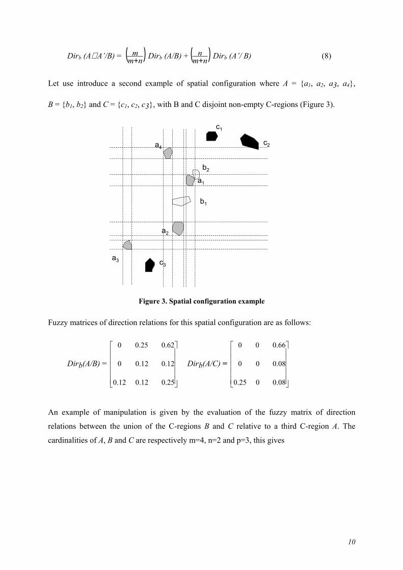
Let use introduce a second example of spatial configuration where A = {a1, a2, a3, a4},

B = {b1, b2} and C = {c1, c2, c3}, with B and C disjoint non-empty C-regions (Figure 3).

a1

a2

a3

b1

b2

a4

c1

c2

c3

Figure 3. Spatial configuration example

Fuzzy matrices of direction relations for this spatial configuration are as follows:

Dirb(A/B) = Dir

25.012.012.0

12.012.00

62.00.25 0

b(A/C) =

08.0025.0

08.000

66.00 0

An example of manipulation is given by the evaluation of the fuzzy matrix of direction

relations between the union of the C-regions B and C relative to a third C-region A. The

cardinalities of A, B and C are respectively m=4, n=2 and p=3, this gives

10

Dirb(A/B∪ C) =

+pnn Dirb (A/B) +

+pnp Dirb (A/ C)

Applying the bounded addition and scalar product of two fuzzy membership function give

Dirb(A/B∪ C)=

52

25.012.012.0

12.012.00

62.00.25 0

+

53

=

08.0025.0

08.000

66.00 0

15.005.02.0

1.005.00

65.01.0 0

Additional properties are defined by applying basic operations on fuzzy subsets. Those will

give a definition for the union and the intersection of fuzzy matrices of direction relations, i.e.,

union and intersection of fuzzy subsets. Although many possible ways have been proposed to

define these operations we consider the default definitions most usually admitted (Yager and

Filev, 1994). This leads to definitions where the union and intersection of fuzzy subsets are

represented by Max and Min operators, respectively.

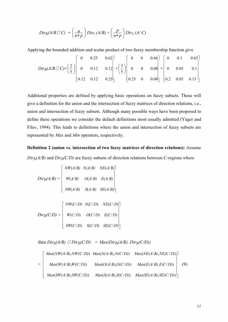
Definition 2 (union vs. intersection of two fuzzy matrices of direction relations): Assume

Dirb(A/B) and Dirb(C/D) are fuzzy subsets of direction relations between C-regions where

Dirb(A/B) =

B)A SEB)A SB)ASW

B)A EB)A OB)AW

B)A NEB)N(AB) NW(A

/(/(/(

/(/(/(

/(//

Dirb(C/D) =

)/()/()/(

)/()/()/(

)/()/()/(

DC SEDC SDCSW

DC EDC ODCW

DC NEDCN DC NW

then Dirb(A/B) ∪ Dirb(C/D) = Max(Dirb(A/B), Dirb(C/D))

= (9)

)/,/()/,/()/,/(

)/,/()/,/()/,/(

)/,/()/,/()/,/(

D)SE(CB)SE(A MaxD)S(CB)S(A MaxD)SW(CB)SW(AMax

D)E(CB)E(A MaxD)O(CB)O(A MaxD)W(CB)W(AMax

D)NE(CB)NE(A MaxD)N(CB)N(AMax D)NW(CB)NW(A Max

11

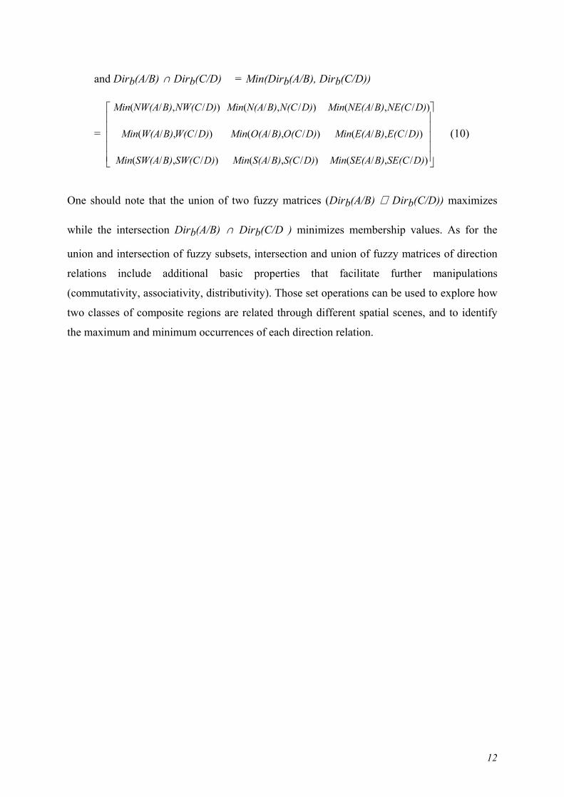
and Dirb(A/B) ∩ Dirb(C/D) = Min(Dirb(A/B), Dirb(C/D))

= (10)

)/,/()/,/()/,/(

)/,/()/,/()/,/(

)/,/()/,/()/,/(

D)SE(CB)SE(A MinD)S(CB)S(A MinD)SW(CB)SW(AMin

D)E(CB)E(A MinD)O(CB)O(A MinD)W(CB)W(AMin

D)NE(CB)NE(A MinD)N(CB)N(AMin D)NW(CB)NW(A Min

One should note that the union of two fuzzy matrices (Dirb(A/B) ∪ Dirb(C/D)) maximizes

while the intersection Dirb(A/B) ∩ Dirb(C/D ) minimizes membership values. As for the

union and intersection of fuzzy subsets, intersection and union of fuzzy matrices of direction

relations include additional basic properties that facilitate further manipulations

(commutativity, associativity, distributivity). Those set operations can be used to explore how

two classes of composite regions are related through different spatial scenes, and to identify

the maximum and minimum occurrences of each direction relation.

12

4. Measures of similarities

Measuring the similarity between different configurations of direction relations should be

analysed by comparing fuzzy matrices. A similarity function usually maps pairs of entities

towards a unique degree of similarity between 0 and 1. We take the usual approach in which

the value 1 corresponds to the maximum similarity and the value 0 the maximum

dissimilarity. Many approaches have been proposed to derive similarities between two fuzzy

subsets (Zwick et al., 1987) such as identifying the maximum value of the intersection

between the membership functions (Jain et al., 1995) or weighing the average distance

between the membership function values. We introduce a two-step technique that first derives

the α–level sets of a fuzzy direction matrix (Zadeh, 1975), and secondly apply Zadeh’s

measure of similarity (Zadeh, 1977). α–level sets present the advantage of giving the position

of the fuzzy subset and its coverage in the crisp Universe of Discourse, favouring thus further

computation and analysis. An α–level set is defined as follows.

Definition 3: Let Dirb(A/B) be a fuzzy matrix of direction relations; the α–level set of

Dirb(A/B), denoted α–Dirb(A/B), is the crisp subset of TILE consisting of all the elements of

TILE for which tile(A/B) ≥ α, it is given by

α–Dirb(A/B) = {tile | tile(A/B) α, tile ∈ TILE} (11) ≥

An α–level set of a fuzzy matrix retains the significant values of the fuzzy matrix, that is,

direction relations whose fuzzy values are higher or equal to the given threshold α. The

threshold value is user-defined and should reflect the degree of membership which is of

interest with respect to a given context. The value of the threshold can be fixed considering

the frequency distribution of direction relations on several spatial configurations under

analysis. For instance, when making comparison of many C-Regions, thresholds may be

chosen using percentile values based on empirical data and their efficiency assessed using

sensitivity analysis (Lootsma, 1997). High values of the threshold have a high level of

selectivity while low values have a low selectivity. It is straightforward to note that α–level

sets are nested, i.e., α1–Dirb(A/B) ⊇ α2–Dirb(A/B) for α1 < α2. A measure of similarity

defined on two distinct α–level sets should evaluate to which degree those two sets share

some common elements or not. Accordingly, we define the measure of similarity among

fuzzy matrices of direction relations as follows.

13

Definition 4: Assume Dirb(A/B) and Dirb(C/D) are fuzzy matrices of direction relations; let

α–Dirb(A/B) and α–Dirb(C/D) be the α–level sets of Dirb(A/B) and Dirb(C/D), respectively.

The α-measure of similarity between Dirb(A/B) and Dirb(C/D) is given by

α–Sim[Dirb(A/B), Dirb(C/D)] = Min

nk

mk ,

(12)

where m is the number of elements of α–Dirb(A/B), n the number of elements of α–

Dirb(C/D) and k is the number of elements of the intersection of α–Dirb(A/B) with α–

Dirb(C/D).

It is easy to show that the α-measure of similarity fulfils some basic properties of similarity

measures, that is, for all A,B,C, D C-regions:

α–Sim[Dirb(A/B), Dirb(C/D)]= α–Sim[Dirb(C/D), Dirb(A/B)] symmetry

α–Sim[Dirb(A/B), Dirb(A/B)] α–Sim[Dir≥ b(C/D), Dirb(A/B)]

The α-measure gives an overall measure of similarity, still bounded by the unit interval, and

flexible as α–level sets are user-defined (i.e. level of significance in selecting the tiles). One

can remark that when k = m (alternatively k = n) then α–Dirb(A/B) ⊆ Dirb(C/D) (alternatively

α–Dirb(C/D) ⊆ Dirb(A/B)). In order to illustrate the similarity concept let us consider the

spatial configurations given by the matrices of fuzzy direction relations Dirb (A/B) and Dirb

(A/ C). In order to analyse different levels of direction relation similarities we give α1 = 0.3

and α2= 0.15, hence

α1–Dirb(A/B) = {tile | tile(A/B) 0.3, tile ∈ TILE}= {NE} ≥

α2–Dirb(A/B) = {tile | tile(A/B) 0.15, tile ∈ TILE}= {NE, N} ≥

α1–Dirb(A/C) = {tile | tile(A/C) ≥ 0.3, tile ∈ TILE}= {NE}

α2–Dirb(A/C) = {tile | tile(A/C) ≥ 0.15, tile ∈ TILE}= {NE, SW}

14

The measures of similarity between these α–level sets are as follows:

α1–Sim[Dirb(A/B), Dirb(A/C)] = Min

11 ,

11 = 1

α2–Sim[Dirb(A/B), Dirb(A/C)] = Min

21 ,

21

=

21

These results show the flexibility of these similarity measures and how, depending on α–

values, two given configuration scenes can be compared and qualified according to a degree

of membership which is of interest for the application. This approach offers a flexible tool by

giving the user the choice of defining what degrees of direction relations should be considered

in analysing two spatial scenes.

5. Application to an illustrative case study

Maritime navigation is an example of an application where relative positions and direction

relations between fleets of concurrent teams is of strategic interest during a race for tactic

decisions (e.g. to compare respective routes with respect to wind and meteorological

conditions), and after a race for debriefing in order to analyse respective performances of the

teams during the race. The sketch example presented in this section reports on the respective

positions of multihulls and monohulls sailing ships during the “Course du Rhum”, an

international sailor ship race that took place in 2002 between St Malo in France and

Guadeloupe. Figure 4 reports on those positions on the 19th (top) and 20th of November

(bottom). For the purpose of the case study MBRs are defined as relatively large areas around

each reference ship.

15

Dir b (A/B)=

Dir b (A/B)=

19 th Nov

20 th Nov B Multihulls A Monohulls

0.25 0.05 0.40

0.1 0 0.05

0.05 0.05 0.2

0.25 0.16 0.58

0 0.08 0.08

0 0.080

Figure 4. Case study 1st configuration example

Fuzzy matrices of direction relations for those two configurations denote the following trends.

The map on the 19th of November shows that monohulls have chosen a route at the South

while multihull have chosen a route at the North at one exception. This is illustrated by

patterns of North-East (0.4) and North West (0.25) directions of the multihulls relative to the

monohulls, although the fact that one multihull took a South route is reflected by the presence

of a South East direction relation (0.2). Between the 19th and the 20th of November one

monohull and one multihull withdrew this reinforcing significantly the North-East direction of

the multihulls (0.58) relative to the monohulls. Those direction patterns stress the good

performance of monohulls with respect to multihulls as the race target (Guadeloupe) is

oriented South West. The local pattern identified at the North West reflects the fact that one of

the multihull competitors took a different course to the North. Figure 5 gives another example

of direction relations but this time making the difference between small multihulls relative to

monohulls (i.e. Dirb(A/B)), with large multihulls relative to monohulls. An application of

Theorem 1 derives the overall direction relation of multihulls relative to monohulls (Dirb

(A/B C)), applied to the night between the 19∪ th and the 20th of November).

16

CB Small multihulls A Monohulls C Large multihulls BA

Dir b (A/B)=

Dir b (A/B)=

Dir b (A/C)=

Dir b (A/BUC)=

0.25 0 0.25

0.37 0 0 0.12 0 0

0.16 0 0.83

0 0 0 0 0 0

0.2 0 0.6

0.15 0 0 0.05 0 0

Figure 5. Case study 2nd configuration example

The configuration above is more contrasted than the previous ones. Monohulls and small

multihulls took similar routes although small multihulls are mostly behind monohulls. Large

multihulls still took a route at the North, one of the two large multihulls leading the race at the

time of the snapshot. This pattern is reflected by the application of the intersection of fuzzy

matrices where minimal values across the two configurations are retained.

Dirb(A/B) ∩ Dirb(A/C) = Min(Dirb(A/B), Dirb(C/D)) =

000

000

25.00 25.0

We go further and apply a similarity measure to the matrices of fuzzy direction relations given

in Figure 5, i.e., Dirb (A/B), Dirb (A/ C) and Dirb (A/B C). In order to retain significant

direction relations we give α

∪1= 0.15 (which is intuitively a relevant threshold to keep the most

important directions in this case), hence

α1–Dirb(A/B) = {tile | tile(A/B) 0.15, tile ∈ TILE}= {NE, NW} ≥

α1–Dirb(A/C) = {tile | tile(A/C) ≥ 0.15, tile ∈ TILE}= {NE, NW, W}

α1–Dirb(A/B ∪ C) = {tile | tile(A/C) 0.15, tile ∈ TILE}= {NE, NW, W} ≥

17

This measure of similarity stresses the relatively high influence of North-East and West

direction relations of B relative to A and C relative to A, respectively; and the fact that the

predominance of the direction North-East is increased when considering the multihulls all

together (i.e. B ∪ C).

α1–Sim[Dirb(A/B), Dirb(A/C)] = Min

32 ,

22

=

32

α1–Sim[Dirb(A/B), Dirb(A/B ∪ C)] = Min

33 ,

33

= 1

α1–Sim[Dirb(A/C), Dirb(A/B C)] = Min∪

32 ,

22

=

32

These figures might help the different teams to adapt in real-time their course depending on

the concurrent positions, directions and navigation conditions, and to analyse respective

performances during debriefing discussions. Those examples also illustrate the adaptability of

the approach as composite regions are derived from local regions on demand according to

some user-defined criteria.

6. Conclusion

Evaluation of spatial relations and derivation of measures of similarity in spatial

configurations are still an open challenge for qualitative spatial reasoning. This paper

introduces a fuzzy modelling technique that computes direction relations in a spatial scene.

The model combines a spatial reasoning approach with fuzzy semantic typing to evaluate the

configuration of direction relations between two given composite regions. Fuzzy semantics

typing provides a flexible and computable mean to assess direction relations between

composite regions. Although it is based on Goyal and Egenhofer’s direction model, it should

be also applicable to other direction models with some minor adaptations.

The fuzzy principles of the approach can be extended and applied at different levels of the

model to integrate further variability and flexibility in the properties represented. Degrees of

membership of S-regions with respect to a C-region, part of a target S-region that intersects a

tile, distance between S-regions (as suggested in Frank, 1996) or their relative sizes can be

also modelled as fuzzy variables. Those fuzzy variables taken independently or aggregated

can give a fuzzy domain to tile(a/b) thus augmenting the semantics of the approach.

18

Similarity measures are introduced on top of the model. They give a flexible tool in assessing

to which degree configuration scenes reveal, or not, some common patterns. Different

measures of similarities can be applied to compare fuzzy directions between spatial scenes.

The approach retained in this paper expresses similarities in a crisp Universe of Discourse but

alternatives in the fuzzy domains might also be of interest.

This approach should be of interest for a wide range of applications for environmental,

biological and epidemiological studies, emergency planning and coordinated navigation. We

also believe that addressing these new issues may contribute to open a bridge between formal

reasoning approaches and spatial data analysis, this for the entire benefits of the GIS

community. Further work concerns the integration of additional fuzzy variables in the model

and the analysis of direction relations in evolving scenes. Another direction to explore is an

evaluation experiment involving typical user groups in order to compare the relevance of

fuzzy direction relations identified by our model with respect to cognitive interpretations.

Acknowledgments

The authors thank the referees for their valuable comments and suggestion which have

significantly improved the quality of the paper.

References

Brun, H. T. and Egenhofer, M. J., 1996, Similarity of spatial scenes. In J. M. Kraak and M. Moleenar

(eds.), Proceedings of the 7th International Symposium on Spatial Data Handling (SDH’96), Taylor

and Francis, London, pp. 173-184.

Chang, C.-C. and Jungert, E., 1990, A spatial knowledge structure for visual information systems. In

T. Ichikawa, E. Jungert and R. Korfhage (eds.), Visual Languages and Applications, Plenum Press,

New York, pp. 277-304.

Clementini, E., Di Felice, P. and Califano, G., 1995, Composite regions in topological queries,

Information Systems, 20(7), 579-594.

Cliff, A. D., Haggett, P. and Ord, J. K., 1975, Elements of Spatial Structure. Cambridge University

Press, Cambridge.

Cohn, A. G., 1997, Qualitative spatial representation and reasoning techniques. In G. Brewka, C.

Habel and B. Nebel (eds.), Proceedings of KI-97, Springer-Verlag, LNAI 1303, Berlin, pp 1-30.

Cressie, N. A. C., 1993, Statistics for Spatial Data. Wiley, New York.

19

Egenhofer, M. and Mark, D., 1995, Naive geography. In A. Frank and W. Kuhn (eds.), Spatial

Information Theory: A Theoretical Basis for GIS, Springer-Verlag, LNCS 988, Berlin, pp. 1-15.

Fontanelle, T., 1999, Semantic tagging: a survey. In Papers in Computational Lexicography

(COMPLEX 99), pp. 39-56.

Frank, A. U., 1996, Qualitative spatial reasoning: cardinal directions as an example. International

Journal of Geographical Information Systems, 10(3), 269-290.

Freksa, C. and Röhrig, R.,1993, Dimensions of qualitative spatial reasoning. In P. Carret, N. and M. G.

Singh (eds.), Qualitative Reasoning and Decision Technologies, Proceedings of QUARDET'93,

CIMNE, Barcelona, pp. 483-492.

Freksa, C., 1992, Using orientation information for qualitative spatial reasoning. In A. U. Frank, I.

Campari and U. Formentini (eds.), Theories and Methods of Spatio-Temporal Reasoning in

Geographic Space, Springer-Verlag, LNCS 639, Nez York, pp. 162-178.

Godoy, F. and Rodriguez, A., 2002, A quantitative description of spatial configurations. In D.

Richardson and P. van Oosterom (eds.), Advances in Spatial Data Handling, Springer-Verlag, Ottawa,

pp. 292-312.

Goodman, J. and Pollack, R., 1993, Allowable sequences and order types in discrete and

computational geometry. In J. Pach (ed.), New Trends in Discrete and Computational Geometry,

Springer-Verlag, pp. 103-134.

Goyal, R. K. and Egenhofer, M. J., 2000, Consistent queries over cardinal directions across different

levels of detail. In A. M. Tjoa, R. Wagner, and A. Al-Zobaidie (eds.), 11th International Workshop on

Database and Expert Systems Applications, Greenwich, UK, pp. 876-880.

Goyal, R. K. and Egenhofer, M. J., 2003, Cardinal directions between extended spatial objects. IEEE

Transactions on Knowledge and Data Engineering, to appear.

Hernández, D., 1994, Qualitative Representation of Spatial Knowledge, LNCS 804, Springer-Verlag.

Jain, R., Murthy, S. N., Tran, L and Chatterjee, S., 1995, Similarity measures for image databases. In

W. Niblack and R. Jain (eds.), Proceedings of IEEE Conference on Storage and Retrieval for Image

and Video Databases (SPIE), San Diego/La Jolla, CA, USA, pp. 58-65.

Kuceral, D. R. and Orr P. W., 1999, Spruce Budworm in the Eastern United States. Forest Insect and

Disease Leaflet 60. U. S. Department of Agriculture, Forest Service. Washington.

Krakover, S., 1986, Progress in the Study of Decentralization, Geographical Analysis, 18, 260-263.

Lootsma, F. A., 1997, Fuzzy Logic for Planning and Decision Making. Kluwer, Dordrecht.

Mardia, K., 1972, Statistics of Directional Data. Academic Press, New York.

20

Mark, D. M., Frank, A. U., Egenhofer, M. J., Freundschuh, S. M., McGranaghan, M. and White, R.

M., 1989, Languages of Spatial Relations: Initiative 2 Meeting Report, TR89-2, NCGIA.

Monmonier, M. and Mark, D., 1992, Directional Profiles and Rose Diagrams to Complement

Centrographic Cartography, Journal of the Pennsylvania Academy of Science, (66) 1, 29-34.

Mukerjee, A. and Joe, G., 1990, A qualitative model for space. In Proceedings of the 8th International

Conference on AI (AAAI-90), Morgan Kaufman, Los Altos, pp. 721-727.

Papadias, D., Arkoumanis, N., Karacapilidis, N., 1998, On The Retrieval of Similar Configurations. In

Proceedings of the 8th International Symposium on Spatial Data Handling (SDH), Vancouver, Canada,

Taylor Francis.

Papadias, D. and Egenhofer, M. J., 1997, Algorithms for hierarchical spatial reasoning.

Geoinformatica, 1(3), 251-273.

Peuquet, D. and Zhan, C.-X., 1987, An algorithm to determine the directional relationship between

arbitrary-shaped polygons in a plane. Pattern Recognition, 20, 65-74.

Prewitt, J. M., 1970, Object enhancement and extraction. In B. S. Lipkin and A. Rosenfeld (eds.),

Picture Processing and Psychopictorics, New York, Academic Press, pp. 75-149.

Pullar, D. V. and Egenhofer, M. J., 1988, Towards the defaction and use of topological relations

among spatial objects. In Proceedings of the 3rd International Symposium on Spatial Data Handling,

IGU, Colombus, pp. 225-242.

Röhrig, R., 1994, A theory for qualitative spatial reasoning based on order relations. In Proceedings of

the 12th International Conference on AI (AAII-94), vol. 2, pp. 1418-1423.

Rosenfeld, A., 1979, Fuzzy digital topology. Information and Control, 40, 76-86.

Saraf, A. K., P. Mishra, S. Mitra, B. Sarma and D. K. Mukhopadhyay, 2003, Remote sensing and GIS

technologies for improvements in geological structures interpretation and mapping, International

Journal of Remote Sensing, in press.

Schlieder, C., 1993, Representing visible locations for qualitative navigation. In N. Piera Carreté and

Singh, M. G. (eds.), Qualitative Reasoning and Decision Technologies, CIMNE, Barcelona, pp. 523-

532.

Sharma, J., 1996, Integrated Spatial Reasoning in GIS: Combining Topology and Direction, PhD

Thesis, Department of Spatial Information Science and Engineering, University of Maine, Orono, ME.

Subasic, P., 2001, Affect analysis of text using semantic typing. IEEE Transactions on Fuzzy Systems,

9(4), 483-496.

21

Theodoridis, Y., Papadias, D. and Stefanakis, E., 1996 Supporting Direction Relations in Spatial

Database systems. In J. M. Kraak and M. Moleenar (eds.), Proceedings of the 7th International

Symposium on Spatial Data Handling (SDH), Delfts, Netherlands, Taylor Francis, 1996, pp. 739-752.

Yager, R. R. and Filev, D. P., 1994, Essential of Fuzzy Modelling and Control, Wiley InterScience.

Zadeh, L. A., 1975, The concept of a liguistic truth variable and its application to approximate

reasoning I, II, III. Information Science, 8, pp. 199-249, 301-357, 9, pp. 43-80.

Zadeh, L. A., 1977, Similarity relations and fuzzy orderings. Information Science, 3, Elsevier Science,

pp. 177-200.

Zadeh, L. A., 1996, Fuzzy logic = computing with words. IEEE Transactions on Fuzzy Systems, pp.

103-111.

Zwick, R., Carlstein, E. and Budescu, D. V., 1987, Measures of similarities among fuzzy concepts: a

comparative analysis. International Journal of Approximate Reasoning, 1, 221-242.

22